aerospace

Article

Experimental Investigation of the Wake and theWingtip Vortices of a UAV Model

Pericles Panagiotou, George Ioannidis ID , Ioannis Tzivinikos and Kyros Yakinthos * ID

Laboratory of Fluid Mechanics and Turbomachinery, Department of Mechanical Engineering,Aristotle University of Thessaloniki, 54124 Thessaloniki, Greece; peripan@eng.auth.gr (P.P.);georioan.meng@gmail.com (G.I.); ioannistzivinikos@gmail.com (I.T.)* Correspondence: kyak@auth.gr; Tel.: +30-231-099-6411

Received: 5 October 2017; Accepted: 30 October 2017; Published: 1 November 2017

Abstract: An experimental investigation of the wake of an Unmanned Aerial Vehicle (UAV) modelusing flow visualization techniques and a 3D Laser Doppler Anemometry (LDA) system is presentedin this work. Emphasis is given on the flow field at the wingtip and the investigation of the tipvortices. A comparison of the velocity field is made with and without winglet devices installed atthe wingtips. The experiments are carried out in a closed-circuit subsonic wind tunnel. The flowvisualization techniques include smoke-wire and smoke-probe experiments to identify the flowphenomena, whereas for accurately measuring the velocity field point measurements are conductedusing the LDA system. Apart from the measured velocities, vorticity and circulation quantitiesare also calculated and compared for the two cases. The results help to provide a more detailedview of the flow field around the UAV and indicate the winglets’ significant contribution to thedeconstruction of wing-tip vortex structures.

Keywords: UAV; measurements; LDA; vortex; winglets

1. Introduction

In recent years, there is an increasing trend in the development and use of fixed-wing UnmannedAerial Vehicles (UAVs) by both military forces and civilian organizations [1]. They are ideal solutionsfor a wide range of operations, such as fire detection, search and rescue, coastline and sea-lanemonitoring, and security surveillance [2]. Due to the absence of crew on-board, they present severaladvantages, such as the reduced operational cost, the ability to operate under hazardous conditions,and the increased flight endurance, which is one the most important characteristics when it comes tothe aforementioned missions. In the case of a UAV, where the endurance is only limited by the availablefuel on-board, it is essentially up to the aerodynamic efficiency of the configuration to maximize theflight time. For a given mission, the required lift force is defined, therefore the optimization process isessentially keeping the corresponding drag force as low as possible.

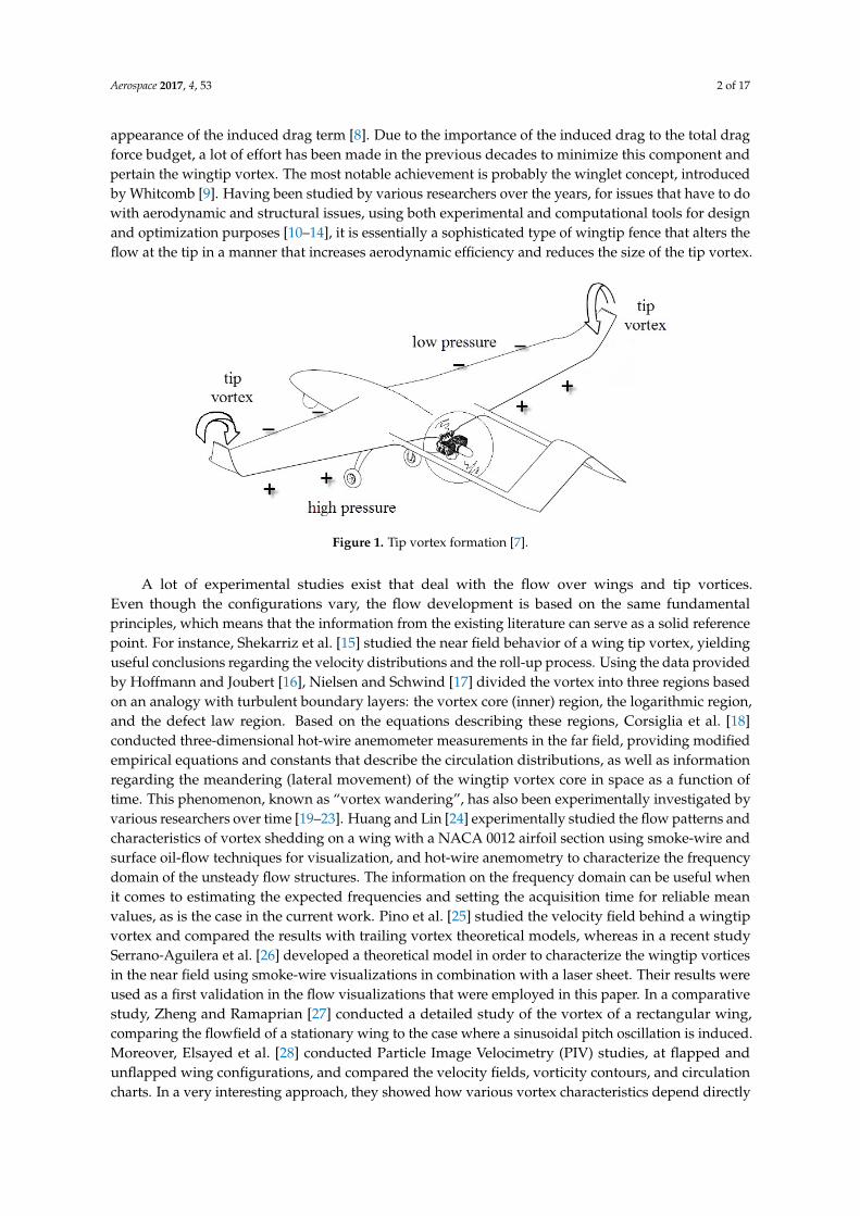
For a UAV that operates in the low subsonic, incompressible regime, as is the case with mostMedium-Altitude-Long-Endurance (MALE) UAVs [3–6], a drag breakdown analysis was conductedin [7], which shows that the part that contributes the most to the total drag force of the aerial vehicle isthe main wing. More specifically, when exposed in subsonic, incompressible flow, a finite wing’s dragis a combination of profile drag and induced drag. The profile drag is the drag due to the shape ofthe body (skin friction + flow separation effects), whereas the induced drag is a result of the pressureimbalance at the tip of a finite wing between its upper (suction side) and lower (pressure side) surfaces.At the tip though, this imbalance causes the high-pressure air from the lower side to move upwards,where the pressure is lower, leading to the formation of a vortex, i.e., the wingtip vortex (Figure 1).This three-dimensional motion alters the flow field above the entire wing as well, thus resulting in the

Aerospace 2017, 4, 53; doi:10.3390/aerospace4040053 www.mdpi.com/journal/aerospace

Aerospace 2017, 4, 53 2 of 17

appearance of the induced drag term [8]. Due to the importance of the induced drag to the total dragforce budget, a lot of effort has been made in the previous decades to minimize this component andpertain the wingtip vortex. The most notable achievement is probably the winglet concept, introducedby Whitcomb [9]. Having been studied by various researchers over the years, for issues that have to dowith aerodynamic and structural issues, using both experimental and computational tools for designand optimization purposes [10–14], it is essentially a sophisticated type of wingtip fence that alters theflow at the tip in a manner that increases aerodynamic efficiency and reduces the size of the tip vortex.

Aerospace 2017, 4, 53 2 of 17

drag to the total drag force budget, a lot of effort has been made in the previous decades to minimize this component and pertain the wingtip vortex. The most notable achievement is probably the winglet concept, introduced by Whitcomb [9]. Having been studied by various researchers over the years, for issues that have to do with aerodynamic and structural issues, using both experimental and computational tools for design and optimization purposes [10–14], it is essentially a sophisticated type of wingtip fence that alters the flow at the tip in a manner that increases aerodynamic efficiency and reduces the size of the tip vortex.

Figure 1. Tip vortex formation [7].

A lot of experimental studies exist that deal with the flow over wings and tip vortices. Even though the configurations vary, the flow development is based on the same fundamental principles, which means that the information from the existing literature can serve as a solid reference point. For instance, Shekarriz et al. [15] studied the near field behavior of a wing tip vortex, yielding useful conclusions regarding the velocity distributions and the roll-up process. Using the data provided by Hoffmann and Joubert [16], Nielsen and Schwind [17] divided the vortex into three regions based on an analogy with turbulent boundary layers: the vortex core (inner) region, the logarithmic region, and the defect law region. Based on the equations describing these regions, Corsiglia et al. [18] conducted three-dimensional hot-wire anemometer measurements in the far field, providing modified empirical equations and constants that describe the circulation distributions, as well as information regarding the meandering (lateral movement) of the wingtip vortex core in space as a function of time. This phenomenon, known as “vortex wandering”, has also been experimentally investigated by various researchers over time [19–23]. Huang and Lin [24] experimentally studied the flow patterns and characteristics of vortex shedding on a wing with a NACA 0012 airfoil section using smoke-wire and surface oil-flow techniques for visualization, and hot-wire anemometry to characterize the frequency domain of the unsteady flow structures. The information on the frequency domain can be useful when it comes to estimating the expected frequencies and setting the acquisition time for reliable mean values, as is the case in the current work. Pino et al. [25] studied the velocity field behind a wingtip vortex and compared the results with trailing vortex theoretical models, whereas in a recent study Serrano-Aguilera et al. [26] developed a theoretical model in order to characterize the wingtip vortices in the near field using smoke-wire visualizations in combination with a laser sheet. Their results were used as a first validation in the flow visualizations that were employed in this paper. In a comparative study, Zheng and Ramaprian [27] conducted a detailed study of the vortex of a rectangular wing, comparing the flowfield of a stationary wing to the case where a sinusoidal pitch oscillation is induced. Moreover, Elsayed et al. [28] conducted Particle Image Velocimetry (PIV) studies, at flapped and unflapped wing configurations, and compared the velocity fields, vorticity contours, and circulation charts. In a very interesting approach, they showed how various vortex characteristics depend directly on the angle of attack, emphasizing on peak tangential velocity, vorticity, and circulation distribution. Finally, Muthusamy [29] carried out experiments in a

Figure 1. Tip vortex formation [7].

A lot of experimental studies exist that deal with the flow over wings and tip vortices.Even though the configurations vary, the flow development is based on the same fundamentalprinciples, which means that the information from the existing literature can serve as a solid referencepoint. For instance, Shekarriz et al. [15] studied the near field behavior of a wing tip vortex, yieldinguseful conclusions regarding the velocity distributions and the roll-up process. Using the data providedby Hoffmann and Joubert [16], Nielsen and Schwind [17] divided the vortex into three regions basedon an analogy with turbulent boundary layers: the vortex core (inner) region, the logarithmic region,and the defect law region. Based on the equations describing these regions, Corsiglia et al. [18]conducted three-dimensional hot-wire anemometer measurements in the far field, providing modifiedempirical equations and constants that describe the circulation distributions, as well as informationregarding the meandering (lateral movement) of the wingtip vortex core in space as a function oftime. This phenomenon, known as “vortex wandering”, has also been experimentally investigated byvarious researchers over time [19–23]. Huang and Lin [24] experimentally studied the flow patterns andcharacteristics of vortex shedding on a wing with a NACA 0012 airfoil section using smoke-wire andsurface oil-flow techniques for visualization, and hot-wire anemometry to characterize the frequencydomain of the unsteady flow structures. The information on the frequency domain can be useful whenit comes to estimating the expected frequencies and setting the acquisition time for reliable meanvalues, as is the case in the current work. Pino et al. [25] studied the velocity field behind a wingtipvortex and compared the results with trailing vortex theoretical models, whereas in a recent studySerrano-Aguilera et al. [26] developed a theoretical model in order to characterize the wingtip vorticesin the near field using smoke-wire visualizations in combination with a laser sheet. Their results wereused as a first validation in the flow visualizations that were employed in this paper. In a comparativestudy, Zheng and Ramaprian [27] conducted a detailed study of the vortex of a rectangular wing,comparing the flowfield of a stationary wing to the case where a sinusoidal pitch oscillation is induced.Moreover, Elsayed et al. [28] conducted Particle Image Velocimetry (PIV) studies, at flapped andunflapped wing configurations, and compared the velocity fields, vorticity contours, and circulationcharts. In a very interesting approach, they showed how various vortex characteristics depend directly

Aerospace 2017, 4, 53 3 of 17

on the angle of attack, emphasizing on peak tangential velocity, vorticity, and circulation distribution.Finally, Muthusamy [29] carried out experiments in a configuration with and without winglets at a lowspeed windtunnel. The study was limited to force balance measurements though, and no informationwas provided regarding the flow development and the effect the winglet has on the tip vortex. To thebest of our knowledge, no study exists where a direct comparison is made in terms of flow fielddevelopment between a configuration with, and without a winglet device installed at the wingtip,and few of the existing studies on wingtip vortices deal with UAV platforms. However, and since inUAV development the time and budget is limited when compared to a commercial airliner, the wingsare of less complex geometry (in terms of airfoil profiles, twist angle etc.) and relatively simple tomanufacture. Thus, the tips are highly loaded and are ideal platforms for winglet studies [11].

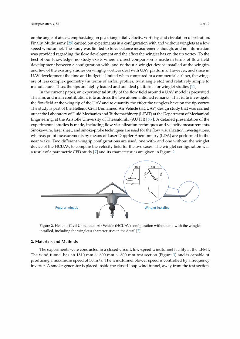
In the current paper, an experimental study of the flow field around a UAV model is presented.The aim, and main contribution, is to address the two aforementioned remarks. That is, to investigatethe flowfield at the wing tip of the UAV and to quantify the effect the winglets have on the tip vortex.The study is part of the Hellenic Civil Unmanned Air Vehicle (HCUAV) design study that was carriedout at the Laboratory of Fluid Mechanics and Turbomachinery (LFMT) at the Department of MechanicalEngineering, at the Aristotle University of Thessaloniki (AUTH) [6,7]. A detailed presentation of theexperimental studies is made, including flow visualization techniques and velocity measurements.Smoke-wire, laser sheet, and smoke-probe techniques are used for the flow visualization investigations,whereas point measurements by means of Laser Doppler Anemometry (LDA) are performed in thenear wake. Two different wingtip configurations are used, one with- and one without the wingletdevice of the HCUAV, to compare the velocity field for the two cases. The winglet configuration wasa result of a parametric CFD study [7] and its characteristics are given in Figure 2.

Aerospace 2017, 4, 53 3 of 17

configuration with and without winglets at a low speed windtunnel. The study was limited to force balance measurements though, and no information was provided regarding the flow development and the effect the winglet has on the tip vortex. To the best of our knowledge, no study exists where a direct comparison is made in terms of flow field development between a configuration with, and without a winglet device installed at the wingtip, and few of the existing studies on wingtip vortices deal with UAV platforms. However, and since in UAV development the time and budget is limited when compared to a commercial airliner, the wings are of less complex geometry (in terms of airfoil profiles, twist angle etc.) and relatively simple to manufacture. Thus, the tips are highly loaded and are ideal platforms for winglet studies [11].

In the current paper, an experimental study of the flow field around a UAV model is presented. The aim, and main contribution, is to address the two aforementioned remarks. That is, to investigate the flowfield at the wing tip of the UAV and to quantify the effect the winglets have on the tip vortex. The study is part of the Hellenic Civil Unmanned Air Vehicle (HCUAV) design study that was carried out at the Laboratory of Fluid Mechanics and Turbomachinery (LFMT) at the Department of Mechanical Engineering, at the Aristotle University of Thessaloniki (AUTH) [6,7]. A detailed presentation of the experimental studies is made, including flow visualization techniques and velocity measurements. Smoke-wire, laser sheet, and smoke-probe techniques are used for the flow visualization investigations, whereas point measurements by means of Laser Doppler Anemometry (LDA) are performed in the near wake. Two different wingtip configurations are used, one with- and one without the winglet device of the HCUAV, to compare the velocity field for the two cases. The winglet configuration was a result of a parametric CFD study [7] and its characteristics are given in Figure 2.

Figure 2. Hellenic Civil Unmanned Air Vehicle (HCUAV) configuration without and with the winglet installed, including the winglet’s characteristics in the detail [7].

2. Materials and Methods

The experiments were conducted in a closed-circuit, low-speed windtunnel facility at the LFMT. The wind tunnel has an 1810 mm × 600 mm × 600 mm test section (Figure 3) and is capable of producing a maximum speed of 50 m/s. The windtunnel blower speed is controlled by a frequency inverter. A smoke generator is placed inside the closed-loop wind tunnel, away from the test section.

Considering the models used in the study, two scaled variants (1:22) of the HCUAV were used, one without and one with the winglet devices installed at the tip. The models were manufactured by means of 3D printing to ensure accurate representation of the original geometry. Specifically, the main wing has a mean chord of 36.5 mm, a tip chord (c) of 21 mm, an Aspect Ratio of 8, and a NASA NLF(1)-1015 airfoil [30], whereas the wing span is 302 mm. A custom mechanism with a supporting rod is used to place the model at the center of the test section area, away from the windtunnel walls, and ensures that the model is accurately positioned within ± 0.5 deg (Figure 4). The model maximum cross-sectional area at the largest examined angle of attack (15 deg) divided by the area of the wind-tunnel cross-section is equal to 1.05%. Hence, no corrections due to the blockage effect were made [31].

Figure 2. Hellenic Civil Unmanned Air Vehicle (HCUAV) configuration without and with the wingletinstalled, including the winglet’s characteristics in the detail [7].

2. Materials and Methods

The experiments were conducted in a closed-circuit, low-speed windtunnel facility at the LFMT.The wind tunnel has an 1810 mm × 600 mm × 600 mm test section (Figure 3) and is capable ofproducing a maximum speed of 50 m/s. The windtunnel blower speed is controlled by a frequencyinverter. A smoke generator is placed inside the closed-loop wind tunnel, away from the test section.

Aerospace 2017, 4, 53 4 of 17Aerospace 2017, 4, 53 4 of 17

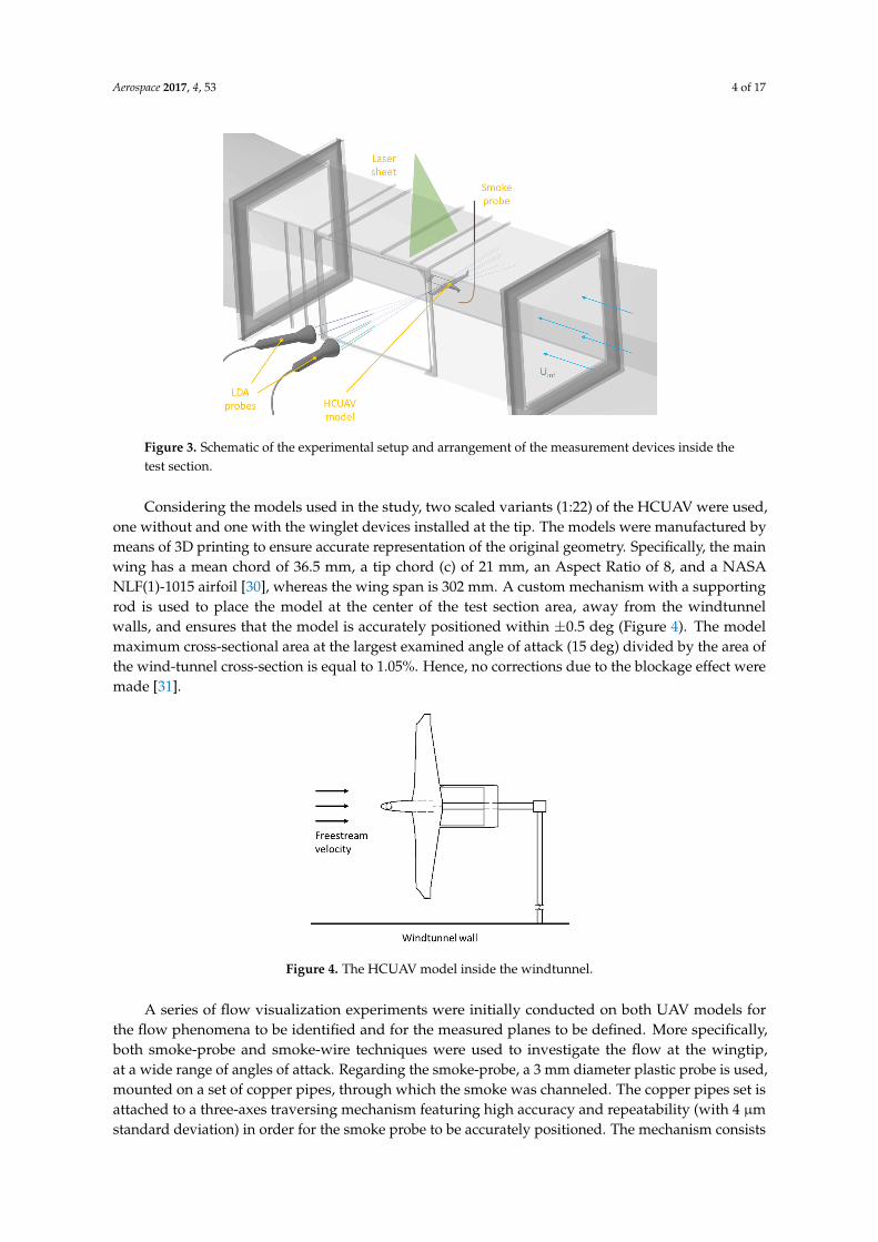
Figure 3. Schematic of the experimental setup and arrangement of the measurement devices inside the test section.

Figure 4. The HCUAV model inside the windtunnel.

A series of flow visualization experiments were initially conducted on both UAV models for the flow phenomena to be identified and for the measured planes to be defined. More specifically, both smoke-probe and smoke-wire techniques were used to investigate the flow at the wingtip, at a wide range of angles of attack. Regarding the smoke-probe, a 3 mm diameter plastic probe is used, mounted on a set of copper pipes, through which the smoke was channeled. The copper pipes set is attached to a three-axes traversing mechanism featuring high accuracy and repeatability (with 4 μm standard deviation) in order for the smoke probe to be accurately positioned. The mechanism consists of a driving bolt connected to a stepper motor for each axis. Finally, a flexible rubber pipe connects the copper pipes with the smoke generator. To carry out the smoke-wire study, a custom frame is used. Specifically, a 0.3 mm diameter wire is mounted on a rigid aluminum frame, and a glass syringe is adjusted on top, where the glycerin-water mixture was stored. The mixture consists of 30% glycerin and 70% distilled water and drips on the wire through the glass syringe. Proper positioning of the syringe ensures the right amount of mixture dripping over the wire. Αn external power supply is used to charge the wire, thus creating a close circuit, in order for the mixture on the wire to be burnt. The entire frame is in turn placed in the test section, close to the model. The photographs were taken using a Nikon D3000 DSLR camera and Nikorr 35 mm, f 1.8 and Nikorr 18–105 mm, f 3.5–5.6 lenses.

Regarding the LDA measurements, and since the flow field is symmetric, only half the wake was examined, so that the experiments were conducted at the right wing of the model. The relative

Figure 3. Schematic of the experimental setup and arrangement of the measurement devices inside thetest section.

Considering the models used in the study, two scaled variants (1:22) of the HCUAV were used,one without and one with the winglet devices installed at the tip. The models were manufactured bymeans of 3D printing to ensure accurate representation of the original geometry. Specifically, the mainwing has a mean chord of 36.5 mm, a tip chord (c) of 21 mm, an Aspect Ratio of 8, and a NASANLF(1)-1015 airfoil [30], whereas the wing span is 302 mm. A custom mechanism with a supportingrod is used to place the model at the center of the test section area, away from the windtunnelwalls, and ensures that the model is accurately positioned within ±0.5 deg (Figure 4). The modelmaximum cross-sectional area at the largest examined angle of attack (15 deg) divided by the area ofthe wind-tunnel cross-section is equal to 1.05%. Hence, no corrections due to the blockage effect weremade [31].

Aerospace 2017, 4, 53 4 of 17

Figure 3. Schematic of the experimental setup and arrangement of the measurement devices inside the test section.

Figure 4. The HCUAV model inside the windtunnel.

A series of flow visualization experiments were initially conducted on both UAV models for the flow phenomena to be identified and for the measured planes to be defined. More specifically, both smoke-probe and smoke-wire techniques were used to investigate the flow at the wingtip, at a wide range of angles of attack. Regarding the smoke-probe, a 3 mm diameter plastic probe is used, mounted on a set of copper pipes, through which the smoke was channeled. The copper pipes set is attached to a three-axes traversing mechanism featuring high accuracy and repeatability (with 4 μm standard deviation) in order for the smoke probe to be accurately positioned. The mechanism consists of a driving bolt connected to a stepper motor for each axis. Finally, a flexible rubber pipe connects the copper pipes with the smoke generator. To carry out the smoke-wire study, a custom frame is used. Specifically, a 0.3 mm diameter wire is mounted on a rigid aluminum frame, and a glass syringe is adjusted on top, where the glycerin-water mixture was stored. The mixture consists of 30% glycerin and 70% distilled water and drips on the wire through the glass syringe. Proper positioning of the syringe ensures the right amount of mixture dripping over the wire. Αn external power supply is used to charge the wire, thus creating a close circuit, in order for the mixture on the wire to be burnt. The entire frame is in turn placed in the test section, close to the model. The photographs were taken using a Nikon D3000 DSLR camera and Nikorr 35 mm, f 1.8 and Nikorr 18–105 mm, f 3.5–5.6 lenses.

Regarding the LDA measurements, and since the flow field is symmetric, only half the wake was examined, so that the experiments were conducted at the right wing of the model. The relative

Figure 4. The HCUAV model inside the windtunnel.

A series of flow visualization experiments were initially conducted on both UAV models forthe flow phenomena to be identified and for the measured planes to be defined. More specifically,both smoke-probe and smoke-wire techniques were used to investigate the flow at the wingtip,at a wide range of angles of attack. Regarding the smoke-probe, a 3 mm diameter plastic probe is used,mounted on a set of copper pipes, through which the smoke was channeled. The copper pipes set isattached to a three-axes traversing mechanism featuring high accuracy and repeatability (with 4 µmstandard deviation) in order for the smoke probe to be accurately positioned. The mechanism consists

Aerospace 2017, 4, 53 5 of 17

of a driving bolt connected to a stepper motor for each axis. Finally, a flexible rubber pipe connects thecopper pipes with the smoke generator. To carry out the smoke-wire study, a custom frame is used.Specifically, a 0.3 mm diameter wire is mounted on a rigid aluminum frame, and a glass syringe isadjusted on top, where the glycerin-water mixture was stored. The mixture consists of 30% glycerinand 70% distilled water and drips on the wire through the glass syringe. Proper positioning of thesyringe ensures the right amount of mixture dripping over the wire. An external power supply isused to charge the wire, thus creating a close circuit, in order for the mixture on the wire to be burnt.The entire frame is in turn placed in the test section, close to the model. The photographs were takenusing a Nikon D3000 DSLR camera and Nikorr 35 mm, f 1.8 and Nikorr 18–105 mm, f 3.5–5.6 lenses.

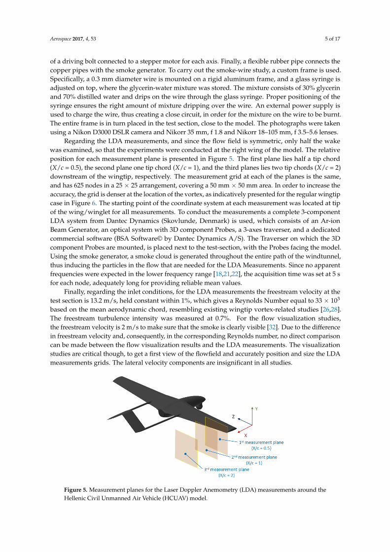
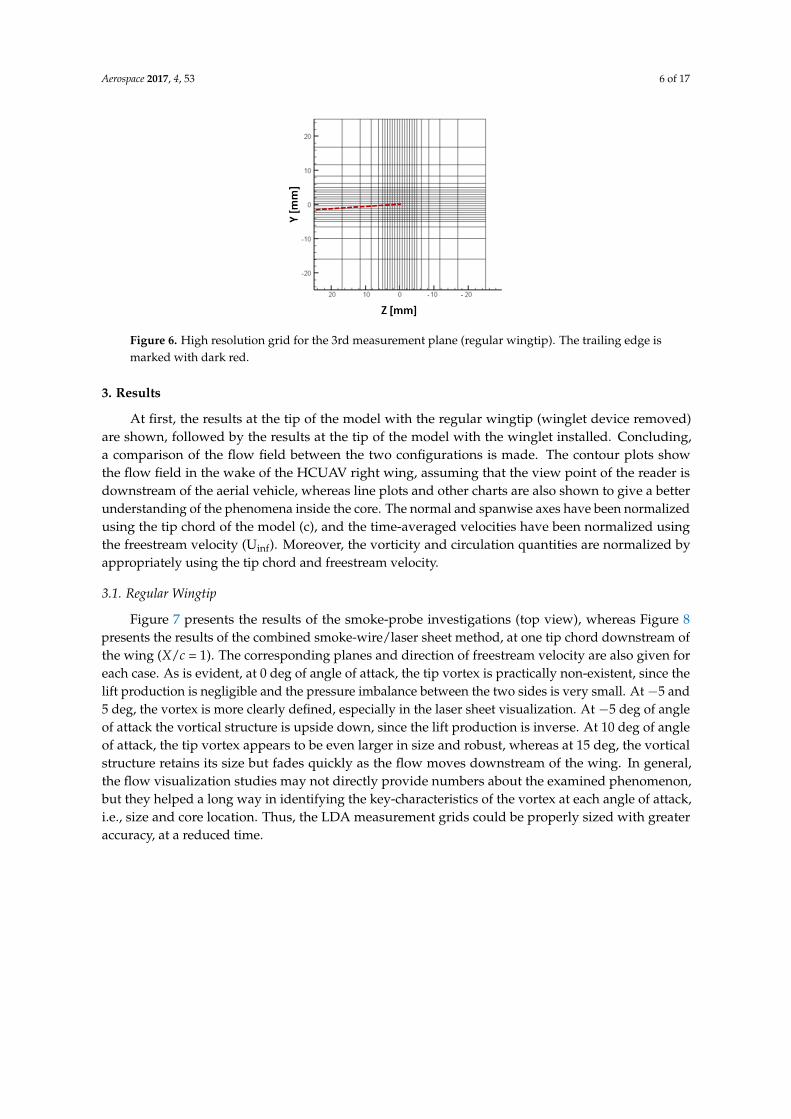
Regarding the LDA measurements, and since the flow field is symmetric, only half the wakewas examined, so that the experiments were conducted at the right wing of the model. The relativeposition for each measurement plane is presented in Figure 5. The first plane lies half a tip chord(X/c = 0.5), the second plane one tip chord (X/c = 1), and the third planes lies two tip chords (X/c = 2)downstream of the wingtip, respectively. The measurement grid at each of the planes is the same,and has 625 nodes in a 25 × 25 arrangement, covering a 50 mm × 50 mm area. In order to increase theaccuracy, the grid is denser at the location of the vortex, as indicatively presented for the regular wingtipcase in Figure 6. The starting point of the coordinate system at each measurement was located at tipof the wing/winglet for all measurements. To conduct the measurements a complete 3-componentLDA system from Dantec Dynamics (Skovlunde, Denmark) is used, which consists of an Ar-ionBeam Generator, an optical system with 3D component Probes, a 3-axes traverser, and a dedicatedcommercial software (BSA Software© by Dantec Dynamics A/S). The Traverser on which the 3Dcomponent Probes are mounted, is placed next to the test-section, with the Probes facing the model.Using the smoke generator, a smoke cloud is generated throughout the entire path of the windtunnel,thus inducing the particles in the flow that are needed for the LDA Measurements. Since no apparentfrequencies were expected in the lower frequency range [18,21,22], the acquisition time was set at 5 sfor each node, adequately long for providing reliable mean values.

Finally, regarding the inlet conditions, for the LDA measurements the freestream velocity at thetest section is 13.2 m/s, held constant within 1%, which gives a Reynolds Number equal to 33 × 103

based on the mean aerodynamic chord, resembling existing wingtip vortex-related studies [26,28].The freestream turbulence intensity was measured at 0.7%. For the flow visualization studies,the freestream velocity is 2 m/s to make sure that the smoke is clearly visible [32]. Due to the differencein freestream velocity and, consequently, in the corresponding Reynolds number, no direct comparisoncan be made between the flow visualization results and the LDA measurements. The visualizationstudies are critical though, to get a first view of the flowfield and accurately position and size the LDAmeasurements grids. The lateral velocity components are insignificant in all studies.

Aerospace 2017, 4, 53 5 of 17

position for each measurement plane is presented in Figure 5. The first plane lies half a tip chord (X/c = 0.5), the second plane one tip chord (X/c = 1), and the third planes lies two tip chords (X/c = 2) downstream of the wingtip, respectively. The measurement grid at each of the planes is the same, and has 625 nodes in a 25 × 25 arrangement, covering a 50 mm × 50 mm area. In order to increase the accuracy, the grid is denser at the location of the vortex, as indicatively presented for the regular wingtip case in Figure 6. The starting point of the coordinate system at each measurement was located at tip of the wing/winglet for all measurements. To conduct the measurements a complete 3-component LDA system from Dantec Dynamics (Skovlunde, Denmark) is used, which consists of an Ar-ion Beam Generator, an optical system with 3D component Probes, a 3-axes traverser, and a dedicated commercial software (BSA Software© by Dantec Dynamics A/S). The Traverser on which the 3D component Probes are mounted, is placed next to the test-section, with the Probes facing the model. Using the smoke generator, a smoke cloud is generated throughout the entire path of the windtunnel, thus inducing the particles in the flow that are needed for the LDA Measurements. Since no apparent frequencies were expected in the lower frequency range [18,21,22], the acquisition time was set at 5 s for each node, adequately long for providing reliable mean values.

Figure 5. Measurement planes for the Laser Doppler Anemometry (LDA) measurements around the Hellenic Civil Unmanned Air Vehicle (HCUAV) model.

Figure 6. High resolution grid for the 3rd measurement plane (regular wingtip). The trailing edge is marked with dark red.

Finally, regarding the inlet conditions, for the LDA measurements the freestream velocity at the test section is 13.2 m/s, held constant within 1%, which gives a Reynolds Number equal to 33 × 103 based on the mean aerodynamic chord, resembling existing wingtip vortex-related studies [26,28].

Figure 5. Measurement planes for the Laser Doppler Anemometry (LDA) measurements around theHellenic Civil Unmanned Air Vehicle (HCUAV) model.

Aerospace 2017, 4, 53 6 of 17

Aerospace 2017, 4, 53 5 of 17

position for each measurement plane is presented in Figure 5. The first plane lies half a tip chord (X/c = 0.5), the second plane one tip chord (X/c = 1), and the third planes lies two tip chords (X/c = 2) downstream of the wingtip, respectively. The measurement grid at each of the planes is the same, and has 625 nodes in a 25 × 25 arrangement, covering a 50 mm × 50 mm area. In order to increase the accuracy, the grid is denser at the location of the vortex, as indicatively presented for the regular wingtip case in Figure 6. The starting point of the coordinate system at each measurement was located at tip of the wing/winglet for all measurements. To conduct the measurements a complete 3-component LDA system from Dantec Dynamics (Skovlunde, Denmark) is used, which consists of an Ar-ion Beam Generator, an optical system with 3D component Probes, a 3-axes traverser, and a dedicated commercial software (BSA Software© by Dantec Dynamics A/S). The Traverser on which the 3D component Probes are mounted, is placed next to the test-section, with the Probes facing the model. Using the smoke generator, a smoke cloud is generated throughout the entire path of the windtunnel, thus inducing the particles in the flow that are needed for the LDA Measurements. Since no apparent frequencies were expected in the lower frequency range [18,21,22], the acquisition time was set at 5 s for each node, adequately long for providing reliable mean values.

Figure 5. Measurement planes for the Laser Doppler Anemometry (LDA) measurements around the Hellenic Civil Unmanned Air Vehicle (HCUAV) model.

Figure 6. High resolution grid for the 3rd measurement plane (regular wingtip). The trailing edge is marked with dark red.

Finally, regarding the inlet conditions, for the LDA measurements the freestream velocity at the test section is 13.2 m/s, held constant within 1%, which gives a Reynolds Number equal to 33 × 103 based on the mean aerodynamic chord, resembling existing wingtip vortex-related studies [26,28].

Figure 6. High resolution grid for the 3rd measurement plane (regular wingtip). The trailing edge ismarked with dark red.

3. Results

At first, the results at the tip of the model with the regular wingtip (winglet device removed)are shown, followed by the results at the tip of the model with the winglet installed. Concluding,a comparison of the flow field between the two configurations is made. The contour plots showthe flow field in the wake of the HCUAV right wing, assuming that the view point of the reader isdownstream of the aerial vehicle, whereas line plots and other charts are also shown to give a betterunderstanding of the phenomena inside the core. The normal and spanwise axes have been normalizedusing the tip chord of the model (c), and the time-averaged velocities have been normalized usingthe freestream velocity (Uinf). Moreover, the vorticity and circulation quantities are normalized byappropriately using the tip chord and freestream velocity.

3.1. Regular Wingtip

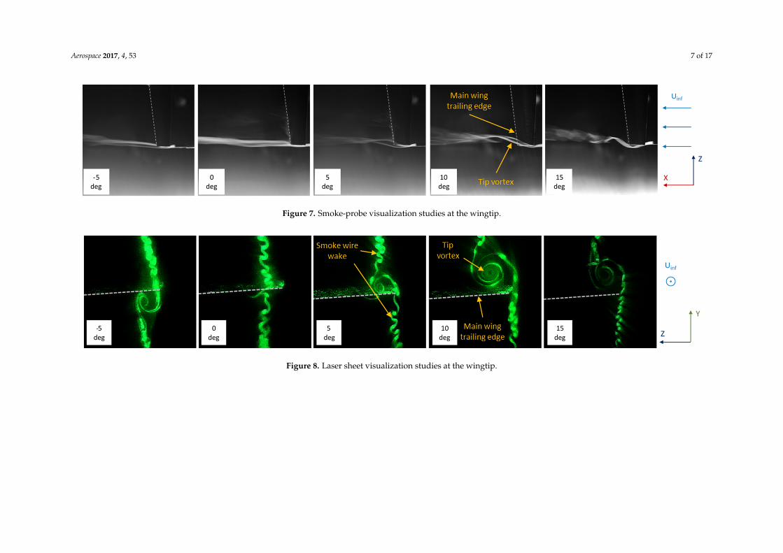
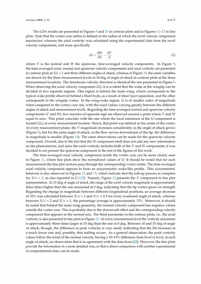
Figure 7 presents the results of the smoke-probe investigations (top view), whereas Figure 8presents the results of the combined smoke-wire/laser sheet method, at one tip chord downstream ofthe wing (X/c = 1). The corresponding planes and direction of freestream velocity are also given foreach case. As is evident, at 0 deg of angle of attack, the tip vortex is practically non-existent, since thelift production is negligible and the pressure imbalance between the two sides is very small. At −5 and5 deg, the vortex is more clearly defined, especially in the laser sheet visualization. At −5 deg of angleof attack the vortical structure is upside down, since the lift production is inverse. At 10 deg of angleof attack, the tip vortex appears to be even larger in size and robust, whereas at 15 deg, the vorticalstructure retains its size but fades quickly as the flow moves downstream of the wing. In general,the flow visualization studies may not directly provide numbers about the examined phenomenon,but they helped a long way in identifying the key-characteristics of the vortex at each angle of attack,i.e., size and core location. Thus, the LDA measurement grids could be properly sized with greateraccuracy, at a reduced time.

Aerospace 2017, 4, 53 7 of 17Aerospace 2017, 4, 53 7 of 17

Figure 7. Smoke-probe visualization studies at the wingtip.

Figure 8. Laser sheet visualization studies at the wingtip.

Figure 7. Smoke-probe visualization studies at the wingtip.

Aerospace 2017, 4, 53 7 of 17

Figure 7. Smoke-probe visualization studies at the wingtip.

Figure 8. Laser sheet visualization studies at the wingtip. Figure 8. Laser sheet visualization studies at the wingtip.

Aerospace 2017, 4, 53 8 of 17

The LDA results are presented in Figures 9 and 10 in contour plots and in Figures 11–13 in lineplots. Note that the vortex core radius is defined as the radius at which the swirl velocity componentmaximizes, whereas the axial vorticity was calculated using the experimental data from the swirlvelocity components, and more specifically

Ω =dWdΥ

− dVd

(1)

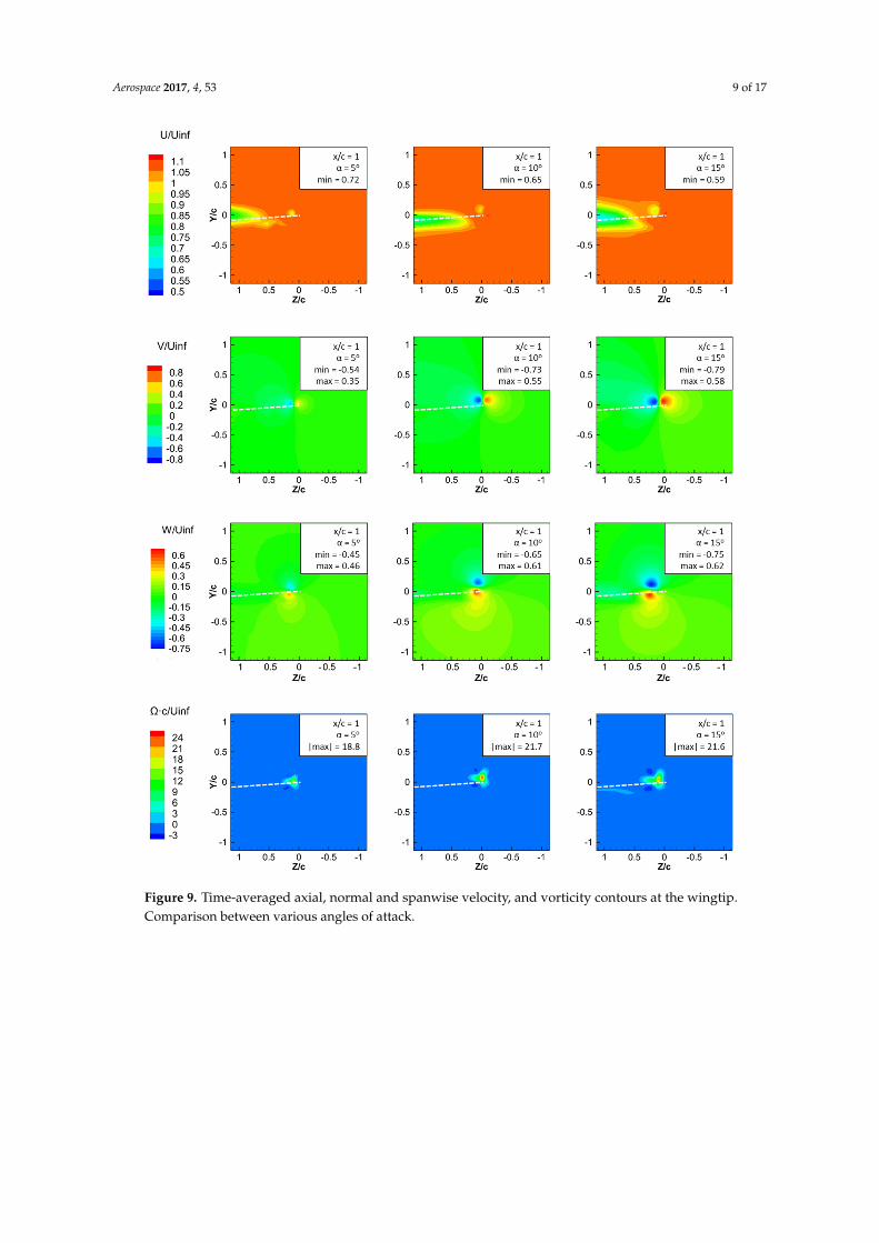
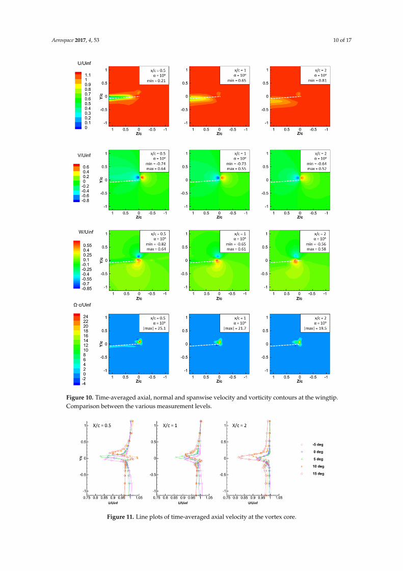
where V is the normal and W the spanwise, time-averaged velocity components. In Figure 9,the time-averaged axial, normal and spanwise velocity components and axial vorticity are presentedin contour plots at X/c = 1 and three different angles of attack, whereas in Figure 10, the same variablesare shown for the three measurement levels at 10 deg of angle of attack in contour plots at the threemeasurement locations. The freestream velocity direction is identical the one presented in Figure 8.When observing the axial velocity component (U), it is evident that the wake at the wingtip can bedivided at two separate regions. One region is behind the main wing, which corresponds to thetypical wake profile observed behind a blunt body, as a result of shear layer separation, and the othercorresponds to the wingtip vortex. In the wing-wake region, U is of smaller order of magnitudewhen compared to the vortex core one, with the exact values varying greatly between the differentangles of attack and measurement levels. Regarding the time-averaged normal and spanwise velocitycomponents (V and W), two maxima of opposite sign are observed around a point where V and Wequal to zero. This point coincides with the one where the local minimum of the U component islocated (U0) at every measurement location. Hence, that point was defined as the center of the vortex.At every measurement plane, the V magnitude increases considerably as the angle of attack grows(Figure 9), but for the same angle of attack, as the flow moves downstream of the tip, the differencein magnitude is smaller (Figure 10). The same observations can be made for the spanwise velocitycomponent. Overall, due to the fact that the W component itself does not add any new informationon the phenomenon, and since the axial vorticity includes both of the V and W components, it wasdecided to not present the spanwise component in the rest of the figures of this work.

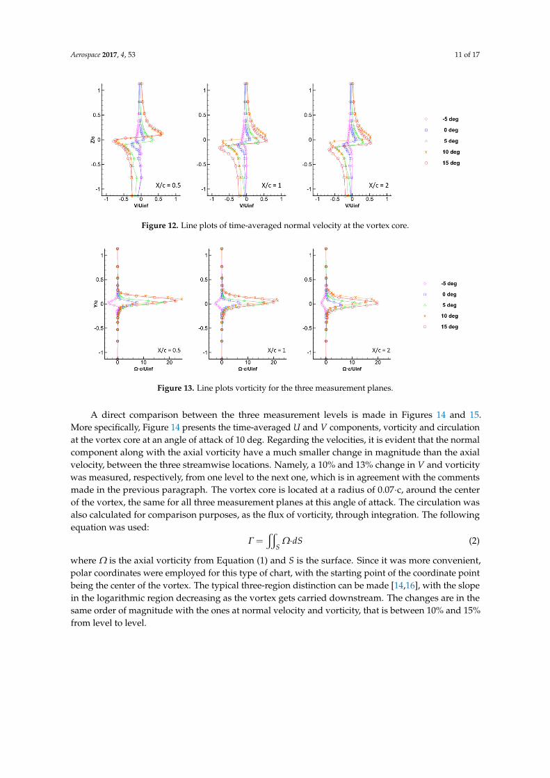
The time-averaged axial velocity component inside the vortex core can be more clearly seenin Figure 11, where line plots show the normalized values of U. It should be noted that for eachmeasurement the line plot sections pass through the corresponding vortex center. The time-averagedaxial velocity component appears to form an axisymmetric wake-like profile. This axisymmetricbehavior is also observed in Figures 12 and 13, which indicate that the roll-up process is completefor X/c < 1, as also reported in [13,25]. Namely, Figure 12 presents the V component in line plotrepresentation. At 15 deg of angle of attack, the range of the swirl velocity magnitude is approximatelythree times higher than the one measured at 0 deg, indicating that the tip vortex grows in strength.Regarding the change in magnitude between different longitudinal positions, an average decreaseof 10% was calculated between X/c = 1 and X/c = 0.5 for every examined angle of attack, whereasbetween X/c = 2 and X/c = 1, the percentage average is approximately 13%. Moreover, it shouldbe noted that behind the main wing geometry, the normal velocity component has negative valuesoutside the vortex core. This is probably due to the downwash effect and the corresponding velocitycomponent that appears in the normal axis. The third parameter in the contour plots, i.e., the axialvorticity, is also presented in line plots in Figure 13. At every measurement level the vorticity maximumis approximately three times larger at 15 deg than the one at 0 deg. Between 10 and 15 deg of angleof attack, though, the difference in peak vorticity is very small, indicating that the lift increases ata much lower rate and, possibly, that stalling occurs. As a general observation, the peak vorticityvalues follow the trend of the normal velocity, having a 10–15% difference from level to level, at eachangle of attack, an observation that is in agreement with the data from [28]. However, the line plotsprovide the information in a more detailed way, so that a direct comparison with another experimentalor computational data, can be made.

Aerospace 2017, 4, 53 9 of 17Aerospace 2017, 4, 53 9 of 17

Figure 9. Time-averaged axial, normal and spanwise velocity, and vorticity contours at the wingtip. Comparison between various angles of attack.

Figure 9. Time-averaged axial, normal and spanwise velocity, and vorticity contours at the wingtip.Comparison between various angles of attack.

Aerospace 2017, 4, 53 10 of 17Aerospace 2017, 4, 53 10 of 17

Figure 10. Time-averaged axial, normal and spanwise velocity and vorticity contours at the wingtip. Comparison between the various measurement levels.

Figure 11. Line plots of time-averaged axial velocity at the vortex core.

Figure 10. Time-averaged axial, normal and spanwise velocity and vorticity contours at the wingtip.Comparison between the various measurement levels.

Aerospace 2017, 4, 53 10 of 17

Figure 10. Time-averaged axial, normal and spanwise velocity and vorticity contours at the wingtip. Comparison between the various measurement levels.

Figure 11. Line plots of time-averaged axial velocity at the vortex core. Figure 11. Line plots of time-averaged axial velocity at the vortex core.

Aerospace 2017, 4, 53 11 of 17Aerospace 2017, 4, 53 11 of 17

Figure 12. Line plots of time-averaged normal velocity at the vortex core.

Figure 13. Line plots vorticity for the three measurement planes.

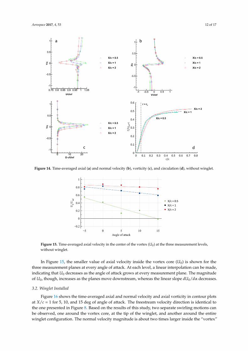
A direct comparison between the three measurement levels is made in Figures 14 and 15. More specifically, Figure 14 presents the time-averaged U and V components, vorticity and circulation at the vortex core at an angle of attack of 10 deg. Regarding the velocities, it is evident that the normal component along with the axial vorticity have a much smaller change in magnitude than the axial velocity, between the three streamwise locations. Namely, a 10% and 13% change in V and vorticity was measured, respectively, from one level to the next one, which is in agreement with the comments made in the previous paragraph. The vortex core is located at a radius of 0.07·c, around the center of the vortex, the same for all three measurement planes at this angle of attack. The circulation was also calculated for comparison purposes, as the flux of vorticity, through integration. The following equation was used: = (2)

where Ω is the axial vorticity from Equation (1) and S is the surface. Since it was more convenient, polar coordinates were employed for this type of chart, with the starting point of the coordinate point being the center of the vortex. The typical three-region distinction can be made [14,16], with the slope in the logarithmic region decreasing as the vortex gets carried downstream. The changes are in the same order of magnitude with the ones at normal velocity and vorticity, that is between 10% and 15% from level to level.

In Figure 15, the smaller value of axial velocity inside the vortex core (U0) is shown for the three measurement planes at every angle of attack. At each level, a linear interpolation can be made, indicating that U0 decreases as the angle of attack grows at every measurement plane. The magnitude of U0, though, increases as the planes move downstream, whereas the linear slope dU0/dα decreases.

Figure 12. Line plots of time-averaged normal velocity at the vortex core.

Aerospace 2017, 4, 53 11 of 17

Figure 12. Line plots of time-averaged normal velocity at the vortex core.

Figure 13. Line plots vorticity for the three measurement planes.

A direct comparison between the three measurement levels is made in Figures 14 and 15. More specifically, Figure 14 presents the time-averaged U and V components, vorticity and circulation at the vortex core at an angle of attack of 10 deg. Regarding the velocities, it is evident that the normal component along with the axial vorticity have a much smaller change in magnitude than the axial velocity, between the three streamwise locations. Namely, a 10% and 13% change in V and vorticity was measured, respectively, from one level to the next one, which is in agreement with the comments made in the previous paragraph. The vortex core is located at a radius of 0.07·c, around the center of the vortex, the same for all three measurement planes at this angle of attack. The circulation was also calculated for comparison purposes, as the flux of vorticity, through integration. The following equation was used: = (2)

where Ω is the axial vorticity from Equation (1) and S is the surface. Since it was more convenient, polar coordinates were employed for this type of chart, with the starting point of the coordinate point being the center of the vortex. The typical three-region distinction can be made [14,16], with the slope in the logarithmic region decreasing as the vortex gets carried downstream. The changes are in the same order of magnitude with the ones at normal velocity and vorticity, that is between 10% and 15% from level to level.

In Figure 15, the smaller value of axial velocity inside the vortex core (U0) is shown for the three measurement planes at every angle of attack. At each level, a linear interpolation can be made, indicating that U0 decreases as the angle of attack grows at every measurement plane. The magnitude of U0, though, increases as the planes move downstream, whereas the linear slope dU0/dα decreases.

Figure 13. Line plots vorticity for the three measurement planes.

A direct comparison between the three measurement levels is made in Figures 14 and 15.More specifically, Figure 14 presents the time-averaged U and V components, vorticity and circulationat the vortex core at an angle of attack of 10 deg. Regarding the velocities, it is evident that the normalcomponent along with the axial vorticity have a much smaller change in magnitude than the axialvelocity, between the three streamwise locations. Namely, a 10% and 13% change in V and vorticitywas measured, respectively, from one level to the next one, which is in agreement with the commentsmade in the previous paragraph. The vortex core is located at a radius of 0.07·c, around the centerof the vortex, the same for all three measurement planes at this angle of attack. The circulation wasalso calculated for comparison purposes, as the flux of vorticity, through integration. The followingequation was used:

Γ =x

SΩ·dS (2)

where Ω is the axial vorticity from Equation (1) and S is the surface. Since it was more convenient,polar coordinates were employed for this type of chart, with the starting point of the coordinate pointbeing the center of the vortex. The typical three-region distinction can be made [14,16], with the slopein the logarithmic region decreasing as the vortex gets carried downstream. The changes are in thesame order of magnitude with the ones at normal velocity and vorticity, that is between 10% and 15%from level to level.

Aerospace 2017, 4, 53 12 of 17Aerospace 2017, 4, 53 12 of 17

Figure 14. Time-averaged axial (a) and normal velocity (b), vorticity (c), and circulation (d), without winglet.

Figure 15. Time-averaged axial velocity in the center of the vortex (U0) at the three measurement levels, without winglet.

3.2. Winglet Installed

Figure 16 shows the time-averaged axial and normal velocity and axial vorticity in contour plots at X/c = 1 for 5, 10, and 15 deg of angle of attack. The freestream velocity direction is identical to the one presented in Figure 8. Based on the results of this study, two separate swirling motions can be observed, one around the vortex core, at the tip of the winglet, and another around the entire winglet configuration. The normal velocity magnitude is about two times larger inside the “vortex” region. However, a second region can be clearly observed around the entire winglet configuration, from now on referred to as the “winglet” region. In terms of vorticity, the difference is even greater, since the vorticity maximum inside the vortex core is at least three times as high, compared to the vorticity values of the “winglet” region. Hence, the “winglet” region indicates that another vortical structure exists, which may be far weaker in terms of magnitude but covers a larger area, since it spreads

Figure 14. Time-averaged axial (a) and normal velocity (b), vorticity (c), and circulation (d), without winglet.

Aerospace 2017, 4, 53 12 of 17

Figure 14. Time-averaged axial (a) and normal velocity (b), vorticity (c), and circulation (d), without winglet.

Figure 15. Time-averaged axial velocity in the center of the vortex (U0) at the three measurement levels, without winglet.

3.2. Winglet Installed

Figure 16 shows the time-averaged axial and normal velocity and axial vorticity in contour plots at X/c = 1 for 5, 10, and 15 deg of angle of attack. The freestream velocity direction is identical to the one presented in Figure 8. Based on the results of this study, two separate swirling motions can be observed, one around the vortex core, at the tip of the winglet, and another around the entire winglet configuration. The normal velocity magnitude is about two times larger inside the “vortex” region. However, a second region can be clearly observed around the entire winglet configuration, from now on referred to as the “winglet” region. In terms of vorticity, the difference is even greater, since the vorticity maximum inside the vortex core is at least three times as high, compared to the vorticity values of the “winglet” region. Hence, the “winglet” region indicates that another vortical structure exists, which may be far weaker in terms of magnitude but covers a larger area, since it spreads

Figure 15. Time-averaged axial velocity in the center of the vortex (U0) at the three measurement levels,without winglet.

In Figure 15, the smaller value of axial velocity inside the vortex core (U0) is shown for thethree measurement planes at every angle of attack. At each level, a linear interpolation can be made,indicating that U0 decreases as the angle of attack grows at every measurement plane. The magnitudeof U0, though, increases as the planes move downstream, whereas the linear slope dU0/dα decreases.

3.2. Winglet Installed

Figure 16 shows the time-averaged axial and normal velocity and axial vorticity in contour plotsat X/c = 1 for 5, 10, and 15 deg of angle of attack. The freestream velocity direction is identical tothe one presented in Figure 8. Based on the results of this study, two separate swirling motions canbe observed, one around the vortex core, at the tip of the winglet, and another around the entirewinglet configuration. The normal velocity magnitude is about two times larger inside the “vortex”

Aerospace 2017, 4, 53 13 of 17

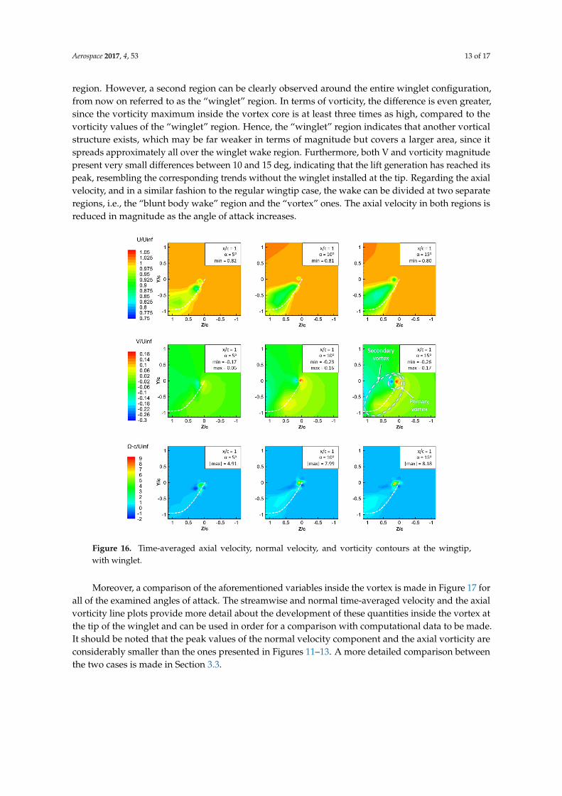
region. However, a second region can be clearly observed around the entire winglet configuration,from now on referred to as the “winglet” region. In terms of vorticity, the difference is even greater,since the vorticity maximum inside the vortex core is at least three times as high, compared to thevorticity values of the “winglet” region. Hence, the “winglet” region indicates that another vorticalstructure exists, which may be far weaker in terms of magnitude but covers a larger area, since itspreads approximately all over the winglet wake region. Furthermore, both V and vorticity magnitudepresent very small differences between 10 and 15 deg, indicating that the lift generation has reached itspeak, resembling the corresponding trends without the winglet installed at the tip. Regarding the axialvelocity, and in a similar fashion to the regular wingtip case, the wake can be divided at two separateregions, i.e., the “blunt body wake” region and the “vortex” ones. The axial velocity in both regions isreduced in magnitude as the angle of attack increases.

Aerospace 2017, 4, 53 13 of 17

approximately all over the winglet wake region. Furthermore, both V and vorticity magnitude present very small differences between 10 and 15 deg, indicating that the lift generation has reached its peak, resembling the corresponding trends without the winglet installed at the tip. Regarding the axial velocity, and in a similar fashion to the regular wingtip case, the wake can be divided at two separate regions, i.e., the “blunt body wake” region and the “vortex” ones. The axial velocity in both regions is reduced in magnitude as the angle of attack increases.

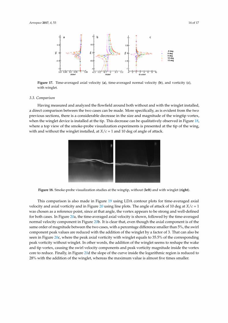
Moreover, a comparison of the aforementioned variables inside the vortex is made in Figure 17 for all of the examined angles of attack. The streamwise and normal time-averaged velocity and the axial vorticity line plots provide more detail about the development of these quantities inside the vortex at the tip of the winglet and can be used in order for a comparison with computational data to be made. It should be noted that the peak values of the normal velocity component and the axial vorticity are considerably smaller than the ones presented in Figures 11–13. A more detailed comparison between the two cases is made in Section 3.3.

Figure 16. Time-averaged axial velocity, normal velocity, and vorticity contours at the wingtip, with winglet.

Figure 17. Time-averaged axial velocity (a), time-averaged normal velocity (b), and vorticity (c), with winglet.

Figure 16. Time-averaged axial velocity, normal velocity, and vorticity contours at the wingtip,with winglet.

Moreover, a comparison of the aforementioned variables inside the vortex is made in Figure 17 forall of the examined angles of attack. The streamwise and normal time-averaged velocity and the axialvorticity line plots provide more detail about the development of these quantities inside the vortex atthe tip of the winglet and can be used in order for a comparison with computational data to be made.It should be noted that the peak values of the normal velocity component and the axial vorticity areconsiderably smaller than the ones presented in Figures 11–13. A more detailed comparison betweenthe two cases is made in Section 3.3.

Aerospace 2017, 4, 53 14 of 17

Aerospace 2017, 4, 53 13 of 17

approximately all over the winglet wake region. Furthermore, both V and vorticity magnitude present very small differences between 10 and 15 deg, indicating that the lift generation has reached its peak, resembling the corresponding trends without the winglet installed at the tip. Regarding the axial velocity, and in a similar fashion to the regular wingtip case, the wake can be divided at two separate regions, i.e., the “blunt body wake” region and the “vortex” ones. The axial velocity in both regions is reduced in magnitude as the angle of attack increases.

Moreover, a comparison of the aforementioned variables inside the vortex is made in Figure 17 for all of the examined angles of attack. The streamwise and normal time-averaged velocity and the axial vorticity line plots provide more detail about the development of these quantities inside the vortex at the tip of the winglet and can be used in order for a comparison with computational data to be made. It should be noted that the peak values of the normal velocity component and the axial vorticity are considerably smaller than the ones presented in Figures 11–13. A more detailed comparison between the two cases is made in Section 3.3.

Figure 16. Time-averaged axial velocity, normal velocity, and vorticity contours at the wingtip, with winglet.

Figure 17. Time-averaged axial velocity (a), time-averaged normal velocity (b), and vorticity (c), with winglet.

Figure 17. Time-averaged axial velocity (a), time-averaged normal velocity (b), and vorticity (c),with winglet.

3.3. Comparison

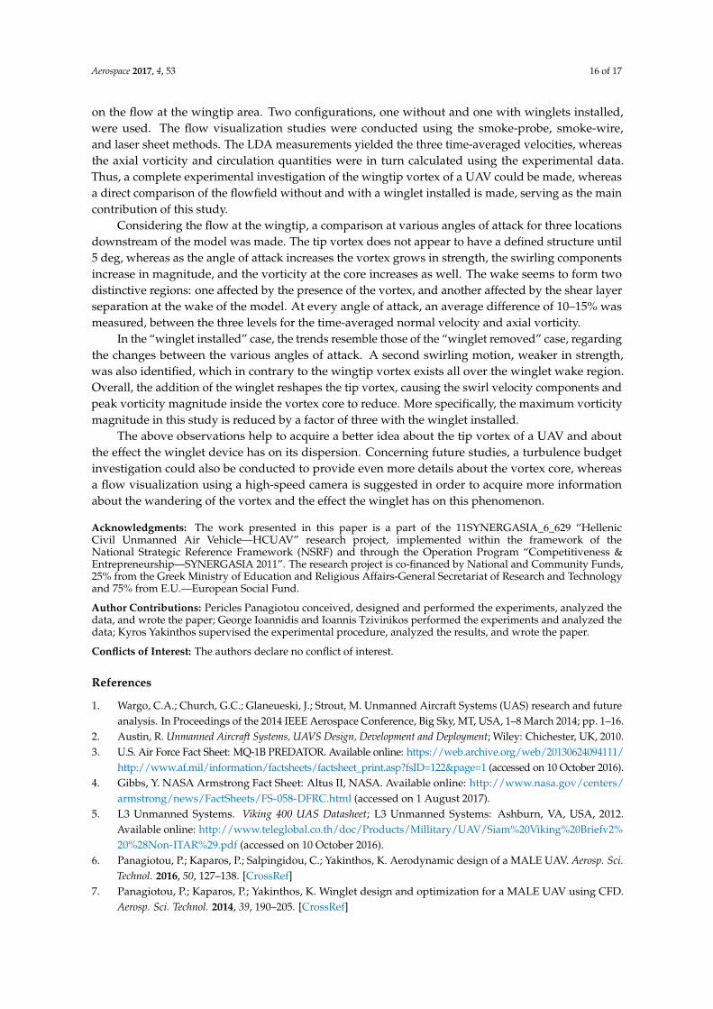
Having measured and analyzed the flowfield around both without and with the winglet installed,a direct comparison between the two cases can be made. More specifically, as is evident from the twoprevious sections, there is a considerable decrease in the size and magnitude of the wingtip vortex,when the winglet device is installed at the tip. This decrease can be qualitatively observed in Figure 18,where a top view of the smoke-probe visualization experiments is presented at the tip of the wing,with and without the winglet installed, at X/c = 1 and 10 deg of angle of attack.

Aerospace 2017, 4, 53 14 of 17

3.3. Comparison

Having measured and analyzed the flowfield around both without and with the winglet installed, a direct comparison between the two cases can be made. More specifically, as is evident from the two previous sections, there is a considerable decrease in the size and magnitude of the wingtip vortex, when the winglet device is installed at the tip. This decrease can be qualitatively observed in Figure 18, where a top view of the smoke-probe visualization experiments is presented at the tip of the wing, with and without the winglet installed, at X/c = 1 and 10 deg of angle of attack.

Figure 18. Smoke-probe visualization studies at the wingtip, without (left) and with winglet (right).

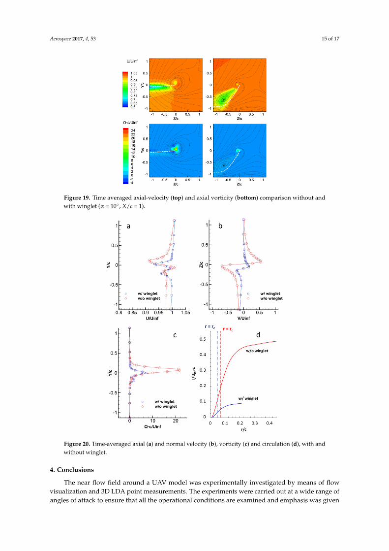
This comparison is also made in Figure 19 using LDA contour plots for time-averaged axial velocity and axial vorticity and in Figure 20 using line plots. The angle of attack of 10 deg at X/c = 1 was chosen as a reference point, since at that angle, the vortex appears to be strong and well-defined for both cases. In Figure 20a, the time-averaged axial velocity is shown, followed by the time-averaged normal velocity component in Figure 20b. It is clear that, even though the axial component is of the same order of magnitude between the two cases, with a percentage difference smaller than 5%, the swirl component peak values are reduced with the addition of the winglet by a factor of 3. That can also be seen in Figure 20c, where the peak axial vorticity with winglet equals to 35.5% of the corresponding peak vorticity without winglet. In other words, the addition of the winglet seems to reshape the wake and tip vortex, causing the swirl velocity components and peak vorticity magnitude inside the vortex core to reduce. Finally, in Figure 20d the slope of the curve inside the logarithmic region is reduced to 28% with the addition of the winglet, whereas the maximum value is almost five times smaller.

Figure 19. Time averaged axial-velocity (top) and axial vorticity (bottom) comparison without and with winglet (α = 10°, X/c = 1).

Figure 18. Smoke-probe visualization studies at the wingtip, without (left) and with winglet (right).

This comparison is also made in Figure 19 using LDA contour plots for time-averaged axialvelocity and axial vorticity and in Figure 20 using line plots. The angle of attack of 10 deg at X/c = 1was chosen as a reference point, since at that angle, the vortex appears to be strong and well-definedfor both cases. In Figure 20a, the time-averaged axial velocity is shown, followed by the time-averagednormal velocity component in Figure 20b. It is clear that, even though the axial component is of thesame order of magnitude between the two cases, with a percentage difference smaller than 5%, the swirlcomponent peak values are reduced with the addition of the winglet by a factor of 3. That can also beseen in Figure 20c, where the peak axial vorticity with winglet equals to 35.5% of the correspondingpeak vorticity without winglet. In other words, the addition of the winglet seems to reshape the wakeand tip vortex, causing the swirl velocity components and peak vorticity magnitude inside the vortexcore to reduce. Finally, in Figure 20d the slope of the curve inside the logarithmic region is reduced to28% with the addition of the winglet, whereas the maximum value is almost five times smaller.

Aerospace 2017, 4, 53 15 of 17

Aerospace 2017, 4, 53 14 of 17

3.3. Comparison

Having measured and analyzed the flowfield around both without and with the winglet installed, a direct comparison between the two cases can be made. More specifically, as is evident from the two previous sections, there is a considerable decrease in the size and magnitude of the wingtip vortex, when the winglet device is installed at the tip. This decrease can be qualitatively observed in Figure 18, where a top view of the smoke-probe visualization experiments is presented at the tip of the wing, with and without the winglet installed, at X/c = 1 and 10 deg of angle of attack.

Figure 18. Smoke-probe visualization studies at the wingtip, without (left) and with winglet (right).

This comparison is also made in Figure 19 using LDA contour plots for time-averaged axial velocity and axial vorticity and in Figure 20 using line plots. The angle of attack of 10 deg at X/c = 1 was chosen as a reference point, since at that angle, the vortex appears to be strong and well-defined for both cases. In Figure 20a, the time-averaged axial velocity is shown, followed by the time-averaged normal velocity component in Figure 20b. It is clear that, even though the axial component is of the same order of magnitude between the two cases, with a percentage difference smaller than 5%, the swirl component peak values are reduced with the addition of the winglet by a factor of 3. That can also be seen in Figure 20c, where the peak axial vorticity with winglet equals to 35.5% of the corresponding peak vorticity without winglet. In other words, the addition of the winglet seems to reshape the wake and tip vortex, causing the swirl velocity components and peak vorticity magnitude inside the vortex core to reduce. Finally, in Figure 20d the slope of the curve inside the logarithmic region is reduced to 28% with the addition of the winglet, whereas the maximum value is almost five times smaller.

Figure 19. Time averaged axial-velocity (top) and axial vorticity (bottom) comparison without and with winglet (α = 10°, X/c = 1).

Figure 19. Time averaged axial-velocity (top) and axial vorticity (bottom) comparison without andwith winglet (α = 10, X/c = 1).

Aerospace 2017, 4, 53 15 of 17

Figure 20. Time-averaged axial (a) and normal velocity (b), vorticity (c) and circulation (d), with and without winglet.

4. Conclusions

The near flow field around a UAV model was experimentally investigated by means of flow visualization and 3D LDA point measurements. The experiments were carried out at a wide range of angles of attack to ensure that all the operational conditions are examined and emphasis was given on the flow at the wingtip area. Two configurations, one without and one with winglets installed, were used. The flow visualization studies were conducted using the smoke-probe, smoke-wire, and laser sheet methods. The LDA measurements yielded the three time-averaged velocities, whereas the axial vorticity and circulation quantities were in turn calculated using the experimental data. Thus, a complete experimental investigation of the wingtip vortex of a UAV could be made, whereas a direct comparison of the flowfield without and with a winglet installed is made, serving as the main contribution of this study.

Considering the flow at the wingtip, a comparison at various angles of attack for three locations downstream of the model was made. The tip vortex does not appear to have a defined structure until 5 deg, whereas as the angle of attack increases the vortex grows in strength, the swirling components increase in magnitude, and the vorticity at the core increases as well. The wake seems to form two distinctive regions: one affected by the presence of the vortex, and another affected by the shear layer separation at the wake of the model. At every angle of attack, an average difference of 10–15% was measured, between the three levels for the time-averaged normal velocity and axial vorticity.

In the “winglet installed” case, the trends resemble those of the “winglet removed” case, regarding the changes between the various angles of attack. A second swirling motion, weaker in strength, was also identified, which in contrary to the wingtip vortex exists all over the winglet wake region. Overall, the addition of the winglet reshapes the tip vortex, causing the swirl velocity

Figure 20. Time-averaged axial (a) and normal velocity (b), vorticity (c) and circulation (d), with andwithout winglet.

4. Conclusions

The near flow field around a UAV model was experimentally investigated by means of flowvisualization and 3D LDA point measurements. The experiments were carried out at a wide range ofangles of attack to ensure that all the operational conditions are examined and emphasis was given

Aerospace 2017, 4, 53 16 of 17

on the flow at the wingtip area. Two configurations, one without and one with winglets installed,were used. The flow visualization studies were conducted using the smoke-probe, smoke-wire,and laser sheet methods. The LDA measurements yielded the three time-averaged velocities, whereasthe axial vorticity and circulation quantities were in turn calculated using the experimental data.Thus, a complete experimental investigation of the wingtip vortex of a UAV could be made, whereasa direct comparison of the flowfield without and with a winglet installed is made, serving as the maincontribution of this study.

Considering the flow at the wingtip, a comparison at various angles of attack for three locationsdownstream of the model was made. The tip vortex does not appear to have a defined structure until5 deg, whereas as the angle of attack increases the vortex grows in strength, the swirling componentsincrease in magnitude, and the vorticity at the core increases as well. The wake seems to form twodistinctive regions: one affected by the presence of the vortex, and another affected by the shear layerseparation at the wake of the model. At every angle of attack, an average difference of 10–15% wasmeasured, between the three levels for the time-averaged normal velocity and axial vorticity.

In the “winglet installed” case, the trends resemble those of the “winglet removed” case, regardingthe changes between the various angles of attack. A second swirling motion, weaker in strength,was also identified, which in contrary to the wingtip vortex exists all over the winglet wake region.Overall, the addition of the winglet reshapes the tip vortex, causing the swirl velocity components andpeak vorticity magnitude inside the vortex core to reduce. More specifically, the maximum vorticitymagnitude in this study is reduced by a factor of three with the winglet installed.

The above observations help to acquire a better idea about the tip vortex of a UAV and aboutthe effect the winglet device has on its dispersion. Concerning future studies, a turbulence budgetinvestigation could also be conducted to provide even more details about the vortex core, whereasa flow visualization using a high-speed camera is suggested in order to acquire more informationabout the wandering of the vortex and the effect the winglet has on this phenomenon.

Acknowledgments: The work presented in this paper is a part of the 11SYNERGASIA_6_629 “HellenicCivil Unmanned Air Vehicle—HCUAV” research project, implemented within the framework of theNational Strategic Reference Framework (NSRF) and through the Operation Program “Competitiveness &Entrepreneurship—SYNERGASIA 2011”. The research project is co-financed by National and Community Funds,25% from the Greek Ministry of Education and Religious Affairs-General Secretariat of Research and Technologyand 75% from E.U.—European Social Fund.

Author Contributions: Pericles Panagiotou conceived, designed and performed the experiments, analyzed thedata, and wrote the paper; George Ioannidis and Ioannis Tzivinikos performed the experiments and analyzed thedata; Kyros Yakinthos supervised the experimental procedure, analyzed the results, and wrote the paper.

Conflicts of Interest: The authors declare no conflict of interest.

References

1. Wargo, C.A.; Church, G.C.; Glaneueski, J.; Strout, M. Unmanned Aircraft Systems (UAS) research and futureanalysis. In Proceedings of the 2014 IEEE Aerospace Conference, Big Sky, MT, USA, 1–8 March 2014; pp. 1–16.

2. Austin, R. Unmanned Aircraft Systems, UAVS Design, Development and Deployment; Wiley: Chichester, UK, 2010.3. U.S. Air Force Fact Sheet: MQ-1B PREDATOR. Available online: https://web.archive.org/web/20130624094111/

http://www.af.mil/information/factsheets/factsheet_print.asp?fsID=122&page=1 (accessed on 10 October 2016).4. Gibbs, Y. NASA Armstrong Fact Sheet: Altus II, NASA. Available online: http://www.nasa.gov/centers/

armstrong/news/FactSheets/FS-058-DFRC.html (accessed on 1 August 2017).5. L3 Unmanned Systems. Viking 400 UAS Datasheet; L3 Unmanned Systems: Ashburn, VA, USA, 2012.

Available online: http://www.teleglobal.co.th/doc/Products/Millitary/UAV/Siam%20Viking%20Briefv2%20%28Non-ITAR%29.pdf (accessed on 10 October 2016).

6. Panagiotou, P.; Kaparos, P.; Salpingidou, C.; Yakinthos, K. Aerodynamic design of a MALE UAV. Aerosp. Sci.Technol. 2016, 50, 127–138. [CrossRef]

7. Panagiotou, P.; Kaparos, P.; Yakinthos, K. Winglet design and optimization for a MALE UAV using CFD.Aerosp. Sci. Technol. 2014, 39, 190–205. [CrossRef]

Aerospace 2017, 4, 53 17 of 17

8. Anderson, J.D. Fundamentals of Aerodynamics, 5th ed.; McGraw-Hill: New York, NY, USA, 2011; p. 415.9. Whitcomb, R.T. A Design Approach and Selected Wind-Tunnel Results at High Subsonic Speeds for Wing-Tip

Mounted Winglets; NASA Langley Research Center: Hampton, VA, USA, 1976.10. Maughmer, M.D.; Timothy, S.S.; Willits, S.M. The Design and Testing of a Winglet Airfoil for Low-Speed

Aircraft. AIAA J. 2001, 39, 654–661.11. Heyson, H.H.; Riebe, G.D.; Fulton, C.L. Theoretical Parametric Study of the Relative Advantages of Winglets and

Wing-Tip Extensions; NASA Langley Research Center: Hampton, VA, USA, 1977.12. Weierman, J.R.; Jacob, J.D. Winglet Design and Optimization for UAVs; American Institute of Aeronautics and

Astronautics: Chicago, IL, USA, 2010.13. Jacobs, E.N.; Sherman, A. Experimental Results of Winglets on First, Second, and Third Generation Jet Transports;

NASA Langley Research Center: Hampton, VA, USA, 1978.14. Asai, K. Theoretical considerations in the aerodynamic effectiveness of winglets. J. Aircr. 1985, 22, 635–637.

[CrossRef]15. Shekarriz, A.; Fu, T.C.; Katz, J.; Huang, T. Near-field behavior of a tip vortex. AIAA J. 1993, 31, 112–118.

[CrossRef]16. Hoffmann, E.R.; Joubert, P.N. Turbulent line vortices. J. Fluid Mech. 1963, 16, 395–411. [CrossRef]17. Nielsen, J.N.; Schwind, R.G. Decay of a Vortex Pair behind an Aircraft. In Aircraft Wake Turbulence and Its

Detection; Olsen, J.H., Goldburg, A., Rogers, M., Eds.; Springer: Boston, MA, USA, 1971; pp. 413–454.18. Corsiglia, V.R.; Schwind, R.G.; Chigier, N.A. Rapid Scanning, Three-Dimensional Hot-Wire Anemometer

Surveys of Wing-Tip Vortices. J. Aircr. 1973, 10, 752–757. [CrossRef]19. Baker, G.R.; Barker, S.J.; Bofah, K.K.; Saffman, P.G. Laser anemometer measurements of trailing vortices in

water. J. Fluid Mech. 1974, 65, 325–336. [CrossRef]20. Devenport, W.J.; Rife, M.C.; Liapis, S.I.; Follin, G.J. The structure and development of a wing-tip vortex.

J. Fluid Mech. 1996, 312, 67–106. [CrossRef]21. Chow, J.S.; Zilliac, G.G.; Bradshaw, P. Mean and Turbulence Measurements in the Near Field of a Wingtip

Vortex. AIAA J. 1997, 35, 1561–1567. [CrossRef]22. Del Pino, C.; López-Alonso, J.M.; Parras, L.; Fernandez-Feria, R. Dynamics of the wing-tip vortex in the near

field of a NACA 0012 aerofoil. Aeronaut. J. 2011, 115, 229–239. [CrossRef]23. Edstrand, A.M.; Davis, T.B.; Schmid, P.J.; Taira, K.; Cattafesta, L.N. On the mechanism of trailing vortex

wandering. J. Fluid Mech. 2016, 801. [CrossRef]24. Huang, R.F.; Lin, C.L. Vortex shedding and shear-layer instability of wing at low-Reynolds numbers. AIAA J.

1995, 33, 1398–1403. [CrossRef]25. Del Pino, C.; Parras, L.; Felli, M.; Fernandez-Feria, R. Structure of trailing vortices: Comparison between

particle image velocimetry measurements and theoretical models. Phys. Fluids 2011, 23, 013602. [CrossRef]26. Serrano-Aguilera, J.J.; García-Ortiz, J.H.; Gallardo-Claros, A.; Parras, L.; del Pino, C. Experimental

characterization of wingtip vortices in the near field using smoke flow visualizations. Exp. Fluids 2016, 57,137. [CrossRef]

27. Zheng, Y.; Ramaprian, B.R. An Experimental Study of Wing Tip Vortex in the Near Wake of a Rectangular Wing;DTIC Document; Report No. MME-TF-93–1; Washington State University: Pullman, WA, USA, 1993.

28. Elsayed, O.A.; Asrar, W.; Omar, A.A.; Kwon, K.; Jung, H. Experimental Investigation of Plain- andFlapped-Wing Tip Vortex. J. Aircr. 2009, 46, 254–262. [CrossRef]

29. Muthusamy, N.; Kumar, S.V.; Senthilkumar, C. Force Measurement on Aircraft Model with and withoutWinglet Using Low Speed Wind Tunnel. Int. J. Eng. Technol. 2015, 6, 2521–2530.

30. Selig, M.S.; Maughmer, M.D.; Somers, D.M. Natural-laminar-flow airfoil for general-aviation applications.J. Aircr. 1995, 32, 710–715. [CrossRef]

31. Barlow, J.B.; Rae, W.H.; Pope, A. Low-Speed Wind Tunnel Testing, 3rd ed.; Wiley: New York, NY, USA, 1999.32. Dol, S.S.; Nor, M.A.M.; Kamaruzaman, M.K. An Improved Smoke-Wire Flow Visualization Technique.

In Proceedings of the 4th WSEAS International Conference on Fluid Mechanics and Aerodynamics,Crete Island, Greece, 21–23 August 2006; pp. 21–23.

© 2017 by the authors. Licensee MDPI, Basel, Switzerland. This article is an open accessarticle distributed under the terms and conditions of the Creative Commons Attribution(CC BY) license (http://creativecommons.org/licenses/by/4.0/).