Robotics and Computer-Integrated Manufacturing 26 (2010) 799–804

Contents lists available at ScienceDirect

Robotics and Computer-Integrated Manufacturing

0736-58

doi:10.1

n Corr

E-m

journal homepage: www.elsevier.com/locate/rcim

Experimental kinematic calibration of parallel manipulators using a relativeposition error measurement system

Mansour Abtahi, Hodjat Pendar, Aria Alasty n, Gholamreza Vossoughi

Center of Excellence in Design, Robotics & Automation (CEDRA), Department of Mechanical Engineering, Sharif University of Technology, Azadi Ave, 1458889694 Tehran, Iran

a r t i c l e i n f o

Article history:

Received 20 January 2009

Received in revised form

27 September 2009

Accepted 15 May 2010

Keywords:

Calibration

Parallel robots

Hexaglide manipulator

Geometric parameters

Optimization

45/$ - see front matter & 2010 Elsevier Ltd. A

016/j.rcim.2010.05.007

esponding author. Tel.: +98 21 6616 5504; fa

ail address: aalasti@sharif.edu (A. Alasty).

a b s t r a c t

Because of errors in the geometric parameters of parallel robots, it is necessary to calibrate them to

improve the positioning accuracy for accurate task performance. Traditionally, to perform system

calibration, one needs to measure a number of robot poses using an external measuring device.

However, this process is often time-consuming, expensive and difficult for robot on-line calibration. In

this paper, a methodical way of calibration of parallel robots is introduced. This method is performable

only by measuring joint variable vector and positioning differences relative to a constant position in

some sets of configurations that the desired positions in each set are fixed, but the moving platform

orientations are different. In this method, measurements are relative, so it can be performed by using a

simple measurement device. Simulations and experimental studies on a Hexaglide parallel robot built

in the Sharif University of Technology reveal the convenience and effectiveness of the proposed robot

calibration method for parallel robots.

& 2010 Elsevier Ltd. All rights reserved.

1. Introduction

Compared to serial manipulators, parallel mechanisms mayexhibit a much better repeatability [1], but their large number oflinks and passive joints often limit their performance in terms ofaccuracy [2]. So calibration methods have to be implemented tocompensate the geometric parameter errors.

The algorithms proposed to conduct calibration for parallelmanipulators can be classified into two categories: the externalcalibration methods and the self-calibration methods. The externalcalibration requires measurement of whole or local poses usingsome external measurement devices. Zhuang et al. [3] usingcommercial electronic theodolite, Nahvi et al. [4] using LVDTsensors, Vincze et al. [5] using laser tracking system and Renaudet al. [6] using camera system are some instances of this category.

The second category is referred to as the self-calibrationmethod, which was first proposed by Everett [7] on a closed-loopmechanism, and was first implemented on a serial manipulator byBennet and Hollerbach [8]. The self-calibration methods may beperformed by adding redundant sensors or by imposing mobilityconstraints to the system. Zhuang and Liu [9] showed that two ormore redundant sensors are adequate to calibrate a Stewartplatform. By using redundant sensors, extra information for thesampled configurations can be obtained, by installing rotarysensors on the passive universal joints of robot [10–13] or by

ll rights reserved.

x: +98 21 6600 0021.

installing displacement sensors between the base and the end-effector of the robot [14,15]. Mobility constraints on the end-effector or on the kinematic chains connecting the base and themoving platform also can be used to obtain extra information andachieve calibration [16–19]. Abtahi et al. [20] proposed acalibration method that applies to parallel kinematic manipulator(PKM) with non-backdrivable linear actuators.

In this paper, a novel calibration method applicable to parallelrobots is presented. In this method the platform is commanded tosome sets of poses that in each set of poses, desired positions aresame but orientations are different. Because of using nominalgeometric parameters of the robot in controlling system insteadof real geometric parameters, there exist some positioningdifferences. This method uses the input joint variables and thesedifferences measured by a simple measurement system tocalibrate the robot and obtain calibrated values of the geometricparameters.

The paper is organized as follows: in Section 2, we present thecalibration method, the description and the kinematic analysis ofthe Hexaglide parallel robot; after that the simulation andexperimental results will be given in Section 3 and finallyconclusion is drawn in Section 4.

2. The calibration method

Consider a 6-DOF parallel manipulator. Obviously, it canapproach a given point in different directions. So, for any given

M. Abtahi et al. / Robotics and Computer-Integrated Manufacturing 26 (2010) 799–804800

position of the end-effector, there are many sets of input jointvariables where their configurations and orientations are different.Because of using nominal geometric parameters in controllingsystem of the robot instead of real geometric parameters, itsperformance is not accurate. So positions of these sets ofconfigurations are not precisely same and there exist someposition differences between them. In this method, these differ-ences can be measured with respect to one of them by using asimple relative position measurement system. By using thesedifferences and input joint variables as input data for calibrationprocedure, real geometric parameters can be obtained and therobot can be calibrated. It is not necessary to know the position ororientations of the end-effector with respect to the base.

The input data for calibration are only vectors of joint variablesmeasured by sensors installed on the actuated joints and positiondifferences measured by a measurement device that is composedof three distance gauges as shown in Fig. 1. These distance gaugesthat have a flat plate as probe are located in three perpendiculardirections around an accurate ball installed on the center of theend-effector. The following measurement sequences can beproposed for the measurement process:

1.

At first, command the robot to a suitable pose with a definitedesired point. Install dial gauges around the ball. These gaugesmust be parallel to principal directions and aligned with centerof the ball, as shown in Fig. 1. Zero out distance gauges andwrite down the input joint variables and errors in dial gaugesthat are zero.

2.

Command the robot to the next configuration so that itsorientation is different. There will probably be some deviationsin the distance gauges from zero. Write down these deviationsand input joint variables.

3.

If any other orientation is considered, then go to step 2; else goto step 1 with a different desired point.

According to this measurement process, in each set of pose, theposition differences are measured with regard to the first positionof each set. For implementing these sequences, other measurementdevices can be used instead of dial gauges, e.g. laser interferom-eters or linear variable differential transformers (LVDTs).

Now, in order to formulate this method, the joint variablevector is denoted by q, where

q¼ q1 q2 q3 q4 q5 q6

h iTð1Þ

The position and pose vectors of the end-effector are denotedby P and w, respectively, which are defined as

P¼ Px Py Pz

h i

Fig. 1. Three distance gauges used as a measurement system.

w¼ Px Py Pz a b gh iT

ð2Þ

where a, b and g are the rotation angles of the end-effector. Thegeometric parameter vector that has N parameters is shown by dand the position difference vector is denoted by d, which isdefined as

d¼ dx dy dz

h iTð3Þ

The number of sets or commanded points is denoted by m andthe number of poses or orientations in each set is denoted by k.The end-effector position vector for each joint variable vector canbe calculated by the forward kinematic of the desired robot as

jPrc ¼ Fðjqr ,dÞ ð4Þ

where jqr is the measured joint variable vector in the jth point andin the rth orientation and jPr

c is the calculated end-effectorposition vector with jqr . Since the position difference vector ismeasured relative to a constant point for all the configurations inthe jth point, it can be written as

99ðjP rc�

jdrÞ�ðjPn

c�jdnÞ99¼ 0

ðranÞ r¼ 1,. . .,k n¼ 1,. . .,k ð5Þ

where jdr is the measured position difference vector in the jthpoint and in the rth orientation. Now the error vector can bedefined as

E¼

1E2E

^mE

266664

377775

ð6Þ

where

jE ¼

jp1c�

jd1Þ�ðjp2c�

jd2� �

jp1c�

jd1�ðjp3c�

jd3� �

^jp1

c�jd1Þ�ðjpk

c�jdk

� �

jp2c�

jd1Þ�ðjp3c�

jd3� �

^jpk�1

c �jdk�1Þ�ðjpk

c�jdk

� �

2666666666666666664

3777777777777777775

ð7Þ

While jE have 3k(k�1)/2 elements, E have 3mk(k�1)/2elements. The error vector is a nonlinear function of the geometricparameter vector d and the input data of calibration. So we have

EM�1 ¼ EðdN�1,Q ,DÞ

M¼ 3mkðk�1Þ=2 ð8Þ

where Q and D are, respectively, the set of measured joint variablevectors and the set of measured position difference vectors thatare defined as

Q ¼ f1q1,. . .,1qk,2q1,. . .,mqkg

D¼ f1d1,. . .,1dk,2d1,. . .,mdkg ð9Þ

E is ideally equal to the zero vector for the real values of thegeometric parameter vector dr:

E¼ Eðdr ,Q ,DÞ ¼ 0M�1 ð10Þ

Because of nonlinearity of E, the Gauss–Newton method [21] istypically employed to estimate this nonlinear function. First,consider input data Q and D as constant numbers and absorb

M. Abtahi et al. / Robotics and Computer-Integrated Manufacturing 26 (2010) 799–804 801

them into the nonlinear function E. The model is linearizedthrough a Taylor series expansion at a current estimate dl of theparameter vector at iteration l

Ec ¼ EðdlþDdÞ

¼ EðdlÞþ@EðdÞ@d d ¼ dlDdþh:o:t� EðdlÞþADd

��� ð11Þ

where Ec is the computed value of the vector E and A¼ @E=@d is aJacobian matrix evaluated at dl. Higher-order terms in the Taylorseries are ignored, yielding the linearized form of (11). By definingDE¼ Ec�EðdlÞ as the error between the desired value Ec¼E¼0 andthe predicted value with the current parameter vector dl, thelinearized Equation (11) becomes

DE¼ Ec�EðdlÞ ¼ �EðdlÞ ¼ ADd ð12Þ

Now by using ordinary least squares, we have

dlþ1¼ dl�ðAT AÞ�1AT EðdlÞ ð13Þ

This process has to be iterated until the error Dd becomessufficiently small. The Gauss–Newton method is very fast,provided that there is a good initial estimate d0 of the geometricparameter vector. Nominal geometric parameter vector dn can beused as the initial estimate.

As another approach for solving this nonlinear optimizationproblem, nonlinear least-square function (lsqnonlin) of MATLABcan be used. This method is not as fast as the Gauss–Newtonmethod but does not need obtaining jacobian matrix A.

3. Simulation and experimental results

3.1. Simulation results

With the calibration method proposed above, we would like tocalibrate a Hexaglide parallel robot. The first Hexaglide parallelrobot has been developed at ETH Zurich [22]. As shown in Fig. 2,Hexaglide is composed of a moving platform that is connected tothe six legs through universal joints and these legs are connectedto six linear actuators or sliders through spherical joints. Thesesliders that are distributed on three parallel rails are actuated byball screws and servo motors. Movements of the sliders or thespherical joints guide the platform in 6 DOF.

Fig. 2. Hexaglide parallel robot.

As shown in Fig. 3, two coordinate systems are used formodeling of this robot. Global coordinate system is fixed to thebase frame and local coordinate system is fixed to the movingplatform whereas its origin is the end-effector center point. Thegeometric parameter vector of this robot can be defined as [20]

d¼ BT1 BT

2 . . . BT6 ST

1 ST2 . . . ST

6 l1 l2 . . . l6h i

ð14Þ

where Bi is the universal joint position vector defined in the localcoordinate system, Si is the spherical joint position vector definedin the global coordinate system when the corresponding jointvariable, qi, is zero and li is length of the ith leg. Thus there are 42geometric parameters (18 coordinates of points Si, 18 coordinatesof points Bi with respect to the local coordinate system and 6lengths of legs) that must be calculated through the calibrationmethod but by selecting the coordinate systems in an appropriateposition and directions, the number of unknown geometricparameters can be reduced to 35 [20].

The kinematic and singularity analysis of the Hexaglideparallel robot has been studied in [23]. A Hexaglide robot’s actualand nominal parameters given in Table 1 have been consideredfor the simulation and this calibration method has beenimplemented on it. The errors on the geometric parametershave been randomly distributed while these are between �7 and7 mm.

This method has been simulated with different numbers ofpoints (m¼1, 2,y, 5) and different numbers of orientations ineach point (k¼5, 11) to show the effect of these conditions oncalibration accuracy. If a sufficient number of iteration steps areconsidered then the calibration error will be zero up to thenumerical calculation precision. To compare the speed andprecision of convergence with different numbers of points andorientations, the number of iteration steps is considered limited.Also to simulate real conditions of calibration, we have consideredrandom noises of 0.01 mm on the input data for calibration thatare joint variable vectors that are measured by the encodersinstalled on the servo motors and the position differencesmeasured by a relative position error measurement device. Thisnoise is much greater than the error on commercial encoders thathave a precision of about 2.4 mm.

After simulating and obtaining the results, maximum errors onthe geometric parameters with regard to the number of pointshave been shown in Fig. 4 while the number of orientation was11, with noise and without noise on measurement system. Thisdiagram shows that the real value of geometric parameterscannot be obtained by using measurement data of one point, someasurement data of at least two different points are needed.If noise has not been considered, using two or more sets of data,including about 11 orientations for each point, will lead toidentification of the real value of the geometric parameters witha precision of 5�10�2 mm. In noisy conditions, the real value of

Fig. 3. Hexaglide parallel robot with notation.

Table 1Actual and nominal values of the geometric parameters (mm).

Nominal Actual

x y z x y z

S1 0 �155 0 0.861 �160.815 1.501

S2 0 0 0 0 0 0

S3 0 155 0 �0.292 152.940 0

S4 0 155 0 �2.822 154.699 1.649

S5 0 0 0 5.006 �3.088 �1.913

S6 0 �155 0 �1.645 �156.057 3.185

B1 �90 �67 �125 �87.446 �63.909 �123.485

B2 �100 56 �120 �102.404 54.881 �118.309

B3 �39 110 �120 �33.782 113.953 �118.309

B4 39 110 �120 44.446 109.800 �118.300

B5 100 56 �120 103.096 54.881 �118.309

B6 90 �67 �125 86.346 �67.912 �130.613

l1 590 583.941

l2 580 578.279

l3 615 610.563

l4 615 614.068

l5 580 585.272

l6 590 593.461

Fig. 4. The maximum error on the geometric parameters with 11 orientations in

each point.

Fig. 5. The maximum error on the geometric parameters with five orientations in

each point.

Table 2Errors of nominal and calibrated parameters (mm).

Nominal Actual

x y z x y z

S1 0.861 �5.815 1.501 �0.023 �0.096 �0.018

S2 0 0 0 �0.087 �0.024 �0.172

S3 �0.292 �2.060 0 �0.050 0.031 �0.172

S4 �2.822 �0.301 1.649 �0.025 �0.022 �0.170

S5 5.006 �3.088 �1.913 0.062 �0.024 �0.172

S6 �1.645 �1.057 3.185 0.170 �0.087 �0.088

B1 2.554 3.091 1.515 0.177 �0.121 0.378

B2 �2.404 �1.119 1.691 0.000 0.000 0.000

B3 5.218 3.953 1.691 0.091 0.082 0.000

B4 5.446 �0.200 1.700 0.226 �0.021 �0.359

B5 3.096 �1.119 1.691 0.437 �0.115 �0.453

B6 �3.654 �0.912 �5.613 0.572 �0.254 �0.376

l1 �6.059 �0.176

l2 �1.721 0.091

l3 �4.437 0.060

l4 �0.932 0.310

l5 5.272 0.456

l6 3.461 0.475

M. Abtahi et al. / Robotics and Computer-Integrated Manufacturing 26 (2010) 799–804802

the geometric parameters can be obtained by using data of fivepoints, with a precision of 6�10�1 mm.

Similarly Fig. 5 gives the maximum error on the geometricparameters with regard to the number of points while the numberof orientations is five. This shows that this robot cannot becalibrated by using data of two or three points while there are fiveorientations in each point. From Figs. 4 and 5, it can be deducedthat when the number of points increases, the maximum errorwill decrease. In practice two or more points with over tenorientations in each point can be used to calibrate the robot.

Errors of the geometric parameters before (nominal values) andafter (calibrated values) the calibration by using measurement dataof 5 points and 11 orientations in each point are given in Table 2.

3.2. Experimental results

For validating the efficiency and generality of the calibrationmethod for industrial applications, a calibration experiment isalso conducted. This calibration method has been tested on a

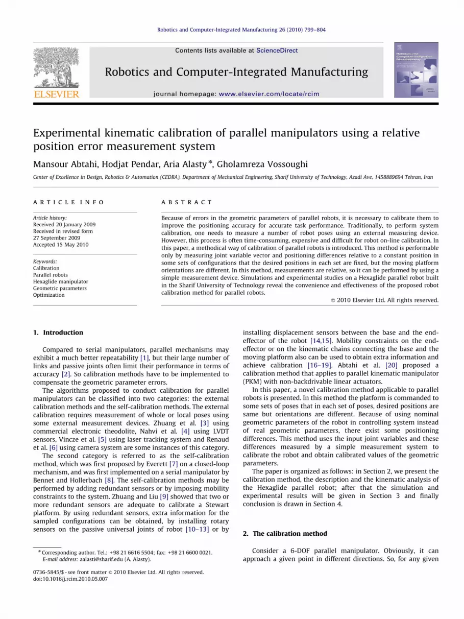
Hexaglide parallel robot built in the Sharif University ofTechnology, shown in Fig. 6.

As shown in Fig. 7, the proposed measurement device with0.01 mm accuracy for measuring position differences in thiscalibration method is implemented. Three flat probes with 10 mmdiameter have been installed on the tip of the dial gauges. Formeasurement process, six different points listed in Table 3 havebeen considered while there are 20 configurations in each point.Measurements from the first three points were employed tocalibrate the Hexaglide parallel robot and the last three pointswere utilized to verify the calibration method. The nominal andcalibrated parameters of the Hexaglide parallel robot are shownin Table 4.

After the calibrating kinematic parameters of the Hexaglideparallel robot, a verification measurement was performed. Thepurpose of the calibration is to increase the accuracy of the robot.Position differences of different orientations to reach a given pointcan show the accuracy of the robot. So results of measurementprocess before and after calibrating can be adopted as a

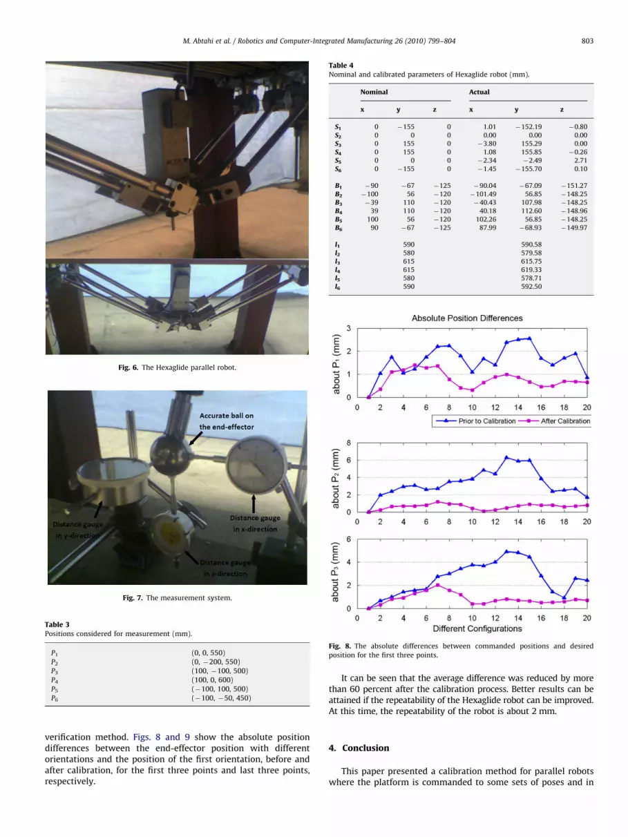
Fig. 6. The Hexaglide parallel robot.

Fig. 7. The measurement system.

Table 3Positions considered for measurement (mm).

P1 (0, 0, 550)

P2 (0, �200, 550)

P3 (100, �100, 500)

P4 (100, 0, 600)

P5 (�100, 100, 500)

P6 (�100, �50, 450)

Table 4Nominal and calibrated parameters of Hexaglide robot (mm).

Nominal Actual

x y z x y z

S1 0 �155 0 1.01 �152.19 �0.80

S2 0 0 0 0.00 0.00 0.00

S3 0 155 0 �3.80 155.29 0.00

S4 0 155 0 1.08 155.85 �0.26

S5 0 0 0 �2.34 �2.49 2.71

S6 0 �155 0 �1.45 �155.70 0.10

B1 �90 �67 �125 �90.04 �67.09 �151.27

B2 �100 56 �120 �101.49 56.85 �148.25

B3 �39 110 �120 �40.43 107.98 �148.25

B4 39 110 �120 40.18 112.60 �148.96

B5 100 56 �120 102.26 56.85 �148.25

B6 90 �67 �125 87.99 �68.93 �149.97

l1 590 590.58

l2 580 579.58

l3 615 615.75

l4 615 619.33

l5 580 578.71

l6 590 592.50

Fig. 8. The absolute differences between commanded positions and desired

position for the first three points.

M. Abtahi et al. / Robotics and Computer-Integrated Manufacturing 26 (2010) 799–804 803

verification method. Figs. 8 and 9 show the absolute positiondifferences between the end-effector position with differentorientations and the position of the first orientation, before andafter calibration, for the first three points and last three points,respectively.

It can be seen that the average difference was reduced by morethan 60 percent after the calibration process. Better results can beattained if the repeatability of the Hexaglide robot can be improved.At this time, the repeatability of the robot is about 2 mm.

4. Conclusion

This paper presented a calibration method for parallel robotswhere the platform is commanded to some sets of poses and in

Fig. 9. The absolute differences between commanded positions and desired

position for the last three points.

M. Abtahi et al. / Robotics and Computer-Integrated Manufacturing 26 (2010) 799–804804

each set of poses, desired positions are same but orientations aredifferent. This method uses only data of the input joint variablesand position differences measured by a simple measurementdevice. Simulations showed that measurement data of one pointcannot calibrate the robot. Simulations show that by increasingthe number of points and number of orientations, better calibra-tion results can be obtained and the validity of the calibrationmethod is verified by real experiments conducted on theHexaglide parallel robot. The following benefits can be describedfor this technique: applicable to over 4 DOF parallel robots, easyinstallation of devices for calibration and no need of internalsensors or external measurement devices to measure the orienta-tion of the moving platform with respect to the base platform.

References

[1] Merlet JP. Les Robots Paralleles, 2nd ed. Paris: Hermes; 1997.

[2] Wang J, Masory O. On the accuracy of a Stewart platform-Part I, theeffect of manufacturing tolerances. In: Proceedings of the IEEE interna-tional conference on robotics and automation, Atlanta, USA, 1993.p. 114–20.

[3] Zhuang H, Yan J, Masory O. Calibration of Stewart platforms and other parallelmanipulator by minimizing inverse kinematics residuals. J Robot Syst1998;15(7):395–405.

[4] Nahvi A, Hollerbach JM, Hayward V, Calibration of parallel robot usingmultiple kinematic closed loops. In: Proceedings of the IEEE internationalconference on robotics and automation, San Diego, CA, 8–13 May, 1994.p. 407–12.

[5] Vincze M, Prenninger JP, Gander H. A laser tracking system to measureposition and orientation of robot end-effectors under motion. Int J Rob Res1994;13(4):305–14.

[6] Renaud P, Andreff N, Lavest JM, Dhome M. Simplifying the kinematiccalibration of parallel mechanisms using vision-based metrology. IEEE TransRob 2006;22(1):12–22.

[7] Everett LJ. Forward calibration of closed-loop jointed manipulators. IntJ Robot Res 1989;8(4):85–91.

[8] Bennett DJ, Hollerbach JM. Autonomous calibration of single-loop closedkinematic chains formed by manipulators with passive endpoint constraints.IEEE Trans Rob Autom 1991;7(3):597–606.

[9] Zhuang H, Liu L, 1996, Self-calibration of a class of parallel manipulators. In:Proceedings of the IEEE international conference on robotics and automation,p. 994–9.

[10] Baron L, Angeles J, The on-line direct kinematics of parallel manipulatorsunder joint-sensor redundancy. In: Proceedings of international symposiumon advances in robot kinematics, Strobl, Austria, 1998. p. 126–37.

[11] Zhuang H. Self-calibration of parallel mechanisms with a case study onStewart platforms. IEEE Trans Rob Autom 1997;13(3):387–97.

[12] Wampler CW, Hollerbach JM, Arai T. An implicit loop method for kinematiccalibration and its application to closed chain mechanisms. IEEE Trans RobAutom 1995;11(5):710–24.

[13] Yiu YK, Meng J, Li ZX, Auto-calibration for a parallel manipulator with sensorredundancy. In: Proceedings of the IEEE international conference on roboticsand automation, Taipei, Taiwan, 2003. p. 3660–5.

[14] Patel AJ, Ehmann KF. Calibration of a hexapod machine tool using aredundant leg. Int J Mach Tools Manu 2000;40(4):489–512.

[15] Pritschow G. Parallel kinematic machines (PKM)–limitations and newsolutions. Ann CIRP 2000;49(1):275–80.

[16] Khalil W, Besnard S. Self-calibration of Stewart–Gough parallel robotswithout extra sensors. IEEE Trans Rob Autom 1999;15(6):1116–21.

[17] Daney D, Self calibration of Gough platform using leg mobility constraints. In:10th international federation for the theory of machines and mechanisms(IFToMM), Oulu, Finland, 20–24 June, 1999. p. 104–9.

[18] Rauf A, Ryu J. Fully autonomous calibration of parallel manipulators byimposing position constraint. In: Proceedings of the IEEE internationalconference on robotics and automation, 2001. p. 2389–94.

[19] Khalil W, Murareci D. Autonomous calibration of parallel robots, inProceedings of the 5th IFAC symposium on robot control, Nantes, France,1997. p. 425–8.

[20] Abtahi M, Pendar H, Alasty A, Vossoughi Gh. Calibration of Parallel KinematicMachine Tools Using Mobility Constraint on the Tool Center Point.International Journal of Advanced Manufacturing Technology, Springer2009. Published online: 21 March 2009. (Doi: 10.1007/s00170-009-1994-y).

[21] Norton JP. An introduction to identification. London: Academic; 1986.[22] Honegger M, Codourey A, Burdet E, Adaptive control of the hexaglide, a 6 dof

parallel manipulator. Proceedings of IEEE international conference onrobotics and automation, Albuquerque, 1997. p. 543–8.

[23] Abtahi M, Pendar H, Alasty A, Vossoughi Gh. Kinematics and singularityanalysis of the hexaglide parallel robot. In: Proceeding of the 2008 ASMEinternational mechanical engineering congress & exposition (IMECE2008),October 31–November 6, Boston, MA, USA, 2008.