Explicit approximate inverse preconditioning techniques

Arch. Comput. Meth. Engng. Vol. 9, 4, 371-402 (2002) Archives of Computat ional

Methods in Engineer ing State of the art reviews

Explicit approximate inverse preconditioning techniques G.A. Gravvanis Department of Information and Communication Systems Engineering University of the Aegean GR 832 00 Karlovasi Samos, Greece Email: [email protected]

Summary

The numerical treatment and the production of related software for solving large sparse linear systems of algebraic equations, derived mainly from the discretization of partial differential equation, by preconditioning techniques has attracted the attention of many researchers. In this paper we give an overview of explicit approximate inverse matrix techniques for computing explicitly various families of approximate inverses based on Choleski and LU - type approximate factorization procedures for solving sparse linear systems, which are derived from the finite difference, finite element and the domain decomposition discretization of elliptic and parabolic partial differential equations. Composite iterative schemes, using inner-outer schemes in conjunction with Picard and Newton method, based on approximate inverse matrix techniques for solving non-linear boundary value problems, are presented. Additionally, isomorphic iterative methods are introduced for the efficient solution of non-linear systems. Explicit preconditioned conjugate gradient - type schemes in conjunction with approximate inverse matrix techniques are presented for the efficient solution of linear and non-linear system of algebraic equations. Theoretical estimates on the rate of convergence and computational complexity of the explicit preconditioned conjugate gradient method are also presented. Applications of the proposed methods on characteristic linear and non-linear problems are discussed and numerical results are given.

1 INTRODUCTION

Many engineering and scientific problems are described by sparse linear systems

A u = s (1)

derived from the discretization of Elliptic and Parabolic Partial Differential Equations in two and three space variables. This category of equations represents a large class of commonly occurring problems in Mathematical Physics and Engineering (i.e. heat conduction and chemical reaction, reactor physics, diffusion theory and plasma physics problems, elasticity, fluid flow, supersonic flow and structural analysis problems, moving boundary problems, percolation problems, see-page flow of irrotational hydro-dynamics flow problems, oil reser- voir modeling and engineering, large electric and electronic circuits, etc.), in Economics (computational finance applications, i.e. multi-asset option pricing problems), in Statistics, in numerical integration, as well as eigenvalue problems, least squares, optimal control problems, medical and seismic tomography and dependability analysis. The solution of sparse linear systems, because of its applicability to real-life problems, although mathematically is trivial, has attracted the attention of many researchers and has been obtained either by direct or iterative methods.

The direct methods were performed by the Gaussian elimination and its variants in order to reduce the required computational complexity and storage requirements and overcome

@2002 by CIMNE, Barcelona (Spain). ISSN: 1134-3060 Received: July 2002

372 G.A. Gravvanis

the numerical instability properties. Additionally, Choleski or LU (which is used as basis for benchmarking of computing systems) factorization, and QR factorizations for least squares problems have been extensively used. Direct solvers, because of the robustness and computational cost, were used as a s tandard solution technique till 1980 for many application areas, cf. [30,45]. The increase of size and complexity of the elimination process (problems) even with the use of supercomputers has become a barrier to such methods, cf. [29].

Classical iterative methods, such as Jacobi or Gauss-Seidel have gained the attention of the researchers because of the reduction of memory requirements, and the development of the Successive Overrelaxation (SOR) method and its variants laid the foundation for further development of iterative methods, cf. [80,135,139]. These methods in conjunction with iterative methods, such as Richardson or Chebyshev method, yield semi-direct iterative methods. The development of the Alternative Direction Implicit (ADI) method, cf. [116], which can be thought as the predecessor of multigrid methods, was equivalent to the Symmetric Successive Overrelaxation (SSOR) method for symmetric positive definite matrices for a certain class of problems, but computationally more expensive, cf. [125]. The conjugate gradient did not receive any real at tention until Reid, cf. [121], had suggested its use as an iterative method for the solution of sparse linear systems. The emergence of Krylov subspace methods (Arnoldi method, GMRES method, Lanczos, Conjugate gradient method and its variants as Bi-CG, CGS, BICG-STAB, etc), based on projection methods, has placed iterative methods in much competitive demand, cf. [13,32,40,46,78,85,90,91,107,108,122,123,127,129,130,133]. It should be mentioned that the conjugate gradient method, proposed by Hestens and Stiefel, was thought at the beginning as a direct solution method, cf. [81,82]. The convergence of the conjugate gradient method has been shown to depend on the distribution of the eigenvalues, cf. [2,5,122,125].

Further, an important achievement over the last decades for the numerical solution of linear systems is the appearance and use of Preconditioning methods, cf. [4,5,35,36,37,105,132], and the preconditioned form of the linear system (1) is

M A u = M s , (2)

where M is a preconditioner. These methods have been extensively used for solving efficiently sparse linear systems of algebraic equations, resulting from the Finite Difference (FD), Finite Element (FE) and Domain Decomposition (DD) discretization method of initial/boundary-value problems in two and three dimensions. Discussions on the form of M derived from splitting techniques, incomplete (IC, ILU and MILU and variants) factorization techniques (based on modifications of Gaussian Elimination) have been presented by many researchers, but are difficult to implement them on parallel systems, cf. [22,131,132]. Level-scheduling or wavefront approach has been used to eliminate the implicitness but was found to be of limited potential, cf. [125,131,132]. In case of polynomial preconditioners although they have inherent parallelism they do not improve considerably the rate of convergence and are of limited use today. Similarly red-black ordering for well-structured problems did not proved to have any success, cf. [125]. Recently sparse approximate inverse preconditioning has been introduced, based on factorized sparse approximate inverses or on the minimization of some convenient norm, cf. [8,20,28,89]. Additionally approximate inverses based on incomplete factors have also been introduced. It should be noted that sparse approximate inverses by minimizing the Frobenious norm of the error, have been presented and can be implemented on parallel systems, cf. [76,83,84].

Hence sparse matrix computations, which have inherent parallelism, are therefore of central importance in scientific and engineering computing and furthermore the need for

Explicit approximate inverse preconditioning techniques 373

high performance computing, which is about 70% of supercomputing time, has had some effect on the design of modern computer systems.

In recent years new parallel numerical algorithms and related software, which are clas- sified as "Parallel Computational Methods", have been produced for solving sparse linear systems, by explicit approximate inverse preconditioning methods, resulting from the finite difference, finite element or domain decomposition discretization of partial differential equations in two and three space variables on multiprocessor systems. The preconditioner M has therefore to satisfy the following conditions: (i) M A should have a "clustered" spectrum, (ii) M can be efficiently computed in parallel and (iii) finally " M x vector" should be fast to compute in parallel, el. [63,83,84,122,131]. The effectiveness of the explicit approximate inverse preconditioning methods, based on adaptive approximate factorization procedures and approximate inverse matrix techniques, is related to the fact that the approximate inverses exhibit a similar "fuzzy" structure as the coefficient matrix and are close approximant to the coefficient matrix.

The derivation of suitable parallel methods was the main objective for which several families of explicit approximate inverses of a given matrix, based on adaptive approximate factorization procedures, have been recently proposed without inverting the corresponding decomposition factors, cf. [41,136]. The main motive for the derivation of the Approximate Inverse Matrix techniques, according to a "fish-bone" computational procedure by using either the "Location-Principle" or the "Magnitude-Principle", lies on the fact that they can be efficiently used in conjunction with explicit preconditioned iterative schemes leading to effective semi-direct solution methods, which possess a high degree of explicitness, and therefore are particularly suitable for solving linear systems on parallel or vector processors and systolic arrays. Optimized forms of the approximate inverse algorithm, in which both sparseness of the original matrix is relatively retained and storage requirements are sub- stantially reduced, have been efficiently used for solving sparse systems on multiprocessor systems.

Hybrid heterogeneous schemes have also been derived, based on t ime implicit approximating schemes in conjunction with explicit preconditioned schemata, for the efficient iterative solution of linear systems, which arise from the discretization of Parabolic Partial Differential Equations in two and three space variables.

Furthermore a class of composite iterative schemes has been derived, based on inner- outer iterative procedures in conjunction with the known Picard/Newton methods, leading to improved composite iterative schemes for solving efficiently non-linear ini t ial /boundary value problems. The Picard and Newton method can be coupled with the explicit preconditioned schemata. Additionally, a class of isomorphic iterative schemes, based on the "composite projection" principle is introduced. The isomorphic schemes in conjunction with explicit preconditioned iterative methods can be efficiently used for solving non-linear systems. The "composite projected isomorphic principle" is related to the Buleev's "com- pensation" principle and the "row/column-sum" criteria.

The cost-effectiveness of explicit preconditioned iterative schemata over parallel direct solution methods for solving large sparse systems is now commonly accepted. It is known that approximate factorization procedures and Approximate Inverse Matrix techniques are in general tediously complicated. However as the demand for solving initial/boundary value problems grows, the need to use efficient sparse linear equations solvers based on approximate factorization procedures and approximate inverse algorithms becomes one of great importance. An important feature of these techniques is the provision of both explicit direct and preconditioned iterative methods for solving partial differential equations in two and three space variables, with the additional facilities on the choice of the "fill-in" parameters (factorization) and "retention" parameters (approximate inverse) such that the best method for the given problem to be selected.

3T4 G.A. Gravvanis

In Section 2, we present approximate factorization procedures and approximate inverse matrix algorithms for the finite difference, finite element and domain decomposition method. Additionally hybrid heterogeneous schemes, based on time implicit approximating schemes in conjunction with explicit approximate inverses are introduced. In Section 3, a class of composite iterative schemes based on inner-outer iterative schemes in conjunction with the Pieard and Newton method for solving efficiently non-linear systems is presented. Isomorphic preconditioned schemes are also introduced for the efficient solution of non- linear systems. In Section 4, explicit preconditioned conjugate gradient - type methods are presented. Furthermore, theoretical results on the rate of convergence and estimates of the computational complexity are also given. Finally, the performance and applicability of the proposed explicit preconditioned iterative methods is illustrated by solving characteristic linear and non-linear problems and numerical results are given.

2 E X P L I C I T A P P R O X I M A T E I N V E R S E M A T R I X T E C H N I Q U E S

In this section we present explicit approximate inverse matrix techniques based on an algorithmic procedure of inverting a real sparse (n • n) matrix A (which can be factorized) by computing the elements of a class of inverses without inverting the corresponding decomposition factor matrices, cf. [50,55,59,69,95,103]. The class of approximate inverses of the coefficient matrix A is derived mainly from the finite difference, finite element and domain decomposition discretization of partial differential equations in two and three space variables.

2.1 T h e F i n i t e E l e m e n t M e t h o d

In this sub-section we present approximate inverse finite element matrix technique, based on sparse Choleski-type factorization procedure, for sparse symmetric matrix of irregular structure derived from the FE discretization of Partial Differential Equations in three-space variables, i.e.

i = l

subject to the general boundary conditions

c~(x)u + fl(x)Ou/&? = 7(x), x e OR, (3.a)

where x = (x l ,x2 , . . . ,XN), R is a bounded domain, OR is the boundary of R, ai(x), c(x) > 0, and ai, c, f , are sufficiently smooth functions on R.

By applying the finite element method, cf. [3,110,117,122,137,141], results in solving the linear system of algebraic equations

= (4 )

Explicit approximate inverse precondit ioning techniques 375

A =

r

bl

p

m --++-- ~1 --+ +-- ~2 --~

Cl ~ C - c71,o ~ ~ - ~ S~,A b

�9 b n n 1

mm r

(5)

where the coefficient matr ix A is a non-singular sparse symmetric (n • n) matr ix of irregular non-zero structure (where all the off-center band terms are grouped in regular bands of width gl and g2 at semi-bandwidth m and p respectively), cf. (5), while u is a FE solution at the nodal points and s is a vector, of which the components result from a combination of source terms and imposed boundary conditions�9

Let us assume in general the approximate Root-free Choleski factorization of the coefficient matr ix A, cf. [14,31,38,53,63,66,67,68,77,92,102], such that:

A + E = L~I,~D~I,~2LrT,r2 rl E [ 1 , m - 1], r2 E [ 1 , p - 1), (6)

where rl, r2 are the so-called "fill-in" parameters, i.e. the number of outermost off-diagonal entries retained in semi-bandwidth rn and p respectively, and rl _< r2 with rl _< m - i, while Drl,r2 is a diagonal matrix, cf. (7), and Lrl,r2 is a sparse strictly lower triangular matrix of the same profile as the coefficient matrix A, cf. (8).

Dri,~2 -- ( d l , d 2 , . . . ,d,~-l " d m , . . . ,dp-l " dp, . . . , dn l , (7)

- 1

f l ,n -p+l" ' " f~2+e2-1,~-p+l hi,n-m+1"" " h~+e~-l,~-~+l 9~-1

/'2 --+ ~ r l --~

376 G.A. Gravvanis

The element of the Lrt,r2 and D~,~ 2 decomposition factors can be obtained by using the Approximate Fini te Element Root - Free Choleski factorization procedure (henceforth called A F E R F C - a D algorithm), cf. [67]. The memory requirements of the A F E R F C - a D algorithm are ~ O(r~ + r2 + 2gl + 2g2 + 2)n words. The computat ional work required by the factorization process is ~ O[(r~ + gl - 1) 2 + (r2 + g2 - 1) 2 + 3]n multiplicative operations, cf. [67]. The A F E R F C - a D algorithm can be implemented on multiprocessor systems by following certain parallel decomposition techniques, cf. [24,39,112].

The stability analysis of these factorization techniques, following Elman's work, cf. [33,34], is given as a formal generalization in [65,71].

When the A F E R F C - a D algori thm is used in conjunction with Implicit Precondi t ioned Conjugate Gradient (IPCG) scheme or similar approaches based on splitting techniques or approximate factorization techniques (obtained by a modified Gaussian elimination procedure) in conjunction with various iterative schemes ( G M R E S ) does not parallelize easily, el. [76,114,125]. The A F E R F C - a D algorithm can then be used as a ' front-end' computational procedure for computing the approximate inverse matrix, yielding parallel iterative methods for solving in i t ia l /boundary value problems.

Let Ma[,r~ = (#~,j), i ~ [1,n], j ~ [ m a x ( 1 , i - 5 l + 1), min(n , i + 5 1 - 1)], a non-singular matrix, be the approximate inverse matr ix of A. A class of approximate inverses can be obtained, by retaining 5I elements next to the main diagonal, and its elements can be determined by solving recursively the following systems:

M ~z = ( L ~ , ~ 2 D -1 f6lr, ,r, Lrl , r2Drz , r 2 : ( f T 1 , r , ) - l a n d ~ trT,r2 r l , r , $-1,7-2 ) , (~l ~ [1, pp) , (9)

where p = 1, 2 , . . . , p - 1, and computed as follows: for i = n , . . . , 1 and j = max( i , i - 5I + 1 ) , . . . , min( , i + 6t - 1).

Then, the elements of the optimized approximate inverse can be computed by the so- called O P T A I F E M - 3 D algorithm, which is particularly effective for solving "banded" sparse FE systems of large order, i.e. 51 < n / 2 or "narrow-banded" sparse FE systems of very large order, i.e. 5l < < n / 2 . The memory requirements of the O P T A I F E M - 3 D algorithm are n • (25l - 1) words and the computat ional work involved is of ~ O in • 5l • (rl + r2 + gl + g2 + 1)] multiplicative operations, cf. [67].

The computat ional implementat ion of the factorization procedure requires the coefficient matr ix A to be stored as diagonal, co-diagonals and the C, S submatrices stored in a band-like scheme, i_e. only gl and g2 vector spaces respectively, cf. (5). In this case the submatr ix C = (cv.o) is to be stored such tha t %,o, 77 E [1, n - m + 1], 0 E [1, gl] denotes the elements of the u-th row and (~ + 0 + m - 2)-th column of the coefficient matr ix A in its usual arrangement, cf. [67,94]. In a similar way the submatr ix S = (s~,~) is to be stored such tha t s~,~, ~ E [1, n - p + 1], ), E [1, g2] denotes the elements of the ~-th row and (~ + A + p - 2)-th column of the coefficient matr ix A.

The factorization procedure requires the submatr ix H = (hi,j), i E [1,rt + gl - 1], j E [1, n - m + 1] of the matr ix Lrl,~2 to be stored such that hi,j (for i _< m - 1) denotes the elements in the i-th row and (m + j - 1)-th column (if j < el) or the elements in the ( i + j - gl)-th row and ( m + j - 1)-th column ( i f j > gl) while h~,j (for i > m - 1) denotes the elements in the i- th row and (i + j ) - t h column (if i + j < m + g l - 1) or the elements in the (2i + j - m - ~t + 1)-t h row and (i + j ) - t h column (if i + j > m + gl - 1) of the coefficient matr ix A in its usual arrangement, cf. [67,94]. The submatr ix F = ( f i , j ) , i E [1, r2 + g2 - 1], j E [1, n - p + 1] of the matr ix L~#2 can be stored such that f i , j (for i <_ p - 1) denotes the elements in the i- th row and (p + j - 1)-th column (if j < g2) or the elements in the (i + j - f2)-th row and (p + j - ] ) - th column (if j > g2) while f i , j (for i > p - 1) denotes the elements in the i- th row and (i + j ) - t h column (if i + j < p + ~ - 1) or the elements in the ( 2 i + j - p - ~ 9 + 1)-th row and (i + j ) - t h column (if i + j > P + g 2 - 1) of the coefficient


matrix A in its usual arrangement. It should be stated that the AFERFC-3D procedure calls an auxiliary procedure call IXNOS, cf. [94], which performs the computation of the zero structure of the matrix Lrt,r2, by locating the first non-zero element of the submatrices C and S of the coefficient matrix A, el. (5).

Note that the largest in magnitude elements of the inverse matrix are clustered around the diagonals at distances rlrn and r2p, @t = 1,2,... ,rn - 1 and r2 = 1,2,... ,p - I), from the main diagonal in a "recurring wave"-like pattern, cf. [53,63,67]. Therefore, it is reasonable to assume, the value of the "retention" parameter 51 can be chosen as multiples of the semi-bandwidth rn and p. Alternative strategies, still under investigation, retain only the large elements of the inverse, which occur along (or near) the diagonals rlrn and r2p, where (rl = I,... ,rn- I and r2 = 1,... ,p- I).

It should be noted that if the width-parameters are gl = 1 and g2 = i, cf. (5), then the AFERFC-3D and OPTAIFEM-3D algorithms are reduced to the corresponding ARFC-3D and OPTAIM-3D algorithms for solving symmetric seven-diagonal linear systems of semi-bandwidth rn and p, which are encountered usually in solving three dimensional boundary value problems by the finite difference method, cf. [53]. It should be also mentioned noted that if the width-parameter is 62 = 0 (i.e. si,j = O, j C [l,g2], i C [l,n-p+l]), cf. (5), then the AFERFC-3D and OPTAIFEM-3D algorithms are reduced to the corresponding AFERFC-2D and OPTAIFEM-2D algorithms for solving symmetric linear systems of semi-bandwidth m, which are encountered usually in solving two dimensional boundary value problems by the finite element method, cf. [101,102]. While, if the width- parameters are ~I = 1 and ~2 = 0, cf. (5), then the AFERFC-3D and OPTAIFEM-3D algorithms are reduced to the corresponding ARFC-2D and OPTAIM-2D algorithms for solving symmetric pentadiagonal linear systems of semi-bandwidth rn, which are encountered usually in solving two dimensional boundary value problems by the finite difference method, cf. [38,66]. When the width-parameters are ~I = 0 and ~2 = 0, cf. (5), then the algorithms are reduced to the corresponding ones for solving tri-diagonal linear systems, which are encountered in solving two-point boundary value problems.

Furthermore, the unsymmetric counterparts are FEALUFA-3D and OPTBGAIFEM- 3D algorithms, cf. [59,61]. It should be noted that if the width-parameters are gl = 1 and g2 = I, el. (5), then the FEALUFA-3D and OPTBGAIFEM-3D algorithms are reduced to the corresponding ALUFA-3D and OPTBGAIM-3D algorithms for solving unsymmetric seven-diagonal linear systems of semi-bandwidth m and p, which are encountered usually in solving three dimensional boundary value problems by the finite difference method, cf. [70].

It should be mentioned that according to the proposed computational strategy this class of approximate inverses can be considered that includes various families of approximate inverses, having in mind the desired requirements of accuracy, storage and computational work, as shown:

class I class II class III class IV

A -1 - M ~ ~l ~ Mi M~l=m_l,r.2=p_ 1 ~ ~ 5 l MS1 r l = m - - l , r 2 = p - - 1 ~ r l , t2 (10)

where the entries of 51 M~1=rn_1,r2=p_ I have been retained after the computation of the exact

inverse (rl = rn-I, r2 --- p-I), while the entries of MS[=m_1,r2=p_ I have been computed and

retained during the computational procedure of the (approximate) inversion. The entries of A/51 have been retained after the computation of the approximate inverse @i < m - i,

T1~2

r2 < p - 1). The M~ class of inverse retains only the diagonal elements of the pseudo-inverse, i.e. 5l = 1, that is we invert the elements of D~,~2, i.e. a fast inverse algorithm. These sparse approximate inverses can be effectively used in conjunction with iterative schemes

3 7 8 G.A. Gravvanis

leading to explicit semi-direct methods. The computation of the elements of the inverse within a given sparsity pattern of a

banded matrix (with full bands of uniform size) can be performed either by the column- wise inversion or the algorithm of Takahashi et al., which is considered identical to the bifactorization procedure of Zollenkopf, cf. [30,97]. These methods are efficient only if a small fraction of diagonal elements are to be determined. The banded matrices involve O(n 2) comparisons due to a minimum degree ordering.

The proposed approximate inverse matrix technique of a banded matrix follows a dif- ferent computational procedure that allows the computation of the elements within and outside the given sparsity of the banded matrix and can be used as an adaptable explicit preconditioner in conjunction with explicit preconditioned iterative schemes for solving sparse systems of algebraic equations resulting from the finite element or finite difference discretization of initial/boundary value problems in two and three dimensions.

2 . 2 D o m a i n D e c o m p o s i t i o n M e t h o d

In this section we present algorithmic procedures for computing the elements of the approximate inverse, based on approximate LU-type factorization procedures, cf. [50,51,52,58,62], derived from the domain decomposition method, cf. [9,10,11,12,16,17,18,19,26,27,30,43,44, 45,75,87,106,120,122,126].

Let us consider a class of time dependent problems defined by the following Parabolic Partial Differential Equation:

Ou Ou Ou Ou ot ai,j(x) + + = g(x , t ) , (11)

i , j - -1 i = 1

(x,t) E f t - - R x [ 0 _ < t < T ] ,

where R is a two dimensional domain, subject to the initial conditions

u(x,O) = uo(x), x e Oft (11.a)

and boundary conditions

u ( x , t ) = O , (x,t) � 9 [ 0 < t < T ] . (11.b)

Let us assume for simplicity that a uniform mesh-size h is used and the time- dependent functions were approximated by certain schemes, cf. [71,72,98], which can be written in the following parametric form:

_ c(k) KC(k+lAt + F(Oc (k+l) - (1 - O)c (k)) = 0b (k+l) + (1 - O)b (k),

(12) k = 1, . . . ,n, 0 �9 [0, 1], and Kc (~ = e,

where the value of the parameter 0 denotes the various "time" - schemes. In the case of 0 = 1, the above parametric form results in the "time-implicit" scheme,

using backward time differences, i.e.

( K + p F ) c (k+l) = K c (k) + Atb (k+l) and Kc (~ = e, (13)

where p = A t / h 2 is the mesh-ratio. This scheme is unconditionally valid, i.e. stable and convergent, and independent of the mesh-ratio. A disadvantage of this scheme is the error of O(At) for the time partial derivative implying that the time step At must be smaller

E x p l i c i t a p p r o x i m a t e i n v e r s e p r e c o n d i t i o n i n g t e c h n i q u e s 3 7 9

than the mesh size h. While, when 0 = 1/2 the "time-implicit" Crank-Nicolson scheme is obtained, using central time differences, i.e.,

1 ~ ~ (k+l) 1 At (b(k+U + b(~)) and K c (~ = e, (K + ~ , F j c = (K - pF)c (k) + -~- (14)

which is unconditionally valid and independent of the mesh-ratio. In the case of 0 : 0 we obtain the "time-explicit" scheme, using forward time differences, i.e.

Kc (k+l) = ( K - p F ) c (k) + Atb (k) and K c (~ = e. (15)

N

This scheme is conditionally stable provided that E Pi < = 1/2 and converges to the i----1

solution of the parabolic partial differential equation. We can then obtain, in compact matrix notation, a linear system, i.e.,

A u = s (16)

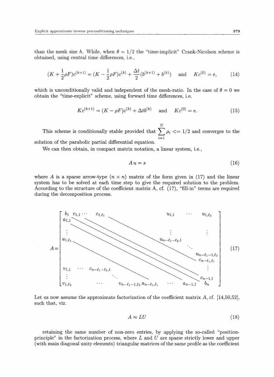
where A is a sparse arrow-type (n • n) matrix of the form given in (17) and the linear system has to be solved at each time step to give the required solution to the problem. According to the structure of the coefficient matrix A, cf. (17), "fill-in" terms are required during the decomposition process.

A =

bl C I , 1 �9 " �9 CI ,~ 1 I t l , 1 " �9 �9 U l , ~ 2

V l , g 2 " " " V n - - ~ l - - l , ~ 2 a n - e l , g 1 �9 " �9 a n - l , 1 b n

(17)

Let us now assume the approximate factorization of the coefficient matrix A, cf. [14,50,52], such that, viz.

A ~ L U (18)

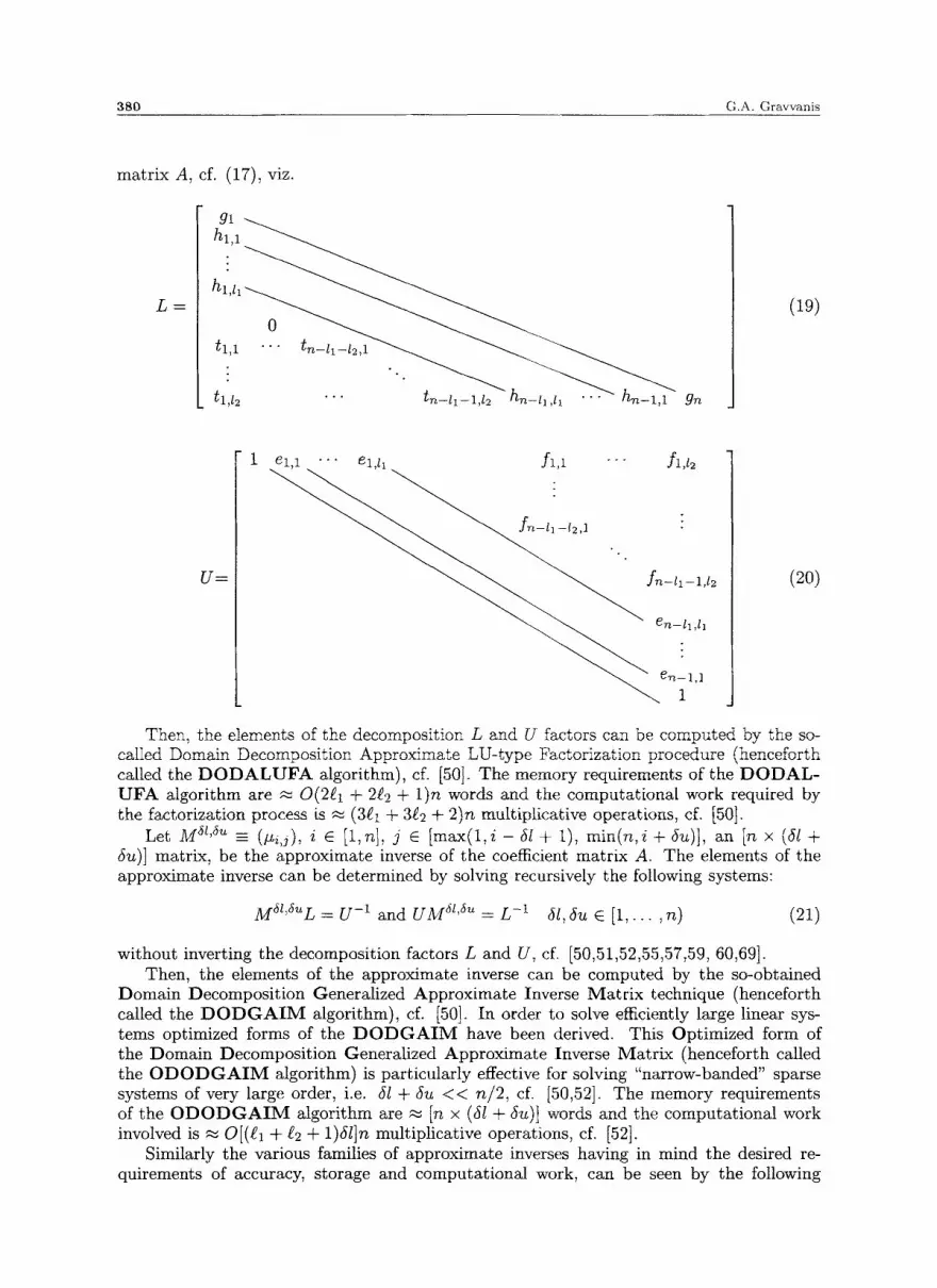
retaining the same number of non-zero entries, by applying the so-called "position- principle" in the factorization process, where L and U are sparse strictly lower and upper (with main diagonal unity elements) triangular matrices of the same profile as the coefficient

2,80 G.A. Gravvanis

matrix A, cf. (17), viz.

L = hi,ll

gn

(19)

U =

1 el,l "'" r fi.,i "'" fi,l~

~ ~ ~ fn-li--l,12 (20)

Then, the elements of the decomposition L and U factors can be computed by the so- called Domain Decomposition Approximate LU-type Factorization procedure (henceforth called the DODALUFA algorithm), cf. [50]. The memory requirements of the DODAL- UFA algorithm are .~ O(2~i 4. 2~2 + l)n words and the computational work required by the factorization process is ~ (3~t 4- 3~2 4. 2)n multiplicative operations, cf. [50].

Let M ~t'~ ~_ (~tJ), i �9 [1, n], j �9 [max(1,i - 6I + 1), min(n, i + 6u)], an [n • (~f + ~u)] matrix, be the approximate inverse of the coefficient matrix A. The elements of the approximate inverse can be determined by solving recursively the following systems:

MSz'SUL = U - t and U M 5l'6~ = L -1 3l, Su E [1,... ,n) (21)

without inverting the decomposition factors L and U, cf. [50,51,52,55,57,59, 60,69]. Then, the elements of the approximate inverse can be computed by the so-obtained

Domain Decomposition Generalized Approximate Inverse Matrix technique (henceforth called the D O D G A I M algorithm), cf. [50]. Irt order to solve efficiently large linear systems optimized forms of the D O D G A I M have been derived. This Optimized form of the Domain Decomposition Generalized Approximate Inverse Matrix (henceforth called the O D O D G A I M algorithm) is particularly effective for solving "narrow-banded" sparse systems of very large order, i.e. ~l + ~u < < n / 2 , cf. [50,52]. The memory requirements of the O D O D G A I M algorithm are ~ [n x (~l 4. ~u)] words and the computational work involved is ~ O[(g] 4. g2 + 1)~/]n multiplicative operations, cf. [52].

Similarly the various families of approximate inverses having in mind the desired requirements of accuracy, storage and computational work, can be seen by the following

E x p l i c i t a p p r o x i m a t e inve r se p r e c o n d i t i o n i n g t e c h n i q u e s 3 8 1

diagrammat ic relationship, i.e.,

class I class II class III class IV

A/fdl,6u M61,Su A -1 = M * - ~ 5 1 , 5 u ~__ ..~n +- +-- M i (22)

where the entries of the ~5t,5~ approximate inverse have been retained after the computation of the exact inverse, while the entries of the M 51,5u approximate inverse have been computed and retained during the computational procedure of the approximate inverse. The entries of the MSn l'Su approximate inverse have been computed and retained during the computational procedure of the approximate inverse by retaining additionally the n-th row and column of the approximate inverse. The diagonal inverse Mi, i.e. class III, was computed based on the inversion of the diagonal entries of the L decomposition factor.

It should be ment ioned tha t if g2 = 0 (i.e. v~,j = 0 and u~,j = 0), cf. (17), then the D O D A L U F A and D O D G A I M algori thms are reduced to B L U F A and O A I B M algo- r i thms respectively, cf. [57,60], for solving banded linear systems. It should be also noted tha t if gl = 1 and g2 = 1, cf. (17), then the D O D A L U F A and D O D G A I M algori thms are reduced to A T A L U F A and O A I A T M algori thms respectively, cf. [58], while if gl = 0 and gz = 1, of. (17), then the D O D A L U F A and D O D G A I M algori thms are reduced to A L U F A and O A I A M algori thms respectively, el. [62]. The symmetr ic counterpar t of the D O D A L U F A and D O D G A I M algori thms are D D A R F C and O D D A I M respectively, cf. [55], when considering self-adjoint elliptic part ial differential equations.

Hence, by considering an implicit approximat ing scheme (0 = 1, 0 = 1/2) in conjunction with explicit approximate inverse matr ix techniques yields hybrid heterogeneous schemes, whereas an explicit approximat ing scheme (0 = 0) combined with explicit approximate inverse mat r ix techniques yields hybrid homogeneous schemes. These hybrid schemes have a universal scope of application for solving parabolic part ial differential equations in two or three space variables, by using the Fini te Difference, Finite Element or Domain Decompo- sition discretization methods , el. [51,56,71,72,99,100].

A =

bl Cl,1 " " " CI,~

( t l , g

0 i

(23)

When the width parameter is g2 = 0, then the coefficient matrix of the linear system (17) is of the banded structure as given in (23), which can be considered having a universal scope of application. These type of linear systems can be derived from higher order discretization schemes applied to second order partial differential equations (e.g. nine-point molecule, etc) or when solving fourth order partial differential equations (e.g. biharmonic equations, occurring in elasticity and in fluid flow) either as a "coupled equation approach" (pair of Poisson equation) or by applying iterative schemes directly to the fourth order equation, cf. [49,57,60].

382 G.A. Gravvanis

The sparse arrow-type structure linear system, cf. (16)-(17), has been considered as resulting either from the domain decomposition method in conjunction with finite difference or finite element discretization method of a partial differential equation or in eigenvalue and eigenstructure problems, cf. [42,47,111,115]. These types of systems are also derived from the Kolmogorov equation, used in Markov modeling for dependability evaluation analysis of various systems.

Over the last years, the rapid evolution of the complexity of industrial, computer and communication systems lead to a constantly increasing interest in the reliability study of such systems. A dependability assessment is particularly needed in the design phase of a large highly available system such as computer networks, power systems, or telecommu- nication systems in order to assure the feasibility by satisfying availability and economic constraints. Markovian modeling is a major tool used in dependability evaluation analysis.

A system is therefore described by means of a state transition diagram containing all the operational states, failure states and the transition rates between them. The Markov assumption is based on the fact that these rates are generally exponentially distributed. When the system is composed of a large amount of components, or when there is a need to distinguish in a very detailed manner all the failure states, results in a large size state transition diagram and the use of efficient solution method is required. The interest is focused on the estimation of the steady state probabilities, which are the crucial elements for the evaluation of the re!iability indicators, as well as another important kind of indices called performability indicators, that combine reliability parameters with the performance of the system. The calculation of all these indicators modeled specifically by a markovian model is necessary for a better decision-making process in the improvement of the system's quality. Dependability indicators modeled by Markov chains or homogeneous Markov processes, based on the resolution of the steady state probability distribution of a markovian model, result generally in solving large sparse linear systems and the profile of the coefficient matrix is of arrow-type structure, cf. [50,58,62].

Hence using explicit preconditioned conjugate gradient - type schemes, which are presented in section 4, in conjunction with explicit approximate inverse matrix techniques is expected to improve considerably the required computational complexity of the computation of the steady state probabilities of a particular type of large size markovian systems, and thus obtain an estimation of the above mentioned reliability and performability indicators, cf. [73,118].

3 C O M P O S I T E I T E R A T I V E S C H E M E S F O R N O N - L I N E A R P R O B L E M S

Let us consider a class of non-linear boundary value problems defined by the non-linear elliptic P.D.E in three space-variables, i.e.:

L u = f(u) , (x ,y , z ) E R, (24)

subject to the boundary conditions

au + fl Ou - ~ = 7 , (x, y, z) C OR, (24.a)

where L is a linear partial differential operator. We may linearize the problem by Picard method, i.e.

Lu(k+l) = f [u(k)] , (25)


or the Newton method, i.e.

- -

Assuming tha t a volumetric network of mesh spacing h~, hy, hz in the X, Y, Z di- rections respectively is superimposed over the region R, and using the finite difference, finite element or domain decomposition method, then the above equations (25)-(26), lead to sparse systems which can be wri t ten equivalently as

> 0, (27)

with Ak = A for the Picard iteration. A system of the form (27) can be explicitly solved by means of composite "inner-outer" iterative schemes, i.e. Picard-Newton and exact inversion procedures resulting in one-level i teration or Picard-Newton and explicit preconditioned iterative schemata based on explicit approximate inverse procedures yielding the usual two-level i teration scheme, of. [96].

Let us consider the non-linear iterative scheme

where the matr ix Ak can be split as Ak = Bk - Ok. Provided tha t the matr ix B k is non-singular we have, cf. [54,96,113], i.e.

2 ink--1 A;' = ( s - B;lC~) -' B ; 1 = [i + H~ + H~ + ... + Hk ] 8 ; 1 (29)

where Hk = B[ICk, k > 0, I is the identity matr ix and only mk first terms have been

retained in the expansion of ( I - B[ICk) -1. Therefore an explicit iterative scheme is derived, i.e.,

rnk--1

which represents the composite i teration in which at the k-th stage star t ing from u (~), mk steps of the linear inner iterations are computed in order to approximate a solution of the

outer iteration. Choosing B~ 1 = ( M ~l '~) depending upon k and retaining only the first

t e rm in the expansion of equation (30), we obtain the first order Newton-ODODGAIM iterative scheme, viz.,

The Newton-DODGEIM scheme can be easily derived from (28) assuming tha t M -- A[t = (LU) -1, eL (22), and is given by

It can be easily seen that the proposed composite "inner-outer" iterative scheme in the case of the exact inversion reduces to an equivalent one-level iteration. While for the case of approximate inversion the "inner-outer" iterative scheme reduces to the usual two-level i teration and the Explicit Precondit ioned Conjugate Gradient - type schemes can be used, cf. [96].

384 G.A. Gravvanis

Thus, the proposed composi te "inner-outer" iterative scheme in the case of the approximate inversion reduces to the usual two-level i terat ion and the Explicit Precondi t ioned Conjugate Gradient - type schemes can be used.

Let us consider the explicit iterative scheme for solving a boundary value problem:

ui+t - ui = ~ i ( f F ) - l ( s - f~ui), i > 0, (33)

where the operator 12" is chosen to be "isomorphous", i.e. to agree closely in a quant i ta t ive sense, to the opera tor f~. The isomorphic relat ionship to the discretized operators f~, and ~'~h has certain similarities to the L2-comparabil i ty between the same operators. It should be noted tha t the isomorphic relat ionship is to be considered in a more general scope t h a n the L2-comparabil i ty in the sense tha t it allows simple manipula t ion and classification of the elements of the approximate inverse 12", cf. [96].

Let us consider the following definitions, cf. [96]:

D e f i n i t i o n 3.1: The operator f ~ is said to be 50-isomorphous to an opera tor ~ h if f ~ is identical to f~h, i.e., t2~ _---- fth.

D e f i n i t i o n 3.2: The operator 12~, ------ {wi*j}, i, j e [1,n], is said to be 5i-isomorphous to an operator f~h -- {a~i,j}, i, j �9 [1, n] if the following relations hold:

n n

wi* i -czi , i + E wi,k + E wk,i, i �9 [1,n] (34) k = i + l k = i + l

n-j+1 wi*,J =-- E a~i,j+k-1, i E [1, n - 1], j E [2,#1, (35)

k = l

and

n-- i+1

- i e j e t i (36) k = l

= ZX (ah), k e [ , + (37)

where A* and A are the corresponding diagonal of operators f ~ and fth respectively. Note tha t the index k in the definition can take only one value out of [1, 2n - 1] in a specified case, where k is the number of diagonals retained next to the main diagonal of the operator f~;.

The operator ~2~ is 53-isomorphous to the operator f~h iff the operator f ~ retains only three modified diagonals, i.e. the main diagonal and two successive diagonals in the lower and upper par t of 12~ wi th its elements derived from the relations (34)-(36) and the re- maining elements of f ~ identical to the corresponding elements of f~h.

D e f i n i t i o n 3.3: An explicit i terative m e t h o d is said to be an Isomorphic i terative m e t h o d iff it involves 5i-isomorphous operators.

An efficient solution of the linear system Au = s can be obta ined by considering a 5i-isomorphic iterative scheme. Let us consider

= s, ( 3 s )

where f ~ is a 5~-isomorphous opera tor to A. Then assuming tha t the const ruct ion of 12~ can be easily obtained the approximate solution u* has to be proved tha t it is an acceptable

Explicit a p p r o x i m a t e inverse precondi t ion ing techniques 385

approximate solution to the original system A u = s, i.e. the norm llu - u* II has very small values.

Let us also consider an explicit 5i-isomorphous iterative scheme:

ui+i - u~ = a~Ms~,su(s i - A u i ) , i > 0 (39)

where M* / fF ~-i �9 51,5u = ~ h] , with f~h a 5i-isomorphous operator to the original coefficient matr ix A, such that f~; = L ' U * + R * , where L* and U* are sparse lower and upper triangular matrices and R* is the correction matrix. Further details on isomorphic iterative schemes can be found in [96].

4 E X P L I C I T P R E C O N D I T I O N E D C O N J U G A T E G R A D I E N T M E T H O D S

In this section we present a class of explicit preconditioned conjugate gradient-type schemes based on the derived Explicit Approximate Inverse Ma t r ix ( E A I M ) techniques of section 2. Additionally, we present the convergence analysis in order to obtain theoretical results on the rate of convergence and estimates of the computat ional complexity. The use of the approximate inverse matr ix techniques in the preconditioned conjugate gradient schemes, cf. [1,36,37,74,85,88,122,124,129,130], eliminates the implicitness due to the forward-backward subst i tut ions required and allows the derivation of explicit precondit ioned conjugate gradient schemes, el. [76,84,95,125].

4 .1 T h e S y m m e t r i c C a s e

Let us assume that matrix A, cf. (5) - finite element coefficient matrix, is real symmetric, positive-definite matr ix and let M~,r 2 denote its approximate inverse.

Then the Explicit Precondit ioning Conjuga te Gradient ( E P C G ) method can be s tated as follows:

Let u0 be an arbi trary initial approximation to the solution vector u. Then,

form ro = s - A u o , (40) * = M ( 4 1 ) COiT lpu t e TO r ~ ,r2 TO '

= * (42) s e t cr 0 r 0 .

Then, for i = 0, 1 , . . . , (until convergence) compute the vectors ui+t, r~+l, cri+l and the scalar quantities a~, ~i+i as follows:

form qi = A~ri, (43) calculate pi = (r~, r*) when i = 0 only, (44) evaluate ai = p i / ( a i , qi), (45) compute u~+l = ui + c~i(ri, (46) and r i + l = ri - a iq i (47)

* = 3//[ zz (48) Then, form r i + 1 r l , r 2 r i + l

set Pi+l = (ri+l,ri*+l), (49) evaluate /3i+1 = P~+I/P~, (50) compute C r i + i = ri*+l +/3i+~ri. (51)

The Explicit Precondi t ioned Biconjugate Conjugate Gradient ( E P B I C G ) algorithm, can be expressed by the following compact scheme:

Let u0 be an arbi trary initial approximation to the solution vector u. Then,

set u0 = 0, (52) compute r0 = M 5l (s - Au0), (53) r l ,v2 \ set ~0 = ~0 = o0 = r0 (54) and p0 = (r0, ~0) (55)

386 G.A. Gravvanis

Then, for i = 0, 1 . . . , (until convergence) compute the vectors Ui+l, ri+l, cri+t, ~ i + 1 and the scalar quantities ai, ~i+1 as follows:

form qi = Acri, (56) 6l calculate ai = P i / (cri,Mr,,r2qi), (57)

compute Ui+I : Ui -~ O l i a i , (58)

r i + 1 = l" i - - ceiM~[,r2qi, (59) ( 6 l ) T (60) and Zi ~- M~l,r 2 O-i

form vi = ATz~, (61) compute ~iH-i = ~i - c~ivi, (62) set Pi+l = (ri+l, Fi+l) (63) evaluate /3i+1 = Pi+l/Pi, (64) compute ai+l = ri+l + f~i+lai (65) and ~i+1 = r'i+l + #i+lYi. (66)

The Explicit Precondi t ioned Conjugate Gradient Square ( E P C G S ) algorithm, can be expressed by the following compact algorithmic scheme:

Let uo be an arbi t rary initial approximation to the solution vector u. Then,

set u0 = 0 and e0 = 0, (67) solve ro = M at (s - Auo) (68)

~I~2

set a0 = r0 and Po = (a0, ro). (69)

Then, for i = 0, 1 , . . . , (until convergence) compute the vectors ui+l, ri+l, dri+l and the scalar quantities ai, /3i+i as follows:

form qi = Acri, (70) 6l calculate a i = p i / (ao, M~lx2qi) , (71)

compute ei+l = ri +/3iei - aiM6r[,r2qi, (72) di = ri +/3iei + ei+l (73)

and U i + I = ui + aidi, (74) form qi = Adi, (75) compute ri+l = ri - aiMa~[#2qi, (76) set pi+l = (co, ri+l), (77) evaluate /3/-}-1 = Pi+l/Pi, (78) compute ai+l = ri+l + 2#i+lei+l +/32+1ai. (79)

In the following we present the Explicit Precondi t ioned BIconjugate Conjugate Gradient- S T A B ( E P B I - C G S T A B ) method, which can be expressed by the following compact scheme:

Let uo be an arbi t rary initial approximation to the solution vector u. Then,

set uo = 0 (80) compute ro = s - Auo, (81) set r~ = r0, Po = a = wo = 1 and vo = p o = 0. (82)

Then, for i = 0, 1 , . . . , (until convergence) compute the vectors u~, ri and the scalar quantities a; fl, wi as follows:

calculate pi = (rio, r i-1) , (83) and fl = (p~ /Pi -1 ) / (a /wi -1 ) , (84)


compute p~ = r~- i + f l (P~- i - w i - l v i - 1 ) , (85) 6l form Yi = M~,~2Pi and v~ = A y i , (86)

calculate c~ = P i / ( r ~ , vi), (87)

compute xi = r i -1 -- o~vi. (88) M 5l x and t i = A z i , (89) form zi = r" 1 ,r 2 z [MaZ , az at az set o o i : , rl,7.26i,M;1,r2Xz) / (M;1,T2~i ,M~l ,r2t i ) (90)

compute ui = u i -1 + a y i + coiq (91) I l k l

and ri = xi - oaiti. (92)

Assuming that the approximate inverse 21//51 rl,r2 can be compactly stored in n • (26l - I) diagonal vectors, then the computational complexity of the explicit preconditioned conjugate gradient - type methods is defined as follows:

i) the E P C G m e t h o d requires ~ 0[(251 + 291 § 2~2 + 7)nmults + 3nadds]~ operat ions

ii) the E P B I C G me thod requires ~ 0[ (451+491 +492+ l l ) n m u l t s + 5 n a d d s ] ~ operat ions

iii) the E P C G S m e t h o d requires ~ 0 [ ( 4 6 l + 491 + 492 + 12)nmults + 8nadds]~ operat ions

iv) the E P B I - C G S T A B me thod is ~ O [(66/+491 +4g2+14)nmul t s+6nadds ]~ operat ions

where y is the number of i terations required for the convergence to a certain level of accuracy and gl, g2 are the wid th parameters of the coefficient matr ix A at semi-bandwidth m and p respectively, cf. (5).

4.2 The U n s y m m e t r i c Case

In order to solve the unsymmetr ic linear system of algebraic equations A u = s, derived by the domain decomposi t ion method , by precondit ioned conjugate gradient - type methods we consider the normal equations, i.e.

A T A u = A T s, (94)

where ATA is a symmetric, positive definite matrix and the corresponding preconditioned system is

M 5l'~u ( A T A ) ( M S l ' S u ) T u = MSl ' sUA Ts . (95)

The application of the conjugate gradient - type methods to the normal equations is expected to increase the number of iterations required for convergence.

The Explicit Preconditioned Generalized Conjugate Gradient (EPGCG) algorithm can be expressed as follows:

Let u0 be an arbitrary initial approximation to the solution vector u. Then,

set u0 = 0 (95) form ro = s - A u o , (96) calculate F0 = A T r o , (97) compute r~ = M & & ' ~ o , (98) set a0 = r~). (99)

388 ('.A. (lravvanis

Then, for i = 0, 1 , . . . , (until convergence) compute the vectors ui+t, r i+t , ai+t and the scalar quanti t ies a i , / J i+ l as follows:

form qi = A ( ~lSl 'Su)T o'i, (100) set Pi = (ri, r*) , (only for i = 0) (101) evaluate ai = P i / ( ~ i , q~), (102) compute ui+l = ui - t -ai(Mhl 'hu)Tcri , (103) and r i + l = ri - aiqi , (104) form ~i+1 = A T r i + l , (105) solve ri*+l = Mhl'hu~i+t, (106) set Pi+l = (~'i+1,~'~'+t), (107") evaluate /3i+1 = p i + l / p i , (108) compute Cq+l = ri*+l +/3i+lai . (109)

The Explici t P recondi t ioned General ized Conjuga te Gradient on Norma l Equat ions ( E P G C G N E ) algor i thm can be expressed by the following compact scheme:

Let u0 be an arbi t rary initial approximat ion to the solution vector u. Then,

set u0 = 0 (110) calculate ro = s - Auo , (111) form ~r0 = Mhz'5~ATro, (112) set z0 = or0. (113)

Then, for i = 0, 1 , . . . , scalar quanti t ies ai, /~i+1 as follows:

(until convergence) compute the vectors Ui+l, r i+l , cri+l and the

form qi = A(MSl 'Su)Tcri , (114) set Pi = (zi, zi), (only for i = O) (115) e v a l u a t e = qd, (116) c o m p u t e ui+l = Ui + a i ( M h l ' h u ) T c r i , (117) and ri+l = ri - aiqi , (118) form zi+l = M h l ' h u A r r i + l , (119) set Pi+l : (Zi+l , Zi+l) , (120) evaluate fli+l = Pi+I /Pi , (121) compute cri+l = Zi+l +/3i+lcri. (122)

The Explici t Precondi t ion ing General ized Biconjugate Con juga te Grad ien t ( E P G - B I C G ) m e t h o d for solving linear systems can be similarly derived from the Explicit Precondi t ion ing Biconjugate Conjuga te Gradient , cf. (52)-(66).

The Explici t P recondi t ioned General ized Con juga te Gradient Square ( E P G C G S ) algor i thm can be expressed by the following compact algorithmic scheme:

Let u0 be an arbi t rary initial approximat ion to the solution vector u. Then,

set u0 = 0 and e0 = 0, (123) solve r0 = M h l ' ~ ( s - A u o ) , (124) set or0 = r0 and P0 = (~r0, r0) (125)

Then, for i = 0, 1 , . . . , (until convergence) compute the vectors ui+l , r i+t , ai+t and the scalar quanti t ies cti,/3i+1 as follows:

form qi = A o i , (126) calculate oq = Pi / (ao, M 51 '5~ qi), (127) compute ei+l = ri + ~iei -- ai3Jhl 'huqi, (128)

t ' :xplicit a.pproxima~'e hwer se p r e c o n d i t i o n i n g t, e chn iques 3 8 9

di = ri +/3~ei + e~+l, (129) and Ui§ = ui + a~d~, (130) form qi ---- Ad~ (131) compute ri+l ---- r i -- o~iMSl 'SUqi , (132) set P~+I = (~0, r i+l) , (133) evaluate /3i+1 = Pi+I/pi , (134) compute ai+~ = ri+~ + 2~+~ei+~ + ~ } + ~ . (135)

In the following we present the Explicit Precondi t ioned Generalized Biconjugate Conjugate G r a d i e n t - S T A B ( E P G B I C G - S T A B ) method, which can be expressed by the following algorithm:

Let u0 be an arbi t rary initial approximation to the solution vector u. Then,

set u0 = 0 (136) compute ro = s - Auo, (137) set r~ = r0, P0 = c~ = w0 = 1 and v0 = p 0 = 0. (138)

Then, for i = 0, 1 , . . . , (until convergence) compute the vectors ui, ri and the scalar quantities c~, ~/, ~i as follows:

ca l cu la t e = (139) and /3 = (p~/pi-1)/(c~/aJi-1) (140) compute Pi : r i - 1 -~ ~ ( P i - 1 - - W i - l V i - 1 ) , (141) form Yi = M~l'5~Pi and vi = Ayi , (142) and a = p~/(r~, vi), (143) compute x~ = ri-~ - avi, (144) form zi = MSZ'Z~xi and Q = Az~, (145)

compute u~ = ui-1 + c~y~ + ~iz~ (147) and r~ = xi - ~it~. (148)

Assuming that the approximate inverse M 5l'5~ can be compactly stored in n x (5l + 5u) diagonal vectors, then the computat ional complexity of the explicit preconditioned generalized conjugate gradient - type schemes is defined as follows:

i) the E P G C G method requires ~ 0125I + 25u + 4Q + 4Q + 7)nmults + 3naddslu operations

ii) the E P G C G N E method requires ~ 0125t + 25u + 4Q + 492 + 7)nmults + 3nadds]u operations

iii) the E P G B I C G method requires ~ 0125l + 25u + 4Q + 4Q + 9)nmults + 5nadds]u operations

iv) the E P G C G S method requires ~ 0125l + 25u + 4Q + 4Q + 11)nmults + 8nadds]u operations

v) the E P G B I C G - S T A B method requires ~ 0135l + 35u + 491 + 4~2 + 12)nmults + 6nadds]u operations

where u is the number of iterations required for the convergence to a certain level of accuracy and Q, ~2 are the width parameters of the coefficient matr ix A, cf. (17).

The effectiveness of the explicit preconditioned conjugate gradient - type methods using the Approximate Inverse Matrix techniques is related to the fact tha t the approximate inverse exhibits a similar "fuzzy" s tructure as the original coefficient matr ix A and is a close approximant to the coefficient matr ix A.

3 9 0 G.A. Gravvanis

4.3 T h e R a t e o f C o n v e r g e n c e a n d t h e C o m p u t a t i o n a l C o m p l e x i t y

The convergence analysis of similar explicit approximate inverse preconditioning has been presented in [48,61,66,92]. The basic propert ies of the E P C G method, cf. [2,5,74,86,109,128], can be s tated by the following Theorem:

T h e o r e m 4.1: Let A be a positive definite matrix, s some given vector and u = A - i s the solution to the linear system Au = s. Let us also consider that u (~) is the solution vector after k iterations of the E P C G method, then we have

(149)

and

I1~- ~(k)ll~ _ rain m a x IP~(z)l, (150) Ilu - u(~ Pk XE[-~mln,~ma.x]

where f~ 5z 5z = M~I,r2A and A, M~l,r ~ is the finite element coefficient matrix, cf. (5), and the finite element approximate inverse, cf. (10), respectively, while P~ is the set of polynomials

of degree k such that Pk(0) = 1, and I lx l lB = ( x , Bx) 1/2. Since e (k) = u - u (k) it can be proved, cf. [109,128],

Ile(k)llB __ min m a x IPk(x)llle(~ (151)

Thus we have to find the smallest k such that

min max IPk(x)l _< r 0 < a < 1. (152) Pk Xe [Amin,-~ . . . . ]

In order to derive an est imate of the number of iterations required for the interval [ /~min , /~max] , the polynomial Pk(x) can be defined in terms of the Chebyshev polynomials T, of degree ~. Assuming [~1, ~2] D [ /~min , /~max] , the maximum value of T,(x) as ~ --+ +oc is given by

max IRk(x)] = {T~, (~22 -~- ~11) }-1 xe[~l,~2] - - , ( 1 5 3 )

with the proper ty that Pk(O) = 1. Let us assume that

Ilall ~ I1~111 = max {~-~ II~i, j l l } �9 jE[1,n] i : 1 (154)

In order to derive bounds on f~, we need the following Lemmas:

L e m m a 4.1: Let Z be a real (n z n) nonsingular matrix, and M z be the M-condi t ion number of Z, cf. [36,66]. Then

i iz_l l I < M~ 1 - ~-~ IlZll

(155)

L e m m a 4.2: Let f~ = A4[ 5z A be the preconditioning matrix of the E P C G iterative r 1 ,r2 scheme. Let n be the order of the coefficient matrix, gl and g2 be the width parameters


of the coefficient matr ix and 5l be the "retention" parameter of the approximate inverse. Then

I I ~(n,e~,g~_,al) ~fiq~o 1 + C~ az) -< Ilall _< -1 + ,~ (156)

~(n,e~ ,g2,51) where "2 is a non-negative constant depending on n, gl, g2, 5l and C~ az) is a constant depending on 5l and independent of the mesh-size, while ~f~ = M ~ / n 2, (Po = IVf2/n 2, with Mf~, Mo be the M-condit ion numbers of the matrices f~ and M respectively, cf. [66].

An upper bound for Amax(f~) can be obtained as follows

_ _ _ _ / u ( n , s , g 2 , 5 1 ) /~max(a) < Ilall < --1 + ~2 (15r)

Similarly a lower bound for /~min(~'~)

1 1 1 1 1

/~min(~) = = - - - ~Sg?~0 1 + C "Sg) max(I/~(a)) max( ,X(a- * ) ) > I la-* l l > . (158)

Let us consider the positive numbers {1, ~2 such that:

_ ~(n,el,g2,5/) ~2 < - 1 + "'2 and ~1

1 1

~,~o 1 + C[ aO (159)

~(n,Q,&,at) It should be noted that the behavior of the values of C} az) and ,~ are closely

related to the eigenvalue distribution of the problem under consideration. In order to derive theoretical results on the rate of convergence and computational

complexity for the Explicit Preconditioned Conjugate Gradient method, there is a need to find an upper bound for the maximum eigenvalue, either for the Finite Element method or the Domain Decomposition method.

It can easily seen from equation (157), that a more accurate estimate, cf. [48, 66], can be derived

{ ~ (160)

which can be equivalently written as

{2 = o (,~(al + el + < ) - i ) . (161)

Then, the following Theorem on the rate of convergence and computational complexity of the EPCG method cf. [63,66], using the Finite Element approximate inverse M~,r2, cf. (9)-(10), can be stated:

Theorem 4.2, Finite Element method: Let ~ = Ma~,r2A be the preconditioning matrix of the Explicit Preconditioned Conjugate Gradient (EPCG) iterative scheme. Suppose there exists positive numbers {1, {2 such that [~I, {2] D [Amin, Amax], where ~I is independent of the mesh size and {2 = O (n(al + gl + g2)-I). Then the number of iterations of the EPCG method required to reduce the L~-norm of the error by a factor c > 0 is given by

V = 0 (nl/2(C~/ -F ~1 ~- ~2) -1/2 log s . (162)

3 9 2 ( ' .A. Graw~anis

Furthermore, the total number of arithmetic operations required for the computation of the solution u. is given by

0(n3/251(51 +el + 6)-1/2(r l + r2 + el + e2)loge - t ) (163)

According to the convergence analysis of explicit approximate inverse preconditioning, cf. [63,66], the rate of convergence is improved when the value of the "retention" parameter 5l is chosen as multiples of the bandwidths, i.e. m and p. It is evident tha t when the value of the "retention" parameter 5l is chosen as multiples of the bandwidths rn and p then the required overall computat ional complexity of the method can be prohibitively high. Thus the determinat ion of the opt imum value of the "retention" parameter of 51 = 1 is recommended, which gives the lowest overall computat ional complexity.

It should be stated that similar theoretical results have been derived for the rate of convergence and computat ional complexity using the Domain Decomposition method, cf. [48].

5 N U M E R I C A L R E S U L T S

In this section we examine the applicability and effectiveness of the proposed schemes for solving characteristic problems. Numerical results have been presented on a number of papers by the author for the finite difference and finite element method, which are quoted in the reference section. In this section we are focusing our at tention on the convergence behavior of explicit preconditioned domain decomposition schemes. M o d e l P r o b l e m I: Let us consider a two dimensional initial value problem, i.e.,

~ = ~x + ~, (~, ~) ~ R, (164)

subject to boundary conditions and initial conditions

~(x , y, t) = 0, (x, y, t) e o R • [0 < t < T], (1~4.a) u(x ,y ,O) = uo(x ,y) , x e OR, (164.b)

where R is the unit square and OR denotes the boundary of R. The domain R was decomposed into a number of sub-domains and was covered by a

non-overlapping regular tr iangular network. The five-point finite difference discretization scheme with a row-wise ordering was used such that the width length gl of the band was kept to low values, i.e. gl = 3. The conjugate gradient process was terminated when Ilrill~ < 10 -5, while the tolerance epss for the steady state solution (s.s.s.) was set to epss = 10 -5, with the initial guess chosen as u0 = 0.05.

Numerical results are presented in Table 1 for the time-implicit backward difference scheme in conjunction with the E P G C G S and the E P B I - C G S T A B methods for several values of the time-step At and the "retention" parameter dl of the approximate inverse with n = 361, gl = 3 and e2 = 76, el. [51]. In Table 2, numerical results are given for the Crank-Nicolson scheme in conjunction with the E P G C G S and the E P B I - C G S T A B methods for several values of the time-step At and the "retention" parameter 5l of the approximate inverse with n = 361, el = 3 and e2 = 76, cf. [51].

It should be noted tha t the convergence behavior of the E P G C G S and E P B I - C G S T A B methods, in conjunction with the D O D A L U F A and O D O D G A I M algorithms, is much bet ter when the domain is subdivided into many sub- domains.

It should be also mentioned that the iterative G M R E S scheme, cf. [123,133,134], al though it has good stability, requires storage of all the basis vectors of the Krylov space

Explicit ~tpproximate inverse precouditioning lec}miques 393

II M e t h o d (s.s .s .) I 6 l = 1 I 61=

E P G C G S

E P B I C G - S T A B

I At I o u t e r i te r . 11 0.0500 4 26 0.0100 6 40 0.0050 8 47 0.0010 13 70 0.0005 17 76 0.0001 35 100

0.0500 5 40 0.0100 7 48 O.O050 8 51 0.0010 14 63 0.00O5 t8 66 0.0001 35 92

= 3 61=211 = 6 20 14 34 21 41 28 61 42 71 50 97 80 32 23 38 30 42 34 57 51 66 59 88 86

Table 1. The convergence behavior of the E P G C G S and E P B I - C G S T A B method for the time-implicit backward difference (0 = 1), with n = 361, m = 2 0 , gl = 3 a n d g 2 = 7 6

II M e t h o d At outer iter. (s .s .s .) 61 = 1 51 = 11 = 3

E P G C G S 0.0005 15 51 48 0.0001 33 73 63

E P B I C G 0.0005 15 47 46 - S T A B 0.0001 32 55 53

= = 6 II 37 57

46 52

Table 2. The convergence behavior of the E P G C G S and E P B I - C G S T A B method for the time-implicit backward difference (0 = 1/2), with n = 3 6 1 , m = 2 0 , gl = 3 a n d g 2 =76

and its performance is depending on the restart vectors used, thus making this method problem dependent. Model Problem II: Let us consider a class of Singular Perturbation time-dependent problems defined by the P.D.E.:

ut(x,y,t)+dux(x,y,t)=cpAu(x,y,t), (x,y) CR, Cp-~O+, t > 0 (165)

subject to the initial conditions:

v, 0) = 9 (x , y) ,

and the b o u n d a r y condi t ions:

0 < z , y _< 1, (165.a)

u(0, 0, t) = a a n d u(1, 1, t) ----/3, t > 0, (165.b)

where R is the unit square, OR denotes the boundary of R, d is real constant, a, /3 are given constants, g(z, y) is a given sufl]ently smooth function and ep is a small (perturbation) parameter.

For the computation of an approximate numerical solution of the perturbation problem (165)-(165.b), the region was decomposed into sub-domains and covered by a regular non- overlapping triangular network. Then, by using backward differences for ut, the (downwind) stable scheme of order O(h) for ux and the five-point finite difference diseretization scheme for the derivatives of second order, with a row-wise ordering used such that the width gl of the band was kept to low values, i.e. gl = 3 then the resulting large linear system is of the form given in (4)-(5).

394 G.A. Gravvanis

The resulting linear system has been solved, by using Explicit Preconditioned Conjugate Gradient methods, i.e. EPGCGS and EPBI-CGSTAB methods. The iterative process was terminated when ]]ri[[oc < 10 -5, while the tolerance epss for the steady state solution (s.s.s.) was set to epss -- 10 -5, with the initial guess chosen as u0 = 0.05. Numerical experiments were carried out for the Singular Perturbation intial value problem in two dimensions with d = 1 and a = 13 -- 0.

Numerical results are presented in Table 3 and Table 4 for the EPGCGS and the EPBI-CGSTAB methods respectively, in conjunction with the DODALUFA and ODODGAIM algorithms, for several values of the "retention" parameter 51 of the approximate i nve r se , t h e t i m e - s t e p A t a n d t h e S P - p a r a m e t e r ~p, w i t h n --- 361, m - - 20,

gl = 3 a n d s = 76, cf. [56].

outer

i t e r a t ions for s.s.s.

1 0.100 6 0.050 7 0.010 11 0.005 15

3 0.100 6 0.050 7 0.010 12 0.005 16

6 0.100 6 0.050 7 0.010 12 0.005

t o t a l no of inner

i t e r a t ions

37 41 54 58

26 32 45 53

17 20 32

ap = 10 -~

ou te r i t e r a t ions for s.s.s.

7 9 16 20

9 16 20

7


i t e ra t ions

23 27 37 42

15 18 26 33

11 15 26

Ep = 10 -4

outer iterations for s.s.s.

15 20

15 20

16 15 16 37 20 32 20


i t e r a t i ons

17 21 34 43

15 20

9 15 20

T a b l e 3. The convergence behavior of the E P G C G S method, using the D O - D A L U F A and O D O D A I M algorithms, with el --- 3

II

1 0.100 0.050 0.010 0.005

3 0.100 0.050 0.010 0.005

6 0.i00 0.050 0.010 0.005

A t [ Sp = 10 - I

outer total no iterations of inner for s.s.s, iterations

6 38 7 43 12 52 15 57

6 3O 7 32 12 46 15 49

6 24 7 29 12 40 15 45

Cp = 10 -'~

ou te r t o t a l no i t e r a t ions of inner for s.s.s, i t e ra t ions

7 26 9 28

16 34 20 40

7 17 9 20

15 27 20 34

7 17 9 20

15 26 20 34

~p = 10 - 4

outer total no iterations of inner for s.s.s, iterations

7 18 9 22 15 35 20 43

7 7 9 9 15 15 20 20

7 7 9 9 15 15 20 20

T a b l e 4. The convergence behavior of the E P B I - C G S T A B method, using the D O D A L U F A and O D O D A I M algorithms, with gl = 3

Explicit approx imate inverse precondi t ioning techniques 395

It should be noted that for the case of Sp = 10 -6 the total number of E P G C G S and E P B I - C G S T A B iterations and the total number of "steady-state" iterations was the same to the iterations as for the case of Sp = 10 -4.

It should be mentioned that the s tructure of the coefficient matrix A derived from the domain decomposit ion method, due to the variable values of the width parameters gl and g2, seems to play a dominant role on the number of iterations required for convergence.

It should be s tated that the explicit preconditioned domain decomposit ion methods, using the D O D A L U F A and O D O D G A I M algorithms, could be efficiently used for solving non-linear boundary value problems. M o d e l P r o b l e m I I I : Let us also consider the 3D non-linear Singular-Perturbed (SP) boundary value problem:

spAu+ux+uy=e ~', (x ,y ,z) �9 (166)

subject to Dirichlet boundary conditions:

y, z) = 0 (x, y, z) �9 a e . (166.a)

The linearized Picard and quasi-linearized Newton iterations are outer iterative schemes respectively of the form:

~pLhu(k+l) = e ~r a n d epLhU (k+l) + e u(k) U ( k + l ) ~--- - - (1 - - U ( k ) ) e u(k) ,

( x , y , z ) �9 (16r)

respectively, with Lh denoting the finite element operator. The domain ~t U 0 ~ is covered by a uniform triangular network consisting of equilateral

triangles with side h and the grid points are ordered and numbered in a column-wise ordering resulting in a sparse system.

The width parameter and the fill-in parameter were chosen to be gl = g2 = 3 and rl = r2 = 2. The initial guess was u (~ = 0. The termination criterion for the inner i teration of the E P G C G S method was Ilriltoo < 10 -5, where ri is the recursive residual. The criterion

for the termination of the outer iteration was max u - u < 10 -5, 2

j e Numerical results for the model problem III of the composi te Picard or Newton method

in conjunction with E P G C G S method, based on F E A L U F A - 3 D and O P T G A I F E M - 3D algorithms, for systems of varying order n, semi-bandwidth m and p, and the "retention" parameters 61 with 6u = 61 - 1 are given in Table 5, cf. [64].

The effectiveness of the isomorphic iterative techniques applied to sparse linear and non-linear systems as well as biharmonic equations has been presented in [49,54,57,58].

Finally, we s tate tha t the explicit precondit ioned iterative methods using explicit generalized approximate inverse finite element or domain decomposit ion matr ix algorithmic techniques can be efficiently used for the numerical solution of highly non-linear Elliptic and Parabolic P.D.E's.

6 C O N C L U S I O N

In this paper we have presented Explicit Precondi t ioned Conjugate Gradient type schemes based on Explicit Approximate Inverse Matr ix (EAIM) techniques derived from the finite difference, finite element and domain decomposi t ion method when discretizing partial differential equation in two and three space variables. The important feature of these techniques is the provision of bo th explicit direct and preconditioned iterative methods for solving

3 9 6 ( ' .A . Gravvanis

1.0 1.0 -~ n m p

125 6 26

343 8 50

m

P Ira~21

m

P

P i c a r d N e w t o n P i c a r d N e w t o n outer inner outer inner outer inner outer inner iter iter iter iter iter iter iter iter 6 12 5 I0 7 20 4 12 6 12 4 9 7 20 4 II 5 9 4 7 6 13 4 9 7 15 6 12 7 21 4 15 6 13 5 ii 6 18 4 12 6 i0 5 8 6 12 4 8

Table 5. The performance of the composite "inner-outer" iterative scheme using the EPGCGS method for the model problem IV

initial/boundary value problems, with the additional facilities on the choice of the "fill-in" parameters (factorization) and "retention" parameters (approximate inverse) such that the best method for the given problem to be selected or allowing the combination of explicit direct and iterative methods.

R E F E R E N C E S

1 Ashby S.F., Manteuffel T.A. and Saylor P.E. (1990). A taxonomy for conjugate gradient methods. SIAM Y. Numer. Anal., 27, 1542-1568.

2 Axelsson O. (1994). Iterative solution methods. Cambridge University Press.

3 Axelsson O. and Barker A. (1984). Finite element solution of boundary value problems. Theory and computation, Academic Press.

4 Axelsson O., Carey G.F. and Lindskog G. (1989). On a class of preconditioned iterative methods for parallel computers. Inter. J. Numer. Meth. Eng., 27, 637-654.

5 Axelsson O. and Lindskog G, (1986). On the eigenvalue distribution of a class of preconditioning matrices. Numer. Math., 48, 479-498.

6 Barrett R., Berry M., Chan T., Demmel J., Donato J., Dongarra J., Eijkhout V., Pozo R., Romine C. and van der Vorst H. (1994). Templates for the Solution of Linear Systems: Building Blocks for Iterative Methods. SIAM.

7 Belman R., Juncosa M.L. and Kalaba R. (1961). Some numerical experiments using Newton's method for non-linear parabolic and elliptic boundary value problems. C.A.C.M., 4, 187-191.

8- Benzi M., Meyer C.D. and Tuma M. (1996). A sparse approximate inverse preconditioner for the conjugate gradient method. SIAM J. Sci. Comput., 17, 1135-1149.

9 Bjorstad P.E. and Widlund O. (1984). Solving elliptic problems on regions partitioned into substructures, in Elliptic Problem Solver II. Birkhoff G. and Sehoenstadt A. (Eds.), Academic Press, 245-256.

10 Bramble J.H., Pasciak J.E. and Schatz A.H. (1988). The construction of Preconditioners for elliptic problems by Substructuring II. Math Comp., 51, 415-430.

11 Bramble J.H., Pasciak J.G. and Schatz A.H. (1986). The construction of preconditioners for elliptic problems by substrueturing I. Math. Comp., 47, 103-134.

12 Bramble J.H., Pasciak J.G. and Schatz A.H. (1986). An iterative method for elliptic problems on regions partitioned in substructures. Math. Comp., 46, 361-369.

13 Bramley R. and Sameh A. (1992). Row projection methods for large nonsymmetric linear sys- terns. SIAM J. Sci. Statist. Comput., 13, 168-193.

Explicit approxirnate inverse pre(onditionin~ techniques 397

14 Buleev N.I. (1960). A numerical method for the solution of two-dimensional and three dimensional equations of diffusion. Math. Sbornik, 51,227-238.

15 Bruaset A.M., Tveito A. and \~'inther R. (1990). On the stability of relaxed incomplete LU factorizations. Math. Comp., 54, 701-719.

16 Chan T.F. and Goovaerts D. (1990). A note on the efficiency of domain decomposed incomplete factorizations. SlAM d. Sci. Stat. Comput., Ii, 794-803.

17 Chan T.F. (1987). Analysis of preconditioners for domain decomposition. SIAM d. Num. Anal., 24, 382-390.

18 Chan T., Glowinski R., Periaux J., and Widlund O. (1988). Domain Decomposition Methods. SIAM. Proceedings of the Second International Symposium on Domain Decomposition Methods.

19 Chan T.F. and Mathew T. (1994). Domain decomposition algorithms. Acta Numerica, 61-144.

20 Cosgrove J.D.F., Dias J.C. and Griewank A. (1992). Approximate inverse preconditioning for sparse linear systems. Inter. J. Comp. Math., 44, 91-110.

21 Cuthill E. and Mckee J. (1969). Reducing the bandwidth of sparse symmetric matrices. ACM Proceedings of the 2~th National Conference.

22 DeLong M.A. and Ortega J.M. (1995). SOR as a preconditioner. Applied Numerical Mathematics, 18, 431-440.

23 Demmel J., Heath M. and van der Vorst H. (1993). Parallel numerical linear algebra. In Acta Numerica 1993, Cambridge University Press.

24 Dongarra J., Duff I., Sorensen D. and van der Vorst H. (1991). Solving linear systems on vector and shared memory computers. SIAM.

25 Dongarra J. and van der Vorst H. (1992). Performance of various computers using standard sparse linear equations solving techniques. Supercomputer, 9(5), 17-29.

26 Dryja M. (1984). A finite element capacitance method for elliptic problems on regions partitioned into subregions. Num. Math., 44, 153-168.

27 Dryja M. (1982). A capacitance matrix method for Dirichlet problem on polygonal region. Num. Math., 39, 51-64.

28 Dubois P., Greenbaum A. and Rodrigue G. (1979). Approximating the inverse of a matrix for use in iterative algorithms on vector processors. Computing, 22, 257-268.

29 Draft I. (2000). The impact of high performance computing in the solution of linear systems : trends and problems. J. Comp. Applied Math., 123, 515-530.

30 Duff I., Erisman M. and Reid J. (1986). Direct methods for sparse matrices. Oxford University Press.

31 Dupont T., Kendall R. and Rachford H. (1968). An approximate factorization procedure for solving self-adjoint elliptic difference equations. SIAM J. Numer. Anal., 5, 559-573.

32 Eisenstat S.C. (1983). A note on the generalized conjugate gradient method. SIAM J. Numer. Anal., 20, 358-361.

33 Elman H.C. (1989). Relaxed and stabilized incomplete factorization for non-self-adjoint linear systems. BIT, 29, 890-915.

34 Elman H.C. (1986). A stability analysis of incomplete LU factorizations. Math. Comp., 47, 191-217.

35 Evans D.J. (1985). Sparsity and its Applications. Cambridge University Press.

36 Evans, D.J. (1983). Preconditioning Methods: Theory and Applications. Gordon and Breach Science Publishers.

37 Evans, D.J. (1967). The use of Preconditioning in iterative methods for solving linear equations with symmetric positive definite matrices. J.I.M.A., 4, 295-314.

398 G.A. (/raw;anis

38 Evans D.J. and Lipitakis E.A. (1983). Implicit semi-direct methods based on root-free sparse faetorization procedures. BIT, 23, 194-208.

39 Evans and Sutti C. (1988). Parallel Computing: Methods, Algorithms and Applications. Pro- ceedings of the International Meeting on Parallel Computing, Adam Hilger.

40 Faber V. and Manteuffel T. (1984). Necessary and sufficient conditions for the existence of a conjugate gradient method. SIAM J. Numer. Anal., 21, 315-339.

41 Fadeeva V.N. (1959). Computational methods of Linear Algebra. Transl. C.D. Benster, Dover.

42 Fisher D., Golub G., Hald O., Leiva C. and Widlund O. (1974). On Fourier-Toeplitz methods for separable elliptic problems. Math Comp., 28, 349-368.

43 Glowinski R., Periaux J., Shi Z.C. and Windlund O. (1997). Domain decomposition methods in sciences and engineering. Wiley.

44 Glowinski R., Golub G. H., Meurant G. A. and Periaux J. (1988). Domain Decomposition Methods for Partial Differential Equations. SIAM.

45 Golub G.H. and van Loan C. (1996). Matrix Computations. The Johns Hopkins University Press.

46 Golub G.H. and O'Leary D.P. (1989). Some history of the conjugate gradient and lanczos algorithms: 1948-1976. SIAM Review, 31, 50-102.

47 Gragg B. and Harrod W. (1984). The numerically stable reconstruction of Jacobi matrix from spectral data. Numer. Math., 44, 317-355.

48 Gravvanis G.A. (2001). A note on the rate of convergence and complexity of domain decomposition approximate inverse preconditioning. Computational Fluid and Solid Mechanics, Pro- ceedings of the First MIT Conference on Computational Fluid and Solid Mechanics, eds. K.J. Bathe, Vol 2, Elsevier, 1586-1589.

49 Gravvanis G.A. (2001). Finite difference schemes using fast generalized approximate inverse banded matrix techniques. Proceedings of the International Conference on Parallel and Dis- tributed Processing Techniques and Applications (PDPTA '2001), H.R. Arabnia (Eds.), VoI. IV, 1755-1761, CSREA Press.

50 Gravvanis G.A. (2000). Explicit preconditioned generalized domain decomposition methods. I. J. Applied Mathematics, 4(1), 57-71.

51 Gravvanis G.A. (2000). Solving initial value problems by explicit domain decomposition approximate inverses. CD-ROM Proceedings of the European Congress on Computational Methods in Applied Sciences and Engineering 2000.

52 Gravvanis G.A. (2000). Domain decomposition approximate inverse preconditioning for solving fourth order equations. Proceedings of the International Conference on Parallel and Distributed Processing Techniques and Applications 2000, H.R. Arabnia (Eds.), Vol. I, CSREA Press, 1-7.

53 Gravvanis G.A. (2000). Fast explicit approximate inverses for solving linear and non-linear finite difference equations. L J. Differential Equations 8_4 Applications, 1(4), 451-473.

54 Gravvanis G.A. (2000). Generalized approximate inverse preconditioning for solving non-linear elliptic boundary-value problems, I. J. Applied Mathematics, 2(11), 1363-1378.

55 Gravvanis G.A. (2000). Domain decomposition approximate inverse matrix techniques. I. Y. Differential Equations and Applications, 1(3), 323-334.

56 Gravvanis G.A. (2000). Using explicit preconditioned domain decomposition methods for solving singular perturbed linear problems. Applications of High Performance Computing in Engineering VI, M. Ingber, H. Power, & C.A. Brebbia (Eds.), WIT Press, 457-466.

57 Gravvanis G.A. (2000). Explicit preconditioning conjugate gradient schemes for solving biharmonic problems. Engineering Computations, 17, 154-165.

58 Gravvanis G.A. (2000). Explicit isomorphic iterative methods for solving arrow-type linear systems. L J. Comp. Math., 74(2), 195-206.


59 Gravvanis G.A. (1999). Generalized approximate inverse finite element matrix techniques. Neural Parallel and Scientific Computations, 7(4), 487-500.

60 Gravvanis G.A. (1999). Approximate inverse banded matrix techniques. Engineering Computa- tions, 16(3), 337-346.

61 Gravvanis G.A. (1999). Preconditioned iterative methods for solving 3D boundary value problems. I. J. Comp. Math., 71, 117-136.

62 Gravvanis G.A. (1998). An approximate inverse matrix technique for arrowhead matrices. I. J. Comp. Math., 70, 35-45.

63 Gravvanis G.A. (1998). Parallel matrix techniques. Computational Fluid Dynamics 98, K.D. Papailiou, D. Tsahalis, J. Periaux, C. Hirsch, M. Pandolfi (Eds.), Vol. I, Part 1, Wiley, 472-477.

64 Gravvanis G.A. (1998). Solving non-linear boundary value problems in three dimensions by explicit preconditioning. Proceedings of the International Conference on Advanced Computa- tional Methods in Engineering, R. Van Keer, B. Verhegghe, M. Hogge, E. Noldus (Eds.), Part 2: Contributed Papers, Shaker Publishing, 755-762.

65 Gravvanis G.A. (1997). On the numerical modelling and sotution of non-linear boundary vMue problems. Numerical Methods in Thermal Problems, R. W. Lewis and J.T. Cross (Eds.), Vol X, Pineridge Press, 898-909.

66 Gravvanis G.A. (1996). The rate of convergence of explicit approximate inverse preconditioning. L J. Comp. Math., 60, 77-89.

67 Gravvanis G.A. (1995). Explicit preconditioned methods for solving 3D boundary value problems by approximate inverse finite element matrix techniques. L J. Comp. Math., 56, 77-93.

68 Gravvanis G.A. (1994). A three dimensional symmetric linear equation solver. Communications in Numerical Methods in Engineemng, 10, 717-730.

69 Gravvanis G.A. and Lipitakis E.A. (1996). An explicit sparse unsymmetric finite element solver. Commun. Numer Meth. in Engin_, 12, 21-29.

70 Gravvanis G.A. and Lipitakis E.A. (1996). A three dimensional explicit preconditioned solver. Comp. Math. with Appl., 32, 111-131.

71 Gravvanis G.A. and Lipitakis E.A. (1995). On the numerical modelling and solution of initial/boundary value problems. Proc. of the 9th Inter. Conference on Numerical Methods in Thermal Problems, Lewis R.W. and Durbetaki P. (Eds.), Vol. IX, Part 2, Pineridge Press, 782- 793.

72 Gravvanis G.A. and Lipitakis E.A. (1994). Using generalized approximate inverse finite element methods for the numerical solution of initial/boundary value problems. Proceedings of the Second Hellenic-European Conference on Mathematics and Informatics, E.A. Lipitakis (Ed.), Vol. 2, 829-838, Hellenic Mathematical Society.

73 Gravvanis G.A., Platis A.N., Violentis I. and Giannoutakis K. (2002). Performability evaluation of replicated database systems by explicit approximate inverses. Proceedings of the International Conference on Parallel and Distributed Processing Techniques and Applications (PDPTA '2002), H.R.Arabnia (Ed.), Vol. 1, 114-120, CSREA Press.

74 Greenbaum A. (1997). Iterative methods for solving linear systems. SIAM.

75 Gropp W.D. and Keyes D.E. (1992). Domain decomposition with local mesh refinement. SIAM J. Sci. Statist. Comput., 13, 967-993.

76 Grote M.J. and Huckle T. (1997)_ Parallel preconditioning with sparse approximate inverses. SIAM J. Sci. Comput., 18, 838-853.

77 Gustafsson I. (1978). A class of first order factorization methods. BIT, 18, 142-156.

78 Gutknecht M.H. (1993). Variants of BICGSTAB for matrices with complex spectrum. SIAM J. Sci. Comput., 14, 1020-1033.

79 Hackbusch W. (1994). Iterative solution of large linear systems of equations. Springer.

4 0 0 ( ;.A. (~,ravvanis

80 Hageman L.A. and Young D.M. (1981). Applied Iterative Methods. Academic Press.

81 Hestenes M.R. (1975). Pseudoinverses and Conjugate gradients. Commun. of A. C.M., 18, 40-43.

82 Hestenes M.R. and Stiefel E. (1954). Methods of conjugate gradients for solving linear systems. J. Res. Natl. Bur. Stand., 49, 409-436.

83 Huckle T. (1999). Approximate sparsity patterns for the inverse of a matrix and preconditioning. Applied Numerical Mathematics, 30, 291-303.

84 Huckle T. (1998). Efficient computations of sparse approximate inverses. Numer. Linear Alg. with Appl., 5, 57-71.

85 Jea K. and Young D. (1980). Generalized conjugate-gradient acceleration of nonsymmetrizable iterative methods. Linear Algebra Appl., 34, 159-194.

86 Kaporin I. (1994). New convergence results and preconditioning strategies for the conjugate gradient method. Numer. Linear Alg. Appl., 1, 179-210.

87 Keyes D.E., Chan T.F., Meurant G., Scroggs J.S., and Voigt R.G. (1992). Domain Decomposition Methods For Partial Differential Equations. SIAM.

88 Kincaid D.R. and Hayes L.J. (1990). Iterative methods for Large Linear Systems. Academic Press.

89 Kolotilina L.Y. and Yeremin A.Y. (1993). Factorized sparse approximate inverse preconditioning. SIAM J. Matrix Anal. Appl., 14, 45-58.

90 Lanczos C. (1952). Solution of systems of linear equations by minimized iterations. J. Res. Natl. Bur. Stand, 49, 33-53.

91 Lanczos C. (1950). An iteration method for the solution of the eigenvalue problem of linear differential and integral operators. Y. Res. Natl. Bur. Stand, 45, 225-280.

92 Lipitakis E.A. (1986). Approximate root-free factorization techniques for solving elliptic difference equations in three-space variables. Linear Algebra and its Applications, 76, 247-269.

93 Lipitakis E.A. (1984). Generalized extended to the limit sparse factorization techniques for solving unsymmetric finite element systems. Computing, 32, 255-270.

94 Lipitakis E.A. (1983). A normalized sparse linear equation solver. Y. Comp. and Applied Maths, 9, 287-298.

95 Lipitakis, E.A. and Evans D.J. (1987). Explicit semi-direct methods based on approximate inverse matrix techniques for solving boundary-value problems on parallel processors. Math. and Computers in Simulation, 29, 1-17.

96 Lipitakis, E.A. and Evans D.J. (1986). Numerical solution of non-linear elliptic boundary-value problems by isomorphic iterative methods. L J. Comp. Math., 20, 261-282.

97 Lipitakis E.A. and Gravvanis G.A. (1995). Explicit preconditioned iterative methods for solving large unsymmetric finite element systems. Computing, 54, 167-183.

98 Lipitakis E.A. and Gravvanis G.A. (1994). Explicit preconditioned methods for computing the inverse and pseudoinverse solutions of unsymmetric finite element systems of linear equations. L J. Mathematical Modelling and Scientific Computing, 4, 886-893.

99 Lipitakis E.A. and Gravvanis G.A. (1993). Hybrid Implicit-Explicit schemes by approximate inverse finite element matrix techniques for solving parabolic partial differential equations. Pro- ceedings of the First Conference on Mathematics and Informatics, E.A. Lipitakis (Ed.), 345-356, Hellenic Mathematical Society.

100 Lipitakis E.A. and Gravvanis G.A. (1992). The use of explicit preconditioned iterative methods for solving singular perturbed linear problems. Numerical Methods in Engineering '92, Hirsch C., Zienkiewicz O.C. and Onate E. (Eds.), 827-832, Elsevier Science Publishers.

101 Lipitakis E.A. and Gravvanis G.A. (1991). The numerical solution of large finite elements by explicit preconditioning semi-direct methods. Bulletin of the Greek Mathematical Society, Special Issue on Computer Mathematics, 32, 63-82.


102 Lipitakis E.A. and Gravvanis G.A. (1991). Implicit preconditioned methods based on root- free sparse finite element factorization techniques. Proc. of the 13th IMACS World Congress on Computation and Applied Mathematics, Vichnevetsky, R. and Miller, J.J.H. (Eds.), Vol. I, 449-450.

103 Lipitakis E.A. and Gravvanis G.A. (1990). A fast direct method for solving elliptic boundary value problems on multiprocessor systems. Proc. of the fnter. Conf. on Numerical Methods in Engineering: Theory and Applications, Pande, G.N. and Middleton, J. (Eds.), Elsevier Applied Science, 622-632.

104 Manteuffel T. (1977). The Tchebychev iteration for nonsymmetric linear systems. Numer. Math., 28, 307-327.

105 Meijerink J.A. and van der Vorst H.A. (1977). An iterative solution method for linear systems of which the coefficient matrix is a symmetric M-matrix. Math.Comp., 31, 148-162.

106 Meurant G. (1988). Domain decomposition methods for partial differential equations on parallel computers. Int. J. Supercomputing Appls., 2, 5-12.

107 Munksgaard N. (1980). Solving sparse symmetric sets of linear equations by preconditioned conjugate gradients. A CM Trans. Math. Software, 6, 206-219.

108 Nachtigal N.M., Reddy S.C. and Trefethen L.N. (1992). How fast are nonsymmetric matrix iterations?. SIAM J. Matrix Anal. Appt., 13, 778-795.

109 Notay Y. (1993). On the convergence rate of the conjugate gradients in presence of rounding errors. Numer. Math., 65, 301-317.

110 Oden J.T. and Reddy J.N. (1976). An introduction to the mathematical theory of Finite Ele- ments. Wiley.

111 O'Leary D. and Stewart G. (1990). Computing the eigenproblem and eigenvectors of arrowhead matrices. J. Comp. Physics, 90, 497 505.

112 Ortega J.M. (1988). Introduction to Parallel and Vector Solution of Linear Systems. Plenum Press.

113 Ortega J.M. and Rheinboldt W.C. (1970). Iterative solution of non-linear equations in several variables. Academic Press.

114 Papadrakakis M. (1977). Parallel solution methods in computational mechanics. Wiley.

115 Parlett B. (I980). The symmetric eigenvalue problem. Prentice-Hail.

116 Peaceman D. and Rachford J.H.H. (1955). The numerical solution of parabolic and elliptic differential equations. J. Soc. Indust. Appl. Math., 3, 28-41.

117 Pinder G.F. and Gray W.G. (1977). Finite element simulation in surface subsurface hydrology. Academic Press.

118 Platis A.N. and Gravvanis G.A. (2002). Dependability evaluation by explicit approximate inverse preconditioning. Accepted L Y. Computational and Numerical Analysis and Applications.

119 Porsching T.A. (1976). On the origins and numerical solution of some sparse non-linear systems. In the book: "Sparse Matrix Computations", Academic Press.

120 Quarteroni A., Periaux J., Kuznetsov Y. and Widlund O. (1992). Domain Decomposition Meth- ods in Science and Engineering. Contemporary Mathematics 157, AMS.

121 Reid J. (1971). On the method of conjugate gradients for the solution of large sparse systems of linear equations. In Large Sparse Sets of Linear Equations, Reid J. (Ed.), Academic Press, 231-254.

122 Sand Y. (1996). Iterative methods for sparse linear systems. PWS.

123 Saad Y. and Schultz M.H. (1986). GMRES: a generalized minimal residual algorithm for solving nonsymmetric linear systems. SIAM ]. Sci. Statist. Comput., 7, 856-869.

402 G.A. Gravvanis

124 Saad Y. and Schultz M.H. (1985). Conjugate Gradient-like algorithms for solving nonsymmetric linear systems. Math. Comp., 44, 417-424.

125 Saad Y. and van der Vorst H.A. (2000). Iterative solution of linear systems in the 20 th century. J. Comp. Applied Math., 123, 1-33.

126 Schwarz H.R. (1989). Finite Element Methods. Academic Press.

127 Sleijpen G.L.G. and van der Vorst H.A. (1995). Maintaining convergence properties of BICGSTAB methods in finite precision arithmetic. Numerical Algorithms, 10, 203-223. Finite Element Methods

128 van der Sluis A. and van der Vorst H.A. (1986). The rate of convergence of conjugate gradients. Numer. Math., 48, 543-560.

129 Sonneveld P. (1989). CGS: a fast Lanczos-type solver for nonsymmetric linear systems. SIAM J. Sci. Statist. Comput., 10, 36-52.

130 van der Vorst H.A. (1992). Bi-CGSTAB: A fast and smoothly converging variant of Bi-CG for the solution of non-symmetric linear systems. SIAM J. Sci. Statist. Comput., 13, 631-644.

131 van der Vorst H.A. (1989). High performance preconditioning. SIAM J. Sci. Stat. Comput., 10, 1174-1185.

132 van der Vorst H.A. (1982). A vectorizable variant of some ICCG methods. SIAM Y. Sci. Star. Comput., 3, 350-356.

133 van der Vorst H.A. and Vuik C. (1994). GMRESR: a family of nested GMRES methods. Numer. Linear Alg. Appl., 1(4), 369-386.

134 Vuik C. and van der Vorst H.A. (1992). A comparison of some GMRES-like methods. Linear Alg. Appl., 160, 131-162.

135 Varga R.S. (1962). Matrix Iterative Analysis. Prentice-Hall.

136 Waugh F.V. and Dwyer P.S. (1945). Compact computation of the inverse of a matrix. Ann. Math. Stat., 16, 259-271.

137 Whiteman J.R. (1975). Some aspects of the mathematics of FE, in the Mathematics of FE and Applications II. MAFELAP 1975, Academic Press.

138 Wittum G. (1989). On the robustness of ILU smoothing. SIAM J. Sci. Stat. Comput., 10, 699-717.

139 Wozniakowski H. (1977). Numerical stability of the Chebyshev method for the solution of large linear systems. Num. Math., 28, 191-209.

140 Young D.M. (1971). Iterative solution of large linear systems. Academic Press.

141 Zienkiewicz O.C. (1977). The finite element method. Mc Graw-Hill.

Please address your comments or questions on this paper to:

International Center for Numerical Methods in Engineering Edificio C-I, Campus Norte UPC. Grand Capits s/n 08034 Barcelona, Spain Phone: 34-93-4106035; Fax: 34-93-4016517 E-maih onate~cimne.upc.es

Documents

Explicit approximate inverse preconditioning techniques