Exploiting Spatial Autocorrelation to EfficientlyProcess Correlation-Based Similarity Queries

Pusheng Zhang?, Yan Huang, Shashi Shekhar??, and Vipin Kumar??

Computer Science & Engineering Department, University of Minnesota,200 Union Street SE, Minneapolis, MN 55455, U.S.A.[pusheng|huangyan|shekhar|kumar]@cs.umn.edu

Abstract. A spatial time series dataset is a collection of time series,each referencing a location in a common spatial framework. Correla-tion analysis is often used to identify pairs of potentially interactingelements from the cross product of two spatial time series datasets (thetwo datasets may be the same). However, the computational cost ofcorrelation analysis is very high when the dimension of the time seriesand the number of locations in the spatial frameworks are large. In thispaper, we use a spatial autocorrelation-based search tree structure topropose new processing strategies for correlation-based similarity rangequeries and similarity joins. We provide a preliminary evaluation of theproposed strategies using algebraic cost models and experimental studieswith Earth science datasets.

1 Introduction

Analysis of spatio-temporal datasets [17, 19, 20, 11] collected by satellites, sensornets, retailers, mobile device servers, and medical instruments on a daily basisis important for many application domains such as epidemiology, ecology, cli-matology, and census statistics. The development of efficient tools [2, 6, 12] toexplore these datasets, the focus of this work, is crucial to organizations whichmake decisions based on large spatio-temporal datasets.

A spatial framework [22] consists of a collection of locations and a neighborrelationship. A time series is a sequence of observations taken sequentially intime [4]. A spatial time series dataset is a collection of time series, each refer-encing a location in a common spatial framework. For example, the collectionof global daily temperature measurements for the last 10 years is a spatial timeseries dataset over a degree-by-degree latitude-longitude grid spatial frameworkon the surface of the Earth.? The contact author. Email: pusheng@cs.umn.edu. Tel: 1-612-626-7515

?? This work was partially supported by NASA grant No. NCC 2 1231 and by ArmyHigh Performance Computing Research Center contract number DAAD19-01-2-0014. The content of this work does not necessarily reflect the position or policyof the government and no official endorsement should be inferred. AHPCRC andMinnesota Supercomputer Institute provided access to computing facilities.

Correlation analysis is important to identify potentially interacting pairs oftime series across two spatial time series datasets. A strongly correlated pair oftime series indicates potential movement in one series when the other time seriesmoves. However, a correlation analysis across two spatial time series datasets iscomputationally expensive when the dimension of the time series and numberof locations in the spaces are large. The computational cost can be reduced byreducing the time series dimensionality or reducing the number of time seriespairs to be tested, or both. Time series dimensionality reduction techniquesinclude discrete Fourier transformation [2], discrete wavelet transformation [6],and singular vector decomposition [9].

Our work focuses on reducing the number of time series pairs to be testedby exploring spatial autocorrelation. Spatial time series datasets comply withTobler’s first law of geography: everything is related to everything else but nearbythings are more related than distant things [21]. In other words, the values ofattributes of nearby spatial objects tend to systematically affect each other. Inspatial statistics, the area devoted to the analysis of this spatial property iscalled spatial autocorrelation analysis [7]. We have proposed a naive uniform-tile cone-based approach for correlation-based similarity joins in our previouswork [23]. This approach groups together time series in spatial proximity withineach dataset using a uniform grid with tiles of fixed size. The number of pairs oftime series can be reduced by using a uniform-tile cone-level join as a filteringstep. All pairs of elements, e.g., the cross product of the two uniform-tile cones,which cannot possibly be highly correlated based on the correlation range of thetwo tile cones are pruned. However, the uniform tile cone approach is vulnerablebecause spatial heterogeneity may make it ineffective.

In this paper, we use a spatial autocorrelation-based search tree to solve theproblems of correlation-based similarity range queries and similarity joins on spa-tial time series datasets. The proposed approach divides a collection of time seriesinto hierarchies based on spatial autocorrelation to facilitate similarity queriesand joins. We propose processing strategies for correlation-based similarity rangequeries and similarity joins using the proposed spatial autocorrelation-basedsearch trees. Algebraic cost models are proposed and the evaluation and exper-iments with Earth science data [15] show that the performance of the similarityrange queries and joins processing strategies using the spatial autocorrelation-based search tree structure often saves a large fraction of computational cost.

An Illustrative Application Domain

NASA Earth observation systems currently generate a large sequence of globalsnapshots of the Earth, including various atmospheric, land, and ocean measure-ments such as sea surface temperature (SST), pressure, precipitation, and NetPrimary Production (NPP) ?. These data are spatial time series data in nature.? NPP is the net photosynthetic accumulation of carbon by plants. Keeping track

of NPP is important because it includes the food source of humans and all otherorganisms and thus, sudden changes in the NPP of a region can have a direct impacton the regional ecology.

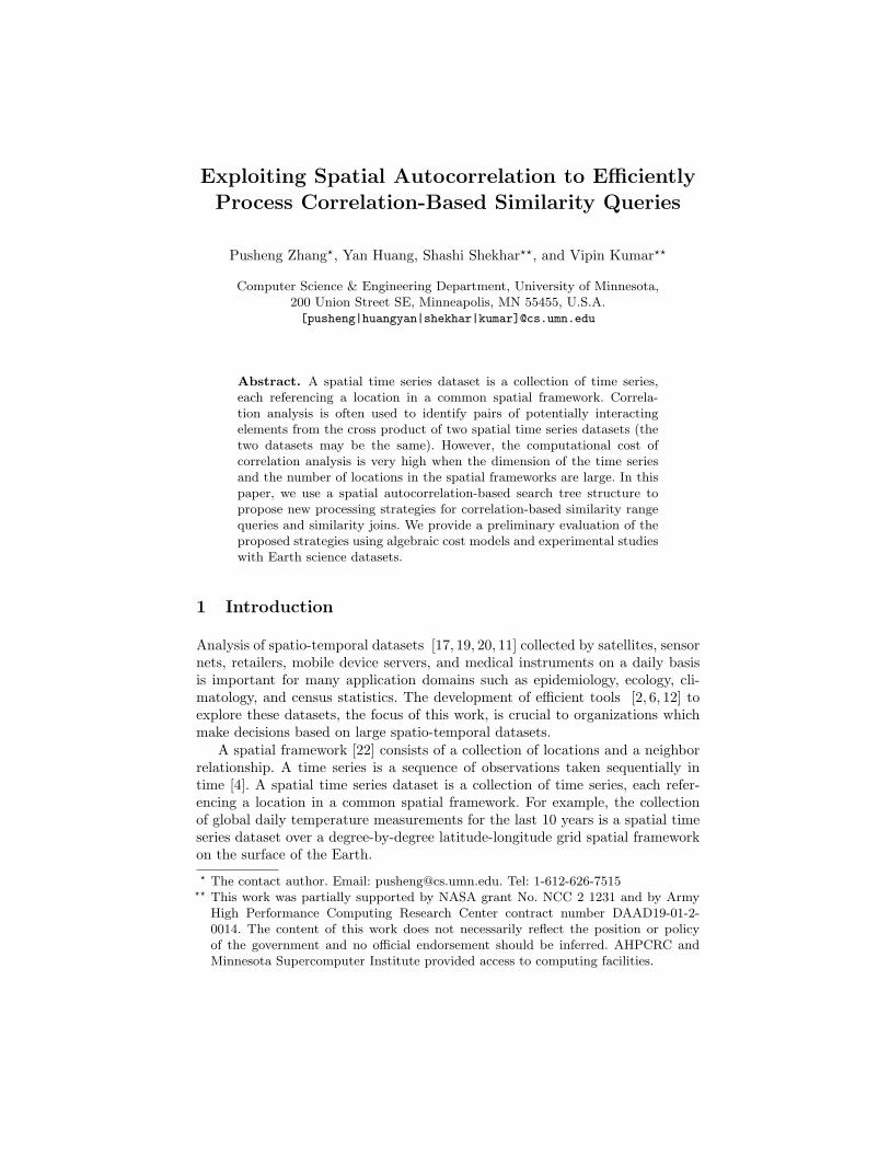
(a) (Reproduced from [10]) World-wide climatic impacts of warm ElNino events during the northernhemisphere winter

max

γmin

γ

O

Cone Cone

δ

Q2

2 Q

1

P2C1C

1 2

P

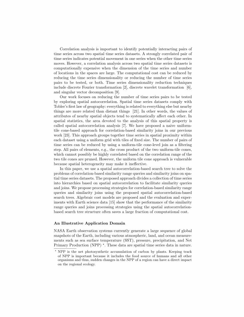
(b) Angle of Time Series in TwoCones

Fig. 1. El Nino Effects and Cones

The climate of the Earth’s land surface is strongly influenced by the behaviorof the oceans. Simultaneous variations in climate and related processes overwidely separated points on the Earth are called teleconnections. For example,every three to seven years, an El Nino event [1], i.e., the anomalous warmingof the eastern tropical region of the Pacific Ocean, may last for months, havingsignificant economic and atmospheric consequences worldwide. El Nino has beenlinked to climate phenomena such as droughts in Australia and heavy rainfallalong the eastern coast of South America, as shown in Figure 1 (a). D indicatesdrought, R indicates unusually high rainfall (not necessarily unusually intenserainfall) and W indicates abnormally warm periods. To investigate such land-sea teleconnections, time series correlation analysis across the land and ocean isoften used to reveal the relationship of measurements of observations.

For example, the identification of teleconnections between Minneapolis andthe eastern tropical region of the Pacific Ocean would help Earth scientists tobetter understand and predict the influence of El Nino in Minneapolis. In ourexample, the query time series is the monthly NPP data in Minneapolis from1982 to 1993, denoted as Tq. The minimal correlation threshold is denoted as θ.This is a correlation-based similarity range query to retrieve all highly correlatedSST time series in the eastern tropical region of the Pacific Ocean with the NPPtime series in Minneapolis. We carry out the range query to retrieve all timeseries which correlate with Tq over θ in the spatial time series data S, whichcontain all the SST time series data in the eastern tropical region of the PacificOcean from 1982 to 1993. The table design of S could be represented as shownin Table 1. This query is represented using SQL as follows:

select SST from S where correlation(SST,Tq) ≥ θ

S: SST of the Eastern Pacific Ocean

Longitude Latitude SST (82-93)

N: NPP of Minnesota

Longitude Latitude NPP (82-93)Table 1. Tables Schema for Table S and Table N

Another interesting example query is to retrieve all the highly correlatedSST time series in the eastern tropical region of the Pacific with the time seriesof NPP in all of Minnesota. This query is a correlation-based similarity joinbetween the NPP of Minnesota land grids and the SST in the eastern tropicalregion of the Pacific. The table design of Minnesota NPP time series data from1982 to 1993, N , is shown in Table 1. The query is represented using SQL asfollows:

select NPP, SST from N, S where correlation(NPP,SST) ≥ θ

Due to large amount of data available, the performance of naive nested loopalgorithms is not sufficient to satisfy the increasing demands to efficiently processcorrelation-based similarity queries in large spatial time series datasets. We pro-pose algorithms that use spatial autocorrelation-based search trees to facilitatethe correlation-based similarity query processing in spatial time series data.

Scope and Outline

In this paper we choose a simple quad-tree like structure as the search tree dueto its simplicity. R-tree, k-d tree, z-ordering tree and their variations [16, 19, 18]could be other possible candidates of the search tree. However, the comparisonof these spatial data structures is beyond the scope of this paper. We focus onthe strategies for correlation-based similarity queries in spatial time series data,and the computation saving methods we examine involve reduction of the timeseries pairs to be tested. Query processing using other similarity measures andcomputation saving methods based on non-spatial properties ( e.g. time seriespower spectrum [2, 6, 9]) are beyond the scope of the paper and will be addressedin future work.

The rest of the paper is organized as follows. In Section 2, the basic conceptsand lemmas related to the cone definition and boundaries are provided. Section 3describes the formation of the spatial autocorrelation-based search tree and thecorrelation-based similarity range query and join strategies using the proposedspatial autocorrelation-based search tree. The cost models are discussed in Sec-tion 4. Section 5 presents the experimental design and results. We summarizeour work and discuss future directions in Section 6.

2 Basic Concepts

Let x = 〈x1, x2, . . . , xm〉 and y = 〈y1, y2, . . . , ym〉 be two time series of lengthm. The correlation coefficient [5] of the two time series is defined as: corr(x, y) =

1m−1

∑mi=1(

xi−xσx

)· (yi−yσy

) = x· y, where x =Pm

i=1 xi

m , σx =√Pm

i=1(xi−x)2

m−1 , y =Pmi=1 yi

m , σy =√Pm

i=1(yi−x)2

m−1 , xi = 1√m−1

xi−xσx

, yi = 1√m−1

yi−yσy

, x = 〈x1, x2,

. . . , xm〉, and y = 〈y1, y2, . . . , ym〉. Because the sum of the xi2 is equal to 1:∑m

i=1 xi2 =

∑mi=1(

1√m−1

xi−xrPmi=1(xi−x)2

m−1

)2 = 1, x is located in a multi-dimensional

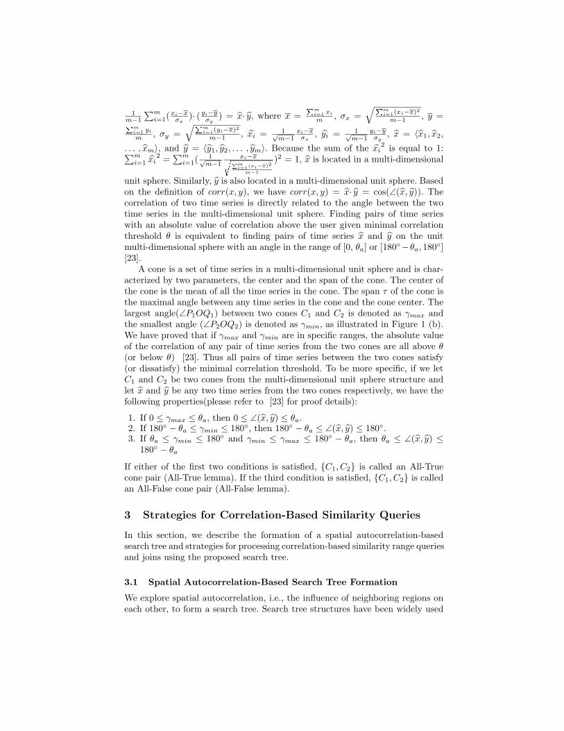
unit sphere. Similarly, y is also located in a multi-dimensional unit sphere. Basedon the definition of corr(x, y), we have corr(x, y) = x· y = cos(∠(x, y)). Thecorrelation of two time series is directly related to the angle between the twotime series in the multi-dimensional unit sphere. Finding pairs of time serieswith an absolute value of correlation above the user given minimal correlationthreshold θ is equivalent to finding pairs of time series x and y on the unitmulti-dimensional sphere with an angle in the range of [0, θa] or [180◦−θa, 180◦][23].

A cone is a set of time series in a multi-dimensional unit sphere and is char-acterized by two parameters, the center and the span of the cone. The center ofthe cone is the mean of all the time series in the cone. The span τ of the cone isthe maximal angle between any time series in the cone and the cone center. Thelargest angle(∠P1OQ1) between two cones C1 and C2 is denoted as γmax andthe smallest angle (∠P2OQ2) is denoted as γmin, as illustrated in Figure 1 (b).We have proved that if γmax and γmin are in specific ranges, the absolute valueof the correlation of any pair of time series from the two cones are all above θ(or below θ) [23]. Thus all pairs of time series between the two cones satisfy(or dissatisfy) the minimal correlation threshold. To be more specific, if we letC1 and C2 be two cones from the multi-dimensional unit sphere structure andlet x and y be any two time series from the two cones respectively, we have thefollowing properties(please refer to [23] for proof details):

1. If 0 ≤ γmax ≤ θa, then 0 ≤ ∠(x, y) ≤ θa.2. If 180◦ − θa ≤ γmin ≤ 180◦, then 180◦ − θa ≤ ∠(x, y) ≤ 180◦.3. If θa ≤ γmin ≤ 180◦ and γmin ≤ γmax ≤ 180◦ − θa, then θa ≤ ∠(x, y) ≤

180◦ − θa

If either of the first two conditions is satisfied, {C1, C2} is called an All-Truecone pair (All-True lemma). If the third condition is satisfied, {C1, C2} is calledan All-False cone pair (All-False lemma).

3 Strategies for Correlation-Based Similarity Queries

In this section, we describe the formation of a spatial autocorrelation-basedsearch tree and strategies for processing correlation-based similarity range queriesand joins using the proposed search tree.

3.1 Spatial Autocorrelation-Based Search Tree Formation

We explore spatial autocorrelation, i.e., the influence of neighboring regions oneach other, to form a search tree. Search tree structures have been widely used

in traditional DBMS (e.g. B-tree and B+ tree) and spatial DBMS (quad-tree,R-tree, R+-tree, R*-tree, and R-link tree [16, 19] ). To fully exploit the spatialautocorrelation property, there are three major criteria for choosing a tree onthe spatial time series datasets. First, a spatial tree structure is preferred toincorporate the spatial component of the datasets. Second, during the tree for-mation the time series calculations such as mean and span should be minimizedwhile still need to maintain a high correlation (high clustering) among time serieswithin a tree node. Third, threaded leaves where leaves are linked are preferredto support sequential scan of files which are useful for high selectivity ratio cor-relation queries. Other desired properties include depth balances of a tree andincremental updates when the time series component changes.

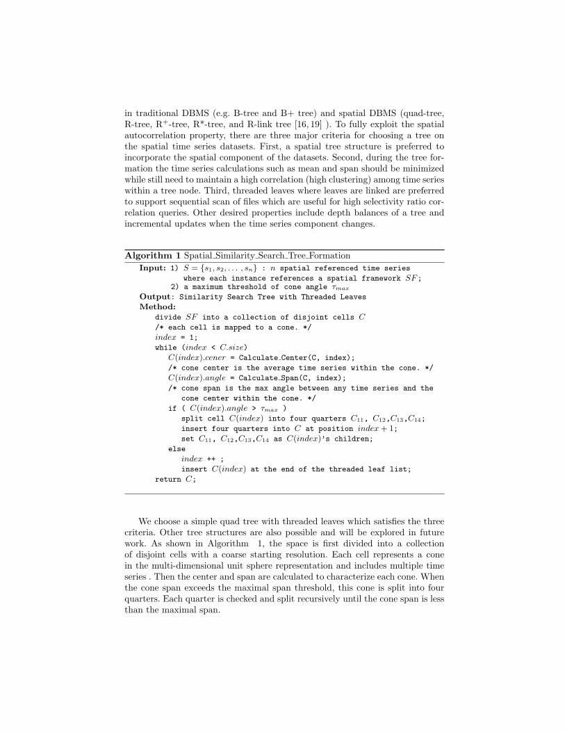
Algorithm 1 Spatial Similarity Search Tree FormationInput: 1) S = {s1, s2, . . . , sn} : n spatial referenced time series

where each instance references a spatial framework SF;2) a maximum threshold of cone angle τmax

Output: Similarity Search Tree with Threaded Leaves

Method:divide SF into a collection of disjoint cells C/* each cell is mapped to a cone. */

index = 1;

while (index < C.size)C(index).cener = Calculate Center(C, index);

/* cone center is the average time series within the cone. */

C(index).angle = Calculate Span(C, index);

/* cone span is the max angle between any time series and the

cone center within the cone. */

if ( C(index).angle > τmax )

split cell C(index) into four quarters C11, C12,C13,C14;

insert four quarters into C at position index + 1;set C11, C12,C13,C14 as C(index)’s children;

else

index ++ ;

insert C(index) at the end of the threaded leaf list;

return C;

We choose a simple quad tree with threaded leaves which satisfies the threecriteria. Other tree structures are also possible and will be explored in futurework. As shown in Algorithm 1, the space is first divided into a collectionof disjoint cells with a coarse starting resolution. Each cell represents a conein the multi-dimensional unit sphere representation and includes multiple timeseries . Then the center and span are calculated to characterize each cone. Whenthe cone span exceeds the maximal span threshold, this cone is split into fourquarters. Each quarter is checked and split recursively until the cone span is lessthan the maximal span.

The maximal span threshold can be estimated by using an algebraic formulaanalyzed as follows. Given a minimal correlation threshold θ (0 < θ < 1), γmax =δ + τ1 + τ2 and γmin = δ − τ1 − τ2, where δ is the angle between the centersof two cones, and the τ1 and τ2 are the spans of the two cones respectively. Forsimplicity, suppose τ1 ' τ2 = τ . We have the following two properties (Pleaserefer to [23] for proof details):

1. Given a minimal correlation threshold θ, if a pair of cones both with span τ

is an All-True cone pair, then τ < arccos(θ)2 .

2. Given a minimal correlation threshold θ, if a pair of cones both with span τ

is an All-False cone pair, then τ < 180◦4 − arccos(θ)

2 .

We use the above two properties to develop a heuristic to bound the maximalspan of a cone. The maximal span of a cone is set to be the minimal of the arccos(θ)

2

and 180◦4 − arccos(θ)

2 .The starting resolution can be investigated by using a spatial correlogram [7].

A spatial correlogram plots the average correlation of pairs of spatial time se-ries with the same spatial distance against the spatial distances of those pairs.We choose the starting resolution size whose average correlation is close to thecorrelation which corresponds to min( arccos(θ)

2 , 180◦4 − arccos(θ)

2 ).

OL

(b)(d) Selective Cones in Unit Circle and SpatialAutocorrelation-based Search Trees for L and O

(b)(a) (d)

OL

(c)

O

L3 4L

O

2L

1O

4O

2O1O

4

2

O

L

O2O3L2L1 O1 O3 O4

(Dim = 2, Multi-dimensional Sphere Reduces to Circle

2

3

O11

O1

L

2L

L4

(Dotted Rectangles Represent Four Quarters after Splitting)

Land Cell

0

1

2

3

0 2 3

0

1

2

3

0 1 2 3

(a)(c) Direction Vectors Attached to Spatial Frameworks

1

0

1

2

3

0 1 2 3

Ocean Cells

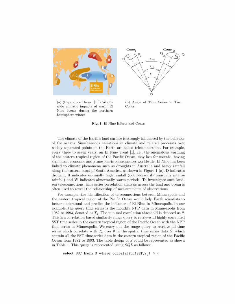
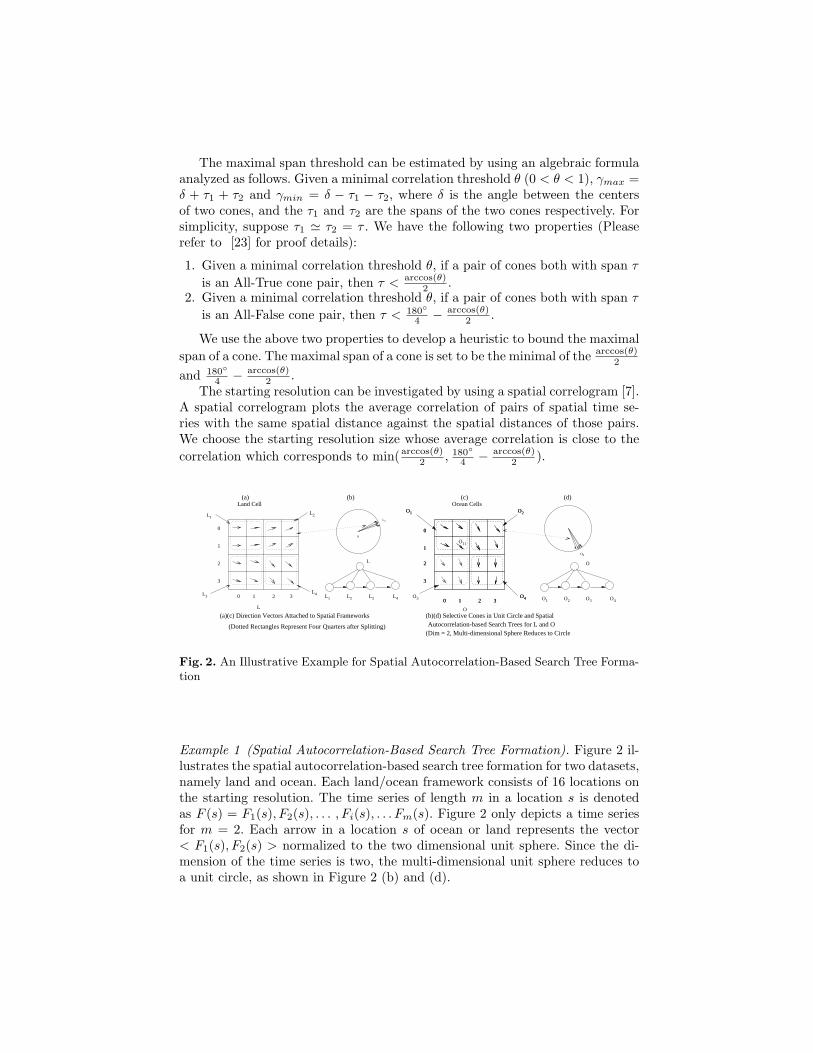
Fig. 2. An Illustrative Example for Spatial Autocorrelation-Based Search Tree Forma-tion

Example 1 (Spatial Autocorrelation-Based Search Tree Formation). Figure 2 il-lustrates the spatial autocorrelation-based search tree formation for two datasets,namely land and ocean. Each land/ocean framework consists of 16 locations onthe starting resolution. The time series of length m in a location s is denotedas F (s) = F1(s), F2(s), . . . , Fi(s), . . . Fm(s). Figure 2 only depicts a time seriesfor m = 2. Each arrow in a location s of ocean or land represents the vector< F1(s), F2(s) > normalized to the two dimensional unit sphere. Since the di-mension of the time series is two, the multi-dimensional unit sphere reduces toa unit circle, as shown in Figure 2 (b) and (d).

Both land and ocean cells are further split into four quarters respectivelydue to the spatial heterogeneity in the cell. The land is partitioned to L1 − L4

and the ocean is partitioned to O1 −O4, as shown in Figure 2 (a) and (c). Eachquarter represents a cone in the multi-dimensional unit sphere. For example, thepatch L2 in Figure 2 (a) matches L2 in the circle in Figure 2 (b). All leaves arethreaded, assuming that L1 to L4 and O1 to O4 are all leaves.

3.2 Strategies for Similarity Range Queries and Similarity Joins

The first step is to pre-process the raw data to the multi-dimensional unitsphere representation. The second step, formation of spatial autocorrelation-based search trees involves grouping similar time series into hierarchical conesusing the one described in Algorithm 1. The query processing functions calledmay be related to similarity range query or similarity join, depending on thequery types.

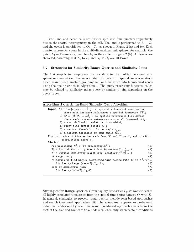
Algorithm 2 Correlation-Based Similarity Query AlgorithmInput: 1) S1 = {s1

1, s12, . . . , s1

n1}: n1 spatial referenced time series

where each instance references a spatial framework SF1;

2) S2 = {s21, s

22, . . . , s2

n2}: n2 spatial referenced time series

where each instance references a spatial framework SF2;3) a user defined correlation threshold θ;4) query time series denote Tq ;

5) a maximum threshold of cone angle τ1max

6) a maximum threshold of cone angle τ2max

Output: pairs of time series each from S1 and S2 or Tq and S2 with

correlations above θ;Method:

Pre-processing(S1); Pre-processing(S2); (1)

T1 = Spatial Similarity Search Tree Formation(S1, τ1max ); (2)

T2 = Spatial Similarity Search Tree Formation(S2, τ2max ); (3)

if range query (4)

/* assume to find highly correlated time series with Tq in S2.*/ (5)

Similarity Range Query(T2,Tq, θ); (6)

else if similarity join (7)

Similarity Join(T1,T2,θ); (8)

Strategies for Range Queries Given a query time series Tq, we want to searchall highly correlated time series from the spatial time series dataset S2 with Tq.In general, strategies to process range queries include scan-based approachesand search tree-based approaches [8]. The scan-based approaches probe eachindividual nodes one by one. The search tree-based approach starts from theroot of the tree and branches to a node’s children only when certain conditions

are satisfied, e.g., the minimal bounding box of the child contains the queryingelement.

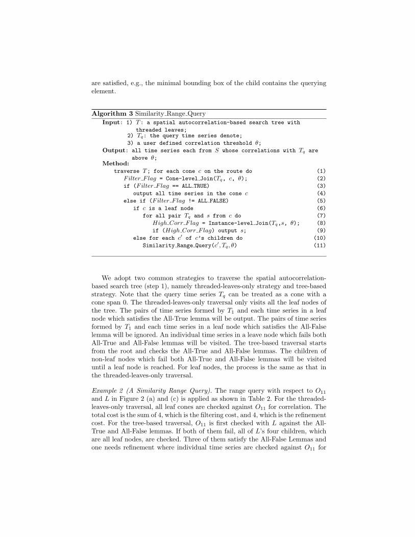
Algorithm 3 Similarity Range QueryInput: 1) T: a spatial autocorrelation-based search tree with

threaded leaves;2) Tq: the query time series denote;

3) a user defined correlation threshold θ;Output: all time series each from S whose correlations with Tq are

above θ;Method:

traverse T; for each cone c on the route do (1)

Filter F lag = Cone-level Join(Tq, c, θ); (2)

if (Filter F lag == ALL TRUE) (3)

output all time series in the cone c (4)

else if (Filter F lag != ALL FALSE) (5)

if c is a leaf node (6)

for all pair Tq and s from c do (7)

High Corr F lag = Instance-level Join(Tq,s, θ); (8)

if (High Corr F lag) output s; (9)

else for each c′ of c’s children do (10)

Similarity Range Query(c′, Tq, θ) (11)

We adopt two common strategies to traverse the spatial autocorrelation-based search tree (step 1), namely threaded-leaves-only strategy and tree-basedstrategy. Note that the query time series Tq can be treated as a cone with acone span 0. The threaded-leaves-only traversal only visits all the leaf nodes ofthe tree. The pairs of time series formed by T1 and each time series in a leafnode which satisfies the All-True lemma will be output. The pairs of time seriesformed by T1 and each time series in a leaf node which satisfies the All-Falselemma will be ignored. An individual time series in a leave node which fails bothAll-True and All-False lemmas will be visited. The tree-based traversal startsfrom the root and checks the All-True and All-False lemmas. The children ofnon-leaf nodes which fail both All-True and All-False lemmas will be visiteduntil a leaf node is reached. For leaf nodes, the process is the same as that inthe threaded-leaves-only traversal.

Example 2 (A Similarity Range Query). The range query with respect to O11

and L in Figure 2 (a) and (c) is applied as shown in Table 2. For the threaded-leaves-only traversal, all leaf cones are checked against O11 for correlation. Thetotal cost is the sum of 4, which is the filtering cost, and 4, which is the refinementcost. For the tree-based traversal, O11 is first checked with L against the All-True and All-False lemmas. If both of them fail, all of L’s four children, whichare all leaf nodes, are checked. Three of them satisfy the All-False Lemmas andone needs refinement where individual time series are checked against O11 for

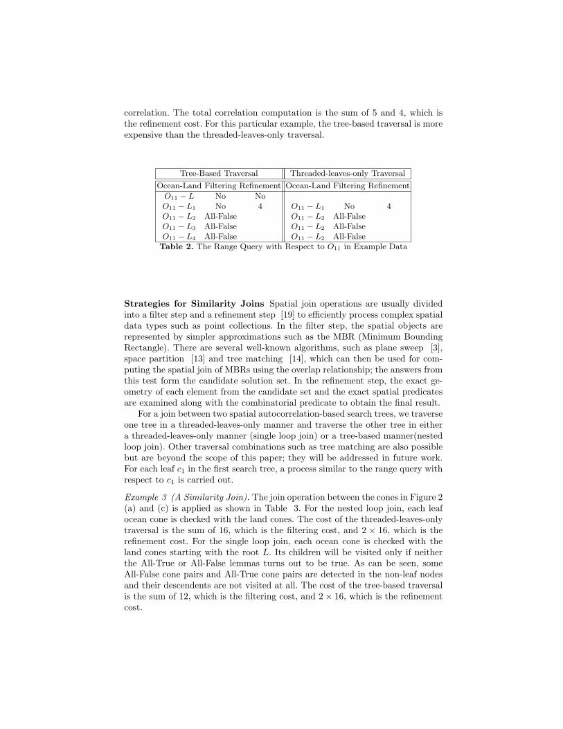
correlation. The total correlation computation is the sum of 5 and 4, which isthe refinement cost. For this particular example, the tree-based traversal is moreexpensive than the threaded-leaves-only traversal.

Tree-Based Traversal Threaded-leaves-only Traversal

Ocean-Land Filtering Refinement Ocean-Land Filtering Refinement

O11 − L No NoO11 − L1 No 4 O11 − L1 No 4O11 − L2 All-False O11 − L2 All-FalseO11 − L3 All-False O11 − L2 All-FalseO11 − L4 All-False O11 − L2 All-FalseTable 2. The Range Query with Respect to O11 in Example Data

Strategies for Similarity Joins Spatial join operations are usually dividedinto a filter step and a refinement step [19] to efficiently process complex spatialdata types such as point collections. In the filter step, the spatial objects arerepresented by simpler approximations such as the MBR (Minimum BoundingRectangle). There are several well-known algorithms, such as plane sweep [3],space partition [13] and tree matching [14], which can then be used for com-puting the spatial join of MBRs using the overlap relationship; the answers fromthis test form the candidate solution set. In the refinement step, the exact ge-ometry of each element from the candidate set and the exact spatial predicatesare examined along with the combinatorial predicate to obtain the final result.

For a join between two spatial autocorrelation-based search trees, we traverseone tree in a threaded-leaves-only manner and traverse the other tree in eithera threaded-leaves-only manner (single loop join) or a tree-based manner(nestedloop join). Other traversal combinations such as tree matching are also possiblebut are beyond the scope of this paper; they will be addressed in future work.For each leaf c1 in the first search tree, a process similar to the range query withrespect to c1 is carried out.

Example 3 (A Similarity Join). The join operation between the cones in Figure 2(a) and (c) is applied as shown in Table 3. For the nested loop join, each leafocean cone is checked with the land cones. The cost of the threaded-leaves-onlytraversal is the sum of 16, which is the filtering cost, and 2 × 16, which is therefinement cost. For the single loop join, each ocean cone is checked with theland cones starting with the root L. Its children will be visited only if neitherthe All-True or All-False lemmas turns out to be true. As can be seen, someAll-False cone pairs and All-True cone pairs are detected in the non-leaf nodesand their descendents are not visited at all. The cost of the tree-based traversalis the sum of 12, which is the filtering cost, and 2× 16, which is the refinementcost.

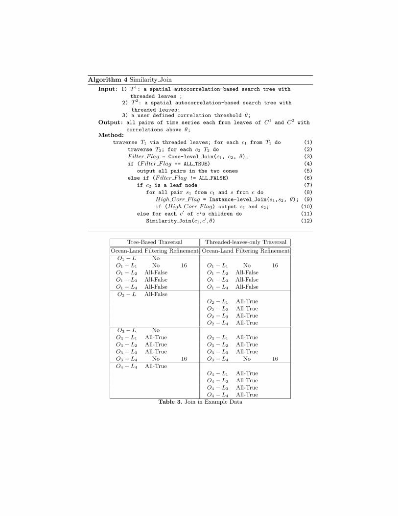
Algorithm 4 Similarity JoinInput: 1) T 1: a spatial autocorrelation-based search tree with

threaded leaves ;2) T 2: a spatial autocorrelation-based search tree with

threaded leaves;3) a user defined correlation threshold θ;

Output: all pairs of time series each from leaves of C1 and C2 with

correlations above θ;Method:

traverse T1 via threaded leaves; for each c1 from T1 do (1)

traverse T2; for each c2 T2 do (2)

Filter F lag = Cone-level Join(c1, c2, θ); (3)

if (Filter F lag == ALL TRUE) (4)

output all pairs in the two cones (5)

else if (Filter F lag != ALL FALSE) (6)

if c2 is a leaf node (7)

for all pair s1 from c1 and s from c do (8)

High Corr F lag = Instance-level Join(s1,s2, θ); (9)

if (High Corr F lag) output s1 and s2; (10)

else for each c′ of c’s children do (11)

Similarity Join(c1, c′, θ) (12)

Tree-Based Traversal Threaded-leaves-only Traversal

Ocean-Land Filtering Refinement Ocean-Land Filtering Refinement

O1 − L NoO1 − L1 No 16 O1 − L1 No 16O1 − L2 All-False O1 − L2 All-FalseO1 − L3 All-False O1 − L3 All-FalseO1 − L4 All-False O1 − L4 All-False

O2 − L All-FalseO2 − L1 All-TrueO2 − L2 All-TrueO2 − L3 All-TrueO2 − L4 All-True

O3 − L NoO3 − L1 All-True O3 − L1 All-TrueO3 − L2 All-True O3 − L2 All-TrueO3 − L3 All-True O3 − L3 All-TrueO3 − L4 No 16 O3 − L4 No 16

O4 − L4 All-TrueO4 − L1 All-TrueO4 − L2 All-TrueO4 − L3 All-TrueO4 − L4 All-True

Table 3. Join in Example Data

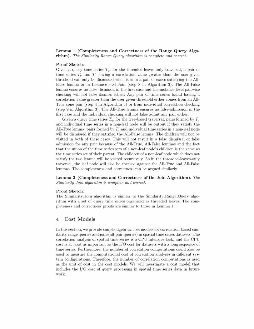
Lemma 1 (Completeness and Correctness of the Range Query Algo-rithm). The Similarity Range Query algorithm is complete and correct.

Proof Sketch:Given a query time series Tq, for the threaded-leaves-only traversal, a pair oftime series Tq and T ′ having a correlation value greater than the user giventhreshold can only be dismissed when it is in a pair of cones satisfying the All-False lemma or in Instance-level Join (step 8 in Algorithm 3). The All-Falselemma ensures no false-dismissal in the first case and the instance level pairwisechecking will not false dismiss either. Any pair of time series found having acorrelation value greater than the user given threshold either comes from an All-True cone pair (step 4 in Algorithm 3) or from individual correlation checking(step 9 in Algorithm 3). The All-True lemma ensures no false-admission in thefirst case and the individual checking will not false admit any pair either.

Given a query time series Tq, for the tree-based traversal, pairs formed by Tq

and individual time series in a non-leaf node will be output if they satisfy theAll-True lemma; pairs formed by Tq and individual time series in a non-leaf nodewill be dismissed if they satisfied the All-False lemma. The children will not bevisited in both of these cases. This will not result in a false dismissal or falseadmission for any pair because of the All-True, All-False lemmas and the factthat the union of the time series sets of a non-leaf node’s children is the same asthe time series set of their parent. The children of a non-leaf node which does notsatisfy the two lemma will be visited recursively. As in the threaded-leaves-onlytraversal, the leaf node will also be checked against the All-True and All-Falselemmas. The completeness and correctness can be argued similarly.

Lemma 2 (Completeness and Correctness of the Join Algorithm). TheSimilarity Join algorithm is complete and correct.

Proof Sketch:The Similarity Join algorithm is similar to the Similarity Range Query algo-rithm with a set of query time series organized as threaded leaves. The com-pleteness and correctness proofs are similar to those in Lemma 1.

4 Cost Models

In this section, we provide simple algebraic cost models for correlation-based sim-ilarity range queries and joins(all-pair queries) in spatial time series datasets. Thecorrelation analysis of spatial time series is a CPU intensive task, and the CPUcost is at least as important as the I/O cost for datasets with a long sequence oftime series. Furthermore, the number of correlation computations could also beused to measure the computational cost of correlation analyses in different sys-tem configurations. Therefore, the number of correlation computations is usedas the unit of cost in the cost models. We will investigate a cost model thatincludes the I/O cost of query processing in spatial time series data in futurework.

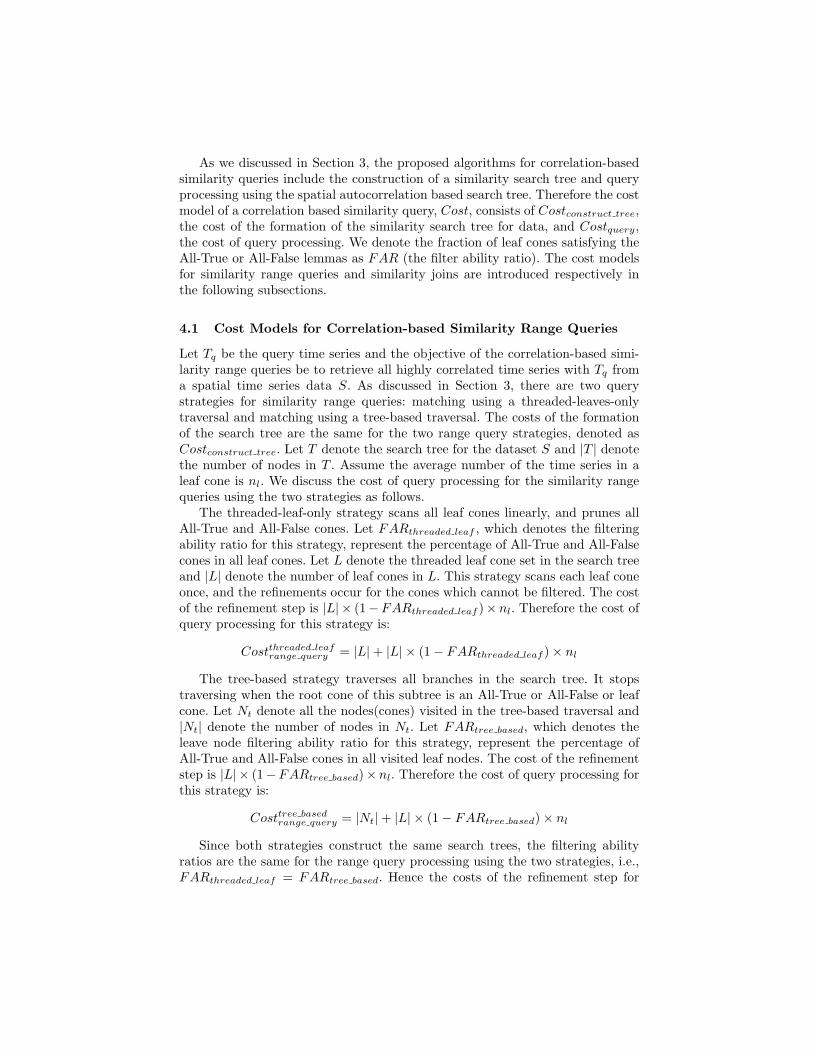
As we discussed in Section 3, the proposed algorithms for correlation-basedsimilarity queries include the construction of a similarity search tree and queryprocessing using the spatial autocorrelation based search tree. Therefore the costmodel of a correlation based similarity query, Cost, consists of Costconstruct tree,the cost of the formation of the similarity search tree for data, and Costquery,the cost of query processing. We denote the fraction of leaf cones satisfying theAll-True or All-False lemmas as FAR (the filter ability ratio). The cost modelsfor similarity range queries and similarity joins are introduced respectively inthe following subsections.

4.1 Cost Models for Correlation-based Similarity Range Queries

Let Tq be the query time series and the objective of the correlation-based simi-larity range queries be to retrieve all highly correlated time series with Tq froma spatial time series data S. As discussed in Section 3, there are two querystrategies for similarity range queries: matching using a threaded-leaves-onlytraversal and matching using a tree-based traversal. The costs of the formationof the search tree are the same for the two range query strategies, denoted asCostconstruct tree. Let T denote the search tree for the dataset S and |T | denotethe number of nodes in T . Assume the average number of the time series in aleaf cone is nl. We discuss the cost of query processing for the similarity rangequeries using the two strategies as follows.

The threaded-leaf-only strategy scans all leaf cones linearly, and prunes allAll-True and All-False cones. Let FARthreaded leaf , which denotes the filteringability ratio for this strategy, represent the percentage of All-True and All-Falsecones in all leaf cones. Let L denote the threaded leaf cone set in the search treeand |L| denote the number of leaf cones in L. This strategy scans each leaf coneonce, and the refinements occur for the cones which cannot be filtered. The costof the refinement step is |L| × (1−FARthreaded leaf )× nl. Therefore the cost ofquery processing for this strategy is:

Costthreaded leafrange query = |L|+ |L| × (1− FARthreaded leaf )× nl

The tree-based strategy traverses all branches in the search tree. It stopstraversing when the root cone of this subtree is an All-True or All-False or leafcone. Let Nt denote all the nodes(cones) visited in the tree-based traversal and|Nt| denote the number of nodes in Nt. Let FARtree based, which denotes theleave node filtering ability ratio for this strategy, represent the percentage ofAll-True and All-False cones in all visited leaf nodes. The cost of the refinementstep is |L| × (1−FARtree based)× nl. Therefore the cost of query processing forthis strategy is:

Costtree basedrange query = |Nt|+ |L| × (1− FARtree based)× nl

Since both strategies construct the same search trees, the filtering abilityratios are the same for the range query processing using the two strategies, i.e.,FARthreaded leaf = FARtree based. Hence the costs of the refinement step for

the two strategies are the same. When the filtering ability ratio of a range queryincreases, the number of nodes visited using the tree-based strategy, |Nt| oftentends to decrease.

4.2 Cost Models for Correlation-based Similarity Joins

Let S1 and S2 be two spatial time series datasets. The objective of the corre-lation based similarity join is to retrieve all highly correlated time series pairsbetween the two datasets. As discussed in Section 3, there are two query strate-gies for a similarity join: the nested loop approach, which iterates the threadedleaves of both search trees, and the single loop approach, which iterates thethreaded leaves of one search tree and traverses the other search tree in a check-ing and branching manner. The costs of the formation of search trees denoted asCostconstruct tree are the same for the two join strategies. Let T1 and T2 denotethe search trees for the dataset S1 and S2 respectively. Let |T1| and |T2| denotethe number of nodes in T1 and T2 respectively. Let L1 and L2 be the leaf conesets for T1 and T2 respectively, and |L1| and |L2| be the number of leaf cones inL1 and L2 respectively. Assume the average numbers of the time series in leafcones are nl1 and nl2 for L1 and L2 respectively. We will discuss the cost of thequery processing for the join processing using the two strategies as follows.

The strategy using a nested loop of the threaded leaf cones is a cone-leveljoin between two leaf cone sets of the two search trees. Let FARnested loop, whichdenotes the filtering ability ratio for this strategy, represent the percentage ofAll-True and All-False cones in the nested loop join. The cost of the nested loopjoin is |L1|×|L2|, and the cost of refinement is |L1|×|L2|× (1−FARnested loop).The total cost of join processing using the nested loop of leaf cones is:

Costnested loopjoin = |L1| × |L2|+ |L1| × |L2| × (1− FARnested loop)× nl1 × nl2

The strategy using a single loop of tree-based traversal chooses the searchtree with the smaller number of leaf cones as the outer loop, and choose theother as the search tree in the inner loop. Without losing the generality, weassume that the leaf cone set of T1 is chosen as the outer loop and T2 is chosenas the search tree in the inner loop. Let Nt2 denote all the visited nodes in thesearch tree T2 and |Nt2| denote the number of nodes in Nt2. Let FARtree based,which denotes the leaf node filtering ability ratio for this strategy, represent thepercentage of All-True and All-False cones of the leaf nodes in the nested loopjoin. We match each leaf cone center in the outer loop with the inner searchtree T2. Therefore each matching is a special range query for each leaf cone withmultiple time series inside, and the cost is |Nt2|+ |L2|×FARsingle loop×nl1×nl2

The total cost of the joins using the single loop is:

Costsingle loopjoin = |L1| × (|Nt2|+ |L2| × (1− FARsingle loop)× nl1 × nl2)

5 Performance Evaluation

We wanted to answer two questions: (1) How do the two query strategies im-prove the performance of correlation-based similarity range query processing?

(2) How do the two query strategies improve the performance of correlationbased similarity join processing?

Pre-

Proc

essi

ngPr

e-Pr

oces

sing

timeseries 1

+

+

+

Answers

Spat

ial A

utoc

orre

latio

n-ba

sed

Sear

ch T

ree

Con

stru

ctio

n

thresholdcorrelationSp

atia

l Aut

ocor

rela

tion-

base

d

Sear

ch T

ree

Con

stru

ctio

n ++

initial cone size 1

initial cone size 2

Threaded Leaves only Traversal

range query

join

Tree-based Traversal

time

Threaded Leaves only Traversal

range query time series

series 2

Note: represents the multiple choices

spatial

spatial

Pre-Processing Refinement

All-True All-False

Filtering

minimal

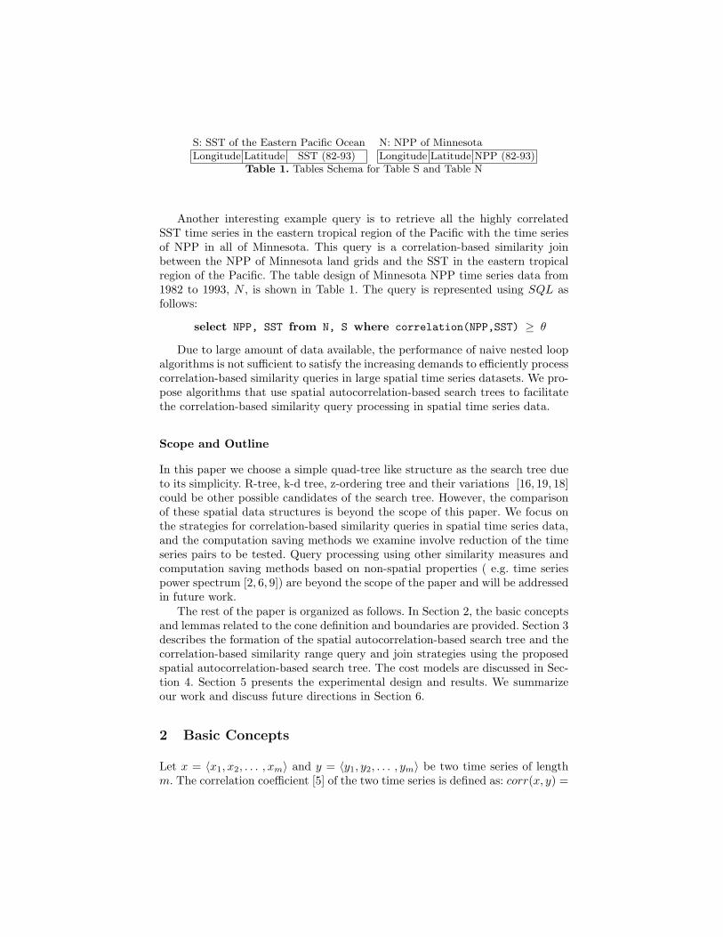
Fig. 3. Experimental Design

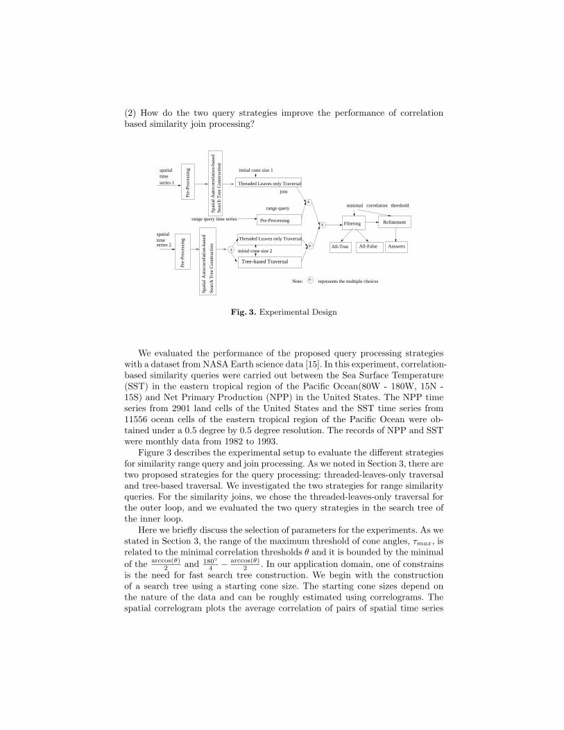
We evaluated the performance of the proposed query processing strategieswith a dataset from NASA Earth science data [15]. In this experiment, correlation-based similarity queries were carried out between the Sea Surface Temperature(SST) in the eastern tropical region of the Pacific Ocean(80W - 180W, 15N -15S) and Net Primary Production (NPP) in the United States. The NPP timeseries from 2901 land cells of the United States and the SST time series from11556 ocean cells of the eastern tropical region of the Pacific Ocean were ob-tained under a 0.5 degree by 0.5 degree resolution. The records of NPP and SSTwere monthly data from 1982 to 1993.

Figure 3 describes the experimental setup to evaluate the different strategiesfor similarity range query and join processing. As we noted in Section 3, there aretwo proposed strategies for the query processing: threaded-leaves-only traversaland tree-based traversal. We investigated the two strategies for range similarityqueries. For the similarity joins, we chose the threaded-leaves-only traversal forthe outer loop, and we evaluated the two query strategies in the search tree ofthe inner loop.

Here we briefly discuss the selection of parameters for the experiments. As westated in Section 3, the range of the maximum threshold of cone angles, τmax, isrelated to the minimal correlation thresholds θ and it is bounded by the minimalof the arccos(θ)

2 and 180◦4 − arccos(θ)

2 . In our application domain, one of constrainsis the need for fast search tree construction. We begin with the constructionof a search tree using a starting cone size. The starting cone sizes depend onthe nature of the data and can be roughly estimated using correlograms. Thespatial correlogram plots the average correlation of pairs of spatial time series

1 2 3 4 5 6 7 8 9 10 11 12 13 14 15 20 25 30 350.6

0.65

0.7

0.75

0.8

0.85

0.9

0.95

1

Distance

Cor

rela

tion

(a) Correlogram for Land

1 2 3 4 5 6 7 8 9 10 11 12 13 14 15 20 25 30 35

0.75

0.8

0.85

0.9

0.950.960.970.980.99

1

Distance

Cor

rela

tion

(b) Correlogram for Ocean

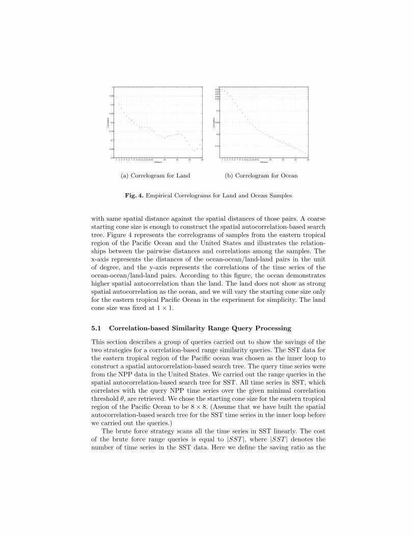
Fig. 4. Empirical Correlograms for Land and Ocean Samples

with same spatial distance against the spatial distances of those pairs. A coarsestarting cone size is enough to construct the spatial autocorrelation-based searchtree. Figure 4 represents the correlograms of samples from the eastern tropicalregion of the Pacific Ocean and the United States and illustrates the relation-ships between the pairwise distances and correlations among the samples. Thex-axis represents the distances of the ocean-ocean/land-land pairs in the unitof degree, and the y-axis represents the correlations of the time series of theocean-ocean/land-land pairs. According to this figure, the ocean demonstrateshigher spatial autocorrelation than the land. The land does not show as strongspatial autocorrelation as the ocean, and we will vary the starting cone size onlyfor the eastern tropical Pacific Ocean in the experiment for simplicity. The landcone size was fixed at 1× 1.

5.1 Correlation-based Similarity Range Query Processing

This section describes a group of queries carried out to show the savings of thetwo strategies for a correlation-based range similarity queries. The SST data forthe eastern tropical region of the Pacific ocean was chosen as the inner loop toconstruct a spatial autocorrelation-based search tree. The query time series werefrom the NPP data in the United States. We carried out the range queries in thespatial autocorrelation-based search tree for SST. All time series in SST, whichcorrelates with the query NPP time series over the given minimal correlationthreshold θ, are retrieved. We chose the starting cone size for the eastern tropicalregion of the Pacific Ocean to be 8× 8. (Assume that we have built the spatialautocorrelation-based search tree for the SST time series in the inner loop beforewe carried out the queries.)

The brute force strategy scans all the time series in SST linearly. The costof the brute force range queries is equal to |SST |, where |SST | denotes thenumber of time series in the SST data. Here we define the saving ratio as the

0.3 0.4 0.5 0.6 0.7 0.8 0.90.4

0.5

0.6

0.7

0.8

0.9

Minimial Correlation Thresholds of Range QueryA

vera

ge S

avin

g R

atio

s

Title: Average Saving Ratios of 10 Range Queries

Leaf Only TraversalTree−based Traversal

0.3 0.4 0.5 0.6 0.7 0.8 0.90

0.1

0.2

0.3

0.4

Minimial Correlation Thresholds of Range Query

Ave

rage

Sel

ectiv

ity R

atio

sTitle: Average Selectivity Ratios of 10 Range Queries

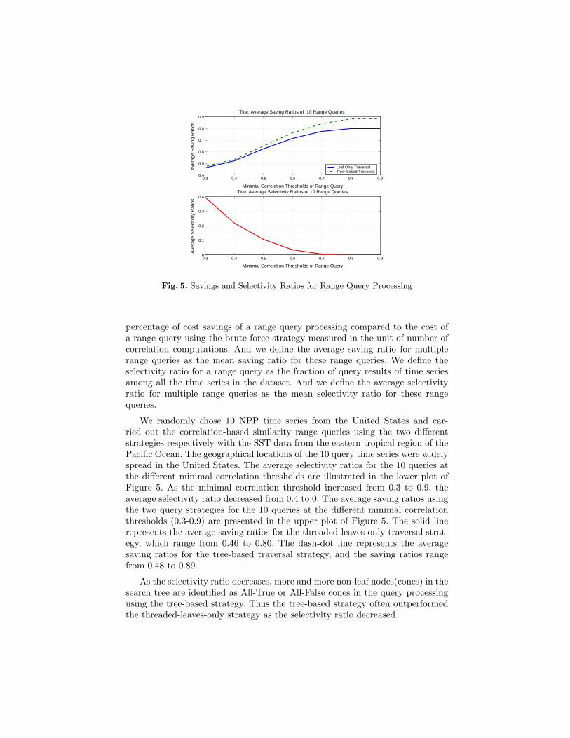
Fig. 5. Savings and Selectivity Ratios for Range Query Processing

percentage of cost savings of a range query processing compared to the cost ofa range query using the brute force strategy measured in the unit of number ofcorrelation computations. And we define the average saving ratio for multiplerange queries as the mean saving ratio for these range queries. We define theselectivity ratio for a range query as the fraction of query results of time seriesamong all the time series in the dataset. And we define the average selectivityratio for multiple range queries as the mean selectivity ratio for these rangequeries.

We randomly chose 10 NPP time series from the United States and car-ried out the correlation-based similarity range queries using the two differentstrategies respectively with the SST data from the eastern tropical region of thePacific Ocean. The geographical locations of the 10 query time series were widelyspread in the United States. The average selectivity ratios for the 10 queries atthe different minimal correlation thresholds are illustrated in the lower plot ofFigure 5. As the minimal correlation threshold increased from 0.3 to 0.9, theaverage selectivity ratio decreased from 0.4 to 0. The average saving ratios usingthe two query strategies for the 10 queries at the different minimal correlationthresholds (0.3-0.9) are presented in the upper plot of Figure 5. The solid linerepresents the average saving ratios for the threaded-leaves-only traversal strat-egy, which range from 0.46 to 0.80. The dash-dot line represents the averagesaving ratios for the tree-based traversal strategy, and the saving ratios rangefrom 0.48 to 0.89.

As the selectivity ratio decreases, more and more non-leaf nodes(cones) in thesearch tree are identified as All-True or All-False cones in the query processingusing the tree-based strategy. Thus the tree-based strategy often outperformedthe threaded-leaves-only strategy as the selectivity ratio decreased.

5.2 Correlation-based Similarity Join Processing

This section describes a group of experiments carried out to show the net sav-ings of the two strategies for the correlation-based similarity joins. The NPPtime series dataset for the United State was chosen as the outer loop. As wediscussed in the selection of parameter, the cone size for the NPP data was fixedat 1 × 1. The SST time series data for the eastern tropical region of the Pa-cific Ocean was chosen as the inner loop. A spatial autocorrelation-based searchtree was constructed for the SST data. (Assume that we have built the spa-tial autocorrelation-based search trees before we carried out the similarity joinoperations.)

2 3 4 5 6 7 80

0.2

0.4

0.6

0.8

1

Starting Ocean Cone Sizes

Sav

ing

Rat

ios

θ = 0.3

Leaf Only TraversalTree−based Traversal

2 3 4 5 6 7 80

0.2

0.4

0.6

0.8

1

Starting Ocean Cone Sizes

Sav

ing

Rat

ios

θ = 0.5

Leaf Only TraversalTree−based Traversal

2 3 4 5 6 7 80

0.2

0.4

0.6

0.8

1

Starting Ocean Cone Sizes

Sav

ing

Rat

ios

θ = 0.7

Leaf Only TraversalTree−based Traversal

2 3 4 5 6 7 80

0.2

0.4

0.6

0.8

1

Starting Ocean Cone Sizes

Sav

ing

Rat

ios

θ = 0.9

Leaf Only TraversalTree−based Traversal

Savings Ratios of Join Processing at Different Minimal Correlation Thresholds

Fig. 6. Savings for Join Processing

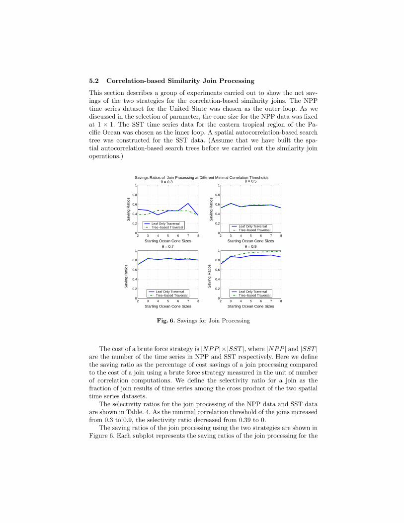
The cost of a brute force strategy is |NPP |×|SST |, where |NPP | and |SST |are the number of the time series in NPP and SST respectively. Here we definethe saving ratio as the percentage of cost savings of a join processing comparedto the cost of a join using a brute force strategy measured in the unit of numberof correlation computations. We define the selectivity ratio for a join as thefraction of join results of time series among the cross product of the two spatialtime series datasets.

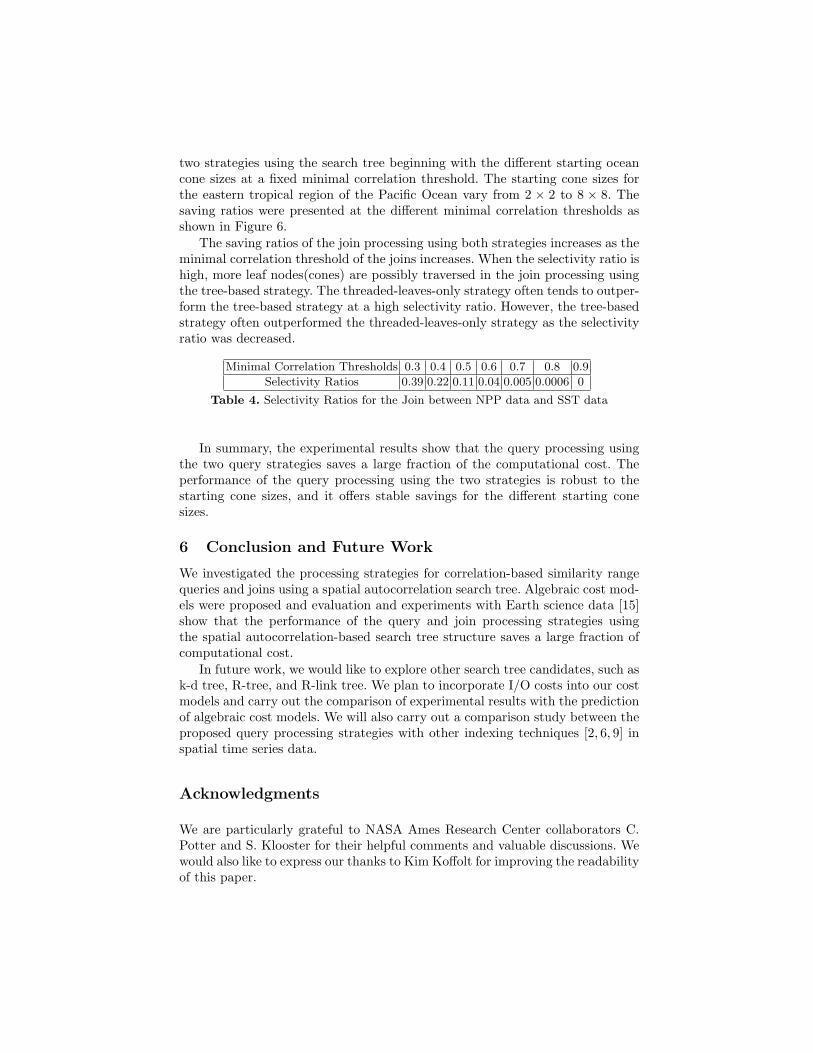
The selectivity ratios for the join processing of the NPP data and SST dataare shown in Table. 4. As the minimal correlation threshold of the joins increasedfrom 0.3 to 0.9, the selectivity ratio decreased from 0.39 to 0.

The saving ratios of the join processing using the two strategies are shown inFigure 6. Each subplot represents the saving ratios of the join processing for the

two strategies using the search tree beginning with the different starting oceancone sizes at a fixed minimal correlation threshold. The starting cone sizes forthe eastern tropical region of the Pacific Ocean vary from 2 × 2 to 8 × 8. Thesaving ratios were presented at the different minimal correlation thresholds asshown in Figure 6.

The saving ratios of the join processing using both strategies increases as theminimal correlation threshold of the joins increases. When the selectivity ratio ishigh, more leaf nodes(cones) are possibly traversed in the join processing usingthe tree-based strategy. The threaded-leaves-only strategy often tends to outper-form the tree-based strategy at a high selectivity ratio. However, the tree-basedstrategy often outperformed the threaded-leaves-only strategy as the selectivityratio was decreased.

Minimal Correlation Thresholds 0.3 0.4 0.5 0.6 0.7 0.8 0.9

Selectivity Ratios 0.39 0.22 0.11 0.04 0.005 0.0006 0

Table 4. Selectivity Ratios for the Join between NPP data and SST data

In summary, the experimental results show that the query processing usingthe two query strategies saves a large fraction of the computational cost. Theperformance of the query processing using the two strategies is robust to thestarting cone sizes, and it offers stable savings for the different starting conesizes.

6 Conclusion and Future Work

We investigated the processing strategies for correlation-based similarity rangequeries and joins using a spatial autocorrelation search tree. Algebraic cost mod-els were proposed and evaluation and experiments with Earth science data [15]show that the performance of the query and join processing strategies usingthe spatial autocorrelation-based search tree structure saves a large fraction ofcomputational cost.

In future work, we would like to explore other search tree candidates, such ask-d tree, R-tree, and R-link tree. We plan to incorporate I/O costs into our costmodels and carry out the comparison of experimental results with the predictionof algebraic cost models. We will also carry out a comparison study between theproposed query processing strategies with other indexing techniques [2, 6, 9] inspatial time series data.

Acknowledgments

We are particularly grateful to NASA Ames Research Center collaborators C.Potter and S. Klooster for their helpful comments and valuable discussions. Wewould also like to express our thanks to Kim Koffolt for improving the readabilityof this paper.

References

1. NOAA El Nino Page. http://www.elnino.noaa.gov/.2. R. Agrawal, C. Faloutsos, and A. Swami. Efficient Similarity Search In Sequence

Databases. In Proc. of the 4th Int’l Conference of Foundations of Data Organiza-tion and Algorithms, 1993.

3. L. Arge, O. Procopiuc, S. Ramaswamy, T. Suel, and J. Vitter. Scalable Sweeping-Based Spatial Join. In Proc. of the 24th Int’l Conf. on VLDB, 1998.

4. G. Box, G. Jenkins, and G. Reinsel. Time Series Analysis: Forecasting and Control.Prentice Hall, 1994.

5. B.W. Lindgren. Statistical Theory (Fourth Edition). Chapman-Hall, 1998.6. K. Chan and A. W. Fu. Efficient Time Series Matching by Wavelets. In Proc. of

the 15th ICDE, 1999.7. N. Cressie. Statistics for Spatial Data. John Wiley and Sons, 1991.8. R. Elmasri and S. Navathe. Fundamentals of Database Systems. Addison Wesley

Higher Education, 2002.9. Christos Faloutsos. Searching Multimedia Databases By Content. Kluwer Academic

Publishers, 1996.10. Food and Agriculture Organization. Farmers brace for extreme weather

conditions as El Nino effect hits Latin America and Australia .http://www.fao.org/NEWS/1997/970904-e.htm.

11. R. Grossman, C. Kamath, P. Kegelmeyer, V. Kumar, and R. Namburu, editors.Data Mining for Scientific and Engineering Applications. Kluwer Academic Pub-lishers, ISBN: 1-4020-0033-2, 2001.

12. D. Gunopulos and G. Das. Time Series Similarity Measures and Time SeriesIndexing. SIGMOD Record, 30(2), 2001.

13. D. J. DeWitt J. M. Patel. Partition Based Spatial-Merge Join. In Proc. of theACM SIGMOD Conference, 1996.

14. S. T. Leutenegger and M. A. Lopez. The Effect of Buffering on the Performanceof R-Trees. In Proc. of the ICDE Conf., pp 164-171, 1998.

15. C. Potter, S. Klooster, and V. Brooks. Inter-annual Variability in Terrestrial NetPrimary Production: Exploration of Trends and Controls on Regional to GlobalScales. Ecosystems, 2(1):36–48, 1999.

16. P. Rigaux, M. Scholl, and A. Voisard. Spatial Databases: With Application to GIS.Morgan Kaufmann Publishers, 2001.

17. J. Roddick, K. Hornsby, and M. Spiliopoulou. An Updated Bibliography of Tempo-ral, Spatial, and Spatio-Temporal Data Mining Research. In First Int’l WorkshopTSDM, 2000.

18. H. Samet. The Design and Analysis of Spatial Data Structures. Addison-WesleyPublishing Company, Inc., 1990.

19. S. Shekhar and S. Chawla. Spatial Databases: A Tour. Prentice Hall,ISBN:0130174807, 2003.

20. S. Shekhar, S. Chawla, S. Ravada, A. Fetterer, X. Liu, and C.T. Lu. SpatialDatabases: Accomplishments and Research Needs. IEEE TKDE, 11(1), 1999.

21. W.R. Tobler. Cellular Geography, Philosophy in Geography. Gale and Olsson, Eds.,Dordrecht, Reidel, 1979.

22. Michael F. Worboys. GIS - A Computing Perspective. Taylor and Francis, 1995.23. Pusheng Zhang, Yan Huang, Shashi Shekhar, and Vipin Kumar. Correlation Anal-

ysis of Spatial Time Series Datasets: A Filter-and-Refine Approach. In the Proc.of the 7th Pacific-Asia Conf. on Knowledge Discovery and Data Mining, 2003.