Embed Size (px)
Citation preview
Exploring Giant Planets and their PotentialMoons in the Habitable Zone
Undergraduate Honours Thesis
Submitted in partial fulfillment of the requirements of
USQ Honours Thesis
By
Michelle L. Hill
ID No. 0061103417
Under the supervision of:
Prof. Stephen Kane
&
Prof. Brad Carter
UNIVERSITY OF SOUTHERN QUEENSLAND, COMPUTATIONAL ENGINEERING
AND SCIENCE RESEARCH CENTRE
July 2018
Declaration of Authorship
I, Michelle L. Hill, declare that this Undergraduate Honours Thesis titled, ‘Exploring Giant
Planets and their Potential Moons in the Habitable Zone’ and the work presented in it are my
own. I confirm that:
⌅ This work was done wholly or mainly while in candidature for a research degree at this
University.
⌅ Where any part of this thesis has previously been submitted for a degree or any other
qualification at this University or any other institution, this has been clearly stated.
⌅ Where I have consulted the published work of others, this is always clearly attributed.
⌅ Where I have quoted from the work of others, the source is always given. With the
exception of such quotations, this thesis is entirely my own work.
⌅ I have acknowledged all main sources of help.
⌅ Where the thesis is based on work done by myself jointly with others, I have made clear
exactly what was done by others and what I have contributed myself.
Signed:
Date:
i
Certificate
This is to certify that the thesis entitled, “Exploring Giant Planets and their Potential Moons in
the Habitable Zone” and submitted by Michelle L. Hill ID No. 0061103417 in partial fulfillment
of the requirements of USQ Honours Thesis embodies the work done by her under our supervision.
Supervisor
Prof. Stephen Kane
Adjunct Professor,
University of Southern Queensland,
Computational Engineering and Science
Research Centre, Toowoomba, Queensland
4350, Australia
University of California, Riverside,
Department of Earth Sciences, CA 92521,
USA
Date:
Co-Supervisor
Prof. Brad Carter
Professor,
University of Southern Queensland,
Computational Engineering and Science
Research Centre, Toowoomba, Queensland
4350, Australia
Date:
ii
UNIVERSITY OF SOUTHERN QUEENSLAND, COMPUTATIONAL ENGINEERING AND
SCIENCE RESEARCH CENTRE
Abstract
Bachelor of Science (Hons.)
Exploring Giant Planets and their Potential Moons in the Habitable Zone
by Michelle L. Hill
The recent discovery of a disturbance in the orbital period of a transiting exoplanet observed with
the Kepler space telescope has provided the first observational hints of a giant satellite orbiting
a planet, or an exomoon. The detection and study of exomoons o↵ers new ways to understand
the formation and evolution of planetary systems, and widens the search for signs of life out in
the universe. This thesis thus provides proposed exoplanet target lists to search for detectable
exomoons and perform more detailed follow-up studies. Improved orbital parameters compared
to previous studies have been calculated to aid exomoon searches, and relevant habitable zone
boundaries have been added. The list of planets has initially been refined to select exoplanets
circular orbits contained within either the optimistic habitable zone (OHZ) or the conservative
habitable zone (CHZ). Taking a giant planet mass to be 0.02MJ (Jupiter masses), 121 giant
planets in the OHZ and 88 giant planets in the CHZ are found. The eccentricity of each planet’s
orbit are then taken into account. In total 61 giant planets eccentric orbits have been found
to remain in the OHZ while 26 giant planets eccentric orbits remain in the CHZ. Each of
the 121 giant planets radial velocity curves are run through RadVel (Fulton et al. 2018) to
confirm the orbital solution and look for linear trends to determine if there are indications
for additional companions; potentially either additional planets in orbit or satellites. Of the
121 giant planets tested, 51 show indications of orbital companions. The potential exomoon
properties of each giant planet have been calculated and tabulated for future imaging missions,
with the results including the Hill radius, Roche limit and expected angular separation of any
potentially detectable exomoon.

Acknowledgements
I would first like to thank my thesis advisor’s Prof. Stephen Kane and Prof. Brad Carter. Prof.
Kane has always made the time to be available for video conferencing whenever I ran into a
trouble spot or had a question about my research or writing and I am indebted to him for his
guidance. Additionally, Prof. Carter was always quick to respond to emails and provide advice
and encouragement during the project. I would like to thank them both sincerely for their time
and help throughout the year.
I would also like to acknowledge Prof. Stephen Marsden and Prof. Rob Wittenmyer for being
the examiners of this thesis, I am grateful to them for their very valuable comments on the
introductory seminar, literature review and draft thesis throughout the year which helped lead
to the completion of this thesis.
I would also like to thank the honours coordinators Joanna Turner and Linda Galligan for their
continued support and assistance throughout the year. Without their administrative help this
thesis could not have been successfully completed.
Finally, I must express my very profound gratitude to my parents and to my partner Ayo for
providing me with unfailing support and continuous encouragement throughout my years of
study and through the process of researching and writing this thesis. This accomplishment would
not have been possible without them. Thank you.
Michelle Hill
iv
Contents
Declaration of Authorship i
Certificate ii
Abstract iii
Acknowledgements iv
Contents v
List of Figures vii
List of Tables viii
Glossary ix
1 Introduction 1
1.1 Introduction . . . . . . . . . . . . . . . . . . . . . . . . . . . . . . . . . . . . . . . 1
2 Literature Review 5
2.1 Exoplanets . . . . . . . . . . . . . . . . . . . . . . . . . . . . . . . . . . . . . . . 5
2.1.1 Detection Methods . . . . . . . . . . . . . . . . . . . . . . . . . . . . . . . 5
2.1.2 The Search for Earth-like Planets . . . . . . . . . . . . . . . . . . . . . . . 8
2.2 Moons & Exomoons . . . . . . . . . . . . . . . . . . . . . . . . . . . . . . . . . . 10
2.2.1 Formation . . . . . . . . . . . . . . . . . . . . . . . . . . . . . . . . . . . . 10
2.2.2 Habitability Potential . . . . . . . . . . . . . . . . . . . . . . . . . . . . . 12
2.2.3 Parameters Needed for Future Detection . . . . . . . . . . . . . . . . . . . 14
3 Method 17
3.1 Habitable Zone Giant Planet Data Analysis . . . . . . . . . . . . . . . . . . . . . 17
3.2 Calculating the Habitable Zone Boundaries . . . . . . . . . . . . . . . . . . . . . 18
3.3 Exomoon Calculations . . . . . . . . . . . . . . . . . . . . . . . . . . . . . . . . . 20
3.4 Confirming Orbital Solutions with RadVel . . . . . . . . . . . . . . . . . . . . . . 22
3.5 Target Selection . . . . . . . . . . . . . . . . . . . . . . . . . . . . . . . . . . . . . 23
4 Results 24
v
Contents vi
4.1 Results . . . . . . . . . . . . . . . . . . . . . . . . . . . . . . . . . . . . . . . . . . 24
4.2 Tables . . . . . . . . . . . . . . . . . . . . . . . . . . . . . . . . . . . . . . . . . . 26
4.2.1 Table Glossary . . . . . . . . . . . . . . . . . . . . . . . . . . . . . . . . . 26
4.2.2 Tables: Parameters . . . . . . . . . . . . . . . . . . . . . . . . . . . . . . . 27
4.2.3 Tables. Habitable Zone Calculations . . . . . . . . . . . . . . . . . . . . . 31
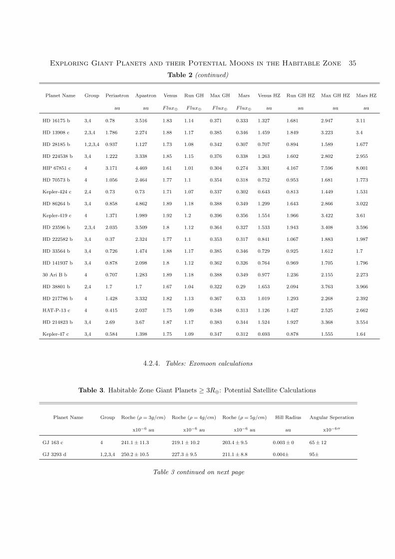
4.2.4 Tables. Exomoon calculations . . . . . . . . . . . . . . . . . . . . . . . . . 35
4.2.5 Tables: RadVel results . . . . . . . . . . . . . . . . . . . . . . . . . . . . . 40
4.2.6 Tables: Observing Strategy . . . . . . . . . . . . . . . . . . . . . . . . . . 44
4.3 Figures . . . . . . . . . . . . . . . . . . . . . . . . . . . . . . . . . . . . . . . . . 50
4.3.1 Figures: Moon Calculations . . . . . . . . . . . . . . . . . . . . . . . . . . 50
4.3.2 Figures: RadVel Curves . . . . . . . . . . . . . . . . . . . . . . . . . . . . 53
5 Discussion 61
5.1 The BRHARVOS Method . . . . . . . . . . . . . . . . . . . . . . . . . . . . . . . 61
5.2 Moon Calculations . . . . . . . . . . . . . . . . . . . . . . . . . . . . . . . . . . . 62
5.3 Observing Strategy . . . . . . . . . . . . . . . . . . . . . . . . . . . . . . . . . . . 63
6 Conclusion and Future Work 67
6.1 A Brief Overview . . . . . . . . . . . . . . . . . . . . . . . . . . . . . . . . . . . . 67
6.2 Future Work . . . . . . . . . . . . . . . . . . . . . . . . . . . . . . . . . . . . . . 68
6.3 Concluding Remarks . . . . . . . . . . . . . . . . . . . . . . . . . . . . . . . . . . 69
A Exploring Kepler Giant Planets in the Habitable Zone 70
Bibliography 71
List of Figures
1.1 Habitable Zone Exomoon . . . . . . . . . . . . . . . . . . . . . . . . . . . . . . . 2
2.1 Transit Depth . . . . . . . . . . . . . . . . . . . . . . . . . . . . . . . . . . . . . . 7
2.2 Exoplanet Detection Methods . . . . . . . . . . . . . . . . . . . . . . . . . . . . . 8
2.3 Habitable Zone Boundaries . . . . . . . . . . . . . . . . . . . . . . . . . . . . . . 9
2.4 The Eccentric Orbit of BD +14 4559 b . . . . . . . . . . . . . . . . . . . . . . . . 13
2.5 Saturn’s Magnetosphere . . . . . . . . . . . . . . . . . . . . . . . . . . . . . . . . 14
2.6 Angular Separation . . . . . . . . . . . . . . . . . . . . . . . . . . . . . . . . . . . 15
4.1 Angular Separation Detectability . . . . . . . . . . . . . . . . . . . . . . . . . . . 50
4.2 Distribution of Angular Separation at Full Hill radii . . . . . . . . . . . . . . . . 51
4.3 Radial Velocity Detectability (Telescope Assignment) . . . . . . . . . . . . . . . . 51
4.4 Radial Velocity Detectability (Group Assignment) . . . . . . . . . . . . . . . . . 52
4.5 Hill Radii Distribution . . . . . . . . . . . . . . . . . . . . . . . . . . . . . . . . . 52
4.6 Roche Limit Distribution . . . . . . . . . . . . . . . . . . . . . . . . . . . . . . . 53
4.7 Radial Velocity Time Series Plot for HD 1605 . . . . . . . . . . . . . . . . . . . . 54
4.8 HD 1605 Markov-Chain Monte Carlo Corner Plot . . . . . . . . . . . . . . . . . . 55
4.9 Radial Velocity Time Series Plot for HD 4113 . . . . . . . . . . . . . . . . . . . . 56
4.10 Radial Velocity Time Series Plot for HD 19994 . . . . . . . . . . . . . . . . . . . 57
4.11 Radial Velocity Time Series Plot for HD 190647 . . . . . . . . . . . . . . . . . . . 58
4.12 Radial Velocity Time Series Plot for HD 73526 . . . . . . . . . . . . . . . . . . . 59
4.13 Radial Velocity Time Series Plot for 55 Cnc . . . . . . . . . . . . . . . . . . . . . 60
vii
List of Tables
4.1 Habitable Zone Giant Planets � 3R�: Parameters . . . . . . . . . . . . . . . . . 27
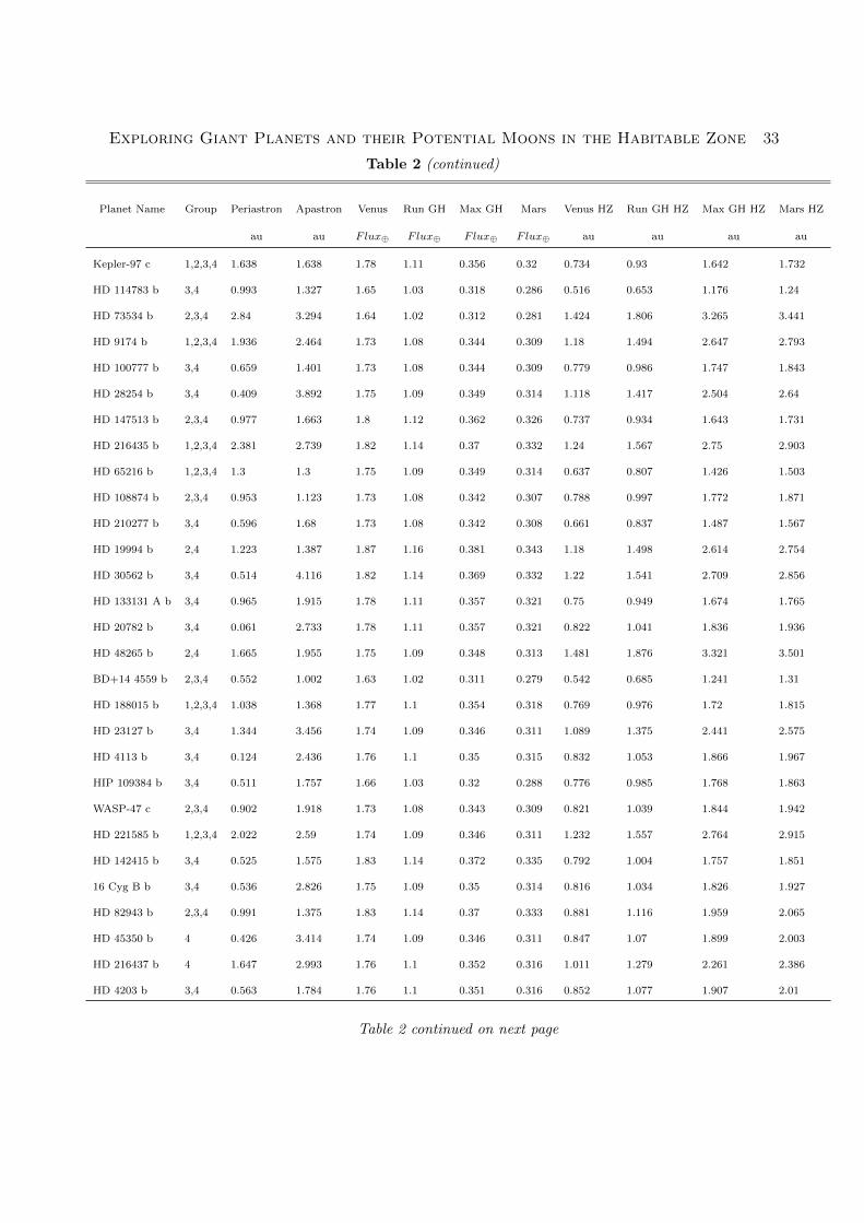
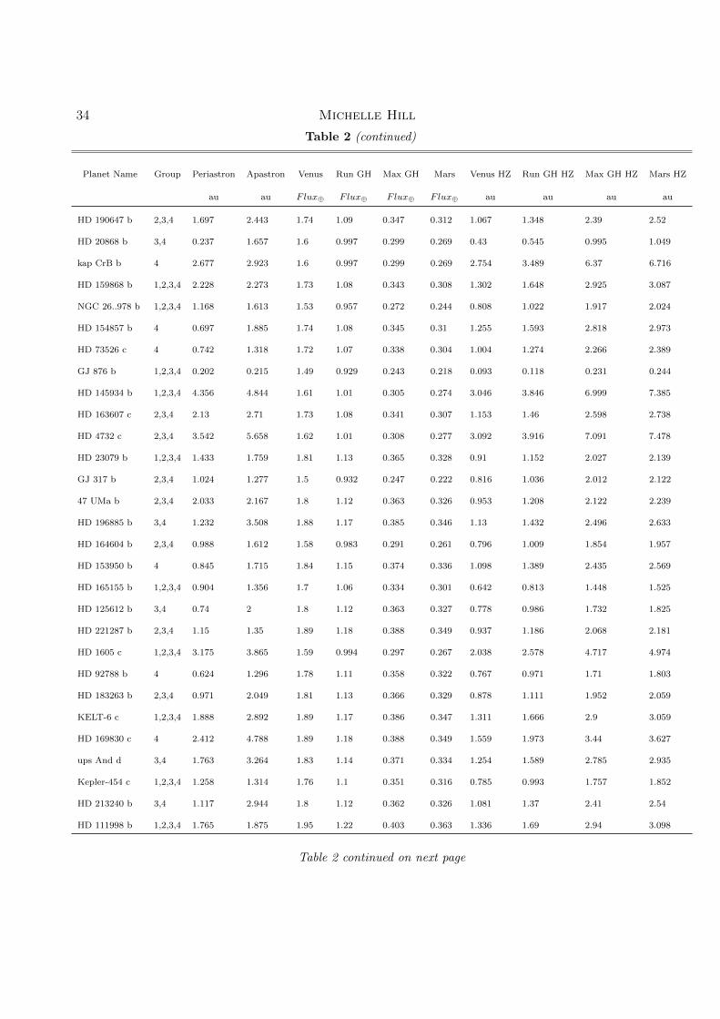
4.2 Habitable Zone Giant Planets � 3R�: Habitable Zone Calculations . . . . . . . . 31
4.3 Habitable Zone Giant Planets � 3R�: Potential Satellite Calculations . . . . . . 35
4.4 Habitable Zone Giant Planets � 3R�: Linear Trends . . . . . . . . . . . . . . . . 40
4.5 Habitable Zone Giant Planets � 3R�: Telescope Strategy of Planets with LinearTrend . . . . . . . . . . . . . . . . . . . . . . . . . . . . . . . . . . . . . . . . . . 44
4.6 Habitable Zone Giant Planets � 3R�: Telescope Strategy of Planets with NoLinear Trend . . . . . . . . . . . . . . . . . . . . . . . . . . . . . . . . . . . . . . 46
viii
Glossary
CHZ conservative habitable zone. iii, 8, 10, 19, 20,
22, 25, 52, 54, 56, 60, 61, 65
HZ habitable zone. 2, 8–10, 12–15, 19, 20, 24–26,
50, 52, 61–65, 68, 69
MAP maximum a posteriori. 22, 53, 56–60
MCMC Markov Chain Monte Carlo. 22, 53, 55
OHZ optimistic habitable zone. iii, 8–10, 19, 20, 22,
25, 52, 57–59, 61, 65
RV radial velocity. 3–6, 8, 15, 17, 18, 22, 61, 62,
65, 67
ix
Chapter 1
Introduction
1.1 Introduction
The field of exoplanets is relatively young, with the detection of the first exoplanet less than 30
years ago. The first extra-solar planet was found around a pulsar star in 1992 (Wolszczan &
Frail 1992), and then another orbiting a sun-like star was found in 1995 (Mayor & Queloz 1995).
From these recent beginnings the field has grown quickly, with 3726 confirmed planets to date
and over 2000 more candidates awaiting confirmation (NASA Exoplanet Archive 2018). While
the progress of this number was initially quite slow due to the di�cult process of discovering
planets, with each new telescope erected on the ground or launched into space our resolution
has improved and we have been able to detect many more planets than ever before. These
planets orbiting stars outside our Solar system have already provided clues to many of questions
regarding the origin and prevalence of life. They have provided further understanding of the
formation and evolution of the planets within our Solar system, and influenced an escalation in
the area of research into what constitutes a habitable planet that could support life.
While a main goal in the detections of exoplanets has been to find Earth like planets; planets of
a similar size, distance from their star and composition as Earth, the hunt for exoplanets has
1
Chapter 1. Introduction 2
revealed examples of many di↵erent planetary systems that has caused us to revise our ideas
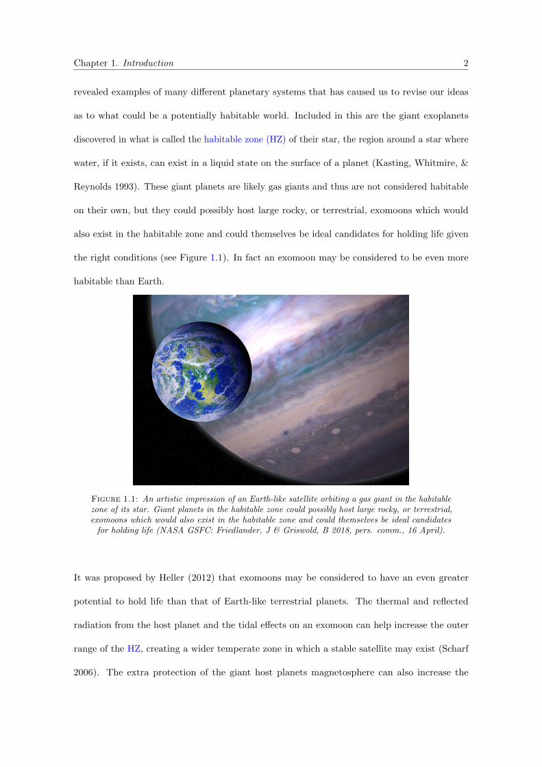
as to what could be a potentially habitable world. Included in this are the giant exoplanets
discovered in what is called the habitable zone (HZ) of their star, the region around a star where
water, if it exists, can exist in a liquid state on the surface of a planet (Kasting, Whitmire, &
Reynolds 1993). These giant planets are likely gas giants and thus are not considered habitable
on their own, but they could possibly host large rocky, or terrestrial, exomoons which would
also exist in the habitable zone and could themselves be ideal candidates for holding life given
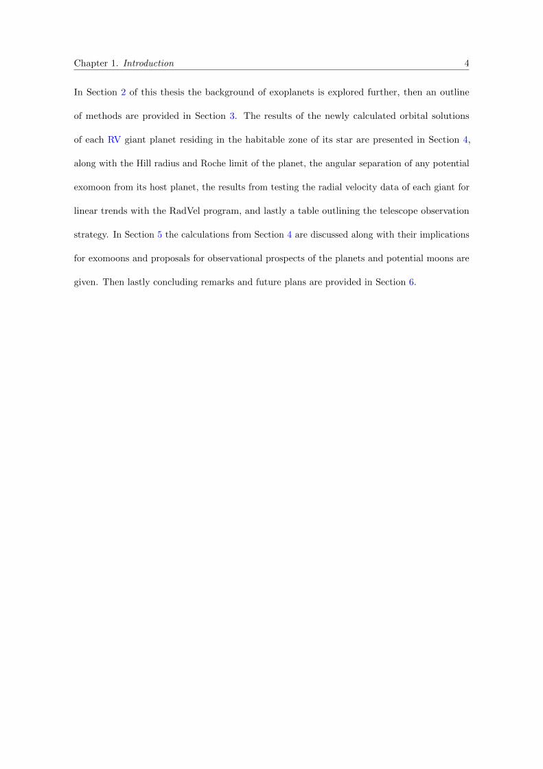
the right conditions (see Figure 1.1). In fact an exomoon may be considered to be even more
habitable than Earth.
Figure 1.1: An artistic impression of an Earth-like satellite orbiting a gas giant in the habitablezone of its star. Giant planets in the habitable zone could possibly host large rocky, or terrestrial,exomoons which would also exist in the habitable zone and could themselves be ideal candidatesfor holding life (NASA GSFC: Friedlander, J & Griswold, B 2018, pers. comm., 16 April).
It was proposed by Heller (2012) that exomoons may be considered to have an even greater
potential to hold life than that of Earth-like terrestrial planets. The thermal and reflected
radiation from the host planet and the tidal e↵ects on an exomoon can help increase the outer
range of the HZ, creating a wider temperate zone in which a stable satellite may exist (Scharf
2006). The extra protection of the giant host planets magnetosphere can also increase the
Chapter 1. Introduction 3
likelihood that a large exomoon will hold on to its atmosphere, another essential ingredient to
life as we know it (Heller & Zuluaga 2013).
This great potential for exomoons has for a long time motivated many others in the hunt for the
first exomoon including Dr David Kipping and the HEK, or Hunt for Exomoons with Kepler
team. [e.g. Kipping et al. 2012, 2013, 2013, 2014, 2015]. Last year the HEK team found
the first potential signature of a planetary companion, Exomoon Candidate Kepler-1625b I
(Teachey, Kipping & Schmitt 2017). Preliminary research indicates that Kepler-1625b is likely a
Jupiter-sized planet with approximately ten times Jupiter’s mass, orbited by a moon roughly
the size of Neptune. Though this discovery is yet to be confirmed, it is the first real evidence of
any such satellite and indicates the beginning of a new phase in the search for exoplanets.
This project contributes to the hunt for exomoons by providing a well refined list of the best
radial velocity (RV) giant planets with the potential to hold large terrestrial exomoons, a giant
planet being a planet with � 0.02MJ . While there is a general consensus that the boundary
between terrestrial and gaseous planets likely lies close to 1.6 Earth radii (R�) [e.g. Weiss
& Marcy 2014, Rodgers 2015, Wolfgang, Rodgers & Ford 2016], 3R� is used as the cuto↵ to
account for uncertainties in the stellar and planetary parameters and prevent the inclusion of
potentially terrestrial planets in the list, as well as planets too small to host detectable exomoons.
Using the mass-radius relation from Chen & Kipping (2016) this corresponds to a mass lower
limit of 0.02MJ . Each giant planet included in this thesis has had their RV data analysed and
their orbital parameters and planetary properties refined using the latest datasets. With the
growing number of known exoplanets and the diversity of exoplanetary orbits, it is becoming
an increasing challenge to maintain a procedure through which one can perform e�cient target
selection. So throughout the target list selection a method was developed, presented in Section 3,
to systematically choose the best habitable zone planet candidates for follow up observations.
Chapter 1. Introduction 4
In Section 2 of this thesis the background of exoplanets is explored further, then an outline
of methods are provided in Section 3. The results of the newly calculated orbital solutions
of each RV giant planet residing in the habitable zone of its star are presented in Section 4,
along with the Hill radius and Roche limit of the planet, the angular separation of any potential
exomoon from its host planet, the results from testing the radial velocity data of each giant for
linear trends with the RadVel program, and lastly a table outlining the telescope observation
strategy. In Section 5 the calculations from Section 4 are discussed along with their implications
for exomoons and proposals for observational prospects of the planets and potential moons are
given. Then lastly concluding remarks and future plans are provided in Section 6.
Chapter 2
Literature Review
2.1 Exoplanets
2.1.1 Detection Methods
In the beginning of the hunt for exoplanets the primary method of detection was called the radial
velocity RV method which involves detecting extremely small movements of the positions of the
stars caused by the gravitational pull of the orbiting planet (Yaqoob 2011). The motion of a single
planet in orbit around a star causes the star to undergo a reflex motion about the star-planet
barycenter (Perryman 2011). This motion is detected through spectroscopy; observations of
the spectrum of light emitted by a star. If the wavelength of characteristic spectral lines in the
spectrum of the star increase and decrease regularly over a period, this indicates the presence of
an orbiting body. The period of motion indicates the period of orbit of the planet. The size
of the motion is related to the mass of the object orbiting the star, as well as the mass of the
star and distance between the star and orbiting body. For a given star and distance, the more
massive the orbiting object, the larger the reflex motion of the host star.
5
Chapter 2. Literature Review 6
The first exoplanet found using this technique was a Jupiter sized planet with an orbital period
of just 4.23 days (Mayor & Queloz 1995). The size and close proximity of the planet’s orbit
made it an ideal candidate for detection as this produced a relatively large movement of the star
that was observable by our then relatively limited observational techniques. It is this ability to
determine the mass (or at least a mass lower limit of m sin i if the inclination of the planets orbit
is not known) of an object that continues to make RV detections and follow up observations
particularly important. Without the mass of a planet, many orbital parameters cannot be
constrained, and the likely structure and composition of an exoplanet would be impossible to
determine. Thus this project uses only the data from those planets with properly constrained
masses obtained through RV detection.
Another method of detection which is used primarily for multi-planet systems is timing variation.
Here the periodic oscillation of the host star about the barycenter between itself and an already
detected planet will show evidence of another orbiting body through the existence of additional
periodic time signatures on the known planets orbit. Changes in the RV and astrometric position
(perceived position in the sky as determined from Earth) of the known planet’s orbit can provide
evidence of another planetary body orbiting and can even give an estimated mass of the new
planet or planets (Perryman 2011, Kipping et al. 2013, 2013). Timing variation is the method
used primarily by the HEK team in the hunt for exomoons; by detecting the slight variations in
transit depth of a transiting planet the existence of a orbiting satellite can be exposed.
The transit method is currently the most fruitful method of detection. It involves the very
slight variation in the luminosity of a star when a planet passes directly in front of it from
our line of sight as shown in Figure 2.1. Transits provide direct evidence for the radius of the
planet. The larger the planet, the greater the amount of star light being blocked during a transit
and so the transit light curve will provide evidence for the size of planet. This information
is another of the key pieces needed to understand the likely structure and composition of an
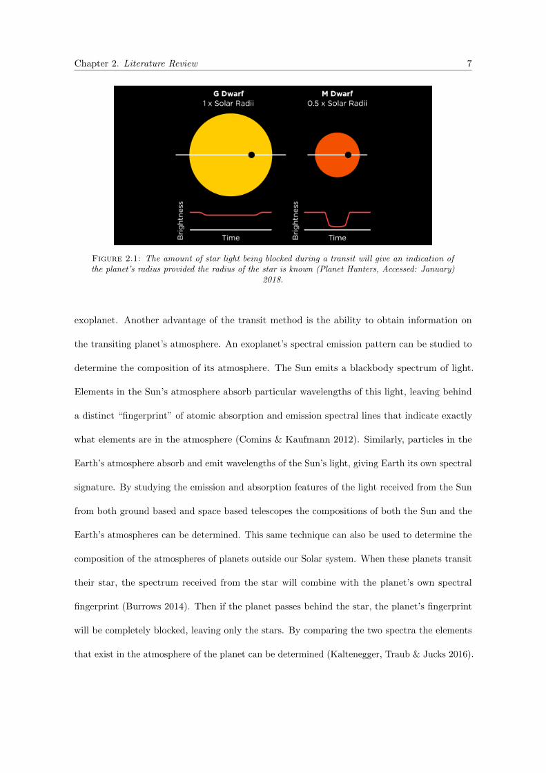
Chapter 2. Literature Review 7
Figure 2.1: The amount of star light being blocked during a transit will give an indication ofthe planet’s radius provided the radius of the star is known (Planet Hunters, Accessed: January)
2018.
exoplanet. Another advantage of the transit method is the ability to obtain information on
the transiting planet’s atmosphere. An exoplanet’s spectral emission pattern can be studied to
determine the composition of its atmosphere. The Sun emits a blackbody spectrum of light.
Elements in the Sun’s atmosphere absorb particular wavelengths of this light, leaving behind
a distinct “fingerprint” of atomic absorption and emission spectral lines that indicate exactly
what elements are in the atmosphere (Comins & Kaufmann 2012). Similarly, particles in the
Earth’s atmosphere absorb and emit wavelengths of the Sun’s light, giving Earth its own spectral
signature. By studying the emission and absorption features of the light received from the Sun
from both ground based and space based telescopes the compositions of both the Sun and the
Earth’s atmospheres can be determined. This same technique can also be used to determine the
composition of the atmospheres of planets outside our Solar system. When these planets transit
their star, the spectrum received from the star will combine with the planet’s own spectral
fingerprint (Burrows 2014). Then if the planet passes behind the star, the planet’s fingerprint
will be completely blocked, leaving only the stars. By comparing the two spectra the elements
that exist in the atmosphere of the planet can be determined (Kaltenegger, Traub & Jucks 2016).
Chapter 2. Literature Review 8
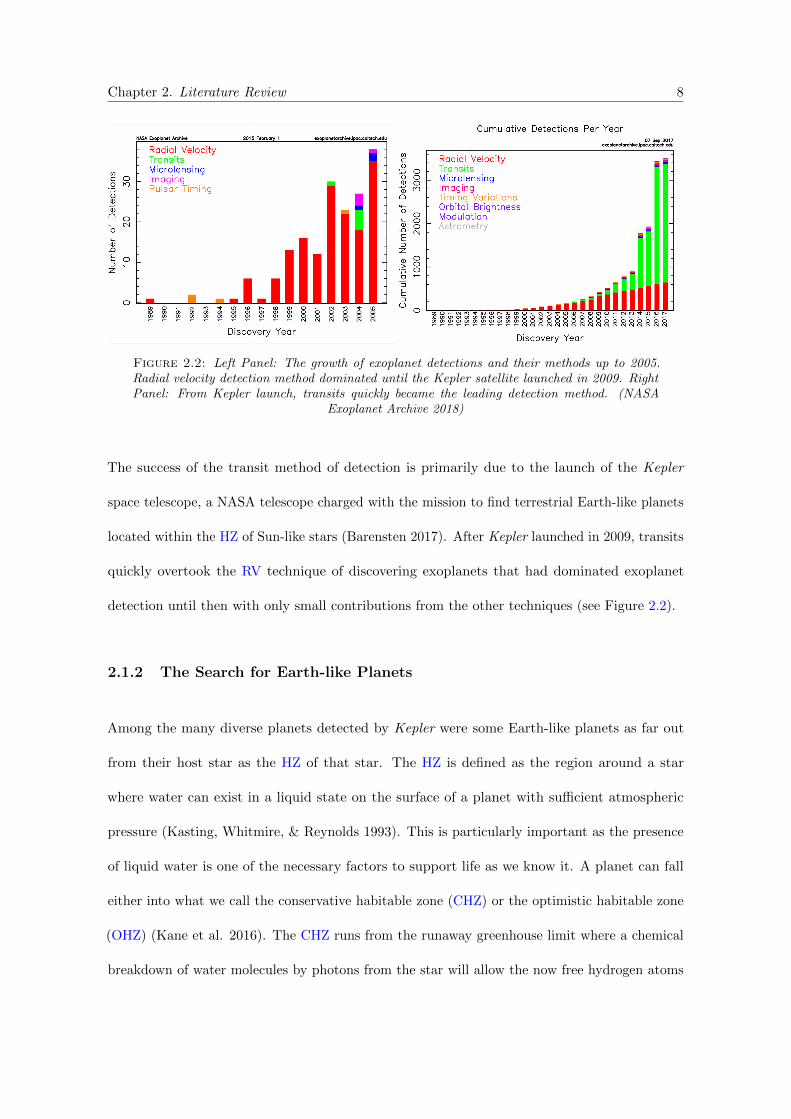
Figure 2.2: Left Panel: The growth of exoplanet detections and their methods up to 2005.Radial velocity detection method dominated until the Kepler satellite launched in 2009. RightPanel: From Kepler launch, transits quickly became the leading detection method. (NASA
Exoplanet Archive 2018)
The success of the transit method of detection is primarily due to the launch of the Kepler
space telescope, a NASA telescope charged with the mission to find terrestrial Earth-like planets
located within the HZ of Sun-like stars (Barensten 2017). After Kepler launched in 2009, transits
quickly overtook the RV technique of discovering exoplanets that had dominated exoplanet
detection until then with only small contributions from the other techniques (see Figure 2.2).
2.1.2 The Search for Earth-like Planets
Among the many diverse planets detected by Kepler were some Earth-like planets as far out
from their host star as the HZ of that star. The HZ is defined as the region around a star
where water can exist in a liquid state on the surface of a planet with su�cient atmospheric
pressure (Kasting, Whitmire, & Reynolds 1993). This is particularly important as the presence
of liquid water is one of the necessary factors to support life as we know it. A planet can fall
either into what we call the conservative habitable zone (CHZ) or the optimistic habitable zone
(OHZ) (Kane et al. 2016). The CHZ runs from the runaway greenhouse limit where a chemical
breakdown of water molecules by photons from the star will allow the now free hydrogen atoms
Chapter 2. Literature Review 9
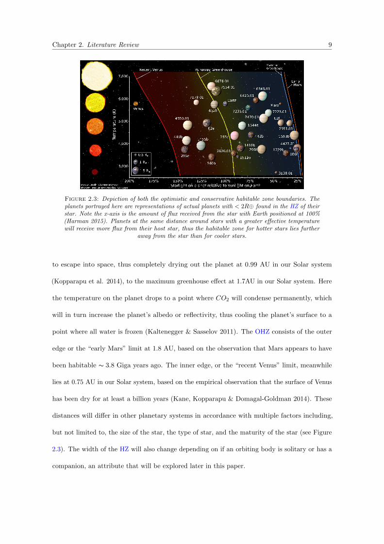
Figure 2.3: Depiction of both the optimistic and conservative habitable zone boundaries. Theplanets portrayed here are representations of actual planets with < 2R� found in the HZ of theirstar. Note the x-axis is the amount of flux received from the star with Earth positioned at 100%(Harman 2015). Planets at the same distance around stars with a greater e↵ective temperaturewill receive more flux from their host star, thus the habitable zone for hotter stars lies further
away from the star than for cooler stars.
to escape into space, thus completely drying out the planet at 0.99 AU in our Solar system
(Kopparapu et al. 2014), to the maximum greenhouse e↵ect at 1.7AU in our Solar system. Here
the temperature on the planet drops to a point where CO2 will condense permanently, which
will in turn increase the planet’s albedo or reflectivity, thus cooling the planet’s surface to a
point where all water is frozen (Kaltenegger & Sasselov 2011). The OHZ consists of the outer
edge or the “early Mars” limit at 1.8 AU, based on the observation that Mars appears to have
been habitable s 3.8 Giga years ago. The inner edge, or the “recent Venus” limit, meanwhile
lies at 0.75 AU in our Solar system, based on the empirical observation that the surface of Venus
has been dry for at least a billion years (Kane, Kopparapu & Domagal-Goldman 2014). These
distances will di↵er in other planetary systems in accordance with multiple factors including,
but not limited to, the size of the star, the type of star, and the maturity of the star (see Figure
2.3). The width of the HZ will also change depending on if an orbiting body is solitary or has a
companion, an attribute that will be explored later in this paper.
Chapter 2. Literature Review 10
In a recent paper (Kane et al. 2016) I helped catalog all the HZ planets found by Kepler and
found that within each HZ (both the OHZ and CHZ) there is a wide variety of planet sizes and
particularly there is a surprising number of giant planets found in the HZ of their star; 76 Kepler
candidates over 3R� were found in the OHZ. Typically giant planets are not looked for in terms
of habitability, however these giant planets raise the possibility of the existence of large terrestrial
exomoons that could themselves be candidates for holding life given the right conditions. The
occurrence rates of these moons is directly linked to the occurrence rate of giant planets in that
region. In Hill et al. (2018) (included in Appendix A) the frequency of giant planets within
the OHZ was calculated using the inverse-detection-e�ciency method. The frequency of giant
planets 3.0� 25R� in the OHZ was found to be 6.5± 1.9% for G stars, 11.5± 3.1% for K stars
and 6± 6% for M stars. Comparing this with previously estimated occurrence rates of terrestrial
planets in the HZ of G, K and M stars found in the literature, it was found that if each giant
planet has only one large terrestrial moon then these moons are less likely to exist in the HZ
than terrestrial planets. However, if each giant planet holds more than one moon, then the
occurrence rates of moons in the HZ could be comparable to that of terrestrial planets, and
could potentially be even more common (Hill et al. 2018).
2.2 Moons & Exomoons
2.2.1 Formation
A moon is generally defined as a body that orbits around a planet or asteroid and whose orbital
barycenter is located inside the surface of the host planet or asteroid (International Astronomical
Union 2006). Currently there are 175 known satellites orbiting the eight planets within the Solar
system, most of which are in orbit around the two largest planets in our system with Jupiter
hosting 69 known moons and Saturn hosting 62 known moons (Sheppard 2017). Moons have
Chapter 2. Literature Review 11
been found to form in many di↵erent ways, leading to a wide variety in the compositions of
these celestial bodies. In fact it is the compositions of the moons in the Solar system that have
given insight into their likely methods of formation (Canup & Ward 2002, Heller, Marleau &
Pudritz 2015). Most moons are thought to be formed from accretion of gas and dust circulating
around planets in the early Solar system. Collisions between dust, rocks and gas due to their
gravitational attraction causes the debris to gradually build, eventually growing to form a satellite
(Elser et al. 2011). Other satellites may have been captured by the gravitational pull of a planet.
If a celestial body passes within a planet’s area of gravitational influence, or Hill radius, the
planet can change the passing body’s trajectory to then orbit the planet. This capture can occur
before the formation of the planet during the proto-planet phase, an idea explored in the nebula
drag theory (Pollack, Burns & Tauber 1979, Holt et al. 2017), or it can occur after the formation
of the planet in a process called dynamical capture. Captured moons could have very di↵erent
orbits and compositions to the host planet and most moons in the solar system with irregular
orbits, such as those with high eccentricities, large inclinations, or even retrograde orbits, are
expected to have been captured by their host planets (Nesvorny et al. 2003, Holt et al. 2017).
The widely accepted theory of the formation of Earth’s Moon is known as the Giant-Collision
formation theory. During formation the large proto-planet of Earth was orbiting in close
proximity to another proto-planet approximately the size of Mars. The two proto-planet’s
mutual gravitational attraction caused them to collide, emitting a large debris disk into orbit
around the Earth and from this material the Moon was formed (Hartmann & Davis 1975,
Cameron & Ward 1976). This theory explains the similarities in the compositions of the Earth
and Moon due to the initial close proximity of the proto-planets. The theoretical impact of the
two large bodies also helps explain the above average size of Earth’s Moon, which is significantly
larger than is possible for any moon formed in situ with the Earth (Elser et al. 2011). The
variety of possible formation methods of moons is promising as this can lead to a range in the
Chapter 2. Literature Review 12
composition and size of moons, as is the number of moons in the Solar system, particularly the
large number orbiting the Jovian planets which indicate a high probability of moons orbiting
giant exoplanets.
2.2.2 Habitability Potential
The Solar system displays a breadth of variety in its moons, with wide ranges in terms of each
moon’s size, mass, and composition. Within each moon lies a diversity of geological phenomena
and many of these Solar system satellites are examples of potentially life holding worlds. Five
moons within the Solar system even show strong evidence of oceans beneath their surfaces:
Ganymede, Europa and Callisto of Jupiter, as well as Enceladus and Titan of Saturn. Enceladus’
geysers have been of enormous interest recently, some believing within the plumes lies the best
potential for humanity to find evidence of life outside of Earth (Porco et al. 2006, Hsu et al.
2015). Ganymede, the largest moon in our Solar system, has its own magnetic field (Kivelson et
al. 1996), an attribute deemed necessary to maintain the habitability of a moon as the magnetic
field provides protection of the moons atmosphere from its host planet (Williams, Kasting &
Wade 1997). And Io’s volcanism (Morabito et al. 1979) is evidence of an internal heating
mechanism that could contribute to the habitability of moons orbiting giant planets. Thus
while the moons within our own HZ have shown no signs of life, namely Earth’s Moon and the
Martian moons of Phobos and Deimos, there is still habitability potential for the moons of giant
exoplanets residing in their HZ.
Exomoons may be found to be even more habitable than Earth, an idea proposed by Dr Rene
Heller, who has explored exomoon habitability in great detail [e.g. Heller 2012, Heller & Barnes
2012, 2013, Heller & Pudritz 2015, Zollinger, Armstrong & Heller 2017]. Exomoons have the
potential to be “super-habitable” because they o↵er a diversity of energy sources to a potential
biosphere, not just a reliance on the energy delivered by a star. The biosphere of a super-habitable
Chapter 2. Literature Review 13
exomoon could receive energy from the reflected light and emitted heat of its nearby giant planet
or even from the giant planet’s gravitational field through tidal forces. These tidal forces can
cause a moons crust to flex back and forth, creating friction that heats the moon from within.
Thus exomoons should then expect to have a more stable, longer period in which the energy
received could maintain a livable temperate surface condition for life to form and thrive in.
Scharf (2006) proposed that this tidal heating mechanism can e↵ectively increase the outer range
of the HZ for a moon as the extra mechanical heating can compensate for the lack of stellar
radiative heating provided to the moon. For the same reason, this could push out the interior
edge of the HZ, causing any moon with surface water to undergo the runaway green house e↵ect
earlier than a lone body otherwise would, though the outwards movement of the inner edge has
been found to be significantly less than that of the outer edge and so the e↵ective habitable
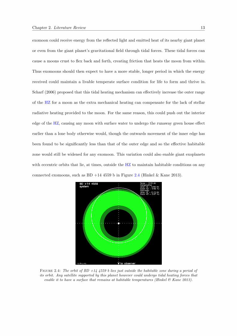
zone would still be widened for any exomoon. This variation could also enable giant exoplanets
with eccentric orbits that lie, at times, outside the HZ to maintain habitable conditions on any
connected exomoons, such as BD +14 4559 b in Figure 2.4 (Hinkel & Kane 2013).
Figure 2.4: The orbit of BD +14 4559 b lies just outside the habitable zone during a period ofits orbit. Any satellite supported by this planet however could undergo tidal heating forces that
enable it to have a surface that remains at habitable temperatures (Hinkel & Kane 2013).
Chapter 2. Literature Review 14
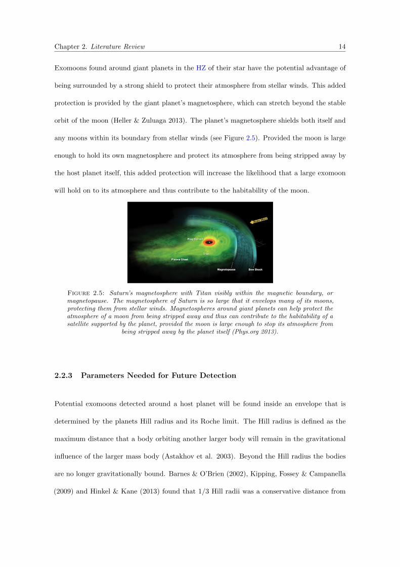
Exomoons found around giant planets in the HZ of their star have the potential advantage of
being surrounded by a strong shield to protect their atmosphere from stellar winds. This added
protection is provided by the giant planet’s magnetosphere, which can stretch beyond the stable
orbit of the moon (Heller & Zuluaga 2013). The planet’s magnetosphere shields both itself and
any moons within its boundary from stellar winds (see Figure 2.5). Provided the moon is large
enough to hold its own magnetosphere and protect its atmosphere from being stripped away by
the host planet itself, this added protection will increase the likelihood that a large exomoon
will hold on to its atmosphere and thus contribute to the habitability of the moon.
Figure 2.5: Saturn’s magnetosphere with Titan visibly within the magnetic boundary, ormagnetopause. The magnetosphere of Saturn is so large that it envelops many of its moons,protecting them from stellar winds. Magnetospheres around giant planets can help protect theatmosphere of a moon from being stripped away and thus can contribute to the habitability of asatellite supported by the planet, provided the moon is large enough to stop its atmosphere from
being stripped away by the planet itself (Phys.org 2013).
2.2.3 Parameters Needed for Future Detection
Potential exomoons detected around a host planet will be found inside an envelope that is
determined by the planets Hill radius and its Roche limit. The Hill radius is defined as the
maximum distance that a body orbiting another larger body will remain in the gravitational
influence of the larger mass body (Astakhov et al. 2003). Beyond the Hill radius the bodies
are no longer gravitationally bound. Barnes & O’Brien (2002), Kipping, Fossey & Campanella
(2009) and Hinkel & Kane (2013) found that 1/3 Hill radii was a conservative distance from
Chapter 2. Literature Review 15
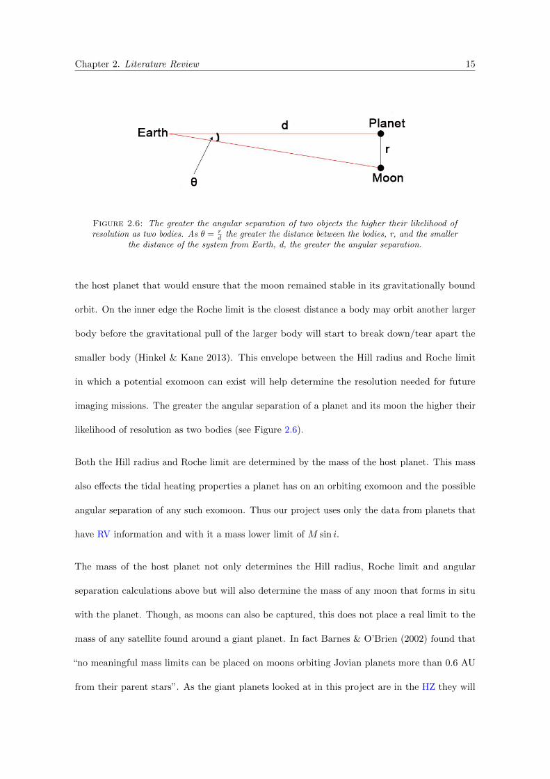
Figure 2.6: The greater the angular separation of two objects the higher their likelihood ofresolution as two bodies. As ✓ = r
d the greater the distance between the bodies, r, and the smallerthe distance of the system from Earth, d, the greater the angular separation.
the host planet that would ensure that the moon remained stable in its gravitationally bound
orbit. On the inner edge the Roche limit is the closest distance a body may orbit another larger
body before the gravitational pull of the larger body will start to break down/tear apart the
smaller body (Hinkel & Kane 2013). This envelope between the Hill radius and Roche limit
in which a potential exomoon can exist will help determine the resolution needed for future
imaging missions. The greater the angular separation of a planet and its moon the higher their
likelihood of resolution as two bodies (see Figure 2.6).
Both the Hill radius and Roche limit are determined by the mass of the host planet. This mass
also e↵ects the tidal heating properties a planet has on an orbiting exomoon and the possible
angular separation of any such exomoon. Thus our project uses only the data from planets that
have RV information and with it a mass lower limit of M sin i.
The mass of the host planet not only determines the Hill radius, Roche limit and angular
separation calculations above but will also determine the mass of any moon that forms in situ
with the planet. Though, as moons can also be captured, this does not place a real limit to the
mass of any satellite found around a giant planet. In fact Barnes & O’Brien (2002) found that
“no meaningful mass limits can be placed on moons orbiting Jovian planets more than 0.6 AU
from their parent stars”. As the giant planets looked at in this project are in the HZ they will

Chapter 2. Literature Review 16
reside beyond this limit and so no upper mass limit will apply to any potential exomoon in these
systems.
Chapter 3
Method
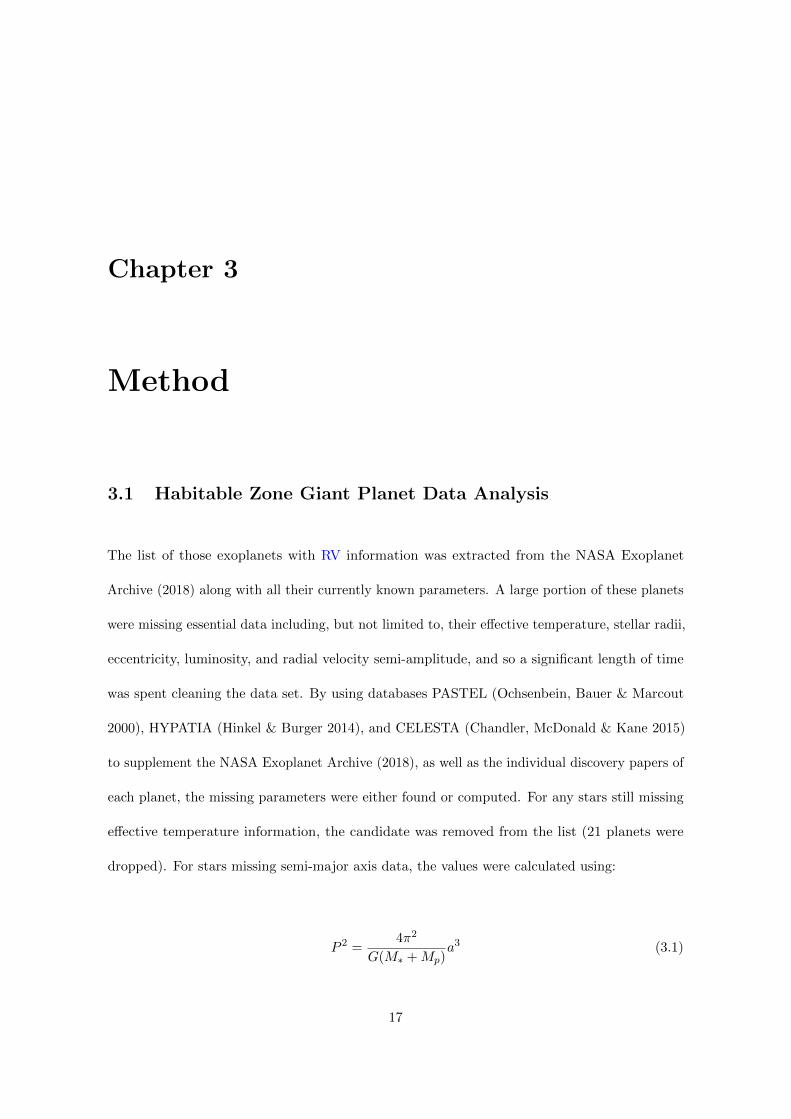
3.1 Habitable Zone Giant Planet Data Analysis
The list of those exoplanets with RV information was extracted from the NASA Exoplanet
Archive (2018) along with all their currently known parameters. A large portion of these planets
were missing essential data including, but not limited to, their e↵ective temperature, stellar radii,
eccentricity, luminosity, and radial velocity semi-amplitude, and so a significant length of time
was spent cleaning the data set. By using databases PASTEL (Ochsenbein, Bauer & Marcout
2000), HYPATIA (Hinkel & Burger 2014), and CELESTA (Chandler, McDonald & Kane 2015)
to supplement the NASA Exoplanet Archive (2018), as well as the individual discovery papers of
each planet, the missing parameters were either found or computed. For any stars still missing
e↵ective temperature information, the candidate was removed from the list (21 planets were
dropped). For stars missing semi-major axis data, the values were calculated using:
P 2 =4⇡2
G(M⇤ +Mp)a3 (3.1)
17
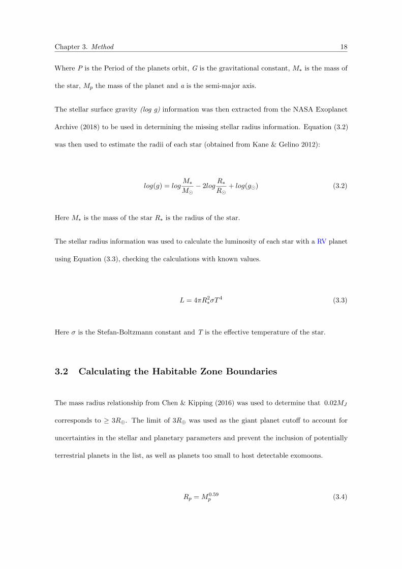
Chapter 3. Method 18
Where P is the Period of the planets orbit, G is the gravitational constant, M⇤ is the mass of
the star, Mp the mass of the planet and a is the semi-major axis.
The stellar surface gravity (log g) information was then extracted from the NASA Exoplanet
Archive (2018) to be used in determining the missing stellar radius information. Equation (3.2)
was then used to estimate the radii of each star (obtained from Kane & Gelino 2012):
log(g) = logM⇤M�
� 2logR⇤R�
+ log(g�) (3.2)
Here M⇤ is the mass of the star R⇤ is the radius of the star.
The stellar radius information was used to calculate the luminosity of each star with a RV planet
using Equation (3.3), checking the calculations with known values.
L = 4⇡R2⇤�T
4 (3.3)
Here � is the Stefan-Boltzmann constant and T is the e↵ective temperature of the star.
3.2 Calculating the Habitable Zone Boundaries
The mass radius relationship from Chen & Kipping (2016) was used to determine that 0.02MJ
corresponds to � 3R�. The limit of 3R� was used as the giant planet cuto↵ to account for
uncertainties in the stellar and planetary parameters and prevent the inclusion of potentially
terrestrial planets in the list, as well as planets too small to host detectable exomoons.
Rp = M0.59p (3.4)
Chapter 3. Method 19
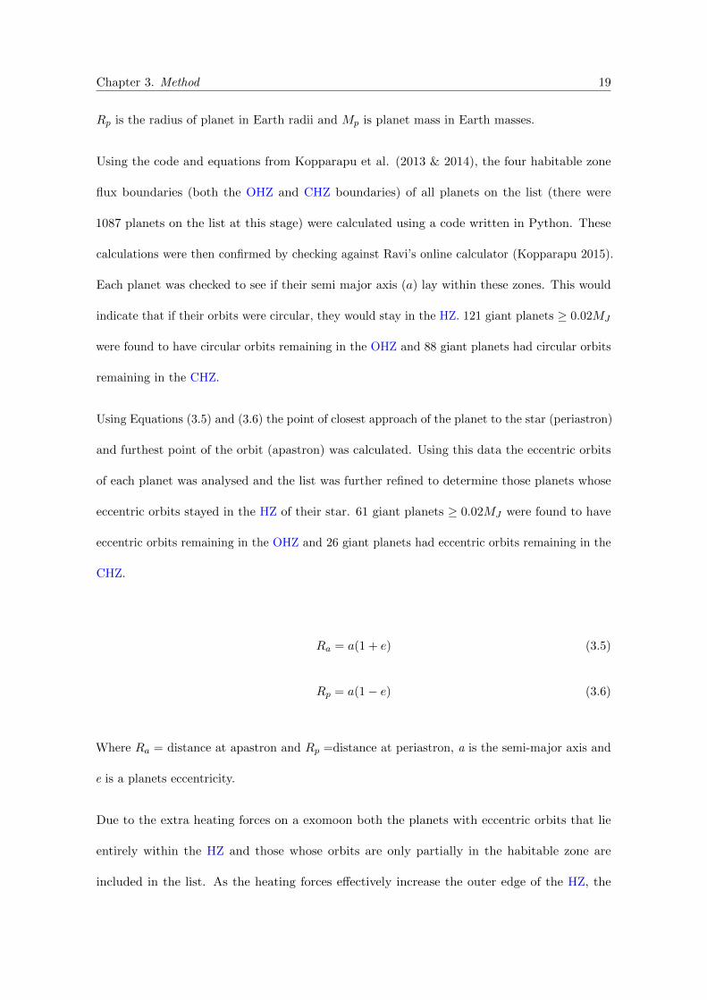
Rp is the radius of planet in Earth radii and Mp is planet mass in Earth masses.
Using the code and equations from Kopparapu et al. (2013 & 2014), the four habitable zone
flux boundaries (both the OHZ and CHZ boundaries) of all planets on the list (there were
1087 planets on the list at this stage) were calculated using a code written in Python. These
calculations were then confirmed by checking against Ravi’s online calculator (Kopparapu 2015).
Each planet was checked to see if their semi major axis (a) lay within these zones. This would
indicate that if their orbits were circular, they would stay in the HZ. 121 giant planets � 0.02MJ
were found to have circular orbits remaining in the OHZ and 88 giant planets had circular orbits
remaining in the CHZ.
Using Equations (3.5) and (3.6) the point of closest approach of the planet to the star (periastron)
and furthest point of the orbit (apastron) was calculated. Using this data the eccentric orbits
of each planet was analysed and the list was further refined to determine those planets whose
eccentric orbits stayed in the HZ of their star. 61 giant planets � 0.02MJ were found to have
eccentric orbits remaining in the OHZ and 26 giant planets had eccentric orbits remaining in the
CHZ.
Ra = a(1 + e) (3.5)
Rp = a(1� e) (3.6)
Where Ra = distance at apastron and Rp =distance at periastron, a is the semi-major axis and
e is a planets eccentricity.
Due to the extra heating forces on a exomoon both the planets with eccentric orbits that lie
entirely within the HZ and those whose orbits are only partially in the habitable zone are
included in the list. As the heating forces e↵ectively increase the outer edge of the HZ, the
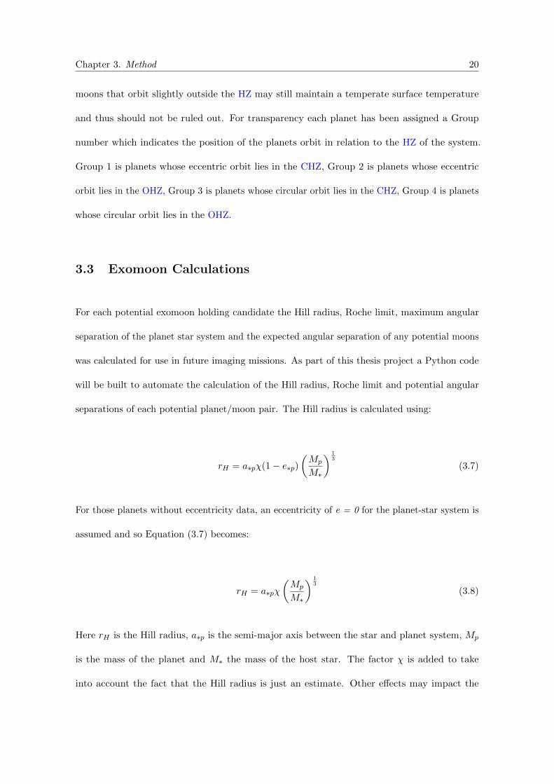
Chapter 3. Method 20
moons that orbit slightly outside the HZ may still maintain a temperate surface temperature
and thus should not be ruled out. For transparency each planet has been assigned a Group
number which indicates the position of the planets orbit in relation to the HZ of the system.
Group 1 is planets whose eccentric orbit lies in the CHZ, Group 2 is planets whose eccentric
orbit lies in the OHZ, Group 3 is planets whose circular orbit lies in the CHZ, Group 4 is planets
whose circular orbit lies in the OHZ.
3.3 Exomoon Calculations
For each potential exomoon holding candidate the Hill radius, Roche limit, maximum angular
separation of the planet star system and the expected angular separation of any potential moons
was calculated for use in future imaging missions. As part of this thesis project a Python code
will be built to automate the calculation of the Hill radius, Roche limit and potential angular
separations of each potential planet/moon pair. The Hill radius is calculated using:
rH = a⇤p�(1� e⇤p)
✓Mp
M⇤
◆ 13
(3.7)
For those planets without eccentricity data, an eccentricity of e = 0 for the planet-star system is
assumed and so Equation (3.7) becomes:
rH = a⇤p�
✓Mp
M⇤
◆ 13
(3.8)
Here rH is the Hill radius, a⇤p is the semi-major axis between the star and planet system, Mp
is the mass of the planet and M⇤ the mass of the host star. The factor � is added to take
into account the fact that the Hill radius is just an estimate. Other e↵ects may impact the
Chapter 3. Method 21
gravitational stability of the system, so following Barnes & O’Brien (2002), Kipping (2009) and
Hinkel & Kane (2013), I have chosen to use a conservative estimate of � 1/3 as any stable
satellite around a giant planet is likely to reside within 1/3 of the planets Hill radius (Barnes &
O’Brien 2002).
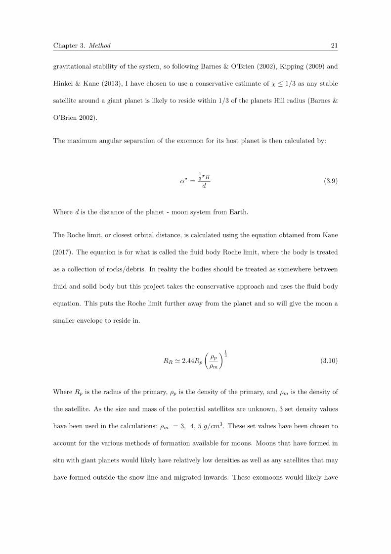
The maximum angular separation of the exomoon for its host planet is then calculated by:
↵” =13rH
d(3.9)
Where d is the distance of the planet - moon system from Earth.
The Roche limit, or closest orbital distance, is calculated using the equation obtained from Kane
(2017). The equation is for what is called the fluid body Roche limit, where the body is treated
as a collection of rocks/debris. In reality the bodies should be treated as somewhere between
fluid and solid body but this project takes the conservative approach and uses the fluid body
equation. This puts the Roche limit further away from the planet and so will give the moon a
smaller envelope to reside in.
RR ' 2.44Rp
✓⇢p⇢m
◆ 13
(3.10)
Where Rp is the radius of the primary, ⇢p is the density of the primary, and ⇢m is the density of
the satellite. As the size and mass of the potential satellites are unknown, 3 set density values
have been used in the calculations: ⇢m = 3, 4, 5 g/cm3. These set values have been chosen to
account for the various methods of formation available for moons. Moons that have formed in
situ with giant planets would likely have relatively low densities as well as any satellites that may
have formed outside the snow line and migrated inwards. These exomoons would likely have
Chapter 3. Method 22
lower densities and higher hydrogen content. Whereas more dense moons could have formed
through collisions or capture of moons, asteroids or planets.
3.4 Confirming Orbital Solutions with RadVel
Each planets radial velocity curve was run through RadVel (Fulton et al. 2018) to confirm the
orbital solution, starting with the most promising candidates whose eccentric orbits always stay
within the CHZ, then those whose eccentric orbits always stay within the OHZ, then those whose
circular orbits stay within the CHZ and finally those whose circular orbits stay within the OHZ.
RadVel enables users to model Keplerian orbits in RV time series. RadVel fits RVs using
maximum a posteriori (MAP) and employs “modern Markov Chain Monte Carlo (MCMC)
sampling techniques and robust convergence criteria to ensure accurately estimated orbital
parameters and their associated uncertainties” (Fulton et al. 2018). RadVel allows users to
either fix parameters or allow them to float free, as well as impose priors and perform Bayesian
model comparison. The five orbital parameters this project used are the orbital period (P), the
time of periastron (Tp), orbital eccentricity (e), the argument of periastron of the star’s orbit
(!), and the velocity semi-amplitude (K). Jitter (�) was also input for inclusion in uncertainty
measurements to account for any noise from astrophysical and instrumental sources.
Once the MCMC chains are well mixed and the orbital parameters which maximize the posterior
probability are found, RadVel then supplies an output of the final parameter values from the
MAP fit, and provides radial velocity time series plots and MCMC corner plots showing all joint
posterior distributions derived from the MCMC sampling.
Chapter 3. Method 23
3.5 Target Selection
After determining which planets show indications of linear trends an observing strategy was
created, outlining which targets are best reserved for either the MINERVA Australis, Keck
HIRES or Lick Automated Planet Finder (APF) telescopes. Each giant planet was assigned to
the telescope that is best qualified to carry out follow-up observations. The magnitude, radial
velocity semi-amplitude and position of the star were all considered during this selection process.
Future projects will use these telescopes to make observations of what is deemed the highest
priority on the refined list provided in this thesis.
Chapter 4
Results
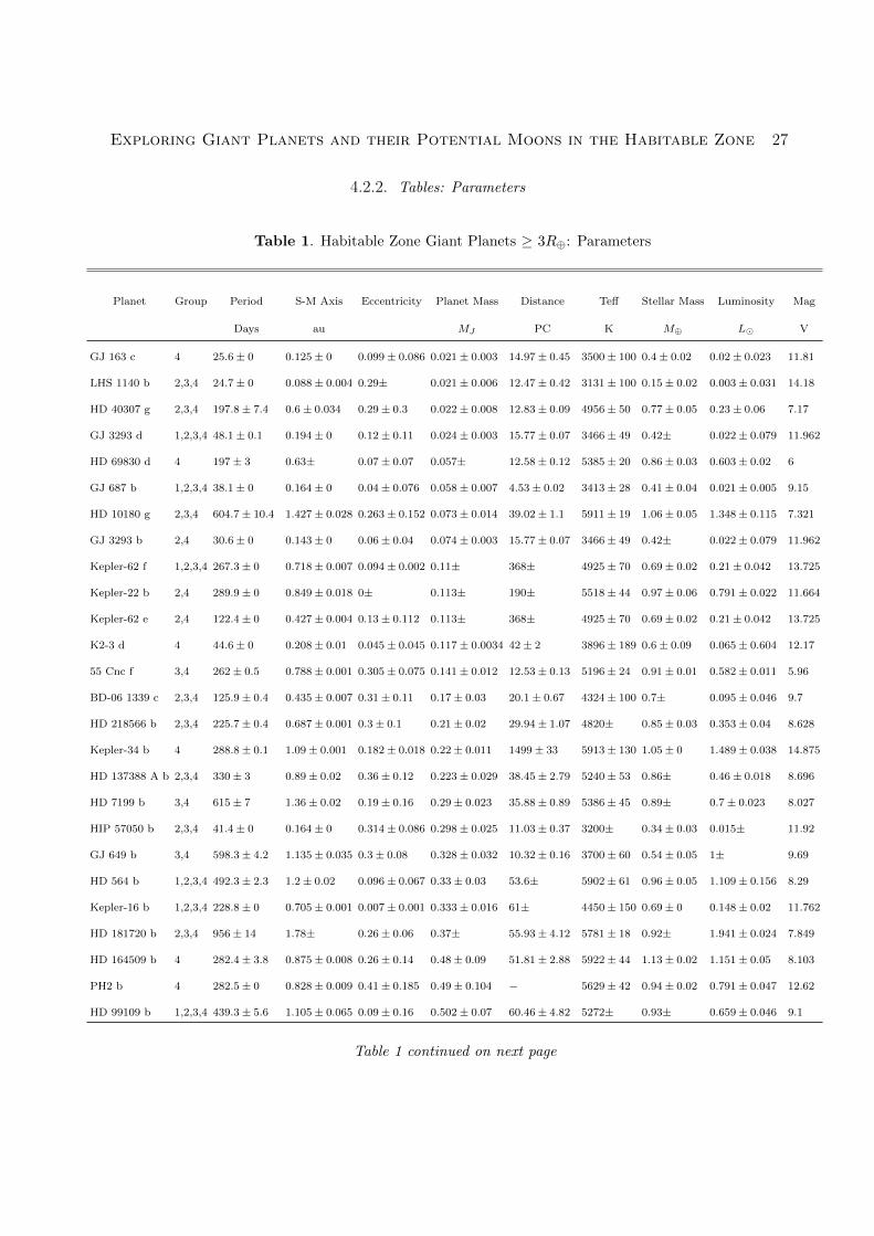
4.1 Results
The parameters used in this project’s calculations are provided in Table 4.1. The parameters
were extracted and compiled from the NASA Exoplanet Archive (2018) as well as the PASTEL
(Ochsenbein, Bauer & Marcout 2000), HYPATIA (Hinkel & Burger 2014), and CELESTA
(Chandler, McDonald & Kane 2015) catalogs. The calculations of the planet HZ flux boundaries
and their corresponding HZ physical boundaries are presented in Table 4.2. Calculations of
Hill radii, Roche limit (with moon densities of 3, 4, and 5 g/cm3), and angular separation of
the potential planet/moon systems at 13 Hill radii are presented in Table 4.3. These estimates
can be used in deciding the ideal candidates for future imaging missions. Each giant planet’s
radial velocity curve was analysed in the RadVel program (Fulton et al. 2018) to confirm the
orbital solution and look for linear trends to determine if there were indications for additional
companions; potentially either additional planets in orbit or satellites. Table 4.4 provides the
results of our RadVel data analysis, indicating those planets with indications linear trends. Of
128 giant planets in the HZ of their star, 55 planets showed indications of linear trends � 3�. The
24
Chapter 4. Results 25
telescope observing strategies for the MINERVA Australis, KECK Hires and LICK Automated
Planet Finder (APF) telescopes are outlined Tables 4.5 and 4.6. For those planets where more
than one telescope is capable of observation, the telescope for whom that target will be assigned
as priority is listed first, priority here determined by expected telescope time available. The
targets that are not observable with these telescopes or whom are missing required data are left
blank.
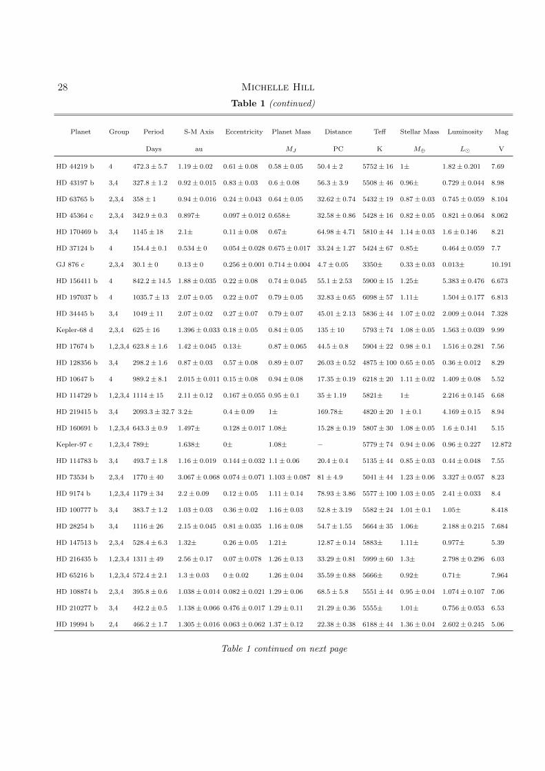
To aid with priority selection for follow up observations, the planets are listed in order of planet
mass within each table. Those planets with a larger mass will have a larger radial velocity
signature, as well as the ability to potentially support a larger moon or satellite, so are the
highest priority for future observations.
In each table the second column is the Group column. Each Group indicates the position of
the planets orbit in relation to the HZ of the system. Group 1 is the highest priority Group
which includes planets whose eccentric orbits always stay within the CHZ. Group 2 is the next
highest priority and includes those planets whose eccentric orbits always stay within the OHZ.
Accounting for uncertainties in eccentricity, Groups 3 and 4 include the planets with circular
orbits: Group 3 includes planets whose circular orbits stay within the CHZ and Group 4 includes
those whose circular orbits stay within the OHZ. Note that some planets are in multiple groups
e.g. Group 1 is a subset of each of the other groups as it has the most constricted criteria.
Within the Tables there is missing data where parameters were unable to be found from any
sources available. For each missing parameter and their subsequent calculations the space has
been left blank, including any uncertainty calculations that did not have the required elements
to allow completion.
Below the Tables are the Figures presenting the results of the calculations (Figures 4.1 - 4.5) as
well as some of the radial velocity fits from the RadVel curve analysis and an example of the
Chapter 4. Results 26
Markov-Chain Monte Carlo (MCMC) posterior distributions (Figures 4.7 - 4.13). Each RadVel
curve fit provides two windows at the top containing the fit and residuals sequentially, followed
by a window for each known planets individual fit.
4.2 Tables
4.2.1 Table Glossary
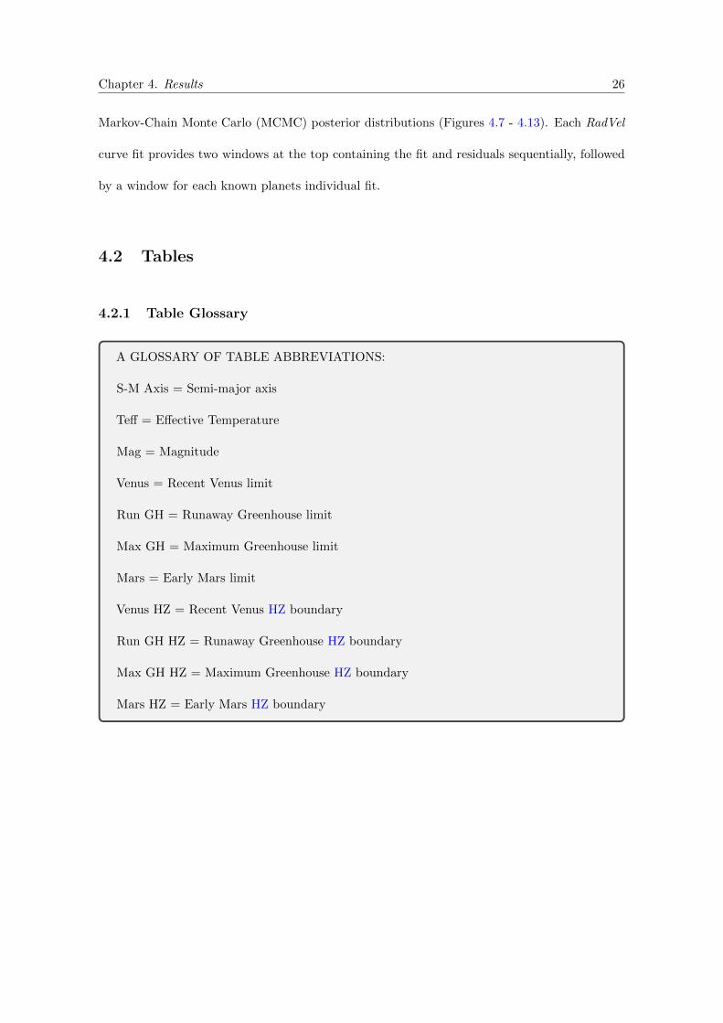
A GLOSSARY OF TABLE ABBREVIATIONS:
S-M Axis = Semi-major axis
Te↵ = E↵ective Temperature
Mag = Magnitude
Venus = Recent Venus limit
Run GH = Runaway Greenhouse limit
Max GH = Maximum Greenhouse limit
Mars = Early Mars limit
Venus HZ = Recent Venus HZ boundary
Run GH HZ = Runaway Greenhouse HZ boundary
Max GH HZ = Maximum Greenhouse HZ boundary
Mars HZ = Early Mars HZ boundary
Exploring Giant Planets and their Potential Moons in the Habitable Zone 27
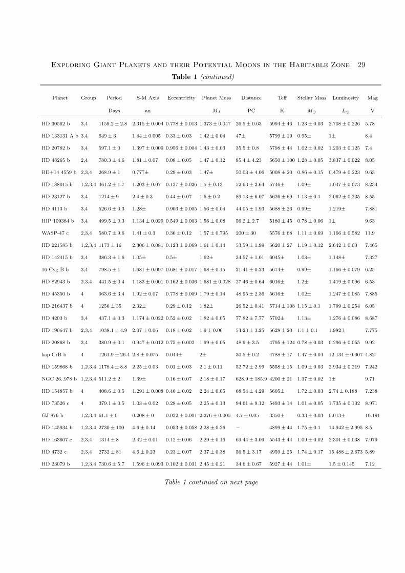
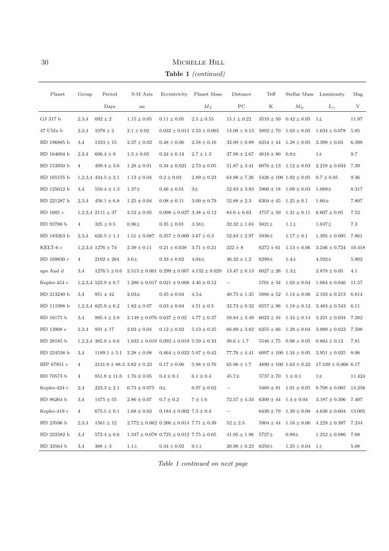
4.2.2. Tables: Parameters
Table 1. Habitable Zone Giant Planets � 3R�: Parameters
Planet Group Period S-M Axis Eccentricity Planet Mass Distance Te↵ Stellar Mass Luminosity Mag
Days au MJ PC K M� L� V
GJ 163 c 4 25.6± 0 0.125± 0 0.099± 0.086 0.021± 0.003 14.97± 0.45 3500± 100 0.4± 0.02 0.02± 0.023 11.81
LHS 1140 b 2,3,4 24.7± 0 0.088± 0.004 0.29± 0.021± 0.006 12.47± 0.42 3131± 100 0.15± 0.02 0.003± 0.031 14.18
HD 40307 g 2,3,4 197.8± 7.4 0.6± 0.034 0.29± 0.3 0.022± 0.008 12.83± 0.09 4956± 50 0.77± 0.05 0.23± 0.06 7.17
GJ 3293 d 1,2,3,4 48.1± 0.1 0.194± 0 0.12± 0.11 0.024± 0.003 15.77± 0.07 3466± 49 0.42± 0.022± 0.079 11.962
HD 69830 d 4 197± 3 0.63± 0.07± 0.07 0.057± 12.58± 0.12 5385± 20 0.86± 0.03 0.603± 0.02 6
GJ 687 b 1,2,3,4 38.1± 0 0.164± 0 0.04± 0.076 0.058± 0.007 4.53± 0.02 3413± 28 0.41± 0.04 0.021± 0.005 9.15
HD 10180 g 2,3,4 604.7± 10.4 1.427± 0.028 0.263± 0.152 0.073± 0.014 39.02± 1.1 5911± 19 1.06± 0.05 1.348± 0.115 7.321
GJ 3293 b 2,4 30.6± 0 0.143± 0 0.06± 0.04 0.074± 0.003 15.77± 0.07 3466± 49 0.42± 0.022± 0.079 11.962
Kepler-62 f 1,2,3,4 267.3± 0 0.718± 0.007 0.094± 0.002 0.11± 368± 4925± 70 0.69± 0.02 0.21± 0.042 13.725
Kepler-22 b 2,4 289.9± 0 0.849± 0.018 0± 0.113± 190± 5518± 44 0.97± 0.06 0.791± 0.022 11.664
Kepler-62 e 2,4 122.4± 0 0.427± 0.004 0.13± 0.112 0.113± 368± 4925± 70 0.69± 0.02 0.21± 0.042 13.725
K2-3 d 4 44.6± 0 0.208± 0.01 0.045± 0.045 0.117± 0.0034 42± 2 3896± 189 0.6± 0.09 0.065± 0.604 12.17
55 Cnc f 3,4 262± 0.5 0.788± 0.001 0.305± 0.075 0.141± 0.012 12.53± 0.13 5196± 24 0.91± 0.01 0.582± 0.011 5.96
BD-06 1339 c 2,3,4 125.9± 0.4 0.435± 0.007 0.31± 0.11 0.17± 0.03 20.1± 0.67 4324± 100 0.7± 0.095± 0.046 9.7
HD 218566 b 2,3,4 225.7± 0.4 0.687± 0.001 0.3± 0.1 0.21± 0.02 29.94± 1.07 4820± 0.85± 0.03 0.353± 0.04 8.628
Kepler-34 b 4 288.8± 0.1 1.09± 0.001 0.182± 0.018 0.22± 0.011 1499± 33 5913± 130 1.05± 0 1.489± 0.038 14.875
HD 137388 A b 2,3,4 330± 3 0.89± 0.02 0.36± 0.12 0.223± 0.029 38.45± 2.79 5240± 53 0.86± 0.46± 0.018 8.696
HD 7199 b 3,4 615± 7 1.36± 0.02 0.19± 0.16 0.29± 0.023 35.88± 0.89 5386± 45 0.89± 0.7± 0.023 8.027
HIP 57050 b 2,3,4 41.4± 0 0.164± 0 0.314± 0.086 0.298± 0.025 11.03± 0.37 3200± 0.34± 0.03 0.015± 11.92
GJ 649 b 3,4 598.3± 4.2 1.135± 0.035 0.3± 0.08 0.328± 0.032 10.32± 0.16 3700± 60 0.54± 0.05 1± 9.69
HD 564 b 1,2,3,4 492.3± 2.3 1.2± 0.02 0.096± 0.067 0.33± 0.03 53.6± 5902± 61 0.96± 0.05 1.109± 0.156 8.29
Kepler-16 b 1,2,3,4 228.8± 0 0.705± 0.001 0.007± 0.001 0.333± 0.016 61± 4450± 150 0.69± 0 0.148± 0.02 11.762
HD 181720 b 2,3,4 956± 14 1.78± 0.26± 0.06 0.37± 55.93± 4.12 5781± 18 0.92± 1.941± 0.024 7.849
HD 164509 b 4 282.4± 3.8 0.875± 0.008 0.26± 0.14 0.48± 0.09 51.81± 2.88 5922± 44 1.13± 0.02 1.151± 0.05 8.103
PH2 b 4 282.5± 0 0.828± 0.009 0.41± 0.185 0.49± 0.104 � 5629± 42 0.94± 0.02 0.791± 0.047 12.62
HD 99109 b 1,2,3,4 439.3± 5.6 1.105± 0.065 0.09± 0.16 0.502± 0.07 60.46± 4.82 5272± 0.93± 0.659± 0.046 9.1
Table 1 continued on next page
28 Michelle Hill
Table 1 (continued)
Planet Group Period S-M Axis Eccentricity Planet Mass Distance Te↵ Stellar Mass Luminosity Mag
Days au MJ PC K M� L� V
HD 44219 b 4 472.3± 5.7 1.19± 0.02 0.61± 0.08 0.58± 0.05 50.4± 2 5752± 16 1± 1.82± 0.201 7.69
HD 43197 b 3,4 327.8± 1.2 0.92± 0.015 0.83± 0.03 0.6± 0.08 56.3± 3.9 5508± 46 0.96± 0.729± 0.044 8.98
HD 63765 b 2,3,4 358± 1 0.94± 0.016 0.24± 0.043 0.64± 0.05 32.62± 0.74 5432± 19 0.87± 0.03 0.745± 0.059 8.104
HD 45364 c 2,3,4 342.9± 0.3 0.897± 0.097± 0.012 0.658± 32.58± 0.86 5428± 16 0.82± 0.05 0.821± 0.064 8.062
HD 170469 b 3,4 1145± 18 2.1± 0.11± 0.08 0.67± 64.98± 4.71 5810± 44 1.14± 0.03 1.6± 0.146 8.21
HD 37124 b 4 154.4± 0.1 0.534± 0 0.054± 0.028 0.675± 0.017 33.24± 1.27 5424± 67 0.85± 0.464± 0.059 7.7
GJ 876 c 2,3,4 30.1± 0 0.13± 0 0.256± 0.001 0.714± 0.004 4.7± 0.05 3350± 0.33± 0.03 0.013± 10.191
HD 156411 b 4 842.2± 14.5 1.88± 0.035 0.22± 0.08 0.74± 0.045 55.1± 2.53 5900± 15 1.25± 5.383± 0.476 6.673
HD 197037 b 4 1035.7± 13 2.07± 0.05 0.22± 0.07 0.79± 0.05 32.83± 0.65 6098± 57 1.11± 1.504± 0.177 6.813
HD 34445 b 3,4 1049± 11 2.07± 0.02 0.27± 0.07 0.79± 0.07 45.01± 2.13 5836± 44 1.07± 0.02 2.009± 0.044 7.328
Kepler-68 d 2,3,4 625± 16 1.396± 0.033 0.18± 0.05 0.84± 0.05 135± 10 5793± 74 1.08± 0.05 1.563± 0.039 9.99
HD 17674 b 1,2,3,4 623.8± 1.6 1.42± 0.045 0.13± 0.87± 0.065 44.5± 0.8 5904± 22 0.98± 0.1 1.516± 0.281 7.56
HD 128356 b 3,4 298.2± 1.6 0.87± 0.03 0.57± 0.08 0.89± 0.07 26.03± 0.52 4875± 100 0.65± 0.05 0.36± 0.012 8.29
HD 10647 b 4 989.2± 8.1 2.015± 0.011 0.15± 0.08 0.94± 0.08 17.35± 0.19 6218± 20 1.11± 0.02 1.409± 0.08 5.52
HD 114729 b 1,2,3,4 1114± 15 2.11± 0.12 0.167± 0.055 0.95± 0.1 35± 1.19 5821± 1± 2.216± 0.145 6.68
HD 219415 b 3,4 2093.3± 32.7 3.2± 0.4± 0.09 1± 169.78± 4820± 20 1± 0.1 4.169± 0.15 8.94
HD 160691 b 1,2,3,4 643.3± 0.9 1.497± 0.128± 0.017 1.08± 15.28± 0.19 5807± 30 1.08± 0.05 1.6± 0.141 5.15
Kepler-97 c 1,2,3,4 789± 1.638± 0± 1.08± � 5779± 74 0.94± 0.06 0.96± 0.227 12.872
HD 114783 b 3,4 493.7± 1.8 1.16± 0.019 0.144± 0.032 1.1± 0.06 20.4± 0.4 5135± 44 0.85± 0.03 0.44± 0.048 7.55
HD 73534 b 2,3,4 1770± 40 3.067± 0.068 0.074± 0.071 1.103± 0.087 81± 4.9 5041± 44 1.23± 0.06 3.327± 0.057 8.23
HD 9174 b 1,2,3,4 1179± 34 2.2± 0.09 0.12± 0.05 1.11± 0.14 78.93± 3.86 5577± 100 1.03± 0.05 2.41± 0.033 8.4
HD 100777 b 3,4 383.7± 1.2 1.03± 0.03 0.36± 0.02 1.16± 0.03 52.8± 3.19 5582± 24 1.01± 0.1 1.05± 8.418
HD 28254 b 3,4 1116± 26 2.15± 0.045 0.81± 0.035 1.16± 0.08 54.7± 1.55 5664± 35 1.06± 2.188± 0.215 7.684
HD 147513 b 2,3,4 528.4± 6.3 1.32± 0.26± 0.05 1.21± 12.87± 0.14 5883± 1.11± 0.977± 5.39
HD 216435 b 1,2,3,4 1311± 49 2.56± 0.17 0.07± 0.078 1.26± 0.13 33.29± 0.81 5999± 60 1.3± 2.798± 0.296 6.03
HD 65216 b 1,2,3,4 572.4± 2.1 1.3± 0.03 0± 0.02 1.26± 0.04 35.59± 0.88 5666± 0.92± 0.71± 7.964
HD 108874 b 2,3,4 395.8± 0.6 1.038± 0.014 0.082± 0.021 1.29± 0.06 68.5± 5.8 5551± 44 0.95± 0.04 1.074± 0.107 7.06
HD 210277 b 3,4 442.2± 0.5 1.138± 0.066 0.476± 0.017 1.29± 0.11 21.29± 0.36 5555± 1.01± 0.756± 0.053 6.53
HD 19994 b 2,4 466.2± 1.7 1.305± 0.016 0.063± 0.062 1.37± 0.12 22.38± 0.38 6188± 44 1.36± 0.04 2.602± 0.245 5.06
Table 1 continued on next page
Exploring Giant Planets and their Potential Moons in the Habitable Zone 29
Table 1 (continued)
Planet Group Period S-M Axis Eccentricity Planet Mass Distance Te↵ Stellar Mass Luminosity Mag
Days au MJ PC K M� L� V
HD 30562 b 3,4 1159.2± 2.8 2.315± 0.004 0.778± 0.013 1.373± 0.047 26.5± 0.63 5994± 46 1.23± 0.03 2.708± 0.226 5.78
HD 133131 A b 3,4 649± 3 1.44± 0.005 0.33± 0.03 1.42± 0.04 47± 5799± 19 0.95± 1± 8.4
HD 20782 b 3,4 597.1± 0 1.397± 0.009 0.956± 0.004 1.43± 0.03 35.5± 0.8 5798± 44 1.02± 0.02 1.203± 0.125 7.4
HD 48265 b 2,4 780.3± 4.6 1.81± 0.07 0.08± 0.05 1.47± 0.12 85.4± 4.23 5650± 100 1.28± 0.05 3.837± 0.022 8.05
BD+14 4559 b 2,3,4 268.9± 1 0.777± 0.29± 0.03 1.47± 50.03± 4.06 5008± 20 0.86± 0.15 0.479± 0.223 9.63
HD 188015 b 1,2,3,4 461.2± 1.7 1.203± 0.07 0.137± 0.026 1.5± 0.13 52.63± 2.64 5746± 1.09± 1.047± 0.073 8.234
HD 23127 b 3,4 1214± 9 2.4± 0.3 0.44± 0.07 1.5± 0.2 89.13± 6.07 5626± 69 1.13± 0.1 2.062± 0.235 8.55
HD 4113 b 3,4 526.6± 0.3 1.28± 0.903± 0.005 1.56± 0.04 44.05± 1.93 5688± 26 0.99± 1.219± 7.881
HIP 109384 b 3,4 499.5± 0.3 1.134± 0.029 0.549± 0.003 1.56± 0.08 56.2± 2.7 5180± 45 0.78± 0.06 1± 9.63
WASP-47 c 2,3,4 580.7± 9.6 1.41± 0.3 0.36± 0.12 1.57± 0.795 200± 30 5576± 68 1.11± 0.69 1.166± 0.582 11.9
HD 221585 b 1,2,3,4 1173± 16 2.306± 0.081 0.123± 0.069 1.61± 0.14 53.59± 1.99 5620± 27 1.19± 0.12 2.642± 0.03 7.465
HD 142415 b 3,4 386.3± 1.6 1.05± 0.5± 1.62± 34.57± 1.01 6045± 1.03± 1.148± 7.327
16 Cyg B b 3,4 798.5± 1 1.681± 0.097 0.681± 0.017 1.68± 0.15 21.41± 0.23 5674± 0.99± 1.166± 0.079 6.25
HD 82943 b 2,3,4 441.5± 0.4 1.183± 0.001 0.162± 0.036 1.681± 0.028 27.46± 0.64 6016± 1.2± 1.419± 0.096 6.53
HD 45350 b 4 963.6± 3.4 1.92± 0.07 0.778± 0.009 1.79± 0.14 48.95± 2.36 5616± 1.02± 1.247± 0.085 7.885
HD 216437 b 4 1256± 35 2.32± 0.29± 0.12 1.82± 26.52± 0.41 5714± 108 1.15± 0.1 1.799± 0.254 6.05
HD 4203 b 3,4 437.1± 0.3 1.174± 0.022 0.52± 0.02 1.82± 0.05 77.82± 7.77 5702± 1.13± 1.276± 0.086 8.687
HD 190647 b 2,3,4 1038.1± 4.9 2.07± 0.06 0.18± 0.02 1.9± 0.06 54.23± 3.25 5628± 20 1.1± 0.1 1.982± 7.775
HD 20868 b 3,4 380.9± 0.1 0.947± 0.012 0.75± 0.002 1.99± 0.05 48.9± 3.5 4795± 124 0.78± 0.03 0.296± 0.055 9.92
kap CrB b 4 1261.9± 26.4 2.8± 0.075 0.044± 2± 30.5± 0.2 4788± 17 1.47± 0.04 12.134± 0.007 4.82
HD 159868 b 1,2,3,4 1178.4± 8.8 2.25± 0.03 0.01± 0.03 2.1± 0.11 52.72± 2.99 5558± 15 1.09± 0.03 2.934± 0.219 7.242
NGC 26..978 b 1,2,3,4 511.2± 2 1.39± 0.16± 0.07 2.18± 0.17 628.9± 185.9 4200± 21 1.37± 0.02 1± 9.71
HD 154857 b 4 408.6± 0.5 1.291± 0.008 0.46± 0.02 2.24± 0.05 68.54± 4.29 5605± 1.72± 0.03 2.74± 0.188 7.238
HD 73526 c 4 379.1± 0.5 1.03± 0.02 0.28± 0.05 2.25± 0.13 94.61± 9.12 5493± 14 1.01± 0.05 1.735± 0.132 8.971
GJ 876 b 1,2,3,4 61.1± 0 0.208± 0 0.032± 0.001 2.276± 0.005 4.7± 0.05 3350± 0.33± 0.03 0.013± 10.191
HD 145934 b 1,2,3,4 2730± 100 4.6± 0.14 0.053± 0.058 2.28± 0.26 � 4899± 44 1.75± 0.1 14.942± 2.995 8.5
HD 163607 c 2,3,4 1314± 8 2.42± 0.01 0.12± 0.06 2.29± 0.16 69.44± 3.09 5543± 44 1.09± 0.02 2.301± 0.038 7.979
HD 4732 c 2,3,4 2732± 81 4.6± 0.23 0.23± 0.07 2.37± 0.38 56.5± 3.17 4959± 25 1.74± 0.17 15.488± 2.673 5.89
HD 23079 b 1,2,3,4 730.6± 5.7 1.596± 0.093 0.102± 0.031 2.45± 0.21 34.6± 0.67 5927± 44 1.01± 1.5± 0.145 7.12
Table 1 continued on next page
30 Michelle Hill
Table 1 (continued)
Planet Group Period S-M Axis Eccentricity Planet Mass Distance Te↵ Stellar Mass Luminosity Mag
Days au MJ PC K M� L� V
GJ 317 b 2,3,4 692± 2 1.15± 0.05 0.11± 0.05 2.5± 0.55 15.1± 0.22 3510± 50 0.42± 0.05 1± 11.97
47 UMa b 2,3,4 1078± 2 2.1± 0.02 0.032± 0.014 2.53± 0.065 14.08± 0.13 5892± 70 1.03± 0.05 1.634± 0.078 5.05
HD 196885 b 3,4 1333± 15 2.37± 0.02 0.48± 0.06 2.58± 0.16 32.99± 0.89 6254± 44 1.28± 0.05 2.399± 0.03 6.398
HD 164604 b 2,3,4 606.4± 9 1.3± 0.05 0.24± 0.14 2.7± 1.3 37.98± 2.67 4618± 80 0.8± 1± 9.7
HD 153950 b 4 499.4± 3.6 1.28± 0.01 0.34± 0.021 2.73± 0.05 51.87± 3.41 6076± 13 1.12± 0.03 2.218± 0.034 7.39
HD 165155 b 1,2,3,4 434.5± 2.1 1.13± 0.04 0.2± 0.03 2.89± 0.23 64.98± 7.26 5426± 100 1.02± 0.05 0.7± 0.05 9.36
HD 125612 b 3,4 559.4± 1.3 1.37± 0.46± 0.01 3± 52.83± 3.93 5900± 18 1.09± 0.03 1.089± 8.317
HD 221287 b 2,3,4 456.1± 6.8 1.25± 0.04 0.08± 0.11 3.09± 0.79 52.88± 2.3 6304± 45 1.25± 0.1 1.66± 7.807
HD 1605 c 1,2,3,4 2111± 37 3.52± 0.05 0.098± 0.027 3.48± 0.12 84.6± 6.63 4757± 50 1.31± 0.11 6.607± 0.05 7.52
HD 92788 b 4 325± 0.5 0.96± 0.35± 0.01 3.58± 32.32± 1.04 5821± 1.1± 1.047± 7.3
HD 183263 b 2,3,4 626.5± 1.1 1.51± 0.087 0.357± 0.009 3.67± 0.3 52.83± 2.97 5936± 1.17± 0.1 1.395± 0.095 7.861
KELT-6 c 1,2,3,4 1276± 74 2.39± 0.11 0.21± 0.038 3.71± 0.21 222± 8 6272± 61 1.13± 0.06 3.246± 0.724 10.418
HD 169830 c 4 2102± 264 3.6± 0.33± 0.02 4.04± 36.32± 1.2 6299± 1.4± 4.592± 5.902
ups And d 3,4 1276.5± 0.6 2.513± 0.001 0.299± 0.007 4.132± 0.029 13.47± 0.13 6027± 26 1.3± 2.878± 0.05 4.1
Kepler-454 c 1,2,3,4 523.9± 0.7 1.286± 0.017 0.021± 0.008 4.46± 0.12 � 5701± 34 1.03± 0.04 1.084± 0.046 11.57
HD 213240 b 3,4 951± 42 2.03± 0.45± 0.04 4.5± 40.75± 1.35 5886± 52 1.14± 0.06 2.103± 0.213 6.814
HD 111998 b 1,2,3,4 825.9± 6.2 1.82± 0.07 0.03± 0.04 4.51± 0.5 32.73± 0.32 6557± 96 1.18± 0.12 3.483± 0.543 6.11
HD 16175 b 3,4 995.4± 2.8 2.148± 0.076 0.637± 0.02 4.77± 0.37 59.84± 3.49 6022± 34 1.34± 0.14 3.221± 0.034 7.282
HD 13908 c 2,3,4 931± 17 2.03± 0.04 0.12± 0.02 5.13± 0.25 66.89± 3.82 6255± 66 1.29± 0.04 3.999± 0.623 7.508
HD 28185 b 1,2,3,4 385.9± 0.6 1.032± 0.019 0.092± 0.019 5.59± 0.33 39.6± 1.7 5546± 75 0.98± 0.05 0.864± 0.12 7.81
HD 224538 b 3,4 1189.1± 5.1 2.28± 0.08 0.464± 0.022 5.97± 0.42 77.76± 4.41 6097± 100 1.34± 0.05 2.951± 0.025 8.06
HIP 67851 c 4 2131.8± 88.3 3.82± 0.23 0.17± 0.06 5.98± 0.76 65.96± 1.7 4890± 100 1.63± 0.22 17.539± 0.066 6.17
HD 70573 b 4 851.8± 11.6 1.76± 0.05 0.4± 0.1 6.1± 0.4 45.7± 5737± 70 1± 0.1 1± 11.424
Kepler-424 c 2,4 223.3± 2.1 0.73± 0.075 0± 6.97± 0.62 � 5460± 81 1.01± 0.05 0.708± 0.065 14.256
HD 86264 b 3,4 1475± 55 2.86± 0.07 0.7± 0.2 7± 1.6 72.57± 4.34 6300± 44 1.4± 0.04 3.187± 0.306 7.407
Kepler-419 c 4 675.5± 0.1 1.68± 0.03 0.184± 0.002 7.3± 0.4 � 6430± 79 1.39± 0.08 4.638± 0.604 13.005
HD 23596 b 2,3,4 1561± 12 2.772± 0.062 0.266± 0.014 7.71± 0.39 52± 2.3 5904± 44 1.16± 0.06 4.229± 0.397 7.244
HD 222582 b 3,4 572.4± 0.6 1.347± 0.078 0.725± 0.012 7.75± 0.65 41.95± 1.96 5727± 0.99± 1.252± 0.086 7.68
HD 33564 b 3,4 388± 3 1.1± 0.34± 0.02 9.1± 20.98± 0.23 6250± 1.25± 0.04 1± 5.08
Table 1 continued on next page
Exploring Giant Planets and their Potential Moons in the Habitable Zone 31
Table 1 (continued)
Planet Group Period S-M Axis Eccentricity Planet Mass Distance Te↵ Stellar Mass Luminosity Mag
Days au MJ PC K M� L� V
HD 141937 b 3,4 653.2± 1.2 1.488± 0.01 0.41± 0.01 9.316± 0.329 33.46± 1.21 5879± 70 1.03± 0.02 1.052± 0.073 7.25
30 Ari B b 4 335.1± 2.5 0.995± 0.012 0.289± 0.092 9.88± 0.94 39.43± 1.72 6300± 60 1.16± 0.04 1.803± 0.165 7.458
HD 38801 b 2,4 696.3± 2.7 1.7± 0.037 0± 10.7± 0.5 99.4± 17.73 5222± 44 1.36± 0.09 4.56± 0.045 8.269
HD 217786 b 4 1319± 4 2.38± 0.04 0.4± 0.05 13± 0.8 54.8± 2 5966± 65 1.02± 0.03 1.888± 0.254 7.8
HAT-P-13 c 4 446.3± 0.2 1.226± 0.025 0.662± 0.005 14.28± 0.28 214± 12 5653± 90 1.22± 0.08 2.218± 0.061 10.622
HD 214823 b 3,4 1877± 15 3.18± 0.12 0.154± 0.014 19.2± 1.4 97.47± 8.42 6215± 30 1.22± 0.13 4.345± 0.058 8.068
Kepler-47 c 3,4 303.1± 0 0.991± 0.016 0.411± 28± 1500± 5636± 100 1.05± 0.06 0.839± 0.035 15.178
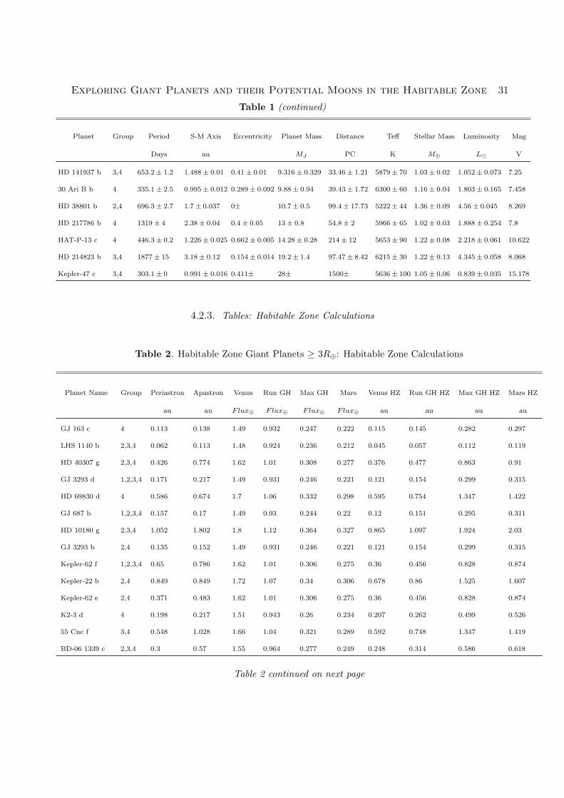
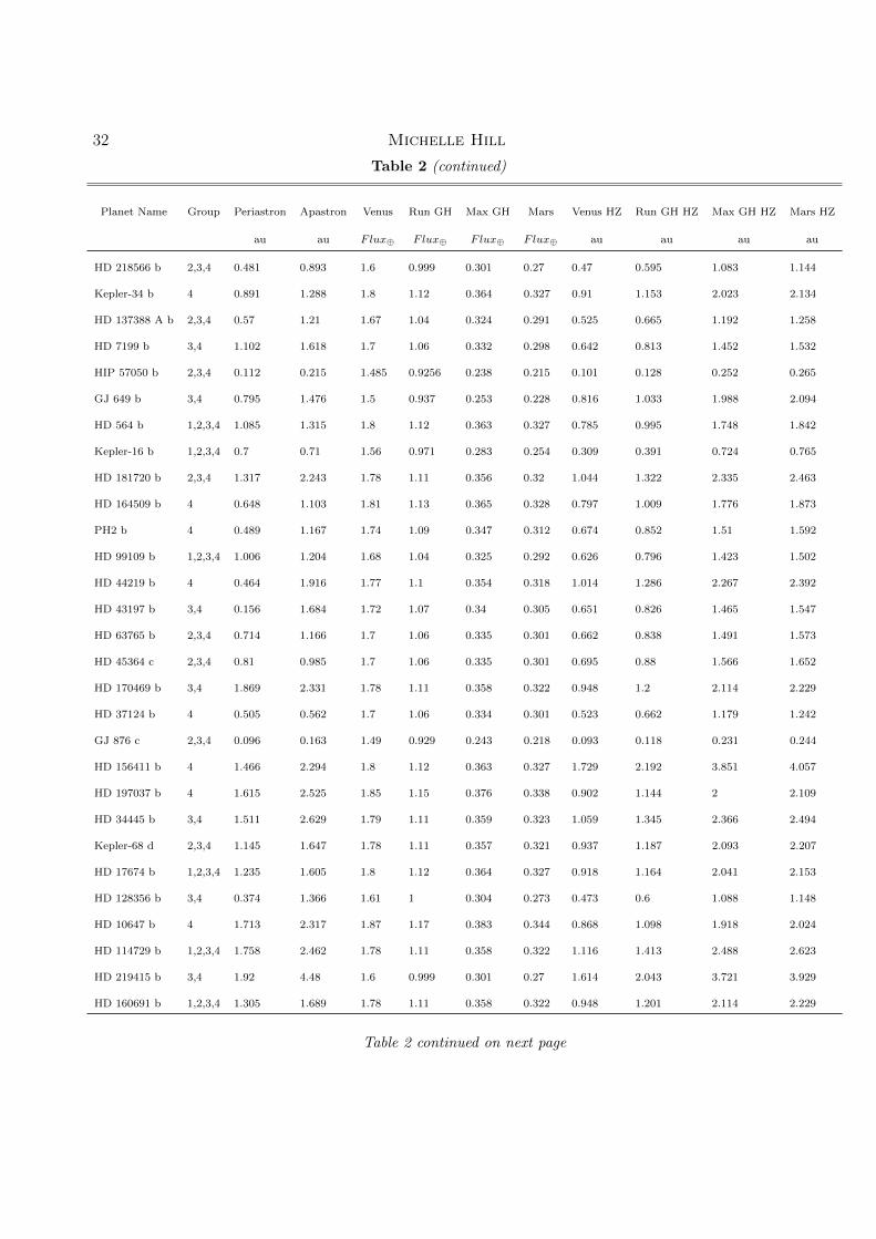
4.2.3. Tables: Habitable Zone Calculations
Table 2. Habitable Zone Giant Planets � 3R�: Habitable Zone Calculations
Planet Name Group Periastron Apastron Venus Run GH Max GH Mars Venus HZ Run GH HZ Max GH HZ Mars HZ
au au F lux� F lux� F lux� F lux� au au au au
GJ 163 c 4 0.113 0.138 1.49 0.932 0.247 0.222 0.115 0.145 0.282 0.297
LHS 1140 b 2,3,4 0.062 0.113 1.48 0.924 0.236 0.212 0.045 0.057 0.112 0.119
HD 40307 g 2,3,4 0.426 0.774 1.62 1.01 0.308 0.277 0.376 0.477 0.863 0.91
GJ 3293 d 1,2,3,4 0.171 0.217 1.49 0.931 0.246 0.221 0.121 0.154 0.299 0.315
HD 69830 d 4 0.586 0.674 1.7 1.06 0.332 0.298 0.595 0.754 1.347 1.422
GJ 687 b 1,2,3,4 0.157 0.17 1.49 0.93 0.244 0.22 0.12 0.151 0.295 0.311
HD 10180 g 2,3,4 1.052 1.802 1.8 1.12 0.364 0.327 0.865 1.097 1.924 2.03
GJ 3293 b 2,4 0.135 0.152 1.49 0.931 0.246 0.221 0.121 0.154 0.299 0.315
Kepler-62 f 1,2,3,4 0.65 0.786 1.62 1.01 0.306 0.275 0.36 0.456 0.828 0.874
Kepler-22 b 2,4 0.849 0.849 1.72 1.07 0.34 0.306 0.678 0.86 1.525 1.607
Kepler-62 e 2,4 0.371 0.483 1.62 1.01 0.306 0.275 0.36 0.456 0.828 0.874
K2-3 d 4 0.198 0.217 1.51 0.943 0.26 0.234 0.207 0.262 0.499 0.526
55 Cnc f 3,4 0.548 1.028 1.66 1.04 0.321 0.289 0.592 0.748 1.347 1.419
BD-06 1339 c 2,3,4 0.3 0.57 1.55 0.964 0.277 0.249 0.248 0.314 0.586 0.618
Table 2 continued on next page
32 Michelle Hill
Table 2 (continued)
Planet Name Group Periastron Apastron Venus Run GH Max GH Mars Venus HZ Run GH HZ Max GH HZ Mars HZ
au au F lux� F lux� F lux� F lux� au au au au
HD 218566 b 2,3,4 0.481 0.893 1.6 0.999 0.301 0.27 0.47 0.595 1.083 1.144
Kepler-34 b 4 0.891 1.288 1.8 1.12 0.364 0.327 0.91 1.153 2.023 2.134
HD 137388 A b 2,3,4 0.57 1.21 1.67 1.04 0.324 0.291 0.525 0.665 1.192 1.258
HD 7199 b 3,4 1.102 1.618 1.7 1.06 0.332 0.298 0.642 0.813 1.452 1.532
HIP 57050 b 2,3,4 0.112 0.215 1.485 0.9256 0.238 0.215 0.101 0.128 0.252 0.265
GJ 649 b 3,4 0.795 1.476 1.5 0.937 0.253 0.228 0.816 1.033 1.988 2.094
HD 564 b 1,2,3,4 1.085 1.315 1.8 1.12 0.363 0.327 0.785 0.995 1.748 1.842
Kepler-16 b 1,2,3,4 0.7 0.71 1.56 0.971 0.283 0.254 0.309 0.391 0.724 0.765
HD 181720 b 2,3,4 1.317 2.243 1.78 1.11 0.356 0.32 1.044 1.322 2.335 2.463
HD 164509 b 4 0.648 1.103 1.81 1.13 0.365 0.328 0.797 1.009 1.776 1.873
PH2 b 4 0.489 1.167 1.74 1.09 0.347 0.312 0.674 0.852 1.51 1.592
HD 99109 b 1,2,3,4 1.006 1.204 1.68 1.04 0.325 0.292 0.626 0.796 1.423 1.502
HD 44219 b 4 0.464 1.916 1.77 1.1 0.354 0.318 1.014 1.286 2.267 2.392
HD 43197 b 3,4 0.156 1.684 1.72 1.07 0.34 0.305 0.651 0.826 1.465 1.547
HD 63765 b 2,3,4 0.714 1.166 1.7 1.06 0.335 0.301 0.662 0.838 1.491 1.573
HD 45364 c 2,3,4 0.81 0.985 1.7 1.06 0.335 0.301 0.695 0.88 1.566 1.652
HD 170469 b 3,4 1.869 2.331 1.78 1.11 0.358 0.322 0.948 1.2 2.114 2.229
HD 37124 b 4 0.505 0.562 1.7 1.06 0.334 0.301 0.523 0.662 1.179 1.242
GJ 876 c 2,3,4 0.096 0.163 1.49 0.929 0.243 0.218 0.093 0.118 0.231 0.244
HD 156411 b 4 1.466 2.294 1.8 1.12 0.363 0.327 1.729 2.192 3.851 4.057
HD 197037 b 4 1.615 2.525 1.85 1.15 0.376 0.338 0.902 1.144 2 2.109
HD 34445 b 3,4 1.511 2.629 1.79 1.11 0.359 0.323 1.059 1.345 2.366 2.494
Kepler-68 d 2,3,4 1.145 1.647 1.78 1.11 0.357 0.321 0.937 1.187 2.093 2.207
HD 17674 b 1,2,3,4 1.235 1.605 1.8 1.12 0.364 0.327 0.918 1.164 2.041 2.153
HD 128356 b 3,4 0.374 1.366 1.61 1 0.304 0.273 0.473 0.6 1.088 1.148
HD 10647 b 4 1.713 2.317 1.87 1.17 0.383 0.344 0.868 1.098 1.918 2.024
HD 114729 b 1,2,3,4 1.758 2.462 1.78 1.11 0.358 0.322 1.116 1.413 2.488 2.623
HD 219415 b 3,4 1.92 4.48 1.6 0.999 0.301 0.27 1.614 2.043 3.721 3.929
HD 160691 b 1,2,3,4 1.305 1.689 1.78 1.11 0.358 0.322 0.948 1.201 2.114 2.229
Table 2 continued on next page
Exploring Giant Planets and their Potential Moons in the Habitable Zone 33
Table 2 (continued)
Planet Name Group Periastron Apastron Venus Run GH Max GH Mars Venus HZ Run GH HZ Max GH HZ Mars HZ
au au F lux� F lux� F lux� F lux� au au au au
Kepler-97 c 1,2,3,4 1.638 1.638 1.78 1.11 0.356 0.32 0.734 0.93 1.642 1.732
HD 114783 b 3,4 0.993 1.327 1.65 1.03 0.318 0.286 0.516 0.653 1.176 1.24
HD 73534 b 2,3,4 2.84 3.294 1.64 1.02 0.312 0.281 1.424 1.806 3.265 3.441
HD 9174 b 1,2,3,4 1.936 2.464 1.73 1.08 0.344 0.309 1.18 1.494 2.647 2.793
HD 100777 b 3,4 0.659 1.401 1.73 1.08 0.344 0.309 0.779 0.986 1.747 1.843
HD 28254 b 3,4 0.409 3.892 1.75 1.09 0.349 0.314 1.118 1.417 2.504 2.64
HD 147513 b 2,3,4 0.977 1.663 1.8 1.12 0.362 0.326 0.737 0.934 1.643 1.731
HD 216435 b 1,2,3,4 2.381 2.739 1.82 1.14 0.37 0.332 1.24 1.567 2.75 2.903
HD 65216 b 1,2,3,4 1.3 1.3 1.75 1.09 0.349 0.314 0.637 0.807 1.426 1.503
HD 108874 b 2,3,4 0.953 1.123 1.73 1.08 0.342 0.307 0.788 0.997 1.772 1.871
HD 210277 b 3,4 0.596 1.68 1.73 1.08 0.342 0.308 0.661 0.837 1.487 1.567
HD 19994 b 2,4 1.223 1.387 1.87 1.16 0.381 0.343 1.18 1.498 2.614 2.754
HD 30562 b 3,4 0.514 4.116 1.82 1.14 0.369 0.332 1.22 1.541 2.709 2.856
HD 133131 A b 3,4 0.965 1.915 1.78 1.11 0.357 0.321 0.75 0.949 1.674 1.765
HD 20782 b 3,4 0.061 2.733 1.78 1.11 0.357 0.321 0.822 1.041 1.836 1.936
HD 48265 b 2,4 1.665 1.955 1.75 1.09 0.348 0.313 1.481 1.876 3.321 3.501
BD+14 4559 b 2,3,4 0.552 1.002 1.63 1.02 0.311 0.279 0.542 0.685 1.241 1.31
HD 188015 b 1,2,3,4 1.038 1.368 1.77 1.1 0.354 0.318 0.769 0.976 1.72 1.815
HD 23127 b 3,4 1.344 3.456 1.74 1.09 0.346 0.311 1.089 1.375 2.441 2.575
HD 4113 b 3,4 0.124 2.436 1.76 1.1 0.35 0.315 0.832 1.053 1.866 1.967
HIP 109384 b 3,4 0.511 1.757 1.66 1.03 0.32 0.288 0.776 0.985 1.768 1.863
WASP-47 c 2,3,4 0.902 1.918 1.73 1.08 0.343 0.309 0.821 1.039 1.844 1.942
HD 221585 b 1,2,3,4 2.022 2.59 1.74 1.09 0.346 0.311 1.232 1.557 2.764 2.915
HD 142415 b 3,4 0.525 1.575 1.83 1.14 0.372 0.335 0.792 1.004 1.757 1.851
16 Cyg B b 3,4 0.536 2.826 1.75 1.09 0.35 0.314 0.816 1.034 1.826 1.927
HD 82943 b 2,3,4 0.991 1.375 1.83 1.14 0.37 0.333 0.881 1.116 1.959 2.065
HD 45350 b 4 0.426 3.414 1.74 1.09 0.346 0.311 0.847 1.07 1.899 2.003
HD 216437 b 4 1.647 2.993 1.76 1.1 0.352 0.316 1.011 1.279 2.261 2.386
HD 4203 b 3,4 0.563 1.784 1.76 1.1 0.351 0.316 0.852 1.077 1.907 2.01
Table 2 continued on next page
34 Michelle Hill
Table 2 (continued)
Planet Name Group Periastron Apastron Venus Run GH Max GH Mars Venus HZ Run GH HZ Max GH HZ Mars HZ
au au F lux� F lux� F lux� F lux� au au au au
HD 190647 b 2,3,4 1.697 2.443 1.74 1.09 0.347 0.312 1.067 1.348 2.39 2.52
HD 20868 b 3,4 0.237 1.657 1.6 0.997 0.299 0.269 0.43 0.545 0.995 1.049
kap CrB b 4 2.677 2.923 1.6 0.997 0.299 0.269 2.754 3.489 6.37 6.716
HD 159868 b 1,2,3,4 2.228 2.273 1.73 1.08 0.343 0.308 1.302 1.648 2.925 3.087
NGC 26..978 b 1,2,3,4 1.168 1.613 1.53 0.957 0.272 0.244 0.808 1.022 1.917 2.024
HD 154857 b 4 0.697 1.885 1.74 1.08 0.345 0.31 1.255 1.593 2.818 2.973
HD 73526 c 4 0.742 1.318 1.72 1.07 0.338 0.304 1.004 1.274 2.266 2.389
GJ 876 b 1,2,3,4 0.202 0.215 1.49 0.929 0.243 0.218 0.093 0.118 0.231 0.244
HD 145934 b 1,2,3,4 4.356 4.844 1.61 1.01 0.305 0.274 3.046 3.846 6.999 7.385
HD 163607 c 2,3,4 2.13 2.71 1.73 1.08 0.341 0.307 1.153 1.46 2.598 2.738
HD 4732 c 2,3,4 3.542 5.658 1.62 1.01 0.308 0.277 3.092 3.916 7.091 7.478
HD 23079 b 1,2,3,4 1.433 1.759 1.81 1.13 0.365 0.328 0.91 1.152 2.027 2.139
GJ 317 b 2,3,4 1.024 1.277 1.5 0.932 0.247 0.222 0.816 1.036 2.012 2.122
47 UMa b 2,3,4 2.033 2.167 1.8 1.12 0.363 0.326 0.953 1.208 2.122 2.239
HD 196885 b 3,4 1.232 3.508 1.88 1.17 0.385 0.346 1.13 1.432 2.496 2.633
HD 164604 b 2,3,4 0.988 1.612 1.58 0.983 0.291 0.261 0.796 1.009 1.854 1.957
HD 153950 b 4 0.845 1.715 1.84 1.15 0.374 0.336 1.098 1.389 2.435 2.569
HD 165155 b 1,2,3,4 0.904 1.356 1.7 1.06 0.334 0.301 0.642 0.813 1.448 1.525
HD 125612 b 3,4 0.74 2 1.8 1.12 0.363 0.327 0.778 0.986 1.732 1.825
HD 221287 b 2,3,4 1.15 1.35 1.89 1.18 0.388 0.349 0.937 1.186 2.068 2.181
HD 1605 c 1,2,3,4 3.175 3.865 1.59 0.994 0.297 0.267 2.038 2.578 4.717 4.974
HD 92788 b 4 0.624 1.296 1.78 1.11 0.358 0.322 0.767 0.971 1.71 1.803
HD 183263 b 2,3,4 0.971 2.049 1.81 1.13 0.366 0.329 0.878 1.111 1.952 2.059
KELT-6 c 1,2,3,4 1.888 2.892 1.89 1.17 0.386 0.347 1.311 1.666 2.9 3.059
HD 169830 c 4 2.412 4.788 1.89 1.18 0.388 0.349 1.559 1.973 3.44 3.627
ups And d 3,4 1.763 3.264 1.83 1.14 0.371 0.334 1.254 1.589 2.785 2.935
Kepler-454 c 1,2,3,4 1.258 1.314 1.76 1.1 0.351 0.316 0.785 0.993 1.757 1.852
HD 213240 b 3,4 1.117 2.944 1.8 1.12 0.362 0.326 1.081 1.37 2.41 2.54
HD 111998 b 1,2,3,4 1.765 1.875 1.95 1.22 0.403 0.363 1.336 1.69 2.94 3.098
Table 2 continued on next page
Exploring Giant Planets and their Potential Moons in the Habitable Zone 35
Table 2 (continued)
Planet Name Group Periastron Apastron Venus Run GH Max GH Mars Venus HZ Run GH HZ Max GH HZ Mars HZ
au au F lux� F lux� F lux� F lux� au au au au
HD 16175 b 3,4 0.78 3.516 1.83 1.14 0.371 0.333 1.327 1.681 2.947 3.11
HD 13908 c 2,3,4 1.786 2.274 1.88 1.17 0.385 0.346 1.459 1.849 3.223 3.4
HD 28185 b 1,2,3,4 0.937 1.127 1.73 1.08 0.342 0.307 0.707 0.894 1.589 1.677
HD 224538 b 3,4 1.222 3.338 1.85 1.15 0.376 0.338 1.263 1.602 2.802 2.955
HIP 67851 c 4 3.171 4.469 1.61 1.01 0.304 0.274 3.301 4.167 7.596 8.001
HD 70573 b 4 1.056 2.464 1.77 1.1 0.354 0.318 0.752 0.953 1.681 1.773
Kepler-424 c 2,4 0.73 0.73 1.71 1.07 0.337 0.302 0.643 0.813 1.449 1.531
HD 86264 b 3,4 0.858 4.862 1.89 1.18 0.388 0.349 1.299 1.643 2.866 3.022
Kepler-419 c 4 1.371 1.989 1.92 1.2 0.396 0.356 1.554 1.966 3.422 3.61
HD 23596 b 2,3,4 2.035 3.509 1.8 1.12 0.364 0.327 1.533 1.943 3.408 3.596
HD 222582 b 3,4 0.37 2.324 1.77 1.1 0.353 0.317 0.841 1.067 1.883 1.987
HD 33564 b 3,4 0.726 1.474 1.88 1.17 0.385 0.346 0.729 0.925 1.612 1.7
HD 141937 b 3,4 0.878 2.098 1.8 1.12 0.362 0.326 0.764 0.969 1.705 1.796
30 Ari B b 4 0.707 1.283 1.89 1.18 0.388 0.349 0.977 1.236 2.155 2.273
HD 38801 b 2,4 1.7 1.7 1.67 1.04 0.322 0.29 1.653 2.094 3.763 3.966
HD 217786 b 4 1.428 3.332 1.82 1.13 0.367 0.33 1.019 1.293 2.268 2.392
HAT-P-13 c 4 0.415 2.037 1.75 1.09 0.348 0.313 1.126 1.427 2.525 2.662
HD 214823 b 3,4 2.69 3.67 1.87 1.17 0.383 0.344 1.524 1.927 3.368 3.554
Kepler-47 c 3,4 0.584 1.398 1.75 1.09 0.347 0.312 0.693 0.878 1.555 1.64
4.2.4. Tables: Exomoon calculations
Table 3. Habitable Zone Giant Planets � 3R�: Potential Satellite Calculations
Planet Name Group Roche (⇢ = 3g/cm) Roche (⇢ = 4g/cm) Roche (⇢ = 5g/cm) Hill Radius Angular Seperation
x10�6 au x10�6 au x10�6 au au x10�600
GJ 163 c 4 241.1± 11.3 219.1± 10.2 203.4± 9.5 0.003± 0 65± 12
GJ 3293 d 1,2,3,4 250.2± 10.5 227.3± 9.5 211.1± 8.8 0.004± 95±
Table 3 continued on next page
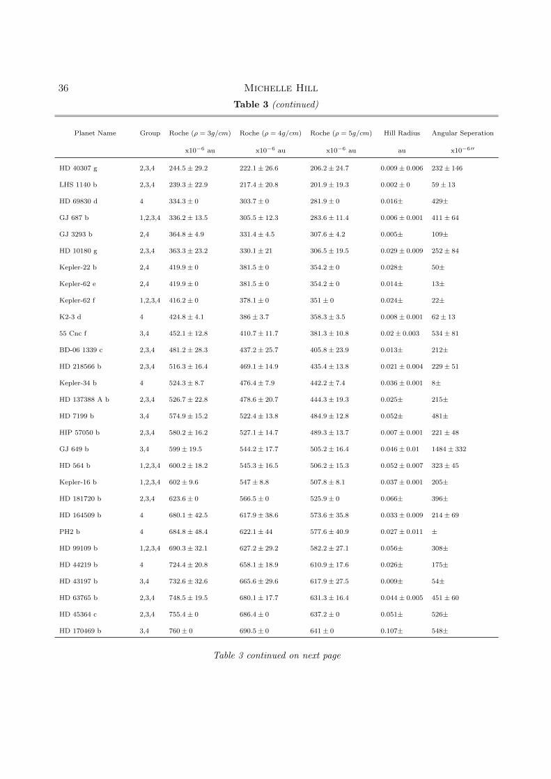
36 Michelle Hill
Table 3 (continued)
Planet Name Group Roche (⇢ = 3g/cm) Roche (⇢ = 4g/cm) Roche (⇢ = 5g/cm) Hill Radius Angular Seperation
x10�6 au x10�6 au x10�6 au au x10�600
HD 40307 g 2,3,4 244.5± 29.2 222.1± 26.6 206.2± 24.7 0.009± 0.006 232± 146
LHS 1140 b 2,3,4 239.3± 22.9 217.4± 20.8 201.9± 19.3 0.002± 0 59± 13
HD 69830 d 4 334.3± 0 303.7± 0 281.9± 0 0.016± 429±
GJ 687 b 1,2,3,4 336.2± 13.5 305.5± 12.3 283.6± 11.4 0.006± 0.001 411± 64
GJ 3293 b 2,4 364.8± 4.9 331.4± 4.5 307.6± 4.2 0.005± 109±
HD 10180 g 2,3,4 363.3± 23.2 330.1± 21 306.5± 19.5 0.029± 0.009 252± 84
Kepler-22 b 2,4 419.9± 0 381.5± 0 354.2± 0 0.028± 50±
Kepler-62 e 2,4 419.9± 0 381.5± 0 354.2± 0 0.014± 13±
Kepler-62 f 1,2,3,4 416.2± 0 378.1± 0 351± 0 0.024± 22±
K2-3 d 4 424.8± 4.1 386± 3.7 358.3± 3.5 0.008± 0.001 62± 13
55 Cnc f 3,4 452.1± 12.8 410.7± 11.7 381.3± 10.8 0.02± 0.003 534± 81
BD-06 1339 c 2,3,4 481.2± 28.3 437.2± 25.7 405.8± 23.9 0.013± 212±
HD 218566 b 2,3,4 516.3± 16.4 469.1± 14.9 435.4± 13.8 0.021± 0.004 229± 51
Kepler-34 b 4 524.3± 8.7 476.4± 7.9 442.2± 7.4 0.036± 0.001 8±
HD 137388 A b 2,3,4 526.7± 22.8 478.6± 20.7 444.3± 19.3 0.025± 215±
HD 7199 b 3,4 574.9± 15.2 522.4± 13.8 484.9± 12.8 0.052± 481±
HIP 57050 b 2,3,4 580.2± 16.2 527.1± 14.7 489.3± 13.7 0.007± 0.001 221± 48
GJ 649 b 3,4 599± 19.5 544.2± 17.7 505.2± 16.4 0.046± 0.01 1484± 332
HD 564 b 1,2,3,4 600.2± 18.2 545.3± 16.5 506.2± 15.3 0.052± 0.007 323± 45
Kepler-16 b 1,2,3,4 602± 9.6 547± 8.8 507.8± 8.1 0.037± 0.001 205±
HD 181720 b 2,3,4 623.6± 0 566.5± 0 525.9± 0 0.066± 396±
HD 164509 b 4 680.1± 42.5 617.9± 38.6 573.6± 35.8 0.033± 0.009 214± 69
PH2 b 4 684.8± 48.4 622.1± 44 577.6± 40.9 0.027± 0.011 ±
HD 99109 b 1,2,3,4 690.3± 32.1 627.2± 29.2 582.2± 27.1 0.056± 308±
HD 44219 b 4 724.4± 20.8 658.1± 18.9 610.9± 17.6 0.026± 175±
HD 43197 b 3,4 732.6± 32.6 665.6± 29.6 617.9± 27.5 0.009± 54±
HD 63765 b 2,3,4 748.5± 19.5 680.1± 17.7 631.3± 16.4 0.044± 0.005 451± 60
HD 45364 c 2,3,4 755.4± 0 686.4± 0 637.2± 0 0.051± 526±
HD 170469 b 3,4 760± 0 690.5± 0 641± 0 0.107± 548±
Table 3 continued on next page
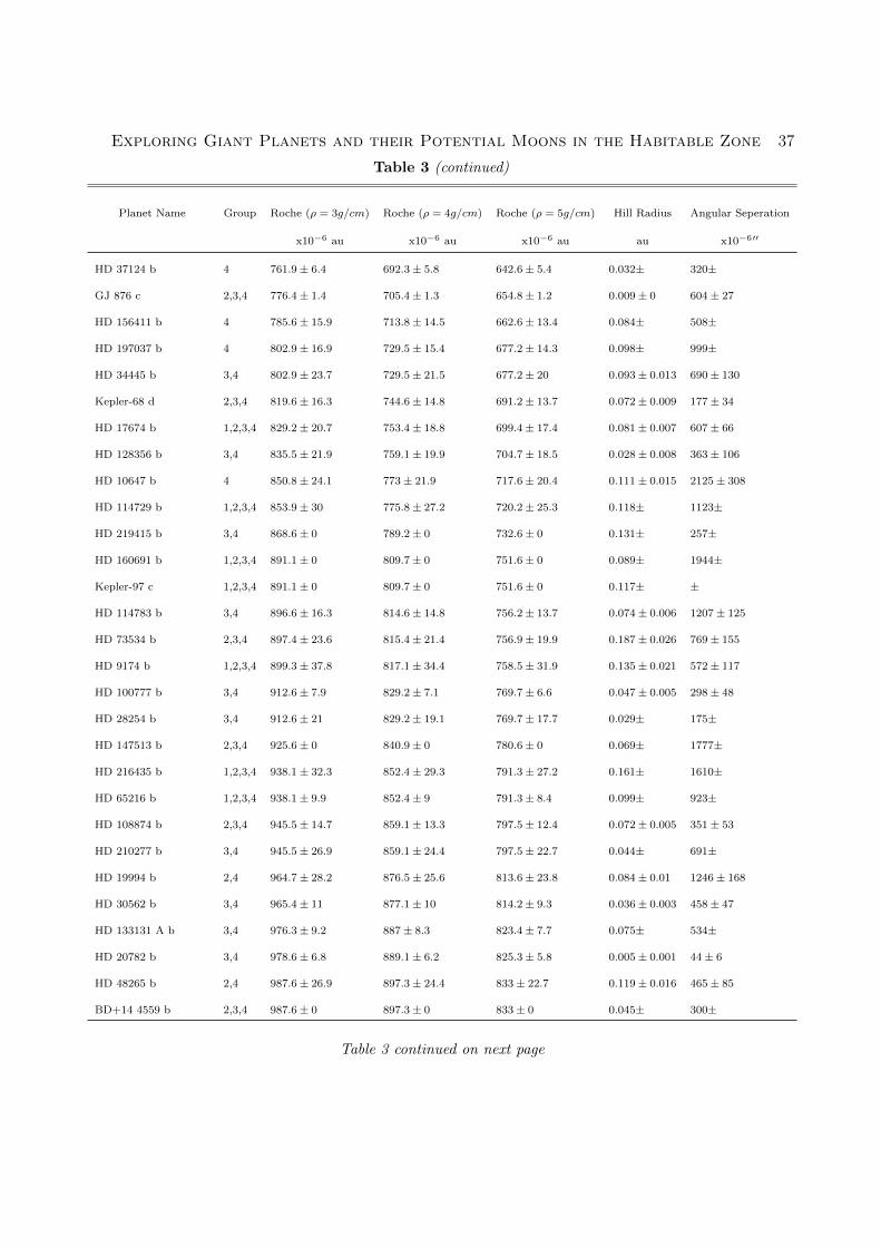
Exploring Giant Planets and their Potential Moons in the Habitable Zone 37
Table 3 (continued)
Planet Name Group Roche (⇢ = 3g/cm) Roche (⇢ = 4g/cm) Roche (⇢ = 5g/cm) Hill Radius Angular Seperation
x10�6 au x10�6 au x10�6 au au x10�600
HD 37124 b 4 761.9± 6.4 692.3± 5.8 642.6± 5.4 0.032± 320±
GJ 876 c 2,3,4 776.4± 1.4 705.4± 1.3 654.8± 1.2 0.009± 0 604± 27
HD 156411 b 4 785.6± 15.9 713.8± 14.5 662.6± 13.4 0.084± 508±
HD 197037 b 4 802.9± 16.9 729.5± 15.4 677.2± 14.3 0.098± 999±
HD 34445 b 3,4 802.9± 23.7 729.5± 21.5 677.2± 20 0.093± 0.013 690± 130
Kepler-68 d 2,3,4 819.6± 16.3 744.6± 14.8 691.2± 13.7 0.072± 0.009 177± 34
HD 17674 b 1,2,3,4 829.2± 20.7 753.4± 18.8 699.4± 17.4 0.081± 0.007 607± 66
HD 128356 b 3,4 835.5± 21.9 759.1± 19.9 704.7± 18.5 0.028± 0.008 363± 106
HD 10647 b 4 850.8± 24.1 773± 21.9 717.6± 20.4 0.111± 0.015 2125± 308
HD 114729 b 1,2,3,4 853.9± 30 775.8± 27.2 720.2± 25.3 0.118± 1123±
HD 219415 b 3,4 868.6± 0 789.2± 0 732.6± 0 0.131± 257±
HD 160691 b 1,2,3,4 891.1± 0 809.7± 0 751.6± 0 0.089± 1944±
Kepler-97 c 1,2,3,4 891.1± 0 809.7± 0 751.6± 0 0.117± ±
HD 114783 b 3,4 896.6± 16.3 814.6± 14.8 756.2± 13.7 0.074± 0.006 1207± 125
HD 73534 b 2,3,4 897.4± 23.6 815.4± 21.4 756.9± 19.9 0.187± 0.026 769± 155
HD 9174 b 1,2,3,4 899.3± 37.8 817.1± 34.4 758.5± 31.9 0.135± 0.021 572± 117
HD 100777 b 3,4 912.6± 7.9 829.2± 7.1 769.7± 6.6 0.047± 0.005 298± 48
HD 28254 b 3,4 912.6± 21 829.2± 19.1 769.7± 17.7 0.029± 175±
HD 147513 b 2,3,4 925.6± 0 840.9± 0 780.6± 0 0.069± 1777±
HD 216435 b 1,2,3,4 938.1± 32.3 852.4± 29.3 791.3± 27.2 0.161± 1610±
HD 65216 b 1,2,3,4 938.1± 9.9 852.4± 9 791.3± 8.4 0.099± 923±
HD 108874 b 2,3,4 945.5± 14.7 859.1± 13.3 797.5± 12.4 0.072± 0.005 351± 53
HD 210277 b 3,4 945.5± 26.9 859.1± 24.4 797.5± 22.7 0.044± 691±
HD 19994 b 2,4 964.7± 28.2 876.5± 25.6 813.6± 23.8 0.084± 0.01 1246± 168
HD 30562 b 3,4 965.4± 11 877.1± 10 814.2± 9.3 0.036± 0.003 458± 47
HD 133131 A b 3,4 976.3± 9.2 887± 8.3 823.4± 7.7 0.075± 534±
HD 20782 b 3,4 978.6± 6.8 889.1± 6.2 825.3± 5.8 0.005± 0.001 44± 6
HD 48265 b 2,4 987.6± 26.9 897.3± 24.4 833± 22.7 0.119± 0.016 465± 85
BD+14 4559 b 2,3,4 987.6± 0 897.3± 0 833± 0 0.045± 300±
Table 3 continued on next page
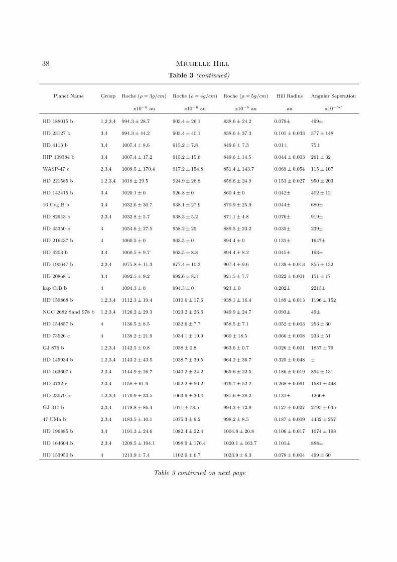
38 Michelle Hill
Table 3 (continued)
Planet Name Group Roche (⇢ = 3g/cm) Roche (⇢ = 4g/cm) Roche (⇢ = 5g/cm) Hill Radius Angular Seperation
x10�6 au x10�6 au x10�6 au au x10�600
HD 188015 b 1,2,3,4 994.3± 28.7 903.4± 26.1 838.6± 24.2 0.079± 499±
HD 23127 b 3,4 994.3± 44.2 903.4± 40.1 838.6± 37.3 0.101± 0.033 377± 148
HD 4113 b 3,4 1007.4± 8.6 915.2± 7.8 849.6± 7.3 0.01± 75±
HIP 109384 b 3,4 1007.4± 17.2 915.2± 15.6 849.6± 14.5 0.044± 0.003 261± 32
WASP-47 c 2,3,4 1009.5± 170.4 917.2± 154.8 851.4± 143.7 0.069± 0.054 115± 107
HD 221585 b 1,2,3,4 1018± 29.5 924.9± 26.8 858.6± 24.9 0.153± 0.027 950± 203
HD 142415 b 3,4 1020.1± 0 926.8± 0 860.4± 0 0.042± 402± 12
16 Cyg B b 3,4 1032.6± 30.7 938.1± 27.9 870.9± 25.9 0.044± 680±
HD 82943 b 2,3,4 1032.8± 5.7 938.3± 5.2 871.1± 4.8 0.076± 919±
HD 45350 b 4 1054.6± 27.5 958.2± 25 889.5± 23.2 0.035± 239±
HD 216437 b 4 1060.5± 0 963.5± 0 894.4± 0 0.131± 1647±
HD 4203 b 3,4 1060.5± 9.7 963.5± 8.8 894.4± 8.2 0.045± 193±
HD 190647 b 2,3,4 1075.8± 11.3 977.4± 10.3 907.4± 9.6 0.139± 0.013 855± 132
HD 20868 b 3,4 1092.5± 9.2 992.6± 8.3 921.5± 7.7 0.022± 0.001 151± 17
kap CrB b 4 1094.3± 0 994.3± 0 923± 0 0.202± 2213±
HD 159868 b 1,2,3,4 1112.3± 19.4 1010.6± 17.6 938.1± 16.4 0.189± 0.013 1196± 152
NGC 2682 Sand 978 b 1,2,3,4 1126.2± 29.3 1023.2± 26.6 949.9± 24.7 0.093± 49±
HD 154857 b 4 1136.5± 8.5 1032.6± 7.7 958.5± 7.1 0.052± 0.003 253± 30
HD 73526 c 4 1138.2± 21.9 1034.1± 19.9 960± 18.5 0.066± 0.008 233± 51
GJ 876 b 1,2,3,4 1142.5± 0.8 1038± 0.8 963.6± 0.7 0.026± 0.001 1857± 79
HD 145934 b 1,2,3,4 1143.2± 43.5 1038.7± 39.5 964.2± 36.7 0.325± 0.048 ±
HD 163607 c 2,3,4 1144.9± 26.7 1040.2± 24.2 965.6± 22.5 0.186± 0.019 894± 131
HD 4732 c 2,3,4 1158± 61.9 1052.2± 56.2 976.7± 52.2 0.268± 0.061 1581± 448
HD 23079 b 1,2,3,4 1170.9± 33.5 1063.9± 30.4 987.6± 28.2 0.131± 1266±
GJ 317 b 2,3,4 1178.8± 86.4 1071± 78.5 994.3± 72.9 0.127± 0.027 2795± 635
47 UMa b 2,3,4 1183.5± 10.1 1075.3± 9.2 998.2± 8.5 0.187± 0.009 4432± 257
HD 196885 b 3,4 1191.3± 24.6 1082.4± 22.4 1004.8± 20.8 0.106± 0.017 1074± 198
HD 164604 b 2,3,4 1209.5± 194.1 1098.9± 176.4 1020.1± 163.7 0.101± 888±
HD 153950 b 4 1213.9± 7.4 1102.9± 6.7 1023.9± 6.3 0.078± 0.004 499± 60
Table 3 continued on next page
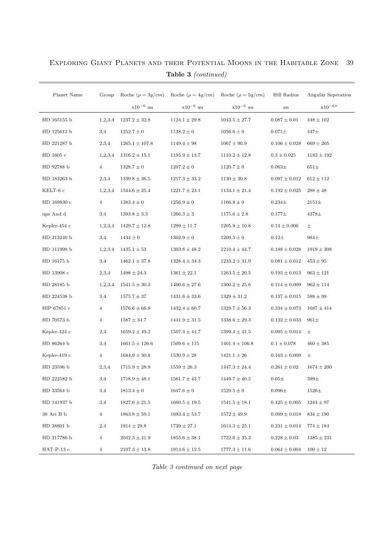
Exploring Giant Planets and their Potential Moons in the Habitable Zone 39
Table 3 (continued)
Planet Name Group Roche (⇢ = 3g/cm) Roche (⇢ = 4g/cm) Roche (⇢ = 5g/cm) Hill Radius Angular Seperation
x10�6 au x10�6 au x10�6 au au x10�600
HD 165155 b 1,2,3,4 1237.2± 32.8 1124.1± 29.8 1043.5± 27.7 0.087± 0.01 448± 102
HD 125612 b 3,4 1252.7± 0 1138.2± 0 1056.6± 0 0.071± 447±
HD 221287 b 2,3,4 1265.1± 107.8 1149.4± 98 1067± 90.9 0.106± 0.028 669± 205
HD 1605 c 1,2,3,4 1316.2± 15.1 1195.9± 13.7 1110.2± 12.8 0.3± 0.025 1183± 192
HD 92788 b 4 1328.7± 0 1207.2± 0 1120.7± 0 0.063± 651±
HD 183263 b 2,3,4 1339.8± 36.5 1217.3± 33.2 1130± 30.8 0.097± 0.012 612± 112
KELT-6 c 1,2,3,4 1344.6± 25.4 1221.7± 23.1 1134.1± 21.4 0.192± 0.025 288± 48
HD 169830 c 4 1383.4± 0 1256.9± 0 1166.8± 0 0.234± 2151±
ups And d 3,4 1393.8± 3.3 1266.3± 3 1175.6± 2.8 0.177± 4378±
Kepler-454 c 1,2,3,4 1429.7± 12.8 1299± 11.7 1205.9± 10.8 0.14± 0.006 ±
HD 213240 b 3,4 1434± 0 1302.9± 0 1209.5± 0 0.12± 984±
HD 111998 b 1,2,3,4 1435.1± 53 1303.8± 48.2 1210.4± 44.7 0.188± 0.028 1919± 308
HD 16175 b 3,4 1462.1± 37.8 1328.4± 34.3 1233.2± 31.9 0.081± 0.012 453± 95
HD 13908 c 2,3,4 1498± 24.3 1361± 22.1 1263.5± 20.5 0.193± 0.013 963± 121
HD 28185 b 1,2,3,4 1541.5± 30.3 1400.6± 27.6 1300.2± 25.6 0.114± 0.009 962± 114
HD 224538 b 3,4 1575.7± 37 1431.6± 33.6 1329± 31.2 0.137± 0.015 588± 99
HIP 67851 c 4 1576.6± 66.8 1432.4± 60.7 1329.7± 56.3 0.334± 0.073 1687± 414
HD 70573 b 4 1587± 34.7 1441.9± 31.5 1338.6± 29.3 0.132± 0.033 961±
Kepler-424 c 2,4 1659.2± 49.2 1507.4± 44.7 1399.4± 41.5 0.095± 0.014 ±
HD 86264 b 3,4 1661.5± 126.6 1509.6± 115 1401.4± 106.8 0.1± 0.078 460± 385
Kepler-419 c 4 1684.9± 30.8 1530.9± 28 1421.1± 26 0.163± 0.009 ±
HD 23596 b 2,3,4 1715.9± 28.9 1559± 26.3 1447.3± 24.4 0.261± 0.02 1674± 200
HD 222582 b 3,4 1718.9± 48.1 1561.7± 43.7 1449.7± 40.5 0.05± 399±
HD 33564 b 3,4 1813.4± 0 1647.6± 0 1529.5± 0 0.096± 1526±
HD 141937 b 3,4 1827.6± 21.5 1660.5± 19.5 1541.5± 18.1 0.125± 0.005 1244± 97
30 Ari B b 4 1863.8± 59.1 1693.4± 53.7 1572± 49.9 0.099± 0.018 834± 190
HD 38801 b 2,4 1914± 29.8 1739± 27.1 1614.3± 25.1 0.231± 0.014 774± 184
HD 217786 b 4 2042.3± 41.9 1855.6± 38.1 1722.6± 35.3 0.228± 0.03 1385± 231
HAT-P-13 c 4 2107.3± 13.8 1914.6± 12.5 1777.3± 11.6 0.064± 0.004 100± 12
Table 3 continued on next page
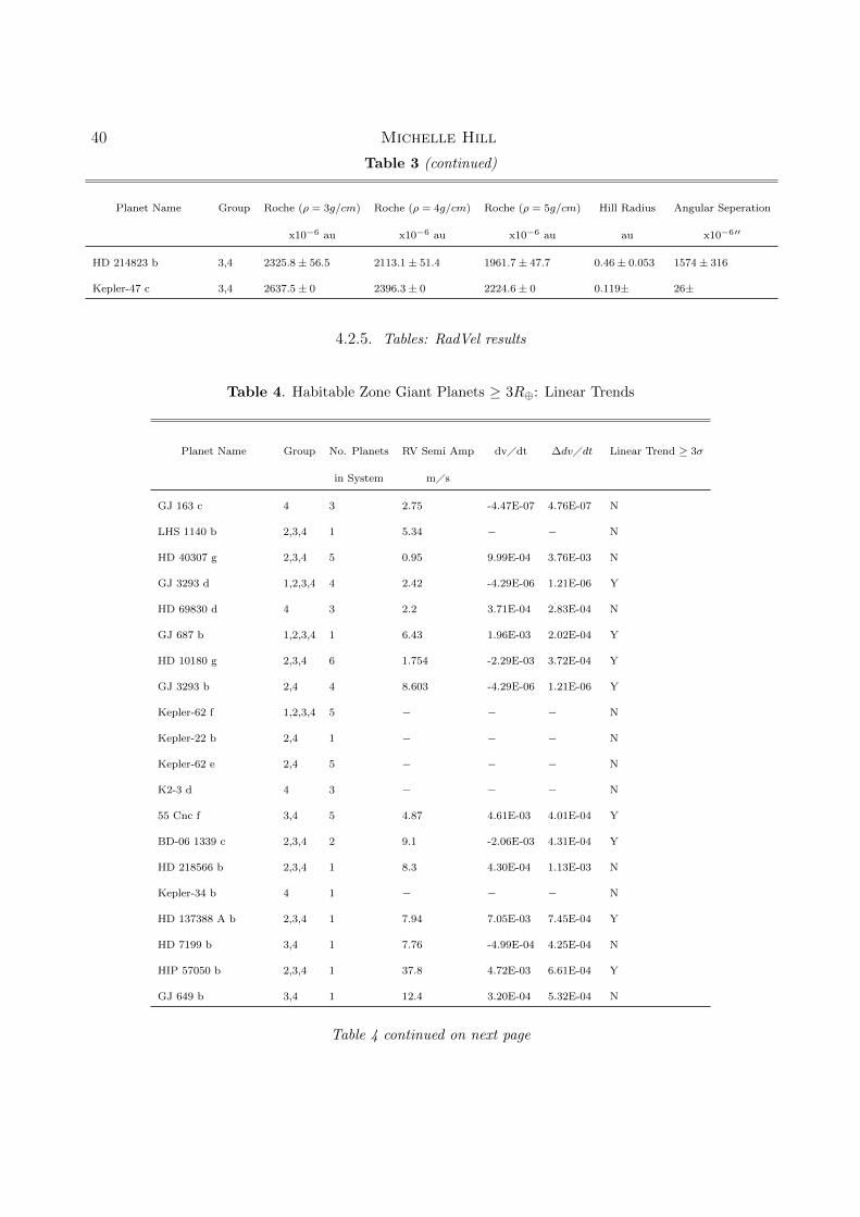
40 Michelle Hill
Table 3 (continued)
Planet Name Group Roche (⇢ = 3g/cm) Roche (⇢ = 4g/cm) Roche (⇢ = 5g/cm) Hill Radius Angular Seperation
x10�6 au x10�6 au x10�6 au au x10�600
HD 214823 b 3,4 2325.8± 56.5 2113.1± 51.4 1961.7± 47.7 0.46± 0.053 1574± 316
Kepler-47 c 3,4 2637.5± 0 2396.3± 0 2224.6± 0 0.119± 26±
4.2.5. Tables: RadVel results
Table 4. Habitable Zone Giant Planets � 3R�: Linear Trends
Planet Name Group No. Planets RV Semi Amp dv�dt �dv�dt Linear Trend � 3�
in System m�s
GJ 163 c 4 3 2.75 -4.47E-07 4.76E-07 N
LHS 1140 b 2,3,4 1 5.34 � � N
HD 40307 g 2,3,4 5 0.95 9.99E-04 3.76E-03 N
GJ 3293 d 1,2,3,4 4 2.42 -4.29E-06 1.21E-06 Y
HD 69830 d 4 3 2.2 3.71E-04 2.83E-04 N
GJ 687 b 1,2,3,4 1 6.43 1.96E-03 2.02E-04 Y
HD 10180 g 2,3,4 6 1.754 -2.29E-03 3.72E-04 Y
GJ 3293 b 2,4 4 8.603 -4.29E-06 1.21E-06 Y
Kepler-62 f 1,2,3,4 5 � � � N
Kepler-22 b 2,4 1 � � � N
Kepler-62 e 2,4 5 � � � N
K2-3 d 4 3 � � � N
55 Cnc f 3,4 5 4.87 4.61E-03 4.01E-04 Y
BD-06 1339 c 2,3,4 2 9.1 -2.06E-03 4.31E-04 Y
HD 218566 b 2,3,4 1 8.3 4.30E-04 1.13E-03 N
Kepler-34 b 4 1 � � � N
HD 137388 A b 2,3,4 1 7.94 7.05E-03 7.45E-04 Y
HD 7199 b 3,4 1 7.76 -4.99E-04 4.25E-04 N
HIP 57050 b 2,3,4 1 37.8 4.72E-03 6.61E-04 Y
GJ 649 b 3,4 1 12.4 3.20E-04 5.32E-04 N
Table 4 continued on next page
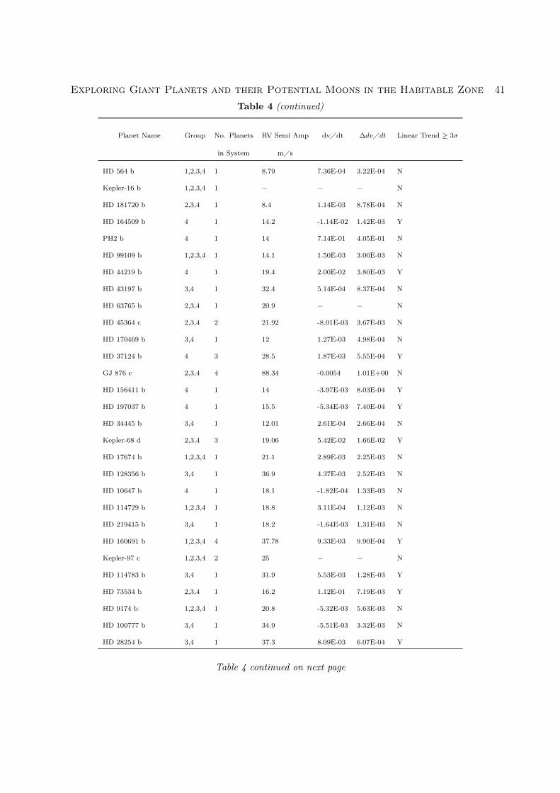
Exploring Giant Planets and their Potential Moons in the Habitable Zone 41
Table 4 (continued)
Planet Name Group No. Planets RV Semi Amp dv�dt �dv�dt Linear Trend � 3�
in System m�s
HD 564 b 1,2,3,4 1 8.79 7.36E-04 3.22E-04 N
Kepler-16 b 1,2,3,4 1 � � � N
HD 181720 b 2,3,4 1 8.4 1.14E-03 8.78E-04 N
HD 164509 b 4 1 14.2 -1.14E-02 1.42E-03 Y
PH2 b 4 1 14 7.14E-01 4.05E-01 N
HD 99109 b 1,2,3,4 1 14.1 1.50E-03 3.00E-03 N
HD 44219 b 4 1 19.4 2.00E-02 3.80E-03 Y
HD 43197 b 3,4 1 32.4 5.14E-04 8.37E-04 N
HD 63765 b 2,3,4 1 20.9 � � N
HD 45364 c 2,3,4 2 21.92 -8.01E-03 3.67E-03 N
HD 170469 b 3,4 1 12 1.27E-03 4.98E-04 N
HD 37124 b 4 3 28.5 1.87E-03 5.55E-04 Y
GJ 876 c 2,3,4 4 88.34 -0.0054 1.01E+00 N
HD 156411 b 4 1 14 -3.97E-03 8.03E-04 Y
HD 197037 b 4 1 15.5 -5.34E-03 7.40E-04 Y
HD 34445 b 3,4 1 12.01 2.61E-04 2.66E-04 N
Kepler-68 d 2,3,4 3 19.06 5.42E-02 1.66E-02 Y
HD 17674 b 1,2,3,4 1 21.1 2.89E-03 2.25E-03 N
HD 128356 b 3,4 1 36.9 4.37E-03 2.52E-03 N
HD 10647 b 4 1 18.1 -1.82E-04 1.33E-03 N
HD 114729 b 1,2,3,4 1 18.8 3.11E-04 1.12E-03 N
HD 219415 b 3,4 1 18.2 -1.64E-03 1.31E-03 N
HD 160691 b 1,2,3,4 4 37.78 9.33E-03 9.90E-04 Y
Kepler-97 c 1,2,3,4 2 25 � � N
HD 114783 b 3,4 1 31.9 5.53E-03 1.28E-03 Y
HD 73534 b 2,3,4 1 16.2 1.12E-01 7.19E-03 Y
HD 9174 b 1,2,3,4 1 20.8 -5.32E-03 5.63E-03 N
HD 100777 b 3,4 1 34.9 -5.51E-03 3.32E-03 N
HD 28254 b 3,4 1 37.3 8.09E-03 6.07E-04 Y
Table 4 continued on next page
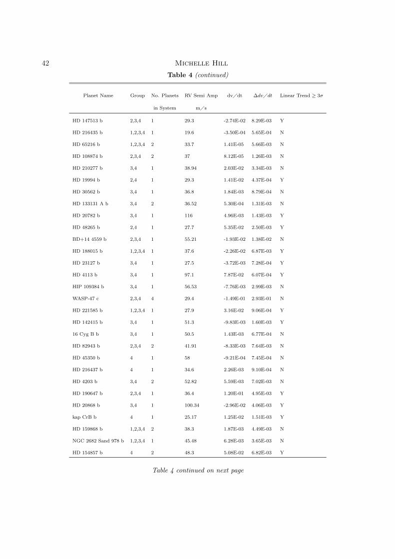
42 Michelle Hill
Table 4 (continued)
Planet Name Group No. Planets RV Semi Amp dv�dt �dv�dt Linear Trend � 3�
in System m�s
HD 147513 b 2,3,4 1 29.3 -2.74E-02 8.29E-03 Y
HD 216435 b 1,2,3,4 1 19.6 -3.50E-04 5.65E-04 N
HD 65216 b 1,2,3,4 2 33.7 1.41E-05 5.66E-03 N
HD 108874 b 2,3,4 2 37 8.12E-05 1.26E-03 N
HD 210277 b 3,4 1 38.94 2.03E-02 3.34E-03 N
HD 19994 b 2,4 1 29.3 1.41E-02 4.37E-04 Y
HD 30562 b 3,4 1 36.8 1.84E-03 8.79E-04 N
HD 133131 A b 3,4 2 36.52 5.30E-04 1.31E-03 N
HD 20782 b 3,4 1 116 4.96E-03 1.43E-03 Y
HD 48265 b 2,4 1 27.7 5.35E-02 2.50E-03 Y
BD+14 4559 b 2,3,4 1 55.21 -1.93E-02 1.38E-02 N
HD 188015 b 1,2,3,4 1 37.6 -2.26E-02 6.87E-03 Y
HD 23127 b 3,4 1 27.5 -3.72E-03 7.28E-04 Y
HD 4113 b 3,4 1 97.1 7.87E-02 6.07E-04 Y
HIP 109384 b 3,4 1 56.53 -7.76E-03 2.99E-03 N
WASP-47 c 2,3,4 4 29.4 -1.49E-01 2.93E-01 N
HD 221585 b 1,2,3,4 1 27.9 3.16E-02 9.06E-04 Y
HD 142415 b 3,4 1 51.3 -9.83E-03 1.60E-03 Y
16 Cyg B b 3,4 1 50.5 1.43E-03 6.77E-04 N
HD 82943 b 2,3,4 2 41.91 -8.33E-03 7.64E-03 N
HD 45350 b 4 1 58 -9.21E-04 7.45E-04 N
HD 216437 b 4 1 34.6 2.26E-03 9.10E-04 N
HD 4203 b 3,4 2 52.82 5.59E-03 7.02E-03 N
HD 190647 b 2,3,4 1 36.4 1.20E-01 4.95E-03 Y
HD 20868 b 3,4 1 100.34 -2.96E-02 4.06E-03 Y
kap CrB b 4 1 25.17 1.25E-02 1.51E-03 Y
HD 159868 b 1,2,3,4 2 38.3 1.87E-03 4.49E-03 N
NGC 2682 Sand 978 b 1,2,3,4 1 45.48 6.28E-03 3.65E-03 N
HD 154857 b 4 2 48.3 5.08E-02 6.82E-03 Y
Table 4 continued on next page
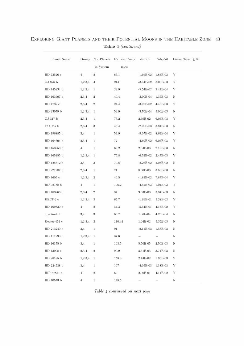
Exploring Giant Planets and their Potential Moons in the Habitable Zone 43
Table 4 (continued)
Planet Name Group No. Planets RV Semi Amp dv�dt �dv�dt Linear Trend � 3�
in System m�s
HD 73526 c 4 2 65.1 -1.66E-02 1.83E-03 Y
GJ 876 b 1,2,3,4 4 214 -3.44E-02 3.05E-03 Y
HD 145934 b 1,2,3,4 1 22.9 -5.54E-02 2.44E-04 Y
HD 163607 c 2,3,4 2 40.4 -3.90E-04 1.35E-03 N
HD 4732 c 2,3,4 2 24.4 -3.97E-02 4.48E-03 Y
HD 23079 b 1,2,3,4 1 54.9 -3.70E-04 5.00E-03 N
GJ 317 b 2,3,4 1 75.2 2.69E-02 6.07E-03 Y
47 UMa b 2,3,4 3 48.4 -2.20E-03 3.84E-03 N
HD 196885 b 3,4 1 53.9 -9.07E-02 8.63E-04 Y
HD 164604 b 2,3,4 1 77 -4.69E-02 6.07E-03 Y
HD 153950 b 4 1 69.2 2.34E-03 2.18E-03 N
HD 165155 b 1,2,3,4 1 75.8 -6.52E-02 2.47E-03 Y
HD 125612 b 3,4 3 79.8 -2.26E-02 2.03E-02 N
HD 221287 b 2,3,4 1 71 8.30E-03 3.59E-03 N
HD 1605 c 1,2,3,4 2 46.5 -1.83E-02 7.87E-04 Y
HD 92788 b 4 1 106.2 -4.52E-03 1.04E-03 Y
HD 183263 b 2,3,4 2 84 9.63E-03 3.84E-03 N
KELT-6 c 1,2,3,4 2 65.7 -1.69E-01 5.38E-02 Y
HD 169830 c 4 2 54.3 -5.54E-01 4.13E-02 Y
ups And d 3,4 3 66.7 1.86E-04 4.25E-04 N
Kepler-454 c 1,2,3,4 2 110.44 1.04E-02 5.35E-03 N
HD 213240 b 3,4 1 91 -2.11E-03 1.53E-03 N
HD 111998 b 1,2,3,4 1 87.6 � � N
HD 16175 b 3,4 1 103.5 5.50E-05 2.50E-03 N
HD 13908 c 2,3,4 2 90.9 3.61E-03 3.71E-03 N
HD 28185 b 1,2,3,4 1 158.8 2.74E-02 1.93E-03 Y
HD 224538 b 3,4 1 107 -4.05E-03 1.18E-03 Y
HIP 67851 c 4 2 69 2.06E-01 4.14E-02 Y
HD 70573 b 4 1 148.5 � � N
Table 4 continued on next page
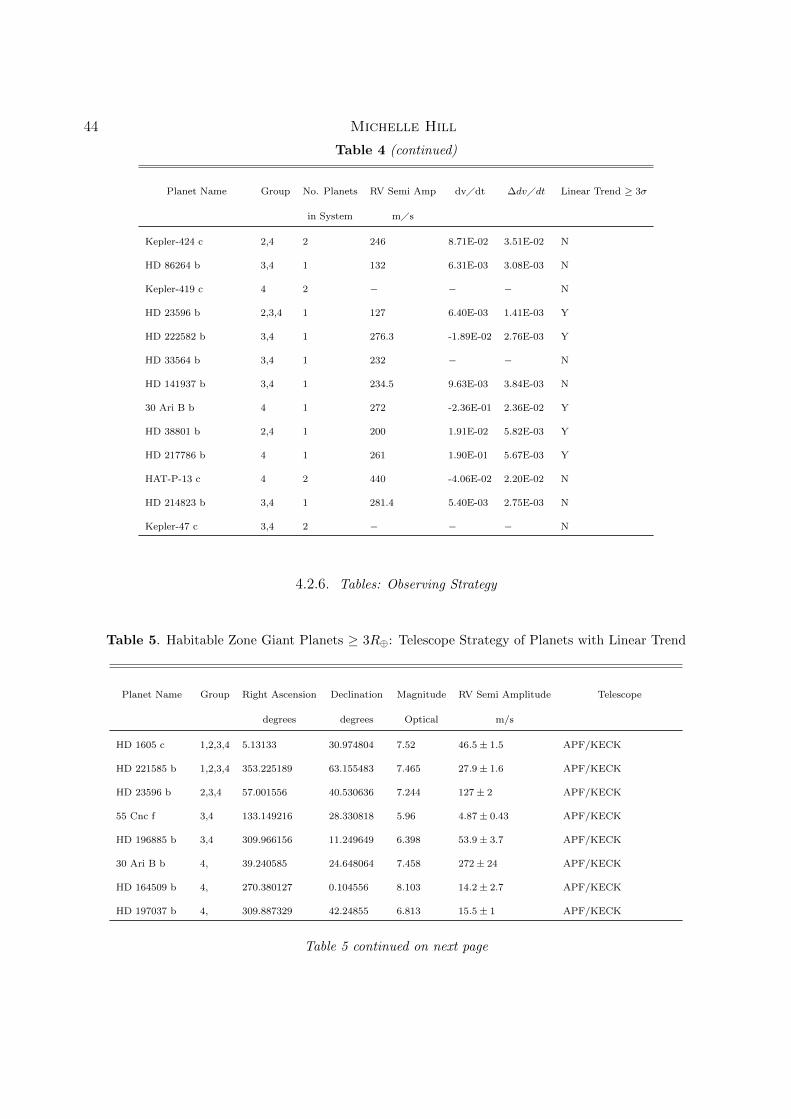
44 Michelle Hill
Table 4 (continued)
Planet Name Group No. Planets RV Semi Amp dv�dt �dv�dt Linear Trend � 3�
in System m�s
Kepler-424 c 2,4 2 246 8.71E-02 3.51E-02 N
HD 86264 b 3,4 1 132 6.31E-03 3.08E-03 N
Kepler-419 c 4 2 � � � N
HD 23596 b 2,3,4 1 127 6.40E-03 1.41E-03 Y
HD 222582 b 3,4 1 276.3 -1.89E-02 2.76E-03 Y
HD 33564 b 3,4 1 232 � � N
HD 141937 b 3,4 1 234.5 9.63E-03 3.84E-03 N
30 Ari B b 4 1 272 -2.36E-01 2.36E-02 Y
HD 38801 b 2,4 1 200 1.91E-02 5.82E-03 Y
HD 217786 b 4 1 261 1.90E-01 5.67E-03 Y
HAT-P-13 c 4 2 440 -4.06E-02 2.20E-02 N
HD 214823 b 3,4 1 281.4 5.40E-03 2.75E-03 N
Kepler-47 c 3,4 2 � � � N
4.2.6. Tables: Observing Strategy
Table 5. Habitable Zone Giant Planets � 3R�: Telescope Strategy of Planets with Linear Trend
Planet Name Group Right Ascension Declination Magnitude RV Semi Amplitude Telescope
degrees degrees Optical m/s
HD 1605 c 1,2,3,4 5.13133 30.974804 7.52 46.5± 1.5 APF/KECK
HD 221585 b 1,2,3,4 353.225189 63.155483 7.465 27.9± 1.6 APF/KECK
HD 23596 b 2,3,4 57.001556 40.530636 7.244 127± 2 APF/KECK
55 Cnc f 3,4 133.149216 28.330818 5.96 4.87± 0.43 APF/KECK
HD 196885 b 3,4 309.966156 11.249649 6.398 53.9± 3.7 APF/KECK
30 Ari B b 4, 39.240585 24.648064 7.458 272± 24 APF/KECK
HD 164509 b 4, 270.380127 0.104556 8.103 14.2± 2.7 APF/KECK
HD 197037 b 4, 309.887329 42.24855 6.813 15.5± 1 APF/KECK
Table 5 continued on next page
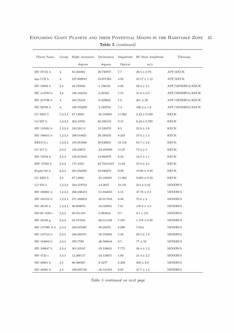
Exploring Giant Planets and their Potential Moons in the Habitable Zone 45
Table 5 (continued)
Planet Name Group Right Ascension Declination Magnitude RV Semi Amplitude Telescope
degrees degrees Optical m/s
HD 37124 b 4, 84.260361 20.730787 7.7 28.5± 0.78 APF/KECK
kap CrB b 4, 237.808044 35.657383 4.82 25.17± 1.12 APF/KECK
HD 19994 b 2,4 48.193485 -1.196101 5.06 29.3± 2.1 APF/MINERVA/KECK
HD 114783 b 3,4 198.182434 -2.26504 7.55 31.9± 0.9 APF/MINERVA/KECK
HD 217786 b 4, 345.78418 -0.429622 7.8 261± 20 APF/MINERVA/KECK
HD 92788 b 4, 160.702209 -2.183756 7.3 106.2± 1.8 APF/MINERVA/KECK
GJ 3293 d 1,2,3,4 67.14882 -25.169301 11.962 2.42± 0.338 KECK
GJ 687 b 1,2,3,4 264.10791 68.339142 9.15 6.43± 0.769 KECK
HD 145934 b 1,2,3,4 243.29114 13.239476 8.5 22.9± 2.6 KECK
HD 188015 b 1,2,3,4 298.018921 28.100376 8.234 37.6± 1.2 KECK
KELT-6 c 1,2,3,4 195.981868 30.640051 10.418 65.7± 2.6 KECK
GJ 317 b 2,3,4 130.24673 -23.456289 11.97 75.2± 3 KECK
HD 73534 b 2,3,4 129.815842 12.960376 8.23 16.2± 1.1 KECK
HIP 57050 b 2,3,4 175.4333 42.75219167 11.92 37.8± 4.5 KECK
Kepler-68 d 2,3,4 291.032305 49.040272 9.99 19.06± 0.58 KECK
GJ 3293 b 2,4 67.14882 -25.169301 11.962 8.603± 0.32 KECK
GJ 876 b 1,2,3,4 343.319733 -14.2637 10.191 214± 0.42 MINERVA
HD 160691 b 1,2,3,4 266.036255 -51.834053 5.15 37.78± 0.4 MINERVA
HD 165155 b 1,2,3,4 271.488953 -29.917253 9.36 75.8± 3 MINERVA
HD 28185 b 1,2,3,4 66.609673 -10.550821 7.81 158.8± 4.2 MINERVA
BD-06 1339 c 2,3,4 88.251183 -5.994844 9.7 9.1± 2.9 MINERVA
HD 10180 g 2,3,4 24.473234 -60.511528 7.321 1.754± 0.38 MINERVA
HD 137388 A b 2,3,4 233.916367 -80.20459 8.696 7.94± MINERVA
HD 147513 b 2,3,4 246.005371 -39.192982 5.39 29.3± 1.8 MINERVA
HD 164604 b 2,3,4 270.7789 -28.560644 9.7 77± 32 MINERVA
HD 190647 b 2,3,4 301.83197 -35.538631 7.775 36.4± 1.2 MINERVA
HD 4732 c 2,3,4 12.308117 -24.136671 5.89 24.4± 2.2 MINERVA
HD 38801 b 2,4 86.996567 -8.3277 8.269 200± 3.9 MINERVA
HD 48265 b 2,4 100.007195 -48.541954 8.05 27.7± 1.2 MINERVA
Table 5 continued on next page
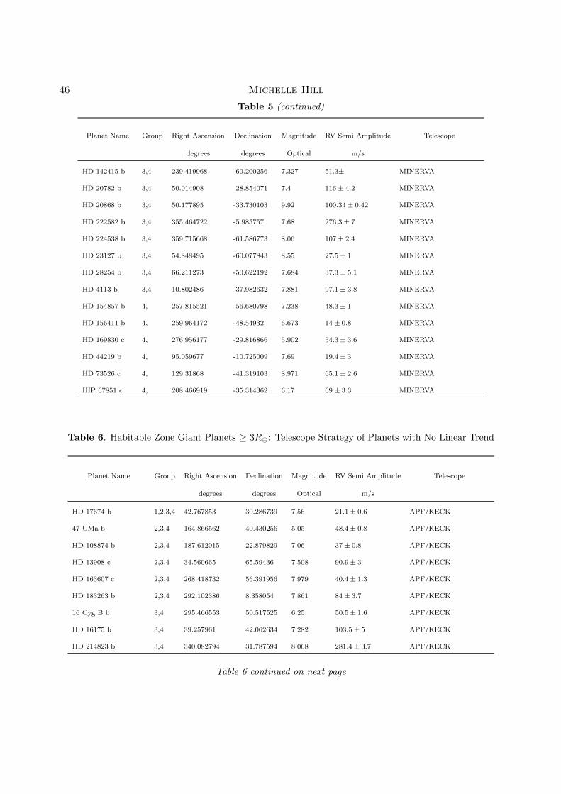
46 Michelle Hill
Table 5 (continued)
Planet Name Group Right Ascension Declination Magnitude RV Semi Amplitude Telescope
degrees degrees Optical m/s
HD 142415 b 3,4 239.419968 -60.200256 7.327 51.3± MINERVA
HD 20782 b 3,4 50.014908 -28.854071 7.4 116± 4.2 MINERVA
HD 20868 b 3,4 50.177895 -33.730103 9.92 100.34± 0.42 MINERVA
HD 222582 b 3,4 355.464722 -5.985757 7.68 276.3± 7 MINERVA
HD 224538 b 3,4 359.715668 -61.586773 8.06 107± 2.4 MINERVA
HD 23127 b 3,4 54.848495 -60.077843 8.55 27.5± 1 MINERVA
HD 28254 b 3,4 66.211273 -50.622192 7.684 37.3± 5.1 MINERVA
HD 4113 b 3,4 10.802486 -37.982632 7.881 97.1± 3.8 MINERVA
HD 154857 b 4, 257.815521 -56.680798 7.238 48.3± 1 MINERVA
HD 156411 b 4, 259.964172 -48.54932 6.673 14 ± 0.8 MINERVA
HD 169830 c 4, 276.956177 -29.816866 5.902 54.3± 3.6 MINERVA
HD 44219 b 4, 95.059677 -10.725009 7.69 19.4± 3 MINERVA
HD 73526 c 4, 129.31868 -41.319103 8.971 65.1± 2.6 MINERVA
HIP 67851 c 4, 208.466919 -35.314362 6.17 69 ± 3.3 MINERVA
Table 6. Habitable Zone Giant Planets � 3R�: Telescope Strategy of Planets with No Linear Trend
Planet Name Group Right Ascension Declination Magnitude RV Semi Amplitude Telescope
degrees degrees Optical m/s
HD 17674 b 1,2,3,4 42.767853 30.286739 7.56 21.1± 0.6 APF/KECK
47 UMa b 2,3,4 164.866562 40.430256 5.05 48.4± 0.8 APF/KECK
HD 108874 b 2,3,4 187.612015 22.879829 7.06 37 ± 0.8 APF/KECK
HD 13908 c 2,3,4 34.560665 65.59436 7.508 90.9± 3 APF/KECK
HD 163607 c 2,3,4 268.418732 56.391956 7.979 40.4± 1.3 APF/KECK
HD 183263 b 2,3,4 292.102386 8.358054 7.861 84 ± 3.7 APF/KECK
16 Cyg B b 3,4 295.466553 50.517525 6.25 50.5± 1.6 APF/KECK
HD 16175 b 3,4 39.257961 42.062634 7.282 103.5± 5 APF/KECK
HD 214823 b 3,4 340.082794 31.787594 8.068 281.4± 3.7 APF/KECK
Table 6 continued on next page
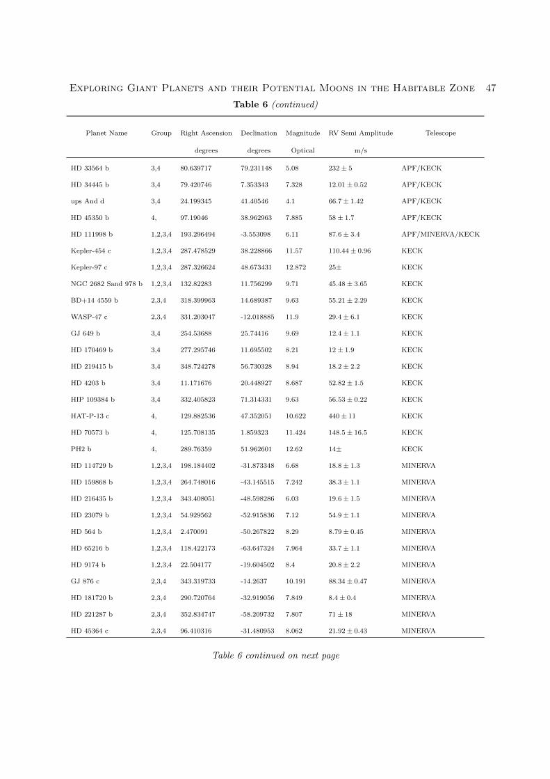
Exploring Giant Planets and their Potential Moons in the Habitable Zone 47
Table 6 (continued)
Planet Name Group Right Ascension Declination Magnitude RV Semi Amplitude Telescope
degrees degrees Optical m/s
HD 33564 b 3,4 80.639717 79.231148 5.08 232± 5 APF/KECK
HD 34445 b 3,4 79.420746 7.353343 7.328 12.01± 0.52 APF/KECK
ups And d 3,4 24.199345 41.40546 4.1 66.7± 1.42 APF/KECK
HD 45350 b 4, 97.19046 38.962963 7.885 58± 1.7 APF/KECK
HD 111998 b 1,2,3,4 193.296494 -3.553098 6.11 87.6± 3.4 APF/MINERVA/KECK
Kepler-454 c 1,2,3,4 287.478529 38.228866 11.57 110.44± 0.96 KECK
Kepler-97 c 1,2,3,4 287.326624 48.673431 12.872 25± KECK
NGC 2682 Sand 978 b 1,2,3,4 132.82283 11.756299 9.71 45.48± 3.65 KECK
BD+14 4559 b 2,3,4 318.399963 14.689387 9.63 55.21± 2.29 KECK
WASP-47 c 2,3,4 331.203047 -12.018885 11.9 29.4± 6.1 KECK
GJ 649 b 3,4 254.53688 25.74416 9.69 12.4± 1.1 KECK
HD 170469 b 3,4 277.295746 11.695502 8.21 12± 1.9 KECK
HD 219415 b 3,4 348.724278 56.730328 8.94 18.2± 2.2 KECK
HD 4203 b 3,4 11.171676 20.448927 8.687 52.82± 1.5 KECK
HIP 109384 b 3,4 332.405823 71.314331 9.63 56.53± 0.22 KECK
HAT-P-13 c 4, 129.882536 47.352051 10.622 440± 11 KECK
HD 70573 b 4, 125.708135 1.859323 11.424 148.5± 16.5 KECK
PH2 b 4, 289.76359 51.962601 12.62 14± KECK
HD 114729 b 1,2,3,4 198.184402 -31.873348 6.68 18.8± 1.3 MINERVA
HD 159868 b 1,2,3,4 264.748016 -43.145515 7.242 38.3± 1.1 MINERVA
HD 216435 b 1,2,3,4 343.408051 -48.598286 6.03 19.6± 1.5 MINERVA
HD 23079 b 1,2,3,4 54.929562 -52.915836 7.12 54.9± 1.1 MINERVA
HD 564 b 1,2,3,4 2.470091 -50.267822 8.29 8.79± 0.45 MINERVA
HD 65216 b 1,2,3,4 118.422173 -63.647324 7.964 33.7± 1.1 MINERVA
HD 9174 b 1,2,3,4 22.504177 -19.604502 8.4 20.8± 2.2 MINERVA
GJ 876 c 2,3,4 343.319733 -14.2637 10.191 88.34± 0.47 MINERVA
HD 181720 b 2,3,4 290.720764 -32.919056 7.849 8.4± 0.4 MINERVA
HD 221287 b 2,3,4 352.834747 -58.209732 7.807 71 ± 18 MINERVA
HD 45364 c 2,3,4 96.410316 -31.480953 8.062 21.92± 0.43 MINERVA
Table 6 continued on next page
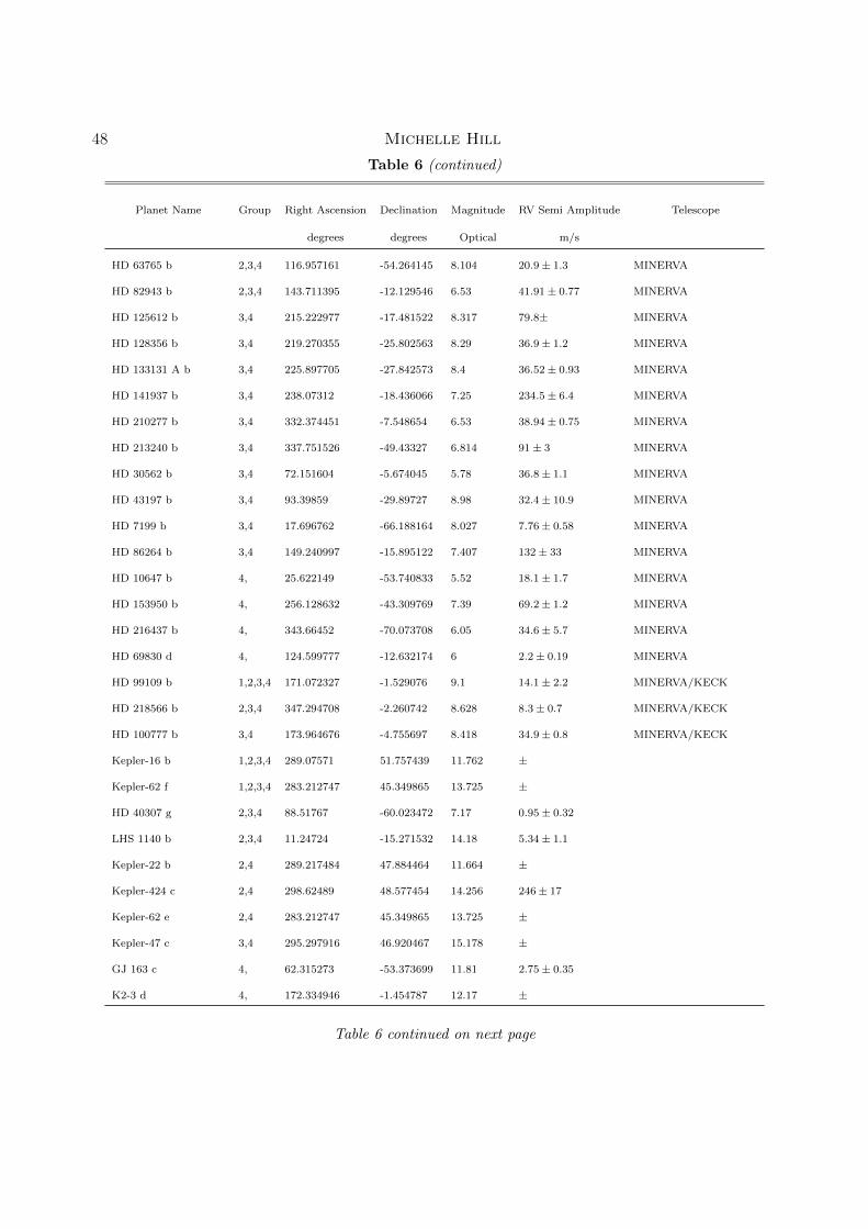
48 Michelle Hill
Table 6 (continued)
Planet Name Group Right Ascension Declination Magnitude RV Semi Amplitude Telescope
degrees degrees Optical m/s
HD 63765 b 2,3,4 116.957161 -54.264145 8.104 20.9± 1.3 MINERVA
HD 82943 b 2,3,4 143.711395 -12.129546 6.53 41.91± 0.77 MINERVA
HD 125612 b 3,4 215.222977 -17.481522 8.317 79.8± MINERVA
HD 128356 b 3,4 219.270355 -25.802563 8.29 36.9± 1.2 MINERVA
HD 133131 A b 3,4 225.897705 -27.842573 8.4 36.52± 0.93 MINERVA
HD 141937 b 3,4 238.07312 -18.436066 7.25 234.5± 6.4 MINERVA
HD 210277 b 3,4 332.374451 -7.548654 6.53 38.94± 0.75 MINERVA
HD 213240 b 3,4 337.751526 -49.43327 6.814 91± 3 MINERVA
HD 30562 b 3,4 72.151604 -5.674045 5.78 36.8± 1.1 MINERVA
HD 43197 b 3,4 93.39859 -29.89727 8.98 32.4± 10.9 MINERVA
HD 7199 b 3,4 17.696762 -66.188164 8.027 7.76± 0.58 MINERVA
HD 86264 b 3,4 149.240997 -15.895122 7.407 132± 33 MINERVA
HD 10647 b 4, 25.622149 -53.740833 5.52 18.1± 1.7 MINERVA
HD 153950 b 4, 256.128632 -43.309769 7.39 69.2± 1.2 MINERVA
HD 216437 b 4, 343.66452 -70.073708 6.05 34.6± 5.7 MINERVA
HD 69830 d 4, 124.599777 -12.632174 6 2.2± 0.19 MINERVA
HD 99109 b 1,2,3,4 171.072327 -1.529076 9.1 14.1± 2.2 MINERVA/KECK
HD 218566 b 2,3,4 347.294708 -2.260742 8.628 8.3± 0.7 MINERVA/KECK
HD 100777 b 3,4 173.964676 -4.755697 8.418 34.9± 0.8 MINERVA/KECK
Kepler-16 b 1,2,3,4 289.07571 51.757439 11.762 ±
Kepler-62 f 1,2,3,4 283.212747 45.349865 13.725 ±
HD 40307 g 2,3,4 88.51767 -60.023472 7.17 0.95± 0.32
LHS 1140 b 2,3,4 11.24724 -15.271532 14.18 5.34± 1.1
Kepler-22 b 2,4 289.217484 47.884464 11.664 ±
Kepler-424 c 2,4 298.62489 48.577454 14.256 246± 17
Kepler-62 e 2,4 283.212747 45.349865 13.725 ±
Kepler-47 c 3,4 295.297916 46.920467 15.178 ±
GJ 163 c 4, 62.315273 -53.373699 11.81 2.75± 0.35
K2-3 d 4, 172.334946 -1.454787 12.17 ±
Table 6 continued on next page

Exploring Giant Planets and their Potential Moons in the Habitable Zone 49
Table 6 (continued)
Planet Name Group Right Ascension Declination Magnitude RV Semi Amplitude Telescope
degrees degrees Optical m/s
Kepler-34 b 4, 296.435821 44.64156 14.875 ±
Kepler-419 c 4, 295.417899 51.184765 13.005 ±
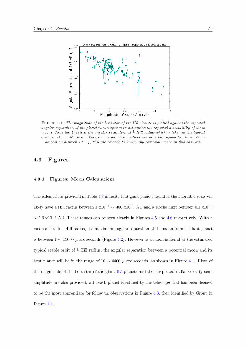
Chapter 4. Results 50
Figure 4.1: The magnitude of the host star of the HZ planets is plotted against the expectedangular separation of the planet/moon system to determine the expected detectability of thesemoons. Note the Y axis is the angular separation at 1
3 Hill radius which is taken as the typicaldistance of a stable moon. Future imaging missions thus will need the capabilities to resolve a
separation between 10 – 4400 µ arc seconds to image any potential moons in this data set.
4.3 Figures
4.3.1 Figures: Moon Calculations
The calculations provided in Table 4.3 indicate that giant planets found in the habitable zone will
likely have a Hill radius between 1 x10�3 ⇠ 460 x10�3 AU and a Roche limit between 0.1 x10�3
⇠ 2.6 x10�3 AU. These ranges can be seen clearly in Figures 4.5 and 4.6 respectively. With a
moon at the full Hill radius, the maximum angular separation of the moon from the host planet
is between 1 ⇠ 13000 µ arc seconds (Figure 4.2). However is a moon is found at the estimated
typical stable orbit of 13 Hill radius, the angular separation between a potential moon and its
host planet will be in the range of 10 ⇠ 4400 µ arc seconds, as shown in Figure 4.1. Plots of
the magnitude of the host star of the giant HZ planets and their expected radial velocity semi
amplitude are also provided, with each planet identified by the telescope that has been deemed
to be the most appropriate for follow up observations in Figure 4.3, then identified by Group in
Figure 4.4.
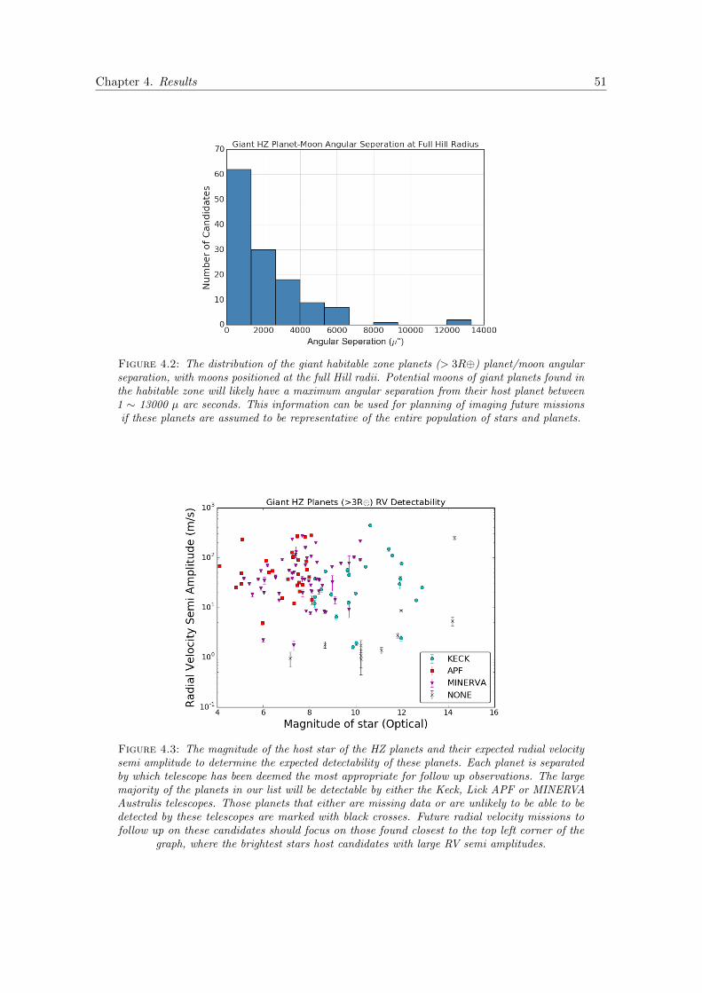
Chapter 4. Results 51
Figure 4.2: The distribution of the giant habitable zone planets (> 3R�) planet/moon angularseparation, with moons positioned at the full Hill radii. Potential moons of giant planets found inthe habitable zone will likely have a maximum angular separation from their host planet between1 ⇠ 13000 µ arc seconds. This information can be used for planning of imaging future missionsif these planets are assumed to be representative of the entire population of stars and planets.
Figure 4.3: The magnitude of the host star of the HZ planets and their expected radial velocitysemi amplitude to determine the expected detectability of these planets. Each planet is separatedby which telescope has been deemed the most appropriate for follow up observations. The largemajority of the planets in our list will be detectable by either the Keck, Lick APF or MINERVAAustralis telescopes. Those planets that either are missing data or are unlikely to be able to bedetected by these telescopes are marked with black crosses. Future radial velocity missions tofollow up on these candidates should focus on those found closest to the top left corner of the
graph, where the brightest stars host candidates with large RV semi amplitudes.
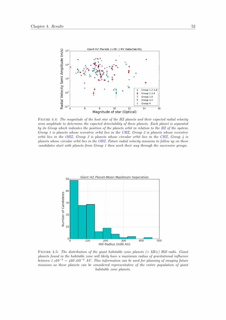
Chapter 4. Results 52
Figure 4.4: The magnitude of the host star of the HZ planets and their expected radial velocitysemi amplitude to determine the expected detectability of these planets. Each planet is separatedby its Group which indicates the position of the planets orbit in relation to the HZ of the system.Group 1 is planets whose eccentric orbit lies in the CHZ, Group 2 is planets whose eccentricorbit lies in the OHZ, Group 3 is planets whose circular orbit lies in the CHZ, Group 4 isplanets whose circular orbit lies in the OHZ. Future radial velocity missions to follow up on thesecandidates start with planets from Group 1 then work their way through the successive groups.
Figure 4.5: The distribution of the giant habitable zone planets (> 3R�) Hill radii. Giantplanets found in the habitable zone will likely have a maximum radius of gravitational influencebetween 1 x10�3 ⇠ 460 x10�3 AU. This information can be used for planning of imaging futuremissions as these planets can be considered representative of the entire population of giant
habitable zone planets.
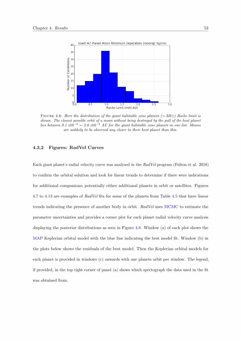
Chapter 4. Results 53
Figure 4.6: Here the distribution of the giant habitable zone planets (> 3R�) Roche limit isshown. The closest possible orbit of a moon without being destroyed by the pull of the host planetlies between 0.1 x10�3 ⇠ 2.6 x10�3 AU for the giant habitable zone planets in our list. Moons
are unlikely to be observed any closer to their host planet than this.
4.3.2 Figures: RadVel Curves
Each giant planet’s radial velocity curve was analysed in the RadVel program (Fulton et al. 2018)
to confirm the orbital solution and look for linear trends to determine if there were indications
for additional companions; potentially either additional planets in orbit or satellites. Figures
4.7 to 4.13 are examples of RadVel fits for some of the planets from Table 4.5 that have linear
trends indicating the presence of another body in orbit. RadVel uses MCMC to estimate the
parameter uncertainties and provides a corner plot for each planet radial velocity curve analysis
displaying the posterior distributions as seen in Figure 4.8. Window (a) of each plot shows the
MAP Keplerian orbital model with the blue line indicating the best model fit. Window (b) in
the plots below shows the residuals of the best model. Then the Keplerian orbital models for
each planet is provided in windows (c) onwards with one planets orbit per window. The legend,
if provided, in the top right corner of panel (a) shows which spectograph the data used in the fit
was obtained from.
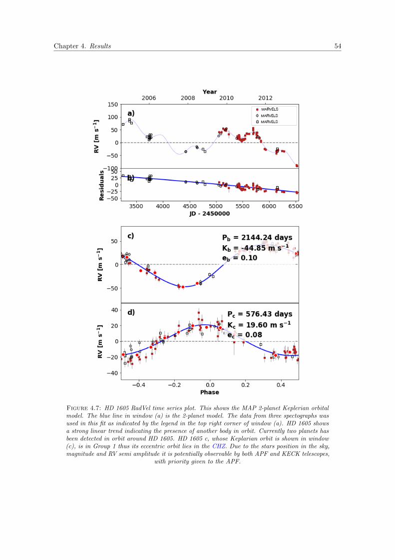
Chapter 4. Results 54
Figure 4.7: HD 1605 RadVel time series plot. This shows the MAP 2-planet Keplerian orbitalmodel. The blue line in window (a) is the 2-planet model. The data from three spectographs wasused in this fit as indicated by the legend in the top right corner of window (a). HD 1605 showsa strong linear trend indicating the presence of another body in orbit. Currently two planets hasbeen detected in orbit around HD 1605. HD 1605 c, whose Keplarian orbit is shown in window(c), is in Group 1 thus its eccentric orbit lies in the CHZ. Due to the stars position in the sky,magnitude and RV semi amplitude it is potentially observable by both APF and KECK telescopes,
with priority given to the APF.
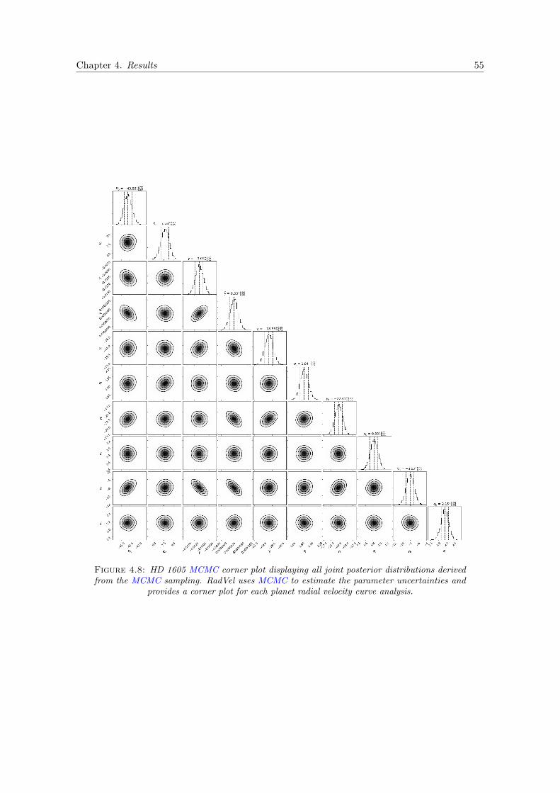
Chapter 4. Results 55
Figure 4.8: HD 1605 MCMC corner plot displaying all joint posterior distributions derivedfrom the MCMC sampling. RadVel uses MCMC to estimate the parameter uncertainties and
provides a corner plot for each planet radial velocity curve analysis.
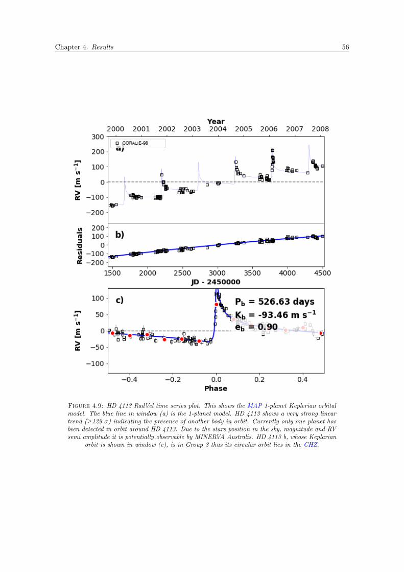
Chapter 4. Results 56
Figure 4.9: HD 4113 RadVel time series plot. This shows the MAP 1-planet Keplerian orbitalmodel. The blue line in window (a) is the 1-planet model. HD 4113 shows a very strong lineartrend (�129 �) indicating the presence of another body in orbit. Currently only one planet hasbeen detected in orbit around HD 4113. Due to the stars position in the sky, magnitude and RVsemi amplitude it is potentially observable by MINERVA Australis. HD 4113 b, whose Keplarian
orbit is shown in window (c), is in Group 3 thus its circular orbit lies in the CHZ.
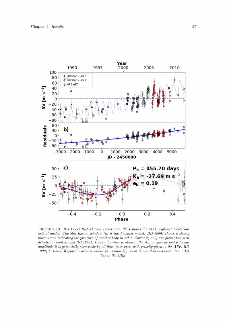
Chapter 4. Results 57
Figure 4.10: HD 19994 RadVel time series plot. This shows the MAP 1-planet Keplerianorbital model. The blue line in window (a) is the 1-planet model. HD 19994 shows a stronglinear trend indicating the presence of another body in orbit. Currently only one planet has beendetected in orbit around HD 19994. Due to the stars position in the sky, magnitude and RV semiamplitude it is potentially observable by all three telescopes, with priority given to the APF. HD19994 b, whose Keplarian orbit is shown in window (c), is in Group 2 thus its eccentric orbit
lies in the OHZ.
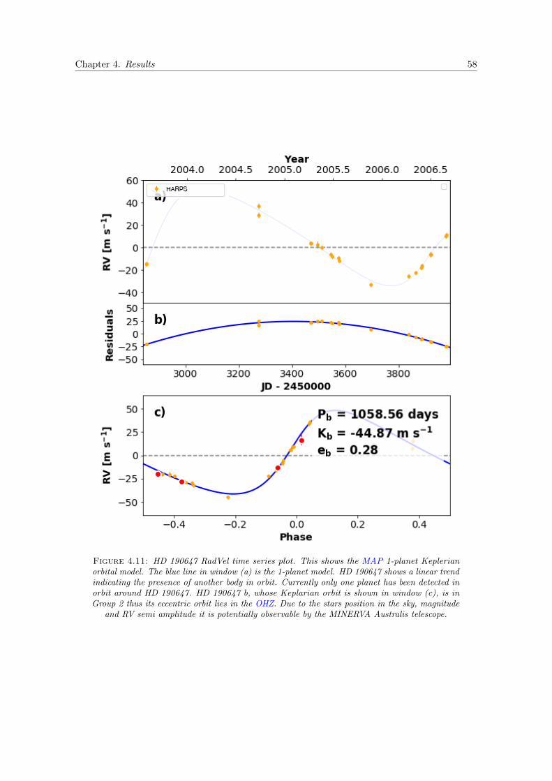
Chapter 4. Results 58
Figure 4.11: HD 190647 RadVel time series plot. This shows the MAP 1-planet Keplerianorbital model. The blue line in window (a) is the 1-planet model. HD 190647 shows a linear trendindicating the presence of another body in orbit. Currently only one planet has been detected inorbit around HD 190647. HD 190647 b, whose Keplarian orbit is shown in window (c), is inGroup 2 thus its eccentric orbit lies in the OHZ. Due to the stars position in the sky, magnitude
and RV semi amplitude it is potentially observable by the MINERVA Australis telescope.
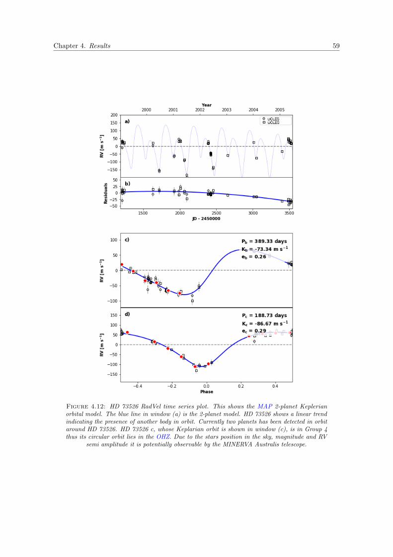
Chapter 4. Results 59
Figure 4.12: HD 73526 RadVel time series plot. This shows the MAP 2-planet Keplerianorbital model. The blue line in window (a) is the 2-planet model. HD 73526 shows a linear trendindicating the presence of another body in orbit. Currently two planets has been detected in orbitaround HD 73526. HD 73526 c, whose Keplarian orbit is shown in window (c), is in Group 4thus its circular orbit lies in the OHZ. Due to the stars position in the sky, magnitude and RV
semi amplitude it is potentially observable by the MINERVA Australis telescope.
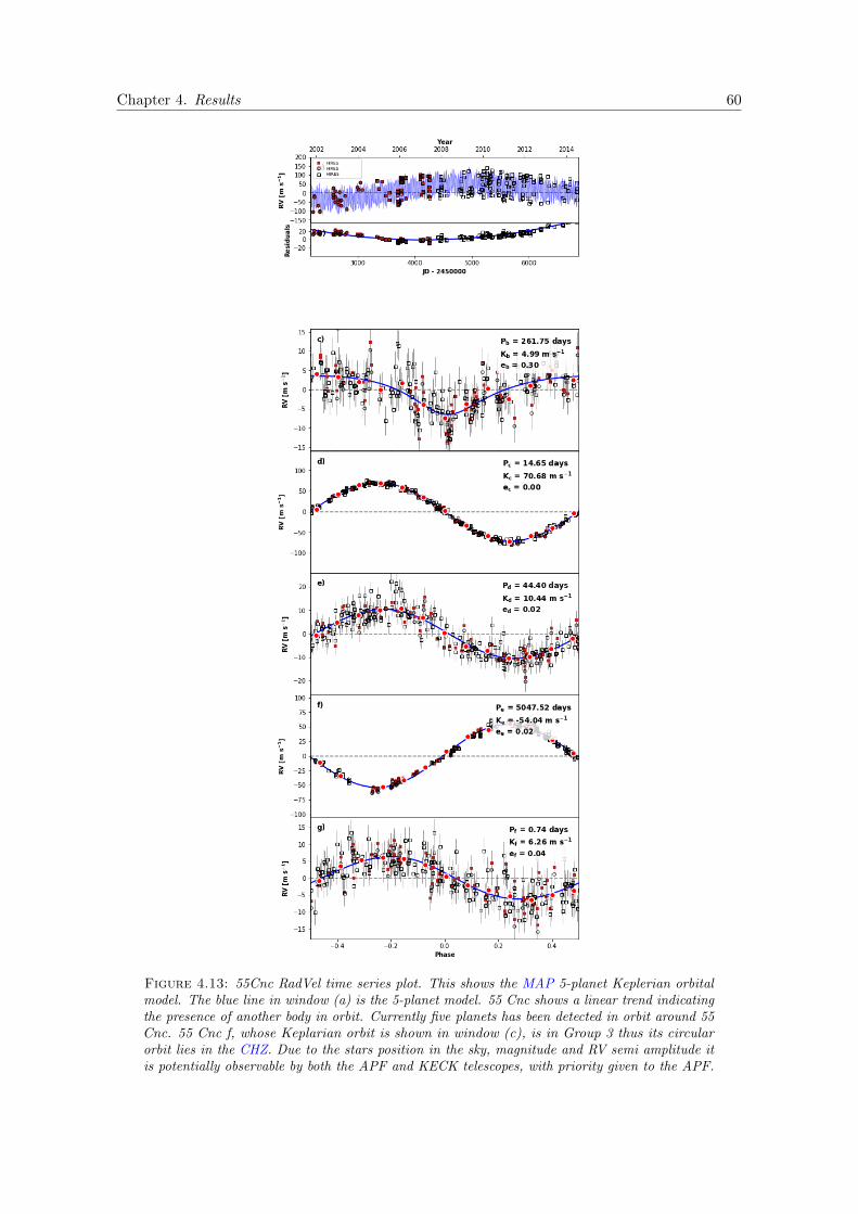
Chapter 4. Results 60
Figure 4.13: 55Cnc RadVel time series plot. This shows the MAP 5-planet Keplerian orbitalmodel. The blue line in window (a) is the 5-planet model. 55 Cnc shows a linear trend indicatingthe presence of another body in orbit. Currently five planets has been detected in orbit around 55Cnc. 55 Cnc f, whose Keplarian orbit is shown in window (c), is in Group 3 thus its circularorbit lies in the CHZ. Due to the stars position in the sky, magnitude and RV semi amplitude itis potentially observable by both the APF and KECK telescopes, with priority given to the APF.
Chapter 5
Discussion
5.1 The BRHARVOS Method
This project aimed to develop a method to be followed in order to determine the best candidates
likely to host HZ satellites. The method, which has been coined the ’BRHARVOS’ method
(pronounced ’Braa-vos’), is outlined in Section 3 and can be followed in future projects to
systematically choose the best habitable zone planet candidates for follow up observations:
B: Future projects should start with calculation of the HZ Boundaries of each star and determine
which planets reside in either the CHZ or the OHZ.
R: Then the Roche limit,
H: Hill radius,
A: and the Angular separation of the planet and potential exomoon should be calculated to
determine those planet-moon systems with the greatest potential observability.
RV: After running the RV curves through RadVel, planets that show indications of orbital
companions can be determined.
61
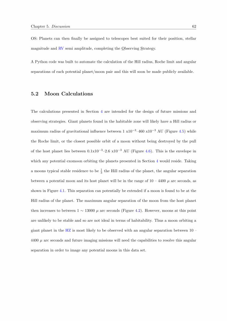
Chapter 5. Discussion 62
OS: Planets can then finally be assigned to telescopes best suited for their position, stellar
magnitude and RV semi amplitude, completing the Observing Strategy.
A Python code was built to automate the calculation of the Hill radius, Roche limit and angular
separations of each potential planet/moon pair and this will soon be made publicly available.
5.2 Moon Calculations
The calculations presented in Section 4 are intended for the design of future missions and
observing strategies. Giant planets found in the habitable zone will likely have a Hill radius or
maximum radius of gravitational influence between 1 x10�3–460 x10�3 AU (Figure 4.5) while
the Roche limit, or the closest possible orbit of a moon without being destroyed by the pull
of the host planet lies between 0.1x10�3–2.6 x10�3 AU (Figure 4.6). This is the envelope in
which any potential exomoon orbiting the planets presented in Section 4 would reside. Taking
a moons typical stable residence to be 13 the Hill radius of the planet, the angular separation
between a potential moon and its host planet will be in the range of 10 – 4400 µ arc seconds, as
shown in Figure 4.1. This separation can potentially be extended if a moon is found to be at the
Hill radius of the planet. The maximum angular separation of the moon from the host planet
then increases to between 1 ⇠ 13000 µ arc seconds (Figure 4.2). However, moons at this point
are unlikely to be stable and so are not ideal in terms of habitability. Thus a moon orbiting a
giant planet in the HZ is most likely to be observed with an angular separation between 10 –
4400 µ arc seconds and future imaging missions will need the capabilities to resolve this angular
separation in order to image any potential moons in this data set.
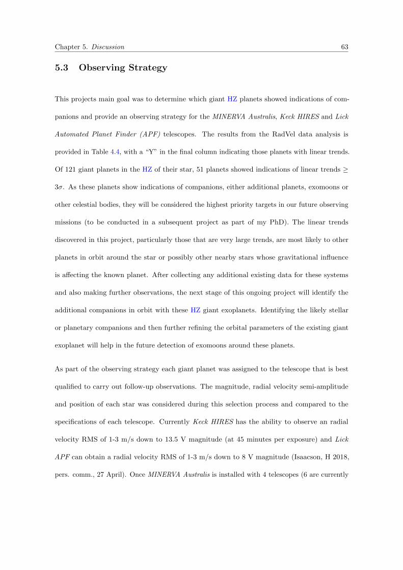
Chapter 5. Discussion 63
5.3 Observing Strategy
This projects main goal was to determine which giant HZ planets showed indications of com-
panions and provide an observing strategy for the MINERVA Australis, Keck HIRES and Lick
Automated Planet Finder (APF) telescopes. The results from the RadVel data analysis is
provided in Table 4.4, with a “Y” in the final column indicating those planets with linear trends.
Of 121 giant planets in the HZ of their star, 51 planets showed indications of linear trends �
3�. As these planets show indications of companions, either additional planets, exomoons or
other celestial bodies, they will be considered the highest priority targets in our future observing
missions (to be conducted in a subsequent project as part of my PhD). The linear trends
discovered in this project, particularly those that are very large trends, are most likely to other
planets in orbit around the star or possibly other nearby stars whose gravitational influence
is a↵ecting the known planet. After collecting any additional existing data for these systems
and also making further observations, the next stage of this ongoing project will identify the
additional companions in orbit with these HZ giant exoplanets. Identifying the likely stellar
or planetary companions and then further refining the orbital parameters of the existing giant
exoplanet will help in the future detection of exomoons around these planets.
As part of the observing strategy each giant planet was assigned to the telescope that is best
qualified to carry out follow-up observations. The magnitude, radial velocity semi-amplitude
and position of each star was considered during this selection process and compared to the
specifications of each telescope. Currently Keck HIRES has the ability to observe an radial
velocity RMS of 1-3 m/s down to 13.5 V magnitude (at 45 minutes per exposure) and Lick
APF can obtain a radial velocity RMS of 1-3 m/s down to 8 V magnitude (Isaacson, H 2018,
pers. comm., 27 April). Once MINERVA Australis is installed with 4 telescopes (6 are currently
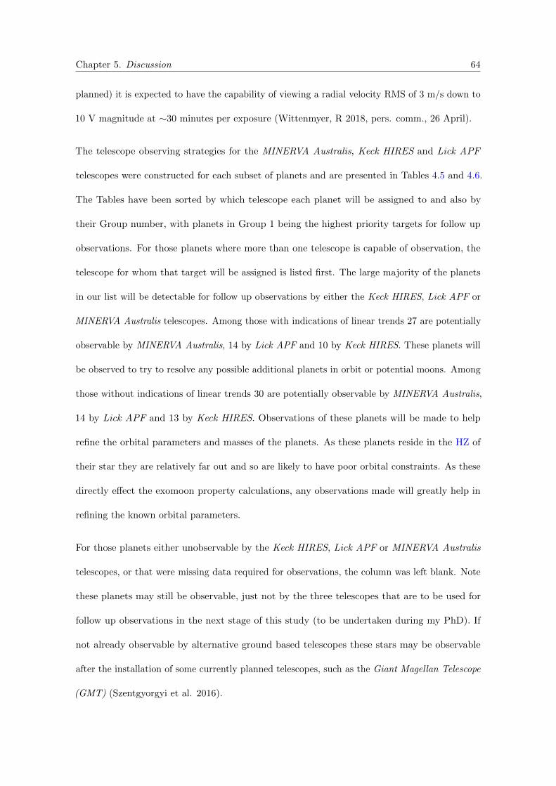
Chapter 5. Discussion 64
planned) it is expected to have the capability of viewing a radial velocity RMS of 3 m/s down to
10 V magnitude at ⇠30 minutes per exposure (Wittenmyer, R 2018, pers. comm., 26 April).
The telescope observing strategies for the MINERVA Australis, Keck HIRES and Lick APF
telescopes were constructed for each subset of planets and are presented in Tables 4.5 and 4.6.
The Tables have been sorted by which telescope each planet will be assigned to and also by
their Group number, with planets in Group 1 being the highest priority targets for follow up
observations. For those planets where more than one telescope is capable of observation, the
telescope for whom that target will be assigned is listed first. The large majority of the planets
in our list will be detectable for follow up observations by either the Keck HIRES, Lick APF or
MINERVA Australis telescopes. Among those with indications of linear trends 27 are potentially
observable by MINERVA Australis, 14 by Lick APF and 10 by Keck HIRES. These planets will
be observed to try to resolve any possible additional planets in orbit or potential moons. Among
those without indications of linear trends 30 are potentially observable by MINERVA Australis,
14 by Lick APF and 13 by Keck HIRES. Observations of these planets will be made to help
refine the orbital parameters and masses of the planets. As these planets reside in the HZ of
their star they are relatively far out and so are likely to have poor orbital constraints. As these
directly e↵ect the exomoon property calculations, any observations made will greatly help in
refining the known orbital parameters.
For those planets either unobservable by the Keck HIRES, Lick APF or MINERVA Australis
telescopes, or that were missing data required for observations, the column was left blank. Note
these planets may still be observable, just not by the three telescopes that are to be used for
follow up observations in the next stage of this study (to be undertaken during my PhD). If
not already observable by alternative ground based telescopes these stars may be observable
after the installation of some currently planned telescopes, such as the Giant Magellan Telescope
(GMT) (Szentgyorgyi et al. 2016).
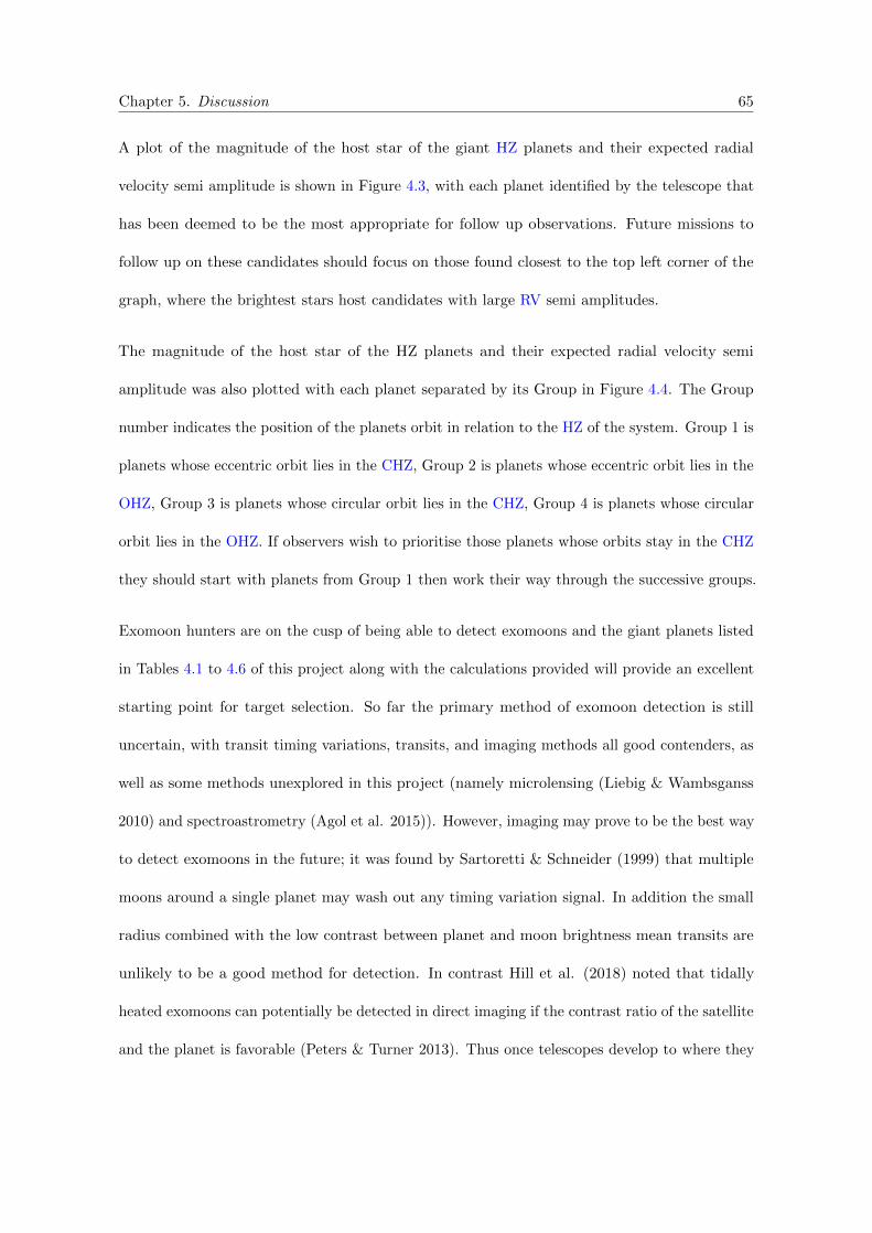
Chapter 5. Discussion 65
A plot of the magnitude of the host star of the giant HZ planets and their expected radial
velocity semi amplitude is shown in Figure 4.3, with each planet identified by the telescope that
has been deemed to be the most appropriate for follow up observations. Future missions to
follow up on these candidates should focus on those found closest to the top left corner of the
graph, where the brightest stars host candidates with large RV semi amplitudes.
The magnitude of the host star of the HZ planets and their expected radial velocity semi
amplitude was also plotted with each planet separated by its Group in Figure 4.4. The Group
number indicates the position of the planets orbit in relation to the HZ of the system. Group 1 is
planets whose eccentric orbit lies in the CHZ, Group 2 is planets whose eccentric orbit lies in the
OHZ, Group 3 is planets whose circular orbit lies in the CHZ, Group 4 is planets whose circular
orbit lies in the OHZ. If observers wish to prioritise those planets whose orbits stay in the CHZ
they should start with planets from Group 1 then work their way through the successive groups.
Exomoon hunters are on the cusp of being able to detect exomoons and the giant planets listed
in Tables 4.1 to 4.6 of this project along with the calculations provided will provide an excellent
starting point for target selection. So far the primary method of exomoon detection is still
uncertain, with transit timing variations, transits, and imaging methods all good contenders, as
well as some methods unexplored in this project (namely microlensing (Liebig & Wambsganss
2010) and spectroastrometry (Agol et al. 2015)). However, imaging may prove to be the best way
to detect exomoons in the future; it was found by Sartoretti & Schneider (1999) that multiple
moons around a single planet may wash out any timing variation signal. In addition the small
radius combined with the low contrast between planet and moon brightness mean transits are
unlikely to be a good method for detection. In contrast Hill et al. (2018) noted that tidally
heated exomoons can potentially be detected in direct imaging if the contrast ratio of the satellite
and the planet is favorable (Peters & Turner 2013). Thus once telescopes develop to where they
Chapter 5. Discussion 66
are able to resolve a separation of 10 – 4400 µ arc seconds, imaging may be our best method of
detecting these potentially habitable worlds.
Chapter 6
Conclusion and Future Work
6.1 A Brief Overview
Using the BRHARVOS method it was found that giant planets in the habitable zones tend
to have a maximum radius of gravitational influence between 1 x10�3 ⇠ 460 x10�3 AU while
the closest possible orbit of a moon without being destroyed by the pull of the host planet lies
between 0.1 x10�3 ⇠ 2.6 x10�3 AU. If imaging of an exomoon orbiting a giant planet in the
habitable zone is desired, instruments must have the capability to resolve a separation between
10 ⇠ 4400 µ arc seconds in order to image any moon found at the estimated stable orbital
distance of 13 Hill radius. Following the RadVel analysis of each planets RV curve, it was found
that among those planets with indications of linear trends, 27 are potentially observable by
MINERVA Australis, 14 by Lick APF and 10 by Keck HIRES. Among those without indications
of linear trends, 30 are potentially observable by MINERVA Australis, 14 by Lick APF and 13
by Keck HIRES.
67
Chapter 6. Conclusion and Future Work 68
6.2 Future Work
Using the calculations and refined list of giant planets found in Section 4, an observation plan to
observe these planets is in development as part of my next project (PhD work). Planets with
indications of linear trends will be observed to try to resolve any possible additional planets in
orbit or potential moons. Following the order of priority, targets in Group 1 will be observed
first and then subsequent groups will follow. Priority will also be given to planets with larger
masses due to their ability to potentially host larger exomoons. Then observations will be made
of the planets with no indications of linear trends in order to help refine the orbital parameters
and masses of the planets.
The length of the observations will vary with each target. As the giant planets from this project
reside in the HZ of their star, their orbital periods can be relatively long. In order to refine
the orbital parameters an observation would ideally survey a full orbit. However, constant
surveillance of the full orbit of a HZ planet could take many hundreds of days and so is a poor
use of the limited telescope time available. Thus a minimum observation time of each target will
be calculated to ensure the observation of just one of the turn around points of a planet. This is
done by assuming the worst case scenario where a beginning observation has just missed the
turn around point of a planets orbit. From this point to the estimated turn around will give the
minimum time needed to observe. From here observing time of the target may indeed be shorter
if the planet was closer to its turn around point than assumed. For those planets with linear
trends, the orbital period for any possible additional planet is not constrained. Thus the time
needed for observation of the turn around point of the planets orbit is unclear.
Chapter 6. Conclusion and Future Work 69
6.3 Concluding Remarks
The inclusion of exomoons orbiting giant planets in the HZ of their star is a significant addition
to the search for habitable worlds. Given the expected occurrence rates of giant planets in the HZ,
and assuming more than one terrestrial moon per giant planet, there may be as many exomoons
in the HZ as there are terrestrial planets, potentially doubling the number of possibly habitable
worlds out in the universe. Due to the nature of these exomoons they may be considered to have
an even greater potential to hold life than that of Earth-like terrestrial planets. These potential
life-supporting characteristics include the thermal and reflected radiation from the host planet
and the tidal e↵ects on an exomoon that help increase the outer range of the HZ, creating a
wider temperate zone in which a stable satellite may exist. The extra protection of the giant
host planets magnetosphere also increases the likelihood that a large exomoon will hold on to
its atmosphere, another essential ingredient to life as we know it. The rich diversity of size,
density and geological phenomena in our own Solar system’s satellites also provide clues as to
the potential of these satellites and are themselves examples of potentially life holding worlds.
Thus the detection and characterisation of exomoons is of utmost importance in the search
for habitable worlds. Once imaging capabilities have improved, the detection of potentially
habitable moons around these giant hosts will be much more accessible. Until then the properties
of the giant host planets must continue to be refined, starting with radial velocity follow-up
observations of giant HZ candidates.
Appendix A
Exploring Kepler Giant Planets in
the Habitable Zone
The following pages contain the paper Exploring Kepler Giant Planets in the Habitable Zone
(Hill et al. 2018) which was written concurrently with this honours thesis. It includes supporting
research and is provided here for reference. This paper has been accepted for publication in The
Astrophysical Journal.
70
Draft version May 22, 2018Typeset using LATEX twocolumn style in AASTeX61
EXPLORING KEPLER GIANT PLANETS IN THE HABITABLE ZONE
Michelle L. Hill,1, 2, 3 Stephen R. Kane,4, 1 Eduardo Seperuelo Duarte,5 Ravi K. Kopparapu,6, 7, 8
Dawn M. Gelino,9 and Robert A. Wittenmyer1
1University of Southern Queensland, Computational Engineering and Science Research Centre, Toowoomba, Queensland 4350, Australia2University of New England, Department of Physics, Armidale, NSW 2351, Australia3San Francisco State University, Department of Physics & Astronomy, 1600 Holloway Avenue, San Francisco, CA 94132, USA4University of California, Riverside, Department of Earth Sciences, CA 92521, USA5Instituto Federal do Rio de Janeiro, Grupo de Fısica e Astronomia, R. Cel. Delio Menezes Porto, 1045, CEP 26530-060, Nilopolis - RJ,
Brazil6NASA Goddard Space Flight Center, 8800 Greenbelt Road, Mail Stop 699.0 Building 34, Greenbelt, MD 207717NASA Astrobiology Institutes Virtual Planetary Laboratory, P.O. Box 351580, Seattle, WA 98195, USA8Sellers Exoplanet Environments Collaboration, NASA Goddard Space Flight Center.9NASA Exoplanet Science Institute, Caltech, MS 100-22, 770 South Wilson Avenue, Pasadena, CA 91125, USA
Submitted to ApJ
ABSTRACT
The Kepler mission found hundreds of planet candidates within the Habitable Zones (HZ) of their host star, including
over 70 candidates with radii larger than 3 Earth radii (R⊕) within the optimistic HZ (OHZ) (Kane et al. 2016). These
giant planets are potential hosts to large terrestrial satellites (or exomoons) which would also exist in the HZ. We
calculate the occurrence rates of giant planets (Rp = 3.0–25 R⊕) in the OHZ and find a frequency of (6.5± 1.9)% for
G stars, (11.5± 3.1)% for K stars, and (6± 6)% for M stars. We compare this with previously estimated occurrence
rates of terrestrial planets in the HZ of G, K and M stars and find that if each giant planet has one large terrestrial
moon then these moons are less likely to exist in the HZ than terrestrial planets. However, if each giant planet holds
more than one moon, then the occurrence rates of moons in the HZ would be comparable to that of terrestrial planets,
and could potentially exceed them. We estimate the mass of each planet candidate using the mass-radius relationship
developed by Chen & Kipping (2016). We calculate the Hill radius of each planet to determine the area of influence
of the planet in which any attached moon may reside, then calculate the estimated angular separation of the moon
and planet for future imaging missions. Finally, we estimate the radial velocity semi-amplitudes of each planet for use
in follow up observations.
Keywords: astrobiology – astronomical databases: miscellaneous – planetary systems – techniques:
photometric, radial velocity, imaging
2 Michelle Hill et al.
1. INTRODUCTION
The search for exoplanets has progressed greatly in
the last 3 decades and the number of confirmed planets
continues to grow steadily. These planets orbiting stars
outside our solar system have already provided clues to
many of the questions regarding the origin and preva-
lence of life. They have provided further understanding
of the formation and evolution of the planets within our
solar system, and influenced an escalation in the area of
research into what constitutes a habitable planet that
could support life. With the launch of NASA’s Kepler
telescope thousands of planets were found, in particular
planets as far out from their host star as the Habitable
Zone (HZ) of that star were found, the HZ being de-
fined as the region around a star where water can exist
in a liquid state on the surface of a planet with suffi-
cient atmospheric pressure (Kasting et al. 1993). The
HZ can further divided into two regions called the con-
servative HZ (CHZ) and the optimistic HZ (OHZ) (Kane
et al. 2016). The CHZ inner edge consists of the run-
away greenhouse limit, where a chemical breakdown of
water molecules by photons from the sun will allow the
now free hydrogen atoms to escape into space, drying
out the planet at 0.99 AU in our solar system (Kop-
parapu et al. 2014). The CHZ outer edge consists of
the maximum greenhouse effect, at 1.7 AU in our solar
system, where the temperature on the planet drops to
a point where CO2 will condense permanently, which
will in turn increase the planet’s albedo, thus cooling
the planet’s surface to a point where all water is frozen
(Kaltenegger & Sasselov 2011). The OHZ in our so-
lar system lies between 0.75–1.8 AU, where the inner
edge is the ”recent Venus” limit, based on the empiri-
cal observation that the surface of Venus has been dry
for at least a billion years, and the outer edge is the
”early Mars” limit, based on the observation that Mars
appears to have been habitable ∼3.8 Gyrs ago (Koppa-
rapu et al. 2013). The positions of the HZ boundaries
vary in other planetary systems in accordance with mul-
tiple factors including the effective temperature, stellar
flux and luminosity of a host star.
A primary goal of the Kepler mission was to determine
the occurrence rate of terrestrial-size planets within the
HZ of their host stars. Kane et al. (2016) cataloged all
Kepler candidates that were found in their HZ, provid-
ing a list of HZ exoplanet candidates using the Kepler
data release 24, Q1–Q17 data vetting process, combined
with the revised stellar parameters from DR25 stellar
properties table. Planets were then split into 4 groups
depending on their position around their host star and
their radius. Categories 1 and 2 held planets that were
< 2 R⊕ in the CHZ and OHZ respectively and Cate-
gories 3 and 4 held planets of any radius in the CHZ
and OHZ respectively. In Category 4, where candidates
of any size radius are found to be in the OHZ, 76 planets
of size 3 R⊕ and above were found.
Often overshadowed by the discoveries of numerous
transiting Earth-size planets in recent years (e.g. Gillon
et al. 2017; Dittmann et al. 2017), Jupiter-like planets
are nonetheless a critical feature of a planetary system
if we are to understand the occurrence of truly Solar-
system like architectures. The frequency of close-in
planets, with orbits a ≤0.5 AU, has been investigated
in great detail thanks to the thousands of Kepler plan-
ets (Howard et al. 2012; Fressin et al. 2013; Burke et
al. 2015). In the icy realm of Jupiter analogs, giant
planets in orbits beyond the ice line ∼3 AU, radial ve-
locity (RV) legacy surveys remain the critical source of
insight. These surveys, with time baselines exceeding
15 years, have the sensitivity to reliably detect or ex-
clude Jupiter analogs (Wittenmyer et al. 2006; Cum-
ming et al. 2008; Wittenmyer et al. 2011; Rowan et al.
2016). For example, an analysis of the 18-year Anglo-
Australian Planet search by Wittenmyer et al. (2016)
yielded a Jupiter-analog occurrence rate of 6.2+2.8−1.6% for
giant planets in orbits from 3 to 7 AU. Similar stud-
ies from the Keck Planet search (Cumming et al. 2008)
and the ESO planet search programs (Zechmeister et
al. 2013) have arrived at statistically identical results:
in general, Jupiter-like planets in Jupiter-like orbits are
present around less than 10% of solar-type stars. While
these giant planets are not favored in the search for
Earth-like planets, the discovery of a number of these
large planets in the habitable zone of their star (Diaz et
al. 2016) do indicate a potential for large rocky moons
also residing in the HZ.
A moon is generally defined as a celestial body that
orbits around a planet or asteroid and whose orbital
barycenter is located inside the surface of the host planet
or asteroid. There are currently 175 known satellites or-
biting the 8 planets within the solar system, most of
which are in orbit around the two largest planets in our
system with Jupiter hosting 69 known moons and Sat-
urn hosting 62 known moons1. The diverse composi-
tions of the satellites in the solar system give insight
into their formation (Canup & Ward 2002; Heller et al.
2015). Most moons are thought to be formed from accre-
tion within the discs of gas and dust circulating around
planets in the early solar system. Through gravitational
collisions between the dust, rocks and gas the debris
gradually builds, bonding together to form a satellite
1 http://www.dtm.ciw.edu/users/sheppard/satellites/
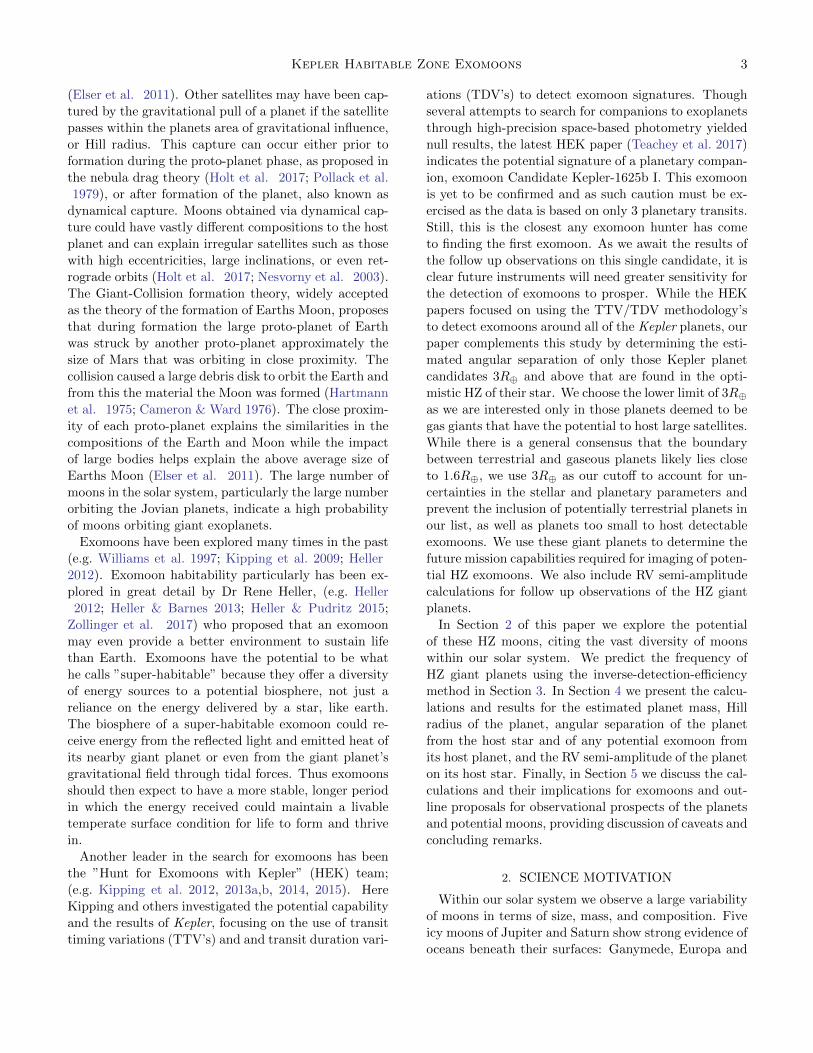
Kepler Habitable Zone Exomoons 3
(Elser et al. 2011). Other satellites may have been cap-
tured by the gravitational pull of a planet if the satellite
passes within the planets area of gravitational influence,
or Hill radius. This capture can occur either prior to
formation during the proto-planet phase, as proposed in
the nebula drag theory (Holt et al. 2017; Pollack et al.
1979), or after formation of the planet, also known as
dynamical capture. Moons obtained via dynamical cap-
ture could have vastly different compositions to the host
planet and can explain irregular satellites such as those
with high eccentricities, large inclinations, or even ret-
rograde orbits (Holt et al. 2017; Nesvorny et al. 2003).
The Giant-Collision formation theory, widely accepted
as the theory of the formation of Earths Moon, proposes
that during formation the large proto-planet of Earth
was struck by another proto-planet approximately the
size of Mars that was orbiting in close proximity. The
collision caused a large debris disk to orbit the Earth and
from this the material the Moon was formed (Hartmann
et al. 1975; Cameron & Ward 1976). The close proxim-
ity of each proto-planet explains the similarities in the
compositions of the Earth and Moon while the impact
of large bodies helps explain the above average size of
Earths Moon (Elser et al. 2011). The large number of
moons in the solar system, particularly the large number
orbiting the Jovian planets, indicate a high probability
of moons orbiting giant exoplanets.
Exomoons have been explored many times in the past
(e.g. Williams et al. 1997; Kipping et al. 2009; Heller
2012). Exomoon habitability particularly has been ex-
plored in great detail by Dr Rene Heller, (e.g. Heller
2012; Heller & Barnes 2013; Heller & Pudritz 2015;
Zollinger et al. 2017) who proposed that an exomoon
may even provide a better environment to sustain life
than Earth. Exomoons have the potential to be what
he calls ”super-habitable” because they offer a diversity
of energy sources to a potential biosphere, not just a
reliance on the energy delivered by a star, like earth.
The biosphere of a super-habitable exomoon could re-
ceive energy from the reflected light and emitted heat of
its nearby giant planet or even from the giant planet’s
gravitational field through tidal forces. Thus exomoons
should then expect to have a more stable, longer period
in which the energy received could maintain a livable
temperate surface condition for life to form and thrive
in.
Another leader in the search for exomoons has been
the ”Hunt for Exomoons with Kepler” (HEK) team;
(e.g. Kipping et al. 2012, 2013a,b, 2014, 2015). Here
Kipping and others investigated the potential capability
and the results of Kepler, focusing on the use of transit
timing variations (TTV’s) and and transit duration vari-
ations (TDV’s) to detect exomoon signatures. Though
several attempts to search for companions to exoplanets
through high-precision space-based photometry yielded
null results, the latest HEK paper (Teachey et al. 2017)
indicates the potential signature of a planetary compan-
ion, exomoon Candidate Kepler-1625b I. This exomoon
is yet to be confirmed and as such caution must be ex-
ercised as the data is based on only 3 planetary transits.
Still, this is the closest any exomoon hunter has come
to finding the first exomoon. As we await the results of
the follow up observations on this single candidate, it is
clear future instruments will need greater sensitivity for
the detection of exomoons to prosper. While the HEK
papers focused on using the TTV/TDV methodology’s
to detect exomoons around all of the Kepler planets, our
paper complements this study by determining the esti-
mated angular separation of only those Kepler planet
candidates 3R⊕ and above that are found in the opti-
mistic HZ of their star. We choose the lower limit of 3R⊕as we are interested only in those planets deemed to be
gas giants that have the potential to host large satellites.
While there is a general consensus that the boundary
between terrestrial and gaseous planets likely lies close
to 1.6R⊕, we use 3R⊕ as our cutoff to account for un-
certainties in the stellar and planetary parameters and
prevent the inclusion of potentially terrestrial planets in
our list, as well as planets too small to host detectable
exomoons. We use these giant planets to determine the
future mission capabilities required for imaging of poten-
tial HZ exomoons. We also include RV semi-amplitude
calculations for follow up observations of the HZ giant
planets.
In Section 2 of this paper we explore the potential
of these HZ moons, citing the vast diversity of moons
within our solar system. We predict the frequency of
HZ giant planets using the inverse-detection-efficiencymethod in Section 3. In Section 4 we present the calcu-
lations and results for the estimated planet mass, Hill
radius of the planet, angular separation of the planet
from the host star and of any potential exomoon from
its host planet, and the RV semi-amplitude of the planet
on its host star. Finally, in Section 5 we discuss the cal-
culations and their implications for exomoons and out-
line proposals for observational prospects of the planets
and potential moons, providing discussion of caveats and
concluding remarks.
2. SCIENCE MOTIVATION
Within our solar system we observe a large variability
of moons in terms of size, mass, and composition. Five
icy moons of Jupiter and Saturn show strong evidence of
oceans beneath their surfaces: Ganymede, Europa and
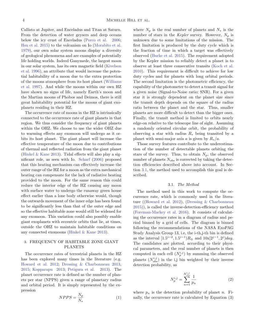
4 Michelle Hill et al.
Callisto at Jupiter, and Enceladus and Titan at Saturn.
From the detection of water geysers and deep oceans
below the icy crust of Enceladus (Porco et al. 2006;
Hsu et al. 2015) to the volcanism on Io (Morabito et al.
1979), our own solar system moons display a diversity
of geological phenomena and are examples of potentially
life holding worlds. Indeed Ganymede, the largest moon
in our solar system, has its own magnetic field (Kivelson
et al. 1996), an attribute that would increase the poten-
tial habitability of a moon due to the extra protection
of the moons atmosphere from its host planet (Williams
et al. 1997). And while the moons within our own HZ
have shown no signs of life, namely Earth’s moon and
the Martian moons of Phobos and Deimos, there is still
great habitability potential for the moons of giant exo-
planets residing in their HZ.
The occurrence rate of moons in the HZ is intrinsically
connected to the occurrence rate of giant planets in that
region. We thus consider the frequency of giant planets
within the OHZ. We choose to use the wider OHZ due
to warming effects any exomoon will undergo as it or-
bits its host planet. The giant planet will increase the
effective temperature of the moon due to contributions
of thermal and reflected radiation from the giant planet
(Hinkel & Kane 2013). Tidal effects will also play a sig-
nificant role, as seen with Io. Scharf (2006) proposed
that this heating mechanism can effectively increase the
outer range of the HZ for a moon as the extra mechanical
heating can compensate for the lack of radiative heating
provided to the moon. For the same reason this could
reduce the interior edge of the HZ causing any moon
with surface water to undergo the runaway green house
effect earlier than a lone body otherwise would, though
the outwards movement of the inner edge has been found
to be significantly less than that of the outer edge and
so the effective habitable zone would still be widened for
any exomoon. This variation could also possibly enable
giant exoplanets with eccentric orbits that lie, at times,
outside the OHZ to maintain habitable conditions on
any connected exomoons (Hinkel & Kane 2013).
3. FREQUENCY OF HABITABLE ZONE GIANT
PLANETS
The occurrence rates of terrestrial planets in the HZ
has been explored many times in the literature (e.g.
Howard et al. 2012; Dressing & Charbonneau 2013,
2015; Kopparapu 2013; Petigura et al. 2013). The
planet occurrence rate is defined as the number of plan-
ets per star (NPPS) given a range of planetary radius
and orbital period. It is simply represented by the ex-
pression
NPPS =Np
N∗(1)
where Np is the real number of planets and N∗ is the
number of stars in the Kepler survey. However, Np is
unknown due to some limitations of the mission. The
first limitation is produced by the duty cycle which is
the fraction of time in which a target was effectively
observed (Burke et al. 2015). The requirement adopted
by the Kepler mission to reliably detect a planet is to
observe at least three consecutive transits (Koch et al.
2010). This requirement is difficult to achieve for low
duty cycles and for planets with long orbital periods.
The second limitation is the photometric efficiency, the
capability of the photometer to detect a transit signal for
a given noise (Signal-to-Noise ratio; SNR). For a given
star it is strongly dependent on the planet size since
the transit depth depends on the square of the radius
ratio between the planet and the star. Thus, smaller
planets are more difficult to detect than the bigger ones.
Finally, the transit method is limited to orbits nearly
edge-on relative to the telescope line of sight. Assuming
a randomly oriented circular orbit, the probability of
observing a star with radius R∗ being transited by a
planet with semi-major axis a is given by R∗/a.
Those survey features contribute to the underestima-
tion of the number of detectable planets orbiting the
stars of the survey. Thus, to obtain Np, the observed
number of planets Nobs is corrected by taking the detec-
tion efficiencies described above into account. In Sec-
tion 3.1, the method used to accomplish this goal is de-
scribed.
3.1. The Method
The method used in this work to compute the oc-
currence rate, which is commonly used in the litera-
ture ((Howard et al. 2012), (Dressing & Charbonneau
2015)), is called the inverse-detection-efficiency method
(Foreman-Mackey et al. 2016). It consists of calculat-
ing the occurrence rates in a diagram of radius and pe-
riod binned by a grid of cells. The diagram is binned
following the recommendations of the NASA ExoPAG
Study Analysis Group 13, i.e, the i-th,j-th bin is defined
as the interval [1.5i−2, 1.5i−1)R⊕ and 10x[2j−1, 2j)day.
The candidates are plotted, according to their physi-
cal parameters, and the real number of planets is then
computed in each cell (N i,jp ) by summing the observed
planets (N i,jobs) in the i,j bin weighted by their inverse
detection probability, as
N i,jp =
Ni,jobs∑
n=1
1
pn(2)
where pn is the detection probability of planet n. Fi-
nally, the occurrence rate is calculated by Equation (3)
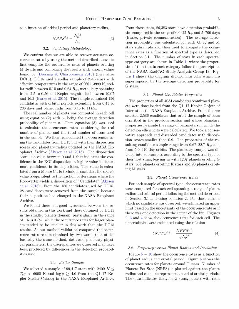
Kepler Habitable Zone Exomoons 5
as a function of orbital period and planetary radius,
NPPSi,j =N i,j
p
N∗(3)
3.2. Validating Methodology
We confirm that we are able to recover accurate oc-
currence rates by using the method described above to
first compute the occurrence rates of planets orbiting
M dwarfs and comparing the results with known values
found by (Dressing & Charbonneau 2015) (here after
DC15). DC15 used a stellar sample of 2543 stars with
effective temperatures in the range of 2661–3999 K, stel-
lar radii between 0.10 and 0.64 R⊕, metallicity spanning
from -2.5 to 0.56 and Kepler magnitudes between 10.07
and 16.3 (Burke et al. 2015). The sample contained 156
candidates with orbital periods extending from 0.45 to
236 days and planet radii from 0.46 to 11R⊕.
The real number of planets was computed in each cell
using equation (2) with pn being the average detection
probability of planet n. Then equation (3) was used
to calculate the occurrence rates considering the real
number of planets and the total number of stars used
in the sample. We then recalculated the occurrences us-
ing the candidates from DC15 but with their disposition
scores and planetary radius updated by the NASA Ex-
oplanet Archive (Akeson et al. 2013). The disposition
score is a value between 0 and 1 that indicates the con-
fidence in the KOI disposition, a higher value indicates
more confidence in its disposition. The value is calcu-
lated from a Monte Carlo technique such that the score’s
value is equivalent to the fraction of iterations where the
Robovetter yields a disposition of ”Candidate” (Akeson
et al. 2013). From the 156 candidates used by DC15,
28 candidates were removed from the sample because
their disposition had changed in the NASA Exoplanet
Archive.
We found there is a good agreement between the re-
sults obtained in this work and those obtained by DC15
in the smaller planets domain, particularly in the range
of 1.5–3.0 R⊕, while the occurrence rates for larger plan-
ets tended to be smaller in this work than the DC15
results. As our method validation compared the occur-
rence rates results obtained by two works that utilize
basically the same method, data and planetary physi-
cal parameters, the discrepancies we observed may have
been produced by differences in the detection probabil-
ities used.
3.3. Stellar Sample
We selected a sample of 99,417 stars with 2400 K ≤Teff < 6000 K and log g ≥ 4.0 from the Q1–17 Ke-
pler Stellar Catalog in the NASA Exoplanet Archive.
From those stars, 86,383 stars have detection probabili-
ties computed in the range of 0.6–25 R⊕ and 5–700 days
(Burke, private communication). The average detec-
tion probability was calculated for each G, K and M
stars subsample and then used to compute the occur-
rence rates as a function of spectral type as described
in Section 3.1. The number of stars in each spectral
type category are shown in Table 1, where the proper-
ties of the stars in each category follow the prescription
of the NASA ExoPAG Study Analysis Group 13. Fig-
ure 1 shows the diagram divided into cells which are
superimposed by the average detection probability for
G stars.
3.4. Planet Candidates Properties
The properties of all 4034 candidates/confirmed plan-
ets were downloaded from the Q1–17 Kepler Object of
Interest on the NASA Exoplanet Archive. From this we
selected 2,586 candidates that orbit the sample of stars
described in the previous section and whose planetary
properties lie inside the range of parameters in which the
detection efficiencies were calculated. We took a conser-
vative approach and discarded candidates with disposi-
tion scores smaller than 0.9. The properties of the re-
sulting candidate sample range from 0.67–22.7 R⊕ and
from 5.0–470 day orbits. The planetary sample was di-
vided into subsamples according to the spectral type of
their host stars, leaving us with 1207 planets orbiting G
stars, 534 planets orbiting K stars and 93 planets orbit-
ing M stars.
3.5. Planet Occurrence Rates
For each sample of spectral type, the occurrence rates
were computed for each cell spanning a range of planet
radius and orbital period following the method described
in Section 3.1 and using equation 2. For those cells in
which no candidate was observed, we estimated an upper
limit based on the uncertainty of the occurrence rate as if
there was one detection in the center of the bin. Figures
2, 3 and 4 show the occurrence rates for each cell. The
uncertainties were estimated using the relation
δNPPSi,j =NPPSi,j
√N i,j
p
(4)
3.6. Frequency versus Planet Radius and Insolation
Figure 5 − 10 show the occurrence rates as a function
of planet radius and orbital period. Figure 5 shows the
occurrence rates for planets around G stars. Number of
Planets Per Star (NPPS) is plotted against the planet
radius and each line represents a band of orbital periods.
The data indicates that, for G stars, planets with radii
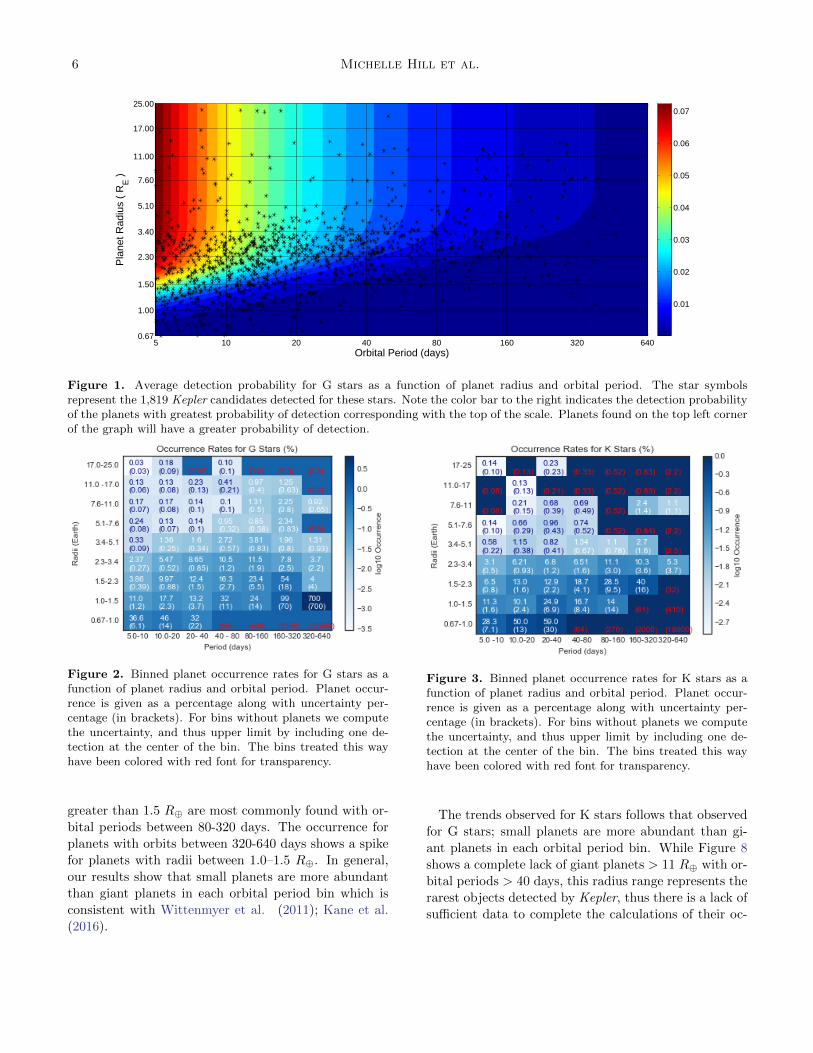
6 Michelle Hill et al.
5 10 20 40 80 160 320 6400.67
1.00
1.50
2.30
3.40
5.10
7.60
11.00
17.00
25.00
Orbital Period (days)
Pla
net R
adiu
s (
RE )
0.01
0.02
0.03
0.04
0.05
0.06
0.07
Figure 1. Average detection probability for G stars as a function of planet radius and orbital period. The star symbolsrepresent the 1,819 Kepler candidates detected for these stars. Note the color bar to the right indicates the detection probabilityof the planets with greatest probability of detection corresponding with the top of the scale. Planets found on the top left cornerof the graph will have a greater probability of detection.
Figure 2. Binned planet occurrence rates for G stars as afunction of planet radius and orbital period. Planet occur-rence is given as a percentage along with uncertainty per-centage (in brackets). For bins without planets we computethe uncertainty, and thus upper limit by including one de-tection at the center of the bin. The bins treated this wayhave been colored with red font for transparency.
greater than 1.5 R⊕ are most commonly found with or-
bital periods between 80-320 days. The occurrence for
planets with orbits between 320-640 days shows a spike
for planets with radii between 1.0–1.5 R⊕. In general,
our results show that small planets are more abundant
than giant planets in each orbital period bin which is
consistent with Wittenmyer et al. (2011); Kane et al.
(2016).
Figure 3. Binned planet occurrence rates for K stars as afunction of planet radius and orbital period. Planet occur-rence is given as a percentage along with uncertainty per-centage (in brackets). For bins without planets we computethe uncertainty, and thus upper limit by including one de-tection at the center of the bin. The bins treated this wayhave been colored with red font for transparency.
The trends observed for K stars follows that observed
for G stars; small planets are more abundant than gi-
ant planets in each orbital period bin. While Figure 8
shows a complete lack of giant planets > 11 R⊕ with or-
bital periods > 40 days, this radius range represents the
rarest objects detected by Kepler, thus there is a lack of
sufficient data to complete the calculations of their oc-
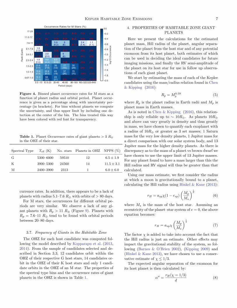
Kepler Habitable Zone Exomoons 7
Figure 4. Binned planet occurrence rates for M stars as afunction of planet radius and orbital period. Planet occur-rence is given as a percentage along with uncertainty per-centage (in brackets). For bins without planets we computethe uncertainty, and thus upper limit by including one de-tection at the center of the bin. The bins treated this wayhave been colored with red font for transparency.
Table 1. Planet Occurrence rates of giant planets > 3 R⊕in the OHZ of their star.
Spectral Type Teff (K) No. stars Planets in OHZ NPPS (%)
G 5300–6000 59510 12 6.5 ± 1.9
K 3900–5300 24560 14 11.5 ± 3.1
M 2400–3900 2313 1 6.0 ± 6.0
currence rates. In addition, there appears to be a lack of
planets with radius 5.1–7.6 R⊕ with orbits of > 80 days.For M stars, the occurrences for different orbital pe-
riods are very similar. We observe a lack of any gi-
ant planets with Rp > 11 R⊕ (Figure 9). Planets with
Rp = 7.6–11 R⊕ tend to be found with orbital periods
between 20–80 days.
3.7. Frequency of Giants in the Habitable Zone
The OHZ for each host candidate was computed fol-
lowing the model described by Kopparapu et al. (2013,
2014). From the sample of candidates selected and de-
scribed in Section 3.3, 12 candidates orbit within the
OHZ of their respective G host stars, 14 candidates or-
bit in the OHZ of their K host stars and only 1 candi-
date orbits in the OHZ of an M star. The properties of
the spectral type bins and the occurrence rates of giant
planets in the OHZ is shown in Table 1.
4. PROPERTIES OF HABITABLE ZONE GIANT
PLANETS
Here we present the calculations for the estimated
planet mass, Hill radius of the planet, angular separa-
tion of the planet from the host star and of any potential
exomoon from its host planet, both estimates of which
can be used in deciding the ideal candidates for future
imaging missions, and finally the RV semi-amplitude of
the planet on its host star for use in follow up observa-
tions of each giant planet.
We start by estimating the mass of each of the Kepler
candidates using the mass/radius relation found in Chen
& Kipping (2016):
Rp = M0.59p (5)
where Rp is the planet radius in Earth radii and Mp is
planet mass in Earth masses.
As is noted in Chen & Kipping (2016), this relation-
ship is only reliable up to ∼ 10R⊕. As planets 10R⊕and above can vary greatly in density and thus greatly
in mass, we have chosen to quantify each exoplanet with
a radius of 10R⊕ or greater as 3 set masses; 1 Saturn
mass for the very low density planets, 1 Jupiter mass for
a direct comparison with our solar system body, and 13
Jupiter mass for the higher density planets. As there is
discrepancy as to the mass of a planet vs brown dwarf we
have chosen to use the upper limit of 13 Jupiter masses.
For any planet found to have a mass larger than this the
Hill radius and RV signal will thus be greater than that
calculated.
Using our mass estimate, we first consider the radius
at which a moon is gravitationally bound to a planet,
calculating the Hill radius using Hinkel & Kane (2013):
rH = aspχ(1− esp)
(Mp
M?
) 13
(6)
where M? is the mass of the host star. Assuming an
eccentricity of the planet–star system of e = 0, the above
equation becomes:
rH = aspχ
(Mp
M?
) 13
(7)
The factor χ is added to take into account the fact that
the Hill radius is just an estimate. Other effects may
impact the gravitational stability of the system, so fol-
lowing (Barnes & O’Brien 2002), (Kipping 2009) and
(Hinkel & Kane 2013), we have chosen to use a conser-
vative estimate of χ ≤ 1/3.
The expected angular separation of the exomoon for
its host planet is then calculated by:
α′′ =rH(χ = 1/3)
d(8)
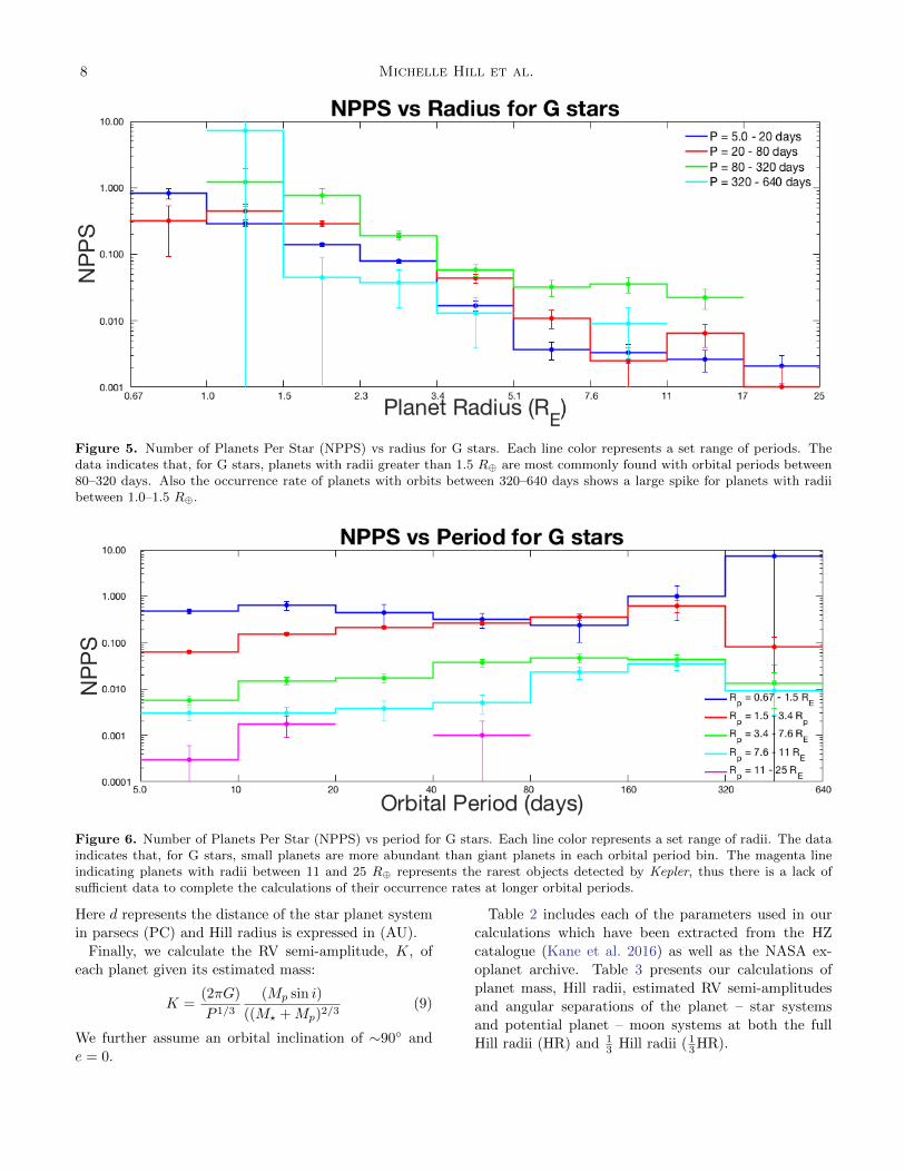
8 Michelle Hill et al.
Figure 5. Number of Planets Per Star (NPPS) vs radius for G stars. Each line color represents a set range of periods. Thedata indicates that, for G stars, planets with radii greater than 1.5 R⊕ are most commonly found with orbital periods between80–320 days. Also the occurrence rate of planets with orbits between 320–640 days shows a large spike for planets with radiibetween 1.0–1.5 R⊕.
Figure 6. Number of Planets Per Star (NPPS) vs period for G stars. Each line color represents a set range of radii. The dataindicates that, for G stars, small planets are more abundant than giant planets in each orbital period bin. The magenta lineindicating planets with radii between 11 and 25 R⊕ represents the rarest objects detected by Kepler, thus there is a lack ofsufficient data to complete the calculations of their occurrence rates at longer orbital periods.
Here d represents the distance of the star planet system
in parsecs (PC) and Hill radius is expressed in (AU).
Finally, we calculate the RV semi-amplitude, K, of
each planet given its estimated mass:
K =(2πG)
P 1/3
(Mp sin i)
((M? +Mp)2/3(9)
We further assume an orbital inclination of ∼90◦ and
e = 0.
Table 2 includes each of the parameters used in our
calculations which have been extracted from the HZ
catalogue (Kane et al. 2016) as well as the NASA ex-
oplanet archive. Table 3 presents our calculations of
planet mass, Hill radii, estimated RV semi-amplitudes
and angular separations of the planet – star systems
and potential planet – moon systems at both the full
Hill radii (HR) and 13 Hill radii (1
3HR).
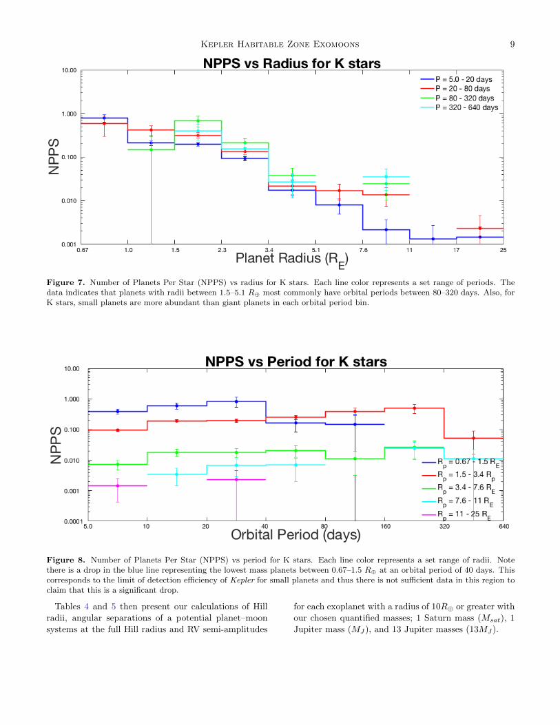
Kepler Habitable Zone Exomoons 9
Figure 7. Number of Planets Per Star (NPPS) vs radius for K stars. Each line color represents a set range of periods. Thedata indicates that planets with radii between 1.5–5.1 R⊕ most commonly have orbital periods between 80–320 days. Also, forK stars, small planets are more abundant than giant planets in each orbital period bin.
Figure 8. Number of Planets Per Star (NPPS) vs period for K stars. Each line color represents a set range of radii. Notethere is a drop in the blue line representing the lowest mass planets between 0.67–1.5 R⊕ at an orbital period of 40 days. Thiscorresponds to the limit of detection efficiency of Kepler for small planets and thus there is not sufficient data in this region toclaim that this is a significant drop.
Tables 4 and 5 then present our calculations of Hill
radii, angular separations of a potential planet–moon
systems at the full Hill radius and RV semi-amplitudes
for each exoplanet with a radius of 10R⊕ or greater with
our chosen quantified masses; 1 Saturn mass (Msat), 1
Jupiter mass (MJ), and 13 Jupiter masses (13MJ).
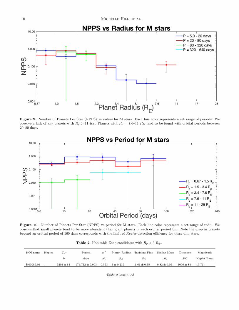
10 Michelle Hill et al.
Figure 9. Number of Planets Per Star (NPPS) vs radius for M stars. Each line color represents a set range of periods. Weobserve a lack of any planets with Rp > 11 R⊕. Planets with Rp = 7.6–11 R⊕ tend to be found with orbital periods between20–80 days.
Figure 10. Number of Planets Per Star (NPPS) vs period for M stars. Each line color represents a set range of radii. Weobserve that small planets tend to be more abundant than giant planets in each orbital period bin. Note the drop in planetsbeyond an orbital period of 160 days corresponds with the limit of Kepler detection efficiency for these dim stars.
Table 2. Habitable Zone candidates with Rp > 3 R⊕.
KOI name Kepler Teff Period a * Planet Radius Incident Flux Stellar Mass Distance Magnitude
K days AU R⊕ F⊕ M? PC Kepler Band
K03086.01 − 5201± 83 174.732± 0.003 0.573 3± 0.235 1.61± 0.35 0.82± 0.05 1006± 84 15.71
Table 2 continued
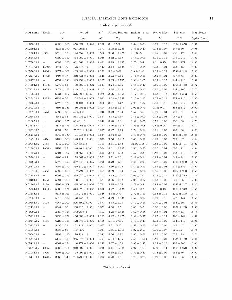
Kepler Habitable Zone Exomoons 11
Table 2 (continued)
KOI name Kepler Teff Period a * Planet Radius Incident Flux Stellar Mass Distance Magnitude
K days AU R⊕ F⊕ M? PC Kepler Band
K06786.01 − 5883± 186 455.624± 0.026 1.153 3± 0.585 0.64± 0.33 0.99± 0.13 3192± 550 11.97
K02691.01 − 4735± 170 97.446± 0 0.373 3.05± 0.265 1.53± 0.49 0.73± 0.07 447± 50 14.98
K01581.02 896b 5510± 158 144.552± 0.003 0.516 3.06± 0.475 2± 0.85 0.88± 0.09 926± 170 15.48
K08156.01 − 6429± 182 364.982± 0.011 1.048 3.12± 0.69 1.74± 0.96 1.15± 0.16 978± 240 14.32
K07700.01 − 6382± 180 631.569± 0.013 1.491 3.13± 0.655 0.75± 0.4 1.1± 0.15 798± 177 14.00
K04016.01 1540b 4641± 79 125.413± 0 0.443 3.14± 0.125 1.19± 0.18 0.73± 0.04 293± 18 14.07
K05706.01 1636b 5977± 201 425.484± 0.009 1.155 3.2± 0.61 0.9± 0.46 1.13± 0.13 1589± 348 15.81
K02210.02 1143c 4895± 78 210.631± 0.002 0.648 3.23± 0.15 0.71± 0.11 0.82± 0.04 607± 38 15.20
K08276.01 − 6551± 183 385.859± 0.005 1.107 3.23± 0.705 1.93± 1.05 1.22± 0.17 944± 216 13.99
K04121.01 1554b 5275± 83 198.089± 0.002 0.631 3.24± 0.36 1.64± 0.47 0.86± 0.05 1164± 143 15.72
K05622.01 1635b 5474± 158 469.613± 0.014 1.117 3.24± 0.46 0.38± 0.15 0.85± 0.09 944± 160 15.70
K07982.01 − 6231± 207 376.38± 0.047 1.029 3.26± 0.665 1.17± 0.63 1.03± 0.13 1436± 333 15.63
K03946.01 1533b 6325± 79 308.544± 0.002 0.963 3.28± 0.565 2.82± 1.12 1.25± 0.11 734± 119 13.22
K08232.01 − 5573± 174 189.184± 0.004 0.610 3.31± 0.77 2.24± 1.32 0.85± 0.1 865± 212 15.05
K05625.01 − 5197± 181 116.454± 0.002 0.414 3.33± 0.375 2.07± 0.75 0.7± 0.07 894± 132 16.02
K02073.01 357d 5036± 200 49.5± 0 0.246 3.43± 2.04 6.57± 8.8 0.79± 0.04 771± 51 15.57
K02686.01 − 4658± 93 211.033± 0.001 0.627 3.43± 0.17 0.51± 0.09 0.74± 0.04 267± 17 13.86
K01855.01 − 4338± 125 58.43± 0 0.248 3.45± 0.3 1.92± 0.55 0.59± 0.06 298± 33 14.78
K02828.02 − 4817± 176 505.463± 0.008 1.153 3.46± 0.315 0.25± 0.08 0.8± 0.05 769± 95 15.77
K02926.05 − 3891± 78 75.731± 0.002 0.297 3.47± 0.19 0.74± 0.14 0.61± 0.03 425± 35 16.28
K08286.01 − 5440± 180 191.037± 0.013 0.634 3.54± 0.6 1.59± 0.75 0.93± 0.09 1654± 335 16.65
K01830.02 967c 5180± 103 198.711± 0.001 0.625 3.56± 0.215 1.06± 0.21 0.83± 0.05 502± 37 14.44
K00951.02 258c 4942± 200 33.653± 0 0.193 3.61± 2.43 12.16± 18.1 0.83± 0.05 1542± 431 15.22
K01986.01 1038b 5159± 82 148.46± 0.001 0.524 3.61± 0.205 1.56± 0.28 0.87± 0.04 606± 42 14.84
K01527.01 − 5401± 107 192.667± 0.001 0.622 3.64± 0.32 1.52± 0.39 0.86± 0.05 743± 71 14.88
K05790.01 − 4899± 82 178.267± 0.003 0.571 3.71± 0.21 0.81± 0.14 0.82± 0.04 643± 44 15.52
K08193.01 − 5570± 158 367.948± 0.005 0.996 3.72± 0.6 0.64± 0.28 0.97± 0.09 1116± 202 15.72
K08275.01 − 5289± 176 389.876± 0.007 1.002 3.76± 0.46 0.44± 0.17 0.89± 0.08 975± 152 15.95
K01070.02 266c 5885± 250 107.724± 0.002 0.457 3.89± 1.89 5.47± 6.24 0.95± 0.06 1562± 280 15.59
K07847.01 − 6098± 217 399.376± 0.069 1.103 3.93± 1.225 2.67± 2.04 1.12± 0.17 2190± 713 13.28
K00401.02 149d 5381± 100 160.018± 0.001 0.571 3.96± 0.68 2.08± 0.77 0.93± 0.05 541± 56 14.00
K01707.02 315c 5796± 108 265.469± 0.006 0.791 4.15± 0.96 1.75± 0.8 0.88± 0.06 1083± 147 15.32
K05581.01 1634b 5636± 171 374.878± 0.008 1.053 4.27± 1.125 1.5± 0.97 1.1± 0.13 1019± 272 14.51
K01258.03 − 5717± 165 148.272± 0.001 0.546 4.3± 0.75 2.52± 1.16 0.98± 0.11 1217± 245 15.77
K02683.01 − 5613± 152 126.445± 0 0.473 4.49± 0.635 2.52± 0.99 0.89± 0.1 947± 147 15.50
K00881.02 712c 5067± 102 226.89± 0.001 0.673 4.53± 0.26 0.73± 0.14 0.79± 0.04 854± 59 15.86
K01429.01 − 5644± 80 205.913± 0.001 0.679 4.68± 0.5 1.86± 0.5 0.98± 0.06 1232± 135 15.53
K00902.01 − 3960± 124 83.925± 0 0.303 4.78± 0.405 0.62± 0.18 0.53± 0.04 348± 43 15.75
K05929.01 − 5830± 158 466.003± 0.003 1.165 4.92± 0.875 0.59± 0.27 0.97± 0.12 780± 168 14.69
K00179.02 458b 6226± 118 572.377± 0.006 1.406 5.8± 0.905 1.15± 0.45 1.13± 0.09 904± 140 13.96
K03823.01 − 5536± 79 202.117± 0.001 0.667 5.8± 0.53 1.59± 0.38 0.96± 0.05 563± 57 13.92
K01058.01 − 3337± 86 5.67± 0 0.034 5.85± 2.015 3.22± 2.55 0.16± 0.07 32± 12 13.78
K00683.01 − 5799± 110 278.124± 0 0.842 5.86± 0.72 1.58± 0.51 1.03± 0.07 622± 73 13.71
K05375.01 − 5142± 150 285.375± 0.004 0.794 5.94± 4.05 7.56± 11.19 0.82± 0.21 1138± 769 13.86
K05833.01 − 6261± 174 440.171± 0.006 1.145 5.97± 1.53 2.97± 1.85 1.03± 0.16 809± 200 13.01
K02076.02 1085b 6063± 181 219.322± 0.001 0.739 6.11± 1.085 2.27± 1.08 1.12± 0.14 1314± 270 15.27
K02681.01 397c 5307± 100 135.499± 0.001 0.480 6.18± 0.56 1.83± 0.47 0.78± 0.05 983± 76 16.00
K05416.01 1628b 3869± 140 76.378± 0.002 0.295 6.28± 0.6 0.79± 0.26 0.59± 0.06 418± 56 16.60
Table 2 continued
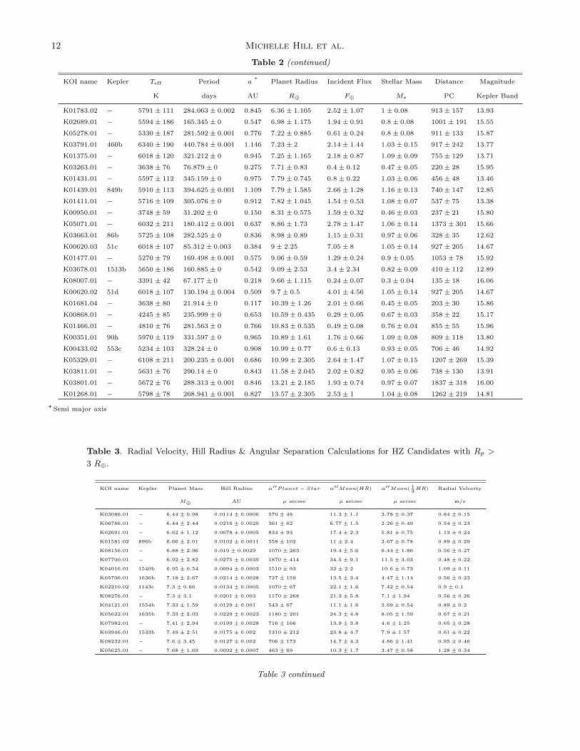
12 Michelle Hill et al.
Table 2 (continued)
KOI name Kepler Teff Period a * Planet Radius Incident Flux Stellar Mass Distance Magnitude
K days AU R⊕ F⊕ M? PC Kepler Band
K01783.02 − 5791± 111 284.063± 0.002 0.845 6.36± 1.105 2.52± 1.07 1± 0.08 913± 157 13.93
K02689.01 − 5594± 186 165.345± 0 0.547 6.98± 1.175 1.94± 0.91 0.8± 0.08 1001± 191 15.55
K05278.01 − 5330± 187 281.592± 0.001 0.776 7.22± 0.885 0.61± 0.24 0.8± 0.08 911± 133 15.87
K03791.01 460b 6340± 190 440.784± 0.001 1.146 7.23± 2 2.14± 1.44 1.03± 0.15 917± 242 13.77
K01375.01 − 6018± 120 321.212± 0 0.945 7.25± 1.165 2.18± 0.87 1.09± 0.09 755± 129 13.71
K03263.01 − 3638± 76 76.879± 0 0.275 7.71± 0.83 0.4± 0.12 0.47± 0.05 220± 28 15.95
K01431.01 − 5597± 112 345.159± 0 0.975 7.79± 0.745 0.8± 0.22 1.03± 0.06 456± 48 13.46
K01439.01 849b 5910± 113 394.625± 0.001 1.109 7.79± 1.585 2.66± 1.28 1.16± 0.13 740± 147 12.85
K01411.01 − 5716± 109 305.076± 0 0.912 7.82± 1.045 1.54± 0.53 1.08± 0.07 537± 75 13.38
K00950.01 − 3748± 59 31.202± 0 0.150 8.31± 0.575 1.59± 0.32 0.46± 0.03 237± 21 15.80
K05071.01 − 6032± 211 180.412± 0.001 0.637 8.86± 1.73 2.78± 1.47 1.06± 0.14 1373± 301 15.66
K03663.01 86b 5725± 108 282.525± 0 0.836 8.98± 0.89 1.15± 0.31 0.97± 0.06 328± 35 12.62
K00620.03 51c 6018± 107 85.312± 0.003 0.384 9± 2.25 7.05± 8 1.05± 0.14 927± 205 14.67
K01477.01 − 5270± 79 169.498± 0.001 0.575 9.06± 0.59 1.29± 0.24 0.9± 0.05 1053± 78 15.92
K03678.01 1513b 5650± 186 160.885± 0 0.542 9.09± 2.53 3.4± 2.34 0.82± 0.09 410± 112 12.89
K08007.01 − 3391± 42 67.177± 0 0.218 9.66± 1.115 0.24± 0.07 0.3± 0.04 135± 18 16.06
K00620.02 51d 6018± 107 130.194± 0.004 0.509 9.7± 0.5 4.01± 4.56 1.05± 0.14 927± 205 14.67
K01681.04 − 3638± 80 21.914± 0 0.117 10.39± 1.26 2.01± 0.66 0.45± 0.05 203± 30 15.86
K00868.01 − 4245± 85 235.999± 0 0.653 10.59± 0.435 0.29± 0.05 0.67± 0.03 358± 22 15.17
K01466.01 − 4810± 76 281.563± 0 0.766 10.83± 0.535 0.49± 0.08 0.76± 0.04 855± 55 15.96
K00351.01 90h 5970± 119 331.597± 0 0.965 10.89± 1.61 1.76± 0.66 1.09± 0.08 809± 118 13.80
K00433.02 553c 5234± 103 328.24± 0 0.908 10.99± 0.77 0.6± 0.13 0.93± 0.05 706± 46 14.92
K05329.01 − 6108± 211 200.235± 0.001 0.686 10.99± 2.305 2.64± 1.47 1.07± 0.15 1207± 269 15.39
K03811.01 − 5631± 76 290.14± 0 0.843 11.58± 2.045 2.02± 0.82 0.95± 0.06 738± 130 13.91
K03801.01 − 5672± 76 288.313± 0.001 0.846 13.21± 2.185 1.93± 0.74 0.97± 0.07 1837± 318 16.00
K01268.01 − 5798± 78 268.941± 0.001 0.827 13.57± 2.305 2.53± 1 1.04± 0.08 1262± 219 14.81
∗ Semi major axis
Table 3. Radial Velocity, Hill Radius & Angular Separation Calculations for HZ Candidates with Rp >
3 R⊕.
KOI name Kepler Planet Mass Hill Radius α′′Planet − Star α′′Moon(HR) α′′Moon( 13HR) Radial Velocity
M⊕ AU µ arcsec µ arcsec µ arcsec m/s
K03086.01 − 6.44 ± 0.98 0.0114 ± 0.0006 570 ± 48 11.3 ± 1.1 3.78 ± 0.37 0.84 ± 0.15
K06786.01 − 6.44 ± 2.44 0.0216 ± 0.0029 361 ± 62 6.77 ± 1.5 2.26 ± 0.49 0.54 ± 0.23
K02691.01 − 6.62 ± 1.12 0.0078 ± 0.0005 834 ± 93 17.4 ± 2.3 5.81 ± 0.75 1.13 ± 0.24
K01581.02 896b 6.66 ± 2.01 0.0102 ± 0.0011 558 ± 102 11 ± 2.4 3.67 ± 0.78 0.89 ± 0.29
K08156.01 − 6.88 ± 2.96 0.019 ± 0.0029 1070 ± 263 19.4 ± 5.6 6.44 ± 1.86 0.56 ± 0.27
K07700.01 − 6.92 ± 2.82 0.0275 ± 0.0039 1870 ± 414 34.5 ± 9.1 11.5 ± 3.03 0.48 ± 0.22
K04016.01 1540b 6.95 ± 0.54 0.0094 ± 0.0003 1510 ± 93 32 ± 2.2 10.6 ± 0.73 1.09 ± 0.11
K05706.01 1636b 7.18 ± 2.67 0.0214 ± 0.0028 727 ± 159 13.5 ± 3.4 4.47 ± 1.14 0.56 ± 0.23
K02210.02 1143c 7.3 ± 0.66 0.0134 ± 0.0005 1070 ± 67 22.1 ± 1.6 7.42 ± 0.54 0.9 ± 0.1
K08276.01 − 7.3 ± 3.1 0.0201 ± 0.003 1170 ± 268 21.3 ± 5.8 7.1 ± 1.94 0.56 ± 0.26
K04121.01 1554b 7.33 ± 1.59 0.0129 ± 0.001 543 ± 67 11.1 ± 1.6 3.69 ± 0.54 0.89 ± 0.2
K05622.01 1635b 7.33 ± 2.03 0.0229 ± 0.0023 1180 ± 201 24.3 ± 4.8 8.05 ± 1.59 0.67 ± 0.21
K07982.01 − 7.41 ± 2.94 0.0199 ± 0.0028 716 ± 166 13.9 ± 3.8 4.6 ± 1.25 0.65 ± 0.28
K03946.01 1533b 7.49 ± 2.51 0.0175 ± 0.002 1310 ± 212 23.8 ± 4.7 7.9 ± 1.57 0.61 ± 0.22
K08232.01 − 7.6 ± 3.45 0.0127 ± 0.002 706 ± 173 14.7 ± 4.3 4.86 ± 1.41 0.95 ± 0.46
K05625.01 − 7.68 ± 1.69 0.0092 ± 0.0007 463 ± 69 10.3 ± 1.7 3.47 ± 0.58 1.28 ± 0.34
Table 3 continued
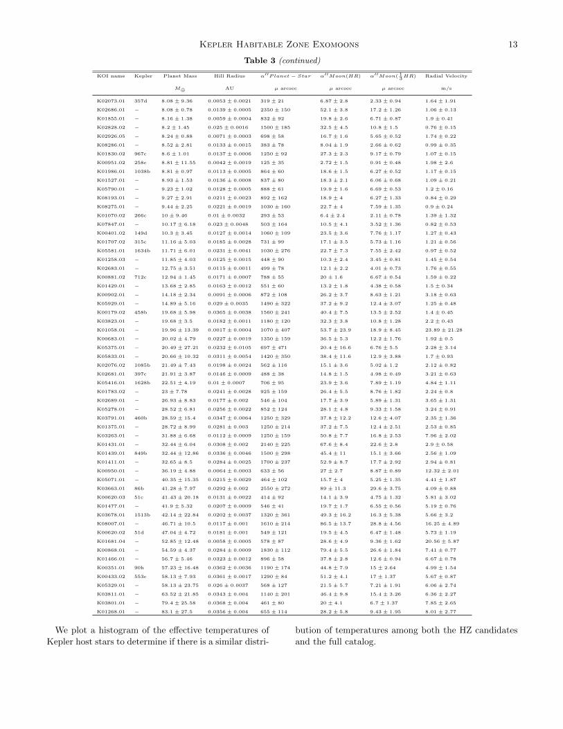
Kepler Habitable Zone Exomoons 13
Table 3 (continued)
KOI name Kepler Planet Mass Hill Radius α′′Planet − Star α′′Moon(HR) α′′Moon( 13HR) Radial Velocity
M⊕ AU µ arcsec µ arcsec µ arcsec m/s
K02073.01 357d 8.08 ± 9.36 0.0053 ± 0.0021 319 ± 21 6.87 ± 2.8 2.33 ± 0.94 1.64 ± 1.91
K02686.01 − 8.08 ± 0.78 0.0139 ± 0.0005 2350 ± 150 52.1 ± 3.8 17.2 ± 1.26 1.06 ± 0.13
K01855.01 − 8.16 ± 1.38 0.0059 ± 0.0004 832 ± 92 19.8 ± 2.6 6.71 ± 0.87 1.9 ± 0.41
K02828.02 − 8.2 ± 1.45 0.025 ± 0.0016 1500 ± 185 32.5 ± 4.5 10.8 ± 1.5 0.76 ± 0.15
K02926.05 − 8.24 ± 0.88 0.0071 ± 0.0003 698 ± 58 16.7 ± 1.6 5.65 ± 0.52 1.74 ± 0.22
K08286.01 − 8.52 ± 2.81 0.0133 ± 0.0015 383 ± 78 8.04 ± 1.9 2.66 ± 0.62 0.99 ± 0.35
K01830.02 967c 8.6 ± 1.01 0.0137 ± 0.0006 1250 ± 92 27.3 ± 2.3 9.17 ± 0.79 1.07 ± 0.15
K00951.02 258c 8.81 ± 11.55 0.0042 ± 0.0019 125 ± 35 2.72 ± 1.5 0.91 ± 0.48 1.98 ± 2.6
K01986.01 1038b 8.81 ± 0.97 0.0113 ± 0.0005 864 ± 60 18.6 ± 1.5 6.27 ± 0.52 1.17 ± 0.15
K01527.01 − 8.93 ± 1.53 0.0136 ± 0.0008 837 ± 80 18.3 ± 2.1 6.06 ± 0.68 1.09 ± 0.21
K05790.01 − 9.23 ± 1.02 0.0128 ± 0.0005 888 ± 61 19.9 ± 1.6 6.69 ± 0.53 1.2 ± 0.16
K08193.01 − 9.27 ± 2.91 0.0211 ± 0.0023 892 ± 162 18.9 ± 4 6.27 ± 1.33 0.84 ± 0.29
K08275.01 − 9.44 ± 2.25 0.0221 ± 0.0019 1030 ± 160 22.7 ± 4 7.59 ± 1.35 0.9 ± 0.24
K01070.02 266c 10 ± 9.46 0.01 ± 0.0032 293 ± 53 6.4 ± 2.4 2.11 ± 0.78 1.39 ± 1.32
K07847.01 − 10.17 ± 6.18 0.023 ± 0.0048 503 ± 164 10.5 ± 4.1 3.52 ± 1.36 0.82 ± 0.53
K00401.02 149d 10.3 ± 3.45 0.0127 ± 0.0014 1060 ± 109 23.5 ± 3.6 7.76 ± 1.17 1.27 ± 0.43
K01707.02 315c 11.16 ± 5.03 0.0185 ± 0.0028 731 ± 99 17.1 ± 3.5 5.73 ± 1.16 1.21 ± 0.56
K05581.01 1634b 11.71 ± 6.01 0.0231 ± 0.0041 1030 ± 276 22.7 ± 7.3 7.55 ± 2.42 0.97 ± 0.52
K01258.03 − 11.85 ± 4.03 0.0125 ± 0.0015 448 ± 90 10.3 ± 2.4 3.45 ± 0.81 1.45 ± 0.54
K02683.01 − 12.75 ± 3.51 0.0115 ± 0.0011 499 ± 78 12.1 ± 2.2 4.01 ± 0.73 1.76 ± 0.55
K00881.02 712c 12.94 ± 1.45 0.0171 ± 0.0007 788 ± 55 20 ± 1.6 6.67 ± 0.54 1.59 ± 0.22
K01429.01 − 13.68 ± 2.85 0.0163 ± 0.0012 551 ± 60 13.2 ± 1.8 4.38 ± 0.58 1.5 ± 0.34
K00902.01 − 14.18 ± 2.34 0.0091 ± 0.0006 872 ± 108 26.2 ± 3.7 8.63 ± 1.21 3.18 ± 0.63
K05929.01 − 14.89 ± 5.16 0.029 ± 0.0035 1490 ± 322 37.2 ± 9.2 12.4 ± 3.07 1.25 ± 0.48
K00179.02 458b 19.68 ± 5.98 0.0365 ± 0.0038 1560 ± 241 40.4 ± 7.5 13.5 ± 2.52 1.4 ± 0.45
K03823.01 − 19.68 ± 3.5 0.0182 ± 0.0011 1180 ± 120 32.3 ± 3.8 10.8 ± 1.28 2.2 ± 0.43
K01058.01 − 19.96 ± 13.39 0.0017 ± 0.0004 1070 ± 407 53.7 ± 23.9 18.9 ± 8.45 23.89 ± 21.28
K00683.01 − 20.02 ± 4.79 0.0227 ± 0.0019 1350 ± 159 36.5 ± 5.3 12.2 ± 1.76 1.92 ± 0.5
K05375.01 − 20.49 ± 27.21 0.0232 ± 0.0105 697 ± 471 20.4 ± 16.6 6.76 ± 5.5 2.28 ± 3.14
K05833.01 − 20.66 ± 10.32 0.0311 ± 0.0054 1420 ± 350 38.4 ± 11.6 12.9 ± 3.88 1.7 ± 0.93
K02076.02 1085b 21.49 ± 7.43 0.0198 ± 0.0024 562 ± 116 15.1 ± 3.6 5.02 ± 1.2 2.12 ± 0.82
K02681.01 397c 21.91 ± 3.87 0.0146 ± 0.0009 488 ± 38 14.8 ± 1.5 4.98 ± 0.49 3.21 ± 0.63
K05416.01 1628b 22.51 ± 4.19 0.01 ± 0.0007 706 ± 95 23.9 ± 3.6 7.89 ± 1.19 4.84 ± 1.11
K01783.02 − 23 ± 7.78 0.0241 ± 0.0028 925 ± 159 26.4 ± 5.5 8.76 ± 1.82 2.24 ± 0.8
K02689.01 − 26.93 ± 8.83 0.0177 ± 0.002 546 ± 104 17.7 ± 3.9 5.89 ± 1.31 3.65 ± 1.31
K05278.01 − 28.52 ± 6.81 0.0256 ± 0.0022 852 ± 124 28.1 ± 4.8 9.33 ± 1.58 3.24 ± 0.91
K03791.01 460b 28.59 ± 15.4 0.0347 ± 0.0064 1250 ± 329 37.8 ± 12.2 12.6 ± 4.07 2.35 ± 1.36
K01375.01 − 28.72 ± 8.99 0.0281 ± 0.003 1250 ± 214 37.2 ± 7.5 12.4 ± 2.51 2.53 ± 0.85
K03263.01 − 31.88 ± 6.68 0.0112 ± 0.0009 1250 ± 159 50.8 ± 7.7 16.8 ± 2.53 7.96 ± 2.02
K01431.01 − 32.44 ± 6.04 0.0308 ± 0.002 2140 ± 225 67.6 ± 8.4 22.6 ± 2.8 2.9 ± 0.58
K01439.01 849b 32.44 ± 12.86 0.0336 ± 0.0046 1500 ± 298 45.4 ± 11 15.1 ± 3.66 2.56 ± 1.09
K01411.01 − 32.65 ± 8.5 0.0284 ± 0.0025 1700 ± 237 52.9 ± 8.7 17.7 ± 2.92 2.94 ± 0.81
K00950.01 − 36.19 ± 4.88 0.0064 ± 0.0003 633 ± 56 27 ± 2.7 8.87 ± 0.89 12.32 ± 2.01
K05071.01 − 40.35 ± 15.35 0.0215 ± 0.0029 464 ± 102 15.7 ± 4 5.25 ± 1.35 4.41 ± 1.87
K03663.01 86b 41.28 ± 7.97 0.0292 ± 0.002 2550 ± 272 89 ± 11.3 29.6 ± 3.75 4.09 ± 0.88
K00620.03 51c 41.43 ± 20.18 0.0131 ± 0.0022 414 ± 92 14.1 ± 3.9 4.75 ± 1.32 5.81 ± 3.02
K01477.01 − 41.9 ± 5.32 0.0207 ± 0.0009 546 ± 41 19.7 ± 1.7 6.55 ± 0.56 5.19 ± 0.76
K03678.01 1513b 42.14 ± 22.84 0.0202 ± 0.0037 1320 ± 361 49.3 ± 16.2 16.3 ± 5.38 5.66 ± 3.2
K08007.01 − 46.71 ± 10.5 0.0117 ± 0.001 1610 ± 214 86.5 ± 13.7 28.8 ± 4.56 16.25 ± 4.89
K00620.02 51d 47.04 ± 4.72 0.0181 ± 0.001 549 ± 121 19.5 ± 4.5 6.47 ± 1.48 5.73 ± 1.19
K01681.04 − 52.85 ± 12.48 0.0058 ± 0.0005 578 ± 87 28.6 ± 4.9 9.36 ± 1.62 20.56 ± 5.87
K00868.01 − 54.59 ± 4.37 0.0284 ± 0.0009 1830 ± 112 79.4 ± 5.5 26.6 ± 1.84 7.41 ± 0.77
K01466.01 − 56.7 ± 5.46 0.0323 ± 0.0012 896 ± 58 37.8 ± 2.8 12.6 ± 0.94 6.67 ± 0.78
K00351.01 90h 57.23 ± 16.48 0.0362 ± 0.0036 1190 ± 174 44.8 ± 7.9 15 ± 2.64 4.99 ± 1.54
K00433.02 553c 58.13 ± 7.93 0.0361 ± 0.0017 1290 ± 84 51.2 ± 4.1 17 ± 1.37 5.67 ± 0.87
K05329.01 − 58.13 ± 23.75 0.026 ± 0.0037 568 ± 127 21.5 ± 5.7 7.21 ± 1.91 6.06 ± 2.74
K03811.01 − 63.52 ± 21.85 0.0343 ± 0.004 1140 ± 201 46.4 ± 9.8 15.4 ± 3.26 6.36 ± 2.27
K03801.01 − 79.4 ± 25.58 0.0368 ± 0.004 461 ± 80 20 ± 4.1 6.7 ± 1.37 7.85 ± 2.65
K01268.01 − 83.1 ± 27.5 0.0356 ± 0.004 655 ± 114 28.2 ± 5.8 9.43 ± 1.95 8.01 ± 2.77
We plot a histogram of the effective temperatures of
Kepler host stars to determine if there is a similar distri-
bution of temperatures among both the HZ candidates
and the full catalog.
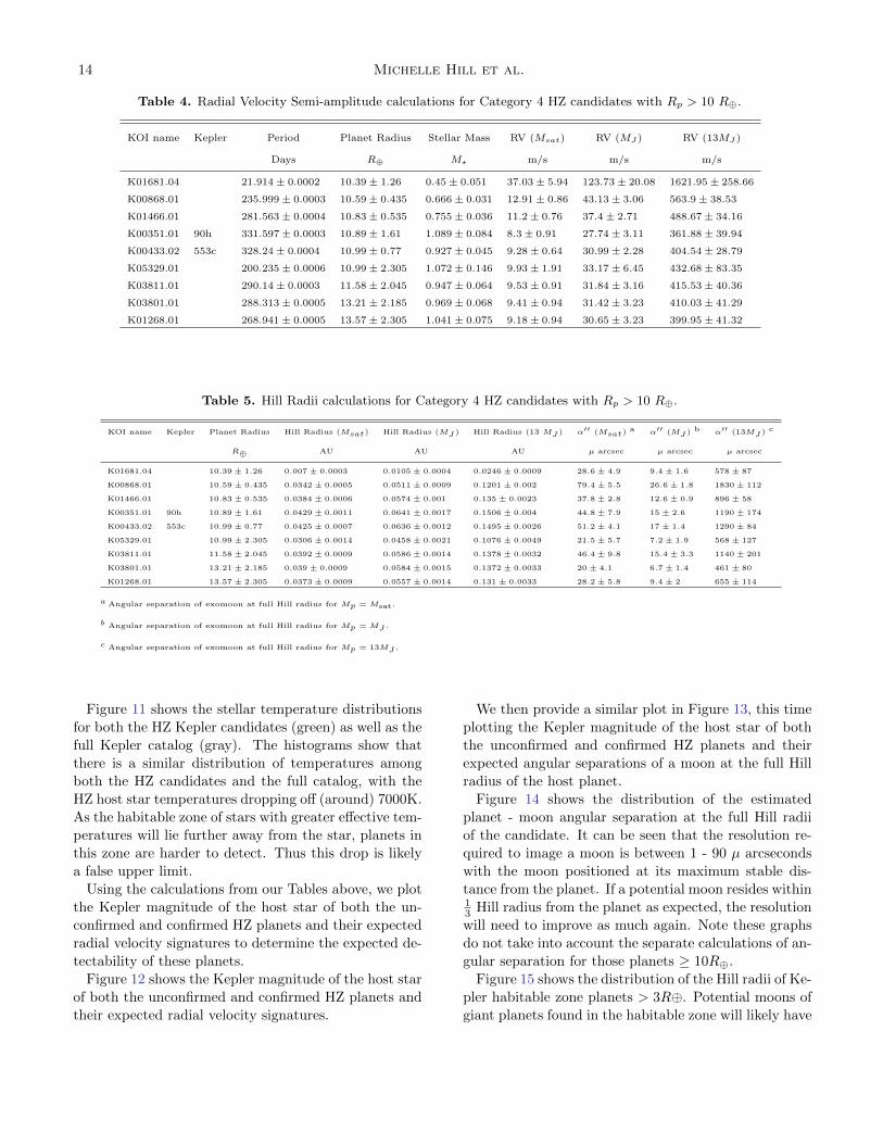
14 Michelle Hill et al.
Table 4. Radial Velocity Semi-amplitude calculations for Category 4 HZ candidates with Rp > 10 R⊕.
KOI name Kepler Period Planet Radius Stellar Mass RV (Msat) RV (MJ ) RV (13MJ )
Days R⊕ M? m/s m/s m/s
K01681.04 21.914± 0.0002 10.39± 1.26 0.45± 0.051 37.03± 5.94 123.73± 20.08 1621.95± 258.66
K00868.01 235.999± 0.0003 10.59± 0.435 0.666± 0.031 12.91± 0.86 43.13± 3.06 563.9± 38.53
K01466.01 281.563± 0.0004 10.83± 0.535 0.755± 0.036 11.2± 0.76 37.4± 2.71 488.67± 34.16
K00351.01 90h 331.597± 0.0003 10.89± 1.61 1.089± 0.084 8.3± 0.91 27.74± 3.11 361.88± 39.94
K00433.02 553c 328.24± 0.0004 10.99± 0.77 0.927± 0.045 9.28± 0.64 30.99± 2.28 404.54± 28.79
K05329.01 200.235± 0.0006 10.99± 2.305 1.072± 0.146 9.93± 1.91 33.17± 6.45 432.68± 83.35
K03811.01 290.14± 0.0003 11.58± 2.045 0.947± 0.064 9.53± 0.91 31.84± 3.16 415.53± 40.36
K03801.01 288.313± 0.0005 13.21± 2.185 0.969± 0.068 9.41± 0.94 31.42± 3.23 410.03± 41.29
K01268.01 268.941± 0.0005 13.57± 2.305 1.041± 0.075 9.18± 0.94 30.65± 3.23 399.95± 41.32
Table 5. Hill Radii calculations for Category 4 HZ candidates with Rp > 10 R⊕.
KOI name Kepler Planet Radius Hill Radius (Msat) Hill Radius (MJ ) Hill Radius (13 MJ ) α′′ (Msat)a α′′ (MJ ) b α′′ (13MJ ) c
R⊕ AU AU AU µ arcsec µ arcsec µ arcsec
K01681.04 10.39 ± 1.26 0.007 ± 0.0003 0.0105 ± 0.0004 0.0246 ± 0.0009 28.6 ± 4.9 9.4 ± 1.6 578 ± 87
K00868.01 10.59 ± 0.435 0.0342 ± 0.0005 0.0511 ± 0.0009 0.1201 ± 0.002 79.4 ± 5.5 26.6 ± 1.8 1830 ± 112
K01466.01 10.83 ± 0.535 0.0384 ± 0.0006 0.0574 ± 0.001 0.135 ± 0.0023 37.8 ± 2.8 12.6 ± 0.9 896 ± 58
K00351.01 90h 10.89 ± 1.61 0.0429 ± 0.0011 0.0641 ± 0.0017 0.1506 ± 0.004 44.8 ± 7.9 15 ± 2.6 1190 ± 174
K00433.02 553c 10.99 ± 0.77 0.0425 ± 0.0007 0.0636 ± 0.0012 0.1495 ± 0.0026 51.2 ± 4.1 17 ± 1.4 1290 ± 84
K05329.01 10.99 ± 2.305 0.0306 ± 0.0014 0.0458 ± 0.0021 0.1076 ± 0.0049 21.5 ± 5.7 7.2 ± 1.9 568 ± 127
K03811.01 11.58 ± 2.045 0.0392 ± 0.0009 0.0586 ± 0.0014 0.1378 ± 0.0032 46.4 ± 9.8 15.4 ± 3.3 1140 ± 201
K03801.01 13.21 ± 2.185 0.039 ± 0.0009 0.0584 ± 0.0015 0.1372 ± 0.0033 20 ± 4.1 6.7 ± 1.4 461 ± 80
K01268.01 13.57 ± 2.305 0.0373 ± 0.0009 0.0557 ± 0.0014 0.131 ± 0.0033 28.2 ± 5.8 9.4 ± 2 655 ± 114
a Angular separation of exomoon at full Hill radius for Mp = Msat.
b Angular separation of exomoon at full Hill radius for Mp = MJ .
c Angular separation of exomoon at full Hill radius for Mp = 13MJ .
Figure 11 shows the stellar temperature distributions
for both the HZ Kepler candidates (green) as well as the
full Kepler catalog (gray). The histograms show that
there is a similar distribution of temperatures among
both the HZ candidates and the full catalog, with the
HZ host star temperatures dropping off (around) 7000K.
As the habitable zone of stars with greater effective tem-
peratures will lie further away from the star, planets in
this zone are harder to detect. Thus this drop is likely
a false upper limit.
Using the calculations from our Tables above, we plot
the Kepler magnitude of the host star of both the un-
confirmed and confirmed HZ planets and their expected
radial velocity signatures to determine the expected de-
tectability of these planets.
Figure 12 shows the Kepler magnitude of the host star
of both the unconfirmed and confirmed HZ planets and
their expected radial velocity signatures.
We then provide a similar plot in Figure 13, this time
plotting the Kepler magnitude of the host star of boththe unconfirmed and confirmed HZ planets and their
expected angular separations of a moon at the full Hill
radius of the host planet.
Figure 14 shows the distribution of the estimated
planet - moon angular separation at the full Hill radii
of the candidate. It can be seen that the resolution re-
quired to image a moon is between 1 - 90 µ arcseconds
with the moon positioned at its maximum stable dis-
tance from the planet. If a potential moon resides within13 Hill radius from the planet as expected, the resolution
will need to improve as much again. Note these graphs
do not take into account the separate calculations of an-
gular separation for those planets ≥ 10R⊕.
Figure 15 shows the distribution of the Hill radii of Ke-
pler habitable zone planets > 3R⊕. Potential moons of
giant planets found in the habitable zone will likely have
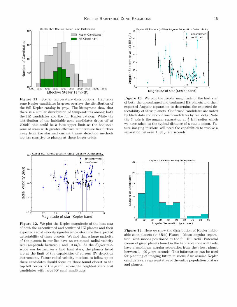
Kepler Habitable Zone Exomoons 15
Figure 11. Stellar temperature distributions. Habitablezone Kepler candidates in green overlays the distribution ofthe full Kepler catalog in gray. The histograms show thatthere is a similar distribution of temperatures among boththe HZ candidates and the full Kepler catalog. While thedistribution of the habitable zone candidates drops off at7000K, this could be a false upper limit as the habitablezone of stars with greater effective temperature lies furtheraway from the star and current transit detection methodsare less sensitive to planets at these longer orbits.
Figure 12. We plot the Kepler magnitude of the host starof both the unconfirmed and confirmed HZ planets and theirexpected radial velocity signatures to determine the expecteddetectability of these planets. We find that a large majorityof the planets in our list have an estimated radial velocitysemi amplitude between 1 and 10 m/s. As the Kepler tele-scope was focused on a field faint stars, the planets listedare at the limit of the capabilities of current RV detectioninstruments. Future radial velocity missions to follow up onthese candidates should focus on those found closest to thetop left corner of the graph, where the brightest stars hostcandidates with large RV semi amplitudes.
Figure 13. We plot the Kepler magnitude of the host starof both the unconfirmed and confirmed HZ planets and theirexpected Angular separation to determine the expected de-tectability of these planets. Confirmed candidates are notedby black dots and unconfirmed candidates by teal dots. Notethe Y axis is the angular separation at 1
3Hill radius which
we have taken as the typical distance of a stable moon. Fu-ture imaging missions will need the capabilities to resolve aseparation between 1 35 µ arc seconds.
Figure 14. Here we show the distribution of Kepler habit-able zone planets (> 3R⊕) Planet - Moon angular separa-tion, with moons positioned at the full Hill radii. Potentialmoons of giant planets found in the habitable zone will likelyhave a maximum angular separation from their host planetbetween 1 - 90 µ arc seconds. This information can be usedfor planning of imaging future missions if we assume Keplercandidates are representative of the entire population of starsand planets.
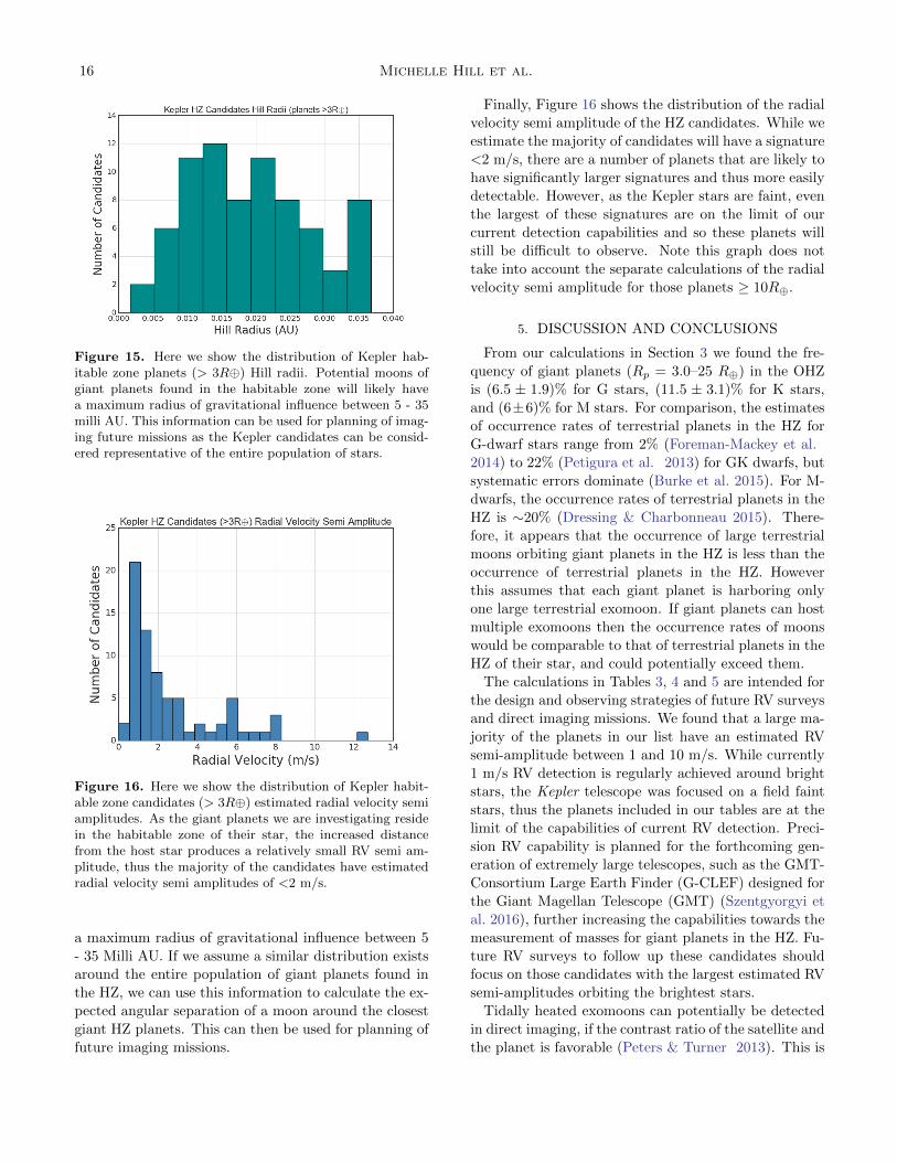
16 Michelle Hill et al.
Figure 15. Here we show the distribution of Kepler hab-itable zone planets (> 3R⊕) Hill radii. Potential moons ofgiant planets found in the habitable zone will likely havea maximum radius of gravitational influence between 5 - 35milli AU. This information can be used for planning of imag-ing future missions as the Kepler candidates can be consid-ered representative of the entire population of stars.
Figure 16. Here we show the distribution of Kepler habit-able zone candidates (> 3R⊕) estimated radial velocity semiamplitudes. As the giant planets we are investigating residein the habitable zone of their star, the increased distancefrom the host star produces a relatively small RV semi am-plitude, thus the majority of the candidates have estimatedradial velocity semi amplitudes of <2 m/s.
a maximum radius of gravitational influence between 5
- 35 Milli AU. If we assume a similar distribution exists
around the entire population of giant planets found in
the HZ, we can use this information to calculate the ex-
pected angular separation of a moon around the closest
giant HZ planets. This can then be used for planning of
future imaging missions.
Finally, Figure 16 shows the distribution of the radial
velocity semi amplitude of the HZ candidates. While we
estimate the majority of candidates will have a signature
<2 m/s, there are a number of planets that are likely to
have significantly larger signatures and thus more easily
detectable. However, as the Kepler stars are faint, even
the largest of these signatures are on the limit of our
current detection capabilities and so these planets will
still be difficult to observe. Note this graph does not
take into account the separate calculations of the radial
velocity semi amplitude for those planets ≥ 10R⊕.
5. DISCUSSION AND CONCLUSIONS
From our calculations in Section 3 we found the fre-
quency of giant planets (Rp = 3.0–25 R⊕) in the OHZ
is (6.5 ± 1.9)% for G stars, (11.5 ± 3.1)% for K stars,
and (6±6)% for M stars. For comparison, the estimates
of occurrence rates of terrestrial planets in the HZ for
G-dwarf stars range from 2% (Foreman-Mackey et al.
2014) to 22% (Petigura et al. 2013) for GK dwarfs, but
systematic errors dominate (Burke et al. 2015). For M-
dwarfs, the occurrence rates of terrestrial planets in the
HZ is ∼20% (Dressing & Charbonneau 2015). There-
fore, it appears that the occurrence of large terrestrial
moons orbiting giant planets in the HZ is less than the
occurrence of terrestrial planets in the HZ. However
this assumes that each giant planet is harboring only
one large terrestrial exomoon. If giant planets can host
multiple exomoons then the occurrence rates of moons
would be comparable to that of terrestrial planets in the
HZ of their star, and could potentially exceed them.
The calculations in Tables 3, 4 and 5 are intended for
the design and observing strategies of future RV surveys
and direct imaging missions. We found that a large ma-
jority of the planets in our list have an estimated RV
semi-amplitude between 1 and 10 m/s. While currently
1 m/s RV detection is regularly achieved around bright
stars, the Kepler telescope was focused on a field faint
stars, thus the planets included in our tables are at the
limit of the capabilities of current RV detection. Preci-
sion RV capability is planned for the forthcoming gen-
eration of extremely large telescopes, such as the GMT-
Consortium Large Earth Finder (G-CLEF) designed for
the Giant Magellan Telescope (GMT) (Szentgyorgyi et
al. 2016), further increasing the capabilities towards the
measurement of masses for giant planets in the HZ. Fu-
ture RV surveys to follow up these candidates should
focus on those candidates with the largest estimated RV
semi-amplitudes orbiting the brightest stars.
Tidally heated exomoons can potentially be detected
in direct imaging, if the contrast ratio of the satellite and
the planet is favorable (Peters & Turner 2013). This is
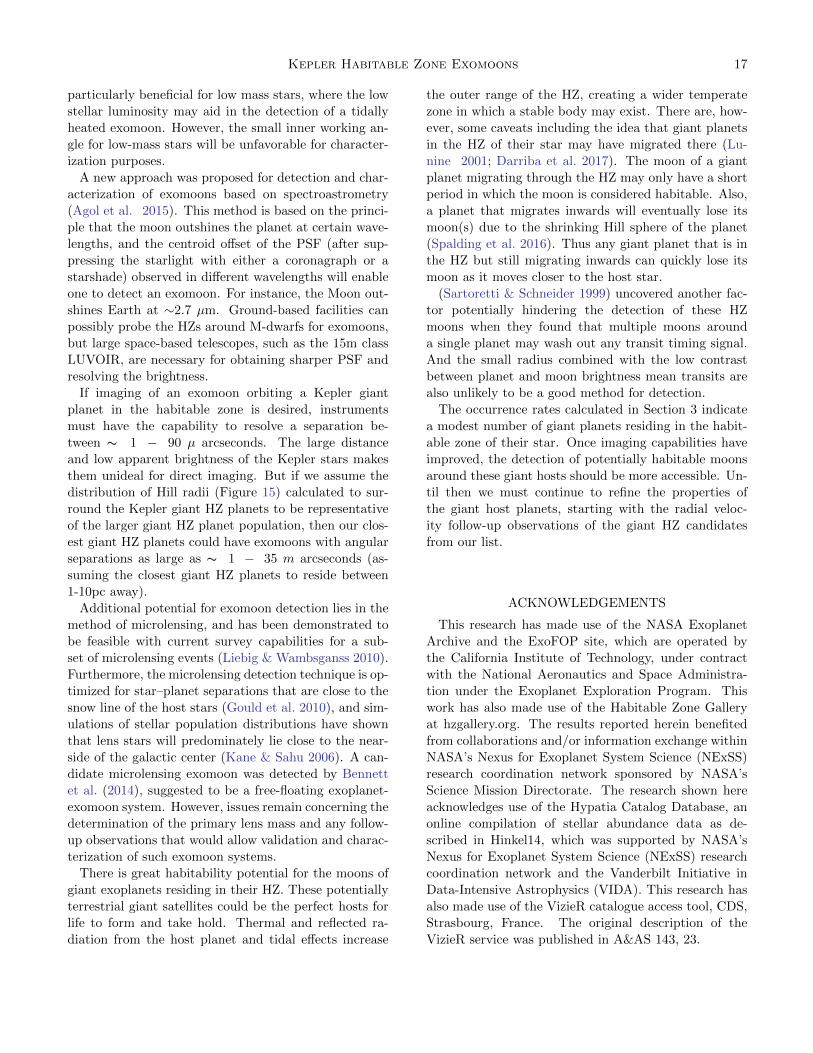
Kepler Habitable Zone Exomoons 17
particularly beneficial for low mass stars, where the low
stellar luminosity may aid in the detection of a tidally
heated exomoon. However, the small inner working an-
gle for low-mass stars will be unfavorable for character-
ization purposes.
A new approach was proposed for detection and char-
acterization of exomoons based on spectroastrometry
(Agol et al. 2015). This method is based on the princi-
ple that the moon outshines the planet at certain wave-
lengths, and the centroid offset of the PSF (after sup-
pressing the starlight with either a coronagraph or a
starshade) observed in different wavelengths will enable
one to detect an exomoon. For instance, the Moon out-
shines Earth at ∼2.7 µm. Ground-based facilities can
possibly probe the HZs around M-dwarfs for exomoons,
but large space-based telescopes, such as the 15m class
LUVOIR, are necessary for obtaining sharper PSF and
resolving the brightness.
If imaging of an exomoon orbiting a Kepler giant
planet in the habitable zone is desired, instruments
must have the capability to resolve a separation be-
tween ∼ 1 − 90 µ arcseconds. The large distance
and low apparent brightness of the Kepler stars makes
them unideal for direct imaging. But if we assume the
distribution of Hill radii (Figure 15) calculated to sur-
round the Kepler giant HZ planets to be representative
of the larger giant HZ planet population, then our clos-
est giant HZ planets could have exomoons with angular
separations as large as ∼ 1 − 35 m arcseconds (as-
suming the closest giant HZ planets to reside between
1-10pc away).
Additional potential for exomoon detection lies in the
method of microlensing, and has been demonstrated to
be feasible with current survey capabilities for a sub-
set of microlensing events (Liebig & Wambsganss 2010).
Furthermore, the microlensing detection technique is op-
timized for star–planet separations that are close to the
snow line of the host stars (Gould et al. 2010), and sim-
ulations of stellar population distributions have shown
that lens stars will predominately lie close to the near-
side of the galactic center (Kane & Sahu 2006). A can-
didate microlensing exomoon was detected by Bennett
et al. (2014), suggested to be a free-floating exoplanet-
exomoon system. However, issues remain concerning the
determination of the primary lens mass and any follow-
up observations that would allow validation and charac-
terization of such exomoon systems.
There is great habitability potential for the moons of
giant exoplanets residing in their HZ. These potentially
terrestrial giant satellites could be the perfect hosts for
life to form and take hold. Thermal and reflected ra-
diation from the host planet and tidal effects increase
the outer range of the HZ, creating a wider temperate
zone in which a stable body may exist. There are, how-
ever, some caveats including the idea that giant planets
in the HZ of their star may have migrated there (Lu-
nine 2001; Darriba et al. 2017). The moon of a giant
planet migrating through the HZ may only have a short
period in which the moon is considered habitable. Also,
a planet that migrates inwards will eventually lose its
moon(s) due to the shrinking Hill sphere of the planet
(Spalding et al. 2016). Thus any giant planet that is in
the HZ but still migrating inwards can quickly lose its
moon as it moves closer to the host star.
(Sartoretti & Schneider 1999) uncovered another fac-
tor potentially hindering the detection of these HZ
moons when they found that multiple moons around
a single planet may wash out any transit timing signal.
And the small radius combined with the low contrast
between planet and moon brightness mean transits are
also unlikely to be a good method for detection.
The occurrence rates calculated in Section 3 indicate
a modest number of giant planets residing in the habit-
able zone of their star. Once imaging capabilities have
improved, the detection of potentially habitable moons
around these giant hosts should be more accessible. Un-
til then we must continue to refine the properties of
the giant host planets, starting with the radial veloc-
ity follow-up observations of the giant HZ candidates
from our list.
ACKNOWLEDGEMENTS
This research has made use of the NASA Exoplanet
Archive and the ExoFOP site, which are operated by
the California Institute of Technology, under contract
with the National Aeronautics and Space Administra-tion under the Exoplanet Exploration Program. This
work has also made use of the Habitable Zone Gallery
at hzgallery.org. The results reported herein benefited
from collaborations and/or information exchange within
NASA’s Nexus for Exoplanet System Science (NExSS)
research coordination network sponsored by NASA’s
Science Mission Directorate. The research shown here
acknowledges use of the Hypatia Catalog Database, an
online compilation of stellar abundance data as de-
scribed in Hinkel14, which was supported by NASA’s
Nexus for Exoplanet System Science (NExSS) research
coordination network and the Vanderbilt Initiative in
Data-Intensive Astrophysics (VIDA). This research has
also made use of the VizieR catalogue access tool, CDS,
Strasbourg, France. The original description of the
VizieR service was published in A&AS 143, 23.
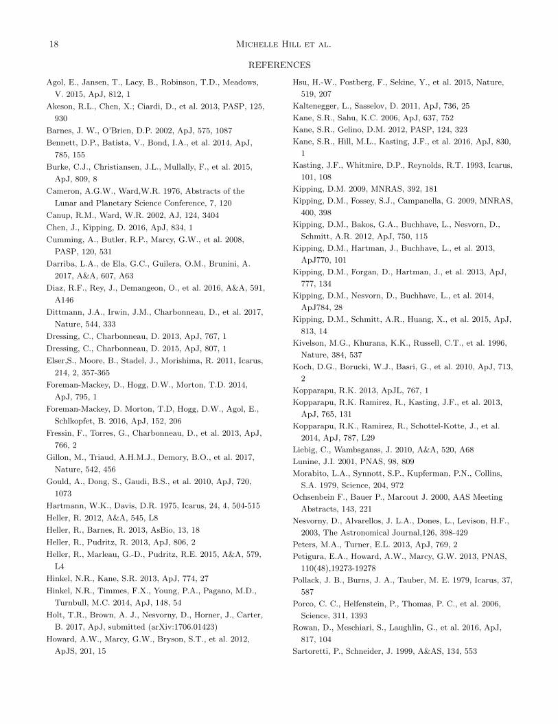
18 Michelle Hill et al.
REFERENCES
Agol, E., Jansen, T., Lacy, B., Robinson, T.D., Meadows,
V. 2015, ApJ, 812, 1
Akeson, R.L., Chen, X.; Ciardi, D., et al. 2013, PASP, 125,
930
Barnes, J. W., O’Brien, D.P. 2002, ApJ, 575, 1087
Bennett, D.P., Batista, V., Bond, I.A., et al. 2014, ApJ,
785, 155
Burke, C.J., Christiansen, J.L., Mullally, F., et al. 2015,
ApJ, 809, 8
Cameron, A.G.W., Ward,W.R. 1976, Abstracts of the
Lunar and Planetary Science Conference, 7, 120
Canup, R.M., Ward, W.R. 2002, AJ, 124, 3404
Chen, J., Kipping, D. 2016, ApJ, 834, 1
Cumming, A., Butler, R.P., Marcy, G.W., et al. 2008,
PASP, 120, 531
Darriba, L.A., de Ela, G.C., Guilera, O.M., Brunini, A.
2017, A&A, 607, A63
Diaz, R.F., Rey, J., Demangeon, O., et al. 2016, A&A, 591,
A146
Dittmann, J.A., Irwin, J.M., Charbonneau, D., et al. 2017,
Nature, 544, 333
Dressing, C., Charbonneau, D. 2013, ApJ, 767, 1
Dressing, C., Charbonneau, D. 2015, ApJ, 807, 1
Elser,S., Moore, B., Stadel, J., Morishima, R. 2011, Icarus,
214, 2, 357-365
Foreman-Mackey, D., Hogg, D.W., Morton, T.D. 2014,
ApJ, 795, 1
Foreman-Mackey, D. Morton, T.D, Hogg, D.W., Agol, E.,
Schlkopfet, B. 2016, ApJ, 152, 206
Fressin, F., Torres, G., Charbonneau, D., et al. 2013, ApJ,
766, 2
Gillon, M., Triaud, A.H.M.J., Demory, B.O., et al. 2017,
Nature, 542, 456
Gould, A., Dong, S., Gaudi, B.S., et al. 2010, ApJ, 720,
1073
Hartmann, W.K., Davis, D.R. 1975, Icarus, 24, 4, 504-515
Heller, R. 2012, A&A, 545, L8
Heller, R., Barnes, R. 2013, AsBio, 13, 18
Heller, R., Pudritz, R. 2013, ApJ, 806, 2
Heller, R., Marleau, G.-D., Pudritz, R.E. 2015, A&A, 579,
L4
Hinkel, N.R., Kane, S.R. 2013, ApJ, 774, 27
Hinkel, N.R., Timmes, F.X., Young, P.A., Pagano, M.D.,
Turnbull, M.C. 2014, ApJ, 148, 54
Holt, T.R., Brown, A. J., Nesvorny, D., Horner, J., Carter,
B. 2017, ApJ, submitted (arXiv:1706.01423)
Howard, A.W., Marcy, G.W., Bryson, S.T., et al. 2012,
ApJS, 201, 15
Hsu, H.-W., Postberg, F., Sekine, Y., et al. 2015, Nature,
519, 207
Kaltenegger, L., Sasselov, D. 2011, ApJ, 736, 25
Kane, S.R., Sahu, K.C. 2006, ApJ, 637, 752
Kane, S.R., Gelino, D.M. 2012, PASP, 124, 323
Kane, S.R., Hill, M.L., Kasting, J.F., et al. 2016, ApJ, 830,
1
Kasting, J.F., Whitmire, D.P., Reynolds, R.T. 1993, Icarus,
101, 108
Kipping, D.M. 2009, MNRAS, 392, 181
Kipping, D.M., Fossey, S.J., Campanella, G. 2009, MNRAS,
400, 398
Kipping, D.M., Bakos, G.A., Buchhave, L., Nesvorn, D.,
Schmitt, A.R. 2012, ApJ, 750, 115
Kipping, D.M., Hartman, J., Buchhave, L., et al. 2013,
ApJ770, 101
Kipping, D.M., Forgan, D., Hartman, J., et al. 2013, ApJ,
777, 134
Kipping, D.M., Nesvorn, D., Buchhave, L., et al. 2014,
ApJ784, 28
Kipping, D.M., Schmitt, A.R., Huang, X., et al. 2015, ApJ,
813, 14
Kivelson, M.G., Khurana, K.K., Russell, C.T., et al. 1996,
Nature, 384, 537
Koch, D.G., Borucki, W.J., Basri, G., et al. 2010, ApJ, 713,
2
Kopparapu, R.K. 2013, ApJL, 767, 1
Kopparapu, R.K. Ramirez, R., Kasting, J.F., et al. 2013,
ApJ, 765, 131
Kopparapu, R.K., Ramirez, R., Schottel-Kotte, J., et al.
2014, ApJ, 787, L29
Liebig, C., Wambsganss, J. 2010, A&A, 520, A68
Lunine, J.I. 2001, PNAS, 98, 809
Morabito, L.A., Synnott, S.P., Kupferman, P.N., Collins,
S.A. 1979, Science, 204, 972
Ochsenbein F., Bauer P., Marcout J. 2000, AAS Meeting
Abstracts, 143, 221
Nesvorny, D., Alvarellos, J. L.A., Dones, L., Levison, H.F.,
2003, The Astronomical Journal,126, 398-429
Peters, M.A., Turner, E.L. 2013, ApJ, 769, 2
Petigura, E.A., Howard, A.W., Marcy, G.W. 2013, PNAS,
110(48),19273-19278
Pollack, J. B., Burns, J. A., Tauber, M. E. 1979, Icarus, 37,
587
Porco, C. C., Helfenstein, P., Thomas, P. C., et al. 2006,
Science, 311, 1393
Rowan, D., Meschiari, S., Laughlin, G., et al. 2016, ApJ,
817, 104
Sartoretti, P., Schneider, J. 1999, A&AS, 134, 553
Kepler Habitable Zone Exomoons 19
Scharf, C.A. 2006, ApJ, 648, 1196
Spalding, C., Batygin, K., Adams, F.C. 2016, ApJ, 817, 1
Spergel, D. 2015, NASA reports
Szentgyorgyi, A., Baldwin, A., Barnes, S., et al. 2016,
SPIE, 9908, 990822
Teachey,A., Kipping, D.M., Schmitt, A.R. 2017, ApJ, 155, 1
Williams, D.M., Kasting, J.F., Wade, R.A. 1997, Nature,
385, 234
Wittenmyer, R.A., Endl, M., Cochran, W.D., et al. 2006,
AJ, 132, 177
Wittenmyer, R.A., Tinney, C.G., O’Toole, S.J., et al. 2011,
ApJ, 727, 102
Wittenmyer, R.A., Tinney, C.G., Butler, R.P., et al. 2011
ApJ, 738, 81
Wittenmyer, R.A., Butler, R.P., Tinney, C.G., et al. 2016,
ApJ, 819, 28
Zechmeister, M., Kurster, M., Endl, M., et al. 2013, A&A,
552, A78
Zollinger, R.R., Armstrong, J.C., Heller, R. 2017,
MNRAS472, 1
Bibliography
Agol, E, Jansen, T, Lacy, B, Robinson, TD & Meadows, V 2015, ’The Center of Light: Spectroastrometric Detection of Exomoons’, The Astrophysical Journal, vol. 812, no. 1 Astakhov, SA, Burbanks AD, Wiggins S & Farrelly D 2003, ’Chaos-assisted capture of irregular moons’, Nature, vol. 423, pp. 6937 Barensten, G 2017, NASA Mission objectives - Kepler, viewed October 2017, <https://keplerscience.arc.nasa.gov/objectives.html> Barnes, JW & O’Brien, DP 2002, ’Stability of Satellites around Close-in Extrasolar Giant Planets’, The Astrophysical Journal, vol. 575, pp. 1087 Burrows, AS 2014, ’Highlights in the Study of Exoplanet Atmospheres’, Nature, vol. 513, pp. 345-352 Cameron, AGW & Ward, WR 1976, ’The Origin of the Moon’, Abstracts of the Lunar and Planetary Science Conference, vol. 7, pp. 120 Canup, RM & Ward, WR 2002, ’Formation of the Galilean Satellites: Conditions of Accretion’, The Astronomical Journal, vol. 124, pp. 3404-3423
Bibliography
Chandler, CO, McDonald, I & Kane, SR 2015, ’The Catalog of Earth-Like Exoplanet Survey TArgets (CELESTA): A Database of Habitable Zones around Nearby Stars’, The Astrophysical Journal, vol. 151, no. 3 Chen, J & Kipping, D 2016, ’Probabilistic Forecasting of the Masses and Radii of Other Worlds’, The Astrophysical Journal, vol. 834, no. 1 Comins, N.F & Kaufmann, W.J 2012, Discovering the Universe, 9th edition, W. H. Freeman and Company, New York. Elser, S, Moore, B, Stadel, J & Morishima, R 2011, ’How common are Earth–Moon planetary systems?’, Icarus, vol. 214, no. 2, pp. 357-365 Fulton, JF, Petigura, EA, Blunt, S & Sinukoff, E 2018, ’RadVel: The Radial Velocity Modeling Toolkit’, PASP, vol. 130, pp. 986 Harman, C 2015, Sonny Harman Images, viewed September 2017, <https://sites.psu.edu/ceh5286/images/> Hartmann, WK & Davis, DR 1975, ’Satellite-sized planetesimals and lunar origin’, Icarus, vol. 24, no. 4, pp. 504-515 Heller, R 2012. ’Exomoon Habitability Constrained by Energy Flux and Orbital Stability’, Astronomy & Astrophysics manuscript, vol. 2012-4 Heller, R & Barnes, R 2012, ’Constraints on the Habitability of Extrasolar Moons’, IAU Symposium, vol. 293 Heller, R & Barnes, R 2013, ’Exomoon Habitability Constrained By Illumination And Tidal Heating’, Astrobiology, vol. 13, no. 1, pp. 18-46 Heller, R, Marleau, GD & Pudritz, RE 2015, ’The Formation of the Galilean Moons and Titan in the Grand Tack Scenario’, Astronomy and Astrophysics, vol. 579, no. L4
Bibliography
Heller, R & Pudritz, R 2013, ’Water Ice Lines And The Formation Of Giant Moons Around Super-Jovian Planets’, The Astrophysical Journal, vol. 806, no. 2 Heller, R & Zuluaga, JI 2013, ’Magnetic shielding of exomoons beyond the circumplanetary habitable edge’, The Astrophysical Journal Letters, vol . 776, no. 2 Hill, ML, Kane, SR, Seperuelo Duarte, E, Kopparapu, RK, Gelino, DA & Wittenmyer, RA 2018, ’Exploring Kepler Giant Planets in the Habitable Zone’, The Astrophysical Journal, Accepted for publication Hinkel, NR & Burger, D 2014, ’Hypatia Catalog Database’, The Astrophysical Journal, vol, 148, no. 3, pp. 54 Hinkel, NR & Kane, SR 2013, ’Habitability of Exomoons at the Hill or Tidal Locking Radius’, The Astrophysical Journal, vol. 774, no. 1, pp. 27 Holt, TR, Brown, AJ, Nesvorny, D, Horner, J & Carter, B 2017, ’Cladistical analysis of the Jovian and Saturnian satellite systems’, The Astrophysical Journal, submitted Hsu, HW, Postberg, F, Sekine, Y, Shibuya, T, Kempf, S, Hor´anyi, M, Juh´asz, A, Altobelli, N, Suzuki, K, Masaki, Y, Kuwatani, T, Tachibana, S, Sirono, S, Moragas-Klostermeyer, G & Srama, R 2015, ’Ongoing Hydrothermal Activities within Enceladus’, Nature, vol. 519, no. 1, pp. 207-10 International Astronomical Union, “Planet Definition” Questions & Answers Sheet 2006, visited March 2018, <https://www.iau.org/news/pressreleases/detail/iau0601/> Kaltenegger, L & Sasselov, D 2011, ’Exploring the Habitable Zone for Kepler Planetary Candidates’, The Astrophysical Journal, vol. 736, pp. 25 Kaltenegger, L, Traub, WA & Jucks, KW 2006, ’Spectral Evolution of an Earth-like Planet’, The Astrophysical Journal, vol. 658, pp. 598-616
Bibliography
Kane, SR 2017, ’Worlds without Moons: Exomoon Constraints for Compact Planetary Systems’, The Astrophysical Journal Letters, vol. 839, no. 2 Kane, SR & Gelino, DM 2012, ’The Habitable Zone Gallery’, PASP, vol. 124, pp. 323-28 Kane, SR, Hill, ML, Kasting, JF, Kopparapu, RK, Quintana, EV, Barclay, T, Batalha, NM, Borucki, WJ, Ciardi, DR, Haghighipour, N, Hinkel, NR, Kaltenegger, L, Selsis, F & Torres, G 2016, ’A Catalog of Kepler Habitable Zone Exoplanet Candidates’, The Astrophysical Journal, vol. 830, no. 1 Kane, SR, Kopparapu, RK & Domagal-Goldman, SD 2014, ’On The Frequency Of Potential Venus Analogs From Kepler Data’, The Astrophysical Journal, vol. 794, no. 1 Kasting, JF, Whitmire, DP & Reynolds, RT 1993, ’Habitable zones around main sequence stars’, Icarus, vol. 101, pp. 108 Kipping, DM 2009, ’Transit Timing Effects Due to an Exomoon’, MNRAS, vol. 392, no. 1, pp. 181-89 Kipping, DM, Bakos, GA, Buchhave, LA, Nesvorny, D & Schmitt, A 2012, ’The Hunt for Exomoons with Kepler (HEK). I. Description of a New Observational Project’, The Astrophysical Journal, vol. 750, no. 2 Kipping, DM, Forgan, D, Hartman, J, Nesvorny, D, Bakos, GA, Schmitt, A & Buchhave, LA 2013, ’The Hunt for Exomoons with Kepler (Hek): III. The First Search for an Exomoon around a Habitable-Zone Planet’, The Astrophysical Journal, vol. 777, no. 1, pp. 134-50 Kipping, DM, Fossey, SJ & Campanella, G 2009, ’On the Detectability of Habitable Exomoons With kepler-Class Photometry’, MNRAS, vol. 400, no. 1, pp. 398-405 Kipping, DM, Hartman, J, Buchhave, LA, Schmitt, A, Bakos, GA & Nesvorny, D 2013, ’The Hunt for Exomoons with Kepler (Hek). II. Analysis
Bibliography
of Seven Viable Satellite-Hosting Planet Candidates’, The Astrophysical Journal, vol. 770, no. 2 Kipping, DM, Nesvorny, D, Buchhave, LA, Hartman, J, Bakos, GA & Schmitt, A 2014, ’The Hunt for Exomoons with Kepler (Hek): IV. A Search for Moons around Eight M-Dwarfs’, The Astrophysical Journal, vol. 784, no. 1, pp. 28-41 Kipping, DM, Schmitt, A, Huang, CX, Torres, G, Nesvorny, D, Buchhave, LA, Hartman, J & Bakos, GA 2015, ’The Hunt for Exomoons with Kepler (Hek): V. A Survey of 41 Planetary Candidates for Exomoons’, The Astrophysical Journal, vol. 813, no. 1 Kivelson, MG, Khurana, KK, Russell, CT, Walker, RJ, Warnecke, J, Coroniti, FV, Polanskey, C, Southwood, DJ, Schubert, G 1996, ’Discovery of Ganymede’s magnetic field by the Galileo spacecraft’, Nature, vol. 384, pp. 537-541 Kopparapu, RK 2015, Calculation of Habitable Zones, visited December 2017 <http://www.geosc.psu.edu//thicksimruk15/planets/> Kopparapu, RK, Ramirez, R, Kasting, JF, Eymet, V, Robinson, TD, Mahadevan, S, Terrien, RC, Domagal-Goldman, S, Meadows, V & Deshpande, R 2013, ’Habitable Zones around Main-sequence Stars: New Estimates’, The Astrophysical Journal, vol. 765, pp. 131 Kopparapu, RK, SchottelKotte, J, Ramirez, R, Kasting, JF, Domagal-Goldman, S & Eymet, V 2014, ’Habitable Zones Around Main-Sequence Stars: Dependence on Planetary Mass’, The Astrophysical Journal, vol. 787, pp. L29 Liebig, C & Wambsganss, J 2010, ’Detectability of extrasolar moons as gravitational microlenses’, Astronomy and Astrophysics, vol. 520, no. A68 Mayor, M & Queloz, D 1995, ’51 Pegasi’, Nature, vol. 378, pp. 6555
Bibliography
Morabito, LA, Synnott, SP, Kupferman, PN & Collins, SA 1979, ’Discovery of Currently Active Extraterrestrial Volcanism’, Science, vol. 204, pp. 4396 NASA Exoplanet Archive 2017, visited May 2018 <http://www.exoplanetarchive.ipac.caltech.edu> Nesvorny, D, Alvarellos, JLA, Dones, L & Levison, HF 2003, ’Orbital and Collisional Evolution of the Irregular Satellites’, The Astronomical Journal, vol. 126, pp. 398-429 Ochsenbein, F, Bauer, P & Marcout, J 2000, ’The VizieR Database of Astronomical Catalogues’, AAS Meeting Abstracts, vol. 143, pp. 221 Perryman, M 2011, The Exoplanet Handbook, Cambridge University Press Peters, MA & Turner, EL 2013, ’On the Direct Imaging of Tidally Heated Exomoons’, The Astrophysical Journal, vol. 769, no. 2 Phys.org 2013, Magnetic shielding of exomoons: to be or not to be, visited 18 May 2018 <https://phys.org/news/2013-09-magneticshielding-exomoons.html> Planet Hunters 2018, The Science, visited January 2018 <http://www.planethunters.org/#/science> Pollack, JB, Burns, JA & Tauber, ME 1979, ’Gas drag in primordial circumplanetary envelopes - A mechanism for satellite capture’, Icarus, vol. 37, pp. 587 Porco, CC, Helfenstein, P, Thomas, PC, Ingersoll, AP, Wisdom, J, West, R, Neukum, G, Denk, T, Wagner, R, Roatsch, T, Kieffer, S, Turtle, E, McEwen, A, Johnson, TV, Rathbun, J, Veverka, J, Wilson, D, Perry, J, Spitale, J, Brahic, A, Burns, JA, DelGenio, AD, Dones, L, Murray, CD, Squyres, S 2006, ’Cassini Observes the Active South Pole of Enceladus’, Science, vol. 311, pp. 1393
Bibliography
Rodgers, LA 2015, ’Most 1.6 Earth-radius Planets are Not Rocky’, The Astrophysical Journal, vol. 801, no. 1, pp. 13 Sartoretti, P & Schneider, J 1999, ’On the detection of satellites of extrasolar planets with the method of transits’, Astronomy & Astrophysics Supplement, vol. 134, pp. 553-560 Scharf, CA 2006, ’The Potential for Tidally Heated Icy and Temperate Moons around Exoplanets’, The Astrophysical Journal, vol. 648, no. 2, pp. 1196 Sheppard, SS 2017, The Jupiter Satellite and Moon Page, visited April 2018 <http://www.dtm.ciw.edu/users/sheppard/satellites/> Szentgyorgyi, A, Baldwin, A, Barnes, S, Bean, J, Ben-Ami, S, Brennan, P, Budynkiewicz, J, Chun, MY, Conroy, C, Crane, JD, Epps, H, Evans, I, Evans, J, Foster, J, Frebel, A, Gauron, T, Guzm´an, J, Hare, T, Jang, B, Jang, JG, Jordan, A, Kim, J, Kim, KM, Mendes Mendes de Oliveira, C, Lopez-Morales, M, McCracken, K, McMuldroch, S, Miller, J, Mueller, M, Sok Oh, J, Onyuksel, C, Ordway, M, Park, BG, Park, C, Park, SJ, Paxson, C, Phillips, D, Plummer, D, Podgorski, W, Seifahrt, A, Stark, D, Steiner, J, Uomoto, A, Walsworth, R & Yu, YS 2016, ’The GMT-Consortium Large Earth Finder (G-CLEF): an optical Echelle spectrograph for the Giant Magellan Telescope (GMT)’, SPIE, vol. 9908 Teachey, A, Kipping, DM & Schmitt, AR 2017, ’HEK VI: On the Dearth of Galilean Analogs in Kepler and the Exomoon Candidate Kepler-1625b I’, The Astrophysical Journal, vol. 155, no. 1 Weiss, LM & Marcy, GW 2014, ’The Mass-Radius Relation for 65 Exoplanets Smaller than 4 Earth Radii’, The Astrophysical Journal, vol. 783, no. 1, pp. 7 Williams, DM, Kasting, JF & Wade, RA 1997, ’Habitable Moons around Extrasolar Giant Planets’, Nature, vol. 385, no. 1, pp. 234-36
Bibliography
Wolfgang, A, Rodgers, LA & Ford, EB 2016, ’Probabilistic Mass-Radius Relationship for Sub-Neptune-Sized Planets’, The Astrophysical Journal, vol. 825, no. 1, pp. 14 Wolszczan, A & Frail, DA 1992, ’A Planetary System around the Millisecond Pulsar PSR1257 + 12’, Nature, vol. 355, pp. 145-147 Yaqoob, T 2011, Exoplanets and alien Solar systems, New Earth Labs, Baltimore Zollinger, RR, Armstrong, JC & Heller, R 2017, ’Exomoon Habitability and Tidal Evolution in Low-Mass Star Systems’, MNRAS, vol. 472, no. 1


