Exploring the Dirac Equation

by

Brie Mackovic

A THESIS SUBMITTED IN PARTIAL FULFILLMENT OF THE

REQUIREMENTS FOR THE DEGREE OF

Master of Science

in

THE FACULTY OF GRADUATE AND POSTDOCTORAL STUDIES

(Physics)

The University of British Columbia

(Vancouver)

July 2018

c©Brie Mackovic, 2018

The following individuals certify that they have read, and recommend to the Faculty of

Graduate and Postdoctoral Studies for acceptance, a thesis/dissertation entitled:

Exploring the Dirac Equation

submitted by Brie Mackovic in partial fulfillment of the requirements for the degree of Mas-

ter of Science in Physics.

Examining Committee:

Dr. Gordon Semenoff, Physics (Supervisor)

Dr. Joanna Karczmarek, Physics (Supervisory Committee Member)

ii

Abstract

In this thesis low energy excitations of perfectly dimerized trans-polyacetylene are mod-

elled using the one-dimensional Dirac equation. The system is solved on both the half-line

and segment, and the solutions are used to explore quantum phenomena. It is discovered

that the zero mode of the half-line is a Majorana fermion quasiparticle. It is also found

that dominate zero mode coupling to an electron on a scanning tunnelling microscope is

achieved with a sufficiently large mass gap of the quantum wire. This allows scattering state

excitations to be ignored in calculations in this thesis. It is also shown that the zero mode

can facilitate entanglement of two electrons, each in proximity to opposite ends of a long seg-

ment of trans-polyacetylene. An algorithm is also developed which teleports the spin state

of an electron on a segment of trans-polyacetylene. The quantum measurement used in this

algorithm conserves fermion parity symmetry, however charge superselection is violated for

three-fourths of the measurement operators. In the thermally isolated system teleportation

is successful for all of the measurement operators on the ground state. However, decoher-

ence occurs in the non-thermally isolated system due to thermal mixing of nearly degenerate

states, leading to teleportation being successful for only half of the measurement operations

on the thermal state.

iii

Lay Summary

In this thesis we model how electrons behave on a special material called polyacetylene.

This material is considered to be quasi one-dimensional since it is a chain of single atoms.

This reduced dimensionally causes electrons on the material to behave in unusual ways. We

explore this unusual behaviour and determine how it can be harnessed for the creation of

devices made from polyacetylene.

iv

Preface

This thesis is an original intellectual product of the author, B. Mackovic. Work inspired

by this material led to the co-authorship of a paper which has been published on the arXiv

and submitted to a journal as M. Ghrear, B. Mackovic, and G. W. Semenoff (2018).

v

Table of Contents

Abstract . . . . . . . . . . . . . . . . . . . . . . . . . . . . . . . . . . . . . . . . . . . . . . . . . . . . . . . . . . . . . . . . . . . . . . . . . . . . iii

Lay Summary . . . . . . . . . . . . . . . . . . . . . . . . . . . . . . . . . . . . . . . . . . . . . . . . . . . . . . . . . . . . . . . . . . . . . . iv

Preface . . . . . . . . . . . . . . . . . . . . . . . . . . . . . . . . . . . . . . . . . . . . . . . . . . . . . . . . . . . . . . . . . . . . . . . . . . . . . v

Table of Contents . . . . . . . . . . . . . . . . . . . . . . . . . . . . . . . . . . . . . . . . . . . . . . . . . . . . . . . . . . . . . . . . . . . vi

List of Figures . . . . . . . . . . . . . . . . . . . . . . . . . . . . . . . . . . . . . . . . . . . . . . . . . . . . . . . . . . . . . . . . . . . . . . vii

Acknowledgements . . . . . . . . . . . . . . . . . . . . . . . . . . . . . . . . . . . . . . . . . . . . . . . . . . . . . . . . . . . . . . . . . . viii

Dedication . . . . . . . . . . . . . . . . . . . . . . . . . . . . . . . . . . . . . . . . . . . . . . . . . . . . . . . . . . . . . . . . . . . . . . . . . . ix

1. Introduction . . . . . . . . . . . . . . . . . . . . . . . . . . . . . . . . . . . . . . . . . . . . . . . . . . . . . . . . . . . . . . . . . . . . 1

2. The Dirac Equation . . . . . . . . . . . . . . . . . . . . . . . . . . . . . . . . . . . . . . . . . . . . . . . . . . . . . . . . . . . . 3

3. Polyacetylene . . . . . . . . . . . . . . . . . . . . . . . . . . . . . . . . . . . . . . . . . . . . . . . . . . . . . . . . . . . . . . . . . . . 7

4. The Dirac Equation on the Half-Line . . . . . . . . . . . . . . . . . . . . . . . . . . . . . . . . . . . . . . . . . . . 13

4.1. Bound and Scattering States . . . . . . . . . . . . . . . . . . . . . . . . . . . . . . . . . . . . . . . . . . . . . . . . 13

4.2. Charge Conjugation and the Majorana Fermion . . . . . . . . . . . . . . . . . . . . . . . . . . . . . 18

4.3. Zero Mode Coupling . . . . . . . . . . . . . . . . . . . . . . . . . . . . . . . . . . . . . . . . . . . . . . . . . . . . . . . . 23

4.4. Electronic Entanglement . . . . . . . . . . . . . . . . . . . . . . . . . . . . . . . . . . . . . . . . . . . . . . . . . . . . 31

5. The Dirac Equation on the Segment . . . . . . . . . . . . . . . . . . . . . . . . . . . . . . . . . . . . . . . . . . . . 36

5.1. Bound and Scattering States . . . . . . . . . . . . . . . . . . . . . . . . . . . . . . . . . . . . . . . . . . . . . . . . 36

5.2. Quantum Teleportation . . . . . . . . . . . . . . . . . . . . . . . . . . . . . . . . . . . . . . . . . . . . . . . . . . . . . 41

6. Summary . . . . . . . . . . . . . . . . . . . . . . . . . . . . . . . . . . . . . . . . . . . . . . . . . . . . . . . . . . . . . . . . . . . . . . . 49

References . . . . . . . . . . . . . . . . . . . . . . . . . . . . . . . . . . . . . . . . . . . . . . . . . . . . . . . . . . . . . . . . . . . . . . . . . . 51

Appendix A. Normalization: Half-Line Scattering States . . . . . . . . . . . . . . . . . . . . . . . . . . . 52

Appendix B. Completeness: Half-Line States . . . . . . . . . . . . . . . . . . . . . . . . . . . . . . . . . . . . . . 55

vi

List of Figures

1. The configuration of trans-polyacetylene . . . . . . . . . . . . . . . . . . . . . . . . . . . . . . . . . . . . . . . . . . . 8

2. Polyacetylene modeled along the quasi-one-dimensional symmetry axis of the chain.

Phases A and B represent the two degenerate ground states of the system. . . . . . . . . 8

3. Scattering state coupling, c, as a function of changing mass gap, m, using the

fixed parameters z0 = 5 × 10−10m, M = .5 × 106eV, k1 =√

2M , k2 =√

20M and

C = D = 1/2 . . . . . . . . . . . . . . . . . . . . . . . . . . . . . . . . . . . . . . . . . . . . . . . . . . . . . . . . . . . . . . . . . . . . . . 30

4. Bound state coupling, c0, as a function of changing mass gap, m, using the fixed

parameters z0 = 5 × 10−10m, M = .5 × 106eV, k1 =√

2M , k2 =√

20M and

C = D = 1/2 . . . . . . . . . . . . . . . . . . . . . . . . . . . . . . . . . . . . . . . . . . . . . . . . . . . . . . . . . . . . . . . . . . . . . . 30

vii

Acknowledgements

I am deeply grateful for my supervisor, Dr. Gordon Semenoff, for his guidance and en-

couragement throughout the course of my graduate studies. I will always hold fondly in my

memory the time we shared discussing the quantum world together.

I would also like to thank NSERC for kindly funding my research.

viii

Dedication

I would like to dedicate this work to my family, for always believing in my dreams and

lovingly supporting my journey towards them. I cannot imagine a better team to have by

my side.

ix

1. Introduction

The Dirac equation is a relativistic and quantum mechanical equation originally developed

by Dirac to describe spin 1/2 free electrons [1]. The development of this beautiful equation

led to the ground-breaking discovery of anti-matter, as Dirac described the negative energy

solutions of the equation as oppositely charged anti-electrons. This postulation was later

confirmed experimentally through the discovery of positrons.

To this day Dirac’s equation is still leading to new discoveries through various extensions

and deformations of the equation. In particular, it has been confirmed that Dirac-like equa-

tions can be used to describe low-energy excitations of condensed matter systems. This has

revealed novel excitations in condensed matter systems when physically interpreting spectral

peculiarities of the Dirac equation. In this thesis it is shown that the Dirac equation can

represent low energy excitations in the quasi-one-dimensional material trans-polyacetylene.

Interesting physical properties and applications of the solutions of the system are then ex-

plored.

In Sec.2 a brief derivation of the Dirac equation is given. Then in Sec.3 it is shown that

the Dirac equation can be used to represent the Hamiltonian of perfectly dimerized trans-

polyacetylene at low energies. In this thesis trans-polyacetylene is referred to simply as

polyacetylene. In Secs.4 and 5 the bound and scattering states of the Dirac equation are

solved on the half-line and segment, respectively. In each of these sections analysis is done

to explore the interesting physical properties of the solutions and how they can be used to

achieve quantum phenomena. In Subsec.4.2 it is seen that the Dirac equation has a charge

conjugation symmetry and it is discovered that the zero mode of the half-line is a Majorana

fermion quasiparticle. In Subsec.4.3 it is found that if polyacetylene has a sufficiently large

mass gap then zero mode coupling to a scanning tunnelling microscope (STM) electron

will dominate over scattering state coupling. This allows scattering state excitations to be

ignored in calculations in this thesis. In Subsec.4.4 it is found that two electrons, one in

proximity to each end of a long chain of polyacetylene, can entangle via the zero mode.

Finally, in Subsec.5.2 a teleportation algorithm is developed which teleports the spin of an

electron on a segment of polyacetylene. The quantum measurement used in this algorithm

conserves fermion parity symmetry, but three-fourths of the measurement operators violate

charge superselection. In the thermally isolated case teleportation is successful for all of the

1

measurement operations on the ground state. However, in the non-thermally isolated case

decoherence occurs as teleportation fails half of the time on the thermal state resulting from

thermal mixing of nearly degenerate states.

2

2. The Dirac Equation

The energy-momentum relationship of a relativistic particle is

gµνpµpν = pνp

ν = m2

where pµ = (E, ~p) is the contravariant four-momentum of the particle in 3 + 1-dimensions,

gµν is the metric tensor with the signature (1,−1,−1,−1), and m is the particle’s proper

mass. Therefore,

E2 − |~p|2 = m2

and substituting in the differential operators,

E → i∂

∂t, p→ −i~∇,

leads to the relativistic Klein-Gordon equation

(− ∂2

∂t2+ ~∇2)ψ(x) = m2ψ(x)(1)

where we have used the notation (x) = (t, ~x).

There are two fundamental issues with the Klein-Gordon equation. For one thing the

equation requires negative energy solutions, since E = ±√m2 + |~p|2, which leads to the

question of what the physical interpretation of the negative energies would be. In addition,

the equation requires the possibility of negative probability density, ρ(x). This can be seen

by considering the continuity equation

∂µjµ(x) = 0

where jµ(x) = (ρ(x),~j(x)), with ρ(x) the probability density and~j(x) the probability current.

In the relativistic case

jµ(x) =i

2m(ψ∗(x)∂µ(ψ(x))− ∂µ(ψ∗(x))ψ(x))

where ∂µ = (∂t,−∂x,−∂y,−∂z) is the four-gradient. Looking at the first component

ρ(x) = j0(x) =i

2m(ψ∗(x)

∂

∂t(ψ(x))− ∂

∂t(ψ∗(x))ψ(x))

we can see the second problem with the Klein-Gordon equation: ρ(x) can be positive or

negative depending on ψ(x) and ∂ψ(x)∂t

. Since the Klein-Gordon equation is a second order3

partial differential equation the functions

ψ(t = 0, ~x),∂

∂tψ(t = 0, ~x)

can arbitrarily be chosen at t = 0, and as such there could be negative values for ρ(t = 0, ~x):

negative probability density. In light of this issue Dirac stepped in to develop a relativistic

wave equation with first order time and space derivatives.

The Dirac equation is described as a “square root” of the Klein-Gordon equation, its

probability density is always positive but it still includes negative energy solutions. By

definition the Dirac equation represents a relativistic wave equation for a free electron and

can be written as

(iγ0 ∂

∂t+ i~γ · ~∇−m)ψ(x) = 0,(2)

or equivalently as

(iγµ∂µ −m)ψ(x) = 0

where γµ = (γ0, ~γ) = (γ0, γ1, γ2, γ3). By multiplying the Dirac equation, Eqn.2, by its

conjugate and requiring it to be equal to the Klein-Gordon equation, Eqn.1, we find the

restrictions on the γµ coefficients. Looking at

ψ†(x)(−iγ0 ∂

∂t− i~γ · ~∇−m)(iγ0 ∂

∂t+ i~γ · ~∇−m)ψ(x) = 0(3)

and comparing Eqn.3 to Eqn.1 gives

(γ0)2 = I, (γn)2 = −I, {γµ, γν} = 0 for µ 6= ν(4)

where n = 1, 2, 3 and µ, ν = 0, 1, 2, 3. We can write the Dirac equation in a slightly different

form by multiplying Eqn.2 by γ0 and using the properties of the gamma matrices, Eqn.4, to

get

(−i~α · ~∇+ γ0m)ψ(x) = i∂

∂tψ(x)(5)

where we have defined αn = γ0γn which gives

(γ0)2 = I, (αn)2 = I, {αn, αm} = 0 for n 6= m, {αn, γ0} = 0(6)

with n,m = 1, 2, 3. In the (3 + 1)-dimensional case the minimum dimension of the matrices

must be 4 × 4 in order to satisfy the conditions in Eqn.6. Using separation of variables4

the solution to Eqn.5 has the form Ψ(~x, t) = ψ(~x)e−iEt, where ψ(~x) satisfies the eigenvalue

equation

(−i~α · ~∇+ γ0m)ψ(~x) = Eψ(~x).(7)

There are two different ways in which Dirac physically interpreted the negative energy

solutions. In one case Dirac developed the Dirac sea model, in which the vacuum is redefined

so that all the negative energy states are filled with electrons, and all the positive energy

states are empty. Therefore, the vacuum state has infinite negative energy, infinite negative

charge, and zero momentum since for every electron with momentum ~p there is an electron

with −~p. Dirac predicted the existence of antiparticles through his postulation of a hole state

which accompanies the lifting of an electron out of the Dirac sea into a positive energy state.

A hole state is a state where all the negative energy states are filled except for one, and a

particle state is a state where all the negative energy states are filled, plus one positive energy

state is filled. If the original electron in the sea has momentum ~p, energy E = −√~p2 +m2

and charge −|e|, then the hole left in its place has momentum −~p, energy E =√~p2 +m2 and

charge |e|. Therefore, the hole state of energy E and charge −|e| represents the antiparticle,

positron, to the particle state, electron, of energy E and charge |e|. Experimental discovery

confirmed the existence of positrons shortly after Dirac’s postulation.

Both the hole and particle states are multi-fermion states, therefore in order to determine

their wave functions we must construct the Slater determinant consisting of the infinite set

of occupied negative energy states minus one negative energy state for the hole, and plus

one positive energy state for the particle. The Slater determinant for an N -electron system

has the form

ψ( ~x1, ~x2, ..., ~xN) =

∣∣∣∣∣∣∣∣∣∣∣∣∣∣∣∣∣

ψ1(~x1) ψ2(~x1) · · · ψN(~x1)

ψ1(~x2) ψ2(~x2) · · · ψN(~x2)

· · ·

· · ·

· · ·

ψ1(~xN) ψ2(~xN) · · · ψN(~xN)

∣∣∣∣∣∣∣∣∣∣∣∣∣∣∣∣∣where ψj(~xi) denotes the wave function of electron j with spatial coordinates ~xi. Con-

structing the wave function from an infinite Slater determinant is clearly an impossible task.5

Therefore, the Dirac sea model predicts the positron wave function but does not give its

wave function, or the wave function of the electron for that matter.

An alternative way in which Dirac deals with the negative energy electron wave functions

is to redefine them as positron wave functions. That is, the electron wave function with

negative energy −E and momentum −~p, is used to describe a positron with positive energy

E and momentum ~p: Ψe+(E, ~p) = Ψe−(−E,−~p). This seems logical since the Dirac equation

describing an electron is in fact a definition in itself, since particle charge does not appear in

the equation. If positrons had been known when Dirac first developed the equation he could

just as easily defined it to represent positrons. Furthermore, since we associate free electrons

with plane waves it seems perfectly natural that positrons should also be associated with

plane waves. Either method of dealing with the negative energy states is appropriate.

It turns out that Dirac-like equations can be used to approximate low-energy excitations in

condensed matter systems, as will be seen in Sec.3. The positive and negative energy states

represent the free conduction and bound valence electrons, respectively. This makes sense

when considering that the ground state of a material would have no conduction electrons,

but all valence electron states would be filled. The mass term, m, in the energy eigenvalue

expression, E = ±√p2 +m2, produces a gap between the conduction and valence bands.

Therefore, the material is an insulator for a non-zero mass term and a conductor if otherwise.

6

3. Polyacetylene

In this section we will show how the Dirac equation can represent the equation of motion

for conduction and valence electrons on trans-polyacetylene, at low energies. Polyacetylene

is classified as a semiconducting quantum wire, or nanowire. Quantum wires are considered

to be quasi one-dimensional because they are essentially a long chain of atoms. This reduced

dimensionality allows for quantum effects to influence the transport of charge. Semiconductor

nanotechnology is a rapidly growing field, leading to the possibility of semiconductor devices

made from polyacetylene.

Polyacetylene is a quasi one-dimensional polymer of Carbon atoms, where two of the four

valence electrons of Carbon are used to create strong covalent bonds to nearest neighbouring

Carbon atoms, one is used to bond covalently to a Hydrogen atom, and the remaining electron

acts as a conduction electron. We consider the tight-binding model in which the conduction

electron of Carbon is sitting in an orbital localized near the atom. There are two different

configurations of polyacetylene, known as trans-polyacetylene and cis-polyacetylene, both of

which have an optimal bond angle of 120o between bonds. In this article we will focus only

on trans-polyacetylene, configuration in Fig.1, and henceforth it will be referred to simply as

polyacetylene. Equilibrium of the polymer is achieved only after the Carbon atoms shift by

about 0.04 angstroms to the left or right. This shifting is called Peierls instability and leads

to alternating double and single Carbon-Carbon bonds on the chain. Letting un represent

this shift from equilibrium the degenerate ground state has either un < 0 and un−1, un+1 > 0

to have a double bond to the left and single bond to the right of the Carbon atom at atomic

site n, or the reverse case, as seen in Fig.2. Peierls instability leads to a gap in the electronic

spectrum of polyacetylene at the Fermi surface, making the material a semiconductor. In

absence of Peierls instability polyacetylene would otherwise behave as a conductor. For some

of the origional literature on polyacetylene see references [2]-[9].

Defining “a” to be the lattice spacing of unshifted polyacetylene, the position of the nth

atom on the chain of one of the degenerate ground states is xn = na+ un. The Lagrangian

for the chain of CH groups in polyacetylene with N atomic sites is then

L =1

2

∑n

Mu2n +

∑n 6=m

u(xn − xm)

7

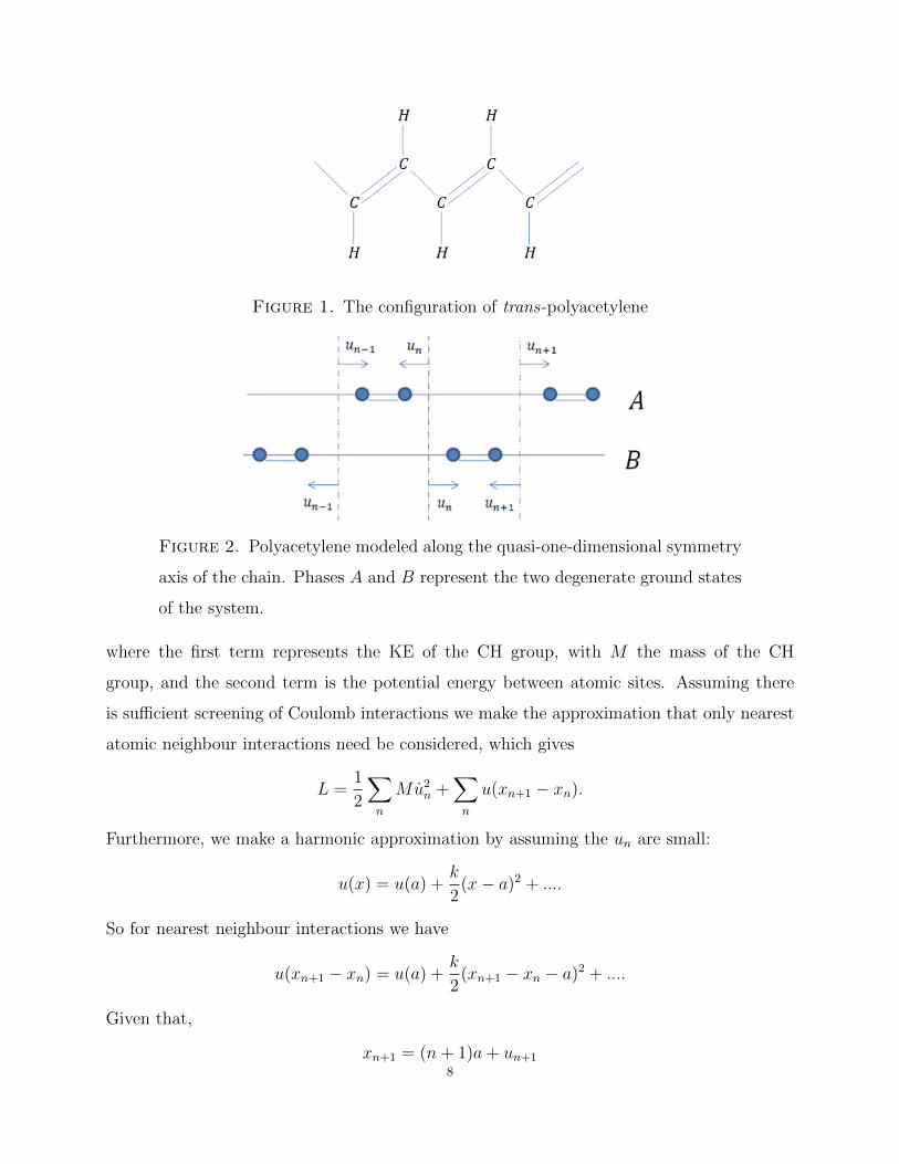
Figure 1. The configuration of trans-polyacetylene

Figure 2. Polyacetylene modeled along the quasi-one-dimensional symmetry

axis of the chain. Phases A and B represent the two degenerate ground states

of the system.

where the first term represents the KE of the CH group, with M the mass of the CH

group, and the second term is the potential energy between atomic sites. Assuming there

is sufficient screening of Coulomb interactions we make the approximation that only nearest

atomic neighbour interactions need be considered, which gives

L =1

2

∑n

Mu2n +

∑n

u(xn+1 − xn).

Furthermore, we make a harmonic approximation by assuming the un are small:

u(x) = u(a) +k

2(x− a)2 + ....

So for nearest neighbour interactions we have

u(xn+1 − xn) = u(a) +k

2(xn+1 − xn − a)2 + ....

Given that,

xn+1 = (n+ 1)a+ un+1

8

and

xn = na+ un,

then

u(xn+1 − xn) = u(a) +k

2(un+1 − un)2 + ...

which gives the approximation

L = Nu(a) +1

2

∑n

Mu2n +

k

2

∑n

(un+1 − un)2

where the first term will be ignored since it is included in the cohesion energy.

Including hopping energy between nearest atomic neighbours the Hamiltonian is

H = −∑nσ

(t1 − α(un+1 − un))(c†(n+1),σcn,σ + c†n,σc(n+1),σ) + L

where c†nσ, cn,σ are the creation and annihilation operators, respectively, for electrons on the

n-th site with spin σ = ±1/2, and t1 and α are some constants. This Hamiltonian is known

as the Su-Schrieffer-Heeger (SSH) model. The Born-Oppenheimer approximation has been

used in this model, which assumes the ions to be “frozen” in their equilibrium positions. For

perfectly dimerized polyacetylene, un = (−1)nu, the Lagrangian is

L =∑n

k

2(−1)n2(−u− u)2 =

∑n

k4

2u2 = 2Nku2.

In order to get our Hamiltonian into a form that resembles the Dirac equation we will ignore

this constant term: we will ignore the PE between nearest neighbour atoms. This leaves,

H = −∑nσ

(t1 + α(−1)n2u)(c†(n+1),σcn,σ + c†n,σc(n+1),σ).

Let t2 = α2u, then

H = −∑nσ

(t1 + t2(−1)n)(c†(n+1),σcn,σ + c†n,σc(n+1),σ).

Also, let the operators be off by a phase: cn = inan and c†n = (−i)na†n, giving,

H = i∑nσ

(t1 + t2(−1)n)(a†(n+1),σan,σ − a†n,σa(n+1),σ).

Notice that the hopping constants alternate, between t1 + t2 and t1 − t2, so the chain now

has an overall lattice constant of 2a and we can model the N -site chain as an N/2-site even9

system plus an N/2-site odd system. Hopping between shorter bonds has a larger probability,

|t1 + t2|2, than hopping between longer bonds, |t1 − t2|2, as expected

H = i∑nσ

((t1 + t2)(a†(2n+1),σa2n,σ − a†2n,σa(2n+1),σ) + (t1 − t2)(a†2n,σa(2n−1),σ − a†(2n−1),σa2n,σ)).

Since the even and odd atomic sites are different the even and odd creation and annihilation

operators must be different. Transforming to k-space these operators are

a2n,σ =1√N

∑k

eik2naak,σ

and

a(2n+1),σ =1√N

∑k

eik(2n+1)abk,σ.

For our model we ignore the spin of the electron, therefore

H =i

N

∑n,k,k′

((t1 + t2)(e−ik(2n+1)ab†keik′2naak′ − e−ik

′2naa†k′eik(2n+1)abk)

+ (t1 − t2)(e−ik′2naa†k′e

ik(2n−1)abk − e−ik(2n−1)ab†keik′2naak′)).

Using the property 1N

∑n e

i(k−k′)n = δk,k′ , then

H = i∑k

((t1 + t2)(e−ikab†kak − eikaa†kbk) + (t1 − t2)(e−ikaa†kbk − e

ikab†kak)).(8)

If we had Periodic Boundary Conditions (PBCs) on our system, so that site 1 ≡ N + 1, then

aN+1 =1√N

∑k

eik(N+1)aak → a1 =1√N

∑k

eikaak

so we need

eikNa = 1

kNa = 2πn

k =2πn

Na

where n → −N2...N

2for unique solutions, therefore k ∈ (−π

a, πa]. In Sec.5 we find that the

energy momentum relationship for the scattering states of the Dirac equation solved on the

segment are: E = mcos kL

and E2 = m2 + k2. These energy momentum relationships can be

combined to give a restriction on k,

k = m tan (kL),10

which can have an infinite number of unique solutions as L → ∞. So we do not have a

Brillion zone in our case. However, as we will see below, the Dirac equation approximates

the Hamiltonian of polyacetylene for only small values of k, so not having a Brillion zone

should not be a problem.

To transition from a discrete to continuous spectrum we write∑k

f(k)→ L

2π

∑k

f(k)δk =Na

2π

∑k

f(k)δk → Na

2π

∫f(k)dk

therefore our Hamiltonian in Eqn.8 can be written as

H =L

2π

∫i((t1 + t2)(e−ikab†kak − e

ikaa†kbk) + (t1 − t2)(e−ikaa†kbk − eikab†kak))dk.

Writing the Hamiltonian in matrix form

H =L

2π

∫ 0 i(−eika(t1 + t2) + e−ika(t1 − t2))

i(e−ika(t1 + t2)− eika(t1 − t2)) 0

dkwhere the top component of a vector in this basis represents an electron on an even atomic

site and the bottom component represents an electron on an odd atomic site. Simplifying

the Hamiltonian

H =L

2π

∫ 0 i(−t12i sin (ka)− t22 cos (ka))

i(−t12i sin (ka) + t22 cos (ka)) 0

dk.Finding the energy eigenvalues of our Hamiltonian from det(H − EI) = 0 gives

E2 = t214 sin2 (ka) + t224 cos2 (ka).

Since t2 = α2u we can see that with Peierls instability, u 6= 0, polyacetylene is a semicon-

ductor, however in its undimerized state, u = 0, it is a conductor. For small k: sin (ka) ' ka

and cos (ka) ' 1 therefore

H =L

2π

∫ 0 i(−t12i(ka)− t22)

i(−t12i(ka) + t22) 0

dk.Choose t22 = m and at12 = 1, then

H =L

2π

∫ 0 k − im

k + im 0

dk.(9)

11

Notice in this form the energy eigenvalues of the Hamiltonian are

E2 − (k + im)(k − im) = 0→ E2 = k2 +m2

which is what we expect for the energy eigenvalues of the relativistic Dirac equation. Here

we can see that dimerized polyacetylene is an insulator with a mass gap of size “m” in the

electronic spectrum. Converting from position to momentum space, using the fact that k = p

in natural units, we replace

k = −i ddx

in Eqn.9

H =L

2π

∫ 0 −i ddx− im

−i ddx

+ im 0

dx.So we see that the Dirac equation allows for an electron travelling on polyacetylene to

be viewed as a relativistic particle travelling in free space, if we give it the effective mass

m rather than the true electron mass me. This viewpoint is equivalent to determining the

equation of motion of the electron with its true electron mass, me, existing on polyacetylene

with all of the forces the polymer is actually exerting on it.

12

4. The Dirac Equation on the Half-Line

4.1. Bound and Scattering States. Using the results of Sec.2 we can write the 1-dimensional

time independent Dirac equation as

(−iα1 d

dx+ γ0m)ψ(x) = Eψ(x)

where ψ(x) is the Dirac spinor, and α1 and γ0 must satisfy

(γ0)2 = (α1)2 = I, {α1, γ0} = 0.

The Pauli matrices, σn, and the identity, I, satisfy these requirements. Since all 2 × 2

Hermitian matrices can be written as linear combinations of σn and I, they are a natural

choice for α1 and γ0. Choosing α1 = σx and γ0 = σz gives the Hamiltonian

H = −i ddxσx +mσz =

m −i ddx

−i ddx−m

(10)

which is related to the Hamiltonian we found in Sec.3,

H ′ = −i ddxσx +mσy =

0 −i ddx− im

−i ddx

+ im 0

,by a simple rotation. The Pauli matrices can be rotated into each other by the following

operation

H = e−i(n·~σ)φ/2H ′ei(n·~σ)φ/2.

Using the identity

ei(n·~σ)φ/2 = I cosφ/2 + i(n · ~σ) sinφ/2

where

n = Pauli axis of rotation

φ = angle of rotation.

In our case n = x and φ = π/2 so we can write the rotation as

ei(n·~σ)φ/2 = I1√2

+ iσx1√2.

13

The rotation can be seen by considering the property of Pauli matrix multiplication: σaσb =

δab + iεabcσc. Therefore, the spinors of the two Hamiltonians are related by

e−i(n·~σ)φ/2ψ′(x) =1√2

1 −i

−i 1

u′(x)

v′(x)

=1√2

u′(x)− iv′(x)

−iu′(x) + v′(x)

= ψ(x)

where in Sec.3 we saw that u′(x) and v′(x) represent the even and odd atomic wave functions,

respectively, of dimerized polyacetylene at location x.

The eigenvalue equation of H is m −i ddx

−i ddx−m

u(x)

v(x)

= E

u(x)

v(x)

which is equivalent to the two equations

(m− E)u(x)− i ddxv(x) = 0(11)

and

−i ddxu(x)− (m+ E)v(x) = 0.(12)

We can solve Eq.11 for u(x)

u(x) =−i

E −md

dxv(x)

and substitute u(x) into Eq.12 to get(p2 +

d2

dx2

)v(x) = 0

where p2 = E2 −m2. For the bound state solutions, |E| < m, we make the ansatz

v(x) = Aeipx +Be−ipx = Ae−kx +Bekx,

u(x) =−ikE −m

(−Ae−kx +Bekx),

E = ±ω(k), ω(k) ≡√−k2 +m2, p = ik.

In order to have a normalizable wave function we must set B = 0, therefore

ψBk= A

ikE−m

1

e−kx.(13)

14

We must ensure that the Hamiltonian remains Hermitian on the half line, a requirement

that places a restriction on the possible boundary conditions. An operator is Hermitian if

< ψ|Hψ >=< Hψ|ψ >,

therefore using our time independent 1-D Dirac equation, equate

< ψ|Hψ >=

∫ ∞0

[u(x)∗ v(x)∗

] m −i ddx

−i ddx−m

u(x)

v(x)

dxand

< Hψ|ψ >=

∫ ∞0

(

m −i ddx

−i ddx−m

u(x)

v(x)

)†

u(x)

v(x)

dxwhich leads to the following boundary condition

0 = (u(x)∗v(x) + v(x)∗u(x))∣∣∣∞0.

From here we see that the Dirac current, u(x)∗v(x)+v(x)∗u(x), must vanish at the boundaries

in order for the Dirac equation to be Hermitian. At infinity the current vanishes since

u(x) and v(x) are assumed to be square integrable, therefore the only remaining boundary

condition is

u∗(0)v(0) + v∗(0)u(0) = 0.

A boundary condition which would satisfy this is

u(0) = −iv(0).(14)

Applying Eqn.14 to the wave function solution in Eqn.13 leads to the following restriction

on the possible momentum values

k = m−√−k2 +m2.

Considering all the positive and negative momentum states the boundary condition is sat-

isfied by our bound state only when k = 0 and k = m. However, k = 0 gives the E = |m|

constant function throughout space, so this cannot be a solution. The k = m solution gives

the normalized wave function for E = 0

ψB = ψ0 =√m

−i1

e−mx.(15)

15

The larger the mass gap of the wire, m, the steeper the wave function’s incline to its peak

at the edge of the wire and the closer it hugs the axis away from the edge. Having a

zero energy solution is a surprising result, one that Dirac did not predict when originally

developing the Dirac equation. Therefore, he did not include a zero energy state in his Dirac

sea interpretation, so there is a question of whether this state should be empty or filled.

To transfer from bound to scattering state equations, |E| > m, all we need to do is replace

ik → k which is equivalent to replacing k → −ik.

v(x) = Aeikx +Be−ikx,

u(x) =k

E −m(Aeikx −Be−ikx),

E = ±ω(k) , ω(k) =√k2 +m2, k = p.

As with the bound state wave functions, take the boundary condition of u(0) = −iv(0). This

leads to the relationship between the constants

A =(q − i)(q + i)

B

where we have defined q = kE−m , giving the scattering state wave functions

ψS = B

q( (q−i)(q+i)

eikx − e−ikx)(q−i)(q+i)

eikx + e−ikx

(16)

which oscillate throughout the wire.

In Appx.A we find B = ((q2 +1)2π)−1/2 when the wave function is Dirac normalized along

the half line ∫ ∞0

ψ†SkψSk′

dx = δ(k − k′)

and in Appx.B the bound and scattering states, Eqns.15 and 16, are used to show complete-

ness of the solutions of the system∫ ∞−∞

ψxψ†x′dk = Iδ(x− x′).

As we wish to analyze many particle systems of electrons we employ the above single

particle wave functions in second quantization formulation. The second quantization field16

operator for a complex fermionic state, relativistic or non-relativistic, is

Ψ(x, t) =∑E>0

ψE(x)e−iEtaE +∑E<0

ψE(x)e−iEtb†−E(17)

where aE is the annihilation operator for a particle with energy E and b†−E is the creation

operator for a hole with energy −E. The operators obey the anticommutator relationships,

{aE, a†E′} = δEE′ , {bE, b†E′} = δEE′ ,

and ψE(x) are the eigenstates of the Hermitian Hamiltonian, H0, for a single non-interacting

particle

H0ψE(x) = EψE(x).

The full wave functions satisfy the Schrodinger equation

i∂

∂tΨ(~x, t) = H0Ψ(~x, t)

and for Ψ(~x, t) to be a second quantized field operator it must also obey the equal-time

anticommutation relation

{Ψ(~x, t),Ψ(~y, t)} = δ(~x− ~y).

Considering the Dirac sea interpretation the ground state of the system has all negative

energy states filled and all positive energy states empty

aE|0 >= 0 = bE|0 > .

The excited states of the system result from creating particles and holes in the ground state,

giving them the form

a†E1...a†Em

b†E1...b†En

|0 > .

Together with the ground state these excited states form a basis for the Fock space of second

quantization theory.17

4.2. Charge Conjugation and the Majorana Fermion. Charge conjugation is an op-

eration where all particles are replaced by their antiparticles, and visa versa,

ψE(x)→ Cψ∗−E(x)

where C is a t-independent matrix that must satisfy the relationships −CH∗ = HC and

C∗C = CC∗ = I. This can be seen by considering the Schrodinger equation

i∂

∂tΨE(x, t) = HΨE(x, t) = EΨE(x, t).(18)

Taking the complex conjugate of Eqn.18 and multiplying it from the left by matrix C gives

i∂

∂tCΨ∗E(x, t) = −CH∗Ψ∗E(x, t) = −ECΨ∗E(x, t).(19)

Therefore CΨ∗E(x, t) satisfies the Dirac equation if ΨE(x, t) satisfies the Dirac equation and

C has the property

−CH∗ = HC.

Assuming the Hamiltonian is t-independent then from Eqn.19 we have

HCψ∗E(x) = −ECψ∗E(x).

Therefore we need ψE(x) → Cψ∗−E(x) for charge to change sign but energy to remain the

same: for the particles and antiparticles to swap. So the energy spectrum of the particle

states is the same as the antiparticle states, but charge is opposite. When this occurs

the Hamiltonian is said to have a charge conjugation symmetry, or particle-antiparticle

symmetry. A particle is said to be self-conjugate if it satisfies

ψE(x) = ±Cψ∗−E(x)(20)

that is the particle is its own antiparticle. When considering the E = 0 case this condition

implies that C must also have the property

C∗C = CC∗ = I.

Self-conjugate fermions are called Majorana fermions. Italian physicist Ettore Majorana

first postulated the Majorana fermion in 1937, as a means to avoid the negative energy states

in the Dirac sea, by identifying the positive and negative energy states as manifestations of

the same excited state [10]. He originally developed the Majorana theory in the context

of particle physics, however most modern day Majorana research takes place in condensed18

matter physics where Majorana quasiparticle states are sought out. Unlike charged particles

and antiparticles which have complex quantum fields, neutral particles that are their own

antiparticles have real fields. The neutral spin-zero pion and the spin-one photon are exam-

ples of bosonic neutral self-conjugate particles. The complex electron field that has a charge

conjugation symmetry can be split into two emergent Majorana fermions by treating the

particle and antiparticle with the same energy as a single excitation: the real and imaginary

components, Re(ψE(x)) and Im(ψE(x)) respectively, of the complex fermion:

Re(ψE(x)) =1

2(ψE(x) + Cψ∗−E(x))

and

Im(ψE(x)) =1

2i(ψE(x)− Cψ∗−E(x)).

Since these linear combinations are self-conjugate

(ψE(x)± Cψ∗−E(x)) = ±C(ψ−E(x)± Cψ∗E(x))∗

both solutions are considered to be emergent Majorana fermions. When a Hamiltonian has

a charge conjugation symmetry it is always possible to impose this mathematical constraint

that decomposes the electron into two Majorana fermions. However, this constraint is not

easily held in reality as these states are not eigenstates of the full Hamiltonian of quantum

electrodynamics. Once decomposing the wave function into its real and imaginary parts

quantum fluctuations re-mix them very quickly: there is no accessible time frame in which

they stay unmixed. This mixing is due to electromagnetic interactions of the system causing

very quick emission and absorption of low energy photons. Therefore, in order to maintain

a Majorana mode this mixing must be damped. This is why superconductors are presently

used to find Majorana fermions, as they stop photons, or at least low energy photons, from

interacting with the electron [11].

An emergent Majorana state can, however, be sustainable if the system is self conjugate:

ψE(x) = ±Cψ∗−E(x). The wave function of a complex fermion can always be written as

ψE(x) = Re(ψE(x)) + iIm(ψE(x)) = 1/2(ψE(x) +Cψ∗−E(x)) + 1/2(ψE(x)−Cψ∗−E(x)), there-

fore if the state is self conjugate the wave function is either purely real, ψ(x) = Re(ψE(x)),

or purely imaginary, ψ(x) = iIm(ψE(x)). So the degrees of freedom is reduced in half for19

a Majorana fermion. Quantum computing has already been making use of single-particle

states which obey a Majorana condition [12]-[14].

Since particles and antiparticles with the same energy are equivalent for a Majorana

fermion, they are treated as a single excitation: the fermion does not have both particles

and antiparticles. Therefore the second quantization field operator is

Ψ(x, t) =∑E>0

(ψE(x)e−iEtaE + Cψ∗E(x)eiEta†E)(21)

where the creation and annihilation operators satisfy the algebra

{aE, a†E′} = δEE′ .

The ground state is annihilated by all annihilation operators,

aE|0 >= 0 ∀aE,

and the excited states come from the creation operators, a†E, acting on the ground state,

a†E1a†E2

...a†Ek|0 > .

The field operator obeys the anticommutation relation

{Ψ(x, t), Ψ†(y, t)} = δ(x− y)

and is considered to be pseudo-real since it obeys

Ψ(x, t) = CΨ∗(x, t).

If the Majorana fermion had a single zero mode then the second quantization field operator,

Eqn.21, would have an additional zero mode term

Ψ(x, t) = ψ0(x)α +∑E>0

(ψE(x)e−iEtaE + Cψ∗E(x)eiEta†E)

where the zero mode operator α is real, α = α†, and satisfies the algebra

α2 = 1/2, {α, aE} = 0 = {α, a†E}.

For our Dirac Hamiltonian on the half line, given in Eqn.10, the charge conjugation matrix

is

C =

0 i

i 0

20

as it satisfies the requirement −CH∗ = HC. Therefore, in our system, charge conjugation

maps the wave function as

ψ(x) =

u(x)

v(x)

→iv∗(x)

iu∗(x)

.In Sec.4.1 we solved the system with the boundary condition u(0) = −iv(0). This boundary

condition allows the Dirac equation to remain Hermitian on the half line. Charge conju-

gation, ψ(x) → Cψ∗(x), doesn’t change the relationship between u(x) and v(x), so the

antiparticle also satisfies the boundary condition if it is satisfied by the particle. Looking at

charge conjugation of the bound state found in Sec.4.1

ψ0 =√m

−i1

e−mxwe see that it is an eigenstate of charge conjugation

Cψ∗0 =√m

i

−1

e−mx = −ψ0.

Therefore, the zero mode is an emergent Majorana fermion! Next look at the scattering

states found in Sec.4.1

ψS = B1

(q + i)

q((q − i)eikx − (q + i)e−ikx)

(q − i)eikx + (q + i)e−ikx

where q = k

E−m and B = ((q2 + 1)2π)−1/2. They are not eigenstates of charge conjugation

Cψ∗S = Bi

(q − i)

(q + i)e−ikx + (q − i)eikx

q((q + i)e−ikx − (q − i)eikx)

6= ±ψS.Since the only self-conjugate state is the zero mode the second quantization field operator

of our system is complex (not Majorana), with the form

Ψ(x, t) = ψ0(x)α +∑E>m

ψE(x)e−iEtaE +∑E<−m

ψE(x)e−iEtb†−E

where the zero mode operator obeys the algebra

{α, α†} = 1(22)

21

and anticommutes with all other creation and annihilation operators of the system. Having

a zero mode with this algebra leads to a degeneracy of the fermion spectrum. The ground

state must still be annihilated by all of the annihilation operators, aE and bE ∀E > m, but

now the algebra of the zero mode, Eqn.22, must also be satisfied. This leads to a degeneracy

of the spectrum since the minimal representation of the algebra is two dimensional: there

are two ground states, |+ > and |− >, which satisfy the properties

aE|+ >= 0 = aE|− >, bE|+ >= 0 = bE|− >

and

α†|− >= |+ >, α†|+ >= 0,

α|− >= 0, α|+ >= |− > .

Therefore, the degenerate excited states of the system have the form

a†E1...a†Em

b†E1...b†En

|− >

and

a†E1...a†Em

b†E1...b†En

|+ > .

Due to the Dirac Hamiltonian satisfying charge conjugation the energy spectrum of the

particles and holes are the same, but with opposite charge. The particle and hole state of

the zero mode differ by a charge of one, so for the two states to have opposite charge the hole

state must have charge −1/2 and the particle state must have charge 1/2: fractional charge

[15]-[17]. There has been experimental confirmation of this unexpected result of charge

fractionalization by observing that it explains some of the unique features of polyacetylene.

Charge conjugation demands that only particle/hole pairs with the same energy can be lifted

into each other, so the Dirac sea remains at the same energy but with opposite charge. This

makes the zero mode of the spectrum of great interest to quantum computation since it is

topologically protected: perturbing the system respects charge conjugation symmetry, so the

zero mode state cannot be lifted because it has no pair to be lifted to.

Since having an electron in an isolated zero mode state holds so much appeal the next

subsection focuses on how the parameters of our quantum wire system on the half-line can

be modified so that an electron interacting with the system would preferably occupy the

empty zero mode state rather than an empty scattering state.22

4.3. Zero Mode Coupling. For the electron source of our system we will use a scanning

tunnelling microscope (STM). We are only interested in how strongly the zero mode, ψ0,

is coupled to the STM wave function, ψT , verses the scattering states, ψk, so to model the

coupling we can just consider the overlap of the wave functions. For example, the coupling

of the bound state will be

c0 =

∫ψ†Tψ0d

3x · h.c.

where h.c. is the Hermitian conjugate of the integral.

As an approximation the tip can be modelled locally as an asymptotic spherical potential

well

V (r) = 0 if r < a,

= V1 if r > a

and solved for the bound, Et < V1, asmyptotic, r →∞, solution of the Schrodinger equation

to get

ψT = A1

k1|~r − ~r0|e−k1|~r−~r0|(23)

where k1 =√

2M(V1 − Et) is the wave number of the tip electron, M is the mass of the

electron, A is a normalization constant, and ~r0 is the center of the spherical well potential.

Normalizing the wave function gives

A =

√k3

1

2π.

The tunnelling current, I, measured from an STM tip depends on 4 variables: x, y, z,

and V . Where V is a bias voltage applied to the STM tip, or sample, causing the Fermi

level of the tip to be a higher energy than the Fermi level of the sample so that tunnelling

occurs from tip to sample, or visa versa. The most common use of STM measurements is

to reveal the topography of a surface of a material by holding I and V constant, V being a

bias voltage to cause tunnelling from sample to STM tip, and measuring the z at each x, y

location that is needed to keep I constant. In other words “z” is not exactly the “height

of the surface”, but rather the tip-sample separation needed for the tunnelling current to

remain constant at a fixed bias voltage. Another common use for STM measurements is to

understand the density of states of the surface of a material. In this case the I and z are23

held fixed, and the bias V changes at each x, y location as needed so that the tunnelling

current from sample to tip remains constant.

In our case the role we want the STM tip to play is simply an electron source at the edge

of the quantum wire. In Sec.4.1 we found that the bound state solution on the half line

is peaked at the end of the quantum wire, and the scattering states oscillate throughout

the quantum wire. Since we wish to couple an electron on the STM tip to the bound state

mode, we make the approximation that the STM tip can be centered on the quantum wire

axis and brought in proximity to the end of the quantum wire. Assuming the quantum wire

lies along the z axis we take x = y = 0 and apply a bias voltage V0 to the tip, therefore

Et → Et + V0, then for a fixed I the system would measure some value z = z0. Since

we are considering a theoretical toy model of the system, and not actually performing any

experimental measurements, we make a best guess at what z0 would be knowing that z0

typically ranges from 4-7 A.

We assume the electron wave functions on the quantum wire are separable: ψ0(z)ψ⊥(ρ, φ)

and ψS(z)ψ⊥(ρ, φ). When the electron is on the quantum wire it acts as a relativistic particle

moving through a vacuum, in the z direction, with an emergent mass, m, equal to the mass

gap of the quantum wire. However, when removed from the quantum wire the electron acts

as a non-relativistic particle with its true electron mass M . The electrons are bound to the

quantum wire in the perpendicular ρ, φ direction, so in analog to the bound STM wave

function we estimate the perpendicular bound states by solving the Schrodinger equation

with a circular potential well. The Schrodinger equation with a circular potential is

V (ρ) = 0 if ρ < a,

= V2 if ρ > a.

Since quantum wires are quasi 1-dimensional let a→ 0, so we are only interested in the wave

function in the region ρ > a. We wish to find the bound state wave functions, because we

want the electrons to be bound to the wire, so we only consider the case Ew < V2 where Ew

is the energy of an electron on the quantum wire.

The Schodinger equation we must solve is

− 1

2M(1

ρ

∂

∂ρ(ρ∂

∂ρ) +

1

ρ2

∂2

∂φ2)ψ(ρ, φ) = (Ew − V2)ψ(ρ, φ)

24

where we use the true mass of the electron, M , because we are solving for the wave function

outside of the quantum wire ρ > a. Using separation of variables ψ⊥(ρ, φ) = R(ρ)Φ(φ), gives

− 1

2M(

1

ρR(ρ)

∂

∂ρ(ρ∂R(ρ)

∂ρ) +

1

ρ2

1

Φ(φ)

∂2Φ(φ)

∂φ2) = (Ew − V2).(24)

Let −α2 be the separation constant

1

Φ(φ)

∂2Φ(φ)

∂2φ= −α2,

which has the solution

Φ(φ) = Aeiαφ(25)

where A is the normalization constant and α = ... − 1, 0, 1... so that the solution is single-

valued under φ-rotations of 2π. Substituting Eqn.25 into Eqn.24 gives

− 1

2M(

1

ρR(ρ)

∂

∂ρ(ρ∂R(ρ)

∂ρ) +

1

ρ2B−1e−iαφ(iα)2Beiαφ) = (Ew − V2)

− 1

2M(ρ∂

∂ρ(ρ∂R(ρ)

∂ρ) +R(ρ)(iα)2) = ρ2R(ρ)(Ew − V2)

ρ2∂2R(ρ)

∂ρ2+ ρ

∂R(ρ)

∂ρ+ (k2

2ρ2 − α2)R(ρ) = 0, ρ > a where k2

2 = 2M(Ew − V2).(26)

Since we are in a bound state, Ew < V2, k2 is imaginary. Eqn.26 is a Bessel equation,

therefore the general solution is

R(ρ) = BJα(k2ρ), ρ > a(27)

where B is a normalization constant. Using Eqns.25 and 27

ψ⊥(ρ, φ) = R(ρ)Φ(φ) = ABJα(k2ρ)eiαφ, ρ > a.

Since we are considering a spherically symmetric potential we want the solution to have

no angular dependence, so we choose α = 0. For every fixed α the infinite sequence of

eigenfunctions Jα(k2ρ) are normalizable on the infinite interval as∫ ∞0

Jα(k′2ρ)Jα(k2ρ)ρdρ =δ(k2 − k′2)

k2

,

therefore our normalized solution is

ψ⊥(ρ, φ) = Jα(k2ρ), ρ > a(28)

where k2 = ±√

2M(Ew − V2).25

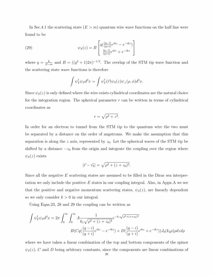
In Sec.4.1 the scattering state (E > m) quantum wire wave functions on the half line were

found to be

ψS(z) = B

q( (q−i)(q+i)

eikz − e−ikz)(q−i)(q+i)

eikz + e−ikz

(29)

where q = kE−m and B = ((q2 + 1)2π)−1/2. The overlap of the STM tip wave function and

the scattering state wave functions is therefore∫ψ†TψSd

3x =

∫ψ†T (~r)ψS(z)ψ⊥(ρ, φ)d3x.

Since ψS(z) is only defined where the wire exists cylindrical coordinates are the natural choice

for the integration region. The spherical parameter r can be written in terms of cylindrical

coordinates as

r =√ρ2 + z2.

In order for an electron to tunnel from the STM tip to the quantum wire the two must

be separated by a distance on the order of angstroms. We make the assumption that this

separation is along the z axis, represented by z0. Let the spherical waves of the STM tip be

shifted by a distance −z0 from the origin and integrate the coupling over the region where

ψS(z) exists

|~r − ~r0| =√ρ2 + (z + z0)2.

Since all the negative E scattering states are assumed to be filled in the Dirac sea interpre-

tation we only include the positive E states in our coupling integral. Also, in Appx.A we see

that the positive and negative momentum scattering states, ψS(z), are linearly dependent

so we only consider k > 0 in our integral.

Using Eqns.23, 28 and 29 the coupling can be written as∫ψ†TψSd

3x = 2π

∫ ∞0

∫ ∞0

A1

k1

√ρ2 + (z + z0)2

e−k1√ρ2+(z+z0)2

B(Cq((q − i)(q + i)

eikz − e−ikz) +D((q − i)(q + i)

eikz + e−ikz))J0(k2ρ)ρdzdρ

where we have taken a linear combination of the top and bottom components of the spinor

ψS(z), C and D being arbitrary constants, since the components are linear combinations of26

the even and odd atomic wave functions of polyacetylene at location z. Scaling the variables:

ρ→ ρk2

and z → zk1

does not change the limits but dρ→ 1k2dρ and dz → 1

k1dz∫

ψ†TψSd3x = 2π

A

k1k22

∫ ∞0

∫ ∞0

1

k1

√( ρk2

)2 + ( z+z0k1

)2e−k1√

(ρ/k2)2+((z+z0)/k1)2

B(Cq((q − i)(q + i)

eikz/k1 − e−ikz/k1) +D((q − i)(q + i)

eikz/k1 + e−ikz/k1))J0(k2ρ

k2

)ρdzdρ

∫ψ†TψSd

3x = 2πA

k1k22

∫ ∞0

∫ ∞0

1√(k1ρk2

)2 + (z + z0)2e−√

(k1ρ/k2)2+(z+z0)2

B(Cq((q − i)(q + i)

eikz/k1 − e−ikz/k1) +D((q − i)(q + i)

eikz/k1 + e−ikz/k1))J0(ρ)ρdzdρ.

There should be a lot less tunnelling from the perpendicular components of the wire, there-

fore from the STM tip we need k1 =√

2M(V1 − Et) << |k2| =√

2M(V2 − Ew), so k1|k2| << 1,

and we can make the approximation:√

(k1ρk2

)2 + (z + z0)2 =√−( k1ρ|k2|)

2 + (z + z0)2 ≈ (z+z0).

Then,∫ψ†TψSd

3x = 2πA

k1k22

∫ ∞0

∫ ∞0

1

z + z0

e−(z+z0)

B(Cq((q − i)(q + i)

eikz/k1 − e−ikz/k1) +D((q − i)(q + i)

eikz/k1 + e−ikz/k1))J0(ρ)ρdzdρ

∫ψ†TψSd

3x = 2πA

k1k22

∫ ∞0

∫ ∞0

1

z + z0

e−(z+z0)B((q − i)(q + i)

(Cq+D)eikz/k1+(−Cq+D)e−ikz/k1)J0(ρ)ρdzdρ

∫ψ†TψSd

3x = 2πA

k1k22

B((q − i)(q + i)

(Cq +D)I1 + (−Cq +D)I2)

where

I1 =

∫ ∞0

∫ ∞0

1

z + z0

e−(z+z0)eikz/k1J0(ρ)ρdzdρ,

I2 =

∫ ∞0

∫ ∞0

1

z + z0

e−(z+z0)e−ikz/k1J0(ρ)ρdzdρ.

In order for the above integrals to converge we must take the upper limit of ρ to be

finite. Since there is minimal tunnelling of the electrons from the quantum wire to the

surrounding vacuum taking a finite upper limit should have minimal effect on the overall

integral. Typically z0 ranges from 4-7 A for tunnelling from STM tip to sample, therefore27

taking an upper limit of ρ = 10m should be more than sufficient. These integrals are solved

using Mathematica:

I1 =

∫ 10

0

e−ikz0/k1J0(ρ)(Γ(0, z0−ikz0/k1)−Log(1−ik/k1)+Log(1/z0)+Log(z0−ikz0/k1))ρdρ

which is a conditional expression of the z integral that is satisfied since Re[z0] > 0 and

Im[k/k1] = 0 > −1,

I1 = 10e−ikz0/k1J1(10)(Γ(0, z0 − ikz0/k1)− Log(1− ik/k1) + Log(1/z0) + Log(z0 − ikz0/k1)).

Similarly,

I2 =

∫ 10

0

eikz0/k1J0(ρ)(Γ(0, z0 + ikz0/k1)−Log[1 + ik/k1] + Log[1/z0] + Log[z0 + ikz0/k1])ρdρ

which is a conditional expression of the z integral that is satisfied since Im[k/k1] = 0 <

1 and Re[z0] > 0,

I2 = 10eikz0/k1J1(10)(Γ(0, z0 + ikz0/k1)− Log(1 + ik/k1) + Log(1/z0) + Log(z0 + ikz0/k1)).

Depending on the state of the system an electron is either annihilated on the STM tip and

created in a scattering state, or the reverse occurs. Therefore, the interaction Hamiltonian

for the scattering states is

Hint =

∫(ckα

†EtaE + c∗ka

†EαEt)dk,

where the coefficent can be approximated as

ck = c∗k =

∫ψ†SψTd

3x

∫ψ†TψSd

3x.

To compare the size of this coefficient relative to the bound state coefficient we must integrate

over all possible k states in which the Hamiltonian of the system can be described by the

Dirac equation. In Sec.3 we found this to be the domain of k values where sin(ka) ≈ ka

and cos(ka) ≈ 1, with a being the lattice spacing of the chain. For simplicity take a to have

unit value, then we can approximate the Dirac equation to hold in the domain where k has

values less then 1/10th the sinusoidal period:

c =

∫ π/5

0

ckdk =

∫ π/5

0

∫ψ†SψTd

3x

∫ψ†TψSd

3xdk.(30)

28

As we see in Appx.B the positive and negative k states are linearly dependent on the half line,

therefore we only integrate over the positive momentum states. This integral is too compli-

cated to evaluate exactly, but since it is being integrated over a small domain Mathematica

can provide a numerical approximation of the integral.

In Sec. 4.1 the bound state (E < m) wave function for Dirac fermions on the half line was

found to be

ψB(z) =√m

−i1

e−mz.Following the same steps as we did for the scattering state coupling, the bound state coupling

is ∫ψ†TψBd

3x = 2πA

k1k22

∫ 10

0

∫ ∞0

1

z + z0

e−(z+z0)√m(−Ci+D)e−mz/k1J0(ρ)ρdzdρ∫

ψ†TψBd3x = 2π

A

k1k22

√m(−Ci+D)I3

where,

I3 =

∫ 10

0

∫ ∞0

1

z + z0

e−(z+z0)e−mz/k1J0(ρ)ρdzdρ.

Solving the integral in Mathematica gives

I3 =

∫ 10

0

emz0/k1J0(ρ)(Γ(0, (k1+m)z0/k1)−Log((k1+m)/k1)+Log(1/z0)+Log((k1+m)z0/k1))ρdρ

which is a conditional expression that is satisfied since Re[(k1+m)/k1] > 0 and 1+Re[m/k1] ≥

0 and Re[z0] > 0 and z0 6= 0 are all satisfied,

I3 = 10emz0/k1J1(10)(Γ(0, (k1+m)z0/k1)−Log((k1+m)/k1)+Log(1/z0)+Log((k1+m)z0/k1)).

The interaction Hamiltonian for the bound state is

Hint = c0α†Eta0 + c∗0a

†0αEt ,

where the coefficent is

c0 = c∗0 =

∫ψ†BψTd

3x

∫ψ†TψBd

3x.(31)

As we wish to obtain an isolated zero mode we are interested in how the parameters of

the system can be modified so that the bound state coupling, Eqn.31, dominates over the

scattering state coupling, Eqn.30. A promising variable to consider is the mass gap, m, of

the quantum wire, since the larger the mass gap the sharper the bound state is peaked at the

boundary. When deriving a Dirac-like equation from the Hamiltonian of polyacetylene in29

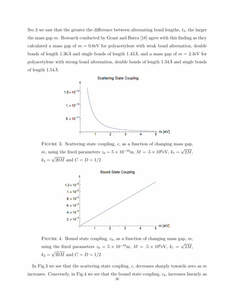
Sec.3 we saw that the greater the difference between alternating bond lengths, t2, the larger

the mass gap m. Research conducted by Grant and Batra [18] agree with this finding as they

calculated a mass gap of m = 0.8eV for polyacetylene with weak bond alternation, double

bonds of length 1.36A and single bonds of length 1.43A, and a mass gap of m = 2.3eV for

polyacetylene with strong bond alternation, double bonds of length 1.34A and single bonds

of length 1.54A.

Figure 3. Scattering state coupling, c, as a function of changing mass gap,

m, using the fixed parameters z0 = 5× 10−10m, M = .5× 106eV, k1 =√

2M ,

k2 =√

20M and C = D = 1/2

Figure 4. Bound state coupling, c0, as a function of changing mass gap, m,

using the fixed parameters z0 = 5 × 10−10m, M = .5 × 106eV, k1 =√

2M ,

k2 =√

20M and C = D = 1/2

In Fig.3 we see that the scattering state coupling, c, decreases sharply towards zero as m

increases. Conversely, in Fig.4 we see that the bound state coupling, c0, increases linearly as30

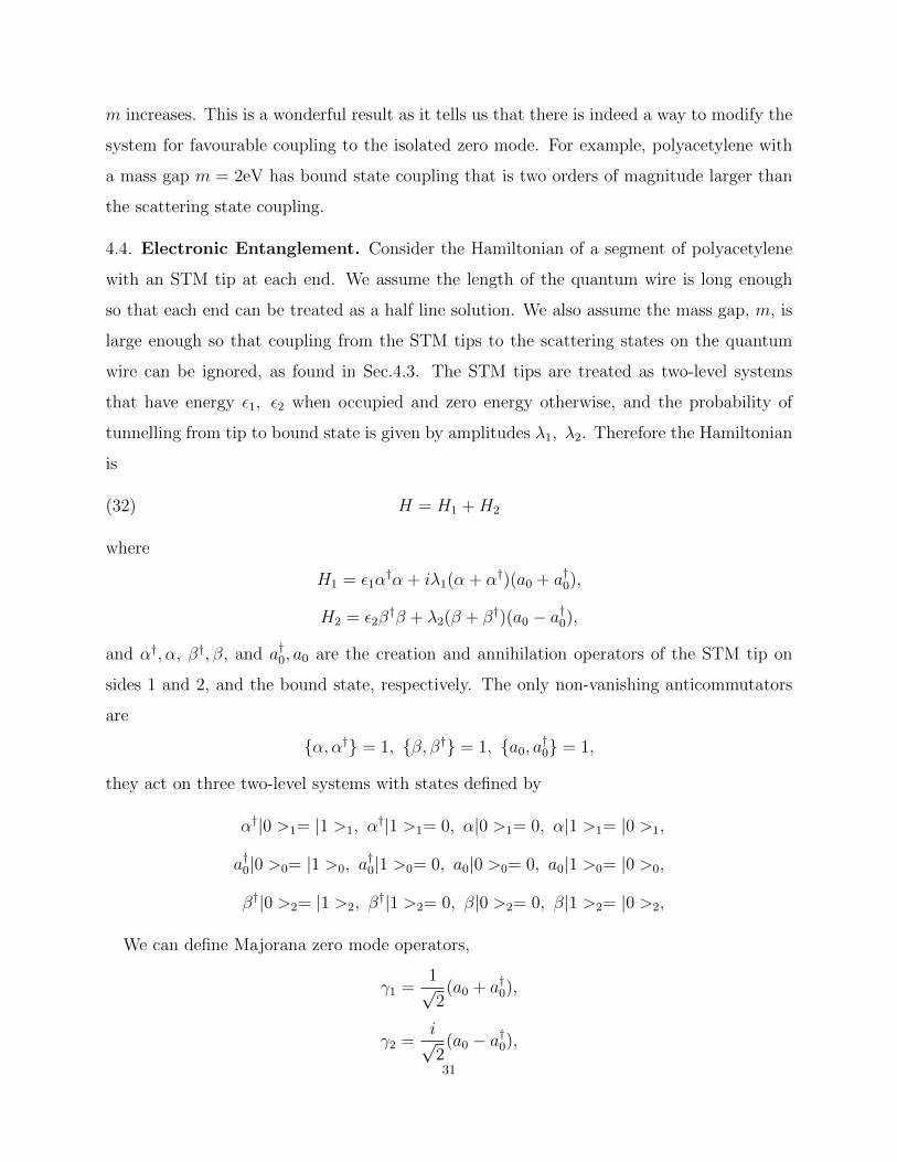
m increases. This is a wonderful result as it tells us that there is indeed a way to modify the

system for favourable coupling to the isolated zero mode. For example, polyacetylene with

a mass gap m = 2eV has bound state coupling that is two orders of magnitude larger than

the scattering state coupling.

4.4. Electronic Entanglement. Consider the Hamiltonian of a segment of polyacetylene

with an STM tip at each end. We assume the length of the quantum wire is long enough

so that each end can be treated as a half line solution. We also assume the mass gap, m, is

large enough so that coupling from the STM tips to the scattering states on the quantum

wire can be ignored, as found in Sec.4.3. The STM tips are treated as two-level systems

that have energy ε1, ε2 when occupied and zero energy otherwise, and the probability of

tunnelling from tip to bound state is given by amplitudes λ1, λ2. Therefore the Hamiltonian

is

H = H1 +H2(32)

where

H1 = ε1α†α + iλ1(α + α†)(a0 + a†0),

H2 = ε2β†β + λ2(β + β†)(a0 − a†0),

and α†, α, β†, β, and a†0, a0 are the creation and annihilation operators of the STM tip on

sides 1 and 2, and the bound state, respectively. The only non-vanishing anticommutators

are

{α, α†} = 1, {β, β†} = 1, {a0, a†0} = 1,

they act on three two-level systems with states defined by

α†|0 >1= |1 >1, α†|1 >1= 0, α|0 >1= 0, α|1 >1= |0 >1,

a†0|0 >0= |1 >0, a†0|1 >0= 0, a0|0 >0= 0, a0|1 >0= |0 >0,

β†|0 >2= |1 >2, β†|1 >2= 0, β|0 >2= 0, β|1 >2= |0 >2,

We can define Majorana zero mode operators,

γ1 =1√2

(a0 + a†0),

γ2 =i√2

(a0 − a†0),

31

where γ†1 = γ1 and γ†2 = γ2, and the only non-vanishing anticommutator is {γi, γ†j} = δij.

These properties can be seen by considering the fact that the bound state is a two-level

system, therefore a20 and a†

20 give zero when acting on the basis states. The bound state

wave function created and annihilated by a†0, a0 is peaked at each end of the quantum wire,

as we have combined two half line solutions. However, γ1 and γ2 create/annihilate particles

that exist at only one end of the quantum wire, ends 1 and 2 respectively.

Solving for the eigenvectors of H, Eqn.32, gives

ψσ,τ,η =(−iλ1η|0 >1 +E1,σ|1 >1)|η >0 (λ2η|0 >2 +E2,τ |1 >2)√

E21,σ + λ2

1

√E2

2,τ + λ22

where,

|η >0=1√2

(|0 >0 +η|1 >0), η = ±1

and the eigenvalues are,

E = E1,σ + E2,τ ,

Ei,σ =εi2

+ σ

√(εi2

)2

+ λ2i , σ = ±1.

Since Eiσ does not depend on η, the eigenstates ψσ,τ,1 and ψσ,τ,−1 have the same energy:

H(ψσ,τ,1 + ψσ,τ,−1) = Hψσ,τ,1 +Hψσ,τ,−1 = Eσ,τ (ψσ,τ,1 + ψσ,τ,−1).

Therefore instead of 8 eigenvalues we have 4, that is we have 4 two-fold degenerate levels.

Consider the general linear combination of degenerate states:

(Aψσ,τ,1 +Bψσ,τ,−1) = (−iλ1λ2(A+B)|0 >1 |0 >0 |0 >2 +E1σE2τ (A−B)|1 >1 |1 >0 |1 >2

−iλ1E2τ (A−B)|0 >1 |0 >0 |1 >2 −iλ1λ2(A−B)|0 >1 |1 >0 |0 >2 −iλ1E2τ (A+B)|0 >1 |1 >0 |1 >2

+E1σλ2(A−B)|1 >1 |0 >0 |0 >2 +E1σE2τ (A+B)|1 >1 |0 >0 |1 >2 +E1σλ2(A+B)|1 >1 |1 >0 |0 >2)

2−1/2(E21,σ + λ2

1)−1/2(E22,τ + λ2

2)−1/2.

At the quantum level fermion parity symmetry states that there is no physical process that

can create or destroy an isolated fermion: the number of fermions in the system is conserved

mod 2 [19]. Therefore, we can either set A = B for eigenstates with fermion number 0 mod32

2 or A = −B for eigenstates with fermion number 1 mod 2:

(33)

ψσ,τ |0mod2 = A(ψσ,τ,−1 + ψσ,τ,1) = A(−iλ1λ2|0 >1 |0 >0 |0 >2 −iλ1E2τ |0 >1 |1 >0 |1 >2

+ E1σE2τ |1 >1 |0 >0 |1 >2 +E1σλ2|1 >1 |1 >0 |0 >2)(E21,σ + λ2

1)−1/2(E22,τ + λ2

2)−1/2,

(34)

ψσ,τ |1mod2 = A(ψσ,τ,−1 − ψσ,τ,1) = A(E1σE2τ |1 >1 |1 >0 |1 >2 −iλ1E2τ |0 >1 |0 >0 |1 >2

− iλ1λ2|0 >1 |1 >0 |0 >2 +E1σλ2|1 >1 |0 >0 |0 >2)(E21,σ + λ2

1)−1/2(E22,τ + λ2

2)−1/2.

For each linear combination, Eqns.33 and 34, we can measure the entanglement between

the bipartitions of the whole system: 1|02, 0|21, and 2|10. To measure the entanglement of

our system we consider the following. First of all, the definition of entanglement is:

a bipartite system, A|B, is entangled if it cannot be written as a direct product of two eigen-

vectors, one from each subsystem.

For example, systems A and B are not entangled if

ψ = ψA ⊗ ψB.

Entropy of entanglement, E(ρ), can be used as a measure of entanglement. Entropy of

entanglement is defined using von Neumann entropy,

S(ρ) = −Tr{ρln(ρ)} = −∑i

pilnpi

where pi are the eigenvalues of ρ and ρ is the density matrix of the system. If the system is

in a single state, |ψ >, then the system is given the label pure state and ρ is defined as

ρ = |ψ >< ψ|.

However, if the system has probability pj of being in state |ψj >, not necessarily orthogonal,

then the system is given the label mixed state and ρ is defined as

ρ =N∑j=1

pj|ψj >< ψj|

33

where N could be anything, it is not limited to the dimension of the Hilbert space, and the

weights pj satisfy

0 < pj ≤ 1;N∑j=1

pj = 1.

To check if the density matrix is pure or not one can test if ρ2 = ρ: pure state, or ρ2 6= ρ:

mixed state.

The von Neumann entropy vanishes for a pure state, S(ρ) = S(|ψ >< ψ|) = 0, and is a

maximum for the completely mixed state, S(ρ) = S( 1NI) = ln(N), where N is the dimension

of the Hilbert space. The density matrix of a subsystem, called the reduced density matrix,

can be found by taking a partial trace of the density matrix of the system:

ρA = TrB(ρ) =k∑j=1

< ψBj |ρ|ψBj >

where |ψB1 >, ....|ψBk > are eigenvectors for the basis of system B. The entropy of entangle-

ment is defined as the von Neumann entropy of one of the reduced density matrices,

E(ρ) = S(ρA) = S(ρB).

If the system can be written as a product state, |ψ >= |ψ >A |ψ >B then its density matrix

can be written as ρ = |ψ >A |ψ >B< ψ|A < ψ|B and therefore E(ρ) = S(ρA) = S(ρB) = 0.

Considering this together with our earlier definition of entanglement, we can conclude:

subsystems A and B of a bipartitioned system, A|B, are entangled if E(ρ) 6= 0.

Taking the partial trace of the density matrix of our system with the bipartition 2|10 gives

ρ2 = Tr10ρ = Tr10|ψ >< ψ|

ρ2 =< 0|0 < 0|1ψ >< ψ|0 >0 |0 >1 + < 0|0 < 1|1ψ >< ψ|0 >0 |1 >1

+ < 1|0 < 0|1ψ >< ψ|1 >0 |0 >1 + < 1|0 < 1|1ψ >< ψ|1 >0 |1 >1 .

34

For the 0 mod 2 case the normalized density matrix is

ρ2|0mod2 =(λ1λ2)2 + (E1σλ2)2

(λ1λ2)2 + (λ1E2τ )2 + (E1σE2τ )2 + (E1σλ2)2|0 >2< 0|2

+(E1σE2τ )

2 + (λ1E2τ )2

(λ1λ2)2 + (λ1E2τ )2 + (E1σE2τ )2 + (E1σλ2)2|1 >2< 1|2.

For the 1 mod 2 case the normalized density matrix is

ρ2|1mod2 =(E1σλ2)2 + (λ1λ2)2

(E1σE2τ )2 + (λ1E2τ )2 + (λ1λ2)2 + (E1σλ2)2|0 >2< 0|2

+(λ1E2τ )

2 + (E1σE2τ )2

(E1σE2τ )2 + (λ1E2τ )2 + (λ1λ2)2 + (E1σλ2)2|1 >2< 1|2.

For both reduced density matrices the eigenvalues are 0 < pi < 1, thus there is entanglement

between the bipartition 2|10. This tells us that bringing an STM tip electron in proximity

to one side of the quantum wire will entangle it with an STM tip electron at the other!

As a check we set λ1 = λ2 = 0, which gives

ρ2|0mod2 = 0|0 >2< 0|2 + |1 >2< 1|2

and

ρ2|1mod2 = 0|0 >2< 0|2 + |1 >2< 1|2.

Since both reduced density matrices are pure states they have zero entropy, therefore there

is no entanglement between the bipartition 2|10. This is the expected result since setting

λ1 = λ2 = 0 means the electron never leaves either STM tip, so there cannot be entanglement

of the tips via the quantum wire.

35

5. The Dirac Equation on the Segment

5.1. Bound and Scattering States. In this section we will solve the bound (|E| < m)

and scattering (|E| > m) state solutions of the Dirac equation on a segment 0 ≤ x ≤ L. In

Sec.4.1 we found that in order for the Dirac Hamiltonian

H = −i ddxσx +mσz =

m −i ddx

−i ddx−m

to remain Hermitian on the segment the Dirac current must satisfy

0 = (u(x)∗v(x) + v(x)∗u(x))∣∣∣L0.(35)

It turns out that not all boundary conditions that satisfy Eqn.35 will produce solutions of

the Hamiltonian. For example, by applying the boundary condition of u(x) or v(x) to be

zero at x = 0 and x = L on H it can be seen that the only solution for the bound states is

k = 0: the E = |m| non-normalizable solution. Since in Sec.4.1 we found a zero mode for the

boundary condition u(0) = −iv(0) a possibility we might choose is an additional boundary

condition of u(L) = iv(L) to satisfy Eqn.35. Below we see that this boundary condition does

indeed have solutions.

In Sec.4.1 we found that to rotate H into

H ′ = −i ddxσx +mσy =

0 −i ddx− im

−i ddx

+ im 0

,the form of the Dirac equation that was derived from the Hamiltonian of polyacetylene in

Sec.3, we must perform the rotation

H ′ = ei(n·~σ)φ/2He−i(n·~σ)φ/2

where

ei(n·~σ)φ/2 = I1√2

+ iσx1√2.

We must also perform this rotation on the boundary conditions in order to be solving the

same system

ψ′(0) = ei(n·~σ)φ/2ψ(0) =1√2

1 i

i 1

−i1

v(0)→ ψ′(0) =1√2

0

2

v(0)

36

and

ψ′(L) = ei(n·~σ)φ/2ψ(L) =1√2

1 i

i 1

i1

v(L)→ ψ′(L) =1√2

2i

0

v(L)

which is the boundary condition u′(0) = 0 and v′(L) = 0. This is a realistic boundary

condition as u′(x) and v′(x) represent even and odd atomic sites, respectively, then it just

requires the chain to begin on an even site and end on an odd one.

To find the bound states of the system consider eigenvalue equation 0 −im− i ddx

im− i ddx

0

u(x)

v(x)

= ε

u(x)

v(x)

which is equivalent to the two equations

−imv(x)− i ddxv(x) = εu(x)(36)

and

imu(x)− i ddxu(x) = εv(x).(37)

We can solve Eqn.36 for u(x)

u(x) =1

ε(−imv(x)− i d

dxv(x))(38)

and substitute u(x) into Eqn.37 to get

(p2 +d2

dx2)v(x) = 0

where p2 = E2 −m2. For the bound state solutions, |E| < m, we make the ansatz

v(x) = Aeipx +Be−ipx = Ae−kx +Bekx,

u(x) =i

ε(A(−m+ k)e−kx −B(m+ k)ekx),

ε = ±ω(k), ω(k) =√−k2 +m2, p = ik.

We want to impose the boundary conditionsu(0)

v(0)

=

u(0)

0

,u(L)

v(L)

=

0

v(L)

.37

Imposing the first boundary condition gives the relationship between the components,

ψε = A

iε((−m+ k)e−kx + (m+ k)ekx)

(e−kx − ekx)

.Imposing the second boundary condition gives the energy momentum relationship,

(m− k)

(m+ k)= e2kL.(39)

Using ε2 = m2 − k2 we can write this as,

ε

m+ k= ekL.(40)

Using Eqns.39 and 40 to simplify the spinor and then normalizing it gives

ψε =1√λ

i sinh (k(L− x))

sinh (kx)

where

λ = L(−1 +e2kL

4Lk+e−2kL

−4Lk).

Notice that the top component of the spinor is peaked at x = 0 and the bottom component

is peaked at x = L.

For the negative energy solutions find a matrix that anticommutes with the Hamiltonian:

CH ′ = −H ′C. For H ′ this matrix is

C =

1 0

0 −1

and therefore, taking ε > 0, the negative energy solution is

ψ−ε = Cψε =1√λ

i sinh (k(L− x))

− sinh (kx)

.Using Eqn.40, ε2 = m2 − k2, and hyperbolic trig identities, the energy-momentum rela-

tionship for the bound states is

ε =m

cosh (kL)(41)

which can be written as

m tanh (kL) = k.(42)

38

From Eqn.41 we clearly see that |ε| < m, since cosh (k) ≥ 1, as expected for the bound

state solutions. Eqn.42 will be satisfied at most twice, once at k = 0 and once more when

f(k) = k outgrows g(k) = m tanh kL, assuming that f ′(0) < g′(0). The zero vector results

from k = 0, so this solution is ignored, and the second solution depends on m and L of the

system. Since cosh (kL) increases exponentially with k, ε will be an infinitesimal value. As

L → ∞, cosh kL → ∞ and tanh kL → 1, therefore the solution of the system has k → m

and ε→ 0: the half line solution.

For the scattering states k = −iκ, using the relationships sinh (x) = −i sin (ix), cosh (x) =

cos (ix) and tanh (x) = −i tan (ix) then,

E = m2 + κ2,

E =m

cos (κL),

m tan (κL) = κ,

ψE =1√λ,

sin (κ(L− x))

−i sin (κx)

,ψ−E = CψE =

1√λ

sin (κ(L− x))

i sin (κx)

.The scattering states oscillate throughout the length of the wire.

The second quantization field operator for the complex fermionic state of the system is

Ψσ(x, t) = ψε(x)e−iεtaεσ + ψ−ε(x)eiεtbεσ +∑E>m

[ψE(x)e−iEtaEσ + ψ−E(x)eiEtb†Eσ]

where σ =↑, ↓ labels the electron spin state, the creation operator for a hole with energy ε

has been unconventionally labelled as bεσ, and the anticommutators of the operators are

{aεσ, a†ετ} = δστ , {bεσ, b†ετ} = δστ ,

{aEσ, a†E′τ} = δστδEE′ , {bEσ, b†E′τ} = δστδEE′ .

In Sec.4.3 we found that if polyacetylene has a sufficiently large mass gap, m, then the bound

state coupling dominates such that the scattering state coupling can be ignored. In this case

the field operator is approximated as

Ψσ(x, t) ≈ ψε(x)e−iεtaεσ + ψ−ε(x)eiεtbεσ39

Ψσ(x, t) ≈ 1√λ

i sinh (k(L− x))

sinh (kx)

e−iεtaεσ +1√λ

i sinh (k(L− x))

− sinh (kx)

eiεtbεσ.Since the bound state wave function is peaked at the ends of the quantum wire we can define

new operators that are localized at the ends of the wire

Ψσ(x, t) ≈√

2

λ

i sinh (k(L− x))βεσ

sinh (kx)αεσ

where αεσ(t)

βεσ(t)

=1√2

e−iεt −eiεte−iεt eiεt

aεσbεσ

(43)

and α†εσ(t), αεσ(t) and β†εσ(t), βεσ(t) are operators that create/annihilate electrons on the

quantum wire at x = L and x = 0, respectively. These operators have a t-dependence

because the wave functions they create are generally not eigenstates of the Hamiltonian.

The only nonvanishing anti-commutators are

{αεσ(t), α†ετ (t)} = δστ , {βεσ(t), β†ετ (t)} = δστ .

The α− system is a two qubit system with the four dimensional basis

|0 >αε↑ |0 >αε↓,

α†ε↑(t)|0 >αε↑ |0 >αε↓= |1 >αε↑ |0 >αε↓,

α†ε↓(t)|0 >αε↑ |0 >αε↓= |0 >αε↑ |1 >αε↓,

α†ε↑(t)α†ε↓(t)|0 >αε↑ |0 >αε↓= |1 >αε↑ |1 >αε↓,

where the direct product symbol has been omitted: we are using notation such that |0 >αε↑

⊗|0 >αε↓= |0 >αε↑ |0 >αε↓. The other systems are defined in a similar manner and we can

write the vacuum state of the whole system as |0 >= |0 >αε↑ |0 >αε↓ |0 >βε↑ |0 >βε↓ |0 >S or

|0 >= |0 >aε↑ |0 >aε↓ |0 >bε↑ |0 >bε↓ |0 >S where |0 >S represents the filled negative energy

and empty positive energy scattering states. For convenience we have defined the vacuum

state, |0 >, to have both the positive and negative energy bound states unoccupied: the two

hole states with spin ↑, ↓ and energy ε are excited. Therefore, this state is annihilated by

the following operators

aεσ|0 >= 0 = bεσ|0 >, aEσ|0 >= 0 = bEσ|0 > where |E| > m40

using Eqn.43 we see the state is also annihilated by the new operators

αεσ(t)|0 >= 0 = βεσ(t)|0 > .

The neutral ground state, |gs >, of the system has all the negative energy states filled and

the positive energy states empty, therefore it is related to the vacuum state, |0 >, by the

annihilation of the two hole states with energy ε: |gs >= b†ε↑b†ε↓|0 >, or |0 >= bε↓bε↑|gs >.

Inverting Eqn.43 aεσbεσ

=1√2

eiεt eiεt

−e−iεt e−iεt

αεσ(t)

βεσ(t)

(44)

allows us to write the ground state in terms of the new operators

|gs >= b†ε↑b†ε↓|0 >=

e2iεt

2(α†ε↑(t)− β

†ε↑(t))(α

†ε↓(t)− β

†ε↓(t))|0 > .(45)

5.2. Quantum Teleportation. Quantum information is transmitted by microparticles from

sender to receiver. All modern technologies process data by microparticles, photons and

electrons, so quantum information is already in effect in these devices. However, since the

devices are macroscopic in size quantum mechanical effects can be ignored and only classical

information theory used. If, however, these devices are shrunk down to the nanoscale, then

quantum mechanical effects can no longer be ignored. Polyacetylene is an excellent candidate

for the possible creation of quantum information communication devices.

Many exciting new technologies are expected to emerge from quantum information, one

of particular intrigue is the quantum computer which promises an exponential speed up

of computational power, enabling currently unsolvable problems to be solved. Quantum

cryptography is another emerging quantum technology with great hype, making use of the

property that quantum mechanical measurements always destroy the state of a system to

secure transmission of a cryptographic key.

Since the state of a quantum system cannot be detected or duplicated then classical

teleportation of these systems cannot occur. State transfer between quantum systems occurs

instead by quantum teleportation, which makes use of quantum entanglement. Unfortunately

entanglement is a rather elusive phenomenon. One obstacle is the highly ordered state of

the system required for its establishment. This is an unfavourable state for the system

to be in since the laws of thermodynamics always favour the system to be in the state of41

highest disorder: entangled pairs are susceptible to decoherence by interactions with the

environment and each other. Experimentalists usually tackle this thermodynamic barrier

by bringing the system to ultra-low temperatures and applying very large magnetic fields

or chemical reactions. Another major obstacle is the heavy reliance on optical components

that most experimental setups require. Photon detectors are extremely sensitive devices.

Major scientific advancements are needed to improve their detection efficiency, spectral range,

signal-to-noise ratio, and ability to resolve photon number [20]. Although there have been

huge efforts to improve photon detectors worldwide, much work still remains to be done. We

aim to develop electron teleportation that could be performed at ambient temperatures and

without the use of photons. To achieve this we look towards the wave function solutions we

found for a segment of polyacetylene.

Consider the ground state of the system, given in Eqn.45, where we will drop the t-

argument of the α(t), β(t) operators from here on out

|gs >= b†ε↑b†ε↓|0 >

|gs >=e2iεt

2

(α†ε↑ − β

†ε↑

)(α†ε↓ − β

†ε↓

)|0 >

|gs >=e2iεt

2

(α†ε↑α

†ε↓ − α

†ε↑β†ε↓ − β

†ε↑α†ε↓ + β†ε↑β

†ε↓

)|0 > .

The ground state is a pure state, however taking a partial trace of the density matrix,

ρ = |gs >< gs|, with respect to the α and β subsystems gives non-zero entanglement.

Considering the eigenstates of the α-system, |0 >,α†ε↑|0 >,α†ε↓|0 >,α

†ε↑α†ε↓|0 >, and the β-

system, |0 >, β†ε↑|0 >, β†ε↓|0 >, β

†ε↑β†ε↓|0 >, the partial traces of the system are ρα = Trβρ =

14Iα and ρβ = Trαρ = 1

4Iβ. Looking at the entanglement entropy of the partial traces

S(ρα) = S(ρβ) = −Tr{ρβln(ρβ)} = −∑

i pβilnpβi = ln(4) for all basis states: the maximum

possible entropy of a system. Therefore the α and β systems are maximally entangled. This

entanglement can be used for quantum teleportation.

If another electron is brought up to one side of the quantum wire the entangled α − β

pair can be used to teleport its spin from one side to the other. This additional electron on

the STM tip with energy E has creation/annihilation operators γ†Eσ, γEσ and is in the spin

state |γ >= (g1γ†E↑ + g2γ

†E↓)|0 > where the state is normalized, g1g

∗1 + g2g

∗2 = 1. We choose

42

the γ-system to be on the α-system side of the quantum wire. The state of the system is

|γ > |gs >=(g1γ

†E↑ + g2γ

†E↓

) e2iεt

2

(α†ε↑α

†ε↓ − α

†ε↑β†ε↓ − β

†ε↑α†ε↓ + β†ε↑β

†ε↓

)|0 >

where the γ-system has the basis |0 >, γ†E↑|0 >, γ†E↓|0 >, γ†E↑γ†E↓|0 > and the only non-

vanishing anticommutator is

{γEσ, γ†Eτ} = δστ .

To simplify the notation write |0 >= |00 >1 |00 >2 |00 >β |0 >S, where we have defined

|00 >1= |0 >γE↑ |0 >αε↑, |00 >2= |0 >γE↓ |0 >αε↓, and |00 >β= |0 >βε↑ |0 >βε↓. We wish to

transfer the α − β entanglement into γ − α entanglement, such that the β-system electron

will be left in the original spin state of the γ-system electron: thus teleporting the γ spin

state. We can write the state of the system as

|γ > |gs >=e2iεt

2g1γ

†E↑

(α†ε↑α

†ε↓ − α

†ε↑β†ε↓ + α†ε↓β

†ε↑ + β†ε↑β

†ε↓

)|0 >

+e2iεt

2g2

(−α†ε↑γ

†E↓α

†ε↓ + α†ε↑γ

†E↓β

†ε↓ + γ†E↓α

†ε↓β†ε↑ + γ†E↓β

†ε↑β†ε↓

)|0 >

(46)

|γ > |gs >=e2iεt

2(g1(|11 >1 |01 >2 |00 >β −|11 >1 |00 >2 |01 >β +|10 >1 |01 >2 |10 >β

+|10 >1 |00 >2 |11 >β)+g2(−|01 >1 |11 >2 |00 >β +|01 >1 |10 >2 |01 >β +|00 >1 |11 >2 |10 >β

+ |00 >1 |10 >2 |11 >β))|0 >S .

We will use a classic “Alice/Bob” teleportation protocol in which Alice is on one side

of the quantum wire with access to the α, γ-systems, and Bob is on the other side with

access to the β-system. Alice takes Bell measurements of the γE↑, αε↑-systems to convert the

entanglement between the αε↑, βε↑ qubits into entanglement between the αε↑, γE↑ qubits,

leaving the βε↑-system in the original spin state of the γE↑-system, and similarly for the spin

down qubits. The Bell states of a two qubit system are

|φ± >=1√2

(|00 > ±|11 >),

|ψ± >=1√2

(|01 > ±|10 >).

Therefore, there are 16 Bell projective measurements that can be taken of the γ − α system

of |gs >. Since Alice cannot act on Bob’s state, the β-system electron, the gate Iβ must be43

acted on Bob’s state. In the Bell basis for systems 1 and 2, where |00 >1= |0 >γE↑ |0 >αε↑

and |00 >2= |0 >γE↓ |0 >αε↓, four of these Bell measurements are

M1 = |φ+ >1 |φ+ >2 ·h.c.⊗ Iβ ⊗ IS = [1

2(|00 > +|11 >)1(|00 > +|11 >)2] · h.c.⊗ Iβ ⊗ IS

= [1

2(|00 >1 |00 >2 +|00 >1 |11 >2 +|11 >1 |00 >2 +|11 >1 |11 >2)] · h.c.⊗ Iβ ⊗ IS,

M5 = |φ+ >1 |ψ+ >2 ·h.c.⊗ Iβ ⊗ IS = [1

2(|00 > +|11 >)1(|01 > +|10 >)2] · h.c.⊗ Iβ ⊗ IS

= [1

2(|00 >1 |01 >2 +|00 >1 |10 >2 +|11 >1 |01 >2 +|11 >1 |10 >2)] · h.c.⊗ Iβ ⊗ IS,

M9 = |ψ+ >1 |φ+ >2 ·h.c.⊗ Iβ ⊗ IS = [1

2(|01 > +|10 >)1(|00 > +|11 >)2] · h.c.⊗ Iβ ⊗ IS

= [1

2(|01 >1 |00 >2 +|01 >1 |11 >2 +|10 >1 |00 >2 +|10 >1 |11 >2)] · h.c.⊗ Iβ ⊗ IS,

M13 = |ψ+ >1 |ψ+ >2 ·h.c.⊗ Iβ ⊗ IS = [1

2(|01 > +|10 >)1(|01 > +|10 >)2] · h.c.⊗ Iβ ⊗ IS

= [1

2(|01 >1 |01 >2 +|01 >1 |10 >2 +|10 >1 |01 >2 +|10 >1 |10 >2] · h.c.⊗ Iβ ⊗ IS.

The remaining 12 measurements have the form of one of the above measurements, but with

different relative signs between terms. They are

M2 = |φ− >1 |φ+ >2 ·h.c.⊗ Iβ ⊗ IS, M3 = |φ− >1 |φ− >2 ·h.c.⊗ Iβ ⊗ IS,

M4 = |φ+ >1 |φ− >2 ·h.c.⊗ Iβ ⊗ IS, M6 = |φ− >1 |ψ+ >2 ·h.c.⊗ Iβ ⊗ IS,

M7 = |φ− >1 |ψ− >2 ·h.c.⊗ Iβ ⊗ IS, M8 = |φ+ >1 |ψ− >2 ·h.c.⊗ Iβ ⊗ IS,

M10 = |ψ− >1 |φ+ >2 ·h.c.⊗ Iβ ⊗ IS, M11 = |ψ− >1 |φ− >2 ·h.c.⊗ Iβ ⊗ IS,

M12 = |ψ+ >1 |φ− >2 ·h.c.⊗ Iβ ⊗ IS, M14 = |ψ− >1 |ψ+ >2 ·h.c.⊗ Iβ ⊗ IS,

M15 = |ψ− >1 |ψ− >2 ·h.c.⊗ Iβ ⊗ IS, M16 = |ψ+ >1 |ψ− >2 ·h.c.⊗ Iβ ⊗ IS.

A measurement in quantum mechanics consists of a set of Hermitian operators, M †n = Mn,

which satisfy ∑n

M †nMn = I(47)

44

where I is the identity for the Hilbert space that the measurement is acting on [21]. Our

measurement operators satisfy M †nMn = M2

n = Mn, where the first equality holds since our

measurements are Hermitian and the last equality holds since we have projective measure-

ment operators. Then, since the Bell states are a basis for the two qubit γ − α space that

our measurement operators are acting on, Eqn.47 is satisfied.

The measurement operators obey fermion parity symmetry which, at the quantum level,

states that there is no physical process that can create or destroy an isolated fermion: the

number of fermions in the system is conserved 0 mod 2. However, unfortunately three-

fourths of these measurements violate charge superselection. Charge superselection states

that no local action can create or destroy a charge, since destroying a charge would require

destroying the electric field lines extending to infinity and no local procedure can achieve

this [21]. Applying the measurement operators to our system in Eqn.46

M1,2|γ > |gs >= |φ+,− >1 |φ+,+ >2e2iεt

4(∓g1|01 >β +g2|10 >β)|0 >S,

M3,4|γ > |gs >= −|φ−,+ >1 |φ−,− >2e2iεt

4(∓g1|01 >β +g2|10 >β)|0 >S,

M5,6|γ > |gs >= |φ+,− >1 |ψ+,+ >2e2iεt

4(±g1|00 >β +g2|11 >β)|0 >S,

M7,8|γ > |gs >= −|φ−,+ >1 |ψ−,− >2e2iεt

4(±g1|00 >β +g2|11 >β)|0 >S,

M9,10|γ > |gs >= |ψ+,− >1 |φ+,+ >2e2iεt

4(±g1|11 >β −g2|00 >β)|0 >S,

M11,12|γ > |gs >= −|ψ−,+ >1 |φ−,− >2e2iεt

4(±g1|11 >β −g2|00 >β)|0 >S,

M13,14|γ > |gs >= |φ+,− >1 |φ+,+ >2e2iεt

4(±g1|10 >β +g2|01 >β)|0 >S,

M15,16|γ > |gs >= −|φ−,+ >1 |φ−,− >2e2iεt

4(±g1|10 >β +g2|01 >β)|0 >S .

The normalized state of the system after these measurements is therefore 4M |γ > |gs >.

Alice then classically communicates the outcome of these Bell projective measurements

to Bob, which lets him know which single qubit gates to apply to his β-system in order to

convert it to the original spin of the γ-system. Expressing the state of a single qubit in

vector form

a|0 > +b|1 >→

ab

45

then the quantum gates we are interested in are

X =

0 1

1 0

,Z =

1 0

0 −1

.For M1,3 Bob applies the X-gate to both of his qubits, and then the Z-gate to his first qubit

Xβ1Xβ24M1,3|γ > |gs >= ±|φ+,− >1 |φ+,− >2 (−g1|10 >β +g2|01 >β)|0 >S

Zβ1Xβ1Xβ24M1,3|γ > |gs >= ±|φ+,− >1 |φ+,− >2 (g1|10 >β +g2|01 >β)|0 >S .

For M2,4 Bob needs to apply the X-gate to both of his qubits, for M5,7 the X-gate to his

first qubit, for M6,8 the X-gate then the Z-gate to his first qubit, for M9,11 the X-gate then

the Z-gate to his second qubit, for M10,12 the X-gate to his second qubit, for M13,15 nothing,

and finally for M14,16 the Z-gate to his first qubit.

Since the bound state energy levels are separated by an infinitesimal energy gap then

unless we have a completely thermally isolated system we must consider the possibility of

the bound state electrons in the lower energy state jumping to the higher energy state and

visa versa: decoherence of the state. That is, we must consider the other states that are

spinless and chargless like the ground state but vary infinitesimally in energy. The basis for

this system is {b†ε↑b

†ε↓|0 >, a

†ε↑a†ε↓|0 >,

1√2

(a†ε↑b†ε↓ + b†ε↑a

†ε↓)|0 >

}.

Notice that the states are all zero under the operation S+ = S1+ + S2

+ telling us that they

are all spinless, and fermion number has not changed so the system remains chargeless.

The state of a quantum system at thermal equilibrium is described by the thermal state

density matrix

ρ =d∑i=1

pi|i >< i| =∑d

i=1 e−βEi|i >< i|Z

where pi = e−βEi/Z is the Boltzmann distribution at temperature T , Z =∑d

i=1 e−βEi is

the partition function, Ei is the energy of the quantum state |i >, β = 1/kBT , and kB is

Boltzmann’s constant. We consider the basis |1 >= (g1γ†E↑ + g2γ

†E↓)b

†ε↑b†ε↓|0 > to be the

ground state so it has E1 = 0, and so |2 >= (g1γ†E↑ + g2γ

†E↓)a

†ε↑a†ε↓|0 > has E2 = 4ε, and

46

|3 >= (g1γ†E↑ + g2γ

†E↓)

1√2(a†ε↑b

†ε↓ + b†ε↑a

†ε↓)|0 > has E3 = 2ε. Therefore, Z = 1 + e−4βε + e−2βε

and

ρ =1

Z[(g1γ

†E↑ + g2γ

†E↓)b

†ε↑b†ε↓|0 > · h.c.]

+e−4βε

Z[(g1γ

†E↑ + g2γ

†E↓)a

†ε↑a†ε↓|0 > · h.c.]

+e−2βε

2Z[(g1γ

†E↑ + g2γ

†E↓)(a

†ε↑b†ε↓ − a

†ε↓b†ε↑)|0 > · h.c.].

We translate from the positive and negative energy bound state operators that exist

throughout the wire, aεσ and bεσ, to the operators located at the edges, αεσ and βεσ, using

the relationship given in Eqn.44:aεσbεσ

=1√2

eiεt eiεt

−e−iεt e−iεt

αεσβεσ

.The vacuum state is defined as before: |0 >= |00 >1 |00 >2 |00 >β |0 >S, where |00 >1=

|0 >γE↑ |0 >αε↑, |00 >2= |0 >γE↓ |0 >αε↓, and |00 >β= |0 >βε↑ |0 >βε↓. This gives

ρ = (1

4Z[(g1(|11 >1 |01 >2 |00 >β −|11 >1 |00 >2 |01 >β +|10 >1 |01 >2 |10 >β +|10 >1 |00 >2 |11 >β)

+ g2(−|01 >1 |11 >2 |00 >β +|01 >1 |10 >2 |01 >β +|00 >1 |11 >2 |10 >β +|00 >1 |10 >2 |11 >β)) · h.c.]

+e−2βε

4Z[(g1(|11 >1 |01 >2 |00 >β +|11 >1 |00 >2 |01 >β −|10 >1 |01 >2 |10 >β +|10 >1 |00 >2 |11 >β)

+ g2(−|01 >1 |11 >2 |00 >β −|01 >1 |10 >2 |01 >β −|00 >1 |11 >2 |10 >β +|00 >1 |10 >2 |11 >β)) · h.c.]

+e−βε

2Z[(g1(|11 >1 |01 >2 |00 >β −|10 >1 |00 >2 |11 >β)

+ g2(−|01 >1 |11 >2 |00 >β −|00 >1 |10 >2 |11 >β)) · h.c.])|0 >S< 0|S.

Applying the Bell state projective measurements to the density matrix gives

M †1,2ρM1,2 =

(1

4Z− e−2βε

4Z

)1

4[|φ+,− >1 |φ+,+ >2 (∓g1|01 >β +g2|10 >β) · h.c.]|0 >S< 0|S,

M †3,4ρM3,4 =

(1

4Z− e−2βε

4Z

)1

4[|φ−,+ >1 |φ−,− >2 (∓g1|01 >β +g2|10 >β) · h.c.]|0 >S< 0|S,

M †5,6ρM5,6 =

(1

4Z+e−2βε

4Z

)1

4[|φ+,− >1 |ψ+,+ >2 (±g1|00 >β +g2|11 >β) · h.c.]|0 >S< 0|S

+e−βε

8Z[|φ+,− >1 |ψ+,+ >2 (±g1|00 >β −g2|11 >β) · h.c.]|0 >S< 0|S,

47

M †7,8ρM7,8 =

(1

4Z+e−2βε

4Z

)1

4[|φ−,+ >1 |ψ−,− >2 (±g1|00 >β +g2|11 >β) · h.c.]|0 >S< 0|S

+e−βε

8Z[|φ−,+ >1 |ψ−,− >2 (±g1|00 >β −g2|11 >β) · h.c.]|0 >S< 0|S,

M †9,10ρM9,10 =

(1

4Z+e−βε

4Z

)1

4[|ψ+,− >1 |φ+,+ >2 (±g1|11 >β −g2|00 >β) · h.c.]|0 >S< 0|S

+e−βε

8Z[|ψ+,− >1 |φ+,+ >2 (∓g1|11 >β −g2|00 >β) · h.c.]|0 >S< 0|S,

M †11,12ρM11,12 =

(1

4Z+e−βε

4Z

)1

4[|ψ−,+ >1 |φ−,− >2 (±g1|11 >β −g2|00 >β) · h.c.]|0 >S< 0|S

+e−βε

8Z[|ψ−,+ >1 |φ−,− >2 (∓g1|11 >β −g2|00 >β) · h.c.]|0 >S< 0|S,

M †13,14ρM13,14 =

(1

4Z− e−2βε

4Z

)1

4[|φ+,− >1 |φ+,+ >2 (±g1|10 >β +g2|01 >β) · h.c.]|0 >S< 0|S,

M †15,16ρM15,16 =

(1

4Z− e−2βε

4Z

)1

4[|φ−,+ >1 |φ−,− >2 (±g1|10 >β +g2|01 >β) · h.c.]|0 >S< 0|S.

Notice that the basis states b†ε↑b†ε↓|0 > and a†ε↑a

†ε↓|0 > give the same state when projected

on by the measurement operators, turning the mixed state thermal density matrix into a

pure state density matrix. However, the basis state 1√2(a†ε↑b

†ε↓ + b†ε↑a

†ε↓)|0 > gives a different

state when acted on by the measurements. Therefore, projective measurements that project

onto b†ε↑b†ε↓|0 > and/or a†ε↑a

†ε↓|0 >, as well as 1√

2(a†ε↑b

†ε↓ + b†ε↑a

†ε↓)|0 > are not purified. This

tells us that for measurements M5−M12 the state cannot be teleported as the thermal state

does not collapse into a pure state density matrix. However, measurements M1 −M4 and

M13 −M16 collapse the thermal state into a pure state density matrix, and so teleportation

can occur by Bob applying the same single qubit gates to the β-system as he did for the

ground state case in thermal isolation.

48

6. Summary

We found that the hopping energy of the Su-Schrieffer-Heeger (SSH) Hamiltonian of per-

fectly dimerized polyacetylene can be written as a Dirac-like equation at low energies. That

is

H = −∑nσ

(t1 + t2(−1)n)(c†(n+1),σcn,σ + c†n,σc(n+1),σ)→ H =L

2π

∫ 0 k − im

k + im 0

dkwhere the top component of a vector in this basis represents an electron on an even atomic

site and the bottom component represents an electron on an odd atomic site. This allowed

us to give our solutions to the Dirac equation a physical interpretation.

When analyzing the half-line solutions of the Dirac equation we discovered that the zero

mode on the half-line is an eigenstate of charge conjugation

Cψ∗0 = −ψ0.

Therefore, the zero mode has half the degrees of freedom of an electron: it is a Majorana

quasiparticle. This Majorana quasiparticle is topologically protected.

We then found that if the mass gap of polyacetylene is sufficiently large an electron on

an STM will dominatly couple to the zero mode over the scattering states. For example, if

polyacetylene has a mass gap m = 2eV then zero mode coupling is two orders of magnitude

larger than scattering state coupling. This allowed us to approximate the second quantization

field operator as

Ψ(x, t) = ψ0(x)α +∑E>m

ψE(x)e−iEtaE +∑E<−m

ψE(x)e−iEtb†−E ≈ ψ0(x)α

and for the remainder of the thesis we were able to ignore scattering state excitations in our

calculations.

We also found that entanglement of two electrons could be achieved via the zero mode on

a long segment of polyacetylene. We assumed the segment to be long enough so that each

end could be treated as a half-line solution, and found that the bipartition of the zero mode

and an electron on one side, systems 0 and 1 respectively, was entangled with the electron

on the other side, system 2. Specifically, the entropy of entanglement of this bipartition,

conserving fermion parity symmetry, was measured to be non-zero: E(ρ) = S(ρ2|0mod2) 6= 0

and E(ρ) = S(ρ2|1mod2) 6= 0.49

When analyzing the bound state solutions of the Dirac equation on the segment we noticed

that the wave function was peaked at both ends of the quantum wire

ψε =1√λ

i sinh (k(L− x))

sinh (kx)

.We used this phenomenon to teleport the spin state of an electron interacting with the bound

state peak on one end to the peak on the other end. Bell projective measurements were used

for this teleportation, providing a quantum measurement which conserved fermion parity

symmetry but violated charge superselection for three-fourths of the measurements. Spin

was successfully teleported for every Bell measurement on the ground state in the thermally

isolated case. However, since there are two bound states with infinitesimal energy levels,

−ε and ε, possible hopping between the two levels needed to be considered. Therefore, Bell

projective measurements were performed on the thermal density matrix that included all

spinless and chargeless basis states, varying infinitesimally in energy to the ground state.

In this case spin was only successfully teleported half of the time, as only half of the Bell

projective measurements purified the mixed state thermal density matrix.

50

References

[1] P.A.M. Dirac, Proc. Roy. Soc. A117, 610 (1928); P. A. M. Dirac, Proc. Roy. Soc. A118, 351 (1928).

[2] W.P. Su, J.R. Schrieffer and A.J. Heeger, Phys. Rev. Lett. 42 1698 (1979).

[3] M.J. Rice, Phys. Lett. A71, 152 (1979).

[4] S.A. Brazovskii, JETP Lett. 28, 656 (1978).

[5] B. Horovitz and J.A. Krumhansl, Solid State Commun. 26, 81 (1978).

[6] H. Shirakawa, T. Ito and S. Ikeda, Die Macromol. Chem. 197, 1565 (1978).

[7] H. Yakayama, Y. Lin-Liu and K. Maki, Phys. Rev. B21, 2388 (1980).

[8] R. Jackiw and J.R. Schrieffer, Nucl. Phys. B 190, 253 (1981).

[9] A. Heeger, Comments Solid State Phys. 10, 53 (1981).

[10] E. Majorana, Nuovo Cimento 14, 171 (1937).

[11] G. W. Semenoff and P. Sodano, Electron. J. Theor. Phys. 10, 157 (2006).

[12] A. Kitaev, [arXiv:cond-mat/0010440].

[13] L.S. Levitov, T.P. Orlando, J.B. Majer and J.E. Mooij, [arXiv:cond-mat/0108266].

[14] U. Dorner, P. Fedichev, D. Jaksch, K. Lewenstein and P. Zoller, [arXiv:quant-ph/0212039].

[15] R. Jackiw and C. Rebbi, Phys. Rev. D 13, 3398 (1976).

[16] A.J. Niemi and G.W. Semenoff, Phys. Rept. 135, 99 (1986).

[17] A.J. Niemi and G.W. Semenoff, Phys. Rev. D 30, 809 (1984).

[18] P.M. Grant and I.P. Batra, Solid State Commun. 29, 225 (1979).

[19] R.F. Streater and A.S. Wightman, PCT, Spin and Statistics, and All That (Advanced Book Classics),

(Redwood City, USA, 1989).

[20] R. H. Hadfield, Nat. Photonics 3, 696 (2009).

[21] H.-K. Lo, S. Popescu, and T. P. Spiller, Introduction to Quantum Computation, (Singapore, 1998), pp.

255-256.

51

Appendix A. Normalization: Half-Line Scattering States

We wish to Dirac normalize the scattering states:∫ ∞0

ψ†SkψSk′

dx = δ(k − k′).

For |E| > m the wave functions for the 1-dimensional Dirac equation solved on the half

line were found in Sec.4.1 to be

ψSk(E) = Bk

q( (q−i)(q+i)

eikx − e−ikx)(q−i)(q+i)

eikx + e−ikx

where Bk is the normalization constant, q = k

E−m , and since

E = ±√k2 +m2

the scattering state wave function is not defined for k = 0. Writing the scattering states as

ψSk= Bk(q + i)−1

q((q − i)eikx − (q + i)e−ikx)

(q − i)eikx + (q + i)e−ikx

and taking k → −k, which gives q → −q, leads to

ψS−k= −B−k(−q + i)−1

q((q − i)eikx − (q + i)e−ikx)

(q − i)eikx + (q + i)e−ikx

therefore the negative and positive momentum scattering states of ψSk

are linearly dependent.

Normalizing the wave functions:∫ ∞0

ψ†SkψSk′

dx =

∫ ∞0

BkB∗k′

[q( (q+i)

(q−i)e−ikx − eikx) (q+i)

(q−i)e−ikx + eikx

]q′( (q′−i)(q′+i)

eik′x − e−ik′x)

(q′−i)(q′+i)

eik′x + e−ik

′x

dx(48)∫ ∞

0

ψ†SkψSk′

dx = BkB∗k′(qq

′+1)(q + i)

(q − i)(q′ − i)(q′ + i)

∫ ∞0

eix(k′−k)dx+BkB∗k′(−qq′+1)

(q + i)

(q − i)

∫ ∞0

e−ix(k+k′)dx

+BkB∗k′(−qq′ + 1)

(q′ − i)(q′ + i)

∫ ∞0

eix(k+k′)dx+BkB∗k′(qq

′ + 1)

∫ ∞0

eix(k−k′)dx.

To solve the integral below we will use the Cauchy principal value, which is a method used

to evaluate improper integrals. Consider,∫ ∞0

eikxdx = limε→0

∫ ∞0

ei(k+iε)xdx

52

then for some small ε ∫ ∞0

ei(k+iε)xdx =1

i(k + iε)eikx−εx

∣∣∞0.

At negative infinity the negative exponential will dominate, making this term zero, so we

are left with ∫ ∞0

ei(k+iε)xdx =ik

k2 + ε2+

ε

k2 + ε2∫ ∞0

ei(k+iε)xdx = iPV (1

k) + πδ(k)

and similarly, ∫ ∞0

ei(−k+iε)xdx =−ik

k2 + ε2+

ε

k2 + ε2∫ ∞0

ei(−k+iε)xdx = −iPV (1

k) + πδ(k)

where PV represents the principle value of the function: a term that is not to be evaluated

at its singularity. Using the above result in Eqn.48 gives,∫ ∞0

ψ†SkψSk′

dx = BkB∗k′(qq

′ + 1)(q + i)

(q − i)(q′ − i)(q′ + i)

(iPV (1

k′ − k) + πδ(k′ − k))

+BkB∗k′(−qq′ + 1)

(q + i)

(q − i)(−iPV (

1

k + k′) + πδ(k + k′))

+BkB∗k′(−qq′+1)

(q′ − i)(q′ + i)

(iPV (1

k + k′)+πδ(k + k′))+BkB

∗k′(qq

′+1)(iPV (1

k − k′)+πδ(k − k′)).

Since the wave equations of this system are linearly dependent for the positive and negative

momentum solutions only positive momentum is integrated over. Therefore, we can never

have k = −k′, so δ(k + k′) will always be zero and these terms can be eliminated,∫ ∞0

ψ†SkψSk′

dx = BkB∗k′(qq

′ + 1)iPV (1

k′ − k)(

(q + i)

(q − i)(q′ − i)(q′ + i)

− 1)

+BkB∗k′(qq

′+1)π((q + i)

(q − i)(q′ − i)(q′ + i)

+1)δ(k′ − k)+BkB∗k′(−qq′+1)iPV (

1

k′ + k)(−(q + i)

(q − i)+

(q′ − i)(q′ + i)

).

As only the terms where k = k′ will survive in front of δ(k′ − k) we can simplify the middle

term,∫ ∞0

ψ†SkψSk′

dx = BkB∗k′(qq

′+1)iPV (1

k′ − k)(

(q + i)

(q − i)(q′ − i)(q′ + i)

−1)+|Bk|2(q2 +1)2πδ(k′ − k)

+BkB∗k′(−qq′ + 1)iPV (

1

k′ + k)(−(q + i)

(q − i)+

(q′ − i)(q′ + i)

).

53

Since we wish to Dirac normalize the scattering state wave functions we must choose Bk

such that

|Bk|2(q2 + 1)2π = 1.

For simplicity assume that Bk is a positive, real constant, therefore

Bk = ((q2 + 1)2π)−1/2.

We hope that the remaining terms in the equation are zero:

BkB∗k′(qq

′+1)iPV (1

k′ − k)(

(q + i)

(q − i)(q′ − i)(q′ + i)

−1)+BkB∗k′(−qq′+1)iPV (

1

k′ + k)(−(q + i)

(q − i)+

(q′ − i)(q′ + i)

).

We can drop the PV in the first term by assuming |k| 6= |k′|, as well as the PV in the second

term since k > 0 and k′ > 0. Therefore,

BkB∗k′if(k, k′) = BkB

∗k′i((qq

′+1)(1

k′ − k)(

(q + i)

(q − i)(q′ − i)(q′ + i)

−1)+(−qq′+1)(1

k′ + k)(−(q + i)

(q − i)+

(q′ − i)(q′ + i)

)).

Since Bk 6= 0 we must have f(k, k′) = 0 ∀k, k′. Writing f(k, k′) as

f(k, k′) =1

(q′ + i)(q − i)((qq′ + 1)(

1

k′ − k)((q + i)(q′ − i)− (q − i)(q′ + i))

+ (−qq′ + 1)(1

k′ + k)(−(q + i)(q′ + i) + (q′ − i)(q − i)))

f(k, k′) =1

(q′ + i)(q − i)g(k, k′).

Ignoring the overall factor we now want g(k, k′) = 0 ∀k, k′. Using q = kE−m and E2 = k2+m2,

k can be found in terms of q

k =2qm

(q − 1)(q + 1).

Sub this into g(k, k′) and simplify to get

g(k, k′) =(q′ − 1)(q′ + 1)(q − 1)(q + 1)

2m((qq′ + 1)

((q + i)(q′ − i)− (q − i)(q′ + i))

(q′(q2 − 1)− q(q′2 − 1))

+ (−qq′ + 1)(−(q + i)(q′ + i) + (q′ − i)(q − i))

(q′(q2 − 1) + q(q′2 − 1)))

g(k, k′) =(q′ − 1)(q′ + 1)(q − 1)(q + 1)

2mj(k, k′).

54

Ignoring the overall factor we now want j(k, k′) = 0, ∀k, k′,

j(k, k′) = ((q′(q2 − 1) + q(q′2 − 1))(q′(q2 − 1)− q(q′2 − 1)))−1

((qq′ + 1)((q + i)(q′ − i)− (q − i)(q′ + i))(q′(q2 − 1) + q(q′2 − 1))

+ (−qq′ + 1)(−(q + i)(q′ + i) + (q′ − i)(q − i))(q′(q2 − 1)− q(q′2 − 1)))

j(k, k′) = ((q′(q2 − 1) + q(q′2 − 1))(q′(q2 − 1)− q(q′2 − 1)))−1m(k, k′).

Ignoring the overall factor we now want m(k, k′) = 0, ∀k, k′. Consider the factors

((q + i)(q′ − i)− (q − i)(q′ + i)) = 2i(−q + q′),(49)

(−(q + i)(q′ + i) + (q′ − i)(q − i)) = −2i(q′ + q),(50)

(qq′ + 1)(−q + q′) = −q′(q2 − 1) + q(q′2 − 1),(51)

(−qq′ + 1)(q + q′) = −q′(q2 − 1)− q(q′2 − 1).(52)

Using Eqn.49 - 52 in m(k, k′) gives

m(k, k′) = 2i((−q′(q2−1)+q(q′2−1))(q′(q2−1)+q(q′2−1))−(q′(q2−1)+q(q′2−1))(−q′(q2−1)+q(q′2−1)) = 0.

Therefore, altogether we have ∫ ∞0

ψ†SkψSk′

dx = δ(k − k′)

when Bk = ((q2 + 1)π2)−1/2.

Appendix B. Completeness: Half-Line States

To show completeness of the eigenstates of the 1-dimensional Dirac Hamiltonian solved

on the half line in Sec.4.1 we wish to prove∫ ∞−∞

ψxψ†x′dk = Iδ(x− x′)

where ψx represents the eigenstates of the system.

For |E| > m the scattering state wave functions were found to be

ψSx(E) = Bk(q + i)−1

q((q − i)eikx − (q + i)e−ikx)

(q − i)eikx + (q + i)e−ikx

(53)

55

where q = kE−m , Bk is found in Appx.A to be Bk = ((q2 + 1)2π)−1/2 and since

E = ±√k2 +m2

the scattering state wave functions are not defined for k = 0. In Appx.A we saw that

the positive and negative momentum states of ψSx are linearly dependent, therefore in the

completeness integral we only consider the positive momentum scattering states. q = kE−m =

√E2−m2

E−m =√

E+mE−m , therefore for the negative energy states E → −E, assuming E > 0, we

simply replace q →√

E−mE+m

= q−1

ψSx(−E) = ((1 + q2)2π)−1/2(i− q)−1

(i+ q)eikx − (i− q)e−ikx

q((i+ q)eikx + (i− q)e−ikx)

.(54)

As with the positive energy states it can be seen that the negative energy states of positive

and negative momentum are linearly dependent.

Using Eqns.53 and 54 completeness of the scattering states is therefore

∫ ∞0

ψSxψ†Sx′dk =

1

2

∫ ∞−∞

B2k

q( (q−i)(q+i)

eikx − e−ikx)(q−i)(q+i)

eikx + e−ikx

[q( (q+i)(q−i)e

−ikx′ − eikx′) (q+i)(q−i)e

−ikx′ + eikx′]dk

+1

2

∫ ∞−∞

B2k

(i+q)(i−q)e

ikx − e−ikx

q( (i+q)(i−q)e

ikx + e−ikx)

[ (i−q)(i+q)

e−ikx′ − eikx′ q( (i−q)

(i+q)e−ikx

′+ eikx

′)]dk

where we have extended the integral to the whole real line since ψSxψ†S′x

is an even function.

Taking the outer product,

(55)

∫ ∞0

ψSxψ†Sx′dk =

1

2

∫ ∞−∞

B2k

q2( (q−i)(q+i)

eikx − e−ikx)( (q+i)(q−i)e

−ikx′ − eikx′) q( (q−i)(q+i)

eikx − e−ikx)( (q+i)(q−i)e

−ikx′ + eikx′)

( (q−i)(q+i)

eikx + e−ikx)q( (q+i)(q−i)e

−ikx′ − eikx′) ( (q−i)(q+i)

eikx + e−ikx)( (q+i)(q−i)e

−ikx′ + eikx′)

dk+

1

2

∫ ∞−∞

B2k

( (i+q)(i−q)e

ikx − e−ikx)( (i−q)(i+q)

e−ikx′ − eikx′) ( (i+q)

(i−q)eikx − e−ikx)q( (i−q)

(i+q)e−ikx

′+ eikx

′)

q( (i+q)(i−q)e

ikx + e−ikx)( (i−q)(i+q)

e−ikx′ − eikx′) q( (i+q)

(i−q)eikx + e−ikx)q( (i−q)

(i+q)e−ikx

′+ eikx

′)

dk.For |E| ≤ m the only bound state wave function found was the zero mode

ψBx =√m

−i1

e−mx.56

Taking k → −k leads to an identical solution so the positive and negative momentum bound

states are also linearly dependent. Therefore,∫ ∞0

ψBxψ†Bx′dk =

1

2

∫ ∞−∞

ψBxψ†Bx′dk =

1

2me−m(x+x′)

−i1

[i 1],

where we have extended the integral to the whole real line since ψBxψ†Bx′

is an even function,

∫ ∞0

ψBxψ†Bx′dk =

1

2me−m(x+x′)

1 −i

i 1

.(56)

Adding the scattering and bound state completeness integrals, Eqns.55 and 56, gives the

full completeness integral of the system with the following matrix components:

[M ]1,1 =1

2

∫ ∞−∞

B2kq

2(eik(x−x′) − (q − i)(q + i)

eik(x+x′) − (q + i)

(q − i)e−ik(x+x′) + e−ik(x−x′))dk

+1

2

∫ ∞−∞

B2k(e

ik(x−x′) − (i+ q)

(i− q)eik(x+x′) − (i− q)

(i+ q)e−ik(x+x′) + e−ik(x−x′))dk +

1

2me−m(x+x′),

[M ]1,2 =1

2

∫ ∞−∞

B2kq(e

ik(x−x′) +(q − i)(q + i)

eik(x+x′) − (q + i)

(q − i)e−ik(x+x′) − e−ik(x−x′))dk

+1

2

∫ ∞−∞

B2kq(e

ik(x−x′) +(i+ q)

(i− q)eik(x+x′) − (i− q)

(i+ q)e−ik(x+x′) − e−ik(x−x′))dk − 1

2ime−m(x+x′),

[M ]2,1 =1

2

∫ ∞−∞

B2kq(e

ik(x−x′) − (q − i)(q + i)

eik(x+x′) +(q + i)

(q − i)e−ik(x+x′) − e−ik(x−x′))dk

+1

2

∫ ∞−∞

B2kq(e

ik(x−x′) − (i+ q)

(i− q)eik(x+x′) +

(i− q)(i+ q)

e−ik(x+x′) − e−ik(x−x′))dk +1

2ime−m(x+x′),

[M ]2,2 =1

2

∫ ∞−∞

B2k(e

ik(x−x′) +(q − i)(q + i)

eik(x+x′) +(q + i)

(q − i)e−ik(x+x′) + e−ik(x−x′))dk

+1

2

∫ ∞−∞

B2kq

2(eik(x−x′) +(i+ q)

(i− q)eik(x+x′) +

(i− q)(i+ q)

e−ik(x+x′) + e−ik(x−x′))dk +1

2me−m(x+x′).

Combining terms,

[M ]1,1 =

∫ ∞−∞

B2kq

2(eik(x−x′)−(q − i)(q + i)

eik(x+x′))dk+

∫ ∞−∞

B2k(e

ik(x−x′)−(i+ q)

(i− q)eik(x+x′))dk+

1

2me−m(x+x′),

[M ]1,2 =

∫ ∞−∞

B2kq(e

ik(x−x′)+(q − i)(q + i)

eik(x+x′))dk+

∫ ∞−∞

B2kq(e

ik(x−x′)+(i+ q)

(i− q)eik(x+x′))dk−1

2ime−m(x+x′),

57

[M ]2,1 =

∫ ∞−∞

B2kq(e

ik(x−x′)−(q − i)(q + i)

eik(x+x′))dk+

∫ ∞−∞

B2kq(e

ik(x−x′)−(i+ q)

(i− q)eik(x+x′))dk+

1

2ime−m(x+x′),

[M ]2,2 =

∫ ∞−∞

B2k(e

ik(x−x′)+(q − i)(q + i)

eik(x+x′))+

∫ ∞−∞

B2kq

2(eik(x−x′)+(i+ q)

(i− q)eik(x+x′))dk+

1

2me−m(x+x′).

Defining the integrals,

I1 =

∫ ∞−∞

B2kq

2 (q − i)(q + i)

eik(x+x′)dk,

I2 =

∫ ∞−∞

B2kq

(q − i)(q + i)

eik(x+x′)dk,

I3 =

∫ ∞−∞

B2k

(q − i)(q + i)

eik(x+x′)dk,

I4 =

∫ ∞−∞

B2kq

2 (i+ q)

(i− q)eik(x+x′)dk,

I5 =

∫ ∞−∞

B2kq

(i+ q)

(i− q)eik(x+x′)dk,

I6 =

∫ ∞−∞

B2k

(i+ q)

(i− q)eik(x+x′)dk,

I7 =

∫ ∞−∞

B2kq

2eik(x−x′)dk,

I8 =

∫ ∞−∞

B2kqe

ik(x−x′)dk,

I9 =

∫ ∞−∞

B2keik(x−x′)dk.

Then,

[M ]1,1 = (I7 − I1 + I9 − I6) +1

2me−m(x+x′),

[M ]1,2 = (2I8 + I2 + I5)− 1

2ime−m(x+x′),

[M ]2,1 = (2I8 − I2 − I5) +1

2ime−m(x+x′),

[M ]2,2 = (I9 + I3 + I7 + I4) +1

2me−m(x+x′).

For the first 6 integrals, I1 − I6, since x and x′ are positive we can extend the contour

integral by adding an additional arc at infinity on the upper half of the complex k plane,

because that section gives an exponentially damped contribution. Then we can use Cauchy’s

integral formula: if f(z) is analytic inside and on the simple closed contour Γ oriented in

the counterclockwise direction, and if z0 is any point inside Γ, then,

f(z0) =1

2πi

∫Γ

f(z)

z − z0

dz.

58

First look at I1, where Bk = ((q2 + 1)2π)−1/2

I1 =

∫ ∞−∞

B2kq

2 (q − i)(q + i)

eik(x+x′)dk

I1 = (2π)−1

∫Γ

q2

(q + i)2eik(x+x′)dk

where q = kE−m and E =

√k2 +m2, therefore,

I1 = (2π)−1

∫Γ

k2

(k + i(E −m))2eik(x+x′)dk.

The singularities of the integrand are k = 0 and k = im. Since the singularity k = 0 is along

the boundary, and leads to a singular integral that converges when the integrand is evaluated

along the real line, we can ignore it. So the only singularity of the integrand on the simply

connected domain contained by Γ occurs at k = im. Therefore re-write the integrand as

I1 = (2π)−1

∫Γ

k2(√

(k − im) + i√

(k + im))−2

(k − im)eik(x+x′)dk.

Notice that f(k) = k2(√

(k − im)+ i√

(k + im))−2 is analytic for every value in the domain.

Therefore, we can use Cauchy’s integral formula to solve the above function

I1 = (2π)−1

∫Γ

k2(√

(k − im) + i√

(k + im))−2

(k − im)eik(x+x′)dk = (2π)−1(2πi)f(im)

I1 =1

2me−m(x+x′).

Evaluating I2 and I3 in a similar manner leads to,

I2 =1

2ime−m(x+x′), I3 = −1

2me−m(x+x′).

Next look at I4, where Bk = ((q2 + 1)2π)−1/2,

I4 =

∫ ∞−∞

B2kq

2 (i+ q)

(i− q)eik(x+x′)dk

I4 = −(2π)−1

∫Γ

q2

(q − i)2eik(x+x′)dk

where q = kE−m and E =

√k2 +m2, therefore,

I4 = −(2π)−1

∫Γ

k2

(k + im)(√

(k + im)− i√

(k − im))2eik(x+x′)dk.

The singularities of the integrand are k = 0 and k = −im. Since the singularity k = 0 is

along the boundary, and leads to a singular integral that converges when the integrand is59

evaluated along the real line, we can ignore it. So the only singularity of the integrand on

the simply connected domain is k = −im, which occurs outside of our simply connected

domain, therefore by Cauchy’s integral theorem the integral is zero

I4 = 0.

I5 and I6 can be solved in a similar manner to find

I5 = I6 = 0.

Now consider integrals I7, I8, and I9. For each integral there are three cases for x− x′:

• Case 1: (x− x′) > 0: add an arc at infinity along the top half of the complex plane,

where the integral is exponentially damped.

• Case 2: (x − x′) < 0: add an arc at infinity along the bottom half of the complex

plane, where the integral is exponentially damped.

• Case 3: (x− x′) = 0

First consider I7, where Bk = ((q2 + 1)2π)−1/2,

I7 =

∫ ∞−∞

B2kq

2eik(x−x′)dk

I7 = (2π)−1

∫Γ

k2

k2 + (E −m)2eik(x−x′)dk

I7 = (4π)−1

∫Γ

k2

((k2 +m2)−√k2 +m2m)

eik(x−x′)dk

I7 = (4π)−1

∫Γ

k2

((k − im)(k + im)−√

(k − im)(k + im)m)eik(x−x′)dk.

The singularities of the above expression occur at k = 0, k = im, and k = −im. Since the

singularity k = 0 is along the boundary, and leads to a singular integral that converges when

the integrand is evaluated along the real line, we can ignore it.

For Case 1 the only singularity is k = im because we added an arc at infinity along the

top half of the complex plane. Therefore,

I7 = (4π)−1

∫Γ

k2√

(k − im)

(k − im)((k + im)√

(k − im)−√

(k + im)m)eik(x−x′)dk

I7 = (4π)−1

∫Γ

1

(k − im)f(k)dk

60

using Cauchy’s integral formula

I7 = (4π)−1(2πi)f(im) = 0.

For Case 2 the only singularity is k = −im because we added an arc at infinity along the

bottom half of the complex plane. Therefore,

I7 = (4π)−1

∫Γ

k2√

(k + im)

(k + im)((k − im)√

(k + im)−√

(k − im)m)eik(x−x′)dk

using Cauchy’s integral formula

I7 = (4π)−1

∫Γ

1

(k + im)f(k)dk

I7 = (4π)−1(2πi)f(−im) = 0.

Now consider Case 3

I7 = (4π)−1

∫ ∞−∞

k2

((k2 +m2)−√k2 +m2m)

dk

it can be seen on Mathematica that this integral diverges, so we assume the integral is

infinite. Therefore since I7 = 0 for x > x′ and x < x′ but is infinite for x = x′ we can

write it as a delta function, and without loss of generality multiply the delta function by an

arbitrary constant

I7 =1

2δ(x− x′).

By a similar argument it can be found that I8 = I9 = 0 for Cases 1 and 2. For Case 3

I8 = (4π)−1

∫Γ

k(√k2 +m2 −m)

((k2 +m2)−√k2 +m2m)

dk

which is an odd function integrated over an even interval so it is zero, therefore altogether

I8 = 0.

Also for Case 3

I9 = (4π)−1

∫Γ

(√k2 +m2 −m)2

((k2 +m2)−√k2 +m2m)

dk

it can be seen on Mathematica that this integral diverges, so we assume the integral is infinite

and therefore

I9 =1

2δ(x− x′).61

Using the above results together with our earlier results

I1 =1

2me−m(x+x′), I2 =

1

2ime−m(x+x′), I3 = −1

2me−m(x+x′),

I4 = I5 = I6 = 0,

the components of the completeness integral are

[M ]1,1 = (I7 − I1 + I9 − I6) +1

2me−m(x+x′) = δ(x− x′),(57)

[M ]1,2 = (2I8 + I2 + I5)− 1

2ime−m(x+x′) = 0,(58)

[M ]2,1 = (2I8 − I2 − I5) +1

2ime−m(x+x′) = 0,(59)

[M ]2,2 = (I9 + I3 + I7 + I4) +1

2me−m(x+x′) = δ(x− x′).(60)

Considering Eqns.57-60 altogether the completeness integral is proven:∫ ∞−∞

ψxψ†x′dk = Iδ(x− x′).

62