C o m p u t i n g 51, 61 77 (1993) C O [ ~ d [ ' ~

�9 Springer-Verlag 1993 Printed in Austria

Extended Backward Differentiation Formulae in the Numerical Solution of General Volterra

Integro-Differential Equations

A. M a k r o g l o u , C o r v a l l i s , O r e g o n

Received October 14, 1991; revised April 20, 1993

Abstract - - Zusammenfassung

Extended Backward Differentiation Formulae in the Numerical Solution of General Volterra Integro- Differential Equations. In this paper nonlinear Volterra integro-differential equations are considered with kernels of the form P(x, s, y(s)) and K(x, s, y(x), y(s)) and extended backward differentiation methods are applied as extended from their introduction for the solution of ordinary differential equations by Cash [4]. An error bound is obtained and a rate of convergence is found and validated by testing the method on some examples. The numerical results are compared with those obtained by applying standard backward differentiation and collocation methods.

1980 Mathematics Subject Classification (1985 Revision): 65R20

Key words: Numerical solution, Volterra integro-differential equations, extendend backward differentia- tion formulae.

Erweiterte riiekw~irtige Differenzenformeln bei der numerisehen LSsung allgemeiner Volterra'seher Integro-Differentialgleichungen. Wir betrachten nichtlineare Volterra'sche Integro-Differentialgleichun- gen mit Kernen der Form P(x, s, y(s)) und K(x, s, y(x), y(s)) und wenden erweiterte r/ickw~irtige Differen- zenmethoden an, wie sie yon Cash [4] f/Jr gew6hnliche Differentialgleichungen eingef/.ihrt wurden. Es wird eine Fehlerschranke abgeleitet und ein Mag f/Jr die Konvergenzordnung gefunden und numerisch best/itigt. Numerische Resultate werden mit denen, die man bei Anwendung gew6hnlicher Differentia- t ions--und Kollokationsmethoden erh~ilt, verglichen.

I. In troduct ion

In this paper we consider nonlinear Volterra integro-differential equations (VIDEs) of the form

O ~ x <~X (1.1)

y(O) = y o .

Equations of the form (1.1) occur in reactor dynamics (Londen [14], [15]) if the delayed neutrons are taken into account. Londen [14], [15] established results concerning the existence of bounded solutions of a particular case of (1.1) and

62 A. Makroglou

particularly for an equation of the form

y'(x) = b(x - s)h(y(s))ds + ~ y ~ ) ds + f ( x ) , (1.2)

y(0) given, 0 _< x < ~ . Equations of the form

,13,

with a = -oe have applications in population dynamics (cf. Volterra [26], Miller [22], [23]) and also in polymer rheology (cf. Markowich and Renardy [21], Lodge, McLeod and Nohel [13], Nevanlinna [24]).

Integro-differential equations of the form (1.1) do not seem to have been treated numerically. For literature on the numerical solution of equations of the form (1.3) with a = 0 or a = -oo we refer to Brunner [11 [2].

The need for the application of more economical methods than spliae collocation methods and their discretized versions which turn out to be implicit Runge-Kutta methods, has been diagnosed by Brunner [2, 3] who suggests the use of linear multistep methods or explicit and diagonally implicit Runge-Kutta methods. Im- plicit Runge-Kutta methods are known to be very accurate both for stiff and non-stiff problems but they are known to be expensive in computer time (see also Makroglou [17], [19]). So, in this paper particular linear multistep methods are applied to (1.1) and namely the so called extendend backward differentiation for- mulae (EBDF) introduced by Cash [4] for the numerical solution of stiff systems of ordinary differential equations.

Extended backward differentiation methods can be thought as hybrid methods where the off-step point is taken to be one point advance of the current point of integration. The numerical analysis of explicit hybrid methods applied to standard Volterra integro-differential equations has been examined in Makroglou [18]. The numerical results obtained there showed that the hybrid methods compared well and in some case were more accurate than linear multistep methods of the same order and explicit Runge Kutta methods but failed when applied to stiff problems. So it seemed natural to examine the application of EBDF as a class of implicit hybrid methods and see how they compare to standard backward differentiation methods and with implicit Runge-Kutta methods on accuracy and efficiency.

EBDF methods have also been applied to a standard VIDE by Makrogl0u [20]. The results of that report can be obtained as a special case of the results presented here.

This paper is organized as follows: In Section 2 is given an existence and uniqueness of solution result for (1.1), in Section 3 is given a description of the EBDF methods applied to (1.1). In Section 4 is given a convergence analysis of the EBDF methods and in Section 5 are given numerical results obtained from two examples and some concluding remarks in Section 6. Stability analysis has not been examined here.

Extended Backward Differentiation Formulae

2. Existence and Uniqueness

Consider (1.1) rewritten in the form

y ' (x) = 6(x , y(x), z(x), ~(x))

y(O) = yo ,

63

(2.1)

where

z(x) = jo~ P(x, s, y(s))ds, (2.2)

(b(x) = j~x K(x , s, y(x), y(s))ds. (2.3)

The existence and uniqueness proof outlined below (Theorem 1) is based on argu- ments from Miller [23], Gripenberg, Londen and Staffans [7] and makes use of the following Lemma (cf. Haaser and Sullivan [8]).

Lemma 1. I f X is a complete metric space and U is a contraction mapping in X then there exists a unique f i x e d point x o E X for U that is there exists a unique point x o ~ X: Ux o = x o.

Theorem 1. Consider the VIDE given by (2 .1 ) - (2 .3 ) . Let

A = {(x ,y , z ,~) : 0 < x < X , ly - Yo] < a, lz[ < b, lq~l < c}

B = {(X,S,y): O N s <_ x N X , Iy -- Yol <_ d}

C = {(x,s, y t ,y2):O<_ s < _ x <_X, ly 1 --Yol <-- e , [y2--Yo] <e}.

Assume that G, P, K satisfy the following conditions:

(i) G, P, K are continuous in all their variables on the domains A, B, C respectively

(ii) G is locally Lipschitz continuous in A with respect to its second, third and fourth variables, i.e. there exist positive constants L 1 - L~(a), L 2 =- L2(b ), L a =- L3(c ) such that

]G(x, yx,z,~b) - G(x, y2,z,O)l < g l l y l - Y2I

for all (x, y l , z , (b), (X, yZ,Z, O ) E A,

I C ( x , y , z ~ , ~ ) - ~ ( x , y , z2,~) l _< L21zl - z21

for all (x ,y , z l , # ) , (x ,y , zz,O) ~ A and,

[G(x,y ,z , qka) - G(x,y,z ,~2)] ~ L31~1 -- ~2[

for all (x, y ,z , ~O, (x, y ,z , ~z) ~ A.

(iii) P is locally Lipschitz continuous in B with respect to the third variable, i.e. there exists a positive constant L4 - L4(d) such that

]P(x,s, Yl) -- P(x ,s , y2)] <- L4]Yl - Y2]

for all (x,s, yl), (x, s, y2) s B.

64 A. Makroglou

(iv) K is locally Lipschitz continuous in C with respect to the third and fourth variable, i.e. there exist positive constants L 5 - L5(e), L 6 -= L6(e ) such that,

IK(x,s, y l , y ) - K(x ,s , y2,Y)I <- LsIy l - Y21

for all (x, s, Yl, Y), (x, s, Y2, Y) ~ C and,

]K(x,s ,y, z l) -- K(x , s ,y , zz) [ < g6lza - - z21

for all (x,s ,y, zl), (x,s,Y, Z2) ~ C (v) Let

N O = maxlG(x,y,z,O)[ on A , N 1 = maxlP(x,s ,y)[ on B and

Nz = maxlK(x ,s , y l ,y2) l on C,

(vi) Let

a b c d e ' ] (3=rain X , - , - , - , - ,

No N~ N2 No NoJ

and assume that 6(L1 + 6(L2L4 + L3L5 + L3L6)) < l.

Then the VIDE (2.1)--(2.3) has a unique continuous solution in 0 <_ x <_ 6.

Proof." Let F be the set of cont inuous functions f on [0, (3] such that f(0) = fo and If(x) - Yol -< (3N0. This set is a complete metric space under the uniform metric p; p(fl,f2) = fiN1 - f 2 1 / o o , Consider the mapping U defined by

(Uf)(x) = ; [ G(t,f(t), z(t), ~)(t))dt + Yo, (2.4)

f �9 F, x z [0, (3]. We have that Uf �9 F since (Uf)(O) = Yo, Uf is cont inuous and for every x �9 [0, (33

I (gf)(x) - Yol = f ~ G(t , f( t) ,z( t) ,4(t))dt < (3No.

U is also a contraction. For suppose f l , f2 e F. Then for every x �9 [0, 6] using assumptions (ii)-(iv) and the triangle inequality, we obtain

II(Sfl)(x) - (Uf2)(x)ll~ < Mllfa(t) - fz(t)ll~,

where M = (3(L1 + (3(L2L4 + L3L5 -4- L3L6)). Thus U is a contract ion mapping since we assumed that M < 1. By Lemma l, there exists a unique y e F such that (Uy)(x) = y(x), that is, there exists a unique y �9 F which satisfies equat ion (2.1) written in the form

f f G(t, y(t), z(t), fk(t))dt + Yo = y(x).

Theorem 1 is a local existence theorem in the sense that it asserts the existence of a solution in a sufficiently small interval [0, (3]. Cont inuat ion of the solution to a larger interval can be proved using Theorem 1 and a translation argument (cf. Miller [23, p. 31-1).

Extended Backward Differentiation Formulae 65

3. Description of the Methods

The numerical results obtained by applying the EBDF methods to (2.1)-(2.3) are compared with those obtained by applying

(i) standard backward differentiation methods (BDF) (ii) collocation methods.

Below a description of EBDF methods in 3.1 is given. For a description of the standard backward differentiation methods we refer to Van der Houwen and te Riele [-10] and to Wolkenfelt [27]. For a description of collocation methods we refer to Brunner [1], [2].

3.1. Extended Backward Differentiation Formulae Methods ( E B D F )

EBDF methods were derived by Cash [4] for the numerical solution of ordinary differential equations. In a k-step EBDF method the solution at step x,+ k is pre- dicted using a conventional BDF and then corrected using the predicted value of the solution at both the step X,+k and an advanced step at X,+k+~. The resulting method was reported there to be more accurate and with better stability charac- teristics than BDF with the same stepnumber.

The EBDF methods applied to (2.1) in combination with q, q'-Gregory quadrature rules (cf. Steinberg [25]) for the approximation of the integrals in (2.2), (2.3) give the equations

k-1 Yn+k - - h f lkGn+k = - - Z (r (3.1)

j=O

k - 2

-~n+k+l - - hf lkGn+k+l = - - Z ~ jYn+j+l - - ~ k - l Y n + k , (3.2) j=O

k -1

Yn+k - - h f lkGn+k = - - 2 ~ jY n +j q- h f lk+l Gn+k+l , (3.3) j=O

n+k-1 - q q - - Z n + k = h ~ Wn+k, iP(Xn+k, Xl, yl) -'1- hw~i+k,n+kP(Xn+k, Xn+k,Yn+k), (3.4)

i=0

n+k-1

Zn+k+l = h ~ q' w;,+k + l,i P(x,+k + l , xi, Y l) , i=0

"t- q' hWn+k + l ,n+k P ( X n + k + l , Xn+k, Yn+k)

_.}_ q" hw;,+k+l,.+k+l P(Xn+k+ l , Xn+k+l , fin +/c+l ), (3.5) n+k

Zn+ k h ~ q" = W;,+k, iP(x,+ k, X~, Yi), (3.6) i=0

and similar expressions for ~,§ ~§ ~b,+k. The convergence results showed that q' -- q + 1-Gregory rule must be used in (3.5), (3.6). The values of the coefficients c~j,/~j, ei, fljfor 1 _< k _< 8 can be found in Cash [4] and in Lambert [11, p. 242].

66 A. M a k r o g l o u

4. Convergence Analysis

In this section we are concerned with a convergence proof for the E B D F method given by (3.1)-(3.6). We shall establish a bound on the error in approximat ions (3.1)-(3.6), see Theorem 2. This bound is achieved in terms of certain quadra ture errors (Qle(h), Qi~(h), Qze(h), Qz/c(h), Q3e(h), Qa/c(h) in the analysis to follow) by using a lemma (cf. [-1, p. 41]) given below as Lemma 2 and following the analysis in Makrog lou 1-18].

n--1

Lemma 2. I f Iq.I < A ~, Iq~l + n f o r n = s, s + 1 . . . . with A > O, B > 0 and i=0

n-1

Iqi] < P t h e n l q , I < (B + AP)(1 + A)"-~,n = s,s + 1 . . . . . Furthermore, i f A = hk ' =0

and nh = x, then Iq, I ~ (B -t- hkP)exp(kx) .

We now define

;? Q,e(h) = max P(x~,s ,y(s) )ds - h O<_m<_N

f? Q1K(h) = max K(xm, s,y(Xm),y(s))ds - h O<_m<N

;? Q2p(h) = max P(xm, s,y(s))ds - h O<_m<_N

;? Q2r(h) = max K(x~,s ,y(Xm),y(s))ds - h O<_m<_N

;? Q3e(h) = max P(xm, s,y(s))ds - h O<m<N

f? QaK(h) = max K(xm, s,y(Xm),y(s))ds - h ONm<_N

I/V q l sup [wq'[, W q~ = sup l w~l, O<_k<N O<_k<_N

ql y(xi)) Wm, iP(Xm, Xi, i=0

w~i,I,;(x,., x,, y(x~) , y (x , ) ) , i=0

wm, i P ( x m , x i , i=o

(4.1)

q~ y(x, ,) ,y(x,)) W ~ , i K ( x m , x i , i=o

~" q~ . y(xi) ) w s x l , i=0

w~SK(x,., x~, y(x,.), y(x3) , i=0

w q ~ = sup [w~]. (4.2) O<_k<N

With the method (3.3) are associated the operators L and M defined by (ek = 1)

and

k

L[y(x . ) ; hi = ~ e2y(x.+j) - hflky'(x,+k) -- hflk+iy'(X.+k+i) j=O

(4.3)

k

M [y(x,); hi = ~ ctiy(x,+ j) - hflk G(X.+ k, y(x.+k), ~(Xn+k), ~(X,+k) ) j=O

- hflk+l G(x.+~+!, y(x.+~+l), ~(x.+~+l), ~(x .+~+l) ) , (4.4)

where f(X,+k), ~(X,+k+l) are given by (3.6), (3.5) respectively, if we put y(xi) in place of Yl and Yi, and similar definition for ~(X,+k), (k(X,+k+O.

Extended Backward Differentiation Formulae 67

The order of the operator L[y(x,); hi is then the order of the EBDF for the solution of y' = f ( x , y), y(O) = Yo. We then assume that for sufficiently differentiable y(x),

k--1

y(x + kh) + ~ ~jy(x + jh) = hfiky'(x + kh) + Dq+ihO+ly(~+~)(x) + 0(hq+2), (4.5) j=0

k - I

y(x + kh) + ~ ajy(x + jh) = hflky'(x + kh) + hflk+~y'(x + (k + 1)h) j=O

+ Dp+~ hP+ay(P+~)(x) + 0(hp+2). (4.6)

The relations (4.5), (4.6) imply the existence of constants C and C such that for 0 <_ x <_ x + kh <_ X and y(x) ~ cmax(q+~'P+a)[O,X],

y(x k-i kh) + kh) + ~ ~jy(x + jh) - - hfiky'(x + < ~hq+l y(q+l), (4.7) j=O

y(x k-i 1)h) + kh) + ~ ctjy(x +jh) - hflky'(x + kh) - hflk+ly'(x + (k + j=O

<_ Chp+i y(p+i), (4.8)

where Yr max ly(m)(x)[;

O<x<_X

the proof is in Henrici [9, Lemma 5.7]. We also assume that

Q1p(h) = 0(h*l), Qlr(h) = 0(h~'),

Q2p(h) = 0(h*2), 02r(h) = 0(h*2), (4.9)

Q3p(h) = 0(h~3), O3K(h) = 0(h~3).

We shall now outline the proof of the following theorem of global convergence for the EBDF given by (3.1)-(3.6). We need the following definition (cf. Makroglou [18], Linz [12]).

Definition 1. The operator (4.3) is (zero)-stable if all roots of the polynomial

p ( Z ) = O~k Zk -1- O~k_l Z k -1 "JV "'" J7 a 0

lie in or on the circle z = ] 1 ] and roots of modulus 1 are simple.

Theorem 2. Let

(i) the operator

k--1 L[y(x); hi = y(x + kh) + ~ ajy(x + jh) - hflky'(x + kh)

j=0

- hflk+lY'(X + (k + 1)h)

be zero-stable (ii) ]Ym -- y(xm)[ --< Ah r', A constant for rn = O, 1 . . . . , k - 1

(iii) y (x )~ C max(q+l'p+l ..... 2,*3) and r = min(z 1 + l , z z , Z 3 , p , q + 1,ri) > 1

Then there exist constants B and h o such that ]y, - y(x,)l <_ Bh" holds for 0 < h <<_ ho, 0 < n <_ X/h.

68 A. Makroglou

Proof" As mentioned before, the EBDF methods can also be seen as hybrid methods where the off-step point is taken to be a point ahead of the current point of integration. Thus the convergence proof for the EBDF methods can proceed along the lines of the proof given in Makroglou [18], compare also Makroglou [16] and Gragg and Stetter [6].

Consider the error quantities

e. = y(x.) - y., d. = 6(x., y(x.), z(x.), r - 6 . ,

3. = G(x . , y(x~ z(x.), r176 - ~ .

From (3.3) and (4.6) we obtain the error equation

k-1 e.+k + Z ~ye.+y = hflk[y'(x.+k) -- G.+k] + hflk+l[Y'(X.+k+l) -- CJ.+k+l]

j=O

+ O.Che+IY <p+I), ]On[ _< 1. (4.10)

Using assumptions (i) and (ii) and proceeding as in Makroglou [16], originally in Henrici [9] we obtain for 0 < n < X/h,

lenl N C~hrz 4- hC2I]flk] ~ ldi' + ]flk+ll ~13i+lI] + i=k (4.1t)

where Ct, C2, C3 are constants independent of h and n.

For n > k we also have

Id.I = IG(x.,y(x.),z(~.),(2(x.))- G.I

= I G(x. , y(x . ) , z(x.), r - a(x . , y . , z(x.) , 0 ( x . ) )

+ G(x., y., z(x.), q)(x.)) - G(x., y., z., qk(x.))

+ G(x.,y. ,z. ,O(x.))- G(x.,y.,z.,~o)l

or

Idol ~ L~]e.I + L2lz(x.) - z.I + Lsl~(x.) - ~]

<-L~Ie"I+L2( hwq~L4~'leil+QaP(h))i=o

t n--1 + L3 hW~3Lsnlenl + hWq3L6 ~ lell i=0

+ hWq3(Ls + L6)le,[ + Q3K(h)), (4.12)

where L1, L2, La, L4, L5, L6 are Lipschitz constants as defined by Theorem 1. Using similar arguments (triangle inequality, Lipschitz constants and the definitions in

Extended Backward Differentiation Formulae 69

(4.1), (4.2)) for Id.+xl we obtain n--1

[d.+~l _< ~ le~l{F3Vh21flk]Wq'(LzL4 + Z3L6) -k F4} i=O

k--1 k - 2

-'}-F3V 2 I~jlle.+j-kl + FlU ~ I~jlle.+j-k+xl j = O j = O

+ h[l~klZ2F3VQ1p(h)+ htflklZ3F3VQ~:(h)

+ (hll~k[L2F~ U + L2)Q2p(h) + (hl~klZ3F~ U + L3)Q2K(h )

q- F3 VI O.ICh q+l y(q+:t) q_ F1 U]O.+I i ~hq+l y(q+l),

10,1, 10.+11-< 1, (4.13) where

V = 1/(1 - hlflklLx -- h21flklWq~(L2L4 + L 3 L 6 ) - hlflklWqiXL3Ls)

U = 1/(1 - hlflklZl - h21flklWq2(Z2Z4 + 2L3L5 + Z 3 L 6 ) - hlflklWq~SZ3Zs)

F1 = L1 + hWq2(L2L4 + 2L3L 5 + L3L6) -k- Wq2XL3L5 (4.14)

F 2 = hWq~(L4L2 + L3L6)

F3 = FiU[h2lflk]Wqz(Z2Z4. + Z3L6) + I~k-xl] + F2

F 4 = F 1 Uh21/~kl wqz(L2L4 -}- L3L6) q- hwq2(L2L4 q- L3L6).

Then by letting H, = max leil, H--n+1 = max Idi+l[ and substituting (4.12), (4.13) in O < i < n O<_i<n

(4.11) we find

n--1

H, <_ hA ~ H~ + B, (4.15) i=O

where

and

A = Mll + hM12 + h2M13 + h3M14 + h'*M15 (4.16)

B = D11Q3p(h) + DI2Q3K(h ) + hD~3Q~e(h ) + hD~4Q~i~(h)

+ D15 Q2e(h) + D16Q2K(h)

+ D17h q+l + Dish p + D19 hrl (4.17)

with M~j, 1 < j < 5 and DIj, 1 < j < 9 constants and Q1P, Qlr , Qz,, QzK, QaP, Q3K defined by (4.1). Using Lemma 1 we obtain the required result for Theorem 2.

5. Numerical Results

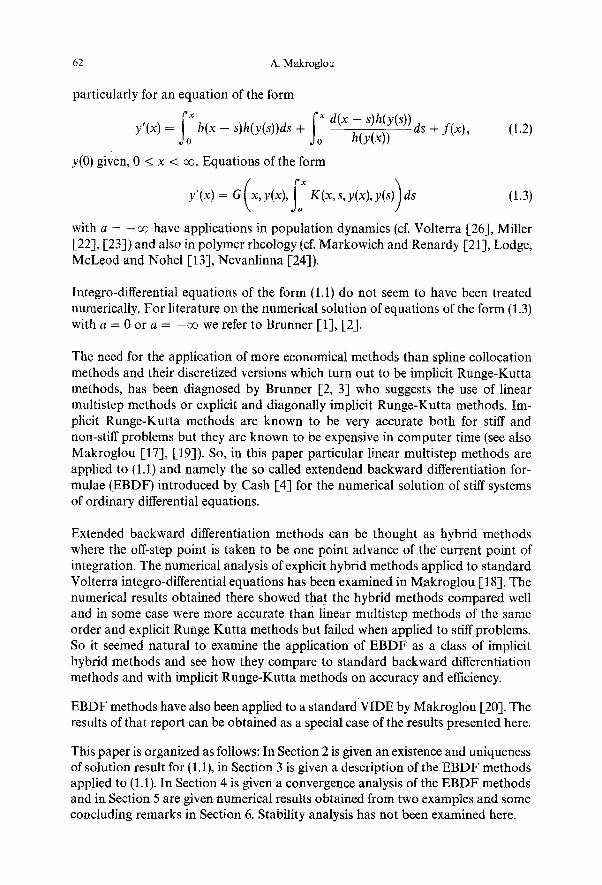
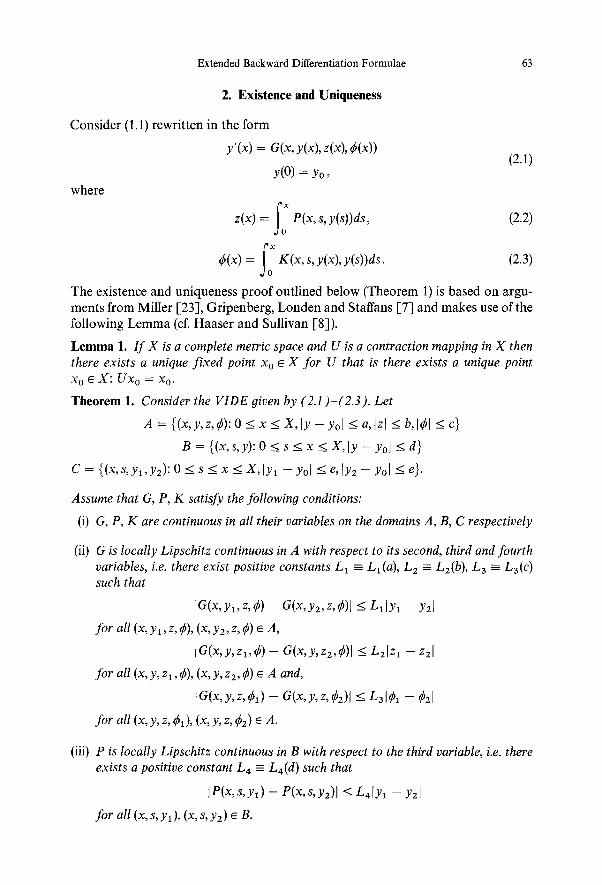
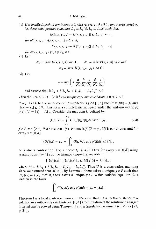
Numerical results are presented for the following examples:

1) y'(x) = f(x) - y(x) + ~ x(1 + 2x)eS(X-S)y(s)ds + ~'~ syZ(x)y(s)ds, y(0) = 1, where

f ( x ) = 1 + 2 x , x2 with true solution, y(x) = e (constructed, based on an example in Linz [12]).

Y

100.000

95.000

90.000

85.000

80.000

75.000

70.000

65.000

60.000

55.000

50.000

45.000

40.000

35.000

30,000

25.000

20.000

15.000

10.000

5,000

0.000

- - I I I

I I I I I -100,000 -50,000 0,000 50,000 100.000

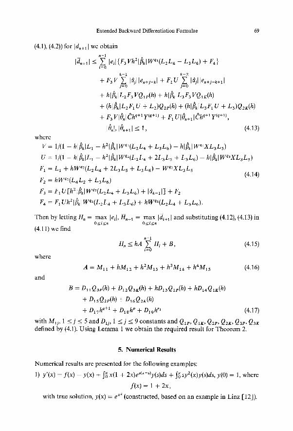
Figure 1. Example 2, EBDF method, k = 7, p = 1 . D 5

70.000

65.000

60.000

55.000

50.000

45~.000

40.000

35.000

30.000

25.000

20.000

15.000

f

I 0 . 0 0 0

5.000

0.000 -- l

-100.000

I I - -

-50.000 0.000 50.000

I

100.000

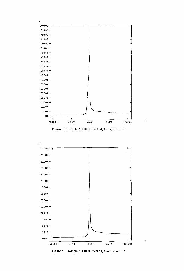
Figure 2. Example 2, EBDF method, k = 7, # = 2.D5

14.000

13.000

12.1300

11.000

10.(300

9.000

8.000

7.000

6.000

5.000

4.000

3.000

2.000

1.000 I

-100.000

E ]

J

I I

1 f I I -50.000 0.000 50.000 i00.000

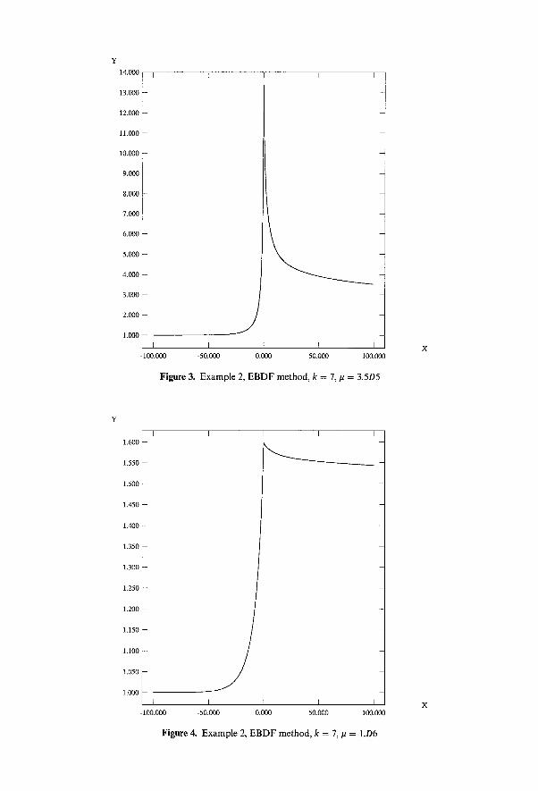
F i g u r e 3. E x a m p l e 2, E B D F m e t h o d , k = 7, # = 3 .5D5

1.600

1.550

1.500

1.450

1.400

1.350

1.300

1.250

1.200

1.150

1.100

1.050

1.0{30 T

-100.000

I I

I I I I -50.000 0.000 50.000 100.000

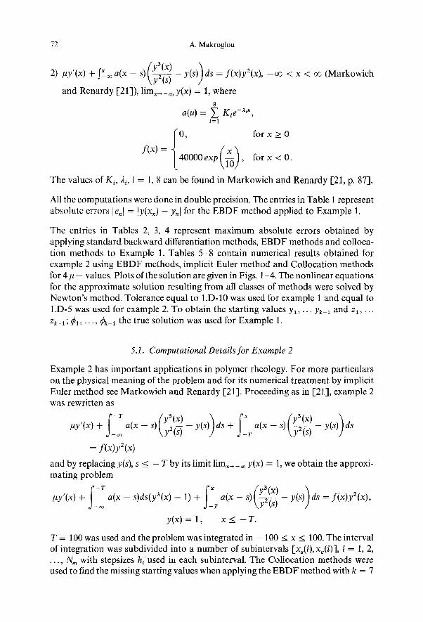
F i g u r e 4. E x a m p l e 2, E B D F m e t h o d , k = 7, # = 1.D6

72 A. Makroglou

2) #y'(x) + ~_~ a(x - s) (y3(x) ) \ y 2 ( s ) - - y(s) ds = f(x)y2(x), - o o < x < oo (Markowich

and Renardy [21]), limx~_~o y(x) = 1, where 8

a(u) = ~ Ki e-a'u, i=1 {0 () orx>0

f(x) = 40000exp ld ' f o r x < 0 .

The values of K i, 2~, i = 1, 8 can be found in Markowich and Renardy [21, p. 87].

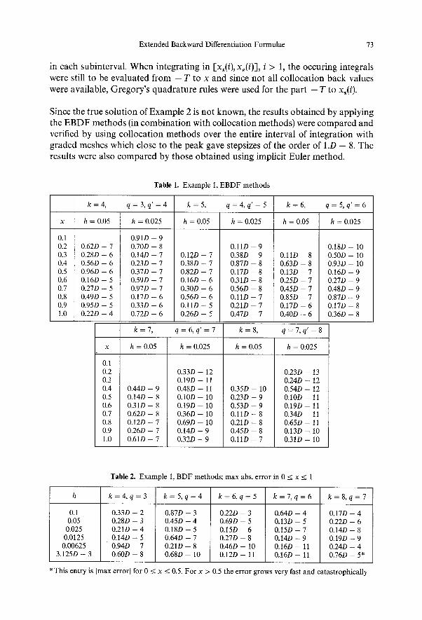
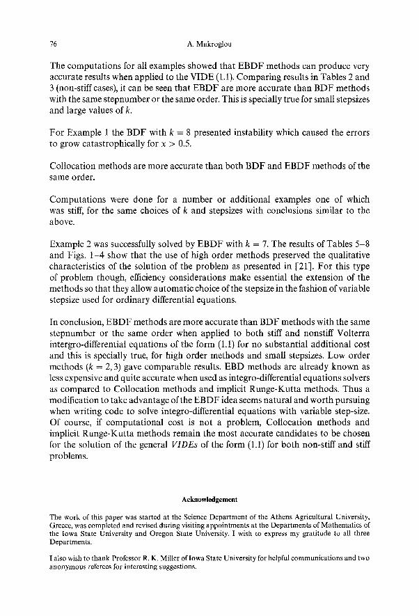
All the computations were done in double precision. The entries in Table 1 represent absolute errors le, l = py(x,) - Y,I for the EBDF method applied to Example 1.

The entries in Tables 2, 3, 4 represent maximum absolute errors obtained by applying standard backward differentiation methods, EBDF methods and colloca- tion methods to Example 1. Tables 5-8 contain numerical results obtained for example 2 using EBDF methods, implicit Euler method and Collocation methods for 4 # - values. Plots of the solution are given in Figs. 1-4. The nonlinear equations for the approximate solution resulting from all classes of methods were solved by Newton's method. Tolerance equal to 1.D-10 was used for example 1 and equal to 1.D-5 was used for example 2. To obtain the starting values Yl . . . . Yk-1 and zl, ... Zk-1; 01 . . . . , q)k-~ the true solution was used for Example 1.

5.1. Computational Details for Example 2

Example 2 has important applications in polymer rheology. For more particulars on the physical meaning of the problem and for its numerical treatment by implicit Euler method see Markowich and Renardy [21]. Proceeding as in [21], example 2 was rewritten as

#y'(x)+ i f [ a ( x - - ) ~ y ~ -- y (s ) )ds+ f f r a ( x - - s, \y2(s) - y ( s ) ) d s

= f(x)yZ(x)

and by replacing y(s), s <_ - T by its limit limx_,_~ y(x) = 1, we obtain the approxi- mating problem

f ;: #y'(x) + a(x - s)ds(y3(x) - 1) + T

y ( x ) = 1,

a(x -- s)//Ya(X) \ y~s ) y(s)) ds = f(x)y2(x),

X ~ - - T .

T = 100 was used and the problem was integrated in - 100 _< x < 100. The interval of integration was subdivided into a number of subintervals [xs(i), x~(i)], i = 1, 2, . . . , N,, with stepsizes hl used in each subinterval. The Collocation methods were used to find the missing starting values when applying the EBDF method with k = 7

Extended Backward Differentiation Formulae 73

in each subinterval. When integrating in [xs(i), xe(i)'], i > 1, the occuring integrals were still to be evaluated from - T to x and since not all collocation back values were available, Gregory's quadrature rules were used for the part - T to xs(i).

Since the true solution of Example 2 is not known, the results obtained by applying the EBDF methods (in combination with collocation methods) were compared and verified by using collocation methods over the entire interval of integration with graded meshes which close to the peak gave stepsizes of the order of 1.D - 8. The results were also compared by those obtained using implicit Euler method.

Table 1. Example 1, E B D F methods

k = 4 , q = 3 , q ' = 4 k = 5 , q = 5 , q ' = 6

h = 0 . 0 5 h = 0 . 0 2 5 h = 0 .05 h = 0 . 0 2 5

0.1

0.2 0 . 6 2 D - 7

0.3 0 . 2 8 D - 6

0 .4 0 . 5 6 D - 6

0.5 0 . 9 6 D - 6

0 .6 0 . 1 6 D - 5

0 .7 0 . 2 7 D - - 5

0 .8 0 . 4 9 D - 5

0 .9 0 . 9 5 D - - 5

1.0 0 . 2 2 D - - 4

0.1

0 .2

0.3

0 .4

0.5

0 .6

0.7

0.8

0.9

1.0

0 . 9 1 D - - 9

0 . 7 0 D - - 8

0 . 1 4 D - - 7

0 . 2 3 D - - 7

0 . 3 7 D - - 7

0 . 5 9 D - - 7

0 . 9 7 D - - 7

0 . 1 7 D - - 6

0 . 3 3 D - - 6

0 . 7 2 D - 6

0 . 1 2 D - 7

0 . 3 8 D - 7

0 . 8 2 D - 7

0 . 1 6 D - 6

0 . 3 0 D - 6

0 . 5 6 D - 6

0 . 1 1 D - - 5

0 . 2 6 D - 5

q = 4 , q ' = 5 k=6,

h = 0 . 0 2 5 h = 0 .05

0 . 1 1 D - - 9

0 . 3 8 D - - 9 0 . 1 1 D - 8

0 . 8 7 D - - 8 0 . 6 3 D - - 8

0 . 1 7 D - - 8 0 . 1 3 D - - 7

0 . 3 1 D - - 8 0 . 2 5 D - - 7

0 . 5 6 D - - 8 0 . 4 5 D - 7

0 . 1 1 D - - 7 0 . 8 5 D - 7

0 . 2 1 D - - 7 0 . 1 7 D - 6

0 . 4 7 D - - 7 0 . 4 0 D - 6

k = 7 , q = 6 , q ' = 7 k = 8 , q = 7 , q ' = 8

h = 0 .05 h = 0 . 0 2 5 h = 0 .05 h = 0 . 0 2 5

0 . 4 4 D - 9

0 . 1 4 D - 8

0 . 3 1 D - 8

0 . 6 2 D - 8

0 . 1 2 D - - 7

0 . 2 6 D - 7

0 . 6 1 D - - 7

0 . 3 3 D - 12 0 . 2 3 D

0 . 1 9 D - 11 0 . 2 4 D

0 . 4 8 D - 11 0 . 3 5 D - 10 0 . 5 4 D

0 . 1 0 D - - 10 0 . 2 3 D - - 9 0 . 1 0 D

0 . 1 9 D - - 10 0 . 5 3 D - - 9 0 . 1 9 D

0 . 3 6 D - - 10 0 . 1 1 D - - 8 0 . 3 4 D

0 . 6 9 D - - 10 0 . 2 1 D - - 8 0 . 6 5 D

0 . 1 4 D - - 9 0 . 4 5 D - - 8 0 . 1 3 D

0 . 3 2 D - - 9 0 . 1 1 D - - 7 0 . 3 1 D

-- 13 -- 12 -- 12

- - 1 1

- - 1 1

- - 1 1

- - 1 1

-- 10

-- 10

0 . 1 8 D - 10

0 . 5 0 D - 10

0 . 9 3 D - 10

0 . 1 6 D - 9

0 . 2 7 D - - 9

0 . 4 8 D - - 9

0 . 8 7 D - 9

0 . 1 7 D - - 8

0 . 3 6 D - - 8

Table 2. E x a m ,le i , B D F methods; max abs. error in 0 < x < 1

h k = 4 , q = 3 k = 5 , q = 4 k = 6 , q = 5 k = 7 , q = 6 k = 8 , q = 7

0 . 3 3 D - - 2

0 . 2 8 D - - 3

0 . 2 1 D - - 4

0 . 1 4 D - - 5

0 . 9 4 D - - 7

0 . 6 0 D - - 8

0.1

0 .05

0 . 0 2 5

0 . 0 1 2 5

0 . 0 0 6 2 5

3 . 1 2 5 D - - 3

0 . 8 7 D - 3

0 . 4 5 D - - 4

0 . 1 8 D - - 5

0 . 6 4 D - - 7

0 . 2 1 D - - 8

0 . 6 8 D - 10

0 . 2 2 D - - 3

0 . 6 9 D - - 5

0 . 1 5 D - - 6

0 . 2 7 D - - 8

0 . 4 6 D - - 10

0 . 1 2 D - - 11

0 . 6 4 D - - 4

0 . 1 3 D - - 5

0 . 1 5 D - - 7

0 . 1 4 D - - 9

0 . 1 6 D - - 11

0 . 1 6 D - - 11

0 . 1 7 D - - 4

0 . 2 2 D - - 6

0 . 1 4 D - - 8

0 . 1 9 D - - 9

0 . 2 4 D - 4

0 . 7 6 D - - 5*

* This entry is [max error[ for 0 < x < 0.5. F o r x > 0 .5 the error grows very fast and catastrophically

74 A. M a k r o g l o u

T a b l e 3. E x a m ~le 1, E B D F m e t h o d s ; m a x abs . e r r o r in 0 < x < 1

k = 4 k = 5 k = 6 k = 7 k = 8

h q = 3 , q ' = 4 q=4 , q ' = 5 q = 5 , q ' = 6 q = 6 , q ' = 7 q = 7 , q ' = 8

0.1

0.05 0 .025

0 .0125 0 .00625

3 .125D - 3

0 .68D - 3

0 .27D - 4 0 .72D - 6

0 .24D - 7

0 . 7 5 D - 9 0 . 2 4 D - 10

0 . 1 4 D - 3

0 .26D - 5 0 .47D - - 7

0 .8D - - 9 0 .13D - - 10

0 . 5 7 D - - 12

0 .35D - - 4

0 .40D - - 6 0 .39D - 8

0 . 3 4 D - 10 0 .25D - 12

0 . 6 1 D - 13

0 .85D - - 5

0 .61D - - 7 0 .32D - - 9

0 .15D - - 11 0 .6D - - 13

0 . 8 5 D - 13

0 .23D - 5

0 .11D - 7 0 .31D - - 10

0 .98D - - 13 0 .36D - - 12

0 . 7 4 D - - 12

T a b l e 4. E x a m p l e 1 C o l l o c a t i o n m e t h o d s ; m a x [Ynm - y(Xnm)[, in 0 < x _< 1 n

m = 2 , r n = 3 , c 1 = 0 m = 4 , c I = 0 , c z = ( 1 - x f O ~ ) / 2 h cl = �89 c2 = 1 c2 = 0.5, c3 = 1 c3 = (1 + x /0 .2 ) /2 , c4 = 1

0.1 0.05

0 .025 0 .0125

0 .00625

3 .125D - - 3

0 . 1 4 D - 3 0 .16D - 4

0 .20D - - 5 0 . 2 5 D - - 6

0 .31D 7 0 .39D - 8

0 .97D - 5

0 . 6 2 D - 6 0 . 3 9 D - 7

0 . 2 4 D - - 8

0 .15D - - 9 0 . 9 4 D - - 11

0 .23D - 7 0 . 3 6 D - 9

0 . 5 6 D - 11 0 . 8 3 D - 13 0 . 1 4 D - 13

0 . 3 1 D - 14

T a b l e 5. E x a m p l e 2, y - v a l u e s fo r /~ = 1.D5

E B D F C o l l o c a t i o n x (k = 7) I m p l i c i t E u l e r (c 1 = 1, c2 = 1)

- 20.0 1.47 1.48 1.47 - -0 .1 94.31 94.72 93.96

0 .0 95.78 96.35 95.58 0.1 33.98 34.28 33.90

20.0 5.14 5.15 5.13

100.0 3.37 3.37 3.37

T a b l e 6. E x a m p l e 2, y - v a l u e s f o r # = 2 .D5

E B D F x (k = 7) I m p l i c i t E u l e r

C o l l o c a t i o n ( L o b a t t o ' s

po in t s )

- 10.0 2 .20 2.20 2.19 0 .0 67.27 67.67 67.36

10.0 5.89 5.91 5.89 100.0 3.49 3.49 3.49

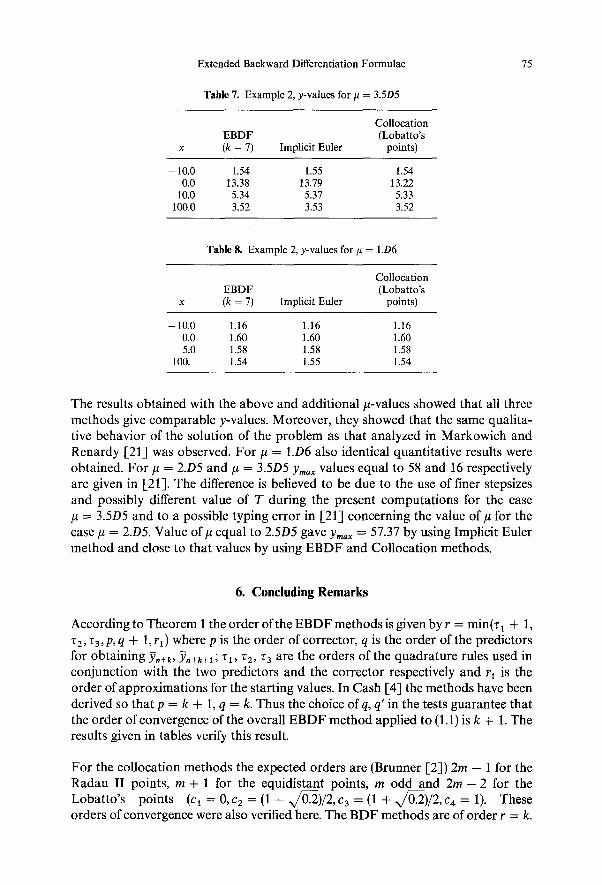
Extended Backward Differentiation Formulae

Table 7. Example 2, y-values for # = 3.5D5

Collocation EBDF (Lobatto's (k = 7) Implicit Euler points)

- - 10.0 1.54 1.55 1.54 0.0 13.38 13.79 13.22

10.0 5.34 5.37 5.33 100.0 3.52 3.53 3.52

75

Table 8. Example 2, y-values for/~ = 1.D6

Collocation EBDF (Lobatto's (k = 7) Implicit Euler points)

-10 .0 1.16 1.16 1.16 0.0 1.60 1.60 1.60 5.0 1.58 1.58 1.58

100. 1.54 1.55 1.54

The results obtained with the above and additional/t-values showed that all three methods give comparable y-values. Moreover, they showed that the same qualita- tive behavior of the solution of the problem as that analyzed in Markowich and Renardy [21] was observed. For # = 1.D6 also identical quantitative results were obtained. For # = 2.D5 and # = 3.5D5 Y,,ax values equal to 58 and 16 respectively are given in [21]. The difference is believed to be due to the use of finer stepsizes and possibly different value of T during the present computations for the case /~ = 3.5D5 and to a possible typing error in [21] concerning the value of # for the case # = 2.D5. Value o f # equal to 2.5D5 gave y,,ax = 57.37 by using Implicit Euler method and close to that values by using EBDF and Collocation methods.

6. Concluding Remarks

According to Theorem 1 the order of the EBDF methods is given by r = min(z 1 + 1, z2, z3, p, q + 1, rl) where p is the order of corrector, q is the order of the predictors for obtaining fin+k, Y,+k+~; Z~, Z2, T 3 are the orders of the quadrature rules used in conjunction with the two predictors and the corrector respectively and r~ is the order of approximations for the starting values. In Cash [4] the methods have been derived so that p = k + 1, q = k. Thus the choice of q, q' in the tests guarantee that the order of convergence of the overall EBDF method applied to (1.1) is k + 1. The results given in tables verify this result.

For the collocation methods the expected orders are (Brunner [2]) 2m - 1 for the Radau II points, m + 1 for the equidistant points, m odd and 2 m - 2 for the Lobat to 's points (c 1 = 0, c 2 = (1 - x / ~ ) / 2 , c 3 = (1 + x/c02)/2, c 4 = 1). These orders of convergence were also verified here. The BDF methods are of order r = k.

76 A. Makroglou

The computations for all examples showed that EBDF methods can produce very accurate results when applied to the VIDE (1.1). Comparing results in Tables 2 and 3 (non-stiff cases), it can be seen that EBDF are more accurate than BDF methods with the same stepnumber or the same order. This is specially true for small stepsizes and large values of k.

For Example 1 the BDF with k = 8 presented instability which caused the errors to grow catastrophically for x > 0.5.

Collocation methods are more accurate than both BDF and EBDF methods of the same order.

Computat ions were done for a number or additional examples one of which was stiff, for the same choices of k and stepsizes with conclusions similar to the above.

Example 2 was successfully solved by EBDF with k = 7. The results of Tables 5-8 and Figs. 1-4 show that the use of high order methods preserved the qualitative characteristics of the solution of the problem as presented in [21]. For this type of problem though, efficiency considerations make essential the extension of the methods so that they allow automatic choice of the stepsize in the fashion of variable stepsize used for ordinary differential equations.

In conclusion, EBDF methods are more accurate than BDF methods with the same stepnumber or the same order when applied to both stiff and nonstiff Volterra intergro-differential equations of the form (1.I) for no substantial additional cost and this is specially true, for high order methods and small stepsizes. Low order methods (k = 2, 3) gave comparable results. EBD methods are already known as less expensive and quite accurate when used as integro-differential equations solvers as compared to Collocation methods and implicit Runge-Kutta methods. Thus a modification to take advantage of the EBDF idea seems natural and worth pursuing when writing code to solve integro-differential equations with variable step-size. Of course, if computational cost is not a problem, Collocation methods and implicit Runge-Kutta methods remain the most accurate candidates to be chosen for the solution of the general VIDEs of the form (1.1) for both non-stiff and stiff problems.

Acknowledgement

The work of this paper was started at the Science Department of the Athens Agricultural University, Greece, was completed and revised during visiting appointments at the Departments of Mathematics of the Iowa State University and Oregon State University. I wish to express my gratitude to all three Departments.

I also wish to thank Professor R. K. Miller of Iowa State University for helpful communications and two anonymous referees for interesting suggestions.

Extended Backward Differentiation Formulae 77

References

[1] Brunner, H., Van der Houwen, P. J.: The numerical solution of Volterra equations. Amsterdam: North Holland 1986 (CWI Monographs, 3).

[2] Brunner, H.: Collocation methods for nonlinear Volterra integro-differential equations with infinite delay. Math Comput. 53, 571-587 (1989).

[3] Brunner, H.: Direct quadrature methods for nonlinear Volterra integro-differential equations with infinite delay. Utilitas Math. 40, 237-250 (1991).

[4] Cash, J. R.: On the integration of stiff systems of ordinary differential equations using extended backward differentiation formulae. Numer. Math. 34, 235-246 (1980).

[5] Cushing, J. M.: Integrodifferential equations and delay models in population dynamics. Berlin, Heidelberg, New York: Springer 1977 (Lecture Notes in Biomathematics, 20).

[6] Gragg, W. B., Stetter, H. J.: Generalized multistep predictor-corrector methods. J. Assoc. Comput. Mach. 11,188-209 (1964).

[7] Gripenberg, G., Londen, S. O., Staffans, O.: Volterra integral and functional equations. Cambridge: Cambridge Univ. Press 1990 (Encycl. Math. Appl. 34) Encycl. Math. Appl. 34 (1990).

[8] Haaser, N. B., Sullivan, J. A.: Real analysis. New York: Dover 1991. [9] Henrici, P.: Discrete variable methods in ordinary differential equations. New York: Wiley 1962.

[10] Van der Houwen, P. J., te Riele, H. J. J.: Backward differentiation type formulas for Volterra integral equations of the second kind. Numer. Math. 37, 205-217 (1981).

[11] Lambert, J. D.: Computational methods in ordinary differential equations. London and New York: Wiley 1973.

[12] Linz, P.: Linear multistep methods for Volterra integro-differential equations. Assoc. Comput. Mach. 16, 295-301 (1969).

[13] Lodge, A. S. McLeod, J. B., Nohel, J. A.: A nonlinear singularly perturbed Volterra integro- differential equation occurring in polymer rheology. Proc. Roy. Soc. Edinburgh Sect. A 80, 99-137 (1978).

[14] Londen, S. O.: On a Volterra integrodifferential equation. Comm. Phys. Math. 38, 1-4 (1969). [15] Londen, S. O.: On a nonlinear Volterra integrodifferential equation. Comm. Phys. Math. 38, 5-11

(1969). [16] Makroglou, A.: On testing hybrid methods in ordinary differential equations, M. Sc. Thesis,

University of Manchester 1974. [17] Makroglou, A.: Convergence of a block-by-block method for nonlinear Volterra integro-

differential equations. Math. Comput. 35, 783-796 (1980). [18] Makroglou, A.: Hybrid methods in the numerical solution of Volterra integro-differential equa-

tions. IMA J. Numer. Anal. 2, 21-35 (1982), 3, 381-382 (1983). [19] Makroglou, A., A block-by-block method for the numerical solution of Volterra delay integro-

differential equations, Computing 30, 49-62 (1983). [20] Makroglou, A.: Extended backward differentiation formulae for Volterra integro-differential

equations. TR-86-12, Dept. of Computer Science, University of Kansas, Lawrence, Kansas. [21] Markowich, P., Renardy, M.: A nonlinear Volterra integrodifferential equation describing the

stretching of polymeric liquids, SIAM J. Math. Anal. 14, 66-97 (1983). [22] Miller, R. K.: On Volterra's population equation, SIAM J. Appl. Math. 14, 446-452 (1966). [23] Miller, R. K.: Nonlinear Volterra Integral Equations. Benjamin: Menlo Park 1971. [24] Nevanlinna, O.: Numerical solution of a singularly perturbed nonlinear Volterra equation. MRC

Tech. Sum. Report No. 1881, University of Wisconsin, Madison 1978. [25] Steinberg, J.: Numerical solution of Volterra integral equations. Numer. Math. 19, 212-217 (1972). [26] Volterra, V.: Leqons sur la th6orie math6matique de la lutte pour la vie. Paris: Gauthier-Villars

1931. [27] Wolkenfelt, P. H. M.: Backward differentiation formulas for Volterra integro-differential equa-

tions. Mathematisch Centrum, Amsterdam, Report NW 53/77.

A. Makroglou Department of Mathematics Oregon State University Corvallis, OR 97331 U.S.A.