Extended SMART Algorithms for Non-NegativeMatrix Factorization

Andrzej CICHOCKI1?, Shun-ichi AMARI2

Rafal ZDUNEK1??, Raul KOMPASS1? ? ? , Gen HORI1 and Zhaohui HE1†

(Invited Paper)

1 Laboratory for Advanced Brain Signal Processing2 Amari Research Unit for Mathematical Neuroscience,

BSI, RIKEN, Wako-shi JAPAN

Abstract. In this paper we derive a family of new extended SMART(Simultaneous Multiplicative Algebraic Reconstruction Technique) al-gorithms for Non-negative Matrix Factorization (NMF). The proposedalgorithms are characterized by improved efficiency and convergencerate and can be applied for various distributions of data and additivenoise. Information theory and information geometry play key roles inthe derivation of new algorithms. We discuss several loss functions usedin information theory which allow us to obtain generalized forms of mul-tiplicative NMF learning adaptive algorithms. We also provide flexibleand relaxed forms of the NMF algorithms to increase convergence speedand impose an additional constraint of sparsity. The scope of these re-sults is vast since discussed generalized divergence functions include alarge number of useful loss functions such as the Amari α– divergence,Relative entropy, Bose-Einstein divergence, Jensen-Shannon divergence,J-divergence, Arithmetic-Geometric (AG) Taneja divergence, etc. Weapplied the developed algorithms successfully to Blind (or semi blind)Source Separation (BSS) where sources may be generally statisticallydependent, however are subject to additional constraints such as non-negativity and sparsity. Moreover, we applied a novel multilayer NMFstrategy which improves performance of the most proposed algorithms.

1 Introduction and Problem Formulation

NMF (Non-negative Matrix Factorization) called also PMF (Positive MatrixFactorization) is an emerging technique for data mining, dimensionality re-duction, pattern recognition, object detection, classification, gene clustering,sparse nonnegative representation and coding, and blind source separation (BSS)[1, 2, 3, 4, 5, 6]. The NMF, first introduced by Paatero and Trapper, and further

? On leave from Warsaw University of Technology, Poland?? On leave from Institute of Telecommunications, Teleinformatics and Acoustics, Wro-

claw University of Technology, Poland? ? ? Freie University, Berlin, Germany

† On leave from the South China University, Guangzhou, China

2

investigated by many researchers [7, 8, 9, 10, 4, 11, 12], does not assume explic-itly or implicitly sparseness, smoothness or mutual statistical independence ofhidden (latent) components, however it usually provides quite a sparse decom-position [1, 13, 9, 5]. NMF has already found a wide spectrum of applications inPET, spectroscopy, chemometrics and environmental science where the matriceshave clear physical meanings and some normalization or constraints are imposedon them (for example, the matrix A has columns normalized to unit length)[7, 2, 3, 5, 14, 15]. Recently, we have applied NMF with temporal smoothnessand spatial constraints to improve the analysis of EEG data for early detectionof Alzheimer’s disease [16]. A NMF approach is promising in many applicationsfrom engineering to neuroscience since it is designed to capture alternative struc-tures inherent in data and, possibly to provide more biological insight. Lee andSeung introduced NMF in its modern formulation as a method to decomposepatterns or images [1, 13].

NMF decomposes the data matrix Y = [y(1), y(2), . . . , y(N)] ∈ Rm×N asa product of two matrices A ∈ Rm×n and X = [x(1), x(2), . . . , x(N)] ∈ Rn×N

having only non-negative elements. Although some decompositions or matrixfactorizations provide an exact reconstruction of the data (i.e., Y = AX), weshall consider here decompositions which are approximative in nature, i.e.,

Y = AX + V , A ≥ 0, X ≥ 0 (1)

or equivalently y(k) = Ax(k) + v(k), k = 1, 2, . . . , N or in a scalar form asyi(k) =

∑nj=1 aijxj(k) +νi(k), i = 1, . . . , m, with aij ≥ 0 and xjk ≥ 0 where

V ∈ Rm×N represents the noise or error matrix (depending on applications),y(k) = [y1(k), . . . , ym(k)]T is a vector of the observed signals (typically positive)at the discrete time instants3 k while x(k) = [x1(k), . . . , xn(k)]T is a vector ofnonnegative components or source signals at the same time instant [17]. Dueto additive noise the observed data might sometimes take negative values. Insuch a case we apply the following approximation: yi(k) = yi(k) if yi(k) ispositive and otherwise yi(k) = ε, where ε is a small positive constant. Ourobjective is to estimate the mixing (basis) matrix A and sources X subject tononnegativity constraints of all entries of A and X. Usually, in BSS applicationsit is assumed that N >> m ≥ n and n is known or can be relatively easilyestimated using SVD or PCA. Throughout this paper, we use the followingnotations: xj(k) = xjk, yi(k) = yik and zik = [AX]ik means ik-th element ofthe matrix (AX), and the ij-th element of the matrix A is denoted by aij .

The main objective of this contribution is to derive a family of new flexibleand improved NMF algorithms that allow to generalize or combine different cri-teria in order to extract physically meaningful sources, especially for biomedicalsignal applications such as EEG and MEG.

3 The data are often represented not in the time domain but in a transform domainsuch as the time frequency domain, so index k may have different meanings.

3

2 Extended Lee-Seung Algorithms and Fixed PointAlgorithms

Although the standard NMF (without any auxiliary constraints) provides sparse-ness of its component, we can achieve some control of this sparsity as well assmoothness of components by imposing additional constraints in addition tonon-negativity constraints. In fact, we can incorporate smoothness or sparsityconstraints in several ways [9]. One of the simple approach is to implementin each iteration step a nonlinear projection which can increase the sparsenessand/or smoothness of estimated components. An alternative approach is to addto the loss function suitable regularization or penalty terms. Let us consider thefollowing constrained optimization problem:Minimize:

D(α)F (A, X) =

12‖Y −AX‖2F + αAJA(A) + αXJX(X)

s. t. aij ≥ 0, xjk ≥ 0, ∀ i, j, k, (2)

where αA and αX ≥ 0 are nonnegative regularization parameters and termsJX(X) and JA(A) are used to enforce a certain application-dependent character-istics of the solution. As a special practical case we have JX(X) =

∑jk fX(xjk),

where f(·) are suitably chosen functions which are the measures of smooth-ness or sparsity. In order to achieve sparse representation we usually choosef(xjk) = |xjk| or simply f(xjk) = xjk, or alternatively f(xjk) = xjk ln(xjk)with constraints xjk ≥ 0. Similar regularization terms can be also implementedfor the matrix A. Note that we treat both matrices A and X in a symmetricway. Applying the standard gradient descent approach, we have

aij ← aij − ηij∂D

(α)F (A,X)∂aij

, xjk ← xjk − ηjk∂D

(α)F (A, X)∂xjk

, (3)

where ηij and ηjk are positive learning rates. The gradient components can beexpressed in a compact matrix form as:

∂D(α)F (A,X)∂aij

= [−Y XT + AXXT ]ij + αA∂JA(A)

∂aij, (4)

∂D(α)F (A,X)∂xjk

= [−AT Y + AT AX]jk + αX∂JX(X)

∂xjk. (5)

Here, we follow the Lee and Seung approach to choose specific learning rates[1, 3]:

ηij =aij

[AXXT ]ij, ηjk =

xjk

[AT A X] jk,(6)

4

that leads to a generalized robust multiplicative update rules:

aij ← aij

[Y XT ]ij − αAϕA(aij)

]ε

[A X XT ]ij + ε, (7)

xjk ← xjk

[[AT Y ]jk − αX ϕX(xjk)

]ε

[AT AX]jk + ε, (8)

where the nonlinear operator is defined as [x]ε = max{ε, x} with a small positiveε and the functions ϕA(aij) and ϕX(xjk) are defined as

ϕA(aij) =∂JA(A)

∂aij, ϕX(xjk) =

∂JX(X)∂xjk

. (9)

Typically, ε = 10−16 is introduced in order to ensure non-negativity constraintsand avoid possible division by zero. The above Lee-Seung algorithm can be con-sidred as an extension of the well known ISRA (Image Space ReconstructionAlgorithm) algorithm. The above algorithm reduces to the standard Lee-Seungalgorithm for αA = αX = 0. In the special case, by using the l1-norm regular-ization terms f(x) = ‖x‖1 for both matrices X and A the above multiplicativelearning rules can be simplified as follows:

aij ← aij

[[Y XT ] ij − αA

]ε

[AX XT ] ij + ε, xjk ← xjk

[[AT Y ] jk − αX

]ε

[AT A X] jk + ε, (10)

with normalization in each iteration as follows aij ← aij/∑m

i=1 aij . Such nor-malization is necessary to provide desired sparseness. Algorithm (10) providesa sparse representation of the estimated matrices and the sparseness measureincreases with increasing values of regularization coefficients, typically αX =0.01 ∼ 0.5.

It is worth to note that we can derive as alternative to the Lee-Seung algo-rithm (10) a Fixed Point NMF algorithm by equalizing the gradient componentsof (4)-(5) (for l1-norm regularization terms) to zero [18] :

∇XD(α)F (Y ||AX) = AT AX −AT Y + αX = 0, (11)

∇AD(α)F (Y ||AX) = AXXT − Y XT + αA = 0. (12)

These equations suggest the following fixed point updates rules:

X ← max{

ε,[(AT A)+(AT Y − αX)

]}=

[(AT A)+(AT Y − αX)

]ε, (13)

A ← max{

ε,[(Y XT − αA)(XXT )+

]}=

[(Y XT − αA)(XXT )+

]ε,(14)

where [A]+ means Moore-Penrose pseudo-inverse and max function is component-wise. The above algorithm can be considered as nonlinear projected AlternatingLeast Squares (ALS) or nonlinear extension of EM-PCA algorithm.

5

Furthermore, using the Interior Point Gradient (IPG) approach an additivealgorithm can be derived (which is written in a compact matrix form usingMATLAB notations):

A ← A− ηA ∗ (A ./ (A ∗X ∗X ′)) . ∗ ((A ∗X − Y ) ∗X ′), (15)X ← X − ηX ∗ (X./(A′ ∗A ∗X)) . ∗ (A′ ∗ (A ∗X − Y )), (16)

where operators .∗ and ./ mean component-wise multiplications and division,respectively, and ηA and ηX are diagonal matrices with positive entries repre-senting suitably chosen learning rates [19].

Alternatively, the mostly used loss function for the NMF that intrinsicallyensures non-negativity constraints and it is related to the Poisson likelihood isbased on the generalized Kullback-Leibler divergence (also called I-divergence):

DKL1(Y ||AX) =∑

ik

(yik ln

yik

[AX]ik+ [AX]ik − yik

), (17)

On the basis of this cost function we proposed a modified Lee-Seung learningalgorithm:

xjk ←(

xjk

∑mi=1 aij (yik/[AX]ik)∑m

q=1 aqj

)1+αsX

, (18)

aij ←(

aij

∑Nk=1 xjk (yik/[A X] ik)∑N

p=1 xjp

)1+αsA

, (19)

where additional small regularization terms αsX ≥ 0 and αsX ≥ 0 are introducedin order to enforce sparseness of the solution, if necessary. Typical values of theregularization parameters are αsX = αsA = 0.001 ∼ 0.005.

Raul Kompass proposed to apply beta divergence to combine the both Lee-Seung algorithms (10) and (18)-(19) into one flexible and elegant algorithm witha single parameter [10]. Let us consider beta divergence in the following gener-alized form as the cost for the NMF problem [10, 20, 6]:

D(β)K (Y ||AX) =

∑

ik

(yik

yβik − [AX]βikβ(β + 1)

+ [AX]βik[AX]ik − yik

β + 1

)

+αX‖X‖1 + αA‖A‖1, (20)

where αX and αA are small positive regularization parameters which controlthe degree of smoothing or sparseness of the matrices A and X, respectively,and l1-norms ||A||1 and ||X||1 are introduced to enforce sparse representationof solutions. It is is interesting to note that for β = 1 we obtain the squareEuclidean distance expressed by Frobenius norm (2), while for the singular casesβ = 0 and β = −1 the beta divergence has to be defined as limiting cases asβ → 0 and β → −1, respectively. When these limits are evaluated one gets for

6

β → 0 the generalized Kullback-Leibler divergence (called I-divergence) definedby equations (17) and for β → −1 the Itakura-Saito distance can be obtained:

DI−S(Y ||AX) =∑

ik

[ln(

[AX]ikyik

) +yik

[AX]ik− 1

]. (21)

The choice of the β parameter depends on statistical distribution of data andthe beta divergence corresponds to the Tweedie models [21, 20]. For example,the optimal choice of the parameter for the normal distribution is β = 1, for thegamma distribution is β → −1, for the Poisson distribution β → 0, and for thecompound Poisson β ∈ (−1, 0).

From the beta generalized divergence we can derive various kinds of NMFalgorithms: Multiplicative based on the standard gradient descent or the Ex-ponentiated Gradient (EG) algorithms (see next section), additive algorithmsusing Projected Gradient (PG) or Interior Point Gradient (IPG), and FixedPoint (FP) algorithms.

In order to derive a flexible NMF learning algorithm, we compute the gradientof (20) with respect to elements of matrices xjk = xj(k) = [X]jk and aij = [A]ij .as follows

∂D(β)K

∂xjk=

m∑

i=1

aij

([AX]βik − yik [AX]β−1

ik

)+ αX , (22)

∂D(β)K

∂aij=

N∑

k=1

([AX]βik − yik[AX]β−1

ik

)xjk + αA. (23)

Similar to the Lee and Seung approach, by choosing suitable learning rates:

ηjk =xjk∑m

i=1 aij [AX]βik, ηij =

aij∑Nk=1[AX]βik xjk

, (24)

we obtain multiplicative update rules [10, 6]:

xjk ← xjk[∑m

i=1 aij (yik/[AX]1−βik )− αX ]ε∑m

i=1 aij [AX]βik, (25)

aij ← aij[∑N

k=1(yik/[AX]1−βik ) yjk − αA]ε∑N

k=1[AX]βik xjk

, (26)

where again the rectification defined as [x]ε = max{ε, x} with a small ε is intro-duced in order to avoid zero and negative values.

3 SMART Algorithms for NMF

There are two large classes of generalized divergences which can be potentiallyused for developing new flexible algorithms for NMF: the Bregman divergences

7

and the Csiszar’s ϕ-divergences [22, 23, 24]. In this contribution we limit ourdiscussion to the some generalized entropy divergences.

Let us consider at beginning the generalized K-L divergence dual to (17):

DKL(AX||Y ) =∑

ik

([AX]ik ln

([AX]ik

yik

)− [AX]ik + yik

)(27)

subject to nonnegativity constraints (see Eq. (17)) In order to derive the learn-ing algorithm let us apply multiplicative exponentiated gradient (EG) descentupdates to the loss function (27):

xjk ← xjk exp(−ηjk

∂DKL

∂xjkxjk

), aij ← aij exp

(−ηij

∂DKL

∂aijaij

), (28)

where

∂DKL

∂xjk=

m∑

i=1

(aij ln[AX]ik − aij ln yik) (29)

∂DKL

∂aij=

N∑

k=1

(xjk ln[AX]ik − xjk ln yik) . (30)

Hence, we obtain the simple multiplicative learning rules:

xjk ← xjk exp

(m∑

i=1

ηjkaij ln(

yik

[AX]ik

))= xjk

m∏

i=1

(yik

[AX]ik

)ηjkaij

(31)

aij ← aij exp

(N∑

k=1

ηijxjk ln(

yik

[AX]ik

))= aij

N∏

k=1

(yik

[AX]ik

)eηijxjk

(32)

The nonnegative learning rates ηjk and ηij can take different forms. Typically,for simplicity and in order to guarantee stability of the algorithm we assumethat ηjk = ηj = ω (

∑mi=1 aij)−1, ηij = ηj = ω (

∑Nk=1 xjk)−1, where ω ∈ (0, 2) is

an over-relaxation parameter. The EG updates can be further improved in termsof convergence, computational efficiency and numerical stability in several ways.

In order to keep weight magnitudes bounded, Kivinen and Warmuth pro-posed a variation of the EG method that applies a normalization step after eachweight update. The normalization linearly rescales all weights so that they sumto a constant. Moreover, instead of the exponent function we can apply its re-linearizing approximation: eu ≈ max{0.5, 1+u}. To further accelerate its conver-gence, we may apply individual adaptive learning rates defined as ηjk ← ηjkc ifthe corresponding gradient component ∂DKL/∂xjk has the same sign in two con-secutive steps and ηjk ← ηjk/c otherwise, where c > 1 (typically c = 1.02− 1.5)[25].

8

The above multiplicative learning rules can be written in a more generalizedand compact matrix form (using MATLAB notations):

X ← X . ∗ exp(ηX . ∗ (A′ ∗ ln(Y ./(A ∗X + ε)))

)(33)

A ← A . ∗ exp(ηA . ∗ (ln(Y ./(A ∗X + ε)) ∗X ′)

), (34)

A ← A ∗ diag{1./sum(A, 1)}, (35)

where in practice a small constant ε = 10−16 is introduced in order to ensurepositivity constraints and/or to avoid possible division by zero, and ηA andηX are non-negative scaling matrices representing individual learning rates. Theabove algorithm may be considered as an alternating minimization/projectionextension of the well known SMART (Simultaneous Multiplicative Algebraic Re-construction Technique) [26, 27]. This means that the above NMF algorithm canbe extended to MART and BI-MART (Block-Iterative Multiplicative AlgebraicReconstruction Technique) [26].

It should be noted that the parameters (weights) {xjk, aij} are restricted topositive values, the resulting updates rules can be written:

ln(xjk) ← ln(xjk)− ηjk∂DKL

∂ ln xjk, ln(aij) ← ln(aij)− ηij

∂DKL

∂ ln aij, (36)

where the natural logarithm projection is applied component-wise. Thus, in asense, the EG approach takes the same steps as the standard gradient descent(GD), but in the space of logarithm of the parameters. In other words, in ourcurrent application the scalings of the parameters {xjk, aij} are best adapted inlog-space, where their gradients are much better behaved.

4 NMF Algorithms Using Amari α-Divergence

It is interesting to note, that the above SMART algorithm can be derived asa special case for a more general loss function called Amari α-divergence (seealso Liese & Vajda, Cressie-Read disparity, Kompass generalized divergence andEguchi-Minami beta divergence)4 [29, 28, 23, 22, 10, 30]):

DA(Y ||AX) =1

α(α− 1)

∑

ik

(yα

ikz1−αik − αyik + (α− 1)zik

)(37)

We note that as special cases of the Amari α-divergence for α = 2, 0.5,−1, weobtain the Pearson’s, Hellinger and Neyman’s chi-square distances, respectively,while for the cases α = 1 and α = 0 the divergence has to be defined by the limitsα → 1 and α → 0, respectively. When these limits are evaluated one obtains

4 Note that this form of α–divergence differs slightly with the loss function of Amarigiven in 1985 and 2000 [28, 23] by the additional term. This term is needed to allowde-normalized variables, in the same way that extended Kullback-Leibler divergencediffers from the standard form (without terms zik − yik) [24].

9

for α → 1 the generalized Kullback-Leibler divergence defined by equations (17)and for α → 0 the dual generalized KL divergence (27).The gradient of the above cost function can be expressed in a compact form as

∂DA

∂xjk=

1α

m∑

i=1

aij

[1−

(yik

zik

)α],

∂DA

∂aij=

1α

N∑

k=1

xjk

[1−

(yik

zik

)α]. (38)

However, instead of applying the standard gradient descent we use the projected(linearly transformed) gradient approach (which can be considered as general-ization of exponentiated gradient):

Φ(xjk) ← Φ(xjk)− ηjk∂DA

∂Φ(xjk), Φ(aij) ← Φ(aij)− ηij

∂DA

∂Φ(aij), (39)

where Φ(x) is a suitable chosen function.Hence, we have

xjk ← Φ−1

(Φ(xjk)− ηjk

∂DA

∂Φ(xjk)

), (40)

aij ← Φ−1

(Φ(aij)− ηij

∂DA

∂Φ(aij)

). (41)

It can be shown that such nonlinear scaling or transformation provides stablesolution and the gradients are much better behaved in Φ space. In our case, weemploy Φ(x) = xα and choose the learning rates as follows

ηjk = α2Φ(xjk)/(x1−αjk

m∑

i=1

aij), ηij = α2Φ(aij)/(a1−αij

N∑

k=1

xjk), (42)

which leads directly to the new learning algorithm 5: (the rigorous convergenceproof is omitted due to lack of space)

xjk ← xjk

(∑mi=1 aij (yik/zik)α

∑mq=1 aqj

)1/α

, aij ← aij

(∑Nk=1 (yik/zik)α

xjk∑Nt=1 xjt

)1/α

(43)

This algorithm can be implemented in similar compact matrix form using theMATLAB notations:

X ← X . ∗ (A′ ∗ ((Y + ε)./ (A ∗X + ε)).α

).1/α, (44)

A ← A . ∗ (((Y + ε)./ (A ∗X + ε)).α ∗X ′) .1/α, (45)

A ← A ∗ diag{1./sum(A, 1)}.5 For α = 0 instead of Φ(x) = xα we have used Φ(x) = ln(x).

10

Alternatively, applying the EG approach, we can obtain the following multiplica-tive algorithm:

xjk ← xjk exp

{ηjk

m∑

i=1

aij

[(yik

zik

)α

− 1]}

, (46)

aij ← aij exp

{ηij

N∑

k=1

[(yik

zik

)α

− 1]

xjk

}. (47)

5 Generalized SMART algorithms

The main objective of this paper is to show that the learning algorithm (31) and(32) can be generalized to the following flexible algorithm:

xjk ← xjk exp

[m∑

i=1

ηjk aij ρ(yik, zik)

], aij ← aij exp

[N∑

k=1

ηij xjk ρ(yik, zik)

]

(48)

where the error functions defined as

ρ(yik, zik) = −∂D(Y ||AX)∂zik

(49)

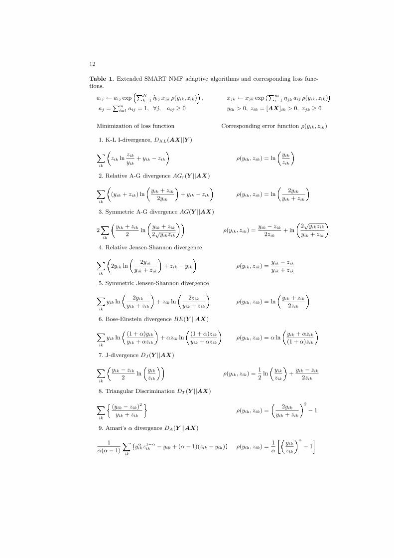
can take different forms depending on the chosen or designed loss (cost) functionD(Y ||AX) (see Table 1).

As an illustrative example let us consider the Bose-Einstein divergence:

BEα(Y ||AX) =∑

ik

yik ln(

(1 + α)yik

yik + αzik

)+ αzik ln

((1 + α)zik

yik + αzik

). (50)

This loss function has many interesting properties:1. BEα(y||z) = 0 if z = y almost everywhere.2. BEα(y||z) = BE1/α(z||y)3. For α = 1, BEα simplifies to the symmetric Jensen-Shannon divergence

measure (see Table 1).4. limα→∞BEα(y||z) = KL(y||z) and for α sufficiently small BEα(y||z) ≈

KL(z||y).The gradient of the Bose-Einstein loss function in respect to zik can be ex-

pressed as

∂BEα(Y ||AX)∂zik

= −α ln(

yik + αzik

(1 + α)zik

)(51)

and in respect to xjk and aij as

∂BEα

∂xjk= −

m∑

i=1

aij∂BEα

∂zik,

∂BEα

∂aij= −

N∑

k=1

xjk∂BEα

∂zik. (52)

11

Hence, applying the standard (un-normalized) EG approach (28) we obtain thelearning rules (48) with the error function ρ(yik, zik) = α ln ((yik + αzik)/((1 + α)zik)).It should be noted that the error function ρ(yik, zik) = 0 if and only if yik = zik.

6 Multi-layer NMF

In order to improve performance of the NMF, especially for ill-conditioned andbadly scaled data and also to reduce risk to get stuck in local minima of non-convex minimization, we have developed a simple hierarchical and multi-stageprocedure in which we perform a sequential decomposition of nonnegative ma-trices as follows: In the first step, we perform the basic decomposition (factor-ization) Y = A1X1 using any available NMF algorithm. In the second stage,the results obtained from the first stage are used to perform the similar decom-position: X1 = A2X2 using the same or different update rules, and so on. Wecontinue our decomposition taking into account only the last achieved compo-nents. The process can be repeated arbitrarily many times until some stoppingcriteria are satisfied. In each step, we usually obtain gradual improvements ofthe performance. Thus, our model has the form: Y = A1A2 · · ·ALXL , with thebasis nonnegative matrix defined as A = A1A2 · · ·AL. Physically, this meansthat we build up a system that has many layers or cascade connections of Lmixing subsystems. The key point in our novel approach is that the learning(update) process to find parameters of sub-matrices X l and Al is performedsequentially, i.e. layer by layer6. In each step or each layer, we can use the samecost (loss) functions, and consequently, the same learning (minimization) rules,or completely different cost functions and/or corresponding update rules. Thiscan be expressed by the following procedure:

(Multilayer NMF Algorithm)Set: X0 = Y ,For l = 1, 2, . . . L, do :

Initialize randomly A(0)l and/or X

(0)l ,

For k = 1, 2, . . . , K , do :

X(k)l = arg min

Xl≥0

{Dl

(X l−1||A(k−1)

l X l

)},

A(k)l = arg min

Al≥0

{Dl

(X l−1||AlX

(k)l

)},

A(k)l ←

[aij∑mi=1 aij

](k)

l

,

EndX l = X

(K)l , Al = A

(K)l ,

End

6 The multilayer system for NMF and BSS is subject of our patent pending in RIKENBSI, March 2006.

12

Table 1. Extended SMART NMF adaptive algorithms and corresponding loss func-tions.

aij ← aij exp�PN

k=1 eηij xjk ρ(yik, zik)�

, xjk ← xjk exp�Pm

i=1 ηjk aij ρ(yik, zik)�

aj =Pm

i=1 aij = 1, ∀j, aij ≥ 0 yik > 0, zik = [AX]ik > 0, xjk ≥ 0

Minimization of loss function Corresponding error function ρ(yik, zik)

1. K-L I-divergence, DKL(AX||Y )Xik

�zik ln

zik

yik+ yik − zik

�ρ(yik, zik) = ln

�yik

zik

�2. Relative A-G divergence AGr(Y ||AX)Xik

�(yik + zik) ln

�yik + zik

2yik

�+ yik − zik

�ρ(yik, zik) = ln

�2yik

yik + zik

�3. Symmetric A-G divergence AG(Y ||AX)

2Xik

�yik + zik

2ln

�yik + zik

2√

yikzik

��ρ(yik, zik) =

yik − zik

2zik+ ln

�2√

yikzik

yik + zik

�4. Relative Jensen-Shannon divergenceXik

�2yik ln

�2yik

yik + zik

�+ zik − yik

�ρ(yik, zik) =

yik − zik

yik + zik

5. Symmetric Jensen-Shannon divergenceXik

yik ln

�2yik

yik + zik

�+ zik ln

�2zik

yik + zik

�ρ(yik, zik) = ln

�yik + zik

2zik

�6. Bose-Einstein divergence BE(Y ||AX)Xik

yik ln

�(1 + α)yik

yik + αzik

�+ αzik ln

�(1 + α)zik

yik + αzik

�ρ(yik, zik) = α ln

�yik + αzik

(1 + α)zik

�7. J-divergence DJ(Y ||AX)Xik

�yik − zik

2ln

�yik

zik

��ρ(yik, zik) =

1

2ln

�yik

zik

�+

yik − zik

2zik

8. Triangular Discrimination DT (Y ||AX)Xik

�(yik − zik)2

yik + zik

�ρ(yik, zik) =

�2yik

yik + zik

�2

− 1

9. Amari’s α divergence DA(Y ||AX)

1

α(α− 1)

Xik

�yα

ikz1−αik − yik + (α− 1)(zik − yik)

�ρ(yik, zik) =

1

α

��yik

zik

�α

− 1

�

13

7 Simulation Results

All the NMF algorithms discussed in this paper (see Table 1) have been exten-sively tested for many difficult benchmarks for signals and images with variousstatistical distributions. Simulations results confirmed that the developed algo-rithms are stable, efficient and provide consistent results for a wide set of param-eters. Due to the limit of space we give here only one illustrative example: The

(a) (b)

(c) (d)

Fig. 1. Example 1: (a) The original 5 source signals; (b) Estimated sources using thestandard Lee-Seung algorithm (7) and (8) with SIR = 8.8, 17.2, 8.7, 19.3, 12.4 [dB]; (c)Estimated sources using 20 layers applied to the standard Lee-Seung algorithm (7) and(8) with SIR = 9.3, 16.1, 9.9, 18.5, 15.8 [dB], respectively; (d) Estimated source signalsusing 20 layers and the new hybrid algorithm (14) with (48) with the Bose Shannondivergence with α = 2; individual performance for estimated source signals: SIR = 15,17.8, 16.5, 19, 17.5 [dB], respectively.

five (partially statistically dependent) nonnegative source signals shown in Fig.1(a) have been mixed by randomly generated uniformly distributed nonnegativematrix A ∈ R50×5. To the mixing signals strong uniform distributed noise withSNR=10 dB has been added. Using the standard multiplicative NMF Lee-Sungalgorithms we failed to estimate the original sources. The same algorithm with 20layers of the multilayer system described above gives better results – see Fig.1(c). However, even better performance for the multilayer system provides thehybrid SMART algorithm (48) with Bose-Einstein cost function (see Table 1)for estimation the matrix X and the Fixed Point algorithm (projected pseudo-

14

inverse) (14) for estimation of the matrix A (see Fig.1 (d). We also tried to applythe ICA algorithms to solve the problem but due to partial dependence of thesources the performance was poor. The most important feature of our approachconsists in applying multi-layer technique that reduces the risk of getting stuckin local minima, and hence, a considerable improvement in the performance ofNMF algorithms, especially projected gradient algorithms.

8 Conclusions and Discussion

In this paper we considered a wide class of loss functions that allowed us to de-rive a family of robust and efficient novel NMF algorithms. The optimal choiceof a loss function depends on the statistical distribution of the data and additivenoise, so different criteria and algorithms (updating rules) should be applied forestimating the matrix A and the matrix X depending on a priori knowledgeabout the statistics of the data. We derived several multiplicative algorithms withimproved performance for large scale problems. We found by extensive simula-tions that multilayer technique plays a key role in improving the performance ofblind source separation when using the NMF approach.

References

[1] Lee, D.D., Seung, H.S.: Learning of the parts of objects by non-negative matrixfactorization. Nature 401 (1999) 788–791.

[2] Cho, Y.C., Choi, S.: Nonnegative features of spectro-temporal sounds for classi-fication. Pattern Recognition Letters 26 (2005) 1327–1336.

[3] Sajda, P., Du, S., Parra, L.: Recovery of constituent spectra using non-negativematrix factorization. In: Proceedings of SPIE – Volume 5207, Wavelets: Applica-tions in Signal and Image Processing (2003) 321–331.

[4] Guillamet, D., Vitri‘a, J., Schiele, B.: Introducing a weighted nonnegative matrixfactorization for image classification. Pattern Recognition Letters 24 (2004) 2447– 2454

[5] Li, H., Adali, T., W. Wang, D.E.: Non-negative matrix factorization with or-thogonality constraints for chemical agent detection in Raman spectra. In: IEEEWorkshop on Machine Learning for Signal Processing), Mystic USA (2005)

[6] Cichocki, A., Zdunek, R., Amari, S.: Csiszar’s divergences for non-negative matrixfactorization: Family of new algorithms. Springer LNCS 3889 (2006) 32–39

[7] Paatero, P., Tapper, U.: Positive matrix factorization: A nonnegative factor modelwith optimal utilization of error estimates of data values. Environmetrics 5 (1994)111–126

[8] Oja, E., Plumbley, M.: Blind separation of positive sources using nonnegativePCA. In: 4th International Symposium on Independent Component Analysis andBlind Signal Separation, Nara, Japan (2003)

[9] Hoyer, P.: Non-negative matrix factorization with sparseness constraints. Journalof Machine Learning Research 5 (2004) 1457–1469.

[10] Kompass, R.: A generalized divergence measure for nonnegative matrix factor-ization, Neuroinfomatics Workshop, Torun, Poland (2005)

15

[11] Dhillon, I., Sra, S.: Generalized nonnegative matrix approximations with Bregmandivergences. In: NIPS -Neural Information Proc. Systems, Vancouver Canada.(2005)

[12] Berry, M., Browne, M., Langville, A., Pauca, P., Plemmons, R.: Al-gorithms and applications for approximate nonnegative matrix fac-torization. Computational Statistics and Data Analysis (2006)http://www.wfu.edu/˜plemmons/papers.htm.

[13] Lee, D.D., Seung, H.S.: Algorithms for nonnegative matrix factorization. Vol-ume 13. NIPS, MIT Press (2001)

[14] Novak, M., Mammone, R.: Use of nonnegative matrix factorization for languagemodel adaptation in a lecture transcription task. In: Proceedings of the 2001IEEE Conference on Acoustics, Speech and Signal Processing. Volume 1., SaltLake City, UT (2001) 541–544

[15] Feng, T., Li, S.Z., Shum, H.Y., Zhang, H.: Local nonnegative matrix factorizationas a visual representation. In: Proceedings of the 2nd International Conferenceon Development and Learning, Cambridge, MA (2002) 178–193

[16] Chen, Z., Cichocki, A., Rutkowski, T.: Constrained non-negative matrix factoriza-tion method for EEG analysis in early detection of Alzheimer’s disease. In: IEEEInternational Conference on Acoustics, Speech, and Signal Processing,, ICASSP-2006, Toulouse, France (2006)

[17] Cichocki, A., Amari, S.: Adaptive Blind Signal And Image Processing (Newrevised and improved edition). John Wiley, New York (2003)

[18] Cichocki, A., Zdunek, R.: NMFLAB Toolboxes for Signal and Image Processingwww.bsp.brain.riken.go.jp, JAPAN (2006)

[19] Merritt, M., Zhang, Y.: An interior-point gradient method for large-scale totallynonnegative least squares problems. Technical report, Department of Computa-tional and Applied Mathematics, Rice University, Houston, Texas, USA (2004)

[20] Minami, M., Eguchi, S.: Robust blind source separation by beta-divergence. Neu-ral Computation 14 (2002) 1859–1886

[21] Jorgensen, B.: The Theory of Dispersion Models. Chapman and Hall (1997)[22] Csiszar, I.: Information measures: A critical survey. In: Prague Conference on

Information Theory, Academia Prague. Volume A. (1974) 73–86.[23] Amari, S., Nagaoka, H.: Methods of Information Geometry. Oxford University

Press, New York (2000)[24] Zhang, J.: Divergence function, duality and convex analysis. Neural Computation

16 (2004) 159–195.[25] Schraudolf, N.: Gradient-based manipulation of non-parametric entropy esti-

mates. IEEE Trans. on Neural Networks 16 (2004) 159–195.[26] Byrne, C.: Accelerating the EMML algorithm and related iterative algorithms by

rescaled block-iterative (RBI) methods. IEEE Transactions on Image Processing7 (1998) 100 – 109.

[27] Byrne, C.: Choosing parameters in block-iterative or ordered subset reconstruc-tion algorithms. IEEE Transactions on Image Progressing 14 (2005) 321–327

[28] Amari, S.: Differential-Geometrical Methods in Statistics. Springer Verlag (1985)[29] Amari, S.: Information geometry of the EM and em algorithms for neural net-

works. Neural Networks 8 (1995) 1379–1408.[30] Cressie, N.A., Read, T.: Goodness-of-Fit Statistics for Discrete Multivariate Data.

Springer, New York (1988)