Embed Size (px)
Citation preview

EXTENDING THE REACH OF COILED TUBING IN DIRECTIONAL WELLS WITH
DOWNHOLE MOTORS
A Thesis
by
OLUWAFEMI ISAAC OYEDOKUN
Submitted to the Office of Graduate Studies of
Texas A&M University in partial fulfillment of the requirements for the degree of
MASTER OF SCIENCE
Chair of Committee, Jerome Schubert Committee Members, Catalin Teodoriu Steve Suh Head of Department, Daniel A. Hill
August 2013
Master Subject: Petroleum Engineering
Copyright 2013 Oluwafemi Isaac Oyedokun

ii
ABSTRACT
A rigorous study has dispelled a longtime myth about coiled-tubing technology. The inability to
rotate the tubing limits its reach in the lateral section of the wellbore. Past and current
extended-reach techniques for coiled-tubing drilling have not been sufficient (individually) in
significantly increasing the reach of the tubing in the wellbore; often four or five extended-reach
methods are combined to have significant displacement in the wellbore, which is quite expensive
to do.
After much rigorous investigations and computer simulation tests, the study has demonstrated
that a downhole motor (second motor) can be used in significantly extending the reach of coiled
tubing in the wellbore. This technique is expected to also improve hole cleaning process (during
coiled-tubing drilling), since the configuration allows for the rotation of the coiled tubing string.
With the proposed technology having two tubing segments (rotating and nonrotating segments),
the investigations show that the two segments will not buckle under applied torsional loads in the
course of using a hydraulic downhole motor. But the nonrotating segment of the tubing string
will be subjected to severe twisting.
Electric downhole motors and a dynamic torque anchor (or full-gaged stabilizer) coupled to a
hydraulic motor can be used to achieve the primary aim of the technology and prevent twisting
of the nonrotating segment (the twisting of the segment destabilizes the drilling process).
Although the use of a dynamic torque anchor or full-gaged stabilizer can be used in arresting the
twisting moment, it induces high frictional forces, which reduce the lateral displacement of the
tubing (relative to an electrodrill). To solve this problem, a new “dynamic torque arrestor” has
been proposed in this project. The simulation tests show that the lateral displacements of the
tubing in the wellbore (when the newly proposed dynamic torque arrestor is coupled to a
hydraulic motor) are greater than the displacements achieved with the use of dynamic torque
anchor or full-gaged stabilizer.
Since the proposed technology does not require the intense modification of the current
configuration of the coiled tubing unit, its application will be inexpensive.
iii
ACKNOWLEDGEMENTS
I bless the name of the Lord for providing me with the wisdom in solving the challenges
associated with the newly proposed coiled- tubing extended-reach technology. Also, I thank the
God of heaven and earth for granting me sound health during the course of these rigorous
investigations.
In addition, I want to appreciate the supports from the US Department of State in sponsoring my
graduate program at Texas A&M University.
Finally, I appreciate the comments from my committee members toward the improvement of this
write up.

iv
TABLE OF CONTENTS
Page
ABSTRACT ................................................................................................................................... ii
ACKNOWLEDGEMENTS .......................................................................................................... iii
TABLE OF CONTENTS .............................................................................................................. iv
LIST OF FIGURES ....................................................................................................................... vi
CHAPTER I INTRODUCTION .............................................................................................. 1
1.1 Background Information ....................................................................................................... 1 1.1.1 What is Coiled Tubing? ................................................................................................. 1 1.1.2 Evolution of Coiled Tubing Unit ................................................................................... 1 1.1.3 Mode of Operation of a Coiled-Tubing Unit for Drilling Application .......................... 2 1.1.4 Past and Current Extended-Reach Techniques ............................................................. 3 1.1.5 Proposed Extended-Reach Technique ........................................................................... 5 1.1.6 Operating Principle of a Downhole Hydraulic Motor ................................................... 6 1.1.7 Operating Methodology of the Proposed Technique ..................................................... 6 1.1.8 Presumed Challenges with the Proposed Extended-Reach Technique .......................... 7
1.2 Research Objectives ........................................................................................................... 10 1.3 Research Summary ............................................................................................................. 10
CHAPTER II KINETICS OF THE COILED-TUBING STRING ......................................... 12
2.1 Rotating Segment of the Coiled-Tubing String .................................................................. 12 2.1.1 Drag Equation .............................................................................................................. 16 2.1.2 Normal Contact Force Model ...................................................................................... 18 2.1.3 Rotating Torque Model ............................................................................................... 19 2.1.4 Total Shear Force in the Coiled Tubing Segment ....................................................... 19
2.2 Nonrotating Segment of the Tubing String ........................................................................ 20 2.2.1 Drag Equation .............................................................................................................. 21 2.2.2 Normal Force Equation ............................................................................................... 22 2.2.3 Shear Force Model ...................................................................................................... 22
2.3 Axial Force Distribution in the Tubing String .................................................................... 23

v
Page
CHAPTER III TORSIONAL BUCKLING OF THE TUBING ............................................. 25
3.1 Torsional Buckling of the Tubing in the Vertical Section of the Wellbore ........................ 28 3.2 Torsional Buckling of the Tubing in the Inclined Section of the Wellbore........................ 32 3.3 Torsional Buckling of the Tubing in the Curved Section of the Wellbore ......................... 33
CHAPTER IV TUBING ROTATING LENGTH AND TWISTING MOMENTS ............... 36
4.1 Determining the Maximum Rotating Length...................................................................... 36 4.2 Rate of Change of the Rotary Torque/ Reactive Torque .................................................... 42 4.3 Twisting Moment in the Nonrotating Tubing Segment ...................................................... 44
4.3.1 Preventive and Remedial Measures against Twisting of the Tubing .......................... 45 4.3.2 How the Dynamic Torque Arrestor Works ................................................................. 47
CHAPTER V MAXIMUM TUBING DISPLACEMENTS IN THE WELLBORE .............. 51
5.1 Maximum Displacement at Zero Hookload or Lockup in the Vertical Section ................. 51 5.1.1 Axial Force Distribution in Sinusoidal Buckled Tubing in Straight Wellbores .......... 55 5.1.2 Axial Force Distribution in Helical Buckled Tubing in Straight Wellbores ............... 60 5.1.3 Maximum-Total Measured Depth and Maximum Tubing Length .............................. 64
5.2 Maximum Displacement with Lockup in the Lateral Section ............................................ 67
CHAPTER VI DISCUSSION ................................................................................................ 72
6.1 Maximum Lateral Displacement with Lockup in the Vertical Section .............................. 72 6.2 Maximum Lateral Displacement with Lockup in the Lateral Section ................................ 81
CHAPTER VII CONCLUSIONS AND RECOMMENDATIONS ....................................... 86
7.1 Conclusions ........................................................................................................................ 86 7.2 Recommendations .............................................................................................................. 88
NOMENCLATURE ..................................................................................................................... 89
REFERENCES ............................................................................................................................. 93

vi
LIST OF FIGURES
FIGURE Page
1.1 Schematic diagram of the use of hydraulic motor in extending the reach of coiled tubing in the wellbore ....................................................................................................... 8
1.2 An adapter can be used to link the coiled tubing connector’s pin and the motor’s connection boxes which have different threading ............................................... 9
2.1a Free-body diagram of the forces and moments acting on an elemental portion of the rotating CT segment in the axial-normal plane .................................................... 13
2.1b Free-body diagram of the forces and moments acting on an elemental portion of the rotating CT segment in the normal-binormal plane .................................................. 13
2.2a Vector diagram of the frictional forces at a point P on a rotating tubing string on the tangent-binormal plane ............................................................................................. 16
2.2b Vector diagram of the frictional forces at a point P on a rotating tubing string on the normal-binormal plane .................................................................................................. 16
2.3 The coiled tubing rolls up the wall of the wellbore in the deviated and inclined sections of the wellbore .................................................................................................. 18
2.4 The shear forces (at a point) aim to bend the tubing string in the normal and binormal directions ......................................................................................................... 20
3.1a The rotary torque on the bit and the weight on bit constitute the cutting forces for the bit ........................................................................................................................ 25
3.1b The resultant cutting force of the bit is the vectorial sum of the side cutting force and the axial load component from the applied weight on bit .............................. 26
3.2 Using a hydraulic motor, as the second motor produces reactive torques which can destabilize the pure rotation of the rotating segment .................................... 27
3.3 Both the rotating and unprotected nonrotating segments of the tubing string will helically buckle when the buckling torque dominates in the interplay of forces and moments .................................................................................................... 29
3.4 As the tubing length buckles helically, it contacts the wall of the wellbore .................... 30
3.5 The additional work done by the weight of the tubing string in resisting the lateral elastic deflection increases the buckling torsional load of the string, when the tubing lies in the inclined section of the wellbore ............................................ 33
3.6 Using a hydraulic motor, as the second motor produces reactive torques which can destabilize the pure rotation of the rotating segment .................................... 34

vii
FIGURE Page
4.1a When the second mud motor approaches the KOP, the maximum torque is applied to the rotating segment ................................................................................................... 39
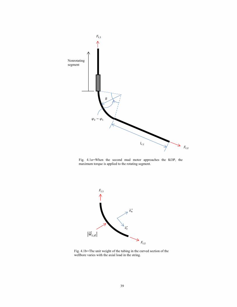
4.1b The unit weight of the tubing in the curved section of the wellbore varies with the axial load in the string ...................................................................................... 39
4.2 The reactive torque acting on the nonrotating segment is the cumulative of the rotary torques on the rotating segment ........................................................................... 43
4.3a The twisting moments induce normal and binormal contact forces between the stabilizer blades and the wellbore (top view) .................................................................. 46
4.3b The twisting moments induce normal and binormal contact forces between the stabilizer blades and the wellbore (end view) ................................................................. 47
4.4 The newly proposed dynamic torque arrestor does not induce normal and binormal contact forces on the string ............................................................................. 48
5.1 The neutral point is at the top of the helically buckled length ........................................ 52
5.2 A zero hookload suggests the whole string is in compression ....................................... 54
5.3a Top view of sinusoidally buckled tubing string segment lying in a straight section of the wellbore .................................................................................................... 56
5.3b End view of sinusoidally buckled tubing string segment lying in a straight section of the wellbore .................................................................................................... 56
5.4a Top view of helically buckled tubing string segment lying in a straight section of the wellbore .................................................................................................... 61
5.4b End view of helically buckled tubing string segment lying in a straight section of the wellbore .................................................................................................... 61
5.5 Schematic representation of zero-hookload phenomenon occurring in a typical extended-reach well with the proposed technology tubing ............................................. 66
5.6 The unit normal force resulting from helical buckling of the tubing increases from points A to C .......................................................................................................... 68
6.1 The induced axial friction caused by the action of the twisting moment on the stabilizer limits the position of the mud motor to the vertical or curved section of the wellbore.………………………………………………………………………..... 75
6.2a The second motor assembly does not have the same curvature as the tubing in the curved section of the wellbore because of high flexural rigidity .............................. 76
6.2b The motor assembly acts as a chord of an arc in the curved section .............................. 77
6.3 The electric motor in the curved section of the wellbore ............................................... 80

viii
FIGURE Page
6.4 Top view of the configuration of the nonrotating segment of the tubing string observed during the computer simulation tests vibrations .............................................. 83
6.5 Short build up section and low inclination angles will help in extending the reach of coiled tubing in the wellbore tubing .................................................................. 84
6.6 The buckled length of the tubing decreases as the inclination angle and the length of the build section increases ............................................................................... 84
6.7 The buckled length of the tubing decreases as the inclination angle, tortuosity, and the length of the build section increases .................................................................. 85

1
CHAPTER I
INTRODUCTION
1.1 Background Information
1.1.1 What is Coiled Tubing?
The Intervention and Coiled Tubing Association (ICoTA) defines coiled tubing as any milled
tubular product with continuous length that needs to be spooled to a take-up reel during the
manufacturing process. Coiled tubing (CT) size ranges from 0.75 in. to 3.5 in., having yield
strengths from 55 kpsi to 120 kpsi; it can be up to 30,000 ft in length. CT is primarily made from
large coils of low-alloy carbon steel sheets, having lengths from 1,000 ft to 3,500 ft and varied
thickness from 0.087-in. to 0.25-in. gauge. The metal sheets are converted to tubings through the
rolling mill manufacturing process. The whole CT can be continuous or joined together by
butt-welding or bias welding.
1.1.2 Evolution of Coiled Tubing Unit
Coiled-tubing technology is a progeny of the Second World War. British engineers trying to
convey fuel to the ALLIED forces in the European continent needed a continuous pipeline for
the supply of fuel; the operation was called “Pluto.” This necessity led to the design and
fabrication of CT in 1944. Improvements in the technology came in 1962 when the California
Company and Bowen Tools developed the first functional CT unit for the sole aim of washing
out sand bridges in wells (ICoTA 2005).
Today, a CT unit is mainly used for well unloading, well cleanouts, stimulation (acidizing),
fishing operations, conveyance of downhole tools, plug setting or retrieving, underbalanced or
overbalanced drilling, hydraulic fracturing, and flowlines in ultradeepwater operations. A CT
unit has some unique capabilities which include drilling and tripping under high pressure,
continuously circulating mud during tripping operations, tripping at a fast rate, operating in slim
holes, and so on. These capabilities make it suitable for underbalanced drilling (where the
pressure in the wellbore is less than the formation pressure). Other benefits of CT drilling
include rapid mobilization and rig-up and ability to act as a medium for conveying electric
signals to the surface from the measured point downhole and vice versa (Byrom 1999).

2
Despite these advantages, CT drilling has been limited by the following: inability to rotate the
string, small diameter tubings, limited fishing capabilities, low circulation rate, high circulating
pressures, short tube life, and limited reach in deviated wellbores.
The application of CT for well services has increased globally; more than 1,778 CT units are in
operation worldwide, with the US having about 25% of that total. CT can be used both on
onshore and offshore locations depending on the configuration of the units (ICoTA 2005). Some
units are limited to well operations at shallow depths because of the design of the injection
system. The combination of the gooseneck and the special injector head (with straighteners) is
suitable for “moderately” deep wells (both offshore and onshore locations) because of the high
injecting force.
1.1.3 Mode of Operation of a Coiled-Tubing Unit for Drilling Application
Applying an axial force on the bit and a rotary torque against the formation are the key
requirements for drilling operations. A mud motor (preferably a positive displacement mud
motor) is used to create a rotary torque for the bit. The motor is driven by the hydraulic energy
from the drilling mud flowing down the drillstring. The mud is pumped into the CT string
through the swivel located on the reel. Frictional pressure drop in the string remains relatively
constant throughout the drilling operations, unlike the conventional drilling method. On the other
hand, the total pressure drop in the string is reduced as more length is unspooled because of the
decrease in the pressure drop caused by centrifugation at the reel (Smalley 2012).
As the mud motor rotates the bit, a reactive torque is induced in the nonrotating CT string; the
bottomhole assembly twists because of the applied torque. Often, the tool face is oriented in a
calculated direction to compensate for the twisting. The applied torque on the bit is usually very
small and the drag in the well helps to dampen its effect over the length of the string.
Conversely, the damping effect is very small in vertical wells because the Coulomb’s friction
between the tubing and the wall of the wellbore is zero (for unbuckled coiled tubing); thus the
twisting of the string can be very significant at the surface (if mud viscosity is low).
Heavy weight drill pipes and/or a limited number of drill collars are used in applying weight on
the bit. In addition, the force of the injector on the coiled-tubing string also contributes to the
weight on bit. Limiting the number of drill collars on a coiled-tubing string is important when

3
drilling through deviated wellbore trajectories to limit the magnitude of the drag. Maintaining a
constant weight on bit is a nightmare in coiled-tubing drilling because of the inability to rotate
the string; consequently, the rate of penetration is erratic.
The selection of the bottomhole assembly depends on the nature of the drilling operation;
orienting tools are added to the string when drilling through deviated wellbores. As the string is
pushed into and out of the wellbore without any “rigid body” rotation, the effect of bent housing
cannot be offset when trying to maintain a constant direction. Therefore, the orientation of the
tool face is changed regularly to reduce this problem.
The drag generated by slide drilling is so enormous that it limits the CT length in deviated and
inclined wellbores more than conventional drillpipes (Wu and Juvkam-Wold 1995b). Also, the
residual curvature in the CT that results from bendings at the reel, guide arch, and straightener
generates additional axial forces in the drillstring; thus, it increases the propensity for buckling.
Stabilizers are used for deviated control purposes and useful for the stability of the drilling
operation. The various types of stabilizers available for different applications include
welded-blade stabilizers for unconsolidated formations (square drill collars can also be used),
adjustable diameter stabilizers for multipurpose functions, helical grooved stabilizers where
pressure differential creates a dynamic problem, and integral blade stabilizers for hard
formations.
1.1.4 Past and Current Extended-Reach Techniques
Drilling under high surface pressures, early production of formation fluids, fast rig up, and other
advantages of CT drilling over conventional jointed-pipe drilling operations have prompted the
oil and gas industry to aspire for an increase in the reach of the tubing string in deviated and
horizontal wellbores. Although many attempts have been made to extend its reach, they are not
sufficient to make CT technology viable for extended-reach operations.
One of the extended-reach techniques is buoyancy reduction. The technique increases the extent
of CT in the wellbore through the reduction of the frictional force acting against the movement
of the tubing. The reduction of the frictional force is achieved by the reduction of the normal
force between the tubing and the wall of the wellbore. Despite the reduction in the frictional
force, the increase in the reach of CT in the wellbore is less than 15% (Bhalla 1995).

4
Similarly, the application of chemical friction reducers has been attempted to extend the reach of
CT in the wellbore. The chemicals decrease the friction factor in the wellbore and consequently
reduce the frictional force on the tubing. Unfortunately, the chemicals are effective in reducing
the steel-to-steel contact friction but are ineffective in reducing the friction factor in the openhole
sections. Similarly, these chemicals cannot be used with air drilling operations. The chemicals
are capable of increasing the reach in the wellbore by 35% (Bhalla 1995).
Another extended-reach technique that has been explored is straightening of coiled tubing.
Deploying CT into the wellbore exposes it to large bending stresses. The tubing plastically
deforms in the process and a permanent residual curvature is induced in it. The residual
curvature limits the extent of the tubing in wellbores. Straighteners are then used to remove the
residual bend by subjecting the curved tubing through a reverse bending process. The removal of
the residual curvature in the tubing has been seen to extend the reach of CT in deviated and
horizontal wellbores by 23% (Bhalla 1995). Although the straightening of the tubing reduces the
magnitude of the normal force on the tubing, it is not sufficient to significantly reduce the
magnitude of the drag in the wellbore. Therefore, another extended-reach technique would need
to be added to further reduce the drag.
Furthermore, the use of tapered CT was considered to prevent early buckling of the tubular in the
wellbore. Delaying the buckling of the tubing in the wellbore postpones lockup (lockup is the
inability to push tubular into the wellbore because of very high friction caused by buckling) so
the tubing can be pushed further into the wellbore (Bhalla 1995). Welding continuous sections of
tubings with different wall thicknesses derates the yield strength of the tubing string; the welding
joints are the points of weakness. Therefore, the use of tapered string has not been fully accepted
in the industry.
In addition, tractors have been designed to pull or push the tubular into the wellbore. The tractors
are powered by the hydraulic energy of the circulated drilling fluid. The tractors are ineffective
in poor hole conditions and increase pipe sticking problems (Leising et al. 1997).
Also, the application of axial vibration on the CT marginally increases its reach in deviated and
horizontal wellbores (Newman 2007). Torsional vibration is ineffective in extending the reach of
the tubing string in the wellbores and that the tubing will be subjected to severe fatigue loads
during the process.

5
Seeing the failures and limitations of some of the extended-reach techniques, efforts were then
directed at revisiting the abandoned idea of Reilly’s coiled-tubing rotary table. In 2003, Reilly
designed a rotary table powered by two guide motors. The proposal was not accepted because of
its impracticality.
Therefore, a canister concept was developed to rotate the coiled-tubing unit in 2006, but the idea
was unfeasible; the concept could not be commercialized because it was too complicated and
ineffective.
Reel Revolution Limited (RRL) in 2007 designed a rotary CT unit having operational
characteristics similar to Reilly’s rotary table; RRL called the design the Revolver. In the design,
the CT reel is placed vertically on a turntable, unlike Reilly’s design, which places the reel
horizontally. The turntable is operated with a guide motor placed on the work platform. The
reel’s weight and other forces are statically and dynamically balanced on the table by a
counterbalanced weight (the other forces on the reel are the axial forces generated by pressurized
mud in the coiled tubing and the tug from the injector).
The Revolver can be rotated both in the counterclockwise and clockwise directions by the guide
motor, thus transferring the rotary motion to the coiled-tubing string, which is tugged down or up
the borehole by a power injector.
The rig accommodates the bottomhole assembly used in conventional rotary drilling with jointed
pipes. The rig can also be used for conventional rotary drilling with jointed pipes, for both
offshore and onshore locations.
Unfortunately, this novel idea is not receiving much enthusiasm from the oil and gas companies.
One of the reasons is that the rotation of the massive coiled tubing reel, mounted on a skid that is
about 4 to 10 ft high, can present itself as a hazard. Furthermore, the design is limited to a
maximum rotary speed of 20 rpm, which will not be effective in overcoming the drag in the
wellbore at high rates of penetration and increased CT diameter size.
1.1.5 Proposed Extended-Reach Technique
Rotation of the coiled-tubing string has significant benefits over other extended-reach
techniques. It not only reduces the drag in the wellbore alone, but improves the hole cleaning

6
efficiency of the drilling mud. Similarly, the rotation of the tubing string offsets the effect of bent
housing during directional drilling operations. With the advantages the rotation of the coiled
tubing presents, this study will investigate the application of downhole hydraulic motors in
rotating the coiled-tubing string.
1.1.6 Operating Principle of a Downhole Hydraulic Motor
A downhole hydraulic motor or a mud motor is driven by the power of the mud pumped down
the drillstring. The velocity and pressure of the mud are very important in determining the output
speed and torque from the motor. The two main types of mud motors are positive displacement
motors and turbodrills. The output torque and speed are also dependent on the rotor-stator lobe
ratio (for the positive displacement motor). The higher the ratio, the higher the value of the
torque, but less speed will be available, and vice versa.
The mechanical power generated by the motor is transferred to the driven tool (the bit) via the
coupling assembly and the drive shaft. Radial and thrust bearings are installed on the drive shaft
to bear the radial and axial loads respectively; they are lubricated by the drilling fluids.
1.1.7 Operating Methodology of the Proposed Technique
The proposed method is based on the rotation of a predetermined section of the CT string while
the section of the string upstream of the mud motor does not rotate. As a result of the lack of
rotation of the upstream section of the tubing string, it will be subjected to twisting caused by the
effect of the reactive torque from the operation of the hydraulic motor.
The rotating section of the CT string will be powered by the hydraulic motor (this is different
from the mud motor rotating the drill bit) installed on the tubing string (Fig. 1.1). CT connectors,
preferably the dimple type, are to link the hydraulic motor to the string at both of the ends of the
motor. The dimple type is preferred because of its ability to withstand high torque and drilling
shocks. In case the pin of the connector does not fit into the mud motor’s top or bottom
connecting box, an adapter which can withstand high torque will connect the motor to the tubing
string (Fig. 1.2).
The mud motor would have high torque and low speed characteristics. This simply means that
the number of turbine stages for a turbo-drill mud motor would be high while a high lobe ratio

7
would be required for a positive displacement motor (PDM). Also, increasing the eccentricity of
the rotor to the stator axis for a PDM can be useful in achieving low rotary speed. Consequently,
the high torque demand by the mud motor would lead to an increase in the pressure drop across
it. Thus, the predetermined pressure drop must be added to the circulating pressure requirement
for the drilling operation to maintain the bottomhole pressure.
A control system is needed to regulate the dynamics of the mud motor while drilling to
normalize nonlinearities during the process. This maintains the ratio of the rate of penetration to
rotary speed and adjusts the torque distribution on the rotating section of the coiled-tubing string.
The location of the hydraulic motor on the coiled-tubing string is primarily determined by
calculating the length of the rotating section of the coiled tubing. The rotating length of the
coiled tubing string is primarily dependent on the hydraulic horse power of the mud motor and
the torsional limit of the coiled tubing.
When drilling the vertical section of the wellbore, the second mud motor is not required as long
as the neutral point is in the drill collars or heavy-weight drillpipes; the conventional coiled-
tubing drilling can be employed for the vertical section. In most directional drilling operations
(for high angle wells), using drill collars and heavy weight drillpipes is discouraged because of
increased drag force. Therefore, this technique is applicable to eliminating the drag force in the
deviated and lateral section of the wellbore only. Nevertheless, the target depth, wellbore
geometry, and the torsional yield strength of the tubing can limit the extent at which the
technique can eliminate the drag forces in the deviated and lateral sections of the wellbore.
1.1.8 Presumed Challenges with the Proposed Extended-Reach Technique
The high torque requirement for the proposed extended-reach technology for coiled tubing can
be a limiting factor when pushing the tubing string further into the wellbore. When the torque
applied on the nonrotating section of the tubing string exceeds a critical value, it can lead to large
deflection of the tubing. Constraining the deflected tubing either by the casing or the wall of the
wellbore causes it to helically buckle.
Helical buckling of the tubing increases the frictional forces in the wellbore. Consequently, the
additional friction enhances the lockup and reduction in the maximum lateral displacement of
CT in the wellbore (Wu and Juvkam-Wold 1993a, 1993b).

8
Furthermore, as more nonrotating length of the coiled tubing is pushed into the deviated or
horizontal section of the wellbore, the tubing string will be prone to buckling; the axial
compression in the string will exceed the critical sinusoidal buckling force, consequently
generating more frictional forces in the wellbore. The tubing will eventually buckle helically and
a lockup condition can be reached (He et al. 1995; Wu and Juvkam-Wold 1995a, 1995b).
Most mathematical models that predict the lockup condition of drillstrings in wellbores fail to
consider the normal contact forces caused by sinusoidal buckling. The normal forces have been
seen to be very significant to lockup in the wellbore (Weltzin et al. 2009; Mitchell and Weltzin
2011).
Residual curvature caused by plastic deformation of the tubing at the reel and guide arch creates
additional normal force which can lead to early lockup in the wellbore. Zheng and Adnan (2007)
considered the early lockup of coiled tubing as a result of inherent bending in the tubing, but it
cannot be applied to solve the problem at hand. The coiled-tubing string is expected to pass
through the straightener, which will reduce the residual curvature.
Fig. 1.1─Schematic diagram of the use of hydraulic motor in extending the reach of coiled tubing in the wellbore.
Second Downhole Motor Assembly
Bottomhole Assembly
Rotating Segment
Nonrotating Segment

9
In addition, there is no CT extended-reach technology that demands the application of high
torsional load on the tubing string; thus, the effect of the torsional load on the lockup condition
has often been considered insignificant (Mitchell 2008) but may be considered significant in this
study. The nonrotating CT segment in the configuration will be subjected to twisting torque,
which will cause destabilization of the drilling operation.
Fig. 1.2─An adapter can be used to link the coiled tubing connector’s pin and the motor’s connection boxes which have different threading.
Downhole Motor
Adapter
CT Connector
Coiled Tubing

10
1.2 Research Objectives
The primary goal of this study is to investigate the practicality of using downhole hydraulic
motors in extending the reach of coiled tubing in the wellbore. In the course of the
investigations, the study will
a. Examine the susceptibility of CT to helical buckling because of the applied torsional
load from the use of a hydraulic downhole motor.
b. Determine the maximum lateral displacements of CT in the wellbore producible by the
technique.
c. Explore how to prevent the destabilization of the drilling operation because of instability
induced by the reactive torque action on the nonrotating CT segment.
1.3 Research Summary
A brief description of the coiled tubing unit and the previous attempts made to extend the reach
of the tubing in the wellbore are presented in Chapter I. Also, the configuration, mode of
operation, and challenges of the proposed extended-reach technique are provided in this chapter.
In Chapter II, rigorous analyses are made in deriving the mathematical models for the forces and
moments acting on the tubing during normal drilling operation. The models constitute the
backbone for other mathematical derivations in subsequent chapters.
An investigation into the susceptibility of the tubing string to torsional buckling is presented in
Chapter III. The chapter aims at developing torsional buckling models for tubing in the vertical,
curved, and lateral sections of the wellbore and compares the results with the tubing torsional
yield strength.
Chapter IV presents mathematical models that predict rate of change of the twist angle of the
nonrotating tubing when a downhole hydraulic motor is employed in rotating the tubing. Also,
the chapter provides preventive and remedial measures that can be applied in arresting the
twisting of the tubing string. In addition, the chapter focuses on deriving mathematical models
that predict the maximum rotating length of the tubing string.

11
Chapter V presents rigorous mathematical solutions that estimate the maximum lateral
displacements of the tubing string at lockup and zero hookload conditions. The chapter also
considers the axial force distribution in buckled-tubing string.
Chapter VI discusses the results of the computer simulation tests conducted in the quest of
validating the mathematical models derived and other predictions proposed in this study. And
Chapter VII contains the conclusions and recommendations for future works.

12
CHAPTER II
KINETICS OF THE COILED-TUBING STRING
The proposed system configuration divides the coiled-tubing string into two segments: rotating
and nonrotating segments. The rotating segment of the string starts from the downstream end of
the “second” mud motor to the drill bit, while the length of the string from the second mud motor
to the surface constitutes the nonrotating segment.
The two segments are subjected to similar forces and moments except that the reactive torque,
which is induced by the reaction of the drilling fluid momentum on the stator of the mud motor,
is not transmitted to the nonrotating segment. The torque is arrested by twisting-restraining tools
placed at the top of the mud motor (see details in Chapter IV).
To give a general description of the kinetics of the CT string for the system configuration, a
small section of the rotating (with no slippage) and nonrotating segments of the tubing lying in
the curved part of the wellbore will be given a consideration. The analysis assumes that the
tubing is deployed slowly in and out of the well; therefore, the dynamic forces caused by
acceleration are assumed to be negligible.
Similarly, the analysis attributes the effect of the pressure forces of the drilling fluid on the
tubing to buoyancy. Thus, the buoyed weight of the tubing will be used in the analysis. Also the
tubing is assumed to be in continuous contact with the walls of the wellbore; and friction force
obeys the Coulomb’s friction law.
2.1 Rotating Segment of the Coiled-Tubing String
Now, deriving the constitutive force and moment equations for static equilibrium for the rotating
CT segment, shown in Figs. 2.1a and 2.1b, the analysis will use a right-hand reference frame
with unit vectors respectively. Because the CT is assumed to follow the path of the
wellbore, its trajectory will be traced using the right-hand Frenet-Serret coordinate system with
unit vectors (which can be converted to the unit vectors in the reference frame to
determine the true kinematic parameters of the system) in the tangent, normal and binormal
directions respectively.

13
Fig. 2.1a─Free-body diagram of the forces and moments acting on an elemental portion of the rotating CT segment in the axial-normal plane
𝐹 + 𝑑𝐹
𝑒𝑛
𝑒𝑡
𝐹
𝑒𝑛
𝑒𝑡
𝑤𝑐
𝑤𝑑 𝑤𝑝
𝑑𝑀𝑡
𝑑𝑠
��
Fig. 2.1b─Free-body diagram of the forces and moments acting on an elemental portion of the rotating CT segment in the normal-binormal plane
𝑒𝑛
𝑒𝑏
𝐹
𝑤𝑝 𝑤𝑐
𝑤𝑑
𝑑𝑀𝑡
𝑑𝑠
𝑚𝑡

14
Considering the static equilibrium of the CT segment: the total external force on the tubing, ,
equals the total force in the tubing,
where is the position vector of the point of interest
in the tubing relative to the surface.
But,
+ +
The external force (per unit length) on the tubing, contributed by its effective weight, is ;
represents the unit normal force as a result of the contact of the tubing with the wall of the
wellbore, while is the unit drag force on the tubing.
Mathematically, the static equilibrium condition for the forces acting on the tubing can be
expressed as
Where
+ +
Similarly, the vector-moment equilibrium equation is
is the internal moment of the CT, while is sum of the externally applied torques (per unit
length) on the coiled tubing. The externally applied torques on the tubing are: the torques to
overcome the viscous drag from the drilling fluid, drag caused by contact forces between the
tubing and the wellbore, and rotate the CT.
+
is the torque required to rotate the CT string, is the flexural rigidity of the tubing, and is
the curvature of the wellbore.
Combining equations “2.1 to 2.5” gives the six governing equations for the system. Resolving
the forces into axial, normal, and binormal directions, the governing equations are
(2.1)
(2.2)
(2.3)
(2.4)
(2.5)

15
Equilibrium of forces in the CT string
+ +
+ + + +
+ + + +
Equilibrium of moments in the CT string
+
+
+ +
(2.6)
(2.7)
(2.8)
(2.9)
(2.10)
(2.11)

16
2.1.1 Drag Equation
Overcoming the drag forces acting on the tubing string is a prerequisite to increasing the tubing
length in the wellbore (especially in the deviated and inclined sections of the wellbore). The
magnitude of the drag determines the amount of torque that will be applied on the string; Eq. 2.9
provides the relation between the drag in the wellbore and the required torque to rotate a certain
length of the tubing string.
Determining the drag over certain length of the tubing requires knowing the frictional forces on
the string. The frictional forces exist in the three dimensions: axial, normal, and binormal
(Figs. 2.2a and 2.2b).
𝑒𝑛
𝑒𝑏
𝜃 𝑤𝑑
Fig. 2.2b─Vector diagram of the frictional forces at a point P on a rotating tubing string on the normal-binormal plane
P
𝛾
Fig. 2.2a─Vector diagram of the frictional forces at a point P on a rotating tubing string on the tangent-binormal plane
P
𝑤𝑑 Direction of drilling

17
The unit frictional force on the tubing string is defined as
| | + +
Where,
(
)
Eq. 2.13 shows that increasing the rotary speed of the tubing string reduces the velocity angle
between the rate of penetration and the resulting linear speed at which a point on the tubing
string rotates about the center of the string. The reduction of the angle suggests that the
component of the frictional force along the axial direction in the wellbore reduces, while the
magnitudes of the drag forces in the binormal and normal directions increase.
The mere rotation of the tubing does not eliminate axial drag forces or drag in the binormal and
normal directions in the wellbore; the rotary speed of the tubing must be sufficient to reduce the
velocity angle to a value that can be approximated to zero. The minimum rotary speed of the
tubing string that can achieve this objective depends on the rate of penetration of the bit into the
formation; the higher the rate of penetration, the higher would be the minimum rotary speed that
will reduce the axial drag force to an insignificant value.
The unit drag in the wellbore can be represented vectorially as
From Fig. 2.3, the outer radius of the coiled tubing,
( | | + | | )
Therefore, by combining equations "2.12, 2.14, and 2.15” the unit drag in a wellbore is derived
as
| | | | +
(2.12)
(2.13)
(2.14)
(2.15)
(2.16)
18
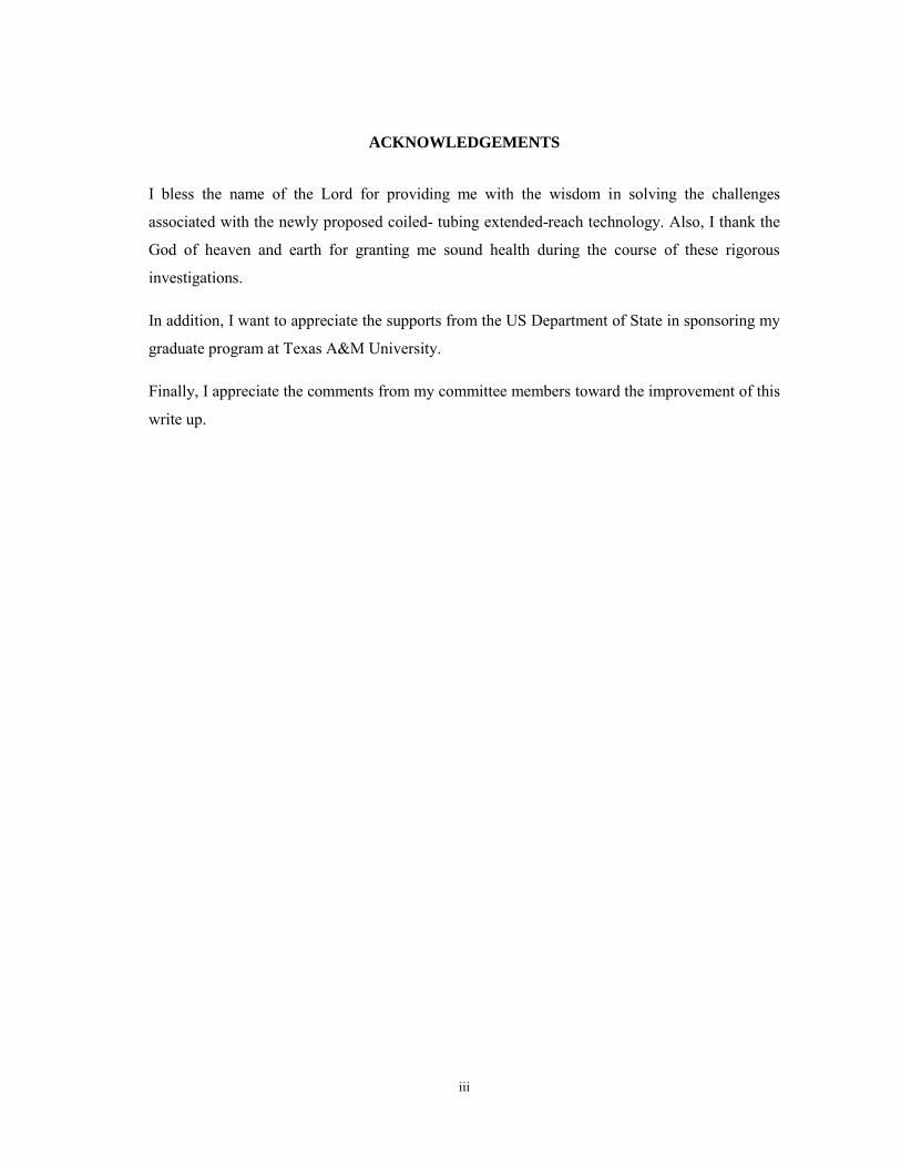
2.1.2 Normal Contact Force Model
When the rotating coiled tubing segment is being pushed into the deviated and lateral sections of
the wellbore, a normal force exists between the contact point of the tubing and the wellbore. The
magnitude of the force depends on the geometry of the wellbore, friction factor, weight of the
tubing, rotary torque, and the roll up angle (Fig. 2.3) of the tubing. The normal force is the
precursor for the drag force in the wellbore.
The relationship between the unit drag force and unit normal contact force is represented thus:
| | | |
Without any lateral deflection of the tubing, the unit normal contact force (when the tubing is
rotating) model is derived by combining equations “2.6 to 2.17”
| |
√
[ +
]
+ [
+
]
( + ) + ( )
Furthermore, as the tubing segment rotates in the wellbore it climbs the wall of the wellbore
either towards the direction of rotation or against the rotating direction (Fig. 2.3).
𝑒𝑛
𝑒𝑏
Fig. 2.3—The coiled tubing rolls up the wall of the wellbore in the deviated and inclined sections of the wellbore.
𝜃
��𝑐
��𝑑 𝑟𝑝
(2.18)
(2.17)

19
The direction towards which the tubing climbs depends on the friction factor, wellbore
geometry, applied torque, and buoyed unit weight of the tubing. The roll up angle of the tubing
against the wall of the wellbore is derived as
{
+
+
}
2.1.3 Rotating Torque Model
For a rotating coiled-tubing segment, the rotary torque can be determined by combining
equations “2.9, 2.10, and 2.16”
√(∫ | | | |
) + ( + + | | | | )
+
When the velocity angle is so small, the rotary torque model becomes
√(∫ | | | |
) + +
+
2.1.4 Total Shear Force in the Coiled Tubing Segment
The modulus of the total shear force (Fig. 2.4) which aims to bend the tubing segment depends
on the magnitude of the applied torque, hole geometry, and the value of the velocity angle. When
the segment is rotated such that the lateral drag forces on the CT are significant, the total shear
force is derived as
√ +
(2.19)
(2.20)
(2.21)
(2.22)

20
Where,
Often when the segment is rotated such that the velocity angle is small, the drag force
component of the shear force vanishes; thus, Eq. 2.22 becomes
√ + (
)
Eq. 2.23 suggests that the total shear force in the straight portion of the rotating segment is zero
when the velocity angle is small.
2.2 Nonrotating Segment of the Tubing String
Since the applied rotary torque to the rotating segment of the tubing has been arrested by the
twisting-restraining tools mounted upstream of the second mud motor, therefore, the tubing
segment will remain under static equilibrium if the following equations are satisfied
Fig. 2.4─The shear forces (at a point) aim to bend the tubing string in the normal and binormal directions.
𝐹𝑛
𝑒𝑛
𝑒𝑏
𝑒𝑡
𝐹𝑏
(2.23)
(2.24)

21
The equilibrium of forces in the segment is the same as equations “2.6 to 2.8.” The equilibrium
of moments equations in the CT string are as follows
+
+ +
On the other hand if the reactive torque is free to act on the nonrotating segment of the tubing,
equations “2.25 and 2.26” will be the same as equations “2.9 and 2.10” respectively. Although
the segment will not be subject to pure rotation but the applied torque will twist the tubing string
(see details in Chapter IV).
2.2.1 Drag Equation
The unit drag force in the nonrotating segment of the tubing is derived from Eq. 2.12 by setting
| |
Consequently, the unit drag on the tubing segment is
| | | |
(2.25)
(2.26)
(2.27)
(2.28)
(2.29)

22
2.2.2 Normal Force Equation
The normal force on the nonrotating segment of the tubing is higher than the normal force acting
on the rotating segment of the tubing in the same section of the wellbore. The normal force
equation is derived by setting in Eq. 2.18
| | √[ +
]
+ [
+
]
Although there is no applied torque on the nonrotating segment but the internal moments
generated by the shear forces cause the segment to roll up the wall of the wellbore. The roll up
angle is derived from Eq. 2.19 by setting
{
+
+
}
If the segment is lying on the straight portion of the wellbore the roll up angle becomes
2.2.3 Shear Force Model
By setting in Eq. 2.23 the shear force acting to bend the tubing segment is
derived as
√( ) + (
)
(2.30)
(2.31)
(2.32)
(2.33)

23
The drag on the tubing increases the shear force on the string; the magnitude of the total shear
force in the nonrotating segment can be greater than total shear force in the rotating segment
when the magnitude of the applied torque is not significantly high.
2.3 Axial Force Distribution in the Tubing String
Without any large lateral deflection of the tubing string, the generalized axial force distribution
in the string, as it is being deployed into the wellbore (rotating and nonrotating segments), is
derived by combining equations “2.6, 2.10, 2.12, and 2.17.”
+ | |( + )
If the rotating segment is rotated such that the velocity angle is small, the axial force distribution
in the segment (when the CT is pushed into the wellbore) is
And if the segment is straight the force distribution model becomes
On the other hand, the axial force distribution in the nonrotating segment of the tubing, when it
is deployed into the well, is derived from Eq. 2.34 by setting :
+ | |( + )
And for straight section of the nonrotating segment of the tubing, the axial force distribution is
(2.34)
(2.35)
(2.36)
(2.37)

24
+ | |
The axial force distribution in the tubing string when it is being pulled out of the hole can also be
represented by equations “2.34 to 2.38;” the only difference is that takes a negative value in
each of the equations.
(2.38)
25
CHAPTER III
TORSIONAL BUCKLING OF THE TUBING
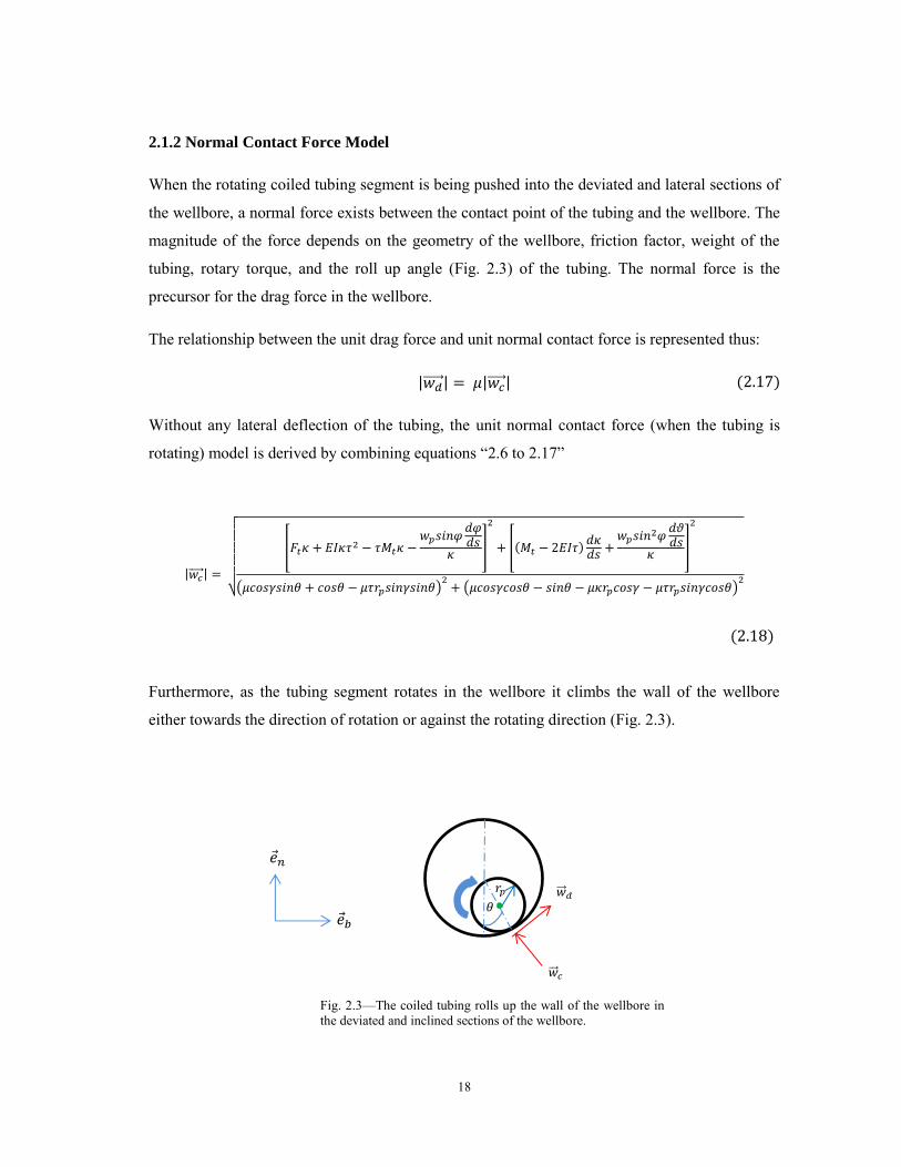
The application of rotary torque in conventional coiled-tubing drilling operations is directed at
increasing the horizontal cutting force of the drill bit, as it penetrates into the formation. The
magnitude of the torque applied on the bit depends primarily on the mechanical properties of the
rock.
The resultant cutting force, of the bit is the vectorial sum of the weight on bit, , (axial
direction) and the horizontal cutting force, , (Figs. 3.1a and 3.1b). The horizontal cutting
force depends on the applied rotary torque on the bit and the side force created by the weight of
the tubing string between the tangency point and the bit. But when stabilizers are arranged along
the bottomhole assembly (BHA) such that the component of the side force due to the applied
weight on bit is zero, then the shear force from the applied rotary torque will provide the
horizontal cutting force for the bit only.
��𝑏𝑖𝑡 ��𝑡 𝑏𝑖𝑡
��𝑡 𝑟 𝑏𝑖𝑡
Fig. 3.1a—The rotary torque on the bit and the weight on bit constitute the cutting forces for the bit (the tangency point is not shown in this picture).

26
For CT drilling operations, lower weight on bit relative to drilling with jointed pipes is usually
applied because of the low flexural rigidity of the tubing.
Using a hydraulic motor to rotate the bit produces a reactive torque (caused by the reaction of the
fluid momentum in the stator of the motor) that twists the nonrotating segment of the tubing
string. More often than not, high rotary torque is applied on the bit when drilling a hard
formation. To reduce the effect of twisting, stabilizers are sometimes installed on the BHA (the
primary aim of stabilizers is to enhance hole deviation control).
Although a high rotary torque may be applied on the bit, the high torsional rigidities of the BHA
components limit the angle of twist (for each section) of the tubing string. In most analyses, the
drag forces from the viscous drilling fluid and Coulomb friction with the wellbore wall, which
may dampen the torque along the length of the tubing string, are often assumed to be negligible.
Fig. 3.1b—The resultant cutting force of the bit is the vectorial sum of the side cutting force and the axial load component from the applied weight on bit.
��𝑡 𝑟 𝑏𝑖𝑡
��
��𝑐 ∅

27
But in the proposed system configuration the tubing string has a higher propensity to be twisted,
since the installation of the second motor will apply higher torsional loads on the string
(Fig. 3.2). The rotary torque applied on the rotating segment of the tubing string depends greatly
on the selected rotating length and wellbore geometry.
If the applied torque exceeds a critical value, the shear forces induced on the tubing string by the
torque will be dominant in the interplay of forces acting on the string; and the string will deflect
laterally. As the tubing string is deployed into the wellbore there is interplay between the
torsional loads and the axial compressive forces. Below the critical value of the applied torque,
the compressive force dominates in the buckling of the tubing string, although the applied
torsional loads reduce the critical buckling forces of the tubing (Wu 1997). When the torsional
��𝑏𝑖𝑡 ��𝑡 𝑏𝑖𝑡
��𝑡 𝑟 𝑏𝑖𝑡
��𝑡
��𝑡 𝑟
��𝑡
Fig. 3.2—Using a hydraulic motor, as the second motor produces reactive torques which can destabilize the pure rotation of the rotating segment.

28
load in the tubing string exceeds this value, the tubing string will buckle under the influence of
the applied torque.
The buckling mode of the compressed nonrotating segment of the tubing string is similar to the
dynamic buckling of the rotating segment. Therefore, the analysis on the torsional buckling of
the rotating segment is applicable to the nonrotating segment.
It should be noted that the torsional buckling of the nonrotating segment of the tubing string may
occur if a hydraulic mud motor is used in the drilling operation without the use of any tool to
arrest the reactive torque. Using an electrodrill in place of the hydraulic motor will not pose any
concern for torsional buckling of the nonrotating segment of the tubing; the reason is because
there is no reactive torque imposed on the segment.
For drilling applications, the applied torque on the tubing string is usually less than the torsional
yield strength. Thus, this section of the research project will also aim to compare the critical
buckling torque (first order) and torsional yield strength of the tubing string.
3.1 Torsional Buckling of the Tubing in the Vertical Section of the Wellbore
Subjecting the tubing string (both the rotating and nonrotating segments) to interplay of axial
forces and torsional loads can make it vulnerable to helical buckling (Fig. 3.3). Although the
tubing’s resistance to helical buckling, resulting from axial forces only, is limited in the vertical
section of the wellbore (Wu 1992), the addition of the torsional loading further reduces its
resistance.
In the interplay of the forces and moments acting on the tubing string, the dominant of the loads
(torque or axial compressive force) buckles the tubing segment.
As the tubing string buckles, the length of the affected segment (rotating or unprotected
nonrotating) shortens by (Fig. 3.4). Lubinski et al. (1962) derived
Where, is the pitch of the buckled tubing length and is the radial clearance between the
tubing and the wellbore
(3.1)

29
Considering the helical buckling of the unprotected nonrotating segment of the tubing under the
applied axial loads and torque, the bending energy stored in the string is
is the Young’s modulus and is the second moment of area of the tubing.
During the buckling process, the axial load in the tubing string remains constant as the axial
displacement increases (Gao and Miska 2008b and 2009).
Fig. 3.3—Both the rotating and unprotected nonrotating segments of the tubing string will helically buckle when the buckling torque dominates in the interplay of forces and moments.
(3.2)
��𝑡
��𝑏
��𝑡 𝑟
��𝑡

30
The work done by the axial load (compressive) at the midpoint of the buckled section towards
the buckling of the tubing is
Since the effect of the weight of the tubing is considered in the buckling process, the negative
work done by the weight of the tubing is
The work done by the applied torque towards the buckling of the tubing segment is
As the first deflection of the tubing string is made and contacts the wall of the wellbore, further
buckling of the length is resisted by the lateral friction resulting from the normal force from the
Fig. 3.4—As the tubing length buckles helically, it contacts the wall of the wellbore. The pitch of the helically buckled length is assumed to be constant for mathematical simplicity; although the assumption is more practical for coiled tubing than a heavy drillpipe.
𝛿
𝑙
Unbuckled length
(3.3)
(3.4)
(3.5)

31
helical buckling. During the buckling process, the axial friction is negligible because the lateral
buckling velocity is dominant (Gao and Miska 2008b). In this analysis, the resistive work done
by the lateral friction will not be put into consideration.
From the conservation law of energy: the elastic deformation energy stored in the tubing string is
equal to the sum of the works done by all external forces on the tubing.
+ +
Substituting equations “3.1 to 3.5” into Eq. 3.6, we have
+
In the vertical section of the wellbore, the normal force resulting from the helical buckling of the
tubing is equal to the normal force caused by the helical buckling of weightless tubing
(Mitchell 1988).
Assuming constant pitch during the buckling process, the first order buckling torque is
+
The buckled length for the first buckling order can be determined by minimizing the first order
buckling torque, i.e.
and solving for in the algebraic equation.
Gao and Miska (2008a) showed that lateral friction affects the buckling of both rotating and
nonrotating pipes. During the buckling process, the axial friction is so negligible that the lateral
friction becomes dominant. But the effect of friction in the buckling process is not considered in
this study (for mathematical simplicity).
When the axial load approaches a small value (for engineering purposes) in the rotating segment
of the tubing and the friction effect is disregarded (for computational simplicity only), the first
order buckling torque approaches
(3.8)
(3.7)
(3.6)

32
(
)
While the first order buckled length resulting from the torsional load only is
√
Eq. 3.9 gives a more accurate result than the model developed by Miska and Cunha (1995):
3.2 Torsional Buckling of the Tubing in the Inclined Section of the Wellbore
In the inclined section of the wellbore (Fig. 3.5), the weight of the tubing further does more work
in resisting the buckling of the tubing. The additional work done ( ) is towards
resisting the lateral deflection of the tubing; the weight also does work (
) in
resisting the axial compression.
The buckling torque (with compressive force acting simultaneously on the tubing) is derived by
incorporating the works done by the weight of the tubing into Eq. 3.7
For constant pitch assumption, the first order buckling torque is
+
+
(3.9)
(3.10)
(3.12)
(3.11)

33
When the tubing is subjected to torsional loads only, the first order buckling torque becomes
+ +
For wells with high inclination angles, the work done by the weight of the tubing in resisting the
axial compression of the tubing will be so small that it can be neglected for practical engineering
purposes.
3.3 Torsional Buckling of the Tubing in the Curved Section of the Wellbore
In the curved section of the wellbore (Fig. 3.6), the internal axial force in the tubing does an
extra work (
) as a result of the interaction with the curvature of the wellbore during the
buckling process. Although the axial compressive force aids in the buckling process, the extra
work done tends to resist the buckling of the tubing.
(3.13)
Fig. 3.5—The additional work done by the weight of the tubing string in resisting the lateral elastic deflection increases the buckling torsional load of the string, when the tubing lies in the inclined section of the wellbore.
��𝑡
��𝑏
��𝑡 𝑟
��𝑡

34
Combining the works done by the weight of the tubing and the axial compressive force in the
tubing (noting that a tensile force will do negative works to oppose the buckling of the tubing),
for constant pitch assumption, the first order buckling torque is
+
+ +
Considering the different torsional buckling loads for the different sections of the wellbore, the
lowest in value is Eq. 3.9. The compressive load that initiates helical buckling of coiled tubing in
the vertical section of the wellbore is so small to affect the magnitude of the torque considerably.
(3.14)
Fig. 3.6—The interaction of the axial compressive force with the curvature of the wellbore results in the generation of a resistive work that increases the buckling torque in the curved section of the wellbore.
��𝑡 𝑟
��𝑏
��𝑡
𝑅
𝜑
��𝑡

35
Similarly, the wellbore geometry affects the value of the buckling torque. The buckling torque is
greatest in the curved section of the wellbore because of the contribution of the axial force.
For drilling operations, the permissible torque in the tubing is usually less than the torsional yield
strength of the tubing. Thus, comparing the lowest buckling torque (first order) values for the
different tubing sizes with their torsional yield strengths (Table 3.1), this project can infer that
the tubing will not buckle under the influence of the applied torque. The tubing sections will
buckle mainly from the compressive forces acting on them. Also, the effect of the applied torque
on the axial buckling loads can be disregarded (Wu 1995).
Table 3.1—Comparison of First Order Buckling Torques and Torsional Yield Strengths of Different Tubing Sizes
Outer Diameter,
in.
Internal Diameter,
in.
Grade Unit Weight,
lb./ft.
First Order Buckling
Torque, lb.-ft.
Torsional Yield Strength, lb.-ft.
0.750 0.584 CT55 0.59 374 138
1.000 0.750 CT90 1.17 1,067 581
1.250 0.900 CT90 2.01 2,423 1,214
1.500 1.150 CT80 2.48 3,924 1,878
1.750 1.374 CT90 3.14 6,177 2,825
2.000 1.624 CT90 3.64 8,710 3,844
2.375 1.999 CT90 4.39 13,476 5,673
2.875 2.469 CT80 5.79 23,194 9,215
3.500 3.094 CT90 7.15 37,837 14,192

36
CHAPTER IV
TUBING ROTATING LENGTH AND TWISTING MOMENTS
4.1 Determining the Maximum Rotating Length
The system configuration provides a rotating segment with a fixed length and a nonrotating
segment with variable length. The length of the nonrotating segment primarily depends on the
total measured depth of the well; the length of the segment is the arithmetic difference between
the fixed length and the total measured depth (if the tubing string is not buckled).
In determining the maximum length of the rotating segment the torsional yield strength of the
CT material plays a big role. Since the applied torque on the string increases as the length to be
rotated increases (for constant rotary speed), at a critical length of the tubing segment the rotary
torque will equal the permissible torque (the product of safety factor and the tubing torsional
yield strength) in the tubing string.
Similarly, Eq. 2.20 signifies that the geometry of the well also affect the length of the rotating
segment. The more tortuous the well path is the lesser would be the rotating length because of
the increase in drag in the wellbore.
When determining the maximum length of the rotating segment, the location in the wellbore
where the maximum hydraulic power would be expended by the second mud motor needs to be
identified. The location of this point could be at the kickoff point or at the end of build. The ratio
of the unit normal forces at the deviated and lateral sections of the wellbore is a key criterion that
can be used in determining the location where the maximum hydraulic power would be
expended as the second mud motor moves down into the wellbore.
The addition of the measured depth downstream of the motor at that location will sum up to
yield the maximum length of the rotating segment (with the assumption that the rotary speed of
the string remains constant).
As an illustration, considering a 2D well profile (Figs. 4.1a and 4.1b); the greatest torque will be
applied to the rotating segment when the hydraulic motor reaches the kickoff point if | |
| | .

37
On the other hand, if | |
| | then the maximum power will be expended when the mud
motor reaches the end of build.
Making reference to Eq. 2.18, the unit normal force in the deviated section of the 2D wellbore,
where
, | | is derived below. Similarly, this analysis assumes that the tubing
string is rotated at an angular speed significant enough to reduce the axial drag in the wellbore to
an inconsequential magnitude.
| |
| |∫ (
)
But Mitchell et al. (2011) derived the curvature of a wellbore as
√(
)
+ (
)
For a well profile with no azimuth change,
For the lateral section of the wellbore, the unit normal force is derived from Eq. 4.1, when
. Therefore, the unit normal force in the straight section is
| |
In the quest to determine the location where the maximum torque would be applied on the
rotating segment, the first case must be examined (i.e. | |
| | . More often than not, this first
case is usually valid for most directional wells; the unit normal force in curved section is usually
greater than the unit normal force in the lateral section, if there is no buckling.
Using the minimum curvature method (Mitchell et al. 2011) to determine the angle of inclination
at any point in the curved section, is
(4.4)
(4.2)
(4.3)
(4.1)

38
{ [ ] + (
) [ ]}
Lubinski et al. (1953) derived the dogleg angle, , as
√ (
) +
(
)
But for a well profile with no change in the azimuth angle, the dogleg angle is
.
The axial force in the tubing, at the end of build, is derived from Eq. 2.35 as
+ .
The torque required to rotate unbuckled tubing (under high tension) in the curved section of the
wellbore is derived from Eq. 2.20 (for a 2D well profile) in Eq. 4.9a as
[
+ + ]
For unbuckled tubing under low tension, the required torque is derived as
[
+ ]
(4.8)
(4.7)
(4.6)
(4.5)
(4.9a)
(4.9b)
39
𝐹𝑡
𝐹𝑡
|��𝑐 𝑑|
𝑒𝑛
𝑒𝑡
Fig. 4.1b─The unit weight of the tubing in the curved section of the wellbore varies with the axial load in the string.
𝑙𝑟 𝑙
𝑅
𝐹𝑡
Nonrotating segment
𝜑 𝜑
𝐹𝑡
Fig. 4.1a─When the second mud motor approaches the KOP, the maximum torque is applied to the rotating segment.

40
But the length of the rotating segment in the lateral section of the wellbore, when the second
mud motor reaches the kick off point, is unknown. Therefore, is derived by summing the
required rotary torques for each of the two sections under consideration (lateral and curved) to
equal the permissible torque in the rotating segment (i.e. the product of the torsional yield
strength of the tubing and a reasonable safety factor).
Considering high tension in the curved section of the wellbore when the mud motor gets to the
kick off point, the lateral length of the rotating segment is
{ ∑
+ }
+
For low tension, the lateral length of the rotating segment is
{ ∑
}
The rotating length is thus derived as
+
Thus, combining equations “4.1 to 4.10c” gives the necessary procedure that should be taken
when calculating the ratio of the unit normal forces and determining the rotating length.
After the vertical section of the well has been drilled, equations “4.10a to 4.10c” can be
employed in determining the length of the tubing to be rotated as the deviated and lateral
sections of the wellbore is being drilled. On the other hand, if the conventional coiled-tubing
drilling approach has been used to drill through the deviated and lateral section to a significant
(4.10a)
(4.10c)
(4.10b)

41
depth, which is greater than the rotating length (Eq. 4.11), then, the second mud motor can be
placed at the end of build before rotating the string.
( ∑
)
Since the tubing in the vertical section of the wellbore has low critical buckling loads, having a
segment of the rotating length buckled is not desirable (although sometimes it cannot but be
allowed). Therefore, to avert the buckling of the rotating length when high weight on bit is
required, the following must be taken into consideration:
a. Ensure the maximum weight on bit is less than the critical buckling loads (especially the
helical buckling load) of the tubing in the lateral section of the wellbore.
b. Determine if the tubing string in the vertical section of the wellbore will buckle anytime
during the drilling operation before reaching the target, by calculating the critical
buckling loads and comparing them with the estimated compressive forces in the string.
c. If the tubing in the vertical section of the wellbore will buckle during the course of
drilling, the rotating length should be calculated by placing the second mud motor at the
kick off point. Since the rotating tubing in the curved and the lateral sections of the
wellbore will not buckle because of higher critical buckling loads (if the maximum
weight on bit is not greater than the critical loads at inclined and curved sections), the
whirling of the rotating segment and other phenomena resulting from the rotation of
buckled tubing will be prevented during the drilling process.
d. The weight of the second mud motor must be considered when determining the weight
of the bottomhole assembly. Mud motors with high torque specification have high
weights which can be very significant for coiled-tubing drilling operations. If the weight
of the second motor is not considered, the rotating length of the tubing string can be
under excessive compressive force than designed for.
Although the proposed system configuration can be applied in a drilling operation demanding a
high weight on bit (greater than helical buckling load), the procedures above will not be
applicable in determining the maximum rotating length of the tubing string.
(4.11)

42
Similarly, it should be noted that the proposed extended-reach technique cannot be effective in
extending the reach of coiled tubing in the wellbore when very high weight on bit (greater than
the helical buckling load of the tubing string) is applied on the string.
With high angle inclined section, the contributions of the bottomhole assemblies to the weight on
bit may not be sufficient. Therefore, the rotating tubing segment will be under high compression.
Since the segment is to be prevented from buckling, the permissible length can be determined
from Eq. 4.12.
∑
In practice, . Thus, the bottomhole assemblies (plus the second motor assembly) must be
adjusted to ensure that the inequality is satisfied.
The length of the rotating tubing (excluding the bottomhole assembly at the bit) that can support
the weight on bit without buckling is thus derived as
By comparing the values of from Eq. 4.13 and Eq. 4.10 (or Eq. 4.11), the lower of the two is
selected as the maximum rotating length of the tubing.
Generally, the rotating length must be selected such that it does not buckle when spooling into
the wellbore.
4.2 Rate of Change of the Rotary Torque/Reactive Torque
From the explanation in Chapters II and III, the nonrotating segment of the tubing string cannot
be buckled under the influence of a high reactive torque. The magnitude of the reactive torque
changes as more length of the rotating segment lies in the deviated and lateral sections of the
wellbore.
(4.12)
(4.13)

43
The rate of change of the reactive torque is also dependent on the position of the second mud
motor relative to the bit (Fig. 4.2). When the rotating segment is not buckled the rate of change
of the reactive torque is derived as
( )
When deploying the tubing string into the wellbore, (with positive sign). The positive
sign assigned to ROP in Eq. 4.14 indicates that the magnitude of the reactive torque (the reactive
torque equals the total rotary torque on the rotating segment) increases as we push the tubing
string into the wellbore.
𝑤𝑐 𝑏𝑖𝑡
𝑤𝑏𝑖𝑡
𝑤𝑐 𝑚𝑡𝑟
��𝑡
��𝑡
��𝑡 𝑟
Fig. 4.2—The reactive torque acting on the nonrotating segment is the cumulative of the rotary torques on the rotating segment. The reactive torque will remain constant when the second mud motor and the BHA are in the same wellbore section.
(4.14)

44
But when the tubing string is being pulled out of the hole, will equal to the tripping velocity
(negative sign); therefore, the magnitude of the reactive torque will decrease as we trip out of the
wellbore.
Preventing the rotating segment from buckling is highly desirable. It is desirable because a high
weight on bit (which is greater than the critical buckling loads of the rotating segment) applied
on the tubing string will cause the rotating segment to buckle and expose the segment to
increased fatigue loads.
4.3 Twisting Moment in the Nonrotating Tubing Segment
Hydraulic downhole motors (positive displacement mud motors and turbo-drills) are often used
for drilling and other well intervention applications. They have proven to be efficient in
directional drilling applications. But one major problem about hydraulic downhole motors is the
twisting moments they impact on the tubing string.
As explained in Chapter I, hydraulic motors are energized through the hydraulic energy of the
fast-flowing drilling fluid, pumped down the drillstring. As the drilling fluid enters the power
section of a hydraulic motor, the fluid pushes against the stator, while its momentum rotates the
rotor.
The rotary torque applied on the rotor is transferred to the “driven load” (in this case, the tubing
and the bottomhole assembly at the bit). From Newton’s third law of motion—to every action
there is equal and opposite reaction—a reactive torque acts on the stator of the motor. This
reactive torque impacts twisting moment on the motor and the nonrotating tubing segment.
Since a high-torque hydraulic motor would be needed in rotating the tubing and the bottomhole
assembly (at the bit), the effect of the twisting of the motor and nonrotating tubing string can
destabilize the drilling process. Similarly, the change in length of the nonrotating segment, as the
bit penetrates into the formation, will impact the twist angle.
From Eq. 4.15, the rate of change of the twist angle depends on both the rates of change of
the reactive torque, and the length of the nonrotating tubing segment, , (neglecting the
effects of the viscous forces and the Coulomb’s friction from contact with the wellbore wall).

45
+
With respect to time, the rate of change of the twist angle is thus derived as
[(
) + (
)]
Substituting Eq. 4.12 into Eq. 4.14, yields
{[ ( )
+
]
}
When the second mud motor is located in the same wellbore section as the bit, the rate of change
of the reactive torque becomes zero, but the rate of change of the angle of twist is not zero
(Eq. 4.18).
(
)
The rate of change of the angle of twist is not zero because the rate of penetration is not zero
when drilling into the formation (or tripping in or out of the wellbore). This suggests that the
destabilization of the drilling process (or tripping of the tubing in or out of the wellbore) will not
be solved by placing the second mud motor in the same wellbore section as the bit.
4.3.1 Preventive and Remedial Measures against Twisting of the Tubing
To prevent the twisting moment on the tubing string, the hydraulic motor can be replaced with
an electrodrill. An electrodrill (downhole electric motor) is a three-phase asynchronous motor
with a spindle (screwed to the motor through a conic thread with journal bearings) that transmits
the rotary torque to the driven load. With the principle of operation of the electric motor
(electromagnetism), no reactive torque that will cause the twisting of the tubing will be
generated during operation.
(4.15)
(4.16)
(4.18)
(4.17)

46
Unfortunately, the application of electrodrill is faced with some challenges: low starting torque
of the induction coils, limited operating life of the motor, unavailability of small-diameter
electrodrills for slimholes, and limitation to the supply of electric voltage for deep-well drilling.
With the problems associated with the use of electrodrill, a hydraulic motor can still be used but
a full-gaged stabilizer or dynamic torque anchor will be needed in arresting the twisting moment.
The associated problem with the use of these tools is the reduction of the hookload.
As the twisting moment acts on the stabilizer (Fig. 4.3a and 4.3b) or the dynamic torque anchor,
additional normal contact forces exist between the tool and the wellbore. The magnitudes of the
normal forces are dependent on the magnitude of the reactive torque and the diameter of the
hole. With the high normal force in the nonrotating segment of the tubing string, the extent of
CT string will be reduced in the wellbore.
Fig. 4.3a—The twisting moments induce normal and binormal contact forces between the stabilizer blades and the wellbore (top view).
𝑒𝑛
𝑒𝑡
𝑤𝑏𝑙𝑏𝑠𝑖𝑛𝜑
6𝑒𝑛
Stab l zer ’ blade w th
elastomeric pads
𝑤𝑏𝑙𝑏𝑠𝑖𝑛𝜑
6𝑒𝑛
𝐹𝑓
𝐹𝑓

47
To reduce (or eliminate) the induced normal forces from the twisting moment when using a
positive displacement mud motor (PDM) or turobdrill, a dynamic torque arrestor (Fig. 4.4) is
being proposed.
4.3.2 How the Dynamic Torque Arrestor Works
The tool resists the twisting moment from the mud motor through a combined effort of the
torsional spring and the viscous fluid. Since the drive behind this invention is to have a
downhole tool that can resist the twisting moment (from the mud motor) without transferring the
torque to the tubing, using a highly viscous fluid will be a good medium for the dissipation of the
twisting energy.
The tool “receives” the twisting moment from the mud motor through the adapter. The adapter
has threaded ends that can be screwed into the top sub of the mud motor. Between the adapter
and the casing is a small aperture. The aperture helps to isolate the casing from receiving the
twisting moment. Similarly, the aperture defines the maximum displacement the machined
spring is allowed under high compressive load. Since the tool will likely be subjected to high
compression downhole, the spring should have high stiffness. Also, the compression of the
𝑀𝑡 𝑟
𝑟𝑏𝑒𝑏
𝑟𝑏
𝑒𝑛
𝑒𝑏
Fig. 4.3b— The twisting moments induce normal and binormal contact forces between the stabilizer blades and the wellbore (end view).
(𝑤𝑏𝑙𝑏𝑠𝑖𝑛𝜑
6𝑒𝑛 +
𝑀𝑡 𝑟
𝑟𝑏𝑒𝑏)
( 𝑤𝑏𝑙𝑏𝑠𝑖𝑛𝜑
6𝑒𝑛
𝑀𝑡 𝑟
𝑟𝑏𝑒𝑛) (
𝑀𝑡 𝑟
𝑟𝑏𝑒𝑛 +
𝑤𝑏𝑙𝑏𝑠𝑖𝑛𝜑
6𝑒𝑛)

48
Machined spring (withstands torsional and axial loads)
Highly viscous fluid
Adapter
Thrust ball bearing
Axial roller bearing
Perforations for mud flow
Elastomeric pad
Casing
Plate-1
Plate-2
Spindle
Fig. 4.4—The newly proposed dynamic torque arrestor does not induce normal and binormal contact forces on the string.

49
spring resulting from pressure forces of the fast moving drilling mud must be considered in the
design analysis.
The mechanical bearings help in supporting the axial loading. Anti-friction bearings (thrust roller
and thrust ball bearings) are used in this design to prevent the transfer of the twisting motion to
the casing. Since the casing is attached to the coiled-tubing connector (may be through an
adapter), the twisting motion of the casing will not solve the destabilization problem. Therefore,
the casing is isolated from the twisting by connecting a spindle from the machined spring to the
viscous fluid.
Apart from the fact that the spindle connects the machined spring and the viscous fluid medium,
it supports the static and dynamic loadings on the spring.
The high viscous fluid (preferably a magnetorheological of electrorheological fluid) gives the
final restraint to the twisting torque. It also gives an “immovable” base for the torsion spring to
deflect rather than rotating.
Plate-2 provides a base for mounting the cylinder containing the viscous fluid. Similarly, the
plate has large perforations for mud-flow diversion. The container is fastened to the plate
through bolts and nuts.
Plate-1 limits the leakage volume of the mud through the small aperture. The plate diverts most
of the mud into the “lead” coil of the spring (the coil is hollow). The small space between this
plate and the lead coil is to prevent the transfer of the twisting torque to the casing. Elastomeric
pads are put at the inner edge of the plate to dampen any periodic or nonperiodic oscillation of
the lead coil.
Improvements need to be made on this invention in eradicating the propensity for leakage
through the aperture. Although the elastomeric pads can be used in closing the gap between
plate-1 and the lead coil, drops of mud will still escape through the aperture to the annulus. On
the other hand when the annulus pressure is greater than the pressure in the drillstring, there will
be influx of mud (with drill cuttings) into this tool.

50
The solid content in the mud (inflowing from the annulus) can build up in this tool and reduce its
effectiveness. Nevertheless, the occurrence of the solid content build up is not rapid; it will take
several cycles of operation before the “clogging” can occur.

51
CHAPTER V
MAXIMUM TUBING DISPLACEMENTS IN THE WELLBORE
Knowing the maximum displacements of the tubing producible by the newly proposed CT
extended-reach drilling technique will be useful in ascertaining its (technique) practicality. The
maximum length of the tubing is not limited by lockup condition encountered during the drilling
operation only but a zero hookload can also be a constraint. Therefore, the project will endeavor
to analyze the different scenarios that will result into the lockup of the tubing string in the
wellbore and consider the zero- hookload phenomenon.
Although the drilling parameters like: weight on bit, mud weight, wellbore geometry, friction
factor, drillstring geometrical and mechanical properties, etc. influence the occurrence of lockup
and zero hookload in the wellbore, the new system configuration can also impact the phenomena
positively or negatively.
The force distribution models in the tubing segments will be used in analyzing the maximum
length from lockup and zero-hookload conditions.
5.1 Maximum Displacement at Zero Hookload or Lockup in the Vertical Section
The maximum length of the tubing string in the wellbore does not only suggest the measured
depth in the wellbore when the lockup condition is encountered in the lateral section. Sometimes,
the maximum length of the tubing in the wellbore may be reached before lockup condition in the
lateral section.
The maximum length of the tubing in the wellbore can be reached when the hookload
approaches zero or the axial compressive force reaches the maximum value. When the hookload
approaches zero it simply suggests that the whole tubing string is under compression and there is
no weight (tensile force) available for lowering the string into the wellbore.
The frictional forces acting on the string increase as more length of the nonrotating segment of
the tubing string is deployed into the deviated and lateral sections of the wellbore. As a result,
more loading force will be required to overcome the drag forces acting on the tubing string in
those sections of the wellbore.

52
In addition to the increased drag forces in the system, increasing the weight on bit because of
increased rock strength can further promote the susceptibility of the tubing to buckling. When
the compressive force in the string exceeds the helical buckling load, the tubing starts changing
configuration; the sinusoidal buckling configuration of the string precedes the helical buckling
configuration. Since the helical buckling load of the tubing in the vertical section of the wellbore
is so small the development of the helices will likely start in that section of the wellbore.
At the top of the helically buckled section the compressive force can be very small. Similarly,
since the tubing length further up the buckled section might be in tension, the neutral point
(Fig. 5.1) is often placed at the top of the buckled section, (Wu and Juvkam-Wold 1995).
A zero-hookload condition will be reached when the neutral point shifts upward to the surface
(the “movement” of the neutral point results from the development of more helices in the vertical
section). Although the injector head system can be employed to further push the tubing into the
Neutral point
��𝑡 𝑏
��𝑡
Fig. 5.1—The neutral point is at the top of the helically buckled length.

53
wellbore, the low critical-helical buckling load of the tubing in the vertical section of the
wellbore will limit the magnitude of the compressive force to be applied. But a compressive
force, higher than this critical load, can be applied on the tubing with the aim of having a
significant increase in the length of the tubing in the wellbore; unfortunately, this act will lead to
more helices being formed in the vertical section of the well. As a result, the neutral point shifts
further up and the tubing can be in “forced fit” (when the rate of elastic-deformation propagation
is greater than the rate of penetration) with the blowout preventer or other surface equipment
(Fig. 5.2), creating potential hazard.
With the rotating segment of the tubing string prevented from buckling (in this analysis), the
axial force distribution in the string can be estimated with equations derived in Chapter 2. On the
other hand, as more length of the nonrotating tubing segment is pushed into the deviated and
lateral sections of the wellbore, the drag forces in the system start mounting up. Therefore, the
configuration of the tubing segment changes and the equations derived in Chapter 2 will not be
applicable in deriving the axial force distribution in the buckled segment.
Since the reactive torque from the second mud motor has been arrested, the effect of torque on
the forces acting on the tubing segment is zero. Although it has been verified in Chapter III that
the applied torque is so small to initiate buckling of the tubing, its effect on the forces acting on
the tubing cannot be totally disregarded (He et al. 1995). But in this configuration, the effect of
torque on the nonrotating segment is zero.
When the compressive force in the nonrotating segment of the tubing exceeds the critical
sinusoidal buckling load, the string has a snaking configuration. With the snaking configuration,
the drag forces in the string will increase further. As more length of the buckled segment is
further pushed into the wellbore, the compressive force in the tubing will increase; the tubing
configuration changes from sinusoid to helix when the compressive force exceeds the critical
helical buckling load.
Knowing the axial force distribution in the tubing string under the different possible
configurations, an estimate can be made for the maximum length of the tubing in the wellbore.
(The axial force distribution in the tubing for unbuckled configuration has been derived in
Chapter II, therefore, only the axial force distribution in the sinusoidally and helically buckled
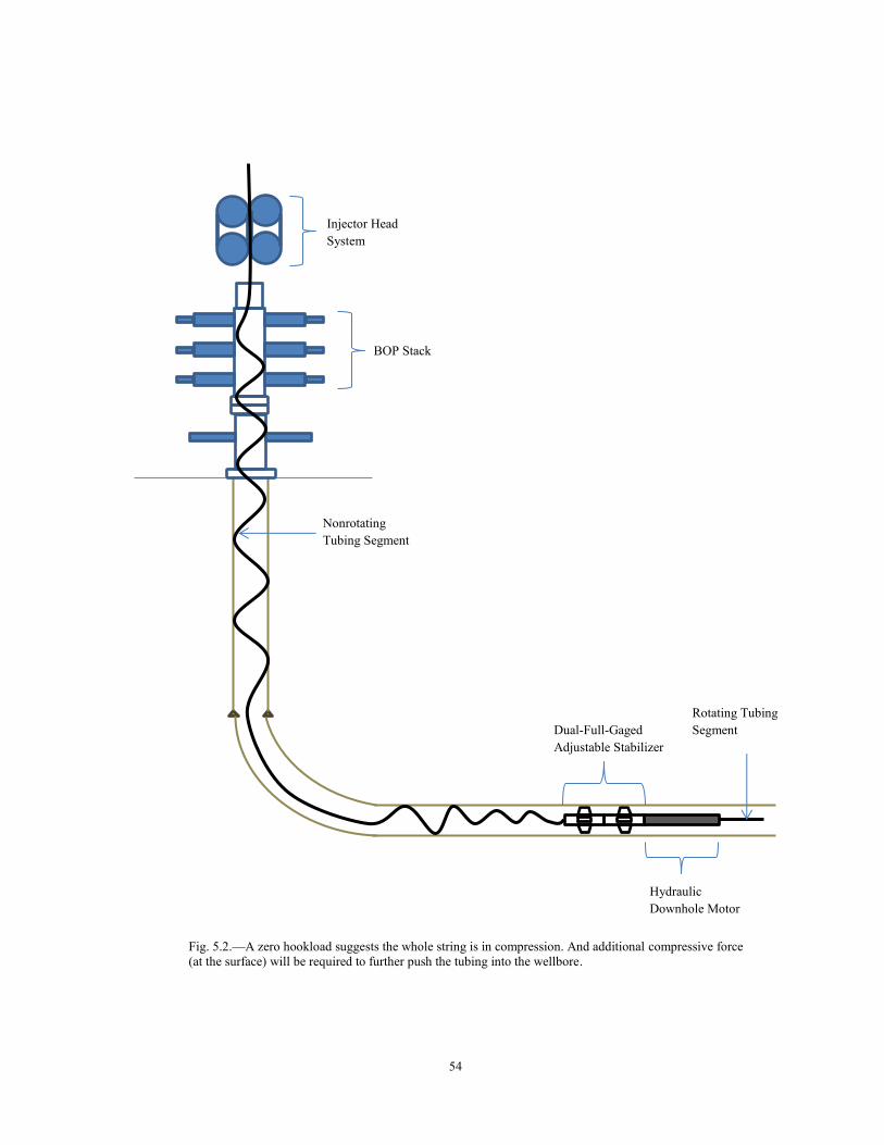
54
Fig. 5.2.—A zero hookload suggests the whole string is in compression. And additional compressive force (at the surface) will be required to further push the tubing into the wellbore.
BOP Stack
Nonrotating Tubing Segment
Rotating Tubing Segment
Hydraulic Downhole Motor
Dual-Full-Gaged Adjustable Stabilizer
Injector Head System

55
tubing segment will be analyzed in this chapter. The equations for the axial force distribution in
the unbuckled tubing will be referenced from Chapter II).
5.1.1 Axial Force Distribution in Sinusoidal Buckled Tubing in Straight Wellbores
When the compressive force in the nonrotating segment of the tubing exceeds the critical
sinusoidal buckling load (Eq. 5.1) the tubing changes its configuration from “straight” to sine
wave (Figs. 5.3a and 5.3b) form, the axial force distribution in the tubing is no more linear.
For tubing in the incline section of the wellbore, the sinusoidal buckling load is
√
For tubing in a vertical wellbore section, the sinusoidal buckling load is
( )
Where represents the correction factor resulting from the effect of lateral friction during the
snaking buckling process
(
) +
( +
+
)
+
The governing differential equation representing the axial force distribution in the buckled string
is
+ ( + )
(5.6)
(5.1)
(5.3)
(5.4)
(5.5)
(5.2)

56
Gao and Miska (2009) derived the unit normal force resulting from sinusoidal buckling ( ).
[ + (√
)
]
Where,
+
6
+
⁄
6
(5.8)
(5.7)
Fig. 5.3b—End view of sinusoidally buckled tubing string segment lying in a straight section of the wellbore
Fig. 5.3a—Top view of sinusoidally buckled tubing string segment lying in a straight section of the wellbore
��𝑡 𝑏
��𝑡 𝑡
𝑙
𝑠

57
6
6
( )
+
6
6
The unit normal contact force resulting from this configuration of the tubing in the wellbore is a
function of the axial force.
Substituting Eq. 5.7 into Eq. 5.6, the differential equation becomes
+ { [ + (√
)
] + }
Solving the ordinary differential equation, the axial force distribution in the sinusoidally buckled
section is
√ √
{
√
[
+
( ( + √ )
√ )
√
]
}
The buckled length is derived from Eq. 5.12 as
(5.9)
(5.10)
(5.11)
(5.12)
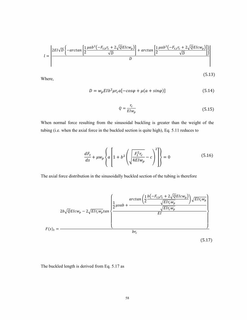
58
|| √ { [
( + √ )
√ ] + [
( + √ )
√ ]}
||
Where,
[ + + ]
When normal force resulting from the sinusoidal buckling is greater than the weight of the
tubing (i.e. when the axial force in the buckled section is quite high), Eq. 5.11 reduces to
+ { [ + (√
)
]}
The axial force distribution in the sinusoidally buckled section of the tubing is therefore
√ √
{
+
( ( + √ )
√
)√
√
}
The buckled length is derived from Eq. 5.17 as
(5.16)
(5.13)
(5.14)
(5.15)
(5.17)

59
||
√ { [
( + √ )
√
] [
( + √ )
√
]}
||
When the sinusoidal buckling occurs in the vertical section of the wellbore, the axial force
distribution in the tubing (when its unit weight is not negligibly compared to the unit normal
force resulting from sinusoidal buckling) is derived as
+ { [ + (√
)
]}
Solving the differential equation, the axial force distribution in the sinusoidally buckled section
of the tubing string becomes
√ √
{
√
[
+
( ( ⁄ + √ )
√ )
√
]
}
Where,
The buckled length of the snaking buckled section of the tubing string in the vertical section of
the wellbore is derived as
(5.18)
(5.19)
(5.20)
(5.21)

60
||
{√ [ ( + √ )
√ ] √ [
( + √ )
√ ]}
||
On the other hand, when the unit weight of the tubing is small compared with the normal force
resulting from the snaking buckling, the axial force distribution is same as Eq. 5.17 and the
buckled length as Eq. 5.18.
5.1.2 Axial Force Distribution in Helical Buckled Tubing in Straight Wellbores
With more compression in the nonrotating segment of the tubing (as more length is pushed into
the wellbore), the axial force at the top of the sinusoidally buckled section approaches the helical
buckling load of the tubing (Eq. 5.23). When more length of the tubing is pushed further into the
wellbore, more helices (Figs. 5.4a and 5.4b) will be formed.
For tubing in an inclined wellbore section, the helical buckling load is
√ √
For tubing in a vertical wellbore section, the helical buckling load is
( )
Where represents the correction factor resulting from the effect of lateral friction in the helical
buckling of long tubing
6
[ +
]
(5.22)
(5.23)
(5.24)
(5.25)

61
The governing differential axial force distribution in the helically buckled section of the tubing
(in the lateral section of the wellbore) is
+ ( + )
Mitchell (1986) and Gao and Miska (2009) developed a mathematical model for the unit normal
contact force (between the tubing and the wellbore) resulting from helical buckling of a
weightless tubing as
Substituting Eq. 5.27 into Eq. 5.26 yields
Fig. 5.4b—End view of helically buckled tubing string segment lying in a straight section of the wellbore
(5.26)
(5.27)
��𝑡 𝑏
��𝑡 𝑡
Fig. 5.4a—Top view of helically buckled tubing string segment lying in a straight section of the wellbore
𝑙
𝑠

62
+ (
+ )
Solving the ordinary differential equation, the axial force distribution in the helically buckled
tubing section is
√
{
√ [ (
√
)
√ ]
}
From Eq. 6.29, the buckled length of the tubing is
|| [√ (
√ ) (
√ )√ ]
||
As the axial compressive force in the tubing approaches high magnitude, the unit normal contact
force resulting from helical buckling will be much higher than the contributions of the tubing
weight to the axial force distribution. Therefore, Eq. 6.28 becomes
+
The axial force distribution in the tubing is thus
(5.28)
(5.29)
(5.32)
(5.30)
(5.31)

63
+
From Eq. 6.33, the buckled length of the tubing string is derived as
| ( )
|
In the vertical section of the wellbore, the axial force distribution in the helically buckled tubing
segment is derived from Eq. 6.28 as
+
Solving the differential equation, the axial force distribution in the tubing string is
[
√ + (
√ )
]
√
The buckled length of the segment is
||
[ (
√ ) (
√ )]
√ ||
(5.33)
(5.34)
(5.35)
(5.36)
(5.37)

64
When the axial compressive force in the tubing is high, the axial force distribution in the tubing
(in the vertical section of the wellbore) is the same as Eq.5.33 and buckled length is equal to
Eq. 5.34.
5.1.3 Maximum-Total Measured Depth and Maximum Tubing Length
With the buckled length for each possible tubing configuration derived above, estimating the
maximum length of the string in the wellbore and maximum-total measured depth can be easily
done. The maximum measured depth is the algebraic sum of the buckled lengths (for each
wellbore section), curved section of the wellbore (assumed no buckling in the curved section),
and the rotating segment of the tubing string (including the bottomhole assembly) when the
hookload is zero.
As an illustration on how this calculation can be done in a typical well configuration, let us
consider Fig. 5.5. Knowing the values of the axial forces at points A to G will be useful in
determining the maximum-total measured depth at zero hookload.
Since the rotating segment of the tubing string is prevented from buckling (the maximum weight
on bit applied is less than its sinusoidal buckling load), the value of the axial force at point A can
be easily determined by using Eq. 2.35. With the twisting moment resulting from the use of a
mud motor arrested by the proposed design in Chapter IV, Eq. 2.35 can also be used in
determining the force at point B (the unit weights of the “second bottomhole assembly” will be
used in the analysis).
On the other hand when a full-gaged stabilizer or dynamic torque anchor is mounted directly to
the mud motor (without the torque arrestor), the force at point B (when drilling) will be
calculated as
+ [∑
]
is the distance from the tip of the stabilizer’s (or torque anchor) blade to the center of the
wellbore.
(5.38)

65
At point C, the sinusoidal buckling of the nonrotating segment is initiated; the value of the axial
force is equal to the sinusoidal buckling load (Eq. 5.1). Similarly, at point D the axial force in the
tubing string is equal to the helical buckling of the tubing.
From equation “5.13 or 5.18,” the buckled length (straight line) from points C to D can be
estimated, with while .
As more length of the nonrotating tubing string lies in the lateral section, points A to D will
behave as “rigid points.” Conversely, the distance (straight line) between D and E continues to
increase until the zero hookload is reached. Although the value of the force at D is known, the
axial force at the end of build cannot be determined with equation “5.29 or 5.33” because the
buckled length from D to E is unknown.
But the axial force at the point G is known to be zero. With the tubing helically buckled to the
kick off point, the axial force at point F can be determined by using equation “5.33 or 5.36.”
From Eq. 2.36 the force at the end of built (point E) can be estimated.
Knowing the force at E, equation “5.30 or 5.34” can be used to determine the buckled length
from points D to E.
The algebraic summation of the lengths of the rotating tubing string and the distances from
points A to F (along the axial direction of the wellbore) is the maximum-total measured depth.
The maximum tubing length in the wellbore (when this phenomenon occurs) is quite different
from the maximum-total measured depth. The arc-length of the tubing from the bottomhole to
the surface (when zero hookload occurs) is the maximum tubing length in the wellbore. For
unbuckled tubing string, the maximum tubing length and the maximum-total measured depth are
the same.

66
The arc-length is defined as
∫√ + [
]
(5.39)
Fig. 5.5.—Schematic representation of zero-hookload phenomenon occurring in a typical extended-reach well with the proposed technology
A
B C
E
F
G
D

67
For a sinusoidally buckled segment, the displacement angle (considering the effect of friction)
was derived by Gao and Miska (2009) as
{
√ [√
]
}
( √
)
For a helically buckled segment, the displacement angle was derived as
√
6
Summing up the arc-lengths for each of the segments (including the unbuckled lengths of the
rotating segment, nonrotating segment, and the curved section), when the hookload is zero, the
maximum tubing length in the wellbore can be estimated.
5.2 Maximum Displacement with Lockup in the Lateral Section
When the nonrotating segment of the tubing is further pushed into the lateral section of the
wellbore, after it has buckled, the axial compressive force in the segment will become so high.
Therefore, further deployment of the tubing into the wellbore will be impossible; this
phenomenon is called lockup.
Many analytical models have been developed to investigate the occurrence of this phenomenon.
Wu and Juvkam-Wold (1993) considered the occurrence of lockup phenomenon in the helical
buckled segment, assuming that the contribution of the sinusoidal buckled segment is negligible.
Mitchell and Weltzin (2011) showed that lockup condition can be encountered when the
drillpipe buckles sinusoidally only (the jamming of the tool joints causes the early lockup with
sinusoidal buckled drillstring).
(5.40)
(5.41)

68
The primary cause of lockup in sinusoidal buckled segment is the jamming of the tool joint (for a
jointed drillpipe). The tool joints jam with the wall of the wellbore because of the lateral
displacement of the tubing (due to buckling). The contact force between the wellbore and the
jammed connectors can be very high. With the high normal contact force, the axial friction
forces acting on the drillpipe will increase, reducing the hookload.
For a coiled-tubing string there are no tool joints that will jam against the wellbore wall. The
outer diameter of the tubing is the same throughout the wellbore. Therefore, lockup condition
will occur after the occurrence of helical buckling of the tubing.
Along the length of the helical buckled segment, at a point, the contribution of the weight of the
buckled segment compared with unit normal force resulting from the helical buckling will be
negligible. From this point, Eq. 5.34 can be used to predict the buckled length before lockup
occurs in the wellbore.
This study will investigate another approach to approximate the buckled length of coiled tubing
before lockup. Considering a helical buckled section of the tubing (Fig. 5.6), at point B the ratio
of the unit normal force resulting from helical buckling and the contributions of the weight of the
tubing exceeds an acceptable factor . The buckled length from points A to B can be determined
using Eq. 5.30. The next task is to determine point C where lockup will occur.
| |
(5.42)
Fig. 5.6—The unit normal force resulting from helical buckling of the tubing increases from points A to C.
C
B
A

69
“A” is the point where the axial force in the tubing is equal to the helical buckling load. While
the axial force in the tubing at point B can be determined from Eq. 5.42 as
√ | |
With the force at point B known, the buckled length from points A to B can be determined using Eq. 5.30.
The buckled length from points B to C is derived as
l
{|
|}
With the lockup point C determined in the wellbore, the maximum-total measured depth at
lockup can be estimated by summing up the buckled and unbuckled lengths of the tuning string
in the wellbore.
With the tubing string helically buckled, the axial compressive force in the inner curve of the
tubing can approach the maximum compressive, derived by Lubinski et al. (1962) as
[
+ ]
is the yield strength of the coiled tubing material, is the cross sectional area of the tubing, and is the outer diameter of the tubing.
For this case, the buckled length can be determined from Eq. 5.44 as
l
{|
|}
| ( )
|
(5.43)
(5.44)
(5.45)
(5.46)
(5.47)

70
Lockup of the tubing can occur when the axial compressive force at the kick off point (KOP)
approaches an infinite value or . Since the curved section of the wellbore has high buckling
load, buckling will not occur (practically).
With the case of an infinite axial compressive force at the KOP, the axial force at the end of built
will also approach infinity (from Eq. 2.33). Therefore Eq. 5.44 can be used to predict the buckled
length from point B (in the lateral section of the wellbore).
Similarly, when the axial compressive force at the KOP approaches , Eq. 2.33 can be used to
determine the force at the end of built. From Eq. 5.30, point B can be estimated; thus, the
maximum-total measured depth can also be determined.
From the arc-length equation above, the maximum tubing length in the wellbore can be
estimated for lockup condition also.
Since a reasonable value for needs to be estimated through semi-empirical methods, another
consideration for lockup length of the tubing can be employed with accurate prediction.
Referring to Eq. 5.30, the lockup length of the tubing string after helically buckled in the
inclined section of the wellbore is derived as
|
√ [ (
√
√ )
]|
The weight contribution of the tubing string at the post buckling configuration is considered in
Eq. 5.48. Although the contribution of the weight of the tubing when the axial force in the
helically buckled segment is high may be insignicant, Eq. 5.48 is still valid for the estimation.
In a horizontal wellbore section, Eq. 5.48 becomes
|
[ ( √ )
]|
(5.48)
(5.49)

71
The maximum compressive force in the tubing in the vertical section of the wellbore is at the
kick off point (when drilling into the formation). As the compressive forces in the lateral and
deviation sections approach very high values (at post helical buckling configuration of the
nonrotating segment), lock up may occur at the kick off point. The buckled length of the tubing
in the vertical section of the wellbore when this phenomenon occurs is derived from Eq. 5.37 as
|
√ l
[l (
+
)]|
is a dummy variable in Eq. 5.50 and is the critical sinusoidal buckling load of the tubing
in a horizontal wellbore section. Solving Eq. 5.50 yields a complex number without a real part.
Therefore, Eq. 5.50 signifies that the axial compressive force at the kick off point in the buckled
tubing in the vertical section of the wellbore cannot approach infinity but has its limiting value,
while the value of the buckled length will be infinite at this limiting value. By mathematical
manipulation in Eq. 5.36, the maximum compressive force at the kick off point is derived as
√ (
√
)
And the limiting value is
√
(5.50)
(5.51)
(5.52)

72
CHAPTER VI
DISCUSSION
6.1 Maximum Lateral Displacement with Lockup in the Vertical Section
Considering the following specification for a horizontal coiled-tubing drilling operation: kick
off point at 6,000 ft, build rate of 150/100 ft, openhole size of 6.5 in., openhole friction factor of
0.35, 6.5 in. internal diameter for the casing in the vertical section, 0.3 friction factor in the
vertical section, mud density of 8.6ppg, and maximum weight on bit of 3,000 lbf.
Assuming a 2 in. tubing with the following specification is being used for the drilling operation:
torsional yield strength (CT grade 90) is 3,844 lbf-ft (70% safety factor is assumed), unit weight
3.64 lbf/ft, internal diameter 1.624 in., Young’s Modulus of steel is 30,000 psi. The weight of the
downhole motor used (electric or hydraulic) in rotating the tubing is assumed to be 1,800 lbf.
The weight of the two stabilizers is assumed to be 550 lbf (with four blades per stabilizer),
coefficient of static friction (elastomeric pad-casing) 0.4, and coefficient of static friction
(elastomeric pad-openhole) 0.42.
Solution: The friction correction factor for sinusoidal buckling load 6 ; and helical
buckling load 6 . Consequently, the buckling loads for the tubing in the horizontal
section are: lbf and 6 lbf.
a. Without the Rotation of the Tubing
The maximum compressive force at the kick off point, from Eq. 5.51
6 (6 6 6 √
) lb
But the axial force at the end of build, derived from Eq. 2.37, assuming constant curvature, is
[
+ ] ⁄ +
+
[ 6
] + 6
+

73
lb
Since , the lateral section of the tubing will not buckle; the tubing displacement in
the lateral section, derived from Eq. 2.37, is thus
| |
| 6 | 6 t
b. Using a hydraulic motor:
From the calculations above, the axial force at the end of build, lb and the axial
friction force presumed to be induced in the lateral section when the hydraulic motor is assumed
to be in the lateral section, from Eq. 5.38 is
( + +
)
[ + ( 6
6 ) +
6 ] lb
Since this frictional force is greater than it suggests that the hydraulic motor is either in the
vertical or curved section of the wellbore, since the induced axial force in the lateral section is
very high; but the hookload may not be zero.
At the end of build, the axial compressive force in the tubing must equal the weight on bit,
because the tubing is subjected to rotation (which eliminates axial drag force). Therefore,
determining the force at the kick off point,
From Eq. 2.34, the axial compressive force at the kick off point is
6 lb
t + +

74
+ + ( 6
6 ) (
6 )
here re lb
The buckled length of the tubing in the vertical section can be obtained from Eq. 5.51:
( √
)(
√ ) (
6 √
)(
6 √ ) 6 t
This suggests that maintaining a constant weight on bit, the lateral displacement is
Since the mud motor is at the kick off point (Fig. 6.1), only the rotating length is in the lateral
section of the wellbore, for this case. From Eq. 4.10a
6 66 ⁄ 6 +
t
To maintain the maximum weight on bit of 3,000 lbf, the compressive force at the kick off point
is lower than the maximum compressive force 4,588 lbf. The tubing can still be pushed a little
bit into the curved section of the wellbore, but the compressive force at “A” may approach the
maximum compressive force.
When the proposed dynamic torque arrestor is used in lieu of the full-gaged- stabilizer:
Assuming the weight of the dynamic torque arrestor is 550 lbf. The compressive force at the end
of build is 3140 lbf. Thus, the tubing in the lateral section of the wellbore will not buckle.
Assuming that the second motor assembly is in the lateral section of the wellbore, the axial
friction induced on the tubing string by the installation of the second motor assembly is 699 lbf.
Estimating the length of the nonrotating tubing length in the lateral section,
| |
6
| 6 | t
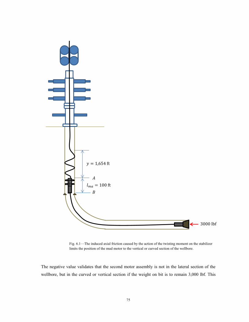
75
The negative value validates that the second motor assembly is not in the lateral section of the
wellbore, but in the curved or vertical section if the weight on bit is to remain 3,000 lbf. This
𝑦 6 t
𝑙𝑚𝑎 t
lb
𝐴
𝐵
Fig. 6.1—The induced axial friction caused by the action of the twisting moment on the stabilizer limits the position of the mud motor to the vertical or curved section of the wellbore.

76
suggests that the force at the end of built will be 3,000 lbf, since only the rotating tubing segment
is in the lateral section of the wellbore.
On the other hand, if the mud motor is in the lateral section of the wellbore, the weight on bit
will be lower than 3,000 lbf. Since, this analysis, assumes a weight on bit of 3,000 lbf, the former
possibility is assumed.
In this scenario, the second mud motor assembly is assumed to be at the end of build and
assuming the length of the mud motor and the dynamic torque arrestor is 100 ft. The second mud
motor and the torque arrestor have high flexural rigidity; thus, this analysis assumes that the
motor assembly will not conform to the wellbore geometry (Figs. 6.2a and 6.2b).
t
Rotating Segment
Nonrotating Segment
Fig. 6.2a—The second motor assembly does not have the same curvature as the tubing in the curved section of the wellbore because of high flexural rigidity.

77
From cosine rule,
It thus implies, the angle of inclination at point Y in Fig. 6.2b is
Therefore, the axial compressive force at point Y
+ 6 lb
And the axial force at the kick off point is
[
+
+ ]
+
+
+
+
But, .
t
𝑅
𝑅 𝜑
𝜑
lb
lb 𝑋
𝑌
𝑍
Fig. 6.2b—The motor assembly acts as a chord of an arc in the curved section.

78
[ 6
+ 6 ] ⁄ +
+ 6
+
+ 6
lb
The axial compressive force at the kick off point is almost equal to the maximum compressive
force, 4,588 lbf.
To estimate the buckled length of the tubing in the vertical section,
( √
)(
√ ) (
√
6)(
6
6 √ ) t
The displacement of the tubing in the lateral section is t
c. Using a Downhole Electric Motor:
Assuming that the electric motor is in the lateral section of the wellbore, the axial friction
induced on the tubing string by the installation of the electric motor is 547 lbf.
Estimating the length of the nonrotating tubing length in the lateral section,
| |
| 6 | 6 t
The negative value validates that the electric motor is not in the lateral section of the wellbore,
but in the curved or vertical section if the weight on bit is to remain 3,000 lbf. This suggests that
the force at the end of built will be 3,000 lbf, since only the rotating tubing segment is in the
lateral section of the wellbore.
Determining the lateral displacement in this case is similar to “b” since the electric motor is
assumed to be at the end of build. But the length of the electric motor is assumed to be 50 ft and
weigh 1800 lbf.

79
From Fig. 6.2b
It thus implies, the angle of inclination at point Y in Fig. 6.2b is
Therefore, the axial compressive force at point Y
+ 6 66 lb
And the axial force at the kick off point is
[
+
+ ]
+
+
+
+
But, .
[
+ 6 ] +
+ 6
+
+ 6
lb
The axial compressive force at the kick off point is greater than the maximum compressive force,
4,588 lbf. This result suggests that the motor assembly is located in the curved section of the
wellbore (Fig. 6.3), but the exact location is unknown. Through a wise guess, the approximate
location of the electric motor can be determined (this same procedure can be used in estimating
the exact location of the hydraulic motor in case “b”).

80
Assuming , noting that
Therefore,
Therefore, the axial compressive force at point Y1
lb
+ 6 66 lb
And the axial force at the kick off point is
[
+ 6 ] +
+ 6
+
+ 6
lb
Therefore, the assumed position of the motor assembly is not exact, but it will be located
between the assumed inclination angle and the end of build.
𝑅
𝑅 𝜑
𝜑
lb 𝑋
𝑍
Fig. 6.3—The electric motor in the curved section of the wellbore.
𝑌
𝜑
𝑌

81
To estimate the buckled length of the tubing in the vertical section,
( √
)(
√ ) (
√
6)(
6
6 √ ) t
The displacement of the tubing in the lateral section is
+
6
6.2 Maximum Lateral Displacement with Lockup in the Lateral Section
For the 2 in. tubing in the well profile specified above, its specifications are: torsional yield
strength (CT grade 90) is 3,844 lbf-ft (70% safety factor is assumed), unit weight 3.64 lbf/ft,
internal diameter 1.624 in., Young’s Modulus of steel is 30,000 psi. The weight of the downhole
motor used (electric or hydraulic) in rotating the tubing is assumed to be 1,800 lbf. The weight of
the two stabilizers is assumed to be 550 lbf (with four blades per stabilizer).
Solution: The friction correction factor for sinusoidal buckling load 6 ; and helical
buckling load 6 . Consequently, the buckling loads are: lbf and
6 lbf.
a. Without the rotation of the tubing string:
The length of the straight section of the tubing at lockup,
| 6 | 6 t
The sinusoidal buckled length, from Eq. 5.13 is
{
[
6 6 ( +
√6 6 6 )
√6 ]
[ 6 6 ( + √6 6 6 )
√6 ]}
√6
t

82
The helical buckled length, from Eq. 5.48 is
6 6 √ [
(
6 √
√ )] t
Therefore, summing the lengths together, the lateral displacement of the tubing at lockup is
t.
b. Using a downhole hydraulic motor to rotate the tubing string (with a stabilizer coupled):
The rotating length of the tubing string is determined from Eq. 4.10c
6 66 ⁄ 6 +
+ (
)
t
The axial force induced in the tubing string as a result of the use of the stabilizer is lbf.
Therefore, the straight section of the nonrotating tubing string is zero, and the sinusoidal buckled
length is 17 ft, because of the high axial friction. The total lateral displacement of the tubing is
36,638 ft.
c. Using a downhole electric motor to rotate the tubing string
The rotating length of the tubing is still 29,491 ft, but the straight section of the nonrotating
section is 774 ft. Therefore, the total lateral displacement is 37,395 ft.
In the same vein, it can be said that this project is applying two methods because it assumes
straightened tubing in the wellbore (the effect of the residual curvature of tubing is not
considered in the analysis).
The results of the computer simulations show that the nonrotating segment of the tubing assumes
straight and helical buckled configurations at lockup (Fig. 6.4). The sinusoidal buckled sections
observed for each of the tubing are short, increasing as the tubing unit weight and flexural
rigidity increases. For 2 in. tubing, the length of the sinusoidal buckled section is 150 ft. while
the buckled length for 3.5 in. is 333ft. The reason for the observed configurations can be traced

83
to the fact that the ratio of the critical helical buckling load to the sinusoidal buckling load is
only √ .
The contributions of small radial clearance and high unit weight of the tubing to extended-reach
technology must be emphasized. Figs. 6.5 and 6.6 validate the conception of increased reach
with slim holes.
At lower inclination angles (with the same build rate) the displacement in the lateral section is
greater. Lower build section and increased axial contribution of the weight of the tubing are the
main causes for the increased lateral displacement.
The gradients of the curves change four times at critical well inclination angles. Below 300 the
gradient of the curve is constant and the buckled length of the tubing is much longer than other
inclination angles. A well inclination angle of 300 was derived by Mitchell et al. (2011) as the
demarcation between high tension and low tension directional wells. Therefore, the curves have
been able to validate this concept.
Between 300 and 450 a gentler slope is observable. Similarly from 450 to 600 the curves have
another gradient. Well inclination angles from 300 to 600 are generally termed intermediate
inclination angles. At these angles, the axial and normal tubing weight contributions to the force
system are equal.
Helical buckled section Straight section
Fig. 6.4—Top view of the configuration of the nonrotating segment of the tubing string observed during the computer simulation tests
Sinusoidal buckled section

84
10 20 30 40 50 60 70 80 900.5
1
1.5
2
2.5
3
3.5
4
4.5
5x 10
4
Well Inclination Angle, degrees
Buckle
d L
ength
, ft
2"
2.375"
2.875"
3.5"
Fig. 6.6—The buckled length of the tubing decreases as the inclination angle and the length of the build section increases.
10 20 30 40 50 60 70 80 900.5
1
1.5
2
2.5
3
3.5x 10
4
Well Inclination Angle, degrees
Buckle
d L
ength
, ft
6.5"
5"
4"
3.875"
Fig. 6.5—Short build up section and low inclination angles will help in extending the reach of coiled tubing in the wellbore. The helically buckled length of 3.5 in. tubing at lockup increases as the hole size reduces.

85
10 20 30 40 50 60 70 80 900
0.5
1
1.5
2
2.5
3
3.5
4
4.5
5x 10
4
Well Inclination Angle, degrees
Buckle
d L
ength
, ft
0.8
0.65
0.5
0.35
Therefore, the frictional drag on the tubing is much higher at intermediate inclination angles than
low inclination angles; consequently, the extent of the tubing in the lateral section of
“intermediate” inclined wellbore is shorter than wells with low inclination angles.
Wells with inclination angles from 600 to 900 are called high angle wells. From Figs. 6.5 and 6.6,
the gradient of the curve is almost flat. Indicating that the extent of the tubing string (with same
build rate, hole size and other drilling parameters) cannot be significantly increased by
increasing the inclination angle.
The effect of tortuosity on the extent of tubing in the wellbore has been identified to increase
torque and drag in the wellbore (Mitchell and Miska 2011); Fig. 6.7 validates this fact.
Tortuosity effects are incorporated into the torque and drag models through the friction factor.
With increased tortuosity the friction factor increases.
Fig. 6.7—The buckled length of the tubing decreases as the inclination angle, tortuosity, and the length of the build section increases.

86
CHAPTER VII
CONCLUSIONS AND RECOMMENDATIONS
7.1 Conclusions
After much rigorous investigations, the application of downhole motors, as an extended-reach
technology for coiled tubing applications, has proven to be practicable. The project has proffered
solutions to the major challenges that would have made the proposed technique impracticable.
The major conclusions from this study are as follows
1. The nonrotating segment of tubing string will not buckle under permissible applied
torsional loads. The investigation showed that the minimum first order buckling torque
is greater than the torsional yield strength of the tubing. Since applied torsional loads on
tubing in the field are lower than its torsional yield strength, the major effect of the
applied torque is the twisting of the nonrotating of the segment of the tubing string.
2. The twisting moment applied on the nonrotating segment will cause great destabilization
during the drilling operation. Although the rate of change of the twisting moment is zero
when the second mud motor and the bit are in the same wellbore section, the rate of
change of the twist angle will not be zero; the destabilization will still persist.
3. Electric downhole motors can be used in lieu of the downhole hydraulic motors (positive
displacement motors and turbodrills) to prevent twisting of the nonrotating tubing string.
The results of the computer simulation tests show significant increase in the lateral
displacement of the tubing in the wellbore when an electrodrill is used. Similarly, with
the use of an electrodrill the dynamic pressure of the mud does not need to be increase in
offsetting the pressure drops across the motor; therefore, the number of total cycles to
failure of the tubing will not be affected.
4. Alternatively, a dynamic torque anchor or a full-gaged stabilizer assembly can be
attached to hydraulic motors to prevent twisting of the nonrotating segment of the tubing
string. The use of these wall contact tools in “arresting” the twisting moment induces
high normal and binormal contact forces in the wellbore. The induced normal and
binormal forces increase the axial frictional force in the wellbore, thus reducing
87
hookload. Nevertheless, the results from the computer simulation tests show significant
increase in the lateral displacement with the use of dynamic torque anchor or stabilizer.
5. Using the newly proposed dynamic torque arrestor in preventing the twisting of the
nonrotating segment of the tubing (when a hydraulic motor is used) produces lateral
displacements of the same magnitude as the electrodrill.
6. Maximizing the length of the rotating segment of the tubing string increases significantly
the lateral displacements of the tubing in the wellbore. The magnitude of the rotating
length primarily depends on the torsional yield strength of the tubing and well geometry.
7. In the course of determining the rotating length of the tubing, the inertia torque model
should be used in lieu of the resultant torque model. Since the safest and maximum
rotating length is desired, the maximum applied torque on the tubing should be used,
which is the inertia torque (the torque to overcome drag).
8. With high tortuosity in the wellbore, the maximum lateral displacement of the tubing at
lockup or zero hookload is reduced drastically.
9. The maximum compressive force at the kick off point doesn’t approach an infinite value
but has its limiting value, which depends on the depth of the kick off point.
10. The weight of the tubing string has significant influence on maximum lateral
displacement achievable in the wellbore. Similarly, the radial clearance between the
tubing and the wellbore influences the lateral displacement obtainable.
11. Designing wells with short build sections can help increase the maximum lateral
displacement of the tubing. With high compressive force at the end of build, the tubing
can be further pushed into the lateral section of the wellbore.
12. In applying this technology in the field, the conventional CT drilling needs to be
employed first. The maximum measured depth produced by the slide-drilling phase of
the whole drilling operations will determine the available rotating length of the tubing
string (if the measured is less than the maximum rotating length).
13. The cutting and rejoining of the tubing string in the field can contribute to non-
productive time. Butt or bias welding can be employed in the field in joining the string
after the whole drilling operation. The rejoining of the tubing string will enhance the
spooling of the whole tubing length to be wound back to the reel.

88
7.2 Recommendations
The operation of the second downhole motor needs to be controlled by a feedback system
because of the dynamic nature of the drilling process. Therefore, a control system needs to
be designed for the proposed system configuration. The controller will regulate the operation
of the downhole motor based on changes on certain parameters. Similarly, the action of the
downhole motor would be controlled from the surface when the feedback system is designed
and incorporated into the proposed system configuration.
In addition, the dynamics of the hole cleaning process for the proposed tubing string
configuration needs to be investigated. The expectation of this study is that the rotation of
part of the whole tubing string will improve cuttings transport in the inclined sections of the
wellbore.
Finally, the dynamics of the proposed coiled-tubing string configuration needs to be
rigorously investigated to improve the robustness of the design.
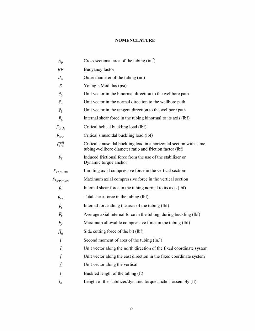
89
NOMENCLATURE
Cross sectional area of the tubing (in.2)
Buoyancy factor
Outer diameter of the tubing (in.)
Young’s Modulus (psi)
Unit vector in the binormal direction to the wellbore path
Unit vector in the normal direction to the wellbore path
Unit vector in the tangent direction to the wellbore path
Internal shear force in the tubing binormal to its axis (lbf)
Critical helical buckling load (lbf)
Critical sinusoidal buckling load (lbf)
Critical sinusoidal buckling load in a horizontal section with same
tubing-wellbore diameter ratio and friction factor (lbf)
Induced frictional force from the use of the stabilizer or Dynamic torque anchor
Limiting axial compressive force in the vertical section
Maximum axial compressive force in the vertical section
Internal shear force in the tubing normal to its axis (lbf)
Total shear force in the tubing (lbf)
Internal force along the axis of the tubing (lbf)
Average axial internal force in the tubing during buckling (lbf)
Maximum allowable compressive force in the tubing (lbf)
Side cutting force of the bit (lbf)
Second moment of area of the tubing (in.4)
Unit vector along the north direction of the fixed coordinate system
Unit vector along the east direction in the fixed coordinate system
Unit vector along the vertical
Buckled length of the tubing (ft)
Length of the stabilizer/dynamic torque anchor assembly (ft)

90
Length of a BHA component (ft)
Lateral displacement of the tubing in the wellbore
Length of helical buckled section at lockup (ft)
Instantaneous length of the nonrotating tubing in the wellbore (ft)
Total rotating length of the tubing string, excluding the length of the BHA (ft)
Rotating length of the tubing when mud motor gets to the KOP (ft)
Straight section of the nonrotating tubing when buckling occurs
Unit drag moment in the wellbore (lbf-ft /ft)
Critical buckling torque (lbf-ft)
Applied torque on the rotating tubing (lbf-ft)
Reactive torque acting on the nonrotating tubing segment (lbf-ft)
Rotary torque applied on the bit (lbf-ft)
Reactive torque on mud motor rotating the bit (lbf-ft)
Radius of curvature (ft)
Distance from the tip of the stabilizer’s (or torque anchor) blade to the center of the wellbore. (in.)
Radius of a BHA component (in.)
Radial clearance between tubing and the wellbore/casing (in.)
Resultant bit cutting force (lbf)
Outer radius of the tubing (in.)
Rate of penetration into the formation or tripping speed of the tubing (ft/hr)
Rotary speed of the tubing (rev/min)
Measured depth along the wellbore path (ft)
Depth of the kick off point (ft.)
Safety factor
Torsional yield strength of the tubing (lbf-ft)
Elastic deformation energy (J)
Axial velocity of deployment of the tubing in the wellbore (ft/hr)
Unit weight of the full-gaged stabilizer assembly or the dynamic torque anchor (lbf/ft)
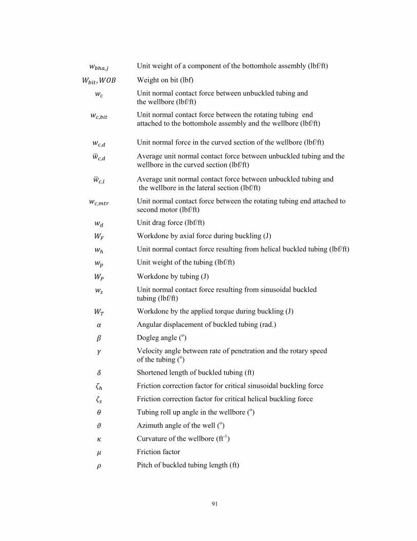
91
Unit weight of a component of the bottomhole assembly (lbf/ft)
Weight on bit (lbf)
Unit normal contact force between unbuckled tubing and the wellbore (lbf/ft)
Unit normal contact force between the rotating tubing end attached to the bottomhole assembly and the wellbore (lbf/ft)
Unit normal force in the curved section of the wellbore (lbf/ft)
Average unit normal contact force between unbuckled tubing and the wellbore in the curved section (lbf/ft)
Average unit normal contact force between unbuckled tubing and the wellbore in the lateral section (lbf/ft)
Unit normal contact force between the rotating tubing end attached to second motor (lbf/ft)
Unit drag force (lbf/ft)
Workdone by axial force during buckling (J)
Unit normal contact force resulting from helical buckled tubing (lbf/ft)
Unit weight of the tubing (lbf/ft)
Workdone by tubing (J)
Unit normal contact force resulting from sinusoidal buckled tubing (lbf/ft)
Workdone by the applied torque during buckling (J)
Angular displacement of buckled tubing (rad.)
Dogleg angle (o)
Velocity angle between rate of penetration and the rotary speed of the tubing (o)
Shortened length of buckled tubing (ft)
Friction correction factor for critical sinusoidal buckling force
Friction correction factor for critical helical buckling force
Tubing roll up angle in the wellbore (o)
Azimuth angle of the well (o)
Curvature of the wellbore (ft-1)
Friction factor
Pitch of buckled tubing length (ft)

92
Yield strength of the tubing (psi)
Torsion of the wellbore (ft-1)
∅
Resultant bit cutting force direction angle (o)
Well inclination angle (o)
Angle of twist of the nonrotating length of the tubing (o)
93
REFERENCES
Bhalla, K. 1995. Coiled Tubing Extended Reach Technology. Paper presented at the Offshore
Europe, Aberdeen, United Kingdom. SPE-30404-MS.
Byrom, T.G. 1999. Coiled-Tubing Drilling in Perspective. SPE Journal of Petroleum
Technology; Journal Volume: 51:6 51 (6): 57-61. SPE-51792-MS.
Gao, G. and Miska, S. Z. 2008a. Dynamic Buckling and Snaking Motion of Rotating Drilling
Pipe in a Horizontal Well. Paper presented at the SPE Annual Technical Conference and
Exhibition, Denver, Colorado, USA. SPE-113883-MS.
Gao, G. and Miska, S. Z. 2008b. Effects of Boundary Conditions and Friction on Static Buckling
of Pipe in a Horizontal Well. Paper presented at the IADC/SPE Drilling Conference,
Orlando, Florida, USA. SPE-111511-MS.
Gao, G. and Miska, S. Z. 2009. Effects of Friction on Post-Buckling Behavior and Axial Load
Transfer in a Horizontal Well. Paper presented at the SPE Production and Operations
Symposium, Oklahoma City, Oklahoma. SPE-120084-MS.
He, X., Halsey, G.W., and Kyllingstad, A. 1995. Interactions between Torque and Helical
Buckling in Drilling. Paper presented at the SPE Annual Technical Conference and
Exhibition, Dallas, Texas. SPE-30521.
International Coiled Tubing Association, 2005, “An Introduction to Coiled tubing; History,
Applications and Benefits”, Montgomery, TX, ICoTA, 1 – 25
Leising, L.J., Onyia, E.C., Townsend, S.C. et al. 1997. Extending the Reach of Coiled Tubing
Drilling (Thrusters, Equalizers and Tractors). Paper presented at the SPE/IADC Drilling
Conference, Amsterdam, Netherlands. SPE-37656-MS.
Lubinski, A. and Althouse, W.S. 1962. Helical Buckling of Tubing Sealed in Packers. Presented
at the SPE Annual Fall Meeting, Dallas, Texas. SPE-178.-PA.
Miska, S. and Cunha, J.C. 1995. An Analysis of Helical Buckling of Tubulars Subjected to Axial
and Torsional Loading in Inclined Wellbores. Paper presented at the SPE Production
Operations Symposium, Oklahoma City, Oklahoma. SPE-29460-MS.
Mitchell, R. F. 1986. Simple Frictional Analysis of Helical Buckling of Tubing. SPE Drilling
Engineering; Journal Volume: 1:6 1 (6): 457-465. SPE-13064.
Mitchell, R. F. 1988. New Concepts for Helical Buckling. SPE Drilling Engineering; Journal
Volume: 3:3 3 (3): 303-310. SPE-15470.

94
Mitchell, R. L., Miska, S. Z., Aadnoy, B. S.,Adams, N., Barker, J.W., Cunha, J.C., Eustes, A.W.,
Kastor, R.L., Kelessidis, V.C., Maglione, R., Ozbayoglu, E., Powers, J., Sweatman, R.
2011. Directional Drilling; In Fundamentals of Drilling Engineering; ed. Mitchell R.L.
and Miska, S.Z., SPE Textbook Series, Vol. 12, Richardson: Society of Petroleum
Engineers.
Mitchell, R. and Weltzin, T. 2011. Lateral Buckling--the Key to Lockup. Presented at the
SPE/IADC Conference, Amsterdam, Netherlands. SPE-139824-PA
Mitchell, R.F. 2008. Tubing Buckling—the State of the Art. Presented at the Annual Technical
Conference, San Antonio , Texas. SPE-104267-PA
Newman, K.R. 2007. Vibration and Rotation Considerations in Extending Coiled-Tubing Reach.
Paper presented at the SPE/ICoTA Coiled Tubing and Well Intervention Conference and
Exhibition, The Woodlands, Texas, U.S.A. SPE-106979-MS.
Nguyen, T. 2012. Directional and Horizontal Drilling Innovative Drilling Methods: Drilling
Tools and Techniques. Presentation at New Mexico Institute of Mining and Technology
Reel Revolution Limited. http://www.reel-revolution.com/. Accessed 2012
Reilly J.P. 2003. Method and Apparatus for Coiled Tubing Operations. USA. 65168-92-B2
Smalley, E. 2012. Coiled Tubing and Its Applications, Training Course presented at the SPE
Annual Technical Conference and Exhibition.
Weltzin, T., Aas, B., Andreassen, E. et al. 2009. Measuring Drillpipe Buckling Using
Continuous Gyro Challenges Existing Theories. Presented at the IADC/SPE Drilling
Technology Conference and Exhibition, Jakarta. SPE-115930-PA
Wu, J. 1997. Torsional Load Effect on Drill-String Buckling. Paper presented at the SPE
Production Operations Symposium, Oklahoma City, Oklahoma. SPE-37477.
Wu, J. and Juvkam-Wold, H.C. 1993a. Helical Buckling of Pipes in Extended Reach and
Horizontal Wells—Part 2: Frictional Drag Analysis. Journal of Energy Resources
Technology; (United States); Journal Volume: 115:3 115 (3): 196-201.
Wu, J. and Juvkam-Wold, H.C. 1993b. Study of Helical Buckling of Pipes in Horizontal Wells.
Paper presented at the SPE Production Operations Symposium, Oklahoma City,
Oklahoma. This paper was prepared for presentation at the Production Operations
Symposium held in Oklahoma City, OK, U.S.A., SPE-25503-MS.
Wu, J. and Juvkam-Wold, H.C. 1995a. Buckling and Lockup of Tubulars in Inclined Wellbores.
Journal of Energy Resources Technology; Journal Volume: 117:3 117 (3): 208-213.

95
Wu, J. and Juvkam-Wold, H.C. 1995b. Coiled Tubing Buckling Implication in Drilling and
Completing Horizontal Wells. SPE Drilling & Completion; Journal Volume: 10:1 10
(1): 16-21. SPE-26336-PA
Zheng, A.S. and Adnan, S. 2007. The Penetration of Coiled Tubing with Residual Bend in
Extended-Reach Wells. SPE Production & Operations Journal Volume: 22:1 22 (1):
78-82. SPE-95239-PA