Embed Size (px)
Citation preview

Extremes (2014) 17:359–385DOI 10.1007/s10687-014-0184-y
Extreme values for characteristic radiiof a Poisson-Voronoi Tessellation
Pierre Calka ·Nicolas Chenavier
Received: 29 March 2013 / Revised: 7 October 2013 /Accepted: 8 November 2013 / Published online: 2 May 2014© Springer Science+Business Media New York 2014
Abstract A homogeneous Poisson-Voronoi tessellation of intensity γ is observed ina convex bodyW . We associate to each cell of the tessellation two characteristic radii:the inradius, i.e. the radius of the largest ball centered at the nucleus and included inthe cell, and the circumscribed radius, i.e. the radius of the smallest ball centered atthe nucleus and containing the cell. We investigate the maximum and minimum ofthese two radii over all cells with nucleus in W . We prove that when γ → ∞, thesefour quantities converge to Gumbel or Weibull distributions up to a rescaling. More-over, the contribution of boundary cells is shown to be negligible. Such approach ismotivated by the analysis of the global regularity of the tessellation. In particular,consequences of our study include the convergence to the simplex shape of the cellwith smallest circumscribed radius and an upper-bound for the Hausdorff distancebetween W and its so-called Poisson-Voronoi approximation.
Keywords Voronoi tessellations · Poisson point process · Random covering of thesphere · Extremes · Boundary effects
AMS 2010 Subject Classifications: 60D05 · 62G32 · 60F05 · 52A22
P. Calka (�) · N. ChenavierUniversite de Rouen, LMRS, avenue de l’Universite, BP 12 76801Saint-Etienne-du-Rouvray cedex, Francee-mail: [email protected]
N. Chenaviere-mail: [email protected]

360 P. Calka, N. Chenavier
1 Introduction
Let χ be a locally finite subset of �d endowed with its natural norm | · |. The Voronoicell of nucleus x ∈ χ is the set
Cχ(x) = {y ∈ �d , |y − x| ≤ |y − x ′|, x �= x ′ ∈ χ}.
When χ = Xγ is a homogeneous Poisson point process of intensity γ , the family{CXγ (x), x ∈ Xγ } is the so-called Poisson-Voronoi tessellation. Such model is exten-sively used in many domains such as cellular biology (Poupon 2004), astrophysics(Ramella et al. 2001), telecommunications (Baccelli 2009) and ecology (Roque1997). For a complete account, we refer to the books (Okabe et al. 2000; Schneiderand Weil 2008; Møller 1994) and the survey (Calka 2010).
To describe the mean behaviour of the tessellation, the notion of typical cell isintroduced. The distribution of this random polytope can be defined as
�[f (Cγ )] = 1
γ λd(B)�
⎡⎣ ∑x∈Xγ∩B
f (CXγ (x)− x)
⎤⎦
where f : Kd → � is any bounded measurable function on the set of con-vex bodies Kd (endowed with the Hausdorff topology), λd is the d-dimensionalLebesgue measure and B is a Borel subset of �d with finite volume λd(B) ∈ (0,∞).Equivalently, Cγ is the Voronoi cell CXγ ∪{0}(0) when we add the origin to thePoisson point process: this fact is a consequence of Slivnyak’s Theorem, see e.g.Theorem 3.3.5 in Schneider and Weil (2008). The study of the typical cell in theliterature includes mean values calculations (Møller 1989), second order properties(Heinrich and Muche 2008) and distributional estimates (Calka 2003; Baumstark andLast 2007; Muche 2005). A long standing conjecture due to D.G. Kendall about theasymptotic shape of large typical cell is proved in Hug et al. (2004).
To the best of our knowledge, extremes of geometric characteristics of the cells,as opposed to their means, have not been studied in the literature up to now. In thispaper, we are interested in the following problem: only a part of the tessellation isobserved in a convex body W (i.e. a convex compact set with non-empty interior) ofvolume λd(W) = 1 where λd denotes the Lebesgue measure in �d . Let f : Kd → �
be a measurable function, e.g. the volume or the diameter of the cells. What is thelimit behaviour of
Mf (γ ) = maxx∈Xγ∩W
f (CXγ (x))
when γ goes to infinity? By scaling invariance of Xγ , it is the same as consideringa tessellation with fixed intensity and observed in a window Wρ := ρ1/dW withρ → ∞. We give below some applications of such approach.
First, the study of extremes describes the regularity of the tessellation. Forinstance, in finite element method, the quality of the approximation depends on someconsistency measurements over the partition, see e.g. Ju et al. (2006).
Another potential application field is statistics of point processes. The key ideawould be to identify a point process from the extremes of its underlying Voronoi

Extreme values for radii of a Poisson-Voronoi tessellation 361
tessellation. A lot of inference methods have been developed for spatial point pro-cesses (Møller and Waagepetersen 2004). A comparison based on Voronoi extremesmay or may not provide stronger results. At least, the regularity seems to discrimi-nate to some extent some point processes (see for instance a comparison between adeterminantal point process and a Poisson point process in LeCaer and Ho (1990)).
A third application is the so-called Poisson-Voronoi approximation i.e. a dis-cretization of a convex body W by the following union of Voronoi cells
VXγ (W) =⋃
x∈X∩WCXγ (x).
The first breakthrough is due to Heveling and Reitzner (2009) and includes varianceestimates of the volume of symmetric difference. However, the Hausdorff distancebetween the convex body and its approximation has not been studied yet. It is stronglyconnected to the maximum of the diameter of the cells which intersect the bound-ary of ∂W . We discuss this in Section 4 and prove a rate of convergence of theapproximation to the convex body with a suitable assumption on W .
Concretely, we are looking for two parameters af (γ ) and bf (γ ) such that
af (γ )Mf (γ )+ bf (γ )D−→
γ→∞ Y
where Y is a non degenerate random variable andD−→ denotes the convergence in
distribution. Up to a normalization, the extreme distributions of real random vari-ables which are iid or with a mixing property are of three types: Frechet, Gumbel orWeibull (see e.g. Loynes 1965 and Leadbetter 1973/74). More about extreme valuetheory can be found in the reference books by de Haan and Ferreira (2006) andby Resnick (1987). Some extremes have been studied in stochastic geometry, forinstance the maximum and minimum of inter-point distances of some point processes(Jammalamadaka and Janson 1986; Mayer and Molchanov 2007; Penrose 2003),extremes of particular random fields (Lantuejoul et al. 2011) or in the field of stere-ology (Hlubinka 2003; Pawlas 2012) but, to the best of our knowledge, nothing hasbeen done for random tessellations. In our framework, the general theory cannotdirectly be applied for several reasons: unknown distribution of the characteristicfor one fixed cell, dependency between cells and boundary effects. Moreover, theexceedances can be realized in clusters. For example, when the distance between theboundary of the cell and its nucleus is small, this is the same for one of its neigh-bors. Such clusters lead to the notion of extremal index, which was introduced byLeadbetter in Leadbetter (1983), and that we will study in a future work.
In this paper, we are interested in the characteristic radii i.e. inscribed andcircumscribed radii of the Voronoi cell CXγ (x) defined as
r(CXγ (x)) = max{r ≥ 0, B(x, r) ⊂ CXγ (x)} and
R(CXγ (x)) = min{R ≥ 0, B(x, R) ⊃ CXγ (x)}where B(x, r) is the ball of radius r centered at x. Two reasons led us to the study ofthese quantities. First, the distribution tails of the inradius and circumscribed radiusof the typical cell are easier to deal with Calka (2002) compared to other character-istics such as the volume or the number of hyperfaces. Secondly, knowing these two

362 P. Calka, N. Chenavier
radii provides a better understanding of the cell shape since the boundary of CXγ (x)
is included in the annulus B(x, R(CXγ (x))) − B(x, r(CXγ (x))). We consider theextremes
rmax(γ ) = maxx∈Xγ∩W
r(CXγ (x)), rmin(γ ) = minx∈Xγ∩W
r(CXγ (x))
Rmax(γ ) = maxx∈Xγ∩W
R(CXγ (x)), Rmin(γ ) = minx∈Xγ∩W
R(CXγ (x)).(1)
In the following theorem, we derive the convergence in distribution of these quantitiesover cells with nucleus in W .
�
(2dκdγ rmax(γ )
d − log(γ ) ≤ t)
−→γ→∞ e−e−t
, t ∈ �, (2a)
�
(2d−1κdγ
2rmin(γ )d ≥ t)
−→γ→∞ e−t , t ≥ 0, (2b)
�
(κdγRmax(γ )
d − log(α1γ (log γ )d−1
)≤ t)
−→γ→∞ e−e−t
, t ∈ �, (2c)
�(α2κdγ(d+2)/(d+1)Rmin(γ )
d ≥ t) −→γ→∞ e−t d+1
, t ≥ 0, (2d)
where α1 and α2 are given in Eqs. 43 and 17 and κd = λd(B(0, 1)).
The limit distributions are of type II and III and do not depend on the shape of W .One can note that the ratios rmax(γ )/rmin(γ ) and Rmax(γ )/Rmin(γ ) are of respectiveorders (γ log γ )1/d and (γ 1/(d+1) log γ )1/d . This quantifies to some extent the irreg-ularity of the Poisson-Voronoi tessellation. Moreover, the ratio rmax(γ )/Rmax(γ ) isbounded. It suggests that large cells tend to be spherical around the nucleus. This factseems to confirm the D.G. Kendall’s conjecture.
As it is written, Theorem 1 is not applicable for concrete data. Indeed, in practice,the only cells which can be measured are included in the window. The followingproposition addresses this problem.
The convergences are illustrated in Fig. 1 for the cells which are included inW = [0, 1]2. For sake of simplicity, the Poisson point process has been realized onlyin W . Because of Proposition 2 and related arguments, this does not affect the dis-tribution over cells included in W . Simulations suggest that the rates of convergenceare not the same for all these quantities. Indeed, in a future work, we will show thatthe rate is of the order of γ−1, γ−1/4 and γ−1/6 for rmin(γ ), rmax(γ ) and Rmin(γ )
respectively.
Theorem 1 Let Xγ be a Poisson point process of intensity γ and W a convex bodyof volume 1 in �d . Then
Proposition 2 The extremes of characteristic radii over all cells included inW or over all cells intersecting ∂W have the same limit distributions asrmax(γ ), rmin(γ ), Rmax(γ ) and Rmin(γ ).

Extreme values for radii of a Poisson-Voronoi tessellation 363
Fig. 1 Empirical densities of the extremes based on 3500 simulations of PVT in 2D with γ = 10000,for the cells included in W = [0, 1]2, on Matlab©. a Cell maximizing the inradius. b Cell minimizing theinradius. c Cell maximizing the circumradius. d Cell minimizing the circumradius
All results of Theorem 1 use geometric interpretations. For the circumscribedradii Rmax(γ ) and Rmin(γ ), we write the distributions as covering probabili-ties of spheres. The inscribed radii can be interpreted as interpoint distances. Astudy of the extremes of these distances has been done in several works such asJammalamadaka and Janson (1986) and Henze (1982). For sake of completeness, wehave rewritten these results in our setting in particular because the boundary effectsare highly non trivial. Convergences (2a) and (2d) could be obtained by consider-ing underlying random fields and using methods inherited for Arratia et al. (1990)and Smith (1988). However, this approach does not provide (2b) and (2c). We willdevelop this idea in a future work and deduce some rates of convergence.
The paper is organized as follows. In Section 2, we provide some preliminaryresult which shows that the boundary cells are negligible and implies Proposition 2.In Sections 3, 4 and 5, proofs of Eqs. 2d, 2a, 2c and 2b are respectively given.Section 3 requires a technical lemma about deterministic covering of the sphere bycaps which is proved in appendix. Section 4 contains an application of Eq. 2c to theHausdorff distance between W and its Poisson-Voronoi approximation. In Section 5,we get a specific treatment of boundary effects which is more precise than inSection 2.
In the rest of the paper, c denotes a generic constant which does not depend onγ but may depend on other quantities. The term uγ denotes a generic function of t ,dependending on γ , which is specified at the beginning of Sections 3, 4 and 5.
2 Preliminaries on boundary effects
In this section, we show that the asymptotic behaviour of an extreme is in gen-eral not affected by boundary cells. We apply that result directly to the extremes ofcharacteristic radii in order to show that Theorem 1 implies Proposition 2.

364 P. Calka, N. Chenavier
Let f : Kd → � be a k-homogeneous measurable function, 0 ≤ k ≤ d (i.e.f (λC) = λkf (C) for all λ ∈ �+ and C ∈ Kd ). We consider for any l ∈ �
Mbf (γ, l) = max
x∈Xγ ,CXγ (x)∩W1+l �=∅
f (CXγ (x)),
Mf (γ, l) = maxx∈Xγ∩W1+l
f (CXγ (x)),
Mif (γ, l) = max
x∈Xγ ,CXγ (x)⊂W1+l
f (CXγ (x)),
where W1+l = (1 + l)W . When l = 0, these maxima are simply denoted byMb
f (γ ),Mf (γ ) and Mif (γ ). We define, for all ε > 0, a function lγ as
lγ = γ−(1−ε)/d . (4)
Under suitable conditions, the following proposition shows that Mbf (γ ),Mf (γ ) and
Mif (γ ) satisfy the same convergence in distribution.
aγ
aγ±−→γ→∞ 1, lγ bγ −→
γ→∞ 0 andbγ aγ± − aγ bγ±
aγ−→γ→∞ 0 (5)
with γ+ = (1 + lγ )kγ and γ− = (1 − lγ )
kγ for a certain ε. Then
aγMbf (γ )+ bγ
D−→γ→∞ Y ⇐⇒ aγMf (γ )+ bγ
D−→γ→∞ Y ⇐⇒ aγM
if (γ )+ bγ
D−→γ→∞ Y.
Before proving Proposition 3, we need an intermediary result due to Heinrich,Schmidt and Schmidt (Lemma 4.1 of Heinrich et al. 2005) which shows that, withhigh probability, the cells which intersect ∂W have nucleus close to ∂W . Actually,they showed it for any stationary tessellation of intensity 1 which is observed in awindow ρW with ρ → ∞. For sake of completeness, we rewrite their result in amore explicit version for a Poisson-Voronoi tessellation.
Aγ =⎧⎨⎩⋂x∈Xγ
{CXγ (x) ∩W = ∅} ∪ {x ∈ W1+lγ }⎫⎬⎭ and
Bγ =⎧⎨⎩⋂x∈Xγ
{CXγ (x) ⊂ W
} ∪ {x �∈ W1−lγ }⎫⎬⎭
where lγ is given in Eq. 4. Then �(Aγ ) and �(Bγ ) converge to 1 as γ goes to infinity.
Proposition 3 Let Y be a random variable and aγ , bγ two functions such that
Lemma 1 (Heinrich, Schmidt and Schmidt) Let us denote by Aγ and Bγ the events

Extreme values for radii of a Poisson-Voronoi tessellation 365
Proof of Lemma 1 In Heinrich et al. (2005), it is shown that
�
⎛⎝⎧⎨⎩⋂x∈X1
{CX1(x) ∩Wρ = ∅} ∪ {x ∈ Wρ+q(ρ)}⎫⎬⎭
× ∩⎧⎨⎩⋂x∈X1
{CX1(x) ⊂ Wρ
} ∪ {x �∈ Wρ−q(ρ)}⎫⎬⎭
⎞⎠ −→
γ→∞ 1 (6)
where q(ρ) is the solution of the functional equation
ρd = H(qd(ρ)).
The function H : �+ → �+ is convex, strictly increasing on its support (x0,∞) (forsome x0 ≥ 0), such that H(x)/x is non-decreasing for x > 0, limx→∞H(x)/x = ∞and �[H(Dd(C1))
]< ∞ where D(C1) is the diameter of the typical cell.
In the case of a Poisson-Voronoi tessellation, q(ρ) can be made explicit. Indeed,we can show that all moments of D(C1) exist since D(C1) ≤ 2R(C1) and R(C1)
is shown to have an exponentially decreasing tail in any dimension by an argumentsimilar to Lemma 1 of Foss and Zuyev (1996). Consequently, for a fixed ε ∈ (0, 1),the functions H and q can be chosen as H(x) = x1/ε and q(ρ) = ρε . Using thescaling property of Poisson point process,
X1 ∩WρD= γ 1/d(Xγ ∩W) and X1 ∩Wρ±q(ρ)
D= γ 1/d(Xγ ∩W1±lγ )
where γ = ρd and lγ = γ−(1−ε)/d . We deduce Lemma 1 from Eq. 6.
Proof of Proposition 3 First equivalence: Let us assume that aγMbf (γ ) + bγ con-
verges in distribution to Y . On the event Aγ , ∀x ∈ Xγ , CXγ (x) ∩W �= ∅ =⇒ x ∈W1+lγ . Hence
Mbf (γ ) ≤ Mf (γ, lγ ) ≤ Mb
f (γ, lγ ). (7)
Because of Lemma 1, it is enough to show the convergence in distribution of therandom variables conditionally on Aγ . Thanks to the scaling property of Poissonpoint process and the k-homogeneity of f
Mbf (γ, lγ )
D= (1 + lγ )kMb
f (γ+) (8)
with γ+ = (1 + lγ )kγ . According to Eqs. 7 and 8, it remains to show that aγ (1 +
lγ )kMb
f (γ+) + bγ converges in distribution to Y . To do so, it is enough by Eq. 5 towrite the equality
aγ (1 + lγ )kMb
f (γ+)+ bγ = aγ
aγ+(1 + lγ )
k(aγ+M
bf (γ+)+ bγ+
)
+bγ aγ+ − aγ bγ+aγ+
+ aγ
aγ+· 1 − (1 + lγ )
k
lγlγ bγ+ .
In conclusion, we get
aγMf (γ )+ bγD−→
γ→∞ Y. (9)

366 P. Calka, N. Chenavier
Conversely, if Eq. 9 holds then, using the fact that
Mf (γ ) ≤ Mbf (γ ) ≤ Mf (γ, lγ )
D= (1 + lγ )kMf (γ+)
and proceeding along the same lines, we get aγMbf (γ )+ bγ
D−→γ→∞ Y .
Second equivalence: On the event Bγ , ∀x ∈ Xγ , x ∈ W1−lγ =⇒ CXγ (x) ⊂ W .We prove the second equivalence as previously noting that, conditionally on Bγ
Mif (γ,−lγ ) ≤ Mf (γ,−lγ ) ≤ Mi
f (γ ) ≤ Mf (γ ). (10)
3 Proof of Eqs. 2d and 2a
Proof of Eq. 2b Let t ≥ 0 be fixed. We denote by uγ the following function:
uγ = uγ (t) =(α−1
2 κ−1d γ−(d+2)/(d+1)t
)1/d(11)
where α2 is given by Eq. 17. Our aim is to prove that �(Rmin(γ ) ≥ uγ ) converges
to e−t d+1where Rmin(γ ) has been defined in Eq. 1. The main idea is to deduce the
asymptotic behaviour of Rmin(γ ) from the study of finite dimensional distributions(R(CXγ ∪{xK }(x1)), . . . , R(CXγ ∪{xK }(xK))
)for all {xK} = {x1, . . . , xK} and K ≥ 1.
To do this, we write a new adapted version of a lemma due to Henze (see Lemma p.345 in Henze 1982) in a context of Poisson point process.
γK
∫WK
�(∀i ≤ K, f (CXγ ∪{xK }(xi)) < uγ , F (CXγ∪{xK }(xi)) ∈ A
)dxK −→
γ→∞ λK
(12)where dxK = dx1 · · · dxK . Then
�
(min
x∈Xγ∩W,F(CXγ (x))∈Af (CXγ (x)) ≥ uγ
)−→γ→∞ e−λ.
Proof of Lemma 2 Let K be a fixed integer. The proof is close to the proof ofHenze’s Lemma and uses Bonferroni inequalities: one can show that if Ax,Xγ is anXγ -measurable event for all x ∈ Xγ ∩W, then
2K∑k=0
(−1)k+1
k! �
⎡⎣ ∑(x1,...,xk) �=∈Xγ∩W
�Ax1,Xγ. . . �Axk,Xγ
⎤⎦ ≤ �
⎛⎝ ⋃
x∈Xγ∩WAx,Xγ
⎞⎠
≤2K+1∑k=0
(−1)k+1
k! �
⎡⎣ ∑(x1,...,xk) �=∈Xγ ∩W
�Ax1 ,Xγ. . .�Axk,Xγ
⎤⎦ . (13)
Lemma 2 Let f : Kd → �, F : Kd → � be two measurable functions and A aBorel subset of �. Let us assume that for any K ≥ 1,

Extreme values for radii of a Poisson-Voronoi tessellation 367
where (x1, . . . , xk)�= means that (x1, . . . , xk) is a k-tuple of distinct points. ApplyingEq. 13 to
Ax,Xγ = {f (CXγ (x)) < uγ } ∩ {F(CXγ (x)) ∈ A},from Slivnyak’s formula (see Corollary 3.2.3 in Schneider and Weil 2008), we obtain
2K+1∑k=0
(−1)k
k! γ k
∫Wk
�(∀i ≤ K, f (CXγ ∪{xK }(xi)) < uγ , F (CXγ∪{xK }(xi)) ∈ A
)dxk
≤�(
minx∈Xγ∩W,F(CXγ (x))∈A
f (CXγ (x)) ≥ uγ
)
≤2K∑k=0
(−1)k
k! γ k
∫Wk
�(∀i≤K, f (CXγ ∪{xK }(xi))<uγ , F (CXγ∪{xK }(xi))∈A
)dxk.
From Eq. 12, we obtain
2K+1∑k=0
(−1)k
k! λk ≤ lim infγ→∞ �
(min
x∈Xγ∩W,F(CXγ (x))∈Af (CXγ (x)) ≥ uγ
)
≤ lim supγ→∞
�
(min
x∈Xγ∩W,F(CXγ (x))∈Af (CXγ (x)) ≥ uγ
)≤
2K∑k=0
(−1)k
k! λk.
We conclude the proof by taking K → ∞.
We apply Lemma 2 to f (CXγ (x)) = R(CXγ (x)). The function F(CXγ (x)) =Fd−1(CXγ (x)) denotes the number of hyperfaces of the cell CXγ (x). In all the proof,the event considered is A = �. We notice that the choice of the function F is ofno importance here but will be essential in the proof of Propositions 4 and 5. FromLemma 2, it is sufficient to study the limit behaviour of
γK
∫WK
�(∀i ≤ K,R(CX∪{xK }(xi)) < uγ
)dxK (14)
for all integer K . We divide the proof into two parts.
Step 1 When K = 1, using the stationarity of Xγ and the fact that λd(W) = 1, weshow that the integral (14) is γ�(R(CXγ ∪{0}(0)) < uγ ). As in Calka (2010)section 5.2.3, we can reinterpret the distribution function of R(CXγ ∪{0}(0))as a covering probability to get
γ�(R(CXγ ∪{0}(0)) < uγ ) = γ
∞∑k=0
e−2dκdγ udγ(2dκdγ udγ )
k
k! pk (15)
where pk is the probability to cover the unit sphere with k independentspherical caps such that their normalized radii are distributed as dν(θ) =

368 P. Calka, N. Chenavier
dπ sin(πθ) cosd−1(πθ)�[0,1/2](θ)dθ . The equality comes from the fact that
R(CXγ ∪{0}(0)) < uγ ⇐⇒ the family {Ay(0), y ∈ Xγ } covers S(0, uγ )
⇐⇒ the family {Ay(0), y ∈ Xγ ∩ B(0, 2uγ )}covers S(0, uγ )
where S(0, uγ ) denotes the sphere of radius uγ and centered at 0,
Ay(x) = S(x, uγ ) ∩H+y (x) (16)
and H+y (x) is the half-space which contains y and delimited by the bisecting
hyperplane of [x, y] (Fig. 2).We denote by
α2 :=(
2d(d+1)
(d + 1)!pd+1
)1/(d+1)
> 0. (17)
For example, when d = 2, α2 =(
512 − 4
π2
)1/3.
Fig. 2 Interpretation of the circumscribed radius as a covering of sphere

Extreme values for radii of a Poisson-Voronoi tessellation 369
Since pk = 0 for all k ≤ d , Eq. 15 gives
γ�(R(CXγ ∪{0}(0)) < uγ ) = γ(2dκdγ udγ )
d+1
(d + 1)! e−2dκdγ udγ pd+1 + γ
×∞∑
k=d+2
e−2dκdγ udγ(2dκdγ udγ )
k
k! pk.
The first term converges to td+1 from Eqs. 11 and 17. The second term isnegligible since γ (γ udγ )
d+2 = c · γ−1/(d+1) converges to 0 as γ tends toinfinity. This shows that
γ
∫W
�(R(CXγ ∪{x}(x)) < uγ )dx −→γ→∞ td+1. (18)
Step 2 When K ≥ 2, we use the same interpretation as in step 1: for all xK =(x1, . . . , xK) ∈ WK , and i ≤ K
R(CXγ ∪{xK }(xi)) < uγ ⇐⇒ the family {Ay(xi), y ∈ Xγ ∪ {xK }−{xi}} covers S(xi, uγ )
⇐⇒ the family {Ay(xi), y ∈ (Xγ ∪ {xK }−{xi}) ∩ B(xi, 2uγ )} covers S(xi, uγ ).
Hence, writing the previous event as “S(xi, uγ ) covered”, we have
�(∀i ≤ K,R(CXγ ∪{xK }(xi)) < uγ
) = �
⎛⎝⋂
i≤K
{S(xi, uγ ) covered}⎞⎠ .
(19)We have now to consider the spherical caps induced by both the pointsxj , j �= i and the points from Xγ . For all xK = (x1, . . . , xK) ∈ WK , wedenote by nl(xK) the number of connected components of
⋃Ki=1 B(xi, 2uγ )
with exactly l balls. Given n1, . . . , nK such that∑K
l=1 lnl = K , we define
WK(n1, . . . , nK) = {xK ∈ WK, nl(xK) = nl for all l ≤ K}. (20)
Let us note that the subsets WK(n1, . . . , nK), with∑K
l=1 lnl = K , partitionWK . We then deal with two cases.
1. If B(xi, 2uγ ) ∩ B(xj , 2uγ ) = ∅ for all i �= j ≤ K i.e. xK ∈WK(K, · · · , 0), the events considered in the right-hand side of Eq. 19are independent.
2. If not, we are going to show that the contribution of such xK in Eq. 14is negligible.
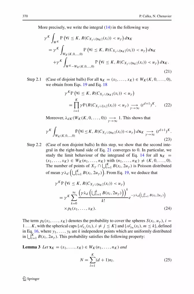
370 P. Calka, N. Chenavier
More precisely, we write the integral (14) in the following way
γK
∫WK
�(∀i ≤ K,R(CXγ ∪{xK }(xi)) < uγ
)dxK
= γK
∫WK(K,0,...,0)
�(∀i ≤ K,R(CXγ ∪{xK }(xi)) < uγ
)dxK
+γK
∫WK−WK(K,0,...,0)
�(∀i ≤ K,R(CXγ ∪{xK }(xi)) < uγ
)dxK.
(21)
Step 2.1 (Case of disjoint balls) For all xK = (x1, . . . , xK) ∈ WK(K, 0, . . . , 0),we obtain from Eqs. 19 and Eq. 18
γK�(∀i ≤ K,R(CXγ ∪{xK }(xi)) < uγ
)
=K∏i=1
γ�(R(CXγ ∪{xi }(xi)) < uγ ) −→γ→∞ (td+1)K. (22)
Moreover, λdK(WK(K, 0, . . . , 0)) −→γ→∞ 1. This shows that
γK
∫WK(K,0,...,0)
�(∀i≤K,R(CXγ ∪{xK }(xi))<uγ
)dxK −→
γ→∞ (td+1)K.
(23)Step 2.2 (Case of non disjoint balls) In this step, we show that the second inte-
gral in the right-hand side of Eq. 21 converges to 0. In particular, westudy the limit behaviour of the integrand of Eq. 14 for all xK =(x1, . . . , xK) ∈ WK(n1, . . . , nK) with (n1, . . . , nK) �= (K, 0, . . . , 0).The number of points of Xγ ∩⋃K
i=1 B(xi, 2uγ ) is Poisson distributed
of mean γ λd
(⋃Ki=1 B(xi, 2uγ )
). From Eq. 19, we deduce that
γK�(∀i ≤ K,R(CXγ ∪{xK }(xi)) < uγ
)
= γK∞∑k=0
(γ λd
(⋃ki=1 B(xi, 2uγ )
))k
k! e−γ λd
(⋃ki=1 B(xi,2uγ )
)
×pk(x1, . . . , xK). (24)
The term pk(x1, . . . , xK) denotes the probability to cover the spheres S(xi, uγ ), i =1 . . .K , with the spherical caps {Axj (xi), i �= j ≤ K} and {Aym(xi), m ≤ k}, definedin Eq. 16, where y1, . . . , yk are k independent points which are uniformly distributedin⋃K
i=1 B(xi, 2uγ ). This probability satisfies the following property:
N =K∑l=1
(d + 1)nl. (25)
Lemma 3 Let xK = (x1, . . . , xK) ∈ WK(n1, . . . , nK) and

Extreme values for radii of a Poisson-Voronoi tessellation 371
Then, for all k < N
pk(x1, . . . , xK) = 0. (26)
Proof The proof of Lemma 3 is postponed to the appendix. From Eqs. 24, 26 and the
trivial inequalities 0 ≤ pk(x1, . . . , xK) ≤ 1 and λd
(⋃ki=1 B(xi, 2uγ )
)≤ k2dκdudγ ,
we deduce that there exists a constant c, depending on K , such that
γK�(∀i≤K,R(CXγ ∪{xK }(xi)) < uγ
) ≤ γK
∞∑k=N
(k2dκdγ udγ )k
k! ∼γ→∞ c·γK(γ udγ )
N
where φ(γ ) ∼γ→∞ ψ(γ ) means φ(γ )
ψ(γ )−→γ→∞ 1. Using Eq. 11), (25) and the fact that
K =∑Kl=1 lnl , we obtain for γ large enough
γK�(∀i ≤ K,R(CXγ ∪{xK }(xi)) < uγ
) ≤ c ·K∏l=2
γ (l−1)nl . (27)
Moreover, using the fact that λdK(WK(n1, . . . , nK)) ≤ c · ∏Kl=2(u
dγ )
(l−1)nl =c ·∏K
l=2 γ− (d+2)(l−1)
d+1 nl and (27), we get
γK
∫WK−WK(K,0,...,0)
�(∀i ≤ K,R(CXγ ∪{xK }(xi)) < uγ
)dxK
=∑
γK
∫WK(n1,...,nK)
�(∀i ≤ K,R(CXγ ∪{xK }(xi)) < uγ
)dxK
≤ c ·∑ K∏
l=2
γ− l−1d+1nl . (28)
The sum above runs over all the K-tuples (n1, . . . , nK) such that∑K
l=1 lnl = K andn1 �= K . Since (n1, . . . , nK) �= (K, 0, . . . , 0), there exists l ≥ 2 such that nl �= 0.Consequently, we get from Eq. 28
γK
∫WK−WK(K,0,...,0)
�(∀i ≤ K,R(CXγ ∪{xK }(xi)) < uγ
)dxK = O
(γ−1/(d+1)
)
(29)where φ(γ ) = O(ψ(γ )) means that φ(γ )
ψ(γ )is bounded.
Conclusion From Eqs. 23 and 29, we deduce that for all K ≥ 1
γK
∫WK
�(∀i ≤ K,R(CXγ ∪{xK }(xi)) < uγ
)dxK −→
γ→∞ (td+1)K.
We then apply Lemma 2, with A = �, to conclude that
�(Rmin(γ ) ≥ uγ
) −→γ→∞ e−t d+1
.

372 P. Calka, N. Chenavier
The cell which minimizes the circumscribed radius is asymptotically a simplex.To show it, we denote by
R′min(γ ) = min
x∈Xγ∩W,Fd−1(CXγ (x))≥d+2R(CXγ (x))
where Fd−1(CXγ (x)) is the number of hyperfaces of CXγ (x). The order of conver-gence of R′
min(γ ) is greater than uγ according to the following proposition.
�
(α2κdγ
(d+2)/(d+1)R′dmin(γ ) ≥ t
)−→γ→∞ 1.
Proof of Proposition 4 We apply Lemma 2 to f (CXγ (x)) = R(CXγ (x)) and A =[d + 2,∞). We then study the finite dimensional distributions i.e.
γK
∫WK
�(∀i ≤ K,R(CXγ ∪{xK }(xi)) < uγ , Fd−1(CXγ ∪{xK }(xi)) ≥ d + 2
)dxK
(30)for all K ≥ 1. When K = 1, the integrand of Eq. 30 is
γ�(R(CXγ ∪{0}(0)) < uγ , Fd−1(CXγ ∪{0}(0)) ≥ d + 2
)
≤ γ�(R(CXγ ∪{0}(0)) < uγ , #(Xγ ∩ B(0, 2uγ )) ≥ d + 2
)
= γ
∞∑k=d+2
(2dκdγ udγ )k
k! e−2dκdγ udγ pk ∼γ→∞ c · γ−1/(d+1).
We deduce that γ∫W�(R(CXγ ∪{x}(x)) < uγ , Fd−1(CXγ ∪{x}(x)) ≥ d + 2
)dx con-
verges to 0. More generally, for all K ≥ 1, we get
γK
∫WK(K,0,...,0)
�(∀i ≤ K,R(CXγ ∪{xK }(xi))
< uγ , Fd−1(CXγ ∪{xK }(xi)) ≥ d + 2)dxK −→
γ→∞ 0. (31)
Moreover, from Eq. 29
γK
∫WK−WK(K,0,...,0)
�(∀i ≤ K,R(CXγ ∪{xK }(xi))
< uγ , Fd−1(CXγ ∪{xK }(xi)) ≥ d + 2)dxK −→
γ→∞ 0.
(32)
From Eqs. 31, 32 and Lemma 2 applied to A = [d + 2,∞), we get
�(R′
min(γ ) ≥ uγ) −→γ→∞ 1.
Proposition 4 Let Xγ be a Poisson point process of intensity γ and W a convex bodyof volume 1. Then, for all t ≥ 0,

Extreme values for radii of a Poisson-Voronoi tessellation 373
�(∀x ∈ Xγ , R(CXγ (x)) = Rmin(γ ) =⇒ Fd−1(CXγ (x)) = d + 1
) −→γ→∞ 1.
Proposition 4 implies Corollary 1 but does not provide the exact order of R′min(γ ).
Nevertheless, when d = 2, it can be made explicit. The key idea is contained inLemma 4 and cannot unfortunately be extended to higher dimensions.
�
(α′
2πγ5/4R′2
min(γ ) ≥ t)
−→γ→∞ e−t4
where α′2 is defined in Eq. 35.
Proof of Proposition 4 Let t ≥ 0 be fixed and let us denote by
u′γ = u′γ (t) =(α′−1
2 π−1γ−5/4t)1/2
(33)
where α′2 is specified in Eq. 35. As in the proof of Eq. 2d, we interpret the distribution
function of R′min(γ ) as a covering probability of the circle. Let μk be the probability
that S(0, u′γ ) is covered with the circular caps {Aym(0), m ≤ k} where y1, . . . , ykare k independent points which are uniformly distributed in B(0, 2u′γ ) and such thatF1(C{0}∪{yk }(0)) ≥ 4 i.e.
�
(R(CXγ ∪{0}(0)) < u′γ , F1(CXγ ∪{0}(0)) ≥ 4
)=
∞∑k=4
1
k! (4πγu′2γ )
ke−4πγu′2γ μk.
(34)The constant α′
2 is defined as
α′2 =(
32
3μ4
)1/4
> 0. (35)
We are going to apply Lemma 2 to the event A = [4,∞) replacing uγ by u′γ . To doit, we need to get the limit behaviour of
γK
∫WK
�
(∀i ≤ K,R(CXγ ∪{xK }(xi)) < u′γ , F1(CXγ ∪{xK }(xi)) ≥ 4
)dxK (36)
for all K ≥ 1.When K = 1, from Eqs. 34 and 33, we deduce that
γ∫W�
(R(CXγ ∪{x}(x)) < u′γ , Fd−1(CXγ ∪{x}(x)) ≥ 4
)dx converges to t4. More
generally, for all K ≥ 1,
γK
∫WK(K,0,...,0)
�(∀i ≤ K,R(CXγ ∪{xK }(xi))
< u′γ , F1(CXγ ∪{xK }(xi)) ≥ 4)dxK −→
γ→∞ t4K. (37)
Corollary 1 Let Xγ be a Poisson point process of intensity γ and W a convex bodyof volume 1. Then
Proposition 5 Let Xγ be a Poisson point process of intensity γ and W a convex bodyof volume 1 in �2. Then, for all t ≥ 0,

374 P. Calka, N. Chenavier
Otherwise, for all xK ∈ WK(n1, . . . , nK) with (n1, . . . , nK) �= (K, 0, . . . , 0), theintegrand of Eq. 36 is
γK�
(∀i ≤ K,R(CXγ ∪{xK }(xi)) < u′γ , F1(CXγ ∪{xK }(xi)) ≥ 4
)
= γK∞∑k=0
(γ λd
(⋃ki=1 B(xi, 2u′γ )
))k
k! e−γ λd
(⋃ki=1 B(xi,2u
′γ ))× μk(x1, . . . , xK).
(38)
The term μk(x1, . . . , xK) denotes the probability that S(xi, u′γ ) is covered with thespherical caps {Axj (xi), i �= j ≤ K} and {Aym(xi), m ≤ k} where y1, . . . , yk are
k independent points which are uniformly distributed in⋃K
i=1 B(xi, 2u′γ ) and suchthat F1(CXγ ∪{xK }(xi)) ≥ 4 for all i ≤ K . This probability satisfies the followingproperty:
N ′ = 4n1 + 4n2 +K∑l=3
3nl. (39)
Then, for all k < N ′
μk(x1, . . . , xK) = 0. (40)
Proof The proof of Lemma 4 is postponed to the appendix. From Eqs. 38, 40 and39, we deduce for γ large enough that
γK�
(∀i ≤ K,R(CXγ ∪{xK }(xi)) < u′γ , F1(CXγ ∪{xK }(xi)) ≥ 4
)
≤ c · γK(γ u′2γ )N′ = c · γ n2
K∏l=3
γ4l−3
4 nl .
Moreover, λ2K(WK(n1, . . . , nK)) ≤ c ·∏Kl=2(u
′2γ )
(l−1)nl = c · γ− 54n2∏K
l=3 γ−5l+5
4 nl .This shows that
γK
∫WK−WK(K,0,...,0)
�
(∀i≤K,R(CXγ ∪{xK }(xi))<u′γ , F1(CXγ ∪{xK }(xi))≥4
)dxK
= O(γ−1/4). (41)
From Eqs. 37, 41 and Lemma 2, we get
�
(R′
min(γ ) ≥ u′γ)
−→γ→∞ e−t4
.
We conclude the section with a quick sketch of proof for Eq. 2a.
Lemma 4 Let xK = (x1, . . . , xK) ∈ WK(n1, . . . , nK) ⊂ �2 and

Extreme values for radii of a Poisson-Voronoi tessellation 375
Proof of Eq. 2a We notice that
rmax(γ ) = maxx∈Xγ∩W
r(CXγ (x)) =1
2max
x∈Xγ∩Wmin
y �=x∈Xγ
d(x, y).
The behaviour of the maximum of nearest neighbor distances was studied by Henzein Theorem 1 of Henze (1982) when the input is a binomial process. His result did notinclude the contribution of boundary effects and is consequently limited to the set ofpoints in W�B(0, uγ ). With Lemma 2 and proceeding along the same lines as in theproof of Eq. 2d, we are able to show the convergence in distribution of the maximalinradius of Voronoi tessellation when the input is a Poisson point process in W .
4 Proof of (2c), consequence on Poisson-Voronoi approximation
Proof of (2c) First, we notice that
Rmax(γ ) = maxx∈Xγ∩W
R(CXγ (x)) = maxx∈Xγ∩W
maxy∈CXγ (x)
d(x, y).
In order to avoid boundary effects, we start by studying an intermediary radiusR′
max(γ ) defined as
R′max(γ ) = max
x∈Xγ ,CXγ (x)∩W �=∅
maxy∈CXγ (x)∩W
d(x, y).
In a first step, we provide the asymptotic behaviour of R′max(γ ). Secondly, we study
the effects of Voronoi cells astride W and Wc.
Step 1 The distribution function of R′max(γ ) can be interpreted as a covering
probability. Indeed, if we denote by
uγ = uγ (t) =(
1
κdγt + 1
κdγlog(α1γ (log γ )d−1
))1/d
(42)
where
α1 := 1
d!
⎛⎝π
1/2�(d2 + 1)
�(d+1
2
)⎞⎠
d−1
(43)
and t is a fixed parameter, we have
R′max(γ ) ≤ uγ ⇐⇒ ∀x ∈ Xγ , s.t. CXγ (x) ∩W �= ∅, ∀y ∈ CXγ (x) ∩W,
d(x, y) ≤ uγ
⇐⇒ ∀y ∈ W, ∃x ∈ Xγ , d(x, y) ≤ uγ
⇐⇒ {B(x, uγ ), x ∈ Xγ
}covers W.
We have to deal with the probability to cover a region with a large number of ballshaving a small radius when γ → ∞. Asymptotics of such covering probabilities havebeen studied by Janson. We apply Lemma 7.3 of Janson (1986) which is rewritten inour particular framework. Actually, Lemma 7.3 of Janson (1986) investigates cover-ing with copies of a general convex body and requires conditions which are clearlysatisfied in the case of the ball (see Lemmas 5.2, 5.4 and (9.24) therein).

376 P. Calka, N. Chenavier
� [λd(aB(0, R))] γ − logλd(W)
� [λd(aB(0, R))]− d log log
λd(W)
� [λd(aB(0, R))]− logα(B(0, R)) −→
γ→∞ t,−∞ < t < ∞ (44)
then�({B(x, R), x ∈ Xγ
}covers W
) −→γ→∞ e−e−t
.
Taking a = uγ , R = 1, λd(W) = 1 and noting that � [λd(aB(0, R))] = κdudγ
and α(B(0, R)) = α1, we check easily Eq. 44. From Lemma 5, we deduce that�({B(x, uγ ), x ∈ Xγ
}covers W
)converges to e−e−t
. Hence, for all t ∈ �,
limγ→∞�
(R′
max(γ ) ≤ uγ) = e−e−t
. (45)
Step 2 Taking f (CXγ (x)) = κd(maxy∈CXγ (x)∩W d(x, y))d , aγ = γ , bγ =log(α1γ (log γ )d−1
)and Y a Gumbel distribution (i.e. �(Y ≤ t) =
e−e−t, t ∈ �), one can check condition (5) with k = d . From Eq. 45
and Proposition 3, we deduce that �(maxx∈Xγ∩W maxy∈CXγ (x)∩W d(x, y) ≤uγ ) converges to e−e−t
for all t ∈ �. Using the fact that, on the event Aγ
(given in Lemma 1),
maxx∈Xγ∩W
maxy∈CXγ (x)∩W
d(x, y) ≤ maxx∈Xγ∩W
maxy∈CXγ (x)
d(x, y)
≤ maxx∈Xγ∩W1+lγ
maxy∈CXγ (x)∩W1+lγ
d(x, y)
and proceeding along the same lines as in the proof of Proposition 3, we get
�(Rmax(γ ) ≤ uγ
) −→γ→∞ e−e−t
. (46)
We can note that the asymptotic behaviour of Rmax(γ ) gives an interpretation ofLemma 7.3 in Janson (1986). Indeed, Eq. 46 shows that the Gumbel distributionwhich appears as a limit probability of a covering is actually the limit distribution ofa maximum.
We now apply this convergence result to the so-called Poisson-Voronoi approxi-mation defined as
VXγ (W) =⋃
x∈Xγ∩WCXγ (x).
It consists in discretizing a given convex window W with a finite union of con-vex polyhedra. This approximation has various applications such as image analysis(reconstructing an image from its intersection with a Poisson point process, seeKhmaladze and Toronjadze 2001) or quantization (see chapter 9 of Graf and Luschgy2000). Estimates of the first two moments of the symmetric difference between the
Lemma 5 (Janson) Let W be a bounded subset of �d such that λd(∂W) = 0 andXγ a Poisson point process of intensity γ . Let R be a random variable such that�[R] > 0 and �[Rd+ε] < ∞ for some ε > 0. We denote by α(B(0, R)) =α1�[Rd−1]d�[Rd ]−(d−1). If a = a(γ ) is a function such that a(γ ) −→
γ→∞ 0 and

Extreme values for radii of a Poisson-Voronoi tessellation 377
convex body and its approximation are given in Heveling and Reitzner (2009) andextended to higher moments in Reitzner et al. (2012). To the best of our knowl-edge, the convergence of VXγ (W) to W in the sense of Hausdorff distance, denotedby dH (·, ·), has not been investigated. Corollary 2 addresses that question with anassumption on the regularity of W which is in the spirit of the n-regularity (seeDefinition 3 in Capasso and Villa 2008).
λd(B(y, v) ∩W) ≥ αλd(B(y, v)). (47)
Then
�
(dH (W,VXγ (W)) ≤
(c(α)γ−1 log
(α1γ (log γ )d−1
))1/d) −→γ→∞ 1 (48)
where c(α) = κ−1d + 2dκ−1
d α−1.
Proof of Corollary 2 Let us denote by
vγ =(c(α)γ−1 log
(α1γ (log γ )d−1
))1/d. (49)
First, we show that maxy∈VXγ (W) d(y,W) ≤ vγ with high probability. For all t ∈ �,using the fact that uγ ≤ vγ for γ large enough, where uγ = uγ (t) is given in (42),we get
�
(max
y∈VXγ (W)d(y,W) ≤ vγ
)≥ �(Rmax(γ ) ≤ vγ
) ≥ �(Rmax(γ ) ≤ uγ
).
From Eq. 46 and Proposition 3, the last term converges to e−e−tas γ goes to infinity.
Taking t → ∞, we get
limγ→∞�
(max
y∈VXγ (W)d(y,W) ≤ vγ
)≥ lim
t→∞ e−e−t = 1. (50)
In a second step, we are going to show that maxy∈W d(y,Xγ ∩W) ≤ vγ with highprobability via the use of a covering of W by balls as in the proof of Eq. 2c. Now,
the convex body W is covered by N = O(v−dγ
)deterministic balls B1, . . . , BN
with center in W and radius equal to vγ /2. From Eqs. 47, 49 and the fact that #(Bi ∩(Xγ ∩W)) is Poisson distributed with mean γ λd(Bi ∩W), we get for γ large enough
�
(maxy∈W d(y,Xγ ∩W) > vγ
)≤ �
⎛⎝
N⋃i=1
{#(Bi ∩ (Xγ ∩W)) = 0}⎞⎠
≤ N e−γ ακd(vγ /2)d ≤ α−1
1 γ−1(log γ )−(d−1)N .
Corollary 2 Let us assume that there exists α > 0 such that, for v small enough andfor all y ∈ W ,

378 P. Calka, N. Chenavier
Using the fact that N = O(v−dγ ) i.e. N = O(γ (log γ )−1) according to (49), the
right-hand side is O((log γ )−d
). Hence
�
(maxy∈W d(y,Xγ ∩W) ≤ vγ
)−→γ→∞ 1. (51)
Since dH (W,VXγ (W)) ≤ max{
maxy∈VXγ (W) d(y,W),maxy∈W d(y,Xγ ∩W)}
,
we deduce from Eqs. 50 and 51 that
�(dH (W,VXγ (W)) ≤ vγ
) −→γ→∞ 1.
In Heveling and Reitzner (2009), Heveling and Reitzner obtain that the volumeof the symmetric difference between W and VXγ (W) is of the order of γ−1/d . Theresult above makes sense and could provide the right order of the Hausdorff distance.Obviously, the constant c(α) = κ−1
d + 2dκ−1d α−1 is not optimal. From Lemma 1, it
would have been possible to get an upper-bound of the order of γ−(1−ε)/d but it isless precise than Corollary 2.
5 Proof of Eq. 2b
Proof of Eq. 2b Let t ≥ 0 be fixed. We denote by uγ the following function:
uγ = uγ (t) =(
2−(d−1)κ−1d γ−2t
)1/d. (52)
We start by finding a different expression of rmin(γ ) which does not rely on theVoronoi structure. Indeed, for all x ∈ Xγ ∩W we have
r(CXγ (x)) = max{r ≥ 0, B(x, r) ⊂ CXγ (x)} =1
2min
y �=x∈Xγ
d(x, y).
Hence, rmin(γ ) can be rewritten as
rmin(γ ) = 1
2min
(x,y) �=∈(Xγ∩W)×Xγ
d(x, y). (53)
The equality (53) implies that the problem is reduced to a study of inter-point dis-tance. Such study is well known for a binomial process X(n) of intensity n in W .In particular, Jammalamadaka and Janson (see Jammalamadaka and Janson 1986,Section 4) have shown that for all t ≥ 0,
�(r ′min,n ≥ un
) −→n→∞ e−t (54)
where r ′min,n is defined as
r ′min,n = 1
2min
(x,y) �=∈X(n)×X(n)d(x, y)

Extreme values for radii of a Poisson-Voronoi tessellation 379
and un given in Eq. 52. In a first elementary step, we extend the limit to a Pois-son point process. Our main contribution is then to compare the obtained limit withrmin(γ ) by dealing with boundary effects. In particular, our study provides a far moreaccurate estimate of the contribution of boundary cells (see Eq. 66) than what wecould have deduced from Proposition 3.
Step 1 We extend Eq. 54 to a Poisson point process. We define
r ′min(γ ) =1
2min
(x,y) �=∈(Xγ∩W)2d(x, y). (55)
Let us note that for all 0 < α < β < 1, and for all n ∈ {0, 1, 2, . . .},|n − γ | ≤ γ α =⇒ |n − γ | ≤ nβ for γ large enough. Consequently, sinceuγ is non-increasing in γ , we have for γ large enough
∣∣� (r ′min(γ )≥uγ)− e−t
∣∣ ≤∞∑n=0
∣∣�(r ′min,n≥uγ )− e−t∣∣�(#(Xγ ∩W) = n)
≤∑
|n−γ |≤γ α
max{∣∣�(r ′min,n ≥ un−nβ )− e−t
∣∣ , ∣∣�(r ′min,n ≥ un+nβ )− e−t∣∣}
× �(#(Xγ ∩W) = n)+ �(|#(Xγ ∩W)− γ | > γα). (56)
The second term of Eq. 56 converges to 0 thanks to a concentrationinequality for Poisson variables (see e.g. Lemma 1.4 in Penrose 2003).
The first term is lower than maxn≥γ−γ α max{∣∣∣�(r ′min,n ≥ un−nβ (t))− e−t
∣∣∣,∣∣∣�(r ′min,n ≥ un+nβ (t))− e−t∣∣∣}
whichtends to 0 according to Eq. 54. This
shows that, for all t ≥ 0,
limγ→∞�
(r ′min(γ ) ≥ uγ
) = e−t . (57)
Step 2 We show that rmin(γ ) = r ′min(γ ) with probability of order of O(γ−ε) withε ∈ (0, 2
d). Indeed, the random variables rmin(γ ) and r ′min(γ ), defined in
Eqs. 53 and 55, are equal if and only if no point of Xγ ∩ Wc falls into theunion of the balls B(x, 2r ′min(γ )) for x ∈ Xγ ∩ W such that d(x, ∂W) <
2r ′min(γ ) i.e.
�(rmin(γ ) �=r ′min(γ ))=�
⎛⎜⎜⎜⎝#
⎛⎜⎜⎜⎝Xγ ∩Wc ∩
⋃x∈Xγ∩W,
d(x,∂W)<2r ′min(γ )
B(x, 2r ′min(γ ))
⎞⎟⎟⎟⎠ �=0
⎞⎟⎟⎟⎠
≤ �
⎡⎢⎢⎢⎣
∑x∈Xγ∩W,
d(x,∂W)<2r ′min(γ )
#(Xγ ∩Wc ∩ B(x, 2r ′min(γ ))
)⎤⎥⎥⎥⎦ .
(58)

380 P. Calka, N. Chenavier
From Slivnyak-Mecke formula (see e.g. Corollary 3.2.3 of Schneider andWeil 2008), we get
�
⎡⎢⎢⎢⎣
∑x∈Xγ∩W,
d(x,∂W)<2r′min(γ )
#(Xγ ∩Wc ∩ B(x, 2r ′min(γ ))
)⎤⎥⎥⎥⎦
=∫W
γ�[#(Xγ ∩Wc ∩ B(x, 2r ′(x)min (γ ))
)�d(x,∂W)<2r ′(x)min (γ )
]dx
where r′(x)min (γ ) = 1
2 min(x ′,y) �=∈(Xγ∪{x}∩W)2 d(x ′, y) for all x ∈ Xγ ∩ W .
Noting that r ′(x)min (γ ) ≤ r ′min(γ ), we then obtain
�
⎡⎢⎢⎢⎣
∑x∈Xγ∩W,
d(x,∂W)<2r′min (γ )
#(Xγ ∩Wc ∩ B(x, 2r ′min(γ ))
)⎤⎥⎥⎥⎦
≤∫W
γ�[#(Xγ ∩Wc ∩ B(x, 2r ′min(γ ))
)�d(x,∂W)<2r ′min(γ )
]dx
=∫W
γ�[�[#(Xγ ∩Wc ∩ B(x, 2r ′min(γ ))
) |Xγ ∩W]�d(x,∂W)<2r ′min(γ )
]dx.
(59)
Since #(Xγ ∩Wc ∩ B(x, 2r ′min(γ ))
)is Poisson distributed, we get
γ�[�[#(Xγ ∩Wc ∩ B(x, 2r ′min(γ ))
) |Xγ ∩W]�d(x,∂W)<2r ′min(γ )
]
= γ 2�
[λd(W
c ∩ B(x, 2r ′min(γ )))�d(x,∂W)<2r ′min(γ )
]
≤ 2dκd · γ 2�
[r ′dmin(γ )�d(x,∂W)<2r ′min(γ )
]. (60)
Using Eqs. 58, 59, 60 and Fubini’s theorem, we obtain
�(rmin(γ ) �= r ′min(γ )) ≤ 2dκd · γ 2�
[r ′dmin(γ )
∫W
�d(x,∂W)<2r ′min(γ )dx
]
≤ c · γ 2�
[r ′d+1
min (γ )]. (61)
The last inequality comes from Steiner formula (see (14.5) in Schneider andWeil 2008) and c denotes a constant depending on W . Hence, to show that
�(rmin(γ ) �= r ′min(γ )
) −→γ→∞ 0 (62)
we have to find some upper-bound of γ 2�[r′d + 1min(γ )]. We know, from
Eqs. 57 and 52, that γ 2r ′dmin(γ ) tends to 0 in distribution but it does not imply(62). Lemma 6 below provides an estimate of the deviation probabilities ofγ 2r ′dmin(γ ) when the window W is a cube.

Extreme values for radii of a Poisson-Voronoi tessellation 381
r ′min|C(γ ) =1
2min
(x,y) �=∈(Xγ∩C)2d(x, y).
Then, for all u ≤ min{ 14Md1/2, 1
2d1/2γ−1/d }, there exists a constant c(M) such that
�(r ′min|C(γ ) ≥ u) ≤ e−c(M)γ 2ud .
Proof of Lemma 6 Let u ≤ min{ 14Md1/2, 1
2d1/2γ−1/d } be fixed.
We subdivide the cube C = [0,M]d into a set of N subcubes C1, . . . , CN ofequal size c with c = 2d−1/2u and N = ⌊Mc−1
⌋d. Since diam(Ci) = 2u for each
i ≤ N , we obtain
�(r ′min|C(γ ) ≥ u) ≤ �
⎛⎝
N⋂i=1
{#(Ci ∩Xγ ) ≤ 1}⎞⎠ =(e−γ cd (1 + γ cd)
)N.
Replacing cd by 2dd−d/2ud and N by �2−1Md1/2u−1�d we obtain the followinginequality:
�(r ′min|C(γ ) ≥ u) ≤ e�2−1Md1/2u−1�d(log(1+γ 2dd−d/2ud)−γ 2dd−d/2ud).
Since γ 2dd−d/2ud ≤ 1 and 2M−1d−1/2u ≤ 12 , we have log(1 + γ 2dd−d/2ud) −
γ 2dd−d/2ud ≤ − 14 22dd−dγ 2u2d and �2−1Md1/2u−1�d ≥ (2−1Md1/2u−1 − 1)d ≥
2−2dMddd/2u−d . Hence
�(r ′min|C(γ ) ≥ u) ≤ e−14 d
−d/2Mdγ 2ud = e−c(M)γ 2ud
where c(M) = 14d
−d/2Md .
Now, we can derive an upper-bound of γ 2�[r ′d+1
min (γ )]. Indeed, since W has non-empty interior, there exists a cube C of side M included in W . Using the fact that#(Xγ ∩ C) ≥ 2 =⇒ r ′min(γ ) ≤ r ′min|C(γ ), we get
γ 2�
[r ′d+1
min (γ )]= γ 2∫ diam(W)
0�
(r ′d+1
min (γ ) ≥ s)ds
≤ diam(W)γ 2�(#(Xγ ∩ C) ≤ 1)+ γ 2
∫ Md1/2
0�
(r ′d+1
min|C(γ ) ≥ s)ds. (63)
Lemma 6 Let C be a cube of side M and Xγ a Poisson point process of intensity γ .Let us denote by

382 P. Calka, N. Chenavier
The first term of the right-hand side of Eq. 63 is decreasing exponentially fast to 0since #(Xγ ∩ C) is Poisson distributed of mean γMd . For the second term, let us
consider a fixed ε in(
0, 2d
). Then
γ 2∫ Md1/2
0�(r ′d+1
min|C(γ ) ≥ s)ds =∫ γ−(2+ε)
0γ 2�
(r ′min|C(γ ) ≥ s1/(d+1)
)ds
+∫ Md1/2
γ−(2+ε)
γ 2�
(r ′min|C(γ ) ≥ s1/(d+1)
)ds
≤ γ−ε +Md1/2γ 2�
(r ′min|C(γ ) ≥ γ−(2+ε)/(d+1)
).
(64)
Since ε > 0, we have γ−(2+ε)/(d+1) ≤ min{ 14Md1/2, 1
2d1/2γ−1/d } for γ large
enough. Hence, from Lemma 6 applied to u := γ−(2+ε)/(d+1), we deduce that for γlarge enough,
γ 2∫ Md1/2
0�(r ′d+1
min|C(γ ) ≥ s)ds ≤ γ−ε +Md1/2γ 2e−c(M)γ (2−εd)/(d+1). (65)
The last term of the right-hand side of Eq. 65 converges exponentially fast to 0 as γgoes to infinity since ε < 2
d. Combining that argument with Eqs. 61, 63 and 65, we
deduce that
�(rmin(γ ) �= r ′min(γ )
) = O(γ−ε). (66)
We then deduce from Eqs. 57 and 66 that
∣∣� (r ′min(γ )≥uγ)−e−t
∣∣≤ ∣∣� (r ′min(γ )≥uγ)−e−t
∣∣+2�(rmin(γ ) �=r ′min(γ )
) −→γ→∞ 0.
∣∣∣�(
2d−1κdγ2rmin(γ )
d ≥ t)− e−t∣∣∣ ≤ c(W)γ
−min{
12 ,ε}.
The study of more extremes for general tessellations and their rates of convergencewill be developed in a future paper.
Acknowledgments This work was partially supported by the French ANR grant PRESAGE (ANR-11-BS02-003) and the French research group GeoSto (CNRS-GDR3477).
Remark 1 The rate for the convergence in distribution of rmin(γ ) to the Weibull dis-tribution can be estimated. For instance, we can show that Theorem 2.1 in Schulteand Thale (2012) implies the rate of convergence of r ′min(γ ). Another way to get itis to use Theorem 1 in Arratia et al. (1990). We then obtain that there exists positiveconstants c(W) and �(W) such that, for all ε < 2
d, t ≥ 0 and γ ≥ �(W),
Extreme values for radii of a Poisson-Voronoi tessellation 383
Appendix
Proof of Lemma 3 Actually, we show the following deterministic result: let K ≥ 2,k < N , (x1, . . . , xK) ∈ WK(n1, . . . , nK) with (n1, . . . , nK) �= (K, 0, . . . , 0) and(y1, . . . , yk) ∈ ⋃K
i=1 B(xi, 2uγ ) such that {xK} ∪ {yk} are in general position i.e.each subset of size n < d + 1 is affinely independent (see Zessin 2008). Then thereexists i ≤ K such that sphere S(xi, uγ ) is not covered by the induced spherical caps{Axj (xi), i �= j ≤ K} ∪ {Aym(xi), m ≤ k}.
Indeed, from Eq. 25 there exists a connected component of⋃K
i=1 B(xi, 2uγ ) ofsize 1 ≤ l ≤ K , say
⋃li=1 B(xi, 2uγ ) without loss of generality, such that Nl < d+1
with
Nl = #
({yk} ∩
l⋃i=1
B(xi, 2uγ )
)(67)
Since {xl} ∪ {yNl} are in general position, the family {xl} is not included in theconvex hull of {yNl }. In particular, there exists i ≤ l such that xi is not in the convexhull of {xl} ∪ {yNl} − {xi}. Since a Voronoi cell induced by a finite number of pointsis not bounded if and only if its nucleus is an extremal point of the polytope inducedby the points, it implies that the circumscribed radius of C{xl}∪{yNl
}(xi) is not finitei.e. S(xi, uγ ) is not covered.
Proof of Lemma 4 We show the following deterministic result: let K ≥ 2, k <
N ′, (x1, . . . , xK) ∈ WK(n1, . . . , nK) with (n1, . . . , nK) �= (K, 0, . . . , 0) and(y1, . . . , yk) ∈ ⋃K
i=1 B(xi, 2uγ ) such that {xK} ∪ {yk} are in general position. Thenthere exists i ≤ K such that either the sphere S(xi, uγ ) is not covered by the inducedspherical caps {Axj (xi), i �= j ≤ K} ∪ {Aym(xi), m ≤ k} or F1(C{xK }∪{yk }(xi)) ≤ 3.
Indeed, from Eq. 39 there exists a connected component of⋃K
i=1 B(xi, 2uγ ) ofsize 1 ≤ l ≤ K , say
⋃li=1 B(xi, 2uγ ) without loss of generality, such that Nl < 4 if
l = 1, 2 and Nl < 3 if l ≥ 3 where Nl is given in Eq. 67.
• If l = 1, either S(x1, uγ ) is covered or F1(C{xK }∪{yk }(x1)) =F1(C{x1}∪{yN1 }(x1)) ≤ 3 since N1 ≤ 3.
• If l ≥ 3, from Lemma 3 there exists i ≤ l such that S(xi, uγ ) is not covered.• If l = 2, we can assume that N2 = 3. We have to prove that if y3 = {y1, y2, y3}
is a set of three points in B(x1, 2uγ )∪B(x2, 2uγ ), then the following properties1 and 2 below cannot hold simultaneously.
1. The circles S(x1, uγ ) and S(x2, uγ ) are covered by the induced circular caps
{Ax1(x2),Ax2(x1)} ∪ {Aym(xi), m ≤ 3}.2. The number of edges of the Voronoi cells satisfy F1(C{x1,x2,y3}(x1)) ≥ 4 and
F1(C{x1,x2,y3}(x2)) ≥ 4.
Let us assume that Properties 1 and 2 hold simultaneously. Let us denote byG the Delaunay graph associated to {x1, x2, y1, y2, y3}. Then G is a connected

384 P. Calka, N. Chenavier
planar graph with v = 5 vertices and e edges. From Euler’s formula on planargraphs, e ≤ 3v − 6 i.e.
e ≤ 9. (68)
From Property 1 and according to the proof of Lemma 3, x1, x2 are in the convexhull of {y1, y2, y3} i.e. {y1, y2}, {y1, y3} and {y2, y3} are edges of the associatedDelaunay triangulation. From Property 2, x1, x2 are connected to every point i.e.{x1, x2}, {x1, y1}, {x1, y2}, {x1, y3}, {x2, y1}, {x2, y2} and {x2, y3} are also edgesof the Delaunay triangulation. The total number of these edges is e = 10. Thiscontradicts Eq. (68).
References
Arratia, R., Goldstein, L., Gordon, L.: Poisson approximation and the Chen-Stein method. Stat. Sci. 5(4),403—434 (1990)
Baccelli, F.B.: Blaszczyszyn. Stochastic geometry and wireless networks volume 2: APPLICATIONS.Foundations and Trends� in Networking 4(1–2), 1–312 (2009)
Baumstark, V., Last, G.: Some distributional results for Poisson-Voronoi tessellations. Adv. Appl. Probab.39(1), 16–40 (2007)
Calka, P.: The distributions of the smallest disks containing the Poisson-Voronoi typical cell and theCrofton cell in the plane. Adv. Appl. Probab. 34(4), 702–717 (2002)
Calka, P.: An explicit expression for the distribution of the number of sides of the typical Poisson-Voronoicell. Adv. Appl. Probab. 35(4), 863–870 (2003)
Calka, P.: Tessellations. In: New Perspectives in Stochastic Geometry, pp. 145–169. Oxford UniversityPress, Oxford (2010)
Capasso, V., Villa, E.: On the geometric densities of random closed sets. Stoch. Anal. Appl. 26(4), 784–808(2008)
de Haan, L., Ferreira, A.: Extreme value theory. In: Springer Series in Operations Research and FinancialEngineering. Springer, New York (2006). An introduction
Foss, S.G., Zuyev, S.A.: On a Voronoi aggregative process related to a bivariate Poisson process. Adv.Appl. Probab. 28(4), 965–981 (1996)
Graf, S., Luschgy, H.: Foundations of Quantization for Probability Distributions. Lecture Notes inMathematics, vol. 1730. Springer-Verlag, Berlin (2000)
Heinrich, L., Muche, L.: Second-order properties of the point process of nodes in a stationary Voronoitessellation. Math. Nachr. 281(3), 350–375 (2008)
Heinrich, L., Schmidt, H., Schmidt, V.: Limit theorems for stationary tessellations with random inner cellstructures. Adv. Appl. Probab. 37(1), 25–47 (2005)
Henze, N.: The limit distribution for maxima of “weighted” rth-nearest-neighbour distances. J. Appl.Probab. 19(2), 344–354 (1982)
Heveling, M., Reitzner, M.: Poisson-Voronoi approximation. Ann. Appl. Probab. 19(2), 719–736 (2009)Hlubinka, D.: Stereology of extremes; shape factor of spheroids. Extremes 6(1), 5–24 (2003)Hug, D., Reitzner, M., Schneider, R.: Large Poisson-Voronoi cells and Crofton cells. Adv. Appl. Probab.
36(3), 667–690 (2004)Jammalamadaka, S.R., Janson, S.: Limit theorems for a triangular scheme of U -statistics with applications
to inter-point distances. Ann. Probab. 14(4), 1347–1358 (1986)Janson, S.: Random coverings in several dimensions. Acta Math. 156(1-2), 83–118 (1986)Ju, L., Gunzburger, M., Zhao, W.: Adaptive finite element methods for elliptic PDEs based on conforming
centroidal Voronoi-Delaunay triangulations. SIAM J. Sci. Comput. 28(6), 2023–2053 (2006)Khmaladze, E., Toronjadze, N.: On the almost sure coverage property of Voronoi tessellation: the �1 case.
Adv. Appl. Probab. 33(4), 756–764 (2001)Lantuejoul, C., Bacro, J.N., Bel, L.: Storm processes and stochastic geometry. Extremes 14(4), 413–428
(2011)

Extreme values for radii of a Poisson-Voronoi tessellation 385
Leadbetter, M.R.: On extreme values in stationary sequences. Z. Wahrscheinlichkeitstheorie und Verw.Gebiete 28, 289–303 (1973/74)
Leadbetter, M.R.: Extremes and local dependence in stationary sequences. Z. Wahrsch. Verw. Gebiete65(2), 291–306 (1983)
LeCaer, G., Ho, J.S.: The Voronoi tessellation generated from eigenvalues of complex random matrices.J. Phys. A :Math. Gen. 23, 3279–3295 (1990)
Loynes, R.M.: Extreme values in uniformly mixing stationary stochastic processes. Ann. Math. Stat. 36,993–999 (1965)
Mayer, M., Molchanov, I.: Limit theorems for the diameter of a random sample in the unit ball. Extremes10(3), 129–150 (2007)
Møller, J.: Random tessellations in Rd . Adv. Appl. Probab. 21(1), 37–73 (1989)Møller, J.: Lectures on Random Voronoı Tessellations. Lecture Notes in Statistics, volume 87. Springer-
Verlag, New York (1994)Møller, J., Waagepetersen, R.P.: Statistical Inference and Simulation for Spatial Point Processes. Mono-
graphs on Statistics and Applied Probability, vol. 100. Chapman & Hall/CRC, Boca Raton, FL(2004)
Muche, L.: The Poisson-Voronoi tessellation: relationships for edges. Adv. Appl. Probab. 37(2), 279–296(2005)
Okabe, A., Boots, B., Sugihara, K., Chiu, S.N.: Spatial tessellations: concepts and applications of Voronoidiagrams, 2nd edn. Wiley Series in Probability and Statistics. Wiley, Chichester (2000)
Pawlas, Z.: Local stereology of extremes. Image Anal. Stereol. 31(2), 99–108 (2012)Penrose, M.: Random geometric graphs. Oxford Studies in Probability, vol. 5. Oxford University Press,
Oxford (2003)Poupon, A.: Voronoi and Voronoi-related tessellations in studies of protein structure and interaction. Curr.
Opin. Struct. Biol. 14(2), 233–241 (2004)Ramella, M., Boschin, W., Fadda, D., Nonino, M.: Finding galaxy clusters using Voronoi tessellations.
Astron. Astrophys. 368, 776–786 (2001)Reitzner, M., Spodarev, E., Zaporozhets, D.: Set reconstruction by Voronoi cells. Adv. Appl. Probab. 44,
938–953 (2012)Resnick, S.I.: Extreme Values, Regular Variation, and Point Processes. Applied Probability, vol. 4. A
Series of the Applied Probability Trust. Springer-Verlag, New York (1987)Roque, W.L.: Introduction to Voronoi diagrams with applications to robotics and landscape ecology. Proc.
II Escuela de Matematica Aplicada 01, 1–27 (1997)Schneider, R., Weil, W.: Stochastic and integral geometry. Probability and its Applications (New York).
Springer-Verlag, Berlin (2008)Schulte, M., Thale, C.: The scaling limit of Poisson-driven order statistics with applications in geometric
probability. Stoch. Process. Appl. 122(12), 4096–4120 (2012)Smith, R.L.: Extreme value theory for dependent sequences via the Stein-Chen method of Poisson
approximation. Stoch. Process. Appl. 30(2), 317–327 (1988)Zessin, H.: Point processes in general position. J. Contemp. Math. Anal., Armen. Acad. Sci. 43(1), 59–65
(2008)