F. Schmelz · E. Aucktor - Universal Joints and Driveshafts

Universal Joints and Driveshafts

H.Chr. Seherr-Thoss · F. Schmelz · E. Aucktor

H.Chr. Seherr-Thoss · F. Schmelz · E. Aucktor

UniversalJoints and DriveshaftsAnalysis, Design, Applications

Second, enlarged edition with 267 Figures and 72 Tables

Translated by J. A. Tipper and S. J. Hill

2 3

Authors:

Hans Christoph Seherr-Thoss, Dipl.-Ing.Holder of the Graf Seherr Archives, Unterhaching

Friedrich Schmelz, Dipl.-Ing.Test- and Computing Engineer, Ingolstadt

Erich Aucktor, Dipl.-Ing.Development- and Design-Engineer, Offenbach a.M.

Translators:

Mrs. Jennifer A. TipperB.A. Hons., Lichfield

Dr. Stuart J. Hill, B. A. (Eng.)Hons. Ph. D., British Railways Board, London

ISBN-10 3-540-30169-0 Springer-Verlag Berlin Heidelberg New YorkISBN-13 978-3-540-30169-1 Springer-Verlag Berlin Heidelberg New York

Library of Congress Cataloging-in-Publication Data

[Gelenke and Gelenkwellen. English]Universal joints and driveshafts: analysis, design, applications/F. SchmelzH. Chr. Seherr-Thoss, E. Aucktor: translated by S. J. Hill and J. A. Tipper. p. cm.Translation of: Gelenke und Gelenkwellen. Includes indexes.ISBN 3-540-41759-11. Universal joints. 2. Automobiles – Powertrains.I. Seherr-Thoss, H.-Chr. (Hans-Christoph), Count, II. Schmelz, F.(Friedrich), III. Aucktor, E. (Erich), 1913–98.TJ1059.S3613 1992 621.8’25—dc20 90-28614

This work is subject to copyright. All rights are reserved, whether the whole or part of the material isconcerned, specifically the rights of translation, reprinting, reuse of illustrations, recitation, broad-casting, reproduction on microfilm or in any other way, and storage in data banks. Duplication of thispublication or parts thereof is permitted only under the provisions of the German Copyright Law of September 9, 1965, in its current version, and permission for use must always be obtained fromSpringer-Verlag. Violations are liable for prosecution under the German Copyright Law.

Springer is a part of Springer Science+Business Mediaspringer.com© Springer-Verlag Berlin Heidelberg 2006Printed in Germany

The use of registered names, trademarks, etc. in this publication does not imply, even in the absence ofa specific statement, that such names are exempt from the relevant protective laws and regulations andtherefore free for general use.

Typesetting: Fotosatz-Service Köhler GmbH, WürzburgProjectmanagement: Reinhold Schöberl, WürzburgCover design: medionet AG, BerlinPrinted on acid-free paper – 62/3020 – 543210

An important date in the history of automotive engineering was celebrated at thestart of the 1980s: 50 years of front-wheel drives in production vehicles. This bicen-tennial event aroused interest in the development, theory and future of driveshaftsand joints. The authors originally presented all the available knowledge on constant-velocity and universal-joint driveshafts in German as long ago as 1988, followed byEnglish in 1992 and Chinese in 1997.

More than ten years have passed since then, in which time technology has alsomade major progress in the field of driveshafts. Driveshaft design and manufac-turing process has kept pace with the constantly growing demands of the varioususers. More powerful engines with higher torques, new fields of application with in-creased stresses, e.g. off-road and heavy goods vehicles or rolling mills, improvedmaterials, new production processes and advanced experimental and test methodshave imposed completely new requirements on the driveshaft as a mechanical com-ponent.

GKN Driveline has made a major contribution to the further development of thedriveshaft and will maintain this effort in the future. At our Research & Product Development Centres, GKN engineers have defined basic knowledge and conceivedproduct improvements for the benefit of the automotive, agricultural, and machi-nery industry of mechanically engineered products for the world. In close coopera-tion with its customers GKN has created low-noise, vibration and maintenance-freedriveshafts.

The cumulative knowledge acquired has been compiled in this second editionbook that has been updated to reflect the latest state of the art. It is intended to serveboth as a textbook and a work of reference for all driveline engineers, designers andstudents who are in some way involved with constant-velocity and universal-jointdriveshafts.

Redditch, England Arthur ConnellyJuly 2005 Chief Executive Officer

GKN Automotive Driveline Driveshafts

Preface to the second English edition

1989 saw the start of a new era of the driveline components and driveshafts, drivenby changing customer demands. More vehicles had front wheel drive and transverseengines, which led to considerable changes in design and manufacture, and tradi-tional methods of production were revisited. The results of this research and deve-lopment went into production in 1994–96:

– for Hooke’s jointed driveshafts, weight savings were achieved through new for-gings, noise reduction through better balancing and greater durability throughimproved lubrication.

– for constant velocity joints, one can talk about a “New Generation’’, employing something more like roller bearing technology, but where the diverging factorsare dealt with. The revised Chapters 4 and 5 re-examine the movement patternsand stresses in these joints.

The increased demands for strength and precision led to even intricate shapes beingforged or pressed. These processes produce finished parts with tolerances of0.025 mm. 40 million parts were forged in 1998. These processes were also reviewed.

Finally, advances were made in combined Hooke’s and constant velocity jointeddriveshafts.

A leading part in these developments was played by the GKN Group in Birming-ham and Lohmar, which has supported the creation of this book since 1982. As a leading manufacturer they supply 600,000 Hooke’s jointed driveshafts and 500,000constant velocity driveshafts a year. I would like to thank Reinhold Schoeberlfor his project-management and typography to carry out the excellent execution ofthis book.

I would also like to thank my wife, Therese, for her elaboration of the indices. More-over my thanks to these contributors:

Gerd Faulbecker (GWB Essen)Joachim Fischer (ZF Lenksysteme Gmünd)Werner Jacob (Ing. Büro Frankfurt/M)Christoph Müller (Ing. Büro Ingolstadt)Prof. Dr. Ing. Ernst-Günter Paland (TU Hannover, IMKT)Jörg Papendorf (Spicer GWB Essen)Stefan Schirmer (Freudenberg)Ralf Sedlmeier (GWB Essen)Armin Weinhold (SMS Eumuco Düsseldorf/Leverkusen)

Preface to the second German edition

GKN Driveline (Lohmar/GERMANY)Wolfgang HildebrandtWerner KrudeStephan MaucherMichael Mirau (Offenbach)Clemens Nienhaus (Walterscheid)Peter Pohl (Walterscheid Trier)Rainer SchaeferdiekKarl-Ernst Strobel (Offenbach)

On 19th July 1989 our triumvirate lost Erich Aucktor. He made a valuable contribu-tion to the development of driveline technology from 1937–1958, as an engine en-gineer, and from 1958–78 as a designer and inventor of constant velocity joints atLöhr & Bromkamp, Offenbach, where he worked in development, design and testing.It is thanks to him that this book has become a reference work for these engineeringcomponents.

Count Hans Christoph Seherr-Thoss

VIII Preface to the second German edition

Index of Tables . . . . . . . . . . . . . . . . . . . . . . . . . . . . . . . . . . . XIII

Notation . . . . . . . . . . . . . . . . . . . . . . . . . . . . . . . . . . . . . . . XVII

Chronological Table . . . . . . . . . . . . . . . . . . . . . . . . . . . . . . . . XXI

Chapter 1 Universal Jointed Driveshafts for Transmitting Rotational Movements . . . . . . . . . . . . . . . . . . . . . . . . . 1

1.1 Early Reports on the First Joints . . . . . . . . . . . . . . . . . . . 11.1.1 Hooke’s Universal Joints . . . . . . . . . . . . . . . . . . . . . . . . 11.2 Theory of the Transmission of Rotational Movements

by Hooke’s Joints . . . . . . . . . . . . . . . . . . . . . . . . . . . . 51.2.1 The Non-univormity of Hooke’s Joints According to Poncelet . . . 51.2.2 The Double Hooke’s Joint to Avoid Non-univormity . . . . . . . . 81.2.3 D’Ocagne’s Extension of the Conditions for Constant Velocity . . 101.2.4 Simplification of the Double Hooke’s Joint . . . . . . . . . . . . . . 101.2.4.1 Fenaille’s Tracta Joint . . . . . . . . . . . . . . . . . . . . . . . . . 121.2.4.2 Various Further Simplifications . . . . . . . . . . . . . . . . . . . . 141.2.4.3 Bouchard’s One-and-a-half Times Universal Joint . . . . . . . . . 141.3 The Ball Joints . . . . . . . . . . . . . . . . . . . . . . . . . . . . . 171.3.1 Weiss and Rzeppa Ball Joints . . . . . . . . . . . . . . . . . . . . . 191.3.2 Developments Towards the Plunging Joint . . . . . . . . . . . . . . 271.4 Development of the Pode-Joints . . . . . . . . . . . . . . . . . . . 321.5 First Applications of the Science of Strength of Materials

to Driveshafts . . . . . . . . . . . . . . . . . . . . . . . . . . . . . . 401.5.1 Designing Crosses Against Bending . . . . . . . . . . . . . . . . . 401.5.2 Designing Crosses Against Surface Stress . . . . . . . . . . . . . . 421.5.3 Designing Driveshafts for Durability . . . . . . . . . . . . . . . . . 471.6 Literature to Chapter 1 . . . . . . . . . . . . . . . . . . . . . . . . . 49

Chapter 2 Theory of Constant Velocity Joints (CVJ) . . . . . . . . . . . . . . 53

2.1 The Origin of Constant Velocity Joints . . . . . . . . . . . . . . . . 542.2 First Indirect Method of Proving Constant Velocity According

to Metzner . . . . . . . . . . . . . . . . . . . . . . . . . . . . . . . 582.2.1 Effective Geometry with Straight Tracks . . . . . . . . . . . . . . . 612.2.2 Effective Geometry with Circular Tracks . . . . . . . . . . . . . . . 64

Contents

2.3 Second, Direct Method of Proving Constant Velocity by Orain . . 662.3.1 Polypode Joints . . . . . . . . . . . . . . . . . . . . . . . . . . . . . 712.3.2 The Free Tripode Joint . . . . . . . . . . . . . . . . . . . . . . . . . 752.4 Literature to Chapter 2 . . . . . . . . . . . . . . . . . . . . . . . . . 78

Chapter 3 Hertzian Theory and the Limits of Its Application . . . . . . . . . 81

3.1 Systems of Coordinates . . . . . . . . . . . . . . . . . . . . . . . . 823.2 Equations of Body Surfaces . . . . . . . . . . . . . . . . . . . . . . 833.3 Calculating the Coefficient cos t . . . . . . . . . . . . . . . . . . . 853.4 Calculating the Deformation d at the Contact Face . . . . . . . . . 883.5 Solution of the Elliptical Single Integrals J1 to J4 . . . . . . . . . . . 943.6 Calculating the Elliptical Integrals K and E . . . . . . . . . . . . . 973.7 Semiaxes of the Elliptical Contact Face for Point Contact . . . . . 983.8 The Elliptical Coefficients m and n . . . . . . . . . . . . . . . . . . 1013.9 Width of the Rectangular Contact Surface for Line Contact . . . . 1013.10 Deformation and Surface Stress at the Contact Face . . . . . . . . 1043.10.1 Point Contact . . . . . . . . . . . . . . . . . . . . . . . . . . . . . . 1043.10.2 Line Contact . . . . . . . . . . . . . . . . . . . . . . . . . . . . . . 1053.11 The validity of the Hertzian Theory on ball joints . . . . . . . . . 1063.12 Literature to Chapter 3 . . . . . . . . . . . . . . . . . . . . . . . . . 107

Chapter 4 Designing Joints and Driveshafts . . . . . . . . . . . . . . . . . . 109

4.1 Design Principles . . . . . . . . . . . . . . . . . . . . . . . . . . . 1094.1.1 Comparison of Theory and Practice by Franz Karas 1941 . . . . . 1104.1.2 Static Stress . . . . . . . . . . . . . . . . . . . . . . . . . . . . . . . 1114.1.3 Dynamic Stress and Durability . . . . . . . . . . . . . . . . . . . . 1124.1.4 Universal Torque Equation for Joints . . . . . . . . . . . . . . . . . 1144.2 Hooke’s Joints and Hooke’s Jointed Driveshafts . . . . . . . . . . . 1164.2.1 The Static Torque Capacity Mo . . . . . . . . . . . . . . . . . . . . 1174.2.2 Dynamic Torque Capacity Md . . . . . . . . . . . . . . . . . . . . . 1184.2.3 Mean Equivalent Compressive Force Pm . . . . . . . . . . . . . . . 1194.2.4 Approximate Calculation of the Equivalent Compressive Force Pm 1244.2.5 Dynamic Transmission Parameter 2 CR . . . . . . . . . . . . . . . 1264.2.5.1 Exemple of Specifying Hooke’s Jointed Driveshafts

in Stationary Applications . . . . . . . . . . . . . . . . . . . . . . . 1284.2.6 Motor Vehicle Driveshafts . . . . . . . . . . . . . . . . . . . . . . . 1304.2.7 GWB’s Design Methodology for Hooke’s joints for vehicles . . . . 1334.2.7.1 Example of Specifying Hooke’s Jointed Driveshafts

for Commercial Vehicles . . . . . . . . . . . . . . . . . . . . . . . . 1364.2.8 Maximum Values for Speed and Articulation Angle . . . . . . . . 1384.2.9 Critical Speed and Shaft Bending Vibration . . . . . . . . . . . . . 1404.2.10 Double Hooke’s Joints . . . . . . . . . . . . . . . . . . . . . . . . . 1444.3 Forces on the Support Bearings of Hooke’s Jointed Driveshafts . . 1484.3.1 Interaction of Forces in Hooke’s Joints . . . . . . . . . . . . . . . . 1484.3.2 Forces on the Support Bearings of a Driveshaft

in the W-Configuration . . . . . . . . . . . . . . . . . . . . . . . . 150

X Contents

4.3.3 Forces on the Support Bearings of a Driveshaft in the Z-Configuration . . . . . . . . . . . . . . . . . . . . . . . . . 152

4.4 Ball Joints . . . . . . . . . . . . . . . . . . . . . . . . . . . . . . . . 1534.4.1 Static and Dynamic Torque Capacity . . . . . . . . . . . . . . . . . 1544.4.1.1 Radial bearing connections forces . . . . . . . . . . . . . . . . . . 1584.4.2 The ball-joint from the perspective of rolling and sliding bearings 1584.4.3 A common, precise joint centre . . . . . . . . . . . . . . . . . . . . 1594.4.3.1 Constant Velocity Ball Joints based on Rzeppa principle . . . . . . 1604.4.4 Internal centering of the ball-joint . . . . . . . . . . . . . . . . . . 1624.4.4.1 The axial play sa . . . . . . . . . . . . . . . . . . . . . . . . . . . . 1634.4.4.2 Three examples for calculating the axial play sa . . . . . . . . . . . 1644.4.4.3 The forced offset of the centre . . . . . . . . . . . . . . . . . . . . 1664.4.4.4 Designing of the sherical contact areas . . . . . . . . . . . . . . . 1694.4.5 The geometry of the tracks . . . . . . . . . . . . . . . . . . . . . . 1704.4.5.1 Longitudinal sections of the tracks . . . . . . . . . . . . . . . . . . 1704.4.5.2 Shape of the Tracks . . . . . . . . . . . . . . . . . . . . . . . . . . 1744.4.5.3 Steering the Balls . . . . . . . . . . . . . . . . . . . . . . . . . . . . 1774.4.5.4 The Motion of the Ball . . . . . . . . . . . . . . . . . . . . . . . . . 1784.4.5.5 The cage in the ball joint . . . . . . . . . . . . . . . . . . . . . . . 1794.4.5.6 Supporting surface of the cage in ball joints . . . . . . . . . . . . . 1834.4.5.7 The balls . . . . . . . . . . . . . . . . . . . . . . . . . . . . . . . . 1844.4.5.8 Checking for perturbations of motion in ball joints . . . . . . . . 1854.4.6 Structural shapes of ball joints . . . . . . . . . . . . . . . . . . . . 1874.4.6.1 Configuration and torque capacity of Rzeppa-type fixed joints . . 1874.4.6.2 AC Fixed Joints . . . . . . . . . . . . . . . . . . . . . . . . . . . . . 1884.4.6.3 UF Fixed joints (undercut free) . . . . . . . . . . . . . . . . . . . . 1934.4.6.4 Jacob/Paland’s CUF (completely undercut free) Joint

for rear wheel drive > 25° . . . . . . . . . . . . . . . . . . . . . . . 1954.4.6.5 Calculation example for a CUF joint . . . . . . . . . . . . . . . . . 1974.4.7 Plunging Joints . . . . . . . . . . . . . . . . . . . . . . . . . . . . . 2004.4.7.1 DO Joints . . . . . . . . . . . . . . . . . . . . . . . . . . . . . . . . 2004.4.7.2 VL Joints . . . . . . . . . . . . . . . . . . . . . . . . . . . . . . . . 2024.4.8 Service Life of Joints Using the Palmgren/Miner Rule . . . . . . . 2074.5 Pode Joints . . . . . . . . . . . . . . . . . . . . . . . . . . . . . . . 2094.5.1 Bipode Plunging Joints . . . . . . . . . . . . . . . . . . . . . . . . 2134.5.2 Tripode Joints . . . . . . . . . . . . . . . . . . . . . . . . . . . . . 2144.5.2.1 Static Torque Capacity of the Non-articulated Tripode Joint . . . . 2154.5.2.2 Materials and Manufacture . . . . . . . . . . . . . . . . . . . . . . 2154.5.2.3 GI Plunging Tripode Joints . . . . . . . . . . . . . . . . . . . . . . 2204.5.2.4 Torque Capacity of the Articulated Tripode Joint . . . . . . . . . . 2224.5.3 The GI-C Joint . . . . . . . . . . . . . . . . . . . . . . . . . . . . . 2284.5.4 The low friction and low vibration plunging tripode joint AAR . . 2294.6 Materials, Heat Treatment and Manufacture . . . . . . . . . . . . . 2314.6.1 Stresses . . . . . . . . . . . . . . . . . . . . . . . . . . . . . . . . . 2314.6.2 Material and hardening . . . . . . . . . . . . . . . . . . . . . . . . 2364.6.3 Effect of heat treatment on the transmittable static

and dynamic torque . . . . . . . . . . . . . . . . . . . . . . . . . . 238

Contents XI

4.6.4 Forging in manufacturing . . . . . . . . . . . . . . . . . . . . . . . 2394.6.5 Manufacturing of joint parts . . . . . . . . . . . . . . . . . . . . . 2404.7 Basic Procedure for the Applications Engineering of Driveshafts . 2434.8 Literature to Chapter 4 . . . . . . . . . . . . . . . . . . . . . . . . . 245

Chapter 5 Joint and Driveshaft Configurations . . . . . . . . . . . . . . . . . 249

5.1 Hooke’s Jointed Driveshafts . . . . . . . . . . . . . . . . . . . . . . 2505.1.1 End Connections . . . . . . . . . . . . . . . . . . . . . . . . . . . . 2515.1.2 Cross Trunnions . . . . . . . . . . . . . . . . . . . . . . . . . . . . 2535.1.3 Plunging Elements . . . . . . . . . . . . . . . . . . . . . . . . . . . 2585.1.4 Friction in the driveline – longitudinal plunges . . . . . . . . . . . 2585.1.5 The propshaft . . . . . . . . . . . . . . . . . . . . . . . . . . . . . 2625.1.6 Driveshaft tubes made out of composite Fibre materials . . . . . . 2635.1.7 Designs of Driveshaft . . . . . . . . . . . . . . . . . . . . . . . . . 2675.1.7.1 Driveshafts for Machinery and Motor Vehicles . . . . . . . . . . . 2675.1.8 Driveshafts for Steer Drive Axles . . . . . . . . . . . . . . . . . . . 2685.2 The Cardan Compact 2000 series of 1989 . . . . . . . . . . . . . . 2695.2.1 Multi-part shafts and intermediate bearings . . . . . . . . . . . . 2735.2.2 American Style Driveshafts . . . . . . . . . . . . . . . . . . . . . . 2755.2.3 Driveshafts for Industrial use . . . . . . . . . . . . . . . . . . . . . 2775.2.4 Automotive Steering Assemblies . . . . . . . . . . . . . . . . . . . 2855.2.5 Driveshafts to DIN 808 . . . . . . . . . . . . . . . . . . . . . . . . 2925.2.6 Grooved Spherical Ball Jointed Driveshafts . . . . . . . . . . . . . 2945.3 Driveshafts for Agricultural Machinery . . . . . . . . . . . . . . . 2965.3.1 Types of Driveshaft Design . . . . . . . . . . . . . . . . . . . . . . 2975.3.2 Requirements to meet by Power Take Off Shafts . . . . . . . . . . 2985.3.3 Application of the Driveshafts . . . . . . . . . . . . . . . . . . . . 3005.4 Calculation Example for an Agricultural Driveshaft . . . . . . . . 3075.5 Ball Jointed Driveshafts . . . . . . . . . . . . . . . . . . . . . . . . 3085.5.1 Boots for joint protection . . . . . . . . . . . . . . . . . . . . . . . 3105.5.2 Ways of connecting constant velocity joints . . . . . . . . . . . . . 3115.5.3 Constant velocity drive shafts in front and rear wheel

drive passenger cars . . . . . . . . . . . . . . . . . . . . . . . . . . 3125.5.4 Calculation Example of a Driveshaft with Ball Joints . . . . . . . . 3165.5.5 Tripode Jointed Driveshaft Designs . . . . . . . . . . . . . . . . . 3215.5.6 Calculation for the Tripode Jointed Driveshaft of a Passenger Car 3225.6 Driveshafts in railway carriages . . . . . . . . . . . . . . . . . . . . 3255.6.1 Constant velocity joints . . . . . . . . . . . . . . . . . . . . . . . . 3255.7 Ball jointed driveshafts in industrial use and special vehicles . . . 3275.8 Hooke’s jointes high speed driveshafts . . . . . . . . . . . . . . . . 3295.9 Design and Configuration Guidelines to Optimise the Drivetrain . 3325.9.1 Exemple of a Calculation for the Driveshafts of a Four Wheel

Drive Passenger Car (Section 5.5.4) . . . . . . . . . . . . . . . . . 3335.10 Literature to Chapter 5 . . . . . . . . . . . . . . . . . . . . . . . . . 343

XII Contents

Independent Tables

Table 1.1 Bipode joints 1902–52 . . . . . . . . . . . . . . . . . . . . . . . . 33Table 1.2 Tripode joints 1935–60 . . . . . . . . . . . . . . . . . . . . . . . 36Table 1.3 Quattropode-joints 1913–94 . . . . . . . . . . . . . . . . . . . . 39Table 1.4 Raised demands to the ball joints by the customers . . . . . . . 39Table 3.1 Complete elliptical integrals by A.M. Legendre 1786 . . . . . . . 96Table 3.2 Elliptical coefficients according to Hertz . . . . . . . . . . . . . 102Table 3.3 Hertzian Elliptical coefficients . . . . . . . . . . . . . . . . . . . 103Table 4.1 Geometry coefficient f1 according to INA . . . . . . . . . . . . . 120Table 4.2 Shock or operating factor fST . . . . . . . . . . . . . . . . . . . . 127Table 4.3 Values for the exponents n1 and n2 after GWB . . . . . . . . . . 138Table 4.4 Maximum Speeds and maximum permissible values

of nb arising from the moment of inertia of the connecting parts . . . . . . . . . . . . . . . . . . . . . . . 139

Table 4.5 Radial bearing connection forces of Constant VelocityJoints (CVJ) with shafts in one plane, from Werner KRUDE . . . 157

Table 4.6 Most favourable track patterns for the two groups of joints . . . 174Table 4.7 Ball joint family tree . . . . . . . . . . . . . . . . . . . . . . . . 176Table 4.8 Steering the balls in ball joints . . . . . . . . . . . . . . . . . . . 177Table 4.9 Effect of the ball size on load capacity and service life . . . . . . 185Table 4.10 Rated torque MN of AC joints . . . . . . . . . . . . . . . . . . . 191Table 4.11 Dynamic torque capacity Md of AC joints . . . . . . . . . . . . . 191Table 4.12 Data for UF-constant velocity joints made by GKN Löbro . . . . 194Table 4.13 VL plunging joint applications . . . . . . . . . . . . . . . . . . . 206Table 4.14 Percentage of time in each gear on various types of roads . . . 208Table 4.15 Percentage of time ax for passenger cars . . . . . . . . . . . . . 208Table 4.16 Surface stresses in pode joints with roller bearings . . . . . . . 212Table 4.17 Surface stresses in pode joints with plain bearings . . . . . . . . 212Table 4.18 Materials and heat treatments of inner and outer races

for UF-constant velocity joints . . . . . . . . . . . . . . . . . . . 234Table 4.19 Values for the tri-axial stress state and the required hardness

of a ball in the track of the UF-joint . . . . . . . . . . . . . . . . 235Table 4.20 Hardness conditions for the joint parts . . . . . . . . . . . . . . 238Table 4.21 Static and dynamic torque capacities for UF constant velocity

joints with outer race surface hardness depth (Rht) of 1.1 and 2.4 mm . . . . . . . . . . . . . . . . . . . . . . . . . . . . . 239

1.2 Theorie der Übertragung von Drehbewegungen durch Kreuzgelenkwellen XIII

Index of Tables

Table 4.22 Applications Engineering procedure for a driveshaft with uniform loading . . . . . . . . . . . . . . . . . . . . . . . . 244

Table 5.1 Maximum articulation angle bmax of joints . . . . . . . . . . . . 250Table 5.2 Examples of longitudinal plunge via balls in drive shafts . . . . 260Table 5.3 Data for composite propshafts for motor vehicles . . . . . . . . 263Table 5.4 Comparison of steel and glass fibre reinforced plastic propshafts

for a high capacity passenger car . . . . . . . . . . . . . . . . . 267Table 5.5 Torque capacity of Hooke’s jointed driveshafts . . . . . . . . . . 268Table 5.6 Steering joint data . . . . . . . . . . . . . . . . . . . . . . . . . . 287Table 5.7 Comparison of driveshafts . . . . . . . . . . . . . . . . . . . . . 309Table 5.8 Examples of standard longshaft systems for passenger cars

around 1998 . . . . . . . . . . . . . . . . . . . . . . . . . . . . . 312Table 5.9 Durability values for the selected tripode joint on rear drive . . 324Table 5.10 Comparison of a standard and a high speed driveshaft

(Fig. 5.83, 5.85) . . . . . . . . . . . . . . . . . . . . . . . . . . . . 331Table 5.11 Durability values for front wheel drive with UF 1300 . . . . . . 335Table 5.12 Calculation of the starting and adhesion torques

in the calculation example (Section 5.9.1) . . . . . . . . . . . . 336Table 5.13 Values for the life of the propshaft for rear wheel drive . . . . . 339

Tables of principal dimensions, torque capacities and miscellaneous data inside the Figures

Figure 1.13 Pierre Fenaille’s Tracta joint 1927 . . . . . . . . . . . . . . . . . 13Figure 1.16 One-and-a-half times universal joint 1949 . . . . . . . . . . . . 16Figure 1.21 Fixed joint of the Weiss type . . . . . . . . . . . . . . . . . . . . 21Figure 4.5 Bearing capacity coefficient f2 of rolling bearings . . . . . . . . 121Figure 4.10 Principal and cross dimensions of a Hooke’s jointed driveshaft

for light loading . . . . . . . . . . . . . . . . . . . . . . . . . . . 128Figure 4.45 Tracks with elliptical cross section . . . . . . . . . . . . . . . . 175Figure 4.58 AC fixed joints of the Rzeppa type according to Wm. Cull . . . . 189Figure 4.59 AC fixed joint (improved) 1999 . . . . . . . . . . . . . . . . . . 190Figure 4.61 UF-constant velocity fixed joint (wheel side) . . . . . . . . . . . 195Figure 4.64 Six-ball DO plunging joints (Rzeppa type) . . . . . . . . . . . . 201Figure 4.65 Five-ball DOS plunging joint from Girguis 1971 . . . . . . . . . 202Figure 4.66 VL plunging joints of the Rzeppa type with inclined tracks

and 6 balls . . . . . . . . . . . . . . . . . . . . . . . . . . . . . . 203Figure 4.77 Glaenzer Spicer GE tripode joint with bmax = 43° to 45° . . . . . 217Figure 4.79 Glaenzer Spicer GI tripode joint . . . . . . . . . . . . . . . . . . 220Figure 4.87 Plunging tripode joint (AAR) . . . . . . . . . . . . . . . . . . . 229Figure 5.3 Driveshaft flange connections . . . . . . . . . . . . . . . . . . . 252Figure 5.8 Levels of balancing quality Q for driveshafts . . . . . . . . . . . 257Figure 5.24 Non-centred double Hooke’s jointed driveshaft with stubshaft

for steer drive axles . . . . . . . . . . . . . . . . . . . . . . . . . 271Figure 5.27 Specifications and physical data of Hooke’s joints

for commercial vehicles with length compensation . . . . . . . 274

XIV Index of Tables

Figure 5.29 Hooke’s jointed driveshaft from Mechanics/USA . . . . . . . . . 277Figure 5.30 Centred double-joint for high and variable articulation angles . 278Figure 5.31 Driving dog and connection kit of a wing bearing driveshaft . . 279Figure 5.32 Specifications, physical data and dimensions of the cross

trunnion of a Hooke’s jointed driveshaft for stationary (industrial) use . . . . . . . . . . . . . . . . . . . . . . . . . . . 280

Figure 5.33 Universal joints crosses for medium and heavy industrial shafts 281Figure 5.34 Specifications, physical data and dimensions of the cross

trunnion of Hooke’s jointed driveshafts for industrial use,heavy type with length compensation and dismantable bearing cocer . . . . . . . . . . . . . . . . . . . . . . . . . . . . . . . . . 282

Figure 5.35 Specifications of Hooke’s heavy driveshafts with length compensation and flange connections for rolling-mills and other big machinery . . . . . . . . . . . . . . . . . . . . . . 282

Figure 5.40 Full complement roller bearing. Thin wall sheet metal bush . . 287Figure 5.42 Steering joints with sliding serration ca. 1970 . . . . . . . . . . 289Figure 5.46 Single and double joint with plain and needle bearings . . . . . 292Figure 5.51 Connection measurement for three tractor sizes

from ISO standards . . . . . . . . . . . . . . . . . . . . . . . . . 296Figure 5.55 Joint sizes for agricultural applications . . . . . . . . . . . . . . 299Figure 5.56 Sizes for sliding profiles of driveshafts on agricultural

machinery . . . . . . . . . . . . . . . . . . . . . . . . . . . . . . 301Figure 5.58 Hooke’s joints in agricultural use with protection covers . . . . 302Figure 5.61 Double joints with misaligned trunnions . . . . . . . . . . . . . 305Figure 5.70 Drive shafts with CV joints for Commercial and Special vehicles 315

Index of Tables XV

Symbol Unit Meaning

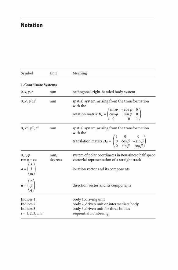
1. Coordinate Systems

0, x, y, z mm orthogonal, right-handed body system

0, x¢, y¢, z¢ mm spatial system, arising from the transformation with the

sin j – cos j 0rotation matrix Dj = �cos j sin j 0�0 0 1

0, x¢¢, y¢¢, z¢¢ mm spatial system, arising from the transformation with the

1 0 0translation matrix Db = � 0 cos b – sin b�0 sin b cos b

0, r, j mm, system of polar coordinates in Boussinesq half spacer = a + tu degrees vectorial representation of a straight track

ka = � l � location vector and its components

m

nu = � p� direction vector and its components

q

Indices 1 body 1, driving unitIndices 2 body 2, driven unit or intermediate bodyIndices 3 body 3, driven unit for three bodiesi = 1, 2, 3, ... n sequential numbering

1.2 Theorie der Übertragung von Drehbewegungen durch Kreuzgelenkwellen XVII

Notation

Symbol Unit Meaning

2. Angles

a degrees pressure angleb degrees articulation angleg degrees skew angle of the trackd degrees divergence of opening angle (d = 2e), offset anglee degrees tilt or inclination angle of the track

(Stuber pledge angle)J degrees complementary angle to a (a = 90° – J)t degrees Hertzian auxiliary anglecos t – Hertzian coefficientj degrees angle of rotation through the joint bodyc degrees angle of intersection of the tracksy degrees angle of the straight generators r

3. Rolling body data

A mm2 contact area2a mm major axis of contact ellipse2b mm minor axis of contact ellipse2c mm separation of cross axes of double Hooke’s jointsc mm offset (displacement of generating centres)d mm roller diameterD mm trunnion diameterDm mm diameter of the pitch circle of the rolling bodiesk N/mm2 specific loadingl mm roller length (from catalogue)lw mm effective length of rollerr mm radius of curvature of rolling surfacesR m effective joint radiussw mm joint plungey reciprocal of the conformity in the track cross sectionkQ conformity in the track cross sectionkL conformity in the longitudinal section of the trackr = 1/r 1/mm curvature of the rolling surfacescp N/mm2 coefficient of conformitypo N/mm2 Hertzian pressuredo mm total elastic deformation at a contact pointdb mm plastic deformationm, n Hertzian elliptical coefficientsE N/mm2 Young’s modulus (2.08 · 1011 for steel)m Poisson’s ratio = 3/10

4J =

3

(1 – m2) mm2/N abbreviation used by HertzE

z – number of balls

XVIII Notation

Symbol Unit Meaning

4. Forces

P N equivalent dynamic compressive forceQ N Hertzian compressive forceF N radial component of equivalent compressive force PA N axial component of equivalent compressive force PQtotal N total radial force on a roller bearing used

by Hertz/Stribeck

5. Moments

M Nm moments in generalM0 Nm static momentMd Nm dynamic momentMN Nm nominal moment (from catalogue)Mb Nm bending momentMB Nm design moment

6. Mathematical constants and coefficients

e ratio of the front and rear axle loads AF/AR

eF fraction of torque to the front axleeR fraction of torque to the rear axlefb articulation coefficientkw equivalence factor for cyclic compressive forcess Stribeck’s distribution factor = 5s0 static safety factor for oscillating bearings

of Hooke’s joints = 0.8 to 1.0u number of driveshaftsm friction coefficient of road

7. Other designations

Peff kW output powerV kph driving speedw s–1 angular velocitym effective number of transmitting elementsn rpm rotational speed (revolutions per minute)p plane of symmetry

Designations which have not been mentioned are explained in the text or shown inthe figures.

Notation XIX

1352–54 Universal jointed driveshaft in the clock mechanism of Strasbourg Cathedral.

1550 Geronimo Cardano’s gimbal suspension.1663 Robert Hooke’s universal joint. 1683 double Hooke’s joint.1824 Analysis of the motion of Hooke’s joints with the aid of spherical

trigonometry and differential calculus, and the calculation of the forces onthe cross by Jean Victor Poncelet.

1841 Kinematic treatment of the Hooke’s joint by Robert Willis.1894 Calculation of surface stresses for crosses by Carl Bach.1901/02 Patents for automotive joints by Arthur Hardt and Robert Schwenke.1904 Series production of Hooke’s joints and driveshafts by Clarence Winfred

Spicer.1908 First ball joint by William A. Whitney. Plunging + articulation separated.1918 Special conditions for the uniform transmission of motion by Maurice

d’Ocagne. 1930 geometrical evidence for the constant velocity characteris-tics of the Tracta joint.

1923 Fixed ball joint steered by generating centres widely separated from thejoint mid-point, by Carl William Weiss. Licence granted to the BendixCorp.

1926 Pierre Fenaille’s “homokinetic” joint.1927 Six-ball fixed joint with 45° articulation angle by Alfred H. Rzeppa. 1934

with offset steering of the balls. First joint with concentric meridian tracks.1928 First Hooke’s joint with needle bearings for the crosses by Clarence

Winfred Spicer. Bipode joint by Richard Bussien.1933 Ball joint with track-offset by Bernard K. Stuber.1935 Tripode joint by J. W. Kittredge, 1937 by Edmund B. Anderson.1938 Plunging ball joint according to the offset principle by Robert Suczek.1946 Birfield-fixed joint with elliptical tracks, 1955 plunging joint, both by

William Cull.1951 Driveshaft with separated Hooke’s joint and middle sections by Borg-

Warner.1953 Wide angle fixed joint (b = 45°) by Kurt Schroeter, 1971 by H. Geisthoff,

Heinrich Welschof and H. Grosse-Entrop.1959 AC fixed joint by William Cull for British Motor Corp., produced by

Hardy-Spicer.1960 Löbro-fixed joint with semicircular tracks by Erich Aucktor/Walter

Willimek. Tripode plunging joint, 1963 fixed joint, both by Michel Orain.

1.2 Theorie der Übertragung von Drehbewegungen durch Kreuzgelenkwellen XXI

Chronological Table

1961 Four-ball plunging joint with a pair of crossed tracks by Henri Faure.DANA-plunging joint by Phil. J. Mazziotti, E. H. Sharp, Zech.

1962 VL-plunging joint with crossed tracks, six balls and spheric cage by ErichAucktor.

1965 DO-plunging joint by Gaston Devos, completed with parallel tracks andcage offset by Birfield. 1966 series for Renault R 4.

1970 GI-tripode plunging joint by Glaenzer-Spicer. UF-fixed joint by Heinr.Welschof/Erich Aucktor. Series production 1972.

1985 Cage-guided balls for plunging in the Triplan joint by Michel Orain.1989 AAR-joint by Löbro in series production.

XXII Chronological Table

The earliest information about joints came from Philon of Byzantium around 230BC in his description of censers and inkpots with articulated suspension. In 1245 ADthe French church architect,Villard de Honnecourt, sketched a small, spherical ovenwhich was suspended on circular rings.Around 1500,Leonardo da Vinci drew a com-pass and a pail which were mounted in rings [1.1].

1.1 Early Reports on the First Joints

Swiveling gimbals were generally known in Europe through the report of the math-ematician, doctor and philosopher, Geronimo Cardano. He also worked in the fieldof engineering and in 1550 he mentioned in his book “De subtilitate libri XXI” asedan chair of Emperor Charles V “which was mounted in a gimbal” [1.2]. In 1557 hedescribed a ring joint in “De armillarum instrumento”. Pivots staggered by 90° con-nected the three rings to one another giving rise to three degrees of freedom (Fig.1.1). This suspension and the joint formed from it were named the “cardan suspen-sion” or the “cardan joint” after the author.

The need to transmit a rotary movement via an angled shaft arose as early as 1300in the construction of clocktowers. Here, because of the architecture of the tower, theclockwork and the clockface did not always lie on the same axis so that the trans-mission of the rotation to the hands had to be displaced upwards, downwards orsideways.An example described in 1664 by the Jesuit, Caspar Schott, was the clock inStrasbourg Cathedral of 1354 [1.3]. He wrote that the inclined drive could best be executed through a cross with four pivots which connected two shafts with forks(fuscinula) fitted to their ends (Fig. 1.2). The universal joint was therefore knownlong before Schott. He took his description from the unpublished manuscript“Chronometria Mechanica Nova”by a certain Amicus who was no longer alive. If oneanalyses Amicus’s joint, the close relationship between the gimbal and the universaljoint can be seen clearly (Figs. 1.3a and b). The mathematics of the transmission ofmovement were however not clear to Schott, because he believed that one fork mustrotate as quickly as the other.

1.1.1 Hooke’s Universal Joints

In 1663 the English physicist, Robert Hooke, built a piece of apparatus which incor-porated an articulated transmission not quite in the form of Amicus’s joint. In 1674he described in his “Animadversions” [1.4] the helioscope of the Danzig astronomer,

1 Universal Jointed Driveshafts for Transmitting Rotational Movements

2 1 Universal Jointed Driveshafts for Transmitting Rotational Movements

Fig. 1.1. Ring joint of Hieronymus Cardanus 1557. In his “Mediolanensis philosophi ac medici”, p. 163, he wrote the following about it: “I saw such a device at the house of EmperorMaximilian’s adviser, Joannem Sagerum (Johann Sager) from Gisenhaigen (Gießenhagen,Geißenhain), an important mathematician, doctor and philosopher in the Pressburg diocese.He did not explain how he had arrived at this, on the other hand I did not ask him about this.”This is proof that the suspension was already known before Cardanus and was only called the“cardan suspension” after this description [1.2]. Translated from the Latin by Theodor Straub,Ingolstadt. Photograph: Deutsches Museum, Munich

Johannes Hevelius, which comprised a universal joint similar to that of Amicus (Fig.1.4). In 1676 he spoke of a “joynt” and a “universal joynt” because it is capable ofmany kinds of movements [1.5–1.7].

Hooke was fully conversant with the mathematics of the time and was also skilledin practical kinematics. In contrast to Schott he knew that the universal joint doesnot transmit the rotary movement evenly. Although Hooke did not publish any the-ory about this we must assume that he knew of the principle of the non-uniformity.He applied his joint for the first time to a machine with which he graduated the facesof sun dials (Fig. 1.5).

Cardano and Hooke can therefore be considered as having prepared the way foruniversal joints and driveshafts. The specialised terms “cardan joint” in ContinentalEurope and “Hooke’s joint” in Anglo-Saxon based languages still remind us of thetwo early scholars.

1.1 Early Reports on the First Joints 3

Fig. 1.2. Universal joint of Amicus (16th century).ABCD is a cross, the opposing arms AB of which are fitted into holes on the ends of a fork ABF (fusci-nula). The other pair of arms CD is received in the same way by the fork CDH and the forks themselves are mounted in fixed rings G and E [1.3, 1.7]. Photo-graph: Deutsches Museum, Munich

Fig. 1.3a, b. Relationship between gimbal and universal joint. a swiveling gimble, the so-cal-led “cardan suspension” (16th century). 1 attachment, 2 revolving ring, 3 pivot ring; b univer-sal joint of Amicus (17th century), extended to make the cardan suspension. 1 drive fork,2 driven fork, 3 cross

ba


Fig. 1.4. Universal joint from the helioscope by Johannes Hevelius [1.5, 1.7]. Photograph:Deutsches Museum, Munich

Fig. 1.5a, b. Principle of the apparatus for graduating the faces of sun dials, according toRobert Hooke 1674 [1.11]. a Double hinge of the dividing apparatus in a shaft system, as in b;b relationship between the universal joint and this element. Photograph: Deutsches Museum,Munich

a b

1.2 Theory of the Transmission of Rotational Movements by Hooke’s Joints

Gaspard Monge established the fundamental principles of his Descriptive Geometryin 1794 at the École Polytechnique for the study of machine parts in Paris. The mostimportant advances then came in the 19th century from the mathematician and en-gineer officer Jean-Victor Poncelet, who had taught applied mathematics and engi-neering since 1824 in Metz at the Ecole d’Application, at a time when mechanical,civiland industrial engineering were coming decisively to the fore. As the creator ofprojective geometry in 1822 he perceived the spatial relationships of machine partsso well that he was also able to derive the movement of the Hooke’s joint [1.8, 1.9]. Itwas used a great deal at that time in the windmills of Holland to drive Archimedesscrews for pumping water.

1.2.1 The Non-Uniformity of Hooke’s Joints According to Poncelet

In 1824 Poncelet proved, with the aid of spherical trigonometry, that the rotationalmovement of Hooke’s joints is non-uniform (Fig. 1.6a and b).

Let the plane, given by the two shafts CL and CM, be the horizontal plane. The starting posi-tion of the cross axis AA’ is perpendicular to it 1. The points of reference ABA’B’ of the crossand the yokes move along circles on the surface of the sphere K with the radius AC = BC = A’C= B’C. The circular surface EBE’B’ stands perpendicular to the shaft CL and the circular sur-face DAD’A’ to the shaft CM. The angle of inclination DCE of these surfaces toone another isthe angle of articulation b of the two shafts CL and CM.

The relationships between the movements were derived by Poncelet from thespherical triangle ABE in Fig. 1.6b. If the axis CM has rotated about the arc EA = j1

1.2 Theory of the Transmission of Rotational Movements by Hooke’s Joints 5

1 Following the VDI 2722 directive of 1978 this is called “orthogonal”. If AA¢ lies in the planeof the shaft then the starting position is “in-phase” [2.14].

Fig. 1.6a, b. Proof of the non-uniform rotational movement of a Hooke’s joint by J. V. Ponce-let 1824. a Original figure [1.8, 1.9]; b spherical triangle from a

b

a

while the axis CL turns about the arc FB = j2 then according to the cosine theorem[1.10, Sect. 3.3.12, p. 92]

cos 90° = cos j1 cos(90 + j2) + sin j1 sin (90 + j2) cos b.

Since cos 90° = 0 it follows that

0 = cos j1 (– sin j2) + sin j1 cos j2 cos b.

After dividing by cos j1 sin j2 Poncelet obtained

tan j2 = cos b tan j1 (1.1a)

orj2 = arctan (cos b tan j1). (1.1b)

For the in-phase starting position, with j1 + 90° and j2 + 90° (1.1a). The followingapplies

tan (j2 + 90°) = cos b tan (j1 + 90°) fi cot j2 = cos b cot j1

or1 1 tan j1

0

= cos b0

fi tan j2 = 0

. (1.1c)tan j2 tan j1 cos b

The first derivative of (1.1b) with respect to time gives the angular velocity

dj2 1 cos b dj17

= 008 92 7dt 1 + tan2j1 cos2b cos2j1 dt

cos b dj1=00004 7cos2j1 + sin2j1(1 – sin2b) dt

dj2 cos b dj17

= 007 7

[1.10, Sect. 4.3.3.13, p. 107]dt 1 – sin2j1 sin2b dt

or because dj2/dt = w2 and dj1/dt = w1

w2 cos b5

=006

. (1.2)w1 1 – sin2b sin2 j1

Equations (1.1a–c) and (1.2) form the basis for calculating the angular differenceshown in Fig. 1.7a:

Dj = j2 – j1

and the ratio of angular velocities w2/w1 shown in Fig. 1.7b.For the two boundary conditions, (1.2) gives

j2 = 0°, j1 = 90° fi w2 = wmin = w1 cos b,

j2 = 90°, j1 = 180° fi w2 = wmax = w1/cos b.

Figure 1.7a shows that an articulation of 45° gives rise to a lead and lag Dj about±10°, and very unpleasant vibrations ensue. The reduction of these vibrations hasbeen very important generally for the mechanical engineering and the motor



Fig. 1.7a, b. Angular difference and angular velocities of Hooke’s joints for articulation anglesof 15°, 30° and 45°. Single Hooke’s joint (schematically) [1.36]. 1 Input shaft; 2 intermediatemember (cross); 3 output shaft. w1, w2 angular velocities of the input and output shafts, bangle of articulation, j1, j2 angle of rotation of the input and output shafts. a Angular differ-ence Dj (cardan error); b angular velocities. Graph of the angular velocity w2 for articulationangles of 15°, 30° and 45°

a

b

vehicle industries: for the development of front wheel drive cars it has been impera-tive. Dj is also called the angular error or “cardan error”.

The second derivative of (1.1b)

dj2 dj1 cos b k¢7

=7 006

=00dt dt 1 – sin2b sin2j1 1 – k2sin2j1

with respect to time gives the angular acceleration

d2j2 dj1 0(1 – k2sin2j1) – 1(– k22sinj1cosj1) dj1a2 = 9

= 7

k¢00000027dt2 dt (1 – k2 sin2j1)2 dt

dj12 k¢k2 2sinj1cosj1 cosb sin2b sin2j1= �7� 009

= w 21000

. (1.3)dt (1 – k2 sin2j1)2 (1 – sin2b sin2 j1)2

This angular acceleration a2 will be required in Sect. 4.2.7, for calculating the result-ing torque, and for the maximum values of speed and articulation nb.

1.2.2 The Double Hooke’s Joint to Avoid Non-uniformity

In 1683 Robert Hooke had the idea of eliminating the non-uniformity in the rota-tional movement of the single universal joint by connecting a second joint (Fig. 1.8).In this arrangement of two Hooke’s joints the yokes of the intermediate shaft whichrotates at w2 lie in-phase, i.e. as shown in Figs. 1.8, 1.9a and b in the same plane, asRobert Willis put forward in 1841 [1.11].

For joint 2j2 is the driving angle and j3 is the driven angle. Therefore from (1.1c)tan j3 = tan j2/cosb2. Using (1.1c) one obtains

cosb1 tanj1tanj3 =00

.cosb2


Fig. 1.8. Robert Hooke’s double universal joint of 1683 [1.6]. 1 Input,2 intermediate part, 3 output

From this uniformity of the driving and driven angles then follows for the conditionb2 + ± b1, because cos(± b) gives the same positive value in both cases. Therefore tan j3 = tan j1 both in the Z-configuration in Fig. 1.9a and in the W-configuration inFig. 1.9b, and also in the double Hooke’s joint in Fig. 1.8. It follows that if j3 = j1

dj3/dt = dj1/dt or w3 = w1 = const. (1.4)

Driveshafts in the Z-configuration are well suited for transmitting uniform angularvelocities w3 = w1 to parallel axes if the intermediate shaft 2 consists of two pris-matic parts which can slide relative to one another, e.g. splined shafts. The inter-mediate shaft 2 then allows the distance l to be altered so that the driven shaft 3which revolves with w3 = w1 can move in any way required, which happens for ex-ample with the table movements of machine tools.

Arthur Hardt suggested in 1901 a double Hooke’s joint in the W-configuration forthe steering axle of cars (DRP 136605),“…in order to make possible a greater wheellock…”. He correctly believed that a single Hooke’s joint is insufficient to accom-modate on the one hand variations in the height of the drive relative to the wheel,and on the other hand sharp steering, up to 45°, with respect to the axle. For this rea-son he divided the steer angle over two Hooke’s joints, the centre of which was on theaxis of rotation of the steering knuckle, “… as symmetrical as possible to this… inorder to achieve a uniform transmission…”. Hardt saw here the possibility of turn-ing the inner wheel twice as much as with a single Hooke’s joint.

If, however, the yokes of the intermediate shaft 2 which revolves at w3 are out ofphase by 90° then the non-uniformity in the case of shaft 3 increases to

wminwmax =00

,cosb1 cosb2

which can be deduced in a similar way to (1.4).


Fig. 1.9a, b. Universal joints with in-phase yokes and b1 = b2 as a precondition for constantvelocity w3 = w1 [1.37]. a Z-configuration, b W-configuration

a

b

1.2.3 D’Ocagne’s Extension of the Conditions for Constant Velocity

Is the condition b2 = ± b1 sufficient for constant velocity? In 1841 Robert Willis de-duced that the double Hooke’s joint possesses constant velocity properties, evenwhen the input and output shafts are neither parallel nor intersecting [1.11]. Onthese spatially oriented shafts constant velocity can only be achieved if the drive anddriven axes are fixed. The yokes of the intermediate shaft 2 must be oppositelyphased and disposed about the articulation angle j according to the equation tan j/2 = tan b2/tan b1. In the case of planar axes b2 = ± b1 can only be attained if theinput and output shafts intersect one another. This was shown by Maurice d’Ocagnein 1918 [1.12]. According to his theory a double Hooke’s joint only transmits in a uniform manner if, in accordance with Fig. 1.10, the following two conditions are fulfilled:

– the axes of the input and output shafts meet at the point O,– the two Hooke’s joints are arranged symmetrically to a plane p which goes

through points O and C.

These conditions are not so simple to fulfil in practice. Without special devices it isnot possible to guarantee that the axes will always intersect and that the angle b1 andb2 are always the same. Figure 1.11a shows a modern design of double Hooke’s jointwithout centring. There are however joint designs (Fig. 1.11b) in which the condi-tions are approximated (quasi-homokinetic joint) and some (Fig. 1.11c) where theyare strictly fulfilled (homokinetic joint)2. In 1971 Florea Duditza dealt with thesethree cases with the methods of kinematics [1.13].

1.2.4 Simplification of the Double Hooke’s Joint

The quasi-homokinetic and also the strictly homokinetic double Hooke’s joint asshown in Fig. 1.11b and c are complicated engineering systems made up of many dif-


Fig. 1.10. Showing the con-stant velocity conditions fordouble Hooke’s joints, accord-ing to d’Ocagne 1930 [1.14]

2 The term “homokinetic” (homo = same, kine = to move) was originated by two FrenchmanCharles Nugue and Andre Planiol in the 1920s.


Fig. 1.11a–c. Various designs of double Hooke’s joints. a Double Hooke’s joint without cen-tring. GWB design; b double Hooke’s joint with centring (quasi-homokinetic), GWB design;c double Hooke’s joint with steereing attachment (strictly homokinetic) according to PaulHerchenbach (German patent 2802 572/1978), made by J. Walterscheid GmbH [2.14]

b

c

a

ferent elements (Fig. 1.12a and b). The task of finding simpler and cheaper solutionswith constant velocity properties has occupied inventors since the second decade ofthis century. The tracta joint of Pierre Fenaille 1926 has had the best success [1.14,1.15].

1.2.4.1 Fenaille’s Tracta Joint

The Tracta joint works on the principle of the double tongue and groove joint (Fig.1.13a–c). It comprises only four individual parts: the two forks F and F¢ and the twosliding pieces T and M (centring spheres) which interlock. These two sliding pieces,guided by spherical grooves, have their centre points C always the same symmetri-cal distance from the centre of the joint O. Constant velocity is thus ensured; inde-pendently of the angle of articulation the plane of symmetry p passes at b/2 throughO. In 1930 Maurice d’Ocagne proved the constant velocity properties of the Tractajoint before the Academie des Sciences in Paris (Fig. 1.13b) [1.14].


Fig. 1.12a, b. Exploded views of double Hooke’s joints. a Citroën design with needle bearingsand centring, 1934. Quasi-homokinetic, b = 40°; b Walterscheid design by Hubert Geisthoff,Heinrich Welschof and Paul Herchenbach 1966–78 (German patent 1302735, 2802572). Fully-homokinetic, b = 80°. 1 ball stud yoke; 2 unit pack; 3 circlip; 4 circlip for double yoke; 5 dou-ble yoke; 6 right angled grease nipple; 7 inboard yoke/guide hub

a

b

Documents

F. Schmelz · E. Aucktor - Universal Joints and Driveshafts