Factors affecting the situation of economically weak farms in Switzerland

Abstract

Data from the Farm Accountancy Data Network (FADN) over the period 2005 to 2010 were

used to determine the factors contributing to the financial performance of economically weak

farms in Switzerland. This study analyses the economic performance of all farms represented

in the 2005-2010 sample period in terms of work income per family labour unit. To address

this issue, the farms were split into two groups: the successful Group A, comprising farms

with incomes above CHF 18,300, and the unsuccessful Group B, in which farms remain below

this threshold. The differences between Group A and B farms were analysed using panel-data logit models.

The study found ample evidence that full-time farms tend to be more successful (i.e. are more

likely to belong to the successful group A) than those run on a part-time basis only. The

analysis also reveals that farms with specialist crops (fruit, vegetables, vines) and finishing

farms (pigs and poultry) more frequently belong to the successful Group A than those geared

to a different type of production (e.g. cattle rearing or dairy farming).

JEL classification: Q12

Key words: farm income, farm success, economic performance, logistic regression, panel

models

1. Introduction The Agroscope Reckenholz Tänikon Research Station ART has been collecting accountancy data

from farms and analysing the economic situation of Swiss farmers since the 1970s. The results are

published in standard works (e.g. Dux and Schmid, 2010), the farming press, ART Reports and

scientific publications. Two press releases on the economic situation in Swiss agriculture are also

issued annually. Assessments are based on the accounts of a (non-random) sample of around 3,500

farms, with the composition changing over the course of time. Weighted extrapolation can be used

to apply the results to the Swiss agricultural sector, with its approx. 50,000 farms. In 2009, Swiss farms earned an agricultural income of around CHF 60,000 per farm. The average

work income (WI) per family labour unit (FLU) was around CHF 41,200. Work income per FLU is

the generated value-added that remains available per FLU after all other production factors (equity

included) have been remunerated. The differences in WI/FLU between the three regions (lowland,

hill, and mountain) are considerable. Over the three years 2007-2009, the median of the WI/FLU in

the lowland region was on average approx. CHF 48,200, whilst this figure was CHF 34,770 for the

hill region and just CHF 25,012 for the mountain region. These figures are considerably lower than

the comparison incomes calculated by the Earnings Structure Survey of the Swiss Federal Office of

Statistics. The comparison wages are defined as the median of the gross wage for the secondary and

tertiary sectors. Thus, WI/FLU stands at 67% of the comparison wage in the lowland region, 53% of

comparison wage in the hill region, and just 41% of the said wage in the mountain region. The aim of this study is to investigate the success of farms with a low WI/FLU in improving their

economic performance. Because – as outlined above – low income levels are the reality for many

farming families, it is of crucial importance to learn more about the structure of farms with very

low income levels.

The farms analysed will be those from the FADN sample from the analysed period of 2005-2010.

Data-panel logit regression analysis (see e.g. Hosmer and Lemeshow, 2000; Cohen et al., 2003;

Backhaus et al., 2006; Greene, 2011) is used to identify factors affecting the probability of

remaining above the first quartile in terms of one‟s income situation. In this paper, the data are described in section 2, followed by the methodology in section 3. The

results are discussed in section 4, and we conclude with a short summary in section 5.

2. Data This paper is based on the bookkeeping data collected at the Swiss Farm Accountancy Data

Network between 2005 and 2010. In 2005, the Swiss Farm Accountancy Data Network sample

comprised 3135 farms. The corresponding sample sizes for the five following years, 2006-2010,

were as follows: 3271 (2006), 3328 (2007), 3376 (2008), 3372 (2009) and 3202 (2010). The

composition of the sample changed from year to year, with around one-fifth of all farms leaving the

sample annually, while roughly the same number of new farms were included in the sample. The

data collected were thoroughly checked for plausibility in several hundred tests, and are therefore

expected to meet high quality standards. Despite this, detailed checking of the data revealed a

number of serious problems, such as negative gross performance or seven-year-old farm managers.

Such outliers were ignored in this study, leading to a total of 16,367 observations or 4457 farms. On

average, therefore, a given farm remains in the sample for approx. 3.7 years.

3. Analytical Framework Indicator for farm success

Farm financial success can be defined in various ways. Although the literature shows an absence of

consensus on what measure should be used (Foreman and Livezey, 2003), most researchers employ

a measure of net income (Tvedt et al., 1989; Ford and Shonkwiler, 1994; McBride and Johnson,

2004).

Here, we define farm profitability on the basis of WI/FLU, i.e. the value-added per FLU remaining

available after the remuneration of all other production factors. Despite its simplicity, this definition

of profitability is very powerful, since WI is the „bottom line‟ of the farm business. Over the long

term, WI (together with non-farm income) is the amount available for discretionary use by the

family and for business development. Due to its major importance, it is thus not surprising that net

farm income – defined as the sum of WI and the interest on loan capital – is used in the definition of

various profitability indices such as return on assets (ROA) or profit margin.

Group allocation

In this investigation, farms are considered successful if their work income is above CHF 18,300,

which corresponds to the (weighted) 25th

percentile of the pooled accountancy data from 2005-

2010. Based on this definition, the sample consists of 13,065 „successful‟ farm-accountancy

datasets, while 3302 datasets belong to the „unsuccessful‟ group. Group A consists of the successful

farms, Group B of the unsuccessful farms. Group affiliation is represented by the target variable Y

(response variable) of interest to us, and, as would seem natural, is coded with the values Y=0

(Group B) and Y=1 (Group A). The response variable is termed group in the model specification.

Factors influencing farm success

This paper focuses primarily on determining the likelihood of a farm remaining in Group A or

Group B subject to a number of predictor variables. An important but challenging task for

modelling Group A and B using data-panel logit regression is to select and define the most

meaningful variables and indicators possible, in order best to characterise the farm in terms of its

structure and economic situation. The selection of possible explanatory variables to describe the

target variable (Group A or Group B) comprised the following three steps: (i) literature review, (ii)

discussion with experts in farm management, and (iii) adoption of suitable indicators to characterise

the farm as accurately as possible.

Numerous studies have analysed factors contributing to (financial) farm success (Haden et al.,

1989; Boessen et al., 1990; Plumley et al., 1991; El-Osta and Johnson, 1998; Mishraet al., 1999;

Foreman and Livezey, 2003; Makokha et al., 2007; Hassan and Nhemachena, 2008). The literature

review provides a basic set of key variables that generally have significant correlations with farm

success: farm size, productivity, percentage of leased land (tenure), age of farm manager, level of

specialisation and off-farm employment, debt-to-asset ratio, and the ratio of variable expenses to the

value of production. Note, however, that the available literature on the success of (economically)

small farms is quite limited (e.g. Yeboah et al., 2010). Furthermore, studies often focus on a single

farm type such as dairy or crop farms, or do not cover all aspects of farm performance but

concentrate, for example, on adaptation to climate change (Carroll et al., 2009; Hassan and

Nhemachena, 2008). Factors chosen for this analysis are those which the literature suggests as

affecting farm success. Since this study does not merely cover a homogeneous group of farms,

several additional variables such as region (reg) and farm type (typ) were added as explanatory

variables. The level of specialisation in this study is estimated by the number of farm sectors (i.e.

farming activities). Age and education of farm manager are used to represent the operator‟s

experience and risk-taking preferences (Foreman and Livezey, 2003). The final result of the three-step procedure described above is reproduced in a grouped form in

Table 1. The capital for the partial productivity indicator „capital productivity‟ is defined as the sum

of amortisations, interest on debts, and calculated interest on equity capital and rents, all measured

in Swiss francs.

The following input variables were subjected to logarithmic transformation (logarithm to the base

10) according to the „firstaid‟ transformation: (i) the three productivity indicators (LaPr, CapPr,

LandPr), and (ii) assets per labour unit (AssLU). The positive side-effect of these transformations

was a significant reduction in the skewness of the corresponding distributions.

It is evident from the literature (e.g. Hassan and Nhemachena, 2010) that numerous other factors

impact on farm success, such as good management practices, knowledge and early adoption of new

technology, and love of farming. In addition, information on the farm manager‟s decision-making

process and the organisation of the farm may affect farm profitability. Note that for this study we

exclude these variables as candidates, since all explanatory variables are exclusively retrieved from

FADN data.

Panel-data logit model

The characteristics of the problem suggest using a panel-data logit model in order to make best use

of the longitudinal data and of the fact that the study aims to predict the binary target variable

group. The panel-data logit model combines the theory of panel-data models and logistic regression.

A brief introduction to the model used is provided below. More details are given in the literature

(e.g. Chaps. 13 & 14 in Wooldridge (2003) for an introduction to panel models, and Chap. 7 in

Dobson and Barnett (2008) for an overview of logistic regression).

Logit model

Logistic regression (sometimes referred to as logit regression) allows the prediction of a discrete

outcome, such as group membership, from a set of variables that may be continuous, discrete,

dichotomous, or a mixture of any of these.

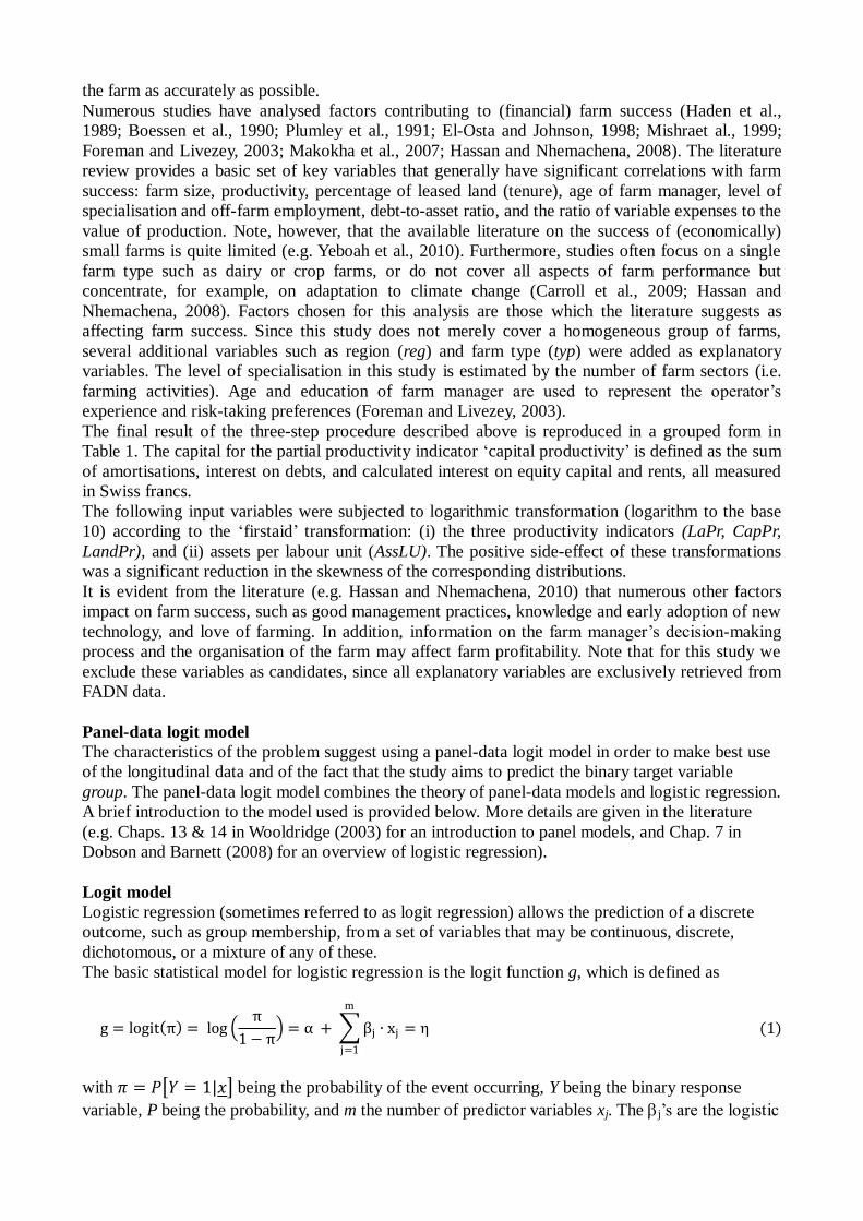
The basic statistical model for logistic regression is the logit function g, which is defined as

g = logit π = log π

1 − π = α + βj

m

j=1

∙ xj = η (1)

with 𝜋 = 𝑃 𝑌 = 1|𝑥 being the probability of the event occurring, Y being the binary response

variable, P being the probability, and m the number of predictor variables xj. The j‟s are the logistic

regression (or logit) coefficients, whilst is termed the linear predictor. For simplicity‟s sake, we

omit the index i (i=1,...,N) for the observation i in Eqs. (1)-(5).

The logit function g is the link function of the logistic regression, and assigns the log odds to the

probabilities . The odds are defined as follows:

θ = 𝑜𝑑𝑑𝑠 𝑌 = 1 𝑥 =𝑃[𝑌 = 1]

𝑃[𝑌 = 0]=

𝑃[𝑌 = 1]

1 − 𝑃[𝑌 = 1]=

𝜋

1 − 𝜋= 𝑒𝛼+𝛽1𝑥1 + 𝛽2𝑥2+⋯+𝛽𝑚 𝑥𝑚 = 𝑒𝜂 (2)

The odds are thus the ratio between the probability of the event occurring (Y=1) and the event not

occurring (Y=0), and can take values between 0 and +∞.

The double ratio (odds ratio) is given by

𝜙 =𝑜𝑑𝑑𝑠 (𝑦=1|𝑥𝑘=𝑙+1)

𝑜𝑑𝑑𝑠 (𝑦=1|𝑥𝑘=𝑙)=

𝑒𝛼+𝛽1𝑥1 + 𝛽2𝑥2+⋯+ 𝛽𝑘 ∙ 𝑙+1 + …+ 𝛽𝑚 𝑥𝑚

𝑒𝛼+𝛽1𝑥1 + 𝛽2𝑥2+⋯+ 𝛽𝑘 ∙𝑙 + … +𝛽𝑚 𝑥𝑚= 𝑒𝛽𝑘 . (3)

From Eqs. (2) & (3) it simply follows that the logarithm of the odds (log odds) are computed as

log 𝜃 = log 𝜋

1 − 𝜋 = α + βj

m

j=1

∙ xj = 𝜂 . (4)

From Eq. (2), the probability of the (binary) target variable Y having the value 1 can be

determined as follows:

𝜋 =1

1+𝑒𝛼+𝛽1𝑥1 + 𝛽2𝑥2+⋯+𝛽𝑚 𝑥𝑚=

1

1+𝑒𝜂. (5)

Marginal effects are commonly used in practice to quantify the effect of variables on an outcome

of interest. The marginal effect of an explanatory variable xk is the effect of a unit change of this

variable on the probability P while all other predictor variables are held constant:

𝜕𝑃 (𝑌=1|𝑥)

𝜕𝑥𝑘

𝑦𝑖𝑒𝑙𝑑𝑠 (𝜕𝑥𝑘=1) 𝑃 𝑌 = 1 𝑥𝑘 = 𝑙 + 1 − 𝑃 𝑌 = 1 𝑥𝑘 = 𝑙 . (6)

The marginal effect thus measures the extent to which the predicted probability changes when the

predictor variable xk increases by 1.

To estimate the intercept and the coefficients, we use the maximum likelihood (ML) method.

ML estimates the model parameters such that the probability of obtaining the observed

characteristics is maximal. The calculations are performed iteratively using the Newton-Raphson

algorithm (Süli and Mayers, 2003).

The performance of the fitted model can be examined using different criteria. The log likelihood

ratio or Wald test is often used to analyse the significance of the coefficients (Dobson and Barnett,

2008). Sometimes the log-likelihood function for the fitted model is compared with that for the

minimal model, in which the values i, i=1,...,N (number of observations) are all equal.

Furthermore, the performance of the model can also be checked by analysing the classification

results. Here, the observed values of the binary target variable Y (0 or 1) are compared with the

probabilities generated, the separation value being set at a probability of P[Y=1]=0.5:

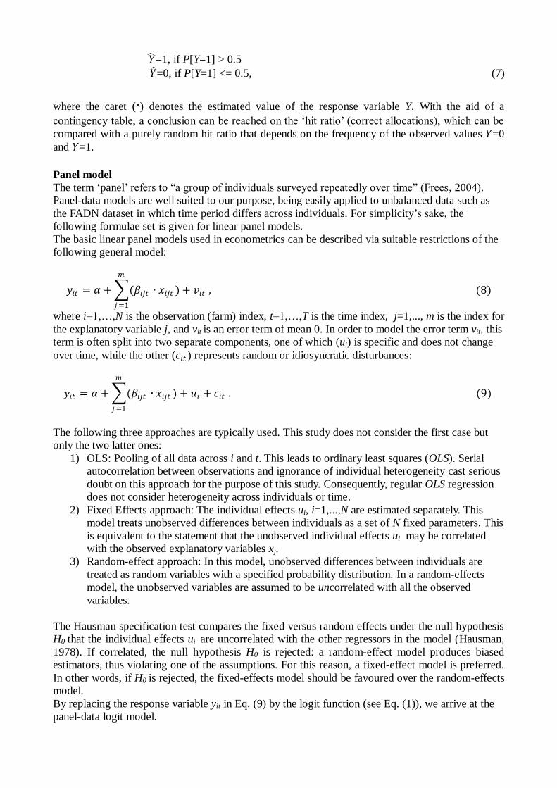
𝑌 =1, if P[Y=1] > 0.5

𝑌 =0, if P[Y=1] <= 0.5, (7)

where the caret (ˆ) denotes the estimated value of the response variable Y. With the aid of a

contingency table, a conclusion can be reached on the „hit ratio‟ (correct allocations), which can be

compared with a purely random hit ratio that depends on the frequency of the observed values 𝑌=0

and 𝑌=1.

Panel model

The term „panel‟ refers to “a group of individuals surveyed repeatedly over time” (Frees, 2004).

Panel-data models are well suited to our purpose, being easily applied to unbalanced data such as

the FADN dataset in which time period differs across individuals. For simplicity‟s sake, the

following formulae set is given for linear panel models.

The basic linear panel models used in econometrics can be described via suitable restrictions of the

following general model:

𝑦𝑖𝑡 = 𝛼 + (𝛽𝑖𝑗𝑡

𝑚

𝑗=1

∙ 𝑥𝑖𝑗𝑡 ) + 𝑣𝑖𝑡 , (8)

where i=1,…,N is the observation (farm) index, t=1,…,T is the time index, j=1,..., m is the index for

the explanatory variable j, and vit is an error term of mean 0. In order to model the error term vit, this

term is often split into two separate components, one of which (ui) is specific and does not change

over time, while the other (𝜖𝑖𝑡 ) represents random or idiosyncratic disturbances:

𝑦𝑖𝑡 = 𝛼 + (𝛽𝑖𝑗𝑡

𝑚

𝑗=1

∙ 𝑥𝑖𝑗𝑡 ) + 𝑢𝑖 + 𝜖𝑖𝑡 . (9)

The following three approaches are typically used. This study does not consider the first case but

only the two latter ones:

1) OLS: Pooling of all data across i and t. This leads to ordinary least squares (OLS). Serial

autocorrelation between observations and ignorance of individual heterogeneity cast serious

doubt on this approach for the purpose of this study. Consequently, regular OLS regression

does not consider heterogeneity across individuals or time.

2) Fixed Effects approach: The individual effects ui, i=1,...,N are estimated separately. This

model treats unobserved differences between individuals as a set of N fixed parameters. This

is equivalent to the statement that the unobserved individual effects ui may be correlated

with the observed explanatory variables xj.

3) Random-effect approach: In this model, unobserved differences between individuals are

treated as random variables with a specified probability distribution. In a random-effects

model, the unobserved variables are assumed to be uncorrelated with all the observed

variables.

The Hausman specification test compares the fixed versus random effects under the null hypothesis

H0 that the individual effects ui are uncorrelated with the other regressors in the model (Hausman,

1978). If correlated, the null hypothesis H0 is rejected: a random-effect model produces biased

estimators, thus violating one of the assumptions. For this reason, a fixed-effect model is preferred.

In other words, if H0 is rejected, the fixed-effects model should be favoured over the random-effects

model.

By replacing the response variable yit in Eq. (9) by the logit function (see Eq. (1)), we arrive at the

panel-data logit model.

4. Results and Discussion

Main differences between Group A and Group B First of all, a short descriptive overview of the differences between the successful (Group A) and

unsuccessful (Group B) farms is given. Table 2 shows the six-year averages (2005-2010) of groups

A and B. The successful (Group A) and unsuccessful (Group B) farms differ considerably from one

another in terms of both structure and economic situation: whereas Group B farmers on average

farmed an area of 17.8 ha and kept a herd of 24.0 livestock units (LUs), the corresponding figures

for the successful farms were substantially higher at 23 ha and 31 LUs. The difference in income

between the two groups was even more significant. At CHF 17,500, the agricultural income of

Group B farms was just one-quarter that of the successful farms (CHF 72,600). Group B farms

earned a small work income per family labour unit (CHF 4400), thus receiving almost no

remuneration for family labour performed, whilst Group A achieved the substantially higher value

of approx.CHF 50,200. These differences were due inter alia to the significantly higher gross

performance of farms in Group A, which stood at around CHF 80,000 above the gross performance

of the B farms, while only just under CHF 24,000 more was disbursed on the cost side (external

costs). The income gap of the B farms in the agricultural sector was at least partially closed by a

significantly higher income from non-agricultural activity, which is why the total income per

consumer unit of the successful group was on average only CHF 8500 above the corresponding

figure for the farms in Group B.

Estimate of coefficients

The fixed- and random-effect logit models are fitted with the Stata xtlogit procedure. The two

methods (fixed vs. random) were compared using the Hausman specification test. This test results

in the highly significant rejection of the null hypothesis H0, indicating that the fixed-effects model

should be favoured over the random-effects model. The likelihood ratio test is virtually zero,

indicating that the fitted model is highly statistically significantly different from the null model

(with all coefficients set to 0). The collinearity of variables was tested using the variance inflation

factor (VIF), which provides an index that measures how much the variance (the square of the

estimate‟s standard deviation) of an estimated regression coefficient is increased due to collinearity.

Here, all VIFs remain below a value of 6.0. Since only values in excess of 20 are suggested as

indicative of a problem (Greene 2011, p. 90), this implies that multicollinearity is unlikely to be a

problem in our model.

The regression coefficients from the fixed-effect logit model are given along with their standard

errors and confidence intervals in Table 3. Of the 17 predictor variables, 10 have proven to be

significant at the 5% level. For both the empl and reg variables, the baseline category is 1.

Note that stepwise regression procedures for reducing the number of covariates were not applied, as

these methods often lack a clear logical foundation and generally produce a set of relatively

uncorrelated variables (Griliches and Intriligator, 1983). Harrell (2001) discovers a number of

further critical issues when applying the stepwise regression procedures, such as “losing valuable

predictive information from deleting marginally significant variables”. Furthermore, Antonakis and

Dietz (2011) stated very recently that “omitted covariates may be jointly significant even if they are

not significant individually”, concluding that important theoretical control variables should never be

dropped from the regression model.

Results and Discussion

Table 3 provides a summary of the regression coefficients and their statistical significance from

fitting the data-panel logit model. For both the variables empl and reg, the baseline category is 1.

We start with the discussion of statistically significant coefficients. According to Eq. (4), j shows

the amount of change in the log odds for a one-unit change in the covariate xj. Unfortunately, log

odds do not have a simple interpretation, so instead of interpreting the sizes of coefficients, we

interpret their signs only: positive coefficients indicate that as xj increases, so does the probability of

remaining in Group A, i.e. =P(Y=1). From this, we conclude that the probability of being in the

successful group A rises with (i) increasing utilised agricultural area (uaa), (ii) an increasing

percentage of paid labour units (fracemp), and (iii) increasing productivity indicators lapr, cappr

and landpr (cf. Table 3). It is evident that higher productivity favours transfer into the successful

group A. Furthermore, a higher percentage of paid labour clearly has a positive effect on

agricultural income. The farming family is better off paying outside workers during e.g. harvest

time in order to avoid the purchase, repair and maintenance of expensive machinery. The positive

scale effect is reflected in the positive value of UAA: The larger the farm, the more likely it is to

remain in Group A. This matches the findings of other studies (e.g. Carroll et al., 2009).

By contrast, decreases with increasing values of the three covariates „debt/equity ratio‟ (der),

„ratio of gross performance from livestock to total gross performance‟ (fracgpcat), and „assets per

labour unit‟ (asslu), the latter possibly suggesting that investments in machinery and buildings have

exceeded optimum levels due to overmechanisation. This offers some proof that as a capital-

intensive business, farming should hire labour rather than invest in (often expensive) machinery.

The higher the debt/equity ratio (der) – sometimes referred to as the leverage ratio – the more likely

the farm is to be long to group B. This makes sense, as the debt/equity ratio reflects the extent to

which farm debt capital is combined with farm equity capital. It is a therefore a good indicator of

the level of financial risk associated with the farm, which in turn may affect net farm incomes.

Furthermore, higher debt capital results in higher interest rates, thereby reducing agricultural

incomes.

A brief description of the predictor variable typ will provide a better understanding of the results

given below. Farm type „typ=1‟characterises farms which tend to earn higher incomes than the

overall Swiss average, though said incomes are also often subject to higher annual variations. This

can be explained – at least in part – by the high interannual variability of the price of pigs (-> pig

cycle) and poultry, vegetables and fruit. Farm type „typ=0‟, on the other hand, comprises mainly

dairy and arable farms, the product prices of which are subject to weaker market-price changes (this

applied at least during the selected study period, when milk prices were not subject to price

fluctuations as great as those experienced recently due to the abolition of the milk-quota system). It

thus makes sense that the probability of belonging to group A is higher for farms producing

specialist crops than for those with other products (typ is positive).

The negative coefficients for empl (form of employment) in Table 3 show that the probability of

belonging to Group A is higher for full-time than for part-time farm managers. Other studies (Meert

et al., 2005; Lien et al., 2010) have also concluded that off-farm employment affects farm success.

The number of farming activities (numactiv) and the age (age) and education (educ) of the farm

manager, among others, do not significantly affect the probability of being in either Group A or

Group B. The lack of significance of farmer‟s age is borne out in other studies where the

relationship between farmer‟s age and farm performance is not clear-cut: whereas a number of

studies (e.g. Stefanou and Saxena, 1988) have reported a positive correlation between age and

efficiency, others (e.g. Kalirajan and Shand, 1985) have noted a non-significant relationship. The

study shows that level of diversification does not play a significant role for the farms analysed.

Given that diversification may reduce risk (e.g. Mesfin et al. (2011) for the case of crop

diversification), this result is somewhat surprising. On the other hand, diversification requires a

well-planned long-term strategy and wise enterprise-management decisions, as well as – possibly –

additional investment.

In order to obtain more precise information on probabilities, results gained from fitting logit models

are often interpreted using odds, odds ratios and marginal effects, since these quantities are easy to

interpret. Odds above 1, for example, mean that the event is more likely to occur (Y=1); odds ratios

represent the change in the estimated odds of an event occurring when the predictor variable

increases by one unit.

Table 4 provides odds ratios along with their confidence intervals and the estimated marginal effects

for all covariates as incorporated in the panel logit model. Note that the marginal effect (me) of

fixed-effects models cannot be computed directly in the Stata program, but must instead be

approximated as

𝑚𝑒 = 𝛽𝑗 ∙ 𝜋 ∙ (1 − 𝜋 ) (8)

where 𝛽𝑗 denotes the estimated logistic coefficient of the predictor variable xj and 𝜋 is the average

sample-predicted probability. In the present study, 𝜋 equals 0.272. A careful interpretation of the log

odds and marginal effects as listed in Table 4 is provided below.

As the uaa increases by one hectare, the odds of belonging to Group A are multiplied by 1.081, i.e.

increase by 8.1%. The probability of belonging to the successful Group A increases by 0.015 for a

one-ha increase in uaa (the marginal effect is 1.015). Although not statistically significant, the

model predicts that farms in the mountain region have a much higher probability of remaining in the

less successful Group B, with the odds of mountain farms remaining in Group A being only 1.7% of

those of farms in the plain region. This result is plausible, since, – owing to harsh climatic and

orographic conditions, mountain farms have less potential for improvement. This fits well with the

fact that the odds ratio for the covariate dpgp (ratio of subsidies to total gross performance) remains

clearly below 1, as dpgp tends to be significantly higher in the mountain region than in the plain

region (see e.g. Mouron, 2010). The numbers listed in Table 4 indicate the strong effect of empl

(form of employment) on group allocation, with the odds of part-time farm managers remaining in

Group A being 1/0.006=167 times smaller than those of full-time farmers. The significantly lower

likelihood of part-time farmers remaining in Group A is also underscored by the negative marginal

effect, which suggests that decreases by roughly 0.8 when switching from full-time to part-time

work.

The results confirm the hypothesis that, owing to a good income from non-agricultural activities,

part-time farms probably have fewer incentives for improvement (in the agricultural sector) than do

other farms. Full-time farms, on the other hand, depend on achieving considerably higher incomes

from agricultural production as quickly as possible, since they have no non-agricultural income on

which they can rely. This finding is supported by Smith (2002), who found that greater involvement

in the off-farm labour market decreases on-farm efficiency – a result consistent with descriptive

statistics (see Table 2). Differences between more-than-half-time and full-time farms are far less

obvious (see Table 4 figures for empl(2) and empl(3)).

With a one-unit increase in the logarithm of labour productivity (lapr), the odds of belonging to

Group A increase by the extremely high factor of approx. 7.3 million, indicating that an increase in

lapr has a strong effect on group allocation. Considering the logarithmic transformation (logarithm

of the base 10), we conclude from the marginal effect of 3.13 that doubling lapr leads to a 0.63

(3.13/5) increase in the probability of being a Group A farm. This finding shows that the (in

Switzerland very expensive) „labour‟ factor plays a crucial role in determining whether a farm can

rise above the prescribed threshold income of CHF 18,300 during the period under investigation.

The other two productivity indices of the full model –capital productivity (cappr) and land

productivity (landpr) – also play a significant role, yet one that is clearly not as significant as lapr,

in predicting group allocation. Doubling cappr and landpr increases the likelihood of belonging to

Group A by 0.15 and 0.2, respectively.

The odds ratio for the predictor variable typ is 3.842 (Table 4). Farms of typ=1 have 3.84-times

higher odds of belonging to Group A than typ=0 farms. Specialist-crop farms and finishing farms

(typ=1) therefore have a distinctly better chance of moving out of the unsuccessful Group B. From

the corresponding marginal effect of 0.266, it follows that, ceteris paribus, the probability of being

a Group A farm is 0.266 higher for specialist-crop and finishing farms than for other types of farms

(i.e. typ=0 farms, see Table 4).

For a 10% change in the percentage of paid labour (fracemp), the odds of remaining in Group A

increase by a factor of 0.346 (3.463/10) or approx. 35%. A 10% increase in fracemp slightly

increases the likelihood of belonging to Group A by 0.0246 (=0.246/10).

The predicted odds for belonging to Group A decrease by 83% [(1-0.168)*100%] when the debt/

equity ratio (der) increases by one unit, suggesting that farmers should avoid excessive increases in

the level of indebtedness compared to equity capital. This characteristic is also reflected in the

negative value of the marginal effects, which suggests a 0.353 decrease in per one-unit increase of

der. An increase in the percentage of gross performance from livestock to total gross performance

(fracgpcat) negatively affects the likelihood of belonging to group A. A 10% increase in fracgpcat

decreases the probability of being in Group A by 0.052. This matches the finding that typ=1 farms

(i.e. those with a fairly low gross performance per hectare, such as the dairy farms which

predominate in Switzerland) tend to have a higher likelihood of remaining in group B than typ=0

farms.

Performance of the fitted panel-data logit model

The classification results using Equation 7 are shown in Table 5. The hit rate of above 85% is

significantly higher than the purely random hit rate of 50%. It is striking that the fitted panel-data

logistic model is better able to predict the Group A of „successful‟ farms than the Group B of

„unsuccessful‟ farms.

The residual analysis of the final model shows a satisfactory model fit (not shown). The leverage of

the individual observations makes it clear that most of the observations have no „excessive‟

leverage, i.e. that the regression function does not „overreact‟ to most of the observations.

5. Summary and Conclusions This paper addresses the development of economically weak farms using panel-data logistic

regression. The analysis reveals considerable differences in terms of operational structure and

orientation between the farms in Group A and B. The study highlights the distinct importance of

non-agricultural activities, showing that the likelihood of full-time farms belonging to Group A is

particularly high, whilst belonging to this group is less important for part-time farms earning a

substantial proportion of non-farm income. Furthermore, the study highlights the importance of

high labour productivity in reducing the risk of remaining in Group B. It also shows that farms tend

to benefit from low assets per labour unit, a higher percentage of paid labour, and a low debt/equity

ratio, which tends to suggest that it is preferable for farms to employ additional labour rather than

invest in (excessively) expensive machinery.

Further research as well as additional data sampling is needed to quantify (among other things) the

effect of the farm manager‟s decision-making process on the economic performance of the farm.

References Antonakis J. and Dietz J. (2011): Looking for validity or testing it? The perils of stepwise regression, extreme-scores analysis, heteroscedasticity, and measurement error. Personality and Individual Differences, 50 (3), 409-415.

Backhaus K., Erichson B., Plinke W. and Weiber R., 2006: Multivariate Analysemethoden: Eine anwendungsorientierte Einführung (11th edition). Berlin, Heidelberg: Springer, 575 pages. Boessen C. R., Featherstone A. M., Langemeier L. N. and Burton, Jr, R. O. (1990): Financial performance of successful and unsuccessful farms. Journal of American Society of Farm Managers and Rural Appraisers, 54, 6-15.

Carroll J., Greene S., O'DonoghueC., Newman C. and Thorne F. S. (2009): Productivity and the Determinants of Efficiency in Irish Agriculture (1996-2006), No. 50941, 83rd Annual Conference, March 30-April 1, 2009, Dublin, Ireland, Agricultural Economics Society, http://econpapers.repec.org/RePEc:ags:aesc09:50941.

Cohen J., Cohen P., West S. G and Aiken L. S. (2003): Applied multiple regression/correlation analysis for the behavioral sciences (Chapter 13: Alternative

regression models, pp. 479-535). Mahwah N. J.: Lawrence Erlbaum.

Dobson, A.J. and Barnett A.G. (2008): An Introduction to Generalized Linear Models. CRC Press, USA, 1–307.

Dux D. and Schmid D.(2010): Grundlagenbericht 2009. Zentrale Auswertung von Buchhaltungsdaten, 1-286. El-Osta H.S. and Johnson J.D. (1998): Determinants of Financial Performance of Commercial Dairy Farms, Department of Agriculture ERS Technical Bulletin No. 1859, Washington DC. Ford S. A. and Shonkwiler J.S. (1994): The Effect of Managerial Ability on Farm Financial Success, Agricultural and Resource Economics Review, 23 (2), 150-157. Foreman L. F. and Livezey J. S. (2003): Factors Contributing To Financially Successful Southern Rice Farms, 2003 Annual Meeting, February 1-5, 2003, Mobile, Alabama 35215, Southern Agricultural Economics Association. Frees E.W. (2004): Longitudinal and Panel Data: Analysis and Application in the Social Sciences, Cambridge University Press, 467 pages. Greene, W.H. (2011): Econometric analysis, 7th ed., NJ: Prentice Hall, 1096 pages. Griliches Z. and Intriligator M. D. (Eds.) (1983): Handbook of Econometrics. North Holland Publishing Company. Haden K. L. and Johnson L.A. (1989): Factors which Contribute to the Financial Performance of Selected Tennessee Dairies, Southern Journal of Agriculture Economics, 21 (1), 105-112.

Harrell F.E. (2001): Regression Modeling Strategies. With Applications to Linear Models, Logistic Regression, and Survival Analysis. Series: Springer Series in Statistics.

Hassan R.M. and Nhemachena C. (2008): Determinants of African farmers’ strategies for adapting to climate change: Multinomial choice analysis. African Journal of Agricultural and Resource Economics,2 (1), 83-104. Hausman J. A. (1978): Specification Tests in Econometrics. Econometrica,46 (6), 1251–1271.

Hosmer D.W., Jr. and Lemeshow S. (2000): Applied Logistic Regression. 2nd edition. New York: John Wiley & Sons. Kalirajan K.P. and Shand R.T. (1985): Types of education and agricultural productivity: A quantitative analysis of Tamil Nadu rice farming. Journal of Development Studies, 21, 232-

243.

Lien G., Kumbhakar S. C. and Hardaker J. B. (2010): Determinants of off-farm work and its

effects on farm performance: the case of Norwegian grain farmers. Agricultural Economics,

41, 577–586. doi: 10.1111/j.1574-0862.2010.00473.x.

Makokha S. N., Karugia J. T., Staal S. J. and Oluoch-Kosura W. (2007): Analysis of Factors Influencing Adoption of Dairy Technologies in Western Kenya, AAAE Conference Proceedings, 209-213. McBride W. D. & Johnson J. D. (2004): Approaches to Management and Farm Business Success, 2004 Annual Meeting, August 1-4, Denver, CO 20131, American Agricultural Economics Association. Meert H., Van Huylenbroeck G., Vernimmen T., Bourgeois M. and Van Hecke E. (2005): Farm household survival strategies and diversification on marginal farms, Journal of Rural Studies, 21 (1), Elsevier, 81-97. Meier B. (2005): Analyse der Repräsentativität im schweizerischen landwirtschaftlichen Buchhaltungsnetz. Messung und Verbesserung der Schätzqualität ökonomischer Kennzahlen in der Zentralen Auswertung von Buchhaltungsdaten. ETH Dissertation No. 15868. Zurich, 147 pages. Mesfin W., Fufa B., Haji, J. (2011): Pattern, Trend and Determinants of Crop Diversification: Empirical Evidence from Smallholders in Eastern Ethiopia. Journal of Economics and Sustainable Development, 2 (8), 78-89.

Mishra A.K., El-Osta H.S., James D. and Johnson J. D. (1999): Factors Contributing to Earnings Success of Cash Grain Farms, Journal of Agricultural and Applied Economics, 31 (3), 623-637.

Mouron P. and Schmid D. (2011):Grundlagenbericht (2010): Zentrale Auswertung von Buchhaltungsdaten. Agroscope Reckenholz-Tänikon Research Station ART. Ettenhausen, 285 pages. Muhammad S., Tegegne F. and Ekanem E. (2004): Factors Contributing to Success of

Small Farm Operationsin Tennessee. Journal of Extension,42 (4), available at:

http://www.joe.org/joe/2004august/rb7.shtml. Plumley G.O. and Hornbaker R.H. (1991): Financial Management Characteristics of Successful Farm Firms, Agricultural Finance Review, 51, 9-20.

Smith K.R. (2002): Does Off-Farm Work Hinder “Smart” Farming? Agricultural Outlook, Economic Research Service/USDA, September, 28-30. Stefanou S.E. and Saxena S. (1988):Education, experience, and allocative efficiency: A dual approach. American Journal of Agricultural Economics, 70(2), 338-345.

Süli E. and Mayers D. (2003): An Introduction to Numerical Analysis, Cambridge University Press, 433 pages. Tvedt D. D., Olson K.D. and Hawkins D.M. (1989): Short-Run Indicators of Financial Success for Southwest Minnesota Farmers, Department of Agricultural and Applied Economics, University of Minnesota, Staff Papers Series pp. 89-7. Wooldridge J. (2003): Introductory Econometrics: A Modern Approach. South-Western College Publishing, 865 pages. Yeboah A. K., Owens J.P., Bynum J. S. and Boisson D. (2010):Validation of Factors Influencing Successful Small Scale Farming in North Carolina, No. 56506, Annual Meeting, February 6-9, 2010, Orlando, Florida, Southern Agricultural Economics Association, http://econpapers.repec.org/RePEc:ags:saea10:56506.

Tables and Figures

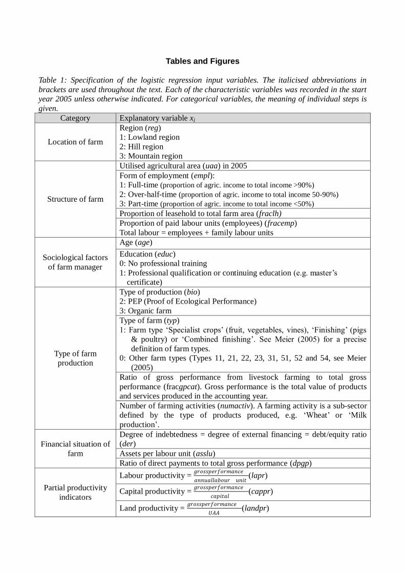
Table 1: Specification of the logistic regression input variables. The italicised abbreviations in

brackets are used throughout the text. Each of the characteristic variables was recorded in the start

year 2005 unless otherwise indicated. For categorical variables, the meaning of individual steps is

given. Category Explanatory variable xj

Location of farm

Region (reg) 1: Lowland region

2: Hill region

3: Mountain region

Structure of farm

Utilised agricultural area (uaa) in 2005

Form of employment (empl):

1: Full-time (proportion of agric. income to total income >90%) 2: Over-half-time (proportion of agric. income to total income 50-90%)

3: Part-time (proportion of agric. income to total income <50%)

Proportion of leasehold to total farm area (fraclh)

Proportion of paid labour units (employees) (fracemp)

Total labour = employees + family labour units

Sociological factors

of farm manager

Age (age)

Education (educ)

0: No professional training

1: Professional qualification or continuing education (e.g. master‟s

certificate)

Type of farm

production

Type of production (bio)

2: PEP (Proof of Ecological Performance)

3: Organic farm

Type of farm (typ)

1: Farm type „Specialist crops‟ (fruit, vegetables, vines), „Finishing‟ (pigs

& poultry) or „Combined finishing‟. See Meier (2005) for a precise

definition of farm types.

0: Other farm types (Types 11, 21, 22, 23, 31, 51, 52 and 54, see Meier

(2005)

Ratio of gross performance from livestock farming to total gross

performance (fracgpcat). Gross performance is the total value of products

and services produced in the accounting year.

Number of farming activities (numactiv). A farming activity is a sub-sector

defined by the type of products produced, e.g. „Wheat‟ or „Milk

production‟.

Financial situation of

farm

Degree of indebtedness = degree of external financing = debt/equity ratio

(der) Assets per labour unit (asslu)

Ratio of direct payments to total gross performance (dpgp)

Partial productivity

indicators

Labour productivity = 𝑔𝑟𝑜𝑠𝑠𝑝𝑒𝑟𝑓𝑜𝑟𝑚𝑎𝑛𝑐𝑒

𝑎𝑛𝑛𝑢𝑎𝑙𝑙𝑎𝑏𝑜𝑢𝑟 𝑢𝑛𝑖𝑡(lapr)

Capital productivity = 𝑔𝑟𝑜𝑠𝑠𝑝𝑒𝑟𝑓𝑜𝑟𝑚𝑎𝑛𝑐𝑒

𝑐𝑎𝑝𝑖𝑡𝑎𝑙(cappr)

Land productivity = 𝑔𝑟𝑜𝑠𝑠𝑝𝑒𝑟𝑓𝑜𝑟𝑚𝑎𝑛𝑐𝑒

𝑈𝐴𝐴(landpr)

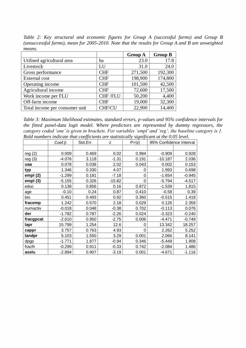
Table 2: Key structural and economic figures for Group A (successful farms) and Group B

(unsuccessful farms), mean for 2005-2010. Note that the results for Group A and B are unweighted

means.

Group A Group B

Utilised agricultural area ha 23.0 17.8

Livestock LU 31.0 24.0

Gross performance CHF 271,500 192,300

External cost CHF 198,900 174,800

Operating income CHF 101,500 42,500

Agricultural income CHF 72,600 17,500

Work income per FLU CHF /FLU 50,200 4,400

Off-farm income CHF 19,000 32,300

Total income per consumer unit CHF/CU 22,900 14,400

Table 3: Maximum likelihood estimates, standard errors, p-values and 95% confidence intervals for

the fitted panel-data logit model. Where predictors are represented by dummy regressors, the

category coded ‘one’ is given in brackets. For variables ‘empl’ and ‘reg’, the baseline category is 1.

Bold numbers indicate that coefficients are statistically significant at the 0.05 level.

Coef. Std.Err. z P>|z| 95% Confidence Interval

reg (2) 0.009 0.469 0.02 0.984 -0.909 0.928

reg (3) -4.076 3.118 -1.31 0.191 -10.187 2.036

uaa 0.078 0.038 2.02 0.043 0.002 0.153

typ 1.346 0.330 4.07 0 1.993 0.698

empl (2) -1.299 0.181 -7.18 0 -1.654 -0.945

empl (3) -5.155 0.326 -15.82 0 -5.794 -4.517

educ 0.138 0.856 0.16 0.872 -1.539 1.815

age -0.10 0.24 0.87 0.410 -0.58 0.39

bio 0.451 0.493 0.92 0.360 -0.515 1.418

fracemp 1.242 0.570 2.18 0.029 0.126 2.359

numactiv -0.018 0.048 -0.38 0.702 -0.113 0.076

der -1.782 0.787 -2.26 0.024 -3.323 -0.240

fracgpcat -2.610 0.950 -2.75 0.006 -4.471 -0.749

lapr 15.799 1.254 12.6 0 13.342 18.257

cappr 3.757 0.763 4.93 0 2.262 5.252

landpr 5.103 1.550 3.29 0.001 2.066 8.141

dpgp -1.771 1.877 -0.94 0.346 -5.449 1.908

fraclh -0.299 0.911 -0.33 0.742 -2.084 1.486

asslu -2.894 0.907 -3.19 0.001 -4.671 -1.116

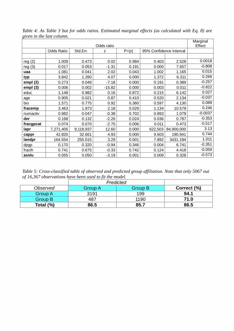
Table 4: As Table 3 but for odds ratios. Estimated marginal effects (as calculated with Eq. 8) are

given in the last column.

Odds ratio Marginal

Effect

Odds Ratio Std.Err. z P>|z| 95% Confidence Interval

reg (2) 1.009 0.473 0.02 0.984 0.403 2.528 0.0018

reg (3) 0.017 0.053 -1.31 0.191 0.000 7.657 -0.808

uaa 1.081 0.041 2.02 0.043 1.002 1.165 0.015

typ 3.842 1.260 4.07 0.000 1.372 6.311 0.266

empl (2) 0.273 0.049 -7.18 0.000 0.191 0.389 -0.257

empl (3) 0.006 0.002 -15.82 0.000 0.003 0.011 -0.822

educ 1.148 0.982 0.16 0.872 0.215 6.142 0.027

age 0.905 0.021 0.87 0.410 0.520 2.134 -0.037

bio 1.571 0.775 0.92 0.360 0.597 4.130 0.089

fracemp 3.463 1.973 2.18 0.029 1.134 10.579 0.246

numactiv 0.982 0.047 -0.38 0.702 0.893 1.079 -0.0037

der 0.168 0.132 -2.26 0.024 0.036 0.787 -0.353

fracgpcat 0.074 0.070 -2.75 0.006 0.011 0.473 -0.517

lapr 7,271,405 9,118,937 12.60 0.000 622,503 84,900,000 3.13

cappr 42.820 32.661 4.93 0.000 9.603 190.941 0.744

landpr 164.554 255.015 3.29 0.001 7.892 3431.184 1.011

dpgp 0.170 0.320 -0.94 0.346 0.004 6.741 -0.351

fraclh 0.741 0.675 -0.33 0.742 0.124 4.418 -0.059

asslu 0.055 0.050 -3.19 0.001 0.009 0.328 -0.573

Table 5: Cross-classified table of observed and predicted group affiliation. Note that only 5067 out

of 16,367 observations have been used to fit the model. Predicted

Observed Group A Group B Correct (%)

Group A 3191 199 94.1

Group B 487 1190 71.0

Total (%) 86.5 85.7 86.5