This content has been downloaded from IOPscience. Please scroll down to see the full text.

Download details:

This content was downloaded by: alikhalighi

IP Address: 194.167.230.227

This content was downloaded on 24/02/2014 at 09:30

Please note that terms and conditions apply.

Fading correlation and analytical performance evaluation of the space-diversity free-space

optical communications system

View the table of contents for this issue, or go to the journal homepage for more

2014 J. Opt. 16 035403

(http://iopscience.iop.org/2040-8986/16/3/035403)

Home Search Collections Journals About Contact us My IOPscience

Journal of Optics

J. Opt. 16 (2014) 035403 (10pp) doi:10.1088/2040-8978/16/3/035403

Fading correlation and analyticalperformance evaluation of thespace-diversity free-space opticalcommunications systemG Yang1, M A Khalighi2, S Bourennane2 and Z Ghassemlooy3

1 College of Communication Engineering, Hangzhou Dianzi University, Hangzhou,People’s Republic of China2 Institut Fresnel, UMR CNRS 7249, Ecole Centrale Marseille, Marseille, France3 Optical Communications Research Group, Faculty of Engineering and Environment,Northumbria University, Newcastle Upon Tyne, UK

E-mail: ali.khalighi@fresnel.fr

Received 29 October 2013, revised 2 January 2014Accepted for publication 13 January 2014Published 21 February 2014

AbstractThis paper investigates fading correlation in space-diversity free-space optical (FSO)communication systems and its effect on the link performance. We firstly evaluate the fadingcorrelation in multiple-aperture FSO systems using wave-optics simulations. The influence ofdifferent system parameters including the link distance and aperture spacing is illustratedunder realistic beam propagation conditions. In particular, we show that, at relatively large linkdistances where the scattering disk is much larger than the receiver aperture size, the fadingcorrelation coefficient is almost independent of the apertures’ diameter and depends only onthe apertures’ edge separation. To investigate the impact of fading correlation on the system’sperformance, we propose an analytical approach to evaluate the performance of thespace-diversity FSO system over a correlated Gamma–Gamma (00) fading channel. Ourapproach is based on approximating the sum of arbitrarily correlated 00 random variables byan α–µ distribution. To validate the accuracy of this method, we evaluate the averagebit-error-rate (BER) performance for the case of a multiple-aperture FSO system and compareit with the BER results obtained via Monte Carlo simulations.

Keywords: free space optics, optical communication, atmospheric turbulence, spatial diversity,fading correlationPACS numbers: 42.25.Dd, 42.60.-v, 42.68.Bz

(Some figures may appear in colour only in the online journal)

1. Introduction

Under clear weather conditions, one of the main challengesin free-space optical (FSO) communications is to reduce theeffect of atmospheric turbulence that can severely degradethe system performance, especially for relatively long linkdistances [1]. Efficient mitigation of the resulting channel

fading can be obtained via spatial diversity, which has beenwidely adopted for applications in radio and microwavefrequency bands. This can be realized by employing multipleapertures at the receiver and/or multiple beams at the trans-mitter [2–7]. However, such techniques lose their efficacyunder the conditions of correlated fading on the underlyingsub-channels, i.e., channels between pairs of transmit–receive

2040-8978/14/035403+10$33.00 1 c© 2014 IOP Publishing Ltd Printed in the UK

J. Opt. 16 (2014) 035403 G Yang et al

apertures [8]. In particular, under strong turbulence conditions,the required spacing between the apertures at the receiverand/or between the laser beams at the transmitter is usuallytoo large to ensure uncorrelated fading and unfeasible for apractical design [5, 6, 9, 10].

In most previous works reported on space-diversity FSOsystems, the fading correlation is either ignored or studiedconsidering a simplified channel model (see [4, 8, 11, 12]). Inthis paper, we consider the Gamma–Gamma (00) distributionthat is widely adopted for modeling the terrestrial FSO channeldue to its excellent agreement with the experimental data overall turbulence conditions [2]. Under the ideal conditions ofindependent 00 fading, the performance of multiple-apertureFSO systems was studied in [2, 5]. Also, two approximationsto the sum of independent 00 random variables (RVs), basedon 00 [13] and α–µ [14] distributions, were used in theperformance analysis of space-diversity FSO systems.

Concerning correlated fading conditions, multi-beamterrestrial and air-to-air FSO systems were studied in [6, 15],respectively. In [6], multiple 00 channels were modeledby a single 00 distribution whose parameters were calcu-lated by approximating the fading coefficients by correlatedGaussian RVs. However, when employed to predict thesystem performance, this solution cannot guarantee sufficientaccuracy. In [15], approximate analytical expressions based onnumerical fitting were proposed to determine the parametersof 00 model taking the fading correlation into account.However, the proposed expressions depend on the underlyingair-to-air system structure and cannot directly be used toaccurately evaluate the BER in general. Also, a multivariate00 model with the exponential correlation was proposedin [16], but this correlation model is not suitable for most FSOsystem configurations. In a recent work [17], we proposed theα–µ approximation to the sum of two correlated 00 RVs forevaluating the performance of a dual-diversity FSO system.

In this paper, we firstly evaluate the fading correlationin a multiple-aperture link using wave-optics simulations,and study the impact of different system parameters on thelink average correlation coefficient. In contrast to a similarstudy presented in [6] for a four-beam single-aperture FSOsystem, we consider here more practical cases for the receiveraperture size and link span. To consider different turbulenceregimes, we use different link spans and fix the turbulencestrength parameter C2

n . Although, in general, C2n depends

on the link distance [18] (because it is altitude dependent),for horizontal FSO paths that we consider in this work,C2

n can be considered as constant (irrespective of the linkspan), which is usually referred to as homogeneous turbulenceconditions [19]. Alternatively, one may consider a fixed linkspan and consider different C2

n values (that could correspondto different moments during the daytime [20, 21], for example)as done in [6].

Note that in a previous work [22] we simply illustratedthe effect of link distance and aperture separation on thefading correlation coefficient and focused on the generationof correlated 00 RVs in order to evaluate the system BERperformance via Monte Carlo simulations. In contrast to [22],here we present a comprehensive investigation of the impact

of link span, aperture diameter, and aperture separation onthe fading correlation. Furthermore, we explain the presentedresults using the scintillation theory and by ascribing thefading correlation to small- and large-scale fading components.Afterwards, we propose an analytical approach to investigatethe impact of fading correlation on the system, BER. For thispurpose, we extend the α–µ approximation method proposedin [17] to the case of multiple diversity by approximatingthe sum of arbitrarily correlated multiple 00 RVs by anα–µ distribution. As a matter of fact, the proposed methodin [17] was based on the joint moments of Gamma-distributedRVs. Therein, we could only find the joint moments of twocorrelated Gamma RVs in a closed-form formula. It is worthmentioning that we cannot obtain the joint moments of morethan two correlated Gamma RVs by the same method. To thebest of our knowledge, there is no previous reported workon the analytical performance evaluation of multiple-diversityFSO systems over arbitrarily correlated 00 fading channels.For this, we derive joint moments of correlated multipleGamma RVs based on the moment generating function (MGF)(as introduced in [23]), and then extend theα–µ approximationmethod to deal with the arbitrarily correlated multiple00 RVs.

The remainder of the paper is organized as follows. Afterpresenting the main assumptions and a brief introductionon wave-optics simulation tool in section 2, we explain ourmethod of approximating the sum of correlated 00 RVsby α–µ distribution in section 3. Then, we provide somenumerical results to evaluate fading correlation by consideringthe case study of a receive-diversity FSO system in section 4.The accuracy of α–µ approximation is next investigated insection 5, where we also contrast the corresponding analyticalperformance results with those obtained via Monte Carlosimulations. Lastly, section 6 concludes the paper.

2. General assumptions and wave-opticssimulations

We assume that the transmitter and the receiver are perfectlyaligned. Also, we reasonably assume that the parameters ofthe 00 model are the same for all underlying sub-channels.

We use the split-step Fourier-transform algorithm forthe numerical simulation of optical wave propagation, wherethe effect of atmospheric turbulence along the propagationpath is taken into account by considering a set of randomphase screens [24]. For each phase screen, we generaterandom harmonic amplitudes over an Ng × Ng grid in thespectral domain based on the modified von Karman powerspectrum, and then, take the inverse 2D discrete Fouriertransform to obtain the phase fluctuations [2]. To achievesufficient accuracy at very low spatial frequencies, we performa spectral correction in the subharmonic regime and alsouse the two-dimensional super-Gaussian function to avoidenergy leakage at the edge of each screen [24]. To obtainaccurate results, the grid spacing, grid size parameter Ng, andthe number of phase screens are set appropriately (see [22]for details). Calculating the transmitted and the receivedintensities on each receiver aperture, we obtain the channel

2

J. Opt. 16 (2014) 035403 G Yang et al

Table 1. Scale sizes for different Z .

Z (km) σ 2R `1 (mm) `2 (mm)

1.0 1.29 21.0 11.72.0 4.61 14.1 34.93.0 9.70 11.2 66.34.0 16.43 9.4 104.75.0 24.74 8.3 149.4

fading coefficients and then calculate the Pearson correlationcoefficient among them [22].

For the later use, we have provided in table 1 the spatialcoherence radius `1 [2] and the scattering disk `2 [2], fordifferent link distances Z together with Rytov variance σ 2

R.

3. α–µ approximation method

3.1. 00 and α–µ distributions

Using the 00 model, we consider the normalized receivedintensity at a receiver aperture I as the product of twoindependent Gamma RVs, X and Y , which represent theirradiance fluctuations arising from large- and small-scaleturbulence, respectively. The PDF of I is [2]:

f I (i)=2(ab)(a+b)/2

0(a)0(b)i(a+b)

2 −1 Ka−b(2√

a b i),

i ≥ 0, (1)

where a and b ≥ 0 denote the effective numbers of large-and small-scale turbulence eddies, respectively, which can bedirectly obtained from the link’s parameters [2]. Also, 0(·) isthe Gamma function and Kυ(·) is the modified Bessel functionof the second kind and order υ. The nth moment of I is [13]:

E{I n} =

0(a+ n) 0(b+ n)0(a) 0(b)

(ab)−n, (2)

where E{·} denotes the expected value.The reason behind choosing the α–µ distribution, which

is also known as generalized Gamma, is that it is a flexibledistribution that can be reduced to several simplified distri-butions such as Gamma, Nakagami-m, exponential, Weibull,one-sided Gaussian, and Rayleigh [25, 26]. Let us denote theα–µ distributed RV by R. The PDF of R is given by [26]:

fR(r)=α µµ rαµ−1

rαµ 0(µ)exp

(−µ

rα

rα

), r > 0, (3)

where α > 0, r = α√

E {Rα}, and µ is the inverse of thenormalized variance of Rα , defined as:

µ=(E {Rα})2

Var {Rα}, (4)

and Var{·} denotes variance. The nth moment of R is givenby [26]:

E{Rn} = rn 0(µ+ n/α)

µn/α 0(µ). (5)

3.2. α–µ approximation to sum of multiple correlated 00 RVs

Let us consider the general case of space-diversity FSOsystems with L diversity branches. The normalized fadingcoefficient of the i th sub-channel is denoted by Ii , which isgoverned by 00 distribution. We approximate the sum Isum =∑L

i=1 Ii by an α–µ RV R by setting equal the correspondingfirst three moments. For the general case of an M-beamN -aperture FSO system, Isum corresponds to the receivedsignal intensity after equal gain combining (EGC) [8] whenrepetition coding (RC) [4] is performed at the transmitter. Inthis case, we have L = M N . (Note that EGC has a performancevery close to the optimal maximal ratio combining [8, 11],and RC has been shown to be the quasi-optimal transmissionscheme in transmit-diversity FSO systems [27, 28].) Then,using the moment-matching method [14, 17], we have:

E{R} = E {Isum} = E

{ L∑i=1

X i Yi

},

E{

R2}= E

{I 2sum

}= E

( L∑

i=1

X i Yi

)2 ,

E{

R3}= E

{I 3sum

}= E

( L∑

i=1

X i Yi

)3 .

(6)

We notice from (6) that we need the first, second, and thirdmoments of Isum. The general expression of the nth momentof Isum is:

E{

I nsum}= E

( L∑

i=1

Ii

)n= E

( L∑

i=1

X i Yi

)n

=

n∑v1=0

v1∑v2=0

· · ·

vL−2∑vL−1=0

( nv1

) (v1v2

)· · ·

(vL−2vL−1

)× E

{Xn−v1

1 Xv1−v22 · · · XvL−1

L

}× E

{Y n−v1

1 Y v1−v22 · · · Y vL−1

L

}(7)

where v1, v2, . . . , vL , and n are non-negative integers [29].One notes that E

{I nsum}

depends on the joint moments ofthe Gamma RVs X i and Yi . The first, second, and third jointmoments of X i and Yi can in turn be calculated using (A.5),(A.6) and (A.17), given in the appendix. Then, setting equalthe first three moments of Isum (using (7)) and R (using(5)), we calculate the three parameters of the approximateα–µ distribution from (6).

Since it is difficult to obtain a closed-form solution forthese parameters due to nonlinear functions in (6), we usenumerical methods to calculate α, µ and r (more specifically,we use the fsolve function of MATLAB).

Note that to calculate the first three moments of X i and Yi ,we need in (A.5), (A.6), and (A.17), the correlation coefficientsbetween X i and X j and those between Yi and Y j . Thesecoefficients can be obtained from the correlation coefficientsbetween Ii and I j (calculated via wave-optics simulations), aswe will explain in section 5.1.

Finally, note that for the simple case of a single-beamsingle-aperture FSO system, where L = 1, the moment match-ing of (6) can simply be done using (2) and (5).

3

J. Opt. 16 (2014) 035403 G Yang et al

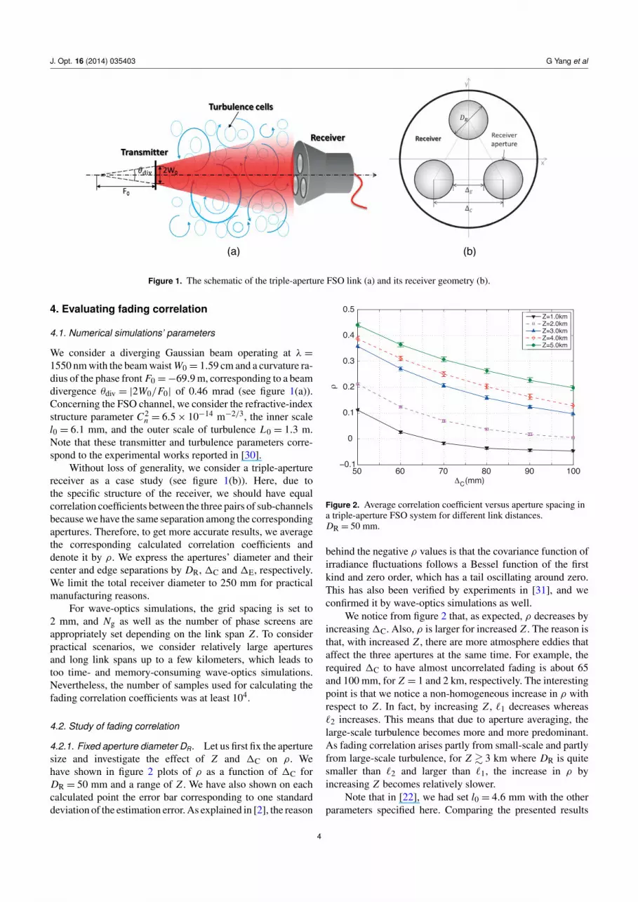
Figure 1. The schematic of the triple-aperture FSO link (a) and its receiver geometry (b).

4. Evaluating fading correlation

4.1. Numerical simulations’ parameters

We consider a diverging Gaussian beam operating at λ =1550 nm with the beam waist W0 = 1.59 cm and a curvature ra-dius of the phase front F0 =−69.9 m, corresponding to a beamdivergence θdiv = |2W0/F0| of 0.46 mrad (see figure 1(a)).Concerning the FSO channel, we consider the refractive-indexstructure parameter C2

n = 6.5× 10−14 m−2/3, the inner scalel0 = 6.1 mm, and the outer scale of turbulence L0 = 1.3 m.Note that these transmitter and turbulence parameters corre-spond to the experimental works reported in [30].

Without loss of generality, we consider a triple-aperturereceiver as a case study (see figure 1(b)). Here, due tothe specific structure of the receiver, we should have equalcorrelation coefficients between the three pairs of sub-channelsbecause we have the same separation among the correspondingapertures. Therefore, to get more accurate results, we averagethe corresponding calculated correlation coefficients anddenote it by ρ. We express the apertures’ diameter and theircenter and edge separations by DR, 1C and 1E, respectively.We limit the total receiver diameter to 250 mm for practicalmanufacturing reasons.

For wave-optics simulations, the grid spacing is set to2 mm, and Ng as well as the number of phase screens areappropriately set depending on the link span Z . To considerpractical scenarios, we consider relatively large aperturesand long link spans up to a few kilometers, which leads totoo time- and memory-consuming wave-optics simulations.Nevertheless, the number of samples used for calculating thefading correlation coefficients was at least 104.

4.2. Study of fading correlation

4.2.1. Fixed aperture diameter DR. Let us first fix the aperturesize and investigate the effect of Z and 1C on ρ. Wehave shown in figure 2 plots of ρ as a function of 1C forDR = 50 mm and a range of Z . We have also shown on eachcalculated point the error bar corresponding to one standarddeviation of the estimation error. As explained in [2], the reason

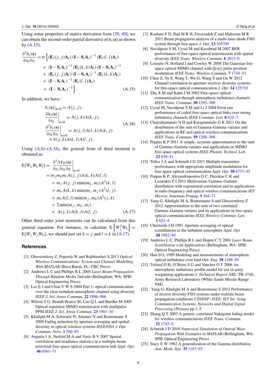
Figure 2. Average correlation coefficient versus aperture spacing ina triple-aperture FSO system for different link distances.DR = 50 mm.

behind the negative ρ values is that the covariance function ofirradiance fluctuations follows a Bessel function of the firstkind and zero order, which has a tail oscillating around zero.This has also been verified by experiments in [31], and weconfirmed it by wave-optics simulations as well.

We notice from figure 2 that, as expected, ρ decreases byincreasing1C. Also, ρ is larger for increased Z . The reason isthat, with increased Z , there are more atmosphere eddies thataffect the three apertures at the same time. For example, therequired 1C to have almost uncorrelated fading is about 65and 100 mm, for Z = 1 and 2 km, respectively. The interestingpoint is that we notice a non-homogeneous increase in ρ withrespect to Z . In fact, by increasing Z , `1 decreases whereas`2 increases. This means that due to aperture averaging, thelarge-scale turbulence becomes more and more predominant.As fading correlation arises partly from small-scale and partlyfrom large-scale turbulence, for Z & 3 km where DR is quitesmaller than `2 and larger than `1, the increase in ρ byincreasing Z becomes relatively slower.

Note that in [22], we had set l0 = 4.6 mm with the otherparameters specified here. Comparing the presented results

4

J. Opt. 16 (2014) 035403 G Yang et al

Figure 3. Average correlation coefficient for a (1× 3) system versusthe aperture spacing 1C for different DR: (a) Z = 2 km,(b) Z = 5 km.

with those of [22], we conclude that l0 has a negligibleinfluence on the correlation among sub-channels.

4.2.2. Fixed link distance Z . Let us now fix Z and see theinfluence of DR and1C on ρ. Figure 3 shows plots for ρ versus1C for Z = 2 and 5 km and a range of DR. Remember thatwe limit the total receiver aperture diameter to 250 mm, whichconfines the choice of 1C for a given DR. From figure 3 wenotice that ρ increases with DR for a fixed1C. In fact, for fixed1C, a larger DR leads to a larger aperture area and a smaller1E (see figure 1). So, there are more turbulent eddies thatintervene at the same time in the scintillation corresponding tothe different apertures. (For Z = 2 km and 1C & 110 mm, ρis too small and its dependence on DR is not manifest.)

Let us now fix 1E to observe the effect of increasingDR on ρ. We have rearranged the results of figure 3 infigure 4 in order to show plots of ρ as a function of DR. Notethat 1C = 1E + DR, and hence, increasing DR implies anincrease of1C for a given1E. We notice that ρ monotonouslydecreases with increases in DR. In fact, by increasing DR, theapertures extend outward from the receiver center, therefore

Figure 4. Average correlation coefficient for a (1× 3) system versusDR for different aperture side-spaces 1E: (a) Z = 2 km,(b) Z = 5 km.

encountering more dissimilar scintillations, which results in asmaller ρ.

We notice from figure 4 thatρ is almost independent of DRfor sufficiently large 1E. To understand this point, we shouldrecall that small scale fading originates mostly from turbulenteddies of size between l0 and `1, and large-scale fading arisesfrom turbulent eddies of size between `2 and L0 [2]. Considerfirst the case of Z = 5 km in figure 4(b). From table 1, wehave `1 = 8.3 mm. Consequently, for1E > 10 mm, dissimilarsmall-scale scintillations affect the different apertures and thefading correlation mostly arises from the large-scale fading.Since `2 = 149.4 mm, we receive almost identical large-scalefading for the different apertures when increasing DR from 30to 70 mm. Moreover, we cannot average over large-scale fadingat each aperture. Consequently, ρ remains almost constantby increasing DR. On the other hand, for 1E . 10 mm,the correlation will arise also from the small-scale fading;however, due to reduced small-scale fading effect because ofaperture averaging by increasing DR, ρ decreases only slightlyby increasing DR. Note that when1E is sufficiently larger than`1, almost no correlation arises from the small-scale turbulenceand, hence, ρ is almost independent of DR.

5

J. Opt. 16 (2014) 035403 G Yang et al

Table 2. KS test statistic T and p-value for α = 5% and 104 samples.

(1× 3) (1× 4) (1× 6)

(a) Test statistic T

ρ = 0 0.0083 0.0082 0.0088ρ1 0.0090 0.0089 0.0092ρ2 0.0096 0.0098 0.0101

(b) p-value

ρ = 0 0.4702 0.5113 0.4261ρ1 0.4384 0.4596 0.3482ρ2 0.4101 0.3758 0.2729

We conclude that for sufficiently large link distances,where `2� DR, ρ practically depends on 1E and is almostindependent of DR. This can be important when designing apractical system.

Concerning the case of Z = 2 km in figure 4(a), here wehave a larger `1 (14.1 mm) and a smaller `2 (34.9 mm), and,hence, we notice a greater dependence of ρ on DR.

5. Effect of fading correlation on BER performance

For analytical performance evaluation in the case of correlatedfading, we use the α–µ approximation method, described insection 3. Let us first investigate the accuracy of approximatingthe distribution of the sum of correlated multiple 00 RVs byan α–µ distribution.

5.1. Goodness-of-fit test for α–µ approximation

To validate the accuracy of the proposed approximationmethod, we use the well known Kolmogorov–Smirnnov (KS)goodness-of-fit test [13, 32, 33]. We should calculate theKS test statistic T which represents the maximal differencebetween the cumulative distribution functions (CDFs) of Isumand R. However, to obtain the CDF of Isum, we need torandomly generate correlated 00 RVs.

5.1.1. Generating correlated 00 RVs. To the best of ourknowledge, there is no reported method to directly generatecorrelated 00 RVs. Here, we consider the fading correlationas arising partly from the large-scale and partly from the small-scale turbulence eddies and denote the corresponding correla-tion coefficients by ρX and ρY , respectively. We have [22]:

ρ =aρY + bρX + ρXρY

a+ b+ 1. (8)

Remember from section 2 that we consider the same00 fadingparameters a and b for different sub-channels. From (8) andfor a given ρ, mathematically, we have an infinite number ofsolutions for ρX and ρY . In a recent work [34], we have shownthat we can practically neglect ρY irrespective of turbulenceconditions. Therefore, we generate independent small-scalefading coefficients and correlated Gamma-distributed large-scale fading coefficients with ρX = ρ

a+b+1b using the method

proposed in [35].

Figure 5. Contrasting the PDFs of the total received intensity Isumobtained from Monte Carlo simulations (using the 00 model) andthe corresponding α–µ approximation R with different fadingcorrelation coefficients ρ.

5.1.2. KS test results. We consider three multiple-apertureFSO cases of (1× 3), (1× 4), and (1× 6) systems. Due to thespecific receiver geometry for the (1× 3) system (see figure 1),we have equal correlation coefficients between each pairof sub-channels. Although the proposed α–µ approximationmethod can be applied to an arbitrary correlation model[33, 36, 37], for the sake of modeling simplicity, let us considerequal correlation coefficients between all sub-channel pairsfor (1× 4) and (1× 6) configurations as well. In fact, thiscorresponds to the worst case correlation scenario [33]. Weconsider Z = 2 km and DR = 50 mm and use the correlationcoefficients from the results of wave-optics simulations infigure 3(a). For instance, we have ρ1 = 0.12 and ρ2 = 0.21,corresponding to the aperture edge separations of1E = 10 mmand 0, respectively.

To carry out the KS test, we have presented in table 2(a)the T values for the considered correlation cases togetherwith the uncorrelated fading case. These results have beenaveraged over 100 runs. To obtain these results, we haveset the significance level to α = 5% and generated n = 104

random samples Isum, which corresponds to the critical value

Tmax '

√−

12n ln α

2 = 0.0136 [13, 32]. (Note that this valueis independent of the specific distribution.) This means thatthe hypothesis that the random samples Isum belong to theapproximate α–µ RV R is accepted with 95% significancewhen T < Tmax. The results in table 2(a) show a good matchbetween Isum and R because all the values of T are smaller thanTmax. However, we notice that T increases withρ, which meansless accuracy of the approximation. We have also less accuracyfor increased diversity order. We have further presented thep-values for the corresponding KS tests in table 2(b). In fact,if the significance level α is smaller than p, then the nullhypothesis is accepted under the significance level. We noticethat all p-values are larger than α, which confirms the resultsin table 2(a).

For the sake of completeness, we have also contrasted infigure 5 the probability density functions (PDFs) of Isum andR for some cases considered in table 2(a), where we notice agood fit between them. Lastly, we have provided in table 3 the

6

J. Opt. 16 (2014) 035403 G Yang et al

Table 3. Values of α, µ and r for α–µ approximation.

(1× 3) (1× 4) (1× 6)

ρ = 0 α = 0.51, µ= 21.79 α = 0.50, µ= 29.94 α = 0.49, µ= 46.49r = 2.87 r = 3.87 r = 5.86

ρ1 α = 0.40, µ= 28.07 α = 0.33, µ= 52.00 α = 0.29, µ= 84.41r = 2.81 r = 3.77 r = 5.71

ρ2 α = 0.42, µ= 22.58 α = 0.36, µ= 35.42 α = 0.27, µ= 78.67r = 2.80 r = 3.74 r = 5.62

values of α, µ and r after α–µ approximation for the differentcase studies.

5.2. Fading correlation effect on BER performance

We consider uncoded on–off keying modulation and the useof PIN photo-detectors at the receiver. Neglecting backgroundradiations, we denote the variance of the receiver thermalnoise by σ 2

n . EGC is performed on the received signalsbefore demodulation assuming perfect channel knowledge.Considering Z = 2 km and DR = 50 mm as before, weevaluate the average BER as a function of the average electricalsignal-to-noise ratio (SNR). Considering a (1× N ) system,by approximating Isum with R, the SNR after EGC is givenby γEGC ≈ R2/(4Nσ 2

n ), where we have set the optical-to-electrical conversion coefficient to unity. Then, the averageBER can be calculated as [17]:

Pe ≈12

∫∞

0pR(r) erfc

(r

2√

2Nσn

)dr. (9)

We have contrasted in figure 6 the BER performance obtainedvia Monte Carlo simulations based on the 00 model and thoseobtained based on α–µ approximation from (9), where theaverage SNR for one branch is taken as the reference. Forreference, we have also shown plots for the (1× 1) system.Notice that we have generally a good agreement between thetwo sets of results. Although quite negligible, the differenceis more considerable for larger ρ: for the (1× 3) system, theSNR difference between the corresponding curves is around0.05 and 0.75 dB at the target BER of 10−6 for the cases ofρ1 and ρ2, respectively. Meanwhile, we notice that there is aperformance degradation of about 2.1 dB at this BER fromρ1 = 0.12 to ρ2 = 0.21 (see [34] for a more detailed analysisof the effect of fading correlation on the system performance).We also have a larger difference for increased diversity order:it is about 1.1 and 1.2 dB for (1× 4) and (1× 6) systems,respectively, with ρ2 at the BER of 10−6. These results confirmthose of KS test in table 2(a). For the sake of completeness,we have also shown in figure 6 results for the (1× 6) systemwith independent fading, where we notice an excellent matchbetween the BER plots.

Lastly, it is worth mentioning that there is a practicallimit on the number of apertures. This is because the relativelysmall performance improvement achieved cannot justify theincreased receiver size and specially the system complexityand cost.

Figure 6. Contrasting BER performance obtained by Monte Carlosimulation (using the 00 model) and based on theα–µ approximation method.

6. Conclusions

We investigated the fading correlation in space-diversity FSOsystems. Considering the case study of a (1× 3) system andrealistic system parameters, we illustrated the effect of thelink distance Z , receiver apertures’ size DR and aperturespacing 1C on the fading correlation. We showed that forrelatively large Z , ρ depends mostly on the aperture edgeseparation 1E and is almost independent of DR. On theother hand, in order to evaluate analytically the systemperformance under correlated fading conditions, we proposedto approximate the sum of arbitrarily correlated 00 RVs byan α–µ distribution. We verified the accuracy of this methodby the KS statistic test and by contrasting the calculated BERperformance with that obtained via Monte Carlo simulationsbased on the00model. Although we noticed a lower accuracyfor increased correlation coefficient and diversity order, weshowed that overall, the accuracy of the method is quiteacceptable.

Acknowledgments

The authors would like to acknowledge the support by EUOpticwise COST Action IC1101. They also wish to thankProf. Yahya Kemal Baykal from Cankaya University, Ankara,for the fruitful discussions on turbulence modeling. They are

7

J. Opt. 16 (2014) 035403 G Yang et al

also thankful to Dr Rausley Adriano Amaral de Souza fromNational Institute of Telecommunication, Minas Gerais, andProf. Michel Daoud Yacoub from University of Campinas,Sao Paulo, Brazil, for discussions on the α–µ approximationmethod.

Appendix. Derivation of third-order moment ofcorrelated Gamma RVs

We explain here how to obtain the moment generating function(MGF) of multiple correlated Gamma RVs. Then, using thisMGF, we derive the first three joint moments of L arbitrarilycorrelated Gamma RVs used in section 3.2.

Lets consider the vector W= [W1,W2, . . . ,WL ], whoseL elements are arbitrarily correlated but not necessarily iden-tically distributed Gamma RVs, which have equal shape andinverse scale parameters, denoted by m1,m2, . . . ,mL , respec-tively. We also denote the auto-correlation matrix of W byRW. Without loss of generality, we assume that the elementsWi are arranged in ascending order of their fading parameters,i.e., 1/2 6 m1 6 m2 6 · · ·6 mL . The MGF of W, denoted byMW(s), can be expressed as [23]:

MW(s)=MW(s1, s2, . . . , sL)=

L∏i=1

det(I−Si Ai )−ni , (A.1)

where I represents an (L × L) Identity matrix and det(·)denotes matrix determinant. Also, S1 = S is a diagonal matrixof diagonal entries s1, s2, . . . , sL , denoted by diag(s1, s2, . . . ,

sL). In addition, A1 =A is a positive-definite symmetric matrixthat can be determined given mi and RW. Having S1 andA1, the other matrices Si and Ai correspond to their lower(L − i + 1)× (L − i + 1) sub-matrices:

Ai =

A(i, i) A(i, i + 1) · · · A(i, L)...

......

A(L , i) A(L , i + 1) · · · A(L , L)

, (A.2)

where A(p, q) is the (p, q)th entry of A, and

Si = diag(si , si+1, . . . , sL). (A.3)

Also, ni in (A.1) denotes the difference of the fading parame-ters, defined as:

ni =

{m1, i = 1mi −mi−1, i = 2, 3, . . . , L . (A.4)

The first and the second moments of W are calculated in [23]and are presented below.

E{W j } =m j A( j, j), (A.5)

E{W j Wk} =m j mk A( j, j)A(k, k)

+ min(m j ,mk)A( j, k)A(k, j). (A.6)

For the moment-matching method explained in section 3.2, wealso need the third moment ofW that we calculate via the MGFMW(s). For this, we should first calculate the matrix A (andAi ). Using (A.5) and (A.6), we can show that the correlation

coefficient ρ jkW between W j and Wk , which is the ( j, k)-th

entry of RW, can be written as:

ρjkW =

min(m j ,mk)√m j mk

A2( j, k)A( j, j)A(k, k)

. (A.7)

Note that A(κ, τ ) = A(τ, κ) due to the symmetry of thecorrelation matrix. Then, to determine the matrix A, thediagonal entries, e.g., A( j, j), can be determined from E{W j }

from (A.5). Consequently, the entries A( j, k) can also bedetermined from (A.7).

The joint moments of W can be directly calculated bytaking the derivatives and partial derivatives of the MGF in(A.1) [38, Theorem 11.7]. To calculate the third moment, let usstart by giving the definitions of the first and second moments,given by (A.5) and (A.6), respectively. We have:

∂MW(s)∂s j

=MW(s)j∑

i=1

ni hi (s), (A.8)

∂2MW(s)∂s j∂sk

=∂MW(s)∂sk

j∑i=1

ni hi (s)

+MW(s)min( j,k)∑

i=1

ni∂hi (s)∂sk

, (A.9)

where hi (s) is defined as:

hi (s)= tr{(

I−STi AT

i

)−1(Ei ( j, j)Ai )

T}, (A.10)

where tr{·} denotes the trace of matrix, (·)T stands for trans-position, and Ei ( j, j) represents an (L − i + 1)× (L − i + 1)matrix specified below.

Ei ( j, j)= diag(0, . . . , 0︸ ︷︷ ︸j−i

, 1, 0, . . . , 0︸ ︷︷ ︸L− j

), j ≥ i. (A.11)

Also, the derivative of hi (s) is given as [23]:

∂hi (s)∂sk

= tr{(Ei ( j, j)Ai )

[(I−Si Ai )

−1

× (Ei (k, k)Ai ) (I−Si Ai )−1]}. (A.12)

Now, given the definition of the third moment:

E{W j Wk Wl} =∂3MW(s)∂s j∂sk∂sl

∣∣∣∣s=0

, (A.13)

we calculate the third order derivative as follows:

∂3MW(s)∂s j∂sk∂sl

=∂2MW(s)∂sk∂sl

j∑i=1

ni hi (s)

+∂MW(s)∂sk

min( j,l)∑i=1

ni∂hi (s)∂sl

+∂MW(s)∂sl

min( j,k)∑i=1

ni∂hi (s)∂sk

+ MW(s)min( j,k,l)∑

i=1

ni∂2hi (s)∂sk∂sl

. (A.14)

8

J. Opt. 16 (2014) 035403 G Yang et al

Using some properties of matrix derivation from [39, 40], wecan obtain the second-order partial derivative of hi (s) as shownby (A.15):

∂2hi (s)∂sk∂sl

= tr{(Ei ( j, j)Ai ) (I−Si Ai )

−1 (Ei (l, l)Ai )

× (I−Si Ai )−1 (Ei (k, k)Ai ) (I−Si Ai )

−1

+ (Ei ( j, j)Ai ) (I−Si Ai )−1 (Ei (k, k)Ai )

× (I−Si Ai )−1 (Ei (l, l)Ai )

× (I−Si Ai )−1}. (A.15)

In addition, we have:

hi (s)|s=0 = A( j, j),∂hi (s)∂sk

∣∣∣∣s=0= A( j, k)A(k, j),

∂2hi (s)∂sk∂sl

∣∣∣∣s=0= A( j, l)A(l, k)A(k, j)

+A( j, k)A(k, l)A(l, j).

(A.16)

Using (A.8)–(A.16), the general from of third moment isobtained as

E{W j Wk Wl} =∂3MW(s)∂s j∂sk∂sl

∣∣∣∣s=0

=m j mkml A( j, j)A(k, k)A(l, l)

+ m j A( j, j)min(mk,ml)A2(k, l)

+ mk A(k, k)min(ml ,m j )A2(l, j)

+ ml A(l, l)min(m j ,mk)A2( j, k)+ 2 min(m j ,mk,ml)

× A( j, k)A(k, l)A(l, j). (A.17)

Other third-order joint moments can be calculated from thisgeneral equation. For instance, to calculate E

{W 2

j Wk

}=

E{W j W j Wk}, we should just set k = j and l = k in (A.17).

References

[1] Ghassemlooy Z, Popoola W and Rajbhandari S 2013 OpticalWireless Communications: System and Channel ModellingWith MATLAB (Boca Raton, FL: CRC Press)

[2] Andrews L C and Phillips R L 2005 Laser Beam PropagationThrough Random Media 2nd edn (Bellingham, WA: SPIEOptical Engineering Press)

[3] Lee E J and Chan V W S 2004 Part 1: optical communicationover the clear turbulent atmospheric channel using diversityIEEE J. Sel. Areas Commun. 22 1896–906

[4] Wilson S G, Brandt-Pearce M, Cao Q L and Baedke M 2005Optical repetition MIMO transmission with multipulsePPM IEEE J. Sel. Areas Commun. 23 1901–10

[5] Khalighi M A, Schwartz N, Aitamer N and Bourennane S2009 Fading reduction by aperture averaging and spatialdiversity in optical wireless systems IEEE/OSA J. Opt.Commun. Netw. 1 580–93

[6] Anguita J A, Neifeld M A and Vasic B V 2007 Spatialcorrelation and irradiance statistics in a multiple-beamterrestrial free-space optical communication link Appl. Opt.46 6561–71

[7] Kashani F D, Rad M R H, Firozzadeh Z and Mahzoun M R2011 Beam propagation analysis of a multi-laser diode FSOsystem through free space J. Opt. 13 105709

[8] Navidpour S M, Uysal M and Kavehrad M 2007 BERperformance of free-space optical transmission with spatialdiversity IEEE Trans. Wireless Commun. 6 2813–9

[9] Letzepis N, Holland I and Cowley W 2008 The Gaussian freespace optical MIMO channel with Q-ary pulse positionmodulation IEEE Trans. Wireless Commun. 7 1744–53

[10] Chen Z, Yu S, Wang T, Wu G, Wang S and Gu W 2012Channel correlation in aperture receiver diversity systemsfor free-space optical communication J. Opt. 14 125710

[11] Zhu X M and Kahn J M 2002 Free-space opticalcommunication through atmospheric turbulence channelsIEEE Trans. Commun. 50 1293–300

[12] Uysal M, Navidpour S M and Li J 2004 Error rateperformance of coded free-space optical links over strongturbulence channels IEEE Commun. Lett. 8 635–7

[13] Chatzidiamantis N D and Karagiannidis G K 2011 On thedistribution of the sum of Gamma–Gamma variates andapplications in RF and optical wireless communicationsIEEE Trans. Commun. 59 1298–308

[14] Peppas K P 2011 A simple, accurate approximation to the sumof Gamma–Gamma variates and applications in MIMOfree-space optical systems IEEE Photon. Technol. Lett.23 839–41

[15] Tellez J A and Schmidt J D 2011 Multiple transmitterperformance with appropriate amplitude modulation forfree-space optical communication Appl. Opt. 50 4737–45

[16] Peppas K P, Alexandropoulos G C, Datsikas C K andLazarakis F I 2011 Multivariate Gamma–Gammadistribution with exponential correlation and its applicationsin radio frequency and optical wireless communications IETMicrow. Antennas Propag. 5 364–71

[17] Yang G, Khalighi M A, Bourennane S and Ghassemlooy Z2012 Approximation to the sum of two correlatedGamma–Gamma variates and its applications in free-spaceoptical communications IEEE Wireless Commun. Lett.1 621–4

[18] Churnside J H 1991 Aperture averaging of opticalscintillations in the turbulent atmosphere Appl. Opt.30 1982–94

[19] Andrews L C, Phillips R L and Hopen C Y 2001 Laser BeamScintillation with Applications (Bellingham, WA: SPIEOptical Engineering Press)

[20] Hutt D L 1999 Modeling and measurements of atmosphericoptical turbulence over land Opt. Eng. 38 1288–95

[21] Tofsted D H, O’Brien S G and Vaucher G T 2006 Anatmospheric turbulence profile model for use in armywargaming applications I. Technical Report ARL-TR-3748,Army Research Laboratory (White Sands Missile RangeNM)

[22] Yang G, Khalighi M A and Bourennane S 2012 Performanceof receive diversity FSO systems under realistic beampropagation conditions CSNDSP: IEEE, IET Int. Symp.Communication Systems, Networks and Digital SignalProcessing (Poznan) pp 1–5

[23] Zhang Q T 2003 A generic correlated Nakagami fading modelfor wireless communications IEEE Trans. Commun.51 1745–8

[24] Schmidt J D 2010 Numerical Simulation of Optical WavePropagation With Examples in MATLAB (Bellingham, WA:SPIE Optical Engineering Press)

[25] Stacy E W 1962 A generalization of the Gamma distributionAnn. Math. Stat. 33 1187–92

9

J. Opt. 16 (2014) 035403 G Yang et al

[26] Yacoub M D 2007 The α-µ distribution: a physical fadingmodel for the Stacy distribution IEEE Trans. Veh. Technol.56 27–34

[27] Safari M and Uysal M 2008 Do we really need OSTBCs forfree-space optical communication with direct detection?IEEE Trans. Wireless Commun. 7 4445–8

[28] Yang G, Khalighi M-A, Virieux T, Bourennane S andGhassemlooy Z 2012 Contrasting space–time schemes forMIMO FSO systems with non-coherent modulation IWOW:Int. Workshop on Optical Wireless Communications (Oct.,Pisa)

[29] Abramowitz M and Stegun I A (ed) 1965 Handbook ofMathematical Functions with Formulas, Graphs, andMathematical Tables (New York: Dover)

[30] Vetelino F S, Young C, Andrews L C and Recolons J 2007Aperture averaging effects on the probability density ofirradiance fluctuations in moderate-to-strong turbulenceAppl. Opt. 46 2099–108

[31] Wheelon A D 2003 Electromagnetic Scintillation: Volume 2,Weak Scattering (Cambridge: Cambridge University Press)

[32] Papoulis A and Pillai S U 2001 Probability, RandomVariables and Stochastic Processes 4th edn (New York:McGraw-Hill)

[33] Zlatanov N, Hadzi-Velkov Z and Karagiannidis G K 2010An efficient approximation to the correlated Nakagami-msums and its application in equal gain diversity receiversIEEE Trans. Wireless Commun. 9 302–10

[34] Yang G, Khalighi M A, Ghassemlooy Z and Bourennane S2013 Performance evaluation of receive-diversity free-spaceoptical communications over correlated Gamma–Gammafading channels Appl. Opt. 52 5903–11

[35] Zhang Q T 2000 A decomposition technique for efficientgeneration of correlated Nakagami fading channels IEEE J.Sel. Areas Commun. 18 2385–92

[36] Simon M K and Alouini M -S 2000 Digital CommunicationOver Fading Channels 1st edn (New York: Wiley)

[37] Alexandropoulos G C, Sagias N C, Lazarakis F I andBerberidis K 2009 New results for the multivariateNakagami-m fading model with arbitrary correlation matrixand applications IEEE Trans. Wireless Commun. 8 245–55

[38] DasGupta A 2010 Fundamentals of Probability: A FirstCourse (Springer Texts in Statistics) (New York: Springer)

[39] Zwillinger D 2002 CRC Standard Mathematical Tables andFormulae 31st edn (New York: Chapman and Hall/CRC)

[40] Petersen K B and Pedersen M S 2012 The Matrix CookbookTechnical University of Denmark Available: www2.imm.dtu.dk/pubdb/p.php?3274 (Online)

10