Embed Size (px)
Citation preview

Fakultät für Maschinenwesen
Lehrstuhl für Carbon Composites
Experimental Characterization and NumericalModeling of the Mechanical Response for
Biaxial Braided Composites
Jörg A. Cichosz
Vollständiger Abdruck der von der Fakultät für Maschinenwesen der TechnischenUniversität München zur Erlangung des akademischen Grades eines
Doktor-Ingenieurs (Dr.-Ing.)
genehmigten Dissertation.
Vorsitzender: Univ.-Prof. Dr.-Ing. Harald Klein
Prüfer der Dissertation: Univ.-Prof. Dr.-Ing. Klaus Drechsler
Prof. Pedro P. Camanho, PhD
(University of Porto, Portugal)
Die Dissertation wurde am 03.03.2015 bei der Technischen Universität Müncheneingereicht und durch die Fakultät für Maschinenwesen am 13.01.2016 angenommen.

All things are difficult before they areeasy.
Thomas Fuller (1608-1661)
i

Abstract
The growing use of composite materials raises the need for automated manufacturing pro-cesses, which increase material throughput, cost-efficiency and part quality. The braidingprocess has considerable potential for cost-efficient high-volume production. It allows au-tomated production of near net-shaped preforms for slender and hollow structures, andcombines low material waste with a high flexibility in mechanical properties.
A number of challenges are given in the design of braided composite structures: thetextile yarn architecture controls the material behavior and is likely to vary on a complexbraided component, resulting in variable material properties. Currently, no establishedmodels are available for prediction of braided composites mechanical properties. Thus,the main goal of this thesis is to create a multi-scale modeling approach for the analysis ofbiaxial braided structural components. This requires efficient unit cell models, predictingmechanical properties for a multitude of yarn architectures, and macroscopic methodsapplicable for analyzing large braided components. Additionally, experimental work onyarn architecture and mechanical characterization, which is needed for model input andvalidation, respectively, has been carried out.
The yarn architecture parameters for (±30°) and (±45°) braided composites could berobustly measured using optical microscopy and image analysis of surface scans. Off-axis tensile and compressive experiments of (±30°) biaxial braided composites showedthat the material behavior was strongly nonlinear. Inelastic deformation and damagewere identified as the underlying mechanisms, attributed to microscopic cracking at thefiber/matrix interface. The failure modes observed were dominated by yarn failure andtransverse cracking, with the transverse yarn stress controlling the latter case.
A novel, generic, computationally efficient and parametric finite element unit cell mod-eling approach, using beam and continuum elements, was developed and applied to predictthe mechanical properties. The stress fields obtained correlated well with classical contin-uum unit cell results. The predictions, employing a phenomenological plasticity model, incombination with a stress-based failure criterion, were in good correlation with the exper-iments. The input parameters of the macroscopic modeling were calculated from the unitcell results. The macroscopic analyses showed that it is crucial for the failure predictionto use an equivalent laminate model providing the stresses in the yarn directions. Theequivalent laminate model in combination with Puck’s 2D failure criterion correlated wellwith the experiments. Furthermore, the macroscopic model has been extended to non-linear predictions with a material subroutine in Abaqus/Explicit, improving the resultsconsiderably.
ii
Übersicht
Der wachsende Einsatz von Faserverbundwerkstoffen erhöht den Bedarf an automatisier-ten Fertigungsprozessen, mit dem Ziel, den Materialdurchsatz zu erhöhen sowie Kostenef-fizienz und Bauteilqualität zu verbessern. Der Flechtprozess bietet ein großes Potentialfür kosteneffiziente Großserienproduktion und erlaubt eine automatisierte Herstellung vonkomplexen, endkonturnahen Preforms für Hohlbauteile. Der Materialverschnitt ist dabeisehr niedrig und die Materialeigenschaften sind flexibel einstellbar.
Die Auslegung von geflochtenen Strukturbauteilen beinhaltet jedoch einige Herausfor-derungen: Die komplexe Garnarchitektur beeinflusst das Materialverhalten, wobei dieGarnarchitektur, und damit die Materialeigenschaften, auf komplexen Strukturbauteilenvariieren. Aktuell existieren keine etablierten Methoden zur Materialmodellierung von ge-flochtenen Verbundwerkstoffen. Daher lag das Hauptziel dieser Arbeit in der Erstellungeines Multi-Skalen-Ansatzes zur Berechnung von biaxial geflochtenen Strukturbauteilen.Dies erforderte effiziente Einheitszellenmodelle zur Vorhersage der Materialeigenschaftenfür eine Vielzahl von Garnarchitekturen, sowie makroskopische Methoden, welche für dieStrukturberechnung geflochtener Verbundstrukturen anwendbar sind. Zudem wurden dieGarnarchitektur und das mechanische Verhalten experimentell charakterisiert und dieErgebnisse als Eingabeparameter und zur Validierung der Modelle verwendet.
Die Garnarchitekturparameter von (±30°) und (±45°) geflochtenen Verbundwerkstof-fen konnten mit Hilfe von Mikroschliffen und Bildanalyse von Oberflächen-Scans robustgemessen werden. Off-Axis Versuche in Zug und Druck von (±30°) geflochtenen Verbund-werkstoffen ergaben ein stark nichtlineares Materialverhalten. Inelastische Deformationund Schädigung, welche auf mikroskopische Risse an der Faser/Matrix-Grenzfläche zu-rückgeführt wurden, waren die dominanten Mechanismen für das nichtlineare Verhalten.Garnversagen und transversale Risse waren die dominanten Versagensmodi, wobei Letz-tere abhängig vom Querspannungszustand im Garn waren.
Ein neuer, generischer, parametrischer und effizienter Ansatz zur FEM Einheitszellen-berechnung mit Balken- und Kontinuumselementen wurde entwickelt, und verwendet, umdie mechanischen Eigenschaften vorherzusagen. Die berechneten Spannungsfelder korre-lierten gut mit klassischen Kontinuums-Einheitszellen. Ein phänomenologisches Plastizi-tätsmodell, in Kombination mit einer spannungsbasierten Versagensvorhersage im Garn,lieferte gute Ergebnisse im Vergleich mit den Experimenten. Die Eingabeparameter dermakroskopischen Modellierung wurden aus den Einheitszellen-Ergebnissen berechnet. Diemakroskopischen Analysen zeigten, dass es für die Versagensvorhersage entscheidend ist,ein äquivalentes Laminatmodell und damit die Spannungen in den Garnrichtungen zuverwenden. Das äquivalente Laminatmodell ergab mit dem Puck 2D Versagenskriteriumgute Übereinstimmung mit den Experimenten. Zudem wurde die makroskopische Model-lierung mit einer Material-Subroutine in Abaqus/Explicit auf nichtlineare Vorhersagenerweitert, was die Ergebnisse deutlich verbesserte.
iii

Acknowledgements
I would likes to thank my academic supervisor Prof. Dr.-Ing. Klaus Drechsler, head of theInstitute for Carbon Composites, for giving the me the opportunity to work on this thesisand for providing the research environment enabling this work. Further, I would like toexpress a great thank to my second supervisor Prof. Pedro Camanho for supporting theprogress of this research work with numerous advises and fruitful discussions. I wouldalso like to sincerely thank Dr. Roland Hinterhoelzl. You helped me a lot, encouragingme and guiding me through my research work.
The financial support from the Polymer Competence Center Leoben GmbH is gratefullyacknowledged. Appreciation is expressed to the technical support of all the colleaguesduring the COMET-K1 research project, Dr. Markus Wolfahrt, Dr. Jakob Garger, andDr. Martin Fleischmann, to name but a few.
Through the time at the Institute for Carbon Composites, I had the chance to workwith many excellent colleagues; thank’s for interesting conversations, inspiration and alot of fun: Christoph Hahn, Petra Fröhlich, Michael Brand, Rhena Helmus, Daniel Leutz,Johannes Neumayer, Roland Lichtinger, and many more. I am also grateful to all mystudents, from which I learned a lot supervising their theses. I am especially thankfulto Tobias Wehrkamp-Richter for the collaboration during my experimental and model-ing work and the many fruitful discussion on my research. Furthermore, the support ofDr. Hannes Körber, during the experimental work, is gratefully acknowledged.
I would like to further express my thanks to the guys from Munich Composites GmbH,Felix Fröhlich and Olaf Rüger, for providing help and knowledge during the productionof the braided preforms.
I am eternally grateful to my parents, Hans and Elly and my brother Thomas, for theirnever ending love, support, and encouragement. To my dear friends, Jonas, Simon, andSteffen: I am much obliged for a great friendship over many years!
Finally, my deepest thank goes to my wonderful wife Carolin. You have been the greatestsupport through all the ups and downs during this thesis. I cannot thank you enough!
iv

Contents
Nomenclature xiii
1. Introduction 11.1. Thesis objective . . . . . . . . . . . . . . . . . . . . . . . . . . . . . . . . . 31.2. Structure of thesis . . . . . . . . . . . . . . . . . . . . . . . . . . . . . . . 4
2. Literature review 72.1. Types of textile composites . . . . . . . . . . . . . . . . . . . . . . . . . . . 92.2. Manufacturing of braided composites . . . . . . . . . . . . . . . . . . . . . 10
2.2.1. Braiding machines . . . . . . . . . . . . . . . . . . . . . . . . . . . 102.2.2. Types of braided reinforcements . . . . . . . . . . . . . . . . . . . . 122.2.3. Basic equations for the braiding process . . . . . . . . . . . . . . . 142.2.4. Resin infusion . . . . . . . . . . . . . . . . . . . . . . . . . . . . . . 16
2.3. Yarn architecture of braided composites . . . . . . . . . . . . . . . . . . . . 162.3.1. Characterization of the yarn architecture . . . . . . . . . . . . . . . 212.3.2. Geometric modeling . . . . . . . . . . . . . . . . . . . . . . . . . . 23
2.4. Mechanical testing of braided composites . . . . . . . . . . . . . . . . . . . 252.4.1. Elastic behavior . . . . . . . . . . . . . . . . . . . . . . . . . . . . . 252.4.2. Nonlinear and failure behavior . . . . . . . . . . . . . . . . . . . . . 25
2.5. Textile composites constitutive behavior prediction . . . . . . . . . . . . . 292.5.1. Analytical models . . . . . . . . . . . . . . . . . . . . . . . . . . . . 302.5.2. Classical laminate theory methods . . . . . . . . . . . . . . . . . . . 312.5.3. Finite element unit cell modeling . . . . . . . . . . . . . . . . . . . 32
2.6. Multi-scale modeling and homogenization . . . . . . . . . . . . . . . . . . . 372.6.1. Averaging and effective properties . . . . . . . . . . . . . . . . . . . 372.6.2. Representative volume element / repeating unit cell . . . . . . . . . 382.6.3. Homogeneous boundary conditions . . . . . . . . . . . . . . . . . . 382.6.4. Periodic boundary conditions . . . . . . . . . . . . . . . . . . . . . 38
2.7. Modeling of nonlinearities, failure and damage in composite materials . . . 412.7.1. Failure theories . . . . . . . . . . . . . . . . . . . . . . . . . . . . . 412.7.2. Damage modeling . . . . . . . . . . . . . . . . . . . . . . . . . . . . 432.7.3. Inelastic deformation . . . . . . . . . . . . . . . . . . . . . . . . . . 43
2.8. Conclusions . . . . . . . . . . . . . . . . . . . . . . . . . . . . . . . . . . . 44
3. Experimental techniques 473.1. Coordinate systems . . . . . . . . . . . . . . . . . . . . . . . . . . . . . . . 473.2. Manufacturing of biaxial braided composites . . . . . . . . . . . . . . . . . 48
3.2.1. Constituent materials . . . . . . . . . . . . . . . . . . . . . . . . . . 483.2.2. Manufacturing of braided composite panels . . . . . . . . . . . . . . 48
v

3.2.3. Quality inspection and assurance . . . . . . . . . . . . . . . . . . . 513.3. Yarn architecture characterization . . . . . . . . . . . . . . . . . . . . . . . 52
3.3.1. Optical microscopy . . . . . . . . . . . . . . . . . . . . . . . . . . . 523.3.2. Micro-CT . . . . . . . . . . . . . . . . . . . . . . . . . . . . . . . . 533.3.3. Analysis of surface images . . . . . . . . . . . . . . . . . . . . . . . 53
3.4. Mechanical characterization . . . . . . . . . . . . . . . . . . . . . . . . . . 573.4.1. Manufacturing of specimen . . . . . . . . . . . . . . . . . . . . . . . 583.4.2. Thickness measurement . . . . . . . . . . . . . . . . . . . . . . . . 593.4.3. Off-axis experiments . . . . . . . . . . . . . . . . . . . . . . . . . . 603.4.4. Test set-up and procedure . . . . . . . . . . . . . . . . . . . . . . . 623.4.5. Strain measurement systems . . . . . . . . . . . . . . . . . . . . . . 643.4.6. Evaluation methods . . . . . . . . . . . . . . . . . . . . . . . . . . . 683.4.7. Fiber volume fraction measurements . . . . . . . . . . . . . . . . . 72
4. Experimental testing and results 754.1. Yarn architecture of braided composites . . . . . . . . . . . . . . . . . . . . 75
4.1.1. Optical microscopy . . . . . . . . . . . . . . . . . . . . . . . . . . . 764.1.2. Braiding angle measurements . . . . . . . . . . . . . . . . . . . . . 814.1.3. Summary of measured yarn architecture properties . . . . . . . . . 844.1.4. Micro-CT . . . . . . . . . . . . . . . . . . . . . . . . . . . . . . . . 854.1.5. Summary and strategy for yarn architecture measurements . . . . . 88
4.2. Off-axis experiments of biaxial braided composites . . . . . . . . . . . . . . 904.2.1. Tensile experiments . . . . . . . . . . . . . . . . . . . . . . . . . . . 904.2.2. Tensile loading/unloading experiments . . . . . . . . . . . . . . . . 1054.2.3. Compression . . . . . . . . . . . . . . . . . . . . . . . . . . . . . . . 1084.2.4. Comparison of tension and compression off-axis experiments . . . . 118
4.3. Conclusion from experimental measurements . . . . . . . . . . . . . . . . . 1214.3.1. Yarn architecture characterization . . . . . . . . . . . . . . . . . . . 1214.3.2. Mechanical characterization with tensile and compressive off-axis
experiments . . . . . . . . . . . . . . . . . . . . . . . . . . . . . . . 122
5. Geometric modeling and analytical predictions 1255.1. Geometric model from WiseTex . . . . . . . . . . . . . . . . . . . . . . . . 125
5.1.1. Input parameters . . . . . . . . . . . . . . . . . . . . . . . . . . . . 1255.1.2. Unit cell geometry . . . . . . . . . . . . . . . . . . . . . . . . . . . 1265.1.3. Comparison of unit cell geometry to micro-CT measurements . . . . 127
5.2. Elastic predictions . . . . . . . . . . . . . . . . . . . . . . . . . . . . . . . 1285.2.1. Comparison of predictions to experiments . . . . . . . . . . . . . . 1295.2.2. Effects of yarn architecture variation on elastic results . . . . . . . . 129
5.3. Elastic predictions based on analytically calculated yarn architecture pa-rameters . . . . . . . . . . . . . . . . . . . . . . . . . . . . . . . . . . . . . 132
5.4. Transfer of WiseTex geometry to finite element unit cell models . . . . . . 1335.5. Conclusion on geometric modeling and analytical predictions . . . . . . . . 134
6. Finite element unit cell modeling 1356.1. Framework for unit cell modeling . . . . . . . . . . . . . . . . . . . . . . . 136
vi

6.2. Binary Beam Model: modeling and idealizations . . . . . . . . . . . . . . . 1366.2.1. Coupling of yarns and matrix . . . . . . . . . . . . . . . . . . . . . 139
6.3. Constitutive laws . . . . . . . . . . . . . . . . . . . . . . . . . . . . . . . . 1396.3.1. Volume fractions . . . . . . . . . . . . . . . . . . . . . . . . . . . . 1406.3.2. Elastic properties . . . . . . . . . . . . . . . . . . . . . . . . . . . . 1406.3.3. Strength properties . . . . . . . . . . . . . . . . . . . . . . . . . . . 1426.3.4. Plasticity model . . . . . . . . . . . . . . . . . . . . . . . . . . . . . 144
6.4. Periodic boundary conditions . . . . . . . . . . . . . . . . . . . . . . . . . 1466.4.1. Coupling equations . . . . . . . . . . . . . . . . . . . . . . . . . . . 1476.4.2. Out-of-plane boundary conditions . . . . . . . . . . . . . . . . . . . 1486.4.3. Unit cell loading . . . . . . . . . . . . . . . . . . . . . . . . . . . . 148
6.5. Stress analysis: volume averaging . . . . . . . . . . . . . . . . . . . . . . . 1496.5.1. Averaging volume shape . . . . . . . . . . . . . . . . . . . . . . . . 1506.5.2. Averaging volume size . . . . . . . . . . . . . . . . . . . . . . . . . 151
6.6. Failure analysis . . . . . . . . . . . . . . . . . . . . . . . . . . . . . . . . . 1516.6.1. Yarn stresses in the BBM . . . . . . . . . . . . . . . . . . . . . . . 1526.6.2. Failure criterion . . . . . . . . . . . . . . . . . . . . . . . . . . . . . 152
6.7. Comparison to continuum unit cell . . . . . . . . . . . . . . . . . . . . . . 1546.7.1. Yarn stress profiles . . . . . . . . . . . . . . . . . . . . . . . . . . . 1556.7.2. Summary and conclusion of comparison . . . . . . . . . . . . . . . . 159
6.8. Elastic predictions . . . . . . . . . . . . . . . . . . . . . . . . . . . . . . . 1596.9. Parametric study: out-of-plane boundary conditions . . . . . . . . . . . . . 163
6.9.1. Nonlinear deformation and failure . . . . . . . . . . . . . . . . . . . 1666.9.2. Summary out-of-plane boundary conditions . . . . . . . . . . . . . 168
6.10. Prediction of failure and comparison to experiments . . . . . . . . . . . . . 1686.10.1. Parameter identification . . . . . . . . . . . . . . . . . . . . . . . . 1686.10.2. Comparison to experiments . . . . . . . . . . . . . . . . . . . . . . 170
6.11. Conclusion on FE unit cell modeling . . . . . . . . . . . . . . . . . . . . . 176
7. Macroscopic modeling of biaxial braided composites 1797.1. Analytical modeling approaches . . . . . . . . . . . . . . . . . . . . . . . . 1797.2. Input property determination for SPA and APA method . . . . . . . . . . 182
7.2.1. Input for SPA . . . . . . . . . . . . . . . . . . . . . . . . . . . . . . 1827.2.2. Input for APA . . . . . . . . . . . . . . . . . . . . . . . . . . . . . . 182
7.3. Analytical failure prediction with APA and SPA . . . . . . . . . . . . . . . 1867.4. Comparison of failure criteria for APA . . . . . . . . . . . . . . . . . . . . 1887.5. APA application to test cases . . . . . . . . . . . . . . . . . . . . . . . . . 190
7.5.1. Discussion and conclusion of linear predictions . . . . . . . . . . . . 1917.6. Nonlinear constitutive law . . . . . . . . . . . . . . . . . . . . . . . . . . . 193
7.6.1. Input properties . . . . . . . . . . . . . . . . . . . . . . . . . . . . . 1937.6.2. Braiding angle update . . . . . . . . . . . . . . . . . . . . . . . . . 1937.6.3. Strain increment transformation . . . . . . . . . . . . . . . . . . . . 1947.6.4. Plasticity model . . . . . . . . . . . . . . . . . . . . . . . . . . . . . 1957.6.5. Damage model . . . . . . . . . . . . . . . . . . . . . . . . . . . . . 1987.6.6. Stress calculation . . . . . . . . . . . . . . . . . . . . . . . . . . . . 199
vii

7.6.7. Material point deletion . . . . . . . . . . . . . . . . . . . . . . . . . 2007.6.8. Implementation . . . . . . . . . . . . . . . . . . . . . . . . . . . . . 200
7.7. BB_APA_NL model validation . . . . . . . . . . . . . . . . . . . . . . . . 2007.7.1. Nonlinear deformation . . . . . . . . . . . . . . . . . . . . . . . . . 2017.7.2. Failure prediction . . . . . . . . . . . . . . . . . . . . . . . . . . . . 204
7.8. Conclusion on macroscopic modeling . . . . . . . . . . . . . . . . . . . . . 206
8. Conclusions and future work 2098.1. Discussions and conclusions . . . . . . . . . . . . . . . . . . . . . . . . . . 2098.2. Potential future work . . . . . . . . . . . . . . . . . . . . . . . . . . . . . . 212
A. Material properties 215
B. Orientation averaging for biaxial braided composites 217
C. Definition of RUC and RVE 219
D. Normalization of properties for braided composites 221
E. Software codes 223
F. Periodic boundary conditions 225
G. Supervised student theses 233
Bibliography 250
viii

Nomenclature
Symbols
Lower case arabic letters
c - crimp ratio
dI - damage variable for mode I
d1 mm yarn height
d2 mm yarn width
dfil mm filament diameter
dm mm mandrel diameter
f MPa value of the yield criterion
fE - stress exposure
fhg 1/s horn gear frequency
h mm laminate thickness
l1 mm unit cell length
l2 mm unit cell width
l3 mm unit cell height
m - inverse hardening exponent
p mm yarn spacing
pi mm periodicity vector
pd % packing density
r MPa hardening function
tply mm ply thickness
u mm displacement vector
vm mm/s mandrel take-up velocity
Upper case arabic letters
Afil mm2 filament area
Ayarn mm2 yarn cross-sectional area
C MPa stiffness matrix
E0 MPa initial Young’s modulus
E1 MPa unloading Young’s modulus
Eψ MPa Young’s modulus in off-axis direction ψ
Eii MPa Young’s modulus in ii direction
ix
Etan MPa tangent modulus
F mm masternode/constraint driver force tensor
FAW g/m2 area weight of preform
GI N/mm fracture toughness for mode I
Gij MPa shear modulus in ij plane
K MPa hardening law parameter
Lc mm characteristic element length
Nc - number of yarn carriers
Nfil - filament number
Nhg - horn gear number
P mm periodicity tensor
Q MPa in-plane stiffness matrix (material coordinate system)
Q MPa in-plane stiffness matrix (global coordinate system)
R - Reuter matrix
S MPa in-plane compliance matrix (material coordinate system)
S MPa in-plane compliance matrix (global coordinate system)
SL MPa in-plane shear strength
T g/km yarn linear density
T - transformation matrix
U mm masternode/constraint driver displacement tensor
Um mm mandrel perimeter
WR - waviness ratio
XC MPa longitudinal compressive strength
XT MPa longitudinal tensile strength
YC MPa transverse compressive strength
YT MPa transverse tensile strength
Greek letters
α - accumulated plastic strain
β ° fiber orientation (from optical sensor)
βtol ° tolerance for yarn orientation
γpl12 - plastic part of the in-plane shear strain
γij - shear strain in ij-plane
δI,eq mm equivalent displacement for mode I
ε - strain vector
〈ε〉 - homogenized strain tensor
εUTS/UCS - failure strain tension / compression
εie - inelastic strain
εii - normal strain in ii direction
ζ ° misalignment angle
x

η - nesting factor
θ ° braiding angle
dλ - plastic multiplier
νij - Poisson’s ratio ij
ρf kg/m3 fiber density
σYii MPa yarn normal stress in ii-direction
σij MPa Ωm volume averaged stress at beam node
σ MPa stress vector
〈σ〉 MPa homogenized stress tensor
σUTS/UCS MPa failure stress tension / compression
σI,eq MPa equivalent stress for mode I
σii MPa normal stress in ii-direction
τij MPa shear stress in ij-plane
τYij MPa yarn shear stress in ij-plane
ϕf % fiber volume fraction
ϕY % yarn volume fraction
χ ° oblique tab angle
ψ ° off-axis angle
Ωm mm3 averaging volume at beam node
ωc rad/s angular velocity of yarn carriers
Superscripts and subscripts
BB quantity in the biaxial braid coordinate system (12 )
el elastic
eq equivalent yarn ply quantity
F+/- quantity in the yarn (ply) coordinate system (1F)
pl plastic
Abbreviations
APA angle ply approach
BB biaxial braided composite
BBM Binary Beam Model
BE beam element
BM Binary Model
CD constraint driver
CLC combined loading compression
CLT classical laminate theory
xi

CT computer tomography
CUC continuum unit cell
CV coefficient of variation
DIC digital image correlation
DOF degrees of freedom
EM effective medium
FE finite element
FRP fiber reinforced plastic
FVF fiber volume fraction
IP in-phase
OA off-axis (angle)
OP out-of-phase
PC plain compressive
PT plain tensile
ROI region of interest
RTM resin transfer molding
RUC representative unit cell
RVE representative volume element
SPA smeared ply approach
STDV standard deviation
UD unidirectional
VAP vacuum assisted process
WWFE world wide failure exercise
XML extensive markup language
xii

1. Introduction
Reducing fuel consumption and CO2 emissions for human transportation has becomeone of the major goals in the automotive and aerospace industry. Among many possibleapproaches, such as improving aerodynamics or developing more efficient engines, thereduction of structural weight yields a significant potential for economic and environmen-tally efficient transportation. Thus, lightweight design of structural components is oneof the major challenges for future aircraft and automotive development. In the field oflightweight design, composite materials are outstanding, offering an excellent stiffness-and strength-to-weight ratio as well as great possibilities for integral design.
This has lead to an increased usage of composite materials in automotive and aerospaceindustry: in 2013, BMW released the electric car i3, whose passenger compartment iscompletely built from composite materials (Fig. 1.1), with an anticipated production of20,000 cars per year [1]. In the same period, Airbus and Boeing released their new aircraftgeneration, the A350 and the 787 Dreamliner, respectively, both having a ratio of over50% composite materials in their structural weight. This increased usage of compositematerials, e.g. 33 tons of composites per Boeing 787 aircraft, has accelerated research anddevelopment in the field of improved and automated manufacturing processes: traditionalhand lay-up, which is too expensive and too slow for such a broad usage of compositematerials, is being replaced by automated and accelerated production processes. How-ever, when competing with traditional light-weight materials like aluminum, compositessuffer from their high raw-material costs, which leads to the challenge of reducing themanufacturing costs, while increasing the material throughput.
Fig. 1.1: BMW i3 passenger compartment [2]
These requirements have lead to a huge interest in textile composite materials: tra-ditional textile processes like weaving or braiding are adapted to the high-strength andhigh-stiffness reinforcing fibers; these processes have been proven to be promising for cost-efficient production of high-volume composite components. Textile fiber preforms can beproduced on well-developed textile machinery with high material throughput, and are
1

Introduction 2
Fig. 1.2: Overbraiding process
capable of producing high-quality composite components, when combined with modernresin transfer molding injection technology.
From the textile processes used for composite materials, the braiding process out-stands in terms of process automation, process flexibility, material efficiency and materialthroughput. Overbraiding (Fig. 1.2) allows production of highly-integrated compositestructures, by forming the raw yarn material to a closed network of interwoven yarnsshaped over a mandrel. Variable cross-sectional shape and dimensions along the lengthof the mandrel are possible; the choice of yarn angle and the number of yarn directions(uniaxial, biaxial, triaxial braid) allows adjusting the material properties to the struc-tural needs. Furthermore, the overbraiding process significantly reduces the cut-waste,producing near-net-shaped preforms in a single process step from the raw yarn material.
Beside the production process itself, the predictability of mechanical properties of com-posite materials and structures is inevitable for their optimal usage. Analytical andnumerical models for composite mechanical behavior prediction have to be available andapplicable for structural analysis during the development process. However, from theperspective of a analysis engineer, braided composite materials still provide a numberof challenges for structural simulation and sizing of components against material failure.For unidirectional (UD) composite materials, well-established predictive failure modelsare available. In the framework of the World Wide Failure Exercise (WWFE) [3], largeefforts have been made to compare and judge the predictive capabilities of different the-ories. As most of the research in the previous decades was focused on UD composites,less knowledge exists on failure and damage prediction for braided composite materials.Additionally, various more challenges are present in the prediction: braided compositescomprise a textile yarn architecture of undulating and crossing yarns, which crucially af-fects the mechanical properties of the material. Purely macroscopic modeling approaches,mostly used within the WWFE, are unlikely to be appropriate, as each yarn architectureconfiguration to be modeled requires a separate test campaign for input property defini-tion.
Considering an example for a typical braided component, the yarn architecture andthus the mechanical properties are likely to change in dependence on the position on
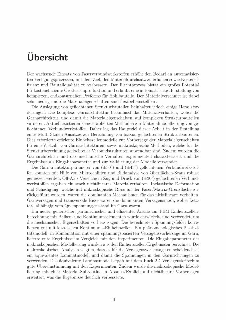
1.1 Thesis objective 3
the component: Fig. 1.3 shows the concept of an braided aircraft frame with integrated“mouseholes” for the crossing stringers. The cross-section not being cylindrical and thevariation of cross-section height introduces a change of yarn architecture (e.g. braiding an-gle, preform thickness). The effort for an experimental material characterization would belargely increased, requiring many test series to cover the variation of yarn architecture andmaterial properties on the component. Thus, a multi-scale modeling approach, predictingthe influence of the yarn architecture on material properties, substituting experimentswith numeric simulations, is much more efficient.
(a) Braided frame concept with crossing stringers (b) Braided frame preform
Fig. 1.3: Braided frame: concept with integrated mouseholes and braided preform [4]
1.1. Thesis objective
The main objective of the research work presented in this thesis was to develop a model-ing framework for predicting the constitutive behavior of biaxial braided composites. Themodeling was intended to incorporate details of yarn architecture and its impact on themechanical properties, while being applicable for strength design of braided compositecomponents. The core of the framework was multi-scale-modeling, including efficient unitcell models and macroscopic methods for structural simulation. Furthermore, experimen-tal techniques for input property determination and model validation were required. Themajor goals of the thesis can be summarized as:
• Yarn architecture characterization: development of an experimental method forrobust internal geometry measurements of braided composites.
• Mechanical characterization: experiments to determine the constitutive and failurebehavior of biaxial braided composites under combined stress states.
• Unit cell modeling: development of an efficient and parametric finite element unitcell modeling approach, required to predict the mechanical behavior for a multitudeof yarn architectures and load cases.
• Macroscopic modeling: formulation of a modeling approach, based on the unit cellsimulation results, which is applicable for structural simulation of large braidedcomposite components.

1.2 Structure of thesis 4
1.2. Structure of thesis
Chapter 2: Literature review
In Chapter 2, a literature review to previous published work in the field of experimentalcharacterization and numerical modeling of braided composites is given: a short introduc-tion is provided to manufacturing aspects of the braiding process and the basic equationsfor braiding process modeling are presented. Additionally, the work published on exper-imental characterization and available analytical and numerical models for textile andbraided composites is reviewed. Finally, a short overview on modeling of failure, damageand inelastic behavior in composite materials is given and applications of the models totextile composite materials are described.
Chapter 3: Experimental techniques
Chapter 3 describes the experimental methods used for yarn architecture and mechanicalcharacterization. A description of the manufacturing process used for the braided com-posites, characterized in this work, is provided. For yarn architecture characterizationthe different techniques are described, including sample preparation and results evalu-ation. Furthermore, specimen preparation, test set-up and evaluation methods for themechanical characterization are given.
Chapter 4: Experimental testing and results
Chapter 4 includes the results of the experimental work conducted for yarn architecturecharacterization and mechanical testing. A strategy for yarn architecture measurement,based on optical microscopy, is introduced. This includes studies on the sample positiondependence and the required number of the samples. Additionally, two braiding anglemeasurement techniques based on surface scanning are compared and three-dimensionaleffects based on micro computer tomography measurements are investigated. Off-axis ten-sion and compression tests have been conducted to characterize the nonlinear and failurebehavior of (±30°) braided composites under combined stress states. Furthermore, themechanics of failure in tension and compression are identified and damage and plasticityeffects in the material are distinguished using loading/unloading experiments.
Chapter 5: Geometric modeling and analytical predictions
Chapter 5 describes the geometric unit cell modeling used in this thesis. Based on thegeometric models, analytical predictions of the braided composite elastic behavior aregiven and parametric studies on yarn architecture variations are presented.
Chapter 6: Finite element unit cell modeling
The development of a novel finite element unit cell modeling approach based on beam andcontinuum elements is described in Chapter 6. The equations and implementation of themodeling approach, including constitutive modeling, periodic boundary conditions anda volume-averaging for stress calculation are presented. An assessment of the predicted

1.2 Structure of thesis 5
stress fields is obtained by comparison of the modeling results to a classical continuum unitcell approach. Furthermore, the influence of boundary conditions in thickness directionis studied, and the modeling results are finally validated by comparison to experimentalresults.
Chapter 7: Macroscopic modeling of biaxial braided composites
The approaches used for macroscopic modeling of braided composites are described inChapter 7. Two analytical modeling approaches for failure prediction are compared anda method for input property definition, based on unit cell modeling results, is derived. Inaddition to the analytical modeling, a numerical modeling approach, considering plasticityand damage effects in the braided composites, is presented and the numerical results arecompared to analytical modeling and experimental results.
Chapter 8: Conclusions and future work
Chapter 8 includes the overall conclusion on the experimental and numerical work con-ducted in this thesis. Topics, identified in experimental characterization and numericalmodeling are discussed and possible solutions are given. Finally, possible points for futureresearch work are discussed.
2. Literature review
Fiber reinforced plastics (FRPs) are composite materials typically consisting of two com-ponents: reinforcing fibers that are embedded into polymeric matrix [5]. The compositematerial utilizes the best properties of both components: the high stiffness and strengthfibers take the task to carry the load and are the reinforcing constituent in the material,while the softer matrix introduces and distributes the load into the fibers, keeps the fibersin place and protects them against environmental effects. The usage of FRP materialsin aerospace, automotive, and other industrial applications has a long history, spanningfrom the first half of the last century. In the 1930s and 1940s the first usages of FRPsfor aircraft wings and fuselages have been reported. The World War II accelerated thedevelopment of composite components, mainly used as secondary structures in militaryairplanes. In Germany, the first usage of FRPs in highly-loaded structures was achievedby academic groups for gliding. In 1957 the glider airplane Phönix, which was the first air-craft built completely from glass fiber reinforced plastics, took off on his maiden flight [5].Application of composite materials in commercial airplanes has been done piece by piece.At first, interior and secondary structures (e.g., leading edge skin vertical tail A300B) werebuilt from composites and long-term behavior was studied before being used in primarystructures [5].
The early applications of FRPs were focused on lightweight design and mass reduction.The components were typically produced using hand-layup of pre-impregnated unidirec-tional tapes, resulting in long and labor-intensive manufacturing processes. With thegrowing usage of composite materials in aerospace and with new applications within theautomotive sector, the reduction of manufacturing costs and cycle times is of increasinginterest. Due the increased interest in reduced costs and automation of manufacturingprocesses, textile reinforcements were established on the composite market [6].
Textile composites are fiber-reinforced plastics produced from a dry fiber textile rein-forcement and a matrix (polymeric resin in most cases). The textile reinforcements areproduced from yarns, typically consisting of several thousand fibers, on textile machineryspecially adapted for high-performance fiber reinforcements [6]. The term textile compos-ites describes a large range of materials, but in most cases, the reinforcements consist oftwo or more sets of tows, which are interwoven in a textile process. The dry fiber rein-forcements are either produced directly in the desired shape (e.g. braiding) or producedin several preforming steps (e.g. woven fabrics). Commonly, the preforms produced arethen impregnated by a liquid resin infusion process yielding the textile composites. Atypical example for a textile process is given in Fig. 2.1.
The main reason for using textile composites is cost-efficiency [6]. Textile processesand textile machinery have been developed and automated over centuries, which serves asa good basis for automated and cost-efficient production processes. The classical textileprocesses have been adapted to enable manufacturing of fragile reinforcement fibers ren-
6

Literature review 7
Fig. 2.1: Textile composite manufacturing process [7]
dering a high material throughput and low manufacturing costs. The variety of differenttextile preforms allows the designer to use a material specifically suited to the structuralneeds. Additionally, with direct textile preforming processes, such as braiding, it is pos-sible to produce near-net-shaped preforms from the raw fiber material, which drasticallydecreases material waste and manual rework.
Applications for textile and braided composites can be found in all areas of the com-posite industry: a textile composite produced by 2D braiding in conjunction with a resintransfer molding (RTM) infused thermoset resin has been used by Dowty Propellers since1987 [6]. The crash-box of the Mercedes-Benz McLaren SLR sports car was produced bybraiding combined with other textile processes. The taper-shaped crash-box was over-braided with a triaxial braid and further reinforced with a tufting technique, yielding avery high specific energy absorption of 70 kJ/kg [8].
The recently developed Boeing 787 Dreamliner aircraft uses triaxial braided compos-ites for the frames in the fuselage [9]. Additionally, General Electric used triaxial braidedcomposites in their jet engine containment of the Boeing 787’s engine for better damagetolerance. The braid provides 30% better containment properties along with approxi-mately 160 kg weight savings per engine [10]. BMW AG also has used triaxial braidedcomposites for the bumper beam of the BMW M6 sports car in a quantity of 6000 partsper year [11].
The following chapter gives an overview of the current state of research regardingbraided composites. First, basic terms and definitions, the current state of braided com-posite manufacturing, and characterization methods for braided composites will be de-scribed. The second part will focus on the modeling of braided composites: an overviewof existing models will be given and further points regarding unit-cell modeling, as wellas modeling non-linear material behavior of composite materials will be dealt with.

2.1 Types of textile composites 8
2.1. Types of textile composites
Textile reinforcements comprise one or more sets of yarns, which are interlaced with eachother or with additional stitching yarns. The yarns, which comprise several thousand fila-ments, are the raw product of the textile reinforcement. The most common classificationof textile reinforcements refers to the directionality of the reinforcing fibers (Fig. 2.2): ifthe fibers in the preform alone (without a matrix) can continuously transport loads in thethickness direction, the reinforcements are termed “three-dimensional” [7].
Fig. 2.2: Textile reinforcement classification adapted from [7, 12, 13]
Two-dimensional textile reinforcement are well suited for in-plane loads, but still offera layered structure akin to conventional composite laminates. They can be producedin processes with high material throughput. The interwoven structure of 2D textile re-inforcements creates an uneven ply interface, which helps to increase the resistance todelamination between the plies [14]. The in-plane properties are decreased due to theout-of-plane waviness caused by the yarn interlacements.
Three dimensional textile composites have a certain volume fraction of fibers runningin the thickness direction. These 3D reinforcements offer great advantages in regions withthree-dimensional stress states and in cases requiring great damage tolerance. Only amodest volume fraction of thickness fibers is needed to improve delamination resistance

2.2 Manufacturing of braided composites 9
[7], and with an increasing volume fraction of thickness fibers the in-plane properties sufferdrastically due to the decreased in-plane volume fraction and additional fiber waviness.The mechanical properties and the complexity of textile machinery reducing the rate ofproduction are the main reasons why the use of 3D textile composites is limited to specialapplications [15].
Cox [7] states that all 2D and most 3D textiles are quasi-laminar. They can be con-sidered to function as laminates, as high fiber volume fractions in the thickness directionare seldom used as they lead to an unacceptable loss of in-plane properties [7]. If a highervolume fraction of the fibers is running in the thickness direction, the textiles are termednonlaminar. This difference between quasi-laminar and nonlaminar textiles is particularlyrelevant when choosing an appropriate modeling approach for the textile composite.
Within the area of quasi-laminar textile composites, the braiding process stands outdue to its high flexibility regarding material properties and the possibility to automatethe production of near-net-shaped preforms. In the following section a brief review of thecurrent state of research regarding manufacturing of braided composites will be given.
2.2. Manufacturing of braided composites
Braiding is a traditional textile manufacturing technique, comprising three or more yarnsthat are interlaced in a defined pattern. Classical applications for braided textiles aretypically un-reinforced tows e.g., ropes or shoelaces. The first applications of the braidingprocess in composite materials were reported in the late 1970s by researchers at Mc-Donnell Douglas Aircraft Company [16]. For composite materials, braiding combines thepossibility of process automation, a high material throughput, low material waste andimproved damage tolerance. This results in a high potential for high-volume productionof composite structures [10, 15, 17, 18].
2.2.1. Braiding machines
Braiding machines can be separated regarding the directionality of the reinforcementproduced into 2D and 3D braiding machines (see Fig. 2.2).
2D braiding machines
Fig. 2.3 presents a state-of-the-art 2D braiding machine. The yarns spools are positionedon an outer ring and point towards the center of the braiding machine. The yarns are takenoff the spools towards the center of the machine, where the braid is formed. The braidscan be produced without a mandrel, resulting in braided sleeves [19], or with a mandrelin the overbraiding process. Commonly the mandrels have near-net-shaped geometry andare guided by a robot through the center of the braiding machine. The basic principleof 2D braiding is similar to the maypole dance: the yarns are stored in spools which arearranged around the center of the braiding machine. The spools are placed on two sets ofyarn carriers; one rotating clockwise and the other counter-clockwise around the center ofthe braiding machine. The yarn carriers move on sinusoidal paths defined by horngears.Two adjacent horngears rotate alternately, passing the yarn spool from one horngear to

2.2 Manufacturing of braided composites 10
Fig. 2.3: 2D maypole braiding machine with 128 yarn carriers.
another, when opposing notches of two horngears meet (Fig. 2.4a). The pattern of yarninterlacement is thus controlled by the number and position of the spools with regardto the number of notches (most commonly: 4 notches) on each horngear: if all availableyarn carriers are used on a four notch machine (“full configuration” see Fig. 2.4b), a 2×2braided fabric is formed. For triaxial braids, additional axial yarns can be introducedinto the process through a tube in the center of the horngear. Special braiding machineconfigurations also allow the introduction of axial yarns between two braided plies ofbiaxial or triaxial braids [20, 21].
3D braiding machines
Through-thickness reinforced braids are manufactured on 3D braiding machines [15, 16,22]. Two examples for 3D braiding processes, namely two-step and four-step braiding, aregiven in [22]. In two-step braiding, axial yarns, which are arranged in the cross-sectionalshape of the desired preform, are interlaced by braider yarns. The braider yarns are thendiagonally moved through an (n×m) arrangement of axial yarns. In four-step braiding,the yarns are arranged rectangularly in the machine bed and interlacement is achieved bytheir relative displacement. One processing step involves four displacements of rows andcolumns that move alternately.
Industrial applications of 3D braiding are still rare and limited to special cases such asbiomedical engineering [15]. In contrast, 2D braiding is a process used in several industrialapplications in the automotive [8] and aerospace industry [6, 10, 17, 20, 21].

2.2 Manufacturing of braided composites 11
(a) Principle of yarn carrier move-ment via horngears [15].
(b) Yarn carriers on a braiding machine.
Fig. 2.4: Yarn carrier movement on maypole braiding machine.
2.2.2. Types of braided reinforcements
Depending on the configuration of the braiding machine, different types of reinforcementscan be produced on 2D braiding machines. The type of reinforcement is primarily dis-tinguished by the number of yarn directions, the braid interlacing pattern, and the typeof preform [15]. The concept of repeating unit cells (RUC) is commonly used to describethe pattern of reinforcement, which can be done due to the periodicity of the interlacingpattern (see Appendix C). Three types of braided reinforcements can be distinguishedaccording to the directionality of the reinforcement (Fig. 2.5):
biaxial braid Two sets of yarns directions are interlaced by the braiding machine withthe braiding angle θ defined relative to the take-up direction (see Fig. 2.5a).
triaxial braid A third set of yarns running in the axial direction is added (Fig. 2.5b).
unidirectional braid A UD braid is a special kind of biaxial braid, where one set of yarns isreplaced by a thin thermoplastic binder yarn. A quasi-unidirectional reinforcementwith reduced waviness is created [21].
(a) biaxial (b) triaxial
Fig. 2.5: Types of braid reinforcements [23].

2.2 Manufacturing of braided composites 12
Braid patterns
The number of active yarn carriers defines the interlacing pattern of the braid (Fig. 2.6).Most common are the 2×2 (regular braid) and 1×1 (diamond braid) patterns, which areachieved by using all or half of the available yarn carriers on a regular 4-notch horngearbraiding machine (full configuration on Fig. 2.4b). Furthermore, 3×3 (hercules) and 4×4braids may be produced by braiding machines with six and eight notches per horngear,respectively, [24]. The waviness reduces with increasing length of the straight yarn region,yielding better in-plane material properties. On the other hand the stability of the braiddecreases, which can be an issue for complex parts with large cross sectional changes.The choice of braid pattern is usually driven by the component dimensions, requiredmechanical properties and preform stability.
(a) diamond 1×1 (b) regular 2×2 (c) hercules 3×3 (d) 4×4
Fig. 2.6: Common of braid patterns with corresponding RUC.
Braided preforms
Braided preforms can be produced in different types regarding the continuity of the yarns(Fig. 2.7). The most common is the overbraiding process, where a near net-shaped man-drel is used to define the contour of the final part. This is achieved by rotating the yarncarriers continuously around the braiding machine center through which the mandrel is
Fig. 2.7: Braided preforms: braided sleeves (left) and braided tapes (right) with the corresponding yarncarrier movement (adapted from [15])

2.2 Manufacturing of braided composites 13
moved. The overbraiding process produces closed braids (braided sleeves [19]): a yarn runscontinuously from the starting point around the mandrel to the end of the component.Flat braided reinforcements (braided slit tapes) may be produced from braided sleevesby cutting the braid along the take-up direction [25] and subsequently draping it to aflat shape. Alternatively, flat reinforcements can be achieved by removing the mandrelfrom the braided sleeve and pressing the reinforcement flat [12, 26]. A special type ofreinforcement are braided tapes, which are produced by introducing a yarn carrier turningpoint into the braiding machine (Fig. 2.7). In braided tapes the yarns are continuous,turning at the edge of the preform and running in the reverse direction.
2.2.3. Basic equations for the braiding process
The braiding process includes complex mechanical processes such as yarn tension, yarndeformation, yarn interaction, yarn mandrel interaction, and many more. Thus, thequality and uniformity of the resulting preform depends on many interacting parameters,such as yarn type, braiding machine size, and mandrel material. For a comprehensivedescription of the braiding process, including prediction of braiding angle distribution orpossible defects, detailed models are needed. Finite element models [27, 28] provide arealistic model of the process including friction and yarn-yarn interaction, but suffer fromthe drawback of very high computational cost. Alternatively, improved kinematic models[29, 30] can be used. These models use complex kinematic equations and are typicallybased on on the description of a single yarn, i.e. yarn-to-yarn contact is not considered.Besides these complex prediction models, some basic equations for the braiding processexist that can be used to estimate the process parameters of the overbraiding process.
Braiding angle
The braiding angle (θ) is the angle of the braid yarns relative to the braiding direction(Fig. 2.5) and is defined for a cylindrical mandrel guided through the center of the braidingmachine [31]:
θ = tan−1(Umωc2πvm
)= tan−1
(dmωc2vm
), (2.1)
where dm and vm are the mandrel diameter and the mandrel take-up speed, respectively,and ωc is the angular velocity of the yarn carriers around the take-up axis. This can becalculated from the horngear rotational speed:
ωc =4πfhgNhg
, (2.2)
where fhg and Nhg are the frequency and the number of the horngears, respectively.Although, strictly, Eq. 2.1 is only applicable to cylindrical cross sections, it can also beused to estimate the braiding angle of other cross sections by replacing the term Um withthe perimeter of the cross-section [15]. However, it should be noted that the braidingangle varies on a non-circular cross-section, i.e. the equation only provides an averagevalue for the cross section.

2.2 Manufacturing of braided composites 14
Coverage
The number of yarns in a braiding process is controlled by braiding machine size and themachine configuration. Commonly the braids are required to be closed1 (see Fig. 2.8)with the active yarns in the process for the given mandrel size. This ensures a highfiber volume fraction and high mechanical properties of the braided composite. Thus, acertain number of yarns put a constraint on the mandrel perimeter and vice versa. Therequirement of a closed braid can be checked by the spacing (p) of two adjacent yarns[16]:
p =2πdmNc
cos(θ) (2.3)
Nc is the number of active yarn carriers, which is twice the number of horngears for afull configuration on a 4-notch horngear machine. As the width of a yarn in the braidingprocess can vary within certain boundaries, three different braid states shown in Fig. 2.8are possible: a closed braid ensures a high fiber volume fraction without matrix-richregions. But if the mandrel dimension changes drastically, the braid may be open (gapsbetween the yarns), or may not fit onto the mandrel (jammed) [27]. The status of thebraid can be evaluated by comparing the calculated spacing with the maximum andminimum yarn width. The values for maximum and minimum yarn width are dependenton the specific manufacturing conditions and the yarn itself and should be determinedexperimentally.
Fig. 2.8: Possible braid states on mandrel with changing cross-section: a) closed, b) jammed, and c)open (mandrel image from [27]).
1closed braid: the state of a braided preform, where all the yarns lie next to each other without a gap,the mandrel surface is no longer visible after the first ply is braided.
2.3 Yarn architecture of braided composites 15
Areal weight
The areal weight of a biaxial braided preform can be estimated by applying geometricalconsiderations. Potluri et al. [16] introduced a correction to account for the yarn crimp:
FAW =NcT (1 + c)
πdmcos(θ), (2.4)
where T is the linear density of one yarn and c is the crimp factor defined in Eq. 2.10.With c = 0, yarn crimp is neglected. If the thickness of the final part (such as in an RTMprocess) and the fiber density is known, the fiber volume fraction can be estimated usingthe fiber areal weight of the braid laminate
ϕf =FAW
ρfh. (2.5)
Preform mass produced per unit time
The preform mass produced within a certain time can be calculated from the fiber arealweight. The mass per unit time is defined as:
mpreform = FAWπdmvm =NcTvmcos(θ)
=NcTdmωc2sin(θ)
(2.6)
For a typical biaxial braid configuration (Nc = 176 carrier braiding machine, T = 800 texwith a dm = 100 mm mandrel and θ = 30° braiding angle) the theoretical fiber massoutput is 14.5 kg/h.
2.2.4. Resin infusion
Braided fabrics are either braided directly on a mandrel defining the shape of the partor produced to semi-finished products, which are subsequently draped into the final ge-ometry. In most applications, a liquid composite molding process in conjunction with apolymeric resin is used for impregnation [6]. Both, closed mold RTM and single sided moldresin infusion with flexible tooling processes have been reported [25, 26, 32–34]. Com-pared to prepreg processes, considerable cost-savings can be achieved by using braidedcomposites in conjunction with resin infusion processes [18, 35].
2.3. Yarn architecture of braided composites
Textile composites are hierarchical materials: the material definition has to be describedon different length scales which are based on each other: the fibers in the yarns on themicro-scale, the internal geometry of yarns and fabric unit cells on the meso-scale, and thetextile reinforcement on the macro-scale. Each scale has its characteristic length, 1-10 µmfor the fibers, 1-30 mm for the fabric the unit cell, and centimeters to several meters forthe composite structures [15, 36].

2.3 Yarn architecture of braided composites 16
It should be noted that the term meso-scale is not consistently used in literature. WhileLomov et al., and others, [15, 37, 38] define the field of composite unit cell mechanicsas meso-mechanics, the same type of models are defined as micro-mechanical in otherpublications [39–41]. Ladeveze et al. [42] define single (unidirectional) plies in compositelaminates as meso-scale. Throughout this thesis, the definition of Lomov et al. [15] givenin Table 2.1 will be used.
Table 2.1.: Definition for micro-, meso-, and macro-scale used.
micro scale of fiber and matrixmeso scale of yarns and fabric unit cellsmacro scale of textile composites and composite structures
The term “yarn architecture” refers to the internal geometry of a textile compositedescribed on the meso-scale. The yarn architecture of a braided composite comprisesthree components, as shown in Fig. 2.9:
• Yarns, consisting of several thousand filaments impregnated with matrix.
• Matrix pockets, regions of pure matrix in-between the yarns.
• Voids: intra- or inter-yarn voids.
In the following section, an overview about previous works regarding the yarn architectureof textile composites with a focus on woven and braided composites will be given.
Fig. 2.9: Micro-CT scan of the internal geometry of a (±45°) biaxial braided composite
Volume fractions
Volume fractions can be defined according to the components in a textile composite [40].The total fiber volume fraction (ϕf ) is the volume of fibers in the composites, while yarnvolume fraction (ϕY ) describes the volume of yarns in the composite and can be considered

2.3 Yarn architecture of braided composites 17
as a measure of the tightness. Additionally, the packing density (pd) describes the fibervolume fraction inside the yarn. These can be described by the following:
ϕf =VfVges
, (2.7)
ϕY =VYVges
, (2.8)
pd =Vf,Y arnVY
=ϕfϕY
. (2.9)
The total fiber volume fraction can be measured directly from braided composites byusing a variety of methods, such as digestion of the matrix [43]. The packing densitycan be calculated from the yarn area (measured, e.g. from micrographs) if the diameterand the number of filaments is known [33]. Typical values of the packing density havebeen reported to vary from 60% to 80% [33, 44, 45] for braided composite fiber volumefractions of 50-60%.
Yarns cross section and yarn path
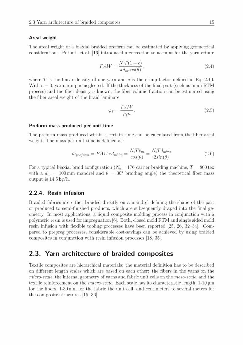
The shape of the yarns in a textile composite is usually described by using the yarn crosssection, cross sectional orientation, and yarn path [46]. Commonly elliptical [40, 47] andlenticular [44, 48, 49] cross sections have been reported in literature. Birkefeld et al. [33]noted that both shapes of cross sections can be seen in micrographs of braided composites.While the braiding yarns typically manifest a mixture of both cross sections, ellipticalcross sections dominate the axial yarns of triaxial braids. Byun [44] reports consistentand regular shapes for the axial yarns in a triaxial braid, while the shapes of the braidingyarns were irregular. Byun also described that the cross sections of the braiding yarnslocated on the surfaces of the specimens tended to flatten. This is in agreement withthe observations from [33], where the flattening was considered to be due to the contactof the yarns with the solid mold or the vacuum bag. Ruijter et al. [50, 51] found thatthe average shape is close to lenticular, by applying an averaging routine to several crosssection images obtained from micrographs of a woven fabric. Ruijter noted that the yarngeometry was variable (aspect ratio between 1:8 and 1:15) and that the automated imageaveraging of cross sections only quantifies the variation, but cannot provide informationabout the possible reasons (e.g. yarn crossover).
The yarn path can be divided into crossover regions (straight regions, floats: AB, CD,EF in Fig. 2.10), where the yarns run over/under the crossing yarns, and undulationregions (BC, DE in Fig. 2.10), where the yarn runs from the upper to the lower surfaceand vice versa [40].
Fig. 2.10: Division of the yarn path [40].

2.3 Yarn architecture of braided composites 18
Different parameters are used to characterize the magnitude of undulation: the crimpangle [7] is the maximum out-of-plane angle of the yarn path inside the undulation re-gion; the yarn crimp ratio c given in Eq. 2.10 is most commonly defined by comparingthe crimped yarn length to the length of the fabric [52] (cf. Fig. 2.11). It should benoted, that different definitions for the yarn crimp ratio have been described, e.g. by [53].Owens et al. [54] use the waviness ratio WR, which is the thickness of the ply dividedthrough the wavelength of the undulation.
c = lyarn/lfabric − 1 (2.10)
WR = hply/lfabric (2.11)
Fig. 2.11: Yarn crimp interval with parameters to calculate crimp measures.
Besides average descriptions of yarn shape and path, considerable effort has been under-taken to describe of variability of the yarn architecture. Vanaerschot et al. [55] presenteda stochastic framework based on the period collation method for the analysis of variationsin the yarn path and yarn cross sectional parameters based on micro-CT measurements.He defines tow geniuses to calculate systematic and stochastic variations of the yarn pathfrom the geometric properties measured. Dips in the crossover region of the yarn pathshown in Fig. 2.12 are solely observed in inner plies, which he relates to the mold contactof the outer plies. Vanaerschot concludes that out-of-plane waviness and cross sectionalparameters vary systematically, dependent on the relative positions on the yarn path,
Fig. 2.12: Systematic yarn path representation from [55]

2.3 Yarn architecture of braided composites 19
i.e. these values do not depend on the lateral and laminate position. However, this isdifferent for the in-plane variation of the yarn path, but a reliable analysis of this wouldrequire a larger specimen. Matveev et al. [49] presented a similar evaluation method forvariability of the yarn paths in a 2×2 carbon-epoxy woven fabric. It was found that thevariations in the out-of-plane coordinates of the yarn path were of the same magnitudeas the resolution of the micro-CT images used for evaluation.
Nesting
Nesting is a phenomenon typically described for textile composite laminates [33, 56–59].When several plies of a textile are stacked on top of each other to build a laminateand compacted in a vacuum or RTM process, the thickness of the plies in the laminatedecreases with increasing number of plies. This effect is described as nesting and leads toan increase of the laminate fiber volume fraction (compared to a single ply) and is mainlyattributed to two mechanisms [58]:
1. If textile composite plies are stacked on top of each other, the discrete yarn archi-tecture comprises regions with free volume within one ply, which is filled by theadjacent plies. Lomov et al. [56] presented a purely geometrical approach to modelthis.
2. The dry yarns themselves deform under the compressive force [60] applied to thepreform during compaction. This may lead to yarn flattening or yarn cross sectiondeformation (Fig. 2.13).
Fig. 2.13: Factors affecting fabric compression [59].
The degree of nesting is given by the nesting factor η
η =Nplies tply
h, (2.12)
where Nplies is the number of plies in the laminate, and tply and h are the thickness of asingle ply and the laminate, respectively.

2.3 Yarn architecture of braided composites 20
Chen [59] conducted compaction experiments with different textile reinforcements andfound that the nesting of the laminate reached a stable state for more than 10 plies. Thedifference in ply thickness in laminates between 10 and 25 plies is negligible. Numericalstudies regarding geometric nesting [56] show that closely packed fabrics are less prone tonesting. The tightness T can be defined as a measure for this
T = (d1 + d2)/(2p), (2.13)
with d1, d2 being yarn height and width and p being the yarn spacing. It has also beenshown that longer floats (i.e. 2×2 compared to 1×1, cf. Fig. 2.7) and shear deformation(braiding angles θ 6= 45° for braids), reduce the nesting. This has also been measuredexperimentally for biaxial and triaxial braided composites with 30-60° braiding angles[33]. In addition to the effects described above, Lomov et al. [56] noted that contradictoryresults were reported for fabric nesting: Pierce [61] found the ply thickness to increasewith increasing number of plies in a plain glass woven fabric.
2.3.1. Characterization of the yarn architecture
Different methods can be used to characterize the internal geometry of textile composites,the most common methods are:
• Analytical equations.
• Optical analysis using photomicrographs.
• X-ray micro computer-tomography (micro-CT).
• Finite element process simulation.
Analytical equations can be used to calculate the width of the yarns in the overbraidingprocess if a closed braid is assumed [7]. The braiding angle can be calculated from theprocess parameters with Eq. 2.1. When assuming a closed braid, the spacing can beset equal to the yarn width and the yarn height can be calculated by estimating thepacking density (Eq. 2.9). The applicability of this method for the prediction of theelastic properties of braided composites has been validated [33, 62].
Desplentere [63] presented a comparison of three methods, namely fabric scaning, op-tical microscopy and micro-CT for dry glass fabrics. Fabric scan images were acquiredwith a resolution of 1200 dpi1 from the fabric surface using a scanner and evaluated man-ually using image analysis software. For optical microscopy, small samples (15×15 mm)were embedded in an epoxy matrix and analyzed under an optical microscope yielding aresolution of 22 µm per pixel. Similar samples were used for the micro-CT scans yieldinga comparable resolution (25 µm voxel2 size). A rather large variation of yarn-architectureparameters was found for the fabrics investigated. The differences in results from thethree methods were found to be not significant at a 95% confidence level.
1dpi: dots per inch2voxel: three dimensional extension of pixel

2.3 Yarn architecture of braided composites 21
Various researchers hvae used optical microscopy to determine the yarn architectureof textile composites [33, 44, 51]. Birkefeld et al. [33] characterized biaxial and triaxialbraided composites with optical microscopy. They noted that an uncertainty was intro-duced as the measured values had to be transformed using the cut angle if the cut planewas not orthogonal to the yarn path. The cut angle is not known exactly due to uncer-tainties in the embedding process of the samples. Crookston [64] therefore recommendsto section the samples perpendicular to the yarn path.
Ruijter [51] proposed a pixel-averaging technique to obtain the cross section from mi-crosections of plain woven fabric composites. He averaged 80 polylines drawn aroundthe yarn cross sections to calculate the average cross section, but the yarn geometry wasrather variable with aspect ratios from 1:8 to 1:15 (Fig. 2.14). Ruijter furthermore notesthat no correlation between yarn shape phenomena and the position of the cross sectionin the textile (e.g. flattened cross sections near the mold) has been done and that theproposed averaging technique suffers from the fact that the conformance of the yarn crosssection with the longitudinal yarns may lead to an underestimation of yarn width.
Fig. 2.14: Yarn cross section obtained by pixel-averaging: distribution (left) and binary image with 0.5threshold (right) [51].
Micro-CT measurements provide three-dimensional information about the yarn archi-tecture. Changes in the yarn architecture can be correlated with the relative positionand information on the variability can be obtained [63]. The main difficulty of an auto-mated evaluation of the samples is segmentation of yarns and matrix pockets: the contrastbetween yarns and matrix is low, attributed to the low density difference of fibers andmatrix in cured composite samples. Vanaerschot et al. [55] described the necessity ofmanual input for the image analysis of micro-CT scans to obtain reliable segmentationresults. Djukic et al. [65] used different techniques to improve the contrast and foundyarn coating prior to impregnation to be the most successful method for carbon/epoxylaminates. In particular, the issue of segmentation of neighboring yarns could be improvedusing coating.
Besides micrographs and micro-CT, which are both suitable for small samples of ap-proximately 10-50 mm, image analysis techniques provide the possibility to investigatelarge areas. Recently, some approaches to image analysis of fabric scans have been pub-lished. Miene [66] presented an approach to automatically detect fiber angles and defectslike gaps for dry fabrics. Thumfart and Tanner [67, 68] presented a sensor based onphotometric stereo for similar purposes. As these approaches allow segmentation of thetextile, yarn width and spacing can also be measured.
A fully predictive approach to the characterization of the yarn architecture of braidedcomposites is FE braiding simulation [28, 69]. An explicit finite element simulation withtruss elements modeling the yarns was conducted, which allows to include the yarn kine-matics and friction during yarn contact. The results provide information about the yarncenterlines on the selected mandrel (Fig. 2.15). Pickett [69] introduced a special post-processing technique for the braiding simulation and calculated a full 3D continuum modelof the yarns including yarn deformation and compaction. The main challenge for unit cell

2.3 Yarn architecture of braided composites 22
simulations has been identified to be the meshing of the small matrix pockets, which wassolved by using particle methods to represent the matrix.
(a) (b)
Fig. 2.15: Finite element braiding simulation for biaxial (a) and triaxial (b) braid.
2.3.2. Geometric modeling
Most geometric models of braided and woven composites use idealized descriptions foryarn paths and yarn cross sections [39, 48, 70, 71]. Several software packages such asWiseTex [46] and TexGen [71] have been developed for geometry modeling of textilecomposites and offer a general framework for idealized geometric modeling of the yarnarchitecture of various textile reinforcements.
WiseTex computes the internal geometry of the textile from user input, such as yarnproperties and weave patterns, based on an energy minimization algorithm [36]. A com-bination of elliptical arcs and a 5th-order polynomial function represents the yarn pathin the undulation interval. The cross section of the yarns can be chosen either circularelliptical or lenticular. WiseTex serves various interfaces, to Mori-Tanaka micromechan-ics (TexComp [72]), permeability modeling (FlowTex [73]), and finite element (FETex)software. Recently, a command-line interface and an open XML-dataformat have beenimplemented in WiseTex [74]. This allows for straightforward integration of WiseTexgeometry models into simulations realized with 3rd-party software.
TexGen [75] is an open-source software package for textile modeling, providing a Pythonscripting interface and various export options to Abaqus [76] FE software. TexGen usesspline interpolation for the yarn path in-between the user-defined master-nodes and pro-vides several possible yarn cross sections including elliptical and lenticular [77]. Themodels from TexGen can be exported to third-party software as common geometric de-scriptions (IGES, STEP) or as a tetrahedral or voxel continuum element mesh to theFE-software Abaqus [38].
Idealized geometric models are rather simple to implement into generic software, how-ever when a tight yarn architecture (high yarn volume fraction, ϕY ) is modeled andused for finite element analysis, one faces the problem of yarn volume interpenetrationas shown in Fig. 2.16 [24]. Finite element meshing with continuum elements requires thegeometries to be consistent, which means that yarn volumes cannot overlap each other.Potluri et al. presented an analytical approach, which overcame this problem by using thesame functions for yarn path and yarn cross section, but the geometry is limited to plain(1×1) fabrics [62].

2.3 Yarn architecture of braided composites 23
Fig. 2.16: Volume interpenetration for biaxial and triaxial braids [24]
Several researchers proposed improvements to overcome the problem of volume inter-penetration by using analytical considerations or finite element contact analysis. Sherburn[77] used an idealized geometry of a 4-harness satin weave modeled with TexGen as a ba-sis, refined the yarn path definition, and changed the cross sectional shape and orientationat the crossover points of the fabric. The improved geometry has been validated againstmicro-CT measurements and provided good correlation of yarn path, cross sectional shape,and rotation. In a second publication an automated algorithm for correction of volumepenetration based on an FE contact analysis using plate elements was proposed [78]. Theapproach has been implemented in TexGen and led to good improvements regarding vol-ume penetration for a 2D textile. On the other hand, the results for a 3D orthogonalweave were less accurate, still showing interpenetrations.
Lomov et al. [24] also presented an approach for interpenetration removal implementedinto the MeshTex [79] software. The unit cell is divided into several sub-problems, eachrepresenting one contact pair, the yarn volumes are moved such that interpenetration isnot occurring and beam elements are defined between the surfaces. The yarns are definedto be volume-constant (ν = 0.5) and pressed together to create tight, non-interpenetratingvolumes. In the last step, the yarns are re-assembled into the complete unit cell.
In addition to idealized geometrical models with the option of volume-interpenetrationcorrection as described above, analytical approaches for detailed geometric modeling oftextile composites exist. Hivet and Boisse presented an analytical approach for consistentgeometric modeling of fabric unit cells [80]. The model ensures a realistic contact surfacewithout interpenetration of the yarns, which is achieved by changing the cross-sectionshape of the yarn along the yarn path. A CAD-preprocessor was used for the creationof the fabric unit cell geometry and export to a finite element code resulting in a high-quality regular mesh of the yarns. However, the model was applied to dry fabric unitcell simulations, which do not face the problem of matrix-meshing in the thin crossoverregions.
Different methods using finite element analysis for modeling of compaction have beenpresented in the literature. Grail et al. presented a geometrical model with consistentsurface meshes, which do not suffer from volume penetration or free volumes (voids)[81]. Meshes from a previous preforming simulation were used as an input and a sub-sequent compaction simulation with multi-layer unit cells yielded realistic yarn volumefractions within the unit cell. Hsu and Cheng presented an approach to geometry cre-ation using multi-step FE-analysis [82]. The method included FE compaction simulation,re-construction of the geometry, and removal of geometric inconsistencies. Stig and Hall-ström recently presented a new FE-based approach for realistic geometric modeling of 3Dwoven textiles [83]. Based on a TexGen geometry, yarns were modeled as inflatable tubes

2.4 Mechanical testing of braided composites 24
in an explicit FE analysis. The validation of the calculated yarn geometry with micro-CTscans shows good accordance. The model combines advantages of a few input parametersand is generic and extendable to other types of textiles.
2.4. Mechanical testing of braided composites
Mechanical characterization of braided composites is an important method for both under-standing the complex and anisotropic material behavior and for creating a basis for the val-idation of predictions. Common standards for composite materials such as ASTM D3039(plain tension, [84]) or ASTM D6641 (plain compression, [85]) were developed primarilyfor UD, angle-ply, or quasi-isotropic laminates. Special considerations regarding coupongeometry, measuring systems, and test procedures for textile composites are given inASTM D6856 [85]. Among other points mentioned in [85], recommendations regardingspecimen width and strain gauge size are given; the specimen width is recommended tobe larger than two times the width of the representative unit cell marked in Fig. 2.6 toensure a representative constitutive behavior. The strain gauge width and length arerecommended to be, at minimum, equal to the unit cell dimensions – as the strain fieldon textile composites varies due to the textile architecture [86]. The recommendationsare based on experimental campaigns on different triaxial braided composites that werecarried out by Masters et al. [86–88].
2.4.1. Elastic behavior
Birkefeld et al. presented an experimental test campaign comprising biaxial and triaxialbraided carbon/epoxy composites with θ = 30°, 45°, and 55° braiding angles [33]. Thetriaxial braided composites exhibit a higher stiffness in both axial and transverse directionwhen compared to biaxial braids with the same braiding angle. The modulus in the axialdirection was reported to decrease with the braiding angle. This is in accordance with theresults presented by Charlebois et al. [25] based on tensile and compressive experiments ofglass/epoxy biaxial braided composites with θ = 35°, 45° , and 50° braiding angles. Theshear behavior of the braided composites was also evaluated; the Iosipecu shear testingmethod used was found unsuitable due to the high stiffness and strength of the braidedcomposites.
2.4.2. Nonlinear and failure behavior
Several publications have reported on the nonlinear and failure behavior of braided com-posites. During the early 90s, many experimental studies were published concerningtriaxial braided composites [87–91]. Minguet and Gunther [92] compared the responseof triaxial braided composites to tape laminates with equivalent material and layup. Itwas found that transverse tensional strength and shear strength was lower for the braids,which was attributed to the braid yarn undulation. Open-hole and filled-hole tensilestrength can be increased with the braids, but all compressive properties were higher forthe equivalent tape laminates.

2.4 Mechanical testing of braided composites 25
A study on the mechanical behavior of biaxial braided composites was conducted byTsai et al. [32]. They used pressurized cylinders with a braiding angle of 45° with biaxialand triaxial braided reinforcements of graphite and glass fibers. The hoop strength ofthe cylinders increased by 25% for graphite compared to glass fibers and triaxial braidswere reported to have a lower hoop strength, which was attributed to the lower volumefraction of circumferential (braid) fibers in the triaxial braid.
An extensive study on glass/epoxy biaxial braids was conducted by Harte and Fleck,characterizing braided tubes with different braiding angles in tension, compression, andshear [93, 94]. The tensile and compressive strength increased with decreasing braidingangles, while shear strength decreased. This was attributed to the increased influenceof the matrix material at higher braiding angles, where the angle between fibers andload direction is higher. The influence of the braiding angle was also observed in thestress-strain behavior, which was linear for small braiding angles and strongly nonlinearat higher angles (Fig. 2.17).
Fig. 2.17: Failure chart (left) and stress strain curves (right) measured from biaxial braided tubes [93].
Similar results have been obtained for glass/epoxy biaxial braids by using flat coupons[25]; a linear increase of strength with the braiding angle was reported in tension, whilethe compressive strength was lowest at a braiding angle of 45°. Further studies regardingstrength at low braiding angles have been carried out by Huang and Ramakrishna [48]: aspecimen with continuous yarns was studied (braided sleeves Section 2.2.2) and showedthat the longitudinal strength increases by 50% for a braiding angle of 15° compared to 25°.While the stress-strain response was linear for small braiding angles, major nonlinearitiesbefore final failure were observed for braiding angles higher than 25°.
Failure modes
The failure modes described for biaxial braided composites follow the same mechanics asthose occurring in UD composites [95]. However, the internal structure of the braidedcomposite triggers different failure modes than the ones observed in UD composites.
The micromechanical events during failure in yarns and matrix of textile compositesare described by Cox et al. [7, 91]: for tensile loads, micro-cracking in the transverseoriented tows (if present) is the first failure event, followed by fiber (tow) rupture, whichis the dominant failure mechanism. Fiber strength is reduced compared to UD materials

2.4 Mechanical testing of braided composites 26
due to the uneven load-distribution within an undulated tow. If the load is not alignedwith one of the fiber directions, shear failure or transverse cracking can become dominant.Compressive failure may involve several mechanisms such as shear micro-cracking, inter-ply and intra-ply delamination, and kink-band formation within the tows (Fig. 2.18).Shear failure within the tows starts with arrays of microcracks involving considerablemicro-plasticity and propagates to larger matrix cracks with the damaged material brokeninto pieces.
Fig. 2.18: Failure mechanisms in compression [7]
Harte and Fleck [93, 94] identified four failure modes for glass/epoxy braided tubes:fiber failure and neck propagation in tension, fiber microbuckling and diamond shapedbuckling in compression and shear. There was a strong dependence of the failure mode onload and braiding angle. The results are summarized in a multi-axial failure mechanismmap, presented in Fig. 2.19.
Fig. 2.19: Failure map for biaxial braided tubes under combined loads [94].

2.4 Mechanical testing of braided composites 27
Fouinneteau [12] further stated that fiber failure in tension and compression and shearinduced fiber/matrix debonding occurs as in-plane failure modes of biaxial braided com-posites. In addition, inter- or intra-laminar delamination, as shown in Fig. 2.18, mayoccur due to tow-straightening.
Cutting of the specimen and coupon geometry
The internal structure of most braided composites is of similar length scales as commoncoupon dimensions for mechanical characterization [84, 85], which draws attention to theinfluence of coupon size [96]. In addition, the overbraiding process yields a continuousfiber network on the mandrel, i.e. a fiber (yarn) runs continuously from the beginning tothe end of the mandrel. This is not the case, if braided coupons are cut from compositepanels. The influence of coupon dimension and the effect of continuous yarns has beeninvestigated by various researchers.
While the elastic properties of braids are not influenced by the continuity of thefibers, the strength of uncut coupons may exceed that of cut configuration coupons (seeFig. 2.20). The effect becomes particularly dominant for small braiding angles: more than100% strength increase was reported by [70] for (±17°) and (±15°) biaxial braids, whilemoderate strength increase of 27.5% and 13.3% is measured by [34] for (±25°) and (±45°)biaxial braids, respectively.
Additionally, the failure mode of the specimen can change between cut and uncut config-uration: while cracks are forming in the center of the specimen in the uncut configuration,edge cracks initiate the failure in the cut configuration [97].
Fig. 2.20: Uncut (left) and cut (right) edge configuration of braided composites [70].
Kelkar and Whitcomb [26] characterized flattened braided sleeves and reported strongbraiding angle variability to be a consequence of process inaccuracy during the flatteningof braided tubes. It was possible to improve the braid angle variation by using “slit tapes”,which are braided on a circular mandrel and slit along the braiding direction.
Van den Berg [96] investigated the influence of the coupon width on the mechanicalproperties of biaxial carbon/epoxy braids. He found the Young’s modulus to be insen-

2.5 Textile composites constitutive behavior prediction 28
sitive, but the yield and ultimate stress were smaller, if the width of the coupon wasdecreased to less than twice the unit cell width. He attributed this fact to the failuremode, which was purely matrix-dominated in the case the coupon width was smaller thewidth of one unit cell. In contrast, the failure mode was fiber-dominated for larger couponwidths.
Damage initiation and progression
A general methodology for the experimental characterization of damage initiation and pro-gression in textile composites was published by Lomov et al. [98]. Different techniques suchas acoustic emission, full-field strain measurement via digital image correlation (DIC), andpostmortem micrograph investigation were proposed to study the occurrence and patternof micro-cracking within different loading stages.
Littell et al. [99] used DIC techniques to obtain information about local deformationand failure mechanisms of triaxial braided composites. It was stated that DIC providesinformation about local failure initiation mechanisms in different yarn orientations andin-situ yarn properties could be measured by local evaluation of the strain field.
2.5. Textile composites constitutive behavior prediction
A variety of analytical and numerical models exist to predict the constitutive behavior oftextile composites. The models can be divided into three major groups:
1. Analytical methods, e.g., Iso-Strain/Stress, Mori-Tanaka, and methods of cells.
2. CLT-Methods: classical laminate theory is adapted to model the textile reinforce-ment.
3. Finite element unit cell models: the yarn architecture is modeled in a unit cell.
The models require different depth of input and numerical effort and offer different levelsof detail regarding the predicted information: analytical models can include detailedgeometric information about the yarn-architecture and provide a very efficient solution.However, such models often suffer problems in correctly representing the stress and strainfields in yarns and matrix, which is important for failure and damage modeling [100].FE unit cell models provide detailed stress and strain fields and can include variousconstitutive models for plasticity and damage in matrix and yarns. However, these modelsrequire a considerable number of input properties, can be very complex to implement andrequire high computational cost [101]. Computational efficiency is the biggest advantageof the CLT-models, which enable ad-hoc implementation into most FE packages and canbe used to analyze structural problems with existing FE methods [12]. The followingsection gives an overview of models for textile composite constitutive behavior prediction,with a focus on models for braided composites.

2.5 Textile composites constitutive behavior prediction 29
2.5.1. Analytical models
The first analytical models for woven composites were presented by Ishikawa and Chou inthe early 1980s [102–105]. Three methods, namely the Mosaic Model, Fiber UndulationModel, and Bridging Model (Fig. 2.21) were developed. The mosaic model neglectedundulation, and used cross-ply laminates assembled under the assumption of iso-strainand iso-stress to model woven fabrics. The fiber undulation model [105] calculates thestiffness knockdown due to yarn crimp in a woven fabric by modeling the out-of-planewaviness of the yarn as an assemblage of various slices of stacked matrix and UD off-axis laminates. The local stiffness of the yarn is transformed into the global coordinatesystem, one slice of yarn and matrix is assembled using iso-strain condition and the slicesare assembled by applying the iso-stress condition. The bridging model can be describedas a combination of mosaic and fiber undulation models: a woven fabric is sub-dividedinto regions of straight and undulating yarns and assembled by a combination of iso-stressand iso-strain conditions [102].
Fig. 2.21: Mosaic, fiber undulation and bridging model [102]
Many extensions and enhancements of Ishikawa’s and Chou’s models have subsequentlybeen developed. Naik and Shembekar [106] extended the fiber undulation model to 2Dusing the Parallel-Series or Series-Parallel models. An iso-stress condition is used alongthe loading direction, while iso-strain is used in the transverse direction: the models aredistinguished by the order of the homogenization. The Parallel-Series model has beennoted to give better results for the elastic constants of woven fabrics.
A general model, namely the “orientation averaging” model, was proposed in [107–109].The model treats the textile composite as an assembly of small volumes of unidirectionalcomposites, weighted by their volume fraction and assembled under iso-stress or iso-strain assumption. Cox and Dadkhah [91, 110] used this method including a correctionfor stiffness knockdown due to fiber undulation and obtained good results for 3D wovenand triaxial braided composites.
Various extensions of iso-strain / iso-stress methods have been applied to braided com-posites. Most models include a more detailed geometric description [44], and some arealso extended to failure prediction [70]. An extensive overview and comparison of thesemodels has recently been given by Hallal et al. [111].
Another approach to homogenization of textile composites using a Mori-Tanaka methodhas been proposed by Huysman et al. [72, 112]. The yarns in a fabric unit cell were sub-divided into smaller segments, with the segments characterized by fiber volume fraction,orientation, cross section, and local curvature. The segments are then replaced with

2.5 Textile composites constitutive behavior prediction 30
ellipsoids of identical cross sectional shape and the length correlated to the curvature.Eshelby’s equivalent inclusion principle and the Mori-Tanka scheme are used for the ho-mogenization. The method was implemented into the TexComp software, which is partof the WiseTex package [46]. Good predictions for the elastic constants of woven andbraided composites have been obtained with the method [33, 63, 112].
Recently, the Methods of Cells [113] has been applied to textile composites. Prodro-mou et al. presented an approach using the geometric description of WiseTex and Methodsof Cells for the prediction of stiffness and strength [100]. It was outlined that the modelis computationally very efficient and general. The results were compared to conventionalmethods and experiments and a promising correlation was achieved.
2.5.2. Classical laminate theory methods
Classical laminate theory (CLT) was primarily designed for UD composites but can beapplied to laminar textile composites [7] using equivalent tape laminates to represent thedirectionality of the reinforcement.
Smith and Swanson used the strain in the axial and braid fiber direction for failureprediction of triaxial braided composites [90, 114–116]. The global strain was transformedinto the fiber directions and a maximum strain criterion in the yarn direction was usedto predict the failure under various loads. The criterion was in good correlation withexperimental data when the failure strain values for axial and braid yarns were obtainedby correlation to selected test results.
Johnson et al. [117] presented a constitutive model for the prediction of nonlinearitiesand damage in woven composites. A continuum damage mechanics approach is usedin conjunction with a one-dimensional plasticity law under shear. The approach wasimplemented in the explicit FE code PAM-Crash. Later, a similar model for braidedcomposites was implemented into PAM-Crash and extended in order to account for tow-straightening and delamination [12]. Comparison to experimental results on coupon testsand sub-structures showed promising correlation, but the coupling between inter- andintra-ply damage was not considered due to the lack of experimental data [12].
Goyal et al. [118] presented an equivalent tape laminate model for biaxial braidedcomposites. The laminate comprises one ply for every yarn direction and an additionalmatrix ply (Fig. 2.22a). Hill’s yield criterion is used in yarn and matrix plies to predictnonlinearities prior to final failure. Comparison of the equivalent tape laminate to 3Dcontinuum unit cell results show only minor deviations; this shows the potential of theequivalent tape laminate modeling approach. The correlation to experiments was goodfor both methods, but the equivalent tape laminates were stiffer than the unit cells asfiber undulation was not considered.
Zebdi et al. [119] presented an inverse modeling approach based on CLT. Equationswere given to calculate the equivalent properties of the single plies within a virtual (±θ)slaminate based on the experimental results of biaxial braided composites. The calculatedproperties of the virtual plies differ significantly from those obtained for UD plies. Theapplicability of the approach to braids of various braiding angles and woven fabrics issuccessfully demonstrated.

2.5 Textile composites constitutive behavior prediction 31
Propert
iesof +θ
tow
Propert
iesof -θ
towPropert
iesof matr
ix
(a) Equivalent tape laminate including matrix layer[118].
(b) Sub-cell approach for triaxial braided compos-ites [120].
Another approach to modeling braided composites using CLT are the so-called sub-cell models [120–122]. These represent the textile architecture macroscopically usingsub-cells with different layups in FE calculations (Fig. 2.22b). Usually, two types of sub-cells, comprising and not comprising axial yarns, are distinguished for triaxial braidedcomposites.
2.5.3. Finite element unit cell modeling
FE unit cell modeling is commonly used for prediction of the elastic and nonlinear be-havior of textile composites. The basis for FE unit cell modeling is a suitable geometricdescription of the yarn architecture of a representative unit cell (RUC). The geometry ofyarn and matrix pockets is imported into FE software, meshed, and solved using periodicboundary conditions. The models typically require high effort for model generation andincreased computational cost [101], which makes these models unattractive for macro-scopic modeling. However, FE unit cell models provide a high level of detail in stressand strain fields inside yarns and matrix, making them suitable for the prediction of fail-ure and damage inside textile composites. Lomov et al. [123] highlighted their potentialby comparing the strain field calculated by FE unit cell models to experimental resultsobtained by shearography. The FE unit cell solution could represent the features of themeasured strain field such as tension-bending coupling of single ply woven fabrics whenloaded along one yarn. The calculated strain values have been reported very close to themeasured values.
In an earlier publication, Lomov et al. [24] summarized the relevant modeling stages tobe considered for meso-FE unit cell modeling:
1. Build a model of the yarn architecture.
2. Transfer the geometry to a volume representation .
3. Correction of volume interpenetration before meshing.
4. Meshing yarns and matrix.
5. Assignment of local material properties.

2.5 Textile composites constitutive behavior prediction 32
6. Definition of the smallest possible unit cell size and application of periodic boundaryconditions.
7. Homogenization procedure.
8. Damage initiation modeling.
9. Damage propagation modeling.
The modeling stages described in [24] mainly refer to full 3D continuum element unit cells.Depending on the FE unit cell modeling technique used and on the aim of modeling, somepoints may be added or skipped; e.g. some of the models do not require a correction ofvolume interpenetration [124, 125] and others use a failure criterion for prediction of thebearable stress, which does not include damage propagation [47, 62]. A classification ofthe different FE unit cell modeling techniques may be given by the meshing technique(i.e. the type of finite elements) used. The following section gives a short overview of theavailable approaches to FE unit cell modeling.
The most common technique for finite element unit cell modeling is 3D continuumelement modeling. Both yarns and matrix pockets are meshed with tetrahedral or hex-ahedral volume elements. As the yarn and the matrix domain have to be meshed withopposing nodes, a consistent geometry description is needed for continuum unit cells. Asidealized geometric models are likely to provide penetrating volume descriptions for theyarns, several methods for interpenetration correction have been proposed [24, 77, 78].For high fiber volume fractions resulting in high yarn volume fractions ϕY , the matrixpockets in the RUCs become very small, which requires small and often distorted elementsof coarse quality [37, 101]. To overcome this problem, models with decreased yarn volumefractions and adapted packing density are sometimes used to achieve a realistic total fibervolume fraction [45]. Alternative techniques including compaction simulation have beenproposed to obtain models with realistic yarn volume fraction [81, 82], but these requirean additional independent simulation step, which highly increases the computational cost.
Despite the complex mesh generation, continuum element unit cells have the advan-tage that common constitutive models can be used to describe damage initiation anddamage progression in the yarns. Early unit cell computations [79, 126] used simple dam-age models, instantly reducing the stiffness to a value near zero after damage initiation.Zako et al. [79] compared the results of unit cell simulations of a single ply woven fabric toexperiments and found that the transverse cracking within the yarns could be predictedin good correlation to the experimental results.
Ivanov et al. [45] used the physically-based Puck criterion [127] to predict damage initi-ation in the yarns and a continuum damage mechanics approach for damage progression.The local damage mechanics – i.e. relating the progression of damage to local values –can result in physically unrealistic predictions of damage progression. Thus, a non-localone-parameter damage evolution law based on the average shear stress in the yarn wasproposed. The unit cell calculations were compared to experimental results and damageinitiation as well as stiffness degradation were in good agreement.
Carvalho et al. [47] recently presented a study on the nonlinear behavior of wovenfabrics, including a yarn failure criterion for failure onset, debonding between tows andmatrix, and a plasticity criterion in the matrix. The predicted compressive strength

2.5 Textile composites constitutive behavior prediction 33
was highly dependent on the out-of-plane boundary conditions used. Considering matrixplasticity and tow/matrix debonding prior to final failure could improve the accuracy ofthe numerical results.
For biaxial braids, severe nonlinearity prior to final failure was described by Goyal[39]. An anisotropic Hill plasticity criterion was used to model the nonlinear behavior ofthe yarns, and hardening was defined by using a single master curve. The parametersfor the yield criterion and hardening were obtained by fiber/matrix unit cell simulationsunder distinct load cases. Non-linearity of the braids prior to failure was predicted by full3D unit cell simulations and compared to experiments for different braiding angles. Thepredictions were in excellent agreement for glass/epoxy braids, while reasonable agreementwas obtained for the carbon/epoxy braids [118].
An alternative technique using 3D continuum elements is voxel meshing. Equivalent tomicro-CT scans, the volume of the unit cell is sub-divided into cuboids of equal size, whichare labeled volumetric pixels. The volume mesh is not consistent to the geometry, i.e. yarnand matrix volumes are solely defined by the material properties assigned to an element(cf. Fig. 2.23). Kim and Swan [128, 129] presented techniques for textile composite unitcell voxel meshing and proposed a refinement technique based on the virtual strain energyto improve the accuracy of the voxel meshes along material boundaries. Voxel meshingwas found to be able to rapidly and automatically generate unit cell models maintainingexcellent shape and aspect ratio of the elements under mesh refinement, which is not thecase for tetrahedral meshes. It was concluded that for voxel-based meshing, a tradeoffexists between a higher computational expense of the models and the reduced time spendon manual mesh generation [128]. Crookston compared conformal tetrahedral and voxelmeshing techniques for woven fabrics [38]. The conformal technique was found to convergefaster in terms of fiber volume fraction and stiffness; however tight textiles with touchingyarn boundaries are unlikely to be successfully meshed by conformal techniques. Thus,voxel meshing may be an appropriate technique for such tight textiles. Recently, Potter[37] presented a new voxel meshing algorithm including surface smoothing, which makesit possible to model tow/matrix debonding in the unit cell simulations.
(a) (b)
Fig. 2.23: Comparison of continuum (a) and voxel (b) mesh for (±45°) biaxial braids [130].
The Binary Model, a reduced approach for textile composites finite element modeling,was presented by Cox et al. [125]. The model uses truss elements for the yarns, which areembedded in continuum elements: this represents a separation of the material propertiesinto the two types of elements. While the longitudinal properties of the yarns are rep-resented by the truss elements, the transverse and shear properties of the yarns, as wellas the isotropic properties of the matrix, are smeared in the effective medium continuum

2.5 Textile composites constitutive behavior prediction 34
elements. Elastic and failure models related to the binary model representation and theimplementation of the model in Abaqus for 2D and 3D woven composites were presented.In a subsequent publication, an improved constitutive model was proposed [131], whichtakes into account the effect of volume doubling and allows to calibrate the constitutivemodel on the basis of UD experiments. The Binary Model predictions were reportedto give excellent correlation for the elastic constants of 3D woven composites. Furthermodels for tensile or compressive fiber failure were provided, including the effect of towmisalignment and uneven load distribution.
Yang and Cox [132, 133] presented a further extension of the model by introducing amulti-point-constraint coupling between truss and continuum elements and an averagingtechnique for the strains in the effective medium. The strain field inside the effectivemedium is mesh dependent, as the mesh size introduces an averaging of the theoreticallydivergent strain at the point where the truss is embedded into the effective medium. Yangand Cox presented a strain averaging technique and demonstrated that the strains aremesh-independent when averaged over volumes with dimensions greater than half thewidth of a tow. It was also noted that these averaged strains were favorable for failureanalysis, as the failure events inside a composite are connected to stresses or strainsaveraged over a distinct length scale [134, 135]. In a later publication, the applicability ofthe strain averaging approach for failure predictions was shown, including the comparisonwith experiments [133]. The material parameters used tor the two failure modes wereobtained from calibration of uniaxial experiments, and the strength of a triaxial braidedcomposite could, in most load cases, be predicted within 10% of the experimental value.
Flores et al. [136] included a plasticity law into the Binary Model to account for matrixnonlinearity prior to final failure. A Drucker-Prager plasticity criterion with fully associ-ated flow rule and perfectly plastic deformation was used in the effective medium. Thematerial parameters were obtained by calibration of the model to uniaxial tests. Com-parison of the model predictions to open-hole tension experiments (see Fig. 2.24) showthat the Drucker-Prager criterion is able to accurately model the matrix nonlinearity andthat gauge-averaged stresses are suitable for predicting the failure stress measured in theexperiments.
Fig. 2.24: Open-hole tension simulations using the Binary Model [136].
Blacklock [137] presented an approach for the generation of virtual textile specimens,using statistical data from micro-computed tomography and used the binary model tocreate a virtual specimen.

2.5 Textile composites constitutive behavior prediction 35
Jiang et al. [124] proposed a domain-superposition technique (DST), which can beconsidered as an extension to the binary model. But in contrast to the binary model,the DST embeds continuum yarns in the continuum matrix elements (Fig. 2.25). Thecoupling uses multi-point-constraints that relate the displacements of the yarn nodes tothe displacement of the matrix host element. This is similar to the embedded elementsfunction described by Yang and Cox [132]. The stiffness of the tow was adjusted byJiang et al. by subtracting the matrix stiffness, which is required due to the doublingof volume. The error in stiffness and stress fields between DST and conventional FEanalysis was reported to be less than 5%, while a significant reduction of model DOF canbe achieved using DST. This was confirmed by Tabatabaei et al. [138], who performeda study on the DST and found the stress fields in good accordance with traditionalcontinuum meshes.
Fig. 2.25: Domain superposition technique: overlay of meshes from tow and matrix [124].
An alternative reduced FE unit cell modeling technique for 2D woven and braided com-posites was proposed by Gager et al. [101, 139, 140]. The technique uses shell elements tomodel yarns and matrix within the unit cell (Fig. 2.26). The shell elements are connectedwith multi-point-constraints and nonlinear material models including damage and plasticdeformation [141] are used for matrix pockets and yarns. The model comprises far fewerDOF compared to a conventional continuum model and thus allows a significant reductionof computational cost [140].
Fig. 2.26: Shell element unit cell [101].

2.6 Multi-scale modeling and homogenization 36
2.6. Multi-scale modeling and homogenization
Multi-scale modeling is based on the principle of homogenization of properties from asmaller (commonly micro) scale to a larger (commonly macro) scale [142]. If a materialhas heterogeneous material properties C(x) on the microscopic scale, the microscopicstress and strain fields σ(x) and ε(x) are also heterogeneous under a given boundarycondition. For a macroscopic problem the microscopic variations of the strain field arenot of interest and thus stress and strain are homogenized to macroscopic properties(〈σ〉 , 〈ε〉). The effect of the changing microstructure can therefore be described by achange of the macroscopic material constitutive tensor C∗ (Fig. 2.27).
Fig. 2.27: Homogenization and characteristic length [142].
In this section, a short overview of homogenization and boundary conditions will begiven.
2.6.1. Averaging and effective properties
A macroscopic material point is related to a microscopic volume with fluctuating stress andstrain fields. The mechanical state of the macroscopic point is related to the microscopicfield through volume averaging:
〈σ〉 =1
V
∫
Vσ(x)dV 〈ε〉 =
1
V
∫
Vε(x)dV . (2.14)
The macroscopic constitutive equation,
〈σ〉 = C∗ · 〈ε〉 (2.15)
can be used to calculate the effective macroscopic constitutive tensor C∗, if macroscopicstress and strain are known [142]. For the calculation of a full constitutive tensor, sixindependent load cases in an FE unit cell are required [40].

2.6 Multi-scale modeling and homogenization 37
2.6.2. Representative volume element / repeating unit cell
The difference in terminology between RVE and RUC is discussed in further detail inAppendix C, only a short description will be provided here. For a material with a statis-tically distributed microstructure, the concept of representative volume elements (RVE) isused: the subvolume investigated needs to be large enough that the volume fractions andthe statistical distribution from the complete material can be reproduced. The repeatingunit cell (RUC) concept describes a material whose microstructure is periodic. The RUCis the smallest volume that can reproduce the microstructure through repetition.
As braided composites have a periodic microstructure introduced through the interlac-ing yarn pattern (see Fig. 2.6), the RUC concept is commonly used for unit cell modeling[39, 40, 45, 62]. The RUCs used in literature are not always the smallest possible volumeto describe the microstructure (cf. [40, 62]); this is primarily due to practical reasons suchas simplicity of the boundary conditions implemented.
2.6.3. Homogeneous boundary conditions
Homogenous boundary conditions prescribe either the traction or the displacement onthe boundary of the investigated volume. Fig. 2.28 presents a 2D example for a uniaxialstress and a uniaxial strain boundary condition. For homogenous materials, homogenousboundary conditions can be used to evaluate the material properties, but for heterogeneousmaterials, the response is dependent on the size of the investigated volume and on whetherdisplacement or traction boundary conditions are used [143]. Applying these simplifiedboundary conditions to finite element unit cell calculations may be valid for some purposes,but should be handled with care as they can lead to artificial stress concentrations, asreported by [64], for an FE unit cell of a woven fabric.
Fig. 2.28: Homogeneous boundary conditions
2.6.4. Periodic boundary conditions
The equations and theory of the periodic boundary conditions presented in this sectionare based on the publications of Pahr [144] and Anthoine [145]. A short review of theequations will be given here. The complete equations and numerical implementation forthe unit cells used in this thesis can be found in Section 6.4.

2.6 Multi-scale modeling and homogenization 38
Each periodic medium is defined by the so-called periodicity vectors pi, which arethe vectors along the edges of a cuboid unit cell. Two periodicity vectors i = A,B aredefined for plane (two-dimensional) periodic and three periodicity vectors i = A,B,Care defined for spatial (3D) periodic media. Periodicity implies that mechanical andgeometrical properties F are invariant for positions which differ by a linear combinationof the periodicity vectors:
F(x + m) = F(x), (2.16)
m = mApA +mBpB +mCpC , (2.17)
where mA,B,C are integers. A graphical interpretation of periodicity is given in Fig. 2.29.
Fig. 2.29: Description of spatial and plane periodic medium [144].
Periodic boundary conditions are applied in cases in which a macroscopic homogeneousstress state is modeled. A homogenous macroscopic stress state in this case implies thatall unit cells are subjected to the same stress and deform in the same way: two initiallyadjacent unit cells must still fit together in any deformed state. In mechanical terms,this enforces the following requirements when passing over a unit cell boundary to theadjacent unit cell:
1. stress vectors σ are identical (tractions t = σ · n are opposite)
2. strains ε are continuous (neither separation nor overlapping of the cell boundary)
To ensure the conditions described above, it is necessary that two opposing sides of theunit cell have identical displacements except for the macroscopic strain introduced intothe unit cell. Such a displacement field is termed a periodic displacement field and can,in the absence of rigid body translation and rotation, be written as [144–146]:
u(x) = 〈ε〉 x + uP (x). (2.18)
The total displacement, u(x), is given by the sum of the macroscopic strain tensor, 〈ε〉,which is constant in the unit cell, multiplied by the position, x, and the periodic part ofthe displacement field, uP (x), which is zero when averaged over the unit cell volume (cf.Fig. 2.30).
The macroscopic strain can be calculated by volume-averaging the microscopic strainfield, but in some cases of FE unit cell calculations this is not possible. In this case, analternative averaging technique based on the displacement of special nodes can be used

2.6 Multi-scale modeling and homogenization 39
Fig. 2.30: Graphical interpretation of constant and periodic part of the displacement field [144].
[144, 145]. If Eq. 2.18 is evaluated at two adjacent points, x and x + pi, of the unit cell,where the periodic part of the displacement is equal (cf. Fig. 2.29), on yields
u(x + pi) − u(x) = 〈ε〉 pi. (2.19)
If x is set to zero and the origin of the unit cell is defined as fixed (u(0) = 0), this leadsto
U = 〈ε〉 · P, (2.20)
or uA1 uB1 uC1uA2 uB2 uC2uA3 uB3 uC3
=
〈ε11〉 〈ε12〉 〈ε13〉〈ε21〉 〈ε22〉 〈ε23〉〈ε31〉 〈ε32〉 〈ε33〉
·
p1
1 p21 p3
1
p12 p2
2 p32
p13 p2
3 p33
, (2.21)
i.e. the homogenized strains are controlled by the displacements of the nodes at the endof the periodicity vectors (see Fig. 2.31).
Fig. 2.31: Description of spatial and plane periodic medium according to [144].
Thus, the displacements to be introduced into the unit cell can be calculated from themacroscopic strain tensor and the periodicity tensor. The strain tensor as a function ofthe masternode displacements can be calculated by multiplying the inverse periodicitytensor:
〈ε〉 = U · P−1. (2.22)

2.7 Modeling of nonlinearities, failure and damage in composite materials 40
Pahr [144] noted that Eq. 2.22 may lead to an non-symmetric strain tensor and suggestsan alternative to calculate a symmetric strain tensor:
〈ε〉 =1
2(U · P−1 + (P−1)T · UT ). (2.23)
In the case that a stress vector is given, considerations including the anti-periodicity ofthe traction on the faces of the unit cell [144] lead to:
〈σ〉 =1
2V
(F · PT + P · FT
), (2.24)
where V is the volume of the unit cell and F is the master node force tensor definedsimilarly to U.
F =
FA
1 FB1 FC
1
FA2 FB
2 FC2
FA3 FB
3 FC3
. (2.25)
From this it is possible to obtain the master node forces from the macroscopic stresstensor.
F = V 〈σ〉 · (PT )−1. (2.26)
With the equations given above, the loading of the unit cell can be stress- or strain-controlled: either forces or displacements are prescribed, and the unknown quantity isobtained as the result of the FE analysis. Six independent load cases are required tocalculate all entries of the effective stiffness tensor C∗ with the macroscopic constitutiveEq. 2.15. The numerical implementation of the periodic boundary conditions into the FEunit cell calculations conducted in this project will be given in Section 6.4.
2.7. Modeling of nonlinearities, failure and damage incomposite materials
The analysis of large composite structures usually involves complex geometries and alarge number of load cases. Due to computational efficiency, this restricts the analysismethods to macroscopic approaches. Thus, for use in structural problems, failure anddamage modeling of braided composite materials on a macroscopic scale is favorable [12].As few failure or damage models with a focus on braided composites are available inliterature, a short overview of existing models for UD composites and applications tobraided composites will be given in this section.
2.7.1. Failure theories
Numerous different failure theories are available in literature. Most of the commonly usedmodels are macroscopic in a way that they are based on the homogenized stress valuesin the material coordinate system, which equates to the fiber and transverse direction forUD composites. This allows for a straightforward usage of these theories within structuralsimulations conducted with the use of FE codes.

2.7 Modeling of nonlinearities, failure and damage in composite materials 41
In the World-Wide Failure Exercise (WWFE) Hinton, Soden, and Kaddour comparedthe predictive capabilities of different failure theories [3, 147–149]. The investigation in-cluded independent (e.g. maximum stress or maximum strain [150, 151]), fully interactive(e.g. Tsai-Wu [152]), and partly-interactive (e.g. Hashin [153], Puck [127]) failure theories.The predictions made by the participants were compared to experimental results and usedto judge the predictive capabilities of the different theories.
No clear recommendation for one failure criterion could be made as the quality ofpredictions differed from the material configuration and the load cases. Among the fivecriteria that were ranked highest by the authors, the two physically-based failure criteriafrom Puck [127] and Cuntze [154] were highlighted as they gave the best predictions andcaptured more general features than the other criteria [3].
Further efforts have been made by the authors to benchmark existing 3D failure criteriain WWFE-II [155, 156] and predictive failure models including damage in the WWFE-III[157].
The considerations published in the framework of Puck’s action-plane failure criterion[127] were used by several researchers to formulate improved failure criteria for UD com-posites. Davila et al. [158] presented the LaRC03 criterion which uses a Mohr-Coulombapproach to calculate the fracture angle under transverse compression and includes a cri-terion for fiber kinking as well as the usage of in-situ strength (cf. [159]) for transversetensile cracking. The criterion was further developed to account for three-dimensionalstress states and named LaRC04 [160]. Recently, Catalanotti et al. [161] presented animproved failure criterion that has been developed to account for in-situ effects undertransverse tension, transverse compression, and in-plane shear.
Application of failure theories to braided composites
Physically based failure criteria have been used to predict failure within the yarns of awoven or braided composite FE unit cell model [41, 45, 47, 101]. The yarns compriseseveral thousand filaments running in the yarn direction and thus can be considered tobehave locally similar to unidirectional composites. Puck states that UD failure theoriesshould be applicable to textile composites with low waviness, but questions the appli-cability for higher waviness as different failure mechanisms may become dominant [95].Regardless of the waviness, it was concluded that the same failure and damage processesare occurring inside the yarns, but it was assumed that the in-situ effect (described indetail by Camanho et al. [159]) may be more prominent, as the yarn area is much smallerthan a common UD ply.
Within macroscopic woven fabric and braided fabric laminate models, usage of inde-pendent failure criteria such as maximum strain [116] or maximum stress [12, 117] wasreported. Charlebois et al. [25] used the Tsai-Wu criterion for the prediction of biaxialbraided strength. They reported good correlation to experiments in tension, but higherdeviations from the experiments in compression were attributed to the effect of fiberundulation.

2.7 Modeling of nonlinearities, failure and damage in composite materials 42
2.7.2. Damage modeling
A general framework for the description of damage in materials has been developed byKachanov [162]. The amount of damage on a specific plane of the material is describedby an internal damage variable. The concept has been integrated by Lemaitre into athermodynamic framework for solid mechanics of isotropic materials [163].
Kachanov’s principle was used by several researchers to model damage in compositematerials [12, 42, 117, 126, 164–168]. Common failure criteria as presented in the previoussection are used to determine the stress state at which damage initiates. The maindifference between the approaches lies in the type of failure criteria used and how damageprogression is calculated. Early models, such as [79, 126], used independent or fully-interactive failure criteria for damage initiation, and the stiffness in the direction that thedamage was predicted was suddenly reduced to a small fraction (typically 1-20%) of theinitial value, by using a discount factor. A comprehensive overview of different stiffnessdegradation models was given by Goyal [39]. He found that the models, although showingdifferences in the way how properties are degraded, produce similar results, when thediscount factors were equalized. A gradual decrease in stiffness after damage initiation canbe modeled by continuum damage mechanics models [159, 164]. While Matzenmiller [164]proposed a damage evolution law based on strains, Maimí, Camanho and co-workers [166,167] presented an improved damage model, based on Bazant’s crack band model, includingregularization of the dissipated energy with respect to the size of the finite element mesh.Fracture toughness values of the material were incorporated into exponential damageevolution laws and a mesh-independent solution was achieved, which is not the case forstrain-controlled damage variables. Similar approaches exist, comprising different failurecriteria and linear as well as exponential damage growth [141, 165, 168].
Application of damage to braided composites
Similar to the failure theories, damage modeling is often used within the yarns of wovenor braided composite FE unit cells [41, 45, 79, 101, 126]. The application of damagemechanics to the macroscopic modeling of braided composites are rather rare. Fouin-neteau [12] used the ply damage model from Ladeveze [42] for biaxial braided composites.He added a phenomenological treatment for stiffness reduction due to delamination un-der fiber tension and assumed that transverse damage under normal stresses is negligible.Furthermore, the shear damage evolution model was improved to account for large strainsobserved experimentally. The model was implemented in the FE code PAM-Crash andvalidated with experiments.
2.7.3. Inelastic deformation
Ladeveze [42] states that damage within composite materials is highly complex and caninclude micromechanical mechanisms such as sliding and friction, which leads to inelasticdeformation. Thus, the phenomenon of damage in composite materials may be coupledwith plasticity or viscoplasticity.
This is in accordance with the experimental observations of Varna et al. [169], who mea-sured a decrease in modulus in (±25° and ±40°) angle-ply laminates, but did not observe

2.8 Conclusions 43
any macroscopic cracking. The underlying mechanism for this behavior was believed to becaused by fiber/matrix microcracking induced by in-plane shearing. Puck also describesthis phenomenon and terms it micro-damage: very small cracks (approximately the size ofthe fiber diameter) in the matrix and the interface. Puck described experimental evidenceof the existence of micro-damage from opaqueness of GFPR laminates [170].
The inelastic deformation of composites is typically modeled using conventional oradapted plasticity models known from metals [12, 42, 117, 141, 171–173]. Early modelsassumed a transverse normal σ22 and in-plane shear τ12 stress, or a combination of both,to cause the inelastic deformation. Flatscher [141] presented a multi-surface plasticitymodel describing plastic deformation under transverse compression and in-plane shear. Anew plasticity model recently presented by Vyas et al. [168, 172] accounts for hydrostaticpressure, non-associated flow, and kinematic hardening. Vogler, Camanho, and co-workers[173, 174] presented an invariant-based plasticity criterion combined with a smeared crackmodel with the use of a structural tensor defining the fiber direction and accountingfor hydrostatic pressure as well as non-associated flow. Vogler et al. [173] noted thathardening in polymer matrix composites was believed to be a mixture of isotropic andkinematic hardening, but used an isotropic hardening law due to a lack of experimentaldata for calibration of a mixed hardening law.
Application of inelastic deformation models to braided composites
One-dimensional in-plane shear plasticity [12, 117] based on Ladeveze’s ply model [42] hasbeen applied to biaxial braided and woven fabric composites. Fouinneteau [12] comparedthe predictions of inelastic strains to experiments and found a good correlation for thebiaxial braided composites investigated. Goyal et al. [39, 118] used an anisotropic Hill-plasticity criterion in an equivalent laminate model and could successfully model thenonlinearities of biaxial braided composites loaded in tension in the take-up direction.The model required additional input-parameters to describe the anisotropy of the yieldsurface, which were calculated using a fiber-matrix unit cell model.
2.8. Conclusions
The published literature regarding the braiding process, yarn architecture of braided com-posites, characterization methods for braided composites, and mechanical modeling ap-proaches including FE unit cell modeling and macroscopic approaches has been reviewed.
Braiding offers significant possibilities for process automation, high-volume production,and cost reduction during the manufacturing process. High flexibility is available, as thetype of reinforcement can be adapted to the mechanical needs and the overbraiding processallows for curved mandrels with changing cross sections. This makes the usage of braidingfavorable for a multitude of lengthy structures.
From the designers viewpoint, the flexibility of the process creates the challenge ofa highly variable yarn architecture and thus changing material properties of the braid.Different possibilities to characterize the yarn architecture and approaches to geometricmodeling of the yarns have been reviewed. Different methods have been used to provideinput for geometric models. However, to date there is no evidence, which of the charac-
2.8 Conclusions 44
terization methods and models provides a suitable balance between effort, level of detail,and robustness.
The mechanical behavior of braided composites was reviewed, with many publicationsdescribing the elastic, nonlinear, and failure behavior of braided composites under uniaxialloads. Failure mechanisms and modes were described for both textile composites andgeneral and braided composites in particular. The mechanisms driving the failure anddamage are similar to those of unidirectional composites, but influenced by the textilearchitecture.
Different approaches for the prediction of textile composite constitutive behavior havebeen evaluated with a focus on: simple and analytical models for stiffness prediction; FEunit cell models for the detailed modeling of the nonlinear effects and failure within abraided composite; and macroscopic CLT based methods favorable for structural simula-tion. Besides the analytical models, which are only suitable for stiffness prediction, FEunit cell methods can be used to provide detailed predictions of different damage and fail-ure events inside the textile. Structural simulations typically use macroscopic approacheswith high computational efficiency and good possibilities for implementation into conven-tional FE analysis. It should be noted that simple failure and damage models are mostlyused for braided composites on a macroscopic scale and to date no validation of thesemodels exists regarding the applicability on multi-axial stress states.
The literature review has emphasized the need for an integrated approach to the char-acterization and simulation of biaxial braided composites on different length scales. Fur-thermore, failure and damage models must to be validated under various combined loadcases. Chapter 5 and 6 address this point, comparing FE unit cell simulations to vari-ous in-plane load cases under tension and compression. The experimental methods andresults for mechanical and yarn architecture characterization are described in Chapter 3and Chapter 4. Additionally, a focus is the transfer of the unit cell results to macroscopicmodeling using CLT. Different failure theories and the effects of inelastic deformation anddamage are investigated in Chapter 7.

3. Experimental techniques
Experimental investigations were carried out in this thesis to gain a knowledge about thematerial behavior and the internal structure of biaxial braided composites. Besides thegoal of providing a phenomenological understanding, the experimental results can be usedto provide both input data for simulation models and an experimental basis to validatethe predictions made by the models.
Flat (±30°) biaxial braided composite panels were produced from overbraiding andcoupons cut from the panels were used in tension and compression off-axis tests. The goalwas to characterize the elastic, nonlinear and failure behavior under combined load states.The manufacturing process of the braided panels, including preforming and infiltration,and the preparation of the specimen for coupon testing is described in this chapter.Furthermore, the test set-up including techniques for strain measurement and evaluationprocedures for the nonlinear and fracture behavior are presented. Additionally, equationsto normalize the mechanical properties of biaxial braided composite to a common fibervolume fraction are given.
Besides the mechanical experiments, different techniques to characterize the yarn archi-tecture of braided composites, namely optical microscopy, micro-CT and image analysis,are explained. The machinery, machine configuration and processes for data acquisitionare given. Furthermore, two evaluation techniques for braiding angle measurements basedon surface images are described.
3.1. Coordinate systems
Different coordinate systems and designations for distinct orientations (e.g. fiber orienta-tion) are used for braided composites [40, 45, 62]. As no common definition is availablefor both meso- and macro-scale, the coordinate systems used are defined in Fig. 3.1 andTable 3.1.
(a) complete (b) short (c) off-axis angle
Fig. 3.1: Coordinate systems for braided composites (a,b) and definition of the off-axis angle (c)
45

3.2 Manufacturing of biaxial braided composites 46
Biaxial braided composites behave macroscopically orthotropic, thus the general or-thotropic coordinate system [175] is used. For braided composites, the 11-axis is equal tothe take-up direction with the yarns oriented at an angle θ to the 11-axis. The longitu-dinal yarn direction and direction transverse to the yarn are labeled with by 1F+/1F−and 2F+/2F−, respectively. Furthermore, the off-axis angle ψ defines the angle betweenthe global (e.g. load) direction and the braid 11-direction.
Table 3.1.: Coordinate systems for braided composites (Ivanov’s designation [45] given for comparison)
designation orientation material-CS Ivanov [45]
take-up direction 0° 11 MDtransverse direction 90° 22 CDfiber (yarn) direction 1 +θ 1F+ BDfiber (yarn) direction 2 −θ 1F− BD
The braided composites used within this thesis were produced from high-strengthcarbon fibers and epoxy matrix. Both constituent materials chosen are aerospace certifiedand the manufacturing processes were configured to provide with minimized waviness andfiber volume fraction of 60%, yielding optimal mechanical properties.
3.2. Manufacturing of biaxial braided composites
3.2.1. Constituent materials
Fiber material
Toho Tenax E HTS40 F13 12K (800 tex) 0z [176] yarn were used for the braiding process.The yarns consist of 12,000 high-tenacity carbon filaments with a polyurethane sizing.Untwisted yarns were used to yield optimal mechanical properties. Prior to the braiding,the yarns were rewound from the 2 kg spools delivered to the braiding spools used on thebraiding machine (cf. Fig. 2.4b). A low yarn tension of 2 N during rewinding was used tominimize yarn damage. An overview of the yarn properties is given in Table 3.3a.
Matrix material
The matrix system used for the impregnation was a Hexcel HexFlow RTM6 monocompo-nent epoxy resin [177]. RTM6 has a high viscosity at room temperature, must be heatedto 80°C prior to infusion and is cured at 180°C. Before the infusion, the resin was degassedfor 15 minutes at a temperature of 80°C. An overview of the RTM6 properties is given inTable 3.3b.
3.2.2. Manufacturing of braided composite panels
The preforms were braided on a Herzog RF 1-176-100 maypole braiding machine at theInstitute for Aircraft Design in Stuttgart. The braiding machine consists of 88 horngears

3.2 Manufacturing of biaxial braided composites 47
Fig. 3.2: Manufacturer data sheet values for yarn and matrix system used
(a) Toho Tenax HTS40 12K yarn
yarn linear density [tex] 800filament count 12000filament diameter [ µm] 7
density [ g/cm3] 1.77tensile strength [MPa] 4300Young’s modulus [GPa] 240failure strain [%] 1.8
(b) RTM6 monocomponent epoxy matrix
density [ g/cm3] 1.14strength [MPa] 75Young’s modulus [MPa] 2890fracture strain [%] 3.4
and 176 yarn carriers. All yarn carriers at the machine were used, yielding a 2x2 braidpattern on a circular mandrel with 100 mm diameter and a length of 1500 mm. Thediameter of the mandrel was found by a preliminary study to be an optimal choice betweenmaximum yarn width (minimal waviness), and a complete coverage of the mandrel. Themandrel used was specially designed for braiding of flat plies and has two cutting channels:one around the cross section at the beginning and end, which is used to cut the ply to thedesired length and one additional channel along its length to cut a flat preform from themandrel. The braid guiding ring diameter was chosen circular with a diameter of 110 mm,which ensures a good deposit of the braided preform. The mandrel was guided by a robot(see Fig. 3.4) and the take-up velocity was constant and calculated by Eq. 2.1 to achievea braiding angle of θ = 30°.
Fig. 3.4: Maypole braider Herzog RF 1-176-100 with 176 yarn carriers
Some of the braided plies yielded quality issues due to an increased tension in the yarns,attributed to lubrication problems within the yarn carriers. The yarn tension and thusyarn-to-yarn friction was increased and defects (uneven braiding angle, locally open braid,etc. Fig. 3.5) arising from broken filaments were visible on some of the braided preforms.

3.2 Manufacturing of biaxial braided composites 48
All braided preforms were therefore visually inspected and only defect-free plies were usedfurther.
Fig. 3.5: Defect in the preform: uneven braiding angle and open braid
The manufacturing process of one braided ply can be summarized with the followingsteps:
1. Braiding of one ply with the length of 1500 mm on a cylindrical mandrel (Fig. 3.4).
2. Cut the ply to the desired length, place the mandrel on the cutting table, cut alongthe mandrel length and unroll the braided preform to the table (Fig. 3.6).
3. Cut two rectangular preforms of 650 × 314 mm2 from the braided ply (Fig. 3.6)
Fig. 3.6: Manufacturing process for flat preforms: braiding on circular mandrel (left) and cutting andunrolling of the ply (right).
All cutting lines were taped before the cutting with a 2 cm wide 180°C temperature-resistant tape1 to avoid distortion of the preform during cutting. The first 150 mm andthe last 50 mm of the braided plies (cf. Fig. 3.6) were not used, as local effects like e.g.yarn slippage at the beginning and end of the braiding process can lead to an uneven yarnarchitecture in these regions.
The described manufacturing process produces panels for coupons of the so-called cutconfiguration without continuous fibers at the edge (cf. Section 2.4.2). The process waschosen, as it is able to produce specimens with even quality and small deviations in theyarn architecture. Producing uncut specimen either requires a special braiding machinewith a yarn carrier turning point (cf. Fig. 2.7) for braided tapes or it introduces an addi-tional preforming step, which includes taking-off the braided sleeve from the mandrel anddraping it flat. For the latter, the additional manual work introduces a high uncertainty
1To prevent a dissolving of the tape during infusion and curing, a 180°C resistant tape was used.

3.2 Manufacturing of biaxial braided composites 49
regarding the distortion of the preform and can result in an increased braiding anglevariation as reported in [26].
Five and eight plies of the preforms were stacked on a flat glass tooling for the tension-and compression-test panels, respectively. For the compression tests, eight-ply laminateswere chosen to prevent specimen buckling during the test. No considerations were givento create a distinct nesting configuration during the stacking. The laminates had a nom-inal thickness of 2.5 mm respectively 4 mm with a desired fiber volume fraction of 60%as calculated from Eq. 2.4 and Eq. 2.5. The braid laminates were vacuum-bagged forinjection as shown in Fig. 3.7 and infiltrated and cured in a convection oven by usingthe vacuum assisted process (VAP) [178]. The infiltration process and cure cycle waschosen according to the resin manufacturers recommendation [177]. First, the resin waspreheated to 80°C and the tool was heated over 120 minutes to 120°C, then the resin wasinjected and cured for 120 minutes at 180°C. After curing, the panels were cooled within90 minutes to room temperature. The pressure loss at the vacuum bagging was checkedprior to infusion to prevent leakage.
Fig. 3.7: VAP-process uncompacted and during infiltration
After curing, the panels were demolded and inspected visually to check for areas on thesurface with incomplete impregnation. The thickness of the panels was measured usinga force triggered thickness gauge with a spherical anvil at 12 evenly distributed points.Additionally, the fiber volume fraction was measured by chemical digestion [43] from threespecimen of each panel.
3.2.3. Quality inspection and assurance
The manufacturing process steps for the braided composite panels may introduce irregu-larities into the specimen, which could influence the material properties. Additionally, thebraiding process introduces some inherent variability into the produced material. There-fore, several quality inspection steps during the production have been conducted to ensurea high and constant quality of the panels.
• The dry preforms were visually inspected and the braiding angle was measured atthree points of every ply.
• Every preform was weighted prior to consolidation.
• The vacuum baggage was checked for leakage prior to infusion.
• Cured panels were visually checked for non-impregnated areas.

3.3 Yarn architecture characterization 50
• Thickness of the panels was measured at 12 points over each panel.
• Fiber volume fraction was measured from 3 specimen per panel.
• Selected coupons were measured using an optical sensor to check the fiber orienta-tion.
3.3. Yarn architecture characterization
The characterization of the yarn architecture of braided composites provides an insideview to the material: characteristics of the yarn architecture can be investigated and theresults can be used for qualitative (e.g. occurrence of voids, yarn architecture compactness)and quantitative (e.g. yarn shape, dimensions) assessment.
This thesis compares different methods for the characterization of braided compositesyarn architecture. The baseline process is optical microscopy, which is simple and robustand can be conducted with standard laboratory equipment. Additionally, the informationobtained from X-ray micro-computed tomography (micro-CT) and surface image analysisis compared to the results obtained from micrographs. All investigations are based oncured samples to include possible effects of compaction and resin infusion. The differentmethods comprise advantages and disadvantages regarding resolution and dimensionalityof the gathered information. In the following section the methodologies and the equipmentused for yarn architecture characterization are described.
3.3.1. Optical microscopy
For optical microscopy, small samples were cut from the cured laminates, embedded intoa mounting resin and investigated under a reflecting-light microscope.
Sample preparation
Samples of 30-40 mm width are cut from the cured panels using a water-cooled diamondsaw. In most cases cut-waste of the panels from mechanical specimen manufacturing wasused. Due to the low depth of field of the microscope, the samples need to be embeddedinto epoxy resin, ground and polished to give a flat surface for microscopy. A cold-settingand transparent epoxy resin (EpoFix [179]) was used for embedding of the samples.
The grinding process was done using a Struers TegraForce-5 grinding and polishingsystem [179]. Several grinding steps with decreasing grain size of the grinding plates wereconducted. A four-step process using subsequent grinding with 180, 220 and 1200 gritSiC1 grinding paper and an additional polishing step with a MD-Largo™ [179] disc anda corresponding diamond suspension was used. The process provided a constant qualityof the samples for yarn architecture measurements.
1SiC: silicon carbide

3.3 Yarn architecture characterization 51
Microscopy measurements
The reflecting-light microscopy Olympus BX41M-LED was used for the measurementsof the samples. The samples were pressed on the object slide to ensure a flat planeof measurements. A 5× amplification of the specimen was found to be adequate formeasurements of yarn cross sections and yarns paths, whereas 20× amplification wasused to investigate single filaments in a yarn. The software Olympus Stream Motion [180]was used for the measurements. In combination with an electronic-adjustable microscopetable it provides the possibility to automatically align and assembly combined images outof several single pictures. Thus a complete sample, which does not fit on a single 5×amplification picture can be recorded in one step with a high resolution of approximately1 µm per pixel.
3.3.2. Micro-CT
Micro-CT images are based on the principle of X-ray absorption in solid materials. Thesample is subjected to X-rays and the absorption is measured by a detector behind thespecimen. A complete micro-CT scan comprises, depending on the sample size and resolu-tion, several thousand images with the sample being rotated to obtain different projectionangles. The complete set of images is reconstructed to a three-dimensional data set ofvoxels (3D pixels) representing the amount of absorption at a point of the sample. Thecontrast between different phases is based on the density of the material, which can bedifficult for carbon/epoxy composites as yarns and matrix have similar densities [65].
The micro-CT scans used in this thesis were taken from small samples of cured braidedmaterial. The measurements were conducted on a GE phönix|x-ray Nanotom 180 NF witha flat 2300×2300 pixel detector an the Fachhochschule Oberösterreich in Wels (Austria).The samples were scanned at voxel sizes of 11 µm and 7 µm, yielding a measurementarea of 20×20×4 mm3 and 15×15×4 mm3, respectively. With 11 µm voxel size shown inFig. 3.8a, longitudinal and transverse yarns could not be distinguished clearly. The 7 µmresolution shown in Fig. 3.8b yielded improved results: the yarns can be clearly identifiedand the contrast between longitudinal and transverse yarns is sufficient. The micro-CTscans have been evaluated by hand using the image analysis software ImageJ [181].
3.3.3. Analysis of surface images
Two techniques were used for the measurement of the fiber orientation on the surface ofthe laminate:
• Manual evaluation of the fiber orientation based on images acquired on a regularscanner.
• Image analysis based on photometric stereo with an optical sensor developed by theProfactor GmbH [67].
Both techniques base on the assumption that the braiding angle of the surface ply isrepresentative for the complete laminate. This is valid, as all plies are braided one afterthe other on the same mandrel. The compaction is believed to have minor effects on the

3.3 Yarn architecture characterization 52
(a) 11 µm voxel size micro-CT scan
(b) 7 µm voxel size micro-CT scan
Fig. 3.8: Comparison of different resolutions from micro-CT scans
braiding angle, thus the surface ply is representative. If several plies are braided over eachother on a mandrel, the braiding angle should be measured for every ply independently.
For the first technique, the braiding angle was obtained from scanned images of thecured braid laminates. The images were acquired on a regular scanner with 600 dpiresolutions and the angles between the two fiber directions were measured by using theimage analysis software ImageJ. The method yields the advantages that a large area can beinvestigated including possible effect of local fiber angle deviations. No special equipmentor software is needed for this method yielding information about average braiding angleand variability. The influence of the manual evaluation was checked by applying thetechnique to the same sample for several times and was found to be negligible. Thebraiding angle was calculated as half the angle between the two fiber directions, as thetake-up direction is defined as the middle in-between the two fiber directions.
The second measurement technique used an optical sensor based on the principle ofphotometric stereo [67] to determine the yarn orientation. The optical sensor was usedto measure the yarn orientations of selected coupons from the off-axis experiments. Incontrast to the scanning technique, the sensor measures the yarn angles on an area ofapproximately 60×30 mm2 and delivers a fiber orientation value for every pixel of theimage recorded. The resolution of the recorded the images was 1600×950 pixels. Theoptical scanner software enables an export of the results to MATLAB, where the resultswere analyzed by a user-written script. The analysis contains the following steps:
• Transform the results to a common coordinate system where 0° is equal to the given11-direction of the braid.
• Remove artifacts from the data.
• Calculate misalignment of the sample.

3.3 Yarn architecture characterization 53
• Calculate braiding angle for the evaluation windows given by the user.
The output from the sensor is a matrix containing the surface fiber azimuth angle βij(definition see Fig. 3.9) for every pixel in the image. The user input for the evaluationscript contains the area of pixels of the image to be analyzed, the approximate value of theexpected braiding angle θ0, the approximate orientation of the braid 11-direction in theimage (off-axis angle) ψ0 and the number of horizontal and vertical evaluation windowsNh, Nw. Furthermore, a tolerance value βtol has to be given to clean the results fromartifacts.
Fig. 3.9: Unit cell size for 2x2 biaxial braided composites and definition for fiber angle β
First, the data set is reduced to the area given by the user to be evaluated. The azimuthangle provided by the sensor may be positive (β > 0) or negative (β − 180° < 0) for thesame physical fiber orientation (see Fig. 3.10a), which leads to an error when averagingthe angles. This is corrected in the analysis by adding 180° to the negative angles.
β′
ij =
βij + ψ0 − 90° if βij > 0
βij + 180° + ψ0 − 90° if βij < 0
The second term ψ0 − 90° added to all azimuth values rotates the coordinate system sothat angles of 0° are equivalent with the braid 11-direction given by the user.
As the orientation of the 11-direction given by the user, ψ0 is only an approximatevalue and might differ from the actual one, the misalignment of the 11-axis is calculated.Therefore, every pixel is either allocated to one of the two fiber directions (fk, k = 1, 2)
βf1,0 = −θ0
βf2,0 = +θ0(3.1)
or rejected as artifact, when lying outside the tolerance βtol provided by the user. Theallocation to the two fiber directions is given by the condition:
βfk
ij =β
′
ij | βfk,0 − βtol < β′
ij < βfk,0 + βtol, k = 1, 2
(3.2)
The removal of artifacts is necessary as the optical sensor serves unrealistic values forthe azimuth angle in the regions with high out-of-plane orientation near the boundariesof the image (see Fig. 3.10b). All the azimuth angles βij lying outside the tolerance givenby βtol are not considered. Fig. 3.10c shows that this criterion removes the non-physicalvalues at the edges of the samples (black areas on right image, βtol = 10°).

3.3 Yarn architecture characterization 54
With the pixels allocated to the two fiber directions, the average fiber orientationscan be calculated. The misalignment angle is calculated from the average values βfk
(calculated from all pixels satisfying Eq. 3.2) of the two fiber orientations:
δβ = −1
2(βf1 + βf2) (3.3)
Subsequently, the misalignment angle is added all azimuth values:
β′
ij = β′
ij + δβ. (3.4)
As the rotation of the reference direction conducted in Eq. 3.4 changes the allocation,whether a azimuth value is an artifact or not (Eq. 3.2), the operations Eq. 3.2-Eq. 3.4are conducted iteratively until the misalignment angle ∆β =
∑δβ converges. When the
misalignment angle has converged, the 11-direction and the average fiber orientations(βf1 = −βf2) are known.
For the next steps, the image is subdivided into Nh × Nw evaluation windows (seeFig. 3.10b), where one evaluation window is an averaging area for the braiding angle.The results from the optical scanner provide a fiber angle information for every pixel,which allows to calculate an overall average and standard deviation of the fiber angle.This information includes rather local misalignment effects, which are not representativefor the braiding angle serving as an input for unit cell or structural simulations. Thus, itis meaningful to introduce a certain averaging. The size of the averaging area is arbitrary,but it is reasonable to choose the area of approximately the size of the repeating unit cellas given in Fig. 3.9. The braiding angle is calculated from
θ =1
2(βf1 − βf2) . (3.5)
The processing described was implemented into MATLAB. An example output, givingthe average braiding angle for each evaluation window, of the image in Fig. 3.10 is:
1 Braiding angle (standard deviation of local fiber orientation) in the ...
windows given by the user:
2 31.31° (3.25°) 31.46° (2.67°)
3 30.14° (2.70°) 30.56° (2.41°)
4 30.11° (2.57°) 30.34° (2.42°)
5 30.54° (2.51°) 30.48° (2.74°)
6
7 Average braiding angle and standard deviation evaluated from windows:
8 30.62° (0.51°)
A short description of braiding_angle_analysis.m is given in Appendix E.1.

3.4 Mechanical characterization 55
(a) (b) (c)
Fig. 3.10: Optical sensor analysis: raw azimuth distribution (a), evaluation windows (b) and artifactpixels marked black (c)
3.4. Mechanical characterization
In this thesis, the elastic, nonlinear and failure behavior of biaxial braided composites ischaracterized with off-axis2 tension and compression tests of a (±30°) braided composites.By using off-axis experiments, the material is subjected to loads in different load directionsdefined by the off-axis angle (see Fig. 3.1). This creates different combined stress statesthat are applied to the braid and thus triggers different failure and damage behavior.
The mechanical characterization of the (±30°) biaxial braided composites was con-ducted according to the ASTM D3039 standard [84] for the tensile and ASTM D6641standard [85] for the compressive tests. As the standards are intended for use with unidi-rectional or multi-directional laminates, additional requirements for textile reinforcementsas given in ASTM D6856 [182] have been considered. Two requirements mainly influencethe coupon manufacturing and testing: the required coupon width and the recommen-dations regarding strain gauge size. The coupon width shall be the minimum of twicethe unit cell width (cf. Fig. 3.9) and the coupon width provided by the standard. Theunit cell criterion yielded for the (±30°) braid a minimum coupon width of approximately13 mm, thus the width of 25 mm specified in the ASTM D3039 was used. The secondrequirement regarding the strain gauge size had no relevance for the tensile test as digi-
2Although, the experiments with off-axis angles of 0° and 90° are, strictly speaking, “in-axis” – the loadis aligned with one of the orthotropy axes – the term off-axis (OA) will also be used for all experimentsthroughout this thesis.

3.4 Mechanical characterization 56
tal image correlation (DIC) was used for deformation measurement. For the compressiontests, the strain gauge size was limited by the free coupon length and the limited space forstrain gauge bonding and wiring inside the combined loading compression (CLC) fixture[183]. The strain gauge was selected to have the maximum possible gauge length of 3 mm(8.8 mm backing length) fitting into the test fixture.
3.4.1. Manufacturing of specimen
The specimens were cut out by using a water-cooled diamond saw from the panels pro-duced by overbraiding and VAP as described in Sec. 3.2.2. In a first step, so-calledsub-plates were cut from the panels, where the size and orientation was chosen accordingto size, number and orientation of the coupons. The orientation of the off-axis couponswas measured from the edge of the panel, which was trimmed along the braid 11-direction.The dimensions of the specimens were chosen according to the standards [84, 85] and ei-ther rectangular or oblique tabs (see Sec. 3.4.3) were used. A 1 mm thick glass/epoxyfabric was used for the tabs and bonded onto the sub-plates at the desired position (seee.g. Fig. 3.11). While a water-cooled diamond saw was used to cut the rectangular tabs,
Fig. 3.11: Sub-plate for off-axis specimen (ψ = 15°) with waterjet-cut oblique tabs
waterjet-cutting was chosen for the oblique tabs to ensure high manufacturing precisionregarding the tab angles. After tab-bonding, the specimens were cut in slices from thesub-plates. An overview about the coupon dimensions is given in Table 3.2.
After cutting from the sub-plates all coupon dimensions were measured as required instandard with a caliper. For the tensile coupons, a random speckle pattern required forthe DIC measurements (see 3.4.5) was sprayed onto the front surface. The coupons werenamed according to the following system:

3.4 Mechanical characterization 57
Table 3.2.: Coupon dimensions for material characterization
tension compression
standard ASTM D3039 ASTM D6641
length [mm] 250 140width [mm] 25 25
thickness [mm] 2.5 4gauge length [mm] 150 13
tab shape rectangular / oblique rectangulartab length [mm] 50 63.5
tab thickness [mm] 1 1
3.4.2. Thickness measurement
For braided composites produced in a vacuum infusion process, the interaction of thevacuum bag and the yarn architecture creates a wavy surface on the vacuum-bag side(c.f. Fig. 3.8b upper side). The waviness of the surface has to be considered for thethickness measurements: when using a common caliper, only the maxima of the wavysurfaces are considered leading to an overestimation of the thickness as reported in [33].Overestimating the coupon thickness t leads to an underestimation of stress calculatedfrom the load cell force F :
σ = F/(wt),
with w being the coupon width. The error introduced by this effect was investigated for the(±30°) biaxial braid to provide a quantification of the overestimation. A first comparisonwith a caliper on a single coupon compared to thickness measurements using a micrometerscrew showed that the caliper measurements provide as assumed an upper bound for thethickness values. To quantify the difference between the average thickness and the oneobtained by caliper-measurements, focus-variation measurements of selected specimen(cf. Fig. 3.12) have been conducted [184]. The focus-variation measurements obtain thevariation of thickness, with a vertical resolution of 0.4 µm, by using the sharpness ofrecorded images.
Fig. 3.12: Two-dimensional thickness profile for a OA00 specimen (shorter edge is 11-direction)

3.4 Mechanical characterization 58
The error of a caliper measurement was estimated from a height profile in 22-direction(which represents the direction of the caliper for a thickness measurement) as
error = tmax − tmean
Four measurements with two specimen (BB30_OA00 and BB30_OA90) revealed an errorbetween 2% and 9% for the measurement of the thickness using the maximum value.For three out of the four specimen the error was around 2% while the bigger deviationwas measured for one specimen that had a thickness gradient across the specimen widthshown in Fig. 3.13. The investigations proofed that the error of the caliper thickness
Fig. 3.13: Height profile with thickness gradient (height values are relative do not reflect actual specimenthickness)
measurement is comparable small for specimen without a thickness gradient. The presenceof a thickness gradient shall be checked with caliper measurements from both sides of thecoupon. Based on the results, caliper measurements were used for all specimens, whichare much more efficient and can be performed with conventional equipment. Beside this,focus-variation measurements were shown to be useful for characterizing the thicknessvariation.
3.4.3. Off-axis experiments
When orthotropic materials are loaded off-axis, i.e. not in one of the orthotropic axes,a coupling exists between the longitudinal normal deformation and the in-plane sheardeformation (shear-extension coupling, see e.g. [175]). This is the case in an off-axisexperiments under uniaxial load. As the in-plane shear deformation is suppressed by themachine gripping system, additional shear stresses may be introduced in the proximityof the tabs, resulting in stress peaks and an undesirable non-uniform stress state on thecoupon.
Sun and Chung [185] addressed this problem and proposed a new oblique tab designfor off-axis experiments, which was shown to improve the homogeneity of the strain fieldfor off-axis coupons. The main points of the theory are reviewed here and modificationsfor the application to braided composites are given.

3.4 Mechanical characterization 59
The theory was originally developed for UD composites under off-axis load, but isapplicable to any orthotropic material. The strains in an orthotropic material underuniaxial stress σxx can be calculated from
εxx = S11 · σxxεyy = S21 · σxxγxy = S61 · σxx
(3.6)
Sij are the components of the compliance matrix S in the global xy-coordinate systemthat can be obtained from the orthotropic compliance matrix S in the material coordi-nate system by transformation. Calculation of the compliance matrix Sij requires theengineering constants E11, E22, G12, ν12 to be known a priori, which was not the case forthe (±30°) braid. Due to this, an general approach using an equivalent laminate model isused. The biaxial braided composite is idealized as an (±30°) angle-ply laminate with theorientations of the plies given by the braiding angle. In this case, the compliance matrix
in the global xy-coordinate system for biaxial braided composite SBB
can be calculatedfrom:
S = SBB
= TT (ψ) · SBB · T(ψ) (3.7)
SBB =[QBB
]−1=[1
2
(QUD+θ
+ QUD−θ
)]−1
(3.8)
QUD±θ
= T−1(±θ) · Q · T−T (±θ) (3.9)
Where QUD
is the global (xy) stiffness matrix of an UD material comprising the samefiber/matrix combination as the braided composites and T is a transformation matrixgiven in Eq. D.9. Under the assumption of a linear displacement field and the stress strainrelations from Eq. 3.6, Sun and Chung [185] showed that the displacement is uniform alonga straight line at the angle φ (Eq. 3.10) to the loading direction.
The definition of the oblique tab angle φ given in [185] is shown in Fig. 3.14. Thedefinition yields the drawback that 90° and -90°describe the same (rectangular) shape ofthe tab, which leads to a discontinuity in the value of the oblique angle over the off-axisangle for biaxial braided composites as shown in Fig. 3.14. To overcome this, the anglebetween y-axis and oblique tab edge is defined as the oblique angle χ.The derivationaccording to [185] yields:
cot(φ) = tan(χ) = − S16
S11
. (3.10)
The oblique angles for the coupons tested in this thesis have been calculated usingmaterial parameters from [186]: E11 = 143000 MPa, E22 = 9400 MPa, G12 = 5100 MPaand ν12 = 0.3. The oblique angles obtained are given in Table 3.3. Due to the small obliquetab angle calculated for the OA30 (ψ = 30°) case, rectangular tabs were used. Linear FEcalculations were conducted for all off-axis load cases to check the influence of the obliquetabs to the homogeneity of the strain field. A stress concentration reduction was foundin all cases, when oblique tabs were used. Furthermore, it was found by a parametric

3.4 Mechanical characterization 60
(a)
off−axis angle Ψ [°]
obliq
ue tab a
ngle
[°
]
0 10 20 30 40 50 60 70 80 90
−80
−60
−40
−20
0
20
40
60
80 BB30: φ (SUN)
BB30: χ
UD: φ (SUN)
UD: χ
(b)
Fig. 3.14: Comparison of oblique-tab angle definition χ and the original one from [185] for UD andbiaxial braid ±30° (BB30)
Table 3.3.: Calculated oblique angles for the (±30°) biaxial braid
ψ[°] 15 30 45 60χ[°] -33.7 8.1 57.7 50.9
study that small changes of the off-axis angle (e.g. due to manufacturing tolerances) donot significantly change this tendency.
3.4.4. Test set-up and procedure
All tensile test series with exception of the BB30_OA30 tests have been conducted on aHegewald & Peschke Inspekt 250 (HP250) universal testing machine with 250 kN maxi-mum force. The BB30_OA30 tensile test series and the compression test have been done ona Hegewald & Peschke Inspekt table 100 (HP100) universal testing machine with 100 kNmaximum force. The load was introduced into the specimen with a servo-hydraulic grip-ping system at the HP250 (Fig. 3.15), and with mechanical wedge type grips for tensiontests and spherical hinge mounted steel platens for the compression tests (Fig. 3.16a) atthe HP100. Load cell force and machine head displacement were recorded from the testingmachines with a frequency of 50 Hz during the experiments. The machine head speed waschosen according to the standards [84, 85] to 2 mm/min and 1.3 mm/min for the tensionrespectively the compression tests.
At least five experiments with monotonic loading up till specimen failure were con-ducted for each configuration in tension and compression. In addition to the monotonicexperiments, two tensile loading/unloading experiments have been conducted for eachoff-axis angle. The goal was to obtain information about modulus change and inelastic

3.4 Mechanical characterization 61
deformation. In the loading/unloading experiments, the specimen were loaded in fourload cycles incrementally to approximately 25%, 50%, 80% and 100% maximum force.For each cycle, the specimen were loaded to the designated load, unloaded completely toa small force (approximately 10 N) and reloaded to the next load level. The machine headspeed for both, loading and unloading was identical to the monotonic experiments. Themaximum force for the first three load cycles was estimated from the previous monotonicexperiments, while the specimen were loaded up till failure in the fourth load cycle.
During the tensile tests, a Photron FASTCAM SA5 high-speed video camera (Fig. 3.15)was used to record the final failure process of the specimen. Due to the limited memoryin the camera, the choice of image resolution, duration of the recording and camera framerate requires a compromise. A resolution of 384×1008 pixels2 gave an image acquisitionrate of 17,500 frames per second and a total recording time of approximately 1.3 secondswas chosen. The chosen frame rate provided enough pictures to observe the final failureprocess and the resolution was fine enough to observe the formation of cracks on thespecimen surface. A 400 watt flood light was used to provide an adequate lighteningfor the high-speed video camera. Due to the coverage of the end of the specimen bythe gripping system, the area filmed by the high-speed camera was around 80×30 mm2
(height×width) and positioned in the middle of the specimen’s gauge section. The camerawas triggered manually directly after final failure with the last 1.3 seconds recorded beingstored on the memory.
Fig. 3.15: Set-up for the tensile experiments (HP250)
The compression test used the combined loading compression (CLC) test fixture ac-cording to ASTM D6641 [85, 183]. The CLC is shown in shown in Fig. 3.16a and consistsof four steel blocks, aligned with vertical rods and eight bolts to fixate the specimen.The load is introduced via shear and end-loading into the specimen, with the bolt torquecontrolling the shear to end-load ratio.
The specimens were installed into the fixture according to the procedure given in thestandard. The torque of the fixture bolts chosen was 3 Nm in all experiments except forthe OA30 test series, where 10 Nm were used. The torque for the OA30 series was increased,

3.4 Mechanical characterization 62
as recommended in the standard, to prevent end-crushing. End-crushing can occur forspecimen with a high amount of fibers in the loading direction. Wegner and Adams [183]investigated the effect of the clamping and showed that torques up till 10 Nm have onlyminor effect on the measured strength.
After the first test series OA90, which was conducted without tabs, preliminary failurein the gripping area resulting in low strength values was observed for the OA00 test se-ries without tabs. The lowered strength is believed to be to the introduction of stressconcentration through the interaction of the wavy specimen surface (Sec. 3.4.2) with therough clamping area of the CLC (see Fig. 3.16b). As a consequence, tabs (dimensionsgiven in Table 3.2) were bonded for all further compression test series (OA00, OA15, OA30,OA45, OA60). The tabbed specimen provided approximately 20% higher strength valuesfor the OA00 test series. For the OA90 test series, the influence of the rough clamping areato the strength could be neglected, as failure occurred within the gauge section and nocracking was observed in the clamping area. The high-speed camera was not used for thecompression tests as it was not possible to capture and illuminate the coupon sufficientin the test fixture.
(a) CLC test fixture placed in the test machine(b) Carbide particle-coated gripping
surface
Fig. 3.16: Combined loading compression (CLC): four blocks of the test fixture assembled (left) andsingle steel block with gripping surface (right)
3.4.5. Strain measurement systems
Strain on mechanical specimen is commonly measured with foil strain gauges bonded tothe surface of the specimen. The conventional strain gauge measurement technique canbe applied to braided composites, but attention has to be paid regarding interpretationof the measured values, as the surface strain field of textile composites normally is inho-

3.4 Mechanical characterization 63
mogeneous [86, 99, 123]. The strain gauge selected should be sufficient big compared tothe yarn architecture, to ensure that the measured strain is representative for the averagespecimen strain: the length of the strain gauge should be bigger than the unit cell sizein load direction [88]. Additionally, the applicability of strain gauges is normally limitedto relative small strains (5% maximum strain according the manufacturers specification[187]) and surface cracking can lead to preliminary failure of the strain gauge [12].
An alternative to strain gauges is digital image correlation, which is a contact-freemeasurement technique for spatial or 3D deformation measurement. The deformation onthe specimen is calculated by correlation of several images of the specimen surface takenduring the experiment. DIC provides a full-field strain information, thus all in-planestrain components can be investigated in the measurement area. This enables correlationof local effects such as strain peaks with the geometry of the local reinforcement. DIC wassuccessfully used to measure local and average strain fields of biaxial braided compositesup to high strains of 20% [12]. Furthermore, DIC results can be used to determineinformation about the damage initiation [123] and damage mechanisms, i.e. crack locationand orientation, of braided composites [99]. The present section gives an overview aboutthe strain measuring methods used in this thesis.
Digital image correlation
The commercial DIC system GOM ARAMIS 4M with 4 megapixel resolution cameraswas used to measure the deformation of the coupon during the tensile tests. The systemwas used in the three-dimensional measuring mode, comprising two cameras aligned tothe surface of the specimen at a defined angle a shown in Fig. 3.15. Three-dimensionaldeformation measurement allows to obtain both, in-plane and out-of-plane deformation.The flood light of the high-speed camera was used as a light source for the DIC.
The choice of the region of interest (ROI) of the DIC measurement requires a compro-mise between size and resolution. For textile composites, a high resolution is required tocapture the quantity of local strain variations, but also low resolutions allow to determinequantitative effects [123]. The ROI was chosen 65×48 mm2(height×width) at the centerof the specimen, which was found to be appropriate to resolve the local variations of thestrain field induced by the discrete yarn architecture.
The DIC system was calibrated prior to the measurements using a calibration panel.The calibration is necessary for the system to recognize the exact position and orientationof the cameras relative to each other and to the specimen. A precise calibration is nec-essary as the system calculates the 3D-deformation of the specimen from the 2D imagesfrom the two cameras. The frequency of image recording was in most cases set to 2 Hz ,which provided appropriate frame rate and storage size of the images recorded during onemeasurement.
In advance to the experiments, the plain tool-surface of the specimen was painted whiteand subsequently sprayed with a black random speckle pattern. The speckle pattern isrequired for the DIC system to recognize the points on the coupon surface. The principleof DIC measurements is described e.g. by [188]: the ROI is divided into an evenly spacedgrid comprising so-called facets, with the center of a facet representing one result pointfor the displacement (Fig. 3.17). The deformation of the facets is tracked by the DICsystem with the use of the gray value distribution inside the facet. Several criteria for

3.4 Mechanical characterization 64
the correlation of the facets are provided by Pan et al. [188]. The choice of the facet sizeis a compromise between local resolution of deformation and noise, which is increasedwith smaller facets, as the averaging area for the deformation is decreased. A facetsize of 17×17 pixels with a 2 pixel overlap of the facets (Fig. 3.17) was chosen for theexperiments. The resolution yielded 50 facets over the width of a coupon, which wasequivalent to approximate 7 facets per yarn width.
(a) Facets (b) Result points
Fig. 3.17: Speckle pattern including facets and corresponding result points for 17x17 pixel facets with15 pixel facet distance (2 pixel overlap)
With the deformed position of the facets known, the displacement and deformationgradient for every result point can be calculated. The deformation gradient at the re-sult points is commonly calculated by a least square fit over a square window (straincalculation window) of a minimum of 3×3 result points. This is equivalent to assumingthe deformation field in the strain calculation window to be a linear function of the co-ordinates. The fitting process helps to largely remove the noise from the strain signal[188], thus a large fitting strain calculation window is desirable for homogenous strainfields. But in the case of inhomogeneous strain fields, a small strain calculation windowis required, thus the minimum 3×3 strain calculation window was used.
DIC: average strain calculation
Digital image correlation provides a strain tensor for every result point on the specimensurface. Different methods can be used to calculate the average specimen strain from thestrain field:
1. Averaging the strain from of all result points (facets) of the strain field
2. Definition of a certain averaging region (virtual strain gauge) on the specimen
3. Calculation of the average strain from discrete points (virtual extensometer)
Every method yields advantages and disadvantages: Averaging of all result points issimple to use, but it may overestimate the average strain, when small cracks are forming

3.4 Mechanical characterization 65
on the specimen surface which are not recognized as cracks by the DIC system1 (markedat the coupon edges in Fig. 3.18). The definition of a virtual strain gauge omits this issueat least for edge cracks which were observed in some of the experiments, but a large partof the deformation field is neglected by the averaging and size and position of the virtualstrain gauge are somehow arbitrary. A virtual extensometer defined between two pointsprovides a simple averaging for longitudinal strains but is more complex to be used fortransverse and shear strain e.g. in the case of a non-rectangular facet field.
Fig. 3.18: DIC measurement of a BB30_PP02_PT_OA00_3 specimen with surface cracks at the edges andin the center, the red area refers to the virtual strain gauge, the black crosses mark the pointsused for the virtual extensometer
The different methods were compared for several measurements, with the results sum-marized in Fig. 3.19. The virtual strain gauge was chosen in the middle of the gauge sec-tion with a size of 10×10 mm2 and the virtual extensometer used the two points markedwith crosses in Fig. 3.18. In many cases the results from the three methods are similaras shown in Fig. 3.19a, where the DIC measurements were additionally compared to themeasurements from a foil strain gauge placed on the backside of the coupon. The strainmeasured from the foil strain gauge is slightly higher as the DIC strain prior to finalfailure, which is due to surface cracking in the area, where the strain gauge is bonded.Furthermore, it should be noted that the strain obtained by the virtual extensometer canvary depending on the position of the points picked. The virtual strain gauge is problem-atic, if the crack localization on the specimen is in the area of the virtual strain gauge,as shown in Fig. 3.18. The average specimen strain is in these cases overestimated by thevirtual gauge method (Fig. 3.19b). Due to the dependence of the average strain on theposition of the chosen strain averaging region for the virtual gauge and the virtual exten-someter, the average over all facets was chosen for all specimen to calculate the averagestrain.
Strain gauge measurements
The alignment rods of the CLC compression test fixture (Fig. 3.16a) inhibit a properview to the surface of the specimen. These geometric constraints prohibit an adequateillumination and image acquisition as required for the DIC system. Additionally, the
1If the DIC-system does not recognize the cracks, a strain value is calculated over the crack, which isartificially high due to the crack opening and has to be judged as non-physical, as no continuum existsin the position of the crack.

3.4 Mechanical characterization 66
time [s]
axia
l str
ain
[%
]
0 20 40 60 80 100 120 1400.0
0.5
1.0
1.5
2.0
2.5
3.0
3.5
strain gauge
virtual strain gauge
all facets
line strain
(a)
time [s]
axia
l str
ain
[%
]
0 20 40 60 80 100 120 1400.0
0.5
1.0
1.5
2.0
2.5
3.0
3.5
virtual strain gauge
all facets
line strain
(b)
Fig. 3.19: Comparison of strain averaging methods for specimens BB30_PP02_PT_OA00_2 (a) andBB30_PP02_PT_OA00_3 (b)
ASTM D6641 standard requires a validation of the coupon test with the bending of thespecimen to ensure that the specimen failed due to material fracture rather than stabilityfailure. The bending is calculated from the strains on two sides of the specimen, whichwould require a two-sided DIC measurement.
Linear foil strain gauges were therefore chosen for the compression experiments in aback-to-back arrangement. Tokyo Sokki Kenkyujo FLA-3-11 strain gauges with a gaugesize of 3×1.7 mm2 and a backing size of 8.8×3.5 mm2 were bonded on both sides of thespecimen. The strain gauges were the maximum size fitting onto the free gauge length ofthe specimen, as additional space is needed for the gauge wires. The gauge signals wererecorded with a HBM MX840A universal data recorder at a frequency of 50 Hz. Bendingof the specimens was calculated over the complete experiment according to
B =ε1 − ε2
ε1 + ε2, (3.11)
where ε1 and ε2 are the strain signals of the two strain gauges.
3.4.6. Evaluation methods
Besides the evaluation procedure given in the standard, advanced methods were used tocharacterize the nonlinear behavior of the (±30°) braided composite in the off-axis experi-ments. The tangent modulus was calculated for each specimen to determine the degree ofnonlinearity of the stress-strain curve. Furthermore, the loading / unloading experimentswere evaluated to determine the degree of inelastic deformation. The following sectiondescribes the evaluation methods used.
Tangent modulus
For both, tension and compression experiments the elastic modulus shall according to thestandards be evaluated within a range of 0.1%-0.3% axial strain. This is appropriate for

3.4 Mechanical characterization 67
materials behaving linear within this strain range, but leads to an overestimation of themodulus for biaxial braided composites, when considering the complete strain range (cf.Fig. 3.20a).
εxx
[−]
σxx [M
Pa]
0 0,005 0,01 0,015 0,02 0.0250
50
100
150
200
250
300
350
400
450
experiment
EASTM
E0
(a) Modulus according to ASTM D3039 and initialmodulus
εxx
[−]
Eta
n [M
Pa]
0 0.005 0.01 0.015 0.02 0.0250
1
2
3
4
5
6x 10
4
difference quotient
EASTM
(b) Progression of the tangent modulus
Fig. 3.20: Stress-strain curve and tangent modulus for specimen BB30_PP02_PT_OA00_2
The tangent modulus evaluated from the stress-strain curve can provide both, the initialmodulus and information about the degree of nonlinearity of the stress-strain curve:
Etan =dσ
dε=
∆σ
∆ε=σi+1 − σiεi+1 − εi
(3.12)
Fig. 3.20b shows that the tangent modulus evaluated with the finite difference quotientgiven in Eq. 3.12 is rather noisy and the initial modulus obtained by the finite differencequotient will be strongly influenced by the noise. To compensate the issues regardingnoise in the tangent modulus, a regression analysis of the stress-strain curve is used. A2nd degree polynomial function given in Eq. 3.13 is fitted to the stress strain curve, whichallows to directly obtain the modulus.
σ = a0 + a1ε+ a2ε2 (3.13)
Fitting the stress strain curve instead of the tangent modulus is beneficial, as the goodnessof the fit can be judged more accurately as in the case of the noisy tangent modulus. Theregression analysis was done within MATLAB by using the polyfit function, whichuses the least square method to calculate the unknown coefficients ai in Eq. 3.13. Thegoodness of fit of the regression was checked by using the R squared (R2) coefficient ofdetermination. A minimum of three data points is required to determine the unknowncoefficients, while a certain smoothing is introduced when more points are used.
The data point intervals for the regression were chosen overlapping as shown in Fig. 3.21.The interval is shifted by one data point to the next interval: the regression for the pointm = 1/2 · (NP + 2i− 1) is calculated over the strain points n = i . . . i+ (NP − 1).

3.4 Mechanical characterization 68
Fig. 3.21: Data point intervals used for data regression
The regression yields the unknown coefficients in Eq. 3.13, i.e. the stress-strain behavioris known in the regression interval. From the stress strain behavior, the tangent moduluscan be calculated directly as
Etan =dσ
dε= a1 + 2a2ε . (3.14)
The initial modulus can be obtained from the first interval (i = 1):
E0 = Etan(ε = 0) = ai=11 (3.15)
For the experiments in this thesis, a window size of NP = 10 was chosen for 2 Hz mea-surements respectively linearly scaled for other frequencies. The progress of the tangentmodulus calculated as described above is shown in Fig. 3.22 and compared to the tangentmodulus obtained by finite differences. The tangent modulus calculation was used todetermine the initial modulus and the progression of the modulus for both, monotonicand loading/unloading experiments.
εxx
[−]
Eta
n [M
Pa]
0 0.005 0.01 0.015 0.02 0.0250
1
2
3
4
5
x 104
difference quotient
regression
Fig. 3.22: Comparison of tangent modulus for BB30_PP02_PT_OA00_2 obtained by finite difference andregression

3.4 Mechanical characterization 69
Evaluation of loading/unloading experiments
During the loading/unloading experiments a significant hysteresis, i.e. loading and un-loading on different paths, was observed within the stress-strain curves, as schematicallyshown in Fig. 3.23. The hysteresis effect is commonly observed in composite materials andattributed to residual stresses at the fiber-matrix interface [189] or fiber-matrix interfacefriction, as well as plastic and viscoelastic effects in the matrix [190]. Fouinneteau [12] re-ported hysteresis for biaxial braided composites and also attributed it to friction betweenfiber and matrix.
For the evaluation of the experiments, the basic theory of elastic and inelastic materialnonlinearities is used [191]. The principle is shown in Fig. 3.23: the unloading modulusis obtained from the unloading (1) and reloading (2) point and compared to the cases ofideal inelastic and ideal elastic deformation.
E1 =σ(1) − σ(2)
ε(1) − ε(2)(3.16)
With the superscripts in brackets referring to the points given in Fig. 3.23. Ideal inelastic
Fig. 3.23: Principle for evaluation of the loading/unloading experiments
deformation is calculated under the assumption that the initial modulus does not change,while ideal elastic deformation, i.e. all the nonlinearity of the stress-strain curve is dueto material damage [163], is calculated under the assumption of zero residual inelasticdeformation. The residual inelastic (ie) deformations yield as
εie = ε(1) − σ(1)/E1 (3.17)
εie,ideal = ε(1) − σ(1)/E0 , (3.18)

3.4 Mechanical characterization 70
where Eq. 3.17 extrapolates the residual inelastic deformation from the unloading curve asshown in Fig. 3.23. The amount of inelastic deformation ηie is determined by comparingthe measured inelastic residual strain with the inelastic strain for the ideal inelastic case:
ηie =εie
εie,ideal(3.19)
Additionally, the damage variable at the unloading point (1) can be evaluated accordingto Lemaitre [163]:
d = 1 − E1
E0(3.20)
The two quantities, the inelastic strain εie and the damage variable d can be used todetermine the mechanics of the nonlinearity in the stress-strain curve, i.e. if dominatedby elastic or inelastic effects.
For the low forces and strains at the beginning of the experiment, some inherent errorsmay influence the loading/unloading evaluation: noise in the force signal, misalignmentof the specimen, setting effects of the gripping or noise in the DIC strain signal. Thesemeasurement errors can lead to two cases that require an idealization for the evaluation,namely a progressive stress strain curve (Fig. 3.24a) or a progressive elastic modulus(Fig. 3.24b). For these cases, the following approximations are introduced:For the first case, the secant modulus of the first cycle is used as the initial modulus:
E0 = Esec,cycle1 =σ(1)
ε(1)(3.21)
For the second case, the first unloading modulus is assumed to be the initial modulus.
E0 = E1,cycle1 (3.22)
As the elastic modulus of the material can be assumed to not increase, the lower tangentmodulus at the start of the test is attributed to setting effects. In this case, the unloadingmodulus is set equal to the initial modulus. The errors reported mainly occurred duringthe first load cycle with small stresses and strain, i.e. high influence of measurementerrors, while the second and third cycle were not influenced.
3.4.7. Fiber volume fraction measurements
Fiber volume fraction (FVF) strongly influences the material properties of composite ma-terials and thus is determined during material characterization to ensure comparability ofthe results. The FVF of the panels used in the mechanical characterization was measuredaccording to the procedure described as Method I in ASTM D3171 [43]. The weight ofthe fibers was obtained after chemical digestion of the matrix, which allows to measurevalues for fiber volume fraction as well as void volume fraction.
At least three specimen evenly distributed over the panel were used. The specimensize was squared with an edge length of 20−25 mm, which included approximately 10rectangular unit cells (Fig. 3.9) of the braided reinforcement.

3.4 Mechanical characterization 71
(a) Progressive stress-strain (b) Progressive elastic modulus
Fig. 3.24: Idealizations during evaluation of the loading/unloading experiments
Normalization of the test results
When comparing mechanical properties from different test series, the results should bereported for equal FVF. As the measured FVF from different panels normally varies, adata normalization procedure needs to be applied. The method commonly reported forcomposite materials is linear normalization of properties to the desired FVF [192]:
NP = EP · ϕnormf
ϕexpf
(3.23)
Where EP , NP are the property determined experimentally and normalized, respec-tively. ϕexpf and ϕnormf are the FVF of the experiment and the normalization FVF. Thenormalization procedure is commonly applied to fiber-dominated values as recommendedin [192], but for matrix-dominated properties, such as e.g. in-plane shear, no normalizationprocedure is commonly accepted. As the mechanical behavior of biaxial braided compos-ites is matrix-dominated for various load cases, a normalization procedure applicable formatrix-dominated values is needed.
Within this thesis the experimental results are normalized based on an alternativeapproach published by Zebdi et al. [119] comprising micromechanics and classical laminatetheory. The approach bases on the assumption that the change of a property due toFVF difference in a biaxial braided composite is equal to the change of a property inan analogous laminate due to the same FVF difference. Zebdi et al. [119] proposed thefollowing equation for normalization of elastic properties:
NP = EP − (PP exp − PP norm) (3.24)
Where PP i is the predicted property of the equivalent laminate at the FVF ϕi obtainedby micromechanics and CLT and EP exp respectively NP norm are the measured and nor-malized value. Furthermore, the strength is assumed to follow the same trend as thestiffness.
Xnorm
Xexp=NP norm
EP exp(3.25)

3.4 Mechanical characterization 72
The approach is used within this thesis with minor modifications to the formulation givenin [119]. The applied procedure can be summarized as:
1. Calculate UD properties of the plies in the equivalent laminate at FVF of ϕexpf andϕnormf . The rule of mixtures is used in the fiber direction and Chamis’ microme-chanics formulae are used for matrix dominated values.
2. Calculate the elastic properties of the (±θ)s equivalent laminate from classical lam-inate theory.
3. Calculate the equivalent laminate’s Young’s modulus (Eψ) in the off-axis direction.
4. Normalize stiffness and strength with the Young’s moduli calculated according toEq. 3.24 and Eq. 3.25.
More details and equations for the normalization are given in Appendix D. The fiberand matrix mechanical properties used for the micromechanical equations are given inTable A.1 and Table A.2. A comparison of the applied normalization procedure to linearnormalization given in Fig. 3.25 shows, that the error of linear normalization can beconsiderable also for small changes of volume fraction.
fiber volume fraction [%]
E2
2 [MPa]
20 30 40 50 60 70 800
0.2
0.4
0.6
0.8
1
1.2
1.4
1.6
1.8
2x 10
4
E22
E22
LINEAR
Fig. 3.25: Comparison of linear and improved normalization for E22 of a (±30°) braided composite
4. Experimental testing and results
Experimental characterization of biaxial braided composites was carried out for two mainpurposes within this thesis:
• Get information about the yarn architecture (internal geometry) of biaxial braidedcomposites.
• Characterize the constitutive behavior, with focus to the elastic, nonlinear andfailure behavior of biaxial braided composites under combined stress states.
For the yarn architecture, the main goal was to define a strategy for characterizationto obtain reliable and robust input parameters for unit cell modeling. The investigationfocuses on methods, which on the one hand serve all relevant information for unit cellmodeling, and on the other hand can be scaled up to capture yarn architecture changeson braided components. Therefore, (±30°) and (±45°) biaxial braided composites wereinvestigated to define the measurement procedures, sample sizes and sample positionsfor the characterization. Optical microscopy and image analysis of surface scans wereused as baseline methods. In addition, micro-CT measurements were conducted to gaininformation about 3D effects in the yarn architecture. The results obtained from theinvestigations are given in Section 4.1.
The main goal of the mechanical characterization was to measure the elastic, non-linearand failure behavior of carbon/epoxy 2×2 biaxial braided composites under combinedstress stated. Most of the experimental work found in literature investigates braidedcomposites with different constituent materials and yarn architectures under uniaxial loadin one of the orthotropic directions (e.g. [12, 26, 33, 96, 193]). Only little informationis available on the mechanical behavior under combines loads (e.g. [32, 93, 94]), whichis essential to judge the quality of predictions from different failure criteria. Off-axisexperiments of (±30°) biaxial braided composites have been used for this purpose, as theyoffer the possibility to introduce combined stress states into a material with a uniaxiallyloaded coupon. Universal testing machines and established standard testing procedurescould be used to conduct the experiments. Six different off-axis angles were tested intension and compression, with the failure behavior being evaluated with DIC, high-speedcamera recordings and postmortem specimen inspection. The results from the off-axistest series are given in Section 4.2.
4.1. Yarn architecture of braided composites
The yarn architecture of braided composites represents the internal geometry of the mate-rial, such as yarn angles, yarn paths and and yarn shapes. These geometric characteristicsare crucial for the material properties on the macroscopic scale: e.g. increased out-of-plane
73

4.1 Yarn architecture of braided composites 74
waviness of yarns will lead to decreased stiffness and strength properties. Thus, the yarnarchitecture is an important input parameter for modeling the mechanical behavior ofbraided composites and needs to be robustly characterized. The method used shouldbe both, capable to capture details of the yarn architecture with a high resolution andapplicable to measure the yarn architecture on big components.
The methods, commonly reported in literature, for yarn architecture characterizationare analytical equations, optical microscopy, micro-CT and image analysis [33, 44, 51,55, 62–67]. The measured values have been successfully used to predict textile compositemechanical behavior [33, 44] and a comparative study using dry fabric materials provedthat the different methods yield comparable results [63]. From the work published on yarnarchitecture characterization, so far no information on the reliability of these methodsto braided composites with high fiber volume fractions is available. Furthermore, noinformation exists on the dependence of the results on the specimen positions and onthe number of required specimen. The goal of the presented study was to provide arobust and efficient strategy for yarn architecture measurement of braided composites.Optical microscopy was chosen as the baseline method for characterization, as its use issuccessfully reported in literature for braided composites [33, 44].
Measurement techniques for the required geometric parameters were proposed and ap-plied to micrographs. A study with a panel from a (±45°) braided composite has beenconducted to gather information about the number of the required sections and to in-vestigate the effect of the micrograph position. In addition, to optical microscopy, twotechniques, based on surface images were investigated: manual measurements of the braid-ing angle from scanned images of the panels and automated evaluation of the fiber angleson the surface with an optical sensor [67].
Furthermore, micro-CT measurements were used to capture 3D effects within the yarnarchitecture. Qualitative considerations are given to the dependence of yarn shape anddimensions to the position along the yarn path. Furthermore, nesting behavior of theplies and yarn shape changes near the surface were investigated.
Finally, the measured properties are summarized and recommendations for the char-acterization of the yarn architecture of braided composites are given. The results arecompared to analytical predictions to illustrate the potential of such predictions, whichcan be used if no measurements of the yarn architecture are available.
4.1.1. Optical microscopy
Optical microscopy was used to measure the yarn architecture of the braided composites.The method yields several advantages compared to other characterization techniques:
• Optical microscopy can be done with standard laboratory equipment, only machin-ery for grinding and a microscope are needed.
• Microscopy serves high quality images of infused and cured samples, thus effects ofcompaction and infusion are included in the measured values.
• It is applicable to both, small materials samples (high resolutions) and also tosamples cut out of bigger components.

4.1 Yarn architecture of braided composites 75
Two materials, namely a (±30°) and a (±45°) biaxial braided composite, were investi-gated. Both braids were manufactured by using similar process conditions for braidingand infusion as described in Section 3.2, with the (±45°) braid comprising eight pliesin the laminate. For the (±45°) braid, a complete panel was available for the charac-terization and 16 specimen were taken distributed alonng the length and width of thepanel. The measurements from the complete panel were used to determine whether thereis a dependence of the results on the position of the micrograph. For the (±30°) braid,the specimen were extracted out of cut-waste from the mechanical specimen production.The specimen were embedded and polished as described in Section 3.3.1. The nominalbraiding and infusion properties of the materials used are given in Table 4.1.
Table 4.1.: Nominal properties of braided composites used for yarn architecture characterization
(±30°) (±45°)
braiding angle [°] 30 45
braid mandrel diameter [mm] 100 125pattern 2x2 2x2plies in laminate 5 8
areal weight (per ply) [g/m2] 520 540laminate thickness [mm] 2.5 4fiber volume fraction [%] 60 60
source of specimen cut-waste frommechanicalcoupons
panel not usedfor specimenproduction
Orientation of cuts and parameters measured
The parameters required to characterize the yarn architecture normally depend on thetype of geometric model used for the yarn architecture. While simple models get alongwith one or two yarn path parameters like amplitude and wavelength of the yarn undula-tion, more detailed models require additional input about yarn shape, yarn dimension andyarn cross section parameters. In this thesis, the geometric models of the braided compos-ites were built with the academic software package WiseTex [46]. WiseTex requires yarnshape (elliptical, lenticular), yarn width, yarn height, spacing of yarns and the braidingangle to built up a geometric model of a biaxial braid. Additionally, the braid laminatethickness is required if nesting of adjacent plies in a laminate shall be considered. Therequired properties are summarized in Table 4.2
All parameters, except the braiding angle, can be measured from an out-of-plane mi-crograph of a braided composite. The required sections A,B to measure the parametersfor both yarn directions F + /F− are shown in Fig. 4.1a: For a measurement of theyarn cross section dimensions, the section should always be perpendicular to the yarns.Additional measurements along the yarn direction (C,D) can be used to get the yarn pathcoordinates, but have a high uncertainty for yarn dimension measurements. When di-mensions are not yarn are not measured perpendicular to the yarn direction, they need

4.1 Yarn architecture of braided composites 76
(a) Required micrographs for yarn architecture measure-ment in a braided composite (±30°)
ζ [°]
corr
ection facto
r
0 5 10 15 20 25 30 35 40 451
1.05
1.1
1.15
1.2
1.25
1.3
1.35
1.4
1.45
1.5
(b) Correction factor 1/(cos ζ) for mis-alignment
Fig. 4.1: Sectioning for biaxial braided composites: required sections and misalignment error
to be corrected. With the misalignment angle ζ, which is the angle between the actualcut and the plane orthogonal to the yarn direction investigated, the correction is e.g. forthe yarn width (d2) conducted by:
d2 = dmeasured2 cos ζ (4.1)
The misalignment angle is normally not known exactly due to tolerances in the embeddingand grinding process. As shown in Fig. 4.1b, the slope of the correction factor, i.e.the potential error due to a wrongly estimated misalignment angle increases with themisalignment angle. Thus, the most robust choice are perpendicular sections ζ = 0,where a small misalignment has a negligible effects.
Measure yarn dimensions
The dimensions measured from the micrographs together with the methods used for themeasurement are given in Table 4.2. The yarn cross sections in the geometrical model canbe chosen as elliptical or lenticular, which makes it reasonable to use a similar approxi-mation for the yarn dimension measurements. An elliptical cross section was found to beappropriate for the investigated braids. The main advantage of this idealization is that itenables the operator of the measurement to determine both dimensions, yarn height andwidth within one measurement. Especially yarns with a certain rotation can be measuredmore precisely.
The operator of the measurement chooses, whether the yarn cross sections in the mi-crograph can be idealized as ellipses. To validate the manual choice of the operator,the manual judgment was compared to the percentage of areal overlapping from ellipseidealization and real yarn cross section for the (±45°) braid. The overlapping area wasmeasured by using a polygon measurement for every cross section. It was found that themanual choice of the operator could be used as a criterion, with the cross sections judgedas good having an average of 88%-96% areal overlap. For the (±45°) braid 88% of theyarn cross section were judged as good, giving a sufficient number of measurements. Most

4.1 Yarn architecture of braided composites 77
Table 4.2.: Parameters describing the yarn architecture of biaxial braids
dimension variable measurement method
yarn height d1 minor axis of ellipseyarn width d2 major axis of ellipsespacing p distance between two ellipse centerslaminate height h perpendicular distance between upper and lower sur-
facebraiding angle θ angle between yarns at crossover or optical sensor mea-
surements
cases of rejecting the ellipse idealization were two adjacent yarns that were grown together(e.g. regions marked blue in Fig. 4.2) and could not be distinguished.
With the yarns defined as ellipses, the spacing can be measured as the distance betweentwo adjacent yarns in the same ply. To avoid the influence of vertical difference betweenthe yarns (see e.g. yarns (28) and (29) in Fig. 4.2), the distance was projected to ahorizontal line defined by the mold side (lower edge in Fig. 4.2). The thickness of thelaminate was measured perpendicular to the horizontal mold side of the laminate.
Fig. 4.2: Yarn architecture measurements: idealization of yarn cross section as ellipse and grown-togetheryarns marked blue
Dependence on position on the panel
As the yarn architecture has an inherent variability, the question arises whether thereis a dependence of the measured properties on the position on the panel. This wasinvestigated for the (±45°) braid by taking a total of 16 micrographs from positionsevenly distributed over a panel. The positions of the samples on the panel are shown inFig. 4.3. At every position, one micrograph in F+ and one in F− direction was takenand at least 15 measurements per property have been conducted at each section. Thefollowing dependencies were evaluated:
• micrographs taken in length (11) or width (22) direction

4.1 Yarn architecture of braided composites 78
Fig. 4.3: Positions of the micrographs on the (±45°) panel
• micrographs taken from F+ or F- yarn direction
• micrographs taken from the border or from the middle of the panel
The statistical significance of difference was checked by using a two-sample t-test at 95%significance level. With exception of the yarn height, the differences for all properties didnot significantly change depending on the criteria defined above. For the yarn height,a significant difference was found for the values at the edge, when compared to the val-ues in the inner region of the plate (Fig. 4.4). This is due to the the tape present at
sample number
ya
rn h
eig
ht
[10
−3 m
m]
0 2 4 6 8 10 12 14 16 18 20
220
240
260
280
300
320
340
samples along length
samples along width
Fig. 4.4: Yarn height in dependence of the position on the panel (sample numbers refer to Fig. 4.3)
this position, which is used during the braiding process for stabilization of the plies (cf.Section 3.2). As it can be seen in Fig. 4.4 the values for the yarn height are less in this re-gion (samples 1,2,10,11,17,18), which is attributed to the increased compaction duringinfusion.
Number of required measurements
Besides the dependence on the position, an important question is how many measurementshave to be conducted to achieve a certain accuracy. The number of required samples

4.1 Yarn architecture of braided composites 79
was calculated by using a two-sided t-test with a significance level of α = 0.05 and theresults are given for a power of 0.8 and 0.95. To determine the required sample size,a technical relevant difference in average values needs to be defined, which was chosenhalf the standard deviation (cf. Table 4.5) for yarn height and width, 0.05 mm for thethickness, which is equivalent to 1% fiber volume fraction change and 1° for the braidingangle. The calculation furthermore requires the standard deviation of the properties to beknown, which was taken from the (±45°) measurements. The results for required sample
Table 4.3.: Required sample sizes for the geometric parameters
value average standard difference of required samples required samplesdeviation technical relevance (power=0.8) (power=0.95)
d1 282.3 µm 29.5 µm 15 µm 62 102d2 3091.5 µm 260.7 µm 130 µm 65 106p 3048.1 µm 246.1 µm 130 µm 58 95h 3886.9 µm 43.1 µm 50 µm 13 21θ 45.6° 1.3° 1° 28 45
sizes are summarized in Table 4.3.
• Yarn width and height need over 100 measurements to be representative with apower of 0.95. With 15-20 measurements per micrograph, which was the case formost micrographs investigated, six to eight different sections need to be investigated.
• The spacing needs the same number of measurements, which is more difficult as lessmeasurements are possible on each section. When not enough measurements areavailable, the approximation of spacing being equal to the yarn width is reasonable.
• For the braiding angle approximately 50 measurements are needed. It should benoted the standard deviation measured is representative for a complete panel, whereeffects like s-shape dominate the variance.
It can be summarized that a high effort is needed to obtain precise results for the yarnarchitecture. However, the position of samples for the sections does not have a significanteffect on the results and the approximation of yarn shape as an ellipse is reasonable.The described procedures for measurements and requirements regarding the number ofsamples were used for the further investigations.
4.1.2. Braiding angle measurements
The braiding angle was not measured from the micrographs, as the samples are limitedin size and the braiding angle is known to vary due to the s-shape of the yarns on a panel[33]. The braiding angle was measured as described in Section 3.3.3 from scanned imagesof the (±30°) and (±45°) panel. For both panels 70 points evenly distributed over thepanel were measured. A repetition of the measurements showed no significant difference,i.e. the influence of the manual measurements in negligible.
The results of the braiding angle measurements are shown in Fig. 4.5. The braiding

4.1 Yarn architecture of braided composites 80
Measurement point
θ [
°]
1 2 3 4 5 6 729.5
30
30.5
31
31.5
32
32.5
Measurement point
θ [
°]
1 2 3 4 5 6 7 8 9 1029.5
30
30.5
31
31.5
32
32.5
samples along length
AVG
samples along width
AVG
(a) BB30
Measurement point
θ [°
]
1 2 3 4 5 6 7 8 9 1042
43
44
45
46
47
48
samples along length
AVG
Measurement point
θ [°
]
1 2 3 4 5 6 742
43
44
45
46
47
48
samples along width
AVG
(b) BB45
Fig. 4.5: Braiding angle over the width and length of the panels (crosses mark the measurements)
angle varies for both braids along the length (equivalent with the take-up direction) andthe width of the panel. While the variation in the length direction is different for thetwo configurations and is attributed to manufacturing tolerances during braiding and plyhandling, a clear trend is visible for the braiding angles measured over the width direction:the braiding angle increases in both cases at the edges of the panel. A difference of 1° forthe (±30°) respectively 1.7° for the (±45°) is measured between center and edge of thepanel. The difference is attributed to the so-called s-shape effect of the yarns (cf. [33]),which is believed to be introduced into the braiding process through the effect of gravity.
The average values of the braiding angle, including the standard deviation, for bothpanels is given in Table 4.4. The braiding angle of (±30°) is 1.3° higher as desired,which is believed to be due to tolerances in the control system of the braiding machine(cf. Section 3.2). The coefficients of variation are small compared to the other yarnarchitecture parameters, but an inherent dependence of the braiding angle on the positionon the panel is observed, which is important for further considerations, as this dependencecan be believed to be also present on braided components.

4.1 Yarn architecture of braided composites 81
Table 4.4.: Results from braiding angle measurements
braid average braid-ing angle [°]
standard de-viation [°]
CV [%] number ofmeasure-ments
BB30 31.29 0.61 1.9 70BB45 45.56 1.23 2.7 70
Image analysis
In addition to the manual measurements, an optical sensor [67] was used to measure thebraiding angle on selected specimen from the off-axis experiments. The sensor reducesthe effort for the measurements of the braiding angle, as the data of the fiber angles canbe acquired very quickly and the evaluation is automated using the user-written scriptdescribed in Section 3.3.3.
The analysis of images from different positions over the panel width, shows that thesensor reproduces the same results regarding the s-shape of the yarns: The braiding angleis lower in the center of the panel and gets bigger towards the edges as shown in Fig. 4.6a.
upper edge 30.70 ± 0.33center 28.95 ± 0.53lower edge 30.28 ± 0.49
(a) S-shape effect on the braiding anglemeasured by the optical scanner (b) Sensor image of the specimen BB30_PP01_PT_OA00_8
Fig. 4.6: Sensor measurements with OA00 specimen
The results of the sensor were compared to the manual measurements for three speci-men oriented in the take-up (11) direction of the (±30°). The specimen were measuredmanually at 42 positions, two images per specimen were taken with the optical sensor,as one image could not capture the complete specimen. One of the images evaluated bythe sensor is shown in Fig. 4.6b. An overview to the comparison of manual and sensormeasurements is given in Fig. 4.7.
The results from both measurements methods show similar trends, with the averagevalues of the hand-measurements being between 0.3° and 1.5° higher. The main reason forthe deviation is believed be the difference of point-wise hand measurements of yarn edgesat crossovers in comparison to complete areal measurements by the sensor. The biggervalues from hand-evaluation indicate that the fiber angles are bigger at the crossoverpoints of the yarns. Summarizing the comparison, it can be concluded that both methodscan be used for braiding angle measurements, but the sensor yields a higher precision ofresults, as the measurement is spatial and the hand-evaluation tends to overestimate thebraiding angle.

4.1 Yarn architecture of braided composites 82
OA00_1 OA00_4 OA00_8
28
29
30
31
32
33
bra
idin
g a
ng
le [°]
Image 1 manual
Image 1 sensor
Image 2 manual
Image 2 sensor
Fig. 4.7: Comparison of values from sensor measurements and manual measurements
4.1.3. Summary of measured yarn architecture properties
An overview to the properties measured is given in Table 4.5. From the dimensions ofthe yarn cross-section the average packing density inside the yarns can be calculated bydividing the area of the filaments in the yarn Afil by the area of the yarn Ayarn.
pd =AfilAyarn
=Nfil · π/4 · d2
fil
π/4 · d1 · d2
=Nfil · d2
fil
d1 · d2
(4.2)
Where Nfil is the number of filaments in the yarn and dfil is the filament diameter. Thenominal filament diameter dfil = 7 µm given in Table 3.3a was used and the values forthe packing density are given in Table 4.5. The nesting factor η was calculated from
η = (Nplies · 2 · d1)/h (4.3)
Table 4.5.: Average values and standard deviation of the measured yarn architecture parameters; thecoefficient of variation is given in brackets
BB30 BB45
d1 [ µm] 276 ±29 (10.4%) 282 ±30 (10.6%)d2 [ µm] 3080 ±251 (8.1%) 3092 ±261 (8.4%)p [ µm] 3189 ±284 (8.9%) 3048 ±246 (8.1%)h [ µm] 2339 ±79 (3.4%) 3887 ±43 (1.1%)θ [°] 31.3 ±0.6 (1.9%) 45.6 ±1.2 (2.7%)
Nplies 5 8pd[%] 69.2 67.4η 1.18 1.16

4.1 Yarn architecture of braided composites 83
Comparison of results to analytical predictions
Besides measurements, the analytical formulae given in Section 2.2.3 can provide anapproximation of the yarn architecture if no measurements are available. For the twobraiding angles, the yarn architecture parameters were calculated based on the equationsEq. 2.1-Eq. 2.5. The spacing of the yarns was assumed to be equal to the yarn widthand the yarn height was approximated as half of the ply thickness. Both, braiding angleand fiber volume fraction are assumed to have the nominal values and serve as inputparameters for the calculations.
An overview of the results is given in Table 4.6. All values except of the yarn heightlie within 5% of the measured values. The yarn height is underestimated by 12% and18%, which shows that the approximation of half the ply thickness, used to calculate theyarn height, is rather rough. In the braid laminates investigated, the yarns locally spreadinto adjacent plies, which leads to a higher yarn height in total. An alternative to thedescribed procedure could be to calculate the yarn height by assuming the packing densityin the yarns as proposed in [33]. But the value of the packing density is commonly notknown a priori and the values reported in literature vary largely between 60% and 80%[33, 44], which puts a high uncertainty to the prediction.
Table 4.6.: Analytical predictions and comparison to the measured values of the yarn architecture
BB30 BB45
calculated deviation calculated deviation
d1[ µm] 244 −11.6% 238 −17.6%d2[ µm] 3092 0.4% 3155 2.0%p [ µm] 3092 −3.0% 3155 3.5%h [ µm] 2437 4.2% 3820 −1.7%
input values
θ[°] 30 45ϕf [%] 60 60
In conclusion, it can be said that a reasonable prediction of the biaxial braided yarnarchitecture can be obtained by simple analytical formulae. But the yarn height show-ing the biggest deviation, should be taken with caution, as it has a big impact on thewaviness and thus mechanical properties. Finally, it should be noted that the braidingprocess for the investigated braids was configured to provide minimal waviness. Thus,yarn architectures observed here were rather regular, with maximum yarn width and themandrel being of constant shape and perimeter. In the case of abrupt mandrel diameterchanges, the deviations can be bigger [27].
4.1.4. Micro-CT
In addition to the optical microscopy, micro-CT was used to determine a 3D informa-tion about the yarn architecture. The main goals of the investigations were to provide

4.1 Yarn architecture of braided composites 84
an estimate for the quality of information obtained from a 2D micrograph of the yarnarchitecture and to asses the possibilities of micro-CT measurements on cured braidedcomposite samples. Publications regarding yarn architecture in textile composites (e.g.[51, 55]) report that the yarn dimensions change along the yarn path. Thus, the questionarises if a 2D sample provides representative results for the yarn architecture. Therefore,the (±45°) braid was measured with micro-CT as described in Section 3.3.2. Only aqualitative evaluation of the data will be given as the resolution of the micro-CT scans(7 µm) is coarse compared to the ones of the micrographs leading to a big inherent errorof the measurement. Additionally, a comprehensive evaluation of the CT-data requires anautomated procedure for thresholding and shape detection, which was out of the scope ofthis study.
The complete micro-CT scan on the (±45°) braid is shown in Fig. 4.8. The yarnarchitecture of the braid can be seen, but the contrast is less compared to the micrographs.For the following investigations, only slices of the complete data will be shown. The focusof the investigations is put on yarn cross section deviations from the idealized ellipticalshape and on the effect of nesting.
Fig. 4.8: 3D view of the (±45°) sample used for micro-CT investigation
Dependence on the yarn shape and rotation on the position
Different yarn shapes were observed on the micrographs. The micro-CT investigationswere used to evaluate the variation of shape, dimensions and orientation of the yarn crosssection along the yarn path. Fig. 4.9 shows a representative yarn cross section variation:the yarn shapes align with the transverse yarns near the crossing point (1), merge whenthe yarns run parallel (2) and split again when the next transverse yarn crosses (3). Thus,the yarn shape aligns with the transverse yarns inside the ply, but also with the yarnsin adjacent plies (4,5). The cross section rotates according to the path of the transverseyarns (1,3), with a rotation angle of approximately ±3° measured for the (±45°). Yarncross section shape and rotation are dependent on both, the position along the yarn pathand on the relative position of the plies above and below the investigated ply. Thus, acomprehensive parametric description of yarn path and cross sections requires additionalinformation on the relative position of the plies.
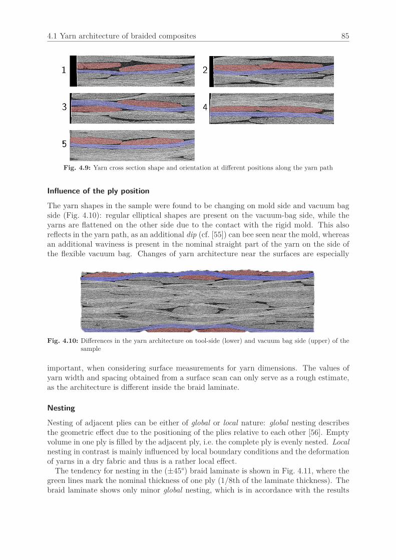
4.1 Yarn architecture of braided composites 85
Fig. 4.9: Yarn cross section shape and orientation at different positions along the yarn path
Influence of the ply position
The yarn shapes in the sample were found to be changing on mold side and vacuum bagside (Fig. 4.10): regular elliptical shapes are present on the vacuum-bag side, while theyarns are flattened on the other side due to the contact with the rigid mold. This alsoreflects in the yarn path, as an additional dip (cf. [55]) can bee seen near the mold, whereasan additional waviness is present in the nominal straight part of the yarn on the side ofthe flexible vacuum bag. Changes of yarn architecture near the surfaces are especially
Fig. 4.10: Differences in the yarn architecture on tool-side (lower) and vacuum bag side (upper) of thesample
important, when considering surface measurements for yarn dimensions. The values ofyarn width and spacing obtained from a surface scan can only serve as a rough estimate,as the architecture is different inside the braid laminate.
Nesting
Nesting of adjacent plies can be either of global or local nature: global nesting describesthe geometric effect due to the positioning of the plies relative to each other [56]. Emptyvolume in one ply is filled by the adjacent ply, i.e. the complete ply is evenly nested. Localnesting in contrast is mainly influenced by local boundary conditions and the deformationof yarns in a dry fabric and thus is a rather local effect.
The tendency for nesting in the (±45°) braid laminate is shown in Fig. 4.11, where thegreen lines mark the nominal thickness of one ply (1/8th of the laminate thickness). Thebraid laminate shows only minor global nesting, which is in accordance with the results

4.1 Yarn architecture of braided composites 86
of Lomov et al. [56], which describe geometric nesting to decrease with the tightness ofthe fabric. As the investigated fabrics are rather tight, there is almost no free volume tofill, thus less global nesting is present. It can be concluded that global nesting only has aminor effect for tight braid laminates. A nesting of the plies can only be observed locally,e.g. at the positions marked red in Fig. 4.11.
The stacking of the plies (i.e. the relative lateral position) does not follow a regulartrend. Both, plies placed identically on each other (In-Phase: IP, plies 6,7) and pliesshifted by twice the yarn width (Out-of-Phase: OP, plies 3,4) are present.
Fig. 4.11: Nesting effects in the (±45°) braid laminate
Assessment of micro-CT investigations
Summarizing the results of the measurements, the micro-CT method provides a goodpossibility to obtain qualitative information about the yarn architecture. The qualitativeresults can yield information for improved geometric models of the yarn architecture. Onthe other hand, optical microscopy offers a resolution seven times better compared tomicro-CT data. Automatic evaluation of the complete CT-data may be possible, butsimple thresholding for segmentation of yarns and matrix did not work for the samples,as the contrast between yarns and matrix was too low. Thus, improved image analysistechniques for post-processing or contrast enhancement techniques like given in [65] arerequired to gather qualitative results.
4.1.5. Summary and strategy for yarn architecture measurements
The investigations conducted on the characterization of yarn architecture of biaxial braidedcomposites can be summarized to a strategy for further measurements. Two sections per-pendicular to the yarn path of the two yarn directions in a biaxial braided compositesneed to be extracted. If yarn cross section dimensions shall be measured, the investigatedsection must be orthogonal to the yarn direction investigated, as this minimizes the errorintroduced by a possible misalignment of the sample. An approximation of the yarn crosssectional shape as an ellipse was shown to be reasonable: it eases the measuring procedure,as it provides both, yarn width and height, from a single measurement. An ellipse shapewas the best approximation of the yarn shapes in the investigated braids, but as otheryarn shapes are reported in literature (cf. Section 2.3), the idealization of shape needs tobe reviewed if different braids are investigated. The position of the extracted samples hadno significant effect on the results, except for the yarn height, which changed near thepanel edges. It is therefore recommended to avoid taking samples in the proximity of the

4.1 Yarn architecture of braided composites 87
panel edges. Six to eight sections for microscopy are required to obtain reliable resultswithin the margins defined above. For the braiding angle, measurements from an opticalsensor are recommended, as they take into account the yarn orientation from the com-plete area scanned. If such measuring techniques are not available, hand-measurementsas described above can be used. But it is noted that the hand measurements were shownto slightly overestimate the braiding angle and the accuracy suffers from the reducednumber of measurement points. The results from optical microscopy and optical sensormeasurements could provide all the information needed to create a geometrical model ofthe biaxial braided composite within WiseTex [46]. If additional details of the yarn archi-tecture are required, a micro-CT analysis can provide useful results regarding 3D-effectson yarn shape and path and for the creation of improved geometric models.

4.2 Off-axis experiments of biaxial braided composites 88
4.2. Off-axis experiments of biaxial braided composites
The elastic, nonlinear and failure behavior of a (±30°) braided composite has been studiedby using off-axis specimen tested under uniaxial load. The different off-axis angles allowto introduce different combinations of combined stress states into the specimens. A totalof six off-axis angles, namely ψ = 0°, 15°, 30°, 45°, 60°, 90° (see Fig. 4.12), were tested intension and compression.
Fig. 4.12: Overview of (±30°) off-axis experiments: ψ = 0°, 15°, 30°, 45°, 60°, 90°
The off-axis angles were chosen from preliminary analytical considerations with anequivalent laminate model. The ψ = 75° experiments were skipped as the test resultswere expected to be very similar to the ψ = 90° results. All experiments were conductedaccording to the procedures described in Section 3.4. The experiments and designationof the test series are summarized in Table 4.7. In the following sections, the results frommonotonic tensile, tensile loading/unloading and compressive experiments are described.Furthermore, a comparison between the tensile and compressive material behavior ofthe biaxial braided composites is given and conclusions for the formulation of predictivemodels are drawn.
Table 4.7.: Off-axis experiments with (±30°) braided composite
ψ = 0° ψ = 15° ψ = 30° ψ = 45° ψ = 60° ψ = 90°
tension PT_OA00 PT_OA15 PT_OA30 PT_OA45 PT_OA60 PT_OA90
compression PC_OA00 PC_OA15 PC_OA30 PC_OA45 PC_OA60 PC_OA90
4.2.1. Tensile experiments
OA00
For the OA00 test series, five monotonic and two loading/unloading experiments wereconducted. The test results are summarized in Table 4.8. The elastic moduli vary sig-nificantly between the coupons with the stiffest specimen having a modulus around 20%higher than the lowest one. This effect is attributed to the s-shape of the braid yarns,as described in Section 4.1.2: the braiding angle in the middle of the panel is higher (cf.Table 4.6a), which explains the increases of stiffness. As the specimen were cut over thewidth of a braided panel with the OA00_1 coupon located close to the panel edge, thecoupons 01 and 08 are the softest.

4.2 Off-axis experiments of biaxial braided composites 89
Table 4.8.: Test results from the BB30_PT_OA00 test series
Test ModulusASTM1
Modulusinitial
Poisson’sratio
Failurestrain
Strength
Ex [MPa] E0x [MPa] νxy [-] εUT S
OA00 [-] σUT SOA00 [MPa]
PT_OA00_01 32148 41641 1.50 0.0246 437.9PT_OA00_02 34326 43148 1.49 0.0235 453.7PT_OA00_03 35606 44249 1.51 0.0238 480.9PT_OA00_05 38843 47024 1.51 0.0212 495.1PT_OA00_06 39116 43461 1.50 0.0206 498.7PT_OA00_072 35245 42637 1.48 0.0235 462.5PT_OA00_082 32854 40252 1.50 0.0243 451.2
MEAN 35448 43202 1.50 0.0231 468.6STDV 2505 1972 0.01 0.0014 21.6CV (%) 7.1 4.6 0.7 6.2 4.6
1: evaluated within εxx = 0.001 − 0.003 2: loading/unloading experiment
The same trend can be observed for the initial stiffness, failure strain and strength:the lower braiding angle in the center of the panel results in higher initial moduli, lowerfailure strains and higher strength. Thus, the increased standard deviation of the valuescan be believed to be systematic and inherent for biaxial braided composites. Only smallinfluence of the braiding angle variation on the Poisson’s ratio was observed.
The effect of varying braiding angle is also visible in the stress-strain curves in Fig. 4.13a:the curves from all coupons are quite similar in shape, but have different initial slopes andend points. Small drops in the stress-strain curves are seen for strains over 1.5%, whichwere found to be due to edge-cracking of the specimen as e.g. shown in Fig. 4.14b.
εxx
[−]
σxx [M
Pa]
0 0.005 0.01 0.015 0.02 0.0250
100
200
300
400
500
01
02
03
05
06
E0
E ASTM
(a) Stress strain (b) Failure modes of the specimen
Fig. 4.13: Stress strain curves and failure modes from the BB30_PT_OA00 test series

4.2 Off-axis experiments of biaxial braided composites 90
Failure mode
The failure mode was similar for all coupons: the major crack1 included a broad area ofdamage oriented along one of the yarn directions, with exception of the coupon 05 thathad a macro crack orthogonal to the load direction. The occurrence of two failure modesfor BB30_OA00 specimens was also observed in a preliminary study [194], but the failuremode had no influence on the strength observed.
The failed specimen show a broad band of damage oriented around 30° to the loaddirection. Several intra-yarn cracks are seen on the yarns in the damaged area. In additionto the in-plane failure, a large delamination of the plies is present in the damaged area(Fig. 4.14a). The recordings from the high-speed camera are shown for a representativespecimen in Fig. 4.14b. The left image shows the coupon ultimately before the final failureand the other two images display the final failure process. Edge cracks are present onthe coupon surface, which was also observed in the DIC-measurements. They start todevelop at approximately 80% of the failure load. The cracks localize in the region, wherethe coupon finally fails: several transverse cracks spread over the coupon width along theF+ direction and the yarns oriented in the F- direction cannot resist the shear force andbreak as shown in the middle picture. The failure of the yarns can be summarized tobe introduced by shearing with many intra-yarn cracks distributed over the width of theyarns after final failure.
(a) Typical failure mode (b) Failure process
Fig. 4.14: Failure modes of the BB30_PT_OA00 test series
OA15
Six specimen were in total tested for the OA15 test series. Four specimen were loadedmonotonic up till failure and two loading/unloading experiments were conducted. Anoverview of the results in given in Table 4.9.
1major crack / macro crack: denotes the visible major crack of final failure, spreading over the completewith of the coupon. In contrast, micro-cracks or micro-cracking describes smaller cracks (size of ayarn width or unit cell) which develop on the coupon.

4.2 Off-axis experiments of biaxial braided composites 91
Table 4.9.: Test results from series BB30_PT_OA15
Test ModulusASTM1
Modulusinitial
Poisson’sratio
Failurestrain
Strength
Ex [MPa] E0x [MPa] νxy [-] εUT S
OA15 [-] σUT SOA15 [MPa]
PT_OA15_01 41079 46618 1.28 0.0184 520.3PT_OA15_02 41053 46895 1.30 0.0193 530.8PT_OA15_03 47663 53062 1.31 0.0169 589.8PT_OA15_042 48990 54315 1.28 0.0156 602.0PT_OA15_052 47295 52692 1.30 0.0151 552.5PT_OA15_06 45446 53598 1.30 0.0174 564.4
MEAN 45254 51197 1.29 0.0171 560.0STDV 3137 3180 0.01 0.0015 29.3CV [%] 6.9 6.2 0.9 8.7 5.2
1: evaluated within εxx = 0.001 − 0.003 2: loading/unloading experiment
Similar to the OA00 series, some variation can be seen within the moduli Ex and E0x
of the OA15 series. This is as for the OA00 series assumed to be related to variationsof the braiding angle. The variation reflects in modulus, strength and failure strain.The specimen 01 and 02 have approximately 13% lower moduli compared to the otherspecimen. This correlates with the optical sensor measurements made on the specimen,which exhibited an average braiding angle of approximately 1.5° higher for these specimen(cf. Fig. 4.26a).
Fig. 4.15a shows the stress-strain behavior of the monotonically loaded specimen. Thestress strain curves smoothly degrade from the start of the experiment up till final failure.This is in accordance with the observations made from DIC and high-speed camera duringthe experiments: they showed, besides a small number of edge cracks, no further crackingon the coupons before final failure.
Failure mode
The same failure mode was observed for all specimen tested, with the failure patternsshown in Fig. 4.15b. A detailed view to a failed specimen given in Fig. 4.16a, showsthe major crack is running along the 1F+ direction, which is oriented 45° to the loadaxis. Intra-yarn cracking in the 1F+ direction and yarn rupture in the 1F- direction wereobserved on the failed specimen. Furthermore, delamination of the plies in the laminateis present in the area of final failure. The high-speed camera videos show that transversecracking localized at the specimen edge is initiating the final failure (Fig. 4.16b). Thetransverse cracking is limited to the edges, no cracks were observed over the completecoupon width. The specimen fails rather abrupt by yarn rupture in the 1F- direction,with the major crack oriented along the 1F+ direction. The failure is believed to bedominated by the yarn rupture in the 1F- direction, but the crack orientation along the

4.2 Off-axis experiments of biaxial braided composites 92
εxx
[−]
σxx [
MP
a]
0 0.005 0.01 0.015 0.020
100
200
300
400
500
600
01
02
03
06
E0
E ASTM
(a) Stress strain (b) Failure modes of the specimen
Fig. 4.15: Stress strain curves and failure modes from the BB30_PT_OA15 test series
1F+ yarns indicated influence from the transverse cracking in the 1F+ directions, asreported by e.g. [122] for triaxial braids.
(a) Typical failure mode(b) Failure process
Fig. 4.16: Failure modes of the BB30_PT_OA15 test series
OA30
Monotonic experiments with six specimen were conducted for the OA30 series. Load-ing/unloading experiments were omitted for this test series, as preliminary experimentsshowed only minor non-linear effects in the stress-strain behavior. For the OA30 test series,the strain on the specimen surface was measured with the DIC-system in 2D mode. The2D mode was found to introduce an error in the strain measurement: due to an out-of-plane movement of the testing machine gripping device, the 2D strain measurement gavean artificial strain gradient on the coupon, which resulted in a non-physical s-shape ofthe stress-strain curve in the strain interval from εxx = 0 . . . 0.3% shown in Fig. 4.17. As

4.2 Off-axis experiments of biaxial braided composites 93
this non-linearity was judged unphysical, the stress-strain curves were linearized in thisregion.
εxx
[−]
σxx [
MP
a]
0 0.005 0.01 0.0150
100
200
300
400
500
600
700
800
900
Fig. 4.17: S-shape of the BB30_PT_OA30 curves due to the DIC error
An overview to the test series results is given in Table 4.10. The initial modulus is notgiven in the table, as it was identical to the ASTM modulus Ex. Modulus, strength andfailure strain all vary within approximately 5%, while the variation of the Poisson’s ratiois higher around 20%. The increased variation is attributed to the fact that the Poisson’sratio for OA30 is very sensitive to small deviations of the off-axis angle (cf. Fig. 4.26b).
Table 4.10.: Test results from series BB30_PT_OA30
Test ModulusASTM1
Poisson’sratio
Failurestrain
Strength
Ex [MPa] νxy [-] εUT SOA30 [-] σUT S
OA30 [MPa]
PT_OA30_01 67151 0.28 0.0121 856.9PT_OA30_02 68899 0.37 0.0113 798.9PT_OA30_03 68266 0.42 0.0116 877.6PT_OA30_04 64625 0.48 0.0116 754.5PT_OA30_05 66360 0.52 0.0115 755.9PT_OA30_06 64902 0.48 0.0126 813.9
MEAN 66701 0.42 0.0118 809.6STDV 1589 0.08 0.0005 46.4CV [%] 2.4 18.7 3.9 5.71: evaluated within εxx = 0.001 − 0.003
Fig. 4.18a shows the stress-strain curves, which are linear up till final failure. Some ofthe specimens exhibit a slight stiffening, which is attributed to spatial alignment of theyarns to the load and to yarn stretching (reduction of waviness). However, the increasein stiffness was not significant and not observed on all of the specimen, as some specimenhad a constant stiffness up till final failure.
Failure mode

4.2 Off-axis experiments of biaxial braided composites 94
εxx
[−]
σxx [M
Pa]
0 0.005 0.01 0.0150
100
200
300
400
500
600
700
800
900
01
02
03
04
05
06
E ASTM
(a) Stress strain (b) Failure modes of the specimen
Fig. 4.18: Stress strain curves and failure modes from the BB30_PT_OA30 test series
The failure mode of the OA30 coupons was similar to the OA15 test series: the majorfailure location is a narrow fracture band along the F+ direction (Fig. 4.19a). Intra-yarn cracking in the F+ direction and yarn rupture in the F- direction are visible frompostmortem inspection. For most of the specimen two major crack locations along thespecimen were present, as shown in Fig. 4.18a. The high speed videos revealed that oneof the two is the location of specimen final failure, while the other one is initiated byan elastic snap-back of the specimen after the first failure. Thus, the second failure iscompressive, which explains kink-band failure of the yarns observed by optical microscopyof the tested specimen. The high-speed videos shown in Fig. 4.19b furthermore show thatfinal failure initiates at the position of a transverse edge crack in the F+ direction. Themain failure is yarn rupture of the yarns in F- direction. The orientation of the majorcrack along the F+ direction furthermore implies that yarn rupture is influenced by strainconcentrations in the 1F+ direction.
(a) Typical failure mode
(b) Failure process
Fig. 4.19: Failure modes of the BB30_PT_OA30 test series
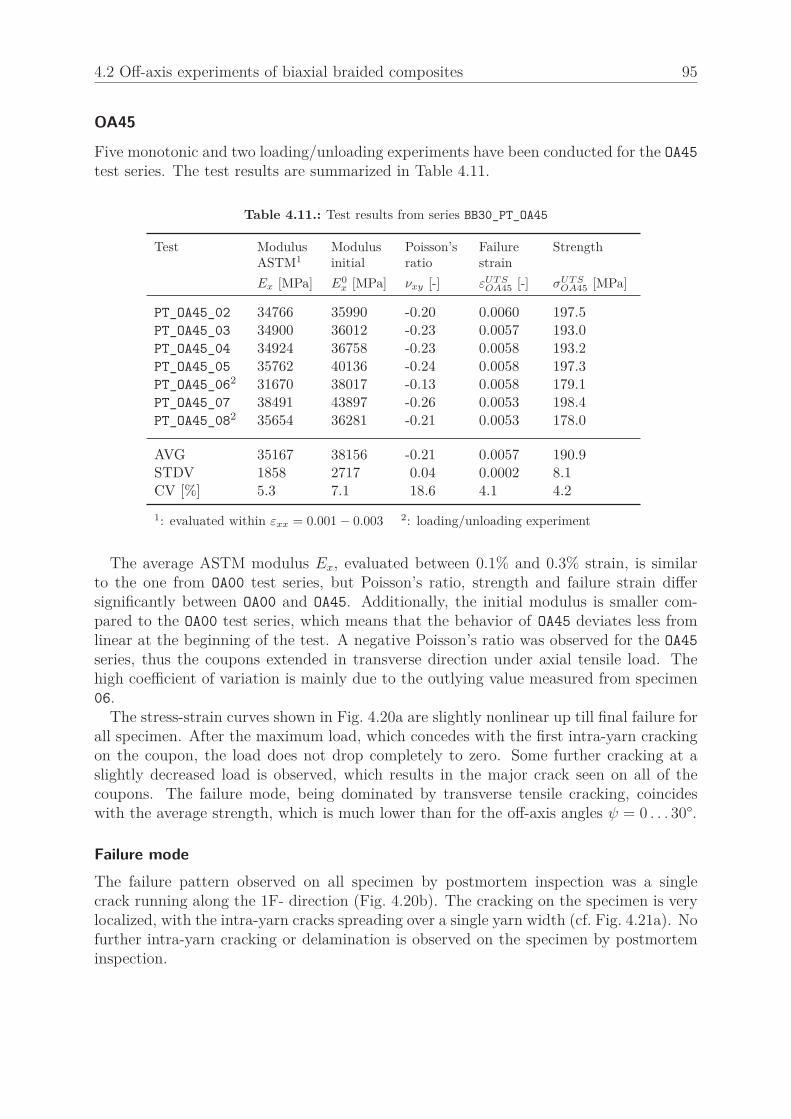
4.2 Off-axis experiments of biaxial braided composites 95
OA45
Five monotonic and two loading/unloading experiments have been conducted for the OA45
test series. The test results are summarized in Table 4.11.
Table 4.11.: Test results from series BB30_PT_OA45
Test ModulusASTM1
Modulusinitial
Poisson’sratio
Failurestrain
Strength
Ex [MPa] E0x [MPa] νxy [-] εUT S
OA45 [-] σUT SOA45 [MPa]
PT_OA45_02 34766 35990 -0.20 0.0060 197.5PT_OA45_03 34900 36012 -0.23 0.0057 193.0PT_OA45_04 34924 36758 -0.23 0.0058 193.2PT_OA45_05 35762 40136 -0.24 0.0058 197.3PT_OA45_062 31670 38017 -0.13 0.0058 179.1PT_OA45_07 38491 43897 -0.26 0.0053 198.4PT_OA45_082 35654 36281 -0.21 0.0053 178.0
AVG 35167 38156 -0.21 0.0057 190.9STDV 1858 2717 0.04 0.0002 8.1CV [%] 5.3 7.1 18.6 4.1 4.2
1: evaluated within εxx = 0.001 − 0.003 2: loading/unloading experiment
The average ASTM modulus Ex, evaluated between 0.1% and 0.3% strain, is similarto the one from OA00 test series, but Poisson’s ratio, strength and failure strain differsignificantly between OA00 and OA45. Additionally, the initial modulus is smaller com-pared to the OA00 test series, which means that the behavior of OA45 deviates less fromlinear at the beginning of the test. A negative Poisson’s ratio was observed for the OA45
series, thus the coupons extended in transverse direction under axial tensile load. Thehigh coefficient of variation is mainly due to the outlying value measured from specimen06.
The stress-strain curves shown in Fig. 4.20a are slightly nonlinear up till final failure forall specimen. After the maximum load, which concedes with the first intra-yarn crackingon the coupon, the load does not drop completely to zero. Some further cracking at aslightly decreased load is observed, which results in the major crack seen on all of thecoupons. The failure mode, being dominated by transverse tensile cracking, coincideswith the average strength, which is much lower than for the off-axis angles ψ = 0 . . . 30°.
Failure mode
The failure pattern observed on all specimen by postmortem inspection was a singlecrack running along the 1F- direction (Fig. 4.20b). The cracking on the specimen is verylocalized, with the intra-yarn cracks spreading over a single yarn width (cf. Fig. 4.21a). Nofurther intra-yarn cracking or delamination is observed on the specimen by postmorteminspection.
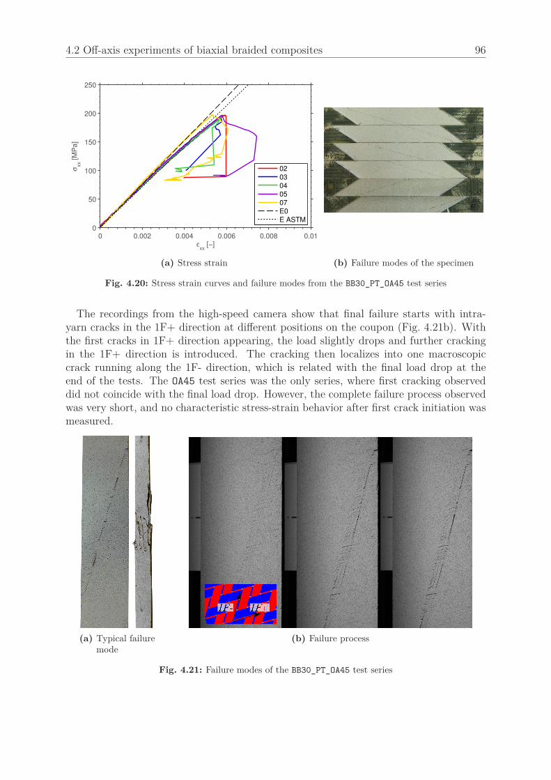
4.2 Off-axis experiments of biaxial braided composites 96
εxx
[−]
σxx [
MP
a]
0 0.002 0.004 0.006 0.008 0.010
50
100
150
200
250
02
03
04
05
07
E0
E ASTM
(a) Stress strain (b) Failure modes of the specimen
Fig. 4.20: Stress strain curves and failure modes from the BB30_PT_OA45 test series
The recordings from the high-speed camera show that final failure starts with intra-yarn cracks in the 1F+ direction at different positions on the coupon (Fig. 4.21b). Withthe first cracks in 1F+ direction appearing, the load slightly drops and further crackingin the 1F+ direction is introduced. The cracking then localizes into one macroscopiccrack running along the 1F- direction, which is related with the final load drop at theend of the tests. The OA45 test series was the only series, where first cracking observeddid not coincide with the final load drop. However, the complete failure process observedwas very short, and no characteristic stress-strain behavior after first crack initiation wasmeasured.
(a) Typical failuremode
(b) Failure process
Fig. 4.21: Failure modes of the BB30_PT_OA45 test series

4.2 Off-axis experiments of biaxial braided composites 97
OA60
For the OA60 test series, six specimen were tested in total. Four of the specimen wereloaded monotonically and two specimen were used for loading/unloading experiments.The results of the test series are summarized in Table 4.12. The initial modulus is onlyslightly higher compared to the ASTM modulus, which shows that the behavior is nearlylinear at the beginning of the test. All values except the Poisson’s ratio show smallvariations less than 5%. The increased variability in the Poisson’s ratio is attributed tothe small amount of transverse deformation, which leads to an increased effect of noisepresent in the strain signal.
Table 4.12.: Test results from series BB30_PT_OA60
Test ModulusASTM1
Modulusinitial
Poisson’sratio
Failurestrain
Strength
Ex [MPa] E0x [MPa] νxy [-] εUT S
OA60 [-] σUT SOA60 [MPa]
PT_OA60_012 16574 17158 0.06 0.0076 105.8PT_OA60_022 16829 17303 0.08 0.0074 105.1PT_OA60_03 16302 17336 0.07 0.0083 116.6PT_OA60_04 16231 18378 0.08 0.0075 108.6PT_OA60_05 15814 15629 0.08 0.0079 110.0PT_OA60_06 16034 16349 0.08 0.0077 109.6
AVG 16297 17025 0.07 0.0077 109.3STDV 333 859 0.01 0.0003 3.7CV [%] 2.0 5.0 11.6 3.8 3.4
1: evaluated within εxx = 0.001 − 0.003 2: loading/unloading experiment
Fig. 4.22a shows the stress-strain behavior of the specimen: the stress strain curve isnearly linear until an axial strain of εxx = 0.4% and progresses in a smooth degradationup till final failure. The stress-strain behavior is similar for all tested coupons and noinfluence from the different failure modes (cracking along 1F+ or 1F- cf. Fig. 4.22b) tothe stress-strain behavior was observed.
Failure mode
Two different failure modes were observed on the specimen after the experiments: themain crack was either running along 1F+ or along 1F- direction (Fig. 4.22a). In bothcases, the yarns in the direction transverse to the final crack showed several intra-yarncracks over the width. The high-speed videos, shown exemplarily in Fig. 4.23b, revealedthat the failure in both cases starts with intra-yarn cracking in one of the yarn directionsand localizes to a main crack oriented along 1F- or 1F+, which is spread over the completecoupon width. The failure of the specimen is rather brittle, as the first observation ofintra-yarn cracks on the specimen surface coincides with the major load drop.

4.2 Off-axis experiments of biaxial braided composites 98
εxx
[−]
σxx [
MP
a]
0 0.002 0.004 0.006 0.008 0.010
20
40
60
80
100
120
03
04
05
06
E0
E ASTM
(a) Stress strain (b) Failure modes of the specimen
Fig. 4.22: Stress strain curves and failure modes from the BB30_PT_OA60 test series
(a) Typical failure mode (b) Failure process
Fig. 4.23: Failure modes of the BB30_PT_OA60 test series
OA90
The results of the OA90 test series are summarized in Table 4.13. Seven specimen weretested at the off-axis angle of 90°, which is equivalent to the 22-direction of the braid.Two specimen were used for loading/unloading experiments, while the others were loadedmonotonically up till failure. All measured values show minor variations and the stiffnessand strength of OA90 are the lowest values measured for all tensile off-axis series.
The stress-strain curves of the OA90 series are shown in Fig. 4.24a. A smooth degrada-tion is observed for all specimen over the complete strain range, with the behavior beingnearly identical for the tested specimen. The first cracking observed on the specimen isidentical with the final load drop within the stress strain curve.
Failure mode
The failure modes observed on all coupons by postmortem inspection were similar to the

4.2 Off-axis experiments of biaxial braided composites 99
Table 4.13.: Test results from series BB30_PT_OA90
Test ModulusASTM1
Modulusinitial
Poisson’sratio
Failurestrain
Strength
Ex [MPa] E0x [MPa] νxy [-] εUT S
OA90 [-] σUT SOA90 [MPa]
PT_OA90_012 9244 10017 0.32 0.0105 76.7PT_OA90_02 9158 9988 0.33 0.0116 82.7PT_OA90_032 8595 10356 0.34 0.0113 80.2PT_OA90_04 8940 9654 0.33 0.0103 75.4PT_OA90_05 8930 9832 0.33 0.0116 80.5PT_OA90_06 8981 9824 0.33 0.0113 80.5PT_OA90_07 9124 10599 0.33 0.0102 76.5
AVG 8996 10039 0.33 0.0110 78.9STDV 197 306 0.00 0.0006 2.5CV [%] 2.2 3.0 1.2 5.1 3.2
1: evaluated within εxx = 0.001 − 0.003 2: loading/unloading experiment
OA60 case: the final failure is dominated by transverse cracking that localizes into a singlecrack, along one of the yarn directions (Fig. 4.25a). As the yarn directions 1F+ and 1F-are oriented at the same angle to the load direction, the cracking is observed in either oneof the two yarn directions (Fig. 4.24b). The high speed videos show that the failure of thespecimen is introduced by transverse cracking in one of the yarn directions and followedby the shear-failure of the other yarn direction shown in Fig. 4.25b. The yarns transverseto the main crack are unable to transport the shear force over the crack and shear off,which manifests in several intra-yarn cracks over the width.
εxx
[−]
σxx [
MP
a]
0 0.005 0.01 0.0150
10
20
30
40
50
60
70
80
90
02
04
05
06
07
E0
E ASTM
(a) Stress strain (b) Failure modes of the specimen
Fig. 4.24: Stress strain curves and failure modes from the BB30_PT_OA90 test series

4.2 Off-axis experiments of biaxial braided composites 100
(a) Typical failure mode (b) Failure process
Fig. 4.25: Failure mode of the BB30_PT_OA90 test series
Summary of the tensile off-axis experiments
The fiber volume fraction of the different off-axis test series varied in the range of 60%-62%. For the comparison of the tensile off-axis experiments, all properties measuredwere normalized to a fiber volume fraction of 60% according to the procedure givenin Section 3.4.7. A summary of the elastic properties measured in the tensile off-axisexperiments is given in Fig. 4.26. Both the initial elastic moduli and the one obtained inthe strain range of 0.1% − 0.3% plotted over the off-axis angle ψ are shown in Fig. 4.26a.The difference between the initial modulus and the one obtained according to the standard[84] within the range of 0.1 − 0.3% axial strain is most prominent for the off-axis anglesψ = 0° . . . 15°, while the difference is small for the bigger off-axis angles. The dotted linesgiven for Ex and E0
x represent the off-axis curves calculated from the measured elasticconstants E11, E22, G12 and ν12 by the equation
1
Eψ=
1
E11
cos4 ψ +1
E22
sin4 ψ + (1
G12
− 2ν12
E11
) sin2 ψ cos2 ψ (4.4)
As the shear modulus G12 was not measured, it was calculated by applying Eq. 4.4 to theψ = 30° off-axis experiment. The calculated off-axis curves show that the biaxial braidedcomposites behave orthotropic and that the ψ = θ experiment can be used to acquire theshear modulus.
To evaluate the influence of textile yarn architecture, the elastic properties are further-more compared to the properties of a angle-ply laminate . A comparison to two angle-plylaminates with (±29°) and (±31°) layup is given in Fig. 4.26a. The layup of the angle-plylaminates represents the range of braiding angles found on the coupons by optical sen-sor measurements. The elastic response of the laminates was calculated, neglecting yarnwaviness, with the UD properties given in Table A.3. The stiffness measured experimen-tally from the braided composite is between 10% and 20% lower as the one obtained fromthe angle-ply laminate. The difference is mainly attributed to the fiber waviness in thebraided composite. As the fiber stiffness dominates the properties for low off-axis anglesψ = 0 . . . 30°, the knock-down due to waviness is more prominent for these cases.
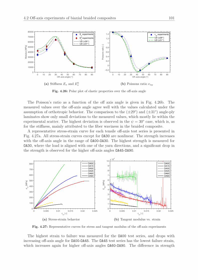
4.2 Off-axis experiments of biaxial braided composites 101
Off−axis angle [°]
Mo
du
lus [
MP
a]
0 10 20 30 40 50 60 70 80 90 0
10000
20000
30000
40000
50000
60000
70000
80000E
x experiments
Ex
0 experiments
UD (±29°)
UD (±31°)
(a) Stiffness Ex and E0x
Off−axis angle [°]
Po
isso
ns r
atio
[−
]
0 10 20 30 40 50 60 70 80 90
−0.2
0
0.2
0.4
0.6
0.8
1
1.2
1.4 νxy
experiments
UD (±29°)
UD (±31°)
(b) Poissons ratio νxy
Fig. 4.26: Polar plot of elastic properties over the off-axis angle
The Poisson’s ratio as a function of the off axis angle is given in Fig. 4.26b. Themeasured values over the off-axis angle agree well with the values calculated under theassumption of orthotropic behavior. The comparison to the (±29°) and (±31°) angle-plylaminates show only small deviations to the measured values, which mostly lie within theexperimental scatter. The highest deviation is observed in the ψ = 30° case, which is, asfor the stiffness, mainly attributed to the fiber waviness in the braided composite.
A representative stress-strain curve for each tensile off-axis test series is presented inFig. 4.27a. All stress-strain curves except for OA30 are nonlinear. The strength increaseswith the off-axis angle in the range of OA00-OA30. The highest strength is measured forOA30, where the load is aligned with one of the yarn directions, and a significant drop inthe strength is observed for the higher off-axis angles OA45-OA90.
εxx
[−]
σxx [M
Pa]
0 0.005 0.01 0.015 0.02 0.0250
100
200
300
400
500
600
700
800 OA00
OA15
OA30
OA45
OA60
OA90
(a) Stress-strain behavior
εxx
[−]
Eta
n [M
Pa]
0 0.005 0.01 0.015 0.02 0.0250
1
2
3
4
5
6
7
8
9
10x 10
4
OA00
OA15
OA30
OA45
OA60
OA90
(b) Tangent modulus vs. strain
Fig. 4.27: Representative curves for stress and tangent modulus of the off-axis experiments
The highest strain to failure was measured for the OA00 test series, and drops withincreasing off-axis angle for OA00-OA45. The OA45 test series has the lowest failure strain,which increases again for higher off-axis angles OA60-OA90. The difference in strength
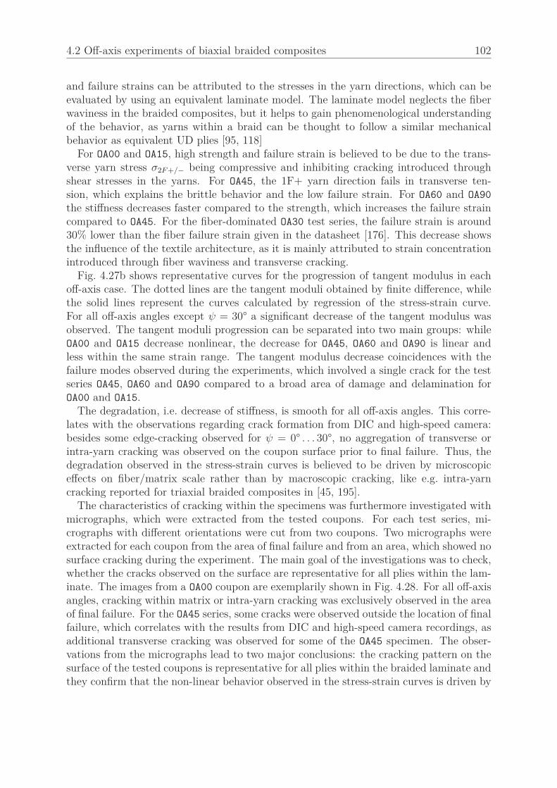
4.2 Off-axis experiments of biaxial braided composites 102
and failure strains can be attributed to the stresses in the yarn directions, which can beevaluated by using an equivalent laminate model. The laminate model neglects the fiberwaviness in the braided composites, but it helps to gain phenomenological understandingof the behavior, as yarns within a braid can be thought to follow a similar mechanicalbehavior as equivalent UD plies [95, 118]
For OA00 and OA15, high strength and failure strain is believed to be due to the trans-verse yarn stress σ2F+/− being compressive and inhibiting cracking introduced throughshear stresses in the yarns. For OA45, the 1F+ yarn direction fails in transverse ten-sion, which explains the brittle behavior and the low failure strain. For OA60 and OA90
the stiffness decreases faster compared to the strength, which increases the failure straincompared to OA45. For the fiber-dominated OA30 test series, the failure strain is around30% lower than the fiber failure strain given in the datasheet [176]. This decrease showsthe influence of the textile architecture, as it is mainly attributed to strain concentrationintroduced through fiber waviness and transverse cracking.
Fig. 4.27b shows representative curves for the progression of tangent modulus in eachoff-axis case. The dotted lines are the tangent moduli obtained by finite difference, whilethe solid lines represent the curves calculated by regression of the stress-strain curve.For all off-axis angles except ψ = 30° a significant decrease of the tangent modulus wasobserved. The tangent moduli progression can be separated into two main groups: whileOA00 and OA15 decrease nonlinear, the decrease for OA45, OA60 and OA90 is linear andless within the same strain range. The tangent modulus decrease coincidences with thefailure modes observed during the experiments, which involved a single crack for the testseries OA45, OA60 and OA90 compared to a broad area of damage and delamination forOA00 and OA15.
The degradation, i.e. decrease of stiffness, is smooth for all off-axis angles. This corre-lates with the observations regarding crack formation from DIC and high-speed camera:besides some edge-cracking observed for ψ = 0° . . . 30°, no aggregation of transverse orintra-yarn cracking was observed on the coupon surface prior to final failure. Thus, thedegradation observed in the stress-strain curves is believed to be driven by microscopiceffects on fiber/matrix scale rather than by macroscopic cracking, like e.g. intra-yarncracking reported for triaxial braided composites in [45, 195].
The characteristics of cracking within the specimens was furthermore investigated withmicrographs, which were extracted from the tested coupons. For each test series, mi-crographs with different orientations were cut from two coupons. Two micrographs wereextracted for each coupon from the area of final failure and from an area, which showed nosurface cracking during the experiment. The main goal of the investigations was to check,whether the cracks observed on the surface are representative for all plies within the lam-inate. The images from a OA00 coupon are exemplarily shown in Fig. 4.28. For all off-axisangles, cracking within matrix or intra-yarn cracking was exclusively observed in the areaof final failure. For the OA45 series, some cracks were observed outside the location of finalfailure, which correlates with the results from DIC and high-speed camera recordings, asadditional transverse cracking was observed for some of the OA45 specimen. The obser-vations from the micrographs lead to two major conclusions: the cracking pattern on thesurface of the tested coupons is representative for all plies within the braided laminate andthey confirm that the non-linear behavior observed in the stress-strain curves is driven by

4.2 Off-axis experiments of biaxial braided composites 103
Fig. 4.28: Micrographs of cracking within a OA00 specimen: cracks are solely observed in the region ofmacro-failure
microscopic damage events at the fiber/matrix scale as described in [170]. In addition,the first cracking observed was equal to the point of final failure for all test series.
4.2.2. Tensile loading/unloading experiments
Loading/unloading experiments were conducted to investigate the mechanics of the non-linear deformation observed in the monotonic experiments. Two loading/unloading ex-periments have been conducted for each of the test series OA00, OA15, OA45, OA60 andOA90. The specimens were loaded to a defined load level, unloaded to a small force andreloaded to the next load level. Four load levels were defined for each off-axis angle, wherethe load was increased up till failure in the fourth load cycle. It should be noted thatthe specimen were instantaneously re-loaded after reaching zero force, i.e. no informationabout time-dependency of the residual deformation has been acquired. However, the ef-fect of stress and strain relaxation were reported to be small for (±30°) carbon/epoxybraided composites by Kelkar and Whitcomb [26]. Thus viscous effects are unlikely tobe dominant. The complete description of test procedure and the evaluation is given inSection 3.4.6.
The assembled stress-strain curves obtained from the loading/unloading experimentsshowed a similar behavior as the ones obtained in the monotonic experiments. Bothstrength and strain to failure were in all cases within the range obtained by monotonicloading, i.e. no effect of the unloading and reloading to the measured response of thespecimen was found.
Stress-strain curves
A representative stress strain curve from a loading/unloading experiment for each off-axisangle tested is displayed in Fig. 4.29. Inelastic deformation is observed for all off-axisangles, with OA00 and OA15 showing the largest inelastic strains. For OA45, the behavioris almost linear and only negligible inelastic strains are observed, whereas a small amountof inelastic deformation is observed for OA60 and OA90.
Fig. 4.30 gives an overview to the inelastic strain εie and the damage variable d cal-culated from the stress-strain behavior of the experiments as described in Section 3.4.6.The lines refer to the average values, whereas the crosses mark the measurements. Thex-axis in the plots is the unloading strain ε(1) (cf. Fig. 3.23).

4.2 Off-axis experiments of biaxial braided composites 104
εxx
[−]
σxx [M
Pa]
0 0.005 0.01 0.015 0.02 0.0250
50
100
150
200
250
300
350
400
450
500
(a) OA00
εxx
[−]
σxx [M
Pa]
0 0.005 0.01 0.015 0.020
100
200
300
400
500
600
700
(b) OA15
εxx
[−]
σxx [M
Pa]
0 1 2 3 4 5 6
x 10−3
0
50
100
150
200
(c) OA45
εxx
[−]
σxx [M
Pa]
0 1 2 3 4 5 6 7 8
x 10−3
0
20
40
60
80
100
120
(d) OA60
εxx
[−]
σxx [M
Pa]
0 0.002 0.004 0.006 0.008 0.01 0.0120
10
20
30
40
50
60
70
80
90
100
(e) OA90
Fig. 4.29: Loading/unloading curves from the off-axis experiments
For the off-axis load-cases OA45, OA60 and OA90, the inelastic stain increases linearlywith the applied strain (Fig. 4.30a) and the inelastic strains measured are generally lowercompared to the other off-axis tests. In contrast to this, a nonlinear dependency isobserved for OA00 and OA15: the inelastic strains increase for higher strain values, i.e. theinelastic deformation is believed to become dominant for lager strains. For the damagevariable the dependency on the strain is also linear for OA45, OA60 and OA90. The slopeis different for the OA45 experiments, but a high scatter of results was observed in theseexperiments, which is attributed to the fact that only minor nonlinearity was observed

4.2 Off-axis experiments of biaxial braided composites 105
for this load case. For OA00 and OA15 the dependency is nonlinear and contrary to theinelastic deformation, as the slope tends to decrease for higher strains.
specimen strain εxx
(1) [−]
ine
lastic s
tra
in [
−]
0 0.005 0.01 0.015 0.020
0.5
1
1.5
2
2.5
3
3.5
4x 10
−3
OA00
OA15
OA45
OA60
OA90
(a) Inelastic strain εie
specimen strain εxx
(1) [−]
da
ma
ge
va
ria
ble
[−
]
0 0.005 0.01 0.015 0.020
0.05
0.1
0.15
0.2
0.25
0.3
0.35
0.4OA00
OA15
OA45
OA60
OA90
(b) Damage variable d
Fig. 4.30: Measures for inelastic deformation and damage from the loading/unloading experiments
Summarizing the loading/unloading experiments, a mixture of damage and inelasticdeformation is driving the non-linear stress-strain behavior of the (±30°) biaxial braidedcomposites. Whereas values of similar ranges are obtained for material damage at allthe off-axis experiments, inelastic strains are bigger for small off-axis angles. Fig. 4.31compares the inelastic deformation observed in the experiments with the case of idealinelastic deformation (cf. Eq. 3.19). The evaluation for the first cycle shows a big scatter,especially for higher off-axis angles. This is attributed to the small strains which arepresent during unloading of these experiments, where an evaluation error introduced bynoise of the strain signal has a higher influence. The scatter is much lower for the secondand third cycle, which reveal a clear trend: inelastic deformation has a higher influencefor the small off-axis angles.
0.3
0
0.4
1
0.4
9
0.4
1
0.3
7
0.4
1
0.2
5
0.2
1
0.2
5
0.9
5
0.2
5
0.2
0
0.4
0
0.2
3
0.1
6
1st cycle 2nd cycle 3rd cycle
0
20
40
60
80
100
ηIE
[%
]
OA00
OA15
OA45
OA60
OA90
Fig. 4.31: Amount of inelastic deformation obtained from comparison to ideal inelastic unloading
The behavior can be explained by qualitatively evaluating the stresses in an equiva-lent laminate model. The higher influence of inelastic strains for small off-axis anglesis mainly attributed to two reasons: firstly, the applied specimen stresses are higher for
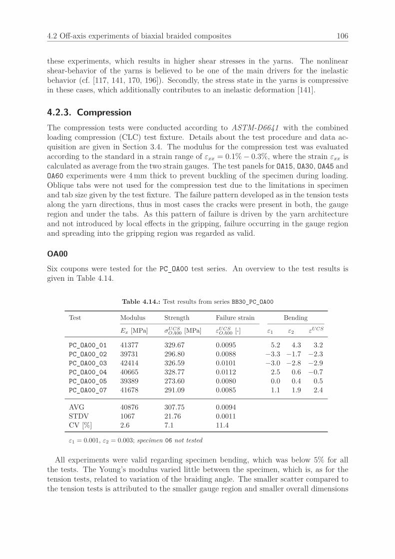
4.2 Off-axis experiments of biaxial braided composites 106
these experiments, which results in higher shear stresses in the yarns. The nonlinearshear-behavior of the yarns is believed to be one of the main drivers for the inelasticbehavior (cf. [117, 141, 170, 196]). Secondly, the stress state in the yarns is compressivein these cases, which additionally contributes to an inelastic deformation [141].
4.2.3. Compression
The compression tests were conducted according to ASTM-D6641 with the combinedloading compression (CLC) test fixture. Details about the test procedure and data ac-quisition are given in Section 3.4. The modulus for the compression test was evaluatedaccording to the standard in a strain range of εxx = 0.1% − 0.3%, where the strain εxx iscalculated as average from the two strain gauges. The test panels for OA15, OA30, OA45 andOA60 experiments were 4 mm thick to prevent buckling of the specimen during loading.Oblique tabs were not used for the compression test due to the limitations in specimenand tab size given by the test fixture. The failure pattern developed as in the tension testsalong the yarn directions, thus in most cases the cracks were present in both, the gaugeregion and under the tabs. As this pattern of failure is driven by the yarn architectureand not introduced by local effects in the gripping, failure occurring in the gauge regionand spreading into the gripping region was regarded as valid.
OA00
Six coupons were tested for the PC_OA00 test series. An overview to the test results isgiven in Table 4.14.
Table 4.14.: Test results from series BB30_PC_OA00
Test Modulus Strength Failure strain Bending
Ex [MPa] σUCSOA00 [MPa] εUCS
OA00 [-] ε1 ε2 εUCS
PC_OA00_01 41377 329.67 0.0095 5.2 4.3 3.2PC_OA00_02 39731 296.80 0.0088 −3.3 −1.7 −2.3PC_OA00_03 42414 326.59 0.0101 −3.0 −2.8 −2.9PC_OA00_04 40665 328.77 0.0112 2.5 0.6 −0.7PC_OA00_05 39389 273.60 0.0080 0.0 0.4 0.5PC_OA00_07 41678 291.09 0.0085 1.1 1.9 2.4
AVG 40876 307.75 0.0094STDV 1067 21.76 0.0011CV [%] 2.6 7.1 11.4
ε1 = 0.001, ε2 = 0.003; specimen 06 not tested
All experiments were valid regarding specimen bending, which was below 5% for allthe tests. The Young’s modulus varied little between the specimen, which is, as for thetension tests, related to variation of the braiding angle. The smaller scatter compared tothe tension tests is attributed to the smaller gauge region and smaller overall dimensions

4.2 Off-axis experiments of biaxial braided composites 107
of the compression coupons. As the braiding angle varies systematically over the panel,less braiding angle variation is present in smaller specimens.
The stress-strain behavior of the specimen is shown in Fig. 4.32a and varies only littlebetween the different experiments, which is an effect of the decreased braiding anglevariation. The knee in the behavior of the specimen 03 is attributed to cracking under
εxx
[−]
σxx [M
Pa]
0 0.002 0.004 0.006 0.008 0.01 0.0120
50
100
150
200
250
300
350
01
02
03
04
05
07
E ASTM
(a) (b)
Fig. 4.32: Stress-strain curves and typical failure modes from the BB30_PC_OA00 test series
one of the two strain gauges directly before final failure.Typical failure modes of the specimen are shown in Fig. 4.32b. All coupons failed within
the gauge region by one or several cracks developing across the width of the coupon. Thecracks were along one of the yarn directions, and thus running partly under the tabs. Forthe single crack failure, one crack along the yarn direction developed over the completewidth of the coupon, while a zig-zag pattern of cracks was observed for the coupons withseveral cracks. No influence of the failure pattern to the strength or failure strain wasobserved, but the specimen failing in several cracks showed some residual strength afterthe first major load drop (not shown in Fig. 4.32a as the strain gauges failed with thefirst major load drop). As observed in the tensile experiments, the failure is abrupt andwithout previous specimen cracking. The damaged region of the coupon is rather small,comparable to the tensile experiments with high off-axis angles (OA45-OA90).
OA15
Seven specimen were tested for the PC_OA15 test series. For three specimen, increasedbending values were measured at the beginning of the experiments (cf. Table 4.15), butas the bending decreased with further increasing load, the experiments were considered tobe valid. The variance in stiffness, strength and failure strain between the experiments isvery small, which, as for PC_OA00, is attributed to the decreased braiding angle variationcompared to the tensile tests. The stress-strain behavior (Fig. 4.32a) is slightly nonlinearup to a specimen strain of εxx = 0.5% and progresses nonlinear up till failure. All

4.2 Off-axis experiments of biaxial braided composites 108
Table 4.15.: Test results from series BB30_PC_OA15
Test Modulus Strength Failure strain Bending
Ex [MPa] σUCSOA15 [MPa] εUCS
OA15 [-] ε1 ε2 εUCS
PC_OA15_01 52717 435.38 0.0095 −2.1 −1.2 −0.7PC_OA15_02 53910 457.19 0.0101 0.6 0.8 0.7PC_OA15_03 54631 436.44 0.0098 14.2 5.8 4.2PC_OA15_04 47904 414.13 0.0104 11.8 7.7 8.2PC_OA15_05 50714 418.58 0.0100 8.3 4.3 3.5PC_OA15_06 50276 425.01 0.0096 −5.5 −5.5 −7.1PC_OA15_07 51801 423.61 0.0096 16.9 10.7 8.7
AVG 51708 430.05 0.0098STDV 2136 13.40 0.0003CV [%] 4.1 3.1 3.1
ε1 = 0.001, ε2 = 0.003
specimen failed in a single crack along the 1F+ direction, which is oriented 45° to theloading direction. A typical failure mode is shown in Fig. 4.33b: the failure is similar tothe OA00_PC series with a single crack running across the width of the coupon and thedamaged region being limited to the cracking surface. Besides the main crack, no furtherdamage is observed on the coupon.
εxx
[−]
σxx [M
Pa]
0 0.002 0.004 0.006 0.008 0.01 0.0120
100
200
300
400
500
01
02
03
04
05
06
07
E ASTM
(a) (b)
Fig. 4.33: Stress-strain curves and typical failure modes from the BB30_PC_OA15 test series

4.2 Off-axis experiments of biaxial braided composites 109
OA30
Seven specimen were tested for the PC_OA30 test series. An overview to the test resultsis given in Table 4.16.
Table 4.16.: Test results from series BB30_PC_OA30
Test Modulus Strength Failure strain Bending
Ex [MPa] σUCSOA30 [MPa] εUCS
OA30 [-] ε1 ε2 εUCS
PC_OA30_01 66367 618.73 0.0101 14.8 15.4 17.5PC_OA30_02 64712 590.43 0.0100 35.6 18.1 13.2PC_OA30_03 67677 672.81 0.0091 1.8 0.1 9.8PC_OA30_04 64411 647.23 0.0127 0.6 −1.2 −12.4PC_OA30_05 64249 580.31 0.0098 2.2 −0.3 −2.2PC_OA30_06 64279 593.41 0.0109 1.9 2.4 6.1PC_OA30_07 65572 633.10 0.0104 1.3 2.7 10.0
AVG 65324 619.43 0.0104STDV 1204 31.30 0.0011CV [%] 1.8 5.1 10.2
ε1 = 0.001, ε2 = 0.003
Large values of specimen bending were present for two specimen (01 and 02) over thecomplete experiment up till failure (Fig. 4.34). Additionally, increased bending valuesat specimen failure were measured for the specimens 04 and 07. In the latter case, theincreased bending values were due to preliminary surface cracking under one of the straingauges, leading to a sudden overshoot of one of the strain signals. For the specimen 01 and
εxx
[−]
be
nd
ing
[%
]
0 0.002 0.004 0.006 0.008 0.01 0.012 0.014−20
−15
−10
−5
0
5
10
15
20
01
02
03
04
05
06
07
Fig. 4.34: Bending values measured for the BB30_PC_OA30 test series
02, increased bending was measured over the complete experiment, but as the specimenshowed no significant difference in stiffness and strength compared to the specimen withlower bending values, they were considered valid. The increased values of bending arebelieved to be an effect of the comparable small strain gauge size: as the strain gauges

4.2 Off-axis experiments of biaxial braided composites 110
are smaller than a unit cell of the braided composite, local inhomogeneity of the strainfield may be the cause of the difference in strain signals.
The stiffness and strength measured from the experiments showed low scatter, with theincreased variation of the failure strain being attributed to the described preliminary straingauge failures. The stress-strain behavior of the specimen is given in Fig. 4.35a: differentto the tensile OA30 experiments, some nonlinearity can be observed in the compressiveOA30 stress-strain curves. The jumps observed in some of the stress-strain curves (e.g. 03
and 06) are the consequence of the preliminary failure of one of the strain gauges.
εxx
[−]
σxx [M
Pa]
0 0.002 0.004 0.006 0.008 0.01 0.0120
100
200
300
400
500
600
700
01
02
03
04
05
06
07
E ASTM
(a) (b)
Fig. 4.35: Stress-strain curves and typical failure modes from the BB30_PC_OA30 test series
Typical failure patterns of the specimen are shown in Fig. 4.35b: all specimens failedwith the major cracking being oriented along the 1F+ yarn direction, which is inclined60° to the load axis. The plies of the braided laminates were spread open at the loca-tion of major cracking and a broad zone of damage within the gauge region is observed.The damage in the specimen includes transverse intra-yarn cracking, intra- and inter-plydelamination as well as yarn compressive failure. Compressive fiber failure is believed tocontrol the failure behavior, as most yarns failed in the 1F- direction.
OA45
For the PC_OA45 test series, six specimen were tested, with an overview of the results givenin Table 4.17. Bending values bigger than 10% were observed during the experiments forall specimens except one. For the specimen 03, 06 and 07, the bending decreased withloading, which indicates that the difference in strain between the two sides is not dueto specimen bending. For the specimens 05 and 08, the measured bending value stayedalmost constant and increased with loading, respectively. As the measured values formodulus, strength and failure strain of these specimen were in the range of the propertiesmeasured from the other tests, the specimens were considered valid. The stress-strainbehavior of the specimen, shown in Fig. 4.36a, is almost linear until εxx = 0.5% and
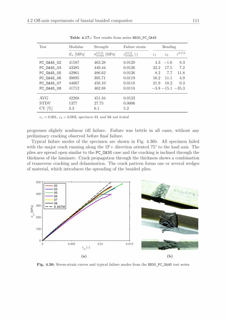
4.2 Off-axis experiments of biaxial braided composites 111
Table 4.17.: Test results from series BB30_PC_OA45
Test Modulus Strength Failure strain Bending
Ex [MPa] σUCSOA45 [MPa] εUCS
OA45 [-] ε1 ε2 εUCS
PC_OA45_02 41587 463.28 0.0120 4.3 −1.6 8.3PC_OA45_03 43385 449.44 0.0126 32.2 17.5 7.2PC_OA45_05 42961 486.62 0.0136 8.2 7.7 11.8PC_OA45_06 39895 395.71 0.0119 16.2 11.1 4.9PC_OA45_07 44067 450.10 0.0118 21.9 10.2 0.3PC_OA45_08 41712 462.88 0.0118 −3.8 −15.1 −35.3
AVG 42268 451.34 0.0123STDV 1377 27.75 0.0006CV [%] 3.3 6.1 5.2
ε1 = 0.001, ε2 = 0.003; specimen 01 and 04 not tested
progresses slightly nonlinear till failure. Failure was brittle in all cases, without anypreliminary cracking observed before final failure.
Typical failure modes of the specimen are shown in Fig. 4.36b. All specimen failedwith the major crack running along the 1F+ direction oriented 75° to the load axis. Theplies are spread open similar to the PC_OA30 case and the cracking is inclined through thethickness of the laminate. Crack propagation through the thickness shows a combinationof transverse cracking and delamination. The crack pattern forms one or several wedgesof material, which introduces the spreading of the braided plies.
εxx
[−]
σxx [M
Pa]
0 0.005 0.01 0.0150
100
200
300
400
500
02
03
05
06
07
08
E ASTM
(a) (b)
Fig. 4.36: Stress-strain curves and typical failure modes from the BB30_PC_OA45 test series
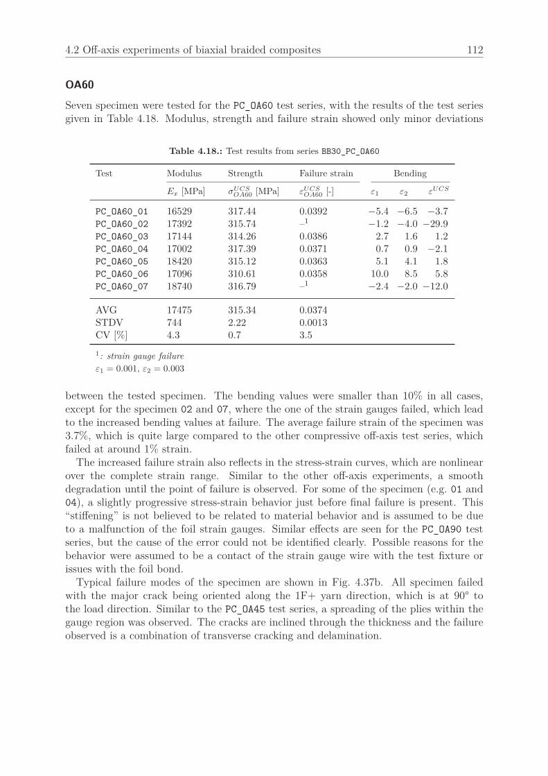
4.2 Off-axis experiments of biaxial braided composites 112
OA60
Seven specimen were tested for the PC_OA60 test series, with the results of the test seriesgiven in Table 4.18. Modulus, strength and failure strain showed only minor deviations
Table 4.18.: Test results from series BB30_PC_OA60
Test Modulus Strength Failure strain Bending
Ex [MPa] σUCSOA60 [MPa] εUCS
OA60 [-] ε1 ε2 εUCS
PC_OA60_01 16529 317.44 0.0392 −5.4 −6.5 −3.7PC_OA60_02 17392 315.74 –1 −1.2 −4.0 −29.9PC_OA60_03 17144 314.26 0.0386 2.7 1.6 1.2PC_OA60_04 17002 317.39 0.0371 0.7 0.9 −2.1PC_OA60_05 18420 315.12 0.0363 5.1 4.1 1.8PC_OA60_06 17096 310.61 0.0358 10.0 8.5 5.8PC_OA60_07 18740 316.79 –1 −2.4 −2.0 −12.0
AVG 17475 315.34 0.0374STDV 744 2.22 0.0013CV [%] 4.3 0.7 3.5
1: strain gauge failure
ε1 = 0.001, ε2 = 0.003
between the tested specimen. The bending values were smaller than 10% in all cases,except for the specimen 02 and 07, where the one of the strain gauges failed, which leadto the increased bending values at failure. The average failure strain of the specimen was3.7%, which is quite large compared to the other compressive off-axis test series, whichfailed at around 1% strain.
The increased failure strain also reflects in the stress-strain curves, which are nonlinearover the complete strain range. Similar to the other off-axis experiments, a smoothdegradation until the point of failure is observed. For some of the specimen (e.g. 01 and04), a slightly progressive stress-strain behavior just before final failure is present. This“stiffening” is not believed to be related to material behavior and is assumed to be dueto a malfunction of the foil strain gauges. Similar effects are seen for the PC_OA90 testseries, but the cause of the error could not be identified clearly. Possible reasons for thebehavior were assumed to be a contact of the strain gauge wire with the test fixture orissues with the foil bond.
Typical failure modes of the specimen are shown in Fig. 4.37b. All specimen failedwith the major crack being oriented along the 1F+ yarn direction, which is at 90° tothe load direction. Similar to the PC_OA45 test series, a spreading of the plies within thegauge region was observed. The cracks are inclined through the thickness and the failureobserved is a combination of transverse cracking and delamination.
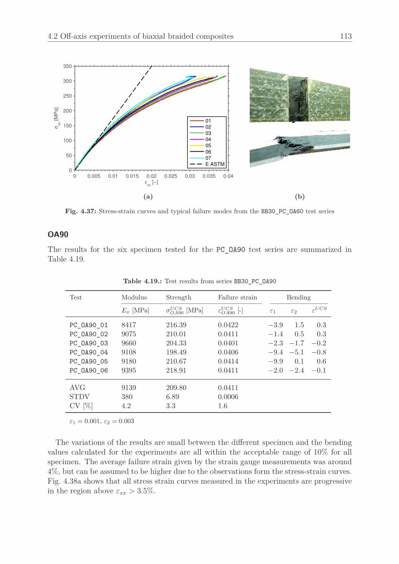
4.2 Off-axis experiments of biaxial braided composites 113
εxx
[−]
σxx [M
Pa]
0 0.005 0.01 0.015 0.02 0.025 0.03 0.035 0.040
50
100
150
200
250
300
350
01
02
03
04
05
06
07
E ASTM
(a) (b)
Fig. 4.37: Stress-strain curves and typical failure modes from the BB30_PC_OA60 test series
OA90
The results for the six specimen tested for the PC_OA90 test series are summarized inTable 4.19.
Table 4.19.: Test results from series BB30_PC_OA90
Test Modulus Strength Failure strain Bending
Ex [MPa] σUCSOA90 [MPa] εUCS
OA90 [-] ε1 ε2 εUCS
PC_OA90_01 8417 216.39 0.0422 −3.9 1.5 0.3PC_OA90_02 9075 210.01 0.0411 −1.4 0.5 0.3PC_OA90_03 9660 204.33 0.0401 −2.3 −1.7 −0.2PC_OA90_04 9108 198.49 0.0406 −9.4 −5.1 −0.8PC_OA90_05 9180 210.67 0.0414 −9.9 0.1 0.6PC_OA90_06 9395 218.91 0.0411 −2.0 −2.4 −0.1
AVG 9139 209.80 0.0411STDV 380 6.89 0.0006CV [%] 4.2 3.3 1.6
ε1 = 0.001, ε2 = 0.003
The variations of the results are small between the different specimen and the bendingvalues calculated for the experiments are all within the acceptable range of 10% for allspecimen. The average failure strain given by the strain gauge measurements was around4%, but can be assumed to be higher due to the observations form the stress-strain curves.Fig. 4.38a shows that all stress strain curves measured in the experiments are progressivein the region above εxx > 3.5%.

4.2 Off-axis experiments of biaxial braided composites 114
εxx
[−]
σxx [M
Pa]
0 0.01 0.02 0.03 0.04 0.050
50
100
150
200
250
01
02
03
04
05
06
E ASTM
(a) (b)
Fig. 4.38: Stress-strain curves and typical failure modes from the BB30_PC_OA90 test series
This effect is similar to the one observed in the PC_OA60 experiments and is assumedto be due to a malfunction of the strain gauge measurement. Linear extrapolation of thestrain signal gave the failure strain to be around εxx = 5%. Neglecting the progressiveregion at the end, the stress strain behavior of all specimen shows a smooth degradationof the stiffness up till final failure. The failure observed for all specimen was abrupt,without preliminary cracking, as in the other off-axis test series. Typical failure patternsare shown in Fig. 4.38b. A zig-zag path of the major crack running across the width ofthe coupons is observed for all of the specimen. The crack runs along the yarn edges ofthe upper ply and is inclined through the thickness (Fig. 4.38b). Different to the PC_OA45
and PC_OA60 experiments, only minor spreading of the plies was seen in the PC_OA90
experiments.
Summary of the off-axis compression experiments
All properties were normalized to a fiber volume fraction of 60% for the comparison. TheYoung’s moduli of the off-axis experiments are summarized in an off-axis plot in Fig. 4.39.Additionally, the off-axis moduli of (±29°) and (±31°) angle-ply laminates, neglecting yarnwaviness (UD properties from Table A.3), are given. The elastic results are similar to theones obtained from the tension tests: stiffness knockdown due to waviness is mainly seenfor the load applied in one of the fiber directions (ψ = 30°) and for the lower off-axisangles (ψ = 0° . . . 30°).
A representative stress-strain curve from every test series is shown in Fig. 4.40a. Indifference to the tension tests, a nonlinear behavior is obtained for all off-axis angles.Also for the ψ = 30° experiments, where one of the yarn directions is aligned with theload, a nonlinear stress-strain behavior was measured. The stress-strain curves show astiffer behavior for ψ = 0 . . . 45°, while ψ = 60 . . . 90° behaves much softer. The higheststrength is measured for the load aligned with one of the yarn directions ψ = 30°, butdifferent to the tensile tests similar strength are measured for ψ = 15° and ψ = 45° aswell as for ψ = 0° and ψ = 60°. The failure strain is lower than 1% for ψ = 0° . . . 30° and
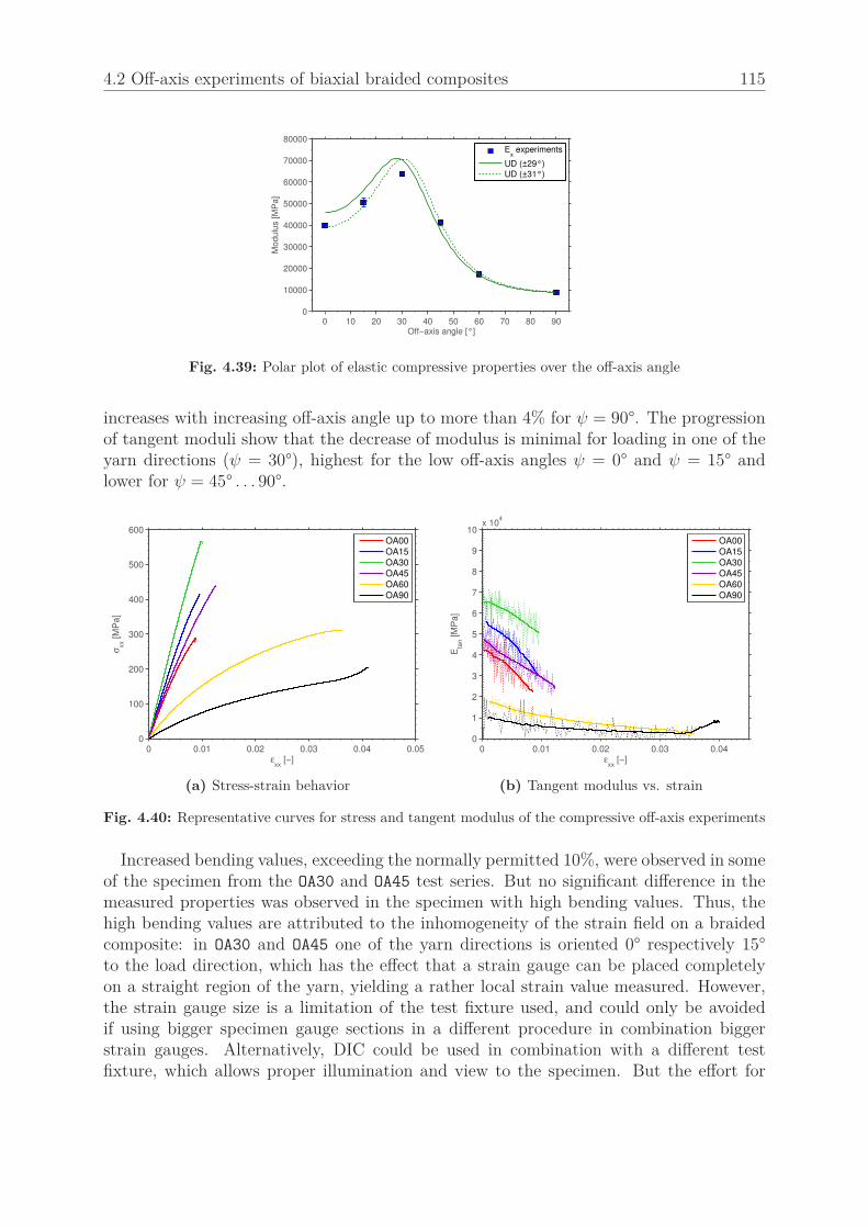
4.2 Off-axis experiments of biaxial braided composites 115
Off−axis angle [°]
Mo
du
lus [
MP
a]
0 10 20 30 40 50 60 70 80 90 0
10000
20000
30000
40000
50000
60000
70000
80000E
x experiments
UD (±29°)
UD (±31°)
Fig. 4.39: Polar plot of elastic compressive properties over the off-axis angle
increases with increasing off-axis angle up to more than 4% for ψ = 90°. The progressionof tangent moduli show that the decrease of modulus is minimal for loading in one of theyarn directions (ψ = 30°), highest for the low off-axis angles ψ = 0° and ψ = 15° andlower for ψ = 45° . . . 90°.
εxx
[−]
σxx [M
Pa]
0 0.01 0.02 0.03 0.04 0.050
100
200
300
400
500
600
OA00
OA15
OA30
OA45
OA60
OA90
(a) Stress-strain behavior
εxx
[−]
Eta
n [M
Pa]
0 0.01 0.02 0.03 0.040
1
2
3
4
5
6
7
8
9
10x 10
4
OA00
OA15
OA30
OA45
OA60
OA90
(b) Tangent modulus vs. strain
Fig. 4.40: Representative curves for stress and tangent modulus of the compressive off-axis experiments
Increased bending values, exceeding the normally permitted 10%, were observed in someof the specimen from the OA30 and OA45 test series. But no significant difference in themeasured properties was observed in the specimen with high bending values. Thus, thehigh bending values are attributed to the inhomogeneity of the strain field on a braidedcomposite: in OA30 and OA45 one of the yarn directions is oriented 0° respectively 15°to the load direction, which has the effect that a strain gauge can be placed completelyon a straight region of the yarn, yielding a rather local strain value measured. However,the strain gauge size is a limitation of the test fixture used, and could only be avoidedif using bigger specimen gauge sections in a different procedure in combination biggerstrain gauges. Alternatively, DIC could be used in combination with a different testfixture, which allows proper illumination and view to the specimen. But the effort for

4.2 Off-axis experiments of biaxial braided composites 116
measurements drastically increases, as two DIC systems are needed to measure strain onboth sides of the specimen. It can be concluded that the CLC test procedure used offers agood possibility for off-axis compression tests of braided composites. Alternative test pro-cedures including bigger specimen gauge sections could be favorable, but the developmentof improved measuring techniques was out of scope of the presented investigations.
The failure patterns observed on the specimen by postmortem inspection (Fig. 4.41) canbe grouped into 2 main failure modes: for OA00 and OA15, a single crack across the widthoccurred with no delamination between the plies and small damaged zone on the specimen.For OA30, OA45, OA60 and OA90 a broad damaged zone with delamination between the pliesand the crack being inclined in the thickness direction was present. For OA30, compressivefiber failure was observed, while the other off-axis angles were dominated by transversecracking. The OA90 test series failed in single crack across the coupon width, with thefailure mode being similar to OA45 and OA60, but with less delamination and withoutspreading of the plies in the specimen.
(a) OA00 (b) OA15 (c) OA30 (d) OA45 (e) OA60 (f) OA90
Fig. 4.41: Failure modes of the specimen observed in the compression tests
4.2.4. Comparison of tension and compression off-axis experiments
For the comparison of tensile and compressive off-axis experiments, all properties werenormalized to 60% FVF according to the procedure given in Section 3.4.7.
Stiffness
The comparison of tensile and compressive Young’s moduli is given in Fig. 4.42. Themodulus evaluated in the strain interval εxx = 0.1% − 0.3% is used for the comparison.The moduli obtained in tension and compression are very similar for all off-axis anglestested, with the OA00, OA15 and OA45 compressive moduli being slightly higher thanthe tensile ones. For OA00 and OA15 this is mainly attributed to the material volumetested being smaller for the compressive tests, which decreases the effects of braidingangle variation observed in the tensile tests. Additionally the stress-strain behavior ofthe compressive experiments was less nonlinear for low strains, i.e. the modulus Ex wascloser to the initial modulus. For the OA45 test series, the difference is likely to be duemanufacturing tolerances in the off-axis angle, which have a high effect on the stiffness ofthe OA45 experiments (cf. Fig. 4.39).

4.2 Off-axis experiments of biaxial braided composites 117
OA00 OA15 OA30 OA45 OA60 OA900
10000
20000
30000
40000
50000
60000
70000
Yo
un
g's
Mo
du
lus [
MP
a]
PT
PC
Fig. 4.42: Comparison of Young’s moduli obtained from tension and compression off-axis experiments
Strength, failure strain and failure modes
A comparison of the strength obtained from the tensile and compressive off-axis exper-iments is given in Fig. 4.43a. For both, tension and compression, the highest strengthis observed in the OA30 case, where the load is aligned with one of the yarn directions.Comparing the strength between tension and compression, the tensile strength exceed thecompressive ones for the low off-axis angles 0° − 30°, while an opposite effect is observedfor the off-axis angles 45° − 90°. For the failure strains given in Fig. 4.43b, a similar trendis observed. Here, the highest failure strains in tension are obtained in the OA00 load case,while the compressive failure strains are maximal for the OA90 experiments.
The difference in strength for the OA30 loading is believed to be due to the difference inlongitudinal fiber strength in tension and compression. For the other off-axis angles, the
OA00 OA15 OA30 OA45 OA60 OA900
100
200
300
400
500
600
700
800
Str
en
gth
[M
Pa
]
PT
PC
(a) strength
OA00 OA15 OA30 OA45 OA60 OA900.00
0.01
0.02
0.03
0.04
0.05
failu
re s
tra
in [
-]
PT
PC
(b) failure strain
Fig. 4.43: Comparison of strength and failure strain from the off-axis experiments
failure modes observed were dominated by the transverse cracking, and the difference instrength and failure strain can be explained by evaluating a (±30°) equivalent laminatemodel. If a uniaxial tensile load is applied, the transverse yarn stress (σ2F+, σ2F−, cf.Fig. 3.1) is compressive for the off-axis angles ψ = 0° and ψ = 15° and tensile forthe higher off-axis angles. For a uniaxial compressive stress, the sign of the transverse

4.2 Off-axis experiments of biaxial braided composites 118
yarn stress is opposite. The equivalent laminate model suggests two explanations for thedifference in tensile and compressive strength:
• The transverse compressive strength of the yarns is, similar to UD composites,significantly higher as the transverse tensile strength. Thus, a failure with tensionaltransverse yarn stresses occurs at lower stresses.
• In the case of a transverse compressive yarn stress, cracks being initiated by shearstresses in the yarns may be kept closed by the transverse compression, i.e. highershear stresses in the yarns are possible.
The comparison of failure stresses measured in the off-axis experiments shows that themechanics of failure in biaxial braided composites follow the same trends as unidirectionalcomposites, when the stresses in the yarn coordinate system are considered. Thus, thestatement of Puck [95] can be approved, which encourages the application of UD failuretheories to the yarn stresses for both, unit cells and macroscopic equivalent laminatemodels.
The differences observed between tensile and compressive loading are also reflected inthe failure modes of the specimen compared in Fig. 4.44. Fiber failure is present in theOA30 experiments in tension and compression. For the other test series, the failure modeis shear-initiated transverse cracking, with a strong dependence of the failure patters tothe transverse yarn stress: a broad damaged area including delamination was observedin PT_OA00 and PT_OA15 experiments as well as in the PC_OA45, PC_OA60 and PC_OA90
series, while failure by a single crack was observed for PC_OA00 and PC_OA15 and PT_OA45,PC_OA60 and PC_OA90.
(a) OA00 (b) OA15 (c) OA30 (d) OA45 (e) OA60 (f) OA90
Fig. 4.44: Failure modes of the specimen observed in the tension (upper) and compression (lower) testseries
Stress-strain behavior
A comparison of the stress-strain behavior obtained from the off-axis experiments in ten-sion and compression is given in Fig. 4.45. A representative stress-strain curve from each

4.3 Conclusion from experimental measurements 119
test series is used. Overall, the stress-strain behavior is very similar in tension and com-pression. The biggest difference is seen for the OA45 test series, where the compressiveresponse is stiffer compared to the tensile one. The difference is, as described aboveattributed to manufacturing tolerances regarding the off-axis angle. But besides the dif-ference in initial stiffness for OA45, the stress strain curves are very similar. Additionally aslight difference is seen for the OA30 load case, where the compressive response is nonlinearin comparison to the linear response from the tensile test.
εxx
[−]
σxx [M
Pa]
0 0.005 0.01 0.015 0.02 0.025 0.03 0.035 0.04 0.0450
100
200
300
400
500
600
700
800 OA00_PT
OA15_PT
OA30_PT
OA45_PT
OA60_PT
OA90_PT
OA00_PC
OA15_PC
OA30_PC
OA45_PC
OA60_PC
OA90_PC
Fig. 4.45: Stress strain curves from tension and compression (±30°) off-axis experiments
The similarity of the stress-strain behavior in tension and compression allows to drawconclusions about the drivers for the nonlinear deformation: as the same mechanics forthe nonlinear deformation are present in tension and compression, the response of thebiaxial braided composites is believed to be mainly governed by the shear behavior of theyarns. However, the small differences observed between tension and compression can bedue to the additional influence of the transverse yarn stress.
4.3. Conclusion from experimental measurements
4.3.1. Yarn architecture characterization
Different methods for the characterization of the yarn architecture of biaxial braidedcomposites have been investigated. As baseline technique, optical microscopy was used,and additional investigations using micro-CT and image analysis of surface scans wereconducted. Optical microscopy was found to be an appropriate technique to acquiremost of the yarn architecture parameters needed to build up a geometric model of thebraided composites. Recommendations regarding the number and position of the samplesrequired to achieve reliable results were summarized into a strategy for yarn architecturemeasurements. Micrographs were found to be not suitable to reliably measure the braidingangle. For this purpose, surface images were investigated with both hand measurements
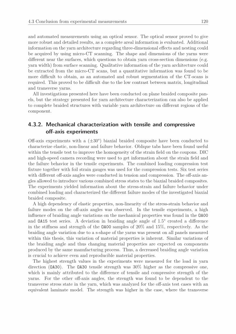
4.3 Conclusion from experimental measurements 120
and automated measurements using an optical sensor. The optical sensor proved to givemore robust and detailed results, as a complete areal information is evaluated. Additionalinformation on the yarn architecture regarding three-dimensional effects and nesting couldbe acquired by using micro-CT scanning. The shape and dimensions of the yarns weredifferent near the surfaces, which questions to obtain yarn cross-section dimensions (e.g.yarn width) from surface scanning. Qualitative information of the yarn architecture couldbe extracted from the micro-CT scans, but a quantitative information was found to bemore difficult to obtain, as an automated and robust segmentation of the CT-scans isrequired. This proved to be difficult due to the low contrast between matrix, longitudinaland transverse yarns.
All investigations presented here have been conducted on plane braided composite pan-els, but the strategy presented for yarn architecture characterization can also be appliedto complete braided structures with variable yarn architecture on different regions of thecomponent.
4.3.2. Mechanical characterization with tensile and compressiveoff-axis experiments
Off-axis experiments with a (±30°) biaxial braided composite have been conducted tocharacterize elastic, non-linear and failure behavior. Oblique tabs have been found usefulwithin the tensile test to improve the homogeneity of the strain field on the coupons. DICand high-speed camera recording were used to get information about the strain field andthe failure behavior in the tensile experiments. The combined loading compression testfixture together with foil strain gauges was used for the compression tests. Six test serieswith different off-axis angles were conducted in tension and compression. The off-axis an-gles allowed to introduce various combined stress states to the biaxial braided composites.The experiments yielded information about the stress-strain and failure behavior undercombined loading and characterized the different failure modes of the investigated biaxialbraided composite.
A high dependency of elastic properties, non-linearity of the stress-strain behavior andfailure modes on the off-axis angles was observed. In the tensile experiments, a highinfluence of braiding angle variations on the mechanical properties was found in the OA00
and OA15 test series. A deviation in braiding angle angle of 1.5° created a differencein the stiffness and strength of the OA00 samples of 20% and 15%, respectively. As thebraiding angle variation due to a s-shape of the yarns was present on all panels measuredwithin this thesis, this variation of material properties is inherent. Similar variations ofthe braiding angle and thus changing material properties are expected on componentsproduced by the same manufacturing process. Thus, a decreased braiding angle variationis crucial to achieve even and reproducible material properties.
The highest strength values in the experiments were measured for the load in yarndirection (OA30). The OA30 tensile strength was 30% higher as the compressive one,which is mainly attributed to the difference of tensile and compressive strength of theyarns. For the other off-axis angles, the strength was found to be dependent to thetransverse stress state in the yarn, which was analyzed for the off-axis test cases with anequivalent laminate model. The strength was higher in the case, where the transverse

4.3 Conclusion from experimental measurements 121
yarn stress was found to be compressive. This was in tension for OA00 and OA15 and incompression for OA45, OA60 and OA90.
While the stress-strain behavior was linear in tension for the braided composites whenthe load was aligned in the yarn direction (PT_OA30), the behavior was nonlinear in allother load cases. Most of the experiments were also nonlinear for small strains, which leadto a big difference between the initial modulus E0
x calculated by regression of the stress-strain curve and the elastic modulus Ex evaluated in a strain range from 0.1% − 0.3%axial strain. This implies that the elastic Ex, when used in a linear elastic models, onlygives an approximate solution for the stress-strain relation. Furthermore, the usage oflinear elastic models for biaxial braided composites is only valid for small loads, as thebehavior is nonlinear over the complete strain range.
The comparison between PT and PC experiments showed that the stress-strain behaviorfor all off-axis angles was found to be very similar in tension and compression. This impliesthat the nonlinear stress-strain behavior of the biaxial braided composites is mainly drivenby the shearing behavior of the yarns. Cyclic loading/unloading experiments in tensionhave been conducted to investigate the source of the nonlinear behavior. Both inelasticdeformation and material damage was found within the cyclic experiments. The inelasticdeformation was found to be more dominant for low off-axis angles, which was mainlyrelated to the higher stresses present in the yarns for these experiments. Beside thephenomenological evaluation done for the experiments here, the stress-strain curves maybe used as a basis for calibration of predictive models.
The failure modes observed in both, tensile and compressive experiments, were sig-nificantly influenced by the yarn architecture. In all experiments, the major crackingdeveloped along one of the yarn directions of the braided composite. The failure modes ob-served in the specimen were fiber failure in tension and compression and shear-dominatedtransverse failure of the yarns. Fiber failure was observed in tension and compressionfor the load in the yarn direction (PT_OA30, PC_OA30) and additionally for the PT_OA15
test series. Shear-dominated transverse failure of the yarns was observed either local-ized into a single crack (PT_OA45, PT_OA60, PT_OA90 and PC_OA00, PC_OA15) or as broadfailure spread accompanied with delamination and several intra-yarn cracking (PT_OA00,PT_OA15 and PC_OA45, PC_OA60, PC_OA90). The failure mode was also found to be con-trolled by the transverse stress state in the yarns: for tensile stresses, the failure localizesinto a single crack, while broad damage is present for compressive transverse stress.
Summarizing the mechanical characterization of biaxial braided composites with off-axis tension and compression experiments, the investigations proved to be very usefulto achieve an understanding about the stress-strain and failure behavior of the braidedcomposites. The high-speed camera used in the tension tests helped to develop an under-standing of the failure process. Also the compression tests were found useful to developa knowledge of the compressive failure of biaxial braided composites. The small straingauges required for the CLC test fixture gave increased bending values for some experi-ments, but specimen buckling was not found to be problematic for the test series. Thenon-linear and failure behavior was found to be mainly driven by in-plane stresses andin-plane shear was dominant for nonlinear and failure behavior. The textile yarn archi-tecture majorly influenced stress-strain behavior and failure modes, and simple equivalentlaminate models were found to be useful to analyze the yarn stresses and explain effects

4.3 Conclusion from experimental measurements 122
observed in the experiments. For all test series conducted, the first cracking in the braidedlaminates was found to coincide with the final failure of the specimen.

5. Geometric modeling and analyticalpredictions
Unit cell modeling is an established method for prediction of the nonlinear constitutivebehavior of braided composites [39, 40, 45]. Basis for a unit cell model is the geometricdescription of yarns and matrix within the unit cell. The academic software packageWiseTex [46] was used for geometric modeling of the biaxial braided unit cells within thisthesis. WiseTex calculates the geometry of yarns and matrix based on yarn architectureinput parameters.
The geometric modeling of the (±30°) and (±45°) braided composites, based on theyarn architecture parameters measured by optical microscopy, is described in this chapter.An assessment of the calculated geometric model is given by comparison of the WiseTexyarn geometry to the micro-CT scan of the (±45°) braided composite. Based on theWiseTex geometric model, the braided composites’ elastic behavior was predicted byusing the micromechanics software TexComp [72]. The elastic predictions for (±30°)and (±45°) braided composites are compared to experimental results and parametricstudies regarding yarn architecture variations are given. Furthermore, predictions basedon analytically calculated yarn architecture parameters are compared to the ones basedon measured parameters. Finally, the export of the yarn architecture geometry for finiteelement unit cell modeling is described.
5.1. Geometric model from WiseTex
The yarn architecture parameters given in Table 4.5 are used as an input for the geometricmodels. With the input, the yarn paths are calculated in WiseTex by using an energyminimization scheme: the fabric structure given by the braid pattern is divided intosmaller parts, with the yarns in the undulation being represented by structural elements.The yarn path is approximated by a parametric function z(x) and the parameters of zare calculated by minimization of the structural elements’ bending energy. A detaileddescription on the method can be found in [46].
5.1.1. Input parameters
The input parameters required to build up a unit cell model of a biaxial braid in WiseTexare given in Table 5.1. The input parameters can be separated into geometric parameters,defining the yarn geometry, and fiber/matrix mechanical parameters, which are stored inthe WiseTex unit cell model for later usage in e.g. micromechanical calculations.
The parameters from optical microscopy given in Table 4.5 are used with the spacingadjusted to be equal to the yarn width. This is reasonable as the geometric model provided
123

5.1 Geometric model from WiseTex 124
by WiseTex does not include effects like yarn overlapping or yarn cross section deformation(cf. Fig. 4.2). Fiber mechanical properties were calculated by reverse engineering fromUD experiments (Table A.1). The matrix mechanical data was taken from bulk matrixexperiments (Table A.2).
Table 5.1.: Input parameters for WiseTex unit cell modeling
name variable source
geometric data
yarn shape - micrographsyarn height d1 micrographsyarn width d2 micrographsspacing p micrographsbraiding angle θ optical sensor
fiber data
filament diameter ffil datasheet [176]number of filaments Nfil datasheet [176]fiber long. Young’s modulus Ef11 reverse engineeringfiber trans. Young’s modulus Ef22 reverse engineeringfiber shear modulus Gf12 reverse engineeringfiber long. Poisson’s ratio νf12 reverse engineeringfiber trans. Poisson’s ratio νf23 estimated (no data available)
matrix data
matrix Young’s modulus Em bulk matrix experimentsmatrix Poisson’s ratio νm bulk matrix experiments
5.1.2. Unit cell geometry
The unit cell geometries for the BB30 and BB45 braids are shown in Fig. 5.1. For braidingangles unequal to 45°, a sheared unit cell is used. The thickness of the unit cell is twicethe yarn thickness, which results in a fiber volume fraction of 54.4% for the BB30 and53.5% for the BB45 unit cell. The unit cell fiber volume fractions thus deviates by 7%and 6.5% to the one experimentally measured from the braided panels of BB30 and BB45,respectively.
Reasons for the smaller fiber volume fractions present in the unit cell models are be-lieved to be the deviations of the idealized geometric model to the real yarn architecture:effects like grown-together yarns, deformation of the yarn cross section, yarn cross sectionrotation or differences in the yarn architecture of the outer plies (cf. Section 4.1.4) arenot considered in the WiseTex geometry model. As the correct fiber volume fraction iscrucial for mechanical property prediction, an artificially increased packing density insidethe yarns, yielding 60% unit cell fiber volume fraction, was used in the models. Theapproach of increased packing density is commonly used for analytical and FE unit cellmodels [22, 45, 57].

5.1 Geometric model from WiseTex 125
(a) BB30 (b) BB45
Fig. 5.1: Geometric models of the biaxial braided composites obtained from WiseTex
5.1.3. Comparison of unit cell geometry to micro-CT measurements
In order to asses the geometric model calculated by WiseTex, the yarn geometry wascompared to the experimental results from the micro-CT measurements. One a slice ofthe micro-CT data, with the WiseTex yarn geometry added to the CT image, is shownin Fig. 5.2. The comparison shows that the overall accordance of the geometric modelto the micro-CT scan is reasonable. Besides local effects, attributed to yarn deforma-tion and yarn path distortion, the yarn path is predicted well by WiseTex. The maindeviations between the model and the real geometry can be summarized as: yarn cross-section deviation, penetration of adjacent plies and deviations from the idealized yarnpath. Deviations from the idealized cross section are visible at different parts of the scan,and attributed to the yarn deformation during compaction. The penetration of adjacent(WiseTex) plies is marked in the figure, and is mainly attributed to the unit cell modelthickness of the transverse yarns (red) being bigger as the thickness of the yarns in theCT scan. However, the displayed geometry of the model represents the transverse yarncut in the center (i.e. thickest part), which is not the case for the CT-scan, where the plyposition varies. Deviations of WiseTex and micro CT yarn path furthermore show, thatthe ideally straight part of the yarn is not straight in all cases.
No regularity in the deviations between CT-scans and geometric model is observed.Whether the models represents the yarn architecture well or deviates, depends on theposition of the ply in the laminate (mold or vacuum bag side) as well as on the lateral
Fig. 5.2: Comparison of yarn geometry of WiseTex and from micro-CT scanning

5.2 Elastic predictions 126
position of the plies relative to each other. A characterization of theses variations, as e.g.described in [55] can yield information for more precise yarn architecture models , but thisrequires improved techniques for micro-CT contrast increase and automated algorithms forimage segmentation and shape detection, which was both beyond the scope of the currentstudy. Furthermore, as the deviations are dependent on the laminate configuration andstacking, an improved geometric model would require additional information about thestacking of the plies relative to each other. For all plies in the laminate are to be modeledin a unit cell, the characterization effort and computational cost drastically increases.Furthermore, it is unlikely, that a distinct stacking, which needs to be defined as input,can be robustly achieved on a component. The focus of the unit cell modeling in thecurrent thesis was on parametric and efficient unit cell modeling. Thus, single ply unitcell models were used to keep the model size small and the models efficient.
Summing up, the WiseTex geometry approximates the yarn path by idealized geometricshapes, which show a good overall accordance with micro-CT measurements. Local devi-ations can be observed between model and measurement, but for the goal of a predictive,efficient and parametric model, the choice of a single ply model based on an idealized yarngeometry is appropriate.
5.2. Elastic predictions
The geometric model from WiseTex was used for elastic predictions with the academicsoftware TexComp [72, 112]. The elastic properties calculation within TexComp comprisesseveral steps: the yarns in the textile are divided in small yarn segments and replacedby ellipsoids with equal geometric and constitutive properties. The aspect ratio of theellipsoids is controlled by the local curvature of the yarn. All ellipsoid problems are solvedby application of Eshelby’s equivalent inclusion principle and the homogenization is doneby using a Mori-Tanaka scheme [142].
A second prediction approach based on orientation averaging of was employed: Astiffness-averaging method was implemented into MATLAB, which is similar to the oneproposed by Quek et al. [197] for triaxial braided composites. The undulation of the yarnsis considered by stiffness-averaging of off-axis UD plies: the undulated yarn is modeledas a series of off-axis oriented UD plies assembled in iso-strain condition. For the yarngeometry, a cosine function was chosen in the undulation region and the yarns were as-sumed to be straight in the crossover region. Only two geometric parameters, namelywidth-to-height ratio of the yarns and the braiding angle are needed as input parametersfor the geometry. The calculation of a UD ply stiffness matrix including yarn waviness isgiven by
CwavyUD =
1
N·N∑
i=1
CUD(φ) (5.1)
CUD(φ) is the stiffness matrix of a UD ply with an out-of-plane angel of φ, whereφ is calculated from the yarn path function. The stiffness matrix Cwavy
UD of one of theyarn directions is used within classical laminate theory to calculate the properties of anequivalent (±θ°) laminate. A comprehensive description of the stiffness-averaging methodis given in Appendix B.
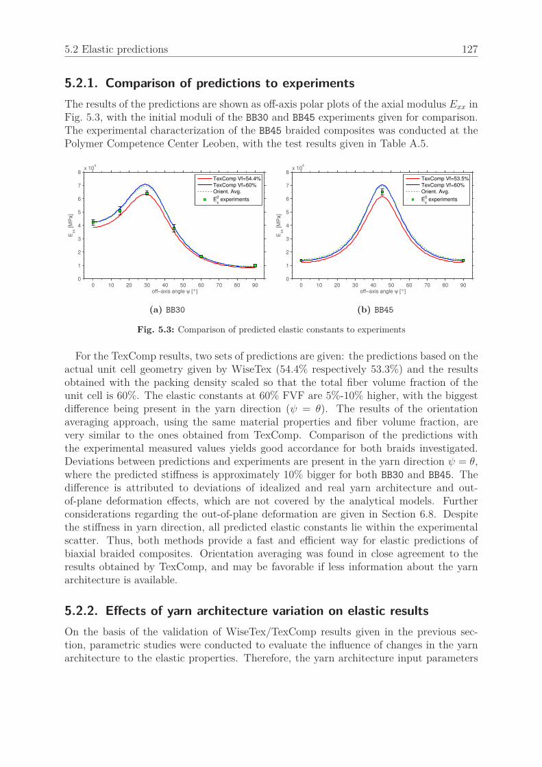
5.2 Elastic predictions 127
5.2.1. Comparison of predictions to experiments
The results of the predictions are shown as off-axis polar plots of the axial modulus Exx inFig. 5.3, with the initial moduli of the BB30 and BB45 experiments given for comparison.The experimental characterization of the BB45 braided composites was conducted at thePolymer Competence Center Leoben, with the test results given in Table A.5.
off−axis angle ψ [°]
Exx [
MP
a]
0 10 20 30 40 50 60 70 80 900
1
2
3
4
5
6
7
8x 10
4
TexComp Vf=54.4%
TexComp Vf=60%
Orient. Avg.
Ex
0 experiments
(a) BB30
off−axis angle ψ [°]
Exx [
MP
a]
0 10 20 30 40 50 60 70 80 900
1
2
3
4
5
6
7
8x 10
4
TexComp Vf=53.5%
TexComp Vf=60%
Orient. Avg.
Ex
0 experiments
(b) BB45
Fig. 5.3: Comparison of predicted elastic constants to experiments
For the TexComp results, two sets of predictions are given: the predictions based on theactual unit cell geometry given by WiseTex (54.4% respectively 53.3%) and the resultsobtained with the packing density scaled so that the total fiber volume fraction of theunit cell is 60%. The elastic constants at 60% FVF are 5%-10% higher, with the biggestdifference being present in the yarn direction (ψ = θ). The results of the orientationaveraging approach, using the same material properties and fiber volume fraction, arevery similar to the ones obtained from TexComp. Comparison of the predictions withthe experimental measured values yields good accordance for both braids investigated.Deviations between predictions and experiments are present in the yarn direction ψ = θ,where the predicted stiffness is approximately 10% bigger for both BB30 and BB45. Thedifference is attributed to deviations of idealized and real yarn architecture and out-of-plane deformation effects, which are not covered by the analytical models. Furtherconsiderations regarding the out-of-plane deformation are given in Section 6.8. Despitethe stiffness in yarn direction, all predicted elastic constants lie within the experimentalscatter. Thus, both methods provide a fast and efficient way for elastic predictions ofbiaxial braided composites. Orientation averaging was found in close agreement to theresults obtained by TexComp, and may be favorable if less information about the yarnarchitecture is available.
5.2.2. Effects of yarn architecture variation on elastic results
On the basis of the validation of WiseTex/TexComp results given in the previous sec-tion, parametric studies were conducted to evaluate the influence of changes in the yarnarchitecture to the elastic properties. Therefore, the yarn architecture input parameters

5.2 Elastic predictions 128
of BB30 and BB45 were varied within the bounds of the standard deviation found in theoptical microscopy measurements (cf. Table 4.5).
Yarn height
The variation of the yarn height yields for BB30 and BB45 d1 − σd1 = 247 µm and 252 µmand d1 + σd1 = 305 µm and 312 µm, respectively. Two different schemes for yarn heightchange are investigated:
(1) Solely the yarn height is changed. With the yarn width being constant, the fibervolume fraction also changes.
(2) Yarn height and width are both changed, in order to keep the unit cell fiber volumefraction constant.
Both cases are relevant for braided composites: the first is achieved if the compactionpressure during infiltration of the braid is increased, while the second refers to the casethat the yarns spread over a bigger area (e.g. mandrel cross section change). Fig. 5.4 showsa comparison of the variation compared to the model with the average yarn architecturevalues (avg) used. A similar trend is observed from both braiding angles: a decreasedyarn height increases the stiffness of the braided composite. The effect of (1) on themechanical behavior is bigger for both BB30 and BB45: the two effects of a fiber volumefraction change in the yarns and the change of waviness add up to the total increaseor decrease of stiffness. The difference in stiffness is around 15%-20%, with the highest
off−axis angle ψ [°]
Exx [
MP
a]
0 10 20 30 40 50 60 70 80 900
1
2
3
4
5
6
7
8x 10
4
avg
(1) d1−σ
d1
(2) d1−σ
d1
(1) d1+σ
d1
(2) d1+σ
d1
(a) BB30
off−axis angle ψ [°]
Exx [
MP
a]
0 10 20 30 40 50 60 70 80 900
1
2
3
4
5
6
7
8x 10
4
avg
(1) d1−σ
d1
(2) d1−σ
d1
(1) d1+σ
d1
(2) d1+σ
d1
(b) BB45
Fig. 5.4: Elastic behavior influence from yarn height variation
changes observed in axial and transverse direction. The second case (2) yields less changesof the elastic properties: the stiffness in the yarn directions of BB30 and BB45 changes by2% and 8%, respectively, while the response is almost similar to the avg case for the otheroff-axis angles. The simulations show that the elastic properties for yarn height variationsare sensitive to changes of the fiber volume fraction, while changes of yarn waviness atconstant fiber volume fraction has less effects.

5.2 Elastic predictions 129
Yarn width
The yarn width is varied for BB30 and BB45 in between d2 − σd2 = 2829 µm and 2831 µmand d2 + σd2 = 3331 µm and 3353 µm, respectively. Similar as for the yarn height, twocases are also distinguished for the yarn width variation: yarn width change with constantyarn height (1) and at constant FVF (2). The results shown in Fig. 5.5 that a a higherwidth in the yarns not necessarily leads to increased mechanical properties: if the yarnheight is constant with increasing yarn width, the fiber volume fraction decreases andthe elastic properties suffer. In contrast, if the fiber volume fraction is kept constant,the wider yarns decrease the waviness, which increases the stiffness, where the biggestchanges are, as for the yarn height, observed in the yarn direction.
off−axis angle ψ [°]
Exx [
MP
a]
0 10 20 30 40 50 60 70 80 900
1
2
3
4
5
6
7
8x 10
4
avg
(1) d2−σ
d2
(2) d2−σ
d2
(1) d2+σ
d2
(2) d2+σ
d2
(a) BB30
off−axis angle ψ [°]
Exx [
MP
a]
0 10 20 30 40 50 60 70 80 900
1
2
3
4
5
6
7
8x 10
4
avg
(1) d2−σ
d2
(2) d2−σ
d2
(1) d2+σ
d2
(2) d2+σ
d2
(b) BB45
Fig. 5.5: Elastic behavior influence from yarn width variation
Braiding angle
The braiding angle standard deviation was measured 0.6° for the BB30 and 1.2° for theBB45 . Despite the rather small standard deviation, a systematic variation of the braidingangle due to the yarns’ s-shape was observed on all panels. The elastic behavior predictedby TexComp is shown in Fig. 5.6. The biggest influence of the braiding angle is presentfor BB30 in the take-up direction and for BB45 in take-up and transverse direction. Thestiffness in take-up direction changes by 5% for BB30 and by 7% for BB45. In opposite, thestiffness in yarn direction is not influenced by the braiding angle change, but the positionof maximum stiffness changes with the braiding angle.
Summary: effect of yarn architecture changes
The numerical investigations of elastic constants made with TexComp show a high sensi-tivity of the elastic behavior for the yarn architecture parameters varied within the boundsof the measured standard deviation. Changes of the unit cell fiber volume fraction werefound to be the strongly affecting the biaxial braid stiffness. Changes of waviness atconstant fiber volume fraction, which refers to the case of wider braid yarns, mainly influ-enced the stiffness in the yarn directions and the change of stiffness was smaller compared
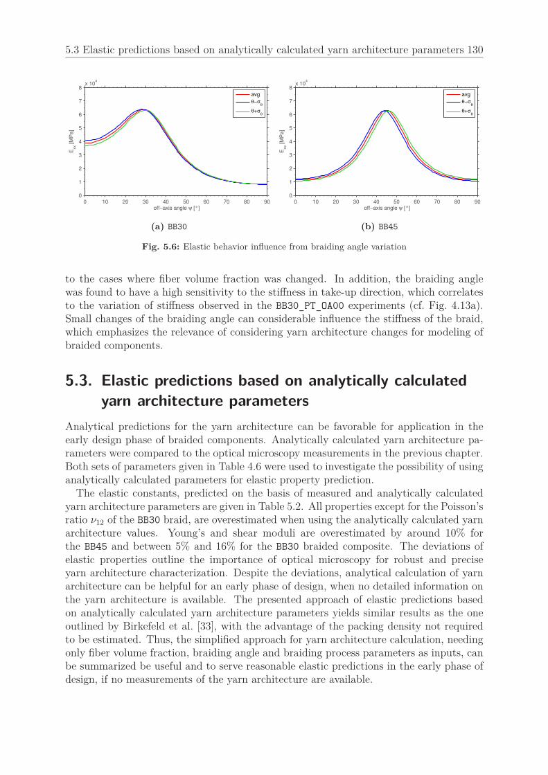
5.3 Elastic predictions based on analytically calculated yarn architecture parameters 130
off−axis angle ψ [°]
Exx [
MP
a]
0 10 20 30 40 50 60 70 80 900
1
2
3
4
5
6
7
8x 10
4
avg
θ−σθ
θ+σθ
(a) BB30
off−axis angle ψ [°]
Exx [
MP
a]
0 10 20 30 40 50 60 70 80 900
1
2
3
4
5
6
7
8x 10
4
avg
θ−σθ
θ+σθ
(b) BB45
Fig. 5.6: Elastic behavior influence from braiding angle variation
to the cases where fiber volume fraction was changed. In addition, the braiding anglewas found to have a high sensitivity to the stiffness in take-up direction, which correlatesto the variation of stiffness observed in the BB30_PT_OA00 experiments (cf. Fig. 4.13a).Small changes of the braiding angle can considerable influence the stiffness of the braid,which emphasizes the relevance of considering yarn architecture changes for modeling ofbraided components.
5.3. Elastic predictions based on analytically calculatedyarn architecture parameters
Analytical predictions for the yarn architecture can be favorable for application in theearly design phase of braided components. Analytically calculated yarn architecture pa-rameters were compared to the optical microscopy measurements in the previous chapter.Both sets of parameters given in Table 4.6 were used to investigate the possibility of usinganalytically calculated parameters for elastic property prediction.
The elastic constants, predicted on the basis of measured and analytically calculatedyarn architecture parameters are given in Table 5.2. All properties except for the Poisson’sratio ν12 of the BB30 braid, are overestimated when using the analytically calculated yarnarchitecture values. Young’s and shear moduli are overestimated by around 10% forthe BB45 and between 5% and 16% for the BB30 braided composite. The deviations ofelastic properties outline the importance of optical microscopy for robust and preciseyarn architecture characterization. Despite the deviations, analytical calculation of yarnarchitecture can be helpful for an early phase of design, when no detailed information onthe yarn architecture is available. The presented approach of elastic predictions basedon analytically calculated yarn architecture parameters yields similar results as the oneoutlined by Birkefeld et al. [33], with the advantage of the packing density not requiredto be estimated. Thus, the simplified approach for yarn architecture calculation, needingonly fiber volume fraction, braiding angle and braiding process parameters as inputs, canbe summarized be useful and to serve reasonable elastic predictions in the early phase ofdesign, if no measurements of the yarn architecture are available.

5.4 Transfer of WiseTex geometry to finite element unit cell models 131
Table 5.2.: Comparison of elastic constants predicted by the use of micrograph measurements and an-alytical predictions
BB30 BB45
micrograph analytical deviation micrograph analytical deviation
E11 [MPa] 42590 47850 12.4% 13700 15220 11.1%E22 [MPa] 8881 10280 15.8% 13700 15220 11.1%G12 [MPa] 26610 28000 5.2% 34130 37810 10.8%ν12 [-] 1.492 1.411 −5.4% 0.811 0.813 0.2%
5.4. Transfer of WiseTex geometry to finite element unitcell models
The geometric models inside WiseTex can be stored as either binary or XML1-type files.If solely the geometry of the model shall be exported, WiseTex offers an export of the
yarn geometry to an ASCII (*.cfl ) file. The cfl file stores the information of the unitcell and the yarns in a structured format, including unit cell dimensions, braiding angleand information about the geometric and material properties of the yarns defined in themodel. An example of an cfl file for a biaxial braid with one type of yarn defined is:
14.2258905200649 14.2258905200649 0.552 # Unit cell dimensions
1.0472 # =2*theta opening angle of yarns [rad]
1 # number of yarn types
1 # Number of the yarn
Tenax HTS40 12K 800tex # designation of the yarn
E # shape of the cross-section
carbon fiber neu # name of the yarn fiber
0.0681 0.007 1.77 240 0.23 28 0.4 13 10 4300 1.8 # fiber data
1.5707963267949 # empriical fitting factor
616 # total number of sections
Furthermore, the information about the yarn architecture is stored segment-wise forevery yarn. The number of segments in one yarn can be adjusted and is controlled bythe points per crimp interval parameter within WiseTex. Every yarn segment includesinformation about the location, cross-section and orientation of the cross section:
## For every cross-section ##
1 # yarn type
76 # no. of cross-sections in yarn
-10.6694028054303 -6.16 0.138 # X Y Z coordinates of the current cross-section
0.187842969245378 # Length around the cross sections
3.08 0.276 # Principal cross-section axes, mm
0.0653168637087045 # Average curvature radius at the cross section center
0 -1 0 # Segment 1-axis, parallel to the major cross-section axis
0 0 1 # Segment 2-axis
1 0 0 # Segment 2-axis, tangent to the heartline.
0.691699604743083 # Fiber volume fraction inside a yarn
0.00129632941822128 # Yarn segment volume fraction
The cfl -file of the WiseTex model is used to import the yarn architecture data intothe FE pre-processor Abaqus/CAE.
1XML: Extensive Markup Languge

5.5 Conclusion on geometric modeling and analytical predictions 132
5.5. Conclusion on geometric modeling and analyticalpredictions
WiseTex was used to calculate the geometry of the biaxial braided composite unit cells.The geometry obtained from WiseTex was compared to the micro-CT measurements anda good agreement was found. Deviations were observed locally, where the micro-CT scanshowed deviations from the idealized yarn cross section and yarn path shape. To includethese local deviations into a geometric model, comprehensive evaluation of the CT-data(cf. [55]) and additional preforming simulation steps [82, 83] are required. In addition, theinfluence of adjacent plies on the geometry would require to model the complete braidedlaminate in a unit cell model. As the focus of FE unit cell modeling in this thesis was putto reduced, parametric and efficient unit cell models, the WiseTex geometry yielded anoptimal choice. No additional simulation step is required to calculate the geometry andXML file format as well as command line capability allow integration of WiseTex into aFE modeling framework.
With the WiseTex geometry models, the elastic properties of the BB30 and BB45 braidedcomposites could be calculated by using the analytical Mori-Tanaka approach imple-mented in TexComp. The predictions made with TexComp correlated well with experi-mental results with maximum 10% deviation being present in the yarn direction. In ad-dition, a simple stiffness-averaging approach used for elastic property prediction yieldedsimilar results as the WiseTex/TexComp modeling approach.
The WiseTex/TexComp model was further used for parametric studies showing a highdependency of the elastic behavior to yarn architecture input parameters: for yarn widthand height changes, the effect of fiber volume fraction was dominant compared to thechange of yarn waviness at constant fiber volume fraction. In addition, the braiding anglevariations crucially affected the stiffness in take-up and transverse direction. Thus, alsosmall braiding angle changes, e.g. introduced by the s-shape of the yarns, need to beconsidered in a structural simulation of a biaxial braided composite component.

6. Finite element unit cell modeling
This chapter describes the finite element (FE) unit cell models used within this thesis topredict the constitutive behavior of biaxial braided composites. The main purpose of theFE unit cell modeling was to predict the effect of the yarn architecture on the elastic,nonlinear and failure behavior of biaxial braided composites. The focus was on parametricand efficient models: with the goal of simulating a complex braided structure, unit cellsimulations have to be able to calculate the constitutive behavior, which will later serveas input for macroscopic modeling, for a multitude of different yarn architectures. Thus,many different configurations of the unit cell need to be modeled and solved, yielding themain requirements for the FE unit cell models:
1. The model has to be parametric, i.e. modeling, solution and post-processing shallbe automated without requiring manual operations like e.g. meshing in the pre- andpost processing.
2. The model needs to be efficient. As many simulations are conducted for differentyarn architectures, a fast modeling and solution is crucial.
These requirements led to the development of a new reduced FE unit cell modeling ap-proach based on Cox’s binary model [125]. In the novel Binary Beam Model (BBM),beams and continuum elements are used to model the yarns and matrix pockets in thebiaxial braided composite unit cell. While the beam elements model the longitudinalproperties of the yarns, the transverse and shear yarn properties and the properties of thematrix pockets are modeled in a smeared way by the so-called effective medium continuumelements. The reduced modeling approach yields advantages in efficiency and automationof model generation, when compared to the classical continuum unit cells [40, 45, 79]:continuum element unit cells serve a detailed representation of the 3D stress field in yarnsand matrix, but often suffer meshing issues and poor element quality, connected to anincreased numerical effort, when applied to high fiber volume fraction textile composites[37, 139]. Through the geometric idealizations introduced, these issues are not present inthe BBM modeling approach.
The BBM modeling approach, implemented into a modeling framework in MATLAB, isdescribed in the following sections. A short overview to the modeling framework, includ-ing the geometric modeling in WiseTex, geometry import into Abaqus/CAE, FE solutionin Abaqus/Standard and post-processing is given. The constitutive laws, adapted to thereduced model formulation, are introduced: the model assumes linear elastic deformationin the beam elements and elastic-plastic behavior in the effective medium. Equationsfor the calculation of the yarn and effective medium material properties at different fibervolume fractions are introduced. This ensures the applicability of the unit cell model-ing approach to braided composites with varying fiber volume fractions. Furthermore,the periodic boundary conditions for the rhombus unit cell used in the biaxial braided
133

6.2 Binary Beam Model: modeling and idealizations 134
composite simulations are given. The mesh-dependency, present in the stress-field of theeffective medium, is removed by introducing an averaging procedure to calculate the yarnstress components at each beam node. Furthermore, the equations for the failure analysisusing the BBM are defined.
BBM stress predictions in the yarns are compared to the solution of a classical contin-uum element unit cell. Elastic simulations with the unit cell under different out-of-planeboundary conditions are correlated to experimental measurements. Additionally, stressprofiles at different out-of-plane boundary conditions are presented and an approach forthe out-of-plane modeling of biaxial braided laminates is given. For the prediction ofbiaxial braided composites strength, a material parameter-identification approach basedon experiments of biaxial braided composites was used. With the strength parameterscalculated, the model predictions are finally validated by comparison to the experimentalresults from BB30 and BB45 off-axis experiments.
6.1. Framework for unit cell modeling
The approach for modeling and solution of the BBM FE unit cell was implemented into aMATLAB framework, which is outlined in Fig. 6.1. The framework allows to build, solveand post-process BBM unit cells without manual work, yielding a parametric and efficientmodeling. First, the geometric, material and numeric input properties have to be definedin MATLAB. The framework builds a WiseTex XML file with the defined parametersand calculates the geometric model with WiseTexCL [74]. The calculated geometry ispassed to a python script, which builds up the model in the Abaqus/CAE pre-processor,generating all the information required for solution and post-processing and finally writesthe model to an ASCII *.inp file. In an additional step, periodic boundary conditions areadded to the model and the solution is started. The solution can be either linear elastic forthe calculation of elastic properties or non-linear for strength prediction. All simulationswere conducted with the implicit commercial FE solver Abaqus/Standard. After the FEsolution is finished, the post-processing of the model is started, where another pythonscript opens the Abaqus output-database (ODB ), calculates the volume averaged stressesand writes these to the ODB. Depending on the type of solution, a failure analysis isconducted, returning the critical nodes for failure of the unit cell as well as the location offailure. Finally, the homogenized elastic constants (linear simulations) or the homogenizedstress-strain behavior of the unit cell is calculated. Further information to the frameworkimplementation is provided in Appendix E.3.
6.2. Binary Beam Model: modeling and idealizations
The main purpose of the BBM is to use a reduced representation of the textile yarnarchitecture, while preserving relevant details of the stress field of biaxial braided com-posite unit cells. The geometric idealization used within this thesis is similar to the oneproposed by Cox and co-workers [125, 131, 198] in the Binary Model (BM): as shown inFig. 6.2, the braided composite, consisting of yarn and matrix pocket volumes, is idealizedby two independent sets of elements: 1D line elements at the yarn centerlines and and 3D

6.2 Binary Beam Model: modeling and idealizations 135
BBM Framework (MATLAB)
B3AInputAparameterAdefinitionAAAANAgeometryAAAANAmaterialApropertiesAAAANAloadAAAANAnumericAparameters
)3AWiseTexAXMLA(ACLAAAANAcreateAXMLAmodelAAAANAexportAgeometryAtoAASCIINfile
43AAbaqus(CAEwAPythonAscriptingAAAANAreadAASCIINfileAAAANAcreateAyarnsAvAmatrixAblockAAAANAassignAmaterialApropertirewAsectionswAmeshAAAANAfindAnodesetsAforAgaugeAaveragingAAAANAwriteAINPNfile
:3APeriodicAboundaryAconditionsAhMATLAB+AAAANAfindAnodesetsAAAANAcalculateAloadhs+AAAANAincludeAequationsAintoAINPNfile
53ASolving:AAbaqus(StandardAAAANAlinearNelasticA(AnonNlinear
*3APostNProcessingAAAANAAbaqus(CAEwAPythonAAAAAAANAcalculateAvolumeNaveragedAstressesAAAAAAANAapplyAfailureAcriterionAAAAAAANAoutputAcriticalAvaluesAtoAk3postNfileAAAAAAANAexportAconstraintAdriverAforces(displacementsAAAANAMATLABAAAAAAANAcalculateAelasticAconstantsAAAAAAANAcalculateAhomogenizedAstressNstrainAbehavior
Fig. 6.1: MATLAB-Framework for Binary Beam Model (BBM) unit cell
elements, defining the unit cell volume. Cox used truss elements for the yarns, based onthe assumption that bending of the yarns is dominated by transverse shear, modeled bythe effective medium. In the BBM, linear Timoshenko beam elements are used instead oftruss elements. This allows to consider the influence of the yarn cross section on both thebending stiffness of the impregnated yarns and the bending-induced stress fluctuations inthe yarns.
Fig. 6.2: Idea of BBM idealization
In the BBM, longitudinal and bending properties of the yarns are modeled by theTimoshenko beam elements, while transverse and shear properties of the yarns and theproperties of the matrix pockets are represented in a smeared way by the 3D continuumelements of the effective medium. The impregnated yarn bending stiffness is influenced

6.2 Binary Beam Model: modeling and idealizations 136
by both, yarn material properties as well as shape and dimensions of the cross section.When loaded in the longitudinal direction, a stress concentration exists in the bendinginterval of the yarns. The stress on the upper and lower surface thus can be considerablyhigher as the yarn center stress (increase of 20% shown for a continuum unit cell model inFig. 6.3). Thus yarn bending considerably influences the longitudinal failure of the yarns.Both effects, bending rigidity and stress concentration, can be considered by using thebeam elements in the BBM.
Fig. 6.3: Stress profile of a yarn loaded in longitudinal direction
The yarn geometry, exported from the WiseTex model, is used to define the coordinates,the tangential direction and the cross-sectional orientation of the beam elements. Theyarn cross section of the WiseTex model is considered in the beam modeling by area andmoments of inertia of the beams. The beam section properties are calculated from theyarn cross section dimensions:
Fig. 6.4: Ellipse cross section
Ayarn =π
4d1d2 (6.1)
Ixx =∫∫
Ay2dA =
πd2d31
64(6.2)
Iyy =∫∫
Ax2dA =
πd1d32
64(6.3)
Izz =∫∫
Ar2dA =
πd32d
31
16(d22 + d2
1)(6.4)
Where Ayarn is the area of the yarn and Ixx, Iyy and Izz are the second moments ofinertia for bending and torsion of the elliptical cross-section given in Fig. 6.4. As given bythe WiseTex model, all yarn cross-section properties are defined constant along the yarnpaths. Size and shape of the WiseTex unit cell define the effective medium volume, i.e.the BBM unit cell includes four yarns in each direction and has the shape of a rhombus forbraiding angles θ 6= 45°. Smaller unit cells of braided composites as e.g. given in [39, 199]can be used for finite element modeling to reduce the computational cost of the solution.However, as the BBM modeling approach yielded a very efficient solution even with thelarger rhombus unit cell given by WiseTex, the unit cell volume was not reduced further.

6.3 Constitutive laws 137
6.2.1. Coupling of yarns and matrix
Two types of finite element meshes, a continuum mesh and a beam element mesh are usedin the BBM. As the meshes of beam and continuum elements are not naturally consis-tent, i.e. do not share nodes, their degrees of freedom (DOFs) need to be coupled. Thecoupling can be either introduced by forcing consistent meshing of beam and continuumelements or alternatively by introducing constraint equations between beam and contin-uum nodes. Consistent meshing requires a fine continuum mesh and can, nevertheless,result in distorted continuum elements, yielding an increased numerical cost and a poorquality of stress and strain predictions. The usage of multi-point-constraint equations forcoupling was reported for the Binary Model [133, 136] and for continuum element unitcells [124, 138] and thus was used for the BBM. The multi-point constraints coupling ofthe beam elements and continuum elements and can be easily established inside Abaqusby using the embedded elements function.
Fig. 6.5: Embedding of beam elements
The embedded elements function couples thetranslational DOFs of beam elements to the con-tinuum elements. As shown in Fig. 6.5, each beamelement node is assigned to the overlapping con-tinuum host element. The beam node displace-ments are calculated from the displacements of thecontinuum element nodes, by interpolation of thebeam node’s relative position inside the host ele-ment. The rotational DOFs of the beam elementare not constraint, thus the torsional behavior of
the yarns is solely controlled by the beam torsional stiffness. Introducing the couplingremoves the requirement of consistent meshes from beam and continuum elements. How-ever, the mesh size of the effective medium continuum elements was chosen in a way, thatall yarns were embedded similar into the effective medium: the number of continuumelements along 1/4 of the unit cell edge should be an uneven integer to have all beamsplaced in-plane centered in one continuum element (cf. Fig. 6.6).
(a) Beam elements (b) Beam element cross section rendered
Fig. 6.6: BBM unit cell with embedded beam elements (half of the effective medium elements removed)
6.3. Constitutive laws
Material properties for beam and continuum elements need to be defined for the BBM. Asthe beam elements represent the axial and bending stiffness of the yarns, longitudinal yarnproperties, namely axial modulus and strength of the yarns, are required for the beam

6.3 Constitutive laws 138
elements. The effective medium models the smeared transverse and shear properties ofyarns as well as the properties of the matrix pockets. As the effective medium is definedisotropic, only shear and transverse modulus are required as elastic properties. Further-more, yarn transverse tensile and compressive strength as well as yarn shear strength arerequired to evaluate transverse yarn failure. For modeling of non-linear deformation priorto final failure, a plasticity model was defined in the effective medium, which requiresmaterial parameters for pressure-dependence and hardening.
The constitutive properties of beam and effective medium elements depend on thepacking density pd in the yarns and on the unit cell fiber volume fraction ϕf . Thus, aparametric unit cell model needs the constitutive properties to be available at differentfiber volume fractions. As most experimental investigations solely provide results forone specific fiber volume fraction, yarn and matrix constitutive properties are calculatedby fiber/matrix micromechanics: fiber and matrix properties are calculated by reverse-engineering from UD experiments at a known fiber volume fraction, and can furtherbe used to calculate yarn and effective medium properties at any desired fiber volumefraction. A variety of methods is available for micromechanics of UD composites, rangingfrom detailed FE unit cell calculations [41, 118], advanced analytical methods like e.g.methods of cells or multicontinuum technology [57, 113] to closed-form analytical formulae[24, 51]. Closed-form analytical equations were chosen in the current work, as they offersthe advantage of straightforward and efficient implementation into the BBM modelingframework and do not require an additional analysis step. Analytical formulae do of coursenot represent the current state of research in micromechanical modeling, but they providean simple and efficient way to scale both, elastic and strength properties to different fibervolume fractions.
6.3.1. Volume fractions
Constitutive property definition in the BBM requires consideration of the volume fractionsinside a unit cell: as the beam elements (BE) have the yarn cross section prescribed andmodel the yarn longitudinal and bending stiffness, the packing density is used to calculatetheir properties. The beam elements introduce stiffness in their longitudinal direction,while the transverse and shear properties of the yarns and the matrix pocket propertiesare represented in a smeared way by the effective medium (EM). Thus, the compositeproperties at the unit cell fiber volume fraction are used for the effective medium elements.
PBE = f(PUD, ϕ = pd)
PEM = f(PUD, ϕ = ϕf )(6.5)
6.3.2. Elastic properties
The elastic properties of beam and effective medium continuum elements are derivedfrom the elastic properties of a yarn. As the yarn can be assumed to behave transverselyisotropic, yarn properties are calculated from UD micromechanics. Different propertyassignments for the Binary Model have been proposed by Cox and co-workers [125, 131,133]. The elastic properties assigned to the BBM follow similar ideas as the ones given

6.3 Constitutive laws 139
by Cox for the Binary Model. The fiber and matrix properties given in Table A.1 andTable A.2 are used throughout the simulations.
Effective medium
The effective medium represents the matrix-dominated properties of shear and transversebehavior of the yarns and the behavior of the matrix. The effective medium can be eitherdefined transversely isotropic or isotropic [131], with the latter yielding the advantagethat no material orientation needs to be defined for the effective medium. As an uniquematerial orientation definition in the effective medium is not possible for the braidedcomposite unit cells modeled, an isotropic effective medium definition is used for theBBM, which has been showed to give appropriate results for the Binary Model [131, 133].The off-axis experiments showed that in-plane shear and transverse behavior of the yarnsdominate the mechanical behavior of biaxial braided composites. Thus, the effectivemedium was assigned with these elastic constants. The elastic constants are calculatedwith Chamis’ micromechanical equations [200]:
EEM = E22 =Em
1 − √ϕf (1 − Em/Ef22)
(6.6)
GEM = G12 =Gm
1 − √ϕf (1 −Gm/Gf12)
(6.7)
The fiber volume fraction of the unit cell ϕf is used, as the effective medium representsthe smeared properties of yarns and matrix pockets (Fig. 6.7). The Poisson’s ratio of theeffective medium yields
νEM = EEM/(2 ·GEM) − 1. (6.8)
Fig. 6.7: Continuum yarn embedded in resin compared to a beam element embedded in effective mediumin the BBM
Yarns
The longitudinal stiffness of a yarn with the packing density pd can be calculated by therule of mixtures
EY11 = Ef1 · pd + Em · (1 − pd) (6.9)
For the stiffness of the beam elements, the volume doubling present in the BBM has tobe considered (Fig. 6.7): the yarn cross section is assigned to the beam element embedded

6.3 Constitutive laws 140
in the effective medium and thus the yarn volume in the BBM is filled twice, by theeffective medium and the beam element. Using the yarn stiffness from Eq. 6.9 would resultin an artificially stiffened behavior, thus the stiffness introduced by the effective mediumhas to be considered in the beam element constitutive definition. The beam elementsstiffness is calculated be equalizing the stiffness of a yarn-in-matrix representation andthe BBM as shown in Fig. 6.7
ECM11 = EBBM
11 (6.10)
EY11 · ϕY + Em · (1 − ϕY ) = EBE · ϕY + EEM (6.11)
ECM11 and EBBM
11 are based on the assumption of equal strains of yarn and matrix, andbeam element and effective medium, in the 11-direction. The equation solved to EBE andwith EY
11 substituted from Eq. 6.9 and ϕY = ϕf/pd yields the beam element stiffness:
EBE = EY11 −
(Em +
pdϕf
·(EEM − Em
))(6.12)
6.3.3. Strength properties
The failure analysis within the BBM is based on failure criteria originally developed forUD composite materials. The yarn longitudinal stresses extracted from beam elementsand the transverse stresses from the effective medium are used within the failure analysis.UD failure criteria were shown to be appropriate for prediction of failure and damageinitiation within the yarns of textile composite unit cells (cf. e.g. [24, 45, 47, 140]). Thestrength input properties needed for a failure analysis with the BBM are yarn tensileand compressive longitudinal and transverse strength and yarn in-plane shear strength.Similar to the elastic constants, these parameters need to be available at arbitrary fibervolume fractions. Murthy and Chamis [200] presented a set of analytical equations in theframework of the Integrated Composite Analyzer (ICAN), which allow to calculate thecomposites UD strength properties based on fiber and matrix constituent properties.
The yarn longitudinal strength properties were calculated by using the rule of mixturesequations, proposed in the ICAN models:
XT = ϕf ·Xf,T + (1 − ϕf ) ·Xf,T · Em/Ef11 (6.13)
XC = ϕf ·Xf,C + (1 − ϕf ) ·Xf,C · Em/Ef11 (6.14)
In addition to the rule-of-mixtures equations, a compressive strength value for mi-crobuckling and one for delamination is given in [200]. However, both equations yieldedunrealistic strength values for high fiber volume fractions, and thus the rule of mixturesequations were used for the BBM. The longitudinal fiber strength values in tension Xf,T
and compression Xf,C , calculated by reverse-engineering from UD experiments, are givenin Table A.1. The increase of strength with fiber volume fraction predicted by the rule ofmixtures yielded a good correlation to internal experimental data with a similar materialat various fiber volume fractions [201].
For the transverse yarn strength, also some approaches for micromechanical calculationof strength properties are available. Ruijter [51] e.g. used the equations given for the ICAN

6.3 Constitutive laws 141
model by Chamis and Lomov et al. [24] used an alternative approach published originallyby Rosen. The values calculated from the two approaches are compared in Fig. 6.8. Thetransverse properties decrease with the fiber volume fraction for both approaches. Thecomparison of the predicted values with internal experimental data [201] showed thatboth predictions do not yield realistic values. The model used by Lomov [24] predicts adecrease of properties with fiber volume fraction largely above the measured values andthe ICAN model results in zero strength properties at a fiber volume fraction of around85%. Ivanov et al. [45] published an alternative approach, assuming the transverse and
fiber volume fraction [−]
str
en
gth
[M
Pa
]
0.4 0.45 0.5 0.55 0.6 0.65 0.7 0.75 0.80
100
200
300
400
500
600
Yt [Lomov2007]
Yc [Lomov2007]
SL [Lomov2007]
Yt [Ruijter2009]
Yc [Ruijter2009]
SL [Ruijter2009]
Fig. 6.8: Strength properties plotted over fiber volume fraction, from [24, 51]
shear strength properties to be constant for different fiber volume fractions. The approachwas successfully used with a unit cell model for prediction of triaxial braided compositesdamage initiation and progression. Due to the lack of the simple models to representa reasonable dependence of strength properties to the fiber volume fraction, Ivanov’sapproach was used, keeping the transverse and shear strength parameters for the BBMconstant over the fiber volume fraction:
YT (ϕf ) = YT YC(ϕf ) = YC SL(ϕf ) = SL (6.15)
The transverse strength properties used in the BBM simulations are given in Table 6.7.It is important to note, that the complex mechanics of transverse and shear failure ofUD composites, which involve damage and plastic deformation in the matrix and fiber-matrix interface failure [41], cannot be covered by analytical considerations. However,detailed analysis models require additional experimental validation, which was out of thescope of the current work. Thus, constant transverse strength properties were consideredappropriate as a first approach.

6.3 Constitutive laws 142
6.3.4. Plasticity model
The off-axis experiments of the (±30°) biaxial braided composites showed considerablenonlinear behavior before final failure. Investigations on crack occurrence and positionshowed the nonlinear behavior is due to microscopic cracking (cf. [170]), and the load-ing/unloading experiments revealed that the stress-strain nonlinearity is due to bothinelastic deformation and material damage. For the Binary Model, Flores et al. [136]showed that matrix-induced nonlinearities in ceramic-matrix composites can be consid-ered in the simulations by using a Drucker-Prager plasticity model. A similar approachwas chosen in the BBM to account for the nonlinear deformation prior to final failure.Using a plasticity criterion to model the nonlinearities, introduced by damage and inelas-tic effects cf. Section 4.2.2, is valid in this case as only monotonically increasing loads areconsidered within the BBM simulations. The nonlinear deformation of braided compos-ites was related to the shear and transverse behavior of the yarns and is thus in the BBMassigned to the effective medium elements. For efficient implementation of the unit cellsimulations within Abaqus, a linear Drucker-Prager plasticity model with associated flowand nonlinear shear hardening was defined in the effective medium continuum elements.The Drucker-Prager yield criterion allows to consider the pressure-dependence of yieldingcommonly reported for composite materials [172, 202, 203].
The Drucker-Prager yield criterion is given as :
f(σ) = σe − b · σm − a = 0 (6.16)
Where σe is the von Mises stress, σm is the hydrostatic part of the stress tensor and a, bare material parameters that define the yield stress and the pressure-dependence. Theparameter b = tan(β) is related to the pressure dependence, with β being the so-calledfriction angle of the material shown in Fig. 6.9a, defining the slope of the yield curve inthe plane of von Mises stress and the hydrostatic pressure.
(a) Drucker-Prager yield criterion in the p-σe-plane, flow rule is associated
(b) Dependence of yield stress on hydrostaticpressure [172], experiments from [203]
Fig. 6.9: Pressure dependence of the DP-plasticity model (−p = σm = σ1 = σ2 = σ3)
The value of β was for the BBM unit cell simulations extracted from the publication ofVyas et al. [172]. Vyas et al. summarized experimental results from Shin and Pae [203],who tested the in-plane shear behavior of carbon/epoxy composites under several hydro-

6.3 Constitutive laws 143
static pressure states (cf. Fig. 6.9b). The friction angle was obtained by linear regressionto the experimental results:
β = tan−1
(√3 · ∆τ12
∆p
), (6.17)
which yielded a friction angle of β = 17.7°. The flow rule of the plasticity model waschosen fully-associated, i.e. the plastic flow is orthogonal to the yield surface (Fig. 6.9a).
Besides the pressure-dependence, the hardening behavior of the effective medium withinthe Drucker-Prager yield criterion needs to be defined. As considerable hardening wasobserved in the braided composites off-axis experiments, assuming ideal plastic deforma-tion, like given by Flores et al. [136], is not suitable. The hardening was defined by usingthe shear-stress over shear-strain curve from a (±45°) UD experiment, shown in Fig. 6.10.The progressive stress-strain behavior ultimately before final failure was not used for the
γ12
[−]
τ12 [M
Pa]
0 0.005 0.01 0.015 0.02 0.025 0.03 0.035 0.04 0.045 0.050
10
20
30
40
50
60
70
80
IPS_01
IPS_02
IPS_03
Fig. 6.10: In-plane shear stress-strain curves used for hardening definition [204]
hardening definition, as it was introduced through failure of the foil strain gauges used. Aleast square fit method was used to calculate the hardening curve from the experimentalresults, with the hardening function a = r(γpl12) defined linear-exponential as proposed byFlatscher [141]:
r = τ y12 =
τ 0
12 + c1 · γpl12 for γpl12 < γpl∗12
K · (γpl12)1
m for γpl12 > γpl∗12
(6.18)
The plastic part of the shear strain is calculated from
γpl12 = γ12 − τ/G , (6.19)
whereG is the shear modulus evaluated in the range of γ12 = 0.05−0.25%. The coefficientsK, m and τ 0
12 are extracted from the experimentally measured curve by regression andthe transition point γpl∗12 as well as the parameter c1 are calculated by forcing the value
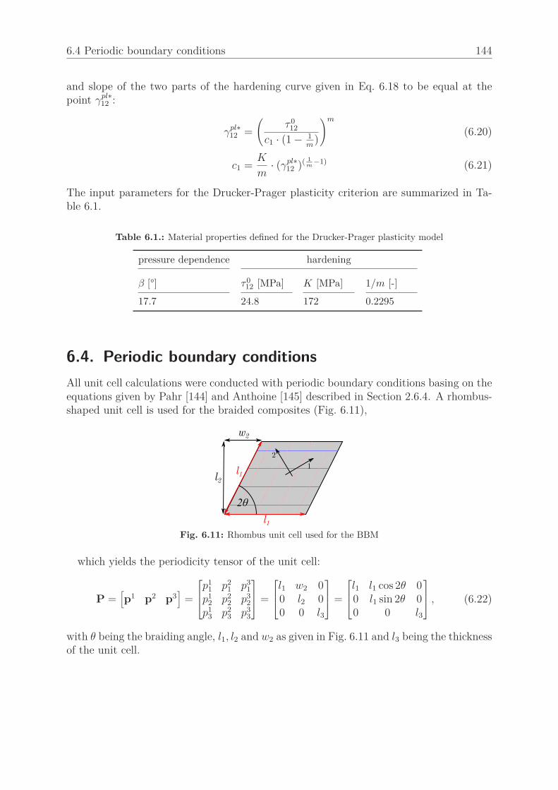
6.4 Periodic boundary conditions 144
and slope of the two parts of the hardening curve given in Eq. 6.18 to be equal at thepoint γpl∗12 :
γpl∗12 =
(τ 0
12
c1 · (1 − 1m
)
)m(6.20)
c1 =K
m· (γpl∗12 )( 1
m−1) (6.21)
The input parameters for the Drucker-Prager plasticity criterion are summarized in Ta-ble 6.1.
Table 6.1.: Material properties defined for the Drucker-Prager plasticity model
pressure dependence hardening
β [°] τ012 [MPa] K [MPa] 1/m [-]
17.7 24.8 172 0.2295
6.4. Periodic boundary conditions
All unit cell calculations were conducted with periodic boundary conditions basing on theequations given by Pahr [144] and Anthoine [145] described in Section 2.6.4. A rhombus-shaped unit cell is used for the braided composites (Fig. 6.11),
l1
l1
w2
l2
2θ
1
2
Fig. 6.11: Rhombus unit cell used for the BBM
which yields the periodicity tensor of the unit cell:
P =[p1 p2 p3
]=
p1
1 p21 p3
1
p12 p2
2 p32
p13 p2
3 p33
=
l1 w2 00 l2 00 0 l3
=
l1 l1 cos 2θ 00 l1 sin 2θ 00 0 l3
, (6.22)
with θ being the braiding angle, l1, l2 and w2 as given in Fig. 6.11 and l3 being the thicknessof the unit cell.

6.4 Periodic boundary conditions 145
6.4.1. Coupling equations
The periodic boundary conditions are implemented into the FE unit cell calculationsbased on the equations given in [205]. The basic relations are given for the displacementsof adjacent faces (naming cf. Fig. 6.12), connected by the periodicity vectors pi
p1 : uA − uB − ∆uAB = 0 (6.23)
p2 : uC − uD − ∆uCD = 0 (6.24)
p3 : uF − uF − ∆uEF = 0 (6.25)
Fig. 6.12: Naming convention for the faces of the unit cell
The first two equations refer to plane periodicity, while spatial periodicity is modeled,if the third equation is added. The relations for faces and the corner nodes of the unitcell are given by the combining the equations above according to the periodicity vectorsconnecting the edges or corner nodes. The last part of the equations ∆uIJ is givenby the macroscopic stress or strain introduced into the unit cell. The concept of non-physical constraint driver (CD) nodes (cf. e.g. [51]) is used to introduce macroscopicloads in the BBM unit cell. Six constraint driver nodes, each connected to a macroscopicstress or strain tensor component, are added to the model. The complete equations forimplementations of the periodic boundary conditions are given in Appendix F.
For shear stresses or strains to be introduced, either for εij, εji or both, are available.Using only one of the shear strains DOFs introduces a simple shear deformation, whilepure shear is achieved if both constraint drivers are displaced identically. For the BBMsimulations, the macroscopic deformation tensor of the unit cell was assumed to be sym-metric, which is equal to applying a pure shear. This was achieved by introducing anadditional equation for each shear strain in the form
uCDn1 − cn · uCDn2 = 0 (6.26)
where uCDn1,2 are the DOFs of one of the shear constraint-driver nodes and cn is the ratioof the unit cell dimensions in the plane where the shear strain is acting; e.g. c1 = l1/l2for the in-plane shear strain. Either displacements or forces are introduced into the unitcell yielding the desired strain or stress state, respectively. The stresses and strains arecalculated from the constraint driver forces and displacements by the equations given inAppendix F.

6.4 Periodic boundary conditions 146
6.4.2. Out-of-plane boundary conditions
In the BBM simulations, a macroscopic plane stress of the unit cell was assumed. Thus,for both, plane and spatial periodicity, the out-of-plane behavior of the unit cell needsto be defined. Different out-of-plane boundary conditions can be related to differentlaminate stacking sequences of adjacent braid plies. To introduce a desired out-of-planebehavior, the displacement in z-direction of the lower face of the unit cell face is eitherrestricted (fixed) or left free to deform (free). The out-of-plane boundary conditions aresummarized in Table 6.2. For plane periodicity, the fixed solution refers to the case of atwo-ply laminate stacked symmetric on top of each other (SYM ), while the unconstrainedout-of-plane deformation refers to a single ply laminate (SUC ). The two cases for spatialperiodicity refer to a laminate with an infinite number of plies, stacked in-phase (IP) orout-of-phase (OP).
In all out-of-plane boundary conditions, the unit cell is not constraint to undergo amacroscopic deformation in z-direction, i.e. a macroscopic strain 〈εzz〉 is present dueto the transverse contraction. The different out-of-plane boundary conditions describedabove rather influence the microscopic (periodic) part of the z-displacements inside theunit cell.
Table 6.2.: Out-of-plane boundary condition cases
plane periodicity (2D) spatial periodicity (3D)
name 2Dfree (SUC ) 2Dfixed (SYM ) 3Dfree (IP) 3Dfixed (OP)
ply number 1 2 ∞ ∞stackingcase
- symmetric in-phase out-of-phase
boundarycondition
upper and lowerface free to deform
upper face free todeform
upper and lowerface restricted byperiodicity
upper and lowerface stay plane
6.4.3. Unit cell loading
In-plane loading was used for the BBM simulations. The constraint drivers connectedto out-of-plane deformation were left free to deform, considering effects of transversecontraction. All simulations were conducted load-controlled, i.e. the macroscopic stressstate was prescribed to the unit cell. For the off-axis load cases, the load was introducedinto the unit cell by transformation of the applied stress into the material coordinatesystem (12 ) of the braid:
〈σ11〉〈σ22〉〈τ12〉
= T(−ψ) ·
〈σxx〉〈σyy〉〈τxy〉
(6.27)

6.5 Stress analysis: volume averaging 147
With the transformation matrix T given in Eq. D.9.
6.5. Stress analysis: volume averaging
Stress fields obtained from unit cell simulations are commonly used for prediction of failurewithin yarns and matrix pockets. However, Sihn et al. [206, 207] showed that singularitiescan exist in the stress field inside a textile composite unit cell and concluded that evenfine FE models fail to given an accurate prediction of the stress values near the singu-larity. Cox [134] also addressed the issue of using point-value stresses for the predictionof failure within textile composites: as detailed and refined models in combination withfracture mechanics drastically increase the computational cost, relative coarse mesh rep-resentations leading to an averaging of stresses and strains are reported to be favorable.However, the models with coarse mesh representation of the textile yarn architecture suf-fer the drawback that the stress and strain fields are mesh dependent, as averaged overthe finite elements.
In the BBM, similar as in the Binary Model, 1D elements are embedded into a 3Dmedium. This would theoretically result in a stress singularity in the effective mediumat the position of the beam nodes. As the effective medium is discretized, the singularityis averaged over the elements leading to a mesh-dependent solution. For the BBM, thiseffect can be shown for different mesh sizes used on the same model: Fig. 6.13 shows thevon Mises stress field inside the effective medium of a BB45 BBM unit cell for two differentmesh-sizes. For the coarser mesh (left), the averaging over the larger elements leads tosmaller maximum stresses inside the effective medium.
Fig. 6.13: Comparison of von Mises stress in the effective medium for different effective medium meshsizes (left: 0.44 mm, right 0.27 mm)
To overcome the issue of mesh-dependency, Cox, Yang and Co-Workers [132–135]proposed a spatial averaging procedure for the effective medium strains called gauge-averaging. Applying the averaging is motivated by phenomenological considerations re-garding textile composite failure modes, which are connected to stresses averaged over acertain length or volume [135]. Volume-averaging was shown to remove mesh-dependencefrom the strain field [132] and the comparison of averaged strains correlated well withDIC-measurement [135].

6.5 Stress analysis: volume averaging 148
The approach of gauge-averaging was adapted for biaxial braided composites within theBBM. A cylindrical gauge-volume appropriate for non-orthogonal textile composites waschosen and the volume-averaging was directly applied to the effective medium stress field,as stress-based failure prediction was employed. The method described in the followingsection was implemented in the BBM modeling framework and the gauge-averaged stresseswere used for failure prediction.
6.5.1. Averaging volume shape
Cox and Co-Workers [132–135] proposed cuboid-shaped averaging volumes for the spa-tially averaging of stresses and strains. A cuboid of the volume
(1/2 tow width) × (1/2 tow width) × (tow thickness)
was shown to provide a mesh-independent solution [132]. A cuboid-shape averaging vol-ume is suitable for composites with orthogonal textile yarn architecture, but yields nooptimal solution for non-orthogonal textile composites such as braided composites: toaccount for the different yarn orientations at different braiding angles, a shearing of thecuboid would be required. However, this would result in different shapes of averagingvolumes for different braiding angels. To define a unique averaging volume for differentbraiding angles, a cylinder-shaped volume with the symmetry-axis oriented along the unitcell thickness direction was chosen (Fig. 6.14). The cylinder height was equal to the yarn
Fig. 6.14: Cylindrical gauge volumes used for volume averaging of strains (red) and volume proposed in[133]
height and the diameter of the cylinder was calculated from volume-equivalence to thecubic volume proposed by Yang and Cox [133]:
dcyl =d2√π
(6.28)
For each beam node, the effective medium nodes in the surrounding volume spannedby the cylinder with the diameter dcyl are searched in the undeformed unit cell model andassigned as the averaging region. After the finite element solution procedure, the volumeaveraging is conducted for all beam nodes in each result step. The volume averaged stressat a beam node m with the averaging volume Ωm is given by:
σmij =1
N
N∑
n=1
σEMnode=nij ,∀n ∈ Ωm. (6.29)

6.6 Failure analysis 149
The averaging is conducted for all stress components in the beam node coordinate systemand the volume averaged stress tensor for each beam node is written to the Abaqusoutput-database-file (odb ).
6.5.2. Averaging volume size
In order to validate the choice of the averaging volume size, a factor scaling the gaugecylinder diameter (gauge factor gf) was introduced. The resulting stress profiles fromBBM simulations with different gauge factors are exemplarily shown in Fig. 6.15. Thestresses were extracted from the transverse (2F) yarns in a BB45 unit cell pulled into the1F yarn direction. Both, in- and out-of-plane stress profiles have sharp peaks attributedto stress singularities for the small averaging volume gf=0.25. These sharp peaks arenot present for the stresses being averaged over the proposed gauge volume (gf=1). Fur-thermore, the stress profile of another unit cell simulation with identical gauge factorgf=1 and the element size increased by 50% is shown. The gauge averaged stress profileswith different mesh refinements correlate well. Thus it can be concluded that a mesh-independent solution of the effective medium stress field in the BBM can be achieved, ifthe stress is averaged over the proposed gauge volume (gf=1).
(a) σ22 (b) σ33
Fig. 6.15: Gauge averaged stresses with different gauge volumes (gf = 0.25, 1), and different meshrefinements (yarn path given in gray)
6.6. Failure analysis
The failure in the BBM model was predicted by using failure criteria applied on theyarn stress tensor given at each beam node. Based on the observations from the off-axis experiments, yarn longitudinal, transverse and shear failure were considered for theprediction of failure.
Using a failure criterion just yields the macroscopic stress at failure initiation, but givesno information about the progression of failure, i.e. what happens after the failure is ini-tiated. In the off-axis experiments, observation of first failure in the yarns coincided withthe final failure of the specimen. Based on these observations the first failure predictedby the failure criteria was treated as final failure within the BBM calculations.

6.6 Failure analysis 150
6.6.1. Yarn stresses in the BBM
Yielding accurate yarn stress predictions from the BBM requires additional considerationsregarding the properties of yarns and matrix: while the phases are explicitly modeledin a continuum element unit cell, the properties are split up to beam and continuumelements in the BBM. The material definition for the beam elements considers the volumeoverlapping present for beam and effective medium continuum elements, by subtractingthe doubled part of the stiffness, cf. Eq. 6.9. Thus, the yarn longitudinal stress has to becalculated by adding the gauge-averaged stress component σEM11 in the effective mediumto the beam element stress σBE11 :
σY11 = σBE11 + σEM11 (6.30)
The transverse stresses in the yarn are derived by considering a simple modeling case:If a single yarn inside the BBM is stressed in transverse tension, the strain of the modelis equal to the one in a continuum unit cell, as the stiffness is identical. However, as theEM yields a lower stiffness as the yarn in transverse direction (EY
22 < EEM), the stressneeds to be corrected with the ratio of effective medium and yarn stiffness:
σYii = σEMii · Eii(ϕ = κ)
EEM(6.31)
τYij = τEMij · Gij(ϕ = κ)
GEM(6.32)
Both corrections of the stresses are conducted inside the BBM modeling framework.The corrected stresses are used for the continuum element unit cell comparison and theyarn failure criterion.
6.6.2. Failure criterion
Longitudinal failure of the yarns in tension and compression was predicted by using themaximum stress criterion:
fE,Y Lt =σY11
XT
= 1, for σY11 > 0 (6.33)
fE,Y Lc =−σY11
XC
= 1, for σY11 < 0 (6.34)
The stress exposure fE,i equals one for fiber failure in tension and compression. Eithertensile (XT ) or compressive strength (XC) of the yarn is used based on the longitudinalyarn stress σY11 given in Eq. 6.30. Longitudinal yarn failure is evaluated at five distinctpoints of the beam cross section given in Table 6.3. This includes the effects of stressconcentrations introduced by yarn bending into the yarn longitudinal failure (cf. Fig. 6.19).
Transverse failure of the yarns was predicted by using the plane-stress (2D) formula-tion of Puck’s phenomenological failure criterion [127]. The criterion distinguishes threedifferent transverse failure modes, considering the different mechanics of transverse fail-

6.6 Failure analysis 151
Table 6.3.: Points for stress evaluation on the beam cross section (cf. Fig. 6.4)
Name center upper lower left right
x 0 0 0 -a ay 0 b -b 0 0
ure in tension and compression. The plane-stress formulation of the criterion yields aclosed-form solution for all failure modes, avoiding an iterative fracture angle search, asrequired in the 3D version of the criterion. Comparative simulations were made by usingthe Pucks 3D failure criterion, but as the results of 2D and 3D Puck criterion were verysimilar, the 2D version of the criterion was used. Three different criteria representing thedifferent transverse yarn failure modes are available:
yarn transverse failure mode A:
for (σY22 > 0):
fE,Y T,A =
√(τY
12
SL
)2
+(1 − pt⊥‖
Yt
SL
)2(σY
22
Yt
)2
+ pt⊥‖σY
22
SL(6.35)
yarn transverse failure mode B
for (σY22 < 0 and 0 ≤∣∣∣∣σY
22
τY12
∣∣∣∣ ≤∣∣∣∣RA
⊥⊥
τY12,c
∣∣∣∣)
fE,Y T,B = 1SL
(√(τY12
)2+(pc⊥‖σ
Y22
)2+ pc⊥‖σ
Y22
)(6.36)
yarn transverse failure mode C
for (σY22 < 0 and 0 ≤∣∣∣∣σY
22
τY12
∣∣∣∣ >∣∣∣∣RA
⊥⊥
τY12,c
∣∣∣∣)
fE,Y T,C =
[(τY
12
2(1+pc⊥⊥
)SL
)2
+
(σY
22
Yc
)2]
Yc
(−σY22
)(6.37)
with
RA⊥⊥ = SL
2p⊥‖
(√1 + 2pc⊥‖
Yc
SL− 1
)pc⊥⊥ = pc⊥‖
RA⊥⊥SL
τ12c = SL√
1 + pc⊥⊥
The gauge-averaged and corrected stresses (σYii and τYij ) as given in Eq. 6.31-Eq. 6.32are used for transverse failure. The failure modes given by Puck for inter-fiber-failure referto yarn transverse failure modes in the BBM. As the gauge-averaged stresses representthe average stress state of the yarn at the beam node position, one transverse yarn stressexposure value is calculated for each beam element node. The inclination parameters usedin the equations are given in Table A.4.

6.7 Comparison to continuum unit cell 152
6.7. Comparison to continuum unit cell
The BBM is a low-order representation unit cell modeling approach for biaxial braidedcomposites. For a failure analysis with the unit cell model, the stress fields predicted bythe model need to capture the relevant effects within the material. In order to asses thestress fields predicted with the BBM unit cell model, a continuum unit cell (CUC) withan identical geometry was built and solved for comparison. The CUC model was buildwith the academic software MeshTex [79], which creates a FE volume mesh based on aWiseTex geometry. MeshTex includes an interpenetration-correction algorithm, changingyarn-path and yarn shape, which ensures to have no overlapping volumes in the unit cell.A detailed description on the procedure used in MeshTex is given in [24].
A WiseTex geometric model was used for both, continuum and BBM unit cell calcula-tions. The yarn architecture parameters measured from the micrographs (cf. Table 4.5),yielded a tight geometric model that could not be meshed properly with volume elements.Thus yarn spacing and unit cell thickness were increased in the geometric model. The ge-ometric parameters used are given in Table 6.4. The continuum unit cell yields a slightlydifferent yarn path (Fig. 6.16), which is due to the interpenetration correction that is notrequired in the BBM modeling approach.
Table 6.4.: Geometric parameters of BBM and continuum unit cell
yarn architecture unit cell dimensions volume fractions
d1 [mm] 3.0915 l1 [mm] 13.2 ϕf 42.54%d2 [mm] 0.283 l2 [mm] 13.2 ϕY 63.30%p [mm] 3.3 l3 [mm] 0.65 pd 67.20%θ [°] 45
yarn length [mm]
z−
co
ord
ina
te [
mm
]
0 2 4 6 8 10 12−0.2
−0.1
0
0.1
0.2
MeshTex
BBM
Fig. 6.16: Comparison of yarn MeshTex and BBM yarn paths
The in-plane elastic constants calculated from the two models given in Table 6.5 arevery similar. The BBM predicts slightly smaller elastic constants in the 11- and 22-direction, which is mainly attributed to the difference in yarn paths and shapes. Theelastic constants were calculated for two out-of-plane boundary condition cases: for SUC,upper and lower face are left free to deform, while the deformation of the unit cell lower

6.7 Comparison to continuum unit cell 153
surface is fixed for SYM. The braided composite unit cell warps out-of-plane, as shown inFig. 6.17, in the case the two yarn directions being stressed unequally. Thus, the differenceis mainly influencing the shear modulus of the BB45 unit cell. The comparison shows, thatthe BBM captures the effect of out-of-plane deformation on the elastic behavior accurately.
Table 6.5.: Comparison of elastic constants from BBM and continuum unit cell (CUC)
CUC BBM
SUC SYM SUC SYM
E11 [MPa] 11421 11434 10120 10143E22 [MPa] 11377 11443 10120 10143G12 [MPa] 13791 23790 13553 24383ν12 [-] 0.776 0.779 0.795 0.800
Fig. 6.17: Out-of-plane deformation of the BBM unit cell
6.7.1. Yarn stress profiles
For the stress profile comparison, two distinct load cases were considered: a tensile stressof 100 MPa was applied in one of the yarn directions (1F) and in the take-up-direction(11), cf. Fig. 6.18. Each of the cases was solved for both, SUC and SYM out-of-planeboundary condition. While the stress profiles in the SYM case are mainly influenced bythe yarn architecture, the stress profiles in the SUC case superimpose effects of the yarnarchitecture and out-of-plane unit cell warping. The stress profiles of all yarns in onedirection are identical, when shifted for half the undulation wavelength per yarn (cf. [39]).Thus, a single stress profile per yarn direction needs to be considered for the comparison.For the in-plane stress profile comparison, mainly the σ1F loadcase is considered, as theσ11 loadcase was found to give similar results.
Yarn longitudinal stress
The comparison of longitudinal yarn stresses in the yarn oriented along the load is givenin Fig. 6.19. Three section points are considered: yarn center, yarn upper surface andyarn lower surface. For both cases, the stress in the center of the yarn correlates very wellbetween BBM and CUC. For the SYM case given in Fig. 6.19a, the maximum stress in the

6.7 Comparison to continuum unit cell 154
Fig. 6.18: Load cases for stress profile comparison between BBM and CUC
undulation interval, present at upper and lower surface, is nearly identical predicted byBBM and CUC. The position of the maximum stress in the undulation interval is slightlyshifted for the BBM, which is mainly attributed to two reasons: the yarn path betweenthe models is slightly different (cf. Fig. 6.16) and the support provided by the transverseyarns (2F) is localized for the BBM as the cross section is not explicitly modeled. Thisalso reflects in the case of free out-of-plane deformation shown in Fig. 6.19b, where thestress peak predicted by the BBM is around 30% higher compared to the CUC. The crosssection being not modeled explicitly in the BBM provides less constraint to the out-of-plane warping (cf. Fig. 6.17) and provides higher bending stresses. However, the SUCboundary condition reflecting a single unit cell is of minor relevance for most braidedcomposite laminates, consisting of two or more plies.
(a) SYM (b) SUC
Fig. 6.19: BBM yarn 1F stress profile (upper, center, lower refer to the positions on the cross section)
Yarn in-plane transverse and shear stress
The transverse stresses are compared at the center of yarn 2F (cf. Fig. 6.18), which isoriented orthogonal to the load. The comparison of the transverse normal stress is shownin Fig. 6.20a. The stress profiles from BBM and CUC agree well: in both out-of-plane

6.7 Comparison to continuum unit cell 155
boundary conditions, the shape of the stress profile is reproduced well by the BBM. TheBBM transverse stresses deviate in both cases by less than 10%, which is a good agreementfor the low-order yarn representation given in the BBM.
A comparison of the shear stress profiles is given in Fig. 6.20b. For the SYM case, onlysmall shear stresses are present in the yarns. For the SUC case, the unit cell warpingintroduces shear stresses in the straight part of the yarn, which is predicted by both,BBM and CUC. The stress profiles are identical, except for the local minimum betweenthe crossing yarns given for the CUC, which can not be observed in the BBM stress profile.
(a) transverse stress σ22 (b) in-plane shear stress τ12
Fig. 6.20: BBM yarn 2F stress profile (evaluated at the center of the yarn)
The deviation of shear stress profiles becomes more evident when considering the stressprofile for the loading applied in take-up direction shown in Fig. 6.21a: where stress peaks
(a) shear stress τ12 (b) CUC shear stress τ12 contour
Fig. 6.21: Shear stress distribution on the yarn surface for loading in take-up direction (11)
between the yarns are observed in the CUC unit cell model, a constant shear stress ispresent in the BBM model. The shear stress peaks in the CUC model are introduced by

6.7 Comparison to continuum unit cell 156
the cross section edges of the yarns (Fig. 6.21b), thus, the constant shear stress in theBBM is an artifact of the modeling abstractions: rotational DOFs are not coupled betweenbeam and continuum elements and the cross sections are not explicitly modeled. Suchlocal variations of the stress field, introduced by the yarn cross-section shape can, as aconsequence of the model idealizations, not be represented by the BBM. However, for thecase of the in-plane shear stress, the sharp stress peaks predicted by the idealized geometryCUC model are unlikely to be present in the real material: the yarn cross sections in thestraight region were shown to grow together in the micro-CT scans (Fig. 4.9), which isbelieved to reduce the shear stress peaks.
Out-of-plane yarn stresses
The out-of-plane yarn stresses predicted by the BBM are compared to stresses in thecenter of the CUC yarns. Two typical stress profiles are shown in Fig. 6.22, which isthe out-of-plane normal stress σ33 and the transverse shear stress σ23, both for for theload applied in the take-up direction. For the cases of the σ33 stress profile shown in
(a) normal stress σ33 (b) shear stress τ23
Fig. 6.22: Comparison of out-of-plane stress profiles for loading in the take-up direction 11
Fig. 6.22a, BBM and CUC agree well, while bigger deviations are observed for τ23, shownin Fig. 6.22b. The reason for good agreement in the σ33 case and the deviation in theτ23 profile can be attributed to the sources of the stress variations: the transverse normalstresses σ33 are mainly introduced by the compression of the crossing yarns to each other(Fig. 6.22a), while the transverse shear stresses τ23 in the yarn are rather due to localeffects. The maximum stress introduced in the undulation interval by local compressionof the yarn cross-section edges to the longitudinal yarn (Fig. 6.22b). Effects of yarn-to-yarn interaction (like for σ33) are represented well in the BBM stress profiles, while theeffects mainly introduced by the local cross sectional geometry (like for τ23) cannot berepresented, as the cross section geometry does not influence the coupling between beamand continuum elements. Other load cases and out-of-plane stress components lead tosimilar results.
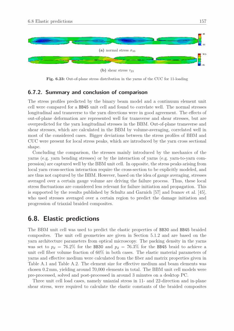
6.8 Elastic predictions 157
(a) normal stress σ33
(b) shear stress τ23
Fig. 6.23: Out-of-plane stress distribution in the yarns of the CUC for 11-loading
6.7.2. Summary and conclusion of comparison
The stress profiles predicted by the binary beam model and a continuum element unitcell were compared for a BB45 unit cell and found to correlate well. The normal stresseslongitudinal and transverse to the yarn directions were in good agreement. The effects ofout-of-plane deformation are represented well for transverse and shear stresses, but areoverpredicted for the yarn longitudinal stresses in the BBM. Out-of-plane transverse andshear stresses, which are calculated in the BBM by volume-averaging, correlated well inmost of the considered cases. Bigger deviations between the stress profiles of BBM andCUC were present for local stress peaks, which are introduced by the yarn cross sectionalshape.
Concluding the comparison, the stresses mainly introduced by the mechanics of theyarns (e.g. yarn bending stresses) or by the interaction of yarns (e.g. yarn-to-yarn com-pression) are captured well by the BBM unit cell. In opposite, the stress peaks arising fromlocal yarn cross-section interaction require the cross-section to be explicitly modeled, andare thus not captured by the BBM. However, based on the idea of gauge averaging, stressesaveraged over a certain gauge volume are driving the failure process. Thus, these localstress fluctuations are considered less relevant for failure initiation and propagation. Thisis supported by the results published by Schultz and Garnich [57] and Ivanov et al. [45],who used stresses averaged over a certain region to predict the damage initiation andprogression of triaxial braided composites.
6.8. Elastic predictions
The BBM unit cell was used to predict the elastic properties of BB30 and BB45 braidedcomposites. The unit cell geometries are given in Section 5.1.2 and are based on theyarn architecture parameters from optical microscopy. The packing density in the yarnswas set to pd = 76.2% for the BB30 and pd = 76.3% for the BB45 braid to achieve aunit cell fiber volume fraction of 60% in both cases. The elastic material parameters ofyarns and effective medium were calculated from the fiber and matrix properties given inTable A.1 and Table A.2. The element size for effective medium and beam elements waschosen 0.2 mm, yielding around 70,000 elements in total. The BBM unit cell models werepre-processed, solved and post-processed in around 3 minutes on a desktop PC.
Three unit cell load cases, namely uniaxial stress in 11- and 22-direction and in-planeshear stress, were required to calculate the elastic constants of the braided composites

6.8 Elastic predictions 158
under the assumption of plane stress. The equations for the calculation of the elasticconstants are given in Appendix F.
(a) BB30
(b) BB45
Fig. 6.24: Young’s modulus Ex predicted by the BBM compared to experimental results
An off-axis polar plot of the predicted elastic modulus, with the off-axis experimentalresults given for comparison, is shown in Fig. 6.24. The initial modulus E0
x, calculatedfrom the tensile experimental data by regression of the stress-strain curve, is used forcomparison to the linear elastic finite element solution. For both braiding angles, four unitcell simulations with different out-of-plane boundary conditions, as described in Table 6.2,were conducted. In the micro-CT scan of the BB45 braided composite, no distinct stackingconfiguration was seen, thus none of the idealized stacking configurations is present in areal braided composite laminate. However, as the unit cell simulations were conducted

6.8 Elastic predictions 159
with a single unit cell, the main goal of the comparison was to find the idealized stackingconfigurations yielding the best approximation of a mixed stacking case.
For both braiding angles, the different out-of-plane boundary conditions mainly influ-ence the stiffness in the the yarn direction (off-axis angle ψ = θ). For this load case, a highlongitudinal stress is present in one of the yarn directions, while the longitudinal stress inthe other yarn direction is comparable small, which introduces the out-of-plane warpingof the unit cell and softens the response. The stiffness reduction is most prominent for theSUC boundary condition, which equals a single ply laminate, where no constraint is givento the out-of-plane deformation. For the stacking of adjacent plies being out-of-phase (cf.Table 6.2), similar results are obtained for two plies (SYM ) and an infinite number of plies(OP). For the out-of-phase stacking, the out-of-plane deformation is locked, as the adja-cent plies tend to deform out-of-plan contrarily. This leads to zero out-of-plane warping,giving an upper bound for the stiffness. If 3D periodicity with IP stacking is assumed,the adjacent plies give a certain support and restrict the out-of-plane deformation, thusthe response in yarn direction is slightly softer compared to the OP case.
Comparing the predicted elastic constants to the experiments, the IP stacking yieldsthe best approximation for the biaxial braided laminates behavior. As the real stackingdoes not match the OP case, a certain amount out-of-plane deformation of the braidedcomposites can be assumed to be present if loaded off-axis. Thus, the IP out-of-planeboundary condition is considered the most realistic for a mixed stacking, which can beassumed to be present in most braided laminates. A more detailed investigation of theeffect of stacking to the predicted properties may be obtained by introducing specialboundary conditions as presented by Ivanov et al. [208, 209]. This may lead to improvedresults for modeling a distinct stacking, but for predictions of mechanical properties, theinformation of laminate stacking is unlikely to be available. Thus, the IP out-of-planeboundary condition can be summarized to yield realistic results for stiffness and out-of-plane deformation of mixed stacking biaxial braided composite laminates.
The Poisson’s ratios calculated by the BBM with the different out-of-plane boundaryconditions are compared to the experimental measured ones in Fig. 6.25. For the BB45
braided composite, no experimental data on the Poisson’s ratio was available, thus only thesimulation results are shown. Comparing the different out-of-plane boundary conditions,the results of the cases considering two or more plies (SYM, IP, OP) are very similar,while the SUC solution overestimates the transverse contraction. The biggest deviationfor both braiding angles is seen for an off-axis angle of ψ = 40 − 50°. The comparisonto the experimental data of the BB30 braid shows, as for the Young’s modulus, that theIP solution yields a good correlation. The deviations observed between prediction andexperiments for the off-axis angles ψ = 30° and Ψ = 45° are mainly attributed to theidealizations made for the effective medium constitutive model.
A comparison of the elastic moduli calculated with the BBM to the analytical predic-tions made with TexComp is given in Fig. 6.26. The TexComp results for both, BB30
and BB45 are very similar to the OP solution of the BBM, with the stiffness in yarndirection, predicted by TexComp, being 2-3% bigger. The elastic modulus in take-upand transverse direction of the TexComp model is 3-5% lower. The deviations for thematrix-dominated values are believed to be due to the different micromechanical methodsused for the yarn elastic properties (Mori-Tanaka in TexComp, Chamis equations in the

6.8 Elastic predictions 160
(a) BB30
(b) BB45
Fig. 6.25: Comparison of predicted Poisson’s ratios at different out-of-plane boundary conditions
BBM). The differences in yarn direction show that proper modeling of the influence ofwaviness on the yarn longitudinal behavior requires considering both, the stiffness knock-down of the yarn itself introduced by the undulation and the softening introduced by theout-of-plane deformation. Therefore, the BBM, which allows to consider different lami-nate stacking configurations, yields a more precise and realistic prediction of the stiffness,while the TexComp modeling overestimates the yarn stiffness. Furthermore, it should benoted that the effect becomes even more prominent, if laminates with a smaller numberof plies (n < 4) are used.

6.9 Parametric study: out-of-plane boundary conditions 161
Fig. 6.26: Comparison of elastic BBM results to Mori-Tanaka homogenization (TexComp)
6.9. Parametric study: out-of-plane boundary conditions
It was shown in the previous section that out-of-plane boundary conditions of unit cellcalculations considerably influence the elastic results. In addition to the elastic influence,the out-of-plane warping of the unit cell introduces an additional bending stress intothe yarn stress profiles. As the additional bending can have a considerable effect on thepredicted failure stresses, the influence of out-of-plane unit cell warping to the yarn stresseswas evaluated in a parametric study: the stresses in the yarns and the failure loads wereevaluated for load in the yarn direction at different out-of-plane boundary conditions.For the stress-profile study, the IP case, which was found to be a good approximationfor the elastic behavior, is compared to the case of maximal and minimal out-of-planedeformation of a single-ply unit cell (SUC ) and 3D-periodic OP stacking, respectively.The unit cell calculations were conducted linear elastic for a BB30 and BB45 unit cell. Astress of 100 MPa was applied in the yarn (F-) direction, as shown in Fig. 6.27.
Fig. 6.27: Load cases considered for the out-of-plane boundary condition study

6.9 Parametric study: out-of-plane boundary conditions 162
The longitudinal stress profiles were evaluated in one of the yarns in loading direction(Yarn F-). The resulting stress profiles are shown in Fig. 6.28. The longitudinal stress
(a) center of the yarn (b) upper side of the yarn
Fig. 6.28: Longitudinal yarn stress profiles in the yarn F-
in the center of the yarn shown in Fig. 6.28a is insensitive to the out-of-plane boundarycondition applied. For IP and OP of both, BB30 and BB45, almost identical stressesare predicted, while the SUC solution yields 3-7% lower stresses in the yarn center. Inopposite, major deviations between the out-of-plane boundary conditions are seen for thelongitudinal stress at the upper point of the yarn cross section. For the BB45, the loweststresses in the undulation interval are predicted for the OP case, while the peak stressincreases by 18% for the IP case and 68% for the SUC case. In addition, the locationstress peak is shifted more towards the straight region of the yarn, the more out-of-planedeformation being present. The increased maximum stresses for the SUC and IP caseare induced by yarn bending through the local out-of-plane deformation of the unit cell(cf. Fig. 6.17). The investigations for BB30 show similar effects as the BB45 stress profiles,but the maximum stresses are lower. However, the difference in stress peaks is of similarrange as for the BB45 braid.
The transverse and shear stress profiles in a yarn oriented transverse to the load (F+) are shown in Fig. 6.29. For both braiding angles, the same effects of the out-of-planedeformation are observed: while the solutions for IP and OP boundary conditions arenearly identical, the SUC solution deviates significantly. The transverse stress in theSUC case is more than twice the one observed in the IP and OP case. Negligible shearstresses are present in the yarns of the BB45 in the IP and OP case, while shear stressesin the straight region are introduces by the warping in the SUC case. For the transversestresses, the influence of unit cell warping is similar for both braiding angles, but for theshear stresses it is increased in the BB45 unit cell.
The out-of-plane normal and shear stresses predicted with the different out-of-planeboundary conditions are shown in Fig. 6.30 and Fig. 6.31. For the normal stresses σ33,the influence of the out-of-plane boundary conditions is contrary to the one observed forthe in-plane stresses: the biggest stresses are present for the OP boundary condition.

6.9 Parametric study: out-of-plane boundary conditions 163
(a) σ22 (b) τ12
Fig. 6.29: Transverse and shear yarn stress profiles in yarn F+
The stress profile in the SUC case is similar, with the peak stresses being smaller, whilethe IP case predicts the lowest stresses. The high stresses in the OP case are due tothe compression of the yarns to each other, which is introduced through the suppressedout-of-plane deformation. This is similar for the SUC solution, where the bended yarnsintroduce transverse compression. As the IP case models infinite plies, deforming in asimilar way, the compression of the yarns to each other is minimal in this case.
Fig. 6.30: Transverse normal stress σ33 in yarn F-
For the out-of-plane shear stresses shown in Fig. 6.31, the highest stresses are presentin the case of IP stacking. This is due to the fact that adjacent unit cell deformingsimilar mainly introduce the support by transverse shear stresses. As not out-of-planedeformation is present in the OP case, only minor transverse shear stresses are observed.The SUC case, where the transverse shear stresses are induced by the big out-of-plane

6.9 Parametric study: out-of-plane boundary conditions 164
(a) τ13 (b) τ23
Fig. 6.31: Transverse shear yarn stress profiles in yarn F-
warping, shows similar stress profiles as the IP unit cell, with the stress peaks beingsmaller for τ13 and similar for τ23.
6.9.1. Nonlinear deformation and failure
In addition to the linear simulations, the influence of the out-of-plane boundary conditionsto the nonlinear deformation and the failure loads predicted by BBM unit cell simulationswas investigated. The simulations included a nonlinear geometry formulation and theDrucker-Prager plasticity model in the effective medium. The load case considered was,as for the stress profiles, load in one of the yarn directions. The homogenized stress-straincurves from the BB30_OA30 and the BB45_OA45 simulations are given in Fig. 6.32. Thelinear (lin) stress-strain curves, given for comparison, were obtained from the linear elasticsimulations.
For both braiding angles, similar effects are seen in the stress-strain behavior: Thesimulations with IP and OP soften under the load, while the SUC case stiffens withthe load applied. For the SUC case, the large out-of-plane deformation of the unit celldominates the nonlinear deformation by stiffening the yarn response, which leads to theglobal stiffening of the unit cell. The decrease of stiffness, observed in the IP and OPnonlinear simulations is mainly due to plastic deformation in the effective medium. Forthe the IP case, also some stiffening of the yarns due to the out-of-plane deformation ispresent, however, this effect is superimposed with the plastic deformation in the effectivemedium.
The unit cell strength for the nonlinear simulations was predicted by evaluating longi-tudinal fiber failure. Due to the increased stress concentration in the undulation intervalof the SUC model, the lowest strength is predicted in this case. The SUC strength is 24%and 30% lower compared to the OP strength for BB30 and BB45, respectively. The differ-ence in strength is lower in magnitude as compared to the peak stress difference observedin the linear elastic simulations. For the high out-of-plane deformation present in the

6.9 Parametric study: out-of-plane boundary conditions 165
homogenized strain <ε1F
>
ho
mo
ge
niz
ed
str
ess <
σ1
F>
[M
Pa
]
0 0.005 0.01 0.0150
100
200
300
400
500
600
700
800
900
1000
SUC
IP
OP
SUC lin
IP lin
OP lin
(a) BB30, ψ = 30°
homogenized strain <ε1F
>
ho
mo
ge
niz
ed
str
ess <
σ1
F>
[M
Pa
]
0 0.005 0.01 0.0150
100
200
300
400
500
600
700
800
900
1000
SUC
IP
OP
SUC lin
IP lin
OP lin
(b) BB45, ψ = 45°
Fig. 6.32: Comparison of linear and nonlinear solutions for different out-of-plane boundary conditions
SUC case, the nonlinear geometric analysis leads to a stiffening of unit cell and a smallerout-of-plane deformation compared to the linear case. In the case of the IP configuration,the strength is 11% lower for the BB30 case and 18% lower for BB45 case, when comparedto the OP configuration. This difference is of similar magnitude as the difference in stresspeaks observed for the linear elastic simulations. Thus, nonlinear geometric effects haveless impact on the results for IP and OP boundary conditions.
To further investigate the effect of nonlinear geometry for the BB30 unit cell in IPconfiguration. The yarns in biaxial braided composites can be considered as discrete rein-forcing structure, which may align with the load (scissoring [94]) or straighten (reducingthe waviness) under load. The influence of these effects on the deformation of a BB30
is shown in Fig. 6.33. Note that a linear-elastic effective medium constitutive law was
Fig. 6.33: Comparison of linear and nonlinear geometry for BB30 in IP configuration
used for these simulations. For tension in transverse direction (22) and tension in ten-sion in yarn direction (1F), linear and nonlinear deformation yield identical results. A

6.10 Prediction of failure and comparison to experiments 166
slight stiffening of the unit cell response is observed in the take-up (11) direction, whichis due to alignment of the ±30° yarns with the load. However, the impact of this effect issmall compared to the nonlinear effects due to material softening observed in the off-axisexperiments.
6.9.2. Summary out-of-plane boundary conditions
The comparison of yarn stress profiles from identical unit cells simulated with differentout-of-plane boundary conditions showed a major effect of the chosen boundary conditionto the stress profiles. Especially the SUC condition lead to a high out-of-plane defor-mation, introducing additional stresses. The IP and OP boundary conditions differ less,with a maximum difference of 20% for the yarn longitudinal stress. As no correlation toexperimental results is possible, no clear recommendation for a ideal choice of boundarycondition can be identified from the stress profile comparison. However, the IP boundarycondition, which was found to be well suited for elastic predictions, also yielded reason-able results for the yarn stresses, when considering a mixed stacking case as observedin the micro-CT scans. Thus, the IP boundary condition will be used for the nonlinearsimulations described in the next sections.
6.10. Prediction of failure and comparison to experiments
The simulations for failure prediction were conducted for the BB30 and BB45 braidedcomposites with the geometric models given in Section 5.1.2. All simulations included theelastic-plastic material definition of the effective medium and spatial periodicity with IPstacking.
6.10.1. Parameter identification
The elastic predictions done with the BBM based on constituent material parametersfrom experiments with UD composite laminates. A similar approach was investigatedfor the strength predictions, taking the strength properties from the same series of UDexperiments. The failure of the braided composite is in the BBM predicted by applyingfailure criteria to the yarn stress tensor calculated. The yarns within a textile compos-ite behave, transversely isotropic and thus the strength parameters for the yarns can bedirectly extracted from UD experiments. Due to the high packing density in the yarn ofbraided composites (pd ≈ 70%), a special manufacturing process for high volume fractionUD laminates of similar fiber/matrix combination is required. The properties were mea-sured from UD coupons, produced by UD braiding and infused with the VAP process,yielding laminates with a fiber volume fraction of 66%. The experiments in tension andcompression were conducted according to an in-house standard procedure at the PolymerCompetence Center Leoben. The shear properties were not tested and thus taken from[204]. The experimental measured strength properties are given in Table 6.6.
The measured strength properties were scaled to the fiber volume fraction present in theyarn according to the procedure given in Section 6.3.3 and used for unit cell simulationsof the BB30 in take-up and transverse direction. The predicted stress-strain behavior is

6.10 Prediction of failure and comparison to experiments 167
Table 6.6.: Experimental strength values for HTS40 / RTM6 normalized to 60% FVF
XT [MPa] XC [MPa] YT [MPa] YC [MPa] SL [MPa]1
1836 905 47 164 71.3
1: taken from [204]
shown in Fig. 6.34. For both, OA00 and OA90 load, the stiffness and non-linear deformationpredicted by the BBM model yields excellent correlation to the experiments. However, thefailure stresses calculated by the BBM model underestimate the experimentally measuredstresses by 25% for the OA00 loading and by 40% for the OA90 loading. The failurepredicted by the model is intra-yarn failure in compression (mode C) for the OA00 andtension (mode A) for the OA90 case. Further load cases that were simulated with thematerial data from Table 6.6 yielded similar magnitudes of strength underestimation.
Fig. 6.34: Comparison of BBM simulations with UD strength parameters and BB30 experiments
The deviation between the BBM predictions with UD strength parameters and experi-mental results is mainly believed to be due to the input parameters being not appropriatefor the behavior to be modeled. For UD laminates, the effect of thin plies known as in-situ-effect yields increased matrix-dominated properties in dependence of the ply positionin the laminate and the ply thickness. Properties determined by UD experiments werefound to be inappropriate for predicting matrix-dominated failure within a compositelaminate. A similar effect is believed to be present for the biaxial braided compositesinvestigated in this work: the transverse cracking in the yarn is believed to be dependenton the boundary conditions given by the textile architecture of crossing and undulatingyarns. The process of failure and thus the material properties obtained by UD experi-ments are unlikely to be representative for the yarns in braided composites. For the in-situeffect in UD laminated composites, Camanho et al. [159] presented an analytical approachfor the calculation of in-situ strength in laminates. But as the approach assumes specific

6.10 Prediction of failure and comparison to experiments 168
boundary conditions for crack opening, these equations are unlikely to be representativefor braided composites. Due to this, an alternative approach will be used in this thesis:the strength parameters required for the yarns will be identified by the comparison ofBBM-simulations of biaxial braided composites with according experimental results. Asimilar approach has been used by Cox, Yang and Co-Workers [133, 136] to obtain crit-ical strain values for failure within the Binary Model. As the failure criteria presentedin Section 6.6 require five independent input parameters for yarn longitudinal, transverseand shear failure prediction, five distinct load cases will be used for the parameter iden-tification. The strength parameters are identified within the simulations by an iterativebest-fit procedure. An overview to the load cases and the identified parameters is givenin Table 6.7.
Table 6.7.: Load cases for parameter identification and identified strength values
Strength XT [MPa] XC [MPa] YT [MPa] YC [MPa] SL [MPa]
Model BB30 BB30 BB30 BB30 BB45
Load Case PT_OA30 PC_OA30 PT_OA90 PT_OA00 PT_OA00
Value1 2192 1545 82 174 112
1: values given for 60% fiber volume fraction
6.10.2. Comparison to experiments
The BBM predictions are compared to the BB30 and BB45 off-axis experiments. For alloff-axis angles characterized experimentally, nonlinear simulations were conducted withthe load introduced into the unit cell calculated by Eq. 6.27. The stress-strain curvesand strength predicted by the BBM simulations are compared to the experimental resultsgiven in Chapter 4 for the BB30. The BB45 tensile and compressive experiments in take-up (OA00) and yarn direction (OA45) were conducted at the Polymer Competence CenterLeoben, with an overview to the experiments is given in Appendix A.1. All BBM unit cellsimulations were nonlinear, including the elastic-plastic material model in the effectivemedium. A linear geometric formulation was used, as the effects of nonlinear geometryobserved were small and the linear geometry models showed an improved convergence forcompressive loads. The element size for effective medium and beam elements was chosen0.2 mm, which yielded 70,000 elements in total. The off-axis stresses applied to the unitcell were calculated according to Eq. 6.27. The unit cell failure stress was obtained fromthe first longitudinal or transverse failure occurring within the yarns.
BB30 tension
The results of the BBM simulations in tension are compared to the off-axis experimentsin Fig. 6.35. Only the experimental stress-strain curves of the monotonically loadedspecimen are shown for clarity. The point, where the BBM stress-strain curves end is thepoint, where failure was predicted in the unit cell model.

6.10 Prediction of failure and comparison to experiments 169
<εxx
> [−]
<σ
xx>
[M
Pa]
0 0.005 0.01 0.015 0.02 0.0250
100
200
300
400
500
experiments
BBM
(a) BB30_PT_OA00
<εxx
> [−]
<σ
xx>
[M
Pa]
0 0.005 0.01 0.015 0.020
100
200
300
400
500
600
700
experiments
BBM
(b) BB30_PT_OA15
<εxx
> [−]
<σ
xx>
[M
Pa]
0 0.005 0.01 0.0150
100
200
300
400
500
600
700
800
900
experiments
BBM
(c) BB30_PT_OA30
<εxx
> [−]
<σ
xx>
[M
Pa]
0 0.002 0.004 0.006 0.0080
50
100
150
200
250
experiments
BBM
(d) BB30_PT_OA45
<εxx
> [−]
<σ
xx>
[M
Pa]
0 0.002 0.004 0.006 0.008 0.010
20
40
60
80
100
120
experiments
BBM
(e) BB30_PT_OA60
<εxx
> [−]
<σ
xx>
[M
Pa]
0 0.002 0.004 0.006 0.008 0.01 0.012 0.0140
20
40
60
80
100
experiments
BBM
(f) BB30_PT_OA90
Fig. 6.35: Comparison of non-linear BBM-simulations with tensile off-axis experiments
The shape of the stress-strain curves, i.e. the decrease of the tangent modulus is pre-dicted excellent by the BBM unit cell. For the OA00 and OA15 experiments, where a largerscatter was observed in the experimental measured stiffness, the BBM simulations agreewith the response of the stiffer stress-strain curves (Fig. 6.35a, 6.35b). The reason forthis is mainly found in the braiding angle: the variations of stiffness in the experimentscould be assigned to braiding angle variations on the panels. The braiding angle was pre-dominantly found to be bigger as the nominal 30°, resulting in a softer response of most

6.10 Prediction of failure and comparison to experiments 170
specimen. For tension applied in the yarn direction (OA30), the stress-strain behavior ofthe BBM unit cell is slightly nonlinear, while the experimental stress-strain curves showa linear response Fig. 6.35c. The source of the deviation is difficult to evaluate, as theOA30 stress-strain curves had to be linearized at the beginning of the experiment (cf. Sec-tion 4.2.1). The nonlinear stress-strain behavior predicted by the BBM is due to plasticdeformation of the effective medium, i.e. the plasticity model is likely to overestimate thedecrease in stiffness in this case. In contrast, for the higher off-axis angles OA45, OA60 andOA90, the predicted response is in excellent agreement with the experiments (Fig. 6.35d-6.35f). Thus the effective medium plasticity model works accurate for matrix-dominatedload cases, but slightly overestimates the nonlinear deformation, if the load is mainlycarried by the longitudinal yarn stiffness.
For the assessment of the strength prediction, the values of OA00, OA30 and OA90 are notconsidered quantitatively, as these load cases were used for the parameter identificationand thus match the experimentally measure strength. In the case of OA00, the failuremode predicted was compressive intra-yarn failure (mode C), which matches with theobservations on the failure mode and process in the experiments. For the OA15 load case,the BBM simulations overestimate the average experimental strength by 12%, whichis attributed to the braiding angle variations. The failure mode predicted for OA15 iscompressive intra-yarn failure (mode C) in the 1F- direction, while yarn tensile rupturewas observed in the experiments. However, the stress exposures of yarn longitudinal andtransverse failure are very close in the model and the difference in failure modes is believedto be due to an interaction of transverse cracking and longitudinal yarn failure. For OA30,the predicted failure mode is yarn longitudinal failure in the 1F- direction, as observedin the experiments. In the yarn direction transverse to the load (1F+) the model doesnot predict preliminary transverse failure, which is in accordance with the experiments,where no cracking was observed in the transverse yarn direction. For the off axis loadcases OA45 and OA60, the predictions made by the BBM unit cell are nearly identicalto the experimentally measured values. The failure mode for these load cases, as wellas for OA90, is tensile transverse yarn failure (mode A). This is in accordance with theexperimental observations for these load cases, where the final failure appeared as tensilecracking in the 1F+ direction.
Summarizing the comparison to the tensile experiments, the nonlinear deformation ofthe braided composites is modeled well by the BBM model and the predicted failurestresses agree well with the experimental measured values. Except for OA15, the failuremodes predicted match the observations from the experiments.
BB30 compression
The comparison of the BBM simulations to the off-axis compression experiments is givenin Fig. 6.36. The predicted non-linear deformation is in good agreement with the experi-ments. In most cases, the non-linear deformation is slightly overestimated by the model,resulting in a softer response of the simulations for higher strains. Except the OA30, thetrend is similar for all cases: the initial stiffness is predicted accurate by the BBM, butwith increasing strains, the predicted response is softer as the measured one. The reasonfor this behavior could be due to the calibration of the plasticity model: the pressuredependence of the model is calibrated with published test data from a similar material

6.10 Prediction of failure and comparison to experiments 171
<εxx
> [−]
<σ
xx>
[M
Pa]
0 0.003 0.006 0.009 0.0120
50
100
150
200
250
300
350
experiments
BBM
(a) BB30_PC_OA00
<εxx
> [−]
<σ
xx>
[M
Pa]
0 0.003 0.006 0.009 0.0120
50
100
150
200
250
300
350
400
450
500
experiments
BBM
(b) BB30_PC_OA15
<εxx
> [−]
<σ
xx>
[M
Pa]
0 0.002 0.004 0.006 0.008 0.01 0.012 0
100
200
300
400
500
600
700
experiments
BBM
(c) BB30_PC_OA30
<εxx
> [−]
<σ
xx>
[M
Pa]
0 0.003 0.006 0.009 0.012 0.015 0.018 0
100
200
300
400
500
experiments
BBM
(d) BB30_PC_OA45
<εxx
> [−]
<σ
xx>
[M
Pa]
0 0.01 0.02 0.03 0.04 0
50
100
150
200
250
300
350
experiments
BBM
(e) BB30_PC_OA60
<εxx
> [−]
<σ
xx>
[M
Pa]
0 0.01 0.02 0.03 0.04 0.05 0
50
100
150
200
250
experiments
BBM
(f) BB30_PC_OA90
Fig. 6.36: Comparison of non-linear BBM-simulations with tensile off-axis experiments
and the flow is assumed to be associated, which is due to the lack of experimental data forHTS40/RTM6 material not validated for the current material. In addition, the hardeningcurve, which was used identical for tension and compression was calibrated for the tensiontest and could be different in compression. The deformation behavior is different for theOA30 case: the measured response is stronger nonlinear compared to the BBM response.The nonlinear deformation in the experiments is believed to be due to the increase ofwaviness under compressive loads, which the linear geometric model does not represent.

6.10 Prediction of failure and comparison to experiments 172
For the OA45 the increased deviation between measured and predicted stress-strain curvesis due to the difference of initial modulus of model and experiment, which is believed tobe introduced by manufacturing tolerances of the coupons: the OA45 mechanical proper-ties are very sensitive to the off-axis angle and the compressive modulus measured wasconsiderably higher as the tensile one (cf. Fig. 4.42). This suggests the off-axis angle inthe experiments being lower than the nominal one, which introduces the difference in stiff-ness. However, summarizing the stress-strain comparison in compression, the nonlineardeformation is predicted accurate by the BBM for all off-axis angles.
The strength predicted by the BBM correlates well with the experiments in the OA30
and OA45 case, but is underestimated in the other off-axis load cases. As the OA30 case(Fig. 6.36c) was used for the parameter identification of the compressive yarn strength,the prediction meets the experiments. The failure mode in this case is yarn failure incompression, which correlates with the observations from the experiments. For the OA00
and the OA15 test series (Fig. 6.36a-6.36b), the strength is underestimated by the model by15% and 20%, respectively. For both test series, the failure mode predicted is transversetensile yarn failure (mode A), which correlates with the experiments, where the PC_00 andPC_15 failed into a single tensile crack (cf. Fig. 4.41). The deviation in strength is mainlyattributed to stress concentrations from local out-of-plane deformation of the yarns in theunit cell: as the yarn-to-effective medium coupling using the MPCs is localized at the beamnodes, a local out-of-plane deformation of the unit cell at the undulation intervals of theyarn is present. The out-of-plane deformation introduces additional stress concentrationsin the yarns, leading to a predictions of a lower strength in the unit cell simulations. Usinga nonlinear geometry formulation could reduce the effects of local stress concentrations,but it lead to convergence issues with the BBM unit cell: for compressive loads withnonlinear geometry, the yarns are twisted along their length, drastically softening theunit cell response and finally resulting in a non-convergence of the FE problem. Thetwisting is due to the fact that the rotational DOFs of the beams are not coupled intothe effective medium, which is an artifact in the model formulation. A solution could beto introduce an improved constraint method, coupling both, rotational and translational,degrees of freedom from the beam nodes.
For the OA45 test series, the predicted strength lies within the experimental scatter andthe failure mode predicted is transverse compressive failure in the 1F+ yarn direction.The mode and location of failure correlate well with the experiments, which showed anthrough-the-thickness inclined crack in the 1F+ direction. Comparing the unit cell predic-tions higher off-axis angles OA60 and OA90 to the experiments, the compressive strengthis underestimated by 29% and 25% respectively. The failure mode predicted is yarntransverse compressive failure (mode C) in the 1F+ direction for OA60 and simultaneousmode C failure in both yarn directions for OA90. The predicted failure modes correlatewith the experiments, where thickness-inclined cracks were observed in both test series.The large deviation between the models and the experiments could not be assigned tomodeling assumptions in the BBM, and it is rather believed that the difference comesfrom the experiments: the CLC test fixture requires specimen with small gauge sectionsand thus local stress concentrations induced by the fixture can have a major effect. Inboth test series, the cracking of the specimen was near the load introduction and the OA90
series showed a zig-zag pattern where the cracks were stopped at the tab location. Thus,

6.10 Prediction of failure and comparison to experiments 173
it is believed that the cracking was inhibited by the load introduction in the experiments,increasing the maximum force and thus strength measured. The theory is supported bythe test results obtained from Birkefeld [193] for an biaxial braided composites of iden-tical fiber/matrix combination: the compressive strength measured by Birkefeld in the11 -direction is identical to the one measured in this thesis (Cichosz: 299.8 MPa, Birkefeld:299.1 MPa), while the strength in 22 -direction measured by Birkefeld is 24% lower as theone measured in this thesis (Cichosz: 204.4 MPa, Birkefeld: 155.7 MPa). The issue isbelieved to be particular for braided composites, as they BB30 has a very high Poisson’sratio (νOA90
yx ≈ 1.5), triggering additional stresses in the material if the deformation isconstraint.
BB45 tension and compression
The BBM unit cell simulations were additionally compared to BB45 experiments. TheBB45 braided composites were manufactured with an identical procedure as described inthis thesis (cf. Section 3.2.2) for the BB30. The comparison of stress-strain behavior fromBBM and the experiments is given in Fig. 6.37. No stress-strain curves were available for
<εxx
> [−]
<σ
xx>
[M
Pa]
0 0.005 0.01 0.015 0.02 0.025 0.03 0
50
100
150
200
experiments
BBM
(a) BB45_PT_OA00
<εxx
> [−]
<σ
xx>
[M
Pa]
0 0.005 0.01 0.015 0
100
200
300
400
500
600
700
800
900
experiments
BBM
(b) BB45_PT_OA45
<εxx
> [−]
<σ
xx>
[M
Pa]
0 0.01 0.02 0.03 0.04 0.05 0
50
100
150
200
experiments
BBM
(c) BB45_PC_OA00
<εxx
> [−]
<σ
xx>
[M
Pa]
0 0.002 0.004 0.006 0.008 0.01 0
100
200
300
400
500
600
experiments
BBM
(d) BB45_PC_OA45
Fig. 6.37: Comparison of non-linear BBM-simulations with tensile off-axis experiments
the OA45 compression experiments, thus only the strength value is given in the plot. Fortension and compression in take-up direction (OA00, Fig. 6.37a, 6.37c), the stress-strain

6.11 Conclusion on FE unit cell modeling 174
behavior of simulations and experiments agrees well. In the tension experiments, the foilstrain gauges, used to measure the strain on the specimen, failed preliminary and thus onlyone stress-strain curve is available up to the the failure strain. In compression, the initialstiffness and thus the stresses over the complete strain range are slightly overestimatedby the BBM unit cell model, which is likely to be due to a braiding angle deviation ofthe specimen. As in tension, the foil strain gauges failed preliminary at approximately3% compressive strain, which marks the point of abrupt load increase at constant strainin the experimental stress-strain curves. For the load applied in the yarn direction (OA45,Fig. 6.37b, 6.37d), the comparison of the stress-strain curve in tension yields a goodaccordance between simulation and experiment. The oscillations in the experimentalcurves are due to a blistering of the stochastic DIC-pattern.
The strength predicted by the BBM unit cell model agree well with the experimentallymeasured ones. The BB45_PT_OA00 was used for parameter identification and thus is notused for assessment of the predictions. For the load applied in the yarn direction, thepredicted tensile and compressive strength lie within the experimental scatter, while thecompressive strength in the take-up direction is underestimated by 13%. This is, as forthe BB30_PC_OA00 case attributed to the local out-of-plane deformation of the unit cell.In general, the BBM unit cell predictions made for BB45 can be judged as very accurate.
The BBM unit cell predicts transverse yarn failure in the yarn orthogonal to the loaddirection as first failure for the BB45_PT_OA45. Failure is predicted at a stress of 582 MPa,which correlates with experimental observations of surface-cracking on the specimen form-ing between 450-550 MPa. In this case, as the load could be further increased and the 1F-yarn direction was mainly stressed in longitudinal direction, transverse yarn failure wasignored and yarn longitudinal failure was used to predict the strength.
6.11. Conclusion on FE unit cell modeling
In this chapter, a novel unit cell modeling approach, the Binary Beam Model (BBM)was proposed for modeling the constitutive behavior of biaxial braided composites. Themodeling approach was integrated into a MATLAB framework, thus parametric unit cellmodels can be built without requiring manual work e.g. for meshing or post-processing ofthe models.
The modeling idealizations base on Cox’s Binary Model and were improved in terms ofconsidering the effects introduced by yarn waviness: beam elements, modeling longitudi-nal and bending stiffness and strength of the yarns are embedded into effective mediumcontinuum elements. The beam elements allow to consider the influence of yarn wavinessand yarn cross-section on stiffness and stress fluctuations in the yarns. Constitutive lawsfor both, effective medium and beam elements have been proposed for the BBM. Theyarn’s constitutive law was chosen linear elastic and considers the volume doubling ofbeam and continuum elements. A Drucker-Prager plasticity model was introduced forthe effective medium, which allows to model nonlinear deformation prior to final failure.
For the matrix-dominated stresses, which are extracted from the effective medium, anaveraging approach based on the idea of volume-averaging was introduced: the averagingremoves the mesh-dependency from the effective medium stress field, while preservinglocal stress fluctuations introduced by the textile yarn architecture of the braided com-

6.11 Conclusion on FE unit cell modeling 175
posites. The stress profiles calculated by the BBM were compared to classical continuumelement unit cell results, and a good correlation was obtained for the stress variationspresent over the complete cross section of the yarns. A major difference was found forthe in-plane shear stress, which yields from the modeling idealizations: rotational DOFsof the beams are not coupled with the effective medium continuum elements and thus noinfluence of yarns crossovers is modeled. However, the in-plane shear stress predicted bythe BBM was conservative compared to the continuum unit cell. Overall, the correlationof BBM and continuum element unit cell was found to be excellent, yielding a good basisfor failure prediction.
Periodic boundary conditions were used for all simulations and the application of differ-ent idealized out-of-plane boundary conditions was investigated. The effect of the chosenout-of-plane boundary condition on the elastic predictions and stress profiles was foundto be severe: the stiffness in the yarn direction was changed up to 40% depending onthe out-of-plane boundary condition and the stress maxima varied up to 70%. Assuminga single unit cell in the simulations was found to be not appropriate for the simulationof a braided laminate with variable stacking of the plies. The comparison of the elasticbehavior under different out-of-plane boundary conditions showed that the IP stackingcorrelated best with the experimental results. As the IP stacking yielded realistic resultsfor the stress profiles, this boundary condition was chosen for further calculations. TheIP stacking idealization, which represents identical stacking of an infinite number of plies,was found to be a good solutions for parametric and predictive calculations.
Strength parameters measured from UD experiments of the same fiber/matrix combi-nation were found to be inappropriate for failure modeling in the yarns. Similar to thein-situ effect known for UD composites, the strength properties of a yarn inside a textilecomposite are believed to be controlled by the boundary conditions given to the crackformation and propagation inside the yarn. Thus, a parameter identification approachbased on experiments of biaxial braided composites was used to identify the strengthproperties used within the BBM. Five experiments out of the off-axis test series werechosen to calibrate the strength properties required for the yarns.
The BBM model predictions were compared to the results of tensile and compressiveBB30 and BB45 off-axis experiments. The non-linear deformation predicted under tensileand compressive loads correlated well with the experiments, approving the modeling ap-proach of using a Drucker-Prager plasticity model in the effective medium. A deviationto the experiments was found for the slight nonlinear deformation predicted by the modelfor the tension applied in one of the yarn directions (Ψ = θ). The deviation could beattributed to nonlinear geometric effects like yarn stretching and yarn alignment, notconsidered in the presented BBM formulation. The off-axis failure predictions correlatedwell in tension, with the failure stresses and the failure modes being predicted accurately.In compression, the failure modes predicted by the BBM simulations matched the onesfound in the experiments, but deviations to the failure stresses determined experimentallyhave been found for just a few of the loadcases. The deviations were mainly attributed tothe out-of-plane deformation behavior of the BBM unit cell under compression, increasingthe maximum yarn stress. In addition, it was found that the compressive test results intransverse (22) direction differ significantly from the ones obtained by Birkefeld [193] witha Celanese test fixture. While the BBM results underestimate the strength measured in

6.11 Conclusion on FE unit cell modeling 176
the off-axis compression experiments with the CLC test fixture, it matches the strengthgiven in [193].
Summarizing the finite element unit cell simulations, the BBM model provides an ac-curate and efficient tool to simulate the effect of a textile yarn architecture on the elasticand nonlinear behavior of biaxial braided composites. The model correlates well withclassical predictions and experimental investigations, and thus builds a good basis forpredicting yarn-architecture dependent solutions of the constitutive behavior of biaxialbraided composites. The predicted response from the BBM can further be used as aninput for macroscopic modeling.

7. Macroscopic modeling of biaxialbraided composites
Macroscopic modeling approaches are necessary for efficient modeling and simulationof structural components made from biaxial braided composites. Explicit modeling ofthe yarn architecture, like it is done in unit cell modeling, is not suitable for structuralsimulation from both, modeling effort and computational cost. Thus, a macroscopicapproach based on shell element modeling is introduced. The assumption of plane-stress,used within most shell elements, was shown to be meaningful for braided composites, asthe textile reinforcement is two-dimensional. Two types of approaches based on CLT willbe employed:
1. Linear and analytical predictions, solely using CLT equations and first failure pre-diction.
2. Nonlinear predictions, including plastic deformation and damage, implemented intoa material subroutine in the finite element code Abaqus/Explicit.
The analytical approach will be used to determine the macroscopic input propertiesbased on the FE unit cell modeling results. Two methods for analytical predictions,either modeling the two yarn directions of the braided composites in separate plies, orsmearing the properties into one orthotropic ply, are compared in terms of elastic andstrength prediction. Furthermore, predictions for different failure criteria are comparedand validated with the off-axis experiments. Due to the analytical model being limitedto linear deformation, a nonlinear modeling approach, including plasticity and damage,is presented.
7.1. Analytical modeling approaches
Using CLT-based plane-stress modeling is common for macroscopic modeling approachesof woven and braided composites (cf. [12, 34, 117, 210, 211]). Beside the computationalefficiency, the shell elements modeling yields the advantage that a distinct laminate stack-ing, i.e. different braiding angles in a braided laminate, can be modeled within a singleelement, by using thickness integration points.
Two different approaches, shown in Table 7.1, will be considered for analytical mod-eling: the smeared ply approach (SPA), common for modeling of woven fabrics [117],and the angle ply approach (APA), reported for biaxial and triaxial braided compos-ites [12, 210]. For the SPA, the behavior of the braided composites is modeled withina single orthotropic ply. The input properties are given as the stiffness and strength ofthe braided composite in take-up and transverse direction and in-plane shear. Thus, the
177

7.1 Analytical modeling approaches 178
Table 7.1.: Macroscopic modeling approaches for biaxial braided composites
Smeared Ply Approach (SPA) Angle Ply Approach (APA)
idealization one orthotropic ply four equivalent yarn plies (±θ)S
input
elastic EBB11 , EBB22 , GBB12 , νBB12 Eeq11F , Eeq22F , Geq12F , νeq12F , θ
strength XBBT , XBB
C , Y BBT , Y BB
C , SBBL XeqT , Xeq
C , Y eqT , Y eq
C , SeqL
calibration direct input from BB unit cell sim-ulation / experiments
elastic: inverse CLT strength: cal-ibration to load cases
braiding angle is not modeled explicitly, but included in the input properties. On theopposite, the APA considers the braiding angle, by modeling the braided composite as anangle ply laminate. A symmetric (±θ)S laminate of four equivalent yarn plies is used foreach braided composite layer, excluding bending-extension effects which are present for atwo-ply (±θ) unsymmetrical laminate. The input properties of the APA are the elasticand strength properties of the equivalent yarn plies: these properties include the effects ofyarn waviness and cannot be obtained directly from unit cell simulations or experiments.
Both methods yield advantages and drawbacks: the SPA input is straightforward toobtain from experimental or unit cell modeling results. Five unit cell load cases or experi-ments are required for elastic and strength calibration. However, only limited informationis given by the SPA about the failure behavior, as neither the yarn direction failing northe failure mode of the yarns can be determined. For the APA, the material properties arenot given directly by unit cell simulations or experiments and thus require a calibrationprocedure. The elastic properties can be calculated from closed-form equations given asinverse CLT by Zebdi et al.[119] and strength properties are determined by an iterativecorrelation procedure of the macroscopic model to the unit cell results. However, theAPA yields major advantages for failure prediction, as the braiding angle is included inthe yarn stress calculation and thus failure prediction. Additionally, following the rec-ommendations given by Puck [95], who noted that the mechanics of wavy yarn plies aresimilar to the ones of UD plies, common UD failure criteria can be applied to the yarnplies. Thus, the critical yarn direction and the yarn ply failure mode can be predicted.

7.1 Analytical modeling approaches 179
Stress calculation and failure criteria
The analytical predictions of failure for both, SPA and APA, are based on failure criteria,applied to the stress vectors available in the approach. For the SPA, the stresses in the 12-material coordinate system are employed (σ11, σ22, τ12 cf. Fig. 7.1), while the APA failurepredictions are based on the yarn ply stresses (σ11F+/−, σ22F+/−, τ12F+/− cf. Fig. 7.1).
Fig. 7.1: Coordinate system used for the braided composites
The stresses in the equivalent yarn plies can be derived by application of CLT, whichyields for the case of a (±θ)S braided composite a closed-form equation for the in-planestresses:
σF+/− = Qeq · εF+/− = Qeq · T(±θ)−T · εBB (7.1)
Where σF+/− is the in-plane stress vector of the yarn plies, Qeq is the stiffness matrix ofthe equivalent yarn ply, T(±θ) is the transformation matrix given in Eq. D.9 and εBB isthe in-plain strain vector of the angle-ply laminate.
For the SPA predictions, the maximum stress criterion is used, as the basing assump-tions for application of phenomenological criteria as e.g. Puck are not given for an or-thotropic ply, representing both yarn directions. All stress components are compared tothe biaxial braided composite strength values, yielding the most critical failure mode:
fBBE,Lt =σ11
XBBT
= 1, for σ11 > 0 fBBE,Lc =−σ11
XBBC
= 1, for σ11 < 0 (7.2)
fBBE,T t =σ22
Y BBT
= 1, for σ22 > 0 fBBE,Tc =−σ22
Y BBC
= 1, for σ22 < 0 (7.3)
fBBE,SL =|τ12|SBBL
= 1 (7.4)
For the APA, two sets of criteria, namely Puck 2D and maximum stress criterion, areused. For Puck 2D, yarn ply transverse failure is predicted by Eq. 6.35-6.37 (with yarnply stresses and strength employed) and yarn ply longitudinal failure is predicted by themaximum stress criterion (Eq. 7.5). For the maximum stress, all failure stress exposuresare calculated by comparing the equivalent ply stresses to the corresponding strengthvalues (Eq. 7.5-Eq. 7.7).

7.2 Input property determination for SPA and APA method 180
fE,Lt =σ11F
XeqT
= 1, for σ11F > 0 fE,Lc =−σ11F
XeqC
= 1, for σ11F < 0 (7.5)
fE,T t =σ22F
Y eqT
= 1, for σ22F > 0 fE,Tc =−σ22F
Y eqC
= 1, for σ22F < 0 (7.6)
fE,SL =|τ12F |SeqL
= 1 (7.7)
7.2. Input property determination for SPA and APAmethod
The input properties required for APA or SPA can be obtained from unit cell simulations,like presented in Chapter 6. Alternatively, experiments of biaxial braided composites couldbe used. While the experimental approach may be feasible, if only few yarn architectureconfigurations are considered, the unit cell simulations offer a more efficient method forcalibration of the approaches to various yarn architectures.
7.2.1. Input for SPA
The elastic properties for the SPA are achieved directly from the unit cell simulations ofa biaxial braided composite. The elastic constants are calculated from linear elastic sim-ulations, presented in Section 6.8. For the strength properties, five nonlinear simulationsare required: tension and compression in take-up and transverse direction and in-planeshear. Alternatively, five experimental test cases, with equal load directions as for theunit cell strength calculation are needed.
7.2.2. Input for APA
The APA requires input properties for the equivalent yarn plies, representing undulatedyarns embedded in matrix from one fiber direction of a biaxial braided composites. Theseproperties can be calculated from unit cell simulations. The unit cell simulations yieldthe stiffness matrix of the braided composite given in the material coordinate system (cf.Fig. 7.1).
QBB = f(EBB11 , EBB
22 , GBB12 , ν
BB12 ) (7.8)
The elastic constants of the equivalent plies can be calculated following the inverse CLTapproach published by Zebdi et al. [119]. The stiffness matrix of the braided compositeQBB can be written as
QBB =1
2
(Q
+θ+ Q
−θ), (7.9)

7.2 Input property determination for SPA and APA method 181
where Q±θ
= T−1(±θ) · Q · T−T (±θ) are the stiffness matrices of the equivalent plies inthe global 12 -coordinate system and T is the transformation matrix given in Eq. D.9.Eq. 7.9 can be re-written to
QBB =1
2
2 · Q+θ
11 2 · Q+θ12 0
2 · Q+θ12 2 · Q+θ
22 00 0 2 · Q+θ
66
, (7.10)
as for arbitrary braiding angles, the components of the Qθ
and Q−θ
stiffness matricesyield:
Q+θ11 = Q−θ
11 Q+θ22 = Q−θ
22 Q+θ12 = Q−θ
12 Q+θ66 = Q−θ
66 and (7.11)
Q+θ16 = −Q−θ
16 Q+θ26 = −Q−θ
26 Q+θ61 = −Q−θ
61 Q+θ62 = −Q−θ
62 (7.12)
Q±θ
is the yarn ply stiffness matrix in the material coordinate system, thus can be writtenas a function of the unknown components of the yarn ply stiffness matrix Qeq (in the yarn1F± coordinate system):
Q+θ11 = Q−θ
11 = Qeq11 · c4 + 2 · (Qeq
12 + 2 ·Qeq66)s
2c2 +Qeq22 · s4
Q+θ22 = Q−θ
22 = Qeq11 · s4 + 2 · (Qeq
12 + 2 ·Qeq66)s
2c2 +Qeq22 · c4
Q+θ12 = Q−θ
12 = (Qeq11 +Qeq
22 − 4 ·Qeq66) · s2c2 +Qeq
12 · (s4 + c4)
Q+θ66 = Q−θ
66 = (Qeq11 +Qeq
22 − 2 ·Qeq12 − 2 ·Qeq
66) · s2c2 +Qeq66 · (s4 + c4)
(7.13)
With c = cos θ, s = sin θ and θ being the braiding angle. Inserting Eq. 7.13 into Eq. 7.10yields a linear system of four equations for the four unknown components of the stiffnessmatrix Qeq and thus delivers a unique solution for the stiffness matrix components of theequivalent ply:
QBB11
QBB22
QBB12
QBB66
=
c4 s4 2s2c2 4s2c2
s4 c4 2s2c2 4s2c2
s2c2 s2c2 s4 + c4 −4s2c2
s2c2 s2c2 −2s2c2 s4 + c4 − 2c2s2
·
Qeq11
Qeq22
Qeq12
Qeq66
(7.14)
However, for θ = 45° the equation system given in Eq. 7.14 is singular, and an additionalconstraint needs to be introduced. In this thesis, the ratio of longitudinal and transversestiffness Z extracted from the BB30 was used:
(Eeq
11
Eeq22
)
θ=45°
=
(Qeq
11
Qeq22
)
θ=45°
= Z =
(Eeq
11
Eeq22
)
θ=30°
(7.15)

7.2 Input property determination for SPA and APA method 182
Eq. 7.15 reduces the system of four equations given in Eq. 7.14 to a three equation systemthat can be uniquely solved. The elastic constants of the equivalent ply are calculatedfrom the compliance matrix, obtained by inversion:
Seq = (Qeq)−1 (7.16)
Eeq11 =
1
Seq11
Eeq22 =
1
Seq22
Geq12 =
1
Seq66
νeq12 = −Seq11
Seq22
(7.17)
With the equivalent elastic constants assigned to the APA equivalent laminate, the in-plane elastic response of the APA is identical to the one obtained with SPA. The equationshave been implemented into a MATLAB function (InverseCLT_BB.m, cf. Appendix E.2),the elastic constants of the equivalent yarn plies calculated for BB30 and BB45 are givenin Table 7.2.
Table 7.2.: Elastic constants of the equivalent yarn plies calculated by inverse CLT
Eeq11 [MPa] Eeq
22 [MPa] Geq12 [MPa] νeq12 [-]
BB30 126006 6887 4522 0.221BB45 121144 7629 4063 0.323
Strength properties
The strength properties for the APA model, when obtained from unit cell modeling results,are connected to the failure criterion used, and cannot be determined analytically likeshown for the elastic constants. Thus, the calculation of the equivalent yarn ply strengthwill be based on an iterative correlation of the APA model to distinct unit cell load cases,cf. Fig. 7.2.
The off-axis experiment showed that the failure modes change with the off-axis an-gle applied, thus the equivalent ply strength parameters are calculated by application ofappropriate load cases. Basically, any multi-axial load case may be chosen for the cali-brations, as arbitrary loads can be introduced into both, BBM unit cell and APA model.However, the choice of load cases was restricted to off-axis loading, as this offers the ad-vantage that off-axis coupon experiments could be used instead for the calibration. Inboth cases, the input for the calibration are the tensile or compressive strength of thebraided composite at five off-axis angles:
σUTS/UCSOAψ , ψ = ψi i = 1 . . . 5
Which yields the five strength parameters required in the failure criteria. For each loadcase, the failure stress is extracted from the BBM simulation and the APA laminate modelis loaded with the unit cell failure load and the strength is adjusted, for the APA modelpredicting the same macroscopic failure stress.
By applying this procedure, the fluctuations in the stress field of the unit cell model areconsidered within the material parameters used in the APA model. To ensure that themethod is valid, identical failure modes have to be predicted by APA and the unit cell.

7.2 Input property determination for SPA and APA method 183
(a) BBM load case (b) APA equivalent laminate model
Fig. 7.2: BBM unit cell and APA equivalent laminate model load case
The load cases chosen for the calibration depend on the yarn architecture and thebraiding angle. The longitudinal tensile and compressive strength of the equivalent plycan be obtained for the loading applied in the yarn direction (ψ = θ). For the transversestrength of the equivalent ply, the choice of load cases is more difficult: as the equationsof the Puck 2D criterion for transverse failure modes A and C include both, transverseand shear strength parameters, no independent solution for the yarn ply strength canbe obtained. Thus, an iterative procedure, including all load cases with transverse yarnfailure, was used to fit the equivalent yarn ply transverse strength parameters. Thechoice of load cases for the BB30 was based on the stress state in the yarns and the failuremodes in the unit cell simulations: OA90 in tension and compression was chosen for thecalibration of Y eq
T and Y eqC and the in-plane shear strength SeqL was calibrated under OA00
tensile loading. For the BB45, the in-plane shear strength SeqL of the equivalent ply wasalso obtained from tensile loading in take-up direction (OA00). However, it was found thatthe transverse strength parameters have only minor effects on the failure behavior of theBB45 over the complete range of off-axis angles. This is in accordance with the results ofFouinneteau [12], who found transverse failure of 1×1 biaxial braided composites to benegligible. Thus, the transverse yarn ply strength was for the BB45 alternatively calibratedfrom the transverse yarn failure under PT_OA45 loading. The macroscopic stress value,where transverse yarn failure was present in the BB45_PT_OA45 simulation, was used forthe calibration. As no preliminary transverse failure under compression in 1F-directionwas present in the BBM unit cell simulations, the value Y eq
C was taken from the yarnmaterial parameters given in Table 6.7.
The calibration of the APA was done for both, maximum stress and Puck 2D criterion,with the results for BB30 and BB45 summarized in Table 7.3. The strength values givencan be interpreted as in-situ values (as described by Schultz and Garnich [57]) for theundulated yarns in a braided composite. The influence of the yarn architecture is e.g.present for the longitudinal direction, where the strength parameters are reduced by30%-40% compared to the yarn strength parameters in the BBM.

7.3 Analytical failure prediction with APA and SPA 184
Table 7.3.: Calculated strength values and load cases used for strength correlation
BB30 calibration
XeqT [MPa] Xeq
C [MPa] Y eqT [MPa] Y eq
C [MPa] SeqL [MPa]
PT_OA30 PC_OA30 PT_OA90 PC_OA90 PT_OA00
Puck 2D 1487.8 1126.5 50.1 102.5 90.2
Max stress 1487.8 1126.5 41.8 79.6 103.4
BB45 calibration
XeqT [MPa] Xeq
C [MPa] Y eqT [MPa] Y eq
C [MPa] SeqL [MPa]
PT_OA45 PC_OA45 PT_OA451 -2 PT_OA00
Puck 2D 1343.1 1035.3 70.3 174.02 85.1
Max stress 1343.1 1035.3 70.3 174.02 79.1
1: calibrated from transverse failure in the F+ yarn direction2: not calibrated
7.3. Analytical failure prediction with APA and SPA
The in-plane stress failure envelopes predicted using the APA and SPA model are shownfor the BB30 and BB45 braided composites in Fig. 7.3 and Fig. 7.4. The axes of the failureenvelopes represent the stress components in the material coordinate system. For theAPA, the failure envelopes were calculated by evaluating the Puck 2D failure criteria inboth yarn plies, with the most critical value of the two plies used to calculate the failurestress. Thus, the earliest failure predicted was used to construct the failure envelopes. Inaddition to the failure envelopes, the results from the off-axis experiments are given inthe plots.
For the SPA, the failure envelopes is cuboid-shaped, regardless of the braiding angle.The difference between SPA failure envelopes at different braiding angles is given bythe dimensions, defined by the input values of strength in the material axes. The BB45
envelope is quadratic in the σ11-σ22 plane as, take-up and transverse direction strength areequal. The highest strength value yields for both braiding angles in shear: with the fibersoriented off-axis (±θ), shearing mainly introduces stresses in the longitudinal direction ofthe fibers, resulting in a high shear stiffness and strength of the braided composites.
The APA failure envelopes differ significantly from the SPA envelopes. The orientationand shape of the of the failure is influenced by the braiding angle: for BB45 the orientationof the failure envelope is 45°, while the orientation of the envelope is shifted more towardsthe σ11-axis for the BB30. This is due to the yarn ply stresses σF+/F− being used for theprediction of failure, inherently including the braiding angle. Thus, e.g. a biaxial σ11-σ22
stress state for the BB45, equivalent to longitudinal tension in both yarn directions yieldsa higher failure stress value as uniaxial σ11 tension, where the yarns are mainly stresses inshear. In addition, for both braiding angles, the failure stress at a combined σ11-σ22 stressstate decreases with a shear stress introduced: A shear stress τ12 introduces additional

7.3 Analytical failure prediction with APA and SPA 185
Fig. 7.3: Comparison of 3D failure envelopes from SPA and APA for BB30
Fig. 7.4: Comparison of 3D failure envelopes from SPA and APA for BB45
stresses in the yarns, which mainly affects the load cases, where stresses are introducedin the yarn direction. The failure modes predicted by the APA method are mainly yarntransverse failure modes, which is in accordance with the off-axis experiments.
A comparison of the APA and SPA predictions to the off-axis experiments is given asa σ11-σ22 cut of the failure envelopes in Fig. 7.5. The failure stresses from the off-axisexperiment results are projected to the plane. It is important to note that all off-axisexperiments except OA00 and OA90 have a non-zero shear stress component, thus the2D comparison can only yield qualitative results: e.g. BB30_PC_OA30 and BB45_PC_OA45,

7.4 Comparison of failure criteria for APA 186
lying on the 3D failure envelopes (cf. Fig. 7.3 and Fig. 7.4) are projected inside thefailure envelope for the 2D representation. However, the off-axis experiments confirmthe shape of the APA failure envelope. The off-axis load cases in yarn direction showthat the orientation of the failure envelopes is captured accurately by the APA approach.In opposite, the SPA approach does not consider the braiding angle and thus stronglyunderestimate the failure stresses for load cases in yarn direction. In addition, for thetension/compression quadrants, the SPA is non-conservative and predicts higher failurestresses as the APA approach. A combination of tension and compression in the materialcoordinate system results in high shear stresses in the yarns, and thus the SPA predictionsare not considered realistic. However, as tension-compression stress states cannot beachieved by off-axis testing, this needs additional experimental verification.
σ11
σ 22
−1000 −500 0 500 1000 1500−1000
−500
0
500
1000
1500
APM: Puck2D
SPM
Exp. OA00
Exp. OA15
Exp. OA30
Exp. OA45
Exp. OA60
Exp. OA90
PT_OA
PC_OA
[MPa]
[MP
a]
(a) BB30
σ11
σ 22
−1000 −500 0 500 1000 1500−1000
−500
0
500
1000
1500
PT_OA
PC_OA
APM: Puck2D
SPM
Exp. OA00
Exp. OA45
Exp. OA90
[MPa]
[MP
a]
(b) BB45
Fig. 7.5: σ11-σ22 failure envelopes for BB30 and BB45 braided composites
Concluding the comparison, the APA approach yields more realistic results for braidedcomposites. The SPA approach, giving accurate results for woven fabrics, where themaximum strength is present along the material axes, fails to consider the influence ofthe braiding angle on the failure envelope. In opposite, the highest failure stresses beingpresent in the yarn direction is captured well by the APA, as the yarn ply stresses areused for the failure prediction. Based on the results of the comparison, the APA was usedfor the failure predictions presented further.
7.4. Comparison of failure criteria for APA
In the APA, the biaxial braided composites are modeled as equivalent yarn plies, whichenables either application of rather simple criteria like maximum stress or phenomenolog-ical criteria like Puck 2D, originally developed for UD plies. To investigate the influenceof the failure criterion used, Puck 2D and maximum stress failure criteria are comparedfor the BB30 and BB45 braided composites. The strength parameters for both criteria aregiven in Table 7.3. The 2D failure envelopes in the planes, given by the in-plane stresscomponents, are shown in Fig. 7.6. In general, the predictions from the two criteria, arevery similar, but some differences can be observed from the comparison.

7.4 Comparison of failure criteria for APA 187
σ11
σ2
2
−1000 −500 0 500 1000 1500
−1000
−500
0
500
1000
1500
APA: Puck2D
APA: Max Stress
[MPa]
[MPa]
(a) BB30: σ11 − σ22
σ11
σ2
2
−1000 −500 0 500 1000 1500
−1000
−500
0
500
1000
1500
APA: Puck2D
APA: Max Stress
[MPa]
[MPa]
(b) BB45: σ11 − σ22
σ11
τ12
−800 −600 −400 −200 0 200 400 600 800
−800
−600
−400
−200
0
200
400
600
800
APA: Puck2D
APA: Max Stress
[MPa]
[MPa]
(c) BB30: σ11 − τ12
σ11
τ12
−800 −600 −400 −200 0 200 400 600 800
−800
−600
−400
−200
0
200
400
600
800
APA: Puck2D
APA: Max Stress
[MPa]
[MPa]
(d) BB45: σ11 − τ12
σ22
τ12
−800 −600 −400 −200 0 200 400 600 800
−800
−600
−400
−200
0
200
400
600
800
APA: Puck2D
APA: Max Stress
[MPa]
[MPa]
(e) BB30: σ22 − τ12
σ22
τ12
−800 −600 −400 −200 0 200 400 600 800
−800
−600
−400
−200
0
200
400
600
800
APA: Puck2D
APA: Max Stress
[MPa]
[MPa]
(f) BB45: σ22 − τ12
Fig. 7.6: BB30 and BB45 failure envelopes with different criteria
The σ11-σ22 failure envelopes (Fig. 7.6a and 7.6b) show that none of the two criteriais in general more conservative. This is mainly due to the maximum stress criterionnot considering stress interaction, which is covered by the Puck criterion: for transversetension in the yarn plies (σ2F+/2F− > 0) the bearable shear stress is reduced (Puckmode A), while a shear stress higher than the uniaxial shear strength can be carried formoderate transverse compressive stresses (Puck mode B). Including the transverse stressinteraction, also has an effect for the BB45 in uniaxial tension/compression in the 11-

7.5 APA application to test cases 188
direction (cf. Fig. 7.6d): the maximum stress criterion predicts shear failure of the yarnplies, with identical failure stresses in tension and compression. For the Puck criterion,different failure modes (mode A in tension, mode B in compression) are predicted, leadingto an increased failure stress in compression, also observed in the coupon experiments (cf.Table A.5).
For the regions, where Puck and maximum stress criterion are identical, e.g. the straightpart of the failure envelope in Fig. 7.6c and Fig. 7.6d, fiber failure is present, which ispredicted by the maximum stress criterion in both cases.
In addition, some deviations between the failure envelopes are due to the different yarnply strength values obtained for the two criteria in the calibration (cf. Table 7.3): foruniaxial compression in the 11-direction of the BB30, the Puck criterion predicts higherfailure stresses (cf. Fig. 7.6c), which is due to the yarn ply transverse tension strength(Y eq
T ) obtained in the calibration.The comparison of different failure criteria within the APA approach shows, that the
failure envelopes predicted by the maximum stress criterion do not differ significantly tothe ones predicted by the Puck 2D criterion. Thus, the major effect to the failure envelopeis given by the braiding angle, used in the calculation of the stresses σF+/F−. However,the Puck criterion is beneficial for shear-dominated load cases, where the influence of thetransverse stress is considered by the different failure modes of the Puck criterion, whilethe failure stress is predicted identically in tension and compression by the maximumstress criterion.
7.5. APA application to test cases
The APA failure predictions are compared to the off-axis experiments in the off-axis failureenvelopes given in Fig. 7.7 and Fig. 7.8. In the off-axis failure envelopes, the theoreticalfailure stresses for all failure modes (longitudinal failure LF, transverse failure TF, shearfailure SF) of the two yarn plies F+ and F- are given. The lowest failure stress valueyields the critical failure mode.
The results from maximum stress and Puck 2D criterion for the BB30 braided compositeare shown in Fig. 7.7. For the Puck criterion, the predictions in tension and compression(Fig. 7.7a and Fig. 7.7b) correlate well with the experimental results. In tension, thefailure stresses for ψ = 15° and 30° underestimate the experimental results: for ψ = 15°,the failure load is predicted is 12% lower and the failure mode predicted is transverse yarnfailure instead of fiber failure observed in the experiments. The deviation is believed tobe due to the linear prediction, which does not consider stress-redistribution by plasticdeformation of the yarns under shear. For tension in the yarn direction (ψ = 30°),transverse failure of the F+ yarn direction is predicted in advance of the yarn rupturein the F- direction. For compression, the predictions agree well with the experimentalresults for ψ = 0°-45°, while the failure stresses are underestimated for ψ = 60°-90°. Thisdeviation is attributed to the calibration using the BBM modeling results, which alsounderestimated the strength for these off-axis angles.
The maximum stress criterion predictions in tension (Fig. 7.7c) also agree well with theoff-axis experiments. For compression, the predictions made with the maximum stresscriterion are slightly less accurate: the failure stress for the take-up direction (ψ = 0°) is

7.5 APA application to test cases 189
overestimated, while the strength values for the higher off-axis angles (ψ = 45°-90°) areunderestimated.
Off−Axis−Angle ψ [°]
σxx [M
Pa]
0 10 20 30 40 50 60 70 80 900
500
1000
1500LF F+
LF F−
TF F+
TF F−
(a) Puck 2D tension
Off−Axis−Angle ψ [°]
σxx [M
Pa]
0 10 20 30 40 50 60 70 80 900
500
1000
1500LF F+
LF F−
TF F+
TF F−
(b) Puck 2D compression
Off−Axis−Angle ψ [°]
σxx [M
Pa]
0 10 20 30 40 50 60 70 80 900
500
1000
1500LF F+
LF F−
TF F+
TF F−
SF F+
SF F−
(c) Maximum stress tension
Off−Axis−Angle ψ [°]
σxx [M
Pa]
0 10 20 30 40 50 60 70 80 900
500
1000
1500LF F+
LF F−
TF F+
TF F−
SF F+
SF F−
(d) Maximum stress compression
Fig. 7.7: BB30 off-axis failure envelopes
The predictions for the BB45 braided composite are compared in Fig. 7.8. Both failurecriteria agree well with the experimental values. For tension in the yarn direction (Ψ =45°), the first failure predicted is for both criteria the transverse failure of the F+ yarns (cf.Fig. 7.8a and Fig. 7.8b). For the BB45, the preliminary F+ yarn failure was also observedin the experiments, however, the predicted stress for transverse failure is, as for the BBMmodel, slightly overestimated. For compression, the failure stress in take-up (ψ = 0°)direction is slightly underpredicted from the maximum stress criterion (Fig. 7.8d). This is,as for the higher off-axis angles of the BB30, due to the maximum stress criterion neglectinginteraction of transverse and shear stresses. In opposite, the Puck 2D prediction meetsthe experimental result.
7.5.1. Discussion and conclusion of linear predictions
Concluding the comparison of failure predictions from maximum stress and Puck 2Dcriteria to the experiments, both criteria yielded reasonable results. The deviations ob-served for the Puck 2D criterion are mainly due to the fact that the linear analysis doesnot consider the non-linear material behavior of the yarn plies. In addition, due to the

7.5 APA application to test cases 190
Off−Axis−Angle ψ [°]
σxx [M
Pa]
0 10 20 30 40 50 60 70 80 900
500
1000
1500LF F+
LF F−
TF F+
TF F−
(a) Puck 2D tension
Off−Axis−Angle ψ [°]
σxx [M
Pa]
0 10 20 30 40 50 60 70 80 900
500
1000
1500LF F+
LF F−
TF F+
TF F−
SF F+
SF F−
(b) Puck 2D compression
Off−Axis−Angle ψ [°]
σxx [M
Pa]
0 10 20 30 40 50 60 70 80 900
500
1000
1500LF F+
LF F−
TF F+
TF F−
(c) Maximum stress tension
Off−Axis−Angle ψ [°]
σxx [M
Pa]
0 10 20 30 40 50 60 70 80 900
500
1000
1500LF F+
LF F−
TF F+
TF F−
SF F+
SF F−
(d) Maximum stress compression
Fig. 7.8: BB45 off-axis failure envelopes
fact that the APA stiffness and strength parameters were calibrated to the BBM sim-ulations, the deviations observed for the compressive failure stresses under high off-axisangles, observed for the BBM, were also present for the APA predictions. The maximumstress criterion predictions were less accurate in comparison to the experiments. Thus,interaction of transverse stresses and different transverse failure modes in tension andcompression, which is both considered by the Puck criterion, is believed to be crucial formodeling failure of braided composites.
A drawback from the linear predictions was present for the tension applied in the yarndirection (ψ = θ): the first failure predicted for both braided composites was transversefailure of the yarns, which meets the experimental observations for BB45, but was notobserved in the BB30 experiments. In both cases, the linear predictions failed to give theinformation, if a load increases is possible after the first failure. For structural simulation,the first failure predicted needs to be considered critical, which is appropriate for mostoff-axis cases considered, but underestimates the failure stress when yarn longitudinaltensile stresses dominate. In addition, the analytical model lacks to consider the influenceof non-linear deformation in the yarn plies, which can have an influence on both, failurestrain and failure mode predicted.

7.6 Nonlinear constitutive law 191
7.6. Nonlinear constitutive law
To overcome the limitations reported in the previous section, a nonlinear constitutivemodel (BB_APA_NL) has been developed and implemented into the commercial finite ele-ment code Abaqus/Explicit. The main idea of the constitutive model was based on theAPA: both equivalent yarn plies of the biaxial braided composite are represented in asingle shell element integration point, employing UD constitutive laws for the equivalentyarn plies. An overview to the implemented constitutive law is given in Fig. 7.9: theconstitutive model includes two levels, the yarn ply and the biaxial braided (BB) ply level.The material properties, required for the BB_APA_NL are, similar to the analytical APA,defined for the yarn plies (Table 7.1) and assembled to yield the BB properties. Thebraiding angle is updated in each iteration by using the strains of the integration point.With the updated braiding angle, the strain increment is transformed into the yarn plycoordinate system of F+ and F- yarn ply, with plasticity and damage laws being evalu-ated in both yarn plies (red box in Fig. 7.9). The plastic strain increment is calculated,updating the elastic strain, which is furthermore used to calculate the damaged stiffnessmatrix of both yarn plies. The two stiffness matrices are then re-assembled to the BB
stiffness matrix and with the elastic strain of the BB ply known, the nominal stresses canbe calculated and returned to the FE solver.
7.6.1. Input properties
The input properties for the BB_APA_NL are similar to the ones required for the analyticalAPA given in Table 7.1. In addition, the yield stress and hardening curve of the equivalentyarn ply under in-plane shear needs to be defined. The hardening parameters required areobtained by least-squares regression of the UD (±45°) experimental data given in Fig. 6.10.In addition, the fracture toughness of the equivalent yarn plies for the failure modesconsidered, namely longitudinal tensile, longitudinal compressive, transverse tensile andtransverse compressive, have to be given. As no experimental data for the fiber/matrixcombination used was available, the material properties were taken from [141]. Theadditional input parameters required are summarized in Table 7.4.
Table 7.4.: Additional material parameters required for BB_APA_NL
fracture toughness hardening parameters
GLt GLc GTt GTc K m τ y,012F
N/mm N/mm N/mm N/mm N/mm2 - N/mm2
89.8 78.3 0.2 0.8 188.9 3.28 13.71
7.6.2. Braiding angle update
The strain increment is passed to the VUMAT in the 12 coordinate system and has to betransformed in the yarn ply coordinate system by using the braiding angle. As the fiber

7.6 Nonlinear constitutive law 192
yarn ply level:
for both equivalentyarn plies F+/F-
Begin BB_APA_NLread material
propertiesupdate braidingangle θ Eq. 7.18
transform strain incre-ment ∆ε
BB to F+/F-
calculate plasticstrain increment ∆λ
update elastic, plas-tic strains ε
el, εpl
calculate eq. yarnply damaged stiff-ness matrices Qeq
calculate BB damagedstiffness matrix QBB
calculate BB elastic andplastic strain ε
el, εpl
calculate BB nom-inal stresses σ
BB
check elementdeletion criterion
End BB_APA_NL
Fig. 7.9: Flowchart for VUMAT BB_APA_NL
orientation changes during deformation, the braiding angle is updated by using the axialand transverse strain in the 12 coordinate system, as given by [12]:
θ = tan−1(
tan(θ0) · 1 + ε22
1 + ε11
)(7.18)
Considering braiding angle change can be deactivated in the BB_APA_NL.
7.6.3. Strain increment transformation
The strain and strain increment are provided to the material subroutine in the material(12 ) coordinate system. As both yarn directions can be believed to be strained iden-tically, the strain and strain increment in the yarn plies can be obtained by coordinatetransformation:
∆εF+ = R T(θ) R−1 ∆εBB
∆εF− = R T(−θ) R−1 ∆εBB
(7.19)

7.6 Nonlinear constitutive law 193
With ∆εF+/F− and ∆εBB being the strain increment in the yarn ply F+/F- and the braidcoordinate system, respectively (cf. Fig. 7.1). The transformation matrix T is given inEq. D.9. The BB_APA_NL internally uses the engineering shear strain, thus the Reutermatrix R is used within the transformation.
7.6.4. Plasticity model
For the BB_APA_NL, a 1D plasticity law was implemented on the yarn ply level, to accountfor the plastic deformation observed in the off-axis experiments. Plastic deformationof UD composites is commonly reported in literature [117, 159, 170, 172, 212], withdifferent plasticity criteria proposed. For the yarn plies in the biaxial braided composites,a rather simple approach was chosen, considering plastic deformation solely under in-plane shear, as proposed by Johnson [117] and Fouinneteau [12] for woven and braidedfabric composites, respectively. Thus, the yarn plies are assumed to deform elastic inlongitudinal and transverse direction and elastic-plastic under in-plane shear:
εpl11F = εpl22F = 0 γpl12F 6= 0
The yield criterion used is:
f = |τ12F | − τ y,012F − r(α) = 0 (7.20)
Where τ y,012F is the initial in-plane shear yield stress and r(α) is the isotropic hardeninglaw, defined as a function of the accumulated plastic strain α. Plastic flow was assumedto be associated and a power-law was used for hardening:
r(α) = K · α(1/m) (7.21)
The deformation is elastic for f < 0 and plastic deformation occurs for stress states onthe yield surface f = 0. The plastic strain increment is given as
dγpl12F = dλ∂f
∂τ12F
= dλ sgn(τ12F ), (7.22)
where sgn is the signum function and dλ ≥ 0 is the plastic multiplier to be determined,which gives the change of the accumulated plastic strain dα = dλ. The accumulatedplastic strain α is calculated by integration of the plastic strain increments:
α =∫ γpl
12F
0sgn(τ12F ) dγpl12F (7.23)
Plastic deformation is considered in the case of an undamaged yarn ply. As soon as oneof the yarn ply damage parameters is unequal to zero, the plastic strain stays constant.
Numerical implementation
The yield criterion in Eq. 7.20 includes the hardening function r(α), yielding a nonlinearequation that needs to be solved in every increment. The equation is solved numerically,

7.6 Nonlinear constitutive law 194
by using an implicit predictor-corrector algorithm: based on an elastic test step, the plasticstrain increment is calculated iteratively with a Newton-algorithm. An overview of thenumerical implementation is given in Fig. 7.10. For the test step, the strain increment is
Start SubNewton
elastic teststep calculate
γ∗ pl12F , τ
∗12F , α
∗, f∗
f∗ > 0
initialize n = 0,∆λ0 = 10−15∆λ = 0
calculate f ′
Eq. 7.30
calculate ∆λn+1
Eq. 7.29
n = n + 1
f(∆λn+1)< fRes
n ≥ nmax
End SubNewton
no
yes
no
yes
no
yes
Fig. 7.10: Flowchart for integration of constitutive equation
assumed purely elastic:
γ∗ pl (k+1)12F = γ
pl (k)12F (7.24)
τ∗(k+1)12F = Geq
12 · (γ(k+1)12F − γ
p (k)12F ) (7.25)
α∗(k+1) = α(k) (7.26)
With (k + 1) being the current strain increment to be solved. For the test value of theyield function f ∗ ≤ 0, the elastic test step is accepted and the plastic strain increment is

7.6 Nonlinear constitutive law 195
set to zero. If f ∗ > 0, a plastic corrector is introduced to relax the stress state satisfyingf (k+1) = 0. To calculate the unknown plastic multiplier ∆λ, the unknown stress in thecurrent increment is written as a function of the test stress and the plastic multiplier:
τ(k+1)12F = τ
∗(k+1)12F − ∆λ ·Geq
12 · ∂f(k+1)
∂σ(7.27)
Eq. 7.27 is inserted into the plasticity criterion Eq. 7.20, which gives:
f (k+1)(∆λ) = |τ ∗(k+1)12F | − ∆λGeq
12 −(τ y,012F + r(α(k) + ∆λ)
)
= |τ ∗(k+1)12F | − ∆λGeq
12 − τ y,012F −K · (α(k) + ∆λ)(1/m) = 0 (7.28)
Eq. 7.28 is nonlinear equation of ∆λ and is solved by using a Newton algorithm, given as
∆λn+1 = ∆λn − f(∆λn)
f ′(∆λn), (7.29)
where n marks the increment of the newton-algorithm. The derivation f ′ of the yieldcriterion is:
f ′ =∂f
∂∆λ= −Geq
12 − K
m(α+ ∆λ)(1/m−1) (7.30)
At the beginning of the constitutive equation integration, ∆λ needs to be assigned a smallvalue to ensure f to be differentiable. If the Newton algorithm does not converge afternmax = 100 iterations, a warning message is printed and the iteration is stopped. Whenthe Newton iteration converges, ∆λ is known and stress, plastic strain increment andaccumulated plastic strain are updated:
γpl (k+1)12F = γ
pl (k)12F + ∆λ sgn(τ12F ) (7.31)
τ(k+1)12F = Geq
12 · (γ(k+1)12F − γ
pl (k+1)12F ) (7.32)
α(k+1) = α(k) + ∆λ (7.33)
Elastic and plastic yarn ply strain
With the plastic strain increment in the yarn plies known, the elastic and plastic strainscan be updated:
εN = εoldN + ∆εN (7.34)
εelN = εN − ε
plN = εN −
00
γpl12N
(7.35)
With N ∈ F+, F− and ε, εel, εpl being the total, elastic and plastic strain, respectively.

7.6 Nonlinear constitutive law 196
7.6.5. Damage model
The damage model in the yarn plies is based on the anisotropic damage model for UDcomposites published by Lapczyk and Hurtado [165]. The damage evolution is definedwith the use of fracture energies, removing the mesh-dependency in the softening regime.For the BB_APA_NL, the damage model was adapted to use the Puck 2D criterion fordamage initiation. Three damage variables for yarn longitudinal, transverse and shearfailure are introduced. The damaged stiffness matrix, as given by [165], yields:
Qeq =1
D
(1 − dL)Eeq11 (1 − dL)(1 − dT )ν21E
eq11 0
(1 − dL)(1 − dT )ν12Eeq22 (1 − dT )Eeq
22 0
0 0 D(1 − dS)Geq12
, (7.36)
withD = 1 − (1 − dL)(1 − dT )ν12ν21
and dL, dT , dS being the internal damage variables introduced for yarn longitudinal,transverse and shear damage. The damage variables are zero in the undamaged state andgrow until 1, which is equivalent to full damage. The damage variables used in the stiffnessmatrix have different values for tension and compression, which are assigned based on thesign of the according normal stress:
dL = dLtσ11F|σ11F | + dLc
−σ11F|σ11F | (7.37)
dT = dTtσ22F|σ22F | + dTc
−σ22F|σ22F | (7.38)
With the Macauley bracket operator x = x+|x|2
. The damage variable for shear failureis calculated as a linear combination of the yarn longitudinal and transverse damagevariable:
dS = 1 − (1 − dLt)(1 − dLc)(1 − dTt)(1 − dTc) (7.39)
The damage initiation criterion is evaluated by using effective quantities, basing on theidea of Lemaitre [163]. With the elastic yarn ply strain updated, the effective stress vectorof the yarn plies can be calculated by using the yarn plies’ undamaged stiffness matrix:
σF+/F− = Qeq,0εelF+/F− (7.40)
The undamaged stiffness matrix is obtained from Eq. 7.36, with dL = dT = dS = 0.The effective stress values are used to calculate the stress exposures from the maximumstress criterion given in Eq. 7.5 for longitudinal failure and the Puck 2D criterion givenin Eq. 6.35-Eq. 6.37 for transverse failure. Four damage initiation values for yarn lon-gitudinal (L) and transverse (T) failure in tension (t) and compression (c) are used:fE,Lt, fE,Lc, fE,T t, fE,Tc. If one of the stress exposure values exceeds one, the correspond-ing damage variable is calculated.
The damage variables calculation is based on the publication of Lapczyk and Hur-tado [165], with the equations adapted to the Puck initiation criterion used. Equiva-

7.6 Nonlinear constitutive law 197
lent values of stresses and strains are used, removing the mesh-dependency for damage-progression. The damage variables for the different failure modes are given by:
dI =δfI,eq(δI,eq − δ0
I,eq)
δI,eq(δfI,eq − δ0
I,eq)(7.41)
with I ∈ Lt, Lc, T t, T c. δI,eq is the equivalent displacement of the failure modes, withthe superscripts 0 and f for the equivalent displacements at damage initiation and fullydamaged state (dI = 1), respectively. The equivalent displacement at failure is calculatedfrom:
δfI,eq =2GI
σ0I,eq
(7.42)
Where GI is the fracture toughness of the active mode. The values of the failure modedamage variables are defined monotonically increasing (dI ≥ 0). The equivalent displace-ments for the different failure modes are given in Table 7.5, where Lc is the equivalentelement length, given from Abaqus/Explicit [76].
Table 7.5.: Equivalent displacements and stresses used for damage variable calculation
mode δI,eq σI,eq
long. tensile (σ11 ≥ 0) Lc ε11 Lcσ11ε11
δfteq
long. compression (σ11 ≤ 0) Lc −ε11 Lc−σ11−ε11
δfceq
trans. tensile (σ22 ≥ 0) Lc
√ε222
+ γ212
Lcσ22ε22+τ12γ12
δmteq
trans. compression (σ22 ≤ 0) Lc
√−ε222
+ γ212
Lc−σ22−ε22+τ12γ12
δmceq
x refers to the Macauley bracket operator x = x+|x|2
7.6.6. Stress calculation
The nominal stress of the BB ply is calculated from the elastic strain and BB damagedstiffness matrix. Therefore, the damaged stiffness matrices of the equivalent yarn pliesare transformed to the BB coordinate system with
Q±θ
= T(±θ)−1 Qeq T(±θ)−T . (7.43)
The BB stiffness matrix QBB is then obtained from the yarn ply stiffness matrices Q±θ
according to Eq. 7.9. The elastic strain of the BB ply is obtained by averaging the trans-formed elastic strains from the yarn plies:
εelBB =
1
2·((R T(θ) R−1
εelF+) + (R T(−θ) R−1
εelF−)
)(7.44)
The nominal stress of the BB ply is finally calculated from
σBB = QBBεelBB. (7.45)

7.7 BB_APA_NL model validation 198
7.6.7. Material point deletion
A criterion for material point deletion is defined, setting all stress components of thematerial point to zero. For the BB_APA_NL subroutine, two different criteria for materialpoint deletion are used. The material point is deleted, if either both yarn directions failin transverse failure (cf. e.g. BB30_PT_OA90 experiments Fig. 4.25), or if one of the yarndirections fails in longitudinal direction (cf. e.g. BB30_PT_OA30 experiments Fig. 4.19).
7.6.8. Implementation
The constitutive law was implemented as a Fortran VUMAT material user subroutine insidethe commercial FE code Abaqus/Explicit. An overview about the user-defined inputproperties for the subroutine are given in Appendix E.4.
7.7. BB_APA_NL model validation
The BB_APA_NL model is validated by comparison to the off-axis experiments. The pre-dictions are obtained from single shell (S4R) element simulations in Abaqus/Explicit. Forthe off-axis load cases, a shear deformation is introduced under the uniaxial stress applied,thus, the boundary conditions of the simulations, shown in Fig. 7.11, were set to not con-straint shear deformation of the element. Furthermore, two equations were introduced,
Fig. 7.11: Boundary conditions for single element simulations
ensuring unconstrained transverse and shear deformation:
uN4x − uN1
x = uN2x (7.46)
uN4y − uN1
y = 0 (7.47)
The off-axis loads were introduced into the element by applying forces to node 1 andnode 2 and rotating the material coordinate system by the off-axis angle. The simu-lations have been conducted without consideration of finite yarn rotations, as the unitcell calculations and the material parameter calibration did not consider this effect. Theelastic, strength and nonlinear material parameters used within the simulations are givenin Table 7.2, 7.3 and 7.4, respectively.

7.7 BB_APA_NL model validation 199
7.7.1. Nonlinear deformation
The stress-strain behavior predicted by the BB_APA_NL for the off-axis tensile load cases isshown in Fig. 7.12. For comparison, the stress-strain curves obtained from the monotonicoff-axis tension experiments (cf. Section 4.2.1) are given. The experimentally observed
εxx
[−]
σxx [M
Pa]
0 0.005 0.01 0.015 0.02 0.0250
100
200
300
400
500
experiments
BB_APA_NL
(a) BB30_PT_OA00
εxx
[−]σ
xx [M
Pa]
0 0.005 0.01 0.015 0.020
100
200
300
400
500
600
700
experiments
BB_APA_NL
(b) BB30_PT_OA15
εxx
[−]
σxx [M
Pa]
0 0.005 0.01 0.0150
100
200
300
400
500
600
700
800
900
experiments
BB_APA_NL
(c) BB30_PT_OA30
εxx
[−]
σxx [M
Pa]
0.000 0.002 0.004 0.006 0.0080
50
100
150
200
250
experiments
BB_APA_NL
(d) BB30_PT_OA45
εxx
[−]
σxx [M
Pa]
0.000 0.002 0.004 0.006 0.008 0.0100
20
40
60
80
100
120
experiments
BB_APA_NL
(e) BB30_PT_OA60
εxx
[−]
σxx [M
Pa]
0.000 0.002 0.004 0.006 0.008 0.010 0.012 0.0140
20
40
60
80
100
experiments
BB_APA_NL
(f) BB30_PT_OA90
Fig. 7.12: Comparison of BB30_PT predicted stress-strain behavior to off-axis experiments
non-linear stress-strain behavior is predicted accurately by the model, for both linear (e.g.OA30 and OA45) and strongly nonlinear (e.g. OA00 and OA15) load cases. For OA60 andOA90, the behavior is less nonlinear, which is predicted well for moderate strains up to

7.7 BB_APA_NL model validation 200
εxx = 0.004, but the decrease of modulus is slightly underpredicted for higher strains. Asthe decrease of modulus was predicted well by the BBM unit cell, the deviation is believedto be due to neglecting the influence of transverse stress (σ22F ) in the 1D yield criterion.For the OA30 case, where the load is applied in the F- yarn direction, a discontinuity inthe predicted stress-strain curve is present at a stress of approximately 550 MPa, whichis not observed in the experiments. This is due to a transverse tensile failure, predictedin the F+ yarn ply (oriented 60° to the load), which was not observed in the off-axisexperiments and the unit cell simulations.
εxx
[−]
σxx [M
Pa]
0.000 0.002 0.004 0.006 0.008 0.010 0.0120
50
100
150
200
250
300
350
experiments
BB_APA_NL
(a) BB30_PC_OA00
εxx
[−]
σxx [M
Pa]
0.000 0.002 0.004 0.006 0.008 0.010 0.0120
100
200
300
400
500
experiments
BB_APA_NL
(b) BB30_PC_OA15
εxx
[−]
σxx [M
Pa]
0.000 0.002 0.004 0.006 0.008 0.010 0.0120
100
200
300
400
500
600
700
experiments
BB_APA_NL
(c) BB30_PC_OA30
εxx
[−]
σxx [M
Pa]
0.000 0.002 0.004 0.006 0.008 0.010 0.012 0.014 0.0160
100
200
300
400
500
experiments
BB_APA_NL
(d) BB30_PC_OA45
εxx
[−]
σxx [M
Pa]
0.000 0.010 0.020 0.030 0.0400
50
100
150
200
250
300
350
experiments
BB_APA_NL
(e) BB30_PC_OA60
εxx
[−]
σxx [M
Pa]
0.000 0.010 0.020 0.030 0.040 0.0500
50
100
150
200
250
experiments
BB_APA_NL
(f) BB30_PC_OA90
Fig. 7.13: Comparison of BB30_PC predicted stress-strain behavior to off-axis experiments

7.7 BB_APA_NL model validation 201
The model predictions for the BB30 off-axis compression load cases are compared tothe experiments in Fig. 7.13. As for the tensile off-axis load cases, the predictions agreewell with the experiments for both, linear and nonlinear behavior. The response is, asin tension, nonlinear for OA00, OA15, OA60, OA90 and rather linear for OA30 and OA45.The small deviations between experimental stress-strain curves and the predictions areattributed to the transverse stress influence to the plastic deformation in the yarn plies.It is noted that the underprediction of the strength in the OA60 and OA90 case is ofsimilar magnitude as observed in the BBM simulations, which were taken as basis forthe calibration of the macroscopic models. Possible reasons for these deviations werediscussed in Section 6.10.2.
A comparison of the predicted response to the experimental results for the BB45 is givenin Fig. 7.14. As no experimental stress-strain curves were available for the BB45_PC_OA45,
εxx
[−]
σxx [M
Pa]
0.000 0.005 0.010 0.015 0.020 0.025 0.0300
50
100
150
200
experiments
BB_APA_NL
(a) BB45_PT_OA00
εxx
[−]
σxx [M
Pa]
0 0.002 0.004 0.006 0.008 0.01 0.012 0.0140
100
200
300
400
500
600
700
800
experiments
BB_APA_NL
(b) BB45_PT_OA45
εxx
[−]
σxx [M
Pa]
0.000 0.010 0.020 0.030 0.040 0.0500
50
100
150
200
experiments
BB_APA_NL
(c) BB45_PC_OA00
εxx
[−]
σxx [M
Pa]
0.000 0.002 0.004 0.006 0.008 0.0100
100
200
300
400
500
600
experiments
BB_APA_NL
(d) BB45_PC_OA45
Fig. 7.14: Comparison of BB45 predicted stress-strain behavior to experiments
only the strength is given. The nonlinear response in tension and compression in thetake-up direction (OA00) is predicted well by the model. In the tension and compressionOA00 test series, the foil strain gauges failed before final failure, i.e. the end point of theexperimental stress-strain curves does not represent the point of final failure. The linearresponse predicted for the load in yarn direction correlates well with the experiments. Asfor the tensile loading in yarn direction of the BB30, a preliminary failure is predictedin the F+ yarn ply, which is oriented orthogonal to the load. The transverse failure

7.7 BB_APA_NL model validation 202
was also observed in the F+ yarns in the experiments, but no discrete load drop wasvisible. Thus, the effect of transverse cracking is in this case overestimated by the linearsoftening damage model. However, no detailed investigation of this effect was possible,as the DIC strain signal was very noisy for higher strains, which was due to a blisteringof the stochastic DIC pattern.
Summarizing the comparison of the stress-strain predictions, the 1D plasticity modelused in the BB_APA_NL allows to represent the dominant nonlinear effects observed inthe biaxial braided composites. The decrease of modulus was predicted accurate for vari-ous load cases, ranging from linear (e.g. BB30_OA30), slightly nonlinear (e.g. BB30_OA90)and strongly nonlinear (e.g. BB30_OA00). Thus, the in-plane shear behavior of the yarnplies can be believed to be dominant for the nonlinear deformation of biaxial braidedcomposites.
7.7.2. Failure prediction
The failure in the BB_APA_NL approach was predicted by applying the damage initiationand progression approach described in Section 7.6.5. The ultimate failure of the materialpoint was in all cases given either by both yarn directions failing in transverse directionimmediately after each other or by longitudinal failure of one of the yarn plies. The pre-dicted failure stresses, strains and failure modes are compared to the off-axis experimentsand analytical predictions.
The comparison of predictions to experiments for the BB30 tensile off-axis load cases isgiven in Table 7.6. The failure stresses predicted by BB_APA_NL (NL) and analytical APA
Table 7.6.: Comparison of BB30 tensile predictions from BB_APA_NL (NL) and analytical APA (lin) tooff-axis experiments (exp)
strength [MPa] failure strain [%] failure mode
NL lin exp. NL lin exp. NL lin exp.
PT_OA00 475 468 468±22 2.2 1.1 2.3±0.14 Tc Tc TcPT_OA15 547 515 581±30 1.8 1.0 1.7±0.15 Lt Tc LtPT_OA30 736 555 787±45 1.2 0.8 1.2±0.04 Lt Tt LtPT_OA45 184 192 198±8 0.5 0.5 0.6±0.02 Tt Tt TtPT_OA60 106 111 114±4 0.7 0.7 0.8±0.03 Tt Tt TtPT_OA90 78 80 79±3 0.9 0.9 1.1±0.06 Tt Tt Tt
(lin) correlate well and lie mostly within the experimental scatter. The largest deviationbetween linear and BB_APA_NL predictions is present for the fiber-dominated load casesin OA15 and OA30: for OA15, the analytically predicted failure stress is around 5% lowercompared to the BB_APA_NL prediction. This is due to considerable plastic deformationbeing present in the nonlinear predictions, leading to a stress-redistribution and changingthe failure mode to longitudinal failure. For the OA30 case, the first failure predictedby both models is transverse failure in the F+ yarn direction oriented 60° to the load.For the BB_APA_NL prediction, final failure is in the longitudinal direction of the F- yarnply, oriented in load direction, which correlates with the experimental observations. Thestrength predicted by the nonlinear model being lower as the experimentally measured

7.7 BB_APA_NL model validation 203
one is due to the overpredicted softening after transverse failure (cf. Fig. 7.12c). Besidethese two cases, the failure modes are predicted identically by linear and nonlinear modeland correlate well with the experimental results.
A major difference between linear and nonlinear predictions is present in the failurestrain: in the cases, where the deformation is strongly nonlinear, the failure strain pre-dicted by the BB_APA_NL model is up to twice as large as the linearly predicted one. Thenonlinear predictions correlate well with the experiments, while the linear model largelyunderpredicts the failure strains.
The comparison of predictions and experiments for the compressive BB30 off-axis casesis given in Table 7.7. For all off-axis cases, the failure stresses predicted by the BB_APA_NL
model are slightly less than the ones predicted linearly. The deviation is mainly due tothe fact that the material parameters for both models were obtained by correlation ofthe linear model to the unit cell calculations (cf. Table 7.3). Thus, the effects of plasticdeformation, present in the BB_APA_NL model, are not included. The predicted failurestrength strongly underestimating the experimental results for OA60 and OA90, is mainlydue to the calibration to the BBM unit cell results. The failure strains are, beside these twocases, predicted accurately and the failure modes match the experimental observations.
Table 7.7.: Comparison of BB30 compressive predictions from BB_APA_NL (NL) and analytical APA (lin)to off-axis experiments (exp)
strength [MPa] failure strain [%] failure mode
NL lin exp. NL lin exp. NL lin exp.
PC_OA00 268 281 300±21 0.9 0.7 0.9±0.11 Tt Tt TtPC_OA15 337 379 420±13 0.8 0.7 1.0±0.03 Tt Tt TtPC_OA30 581 601 605±31 0.9 0.9 1.0±0.11 Lc Lc LcPC_OA45 356 389 438±29 1.0 1.0 1.2±0.06 Tc Tc TcPC_OA60 199 219 312±2 1.4 1.3 3.7±0.13 Tc Tc TcPC_OA90 143 153 204±7 2.2 1.7 4.1±0.06 Tc Tc Tc
The failure predictions for the BB45 braid are compared to the experimental resultsin Table 7.8. As for the other cases, the predicted strength values correlate well with
Table 7.8.: Comparison of BB45 tensile and compressive predictions from BB_APA_NL (NL) and analyt-ical APA (lin) to off-axis experiments (exp)
strength [MPa] failure strain [%] failure mode
NL lin exp. NL lin exp. NL lin exp.
PT_OA00 160 161 159±19 2.7 1.1 >2.51 Tt Tt -3
PT_OA45 671 598 706±13 1.1 1.1 1.12 Lt Tt LtPC_OA00 178 178 188±7 3.6 1.2 >31 Tc Tc -3
PC_OA45 550 550 540±19 0.8 0.8 0.92 Lc Lc -3
1: failure strain not measured due to preliminary strain gauge failure2: failure strain not measured, calculated from strength and elastic modulus3: no information about failure mode

7.8 Conclusion on macroscopic modeling 204
the experimental results. The difference in the BB_PT_OA45 case is attributed to theoverestimation of damage of the transverse yarns, similarly observed in the BB30_PT_OA30
simulation. For this case, the linear model predicts transverse failure, underestimating thestrength. The strain measurement in the experiments was not available up till final failure,as either the foil gauge bond failed or transverse cracking destroyed the DIC stochasticpattern on the coupon surface. However, the measured maximal strains approve thenonlinear modeling approach, as the linear model strongly underestimated the failurestrains.
7.8. Conclusion on macroscopic modeling
Analytical linear, as well as a nonlinear modeling approach based on CLT have beenused for failure prediction of biaxial braided composites. The analytical failure modeling,presented in Section 7.1, included two approaches, SPA and APA. For both approaches,input property assignment strategies based on results from FE unit cell calculations orexperiments have been given. For the APA, the properties of the equivalent yarn plies,including the yarn waviness present in braided composites, have been derived by applyingan inverse CLT approach for elastic properties and an iterative calibration procedure forthe strength parameters. The predictions from SPA and APA have been compared tothe off-axis experimental results in Section 7.3. The comparison showed that the SPA,commonly used for woven fabrics, lacks to represent the characteristics of the failureenvelopes, being influenced by the braiding angle. The APA represents well the braidingangle influence, by basing the failure predictions on the equivalent yarn ply stresses.
Two failure criteria, the maximum stress and the Puck 2D failure criterion, were com-pared within the APA predictions in Section 7.4. The results from the two criteria werevery similar, emphasizing that the yarn architecture and braiding angle, given by the yarnply properties and the ply angle, respectively, are majorly affecting the failure envelopeshape. However, the Puck 2D gave slightly better results, considering the different me-chanics of yarn ply transverse failure under tension and compression. The predictionscompared well to the off-axis experiments, with the first failure predicted coinciding withthe final failure in the experiments for most cases. An exception were the cases, wherethe load applied was tensile in the yarn direction: preliminary transverse failure in thecrossing yarn was predicted. Summing up, the analytical failure prediction correlated wellwith final failure in most of the cases, but underestimated the failure load for tension inyarn direction.
As the analytical predictions did not include the effects of plastic deformation, ob-served in the experiments, a nonlinear constitutive model for FE simulations was furtherintroduced. The model bases on the APA and considers both yarn directions in a singlematerial point of a shell element. Plastic deformation is considered in shear of the equiv-alent yarn plies and a damage law, including linear softening after damage initiation, wasused.
The comparison of the linear and nonlinear modeling showed that the failure stressespredicted did not differ significantly and were in good correlation with the experimentalresults. An improvement of the predictions is given by the nonlinear model, for tensileloading in the yarn directions, where linear predictions are limited to the first failure,

7.8 Conclusion on macroscopic modeling 205
occurring in the yarn ply oriented transverse to the load. Furthermore, the failure strainpredictions for the cases with strong nonlinear deformation prior to final failure couldbe significantly improved with the nonlinear model. The deformation predicted by thelinear model is not conservative, which is of major importance for structural simulations,as load re-distribution induced by the nonlinear deformation can significantly change thepredictions. The comparison of the model predictions to the off-axis experiments showeda good correlation for the BB30 and BB45 braided composites. The deviation present forthe high off-axis angles for BB30 under compression were also observed in the unit cellsimulations and are thus attributed to the calibration of the material parameters to theunit cell simulations.
Summing up, linear and nonlinear approach yield accurate failure stress predictions,with the first failure predicted being identical with the final failure in the experiment.This is not the case for fiber-dominated load cases, where the nonlinear model predicts afurther load increase after the first failure, which is in agreement with the experiments.Furthermore, the failure modes and failure strains are predicted more accurately by thenonlinear model.
With the models discussed in this chapter, a basis for macroscopic modeling of biaxialbraided composites has been provided. The models use the framework of classical lami-nate theory and can be straightforwardly applied for the structural simulation of braidedcomponents.

8. Conclusions and future work
The goal of the presented research work was to create an approach for failure modeling ofbraided composites, applicable for simulations on structural components. This required toconsider both, detailed unit cell modeling and experimental characterization to predict theyarn architecture influence on elastic, nonlinear and failure properties, and macroscopicmodeling suitable for component simulation. From the literature review, presented inChapter 2, the main working points of the thesis were identified as:
• Define a methodology for robust yarn architecture characterization, yielding a robustinput for geometric modeling.
• Mechanical characterization of biaxial braided composites under combined stressstates, to provide a phenomenological description of failure and serve a basis formodel validation.
• Predict the influence of the yarn architecture on the mechanical behavior with unitcell modeling, including geometric modeling, analytical elastic predictions and non-linear FE unit cell simulations.
• Develop a macroscopic modeling approach for biaxial braided composite failure pre-diction, applicable to structural components.
8.1. Discussions and conclusions
In Chapter 3, the experimental techniques, used for yarn architecture and mechanicalcharacterization, were given. The manufacturing process using closed cylindrical preforms,which are slit and draped into a flat preform shape, was found to be appropriate for high-quality specimen production. Quality assurance over the complete specimen production iscrucial to obtain reproducible results. Optical sensor fiber orientation measurements werefound suitable for braiding angle characterization. However, the scanned images includedartifacts, which required the application of an automated data reduction routine.
The precision of thickness measurements of the specimen using a caliper was investi-gated: focus-variation measurements of the wavy vacuum-bag surface showed that calipermeasurements are appropriate for the braided composites investigated. Deformation mea-surements using DIC were found to be useful for obtaining the specimen strain. Compar-ison of different techniques for average strain calculation from DIC measurements showedthat considering the complete spatial strain distribution of the specimen is required forbraided composites. Local strain measurements are prone to local effects, resulting inconsiderable deviations of the failure strain.
206

8.1 Discussions and conclusions 207
The first part of Chapter 4 presented the experimental results, obtained from yarn ar-chitecture characterization. The yarn architecture parameters required for the geometricmodels could, with exception of the braiding angle, be reliably measured from optical mi-croscopy. A study on a (±45°) braided composite panel showed that the sample positionon the braided panel has no significant effect on the results. Furthermore, it was shownthat 6-8 micrograph sections provide an appropriate number of measurements to identifydifferences in the magnitude of half the standard deviation. The braiding angle was ob-tained from surface scans of the braided composites by two methods: hand measurementsfrom images and automated evaluation with an optical sensor. Both methods yielded avariable braiding angle transverse to the take-up direction, which was attributed to the s-shape of the yarns, caused by friction and gravity-effects during the braiding process. Theaverage values obtained from the two methods compared well, but the hand-measurmentsprovided slightly higher braiding angle values, attributed to the local measurements atyarn crossing points. Summing up, the sensor-measurements were found to be beneficialfor application to structural components, offering an automated evaluation and an spatialmeasurement over the complete image.
Micro-CT was used for evaluation of 3D effects in the yarn architecture. Quantitativeevaluation was less accurate, which is due to the reduced contrast and resolution of theCT-scans compared to micrographs. However, qualitative information regarding localvariations of yarn cross-sections can be useful for improved geometric modeling.
Finally, analytically calculated yarn architecture parameters were compared to the mea-sured values, yielding 10%-20% underestimation of the yarn height and good correlationfor the other values. Attention needs to be paid, as underestimating the yarn height leadsto non-conservative mechanical predictions (cf. Section 5.3).
The experimental results from the off-axis tension and compression testing of (±30°)2x2 braided composites were presented in the second part of Chapter 4. Off-axis testingintroduces combined stress states into the material, triggering different fiber and matrixdominated failure modes.
A high dependence of mechanical properties on the braiding angle was found for loadingin take-up direction: A braiding angle decrease of 1.5° yielded a strength increase of15%. Similar braiding variations are expected on braided components, emphasizing theneed of considering local braiding angle variations in structural simulation. The stress-strain behavior was, except for the load in yarn direction, nonlinear for all off-axis anglesmeasured. Especially for the load in take-up direction, the initial modulus was morethan 20% higher as the one obtained in the strain range given in the ASTM standard(εxx = 0.1-0.3%). In contrast, for the complete strain range till failure, the ASTM modulusoverestimates the stiffness.
The tensile loading/unloading experiments showed that both inelastic deformation anddamage are driving the nonlinear deformation, with the first being dominant for lowoff-axis angles (ψ = 0°, 15°). Post-mortem microscopy investigations revealed intra-yarncracking solely in the proximity of the macroscopic failure of the specimen. Thus, non-linear deformation was mainly attributed to microscopic damage on fiber-matrix scale,commonly reported for UD composites under shear [159, 170]. This was also supportedby the compressive stress-strain behavior being very similar to the tensile one.

8.1 Discussions and conclusions 208
Failure of the specimen was, except for the load in yarn direction, dominated by trans-verse yarn cracking. The strength values for the cases with transverse failure were foundto be majorly influenced by the yarn transverse stress: for the same off-axis angle, thestrength was higher in tension or compression, when the transverse yarn stress was com-pressive. A similar trend was observed in the failure modes of the coupons, being similarfor the yarn transverse stresses sign being equal. The high-speed camera videos, used forthe tensile experiments, showed that the first cracking occurring on the specimen surfacecoincided with the final failure of the specimen. Similar observations were made for thecompressive experiments, yielding the conclusion that stable intra-yarn crack develop-ment like reported for triaxial braids [210] has less effect on the failure of biaxial braidedcomposites.
The geometric unit cell modeling of the biaxial braided composites, conducted with thesoftware WiseTex, was presented in Chapter 5. The geometric models compared wellwith the micro-CT measurements. Deviations in yarn shape and local nesting effects ofthe plies were identified as the cause for the reduced fiber volume fraction within theunit cells. Analytical predictions with the micromechanics software TexComp were inreasonable agreement with experimental results. Parametric studies yielded fiber volumefraction and braiding angle being the parameters majorly influencing the elastic constants.
The finite element unit cell modeling approach used for failure prediction of biaxialbraided composites was presented in Chapter 6. The Binary Beam Model was formulatedas a extension of the Binary Model [125]: by modeling the yarns with beam elements,stress concentration due to yarn bending could be included in the model, while keepingthe numerical efficiency. Nonlinear behavior could efficiently be included using a Drucker-Prager plasticity model and volume averaging was shown to eliminate mesh-dependencein the effective medium stress field.
The stress profiles calculated by the BBM were compared to a classical continuumunit cell model, yielding a good correlation for most stress components. A deviationwas present for stress fluctuations, introduced by the yarn cross section, which are notcovered in the BBM: the coupling of beam and continuum elements does not include thecross-section definition.
With the periodic boundary conditions defined for the finite element unit cell, differ-ent out-of-plane boundary conditions, referring to laminate stacking configurations, wereinvestigated for elastic solution and stress prediction. The out-of-plane boundary condi-tions had a major effect on predicted elastic behavior and stress fields, which varied up to40% and 70%, respectively. For the random stacking observed in the braided laminates,considered in this work, 3D periodic boundary conditions with in-phase stacking werefound to yield appropriate results.
The BBM predictions were compared to the off-axis experiments, yielding an excel-lent agreement for stiffness and non-linear behavior. For the failure prediction, strengthparameters extracted from UD experiments were found to strongly underestimate thestrength, thus a parameter identification based approach on biaxial braided compositeexperiments was used. The failure predictions of the BBM compared well with the off-axis experiments in tension and reasonable in compression. For the compressive loadcases, nonlinear geometric effects, not considered in the simulation, could be causing the

8.2 Potential future work 209
deviations. However, also stress concentration effects in the compressive experiments,influencing the crack initiation and growth, could be a reason for the deviations. Thus,further experimental and numerical work is required for improved compressive failure pre-dictions of biaxial braided composites.
Approaches used for macroscopic modeling were presented in Chapter 7. Due to compu-tational efficiency, shell element and classical laminate theory based modeling was chosen.The input properties for the macroscopic models were obtained from unit cell modeling orexperimental results: this yields the advantage that stress fluctuations, introduced by thetextile yarn architecture, are considered in the material properties. Two analytical predic-tion methods were compared: the SPA, considering the stresses in the material coordinatesystem, and the APA, considering the stresses in equivalent yarn plies. Form analyticalfailure predictions, it could be concluded the failure modeling based on the stresses inequivalent yarn plies (APA) is favorable for braided composites. Two failure criteria,maximum stress and Puck 2D, were used in the APA, both yielding a good agreementto the unit cell modeling and off-axis experimental results. However, the interaction ofstresses for transverse failure prediction, considered in the Puck 2D criterion, was shownto improve the results.
Basing on the analytical APA modeling, a nonlinear modeling approach (BB_APA_NL),considering plastic deformation and damage was implemented into a material user subrou-tine of the finite element code Abaqus/Explicit. The BB_APA_NL stress-strain predictionsyielded good agreement to the experimental results, approving the 1D plasticity modelused. Considering nonlinear deformation significantly improved the failure strain pre-diction compared to the analytical model. The linear-softening damage model used wasshown to work accurate for matrix-dominated load cases, but overestimated the effects oftransverse cracking for fiber-dominated load cases. Summing up, considering the nonlin-ear deformation behavior of biaxial braided composites is crucial for structural simulation,as the deformation can be predicted more accurately and effects of load-redistribution canbe considered.
The work presented on modeling of braided composites demonstrates the potential ofmulti-scale modeling. Finite element unit cells provide an insight to the mechanical be-havior, considering the details of the textile yarn architecture. The BBM unit cell modelpresented allows computationally efficient and parametric modeling of biaxial braidedcomposites, while preserving relevant details of the stress field. Furthermore, the macro-scopic methods presented can be used for structural simulation, while incorporating theeffects of yarn architecture by obtaining the mechanical properties from unit cell results.The modeling framework presented is straightforward applicable to structural simulationof biaxial braided components.
8.2. Potential future work
Every new method or model opens the door for a number of possible improvements.Some points for potential future research, arising from the research work conducted inthe framework of this thesis, are given below.

8.2 Potential future work 210
Yarn architecture
• Evaluate micro-CT scans quantitatively for yarn architecture characterization. Thisrequires contrast enhancement and 3D segmentation methods for yarns and matrix.
Mechanical characterization
• Investigate improved methods for compression testing, avoiding issues with specimenbending and crack growth under the loading tabs, both encountered with the CLCtest fixture. New test methods require: larger gauge sections, reduction of shear-extension coupling, DIC measurement, and high-speed camera recordings.
• The off-axis characterization should be extended to more braiding angles; stressstates that cannot be tested with off-axis experiments, should be characterized byusing multi-axial testing.
Unit cell modeling
• Investigate refined geometric modeling approaches with CT-scan results to obtainmore realistic fiber volume fractions in the unit cells.
• Improving the accuracy of the BBM stress fields in the effective medium by newcoupling methods for beam and continuum elements, considering the yarn crosssection and coupling both, rotational and translational DOFs.
• Investigate experimental methods for measuring yarn strength and numerical meth-ods to scale strength parameters to different fiber volume fractions.
• Extend the investigations on out-of-plane boundary conditions with comparisonsto DIC measurements of the out-of-plane deformation. This requires a higher DIC-resolution on the specimen and experiments with laminates of different ply numbers.
Macroscopic modeling
• The applicability of the proposed macroscopic modeling methods for braided lami-nates with a small number of plies (n < 4) needs to be investigated. For these cases,the local out-of-plane deformation can become more prominent.
• Apply an improved plasticity model for the equivalent yarn plies, considering theinfluence of transverse stresses. Furthermore, coupling of damage and plasticity canbe addressed based on the loading/unloading experiments conducted in this work.
• The effect of transverse yarn damage was overestimated for the models used, whenthe load applied was in one of the yarn directions. This requires additional ex-perimental investigation, to obtain reliable data about the damage initiation andprogression as well as improved damage models, to consider the stable damage de-velopment observed in the transverse yarns.

A. Material properties
Fiber material properties (Table A.1) were obtained by reverse engineering from UDexperiments, using Chamis’ micromechanics equations (Eq. D.1-Eq. D.6). The matrix(RTM6) material properties given in Table A.2. The UD experiments have been conductedat the Polymer Competence Center Leoben, Austria.
Table A.1.: HTS40 fiber properties, shear modulus and strength from [204]
elastic strength
Ef11 [MPa] 218400 Xf,T [MPa] 3040Ef22 [MPa] 18100 Xf,C [MPa] 1499Gf12 [MPa] 21800νf12 [-] 0.305
RTM6 material properties obtained from bulk matrix experiments at the Polymer Com-petence Center Leoben, Austria.
Table A.2.: RTM6 material properties
Em [MPa] νm [-]2890 0.35
For 60% fiber volume fraction this yields the properties given in Table A.3
Table A.3.: Elastic constants of a HTS40/RTM6 UD ply with ϕf = 60%
E11 [MPa] E22 [MPa] G12 [MPa] ν12 [-]131900 8300 4100 0.29
211

A.1 BB45 test results 212
Inclination parameters used for failure analysis with Puck’s 2D failure criterion.
Table A.4.: Inclination parameters for Puck 2D criterion (from [213])
pt⊥‖ pc⊥‖ pt⊥⊥
0.35 0.3 0.25
A.1. BB45 test results
Table A.5.: Elastic and strength properties of (±45°) biaxial braided composite
Modulus ASTM Modulus initial
Test series MEAN[MPa]
STD[MPa]
CV [%] MEAN[MPa]
STD[MPa]
CV [%]
B45_PT_OA00 13760 547 4.0 15804 800 5.1B45_PT_OA45 65136 2282 3.5 63092 1442 2.3B45_PC_OA00 12857 408 3.2 - - -B45_PC_OA45 62333 1458 2.3 - - -
Strength
Test series MEAN[MPa]
STD[MPa]
CV [%] ϕf1 [%]
B45_PT_OA00 159.4 18.6 11.7 56.8B45_PT_OA45 705.9 13.1 1.9 62.9B45_PC_OA00 187.8 7.1 3.8 58.8B45_PC_OA45 539.7 18.5 3.4 61.7
1: fiber volume fraction of the panels, the results given arenormalized to a fiber volume fraction of 60% according toEq. 3.24-Eq. 3.25

B. Orientation averaging for biaxialbraided composites
The equations given here are implemented into the MATLAB routineOrientationAveraging.m.
Input
• Elastic constants of fibers and matrix
• Fiber volume fraction of the braided composite
• Yarn height d1, yarn width d2 and braiding angle θ
Equations
The properties of the (straight) UD segments are calculated by Chamis´ micromechanicalformulae (Eq. D.1-Eq. D.6). The 3D stiffness matrix is calculated as:
C = S−1 =
S11 S12 S12 0 0 0S12 S22 S23 0 0 0S12 S23 S22 0 0 00 0 0 S44 0 00 0 0 0 S44 00 0 0 0 0 S66
−1
(B.1)
with the assumption of transversal isotropy
E22 = E33, G12 = G13, ν12 = ν13, G23 =E33
2(1 + ν). (B.2)
The compliance matrix components yield:
S11 =1
E11
S22 =1
E22
S12 = − ν12
E11
S23 = − ν31
E33
S44 =1
G13
S66 =1
G23
(B.3)
The stiffness matrix is transformed in the global system by the angle φ:
CUD(φ) = TT C T (B.4)
213

Orientation averaging for biaxial braided composites 214
With
T =
cos2 φ 0 sin2 φ 0 cosφ sinφ 00 1 0 0 0 0
sin2 φ 0 cos2 φ 0 − cosφ sinφ 00 0 0 cosφ 0 − sinφ
−2 cosφ sinφ 0 2 sinφ cosφ 0 cos2 φ− sin2 φ 00 0 0 sinφ 0 cosφ
−1
(B.5)
The out-of-plane yarn angle φ is given by the yarn geometry with A = d1/2 and λ = 2d2:
φ = tan−1
(dy
dx
)(B.6)
and the yarn path function:
y(x) =
A · cos(2 · πx/λ) x = 0 . . . d2
−A x = d2 . . . 2 · d2
−A · cos(2 · πx/λ) x = 2 · d2 . . . 3 · d2
(B.7)
The stiffness matrix of a wavy ply is:
CwavyUD =
1
3 · d2
·∫ 3·d2
x=0CUD(φ)dx =
1
N·N∑
i=1
CUD(φi) (B.8)
The elastic constants of the biaxial braided composite are calculated by an equivalentlaminate model as given in Eq. D.10 and Eq. D.11.

C. Definition of RUC and RVE
The definition for the terms Repeating Unit Cell (RUC) and Representative Volume Ele-ment (RVE) are based on the publication from Pindera et. al. [143]. It is important tonote that the concepts of RUC and RVE have not been used consistent in the literature:RUCs are designated RVE and vice versa.
C.1. Representative Volume Element
The RVE concept is based on the statistical homogeneity: a RVE is the smallest sub-volume of a microstructure that has the same volume fractions and same statisticaldistributions as the complete material (c.f. Fig. C.1(a)). The sub-volume response isidentical as the response of the complete material when either homogenous traction ordisplacement boundary conditions are applied. Examples for RVE could a volume withstatistical distributed fibers in a unidirectional composite that has the same fiber volumefraction and the same arrangement of fibers as the one measured from a real material.If the RVE size is chosen appropriate, the strain energy density is identical for eitherdisplacement or traction boundary conditions applied, resulting in the same homogenizedmaterial properties.
C.2. Repeating Unit Cell
The RUC concept bases on a periodic microstructure of the material (see Fig. C.1(b)).The RUC is the smallest volume of microstructure, which is able to reproduce the completemicrostructure through replication (translation and rotation) of the volume. Note thatdue to practical reasons it is sometimes feasible to use a bigger sub-volume of the material.The response of the sub-volume is identical to the response of the complete material whenperiodic boundary conditions are applied to the RUC.
Fig. C.1: Definition of RUC and RVE according to [143]
215

D. Normalization of properties forbraided composites
D.1. UD properties for the equivalent laminate
Chamis’ micromechanical equations [200] are used to calculated the UD properties fromfiber and matrix properties. The indexes f and m denote the constituent properties offiber and matrix
E11 = ϕfEf11 + (1 − ϕf )Em (D.1)
E22 = E33 =Em
1 − √ϕf (1 − Em/Ef22)
(D.2)
G12 = G13 =Gm
1 − √ϕf (1 −Gm/Gf12)
(D.3)
G23 =Gm
1 − ϕf (1 −Gm/Gf23)(D.4)
ν12 = ν13 = νm + ϕf (νf12 − νm) (D.5)
ν23 = ϕfνf23 + (1 − ϕf )(2νm − ν12
E11
E22) (D.6)
D.2. Equivalent laminate properties
The stiffness matrix Q of an equivalent ply yields
Q =
Q11 Q12 0Q12 Q22 00 0 Q66
(D.7)
with
Q11 =E11
1 − ν12ν21
Q22 =E22
1 − ν12ν21
Q12 =ν12E22
1 − ν12ν21
=ν21E11
1 − ν12ν21
Q66 = G12
The stiffness matrix is transformed to the material coordinate system (of the biaxialbraided composite)
QUD±θ
= T−1(±θ) · Q · T−T (±θ) (D.8)
216

D.3 Normalization 217
with T the transformation matrix
T(φ) =
cos2 φ sin2 φ 2 cosφ sinφsin2 φ cos2 φ −2 cosφ sinφ
− cosφ sinφ cosφ sinφ cos2 φ− sin2 φ
(D.9)
The elastic constants are obtained from the compliance matrix of the biaxial braidedcomposite:
SBB =[QBB
]−1=[1
2
(QUD+θ
+ QUD−θ
)]−1
(D.10)
EBB11 =
1
SBB11
EBB22 =
1
SBB22
GBB12 =
1
SBB66
νBB12 = −SBB11
SBB22
(D.11)
D.3. Normalization
Young modulus in load direction:
1
EBBψ
=1
EBB11
cos4(ψ) +
[1
GBB12
− 2νBB12
EBB11
]sin2 ψ cos2 ψ +
1
EBB22
sin4(ψ) (D.12)
The experimentally measured Young’s modulus EexpX , in off-axis direction ψ, with the
experimental fiber volume fraction ϕexp is normalized to ϕnorm:
Enormx = Eexp
x − (EBBψ (ϕexp) − EBB
ψ (ϕnorm)) (D.13)
Enormx is the normalized value and EBB
ψ (ϕexp), EBBψ (ϕnorm) are determined by the proce-
dure described above.

E. Software codes
E.1. Optical sensor data reduction
The analysis script braiding_angle_analysis.m is included in a folder on the attachedDVD. A short description of input required and output printed is given in the user manual.
E.2. Inverse CLT
The inverse CLT approach has been implemented into the MATLAB functionInverseCLT_BB.m. The script and a user manual are included on the DVD attached tothis thesis.
E.3. BBM modeling framework
The BBM modeling framework programmed in MATLAB and Python is included in thefolder BinaryBeamModel on the DVD attached to this thesis. The framework is startedusing the file.\BinaryBeamModel\Tool\30_MATLAB\32_Framework\Master_File30.m
Explanations to the input parameters are given in the user manual.
E.4. Abaqus VUMAT: BB_APA_NL
The input requires 23 parameters to be defined. The input properties, together with anexample input are given in the user manual. The Fortran subroutine is included in afolder of the DVD attached to this thesis.
218

F. Periodic boundary conditions
F.1. Constrain driver displacements and forces
(a)
(b)
(c)
Fig. F.1: Constraint driver deformations
Table F.1.: Macroscopic stresses / strains and corresponding constraint driver displacements
stress strain CD displacement
σxx ǫxx uCD01
σyy ǫyy uCD11
σzz ǫzz uCD21
τxy γxy uCD31,2
τxz γxz uCD41,2
τyz γyz uCD51,2
U =
uCD0
1 uCD31 uCD4
1
uCD32 uCD1
1 uCD51
uCD42 uCD5
2 uCD21
F =
FCD0
1 FCD31 FCD4
1
FCD32 FCD1
1 FCD51
FCD42 FCD5
2 FCD21
(F.1)
219

F.3 Elastic constants calculation 220
F.2. Loading of the unit cell
F.2.1. Strain controlled loading
Calculate constraint driver displacements from macroscopic strain tensor:
U = 〈ε〉· P (F.2)
The displacements are prescribed to the unit cell and the macroscopic stress tensor iscalculated from the constraint driver forces, given by the FE solution:
〈σ〉 =1
2V
(F · PT + P · FT
)(F.3)
F.2.2. Stress controlled loading
Calculate constraint driver forces from macroscopic stress tensor:
F = V · 〈σ〉(PT )−1 (F.4)
The forces are prescribed to the unit cell and the macroscopic strain tensor is calculatedfrom the constraint driver displacements, given by the FE solution:
〈ε〉 =1
2(U · P−1 + (P−1)T · UT ) (F.5)
F.3. Elastic constants calculation
• Elastic constants are calculated under plane stress assumption and the unit cellresponse is assumed orthotropic in the (12 ) material coordinate system.
• Three loadcases required to calculate the 2D orthotropic elastic constants, with themagnitude of loading C being arbitrary.
Macroscopic constitutive equation
〈ε11〉〈ε22〉〈γ12〉
=
S11 S12 S16
S21 S22 S26
S61 S62 S66
·
〈σ11〉〈σ22〉〈σ12〉
(F.6)
Orthotropy holds true ifS16 = S26 = S61 = S62 = 0. (F.7)
The elastic constants are obtained from
E11 = 1/S11 E22 = 1/S22 G12 = 1/S66 ν12 = −S21/S11. (F.8)

F.4 Coupling equations 221
Normal load in 11-direction
Loading : 〈σ〉 = C ·
1 0 00 0 00 0 0
(F.9)
Calculation of S-Matrix entries:
S11 =〈ε11〉〈σ11〉
S21 =〈ε22〉〈σ11〉
S61 =〈ε12〉 + 〈ε21〉
〈σ11〉(F.10)
Normal load in 22-direction
Loading : 〈σ〉 = C ·
0 0 00 1 00 0 0
(F.11)
Calculation of S-Matrix entries:
S12 =〈ε11〉〈σ22〉
S22 =〈ε22〉〈σ22〉
S62 =〈ε12〉 + 〈ε21〉
〈σ22〉(F.12)
In-plane shear load (12)
Loading : 〈σ〉 = C ·
0 1 01 0 00 0 0
(F.13)
Calculation of S-Matrix entries:
S16 =2 〈ε11〉
〈σ12〉 + 〈σ21〉S26 =
2 〈ε22〉〈σ12〉 + 〈σ21〉
S66 =2(〈ε12〉 + 〈ε21〉)〈σ12〉 + 〈σ21〉
(F.14)
F.4. Coupling equations
For the implementation of the periodic boundary conditions, the surfaces of the unitcell need to be split up in faces (excluding edges and masternodes), edges (excludingmasternodes) and masternodes (corner nodes). The naming of unit cell faces, edges andmasternodes is given in Fig. F.2.
F.4.1. Coupling equations for 2D periodicity
Equation for faces
uA1 − uB1 − uCD01 = 0 uC1 − uD1 − uCD3
1 = 0
uA2 − uB2 − uCD32 = 0 uC2 − uD2 − uCD1
1 = 0
uA3 − uB3 = 0 uC3 − uD3 = 0

F.4 Coupling equations 222
Fig. F.2: Naming convention for faces (F), edges (E) and masternodes (M)
Equation for edges
uE21 − uE1
1 − uCD01 = 0 uE3
1 − uE11 − uCD0
1 − uCD31 = 0
uE22 − uE1
2 − uCD32 = 0 uE3
2 − uE12 − uCD1
1 − uCD32 = 0
uE23 − uE1
3 = 0 uE33 − uE1
3 = 0
uE41 − uE1
1 − uCD31 = 0 uE6
1 − uE51 − uCD0
1 = 0
uE42 − uE1
2 − uCD11 = 0 uE6
2 − uE52 − uCD3
2 = 0
uE43 − uE1
3 = 0 uE63 − uE5
3 = 0
uE71 − uE8
1 − uCD01 = 0 uE10
1 − uE91 − uCD3
1 = 0
uE72 − uE8
2 − uCD32 = 0 uE10
2 − uE92 − uCD1
1 = 0
uE73 − uE8
3 = 0 uE103 − uE9
3 = 0
uE111 − uE12
1 − uCD31 = 0
uE112 − uE12
2 − uCD11 = 0
uE113 − uE12
3 = 0

F.4 Coupling equations 223
Equation for masternodes
uM21 − uM1
1 − uCD01 = 0 uM3
1 − uM11 − uCD0
1 − uCD31 = 0
uM22 − uM1
2 − uCD32 = 0 uM3
2 − uM12 − uCD1
1 − uCD32 = 0
uM23 − uM1
3 = 0 uM33 − uM1
3 = 0
uM41 − uM1
1 − uCD31 = 0 uM6
1 − uM51 − uCD0
1 = 0
uM42 − uM1
2 − uCD11 = 0 uM6
2 − uM52 − uCD3
2 = 0
uM43 − uM1
3 = 0 uM63 − uM5
3 = 0
uM71 − uM5
1 − uCD01 − uCD3
1 = 0 uM81 − uM5
1 − uCD31 = 0
uM72 − uM5
2 − uCD11 − uCD3
2 = 0 uM82 − uM5
2 − uCD11 = 0
uM73 − uM5
3 = 0 uM83 − uM5
3 = 0
F.4.2. Coupling equations for 3D periodicity
Equation for faces
uA1 − uB1 − uCD01 = 0 uC1 − uD1 − uCD3
1 = 0 uE1 − uF1 − uCD41 = 0
uA2 − uB2 − uCD32 = 0 uC2 − uD2 − uCD1
1 = 0 uE2 − uF2 − uCD51 = 0
uA3 − uB3 − uCD42 = 0 uC3 − uD3 − uCD5
2 = 0 uE3 − uF3 − uCD21 = 0

F.4 Coupling equations 224
Equation for edges
uE21 − uE1
1 − uCD01 = 0 uE3
1 − uE11 − uCD0
1 − uCD31 = 0
uE22 − uE1
2 − uCD32 = 0 uE3
2 − uE12 − uCD1
1 − uCD32 = 0
uE23 − uE1
3 − uCD42 = 0 uE3
3 − uE13 − uCD4
2 − uCD52 = 0
uE41 − uE1
1 − uCD31 = 0 uE6
1 − uE51 − uCD0
1 = 0
uE42 − uE1
2 − uCD11 = 0 uE6
2 − uE52 − uCD3
2 = 0
uE43 − uE1
3 − uCD52 = 0 uE6
3 − uE53 − uCD4
2 = 0
uE71 − uE5
1 − uCD01 − uCD4
1 = 0 uE81 − uE5
1 − uCD41 = 0
uE72 − uE5
2 − uCD32 − uCD5
1 = 0 uE82 − uE5
2 − uCD51 = 0
uE73 − uE5
3 − uCD42 − uCD2
1 = 0 uE83 − uE5
3 − uCD21 = 0
uE101 − uE9
1 − uCD31 = 0 uE11
1 − uE91 − uCD3
1 − uCD41 = 0
uE102 − uE9
2 − uCD11 = 0 uE11
2 − uE92 − uCD1
1 − uCD51 = 0
uE103 − uE9
3 − uCD52 = 0 uE11
3 − uE93 − uCD5
2 − uCD21 = 0
uE121 − uE9
1 − uCD41 = 0
uE122 − uE9
2 − uCD51 = 0
uE123 − uE9
3 − uCD21 = 0
Equation for masternodes
uM21 − uM1
1 − uCD01 = 0 uM3
1 − uM11 − uCD0
1 − uCD31 = 0
uM22 − uM1
2 − uCD32 = 0 uM3
2 − uM12 − uCD1
1 − uCD32 = 0
uM23 − uM1
3 − uCD42 = 0 uM3
3 − uM13 − uCD4
2 − uCD52 = 0
uM41 − uM1
1 − uCD31 = 0 uM5
1 − uM11 − uCD4
1 = 0
uM42 − uM1
2 − uCD11 = 0 uM5
2 − uM12 − uCD5
1 = 0
uM43 − uM1
3 − uCD52 = 0 uM5
3 − uM13 − uCD2
1 = 0
uM61 − uM1
1 − uCD01 − uCD4
1 = 0 uM71 − uM1
1 − uCD01 − uCD3
1 − uCD41 = 0
uM62 − uM1
2 − uCD32 − uCD5
1 = 0 uM72 − uM1
2 − uCD11 − uCD3
2 − uCD51 = 0
uM63 − uM1
3 − uCD42 − uCD2
1 = 0 uM73 − uM1
3 − uCD42 − uCD5
2 − uCD21 = 0
uM81 − uM1
1 − uCD31 − uCD4
1 = 0
uM82 − uM1
2 − uCD11 − uCD5
1 = 0
uM83 − uM1
3 − uCD52 − uCD2
1 = 0

F.5 Implementation into FE unit cell model 225
F.5. Implementation into FE unit cell model
• The equations are implemented into the analysis in the with the *equation com-mand into the Abaqus input-file [76].
• The equations are defined for complete nodesets of the faces / edges / masternodes.Therefore, identically ordered nodesets on opposing sides are required. The orderingis done within the MATLAB-script pbc_creator.m
• All operations required for the application of periodic boundary conditions are donewithin the MATLAB-script pbc_creator.m, which takes the unit cell inp file asinput.
Suppress rigid body motion
To suppress the rigid body motion of the unit cell, the displacements in x-, y- and z-direction of the masternode 1 are fixed. All rigid body rotations are suppressed implicitlyby the coupling of shear strain constraint drivers given in Eq. 6.26.

G. Supervised student theses
Thesis type Date Student Title
Semester 10/2010 Pascal Traub Materialmodellierung eines 2D-Geflechtes in WiseTex
Semester 04/2011 Florian Kozak Modellierung von geflochtenen Faserverbundcrashboxen
Semester 06/2011 Daniel Türk Auslegung eines geflochtenen Fahrradrahmens aus CFK
Semester 07/2011 Ludwig Eberl Strukturanalyse eines Hochleistungs-Rennruderbootes
Bachelor 10/2011 Monika Humbs Charakterisierung und Materialmodellierung vongeflochtenen Verbundwerkstoffen
Master 11/2011 Gasper Kokelj FE Simulation of the Braiding Process
Diploma 12/2011 Tobias Wehrkamp-Richter
Strength Analysis of Biaxial Braided Carbon Compos-ites Under Tension
Semester 02/2012 Martin Haubold Vernetzung von FE-Einheitszellen für geflochtene Ver-bundwerkstoffe
Diploma 09/2012 Johannes Bueckle Festigkeitsvorhersage von Biaxialgeflechten mit FE-Einheitszellen
Semester 09/2012 Florian Kozak Geometrieerstellung von FE-Einheitszellen für geflocht-ene Verbundwerkstoffe
Bachelor 10/2012 Michael Sams Berechnung von geflochtenen Verbundwerkstoffen mitFE-Einheitszellen
Semester 01/2013 Christoph Hannich Auslegung eines geflochtenen Fahrradrahmens aus CFK
Semester 06/2013 Philipp Huber Experimentelle Charakterisierung eines biaxialen CFK-Geflechts
Diploma 09/2013 Christoph Hannich Implementierung und Validierung eines makroskopis-chen Materialgesetzes für biaxial geflochtene Verbundw-erkstoffe
226
Bibliography
[1] http://www.manager-magazin.de/unternehmen/autoindustrie/elektroauto-herstellung-bmw-faehrt-i3-produktion-um-40-prozent-hoch-a-964633.html. ac-cessed: 02/05/14.
[2] http://www.bmw.com/com/de/insights/corporation/bmwi/concept.html. acessed:13/05/14.
[3] Soden P, Kaddour A, and Hinton M. Recommendations for designers and researchersresulting from the world-wide failure exercise. Composites Science and Technology,64(3-4):589 – 604, 2004.
[4] Nguyen LH, Horejsi K, Bartz K, Noisternig J, Filsinger J, and Steinhilber M. ResinInfusion with Braided Preform Concept for Aircraft Fuselage Frames. In SEICO11, Paris, March 28-29 2011.
[5] Schürmann H. Konstruieren mit Faser-Kunststoff-Verbunden. Springer-VerlagBerlin Heidelberg, 2007.
[6] Long A. Design and Manufacture of Textile Composites. Woodhead PublishingLimited. Taylor & Francis, Cambridge England, 2006.
[7] Cox BN and Flanagan G. Handbook of Analytical Methods for Textile Composites.Number 4750 in NASA Contractor Report. Langley Research Center, March 1997.
[8] Dölle N. FVK-Anwendungen bei Daimler - Lessons learned. In CCeV AutomotiveForum, Neckarsulm, 24 June 2010.
[9] National Composites Network. HYBRIDMAT 3:Advances in the manufacture ofadvanced structural composites in aerospace. Technical report, National CompositesNetwork, 2006.
[10] A&P Technology. GEnx engine. http://www.braider.com/Case-Studies/GEnx-Engine.aspx. Accessed: 13/02/2014.
[11] Rüger O. Preforming: Stand der Technik & Ausblick. http://www.carbon-composites.eu/, 13 October 2009. acessed 24/02/2014.
[12] Fouinneteau M. Damage and failure modelling of carbon and glass 2D braidedcomposites. PhD thesis, Cranfield University School of Applied Sciences, 2006.
[13] Hu J. 3-D Fibrous Assemblies: Properties, Applications And Modelling Of Three-Dimensional Textile Structures. Woodhead Publishing Series in Textiles. WoodheadPublishing Limited, Cambridge England, 2008.
227

Bibliography 228
[14] Erber A, Birkefeld K, and Drechsler K. The Influence of Braiding Configuration onDamage Tolerance of Drive Shafts. In SEICO 09, SAMPE Europe 30th. Interna-tional Jubilee Conference and Forum, Paris, France, 23-25 March 2009.
[15] Lomov S, Verpoest I, and Robitaille F. Manufacturing and internal geometry of tex-tiles. In Long AC, editor, Design and manufacture of textile composites. WoodheadPublishing Limited, Cambridge England, 2005.
[16] Potluri P, Rawal A, Rivaldi M, and Porat I. Geometrical modelling and control of atriaxial braiding machine for producing 3D preforms. Composites Part A: AppliedScience and Manufacturing, 34(6):481 – 492, 2003.
[17] A&P Technology. Damage-Tolerant Fan Casings for Jet Engines. Technical report,National Aeronautics and Space Administration, September 2006.
[18] Wettemann T. Kostenaspekte beim Einsatz neuer Composite-Technologien – einFallbeispiel. In Bayern Innovativ: Clustertreffen neue Werkstoffe, Augsburg, 13October 2007.
[19] A&P Techology. Applications in Braid Technology.https://depts.washington.edu/amtas/events/amtas_08spring/AP_braiding.pdf.accessed: 14/02/14.
[20] de Haan P. Development of a composite trailing arm for a helicopter main landinggear. In Proceedings of the International Symposium on Composites Manufacturingfor Aircraft Structures, Marknesse, The Netherlands, 6-7 October 2010.
[21] Gardiner G. Airbus A350 Update. High-Performance Composites, 20:32–39, 2012.
[22] Byun JH and Chou TW. Process-microstructure relationships of 2-step and 4-stepbraided composites. Composites Science and Technology, 56(3):235 – 251, 1996.
[23] Birkefeld K, von Reden T, and Boehler P. Analysis and Process Simulation ofBraided Structures. In Proceedings of the 4th EUCOMAS, Hamburg, 07 February2012.
[24] Lomov SV, Ivanov DS, Verpoest I, Zako M, Kurashiki T, Nakai H, and HirosawaS. Meso-FE modelling of textile composites: Road map, data flow and algorithms.Composites Science and Technology, 67(9):1870 – 1891, 2007.
[25] Charlebois KM, Boukhili R, Zebdi O, Trochu F, and Gasmi A. Evaluation ofthe Physical and Mechanical Properties of Braided Fabrics and their Composites.Journal of Reinforced Plastics and Composites, 24(14):1539–1554, 2005.
[26] Kelkar AD and Whitcomb JD. Characterization and Structural Behavior of BraidedComposites. Technical Report DOT/FAA/AR-08/52, U.S. Department of Trans-portation Federal Aviation Administration, January, 2009.

Bibliography 229
[27] Pickett A, Erber A, von Reden T, and Drechsler K. Comparison of analytical andfinite element simulation of 2D braiding. Plastics, Rubber and Composites, 38(9-10):387–395, 2009.
[28] Kokelj G. FE Simulation of the braiding process. Diploma thesis, Institute forCarbon Composites, Technische Universität München, Munich, December 2011.
[29] Du Gw and Popper P. Analysis of a Circular Braiding Process for Complex Shapes.Journal of the Textile Institute, 85(3):316–337, 1994.
[30] Akkerman R and Villa Rodriguez B. Braiding simulation for RTM preforms. InProceedings of the 8th International Conference on Textile Composites, TexComp-8,Nottingham, UK, 16-18 October 2006.
[31] Long A. Process modelling for liquid moulding of braided preforms. CompositesPart A: Applied Science and Manufacturing, 32(7):941 – 953, 2001.
[32] Tsai JS, Li SJ, and Lee LJ. Microstructural Analysis of Composite Tubes Madefrom Braided Preform and Resin Transfer Molding. Journal of Composite Materials,32(9):829–850, 1998.
[33] Birkefeld K, Röder M, von Reden T, Bulat M, and Drechsler K. Characterization ofBiaxial and Triaxial Braids: Fiber Architecture and Mechanical Properties. AppliedComposite Materials, 19:259–273, 2012.
[34] Pickett A and Fouinneteau M. Material characterisation and calibration of a meso-mechanical damage model for braid reinforced composites. Composites Part A:Applied Science and Manufacturing, 37(2):368 – 377, 2006.
[35] Uozumi T, Kito A, and Yamamoto T. CFRP using braided preforms/RTM processfor aircraft applications. Advanced Composite Materials, 14(4):365–383, 2005.
[36] Lomov SV, Huysmans G, and Verpoest I. Hierarchy of Textile Structures andArchitecture of Fabric Geometric Models. Textile Research Journal, 71(6):534–543,2001.
[37] Potter E, Pinho S, Robinson P, Iannucci L, and McMillan A. Mesh generation andgeometrical modelling of 3D woven composites with variable tow cross-sections.Computational Materials Science, 51(1):103 – 111, 2012.
[38] Crookston J, Ruijter W, Long A, Warrior N, and Jones I. A Comparison Of Mechan-ical Property Prediction Techniques Using Conformal Tetrahedra and Voxel-BasedFinite Element Meshes for Textile Composite Unit Cells. In Finite element mod-elling of textiles and textile composites, St-Petersburg, 26-28 September 2007.
[39] Goyal D. Analysis of Linear Elasticity and Non-Linearity Due to Plasticity andMaterial Damage in Woven and Biaxial Braided Composites. PhD thesis, TexasA&M University, 2007.

Bibliography 230
[40] Qu P, Guan X, Jia Y, Lou S, and Nie J. Effective elastic properties and stress dis-tribution of 2D biaxial nonorthogonally braided composites. Journal of CompositeMaterials, 46(8):997–1008, 2012.
[41] Melro AR. Analytical and numerical modelling of damage and fracture of advancedcolposites. PhD thesis, University of Porto, Februar 2011.
[42] Ladevèze P, Allix O, Deü JF, and Lévêque D. A mesomodel for localisation anddamage computation in laminates. Computer Methods in Applied Mechanics andEngineering, 183(1-2):105 – 122, 2000.
[43] ASTM D3171 (1999). Standard Test Methods for Constituent Content of Compos-ite Materials. ASTM International, 100 Barr Harbor Drive, PO Box C700, WestConshohocken, PA 19428-2959, United States.
[44] Byun JH. The analytical characterization of 2-D braided textile composites. Com-posites Science and Technology, 60(5):705 – 716, 2000.
[45] Ivanov DS, Baudry F, Van Den Broucke B, Lomov SV, Xie H, and Verpoest I.Failure analysis of triaxial braided composite. Composites Science and Technology,69(9):1372 – 1380, 2009.
[46] Verpoest I and Lomov SV. Virtual textile composites software WiseTex: Integrationwith micro-mechanical, permeability and structural analysis. Composites Scienceand Technology, 65:2563 – 2574, 2005.
[47] Carvalho ND, Pinho S, and Robinson P. Numerical modelling of woven composites:Biaxial loading. Composites Part A: Applied Science and Manufacturing, 43(8):1326– 1337, 2012.
[48] Huang ZM and Ramakrishna S. Towards Automatic Designing of 2D Biaxial Wo-ven and Braided Fabric Reinforced Composites. Journal of Composite Materials,36(13):1541–1579, 2002.
[49] Matveev MY, Long AC, Jones IA, and Lu G. Modelling Effects of GeometricVariability on Mechanical Properties of 2D Textile Composites. In Proccedings ofthe 19th International Conference of Compsite Materials, Montreal, Canada, 28July - 2 August 2013.
[50] Ruijter W, Crookston J, and Long A. Effects of Variable Fibre Density on Mechan-ical Properties of a Plain Weave Glass Reinforced Polyester. In 16th InternationalConference on Composite Materials, 2007.
[51] Ruijter W. Analysis of mechanical properties of woven textile composites as a func-tion of textile geometry. PhD thesis, University of Nottingham, 2008.
[52] Adanur S. Handbook of Weaving. Taylor & Francis, 2000.
[53] Ivanov DS. Damage analysis of textile composites. PhD thesis, Katholieke Univer-siteit Leuven, 2009.

Bibliography 231
[54] Owens BC, Whitcomb JD, and Varghese J. Effect of Finite Thickness and FreeEdges on Stresses in Plain Weave Composites. Journal of Composite Materials,44(6):675–692, 2010.
[55] Vanaerschot A, Cox BN, Lomov SV, and Vandepitte D. Stochastic framework forquantifying the geometrical variability of laminated textile composites using micro-computed tomography. Composites Part A: Applied Science and Manufacturing,44(0):122 – 131, 2013.
[56] Lomov S, Verpoest I, Peeters T, Roose D, and Zako M. Nesting in textile lami-nates: geometrical modelling of the laminate. Composites Science and Technology,63(7):993 – 1007, 2003.
[57] Schultz J and Garnich M. Meso-scale and multicontinuum modeling of a triaxialbraided textile composite. Journal of Composite Materials, 47(3):303–314, 2013.
[58] Chen B and Chou TW. Compaction of woven-fabric preforms: nesting and multi-layer deformation. Composites Science and Technology, 60(12-13):2223 – 2231, 2000.
[59] Chen B, Lang EJ, and Chou TW. Experimental and theoretical studies of fabriccompaction behavior in resin transfer molding. Materials Science and Engineering:A, 317(1-2):188 – 196, 2001.
[60] Lomov SV, Huysmans G, Luo Y, Parnas RS, Prodromou A, Verpoest I, and PhelanFR. Textile composites: modelling strategies. Composites Part A: Applied Scienceand Manufacturing, 32(10):1379 – 1394, 2001.
[61] Pearce N and Summerscales J. The compressibility of a reinforcement fabric. Com-posites Manufacturing, 6(1):15 – 21, 1995.
[62] Potluri P and Manan A. Mechanics of non-orthogonally interlaced textile compos-ites. Composites Part A: Applied Science and Manufacturing, 38(4):1216 – 1226,2007.
[63] Desplentere F, Lomov S, Woerdeman D, Verpoest I, Wevers M, and BogdanovichA. Micro-CT characterization of variability in 3D textile architecture. CompositesScience and Technology, 65(13):1920 – 1930, 2005.
[64] Crookston JJ. Prediction of elastic behaviour and initial failure of textile composites.PhD thesis, University of Nottingham, 2004.
[65] Djukic LP, Herszberg I, Walsh WR, Schoeppner GA, Prusty BG, and Kelly DW.Contrast enhancement in visualisation of woven composite tow architecture using aMicroCT Scanner. Part 1: Fabric coating and resin additives. Composites Part A:Applied Science and Manufacturing, 40(5):553 – 565, 2009.
[66] Miene A. Bildanalytische Qualitätssicherung in der Preformfertigung. In 5. Sitzungder Arbeitsgruppe „Werkstoff- und Bauteilprüfung“, Augsburg, Germany, 05 March2010.

Bibliography 232
[67] Thumfart S, Palfinger W, Stöger M, and Eitzinger C. Accurate Fibre Orienta-tion Measurement for Carbon Fibre Surfaces. In Wilson R, Hancock E, Bors A,and Smith W, editors, Computer Analysis of Images and Patterns, volume 8048 ofLecture Notes in Computer Science, pages 75–82. Springer Berlin Heidelberg, 2013.
[68] Thanner P and Palfinger W. Qualitätssicherung von Carbonfaserteilen mittels Bild-verarbeitung. In Handhabungstechnik, Der Schlüssel für eine automatisierte Her-stellung von Composite-Bauteilen, Augsburg, 8 July 2010.
[69] Pickett AK, Sirtautas J, and Erber A. Braiding Simulation and Prediction of Me-chanical Properties. Applied Composite Materials, 16(6):345–364, 2009.
[70] Aggarwal A, Ramakrishna S, and Ganesh VK. Predicting the Strength of DiamondBraided Composites. Journal of Composite Materials, 36(5):625–643, 2002.
[71] Robitaille F, Long A, Jones I, and Rudd C. Automatically generated geometricdescriptions of textile and composite unit cells. Composites Part A: Applied Scienceand Manufacturing, 34(4):303 – 312, 2003.
[72] Huysmans G, Verpost I, and van Houtte P. A poly-Inclusion Approach for theElastic Modelling of Knitted Fabric Composites. Acta Metallurgica Inc., 46(9):3003–3013, 1998.
[73] Verleye B, Lomov S, Long A, Verpoest I, and Roose D. Permeability prediction forthe meso-macro coupling in the simulation of the impregnation stage of Resin Trans-fer Moulding. Composites Part A: Applied Science and Manufacturing, 41(1):29 –35, 2010. Special Issue: Flow Processes in Composite Materials.
[74] Lomov SV, Verpoest I, Cichosz J, Hahn C, Ivanov DS, and Verleye B. Meso-level textile composites simulations: Open data exchange and scripting. Journal ofComposite Materials, 2013.
[75] TexGen. http://texgen.sourceforge.net. acessed: 21/02/2014.
[76] Dassault Systèmes. Abaqus 6.13 Documentation, 2013.
[77] Sherburn M. Geometric and Mechanical Modelling of Textiles. PhD thesis, Univer-sity of Nottingham, 2007.
[78] Sherburn M, Long A, Jones A, Crookston J, and Brown L. Prediction of textilegeometry using an energy minimization approach. Journal of Industrial Textiles,41(4):345–369, 2012.
[79] Zako M, Uetsuji Y, and Kurashiki T. Finite element analysis of damaged wovenfabric composite materials. Composites Science and Technology, 63:507 – 516, 2003.
[80] Hivet G and Boisse P. Consistent 3D geometrical model of fabric elementary cell.Application to a meshing preprocessor for 3D finite element analysis. Finite Ele-ments in Analysis and Design, 42(1):25 – 49, 2005.

Bibliography 233
[81] Grail G, Hirsekorn M, Wendling A, Hivet G, and Hambli R. Consistent FiniteElement mesh generation for meso-scale modeling of textile composites with pre-formed and compacted reinforcements. Composites Part A: Applied Science andManufacturing, 55(0):143 – 151, 2013.
[82] Hsu SY and Cheng RB. Modeling geometry and progressive interfacial damage intextile composites. Journal of Composite Materials, 47(11):1343–1356, 2013.
[83] Stig F and Hallström S. Spatial modelling of 3D-woven textiles. Composite Struc-tures, 94(5):1495 – 1502, 2012.
[84] ASTM D3039 (2000). Standard Test Method for Tensile Properties of PolymerMatrix Composite Materials. ASTM International, 100 Barr Harbor Drive, PO BoxC700, West Conshohocken, PA 19428-2959, United States.
[85] ASTM D6641 (2009). Standard Test Method for Compressive Properties of Poly-mer Matrix Composite Materials Using a Combined Loading Compression (CLC)Test Fixture. ASTM International, 100 Barr Harbor Drive, PO Box C700, WestConshohocken, PA 19428-2959, United States.
[86] Masters JE. Strain Gage Selection Criteria for Textile Composite Materials. NASAConractors Report 198286, National Aeronautics and Space Administration, 1996.
[87] Masters JE and Portanova MA. Standard Test Methods for Textile Composites.NASA Contractor Report 4751, National Aeronautics and Space Administration,1996.
[88] Minguet PJ, Fedro MJ, and Gunther CK. Test Methods for Textile Composites.NASA Contractor Report 4609, National Aeronautics and Space Administration,1994.
[89] Naik RA, Ifju PG, and Masters JE. Effect of Fiber Architecture Parameters onDeformation Fields and Elastic Moduli of 2-D Braided Composites. Journal ofComposite Materials, 28(7):656–681, 1994.
[90] Smith LV and Swanson SR. Failure of Braided Carbon/Epoxy Composites underBiaxial Compression. Journal of Composite Materials, 28(12):1158–1178, 1994.
[91] Dadkhah M, Flintoff J, Kniveton T, and Cox B. Simple models for triaxially braidedcomposites. Composites, 26(8):561 – 577, 1995.
[92] Minguet PJ and Gunther CK. A Comparison of Graphite/Epoxy Tape Laminatesand 2-D Braided Composites Mechanical Properties. NASA Contractor Report4610, National Aeronautics and Space Administration, 1994.
[93] Harte AM and Fleck NA. On the mechanics of braided composites in tension.European Journal of Mechanics - A/Solids, 19(2):259 – 275, 2000.
[94] Harte AM and Fleck N. Deformation and failure mechanisms of braided compositetubes in compression and torsion. Acta Materialia, 48(6):1259 – 1271, 2000.

Bibliography 234
[95] Puck A. Festigkeitsanalyse von Faser-Matrix-Laminaten (Modelle für die Praxis).Hanser, München, Wien, 1996.
[96] van den Berg S. Braid Property Prediction. In SAMPE 2010 - Seattle, WA, 17-20May 2010.
[97] Fujita A, Maekawa Z, Hamada H, and Yokoyama A. Mechanical Behavior andFracture Mechanism in Flat Braided Composites. Part 1: Braided Flat Bar. Journalof Reinforced Plastics and Composites, 11(6):600–617, 1992.
[98] Lomov S, Ivanov D, Truong T, Verpoest I, Baudry F, Bosche KV, and Xie H.Experimental methodology of study of damage initiation and development in textilecomposites in uniaxial tensile test. Composites Science and Technology, 68(12):2340– 2349, 2008.
[99] Littell JD, Goldberg RK, Roberts GD, and Binienda WK. Full-Field Strain Methodsfor Investigating Failure Mechanisms in Triaxial Braided Composites. In Proceed-ings of the Earth and Space 2008, 11th International Conference on Engineering,Science, Construction, and Operations in Challenging Environments, pages 1–12,Long Beach, California, 3–5 March 2008.
[100] Prodromou AG, Lomov SV, and Verpoest I. The method of cells and the mechanicalproperties of textile composites. Composite Structures, 93(4):1290 – 1299, 2011.
[101] Gager J, Flatscher T, and Pettermann HE. Elasto-plasto-damage modelling of FRPfabrics - a shell unit cell approach. In 3rd ECCOMAS Thematic Conference on theMechanical Response of Composites, Hannover, Germany, 21 - 23 September 2011.
[102] Ishikawa T and Chou TW. Stiffness and strength behaviour of woven fabric com-posites. Journal of Materials Science, 17(11):3211–3220, 1982.
[103] Ishikawa T and Chou TW. Elastic Behavior of Woven Hybrid Composites. Journalof Composite Materials, 16(1):2–19, 1982.
[104] Ishikawa T and Chou TW. Nonlinear Behavior of Woven Fabric Composites. Jour-nal of Composite Materials, 17(5):399–413, 1983.
[105] Chou TW and Ishikawa T. One-dimensional micromechanical analysis of wovenfabric composites. AIAA Journal, 21(12):1714–1721, December 1983.
[106] Naik N and Shembekar P. Elastic Behavior of Woven Fabric Composites: I–LaminaAnalysis. Journal of Composite Materials, 26(15):2196–2225, 1992.
[107] Tarnopol’skii Y, Polyakov V, and Zhigun I. Composite materials reinforced with asystem of three straight, mutually orthogonal fibers. Polymer Mechanics, 9(5):754–759, 1973.
[108] Kregers A and Melbardis Y. Determination of the deformability of three-dimensionally reinforced composites by the stiffness averaging method. PolymerMechanics, 14(1):1–5, 1978.

Bibliography 235
[109] Kregers A and Teters G. Determination of the elastoplastic properties of spatiallyreinforced composites by the averaging method. Mechanics of Composite Materials,17(1):25–31, 1981.
[110] Cox BN and Dadkhah MS. The Macroscopic Elasticity of 3D Woven Composites.Journal of Composite Materials, 29(6):785–819, 1995.
[111] Hallal A, Younes R, and Fardoun F. Review and comparative study of analyti-cal modeling for the elastic properties of textile composites. Composites Part B:Engineering, 50(0):22 – 31, 2013.
[112] Huysmans G, Verpoest I, and Van Houtte P. Eshelby Models Applied to Woven Fab-ric Composites: A Benchmark Study. Technical report, Department of Metallurgyand Materials Engineering, Katholieke Universiteit Leuven, 2004.
[113] Aboudi J, Arnold S, and Bednarcyk B. Micromechanics of Composite Materials: AGeneralized Multiscale Analysis Approach. Elsevier Science, 2012.
[114] Smith L and Swanson S. Micro-mechanics parameters controlling the strength ofbraided composites. Composites Science and Technology, 54(2):177 – 184, 1995.
[115] Smith LV and Swanson SR. Failure of Braided Composite Cylinders under BiaxalTension. Journal of Composite Materials, 29(6):766–784, 1995.
[116] Smith LV and Swanson SR. Strength design with 2-D triaxial braid textile compos-ites. Composites Science and Technology, 56(3):359 – 365, 1996.
[117] Johnson A, Pickett A, and Rozycki P. Computational methods for predicting impactdamage in composite structures. Composites Science and Technology, 61(15):2183– 2192, 2001.
[118] Goyal D, Whitcomb JD, and Tang X. Validation of full 3D and equivalent tapelaminate modeling of plasticity induced non-linearity in 2x2 braided composites.Composites Part A: Applied Science and Manufacturing, 39(5):747 – 760, 2008.
[119] Zebdi O, Boukhili R, and Trochu F. An Inverse Approach Based on LaminateTheory to Calculate the Mechanical Properties of Braided Composites. Journal ofReinforced Plastics and Composites, 28(23):2911–2930, 2009.
[120] Xiao X, Kia HG, and Gong XJ. Strength prediction of a triaxially braided composite.Composites Part A: Applied Science and Manufacturing, 42(8):1000 – 1006, 2011.
[121] Beard S and Chang FK. Design of Braided Composites for Energy Absorption.Journal of Thermoplastic Composite Materials, 15(1):3–12, 2002.
[122] Littell J. The Experimental and Analytical Characterization of the MacromechanicalResponse for Triaxial Braided Composite Materials. PhD thesis, The GraduateFaculty of The University of Akron, 2008.

Bibliography 236
[123] Lomov SV, Ivanov DS, Verpoest I, Zako M, Kurashiki T, Nakai H, Molimard J, andVautrin A. Full-field strain measurements for validation of meso-FE analysis of tex-tile composites. Composites Part A: Applied Science and Manufacturing, 39(8):1218– 1231, 2008. Full-field Measurements in Composites Testing and Analysis.
[124] Jiang WG, Hallett SR, and Wisnom MR. Development of Domain SuperpositionTechnique for the Modelling of Woven Fabric Composites. In Camanho PP, DavilaCG, Pinho ST, and Remmers JJC, editors, Mechanical Response of Composites,volume 10 of Computational Methods in Applied Sciences, pages 281–291. SpringerNetherlands, 2008.
[125] Cox B, Carter W, and Fleck N. A binary model of textile composites-I. Formulation.Acta Metallurgica et Materialia, 42(10):3463 – 3479, 1994.
[126] Blackketter D, Walrath D, and Hansen A. Modeling Damage in a Plain WeaveFabric-Reinforced Composite Material. Journal of Composites, Technology and Re-search, 15(2):136–142, 1993.
[127] Puck A and Schuermann H. Failure Analysis of FRP Laminates by Means ofPhysically Based Phenomenological Models. Composites Science and Technology,58(7):1045 – 1067, 1998.
[128] Kim HJ and Swan CC. Voxel-based meshing and unit-cell analysis of textile compos-ites. International Journal for Numerical Methods in Engineering, 56(7):977–1006,2003.
[129] Kim HJ and Swan CC. Algorithms for automated meshing and unit cell analysisof periodic composites with hierarchical tri-quadratic tetrahedral elements. Inter-national Journal for Numerical Methods in Engineering, 58(11):1683–1711, 2003.
[130] Gager J, Cichosz J, Wolfahrt M, Hinterhölzl R, Pettermann HE, Fleischmann M,and Schubert M. Materialmodellierung von kohlenstofffaserverstärkten Geflecht-laminaten. In Presentations of the PCCL-Symposium, Leoben, Austria, 04-05 Oct2012.
[131] Xu J, Cox B, McGlockton M, and Carter W. A binary model of textile compos-ites—II. The elastic regime. Acta Metallurgica et Materialia, 43(9):3511 – 3524,1995.
[132] Yang Q and Cox B. Spatially Averaged Local Strains in Textile Composites Viathe Binary Model Formulation. Journal of Engineering Materials and Technology,125(4):418–425, 2003.
[133] Yang Q and Cox B. Predicting failure in textile composites using the Binary Modelwith gauge-averaging. Engineering Fracture Mechanics, 77(16):3174 – 3189, 2010.
[134] Cox B and Yang Q. Failure Prediction for Textile Composites via Micromechanics.In Proceedings of IMECE, Washington D.C., 15-21 November 2003.

Bibliography 237
[135] Yang Q and Cox B. Fracture and Failure Prediction of Textile Composites usingMechanism-Based Models. In 37th International SAMPE Technical Conference,Seattle, USA, Oct 31 - Nov 3 2005.
[136] Flores S, Evans AG, Zok FW, Genet M, Cox B, Marshall D, Sudre O, and Yang Q.Treating matrix nonlinearity in the binary model formulation for 3D ceramic com-posite structures. Composites Part A: Applied Science and Manufacturing, 41(2):222– 229, 2010.
[137] Blacklock M, Bale H, Begley M, and Cox B. Generating virtual textile compositespecimens using statistical data from micro-computed tomography: 1D tow repre-sentations for the Binary Model. Journal of the Mechanics and Physics of Solids,60(3):451 – 470, 2012.
[138] Tabatabaei S, Lomov S, and Verpoest I. Assessment of embedded element tech-nique in meso-FE modelling of fibre reinforced composites. Composite Structures,107(0):436 – 446, 2014.
[139] Gager J and Pettermann H. Numerical homogenization of textile composites basedon shell element discretization. Composites Science and Technology, 72(7):806 –812, 2012.
[140] Gager J. Modeling and simulation conceptes for Advanced braided composites. PhDthesis, Technische Universität Wien, 2013.
[141] Flatscher T. A constitutive model for the elasto-plasto-damage ply behavior in lam-inated FRP composites: its development, implementation and application in FEMsimulations. PhD thesis, Technische Universität Wien, 2010.
[142] Gross D and Seelig T. Bruchmechanik: Mit einer Einführung in die Mikromechanik.Springer-Verlag Berlin Heidelberg, 2007.
[143] Pindera MJ, Khatam H, Drago AS, and Bansal Y. Micromechanics of spatially uni-form heterogeneous media: A critical review and emerging approaches. CompositesPart B: Engineering, 40(5):349 – 378, 2009.
[144] Pahr D. Experimental and Numerical Investigations of Perforated Laminates. PhDthesis, Vienna University of Technology, VDI Verlag GmbH, Düsseldorf, 2003.
[145] Anthoine A. Derivation of the in-plane elastic characteristics of masonry throughhomogenization theory. International Journal of Solids and Structures, 32(2):137 –163, 1995.
[146] Carvelli V and Poggi C. A homogenization procedure for the numerical analysis ofwoven fabric composites. Composites Part A: Applied Science and Manufacturing,32(10):1425 – 1432, 2001.
[147] Soden PD, Hinton MJ, and Kaddour AS. Lamina Properties, Lay-Up Configurationsand Loading Conditions for a Range of Fibre-Reinforced Composite Laminates.Composites Science and Technology, 58:1011–1022, 1998.
Bibliography 238
[148] Soden PD, Hinton MJ, and Kaddour AS. A Comparison of the Predictive Capabil-ities of Current Failure Theories for Composite Laminates. Composites Science andTechnology, 58:1225–1254, 1998.
[149] Hinton MJ, Kaddour AS, and Soden PD. A comparison of the predictive capabilitiesof current failure theories for composite laminates, judged against experimentalevidence. Composites Science and Technology, 62:1725–1797, 2002.
[150] Bogetti TA, Hoppel CP, Harik VM, Newill JF, and Burns BP. Predicting the non-linear response and progressive failure of composite laminates. Composites Scienceand Technology, 64(3-4):329 – 342, 2004. Failure criteria in fibre reinforced polymercomposites Part C: Additional theories conclusions and recommendations.
[151] Zinoviev PA, Grigoriev SV, Lebedeva OV, and Tairova LP. The strength of multi-layered composites under a plane-stress state. Composites Science and Technology,58(7):1209 – 1223, 1998.
[152] Tsai SW and Wu EM. A General Theory of Strength for Anisotropic Materials.Journal of Composite Materials, 5(1):58–80, 1971.
[153] Hashin Z. Failure criteria for unidirectional fiber composites. Journal of AppliedMechanics, 47(6):329 – 334, 1980.
[154] Cuntze R. The predictive capability of failure mode concept-based strength criteriafor multi-directional laminates - part B. Composites Science and Technology, 64(3-4):487 – 516, 2004. Failure criteria in fibre reinforced polymer composites Part C:Additional theories conclusions and recommendations.
[155] Kaddour A and Hinton M. Benchmarking of triaxial failure criteria for compos-ite laminates: Comparison between models of Part A of WWFE-II. Journal ofComposite Materials, 46(19-20):2595–2634, 2012.
[156] Kaddour A and Hinton M. Maturity of 3D failure criteria for fibre-reinforced com-posites: Comparison between theories and experiments: Part B of WWFE-II. Jour-nal of Composite Materials, 47(6-7):925–966, 2013.
[157] Kaddour A, Hinton M, Smith P, and Li S. The background to the third world-widefailure exercise. Journal of Composite Materials, 47(20-21):2417–2426, 2013.
[158] Davila CG, Camanho PP, and Rose CA. Failure Criteria for FRP Laminates. Jour-nal of Composite Materials, 39(4):323–345, 2005.
[159] Camanho PP, Dávila CG, Pinho ST, Iannucci L, and Robinson P. Prediction ofin situ strengths and matrix cracking in composites under transverse tension andin-plane shear. Composites Part A: Applied Science and Manufacturing, 37(2):165– 176, 2006. CompTest 2004.
[160] Pinho ST, Davila CG, Camanho PP, Iannucci L, and Robinson P. Failure Modelsand Criteria for FRP Under In-Plane or Three-Dimensional Stress States Including
Bibliography 239
Shear Non-Linearity. Technical Memorandum NASA/TM-2005-213530, NationalAeronautics and Space Administration, 2005.
[161] Catalanotti G, Camanho P, and Marques A. Three-dimensional failure criteria forfiber-reinforced laminates. Composite Structures, 95(0):63 – 79, 2013.
[162] Kachanov LM. Time of the rupture process under creep conditions. Izv. Akad.Nauk. S.S.R. Otd. Tech. Nauk., 8:26–31, 1958.
[163] Lemaitre J. A Course on Damage Mechanics. Springer-Verlag, 1992.
[164] Matzenmiller A, Lubliner J, and Taylor RL. A Constitutive Model for AnisotropicDamage in Fiber-Composites. Mechanics of Materials, 20:125–152, 1995.
[165] Lapczyk I and Hurtado JA. Progressive damage modeling in fiber-reinforced mate-rials. Composites Part A: Applied Science and Manufacturing, 38(11):2333 – 2341,2007.
[166] Maimi P, Camanho PP, Mayugo JA, and Davila CG. A continuum damage modelfor composite laminates: Part I - Constitutive model. Mechanics of Materials,39(10):897 – 908, 2007.
[167] Maimi P, Camanho PP, Mayugo JA, and Davila CG. A continuum damage modelfor composite laminates: Part II - Computational implementation and validation.Mechanics of Materials, 39(10):909 – 919, 2007.
[168] Vyas G and Pinho S. Computational implementation of a novel constitutive modelfor multidirectional composites. Computational Materials Science, 51(1):217 – 224,2012.
[169] Varna J, Joffe R, Akshantala N, and Talreja R. Damage in composite laminateswith off-axis plies. Composites Science and Technology, 59(14):2139 – 2147, 1999.
[170] Puck A and Schürmann H. Failure analysis of FRP laminates by means of physi-cally based phenomenological models. Composites Science and Technology, 62(12-13):1633 – 1662, 2002.
[171] Sun C and Yoon K. Elastic-Plastic Analysis of AS4/PEEK Composite Laminate Us-ing a One-Parameter Plasticity Model. Journal of Composite Materials, 26(2):293–308, 1992.
[172] Vyas G, Pinho S, and Robinson P. Constitutive modelling of fibre-reinforced com-posites with unidirectional plies using a plasticity-based approach. Composites Sci-ence and Technology, 71(8):1068 – 1074, 2011.
[173] Vogler M, Rolfes R, and Camanho PP. Modeling the inelastic deformation andfracture of polymer composites - Part I: Plasticity model. Mechanics of Materials,59(0):50 – 64, 2013.

Bibliography 240
[174] Camanho P, Bessa M, Catalanotti G, Vogler M, and Rolfes R. Modeling the inelasticdeformation and fracture of polymer composites - Part II: Smeared crack model.Mechanics of Materials, 59(0):36 – 49, 2013.
[175] Jones R. Mechanics of composite materials. Materials Science and EngineeringSeries. Taylor & Francis, 1999.
[176] Datenblatt: Produktprogramm und Eigenschaften für Tenax® HTS Filamentgarn.http://www.tohotenax-eu.com/. acessed: 17/02/14.
[177] HexFlow® RTM 6 - Product Data. http://www.hexcel.com/. acessed: 17/02/14.
[178] VAP - Vacuum Assisted Process. http://www.vap-info.com. acessed: 17/02/14.
[179] STRUERS GmbH. http://www.struers.de. acessed: 17/02/14.
[180] Olympus Stream Motion software. http://www.olympus-ims.com/en/microscope/stream/. acessed: 18/02/2014.
[181] Image J. http://imagej.nih.gov/ij/. acessed 15/02/14.
[182] ASTM D6856 (2003). Standard Guide for Testing Fabric-Reinforced “Textile” Com-posite Materials. ASTM International, 100 Barr Harbor Drive, PO Box C700, WestConshohocken, PA 19428-2959, United States.
[183] Wegner PM and Adams DF. Verification of the Combined Load Compression (CLC)Test Method. Technical Report DOT/FAA/AR-00/26, U.S. Department of Trans-portation Federal Aviation Administration, Aug, 2000.
[184] Huber P. Experimentelle Charakteriiserung eines biaxialen CFK-Geflechtes.Semesterarbeit, Institute for Carbon Composites, Technische Universität München,June 2013.
[185] Sun C and Chung I. An oblique end-tab design for testing off-axis composite spec-imens. Composites, 24(8):619–623, 1993.
[186] ESAComp 4.4 Material Database:. Toho Tenax HTS 5631 / HTS40.
[187] Preußer-Messtechnik: F-Series. http://dms-technik.de/. acessed: 26/02/14.
[188] Pan B, Qian K, Xie H, and Asundi A. Two-dimensional digital image correlationfor in-plane displacement and strain measurement: a review. Measurement Scienceand Technology, 20(6):062001, 2009.
[189] Kim HC and Matthews FL. Hysteresis behaviour in CFRP. Journal of Physics D:Applied Physics, 6(15):1755, 1973.
[190] Kotil T, Holmes JW, and Comninou M. Origin of Hysteresis Observed DuringFatigue of Ceramic-Matrix Composites. Journal of the American Ceramic Society,73(7):1879–1883, 1990.
Bibliography 241
[191] Ladevèze P. Inelastic Strains and Damage. In Talreja R, editor, Damage Mechanicsof Composite Materials, volume 9. Elsevier Science B.V., 1994.
[192] Department of Defense. Composite Materials Handbook - Volume 3. Polymer MatrixComposites Materials Usage, Design and Analysis, June 2002.
[193] Birkefeld K. Virtuelle Optimierung von Geflecht-Preforms unter Berücksichtigungvon Fertigungsaspekten. PhD thesis, Universität Stuttgart, 2013.
[194] Wehrkamp-Richter T. Strength Analysis of Biaxial Braided Carbon CompositesUnder Tension. Diploma thesis, Institute for Carbon Composites, Technische Uni-versität München, Munich, December 2011.
[195] Wehrkamp-Richter T, Humbs M, Schultheiss D, and Hinterhoelzl R. Damage Char-acterization of Triaxial Braided Composites Under Tension Using Full-Field StrainMeasurement. In Proceedings of the 19th International Conference of CompositeMaterials, Montreal, Canada, July 2013.
[196] de Verdiere MC, Pickett A, Skordos A, and Witzel V. Evaluation of the mechani-cal and damage behaviour of tufted non crimped fabric composites using full fieldmeasurements. Composites Science and Technology, 69(2):131 – 138, 2009.
[197] Quek SC, Waas AM, Shahwan KW, and Agaram V. Analysis of 2D triaxial flatbraided textile composites. International Journal of Mechanical Sciences, 45(6-7):1077 – 1096, 2003.
[198] McGlockton M, Cox B, and McMeeking R. A Binary Model of textile composites:III high failure strain and work of fracture in 3D weaves. Journal of the Mechanicsand Physics of Solids, 51(8):1573 – 1600, 2003.
[199] Carvalho ND, Pinho S, and Robinson P. Reducing the domain in the mechanicalanalysis of periodic structures, with application to woven composites. CompositesScience and Technology, 71(7):969 – 979, 2011.
[200] Murthy PLN and Chamis CC. Integrated Composite Analyzer (ICAN) - Users andProgrammers Manual. NASA Technical Paper 2515, NASA, March 1986.
[201] Toho Tenax Europe. Internal report, 2001.
[202] Pinho S, Darvizeh R, Robinson P, Schuecker C, and Camanho P. Material and struc-tural response of polymer-matrix fibre-reinforced composites. Journal of CompositeMaterials, 46(19-20):2313–2341, 2012.
[203] Shin E and Pae K. Effects of Hydrostatic Pressure on In-Plane Shear Properties ofGraphite/Epoxy Composites. Journal of Composite Materials, 26(6):828–868, 1992.
[204] Schubert M. Vergleich eines Resin Transfer Moulding Epoxidharzsystems mit einemPrepregharzsystem. Technical report, Toho Tenax Europe GmbH, Wuppertal, 2009.
Bibliography 242
[205] Li S and Wongsto A. Unit cells for micromechanical analyses of particle-reinforcedcomposites. Mechanics of Materials, 36(7):543 – 572, 2004.
[206] Sihn S, Iarve EV, and Roy AK. Three-dimensional stress analysis of textile com-posites: Part I. Numerical analysis. International Journal of Solids and Structures,41(5-6):1377 – 1393, 2004.
[207] Sihn S, Iarve EV, and Roy AK. Three-dimensional stress analysis of textile compos-ites. Part II: Asymptotic analysis. International Journal of Solids and Structures,41(5-6):1395 – 1410, 2004.
[208] Ivanov DS, Lomov SV, Ivanov SG, and Verpoest I. Stress distribution in outer andinner plies of textile laminates and novel boundary conditions for unit cell analysis.Composites Part A: Applied Science and Manufacturing, 41(4):571 – 580, 2010.
[209] Ivanov DS, Ivanov SG, Lomov SV, and Verpoest I. Unit cell modelling of tex-tile laminates with arbitrary inter-ply shifts. Composites Science and Technology,72(1):14 – 20, 2011.
[210] Littell JD, Binienda WK, Goldberg RK, and Roberts G. Modeling of Failure forAnalysis of Triaxial Braided Carbon Fiber Composites. Technical Support PackageLEW-18435-1, NASA, 2008.
[211] Xiao X. A Coupled Damage-plasticity Model for Energy Absorption in Composite.International Journal of Damage Mechanics, 19(6):727–751, 2010.
[212] Körber H. Mechanical Response of Advanced Composites under High Strain Rates.PhD thesis, Faculdade de Engenharia da Universidade do Porto Departamento deEngenharia Mecanica, 2010.
[213] Puck A, Kopp J, and Knops M. Guidelines for the determination of the parame-ters in Puck’s action plane strength criterion. Composites Science and Technology,62(3):371 – 378, 2002.


