Fast Convergence Least-Mean-Square Algorithms for MMSE Receivers in DS-CDMA Systems

30

International Journal On Advances in Networks and Services, vol 1 no 1, year 2008, http://www.iariajournals.org/networks_and_services/

Fast Convergence Least-Mean-Square Algorithms for MMSE Receivers in DS-CDMA Systems

Constantin Paleologu1, Călin Vlădeanu

1, and Safwan El Assad2

1Department of Telecommunications, University Politehnica of Bucharest Bucharest, Romania

{pale, calin}@comm.pub.ro 2IREENA, Ecole Polytechnique de l’Université de Nantes

Nantes, France [email protected]

Abstract—This paper considers a minimum mean-squared error

(MMSE) single user adaptive receiver for the asynchronous

direct-sequence code-division multiple-access (DS-CDMA)

system, based on the least-mean-square (LMS) algorithm. It is

known that in this context the adaptive algorithm can be iterated

several times during the same bit interval in order to achieve a

faster convergence rate, which further reduces the length of the

training sequence. The objective of this paper is twofold. First,

instead of using such multiple iterations, we propose a single

equivalent formula for updating the receiver coefficients, saving

significant time processing. Secondly, in order to further increase

the convergence rate, a division-free version of the gradient

adaptive lattice (GAL) algorithm is proposed. Since the lattice

predictor orthogonalizes the input signals, this algorithm

achieves a faster convergence rate than the transversal LMS

algorithm.

Keywords: Code-division multiple-access (CDMA) system;

gradient adaptive lattice (GAL) algorithm; least-mean-square

(LMS) algorithm; minimum mean-squared error (MMSE) receiver.

I. INTRODUCTION

There are a lot of mobile communications systems that employ the code-division multiple-access (CDMA) technique, where the users transmit simultaneously within the same bandwidth by means of different code sequences. This technique has been found to be attractive because of such characteristics as potential capacity increases over competing multiple access methods, anti-multipath capabilities, soft capacity, narrow-bandwidth anti-jamming, and soft handoff. In the Direct Sequence CDMA (DS-CDMA) system [1], each code sequence is used to spread the user data signal over a larger bandwidth and to encode the information into a random waveform. A simple multiplication between the data signal and the code sequence waveform is needed, and the resulted signal inherits its spectral characteristics from the spreading sequence. Due to its linear signal processing function this scheme may be a subject for possible performance improvements by developing new signal processing techniques for the receiver.

In DS-CDMA systems the conventional matched filter receiver distinguishes each user’s signal by correlating the received multi-user signal with the corresponding signature

waveform. The data symbol decision for each user is affected by multiple-access interference (MAI) from other users and by channel distortions. Hence, the conventional matched filter receiver performances are limited by its original purpose. It was designed to be optimum only for a single user channel where no MAI is present and to be optimum for a perfect power control, so it suffers from the near-far problem. Motivated by these limitations, adaptive minimum mean-squared error (MMSE) receivers have been introduced [2], [3]. The principle consists of a single user detector that works only with the bit sequence of that user. In this case, the detection process is done in a bit by bit manner, and the final decision is taken for a single bit interval from the received signal. The complexity of an adaptive MMSE receiver is slightly higher than that of a conventional receiver, but with superior performance. Besides its facile implementation the adaptive MMSE receiver has the advantage that it needs no supplementary information during the detection process.

The “brain” of an adaptive MMSE receiver is the adaptive algorithm. There are two major categories of such algorithms [4]. The first one contains the algorithms based on the mean square error minimization, whose representative member is the least-mean-square (LMS) algorithm. The second category of algorithms uses an optimization procedure in the least-squares (LS) sense, and its representative is the recursive-least-squares (RLS) algorithm. The LMS algorithm with its simple implementation suffers from slow convergence, which implies long training overhead with low system throughput. On the other hand, LS algorithms offer faster convergence rate, paying with increased computational complexity and numerical stability problems. Due to these reasons, LMS based algorithms are still preferred in practical implementations of adaptive MMSE receivers. Lattice structures have also been considered for this type of applications [5], [6], [7]. Since the lattice predictor orthogonalizes the input signals, the gradient adaptation algorithms using this structure are less dependent on the eigenvalues spread of the input signal and may converge faster than their transversal counterparts. The computational complexity of these algorithms is between transversal LMS and LS algorithms. In addition, several simulation examples and also numerical comparison of the analytical results have shown

This work was supported by the UEFISCSU Romania under Grant PN-II-PCE no. 331/01.10.2007.

31


that adaptive lattice filters have better numerical properties than their transversal counterparts [8], [9]. Moreover, stage-to-stage modularity of the lattice structure has benefits for efficient hardware implementations.

A solution for increasing the convergence rate of the MMSE receiver is to adjust the filter tap weights iteratively several times every transmitted bit interval [10]. Moreover, this procedure can be combined with a parallel interference cancellation (PIC) mechanism for further reducing the multiple access interference (MAI) [11]. A drawback of these approaches is that they are time consumers. During a bit interval, every single iteration has to “wait” the result from the previous one, which is the natural function mode for every iterative process. Anyway, from the time processing reason, it would be more convenient to use a single formula instead of those multiple iterations. A first objective of this paper is to propose a relation for updating the LMS adaptive filter coefficients, which is equivalent with the multiple iterations algorithm [12]. We will demonstrate that the multiple iterations process is equivalent with an unique iteration with a particular step size of the algorithm. Secondly, for further increasing the convergence rate, a lattice MMSE receiver based on a division-free gradient adaptive lattice (GAL) algorithm [13] is developed.

The paper is organized as follows. In Section II we briefly describe the asynchronous DS-CDMA system model. The analytical expression equivalent with the multiple iterations of the LMS algorithm is developed in Section III. Section IV is focused on the lattice receiver, revealing in this context the division-free GAL algorithm. The experimental results are presented in Section V. Finally, Section VI concludes this work.

II. DS-CDMA SYSTEM MODEL

In the transmitter part of the DS-CDMA system, each user data symbol is modulated using a unique signature waveform ai(t), with a normalized energy over a data bit interval T,

20

( ) 1T

ia t dt =∫ , given by 1( ) ( ) ( )Ni i c cj

a t a j p t jT== −∑ [1],

with i = 1, …, K, where K is the number of users in the system. Parameter ai(j) represents the jth chip of the ith user’s code sequence and pc(t) is the chip pulse waveform defined over the interval [0; Tc), with Tc as the chip duration (it is related to the bit duration through the processing gain N by Tc=T/N). In the following analysis we consider binary-phase shift keying (BPSK) transmission. The ith user transmitted signal is [1]

0( ) 2 ( ) ( ) cos( )i i i i is t P b t a t t= ω + θ , 1,i K= (1)

where 1( ) ( ) ( )bNi im

b t b m p t mT== −∑ is the binary data

sequence for ith user (Nb is the number of received data bits), with { }( ) 1, 1ib m ∈ − + , Pi is the ith user bit power, 0ω and iθ

represent the common carrier pulsation and phase, respectively.

After converting the received signal to its baseband form using a down converter, the received signal is given by [1]:

01

( ) ( ) ( ) cos( ) ( ) cos( )2

Ki

i i i i ii

Pr t b t a t n t t

== − τ − τ θ + ω∑ (2)

where n(t) is the two-sided power spectral density N0/2 additive white Gaussian noise. The asynchronous DS-CDMA system consists of random initial phases of the carrier 0 2i≤ θ < π and random propagation delays 0 i T≤ τ < for all

the users 1,i K= . There is no loss of generality to assume

that 0kθ = and 0kτ = for the desired user k, and to consider

only 0 i T≤ τ < and 0 2i≤ θ < π for any i k≠ [2]. Assuming perfect chip timing at the receiver, the received signal from (2) is passed through a chip-matched filter followed by sampling at the end of each chip interval to give for the mth data bit interval:

( 1)

, ( ) ( ) , 0, 1, ..., 1c

c

mT l T

m l c

mT lT

r r t p t lT dt l N

+ +

+

= − = −∫ (3)

where p(t) is the chip pulse shape, which is taken to be a

rectangular pulse with amplitude 1/ N . Using (3) and taking the kth user as the desired one, the output of the chip matched filter after sampling for the mth data bit is given by:

( )

( )

,

,1

( )2

1cos ( ) , ( , )

2

km l c k k

K

i i i i kii k

Pr T b m a l

N

P b m I m l n m lN =

≠

= +

+ θ +∑ (4)

( )( ) ( )

( ) ( )( ) ( )

( ) ( ) ( )( ) ( )

( ) ( )

, ,

1 [ 1

], 0 1

1 1

0 ,

[ 1

], 1 1

i k

i i i i

c i i i i

i i i

i c i i i

i i i i

c i i i i

I m l

b m a N N l

T a N N l l N

b m a N

b m T a l N

b m a l N

T a l N N l N

=

− ε − − + +

+ − ε − + ≤ ≤ −

− ε − +=

+ − ε = ε − − + + − ε − + ≤ ≤ −

(5)

with i i c iN Tτ = + ε , 0 1iN N≤ ≤ − , 0 i cT< ε < .

A block diagram of the transversal MMSE receiver structure is depicted in Fig. 1. In the training mode, the receiver adapts its coefficients using a short training sequence employing an adaptive algorithm. After training is acquired, the receiver switches to the decision-directed mode and continues to adapt and track channel variations.

Let us consider the following vectors:

where

32


0 1 1

,0 ,1 , 1

( ) [ ( ), ( ),...., ( )]

( ) [ , , , ]

TN

Tm m m N

m w m w m w m

m r r r

−

−

=

= …

w

r, (6)

with rm,l given by (4). The output signal y(m) will be an estimate of b(m). For the estimation of w(m) a stochastic-gradient approach based on the LMS adaptive algorithm is used. The output signal is y(m)=w

T(m)r(m). The receiver forms an error signal e(m) = b(m) – y(m) and a new filter tap weight vector is estimated according to

( 1) ( ) ( ) ( )m m m e m+ = + µw w r . (7)

The parameter µ represents the adaptation step size of the algorithm; its value is based on a compromise between fast convergence rate and low mean squared error [4].

A solution to increase the overall performances of the MMSE receiver is to adjust the filter tap weights iteratively several times every transmitted bit interval [10]. The coefficients obtained after the Gth iteration of the mth data bit is used by the algorithm in the first iteration of the (m+1)th data bit. It is obvious that this multiple iterations process will increase the computational complexity. This procedure can be combined with a PIC mechanism for further reducing the MAI [11]. This approach also makes use of the available knowledge of all users’ training sequences at the base-station receiver to jointly cancel MAI and adapts to the MMSE optimum filter taps using the combined adaptive MMSE/PIC receiver.

III. MULTIPLE ITERATIONS LMS ALGORITHM

It can be noticed that the LMS adaptive algorithm used for MMSE receiver does not work in a sample-by-sample manner (chip-by-chip), as usually adaptive filters works, but in a block-by-block mode (bit-by-bit).

Therefore, by using multiple iterations for every input data bit the converge rate of the adaptive algorithm increases. Nevertheless, this process is time consumer and it would be more convenient to use a one step formula instead of those multiple iterations per bit. Using the notations from the previous section, the multiple iterations LMS algorithm (without PIC mechanism) for the mth input data bit can be resume as follows:

for 1,2, ,g G= … (G is the number of iterations per bit)

( ) ( ) ( ) ( ) ( )T

g gy m m m= w r

( ) ( ) ( ) ( ) ( )g ge m b m y m= −

( ) ( ) ( ) ( ) ( ) ( ) ( )1g g gm m m e m

+ = + µw w r

end

As we have mentioned in the previous section, the first iteration for the (m+1)th data bit begins with the initial values

of the filter coefficients given by ( ) ( ) ( ) ( )1 11 Gm m

++ =w w . In

order to simplify the presentation, we renounce at the temporal index m and we will use the following notations: ( )m =r r ,

( )b m b= , ( ) ( )10m =w w , 0 0

Ty = w r , ( ) ( )10 0e m b y e= − = ,

Ts = r r . In the first three iteration we have:

g = 1: ( ) ( )10 0e m b y e= − =

( )20 0e= + µw w r

g = 2: ( ) ( ) ( ) ( )2 20 0 0 1

T Te b b e e s= − = − + µ = − µw r w r r

( ) ( ) ( ) ( )3 2 20 0 2e e s= + µ = + µ − µw w r w r

t = Tc

rm,l Tc

w0(m) w1(m) wN-2(m)

wN-1(m)

t = T

y(m)

r(t)

Decision

Training

Adaptive algorithm

b(m)

- e(m)

Tc Tc ∫∫∫∫

Figure 1. Transversal MMSE receiver scheme

33


g = 3: ( ) ( ) ( )( )

( )

3 30 0

2 20

2

1 2

T Te b b e s

e s s

= − = − + µ − µ =

= − µ + µ

w r w r r

( ) ( ) ( ) ( )4 3 3 2 20 0 3 3e e s s= + µ = + µ − µ + µw w r w r

By performing simple polynomial operations we obtain in a similar manner:

( ) ( )5 2 2 3 30 0 4 6 4e s s s= + µ − µ + µ − µw w r

( ) ( )6 2 2 3 3 4 40 0 5 10 10 5e s s s s= + µ − µ + µ − µ + µw w r

( ) ( )7 2 2 3 3 4 4 5 50 0 6 15 20 15 6e s s s s s= + µ − µ + µ − µ + µ − µw w r

Let us denote s−µ = α . It can be noticed that

( ) ( )10 0

Ge F

+ = + µ αw w r , (8)

where

( ) ( ) ( ) ( )1

0

TGG G Gk

kk

F f−

=α = α =∑ f α . (9)

The column vectors from (9) are

( ) ( ) ( ) ( )0 1 1, , ,

TG G GG

Gf f f − =

f … , (10)

( ) 2 11, , , ,TG G− = α α α α … . (11)

The first element of the vector from (10) is ( )0

Gf G= .

Comparing (8) with (7) we can conclude that the LMS algorithm with multiple iterations per bit is equivalent with a LMS algorithm with a single iteration per bit but using a particular step size parameter given by

( ) ( )GFµ = µ α . (12)

To compute this parameter we need for the elements of the vector from (10). Let us consider the row vectors:

( ) ( )( )1, , 1,

Tg g

G g g G× −

= =

f f 0 . (13)

It can be noticed that ( ) ( )TG G=f f . Using the vectors from (13) we can obtain the matrix

( )

( )

( )

( )

1

2G

G

=

f

fF

f

⋮. (14)

Each row of this matrix corresponds to a specific iteration. The elements of this matrix can be computed using

( ) ( ) ( ) ( ) ( ) ( ), 1, 1 1, , , 2,G G Gi j i j i j i j G= − − + − =F F F .(15)

It is obvious that ( ) ( ) ( )0,1

jG j f j= =F , with 1,j G= , and

( )( )

11 11, G× −

= f 0 . Once we have set the value of parameter

G, this matrix can be computed a priori and we will use only the elements of its last row. For example, assuming that we choose G = 10, the matrix from (14) results

( )10

1 0 0 0 0 0 0 0 0 0

2 1 0 0 0 0 0 0 0 0

3 3 1 0 0 0 0 0 0 0

4 6 4 1 0 0 0 0 0 0

5 10 10 5 1 0 0 0 0 0

6 15 20 15 6 1 0 0 0 0

7 21 35 35 21 7 1 0 0 0

8 28 56 70 56 28 8 1 0 0

9 36 84 126 126 84 36 9 1 0

10 45 120 210 252 210 120 45 10 1

=

F .

The last row of this matrix contains the elements of f(10) which will be a priori computed in this manner. Of course, there is a need for the elements of the vector from (11), which have to be computed for each input data bit. After that, the parameter from (9) has to be computed, which requires G multiplication operations and (G – 1) addition operations. Finally, we update the filter coefficients according to (8). From the computational complexity point of view our approach requires almost the same number of operations as the multiple iterations per bit algorithm. Nevertheless, there is a significant time processing gain because our final result from (8) does not “wait” for the previous G iterations results, as in the multiple iterations process.

According to the theory of stability [4], the LMS adaptive algorithm is stable if the value of the step size parameter (which is a positive constant) is smaller than λmax, which is the largest eigenvalue of the correlation matrix of the input signal (i.e., the input data bit). In the case of the multiple iterations LMS algorithm, the stability condition has to take into account the number of iteration per bit. In our approach this is very facile because we use a single iteration as in (8), with the step

34


size parameter given by (12). Consequently, the stability condition become

( )max

2Gµ <λ

. (16)

Even if the multiple iterations algorithm is used, the previous condition can be used to determine the stability upper bound value of the step size parameter µ. According to (12) and (16)

( )max

2F

µ <λ α

. (17)

An interesting situation appears if we use the Normalized LMS (NLMS) adaptive algorithm [4], which is another member of the stochastic gradient family. In this case, the algorithm step size parameter is computed as

NLMS T s

µ µµ = =

r r. (18)

where µ is a positive constant. In the case of the classical NLMS algorithm the previous constant has to be smaller than 2, in order to assure the stability of the algorithm [4]. Following the same procedure, it will result that

( ) ( )10 0

GNLMS e F+ = + µ µw w r , (19)

where

( ) ( ) ( ) ( ) ( )1

0

TG kG G Gk

k

F f−

=µ = −µ =∑ f β , (20)

( ) ( ) ( )2 11, , , ,

TGG −

= −µ −µ −µ β … . (21)

Similarly, the NLMS algorithm with multiple iterations per bit is equivalent with a NLMS algorithm with a single iteration per bit but using a step size parameter given by

( ) ( ) ( )GNLMSNLMS T

FF

µ µµ = µ µ =

r r (22)

The following condition has to be satisfied for the stability:

( )0 2F< µ µ < (23)

Because it is more facile to compute the elements of the vector from (21), as compared with the elements of the vector from (11), the NLMS algorithm could be an attractive alternative to the LMS algorithm. Moreover, it is a more robust algorithm because it overcomes in some sense the gradient noise amplification problem associated with the LMS algorithm [4]. Nevertheless, a division operation is required for computing the step size parameter from (22), which could be a difficulty and a source of numerical errors especially in a fixed-point implementation.

IV. GAL ALGORITHM FOR MMSE RECEIVER

Expected advantages of the adaptive lattice filters over the conventional LMS transversal filters include faster convergence rates with spectrally deficient inputs, automatic determination of the system’s order, stage-to-stage modularity for efficient hardware implementations, and better data tracking abilities.

The (N – 1)-th-order multistage lattice predictor from Fig. 2 is specified by the recursive equations

*

1 1

1 1

( ) ( ) ( ) ( 1)

( ) ( 1) ( ) ( )

f f bp pp p

fb bp pp p

e l e l k l e l

e l e l k l e l

− −

− −

= + −

= − + (24)

with p=1,…,N–1. We denoted by ( )fpe l the forward prediction

error, by ( )bpe l the backward prediction error, and by kp(l) the

reflection coefficient at the pth stage and chip-time l. The initial

prediction errors are ,0 0( ) ( )f bm le l e l r= = .

The cost function used for the estimation of kp(l) is [4]

( )2 21

( ) ( )2

f bp p pJ l E e l e l

= +

(25)

where E is the statistical expectation operator. Substituting (24) into (25), then differentiating the cost function Jp(l) with respect to the complex-valued reflection coefficient kp(l) and imposing the gradient equal to zero, the optimum value of the reflection coefficient for which the cost function is minimum results

{ }*

1 1

2 2

1 1

2 ( 1) ( )

( ) ( 1)

fbp popt

pf bp p

E e l e lk

E e l e l

− −

− −

−= −

+ −

(26)

Assuming that the input signal is ergodic, the expectations can be substituted by time averages, resulting the Burg estimate for the reflection coefficient kp

opt for stage p:

35


*1 1

1

2 2

1 11

2 ( 1) ( )

( )

( ) ( 1)

lfb

p pq

p lf bp p

q

e q e q

k l

e q e q

− −=

− −=

−

= −

+ −

∑

∑ (27)

Let us denoted by Wp–1(l) the total energy of both the forward and backward prediction errors at the input of the pth lattice stage. It is expressed as:

2 21 1 1

1

2 21 1 1

( ) ( ) ( 1)

( 1) ( ) ( 1)

lf b

p p pq

f bp p p

W l e q e q

W l e l e l

− − −=

− − −

= + − =

= − + + −

∑ (28)

It can be demonstrated [4] that the GAL algorithm updates the reflection coefficients using

* *1 1

1( 1) ( ) ( ) ( 1) ( ) ( )

( )f fb b

p p p pp pp

k l k l e l e l e l e lW l − −

−

η + = − ⋅ − +

(29)

where the constant η controls the convergence of the algorithm. For a well-behaved convergence of the GAL algorithm, it is recommended to set η < 0.1. In practice, a minor modification is made to the energy estimator from (28) by writing it in the form of a single-pole average of squared data:

2 21 1 1 1( ) ( 1) (1 ) ( ) ( 1)f b

p p p pW l W l e l e l− − − −

= β − + − β ⋅ + −

(30)

where 0 < β < 1. The introduction of parameter β in (30) provides the GAL algorithm with a finite memory, which helps it to deal better with statistical variations when operating in a nonstationary environment. As it was reported in [8] and it was demonstrated in [14], the proper choice is β = 1 – η.

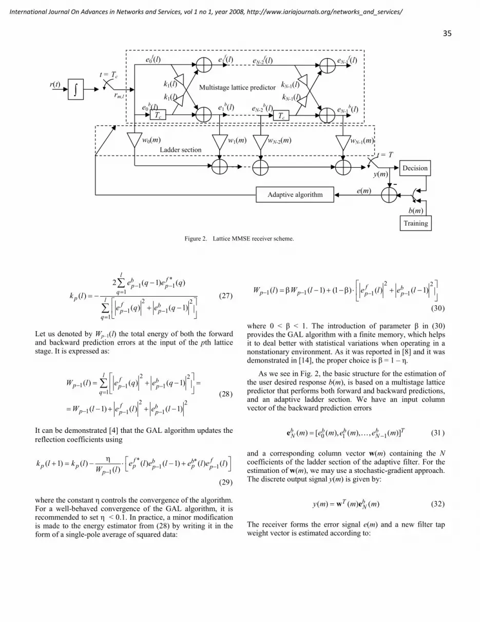
As we see in Fig. 2, the basic structure for the estimation of the user desired response b(m), is based on a multistage lattice predictor that performs both forward and backward predictions, and an adaptive ladder section. We have an input column vector of the backward prediction errors

0 1 1( ) [ ( ), ( ), , ( )]b b b b TN Nm e m e m e m−=e … (31)

and a corresponding column vector w(m) containing the N coefficients of the ladder section of the adaptive filter. For the estimation of w(m), we may use a stochastic-gradient approach. The discrete output signal y(m) is given by:

( ) ( ) ( )T bNy m m m= w e (32)

The receiver forms the error signal e(m) and a new filter tap weight vector is estimated according to:

t = Tc

rm,l

Tc

k1(l)

k1(l)

e0b(l)

e0f(l) e1

f(l)

e1b(l)

w0(m) w1(m)

Tc

kN-1(l)

eN-2b(l)

eN-2f(l) eN-1

f(l)

eN-1b(l)

wN-2(m) wN-1(m)

kN-1(l)

t = T

y(m)

∫ r(t)

Decision

Training

Adaptive algorithm

b(m)

- e(m)

Multistage lattice predictor

Figure 2. Lattice MMSE receiver scheme.

Ladder section

36


( 1) ( ) ( ) ( )bNm m e m m+ = + µw w eɶ (33)

The parameter µɶ is the ladder structure adaptation step size, chosen to optimize both the convergence rate and the misadjustment of the algorithm.

Summarizing, we will use (24), (30), and (29) for the lattice predictor part of the scheme, together with (32) and (33) for the ladder section. As compared to its transversal counterpart based on the LMS algorithm, the lattice MMSE receiver implies an increased computational complexity due to the multistage lattice predictor. Nevertheless, due to the fact that the lattice predictor orthogonalizes the input signals, a faster convergence rate is expected.

It can be noticed that in the lattice predictor part of the classical GAL algorithm a division operation per stage is used, which significantly grows the computational complexity in a fixed-point implementation context. Due to cost considerations, equipment manufactures generally prefer the use of fixed-point Digital Signal Processors (DSPs) over floating-point ones in their products. In fixed point DSPs, every division operation requires a number of iterations equal to the word length (i.e., the number of representation bits), while the multiplication and addition operations can be performed in a single iteration. In the following, we will propose an approximate version of the GAL algorithm that replaces the division operation using three multiplication operations and one addition operation instead. This is much more convenient from the computational complexity point of view in a fixed-point DSP implementation.

We start from equation (30) and we may write:

1

2 2

1 1 1

2 21 1 1

1

1( )

1

( 1) (1 ) ( ) ( 1)

1 1( 1) ( ) ( 1)1

1( 1)

p

f bp p p

f bp

p p

p

W l

W l e l e l

W l e l e l

W l

−

− − −

− − −

−

=

= =β − + −β + −

= ⋅β − + −− β

+ ⋅β −

Let us denote

11

1( 1)

( 1)p

p

T lW l

−−

− =−

(35)

and

2 2

1 1 1( ) ( ) ( 1)f bp p pc l e l e l− − −= + − (36)

Using the previous notations we may rewrite equation (34) as follows:

1 1

1 1

1 1( ) ( 1)

11 ( ) ( 1)

p p

p p

T l T l

c n T l− −

− −

= − ⋅− ββ + −β

(37) Supposing that the sum of the squared prediction errors at

time l, i.e., 1( )pc l− , is much smaller than the sum of all

squared prediction errors until that moment of time,

1( 1)pW l− − , we may write that

1 1( ) ( 1) 1p pc l T l− − − << (38)

Taking into account that

0

1( 1) for 1

1n n

n

x xx

∞

=

= − <+

∑ (39)

we may use the following approximate relation instead of equation (37):

1 1 1 1

1 1( ) ( 1) 1 ( ) ( 1)p p p pT l T l c l T l− − − −

− β≅ − ⋅ − − β β

(40)

In order to prevent any unwanted situations that can affect the supposition made in equation (38) (e.g., impulse perturbation of the input signal) we may compute the following minimum value:

1 1 1

1( ) min , ( ) ( 1)p p pt l c l T l− − −

− β= λ − β

(41)

where 1λ < is a positive constant, and than rewrite the equation (40) as follows:

1 1 1

1( ) ( 1)(1 ( ))p p pT l T l t l− − −≅ − −

β (42)

Finally, the reflection coefficients are updated using

1

* *1 1

( ) ( 1) ( )

( ) ( 1) ( ) ( )

p p p

ff b bp p p p

k l k l T l

e l e l e l e l

−

− −

= − − η ⋅

⋅ − + (43)

The new step-size parameter of the division-free GAL algorithm is 1( )pT l−η and it acts similar to 1/ ( )pW l−η from the

classical GAL algorithm. It can be noticed that the “unwanted” division operation from the classical GAL algorithm is replaced by three multiplication operations and one addition operation, which is more suitable in a fixed-point implementation context.

(34)

37


0 100 200 300 400 500 600 700 800 900 1000-80

-70

-60

-50

-40

-30

-20

-10

0

10

samples

MSE [dB]

G=1 (conventional LMS)

G=3

G=6

G=10

100 200 300 400 500 600 700 800 900 10000.1

0.15

0.2

0.25

samples

V. SIMULATION RESULTS

In order to analyze the convergence of the multiple-iteration LMS algorithm, a first set of experimental tests is performed in a simple “system identification” configuration. In this class of applications, an adaptive filter is used to provide a linear model that represents the best “fit” to an unknown system. The adaptive filter and the unknown system are driven by the same input. The unknown system output supplies the desired response for the adaptive filter. These two signals are used to compute the estimation error, in order to adjust the filter coefficients. The input signal is a random sequence with an uniform distribution on the interval (–1;1). In this first set of experiments the adaptation process is performed in a sample-by-sample manner. The mean square error (MSE) is estimated by averaging over 100 independent trials. In Fig. 3 are depicted the convergence curves for the multiple iterations LMS algorithm and the proposed equivalent algorithm, for different values of G. As expected, the curves for these two algorithms are perfectly matched, due to the mathematical equivalency

between them. It can be notice that the convergence rate of the algorithms increases with the value of G and the MSE decreasing. In Fig. 4 we plot the evolution of the step size parameter of the proposed algorithm, given by (12), for G =10.

A second set of simulations employs the asynchronous DS-CDMA system, using the transversal MMSE iterative receiver. A BPSK transmission in a training mode scenario was considered. The binary spreading sequences are pseudo-random. The system simulation parameters are N = 16 and K = 8. The signal-to-noise ratio (SNR) is 15 dB. The LMS adaptive algorithm is iterated several times for each data bit using the proposed equivalent relation from (8). The adaptive process works now in a block-by-block manner. The MSE is also estimated by averaging over 100 independent trials. The results are presented in Fig. 5. It can be noticed that the MSE is decreased every new iteration.

Next, we investigated the steady-state BER (Bit Error Rate) performance as a function of the energy per bit to noise power

Figure 3. Convergence for the multiple iterations LMS algorithms.

Figure 4. Evolution of the step size parameter µ(10) given by (12).

Figure 5. Convergence of the MMSE receiver based on the multiple iterations LMS algorithm. K = 8, N = 16, SNR = 15dB.

Figure 6. BER performance of the MMSE receiver based on the multiple iterations LMS algorithm. Other conditions as in Fig. 5.

38


spectral density ratio (Eb/N0) of the iterative MMSE receiver considered above. These results are shown in Fig. 6, where we compared the performance of the iterative MMSE receiver using 1 to 6 additional iterations (i.e., G = 2 to 7) with the conventional adaptive LMS receiver, using one iteration per bit (i.e., G =1). The simulation results were obtained using 2000 bits training period for each value of Eb/N0, in order to assure that the steady-state is reached. It is very important to note that under the same conditions the BER is improved every new iteration. Nevertheless, one should make a compromise between the computational complexity and the BER performances.

For further increasing the convergence rate, the lattice MMSE receiver based on the division-free GAL algorithm is tested as compared with its transversal counterpart based on the LMS algorithm. The simulation parameters were fixed as follows. The processing gain is N = 64, the number of users is K = 32, and SNR = 15 dB. The MSE is estimated by averaging

over 100 independent trials. First, the conventional MMSE receivers are compared (Fig. 7). The superior convergence rate achieved by the GAL algorithm as compared to the transversal LMS algorithm is obvious. This faster convergence rate of the GAL algorithm over the transversal LMS algorithm can be explained by the fact that the lattice predictor orthogonalizes the input signals. Hence, the gradient adaptation algorithm using this structure is less dependent on the eigenvalues spread of the input signal. In order to support these remarks, in Fig. 8 the mean autocorrelation function is depicted for both inputs, i.e. r(m) (used as the direct input for the transversal LMS receiver) and the sequence of backward prediction errors

( )bN me (the input of the ladder section of the GAL receiver). It

can be noticed that the input of the GAL ladder section has a higher variance as compared to the LMS input sequence. We should note that the faster convergence rate offered by the iterative MMSE receivers over the conventional receivers is mainly due to the interference rejection capability of the

0 50 100 150 200 250 300 350 400 450 500-20

-18

-16

-14

-12

-10

-8

-6

-4

-2

Number of bits

M

SE

[d

B]

LMS

GAL

-60 -40 -20 0 20 40 60-2

0

2

4

6

8

10

12

14

16

18 a

Number of chips

A

uto

co

rre

lati

on

-60 -40 -20 0 20 40 60-2

0

2

4

6

8

10

12

14

16

18 b

Number of chips

A

uto

co

rre

lati

on

Figure 7. Convergence of the MMSE receivers. K = 32, N = 64, SNR = 15dB.

Figure 8. Autocorrelation functions for (a) r(m) - LMS input, (b) ebN(m) -

GAL ladder section input. Other conditions as in Fig. 7.

0 50 100 150 200 250 300 350 400 450 500-45

-40

-35

-30

-25

-20

-15

-10

-5

0

Number of bits

M

SE

[dB

]

Conventional MMSE

Iterative MMSE, 2 iterations Iterative MMSE, 4 iterations

0 50 100 150 200 250 300 350 400 450 500-45

-40

-35

-30

-25

-20

-15

-10

-5

0

Number of bits

M

SE

[dB

]

Conventional MMSE

Iterative MMSE, 2 iterations

Iterative MMSE, 4 iterations

Figure 9. Convergence of the iterative LMS receiver. Other conditions as in Fig. 7.

Figure 10. Convergence of the iterative GAL receiver. Other conditions as in Fig. 7.

39


multiple iterations procedure within the adaptive algorithm. This improvement leads to a reduced level of MAI, which translates into a convergence rate close to the single user case.

Finally, a last set of simulations is performed in order to compare the multiple iterations MMSE receivers based on both LMS and GAL algorithms. Both algorithms are iterated for G = 4 within each data bit. The results are presented in Figs. 9 and 10. In both cases it can be noticed that MSE is decreased every new iteration. Also, the division-free GAL algorithm outperforms the LMS algorithm in terms of convergence rate.

VI. CONCLUSION AND PERSPECTIVES

In this paper we first propose a relation for updating the LMS adaptive filter coefficients, which is equivalent with a multiple iterations LMS algorithm used in MMSE receivers for DS-CDMA communications systems. It was demonstrated that the multiple iterations process is equivalent with an unique iteration with a particular step size of the algorithm. Our proposed solution requires almost the same number of operations as the multiple iterations per bit algorithm but a significant time processing gain is achieved. The stability condition for the proposed algorithm was also derived. The simulation results proved the equivalency between the classical multiple iteration LMS algorithm and our proposed approach.

The MMSE iterative receiver considered in this paper was shown to improve the asynchronous DS-CDMA system performances. Thus, the MSE is decreased every new iteration by reducing MAI. This decrease offers a faster training mode for the receiver. A very important result is that the BER is considerably improved every new iteration.

The lattice MMSE receiver based on the division-free GAL algorithm improves the convergence rate as compared to the transversal LMS receiver. The lattice predictor orthogonalizes the input signals, so that the GAL algorithm is less dependent on the eigenvalues spread of the input signal and it converges faster than their transversal counterpart, the LMS algorithm. As a practical consequence, the lattice receiver will require a shorter training sequence as compared to the transversal one. Also, the GAL iterative receiver was shown to improve the asynchronous DS-CDMA system performances. The MSE decrease offers a faster training mode for the receiver. Hence, the designing procedure may consider two aspects, i.e., to

shorten the training sequence for maintaining the same MAI in the system or to strongly reduce the MAI by keeping the same length of the training sequence. An analytical estimation of BER for the GAL receiver will be considered in perspective.

REFERENCES [1] S. Glisic and B. Vucetic, CDMA Systems for Wireless Communications,

Artech House, 1997.

[2] S. Miller, “An adaptive direct-sequence code-division multiple-access receiver for multi-user interference rejection,” IEEE Trans. Communications, vol. 43, pp. 1746-1755, Apr. 1995.

[3] P. Rapajic and B. Vucetic, “Adaptive receiver structures for asynchronous CDMA systems,” IEEE J. Select. Areas Communic., vol. 12, no. 4, pp. 685-697, May 1994.

[4] A. H. Sayed, Adaptive Filters, Wiley, 2008.

[5] F. Takawira, “Adaptive lattice filters for narrowband interference rejection in DS spread spectrum systems,” Proc. IEEE South African Symp. Communications and Signal Processing, 1994.

[6] J. Wang and V. Prahatheesan, “Adaptive lattice filters for CDMA overlay,” IEEE Trans. Commun., vol. 48, no. 5, May 2000, pp. 820-828.

[7] C. Paleologu, C. Vlădeanu, and A.A. Enescu, “Lattice MMSE single user receiver for asyncronous DS-CDMA systems,” Proc. of IEEE Int. Symp. ETc 2006, pp. 97-102.

[8] V. J. Mathews and Z. Xie, “Fixed-point error analysis of stochastic gradient adaptive lattice filters,” IEEE Trans. Acoustics, Speech and Signal Processing, vol. 38, no. 1, January 1990, pp. 70-79.

[9] R. C. North, J. R. Zeidler, W. H. Ku, and T. R. Albert, “A floating-point arithmetic error analysis of direct and indirect coefficient updating techniques for adaptive lattice filters,” IEEE Trans. on Signal Processing, vol. 41, no. 5, May 1993, pp. 1809-1823.

[10] W. Hamouda and P. McLane, “Multiuser interference cancellation aided adaptation of a MMSE receiver for direct-sequence code-division multiple-access systems,” Proc. IEEE Communications Theory Mini-Conf. (GLOBECOM), 2001.

[11] W. Hamouda and P. McLane, “A fast adaptive algorithm for MMSE receivers in DS-CDMA systems,” IEEE Sign Proc. Letters, vol. 11, no. 2, pp. 86-89, Feb. 2004.

[12] C. Paleologu and C. Vlădeanu, “On the behavior of LMS adaptive algorithm in MMSE receivers for DS-CDMA systems,” Proc. of ICCGI 2007, pp.12-17.

[13] C. Paleologu, S. Ciochină, A. A. Enescu, and C. Vlădeanu, “Gradient adaptive lattice algorithm suitable for fixed point implementation,” Proc. of ICDT 2008, pp. 41-46.

[14] C. Paleologu, S. Ciochină, and A.A. Enescu, “Modified GAL algorithm suitable for DSP implementation,” Proc. of IEEE Int. Symp. ETc 2002, vol. 1, pp. 2-7.

Documents

Fast Convergence Least-Mean-Square Algorithms for MMSE Receivers in DS-CDMA Systems