1

Fast Data Collection in Tree-Based WirelessSensor Networks

Ozlem Durmaz Incel, Amitabha Ghosh, Bhaskar Krishnamachari, and Krishnakant Chintalapudi

Abstract—We investigate the following fundamental question - how fast can information be collected from a wireless sensor networkorganized as tree? To address this, we explore and evaluate a number of different techniques using realistic simulation models underthe many-to-one communication paradigm known as convergecast. We first consider time scheduling on a single frequency channelwith the aim of minimizing the number of time slots required (schedule length) to complete a convergecast. Next, we combine schedulingwith transmission power control to mitigate the effects of interference, and show that while power control helps in reducing the schedulelength under a single frequency, scheduling transmissions using multiple frequencies is more efficient. We give lower bounds on theschedule length when interference is completely eliminated, and propose algorithms that achieve these bounds. We also evaluate theperformance of various channel assignment methods and find empirically that for moderate size networks of about 100 nodes, the useof multi-frequency scheduling can suffice to eliminate most of the interference. Then, the data collection rate no longer remains limitedby interference but by the topology of the routing tree. To this end, we construct degree-constrained spanning trees and capacitatedminimal spanning trees, and show significant improvement in scheduling performance over different deployment densities. Lastly, weevaluate the impact of different interference and channel models on the schedule length.

Index Terms—Convergecast, TDMA scheduling, multiple channels, power-control, routing trees.

F

1 INTRODUCTION

CONVERGECAST, namely the collection of data froma set of sensors toward a common sink over a tree-

based routing topology, is a fundamental operation inwireless sensor networks (WSN) [1]. In many applica-tions, it is crucial to provide a guarantee on the deliverytime as well as increase the rate of such data collection.For instance, in safety and mission-critical applicationswhere sensor nodes are deployed to detect oil/gas leakor structural damage, the actuators and controllers needto receive data from all the sensors within a specificdeadline [2], failure of which might lead to unpredictableand catastrophic events. This falls under the category ofone-shot data collection. On the other hand, applicationssuch as permafrost monitoring [3] require periodic andfast data delivery over long periods of time, which fallsunder the category of continuous data collection.

In this paper, we consider such applications and focuson the following fundamental question: “How fast candata be streamed from a set of sensors to a sink over a tree-based topology?” We study two types of data collection: (i)aggregated convergecast where packets are aggregated ateach hop, and (ii) raw-data convergecast where packets areindividually relayed toward the sink. Aggregated con-

• O.D. Incel is with the Department of Computer Engineering, BogaziciUniversity, Istanbul, Turkey, Email: ozlem.durmaz@tam.boun.edu.tr

• A. Ghosh is with the Department of Electrical Engineering, PrincetonUniversity, NJ, Email: amitabhg@princeton.edu

• B. Krishnamachari is with the Ming Hsieh Department of ElectricalEngineering, University of Southern California, Los Angeles, CA, Email:bkrishna@usc.edu

• K. Chintalapudi is with Microsoft Research, Bangalore, India.

vergecast is applicable when a strong spatial correlationexists in the data, or the goal is to collect summarizedinformation such as the maximum sensor reading. Raw-data convergecast, on the other hand, is applicable whenevery sensor reading is equally important, or the cor-relation is minimal. We study aggregated convergecastin the context of continuous data collection, and raw-data convergecast for one-shot data collection. These twotypes correspond to two extreme cases of data collection.In an earlier work [4], the problem of applying differentaggregation factors, i.e., data compression factors, wasstudied, and the latency of data collection was shown tobe within the performance bounds of the two extremecases of no data compression (raw-data convergecast)and full data compression (aggregated convergecast).

For periodic traffic, it is well known that contention-free medium access control (MAC) protocols such asTDMA (Time Division Multiple Access) are better fitfor fast data collection, since they can eliminate colli-sions and retransmissions and provide guarantee on thecompletion time as opposed to contention-based proto-cols [1]. However, the problem of constructing conflict-free (interference-free) TDMA schedules even under thesimple graph-based interference model has been provedto be NP-complete. In this work, we consider a TDMAframework and design polynomial-time heuristics tominimize the schedule length for both types of con-vergecast. We also find lower bounds on the achievableschedule lengths and compare the performance of ourheuristics with these bounds.

We start by identifying the primary limiting factorsof fast data collection, which are: (i) interference in thewireless medium, (ii) half-duplex transceivers on the sen-

2

sor nodes, and (iii) topology of the network. Then, weexplore a number of different techniques that providea hierarchy of successive improvements, the simplestamong which is an interference-aware, minimum-length,TDMA scheduling that enables spatial reuse. To achievefurther improvement, we combine transmission powercontrol with scheduling, and use multiple frequencychannels to enable more concurrent transmissions. Weshow that once multiple frequencies are employed alongwith spatial-reuse TDMA, the data collection rate oftenno longer remains limited by interference but by thetopology of the network. Thus, in the final step, weconstruct network topologies with specific propertiesthat help in further enhancing the rate. Our primaryconclusion is that, combining these different techniquescan provide an order of magnitude improvement for ag-gregated convergecast, and a factor of two improvementfor raw-data convergecast, compared to single-channelTDMA scheduling on minimum-hop routing trees.

Although the techniques of transmission power con-trol and multi-channel scheduling have been well stud-ied for eliminating interference in general wireless net-works, their performances for bounding the completionof data collection in WSNs have not been explored indetail in the previous studies. The fundamental noveltyof our approach lies in the extensive exploration ofthe efficiency of transmission power control and multi-channel communication on achieving fast convergecastoperations in WSNs. Besides, we evaluate the impactof routing trees on fast data collection and to the bestof our knowledge this has not been the topic of pre-vious studies. As we will discuss in Section 2, someof the existing work had the objective of minimizingthe completion time of convergecasts. However, none ofthe previous work discussed the effect of multi-channelscheduling together with the comparisons of differentchannel assignment techniques and the impact of routingtrees and none considered the problems of aggregatedand raw convergecast, which represent two extremecases of data collection, together.

As the new concepts in this paper, we introducepolynomial-time heuristics for TDMA scheduling forboth types of data collection, i.e., Algorithms 1 and 2,and prove that they do achieve the lower bound of datacollection time once interference is eliminated. Besides,we elaborate on the performance of our previous work,a receiver-based channel assignment method, and com-pare its efficiency with other channel assignment meth-ods and introduce heuristics for constructing optimalrouting trees to further enhance data collection rate. Thefollowing lists our key findings and contributions:

• Bounds on Convergecast Scheduling: We show thatif all interfering links are eliminated, the sched-ule length for aggregated convergecast is lowerbounded by the maximum node degree in therouting tree, and for raw-data convergecast bymax(2nk−1, N), where nk is the maximum numberof nodes on any branch in the tree, and N is the

number of source nodes. We then introduce optimaltime slot assignment schemes under this scenariowhich achieve these lower bounds.

• Evaluation of Power Control under Realistic Set-ting: It was shown recently [5] that under the ide-alized setting of unlimited power and continuousrange, transmission power control can provide anunbounded improvement in the asymptotic capac-ity of aggregated convergecast. In this work, weevaluate the behavior of an optimal power controlalgorithm [6] under realistic settings considering thelimited discrete power levels available in today’sradios. We find that for moderate size networks of100 nodes power control can reduce the schedulelength by 15− 20%.

• Evaluation of Channel Assignment Methods: Us-ing extensive simulations, we show that schedulingtransmissions on different frequency channels ismore effective in mitigating interference as com-pared to transmission power control. We evaluatethe performance of three different channel assign-ment methods: (i) Joint Frequency and Time SlotScheduling (JFTSS), (ii) Receiver-Based Channel As-signment (RBCA) [7], and (iii) Tree-Based ChannelAssignment (TMCP) [8]. These methods consider thechannel assignment problem at different levels: thelink level, node level, or cluster level. We show thatfor aggregated convergecast, TMCP performs betterthan JFTSS and RBCA on minimum-hop routingtrees, while performs worse on degree-constrainedtrees. For raw-data convergecast, RBCA and JFTSSperform better than TMCP, since the latter suffersfrom interference inside the branches due to con-current transmissions on the same channel.

• Impact of Routing Trees: We investigate the effect ofnetwork topology on the schedule length, and showthat for aggregated convergecast the performancecan be improved by up to 10 times on degree-constrained trees using multiple frequencies as com-pared to that on minimum-hop trees using a singlefrequency. For raw-data convergecast, multi-channelscheduling on capacitated minimal spanning treescan reduce the schedule length by 50%.

• Impact of Channel Models and Interference: Un-der the setting of multiple frequencies, one simpli-fying assumption often made is that the frequenciesare orthogonal to each other. We evaluate this as-sumption and show that the schedules generatedmay not always eliminate interference, thus causingconsiderable packet losses. We also evaluate andcompare the two most commonly used interferencemodels: (i) the graph-based protocol model, and (ii)the SINR (Signal-to-Interference-plus-Noise Ratio)based physical model.

The rest of the paper is organized as follows: InSection 2, we discuss related works. In Section 3, wedescribe the problem formulation and state our assump-

3

tions. In Section 4, we analyze the lower bounds on theschedule length for aggregated and raw convergecast,and propose algorithms that achieve the correspondingbounds. In Section 5, we focus on power control andmulti-channel scheduling as mechanisms to eliminateinterference. Section 6 explains the impact of routingtopologies, and Section 7 presents detailed evaluationresults. Finally, we draw our conclusions in Section 8.

2 RELATED WORK

Fast data collection with the goal to minimize the sched-ule length for aggregated convergecast has been studiedby us in [7], [9], and also by others in [5], [10], [11]. In [7],we experimentally investigated the impact of transmis-sion power control and multiple frequency channels onthe schedule length, while the theoretical aspects werediscussed in [9], where we proposed constant factorand logarithmic approximation algorithms on geomet-ric networks (disk graphs). Raw-data convergecast hasbeen studied in [1], [12]–[14], where a distributed timeslot assignment scheme is proposed by Gandham etal. [1] to minimize the TDMA schedule length for asingle channel. The problem of joint scheduling andtransmission power control is studied by Moscibroda [5]for constant and uniform traffic demands. Our presentwork is different from the above in that we evaluatetransmission power control under realistic settings andcompute lower bounds on the schedule length for treenetworks with algorithms to achieve these bounds. Wealso compare the efficiency of different channel assign-ment methods and interference models, and proposeschemes for constructing specific routing tree topologiesthat enhance the data collection rate for both aggregatedand raw-data convergecast.

The use of orthogonal codes to eliminate interferencehas been studied by Annamalai et al. [10], where nodesare assigned time slots from the bottom of the tree to thetop such that a parent node does not transmit before itreceives all the packets from its children. This problemand the one addressed by Chen et al. [11] are for one-shotraw-data convergecast. In this work, since we constructdegree-constrained routing topologies to enhance thedata collection rate, it may not always lead to schedulesthat have low latency, because the number of hops ina tree goes up as its degree goes down. Therefore,if minimizing latency is also a requirement, then fur-ther optimization, such as constructing bounded-degree,bounded-diameter trees, is needed. A study along thisline with the objective to minimize the maximum latencyis presented by Pan and Tseng [15], where they assign abeacon period to each node in a Zigbee network duringwhich it can receive data from all its children.

For raw-data convergecast, Song et al. [12] presenteda time-optimal, energy-efficient, packet scheduling algo-rithm with periodic traffic from all the nodes to the sink.Once interference is eliminated, their algorithm achievesthe bound that we present here, however, they briefly

mention a 3-coloring channel assignment scheme, and itis not clear whether the channels are frequencies, codes,or any other method to eliminate interference. Moreover,they assume a simple interference model where eachnode has a circular transmission range and cumula-tive interference from concurrent multiple senders isavoided. Different from their work, we consider multiplefrequencies and evaluate the performance of three dif-ferent channel assignment methods together with eval-uating the effects of transmission power control usingrealistic interference and channel models, i.e., physicalinterference model and overlapping channels and con-sidering the impact of routing topologies. Song et al. [12]extended their work and proposed a TDMA based MACprotocol for high data rate WSNs in [16]. TreeMACconsiders the differences in load at different levels ofa routing tree and assigns time slots according to thedepth, i.e. the hop count, of the nodes on the routingtree, such that nodes closer to the sink are assigned moreslots than their children in order to mitigate congestion.However, TreeMAC operates on a single channel andachieves 1/3 of the maximum throughput similar to thebounds presented by Gandham et al. [1] since the sinkcan receive every 3 time slots.

The problem of minimizing the schedule length forraw-data convergecast on single channel is shown tobe NP-complete on general graphs by Choi et al. [13].Maximizing the throughput of convergecast by findinga shortest-length, conflict-free schedule is studied by Laiet al. [14], where a greedy graph coloring strategy as-signs time slots to the senders and prevent interference.They also discussed the impact of routing trees on theschedule length and proposed a routing scheme calleddisjoint strips to transmit data over different shortestpaths. However, since the sink remains as the bottleneck,sending data over different paths does not reduce theschedule length. As we will show in this paper, theimprovement due to the routing structure comes fromusing capacitated minimal spanning trees for raw-dataconvergecast, where the number of nodes in a subtreeis no more than half the total number of nodes in theremaining subtrees.

The use of multiple frequencies has been studied ex-tensively in both cellular and ad hoc networks, however,in the domain of WSN, there exist a few studies thatutilize multiple channels [8], [17], [18]. To this end, weevaluate the efficiency of three particular schemes thattreat the channel assignment at different levels.

3 MODELING AND PROBLEM FORMULATION

We model the multi-hop WSN as a graph G = (V, E),where V is the set of nodes, E = {(i, j) | i, j ∈ V } is theset of edges representing the wireless links. A designatednode s ∈ V denotes the sink. The Euclidean distancebetween two nodes i and j is denoted by dij . All thenodes except s are sources, which generate packets andtransmit them over a routing tree to s. We denote the

4

spanning tree on G rooted at s by T = (V, ET ), whereET ⊆ E represents the tree edges. Each node is assumedto be equipped with a single half-duplex transceiver,which prevents it from sending and receiving packetssimultaneously. We consider a TDMA protocol wheretime is divided into slots, and consecutive slots aregrouped into equal sized non-overlapping frames.

We use two types of interference models for our eval-uation: the graph-based protocol model and the SINR-based physical model. In the protocol model, we assumethat the interference range of a node is equal to itstransmission range, i.e., two links cannot be scheduledsimultaneously if the receiver of at least one link iswithin the range of the transmitter of the other link.In the physical model, the successful reception of apacket from i to j depends on the ratio between thereceived signal strength at j and the cumulative interfer-ence caused by all other concurrently transmitting nodesand the ambient noise level. Thus, a packet is receivedsuccessfully at j if the signal-to-interference-plus-noiseratio, SINRij , is greater than a certain threshold β, i.e.,

SINRij =Pi · gij∑

k =i Pk · gkj +N(1)

where Pi is the transmitted signal power at node i, Nis the ambient noise level, and gij is the propagationattenuation (link gain) between i and j. We use a simpledistance dependent path-loss model to calculate the linkgains as gij = d−α

ij , where the path-loss exponent α is aconstant between 2 and 6, whose exact value depends onexternal conditions of the medium (humidity, obstacles,etc.), as well as the sender-receiver distance. We assumethat the level of interference is static and does not changeover time. For simplicity and ease of illustration, we usethe protocol model in all the figures.

We study aggregated convergecast in the context ofperiodic data collection where each source node gener-ates a packet at the beginning of every frame, and raw-data convegecast for one-shot data collection where eachnode has only one packet to send. We assume that thesize of each packet is constant. Our goal is to deliverthese packets to the sink over the routing tree as fast aspossible. More specifically, we aim to schedule the edgesET of T using a minimum number of time slots whilerespecting the following two constraints:

• Adjacency Constraint: Two edges (i, j) ∈ ET and(k, l) ∈ ET cannot be scheduled in the sametime slot if they are adjacent to each other, i.e., if{i, j}

∩{k, l} = ϕ. This constraint is due to the half-

duplex transceiver on each node which prevents itfrom simultaneous transmission and reception.

• Interfering Constraint: The interfering constraint de-pends on the choice of the interference model. Inthe protocol model, two edges (i, j) ∈ ET and(k, l) ∈ ET cannot be scheduled simultaneouslyif they are at two hop distance of each other. Inthe physical model, an edge (i, j) ∈ ET cannot be

scheduled if the SINR at receiver j is not greaterthan the threshold β.

Since we consider data collection to be periodic inaggregated convergecast, each of the edges in ET isscheduled only once within each frame, and this sched-ule is repeated over multiple frames. Thus, a pipelineis established after a certain frame, and then onwardsthe sink continues to receive aggregated packets fromall the source nodes once per frame. We explain furtherdetails about the pipelining in the next section. On theother hand, in one-shot data collection for raw-data con-vergecast, the edges in ET may be scheduled multipletimes and no pipelining takes place. We use the termslink scheduling and node scheduling interchangeably asthey are equivalent in our case. Note that the two otherscenarios, which we do not consider in this paper due tospace constraints, are one-shot aggregated convergecastand periodic raw-data convergecast.

The key difference in terms of scheduling betweenperiodic and one-shot data collection is that a node inthe periodic case does not have to wait for data from itschildren before being scheduled. This is because a linkis scheduled only once within each frame and each nodegenerates a packet in the beginning of every frame, soa pipelining is eventually established. However, in thecase of one-shot data collection, a node needs to wait fordata from its children before being scheduled, which werefer to as the causality constraint.

To summarize the steps in our design, we start withtree construction and then continue with interference-aware scheduling. If the nodes can control their trans-mission power, scheduling phase is coupled with atransmission power control algorithm. If the nodes canchange their operating frequency, channel schedulingcan be coupled with time slot scheduling as it is the casewith the JFTSS algorithm (Section 5.2.1) or first channelsare assigned and then time slot scheduling continues asin the case of RBCA explained in Section 5.2.3. However,the TMCP algorithm (Section 5.2.2), considers tree con-struction and channel assignment jointly and then doesthe scheduling of time slots.

4 TDMA SCHEDULING OF CONVERGECASTS

In this section, we first focus on periodic aggregated con-vergecast and then on one-shot raw-data convergecast.Our objective is to calculate the minimum achievableschedule lengths using an interference-aware TDMAprotocol. We first consider the case where the nodescommunicate on the same channel using a constanttransmission power, and then discuss improvements us-ing transmission power control and multiple frequenciesin the next section.

4.1 Periodic Aggregated Convergecast

In this section, we consider the scheduling problemwhere packets are aggregated. Data aggregation is a

5

(a)

Frame 1 Frame 2S1 S2 S3 S4 S5 S6 S1 S2 S3 S4 S5 S6

s 1 2 3 - - - {1,4} {2,5,6} 3 - - -1 - - - 4 - - - - - 4 - -2 - - - - 5 6 - - - - 5 6

(b)

(c)

Fig. 1: Aggregated convergecast and pipelining: (a) Schedule length of 6 in the presence of interfering links. (b) Node ids from which(aggregated) packets are received by their corresponding parents in each time slot over different frames. (c) Schedule length of 3 using BFS-TIMESLOTASSIGNMENT when all the interfering links are eliminated.

commonly used technique in WSN that can eliminateredundancy and minimize the number of transmissions,thus saving energy and improving network lifetime [19].Aggregation can be performed in many ways, such as bysuppressing duplicate messages; using data compressionand packet merging techniques; or taking advantage ofthe correlation in the sensor readings.

We consider continuous monitoring applicationswhere perfect aggregation is possible, i.e., each nodeis capable of aggregating all the packets received fromits children as well as that generated by itself into asingle packet before transmitting to its parent. The sizeof aggregated data transmitted by each node is constantand does not depend on the size of the raw sensorreadings. Typical examples of such aggregation functionsare MIN, MAX, MEDIAN, COUNT, AVERAGE, etc.

In Fig. 1(a) and 1(b), we illustrate the notion of pipelin-ing in aggregated convergecast and that of a schedulelength on a network of 6 source nodes. The solid linesrepresent tree edges, and the dotted lines represent inter-fering links. The numbers beside the links represent thetime slots at which the links are scheduled to transmit,and the numbers inside the circles denote node id’s. Theentries in the table list the nodes from which packets arereceived by their corresponding receivers in each timeslot. We note that at the end of frame 1, the sink doesnot have packets from nodes 5 and 6; however, as theschedule is repeated, it receives aggregated packets from2, 5, and 6 in slot 2 of the next frame. Similarly, thesink also receives aggregated packets from nodes 1 and4 starting from slot 1 of frame 2. The entries {1, 4} and{2, 5, 6} in the table represent single packets comprisingaggregated data from nodes 1 and 4, and from nodes 2, 5,and 6, respectively. Thus, a pipeline is established fromframe 2, and the sink continues to receive aggregatedpackets from all the nodes once every 6 time slots. Thus,the minimum schedule length is 6.

4.1.1 Lower Bound on Schedule Length

We first consider aggregated convergecast when all theinterfering links are eliminated by using transmissionpower control or multiple frequencies. Although theproblem of minimizing the schedule length is NP-complete on general graphs, we show in the followingthat once interference is eliminated, the problem reducesto one on a tree, and can be solved in polynomial time.To this end, we first give a lower bound on the schedulelength, and then propose a time slot assignment scheme

that achieves the bound.LEMMA 1: If all the interfering links are eliminated, the

schedule length for aggregated convergecast is lower boundedby ∆(T ), where ∆(T ) is the maximum node degree in therouting tree T .

Proof: If all the interfering links are eliminated, thescheduling problem reduces to one on a tree. Now sinceeach of the tree edges needs to be scheduled only oncewithin each frame, it is equivalent to edge coloring ona graph, which needs number of colors at least equal tothe maximum node degree.

Once all the interfering links are eliminated, concur-rency is still limited by the adjacency constraint due tothe half-duplex transceivers, which prevents a parentfrom transmitting when it is already receiving from itschildren, or when its parent is transmitting.

4.1.2 Assignment of Timeslots

Given the lower bound ∆(T ) on the schedule lengthin the absence of interfering links, we now present atime slot assignment scheme in Algorithm 1, called BFS-TIMESLOTASSIGNMENT, that achieves this bound.

In each iteration of BFS-TIMESLOTASSIGNMENT (lines2-6), an edge e is chosen in the Breadth First Search(BFS) order starting from any node, and is assigned theminimum time slot that is different from all its adjacentedges respecting interfering constraints. Note that, sincewe evaluate the performance of this algorithm also forthe case when the interfering links are present, we checkfor the corresponding constraint in line 4; however, wheninterference is eliminated this check is redundant. Thealgorithm runs in O(|ET |2) time and minimizes theschedule length when there are no interfering links, asproved in Theorem 1. To illustrate, we show the samenetwork of Fig. 1(a) in 1(c) with all the interfering linksremoved, and so the network is scheduled in 3 time slots.

Algorithm 1 BFS-TIMESLOTASSIGNMENT

1. Input: T = (V, ET )2. while ET = ϕ do3. e← next edge from ET in BFS order4. Assign minimum time slot t to edge e respecting adjacency and

interfering constraints5. ET ← ET \ {e}6. end while

Although BFS-TIMESLOTASSIGNMENT may not be anapproximation to ideal scheduling under the physicalinterference model, it is a heuristic that can achieve the

6

lower bound if all the interfering links are eliminated.Therefore, together with a method to eliminate interfer-ence the algorithm can optimally schedule the network.

THEOREM 1: If all the interfering links are eliminated, theschedule length for aggregated convergecast achieved by BFS-TIMESLOTASSIGNMENT is the minimum, i.e., ∆(T ).

Proof: The proof is by induction on i. Let T i =(V i, Ei

T ) denote the subtree of T in the ith iterationconstructed in the BFS order, where Ei

T comprises allthe edges that are assigned a slot, and V i comprises theset of nodes on which the edges in Ei

T are incident. Notethat, |Ei

T | = i, because at every iteration exactly one edgeis assigned a slot. For i = 1, clearly the number of slotsused is 1, equal to ∆(T 1).

Now, assume that the number of slots N(i) neededto schedule the edges in T i is ∆(T i). In the (i + 1)th

iteration, after assigning a slot to the next edge in BFSorder, the number of slots needed in T i+1 can eitherremain the same as before, or increase by one. Thus,

N(i+ 1) = max {N(i), N(i) + 1} (2)

If it remains the same, N(i + 1) is still the maximumdegree of T i+1 at end of (i + 1)th iteration. Otherwise,if it increases by one, the new edge must be incidenton a node v∗, common to both T i and T i+1, such thatthe number of incident edges on v∗ that were alreadyassigned a time slot at the end of ith iteration was ∆(T i).This is so because in the BFS traversal, all the edgesincident on a node are assigned a slot first before movingon to the next node, and because the slot assigned to thenew edge is the minimum possible that is different fromall that already assigned to the edges incident on v∗ untilthe ith iteration. Thus, at the end of (i + 1)th iteration,the number of slots used N(i)+1 is equal to the numberof assigned edges incident on v∗ which, in turn, equals∆(T i+1). This proves the inductive step. Therefore, itholds at every iteration of the algorithm until the endwhen i = |V | − 2, yielding a schedule length equal tothe maximum degree ∆(T ) = ∆(T |V |−1). Now, sinceassigning different time slots to the adjacent edges of Tis equivalent to edge coloring T , which requires at least∆(T ) colors, the schedule length is minimum.

4.2 One-Shot Raw-Data ConvergecastIn this section, we consider one-shot data collectionwhere every sensor reading is equally important, and soaggregation may not be desirable or even possible. Thus,each of the packets has to be individually scheduledat each hop en route to the sink. As before, we focuson minimizing the schedule length. Unlike in the caseof periodic aggregated convergecast where a pipeliningtakes place and each of the tree edges is scheduledonly once within each frame, here the edges could bescheduled multiple times and there is no pipelining.

The problem of minimizing the scheduling length forraw-data convergecast is proved to be NP-complete evenunder the protocol interference model by a reduction

s

nk-1

nk

Fig. 2: Raw-data convergecast: largest top-subtree with nk nodes.from the well known Partition Problem [13]. Before get-ting into the details, we first define the following terms:a branch is defined as a subtree containing the sink as anendpoint; a top-subtree is defined as a subtree that has achild of the sink as its root. For instance, in Fig. 3, thebranches are {s, 1, 4}, {s, 2, 5, 6}, and {s, 3, 7}, while thetop-subtrees are {1, 4}, {2, 5, 6}, and {3, 7}.

4.2.1 Lower Bound on Schedule LengthAs mentioned in Section 4.1.1, if all the interfering linksare eliminated using multiple frequencies, the only limit-ing factor in minimizing the schedule length is the half-duplex transceivers. In the following, we give a lowerbound on the schedule length under this scenario.

LEMMA 2: If all the interfering links are eliminated, theschedule length for one-shot raw-data convergecast is lowerbounded by max(2nk − 1, N), where nk is the maximumnumber of nodes in any top-subtree of the routing tree, andN is the number of sources in the network.

Proof: Let ni denote the number of nodes in top-subtree i. Order the top-subtrees in non-increasing orderof their sizes: nk ≥ nk−1 ≥ . . . ≥ n1. Consider therouting tree shown in Fig. 2. Since the nodes cannotreceive multiple packets simultaneously, N is a triviallower bound to receive all the packets. Next, consider thelargest top-subtree k, the root of which has to transmitnk packets to the sink, and the children of this roothave to forward nk − 1 packets in total. Because ofthe half-duplex transceivers, time slots assigned to theroot of this top-subtree must be distinct from all thoseassigned to its children. Thus, in total we need at leastnk + (nk − 1) = 2nk − 1 distinct time slots.

We note that this bound of max(2nk − 1, N), whichapplies only when all the interfering links are removed,is smaller than the lower bound of 3N for generalnetworks and that of max(3nk − 3, N) for tree networks,as computed by Gandham et al. [1] for the 2-hop inter-ference model. They proposed a time slot assignmentscheme for tree networks, which requires each node tomaintain a buffer that stores at most two packets andminimizes the schedule length. In the following, wedescribe a time slot assignment scheme that computesa schedule of length exactly equal to the lower boundwhen interference is eliminated and does not require tostore more than one packet in buffers at any time.

4.2.2 Assignment of TimeslotsWe now describe a time slot assignment scheme in Al-gorithm 2, called LOCAL-TIMESLOTASSIGNMENT, whichis run locally by each node at every time slot. The keyidea is to: (i) schedule transmissions in parallel alongmultiple branches of the tree, and (ii) keep the sink busyin receiving packets for as many time slots as possible.

7

Because the sink can receive from the root of at mostone top-subtree in any time slot, we need to decidewhich top-subtree should be made active. We assumethat the sink is aware of the number of nodes in eachtop-subtree. Each source node maintains a buffer andits associated state, which can be either full or emptydepending on whether it contains a packet or not. Ouralgorithm does not require any of the nodes to storemore than one packet in their buffer at any time. Weinitialize all the buffers as full, and assume that the sink’sbuffer is always full for the ease of explanation.

Algorithm 2 LOCAL-TIMESLOTASSIGNMENT

1. node.buffer = full2. if {node is sink} then3. Among the eligible top-subtrees, choose the one with the largest

number of total (remaining) packets, say top-subtree i4. Schedule link (root(i), s) respecting interfering constraint5. else6. if {node.buffer == empty} then7. Choose a random child c of node whose buffer is full8. Schedule link (c, node) respecting interfering constraint9. c.buffer = empty

10. node.buffer = full11. end if12. end if

The first block of the algorithm in lines 2-4 givesthe scheduling rules between the sink and the roots ofthe top-subtrees. We define a top-subtree to be eligibleif its root has at least one packet to transmit. For agiven time slot, we schedule the root of an eligible top-subtree which has the largest number of total (remaining)packets. If none of the top-subtrees are eligible, the sinkdoes not receive any packet during that time slot.

Inside each top-subtree, nodes are scheduled accord-ing to the rules in lines 5-12. We define a subtree tobe active if there are still packets left in the subtree(excluding its root) to be relayed. If a node’s buffer isempty and the subtree rooted at this node is active, weschedule one of its children at random whose bufferis not empty. Our algorithm guarantees (as proved inLemma 3) that in an active subtree there will alwaysbe at least one child whose buffer is not empty, andso whenever a node empties its buffer, it will receive apacket in the next time slot, thus emptying buffers fromthe bottom of the subtree to the top.

We run through an example shown in Fig. 3(a) toexplain the algorithm. In the first time slot, since theeligible top-subtree containing the largest number ofremaining packets is {2, 5, 6}, we schedule the link (2, s),and the sink receives a packet from node 2 in slot 1. Inthe second time slot, the eligible top-subtrees are {1, 4}and {3, 7}, both of which have 2 remaining packets. Wechoose one of them at random, say {1, 4}, and schedulethe link (1, s). Also, in the same time slot since node2’s buffer is empty, it chooses one of its children atrandom, say node 5, and schedule the link (5, 2). Inthe third time slot, the eligible top-subtrees are {2, 5, 6}and {3, 7}, both of which have 2 remaining packets. Wechoose the first one at random and schedule the link

(a) (b)Fig. 3: Raw-data convergecast using algorithm LOCAL-TIMESLOTASSIGNMENT: (a) Schedule length of 7 when all theinterfering links are removed. (b) Schedule length of 10 when theinterfering links are present.(2, s), and so the sink receives node 5’s packet (relayedby node 2). We also schedule the link (4, 1) in the thirdtime slot because node 1’s buffer is empty at this point.This process continues until all the packets are deliveredto the sink, yielding an assignment that requires 7 timeslots. Note that, in this example, 2nk − 1 = 5, and somax(2nk−1, N) = 7. In Fig. 3(b), we show an assignmentwhen all the interfering links are present, yielding aschedule length of 10.

In the following, we prove that the algorithm requiresexactly max(2nk − 1, N ) slots when all the interferinglinks are eliminated. Before giving the details of theproof, we first highlight the two key insights of thealgorithm: (i) the sink is kept busy in receiving packetsfor as many time slots as possible, and (ii) a node’s bufferis not empty for 2 or more consecutive time slots so longas the subtree rooted at this node is active. The first oneis evident from the scheduling rule between the sinkand the top-subtrees. We prove the second insight in thefollowing lemma.

LEMMA 3: In an active subtree, a node with an emptybuffer always has a child and a parent whose buffers are full.

Proof: We prove it by induction on time slot t. Theparent and grandparent of node i are denoted by p(i)and gp(i); similarly a child and a grandchild of i aredenoted by c(i) and gc(i), respectively. Slightly abusingnotation, we also use these symbols to denote the stateof the buffers on the respective nodes.

At t = 1, the lemma is trivially true because all thebuffers are full. Suppose the lemma holds for t = k, i.e.,every node whose buffer is empty has a child and aparent whose buffers are full. At t = k + 1, each nodewith an empty buffer schedules one of its children whosebuffer is full. The following two situations can occur:

• Node i is full, while p(i) and c(i) are both empty.• Nodes i and p(i) are both full, while c(i) is empty.For the first case, we need to show that both p(i) and

c(i) (since now they are empty) have a child and a parentwhose buffers are full. Clearly, p(i) has a child with afull buffer because i is now full. Similarly, p(i) also hasa parent with a full buffer because a transmission tookplace from p(i) to its parent at t = k + 1. For the latter,c(i) has a parent with a full buffer because transmissiontook place from c(i) to i at t = k+ 1. If the child of c(i),i.e., gc(i), was empty at t = k, then gc(i) also had a childwith a full buffer because the lemma was true at t = k.Therefore, at t = k + 1 the child of gc(i) transmits andfills up its parent’s buffer. Otherwise, if gc(i) was full at

8

t = k, then it also remains full at t = k + 1 because itcannot transmit to its parent c(i), which was full at t.

For the second case, c(i) transmitted and p(i) did not.For this to happen, gp(i) was full at t = k and eitherempties or remains full at t = k + 1. If it empties, gp(i)has a parent with a full buffer because it transmitted att = k+1, and also has a child with a full buffer becausep(i) did not transmit. If it remains full, at t = k+1 nodesi, p(i), and gp(i) are full, c(i) is empty and gc(i) is fullas we showed in the first case. So, the lemma holds fort = k + 1, and the proof follows.

THEOREM 2: If all the interfering links are eliminated, theschedule length for raw-data convergecast achieved by algo-rithm LOCAL-TIMESLOTASSIGNMENT is the minimum, i.e.,max(2nk − 1, N).

Proof: Let ni be the number of nodes in top-subtreei. Order the top-subtrees in non-increasing order of theirsizes: nk ≥ nk−1 ≥ . . . ≥ n1. Suppose nk >

∑k−1i=1 ni; then

max(2nk−1, N) = 2nk−1. From Lemma 1, we know thatit takes at least 2nk − 1 slots to schedule all the packetsoriginated in top-subtree k. Out of these, the sink can useat most nk−1 slots to receive packets from the other top-subtrees, which have a total of at most nk − 1 packets.Also, when nk >

∑k−1i=1 ni, the root of the largest top-

subtree k gets scheduled once in every two time slots.Therefore, the schedule length is at most 2nk − 1.

Now suppose nk ≤∑k−1

i=1 ni; then max(2nk − 1, N) =N . We need to show that there always exists an eligibletop-subtree to complement for the largest one when itis not eligible. In this case, the sink will receive packetsin every slot, because otherwise it remains idle duringsome time slots and the first condition nk >

∑k−1i=1 ni will

be met. Thus, we will prove that the algorithm keeps theinequality nk ≤

∑k−1i=1 ni as an invariant.

In any given time slot t, the algorithm schedulesan eligible top-subtree that has the largest number ofremaining packets. At slot t + 1, therefore, we havenk = nk − 1, and the following three cases might arise:

• Top-subtree k still has the largest number of remain-ing packets with nk ≥ nk−1 ≥ . . . ≥ n1. Then, theroot of k is again chosen to transmit at t + 1, andthe inequality still holds as nk − 1 ≤

∑k−1i=1 ni.

• Top-subtree k and at least another one, say j, havean equal number of remaining packets. Then, theroot of j is chosen, and the inequality still holdsbecause nj − 1 ≤

∑k−1i=1 ni − 1 (since nj = nk − 1).

• Top-subtree k does not have the largest number ofremaining packets, implying that there were othertop-subtrees with an equal number of packets leftas k in slot t. Then, the root of a new largest top-subtree j is chosen, and the inequality holds sincenj − 1 ≤

∑k−1i=1 ni − 1 (since nj = nk).

Thus, the algorithm keeps the inequality as an invari-ant, and there always exists a top-subtree that can bealternately scheduled with the largest top-subtree. Whennk = 1,

∑k−1i=1 ni − 1 = 1, which means that there are

2 packets left at two different top-subtrees that can be

scheduled in alternate slots. Since this inequality holdsfor all the N steps, the sink always finds a top-subtreeto receive packets from, and therefore it takes N slots.Moreover, Lemma 1 implies that a top-subtree becomeseligible after a transmission because its root is filled upin the next slot. Therefore, the theorem follows.

5 IMPACT OF INTERFERENCE

So far, we have focused on computing spatial-reuseTDMA schedules where transmissions take place on thesame frequency at a constant transmission power. In thissection, we focus on different methods to mitigate theeffects of interference on the schedule length. First, wediscuss the benefits of using transmission power controland explain the basics of a possible algorithm. Then wediscuss the advantages of using multiple channels byconsidering 3 different channel assignment schemes.

5.1 Transmission Power Control

In wireless networks, excessive interference can be elim-inated by using transmission power control [6], [20],i.e., by transmitting signals with just enough powerinstead of maximum power. To this end, we evaluatethe impact of transmission power control on fast datacollection using discrete power levels, as opposed toa continuous range where an unbounded improvementin the asymptotic capacity can be achieved by using anon-linear power assignment [5]. We first explain thebasics of one particular algorithm that we use in ourevaluations in Section 7.

The algorithm proposed by El Batt et al. [6] is a crosslayer method for joint scheduling and power control andit is an optimal distributed algorithm to improve thethroughput capacity of wireless networks. The goal is tofind a TDMA schedule that can support as many trans-missions as possible in every time slot. It has two phases:(i) scheduling and (ii) power control that are executed atevery time slot. First the scheduling phase searches fora valid transmission schedule, i.e., largest subset of nodes,where no node is to transmit and receive simultaneously,or to receive from multiple nodes simultaneously. Then,in the given valid schedule the power control phaseiteratively searches for an admissible schedule with powerlevels chosen to satisfy all the interfering constraints. Ineach iteration, the scheduler adjusts the power levelsdepending on the current RSSI at the receiver and theSINR threshold according to the iterative rule: Pnew =

βSINR ·Pcurrent. According to this rule, if a node transmitswith a power level higher than what is required by thethreshold value, it should decrease its power and if it isbelow the threshold it should increase its transmissionpower, within the available range of power levels on theradio. If all the nodes meet the interfering constraint,the algorithm proceeds with the schedule calculation forthe next time slot. On the other hand, if the maximumnumber of iterations is reached and there are nodes

9

which cannot meet the interfering constraint, the algo-rithm excludes the link with minimum SINR from theschedule and restarts the iterations with the new subsetof nodes. The power control phase is repeated until anadmissible transmission scenario is found.

5.2 Multi-Channel SchedulingMulti-channel communication is an efficient method toeliminate interference by enabling concurrent transmis-sions over different frequencies [21]. Although typicalWSN radios operate on a limited bandwidth, their op-erating frequencies can be adjusted, thus allowing moreconcurrent transmissions and faster data delivery. Here,we consider fixed-bandwidth channels, which are typ-ical of WSN radios, as opposed to the possibility ofimproving link bandwidth by consolidating frequencies.In this section, we explain three channel assignmentmethods that consider the problem at different levelsallowing us to study their pros and cons for both typesof convergecast. These methods consider the channelassignment problem at different levels: the link level(JFTSS), node level (RBCA), or cluster level (TMCP).

5.2.1 Joint Frequency Time Slot Scheduling (JFTSS)JFTSS offers a greedy joint solution for constructinga maximal schedule, such that a schedule is said tobe maximal if it meets the adjacency and interferingconstraints, and no more links can be scheduled forconcurrent transmissions on any time slot and chan-nel without violating the constraints. Approximationbounds on JFTSS for single-channel systems and itscomparison with multi-channel systems are discussedin [22] and [23], respectively.

JFTSS schedules a network starting from the linkthat has the highest number of packets (load) to betransmitted. When the link loads are equal, such asin aggregated convergecast, the most constrained linkis considered first, i.e., the link for which the numberof other links violating the interfering and adjacencyconstraints when scheduled simultaneously is the maxi-mum. The algorithm starts with an empty schedule andfirst sorts the links according to the loads or constraints.The most loaded or constrained link in the first availableslot-channel pair is scheduled first and added to theschedule. All the links that have an adjacency constraintwith the scheduled link are excluded from the list of thelinks to be scheduled at a given slot. The links that donot have an interfering constraint with the scheduledlink can be scheduled in the same slot and channelwhereas the links that have an interfering constraintshould be scheduled on different channels, if possible.The algorithm continues to schedule the links accordingto the most loaded (or most constrained) metric. Whenno more links can be scheduled for a given slot, thescheduler continues with scheduling in the next slot.Fig. 4(a) shows the same tree given in Fig. 1(a) whichis scheduled according to JFTSS where aggregated data

(a) (b) (c)Fig. 4: Scheduling with multi-channels for aggregated convergecast:(a) Schedule generated with JFTSS. (b) Schedule generated with TMCP.(c) Schedule generated with RBCA. (b) Schedule generated with RBCA.

is collected. JFTSS starts with link (2, sink) on frequency1 and then schedules link (4, 1) next on the first sloton frequency 2. Then, links (5, 2) on frequency 1 and(1, sink) on frequency 2 are scheduled on the second slotand links (6, 2) on frequency 1 and (3, sink) on frequency2 are scheduled on the last slot.

An advantage of JFTSS is that it is easy to incorporatethe physical interference model, however, it is hard tohave a distributed solution since the interference rela-tionship between all the links must be known.

5.2.2 Tree-Based Multi-Channel Protocol (TMCP)TMCP is a greedy, tree-based, multi-channel protocolfor data collection applications [8]. It partitions the net-work into multiple subtrees and minimizes the intra-tree interference by assigning different channels to thenodes residing on different branches starting from thetop to the bottom of the tree. Figure 4(b) shows the sametree given in Fig. 1(a) which is scheduled according toTMCP for aggregated data collection. Here, the nodeson the leftmost branch is assigned frequency F1, secondbranch is assigned frequency F2 and the last branchis assigned frequency F3 and after the channel assign-ments, time slots are assigned to the nodes with the BFS-TimeSlotAssignment algorithm. The advantage of TMCPis that it is designed to support convergecast traffic anddoes not require channel switching. However, contentioninside the branches is not resolved since all the nodes onthe same branch communicate on the same channel.

5.2.3 Receiver-Based Channel Assignment (RBCA)In our previous work [7], we proposed a channel assign-ment method called RBCA where we statically assignedthe channels to the receivers (parents) so as to removeas many interfering links as possible. In RBCA, thechildren of a common parent transmit on the samechannel. Every node in the tree, therefore, operates on atmost two channels, thus avoiding pair-wise, per-packet,channel negotiation overheads. The algorithm initiallyassigns the same channel to all the receivers. Then,for each receiver, it creates a set of interfering parentsbased on SINR thresholds and iteratively assigns thenext available channel starting from the most interferedparent (the parent with the highest number of interferinglinks). However, due to adjacent channel overlaps, SINRvalues at the receivers may not always be high enoughto tolerate interference, in which case the channels areassigned according to the ability of the transceivers to

10

reject interference. We proved approximation factors forRBCA when used with greedy scheduling in [9]. Fig-ure 4(c) shows the same tree given in Fig. 1(a) scheduledwith RBCA for aggregated convergecast. Initially allnodes are on frequency F1. RBCA starts with the mostinterfered parent, node 2 in this example, and assigns F2.Then it continues to assign F3 to node 3 as the secondmost interfered parent. Since all interfering parents areassigned different frequencies sink can receive on F1.

6 IMPACT OF ROUTING TREES

Besides transmission power control and multiple chan-nels, the network topology and the degree of connectiv-ity also affect the scheduling performance. In this section,we describe schemes to construct topologies with specificproperties that help to reduce the schedule length.

6.1 Aggregated Data Collection

We first construct balanced trees and compare their per-formance with unbalanced trees. We observe that in bothcases the sink often creates a high-degree bottleneck. Toovercome this, we then propose a heuristic, as describedin Algorithm 3, by modifying Dijkstra’s shortest pathalgorithmto construct degree-constrained treesNote thatconstructing such a degree-constrained tree is NP-hard.Each source node i in our heuristic keeps track of thenumber of its children, C(i), which is initialized to 0,and a hop count to the sink, HC(i), which is initializedto ∞. The algorithm starts with the sink node, and adds anode i′ ∈ T at every iteration to the tree such that HC(i′)is minimized. It stops when |T | = |V |, or when no morenodes can be added to the tree because the neighborsof all these new nodes have reached the limit on theirmaximum degree. Consequently, in this latter situation,the heuristic might not always generate a spanning tree.In our evaluation presented in Section 7.3, we consideronly those instances of the topologies where spanningtrees with the specified degree constraint are produced.

To illustrate the gains of degree-constrained trees,consider the case when all the N nodes are in range of

Algorithm 3 DEGREE-CONSTRAINED TREES

1. Input: G(V,E), s, max degree2. T ← {s}3. for all i ∈ V do4. C(i)← 0; HC(i)←∞5. end for6. HC(s)← 07. while |T | = |V | do8. Choose i′ /∈ T such that:9. (a) (i, i′) ∈ E, for some i ∈ T with C(i) < max degree− 1

10. (b) HC(i′) is minimized11. T ← T ∪ {i′}12. HC(i′) = HC(i) + 113. C(i)← C(i) + 114. if ∀i ∈ V , C(i) = max degree then15. break16. end if17. end while

each other and that of the sink. If the nodes select theirparents according to minimum-hop without a degreeconstraint, then all of them will select the sink, and thiswill give a schedule length of N . However, if we limit thenumber of children per node to 2, then this will result intwo subtrees rooted at the sink, and if there are enoughfrequencies to eliminate interference, the network can bescheduled using only 2 time slots, thus achieving a factorof N/2 reduction in the schedule length.

6.2 Raw Data CollectionAs emphasized in [13], routing trees that allow moreparallel transmissions do not necessarily result in smallschedule lengths. For instance, the schedule length is Nfor a network connected as a star topology, whereas itis (2N − 1) for a line topology once interference is elim-inated. Theorem 1 suggests that the routing tree shouldbe constructed such that all the branches have a balancednumber of nodes and the constraint nk < (N + 1)/2holds. In this section, we construct such routing trees.

A balanced tree satisfying the above constraint is avariant of a capacitated minimal spanning tree (CMST) [24].The CMST problem, which is known to be NP-complete,is to determine a minimum-hop spanning tree in avertex weighted graph such that the weight of everysubtree linked to the root does not exceed a prescribedcapacity. In our case, the weight of each link is 1, andthe prescribed capacity is (N + 1)/2. Here, we proposea heuristic, as described in Algorithm 4, based on thegreedy scheme presented by Dai et al. [25], which solvesa variant of the CMST problem by searching for routingtrees with an equal number of nodes on each branch. Weaugment their scheme with a new set of rules and growthe tree hop by hop outwards from the sink. We assumethat the nodes know their minimum-hop counts to sink.

Rule 1: Nodes with single potential parents are con-nected first.

Rule 2: For nodes with multiple potential parents,we first construct their growth sets (GS) and choose theone with the largest cardinality for further processing,breaking ties based on the smallest id. We define thegrowth set of a node as the set of neighbors (potentialchildren) that are not yet connected to the tree and havelarger hop counts.

Rule 3: Once a node is chosen based on the growthsets according to Rule 2, we construct search sets (SS) todecide which potential branch the node should be addedto. A search set is thus branch-specific and includes thenodes that are not yet connected to the tree and areneighbors of a node that are at a higher hop count. Inparticular, if the chosen node has access to branch b, andhas a neighbor that can connect to only branch b if b isselected, then this neighbor and its potential children areincluded in the search set for b. However, if the neighborhas access to at least one other branch even after b isselected, then it is not included in the search set.

The search sets guarantee that the choices for thenodes at longer hops to join a particular branch are

11

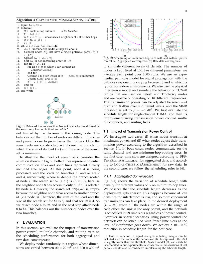
Algorithm 4 CAPACITATED-MINIMALSPANNINGTREE

1. Input: G(V,E), s2. Initialize:3. B ← roots of top subtrees // the branches4. T ← {s} ∪B5. ∀i ∈ V , GS(i)← unconnected neighbors of i at further hops6. ∀b ∈ B, W (b)← 17. h← 28. while h = max hop count do9. Nh ← unconnected nodes at hop distance h

10. Connect nodes N ′h that have a single potential parent: T ←

T∪

N ′h

11. Update Nh ← Nh \N ′h

12. Sort Nh in non-increasing order of |GS|13. for all i ∈ Nh do14. for all b ∈ B to which i can connect do15. Construct SS(i, b)16. end for17. Connect i to b for which W (b) + |SS(i, b)| is minimum18. Update GS(i) and W (b)19. T ← T

∪{i}

∪SS(i, b)

20. end for21. h← h+ 122. end while

1 2

3 4 5 6 7

8

9 10

chosen link

Fig. 5: Balanced tree construction: Node 4 is attached to b2 based onthe search sets; load on both b1 and b2 is 5.

not limited by the decision of the joining node. Thisbalances out the number of nodes on different branchesand prevents one to grow faster than others. Once thesearch sets are constructed, we choose the branch forwhich the sum of its load (W ) and the size of the searchset is minimum.

To illustrate the merit of search sets, consider thesituation shown in Fig. 5. Dotted lines represent potentialcommunication links and solid lines represent alreadyincluded tree edges. At this point, node 4 is beingprocessed, and the loads on branches b1 and b2 are 2and 4, respectively, where bi denote the branch rootedat node i. The search set SS(4, b1) is {8, 9, 10}, becausethe neighbor node 8 has access to only b1 if b1 is selectedby node 4. However, the search set SS(4, b2) is empty,because the neighbor node 8 has access to another branchb1 (via node 3). Therefore, the sum of the load and thesize of the search set for b1 is 5, and that for b2 is 4. Sowe attach node 4 to b2, and in the next step attach node8 to b1. This balances out the number of nodes over thetwo branches.

7 EVALUATION

In this section, we evaluate the impact of transmissionpower control, multiple channels, and routing trees onthe scheduling performance for both aggregated andraw-data convergecast.

We deploy nodes randomly in a region whose dimen-sions are varied between 20 × 20 m2 and 300 × 300 m2

0

10

20

30

40

50

60

70

80

90

100

25 50 75 100 125 150 175 200 225 250 275 300

Nu

mb

er

of

tim

eslo

ts

Side Length - L

Max Power(α:3.0)Power Control(α:3.0)

Max Power(α:3.5)Power Control(α:3.5)

Max Power(α:4.0)Power Control(α:4.0)

(a)

80

90

100

110

120

130

140

150

160

170

180

190

200

210

220

25 50 75 100 125 150 175 200 225 250 275 300

Nu

mb

er

of

tim

eslo

ts

Side Length - L

Max Power(α:3.0)Power Control(α:3.0)

Max Power(α:3.5)Power Control(α:3.5)

Max Power(α:4.0)Power Control(α:4.0)

(b)Fig. 6: Scheduling on minimum-hop trees with and without powercontrol: (a) Aggregated convergecast. (b) Raw-data convergecast.

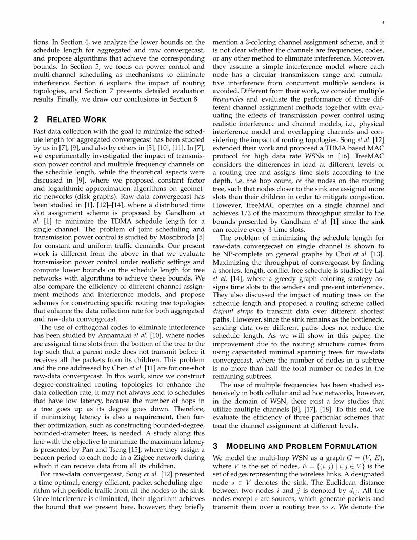
to simulate different levels of density. The number ofnodes is kept fixed at 100. For different parameters, weaverage each point over 1000 runs. We use an expo-nential path-loss model for signal propagation with thepath-loss exponent α varying between 3 and 4, which istypical for indoor environments. We also use the physicalinterference model and simulate the behavior of CC2420radios that are used on Telosb and TmoteSky motesand are capable of operating on 16 different frequencies.The transmission power can be adjusted between −24dBm and 0 dBm over 8 different levels, and the SINRthreshold is set to β = −3 dB1. We first evaluate theschedule length for single-channel TDMA, and then itsimprovement using transmission power control, multi-ple channels, and routing trees.

7.1 Impact of Transmission Power ControlWe investigate two cases: (i) when nodes transmit atmaximum power, and (ii) when nodes adjust their trans-mission power according to the algorithm described inSection 5.1. In both cases, nodes communicate on thesame channel and use minimum-hop routing trees. Inthe first case, time slots are assigned according to BFS-TIMESLOTASSIGNMENT for aggregated data, and accord-ing to LOCAL-TIMESLOTASSIGNMENT for raw data. Inthe second case, we follow the scheduling rules in [6].

7.1.1 Aggregated ConvergecastFig. 6(a) shows the variation of schedule length withdensity for different values of α on minimum-hop trees.We observe that the schedule length decreases as thedeployment gets sparser. This happens because at lowdensities the interference is less, and so more concurrenttransmissions can take place. In the densest deployment(L = 20) when all the nodes are within the range ofeach other, the sink is the only parent, and the networkis scheduled in 99 time slots regardless of power control.However, in sparser scenarios, using power control thenetwork can be scheduled with fewer time slots as thelevel of interference goes down. We achieve a 10− 20%reduction in schedule length for the best case.

1. Due to variation in signal strength, a fading margin can beincluded such that some of the packets can still be captured if the RSSIis slightly lower than the threshold. Such a model [26] can easily beincorporated in our experiments, in which case retransmissions of lostpackets should also be considered in calculating the schedule length.

12

0

10

20

30

40

50

60

70

80

90

100

25 50 75 100 125 150 175 200 225 250 275 300

Nu

mb

er

of

tim

eslo

ts

Side Length - L

JFTSS, channels:2JFTSS, channels:16

RBCA, channels:2RBCA, channels:16TMCP, channels:2

TMCP, channels:16Lower Bound-MHSTLower Bound-TMCP

(a)

80

90

100

110

120

130

140

150

160

170

180

190

200

25 50 75 100 125 150 175 200 225 250 275 300

Nu

mb

er

of

tim

eslo

ts

Side Length - L

JFTSS, channels:2

JFTSS, channels:16

RBCA, channels:2

RBCA, channels:16

TMCP, channels:2

TMCP, channels:16

Lower Bound-MHST

Lower Bound-TMCP

(b)Fig. 7: Scheduling on minimum-hop trees with multiple channels: (a)Aggregated convergecast. (b) Raw-data convergecast.

We also observe that power control is more effectivein reducing the schedule length for denser deploymentsthan in sparser ones where the results tend to be similar.This is due to the discrete power levels and limitedpower range. Moreover, due to the −95 dBm thresholdfor the transceivers to be able to decode a signal success-fully, further power reduction is limited.

7.1.2 Raw Data Convergecast

For raw-data convergecast, we observe in Fig. 6(b) thatthe schedule length increases as the network gets sparseron minimum-hop trees. This is counter intuitive becausein sparse networks the reuse of slots should be higherwhich would reduce the schedule length. However, asthe network gets sparser, the number of nodes that candirectly reach the sink decreases and packets have tobe relayed over more hops. Thus, more packets needto be scheduled than in a single-hop. We see that thenumber of packets to be scheduled increases faster thanthe reuse ratio. In the densest setting where all the nodescan directly reach the sink, the schedule length is 99,which is equal to the number of sources.

With power control, we observe a reduction in theschedule length in Fig. 6(b) as some of the interferinglinks are eliminated, thus increasing slot re-usability.When α = 3.0, most of the interference can be eliminatedby power control, and beyond which the structure ofthe routing tree, especially the number of nodes nk onthe largest branch with (2nk − 1) > N , becomes thebottleneck. However, for α ≥ 3.5, power control cannotalways eliminate interference as networks gets sparserand nodes tend to transmit at their maximum power.

7.2 Impact of Multi-Channel Scheduling

In this section, we analyze the performance of thechannel assignment methods discussed in Section 5.2.We use CC2420 radios that have 16 channels in the2.4 GHz range, with adjacent channels overlapping ac-cording to the rejection and blocking values given inthe data sheet. We assume that the nodes transmit atmaximum power and use minimum-hop trees. In TMCPand RBCA, time slots are assigned according to BFS-TIMESLOTASSIGNMENT for aggregated convergecast andLOCAL-TIMESLOTASSIGNMENT for raw data converge-cast. The path loss exponent is taken as 3.5.

7.2.1 Aggregated Convergecast

Comparing the plots in Fig. 7(a) and Fig. 6(a), weobserve that the channel assignment methods achieveschedule lengths that are shorter than those achievedby power control. While it’s true that power controlhelps in reducing the effects of interference, this gainis limited due to the discrete levels and limited rangeof transmission power (e.g., CC2420 has 8 differentpower levels between 0 dBm and −24 dBm). In sparsedeployments, nodes cannot reduce their transmit powerbelow a certain threshold because a transceiver cannotdecode signals below the sensitivity level (−95dBm). Asshown in Fig. 6(a), for L > 200, the schedule lengthsare similar when nodes transmit at maximum poweror when they adjust their power levels. Moreover, inmid-sparse deployments(60 ≤ L ≤ 180, Fig. 6(a)) thelimited range and discrete power levels restrict thenodes to adjust their transmit powers. On the otherhand, multi-channel communication even with just twofrequencies (Fig. 7(a)), can eliminate the interferencelimitations, and beyond this, the performance gains arelimited by the connectivity structure. By transmitting ondifferent channels, interference is eliminated by the highadjacent/alternate channel rejection values of the C2420radio, and the channels behave like orthogonal.

In Fig 7(a), sparser deployments (L > 140) withmulti-channel communication show a 40% reduction inschedule length as compared to transmitting on a singlechannel with maximum power. However, in denser de-ployments, multiple channels do not help much due toincreased connectivity, with the sink as a bottleneck inthe densest setting. From Fig 7(a), we observe that JFTSSand RBCA can optimally schedule the network using 16channels, i.e., they achieve the lower bound, as shown bythe line “Lower Bound-MHST”. The advantage of RBCAover JFTSS is that it takes into account the topologicalcharacteristics: a parent node receives data on the samechannel from its children, and does not have to switchchannels in every slot. In dense deployments, TMCPperforms better due to the different routing trees con-structed, i.e., when L = 20, RBCA and JFTSS construct astar-topology, whereas TMCP constructs a 2-branch treewith 2 channels, a 16-branch tree with 16 channels.

7.2.2 Raw Data Convergecast

In Fig. 7(b), we observe that none of the methods caneliminate interference completely with 2 channels, how-ever, JFTSS and RBCA can do so with 6 or more channelsat different densities (plots are not shown due to lackof space). We also see that TMCP needs 16 channels toreach a performance similar to that achieved by RBCAand JFTSS with only 2 channels. This is because inJFTSS and RBCA, when a node is receiving from itschildren, its parent can transmit simultaneously on adifferent channel, which is not possible due to intra-branch interference in TMCP. The results also verify thatJFTSS and RBCA can achieve a schedule length which is

13

0

10

20

30

40

50

60

70

80

90

100

25 50 75 100 125 150 175 200 225 250 275 300

Nu

mb

er

of

tim

eslo

ts

Side Length - L

RBCA-MHSTJFTSS-MHST

TMCP

(a)

0

2

4

6

8

10

12

14

16

18

20

22

24

25 50 75 100 125 150 175 200 225 250 275 300

Inco

rre

ctly s

ch

ed

ule

d lin

ks (

%)

Side Length - L

JFTSS-MHST, 2ch.JFTSS-MHST, 16ch.

JFTSS-MHST, 16ch. (orthogonal)

(b)Fig. 8: (a) Bounds on the number of frequencies. (b) Percentage ofincorrectly scheduled links.

bounded by max(2nk − 1, N), shown as “Lower Bound-MHST”, so long as the number of available channels issufficient to eliminate interference. Compared to the re-sults on a single channel in sparser scenarios, we achievea reduction of up to 40% on the schedule length. Invery dense scenarios, the improvement is small becausemost of the nodes can directly reach the sink, and so thelimiting factor becomes the half-duplex transceiver.

7.2.3 Required Number of Channels

In this section, for the different channel assignmentmethods, we evaluate the required number of channelsto completely eliminate interference as a function ofdeployment density. In our simulation results, as shownin Fig. 8(a), we assume that the number of availablechannels is unlimited so as to show the upper bounds.

With RBCA and JFTSS, the number of channels re-quired is low for dense networks as the number ofreceivers is low. In particular, when L = 20, all thenodes can directly connect to the sink, and so only onefrequency is needed. As the network gets sparser, thenumber of receivers increases, and thus more frequen-cies are required to support concurrent transmissions.However, for L ≥ 80, the number of nodes that are beingconnected to the same parent slowly dominates the effectof the number of receivers, and since the network getsvery sparse, the number of channels required furthergoes down as the level of interference decreases.

The trends of both RBCA and JFTSS are quite similar,and the number of channels required is no more thanthe number of available channels on CC2420 radios (16channels). On the other hand, TMCP requires manymore channels as each branch is on a different channel.This is expensive for deployments where a lot of nodescan directly connect to the sink, and thus are assigneddifferent channels because they form different branches.Thus, one needs to optimize the channel usage.

7.2.4 Interference Models and Orthogonal Channels

We now evaluate the impact of interference and channelmodels on the schedules, in particular, the idealisticassumption of the protocol model and the orthogonalityassumption. We examine the feasibility of the schedulesbased on the adjacent and alternate channel rejectionvalues of the transceivers and the SINR threshold.

0

10

20

30

40

50

60

70

80

90

100

25 50 75 100 125 150 175 200 225 250 275 300

Nu

mb

er

of

tim

eslo

ts

Side Length - L

Max Power, Degree-3 TreePower Control, Degree-3 TreeRBCA - 16 ch., Degree-3 TreeJFTSS - 16 ch., Degree-3 Tree

(a)

80

90

100

110

120

130

140

150

160

170

180

190

200

25 50 75 100 125 150 175 200 225 250 275 300

Nu

mb

er

of

tim

eslo

ts

Side Length - L

Max PowerPower ControlRBCA - 16 ch.JFTSS - 16 ch.

(b)Fig. 9: (a) Scheduling on degree-constrained minimum-hop trees. (b)Scheduling on CMST.

Fig. 8(b) shows the results for JFTSS in terms ofthe percentage of nodes that are incorrectly scheduled(henceforth, referred to as errors). The top two linesshow the errors for 2 and 16 channels with both theassumptions, whereas the bottom line shows the errorsonly for the orthogonality assumption. We observe thatthe errors are much higher in sparser deployments, be-cause although the interference created by an individualsender is not high enough to jam concurrent transmis-sions, the cumulative effect from multiple senders isvery high, which is not captured in the protocol model.On the other hand, in dense deployments, a singletransmitter can jam another one because of smaller inter-node distances and higher level of interference. In suchcases, some of the nodes might select the next availablechannels for concurrent transmissions, however, inter-ference can still be high because the channels in realityare not perfectly orthogonal. After the peak, the networkgets sparser and interference reduces. We note that, oursimulations corroborate previous results [27] that theprotocol model may result in serious interference.

7.3 Impact of Routing TreesIn the preceding sections, we observed that althoughinterference can be substantially eliminated by usingpower control and multiple channels, connectivity of thetree still limits the performance. In the following, wediscuss the improvements with routing tress.

7.3.1 Aggregated Convergecast on Degree-Constrained TreesFig. 9(a) shows the variation of schedule length withdensity when the maximum tree degree is 3 (in sparserscenarios, with a maximum degree of 2, it was notalways possible to construct connected topologies). Thetop two lines are for nodes transmitting at maximumpower, and nodes using power control. The bottom twolines are for JFTSS and RBCA. When nodes transmitwith maximum power, we observe a reduction in theschedule length in dense deployments as compared tonon-degree constrained trees shown in Fig. 6(a). Wealso notice further improvement with power control indenser deployments than in sparser ones.

When nodes are assigned channels using RBCA, wesee a factor of more than 2 reduction in the schedulelength in dense deployments (L < 120), as compared to

14

that using RBCA on minimum-hop spanning trees. Wealso observe that the schedule lengths are much largerthan the maximum degree in the routing tree for densedeployments, as compared to those in sparse scenarios(L ≥ 120). Considering deployments at different den-sities, routing over minimum-hop degree-constrainedspanning trees together with RBCA achieves an order ofmagnitude improvement than routing over minimum-hop spanning trees while transmitting at maximumpower. When we use JFTSS, the schedule length is closeor equal to the maximum degree since it can handleinterference using multiple channels more effectively byreusing and assigning them to the links instead of thereceivers.

7.3.2 Raw Data Convergecast on CMST

Fig. 9(b) shows the variation of schedule length onCMST. The impact of such routing trees is more promi-nent in sparser networks (L ≥ 200) than routing overminimum-hop spanning trees (Fig. 7(b)). When L < 200,the length is bounded by N . Beyond this point, it isalmost always not possible to construct trees where theconstraint 2nk−1 < N holds. In such cases, the schedulelength is limited by 2nk − 1. These results indicate thatRBCA and JFTSS combined with a suitable tree construc-tion mechanism can achieve a reduction of up to 50%in the schedule length as compared to single-channelcommunication on minimum-hop spanning trees.

8 CONCLUSIONS

In this paper, we studied fast convergecast in WSNwhere nodes communicate using a TDMA protocol tominimize the schedule length. We addressed the funda-mental limitations due to interference and half-duplextransceivers on the nodes and explored techniques toovercome the same. We found that while transmissionpower control helps in reducing the schedule length,multiple channels are more effective. We also observedthat node-based (RBCA) and link-based (JFTSS) channelassignment schemes are more efficient in terms of elim-inating interference as compared to assigning differentchannels on different branches of the tree (TMCP).

Once interference is completely eliminated, we provedthat with half-duplex radios the achievable schedulelength is lower-bounded by the maximum degree inthe routing tree for aggregated convergecast, and bymax(2nk − 1, N) for raw-data convergecast. Using op-timal convergecast scheduling algorithms, we showedthat the lower bounds are achievable once a suitablerouting scheme is used. Through extensive simulations,we demonstrated up to an order of magnitude reductionin the schedule length for aggregated, and a 50% reduc-tion for raw-data convergecast. In future, we will explorescenarios with variable amounts of data and implementand evaluate the combination of the schemes considered.

REFERENCES[1] S. Gandham, Y. Zhang and Q. Huang, “Distributed Time-Optimal

Scheduling for Convergecast in Wireless Sensor Networks”, Com-puter Networks, vol. 52, nr. 3, 2008, pp. 610–629.

[2] K.K. Chintalapudi and L. Venkatraman, “On the Design of MACProtocols for Low-Latency Hard Real-Time Discrete Control Ap-plications over 802.15.4 Hardware”, in IPSN ’08, pp. 356–367.

[3] I. Talzi, A. Hasler, G. Stephan and C. Tschudin, “PermaSense:investigating permafrost with a WSN in the Swiss Alps”, inEmNets ’07, pp. 8–12.

[4] S. Upadhyayula and S.K.S. Gupta, “Spanning tree based algo-rithms for low latency and energy efficient data aggregationenhanced convergecast (DAC) in wireless sensor networks”, AdHoc Networks, vol. 5, nr.5, 2007, pp. 626–648.

[5] T. Moscibroda, “The worst-case capacity of wireless sensor net-works”, in IPSN ’07, pp. 1–10.

[6] T.ElBatt and A. Ephremides, “Joint Scheduling and Power Controlfor Wireless Ad-hoc Networks”, in INFOCOM ’02, pp. 976–984.

[7] O. Durmaz Incel and B. Krishnamachari, “Enhancing the DataCollection Rate of Tree-Based Aggregation in Wireless SensorNetworks”, in SECON ’08, pp. 569–577.

[8] Y. Wu, J.A. Stankovic, T. He and S. Lin, “Realistic and EfficientMulti-Channel Communications in Wireless Sensor Networks”, inINFOCOM ’08, pp. 1193–1201.

[9] A. Ghosh, O. Durmaz Incel, V.A. Kumar and B. Krishnamachari,“Multi-Channel Scheduling Algorithms for Fast Aggregated Con-vergecast in Sensor Networks”, in MASS ’09, pp. 363–372.

[10] V. Annamalai, S.K.S. Gupta, L. Schwiebert, “On tree-based con-vergecasting in wireless sensor networks”, in WCNC ’03, pp.1942–1947.

[11] X. Chen, X. Hu and J. Zhu, “Minimum Data Aggregation TimeProblem in Wireless Sensor Networks”, in MSN ’05, pp. 133–142.

[12] W. Song, F. Yuan and R. LaHusen, “Time-Optimum PacketScheduling for Many-to-One Routing in Wireless Sensor Net-works”, in MASS ’06, pp. 81–90.

[13] H. Choi, J. Wang and E. Hughes, “Scheduling for InformationGathering on Sensor Network”, Wireless Networks (Online), 2007.

[14] N. Lai, C.King and C. Lin, “On Maximizing the Throughput ofConvergecast in Wireless Sensor Networks”, in GPC ’08, pp. 396.

[15] M. Pan and Y. Tseng, “Quick convergecast in ZigBee beacon-enabled tree-based wireless sensor networks”, Computer Commu-nications, vol. 31, nr. 5, 2008, pp. 999-1011.

[16] W. Song, H. Renjie, B. Shirazi, R. LaHusen, “TreeMAC: Local-ized TDMA MAC protocol for real-time high-data-rate sensornetworks”, Pervasive Mob. Comput., vol. 5, nr. 6, 2009, pp. 750.

[17] G. Zhou, C. Huang, T. Yan, T. He, J. Stankovic and T. Abdelzaher,“MMSN: Multi-Frequency Media Access Control for WirelessSensor Networks”, in INFOCOM ’06, pp. 1–13.

[18] Y. Kim, H. Shin, H. Cha, “Y-MAC: An Energy-Efficient Multi-channel MAC Protocol for Dense Wireless Sensor Networks”, inIPSN ’08, pp. 53–63.

[19] B. Krishnamachari, D. Estrin and S.B. Wicker, “The Impact of DataAggregation in Sensor Networks”, in ICDCSW ’02, pp. 575–578.

[20] J. Zander, “Performance of optimum transmitter power control incellular radio systems”, IEEE Transactions on Vehicular Technology,vol. 41, nr. 1, 1992, pp. 57–62.

[21] P. Kyasanur and N. H. Vaidya, “Capacity of multi-channel wire-less networks: impact of number of channels and interfaces”, inMobiCom ’05, pp. 43–57.

[22] G. Sharma, R.R. Mazumdar and N.B. Shroff, “On the complexityof scheduling in wireless networks”, in MobiCom ’06, pp. 227–238.

[23] X. Lin and S. Rasool, “A Distributed Joint Channel-Assignment,Scheduling and Routing Algorithm for Multi-Channel Ad-hocWireless Networks”, in INFOCOM ’07, pp. 1118–1126.

[24] C.H. Papadimitriou, “The complexity of the capacitated treeproblem”, Networks, vol. 8, nr. 3, 1978, pp. 217-230.

[25] H. Dai and R. Han, “A node-centric load balancing algorithm forwireless sensor networks”, in GLOBECOM ’03, pp. 548–552.

[26] M. Zuniga and B. Krishnamachari, “An analysis of unreliabilityand asymmetry in low-power wireless links”, ACM Trans. Sen.Netw., vol. 3, nr. 2, 2007, pp. 7.

[27] J. Gronkvist and A. Hansson, “Comparison between graph-basedand interference-based STDMA scheduling”, in MobiHoc ’01, pp.255–258.

15

Ozlem Durmaz Incel is currently a postdoctoral re-searcher in the Networking Laboratory of Bogazici Uni-versity, Turkey. She received her Ph.D. in ComputerScience from the University of Twente, Netherlands,in March 2009. Her dissertation focused on efficientdata collection in wireless sensor networks. She was avisiting student in the Autonomous Networks ResearchGroup of the University of Southern California as partof her Ph.D. studies in 2007 and 2008.

Amitabha Ghosh is currently a postdoctoral re-searcher in Princeton University. He received his Ph.D.in Electrical Engineering from the University of South-ern California in August 2010. His research interest ison design and analysis of algorithms for scheduling,routing, and power control for cellular and wirelesssensor networks. He received his B.S. in Physics fromthe Indian Institute of Technology, Kharagpur in 1996,and his M.E. in Computer Science and Engineeringfrom the Indian Institute of Science, Bangalore in 2000.

Bhaskar Krishnamachari is an Associate Professor inthe Ming Hsieh Electrical Engineering department atthe USC Viterbi School of Engineering. He received hisB.E. in Electrical Engineering from The Cooper Union in1998, and his M.S. and Ph.D. in Electrical Engineeringfrom Cornell University in 1999 and 2002 respectively.His research interests are in design and performanceanalysis of protocols for next-generation wireless net-works. He received the NSF CAREER award in 2004.

Krishnakant Chintalapudi is currently working as anassociate researcher at Microsoft Research, India. Hisresearch interests include delay-sensitive and fault-tolerant wireless sensor networks, high-data-rate wire-less sensor network applications, hybrid sensor net-works, and wireless control and automation. Chintala-pudi has a Ph.D. in Computer Science from the Uni-versity of Southern California and an M.S. in ElectricalEngineering from Drexel University.