Feasibility Boundary in Dense and Semi-Dense Stereo Matching

Jana Kostliva and Jan Cech and Radim SaraCenter for Machine Perception, Czech Technical University in Prague, Czech Republic

{kostliva, cechj, sara}@cmp.felk.cvut.cz

Abstract

In stereo literature, there is no standard method for eval-uating algorithms for semi-dense stereo matching. More-over, existing evaluations for dense methods require a fixedparameter setting for the tested algorithms. In this paper,we propose a method that overcomes these drawbacks andstill is able to compare algorithms based on a simple numer-ical value, so that reporting results does not take up muchspace in a paper. We propose evaluation of stereo algo-rithms based on Receiver Operating Characteristics (ROC)which captures both errors and sparsity. By comparingROC curves of all tested algorithms we obtain the Feasi-bility Boundary, the best possible performance achieved bya set of tested stereo algorithms, which allows stereo al-gorithm users to select the proper method and parametersetting for a required application.

1. IntroductionDense stereopsis plays a very important role in the field

of computer vision, since its results are usable to many(even very distinct) tasks. In recent years, stereo vision hasbeen re-investigated by many researches, leading to a hugenumber of algorithms and the need for their comparison andevaluation immediately rose up. Several performance stud-ies [2, 9, 5, 16, 15] showed, that there is not a single winnerover the other methods, but some of the algorithms are bet-ter in some of the errors and scenes than the others, while onother errors and scenes it is vice versa. Thus, a study show-ing algorithm potentials and drawbacks, allowing users toselect a proper method for their purposes, is desired.

There are two main properties characterising a matchingalgorithm: its disparity map density and accuracy measuredwith respect to the ground-truth matching.

One of the most important problems is the setting ofalgorithm parameters. Typically, each algorithm has sev-eral adjustable parameters and some of them basically de-termine the quality of results. Standard evaluations, suchas [2, 15, 9, 5, 16], leave parameter setting on an authorand keep this setting fixed over the whole evaluation dataset

(which often consists of scenes with different and some-times even very distinct character). In other words, it as-sumes uniform behaviour with respect to scenes (i.e. insen-sitivity to scene character) which not many algorithms fulfil.

In contrast, our goal is to evaluate the algorithms inde-pendently on parameter settings. To this end, we proposea kind of ROC analysis of stereo algorithm performance,where we study how the result accuracy and density changewith respect to different parameter settings. An attempt to-wards this goal has been published in [7], where, based onerrors defined in [15], ROC curves of the algorithm havebeen presented. Unlike in [15], we define the errors to bemutually independent and complete and base our decisionabout the algorithm quality on a well-defined relation “isbetter”. Furthermore, we propose quantitative characteris-tics of algorithms for numerical comparison. As it is com-mon, the test images are given and fixed. We are preparinga web-site [11] for an automatic evaluation, so that other re-searchers can easily use this method. Such a collection ofevaluation results is also useful for users, who can simplyselect the most suitable algorithm for a desired application.

In the next section, we introduce our ROC analysis, inSec. 3, the feasibility boundary. In Sec. 4, we present theexperimental dataset. The algorithm evaluation itself is dis-cussed in Sec. 5. Finally, in Sec. 6, we give conclusions.

2. ROC Analysis

To evaluate the stereo algorithm performance, we adoptthe Receiver Operating Characteristics (ROC) analysis. TheROC study has been long used in signal theory to show thetradeoff between hit rates and false alarm rates [4]. Theoriginal approach has been extended to many distinct fields,such as recognition, object detection, etc [6, 1, 18, 12].

2.1. Error Definitions

We are interested in studying the matching quality, thuswill measure two kinds of error statistics: how often an al-gorithm makes an error and how often an algorithm doesnot decide when it should. The Error rate is defined as thepercentage of incorrect (assigned) correspondences (thus,

we do not count a hole as an incorrect correspondence):

ER =incorrect correspondences

all pixels. (1)

The Sparsity rate is defined as the percentage of all miss-ing correspondences which are not ruled out1 by any otherincorrect correspondence:

SR =missing correspondences

all matchable pixels. (2)

We base our evaluation on the error statistics which fulfilthe following four principles, adopted from [9]:

1. Orthogonality: one error must not influence (or imply)any other error.

2. Symmetry: the errors have to be invariant to the selec-tion of the reference image.

3. Completeness: the errors are well-defined in all typesof scene structure.

4. Algorithm independence: the errors do not requirecompletely dense results or one-to-one matchings.

Assuming rectified images, the errors are defined bymeans of various events in the matching table, which is theset of all possible matches P (per image row), P = X×X ′,where X, X ′ are pixels in the left, and right image rows,respectively. Every ground-truth disparity map (as well asresulting matching or disparity map of a tested algorithm) isdirectly transformable to matching tables, and thus this def-inition holds for every scene. This representation has beenselected since all errors are easily visible there.

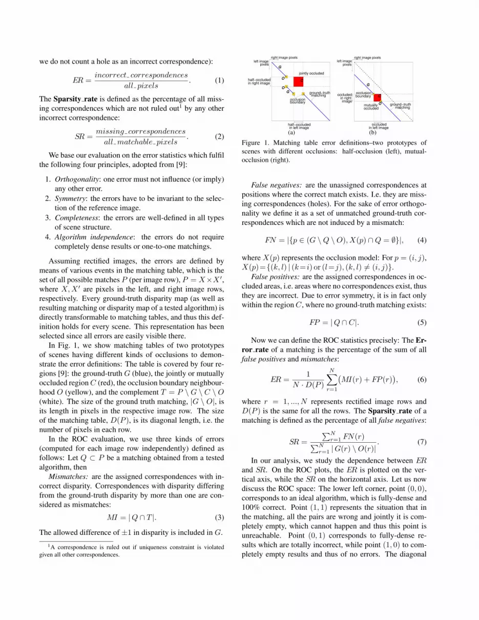
In Fig. 1, we show matching tables of two prototypesof scenes having different kinds of occlusions to demon-strate the error definitions: The table is covered by four re-gions [9]: the ground-truth G (blue), the jointly or mutuallyoccluded region C (red), the occlusion boundary neighbour-hood O (yellow), and the complement T = P \G \ C \ O(white). The size of the ground truth matching, |G \ O|, isits length in pixels in the respective image row. The sizeof the matching table, D(P ), is its diagonal length, i.e. thenumber of pixels in each row.

In the ROC evaluation, we use three kinds of errors(computed for each image row independently) defined asfollows: Let Q ⊂ P be a matching obtained from a testedalgorithm, then

Mismatches: are the assigned correspondences with in-correct disparity. Correspondences with disparity differingfrom the ground-truth disparity by more than one are con-sidered as mismatches:

MI = |Q ∩ T |. (3)

The allowed difference of ±1 in disparity is included in G.

1A correspondence is ruled out if uniqueness constraint is violatedgiven all other correspondences.

jointly occluded

matchingground−truth

occlusionboundary

left imagepixels

in left imagehalf−occluded

half−occludedin right image

right image pixels

C

G

O

O

G

(a)

matching

right image pixels

occluded

left image

mutually

occlusion

pixels

occludedin rightimage

in left image

boundary

ground−truthoccluded

G

C

O

(b)

Figure 1. Matching table error definitions–two prototypes ofscenes with different occlusions: half-occlusion (left), mutual-occlusion (right).

False negatives: are the unassigned correspondences atpositions where the correct match exists. I.e. they are miss-ing correspondences (holes). For the sake of error orthogo-nality we define it as a set of unmatched ground-truth cor-respondences which are not induced by a mismatch:

FN = |{p ∈ (G \Q \O), X(p) ∩Q = ∅}|, (4)

where X(p) represents the occlusion model: For p = (i, j),X(p)={(k, l) | (k= i) or (l=j), (k, l) 6= (i, j)}.

False positives: are the assigned correspondences in oc-cluded areas, i.e. areas where no correspondences exist, thusthey are incorrect. Due to error symmetry, it is in fact onlywithin the region C, where no ground-truth matching exists:

FP = |Q ∩ C|. (5)

Now we can define the ROC statistics precisely: The Er-ror rate of a matching is the percentage of the sum of allfalse positives and mismatches:

ER =1

N ·D(P )

N∑r=1

(MI(r) + FP (r)

), (6)

where r = 1, ..., N represents rectified image rows andD(P ) is the same for all the rows. The Sparsity rate of amatching is defined as the percentage of all false negatives:

SR =∑N

r=1 FN(r)∑Nr=1 |G(r) \O(r)|

. (7)

In our analysis, we study the dependence between ERand SR. On the ROC plots, the ER is plotted on the ver-tical axis, while the SR on the horizontal axis. Let us nowdiscuss the ROC space: The lower left corner, point (0, 0),corresponds to an ideal algorithm, which is fully-dense and100% correct. Point (1, 1) represents the situation that inthe matching, all the pairs are wrong and jointly it is com-pletely empty, which cannot happen and thus this point isunreachable. Point (0, 1) corresponds to fully-dense re-sults which are totally incorrect, while point (1, 0) to com-pletely empty results and thus of no errors. The diagonal

0 10

1

Sparsity_rate

Err

or_

rate

A

B

(a) ROC space0 1

0

1

Sparsity_rateE

rror_

rate

(b) ROC curve

Figure 2. (a) ROC space with two ROC curves of algorithms A andB. Dashed black line represents reachable boundary. The greencurve is SFB of algorithms A and B (Sec. 3). (b) ROC curveconstruction from all ROC points produced by a single algorithm.Blue circled points are selected to represent the ROC curve (blue).

line y = 1 − x (dashed black line in Fig. 2) represents theworst-case boundary, which we call zero-algorithm.

An important property of ROC plots is that they measurethe matching accuracy with respect to the matching density,which are in contradiction. Hence, it gives the possibility toa user to select the most suitable algorithm: E.g. View pre-diction requires low sparsity rate, while a few local errorsdo not affect result quality, while 3D scene reconstructionrequires low error rate, while lower density is acceptable.

2.2. ROC curve

One parameter setting of an algorithm gives a pair(SR, ER), hence, a single point in the ROC space, aROC point. A different setting gives (generally) different(SR, ER) pair. Since the parameters are given discretely,one in fact only samples the ROC space. It is the respon-sibility of an author to select parameter quantisation whichgives results as close to the best ROC results as possible.

All output pairs under the varying parameter settingsdetermine the ROC curve of an algorithm (two exem-plary ROC curves are shown in Fig. 2(a)): we define itas the lower hull of all its ROC points.2 First, we de-fine relation between them: We say that ROC point u =(SR(u), ER(u)) is better than point v = (SR(v), ER(v)),which we write u < v, if it is more accurate and denser:

u<v⇔{u6=v &SR(u)≤SR(v) &ER(u)≤ER(v)}. (8)

For the ROC curve, points for which there is no better pointare selected. Hence, the ROC curve is formed by the fol-lowing set of points:

R = {u ∈ P : @ v ∈ P, v < u}, (9)

where P is a set of all ROC points. Points which are not inR are worse (in ER or SR, or even in both statistics), and

2More precisely, it is the lower hull of the ROC points of the algorithmunified with the ROC points for the zero-algorithm.

thus they are in fact redundant. The ROC curve constructedfrom the ROC points is shown in Fig. 2(b): red crosses rep-resent all ROC points, those marked by blue circles havebeen selected to R, dotted black lines originating in each ofthese points show regions of ROC points dominated by theROC curve points.

Points R defined in (9) form the ROC curve. Only inthese points we know the exact position of the curve. Thus,we define the ROC curve as a curve connecting points R bya piecewise constant line, alternately with respect to SR andER (shown as blue solid line in Fig. 2(b)). Above this curveall points are worse than those in R (i.e. it is a worst caseboundary between ROC curve points). Since the ROC curveis directly determined by points R, we write it as C(R).

2.3. Algorithm Characteristics

For quantitative comparison, we define two numericalcharacteristics, derived from algorithm’s ROC curve. Thedefinition requires the ROC curve representation as a func-tion: only piecewise constant parts of the ROC curve withrespect to one of the axes are selected for ROC function.

Efficiency The efficiency is an integral characteristicwhich expresses the algorithm qualities along the entireROC space. The efficiency E is defined as

E(A) = 2∫ 1

0

(Z(x)−A(x)

)dx, (10)

where Z(x) = 1 − x represents the ROC function of zero-algorithm (shown in Fig. 3 as a diagonal line). The A(x) isthe ROC function of the measured algorithm, Fig. 3(a). Themeaning of this characteristic is the measure of improve-ment compared to the worst case. The range of the effi-ciency is E ∈ [0, 1], where E = 0 is for the zero-algorithmwhich produces the worst possible results, and E = 1 is forthe ideal algorithm which is error free and fully dense, i.e.has a single point (0, 0) forming the ROC curve.

The efficiency characterises over-all behaviour of the al-gorithm. But, it does not mean that if the efficiency of al-gorithm A is higher than that of algorithm B, the algorithmA is better. The reason is that in some region of ROC spacealgorithm B can be better than A, i.e. the B(x) < A(x) forsome x ∈ [0, 1].

Improvement The improvement is a comparative char-acteristic which measures how much one algorithm is betterthan the other in areas where it is better. We define the im-provement I(A|B) of algorithm A over B, as:

I(A|B) = 2∫{x:A(x)<B(x)}

(B(x)−A(x)

)dx, (11)

where A(x) is the ROC curve of the measured algorithm,B(x) is the ROC curve of a reference algorithm, Fig. 3(b).The set, where the algorithm is better than the other, we callalgorithm’s dominant interval. Dominant intervals of eachalgorithm are marked on the axes by their respective colour

Err

or_

rate

Sparsity_rate

Z

A

00 1

1

(a) efficiency

B

A

Err

or_

rate

Sparsity_rate00 1

1

(b) improvement

Figure 3. Definitions of: (a) E(A), and (b) I(A|B).

in Fig. 3(b). If the measured algorithm is nowhere better,the dominant interval is empty, and its improvement is zero.Note that I(A|B) ∈ [0, 1], I(A|Z) = E(A), and in general,I(A|B) 6= I(B|A).

3. Stereo Feasibility BoundaryEach algorithm produces its own ROC curve. For algo-

rithm’s developers, the ROC curve shape and its comparisonwith other algorithm curves is very significant and useful.However, for stereo users it is important to know what canbe done by existing algorithms. This we call the Stereo Fea-sibility Boundary and define it as the ROC curve of all ROCpoints of all the (already examined) algorithms altogether:

SFB = {u ∈n⋃

i=1

Ri : @ v ∈n⋃

i=1

Ri, v < u}, (12)

where Ri are ROC curve points of all n examined algo-rithms. In Fig. 2(a), we show the C(SFB) as a green curve.

Some of the algorithms need not have any representativepoint in SFB. It is the situation when those algorithms arebetter neither in density nor in accuracy comparing to otherapproaches. Each of the SFB points is associated with thealgorithm name, and jointly with its parameter setting aswell as the corresponding disparity map.

The defined numerical characteristics of Sec. 2.3 can beevaluated also for the stereo feasibility boundary. The ef-ficiency describes how far the nowadays stereo methodsare, which will be true when state-of-the-art algorithms aretested. Therefore, we are preparing an on-line evaluationtool. Improvement is however even more interesting: Anevaluated algorithm can measure its improvement over thecurrent SFB. This is an important characteristic of the algo-rithm, since it measures how much the algorithm improvesover the best algorithms. The dominant interval then deter-mines where this occurs in ROC space.

3.1. Worst, Best, and Mean SFBs

The ROC curve and also Stereo Feasibility Boundary aredefined over results on one scene (which guarantees a faircomparison). However, it is interesting to study the algo-rithm’s performance, over all the scenes. To this end, wedefine three more SFBs:

The Worst SFB is defined as the worst case over SFBs ofall m scenes:

W = {u ∈m⋃

s=1

SFBs : @ v ∈m⋃

s=1

SFBs, u < v}. (13)

The W then represents a kind of (min,max) (pessimistic)strategy, where over the best for each scene (SFB) we selectthose minimising the risk (the worst), i.e. it is very unlikelywe get worse results than these.

The Best SFB, on contrary, is defined as the best caseover SFBs of all m scenes:

B = {u ∈m⋃

s=1

SFBs : @ v ∈m⋃

s=1

SFBs, v < u}. (14)

The B represents the (optimistic) strategy with maximalrisk, i.e. it is almost sure, the results we will get will beof worse performance.

Since it is not possible to evaluate algorithms on allscenes which may exist, we define Mean SFB to measurealgorithm’s expected performance, based on the followingpoints:

P (θ) =m∑

s=1

ws · Ps(θ),m∑

s=1

ws = 1, (15)

where Ps(θ) is ROC point for parameter setting θ on scenes, and ws is the weight (probability) of scene s, giving thescene representativity. Points P are used in the same wayas in (9) to obtain ROC curve C(Ri) for each algorithm i.Hence, the Mean SFB is:

M = {u ∈n⋃

i=1

Ri : @ v ∈n⋃

i=1

Ri, v < u}. (16)

We believe that this statistic is useful mainly for applyingstereo algorithms on new unknown scenes since it gives theexpectation of algorithm’s behaviour.

4. Experimental DataFor our ROC analysis, we use a wide range of stereo

scenes with ground-truths (shown in Fig. 4): Tsukuba,Venus, Teddy, Cones, Stripes, and Slits. Ground-truth dis-parity maps are colour coded: warmer the colour higher thedisparity, gray is occluded, black excluded.

The first four scenes are from Middlebury dataset [15,14] (courtesy of D. Scharstein), which is a well knowndataset and thus we show only the ground-truths. To en-hance the set for more complex occlusions, we add Stripesand Slits scenes [9]. Both of them are based on artificialscenes with varying texture contrast over the scene. Stripesscene consists of five thin textured stripes in front of aslanted textured plane, with half-occlusions, Fig. 1(a). Slitsscene consists of two parallel textured planes, the front onecontains narrow slits, in which cameras see the backgroundplane. However, each of the cameras captures in these areasdifferent part of the background and thus the background

tsukuba venus teddy cones

stripes slits

Figure 4. Ground-truths of selected testing scenes. Top row: Mid-dlebury dataset, bottom row: Stripes and Slits scenes. Dispari-ties are colour coded: higher the disparity, warmer the colour (asshows the rightmost bar), occlusions are gray, black is excluded.

is not binocularly visible. These regions we call mutuallyoccluded (shown in Fig. 1(b), as red area).

Each scene has prescribed (known and fixed) disparitysearch range, which has been constructed from ground-truthdisparity range [d1, d2] as [d1− d2−d1

2 , d2+ d2−d12 ]. A wider

range is used intentionally, since in many applications itneed not be defined precisely or even to be known.

We have selected testing scenes to cover distinct typesof configurations: well-textured together with un-texturedregions, various planes, slanted as well as curved surfaces,different types of occlusions, etc. Too simple scenes (e.g. aconstant disparity well-textured plane) or too tricky (unre-alistic) scenes are excluded on purpose, since they are notrepresentative to contribute to (16).

5. Evaluation/ResultsFor our evaluation, we have chosen five algorithms, rep-

resentatives of different approaches, with available imple-mentations. They can be roughly divided into two groups,based on prior models: (1) a strong continuity model, (2) aweak continuity model. The first group is represented by:MAP matching via graph cuts (GC) [8], MAP matching viadynamic programming (DP) [3], and MAP matching via be-lief propagation (BP) [17]. The second group is representedby: Confidently-Stable Matching (CSM) [13], and Strati-fied Dense Matching (SDM) [10]. We have selected algo-rithms whose implementations are publicly available, whichallows experimental reproducibility.

Each of the algorithms has its own adjustable parame-ters, and we let an author to define himself/herself adequaterange for the parameters together with the step of parame-ter change. For this study, the fundamental parameters forthe tested algorithms have been spanned in the followingintervals:

• GC: λ = 0:30:180, penalty0 = p = 0:20:140.• BP: opt smoothness = s = 0:25:50, opt grad thresh

= t = 0:2:8, opt grad penalty = p = 0:4.• CSM: α = {0:5:20,50:50:150},

β = {0,0.02,0.03,0.05,0.07,0.1,0.3,0.5,0.7}.

• SDM: α = {0:5:20,50:50:150},β = {0,0.02,0.03,0.05,0.07,0.1,0.3,0.5,0.7}.

• DP: penalty = p = {0:20:140, 150:50:1000}.

For each algorithm, the errors are computed under all pa-rameter combinations (e.g. BP under 75 different settings).

We present the results as plots (Figs. 5-6). All the plotsare shown in scales modified by log(x + c) function, wherec = 0.001, in both axes to allow a detailed study. The diag-onal line y = 1 − x of reachable area is shown as a curve(dashed black) due to this modification. For visual inspec-tion, we show selected disparity maps in Fig. 8. They cor-respond to ROC points which are the best of each algorithmwith respect to SFB of each scene, if there are more of them,the middle one is reported.

In Fig. 5, we show results on Stripes scene. Each algo-rithm has a different colour and marker (for description seelegend). Fig. 5(a) shows all the ROC points (SR, ER) ofall tested algorithms resulting from all parameter settings.Algorithms with a strong continuity prior model (DP, GC,and BP) give results with higher ER, mainly due to thatthey fail if the prior model overweights the data (cf. Fig. 8).The density of GC and DP is varying (up to completelyempty results) because both the approaches have incorpo-rated occlusion model, unlike BP. GC and DP perform com-parably (and even more, the DP is slightly better) whichis mainly due to the fact that the planparalelity model ofGC is violated in this scene. Algorithms with only weakmodel (CSM and SDM) give more accurate (about an orderof magnitude) results, which are sparse however. The im-proved matching feature modelling in SDM decreased theER about 2× with the same density compared to CSM.

In Fig. 5(b), we show the ROC curves. Each algorithmhas its own, in BP it is only a single point since all its ROCpoints have the same SR. In Fig. 5(c), the SFB is shown: Itshows that SDM is mostly better than CSM (as it has beenvisible already in previous plots) and thus CSM has onlyone point on the SFB, but with SR = 1. It also clearlyshows that DP is better than GC in most of the range.

In Fig. 6, we show results on the other scenes (the figureis best viewed zoomed-in in the electronic version). TheSlits scene shows that although the GC and DP have occlu-sion model incorporated, their model corresponds to half-occlusion only and thus they are not able to identify mu-tually occluded region (causing false positives), cf. Fig. 8.Tsukuba is the only scene, where GC reached the SFB. Onthis kind of scene, i.e. of narrow disparity range of only 10pixels, nearly frontoparallel objects of almost constant dis-parity, GC is very good (its model holds) and thus it is forsuch scenes a suitable algorithm. Unlike in GC, for SDMand CSM, this scene is the most difficult one among all thetested. The last three scenes (Venus, Teddy, and Cones)show a common behaviour: GC is about 5× worse than DPon average and thus has no representative at any scene SFB.

0 0.01 0.05 0.1 0.5 10

0.01

0.05

0.1

0.5

1

Sparsity rate

Err

or

rate

Scene: stripes

CSMGCDPSDMBP

0 0.01 0.05 0.1 0.5 10

0.01

0.05

0.1

0.5

1

Sparsity rate

Err

or

rate

Scene: stripes

(a) ROC points0 0.01 0.05 0.1 0.5 1

0

0.01

0.05

0.1

0.5

1

Sparsity rate

Err

or

rate

ROC curves − Scene: stripes

CSMGCDPSDMBP

0 0.01 0.05 0.1 0.5 10

0.01

0.05

0.1

0.5

1

Sparsity rate

Err

or

rate

ROC curves − Scene: stripes

(b) ROC curves0 0.01 0.05 0.1 0.5 1

0

0.01

0.05

0.1

0.5

1

Sparsity rate

Err

or

rate

SFB − Scene: stripes

CSMGCDPSDMBP

0 0.01 0.05 0.1 0.5 10

0.01

0.05

0.1

0.5

1

Sparsity rate

Err

or

rate

SFB − Scene: stripes

(c) SFB

Figure 5. ROC statistics on Stripes scene. The plots are best viewed in the electronic version.

slits tsukuba venus teddy cones expected

0 0.01 0.1 0.5 10

0.01

0.1

0.5

1

Sparsity rate

Err

or

rate

Scene: slits

CSMGCDPSDMBP

0 0.01 0.1 0.5 10

0.01

0.1

0.5

1

Sparsity rate

Err

or

rate

Scene: slits

0 0.01 0.1 0.5 10

0.01

0.1

0.5

1

Sparsity rate

Err

or

rate

Scene: tsukuba

CSMGCDPSDMBP

0 0.01 0.1 0.5 10

0.01

0.1

0.5

1

Sparsity rate

Err

or

rate

Scene: tsukuba

0 0.01 0.1 0.5 10

0.01

0.1

0.5

1

Sparsity rate

Err

or

rate

Scene: venus

CSMGCDPSDMBP

0 0.01 0.1 0.5 10

0.01

0.1

0.5

1

Sparsity rate

Err

or

rate

Scene: venus

0 0.01 0.1 0.5 10

0.01

0.1

0.5

1

Sparsity rate

Err

or

rate

Scene: teddy

CSMGCDPSDMBP

0 0.01 0.1 0.5 10

0.01

0.1

0.5

1

Sparsity rate

Err

or

rate

Scene: teddy

0 0.01 0.1 0.5 10

0.01

0.1

0.5

1

Sparsity rate

Err

or

rate

Scene: cones

CSMGCDPSDMBP

0 0.01 0.1 0.5 10

0.01

0.1

0.5

1

Sparsity rate

Err

or

rate

Scene: cones

0 0.01 0.1 0.5 10

0.01

0.1

0.5

1

Sparsity rate

Err

or

rate

Mean

CSMGCDPSDMBP

0 0.01 0.1 0.5 10

0.01

0.1

0.5

1

Sparsity rate

Err

or

rate

Mean

0 0.01 0.1 0.5 10

0.01

0.1

0.5

1

Sparsity rate

Err

or

rate

ROC curves − Scene: slits

CSMGCDPSDMBP

0 0.01 0.1 0.5 10

0.01

0.1

0.5

1

Sparsity rate

Err

or

rate

ROC curves − Scene: slits

0 0.01 0.1 0.5 10

0.01

0.1

0.5

1

Sparsity rate

Err

or

rate

ROC curves − Scene: tsukuba

CSMGCDPSDMBP

0 0.01 0.1 0.5 10

0.01

0.1

0.5

1

Sparsity rate

Err

or

rate

ROC curves − Scene: tsukuba

0 0.01 0.1 0.5 10

0.01

0.1

0.5

1

Sparsity rate

Err

or

rate

ROC curves − Scene: venus

CSMGCDPSDMBP

0 0.01 0.1 0.5 10

0.01

0.1

0.5

1

Sparsity rate

Err

or

rate

ROC curves − Scene: venus

0 0.01 0.1 0.5 10

0.01

0.1

0.5

1

Sparsity rate

Err

or

rate

ROC curves − Scene: teddy

CSMGCDPSDMBP

0 0.01 0.1 0.5 10

0.01

0.1

0.5

1

Sparsity rate

Err

or

rate

ROC curves − Scene: teddy

0 0.01 0.1 0.5 10

0.01

0.1

0.5

1

Sparsity rate

Err

or

rate

ROC curves − Scene: cones

CSMGCDPSDMBP

0 0.01 0.1 0.5 10

0.01

0.1

0.5

1

Sparsity rate

Err

or

rate

ROC curves − Scene: cones

0 0.01 0.1 0.5 10

0.01

0.1

0.5

1

Sparsity rate

Err

or

rate

ROC curves − Mean

CSMGCDPSDMBP

0 0.01 0.1 0.5 10

0.01

0.1

0.5

1

Sparsity rate

Err

or

rate

ROC curves − Mean

0 0.01 0.1 0.5 10

0.01

0.1

0.5

1

Sparsity rate

Err

or

rate

SFB − Scene: slits

CSMSDMBP

0 0.01 0.1 0.5 10

0.01

0.1

0.5

1

Sparsity rate

Err

or

rate

SFB − Scene: slits

0 0.01 0.1 0.5 10

0.01

0.1

0.5

1

Sparsity rate

Err

or

rate

SFB − Scene: tsukuba

CSMGCDPSDMBP

0 0.01 0.1 0.5 10

0.01

0.1

0.5

1

Sparsity rate

Err

or

rate

SFB − Scene: tsukuba

0 0.01 0.1 0.5 10

0.01

0.1

0.5

1

Sparsity rate

Err

or

rate

SFB − Scene: venus

CSMDPSDMBP

0 0.01 0.1 0.5 10

0.01

0.1

0.5

1

Sparsity rate

Err

or

rate

SFB − Scene: venus

0 0.01 0.1 0.5 10

0.01

0.1

0.5

1

Sparsity rate

Err

or

rate

SFB − Scene: teddy

CSMDPSDMBP

0 0.01 0.1 0.5 10

0.01

0.1

0.5

1

Sparsity rate

Err

or

rate

SFB − Scene: teddy

0 0.01 0.1 0.5 10

0.01

0.1

0.5

1

Sparsity rate

Err

or

rate

SFB − Scene: cones

CSMGCDPSDMBP

0 0.01 0.1 0.5 10

0.01

0.1

0.5

1

Sparsity rate

Err

or

rate

SFB − Scene: cones

0 0.01 0.1 0.5 10

0.01

0.1

0.5

1

Sparsity rate

Err

or

rate

SFB − Mean

CSMDPSDMBP

0 0.01 0.1 0.5 10

0.01

0.1

0.5

1

Sparsity rate

Err

or

rate

SFB − Mean

Figure 6. ROC statistics on other tested scenes, and expected.

The SFBs are of the same character consisting of BP, DP,SDM, and CSM points.

The rightmost column of Fig. 6 shows plots with ex-pected performance, defined in (15), scene weights wereset equally (ws = 1

m ). They show interesting properties:ROC points of DP are monotonous and do not exhibit anyworsening, unlike in individual scenes. GC has no point inM which shows its sensitivity to both scene character (andprior model) and parameter setting. SDM and CSM alter-nate on M which shows their comparable performance.

For easier comparison, in Fig. 7, we show SFBs of allscenes: each scene has its own colour, the algorithm mark-ers are unchanged, and the W and B boundaries are plottedas red solid lines, while the M boundary as a red dashedline. Consequently, we can directly compare scene diffi-

culty with respect to the tested algorithms. The worst han-dled scene is Stripes (for GC, DP, and BP), since thin ob-jects at foreground together with low data regions make thisscene rather difficult for them. Second scene is Tsukuba (forCSM and SDM) due to poor textured regions and repetitivepatterns. However, Tsukuba is also handled the best (forGC) since it well fulfils its prior model. The Slits scene ishandled the best (for SDM), even in regions of poor texture,cf. Fig. 8. To conclude: Stripes are handled the worst, Slitsthe best and Tsukuba the worst and simultaneously the best.

In Tab. 1, we show algorithm’s efficiency E(A) on allscenes: for each scene, the best is shown in bold, the worstin italic. The last column shows expected E computed forR defined in Sec. 3.1. This could be considered as overallalgorithm ranking. The table confirms conclusions from the

0 0.01 0.1 0.5 10

0.01

0.1

0.5

1

Sparsity rate

Err

or

rate

SFB − All scenes

tsukubateddyconesvenusstripesslitsbest/worstmean

0 0.01 0.1 0.5 10

0.01

0.1

0.5

1

Sparsity rate

Err

or

rate

SFB − All scenes

Figure 7. All scene SFBs together with B, W, M .

plots: SDM and CSM have the best efficiency on all scenesexcept Tsukuba. GC has the best efficiency on Tsukuba.DP is consistently better in all scenes than BP and exceptTsukuba also than GC.

The improvement I(A|B) we demonstrate using MeanROC curves C(R) since it gives performance expectation.Detailed results on each scene independently, together withits dominant intervals are given in [11]. Tab. 2 shows theresults: all algorithms are somewhere better than the othersand elsewhere worse, confirming previous conclusions thatthere is not a single winner.

6. ConclusionsIn this paper, we have presented ROC-based evaluation

of stereo algorithm performance allowing to study algo-rithms over a wide range of different parameter settings.ROC curve of each algorithm shows its best performance,Stereo feasibility boundary shows the best performanceover the tested algorithms. Consequently, it is easy to seewhich algorithms are worth testing and under which param-eter settings, which is useful also for stereo algorithm users.

For demonstration of our method, we have selected fivedistinct algorithms which have available implementations:GC, DP, BP, SDM, and CSM. The evaluation showed thatif high density is required, MAP methods (GC, DP, BP)should be used; if, on contrary, low errors, methods basedon stability principle (SDM, CSM) should be applied. Weconclude that the main problem of MAP methods is inprior model definition: if the scene slightly violates themodel, the performance is significantly decreased, thus aprior model of higher order is required (as it has been re-cently recognised in community).

It might seem that some of the tested algorithms (GC orDP) do not have parameters controling disparity map den-sity directly. But these algorithms do it indirectly by as-signing the label “occluded” even if there is in fact no otherassigned correspondence that would imply such label at agiven position. This happens when the energy for this label

Table 1. Efficiency E(A).Tsukuba Teddy Cones Venus Stripes Slits Expected

CSM 0.784 0.814 0.927 0.817 0.654 0.962 0.822GC 0.789 0.236 0.510 0.687 0.243 0.412 0.445DP 0.760 0.795 0.865 0.870 0.269 0.609 0.634SDM 0.714 0.842 0.901 0.896 0.743 0.961 0.841BP 0.712 0.253 0.519 0.772 0.090 0.575 0.437

Table 2. Expected Improvement I(A|B).

AB CSM GC DP SDM BP

CSM – 0.454 0.266 0.002 0.467GC 0.078 – 0.013 0.073 0.013DP 0.078 0.201 – 0.073 0.211SDM 0.022 0.470 0.280 – 0.483BP 0.083 0.005 0.015 0.079 –

is lower than the energy for a disparity. Such mechanismis a valid way to generate semi-dense maps. Therefore, weconsider these methods as semi-dense. If an algorithm istruly a dense method (BP in our case) then its ROC curveis induced by just a single point with the best achieved ER,which gives correct conclusions using the proposed methodsince the quality measures E, I works in this case as well.3

We are aware that one should not directly compare al-gorithms that use a different occlusion model (uniqueness,ordering). Instead, one should create a boundary for eachtype of model. In our study, we did mix all algorithms to-gether, not to overload the paper. The goal of computationalstereovision is to obtain algorithms that work under realisticconditions, after all, and comparing all algorithms togetheris important for studying where we are in stereovision.

There are open questions: We have selected a wide rangeof test scenes having available ground-truths. Our selectionis biased towards scenes with planar objects, however, formore complex objects it is difficult to compute the ground-truth. It might be necessary to revise the selection and rep-resentativity of scenes suitable for such analysis, which weleave for open discussion. Algorithm running-time is alsoan important characteristic, mainly for algorithm’s users.Thus, time-based evaluation would be interesting enhance-ment of performance evaluation.

We are preparing on-line test-bed for an automatic eval-uation [11] and encourage other researchers to contributewith their algorithms to create a wider study.

Acknowledgements. This work has been supported by theCzech Academy of Sciences under project 1ET101210406, bythe EC projects FP6-IST-027113 eTRIMS and MRTN-CT-2004-005439 VISIONTRAIN, and by the STINT Foundation underproject Dur IG2003-2 062.

3In case when an author wants to see a more complex ROC curve itis not difficult to make a dense algorithm semi-dense by adding a post-processing thresholding based on image similarity and/or contrast.

stripes slits tsukuba venus teddy cones

SDM

α = 5, β = 0.07 α = 0, β = 0.3 α = 150, β = 0.03 α = 50, β = 0.05 α = 50, β = 0.07 α = 100, β = 0

CSM

α = 0, β = 0 α = 0, β = 0 α = 150, β = 0.03 α = 100, β = 0.02 α = 100, β = 0.05 α = 150, β = 0.05

DP

p = 120 p = 80 p = 700 p = 350 p = 850 p = 1000

GC

λ = 150, p = 60 λ = 30, p = 20 λ = 60, p = 140 λ = 30, p = 20 λ = 60, p = 140 λ = 60, p = 40

BP

s = 50, t = 2, p = 0 s = 50, t = 2, p = 0 s = 50, t = 0, p = 0 s = 25, t = 0, p = 0 s = 25, t = 0, p = 0 s = 25, t = 0, p = 0

Figure 8. Disparity maps of the best ROC points with respect to each scene SFB.

References[1] H. Blockeel and J. Struyf. Deriving biased classifiers for

better ROC performance. Informatica, 26(1):77–84, 2002.[2] R. C. Bolles, H. H. Baker, and M. J. Hannah. The JISCT

stereo evaluation. In DARPA Image Understanding Work-shop, pp. 263–274, 1993.

[3] I. J. Cox, S. L. Higorani, S. B. Rao, and B. M. Maggs. Amaximum likelihood stereo algorithm. CVIU, 63(3):542–567, 1996.

[4] J. P. Egan. Signal Detection Theory and ROC Analysis. Cog-nition and Perception. Academic Press, New York, 1975.

[5] G. Egnal and R. P. Wildes. Detecting binocular half-occlusions: Empirical comparison of five approaches. IEEETrans PAMI, 24(8):1127–1133, Aug. 2002.

[6] T. Fawcett. Using rule sets to maximize ROC performance.In ICDM, pp. 131–138, 2001.

[7] M. Gong and Y.-H. Yang. Fast unambiguous stereo matchingusing reliability-based dynamic programming. IEEE TransPAMI, 27(6):998–1003, 2005.

[8] V. Kolmogorov and R. Zabih. Computing visual correspon-dence with occlusions using graph cuts. In ICCV, pp. 508–515, 2001.

[9] J. Kostkova, J. Cech, and R. Sara. Dense stereomatchingalgorithm performance for view prediction and structure re-construction. In SCIA, pp. 101–107, 2003.

[10] J. Kostkova and R. Sara. Stratified dense matching for stere-opsis in complex scenes. In BMVC, pp. 339–348, 2003.

[11] J. Kostliva, J. Cech, and R. Sara. ROC based evaluation ofstereo algorithms. RR CTU–CMP–2007–08, Center for Ma-chine Perception, 2007. http://cmp.felk.cvut.cz/ ˜stereo.

[12] M. Maloof. On machine learning, roc analysis, and statisticaltests of significance. In ICPR, pp. 204–207, 2002.

[13] R. Sara. Finding the largest unambiguous component ofstereo matching. In ECCV, pp. 900–914, 2002.

[14] D. Scharstein and R. Szeliski. High-accuracy stereo depthmaps using structured light. In CVPR, pp. 195–202, 2003.

[15] D. Scharstein, R. Szeliski, and R. Zabih. A taxonomy andevaluation of dense two-frame stereo correspondence algo-rithms. IJCV, 47(1):7–42, 2002.

[16] R. Szeliski et al. A comparative study of energy minimiza-tion methods for Markov random fields. In ECCV, pp. 16–29,2006.

[17] M. F. Tappen and W. T. Freeman. Comparison of graph cutswith belief propagation for stereo, using identical MRF pa-rameters. In ICCV, pp. 900–907, 2003.

[18] G. I. Webb and K. M. Ting. On the application of ROC anal-ysis to predict classification performance under varying classdistributions. Machine Learning, 58(1):25–32, 2005.