FEDSM2021-65621 - Mark J. Stock

Proceedings of the ASME 2021Fluids Engineering Division Summer Meeting

FEDSM2021August 10-12, 2021, Virtual, Online

FEDSM2021-65621

SOLUTION-RESPONSIVE PARTICLE SIZE ADAPTIVITY IN LAGRANGIAN VORTEXPARTICLE METHODS

Mark J. StockApplied Scientific Research, Inc.

Irvine, CaliforniaEmail: [email protected]

Adrin GharakhaniApplied Scientific Research, Inc.

Irvine, [email protected]

ABSTRACTIn order to minimize the computational resources necessary

for a given level of accuracy in a Lagrangian Vortex ParticleMethod, a novel particle core size adaptivity scheme has beencreated. The method adapts locally to the solution while prevent-ing large particle size gradients, and optionally adapts globallyto focus effort on important regions. It is implemented in the dif-fusion solver, which uses the Vorticity Redistribution Method, byallowing and accounting for variations in the core radius of par-ticipating particles. We demonstrate the effectiveness of this newmethod on the diffusion of a δ-function and impulsively startedflow over a circular cylinder at Re = 9,500. In each case, theadaptive method provides solutions with marginal loss of accu-racy but with substantially fewer computational elements.

NOMENCLATUREC2 2nd moment of a distribution along the x- or y-axis.D Diameter.h Cell size.hν Diffusion length scale.Nv Number of vortex particles.R Radius.Re Reynolds number.t Time.tR Time non-dimensionalized by radius.u Velocity vector.U∞ Freestream velocity vector.x Position vector.

Γ Circulation (ω dA in 2-D).∆t Computational time step.∆x Cell size or interparticle spacing.ε Strength threshold, relative or absolute.ν Kinematic viscosity.σ Core radius of particle smoothing function.ω Vorticity.

INTRODUCTIONLagrangian Vortex Particle Methods (LVPM) are regularly

used to simulate highly-unsteady vortical flows, often with manymoving boundaries, and at high Reynolds numbers. As a con-tinuous vorticity field must be represented by a finite numberof particles, and computational expense scales at best linearlywith the number of particles, methods to control the number ofcomputational elements are necessary for practical simulations.

Early LVPM implementations either disregarded diffusionaltogether, or treated it with random walk [1] or core-spreading[2] methods, each of which did not require generation of newparticles. When Greengard [3] showed that core-spreading wasnot convergent due to lack of deformation of large particles, Rossi[4] resolved it by splitting large vortex blobs into many smallerones. Since then, more accurate and convergent methods toaccount for diffusion emerged: the Particle Strength Exchange(PSE) [5, 6] and Vorticity Redistribution Methods (VRM) [7],both with the requirement that new particles be created at theouter reaches of the vorticity support to accommodate accuratediffusion.

1 Copyright © 2021 by ASME

The most basic methods for reducing Nv involve shrinkingthe vorticity-containing region. This is trivially accomplished byremoving any vortex particles that pass through a plane or movefar enough away from the study area to be considered irrelevant.An issue that emerges is that the absence of vorticity on the otherside of this threshold makes the remaining vorticity “bounce” offthe interface. Our experience shows that this can be suppressed byslowly weakening the particles as they pass through the thresholdbefore removing them. The detrimental effects of modifying thevorticity can be controlled by simply moving this threshold fartherdownstream.

Most current methods to reduce particle count involve reduc-ing the number of particles necessary to represent a given parcelof fluid; these involve merging, remeshing, and higher-order par-ticles. Each of these methods is also able to accommodate thesolution by varying the resolution or particle density.

Through the action of convection particle distributions be-come uneven and crowded. Merging (also called “lumping” or“fusion”) aims to reduce the crowding by identifying pairs orgroups of nearby particles whose merging would least modifythe vorticity. Spalart [8] discusses using a combination of sizeand strength as the merging criterion, and even suggests thatit could be made more aggressive far from regions of interest,such as a far wake. Rossi [4] elaborates with a discussion ofthe error involved in merging, and provides formulas for mini-mizing errors in the first three moments. The author mentionsthe use of r | |∇u| | as a metric for spatial adaptivity, but does notdemonstrate it. Dehnen [9], referring to astrophysical N-bodysimulations, proposes to use the threshold for merging to enforcepre-defined spatial adaptivity, allowing more aggressive mergingin areas with lower spatial gradients. More recently, Lakkis &Ghoniem [10] conclude that merging of close particles can reduceparticle count with a minimal effect on accuracy.

Remeshing is designed to reduce the errors due to scatteredparticle interpolation by generating new particles on a temporaryregular mesh to replace a previous set of scattered particles [11,12]. An advantage of this method is that its regularity allows theuse of finite-difference methods to calculate diffusion. The gridused for remeshing does not have to be uniform and regular, butmay use smoothly spatially-varying cell sizes, especially in thefar wake [13–15], and thus the remeshing step generates largerparticles in regions where the decrease in accuracy is deemedallowable. But this requires a remapping of the distorted grid toa uniform grid, which is typically predefined, and only globallysolution-adaptive.

Barba et al. [16] demonstrate remeshing using Radial BasisFunctions (RBFs) to be more accurate than regular-grid remesh-ing, and effective on irregular particle distributions. RBFs cantheoretically remesh to any particle distribution, including onewith more target points in areas with higher gradients. Rebouxet al. [17] define methods for creating such a solution-adaptiveparticle distribution, and rely on an RBF or similar method to

initialize a new set of particles from an old set.Of course, remeshing may also be done with an adaptive-

mesh-refined (AMR) grid, which supports dynamic regions withincremental-resolution (usually 2×) grids. Bergdorf et al. [18]apply these methods to refine cells, but use only the lowest resolu-tion data to advance the solution. In addition, the method imposesa CFL-like condition on the time step to accommodate the algo-rithmic growth of the domain at any given resolution. Rasmussenet al. [19] present a hybrid Lagrangian-Eulerian Vortex-In-Cell(VIC) method using an AMR grid instead of the traditional grid.In VIC, a temporary grid is used only to accelerate calculationof the velocity field, not to remesh particles. In this work, asmall number of large regions of the flow are tagged for refine-ment, though regular grid calculations can proceed with greaterefficiency than scattered particle methods.

Finally, if particles are allowed to deform due to convection,forming ovals or higher-order shapes, fewer particles should benecessary to represent any given vorticity field, though otherportions of the LVPM, such as the Biot-Savart integration becomemore difficult [20–23].

Relatively little work to date has demonstrated true, solution-responsive particle size adaptivity. While the AMR regriddingof Bergdorf et al. [18] and the hybrid VIC work of Rasmussen etal. [19] were successful, the zones of adaptivity were large andstrongly quantized (factors of 2 only). Lakkis & Ghoniem [10]present a method most similar to ours, in that particles performcore-spreading and/or VRM in order to achieve a desired particlecore size. It does not, though, provide for solution-responsiveadaptivity of particle core sizes, instead pre-defining the coresize as a function of location. In order to minimize error, coresizes are quantized to σ2 = 4m ν∆t where m is an integer.

We propose a local (in time and space) and solution-adaptivemethod for determining and maintaining particle sizes for the so-lution of incompressible advection-diffusion problems. This isaccomplished with a combination of VRM, core-spreading, andmerging. Each particle’s strength (circulation in 2-D) serves asthe criterion for adaptivity, and a particle radius-gradient limiterprovides error control. The primary computational costs in thepresent method are the Biot-Savart integrations (which are trivialto parallelize) and the least-squares solutions to the VRM equa-tions. As a result of these new methods, we have been able toachieve significant improvements in speed or accuracy for severalcanonical flow cases.

PROPOSED METHODThe software uses a desingularized LVPM to discretize the

vorticity and an augmented Boundary Element Method (BEM)to enforce boundary conditions. These methods are summarizedbelow, but extensive background [8, 24] and implementation-specific details [25–27] can be found elsewhere.


Lagrangian Vortex Particle Methods

The governing equations of incompressible fluid flow interms of the transport of vorticity are

∂ω

∂t+u · ∇ω = ω · ∇u+

1Re

∇2ω (1)

∇ ·u = 0 (2)∇×u = ω (3)

supplemented with the appropriate velocity and vorticity bound-ary conditions. In two dimensions, vorticity is a scalar and thestretching term is identically zero. Specific details of the methodsand algorithms used presently appear in our previous work [27].

In the LVPM, the vorticity field is discretized using Nv

smooth vortex particles, assigned circulations Γ, and smoothcore radius σ. Viscous diffusion is evaluated using the Vor-ticity Redistribution Method (see below). Velocities are com-puted from the integration of the Biot-Savart equation over theentire vorticity-containing region. A Boundary Element Methodserves to enforce boundary condition at walls, and explicitly gen-erates vorticity on the fluid side of the boundary. Convectionis integrated using a second-order Runge-Kutta method. Theconvection and diffusion functions operate within a 2nd orderoperator-splitting scheme, in which one half step of diffusion isfollowed by a full convection step and then another half step ofdiffusion.

Vorticity Redistribution Method

The Vorticity Redistribution Method (VRM) [7,28] is a pow-erful tool for calculating diffusion in a disordered collection ofparticles because it satisfies moment conservation up to arbitrarylevels and automatically generates new particles where they areneeded. In its original form, every particle has uniform corefunction and radius, simplifying the moment conservation equa-tions that must be solved for the coefficients of strength exchange.They do not depend on the core radius or core function (shape)at all. This idea was later generalized to increase the accuracyof the popular Particle-Strength Exchange (PSE) for calculatingdiffusion among scattered particles [29].

In this and subsequent equations, we will consider only thetwo-dimensional case, but the extension to three dimensions istrivial. For a given particle at (xi,yi), all nearby particles’ posi-tions (xj,yj) are transformed into a local frame around particle i

and scaled by the diffusion length scale hν .

xj =xj − xi

hν(4)

yj =yj − yi

hν(5)

hν =

√∆tRe

(6)

The following set of equations for the 0th to 2nd moments ofthe distribution is then solved for the unknown fractions fj ofcirculation that will be moved from particle i to particles j.∑

j

fj = 1 (7)∑j

xj fj = 0 (8)∑j

yj fj = 0 (9)∑j

x2j fj = 2 (10)∑

j

xj yj fj = 0 (11)∑j

y2j fj = 2 (12)

If a solution does not exist, a new particle is placed in the vicinityof particle i, at a specific distance δν , and in the largest "hole" inthe particle distribution, and the procedure is repeated.

The desired nominal separation between particles (used toinsert new particles in the above procedure) and the particles’core radii are related to the diffusion length scale according to thefollowing relationships.

δν = Cδ hν particle nominal separation (13)σ = Cσ δν particle core radius (14)

These constants can vary somewhat and VRM will still providea solution, with the constraint Cδ ≥

√4. The two-dimensional

simulations below will use Cδ =√

6 and Cσ = 2.0.Additionally, a threshold circulation (ε) is typically defined,

below which a particle will not diffuse its strength to neighboringparticles. This serves to limit the endless growth of particles onthe fringes of the vorticity support. This threshold can be set to anabsolute value, or as a fraction of the circulation of the strongestparticle(s).

The above equations can be solved with the NNLS (non-negative least squares) solver available in Eigen [30]. This solver


will only distribute circulation to a number of neighbors equalto the total number of moment equations (6 for 2nd moments in2-D). Alternatively, these VRM equations can be solved with amodified simplex solver [28, 31], which will distribute circula-tions to potentially all participating particles. The performancedifference between these solvers is minimal.

Extension to Variable-Radius ParticlesFor uniform-radius particles, the VRM equations are writ-

ten as if each particle is a singular distribution (the momentsof the core function of each particle cancel). To allow solutionof the equations for particles with differing core radii, the mo-ment conservation equations must be modified to account for themoments of vorticity of the particles’ own cores. This modifi-cation to the original VRM equations was introduced by Lakkis& Ghoniem [32] in the context of axisymmetric diffusion. If wedefine σi to be the radius of particle i at the beginning of the dif-fusion step, and σi its radius at the end of the step, we must thensolve the following set of equations for the unknown fractions fjof circulation that will be moved from particle i to particles j.∑

j

fj = 1 (15)∑j

xj fj = 0 (16)∑j

yj fj = 0 (17)

∑j

(x2j +C2

( σjhν

) 2)

fj = 2+C2

(σihν

) 2(18)∑

j

xj yj fj = 0 (19)

∑j

(y2j +C2

( σjhν

) 2)

fj = 2+C2

(σihν

) 2(20)

In these equations, C2 is the second moment of vorticity alongthe x- or y-axis of a thick-cored particle whose radius is nor-malized by hν , which for a true Gaussian is 0.5. Just as in theuniform-core-size method, if a solution to these equations doesnot exist, a new particle is place in the vicinity of particle i witha post-step radius of σi and the procedure is repeated. Note thatVRM allows solving to arbitrarily high moments [28], thoughthe present work limits the solution to 2nd moments. Lakkis &Ghoniem [10] show increased error when VRM includes parti-cles with core sizes different from the diffusing particle, so theirmethod specifically excludes those other particles from the abovecalculation. But because particle core sizes in the present methodare not quantized at all, and grow under a particle radius gradientconstraint, neighboring particles have only slightly different radii,and any additional error is limited.

Strength ThresholdsIn the uniform-radius method, there must exist a threshold

circulation (ε) below which a particle will not shed circulationto its neighbors. This limits the infinite geometric growth of theparticle distribution at the expense of accuracy at the edge of thevorticity support. We keep this threshold in our adaptive-radiusmethod, but call it εignore. We introduce another threshold,εadapt , which is the circulation magnitude above which the par-ticle’s core radius will not grow (it will diffuse via pure VRM).This leaves the range of circulations for which a particle willperform VRM and possibly grow to εadapt > |Γ| > εignore. Inthe adaptive-radius method, if |Γ | < εignore, the particle will notperform VRM, but will be allowed to grow only up to a spe-cific size. This introduces some inaccuracies again at the edgeof the vorticity support, but not as much as disallowing diffusionaltogether.

Selecting the Desired RadiusWhen solving the VRM equations, though, we must account

for the different radii of the participating particles, and to do thiscorrectly requires knowing the radii of all participating particlesbefore and after the diffusion step. Two criteria will determinethe desired particle sizes: the relative strength of the particle vs. athreshold, and a limitation on the spatial gradient of particle coresizes (called the lapse ratio). These criteria will determine howmuch of the particle’s diffusion will be accounted for via a changein size (growth or shrinking) and via sharing its strength with itsneighbors according to a solution to the VRM equations.

Our proposed spatially-adaptive VRM uses the followingprocedure:

1. Compute post-step core radii for all particles; for each parti-cle whose strength magnitude is below the adaptivity thresh-old (εadapt ):

(a) Search nearby particles to find maximum size allowedby radius lapse ratio

(b) Determine new size if all diffusion goes into core-spreading

(c) Find minimum radius from these two calculations(d) Set post-diffusion radius to be between this and the

current radius

2. Perform VRM, using pre- and post-step radii to adjust themoment equations

3. Apply the strength and radius changes to all particles

The formulae for the desired new particle radius σi , giventhe radius lapse ratio Clapse and second moment coefficient C2,are as follows:


σi,lapse =min[σj +Clapse | | ®xi − ®xj | |2

]j,i

(21)

σi,grow =√σ2i +2 h2

ν/C2 (22)

σi,test =min[σi,lapse, σi,grow

](23)

σi =

{3σi+σi ,t est

4 , ifσi,test > σimax[σi,test, 0.9σi], ifσi,test < σi

(24)

Note that because of the averaging of the old and ideal radiithe particles grow smoothly up to their desired radius, avoid-ing excessive grow-then-shrink cycles. Also, unlike Lakkis &Ghoniem [10], particle core sizes are not quantized and can takeany value at or above the limit imposed by the global time step(σmin = Cσ Cδ

√ν∆t). A final note is that the above method for

determining particle core size is not exclusive of other methods—one can additionally allow particle sizes to increase linearly withdistance from the origin or from a solid body, as is done frequentlyin the literature [10, 13, 15].

Avoiding Excessive OverlapConvective accuracy in LVPMs is hindered by velocity errors

from excessive particle overlap [3] (and smoothness hindered byinsufficient overlap), and in an incompressible flow with time-varying core radii, it is highly likely that particles will grow insize and overlap more with their neighbors. The solution for this isto merge neighboring particles while simultaneously conservingthe moments of the local vorticity field [8]. In the present method,particles are allowed to merge if a measure of the relative error duethe proposed merge is below a threshold; and when they merge,the 0th and 1st moments are conserved, and the new radius is set tominimize the error in the 2nd moment, in a manner similar to [4].Note that the combined action of growth and merging serves tomaintain approximately the same number of particles in eachparticles’ radius-normalized neighborhood, a situation noted byDehnen [9] as minimizing the error in “softened” (desingularized)N-body gravitational systems.

ImplementationThe open-source Omega2D [33] solver was used as the driver

for the present method. This is an open-source, cross-platform,C++11/14/17 program with a graphical user interface, for per-forming LVPM simulations. All Biot-Savart summations in thisprogram use direct O (N2) summations, though algorithms withlower order of operations [34,35] will be supported in the future.Nevertheless, extensive performance optimization using multi-threading and explicit vectorization [27] allow small simulationsto run at interactive rates. All tests below were performed on a16-core AMD Ryzen 9 3950X workstation running Fedora Linux.

FIGURE 1. 2-D DIFFUSION PROBLEM, STEP 250, PARTICLE DIS-TRIBUTIONS, UNIFORM, NV = 8,105 (LEFT), ADAPTIVE, NV =

2,458 (RIGHT).

VALIDATIONTwo canonical flows were created and run with the present

method: pure diffusion of a δ-function and flow over animpulsively-started circular cylinder. In each case, the resultsindicate the method can significantly reduce the number of com-putational elements necessary to represent the system without anunreasonable loss of accuracy.

Point DiffusionThe simplest test, diffusion of a δ-function without convec-

tion, is an ideal test to compare uniform VRM with the proposedadaptive method. The resulting field at time t is the well-knownGaussian distribution.

ω(r) =Γ

4πνte−

r24νt (25)

The system is initialized with ν = 1 and a single particle of strengthΓ = 1. Because the core function is a Gaussian with core radiusσ = 2

√6ν∆t, the time is initialized to 6∆t instead of 0 to account

for diffusion of the δ-function. Relative thresholds for VRM areεignore = 10−6 and εadapt = 10−3, and the adaptive case usesClapse = 0.1.

The above system was run with a variety of time step sizes∆t, each corresponding to a different particle core size. Errorsin moment conservation were calculated for each run at t = 100,with even moments normalized by the theoretical value, and odd


FIGURE 2. 2-D HEAT PROBLEM, ν = 1, T = 100, MOMENTCONSERVATION, UNIFORM (SOLID) AND ADAPTIVE (DASHED)CASES.

moments by the square root of the product of the adjacent (even)moments. Sample particle distributions (with point sizes scaledby particle radius) appear in Fig. 1 for the 250th time step ofthe ∆t = 0.1 case, where Nv = 8,105 for the uniform run andNv = 2,458 for the adaptive run. Numerical results in Fig. 2 indi-cate that the 0th and 1st moments are resolved to approximatelymachine precision (double-precision is used for these calcula-tions), while 2nd moment is conserved to approximately εignore.Notable is that the adaptive case exhibits lower second momenterrors than the uniform case—this is due to better resolution of theouter reaches of the field by particles with larger radii. Despitethe VRM equations conserving up to only the second momentexplicitly, the third moment for both uniform and adaptive runsdecreases as resolution increases. Finally, the fourth moment forthe adaptive case appears to suffer near-constant error while theuniform case shows a second-order convergence vs. h ∼

√∆t.

Another test with ν = 10−3 and ∆t = 0.02 illuminates thetradeoff between element count and pointwise error as a pointdiffuses. The error is measured using an L2 pointwise norm,h2√∑

i(ωi −ω)2, integrated over 40,000 points in a regular lattice

in the range ±8√

4ν t and compared to the true solution. Resultsfor a uniform case and two adaptive cases, with Clapse = 0.05 andClapse = 0.1, appear in Fig. 3. The extra error associated withthe adaptive scheme is clear here, but it comes with a substantialreduction in the number of particles necessary. With one-thirdas many particles, the L2 error doubles, while an 80% reductionin particles comes with a roughly 4-fold increase in error to3.4×10−4. Further progression of these test cases in time would

FIGURE 3. 2-D HEAT PROBLEM, ν = 0.001, ∆T = 0.02, PARTICLECOUNT AND L2 INTEGRATED ERROR, UNIFORM (SOLID) ANDADAPTIVE (DASHED, DOTTED) CASES.

show improvement in the reduction of problem size with littleextra loss of accuracy. Figure 15 in Lakkis & Ghoniem [10]shows that a case with two initial diffusing particles and variable-core variable-spacing with redistribution with variable cores (themost comparable to our method) achieves, after 500 steps, L2error of 0.000365 with 7,500 particles (a single diffusing particlecould be assumed to require a little more than 3,750). Our methodwith Clapse = 0.1 and larger∆t, after as many steps, demonstratesL2 error of 0.000345 while using 3,110 particles.

Impulsively Started Cylinder at Re=9,500Impulsively started flow over a circular cylinder is a well-

studied problem in two-dimensional fluid dynamics. At interme-diate Reynolds numbers, capturing the vorticity field correctlyrequires careful accounting of the vorticity creation at the bound-ary, something that has been a challenge for traditional LVPMs.Below we will demonstrate this canonical flow with ReD = 9,500,study the influence of important parameters, and compare our re-sults with previous computations [36–40].

This problem is frequently studied with LVPMs, most no-tably with Koumoutsakos & Leonard [36] using a PSE schemefor diffusion, Shankar [37] the same VRM as the present work,and Wang [39] a diffusion-velocity approach. In a recent im-plementation of the vortex penalization method [40], diffusionwas accomplished with finite differences on a high-resolutionregular grid. Our final comparison is with a spectral elementmethod solution by Kruse [38], results of which were gatheredfrom Shankar [37]. The studies by Lakkis & Ghoniem [10] and


FIGURE 4. 2-D FLOW OVER IMPULSIVELY STARTED CYLIN-DER WITH RED = 9,500, VORTICITY FIELD AT TR = 3, FROMREFERENCES [36], [38], [37], AND PRESENT METHOD (TOP TOBOTTOM).

Rasmussen et al. [19] exhibited results very similar to those ofShankar [37] and the present method. Other notable studies ofthis case [41, 42] did not present vorticity fields at the same timesteps as the above.

The cases presented below use D = 1, U∞ = 1, ReD = 9,500,and were completed with our open-source Omega2D LVPMsolver. The Biot-Savart intgration uses the Vatistas n = 2 compactcore function [43], and the BEM uses constant-strength source

FIGURE 5. 2-D FLOW OVER IMPULSIVELY STARTED CYLIN-DER WITH RED = 9,500, TR = {1,2,3}, X-VELOCITY ALONGTRAILING CENTERLINE, FROM REFERENCES [38], [44], ANDPRESENT METHOD WITH ∆TR = 0.01.

and vortex panels. Following previous authors, time reportedin the figures is non-dimensionalized based on the cylinder ra-dius, and most results will be reported at tR = 3 (tD = 1.5 ifnon-dimensionalized by diameter). Each vorticity field in the fol-lowing figures is made by performing a Biot-Savart integrationof the particles and panels onto an annular grid of 80×500 2ndorder quadrilateral elements in the range 1 ≤ r/R ≤ 1.6. Thesimulation still proceeds in a Lagrangian manner—these Eule-rian vorticity fields are for plotting only. With the exception ofFigure 4, subsequent vorticity plots are made in ParaView withthe “Cool to Warm (Extended)” palette and a range of ±80.

Figure 4 compares three previous methods to our results with∆tR = 0.0025, εadapt = 10−2, εignore = 10−4, and Clapse = 0.15,which at tR = 3 required 240,662 particles. Details in the vorticityfield downstream of the separation point are difficult to discernfrom the older references, but all four methods seem to capturethe position and sizes of the secondary parcels of vorticity. Themost notable difference is in the thin region of positive vorticity(red) immediately adjacent to the first primary shed vortex (blue),the magnitude of which is not reported in the literature, thoughthe position is readily comparable. On this criterion, the presentresults more closely resemble the earlier VRM calculations thanthe spectral method. A second valuable comparison is the shapeof the first primary vortex, which seems more circular in the


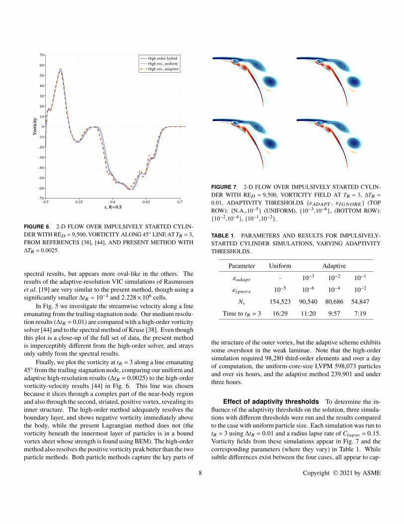
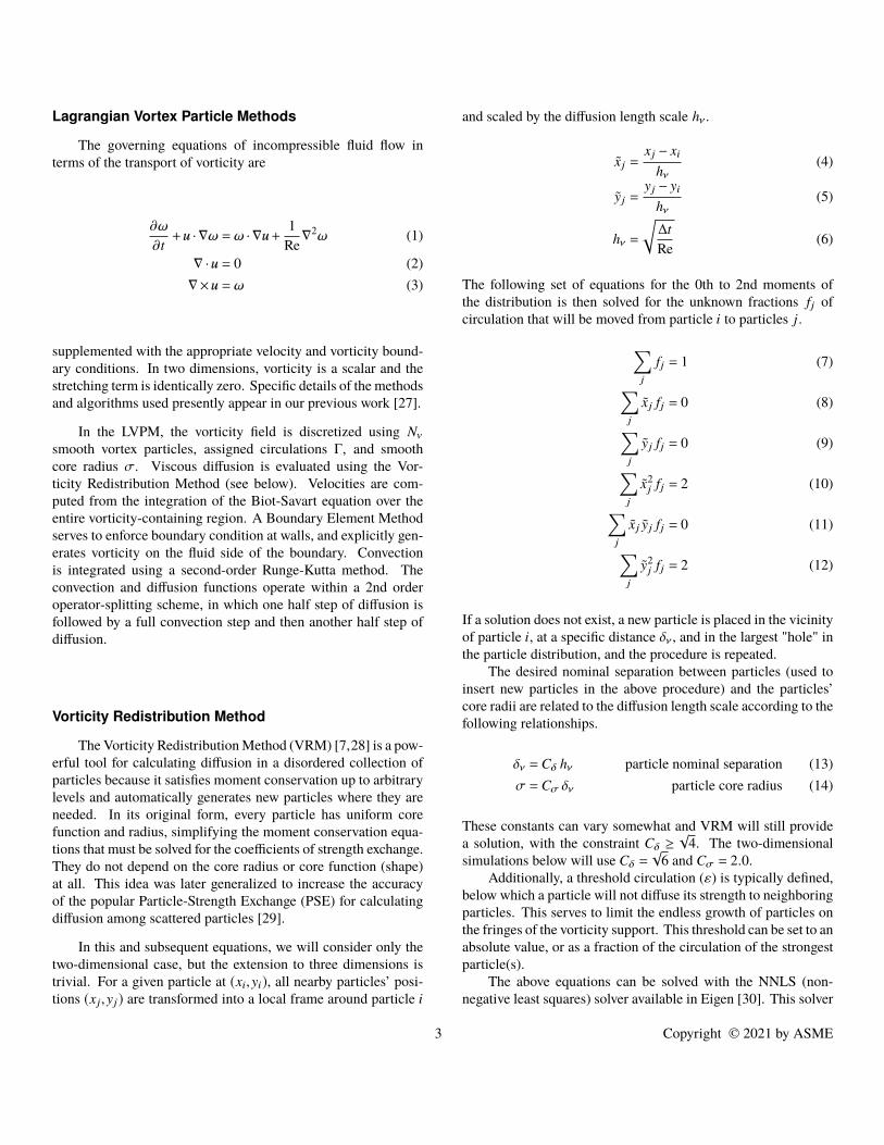
FIGURE 6. 2-D FLOW OVER IMPULSIVELY STARTED CYLIN-DER WITH RED = 9,500, VORTICITY ALONG 45◦ LINE AT TR = 3,FROM REFERENCES [38], [44], AND PRESENT METHOD WITH∆TR = 0.0025.

spectral results, but appears more oval-like in the others. Theresults of the adaptive-resolution VIC simulations of Rasmussenet al. [19] are very similar to the present method, though using asignificantly smaller ∆tR = 10−4 and 2.228×106 cells.

In Fig. 5 we investigate the streamwise velocity along a lineemanating from the trailing stagnation node. Our medium resolu-tion results (∆tR = 0.01) are compared with a high-order vorticitysolver [44] and to the spectral method of Kruse [38]. Even thoughthis plot is a close-up of the full set of data, the present methodis imperceptibly different from the high-order solver, and straysonly subtly from the spectral results.

Finally, we plot the vorticity at tR = 3 along a line emanating45◦ from the trailing stagnation node, comparing our uniform andadaptive high-resolution results (∆tR = 0.0025) to the high-ordervorticity-velocity results [44] in Fig. 6. This line was chosenbecause it slices through a complex part of the near-body regionand also through the second, striated, positive vortex, revealing itsinner structure. The high-order method adequately resolves theboundary layer, and shows negative vorticity immediately abovethe body, while the present Lagrangian method does not (thevorticity beneath the innermost layer of particles is in a boundvortex sheet whose strength is found using BEM). The high-ordermethod also resolves the positive vorticity peak better than the twoparticle methods. Both particle methods capture the key parts of

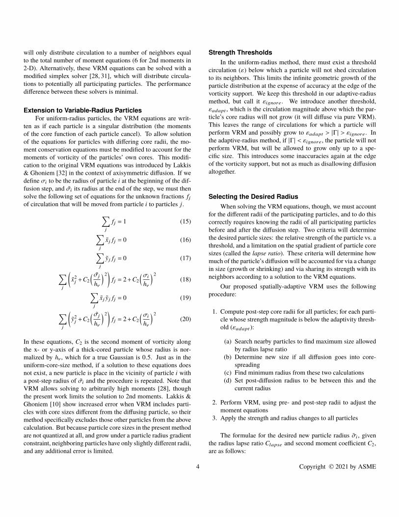
FIGURE 7. 2-D FLOW OVER IMPULSIVELY STARTED CYLIN-DER WITH RED = 9,500, VORTICITY FIELD AT TR = 3, ∆TR =0.01, ADAPTIVITY THRESHOLDS {εADAPT , εIGNORE } (TOPROW): {N.A.,10−5} (UNIFORM), {10−3,10−6}, (BOTTOM ROW):{10−2,10−4}, {10−1,10−2}.

TABLE 1. PARAMETERS AND RESULTS FOR IMPULSIVELY-STARTED CYLINDER SIMULATIONS, VARYING ADAPTIVITYTHRESHOLDS.

Parameter Uniform Adaptive

εadapt - 10−3 10−2 10−1

εignore 10−5 10−6 10−4 10−2

Nv 154,523 90,540 80,686 54,847

Time to tR = 3 16:29 11:20 9:57 7:19

the structure of the outer vortex, but the adaptive scheme exhibitssome overshoot in the weak laminae. Note that the high-ordersimulation required 98,280 third-order elements and over a dayof computation, the uniform-core-size LVPM 598,073 particlesand over six hours, and the adaptive method 239,901 and underthree hours.

Effect of adaptivity thresholds To determine the in-fluence of the adaptivity thresholds on the solution, three simula-tions with different thresholds were run and the results comparedto the case with uniform particle size. Each simulation was run totR = 3 using ∆tR = 0.01 and a radius lapse rate of Clapse = 0.15.Vorticity fields from these simulations appear in Fig. 7 and thecorresponding parameters (where they vary) in Table 1. Whilesubtle differences exist between the four cases, all appear to cap-


FIGURE 8. 2-D FLOW OVER IMPULSIVELY STARTED CYLIN-DER WITH RED = 9,500, VORTICITY FIELD AT TR = 3,∆TR = 0.01,RADIUS LAPSE RATES (TOP ROW): 0 (UNIFORM), 0.1, (BOTTOMROW): 0.2, 0.4.

TABLE 2. PARAMETERS AND RESULTS FOR IMPULSIVELY-STARTED CYLINDER SIMULATIONS, VARYING LAPSE RATES.

Parameter Uniform Adaptive

Clapse 0 0.1 0.2 0.4

Nv 154,523 87,049 77,469 74,637

Time to tR = 3 16:29 10:43 9:43 9:26

ture the oval-shaped primary vortex (blue), the striated secondarycoalescing vortex (blue), and the arrangement and size of thesmall number of wall-bounded vortices. A noticeable differenceis the shape of the primary vortex, with the most aggressive levelof adaptivity (εadapt = 10−1) resulting in a more circular vortexwith noticeable striations. The performance data reveal that, evenat this early stage, the particle count and wall-clock time can becut in half with little effect on the vorticity.

Effect of radius lapse rate Recall that the radius lapserate Clapse is the maximum allowable change in particle radiusper unit distance between particles. Enforcing this puts a limit onthe range of particle radii that participate in any VRM solution.Tests were run with ∆tR = 0.01, relative thresholds εignore =10−4 and εadapt = 10−2, and varying Clapse from 0 (uniform)to 0.4 (very aggressive). Vorticity fields for these simulationsappear in Fig. 8. One subtle but noticeable difference involvesthe position of the thin wisp of positive vorticity (red) just below

FIGURE 9. 2-D FLOW OVER IMPULSIVELY STARTED CYLIN-DER WITH RED = 9,500, VORTICITY FIELD AT TR = 3, VARYINGPARTICLE RESOLUTIONS (TOP ROW): ∆TR = 0.0025 UNIFORMAND ADAPTIVE, (BOTTOM ROW): ∆TR = {0.01,0.04} ADAPTIVE.

TABLE 3. PARAMETERS AND RESULTS FOR IMPULSIVELY-STARTED CYLINDER SIMULATIONS, VARYING PARTICLE RES-OLUTION.

Parameter Low Medium High

∆tR 0.04 0.01 0.0025

∆x 0.003554 0.001777 0.000889

Nv uniform 40,611 154,523 598,073

Nv adaptive 26,502 80,686 239,901

Time to tR = 3, unif. 0:51.3 16:29 6:43:58

Time to tR = 3, adapt. 0:39.4 9:57 2:39:54

the first primary negative vortex (blue), which is smaller andfurther rotated around the primary vortex when Clapse = 0.4,more similar to the Shankar [37] results from Fig. 4, than ofpresent results with higher resolution. In addition, the Clapse =

0.4 case exhibits a smaller wall-bounded positive vortex (red)than the other cases. Numerical results in Table 2 show littledifference between the Clapse = 0.2 and 0.4 cases, though that isunlikely to be the case for longer runs with more diffused wakes.

Effect of particle resolution We finally examine theeffect of particle resolution on the results. Because interparti-cle spacing varies with time step size as ∆x =

√6ν∆tD , smaller

time steps require more particles and longer run time. Parame-


FIGURE 10. 2-D FLOW OVER IMPULSIVELY STARTED CYLIN-DER WITH RED = 9,500, DISTRIBUTION OF PARTICLE CORERADII at TR = 3, ∆TR = 0.0025.

ters common to adaptive runs are εignore = 10−4, εadapt = 10−2,and Clapse = 0.15, while the uniform resolution runs usedεignore = 10−5. Table 3 presents the varying parameters andquantitative results, while vorticity fields at tR = 3 for selectruns appear in Fig. 9. Readily apparent is the unconverged low-resolution result—the primary vortex is misshapen and its orbit-ing red vortex patch is not elongated like the other results. Asparticle resolution increases, though, the adaptive results quicklyapproach the uniform high resolution case. By way of compari-son, Lakkis & Ghoniem [10] achieve similarly good results withtheir adaptive method using 200,000 particles with ∆tR = 0.01.

Figure 10 illustrates clearly that the present method adaptsthe particle core sizes to the solution, as demanded by the adap-tivity thresholds and the radius lapse rate. More and smallerparticles are used to resolve the vortices and boundary layer, andfewer, larger particles the outer reaches of the vorticity.

CONCLUSIONSA fully-local and solution-adaptive spatial adaptivity scheme

for Lagrangian Vortex Particle Methods requiring no a prioriknowledge of regions of interest and no regridding or remeshingof any kind has been devised and tested. It effectively maintainsresolution near boundaries and in areas of high vorticity, whilereducing particle density in areas of lesser importance. Theperformance benefits increase as resolution and simulation lengthincrease and the concept is extensible to three dimensions withlittle extra effort.

ACKNOWLEDGMENTResearch reported in this publication was supported by the

National Institute Of Biomedical Imaging And Bioengineer-ing of the National Institutes of Health under Award NumberR01EB022180. The content is solely the responsibility of theauthors and does not necessarily represent the official views ofthe National Institutes of Health.

REFERENCES[1] Chorin, A. J., 1973. “Numerical study of slightly viscous

flow”. J. Fluid Mech., 57, pp. 785–796.[2] Kuwahara, K., and Takami, H., 1973. “Numerical stud-

ies of two-dimensional vortex motion by a system of pointvortices”. J. Phys. Soc. Japan, 34(1), pp. 247–253.

[3] Greengard, L., 1985. “The core spreading vortex methodapproximates the wrong equation”. J. Comput. Phys., 61,pp. 345–348.

[4] Rossi, L. F., 1996. “Resurrecting core spreading vortexmethods: A new scheme that is both deterministic and con-vergent”. SIAM J. Sci. Comput., 17(3), pp. 370–397.

[5] Mas-Gallic, S., 1987. “Contribution à l’analyse numériquedes méthodes particulaires”. PhD thesis, Université ParisVI.

[6] Degond, P., and Mas-Gallic, S., 1989. “The weighted parti-cle method for convection-diffusion equations, Part 1: Thecase of an isotropic viscosity”. Math. Comput., 53(188),pp. 485–507.

[7] Shankar, S., and van Dommelen, L., 1996. “A New Dif-fusion Procedure for Vortex Methods”. J. Comput. Phys.,127, pp. 88–109.

[8] Spalart, P. R., 1988. “Vortex Methods for Separated Flows”.Tech. Rep. NASA TM-100068.

[9] Dehnen, W., 2001. “Towards optimal softening in three-dimensional N-body codes - I. Minimizing the force error”.Mon. Not. R. Astron. Soc., 324, pp. 273–291.

[10] Lakkis, I., and Ghoniem, A., 2009. “A high resolutionspatially adaptive vortex method for separating flows. PartI: Two-dimensional domains”. J. Comput. Phys., 228(2),pp. 491–515.

[11] Beale, J. T., and Majda, A., 1982. “Vortex methods I: Con-vergence in three dimensions”. Math. Comput., 29(159),pp. 1–27.

[12] Hou, T. Y., Lowengrub, J., and Shelley, M. J., 1991. “Exactdesingularization and local regriding for vortex methods”.Lectures in Applied Mathematics: Vortex Methods and Vor-tex Dynamics, pp. 341–362.

[13] Salihi, M. L. O., 1998. “Couplage de méthodes numériquesen simulation directe d’écoulements incompressibles”. PhDthesis, Université Joseph-Fourier-Grenoble I.

[14] Cottet, G.-H., Koumoutsakos, P., and Salihi, M. L. O., 2000.


“Vortex methods with spatially varying cores”. J. Com-put. Phys., 162(1), pp. 164–185.

[15] Ploumhans, P., Winckelmans, G. S., Salmon, J. K., Leonard,A., and Warren, M. S., 2002. “Vortex methods for di-rect numerical simulation of three-dimensional bluff bodyflows: Application to the sphere at Re=300, 500, and 1000”.J. Comput. Phys., 178, pp. 427–463.

[16] Barba, L., Leonard, A., and Allen, C., 2005. “Advances inviscous vortex methods—meshless spatial adaption basedon radial basis function interpolation”. Intl. J. Numer. Meth-ods Fluids, 47(5), pp. 387–421.

[17] Reboux, S., Schrader, B., and Sbalzarini, I. F., 2012. “Aself-organizing lagrangian particle method for adaptive-resolution advection–diffusion simulations”. J. Com-put. Phys., 231(9), pp. 3623–3646.

[18] Bergdorf, M., Cottet, G.-H., and Koumoutsakos, P.,2005. “Multilevel adaptive particle methods for convection-diffusion equations”. Multiscale Modeling & Simulation,4(1), pp. 328–357.

[19] Rasmussen, J. T., Cottet, G.-H., and Walther, J. H., 2011.“A multiresolution remeshed vortex-in-cell algorithm usingpatches”. J. Comput. Phys., 230(17), pp. 6742–6755.

[20] Teng, Z.-H., 1982. “Elliptic-vortex method for incompress-ible flow at high reynolds number”. J. Comput. Phys., 46(1),pp. 54–68.

[21] Rossi, L. F., 2006. “A comparative study of Lagrangianmethods using axisymmetric and deforming blobs”. SIAMJ. Sci. Comput., 27(4), pp. 1168–1180.

[22] Rossi, L. F., 2006. “Evaluation of the biot–savart integralfor deformable elliptical gaussian vortex elements”. SIAMJ. Sci. Comput., 28(4), pp. 1509–1532.

[23] Häcki, C., Reboux, S., and Sbalzarini, I. F., 2015. “Aself-organizing adaptive-resolution particle method withanisotropic kernels”. Procedia IUTAM, 18, pp. 40–55.

[24] Cottet, G.-H., and Koumoutsakos, P., 1999. Vortex Methods:Theory and Practice. Cambridge Univ. Press, Cambridge,UK.

[25] Gharakhani, A., 2007. “3-D Vortex Simulation Of Acceler-ating Flow Over A Simplified Opening Bileaflet Valve”. InProceedings of FEDSM2007 5th Joint ASME/JSME FluidsEngineering Conference, no. FEDSM2007-37134.

[26] Stock, M. J., and Gharakhani, A., 2011. “Graphics Pro-cessing Unit-Accelerated Boundary Element Method andVortex Particle Method”. J. Aero. Comp. Inf. Com., 8(7),July, pp. 224–236.

[27] Stock, M. J., and Gharakhani, A., 2020. “Open-source ac-celerated vortex particle methods for unsteady flow simula-tion”. In Proceedings of the ASME 2020 Fluids EngineeringDivision Summer Meeting, Vol. FEDSM2020-83730.

[28] Gharakhani, A., 2000. “A higher order vorticity redistri-bution method for 3-D diffusion in free space”. Tech. Rep.Report No. SAND2000-2505, Sandia National Laborato-

ries.[29] Schrader, B., Reboux, S., and Sbalzarini, I. F., 2010.

“Discretization correction of general integral pse opera-tors for particle methods”. J. Comput. Phys., 229(11),pp. 4159–4182.

[30] Guennebaud, G., Jacob, B., et al., 2010. “Eigen v3”.http://eigen.tuxfamily.org.

[31] Abdelmalek, N. N., 1977. “Minimum L∞ Solution of under-determined systems of linear equations”. J. Approx. Theory,20, pp. 57–69.

[32] Lakkis, I., and Ghoniem, A. F., 2003. “Axisymmetric vortexmethod for low-mach number, diffusion-controlled combus-tion”. J. Comput. Phys., 184(2), pp. 435–475.

[33] Stock, M. J., and Gharakhani, A., 2020. “Omega2D:Two-Dimensional Flow Solver with GUI UsingVortex Particle and Boundary Element Methods”.https://github.com/Applied-Scientific-Research/Omega2D.

[34] Barnes, J. E., and Hut, P., 1986. “A Hierarchical O (N log N)Force Calculation Algorithm”. Nature, 324, pp. 446–449.

[35] Greengard, L., and Rokhlin, V., 1987. “A Fast Algorithm forParticle Simulations”. J. Comput. Phys., 73, pp. 325–348.

[36] Koumoutsakos, P., and Leonard, A., 1995. “High-resolutionsimulations of the flow around an impulsively started cylin-der using vortex methods”. J. Fluid Mech., 296, pp. 1–357.

[37] Subramaniam, S., 1996. “A new mesh-free vortex method”.PhD thesis, Florida State University.

[38] Kruse, G. W., 1997. “Parallel nonconforming spectral ele-ment methods”. PhD thesis, Brown University.

[39] Wang, L., 2016. “High-performance discrete-vortex algo-rithms for unsteady viscous-fluid flows near moving bound-aries”. PhD thesis, University of California, Berkeley.

[40] Lee, S.-J., 2017. “Numerical simulation of vortex-Dominated flows using the penalized VIC method”. InVortex Dynamics and Optical Vortices, InTech, pp. 55–83.

[41] Chang, C.-C., and Chern, R.-L., 1991. “Vortex SheddingFrom an Impulsively Started Rotating and Translating Cir-cular Cylinder”. J. Fluid Mech., 233, pp. 265–298.

[42] Rossinelli, D., Hejazialhosseini, B., van Rees, W., Gazzola,M., Bergdorf, M., and Koumoutsakos, P., 2015. “MRAG-I2D: Multi-resolution adapted grids for remeshed vortexmethods on multicore architectures”. J. Comput. Phys.,288, pp. 1–18.

[43] Vatistas, G. H., Kozel, V., and Mih, W., 1991. “A sim-pler model for concentrated vortices”. Exp. Fluids, 11(1),pp. 73–76.

[44] Stock, M., and Gharakhani, A., 2021. “A Hybrid High-Order Vorticity-Based Eulerian and Lagrangian VortexParticle Method, the 2-D Case”. In Proceedings of theASME 2021 Fluids Engineering Division Summer Meet-ing, no. FEDSM2021-65637.


Documents

FEDSM2021-65621 - Mark J. Stock