Fermions and Type IIB Supergravity On SquashedSasaki-Einstein Manifolds

Ibrahima Bah1, Alberto Faraggi1, Juan I. Jottar2 and Robert G. Leigh2

1Michigan Center for Theoretical Physics, Randall Laboratory of Physics,

University of Michigan, Ann Arbor, MI 48109, U.S.A.

2Department of Physics, University of Illinois,

1110 W. Green Street, Urbana, IL 61801, U.S.A.

ibbah@umich.edu, faraggi@umich.edu, jjottar2@illinois.edu,

rgleigh@illinois.edu

Abstract

We discuss the dimensional reduction of fermionic modes in a recently found class of con-

sistent truncations of type IIB supergravity compactified on squashed five-dimensional

Sasaki-Einstein manifolds. We derive the lower dimensional equations of motion and

effective action, and comment on the supersymmetry of the resulting theory, which is

consistent with N = 4 gauged supergravity in d = 5, coupled to two vector multiplets.

We compute fermion masses by linearizing around two AdS5 vacua of the theory: one

that breaks N = 4 down to N = 2 spontaneously, and a second one which preserves

no supersymmetries. The truncations under consideration are noteworthy in that they

retain massive modes which are charged under a U(1) subgroup of the R-symmetry, a

feature that makes them interesting for applications to condensed matter phenomena

via gauge/gravity duality. In this light, as an application of our general results we

exhibit the coupling of the fermions to the type IIB holographic superconductor, and

find a consistent further truncation of the fermion sector that retains a single spin-1/2

mode.

arX

iv:1

009.

1615

v2 [

hep-

th]

20

Dec

201

0

Contents

1 Introduction 1

2 Type IIB supergravity on squashed Sasaki-Einstein five-manifolds 4

2.1 Bosonic ansatz . . . . . . . . . . . . . . . . . . . . . . . . . . . . . . . . . . 4

2.2 Fermionic ansatz . . . . . . . . . . . . . . . . . . . . . . . . . . . . . . . . . 7

3 Five-dimensional equations of motion and effective action 9

3.1 Field redefinitions . . . . . . . . . . . . . . . . . . . . . . . . . . . . . . . . 10

3.2 Effective action . . . . . . . . . . . . . . . . . . . . . . . . . . . . . . . . . . 11

4 N = 4 supersymmetry 14

5 Linearized analysis 15

5.1 The supersymmetric vacuum solution . . . . . . . . . . . . . . . . . . . . . 15

5.2 The Romans AdS5 vacuum . . . . . . . . . . . . . . . . . . . . . . . . . . . 16

6 Examples 17

6.1 Minimal N = 2 gauged supergravity in five dimensions . . . . . . . . . . . . 17

6.2 No p = 3 sector . . . . . . . . . . . . . . . . . . . . . . . . . . . . . . . . . . 18

6.3 Type IIB holographic superconductor . . . . . . . . . . . . . . . . . . . . . 19

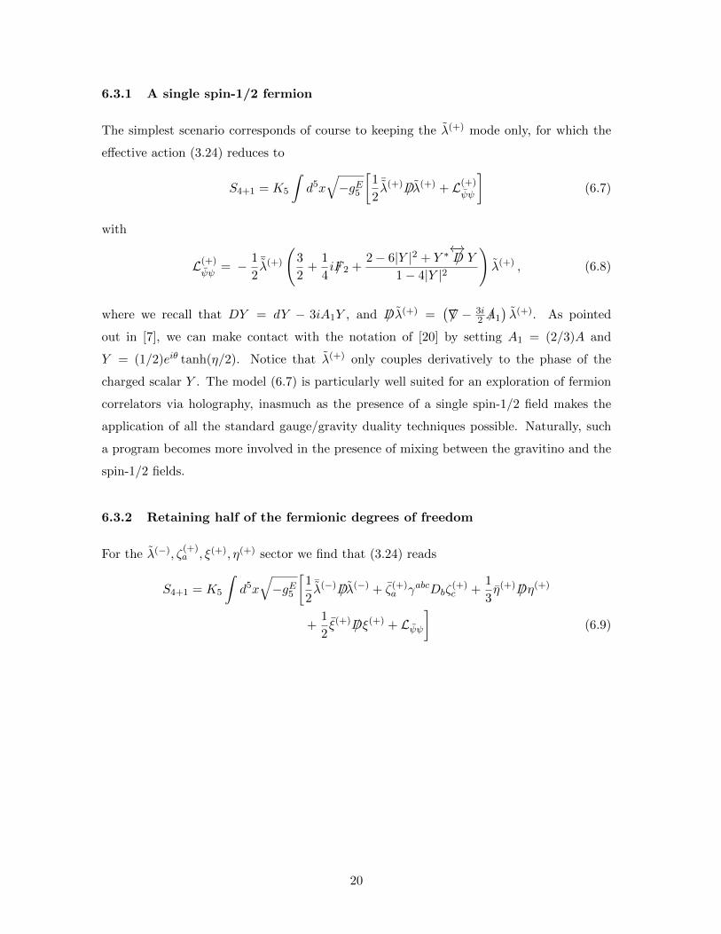
6.3.1 A single spin-1/2 fermion . . . . . . . . . . . . . . . . . . . . . . . . 20

6.3.2 Retaining half of the fermionic degrees of freedom . . . . . . . . . . 20

6.3.3 The ζ(−)a , η(−), ξ(−) sector . . . . . . . . . . . . . . . . . . . . . . . . 21

7 Conclusions 22

A Conventions and useful formulae 23

A.1 Conventions for forms and Hodge duality . . . . . . . . . . . . . . . . . . . 23

A.2 Zehnbein and spin connection . . . . . . . . . . . . . . . . . . . . . . . . . . 24

2

A.3 Fluxes . . . . . . . . . . . . . . . . . . . . . . . . . . . . . . . . . . . . . . . 25

A.4 Clifford algebra . . . . . . . . . . . . . . . . . . . . . . . . . . . . . . . . . . 26

A.5 Charge conjugation conventions . . . . . . . . . . . . . . . . . . . . . . . . . 27

B Type IIB supergravity 28

B.1 Bosonic content and equations of motion . . . . . . . . . . . . . . . . . . . . 28

B.2 Fermionic content and equations of motion . . . . . . . . . . . . . . . . . . 30

C d = 5 Equations of motion 31

C.1 Reduction of the dilatino equation of motion . . . . . . . . . . . . . . . . . 31

C.1.1 Derivative operator . . . . . . . . . . . . . . . . . . . . . . . . . . . . 31

C.1.2 Couplings . . . . . . . . . . . . . . . . . . . . . . . . . . . . . . . . . 31

C.2 Reduction of the gravitino equation of motion . . . . . . . . . . . . . . . . . 32

C.2.1 Derivative operator . . . . . . . . . . . . . . . . . . . . . . . . . . . . 32

C.2.2 Couplings . . . . . . . . . . . . . . . . . . . . . . . . . . . . . . . . . 34

C.3 Equations of motion in terms of diagonal fields . . . . . . . . . . . . . . . . 36

1 Introduction

Recently, consistent truncations of type IIB and 11-d supergravity including massive (charged)

modes have sparked a great deal of interest. The relevance of these reductions is two-fold:

not only are they novel from the supergravity perspective, but they also constitute an inter-

esting arena to test and extend the ideas of gauge/gravity duality. Indeed, these truncations

provide a powerful way of generating solutions of the ten and eleven-dimensional super-

gravity theories via uplifting of lower dimensional solutions. By definition, this possibility

is guaranteed by the consistency of the reduction. Also from a supergravity perspective,

the inclusion of massive modes is highly non-trivial; consistent truncations are hard to find,

even when truncating to the massless Kaluza-Klein (KK) spectrum. In fact, until not long

ago it was widely believed that consistency prevents one from keeping a finite number of

massive KK modes. From the gauge/gravity correspondence perspective, in turn, the lower

dimensional supergravity theories obtained from these reductions are assumed to possess

1

field theory duals with various amounts of unbroken super(-conformal)symmetry. Strik-

ingly, the inclusion of charged operators on the field theory side, dual to massive bulk fields,

opened the door for a stringy (“top-down”) modelling of condensed matter phenomena,

such as superfluidity and superconductivity and systems with non-relativistic conformal

symmetries, via the holographic correspondence. Even though the original work in these

directions [1, 2, 3, 4, 5] was based on a phenomenological, “bottom-up” approach, it is

clearly advantageous to consider top-down descriptions of these (or similar) systems. In-

deed, a description in terms of ten or eleven-dimensional supergravity backgrounds may

shed light on the existence of a consistent UV completion of the lower-dimensional effective

bulk theories, while possibly fixing various parameters that appear to be arbitrary in the

bottom-up constructions.

In this paper we shall be concerned with the consistent truncations of type IIB su-

pergravity on squashed Sasaki-Einstein five-manifolds (SE5) whose bosonic content was

recently considered in [6, 7, 8] (see [9] for related work). These constructions were largely

motivated by the results of [10] ( see [11, 12] also), which had a quite interesting by-product:

while searching for solutions of type IIB supergravity with non-relativistic asymptotic sym-

metry groups, consistent five-dimensional truncations including massive bosonic modes were

constructed. In particular, massive scalars arise from the breathing and squashing modes

in the internal manifold, which is then a “deformed” Sasaki-Einstein space, generalizing the

case of breathing and squashing modes on spheres that had been studied in [13, 14] (see

also [15]). Regarding the internal SE5 manifold as a U(1) bundle over a Kahler-Einstein

(KE) base space of complex dimension two, the guiding principle behind these consistent

truncations is to keep modes which are singlets only under the structure group of the KE

base. The bosonic sector of the corresponding truncations including massive modes in 11-d

supergravity on squashed SE7 manifolds had been previously discussed in [16], and pro-

vided the basis for the embedding of the original holographic AdS4 superconductors of [2, 3]

into M-theory, a connection that was explored in [17, 18]. In our recent work [19] we have

extended the consistent truncation of 11-d supergravity on squashed SE7 to include the

fermionic sector, and in particular provided the effective 4-d action describing the coupling

of fermion modes to the M-theory holographic superconductor.

At the same time that the work of [17] appeared, the embedding of an asymptotically

AdS5 holographic superconductor into type IIB supergravity was reported in [20]. Contin-

uing with the program we initiated in [19], in the present work we discuss the extension of

the consistent truncation of type IIB supergravity on SE5 discussed in [6, 7, 8] to include

2

the fermionic sector. In particular, as an application of our results we present the effective

action describing the coupling of the fermion modes to the holographic superconductor of

[20]. Knowing the precise form of said couplings is important from the point of view of the

applications of gauge/gravity duality to the description of strongly coupled condensed mat-

ter phenomena, insofar as it determines the nature of fermionic correlators in the presence

of superconducting condensates, that rely on how the fermionic operators of the dual theory

couple to scalars. Hence, we set the stage for the discussion of these and related questions

from a top-down perspective. A related problem involving a superfluid p-wave transition

was studied in [21], in the context of (3+1)-dimensional supersymmetric field theories dual

to probe D5-branes in AdS5 × S5. In the top-down approach starting from either ten or

eleven-dimensional supergravity, inevitably the consistent truncations will include not only

spin-1/2 fermions that might be of phenomenological interest but also spin-3/2 fields. One

finds that these generally mix together via generalized Yukawa couplings, and this mixing

will have implications for correlation functions in the dual field theory. One of our original

motivations for the present work as well as [19] was to understand this mixing in more de-

tail and to investigate the existence of “further truncations” which might involve (charged)

spin-1/2 fermions alone. As we explain in section 6, in the present case we have indeed

found such a model, containing a single spin-1/2 field, in the truncation corresponding to

the type IIB holographic superconductor.

This paper is organized as follows. In section 2 we briefly review some aspects of

the truncations of type IIB supergravity constructed in [6, 7, 8] and the extension of the

bosonic ansatz to include the fermion modes. In section 3 we present our main result:

the effective five-dimensional action functional describing the dynamics of the fermions and

their couplings to the bosonic fields. We chose to perform this calculation by directly

reducing the 10-d equations of motion for the gravitino and dilatino. The resulting action

is consistent with 5-d N = 4 gauged supergravity, as has been anticipated. In section 4

we reduce the supersymmetry variation of the gravitino and dilatino, and comment on the

supersymmetric structure of the five-dimensional theory by considering how the fermions

fit into the supermultiplets of N = 4 gauged supergravity. In principle, a complete mapping

to the highly constrained form of N = 4 actions could be made, although we do not give

all of the details here. The N = 4 theory has two vacuum AdS5 solutions, one with N = 2

supersymmetry and one without supersymmetry. In section 5 we linearize the fermionic

sector in each of these vacua and demonstrate that as expected the gravitini attain masses

via the Stuckelberg mechanism, which is a useful check on the consistency of our results.

3

In section 6 we apply our results to several further truncations of interest: the minimal

gauged N = 2 supergravity theory in five dimensions, and the dual [20] of the (3 + 1)-

dimensional holographic superconductor. We conclude in section 7. The details of many

of our computations as well as a full accounting of our conventions appear in a series of

appendices.

2 Type IIB supergravity on squashed Sasaki-Einstein five-

manifolds

2.1 Bosonic ansatz

In this section we briefly review the ansatz for the bosonic fields in the consistent truncations

of [6, 7, 8]. In the following subsection, we will discuss the extension of this ansatz to

include the fermionic fields of type IIB supergravity. Here we mostly follow the type IIB

conventions of [7, 22, 23], with slight modifications as we find appropriate. Further details

of these conventions can be found in appendix A.

The Kaluza-Klein metric ansatz in the truncations of interest is given by [6, 7, 8]

ds210 = e2W (x)ds2

E(M) + e2U(x)ds2(KE) + e2V (x)(η +A1(x)

)2, (2.1)

where W (x) = −13(4U(x)+V (x)). Here, M is an arbitrary “external” five-dimensional ma-

nifold, with coordinates denoted generically by x and five-dimensional Einstein-frame metric

ds2E(M), and KE is an “internal” four-dimensional Kahler-Einstein manifold (henceforth

referred to as “KE base”) coordinatized by y and possessing Kahler form J . The one-form

A1 is defined in T ∗M and η ≡ dχ + A(y), where A is an element of T ∗KE satisfying

dA ≡ F = 2J . For a fixed point in the external manifold, the compact coordinate χ

parameterizes the fiber of a U(1) bundle over KE, and the five-dimensional internal mani-

fold spanned by (y, χ) is then a squashed Sasaki-Einstein manifold, with the breathing and

squashing modes parameterized by the scalars U(x) and V (x).1 In addition to the metric,

the bosonic content of type IIB supergravity [24, 25] includes the dilaton Φ, the NSNS

3-form field strength H(3), and the RR field strengths F(1) ≡ dC0, F(3) and F(5), where

C0 is the axion and F(5) is self-dual. The rationale behind the corresponding ansatze is

1In particular, U − V is the squashing mode, describing the squashing of the U(1) fiber with respect to

the KE base, while the breathing mode 4U + V modifies the overall volume of the internal manifold. When

U = V = 0, the internal manifold becomes a five-dimensional Sasaki-Einstein manifold SE5.

4

the idea that the consistency of the dimensional reduction is a result of truncating the KK

tower to include fields that transform as singlets only under the structure group of the KE

base, which in this case corresponds to SU(2). This prescription allows for an interesting

spectrum in the lower dimensional theory, inasmuch as the SU(2) singlets include fields that

are charged under the U(1) isometry generated by ∂χ. The globally defined Kahler 2-form

J = dA/2 and the holomorphic (2, 0)-form Σ(2,0) define the Kahler and complex structures,

respectively, on the KE base. They are SU(2)-invariant and can be used in the reduction

of the various fields to five dimensions. The U(1)-bundle over KE is such that they satisfy

Σ(2,0) ∧ Σ∗(2,0) = 2J2 , and dΣ(2,0) = 3iA ∧ Σ(2,0) . (2.2)

More precisely, as will be clear from the discussion to follow below, the relevant charged

form Ω on the total space of the bundle that should enter the ansatz for the various form

fields is given by

Ω ≡ e3iχΣ(2,0) , (2.3)

and satisfies

dΩ = 3iη ∧ Ω . (2.4)

The ansatze for the bosonic fields is then [7]

F(5) = 4e8W+ZvolE5 + e4(W+U) ∗K2 ∧ J +K1 ∧ J ∧ J

+[2eZJ ∧ J − 2e−8U ∗K1 +K2 ∧ J

]∧ (η +A1)

+[e4(W+U) ∗ L2 ∧ Ω + L2 ∧ Ω ∧ (η +A1) + c.c.

](2.5)

F(3) = G3 +G2 ∧ (η +A1) +G1 ∧ J +G0 J ∧ (η +A1)

+[N1 ∧ Ω +N0 Ω ∧ (η +A1) + c.c.

](2.6)

H(3) = H3 +H2 ∧ (η +A1) +H1 ∧ J +H0 J ∧ (η +A1)

+[M1 ∧ Ω +M0 Ω ∧ (η +A1) + c.c.

](2.7)

C(0) = a (2.8)

Φ = φ (2.9)

where volE5 and ∗ are the volume form and Hodge dual appropriate to the five-dimensional

Einstein-frame metric ds2E(M), and W (x) = −1

3(4U(x)+V (x)) as before. Several comments

are in order. First, all the fields other than (η, J,Ω) are defined on Λ∗T ∗M . Z, a, φ, G0,

5

H0 are real scalars, and M0, N0 are complex scalars. The form fields G1, G2, G3, H1, H2,

H3, K1 and K2 are real, while M1, N1 and L2 are complex forms. As pointed out in [7],

the scalars G0 and H0 vanish by virtue of the type IIB Bianchi identities. We also notice

that the self-duality of F(5) is automatic in the ansatz (2.5): the first two lines are duals of

each other, while the last line is self-dual.

Inserting the ansatz into the type IIB equations of motion and Bianchi identities (Ap-

pendix B), one finds that the various fields are related as2

H3 = dB2 +1

2(db− 2B1) ∧ F2

G3 = dC2 − adB2 +1

2(dc− adb− 2C1 + 2aB1) ∧ F2

H2 = dB1

F2 = dA1

G2 = dC1 − adB1

K2 = dE1 +1

2(db− 2B1) ∧ (dc− 2C1)

G1 = dc− adb− 2C1 + 2aB1

H1 = db− 2B1

K1 = dh− 2E1 − 2A1 + Y ∗DX + Y DX∗ −XDY ∗ −X∗DY

M1 = DY

N1 = DX − aDY

M0 = 3iY

N0 = 3i(X − aY )

eZ = 1 + 3i(Y ∗X − Y X∗), (2.10)

where F2 ≡ dA1, X,Y and L2,M1, N1 are complex, and DY = dY − 3iA1Y , DX =

dX − 3iA1X.

As was explained in detail in [6, 7], the physical scalars parameterize the coset SO(1, 1)×(SO(5, 2)/(SO(5)× SO(2))

), while the structure of the 1-forms and 2-forms is such that a

Heis3 × U(1) subgroup is gauged.

2We have chosen the notation of Ref. [7] apart from replacing their χ, ξ with X,Y , to avoid confusion

with the fiber coordinate.

6

2.2 Fermionic ansatz

The fermionic content of type IIB supergravity comprises a positive chirality dilatino and a

negative chirality gravitino. Instead of expressing the theory in terms of pairs of Majorana-

Weyl fermions, we find it notationally simplest to use complex Weyl spinors. Quite generally,

we would like to decompose the gravitino using an ansatz of the form

Ψa(x, y, χ) =∑I

ψIa(x)⊗ ηI(y, χ) (2.11)

Ψα(x, y, χ) =∑I

λI(x)⊗ ηIα(y, χ) (2.12)

Ψf(x, y, χ) =∑I

ϕI(x)⊗ ηIf (y, χ) , (2.13)

where a, α and f denote the indices in the direction of the external manifold, the KE

base, and the fiber, respectively. The projection to singlets under the structure group of

the KE base was recently described in great detail for the case of D = 11 supergravity

compactified on squashed SE7 manifolds [19]. Since the principles at work in the present

case are essentially the same, here we limit ourselves to pointing to a few relevant facts

and results. As we have discussed, the five-dimensional internal space is the total space of

a U(1) bundle over a KE base. In general, the base is not spin, and therefore spinors do

not necessarily exist globally on the base. However, it is always possible to define a Spinc

bundle globally on KE (see [26], for example), and our (c-)spinors will then be sections

of this bundle. Indeed, we have seen above that the holomorphic form Ω is also charged

under this U(1). The U(1) generator is proportional to ∂χ, and hence ∇α − Aα∂χ is the

gauge connection on the Spinc bundle, where ∇α is the covariant derivative on KE. Of

central importance to us in the reduction to invariants of the structure group are the gauge-

covariantly-constant spinors, which can be defined on any Kahler manifold [27] and satisfy

in the present context

(∇α −Aα∂χ)ε(y, χ) = 0 , (2.14)

where

ε(y, χ) = ε(y)eieχ (2.15)

for fixed “charge” e. For a KE base of real dimension db, these satisfy (see [19],[28] for

example)3

Qε ≡ −iJαβΓαβε =4edbdb + 2

ε . (2.16)

3All of our Clifford algebra and spinor conventions are compiled in Appendix A.

7

In other words, the matrix Q = −iJαβΓαβ on the left is (up to normalization) the U(1)

charge operator. It has maximum eigenvalues ±db, and the corresponding spinors have

charge

e = ±db + 2

4. (2.17)

These two spinors are charge conjugates of one another, and we will henceforth denote them

by ε±. By definition, they satisfy F/ ε± = iQε± = ±idb ε±, where F/ ≡ (1/2)FαβΓαβ. These

spinors with maximal Q-charge are in fact the singlets under the structure group, and they

constitute the basic building blocks of the reduction ansatz for the fermions. In the case at

hand db = 4 and the structure group is SU(2); in fact we have an unbroken SU(2)L×U(1)

subgroup of Spin(4) in which the spinor transforms as 20 ⊕ 1+ ⊕ 1−. In the complex basis

introduced in A.3, we find

Qαε± = ±1

2ε± (α = 1, 2) (2.18)

and

Pαε+ = 0, Pαε− = 0 , (2.19)

where Qα = Γαα, Pα = ΓαΓα, and Pα = ΓαΓα. In the Fock state basis, these are ε± ↔| ± 1

2 ,±12〉 and the remaining two states form a (charge-zero) doublet. Unlike the two

SU(3) singlet spinors that were used to reduce the gravitino in the 11-d case, here the two

singlets have the same chirality in 4 + 0 dimensions, that is γfε± = ε± (this follows, since

γf = −γ1234 =∏α 2Qα). Similarly, for the complex form Σ(2,0) we find [Q, /Σ] = 8/Σ, which

means that Σ(2,0) carries charge eΣ = 3 and justifies the definition Ω = e3iχΣ(2,0) discussed

above.

We are now in position to write the reduction ansatz for the gravitino and dilatino.

Dropping all the SU(2) representations other than the singlets, we take

Ψa(x, y, χ) = ψ(+)a (x)⊗ ε+(y)e

32iχ ⊗ u− + ψ(−)

a (x)⊗ ε−(y)e−32iχ ⊗ u− (2.20)

Ψα(x, y, χ) = ρ(+)(x)⊗ γαε+(y)e32iχ ⊗ u− (2.21)

Ψα(x, y, χ) = ρ(−)(x)⊗ γαε−(y)e−32iχ ⊗ u− (2.22)

Ψf(x, y, χ) = ϕ(+)(x)⊗ ε+(y)e32iχ ⊗ u− + ϕ(−)(x)⊗ ε−(y)e−

32iχ ⊗ u− (2.23)

λ(x, y, χ) = λ(+)(x)⊗ ε+(y)e32iχ ⊗ u+ + λ(−)(x)⊗ ε−(y)e−

32iχ ⊗ u+ (2.24)

where ϕ(±), ρ(±) and ψ(±)a are (4 + 1)-dimensional spinors on M , the superscript c denotes

charge conjugation, and we have used the complex basis introduced in A.3 for the KE base

directions (α, α = 1, 2). The constant spinors u+ =(

10

)and u− =

(01

)have been introduced

8

as bookkeeping devices to keep track of the D = 10 chiralities. Since our starting spinors

were only Weyl in D = 10 (as opposed to Majorana-Weyl) there is no relation between,

say, λ(+) and λ(−); they are independent Dirac spinors in 4 + 1 dimensions, and the same

applies to the rest of the spinors in the ansatz. Although one could write the (4+1)-spinors

as symplectic Majorana, there is no real benefit to introducing such notation at this point

in the discussion. Notice that all of these modes are annihilated by the gauge-covariant

derivative on KE. Equations (2.20)-(2.24) provide the starting point for the dimensional

reduction of the D = 10 equations of motion of type IIB supergravity down to d = 5.

According to the charge conjugation conventions in A.5, we also find

Ψca(x, y, χ) = ψ(−)c

a (x)⊗ ε+(y)e32iχ ⊗ u− − ψ(+)c

a (x)⊗ ε−(y)e−32iχ ⊗ u− (2.25)

(Ψα)c(x, y, χ) = −ρ(+)c(x)⊗ γαε−(y)e−32iχ ⊗ u− (2.26)

(Ψα)c(x, y, χ) = ρ(−)c(x)⊗ γαε+(y)e32iχ ⊗ u− (2.27)

Ψcf (x, y, χ) = ϕ(−)c(x)⊗ ε+(y)e

32iχ ⊗ u− − ϕ(+)c(x)⊗ ε−(y)e−

32iχ ⊗ u− (2.28)

λc(x, y, χ) = −λ(−)c(x)⊗ ε+(y)e32iχ ⊗ u+ + λ(+)c(x)⊗ ε−(y)e−

32iχ ⊗ u+ (2.29)

3 Five-dimensional equations of motion and effective action

The type IIB fermionic equations of motion to linear order in the fermions are given by (see

appendix B for details)

D/ λ =i

8F/ (5)λ+O(Ψ2) (3.1)

ΓABCDBΨC = −1

8G/ ∗ΓAλ+

1

2P/ ΓAλc +O(Ψ3) (3.2)

Here, D denotes the flux-dependent supercovariant derivative, which acts as follows:

D/ λ =

(/∇− 3i

2/Q

)λ− 1

4ΓAG/ΨA − ΓAP/Ψc

A , (3.3)

DBΨC =

(∇B −

i

2QB

)ΨC +

i

16F/ (5)ΓBΨC −

1

16SBΨc

C , (3.4)

where ∇B denotes the ordinary 10-d covariant derivative and we have defined

SB ≡1

6

(ΓB

DEFGDEF − 9ΓDEGBDE). (3.5)

As described in Appendix B.1, defining the axion-dilaton τ = C(0) + ie−Φ = a + ie−φ our

conventions imply

G = ieΦ/2(τdB − dC(2)

)= −

(e−φ/2H(3) + ieφ/2F(3)

), (3.6)

9

and

P =i

2eΦdτ =

dφ

2+i

2eφda , Q = −1

2eΦdC(0) = −1

2eφda . (3.7)

It will prove convenient to introduce a compact notation as follows:

G1 = e12

(φ−4U)(G1 − ie−φH1

)G1 = e

12

(φ−4U)(G1 + ie−φH1

)(3.8)

G2 = e12

(φ+4U)Σ(G2 − ie−φH2

)G2 = e

12

(φ+4U)Σ(G2 + ie−φH2

)(3.9)

G3 = e12

(φ+4U)Σ−1(G3 − ie−φH3

)G3 = e

12

(φ+4U)Σ−1(G3 + ie−φH3

)(3.10)

N (+)1 = e

12

(φ−4U)(N1 − ie−φM1

)N (+)

1 = e12

(φ−4U)(N1 + ie−φM1

)(3.11)

N (−)1 = e

12

(φ−4U)(N∗1 − ie−φM∗1

)N (−)

1 = e12

(φ−4U)(N∗1 + ie−φM∗1

)(3.12)

N (+)0 = e

12

(φ−4U)Σ2(N0 − ie−φM0

)N (+)

0 = e12

(φ−4U)Σ2(N0 + ie−φM0

)(3.13)

N (−)0 = e

12

(φ−4U)Σ2(N∗0 − ie−φM∗0

)N (−)

0 = e12

(φ−4U)Σ2(N∗0 + ie−φM∗0

)(3.14)

where the scalar Σ is defined as Σ ≡ e2(W+U) = e−23

(U+V ). Its significance will be reviewed

later in the paper.

The detailed derivation of the equations of motion is performed in Appendix C, and we

will not reproduce them here in the main body of the paper as the expressions are lengthy.

Given those equations of motion, we will write an action from which they may be derived.

Before doing so, we first consider the kinetic terms and introduce a field redefinition such

that the kinetic terms are diagonalized.

3.1 Field redefinitions

In order to find the appropriate field redefinitions it is enough to consider the derivative

terms, which follow from a Lagrangian density of the form (with respect to the 5-d Einstein

frame-measure d5x√−gE5 )

L(±)kin = eW

[1

2λ(±)D/λ(±) + ψ(±)

a

(γabcDbψ

(±)c − 4iγabDbρ

(±) − iγabDbϕ(±))

− iρ(±)(

4γabDaψ(±)b − 12iD/ ρ(+) − 4iD/ϕ(±)

)+ ϕ(±)

(−iγabDaψ

(±)b − 4D/ρ(±)

)]. (3.15)

Shifting the gravitino as4

ψ(±)a = ψ(±)

a +i

3γa

(ϕ(±) + 4ρ(±)

)⇒ ψ(±)

a =¯ψ(±)a +

i

3

(ϕ(±) + 4ρ(±)

)γa , (3.16)

4To avoid confusion, we note that the notation ϕ(±) means (ϕ(±))†γ0, etc.

10

we obtain

L(±)kin = eW

[1

2λ(±)D/λ(±) +

¯ψ(±)a γabcDbψ

(±)c + 8ρ(±)D/ρ(±)

+4

3

(ρ(±) + ϕ(±)

)D/(ρ(±) + ϕ(±)

)]. (3.17)

Then we are led to define5

λ(±) = eW/2λ(±) (3.18)

ζ(±)a = eW/2

[ψ(±)a − i

3γa

(ϕ(±) + 4ρ(±)

)](3.19)

ξ(±) = 4eW/2ρ(±) (3.20)

η(±) = 2eW/2(ρ(±) + ϕ(±)

), (3.21)

which results in

L(±)kin =

1

2¯λ(±)D/λ(±) + ζ(±)

a γabcDbζ(±)c +

1

2ξ(±)D/ ξ(±) +

1

3η(±)D/η(±) (3.22)

− 1

2

[ζ(±)a γabc (∂bW ) ζ(±)

c +1

2ξ(±) (∂/W ) ξ(±) +

1

3η(±) (∂/W ) η(±)

]. (3.23)

The W -dependent interaction terms in the second line are produced by the action of the

derivatives on the warping factors involved in the field redefinitions, and they will cancel

against similar terms in the interaction Lagrangian. We note that the fields we have defined

are not canonically normalized. We have done this simply to avoid square-root factors.

The equations of motion written in terms of the fields (3.18)-(3.21) are given explicitly

in Appendix C. They follow from an effective d = 5 action that we derive below.

3.2 Effective action

The equations of motion for the 5d fields (3.18)-(3.21), which are explicitly displayed in

appendix C, follow from an effective action functional of the form

S4+1 = K5

∫d5x√−gE5

[1

2¯λ(+)D/λ(+) + ζ(+)

a γabcDbζ(+)c +

1

2ξ(+)D/ ξ(+) +

1

3η(+)D/η(+)

+1

2¯λ(−)D/λ(−) + ζ(−)

a γabcDbζ(−)c +

1

2ξ(−)D/ ξ(−) +

1

3η(−)D/η(−)

+ L(+)

ψψ+ L(−)

ψψ+

1

2

(L(+)

ψψc + L(−)

ψψc + c.c.)]

(3.24)

5One should not confuse the one-form η dual to the Reeb vector field with the fermions η(±).

11

where K5 is a normalization constant depending on the volume of the KE base, the length

of the fiber parameterized by χ, and the normalization of the spinors ε±. Here, Daψ(±) =(

∇a ∓ 3i2 A1a

)ψ(±) for ψ = λ, ψa, η, ξ, and the interaction Lagrangians are given by

L(±)

ψψ= L(±)

mass + L(±)1 + L(±)

2 (3.25)

where we have defined

L(±)mass = ∓ 1

2

(e−4UΣ−1 +

3

2Σ2 ± eZ+4W

)¯λ(±)λ(±) ∓

(e−4UΣ−1 +

3

2Σ2 ∓ eZ+4W

)ζ(±)a γacζ(±)

c

∓ 1

9

(e−4UΣ−1 − 15

2Σ2 ± 5eZ+4W

)η(±)η(±) ± 3

2

(e−4UΣ−1 − 1

2Σ2 ∓ eZ+4W

)ξ(±)ξ(±)

± 1

3i(e−4UΣ−1 − 3Σ2 ± 2eZ+4W

) (ζ(±)a γaη(±) + η(±)γaζ(±)

a

)∓ 2

3

(e−4UΣ−1 ± 2eZ+4W

) (η(±)ξ(±) + ξ(±)η(±)

)∓ i(e−4UΣ−1 ∓ eZ+4W

) (ζ(±)a γaξ(±) + ξ(±)γaζ(±)

a

)±N (±)

0

[1

2¯λ(±)γaζ(∓)

a +2

3i¯λ(±)η(∓) +

1

2i¯λ(±)ξ(∓)

]± N (±)

0

[1

2ζ(±)a γaλ(∓) +

2

3iη(±)λ(∓) +

1

2iξ(±)λ(∓)

](3.26)

L(±)1 = +

1

8i¯λ(±)

[3eφ(∂/a) + 2e−4U /K1

]λ(±) +

1

4ie−4U ζ(±)

a

(eφγabc(∂ba) + 2γ[c /K1γ

a])ζ(±)c

+1

8iξ(±)

[eφ(∂/a) + 6e−4U /K1

]ξ(±) +

1

12iη(±)

[eφ(∂/a)− 2e−4U /K1

]η(±)

+ ζ(±)a

(i(∂/U)− 1

2e−4U /K1

)γaξ(±) + ξ(±)γa

(−i(∂/U)− 1

2e−4U /K1

)ζ(±)a

− 1

2iζ(±)a (Σ−1∂/Σ)γaη(±) +

1

2iη(±)γa(Σ−1∂/Σ)ζ(±)

a

± 1

2i¯λ(±)γa /N (±)

1 ζ(∓)a ± 1

2iζ(±)a /N

(±)

1 γaλ(∓) ± 1

2¯λ(±) /N (±)

1 ξ(∓) ± 1

2ξ(±) /N

(±)

1 λ(∓)

± 1

4i(

¯λ(±)/G1ξ

(±) + ξ(±) /G1λ(±))∓ 1

4

(¯λ(±)γa/G1ζ

(±)a + ζ(±)

a /G1γaλ(±)

)(3.27)

12

and

L(±)2 = +

1

8¯λ(±)γa (i/G3 + /G2) ζ(±)

a +1

8ζ(±)a

(i/G3 + /G2

)γaλ(±)

+1

12i¯λ(±) (i/G3 + /G2) η(±) +

1

12iη(±)

(i/G3 + /G2

)λ(±)

+1

8i¯λ(±)

(i/G3 − /G2

)ξ(±) +

1

8iξ(±)

(i/G3 − /G2

)λ(±)

− 1

4iζ(±)a

(Σ−2γ[cF/2γ

a] ∓ 2Σγ[c /K2γa])ζ(±)c ± Σζ(±)

a γ[c/L(±)2 γa]ζ(∓)

c

+1

6ζ(±)a

(Σ−2F/2 ± Σ /K2

)γaη(±) ∓ 1

3iΣζ(±)

a /L(±)2 γaη(∓)

+1

6η(±)γc

(Σ−2F/2 ± Σ /K2

)ζ(±)c ∓ 1

3iΣη(±)γc/L

(±)2 ζ(∓)

c

+1

8i¯λ(±)

(Σ−2F/2 ± 2Σ /K2

)λ(±) ± 1

2Σ

¯λ(±)/L

(±)2 λ(∓)

+1

8iξ(±)

(Σ−2F/2 ∓ 2Σ /K2

)ξ(±) ∓ 1

2Σξ(±)/L

(±)2 ξ(∓)

− 1

36iη(±)

(5Σ−2F/2 ± 2Σ /K2

)η(±) ∓ 1

9Ση(±)/L

(±)2 η(∓) (3.28)

Similarly, the interaction Lagrangian for the coupling to the charge conjugate fields reads

L(±)

ψψc = ∓ 1

2¯λ(±)γaP/ ζ(∓)c

a ± 1

2ζ(±)a P/ γaλ(∓)c

± 1

4ζ(±)a γ[a (−i/G3 + /G2 ± 2/G1) γd]ζ

(∓)cd + ζ(±)

a

[iN (±)

1b γabd −N (±)0 γad

]ζ

(±)cd

∓ 1

12iζ(±)a (i/G3 − /G2) γaη(∓)c − 2

3iN (±)

0 ζ(±)a γaη(±)c

∓ 1

12iη(±)γd (i/G3 − /G2) ζ

(∓)cd − 2

3iN (±)

0 η(±)γdζ(±)cd

∓ 1

8iζ(±)a (i/G3 + /G2 ± 2/G1) γaξ(∓)c +

1

2ζ(±)a

(/N (±)

1 − iN (±)0

)γaξ(±)c

∓ 1

8iξ(±)γd (i/G3 + /G2 ± 2/G1) ζ

(∓)cd +

1

2ξ(±)γd

(/N (±)

1 − iN (±)0

)ζ

(±)cd

± 1

12ξ(±) (i/G3 + /G2) η(∓)c +

2

3N (±)

0 ξ(±)η(±)c ± 3

16ξ(±)/G2ξ

(∓)c

∓ 1

36η(±) (i/G3 − /G2 ∓ 6/G1) η(∓)c +

1

9iη(±)

(3 /N (±)

1 − 5iN (±)0

)η(±)c

± 1

12η(±) (i/G3 + /G2) ξ(∓)c +

2

3N (±)

0 η(±)ξ(±)c (3.29)

where, in a slight abuse of notation, P/ now denotes the 5-d quantity P/ = (1/2)γb(∂bφ+ ieφ∂ba

).

It is worth noticing that this action can be also obtained by direct dimensional reduction

13

of the following D = 10 action:

S9+1 = K10

∫d10x√−g10

[1

2λ

(∇/ − 3i

2/Q− i

8F/ (5)

)λ+

1

8

(ΨAG/

∗ΓAλ− λΓAG/ΨA

)− 1

4

(λΓAP/Ψc

A + ΨAP/ ΓAλc +1

8ΨAΓABCSBΨc

C + c.c.

)+ ΨAΓABC

(∇B −

i

2QB +

i

16F/ (5)ΓB

)ΨC

], (3.30)

from which the 10-d fermionic equations of motion can be derived. As usual in the context of

AdS/CFT, the bulk action would have to be supplemented by appropriate boundary terms

in order to compute correlation functions of the dual field theory operators holographically.

4 N = 4 supersymmetry

It is expected that the Lagrangian we have derived has N = 4 d = 5 supersymmetry, and

we will provide evidence that that is the case. We expect to find the gravity multiplet (con-

taining the graviton, the scalar Σ and vectors) and a pair of vector multiplets (containing

the rest of the scalars and vectors). Let us consider the supersymmetry variations of the

10-d theory. These are

δλ = P/ εc +1

4G/ ε (4.1)

δΨA = ∇Aε−1

2iQAε+

i

16F/ (5)ΓAε−

1

16SAε

c (4.2)

where

SA =1

6

(ΓA

DEFGDEF − 9ΓDEGADE)

= ΓAG/ − 2GADEΓDE (4.3)

as before. Given the consistent truncation (assuming throughout that the SE5 is not S5),

the variational parameters must also be SU(2) singlets:

ε = eW/2θ(+)(x)⊗ ε+(y)e32iχ ⊗ u− + eW/2θ(−)(x)⊗ ε−(y)e−

32iχ ⊗ u− (4.4)

εc = eW/2θ(−)c(x)⊗ ε+(y)e32iχ ⊗ u− − eW/2θ(+)c(x)⊗ ε−(y)e−

32iχ ⊗ u− . (4.5)

The evaluation of the variations proceeds much as the calculations leading to the equations

of motion, and we find

δλ(±) = ±P/ θ(∓)c − 1

4

(i/G3 + /G2 ∓ 2/G1

)θ(±) ∓ i

(/N (±)

1 − iN (±)0

)θ(∓) (4.6)

δξ(±) =[2i(∂/U) + e−4U /K1 − 2ieZ+4W ± 2ie−4UΣ−1

]θ(±)

∓1

4

(/G3 − i/G2 ∓ 2i/G1

)θ(∓)c −

(/N (±)

1 − iN (±)0

)θ(±)c (4.7)

14

δη(±) =

[−3

2i(Σ−1∂/Σ)− 1

2Σ−2F/2 ∓

1

2Σ /K2 ∓ ie−4UΣ−1 ± 3iΣ2 − 2ieZ+4W

]θ(±)

±iΣ/L(±)2 θ(∓) ∓ 1

4

(/G3 + i/G2

)θ(∓)c + 2iN (±)

0 θ(±)c (4.8)

δζ(±)a =

[∇a ∓

3

2iAa +

1

4ieφ∂aa−

1

2ie−4UK1a

]θ(±) + γa

(±1

3e−4UΣ−1 ± 1

2Σ2 − 1

3eZ+4W

)θ(±)

+1

8iΣ−2

(/F 2γa −

1

3γa /F 2

)θ(±) ∓ 1

4iΣ

(/K2γa −

1

3γa /K2

)θ(±)

∓1

8

[i

(/G3γa −

1

3γa/G3

)−(/G2γa −

1

3γa/G2

)∓ 4G1a

]θ(∓)c

∓1

2Σ

(/L

(±)2 γa −

1

3γa/L

(±)2

)θ(∓) +

(iN (±)

1a +1

3N (±)

0 γa

)θ(±)c . (4.9)

Consulting for example [29, 30], one sees immediately that it is δη(±) that contains

Σ−1∂/Σ, and thus we deduce that it is η(±) that sits in the N = 4 gravity multiplet. These

could be assembled into four symplectic-Majorana spinors, forming the 4 of USp(4) ∼SO(5). The remaining fermions ξ(±), λ(±) can then be arranged into an SO(2) doublet of

USp(4) quartets, appropriate to the pair of vector multiplets.

5 Linearized analysis

5.1 The supersymmetric vacuum solution

It has been shown that the N = 4 possesses a supersymmetric vacuum with N = 2 su-

persymmetry. To see the details of the Stuckelberg mechanism at work, we linearize the

fermions around the vacuum, in which all of the fluxes are zero and the scalars take the

values U = V = X = Y = Z = 0. Around this vacuum, the supersymmetry variations

reduce to

δη(+) = δξ(+) = δλ(+) = 0 (5.1)

δζ(+)a = Daθ

(+) +1

2γaθ

(+) (5.2)

δη(−) = δξ(−) = −4iθ(−) (5.3)

δλ(−) = 0 (5.4)

δζ(−)a = Daθ

(−) − 7

6γaθ

(−) . (5.5)

These correspond to unbroken N = 2 supersymmetry parametrized by θ(+), while the

supersymmetry given by θ(−) is broken. In our somewhat unusual normalizations of the

15

fermions, as given in (3.22), we can deduce that the Goldstino is proportional to g =

110

(η(−) + 3

2ξ(−))

(orthogonal to the invariant mode 110

(η(−) − ξ(−)

)). The kinetic terms in

this vacuum then take the form

Ssvac =1

2

(¯λ(+)D/ λ(+) − 7

2¯λ(+)λ(+)

)+

1

2

(¯λ(−)D/ λ(−) +

3

2¯λ(−)λ(−)

)+

2

15

(κ

(+)1 D/ κ

(+)1 − 11

2κ

(+)1 κ

(+)1

)+

1

5

(κ

(+)2 D/ κ

(+)2 +

9

2κ

(+)2 κ

(+)2

)+ 20

(hD/ h− 5

2hh

)+ ζ(−)

a γabcDbζ(−)c +

7

2ζ(−)a γacζ(−)

c +

(40

3iζ(−)a γag + c.c.

)− 700

9gg +

40

3gD/ g

+ ζ(+)a γabcDbζ

(+)c − 3

2ζ(+)a γacζ(+)

c , (5.6)

where κ(+)1,2 are linear combinations of η(+), ξ(+). Since the geometry is AdS5, the fourth line

represents a “massless” gravitino, while, defining the invariant combination Ψa = ζ(−)a +

76 iγag − iDag, the third line becomes

ΨaγabcDbΨc +

7

2Ψaγ

abΨb , (5.7)

the action of a massive gravitino. This is the Proca/Stuckelberg mechanism. We see then

that we have fermion modes of mass 112 ,

72 ,

52 ,

32 ,−3

2 ,−72 ,−9

2 which correspond to the

fermionic modes of unitary irreps of SU(2, 2|1) and which also coincide with the lowest

rungs of the KK towers of the sphere compactification [31]. The corresponding features in

the bosonic spectrum were noted in [6, 7]. Specifically, in the language of Ref. [32], the

p = 2 sector contains ζ(+)a , λ(−), p = 3 contains ζ

(−)a , λ(+), η(−), ξ(−) and p = 4 contains

η(+), ξ(+).

5.2 The Romans AdS5 vacuum

The non-supersymmetric AdS vacuum [33, 32] of the theory has radius√

8/9, and vevs

e4U = e−4V =2

3, Y =

eiθ√12eφ/2 X = (a+ ie−φ)Y , (5.8)

where θ is an arbitrary constant phase. The axion a and dilaton φ are arbitrary [6, 7]. For

the various quantities appearing in the effective action we have

Gi = Gi = N (±)1 = N (±)

1 = N (+)0 = N (−)

0 = K1 = K2 = L2 = 0 , (5.9)

where i = 1, 2, 3, and

e−4W =2

3, Σ = 1 , eZ =

1

2, P = 0 ,

(N (−)

0

)∗= N (+)

0 = − 3√2eiθ . (5.10)

16

We then find

L(+)mass = − 15

8¯λ(+)λ(+) − 9

4ζ(+)a γacζ(+)

c +1

4η(+)η(+) +

3

8ξ(+)ξ(+)

− 2(η(+)ξ(+) + ξ(+)η(+)

)− 3

4i(ζ(+)a γaξ(+) + ξ(+)γaζ(+)

a

)− 3√

2eiθ(

1

2ζ(+)a γaλ(−) +

2

3iη(+)λ(−) +

1

2iξ(+)λ(−)

)(5.11)

L(−)mass =

9

8¯λ(−)λ(−) +

15

4ζ(−)a γacζ(−)

c − 13

12η(−)η(−) − 21

8ξ(−)ξ(−)

+ i(ζ(−)a γaη(−) + η(−)γaζ(−)

a

)+

9

4i(ζ(−)a γaξ(−) + ξ(−)γaζ(−)

a

)+

3√2e−iθ

(1

2¯λ(−)γaζ(+)

a +2

3i¯λ(−)η(+) +

1

2i¯λ(−)ξ(+)

)(5.12)

L(−)

ψψc =3√2e−iθ

(ζ(−)a γadζ

(−)cd − 5

9η(−)η(−)c +

2

3iζ(−)a γaη(−)c +

2

3iη(−)γdζ

(−)cd

+i

2ζ(−)a γaξ(−)c +

i

2ξ(−)γdζ

(−)cd − 2

3ξ(−)η(−)c − 2

3η(−)ξ(−)c

)(5.13)

and

L(±)1 = L(±)

2 = L(+)

ψψc = 0 . (5.14)

We see by inspection that indeed both gravitinos are massive. For example, ζ(+)a eats the

goldstino proportional to g(+) = 32 iξ

(+)−N (−)0

∗λ(−), while the Goldstino eaten by ζ

(−)a is a

linear combination of ξ(−), η(−) and their conjugates.

6 Examples

As an application of our general result (3.24), in this section we discuss the coupling of

the fermions to some further bosonic truncations of interest, including the minimal gauged

N = 2 supergravity theory in d = 5, and the holographic AdS5 superconductor of [20].

6.1 Minimal N = 2 gauged supergravity in five dimensions

Perhaps the simplest further truncation one could consider that retains fermion modes

entails taking U = V = Z = K1 = L2 = Gi = Hi = Mq = Nq = 0 (i = 1, 2, 3 and q = 0, 1)

and K2 = −F2. It is then consistent to set λ(±) = η(±) = ξ(±) = 0 together with ζ(−)a = 0.

17

This gives the right fermion content of minimal N = 2 gauged supergravity in d = 5, which

is one Dirac gravitino (ζ(+)a in our notation), with an action given by

S4+1 = K5

∫d5x√−gE5

[ζ(+)a γabcDbζ

(+)c + L(+)

ψψ

](6.1)

where

L(+)

ψψ= − 3

2ζ(+)a γacζ(+)

c − 3

4iζ(+)a γ[cF/2γ

a]ζ(+)c , (6.2)

and Da = ∇a − (3i/2)A1a as before.

6.2 No p = 3 sector

A possible further truncation of the bosonic sector considered in [7] entails taking Gi =

Hi = L2 = 0 (i = 1, 2, 3). In the notation of [32], this corresponds to eliminating the

bosonic fields belonging to the p = 3 sector. By studying the equations of motion provided

in appendix C we find that the fermion modes split into two decoupled sectors, as depicted

in figure 1. It is therefore consistent to set the modes in either of these sectors to zero.

No p = 3 bosons

λ(+), ζ(−)a , η(−), ξ(−)

λ(−), ζ(+)a , η(+), ξ(+)

Figure 1: Decoupling of the fermion modes in the futher truncation obtained by eliminating the

bosons in the “p = 3 sector”.

We note the first set of fermion fields are all in the p = 3 sector, while the second

set are in p = 2, 4. It seems reasonable therefore to suggest that the latter truncation

corresponds to an N = 2 gauged supergravity theory coupled to a vector multiplet and

two hypermultiplets (this was suggested in [6, 7] in the context of the bosonic sector.) The

former truncation would apparently be non-supersymmetric.

18

6.3 Type IIB holographic superconductor

As discussed in [6, 7], the type IIB holographic superconductor of [20] can be obtained

by truncating out the bosons of the p = 3 sector as discussed above, and further setting

a = φ = h = 0 and X = iY , K2 = −F2, e4U = e−4V = 1− 4|Y |2, which implies E1 = 0 and

eZ = 1− 6|Y |2 , K1 = 2i (Y ∗DY − Y DY ∗) ≡ 2iY ∗←→DY . (6.3)

In terms of the variables we have defined, this truncation implies

Gi = Gi = N (+)q = N (−)

q = 0 (6.4)

(i = 1, 2, 3 and q = 0, 1) together with

N (−)1 = −2ie−2UDY ∗ , N (−)

0 = −6e−2UY ∗ ,

N (+)1 = 2ie−2UDY , N (+)

0 = −6e−2UY , (6.5)

and

P = 0 , Σ = 1 , e−4W = 1− 4|Y |2 . (6.6)

By analyzing the equations of motion given in appendix C, we find that in this case there

is a further decoupling of the fermion modes with respect to the no p = 3 sector truncation

discussed above. As depicted in figure 2, the λ(+) mode now decouples from ζ(−)a , η(−), ξ(−)

as well, resulting in three fermion sectors, which can then be set to zero independently.

No p = 3 bosons

λ(+), ζ(−)a , η(−), ξ(−)

λ(−), ζ(+)a , η(+), ξ(+)

λ(+)

ζ(−)a , η(−), ξ(−) type IIB s.c.

Figure 2: Further decoupling of fermion modes in the type IIB holographic superconductor trun-

cation.

19

6.3.1 A single spin-1/2 fermion

The simplest scenario corresponds of course to keeping the λ(+) mode only, for which the

effective action (3.24) reduces to

S4+1 = K5

∫d5x√−gE5

[1

2¯λ(+)D/λ(+) + L(+)

ψψ

](6.7)

with

L(+)

ψψ= − 1

2¯λ(+)

(3

2+

1

4iF/2 +

2− 6|Y |2 + Y ∗←→D/ Y

1− 4|Y |2

)λ(+) , (6.8)

where we recall that DY = dY − 3iA1Y , and D/ λ(+) =(∇/ − 3i

2/A1

)λ(+). As pointed

out in [7], we can make contact with the notation of [20] by setting A1 = (2/3)A and

Y = (1/2)eiθ tanh(η/2). Notice that λ(+) only couples derivatively to the phase of the

charged scalar Y . The model (6.7) is particularly well suited for an exploration of fermion

correlators via holography, inasmuch as the presence of a single spin-1/2 field makes the

application of all the standard gauge/gravity duality techniques possible. Naturally, such

a program becomes more involved in the presence of mixing between the gravitino and the

spin-1/2 fields.

6.3.2 Retaining half of the fermionic degrees of freedom

For the λ(−), ζ(+)a , ξ(+), η(+) sector we find that (3.24) reads

S4+1 = K5

∫d5x√−gE5

[1

2¯λ(−)D/λ(−) + ζ(+)

a γabcDbζ(+)c +

1

3η(+)D/η(+)

+1

2ξ(+)D/ ξ(+) + Lψψ

](6.9)

20

with

Lψψ =3

8i¯λ(−)F/2λ

(−) + 3

(e−4U |Y |2 +

1

4

)¯λ(−)λ(−) − 1

2e−4U ¯

λ(−)(Y ∗←→D/ Y

)λ(−)

− 3

4iζ(+)a γ[cF/2γ

a]ζ(+)c − 3

(2e−4U |Y |2 +

1

2

)ζ(+)a γacζ(+)

c − e−4U ζ(+)a γ[c

(Y ∗←→D/ Y

)γa]ζ(+)

c

− i

12η(+)F/2η

(+) +1

6e−4U η(+)

(1 + 2Y ∗

←→D/ Y

)η(+)

+3

8iξ(+)F/2ξ

(+) +3

4e−4U ξ(+)

(3− 2Y ∗

←→D/ Y

)ξ(+) − 3ξ(+)ξ(+)

− e−2U ¯λ(−)γa

(D/Y ∗ − 3Y ∗

)ζ(+)a − e−2U ζ(+)

a

(D/Y + 3e−2UY

)γaλ(−)

+ 2ie−4U ξ(+)γa(Y D/Y ∗ − 3|Y |2

)ζ(+)a − 2ie−4U ζ(+)

a

(Y ∗D/Y + 3|Y |2

)γaξ(+)

+ ie−2U ¯λ(−)

(D/Y ∗ + 3Y ∗

)ξ(+) + ie−2U ξ(+)

(D/Y − 3Y

)λ(−)

− 4ie−2U(Y η(+)λ(−) − Y ∗ ¯λ(−)η(+)

)− 2

(ξ(+)η(+) + η(+)ξ(+)

), (6.10)

where we recall that e4U = 1−4|Y |2. We note the presence of a variety of couplings between

the fermions and the charged scalar, as well as Pauli couplings.

6.3.3 The ζ(−)a , η(−), ξ(−) sector

For the remaining decoupled sector containing the ζ(−)a , η(−), ξ(−) modes we find

S4+1 = K5

∫d5x√−gE5

[ζ(−)a γabcDbζ

(−)c +

1

3η(−)D/η(−) +

1

2ξ(−)D/ ξ(−)

+ Lψψ +1

2

(L(−)

ψψc + c.c.)]

(6.11)

where now

Lψψ = e−4U

[(7

2− 12|Y |2

)ζ(−)a γacζ(−)

c +1

9

(−23

2+ 60|Y |2

)η(−)η(−)

− 3

2

(3

2− 4|Y |2

)ξ(−)ξ(−) +

2

3

(−1 + 12|Y |2

) (η(−)ξ(−) + ξ(−)η(−)

)+

4

3i(1− 6|Y |2

) (ζ(−)a γaη(−) + η(−)γaζ(−)

a

)+ 2i

(1− 3|Y |2

) (ζ(−)a γaξ(−) + ξ(−)γaζ(−)

a

)− ζ(−)

a γ[cY ∗←→D/ Y γa]ζ(−)

c − 3

2ξ(−)Y ∗

←→D/ Y ξ(−) +

1

3η(−)Y ∗

←→D/ Y η(−)

− 2iζ(−)a Y ∗D/Y γaξ(−) + 2iξ(−)γaY D/Y ∗ζ(−)

a

]+

1

4iζ(−)a γ[cF/2γ

a]ζ(−)c − 1

8iξ(−)F/2ξ

(−) − 7

36iη(−)F/2η

(−)

+1

3ζ(−)a F/2γ

aη(−) +1

3η(−)γcF/2ζ

(−)c (6.12)

21

and

L(−)

ψψc = e−2U

[2ζ(−)a

(γabdDbY

∗ + 3γadY ∗)ζ

(−)cd + 4iY ∗

(ζ(−)a γaη(−)c + η(−)γaζ(−)c

a

)− iζ(−)

a (D/Y ∗ − 3Y ∗) γaξ(−)c − iξ(−)γd (D/Y ∗ − 3Y ∗) ζ(−)cd

− 4Y ∗(ξ(−)η(−)c + η(−)ξ(−)c

)+

2

3η(−) (D/Y ∗ − 5Y ∗) η(−)c

]. (6.13)

The models (6.7), (6.9) and (6.11) display a variety of couplings between the fermions

and the charged scalar, the fermions and their charge conjugates, and Pauli couplings as well.

From the gauge/gravity duality point of view, these couplings might be of phenomenological

interest and give rise to features that have not been observed so far in the simpler non-

interacting fermion models in the literature. The exploration of these directions in the

context of AdS/CFT will be pursued elsewhere.

7 Conclusions

Continuing with the program initiated in [19], where we performed the reduction of the

fermionic sector in the consistent truncations of D = 11 supergravity on squashed Sasaki-

Einstein seven-manifolds [16], in the present paper we have considered the reduction of

fermions in the recently found consistent truncations of type IIB supergravity on squashed

Sasaki-Einstein five-manifolds [6, 8, 7]. A common denominator of these KK reductions is

that they consistently retain charged (massive) scalar and p-form fields. This feature not

only establishes them as relevant from a supergravity perspective, but it also makes them

particulary suitable for the description of various phenomena, such as superfluidity and

superconductivity, by means of holographic techniques.

In particular, as an application of our results we have discussed the coupling of fermions

to the (4 + 1)-dimensional type IIB holographic superconductor of [20], which complements

our previous result for the coupling of fermions to the (3 + 1)-dimensional M-theory holo-

graphic superconductor constructed in [17]. It is interesting to note the differences between

these two effective theories. For example, the coupling of the fermions to their charge con-

jugates (i.e. Majorana-like couplings) was found to play a central role in the (3 + 1)-model

of [19]. Although such couplings are still present in the general truncation discussed in the

present work, they are absent in the further truncation corresponding to the holographic

(4 + 1)-dimensional superconductor. More importantly, while a simple further truncation

of the fermion sector that could result in a more manageable system well suited for holo-

22

graphic applications eluded us in our previous work, in the present scenario we have found

a very simple model (c.f. (6.7)) describing a single spin-1/2 Dirac fermion interacting with

the charged scalar that has been shown to condense for low enough temperatures of a cor-

responding black hole solution of the bosonic field equations [20]. It would be interesting

to apply our results to the holographic computation of fermion correlators in the presence

of these superconducting condensates. Similarly, our results can be used to explore fermion

correlators in other situations as well.

Acknowledgments

We are grateful to Leo Pando-Zayas for many helpful discussions and collaboration

on an early stage of this project, and to Sean Hartnoll for helpful correspondence. J.I.J.

and R.G.L. are thankful to the Michigan Center for Theoretical Physics (MCTP) for their

hospitality during the initial stages of this project. R.G.L. is supported by DOE grant

FG02-91-ER40709. J.I.J. and A.T.F. are supported by Fulbright-CONICYT fellowships.

I.B. is partially supported by DOE grant DE-FG02-95ER40899 and a University of Michigan

Rackham Science Award.

A Conventions and useful formulae

In this Appendix we introduce the various conventions used in the body of the paper, and

collect some useful results.

A.1 Conventions for forms and Hodge duality

We normalize all the form fields according to

ω = ωa1...ap ea1 ⊗ ea2 · · · ⊗ eap

=1

p!ωa1...ap e

a1 ∧ · · · ∧ eap . (A.1)

Similarly, all the slashed p-forms are defined with the normalization

/ω =1

p!γa1...apωa1...ap . (A.2)

In d spacetime dimensions, the Hodge dual acts on the basis of forms as

∗ (ea1 ∧ · · · ∧ eap) =1

(d− p)!εb1...bd−pa1...ap eb1 ∧ · · · ∧ ebd−p , (A.3)

23

where εb1...bd−pa1...ap are the components of the Levi-Civita tensor. Equivalently, for the

components of the Hodge dual ∗ω of a p-form ω we have

(∗ω)a1...ad−p =1

p!εa1...ad−p

b1...bpωb1...bp . (A.4)

In the (4 + 1)-dimensional external manifold M we adopt the convention ε01234 = +1 for

the components of the Levi-Civita tensor in the orthonormal frame.

A.2 Zehnbein and spin connection

As discussed in section 2, the Kaluza-Klein metric ansatz of [6], [7], [8], [9] is given by

ds210 = e2W (x)ds2

E(M) + e2U(x)ds2(KE) + e2V (x)(dχ+A(y) +A1(x)

)2, (A.5)

where W (x) = −13 (4U(x) + V (x)) as in the body of the paper. We now introduce the

ten-dimensional orthonormal frame eM . Denoting by a, b, . . . the tangent indices to M , by

α, β, . . . the tangent indices to the Kahler-Einstein base KE, and by f the index associated

with the U(1) fiber direction χ, our choice of zehnbein reads

ea = eW ea (A.6)

eα = eUeα (A.7)

ef = eV(dχ+A(y) +A1(x)

), (A.8)

where ea and eα are orthonormal frames for M and KE, respectively. The dual basis is

then

ea = e−W(ea −A1a∂χ

)(A.9)

eα = e−U(eα −Aα∂χ

)(A.10)

ef = e−V ∂χ . (A.11)

Denoting by ωab the spin connection associated with ds2E(M) and by ωαβ the spin connection

appropriate to ds2(KE), for the ten-dimensional spin connection ωMN we find

ωαa = eU−W (∂aU)eα (A.12)

ω fa = eV−W

[1

2F2 abe

b + (∂aV )(dχ+A+A1

)](A.13)

ω fα = eV−U

1

2Fαβeβ (A.14)

ωab = ωab − 2ηac∂[cWηb]ded − 1

2e2(V−W )F a2 b

(dχ+A+A1

)(A.15)

ωαβ = ωαβ −1

2e2(V−U)Fαβ

(dχ+A+A1

), (A.16)

24

where ηab is the flat metric in (4 + 1) dimensions, F2 ≡ dA1 and F ≡ dA = 2J , J being the

Kahler form on KE.

A.3 Fluxes

The ansatze for the form fields fields, reproduced here for convenience, is as presented in

Ref. [7]

F(5) = 4e8W+ZvolE5 + e4(W+U) ∗K2 ∧ J +K1 ∧ J ∧ J

+[2eZJ ∧ J − 2e−8U ∗K1 +K2 ∧ J

]∧ (η +A1)

+[e4(W+U) ∗ L2 ∧ Ω + L2 ∧ Ω ∧ (η +A1) + c.c.

](A.17)

F(3) = G3 +G2 ∧ (η +A1) +G1 ∧ J +G0 J ∧ (η +A1)

+[N1 ∧ Ω +N0 Ω ∧ (η +A1) + c.c.

](A.18)

H(3) = H3 +H2 ∧ (η +A1) +H1 ∧ J +H0 J ∧ (η +A1)

+[M1 ∧ Ω +M0 Ω ∧ (η +A1) + c.c.

](A.19)

As pointed out in the body of the paper, notice that we have G0 = H0 = 0 by virtue of

the type IIB Bianchi identities. We will often use a complex basis on T ∗KE. If y denote

real coordinates on KE, we define z1 ≡ 12(y1 + iy2), z1 ≡ 1

2

(y1 − iy2

), and similarly for

z2, z2. With this normalization, the Kahler form J and the holomorphic (2,0)-form Σ(2,0)

are given by

J = 2i∑α=1,2

eα ∧ eα (A.20)

Σ(2,0) =22

2!εαβ e

α ∧ eβ , (A.21)

where we have chosen ε12 = +1. The components of F(5) with respect to the ten-dimensional

frame eM are then (in the real basis for T ∗KE)

F(5)abcde = 4eZ+3W εabcde (A.22)

F(5)abcdf = −2e−4U−W ε eabcd K1;e (A.23)

F(5)aαβγδ = 6e−4U−WK1;aJ[αβJγδ] (A.24)

F(5)αβγδ f = 12eZ+3WJ[αβJγδ] (A.25)

F(5)abcαβ =1

2eW+2U ε de

abc

(K2;deJαβ + L2;deΩαβ + L∗2;deΩαβ

)(A.26)

F(5)abαβ f = eW+2U(K2;abJαβ + L2;abΩαβ + L∗2;abΩαβ

). (A.27)

25

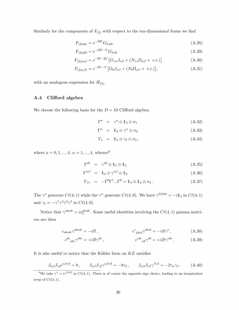
Similarly for the components of F(3) with respect to the ten-dimensional frame we find

F(3)abc = e−3WG3 abc (A.28)

F(3)abf = e−2W−VG2 ab (A.29)

F(3)aαβ = e−W−2U[G1 aJαβ + (N1 aΩαβ + c.c.)

](A.30)

F(3)αβ f = e−2U−V [G0Jαβ + (N0Ωαβ + c.c.)], (A.31)

with an analogous expression for H(3).

A.4 Clifford algebra

We choose the following basis for the D = 10 Clifford algebra:

Γa = γa ⊗ 14 ⊗ σ1 (A.32)

Γα = 14 ⊗ γα ⊗ σ2 (A.33)

Γf = 14 ⊗ γf ⊗ σ2 , (A.34)

where a = 0, 1, ..., 4, α = 1, ..., 4, whence6

Γab = γab ⊗ 14 ⊗ 12 (A.35)

Γαβ = 14 ⊗ γαβ ⊗ 12 (A.36)

Γ11 = −Γ0Γ1...Γ9 = 14 ⊗ 14 ⊗ σ3 . (A.37)

The γa generate C`(4, 1) while the γα generate C`(4, 0). We have γ01234 = −i14 in C`(4, 1)

and γf = −γ1γ2γ3γ4 in C`(4, 0).

Notice that γabcde = iεabcde5 . Some useful identities involving the C`(4, 1) gamma matri-

ces are then

εabcdeγabcde = −i5! , εeabcdγ

abcd = −i4!γe , (A.38)

εdeabcγabc = +i3!γde , εcdeabγ

ab = +i2!γcde . (A.39)

It is also useful to notice that the Kahler form on KE satisfies

JαβJγδεαβγδ = 8 , JαβJγδγ

αβγδ = −8γf , JαβJγδγβγδ = −2γαγf . (A.40)

6We take γ4 = iγ0123 in C`(4, 1). There is of course the opposite sign choice, leading to an inequivalent

irrep of C`(4, 1).

26

A.5 Charge conjugation conventions

In d = 5 dimensions with signature (−,+,+,+,+) we can define unitary intertwiners B4,1

and C4,1 (the charge conjugation matrix), unique up to a phase, satisfying

B4,1γaB−1

4,1 = −γa∗ , BT4,1 = −B4,1 , B∗4,1B4,1 = −1 , (A.41)

and

C4,1γaC−14,1 = γTa , CT4,1 = −C4,1 , C4,1 = BT

4,1γ0 = −B4,1γ0 . (A.42)

If ψ is any spinor in (4 + 1) dimensions, its charge conjugate ψc is then defined as

ψc = B−14,1ψ

∗ = B†4,1ψ∗ = −γ0C

†4,1ψ

∗ . (A.43)

In (4+1) dimensions it is not possible to define Majorana spinors satisfying ψc = ψ. It is

possible, however, to define symplectic Majorana spinors. These satisfy ψci = Ωijψj , where

Ωij is the USp(4)-invariant symplectic form. This fact becomes particulary relevant when

dealing with N = 4 supergravity in d = 5 dimensions, inasmuch as the symplectic Majorana

spinors allow to make the action of the R-symmetry manifest.

In analogy with (A.43), we can define the charge conjugates of a spinor Ψ in (9+1)

dimensions and a spinor ε in 5 Euclidean dimensions as

Ψc = B−19,1Ψ∗ , where B9,1ΓMB

−19,1 = Γ∗M , BT

9,1 = B9,1 (A.44)

εc = B−15 ε∗ , where B5γαB

−15 = γ∗α , BT

5 = −B5 , (A.45)

where B5 and B9,1 are the corresponding unitary intertwiners. We then find

B9,1 = B4,1 ⊗B5 ⊗ σ3 . (A.46)

Notice that B5 is unitary and antisymmetric, and therefore for a spinor ε in five Euclidean

dimensions we have (εc)c = −ε. In particular, in terms of the gauge-covariantly constant

spinors ε± introduced in section 2, we have that defining ε− as the charge conjugate of

ε+, this is e−3i2χε− ≡

(e

3i2χε+

)c, implies that

(e−

3i2χε−

)c= −e 3i

2χε+. We also define

the unitary intertwiner C9,1 (the charge-conjugation matrix) in (9 + 1) dimensions, which

satisfies

C9,1ΓMC−19,1 = −ΓTM C9,1 = BT

9,1Γ0 = B9,1Γ0 . (A.47)

27

Notice that defining Ψc in the (9+1)-dimensional space by using the intertwiner B9,1 in-

troduced above (as opposed to using an intertwiner B−9,1 satisfying B−9,1ΓMB−†9,1 = −Γ∗M )

allows one to choose a basis, if so desired, where the charge conjugation operation in D = 10

reduces to complex conjugation. In this basis all the C`(9, 1) gamma-matrices are real, with

B9,1 = 1 and a corresponding (9+1) charge-conjugation matrix C9,1 = BT9,1Γ0 = Γ0.

B Type IIB supergravity

In this appendix we briefly review the field content and equations of motion of type IIB

supergravity [24, 25]. We follow the conventions of [7], [22], [23] closely, and adapt our

fermionic conventions accordingly.

B.1 Bosonic content and equations of motion

In the SU(1, 1) language of [24], the bosonic content of type IIB supergravity includes the

metric, a complex scalar B, “composite” complex 1-forms P and Q (that can be written

in terms of B), a complex 3-form G, and a real self dual five-form F(5). The corresponding

equations of motion read (to linear order in the fermions)

D ∗ P = −1

4G ∧ ∗G (B.1)

D ∗G = P ∧ ∗G∗ − iG ∧ F(5) (B.2)

RMN = PMP∗N + PNP

∗M +

1

96F(5)MP1P2P3P4

FP1P2P3P4

(5)N

+1

8

(GM

P1P2G∗NP1P2+GN

P1P2G∗MP1P2− 1

6gMNG

P1P2P3G∗P1P2P3

)(B.3)

together with the self-duality condition ∗F(5) = F(5). Similarly, the Bianchi identities read

dF(5) −i

2G ∧G∗ = 0 (B.4)

DG+ P ∧G∗ = 0 (B.5)

DP = 0 . (B.6)

In this language there is a manifest local U(1) invariance and Q is the corresponding gauge

field, with field-strength dQ = −iP ∧ P ∗. Similarly, G has charge 1 and P has charge 2

under the U(1), so D ∗ G ≡ d ∗ G − iQ ∧ ∗G and D ∗ P ≡ d ∗ P − 2iQ ∧ ∗P . Notice that

Einstein’s equation (B.3) has been rewritten by using the trace condition R = 2PRP ∗R +

124G

P1P2P3G∗P1P2P3.

28

In the body of the paper we have worked in the SL(2,R) language which is more

familiar to string theorists. The translation between the two formalisms involves a gauge-

transformation and field-redefinitions.7 Here we just quote the result that links this formal-

ism with the fields used in the rest of the paper. Writing the axion-dilaton τ and the NSNS

and RR 3-forms H(3) and F(3) as

τ ≡ C(0) + ie−Φ , F(3) = dC(2) − C(0)dB(2) , H(3) = dB(2) , (B.7)

for the 3-form G we have8 [22]

G = ieΦ/2(τdB − dC(2)

)= −

(e−Φ/2H(3) + ieΦ/2F(3)

), (B.8)

and similarly

P =i

2eΦdτ , Q = −1

2eΦdC(0) . (B.9)

In terms of these fields, the equations of motion (B.1)-(B.3) become [7] (to linear order in

the fermions)

0 = d(eΦ ∗ F(3))− F(5) ∧H(3) (B.10)

0 = d(e2Φ ∗ F(1)) + eΦH(3) ∧ ∗F(3) (B.11)

0 = d(e−Φ ∗H(3))− eΦF(1) ∧ ∗F(3) − F(3) ∧ F(5) (B.12)

0 = d ∗ dΦ− e2ΦF(1) ∧ ∗F(1) +1

2e−ΦH(3) ∧ ∗H(3) −

1

2eΦF(3) ∧ ∗F(3) (B.13)

RMN =1

2e2Φ∇MC(0)∇NC(0) +

1

2∇MΦ∇NΦ +

1

96FMP1P2P3P4F

P1P2P3P4N

+1

4e−Φ

(HM

P1P2HNP1P2 −1

12gMNH

P1P2P3HP1P2P3

)+

1

4eΦ

(FM

P1P2FNP1P2 −1

12gMNF

P1P2P3FP1P2P3

)(B.14)

7The gauge transformation has the form P → e2iθP , Q→ Q+ dθ, G→ ei2θG, where θ is a τ -dependent

phase. These phases are then absorbed by a redefinition of the fermions. More details can be found in

[34, 35], for example.8Note that our forms F(3) and G are related to the traditional string theory forms F(3)st = dC(2) and

Gst = F(3)st − τH(3) by F(3) = F(3)st − C(0)H(3) and G = −iGst/√

Imτ . It’s not our fault.

29

while the Bianchi identities (B.4)-(B.6) now read

dF(5) + F(3) ∧H(3) = 0 (B.15)

dF(3) + F(1) ∧H(3) = 0 (B.16)

dF(1) = 0 (B.17)

dH(3) = 0 . (B.18)

These identities are solved by writing F(5) = dC(4)−C(2)∧H(3), F(1) = dC(0), together with

H(3) = dB(2) and F(3) = dC(2) − C(0)dB(2) as in (B.7).

B.2 Fermionic content and equations of motion

Our conventions for the type IIB fermionic sector are based on those of [34], [36], with slight

modifications needed to conform with our bosonic conventions. The type IIB fermionic

content consists of a chiral dilatino λ and a chiral gravitino Ψ, with equations of motion

given by (to linear order in the fermions)

D/λ =i

8F/ (5)λ+O(Ψ2) (B.19)

ΓABCDBΨC = −1

8G/ ∗ΓAλ+

1

2P/ ΓAλc +O(Ψ3) (B.20)

Here, D denotes the flux-dependent supercovariant derivative, which acts as follows:

D/λ =

(/∇− 3i

2/Q

)λ− 1

4ΓAG/ΨA − ΓAP/Ψc

A (B.21)

DBΨC =

(∇B −

i

2QB

)ΨC +

i

16F/ (5)ΓBΨC −

1

16SBΨc

C , (B.22)

where ∇B denotes the ordinary 10-d spinor covariant derivative and we have defined

SB ≡1

6

(ΓB

DEFGDEF − 9ΓDEGBDE). (B.23)

The gravitino and dilatino have opposite chirality in d = 10, and we choose Γ11ΨA =

−ΨA, Γ11λ = +λ. Since F(5) is self-dual, our conventions then imply F/ (5) = −Γ11F/ (5).

Thus, for any spinor ε satisfying Γ11ε = −ε we have F/ (5)ε = 0 and F/ (5)ΓAε = F/ (5),ΓAε =

112F(5)ACDEFΓCDEF ε. The corresponding SUSY variations of the fermions read

δλ = P/ εc +1

4G/ ε (B.24)

δΨA =

(∇A −

i

2QA

)ε+

i

16F/ (5)ΓAε−

1

16SAε

c . (B.25)

30

C d = 5 Equations of motion

In this appendix we present the dimensional reduction of the fermionic equations of motion

in full detail, and rewrite them in final form in terms of the fields (3.18)-(3.21) which possess

diagonal kinetic terms in the effective action. In the calculations below we encounter a

number of expressions involving ε± that need evaluation. We collect them here:

J/ ε+ =1

2iQε+ = 2iε+ J/ ε− =

1

2iQε− = −2iε− (C.1)

Ω/ ε−e− 3

2iχ = 4ε+e

32iχ Ω/ ε+e

32iχ = −4ε−e

− 32iχ (C.2)

γαγαε+ = 4ε+ γαJ/ γαε+ = γαΩ/ γαε− = 0 . (C.3)

C.1 Reduction of the dilatino equation of motion

We begin by performing the reduction of the D = 10 equation of motion for the dilatino,

as given in (B.19).

C.1.1 Derivative operator

We first reduce the 10-d derivative operator ∇A− (3i/2)QA acting on the dilatino. Defining

eW(∇/ − 3i

2Q/

)λ ≡ L+

λ ⊗ ε+e3i2χ ⊗ u− + L−λ ⊗ ε−e−

3i2χ ⊗ u− (C.4)

we find

L±λ =

(D/+

1

2∂/W +

3

4ieφ(∂/a)

)λ(±) +

1

4iΣ−2F/2λ

(±) ∓(e−4UΣ−1 +

3

2Σ2

)λ(±) , (C.5)

where D/λ(±) =(∇/ ∓ 3

2 iA/1

)λ(±) is the gauge-covariant five-dimensional connection acting

on λ(±).

C.1.2 Couplings

We now reduce the various terms involving the couplings of the dilatino, including the

flux-dependent terms in the supercovariant derivative. Defining

eW(i

8F/ (5)λ+

1

4ΓAG/ΨA

)≡ R+

1λ ⊗ ε+e3i2χ ⊗ u− +R−1λ ⊗ ε−e−

3i2χ ⊗ u− (C.6)

31

we find

R(±)1λ = eZ+4Wλ(±) − 1

2ie−4U /K1λ

(±) ∓ 1

2iΣ /K2λ

(±) ∓ Σ/L(±)2 λ(∓)

− 1

4iγa/G3ψ

(±)a − 1

4γa/G2ψ

(±)a +

1

4/G3

(ϕ(±) + 4ρ(±)

)− 1

4i/G2

(ϕ(±) − 4ρ(±)

)± 1

2γa/G1ψ

(±)a ± 1

2i/G1ϕ

(±) ∓ iγa /N (±)1 ψ(∓)

a ± /N (±)1 ϕ(∓)

∓ γaN (±)0 ψ(∓)

a ∓ iN (±)0 ϕ(∓) , (C.7)

where we have introduced the notation /L(+)2 = (1/2!)L2 abγ

ab and /L(−)2 = (1/2!)L∗2 abγ

ab.

Similarly, defining

eWΓAP/ΨcA ≡ R+

2λ ⊗ ε+e3i2χ ⊗ u− +R−2λ ⊗ ε−e−

3i2χ ⊗ u− (C.8)

we obtain

R(±)2λ =± P/ ψ(∓)c

a ± iP/(

4ρ(∓)c + ϕ(∓)c). (C.9)

where, in a slight abuse of notation, P/ = (1/2)(∂/φ+ ieφ∂/a

)when appearing in 5-d equa-

tions. In terms of the quantities computed above, the 10-d dilatino equation reduces to two

equations for the five-dimensional fields, given by

L(±)λ −R(±)

1λ −R(±)2λ = 0 . (C.10)

C.2 Reduction of the gravitino equation of motion

We now reduce the equation of motion for the D = 10 gravitino, as given in (B.20).

C.2.1 Derivative operator

Here we define

eWΓaBC(∇B −

i

2QB

)ΨC = L(+)a ⊗ ε+e

3i2χ ⊗ u+ + L(−)a ⊗ ε−e−

3i2χ ⊗ u+ (C.11)

eW σ2ΓαΓαBC(∇B −

i

2QB

)ΨC = L(+)

base ⊗ ε+e3i2χ ⊗ u+ + L(−)

base ⊗ ε−e−3i2χ ⊗ u+ (C.12)

eWΓfBC

(∇B −

i

2QB

)ΨC = L(+)

f ⊗ ε+e3i2χ ⊗ u+ + L(−)

f ⊗ ε−e−3i2χ ⊗ u+ (C.13)

32

where σ2 ≡ 14⊗14⊗σ2. Then, for the components of the derivative operator in the external

manifold directions we find

L(±)a = γabc(Db +

1

2∂bW +

1

4ieφ(∂ba)

)ψ(±)c

− 1

4iΣ−2γ[cF/2γ

a]ψ(±)c ∓

(Σ−1e−4U +

3

2Σ2

)γabψ

(±)b

− 4iγab[Db +

1

2∂bW +

1

4ieφ(∂ba)

]ρ(±) − i(Σ−1∂/Σ)γaρ(±) + 4i(∂/U)γaρ(±)

± 2i(3Σ2 + Σ−1e−4U

)γaρ(±) − 1

2Σ−2F2 bdγ

bγaγdρ(±)

− iγab[Db +

1

2∂bW +

1

4ieφ(∂ba)

]ϕ(±) − i(Σ−1∂/Σ)γaϕ(±)

± 2iΣ−1e−4Uγaϕ(±) +1

4Σ−2F2 bcγ

cγabϕ(±) . (C.14)

Similarly, the components in the direction of the KE base yield

L(±)base = − 4iγab

[Da +

1

2∂aW +

1

4ieφ(∂aa)

]ψ

(±)b + iγb(Σ−1∂/Σ)ψ

(±)b − 4iγb(∂/U)ψ

(±)b

+1

2Σ−2F2 daγ

aγbγdψ(±)b ± 2i

(Σ−1e−4U + 3Σ2

)γbψ

(±)b

− 12

[D/+

1

2(∂/W ) +

1

4ieφ(∂/a)

]ρ(±) ± 2

(2Σ−1e−4U + 9Σ2

)ρ(±) − 3iΣ−2F/2ρ

(±)

− 4

[D/+

1

2∂/W +

1

4ieφ(∂/a)− 3

4(Σ−1∂/Σ)− (∂/U)

]ϕ(±)

± 2Σ−1e−4Uϕ(±) − 2iΣ−2F/2ϕ(±) . (C.15)

Finally, for the fiber component of the derivative operator we obtain

L(±)f =− iγab

[Da +

1

2∂aW +

1

4ieφ(∂aa)

]ψ

(±)b + iγb(Σ−1∂/Σ)ψ

(±)b

± 2iΣ−1e−4Uγbψ(±)b +

1

4Σ−2F2 daγ

abγdψ(±)b

− 4

[D/+

1

2∂/W +

1

4ieφ(∂/a) +

3

4(Σ−1∂/Σ) + ∂/U

]ρ(±)

± 2Σ−1e−4U(

2ϕ(±) + ρ(±))− iF/2Σ−2

(ϕ(±) + 2ρ(±)

). (C.16)

33

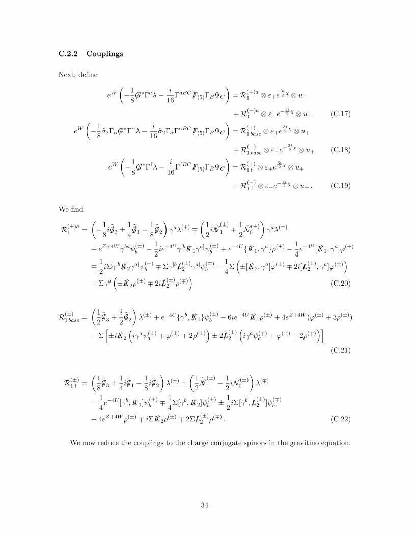
C.2.2 Couplings

Next, define

eW(−1

8G/ ∗Γaλ− i

16ΓaBCF/ (5)ΓBΨC

)= R(+)a

1 ⊗ ε+e3i2χ ⊗ u+

+R(−)a1 ⊗ ε−e−

3i2χ ⊗ u+ (C.17)

eW(−1

8σ2ΓαG/

∗Γαλ− i

16σ2ΓαΓαBCF/ (5)ΓBΨC

)= R(+)

1 base ⊗ ε+e3i2χ ⊗ u+

+R(−)1 base ⊗ ε−e−

3i2χ ⊗ u+ (C.18)

eW(−1

8G/ ∗Γfλ− i

16ΓfBCF/ (5)ΓBΨC

)= R(+)

1 f ⊗ ε+e3i2χ ⊗ u+

+R(−)1 f ⊗ ε−e−

3i2χ ⊗ u+ . (C.19)

We find

R(±)a1 =

(−1

8i/G3 ±

1

4/G1 −

1

8/G2

)γaλ(±) ∓

(1

2i /N

(±)

1 +1

2N (±)

0

)γaλ(∓)

+ eZ+4Wγbaψ(±)b − 1

2ie−4Uγ[b /K1γ

a]ψ(±)b + e−4U /K1, γ

aρ(±) − 1

4e−4U [ /K1, γ

a]ϕ(±)

∓ 1

2iΣγ[b /K2γ

a]ψ(±)b ∓ Σγ[b/L

(±)2 γa]ψ

(∓)b − 1

4Σ(±[ /K2, γ

a]ϕ(±) ∓ 2i[/L(±)2 , γa]ϕ(∓)

)+ Σγa

(± /K2ρ

(±) ∓ 2i/L(±)2 ρ(∓)

)(C.20)

R(±)1 base =

(1

2/G3 +

i

2/G2

)λ(±) + e−4Uγb, /K1ψ(±)

b − 6ie−4U /K1ρ(±) + 4eZ+4W (ϕ(±) + 3ρ(±))

− Σ[±i /K2

(iγaψ(±)

a + ϕ(±) + 2ρ(±))± 2/L

(±)2

(iγaψ(∓)

a + ϕ(∓) + 2ρ(∓))]

(C.21)

R(±)1 f =

(1

8/G3 ±

1

4i/G1 −

1

8i/G2

)λ(±) ±

(1

2/N

(±)

1 − 1

2iN (±)

0

)λ(∓)

− 1

4e−4U [γb, /K1]ψ

(±)b ∓ 1

4Σ[γb, /K2]ψ

(±)b ± 1

2iΣ[γb, /L

(±)2 ]ψ

(∓)b

+ 4eZ+4Wρ(±) ∓ iΣ /K2ρ(±) ∓ 2Σ/L

(±)2 ρ(∓) . (C.22)

We now reduce the couplings to the charge conjugate spinors in the gravitino equation.

34

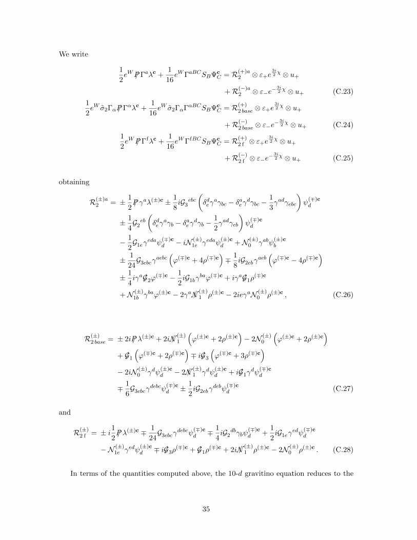
We write

1

2eWP/ Γaλc +

1

16eWΓaBCSBΨc

C = R(+)a2 ⊗ ε+e

3i2χ ⊗ u+

+R(−)a2 ⊗ ε−e−

3i2χ ⊗ u+ (C.23)

1

2eW σ2ΓαP/ Γαλc +

1

16eW σ2ΓαΓαBCSBΨc

C = R(+)2 base ⊗ ε+e

3i2χ ⊗ u+

+R(−)2 base ⊗ ε−e−

3i2χ ⊗ u+ (C.24)

1

2eWP/ Γfλc +

1

16eWΓfBCSBΨc

C = R(+)2 f ⊗ ε+e

3i2χ ⊗ u+

+R(−)2 f ⊗ ε−e−

3i2χ ⊗ u+ (C.25)

obtaining

R(±)a2 = ± 1

2P/ γaλ(±)c ± 1

8iG ebc

3

(δdeγ

aγbc − δaeγdγbc −1

3γadγebc

)ψ

(∓)cd

± 1

4G eb

2

(δdeγ

aγb − δaeγdγb −1

2γadγeb

)ψ

(∓)cd

− 1

2G1eγ

edaψ(∓)cd − iN (±)

1e γedaψ(±)cd +N (±)

0 γabψ(±)cb

± 1

24G3ebcγ

aebc(ϕ(∓)c + 4ρ(∓)c

)∓ 1

8iG2ebγ

aeb(ϕ(∓)c − 4ρ(∓)c

)± 1

4iγa/G2ϕ

(∓)c − 1

2iG1bγ

baϕ(∓)c + iγa/G1ρ(∓)c

+N (±)1b γbaϕ(±)c − 2γa /N (±)

1 ρ(±)c − 2ieγaN (±)0 ρ(±)c , (C.26)

R(±)2 base = ± 2iP/ λ(±)c + 2i /N (±)

1

(ϕ(±)c + 2ρ(±)c

)− 2N (±)

0

(ϕ(±)c + 2ρ(±)c

)+ /G1

(ϕ(∓)c + 2ρ(∓)c

)∓ i/G3

(ϕ(∓)c + 3ρ(∓)c

)− 2iN (±)

0 γdψ(±)cd − 2 /N (±)

1 γdψ(±)cd + i/G1γ

dψ(∓)cd

∓ 1

6G3ebcγ

debcψ(∓)cd ± 1

2iG2ebγ

debψ(∓)cd (C.27)

and

R(±)2 f = ± i1

2P/ λ(±)c ∓ 1

24G3ebcγ

debcψ(∓)cd ∓ 1

4iG db

2 γbψ(∓)cd +

1

2iG1eγ

edψ(∓)cd

−N (±)1e γedψ

(±)cd ∓ i/G3ρ

(∓)c + /G1ρ(∓)c + 2i /N (±)

1 ρ(±)c − 2N (±)0 ρ(±)c . (C.28)

In terms of the quantities computed above, the 10-d gravitino equation reduces to the

35

following set of equations for the five-dimensional fields:

0 = L(±)a −R(±)a1 −R(±)a

2 (C.29)

0 = L(±)base −R

(±)1 base −R

(±)2 base (C.30)

0 = L(±)f −R(±)

1 f −R(±)2 f . (C.31)

Instead of working with the equations of motion given in this form, it is convenient to

rewrite them in terms of the fields (3.18)-(3.21) whose kinetic terms are diagonal. We do

so below.

C.3 Equations of motion in terms of diagonal fields

The d = 5 equations of motion for the diagonal fields (3.18)-(3.21) are given by

0 = L(±)

λ−R(±)

1λ−R(±)

2λ(C.32)

0 = L(±)aζ −R(±)a

1 ζ −R(±)a2 ζ (C.33)

0 = L(±)η −R(±)

1 η −R(±)2 η (C.34)

0 = L(±)ξ −R(±)

1 ξ −R(±)2 ξ (C.35)

Here,

L(±)

λ= eW/2L(±)

λ (C.36)

= D/λ(±) +1

4iΣ−2F/2λ

(±) ∓(e−4UΣ−1 +

3

2Σ2

)λ(±) +

3

4ieφ(∂/a)λ(±) (C.37)

where now D/λ(±) =(∇/ ∓ 3i

2 A/)λ(±) and

R(±)

1λ= eW/2R(±)

1λ (C.38)

=

(eZ+4W − 1

2ie−4U /K1 ∓

1

2iΣ /K2

)λ(±) ∓ Σ/L

(±)2 λ(∓)

+

(−1

4iγa/G3 −

1

4γa/G2 ±

1

2γa/G1

)ζ(±)a ∓

(iγa /N (±)

1 + γaN (±)0

)ζ(∓)a

+

(1

6/G3 −

1

6i/G2

)η(±) ∓ 4

3iN (±)

0 η(∓) +1

4

(/G3 + i/G2 ∓ 2i/G1

)ξ(±)

∓(/N (±)

1 + iN (±)0

)ξ(∓) (C.39)

Similarly,

R(±)

2λ= eW/2R(±)

2λ = ±γaP/ ζ(∓)ca . (C.40)

36

In the same way, for the ζ(±)a equation of motion we find

L(±)aζ = eW/2L(±)a (C.41)

= γabc[Db +

1

4ieφ(∂ba)

]ζ(±)c ∓

(e−4UΣ−1 +

3

2Σ2

)γacζ(±)

c

− 1

4iΣ−2γ[cF/2γ

a]ζ(±)c +

[i(∂/U)γa ∓ ie−4UΣ−1γa

]ξ(±)

− 1

2i(Σ−1∂/Σ)γaη(±) +

1

6Σ−2F/2γ

aη(±) ± i

3

(e−4UΣ−1 − 3Σ2

)γaη(±) (C.42)

R(±)a1 ζ = eW/2R(±)a

1 (C.43)

=

(−1

8i/G3 −

1

8/G2 ±

1

4/G1

)γaλ(±) ∓

(1

2i /N

(±)

1 +1

2N (±)

0

)γaλ(∓)

+

(eZ+4Wγca − 1

2ie−4Uγ[c /K1γ

a] ∓ 1

2iΣγ[c /K2γ

a]

)ζ(±)c ∓ Σγ[c/L

(±)2 γa]ζ(∓)

c

+(−ieZ+4W +

1

2e−4U /K1

)γaξ(±) +

(−2i

3eZ+4W ∓ 1

6Σ /K2

)γaη(±)

± 1

3iΣ/L

(±)2 γaη(∓) (C.44)

and

R(±)a2 ζ = eW/2R(±)a

2 (C.45)

= ∓ 1

2P/ γaλ(∓)c ± 1

8iG ebc

3

[1

3γdaγebc + (δdeγ

a − δaeγd)γbc]ζ

(∓)cd

±(

1

8G eb

2 γeγdaγb ∓

1

2G1bγ

abd

)ζ

(∓)cd +

(−iN (±)

1b γabd +N (±)0 γad

)ζ

(±)cd

∓(

1

12/G3 +

i

12/G2

)γaη(∓)c +

2

3iN (±)

0 γaη(±)c

∓ 1

8(/G3 − i/G2 ∓ 2i/G1) γaξ(∓)c − 1

2

(/N (±)

1 − iN (±)0

)γaξ(±)c . (C.46)

For the η(±) equation of motion we have

L(±)η = eW/2

(L(±)

f +i

3γaL(±)a

)(C.47)

=2

3

[D/+

1

4ieφ(∂/a)

]η(±) +

(− 5

18iΣ−2F/2 ∓

2

9e−4UΣ−1 ± 5

3Σ2

)η(±)

+

[1

3Σ−2γcF/2 + iγc(Σ−1∂/Σ)± 2

3ie−4UΣ−1γc ∓ 2iΣ2γc

]ζ(±)c

∓ 4

3e−4UΣ−1ξ(±) (C.48)

37

R(±)1η = eW/2

(R±1 f +

i

3γaR(±)a

1

)(C.49)

=

(1

6/G3 −

1

6i/G2

)λ(±) ∓ 4

3iN (±)

0 λ(∓)

+

(−4

3ieZ+4Wγc ∓ 1

3Σγc /K2

)ζ(±)c ± 2

3iΣγc/L

(±)2 ζ(∓)

c +8

3eZ+4W ξ(±)

+

(10

9eZ+4W +

1

3ie−4U /K1 ±

1

9iΣ /K2

)η(±) ± 2

9Σ/L

(±)2 η(∓) (C.50)

and

R(±)2η = eW/2

(R(±)

2 f +i

3γaR(±)a

2

)(C.51)

= ∓ 1

6γd (/G3 + i/G2) ζ

(∓)cd +

4

3iN (±)

0 γdζ(±)cd

± 1

18(i/G3 − /G2 ∓ 6/G1) η(∓)c −

(10

9N (±)

0 +2i

3/N (±)

1

)η(±)c

∓ 1

6(i/G3 + /G2) ξ(∓)c − 4

3N (±)

0 ξ(±)c . (C.52)

Finally, for the ξ(±) equation of motion we have

L(±)ξ = eW/2

(iγaL(±)a + L(±)

base − L(±)f

)(C.53)

= 2

[D/+

1

4ieφ(∂/a)

]ξ(±) +

1

2iΣ−2F/2ξ

(±) ± 3(2e−4UΣ−1 − Σ2

)ξ(±)

+[∓4ie−4UΣ−1γc − 4iγc(∂/U)

]ζ(±)c ∓ 8

3e−4UΣ−1η(±) (C.54)

R(±)1ξ = eW/2

(iγaR(±)a

1 +R(±)1 base −R

(±)1 f

)(C.55)

=

(1

2/G3 +

1

2i/G2 ∓ i/G1

)λ(±) ∓

(2 /N

(±)

1 + 2iN (±)0

)λ(∓)

+(−4ieZ+4Wγc + 2e−4Uγc /K1

)ζ(±)c +

16

3eZ+4W η(±)

+(6eZ+4W − 3ie−4U /K1 ± iΣ /K2

)ξ(±) ± 2Σ/L

(±)2 ξ(∓) (C.56)

and

R(±)2ξ = eW/2

(iγaR(±)a

2 +R(±)2 base −R

(±)2 f

)(C.57)

= ∓(

1

2γd/G3 −

1

2iγd/G2 ∓ iγd/G1

)ζ

(∓)cd +

(2iN (±)

0 γd − 2γd /N (±)1

)ζ

(±)cd

∓(

1

3i/G3 +

1

3/G2

)η(∓)c − 8

3N (±)

0 η(±)c ∓ 3

4/G2ξ

(∓)c . (C.58)

38

References

[1] S. S. Gubser, “Breaking an Abelian gauge symmetry near a black hole horizon,”

Phys. Rev. D78 (2008) 065034, arXiv:0801.2977 [hep-th].

[2] S. A. Hartnoll, C. P. Herzog, and G. T. Horowitz, “Building a Holographic

Superconductor,” Phys. Rev. Lett. 101 (2008) 031601, arXiv:0803.3295 [hep-th].

[3] S. A. Hartnoll, C. P. Herzog, and G. T. Horowitz, “Holographic Superconductors,”

JHEP 12 (2008) 015, arXiv:0810.1563 [hep-th].

[4] D. T. Son, “Toward an AdS/cold atoms correspondence: a geometric realization of

the Schroedinger symmetry,” Phys. Rev. D78 (2008) 046003, arXiv:0804.3972

[hep-th].

[5] K. Balasubramanian and J. McGreevy, “Gravity duals for non-relativistic CFTs,”

Phys. Rev. Lett. 101 (2008) 061601, arXiv:0804.4053 [hep-th].

[6] D. Cassani, G. Dall’Agata, and A. F. Faedo, “Type IIB supergravity on squashed

Sasaki-Einstein manifolds,” arXiv:1003.4283 [hep-th].

[7] J. P. Gauntlett and O. Varela, “Universal Kaluza-Klein reductions of type IIB to

N=4 supergravity in five dimensions,” arXiv:1003.5642 [hep-th].

[8] J. T. Liu, P. Szepietowski, and Z. Zhao, “Consistent massive truncations of IIB

supergravity on Sasaki-Einstein manifolds,” arXiv:1003.5374 [hep-th].

[9] K. Skenderis, M. Taylor, and D. Tsimpis, “A consistent truncation of IIB supergravity

on manifolds admitting a Sasaki-Einstein structure,” arXiv:1003.5657 [hep-th].

[10] J. Maldacena, D. Martelli, and Y. Tachikawa, “Comments on string theory

backgrounds with non- relativistic conformal symmetry,” JHEP 10 (2008) 072,

arXiv:0807.1100 [hep-th].

[11] C. P. Herzog, M. Rangamani, and S. F. Ross, “Heating up Galilean holography,”

JHEP 11 (2008) 080, arXiv:0807.1099 [hep-th].

[12] A. Adams, K. Balasubramanian, and J. McGreevy, “Hot Spacetimes for Cold

Atoms,” JHEP 11 (2008) 059, arXiv:0807.1111 [hep-th].

39

[13] M. S. Bremer, M. J. Duff, H. Lu, C. N. Pope, and K. S. Stelle, “Instanton cosmology

and domain walls from M-theory and string theory,” Nucl. Phys. B543 (1999)

321–364, arXiv:hep-th/9807051.

[14] J. T. Liu and H. Sati, “Breathing mode compactifications and supersymmetry of the

brane-world,” Nucl. Phys. B605 (2001) 116–140, arXiv:hep-th/0009184.

[15] A. Buchel and J. T. Liu, “Gauged supergravity from type IIB string theory on Y(p,q)

manifolds,” Nucl. Phys. B771 (2007) 93–112, arXiv:hep-th/0608002.

[16] J. P. Gauntlett, S. Kim, O. Varela, and D. Waldram, “Consistent supersymmetric

Kaluza–Klein truncations with massive modes,” JHEP 04 (2009) 102,

arXiv:0901.0676 [hep-th].

[17] J. P. Gauntlett, J. Sonner, and T. Wiseman, “Holographic superconductivity in

M-Theory,” Phys. Rev. Lett. 103 (2009) 151601, arXiv:0907.3796 [hep-th].

[18] J. P. Gauntlett, J. Sonner, and T. Wiseman, “Quantum Criticality and Holographic

Superconductors in M- theory,” JHEP 02 (2010) 060, arXiv:0912.0512 [hep-th].

[19] I. Bah, A. Faraggi, J. I. Jottar, R. G. Leigh, and L. A. P. Zayas, “Fermions and

D = 11 Supergravity On Squashed Sasaki- Einstein Manifolds,” arXiv:1008.1423

[hep-th].

[20] S. S. Gubser, C. P. Herzog, S. S. Pufu, and T. Tesileanu, “Superconductors from

Superstrings,” arXiv:0907.3510 [hep-th].

[21] M. Ammon, J. Erdmenger, M. Kaminski, and A. O’Bannon, “Fermionic Operator

Mixing in Holographic p-wave Superfluids,” JHEP 05 (2010) 053, arXiv:1003.1134

[hep-th].

[22] J. P. Gauntlett, D. Martelli, J. Sparks, and D. Waldram, “Supersymmetric AdS(5)

solutions of type IIB supergravity,” Class. Quant. Grav. 23 (2006) 4693–4718,

arXiv:hep-th/0510125.

[23] J. P. Gauntlett and O. Varela, “Consistent Kaluza-Klein Reductions for General

Supersymmetric AdS Solutions,” Phys. Rev. D76 (2007) 126007, arXiv:0707.2315

[hep-th].

[24] J. H. Schwarz, “Covariant Field Equations of Chiral N=2 D=10 Supergravity,” Nucl.

Phys. B226 (1983) 269.

40

[25] P. S. Howe and P. C. West, “The Complete N=2, D=10 Supergravity,” Nucl. Phys.

B238 (1984) 181.

[26] D. Martelli, J. Sparks, and S.-T. Yau, “Sasaki-Einstein manifolds and volume

minimisation,” Commun. Math. Phys. 280 (2008) 611–673, arXiv:hep-th/0603021.

[27] N. Hitchin, “Harmonic spinors,” Advances in Mathematics 14 (1974) no. 1, 1 – 55.

[28] G. W. Gibbons, S. A. Hartnoll, and C. N. Pope, “Bohm and Einstein-Sasaki metrics,

black holes and cosmological event horizons,” Phys. Rev. D67 (2003) 084024,

arXiv:hep-th/0208031.

[29] J. Schon and M. Weidner, “Gauged N = 4 supergravities,” JHEP 05 (2006) 034,

arXiv:hep-th/0602024.

[30] G. Dall Agata, C. Herrmann, and M. Zagermann, “General matter coupled N = 4

gauged supergravity in five dimensions,” Nucl. Phys. B612 (2001) 123–150,

arXiv:hep-th/0103106.

[31] H. J. Kim, L. J. Romans, and P. van Nieuwenhuizen, “The Mass Spectrum of Chiral

N=2 D=10 Supergravity on S**5,” Phys. Rev. D32 (1985) 389.

[32] M. Gunaydin and N. Marcus, “The Spectrum of the s**5 Compactification of the

Chiral N=2, D=10 Supergravity and the Unitary Supermultiplets of U(2, 2/4),”

Class. Quant. Grav. 2 (1985) L11.

[33] L. J. Romans, “NEW COMPACTIFICATIONS OF CHIRAL N=2 d = 10

SUPERGRAVITY,” Phys. Lett. B153 (1985) 392.

[34] O. DeWolfe and S. B. Giddings, “Scales and hierarchies in warped compactifications

and brane worlds,” Phys. Rev. D67 (2003) 066008, arXiv:hep-th/0208123.

[35] M. Chiodaroli, M. Gutperle, and D. Krym, “Half-BPS Solutions locally asymptotic to

AdS3 × S3 and interface conformal field theories,” JHEP 02 (2010) 066,

arXiv:0910.0466 [hep-th].

[36] R. Argurio, G. Ferretti, and C. Petersson, “Massless fermionic bound states and the

gauge / gravity correspondence,” JHEP 03 (2006) 043, arXiv:hep-th/0601180.

41