arX

iv:c

ond-

mat

/040

1264

v2 [

cond

-mat

.str

-el]

13

Oct

200

4

Ferrimagnetic mixed-spin ladders in weak and strong coupling limits

D.N.Aristov∗

Max-Planck-Institute FKF, Heisenbergstraße 1, 70569 Stuttgart, Germany

M.N. KiselevInstitut fur Theoretische Physik und Astrophysik, Universitat Wurzburg, D-97074, Germany

(Dated: February 2, 2008)

We study two similar spin ladder systems with the ferromagnetic leg coupling. First model includestwo sorts of spins, s = 1/2 and s = 1, and the second model comprises only s = 1/2 legs coupled bya ”triangular” rung exchange. We show that the antiferromagnetic (AF) rung coupling destroys thelong-range order and eventually makes the systems equivalent to the AF s = 1/2 Heisenberg chain.We study the crossover from the weak to strong coupling regime by different methods, particularlyby comparing the results of the spin-wave theory and the bosonization approach. We argue thatthe crossover regime is characterized by the gapless spectrum and non-universal critical exponentsare different from those in XXZ model.

PACS numbers: 75.10.Jm, 75.10.Pq, 75.40.Gb

I. INTRODUCTION

The strongly correlated systems in one spatial dimen-sion (1D) attracted an enormous theoretical and experi-mental interest last decade. The 1D fermionic and spinsystems were recognized long ago as the useful theoreticalmodels, where the interaction effects are very importantand at the same time are subject to rigorous analysis.1,2

The experimental discovery of the systems of predomi-nantly 1D character inspired the renewed interest to thisclass of problems. Among the experimental realizationsof the 1D systems one can mention the Bechgaards salts,carbon nanotubes, copper oxides spin ladders and purelyorganic spin chain compounds.2

While the physics of purely one-dimensional objects,or chains, is well understood,1,2 the spin ladders arestill under intense investigation. Even the isolated spinchains reveal a variety of unusual phenomena, includingthe Haldane gap, spin-Peierls transition, magnetizationplateaus. The ladders, consisting of a few coupled spinchains are generally much richer in their behavior, andpose additional theoretical problems.

The interest to the problem of ladders may be tracedback to the earlier attempts to construct the continousrepresentation of spin S = 1 variable in 1D out of s = 1/2quantities.3 The methods elaborated in these studies arenow widely used in the analysis of the ladder systems.

The basic model for the spin chain, the antiferromag-netic (AF) Heisenberg s = 1/2 chain, is thoroughly stud-ied by various methods.2 This may be one of the rea-sons, why a majority of the theoretical papers discussingthe spin ladders are now confined to the treatment ofquantum spin s = 1/2 with antiferromagnetic interac-tion along the legs. Spin ladders with different spins orwith a ferromagnetic leg exchange attracted much lessattention.

The spin chains and ladders consisting of differentspins4 and with the AF leg exchange were considered re-cently in5,6,7,8,9. Particularly, the ferrimagnetic chains

with alternating spin-1/2 and spin-1 were discussedthere. It was shown that, contrary to the case of equalspins, the uncompensated spin value in a unit cell leadsto the gap in the spectrum and the appearance of thelong range magnetic order.10

The spin-1/2 ladder with ferromagnetic exchange alongthe legs was studied in11,12. A rather rich phase diagramwas demonstrated, depending on the details of the mag-netic anisotropies for the leg and rung couplings.

In the present paper we study the mixed spin (S = 1,s = 1/2) spin ladder with the ferromagnetic exchangealong the legs and antiferromagnetic interaction on therungs.In the absence of the rung coupling, the individualchains show the ferromagnetic long-range order (LRO),and the ground state is classical. The spectrum and theground state energy is well described in terms of the lin-ear spin-wave theory.5 We show that the inclusion ofthe antiferromagnetic rung coupling drives the systeminto the quantum regime, understood in terms of theAF Heisenberg spin-1/2 chain. In this regime the mag-netic LRO is absent, and the spatial correlations showthe power-law decay. Note that the uncompensated spinin a unit cell leads to the absence of the gap in low-lyingexcitation spectra.

This primary observation is interesting on its own, be-cause two limiting cases of the model allow the asymp-totically exact solutions with gapless spectra. Hence ourfurther motivation to study the crossover region startingfrom both limiting points.

We discuss the regimes of weak and strong rung cou-pling for different types of the leg exchange anisotropy.The consideration is somewhat complicated by the ab-sence of the established routines for our case. Thebosonization, an extremely useful tool in dealing withAF s=1/2 systems, does not fully work here on two rea-sons. First is the existence of two sorts of spins in a unitcell, and another is the ferromagnetic leg exchange.

Hence we supplement our study by the consideration ofa similar model, written entirely for s = 1/2 but with the

2

���

���

���

���

����

����

����

����

����

����

����

����

��������

����

����

����

2i−1 2i 2i+11

2

J

J

FIG. 1: A ladder of spins S = 1, s = 1/2

modified rung couplings. Using these models and com-paring different approaches, the spin-wave theory andbosonization, we arrive at the unified description of theferrimagnetic spin ladders. Particuarly, we discuss thespectrum and the correlations and observe the crossoverfrom the weak to strong coupling regime. An attentionis paid to a subtler point in the bosonization procedure,a seemingly unstable Gaussian effective action near theferromagnetic point.

The rest of the paper is organized as follows. We dis-cuss the mixed spin model in strong and weak rung cou-pling regime in Sec. II. The spin s = 1/2 ladder with”triangular” rung exchange is introduced and analyzedin Sec. III. The existence of different order parametersin a system is discussed in Sec. IV. The discussion andconclusions are in Sec. V

II. MIXED SPIN LADDER

We investigate the properties of a ladder system, con-sisting of two sorts of spins, s = 1/2 and S = 1, arrangedin a checkerboard manner. The unit cell comprises fourspins and the Hamiltonian is

H = −∑

i

Jα‖

(

sα1,2iS

α1,2i±1 + sα

2,2i±1Sα2,2i

)

+J⊥∑

i

(s1,2iS2,2i + S1,2i+1s2,2i+1) (1)

with the first subscript (e.g. 1 in s1,2i) labeling the leg,and the second one denoting the site on it (odd oreven). Below we mostly consider the case of the AFrung coupling, J⊥ > 0. The overall ferromagnetic ex-change along the chains allows the uniaxial anisotropy,Jx‖ = Jy

‖ = J > 0, Jz‖ = J + D > 0, |D| ≪ J . In what

follows, we consider also a useful generalization to higherspins, s ≫ 1 with the difference S − s = 1/2 kept fixed.The whole consideration is done for zero temperature.

First let us briefly describe two simple limiting cases.At D = 0+ and J⊥ = 0, we have two ferromagneticchains, which possess the long-range magnetic order. Thespectrum is quadratic at small wave vectors, ω ∼ Jq2.We put the lattice spacing a to unity everywhere exceptthe Sec. III D.

In the opposite limiting case, J⊥ ≫ J , the groundstate of two spins on the rung, say, s1,2i and S2,2i is

doublet, described by a spin s = 1/2 variable σ2i. Weshow below, that the effective interaction between theseσi is antiferromagnetic for the above choice J > 0 andhence the situation is mapped onto a well-known problemof s = 1/2 Heisenberg antiferromagnet. One does notexpect the long-range order at D = 0 and the spectrumis linear εk ∼ Jk. The correlation functions for this caseare described below.

The intermediate situation, J ∼ J⊥, D 6= 0, is harderto analyze and we present several ways to discuss it be-low.

A. Strong rung coupling

Consider first the case of strong perpendicular cou-pling, J⊥ ≫ J . Taking first J = D = 0, one seesthat each pair of spins s, S is characterized by a totalspin j = s + S and by the rung energy Ej = J⊥sS =12J⊥(j(j+1)−s(s+1)−S(S+1)). The lowest state hereis doublet, j = 1/2, the first excited state is quadrupletj = 3/2, with E3/2 − E1/2 = 3J⊥/2. The wave functionof a multiplet is

|j,m〉 =∑

m1,m2

Cjmsm1Sm2

|sm1〉|Sm2〉 (2)

with Clebsch-Gordan coefficients Cjmsm1Sm2

. The inter-action along the chain is considered now as a perturba-tion. The formula (2) and consideration below are ap-plicable for larger spins as well. In this more generalcase of s = S − 1/2 ≥ 1/2, the operators sα, Sα actwithin the lowest doublet and connect the doublet withthe quadruplet, but the direct transitions to the higherstates, j = 1/2 → j ≥ 5/2, are absent. One can checkthat the corresponding matrix elements are given by

〈j = 1/2,m|sα|j = 1/2,m′〉 = −s3σα

mm′ ,

〈j = 1/2,m|Sα|j = 1/2,m′〉 =S + 1

3σα

mm′ , (3)

with σαmm′ the Pauli matrices. For s = 1/2 this reads

sα ↔ −1

6σα, Sα ↔ 2

3σα. (4)

It shows that if we consider only the projection of thespin operators onto the lowest doublet, then the aboveHamiltonian corresponds to the AF Heisenberg spin-1/2model of the form :

Heff =∑

i

Jαeffσ

αi σ

αi+1, (5)

where

Jαeff (J⊥ → ∞) = 2Jα

‖ s(S + 1)/9. (6)

3

Below we will refer to this estimate of Jαeff as Jα

eff (∞).

For s = 1/2 we have Jαeff (∞) = 2Jα

‖ /9.

Let us next consider the role of the higher states on arung. We do not list here the matrix elements of the spinoperators Sα, sα for the transitions j = 1/2 → j = 3/2.

We only note that they are proportional to√

s(S + 1)and are the same for Sα and sα, except for the sign.The second-order correction in J‖ between the adjacentrungs, labeled by 1 and 2 below, can be written as

Jα‖ J

β‖

4〈12 |sα

1 | 32 〉〈32 |s

β1 | 12 〉〈1

2 |Sα2 | 32 〉〈3

2 |Sβ2 | 12 〉

2E1/2 − 2E3/2, (7)

with factor 4 coming from the above property of coinci-dence of the matrix elements. Noting that

〈12,m|sα

1 |3

2〉〈3

2|sβ

1 |1

2,m′〉

=s(S + 1)

9(2δαβδmm′ − iǫαβγσ

γmm′), (8)

we find that the second order in J‖ results in (5) withthe renormalized value of effective interaction :

Jαeff (J⊥) = Jα

eff (∞) + ǫ2αβγ

Jβeff (∞)Jγ

eff (∞)

9J⊥. (9)

with Jαeff from (6). For the above parameters Jα

‖ and

s = 1/2 one has

Jxeff = Jy

eff =2

9J +

8J(J +D)

729J⊥, (10)

Jzeff =

2

9(J +D) +

8J2

729J⊥, (11)

which particularly means that the relative value ofanisotropy decreases with decreasing J⊥. The perturba-tion theory is expected to break down when the correc-tion in J−1

⊥ is comparable to the first term in (9), whichhappens roughly at J⊥ ∼ Jα

‖ s2. Note that this crite-

rion also corresponds to the point where the bandwidthinduced by Jeff becomes comparable to the separation∼ J⊥ between the quadrupet and doublet. At larger J⊥the low-energy dynamics is described by the AF spin-one-half XXZ model (5) which is exactly solvable.

In the isotropic case, D = 0, the spectrum is linear,ω = π

8 Jeff |q| and the correlations are of the form

〈σαi σ

αi+n〉 ∼ |n|−2 + (−1)n|n|−1,

with the omitted minor logarithmic corrections.13

Taking into account the matrix elements (3) we findthat the leading asymptotes in the isotropic, s = 1/2, S =1 case are :

〈sα1,is

α1,i+2n〉 ∼ |2n|−1

〈sα1,iS

α1,i+2n+1〉 ∼ 4|2n+ 1|−1 (12)

〈Sα1,iS

α1,i+2n〉 ∼ 16|2n|−1

Thus the long-range ferromagnetic order is absent, butthe correlations are ferromagnetic and slowly decaying.In addition, there is a subleading sign-reversal asymp-tote and modulation depending on the spin value (s =1/2, 1). The correlations between the spins in differentchains are slowly decaying antiferromagnetic ones, e.g.〈sα

1,isα2,i+2n+1〉 ∼ −|2n + 1|−1. The above form of the

correlations is obviously unchanged as long as J⊥ . J .

B. Weak rung coupling, spin-wave analysis

Let us consider next the opposite limiting case, whenthe leg exchange dominates and J⊥ can be consideredas perturbation. First we explore the spin-wave formal-ism for the easy-axis anisotropy, D > 0. It was shownrecently5 that in case of ferrimagnetic system in 1D thespin-wave description gives very good estimate for theground state energy and on-site magnetization. Perform-ing the standard Dyson-Maleyev expansion,

Sz1 = −S + a†a, sz

1 = −s+ b†b

S+1 =

√2Sa†(1 − a†a/(2S)),

s+1 =√

2sb†(1 − b†b/(2s))

S−1 =

√2Sa, s−1 =

√2sb

Sz2 = S − c†c, sz

2 = s− d†d

S+2 =

√2S(1 − c†c/(2S))c,

s+2 =√

2s(1 − d†d/(2s))d

S−2 =

√2Sc†, s−2 =

√2sd† (13)

we write for the magnon Green function in the linearspin-wave theory (LSWT) approximation

Φ† = (a†k, b†k, c−k, d−k)

Gij(k, t) = −iθ(t)〈[Φi(k, t),Φ†j(k, 0)]〉 (14)

G(k, ω)−1 = −

s(2Jz‖ + J⊥) − ω

√sSJγk 0

√sSJ⊥√

sSJγk S(2Jz‖ + J⊥) − ω

√sSJ⊥ 0

0√sSJ⊥ s(2Jz

‖ + J⊥) + ω√sSJγk√

sSJ⊥ 0√sSJγk S(2Jz

‖ + J⊥) + ω

(15)

4

Here γk = 2 cosk. The spectrum consists of doubly de-generate acoustic and optical modes. The optical modehas the energy ∼

√sSJ for all wave vectors and the

acoustic branch at small k is

εk ≃ 2sS

s+ S

√

(2D + Jk2)(2D + Jk2 + 2J⊥) (16)

so instead of the quadratic spectrum of purely FM case,we have an approximately linear spectrum at small en-ergies εk . sJ⊥. The contribution of the zero-point fluc-tuations into the average on-site magnetization can beestimated for D ≪ J⊥ ≪ J as follows

s− 〈s1i〉 ∼√

J⊥/J ln(√

J⊥/D). (17)

It means that the spin-wave approximation fails whenthe latter quantity is of order of s. It happens roughlyat J⊥ & s2J(ln s2J/D)−2, which corresponds to thecrossover point γ∗ in11. Apart from the logarithmic fac-tor, this estimate agrees with the above value J⊥ ∼ s2J‖,obtained in the large J⊥ limit. For lower J⊥ the systemshows the long-range order.

It might be instructive to consider the FM rung cou-pling J⊥ < 0. In this case all the branches of the spec-trum are gapful, the lowest modes are

ε1,k ≃ 2sS

s+ S(2D + Jk2),

ε2,k ≃ 2sS

s+ S(2D + 2|J⊥| + Jk2), (18)

Note that at the isotropic point D = 0, the long-rangeFM order and hence the applicability of the LSWT is lostfor any J⊥ > 0. The spectrum (16) in this case is gap-less and linear with the spin-wave velocity ∼ s

√JJ⊥, the

limit of s ≃ S ≫ 1 is assumed. We know that increas-ing J⊥ we should eventually recover the effective model(5), characterized by spinon velocity ∼ s2J . These twovelocities match again at J⊥ ∼ s2J .

Concluding this section, we also present the LSWTresults for the lowest branches of dispersion for the caseof easy-plane anisotropy, D < 0. For the AF sign of theexchange J⊥ one has

ε1,k ≃ 2sS

s+ S

√

Jk2(2|D| + Jk2 + 2J⊥),

ε2,k ≃ 2sS

s+ S

√

(2|D| + Jk2)(2J⊥ + Jk2), (19)

while for the FM exchange J⊥ < 0 we obtain

ε1,k ≃ 2sS

s+ S

√

Jk2(2|D| + Jk2), (20)

ε2,k ≃ 2sS

s+ S

√

(2|J⊥| + Jk2)(2|D| + 2|J⊥| + Jk2),

In this case LSWT is formally inapplicable, but the aboveformulas might be useful for a comparison with furtherresults.

Summarizing, we observe that while the LSWT cannottreat the correlations correctly and formally is inapplica-ble in the absence of the LRO, it provides simple andreasonable formulas for the excitation spectra in a com-plicated one-dimensional ladder. We illustrate this pointbelow by discussing the spin-1/2 ladder, where a rigorousdescription of the low-energy action is available.

C. Equations of motion

This subsection is devoted to the macroscopic equa-tions describing the behavior of spins in two coupledchains. To make our calculations more transparent, wedefine new operators on a rung as superpositions of twospin operators

Qα2i = Sα

2,2i + sα1,2i, Rα

2i = Sα2,2i − sα

1,2i, (21)

Qα2i+1 = Sα

1,2i+1 + sα2,2i+1, Rα

2i+1 = Sα1,2i+1 − sα

2,2i+1,

satisfying the following commutation relations:

[Qαi , Q

βi ] = iǫαβγQ

γi , [Rα

i , Rβi ] = iǫαβγQ

γi ,

[Rαi , Q

βi ] = iǫαβγR

γi . (22)

with ǫαβγ totally antisymmetric tensor ; the operatorsQα and Rα commute at different sites.

The commutation relations (22) define theSU(2)

⊗

SU(2) = SO(4) group with two Casimiroperators given by

Q · R =5

4, Q2 + R2 =

11

2. (23)

The Hamiltonian H = H‖ +H⊥ takes the form

H‖ = −1

2

∑

i

Jα‖

(

Qαi Q

αi+1 −Rα

i Rαi+1

)

H⊥ =J⊥4

∑

i

(

Q2i − R2

i

)

=J⊥2

∑

i

Q2i + cst (24)

The equation of motions for operators Q and R are givenby

Qαj = i[H,Qα

j ], Rαj = i[H,Rα

j ]. (25)

These equations correspond to the well-known Blochequations for precession of the magnetic moment of fer-romagnets (antiferromagnets). Taking into account thatthe operators Qα (Rα) are different on two differentsublattices corresponding to odd(even) sites, we use theproperties

[Q2i , Q

αi ] = [R2

i , Qαi ] = 0,

[Q2i , R

αi ] = −[R2

i , Rαi ] = iǫαβγ{Rβ

i Qγi }

5

and adopt a symbolic notation

iǫαβγ{Rβi Q

γi } = i (Ri × Qi − Qi × Ri)

α .

Then we obtain the following system of coupled Blochequations for the isotropic Jα

‖

∂tQi =J‖

2(Qi × Qi±1 − Ri × Ri±1)

∂tRi =J‖

2(Qi × Ri±1 − Ri × Qi±1) +

+J⊥2

(Qi × Ri − Ri × Qi) . (26)

Taking the continuum limit here, one has:

∂tQ =

(

AαβQ× ∂2Q

∂xα∂xβ−BαβR × ∂2R

∂xα∂xβ

)

∂tR =

(

BαβQ× ∂2R

∂xα∂xβ−AαβR × ∂2Q

∂xα∂xβ

)

+

+ C (Q× R − R × Q) . (27)

where for asymmetric two-leg ladder α = β = x andAxx = Bxx = J‖a

2/2, C = J⊥/2. The lattice index i isomitted. Being re-written in terms of densities of mag-netic moments, equations (27)correspond to the gener-alized Landau-Lifshitz equations for the dynamic SO(4)group. Note that the operator Q represents a total spinon the rung, and the operator R does not have a simpleinterpretation.

We introduce the densities of magnetic moment char-acterizing two sublattices

M =2

N∑

l

Ql, N =2

N∑

l

(−1)lQl,

O =2

N∑

l

Rl, T =2

N∑

l

(−1)lRl, (28)

with N being total number of rungs in the ladder.Obviously, M and N represent the uniform and stag-

gered magnetizations along the ladder, whereas T andO can be interpreted as “staggered rung” magnetizationin the uniform and staggered channels along the chain,respectively. The different ordered phases are charac-tererized by nontrivial values of M,N,O,T or somecombinations of them whereas in disordered phase thesequantities are equal to zero. For example, the orderedFM phase is characterized by M 6= 0. In Neel phaseN 6= 0. In ferrimagnetic phase both M 6= 0 and N 6= 0.Therefore, the information about the order parameter isnecessary for deriving the macroscopic Landau-Lifshitzequations from the microscopic Bloch equations.

We point out that the scalar product of two spins ona rung

s1S2 =1

4

(

Q2 − R2)

1

2

S S

S

1 2

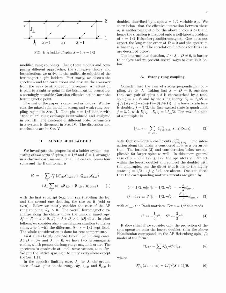
3

J J

unit cell

J

FIG. 2: A triangular ladder of spins s = 1/2

may also be considered as a local order parameter (seediscussion in the Section III).

Eqs. (26) are the central result of this subsection. Uponthe assumption of the certain order parameter(s) theylead to macroscopic “equations of motion”. Applying astandard routine14 one can show that these equations areequivalent to LSWT treatment and reproduce magnondispersion laws discussed in the previous subsection. Thedetailed analysis of the Bloch equations for asymmetricSO(4) ladders will be presented elsewhere.

III. TRIANGULAR s = 1/2 LADDER

One may regard spin 1 as a ground state triplet of twospins 1/2 coupled ferromagnetically. Our model assumesthat this triplet is also FM coupled to other spins 1/2 ona chain. Therefore instead of the FM chain of n spins1 and n spins 1/2, one may consider 3n spins 1/2. Themodel we propose is

H = −∑

i

Jα‖

(

sα1,is

α1,i+1 + sα

2,isα2,i+1

)

+J⊥∑

i

[s1,3i (s2,3i + s2,3i+1)

+ (s1,3i+1 + s1,3i+2) s2,3i+2] (29)

with the above choice of Jα‖ . The model (29) is not

equivalent to the previous one, eq. (1). Indeed, the exactmapping of (1) to (29) would include the strong trimer-ized isotropic FM in-chain exchange, at those links whichform the bases of the triangles in Fig. 2. In that case onewould first consider the triangles and then couple themto each other, fully restoring the consideration of the pre-vious Section. We show below that the model (29) withuniform value of the rung exchange has two advantages.First, it is equivalent to (1) at J⊥ → ∞ and second, itis easier tractable in the opposite case J⊥ → 0, since theexact form of the low-energy action is available for theuniform Jα

‖ .

6

A. Strong rung coupling

We consider a case when the AF exchange J⊥ is muchlarger than Jα

‖ , first for the isotropic Jα‖ = J‖. In this

case a main block is a triangle formed by two rungs, andthe coupling of triangles is a perturbation. The Hamil-tonian for the triangle is

H△ = J⊥(s1 + s2)s3 − J‖(s1s2 − 1/4) (30)

The structure of the energy levels is as follows. Theterm J‖ groups the spins on one leg, s1 and s2, into atriplet |T 〉 and a singlet |S〉. The singlet does not coupleto s3 and results in a total doublet denoted as |D0〉 withthe energy ED0 = J‖. The triplet |T 〉 of zero energy cou-ples to s3 with the formation of doublet |D1〉 and quadru-plet |Q〉. The corresponding energies areED1 = −J⊥ andEQ = J⊥/2. For J‖ → ∞ the state |D0〉 is unimportant,and s1, s2 act as one spin S = 1. At the same time, thelow-energy sector of the problem is associated with thedoublet |D1〉, and this doublet is the lowest state also forthe situation J⊥ ≫ J‖. Therefore the strong couplinglimit of the asymmetric ladder with two spins s = 1,s = 1/2 is described as well by the triangular latticedepicted in Fig.(2) in the same limit. The demand forin-triangle J‖ to be large, in order to organize the effec-tive spin-1, is relaxed in this limit, and one can considerthe situation with the uniform value of the exchange J‖along the whole leg.

The presence of the anisotropy term −Dsz1s

z2 in (29) is

a negligible effect in the described picture. Indeed, thisterm translates into a single-ion anisotropy of the tripletstate, (Sz)2 and the application of the formulas (3), (8)shows that it is only the higher |Q〉 state, which becomessplit accordingly, ∼ D(Sz)2.

Let us discuss the analog of Eq. (9) for the Hamil-tonian (29). In the limit J⊥ → ∞ the effective inter-action is given by (5) with σα acting within |D1〉 andJα

eff (∞) = 19J

α‖ . The analog of (4) for eq. (30) reads

sα1,2 ↔ 1

3σα, sα

3 ↔ −1

6σα. (31)

The second order in Jα‖ corresponds to transitions to

higher |D0〉 and |Q〉 states. After some calculations wefind

Jαeff (J⊥) ≃ Jα

eff (∞) (32)

+ǫ2αβγJβeff (∞)Jγ

eff (∞)

[

1

3J⊥− 3

5J⊥ + 2J

]

.

In (32) the second term is negative for J⊥ & J , in con-trast to (9). It means that the value of Jeff and the

relative exchange anisotropy Jzeff/J

xeff − 1 increase with

decreasing of J⊥.Thus we conclude that the strong coupling limit of

the the trinagular ladder is described by the Hamiltonian(5) with Jeff given by (32). Similarly to (12), the in-leg correlations are slowly decaying ferromagnetic ones,although their modulation is different due to eq. (31)instead of (4).

B. Weak rung coupling, LSWT analysis

For the case of ferromagnetic exchange with the easy-axis anisotropy we employ the spin-wave formalism. Thesituation is complicated by the existence of six spins ina unit cell. As a result, the quadratic Hamiltonian isrepresented as 6 × 6 matrix. The Hamiltonian for theinteraction along the leg is standard, while the rung ex-change needs some care.

Consider first two quantities Ai and Bi referring to ithsite on the upper and lower leg, respectively. If Ai andBi are coupled by the triangular rung exchange, Fig. 2,then we have an expression

J⊥∑

j

(A3j +A3j+1)B3j +A3j+2(B3j+1 +B3j+2), (33)

with one term in the sum (33) describing the couplingin the unit cell, and three-site periodicity of the overallstructure. Going to Fourier components we have

∑

q

Aq(B−qgq +B−q+κfq +B−q−κf∗−q), (34)

with κ = 2π/3 and

gq =2

3J⊥(1 + eiq) fq = −1

3J⊥(eiκ + eiq−iκ). (35)

Particularly, for Aj = A = cst, we obtain

1

3J⊥A(4B0 +Bκ +B−κ).

These preliminary notes show that the rung interactionhybridizes the magnons with the wave vectors q and q±κ.The LSWT Hamiltonian H =

∑

k Ψ†kHkΨk is obtained

as a matrix defined for the vector

Ψ†k = (a†k−κ, a

†k, a

†k+κ, b−k+κ, b−k, b−k−κ).

The Green function Gij(k, t) =

−iθ(t)〈[Ψi(k, t),Ψ†j(k, 0)]〉 takes the form

7

G(q, ω)−1 = −

ωq−κ + g0 + ω f∗κ fκ gq−κ f∗

κ−q fq−κ

fκ ωq + g0 + ω f∗κ fq gq f∗

−q

f∗κ fκ ωq+κ + g0 + ω f∗

−κ−q fq+κ gq+κ

g−q+κ f∗q f−q−κ ωq−κ + g0 − ω f∗

0 f0f−q+κ g−q f∗

κ+q f0 ωq + g0 − ω f∗0

f∗−κ+q f−q g−q−κ f∗

0 f0 ωq+κ + g0 − ω

, (36)

where ωq = Jz‖ − J‖ cos q is the magnon spectrum for

isolated chains, easy-axis anisotropy Jz‖ − J‖ > 0 is as-

sumed. The new spectrum is determined from the equa-tion det[G(q, ω)−1] = 0. The last equation amounts tothe third-order polynomial in ω2, which can be subse-quently solved.

In order to analyze the lowest energies in the spec-trum, ω ≃ 0 at q ≃ 0 it is sufficient to deal with smallermatrices. It can be shown that in this case one may con-sider almost degenerate 2×2 block formed by second andfifth lines (columns). The asymptotic expressions for theenergies obtained this way coincide with those obtaineddirectly from (36).

This simplified analysis can be also performed for othercases of the in-chain exchange anisotropy and rung ex-change. Particularly it is useful when the analytic treat-ment of the spectrum becomes problematic. For instance,the full LSWT consideration of the easy-plane D < 0 for(29) amounts to the analysis of 12 × 12 matrix Green’sfunction, while the simplified treatment reduces the cal-culation to bi-quadratic equation.

In the subsequent equations of this Section, the rungexchange J⊥ appears with a prefactor 2gq=0 = 8/3. Thisprefactor is conveniently incorporated into the quantity

J1 ≡ 8J⊥/3, (37)

which is used below. Thus we interchangeably call J1

and J⊥ as the rung coupling value.For the small anisotropy D, and |J1| ≪ J we find the

following asymptotic expressions.i) Easy-axis, D > 0, AF sign J⊥ > 0. Doubly degenerategapful mode.

ε1,2,k ≃ 1

2

√

(2D + Jk2)(2D + 2J1 + Jk2). (38)

ii) Easy-plane, D < 0, AF sign J⊥ > 0. One gapless, onegapful mode.

ε1,k ≃ 1

2

√

Jk2(2|D| + 2J1 + Jk2),

ε2,k ≃ 1

2

√

(2|D| + Jk2)(2J1 + Jk2). (39)

iii) Easy-axis, D > 0, FM sign J⊥ < 0. Two gapfulmodes.

ε1,k ≃ D +1

2Jk2, ε2,k ≃ D + |J1| +

1

2Jk2. (40)

AF

FM

Easy−plane Easy−axis

PSfrag repla ements Gapful, doubly degenerate�1 = �2 = pD(D + J1)One gapless, one gapful�1 = 0; �2 = pDJ1 Two gapful modes�1 = D; �2 = D + jJ1jOne gapless, one gapful�1 = 0; �2 = pjJ1j(D + jJ1j)J?

DFIG. 3: The character of dispersion in different domain ofparameters, the uniaxial anisotropy D and the rung couplingJ⊥.

iv) Easy-plane, D < 0, FM sign J⊥ < 0. One gapless,one gapful mode.

ε1,k ≃ 1

2

√

Jk2(2|D| + Jk2), (41)

ε2,k ≃ 1

2

√

(2|D| + 2|J1| + Jk2)(2|J1| + Jk2).

These results are similar with eqs. (16), (18), (19),(20) and will be compared below with the treatment bybosonization. Particularly they show that the low-energydynamics of the triangular ladder is similar to the mixed-spin ladder of Sec. II not only in the strong rung couplingregime, but also for the weak rung coupling. In Fig. 3 wedepict the character of dispersion in different domains ofthe small parameters, D, J⊥, according to eqs. (38)-(41).

C. Weak rung coupling, bosonization

As discussed above, the spin-wave theory becomes in-applicable at larger J⊥ when the role of quantum fluctu-ations grows. Instead, one may use the formalism whichdoes not assume the average on-site magnetization and issuitable for spin-one-half chains. This formalism includesthe Jordan-Wigner transformation to spinless fermions,and the eventual continuum description with the use offermion-boson duality described elsewhere.2

This procedure is well defined for an easy-planeanisotropy, D < 0 in (29), which is the case to be consid-ered in this subsection; the AF sign J⊥ is implied. The

8

continuum representation of the spin operators in eachof the chains reads as

s±x = e±iθ(C + cos(πx+ 2φ)), (42)

szx = π−1∂xφ+ cos(πx + 2φ),

with the omitted normalization factors before cosines andconstant C defined below. The bosonic fields φi(r), θi(x)are characterized by the chain index i and a continuouscoordinate x. The Hamiltonian H = H1 +H2 +H⊥ hasa part for the noninteracting chains

Hi =

∫

dx

(

πuK

2Π2

i +u

2πK(∂xφi)

2

)

(43)

where i = 1, 2 and Πi = π−1∂xθi canonically conjugatedmomentum to φi. The form of H⊥ in bosonization no-tation is discussed below. The general form of the legHamiltonian (43) prescribed by the bosonization proce-dure is complemented by the exact form of its coefficients,known from Bethe Ansatz.15 Denoting cosπη = Jz/J , wehave

1/K = 2η, u = J(sinπη)/(2 − 2η).

For |D| ≪ J these formulas are simplified

πη ≃√

2|D|J

, K ≃√

π2J

8|D| , u ≃√

|D|J2

. (44)

and the coefficient C in (42) becomes16 C2 ≃ (πη)−η/8 ≃1/8. Note that the spinon velocity u in (44) coincideswith the one obtained by LSWT, eq. (39) at J1 = 0.This unusual observation relates to the fact that the fer-romagnetic ground state is describable in classical termsof the total magnetization, and the semiclassical LSWTapproach should work well in the nearly ferromagneticsituation even without LRO.

The rung interaction H⊥ couples different terms of thespin densities. However the interaction of the AF com-ponents, ∼ cos(πx+2φ) in (42) is irrelevant in the renor-malization group sense ; moreover, the structure of H⊥,eq.(34), shows that this interaction is absent in the lowestorder.

It is convenient to introduce the symmetrized combi-nations φ± = (φ1±φ2)/

√2, θ± = (θ1±θ2)/

√2. In terms

of these, the relevant and marginally relevant terms ofH⊥ are

H⊥ ≃ J1

∫

dx [C2 cos(√

2θ−) + 8−1/2C2∂xθ+ sin(√

2θ−)

+(2π)−2((∂xφ+)2 − (∂xφ−)2)]. (45)

The second term in (45) comes from the gradient expan-sion of (34). Its inclusion however does not change theGaussian character of the action for the field θ+ (see be-low). Integration over this latter field produces a contri-

bution ∼ (J21 /J) cos 2

√2θ−, which i) is less relevant and

ii) has a smaller prefactor than the first term in (45).

That is why we omit the term ∂xθ+ sin(√

2θ−) below.The remaining terms are combined into the Hamilto-

nian of the form H = H+ +H− with

H+ =

∫

dx (πu+K+

2Π2

+ +u+

2πK+(∂xφ+)2), (46)

H− =

∫

dx (πu−K−

2Π2

− +u−

2πK−(∂xφ−)2

+J1C2 cos

√2θ−), (47)

where

u+K+ = u−K− = uK ≃ πJ/4,

u±/K± = u/K ± J1/2π ≃ (2|D| ± J1/2)/π. (48)

Eqs. (46), (48) show that the mode φ+ remains gapless,and its velocity is increased with J⊥, hence it correspondsto ε1 mode in (39), (19).

The situation with the φ− mode is more complicated.Two features are noted here, the instability of the Gaus-sian action at J1 > 4|D| and the appearance of the gapin the spectrum.

Indeed, the scaling dimension of the operator cos√

2θ−in (47) is 1/(2K−) ≪ 1 and the dynamics of θ− modeis desribed by the sine-Gordon model in the quasiclassi-cal limit, with a large number of quantum bound states,or ”breathers”. The gap ∆ in the spectrum of θ− fieldis given by the mass of the lightest breather, which isroughly found by expanding the cosine term and rescal-ing the field θ− → θ−/

√

K−

∆2 ≃ 2πu−J1C2/K− ≃ |J1|

2

(

|D| − J1

4

)

(49)

In the leading order in J1 this expresssion correspondsto the mode ε2 in (39), (19). The refined value of thegap can be obtained after usual scaling arguments17,18 ordirectly from the exact formulas in16. The identificationof our model parameters with those of Lukyanov andZamolodchikov reads as

µ = u−J1C2/2, β2 = (4K−)−1

and u− stands for the overall energy scale.The gap (m in notation of16) is then found as

∆2 ≃ J

2

(

|D| − J1

4

) ( |J1|J

)1/(1−1/(4K−))

(50)

and the spectrum becomes

ε2+,k =1

2

(

|D| + J1

4

)

Jk2,

ε2−,k =1

2

(

|D| − J1

4

)

(|J1| + Jk2), (51)

The mean value of the cosine term is given by the ex-pression

〈cos√

2θ−〉 ≃ −(

∆

4u−

)1

2K−

≃ −( |J1|

16J

)1

4K−

(52)

9

According to (48), (52), the increase of J1 leads to theinstability of the Gaussian action, which happens simul-taneously with the saturation of the quantity 〈cos

√2θ−〉.

Note that the similar situation was observed in12 for thesimple two-leg ferromagnetic ladder.

For one chain, the breakdown of the Gaussian actionhappens at D ≥ 0, and corresponds to the transition tothe ferromagnetic ground state. The average value ofspin in this case becomes 〈sz〉 = π−1〈∂xφ〉 = ±1/2.

For a ladder, the discussed instability and the satura-tion of cosine term correspond to the saturation of thescalar product of spins in different chains, 〈s1,js2,j〉 (seebelow). It means that the spins in adjacent chains form asinglet state. The peculiarity of this phenomenon is theenergy scale when it happens, J⊥ ∼ |D|, following fromthe bosonization (cf.12).

This small energy scale is unusual and may be com-pared to the LSWT treatment. Successful enough forisolated chains, LSWT is in qualitative agreement withbosonization, regarding the increase of the spinon veloc-ity with J⊥ for the symmetric mode φ+ as well as thegap value for the φ− mode. At the same time, LSWTpredicts the increase in the velocity of φ− with J⊥ at theenergies higher than the gap value. The bosonizationsays the opposite.

At this moment it is also instructive to consider the FMrung coupling J1 < 0. In this case the LSWT formulas(20), (41) show again one gapless and one gapful mode,with the unchanged and increased velocities, respectively.The bosonization, (51), provides the similar picture, butsays again about the collapse of the gapless φ+ mode at|J1| ∼ |D|.

It is worth to note here that the average cosine term(52) and the correlation length, eq. (55) below, does notshow any peculiarities at J1 ∼ |D|.

A possible explanation for the above discrepancy stemsfrom the observation that ε2 mode (39) at J1 = |D| at-tains the form ε2 ≃ |D| + Jk2/2. The region of lineardispersion of bosons, a cornerstone of conformal treat-ment, is lost here, which may be reflected by vanishingvelocity in the bosonization treatment. Note also, thateq. (39) shows the roughly linear gapful spectrum uponthe further increase of the rung exchange, J1 ≫ |D|.This feature should assumably be valid in the correctedbosonization treatment.

We suggest here that the action (47) should be comple-mented by the irrelevant terms, usually dropped in theinfrared limit. They come from the consideration of thelattice Hamiltonian and are of the structure

a2[(∂xφ)4 + (∂2xφ)2], (53)

with a the lattice spacing. The appearance of these termsis most easily observed by the consideration of one-chainXY model. In terms of the Jordan-Wigner fermions ψ ,one has the tight-binding fermionic spectrum, cos q. Nearthe Fermi points q = ±π/2 the leading terms in the ex-pansion of the fermionic dispersion are the linear andcubic terms. The linear-in-q fermionic term,∼ ψ†∂xψ,

transforms into (∂xφ)2 in the bosonic language, and thecubic term ∼ ψ†∂3

xψ attains the form (53). Omitting theunknown coefficients ∼ a2 ∼ 1 and denoting ∂xφ− = φ′−etc., the new Hamiltonian (47) is then schematically writ-ten as

J

2Π2

−+J1

2θ2−+

|D| − J1

2(φ′−)2 +

J

2(φ′′−)2 +

J

4(φ′−)4 (54)

Let us consider first the case J1 = 0. The interac-tion term (∂xφ)4 may be discarded in the infrared action,and the quadratic term (∂2

xφ)2 modifies the spectrum,ε2k ∼ |D|Jk2 + J2k4, so the spectrum may be regarded

as linear only at k .√

|D|/J . The latter estimate isin accordance with the LSWT formulas(39), (19). Thedynamical correlation function becomes

〈∂xφ−, ∂xφ−〉k,ω ∼ Jk2

ω2 − J |D|k2 − J2k4

which leads to the estimate for the average square(correlation function at x = t = 0), 〈(∂xφ−)2〉 ∼∫ 1

0dk k/

√

k2 + |D|/J . The latter quantity is defined bylarge k ∼ 1 and shows that the fluctuations are strong,〈(∂xφ−)2〉 ∼ 1, as should be expected from (42) for thefluctuating spins without LRO.

Consider now the case J1 6= 0 in (54). In the regimewith the negative coefficient before (∂xφ−)2, the inter-action term (∂xφ)4 stabilizes the action against the di-vergent static mean value ∂xφ−. The usual recipe hereis first to determine the variational static solution tothe above Hamiltonian letting Π− = 0 = θ−, see,e.g.19 and references therein. The trivial classical so-

lution is the doubly degenerate vacuum ∂xφ(0)− ≡ ρ0 ∼

±√

(J1 − |D|)/J . The spectrum of fluctuations around itis well-defined with the velocity u2

∗ ∼ J(J1−|D|) and theLuttinger exponent K2

∗ ∼ J/(J1 − |D|). The short-rangefluctuations are still determined by the quadratic part ofthe spectrum, εk ∼ Jk2, and the average square of the

fluctuations is similarly estimated, 〈(∂xφ− − ∂xφ(0)− )2〉 ∼

1. It shows that the amplitude of the quantum fluctua-tions exceeds the distance between the vacua, 2ρ0, whichmakes the choice of the classical vacuum dubious.

The refined analysis reveals the existence of multi-soliton classical solutions to (54). Variating the staticLagrangian over φ′(x) and letting φ′(x) = ρ0f(y) withy = ρ0x we obtain an equation −d2f/(dy)2 = f − f3,which allows a solution of the form f = α1sn(α2y, κ)with sn(y, κ) the Jacobi elliptic function and κ the ellipticindex. It leads to the N -soliton solution for classical vac-uum, ∂xφ

(0)− = ±ρ0

√

2κ2/(1 + κ2)sn(xρ0/√

1 + κ2, κ),

with the soliton density N/L = ρ0/(2√

1 + κ2K(κ)).19

In the limiting case κ = 1 one has one soliton, ∂xφ(0)− ∼

ρ0 tanh(xρ0/√

2). The difference in the classical energybetween these N -soliton solutions and the above trivialvacua is estimated as ∼ NJρ3

0, i.e. a small quantityat N ∼ 1 ≪ ρ0L, as compared to the classical energy∼ LJρ4

0. The full analysis of the problem should hence

10

include the summation over the N -soliton solutions. Theexistence of the quantum gap, ∆2 ∼ J1(J1 − |D|), ex-pected from the J1θ

2− term in (54), only adds to the

complexity of this problem, which should be dicussedelsewhere. One can only observe here that the neces-sity of summation over the classical vacua provides theabsence of the staggered magnetization along the z−axis,associated with the non-zero classical ∂xφ−.

Knowing the spectrum and the Luttinger exponents,one can use the principal advantage of the bosonizationin evaluation of the correlation functions. These correla-tions are discussed in the next section upon the assump-tion of the weaker coupling, J1 . |D|.

D. Correlation functions

The spectrum of (47) consists of one gapless and onegapful mode.The gap ∆ corresponds to a finite correla-tion length

ξ = u/∆ ∼√

J/J1 (55)

separating domains of different behavior of the correla-tion functions. The transverse spin correlations in onechain, j = 1, 2, have the form20

〈s+j,0s−j,r〉 ∼ r−1/4K+e(K0(r/ξ)−K0(a/ξ))/(4K−), (56)

with K0(x),K1(x) modified Bessel functions and a thelattice spacing. At shorter distances, r < ξ, this expres-sion becomes 〈sxsx〉 ∼ r−1/4K+−1/4K− , while at larger & ξ one has 〈sxsx〉 ∼ r−1/4K+ξ−1/4K− . The interchaincorrelations are

〈s+1,0s−2,r〉 ∼ −r−1/4K+e−(K0(r/ξ)+K0(a/ξ))/(4K−),(57)

with the behavior −r−1/4K++1/4K−ξ−1/2K− and−r−1/4K+ξ−1/4K− at shorter and larger distances,respectively. Hence the interchain correlations decayfaster beyond the scale r ∼ ξ.

The longitudinal correlations are obtained in the form

〈sz1,0s

z1,r〉 ∼ K+

r2+K−

ξrK1(r/ξ), (58)

〈sz1,0s

z2,r〉 ∼ K+

r2− K−

ξrK1(r/ξ), (59)

which shows particularly that at r < ξ the interchaincorrelations are of the AF character.

The parameters K−1+ , u+,∆, ξ

−1 increase with J⊥.Hence the transverse correlations decay faster at largerJ⊥. We argued above that in the strong-coupling limitJ⊥ → ∞ one deals approximately with the AF Heisen-berg chain situation, wherein 〈sxsx〉 ∼ r−1. Compar-ing it with (56), (57) one may conclude that K−1

+ shouldreach the value 1/4 in the strong coupling regime J⊥ ∼ J .Actually it is not so simple, since the derivation of (47)assumed K+ > 1, and other terms of the rung interac-tion become important at smaller K+. As a result, one

expects that the increase of J⊥ eventually changes thestructure of the effective low-energy action.

Summarizing, we show that the “triangular” modelof this section is equivalent to one of Sec. II for thestrong rung couplings. Further its dynamics is similarto one of the mixed spin ladder also for the weak rungcoupling, as shown by LSWT approach complementedby the bosonization. Two latter techniques reveal cer-tain shortcomings in the decription of the situation, asLSWT becomes formally inapplicable without LRO andthe bosonization becomes unstable at the level of theGaussian action.

Working in the close vicinity of the FM point in theparameter space (D, J⊥), we observe that the transi-tion to the FM ordered phase is of the first order atthe line D 6= 0, J⊥ = 0. At non-zero AF values of J⊥,this transition becomes the second-order one, at the lineJ∗⊥ ∼ D > 0. Approaching this transtion line from above,J⊥ > J∗

⊥, one should observe the divergence of the cor-relation length and vanishing critical exponents of thecorrelation functions.

Combining the results of Sec. II and Sec. III, we conjec-ture that the crossover from the weak to strong rung cou-pling regime for the isotropic situation, D = 0, is charac-terized by the absence of the long-range order and gaplesscharacter of dispersion. Increasing the AF value of J⊥ onhas εk ∼ √

JJ⊥k until J⊥ . J and εk ∼ Jk at J⊥ & J .

This form of dispersion takes place at k . ξ−1 ∼√

J⊥/J.The correlation functions are of the form 〈sα

0 sαr 〉 ∼ r−γ

beyond the correlation length, ξ, with γ ∼√

J⊥/J atJ⊥ . J and γ = 1 otherwise.

Note that this non-universal behavior of the criticalexponent γ characterizes the isotropic gapless situationand should be contrasted to the well-studied case of agapless XXZ chain.2 In the latter case one has differentexponents γα for different spin projections α, with certainrelations between them, e.g. γxγz = 1/4.

IV. ORDER PARAMETERS

A. String order parameter vs. scalar product

In the paper21 (see also22,23) a model of a symmetricAF Heisenberg ladder of spins s = 1/2 was considered.Particularly, the authors discussed the string order pa-rameter (OP), which was associated with the topologicalOP introduced earlier24 for the spin-1 chain. In fact, thediscussion by Shelton et al.21 for non-zero AF rung ex-change J⊥ can be reduced to the observation that thescalar product s1s2 on the rung assumes the non-zerovalue.

Let us characterize each state of two spins on a rung jin terms of singlet |Sj〉 and triplet |Tj〉. The ground state|G〉 of the whole ladder has a component comprised ofall rung singlets, |Stot〉 = ⊗j|Sj〉. It is clear that for thecase of extremely large AF rung exchange the weight Wof |Stot〉 in |G〉 is unity. One expects that for moderate

11

AF J⊥ ∼ J‖ this weight W is finite. Consider now thespin product on jth rung −4sα

j,1sαj,2 = exp iπ(sα

j,1 + sαj,2)

with α = x, y, z, which may be represented as

−4sαj,1s

αj,2 = Ps,j + (1 − Ps,j)e

iπSαj (60)

with Ps,j projecting onto the jth singlet and Sαj spin-1

operator for the jth triplet. Note that the presence ofPs,j makes (60) different from the operator eiπSα

j usedby den Nijs and Rommelse in their discussion24 of thespin-1 chain.

Indeed, the ”string” operator∏n

j=l(−4sαj,1s

αj,2) has its

ground-state expectation value contributed by the weightof the |Stot〉 state. This partial contribution is equal toWand does not depend on the distance (n−l). Particularly,the expectation value of the scalar product −4sj,1sj,2 =4Ps,j − 1 has a contribution 3W from |Stot〉 state. Inbosonization notation we have,

〈sj,1sj,2〉 ∼ 〈cos√

2θ−〉 − 〈cos√

8φ+〉 + 〈cos√

8φ−〉.

For the AF signs of J‖, J⊥, considered in21, first twocosines in the latter expression have nonzero values.Some inspection shows that these values correspond toones reported in21 for the infinitely long string OP.

Hence we conclude that the string OP discussed in21,22

for AF rung interaction can be identified with the scalarproduct of spins on a rung and measures the weight Wof the total singlet in the ground state. It should bestressed, that our above arguments are not applicablefor the FM rung interaction, when the lowest rung stateis triplet. In this latter case the string order parame-ter discussed in21,22,23 is the appropriate description andcannot be reduced to a local scalar product.

Clearly, the non-zero average value of the scalar prod-uct is disconnected from the appearance of the on-sitemagnetization, as discussed below.

B. Asymmetric ladders

Applying the same type of consideration to our abovesystems, we can say, e.g., that for the mixed spin ladderthe order parameter is the average value of the scalarproduct on the rung pj = Sjsj . It assumes two values,pj = −1 and 1/2 for the rung doublet and quadruplet,respectively. For J⊥ = 0 all these six states have thesame weight, resulting in 〈pj〉 = 0. With the increase ofAF rung exchange, 〈pj〉 saturates into −1 value.

Similarly, for the triangular ladder, one considers thecombined scalar product p△ = (s1 + s2)s3, see Eq.(30).This quantity takes three possible values p△ = −1, 0, 1/2in the states |D1〉, |D0〉, |Q〉, respectively. Increasing J⊥,the |D1〉 state becomes favorable, with 〈p△〉 → −1.

Notice, that the discussed order parameter is bilin-ear in spins, independent of the in-leg spin exchangeanisotropy and does not imply the ordering of individ-ual spins.

The spin ordering in a proper sense depends on thesign of the uniaxial anisotropy. Particularly, in the caseof the easy-plane anisotropy, both the weak and strongrung coupling regimes correspond to XXZ model in theabsence of LRO. Therefore one does not expect the spinordering here.

The case of the easy-axis anisotropy can be analyzedfor the mixed spin model. We showed in Sec. II thatthe LSWT, applicable for isolated chains, fails for theintermediate J⊥. At the same time, the strong cou-pling Hamiltonian (5) is the AF easy-axis XXZ model.It means the appearance of non-zero staggered magne-tization for the effective spins σz

j in (5). Scaling esti-

mates (see e.g.18) show that 〈σzj 〉 ∼ (−1)j(D/J)α with

α = (π/4)√

J/D. This exponentially small value of theorder parameter for the effective Hamiltonian (5) trans-lates into the corresponding values for initial spins ac-cording to (4). Note that the average spins in one legare aligned in one direction, but due to the differencein their contribution to the rung doublet state, eqs. (4),(31), both the uniform and the staggered magnetizationis present in the system.10

V. CONCLUSIONS

We demonstrate above that the mixed spin ladders andtriangular ladders with the ferromagnetic coupling alongthe legs are generic models for description of a transi-tion from the classical (ferrimagnetic) to quantum (an-tiferromagnetic) regime. The individual legs with theisotropic Heisenberg exchange show the classical ground-state and their dynamics is well described by the quasi-classical spin-wave theory. Turning on the AF rung cou-pling introduces strong fluctuations, which destroy thelong-range order and eventually make the system equiv-alent to the quantum AF spin s = 1/2 Heisenberg model.

We showed that in a large domain of parameters forthese ladders the spin wave theory, although missing cer-tain features caused by quantum fluctuations in one di-mension, is still quite instructive for the qualitative deter-mination of the spectra, which allows the further compar-ison with more sophisticated methods. The refined anal-ysis of the spectrum and correlations by the bosonizationtechnique complements the investigation of the ”quan-tum” regions of the phase diagram. As a result, theunified description of the model becomes possible, partlyincluding the complicated crossover region from the weakto strong rung coupling limit.

We argue that for the isotropic spin exchange thiscrossover is characterized by the gapless spectrum with(spinon) velocity ∼ √

JJ⊥. The vanishing velocity atJ⊥ = 0 corresponds to the first-order phase transition tothe ferromagnetic state. The asymptotic decay of corre-lation functions is described by unique critical exponent,γ ∼

√

J⊥/J, for all three projections of spin. This typeof behavior makes the mixed spin ladder in its crossoverregime quite distinct from the AF s = 1/2 Heisenberg

12

model, which would be very interesting to verify by in-dependent, e.g. numerical, methods.

Acknowledgments

We thank A.Katanin, K.A.Kikoin, A.Luther,A.Muramatsu for useful discussions. This work is

partially supported by SFB-410 project and theTransnational Access program # RITA-CT-2003-506095at Weizmann Institute of Sciences (MNK).

∗ On leave from Petersburg Nuclear Physics Institute,Gatchina 188300, Russia.

1 H.J. Schulz, G. Cuniberti, P. Pieri, in Field The-

ories for Low-Dimensional Condensed Matter Sys-

tems, eds. G.Morandi et al., (Springer 2000) ; alsocond-mat/9807366.

2 A.O.Gogolin, A.A.Nersesyan, A.M.Tsvelik, Bosonization

and Strongly Correlated Systems, (Cambridge UniversityPress, 1998).

3 J.Timonen, A.Luther, J.Phys. C 18, 1439 (1985); H.J.Schulz, Phys.Rev. B34, 6372 (1986).

4 S.Shiomi, M.Nishizawa, K.Sato, T.Takui, K.Itoh,H.Sakurai, A.Izuoka, T.Sugawara, J.Phys.Chem. B101, 3342 (1997); M.Nishizawa, S.Shiomi, K.Sato,T.Takui, K.Itoh, H.Sawa, R.Kato, H.Sakurai, A.Izuoka,T.Sugawara, ibid. 104, 503 (2000).

5 N.B. Ivanov, J. Richter, Phys.Rev. B63, 144429 (2001);N.B. Ivanov, Phys.Rev. B57, R14024 (1998).

6 Congjun Wu, Bin Chen, Xi Dai, Yue Yu, Zhao-Bin Su,Phys.Rev. B60, 1057 (1999).

7 A.E. Trumper, C. Gazza, Phys.Rev. B64, 134408 (2001).8 T.Sakai, K.Okamoto, Phys.Rev. B65, 214403 (2002).9 S. Brehmer, H.-J. Mikeska, S. Yamamoto,

J.Phys.:Condens.Matter 9, 3921 (1997).10 G.-S. Tian, Phys.Rev. B56, 5355 (1997).

11 M.Roji, S. Miyashita, J.Phys.Soc.Japan 65, 883 (1996).12 T. Vekua, G.I. Japaridze, H.-J. Mikeska, Phys.Rev. B67,

064419 (2003).13 I. Affleck, J.Phys. A:Math.Gen. 31, 4573 (1998).14 E.M.Lifshitz, L.P.Pitaevskii, Statistical Physics, (Perga-

mon Press, Oxford), 1980.15 A.Luther, I.Peschel, Phys.Rev. B12, 3908 (1975).16 S. Lukyanov, A. Zamolodchikov, Nucl.Phys. B 493, 571

(1997).17 I. Affleck, M. Oshikawa, Phys.Rev. B60, 1038 (1999).18 D.V. Dmitriev, V.Ya. Krivnov, A.A. Ovchinnikov,

Phys.Rev. B65, 172409 (2002); D.V. Dmitriev, V.Ya.Krivnov, A.A. Ovchinnikov, A. Langari, JETP 95, 538(2002).

19 D.N. Aristov, A. Luther, Phys.Rev. B 65, 165412 (2002).20 S. Lukyanov, Mod.Phys.Letters A 12, 2543 (1997).21 D.G. Shelton, A.A. Nersesyan, A.M. Tsvelik, Phys.Rev.

B53, 8521 (1996).22 Y.-J. Wang, F.H.L. Essler, M. Fabrizio, A.A. Nersesyan,

Phys.Rev. B66, 024412 (2002).23 Y. Nishiyama, N. Hatano and M. Suzuki, J.Phys.Soc.Jpn.

64, 1967 (1995).24 M. den Nijs, K. Rommelse, Phys.Rev. B40, 4709 (1989).