Embed Size (px)
Citation preview

FIBER-REINFORCEDCOMPOSITESMaterials, Manufacturing,and Design
TH IRD ED I T ION
� 2007 by Taylor & Francis Group, LLC.

� 2007 by Taylor & Francis Group, LLC.
CRC Press is an imprint of theTaylor & Francis Group, an informa business
Boca Raton London New York
FIBER-REINFORCEDCOMPOSITESMaterials, Manufacturing,and Design
P.K. MallickDepartment of Mechanical EngineeringUniversity of Michigan-DearbornDearborn, Michigan
TH IRD ED I T ION
� 2007 by Taylor & Francis Group, LLC.
CRC PressTaylor & Francis Group6000 Broken Sound Parkway NW, Suite 300Boca Raton, FL 33487-2742
© 2008 by Taylor & Francis Group, LLC CRC Press is an imprint of Taylor & Francis Group, an Informa business
No claim to original U.S. Government worksPrinted in the United States of America on acid-free paper10 9 8 7 6 5 4 3 2 1
International Standard Book Number-13: 978-0-8493-4205-9 (Hardcover)
This book contains information obtained from authentic and highly regarded sources. Reprinted material is quoted with permission, and sources are indicated. A wide variety of references are listed. Reasonable efforts have been made to publish reliable data and information, but the author and the publisher cannot assume responsibility for the validity of all materials or for the consequences of their use.
No part of this book may be reprinted, reproduced, transmitted, or utilized in any form by any electronic, mechanical, or other means, now known or hereafter invented, including photocopying, microfilming, and recording, or in any information storage or retrieval system, without written permission from the publishers.
For permission to photocopy or use material electronically from this work, please access www.copyright.com (http://www.copyright.com/) or contact the Copyright Clearance Center, Inc. (CCC) 222 Rosewood Drive, Danvers, MA 01923, 978-750-8400. CCC is a not-for-profit organization that provides licenses and registration for a variety of users. For organizations that have been granted a photocopy license by the CCC, a separate system of payment has been arranged.
Trademark Notice: Product or corporate names may be trademarks or registered trademarks, and are used only for identification and explanation without intent to infringe.
Library of Congress Cataloging-in-Publication Data
Mallick, P.K., 1946-Fiber-reinforced composites : materials, manufacturing, and design / P.K. Mallick.
-- 3rd ed.p. cm.
Includes bibliographical references and index.ISBN-13: 978-0-8493-4205-9 (alk. paper)ISBN-10: 0-8493-4205-8 (alk. paper)1. Fibrous composites. I. Title.
TA418.9.C6M28 2007620.1’18--dc22 2007019619
Visit the Taylor & Francis Web site athttp://www.taylorandfrancis.com
and the CRC Press Web site athttp://www.crcpress.com
� 2007 by Taylor & Francis Group, LLC.

To
my parents
� 2007 by Taylor & Francis Group, LLC.

� 2007 by Taylor & Francis Group, LLC.
Contents
Preface to the Third Edition
Author
Chapter 1 Introduction
1.1 Definition
1.2 General Characteristics
1.3 Applications
1.3.1 Aircraft and Military Applications
1.3.2 Space Applications
1.3.3 Automotive Applications
1.3.4 Sporting Goods Applications
1.3.5 Marine Applications
1.3.6 Infrastructure
1.4 Material Selection Process
References
Problems
Chapter 2 Materials
2.1 Fibers
2.1.1 Glass Fibers
2.1.2 Carbon Fibers
2.1.3 Aramid Fibers
2.1.4 Extended Chain Polyethylene Fibers
2.1.5 Natural Fibers
2.1.6 Boron Fibers
2.1.7 Ceramic Fibers
2.2 Matrix
2.2.1 Polymer Matrix
� 2007 by Taylor &
2.2.1.1 Thermoplastic and Thermoset Polymers
2.2.1.2 Unique Characteristics of Polymeric Solids
2.2.1.3 Creep and Stress Relaxation
2.2.1.4 Heat Deflection Temperature
2.2.1.5 Selection of Matrix: Thermosets
vs. Thermoplastics
Francis Group, LLC.
2.2.2 Metal Matrix
2.2.3 Ceramic Matrix
2.3 Thermoset Matrix
2.3.1 Epoxy
2.3.2 Polyester
2.3.3 Vinyl Ester
2.3.4 Bismaleimides and Other Thermoset Polyimides
2.3.5 Cyanate Ester
2.4 Thermoplastic Matrix
2.4.1 Polyether Ether Ketone
2.4.2 Polyphenylene Sulfide
2.4.3 Polysulfone
2.4.4 Thermoplastic Polyimides
2.5 Fiber Surface Treatments
2.5.1 Glass Fibers
2.5.2 Carbon Fibers
2.5.3 Kevlar Fibers
2.6 Fillers and Other Additives
2.7 Incorporation of Fibers into Matrix
2.7.1 Prepregs
2.7.2 Sheet-Molding Compounds
2.7.3 Incorporation of Fibers into Thermoplastic Resins
2.8 Fiber Content, Density, and Void Content
2.9 Fiber Architecture
References
Problems
Chapter 3 Mechanics
3.1 Fiber–Matrix Interactions in a Unidirectional Lamina
3.1.1 Longitudinal Tensile Loading
� 2007 by Taylor &
3.1.1.1 Unidirectional Continuous Fibers
3.1.1.2 Unidirectional Discontinuous Fibers
3.1.1.3 Microfailure Modes in Longitudinal Tension
3.1.2 Transverse Tensile Loading
3.1.3 Longitudinal Compressive Loading
3.1.4 Transverse Compressive Loading
3.2 Characteristics of a Fiber-Reinforced Lamina
3.2.1 Fundamentals
3.2.1.1 Coordinate Axes
3.2.1.2 Notations
3.2.1.3 Stress and Strain Transformations in a Thin
Lamina under Plane Stress
3.2.1.4 Isotropic, Anisotropic, and Orthotropic Materials
Francis Group, LLC.
3.2.2 Elastic Properties of a Lamina
� 2007 by Taylor &
3.2.2.1 Unidirectional Continuous Fiber 08 Lamina
3.2.2.2 Unidirectional Continuous Fiber
Angle-Ply Lamina
3.2.2.3 Unidirectional Discontinuous Fiber 08 Lamina
3.2.2.4 Randomly Oriented Discontinuous Fiber Lamina
3.2.3 Coefficients of Linear Thermal Expansion
3.2.4 Stress–Strain Relationships for a Thin Lamina
3.2.4.1 Isotropic Lamina
3.2.4.2 Orthotropic Lamina
3.2.5 Compliance and Stiffness Matrices
3.2.5.1 Isotropic Lamina
3.2.5.2 Specially Orthotropic Lamina (u¼ 08 or 908)3.2.5.3 General Orthotropic Lamina (u 6¼ 08 or 908)
3.3 Laminated Structure
3.3.1 From Lamina to Laminate
3.3.2 Lamination Theory
3.3.2.1 Assumptions
3.3.2.2 Laminate Strains
3.3.2.3 Laminate Forces and Moments
3.3.2.4 Elements in Stiffness Matrices
3.3.2.5 Midplane Strains and Curvatures
3.3.2.6 Lamina Strains and Stresses
Due to Applied Loads
3.3.2.7 Thermal Strains and Stresses
3.4 Interlaminar Stresses
References
Problems
Chapter 4 Performance
4.1 Static Mechanical Properties
4.1.1 Tensile Properties
4.1.1.1 Test Method and Analysis
4.1.1.2 Unidirectional Laminates
4.1.1.3 Cross-Ply Laminates
4.1.1.4 Multidirectional Laminates
4.1.1.5 Woven Fabric Laminates
4.1.1.6 Sheet-Molding Compounds
4.1.1.7 Interply Hybrid Laminates
4.1.2 Compressive Properties
4.1.3 Flexural Properties
4.1.4 In-Plane Shear Properties
4.1.5 Interlaminar Shear Strength
Francis Group, LLC.
4.2 Fatigue Properties
4.2.1 Fatigue Test Methods
4.2.2 Fatigue Performance
� 2007 by Taylor &
4.2.2.1 Tension–Tension Fatigue
4.2.2.2 Flexural Fatigue
4.2.2.3 Interlaminar Shear Fatigue
4.2.2.4 Torsional Fatigue
4.2.2.5 Compressive Fatigue
4.2.3 Variables in Fatigue Performance
4.2.3.1 Effect of Material Variables
4.2.3.2 Effect of Mean Stress
4.2.3.3 Effect of Frequency
4.2.3.4 Effect of Notches
4.2.4 Fatigue Damage Mechanisms in Tension–
Tension Fatigue Tests
4.2.4.1 Continuous Fiber 08 Laminates
4.2.4.2 Cross-Ply and Other Multidirectional Continuous
Fiber Laminates
4.2.4.3 SMC-R Laminates
4.2.5 Fatigue Damage and Its Consequences
4.2.6 Postfatigue Residual Strength
4.3 Impact Properties
4.3.1 Charpy, Izod, and Drop-Weight Impact Test
4.3.2 Fracture Initiation and Propagation Energies
4.3.3 Material Parameters
4.3.4 Low-Energy Impact Tests
4.3.5 Residual Strength After Impact
4.3.6 Compression-After-Impact Test
4.4 Other Properties
4.4.1 Pin-Bearing Strength
4.4.2 Damping Properties
4.4.3 Coefficient of Thermal Expansion
4.4.4 Thermal Conductivity
4.5 Environmental Effects
4.5.1 Elevated Temperature
4.5.2 Moisture
4.5.2.1 Moisture Concentration
4.5.2.2 Physical Effects of Moisture Absorption
4.5.2.3 Changes in Performance Due to Moisture
and Temperature
4.6 Long-Term Properties
4.6.1 Creep
4.6.1.1 Creep Data
Francis Group, LLC.
� 2007 by Taylor &
4.6.1.2 Long-Term Creep Behavior
4.6.1.3 Schapery Creep and Recovery Equations
4.6.2 Stress Rupture
4.7 Fracture Behavior and Damage Tolerance
4.7.1 Crack Growth Resistance
4.7.2 Delamination Growth Resistance
4.7.2.1 Mode I Delamination
4.7.2.2 Mode II Delamination
4.7.3 Methods of Improving Damage Tolerance
4.7.3.1 Matrix Toughness
4.7.3.2 Interleaving
4.7.3.3 Stacking Sequence
4.7.3.4 Interply Hybridization
4.7.3.5 Through-the-Thickness Reinforcement
4.7.3.6 Ply Termination
4.7.3.7 Edge Modification
References
Problems
Chapter 5 Manufacturing
5.1 Fundamentals
5.1.1 Degree of Cure
5.1.2 Viscosity
5.1.3 Resin Flow
5.1.4 Consolidation
5.1.5 Gel-Time Test
5.1.6 Shrinkage
5.1.7 Voids
5.2 Bag-Molding Process
5.3 Compression Molding
5.4 Pultrusion
5.5 Filament Winding
5.6 Liquid Composite Molding Processes
5.6.1 Resin Transfer Molding
5.6.2 Structural Reaction Injection Molding
5.7 Other Manufacturing Processes
5.7.1 Resin Film Infusion
5.7.2 Elastic Reservoir Molding
5.7.3 Tube Rolling
5.8 Manufacturing Processes for Thermoplastic Matrix Composites
5.9 Quality Inspection Methods
5.9.1 Raw Materials
5.9.2 Cure Cycle Monitoring
Francis Group, LLC.
5.9.3 Cured Composite Part
� 2007 by Taylor &
5.9.3.1 Radiography
5.9.3.2 Ultrasonic
5.9.3.3 Acoustic Emission
5.9.3.4 Acousto-Ultrasonic
5.9.3.5 Thermography
5.10 Cost Issues
References
Problems
Chapter 6 Design
6.1 Failure Prediction
6.1.1 Failure Prediction in a Unidirectional Lamina
6.1.1.1 Maximum Stress Theory
6.1.1.2 Maximum Strain Theory
6.1.1.3 Azzi–Tsai–Hill Theory
6.1.1.4 Tsai–Wu Failure Theory
6.1.2 Failure Prediction for Unnotched Laminates
6.1.2.1 Consequence of Lamina Failure
6.1.2.2 Ultimate Failure of a Laminate
6.1.3 Failure Prediction in Random Fiber Laminates
6.1.4 Failure Prediction in Notched Laminates
6.1.4.1 Stress Concentration Factor
6.1.4.2 Hole Size Effect on Strength
6.1.5 Failure Prediction for Delamination Initiation
6.2 Laminate Design Considerations
6.2.1 Design Philosophy
6.2.2 Design Criteria
6.2.3 Design Allowables
6.2.4 General Design Guidelines
6.2.4.1 Laminate Design for Strength
6.2.4.2 Laminate Design for Stiffness
6.2.5 Finite Element Analysis
6.3 Joint Design
6.3.1 Mechanical Joints
6.3.2 Bonded Joints
6.4 Design Examples
6.4.1 Design of a Tension Member
6.4.2 Design of a Compression Member
6.4.3 Design of a Beam
6.4.4 Design of a Torsional Member
6.5 Application Examples
Francis Group, LLC.
6.5.1 Inboard Ailerons on Lockheed L-1011 Aircraft
6.5.2 Composite Pressure Vessels
6.5.3 Corvette Leaf Springs
6.5.4 Tubes for Space Station Truss Structure
References
Problems
Chapter 7 Metal, Ceramic, and Carbon Matrix Composites
7.1 Metal Matrix Composites
7.1.1 Mechanical Properties
� 2007 by Taylor &
7.1.1.1 Continuous-Fiber MMC
7.1.1.2 Discontinuously Reinforced MMC
7.1.2 Manufacturing Processes
7.1.2.1 Continuously Reinforced MMC
7.1.2.2 Discontinuously Reinforced MMC
7.2 Ceramic Matrix Composites
7.2.1 Micromechanics
7.2.2 Mechanical Properties
7.2.2.1 Glass Matrix Composites
7.2.2.2 Polycrystalline Ceramic Matrix
7.2.3 Manufacturing Processes
7.2.3.1 Powder Consolidation Process
7.2.3.2 Chemical Processes
7.3 Carbon Matrix Composites
References
Problems
Chapter 8 Polymer Nanocomposites
8.1 Nanoclay
8.2 Carbon Nanofibers
8.3 Carbon Nanotubes
8.3.1 Structure
8.3.2 Production of Carbon Nanotubes
8.3.3 Functionalization of Carbon Nanotubes
8.3.4 Mechanical Properties of Carbon Nanotubes
8.3.5 Carbon Nanotube–Polymer Composites
8.3.6 Properties of Carbon Nanotube–Polymer
Composites
References
Problems
Francis Group, LLC.
Appendixes
A.1 Woven Fabric Terminology
A.2 Residual Stresses in Fibers and Matrix in a Lamina
Due to Cooling
Reference
A.3 Alternative Equations for the Elastic and Thermal
Properties of a Lamina
References
A.4 Halpin–Tsai Equations
References
A.5 Typical Mechanical Properties of Unidirectional
Continuous Fiber Composites
A.6 Properties of Various SMC Composites
A.7 Finite Width Correction Factor for Isotropic Plates
A.8 Determination of Design Allowables
A.8.1 Normal Distribution
A.8.2 Weibull Distribution
Reference
A.9 Typical Mechanical Properties of Metal Matrix Composites
A.10 Useful References
A.10.1 Text and Reference Books
A.10.2 Leading Journals on Composite Materials
A.10.3 Professional Societies Associated with Conferences
and Publications on Composite Materials
A.11 List of Selected Computer Programs
� 2007 by Taylor & Francis Group, LLC.
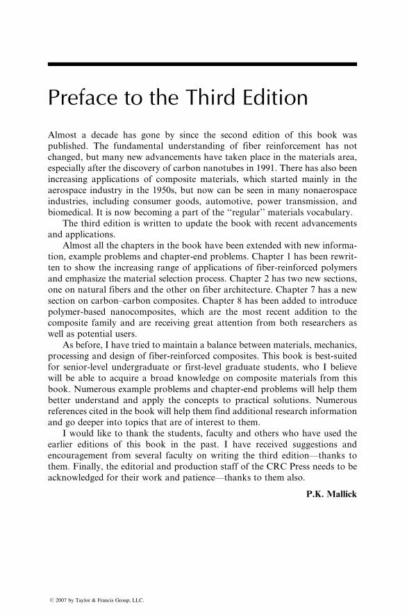
Preface to the Third Edition
Almost a decade has gone by since the second edition of this book was
published. The fundamental understanding of fiber reinforcement has not
changed, but many new advancements have taken place in the materials area,
especially after the discovery of carbon nanotubes in 1991. There has also been
increasing applications of composite materials, which started mainly in the
aerospace industry in the 1950s, but now can be seen in many nonaerospace
industries, including consumer goods, automotive, power transmission, and
biomedical. It is now becoming a part of the ‘‘regular’’ materials vocabulary.
The third edition is written to update the book with recent advancements
and applications.
Almost all the chapters in the book have been extended with new informa-
tion, example problems and chapter-end problems. Chapter 1 has been rewrit-
ten to show the increasing range of applications of fiber-reinforced polymers
and emphasize the material selection process. Chapter 2 has two new sections,
one on natural fibers and the other on fiber architecture. Chapter 7 has a new
section on carbon–carbon composites. Chapter 8 has been added to introduce
polymer-based nanocomposites, which are the most recent addition to the
composite family and are receiving great attention from both researchers as
well as potential users.
As before, I have tried to maintain a balance between materials, mechanics,
processing and design of fiber-reinforced composites. This book is best-suited
for senior-level undergraduate or first-level graduate students, who I believe
will be able to acquire a broad knowledge on composite materials from this
book. Numerous example problems and chapter-end problems will help them
better understand and apply the concepts to practical solutions. Numerous
references cited in the book will help them find additional research information
and go deeper into topics that are of interest to them.
I would like to thank the students, faculty and others who have used the
earlier editions of this book in the past. I have received suggestions and
encouragement from several faculty on writing the third edition—thanks to
them. Finally, the editorial and production staff of the CRC Press needs to be
acknowledged for their work and patience—thanks to them also.
P.K. Mallick
� 2007 by Taylor & Francis Group, LLC.

� 2007 by Taylor & Francis Group, LLC.

Author
P.K. Mallick is a professor in the Department of Mechanical Engineering and
the director of Interdisciplinary Programs at the University of Michigan-Dear-
born. He is also the director of the Center for Lightweighting Automotive
Materials and Processing at the University. His areas of research interest are
mechanical properties, design considerations, and manufacturing process
development of polymers, polymer matrix composites, and lightweight alloys.
He has published more than 100 technical articles on these topics, and also
authored or coauthored several books on composite materials, including
Composite Materials Handbook and Composite Materials Technology. He is a
fellow of the American Society of Mechanical Engineers. Dr Mallick received
his BE degree (1966) in mechanical engineering from Calcutta University,
India, and the MS (1970) and PhD (1973) degrees in mechanical engineering
from the Illinois Institute of Technology.
� 2007 by Taylor & Francis Group, LLC.

� 2007 by Taylor & Francis Group, LLC.
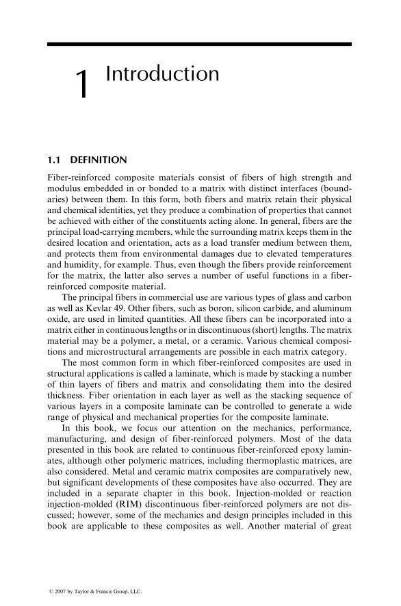
1 Introduction
� 2007 by Taylor & Fr
1.1 DEFINITION
Fiber-reinforced composite materials consist of fibers of high strength and
modulus embedded in or bonded to a matrix with distinct interfaces (bound-
aries) between them. In this form, both fibers and matrix retain their physical
and chemical identities, yet they produce a combination of properties that cannot
be achieved with either of the constituents acting alone. In general, fibers are the
principal load-carrying members, while the surrounding matrix keeps them in the
desired location and orientation, acts as a load transfer medium between them,
and protects them from environmental damages due to elevated temperatures
and humidity, for example. Thus, even though the fibers provide reinforcement
for the matrix, the latter also serves a number of useful functions in a fiber-
reinforced composite material.
The principal fibers in commercial use are various types of glass and carbon
as well as Kevlar 49. Other fibers, such as boron, silicon carbide, and aluminum
oxide, are used in limited quantities. All these fibers can be incorporated into a
matrix either in continuous lengths or in discontinuous (short) lengths. Thematrix
material may be a polymer, a metal, or a ceramic. Various chemical composi-
tions and microstructural arrangements are possible in each matrix category.
The most common form in which fiber-reinforced composites are used in
structural applications is called a laminate, which is made by stacking a number
of thin layers of fibers and matrix and consolidating them into the desired
thickness. Fiber orientation in each layer as well as the stacking sequence of
various layers in a composite laminate can be controlled to generate a wide
range of physical and mechanical properties for the composite laminate.
In this book, we focus our attention on the mechanics, performance,
manufacturing, and design of fiber-reinforced polymers. Most of the data
presented in this book are related to continuous fiber-reinforced epoxy lamin-
ates, although other polymeric matrices, including thermoplastic matrices, are
also considered. Metal and ceramic matrix composites are comparatively new,
but significant developments of these composites have also occurred. They are
included in a separate chapter in this book. Injection-molded or reaction
injection-molded (RIM) discontinuous fiber-reinforced polymers are not dis-
cussed; however, some of the mechanics and design principles included in this
book are applicable to these composites as well. Another material of great
ancis Group, LLC.
commer cial inter est is class ified as particulat e composi tes. The major con stitu-
ents in these composi tes are parti cles of mica , silica, glass spheres , calciu m
carbonat e, and others . In general , these particles do not contrib ute to the load-
carryin g cap acity of the material an d act more like a filler than a reinfo rceme nt
for the matr ix. Par ticulate compo sites, by thems elves , deserve a specia l atten -
tion an d are not address ed in this book.
Anothe r type of composi tes that have the potenti al of becoming an impor t-
ant mate rial in the future is the nano composi tes. Even though nan ocomposi tes
are in the early stage s of developm ent, they are now receiving a high de gree of
atten tion from a cademia as well as a large num ber of indust ries, includi ng
aerospac e, automot ive, and biomedi cal indust ries. The reinf orcement in nan o-
composi tes is either nan oparticles , na nofibers, or carbon nano tubes. The effect-
ive diameter of these reinforcements is of the order of 10� 9 m, whereas the effective
diame ter of the reinf orcement s used in traditi onal fiber -reinforce d composi tes
is of the ord er of 10 � 6 m. The nano composi tes are introdu ced in Chapt er 8.
1.2 GENERAL CHARACTERISTICS
Many fiber-re infor ced poly mers offer a combinat ion of stre ngth and modu lus
that are either compara ble to or better than man y tradi tional metallic mate rials.
Becau se of their low density, the strength–w eight rati os and modulus– weigh t
ratios of these comp osite mate rials are markedl y sup erior to those of metallic
mate rials (Table 1.1). In addition, fatigue stre ngth as well as fatigu e damage
tolerance of many composite laminates are excellent. For these reasons, fiber-
reinforced polymers have emerged as a major class of structural materials and
are either used or being considered for use as substitution for metals in many
weight-critical components in aerospace, automotive, and other industries.
Traditional structural metals, such as steel and aluminum alloys, are consid-
ered isotropic, since they exhibit equal or nearly equal properties irrespective of the
direction of measurement. In general, the properties of a fiber-reinforced compos-
ite depend strongly on the direction of measurement, and therefore, they are not
isotropic materials. For example, the tensile strength and modulus of a unidirec-
tionally oriented fiber-reinforced polymer aremaximumwhen these properties are
measured in the longitudinal direction of fibers. At any other angle of measure-
ment, these properties are lower. The minimum value is observed when they are
measured in the transverse direction of fibers, that is, at 908 to the longitudinal
direction. Similar angular dependence is observed for other mechanical and
thermal properties, such as impact strength, coefficient of thermal expansion
(CTE), and thermal conductivity. Bi- or multidirectional reinforcement yields a
more balanced set of properties. Although these properties are lower than the
longitudinal properties of a unidirectional composite, they still represent a
considerable advantage over common structural metals on a unit weight basis.
The design of a fiber-reinforced composite structure is considerably more
difficult than that of a metal structure, principally due to the difference in its
� 2007 by Taylor & Francis Group, LLC.
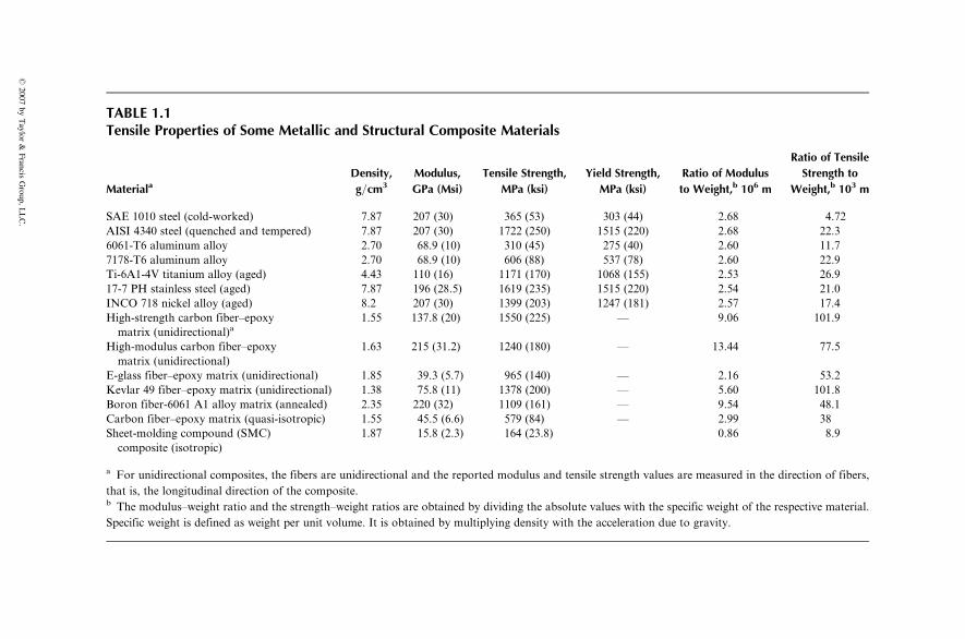
TABLE 1.1Tensile Properties of Some Metallic and Structural Composite Materials
MaterialaDensity,
g=cm3
Modulus,
GPa (Msi)
Tensile Strength,
MPa (ksi)
Yield Strength,
MPa (ksi)
Ratio of Modulus
to Weight,b 106 m
Ratio of Tensile
Strength to
Weight,b 103 m
SAE 1010 steel (cold-worked) 7.87 207 (30) 365 (53) 303 (44) 2.68 4.72
AISI 4340 steel (quenched and tempered) 7.87 207 (30) 1722 (250) 1515 (220) 2.68 22.3
6061-T6 aluminum alloy 2.70 68.9 (10) 310 (45) 275 (40) 2.60 11.7
7178-T6 aluminum alloy 2.70 68.9 (10) 606 (88) 537 (78) 2.60 22.9
Ti-6A1-4V titanium alloy (aged) 4.43 110 (16) 1171 (170) 1068 (155) 2.53 26.9
17-7 PH stainless steel (aged) 7.87 196 (28.5) 1619 (235) 1515 (220) 2.54 21.0
INCO 718 nickel alloy (aged) 8.2 207 (30) 1399 (203) 1247 (181) 2.57 17.4
High-strength carbon fiber–epoxy
matrix (unidirectional)a1.55 137.8 (20) 1550 (225) — 9.06 101.9
High-modulus carbon fiber–epoxy
matrix (unidirectional)
1.63 215 (31.2) 1240 (180) — 13.44 77.5
E-glass fiber–epoxy matrix (unidirectional) 1.85 39.3 (5.7) 965 (140) — 2.16 53.2
Kevlar 49 fiber–epoxy matrix (unidirectional) 1.38 75.8 (11) 1378 (200) — 5.60 101.8
Boron fiber-6061 A1 alloy matrix (annealed) 2.35 220 (32) 1109 (161) — 9.54 48.1
Carbon fiber–epoxy matrix (quasi-isotropic) 1.55 45.5 (6.6) 579 (84) — 2.99 38
Sheet-molding compound (SMC)
composite (isotropic)
1.87 15.8 (2.3) 164 (23.8) 0.86 8.9
a For unidirectional composites, the fibers are unidirectional and the reported modulus and tensile strength values are measured in the direction of fibers,
that is, the longitudinal direction of the composite.b The modulus–weight ratio and the strength–weight ratios are obtained by dividing the absolute values with the specific weight of the respective material.
Specific weight is defined as weight per unit volume. It is obtained by multiplying density with the acceleration due to gravity.
�2007
byTaylor
&Francis
Group,
LLC.
propert ies in diff erent directions. How ever, the noni sotropic nature of a fiber -
reinfo rced composi te material creates a uniqu e opportunit y of tailori ng its
propert ies accordi ng to the design requir ement s. This de sign flexibil ity can be
used to selective ly reinforce a structure in the directions of major stre sses,
increa se its stiffne ss in a pre ferred direct ion, fabri cate curved pan els withou t
any secondary form ing ope ration, or produce struc tures with zero coefficie nts
of thermal expansi on.
The use of fiber -reinforce d pol ymer as the skin mate rial and a lightw eight
core, such as aluminu m hone ycomb, plast ic foam, meta l foam, and balsa wood,
to build a san dwich beam, plate , or shell pro vides an other de gree of de sign
flexibil ity that is not easily ach ievable with metals. Such sand wich constru ction
can produ ce high stiffness with very little, if any, increase in weight. Ano ther
sandw ich constr uction in which the skin material is an aluminum alloy and the
core material is a fiber-reinforced polyme r has found wi despread use in aircraft s
and other app lications , prim arily due to their higher fatigue perfor mance and
damage toleran ce than alumi num alloys.
In additio n to the directional depend ence of prop erties, there are a numb er
of other differen ces betw een structural meta ls an d fiber -reinforce d compo sites.
For exampl e, metals in general exhibi t yield ing and plastic deformati on. M ost
fiber-re infor ced co mposi tes are elastic in their tensi le stress–s train charact er-
istics. How ever, the heterog eneo us nature of these material s pro vides mecha n-
isms for energy absorpt ion on a micro scopic scale, which is compara ble to the
yield ing process . Dep ending on the type and severity of exter nal loads, a
composi te laminate may exh ibit gradual deteri oration in propert ies but usually
would not fail in a catastrophic manner. Mechanisms of damage development
and growth in metal and composite structures are also quite different and must
be carefully considered during the design process when the metal is substituted
with a fiber-reinforced polymer.
Coefficient of thermal expansion (CTE) for many fiber-reinforced composites
is much lower than that for metals (Table 1.2). As a result, composite structures
may exhibit a better dimensional stability over a wide temperature range. How-
ever, the differences in thermal expansion betweenmetals and compositematerials
may create undue thermal stresses when they are used in conjunction, for example,
near an attachment. In some applications, such as electronic packaging, where
quick and effective heat dissipation is needed to prevent component failure or
malfunctioning due to overheating and undesirable temperature rise, thermal
conductivity is an important material property to consider. In these applications,
some fiber-reinforced composites may excel over metals because of the combin-
ation of their high thermal conductivity–weight ratio (Table 1.2) and lowCTE.On
the other hand, electrical conductivity of fiber-reinforced polymers is, in general,
lower than that of metals. The electric charge build up within the material because
of low electrical conductivity can lead to problems such as radio frequency
interference (RFI) and damage due to lightning strike.
� 2007 by Taylor & Francis Group, LLC.
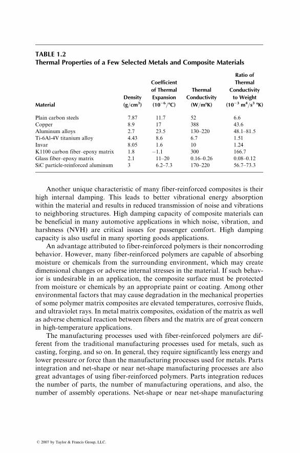
TABLE 1.2Thermal Properties of a Few Selected Metals and Composite Materials
Material
Density
(g=cm3)
Coefficient
of Thermal
Expansion
(10�6=8C)
Thermal
Conductivity
(W=m8K)
Ratio of
Thermal
Conductivity
to Weight
(10�3 m4=s3 8K)
Plain carbon steels 7.87 11.7 52 6.6
Copper 8.9 17 388 43.6
Aluminum alloys 2.7 23.5 130–220 48.1–81.5
Ti-6Al-4V titanium alloy 4.43 8.6 6.7 1.51
Invar 8.05 1.6 10 1.24
K1100 carbon fiber–epoxy matrix 1.8 �1.1 300 166.7
Glass fiber–epoxy matrix 2.1 11–20 0.16–0.26 0.08–0.12
SiC particle-reinforced aluminum 3 6.2–7.3 170–220 56.7–73.3
Another unique characteristic of many fiber-reinforced composites is their
high internal damping. This leads to better vibrational energy absorption
within the material and results in reduced transmission of noise and vibrations
to neighboring structures. High damping capacity of composite materials can
be beneficial in many automotive applications in which noise, vibration, and
harshness (NVH) are critical issues for passenger comfort. High damping
capacity is also useful in many sporting goods applications.
An advantage attributed to fiber-reinforced polymers is their noncorroding
behavior. However, many fiber-reinforced polymers are capable of absorbing
moisture or chemicals from the surrounding environment, which may create
dimensional changes or adverse internal stresses in the material. If such behav-
ior is undesirable in an application, the composite surface must be protected
from moisture or chemicals by an appropriate paint or coating. Among other
environmental factors that may cause degradation in the mechanical properties
of some polymer matrix composites are elevated temperatures, corrosive fluids,
and ultraviolet rays. In metal matrix composites, oxidation of the matrix as well
as adverse chemical reaction between fibers and the matrix are of great concern
in high-temperature applications.
The manufacturing processes used with fiber-reinforced polymers are dif-
ferent from the traditional manufacturing processes used for metals, such as
casting, forging, and so on. In general, they require significantly less energy and
lower pressure or force than the manufacturing processes used for metals. Parts
integration and net-shape or near net-shape manufacturing processes are also
great advantages of using fiber-reinforced polymers. Parts integration reduces
the number of parts, the number of manufacturing operations, and also, the
number of assembly operations. Net-shape or near net-shape manufacturing
� 2007 by Taylor & Francis Group, LLC.
process es, such as filament winding and pultr usion, used for making many
fiber-re infor ced pol ymer parts , eithe r reduce or eliminate the finishing ope r-
ations su ch as mach ining an d grinding , whi ch are co mmonl y req uired as
finishing operati ons for cast or forged meta llic pa rts.
1.3 APPLICATIONS
Com mercial and indu strial ap plications of fiber-re infor ced polyme r composi tes
are so varie d that it is impos sible to list them all. In this section, we highligh t
only the major struc tural applic ation areas, which include aircraft , space,
automot ive, spo rting goo ds, mari ne, and infr astructure. Fiber- reinforced poly-
mer co mposites are also used in electronics (e.g., print ed circuit boards) ,
buildi ng con struction (e.g ., floor be ams), furni ture (e.g., chair spring s), power
industry (e.g., transformer housing), oil industry (e.g., offshore oil platforms and
oil sucker rods used in lifting underground oil), medical industry (e.g., bone plates
for fract ure fixa tion, implan ts, and prosthe tics), and in many ind ustrial pro d-
ucts, such as step ladde rs, oxygen tanks, and power transmis sion shafts. Pote n-
tial use of fiber-re infor ced composi tes exists in many engineer ing fields. Putting
them to actual use requ ires ca reful de sign practice and approp riate pro cess
developm ent based on the unde rstand ing of their unique mechani cal, physica l,
and therm al charact eris tics.
1.3.1 AIRCRAFT AND MILITARY APPLICATIONS
The major struc tural applic ations for fiber -reinforce d composi tes are in the
field of milit ary and commer cial aircrafts, for which weight redu ction is critical
for higher speeds an d increa sed payloads . Eve r since the producti on applic ation
of boro n fiber -reinforce d epoxy skins for F-14 horizon tal stabi lizers in 1969,
the use of fiber-re inforced pol ymers has experi enced a steady grow th in the
aircraft indust ry. With the intro duction of carbo n fibers in the 1970s, carbon
fiber-re infor ced epoxy has become the primary mate rial in many win g, fusel age,
and empennage componen ts (Tab le 1.3). The struc tural integ rity an d durab ility
of these early components have built up con fidenc e in their perfor mance and
prompt ed developm ents of other structural aircr aft compon ents, resulting in an
increasing amount of composites being used in military aircrafts. For example,
the airframe of AV-8B, a vertical and short take-off and landing (VSTOL)
aircraft introduced in 1982, contains nearly 25% by weight of carbon fiber-
reinforced epoxy. The F-22 fighter aircraft also contains ~25% by weight of
carbon fiber-reinforced polymers; the other major materials are titanium (39%)
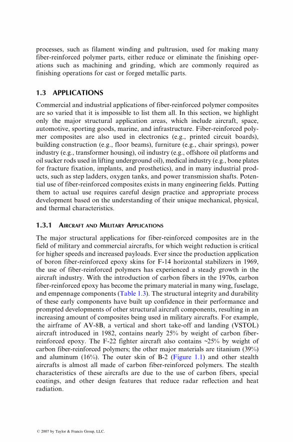
and aluminum (16%). The outer skin of B-2 (Figure 1.1) and other stealth
aircrafts is almost all made of carbon fiber-reinforced polymers. The stealth
characteristics of these aircrafts are due to the use of carbon fibers, special
coatings, and other design features that reduce radar reflection and heat
radiation.
� 2007 by Taylor & Francis Group, LLC.
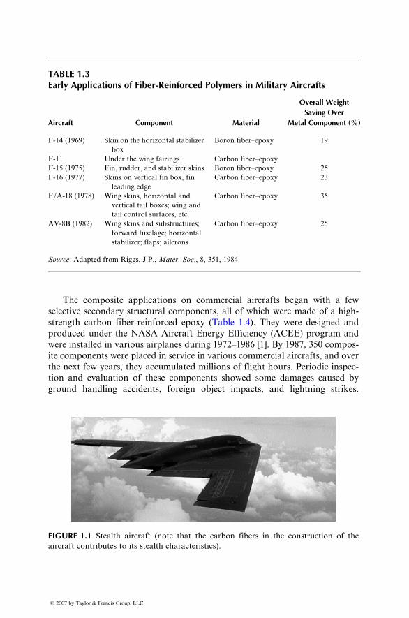
TABLE 1.3Early Applic ation s of Fiber -Reinfo rced Polym ers in Military Aircra fts
Aircraft Component Material
Overall Weight
Saving Over
Metal Component (%)
F-14 (1969) Skin on the horizontal stabilizer
box
Boron fiber–epoxy 19
F-11 Under the wing fairings Carbon fiber–epoxy
F-15 (1975) Fin, rudder, and stabilizer skins Boron fiber–epoxy 25
F-16 (1977) Skins on vertical fin box, fin
leading edge
Carbon fiber–epoxy 23
F=A-18 (1978) Wing skins, horizontal and
vertical tail boxes; wing and
tail control surfaces, etc.
Carbon fiber–epoxy 35
AV-8B (1982) Wing skins and substructures;
forward fuselage; horizontal
stabilizer; flaps; ailerons
Carbon fiber–epoxy 25
Source: Adapted from Riggs, J.P., Mater. Soc., 8, 351, 1984.
The compo site ap plications on co mmercial aircr afts be gan with a few
selective secondary structural componen ts, all of whi ch were made of a high -
strength carbon fiber -reinforce d epoxy (Table 1.4). They were designe d and
produc ed unde r the NASA Air craft Energy Efficiency (ACEE ) program and
were install ed in v arious airplane s during 197 2–1986 [1]. By 1 987, 350 comp os-
ite compon ents were placed in servi ce in various commer cial aircr afts, and over
the ne xt few years, they accumu lated milli ons of fligh t hours. Periodic inspec-
tion an d evaluation of these componen ts showe d some damages caused by
ground ha ndling acc idents, foreign object impac ts, and lightn ing strik es.
FIGURE 1.1 Stealth aircraft (note that the carbon fibers in the construction of the
aircraft contributes to its stealth characteristics).
� 2007 by Taylor & Francis Group, LLC.
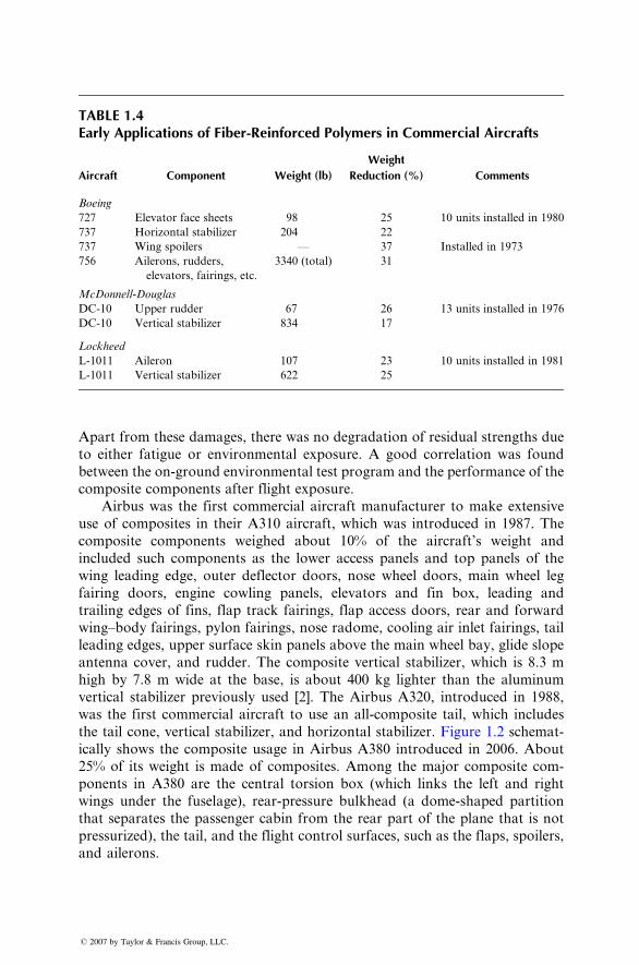
TABLE 1.4Early Applications of Fiber-Reinforced Polymers in Commercial Aircrafts
Aircraft Component Weight (lb)
Weight
Reduction (%) Comments
Boeing
727 Elevator face sheets 98 25 10 units installed in 1980
737 Horizontal stabilizer 204 22
737 Wing spoilers — 37 Installed in 1973
756 Ailerons, rudders,
elevators, fairings, etc.
3340 (total) 31
McDonnell-Douglas
DC-10 Upper rudder 67 26 13 units installed in 1976
DC-10 Vertical stabilizer 834 17
Lockheed
L-1011 Aileron 107 23 10 units installed in 1981
L-1011 Vertical stabilizer 622 25
Apart from these damages , there was no deg radation of resi dual stre ngths due
to eithe r fatigue or environm ental exposu re. A good correlati on was found
between the on-ground en vironmen tal test pro gram an d the performan ce of the
composi te co mponents after flight exp osure.
Airb us was the first co mmercial aircr aft manufa cturer to make extens ive
use of co mposites in their A310 aircraft , whi ch was introd uced in 1987. The
composi te co mponents wei ghed about 10% of the aircra ft’s weigh t and
included such co mponents as the lower access panels an d top panels of the
wing leading edge, outer de flector doors, nose wheel doors, main wheel leg
fairing doors, engine cowling panels, elevato rs and fin box, leadi ng and
traili ng edges of fins, flap track fair ings, flap access doors, rear and forward
wing–b ody fair ings, py lon fairings , nose rad ome, cooling air inlet fair ings, tail
leadi ng edges, uppe r surface skin panels above the main wheel ba y, glide slope
antenna co ver, an d rudder. The composi te vertical stabili zer, whi ch is 8.3 m
high by 7.8 m wid e at the base, is ab out 400 kg lighter than the aluminu m
vertical stabilizer previously used [2]. The Airbus A320, introduced in 1988,
was the first commercial aircraft to use an all-composite tail, which includes
the tail con e, vertical stabi lizer, a nd hor izonta l stabili zer. Figure 1.2 schema t-
ically shows the composite usage in Airbus A380 introduced in 2006. About
25% of its weight is made of composites. Among the major composite com-
ponents in A380 are the central torsion box (which links the left and right
wings under the fuselage), rear-pressure bulkhead (a dome-shaped partition
that separates the passenger cabin from the rear part of the plane that is not
pressurized), the tail, and the flight control surfaces, such as the flaps, spoilers,
and ailerons.
� 2007 by Taylor & Francis Group, LLC.
Outer wing
Ailerons
Flap track fairings
Outer flap
Radome
Fixed leading edgeupper and lower panels
Main landinggear leg fairing
door
Main andcenter landing
gear doors
Nose landinggear doors
Central torsion box
Pylonfairings,nacelles,
andcowlings
Pressurebulkhead
Keel beam
Tail cone
Verticalstabilizer
Horizontalstabilizer
Outer boxes
Over-wing panelBelly fairing skins
Trailing edge upper and lowerpanels and shroud box
Spoilers
Wing box
FIGURE 1.2 Use of fiber-reinforced polymer composites in Airbus 380.
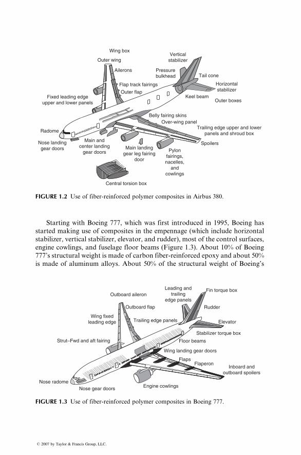
Starting with Boeing 777, which was first introduced in 1995, Boeing has
started making use of composites in the empennage (which include horizontal
stabilizer, vertical stabilizer, elevator, and rudder), most of the control surfaces,
engine cowlings, and fuselage floor beams (Figure 1.3). About 10% of Boeing
777’s structural weight is made of carbon fiber-reinforced epoxy and about 50%
is made of aluminum alloys. About 50% of the structural weight of Boeing’s
Rudder
Fin torque box
Elevator
Stabilizer torque box
Floor beams
Wing landing gear doors
FlapsFlaperon
Inboard andoutboard spoilers
Engine cowlingsNose gear doorsNose radome
Strut–Fwd and aft fairing
Wing fixedleading edge
Outboard aileron
Outboard flap
Trailing edge panels
Leading andtrailing
edge panels
FIGURE 1.3 Use of fiber-reinforced polymer composites in Boeing 777.
� 2007 by Taylor & Francis Group, LLC.
next line of airplanes, called the Boeing 787 Dreamliner, will be made of carbon
fiber-reinforced polymers. The other major materials in Boeing 787 will be
aluminum alloys (20%), titanium alloys (15%), and steel (10%). Two of the
major composite components in 787 will be the fuselage and the forward
section, both of which will use carbon fiber-reinforced epoxy as the major
material of construction.
There are several pioneering examples of using larger quantities of com-
posite materials in smaller aircrafts. One of these examples is the Lear Fan
2100, a business aircraft built in 1983, in which carbon fiber–epoxy and Kevlar
49 fiber–epoxy accounted for ~70% of the aircraft’s airframe weight. The
composite components in this aircraft included wing skins, main spar, fuselage,
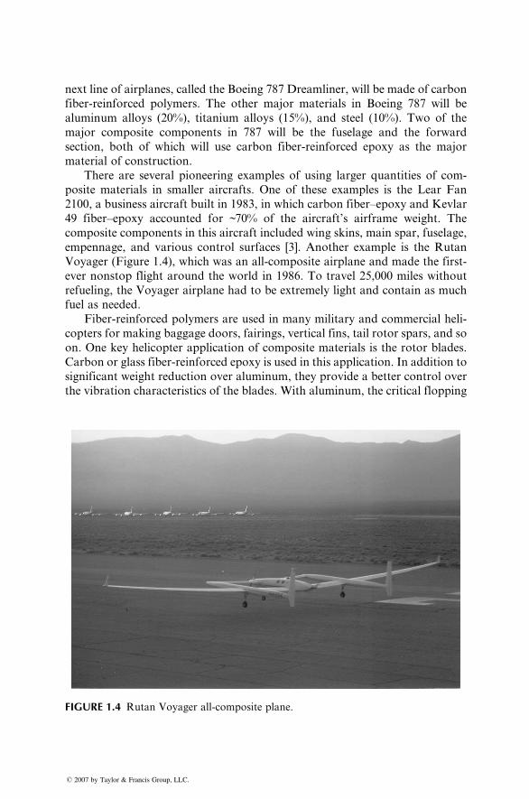
empennage, and various control surfaces [3]. Another example is the Rutan
Voyager (Figure 1.4), which was an all-composite airplane and made the first-
ever nonstop flight around the world in 1986. To travel 25,000 miles without
refueling, the Voyager airplane had to be extremely light and contain as much
fuel as needed.
Fiber-reinforced polymers are used in many military and commercial heli-
copters for making baggage doors, fairings, vertical fins, tail rotor spars, and so
on. One key helicopter application of composite materials is the rotor blades.
Carbon or glass fiber-reinforced epoxy is used in this application. In addition to
significant weight reduction over aluminum, they provide a better control over
the vibration characteristics of the blades. With aluminum, the critical flopping
FIGURE 1.4 Rutan Voyager all-composite plane.
� 2007 by Taylor & Francis Group, LLC.
and twisting frequencies are controlled principally by the classical method of
mass distribution [4]. With fiber-reinforced polymers, they can also be con-
trolled by varying the type, concentration, distribution, as well as orientation of
fibers along the blade’s chord length. Another advantage of using fiber-
reinforced polymers in blade applications is the manufacturing flexibility of
these materials. The composite blades can be filament-wound or molded into
complex airfoil shapes with little or no additional manufacturing costs, but
conventional metal blades are limited to shapes that can only be extruded,
machined, or rolled.
The principal reason for using fiber-reinforced polymers in aircraft and
helicopter applications is weight saving, which can lead to significant fuel
saving and increase in payload. There are several other advantages of using
them over aluminum and titanium alloys.
1. Reduction in the number of components and fasteners, which results in
a reduction of fabrication and assembly costs. For example, the vertical
fin assembly of the Lockheed L-1011 has 72% fewer components and
83% fewer fasteners when it is made of carbon fiber-reinforced epoxy
than when it is made of aluminum. The total weight saving is 25.2%.
2. Higher fatigue resistance and corrosion resistance, which result in a
reduction of maintenance and repair costs. For example, metal fins
used in helicopters flying near ocean coasts use an 18 month repair
cycle for patching corrosion pits. After a few years in service, the
patches can add enough weight to the fins to cause a shift in the center
of gravity of the helicopter, and therefore the fin must then be rebuilt or
replaced. The carbon fiber-reinforced epoxy fins do not require any
repair for corrosion, and therefore, the rebuilding or replacement cost
is eliminated.
3. The laminated construction used with fiber-reinforced polymers allows
the possibility of aeroelastically tailoring the stiffness of the airframe
structure. For example, the airfoil shape of an aircraft wing can be
controlled by appropriately adjusting the fiber orientation angle in
each lamina and the stacking sequence to resist the varying lift and
drag loads along its span. This produces a more favorable airfoil
shape and enhances the aerodynamic characteristics critical to the air-
craft’s maneuverability.
The key limiting factors in using carbon fiber-reinforced epoxy in aircraft
structures are their high cost, relatively low impact damage tolerance (from
bird strikes, tool drop, etc.), and susceptibility to lightning damage. When they
are used in contact with aluminum or titanium, they can induce galvanic
corrosion in the metal components. The protection of the metal components
from corrosion can be achieved by coating the contacting surfaces with a
corrosion-inhibiting paint, but it is an additional cost.
� 2007 by Taylor & Francis Group, LLC.
1.3.2 SPACE APPLICATIONS
Weight reduction is the primary reason for using fiber-reinforced composites in
many space vehicles [5]. Among the various applications in the structure of
space shuttles are the mid-fuselage truss structure (boron fiber-reinforced alu-
minum tubes), payload bay door (sandwich laminate of carbon fiber-reinforced
epoxy face sheets and aluminum honeycomb core), remote manipulator arm
(ultrahigh-modulus carbon fiber-reinforced epoxy tube), and pressure vessels
(Kevlar 49 fiber-reinforced epoxy).
In addition to the large structural components, fiber-reinforced polymers are
used for support structures for many smaller components, such as solar arrays,
antennas, optical platforms, and so on [6]. A major factor in selecting them for
these applications is their dimensional stability over a wide temperature range.
Many carbon fiber-reinforced epoxy laminates can be ‘‘designed’’ to produce a
CTE close to zero. Many aerospace alloys (e.g., Invar) also have a comparable
CTE. However, carbon fiber composites have a much lower density, higher
strength, as well as a higher stiffness–weight ratio. Such a unique combination
ofmechanical properties andCTEhas led to a number of applications for carbon
fiber-reinforced epoxies in artificial satellites. One such application is found in
the support structure for mirrors and lenses in the space telescope [7]. Since the
temperature in space may vary between �1008C and 1008C, it is critically
important that the support structure be dimensionally stable; otherwise, large
changes in the relative positions of mirrors or lenses due to either thermal
expansion or distortion may cause problems in focusing the telescope.
Carbon fiber-reinforced epoxy tubes are used in building truss structures for
low earth orbit (LEO) satellites and interplanetary satellites. These truss structures
support optical benches, solar array panels, antenna reflectors, and othermodules.
Carbon fiber-reinforced epoxies are preferred over metals or metal matrix com-
posites because of their lower weight as well as very lowCTE.However, one of the
major concerns with epoxy-based composites in LEO satellites is that they are
susceptible to degradation due to atomic oxygen (AO) absorption from the
earth’s rarefied atmosphere. This problem is overcome by protecting the tubes
from AO exposure, for example, by wrapping them with thin aluminum foils.
Other concerns for using fiber-reinforced polymers in the space environ-
ment are the outgassing of the polymer matrix when they are exposed to
vacuum in space and embrittlement due to particle radiation. Outgassing can
cause dimensional changes and embrittlement may lead to microcrack forma-
tion. If the outgassed species are deposited on the satellite components, such as
sensors or solar cells, their function may be seriously degraded [8].
1.3.3 AUTOMOTIVE APPLICATIONS
Applications of fiber-reinforced composites in the automotive industry can be
classified into three groups: body components, chassis components, and engine
� 2007 by Taylor & Francis Group, LLC.
compon ents. Exteri or body components , such as the hood or door pa nels,
requir e high sti ffness and damage toler ance (dent resi stance ) as well as a
‘‘Class A’’ surfa ce fini sh for app earance. The compo site mate rial used for
these compon ents is E-glas s fiber -reinforce d sheet moldi ng compound (SMC )
composi tes, in which discont inuous glass fibers (typi cally 25 mm in lengt h) are
randoml y dispersed in a poly ester or a vinyl ester resi n. E-g lass fiber is used
instead of carbon fiber because of its signi fican tly low er cost. The manufa ctur-
ing process used for making SMC pa rts is ca lled compres sion moldi ng. One of
the design requir ement s for many exter ior body panels is the ‘‘Cla ss A’’ surface
finish, which is not easily ach ieved with compres sion- molded SMC. Thi s prob -
lem is usu ally overcome by in-mo ld coati ng of the exter ior molded surface with
a flex ible resi n. How ever, there are many unde rbody and under-th e-hood co m-
ponen ts in whi ch the exter nal appearance is not critical . Example s of such
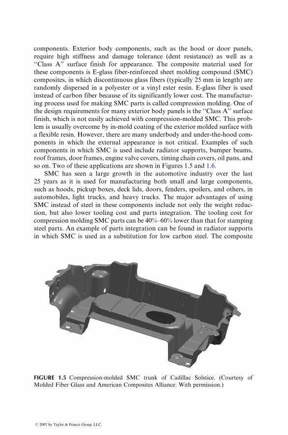
components in which SMC is used include radiator supports, bumper beams,
roof frames, door frames, engine valve covers, timing chain covers, oil pans, and
so on. Two of these ap plications are shown in Figures 1.5 and 1.6.
SMC has seen a large growth in the automotive industry over the last
25 years as it is used for manufacturing both small and large components,
such as hoods, pickup boxes, deck lids, doors, fenders, spoilers, and others, in
automobiles, light trucks, and heavy trucks. The major advantages of using
SMC instead of steel in these components include not only the weight reduc-
tion, but also lower tooling cost and parts integration. The tooling cost for
compression molding SMC parts can be 40%–60% lower than that for stamping
steel parts. An example of parts integration can be found in radiator supports
in which SMC is used as a substitution for low carbon steel. The composite
FIGURE 1.5 Compression-molded SMC trunk of Cadillac Solstice. (Courtesy of
Molded Fiber Glass and American Composites Alliance. With permission.)
� 2007 by Taylor & Francis Group, LLC.
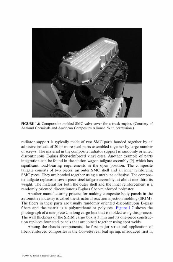
FIGURE 1.6 Compression-molded SMC valve cover for a truck engine. (Courtesy of
Ashland Chemicals and American Composites Alliance. With permission.)
radiato r supp ort is typic ally made of two SMC parts bonde d toget her by an
adhesiv e inst ead of 20 or more steel parts assem bled toget her by large numb er
of screws. The material in the c omposi te radiat or sup port is randoml y or iented
discont inuous E-glas s fiber -reinforce d vinyl ester. Anothe r exampl e of parts
integ ration can be foun d in the stat ion wagon tailgat e assem bly [9], whic h ha s
signifi cant load-be aring requir ement s in the open posit ion. The co mposite
tailgat e consis ts of two pieces , an outer SMC shell and an inner reinfo rcing
SMC piece. They are bonde d toget her us ing a urethane a dhesive . The co mpos-
ite tailgat e replac es a seven-p iece steel tailgate assem bly, at abo ut one -third its
weight. The material for both the outer shell and the inner reinf orcement is a
randoml y oriented discon tinuous E-glas s fiber-re inforced polyest er.
Anothe r manufa cturin g process for making co mposite body panels in the
automot ive indust ry is called the struc tural react ion injec tion moldi ng (SRI M).
The fiber s in these parts are usuall y randoml y orient ed discont inuous E-glas s
fibers and the matr ix is a polyu rethane or polyurea . Figure 1.7 shows the
photograp h of a one-pie ce 2 m long cargo box that is molded using this process .
The wal l thickne ss of the SRIM cargo box is 3 mm and its one-pie ce constr uc-
tion replaces four steel panels that are joined together using spot welds.
Among the chassis components, the first major structural application of
fiber-reinforced composites is the Corvette rear leaf spring, introduced first in
� 2007 by Taylor & Francis Group, LLC.
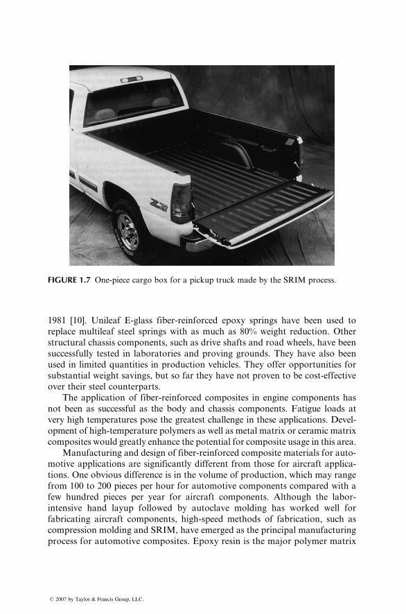
FIGURE 1.7 One-piece cargo box for a pickup truck made by the SRIM process.
1981 [10]. Unileaf E-glass fiber-reinforced epoxy springs have been used to
replace multileaf steel springs with as much as 80% weight reduction. Other
structural chassis components, such as drive shafts and road wheels, have been
successfully tested in laboratories and proving grounds. They have also been
used in limited quantities in production vehicles. They offer opportunities for
substantial weight savings, but so far they have not proven to be cost-effective
over their steel counterparts.
The application of fiber-reinforced composites in engine components has
not been as successful as the body and chassis components. Fatigue loads at
very high temperatures pose the greatest challenge in these applications. Devel-
opment of high-temperature polymers as well as metal matrix or ceramic matrix
composites would greatly enhance the potential for composite usage in this area.
Manufacturing and design of fiber-reinforced composite materials for auto-
motive applications are significantly different from those for aircraft applica-
tions. One obvious difference is in the volume of production, which may range
from 100 to 200 pieces per hour for automotive components compared with a
few hundred pieces per year for aircraft components. Although the labor-
intensive hand layup followed by autoclave molding has worked well for
fabricating aircraft components, high-speed methods of fabrication, such as
compression molding and SRIM, have emerged as the principal manufacturing
process for automotive composites. Epoxy resin is the major polymer matrix
� 2007 by Taylor & Francis Group, LLC.
used in aerospace c omposites; however , the curing time for e poxy r esin is very
long, which means t he produc t ion tim e f or epoxy matrix composites is also
very long. For this reason, epoxy i s not considered the primary matrix
m at e ri al in aut o mot ive composit es. T he polymer matrix used in automotive
applications is either a polyester, a vi nyl ester, or polyurethane, all of which
require significantly l ower curing time than epox y. The high cost of carbon
fibers has prevented their use in the cost-cons cious aut omot ive industry.
Ins t ead of carbo n f ibers, E-glass f ibers are used in automotive composites
because of their significantly lower cost. Even with E-glass fiber-reinforced
composi tes, the cost-eff ectiven ess issue has remai ned pa rticular ly critical , since
the basic material of constru ction in pr esent-day au tomobi les is low-car bon
steel, whi ch is much less expensi ve than most fiber -reinforce d c omposi tes on a
unit wei ght ba sis.
Altho ugh glass fiber-re infor ced polyme rs are the prim ary composi te mate r-
ials used in today’s automobi les, it is wel l recogni zed that signi fican t vehicle
weight reduc tion ne eded for impr oved fuel efficie ncy can be achieve d only wi th
carbon fiber-re infor ced polyme rs, since they have mu ch higher strength–w eight
and modulus– weig ht ratios. The problem is that the cu rrent carbon fiber price,
at $16 =kg or high er, is not con sidered cost-eff ective for automot ive applic a-
tions . Never thele ss, many attemp ts ha ve been made in the pa st to manufa cture
struc tural automotive parts using carbo n fiber -reinforce d polyme rs; unfortu -
natel y most of them did not go beyond the stages of prototyping and structural
testing. Recently, several high-priced vehicles have started using carbon fiber-
reinforced polymers in a few selected components. One recent example of this is
seen in the BMW M6 roof panel (Figure 1.8), which was prod uced by a pro cess
called resin trans fer moldin g (RTM) . This pa nel is twice as thick as a c ompar-
able steel panel, but 5.5 kg lighter. One ad ded be nefit of redu cing the weigh t of
the roof panel is that it slightl y low ers the cen ter of gravity of the vehicle, which
is impor tant for sports cou pe.
Fiber- reinfo rced c omposi tes have become the material of choice in motor
sports wher e lightw eight struc ture is used for gaining co mpetitiv e ad vantage of
higher speed [11] and cost is not a major mate rial selec tion de cision facto r. The
first major app lication of co mposites in race cars was in the 1950s when glass
fiber-re infor ced polyest er was intr oduced as replac ement for aluminum body
panels. Today , the composi te mate rial used in race cars is most ly carbo n fiber -
reinforced epoxy. All major body, chassis, interior, and suspension components
in today’ s For mula 1 race cars use carbon fiber-re inforced ep oxy. Fi gure 1.9
shows an example of carbon fiber-reinforced composite used in the gear box
and rear suspension of a Formula 1 race car. One major application of carbon
fiber-reinforced epoxy in Formula 1 cars is the survival cell, which protects the
driver in the event of a crash. The nose cone located in front of the survival cell
is also made of carbon fiber-reinforced epoxy. Its controlled crush behavior is
also critical to the survival of the driver.
� 2007 by Taylor & Francis Group, LLC.
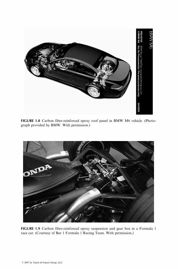
FIGURE 1.8 Carbon fiber-reinforced epoxy roof panel in BMW M6 vehicle. (Photo-
graph provided by BMW. With permission.)
FIGURE 1.9 Carbon fiber-reinforced epoxy suspension and gear box in a Formula 1
race car. (Courtesy of Bar 1 Formula 1 Racing Team. With permission.)
� 2007 by Taylor & Francis Group, LLC.
1.3.4 S PORTING GOODS A PPLICATIONS
Fiber- reinforced polyme rs are extens ivel y used in sporti ng goo ds ranging
from tennis rackets to athletic sho es (Tab le 1.5) and are selected over such
traditi onal mate rials as wood, metals, and leat her in many of these applic ations
[12]. The advantag es of using fiber-re inforced polyme rs a re wei ght reductio n,
vibration damping , and de sign flexibil ity. W eight reductio n ach ieved by subs t i -
tuting carbon fiber-reinforced epoxies for metals leads t o higher speeds and
quick maneuvering i n competitive sports, such as bicycle races and canoe races.
In some applications, such as tennis rac kets or snow skis, s andwich construc-
tions of carbon or boron fibe r-reinforced epoxies as the skin material and a
sof t, l ighter weight urethane foam as the core m aterial produces a higher w eight
reduction without sacrificing s tiffness . Faster damping of vibrations provided
by fiber-reinforced polymers r educes th e shock t ransmitted to the player’s arm
in tennis or racket ball games and provides a better ‘‘feel’’ for the ball. In
archery bows and pole-vault poles, the hi gh st if fnes s–wei ght r at io of f iber -
reinforced composites is used to store high e lastic energy pe r uni t w ei ght, which
helps i n pr opelling the arrow ov er a longer distance or the pole-vaulter to j ump
a greater height. Some of these applications are described later.
Bicycle frames for racing bikes today are mostly made of carbon fiber-
reinforced epoxy tubes, fitted together by titanium fittings and inserts. An
exampl e is sho wn in Figu re 1.10. The prim ary purp ose of using carbon fibers is
TABLE 1.5Applications of Fiber-Reinforced Polymers
in Sporting Goods
Tennis rackets
Racket ball rackets
Golf club shafts
Fishing rods
Bicycle frames
Snow and water skis
Ski poles, pole vault poles
Hockey sticks
Baseball bats
Sail boats and kayaks
Oars, paddles
Canoe hulls
Surfboards, snow boards
Arrows
Archery bows
Javelins
Helmets
Exercise equipment
Athletic shoe soles and heels
� 2007 by Taylor & Francis Group, LLC.
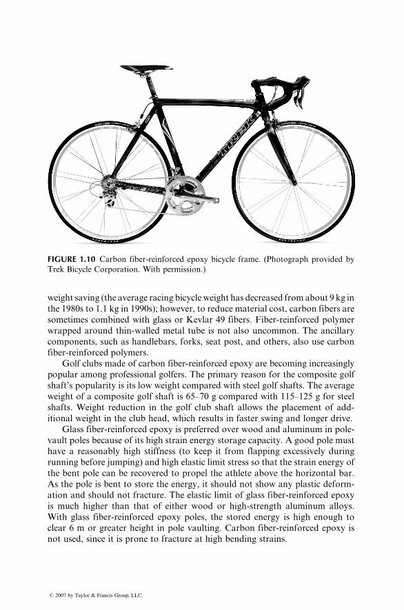
FIGURE 1.10 Carbon fiber-reinforced epoxy bicycle frame. (Photograph provided by
Trek Bicycle Corporation. With permission.)
weight saving (the average racing bicycle weight has decreased from about 9 kg in
the 1980s to 1.1 kg in 1990s); however, to reduce material cost, carbon fibers are
sometimes combined with glass or Kevlar 49 fibers. Fiber-reinforced polymer
wrapped around thin-walled metal tube is not also uncommon. The ancillary
components, such as handlebars, forks, seat post, and others, also use carbon
fiber-reinforced polymers.
Golf clubs made of carbon fiber-reinforced epoxy are becoming increasingly
popular among professional golfers. The primary reason for the composite golf
shaft’s popularity is its low weight compared with steel golf shafts. The average
weight of a composite golf shaft is 65–70 g compared with 115–125 g for steel
shafts. Weight reduction in the golf club shaft allows the placement of add-
itional weight in the club head, which results in faster swing and longer drive.
Glass fiber-reinforced epoxy is preferred over wood and aluminum in pole-
vault poles because of its high strain energy storage capacity. A good pole must
have a reasonably high stiffness (to keep it from flapping excessively during
running before jumping) and high elastic limit stress so that the strain energy of
the bent pole can be recovered to propel the athlete above the horizontal bar.
As the pole is bent to store the energy, it should not show any plastic deform-
ation and should not fracture. The elastic limit of glass fiber-reinforced epoxy
is much higher than that of either wood or high-strength aluminum alloys.
With glass fiber-reinforced epoxy poles, the stored energy is high enough to
clear 6 m or greater height in pole vaulting. Carbon fiber-reinforced epoxy is
not used, since it is prone to fracture at high bending strains.
� 2007 by Taylor & Francis Group, LLC.
Glass and carbon fiber-reinforced epoxy fishing rods are very common
today, even though traditional materials, such as bamboo, are still used. For
fly-fishing rods, carbon fiber-reinforced epoxy is preferred, since it produces a
smaller tip deflection (because of its higher modulus) and ‘‘wobble-free’’ action
during casting. It also dampens the vibrations more rapidly and reduces the
transmission of vibration waves along the fly line. Thus, the casting can be
longer, quieter, and more accurate, and the angler has a better ‘‘feel’’ for the
catch. Furthermore, carbon fiber-reinforced epoxy rods recover their original
shape much faster than the other rods. A typical carbon fiber-reinforced epoxy
rod of No. 6 or No. 7 line weighs only 37 g. The lightness of these rods is also a
desirable feature to the anglers.
1.3.5 MARINE APPLICATIONS
Glass fiber-reinforced polyesters have been used in different types of boats (e.g.,
sail boats, fishing boats, dinghies, life boats, and yachts) ever since their
introduction as a commercial material in the 1940s [13]. Today, nearly 90% of
all recreational boats are constructed of either glass fiber-reinforced polyester or
glass fiber-reinforced vinyl ester resin. Among the applications are hulls, decks,
and various interior components. The manufacturing process used for making a
majority of these components is called contact molding. Even though it is
a labor-intensive process, the equipment cost is low, and therefore it is afford-
able to many of the small companies that build these boats. In recent years,
Kevlar 49 fiber is replacing glass fibers in some of these applications because of its
higher tensile strength–weight and modulus–weight ratios than those of glass
fibers. Among the application areas are boat hulls, decks, bulkheads, frames,
masts, and spars. The principal advantage is weight reduction, which translates
into higher cruising speed, acceleration, maneuverability, and fuel efficiency.
Carbon fiber-reinforced epoxy is used in racing boats in which weight
reduction is extremely important for competitive advantage. In these boats,
the complete hull, deck, mast, keel, boom, and many other structural compon-
ents are constructed using carbon fiber-reinforced epoxy laminates and sand-
wich laminates of carbon fiber-reinforced epoxy skins with either honeycomb
core or plastic foam core. Carbon fibers are sometimes hybridized with other
lower density and higher strain-to-failure fibers, such as high-modulus poly-
ethylene fibers, to improve impact resistance and reduce the boat’s weight.
The use of composites in naval ships started in the 1950s and has grown
steadily since then [14]. They are used in hulls, decks, bulkheads, masts,
propulsion shafts, rudders, and others of mine hunters, frigates, destroyers,
and aircraft carriers. Extensive use of fiber-reinforced polymers can be seen in
Royal Swedish Navy’s 72 m long, 10.4 m wide Visby-class corvette, which is the
largest composite ship in the world today. Recently, the US navy has commis-
sioned a 24 m long combat ship, called Stiletto, in which carbon fiber-
reinforced epoxy will be the primary material of construction. The selection
� 2007 by Taylor & Francis Group, LLC.
of carbon fiber -reinforce d ep oxy is based on the design requir ements of light -
weight and high stre ngth need ed for high speed , maneuver ability, ran ge, and
payload cap acity of these ships. Their stealth cha racteris tics are also impor tant
in mini mizing radar reflecti on.
1.3.6 INFRASTRUCTURE
Fiber- reinforced polyme rs have a great potential for replac ing reinforced con -
crete an d steel in bridges , buildi ngs, and other civil infrastr uctures [15]. The
princip al reason for selec ting these compo sites is their corrosio n resi stance,
which leads to longer life and low er maint enance an d repair co sts. Reinforced
concret e bridges tend to deteriorat e after severa l ye ars of use becau se of
corrosi on of steel -reinforci ng bars (rebars) used in their constr uction. The
corrosi on pro blem is exacerba ted be cause of deicing salt sp read on the bridge
road surface in wi nter months in many parts of the world. The deterio ration
can become so severe that the concret e su rrounding the steel rebars can start to
crack (due to the expan sion of corrodi ng steel bars) and ultimat ely fall off, thus
weake ning the struc ture’s load-c arryi ng capacit y. The co rrosion problem does
not exist wi th fiber-re inforced polyme rs. Anothe r ad vantage of using fiber-
reinforced polyme rs for large bridge struc tures is their light weight, whi ch
means low er dead weight for the bridge, easie r trans portation from the pro -
duction fact ory (where the c omposi te struc ture can be prefabr icated) to the
bridge locat ion, easie r ha uling and inst allation, and less injur ies to pe ople in
case of an earthqua ke . W ith lightw eight constr uction, it is also possibl e to
design bridges with longer span between the suppo rts.
One of the early demonst ration s of a c omposi te traffic bridge was made in
1995 by Lockhe ed Marti n Resea rch Laborator ies in Palo Alto, Cal ifornia. The
bridge deck was a 9 m long 3 5.4 m wid e qua rter-sca le section and the mate rial
selected was E-glas s fiber -reinforce d polyester. The composi te deck was a
sandw ich lamin ate of 15 mm thick E-glas s fiber-re infor ced poly ester face sheets
and a seri es of E-glas s fiber-re infor ced pol yester tubes bonde d toget her to form
the co re. The deck was suppo rted on three U-s haped beams made of E-glass
fabric-r einfor ced polyest er. The design was mod ular and the compon ents were
stacka ble, which sim plified both their trans portation and assem bly.
In recent years, a number of composite bridge decks have been constructed
and commissioned for service in the United States and Canada. The Wickwire
Run Bridge located in West Virginia, United States is an example of one such
construction. It consists of full-depth hexagonal and half-depth trapezoidal
profiles made of glass fabric-reinforced polyester matrix. The profiles are
supported on steel beams. The road surface is a polymer-modified concrete.
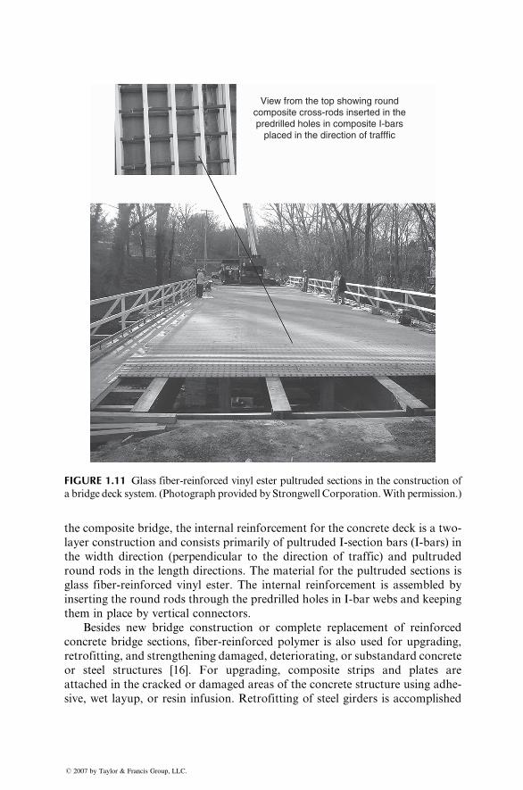
Anothe r ex ample of a composi te bridge structure is sho wn in Figure 1.11,
which replaced a 73 year old concrete bridge with steel rebars. The replacement
was necessary because of the severe deterioration of the concrete deck, which
reduced its load rating from 10 to only 4.3 t and was posing safety concerns. In
� 2007 by Taylor & Francis Group, LLC.
View from the top showing roundcomposite cross-rods inserted in thepredrilled holes in composite I-bars
placed in the direction of trafffic
FIGURE 1.11 Glass fiber-reinforced vinyl ester pultruded sections in the construction of
a bridge deck system. (Photograph provided by Strongwell Corporation.With permission.)
the composite bridge, the internal reinforcement for the concrete deck is a two-
layer construction and consists primarily of pultruded I-section bars (I-bars) in
the width direction (perpendicular to the direction of traffic) and pultruded
round rods in the length directions. The material for the pultruded sections is
glass fiber-reinforced vinyl ester. The internal reinforcement is assembled by
inserting the round rods through the predrilled holes in I-bar webs and keeping
them in place by vertical connectors.
Besides new bridge construction or complete replacement of reinforced
concrete bridge sections, fiber-reinforced polymer is also used for upgrading,
retrofitting, and strengthening damaged, deteriorating, or substandard concrete
or steel structures [16]. For upgrading, composite strips and plates are
attached in the cracked or damaged areas of the concrete structure using adhe-
sive, wet layup, or resin infusion. Retrofitting of steel girders is accomplished
� 2007 by Taylor & Francis Group, LLC.
by attaching composite plates to their flanges, which improves the flange stiff-
ness and strength. The strengthening of reinforced concrete columns in earth-
quake prone areas is accomplished by wrapping them with fiber-reinforced
composite jackets in which the fibers are primarily in the hoop direction. They
are found to be better than steel jackets, since, unlike steel jackets, they do not
increase the longitudinal stiffness of the columns. They are also much easier to
install and they do not corrode like steel.
1.4 MATERIAL SELECTION PROCESS
Material selection is one of the most important and critical steps in the
structural or mechanical design process. If the material selection is not done
properly, the design may show poor performance; may require frequent main-
tenance, repair, or replacement; and in the extreme, may fail, causing damage,
injuries, or fatalities. The material selection process requires the knowledge of
the performance requirements of the structure or component under consider-
ation. It also requires the knowledge of
1. Types of loading, for example, axial, bending, torsion, or combination
thereof
2. Mode of loading, for example, static, fatigue, impact, shock, and so on
3. Service life
4. Operating or service environment, for example, temperature, humidity
conditions, presence of chemicals, and so on
5. Other structures or components with which the particular design under
consideration is required to interact
6. Manufacturing processes that can be used to produce the structure or
the component
7. Cost, which includes not only the material cost, but also the cost of
transforming the selected material to the final product, that is, the
manufacturing cost, assembly cost, and so on
The material properties to consider in the material selection process depend on
the performance requirements (mechanical, thermal, etc.) and the possible
mode or modes of failure (e.g., yielding, brittle fracture, ductile failure, buck-
ling, excessive deflection, fatigue, creep, corrosion, thermal failure due to over-
heating, etc.). Two basic material properties often used in the preliminary
selection of materials for a structural or mechanical design are the modulus
and strength. For a given design, the modulus is used for calculating the
deformation, and the strength is used for calculating the maximum load-carrying
capacity. Which property or properties should be considered in making a
preliminary material selection depends on the application and the possible
failure modes. For example, yield strength is considered if the design of
a structure requires that no permanent deformation occurs because of the
� 2007 by Taylor & Francis Group, LLC.
applic ation of the load . If, on the other hand , there is a possibi lity of brittle
failure becau se of the influ ence of the operatin g environm ental co ndition s,
fracture toughn ess is the mate rial propert y to consider .
In many designs the perfor mance requir ement may include stiffne ss, which
is define d as load per unit deform ation. Stiffnes s should not be co nfused wi th
modulus, since stiffne ss depen ds not only on the mo dulus of the mate rial
(which is a mate rial prop erty), but also on the design. For exampl e, the stiffne ss
of a stra ight be am with soli d circular c ross secti on de pends not only on the
modulus of the mate rial, but also on its length, diame ter, and how it is
suppo rted (i.e., bounda ry co ndition s). For a given beam lengt h and supp ort
cond itions, the stiffne ss of the beam with solid circul ar cross section is prop or-
tional to Ed 4, wher e E is the modulus of the beam mate rial and d is its diame ter.
Therefor e, the stiffness of this beam can be increa sed by eithe r selec ting a high er
modulus mate rial, or increa sing the diame ter, or doing both. Increas ing the
diame ter is more effe ctive in increa sing the stiffne ss, but it also increa ses
the weigh t and c ost of the beam. In some designs , it may be pos sible to increa se
the be am stiffne ss by incorpora ting other design feat ures, such as ribs, or by
using a sand wich constr uction.
In de signing structures wi th minimum mass or minimum cost, mate rial
propert ies must be combined wi th mass density ( r), co st per unit mass ($ =kg),and so on. For exampl e, if the de sign object ive for a tension linkag e or a tie ba r
is to meet the stiffne ss perfor mance criteri on wi th minimum mass , the mate rial
selection criterion involves not just the tensile modulus of the material (E), but
also the modulus–density ratio (E=r). The modulus–density ratio is a material
index, and the material that produces the highest value of this material index
should be selected for minimum mass design of the tension link. The material
index de pends on the application and the design object ive. Table 1.6 lis ts the
material indices for minimum mass design of a few simple structures.
As an example of the use of the material index in preliminary material
selection, consider the carbon fiber–epoxy quasi-isotropic laminate in Table 1.1.
Thin laminates of this type are considered well-suited for many aerospace
applications [1], since they exhibit equal elastic properties (e.g., modulus) in
all directions in the plane of load application. The quasi-isotropic laminate
in Table 1.1 has an elastic modulus of 45.5 GPa, which is 34% lower than that
of the 7178-T6 aluminum alloy and 59% lower than that of the Ti-6 Al-4V
titanium alloy. The aluminum and the titanium alloys are the primary metallic
alloys used in the construction of civilian and military aircrafts. Even though
the quasi-isotropic carbon fiber–epoxy composite laminate has a lower modulus,
it is a good candidate for substituting the metallic alloys in stiffness-critical
aircraft structures. This is because the carbon fiber–epoxy quasi-isotropic
laminate has a superior material index in minimum mass design of stiffness-
critical structures. This can be easily verified by comparing the values of
the material index E1=3
r of all three materials, assuming that the structure can
be modeled as a thin plate under bending load.
� 2007 by Taylor & Francis Group, LLC.
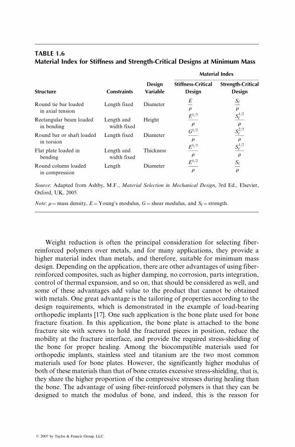
TABLE 1.6Material Index for Stiffness and Strength-Critical Designs at Minimum Mass
Structure Constraints
Design
Variable
Material Index
Stiffness-Critical
Design
Strength-Critical
Design
Round tie bar loaded
in axial tension
Length fixed DiameterE
r
Sf
r
Rectangular beam loaded
in bending
Length and
width fixed
HeightE1=3
r
S1=2f
r
Round bar or shaft loaded
in torsion
Length fixed DiameterG1=2
r
S2=3f
r
Flat plate loaded in
bending
Length and
width fixed
ThicknessE1=3
r
S1=2f
r
Round column loaded
in compression
Length DiameterE1=2
r
Sf
r
Source: Adapted from Ashby, M.F., Material Selection in Mechanical Design, 3rd Ed., Elsevier,
Oxford, UK, 2005.
Note: r¼mass density, E¼Young’s modulus, G¼ shear modulus, and Sf¼ strength.
Weight reduction is often the principal consideration for selecting fiber-
reinforced polymers over metals, and for many applications, they provide a
higher material index than metals, and therefore, suitable for minimum mass
design. Depending on the application, there are other advantages of using fiber-
reinforced composites, such as higher damping, no corrosion, parts integration,
control of thermal expansion, and so on, that should be considered as well, and
some of these advantages add value to the product that cannot be obtained
with metals. One great advantage is the tailoring of properties according to the
design requirements, which is demonstrated in the example of load-bearing
orthopedic implants [17]. One such application is the bone plate used for bone
fracture fixation. In this application, the bone plate is attached to the bone
fracture site with screws to hold the fractured pieces in position, reduce the
mobility at the fracture interface, and provide the required stress-shielding of
the bone for proper healing. Among the biocompatible materials used for
orthopedic implants, stainless steel and titanium are the two most common
materials used for bone plates. However, the significantly higher modulus of
both of these materials than that of bone creates excessive stress-shielding, that is,
they share the higher proportion of the compressive stresses during healing than
the bone. The advantage of using fiber-reinforced polymers is that they can be
designed to match the modulus of bone, and indeed, this is the reason for
� 2007 by Taylor & Francis Group, LLC.
selecting carbon fiber-reinforced epoxy or polyether ether ketone (PEEK) for
such an application [18,19].
REFERENCES
1.
� 20
C.E. Harris, J.H. Starnes, Jr., and M.J. Shuart, Design and manufacturing of
aerospace composite structures, state-of-the-art assessment, J. Aircraft, 39:545
(2002).
2.
C. Soutis, Carbon fiber reinforced plastics in aircraft applications, Mater. Sci. Eng.,A, 412:171 (2005).
3.
J.V. Noyes, Composites in the construction of the Lear Fan 2100 aircraft, Compos-ites, 14:129 (1983).
4.
R.L. Pinckney, Helicopter rotor blades, Appl. Composite Mat., ASTM STP, 524:108(1973).
5.
N.R. Adsit, Composites for space applications, ASTM Standardization News,December (1983).
6.
H. Bansemir and O.Haider, Fibre composite structures for space applications—recentand future developments, Cryogenics, 38:51 (1998).
7.
E.G. Wolff, Dimensional stability of structural composites for spacecraft applica-tions, Metal Prog., 115:54 (1979).
8.
J. Guthrie, T.B. Tolle, and D.H. Rose, Composites for orbiting platforms, AMP-TIAC Q., 8:51 (2004).
9.
D.A. Riegner, Composites in the automotive industry, ASTM StandardizationNews, December (1983).
10.
P. Beardmore, Composite structures for automobiles, Compos. Struct., 5:163 (1986).11.
G. Savage, Composite materials in Formula 1 racing, Metals Mater., 7:617 (1991).12.
V.P. McConnell, Application of composites in sporting goods, Comprehensive Com-posite Materials, Vol. 6, Elsevier, Amsterdam, pp. 787–809 (2000).
13.
W. Chalmers, The potential for the use of composite materials in marine structures,Mar. Struct., 7:441 (1994).
14.
A.P. Mouritz, E. Gellert, P. Burchill, and K. Challis, Review of advanced compositestructures for naval ships and submarines, Compos. Struct., 53:21 (2001).
15.
L.C. Hollaway, The evolution of and the way forward for advanced polymercomposites in the civil infrastructure, Construct. Build. Mater., 17:365 (2003).
16.
V.M. Karbhari, Fiber reinforced composite bridge systems—transition from thelaboratory to the field, Compos. Struct., 66:5 (2004).
17.
S.L. Evans and P.J. Gregson, Composite technology in load-bearing orthopedicimplants, Biomaterials, 19:1329 (1998).
18.
M.S. Ali, T.A. French, G.W. Hastings, T. Rae, N. Rushton, E.R.S. Ross, andC.H. Wynn-Jones, Carbon fibre composite bone plates, J. Bone Joint Surg.,
72-B:586 (1990).
19.
Z.-M. Huang and K. Fujihara, Stiffness and strength design of composite boneplate, Compos. Sci. Tech., 65:73 (2005).
07 by Taylor & Francis Group, LLC.
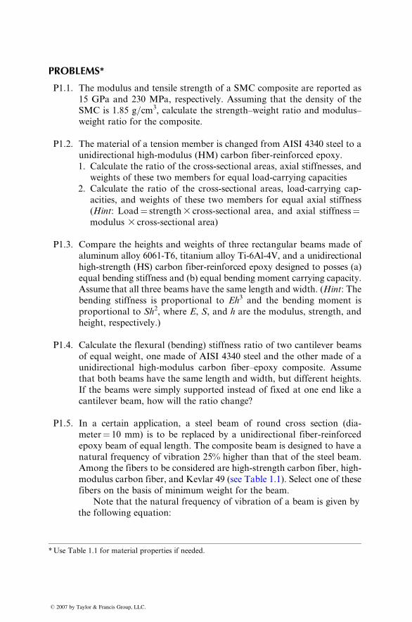
PROBLEMS*
P1.1. The modu lus and tensile stre ngth of a SMC compo site are report ed as
15 GPa an d 230 MPa , respectivel y. Ass uming that the density of the
SMC is 1.85 g=cm 3, ca lculate the strength–w eight rati o and modulus–
weight ratio for the compo site.
P1.2. The material of a tensi on membe r is ch anged from AISI 4340 steel to a
unidir ection al high-m odulus (HM) carbon fiber -reinforce d epoxy.
1. Calculat e the rati o of the cross-sect ional areas, axial sti ffnesses, and
weights of these two member s for equal load-c arrying capacit ies
2. Calculat e the rati o of the cross-sect ional areas, load-c arrying cap -
acities, and wei ghts of these two member s for equal axial stiffne ss
( Hint : Load ¼ strength 3 cross-sect ional area, and axial sti ffness ¼modulus 3 cross-sect ional area)
P1.3. Com pare the height s and weigh ts of three rectan gular beams made of
aluminum alloy 6061-T6, titanium alloy Ti-6Al-4V, and a unidirectional
high-strength (HS) carbon fiber-reinforced epoxy designed to posses (a)
equal bending stiffness and (b) equal bending moment carrying capacity.
Assume that all three beams have the same lengt h an d wid th. (Hint : The
bend ing stiffne ss is proporti onal to Eh3 an d the be nding mo ment is
propo rtional to Sh 2, where E, S, and h are the mod ulus, stren gth, and
height , respect ively.)
P1.4. Calculat e the flexu ral (bending ) sti ffness ratio of tw o can tilever bea ms
of e qual wei ght, one made of AISI 4340 steel an d the other made of a
unidir ection al high-m odulus carbon fiber–ep oxy c omposi te. Assume
that both beams have the same lengt h and width, but differen t height s.
If the beams were sim ply supporte d inst ead of fixed at one end like a
canti lever beam, how will the ratio ch ange?
P1.5. In a certain app lication, a steel be am of roun d cross secti on (dia-
meter¼ 10 mm) is to be replaced by a unidirectional fiber-reinforced
epoxy beam of equal length. The composite beam is designed to have a
natural frequency of vibration 25% higher than that of the steel beam.
Among the fibers to be considered are high-strength carbon fiber, high-
modulus carbon fiber , and Kevl ar 49 (see Table 1.1) . Select one of these
fibers on the basis of minimum weight for the beam.
Note that the natural frequency of vibration of a beam is given by
the following equation:
*Use Table 1.1 for material properties if needed.
� 2007 by Taylor & Francis Group, LLC.
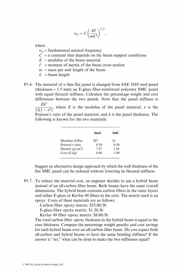
wn ¼ CEI
mL4
� �1=2
,
where
wn¼ fundamental natural frequency
C ¼ a constant that depends on the beam support conditions
E ¼modulus of the beam material
I ¼moment of inertia of the beam cross section
m ¼mass per unit length of the beam
L ¼ beam length
P1.6. The material of a thin flat panel is changed from SAE 1010 steel panel
(thickness¼ 1.5 mm) an E-glass fiber-reinforced polyester SMC panel
with equal flexural stiffness. Calculate the percentage weight and cost
differences between the two panels. Note that the panel stiffness is
Eh3
12(1� n2), where E is the modulus of the panel material, n is the
Poisson’s ratio of the panel material, and h is the panel thickness. The
following is known for the two materials:
� 2007 by Taylor & Francis Group, L
Steel SMC
LC.
Modulus (GPa)
207 16Poisson’s ratio
0.30 0.30Density (g=cm3)
7.87 1.85Cost ($=kg)
0.80 1.90Suggest an alternative design approach by which the wall thickness of the
flat SMC panel can be reduced without lowering its flexural stiffness.
P1.7. To reduce the material cost, an engineer decides to use a hybrid beam
instead of an all-carbon fiber beam. Both beams have the same overall
dimensions. The hybrid beam contains carbon fibers in the outer layers
and either E-glass or Kevlar 49 fibers in the core. The matrix used is an
epoxy. Costs of these materials are as follows:
Carbon fiber–epoxy matrix: $25.00=lbE-glass fiber–epoxy matrix: $1.20=lbKevlar 49 fiber–epoxy matrix: $8.00=lb
The total carbon fiber–epoxy thickness in the hybrid beam is equal to the
core thickness. Compare the percentage weight penalty and cost savings
for each hybrid beam over an all-carbon fiber beam. Do you expect both
all-carbon and hybrid beams to have the same bending stiffness? If the
answer is ‘‘no,’’ what can be done to make the two stiffnesses equal?
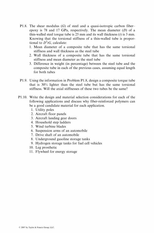
P1.8. The shear modulus (G) of steel and a quasi-isotropic carbon fiber–
epoxy is 78 and 17 GPa, respectively. The mean diameter (D) of a
thin-walled steel torque tube is 25 mm and its wall thickness (t) is 3 mm.
Knowing that the torsional stiffness of a thin-walled tube is propor-
tional to D3tG, calculate:
1. Mean diameter of a composite tube that has the same torsional
stiffness and wall thickness as the steel tube
2. Wall thickness of a composite tube that has the same torsional
stiffness and mean diameter as the steel tube
3. Difference in weight (in percentage) between the steel tube and the
composite tube in each of the previous cases, assuming equal length
for both tubes
P1.9. Using the information in Problem P1.8, design a composite torque tube
that is 30% lighter than the steel tube but has the same torsional
stiffness. Will the axial stiffnesses of these two tubes be the same?
P1.10. Write the design and material selection considerations for each of the
following applications and discuss why fiber-reinforced polymers can
be a good candidate material for each application.
1. Utility poles
2. Aircraft floor panels
3. Aircraft landing gear doors
4. Household step ladders
5. Wind turbine blades
6. Suspension arms of an automobile
7. Drive shaft of an automobile
8. Underground gasoline storage tanks
9. Hydrogen storage tanks for fuel cell vehicles
10. Leg prosthetic
11. Flywheel for energy storage
� 2007 by Taylor & Francis Group, LLC.

� 2007 by Taylor & Francis Group, LLC.
2 Materials
� 2007 by Taylor & Fr
Major constituents in a fiber-reinforced composite material are the reinforcing
fibers and a matrix, which acts as a binder for the fibers. Other constituents that
may also be found are coupling agents, coatings, and fillers. Coupling agents
and coatings are applied on the fibers to improve their wetting with the matrix
as well as to promote bonding across the fiber–matrix interface. Both in turn
promote a better load transfer between the fibers and the matrix. Fillers are
used with some polymeric matrices primarily to reduce cost and improve their
dimensional stability.
Manufacturing of a composite structure starts with the incorporation of a
large number of fibers into a thin layer of matrix to form a lamina (ply). The
thickness of a lamina is usually in the range of 0.1–1 mm (0.004–0.04 in.). If
continuous (long) fibers are used in making the lamina, they may be arranged
either in a unidirectional orientation (i.e., all fibers in one direction, Figure 2.1a),
in a bidirectional orientation (i.e., fibers in two directions, usually normal to
each other, Figure 2.1b), or in a multidirectional orientation (i.e., fibers in more
than two directions, Figure 2.1c). The bi- or multidirectional orientation of
fibers is obtained by weaving or other processes used in the textile industry. The
bidirectional orientations in the form of fabrics are shown in Appendix A.1.
For a lamina containing unidirectional fibers, the composite material has the
highest strength and modulus in the longitudinal direction of the fibers. How-
ever, in the transverse direction, its strength and modulus are very low. For a
lamina containing bidirectional fibers, the strength and modulus can be varied
using different amounts of fibers in the longitudinal and transverse directions.
For a balanced lamina, these properties are the same in both directions.
A lamina can also be constructed using discontinuous (short) fibers in a
matrix. The discontinuous fibers can be arranged either in unidirectional
orientation (Figure 2.1c) or in random orientation (Figure 2.1d). Disconti-
nuous fiber-reinforced composites have lower strength and modulus than
continuous fiber composites. However, with random orientation of fibers
(Figure 2.1e), it is possible to obtain equal mechanical and physical properties
in all directions in the plane of the lamina.
The thickness required to support a given load or to maintain a given
deflection in a fiber-reinforced composite structure is obtained by stacking
several laminas in a specified sequence and then consolidating them to form a
laminate. Various laminas in a laminate may contain fibers either all in one
ancis Group, LLC.
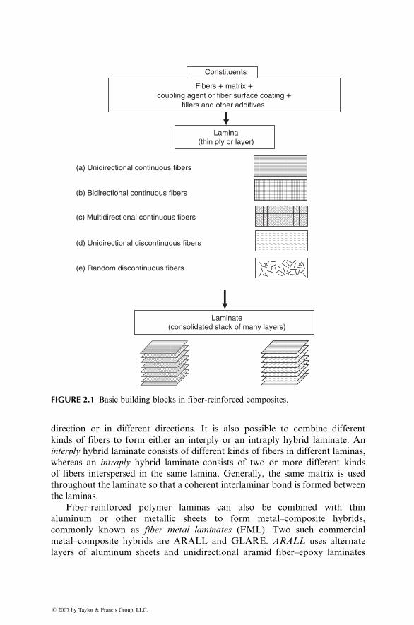
Constituents
Fibers + matrix +coupling agent or fiber surface coating +
fillers and other additives
Lamina(thin ply or layer)
(a) Unidirectional continuous fibers
(b) Bidirectional continuous fibers
(c) Multidirectional continuous fibers
(d) Unidirectional discontinuous fibers
(e) Random discontinuous fibers
Laminate(consolidated stack of many layers)
FIGURE 2.1 Basic building blocks in fiber-reinforced composites.
direction or in different directions. It is also possible to combine different
kinds of fibers to form either an interply or an intraply hybrid laminate. An
interply hybrid laminate consists of different kinds of fibers in different laminas,
whereas an intraply hybrid laminate consists of two or more different kinds
of fibers interspersed in the same lamina. Generally, the same matrix is used
throughout the laminate so that a coherent interlaminar bond is formed between
the laminas.
Fiber-reinforced polymer laminas can also be combined with thin
aluminum or other metallic sheets to form metal–composite hybrids,
commonly known as fiber metal laminates (FML). Two such commercial
metal–composite hybrids are ARALL and GLARE. ARALL uses alternate
layers of aluminum sheets and unidirectional aramid fiber–epoxy laminates
� 2007 by Taylor & Francis Group, LLC.
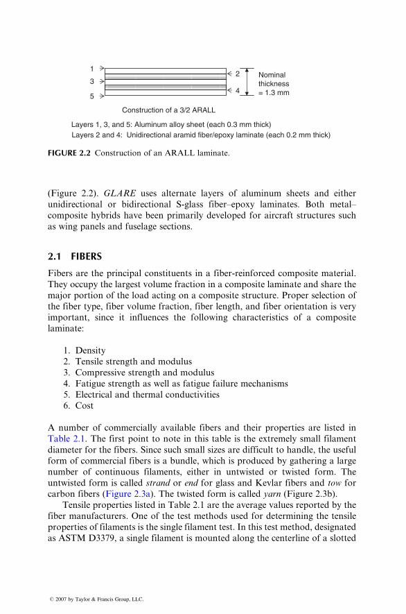
Nominalthickness= 1.3 mm
1
3
5
2
4
Construction of a 3/2 ARALL
Layers 1, 3, and 5: Aluminum alloy sheet (each 0.3 mm thick) Layers 2 and 4: Unidirectional aramid fiber/epoxy laminate (each 0.2 mm thick)
FIGURE 2.2 Construction of an ARALL laminate.
(Figur e 2.2) . GLARE uses alte rnate layers of alumi num sh eets and either
unidir ectiona l or bidir ection al S-gla ss fiber–epoxy lami nates. Both metal–
composi te hybrids have be en prim arily developed for aircraft struc tures such
as wi ng panels an d fusel age sections.
2.1 FIBERS
Fibers are the princi pal constituent s in a fiber -reinforce d compo site material .
They occup y the largest vo lume fraction in a composi te lamin ate and share the
major portio n of the load acting on a composi te structure. Prop er selection of
the fiber type, fiber volume fraction , fiber lengt h, and fiber orient ation is very
impor tant, since it influen ces the followi ng charact eristic s of a co mposite
laminate:
1. Densi ty
2. Tensil e strength and modu lus
3. Com pressive stren gth and mod ulus
4. Fatigue strength as well as fatigue failure mechani sms
5. Electr ical and therm al con ductivities
6. Cost
A num ber of commerc ially available fibers and their propert ies are lis ted in
Table 2.1. The first point to note in this table is the extre mely smal l filamen t
diame ter for the fiber s. Since such small sizes are diff icult to han dle, the useful
form of co mmercial fiber s is a bundle, whi ch is produced by gather ing a large
number of continuous filaments, either in untwisted or twisted form. The
untwisted form is called strand or end for glass and Kevlar fibers and tow for
carbon fiber s (Figur e 2.3a). The twisted form is called yarn (Figur e 2.3b).
Tensile properties listed in Table 2.1 are the average values reported by the
fiber manufacturers. One of the test methods used for determining the tensile
properties of filaments is the single filament test. In this test method, designated
as ASTM D3379, a single filament is mounted along the centerline of a slotted
� 2007 by Taylor & Francis Group, LLC.
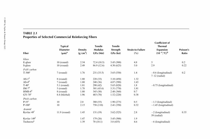
TABLE 2.1Properties of Selected Commercial Reinforcing Fibers
Fiber
Typical
Diameter
(mm)aDensity
(g=cm3)
Tensile
Modulus
GPa (Msi)
Tensile
Strength
GPa (ksi)
Strain-to-Failure
(%)
Coefficient of
Thermal
Expansion
(10�6=8C)bPoisson’s
Ratio
Glass
E-glass 10 (round) 2.54 72.4 (10.5) 3.45 (500) 4.8 5 0.2
S-glass 10 (round) 2.49 86.9 (12.6) 4.30 (625) 5.0 2.9 0.22
PAN carbon
T-300c 7 (round) 1.76 231 (33.5) 3.65 (530) 1.4 �0.6 (longitudinal) 0.2
7–12 (radial)
AS-1d 8 (round) 1.80 228 (33) 3.10 (450) 1.32
AS-4d 7 (round) 1.80 248 (36) 4.07 (590) 1.65
T-40c 5.1 (round) 1.81 290 (42) 5.65 (820) 1.8 �0.75 (longitudinal)
IM-7d 5 (round) 1.78 301 (43.6) 5.31 (770) 1.81
HMS-4d 8 (round) 1.80 345 (50) 2.48 (360) 0.7
GY-70e 8.4 (bilobal) 1.96 483 (70) 1.52 (220) 0.38
Pitch carbon
P-55c 10 2.0 380 (55) 1.90 (275) 0.5 �1.3 (longitudinal)
P-100c 10 2.15 758 (110) 2.41 (350) 0.32 �1.45 (longitudinal)
Aramid
Kevlar 49f 11.9 (round) 1.45 131 (19) 3.62 (525) 2.8 �2 (longitudinal) 0.35
59 (radial)
Kevlar 149f 1.47 179 (26) 3.45 (500) 1.9
Technorag 1.39 70 (10.1) 3.0 (435) 4.6 �6 (longitudinal)
�2007
byTaylor
&Francis
Group,L
LC.
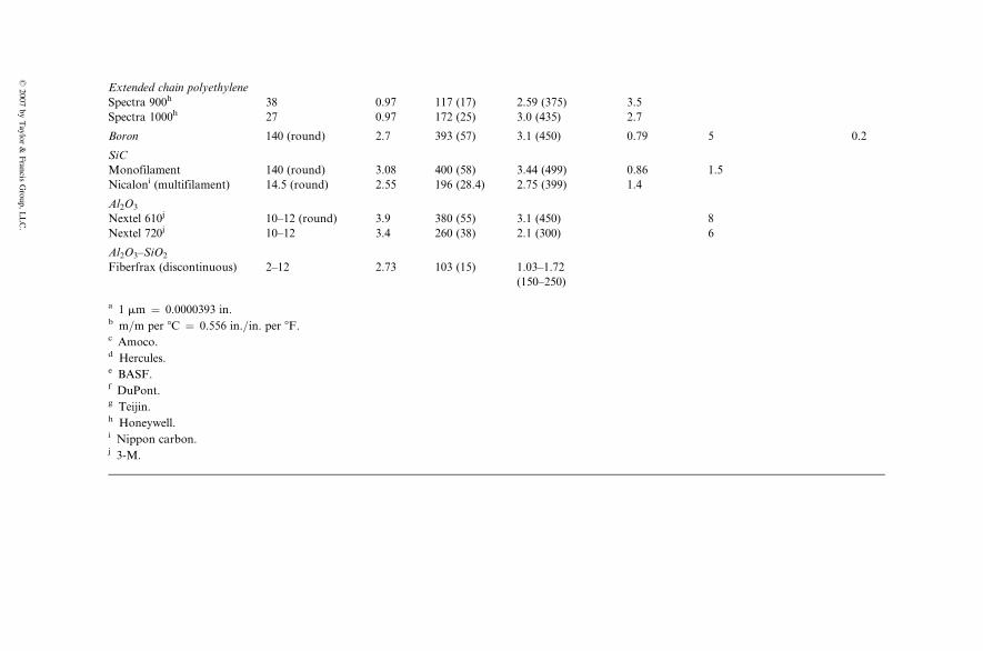
Extended chain polyethylene
Spectra 900h 38 0.97 117 (17) 2.59 (375) 3.5
Spectra 1000h 27 0.97 172 (25) 3.0 (435) 2.7
Boron 140 (round) 2.7 393 (57) 3.1 (450) 0.79 5 0.2
SiC
Monofilament 140 (round) 3.08 400 (58) 3.44 (499) 0.86 1.5
Nicaloni (multifilament) 14.5 (round) 2.55 196 (28.4) 2.75 (399) 1.4
Al2O3
Nextel 610j 10–12 (round) 3.9 380 (55) 3.1 (450) 8
Nextel 720j 10–12 3.4 260 (38) 2.1 (300) 6
Al2O3–SiO2
Fiberfrax (discontinuous) 2–12 2.73 103 (15) 1.03–1.72
(150–250)
a 1 mm ¼ 0.0000393 in.b m=m per 8C ¼ 0.556 in.=in. per 8F.c Amoco.d Hercules.e BASF.f DuPont.g Teijin.h Honeywell.i Nippon carbon.j 3-M.
�2007
byTaylor
&Francis
Group,
LLC.
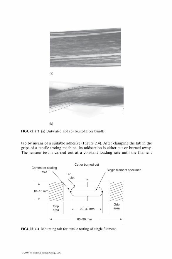
(a)
(b)
FIGURE 2.3 (a) Untwisted and (b) twisted fiber bundle.
tab by means of a suitable adhesive (Figure 2.4). After clamping the tab in the
grips of a tensile testing machine, its midsection is either cut or burned away.
The tension test is carried out at a constant loading rate until the filament
Cement or sealingwax
Cut or burned out
Single filament specimenTab
slot
20−30 mm
60−90 mm
10−15 mm
Griparea
Griparea
FIGURE 2.4 Mounting tab for tensile testing of single filament.
� 2007 by Taylor & Francis Group, LLC.
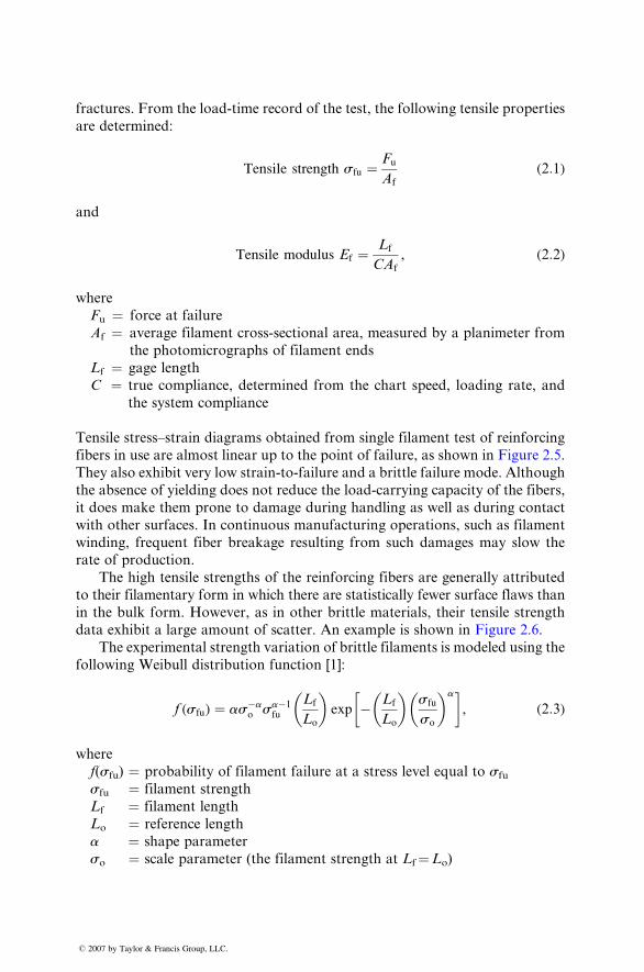
fractures . Fro m the load-t ime record of the test, the followin g tensi le propert ies
are de termined:
Tensi le strength sfu ¼ Fu
Af
( 2: 1)
and
Tensile modu lus Ef ¼ Lf
CAf
, ( 2: 2)
where
Fu ¼ force at fail ure
Af ¼ average filament cross-sect ional area, measur ed by a planim eter from
the photomi crographs of fil ament end s
Lf ¼ gage length
C ¼ true co mpliance, determ ined from the chart speed, loading rate, and
the syst em complian ce
Tensil e stre ss–strain diagra ms obtaine d from single filament test of reinforcing
fibers in use are almos t linea r up to the point of failu re, as shown in Figure 2.5.
They also exh ibit very low strain-to-f ailure an d a brit tle failure mod e. Alth ough
the absence of yield ing does not reduce the load-c arryi ng capacity of the fiber s,
it does make them prone to damage during handling as well as during co ntact
with other surfa ces. In con tinuous manufa cturin g operati ons, such as filamen t
winding, frequen t fiber breakage resul ting from such damages may slow the
rate of producti on.
The high tensile strengths of the reinforcing fiber s are gen erally attribut ed
to their filamentary form in which there are statistically fewer surface flaws than
in the bulk form . However, as in other brit tle mate rials, their tensi le strength
data e xhibit a large amount of scatt er. An exampl e is shown in Figure 2.6.
The experimental strength variation of brittle filaments is modeled using the
following Weibull distribution function [1]:
f (sfu) ¼ as�ao sa�1
fu
Lf
Lo
� �exp � Lf
Lo
� �sfu
so
� �a� �, (2:3)
where
f(sfu) ¼ probability of filament failure at a stress level equal to sfu
sfu ¼ filament strength
Lf ¼ filament length
Lo ¼ reference length
a ¼ shape parameter
so ¼ scale parameter (the filament strength at Lf¼Lo)
� 2007 by Taylor & Francis Group, LLC.
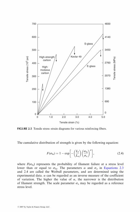
700 4830
4140
3450
2760
2070
Ten
sile
str
ess
(MP
a)
Ten
sile
str
ess
(103
psi)
1380
690
0
600
500
High-strengthcarbon
High-moduluscarbon
400
300
200
100
00 1.0 2.0
Tensile strain (%)
S-glass
E-glass
Kevlar 49
3.0 4.0 5.0
FIGURE 2.5 Tensile stress–strain diagrams for various reinforcing fibers.
The cumu lative dist ribut ion of stren gth is given by the followi ng eq uation:
F ( sfu ) ¼ 1 � exp � Lf
Lo
� �sfu
so
� �a� �, ( 2: 4)
wher e F( sfu ) represen ts the pro bability of filament failure at a stre ss level
lower than or equal to sfu . The parame ters a and s o in Equat ions 2.3
and 2.4 are called the Weibull parameters, and are determined using the
experimental data. a can be regarded as an inverse measure of the coefficient
of variation. The higher the value of a, the narrower is the distribution
of filament strength. The scale parameter so may be regarded as a reference
stress level.
� 2007 by Taylor & Francis Group, LLC.
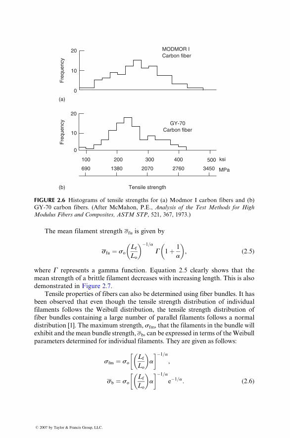
20
(a)
MODMOR ICarbon fiber
(b)
GY-70Carbon fiber
Fre
quen
cyF
requ
ency
10
0
20
10
0
100 200 300 400 500 ksi
MPa690 1380 2070
Tensile strength
2760 3450
FIGURE 2.6 Histograms of tensile strengths for (a) Modmor I carbon fibers and (b)
GY-70 carbon fibers. (After McMahon, P.E., Analysis of the Test Methods for High
Modulus Fibers and Composites, ASTM STP, 521, 367, 1973.)
The mean filament strength �fu is given by
sfu ¼ s oLf
Lo
� �� 1 =a
G 1 þ 1
a
� �, ( 2: 5)
where G repres ents a gamm a functi on. Equat ion 2.5 clear ly shows that the
mean strength of a brittle filamen t decreas es wi th increa sing lengt h. This is also
demonst rated in Figure 2.7.
Tensile properties of fibers can also be determined using fiber bundles. It has
been observed that even though the tensile strength distribution of individual
filaments follows the Weibull distribution, the tensile strength distribution of
fiber bundles containing a large number of parallel filaments follows a normal
distribution [1]. The maximum strength, sfm, that the filaments in the bundle will
exhibit and the mean bundle strength, �b, can be expressed in terms of the Weibull
parameters determined for individual filaments. They are given as follows:
sfm ¼ s oLf
Lo
� �a
� �� 1= a
,
sb ¼ s oLf
Lo
� �a
� �� 1= a
e � 1 = a : ( 2: 6)
� 2007 by Taylor & Francis Group, LLC.
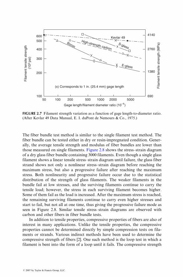
600 4140
2760
1380
690
500
400
300
Fila
men
t ten
sile
str
engt
h (1
03 p
si)
Fila
men
t ten
sile
str
engt
h (M
Pa)
200
10050 100 200
(x) Corresponds to 1 in. (25.4 mm) gage length
500
Gage length/filament diameter ratio (10−4 )
1000 2000
Boron
High-strength carbon
Kevlar 49
S-glass
E-glass
5000
FIGURE 2.7 Filament strength variation as a function of gage length-to-diameter ratio.
(After Kevlar 49 Data Manual, E. I. duPont de Nemours & Co., 1975.)
The fiber bundle test method is simila r to the single filament test method. The
fiber bundl e can be test ed either in dry or resi n-impregna ted con dition. Gener-
ally, the average tensi le stre ngth and modulus of fiber bundl es are lower than
those measur ed on single fila ments. Figure 2.8 shows the stress–s train diagra m
of a dry glass fiber bundle contai ning 3000 filament s. Even thou gh a single glass
filament shows a linea r tensile stre ss–strai n diagra m until failure, the glass fiber
stran d shows not only a nonlinear stress–s train diagram be fore reach ing the
maxi mum stre ss, but also a progres sive failure after reachi ng the maximum
stress. Both nonlinear ity and pro gressive failu re occur due to the stat istical
distribut ion of the strength of glass filamen ts. The weake r filament s in the
bundle fail at low stre sses, a nd the survi ving filament s continue to carry the
tensile load; howeve r, the stre ss in each survi ving fil ament be comes higher.
Some of them fail as the load is increased. After the maximum stress is reach ed,
the remai ning surviving filament s con tinue to ca rry even higher stre sses and
start to fail, but not all at one tim e, thu s giving the progres sive failure mode as
seen in Figure 2.8. Simi lar tensile stress–s train diagrams are observed with
carbon and other fiber s in fiber bundle tests.
In addition to tensile pro perties, compres sive pro perties of fibers are also of
interest in many app lications . Un like the tensi le pro perties, the compres sive
propert ies canno t be de termined directly by simp le compres sion tests on fila-
ments or strand s. Var ious indirect methods ha ve been used to determine the
compres sive strength of fiber s [2]. One such method is the loop test in which a
filament is ben t into the form of a loop unt il it fails. The comp ressive streng th
� 2007 by Taylor & Francis Group, LLC.
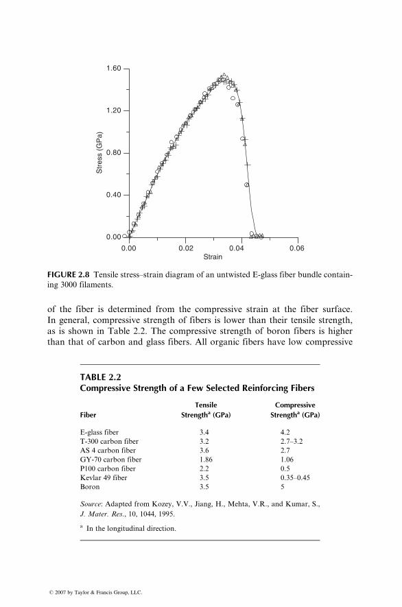
0.00 0.02 0.04 0.06Strain
0.00
0.40
0.80
1.20
1.60
Str
ess
(GP
a)
FIGURE 2.8 Tensile stress–strain diagram of an untwisted E-glass fiber bundle contain-
ing 3000 filaments.
of the fiber is determined from the compressive strain at the fiber surface.
In general, compressive strength of fibers is lower than their tensile strength,
as is shown in Table 2.2. The compressive strength of boron fibers is higher
than that of carbon and glass fibers. All organic fibers have low compressive
TABLE 2.2Compressive Strength of a Few Selected Reinforcing Fibers
Fiber
Tensile
Strengtha (GPa)
Compressive
Strengtha (GPa)
E-glass fiber 3.4 4.2
T-300 carbon fiber 3.2 2.7–3.2
AS 4 carbon fiber 3.6 2.7
GY-70 carbon fiber 1.86 1.06
P100 carbon fiber 2.2 0.5
Kevlar 49 fiber 3.5 0.35–0.45
Boron 3.5 5
Source: Adapted from Kozey, V.V., Jiang, H., Mehta, V.R., and Kumar, S.,
J. Mater. Res., 10, 1044, 1995.
a In the longitudinal direction.
� 2007 by Taylor & Francis Group, LLC.
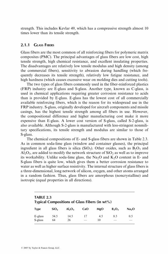
strength. This includes Kevlar 49, which has a compressive strength almost 10
times lower than its tensile strength.
2.1.1 GLASS FIBERS
Glass fibers are the most common of all reinforcing fibers for polymeric matrix
composites (PMC). The principal advantages of glass fibers are low cost, high
tensile strength, high chemical resistance, and excellent insulating properties.
The disadvantages are relatively low tensile modulus and high density (among
the commercial fibers), sensitivity to abrasion during handling (which fre-
quently decreases its tensile strength), relatively low fatigue resistance, and
high hardness (which causes excessive wear on molding dies and cutting tools).
The two types of glass fibers commonly used in the fiber-reinforced plastics
(FRP) industry are E-glass and S-glass. Another type, known as C-glass, is
used in chemical applications requiring greater corrosion resistance to acids
than is provided by E-glass. E-glass has the lowest cost of all commercially
available reinforcing fibers, which is the reason for its widespread use in the
FRP industry. S-glass, originally developed for aircraft components and missile
casings, has the highest tensile strength among all fibers in use. However,
the compositional difference and higher manufacturing cost make it more
expensive than E-glass. A lower cost version of S-glass, called S-2-glass, is
also available. Although S-2-glass is manufactured with less-stringent nonmili-
tary specifications, its tensile strength and modulus are similar to those of
S-glass.
The chemical compositions of E- and S-glass fibers are shown in Table 2.3.
As in common soda-lime glass (window and container glasses), the principal
ingredient in all glass fibers is silica (SiO2). Other oxides, such as B2O3 and
Al2O3, are added to modify the network structure of SiO2 as well as to improve
its workability. Unlike soda-lime glass, the Na2O and K2O content in E- and
S-glass fibers is quite low, which gives them a better corrosion resistance to
water as well as higher surface resistivity. The internal structure of glass fibers is
a three-dimensional, long network of silicon, oxygen, and other atoms arranged
in a random fashion. Thus, glass fibers are amorphous (noncrystalline) and
isotropic (equal properties in all directions).
TABLE 2.3Typical Compositions of Glass Fibers (in wt%)
Type SiO2 Al2O3 CaO MgO B2O3 Na2O
E-glass 54.5 14.5 17 4.5 8.5 0.5
S-glass 64 26 — 10 — —
� 2007 by Taylor & Francis Group, LLC.
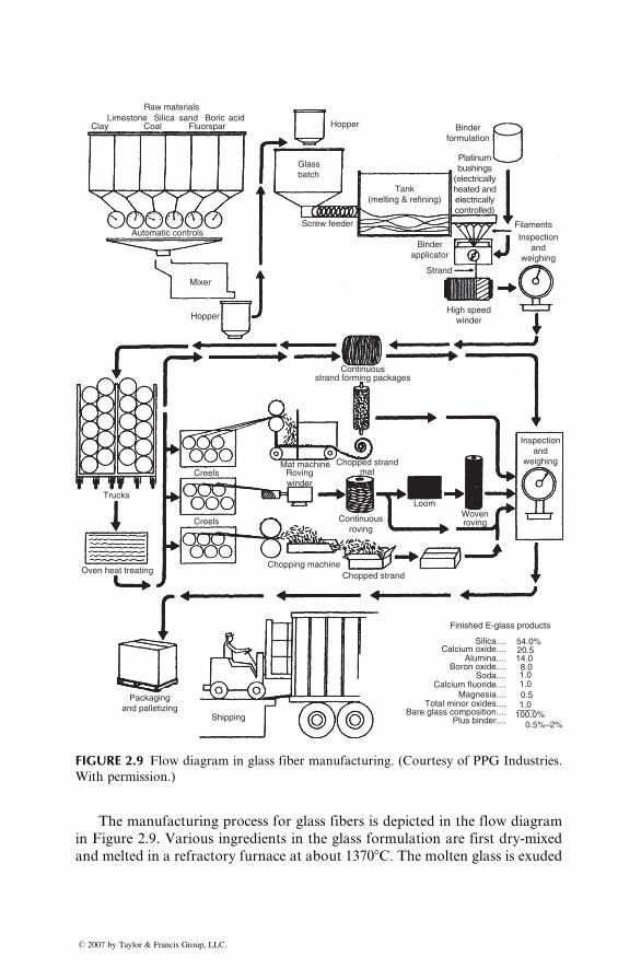
Raw materialsLimestone
Clay Coal
Automatic controls
Fluorspar Hopper
Tank(melting & refining)
Binderformulation
Platinumbushings
(electricallyheated andelectricallycontrolled)
Mixer
Screw feeder
Continuousstrand forming packages
Hopper
Creels
LoomWovenroving
Mat machineRovingwinder
Chopped strandmat
Creels
Chopping machine
Continuousroving
Chopped strand
Finished E-glass products
Silica.... 54.0%20.514.08.01.01.00.5
100.0%0.5%–2%
1.0
Calcium oxide....Alumina....
Boron oxide....Soda....
Calcium fluoride....Magnesia....
Total minor oxides....Bare glass composition....
Plus binder....
Inspectionand
weighing
Shipping
Trucks
Packagingand palletizing
Oven heat treating
Glassbatch
Filaments
Strand
High speedwinder
Inspectionand
weighing
Binderapplicator
Silica sand Boric acid
FIGURE 2.9 Flow diagram in glass fiber manufacturing. (Courtesy of PPG Industries.
With permission.)
The manufacturing process for glass fibers is depicted in the flow diagram
in Figure 2.9. Various ingredients in the glass formulation are first dry-mixed
and melted in a refractory furnace at about 13708C. The molten glass is exuded
� 2007 by Taylor & Francis Group, LLC.
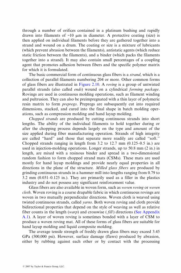
through a number of orifices co ntaine d in a platinu m bush ing an d rapidly
draw n into filament s of ~10 m m in diame ter. A pro tective co ating (size) is
then app lied on individu al fil aments be fore they a re g athered togeth er into a
stran d and woun d on a dru m. The coati ng or size is a mixt ure of lubri cants
(which prevent abrasio n be tween the fila ments), antis tatic a gents (which reduce
static fri ction between the filamen ts), and a binder (which packs the filament s
toget her into a strand ). It may also con tain small percent ages of a cou pling
agent that promot es adhesion betwee n fiber s and the specific pol ymer matr ix
for whi ch it is form ulated .
The basic co mmercial form of continuous glass fiber s is a strand , whi ch is a
colle ction of pa rallel filament s num bering 204 or more. Other common form s
of glass fibers are illu strated in Fig ure 2.10. A rovin g is a gro up of untw isted
parallel stra nds (als o called ends ) wound on a cyli ndrical forming packag e.
Rovi ngs are used in con tinuous moldin g operatio ns, su ch as filament winding
and pultr usion. They can also be preim pregnat ed with a thin layer of polyme ric
resin matrix to form prepre gs . Prepregs are sub sequentl y cut into requir ed
dimens ions, stacke d, and cu red into the final shap e in ba tch molding ope r-
ations , such as compres sion moldi ng and han d layup moldi ng.
Chop ped stra nds are produced by cutting continuous strand s into short
lengt hs. The ability of the indivi dual filament s to hold toget her during or
after the chop ping process de pends largely on the type and a mount of the
size ap plied dur ing fiber manufa cturing ope ration. Strands of high integ rity
are called ‘‘hard’’ and those that separat e more readil y are called ‘‘s oft.’’
Chopped stran ds ranging in length from 3.2 to 12.7 mm (0.12 5–0.5 in.) are
used in injec tion-moldi ng operati ons. Longe r stra nds, up to 50.8 mm (2 in.) in
lengt h, are mixed with a resi nous binder and spread in a tw o-dimen sional
random fashi on to form ch opped stra nd mats (CSMs). Thes e mats are used
most ly for hand layup moldings and provide nearly equal propert ies in all
direction s in the plane of the structure. Milled glass fibe rs are produ ced by
grindi ng con tinuous stra nds in a hamme r mil l into length s ranging from 0.79 to
3.2 mm (0.031–0. 125 in.). They are prim arily used as a filler in the plast ics
indust ry an d do not pos sess any signi ficant reinforcem ent value.
Glas s fiber s are also availa ble in woven form , such as woven rovin g or woven
cloth . Woven roving is a coarse drapable fabric in which co ntinuous rovings are
woven in two mutual ly perpen dicular directions. Wo ven cloth is weav ed us ing
twisted continuous strands, called yarns. Both woven roving and cloth provide
bidirectional properties that depend on the style of weaving as well as relative
fiber counts in the length ( warp ) and crosswi se ( fill ) direction s (See Append ix
A.1). A layer of woven roving is sometime s bonded wi th a layer of CSM to
produce a woven roving mat. All of these forms of glass fibers are suitable for
hand layup molding and liquid composite molding.
The average tensile strength of freshly drawn glass fibers may exceed 3.45
GPa (500,000 psi). However, surface damage (flaws) produced by abrasion,
either by rubbing against each other or by contact with the processing
� 2007 by Taylor & Francis Group, LLC.
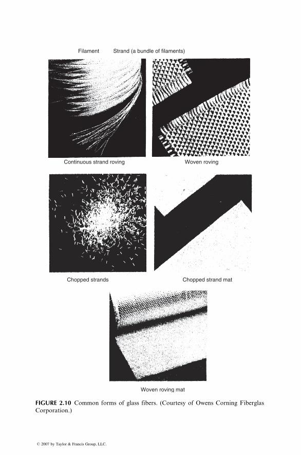
Strand (a bundle of filaments)
Woven roving
Filament
Continuous strand roving
Woven roving mat
Chopped strands Chopped strand mat
FIGURE 2.10 Common forms of glass fibers. (Courtesy of Owens Corning Fiberglas
Corporation.)
� 2007 by Taylor & Francis Group, LLC.
500T
ensi
le s
tres
s (1
03 ps
i)
24�C (75�F)
400�C (750�F)
500�C (930�F)
600�C (1,110�F)
400
300
200
100
01 10 100
Load duration (min)
Ten
sile
str
ess
(MP
a)
1,000 10,000
2,760
1,380
0
FIGURE 2.11 Reduction of tensile stress in E-glass fibers as a function of time at various
temperatures. (After Otto, W.H., Properties of glass fibers at elevated temperatures,
Owens Corning Fiberglas Corporation, AD 228551, 1958.)
equipment, tends to reduce it to values that are in the range of 1.72–2.07 GPa
(250,000–300,000 psi). Strength degradation is increased as the surface flaws
grow under cyclic loads, which is one of the major disadvantages of using glass
fibers in fatigue applications. Surface compressive stresses obtained by alkali
ion exchange [3] or elimination of surface flaws by chemical etching may reduce
the problem; however, commercial glass fibers are not available with any such
surface modifications.
The tensile strength of glass fibers is also reduced in the presence of water or
under sustained loads (static fatigue). Water bleaches out the alkalis from the
surface and deepens the surface flaws already present in fibers. Under sustained
loads, the growth of surface flaws is accelerated owing to stress corrosion by
atmospheric moisture. As a result, the tensile strength of glass fibers is
decreased with increasing time of load duration (Figure 2.11).
2.1.2 CARBON FIBERS
Carbon fibers are commercially available with a variety of tensile modulus
values ranging from 207 GPa (303 106 psi) on the low side to 1035 GPa
(1503 106 psi) on the high side. In general, the low-modulus fibers have
lower density, lower cost, higher tensile and compressive strengths, and higher
tensile strains-to-failure than the high-modulus fibers. Among the advantages
of carbon fibers are their exceptionally high tensile strength–weight ratios as
well as tensile modulus–weight ratios, very low coefficient of linear thermal
expansion (which provides dimensional stability in such applications as space
antennas), high fatigue strengths, and high thermal conductivity (which is even
� 2007 by Taylor & Francis Group, LLC.
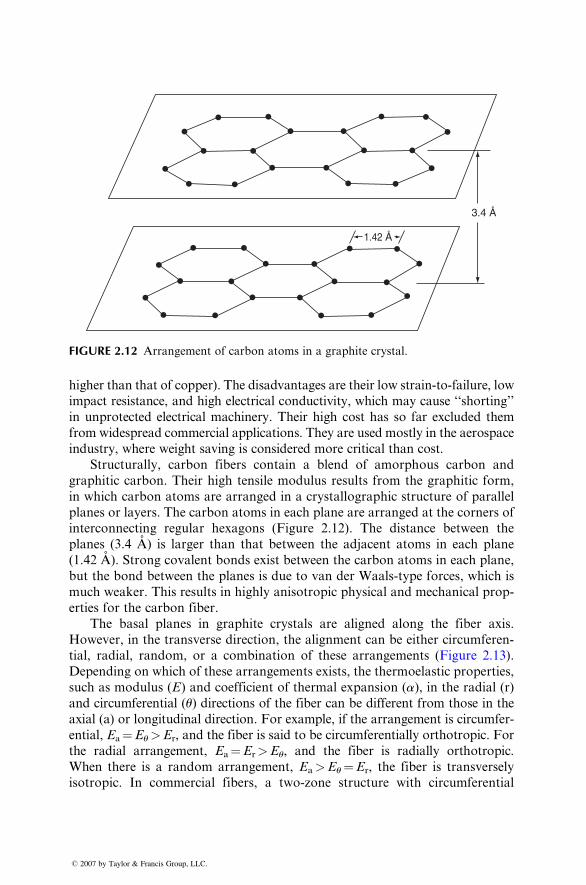
1.42 Å
3.4 Å
FIGURE 2.12 Arrangement of carbon atoms in a graphite crystal.
higher than that of copper). The disadvantages are their low strain-to-failure, low
impact resistance, and high electrical conductivity, which may cause ‘‘shorting’’
in unprotected electrical machinery. Their high cost has so far excluded them
from widespread commercial applications. They are used mostly in the aerospace
industry, where weight saving is considered more critical than cost.
Struct urally, carbon fibers con tain a blend of amorph ous carbon and
graphit ic carb on. Their high tensi le modulus resul ts from the graph itic form ,
in which carbon atoms are arrange d in a cryst allograp hic structure of parall el
planes or layer s. The carbon atoms in each plane are arrange d at the corners of
interco nnectin g regula r hexagons (Figur e 2.12) . The dist ance between the
planes (3.4 A ) is larger than that be tween the adjacent atoms in each plane
(1.42 A ). Strong co valent bonds exist between the carbon atoms in each plan e,
but the bond between the planes is due to van der Waals -type forces , whi ch is
much weaker. This resul ts in highly anisotropic physica l and mechani cal prop -
erties for the carbon fiber .
The basal plan es in grap hite cryst als are alig ned along the fiber axis.
Howev er, in the trans verse direction, the alig nment can be either circum feren-
tial, radial, rando m, or a combinat ion of these arrange ments (Figur e 2.13) .
Depending on whi ch of these a rrangemen ts e xists, the therm oelastic prope rties,
such as modulus ( E ) and coefficie nt of therm al expansi on ( a), in the radial (r)a n d c ir cu m f er en t i al ( u) directions of the fiber can be different from those in the
axial (a) or longitudinal direction. For example, if the arrangement is circumfer-
ential, Ea¼Eu>Er, and the fiber is said to be circumferentially orthotropic. For
the radial arrangement, Ea¼Er>Eu, and the fiber is radially orthotropic.
When there is a random arrangement, Ea>Eu¼Er, the fiber is transversely
isotropic. In commercial fibers, a two-zone structure with circumferential
� 2007 by Taylor & Francis Group, LLC.
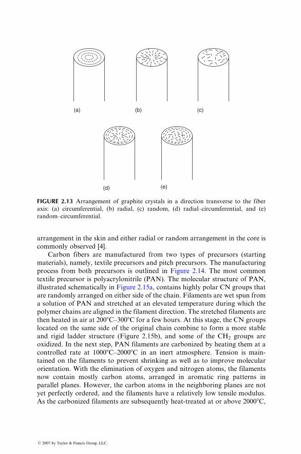
(a) (b) (c)
(d) (e)
FIGURE 2.13 Arrangement of graphite crystals in a direction transverse to the fiber
axis: (a) circumferential, (b) radial, (c) random, (d) radial–circumferential, and (e)
random–circumferential.
arrange ment in the skin and eithe r radial or ran dom arrange ment in the core is
commonl y observed [4].
Car bon fiber s are manufa ctured from two types of pr ecursor s (st arting
mate rials), namely, textile precurs ors an d pitch pr ecursor s. The manufa cturing
process from both precurs ors is outlined in Figure 2 .14. The most common
textile precurs or is polyacr ylonitri le (PAN ). The mo lecular structure of PAN,
illustr ated schema tically in Figu re 2.15a, con tains highly polar CN gro ups that
are rando mly arrange d on either side of the chain. Filamen ts are wet spun from
a solut ion of PAN and stretched a t an elevated temperatur e dur ing which the
polyme r chains are align ed in the filament direction . The stretched filament s are
then he ated in air at 200 8 C–30 08C for a few hour s. At this stage , the CN group s
locat ed on the same side of the origin al chain combine to form a more stable
and rigid ladd er structure (Figure 2.15b), a nd some of the CH2 groups are
oxidiz ed. In the next step, PAN filament s are carbonize d by heating them at a
control led rate at 1000 8 C–2000 8 C in an inert atmos phere. Tension is main-
taine d on the fil aments to prevent shrinking as well as to impr ove molec ular
orient ation. With the eliminat ion of oxygen and nitr ogen atoms , the filament s
now con tain mostly carbo n atoms , arrange d in aromatic ring pa tterns in
parallel planes. However, the carbon atoms in the neighboring planes are not
yet perfectly ordered, and the filaments have a relatively low tensile modulus.
As the carbonized filaments are subsequently heat-treated at or above 20008C,
� 2007 by Taylor & Francis Group, LLC.
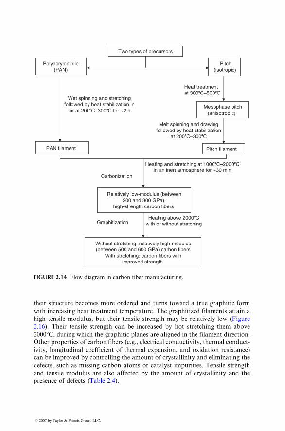
Polyacrylonitrile(PAN)
Two types of precursors
Pitch(isotropic)
Wet spinning and stretchingfollowed by heat stabilization in
air at 2008C–3008C for ~2 h
Heat treatmentat 3008C–5008C
PAN filament
Mesophase pitch (anisotropic)
Melt spinning and drawingfollowed by heat stabilization
at 2008C–3008C
Pitch filament
Carbonization
Heating and stretching at 10008C–20008Cin an inert atmosphere for ~30 min
Heating above 20008Cwith or without stretching
Relatively low-modulus (between200 and 300 GPa),
high-strength carbon fibers
Graphitization
Without stretching: relatively high-modulus(between 500 and 600 GPa) carbon fibers
With stretching: carbon fibers withimproved strength
FIGURE 2.14 Flow diagram in carbon fiber manufacturing.
their struc ture beco mes more ordered and turns toward a true grap hitic form
with increa sing heat treatmen t temperatur e. The graphit ized filament s attain a
high tensi le modulus, but their tensile stre ngth may be relat ively low (Figur e
2.16). Their tensi le strength can be increa sed by hot stre tching them above
2000 8 C, dur ing whi ch the graphit ic planes are alig ned in the filament direct ion.
Other propert ies of c arbon fiber s (e.g., electrica l condu ctivity , therm al cond uct-
ivity, longitud inal coeff icien t of therm al expansi on, and ox idation resi stance )
can be impro ved by control ling the amount of cryst allinity and elim inating the
defects, such as mis sing carbon atoms or catal yst impur ities. Tensil e strength
and tensi le modulus are a lso a ffected by the amount of cryst allinity and the
presence of de fects (Table 2.4) .
� 2007 by Taylor & Francis Group, LLC.
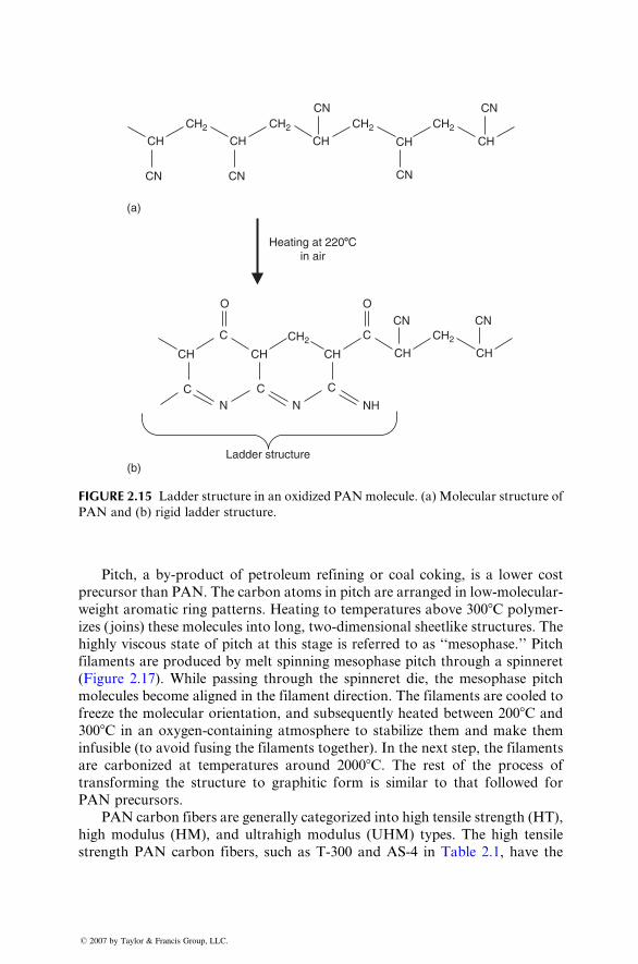
CH CH CH CH
CN
CN
Heating at 2208Cin air
CH
CNCH2
O O
CH2
CH2 CH2
CH2 CH2
CN
(a)
(b)
CH CH
CN
CH
CN
CH
C C
C
CH
NH
C
N NC
CN
Ladder structure
FIGURE 2.15 Ladder structure in an oxidized PANmolecule. (a) Molecular structure of
PAN and (b) rigid ladder structure.
Pitch, a by-product of pe troleum refin ing or co al cok ing, is a low er cost
precurs or than PAN. The carbon atoms in pitch are arrange d in low-mol ecular -
weight aromat ic ring pattern s. Heat ing to tempe ratur es ab ove 300 8C polyme r-
izes ( joins) these molec ules into long, two-dim ensional sheetlike struc tures. The
highly viscous state of pitch at this stage is referred to as ‘‘m esophase. ’’ Pitch
filament s are produce d by melt spinnin g mesophas e pitch through a spinner et
(Figur e 2.17) . Wh ile passing through the spinner et die, the mesophas e pitch
molec ules be come aligned in the filament direct ion. The filament s are co oled to
freez e the molec ular orient ation, an d su bsequentl y he ated be tween 200 8 C and300 8 C in an oxygen-c ontaini ng atmos phere to stabilize them and make them
infus ible (to avoid fusin g the fil aments toget her). In the ne xt step, the filament s
are carbonize d at tempe ratur es aro und 2000 8 C. The rest of the process oftrans forming the struc ture to graphit ic form is sim ilar to that foll owed for
PAN precurs ors.
PAN carbon fiber s are general ly categor ized into high tensile strength (HT) ,
high modulus (HM), and ultrahigh modulus (UHM ) types. The high tensi le
stren gth PAN carbon fibers, su ch as T-300 and AS-4 in Table 2 .1, have the
� 2007 by Taylor & Francis Group, LLC.
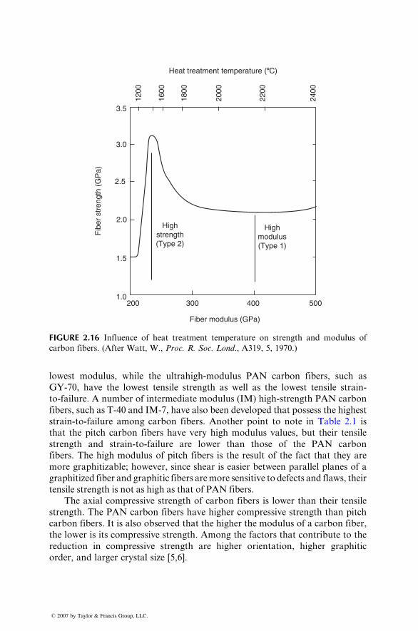
3.5
Highstrength(Type 2)
Highmodulus(Type 1)
1200
1600
1800
2000
2200
2400
Heat treatment temperature (8C)
3.0
2.5
2.0
1.5
1.0200
Fib
er s
tren
gth
(GP
a)
300
Fiber modulus (GPa)
400 500
FIGURE 2.16 Influence of heat treatment temperature on strength and modulus of
carbon fibers. (After Watt, W., Proc. R. Soc. Lond., A319, 5, 1970.)
lowest modulus, whi le the ultrah igh-modu lus PAN carbon fiber s, such as
GY-70, ha ve the lowest tensile stre ngth as well as the lowest tensi le stra in-
to-failu re. A num ber of intermedi ate modu lus (IM) high-s trength PAN carbon
fibers, such as T-40 and IM-7, have also been developed that possess the highest
strain-t o-failur e amon g ca rbon fibers. Anothe r point to note in Table 2.1 is
that the pitch carbon fiber s have very high modu lus values , but their tensile
strength and strain-t o-failur e are lower than those of the PAN carbon
fibers. The high modulus of pitch fiber s is the resul t of the fact that they are
more graphitizabl e; howeve r, since shear is easie r between pa rallel plan es of a
graphit ized fiber and graphit ic fiber s are more sensi tive to defects and flaws, their
tensile stre ngth is not as high as that of PAN fibers.
The ax ial compres sive stre ngth of carbon fibers is lower than their tensi le
strength. The PAN carbon fiber s have higher compres sive stre ngth than pitch
carbon fibers. It is also observed that the higher the modulus of a c arbon fiber ,
the low er is its c ompres sive strength. Among the facto rs that contri bute to the
reducti on in comp ressive stren gth are higher orient ation, high er graphitic
order, and larger crystal size [5,6].
� 2007 by Taylor & Francis Group, LLC.
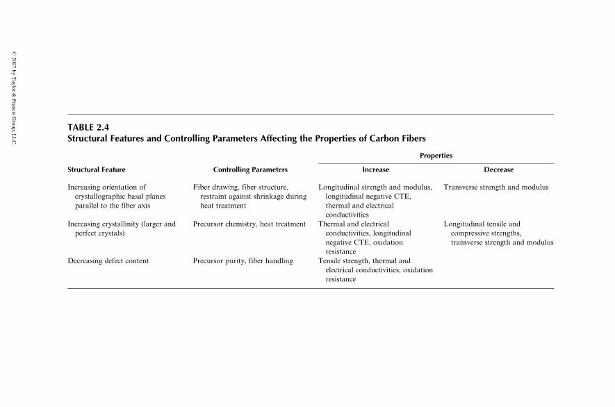
TABLE 2.4Structural Features and Controlling Parameters Affecting the Properties of Carbon Fibers
Structural Feature Controlling Parameters
Properties
Increase Decrease
Increasing orientation of
crystallographic basal planes
parallel to the fiber axis
Fiber drawing, fiber structure,
restraint against shrinkage during
heat treatment
Longitudinal strength and modulus,
longitudinal negative CTE,
thermal and electrical
conductivities
Transverse strength and modulus
Increasing crystallinity (larger and
perfect crystals)
Precursor chemistry, heat treatment Thermal and electrical
conductivities, longitudinal
negative CTE, oxidation
resistance
Longitudinal tensile and
compressive strengths,
transverse strength and modulus
Decreasing defect content Precursor purity, fiber handling Tensile strength, thermal and
electrical conductivities, oxidation
resistance
�2007
byTaylor
&Francis
Group,L
LC.
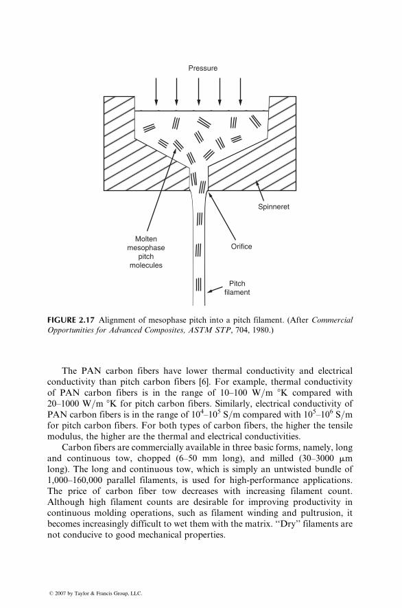
Pressure
Spinneret
OrificeMolten
mesophasepitch
molecules
Pitchfilament
FIGURE 2.17 Alignment of mesophase pitch into a pitch filament. (After Commercial
Opportunities for Advanced Composites, ASTM STP, 704, 1980.)
The PAN carbon fibers have lower thermal conductivity and electrical
conductivity than pitch carbon fibers [6]. For example, thermal conductivity
of PAN carbon fibers is in the range of 10–100 W=m 8K compared with
20–1000 W=m 8K for pitch carbon fibers. Similarly, electrical conductivity of
PAN carbon fibers is in the range of 104–105 S=m compared with 105–106 S=mfor pitch carbon fibers. For both types of carbon fibers, the higher the tensile
modulus, the higher are the thermal and electrical conductivities.
Carbon fibers are commercially available in three basic forms, namely, long
and continuous tow, chopped (6–50 mm long), and milled (30–3000 mmlong). The long and continuous tow, which is simply an untwisted bundle of
1,000–160,000 parallel filaments, is used for high-performance applications.
The price of carbon fiber tow decreases with increasing filament count.
Although high filament counts are desirable for improving productivity in
continuous molding operations, such as filament winding and pultrusion, it
becomes increasingly difficult to wet them with the matrix. ‘‘Dry’’ filaments are
not conducive to good mechanical properties.
� 2007 by Taylor & Francis Group, LLC.
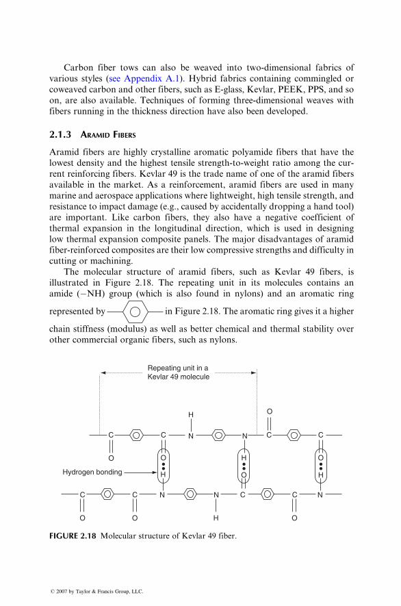
Car bon fiber tow s can also be weaved into two-dim ensional fabri cs of
various styles (see App endix A.1). Hyb rid fabri cs contain ing commingled or
cowea ved carbon and other fiber s, such as E-glass, Kevl ar, PEEK, PPS, and so
on, are also availab le. Techn iques of forming three- dimension al weav es with
fibers running in the thickne ss direction have also been developed.
2.1.3 ARAMID FIBERS
Aramid fibers are highly cryst alline aromatic polyam ide fiber s that have the
lowest de nsity an d the highest tensile stre ngth-to-w eight ratio among the cur-
rent reinfo rcing fiber s. Kevlar 49 is the trade name of one of the arami d fiber s
availab le in the market. As a reinf orcement, arami d fiber s are used in many
marin e a nd aerospac e applic ations wher e lightw eight, high tensile streng th, and
resistance to impac t da mage (e.g., caused by accident ally dropp ing a ha nd tool)
are impor tant. Li ke carbon fibers, they also ha ve a negati ve coeff icient of
therm al expan sion in the longitudinal direction, which is us ed in designi ng
low therm al exp ansion c omposi te pan els. The major disadva ntages of aramid
fiber-re infor ced composi tes are their low co mpressive stre ngths a nd difficul ty in
cutting or machi ning.
The molecular struc ture of arami d fibers, such as Kevl ar 49 fibers, is
illustr ated in Figu re 2.18. The repeat ing unit in its molecules contai ns an
amide ( � NH) group (which is also found in ny lons) and an aromatic ring
represented by in Figure 2.18. The aromatic ring gives it a higher
chain stiffness (modulus) as well as better chemical and thermal stability over
other commercial organic fibers, such as nylons.
Repeating unit in aKevlar 49 molecule
Hydrogen bonding
C
O
H
C C CN
N N N
N
H O
O
C
O H O
C C C
O
H
O
O
H
FIGURE 2.18 Molecular structure of Kevlar 49 fiber.
� 2007 by Taylor & Francis Group, LLC.
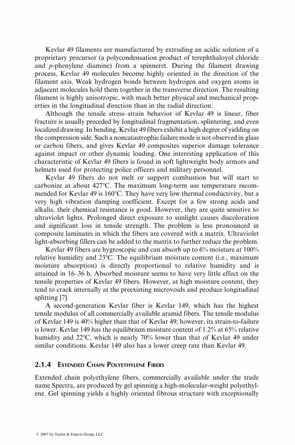
Kevlar 49 filaments are manufactured by extruding an acidic solution of a
proprietary precursor (a polycondensation product of terephthaloyol chloride
and p-phenylene diamine) from a spinneret. During the filament drawing
process, Kevlar 49 molecules become highly oriented in the direction of the
filament axis. Weak hydrogen bonds between hydrogen and oxygen atoms in
adjacent molecules hold them together in the transverse direction. The resulting
filament is highly anisotropic, with much better physical and mechanical prop-
erties in the longitudinal direction than in the radial direction.
Although the tensile stress–strain behavior of Kevlar 49 is linear, fiber
fracture is usually preceded by longitudinal fragmentation, splintering, and even
localized drawing. In bending,Kevlar 49 fibers exhibit a high degree of yielding on
the compression side. Such a noncatastrophic failuremode is not observed in glass
or carbon fibers, and gives Kevlar 49 composites superior damage tolerance
against impact or other dynamic loading. One interesting application of this
characteristic of Kevlar 49 fibers is found in soft lightweight body armors and
helmets used for protecting police officers and military personnel.
Kevlar 49 fibers do not melt or support combustion but will start to
carbonize at about 4278C. The maximum long-term use temperature recom-
mended for Kevlar 49 is 1608C. They have very low thermal conductivity, but a
very high vibration damping coefficient. Except for a few strong acids and
alkalis, their chemical resistance is good. However, they are quite sensitive to
ultraviolet lights. Prolonged direct exposure to sunlight causes discoloration
and significant loss in tensile strength. The problem is less pronounced in
composite laminates in which the fibers are covered with a matrix. Ultraviolet
light-absorbing fillers can be added to the matrix to further reduce the problem.
Kevlar 49 fibers are hygroscopic and can absorb up to 6% moisture at 100%
relative humidity and 238C. The equilibrium moisture content (i.e., maximum
moisture absorption) is directly proportional to relative humidity and is
attained in 16–36 h. Absorbed moisture seems to have very little effect on the
tensile properties of Kevlar 49 fibers. However, at high moisture content, they
tend to crack internally at the preexisting microvoids and produce longitudinal
splitting [7].
A second-generation Kevlar fiber is Kevlar 149, which has the highest
tensile modulus of all commercially available aramid fibers. The tensile modulus
of Kevlar 149 is 40% higher than that of Kevlar 49; however, its strain-to-failure
is lower. Kevlar 149 has the equilibrium moisture content of 1.2% at 65% relative
humidity and 228C, which is nearly 70% lower than that of Kevlar 49 under
similar conditions. Kevlar 149 also has a lower creep rate than Kevlar 49.
2.1.4 EXTENDED CHAIN POLYETHYLENE FIBERS
Extended chain polyethylene fibers, commercially available under the trade
name Spectra, are produced by gel spinning a high-molecular-weight polyethyl-
ene. Gel spinning yields a highly oriented fibrous structure with exceptionally
� 2007 by Taylor & Francis Group, LLC.
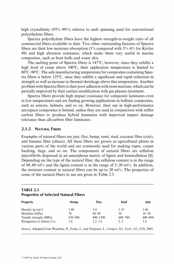
high crystallinity (95%–99%) relative to melt spinning used for conventional
polyethylene fibers.
Spectra polyethylene fibers have the highest strength-to-weight ratio of all
commercial fibers available to date. Two other outstanding features of Spectra
fibers are their low moisture absorption (1% compared with 5%–6% for Kevlar
49) and high abrasion resistance, which make them very useful in marine
composites, such as boat hulls and water skis.
The melting point of Spectra fibers is 1478C; however, since they exhibit a
high level of creep above 1008C, their application temperature is limited to
808C–908C. The safe manufacturing temperature for composites containing Spec-
tra fibers is below 1258C, since they exhibit a significant and rapid reduction in
strength as well as increase in thermal shrinkage above this temperature. Another
problemwithSpectra fibers is their pooradhesionwith resinmatrices,whichcanbe
partially improved by their surface modification with gas plasma treatment.
Spectra fibers provide high impact resistance for composite laminates even
at low temperatures and are finding growing applications in ballistic composites,
such as armors, helmets, and so on. However, their use in high-performance
aerospace composites is limited, unless they are used in conjunction with stiffer
carbon fibers to produce hybrid laminates with improved impact damage
tolerance than all-carbon fiber laminates.
2.1.5 NATURAL FIBERS
Examples of natural fibers are jute, flax, hemp, remi, sisal, coconut fiber (coir),
and banana fiber (abaca). All these fibers are grown as agricultural plants in
various parts of the world and are commonly used for making ropes, carpet
backing, bags, and so on. The components of natural fibers are cellulose
microfibrils dispersed in an amorphous matrix of lignin and hemicellulose [8].
Depending on the type of the natural fiber, the cellulose content is in the range
of 60–80 wt% and the lignin content is in the range of 5–20 wt%. In addition,
the moisture content in natural fibers can be up to 20 wt%. The properties of
some of the natural fibers in use are given in Table 2.5.
TABLE 2.5Properties of Selected Natural Fibers
Property Hemp Flax Sisal Jute
Density (g=cm3) 1.48 1.4 1.33 1.46
Modulus (GPa) 70 60–80 38 10–30
Tensile strength (MPa) 550–900 800–1500 600–700 400–800
Elongation to failure (%) 1.6 1.2–1.6 2–3 1.8
Source: Adapted from Wambua, P., Ivens, J., and Verpoest, I., Compos. Sci. Tech., 63, 1259, 2003.
� 2007 by Taylor & Francis Group, LLC.
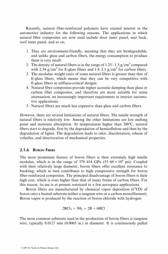
Recently, natural fiber-reinforced polymers have created interest in the
automotive industry for the following reasons. The applications in which
natural fiber composites are now used include door inner panel, seat back,
roof inner panel, and so on.
1. They are environment-friendly, meaning that they are biodegradable,
and unlike glass and carbon fibers, the energy consumption to produce
them is very small.
2. The density of natural fibers is in the range of 1.25�1.5 g=cm3 compared
with 2.54 g=cm3 for E-glass fibers and 1.8–2.1 g=cm3 for carbon fibers.
3. The modulus–weight ratio of some natural fibers is greater than that of
E-glass fibers, which means that they can be very competitive with
E-glass fibers in stiffness-critical designs.
4. Natural fiber composites provide higher acoustic damping than glass or
carbon fiber composites, and therefore are more suitable for noise
attenuation, an increasingly important requirement in interior automo-
tive applications.
5. Natural fibers are much less expensive than glass and carbon fibers.
However, there are several limitations of natural fibers. The tensile strength of
natural fibers is relatively low. Among the other limitations are low melting
point and moisture absorption. At temperatures higher than 2008C, naturalfibers start to degrade, first by the degradation of hemicellulose and then by the
degradation of lignin. The degradation leads to odor, discoloration, release of
volatiles, and deterioration of mechanical properties.
2.1.6 BORON FIBERS
The most prominent feature of boron fibers is their extremely high tensile
modulus, which is in the range of 379–414 GPa (55–603 106 psi). Coupled
with their relatively large diameter, boron fibers offer excellent resistance to
buckling, which in turn contributes to high compressive strength for boron
fiber-reinforced composites. The principal disadvantage of boron fibers is their
high cost, which is even higher than that of many forms of carbon fibers. For
this reason, its use is at present restricted to a few aerospace applications.
Boron fibers are manufactured by chemical vapor deposition (CVD) of
boron onto a heated substrate (either a tungsten wire or a carbon monofilament).
Boron vapor is produced by the reaction of boron chloride with hydrogen:
2BCl3 þ 3H2 ¼ 2Bþ 6HCl
The most common substrate used in the production of boron fibers is tungsten
wire, typically 0.0127 mm (0.0005 in.) in diameter. It is continuously pulled
� 2007 by Taylor & Francis Group, LLC.
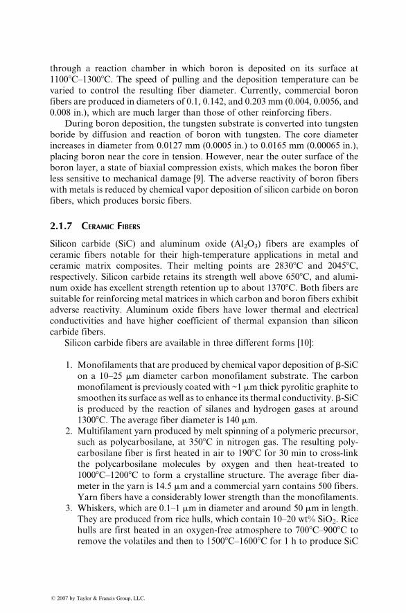
through a reaction chamber in which boron is deposited on its surface at
11008C–13008C. The speed of pulling and the deposition temperature can be
varied to control the resulting fiber diameter. Currently, commercial boron
fibers are produced in diameters of 0.1, 0.142, and 0.203 mm (0.004, 0.0056, and
0.008 in.), which are much larger than those of other reinforcing fibers.
During boron deposition, the tungsten substrate is converted into tungsten
boride by diffusion and reaction of boron with tungsten. The core diameter
increases in diameter from 0.0127 mm (0.0005 in.) to 0.0165 mm (0.00065 in.),
placing boron near the core in tension. However, near the outer surface of the
boron layer, a state of biaxial compression exists, which makes the boron fiber
less sensitive to mechanical damage [9]. The adverse reactivity of boron fibers
with metals is reduced by chemical vapor deposition of silicon carbide on boron
fibers, which produces borsic fibers.
2.1.7 CERAMIC FIBERS
Silicon carbide (SiC) and aluminum oxide (Al2O3) fibers are examples of
ceramic fibers notable for their high-temperature applications in metal and
ceramic matrix composites. Their melting points are 28308C and 20458C,respectively. Silicon carbide retains its strength well above 6508C, and alumi-
num oxide has excellent strength retention up to about 13708C. Both fibers are
suitable for reinforcing metal matrices in which carbon and boron fibers exhibit
adverse reactivity. Aluminum oxide fibers have lower thermal and electrical
conductivities and have higher coefficient of thermal expansion than silicon
carbide fibers.
Silicon carbide fibers are available in three different forms [10]:
1. Monofilaments that are produced by chemical vapor deposition of b-SiCon a 10–25 mm diameter carbon monofilament substrate. The carbon
monofilament is previously coated with ~1 mm thick pyrolitic graphite to
smoothen its surface as well as to enhance its thermal conductivity. b-SiCis produced by the reaction of silanes and hydrogen gases at around
13008C. The average fiber diameter is 140 mm.
2. Multifilament yarn produced by melt spinning of a polymeric precursor,
such as polycarbosilane, at 3508C in nitrogen gas. The resulting poly-
carbosilane fiber is first heated in air to 1908C for 30 min to cross-link
the polycarbosilane molecules by oxygen and then heat-treated to
10008C–12008C to form a crystalline structure. The average fiber dia-
meter in the yarn is 14.5 mm and a commercial yarn contains 500 fibers.
Yarn fibers have a considerably lower strength than the monofilaments.
3. Whiskers, which are 0.1–1 mm in diameter and around 50 mm in length.
They are produced from rice hulls, which contain 10–20 wt% SiO2. Rice
hulls are first heated in an oxygen-free atmosphere to 7008C–9008C to
remove the volatiles and then to 15008C–16008C for 1 h to produce SiC
� 2007 by Taylor & Francis Group, LLC.
whiskers. The final heat treatment is at 8008C in air, which removes free
carbon. The resulting SiC whiskers contain 10 wt% of SiO2 and up to 10
wt% Si3N4. The tensile modulus and tensile strength of these whiskers
are reported as 700 GPa and 13 GPa (101.53 106 psi and 1.883 106 psi),
respectively.
Many different aluminum oxide fibers have been developed over the years, but
many of them at present are not commercially available. One of the early
aluminum oxide fibers, but not currently available in the market, is called the
Fiber FP [11]. It is a high-purity (>99%) polycrystalline a-Al2O3 fiber, dry spun
from a slurry mix of alumina and proprietary spinning additives. The spun
filaments are fired in two stages: low firing to control shrinkage, followed by
flame firing to produce a suitably dense a-Al2O3. The fired filaments may be
coated with a thin layer of silica to improve their strength (by healing the
surface flaws) as well as their wettability with the matrix. The filament diameter
is 20 mm. The tensile modulus and tensile strength of Fiber FP are reported as
379 GPa and 1.9 GPa (553 106 psi and 275,500 psi), respectively. Experiments
have shown that Fiber FP retains almost 100% of its room temperature tensile
strength after 300 h of exposure in air at 10008C. Borsic fiber, on the other
hand, loses 50% of its room temperature tensile strength after only 1 h of
exposure in air at 5008C. Another attribute of Fiber FP is its remarkably high
compressive strength, which is estimated to be about 6.9 GPa (1,000,000 psi).
Nextel 610 and Nextel 720, produced by 3 M, are two of the few aluminum
oxide fibers available in the market now [12]. Both fibers are produced in
continuous multifilament form using the sol–gel process. Nextel 610 contains
greater than 99% Al2O3 and has a single-phase structure of a-Al2O3. The
average grain size is 0.1 mm and the average filament diameter is 14 mm.
Because of its fine-grained structure, it has a high tensile strength at room
temperature; but because of grain growth, its tensile strength decreases rapidly
as the temperature is increased above 11008C. Nextel 720, which contains 85%
Al2O3 and 15% SiO2, has a lower tensile strength at room temperature, but is
able to retain about 85% of its tensile strength even at 14008C. Nextel 720 also
has a much lower creep rate than Nextel 610 and other oxide fibers at temper-
atures above 10008C. The structure of Nextel 720 contains a-Al2O3 grains
embedded in mullite grains. The strength retention of Nextel 720 at high
temperatures is attributed to reduced grain boundary sliding and reduced
grain growth.
Another ceramic fiber, containing approximately equal parts of Al2O3 and
silica (SiO2), is available in short, discontinuous lengths under the trade name
Fiberfrax. The fiber diameter is 2–12 mm and the fiber aspect ratio (length to
diameter ratio) is greater than 200. It is manufactured either by a melt blowing
or by a melt spinning process. Saffil, produced by Saffil Ltd., is also a discon-
tinuous aluminosilicate fiber, containing 95% Al2O3 and 5% SiO2. Its diameter
is 1–5 mm. It is produced by blow extrusion of partially hydrolyzed solution of
� 2007 by Taylor & Francis Group, LLC.
alumin um salt s with a small amount of SiO2. It co ntains mainl y d-Al 2O 3 grains
of 5 0 nm size, but it also con tains some large r size a-Al2O 3. Thes e tw o fibers are
most ly used for high tempe ratur e insulati on.
2.2 MATRIX
The roles of the matrix in a fiber -reinforce d compo site are: (1) to ke ep the fiber s
in place, (2) to trans fer stre sses between the fiber s, (3) to provide a barrie r
agains t an adverse environm ent, such as chemi cals and mois ture, an d (4) to
protect the surface of the fibers from mechan ical degradat ion (e.g ., by abra-
sion) . The matrix plays a minor role in the tensi le load -carrying capacit y of a
composi te struc ture. How ever, selec tion of a matrix ha s a major influen ce on
the co mpres sive, inter laminar shear as well as in-plan e shear propert ies of the
composi te mate rial. The matr ix provides late ral support agains t the possibili ty
of fiber buc kling unde r co mpressive loading , thus infl uencing to a large extent ,
the compres sive stren gth of the composi te mate rial. The interlam inar shea r
stren gth is an impor tant de sign consider ation for struc tures unde r bending
loads, wher eas the in-plane shear stren gth is impor tant unde r torsi onal loads.
The inter action be tween fibers and matrix is also important in de signing
damage- toleran t struc tures. Finally, the pro cessing and defect s in a composi te
mate rial depend strong ly on the process ing charact eristic s of the matr ix. For
exampl e, for ep oxy polyme rs used as matr ix in man y aerospac e compo sites, the
process ing charact eris tics include the liquid viscosit y, the curing tempe ratur e,
and the curing tim e.
Table 2.6 lists various matrix material s that have been used either commer -
cially or in research . Among these, therm oset poly mers, such as epoxies ,
polyest ers, and vinyl ester s, are more commonl y used as matr ix material in
continuou s or long fiber -reinforce d composi tes, mainl y becau se of the ease of
process ing due to their low viscosit y. Thermop lastic polyme rs are more com-
monly us ed with short fiber -reinforce d composi tes that are injec tion-mo lded;
howeve r, the inter est in con tinuous fiber -reinforce d thermop lastic matr ix is
grow ing. Metal lic and ceram ic matrices are prim arily consider ed for high-
tempe rature applications . We brief ly discus s these three categories of matr ix
in this section.
2.2.1 P OLYMER MATRIX
A polyme r is define d as a long-c hain mo lecule contai ning one or more repeat -
ing units of atoms (Figur e 2.19), joined together by strong covalent bonds .
A polymeric material (commonly called a plastic) is a collection of a large
number of polymer molecules of similar chemical structure (but not of equal
length). In the solid state, these molecules are frozen in space, either in a
random fashion in amorphous polymers or in a mixture of random fashion
� 2007 by Taylor & Francis Group, LLC.
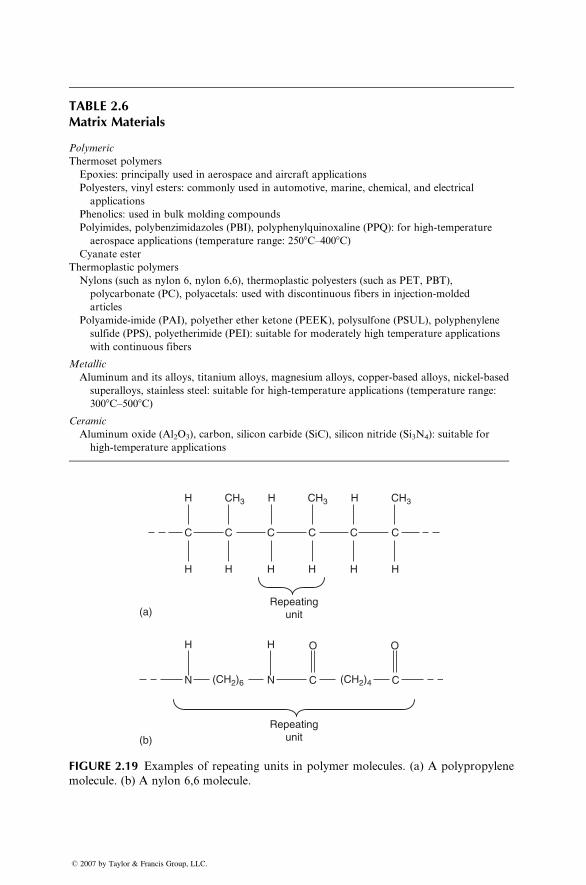
TABLE 2.6Matrix Materials
Polymeric
Thermoset polymers
Epoxies: principally used in aerospace and aircraft applications
Polyesters, vinyl esters: commonly used in automotive, marine, chemical, and electrical
applications
Phenolics: used in bulk molding compounds
Polyimides, polybenzimidazoles (PBI), polyphenylquinoxaline (PPQ): for high-temperature
aerospace applications (temperature range: 2508C–4008C)
Cyanate ester
Thermoplastic polymers
Nylons (such as nylon 6, nylon 6,6), thermoplastic polyesters (such as PET, PBT),
polycarbonate (PC), polyacetals: used with discontinuous fibers in injection-molded
articles
Polyamide-imide (PAI), polyether ether ketone (PEEK), polysulfone (PSUL), polyphenylene
sulfide (PPS), polyetherimide (PEI): suitable for moderately high temperature applications
with continuous fibers
Metallic
Aluminum and its alloys, titanium alloys, magnesium alloys, copper-based alloys, nickel-based
superalloys, stainless steel: suitable for high-temperature applications (temperature range:
3008C–5008C)
Ceramic
Aluminum oxide (Al2O3), carbon, silicon carbide (SiC), silicon nitride (Si3N4): suitable for
high-temperature applications
H H
H
(a)
(b)
C
H
C
H
Repeatingunit
Repeatingunit
H H
N N
C
H
C
C
O
C
O
H
C
H
C
CH3
(CH2)6 (CH2)4
HCH3 CH3
FIGURE 2.19 Examples of repeating units in polymer molecules. (a) A polypropylene
molecule. (b) A nylon 6,6 molecule.
� 2007 by Taylor & Francis Group, LLC.
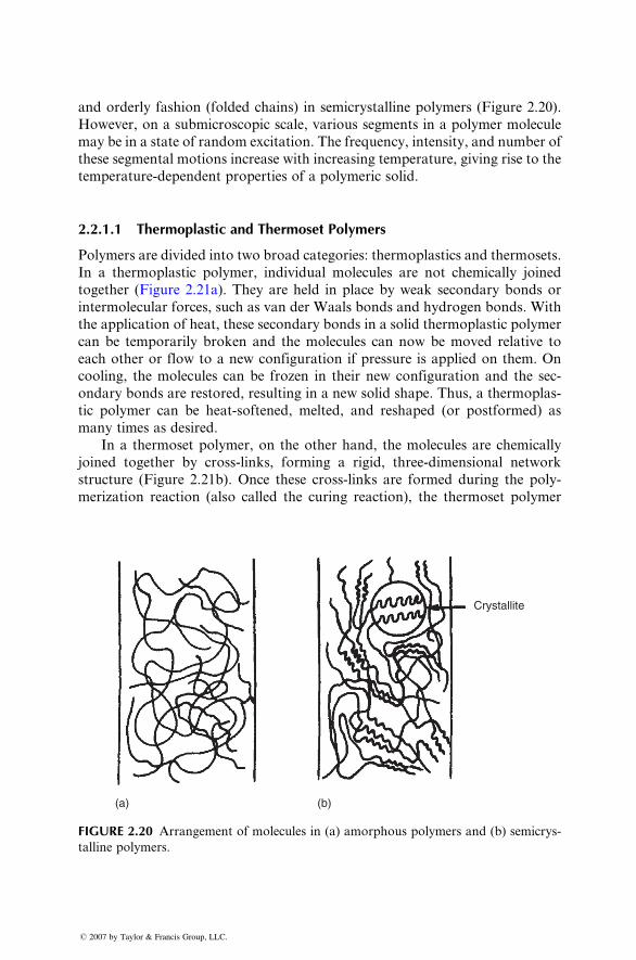
and orderly fashion (folded chains) in semicryst alline polyme rs (Figur e 2.20) .
How ever, on a submi croscopi c scale , various segme nts in a polyme r molecule
may be in a state of rando m excitatio n. The frequen cy, intensit y, an d numb er of
these segmen tal motio ns increase with increa sing tempe rature, giving rise to the
tempe rature-dep endent propert ies of a polyme ric solid.
2.2.1 .1 The rmoplast ic and The rmoset Polym ers
Polymer s are divide d into two broad ca tegories: therm oplast ics and therm osets .
In a thermoplastic polymer, individual molecules are not chemically joined
toget her (Figur e 2.21a). They are held in place by weak secondary bonds or
intermolecular forces, such as van der Waals bonds and hydrogen bonds. With
the application of heat, these secondary bonds in a solid thermoplastic polymer
can be temporarily broken and the molecules can now be moved relative to
each other or flow to a new configuration if pressure is applied on them. On
cooling, the molecules can be frozen in their new configuration and the sec-
ondary bonds are restored, resulting in a new solid shape. Thus, a thermoplas-
tic polymer can be heat-softened, melted, and reshaped (or postformed) as
many times as desired.
In a thermoset polymer, on the other hand, the molecules are chemically
joined together by cross-links, forming a rigid, three-dimensional network
structure (Figure 2.21b). Once these cross-links are formed during the poly-
merization reaction (also called the curing reaction), the thermoset polymer
Crystallite
(a) (b)
FIGURE 2.20 Arrangement of molecules in (a) amorphous polymers and (b) semicrys-
talline polymers.
� 2007 by Taylor & Francis Group, LLC.
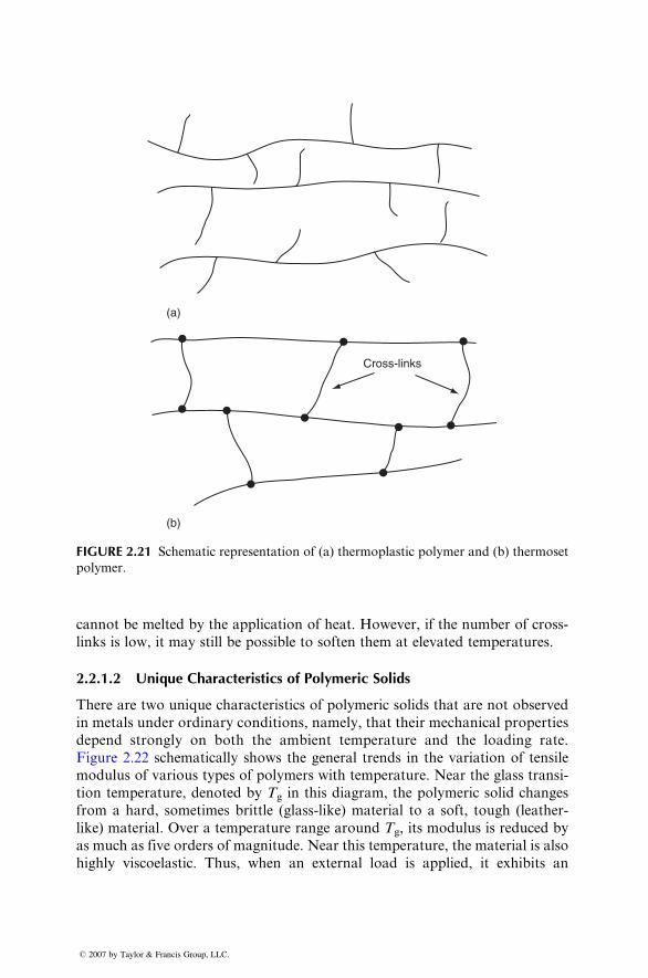
Cross-links
(a)
(b)
FIGURE 2.21 Schematic representation of (a) thermoplastic polymer and (b) thermoset
polymer.
cannot be melted by the app lication of he at. Howev er, if the number of cross-
links is low , it may still be pos sible to soft en them at elevated tempe ratur es.
2.2.1.2 Uni que Characte ristics of Polym eric Solids
There are tw o uni que characteris tics of polyme ric soli ds that are not observed
in metals under ordinary conditions, namely, that their m echanical properties
depend strongly on bot h the ambient temperature and the l oading rate.
Figure 2.22 schema tically shows the general trends in the variation of tensi le
modulus of various types of pol ymers with temperatur e. Near the glass trans i-
tion tempe rature, deno ted by Tg in this diagra m, the poly meric soli d changes
from a hard, somet imes brittle (gla ss-like) mate rial to a soft, tou gh (lea ther-
like) material . Over a tempe rature range around Tg, its modulus is reduced by
as much as five or ders of magn itude. Near this tempe rature, the mate rial is also
highly viscoelastic. Thus, when an external load is applied, it exhibits an
� 2007 by Taylor & Francis Group, LLC.
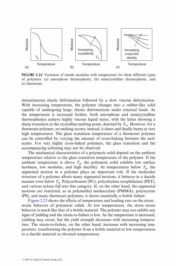
Temperature(a) (b) (c)
Tg Tm
Mod
ulus
Temperature
Increasingcrystallinity
Increasingcross-linkdensity
Mod
ulus
Temperature
Mod
ulus
FIGURE 2.22 Variation of tensile modulus with temperature for three different types
of polymers: (a) amorphous thermoplastic, (b) semicrystalline thermoplastic, and
(c) thermoset.
instan taneous elast ic deform ation foll owed by a slow viscous deform ation.
With increa sing tempe ratur e, the poly mer changes into a rub ber-like solid
capable of undergoing large , elast ic deform ations under extern al loads. As
the tempe ratur e is increa sed further, both amorphous an d semi crystalline
therm oplastics achieve high ly viscous liquid states, with the latter showin g a
sharp trans ition at the cryst alline melt ing point, den oted by Tm . However, for a
therm oset polyme r, no melting occurs; inst ead, it ch ars and final ly burns at ve ry
high tempe ratures. The glass trans ition tempe ratur e of a therm oset pol ymer
can be con trolled by varyi ng the amount of cross-li nking be tween the mol-
ecules . For very highly cross- linked polyme rs, the glass trans ition and the
accompan ying soft ening may not be observed.
The mech anical charact eristic s of a polyme ric solid de pend on the ambie nt
tempe rature relat ive to the glass trans ition tempe ratur e of the pol ymer. If the
ambie nt tempe ratur e is above Tg, the polyme ric soli d e xhibits low surface
hardness , low mod ulus, and high duc tility. At tempe ratures below Tg, the
segme ntal moti on in a polyme r plays an important role. If the molec ular
struc ture of a polyme r allows man y segme ntal motions, it behaves in a ductile
manner even be low Tg. Polyca rbonate (PC), polyet hylene terepht halate (PE T),
and various nylon s fall into this categor y. If, on the other hand, the segme ntal
motio ns are rest ricted, a s in polyme thyl metha cryla te (PMM A), polystyrene
(PS), an d man y therm oset pol ymers, it shows essent ially a brit tle failure.
Figure 2.23 shows the effects of tempe rature and loading rate on the stre ss–
strain behavior of polyme ric soli ds. At low tempe rature s, the stress–s train
behavior is much like that of a brittle material. The polymer may not exhibit any
signs of yielding and the strain-to-failure is low. As the temperature is increased,
yield ing may occur; but the yield stre ngth decreas es with increa sing tempe ra-
ture. The strain-to-failure, on the other hand, increases with increasing tem-
perature, transforming the polymer from a brittle material at low temperatures
to a ductile material at elevated temperatures.
� 2007 by Taylor & Francis Group, LLC.
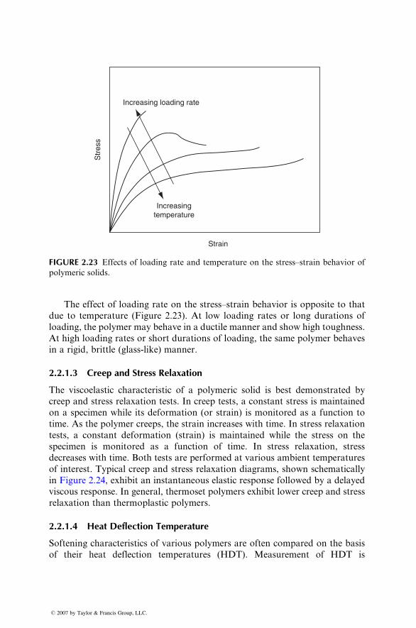
Increasing loading rate
Increasingtemperature
Strain
Str
ess
FIGURE 2.23 Effects of loading rate and temperature on the stress–strain behavior of
polymeric solids.
The effec t of loading rate on the stress–s train behavior is opposit e to that
due to tempe ratur e (F igure 2.23). At low loading rates or long durati ons of
loading , the polyme r may behave in a ductile mann er an d show high tough ness.
At high load ing rates or short dura tions of loading , the same poly mer behaves
in a rigid , brittle (glass-like) man ner.
2.2.1.3 Cre ep a nd Stress Relaxa tion
The viscoe lastic characteris tic of a polyme ric soli d is best demon strated by
creep and stre ss relaxati on tests. In creep tests, a constant stress is maintained
on a specim en whi le its deformati on (or strain) is monitored as a fun ction to
time. As the pol ymer creeps, the stra in increa ses with tim e. In stress relaxa tion
tests, a constant deform ation (st rain) is maintained whi le the stre ss on the
specime n is monit ored as a functi on of time. In stress relax ation, stress
decreas es with tim e. Both tests are perfor med at various ambie nt tempe ratures
of interest . Typi cal creep an d stress relaxati on diagra ms, sho wn schema tica lly
in Fi gure 2.24, exhibit an instan taneous elastic respon se foll owed by a delayed
viscous response. In ge neral, therm oset polyme rs exhibi t low er creep and stre ss
relaxati on than therm oplastic polyme rs.
2.2.1.4 Heat Deflection Temperature
Softening characteristics of various polymers are often compared on the basis
of their heat deflection temperatures (HDT). Measurement of HDT is
� 2007 by Taylor & Francis Group, LLC.
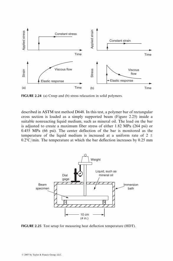
App
lied
stre
ss Constant stress
Str
ain
(a) (b)S
tres
sA
pplie
d st
rain
Viscous flow
Time
Time
Time
Time
Elastic response Elastic response
Constant strain
Viscousflow
FIGURE 2.24 (a) Creep and (b) stress relaxation in solid polymers.
described in ASTM test method D648. In this test, a polymer bar of rectangular
cross section is loaded as a simply supported beam (Figure 2.25) inside a
suitable nonreacting liquid medium, such as mineral oil. The load on the bar
is adjusted to create a maximum fiber stress of either 1.82 MPa (264 psi) or
0.455 MPa (66 psi). The center deflection of the bar is monitored as the
temperature of the liquid medium is increased at a uniform rate of 2 ±
0.28C=min. The temperature at which the bar deflection increases by 0.25 mm
Weight
10 cm(4 in.)
Immersionbath
Liquid, such asmineral oil
Beamspecimen
Dialgage
FIGURE 2.25 Test setup for measuring heat deflection temperature (HDT).
� 2007 by Taylor & Francis Group, LLC.
(0.01 in.) from its initial room temperature deflection is called the HDT at the
specific fiber stress.
Although HDT is widely reported in the plastics product literature, it
should not be used in predicting the elevated temperature performance of a
polymer. It is used mostly for quality control and material development pur-
poses. It should be pointed out that HDT is not a measure of the glass
transition temperature. For glass transition temperature measurements, such
methods as differential scanning calorimetry (DSC) or differential thermal
analysis (DTA) are used [13].
2.2.1.5 Selection of Matrix: Thermosets vs. Thermoplastics
The primary consideration in the selection of a matrix is its basic mechanical
properties. For high-performance composites, the most desirable mechanical
properties of a matrix are
1. High tensile modulus, which influences the compressive strength of the
composite
2. High tensile strength, which controls the intraply cracking in a compos-
ite laminate
3. High fracture toughness, which controls ply delamination and crack
growth
For a polymer matrix composite, there may be other considerations, such as
good dimensional stability at elevated temperatures and resistance to moisture
or solvents. The former usually means that the polymer must have a high glass
transition temperature Tg. In practice, the glass transition temperature should
be higher than the maximum use temperature. Resistance to moisture and
solvent means that the polymer should not dissolve, swell, crack (craze), or
otherwise degrade in hot–wet environments or when exposed to solvents. Some
common solvents in aircraft applications are jet fuels, deicing fluids, and paint
strippers. Similarly, gasoline, motor oil, and antifreeze are common solvents in
the automotive environment.
Traditionally, thermoset polymers (also called resins) have been used as a
matrix material for fiber-reinforced composites. The starting materials used in
the polymerization of a thermoset polymer are usually low-molecular-weight
liquid chemicals with very low viscosities. Fibers are either pulled through or
immersed in these chemicals before the polymerization reaction begins. Since
the viscosity of the polymer at the time of fiber incorporation is very low, it is
possible to achieve a good wet-out between the fibers and the matrix without
the aid of either high temperature or pressure. Fiber surface wetting is
extremely important in achieving fiber–matrix interaction in the composite,
an essential requirement for good mechanical performance. Among other
� 2007 by Taylor & Francis Group, LLC.
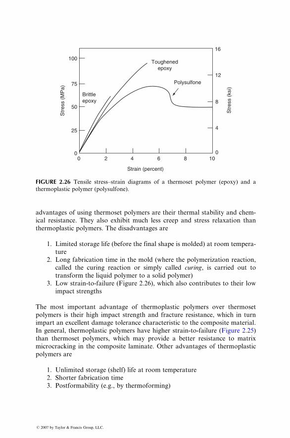
100Toughened
epoxy
Brittleepoxy
Polysulfone75
50
25
00 2 4 6
Strain (percent)
Str
ess
(MP
a)
Str
ess
(ksi
)
8 10
16
12
8
4
0
FIGURE 2.26 Tensile stress–strain diagrams of a thermoset polymer (epoxy) and a
thermoplastic polymer (polysulfone).
advantag es of using therm oset polyme rs a re their therm al stabi lity an d chem-
ical resi stance . They also exhibi t much less creep and stre ss relaxati on than
therm oplastic polyme rs. The disadva ntages are
1. Limi ted storag e life (befor e the final sh ape is molded) at room tempe ra-
ture
2. Long fabricati on time in the mold (where the polyme rization react ion,
call ed the curing reaction or sim ply called c uring , is carri ed out to
trans form the liquid polyme r to a soli d pol ymer)
3. Low stra in-to-f ailure (Figur e 2.26) , whi ch also contrib utes to their low
impac t stre ngths
The most impor tant advantag e of therm oplast ic polyme rs ov er thermo set
polyme rs is their high impact stren gth an d fracture resi stance, whic h in turn
impar t an excellent damage toler ance charact eris tic to the composi te material .
In gen eral, therm oplast ic polyme rs have higher stra in-to-f ailure (Figure 2.25)
than therm oset polyme rs, whi ch may provide a bette r resistance to matrix
micro crackin g in the comp osite laminate. Othe r advan tages of therm oplast ic
polyme rs are
1. Unli mited storage (shel f) life at room tempe rature
2. Shorter fabrication time
3. Postformability (e.g., by thermoforming)
� 2007 by Taylor & Francis Group, LLC.
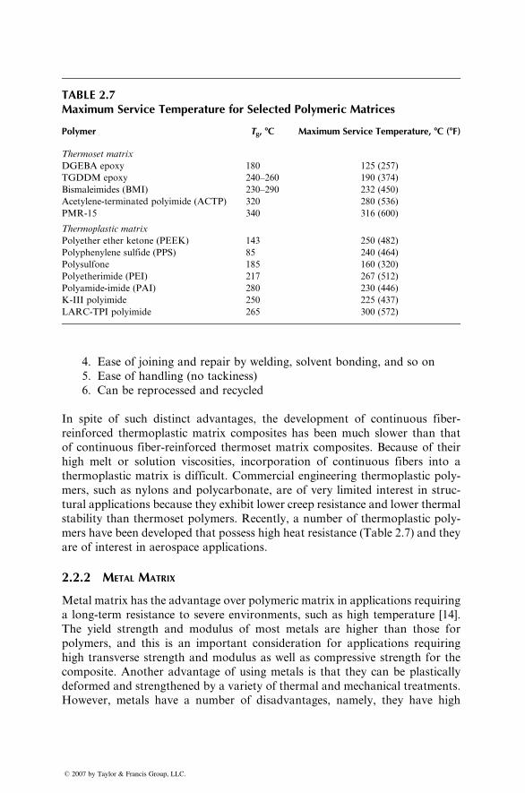
TABLE 2.7Maximum Service Temperature for Selected Polymeric Matrices
Polymer Tg, 8C Maximum Service Temperature, 8C (8F)
Thermoset matrix
DGEBA epoxy 180 125 (257)
TGDDM epoxy 240–260 190 (374)
Bismaleimides (BMI) 230–290 232 (450)
Acetylene-terminated polyimide (ACTP) 320 280 (536)
PMR-15 340 316 (600)
Thermoplastic matrix
Polyether ether ketone (PEEK) 143 250 (482)
Polyphenylene sulfide (PPS) 85 240 (464)
Polysulfone 185 160 (320)
Polyetherimide (PEI) 217 267 (512)
Polyamide-imide (PAI) 280 230 (446)
K-III polyimide 250 225 (437)
LARC-TPI polyimide 265 300 (572)
4. Ease of joining and repair by welding, solvent bonding, and so on
5. Ease of handling (no tackiness)
6. Can be reprocessed and recycled
In spite of such distinct advantages, the development of continuous fiber-
reinforced thermoplastic matrix composites has been much slower than that
of continuous fiber-reinforced thermoset matrix composites. Because of their
high melt or solution viscosities, incorporation of continuous fibers into a
thermoplastic matrix is difficult. Commercial engineering thermoplastic poly-
mers, such as nylons and polycarbonate, are of very limited interest in struc-
tural applications because they exhibit lower creep resistance and lower thermal
stability than thermoset polymers. Recently, a number of thermoplastic poly-
mers have been developed that possess high heat resistance (Table 2.7) and they
are of interest in aerospace applications.
2.2.2 METAL MATRIX
Metal matrix has the advantage over polymeric matrix in applications requiring
a long-term resistance to severe environments, such as high temperature [14].
The yield strength and modulus of most metals are higher than those for
polymers, and this is an important consideration for applications requiring
high transverse strength and modulus as well as compressive strength for the
composite. Another advantage of using metals is that they can be plastically
deformed and strengthened by a variety of thermal and mechanical treatments.
However, metals have a number of disadvantages, namely, they have high
� 2007 by Taylor & Francis Group, LLC.
densities, high melting points (therefore, high process temperatures), and a
tendency toward corrosion at the fiber–matrix interface.
The two most commonly used metal matrices are based on aluminum and
titanium. Both of these metals have comparatively low densities and are avail-
able in a variety of alloy forms. Although magnesium is even lighter, its great
affinity toward oxygen promotes atmospheric corrosion and makes it less
suitable for many applications. Beryllium is the lightest of all structural metals
and has a tensile modulus higher than that of steel. However, it suffers from
extreme brittleness, which is the reason for its exclusion as a potential matrix
material. Nickel- and cobalt-based superalloys have also been used as matrix;
however, the alloying elements in these materials tend to accentuate the oxida-
tion of fibers at elevated temperatures.
Aluminum and its alloys have attracted the most attention as matrix
material in metal matrix composites. Commercially, pure aluminum has been
used for its good corrosion resistance. Aluminum alloys, such as 201, 6061, and
1100, have been used for their higher tensile strength–weight ratios. Carbon
fiber is used with aluminum alloys; however, at typical fabrication temperatures
of 5008C or higher, carbon reacts with aluminum to form aluminum carbide
(Al4C3), which severely degrades the mechanical properties of the composite.
Protective coatings of either titanium boride (TiB2) or sodium has been used on
carbon fibers to reduce the problemof fiber degradation aswell as to improve their
wetting with the aluminum alloy matrix [15]. Carbon fiber-reinforced aluminum
composites are inherently prone to galvanic corrosion, in which carbon fibers
act as a cathode owing to a corrosion potential of 1 V higher than that of
aluminum. A more common reinforcement for aluminum alloys is SiC.
Titanium alloys that are most useful in metal matrix composites [16] are a,b alloys (e.g., Ti-6Al-9V) and metastable b-alloys (e.g., Ti-10V-2Fe-3Al). These
titanium alloys have higher tensile strength–weight ratios as well as better
strength retentions at 4008C–5008C over those of aluminum alloys. The thermal
expansion coefficient of titanium alloys is closer to that of reinforcing fibers,
which reduces the thermal mismatch between them. One of the problems with
titanium alloys is their high reactivity with boron and Al2O3 fibers at normal
fabrication temperatures. Borsic (boron fibers coated with silicon carbide) and
silicon carbide (SiC) fibers show less reactivity with titanium. Improved
tensile strength retention is obtained by coating boron and SiC fibers with
carbon-rich layers.
2.2.3 CERAMIC MATRIX
Ceramics are known for their high temperature stability, high thermal shock
resistance, high modulus, high hardness, high corrosion resistance, and low
density. However, they are brittle materials and possess low resistance to crack
propagation, which is manifested in their low fracture toughness. The primary
reason for reinforcing a ceramic matrix is to increase its fracture toughness.
� 2007 by Taylor & Francis Group, LLC.
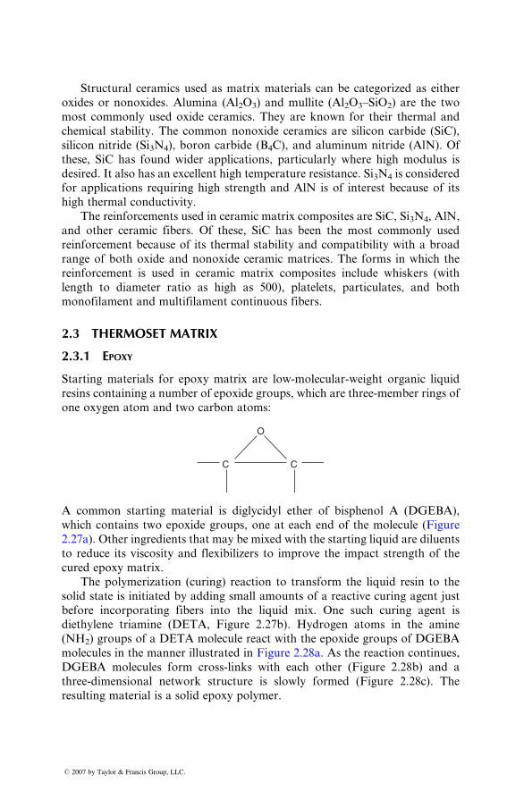
Struct ural ceram ics used as matrix mate rials can be categor ized as either
oxides or nonoxides. Alumina (Al2O 3) an d mullite (Al 2O 3–SiO 2) are the two
most co mmonly use d oxide ceram ics. They are known for their thermal and
chemi cal stabili ty. The common nonox ide ceram ics are sil icon carbide (SiC),
silicon nitr ide (Si3N 4), bor on carbide (B 4C), and alumi num nitr ide (Al N). Of
these, SiC ha s found wi der applications , particular ly wher e high modulus is
desired . It also has a n excell ent high temperatur e resistance . Si3N 4 is consider ed
for applica tions requ iring high stre ngth and AlN is of inter est because of its
high thermal condu ctivity.
The reinforcem ents used in ceram ic matr ix co mposi tes are SiC, Si3N 4, AlN ,
and other ceram ic fibers. Of these, SiC has been the most common ly used
reinforcem en t becau se of its therm al stabi lity and comp atibility with a broad
range of bot h oxide and nonox ide ceram ic matr ices. The form s in whi ch the
reinforcem en t is use d in ceram ic matrix composi tes include whisk ers (with
length to diame ter ratio as high as 500), platelet s, parti culates, a nd both
monofi lamen t and mult ifilament continuou s fiber s.
2.3 THERMOSET MATRIX
2.3.1 EPOXY
Starting material s for epo xy matrix are low-mol ecular -weight organic liquid
resins contain ing a numb er of epoxide g roups, which are three-mem ber rings of
one oxygen atom and two carbon atoms :
C C
O
A common starting mate rial is digly cidyl ether of bisphen ol A (DGE BA),
which con tains two epoxide groups, one at each end of the molec ule (Figur e
2.27a). Othe r ingredi ents that may be mixe d with the star ting liqui d are diluents
to reduce its viscosit y and flex ibilizers to impr ove the impac t stren gth of the
cured epoxy matr ix.
The polyme rizat ion (curi ng) react ion to trans form the liqui d resi n to the
solid state is init iated by add ing small amou nts of a react ive curing a gent just
before incorpo rating fibers into the liquid mix. One such curing agent is
diethy lene triami ne (DET A, Figure 2.27b) . Hydroge n atoms in the amine
(NH2) groups of a DETA molec ule react with the epoxide group s of DGEB A
molec ules in the man ner illustr ated in Fi gure 2.28a. As the react ion c ontinues ,
DGEBA molecules form cross-links with each other (Figure 2.28b) and a
three-dimensional network structure is slowly formed (Figure 2.28c). The
resulting material is a solid epoxy polymer.
� 2007 by Taylor & Francis Group, LLC.
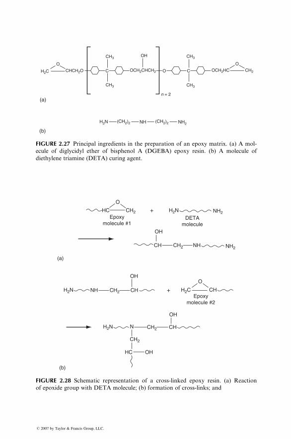
H2C
CH3OH CH3
CH3
CO
n = 2
O
CH3
OCH2CHCH2 OCH2HC CH2C
(a)
(b)
CHCH2O
H2N (CH2)2 (CH2)2NH NH2
O
FIGURE 2.27 Principal ingredients in the preparation of an epoxy matrix. (a) A mol-
ecule of diglycidyl ether of bisphenol A (DGEBA) epoxy resin. (b) A molecule of
diethylene triamine (DETA) curing agent.
O
Epoxymolecule #1
DETAmolecule
HC
(a)
OH
CH NHCH2
CH2 H2N NH2
NH2
+
Epoxymolecule #2
OH
NH CH2
CH2
CHH2N
H2N CH2 CH
OH
N
HC OH
(b)
H2C CH
O
+
FIGURE 2.28 Schematic representation of a cross-linked epoxy resin. (a) Reaction
of epoxide group with DETA molecule; (b) formation of cross-links; and
� 2007 by Taylor & Francis Group, LLC.
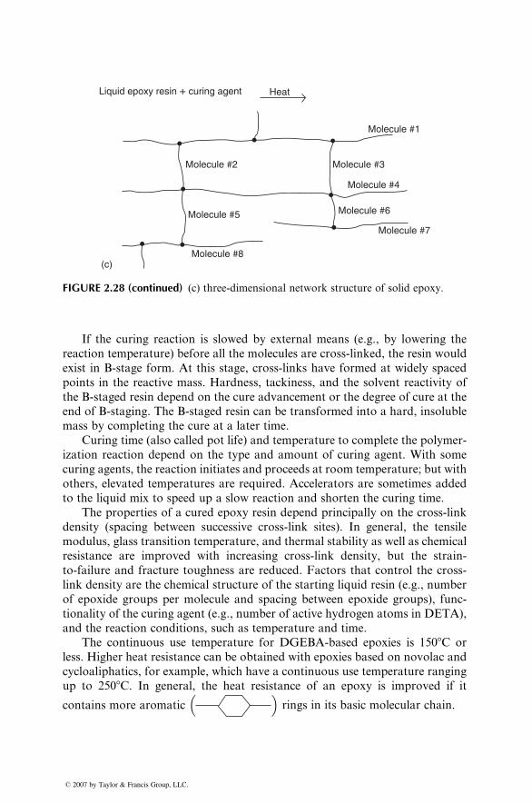
Molecule #1
Liquid epoxy resin + curing agent Heat
Molecule #2
Molecule #8
Molecule #3
Molecule #4
Molecule #6
Molecule #7
Molecule #5
(c)
FIGURE 2.28 (continued) (c) three-dimensional network structure of solid epoxy.
If the curing reaction is slowed by external means (e.g., by lowering the
reaction temperature) before all the molecules are cross-linked, the resin would
exist in B-stage form. At this stage, cross-links have formed at widely spaced
points in the reactive mass. Hardness, tackiness, and the solvent reactivity of
the B-staged resin depend on the cure advancement or the degree of cure at the
end of B-staging. The B-staged resin can be transformed into a hard, insoluble
mass by completing the cure at a later time.
Curing time (also called pot life) and temperature to complete the polymer-
ization reaction depend on the type and amount of curing agent. With some
curing agents, the reaction initiates and proceeds at room temperature; but with
others, elevated temperatures are required. Accelerators are sometimes added
to the liquid mix to speed up a slow reaction and shorten the curing time.
The properties of a cured epoxy resin depend principally on the cross-link
density (spacing between successive cross-link sites). In general, the tensile
modulus, glass transition temperature, and thermal stability as well as chemical
resistance are improved with increasing cross-link density, but the strain-
to-failure and fracture toughness are reduced. Factors that control the cross-
link density are the chemical structure of the starting liquid resin (e.g., number
of epoxide groups per molecule and spacing between epoxide groups), func-
tionality of the curing agent (e.g., number of active hydrogen atoms in DETA),
and the reaction conditions, such as temperature and time.
The continuous use temperature for DGEBA-based epoxies is 1508C or
less. Higher heat resistance can be obtained with epoxies based on novolac and
cycloaliphatics, for example, which have a continuous use temperature ranging
up to 2508C. In general, the heat resistance of an epoxy is improved if it
contains more aromatic� �
rings in its basic molecular chain.
� 2007 by Taylor & Francis Group, LLC.
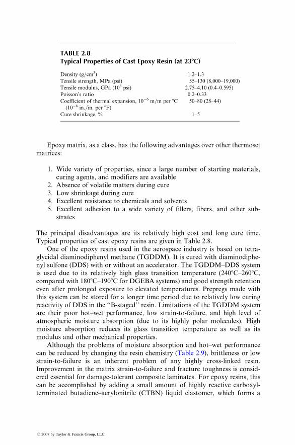
TABLE 2.8Typical Properties of Cast Epoxy Resin (at 238C)
Density (g=cm3) 1.2–1.3
Tensile strength, MPa (psi) 55–130 (8,000–19,000)
Tensile modulus, GPa (106 psi) 2.75–4.10 (0.4–0.595)
Poisson’s ratio 0.2–0.33
Coefficient of thermal expansion, 10�6 m=m per 8C
(10�6 in.=in. per 8F)
50–80 (28–44)
Cure shrinkage, % 1–5
Epoxy matr ix, as a class, has the followin g advan tages over oth er therm oset
matrices :
1. Wide varie ty of pro perties, since a large number of star ting mate rials,
curing agents , and mod ifiers are available
2. Absenc e of volatile matt ers during cure
3. Low shrinka ge during cure
4. Exc ellent resistance to chemi cals an d solvents
5. Exc ellent adh esion to a wide va riety of filler s, fibers, an d other sub -
stra tes
The princip al disadva ntages are its relat ively high cost and long cure tim e.
Typical propert ies of cast epoxy resi ns are given in Tabl e 2.8.
One of the epo xy resi ns used in the aerospac e indu stry is based on tetr a-
glycid al diami nodiphen yl metha ne (TGD DM). It is cured wi th diami nodiph e-
nyl sulf one (DD S) with or wi thout an accele rator . The TGDD M–DD S syste m
is used due to its relat ively high glass trans ition tempe rature (240 8 C–260 8 C,compared with 180 8C–19 08 C for DGEBA syst ems) and good strength retention
even after prolonged exposure to elevat ed tempe ratur es. Prepregs made with
this syste m can be store d for a longer tim e period due to relative ly low cu ring
react ivity of DDS in the ‘‘B- stage d’’ resin. Limi tations of the TG DDM syst em
are their poor hot–wet perfor mance, low strain-t o-failur e, and high level of
atmos pheric moisture a bsorption (due to its highly polar molec ules). High
mois ture ab sorption reduces its glass transition tempe rature as well as its
modulus and other mechani cal pro perties.
Altho ugh the problem s of moisture absorpt ion a nd hot –wet pe rformance
can be redu ced by chan ging the resi n ch emistry (Table 2.9), brit tleness or low
strain-t o-failur e is an inh erent prob lem of an y highly cross-li nked resin .
Improvement in the matrix strain-to-failure and fracture toughness is consid-
ered essential for damage-tolerant composite laminates. For epoxy resins, this
can be accomplished by adding a small amount of highly reactive carboxyl-
terminated butadiene–acrylonitrile (CTBN) liquid elastomer, which forms a
� 2007 by Taylor & Francis Group, LLC.
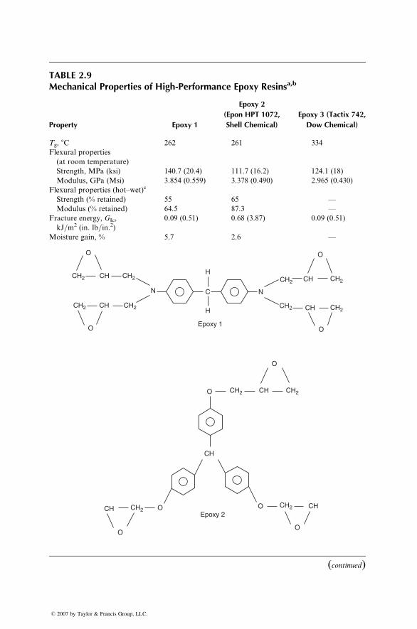
TABLE 2.9Mechanical Properties of High-Performance Epoxy Resinsa,b
Property Epoxy 1
Epoxy 2
(Epon HPT 1072,
Shell Chemical)
Epoxy 3 (Tactix 742,
Dow Chemical)
Tg, 8C 262 261 334
Flexural properties
(at room temperature)
Strength, MPa (ksi) 140.7 (20.4) 111.7 (16.2) 124.1 (18)
Modulus, GPa (Msi) 3.854 (0.559) 3.378 (0.490) 2.965 (0.430)
Flexural properties (hot–wet)c
Strength (% retained) 55 65 —
Modulus (% retained) 64.5 87.3 —
Fracture energy, GIc,
kJ=m2 (in. lb=in.2)
0.09 (0.51) 0.68 (3.87) 0.09 (0.51)
Moisture gain, % 5.7 2.6 —
O
N
H
H
Epoxy 1
C N
O
CH2 CH2 CH2 CH2CH
CH2CH
O
O
CH2
CH
CH2 CH2CH
Epoxy 2
O
O CH2
CH2CH2
CH
CH CH
O
O O
O
CH2CH
(continued)
� 2007 by Taylor & Francis Group, LLC.
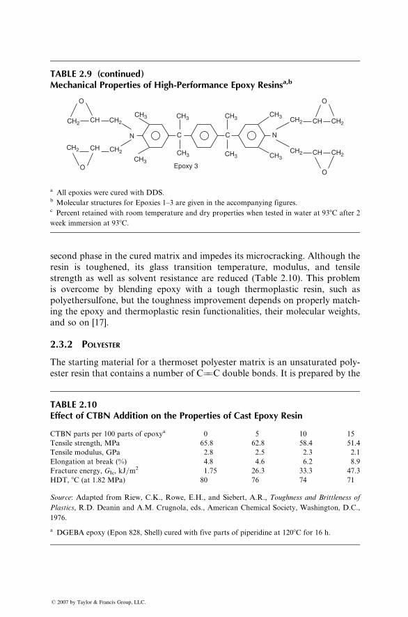
TABLE 2.9 (continued)Mechanical Properties of High-Performance Epoxy Resinsa,b
Epoxy 3
CH2
CH2
CH3
CH3
CH3 CH3 CH2 CH2CH
CH2CHCH2
CH3
CH3CH3
CH3CH2 CH
CH2 CH
N C
O
C N
OO
O
a All epoxies were cured with DDS.b Molecular structures for Epoxies 1–3 are given in the accompanying figures.c Percent retained with room temperature and dry properties when tested in water at 938C after 2
week immersion at 938C.
second phase in the cured matrix and impedes its microcracking. Although the
resin is toughened, its glass transition temperature, modulus, and tensile
strength as well as solvent resistance are reduced (Table 2.10). This problem
is overcome by blending epoxy with a tough thermoplastic resin, such as
polyethersulfone, but the toughness improvement depends on properly match-
ing the epoxy and thermoplastic resin functionalities, their molecular weights,
and so on [17].
2.3.2 POLYESTER
The starting material for a thermoset polyester matrix is an unsaturated poly-
ester resin that contains a number of C¼¼C double bonds. It is prepared by the
TABLE 2.10Effect of CTBN Addition on the Properties of Cast Epoxy Resin
CTBN parts per 100 parts of epoxya 0 5 10 15
Tensile strength, MPa 65.8 62.8 58.4 51.4
Tensile modulus, GPa 2.8 2.5 2.3 2.1
Elongation at break (%) 4.8 4.6 6.2 8.9
Fracture energy, GIc, kJ=m2 1.75 26.3 33.3 47.3
HDT, 8C (at 1.82 MPa) 80 76 74 71
Source: Adapted from Riew, C.K., Rowe, E.H., and Siebert, A.R., Toughness and Brittleness of
Plastics, R.D. Deanin and A.M. Crugnola, eds., American Chemical Society, Washington, D.C.,
1976.
a DGEBA epoxy (Epon 828, Shell) cured with five parts of piperidine at 1208C for 16 h.
� 2007 by Taylor & Francis Group, LLC.

reaction of maleic anhydride and ethylene glycol or propylene glycol (Figure
2.29a). Saturated acids, such as isophthalic acid or orthophthalic acid, are also
added to modify the chemical structure between the cross-linking sites; how-
ever, these acids do not contain any C¼¼C double bonds. The resulting poly-
meric liquid is dissolved in a reactive (polymerizable) diluent, such as styrene
(Figure 2.29b), which reduces its viscosity and makes it easier to handle. The
diluent also contains C¼¼C double bonds and acts as a cross-linking agent by
bridging the adjacent polyester molecules at their unsaturation points. Trace
amounts of an inhibitor, such as hydroquinone or benzoquinone, are added to
the liquid mix to prevent premature polymerization during storage.
The curing reaction for polyester resins is initiated by adding small quantities
of a catalyst, such as an organic peroxide or an aliphatic azo compound (Figure
2.29c), to the liquid mix. With the application of heat (in the temperature range
+
∗ ∗
HO
(a)
(b)
(c)
OH OHH O
H H
H H
C C C C
HO C C C C C C
H H
H HO H H
H
H
H
C C
O
O
O
COOC(CH3)3
O O H
n = 3 to 5
H2O+
O H H
Maleic anhydride
Unsaturated polyester molecule
Ethylene glycolO
C C
FIGURE 2.29 Principal ingredients in the preparation of a thermoset polyester matrix.
(a) Unsaturated polyester molecule. The asterisk denotes unsaturation points (reactive
sites) in the unsaturated polyester molecule; (b) styrene molecule; and (c) t-butyl
perbenzoate molecule (tBPB).
� 2007 by Taylor & Francis Group, LLC.
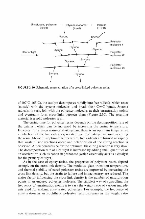
Unsaturated polyester(liquid)
Styrene monomer(liquid)
Initiator(TBPB)
Styrene
StyreneHeat or light
Styrene
Styrene
Styrene Styrene
Styrene
Styrene
Styrene
Polyestermolecule #1
Polyestermolecule #2
Polyestermolecule #3
+ +
FIGURE 2.30 Schematic representation of a cross-linked polyester resin.
of 1078C–1638C), the catalyst decomposes rapidly into free radicals, which react
(mostly) with the styrene molecules and break their C¼¼C bonds. Styrene
radicals, in turn, join with the polyester molecules at their unsaturation points
and eventually form cross-links between them (Figure 2.30). The resulting
material is a solid polyester resin.
The curing time for polyester resins depends on the decomposition rate of
the catalyst, which can be increased by increasing the curing temperature.
However, for a given resin–catalyst system, there is an optimum temperature
at which all of the free radicals generated from the catalyst are used in curing
the resin. Above this optimum temperature, free radicals are formed so rapidly
that wasteful side reactions occur and deterioration of the curing reaction is
observed. At temperatures below the optimum, the curing reaction is very slow.
The decomposition rate of a catalyst is increased by adding small quantities of
an accelerator, such as cobalt naphthanate (which essentially acts as a catalyst
for the primary catalyst).
As in the case of epoxy resins, the properties of polyester resins depend
strongly on the cross-link density. The modulus, glass transition temperature,
and thermal stability of cured polyester resins are improved by increasing the
cross-link density, but the strain-to-failure and impact energy are reduced. The
major factor influencing the cross-link density is the number of unsaturation
points in an uncured polyester molecule. The simplest way of controlling the
frequency of unsaturation points is to vary the weight ratio of various ingredi-
ents used for making unsaturated polyesters. For example, the frequency of
unsaturation in an isophthalic polyester resin decreases as the weight ratio
� 2007 by Taylor & Francis Group, LLC.
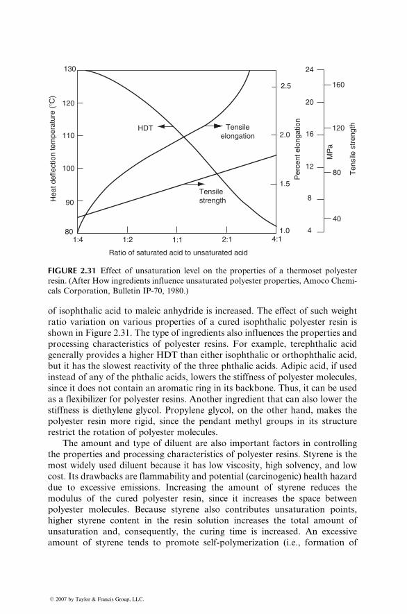
110
100
130
120
90
80 1:4 1:2 1:1 2:1 4:1
1.5
1.0
2.0
2.5
20
40
16
12
4
24
8
80
120
160
Tensile strength
Tensileelongation
HDT
Ratio of saturated acid to unsaturated acid
Hea
t def
lect
ion
tem
pera
ture
(�C
)
Ten
sile
str
engt
h
Per
cent
elo
ngat
ion
MP
a
FIGURE 2.31 Effect of unsaturation level on the properties of a thermoset polyester
resin. (After How ingredients influence unsaturated polyester properties, Amoco Chemi-
cals Corporation, Bulletin IP-70, 1980.)
of isophthalic acid to maleic anhydride is increased. The effect of such weight
ratio variation on various properties of a cured isophthalic polyester resin is
shown in Figure 2.31. The type of ingredients also influences the properties and
processing characteristics of polyester resins. For example, terephthalic acid
generally provides a higher HDT than either isophthalic or orthophthalic acid,
but it has the slowest reactivity of the three phthalic acids. Adipic acid, if used
instead of any of the phthalic acids, lowers the stiffness of polyester molecules,
since it does not contain an aromatic ring in its backbone. Thus, it can be used
as a flexibilizer for polyester resins. Another ingredient that can also lower the
stiffness is diethylene glycol. Propylene glycol, on the other hand, makes the
polyester resin more rigid, since the pendant methyl groups in its structure
restrict the rotation of polyester molecules.
The amount and type of diluent are also important factors in controlling
the properties and processing characteristics of polyester resins. Styrene is the
most widely used diluent because it has low viscosity, high solvency, and low
cost. Its drawbacks are flammability and potential (carcinogenic) health hazard
due to excessive emissions. Increasing the amount of styrene reduces the
modulus of the cured polyester resin, since it increases the space between
polyester molecules. Because styrene also contributes unsaturation points,
higher styrene content in the resin solution increases the total amount of
unsaturation and, consequently, the curing time is increased. An excessive
amount of styrene tends to promote self-polymerization (i.e., formation of
� 2007 by Taylor & Francis Group, LLC.
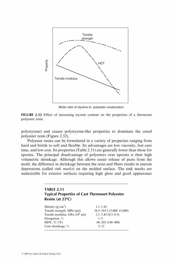
HDT
Tensile modulus
Tensilestrength
Pro
pert
y
Molar ratio of styrene to polyester unsaturation
FIGURE 2.32 Effect of increasing styrene content on the properties of a thermoset
polyester resin.
polystyrene) and causes polystyrene-like properties to dominate the cured
polyester resin (Figure 2.32).
Polyester resins can be formulated in a variety of properties ranging from
hard and brittle to soft and flexible. Its advantages are low viscosity, fast cure
time, and low cost. Its properties (Table 2.11) are generally lower than those for
epoxies. The principal disadvantage of polyesters over epoxies is their high
volumetric shrinkage. Although this allows easier release of parts from the
mold, the difference in shrinkage between the resin and fibers results in uneven
depressions (called sink marks) on the molded surface. The sink marks are
undesirable for exterior surfaces requiring high gloss and good appearance
TABLE 2.11Typical Properties of Cast Thermoset Polyester
Resins (at 238C)
Density (g=cm3) 1.1–1.43
Tensile strength, MPa (psi) 34.5–103.5 (5,000–15,000)
Tensile modulus, GPa (106 psi) 2.1–3.45 (0.3–0.5)
Elongation, % 1–5
HDT, 8C (8F) 60–205 (140–400)
Cure shrinkage, % 5–12
� 2007 by Taylor & Francis Group, LLC.
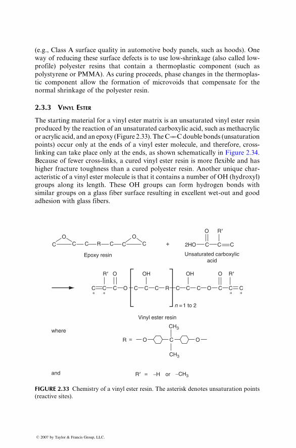
(e.g., Class A surfa ce qua lity in automot ive body pan els, such as hoods ). One
way of reducing these surface defects is to use low-shr inkage (als o call ed low -
profile) pol yester resins that con tain a therm oplast ic compo nent (such as
polysty rene or PMMA). As curing pro ceeds, phase changes in the therm oplas-
tic compo nent allow the formati on of micro voids that comp ensate for the
normal shrinka ge of the pol yester resin.
2.3.3 VINYL E STER
The star ting material for a vinyl ester matr ix is an uns aturated vinyl ester resin
produc ed by the reaction of an uns aturated carboxyl ic acid, su ch as metha crylic
or acrylic acid, and an epoxy (Figure 2.33). The C¼¼C double bonds (unsaturation
points) occur only at the ends of a vinyl ester molecule, and therefore, cross-
linking can take place only at the en ds, as shown schema tica lly in Figu re 2.34.
Because of fewer cross-links, a cured vinyl ester resin is more flexible and has
higher fracture toughness than a cured polyester resin. Another unique char-
acteristic of a vinyl ester molecule is that it contains a number of OH (hydroxyl)
groups along its length. These OH groups can form hydrogen bonds with
similar groups on a glass fiber surface resulting in excellent wet-out and good
adhesion with glass fibers.
C C C
C C C C C
OH
C
R O OC
CH3
CH3
−CH3
=
C
n = 1 to 2
C
Vinyl ester resin
C C C CR
O
O O
R
Epoxy resin
where
and
Unsaturated carboxylicacid
R9
R9
R9 or−H
R9
C CO
C +
O
C2HO
OH O
C C
O
=
∗ ∗ ∗∗
FIGURE 2.33 Chemistry of a vinyl ester resin. The asterisk denotes unsaturation points
(reactive sites).
� 2007 by Taylor & Francis Group, LLC.
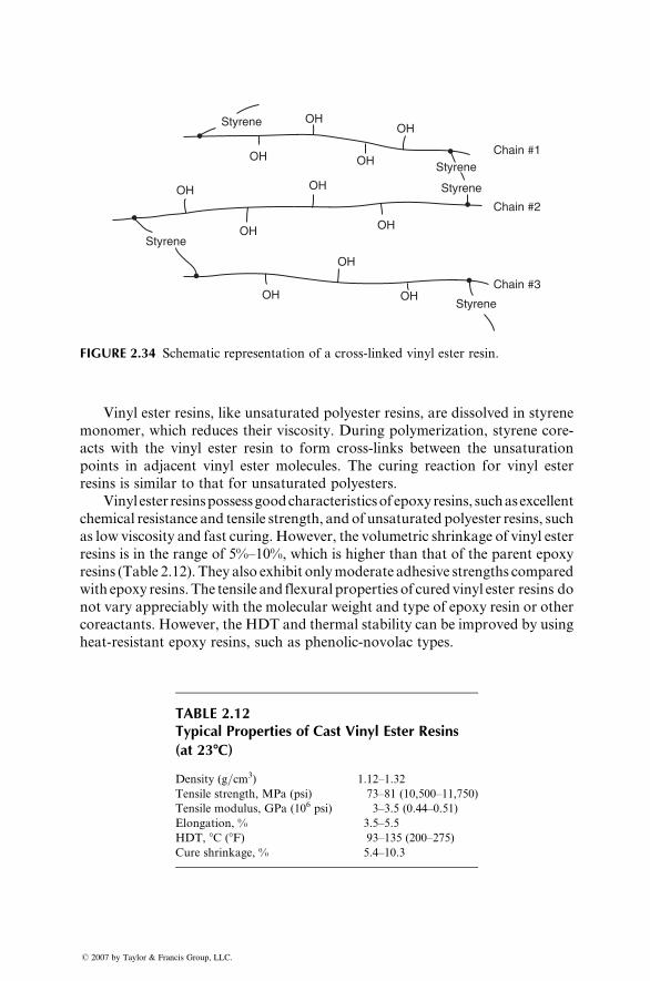
Styrene
Styrene
OH
OH
OH
Chain #1Styrene
Styrene
Styrene
Chain #2
Chain #3
OH
OH
OHOH
OH
OH OH
OH
FIGURE 2.34 Schematic representation of a cross-linked vinyl ester resin.
Vinyl ester resins, like unsaturated polyester resins, are dissolved in styrene
monomer, which reduces their viscosity. During polymerization, styrene core-
acts with the vinyl ester resin to form cross-links between the unsaturation
points in adjacent vinyl ester molecules. The curing reaction for vinyl ester
resins is similar to that for unsaturated polyesters.
Vinyl ester resinspossessgoodcharacteristicsof epoxyresins, suchasexcellent
chemical resistance and tensile strength, andof unsaturated polyester resins, such
as low viscosity and fast curing. However, the volumetric shrinkage of vinyl ester
resins is in the range of 5%–10%, which is higher than that of the parent epoxy
resins (Table 2.12). They also exhibit onlymoderate adhesive strengths compared
with epoxy resins.The tensile and flexural properties of cured vinyl ester resins do
not vary appreciably with the molecular weight and type of epoxy resin or other
coreactants. However, the HDT and thermal stability can be improved by using
heat-resistant epoxy resins, such as phenolic-novolac types.
TABLE 2.12Typical Properties of Cast Vinyl Ester Resins
(at 238C)
Density (g=cm3) 1.12–1.32
Tensile strength, MPa (psi) 73–81 (10,500–11,750)
Tensile modulus, GPa (106 psi) 3–3.5 (0.44–0.51)
Elongation, % 3.5–5.5
HDT, 8C (8F) 93–135 (200–275)
Cure shrinkage, % 5.4–10.3
� 2007 by Taylor & Francis Group, LLC.
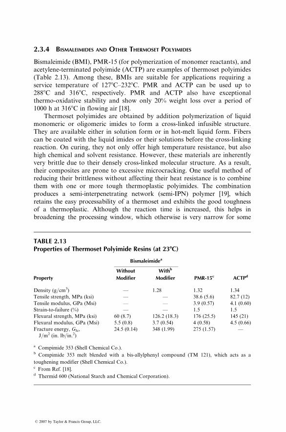
2.3.4 BISMALEIMIDES AND OTHER THERMOSET POLYIMIDES
Bismaleimide (BMI), PMR-15 (for polymerization of monomer reactants), and
acetylene-terminated polyimide (ACTP) are examples of thermoset polyimides
(Table 2.13). Among these, BMIs are suitable for applications requiring a
service temperature of 1278C–2328C. PMR and ACTP can be used up to
2888C and 3168C, respectively. PMR and ACTP also have exceptional
thermo-oxidative stability and show only 20% weight loss over a period of
1000 h at 3168C in flowing air [18].
Thermoset polyimides are obtained by addition polymerization of liquid
monomeric or oligomeric imides to form a cross-linked infusible structure.
They are available either in solution form or in hot-melt liquid form. Fibers
can be coated with the liquid imides or their solutions before the cross-linking
reaction. On curing, they not only offer high temperature resistance, but also
high chemical and solvent resistance. However, these materials are inherently
very brittle due to their densely cross-linked molecular structure. As a result,
their composites are prone to excessive microcracking. One useful method of
reducing their brittleness without affecting their heat resistance is to combine
them with one or more tough thermoplastic polyimides. The combination
produces a semi-interpenetrating network (semi-IPN) polymer [19], which
retains the easy processability of a thermoset and exhibits the good toughness
of a thermoplastic. Although the reaction time is increased, this helps in
broadening the processing window, which otherwise is very narrow for some
TABLE 2.13Properties of Thermoset Polyimide Resins (at 238C)
Bismaleimidea
Property
Without
Modifier
Withb
Modifier PMR-15c ACTPd
Density (g=cm3) — 1.28 1.32 1.34
Tensile strength, MPa (ksi) — — 38.6 (5.6) 82.7 (12)
Tensile modulus, GPa (Msi) — — 3.9 (0.57) 4.1 (0.60)
Strain-to-failure (%) — — 1.5 1.5
Flexural strength, MPa (ksi) 60 (8.7) 126.2 (18.3) 176 (25.5) 145 (21)
Flexural modulus, GPa (Msi) 5.5 (0.8) 3.7 (0.54) 4 (0.58) 4.5 (0.66)
Fracture energy, GIc,
J=m2 (in. lb=in.2)
24.5 (0.14) 348 (1.99) 275 (1.57) —
a Compimide 353 (Shell Chemical Co.).b Compimide 353 melt blended with a bis-allylphenyl compound (TM 121), which acts as a
toughening modifier (Shell Chemical Co.).c From Ref. [18].d Thermid 600 (National Starch and Chemical Corporation).
� 2007 by Taylor & Francis Group, LLC.
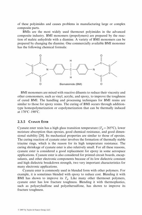
of these polyimides and causes problems in manufacturing large or complex
composite parts.
BMIs are the most widely used thermoset polyimides in the advanced
composite industry. BMI monomers (prepolymers) are prepared by the reac-
tion of maleic anhydride with a diamine. A variety of BMI monomers can be
prepared by changing the diamine. One commercially available BMI monomer
has the following chemical formula:
N C N
H
H
Bismaleimide (BMI)
C
C
C
C
O
O
C
C
C
C
O
O
BMI monomers are mixed with reactive diluents to reduce their viscosity and
other comonomers, such as vinyl, acrylic, and epoxy, to improve the toughness
of cured BMI. The handling and processing techniques for BMI resins are
similar to those for epoxy resins. The curing of BMI occurs through addition-
type homopolymerization or copolymerization that can be thermally induced
at 1708C–1908C.
2.3.5 CYANATE ESTER
Cyanate ester resin has a high glass transition temperature (Tg¼ 2658C), lowermoisture absorption than epoxies, good chemical resistance, and good dimen-
sional stability [20]. Its mechanical properties are similar to those of epoxies.
The curing reaction of cyanate ester involves the formation of thermally stable
triazine rings, which is the reason for its high temperature resistance. The
curing shrinkage of cyanate ester is also relatively small. For all these reasons,
cyanate ester is considered a good replacement for epoxy in some aerospace
applications. Cyanate ester is also considered for printed circuit boards, encap-
sulants, and other electronic components because of its low dielectric constant
and high dielectric breakdown strength, two very important characteristics for
many electronic applications.
Cyanate ester is commonly used in blended form with other polymers. For
example, it is sometimes blended with epoxy to reduce cost. Blending it with
BMI has shown to improve its Tg. Like many other thermoset polymers,
cyanate ester has low fracture toughness. Blending it with thermoplastics,
such as polyarylsulfone and polyethersulfone, has shown to improve its
fracture toughness.
� 2007 by Taylor & Francis Group, LLC.
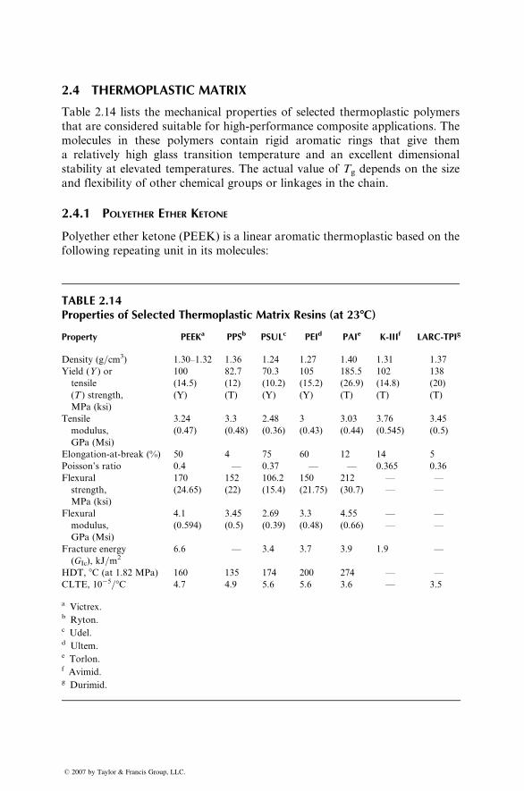
2.4 THERMOPLASTIC MATRIX
Table 2.14 lists the mechanical properties of selected thermoplastic polymers
that are considered suitable for high-performance composite applications. The
molecules in these polymers contain rigid aromatic rings that give them
a relatively high glass transition temperature and an excellent dimensional
stability at elevated temperatures. The actual value of Tg depends on the size
and flexibility of other chemical groups or linkages in the chain.
2.4.1 POLYETHER ETHER KETONE
Polyether ether ketone (PEEK) is a linear aromatic thermoplastic based on the
following repeating unit in its molecules:
TABLE 2.14Properties of Selected Thermoplastic Matrix Resins (at 238C)
Property PEEKa PPSb PSULc PEId PAIe K-IIIf LARC-TPIg
Density (g=cm3) 1.30–1.32 1.36 1.24 1.27 1.40 1.31 1.37
Yield (Y ) or
tensile
(T ) strength,
MPa (ksi)
100 82.7 70.3 105 185.5 102 138
(14.5) (12) (10.2) (15.2) (26.9) (14.8) (20)
(Y) (T) (Y) (Y) (T) (T) (T)
Tensile
modulus,
GPa (Msi)
3.24 3.3 2.48 3 3.03 3.76 3.45
(0.47) (0.48) (0.36) (0.43) (0.44) (0.545) (0.5)
Elongation-at-break (%) 50 4 75 60 12 14 5
Poisson’s ratio 0.4 — 0.37 — — 0.365 0.36
Flexural
strength,
MPa (ksi)
170 152 106.2 150 212 — —
(24.65) (22) (15.4) (21.75) (30.7) — —
Flexural
modulus,
GPa (Msi)
4.1 3.45 2.69 3.3 4.55 — —
(0.594) (0.5) (0.39) (0.48) (0.66) — —
Fracture energy
(GIc), kJ=m2
6.6 — 3.4 3.7 3.9 1.9 —
HDT, 8C (at 1.82 MPa) 160 135 174 200 274 — —
CLTE, 10�5=8C 4.7 4.9 5.6 5.6 3.6 — 3.5
a Victrex.b Ryton.c Udel.d Ultem.e Torlon.f Avimid.g Durimid.
� 2007 by Taylor & Francis Group, LLC.
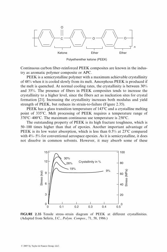
O
C
Ketone Ether
Polyetherether ketone (PEEK)
Ether
O O
n
Continuous carbon fiber-reinforced PEEK composites are known in the indus-
try as aromatic polymer composite or APC.
PEEK is a semicrystalline polymer with a maximum achievable crystallinity
of 48% when it is cooled slowly from its melt. Amorphous PEEK is produced if
the melt is quenched. At normal cooling rates, the crystallinity is between 30%
and 35%. The presence of fibers in PEEK composites tends to increase the
crystallinity to a higher level, since the fibers act as nucleation sites for crystal
formation [21]. Increasing the crystallinity increases both modulus and yield
strength of PEEK, but reduces its strain-to-failure (Figure 2.35).
PEEK has a glass transition temperature of 1438C and a crystalline melting
point of 3358C. Melt processing of PEEK requires a temperature range of
3708C–4008C. The maximum continuous use temperature is 2508C.The outstanding property of PEEK is its high fracture toughness, which is
50–100 times higher than that of epoxies. Another important advantage of
PEEK is its low water absorption, which is less than 0.5% at 238C compared
with 4%–5% for conventional aerospace epoxies. As it is semicrystalline, it does
not dissolve in common solvents. However, it may absorb some of these
Str
ess
(ksi
)
Str
ess
(MP
a)
Crystallinity in %
15
12
9
6
3
0 0.20.1 0.3 0.4 0.50 0
20
40
60
80
100
30%
19%
26%
9%
FIGURE 2.35 Tensile stress–strain diagram of PEEK at different crystallinities.
(Adapted from Seferis, J.C., Polym. Compos., 71, 58, 1986.)
� 2007 by Taylor & Francis Group, LLC.
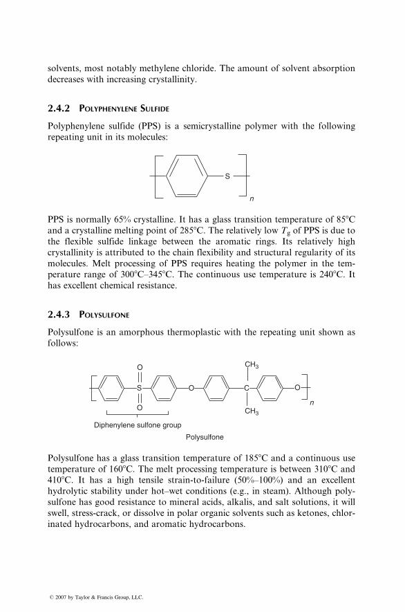
solvents, most notably methylene chloride. The amount of solvent absorption
decreases with increasing crystallinity.
2.4.2 POLYPHENYLENE SULFIDE
Polyphenylene sulfide (PPS) is a semicrystalline polymer with the following
repeating unit in its molecules:
S
n
PPS is normally 65% crystalline. It has a glass transition temperature of 858Cand a crystalline melting point of 2858C. The relatively low Tg of PPS is due to
the flexible sulfide linkage between the aromatic rings. Its relatively high
crystallinity is attributed to the chain flexibility and structural regularity of its
molecules. Melt processing of PPS requires heating the polymer in the tem-
perature range of 3008C–3458C. The continuous use temperature is 2408C. Ithas excellent chemical resistance.
2.4.3 POLYSULFONE
Polysulfone is an amorphous thermoplastic with the repeating unit shown as
follows:
O
O
O
Diphenylene sulfone group
Polysulfone
O C
CH3
CH3
n
S
Polysulfone has a glass transition temperature of 1858C and a continuous use
temperature of 1608C. The melt processing temperature is between 3108C and
4108C. It has a high tensile strain-to-failure (50%–100%) and an excellent
hydrolytic stability under hot–wet conditions (e.g., in steam). Although poly-
sulfone has good resistance to mineral acids, alkalis, and salt solutions, it will
swell, stress-crack, or dissolve in polar organic solvents such as ketones, chlor-
inated hydrocarbons, and aromatic hydrocarbons.
� 2007 by Taylor & Francis Group, LLC.
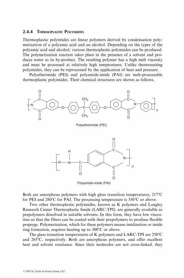
2.4.4 THERMOPLASTIC POLYIMIDES
Thermoplastic polyimides are linear polymers derived by condensation poly-
merization of a polyamic acid and an alcohol. Depending on the types of the
polyamic acid and alcohol, various thermoplastic polyimides can be produced.
The polymerization reaction takes place in the presence of a solvent and pro-
duces water as its by-product. The resulting polymer has a high melt viscosity
and must be processed at relatively high temperatures. Unlike thermosetting
polyimides, they can be reprocessed by the application of heat and pressure.
Polyetherimide (PEI) and polyamide-imide (PAI) are melt-processable
thermoplastic polyimides. Their chemical structures are shown as follows.
O
O O
O
CH3
O ON
C
CC
CCH3
C
N
n
Polyetherimide (PEI)
R C
C
C n
N
OO
H
N
O
Polyamide-imide (PAI)
Both are amorphous polymers with high glass transition temperatures, 2178Cfor PEI and 2808C for PAI. The processing temperature is 3508C or above.
Two other thermoplastic polyimides, known as K polymers and Langley
Research Center Thermoplastic Imide (LARC-TPI), are generally available as
prepolymers dissolved in suitable solvents. In this form, they have low viscos-
ities so that the fibers can be coated with their prepolymers to produce flexible
prepregs. Polymerization, which for these polymers means imidization or imide
ring formation, requires heating up to 3008C or above.
The glass transition temperatures of K polymers and LARC-TPI are 2508Cand 2658C, respectively. Both are amorphous polymers, and offer excellent
heat and solvent resistance. Since their molecules are not cross-linked, they
� 2007 by Taylor & Francis Group, LLC.
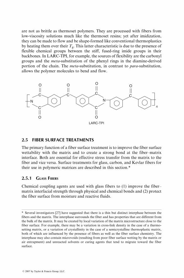
are not as brittle as thermoset polymers. They are processed with fibers from
low-viscosity solutions much like the thermoset resins; yet after imidization,
they can be made to flow and be shape-formed like conventional thermoplastics
by heating them over their Tg. This latter characteristic is due to the presence of
flexible chemical groups between the stiff, fused-ring imide groups in their
backbones. In LARC-TPI, for example, the sources of flexibility are the carbonyl
groups and the meta-substitution of the phenyl rings in the diamine-derived
portion of the chain. The meta-substitution, in contrast to para-substitution,
allows the polymer molecules to bend and flow.
O
O
LARC-TPI
C
O
C
O
C
C
O
O
C
nC
N N
2.5 FIBER SURFACE TREATMENTS
The primary function of a fiber surface treatment is to improve the fiber surface
wettability with the matrix and to create a strong bond at the fiber–matrix
interface. Both are essential for effective stress transfer from the matrix to the
fiber and vice versa. Surface treatments for glass, carbon, and Kevlar fibers for
their use in polymeric matrices are described in this section.*
2.5.1 GLASS FIBERS
Chemical coupling agents are used with glass fibers to (1) improve the fiber–
matrix interfacial strength through physical and chemical bonds and (2) protect
the fiber surface from moisture and reactive fluids.
* Several investigators [27] have suggested that there is a thin but distinct interphase between the
fibers and the matrix. The interphase surrounds the fiber and has properties that are different from
the bulk of the matrix. It may be created by local variation of the matrix microstructure close to the
fiber surface. For example, there may be a variation in cross-link density in the case of a thermo-
setting matrix, or a variation of crystallinity in the case of a semicrystalline thermoplastic matrix,
both of which are influenced by the presence of fibers as well as the fiber surface chemistry. The
interphase may also contain microvoids (resulting from poor fiber surface wetting by the matrix or
air entrapment) and unreacted solvents or curing agents that tend to migrate toward the fiber
surface.
� 2007 by Taylor & Francis Group, LLC.
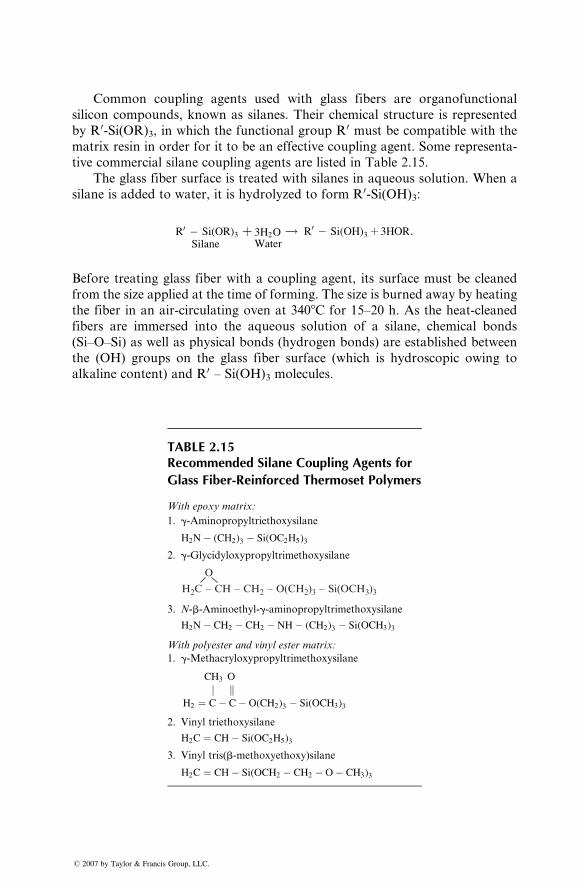
Common coupling agents used with glass fibers are organofunctional
silicon compounds, known as silanes. Their chemical structure is represented
by R0-Si(OR)3, in which the functional group R0 must be compatible with the
matrix resin in order for it to be an effective coupling agent. Some representa-
tive commercial silane coupling agents are listed in Table 2.15.
The glass fiber surface is treated with silanes in aqueous solution. When a
silane is added to water, it is hydrolyzed to form R0-Si(OH)3:
R0 � Si(OR)3Silane
þ 3H2OWater
! R0 � Si(OH)3 þ 3HOR:
Before treating glass fiber with a coupling agent, its surface must be cleaned
from the size applied at the time of forming. The size is burned away by heating
the fiber in an air-circulating oven at 3408C for 15–20 h. As the heat-cleaned
fibers are immersed into the aqueous solution of a silane, chemical bonds
(Si–O–Si) as well as physical bonds (hydrogen bonds) are established between
the (OH) groups on the glass fiber surface (which is hydroscopic owing to
alkaline content) and R0 – Si(OH)3 molecules.
TABLE 2.15Recommended Silane Coupling Agents for
Glass Fiber-Reinforced Thermoset Polymers
With epoxy matrix:
1. g-Aminopropyltriethoxysilane
H2N� (CH2)3 � Si(OC2H5)3
2. g-Glycidyloxypropyltrimethoxysilane
H2C – CH – CH2 – O(CH2)3 – Si(OCH3)3
O
3. N-b-Aminoethyl-g-aminopropyltrimethoxysilane
H2N� CH2 � CH2 � NH� (CH2)3 � Si(OCH3)3
With polyester and vinyl ester matrix:
1. g-Methacryloxypropyltrimethoxysilane
CH3 O
j kH2 ¼ C� C� O(CH2)3 � Si(OCH3)3
2. Vinyl triethoxysilane
H2C ¼ CH� Si(OC2H5)3
3. Vinyl tris(b-methoxyethoxy)silane
H2C ¼ CH� Si(OCH2 � CH2 � O� CH3)3
� 2007 by Taylor & Francis Group, LLC.
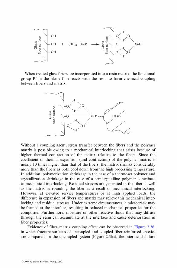
OHH
H
H
H
OO
OO
OOH (HO)3 Si-R9 Si-R9+
Gla
ssfib
er s
urfa
ce
Gla
ssfib
er s
urfa
ce
OH
When treated glass fiber s are incorpora ted into a resi n matrix, the function al
group R 0 in the sil ane film react s with the resin to form ch emical coup ling
between fiber s an d matr ix.
H
H
H
H
O
Si-R9 ResinGla
ssfib
er s
urfa
ce
O
O
O O
Without a coup ling agen t, stress trans fer between the fiber s and the poly mer
matrix is possibl e owin g to a mech anical inter locking that aris es because of
higher thermal contrac tion of the matr ix relative to the fiber s. Since the
coefficie nt of therm al expansi on (and contrac tion) of the polyme r matr ix is
nearly 10 times higher than that of the fibers, the matrix shrinks con siderab ly
more than the fibers as both coo l down from the high pr ocessing tempe ratur e.
In add ition, polyme rization shrinka ge in the case of a therm oset polyme r and
crystall ization shrinka ge in the case of a semicryst alline polyme r co ntribu te
to mechani cal interlocki ng. Residu al stre sses are generate d in the fiber as wel l
as the matr ix surround ing the fiber as a result of mechan ical interlocki ng.
Howev er, at elevat ed servi ce temperatur es or at high ap plied loads, the
difference in expansi on of fiber s an d matrix may relieve this mech anical inter -
locking and residu al stresses . Un der extre me circumsta nces, a micr ocrack may
be form ed at the interface, resul ting in redu ced mechani cal propert ies for the
composite. Furthermore, moisture or other reactive fluids that may diffuse
through the resin can accumulate at the interface and cause deterioration in
fiber properties.
Eviden ce of fiber–mat rix coupling e ffect can be observed in Figure 2.36,
in which fracture surfaces of uncoupled and coupled fiber-reinforced epoxies
are compared. In the uncoupled system (Figure 2.36a), the interfacial failure
� 2007 by Taylor & Francis Group, LLC.
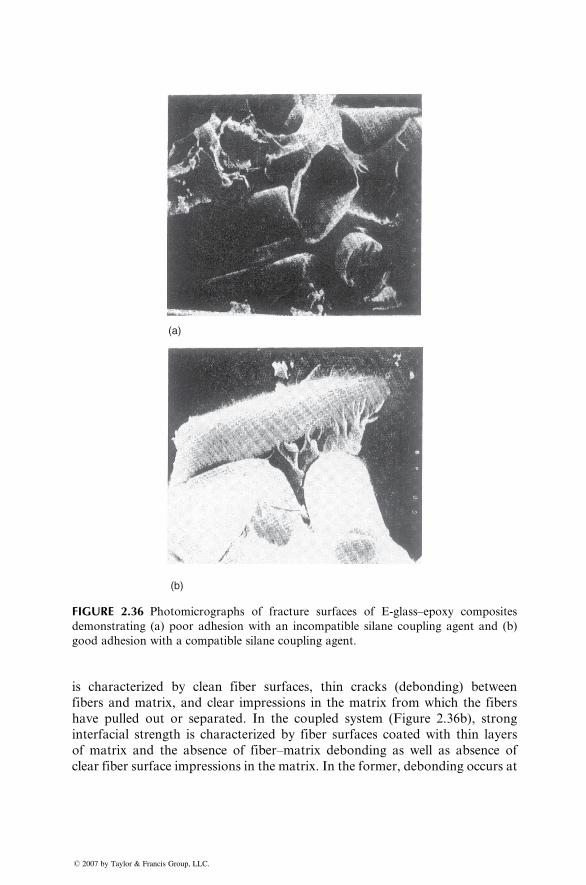
(a)
(b)
FIGURE 2.36 Photomicrographs of fracture surfaces of E-glass–epoxy composites
demonstrating (a) poor adhesion with an incompatible silane coupling agent and (b)
good adhesion with a compatible silane coupling agent.
is characterized by clean fiber surfaces, thin cracks (debonding) between
fibers and matrix, and clear impressions in the matrix from which the fibers
have pulled out or separated. In the coupled system (Figure 2.36b), strong
interfacial strength is characterized by fiber surfaces coated with thin layers
of matrix and the absence of fiber–matrix debonding as well as absence of
clear fiber surface impressions in the matrix. In the former, debonding occurs at
� 2007 by Taylor & Francis Group, LLC.
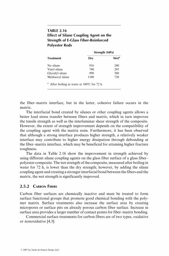
TABLE 2.16Effect of Silane Coupling Agent on the
Strength of E-Glass Fiber-Reinforced
Polyester Rods
Strength (MPa)
Treatment Dry Weta
No silane 916 240
Vinyl silane 740 285
Glycidyl silane 990 380
Methacryl silane 1100 720
a After boiling in water at 1008C for 72 h.
the fiber–matrix interface, but in the latter, cohesive failure occurs in the
matrix.
The interfacial bond created by silanes or other coupling agents allows a
better load stress transfer between fibers and matrix, which in turn improves
the tensile strength as well as the interlaminar shear strength of the composite.
However, the extent of strength improvement depends on the compatibility of
the coupling agent with the matrix resin. Furthermore, it has been observed
that although a strong interface produces higher strength, a relatively weaker
interface may contribute to higher energy dissipation through debonding at
the fiber–matrix interface, which may be beneficial for attaining higher fracture
toughness.
The data in Table 2.16 show the improvement in strength achieved by
using different silane coupling agents on the glass fiber surface of a glass fiber–
polyester composite. Thewet strength of the composite,measured after boiling in
water for 72 h, is lower than the dry strength; however, by adding the silane
coupling agent and creating a stronger interfacial bondbetween the fibers and the
matrix, the wet strength is significantly improved.
2.5.2 CARBON FIBERS
Carbon fiber surfaces are chemically inactive and must be treated to form
surface functional groups that promote good chemical bonding with the poly-
mer matrix. Surface treatments also increase the surface area by creating
micropores or surface pits on already porous carbon fiber surface. Increase in
surface area provides a larger number of contact points for fiber–matrix bonding.
Commercial surface treatments for carbon fibers are of two types, oxidative
or nonoxidative [4,5]:
� 2007 by Taylor & Francis Group, LLC.
1. Oxidative surface treatments produce acidic functional groups, such as
carboxylic, phenolic, and hydroxylic, on the carbon fiber surface. They
may be carried out either in an oxygen-containing gas (air, oxygen, carbon
dioxide, ozone, etc.) or in a liquid (nitric acid, sodium hypochloride, etc.).
The gas-phase oxidation is conducted at 2508C or above and often in
the presence of a catalyst. Oxidation at very high temperatures causes
excessive pitting on the carbon fiber surface and reduces the fiber
strength.
Nitric acid is the most common liquid used for the liquid-phase
oxidation. The effectiveness of treatment in improving the surface prop-
erties depends on the acid concentration, treatment time, and tempera-
ture, as well as the fiber type.
2. Several nonoxidative surface treatments have been developed for carbon
fibers. In one of these treatments, the carbon fiber surface is coated with
an organic polymer that has functional groups capable of reacting with
the resin matrix. Examples of polymer coatings are styrene–maleic
anhydride copolymers, methyl acrylate–acrylonitrile copolymer, and
polyamides. The preferred method of coating the fiber surface is electro-
polymerization, in which carbon fibers are used as one of the electrodes in
an acidic solution of monomers or monomer mixtures [22]. Improved
results are obtained if the carbon fiber surface is oxidized before the
coating process.
2.5.3 KEVLAR FIBERS
Similar to carbon fibers, Kevlar 49 fibers also suffer from weak interfacial
adhesion with most matrix resins. Two methods have been successful in
improving the interfacial adhesion of Kevlar 49 with epoxy resin [7]:
1. Filament surface oxidation or plasma etching, which reduces the fiber
tensile strength but tends to improve the off-axis strength of the com-
posite, which depends on better fiber–matrix interfacial strength.
2. Formation of reactive groups, such as amines (�NH2), on the fiber
surface. These reactive groups form covalent bonds with the epoxide
groups across the interface.
2.6 FILLERS AND OTHER ADDITIVES
Fillers are added to a polymer matrix for one or more of the following reasons:
1. Reduce cost (since most fillers are much less expensive than the matrix
resin)
2. Increase modulus
� 2007 by Taylor & Francis Group, LLC.
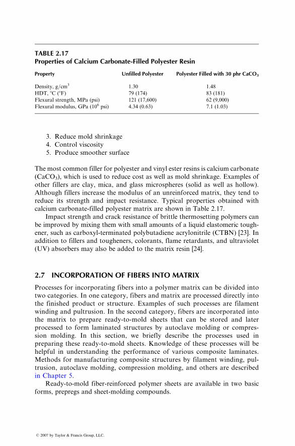
TABLE 2.17Properties of Calcium Carbonate-Filled Polyester Resin
Property Unfilled Polyester Polyester Filled with 30 phr CaCO3
Density, g=cm3 1.30 1.48
HDT, 8C (8F) 79 (174) 83 (181)
Flexural strength, MPa (psi) 121 (17,600) 62 (9,000)
Flexural modulus, GPa (106 psi) 4.34 (0.63) 7.1 (1.03)
3. Reduce mold shrinka ge
4. Cont rol viscos ity
5. Prod uce smooth er surfa ce
The mo st common filler for polyest er and vinyl ester resi ns is calci um carbon ate
(CaCO3), which is used to reduce cost as well as mold shrinka ge. Exa mples of
other filler s are clay, mica , and glass micro spheres (solid as well as hollow ).
Althou gh fillers increa se the mod ulus of an unreinf orced matr ix, they tend to
reduce its stren gth an d impac t resistance . Typical pro perties obtaine d with
calcium carbon ate-filled polyester matr ix are shown in Table 2.17.
Impact stren gth and crack resi stance of brit tle therm osett ing polyme rs can
be improved by mixing them with small amounts of a liquid elastomeric tough-
ener, such as carboxyl -termi nated polyb utadien e acryl onitrile (CTBN ) [23]. In
additio n to filler s an d tou gheners, colorant s, flam e retar dants, an d ultr aviol et
(UV) ab sorbers may also be ad ded to the matrix resin [24] .
2.7 INCORPORATION OF FIBERS INTO MATRIX
Processes for incorporating fibers into a polymer matrix can be divided into
two categories. In one category, fibers and matrix are p rocessed d irectly into
the finished produ ct or structure . E xamples o f such p rocesses are filamen t
win ding and pultrusion. In the se cond c ategory, f ib ers are incorp orated into
the m atrix to p repare ready-to-mol d shee ts t hat ca n b e stored an d l ater
proc essed t o f orm l amin ated structures by a utoclave m old in g or comp re s-
sion molding. In this se ctio n, we brie fly describe the processes used in
preparing these ready-to-mold sheets. Knowledge of these processes w ill be
helpful in u nderstand i ng th e pe rfo rmance of va rio us co m posite lamin ate s.
Methods for manufacturing composite structures by filament winding, pul-
trusion, autoclave molding, compression molding, and others are described
in Chapter 5.
Ready- to-mold fiber-re inforce d polyme r sheets are available in two basic
forms, prepregs and sheet-molding compounds.
� 2007 by Taylor & Francis Group, LLC.
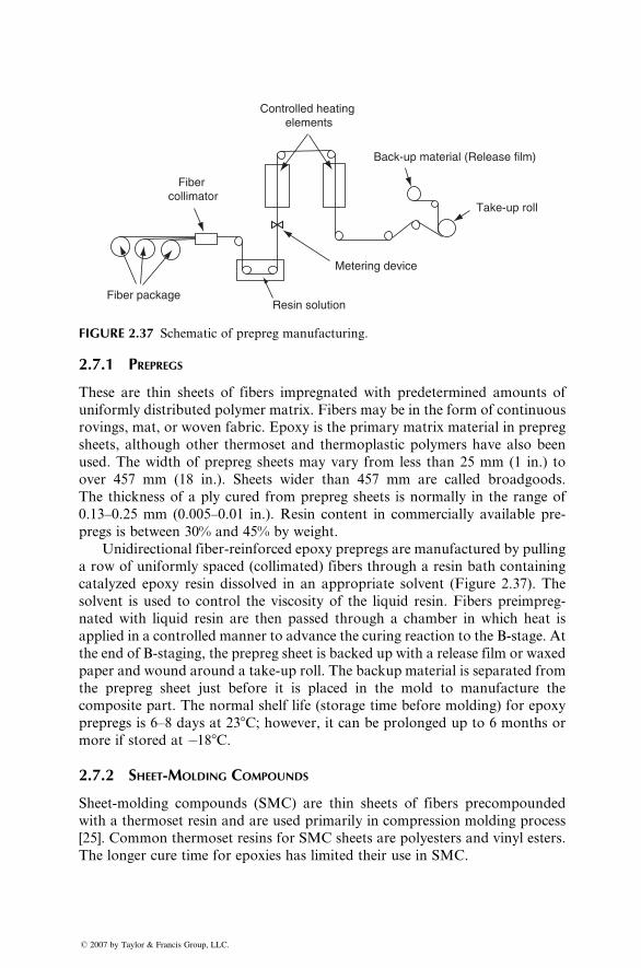
Controlled heating elements
Resin solution
Fiber collimator
Metering device
Take-up roll
Back-up material (Release film)
Fiber package
FIGURE 2.37 Schematic of prepreg manufacturing.
2.7.1 PREPREGS
These are thin sheets of fibers impregnated with predetermined amounts of
uniformly distributed polymer matrix. Fibers may be in the form of continuous
rovings, mat, or woven fabric. Epoxy is the primary matrix material in prepreg
sheets, although other thermoset and thermoplastic polymers have also been
used. The width of prepreg sheets may vary from less than 25 mm (1 in.) to
over 457 mm (18 in.). Sheets wider than 457 mm are called broadgoods.
The thickness of a ply cured from prepreg sheets is normally in the range of
0.13–0.25 mm (0.005–0.01 in.). Resin content in commercially available pre-
pregs is between 30% and 45% by weight.
Unidirectional fiber-reinforced epoxy prepregs are manufactured by pulling
a row of uniformly spaced (collimated) fibers through a resin bath containing
catalyzed epoxy resin dissolved in an appropriate solvent (Figure 2.37). The
solvent is used to control the viscosity of the liquid resin. Fibers preimpreg-
nated with liquid resin are then passed through a chamber in which heat is
applied in a controlled manner to advance the curing reaction to the B-stage. At
the end of B-staging, the prepreg sheet is backed up with a release film or waxed
paper and wound around a take-up roll. The backup material is separated from
the prepreg sheet just before it is placed in the mold to manufacture the
composite part. The normal shelf life (storage time before molding) for epoxy
prepregs is 6–8 days at 238C; however, it can be prolonged up to 6 months or
more if stored at �188C.
2.7.2 SHEET-MOLDING COMPOUNDS
Sheet-molding compounds (SMC) are thin sheets of fibers precompounded
with a thermoset resin and are used primarily in compression molding process
[25]. Common thermoset resins for SMC sheets are polyesters and vinyl esters.
The longer cure time for epoxies has limited their use in SMC.
� 2007 by Taylor & Francis Group, LLC.
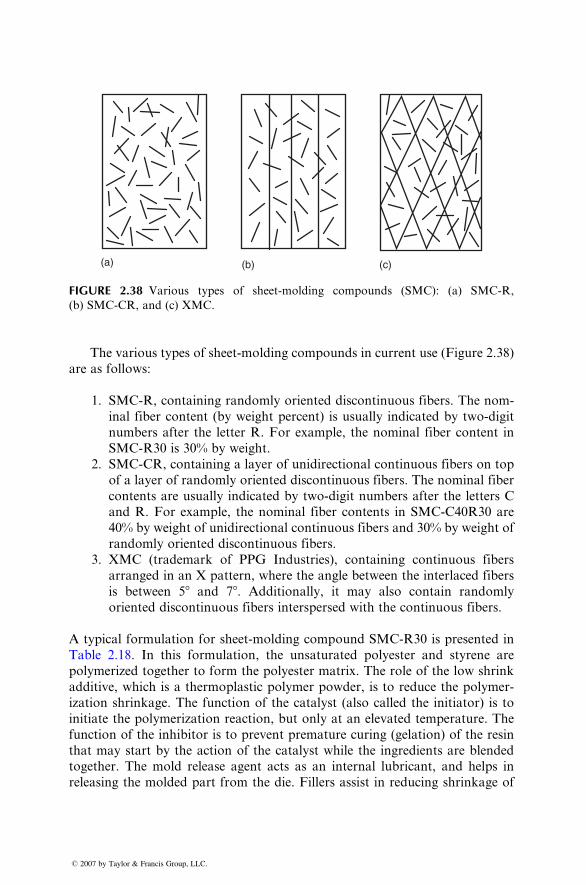
(b)(a) (c)
FIGURE 2.38 Various types of sheet-molding compounds (SMC): (a) SMC-R,
(b) SMC-CR, and (c) XMC.
The various types of sheet-mo lding co mpounds in current use (Figur e 2.38)
are as follo ws:
1. SMC- R, con taining rando mly orient ed discont inuou s fibers. The nom -
inal fiber content (by weigh t percent ) is usu ally indica ted by two-dig it
numbe rs afte r the letter R. For examp le, the nominal fiber co ntent in
SMC- R30 is 30 % by weigh t.
2. SMC- CR, contain ing a layer of unidir ection al con tinuous fibers on top
of a layer of rand omly orient ed discont inuou s fiber s. The nominal fiber
content s are usu ally indica ted by two-dig it num bers after the letters C
and R. For examp le, the nominal fiber co ntents in SM C-C40 R30 are
40% by weigh t of unid irectional continuous fiber s and 30% by weig ht of
randoml y oriente d discon tinuous fiber s.
3. XMC (trademar k of PPG Indu stries), co ntaining continuous fibers
arrange d in an X pa ttern, wher e the a ngle between the inter laced fibers
is between 58 and 78. Addition ally, it may also contai n rando mly
orient ed discontinu ous fibers interspers ed with the co ntinuous fibers.
A typic al formu lation for sheet-mol ding comp ound SM C-R30 is present ed in
Table 2.18. In this form ulation , the uns aturated polyest er and styren e are
polyme rized toget her to form the polyest er matrix. The ro le of the low shrink
additive, whi ch is a thermo plastic polyme r powder , is to reduc e the polyme r-
ization shrinka ge. The functi on of the catal yst (also called the init iator) is to
initiate the pol ymerizati on react ion, but onl y at an elevated tempe ratur e. The
function of the inhibitor is to prevent premature curing (gelation) of the resin
that may start by the action of the catalyst while the ingredients are blended
together. The mold release agent acts as an internal lubricant, and helps in
releasing the molded part from the die. Fillers assist in reducing shrinkage of
� 2007 by Taylor & Francis Group, LLC.
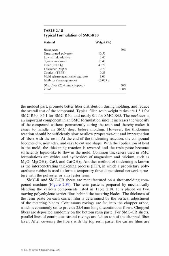
TABLE 2.18Typical Formulation of SMC-R30
Material Weight (%)
Resin paste 70%
Unsaturated polyester 10.50
Low shrink additive 3.45
Styrene monomer 13.40
Filler (CaCO3) 40.70
Thickener (MgO) 0.70
Catalyst (TBPB) 0.25
Mold release agent (zinc stearate) 1.00
Inhibitor (benzoquinone) <0.005 g
Glass fiber (25.4 mm, chopped) 30%
Total 100%
the molded part, promot e better fiber distribut ion dur ing moldi ng, and reduce
the ov erall co st of the co mpound. Typical filler –resin weight ratios are 1.5:1 for
SMC- R30, 0.5: 1 for SMC-R50 , and ne arly 0:1 for SMC- R65. The thickene r is
an impor tant compon ent in a n SMC form ulation since it increa ses the viscos ity
of the compou nd withou t pe rmanent ly cu ring the resin and thereby makes it
easie r to ha ndle an SM C sheet before moldi ng. Howeve r, the thicke ning
react ion should be suff iciently slow to allow proper wet-ou t and impregn ation
of fibers wi th the resin. At the end of the thicke ning reaction, the comp ound
becomes dry , nont acky, and easy to cut and shape. With the ap plication of he at
in the mold, the thicke ning react ion is revers ed an d the resin pa ste beco mes
suffici ently liquid-li ke to flow in the mold. Commo n thicke ners used in SM C
form ulations are oxides and hy droxides of magnes ium and calciu m, such a s
MgO, Mg(O H)2, CaO, a nd Ca( OH) 2. Anothe r method of thicke ning is known
as the inter penetra ting thicke ning process (ITP ), in whi ch a prop rietary poly-
urethane rubber is used to form a temporary three-dimensional network struc-
ture with the polyester or vinyl ester resin.
SMC-R and SMC-CR sheets are manufactured on a sheet-molding com-
pound machi ne (Figur e 2.39) . The resi n paste is prepared by mechani cally
blending the various components listed in Table 2.18. It is placed on two
moving polyethylene carrier films behind the metering blades. The thickness of
the resin paste on each carrier film is determined by the vertical adjustment
of the metering blades. Continuous rovings are fed into the chopper arbor,
which is commonly set to provide 25.4 mm long discontinuous fibers. Chopped
fibers are deposited randomly on the bottom resin paste. For SMC-CR sheets,
parallel lines of continuous strand rovings are fed on top of the chopped fiber
layer. After covering the fibers with the top resin paste, the carrier films are
� 2007 by Taylor & Francis Group, LLC.
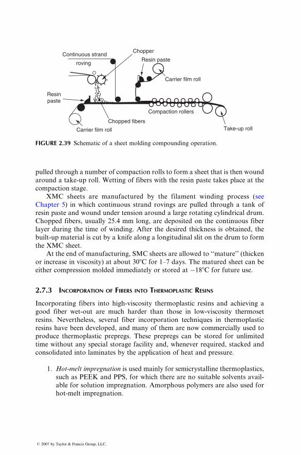
Continuous strandChopper
Resin paste
Carrier film roll
Compaction rollers
Take-up roll
roving
Resinpaste
Carrier film roll
Chopped fibers
FIGURE 2.39 Schematic of a sheet molding compounding operation.
pulled through a number of compact ion roll s to form a sh eet that is then wound
around a take-u p ro ll. Wett ing of fibers with the resi n pa ste takes place at the
compact ion stage .
XMC s heets are manufactured by the filament winding process ( see
Chapte r 5) in which continuous stra nd rovings are pulled through a tank of
resin pa ste and woun d under tensi on around a large rotat ing cyli ndrical dr um.
Chopped fibers, usually 25.4 mm long, are de posited on the continuous fiber
layer dur ing the tim e of wi nding. After the de sired thickne ss is obt ained, the
built-up mate rial is cut by a knife alon g a longitu dinal slit on the dru m to form
the XMC sheet.
At the end of man ufacturing, SM C sheets are allowed to ‘‘matur e’’ (thicken
or increa se in viscos ity) at abou t 30 8 C for 1–7 days. The matur ed sheet can be
either compres sion molded immediat ely or store d at � 18 8 C for futur e use.
2.7.3 INCORPORATION OF FIBERS INTO T HERMOPLASTIC R ESINS
Incorporat ing fiber s into high-v iscosity therm oplastic resi ns and achievi ng a
good fiber wet -out are much harder than tho se in low-vi scosity thermo set
resins. Never thele ss, severa l fiber incorpora tion techn iques in therm oplastic
resins have be en develop ed, and many of them are now commer cial ly used to
produc e therm oplastic pr epregs. These prepregs can be stored for unlim ited
time without any specia l storage faci lity and, whene ver requ ired, stacke d and
consoli dated into lamin ates by the a pplication of he at and pressur e.
1. Hot-me lt imp regnat ion is used mainl y for semi crystall ine thermo plastics ,
such as PEEK and PPS, for which there are no suitable solvents avail-
able for solution impregnation. Amorphous polymers are also used for
hot-melt impregnation.
� 2007 by Taylor & Francis Group, LLC.
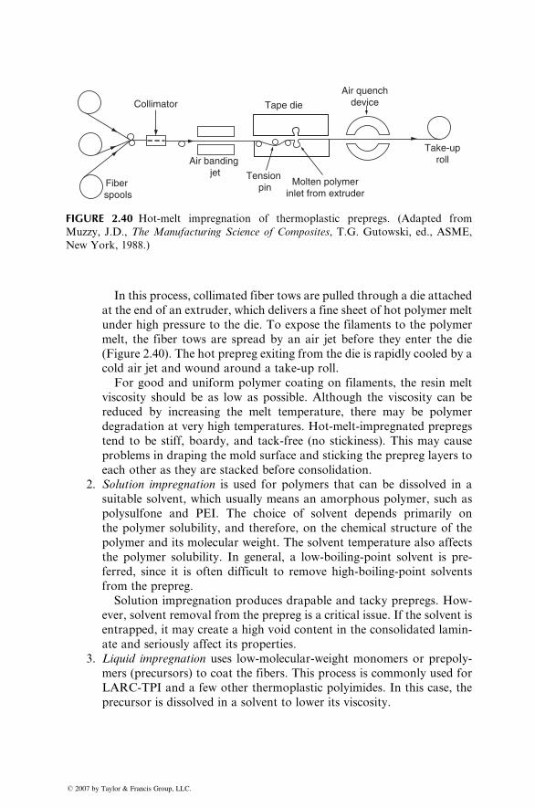
Collimator
Air banding jet
Fiber spools
Molten polymerinlet from extruder
Tension pin
Tape die
Air quenchdevice
Take-uproll
FIGURE 2.40 Hot-melt impregnation of thermoplastic prepregs. (Adapted from
Muzzy, J.D., The Manufacturing Science of Composites, T.G. Gutowski, ed., ASME,
New York, 1988.)
In this process, collimated fiber tows are pulled through a die attached
at the end of an extruder, which delivers a fine sheet of hot polymer melt
under high pressure to the die. To expose the filaments to the polymer
melt, the fiber tows are spread by an air jet before they enter the die
(Figure 2.40). The hot prepreg exiting from the die is rapidly cooled by a
cold air jet and wound around a take-up roll.
For good and uniform polymer coating on filaments, the resin melt
viscosity should be as low as possible. Although the viscosity can be
reduced by increasing the melt temperature, there may be polymer
degradation at very high temperatures. Hot-melt-impregnated prepregs
tend to be stiff, boardy, and tack-free (no stickiness). This may cause
problems in draping the mold surface and sticking the prepreg layers to
each other as they are stacked before consolidation.
2. Solution impregnation is used for polymers that can be dissolved in a
suitable solvent, which usually means an amorphous polymer, such as
polysulfone and PEI. The choice of solvent depends primarily on
the polymer solubility, and therefore, on the chemical structure of the
polymer and its molecular weight. The solvent temperature also affects
the polymer solubility. In general, a low-boiling-point solvent is pre-
ferred, since it is often difficult to remove high-boiling-point solvents
from the prepreg.
Solution impregnation produces drapable and tacky prepregs. How-
ever, solvent removal from the prepreg is a critical issue. If the solvent is
entrapped, it may create a high void content in the consolidated lamin-
ate and seriously affect its properties.
3. Liquid impregnation uses low-molecular-weight monomers or prepoly-
mers (precursors) to coat the fibers. This process is commonly used for
LARC-TPI and a few other thermoplastic polyimides. In this case, the
precursor is dissolved in a solvent to lower its viscosity.
� 2007 by Taylor & Francis Group, LLC.
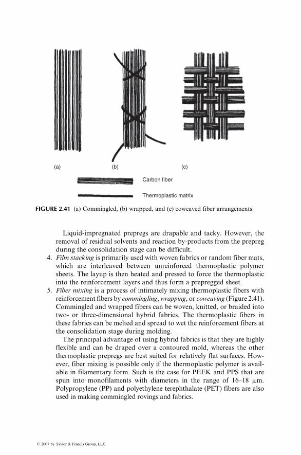
(a) (b)
Carbon fiber
Thermoplastic matrix
(c)
FIGURE 2.41 (a) Commingled, (b) wrapped, and (c) coweaved fiber arrangements.
Liquid-impregnated prepregs are drapable and tacky. However, the
removal of residual solvents and reaction by-products from the prepreg
during the consolidation stage can be difficult.
4. Film stacking is primarily used with woven fabrics or random fiber mats,
which are interleaved between unreinforced thermoplastic polymer
sheets. The layup is then heated and pressed to force the thermoplastic
into the reinforcement layers and thus form a prepregged sheet.
5. Fiber mixing is a process of intimately mixing thermoplastic fibers with
reinforcement fibers by commingling,wrapping, or coweaving (Figure 2.41).
Commingled and wrapped fibers can be woven, knitted, or braided into
two- or three-dimensional hybrid fabrics. The thermoplastic fibers in
these fabrics can be melted and spread to wet the reinforcement fibers at
the consolidation stage during molding.
The principal advantage of using hybrid fabrics is that they are highly
flexible and can be draped over a contoured mold, whereas the other
thermoplastic prepregs are best suited for relatively flat surfaces. How-
ever, fiber mixing is possible only if the thermoplastic polymer is avail-
able in filamentary form. Such is the case for PEEK and PPS that are
spun into monofilaments with diameters in the range of 16–18 mm.
Polypropylene (PP) and polyethylene terephthalate (PET) fibers are also
used in making commingled rovings and fabrics.
� 2007 by Taylor & Francis Group, LLC.
6. Dry powder coating [26] uses charged and fluidized thermoplastic pow-
ders to coat the reinforcement fibers. After passing through the fluidized
bed, the fibers enter a heated oven, where the polymer coating is melted
on the fiber surface.
2.8 FIBER CONTENT, DENSITY, AND VOID CONTENT
Theoretical calculations for strength, modulus, and other properties of a fiber-
reinforced composite are based on the fiber volume fraction in the material.
Experimentally, it is easier to determine the fiber weight fraction wf, from
which the fiber volume fraction vf and composite density rc can be calculated:
vf ¼ wf=rf(wf=rf )þ (wm=rm)
, (2:7)
rc ¼1
(wf=rf )þ (wm=rm), (2:8)
where
wf ¼ fiber weight fraction (same as the fiber mass fraction)
wm¼matrix weight fraction (same as the matrix mass fraction) and is equal
to (1�wf)
rf ¼ fiber density
rm ¼matrix density
In terms of volume fractions, the composite density rc can be written as
rc ¼ rfvf þ rmvm, (2:9)
where vf is the fiber volume fraction and vm is the matrix volume fraction. Note
that vm is equal to (1�vf).
The fiber weight fraction can be experimentally determined by either the
ignition loss method (ASTM D2854) or the matrix digestion method (ASTM
D3171). The ignition loss method is used for PMC-containing fibers that do not
lose weight at high temperatures, such as glass fibers. In this method, the cured
resin is burned off from a small test sample at 5008C–6008C in a muffle furnace.
In the matrix digestion method, the matrix (either polymeric or metallic) is
dissolved away in a suitable liquid medium, such as concentrated nitric acid.
In both cases, the fiber weight fraction is determined by comparing the weights
of the test sample before and after the removal of the matrix. For unidirectional
composites containing electrically conductive fibers (such as carbon) in a
� 2007 by Taylor & Francis Group, LLC.
nonco nductiv e matr ix, the fiber volume fraction c an be determ ined direct ly by
compari ng the elect rical resi stivity of the compo site with that of fibers (ASTM
D3355) .
Duri ng the incorpora tion of fibers into the matrix or dur ing the man ufac-
turing of laminates , a ir or other vo latiles may be trapped in the mate rial. The
trapped air or volat iles exist in the laminate as micr ovoids, which may signifi -
cantly affect some of its mechani cal propert ies. A high void content (over 2%
by volume ) usu ally leads to lower fatigue resi stance, greater suscept ibilit y to
water diffu sion, an d increa sed varia tion (scatter) in mechan ical pro perties. The
void content in a composite laminate can be estimated by comparing the
theoretical density with its actual density:
vv ¼ rc � r
rc , ( 2:10 )
where
vv¼ volume fraction of vo ids
rc ¼ theoretical de nsity, calculated from Equat ion 2.8 or 2.9
r ¼ actual density, measured experimentally on composite specimens (which
is less than rc due to the presence of voids)
EXAMPLE 2.1
Calculate vf and rc for a composite laminate containing 30 wt% of E-glass fibers in
a polyester resin. Assume rf¼ 2.54 g=cm3 and rm¼ 1.1 g=cm3.
� 2
SOLUTION
Assume a small composite sample of mass 1 g and calculate its volume.
007 by Taylor & Francis
Fiber Matrix
Group, LLC.
Mass (g)
0.3 1 � 0.3¼ 0.7Density (g=cm3)
2.54 1.1Volume (cm3)
0:32:54¼ 0:118
0:7
1:1¼ 0:636
Therefore, volume of 1 g of composite is (0.118 þ 0.636) or 0.754 cm3. Now, we
calculate
Fiber volume fraction vf ¼ 0:118
0:754¼ 0:156 or 15.6%
Matrix volume fraction vm¼ 1 � vf¼ 1 � 0.156¼ 0.844 or 84.4%
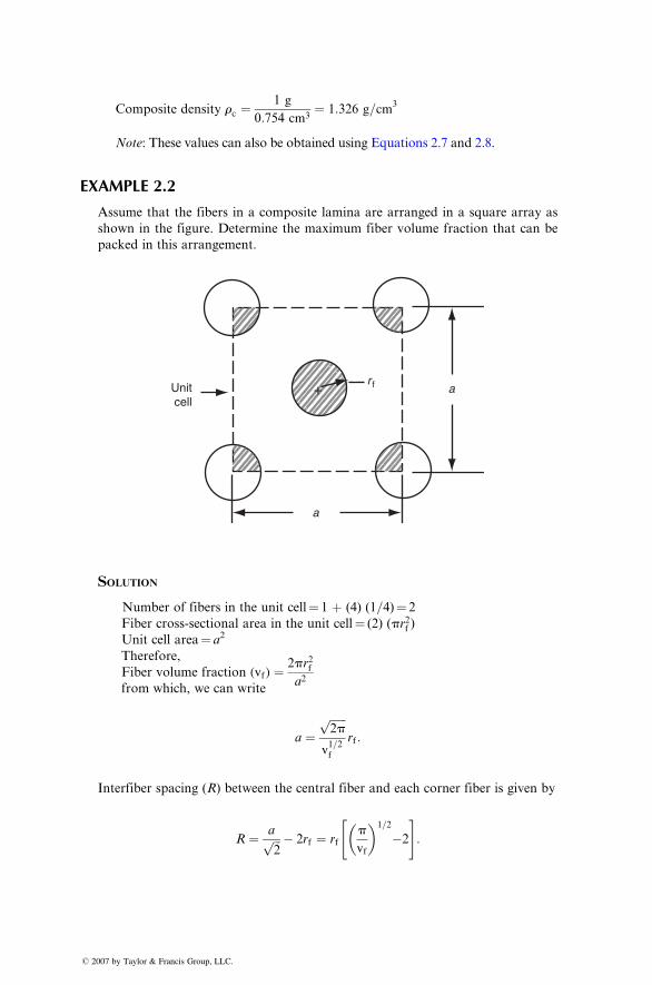
Composite density r c ¼1 g
0:754 cm 3 ¼ 1:326 g= cm3
Note: These values can also be obtained using Equations 2.7 and 2.8.
EXAMPLE 2.2
Assume that the fibers in a composite lamina are arranged in a square array as
shown in the figure. Determine the maximum fiber volume fraction that can be
packed in this arrangement.
+Unitcell
a
ar f
� 2
SOLUTION
Number of fibers in the unit cell¼ 1 þ (4) (1=4)¼ 2
Fiber cross-sectional area in the unit cell¼ (2) (pr2f )Unit cell area¼ a2
Therefore,
Fiber volume fraction (vf) ¼ 2pr2fa2
from which, we can write
a ¼ffiffiffiffiffiffi2p
p
v1=2f
rf :
Interfiber spacing (R) between the central fiber and each corner fiber is given by
R ¼ affiffiffi2
p � 2rf ¼ rfp
vf
� �1=2
�2
" #:
007 by Taylor & Francis Group, LLC.
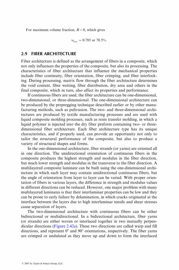
� 2
For maximum volume fraction, R ¼ 0, which gives
vfmax¼ 0: 785 or 78:5% :
2.9 FIBER ARCHITECTURE
Fiber a rchitectur e is de fined as the arrange ment of fibers in a composi te, which
not onl y influ ences the propert ies of the composi te, but also its process ing. The
charact eristic s of fiber archit ecture that influence the mechani cal propert ies
include fiber co ntinuity, fiber orient ation, fiber crimping, and fiber interlock -
ing. Durin g process ing, matr ix flow through the fiber archit ecture determ ines
the void content , fiber wet ting, fiber dist ribution, dry area and others in the
final composi te, which in turn, also affect its propert ies and perfor mance.
If co ntinuous fibers are used, the fiber archit ecture ca n be one-dim ensional ,
two-dim ensional , or three- dimensiona l. The one -dimensiona l archit ecture can
be produ ced by the prepregg ing techni que descri bed earlier or by other manu -
facturing methods , su ch as pultr usion. The two- and three-d imensional archi-
tectures are produced by text ile man ufacturing pr ocesses and are used with
liquid comp osite moldin g pro cesses, such as resi n trans fer moldi ng, in which a
liquid polyme r is injec ted into the dry fiber pr eform con taining two- or three-
dimens ional fiber a rchitectur e. Eac h fiber architec ture type has its unique
charact eristic s, and if prop erly used, can provide an opportunit y not onl y to
tailor the struc tural pe rformance of the co mposite, but a lso to produce a
variety of struc tural shap es and form s.
In the one -dimensiona l a rchitectur e, fiber stra nds (or yarns) are or iented all
in one direct ion. The unidire ctional orientati on of co ntinuous fibers in the
composi te pr oduces the highest stre ngth and modu lus in the fiber direction ,
but much lower strength and mo dulus in the transverse to the fiber direction . A
multil ayered composi te laminate can be bui lt using the one-dim ensional archi-
tecture in which each layer may contain unidir ection al co ntinuous fibers, but
the angle of orient ation from layer to layer can be varie d. With prope r orien-
tation of fibers in various layer s, the difference in strength an d modulus va lues
in different directions c an be reduced. Ho wever, one major prob lem with many
multil ayered laminates is that their interlam inar propert ies can be low and they
can be prone to early failure by delamination, in which cracks originated at the
interface between the layers due to high interlaminar tensile and shear stresses
cause separation of layers.
The two-dimensional architecture with continuous fibers can be either
bidirectional or multidirectional. In a bidirectional architecture, fiber yarns
(or strands) are either woven or interlaced together in two mutually perpen-
dicula r direct ions (Figur e 2.42a). Thes e tw o direct ions are called war p a nd fill
directions, and represent 08 and 908 orientations, respectively. The fiber yarns
are crimped or undulated as they move up and down to form the interlaced
007 by Taylor & Francis Group, LLC.
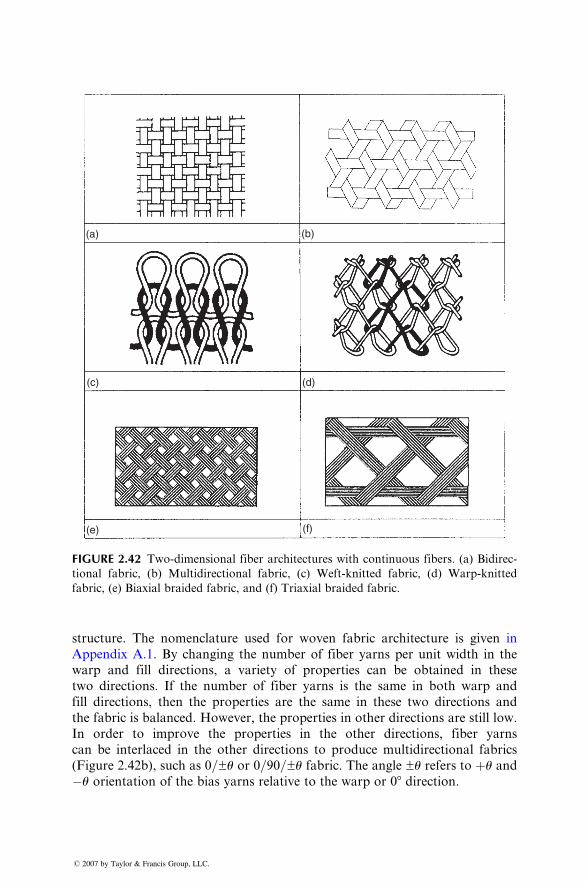
(a) (b)
(c) (d)
(e) (f)
FIGURE 2.42 Two-dimensional fiber architectures with continuous fibers. (a) Bidirec-
tional fabric, (b) Multidirectional fabric, (c) Weft-knitted fabric, (d) Warp-knitted
fabric, (e) Biaxial braided fabric, and (f) Triaxial braided fabric.
struc ture. The nom enclature used for woven fabric arch itecture is given in
Appendix A.1 . By ch anging the numb er of fiber yarn s per unit width in the
warp and fill directions, a variety of properties can be obtained in these
two directions. If the number of fiber yarns is the same in both warp and
fill directions, then the properties are the same in these two directions and
the fabric is balanced. However, the properties in other directions are still low.
In order to improve the properties in the other directions, fiber yarns
can be interlaced in the other directions to produce multidirectional fabrics
(Figure 2.42b), such as 0=±u or 0=90=±u fabric. The angle ±u refers to þu and
�u orientation of the bias yarns relative to the warp or 08 direction.
� 2007 by Taylor & Francis Group, LLC.
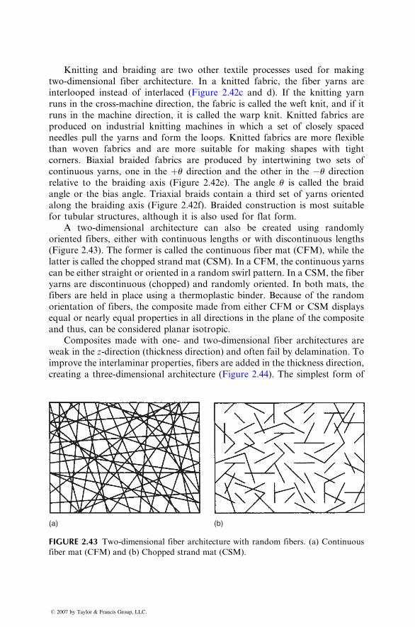
Knitti ng and braidi ng are two other textile process es us ed for making
two-dim ensional fiber arch itecture. In a knitt ed fabric , the fiber yarns are
interloop ed inst ead of interlaced (Figure 2.42c and d). If the knitt ing yarn
runs in the cross-mach ine direct ion, the fabric is called the weft knit, and if it
runs in the machi ne direction, it is call ed the warp knit. Knitted fabrics are
produc ed on indust rial knitting mach ines in whic h a set of closely spaced
needles pull the yarns and form the loops. Kn itted fabri cs are more flex ible
than woven fabrics and are more suit able for making shapes with tight
corners . Biaxia l braided fabri cs are produced by intertw ining two sets of
continuous yarns, one in the þu direction and the other in the � u directionrelative to the braidi ng a xis (Figure 2.42e). The angle u is called the braidangle or the bias angle. Triaxial braids contai n a third set of ya rns orient ed
along the braidi ng axis (Figur e 2.42f). Braided co nstruc tion is most suitab le
for tubular struc tures , a lthough it is also used for flat form.
A two -dimensiona l archit ecture can also be c reated using rando mly
oriente d fibers, either with con tinuous lengths or wi th discon tinuous lengths
(Figur e 2.43) . The former is call ed the continuous fiber mat (C FM), whi le the
latter is called the cho pped stran d mat (CS M). In a CFM, the continuou s yarns
can be eithe r stra ight or orient ed in a random swirl pa ttern. In a CSM, the fiber
yarns are discontinu ous (chop ped) and randoml y oriented. In both mats, the
fibers are he ld in place using a therm oplastic binder. Bec ause of the random
orienta tion of fibers, the compo site made from eithe r CFM or CSM displays
equal or nearly equal propert ies in all directions in the plane of the co mposi te
and thus, can be considered planar isotropic.
Composites made with one- and two-dimensional fiber architectures are
weak in the z-direction (thickness direction) and often fail by delamination. To
improve the interlaminar properties, fibers are added in the thickness direction,
creating a three- dimens ional archite cture (Figur e 2.44) . The simp lest form of
(a) (b)
FIGURE 2.43 Two-dimensional fiber architecture with random fibers. (a) Continuous
fiber mat (CFM) and (b) Chopped strand mat (CSM).
� 2007 by Taylor & Francis Group, LLC.
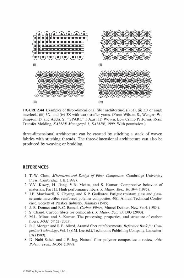
(i) (ii)
(iii) (iv)
FIGURE 2.44 Examples of three-dimensional fiber architecture. (i) 3D, (ii) 2D or angle
interlock, (iii) 3X, and (iv) 3X with warp stuffer yarns. (From Wilson, S., Wenger, W.,
Simpson, D. and Addis, S., ‘‘SPARC’’ 5 Axis, 3D Woven, Low Crimp Performs, Resin
Transfer Molding, SAMPE Monograph 3, SAMPE, 1999. With permission.)
three-dimensional architecture can be created by stitching a stack of woven
fabrics with stitching threads. The three-dimensional architecture can also be
produced by weaving or braiding.
REFERENCES
1.
� 20
T.-W. Chou, Microstructural Design of Fiber Composites, Cambridge University
Press, Cambridge, UK (1992).
2.
V.V. Kozey, H. Jiang, V.R. Mehta, and S. Kumar, Compressive behavior ofmaterials: Part II. High performance fibers, J. Mater. Res., 10:1044 (1995).
3.
J.F. Macdowell, K. Chyung, and K.P. Gadkaree, Fatigue resistant glass and glass-ceramic macrofiber reinforced polymer composites, 40th Annual Technical Confer-
ence, Society of Plastics Industry, January (1985).
4.
J.-B. Donnet and R.C. Bansal, Carbon Fibers, Marcel Dekker, New York (1984).5.
S. Chand, Carbon fibres for composites, J. Mater. Sci., 35:1303 (2000).6.
M.L. Minus and S. Kumar, The processing, properties, and structure of carbonfibers, JOM, 57:52 (2005).
7.
R.J. Morgan and R.E. Allred, Aramid fiber reinforcements, Reference Book for Com-posites Technology, Vol. 1 (S.M. Lee, ed.), Technomic PublishingCompany, Lancaster,
PA (1989).
8.
D. Nabi Saheb and J.P. Jog, Natural fiber polymer composites: a review, Adv.Polym. Tech., 18:351 (1999).
07 by Taylor & Francis Group, LLC.
9.
� 20
J.G. Morley, Fibre reinforcement of metals and alloys, Int. Metals Rev., 21:153
(1976).
10.
C.-H. Andersson and R. Warren, Silicon carbide fibers and their potential for use incomposite materials, Part 1, Composites, 15:16 (1984).
11.
A.K. Dhingra, Alumina Fibre FP, Phil. Trans. R. Soc. Lond., A, 294:1 (1980).12.
A.R. Bunsell, Oxide fibers for high-temperature reinforcement and insulation,JOM, 57, 2:48 (2005).
13.
C.D. Armeniades and E. Baer, Transitions and relaxations in polymers, Introductionto Polymer Science and Technology (H.S. Kaufman and J.J. Falcetta, eds.), John
Wiley & Sons, New York (1977).
14.
J.E. Schoutens, Introduction to metal matrix composite materials, MMCIACTutorial Series, DOD Metal Matrix Composites Information Analysis Center,
Santa Barbara, CA (1982).
15.
M.U. Islam and W. Wallace, Carbon fibre reinforced aluminum matrix composites:a critical review, Report No. DM-4, National Research Council, Canada (1984).
16.
P.R. Smith and F.H. Froes, Developments in titanium metal matrix composites,J. Metal, March (1984).
17.
H.G. Recker et al., Highly damage tolerant carbon fiber epoxy composites forprimary aircraft structural applications, SAMPE Q., October (1989).
18.
D.A. Scola and J.H. Vontell, High temperature polyimides: chemistry and proper-ties, Polym. Compos., 9:443 (1988).
19.
R.H. Pater, Improving processing and toughness of a high performance compositematrix through an interpenetrating polymer network, Part 6, SAMPE J., 26 (1990).
20.
I. Hamerton and J.H. Nay, Recent technological developments in cyanate esterresins, High Perform. Polym., 10:163 (1998).
21.
H.X. Nguyen and H. Ishida, Poly(aryl-ether-ether-ketone) and its advanced com-posites: a review, Polym. Compos., 8:57 (1987).
22.
J.P. Bell, J. Chang, H.W. Rhee, and R. Joseph, Application of ductile polymericcoatings onto graphite fibers, Polym. Compos., 8:46 (1987).
23.
E.H. Rowe, Developments in improved crack resistance of thermoset resins and com-posites, 37th Annual Technical Conference, Society of Plastics Engineers, May (1979).
24.
Modern Plastics Encyclopedia, McGraw-Hill, New York (1992).25.
P.K. Mallick, Sheet Molding Compounds, Composite Materials Technology(P.K. Mallick and S. Newman, eds.), Hanser Publishers, Munich (1990).
26.
J.D. Muzzy, Processing of advanced thermoplastic composites, The ManufacturingScience of Composites (T.G. Gutowski, ed.), ASME, New York (1988).
27.
L.T. Drzal, Composite property dependence on the fiber, matrix, and the inter-phase, Tough Composite Materials: Recent Developments, Noyes Publications, Park
Ridge, NJ, p. 207 (1985).
07 by Taylor & Francis Group, LLC.
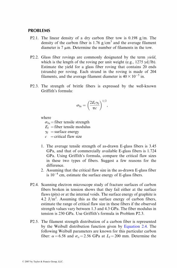
� 20
PROBLEMS
P2.1. The linea r density of a dry carbon fiber tow is 0.198 g =m. The
den sity of the carbon fiber is 1.76 g =cm 3 and the average fil ament
diame ter is 7 m m. Dete rmine the number of filamen ts in the tow.
P2.2. Glas s fiber rovings are co mmonly designa ted by the term yield ,
whi ch is the lengt h of the roving pe r unit wei ght (e.g., 1275 yd=lb).Estim ate the yiel d for a glass fiber roving that contai ns 20 end s
(strand s) per roving. Each strand in the roving is made of 204
filament s, and the average filament diame ter is 40 3 10 � 5 in.
P2.3. The strength of brittle fibers is express ed by the well- known
Gri ffith’s formu la:
sfu ¼ 2Ef g fpc
� �1 =2
,
wher esfu ¼ fiber tensile stre ngth
Ef ¼ fiber tensi le mod ulus
gf ¼ surface energy
c ¼ critical flaw size
1. The average tensile strength of as-dr awn E-glas s fibers is 3.45
GP a, and that of co mmercial ly available E-glas s fiber s is 1.724
GP a. Usi ng Griffith’ s form ula, comp are the critical flaw sizes
in these tw o types of fiber s. Sug gest a few reason s for the
diff erence.
2. Ass uming that the c ritical flaw size in the as-dr awn E-glas s fiber
is 10 �4 cm, e stimate the surface energy of E-glass fibers.
P2.4. Scan ning electron micro scope study of fract ure surfa ces of carbon
fiber s broken in tension shows that they fail either at the surface
flaws (pits) or at the internal voids. The surfa ce e nergy of graph ite is
4.2 J =m 2. Assuming this as the surface energy of carbon fiber s,
estimate the range of critical flaw size in these fibers if the observed
strength values vary between 1.3 and 4.3 GPa. The fiber modulus in
tension is 230 GPa. Use Griffith’s formula in Problem P2.3.
P2.5. The filament strength distribution of a carbon fiber is represented
by the Weibull distribut ion functi on given by Equat ion 2.4. The
following Weibull parameters are known for this particular carbon
fiber: a¼ 6.58 and so¼ 2.56 GPa at Lf¼ 200 mm. Determine the
07 by Taylor & Francis Group, LLC.
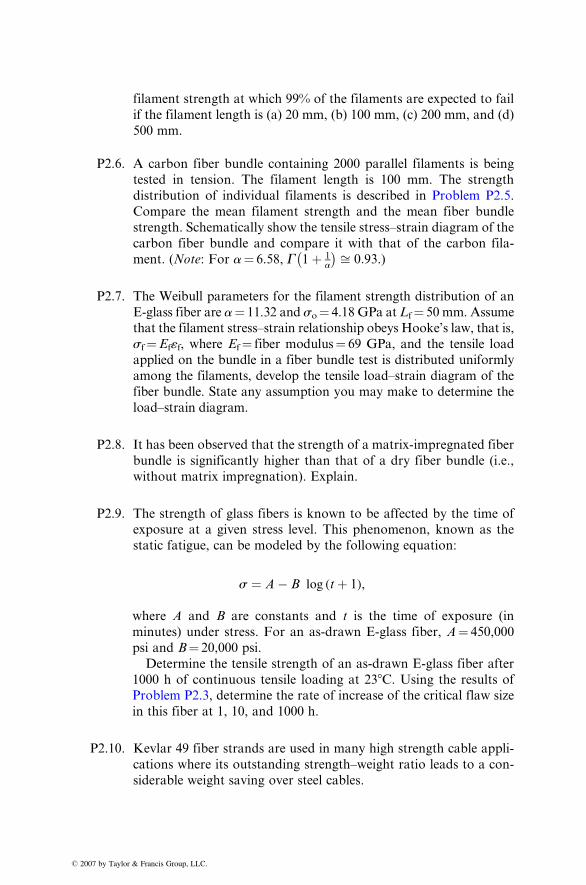
� 20
filament stren gth at whi ch 99% of the filament s are expecte d to fail
if the filament lengt h is (a) 20 mm, (b) 100 mm, (c) 200 mm, and (d)
500 mm.
P2.6. A carbon fiber bundl e contai ning 2000 parallel filament s is being
tested in tensio n. The filament length is 100 mm. The strength
distribut ion of indivi dual filament s is descri bed in Problem P2. 5.
Com pare the mean filamen t strength and the mean fiber bundle
stren gth. Sc hematical ly show the tensile stress–s train diagram of the
carbon fiber bundl e and comp are it with that of the carbon fil a-
ment. ( Note : For a ¼ 6.58, G 1 þ 1a
ffi 0:93.)
P2.7. The Weibull parameters for the filament strength distribution of an
E-glass fiber are a ¼ 11.32 and so ¼ 4.18 GPa at Lf ¼ 50 mm. Assume
that the filament stress–strain relationship obeys Hooke’s law, that is,
sf ¼ Ef«f, where Ef ¼ fiber modulus ¼ 69 GPa, and the tensile load
applied on the bundle in a fiber bundle test is distributed uniformly
among the filaments, develop the tensile load–strain diagram of the
fiber bundle. State any assumption you may make to determine the
load–strain diagram.
P2.8. It has been obse rved that the stre ngth of a matrix- impr egnated fiber
bundle is signifi cantly higher than that of a dr y fiber bundle (i.e.,
without matrix impregnation). Explain.
P2.9. The stre ngth of glass fibers is known to be affe cted by the tim e of
exposure at a given stre ss level. This pheno menon, known as the
static fatigue, can be mod eled by the followi ng equatio n:
s ¼ A � B log ( t þ 1) ,
wher e A and B are co nstants and t is the time of exposure (in
minut es) unde r stre ss. For an as-dr awn E-glas s fiber, A ¼ 450,00 0
psi and B ¼ 2 0,000 psi.
Dete rmine the tensi le stren gth of an as-drawn E-glass fiber after
1000 h of continuous tensile loading at 238C. Using the results of
Pro blem P2.3, determine the rate of increa se of the critical flaw size
in this fiber at 1, 10, and 1000 h.
P2.10. Kevlar 49 fiber strands are used in many high strength cable appli-
cations where its outstanding strength–weight ratio leads to a con-
siderable weight saving over steel cables.
07 by Taylor & Francis Group, LLC.
� 20
1. Com pare the breaking loads and wei ghts of Kevl ar 49 and steel
ca bles, each with a 6.4 mm diame ter
2. Com pare the maxi mum stre sses and elongat ions in 1000 m long
Kevl ar 49 a nd steel cables due to their own weights
P2.11. The smallest radius to which a fiber can be bent or knot ted witho ut
fract uring is an indica tion of how easily it can be hand led in a
manu facturing operati on. The ha ndling charact eristic of a fiber is
parti cularly important in continuous man ufacturing operatio ns,
such as filament wind ing or pultru sion, in whi ch continuous strand
rovings are pul led through a numb er of guides or eyelet s wi th sharp
corn ers. Frequen t breakage of fiber s at these locat ions is undesir -
able since it slows down the produ ction rate.
Usi ng the followi ng relat ionship betwee n the be nding rad ius rban d the maxi mum tensi le stra in in the fiber,
rb ¼ df
2«max
,
co mpare the smal lest radii to which various glass, carbo n, and
Kevl ar fibers in Table 2.1 can be bent wi thout fract uring.
P2.12. Duri ng a fil ament winding ope ration, T-300 carbon fiber tows
con taining 6000 filament s pe r tow are pulled over a set of guide
roll ers 6 mm in diame ter. The mean tensile strength of the filament s
is 3000 M Pa, an d the standar d deviat ion is 865 MPa (assu ming
a standar d normal dist ribut ion for filament stre ngth). Dete rmine
the pe rcentag e of filament s that may snap as the tows are pulled
ove r the rollers. The fiber modulus is 345 GPa, and the fil ament
diame ter is 7 m m.
P2.13. The energy requir ed to snap (break) a brittle fiber is equal to
the stra in energy store d (w hich is equal to the area under the
stress–strain diagram) in the fiber at the time of its failure. Com-
pare the strain energies of E-glass, T-300, IM-7, GY-70, Kevlar 49,
and Spectra 900 fibers.
P2.14. Assume that the area under the stress–strain diagram of a material
is a measure of its toughness. Using the stress–strain diagrams
shown in the following figure, compare the toughness values of
the three matrix resins considered.
07 by Taylor & Francis Group, LLC.

� 20
Matrix 1Matrix 2
Matrix 3
2100
25
75
100
125
150
175
50
3 5 6 8 121110974
Str
ess
(MP
a)
Strain (percent)
P2.15. Assuming that the unidirectional continuous fibers of round cross
section are arranged in a simple square array as shown in the
accompanying figure, calculate the theoretical fiber volume fraction
in the composite lamina. What is the maximum fiber volume frac-
tion that can be arranged in this fashion?
a
a
rf
07 by Taylor & Francis Group, LLC.
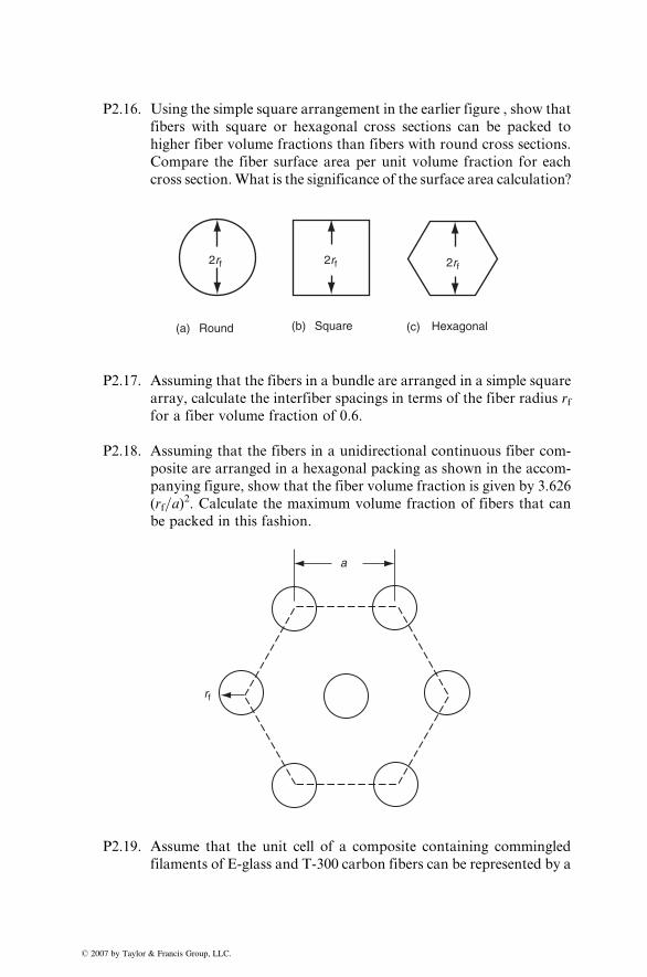
� 20
P2.16. Using the simple square arrangement in the earlier figure , show that
fibers with square or hexagonal cross sections can be packed to
higher fiber volume fractions than fibers with round cross sections.
Compare the fiber surface area per unit volume fraction for each
cross section.What is the significance of the surface area calculation?
(a) Round
2rf 2rf 2rf
(b) Square (c) Hexagonal
P2.17. Assuming that the fibers in a bundle are arranged in a simple square
array, calculate the interfiber spacings in terms of the fiber radius rffor a fiber volume fraction of 0.6.
P2.18. Assuming that the fibers in a unidirectional continuous fiber com-
posite are arranged in a hexagonal packing as shown in the accom-
panying figure, show that the fiber volume fraction is given by 3.626
(rf=a)2. Calculate the maximum volume fraction of fibers that can
be packed in this fashion.
a
rf
P2.19. Assume that the unit cell of a composite containing commingled
filaments of E-glass and T-300 carbon fibers can be represented by a
07 by Taylor & Francis Group, LLC.
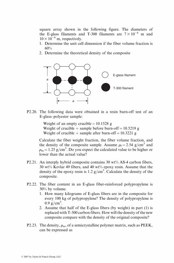
� 20
square array shown in the following figure. The diameters of
the E-glass filaments and T-300 filaments are 73 10�6 m and
103 10�6 m, respectively.
1. Determine the unit cell dimension if the fiber volume fraction is
60%
2. Determine the theoretical density of the composite
E-glass filament
T-300 filament
a
a
P2.20. The following data were obtained in a resin burn-off test of an
E-glass–polyester sample:
Weight of an empty crucible¼ 10.1528 g
Weight of crucible þ sample before burn-off¼ 10.5219 g
Weight of crucible þ sample after burn-off¼ 10.3221 g
Calculate the fiber weight fraction, the fiber volume fraction, and
the density of the composite sample. Assume rf¼ 2.54 g=cm3 and
rm¼ 1.25 g=cm3. Do you expect the calculated value to be higher or
lower than the actual value?
P2.21. An interply hybrid composite contains 30 wt% AS-4 carbon fibers,
30 wt% Kevlar 49 fibers, and 40 wt% epoxy resin. Assume that the
density of the epoxy resin is 1.2 g=cm3. Calculate the density of the
composite.
P2.22. The fiber content in an E-glass fiber-reinforced polypropylene is
30% by volume.
1. How many kilograms of E-glass fibers are in the composite for
every 100 kg of polypropylene? The density of polypropylene is
0.9 g=cm3.
2. Assume that half of the E-glass fibers (by weight) in part (1) is
replacedwith T-300 carbon fibers. Howwill the density of the new
composite compare with the density of the original composite?
P2.23. The density, rm, of a semicrystalline polymer matrix, such as PEEK,
can be expressed as
07 by Taylor & Francis Group, LLC.
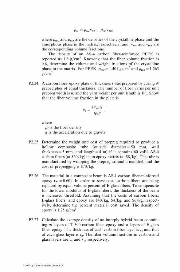
� 20
rm ¼ rmcvmc þ rmavma,
where rmc and rma are the densities of the crystalline phase and the
amorphous phase in the matrix, respectively, and, vmc and vma are
the corresponding volume fractions.
The density of an AS-4 carbon fiber-reinforced PEEK is
reported as 1.6 g=cm3. Knowing that the fiber volume fraction is
0.6, determine the volume and weight fractions of the crystalline
phase in the matrix. For PEEK, rmc¼ 1.401 g=cm3 and rma¼ 1.263
g=cm3.
P2.24. A carbon fiber–epoxy plate of thickness t was prepared by curing N
prepeg plies of equal thickness. The number of fiber yarns per unit
prepreg width is n, and the yarn weight per unit length is Wy. Show
that the fiber volume fraction in the plate is
vf ¼ WynN
trfg,
where
rf is the fiber densityg is the acceleration due to gravity
P2.25. Determine the weight and cost of prepreg required to produce a
hollow composite tube (outside diameter¼ 50 mm, wall
thickness¼ 5 mm, and length¼ 4 m) if it contains 60 vol% AS-4
carbon fibers (at $60=kg) in an epoxy matrix (at $8=kg). The tube ismanufactured by wrapping the prepreg around a mandrel, and the
cost of prepregging is $70=kg.
P2.26. The material in a composite beam is AS-1 carbon fiber-reinforced
epoxy (vf¼ 0.60). In order to save cost, carbon fibers are being
replaced by equal volume percent of E-glass fibers. To compensate
for the lower modulus of E-glass fibers, the thickness of the beam
is increased threefold. Assuming that the costs of carbon fibers,
E-glass fibers, and epoxy are $40=kg, $4=kg, and $6=kg, respect-ively, determine the percent material cost saved. The density of
epoxy is 1.25 g=cm3.
P2.27. Calculate the average density of an interply hybrid beam contain-
ing m layers of T-300 carbon fiber–epoxy and n layers of E-glass
fiber–epoxy. The thickness of each carbon fiber layer is tc and that
of each glass layer is tg. The fiber volume fractions in carbon and
glass layers are vc and vg, respectively.
07 by Taylor & Francis Group, LLC.
� 20
P2.28. An interply hybrid laminate contains 24 layers of GY-70 carbon
fiber–epoxy and 15 layers of Kevlar 49 fiber–epoxy. The
fiber weight fraction in both carbon and Kevlar 49 layers is 60%.
Determine
1. Overall volume fraction of carbon fibers in the laminate
2. Volume fraction of layers containing carbon fibers
07 by Taylor & Francis Group, LLC.

� 2007 by Taylor & Francis Group, LLC.
3 Mechanics
� 2007 by Taylor & Fr
The mechanics of materials deal with stresses, strains, and deformations in
engineering structures subjected to mechanical and thermal loads. A common
assumption in the mechanics of conventional materials, such as steel and
aluminum, is that they are homogeneous and isotropic continua. For a homo-
geneous material, properties do not depend on the location, and for an iso-
tropic material, properties do not depend on the orientation. Unless severely
cold-worked, grains in metallic materials are randomly oriented so that, on a
statistical basis, the assumption of isotropy can be justified. Fiber-reinforced
composites, on the other hand, are microscopically inhomogeneous and non-
isotropic (orthotropic). As a result, the mechanics of fiber-reinforced composites
are far more complex than that of conventional materials.
The mechanics of fiber-reinforced composite materials are studied at
two levels:
1. The micromechanics level, in which the interaction of the constituent
materials is examined on a microscopic scale. Equations describing the
elastic and thermal characteristics of a lamina are, in general, based on
micromechanics formulations. An understanding of the interaction
between various constituents is also useful in delineating the failure
modes in a fiber-reinforced composite material.
2. The macromechanics level, in which the response of a fiber-reinforced
composite material to mechanical and thermal loads is examined on a
macroscopic scale. The material is assumed to be homogeneous. Equa-
tions of orthotropic elasticity are used to calculate stresses, strains, and
deflections.
In this chapter, we look into a few basic concepts as well as a number of simple
working equations used in the micro- and macromechanics of fiber-reinforced
composite materials. Detailed derivations of these equations are given in the
references cited in the text.
ancis Group, LLC.
3.1 FIBER–MATRIX INTERACTIONS IN A UNIDIRECTIONALLAMINA
We consider the mechanics of materials approach [1] in describing fiber–matrix
interactions in a unidirectional lamina owing to tensile and compressive load-
ings. The basic assumptions in this vastly simplified approach are as follows:
1. Fibers are uniformly distributed throughout the matrix.
2. Perfect bonding exists between the fibers and the matrix.
3. The matrix is free of voids.
4. The applied force is either parallel to or normal to the fiber direction.
5. The lamina is initially in a stress-free state (i.e., no residual stresses are
present in the fibers and the matrix).
6. Both fibers and matrix behave as linearly elastic materials.
A review of other approaches to the micromechanical behavior of a composite
lamina is given in Ref. [2].
3.1.1 LONGITUDINAL TENSILE LOADING
In this case, the load on the composite lamina is a tensile force applied parallel
to the longitudinal direction of the fibers.
3.1.1.1 Unidirectional Continuous Fibers
Assuming a perfect bonding between fibers and matrix, we can write
«f ¼ «m ¼ «c, (3:1)
where «f, «m, and «c are the longitudinal strains in fibers, matrix, and compos-
ite, respectivel y (Figure 3.1) .
Since both fibers and matrix are elastic, the respective longitudinal stresses
can be calculated as
sf ¼ Ef«f ¼ Ef«c, (3:2)
sm ¼ Em«m ¼ Em«c: (3:3)
Comparing Equation 3.2 with Equation 3.3 and noting that Ef > Em, we
conclude that the fiber stress sf is always greater than the matrix stress sm.
The tensile force Pc applied on the composite lamina is shared by the fibers
and the matrix so that
Pc ¼ Pf þ Pm: (3:4)
� 2007 by Taylor & Francis Group, LLC.
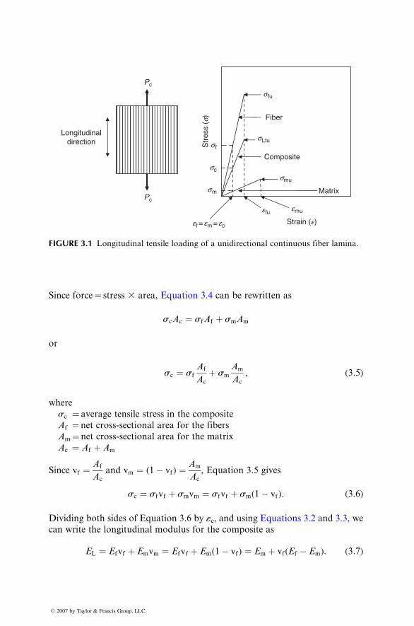
Strain (e)
Pc
Pc
Longitudinaldirection sf
sm
sc
Fiber
Matrix
Composite
sfu
Str
ess
(s)
emuefu
sLtu
smu
ef = em = ec
FIGURE 3.1 Longitudinal tensile loading of a unidirectional continuous fiber lamina.
Since force ¼ stress 3 area, Equat ion 3.4 can be rew ritten a s
sc Ac ¼ s f A f þ s m Am
or
sc ¼ s fAf
Ac
þ sm
Am
Ac
, ( 3: 5)
where
sc ¼ average tensile stress in the composi te
Af ¼ net c ross-sect ional area for the fibers
Am ¼ net cross-sect ional area for the matrix
Ac ¼ A f þ Am
Since vf ¼ Af
Ac
and vm ¼ ( 1 � vf ) ¼ Am
Ac
, Equation 3.5 gives
sc ¼ s f vf þ s m vm ¼ s f vf þ s m (1 � vf ) : ( 3: 6)
Dividing both sides of Equation 3.6 by «c , and using Equat ions 3.2 and 3.3, wecan write the longitudinal modulus for the composite as
EL ¼ Efvf þ Emvm ¼ Efvf þ Em(1� vf) ¼ Em þ vf(Ef � Em): (3:7)
� 2007 by Taylor & Francis Group, LLC.
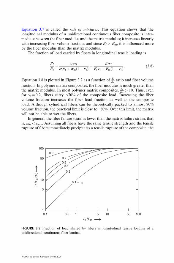
Equation 3.7 is called the rule of mixtures . This equati on shows that the
longitudinal modulus of a unidirectional continuous fiber composite is inter-
mediate between the fiber modulus and the matrix modulus; it increases linearly
with increasing fiber volume fraction; and since Ef > Em, it is influenced more
by the fiber modulus than the matrix modulus.
The fraction of load carried by fibers in longitudinal tensile loading is
Pf
Pc
¼ sfvf
sfvf þ sm(1� vf)¼ Efvf
Efvf þ Em(1� vf): (3:8)
Equation 3.8 is plotted in Figure 3.2 as a function of Ef
Emratio and fiber volume
fraction. In polymer matrix composites, the fiber modulus is much greater than
the matrix modulus. In most polymer matrix composites, Ef
Em> 10. Thus, even
for vf¼ 0.2, fibers carry >70% of the composite load. Increasing the fiber
volume fraction increases the fiber load fraction as well as the composite
load. Although cylindrical fibers can be theoretically packed to almost 90%
volume fraction, the practical limit is close to ~80%. Over this limit, the matrix
will not be able to wet the fibers.
In general, the fiber failure strain is lower than the matrix failure strain, that
is, «fu < «mu. Assuming all fibers have the same tensile strength and the tensile
rupture of fibers immediately precipitates a tensile rupture of the composite, the
100
0.9
0.70.6
0.5
0.3
0.1 = vf
50
10
5
10.1 0.5 1 5
Pf /P
c (%
)
10 50 100
Ef /Em
FIGURE 3.2 Fraction of load shared by fibers in longitudinal tensile loading of a
unidirectional continuous fiber lamina.
� 2007 by Taylor & Francis Group, LLC.
longitu dinal tensile stren gth sLtu of a unidir ectio nal con tinuous fiber c omposi te
can be estimat ed as
sLtu ¼ s fu vf þ s 0m ( 1 � vf ) , ( 3: 9)
where
sfu ¼ fiber tensi le stre ngth (assuming a single tensi le stre ngth v alue for all
fibers, which is not actual ly the case)
s 0m ¼ matr ix stre ss at the fiber fail ure stra in, that is, at «m ¼ «fu (Figur e 3.1)
For effe ctive reinfo rceme nt of the matrix, that is, for sLtu > s mu , the fiber
volume fract ion in the composi te must be greate r than a critical value. This
critical fiber volume fract ion is calculated by sett ing sLtu ¼ smu . Thus , from
Equation 3.9,
Critic al vf ¼ smu � s 0msfu � s 0m
: ( 3: 10 a)
Equation 3.9 assum es that the matrix is una ble to ca rry the load transferr ed to
it after the fiber s ha ve fail ed, and theref ore, the matrix fails imm ediat ely after
the fiber failure. How ever, at low fiber volume fract ions, it is pos sible that the
matrix wi ll be able to carry ad ditional load even afte r the fiber s have failed. For
this to occur,
smu ( 1 � vf ) > s fu vf þ s 0m ( 1 � v f ),
from whi ch the min imum fiber volume fraction can be c alculated as
Minimum vf ¼ smu � s 0msmu þ s fu � s 0m
: ( 3:10b)
If the fiber vo lume fraction is less than the minimum value given by Equation
3.10b, the matr ix will con tinue to carry the load even afte r the fiber s have failed
at sf ¼ sfu . As the load on the composi te is increased, the stra in in the matr ix
will also increa se, but some of the load will be trans ferred to the fiber s. The
fibers will continue to break into smal ler and smaller lengths, and wi th decreas -
ing fiber lengt h, the a verage stress in the fiber s will con tinue to de crease.
Eventual ly, the matrix will fail when the stre ss in the matr ix reaches smu ,
causing the composi te to fail also. The longitud inal tensile stre ngth of the
composi te in this case will be smu (1� vf).
Figure 3.3 shows the longitu dinal stren gth varia tion with fiber volume
fraction for a unid irectional continuou s fiber compo site con taining an elastic,
brittle matrix. Table 3.1 shows critical fiber volume fraction and minimum fiber
� 2007 by Taylor & Francis Group, LLC.
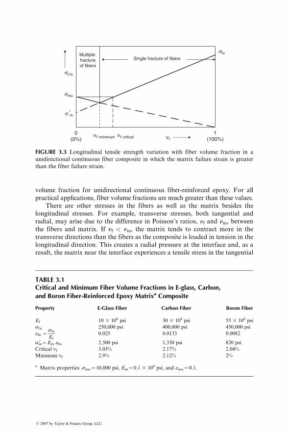
vf
sLtu
sfu
smu
s 9m
vf minimum vf critical0
(0%)1
(100%)
Single fracture of fibers Multiple fractureof fibers
FIGURE 3.3 Longitudinal tensile strength variation with fiber volume fraction in a
unidirectional continuous fiber composite in which the matrix failure strain is greater
than the fiber failure strain.
volume fraction for unidirectional continuous fiber-reinforced epoxy. For all
practical applications, fiber volume fractions are much greater than these values.
There are other stresses in the fibers as well as the matrix besides the
longitudinal stresses. For example, transverse stresses, both tangential and
radial, may arise due to the difference in Poisson’s ratios, nf and nm, betweenthe fibers and matrix. If nf < nm, the matrix tends to contract more in the
transverse directions than the fibers as the composite is loaded in tension in the
longitudinal direction. This creates a radial pressure at the interface and, as a
result, the matrix near the interface experiences a tensile stress in the tangential
TABLE 3.1Critical and Minimum Fiber Volume Fractions in E-glass, Carbon,
and Boron Fiber-Reinforced Epoxy Matrixa Composite
Property E-Glass Fiber Carbon Fiber Boron Fiber
Ef 10 3 106 psi 30 3 106 psi 55 3 106 psi
sfu 250,000 psi 400,000 psi 450,000 psi
«fu ¼ sfu
Ef
0.025 0.0133 0.0082
sm0 ¼Em «fu 2,500 psi 1,330 psi 820 psi
Critical vf 3.03% 2.17% 2.04%
Minimum vf 2.9% 2.12% 2%
a Matrix properties: smu¼ 10,000 psi, Em¼ 0.1 3 106 psi, and «mu¼ 0.1.
� 2007 by Taylor & Francis Group, LLC.
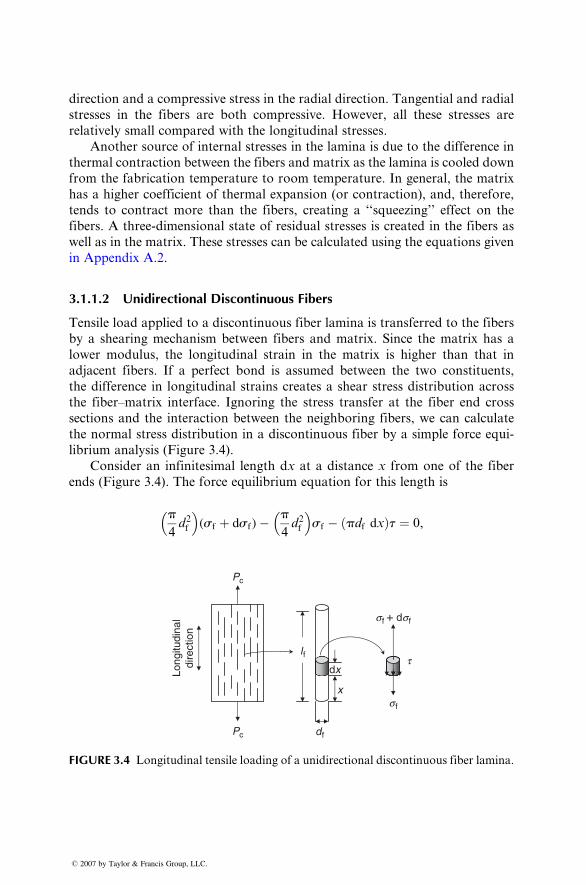
direction an d a compres sive stre ss in the radial direct ion. Tangenti al an d radial
stresses in the fiber s are both compres sive. How ever, all these stre sses are
relative ly smal l compa red wi th the longitu dinal stresses .
Anothe r source of intern al stresses in the lamina is due to the diff erence in
therma l con traction betw een the fibers and matrix as the lamina is cooled down
from the fabri cation tempe rature to room tempe ratur e. In general, the matr ix
has a higher coefficie nt of therm al expansi on (or contrac tion), and, therefo re,
tends to co ntract more than the fibers, creating a ‘‘squ eezing’’ effect on the
fibers. A three- dimens ional state of resi dual stre sses is created in the fibers as
well as in the matrix. These stresses can be calculated using the equations given
in App endix A.2 .
3.1.1.2 Unidirectional Discontinuous Fibers
Tensile load applied to a discontinuous fiber lamina is transferred to the fibers
by a shearing mechanism between fibers and matrix. Since the matrix has a
lower modulus, the longitudinal strain in the matrix is higher than that in
adjacent fibers. If a perfect bond is assumed between the two constituents,
the difference in longitudinal strains creates a shear stress distribution across
the fiber–matrix interface. Ignoring the stress transfer at the fiber end cross
sections and the interaction between the neighboring fibers, we can calculate
the normal stress distribution in a discontinuous fiber by a simple force equi-
librium analysis (Figure 3.4).
Consider an infinitesimal length dx at a distance x from one of the fiber
ends (Figure 3.4). The force equilibrium equation for this length is
p
4d2f
� �(sf þ dsf )� p
4d2f
� �sf � pdf dxð Þt ¼ 0,
dx
sf + dsf
sf
tlf
df
x
Pc
Pc
Long
itudi
nal
dire
ctio
n
FIGURE 3.4 Longitudinal tensile loading of a unidirectional discontinuous fiber lamina.
� 2007 by Taylor & Francis Group, LLC.
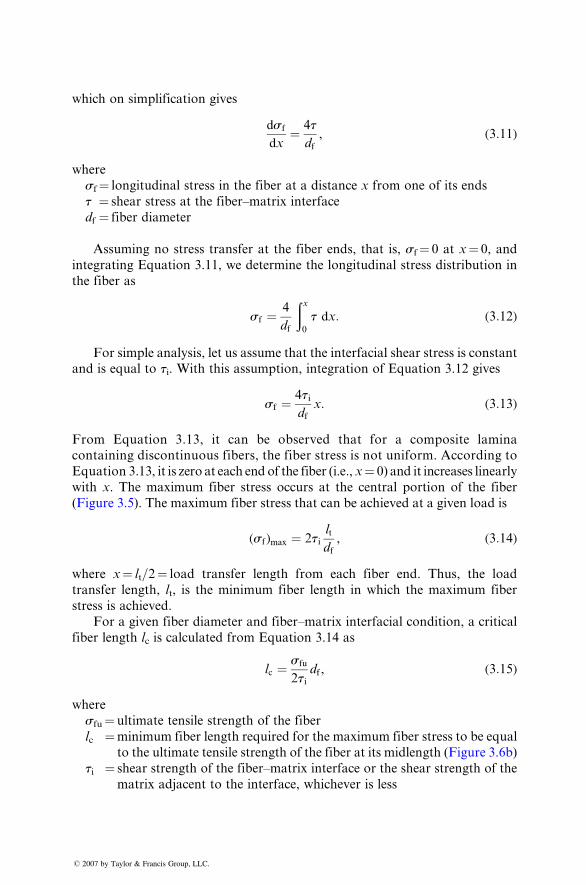
which on sim plificat ion gives
dsf
dx¼ 4t
df, ( 3: 11 )
wher e
sf ¼ longit udinal stre ss in the fiber at a distan ce x from one of its en ds
t ¼ shear stress at the fiber–mat rix inter face
df ¼ fiber diame ter
Ass uming no stre ss trans fer at the fiber end s, that is, sf ¼ 0 at x ¼ 0, and
integ rating Equation 3.11, we determine the longitudinal stress distribut ion in
the fiber as
sf ¼ 4
df
ðx0
t dx: ( 3: 12 )
For simp le analys is, let us assum e that the inter facial shear stress is constant
and is eq ual to ti. With this assump tion, integrati on of Equat ion 3.12 gives
sf ¼ 4tidf
x: ( 3: 13 )
From Equation 3.13, it c an be observed t hat for a composite lamina
containi ng discontinuous fibers, t he fiber stress is not uniform. According to
E q u a t i o n 3.13, it is zero at each end of the fiber (i.e., x ¼ 0) and it increases linea rly
with x. The maximum fiber stress occurs at the central porti on of the fiber
(Figur e 3.5). The maxi mum fiber stre ss that can be ach ieved a t a given load is
( sf ) max ¼ 2t ilt
df, ( 3: 14 )
wher e x ¼ lt=2 ¼ load trans fer lengt h from each fiber end. Thus , the load
trans fer lengt h, lt, is the mini mum fiber lengt h in whi ch the maxi mum fiber
stress is achieve d.
For a given fiber diame ter an d fiber –matrix inter facial con dition, a critical
fiber lengt h lc is calcul ated from Equation 3.14 as
lc ¼ sfu
2tidf , ( 3: 15 )
wher e
sfu ¼ ultimat e tensile stre ngth of the fiber
lc ¼ mini mum fiber lengt h requ ired for the maxi mum fiber stress to be eq ual
to the ultimate tensi le stren gth of the fiber at its midlen gth (Figur e 3.6b)
ti ¼ shear strength of the fiber–matrix interface or the shear strength of the
matrix adjacent to the interface, whichever is less
� 2007 by Taylor & Francis Group, LLC.
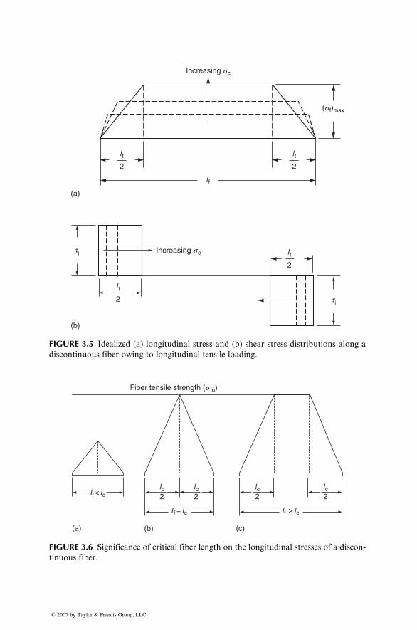
Increasing sc
Increasing sc
(s f)max
l f
l t
2
(a)
(b)
l t
2
t i
t i
l t
2
l t
2
FIGURE 3.5 Idealized (a) longitudinal stress and (b) shear stress distributions along a
discontinuous fiber owing to longitudinal tensile loading.
lf < lc
(a) (b) (c)
lc
l f = lc lf > lc
Fiber tensile strength (s fu)
2lc2
lc2
lc2
FIGURE 3.6 Significance of critical fiber length on the longitudinal stresses of a discon-
tinuous fiber.
� 2007 by Taylor & Francis Group, LLC.
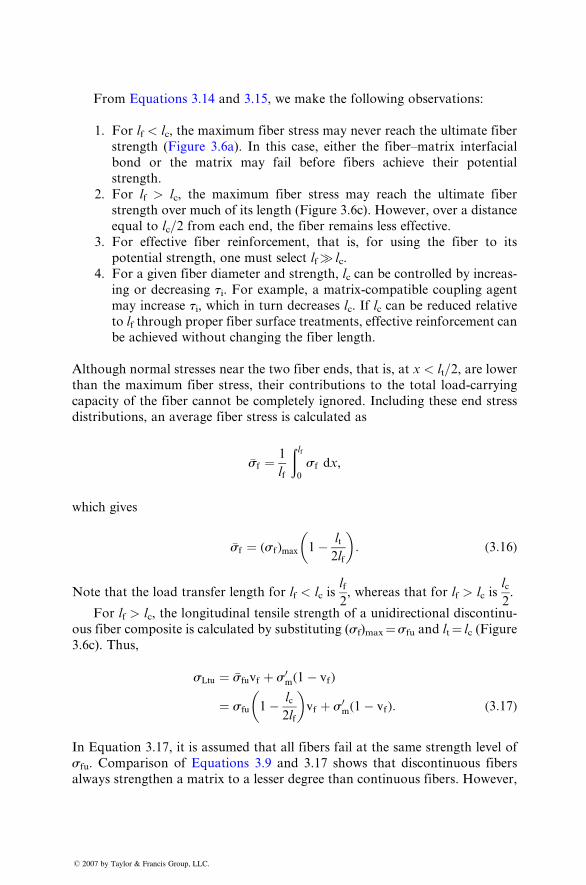
Fro m Equat ions 3.14 and 3.15, we mak e the followi ng observat ions:
1. For lf < l c , the maximum fiber stre ss may never reach the ulti mate fiber
stre ngth (Figur e 3.6a). In this case, eithe r the fiber–mat rix interfaci al
bond or the matr ix may fail before fibers achieve their potential
stre ngth.
2. For lf > l c, the maximum fiber stre ss may reach the ultimat e fiber
stre ngth over much of its lengt h (Figur e 3.6c) . How ever, ov er a distance
equ al to lc =2 from each end , the fiber remain s less effe ctive.
3. For effective fiber reinfo rcement, that is, for using the fiber to its
potenti al stre ngth, one must select lf � l c .
4. For a given fiber diame ter and stren gth, lc can be co ntrolled by increa s-
ing or decreas ing ti . For exampl e, a matrix-co mpatible cou pling age nt
may increase ti, which in turn decreas es l c . If lc can be redu ced relat iveto lf through proper fiber surface treat ments, effecti ve reinforcem en t can
be achieve d withou t changing the fiber lengt h.
Althou gh normal stresses near the two fiber end s, that is, at x < lt=2, are low erthan the maxi mum fiber stress, their con tributions to the total load-c arrying
capacit y of the fiber can not be complet ely ignored. Includin g these end stre ss
distribut ions, an average fiber stre ss is calcul ated as
�sf ¼ 1
lf
ðlf0
sf dx,
which gives
�sf ¼ ( s f ) max 1 � lt
2lf
� �: ( 3:16)
Note that the load trans fer length for lf < lc islf
2 , whereas that for lf > lc is
lc
2 .
For l f > lc , the longit udinal tensile strength of a unidir ectional discont inu-
ous fiber composi te is calculated by substitut ing ( sf) max ¼ sfu and lt¼ lc (Figure
3.6c). Thus,
sLtu ¼ �sfuvf þ s0m(1� vf)
¼ sfu 1� lc
2lf
� �vf þ s 0m (1 � vf ) : ( 3: 17 )
In Equation 3.17, it is assum ed that all fibers fail at the same strength level of
sfu . Com pariso n of Equations 3.9 and 3.17 shows that discon tinuous fiber s
always strengthen a matrix to a lesser degree than continuous fibers. However,
� 2007 by Taylor & Francis Group, LLC.
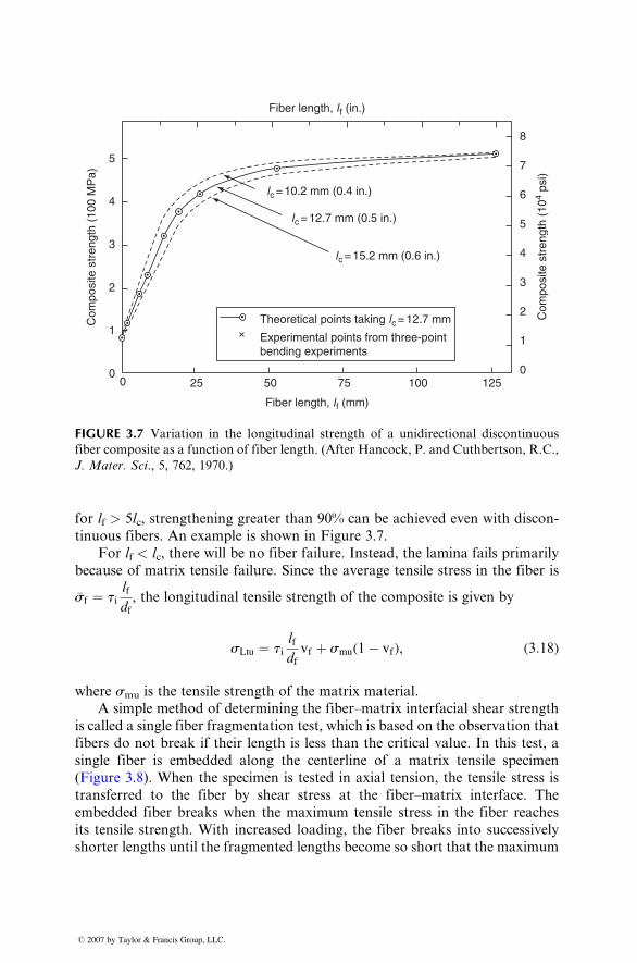
Fiber length, l f (in.)
lc = 10.2 mm (0.4 in.)
lc = 12.7 mm (0.5 in.)
lc = 15.2 mm (0.6 in.)
Theoretical points taking lc = 12.7 mm
Experimental points from three-pointbending experiments
Fiber length, lf (mm)
Com
posi
te s
tren
gth
(104
psi)
Com
posi
te s
tren
gth
(100
MP
a)
0
1
2
3
4
5
8
7
6
5
4
3
2
1
00 25 50 75 100 125
FIGURE 3.7 Variation in the longitudinal strength of a unidirectional discontinuous
fiber composite as a function of fiber length. (After Hancock, P. and Cuthbertson, R.C.,
J. Mater. Sci., 5, 762, 1970.)
for lf > 5l c , streng thening great er than 90% can be ach ieved even with discon -
tinuous fibers. An exampl e is shown in Figure 3.7.
For lf < lc , there will be no fiber failu re. Instead , the lamina fails prim arily
because of matr ix tensi le failure. Since the average tensile stre ss in the fiber is
�sf ¼ t ilf
df, the longitud inal tensile streng th of the co mposite is given by
sLtu ¼ t ilf
dfvf þ s mu (1 � v f ) , ( 3: 18 )
where smu is the tensi le stre ngth of the matrix material .
A sim ple method of de termining the fiber–mat rix inter facial shear strength
is called a single fiber fragm entat ion test, whi ch is based on the obs ervation that
fibers do not break if their lengt h is less than the crit ical value. In this test, a
single fiber is embedded along the center line of a matr ix tensi le specim en
(Figur e 3.8). When the sp ecimen is tested in axial tensio n, the tensi le stress is
transferr ed to the fiber by shear stre ss at the fiber–mat rix interface. The
embedded fiber breaks when the maxi mum tensi le stress in the fiber reaches
its tensi le stren gth. With increa sed loading , the fiber break s into success ively
shorte r lengths until the fragmen ted length s be come so short that the maximum
� 2007 by Taylor & Francis Group, LLC.
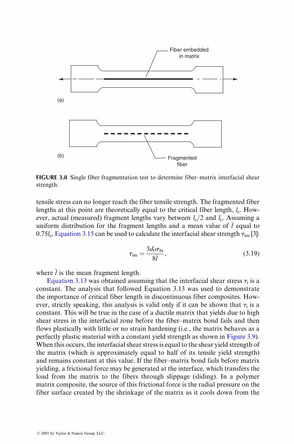
Fiber embeddedin matrix
Fragmentedfiber
(a)
(b)
FIGURE 3.8 Single fiber fragmentation test to determine fiber–matrix interfacial shear
strength.
tensile stress can no longer reach the fiber tensile strength. The fragmented fiber
lengths at this point are theoretically equal to the critical fiber length, lc. How-
ever, actual (measured) fragment lengths vary between lc=2 and lc. Assuming a
uniform distribution for the fragment lengths and a mean value of �l equal to0.75lc, Equation 3.15 can be used to calculate the interfacial shear strength tim [3]:
tim ¼ 3df s fu
8�l, ( 3: 19 )
wher e �l is the mean fragment length .
Equat ion 3.13 was obtaine d assum ing that the inter facial shear stre ss ti is aconstant . The analysis that follo wed Equat ion 3.13 was used to demonst rate
the impor tance of critical fiber lengt h in discon tinuous fiber composi tes. How -
ever, strictl y sp eaking, this ana lysis is valid only if it can be shown that ti is aconstant . This wi ll be true in the case of a duc tile matr ix that y ields due to high
shear stre ss in the interfaci al zon e before the fiber –matrix bond fails an d then
flows plastical ly with littl e or no strain hardening (i.e., the matr ix be haves as a
perfec tly plastic mate rial wi th a co nstant yield strength as shown in Figure 3.9) .
When this occurs, the interfaci al shear stre ss is equal to the shear y ield strength of
the matrix (w hich is approxim ately eq ual to half of its tensile yiel d stre ngth)
and remai ns con stant at this value. If the fiber –matrix bond fails before matr ix
yield ing, a frictio nal force may be generated at the inter face, whi ch trans fers the
load from the matrix to the fibers through slippage (sliding). In a polymer
matrix composite, the source of this frictional force is the radial pressure on the
fiber surface created by the shrinkage of the matrix as it cools down from the
� 2007 by Taylor & Francis Group, LLC.
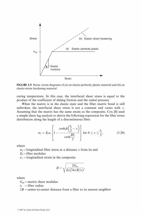
(b) Elastic–strain hardening
(a) Elastic–perfectly plastic
Elasticmodulus
Strain
Stress
smy
FIGURE 3.9 Stress–strain diagrams of (a) an elastic-perfectly plastic material and (b) an
elastic-strain hardening material.
curing temperature. In this case, the interfacial shear stress is equal to the
product of the coefficient of sliding friction and the radial pressure.
When the matrix is in the elastic state and the fiber–matrix bond is still
unbroken, the interfacial shear stress is not a constant and varies with x.
Assuming that the matrix has the same strain as the composite, Cox [4] used
a simple shear lag analysis to derive the following expression for the fiber stress
distribution along the length of a discontinuous fiber:
sf ¼ Ef«1 1�coshb
lf
2� x
� �
coshblf2
2664
3775 for 0 � x � lf
2, (3:20)
where
sf¼ longitudinal fiber stress at a distance x from its end
Ef¼ fiber modulus
«1¼ longitudinal strain in the composite
b ¼ffiffiffiffiffiffiffiffiffiffiffiffiffiffiffiffiffiffiffiffiffiffiffiffiffiffiffi
2Gm
Efr2f ln (R=rf )
s,
where
Gm¼matrix shear modulus
rf ¼ fiber radius
2R ¼ center-to-center distance from a fiber to its nearest neighbor
� 2007 by Taylor & Francis Group, LLC.
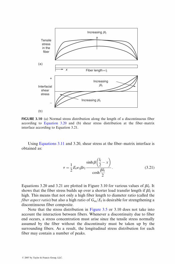
Increasing bl f
Tensilestressin thefiber
Interfacialshearstress
+
−
x Fiber length = l f
Increasingbl f
Increasing bl f
(a)
(b)
FIGURE 3.10 (a) Normal stress distribution along the length of a discontinuous fiber
according to Equation 3.20 and (b) shear stress distribution at the fiber–matrix
interface according to Equation 3.21.
Usi ng Equation s 3.11 and 3.20, shear stre ss a t the fiber–mat rix inter face is
obtaine d as:
t ¼ 1
2 Ef «1 br f
sinh blf
2 � x
� �
coshblf2
: ( 3: 21 )
Equation s 3.20 and 3.21 are plotted in Figure 3.10 for various values of blf. Itshows that the fiber stress builds up over a shorte r load trans fer lengt h if blf ishigh. This means that not only a high fiber lengt h to diameter rati o (called the
fiber aspect rati o) but also a high rati o of Gm=E f is desir able for streng thening adiscont inuous fiber compo site.
Note that the stre ss distribut ion in Figu re 3.5 or 3.10 doe s not take into
accoun t the inter actio n between fibers. When ever a discont inuity due to fiber
end oc curs, a stress con centration must arise since the tensile stress normal ly
assum ed by the fiber without the discont inuity mu st be taken up by the
surround ing fibers. As a resul t, the longit udinal stre ss dist ribution for each
fiber may contai n a num ber of peaks.
� 2007 by Taylor & Francis Group, LLC.
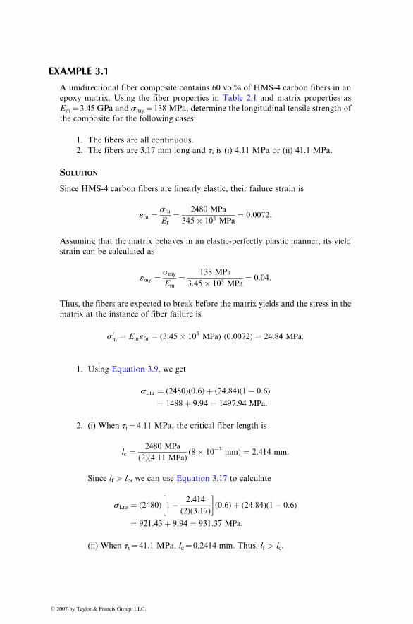
EXAMPLE 3.1
A unidirectional fiber composite contains 60 vol% of HMS-4 carbon fibers in an
epoxy matrix. Using the fiber properties in Table 2.1 and matrix properties as
Em ¼ 3.45 GPa and smy ¼ 138 MPa, determine the longitudinal tensile strength of
the composite for the following cases:
1. The fibers are all continuous.
2. The fibers are 3.17 mm long and ti is (i) 4.11 MPa or (ii) 41.1 MPa.
SOLUTIO N
Since HMS-4 carbon fibers are linearly elastic, their failure strain is
«fu ¼ sfu
Ef
¼ 2480 MPa
345 � 103 MPa ¼ 0: 0072:
Assuming that the matrix behaves in an elastic-perfectly plastic manner, its yield
strain can be calculated as
«my ¼ smy
Em
¼ 138 MPa
3: 45 � 103 MPa ¼ 0: 04:
Thus, the fibers are expected to break before the matrix yields and the stress in the
matrix at the instance of fiber failure is
s 0m ¼ Em «fu ¼ ( 3: 45 � 103 MPa) (0: 0072 ) ¼ 24: 84 MPa:
1. Using Equation 3.9, we get
sLtu ¼ (2480 )(0: 6) þ (24 :84 )(1 � 0: 6)
¼ 1488 þ 9: 94 ¼ 1497: 94 MPa:
2. (i) When ti ¼ 4.11 MPa, the critical fiber length is
lc ¼ 2480 MPa
( 2)(4: 11 MPa) ( 8 � 10� 3 mm) ¼ 2: 414 mm:
Since lf > l c , we can use Equation 3.17 to calculate
sLtu ¼ (2480) 1� 2:414
(2)(3:17)
� �(0:6)þ (24:84)(1� 0:6)
¼ 921:43þ 9:94 ¼ 931:37 MPa:
(ii) When ti¼ 41.1 MPa, lc¼ 0.2414 mm. Thus, lf > lc.
� 2007 by Taylor & Francis Group, LLC.
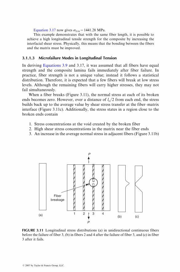
Equation 3.17 now gives sLtu ¼ 1441.28 MPa.
This example demonstrates that with the same fiber length, it is possible to
achieve a high longitudinal tensile strength for the composite by increasing the
interfacial shear stress. Physically, this means that the bonding between the fibers
and the matrix must be improved.
3.1.1 .3 Mic rofailure Modes in Lon gitudinal Ten sion
In derivin g Equations 3.9 and 3.17, it was assumed that all fibers have equ al
strength and the composite lamina fails immediately after fiber failure. In
practice, fiber strength is not a unique value; instead it follows a statistical
distribution. Therefore, it is expected that a few fibers will break at low stress
levels. Although the remaining fibers will carry higher stresses, they may not
fail simultaneously.
When a fiber breaks (Figure 3.11), the normal stress at each of its broken
ends becomes zero. However, over a distance of lc=2 from each end, the stress
builds back up to the average value by shear stress transfer at the fiber–matrix
interface (Figure 3.11c). Additionally, the stress states in a region close to the
broken ends contain
1. Stress concentrations at the void created by the broken fiber
2. High shear stress concentrations in the matrix near the fiber ends
3. An increase in the average normal stress in adjacent fibers (Figure 3.11b)
(a) (b) (c)1 2 3 4
P
P
Fiberbreakage
FIGURE 3.11 Longitudinal stress distributions (a) in unidirectional continuous fibers
before the failure of fiber 3, (b) in fibers 2 and 4 after the failure of fiber 3, and (c) in fiber
3 after it fails.
� 2007 by Taylor & Francis Group, LLC.
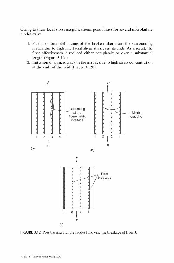
Owing to these local stress magnifications, possibilities for several microfailure
modes exist:
1. Partial or total debonding of the broken fiber from the surrounding
matrix due to high interfacial shear stresses at its ends. As a result, the
fiber effectiveness is reduced either completely or over a substantial
length (Figure 3.12a).
2. Initiation of a microcrack in the matrix due to high stress concentration
at the ends of the void (Figure 3.12b).
P
Fiberbreakage
(c)P
1 2 3 4
P
Matrixcracking
P(b)
1 2 3 4
P
P(a)
1 2 3 4
Debondingat the
fiber–matrixinterface
FIGURE 3.12 Possible microfailure modes following the breakage of fiber 3.
� 2007 by Taylor & Francis Group, LLC.
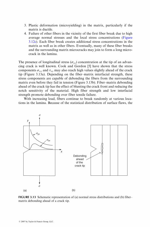
3. Plast ic deform ation (mi croyielding) in the matr ix, particular ly if the
matr ix is duc tile.
4. Failur e of other fiber s in the vicin ity of the fir st fiber break due to high
average normal stre sses and the local stre ss co ncentra tions (Figur e
3.12c) . Each fiber break creates additio nal stre ss con centrations in the
matr ix a s well as in other fiber s. Eve ntually, many of these fiber break s
and the surroun ding matr ix microcracks may join to form a long micr o-
crack in the lami na.
The presence of long itudinal stre ss (syy ) co ncentra tion at the tip of an advan -
cing crack is well know n. Cook and Gordon [5] have shown that the stre ss
components sxx and txy may also reach high values slightly ahead of the crack
tip (Figure 3.13a). Depending on the fiber–matrix interfacial strength, these
stress components are capable of debonding the fibers from the surrounding
matrix even before they fail in tension (Figure 3.13b). Fiber–matrix debonding
ahead of the crack tip has the effect of blunting the crack front and reducing the
notch sensitivity of the material. High fiber strength and low interfacial
strength promote debonding over fiber tensile failure.
With increasing load, fibers continue to break randomly at various loca-
tions in the lamina. Because of the statistical distribution of surface flaws, the
Debondingaheadof the
crack tip
s
syy
sxx
s
x
y
(a) (b)
FIGURE 3.13 Schematic representation of (a) normal stress distributions and (b) fiber–
matrix debonding ahead of a crack tip.
� 2007 by Taylor & Francis Group, LLC.
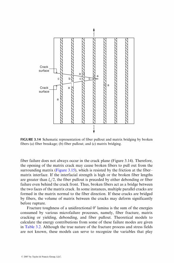
a
a
c b c c
aa
a
Cracksurface
Cracksurface
FIGURE 3.14 Schematic representation of fiber pullout and matrix bridging by broken
fibers (a) fiber breakage; (b) fiber pullout; and (c) matrix bridging.
fiber failure does not alw ays oc cur in the crack plane (Figur e 3.14). Ther efore,
the open ing of the matrix crack may cause broken fibers to pull out from the
surroundi ng matrix (Figure 3.15), which is resisted by the friction at the fiber–
matrix inter face. If the inter facial stre ngth is high or the broken fiber lengths
are greater than lc =2, the fiber pullout is preceded by either debo nding or fiberfailure even behind the crack front . Thus , brok en fibers act as a bridge between
the tw o faces of the matr ix crack. In some instan ces, multiple parallel cracks are
formed in the matrix normal to the fiber direction. If these cracks are bridged
by fibers, the volume of matr ix between the cracks may deform signifi cantly
before rupture .
Fractur e tough ness of a unid irectional 08 lamin a is the sum of the energies
consumed by various micr ofailure proc esses, namel y, fiber fracture, matrix
cracki ng or yield ing, de bonding, and fiber pullout . Theoreti cal mo dels to
calcula te the energy contribu tions from some of these failure mod es are given
in Table 3.2. Although the true nature of the fracture process and stress fields
are not known, these models can serve to recognize the variables that play
� 2007 by Taylor & Francis Group, LLC.
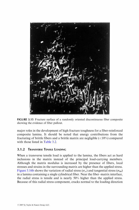
FIGURE 3.15 Fracture surface of a randomly oriented discontinuous fiber composite
showing the evidence of fiber pullout.
major roles in the developm en t of high fractu re toughness for a fiber -reinforce d
composi te lami na. It should be noted that en ergy co ntributions from the
fracturi ng of brit tle fiber s and a brit tle matr ix are ne gligible (< 10%) compared
with those lis ted in Table 3.2.
3.1.2 T RANSVERSE TENSILE LOADING
When a transve rse tensi le load is ap plied to the lamina, the fibers act as hard
inclus ions in the matrix instead of the princi pal load-c arryi ng member s.
Althou gh the matrix mod ulus is increa sed by the presence of fiber s, local
stresses and stra ins in the surroundi ng matr ix are higher than the applie d stress.
Figure 3.16b shows the varia tion of radial stress ( srr ) and tangent ial stre ss ( suu )
in a lamin a contain ing a single cyli ndrical fiber. Near the fiber–mat rix interface,
the radial stress is tensile and is nearly 50% higher than the applied stress.
Because of this radial stress component, cracks normal to the loading direction
� 2007 by Taylor & Francis Group, LLC.
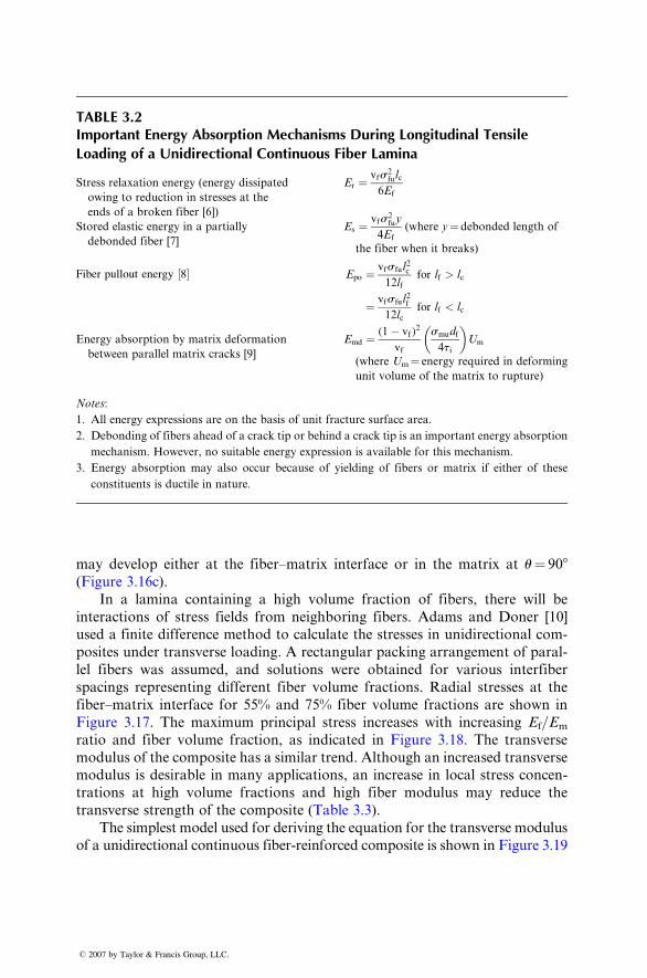
TABLE 3.2Important Energy Absorpti on Mechani sms During Longit udinal Ten sile
Loading of a Uni directi onal Cont inuous Fiber Lamin a
Stress relaxation energy (energy dissipated
owing to reduction in stresses at the
ends of a broken fiber [6])
Er ¼ vf s 2fu lc
6Ef
Stored elastic energy in a partially
debonded fiber [7]
Es ¼ vf s 2fu y
4Ef
(where y ¼ debonded length of
the fiber when it breaks)
Fiber pullout energy ½8� Epo ¼ vf s fu l 2c
12lffor lf > lc
¼ vf s fu l 2f
12lcfor lf < lc
Energy absorption by matrix deformation
between parallel matrix cracks [9]
Emd ¼ (1 � vf ) 2
vf
smu df
4ti
� �Um
(where Um ¼ energy required in deforming
unit volume of the matrix to rupture)
Notes:
1. All energy expressions are on the basis of unit fracture surface area.
2. Debonding of fibers ahead of a crack tip or behind a crack tip is an important energy absorption
mechanism. However, no suitable energy expression is available for this mechanism.
3. Energy absorption may also occur because of yielding of fibers or matrix if either of these
constituents is ductile in nature.
may develop either at the fiber –matrix inter face or in the matrix at u ¼ 908(Figur e 3.16c) .
In a lamin a contai ning a high volume fraction of fiber s, there wi ll be
interacti ons of stre ss fields from neighbo ring fibers. Adams and Doner [10]
used a finite difference method to calcul ate the stre sses in unidir ectio nal co m-
posites unde r trans verse loading . A rectan gular pac king arrange men t of paral-
lel fiber s was assum ed, and solutions wer e obtaine d for various inter fiber
spacing s repres enting different fiber volume fract ions. Radi al stre sses at the
fiber–mat rix interface for 55% a nd 75% fiber volume fract ions are shown in
Figure 3.17. The maxi mum princi pal stress increases with increasing Ef=E mratio and fiber vo lume fraction, as indica ted in Figu re 3.18. The transverse
modulus of the compo site ha s a sim ilar trend. Alt hough an increa sed transv erse
modulus is desir able in many a pplications , an increa se in local stre ss concen -
trations at high volume fract ions and high fiber modulus may redu ce the
transve rse stren gth of the composi te (Table 3.3).
The simplest model used for deriving the equation for the transverse modulus
of a unidirectional continuous fiber-reinforced composite is shown in Figure 3.19
� 2007 by Taylor & Francis Group, LLC.
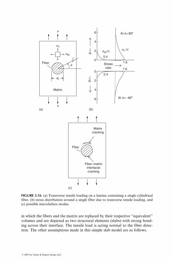
s
srr
r
Fiberq
sqq
s(a)
Matrix
df
At q = 908
At q = −908
6
4
rdf
2
0
0
2
4
6
1.6Stressratio 1.6
0.4
0.4
srr /ssqq /s
rd f
(b)
Matrixcracking
Fiber–matrixinterfacialcracking
Fiber
(c)
FIGURE 3.16 (a) Transverse tensile loading on a lamina containing a single cylindrical
fiber, (b) stress distribution around a single fiber due to transverse tensile loading, and
(c) possible microfailure modes.
in which the fibers and the matrix are replaced by their respective ‘‘equivalent’’
volumes and are depicted as two structural elements (slabs) with strong bond-
ing across their interface. The tensile load is acting normal to the fiber direc-
tion. The other assumptions made in this simple slab model are as follows.
� 2007 by Taylor & Francis Group, LLC.
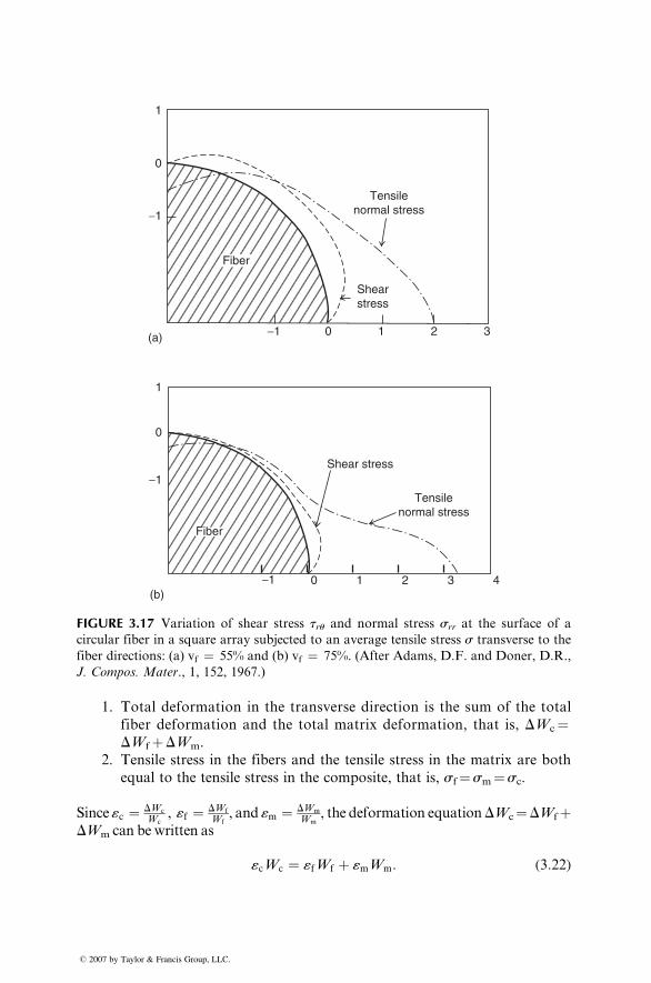
(a)
41 2 30(b)
−1
1
Shear stress
0
−1
Tensilenormal stress
Fiber
1
0
−1 0 1 2 3
−1
Tensilenormal stress
Shearstress
Fiber
FIGURE 3.17 Variation of shear stress tru and normal stress srr at the surface of a
circular fiber in a square array subjected to an average tensile stress s transverse to the
fiber directions: (a) vf ¼ 55% and (b) vf ¼ 75%. (After Adams, D.F. and Doner, D.R.,
J. Compos. Mater., 1, 152, 1967.)
1. Total deformation in the transverse direction is the sum of the total
fiber deformation and the total matrix deformation, that is, DWc¼DWfþDWm.
2. Tensile stress in the fibers and the tensile stress in the matrix are both
equal to the tensile stress in the composite, that is, sf¼sm¼sc.
Since «c ¼ DWc
Wc, «f ¼ DWf
Wf, and «m ¼ DWm
Wm, the deformation equationDWc¼DWfþ
DWm can be written as
«cWc ¼ «fWf þ «mWm: (3:22)
� 2007 by Taylor & Francis Group, LLC.
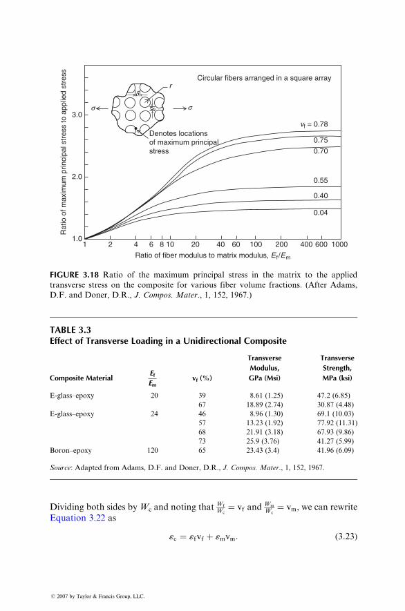
1.01 2 4 6 8 10 20 40
Circular fibers arranged in a square array
Denotes locationsof maximum principalstress
rd
ss
vf = 0.78
0.75
0.70
0.55
0.40
0.04
60 100 200 400 600 1000
2.0
Rat
io o
f max
imum
prin
cipa
l str
ess
to a
pplie
d st
ress
Ratio of fiber modulus to matrix modulus, E f /Em
3.0
d
FIGURE 3.18 Ratio of the maximum principal stress in the matrix to the applied
transverse stress on the composite for various fiber volume fractions. (After Adams,
D.F. and Doner, D.R., J. Compos. Mater., 1, 152, 1967.)
TABLE 3.3Effect of Transverse Loading in a Unidirectional Composite
Composite MaterialEfEm
vf (%)
Transverse
Modulus,
GPa (Msi)
Transverse
Strength,
MPa (ksi)
E-glass–epoxy 20 39 8.61 (1.25) 47.2 (6.85)
67 18.89 (2.74) 30.87 (4.48)
E-glass–epoxy 24 46 8.96 (1.30) 69.1 (10.03)
57 13.23 (1.92) 77.92 (11.31)
68 21.91 (3.18) 67.93 (9.86)
73 25.9 (3.76) 41.27 (5.99)
Boron–epoxy 120 65 23.43 (3.4) 41.96 (6.09)
Source: Adapted from Adams, D.F. and Doner, D.R., J. Compos. Mater., 1, 152, 1967.
Dividing both sides by Wc and noting thatWf
Wc¼ vf an d
Wm
Wc¼ vm , we can rewrite
Equation 3.22 as
«c ¼ «fvf þ «mvm: (3:23)
� 2007 by Taylor & Francis Group, LLC.
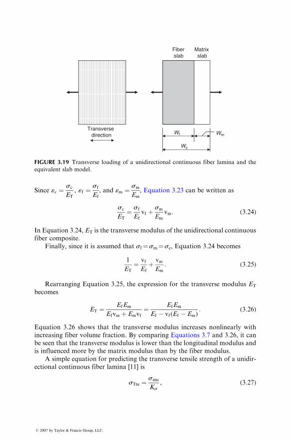
Fiber slab
Matrix slab
Transverse direction
Wc
Wf Wm
FIGURE 3.19 Transverse loading of a unidirectional continuous fiber lamina and the
equivalent slab model.
Since «c ¼ sc
ET
, «f ¼ sf
Ef
, and «m ¼ sm
Em
, Equat ion 3.23 can be writt en as
sc
ET
¼ sf
Ef
vf þ sm
Em
vm : ( 3: 24 )
In Equation 3.24, ET is the trans verse modulus of the uni directional continuous
fiber compo site.
Finall y, since it is assum ed that sf ¼ sm ¼ sc , Equation 3.24 becomes
1
ET
¼ vf
Ef
þ vm
Em
: ( 3: 25 )
Rear ranging Equat ion 3.25, the express ion for the transverse mod ulus ET
becomes
ET ¼ Ef Em
Ef vm þ Em v f¼ Ef Em
Ef � vf (E f � Em ) : ( 3: 26 )
Equation 3.26 shows that the trans verse mod ulus increa ses nonlinear ly with
increa sing fiber volume fraction . By compari ng Equat ions 3.7 an d 3.26, it can
be seen that the trans verse modulus is low er than the lon gitudinal mod ulus and
is influ enced more by the matr ix modulus than by the fiber modulus.
A simp le equati on for predicting the transve rse tensile stre ngth of a unidir -
ection al con tinuous fiber lami na [11] is
sTtu ¼ smu
Ks, (3:27)
� 2007 by Taylor & Francis Group, LLC.
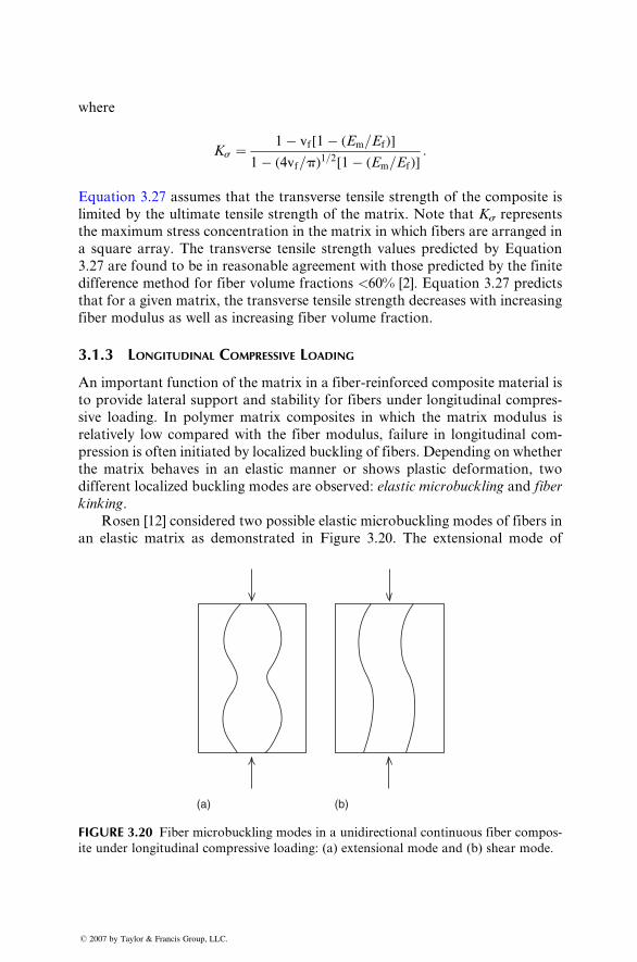
wher e
Ks ¼ 1 � vf [1 � ( Em = Ef )]
1 � ( 4vf =p )1 = 2 [ 1 � (E m =Ef )]
:
Equation 3.27 a ssumes that the transverse tensile stre ngth of the co mposi te is
limited by the ultimate tensile strength of the matrix. Note that Ks represents
the maximum stress concentration in the matrix in which fibers are arranged in
a square array. The transverse tensile strength values predicted by Equation
3.27 are found to be in reasonable agreement with those predicted by the finite
difference method for fiber volume fractions <60% [2]. Equation 3.27 predicts
that for a given matrix, the transverse tensile strength decreases with increasing
fiber modulus as well as increasing fiber volume fraction.
3.1.3 LONGITUDINAL COMPRESSIVE LOADING
An important function of the matrix in a fiber-reinforced composite material is
to provide lateral support and stability for fibers under longitudinal compres-
sive loading. In polymer matrix composites in which the matrix modulus is
relatively low compared with the fiber modulus, failure in longitudinal com-
pression is often initiated by localized buckling of fibers. Depending on whether
the matrix behaves in an elastic manner or shows plastic deformation, two
different localized buckling modes are observed: elastic microbuckling and fiber
kinking.
Rosen [12] considered two possible elastic microbuckling modes of fibers in
an elastic matrix as demonstrated in Figure 3.20. The extensional mode of
(a) (b)
FIGURE 3.20 Fiber microbuckling modes in a unidirectional continuous fiber compos-
ite under longitudinal compressive loading: (a) extensional mode and (b) shear mode.
� 2007 by Taylor & Francis Group, LLC.
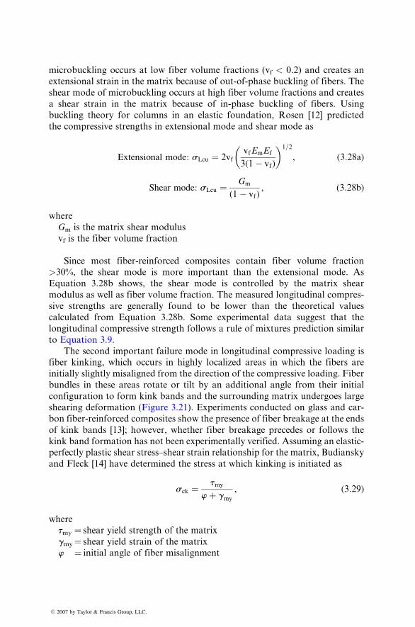
microb uckling occurs at low fiber vo lume fract ions (vf < 0.2) and creates an
extens ional strain in the matrix becau se of out-of-ph ase buckling of fiber s. The
shear mod e of micr obuck ling occurs at high fiber volume fract ions and creates
a shear stra in in the matr ix because of in-phas e buckling of fiber s. Usi ng
buckling theory for columns in an elastic foun dation, Rosen [12] pred icted
the co mpres sive streng ths in extension al mode and shear mode as
Exten sional mode : sLcu ¼ 2vfvf Em E f
3( 1 � vf )
� �1= 2
, ( 3: 28 a)
Shear mode : sLcu ¼ Gm
( 1 � vf ) , ( 3:28b)
where
Gm is the matr ix shear modulus
vf is the fiber vo lume fraction
Since most fiber-re inforced composi tes con tain fiber volume fraction
> 30%, the shear mode is more impor tant than the extens ional mode. As
Equation 3.28b shows, the shear mode is controlled by the matr ix shear
modulus as well as fiber volume fraction. The measur ed lon gitudinal compres -
sive strengths are generally foun d to be lower than the theoret ical values
calcula ted from Equation 3.28b. Som e exp erimental data suggest that the
longitu dinal co mpressive stre ngth follows a rule of mixt ures prediction similar
to Equat ion 3.9.
The second impor tant fail ure mode in longitud inal co mpres sive load ing is
fiber kink ing, whi ch occu rs in high ly local ized areas in whi ch the fibers are
initially sli ghtly misalign ed from the direct ion of the comp ressive loading . Fiber
bundles in these areas ro tate or tilt by an add itional angle from their initial
config uration to form kink ba nds an d the surroundi ng matrix undergoes large
shearin g deform ation (Figur e 3.21) . Expe riments con ducted on glass and car-
bon fiber-reinforced composites show the presence of fiber breakage at the ends
of kink bands [13]; however, whether fiber breakage precedes or follows the
kink band formation has not been experimentally verified. Assuming an elastic-
perfectly plastic shear stress–shear strain relationship for the matrix, Budiansky
and Fleck [14] have determined the stress at which kinking is initiated as
sck ¼ tmy
wþ gmy
, (3:29)
where
tmy ¼ shear yield strength of the matrix
gmy¼ shear yield strain of the matrix
w ¼ initial angle of fiber misalignment
� 2007 by Taylor & Francis Group, LLC.
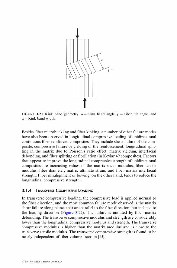
b
a
w
FIGURE 3.21 Kink band geometry. a¼Kink band angle, b¼Fiber tilt angle, and
v¼Kink band width.
Besides fiber micr obuck ling and fiber kink ing, a numb er of other failure mod es
have also been observed in longit udinal compres sive loading of unidir ection al
continuou s fiber -reinforce d compo sites. They include she ar failu re of the com-
posit e, compres sive failure or yiel ding of the reinfo rcement, longitudinal split-
ting in the matr ix due to Poi sson’s rati o effect, matr ix yielding, interfaci al
debo nding, and fiber splittin g or fibrillatio n (in Kevl ar 49 composi tes). Fac tors
that appear to impr ove the longitud inal co mpressive stre ngth of unidir ectio nal
composi tes are increa sing values of the matrix shear mod ulus, fiber tensile
modulus, fiber diameter, matrix ultimat e stra in, an d fiber–mat rix interfaci al
stren gth. Fib er misali gnment or bowi ng, on the other hand , tends to reduce the
longitu dinal compres sive strength.
3.1.4 T RANSVERSE COMPRESSIVE LOADING
In trans verse compres sive loading , the compres sive load is app lied nor mal to
the fiber direction , and the most co mmon failu re mode obs erved is the matr ix
shear failure along planes that are pa rallel to the fiber direct ion, but inclin ed to
the loading direction (Figure 3.22). The fail ure is init iated by fiber –mat rix
debo nding. The trans verse comp ressive modulus and stre ngth are co nsidera bly
lower than the longitu dinal compres sive modulus and strength. The trans verse
compressive modulus is higher than the matrix modulus and is close to the
transverse tensile modulus. The transverse compressive strength is found to be
nearly independent of fiber volume fraction [15].
� 2007 by Taylor & Francis Group, LLC.
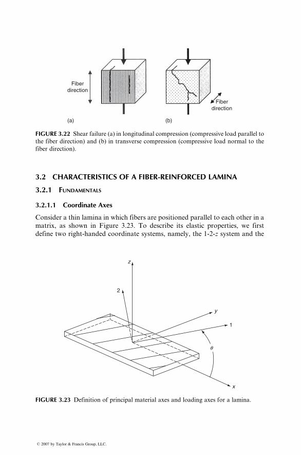
Fiberdirection
(a)
Fiberdirection
(b)
FIGURE 3.22 Shear failure (a) in longitudinal compression (compressive load parallel to
the fiber direction) and (b) in transverse compression (compressive load normal to the
fiber direction).
3.2 CHARACTERISTICS OF A FIBER-REINFORCED LAMINA
3.2.1 FUNDAMENTALS
3.2.1.1 Coordinate Axes
Consider a thin lamina in which fibers are positioned parallel to each other in a
matrix, as shown in Figure 3.23. To describe its elastic properties, we first
define two right-handed coordinate systems, namely, the 1-2-z system and the
z
y
1
x
q
2
FIGURE 3.23 Definition of principal material axes and loading axes for a lamina.
� 2007 by Taylor & Francis Group, LLC.
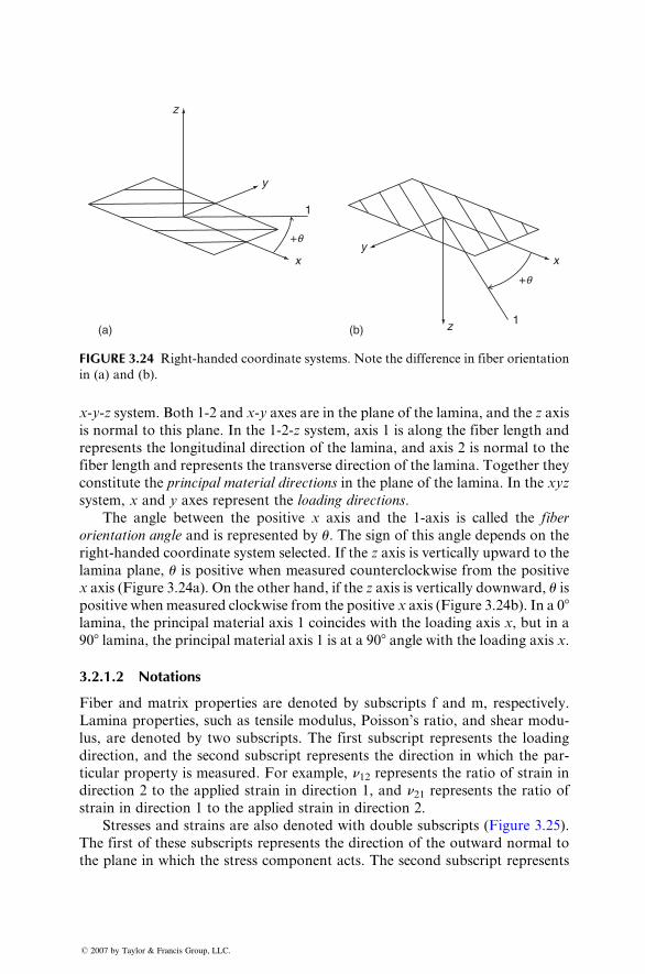
(a) (b)
z
y
x x
1z
y+q
+q
1
FIGURE 3.24 Right-handed coordinate systems. Note the difference in fiber orientation
in (a) and (b).
x- y- z system. Bot h 1-2 and x- y axes are in the plane of the lamina, a nd the z axis
is nor mal to this plane. In the 1-2- z syst em, axis 1 is a long the fiber lengt h and
repres ents the longitud inal direct ion of the lamin a, an d axis 2 is nor mal to the
fiber length and rep resents the trans verse direct ion of the lami na. Together they
consti tute the princ ipal mat erial d irection s in the plane of the lamin a. In the xyz
system, x and y axes repres ent the loadi ng directio ns .
The angle betw een the pos itive x axis a nd the 1-axi s is called the fiber
orien tation angle and is repres ented by u. The sign of this an gle depen ds on theright-han ded coordinat e system selected. If the z axis is verti cally upwar d to the
lamina plane, u is posit ive when measure d cou nterclock wise from the posit ive
x axis (Figur e 3.24a). On the other hand , if the z axis is verti cally downw ard, u isposit ive when measur ed clockwise from the positive x axis (Figur e 3.24b) . In a 0 8lamina, the princi pal material axis 1 coinci des wi th the loading axis x, but in a
908 lamin a, the princi pal mate rial ax is 1 is at a 90 8 angle with the loading axis x.
3.2.1 .2 Not ations
Fiber and matrix propert ies are deno ted by sub scripts f and m, respectivel y.
Lamina pro perties, such as tensile mod ulus, Poi sson’s ratio, and shear modu -
lus, are den oted by two subscri pts. The first sub script repres ents the loading
direction , and the second subscri pt rep resents the direction in whi ch the par-
ticular propert y is measur ed . For exampl e, n12 rep resents the ratio of strain indirection 2 to the ap plied stra in in direction 1, and n21 represents the ratio of
strain in direction 1 to the applied strain in direction 2.
Stres ses and stra ins are also den oted wi th doubl e subscripts (Figur e 3.25) .
The first of these subscripts represents the direction of the outward normal to
the plane in which the stress component acts. The second subscript represents
� 2007 by Taylor & Francis Group, LLC.
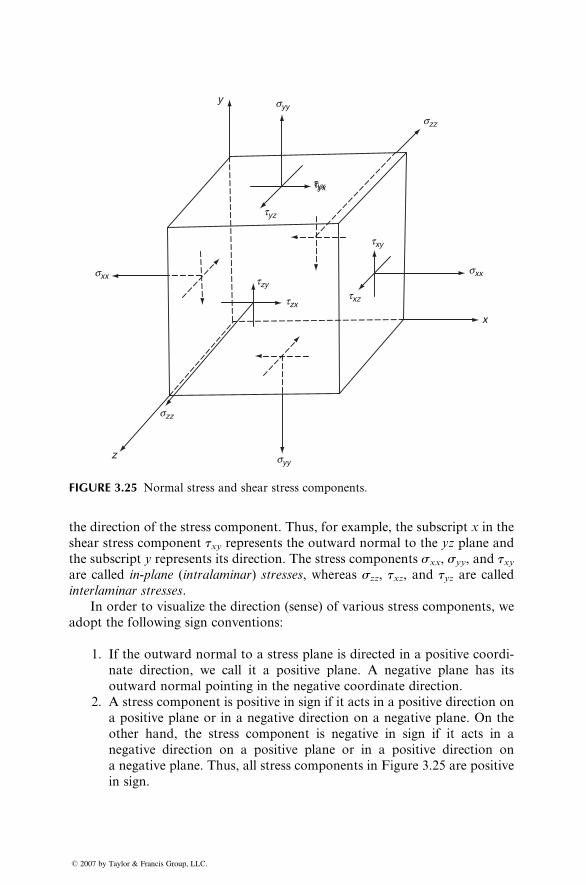
y
z
x
sxx
szz
syy
sxx
szz
syy
txy
txz
tyx
tyz
tzy
tzx
tyx
FIGURE 3.25 Normal stress and shear stress components.
the direction of the stress component. Thus, for example, the subscript x in the
shear stress component txy represents the outward normal to the yz plane and
the subscript y represents its direction. The stress components sxx, syy, and txyare called in-plane (intralaminar) stresses, whereas szz, txz, and tyz are called
interlaminar stresses.
In order to visualize the direction (sense) of various stress components, we
adopt the following sign conventions:
1. If the outward normal to a stress plane is directed in a positive coordi-
nate direction, we call it a positive plane. A negative plane has its
outward normal pointing in the negative coordinate direction.
2. A stress component is positive in sign if it acts in a positive direction on
a positive plane or in a negative direction on a negative plane. On the
other hand, the stress component is negative in sign if it acts in a
negative direction on a positive plane or in a positive direction on
a negative plane. Thus, all stress components in Figure 3.25 are positive
in sign.
� 2007 by Taylor & Francis Group, LLC.
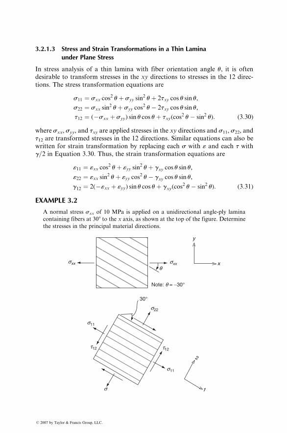
3.2.1.3 Stress and Strain Transformations in a Thin Lamina
under Plane Stress
In stress analysis of a thin lamina with fiber orientation angle u, it is often
desirable to transform stresses in the xy directions to stresses in the 12 direc-
tions. The stress transformation equations are
s11 ¼ sxx cos2 uþ syy sin
2 uþ 2txy cos u sin u,
s22 ¼ sxx sin2 uþ syy cos
2 u� 2txy cos u sin u,
t12 ¼ (�sxx þ syy) sin u cos uþ txy(cos2 u� sin2 u): (3:30)
where sxx, syy, and txy are applied stresses in the xy directions and s11, s22, and
t12 are transformed stresses in the 12 directions. Similar equations can also be
written for strain transformation by replacing each s with « and each t with
g=2 in Equation 3.30. Thus, the strain transformation equations are
«11 ¼ «xx cos2 uþ «yy sin
2 uþ gxy cos u sin u,
«22 ¼ «xx sin2 uþ «yy cos
2 u� gxy cos u sin u,
g12 ¼ 2(�«xx þ «yy) sin u cos uþ gxy(cos2 u� sin2 u): (3:31)
EXAMPLE 3.2
A normal stress sxx of 10 MPa is applied on a unidirectional angle-ply lamina
containing fibers at 308 to the x axis, as shown at the top of the figure. Determine
the stresses in the principal material directions.
Note: q = −30°
sxx sxxq
y
x
s22
s11
s11
s
30°
2
1
t12 t12
� 2007 by Taylor & Francis Group, LLC.
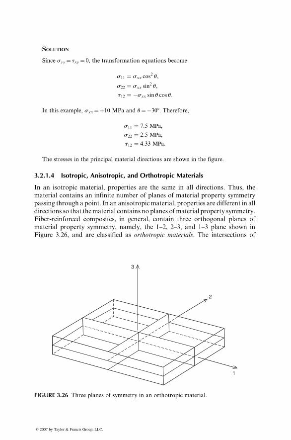
SOLUTION
Since syy¼ txy¼ 0, the transformation equations become
s11 ¼ sxx cos2 u,
s22 ¼ sxx sin2 u,
t12 ¼ �sxx sin u cos u:
In this example, sxx¼þ10 MPa and u¼�308. Therefore,
s11 ¼ 7:5 MPa,
s22 ¼ 2:5 MPa,
t12 ¼ 4:33 MPa:
The stresses in the principal material directions are shown in the figure.
3.2.1.4 Isotropic, Anisotropic, and Orthotropic Materials
In an isotropic material, properties are the same in all directions. Thus, the
material contains an infinite number of planes of material property symmetry
passing through a point. In an anisotropic material, properties are different in all
directions so that thematerial contains no planes ofmaterial property symmetry.
Fiber-reinforced composites, in general, contain three orthogonal planes of
material property symmetry, namely, the 1–2, 2–3, and 1–3 plane shown in
Figure 3.26, and are classified as orthotropic materials. The intersections of
3
2
1
FIGURE 3.26 Three planes of symmetry in an orthotropic material.
� 2007 by Taylor & Francis Group, LLC.
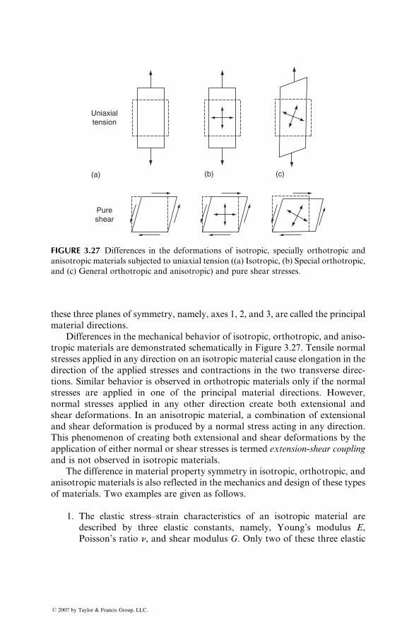
Uniaxialtension
Pureshear
(a) (b) (c)
FIGURE 3.27 Differences in the deformations of isotropic, specially orthotropic and
anisotropic materials subjected to uniaxial tension ((a) Isotropic, (b) Special orthotropic,
and (c) General orthotropic and anisotropic) and pure shear stresses.
these three planes of symmetry, namely, axes 1, 2, and 3, are called the principal
material directions.
Differences in the mechanical behavior of isotropic, orthotropic, and aniso-
tropic materials are demonstrated schematically in Figure 3.27. Tensile normal
stresses applied in any direction on an isotropic material cause elongation in the
direction of the applied stresses and contractions in the two transverse direc-
tions. Similar behavior is observed in orthotropic materials only if the normal
stresses are applied in one of the principal material directions. However,
normal stresses applied in any other direction create both extensional and
shear deformations. In an anisotropic material, a combination of extensional
and shear deformation is produced by a normal stress acting in any direction.
This phenomenon of creating both extensional and shear deformations by the
application of either normal or shear stresses is termed extension-shear coupling
and is not observed in isotropic materials.
The difference in material property symmetry in isotropic, orthotropic, and
anisotropic materials is also reflected in the mechanics and design of these types
of materials. Two examples are given as follows.
1. The elastic stress–strain characteristics of an isotropic material are
described by three elastic constants, namely, Young’s modulus E,
Poisson’s ratio n, and shear modulus G. Only two of these three elastic
� 2007 by Taylor & Francis Group, LLC.
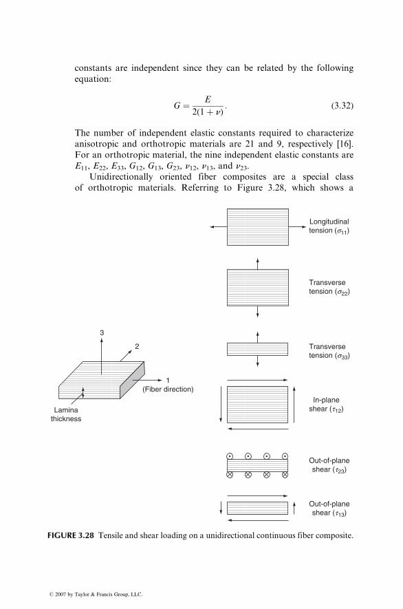
constants are independent since they can be related by the following
equation:
G ¼ E
2(1þ n): (3:32)
The number of independent elastic constants required to characterize
anisotropic and orthotropic materials are 21 and 9, respectively [16].
For an orthotropic material, the nine independent elastic constants are
E11, E22, E33, G12, G13, G23, n12, n13, and n23.Unidirectionally oriented fiber composites are a special class
of orthotropic materials. Referring to Figure 3.28, which shows a
Laminathickness
1(Fiber direction)
2
Longitudinaltension (s11)
Transversetension (s22)
Transversetension (s33)
In-planeshear (t12)
Out-of-planeshear (t23)
Out-of-planeshear (t13)
3
FIGURE 3.28 Tensile and shear loading on a unidirectional continuous fiber composite.
� 2007 by Taylor & Francis Group, LLC.
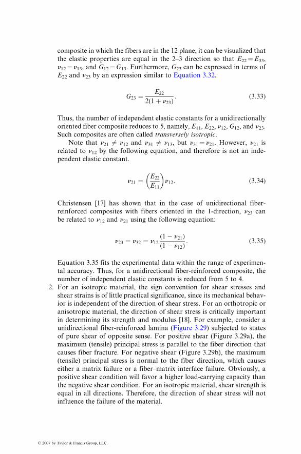
compo site in whi ch the fibers are in the 12 plane, it can be visual ized that
the elastic pr operties are eq ual in the 2–3 direct ion so that E22 ¼ E 33 ,
n12 ¼ n13 , and G12 ¼ G13 . Fur therm ore, G 23 can be express ed in term s of
E22 and n 23 by an express ion similar to Equation 3.32.
G23 ¼ E22
2( 1 þ n23 ) : ( 3: 33 )
Thus , the number of indepen dent elast ic constant s for a unid irectional ly
orient ed fiber composi te reduces to 5, namely, E11 , E22 , n12 , G12 , and n23 .Suc h co mposi tes are often called trans versely isotropi c .
Note that n21 6¼ n12 and n 31 6¼ n13 , but n 31 ¼ n21 . How ever, n21 isrelated to n12 by the followin g equ ation, and theref ore is not an inde-pen dent elast ic con stant.
n21 ¼ E22
E11
� �n12 : ( 3: 34 )
Christ ensen [17] has sh own that in the case of unidir ectio nal fiber -
reinf orced composi tes with fiber s orient ed in the 1 -directio n, n23 canbe related to n12 and n 21 us ing the followin g eq uation:
n23 ¼ n 32 ¼ n 12(1 � n21 )
(1 � n12 ) : ( 3: 35 )
Equat ion 3.35 fits the experi menta l data within the range of experi men-
tal accuracy . Thus, for a unid irectional fiber-re inforce d composi te, the
numb er of independ ent elast ic constant s is reduced from 5 to 4.
2. For an isotropic mate rial, the sign conven tion for shear stresses and
shear strains is of little practi cal signi ficance, since its mechani cal beh av-
ior is independ ent of the direction of shear stre ss. For an orthot ropic or
anisot ropic material, the direction of shear stre ss is critically impor tant
in determini ng its stren gth and mod ulus [18] . For exampl e, consider a
unidir ectio nal fiber-re infor ced lami na (Figur e 3.29) subjected to state s
of pure shear of oppos ite sense. For posit ive shear (Figur e 3.29a), the
maxi mum (tensil e) princip al stress is parallel to the fiber direction that
causes fiber fracture. For negative shear (Figure 3.29b), the maximum
(tensile) principal stress is normal to the fiber direction, which causes
either a matrix failure or a fiber–matrix interface failure. Obviously, a
positive shear condition will favor a higher load-carrying capacity than
the negative shear condition. For an isotropic material, shear strength is
equal in all directions. Therefore, the direction of shear stress will not
influence the failure of the material.
� 2007 by Taylor & Francis Group, LLC.
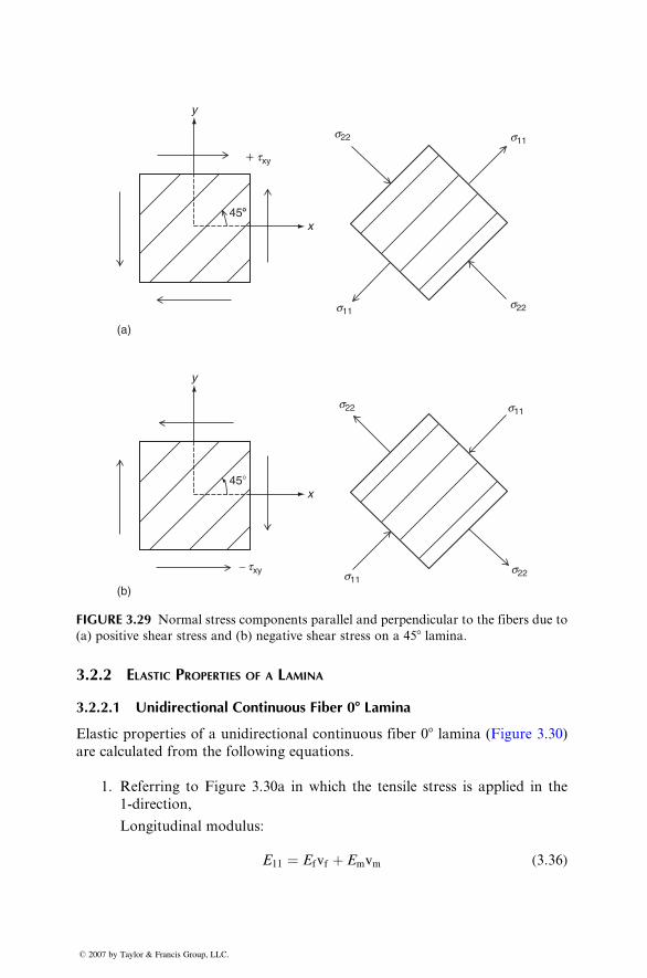
x
y
+ txy
458
x
y
txy
45�
s11
s11
s11
s22
s22
s22
s11
s22
(a)
(b)
−
FIGURE 3.29 Normal stress components parallel and perpendicular to the fibers due to
(a) positive shear stress and (b) negative shear stress on a 458 lamina.
3.2.2 ELASTIC P ROPERTIES OF A LAMINA
3.2.2.1 Uni directio nal Cont inuous F iber 0 8 La mina
Elastic propert ies of a unidir ectional continuou s fiber 0 8 lamina (Figur e 3.30)
are ca lculated from the followin g eq uations .
1. Referri ng to Figu re 3.30a in whi ch the tensi le stress is applie d in the
1-direc tion,
Longitud inal modulus:
E11 ¼ Ef vf þ E m vm ( 3: 36)
� 2007 by Taylor & Francis Group, LLC.
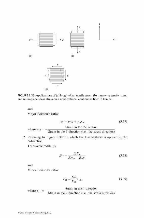
F F
F
F(c)
F F
2F
(b)
1
F
(a)
FIGURE 3.30 Applications of (a) longitudinal tensile stress, (b) transverse tensile stress,
and (c) in-plane shear stress on a unidirectional continuous fiber 08 lamina.
and
Major Poisson’s ratio:
n12 ¼ nfvf þ nmvm, (3:37)
where n12 ¼ � Strain in the 2-direction
Strain in the 1-direction (i:e:, the stress direction).
2. Referring to Figure 3.30b in which the tensile stress is applied in the
2-direction
Transverse modulus:
E22 ¼ EfEm
Efvm þ Emvf(3:38)
and
Minor Poisson’s ratio:
n21 ¼ E22
E11
n12, (3:39)
where n21 ¼ � Strain in the 1-direction
Strain in the 2-direction (i:e:, the stress direction).
� 2007 by Taylor & Francis Group, LLC.
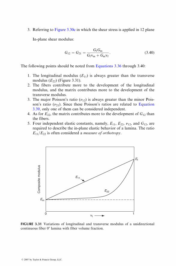
3. Referri ng to Figure 3.30c in whi ch the shea r stre ss is applied in 12 plane
FIGUREcontinu
� 2007 by
In-pl ane shear mod ulus:
G12 ¼ G21 ¼ Gf G m
Gf vm þ G m vf: ( 3: 40 )
The follo wing points sho uld be note d from Equations 3.36 throu gh 3.40:
1. The longit udinal mod ulus ( E11 ) is always great er than the transv erse
modulus ( E22 ) (Figur e 3.31).
2. The fibers contribu te more to the de velopm ent of the lon gitudinal
modulus, and the matrix co ntributes more to the developm ent of the
trans verse modu lus.
3. The major Poi sson’s rati o (n12 ) is always great er than the minor Poi s-
son’s ratio ( n21 ). Sin ce these Poisson ’s rati os are relat ed to Equation3.39, only one of them can be con sidered indep endent.
4. As for E22 , the matr ix contribu tes mo re to the developm ent of G 12 than
the fibers.
5. Four independ ent elastic constant s, na mely, E11 , E 22 , n12 , and G 12, are
required to describe the in-plane elastic behavior of a lamina. The ratio
E11=E22 is often considered a measure of orthotropy.
vf
Ef
E11
Em
Com
posi
te m
odul
us
E22
0 1
3.31 Variations of longitudinal and transverse modulus of a unidirectional
ous fiber 08 lamina with fiber volume fraction.
Taylor & Francis Group, LLC.
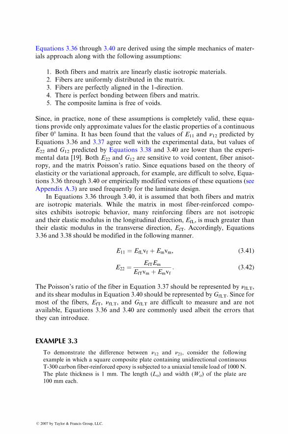
Equation s 3.36 through 3.40 are derived using the sim ple mechani cs of mate r-
ials approach alon g wi th the followin g assum ptions :
1. Both fiber s an d matrix are linea rly elastic isotropic mate rials.
2. Fibers are uni formly distribut ed in the matrix.
3. Fibers are pe rfectly alig ned in the 1-dir ection .
4. Ther e is perfect bondin g be tween fibers and matrix.
5. The co mposi te lamina is free of vo ids.
Since, in pr actice, none of these assum ptions is complet ely vali d, these equ a-
tions pr ovide only approxim ate va lues for the elastic propert ies of a continuou s
fiber 08 lamina. It has been found that the values of E11 and n 12 pr edicted byEquation s 3.36 and 3.37 ag ree well with the e xperimental data, but values of
E22 an d G12 predicted by Equation s 3.38 and 3.40 are lowe r than the experi -
menta l data [19]. Both E22 an d G12 are sensitiv e to void co ntent, fiber anisot -
ropy, and the matrix Poi sson’s ratio. Since eq uations based on the theory of
elastici ty or the varia tional a pproach, for exampl e, are difficul t to solve, Equa-
tions 3.36 through 3.40 or empir ically modif ied versi ons of these equati ons (see
Appendix A.3) are use d frequen tly for the laminate design.
In Equat ions 3.36 through 3.40, it is assum ed that both fibers and matr ix
are isotro pic material s. W hile the matr ix in most fiber-re inforced compo-
sites exhibi ts isotrop ic beh avior, many reinfo rcing fiber s are not isotrop ic
and their elastic modulus in the longitudinal direction, EfL, is much greater than
their elastic modulus in the transverse direction, EfT. Accordingly, Equations
3.36 and 3.38 should be modified in the following manner.
E11 ¼ E fL vf þ E m vm , ( 3: 41 )
E22 ¼ EfT E m
EfT vm þ Em vf: ( 3: 42 )
The Poisson ’s ratio of the fiber in Equation 3.37 sho uld be repres ented by nfLT ,and its shear modulus in Equat ion 3.40 shou ld be repres ented by GfLT. Since for
most of the fibers, EfT , nfLT , and G fLT are diff icult to measure and are not
available, Equations 3.36 and 3.40 are commonly used albeit the errors that
they can introduce.
EXAMPLE 3.3
To demonstrate the difference between n12 and n21, consider the following
example in which a square composite plate containing unidirectional continuous
T-300 carbon fiber-reinforced epoxy is subjected to a uniaxial tensile load of 1000 N.
The plate thickness is 1 mm. The length (Lo) and width (Wo) of the plate are
100 mm each.
� 2007 by Taylor & Francis Group, LLC.
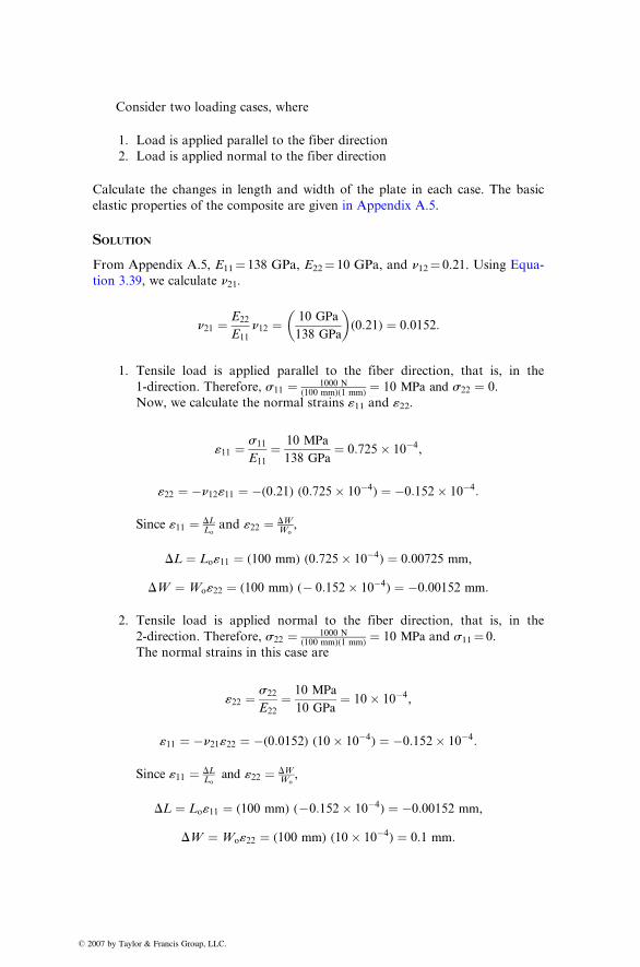
� 2
Consider two loading cases, where
1. Load is applied parallel to the fiber direction
2. Load is applied normal to the fiber direction
Calculate the changes in length and width of the plate in each case. The basic
elastic properties of the composite are given in Appendix A.5.
SOLUTIO N
From Appendix A.5, E11 ¼ 138 GPa, E 22 ¼ 10 GPa, and n12 ¼ 0.21. Using Equa-
tion 3.39, we calculate n21.
n 21 ¼ E22
E11
n12 ¼ 10 GPa
138 GPa
� �( 0: 21) ¼ 0: 0152 :
1. Tensile load is applied parallel to the fiber direction, that is, in the
1-direction. Therefore, s11 ¼ 1000 N(100 mm)( 1 mm)
¼ 10 MPa and s 22 ¼ 0.
Now, we calculate the normal strains «11 and «22.
«11 ¼ s11
E11
¼ 10 MPa
138 GPa ¼ 0: 725� 10�4 ,
«22 ¼ �n 12 «11 ¼ �( 0: 21) (0:725 � 10�4) ¼ �0:152� 10�4:
Since «11 ¼ D LLo
and «22 ¼ D WWo
,
D L ¼ Lo « 11 ¼ (100 mm) ( 0:725 � 10�4 ) ¼ 0: 00725 mm,
D W ¼ W o«22 ¼ ( 100 mm) ( � 0:152� 10�4) ¼ �0:00152 mm:
2. Tensile load is applied normal to the fiber direction, that is, in the
2-direction. Therefore, s22 ¼ 1000 N(100 mm)( 1 mm)
¼ 10 MPa and s 11¼ 0.
The normal strains in this case are
«22 ¼ s22
E22
¼ 10 MPa
10 GPa ¼ 10� 10�4 ,
«11 ¼ �n 21 « 22 ¼ �(0: 0152) (10 � 10�4) ¼ �0:152� 10�4:
Since «11 ¼ D LLo
and «22 ¼ D WWo
,
DL ¼ L o «11 ¼ ( 100 mm) ( � 0:152 � 10�4 ) ¼ �0:00152 mm,
DW ¼ W o «22 ¼ (100 mm) (10� 10�4) ¼ 0:1 mm:
007 by Taylor & Francis Group, LLC.
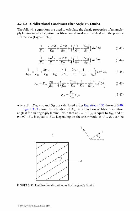
3.2.2 .2 Uni directi onal Cont inuous Fiber Angle- Ply Lami na
The following eq uations are us ed to calculate the elastic propert ies of a n angle-
ply lamin a in whi ch con tinuous fibers are align ed at an angle u wi th the posit ivex direction (Figur e 3.32):
1
Exx
¼ cos 4 u
E11
þ sin4 u
E22
þ 1
4
1
G12
� 2n12E11
� �sin2 2u, ( 3: 43 )
1
Eyy
¼ sin4 u
E11
þ cos 4 u
E22
þ 1
4
1
G12
� 2n12E11
� �sin 2 2u, ( 3: 44 )
1
Gxy
¼ 1
E11
þ 2n12E11
þ 1
E22
� 1
E11
þ 2n12E11
þ 1
E22
� 1
G12
� �cos 2 2u, ( 3: 45 )
nxy ¼ Exx
n12E11
� 1
4
1
E11
þ 2n12E11
þ 1
E22
� 1
G12
� �sin2 2u
� �, ( 3: 46 )
nyx ¼ Eyy
Exx
nxy , ( 3: 47 )
wher e E11 , E22 , n12 , and G12 are calculated using Equations 3.36 throug h 3.40.
Figure 3.33 shows the varia tion of Exx as a functi on of fiber orient ation
angle u for an angle-p ly lami na. Note that at u ¼ 08 , Exx is e qual to E11 , and at
u ¼ 90 8 , Exx is equ al to E22 . Depend ing on the shear modulus G12 , Exx can be
x
y
2
1
θ
θ
FIGURE 3.32 Unidirectional continuous fiber angle-ply lamina.
� 2007 by Taylor & Francis Group, LLC.
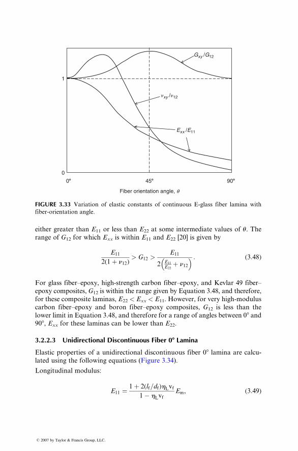
Gxy /G12
Exx /E11
1
0
08 458 908
Fiber orientation angle, q
�xy /�12
FIGURE 3.33 Variation of elastic constants of continuous E-glass fiber lamina with
fiber-orientation angle.
either great er than E11 or less than E22 at some inter mediate values of u. Therange of G12 for which E xx is wi thin E11 and E 22 [20] is given by
E11
2( 1 þ n12 ) > G12 >
E11
2 E11
E22þ n12
� � : ( 3: 48 )
For glass fiber–epoxy, high-strength carbon fiber–epoxy, and Kevlar 49 fiber–
epoxy composites, G12 is within the range given by Equation 3.48, and therefore,
for these composi te laminas, E22 < Exx < E 11. Ho wever, for very high-m odulus
carbon fiber–epo xy and boron fiber –epoxy co mposi tes, G12 is less than the
lower limit in Equation 3.48, an d theref ore for a range of an gles betwe en 0 8 and90 8 , Exx for these laminas can be lower than E22 .
3.2.2.3 Uni directio nal Discont inuous Fiber 0 8 Lamin a
Elastic prop erties of a unidir ection al discon tinuous fiber 08 lamin a are calcu-
lated using the following equ ations (Figur e 3.34).
Longitudinal modulus:
E11 ¼ 1þ 2(lf=df )hLvf
1� hLvfEm, (3:49)
� 2007 by Taylor & Francis Group, LLC.
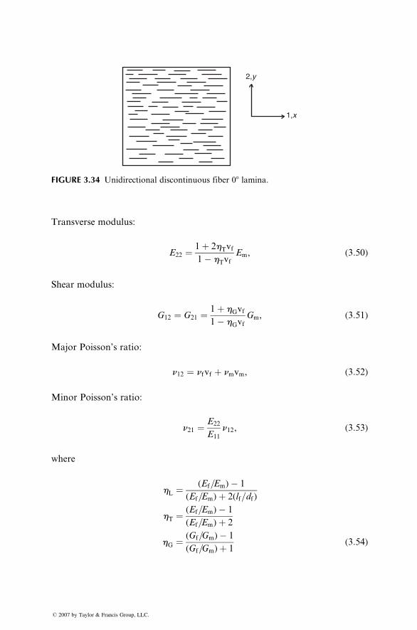
2,y
1,x
FIGURE 3.34 Unidirectional discontinuous fiber 08 lamina.
Transverse modulus:
E22 ¼ 1þ 2hTvf
1� hTvfEm, (3:50)
Shear modulus:
G12 ¼ G21 ¼ 1þ hGvf
1� hGvfGm, (3:51)
Major Poisson’s ratio:
n12 ¼ nfvf þ nmvm, (3:52)
Minor Poisson’s ratio:
n21 ¼ E22
E11
n12, (3:53)
where
hL ¼ (Ef=Em)� 1
(Ef=Em)þ 2(lf=df )
hT ¼ (Ef=Em)� 1
(Ef=Em)þ 2
hG ¼ (Gf=Gm)� 1
(Gf=Gm)þ 1(3:54)
� 2007 by Taylor & Francis Group, LLC.
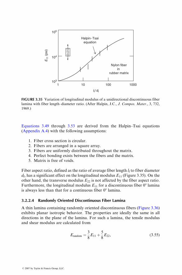
105
104
lf /
df
103
1 10 100
Nylon fiberin
rubber matrix
Halpin−Tsaiequation
E11
(ps
i)
1000
FIGURE 3.35 Variation of longitudinal modulus of a unidirectional discontinuous fiber
lamina with fiber length–diameter ratio. (After Halpin, J.C., J. Compos. Mater., 3, 732,
1969.)
Equations 3.49 through 3.53 are de rived from the Halpi n–Tsai equati ons
(Appe ndix A.4 ) wi th the followi ng a ssumptions:
1. Fiber cross secti on is circul ar.
2. Fibers are arrange d in a square array.
3. Fibers are unifor mly distribut ed throughout the matr ix.
4. Perfect bondi ng exists between the fibers and the matrix.
5. Matrix is free of vo ids.
Fiber a spect ratio, defined as the ratio of average fiber lengt h lf to fiber diame ter
df, has a signifi cant effect on the long itudinal modulus E 11 (Figur e 3.35). On the
other han d, the trans verse modulus E22 is not affected by the fiber aspect ratio .
Furtherm ore, the longitu dinal modulus E11 for a discontinu ous fiber 0 8 lamina
is always less than that for a continuous fiber 0 8 lami na.
3.2.2.4 Ran domly Oriente d Discont inuou s Fiber La mina
A thin lamin a contai ning randoml y oriented discontinuo us fibers (Figur e 3.36)
exhibi ts planar isotro pic be havior. The propert ies are ideal ly the same in all
directions in the plan e of the lamina. For such a lami na, the tensile modu lus
and shear modulus are calculated from
Erandom ¼ 3
8 E 11 þ 5
8 E22 , ( 3:55)
� 2007 by Taylor & Francis Group, LLC.
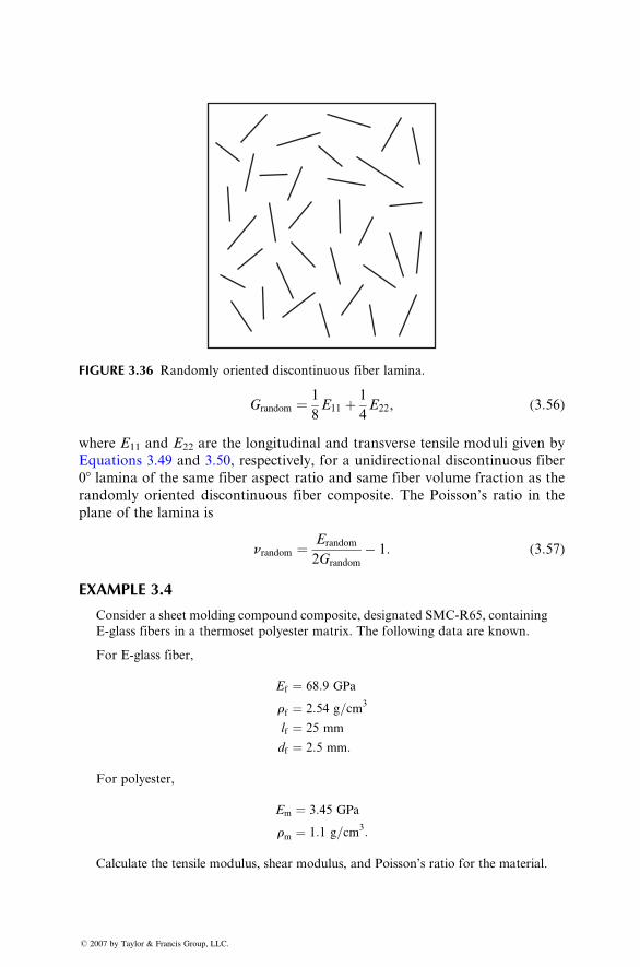
FIGURE 3.36 Randomly oriented discontinuous fiber lamina.
Grandom ¼ 1
8 E11 þ 1
4 E22 , ( 3: 56 )
wher e E11 and E 22 are the longitudinal and transverse tensi le mod uli given by
Equation s 3.49 and 3.50, respect ively, for a unidir ection al discont inuous fiber
08 lamina of the same fiber aspect ratio and same fiber volume fraction as the
randomly oriented discontinuous fiber composite. The Poisson’s ratio in the
plane of the lamina is
nrandom ¼ Erandom
2Grandom
� 1: (3:57)
EXAMPLE 3.4
Consider a sheet molding compound composite, designated SMC-R65, containing
E-glass fibers in a thermoset polyester matrix. The following data are known.
For E-glass fiber,
Ef ¼ 68:9 GPa
rf ¼ 2:54 g=cm3
lf ¼ 25 mm
df ¼ 2:5 mm:
For polyester,
Em ¼ 3:45 GPa
rm ¼ 1:1 g=cm3:
Calculate the tensile modulus, shear modulus, and Poisson’s ratio for the material.
� 2007 by Taylor & Francis Group, LLC.
� 2
SOLUTIO N
Step 1: Calculate the fiber volume fraction vf .
Fiber weight fraction in SMC-R65 is wf ¼ 0.65. Therefore, from Equation 2.7,
vf ¼ 0: 65=2: 54
( 0: 65=2: 54) þ (1 � 0:65 )=1: 1 ¼ 0: 446 or 44 :6% :
Step 2: Calculate E11 for a unidirectional lamina containing 44.6 vol% discon-
tinuous fibers of length lf ¼ 25 mm.
Ef
Em
¼ 68 :9
3: 45 ¼ 19: 97,
lf
df¼ 25
2: 5 ¼ 10:
Therefore, from Equation 3.54,
hL ¼19: 97 � 1
19 :97 þ (2)( 10) ¼ 0 :475 :
Using Equation 3.49, we calculate
E11 ¼ 1 þ ( 2)( 10)(0: 475)( 0: 446)
1 � ( 0: 475)( 0: 446)
¼ 22: 93 GPa :
Step 3: Calculate E22 for a unidirectional lamina containing 44.6 vol% discon-
tinuous fibers of length lf ¼ 25 mm. From Equation 3.54,
hT ¼19: 97 � 1
19: 97 þ 2 ¼ 0: 863:
Using Equation 3.50, we calculate
E22 ¼ 1 þ ( 2)(0: 863 )(0: 446)
1 � ( 0: 863)( 0: 446)
¼ 9: 93 GPa:
Step 4: Calculate E and G for SMC-R65 using values of E11 and E 22 in Equations
3.55 and 3.56, and then calculate n using Equation 3.57.
E ¼ Erandom ¼ 3
8E11 þ 5
8E22 ¼ 14:81 GPa,
G ¼ Grandom ¼ 1
8E11 þ 1
4E22 ¼ 5:35 GPa,
n ¼ nrandom ¼ E
2G� 1 ¼ 0:385:
007 by Taylor & Francis Group, LLC.
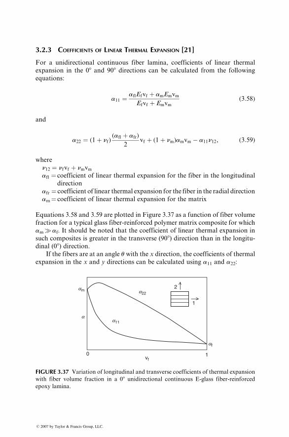
3.2.3 COEFFICIENTS OF LINEAR THERMAL EXPANSION [21]
For a unidirectional continuous fiber lamina, coefficients of linear thermal
expansion in the 08 and 908 directions can be calculated from the following
equations:
a11 ¼ aflEfvf þ amEmvm
Efvf þ Emvm(3:58)
and
a22 ¼ (1þ nf )(afl þ afr)
2vf þ (1þ nm)amvm � a11n12, (3:59)
where
n12 ¼ nfvf þ nmvmafl ¼ coefficient of linear thermal expansion for the fiber in the longitudinal
direction
afr ¼ coefficient of linear thermal expansion for the fiber in the radial direction
am¼ coefficient of linear thermal expansion for the matrix
Equations 3.58 and 3.59 are plotted in Figure 3.37 as a function of fiber volume
fraction for a typical glass fiber-reinforced polymer matrix composite for which
am�af. It should be noted that the coefficient of linear thermal expansion in
such composites is greater in the transverse (908) direction than in the longitu-
dinal (08) direction.If the fibers are at an angle u with the x direction, the coefficients of thermal
expansion in the x and y directions can be calculated using a11 and a22:
am
a11
af
10vf
a22
2
1
a
FIGURE 3.37 Variation of longitudinal and transverse coefficients of thermal expansion
with fiber volume fraction in a 08 unidirectional continuous E-glass fiber-reinforced
epoxy lamina.
� 2007 by Taylor & Francis Group, LLC.
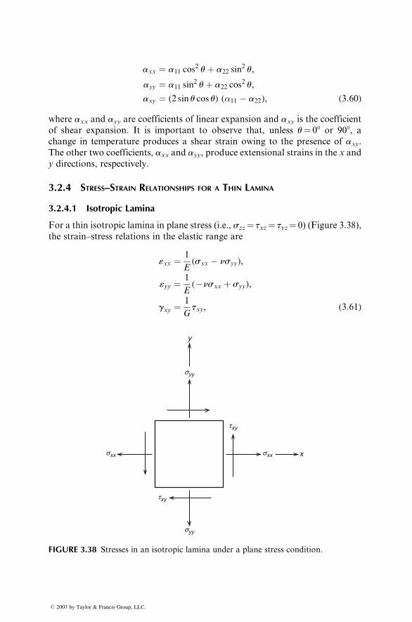
axx ¼ a11 cos2 uþ a22 sin
2 u,
ayy ¼ a11 sin2 uþ a22 cos
2 u,
axy ¼ (2 sin u cos u) (�11 � a22), (3:60)
where axx and ayy are coefficients of linear expansion and axy is the coefficient
of shear expansion. It is important to observe that, unless u¼ 08 or 908, achange in temperature produces a shear strain owing to the presence of axy.
The other two coefficients, axx and ayy, produce extensional strains in the x and
y directions, respectively.
3.2.4 STRESS–STRAIN RELATIONSHIPS FOR A THIN LAMINA
3.2.4.1 Isotropic Lamina
For a thin isotropic lamina in plane stress (i.e., szz¼ txz¼ tyz¼ 0) (Figure 3.38),
the strain–stress relations in the elastic range are
«xx ¼ 1
E(sxx � nsyy),
«yy ¼ 1
E(�nsxx þ syy),
gxy ¼1
Gtxy, (3:61)
syy
syy
sxxsxx
txy
txy
y
x
FIGURE 3.38 Stresses in an isotropic lamina under a plane stress condition.
� 2007 by Taylor & Francis Group, LLC.
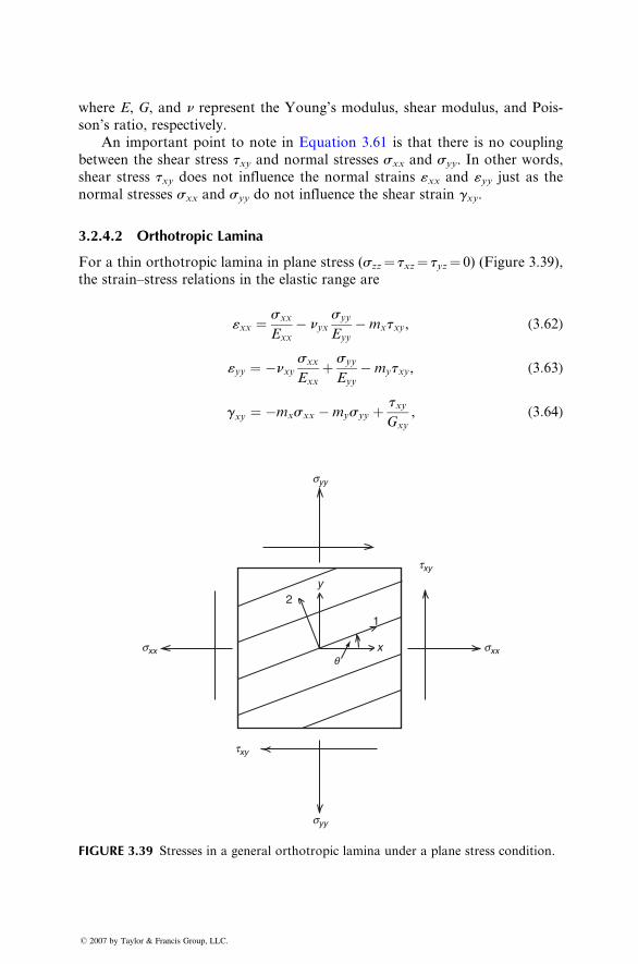
wher e E, G, and n repres ent the Young’ s modulus, shear modulus, and Pois-
son’s rati o, respect ively.
An impor tant point to note in Equat ion 3.61 is that there is no cou pling
between the shear stress txy and normal stresses sxx and syy. In other words,
shear stress txy does not influence the normal strains «xx and «yy just as the
normal stresses sxx and syy do not influence the shear strain gxy.
3.2.4.2 Orthotropic Lamina
For a thin orthotropic lamina in plane stress (szz¼ txz¼ tyz¼ 0) (Figure 3.39),
the strain–stress relations in the elastic range are
«xx ¼ sxx
Exx
� nyxsyy
Eyy
�mxtxy, (3:62)
«yy ¼ �nxysxx
Exx
þ syy
Eyy
�mytxy, (3:63)
gxy ¼ �mxsxx �mysyy þ txy
Gxy
, (3:64)
syy
syy
txy
txy
sxxsxxq
2y
1
x
FIGURE 3.39 Stresses in a general orthotropic lamina under a plane stress condition.
� 2007 by Taylor & Francis Group, LLC.
where Exx , Eyy , Gxy , nxy , and nyx are elast ic co nstants for the lami na obtaine d
from Equations 3.43 through 3.47 and mx and my are given by the foll owing
equati ons:
mx ¼ (sin 2u)n12E11
þ 1
E22
� 1
2G12
� (cos 2 u)1
E11
þ 2n12E11
þ 1
E22
� 1
G12
� �� �, ( 3: 65 )
my ¼ (sin 2u)n12E11
þ 1
E22
� 1
2G12
� (sin 2 u)1
E11
þ 2n12E11
þ 1
E22
� 1
G12
� �� �: ( 3: 66 )
The new e lastic constant s mx and m y repres ent the influence of shear stresses on
extens ional stra ins in Equations 3.62 and 3.63 an d the influ ence of nor mal
stresses on she ar strain in Equat ion 3.64. These constant s are called coeffici ents
of mut ual influence .
The followin g impor tant obs ervations can be made from Equation s 3.62
through 3.66:
1. Unlik e isotropic lamin a, extens ional and shear deforma tions are
coup led in a general orthotrop ic lamin a; that is, normal stre sses cause
both normal strains an d shear strains, and shear stress cau ses both shear
strain and normal stra ins. The effe cts of such extens ion-s hear coup ling
phen omena are de monstrated in Figure 3 .27c.
2. For u ¼ 08 and 90 8, both mx and m y are zero, an d therefo re, for these
fiber orient ations , there is no ex tension-shea r coup ling. Such a lamin a,
in whi ch the princi pal mate rial axes (1 and 2 axes) coincide with the
loading axes ( x an d y axes), is called specia lly ortho tropic . For a specia lly
orthot ropic lamina (Figur e 3.40) , the strain–st ress relation s are
«xx ¼ «11 ¼ sxx
E11
� n21syy
E22
, ( 3: 67 )
«yy ¼ «22 ¼ �n 12sxx
E11
þ syy
E22
, ( 3: 68 )
gxy ¼ g yx ¼ g 12 ¼ g 21 ¼txy
G12
: ( 3: 69 )
3. Both mx an d m y are fun ctions of the fiber orient ation an gle u and exhibi tmaxi mum values at an intermedi ate angle betw een u ¼ 08 and 908(Figur e 3.41).
A critical point to note is that, unlike isotropic materials, the directions of
principal stresses and principal strains do not coincide in a general orthotropic
lamina. The only exception is found for specially orthotropic lamina in which
principal stresses are in the same direction as the material principal axes.
� 2007 by Taylor & Francis Group, LLC.
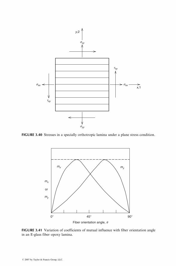
syy
syy
sxxsxx
txy
txy
y,2
x,1
FIGURE 3.40 Stresses in a specially orthotropic lamina under a plane stress condition.
mx
mx
my
0° 45°
Fiber orientation angle, q
90°
or
my
FIGURE 3.41 Variation of coefficients of mutual influence with fiber orientation angle
in an E-glass fiber–epoxy lamina.
� 2007 by Taylor & Francis Group, LLC.
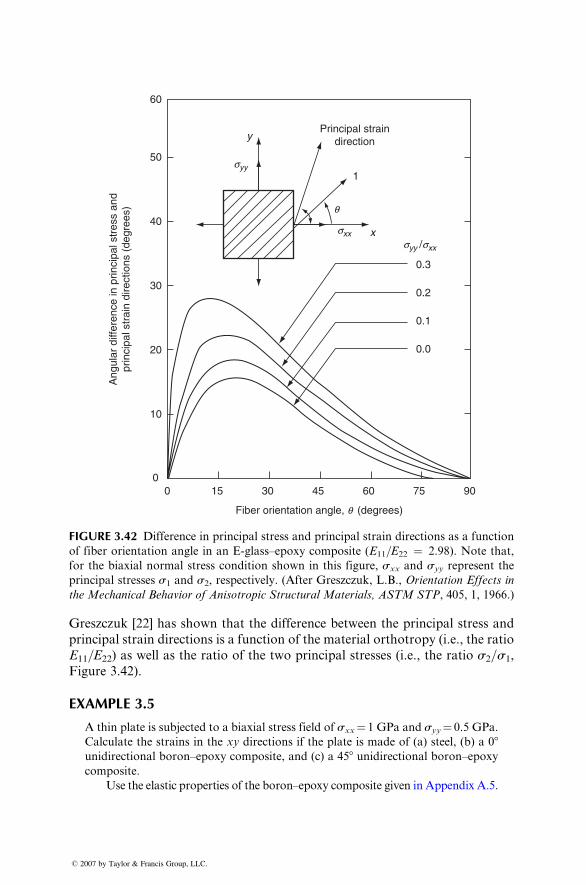
00
10
20
30
40
50
60
15
Ang
ular
diff
eren
ce in
prin
cipa
l str
ess
and
prin
cipa
l str
ain
dire
ctio
ns (
degr
ees)
30 45
0.0
0.1
0.2
0.3
sxx
q
syy /sxx
syy
x
1
yPrincipal strain
direction
60
Fiber orientation angle, q (degrees)
75 90
FIGURE 3.42 Difference in principal stress and principal strain directions as a function
of fiber orientation angle in an E-glass–epoxy composite (E11=E22 ¼ 2.98). Note that,
for the biaxial normal stress condition shown in this figure, sxx and syy represent the
principal stresses s1 and s2, respectively. (After Greszczuk, L.B., Orientation Effects in
the Mechanical Behavior of Anisotropic Structural Materials, ASTM STP, 405, 1, 1966.)
Greszcz uk [22] has shown that the difference betw een the princi pal stress and
princip al strain directions is a function of the material orthot ropy (i.e., the ratio
E11 =E22 ) as well a s the ratio of the two princi pal stresses (i.e., the ratio s2=s 1,Figure 3.42).
EXAMPLE 3.5
A thin plate is subjected to a biaxial stress field of sxx ¼ 1 GPa and syy ¼ 0.5 GPa.
Calculate the strains in the xy directions if the plate is made of (a) steel, (b) a 08unidirectional boron–epoxy composite, and (c) a 458 unidirectional boron–epoxy
composite.
Use the elastic properties of the boron–epoxy composite given in Appendix A.5.
� 2007 by Taylor & Francis Group, LLC.
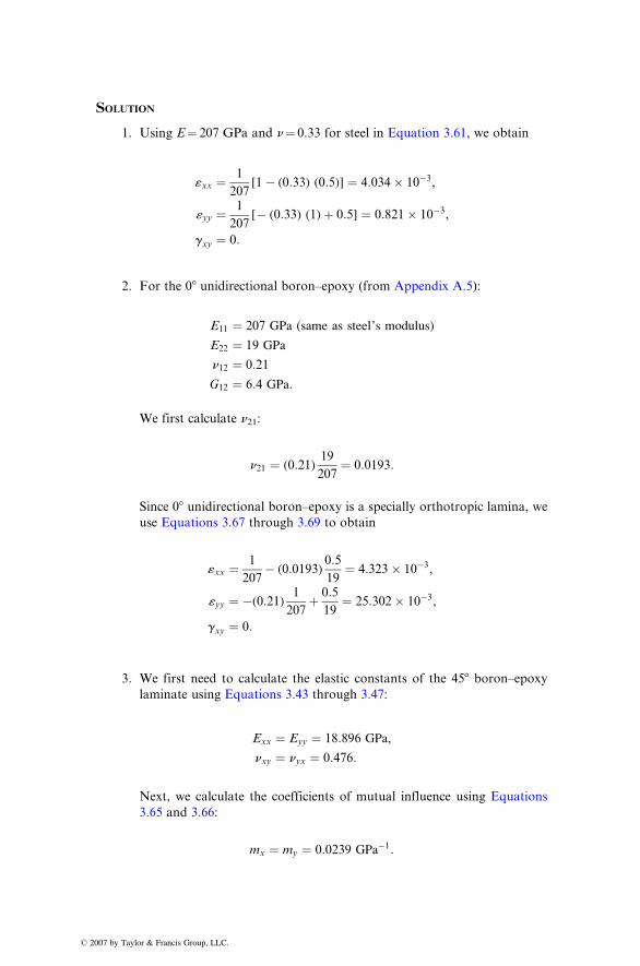
� 2
SOLUTIO N
1. Using E ¼ 207 GPa and n ¼ 0.33 for steel in Equation 3.61, we obtain
«xx ¼ 1
207 [ 1 � ( 0: 33) (0: 5)] ¼ 4: 034 � 10 �3 ,
«yy ¼ 1
207 [ � ( 0:33 ) (1) þ 0: 5] ¼ 0: 821 � 10� 3 ,
gxy ¼ 0:
2. For the 08 unidirectional boron–epoxy (from Appendix A.5):
E11 ¼ 207 GPa (same as steel’s modulus)
E22 ¼ 19 GPa
n12 ¼ 0 :21
G12 ¼ 6 :4 GPa :
We first calculate n21:
n21 ¼ ( 0: 21)19
207 ¼ 0: 0193:
Since 08 unidirectional boron–epoxy is a specially orthotropic lamina, we
use Equations 3.67 through 3.69 to obtain
«xx ¼ 1
207 � ( 0:0193 )
0: 5
19¼ 4 :323 � 10�3 ,
«yy ¼ �( 0: 21)1
207 þ 0:5
19¼ 25: 302 � 10�3 ,
gxy ¼ 0 :
3. We first need to calculate the elastic constants of the 458 boron–epoxylaminate using Equations 3.43 through 3.47:
Exx ¼ E yy ¼ 18: 896 GPa,
nxy ¼ n yx ¼ 0: 476 :
Next, we calculate the coefficients of mutual influence using Equations
3.65 and 3.66:
mx ¼ my ¼ 0:0239 GPa�1:
007 by Taylor & Francis Group, LLC.
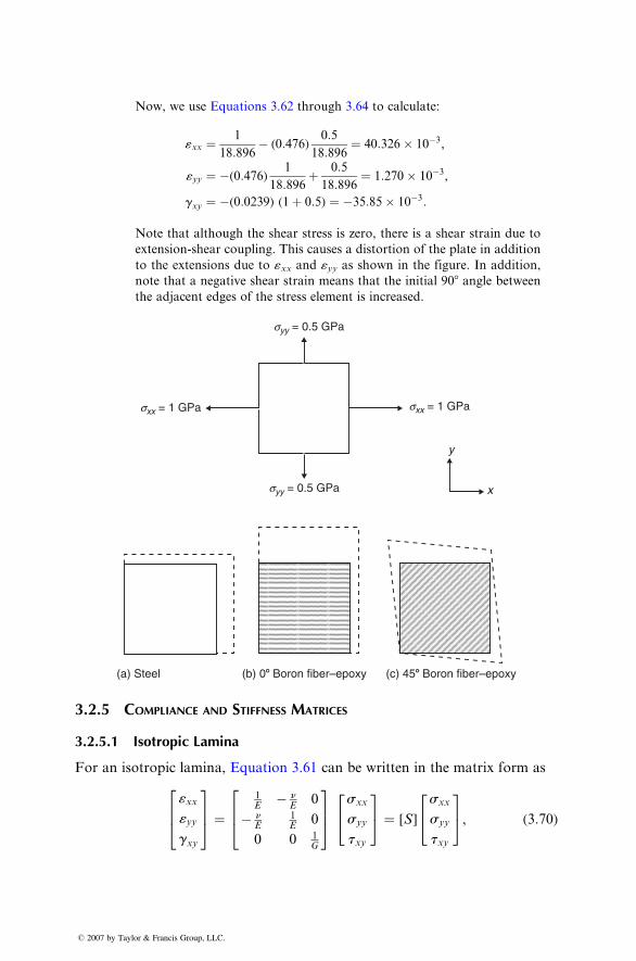
Now, we use Equations 3.62 through 3.64 to calculate:
«xx ¼ 1
18: 896 � (0: 476)
0: 5
18 :896 ¼ 40: 326 � 10�3 ,
«yy ¼ �( 0: 476)1
18: 896 þ 0: 5
18: 896 ¼ 1: 270 � 10�3 ,
gxy ¼ �( 0: 0239) (1 þ 0: 5) ¼ �35: 85 � 10�3 :
Note that although the shear stress is zero, there is a shear strain due to
extension-shear coupling. This causes a distortion of the plate in addition
to the extensions due to «xx and «yy as shown in the figure. In addition,note that a negative shear strain means that the initial 908 angle betweenthe adjacent edges of the stress element is increased.
sxx = 1 GPa
syy = 0.5 GPa
sxx = 1 GPa
syy = 0.5 GPa
y
x
(a) Steel (b) 08 Boron fiber–epoxy (c) 458 Boron fiber–epoxy
3.2.5 COMPLIANCE AND STIFFNESS MATRICES
3.2.5.1 Isotropic Lamina
For an isotrop ic lamin a, Equat ion 3.61 can be written in the matr ix form as
«xx
«yy
gxy
264
375 ¼
1E
� nE
0
� nE
1E
0
0 0 1G
264
375
sxx
syy
txy
24
35 ¼ [S]
sxx
syy
txy
24
35, (3:70)
� 2007 by Taylor & Francis Group, LLC.
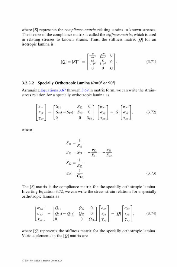
wher e [S ] rep resents the compl iance mat rix relating strains to known stresses .
The inverse of the compli ance matr ix is called the stiffness mat rix, whi ch is used
in relating stresses to known strains. Thus , the stiffne ss matrix [ Q ] for an
isotrop ic lamin a is
[ Q] ¼ [ S ]� 1 ¼E
1 � n 2n E1 � n 2
0
n E1 � n 2
E1 � n 2
0
0 0 G
264
375: (3:71)
3.2.5.2 Specially Orthotropic Lamina (u508 or 908)
Arran ging Equations 3.67 through 3.69 in matr ix form , we can write the stra in–
stress relation for a specially orthotropic lamina as
«xx
«yy
gxy
264
375 ¼
S11 S12 0
S21(¼S12) S22 0
0 0 S66
24
35 sxx
syy
txy
24
35 ¼ [S]
sxx
syy
txy
24
35, (3:72)
where
S11 ¼ 1
E11
S12 ¼ S21 ¼ � n12E11
¼ � n21E22
S22 ¼ 1
E22
S66 ¼ 1
G12
(3:73)
The [S] matrix is the compliance matrix for the specially orthotropic lamina.
Inverting Equation 3.72, we can write the stress–strain relations for a specially
orthotropic lamina as
sxx
syy
txy
24
35 ¼
Q11 Q12 0
Q21(¼ Q12) Q22 0
0 0 Q66
24
35
«xx
«yy
gxy
264
375 ¼ [Q]
«xx
«yy
gxy
264
375, (3:74)
where [Q] represents the stiffness matrix for the specially orthotropic lamina.
Various elements in the [Q] matrix are
� 2007 by Taylor & Francis Group, LLC.
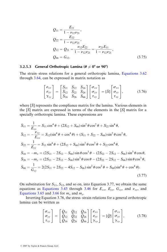
Q11 ¼ E11
1 � n12 n 21,
Q22 ¼ E22
1 � n12 n 21,
Q12 ¼ Q 21 ¼ n12 E22
1 � n12 n 21¼ n21 E11
1 � n12 n 21,
Q66 ¼ G 12 : ( 3: 75 )
3.2.5.3 Gener al Orth otropic Lamin a ( u 6¼ 0 8 or 908 )
The stra in–stress relat ions for a gen eral orthot ropic lami na, Equat ions 3 .62
through 3.64, can be express ed in matr ix nota tion as
«xx«yygxy
24
35 ¼
�S11�S12
�S16�S12
�S22�S26
�S16�S26
�S66
24
35 sxx
syy
txy
24
35 ¼ [ �S ]
sxx
syy
txy
24
35, ( 3: 76 )
where [ �S ] repres ents the compli ance matrix for the lamin a. Variou s elem ents in
the [ �S ] matrix are express ed in terms of the elem ents in the [ S ] matr ix for a
specia lly orthot ropic lami na. Thes e e xpressions are
�S11 ¼ 1
Exx
¼ S11 cos4 u þ ( 2S12 þ S66 ) sin
2 u cos2 u þ S22 sin4 u,
�S12 ¼ � nxy
Exx
¼ S12 (sin 4 u þ cos 4 u) þ ( S11 þ S22 � S66 ) sin
2 u cos 2 u,
�S22 ¼ 1
Eyy
¼ S11 sin4 u þ (2S 12 þ S66 ) sin
2 u cos 2 u þ S22 cos 4 u,
�S16 ¼ �m x ¼ ( 2S11 � 2S12 � S66 ) sin u cos 3 u � (2 S22 � 2S12 � S66 ) sin
3 u cos u,
�S26 ¼ �m y ¼ ( 2S 11 � 2S 12 � S66 ) sin3 u cos u � ( 2S22 � 2S 12 � S66 ) sin u cos
3 u,
�S66 ¼ 1
Gxy
¼ 2(2S11 þ 2S22 � 4S12 � S66) sin2 u cos2 uþ S66(sin
4 uþ cos4 u):
(3:77)
On substitution for S11, S12, and so on, into Equation 3.77, we obtain the same
equati ons as Equat ions 3 .43 through 3.46 for Exx, Eyy, Gxy, and nxy, and
Equations 3.65 a nd 3.66 for mx and my.
Inverting Equation 3.76, the stress–strain relations for a general orthotropic
lamina can be written as
sxx
syy
txy
24
35 ¼
�Q11�Q12
�Q16�Q12
�Q22�Q26
�Q16�Q26
�Q66
24
35 «xx
«yygxy
24
35 ¼ [�Q]
sxx
syy
gxy
24
35, (3:78)
� 2007 by Taylor & Francis Group, LLC.
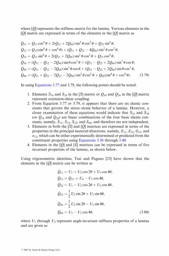
wher e [ �Q] repres ents the stiffne ss matrix for the lamina. Var ious elemen ts in the
[ �Q] matrix are exp ressed in terms of the elem ents in the [Q ] matr ix as
�Q11 ¼ Q 11 cos 4 u þ 2( Q 12 þ 2Q66 ) sin
2 u cos 2 u þ Q 22 sin 4 u,
�Q12 ¼ Q 12 (sin 4 u þ cos 4 u) þ ( Q 11 þ Q22 � 4Q 66 ) sin
2 u cos 2 u,
�Q22 ¼ Q 11 sin4 u þ 2( Q12 þ 2Q 66 ) sin
2 u cos 2 u þ Q22 cos 4 u,
�Q16 ¼ ( Q11 � Q 12 � 2Q 66 ) sin u cos3 u þ ( Q12 � Q 22 þ 2Q66 ) sin
3 u cos u,
�Q26 ¼ ( Q11 � Q 12 � 2Q 66 ) sin3 u cos u þ ( Q12 � Q 22 þ 2Q66 ) sin u cos
3 u,
�Q66 ¼ ( Q11 þ Q 22 � 2Q 12 � 2Q 66 ) sin 2 u cos2 u þ Q 66 (sin
4 u þ cos 4 u): ( 3: 79 )
In using Equations 3.77 and 3.79, the following poi nts sho uld be noted:
1. Element s �S16 and �S 26 in the [ �S ] matrix or �Q 16 and �Q 26 in the [ �Q] matr ix
repres ent extension -shear coup ling.
2. Fro m Equat ion 3.77 or 3.79, it appears that there are six elastic con -
stant s that gove rn the stress–s train behavior of a lamina. Ho wever, a
closer examin ation of these eq uations would ind icate that �S16 an d �S 26(or �Q16 and �Q 26) are linear combinations of the four basic elastic con-
stants, namely, �S11, �S 12, �S 22, and �S 66, and therefore are not independent.3. Element s in both the [ �S ] and [ �Q] matrices are exp ressed in terms of the
prop erties in the principal mate rial direct ions, namel y, E11 , E22 , G12 , and
n12 , which can be eithe r experi mentally determ ined or pre dicted from the
con stituent pro perties using Equat ions 3.36 through 3.40.
4. Elements in the [�Q] and [�S] matrices can be expressed in terms of five
invariant properties of the lamina, as shown below.
Using trigonometric identities, Tsai and Pagano [23] have shown that the
elements in the [�Q] matrix can be written as
�Q11 ¼ U1 þU2 cos 2uþU3 cos 4u,
�Q12 ¼ �Q21 ¼ U4 �U3 cos 4u,
�Q22 ¼ U1 �U2 cos 2uþU3 cos 4u,
�Q16 ¼ 1
2U2 sin 2uþU3 sin 4u,
�Q26 ¼ 1
2U2 sin 2u�U3 sin 4u,
�Q66 ¼ U5 �U3 cos 4u, (3:80)
where U1 through U5 represent angle-invariant stiffness properties of a lamina
and are given as
� 2007 by Taylor & Francis Group, LLC.
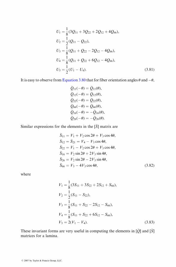
U1 ¼ 1
8 (3Q 11 þ 3Q 22 þ 2 Q12 þ 4Q 66 ) ,
U2 ¼ 1
2 (Q 11 � Q 22 ),
U3 ¼ 1
8 (Q 11 þ Q 22 � 2Q 12 � 4Q 66 ),
U4 ¼ 1
8 (Q 11 þ Q 22 þ 6Q 12 � 4Q 66 ),
U5 ¼ 1
2(U1 �U4): (3:81)
It is easy to observe from Equation 3.80 that for fiber orientation angles u and �u,
�Q11(�u) ¼ �Q11(u),
�Q12(�u) ¼ �Q12(u),
�Q22(�u) ¼ �Q22(u),
�Q66(�u) ¼ �Q66(u),
�Q16(�u) ¼ ��Q16(u),
�Q26(�u) ¼ ��Q26(u):
Similar expressions for the elements in the [�S] matrix are
�S11 ¼ V1 þ V2 cos 2uþ V3 cos 4u,
�S12 ¼ �S21 ¼ V4 � V3 cos 4u,
�S22 ¼ V1 � V2 cos 2uþ V3 cos 4u,
�S16 ¼ V2 sin 2uþ 2V3 sin 4u,
�S26 ¼ V2 sin 2u� 2V3 sin 4u,
�S66 ¼ V5 � 4V3 cos 4u, (3:82)
where
V1 ¼ 1
8(3S11 þ 3S22 þ 2S12 þ S66),
V2 ¼ 1
2(S11 � S22),
V3 ¼ 1
8(S11 þ S22 � 2S12 � S66),
V4 ¼ 1
8(S11 þ S22 þ 6S12 � S66),
V5 ¼ 2(V1 � V4): (3:83)
These invariant forms are very useful in computing the elements in [�Q] and [�S]matrices for a lamina.
� 2007 by Taylor & Francis Group, LLC.
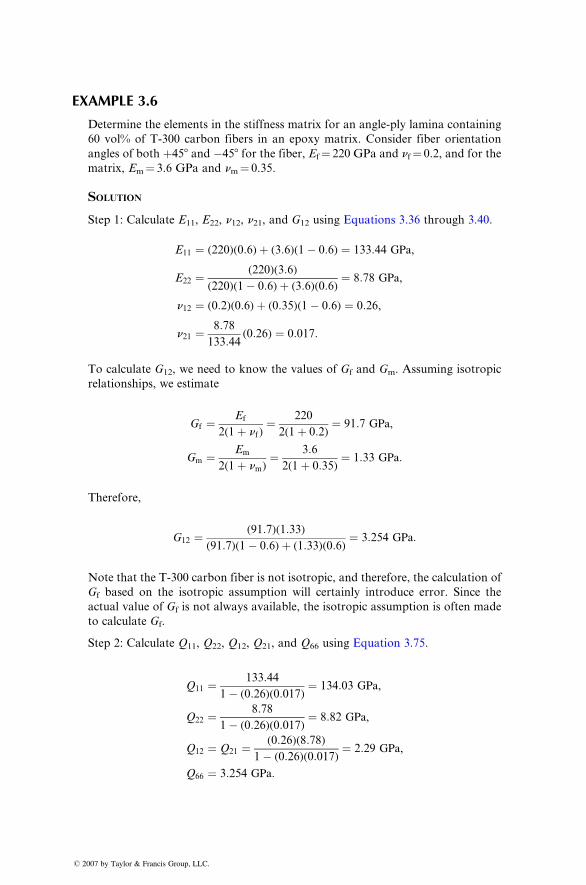
EXAMPLE 3.6
Determine the elements in the stiffness matrix for an angle-ply lamina containing
60 vol% of T-300 carbon fibers in an epoxy matrix. Consider fiber orientation
angles of both þ45 8 and �458 for the fiber, Ef ¼ 220 GPa and nf ¼ 0.2, and for the
matrix, Em ¼ 3.6 GPa and nm ¼ 0.35.
SOLUTIO N
Step 1: Calculate E11 , E22 , n12 , n21, and G12 using Equations 3.36 through 3.40.
E11 ¼ ( 220)( 0: 6) þ ( 3: 6)( 1 � 0: 6) ¼ 133: 44 GPa ,
E22 ¼ ( 220)( 3: 6)
( 220)( 1 � 0: 6) þ (3: 6)( 0: 6) ¼ 8: 78 GPa ,
n12 ¼ ( 0: 2)(0: 6) þ ( 0: 35)(1 � 0: 6) ¼ 0: 26,
n21 ¼ 8: 78
133: 44 ( 0:26 ) ¼ 0: 017:
To calculate G12, we need to know the values of G f and G m . Assuming isotropic
relationships, we estimate
Gf ¼ Ef
2(1 þ nf ) ¼ 220
2(1 þ 0: 2) ¼ 91: 7 GPa ,
Gm ¼ Em
2(1 þ nm ) ¼ 3: 6
2(1 þ 0:35 ) ¼ 1: 33 GPa :
Therefore,
G12 ¼ ( 91: 7)(1: 33)
( 91: 7)(1 � 0: 6) þ ( 1: 33)(0: 6) ¼ 3: 254 GPa:
Note that the T-300 carbon fiber is not isotropic, and therefore, the calculation of
Gf based on the isotropic assumption will certainly introduce error. Since the
actual value of Gf is not always available, the isotropic assumption is often made
to calculate Gf.
Step 2: Calculate Q11 , Q 22 , Q 12 , Q 21 , and Q 66 using Equation 3.75.
Q11 ¼ 133:44
1� (0:26)(0:017)¼ 134:03 GPa,
Q22 ¼ 8:78
1� (0:26)(0:017)¼ 8:82 GPa,
Q12 ¼ Q21 ¼ (0:26)(8:78)
1� (0:26)(0:017)¼ 2:29 GPa,
Q66 ¼ 3:254 GPa:
� 2007 by Taylor & Francis Group, LLC.
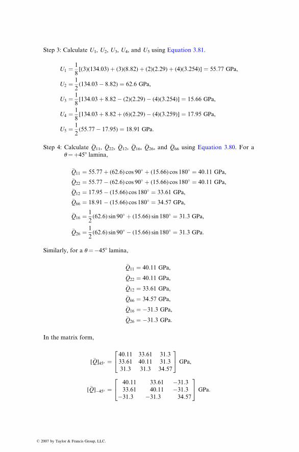
� 2
Step 3: Calculate U1, U 2, U 3 , U 4, and U5 using Equation 3.81.
U1 ¼ 1
8 [( 3)(134: 03) þ ( 3)(8: 82) þ ( 2)(2: 29) þ ( 4)(3 :254 )] ¼ 55: 77 GPa,
U2 ¼ 1
2 ( 134: 03 � 8: 82) ¼ 62: 6 GPa ,
U3 ¼ 1
8 [ 134: 03 þ 8: 82 � ( 2)( 2:29 ) � ( 4)( 3: 254)] ¼ 15: 66 GPa ,
U4 ¼ 1
8 [ 134: 03 þ 8: 82 þ ( 6)( 2:29 ) � ( 4)( 3: 259)] ¼ 17: 95 GPa ,
U5 ¼ 1
2 ( 55: 77 � 17: 95) ¼ 18: 91 GPa :
Step 4: Calculate �Q11 , �Q 22 , �Q 12 , �Q 16 , �Q 26 , and �Q 66 using Equation 3.80. For a
u¼þ458 lamina,
�Q11 ¼ 55:77þ (62:6) cos 90� þ (15:66) cos 180� ¼ 40:11 GPa,
�Q22 ¼ 55:77� (62:6) cos 90� þ (15:66) cos 180� ¼ 40:11 GPa,
�Q12 ¼ 17:95� (15:66) cos 180� ¼ 33:61 GPa,
�Q66 ¼ 18:91� (15:66) cos 180� ¼ 34:57 GPa,
�Q16 ¼ 1
2(62:6) sin 90� þ (15:66) sin 180� ¼ 31:3 GPa,
�Q26 ¼ 1
2(62:6) sin 90� � (15:66) sin 180� ¼ 31:3 GPa:
Similarly, for a u¼�458 lamina,
�Q11 ¼ 40:11 GPa,
�Q22 ¼ 40:11 GPa,
�Q12 ¼ 33:61 GPa,
�Q66 ¼ 34:57 GPa,
�Q16 ¼ �31:3 GPa,
�Q26 ¼ �31:3 GPa:
In the matrix form,
[�Q]45� ¼40:11 33:61 31:333:61 40:11 31:331:3 31:3 34:57
24
35 GPa,
[�Q]�45� ¼40:11 33:61 �31:333:61 40:11 �31:3
�31:3 �31:3 34:57
24
35 GPa:
007 by Taylor & Francis Group, LLC.
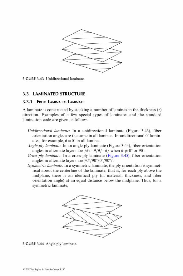
FIGURE 3.43 Unidirectional laminate.
3.3 LAMINATED STRUCTURE
3.3.1 F ROM L AMINA TO L AMINATE
A lamin ate is con structed by stacki ng a num ber of laminas in the thickne ss ( z)
direction . Exa mples of a few specia l types of lami nates and the standar d
laminati on code are given a s follo ws:
Unidire ctional lam inate : In a unid irectional lami nate (Figur e 3.43) , fiber
orientati on ang les are the same in all laminas. In unidir ection al 08 lami n-
ates, for exampl e, u ¼ 08 in all laminas.
Angle-p ly laminat e : In an an gle-ply lami nate (Figur e 3.44), fiber orient ation
angles in alternate layers are =u=�u =u=�u= when u 6¼ 08 or 90 8 .Cross- ply laminat e : In a cross- ply laminate (F igure 3.45), fiber orient ation
angles in alternate layers are =08=908=08 =90 8 =.Symm etric laminat e: In a symm etric lamin ate, the ply orient ation is symm et-
rical abo ut the center line of the laminate; that is, for each ply above the
midplane, there is an identical ply (in material, thickness, and fiber
orientation angle) at an equal distance below the midplane. Thus, for a
symmetric laminate,
FIGURE 3.44 Angle-ply laminate.
� 2007 by Taylor & Francis Group, LLC.
FIGURE 3.45 Cross-ply laminate.
u(z) ¼ u(�z),
where z is the distance from the midplane of the laminate. Some examples
of symmetric laminates and their codes are listed.
1 2 3 4 5 6
1. [0=þ45=90=90 þ45=0]Code: [0=45=90]S
Subscript S in the code indicates symmetry about the midplane.
1 2 3 4 5
2. [0=þ45=90=þ45=0]Code: [0=45=90]S
The bar over 90 indicates that the plane of symmetry passes midway
through the thickness of the 908 lamina.
1 2 3 4 5 6 7
3. [0=þ45=�45=90=�45=þ45=0]Code: [0=+45=90]S
Adjacent þ458 and �458 laminas are grouped as ±458.
1 2 3 4 5 6 7 8 9 10 11 12 13 14
4. [0 = 90 = 0 = 0 = 0 = 0 = 45 = 45 = 0 = 0 = 0 = 0 = 90 = 0]Code: [0=90=04=45]S
Four adjacent 08 plies are grouped together as 04.
1 2 3 4 5 6 7 8 9 10
5. [0=45=�45=þ45=�45=�45=þ45=�45=þ45=0]Code: [0=(±45)2]S
Two adjacent ±458 plies are grouped as (±45)2.
� 2007 by Taylor & Francis Group, LLC.
6. [0=45=�45=45=�45=45=�45=0=0=0=0=0=�45=45=�45=45=�45=45=0]Code: [0=(+45)3=02=�0]S
7. [u=�u=u=�u=�u=u=�u=u]Code: [u=� u]2S or [±u]2S
Two adjacent ±u plies on each side of the plane of symmetry are denoted
by the subscript 2S.
8. Symmetric angle-ply laminate
[u= �u= u=�u=u=�u=u]Code: [�u=u=��u]S
Note that symmetric angle-ply laminates contain an odd number of plies.
9. Symmetric cross-ply laminate
[0=90=0=90=0=90=0=90=0]Code: [(0=90)2=�0]S
Note that symmetric cross-ply laminates contain an odd number of plies.
10. Hybrid (interply) laminate.
[0B=0B=45C=�45C=90G=90G=�45C=45C=0B=0B]Code: [02B=(±45)C=90G]S
where B, C, and G represent boron, carbon, and glass fiber, respectively.
Antisymmetric laminate: In antisymmetric laminates, the ply orientation is
antisymmetric about the centerline of the laminate; that is, for each ply of
fiber orientation angle u above the midplane, there is a ply of fiber
orientation angle �u with identical material and thickness at an equal
distance below the midplane. Thus, for an antisymmetric laminate,
u(z) ¼ �u(�z):
For example, u= �u= u = �u is an antisymmetric laminate. In contrast,
u=�u=� u=u is symmetric.
Unsymmetric laminate: In unsymmetric laminates, there is no symmetry or
antisymmetry. Examples are 0=0=0=90=90=90 and 0=u=�u=90.Quasi-isotropic laminate: These laminates are made of three or more laminas
of identical thickness and material with equal angles between each
adjacent lamina. Thus, if the total number of laminas is n, the orientation
angles of the laminas are at increments of p=n. The resulting laminate
� 2007 by Taylor & Francis Group, LLC.
exhibits an in-plan e isot ropic elastic behavior in the xy plane. How ever,
its strength pro perties may still vary with the direction of loading .
Example s of simp le quasi-isot ropic laminates are [ þ 60 =0=� 60] and
[þ 45=0=� 45 =90]. Othe r combinat ions of these stackin g sequences, such
as [0 =þ60=�60] and [0=þ 45 =� 45 =90], also exh ibit in-pl ane isotropicelastic behavior . A very common an d wid ely used qua si-isotro pic sym-
metrical stacki ng sequence is [0 =±45=90 ]S .
3.3.2 LAMINATION THEORY
Laminat ion theory is useful in calcul ating stresses and strains in each lamina of
a thin laminated structure. Beginning with the stiffne ss matrix of each lamin a,
the step- by-step pro cedure in lami nation theory includes
1. Calculat ion of sti ffness matrices for the laminate
2. Calculat ion of midplane strains an d curvat ures for the laminate due to a
given set of applied forces and moment s
3. Calculat ion of in-pl ane strains «xx, «yy , and g xy for each lamina
4. Calculat ion of in-pl ane stresses sxx, syy , and txy in each lamina
The deriva tion of laminati on theory is given in Ref. [16]. The princi pal equ a-
tions and a numb er of exampl es are present ed in the followi ng sections.
3.3.2.1 Assu mptions
Basic assump tions in the lamin ation theory are
1. Laminat e is thin an d wide (width � thickne ss).
2. A pe rfect interlam inar bond exists between various laminas.
3. Strain dist ribution in the thickne ss direct ion is linear.
4. All laminas are macros copical ly homo geneous and behave in a linea rly
elastic manner.
The geometric midplane of the laminate contains the xy axes, and the z
axis defines the thickness direction. The total thickness of the laminate is h,
and the thickness of various laminas are represented by t1, t2, t3, and so on.
The total number of laminas is N. A sketch for the laminate is shown in
Figure 3.46.
3.3.2.2 Laminate Strains
Following assumption 3, laminate strains are linearly related to the distance
from the midplane as
� 2007 by Taylor & Francis Group, LLC.
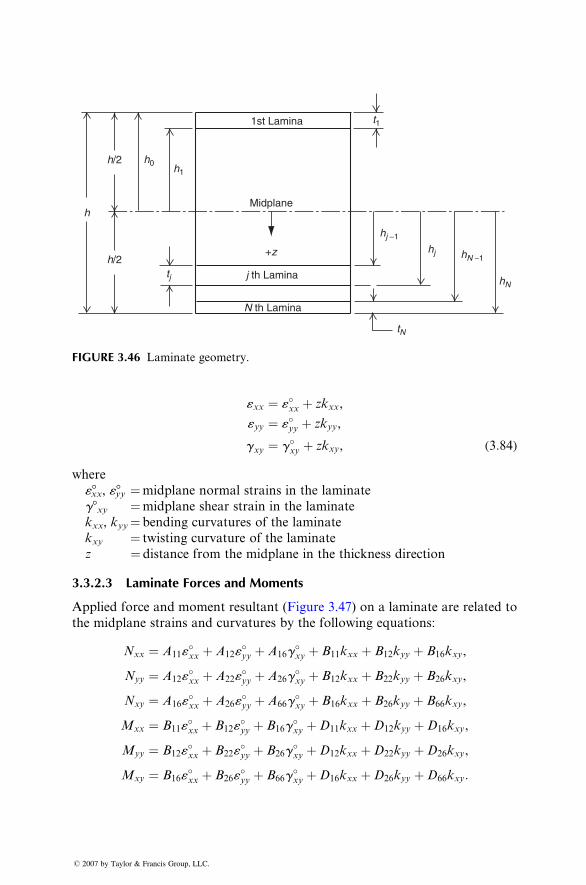
tN
hN
hN −1
hj −1
Midplane
1st Lamina t1
j th Laminatj
h/2
h/2 h0h1
h
+z
N th Lamina
hj
FIGURE 3.46 Laminate geometry.
«xx ¼ «�xx þ zk xx ,
«yy ¼ «�yy þ zk yy ,
gxy ¼ g �xy þ zk xy , ( 3: 84 )
wher e
«8xx , «8yy ¼ midpl ane normal stra ins in the lami nate
g8xy ¼ midpl ane shear stra in in the laminate
kxx , k yy ¼ bend ing cu rvatures of the lamin ate
kxy ¼ twist ing cu rvature of the lamin ate
z ¼ distan ce from the midpl ane in the thickne ss direction
3.3.2 .3 Lami nate Fo rces and Mome nts
Applied force an d momen t resultant (Figure 3.47) on a lami nate are related to
the midplane stra ins and cu rvatures by the foll owing equ ations:
Nxx ¼ A 11 «�xx þ A12 «
�yy þ A 16 g
�xy þ B 11 kxx þ B12 k yy þ B16 k xy ,
Nyy ¼ A 12 «�xx þ A22 «
�yy þ A 26 g
�xy þ B 12 kxx þ B22 k yy þ B26 k xy ,
Nxy ¼ A 16 «�xx þ A26 «
�yy þ A 66 g
�xy þ B 16 kxx þ B26 k yy þ B66 k xy ,
Mxx ¼ B 11 «�xx þ B 12 «
�yy þ B16 g
�xy þ D 11 kxx þ D 12 kyy þ D 16 kxy ,
Myy ¼ B12«�xx þ B22«
�yy þ B26g
�xy þD12kxx þD22kyy þD26kxy,
Mxy ¼ B16«�xx þ B26«
�yy þ B66g
�xy þD16kxx þD26kyy þD66kxy:
� 2007 by Taylor & Francis Group, LLC.
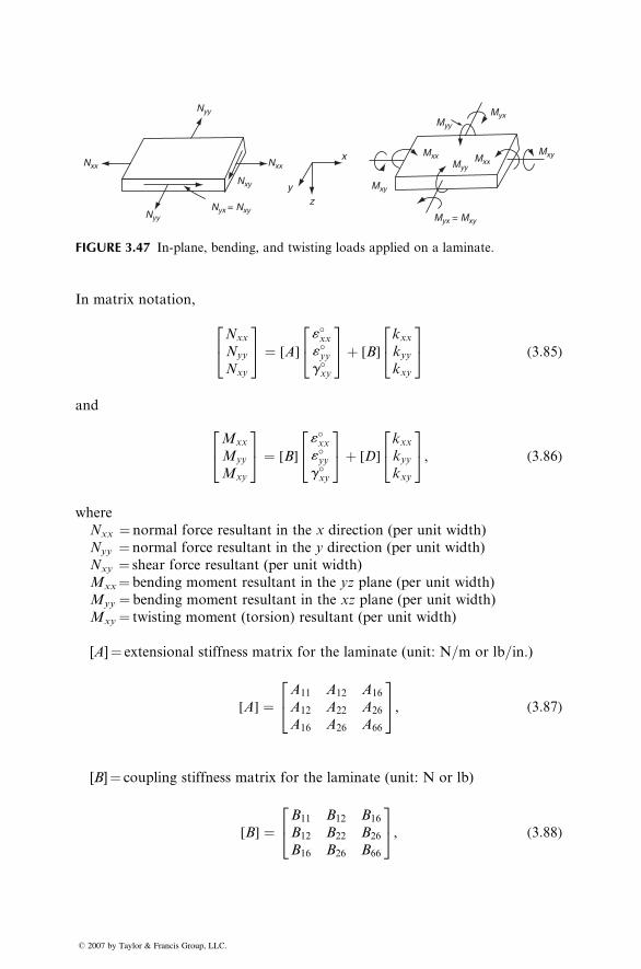
Nxx Nxx
Nyy
Nyy
Mxy
Myx = Mxy
Myy
MyyMxx
Mxx Mxy
Myx
yz
x
Nyx = Nxy
Nxy
FIGURE 3.47 In-plane, bending, and twisting loads applied on a laminate.
In matrix notation,
Nxx
Nyy
Nxy
24
35 ¼ [A]
«�xx«�yyg�xy
24
35þ [B]
kxxkyykxy
24
35 (3:85)
and
Mxx
Myy
Mxy
24
35 ¼ [B]
«�xx«�yyg�xy
24
35þ [D]
kxxkyykxy
24
35, (3:86)
where
Nxx ¼ normal force resultant in the x direction (per unit width)
Nyy ¼ normal force resultant in the y direction (per unit width)
Nxy ¼ shear force resultant (per unit width)
Mxx¼ bending moment resultant in the yz plane (per unit width)
Myy ¼ bending moment resultant in the xz plane (per unit width)
Mxy¼ twisting moment (torsion) resultant (per unit width)
[A]¼ extensional stiffness matrix for the laminate (unit: N=m or lb=in.)
[A] ¼A11 A12 A16
A12 A22 A26
A16 A26 A66
24
35, (3:87)
[B]¼ coupling stiffness matrix for the laminate (unit: N or lb)
[B] ¼B11 B12 B16
B12 B22 B26
B16 B26 B66
24
35, (3:88)
� 2007 by Taylor & Francis Group, LLC.
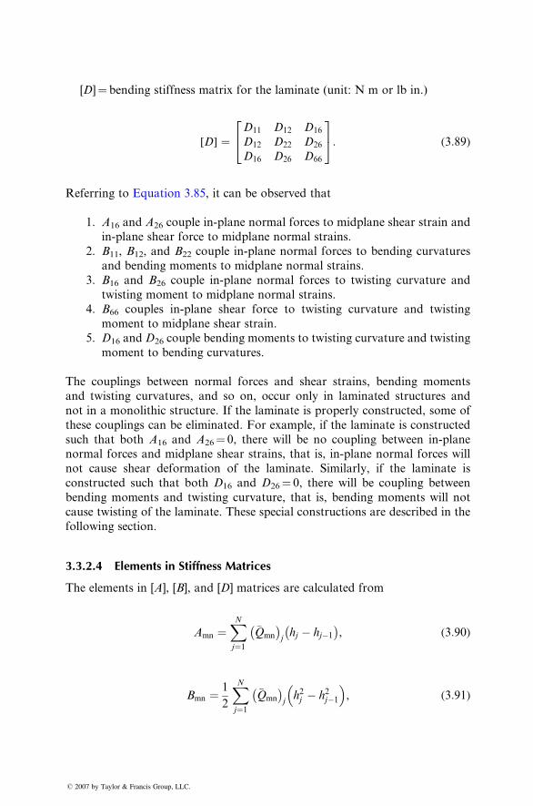
[D ] ¼ ben ding sti ffness matrix for the laminate (unit: N m or lb in.)
[ D] ¼
D 11 D12 D16
D 12 D22 D 26D 16 D26 D 66
24
35: ( 3: 89 )
Referri ng to Equat ion 3.85, it can be observed that
1. A 16 and A26 couple in-plane normal forces to midplane shear strain and
in-plane shear force to midplane normal strains.
2. B11, B12, and B22 couple in-plane normal forces to bending curvatures
and bending moments to midplane normal strains.
3. B16 and B26 couple in-plane normal forces to twisting curvature and
twisting moment to midplane normal strains.
4. B66 couples in-plane shear force to twisting curvature and twisting
moment to midplane shear strain.
5. D16 and D26 couple bending moments to twisting curvature and twisting
moment to bending curvatures.
The couplings between normal forces and shear strains, bending moments
and twisting curvatures, and so on, occur only in laminated structures and
not in a monolithic structure. If the laminate is properly constructed, some of
these couplings can be eliminated. For example, if the laminate is constructed
such that both A16 and A26¼ 0, there will be no coupling between in-plane
normal forces and midplane shear strains, that is, in-plane normal forces will
not cause shear deformation of the laminate. Similarly, if the laminate is
constructed such that both D16 and D26¼ 0, there will be coupling between
bending moments and twisting curvature, that is, bending moments will not
cause twisting of the laminate. These special constructions are described in the
following section.
3.3.2.4 Elements in Stiffness Matrices
The elements in [A], [B], and [D] matrices are calculated from
Amn ¼XNj¼1
�Qmn
jhj � hj�1
, (3:90)
Bmn ¼ 1
2
XNj¼1
�Qmn
jh2j � h2j�1
� �, (3:91)
� 2007 by Taylor & Francis Group, LLC.
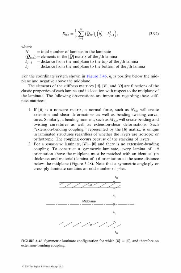
Dmn ¼ 1
3
XNj ¼ 1
�Qmn
jh3j � h3j � 1
� �, ( 3: 92 )
where
N ¼ total num ber of lamin as in the laminate
( �Qmn) j ¼ elem ents in the [ �Q ] matr ix of the j th lamina
hj� 1 ¼ distan ce from the midpl ane to the top of the j th lamina
hj ¼ dist ance from the midplan e to the bottom of the j th lamina
For the coordinat e system sho wn in Figure 3.46, hj is positive be low the mid-
plane and negative above the midplane.
The elements of the stiffness matrices [A], [B], and [D] are functions of the
elastic properties of each lamina and its location with respect to the midplane of
the laminate. The following observations are important regarding these stiff-
ness matrices:
1. If [B] is a nonzero matrix, a normal force, such as Nxx, will create
extension and shear deformations as well as bending–twisting curva-
tures. Similarly, a bending moment, such as Mxx, will create bending and
twisting curvatures as well as extension-shear deformations. Such
‘‘extension-bending coupling,’’ represented by the [B] matrix, is unique
in laminated structures regardless of whether the layers are isotropic or
orthotropic. The coupling occurs because of the stacking of layers.
2. For a symmetric laminate, [B]¼ [0] and there is no extension-bending
coupling. To construct a symmetric laminate, every lamina of þuorientation above the midplane must be matched with an identical (in
thickness and material) lamina of þu orientation at the same distance
below the midplane (Figure 3.48). Note that a symmetric angle-ply or
cross-ply laminate contains an odd number of plies.
t 0
t 0
Midplane
h1
h1
+q
+q
FIGURE 3.48 Symmetric laminate configuration for which [B] ¼ [0], and therefore no
extension-bending coupling.
� 2007 by Taylor & Francis Group, LLC.
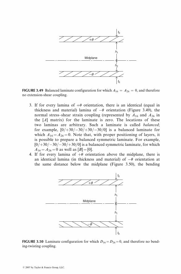
Midplane
+q
−q
t0
t0
h2
h1
FIGURE 3.49 Balanced laminate configuration for which A16 ¼ A26 ¼ 0, and therefore
no extension-shear coupling.
3. If for every lamina of þu orientation, there is an identical (equal in
thickness and material) lamina of �u orientation (Figure 3.49), the
normal stress–shear strain coupling (represented by A16 and A26 in
the [A] matrix) for the laminate is zero. The locations of these
two laminas are arbitrary. Such a laminate is called balanced;
for example, [0=þ30=�30=þ30=�30=0] is a balanced laminate for
which A16¼A26¼ 0. Note that, with proper positioning of layers, it
is possible to prepare a balanced symmetric laminate. For example,
[0=þ30=�30=�30=þ30=0] is a balanced symmetric laminate, for which
A16¼A26¼ 0 as well as [B]¼ [0].
4. If for every lamina of þu orientation above the midplane, there is
an identical lamina (in thickness and material) of �u orientation at
the same distance below the midplane (Figure 3.50), the bending
Midplane
+q
−q
t0
t0
h1
h1
FIGURE 3.50 Laminate configuration for which D16¼D26¼ 0, and therefore no bend-
ing-twisting coupling.
� 2007 by Taylor & Francis Group, LLC.
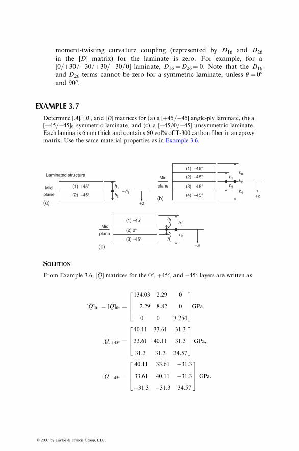
moment-twisting curvature coupling (represented by D16 and D26
in the [D] matrix) for the laminate is zero. For example, for a
[0=þ30=�30=þ30=�30=0] laminate, D16¼D26¼ 0. Note that the D16
and D26 terms cannot be zero for a symmetric laminate, unless u¼ 08and 908.
EXAMPLE 3.7
Determine [A], [B], and [D] matrices for (a) a [þ45=�45] angle-ply laminate, (b) a
[þ45=�45]S symmetric laminate, and (c) a [þ45=0=�45] unsymmetric laminate.
Each lamina is 6 mm thick and contains 60 vol% of T-300 carbon fiber in an epoxy
matrix. Use the same material properties as in Example 3.6.
Laminated structure
Mid
plane
(a)
Mid
plane
(b)
h0
h0
h0
h2
h2
h4h2
h1
h1
h3
−h3
+z
+z
+z
(1) +45�
(2) −45�
(1) +45�
(4) +45�
(2) −45�
(1) +45�
(2) 0�
(3) −45�
(3) −45�
−h1
Mid
plane
(c)
SOLUTION
From Example 3.6, [�Q] matrices for the 08, þ458, and �458 layers are written as
[�Q]0� ¼ [Q]0� ¼134:03 2:29 0
2:29 8:82 0
0 0 3:254
2664
3775GPa,
[�Q]þ45� ¼40:11 33:61 31:3
33:61 40:11 31:3
31:3 31:3 34:57
2664
3775 GPa,
[�Q]�45� ¼40:11 33:61 �31:3
33:61 40:11 �31:3
�31:3 �31:3 34:57
2664
3775 GPa:
� 2007 by Taylor & Francis Group, LLC.
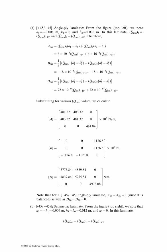
� 2
(a) [þ45=�45] Angle-ply laminate: From the figure (top left), we note
h0¼�0.006 m, h1¼ 0, and h2¼ 0.006 m. In this laminate, (�Qmn)1¼(�Qmn)þ458 and (�Qmn)2¼ (�Qmn)�458. Therefore,
Amn ¼ (�Qmn)1(h1 � h0)þ (�Qmn)2(h2 � h1)
¼ 6� 10�3(�Qmn)þ45� þ 6� 10�3(�Qmn)�45� ,
Bmn ¼ 1
2(�Qmn)1 h21 � h20
þ (�Qmn)2 h22 � h21 � �
¼ �18� 10�6(�Qmn)þ45� þ 18� 10�6(�Qmn)�45� ,
Dmn ¼ 1
3(�Qmn)1 h31 � h30
þ (�Qmn)2 h32 � h31 � �
¼ 72� 10�9(�Qmn)þ45� þ 72� 10�9(�Qmn)�45� :
Substituting for various (�Qmn) values, we calculate
[A] ¼481:32 403:32 0
403:32 481:32 0
0 0 414:84
26664
37775� 106 N=m,
[B] ¼0 0 �1126:8
0 0 �1126:8
�1126:8 �1126:8 0
26664
37775� 103 N,
[D] ¼5775:84 4839:84 0
4839:84 5775:84 0
0 0 4978:08
26664
37775Nm:
Note that for a [þ45=�45] angle-ply laminate, A16¼A26¼ 0 (since it is
balanced) as well as D16¼D26¼ 0.
(b) [(45=�45)]S Symmetric laminate: From the figure (top right), we note that
h3¼�h1¼ 0.006 m, h4¼ h0¼ 0.012 m, and h2¼ 0. In this laminate,
(�Qmn)4 ¼ (�Qmn)1 ¼ (�Qmn)þ45�
007 by Taylor & Francis Group, LLC.
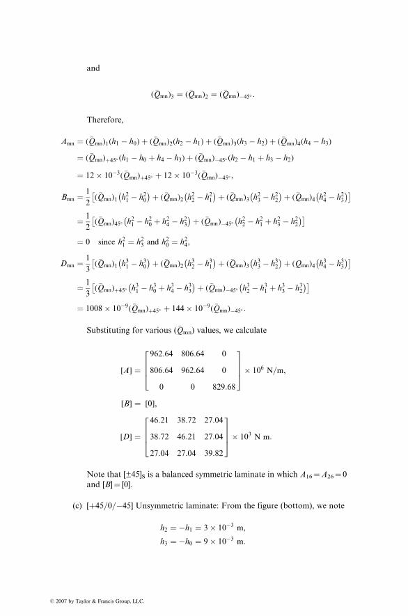
� 2
and
(�Qmn)3 ¼ (�Qmn)2 ¼ (�Qmn)�45� :
Therefore,
Amn ¼ (�Qmn)1(h1 � h0)þ (�Qmn)2(h2 � h1)þ (�Qmn)3(h3 � h2)þ (�Qmn)4(h4 � h3)
¼ (�Qmn)þ45� (h1 � h0 þ h4 � h3)þ (�Qmn)�45� (h2 � h1 þ h3 � h2)
¼ 12� 10�3(�Qmn)þ45� þ 12� 10�3(�Qmn)�45� ,
Bmn ¼ 1
2(�Qmn)1 h21 � h20
þ (�Qmn)2 h22 � h21 þ (�Qmn)3 h23 � h22
þ (�Qmn)4 h24 � h23 � �
¼ 1
2(�Qmn)45� h21 � h20 þ h24 � h23
þ (�Qmn)�45� h22 � h21 þ h23 � h22 � �
¼ 0 since h21 ¼ h23 and h20 ¼ h24,
Dmn ¼ 1
3(�Qmn)1 h31 � h30
þ (�Qmn)2 h32 � h31 þ (�Qmn)3 h33 � h32
þ (Qmn)4 h34 � h33 � �
¼ 1
3(�Qmn)þ45� h31 � h30 þ h34 � h33
þ (�Qmn)�45� h32 � h31 þ h33 � h32 � �
¼ 1008� 10�9(�Qmn)þ45� þ 144� 10�9(�Qmn)�45� :
Substituting for various (�Qmn) values, we calculate
[A] ¼962:64 806:64 0
806:64 962:64 0
0 0 829:68
2664
3775� 106 N=m,
[B] ¼ [0],
[D] ¼46:21 38:72 27:04
38:72 46:21 27:04
27:04 27:04 39:82
2664
3775� 103 N m:
Note that [±45]S is a balanced symmetric laminate in which A16¼A26¼ 0
and [B]¼ [0].
(c) [þ45=0=�45] Unsymmetric laminate: From the figure (bottom), we note
h2 ¼ �h1 ¼ 3� 10�3 m,
h3 ¼ �h0 ¼ 9� 10�3 m:
007 by Taylor & Francis Group, LLC.
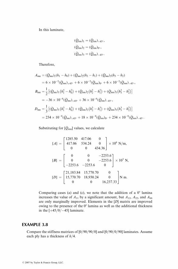
� 2
In this laminate,
(�Qmn)1 ¼ (�Qmn)þ45� ,
(�Qmn)2 ¼ (�Qmn)0� ,
(�Qmn)3 ¼ (�Qmn)�45� :
Therefore,
Amn ¼ (�Qmn)1(h1 � h0)þ (�Qmn)2(h2 � h1)þ (�Qmn)3(h3 � h2)
¼ 6� 10�3(�Qmn)þ45� þ 6� 10�3(�Qmn)0� þ 6� 10�3(�Qmn)�45� ,
Bmn ¼ 1
2(�Qmn)1 h21 � h20
þ (�Qmn)2 h22 � h21 þ (�Qmn)3 h23 � h22
� �
¼ �36� 10�6(�Qmn)þ45� þ 36� 10�6(�Qmn)�45� ,
Dmn ¼ 1
3(�Qmn)1 h31 � h30
þ (�Qmn)2 h32 � h31 þ (�Qmn)3 h33 � h32
� �
¼ 234� 10�9(�Qmn)þ45� þ 18� 10�9(�Qmn)0� þ 234� 10�9(�Qmn)�45� :
Substituting for [�Qmn] values, we calculate
[A] ¼1285:50 417:06 0
417:06 534:24 0
0 0 434:36
24
35� 106 N=m,
[B] ¼0 0 �2253:6
0 0 �2253:6
�2253:6 �2253:6 0
24
35� 103 N,
[D] ¼21,183:84 15,770:70 0
15,770:70 18,930:24 0
0 0 16,237:33
24
35N m:
Comparing cases (a) and (c), we note that the addition of a 08 lamina
increases the value of A11 by a significant amount, but A12, A22, and A66
are only marginally improved. Elements in the [D] matrix are improved
owing to the presence of the 08 lamina as well as the additional thickness
in the [þ45=0=�45] laminate.
EXAMPLE 3.8
Compare the stiffness matrices of [0=90=90=0] and [0=90=0=90] laminates. Assume
each ply has a thickness of h=4.
007 by Taylor & Francis Group, LLC.
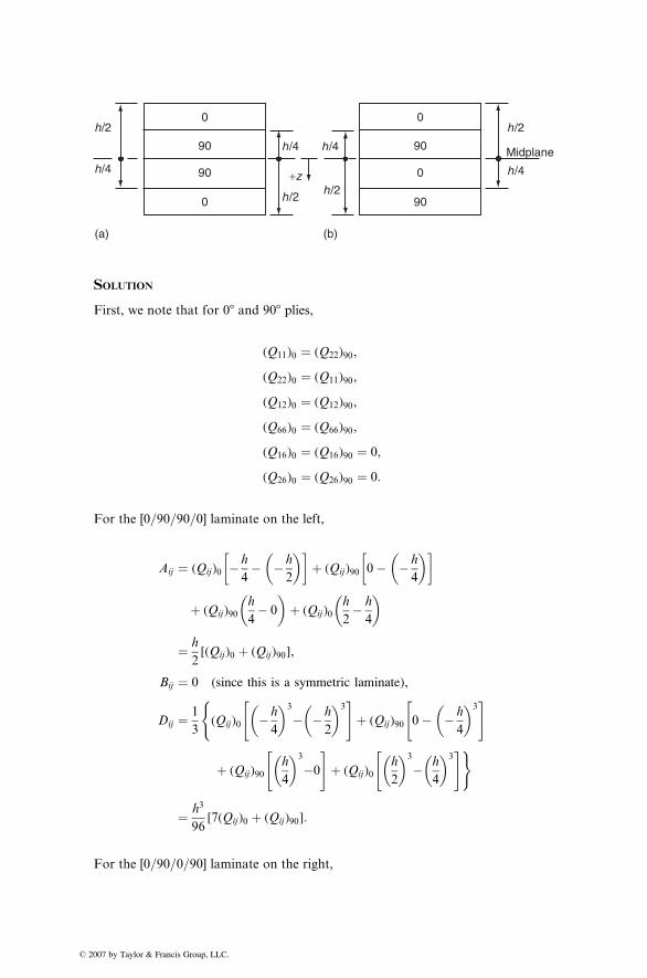
� 2
0
90
h/2
h/2h/2
h/2
+z
h/4
h/4
Midplaneh/4
h/4 90
0
(a) (b)
0
90
0
90
SOLUTION
First, we note that for 08 and 908 plies,
(Q11)0 ¼ (Q22)90,
(Q22)0 ¼ (Q11)90,
(Q12)0 ¼ (Q12)90,
(Q66)0 ¼ (Q66)90,
(Q16)0 ¼ (Q16)90 ¼ 0,
(Q26)0 ¼ (Q26)90 ¼ 0:
For the [0=90=90=0] laminate on the left,
Aij ¼ (Qij)0 � h
4� � h
2
� �� �þ (Qij)90 0� � h
4
� �� �
þ (Qij)90h
4� 0
� �þ (Qij)0
h
2� h
4
� �
¼ h
2[(Qij)0 þ (Qij)90],
Bij ¼ 0 (since this is a symmetric laminate),
Dij ¼ 1
3
((Qij)0 � h
4
� �3
� � h
2
� �3" #
þ (Qij)90 0� � h
4
� �3" #
þ (Qij)90h
4
� �3
�0
" #þ (Qij)0
h
2
� �3
� h
4
� �3" #)
¼ h3
96[7(Qij)0 þ (Qij)90]:
For the [0=90=0=90] laminate on the right,
007 by Taylor & Francis Group, LLC.
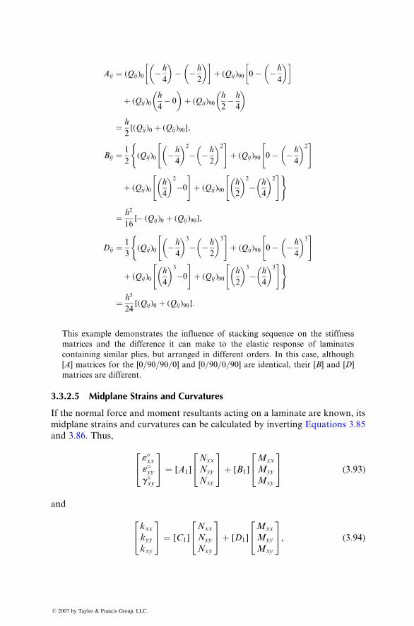
Aij ¼ ( Q ij ) 0 � h
4
� �� � h
2
� �� �þ (Qij )90 0 � � h
4
� �� �
þ (Qij )0h
4 � 0
� �þ ( Qij ) 90
h
2 � h
4
� �
¼ h
2 [( Q ij ) 0 þ ( Q ij ) 90 ] ,
Bij ¼ 1
2
(( Qij ) 0 � h
4
� �2
� � h
2
� �2" #
þ ( Qij ) 90 0 � � h
4
� �2" #
þ (Qij )0h
4
� �2
�0
" #þ (Qij ) 90
h
2
� �2
� h
4
� �2" #)
¼ h2
16 [� (Qij )0 þ (Qij )90 ],
Dij ¼ 1
3
(( Qij ) 0 � h
4
� �3
� � h
2
� �3" #
þ (Qij ) 90 0 � � h
4
� �3" #
þ (Qij )0h
4
� �3
�0
" #þ (Qij )90
h
2
� �3
� h
4
� �3" #)
¼ h3
24 [(Q ij ) 0 þ ( Q ij ) 90 ] :
This example demonstrates the influence of stacking sequence on the stiffness
matrices and the difference it can make to the elastic response of laminates
containing similar plies, but arranged in different orders. In this case, although
[ A] matrices for the [0=90 =90=0] and [0 =90=0=90] are identical, their [B ] and [ D]
matrices are different.
3.3.2 .5 Midpl ane Strains and Curvatur es
If the normal force and moment resultant s acting on a lami nate are known , its
midpl ane stra ins an d cu rvatures can be ca lculated by inverting Equations 3.85
and 3.86. Thus ,
«�xx«�yyg�xy
24
35 ¼ [A1]
Nxx
Nyy
Nxy
24
35þ [B1]
Mxx
Myy
Mxy
24
35 (3:93)
and
kxxkyykxy
24
35 ¼ [C1]
Nxx
Nyy
Nxy
24
35þ [D1]
Mxx
Myy
Mxy
24
35, (3:94)
� 2007 by Taylor & Francis Group, LLC.
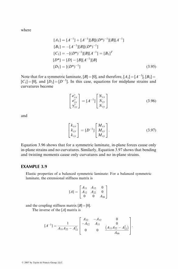
where
[A1] ¼ [A�1]þ [A�1][B][(D*)�1][B][A�1]
[B1] ¼ �[A�1][B][(D*)�1]
[C1] ¼ �[(D*)�1][B][A�1] ¼ [B1]T
[D*] ¼ [D]� [B][A�1][B]
[D1] ¼ [(D*)�1] (3:95)
Note that for a symmetric laminate, [B]¼ [0], and therefore, [A1]¼ [A�1], [B1]¼[C1]¼ [0], and [D1]¼ [D�1]. In this case, equations for midplane strains and
curvatures become
«�xx«�yyg�xy
24
35 ¼ [A�1]
Nxx
Nyy
Nxy
24
35 (3:96)
and
kxxkyykxy
24
35 ¼ [D�1]
Mxx
Myy
Mxy
24
35: (3:97)
Equation 3.96 shows that for a symmetric laminate, in-plane forces cause only
in-plane strains and no curvatures. Similarly, Equation 3.97 shows that bending
and twisting moments cause only curvatures and no in-plane strains.
EXAMPLE 3.9
Elastic properties of a balanced symmetric laminate: For a balanced symmetric
laminate, the extensional stiffness matrix is
[A] ¼A11 A12 0
A12 A22 0
0 0 A66
24
35
and the coupling stiffness matrix [B]¼ [0].
The inverse of the [A] matrix is
[A�1] ¼ 1
A11A22 � A212
A22 �A12 0
�A12 A11 0
0 0A11A22 � A2
12
A66
2664
3775:
� 2007 by Taylor & Francis Group, LLC.
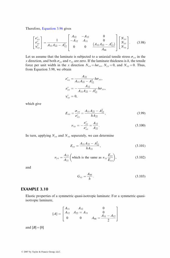
EX
� 2
Therefore, Equation 3.96 gives
«�xx«�yyg�xy
24
35 ¼ 1
A11A22 � A212
A22 �A12 0
�A12 A11 0
0 0A11A22 � A2
12
� �A66
2664
3775
Nxx
Nyy
Nxy
24
35: (3:98)
Let us assume that the laminate is subjected to a uniaxial tensile stress sxx in the
x direction, and both syy and txy are zero. If the laminate thickness is h, the tensile
force per unit width in the x direction Nxx¼ hsxx, Nyy¼ 0, and Nxy¼ 0. Thus,
from Equation 3.98, we obtain
«�xx ¼ A22
A11A22 � A212
hsxx,
«�yy ¼ � A12
A11A22 � A212
hsxx,
g�xy ¼ 0,
which give
Exx ¼ sxx
«�xx¼ A11A22 � A2
12
hA22
, (3:99)
nxy ¼ � «�yy«�xx
¼ A12
A22
: (3:100)
In turn, applying Nyy and Nxy separately, we can determine
Eyy ¼ A11A22 � A212
hA11
, (3:101)
nyx ¼ A12
A11
which is the same as nxyEyy
Exx
� �, (3:102)
and
Gxy ¼ A66
h: (3:103)
AMPLE 3.10
Elastic properties of a symmetric quasi-isotropic laminate: For a symmetric quasi-
isotropic laminate,
[A] ¼A11 A12 0
A12 A22 ¼ A11 0
0 0 A66 ¼ A11 � A12
2
264
375
and [B]¼ [0]
007 by Taylor & Francis Group, LLC.
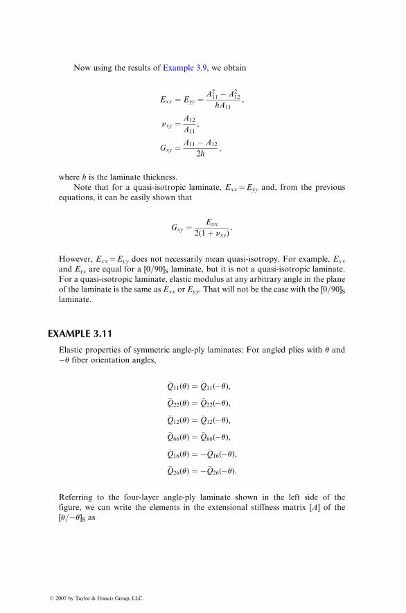
� 2
Now using the results of Example 3.9, we obtain
Exx ¼ Eyy ¼ A211 � A2
12
hA11
,
nxy ¼ A12
A11
,
Gxy ¼ A11 � A12
2h,
where h is the laminate thickness.
Note that for a quasi-isotropic laminate, Exx¼Eyy and, from the previous
equations, it can be easily shown that
Gxy ¼ Exx
2(1þ nxy):
However, Exx¼Eyy does not necessarily mean quasi-isotropy. For example, Exx
and Eyy are equal for a [0=90]S laminate, but it is not a quasi-isotropic laminate.
For a quasi-isotropic laminate, elastic modulus at any arbitrary angle in the plane
of the laminate is the same as Exx or Eyy. That will not be the case with the [0=90]Slaminate.
EXAMPLE 3.11
Elastic properties of symmetric angle-ply laminates: For angled plies with u and
�u fiber orientation angles,
�Q11(u) ¼ �Q11(�u),
�Q22(u) ¼ �Q22(�u),
�Q12(u) ¼ �Q12(�u),
�Q66(u) ¼ �Q66(�u),
�Q16(u) ¼ ��Q16(�u),
�Q26(u) ¼ ��Q26(�u):
Referring to the four-layer angle-ply laminate shown in the left side of the
figure, we can write the elements in the extensional stiffness matrix [A] of the
[u=�u]S as
007 by Taylor & Francis Group, LLC.
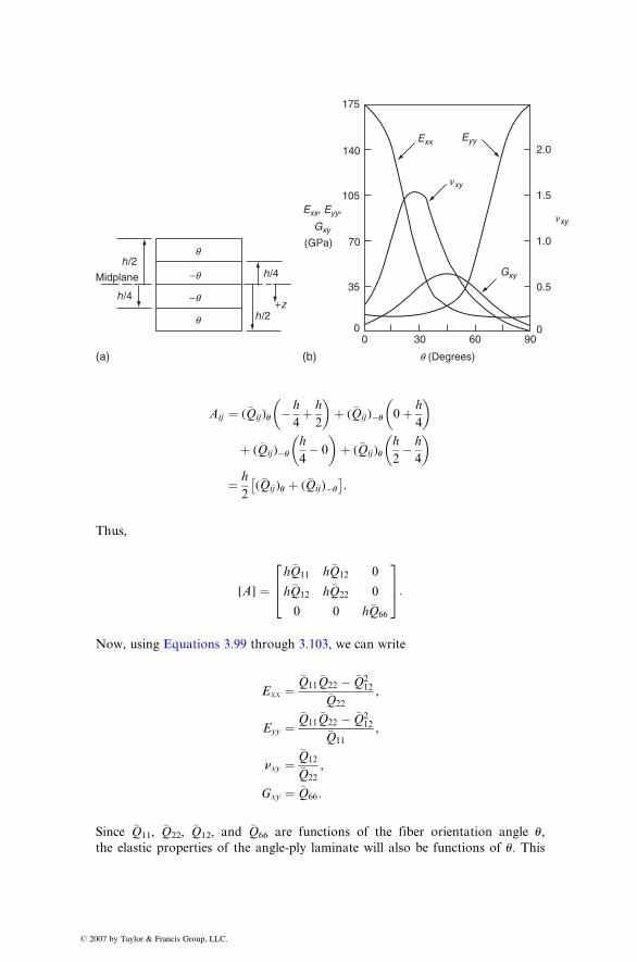
�xy
� 2
175
Exx
Exx, Eyy,
Gxy
(GPa)
Eyy
Gxy
�xy
140
105
70
35
00 30 60
q (Degrees)(b)
90
2.0
1.5
1.0
0.5
0
h/2
h/2
h/4
q
q
−q
+z−qh/4
(a)
Midplane
Aij ¼ ( �Q ij ) u � h
4 þ h
2
� �þ ( �Q ij )�u 0 þ h
4
� �
þ ( �Q ij )� u
h
4 � 0
� �þ ( �Qij )u
h
2 � h
4
� �
¼ h
2( �Q ij )u þ ( �Qij ) �u
� �:
Thus,
[ A ] ¼h �Q11 h �Q 12 0
h �Q12 h �Q 22 0
0 0 h�Q66
264
375:
Now, using Equations 3.99 through 3.103, we can write
Exx ¼�Q11
�Q22 � �Q212
�Q22
,
Eyy ¼�Q11
�Q22 � �Q212
�Q11
,
nxy ¼�Q12
�Q22
,
Gxy ¼ �Q66:
Since �Q11, �Q22, �Q12, and �Q66 are functions of the fiber orientation angle u,
the elastic properties of the angle-ply laminate will also be functions of u. This
007 by Taylor & Francis Group, LLC.
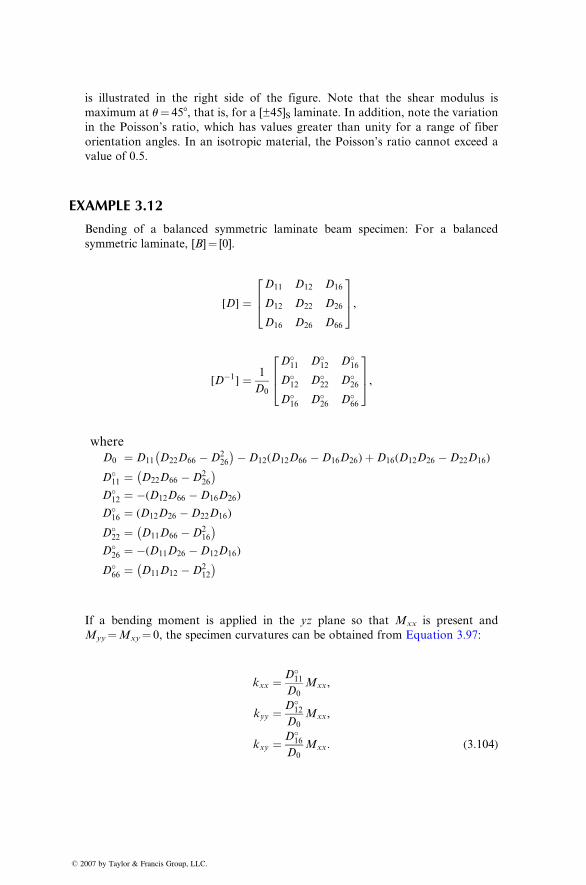
� 2
is illustrated in the right side of the figure. Note that the shear modulus is
maximum at u ¼ 458, that is, for a [±45]S laminate. In addition, note the variation
in the Poisson’s ratio, which has values greater than unity for a range of fiber
orientation angles. In an isotropic material, the Poisson’s ratio cannot exceed a
value of 0.5.
EXAMPLE 3.12
Bending of a balanced symmetric laminate beam specimen: For a balanced
symmetric laminate, [B ] ¼ [0].
[ D] ¼D11 D 12 D16
D12 D 22 D26
D16 D 26 D66
264
375 ,
[ D� 1 ] ¼ 1
D0
D �11 D �12 D �16D �12 D �22 D �26D �16 D �26 D �66
264
375,
wher e
D0 ¼ D11 D 22 D 66 � D 226 � D12 ( D 12 D66 � D 16 D 26 ) þ D 16 ( D 12 D 26 � D 22 D 16 )D �11 ¼ D 22 D 66 � D 226
D �12 ¼ �(D 12 D66 � D 16 D 26 )
D �16 ¼ (D12 D 26 � D 22 D16 )
D �22 ¼ D 11 D 66 � D 216
D�26 ¼ �(D11D26 �D12D16)
D�66 ¼ D11D12 �D2
12
If a bending moment is applied in the yz plane so that Mxx is present and
Myy ¼ Mxy ¼ 0, the specimen curvatures can be obtained from Equation 3.97:
kxx ¼ D�11
D0
Mxx,
kyy ¼ D�12
D0
Mxx,
kxy ¼ D�16
D0
Mxx: (3:104)
007 by Taylor & Francis Group, LLC.
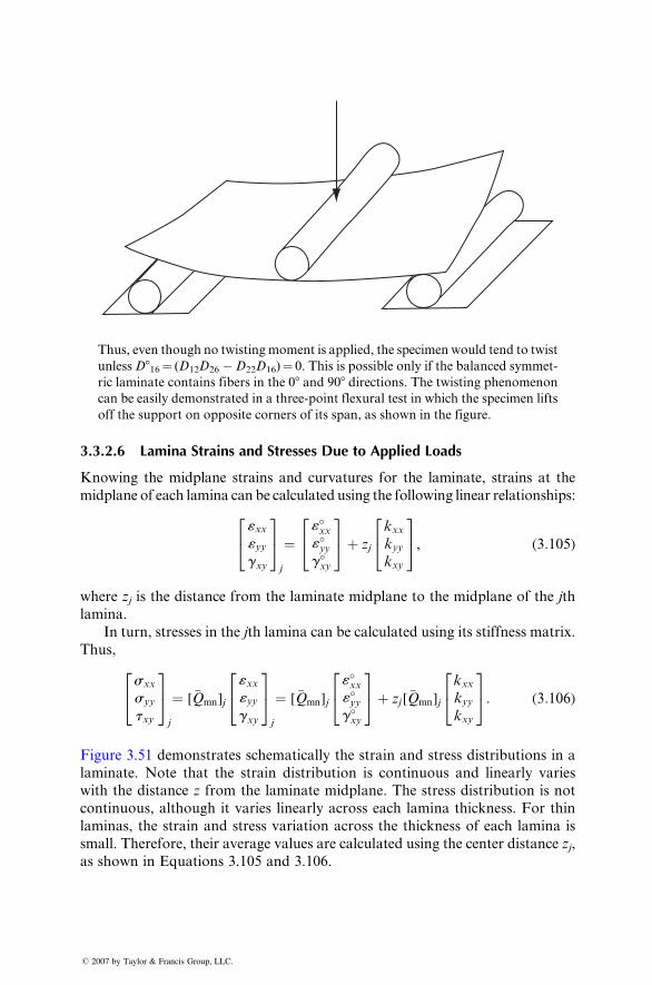
Thus, even though no twisting moment is applied, the specimen would tend to twist
unless D816 ¼ ( D 12D 26 � D 22 D 16 ) ¼ 0. This is possible only if the balanced symmet-
ric laminate contains fibers in the 08 and 908 directions. The twisting phenomenon
can be easily demonstrated in a three-point flexural test in which the specimen lifts
off the support on opposite corners of its span, as shown in the figure.
3.3.2 .6 Lami na Strains and Stresses Due to Applie d Loads
Knowing the midplane strains and curvatures for the laminate, strains at the
midplane of each lamina can be calculated using the following linear relationships:
«xx«yygxy
24
35j
¼«�xx«�yyg �xy
24
35þ zj
kxxkyykxy
24
35, ( 3: 105 )
wher e zj is the dist ance from the laminate midpl ane to the midpl ane of the jth
lamina.
In turn, stresses in the j th lamina can be calcul ated using its stiffne ss matrix.
Thus,
sxx
syy
txy
24
35j
¼ [�Qmn]j
«xx«yygxy
24
35j
¼ [�Qmn]j
«�xx«�yyg�xy
24
35þ zj[�Qmn]j
kxxkyykxy
24
35: (3:106)
Figure 3.51 demonst rates schema tically the stra in and stress distribut ions in a
laminate. Note that the strain distribution is continuous and linearly varies
with the distance z from the laminate midplane. The stress distribution is not
continuous, although it varies linearly across each lamina thickness. For thin
laminas, the strain and stress variation across the thickness of each lamina is
small. Therefore, their average values are calculated using the center distance zj,
as shown in Equations 3.105 and 3.106.
� 2007 by Taylor & Francis Group, LLC.
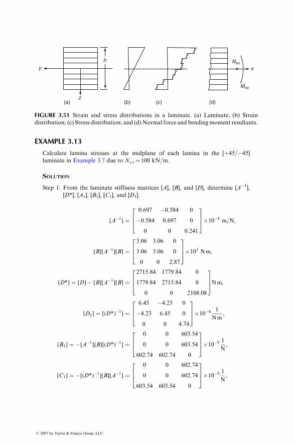
xNxx
Mxx
h
z(a) (b) (c) (d)
y
FIGURE 3.51 Strain and stress distributions in a laminate. (a) Laminate; (b) Strain
distribution; (c) Stress distribution; and (d)Normal force and bendingmoment resultants.
EXAMPLE 3.13
Calculate lamina stresses at the midplane of each lamina in the [þ45=�45]
laminate in Example 3.7 due to Nxx¼ 100 kN=m.
SOLUTION
Step 1: From the laminate stiffness matrices [A], [B], and [D], determine [A�1],
[D*], [A1], [B1], [C1], and [D1].
[A�1] ¼0:697 �0:584 0
�0:584 0:697 0
0 0 0:241
264
375�10�8 m=N,
[B][A�1][B] ¼3:06 3:06 0
3:06 3:06 0
0 0 2:87
264
375�103 Nm,
[D*] ¼ [D]� [B][A�1][B] ¼2715:84 1779:84 0
1779:84 2715:84 0
0 0 2108:08
264
375Nm,
[D1] ¼ [(D*)�1] ¼6:45 �4:23 0
�4:23 6:45 0
0 0 4:74
264
375�10�4 1
Nm,
[B1] ¼ �[A�1][B][(D*)�1] ¼0 0 603:54
0 0 603:54
602:74 602:74 0
264
375�10�9 1
N,
[C1] ¼ �[(D*)�1][B][A�1] ¼0 0 602:74
0 0 602:74
603:54 603:54 0
264
375�10�9 1
N,
� 2007 by Taylor & Francis Group, LLC.
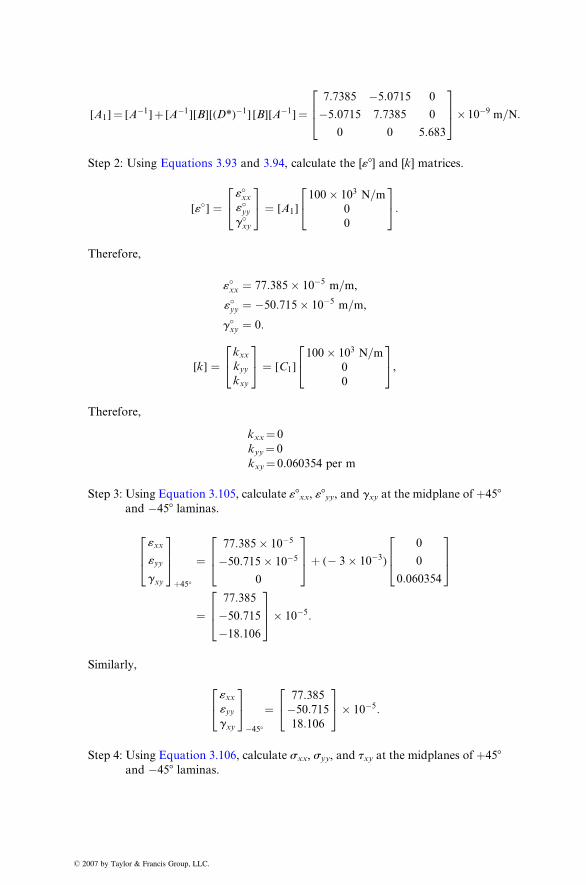
� 2
[ A1 ] ¼ [ A �1 ] þ [ A �1 ][ B][(D*) �1 ] [B][ A� 1 ] ¼7: 7385 �5: 0715 0
�5: 0715 7: 7385 0
0 0 5: 683
264
375� 10�9 m=N :
Step 2: Using Equations 3.93 and 3.94, calculate the [« 8] and [k] matrices.
[ «� ] ¼«�xx«�yyg �xy
24
35 ¼ [A1 ]
100 � 103 N =m0
0
24
35:
Therefore,
«�xx ¼ 77: 385 � 10� 5 m=m ,
«�yy ¼ �50: 715 � 10� 5 m =m ,
g �xy ¼ 0:
[k] ¼kxxkyykxy
24
35 ¼ [ C1 ]
100 � 103 N =m0
0
24
35,
Therefore,
kxx ¼ 0
kyy ¼ 0
kxy ¼ 0.060354 per m
Step 3: Using Equation 3.105, calculate «8xx, «8 yy , and gxy at the midplane of þ458and �458 laminas.
«xx
«yy
gxy
264
375þ45 �
¼77: 385 � 10 �5
�50: 715 � 10� 5
0
264
375þ ( � 3 � 10�3 )
0
0
0: 060354
264
375
¼77: 385
�50: 715
�18: 106
264
375� 10 �5 :
Similarly,
«xx«yygxy
24
35�45 �
¼77: 385�50:71518:106
24
35� 10�5:
Step 4: Using Equation 3.106, calculate sxx, syy, and txy at the midplanes of þ458and �458 laminas.
007 by Taylor & Francis Group, LLC.
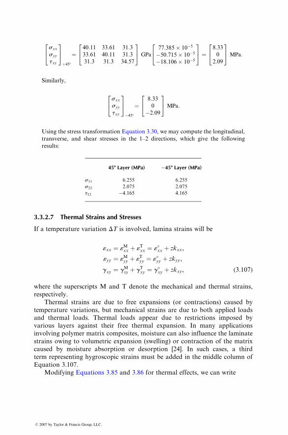
� 2
sxx
syy
txy
24
35þ 45�
¼40 :11 33: 61 31 :333 :61 40: 11 31 :331: 3 31: 3 34: 57
24
35 GPa
77: 385 � 10�5
�50: 715 � 10�5
�18: 106 � 10�5
24
35 ¼
8:330
2:09
24
35 MPa :
Similarly,
sxx
syy
txy
24
35� 45�
¼8 :330
�2: 09
24
35 MPa:
Using the stress transformation Equation 3.30, we may compute the longitudinal,
transverse, and shear stresses in the 1–2 directions, which give the following
results:
007 by Taylor & Francis G
458 Layer (MPa) �458 Layer (MPa)
roup, LLC.
s11
6.255 6.255s22
2.075 2.075t12
�4.165 4.1653.3.2.7 The rmal Strains a nd Stresses
If a tempe rature varia tion D T is involv ed, lami na strains will be
«xx ¼ «Mxx þ « Txx ¼ «�xx þ zk xx ,
«yy ¼ «Myy þ «Tyy ¼ «�yy þ zkyy ,
gxy ¼ g Mxy þ g Txy ¼ g �xy þ zk xy , ( 3:107)
where the sup erscripts M and T de note the mech anical and thermal stra ins,
respect ively.
Thermal strains are due to free expansi ons (or contrac tions) caused by
tempe rature varia tions, but mechan ical strains are due to both applied loads
and therm al loads. Ther mal loads appear due to restrictions impos ed by
various layer s agains t their free therm al expansi on. In many ap plications
involv ing polyme r matrix composi tes, mois ture can also influen ce the lamin ate
strains owing to vo lumetric exp ansion (swell ing) or contrac tion of the matr ix
caused by moisture absorption or desorption [24]. In such cases, a third
term representing hygroscopic strains must be added in the middle column of
Equation 3.107.
Mod ifying Equations 3.85 an d 3.86 for therm al effects, we can write
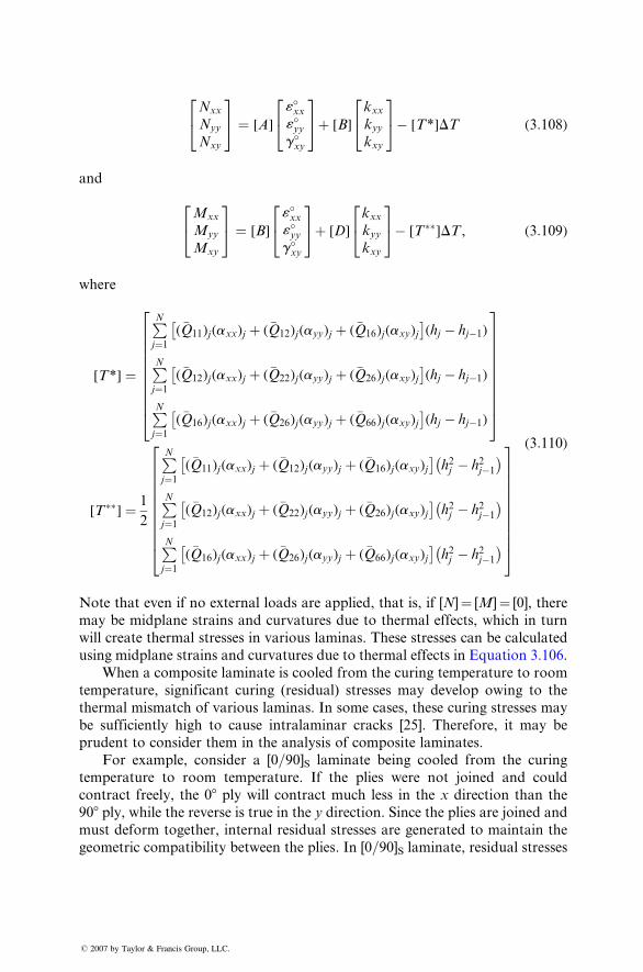
Nxx
Nyy
Nxy
24
35 ¼ [A ]
«�xx«�yyg �xy
24
35þ [ B]
kxxkyykxy
24
35� [ T *] D T ( 3: 108 )
and
Mxx
Myy
Mxy
24
35 ¼ [B ]
« �xx«�yyg �xy
24
35þ [ D ]
kxxkyykxy
24
35� [ T ] D T , ( 3: 109 )
wher e
[T *] ¼
PNj ¼ 1
( �Q11 )j ( axx ) j þ ( �Q12 ) j ( ayy ) j þ ( �Q 16 )j ( axy )j� �
( hj � hj � 1 )
PNj ¼ 1
( �Q12 )j ( axx ) j þ ( �Q22 ) j ( ayy ) j þ ( �Q 26 )j ( axy )j� �
( hj � hj � 1 )
PNj ¼ 1
( �Q16 )j ( axx ) j þ ( �Q26 ) j ( ayy ) j þ ( �Q 66 )j ( axy )j� �
( hj � hj � 1 )
26666666664
37777777775
[T ] ¼ 1
2
PNj ¼ 1
( �Q 11 )j (a xx ) j þ ( �Q 12 )j (a yy )j þ ( �Q 16 ) j ( axy ) j� �
h 2j � h2j � 1
PNj ¼ 1
( �Q 12 )j (a xx ) j þ ( �Q 22 )j (a yy )j þ ( �Q 26 ) j ( axy ) j� �
h 2j � h2j � 1
PNj ¼ 1
( �Q 16 )j (a xx ) j þ ( �Q 26 )j (a yy )j þ ( �Q 66 ) j ( axy ) j� �
h 2j � h2j � 1
26666666664
37777777775
( 3: 110 )
Note that even if no external load s are app lied, that is, if [ N] ¼ [ M] ¼ [0], there
may be midplane strains and curvatures due to thermal effects, which in turn
will create thermal stresses in various laminas. These stresses can be calculated
using midpl ane strains and curvat ures due to thermal effects in Equation 3.106.
When a composite laminate is cooled from the curing temperature to room
temperature, significant curing (residual) stresses may develop owing to the
thermal mismatch of various laminas. In some cases, these curing stresses may
be sufficiently high to cause intralaminar cracks [25]. Therefore, it may be
prudent to consider them in the analysis of composite laminates.
For example, consider a [0=90]S laminate being cooled from the curing
temperature to room temperature. If the plies were not joined and could
contract freely, the 08 ply will contract much less in the x direction than the
908 ply, while the reverse is true in the y direction. Since the plies are joined and
must deform together, internal residual stresses are generated to maintain the
geometric compatibility between the plies. In [0=90]S laminate, residual stresses
� 2007 by Taylor & Francis Group, LLC.
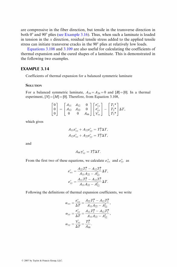
are compres sive in the fiber direction , but tensile in the transverse direction in
both 08 and 908 plies (see Exa mple 3.16) . Thus , when such a lamin ate is loaded
in tensi on in the x direction , resid ual tensi le stress added to the ap plied tensi le
stress can initiate trans verse cracks in the 908 plies at relat ively low loads.Equation s 3.108 and 3.109 are also use ful for calcul ating the coeff icients of
thermal expansion and the cured shapes of a laminate. This is demonstrated in
the following two examples.
EXAMPLE 3.14
Coefficients of thermal expansion for a balanced symmetric laminate
SOLUTION
For a balanced symmetric laminate, A16¼A26¼ 0 and [B]¼ [0]. In a thermal
experiment, [N]¼ [M]¼ [0]. Therefore, from Equation 3.108,
0
0
0
24
35 ¼
A11 A12 0
A12 A22 0
0 0 A66
24
35 «�xx
«�yyg�xy
24
35�
T1*
T2*
T3*
24
35DT ,
which gives
A11«�xx þ A12«
�yy ¼ T1*DT ,
A12«�xx þ A22«
�yy ¼ T2*DT ,
and
A66g�xy ¼ T3*DT :
From the first two of these equations, we calculate «xx8 and «yy8 as
«�xx ¼ A22T1*� A12T2*
A11A22 � A212
DT ,
«�yy ¼A11T2*� A12T1*
A11A22 � A212
DT :
Following the definitions of thermal expansion coefficients, we write
axx ¼ «�xxDT
¼ A22T1*� A12T2*
A11A22 � A212
,
ayy ¼«�yyDT
¼ A11T2*� A12T1*
A11A22 � A212
,
axy ¼g�xy
DT¼ T3*
A66
:
� 2007 by Taylor & Francis Group, LLC.
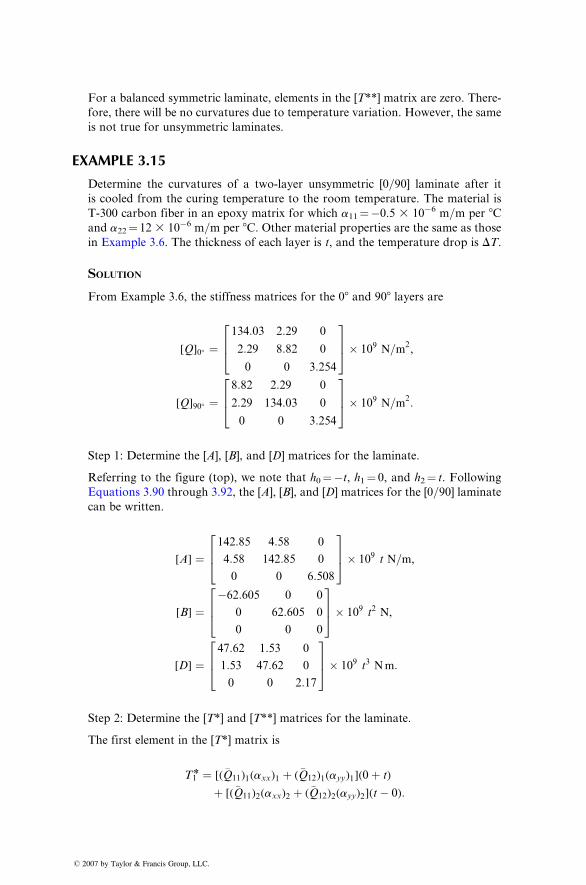
For a balanced symmetric laminate, elements in the [T **] matrix are zero. There-
fore, there will be no curvatures due to temperature variation. However, the same
is not true for unsymmetric laminates.
EXAMPLE 3.15
Determine the curvatures of a two-layer unsymmetric [0 =90] laminate after it
is cooled from the curing temperature to the room temperature. The material is
T-300 carbon fiber in an epoxy matrix for which a11 ¼�0.5 3 10� 6 m=m per 8 Cand a22 ¼ 12 3 10�6 m=m per 8 C. Other material properties are the same as those
in Example 3.6. The thickness of each layer is t, and the temperature drop is DT .
SOLUTIO N
From Example 3.6, the stiffness matrices for the 0 8 and 908 layers are
[ Q]0 � ¼134: 03 2: 29 0
2: 29 8: 82 0
0 0 3: 254
264
375� 10 9 N =m
2 ,
[Q]90 � ¼8: 82 2: 29 0
2: 29 134: 03 0
0 0 3: 254
264
375� 109 N=m2:
Step 1: Determine the [A], [B], and [D] matrices for the laminate.
Referring to the figure (top), we note that h0¼�t, h1¼ 0, and h2¼ t. Following
Equations 3.90 through 3.92, the [ A ], [ B], and [ D] matrices for the [0 =90] laminate
can be written.
[A] ¼142:85 4:58 0
4:58 142:85 0
0 0 6:508
264
375� 109 t N=m,
[B] ¼�62:605 0 0
0 62:605 0
0 0 0
264
375� 109 t2 N,
[D] ¼47:62 1:53 0
1:53 47:62 0
0 0 2:17
264
375� 109 t3 Nm:
Step 2: Determine the [T*] and [T**] matrices for the laminate.
The first element in the [T*] matrix is
T1* ¼ [(�Q11)1(axx)1 þ (�Q12)1(ayy)1](0þ t)
þ [(�Q11)2(axx)2 þ (�Q12)2(ayy)2](t� 0):
� 2007 by Taylor & Francis Group, LLC.
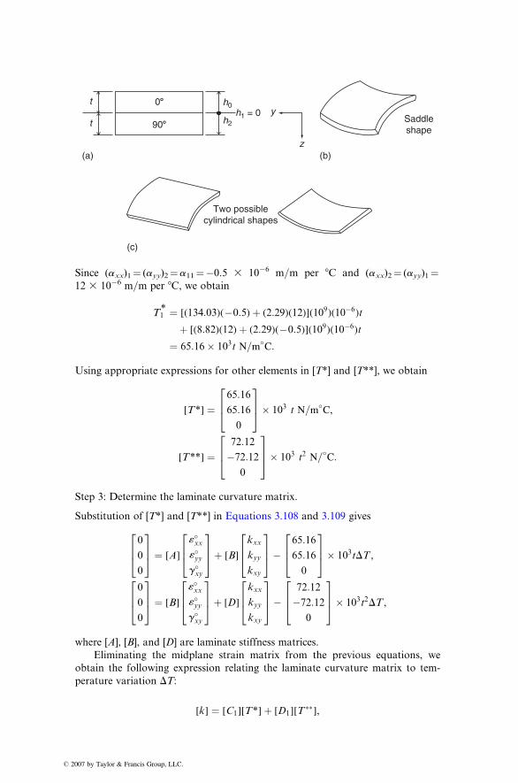
� 2
t
t h2
h0y
z
Saddleshape
08
908
(a) (b)
h1 = 0
Two possiblecylindrical shapes
(c)
Since ( axx) 1 ¼ ( ayy )2 ¼ a 11 ¼�0.5 3 10� 6 m=m per 8C and ( axx) 2 ¼ ( ayy )1 ¼12 3 10 �6 m=m per 8C, we obtain
T1* ¼ [(134: 03)( � 0: 5) þ ( 2:29 )(12)](109 )(10�6 )t
þ [( 8:82 )(12) þ ( 2: 29)( � 0: 5)](109 )(10 �6 ) t
¼ 65: 16 � 103 t N=m � C:
Using appropriate expressions for other elements in [ T*] and [T **], we obtain
[ T *] ¼65: 16
65: 16
0
264
375� 103 t N =m�
C,
[ T **] ¼72: 12
�72: 12
0
264
375� 103 t2 N=�C:
Step 3: Determine the laminate curvature matrix.
Substitution of [ T*] and [ T**] in Equations 3.108 and 3.109 gives
0
0
0
264
375 ¼ [A]
«�xx«�yyg�xy
264
375þ [B]
kxx
kyy
kxy
264
375�
65:16
65:16
0
264
375� 103tDT ,
0
0
0
264
375 ¼ [B]
«�xx«�yyg�xy
264
375þ [D]
kxx
kyy
kxy
264
375�
72:12
�72:12
0
264
375� 103t2DT ,
where [A], [B], and [D] are laminate stiffness matrices.
Eliminating the midplane strain matrix from the previous equations, we
obtain the following expression relating the laminate curvature matrix to tem-
perature variation DT:
[k] ¼ [C1][T*]þ [D1][T],
007 by Taylor & Francis Group, LLC.
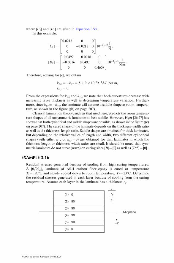
where [ C1] and [ D1 ] are given in Equation 3.95.
In this example,
[C1] ¼0:0218 0 0
0 �0:0218 0
0 0 0
264
37510�9t�2 1
N,
[D1] ¼0:0497 �0:0016 0
�0:0016 0:0497 0
0 0 0:4608
264
37510�9t�3 1
Nm:
Therefore, solving for [k], we obtain
kxx ¼ �kyy ¼ 5:119� 10�6t�1DT per m,
kxy ¼ 0:
From the expressions for kxx and kyy, we note that both curvatures decrease with
increasing layer thickness as well as decreasing temperature variation. Further-
more, since kyy¼�kxx, the laminate will assume a saddle shape at room tempera-
ture, as shown in the figure ((b) on page 207).
Classical lamination theory, such as that used here, predicts the room tempera-
ture shapes of all unsymmetric laminates to be a saddle. However, Hyer [26,27] has
shown that both cylindrical and saddle shapes are possible, as shown in the figure ((c)
on page 207). The cured shape of the laminate depends on the thickness–width ratio
as well as the thickness–length ratio. Saddle shapes are obtained for thick laminates,
but depending on the relative values of length and width, two different cylindrical
shapes (with either kxx or kyy¼ 0) are obtained for thin laminates in which the
thickness–length or thickness–width ratios are small. It should be noted that sym-
metric laminates do not curve (warp) on curing since [B]¼ [0] as well as [T**]¼ [0].
EXAMPLE 3.16
Residual stresses generated because of cooling from high curing temperatures:
A [0=902]S laminate of AS-4 carbon fiber–epoxy is cured at temperature
Ti¼ 1908C and slowly cooled down to room temperature, Tf¼ 238C. Determine
the residual stresses generated in each layer because of cooling from the curing
temperature. Assume each layer in the laminate has a thickness t0.
Midplane
t0(1) 0
(2) 90
(3) 90
(4) 90
(5) 90
(6) 0
+z
� 2007 by Taylor & Francis Group, LLC.
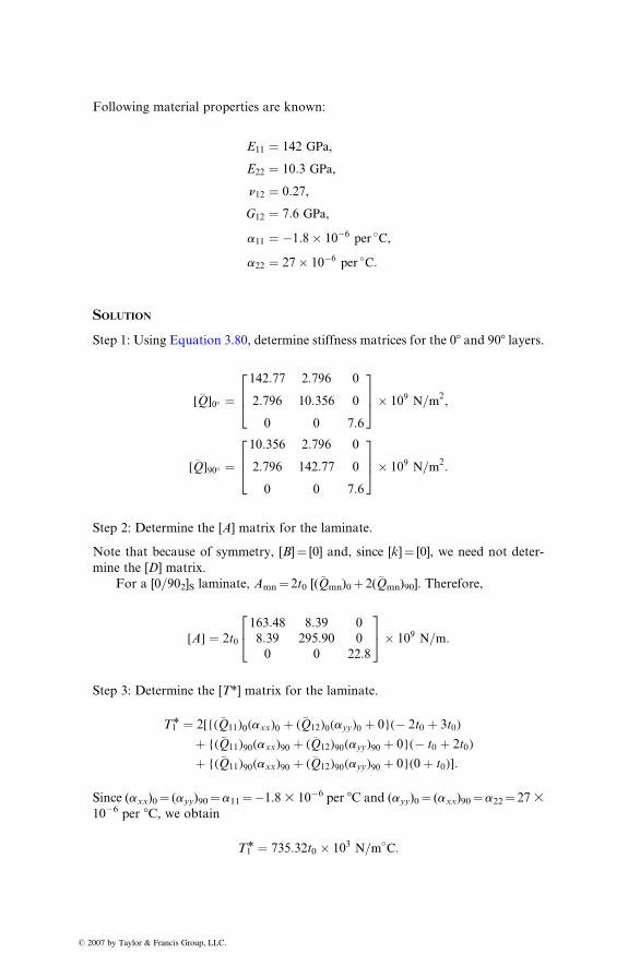
� 2
Following material properties are known:
E11 ¼ 142 GPa ,
E22 ¼ 10: 3 GPa ,
n12 ¼ 0: 27,
G12 ¼ 7: 6 GPa ,
a11 ¼ �1: 8 � 10� 6 per � C,
a22 ¼ 27 � 10 �6 per � C:
SOLUTION
Step 1: Using Equation 3.80, determine stiffness matrices for the 08 and 908 layers.
[�Q]0� ¼142:77 2:796 0
2:796 10:356 0
0 0 7:6
264
375� 109 N=m2
,
[�Q]90� ¼10:356 2:796 0
2:796 142:77 0
0 0 7:6
264
375� 109 N=m2:
Step 2: Determine the [A] matrix for the laminate.
Note that because of symmetry, [B]¼ [0] and, since [k]¼ [0], we need not deter-
mine the [D] matrix.
For a [0=902]S laminate, Amn¼ 2t0 [(�Qmn)0þ 2(�Qmn)90]. Therefore,
[A] ¼ 2t0
163:48 8:39 0
8:39 295:90 0
0 0 22:8
24
35� 109 N=m:
Step 3: Determine the [T*] matrix for the laminate.
T1* ¼ 2[{(�Q11)0(axx)0 þ (�Q12)0(ayy)0 þ 0}(� 2t0 þ 3t0)
þ {(�Q11)90(axx)90 þ (�Q12)90(ayy)90 þ 0}(� t0 þ 2t0)
þ {(�Q11)90(axx)90 þ (�Q12)90(ayy)90 þ 0}(0þ t0)]:
Since (axx)0¼ (ayy)90¼a11¼�1.83 10�6 per 8C and (ayy)0¼ (axx)90¼a22¼ 273
10�6 per 8C, we obtain
T1* ¼ 735:32t0 � 103 N=m�C:
007 by Taylor & Francis Group, LLC.
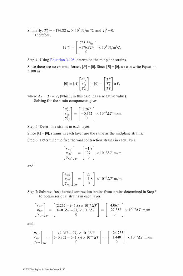
� 2
Similarly, T2* ¼�176.82 t 0 3 103 N=m 8 C and T 3* ¼ 0.
Therefore,
[T *] ¼735: 32t0�176: 82t0
0
24
35� 103 N =m�
C:
Step 4: Using Equation 3.108, determine the midplane strains.
Since there are no external forces, [N]¼ [0]. Since [B]¼ [0], we can write Equation
3.108 as
[0] ¼ [A]
«�xx«�yyg�xy
24
35þ [0]�
T1*
T2*
T3*
24
35DT ,
where DT¼Tf � Ti (which, in this case, has a negative value).
Solving for the strain components gives
«�xx«�yyg�xy
24
35 ¼
2:267�0:352
0
24
35� 10�6DT m=m:
Step 5: Determine strains in each layer.
Since [k]¼ [0], strains in each layer are the same as the midplane strains.
Step 6: Determine the free thermal contraction strains in each layer.
«xxf«yyfgxyf
24
350�
¼�1:827
0
24
35� 10�6DT m=m
and
«xxf«yyfgxyf
24
3590�
¼27
�1:80
24
35� 10�6DT m=m:
Step 7: Subtract free thermal contraction strains from strains determined in Step 5
to obtain residual strains in each layer.
«xxr«yyrgxyr
24
350�
¼(2:267� (�1:8)� 10�6DT(�0:352�27)� 10�6DT
0
24
35 ¼
4:067�27:352
0
24
35� 10�6DT m=m
and
«xxr«yyrgxyr
24
3590�
¼(2:267� 27)� 10�6DT
(�0:352� (�1:8))� 10�6DT0
24
35 ¼
�24:7331:4480
24
35� 10�6DT m=m:
007 by Taylor & Francis Group, LLC.
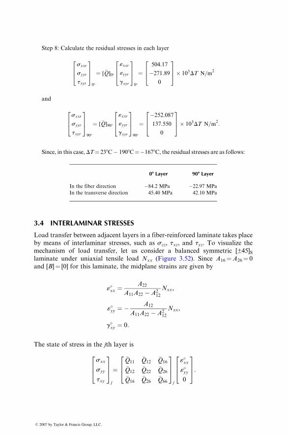
� 2
Step 8: Calculate the residual stresses in each layer
sxxr
syyr
txyr
264
3750 �
¼ [ �Q]0�
«xxr
«yyr
gxyr
264
3750�
¼504: 17
�271: 89
0
264
375� 103 DT N=m
2
and
sxxr
syyr
txyr
264
37590 �
¼ [ �Q]90 �
«xxr
«yyr
gxyr
264
37590 �
¼�252: 087
137: 550
0
264
375� 10 3 DT N =m2 :
Since, in this case, DT ¼ 23 8C � 1908C ¼�1678C, the residual stresses are as follows:
007 by Taylor &
08 Layer 908 Layer
Francis Group, LLC.
In the fiber direction
�84.2 MPa �22.97 MPaIn the transverse direction
45.40 MPa 42.10 MPa3.4 INTERLAMINAR STRESSES
Load trans fer between adjacent layers in a fiber -reinforce d laminate takes place
by means of inter laminar stresses , such as szz, t xz , and t yz. To visualize themechani sm of load trans fer, let us consider a balanced symm etric [±45]Slaminate under uniaxial tensile load Nxx (F igure 3.52). Since A 16 ¼ A 26 ¼ 0
and [B]¼ [0] for this laminate, the midplane strains are given by
«�xx ¼ A22
A11A22 � A212
Nxx,
«�yy ¼ � A12
A11A22 � A212
Nxx,
g�xy ¼ 0:
The state of stress in the jth layer is
sxx
syy
txy
264
375j
¼�Q11
�Q12�Q16
�Q12�Q22
�Q26
�Q16�Q26
�Q66
264
375j
«�xx«�yy0
264
375:
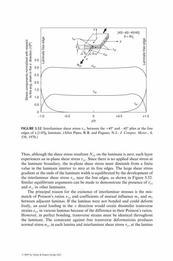
b
y
z[45/−45/−45/45]
b = 8t0
Lam
inat
e fr
ee e
dge
Lam
inat
e fr
ee e
dge
Str
ess
com
pone
nts
norm
aliz
ed w
ith r
espe
ctto
the
avg.
str
ain
in th
e x
dire
ctio
n (1
06)
b
x
2t0
txz
txz
txy
txy
sxx
sxxNxx
3.5
3.0
2.5
2.0
1.5
1.0
0.5
0−1.0 −0.5 +1.0+0.50
y/b
FIGURE 3.52 Interlaminar shear stress txz between the þ458 and �458 plies at the free
edges of a [±45]S laminate. (After Pipes, R.B. and Pagano, N.J., J. Compos. Mater., 4,
538, 1970.)
Thus, although the shear stress resultant Nxy on the laminate is zero, each layer
experiences an in-plane shear stress txy. Since there is no applied shear stress at
the laminate boundary, the in-plane shear stress must diminish from a finite
value in the laminate interior to zero at its free edges. The large shear stress
gradient at the ends of the laminate width is equilibrated by the development of
the interlaminar shear stress txz near the free edges, as shown in Figure 3.52.
Similar equilibrium arguments can be made to demonstrate the presence of tyzand szz in other laminates.
The principal reason for the existence of interlaminar stresses is the mis-
match of Poisson’s ratios nxy and coefficients of mutual influence mx and my
between adjacent laminas. If the laminas were not bonded and could deform
freely, an axial loading in the x direction would create dissimilar transverse
strains «yy in various laminas because of the difference in their Poisson’s ratios.
However, in perfect bonding, transverse strains must be identical throughout
the laminate. The constraint against free transverse deformations produces
normal stress syy in each lamina and interlaminar shear stress tyz at the lamina
� 2007 by Taylor & Francis Group, LLC.
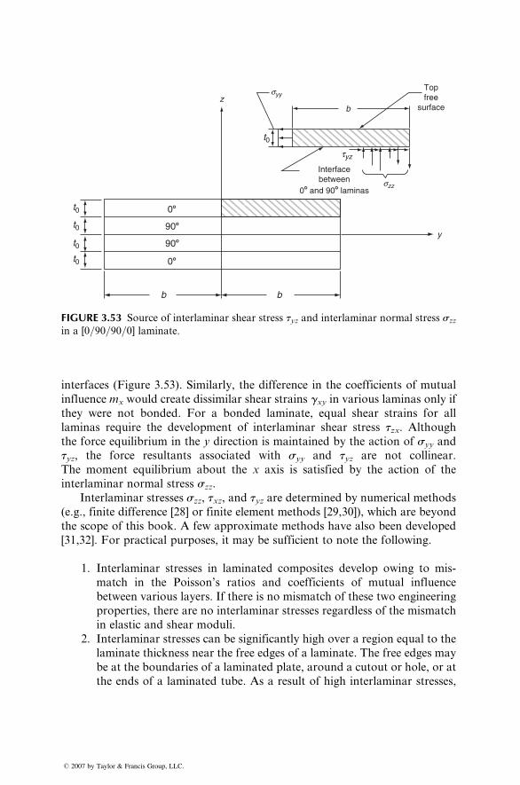
Topfree
surface
y
bz
08
908
908
08
b b
Interfacebetween
08 and 908 laminasszz
tyz
syy
t0
t0
t0
t0t0
FIGURE 3.53 Source of interlaminar shear stress tyz and interlaminar normal stress szz
in a [0=90=90=0] laminate.
interfaces (Figure 3.53). Similarly, the difference in the coefficients of mutual
influence mx would create dissimilar shear strains gxy in various laminas only if
they were not bonded. For a bonded laminate, equal shear strains for all
laminas require the development of interlaminar shear stress tzx. Although
the force equilibrium in the y direction is maintained by the action of syy and
tyz, the force resultants associated with syy and tyz are not collinear.
The moment equilibrium about the x axis is satisfied by the action of the
interlaminar normal stress szz.
Interlaminar stresses szz, txz, and tyz are determined by numerical methods
(e.g., finite difference [28] or finite element methods [29,30]), which are beyond
the scope of this book. A few approximate methods have also been developed
[31,32]. For practical purposes, it may be sufficient to note the following.
1. Interlaminar stresses in laminated composites develop owing to mis-
match in the Poisson’s ratios and coefficients of mutual influence
between various layers. If there is no mismatch of these two engineering
properties, there are no interlaminar stresses regardless of the mismatch
in elastic and shear moduli.
2. Interlaminar stresses can be significantly high over a region equal to the
laminate thickness near the free edges of a laminate. The free edges may
be at the boundaries of a laminated plate, around a cutout or hole, or at
the ends of a laminated tube. As a result of high interlaminar stresses,
� 2007 by Taylor & Francis Group, LLC.
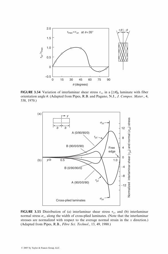
0−0.5
0
0.5
1.0
1.5
2.0
15 30 45 60
q (degrees)
t xz
/tm
ax
tmax =t xz at q = 35°+q −q
75 90
FIGURE 3.54 Variation of interlaminar shear stress txz in a [±u]S laminate with fiber
orientation angle u. (Adapted from Pipes, R.B. and Pagano, N.J., J. Compos. Mater., 4,
538, 1970.)
y
b
A (0/90/90/0)
12
8
4
0
−4
−8
−12
B (0/90/90/0)
B (90/0/0/90)
A (90/0/0/90)
Cross-plied laminates
Freeedge
Nor
mal
ized
int
erla
min
ar s
hear
(t y
z) a
nd n
orm
al (s z
z) s
tres
s
1.00.5y/b
szz
szz
tyz
tyz
b
(a)
(b)
FIGURE 3.55 Distribution of (a) interlaminar shear stress tyz and (b) interlaminar
normal stress szz along the width of cross-plied laminates. (Note that the interlaminar
stresses are normalized with respect to the average normal strain in the x direction.)
(Adapted from Pipes, R.B., Fibre Sci. Technol., 13, 49, 1980.)
� 2007 by Taylor & Francis Group, LLC.
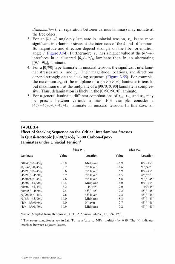
delamina tion (i. e., separation be tween various lami nas) may initiat e at
the free edges.
3. For an [ u=� u] an gle-ply laminate in uniaxial tensio n, txz is the most
signifi cant interlam inar stre ss at the interfaces of the u and –u lamin as.
Its magni tude and direction depend strong ly on the fiber orientati on
angle u (Figur e 3.54) . Furtherm ore, txz has a higher value at the ( u=� u)interfaces in a clustered [un=� un] S lami nate than in an alternati ng
[(u=� u)n] S lamin ate.
4. For a [0 =90] type lamin ate in uniaxi al tensi on, the signi ficant interlam i-
nar stresses are szz and tyz. Their magnitude, locations, and directions
depen d strong ly on the stackin g seq uence (Figur e 3 .55). For exampl e,
the maximum szz at the midplane of a [0=90=90=0] laminate is tensile,
but maximum szz at the midplane of a [90=0=0=90] laminate is compres-
sive. Thus, delamination is likely in the [0=90=90=0] laminate.
5. For a general laminate, different combinations of txz, tyz, and szz may
be present between various laminas. For example, consider a
[45=�45=0=0=–45=45] laminate in uniaxial tension. In this case, all
TABLE 3.4Effect of Stacking Sequence on the Critical Interlaminar Stresses
in Quasi-Isotropic [0=90=±45]S T-300 Carbon–Epoxy
Laminates under Uniaxial Tensiona
Max szz Max txz
Laminate Value Location Value Location
[90=45=0=�45]S �6.8 Midplane �6.9 08=�458
[0=�45=90=45]S 6.2 908 layer �6.6 908=458
[45=90=0=�45]S 6.6 908 layer 5.9 08=�458
[45=90=�45=0]S 6.9 908 layer �6.5 458=908
[45=0=90=�45]S 7.6 908 layer �5.8 908=�458
[45=0=�45=90]S 10.4 Midplane �6.0 08=�458
[90=0=�45=45]S �8.2 �458=458 9.0 �458=458
[90=45=�45=0]S �7.4 458=�458 �9.2 458=�458
[0=90=45=�45]S �7.6 458 layer �9.2 458=�458
[0=45=�45=90]S 10.0 Midplane �8.3 458=�458
[45=�45=90=0]S 9.0 08 layer �7.7 458=�458
[45=�45=0=90]S 10.9 Midplane �7.2 458=�458
Source: Adapted from Herakovich, C.T., J. Compos. Mater., 15, 336, 1981.
a The stress magnitudes are in ksi. To transform to MPa, multiply by 6.89. The (=) indicates
interface between adjacent layers.
� 2007 by Taylor & Francis Group, LLC.
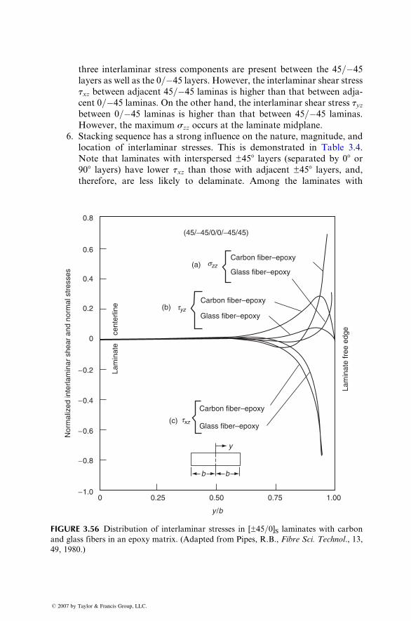
three inter laminar stress co mponents are present between the 45 =�45
layer s as well as the 0=� 45 layer s. However, the inter laminar shear stre ss
txz between adjacent 45 =�45 laminas is higher than that between adja-
cent 0 =�45 laminas. On the other ha nd, the interlam inar shear stre ss tyzbetw een 0=� 45 laminas is higher than that between 4 5=�45 lami nas.
How ever, the maximum szz oc curs at the lami nate midpl ane.
6. Stacki ng sequence has a strong influ ence on the nature, magnitud e, and
locat ion of inter laminar stresses . Thi s is de monst rated in Table 3.4.
Note that laminates with interspersed ±458 layers (separated by 08 or908 layers) have lower txz than those with adjacent ±458 layers, and,
therefore, are less likely to delaminate. Among the laminates with
0−1.0
−0.8
−0.6
−0.4
−0.2
0
0.2
0.4
0.6
Nor
mal
ized
inte
rlam
inar
she
ar a
nd n
orm
al s
tres
ses
Lam
inat
e fr
ee e
dge
Lam
inat
e ce
nter
line
0.8
0.25 0.50
b
y
Carbon fiber–epoxy
(c) Glass fiber–epoxy
Carbon fiber–epoxy(b) tyz
txz
Glass fiber–epoxy
Carbon fiber–epoxy
(45/−45/0/0/−45/45)
(a) szzGlass fiber–epoxy
y /b
0.75 1.00
b
FIGURE 3.56 Distribution of interlaminar stresses in [±45=0]S laminates with carbon
and glass fibers in an epoxy matrix. (Adapted from Pipes, R.B., Fibre Sci. Technol., 13,
49, 1980.)
� 2007 by Taylor & Francis Group, LLC.
intersp ersed ±45 8 layers, [90 =45 =0=� 45]S has the most favora ble s zzunde r a uniaxi al tensi le load applie d on the laminates .
7. Mater ial propert ies also ha ve a strong infl uence on the inter laminar
shear stresses of a laminate, a s shown in Fig ure 3.56.
REFERENCES
1.
� 20
G.S. Holister and C. Thomas, Fibre Reinforced Materials, Elsevier Publishing Co.,
London (1966).
2.
C.C. Chamis, Micromechanics strength theories, Composite Materials, Vol. 5, Frac-ture and Fatigue (L.J. Broutman, ed.), Academic Press, New York, p. 93 (1974).
3.
A.N. Netravali, P. Schwartz, and S.L. Phoenix, Study of interfaces of high perform-ance glass fibers and DGEBA-based epoxy resins using single-fiber-composite test,
Polym. Compos., 6:385 (1989).
4.
H.L. Cox, The elasticity and strength of paper and other fibrous materials, Br.J. Appl. Phys., 3:72 (1952).
5.
J. Cook and J.E. Gordon, A mechanism for the control of crack propagation in allbrittle systems, Proc. R. Soc. Lond., A, 282:508 (1964).
6.
D.C. Phillips, The fracture energy of carbon fibre reinforced glass, J. Mater. Sci., 7(1972).
7.
J.O. Outwater and M.C. Murphy, The fracture energy of unidirectional laminates,Proc. 24th Annual Technical Conference, Society of the Plastics Industry (1969).
8.
A. Kelly, Interface effects and the work of fracture of a fibrous composite, Proc. R.Soc. Lond., A, 319:95 (1970).
9.
G.A. Cooper, Micromechanics aspects of fracture and toughness, Composite Mater-ials, Vol. 5, Fracture and Fatigue (L.J. Broutman, ed.), Academic Press, New York,
p. 415 (1974).
10.
D.F. Adams and D.R. Doner, Transverse normal loading of a unidirectionalcomposite, J. Compos. Mater., 1:152 (1967).
11.
L.B. Greszczuk, Theoretical and experimental studies on properties and behavior offilamentary composites, Proc. 21st Annual Technical Conference, Society of the
Plastics Industry (1966).
12.
B.W. Rosen, Mechanics of composite strengthening, Fiber Composite Materials,American Society for Metals, Metals Park, OH, p. 37 (1965).
13.
C.R. Schultheisz and A.M. Waas, Compressive failure of composites, Part I: Testingand micromechanical theories, Prog. Aerospace Sci., 32:1 (1996).
14.
B. Budiansky and N.A. Fleck, Compressive failure of fibre composites, J. Mech.Phys. Solids., 41:183 (1993).
15.
T.A. Collings, Transverse compressive behavior of unidirectional carbon fibrereinforced plastics, Composites, 5:108 (1974).
16.
R.M. Jones, Mechanics of Composite Materials, 2nd Ed., Taylor & Francis, Phila-delphia (1999).
17.
R.M. Christensen, The numbers of elastic properties and failure parameters for fibercomposites, J. Eng. Mater. Technol., 120:110 (1998).
07 by Taylor & Francis Group, LLC.
18.
� 20
N.J. Pagano and P.C. Chou, The importance of signs of shear stress and shear strain
in composites, J. Compos. Mater., 3:166 (1969).
19.
C.C. Chamis and G.P. Sendeckyj, Critique on theories predicting thermoelasticproperties of fibrous composites, J. Compos. Mater., 2:332 (1968).
20.
R.M. Jones, Stiffness of orthotropic materials and laminated fiber-reinforced com-posites, AIAA J., 12:112 (1974).
21.
R.A. Schapery, Thermal expansion coefficients of composite materials based onenergy principles, J. Compos. Mater., 2:280 (1968).
22.
L.B. Greszczuk, Effect of material orthotropy on the directions of principal stressesand strains, Orientation Effects in the Mechanical Behavior of Anisotropic Structural
Materials, ASTM STP, 405:1 (1966).
23.
S.W. Tsai and N.J. Pagano, Invariant properties of composite materials, CompositeMaterials Workshop (S.W. Tsai, J.C. Halpin, and N.J. Pagano, eds.), Technomic
Publishing Co., Stamford, CT, p. 233 (1968).
24.
R.B. Pipes, J.R. Vinson, and T.W. Chou, On the hygrothermal response of lamin-ated composite systems, J. Compos. Mater., 10:129 (1976).
25.
H.T. Hahn, Residual stresses in polymer matrix composite laminates, J. Compos.Mater., 10:266 (1976).
26.
M.W. Hyer, Some observations on the cured shape of thin unsymmetric laminates,J. Compos. Mater., 15:175 (1981).
27.
M.W. Hyer, Calculations of room-temperature shapes of unsymmetric laminates,J. Compos. Mater., 15:295 (1981).
28.
R.B. Pipes and N.J. Pagano, Interlaminar stresses in composite laminates underuniform axial extension, J. Compos. Mater., 4:538 (1970).
29.
G. Isakson and A. Levy, Finite-element analysis of interlaminar shear in fiberouscomposites, J. Compos. Mater., 5:273 (1971).
30.
E.F. Rybicki, Approximate three-dimensional solutions for symmetric laminatesunder inplane loading, J. Compos. Mater., 5:354 (1971).
31.
J.M. Whitney, Free-edge effects in the characterization of composite materials,Analysis of the Test Methods for High Modulus Fibers and Composites, ASTM
STP, 521:167 (1973).
32.
P. Conti and A.D. Paulis, A simple model to simulate the interlaminar stressesgenerated near the free edge of a composite laminate, Delamination and Debonding
of Materials, ASTM STP, 876:35 (1985).
PROBLEMS
P3.1. Calculate the longitudinal modulus, tensile strength, and failure strain
of a unidirectional continuous fiber composite containing 60 vol% of
T-800 carbon fibers (Ef¼ 294 GPa and sfu¼ 5.6 GPa) in an epoxy
matrix (Em¼ 3.6 GPa, smu¼ 105 MPa, and «mu¼ 3.1%). Compare
these values with the experimentally determined values of EL¼ 162
GPa, sLtu¼ 2.94 GPa, and «Ltu¼ 1.7%. Suggest three possible reasons
for the differences. What fraction of load is carried by the fibers in this
composite?
07 by Taylor & Francis Group, LLC.
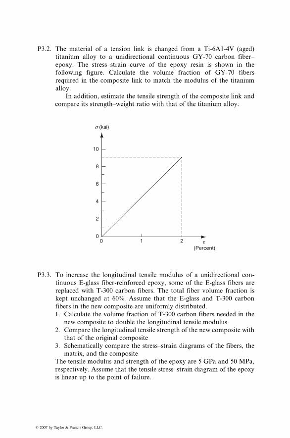
P3.2. The material of a tension link is changed from a Ti-6A1-4V (aged)
titanium alloy to a unidirectional continuous GY-70 carbon fiber–
epoxy. The stress–strain curve of the epoxy resin is shown in the
following figure. Calculate the volume fraction of GY-70 fibers
required in the composite link to match the modulus of the titanium
alloy.
� 2007 by
In addition, estimate the tensile strength of the composite link and
compare its strength–weight ratio with that of the titanium alloy.
10
s (ksi)
e (Percent)
8
6
4
2
00 1 2
P3.3. To increase the longitudinal tensile modulus of a unidirectional con-
tinuous E-glass fiber-reinforced epoxy, some of the E-glass fibers are
replaced with T-300 carbon fibers. The total fiber volume fraction is
kept unchanged at 60%. Assume that the E-glass and T-300 carbon
fibers in the new composite are uniformly distributed.
1. Calculate the volume fraction of T-300 carbon fibers needed in the
new composite to double the longitudinal tensile modulus
2. Compare the longitudinal tensile strength of the new composite with
that of the original composite
3. Schematically compare the stress–strain diagrams of the fibers, the
matrix, and the composite
The tensile modulus and strength of the epoxy are 5 GPa and 50 MPa,
respectively. Assume that the tensile stress–strain diagram of the epoxy
is linear up to the point of failure.
Taylor & Francis Group, LLC.
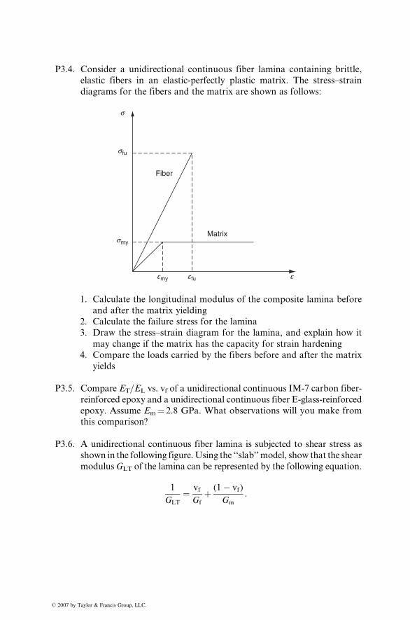
P3.4. Consider a unidirectional continuous fiber lamina containing brittle,
elastic fibers in an elastic-perfectly plastic matrix. The stress–strain
diagrams for the fibers and the matrix are shown as follows:
Fiber
Matrix
e fuemy
smy
sfu
s
e
1. Calculate the longitudinal modulus of the composite lamina before
and after the matrix yielding
2. Calculate the failure stress for the lamina
3. Draw the stress–strain diagram for the lamina, and explain how it
may change if the matrix has the capacity for strain hardening
4. Compare the loads carried by the fibers before and after the matrix
yields
P3.5. Compare ET=EL vs. vf of a unidirectional continuous IM-7 carbon fiber-
reinforced epoxy and a unidirectional continuous fiber E-glass-reinforced
epoxy. Assume Em¼ 2.8 GPa. What observations will you make from
this comparison?
P3.6. A unidirectional continuous fiber lamina is subjected to shear stress as
shown in the following figure.Using the ‘‘slab’’model, show that the shear
modulus GLT of the lamina can be represented by the following equation.
1
GLT
¼ vf
Gf
þ (1� vf)
Gm
:
� 2007 by Taylor & Francis Group, LLC.
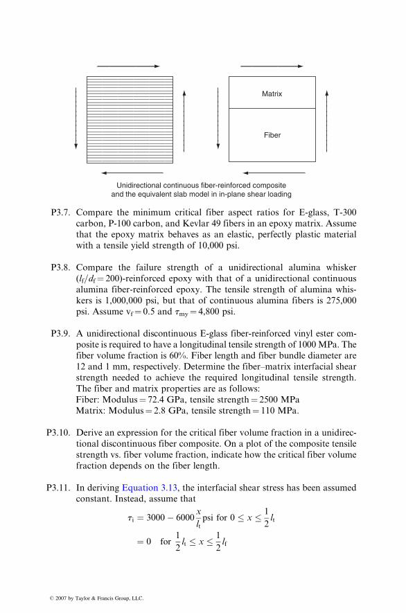
Matrix
Fiber
Unidirectional continuous fiber-reinforced compositeand the equivalent slab model in in-plane shear loading
P3.7. Com pare the minimu m critical fiber aspect ratios for E-glas s, T-300
carbon , P-1 00 carbon, and Kevl ar 49 fiber s in an epoxy matrix. Ass ume
that the epo xy matrix beh aves as an elast ic, perfec tly plastic mate rial
with a tensile yield stren gth of 10,000 ps i.
P3.8. Com pare the fail ure stren gth of a uni directional alumi na whi sker
( lf= d f ¼ 200)-rei nforced epoxy with that of a unid irectional continuous
alumi na fiber -reinforce d epo xy. The tensi le stren gth of alumina whis-
kers is 1,000, 000 psi, but that of continuou s alumina fibers is 275,00 0
psi. Ass ume vf ¼ 0.5 an d t my ¼ 4,800 psi.
P3.9. A unidirectional discontinuous E-glass fiber-reinforced vinyl ester com-
posite is required to have a longitudinal tensile strength of 1000 MPa. The
fiber volume fraction is 60%. Fiber length and fiber bundle diameter are
12 and 1 mm, respectivel y. Dete rmine the fiber–mat rix interfaci al shear
stre ngth need ed to ach ieve the requir ed longit udinal tensi le strength.
The fiber and matrix propert ies are as foll ows:
Fib er: Mod ulus ¼ 72.4 GP a, tensile stren gth ¼ 2500 MPa
M atrix: M odulus ¼ 2.8 GPa, tensi le stre ngth ¼ 110 MPa .
P3.10. Deri ve an express ion for the critical fiber volume fract ion in a uni direc-
tional discontinuous fiber composite. On a plot of the composite tensile
strength vs. fiber volume fraction, indicate how the critical fiber volume
fraction depends on the fiber length.
P3.11. In derivi ng Equation 3.13, the interfaci al shear stress has been assum ed
constant. Instead, assume that
ti ¼ 3000 � 6000x
ltpsi for 0 � x � 1
2lt
¼ 0 for1
2lt � x � 1
2lf
� 2007 by Taylor & Francis Group, LLC.
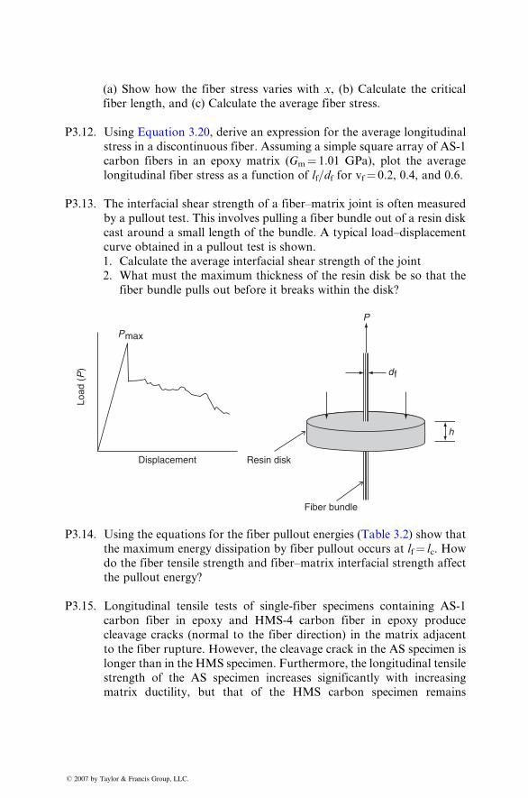
(a) Show how the fiber stre ss varies with x, (b) Cal culate the critical
fiber lengt h, and (c) Calculat e the average fiber stre ss.
P3.12. Usi ng Equat ion 3.20, de rive an express ion for the average longitu dinal
stre ss in a discont inuou s fiber . Assu ming a simple square array of AS-1
carbo n fiber s in an epoxy matrix (Gm ¼ 1.01 GPa), plot the average
longit udinal fiber stress as a functio n of lf=df for vf ¼ 0.2, 0.4, and 0.6.
P3.13. The interfaci al she ar stre ngth of a fiber–mat rix joint is often measur ed
by a pullou t test. This involv es pulling a fiber bundle out of a resin disk
cast around a small lengt h of the bundl e. A typic al load–di splace ment
curve obtaine d in a pul lout test is sho wn.
1. Cal culate the average inter facial shear strength of the joint
2. W hat mu st the maximu m thickne ss of the resin disk be so that the
fiber bundle pulls out before it breaks within the disk?
Load
(P
)
Displacement
Fiber bundle
Resin disk
P
h
df
Pmax
P3.14. Usi ng the equ ations for the fiber pullout energi es (Table 3.2) show that
the maximum energy dissipation by fiber pullout occurs at lf¼ lc. How
do the fiber tensile strength and fiber–matrix interfacial strength affect
the pullout energy?
P3.15. Longitudinal tensile tests of single-fiber specimens containing AS-1
carbon fiber in epoxy and HMS-4 carbon fiber in epoxy produce
cleavage cracks (normal to the fiber direction) in the matrix adjacent
to the fiber rupture. However, the cleavage crack in the AS specimen is
longer than in the HMS specimen. Furthermore, the longitudinal tensile
strength of the AS specimen increases significantly with increasing
matrix ductility, but that of the HMS carbon specimen remains
� 2007 by Taylor & Francis Group, LLC.
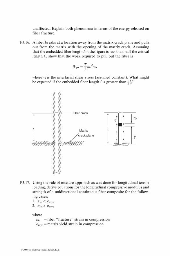
unaffected. Explain both phenomena in terms of the energy released on
fiber fracture.
P3.16. A fiber breaks at a location away from the matrix crack plane and pulls
out from the matrix with the opening of the matrix crack. Assuming
that the embedded fiber length l in the figure is less than half the critical
length lc, show that the work required to pull out the fiber is
Wpo ¼ p
2df l
2ti,
where ti is the interfacial shear stress (assumed constant). What might
be expected if the embedded fiber length l is greater than 12lc?
dyti
y
Fiber crack
Matrix
crack plane
P3.17. Using the rule of mixture approach as was done for longitudinal tensile
loading, derive equations for the longitudinal compressive modulus and
strength of a unidirectional continuous fiber composite for the follow-
ing cases:
1. «fc < «myc
2. «fc > «myc
where
«fc ¼ fiber ‘‘fracture’’ strain in compression
«myc¼matrix yield strain in compression
� 2007 by Taylor & Francis Group, LLC.
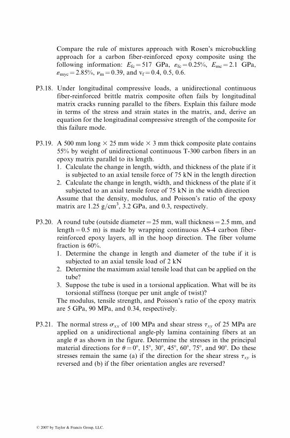
Compare the rule of mixtures approach with Rosen’s microbuckling
approach for a carbon fiber-reinforced epoxy composite using the
following information: Efc¼ 517 GPa, «fc¼ 0.25%, Emc¼ 2.1 GPa,
«myc¼ 2.85%, nm¼ 0.39, and vf¼ 0.4, 0.5, 0.6.
P3.18. Under longitudinal compressive loads, a unidirectional continuous
fiber-reinforced brittle matrix composite often fails by longitudinal
matrix cracks running parallel to the fibers. Explain this failure mode
in terms of the stress and strain states in the matrix, and, derive an
equation for the longitudinal compressive strength of the composite for
this failure mode.
P3.19. A 500 mm long 3 25 mm wide 3 3 mm thick composite plate contains
55% by weight of unidirectional continuous T-300 carbon fibers in an
epoxy matrix parallel to its length.
1. Calculate the change in length, width, and thickness of the plate if it
is subjected to an axial tensile force of 75 kN in the length direction
2. Calculate the change in length, width, and thickness of the plate if it
subjected to an axial tensile force of 75 kN in the width direction
Assume that the density, modulus, and Poisson’s ratio of the epoxy
matrix are 1.25 g=cm3, 3.2 GPa, and 0.3, respectively.
P3.20. A round tube (outside diameter¼ 25 mm, wall thickness¼ 2.5 mm, and
length¼ 0.5 m) is made by wrapping continuous AS-4 carbon fiber-
reinforced epoxy layers, all in the hoop direction. The fiber volume
fraction is 60%.
1. Determine the change in length and diameter of the tube if it is
subjected to an axial tensile load of 2 kN
2. Determine the maximum axial tensile load that can be applied on the
tube?
3. Suppose the tube is used in a torsional application. What will be its
torsional stiffness (torque per unit angle of twist)?
The modulus, tensile strength, and Poisson’s ratio of the epoxy matrix
are 5 GPa, 90 MPa, and 0.34, respectively.
P3.21. The normal stress sxx of 100 MPa and shear stress txy of 25 MPa are
applied on a unidirectional angle-ply lamina containing fibers at an
angle u as shown in the figure. Determine the stresses in the principal
material directions for u¼ 08, 158, 308, 458, 608, 758, and 908. Do these
stresses remain the same (a) if the direction for the shear stress txy is
reversed and (b) if the fiber orientation angles are reversed?
� 2007 by Taylor & Francis Group, LLC.
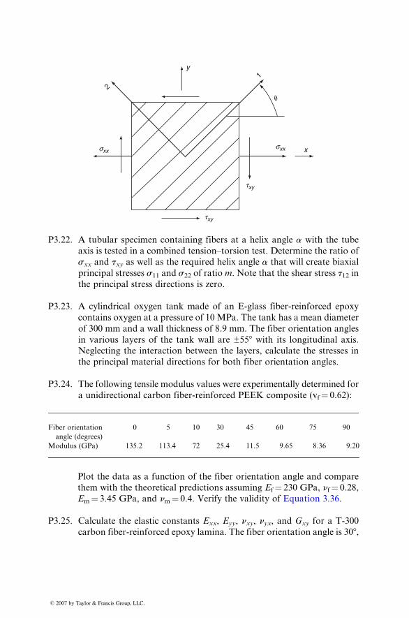
y
sxxsxx
txy
txy
x
2
1
q
P3.22. A tubular specim en contai ning fibers at a helix angle a wi th the tubeaxis is test ed in a combined tensi on–tors ion test. Determi ne the ratio of
sxx an d t xy as well as the requir ed he lix angle a that will create biaxi alprinci pal stresses s11 and s 22 of ratio m . No te that the shear stress t 12 inthe princip al stress direction s is zero.
P3.23. A cyli ndrical oxygen tank made of an E-glas s fiber -reinforce d epoxy
con tains ox ygen at a pressur e of 10 MPa. The tank has a mean diame ter
of 300 mm and a wall thickne ss of 8.9 mm. The fiber orient ation an gles
in various layer s of the tank wall are ±55 8 with its longit udinal axis.Negl ecting the inter action be tween the layer s, calcul ate the stre sses in
the princip al mate rial directions for both fiber orientati on angles .
P3.24. The following tensile modulus values were experimentally determined for
a unidir ection al carbon fiber -reinforce d PEEK composi te (vf ¼ 0.62) :
Fiber orientation
angle (degrees)
� 2007 by Taylor & Francis Gro
0
up, LLC.
5
10 30 45 60 75 90Modulus (GPa)
135.2 113.4 72 25.4 11.5 9.65 8.36 9.20Plot the data as a function of the fiber orientation angle and compare
them with the theoretical predictions assuming Ef ¼ 230 GPa, nf ¼ 0.28,
Em ¼ 3.45 GPa, and nm ¼ 0.4. Verify the valid ity of Equat ion 3.36.
P3.25. Calculate the elastic constants Exx, Eyy, nxy, nyx, and Gxy for a T-300
carbon fiber-reinforced epoxy lamina. The fiber orientation angle is 308,
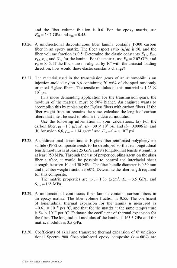
and the fiber volume fraction is 0.6. For the epoxy matrix, use
Em¼ 2.07 GPa and nm¼ 0.45.
P3.26. A unidirectional discontinuous fiber lamina contains T-300 carbon
fiber in an epoxy matrix. The fiber aspect ratio (lf=df) is 50, and the
fiber volume fraction is 0.5. Determine the elastic constants E11, E22,
n12, n21, and G12 for the lamina. For the matrix, use Em¼ 2.07 GPa and
nm¼ 0.45. If the fibers are misaligned by 108 with the uniaxial loading
direction, how would these elastic constants change?
P3.27. The material used in the transmission gears of an automobile is an
injection-molded nylon 6,6 containing 20 wt% of chopped randomly
oriented E-glass fibers. The tensile modulus of this material is 1.25 3106 psi.
In a more demanding application for the transmission gears, the
modulus of the material must be 50% higher. An engineer wants to
accomplish this by replacing the E-glass fibers with carbon fibers. If the
fiber weight fraction remains the same, calculate the length of carbon
fibers that must be used to obtain the desired modulus.
Use the following information in your calculations. (a) For the
carbon fiber, rf¼ 1.8 g=cm3, Ef¼ 30 3 106 psi, and df¼ 0.0006 in. and
(b) for nylon 6,6, rm¼ 1.14 g=cm3 and Em¼ 0.4 3 106 psi.
P3.28. A unidirectional discontinuous E-glass fiber-reinforced polyphenylene
sulfide (PPS) composite needs to be developed so that its longitudinal
tensile modulus is at least 25 GPa and its longitudinal tensile strength is
at least 950 MPa. Through the use of proper coupling agent on the glass
fiber surface, it would be possible to control the interfacial shear
strength between 10 and 30 MPa. The fiber bundle diameter is 0.30 mm
and the fiber weight fraction is 60%. Determine the fiber length required
for this composite.
The matrix properties are: rm¼ 1.36 g=cm3, Em¼ 3.5 GPa, and
Smu¼ 165 MPa.
P3.29. A unidirectional continuous fiber lamina contains carbon fibers in
an epoxy matrix. The fiber volume fraction is 0.55. The coefficient
of longitudinal thermal expansion for the lamina is measured as
�0.61 3 10�6 per 8C, and that for the matrix at the same temperature
is 54 3 10�6 per 8C. Estimate the coefficient of thermal expansion for
the fiber. The longitudinal modulus of the lamina is 163.3 GPa and the
matrix modulus is 3.5 GPa.
P3.30. Coefficients of axial and transverse thermal expansion of 08 unidirec-tional Spectra 900 fiber-reinforced epoxy composite (vf¼ 60%) are
� 2007 by Taylor & Francis Group, LLC.
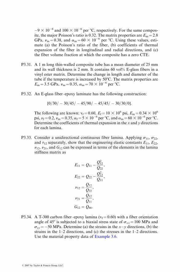
�9 3 10�6 and 100 3 10�6 per 8C, respectively. For the same compos-
ite, the major Poisson’s ratio is 0.32. The matrix properties are Em¼ 2.8
GPa, nm¼ 0.38, and am¼ 60 3 10�6 per 8C. Using these values, esti-
mate (a) the Poisson’s ratio of the fiber, (b) coefficients of thermal
expansion of the fiber in longitudinal and radial directions, and (c)
the fiber volume fraction at which the composite has a zero CTE.
P3.31. A 1 m long thin-walled composite tube has a mean diameter of 25 mm
and its wall thickness is 2 mm. It contains 60 vol% E-glass fibers in a
vinyl ester matrix. Determine the change in length and diameter of the
tube if the temperature is increased by 508C. The matrix properties are
Em¼ 3.5 GPa, nm¼ 0.35, am¼ 70 3 10�6 per 8C.
P3.32. An E-glass fiber–epoxy laminate has the following construction:
[0=30=� 30=45=� 45=90=� 45=45=� 30=30=0]:
The following are known: vf¼ 0.60, Ef¼ 10 3 106 psi, Em¼ 0.34 3 106
psi, nf¼ 0.2, nm¼ 0.35, af¼ 53 10�6 per 8C, and am¼ 603 10�6 per 8C.Determine the coefficients of thermal expansion in the x and y directions
for each lamina.
P3.33. Consider a unidirectional continuous fiber lamina. Applying s11, s22,
and t12 separately, show that the engineering elastic constants E11, E22,
n12, n21, and G12 can be expressed in terms of the elements in the lamina
stiffness matrix as
E11 ¼ Q11 �Q212
Q22
,
E22 ¼ Q22 �Q212
Q11
,
n12 ¼ Q12
Q22
,
n21 ¼ Q12
Q11
,
G12 ¼ Q66:
P3.34. A T-300 carbon fiber–epoxy lamina (vf¼ 0.60) with a fiber orientation
angle of 458 is subjected to a biaxial stress state of sxx¼ 100 MPa and
syy¼�50 MPa. Determine (a) the strains in the x�y directions, (b) the
strains in the 1–2 directions, and (c) the stresses in the 1–2 directions.
Use the material property data of Example 3.6.
� 2007 by Taylor & Francis Group, LLC.
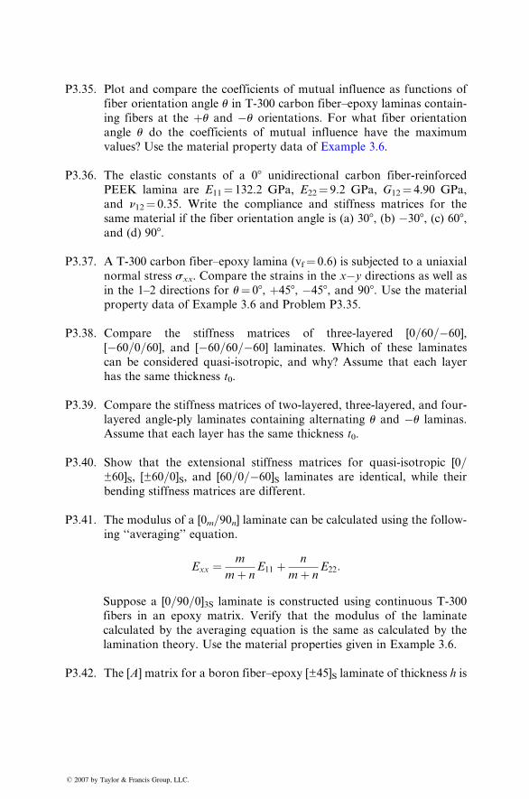
P3.35. Plot and compare the coefficients of mutual influence as functions of
fiber orientation angle u in T-300 carbon fiber–epoxy laminas contain-
ing fibers at the þu and �u orientations. For what fiber orientation
angle u do the coefficients of mutual influence have the maximum
values? Use the material property data of Example 3.6.
P3.36. The elastic constants of a 08 unidirectional carbon fiber-reinforced
PEEK lamina are E11¼ 132.2 GPa, E22¼ 9.2 GPa, G12¼ 4.90 GPa,
and n12¼ 0.35. Write the compliance and stiffness matrices for the
same material if the fiber orientation angle is (a) 308, (b) �308, (c) 608,and (d) 908.
P3.37. A T-300 carbon fiber–epoxy lamina (vf¼ 0.6) is subjected to a uniaxial
normal stress sxx. Compare the strains in the x�y directions as well as
in the 1–2 directions for u¼ 08, þ458, �458, and 908. Use the material
property data of Example 3.6 and Problem P3.35.
P3.38. Compare the stiffness matrices of three-layered [0=60=�60],
[�60=0=60], and [�60=60=�60] laminates. Which of these laminates
can be considered quasi-isotropic, and why? Assume that each layer
has the same thickness t0.
P3.39. Compare the stiffness matrices of two-layered, three-layered, and four-
layered angle-ply laminates containing alternating u and �u laminas.
Assume that each layer has the same thickness t0.
P3.40. Show that the extensional stiffness matrices for quasi-isotropic [0=±60]S, [±60=0]S, and [60=0=�60]S laminates are identical, while their
bending stiffness matrices are different.
P3.41. The modulus of a [0m=90n] laminate can be calculated using the follow-
ing ‘‘averaging’’ equation.
Exx ¼ m
mþ nE11 þ n
mþ nE22:
Suppose a [0=90=0]3S laminate is constructed using continuous T-300
fibers in an epoxy matrix. Verify that the modulus of the laminate
calculated by the averaging equation is the same as calculated by the
lamination theory. Use the material properties given in Example 3.6.
P3.42. The [A] matrix for a boron fiber–epoxy [±45]S laminate of thickness h is
� 2007 by Taylor & Francis Group, LLC.
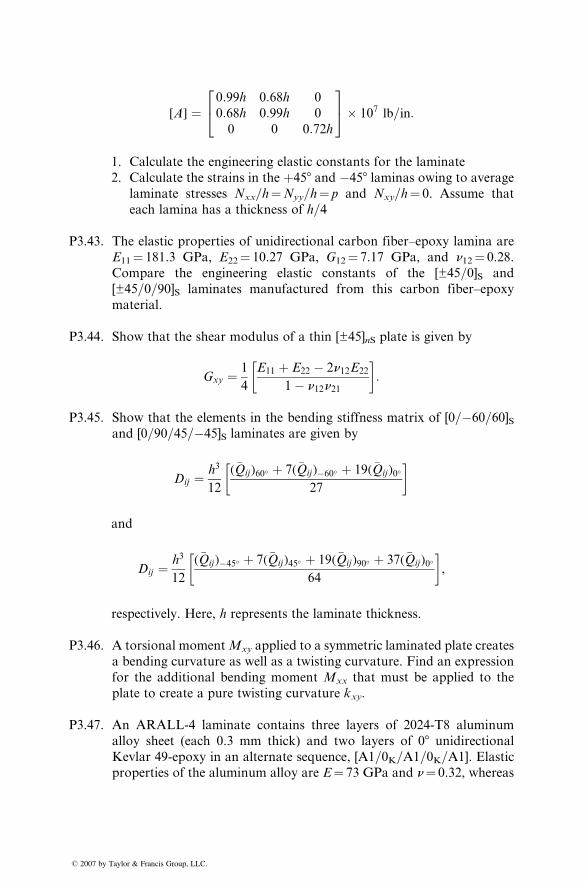
[A] ¼0:99h 0:68h 0
0:68h 0:99h 0
0 0 0:72h
24
35� 107 lb=in:
1. Calculate the engineering elastic constants for the laminate
2. Calculate the strains in the þ458 and �458 laminas owing to average
laminate stresses Nxx=h¼Nyy=h¼ p and Nxy=h¼ 0. Assume that
each lamina has a thickness of h=4
P3.43. The elastic properties of unidirectional carbon fiber–epoxy lamina are
E11¼ 181.3 GPa, E22¼ 10.27 GPa, G12¼ 7.17 GPa, and n12¼ 0.28.
Compare the engineering elastic constants of the [±45=0]S and
[±45=0=90]S laminates manufactured from this carbon fiber–epoxy
material.
P3.44. Show that the shear modulus of a thin [±45]nS plate is given by
Gxy ¼ 1
4
E11 þ E22 � 2n12E22
1� n12n21
� �:
P3.45. Show that the elements in the bending stiffness matrix of [0=�60=60]Sand [0=90=45=�45]S laminates are given by
Dij ¼ h3
12
(�Qij)60� þ 7(�Qij)�60� þ 19(�Qij)0�
27
� �
and
Dij ¼ h3
12
(�Qij)�45� þ 7(�Qij)45� þ 19(�Qij)90� þ 37(�Qij)0�
64
� �,
respectively. Here, h represents the laminate thickness.
P3.46. A torsional momentMxy applied to a symmetric laminated plate creates
a bending curvature as well as a twisting curvature. Find an expression
for the additional bending moment Mxx that must be applied to the
plate to create a pure twisting curvature kxy.
P3.47. An ARALL-4 laminate contains three layers of 2024-T8 aluminum
alloy sheet (each 0.3 mm thick) and two layers of 08 unidirectional
Kevlar 49-epoxy in an alternate sequence, [A1=0K=A1=0K=A1]. Elastic
properties of the aluminum alloy are E¼ 73 GPa and n¼ 0.32, whereas
� 2007 by Taylor & Francis Group, LLC.
those for the Kevlar layers are E11¼ 56.2 GPa, E22¼ 4.55 GPa,
n12¼ 0.456, and G12¼ 1.85 GPa. The nominal thickness of the laminate
is 1.3 mm. Calculate the elastic properties of the ARALL-4 laminate.
P3.48. Using the basic ply level properties of Example 3.6, determine the
stresses in each layer of a [±45]32S laminate subjected to Nxx¼ 0.1
N=mm. The ply thickness is 0.013 mm.
P3.49. Using the material properties in Example 3.16, determine the residual
thermal stresses in each lamina of (i) a [902=0]S and (ii) a [0=90=0]Slaminate. Both laminates are slowly cooled down from a curing tem-
perature of 1908C to 238C.
P3.50. The following thermomechanical properties are known for a carbon
fiber–epoxy composite: E11¼ 145 GPa, E22¼ 9 GPa, G12¼ 4.5 GPa,
n12¼ 0.246, a11¼�0.25 3 10�6 per 8C, and a22¼ 34.1 3 10�6 per 8C.Determine the coefficients of thermal expansion of a [45=�45]S lamin-
ate of this material.
P3.51. Using the ply level thermomechanical properties given in Problem 3.49,
determine the coefficients of thermal expansion of a [0=45=�45=90]Slaminate of this material.
P3.52. An approximate expression for the maximum interlaminar shear stress
txz in a [u=�u]nS class of laminates* is
Max txz ¼ 1
2n
A22�Q16 � A12
�Q26
A11A22 � A212
� �Nxx
h,
where Nxx=h is the average tensile stress on the laminate in the x
direction.
* J.M. W
posite M
� 2007 by
Using this expression, compare the maximum interlaminar shear
stress txz in [15=�15]8S and [45=�45]8S T-300 carbon–epoxy laminates.
Use Example 3.6 for the basic material property data.
P3.53. Following is an approximate expression* for the maximum interlami-
nar normal stress, szz, at an interface position z from the midplane of a
symmetric [0=90]S type laminate:
hitney, I.M. Daniel, and R.B. Pipes, Experimental Mechanics of Fiber Reinforced Com-
aterials, Society for Experimental Mechanics, Brookfield Center, CT (1984).
Taylor & Francis Group, LLC.
Maxszz(z) ¼ 90�sxx
7Ah
Xj
A22�Q12
j�A12
�Q22
j
h itj(hj � z),
where
sxx¼ applied normal stress in the x direction
A ¼A11A22 � A122
h ¼ laminate thickness
hj ¼ distance from the midplane of the laminate to the midplane of
the jth lamina
tj ¼ thickness of the jth lamina
and the summation extends over all the laminas above the interface
position z. This equation is valid for thin laminas in which the variation
of in-plane stresses is assumed to be negligible over the thickness of each
lamina.
Using this approximate expression, compare the maximum inter-
laminar normal stresses at the midplanes of [0=90=90=0] and
[90=0=0=90] laminates.
� 2007 by Taylor & Francis Group, LLC.

� 2007 by Taylor & Francis Group, LLC.
4 Performance
� 2007 by Taylor & Fr
The performance of an engineering material is judged by its properties and
behavior under tensile, compressive, shear, and other static or dynamic loading
conditions in both normal and adverse test environments. This information is
essential for selecting the proper material in a given application as well as
designing a structure with the selected material. In this chapter, we describe
the performance of fiber-reinforced polymer composites with an emphasis
on the general trends observed in their properties and behavior. A wealth of
property data for continuous fiber thermoset matrix composites exists in the
published literature. Continuous fiber-reinforced thermoplastic matrix com-
posites are not as widely used as continuous fiber-reinforced thermoset matrix
composites and lack a wide database.
Material properties are usually determined by conducting mechanical and
physical tests under controlled laboratory conditions. The orthotropic nature
of fiber-reinforced composites has led to the development of standard test
methods that are often different from those used for traditional isotropic
materials. These unique test methods and their limitations are discussed
in relation to many of the properties considered in this chapter. The effects of
environmental conditions, such as elevated temperature or humidity, on the
physical and mechanical properties of composite laminates are presented near
the end of the chapter. Finally, long-term behavior, such as creep and stress
rupture, and damage tolerance are also discussed.
4.1 STATIC MECHANICAL PROPERTIES
Static mechanical properties, such as tensile, compressive, flexural, and shear
properties, of a material are the basic design data in many, if not most,
applications. Typical mechanical property values for a number of 08 laminates
and sheet-molding compound (SMC) laminates are given in Appendix A.5 and
Appendix A.6, respectively.
4.1.1 TENSILE PROPERTIES
4.1.1.1 Test Method and Analysis
Tensile properties, such as tensile strength, tensile modulus, and Poisson’s ratio
of flat composite laminates, are determined by static tension tests in accordance
ancis Group, LLC.
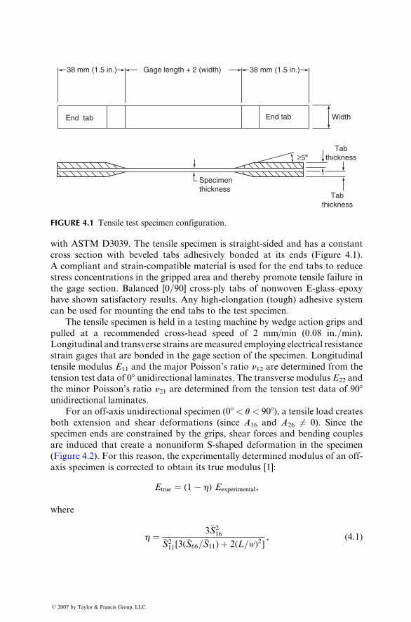
≥58
Specimenthickness
Tabthickness
Tabthickness
WidthEnd tab
38 mm (1.5 in.)38 mm (1.5 in.) Gage length + 2 (width)
End tab
FIGURE 4.1 Tensile test specimen configuration.
with ASTM D3039. The tensile specimen is straight-sided and has a constant
cross section with beveled tabs adhesively bonded at its ends (Figure 4.1).
A compliant and strain-compatible material is used for the end tabs to reduce
stress concentrations in the gripped area and thereby promote tensile failure in
the gage section. Balanced [0=90] cross-ply tabs of nonwoven E-glass–epoxy
have shown satisfactory results. Any high-elongation (tough) adhesive system
can be used for mounting the end tabs to the test specimen.
The tensile specimen is held in a testing machine by wedge action grips and
pulled at a recommended cross-head speed of 2 mm=min (0.08 in.=min).
Longitudinal and transverse strains aremeasured employing electrical resistance
strain gages that are bonded in the gage section of the specimen. Longitudinal
tensile modulus E11 and the major Poisson’s ratio n12 are determined from the
tension test data of 08 unidirectional laminates. The transverse modulus E22 and
the minor Poisson’s ratio n21 are determined from the tension test data of 908unidirectional laminates.
For an off-axis unidirectional specimen (08 < u < 908), a tensile load creates
both extension and shear deformations (since A16 and A26 6¼ 0). Since the
specimen ends are constrained by the grips, shear forces and bending couples
are induced that create a nonuniform S-shaped deformation in the specimen
(Figur e 4.2). For this reason, the experi menta lly determ ined modulus of an off-
axis specimen is corrected to obtain its true modulus [1]:
Etrue ¼ (1� h) Eexperimental,
where
h ¼ 3�S216
�S211[3(
�S66=�S11)þ 2(L=w)2], (4:1)
� 2007 by Taylor & Francis Group, LLC.
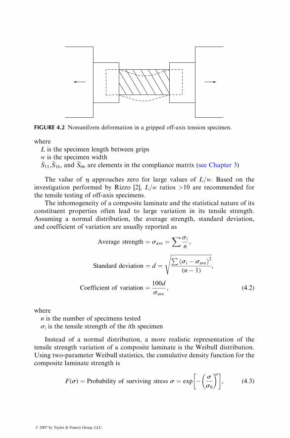
FIGURE 4.2 Nonuniform deformation in a gripped off-axis tension specimen.
where
L is the specimen lengt h between grips
w is the specimen wid th�S11 , �S16 , and �S66 are elem ents in the complian ce matr ix (see Chapter 3)
The value of h approaches zero for large values of L=w. Based on the
investigation performed by Rizzo [2], L=w ratios >10 are recommended for
the tensile testing of off-axis specimens.
The inhomogeneity of a composite laminate and the statistical nature of its
constituent properties often lead to large variation in its tensile strength.
Assuming a normal distribution, the average strength, standard deviation,
and coefficient of variation are usually reported as
Average strength ¼ save ¼Xsi
n,
Standard deviation ¼ d ¼ffiffiffiffiffiffiffiffiffiffiffiffiffiffiffiffiffiffiffiffiffiffiffiffiffiffiffiffiffiffiP
si � saveð Þ2(n� 1)
s,
Coefficient of variation ¼ 100d
save
, (4:2)
where
n is the number of specimens tested
si is the tensile strength of the ith specimen
Instead of a normal distribution, a more realistic representation of the
tensile strength variation of a composite laminate is the Weibull distribution.
Using two-parameter Weibull statistics, the cumulative density function for the
composite laminate strength is
F (s) ¼ Probability of surviving stress s ¼ exp � s
s0
� �a� �, (4:3)
� 2007 by Taylor & Francis Group, LLC.
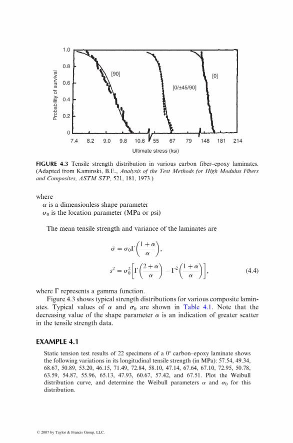
1.0
0.8[90] [0]
[0/±45/90]0.6
0.4
0.2
0
7.4 8.2 9.0 9.8 10.6 55 67
Ultimate stress (ksi)
Pro
babi
lity
of s
urvi
val
79 148 181 214
FIGURE 4.3 Tensile strength distribution in various carbon fiber–epoxy laminates.
(Adapted from Kaminski, B.E., Analysis of the Test Methods for High Modulus Fibers
and Composites, ASTM STP, 521, 181, 1973.)
wher e
a is a dimension less shape parame ter
s0 is the locat ion parame ter (MP a or psi)
The mean tensi le stre ngth a nd varianc e of the laminates are
�s ¼ s0 G1 þ a
a
� �,
s 2 ¼ s 20 G2 þ a
a
� �� G2 1 þ a
a
� �� �, ( 4: 4)
wher e G repres ents a gamm a functio n.
Figure 4.3 shows typical stre ngth dist ribution s for various compo site lami n-
ates. Typical values of a and s0 are shown in Tabl e 4.1. Note that the
decreasing value of the shape parameter a is an indication of greater scatter
in the tensile strength data.
EXAMPLE 4.1
Static tension test results of 22 specimens of a 08 carbon–epoxy laminate shows
the following variations in its longitudinal tensile strength (in MPa): 57.54, 49.34,
68.67, 50.89, 53.20, 46.15, 71.49, 72.84, 58.10, 47.14, 67.64, 67.10, 72.95, 50.78,
63.59, 54.87, 55.96, 65.13, 47.93, 60.67, 57.42, and 67.51. Plot the Weibull
distribution curve, and determine the Weibull parameters a and s0 for this
distribution.
� 2007 by Taylor & Francis Group, LLC.
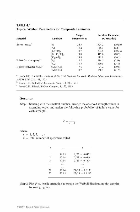
TABLE 4.1Typical Weibull Parameters for Composite Laminates
Material Laminate
Shape
Parameter, a
Location Parameter,
s0 MPa (ksi)
Boron–epoxya [0] 24.3 1324.2 (192.0)
[90] 15.2 66.1 (9.6)
[02=±45]S 18.7 734.5 (106.6)
[0=±45=90]S 19.8 419.6 (60.9)
[902=45]S 19.8 111.9 (16.1)
T-300 Carbon–epoxyb [08] 17.7 1784.5 (259)
[016] 18.5 1660.5 (241)
E-glass–polyester SMCc SMC-R25 7.6 74.2 (10.8)
SMC-R50 8.7 150.7 (21.9)
a From B.E. Kaminski, Analysis of the Test Methods for High Modulus Fibers and Composites,
ASTM STP, 521, 181, 1973.b From R.E. Bullock, J. Composite Mater., 8, 200, 1974.c From C.D. Shirrell, Polym. Compos., 4, 172, 1983.
SOLUTION
Step 1: Starting with the smallest number, arrange the observed strength values in
ascending order and assign the following probability of failure value for
each strength.
P ¼ i
nþ 1,
where
i ¼ 1, 2, 3, . . . , n
n ¼ total number of specimens tested
� 2007 by Taylor & Francis Group, LL
i
C.
s
P1
46.15 1=23 ¼ 0.04352
47.14 2=23 ¼ 0.08693
47.94 3=23 ¼ 0.1304. . .
. . . . . .. . .
. . . . . .21
72.84 21=23 ¼ 0.913022
72.95 22=23 ¼ 0.9565Step 2: Plot P vs. tensile strength s to obtain the Weibull distribution plot (see the
following figure).
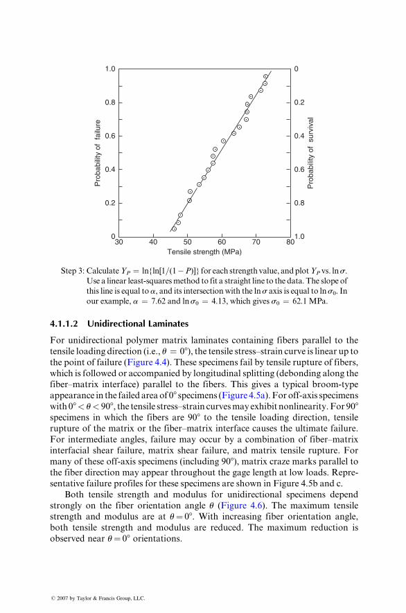
1.0
0.8
0.6
0.4
Pro
babi
lity
of f
ailu
re
Pro
babi
lity
of s
urvi
val
Tensile strength (MPa)
0.2
030 40 50 60 70 80
0
0.2
0.4
0.6
0.8
1.0
Step 3: Calculate YP ¼ ln{ln[1=(1 � P)]} for each strength value, and plot YP vs . l n s.Use a linear least-squares method to fit a straight line to the data. The slope of
this line is equal to a, and its intersection with the ln s axis is equal to ln s0. In
our example, a ¼ 7 .62 an d l n s0 ¼ 4. 13 , w hi ch g ive s s0 ¼ 62.1 MPa.
4.1.1 .2 Uni directi onal Lami nates
For unidir ectio nal polyme r matrix laminates co ntaining fibers paralle l to the
tensile loading direction (i.e., u ¼ 08 ), the tensile stre ss–strai n cu rve is linear up tothe poi nt of failure (Figur e 4.4). These specimen s fail by tensile rup ture of fiber s,
which is followe d or acco mpanie d by longitudinal splitting (debo nding along the
fiber–mat rix inter face) parallel to the fiber s. This gives a typic al bro om-type
appearan ce in the failed area of 08 specim ens (Figure 4.5a). For off- axis specimen s
with 08 < u < 90 8 , the tensi le stress–s train curves may exh ibit nonl inearity. For 908specim ens in which the fibers are 90 8 to the tensile loading direct ion, tensilerupture of the matrix or the fiber –mat rix inter face causes the ulti mate fail ure.
For inter mediate angles , failure may occur by a co mbination of fiber–mat rix
interfaci al shear failure, matr ix shear failure, an d matrix tensi le rupture . For
many of these off-axis specim ens (inclu ding 90 8), matrix craze marks pa rallel to
the fiber direct ion may appear throu ghout the gage lengt h at low loads. Repre -
sentative failure profiles for these sp ecimens are sh own in Figure 4.5b and c.
Both tensile strength and modulus for unidirectional specimens depend
strong ly on the fiber orient ation an gle u (Figur e 4.6) . The maximum tensi le
strength and modulus are at u¼ 08. With increasing fiber orientation angle,
both tensile strength and modulus are reduced. The maximum reduction is
observed near u¼ 08 orientations.
� 2007 by Taylor & Francis Group, LLC.
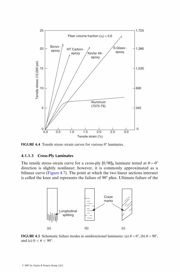
1,725
1,380
1,035
690
345
0
25
Fiber volume fraction (vf) = 0.6
Boron−epoxy HT Carbon−
epoxy Kevlar 49−epoxy
S-Glass−epoxy
Aluminum(7075-T6)
Tensile strain (%)0.0 0.5 1.0 1.5 2.0 2.5 3.0
20
15
10
Ten
sile
str
ess
(10,
000
psi)
5
0
FIGURE 4.4 Tensile stress–strain curves for various 08 laminates.
4.1.1.3 Cro ss-Ply Laminate s
The tensi le stre ss–strai n curve for a cross-p ly [0 =90]S lami nate test ed at u ¼ 08direction is sligh tly nonlinear ; howeve r, it is common ly approxim ated a s a
bilinear curve (Figur e 4.7) . The point at which the two linea r sections inter sect
is ca lled the kne e and repres ents the failure of 90 8 plies . Ult imate failure of the
Longitudinalsplitting
Crazemarks
(a) (b) (c)
FIGURE 4.5 Schematic failure modes in unidirectional laminates: (a) u¼ 08, (b) u¼ 908,and (c) 0 < u < 908.
� 2007 by Taylor & Francis Group, LLC.
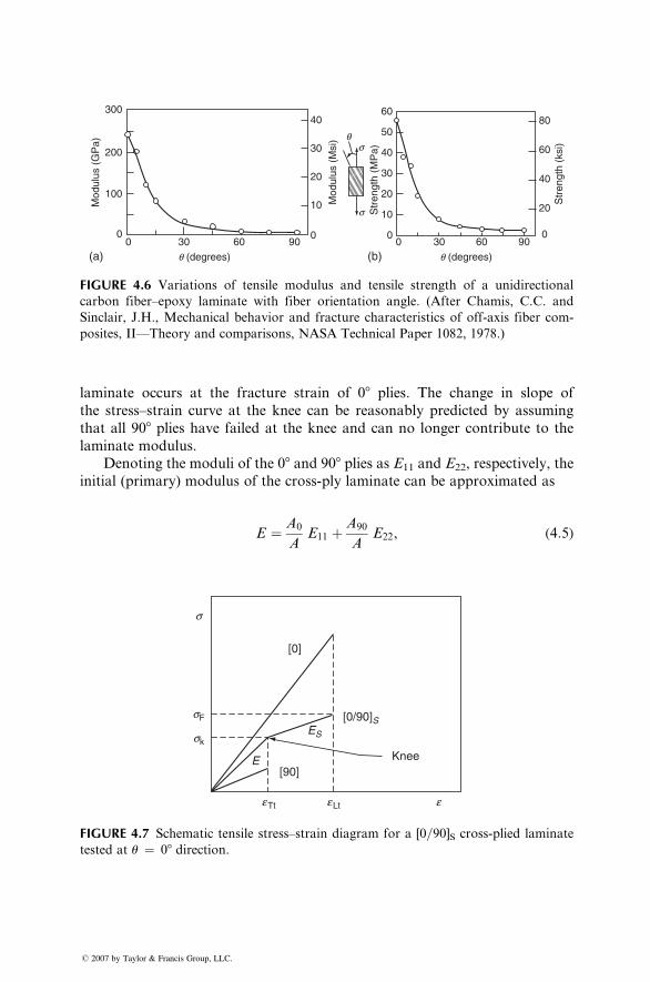
80
60
40
Str
engt
h (k
si)
20
0
40
30
20
10
000 30 60 90
100
200
300
9060
q (degrees)q (degrees)
300(b)(a)
0
10
20
Str
engt
h (M
Pa)
Mod
ulus
(M
si)
Mod
ulus
(G
Pa)
30
40
50
sq
s
60
FIGURE 4.6 Variations of tensile modulus and tensile strength of a unidirectional
carbon fiber–epoxy laminate with fiber orientation angle. (After Chamis, C.C. and
Sinclair, J.H., Mechanical behavior and fracture characteristics of off-axis fiber com-
posites, II—Theory and comparisons, NASA Technical Paper 1082, 1978.)
laminate occurs at the fracture strain of 08 plies. The change in slope of
the stress–strain curve at the knee can be reasonably predicted by assuming
that all 908 plies have failed at the knee and can no longer contribute to the
laminate modulus.
Denoting the moduli of the 08 and 908 plies as E11 and E22, respectively, the
initial (primary) modulus of the cross-ply laminate can be approximated as
E ¼ A0
AE11 þ A90
AE22, (4:5)
[90]
[0]
s
sF
sk
[0/90]S
KneeE
e Tt e Lt e
ES
FIGURE 4.7 Schematic tensile stress–strain diagram for a [0=90]S cross-plied laminate
tested at u ¼ 08 direction.
� 2007 by Taylor & Francis Group, LLC.
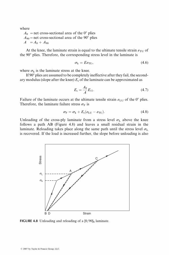
where
A0 ¼ net cross-sectional area of the 08 pliesA90¼ net cross-sectional area of the 908 pliesA ¼A0 þ A90
At the knee, the laminate strain is equal to the ultimate tensile strain «TU of
the 908 plies. Therefore, the corresponding stress level in the laminate is
sk ¼ E«TU, (4:6)
where sk is the laminate stress at the knee.
If 908plies are assumed to be completely ineffective after they fail, the second-
ary modulus (slope after the knee) Es of the laminate can be approximated as
Es ¼ A0
AE11: (4:7)
Failure of the laminate occurs at the ultimate tensile strain «LU of the 08 plies.Therefore, the laminate failure stress sF is
sF ¼ sk þ Es «LU � «TUð Þ: (4:8)
Unloading of the cross-ply laminate from a stress level sL above the knee
follows a path AB (Figure 4.8) and leaves a small residual strain in the
laminate. Reloading takes place along the same path until the stress level sL
is recovered. If the load is increased further, the slope before unloading is also
As L
s k
C
B D
Str
ess
Strain
FIGURE 4.8 Unloading and reloading of a [0=90]S laminate.
� 2007 by Taylor & Francis Group, LLC.
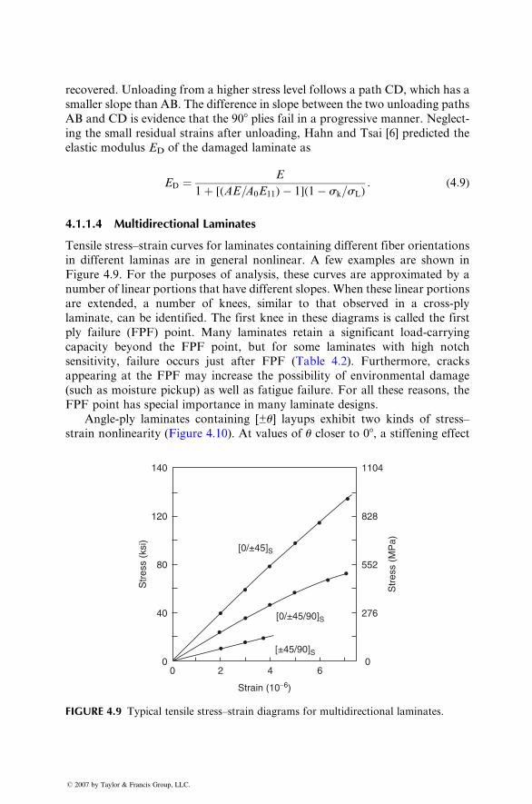
recover ed. Unloadi ng from a high er stre ss level follows a path CD, which ha s a
smaller slope than AB. The difference in slope between the two unloading pa ths
AB and CD is eviden ce that the 90 8 plies fail in a pro gressive manner. Negl ect-
ing the smal l resi dual strains after unloading, Hahn and Tsai [6] predicted the
elastic modulus ED of the damaged laminate as
ED ¼ E
1 þ [(AE =A0 E11 ) � 1]( 1 � s k =s L ) : ( 4: 9)
4.1.1 .4 Mult idirect ional Laminate s
Tensil e stre ss–strai n curves for laminates co ntaining different fiber orient ations
in different lami nas are in gen eral nonl inear. A few exampl es are shown in
Figure 4.9. For the purposes of analys is, these cu rves are app roximated by a
number of linea r por tions that have different slopes . When these linea r portion s
are extend ed, a number of kne es, simila r to that observed in a cross-ply
laminate, can be iden tified. The first knee in these diagra ms is called the first
ply failure (FPF) point. Man y lami nates retai n a signi ficant load-c arrying
capacit y bey ond the FPF point, but for some laminates with high notch
sensi tivity, failure occurs just after FPF (Tab le 4.2). Furtherm ore, crack s
appeari ng at the FPF may increa se the possibi lity of environm en tal damage
(such a s mois ture pickup ) as wel l as fatigu e failu re. For all these reasons , the
FPF point ha s specia l importance in many laminate designs.
Angl e-ply laminates con taining [± u] layup s exhibi t two kind s of stress–strain nonlinear ity (Figur e 4.10). At va lues of u closer to 08 , a stiffen ing effe ct
140
120
80
40
00 2 4
Strain (10−6)
[0/±45]S
[0/±45/90]S
[±45/90]S
Str
ess
(MP
a)
Str
ess
(ksi
)
6
1104
828
552
276
0
FIGURE 4.9 Typical tensile stress–strain diagrams for multidirectional laminates.
� 2007 by Taylor & Francis Group, LLC.
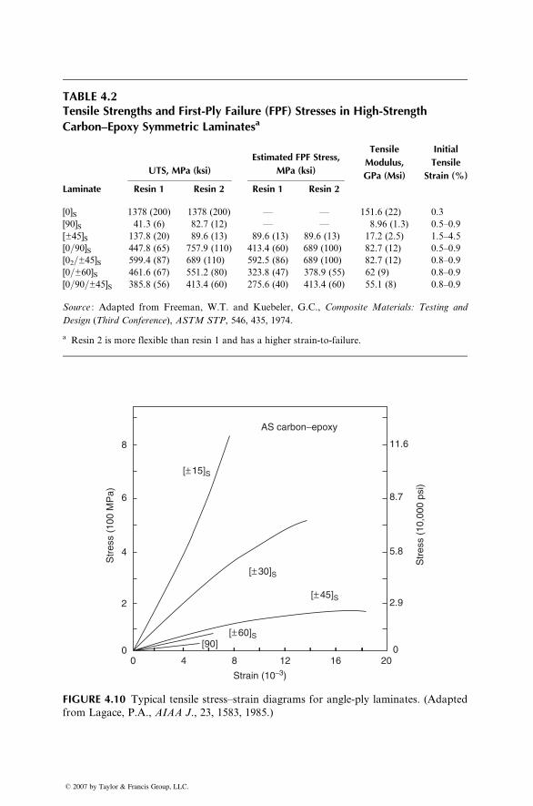
TABLE 4.2Tensile Strengths and First-Ply Failure (FPF) Stresses in High-Strength
Carbon–Epoxy Symmetric Laminatesa
UTS, MPa (ksi)
Estimated FPF Stress,
MPa (ksi)
Tensile
Modulus,
GPa (Msi)
Initial
Tensile
Strain (%)
Laminate Resin 1 Resin 2 Resin 1 Resin 2
[0]S 1378 (200) 1378 (200) — — 151.6 (22) 0.3
[90]S 41.3 (6) 82.7 (12) — — 8.96 (1.3) 0.5–0.9
[±45]S 137.8 (20) 89.6 (13) 89.6 (13) 89.6 (13) 17.2 (2.5) 1.5–4.5
[0=90]S 447.8 (65) 757.9 (110) 413.4 (60) 689 (100) 82.7 (12) 0.5–0.9
[02=±45]S 599.4 (87) 689 (110) 592.5 (86) 689 (100) 82.7 (12) 0.8–0.9
[0=±60]S 461.6 (67) 551.2 (80) 323.8 (47) 378.9 (55) 62 (9) 0.8–0.9
[0=90=±45]S 385.8 (56) 413.4 (60) 275.6 (40) 413.4 (60) 55.1 (8) 0.8–0.9
Source : Adapted from Freeman, W.T. and Kuebeler, G.C., Composite Materials: Testing and
Design (Third Conference), ASTM STP, 546, 435, 1974.
a Resin 2 is more flexible than resin 1 and has a higher strain-to-failure.
AS carbon−epoxy
[± 15]S
[± 30]S
[± 45]S
[± 60]S
Str
ess
(100
MP
a)
Str
ess
(10,
000
psi)
[90]
00
2
4
6
8
4 8 12
Strain (10−3)
16 200
2.9
5.8
8.7
11.6
FIGURE 4.10 Typical tensile stress–strain diagrams for angle-ply laminates. (Adapted
from Lagace, P.A., AIAA J., 23, 1583, 1985.)
� 2007 by Taylor & Francis Group, LLC.
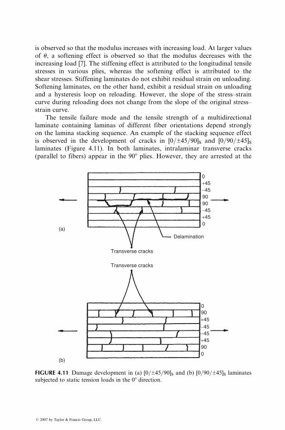
is observed so that the modulus increases with increasing load. At larger values
of u, a softening effect is observed so that the modulus decreases with the
increasing load [7]. The stiffening effect is attributed to the longitudinal tensile
stresses in various plies, whereas the softening effect is attributed to the
shear stresses. Stiffening laminates do not exhibit residual strain on unloading.
Softening laminates, on the other hand, exhibit a residual strain on unloading
and a hysteresis loop on reloading. However, the slope of the stress–strain
curve during reloading does not change from the slope of the original stress–
strain curve.
The tensile failure mode and the tensile strength of a multidirectional
laminate containing laminas of different fiber orientations depend strongly
on the lamina stacking sequence. An example of the stacking sequence effect
is observed in the development of cracks in [0=±45=90]S and [0=90=±45]Slaminates (Figure 4.11). In both laminates, intralaminar transverse cracks
(parallel to fibers) appear in the 908 plies. However, they are arrested at the
0
0
0
+45−4590
+45
+45
−45−45
90
90
90−45+450
Delamination
Transverse cracks
Transverse cracks
(a)
(b)
FIGURE 4.11 Damage development in (a) [0=±45=90]S and (b) [0=90=±45]S laminates
subjected to static tension loads in the 08 direction.
� 2007 by Taylor & Francis Group, LLC.
lamina interfaces and do not imm ediately propagat e into the a djacent plies. The
number of transverse cracks in the 908 plies increases unt il unifor mly spaced
cracks a re form ed throughout the specim en lengt h [8]; howeve r, these trans -
verse crack s are more closely spaced in [0 =90 =±45]S laminates than [0 =±45 =90]Slaminates . Increas ing the tensi le load also creates a few intralam inar cracks
parallel to the fiber direct ions in both � 45 8 and þ 45 8 plies. Apart from these
intralam inar crack patterns, su bsequent fail ure modes in these tw o ap parently
simila r lamina tes are distinct ly diff erent. In [0 =±45=90]S lami nates, longitud inal
interlam inar cracks grow between the 90 8 plies , which join toget her to formcontinuous edge delam inatio ns with occ asional jogging into the 90 =� 45 inter -
faces. With increa sing load, the edge delam ination extends toward the c enter of
the specimen ; howeve r, the spec imen fails by the rupture of 08 fiber s be fore theentire wid th is delam inated . In con trast to the [0 =±45=90]S laminate, there is no
edge de laminatio n in the [0 =90 =±45 ]S lami nate; instead, trans verse cracks
appear in both þ45 8 an d � 45 8 plies before the laminate fail ure. The difference
in ed ge de laminati on behavior between the [0 =±45=90]S an d [0=90 =±45 ] S lamin -
ates can be explain ed in term s of the inter laminar normal stress szz , which is
tensile in the former and compres sive in the latter.
Table 4.3 pr esents the tensile test da ta and failu re modes observed in severa l
multidir ection al carb on fiber –epoxy lamin ates. If the laminate con tains 90 8plies, failure begins with transv erse micr ocracks appeari ng in these plies . W ith
increa sing stre ss level , the numb er of these transve rse micr ocracks increa ses
until a saturati on num ber, called the charact eristic damage state (C DS),
is reached. Other types of damages that may follow trans verse micr ocracki ng
are de laminati on, long itudinal crackin g, and fiber fail ure.
4.1.1.5 Wo ven Fabric Laminate s
The princi pal advantag e of using woven fabric lamin ates is that they provide
propert ies that are more balanced in the 0 8 and 908 directions than unidir ec-tional laminates . Although multil ayered lamin ates can also be designe d to
produc e balanced prop erties, the fabricati on (layup) time for woven fabric
laminates is less than that of a multil ayered laminate. How ever, the tensi le
strength and mod ulus of a woven fabri c lami nate are, in general , lower than
those of multil ayered laminates . The princi pal reason for their lower tensi le
propert ies is the presence of fiber undulati on in woven fabri cs as the fiber yarns
in the fil l direct ion cross ov er and unde r the fiber yarns in the war p direction to
create an inter locked structure. Under tensile loading , these crim ped fibers tend
to straight en out, which creat es high stresses in the matrix. As a resul t, micro -
cracks are form ed in the matr ix at relat ively low loads. This is also ev idenced by
the a ppearance of one or more kne es in the stress–s train diagra ms of woven
fabric laminates (Figure 4.12) . Anothe r fact or to consider is that the fiber s in
woven fabrics are subjected to additional mechanical handling during the
weaving process, which tends to reduce their tensile strength.
� 2007 by Taylor & Francis Group, LLC.
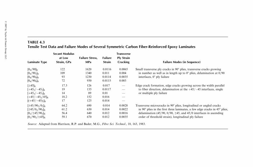
TABLE 4.3Tensile Test Data and Failure Modes of Several Symmetric Carbon Fiber-Reinforced Epoxy Laminates
Laminate Type
Secant Modulus
at Low
Strain, GPa
Failure Stress,
MPa
Failure
Strain
Transverse
Ply Strain
Cracking Failure Modes (in Sequence)
[04=90]S[04=902]S[04=904]S[04=908]S
122
109
93
72
1620
1340
1230
930
0.0116
0.011
0.0114
0.0115
0.0065
0.004
0.0035
0.003
Small transverse ply cracks in 908 plies, transverse cracks growing
in number as well as in length up to 08 plies, delamination at 0=90
interfaces, 08 ply failure
[±45]S[þ452=�452]S[þ453=�453]S[þ45=�452=45]S[(þ45=�45)2]S
17.3
19
14
18.2
17
126
135
89
152
125
0.017
0.0117
0.01
0.016
0.014
—
—
—
—
—
Edge crack formation, edge cracks growing across the width parallel
to fiber direction, delamination at the þ45=�45 interfaces, single
or multiple ply failure
[±45=902=02]S[±45=02=902]S[02=±45=902]S[02=902=±45]S
64.2
61.2
56.4
59.1
690
630
640
670
0.014
0.014
0.012
0.012
0.0028
0.0022
0.0016
0.0035
Transverse microcracks in 908 plies, longitudinal or angled cracks
in 908 plies in the first three laminates, a few edge cracks in 458 plies,
delamination (45=90, 0=90, ±45, and 45=0 interfaces in ascending
order of threshold strain), longitudinal ply failure
Source: Adapted from Harrison, R.P. and Bader, M.G., Fibre Sci. Technol., 18, 163, 1983.
�2007
byTaylor
&Francis
Group,L
LC.
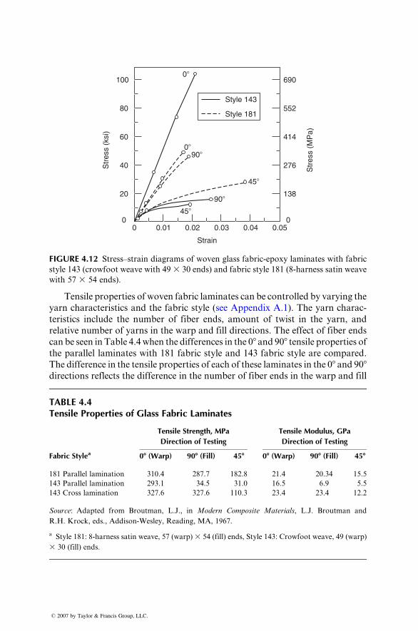
100
80
60
Str
ess
(ksi
)
Str
ess
(MP
a)
Style 143
Style 181
40
20
00 0.01 0.02 0.03
Strain
0.04 0.05
690
552
414
276
138
0
0�
0�90�
90�
45�
45�
FIGURE 4.12 Stress–strain diagrams of woven glass fabric-epoxy laminates with fabric
style 143 (crowfoot weave with 493 30 ends) and fabric style 181 (8-harness satin weave
with 57 3 54 ends).
Tensil e prop erties of woven fabric laminates can be co ntrolled by varyi ng the
yarn charact eristics and the fabric style (see Appendix A.1). The y arn ch arac-
teristics include the number of fiber ends, amount of twist in the yarn, and
relative number of yarns in the warp and fill directions. The effect of fiber ends
can be seen in Table 4.4 when the differences in the 08 and 908 tensile properties ofthe parallel laminates with 181 fabric style and 143 fabric style are compared.
The difference in the tensile properties of each of these laminates in the 08 and 908directions reflects the difference in the number of fiber ends in the warp and fill
TABLE 4.4Tensile Properties of Glass Fabric Laminates
Tensile Strength, MPa
Direction of Testing
Tensile Modulus, GPa
Direction of Testing
Fabric Stylea 08 (Warp) 908 (Fill) 458 08 (Warp) 908 (Fill) 458
181 Parallel lamination 310.4 287.7 182.8 21.4 20.34 15.5
143 Parallel lamination 293.1 34.5 31.0 16.5 6.9 5.5
143 Cross lamination 327.6 327.6 110.3 23.4 23.4 12.2
Source: Adapted from Broutman, L.J., in Modern Composite Materials, L.J. Broutman and
R.H. Krock, eds., Addison-Wesley, Reading, MA, 1967.
a Style 181: 8-harness satin weave, 57 (warp)3 54 (fill) ends, Style 143: Crowfoot weave, 49 (warp)
3 30 (fill) ends.
� 2007 by Taylor & Francis Group, LLC.
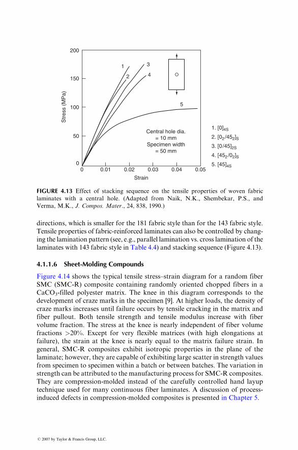
1
2
3
4
5
1. [0]4S
2. [02 /452]S
3. [0 /45]2S
4. [452 /02]S
5. [45]4S
Central hole dia.= 10 mm
Specimen width= 50 mm
200
150
100
Str
ess
(MP
a)
Strain
50
00 0.01 0.02 0.03 0.04 0.05
FIGURE 4.13 Effect of stacking sequence on the tensile properties of woven fabric
laminates with a central hole. (Adapted from Naik, N.K., Shembekar, P.S., and
Verma, M.K., J. Compos. Mater., 24, 838, 1990.)
direction s, which is smaller for the 181 fabric style than for the 143 fabri c styl e.
Tensile properties of fabric-reinforced laminates can also be controlled by chang-
ing the lamination pattern (see, e.g., parallel lamination vs. cross lamination of the
laminates with 143 fabric style in Table 4.4) and stacking sequence (Figure 4.13).
4.1.1 .6 Sh eet-Mol ding Com pounds
Figure 4.14 shows the typica l tensile stress–s train diagra m for a random fiber
SMC (SM C-R) composi te contai ning ran domly orient ed chopped fiber s in a
CaCO3-filled polyest er matr ix. The kne e in this diagra m corresp onds to the
developm ent of craze marks in the sp ecimen [9]. At higher loads, the de nsity of
craze marks increa ses until failu re occurs by tensi le crack ing in the matrix and
fiber pullout . Both tensi le stren gth and tensile modulus increase with fiber
volume fraction. The stre ss at the knee is nearly independen t of fiber vo lume
fractions > 20%. Except for very flexible matrices (with high elongat ions at
failure) , the stra in at the kne e is nearly equal to the matrix fail ure strain. In
general , SM C-R co mposites exhibi t isotro pic prop erties in the plane of the
laminate; howeve r, they are capable of exhibi ting large scatte r in stre ngth values
from specim en to specim en within a batch or between batches . The v ariation in
stren gth can be attribut ed to the manu facturing pro cess for SM C-R compo sites.
They are compres sion-molded instead of the caref ully control led han d layup
techni que use d for many con tinuous fiber laminates . A discussion of process -
induced defects in compres sion-molded composi tes is present ed in Chapter 5.
� 2007 by Taylor & Francis Group, LLC.
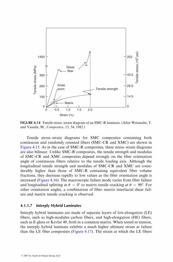
1400
300
203
43.5
29.0
14.5
0
200
100
00 0.5 1.0
Matrix
Kneepoint
Glassfiber
Tensile strength
Strain (%)
Ten
sile
str
ess
(MP
a)
Ten
sile
str
ess
(103
psi)
1.5 2.0
FIGURE 4.14 Tensile stress–strain diagram of an SMC-R laminate. (After Watanabe, T.
and Yasuda, M., Composites, 13, 54, 1982.)
Tensil e stre ss–strai n diagra ms for SMC compo sites co ntaining both
continuous and randoml y orient ed fiber s (SMC -CR and XMC ) are shown in
Figure 4.15. As in the case of SM C-R composi tes, these stre ss–strain diagra ms
are also bilin ear. Unlik e SM C-R composi tes, the tensi le stre ngth and modu lus
of SMC- CR and XMC c omposi tes de pend strong ly on the fiber orientati on
angle of continuous fibers relative to the tensile loading axis. Althou gh the
longitu dinal tensile stre ngth and modulus of SMC-CR and XMC are consi-
derably higher than those of SMC-R contai ning eq uivalen t fiber volume
fractions , they decreas e rapidl y to low values as the fiber orient ation angle is
increa sed (Figur e 4.16). The macros copic failure mode varies from fiber failure
and longit udinal splittin g at u ¼ 08 to matrix tensile cracki ng at u ¼ 90 8 . Forother orient ation angles , a combinat ion of fiber –matrix inter facial shear fail -
ure and matr ix tensile cracki ng is obs erved.
4.1.1.7 Inter ply Hybr id Lami nates
Interp ly hybrid lamin ates are mad e of separat e layer s of low-el ongatio n (LE )
fibers, such as high-mod ulus carbo n fiber s, and high-e longation (HE) fiber s,
such as E-glas s or Kevl ar 49 , both in a common matr ix. When tested in tension ,
the interp ly hybrid lamin ate exhibits a mu ch higher ulti mate strain at failure
than the LE fiber compo sites (Figur e 4.17) . The stra in at whi ch the LE fibers
� 2007 by Taylor & Francis Group, LLC.
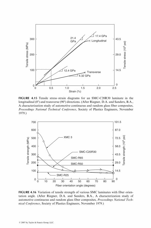
300 43.5
29.0
14.5
200
100
Ten
sile
str
ess
(MP
a)
Ten
sile
str
ess
(103
psi)
00 0.5 1.0
Strain (%)
21.4GPa
17.4 GPa
Longitudinal
12.4 GPa Transverse4.32 GPa
1.5 2.0 2.50
FIGURE 4.15 Tensile stress–strain diagrams for an SMC-C20R30 laminate in the
longitudinal (08) and transverse (908) directions. (After Riegner, D.A. and Sanders, B.A.,
A characterization study of automotive continuous and random glass fiber composites,
Proceedings National Technical Conference, Society of Plastics Engineers, November
1979.)
XMC 3
SMC-C20R30
SMC-R65
SMC-R50
Fiber orientation angle (degrees)
SMC-R25
700
600
500
400
Ten
sile
str
engt
h (M
Pa)
300
200
100
00 10 20 30 40 50 60 70 80 90
101.5
87.0
72.5
58.0
Ten
sile
str
engt
h (1
03 ps
i)
43.5
29.0
14.5
0
FIGURE 4.16 Variation of tensile strength of various SMC laminates with fiber orien-
tation angle. (After Riegner, D.A. and Sanders, B.A., A characterization study of
automotive continuous and random glass fiber composites, Proceedings National Tech-
nical Conference, Society of Plastics Engineers, November 1979.)
� 2007 by Taylor & Francis Group, LLC.
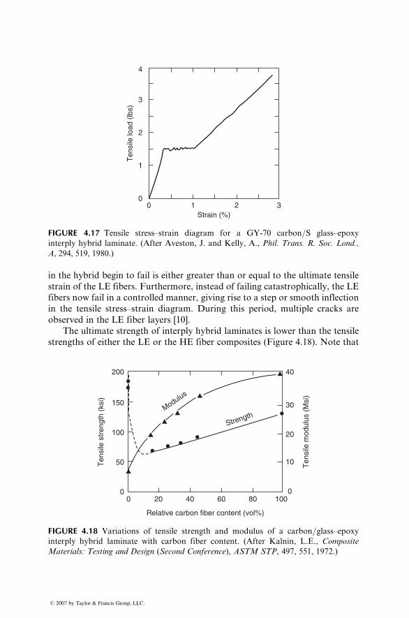
4
3
2
1
00 1
Strain (%)
Ten
sile
load
(lb
s)
2 3
FIGURE 4.17 Tensile stress–strain diagram for a GY-70 carbon=S glass–epoxy
interply hybrid laminate. (After Aveston, J. and Kelly, A., Phil. Trans. R. Soc. Lond.,
A, 294, 519, 1980.)
in the hybrid begin to fail is either greater than or equal to the ultimate tensile
strain of the LE fibers. Furthermore, instead of failing catastrophically, the LE
fibers now fail in a controlled manner, giving rise to a step or smooth inflection
in the tensile stress–strain diagram. During this period, multiple cracks are
observed in the LE fiber layers [10].
The ultimate strength of interply hybrid laminates is lower than the tensile
strengths of either the LE or the HE fiber composites (Figure 4.18). Note that
200 40
30
20
10
0
150
100
50
StrengthModulus
00 20 40
Relative carbon fiber content (vol%)
Ten
sile
mod
ulus
(M
si)
Ten
sile
str
engt
h (k
si)
60 80 100
FIGURE 4.18 Variations of tensile strength and modulus of a carbon=glass–epoxyinterply hybrid laminate with carbon fiber content. (After Kalnin, L.E., Composite
Materials: Testing and Design (Second Conference), ASTM STP, 497, 551, 1972.)
� 2007 by Taylor & Francis Group, LLC.
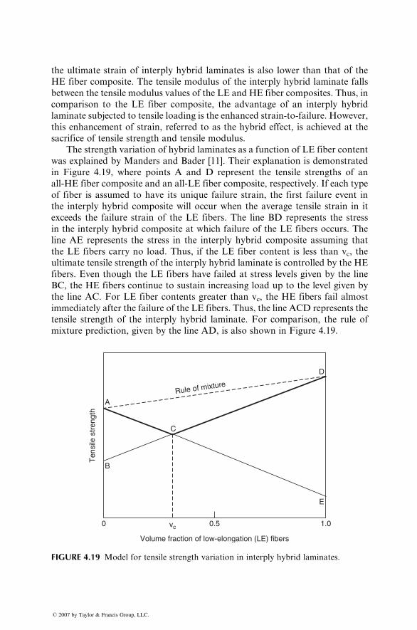
the ultimate strain of interply hybrid laminates is also lower than that of the
HE fiber composite. The tensile modulus of the interply hybrid laminate falls
between the tensile modulus values of the LE and HE fiber composites. Thus, in
comparison to the LE fiber composite, the advantage of an interply hybrid
laminate subjected to tensile loading is the enhanced strain-to-failure. However,
this enhancement of strain, referred to as the hybrid effect, is achieved at the
sacrifice of tensile strength and tensile modulus.
The strength variation of hybrid laminates as a function of LE fiber content
was explained by Manders and Bader [11]. Their explanation is demonstrated
in Figure 4.19, where points A and D represent the tensile strengths of an
all-HE fiber composite and an all-LE fiber composite, respectively. If each type
of fiber is assumed to have its unique failure strain, the first failure event in
the interply hybrid composite will occur when the average tensile strain in it
exceeds the failure strain of the LE fibers. The line BD represents the stress
in the interply hybrid composite at which failure of the LE fibers occurs. The
line AE represents the stress in the interply hybrid composite assuming that
the LE fibers carry no load. Thus, if the LE fiber content is less than vc, the
ultimate tensile strength of the interply hybrid laminate is controlled by the HE
fibers. Even though the LE fibers have failed at stress levels given by the line
BC, the HE fibers continue to sustain increasing load up to the level given by
the line AC. For LE fiber contents greater than vc, the HE fibers fail almost
immediately after the failure of the LE fibers. Thus, the line ACD represents the
tensile strength of the interply hybrid laminate. For comparison, the rule of
mixture prediction, given by the line AD, is also shown in Figure 4.19.
A
B
0 0.5vc
Volume fraction of low-elongation (LE) fibers
1.0
Ten
sile
str
engt
h
C
Rule of mixture
D
E
FIGURE 4.19 Model for tensile strength variation in interply hybrid laminates.
� 2007 by Taylor & Francis Group, LLC.
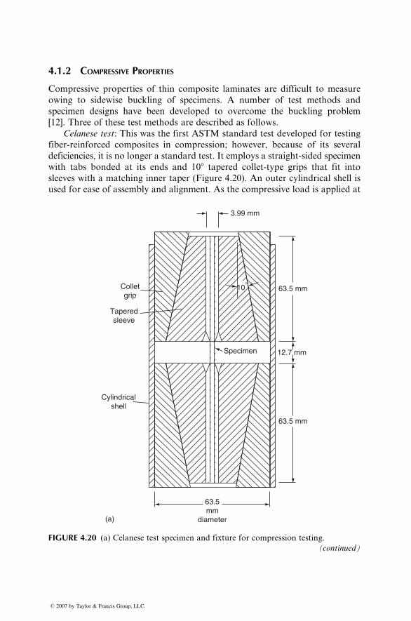
4.1.2 COMPRESSIVE PROPERTIES
Compressive properties of thin composite laminates are difficult to measure
owing to sidewise buckling of specimens. A number of test methods and
specimen designs have been developed to overcome the buckling problem
[12]. Three of these test methods are described as follows.
Celanese test: This was the first ASTM standard test developed for testing
fiber-reinforced composites in compression; however, because of its several
deficiencies, it is no longer a standard test. It employs a straight-sided specimen
with tabs bonded at its ends and 108 tapered collet-type grips that fit into
sleeves with a matching inner taper (Figure 4.20). An outer cylindrical shell is
used for ease of assembly and alignment. As the compressive load is applied at
Specimen
3.99 mm
(a)
Colletgrip
Taperedsleeve
Cylindricalshell
63.5mm
diameter
63.5 mm
12.7 mm
63.5 mm10�
FIGURE 4.20 (a) Celanese test specimen and fixture for compression testing.
(continued)
� 2007 by Taylor & Francis Group, LLC.
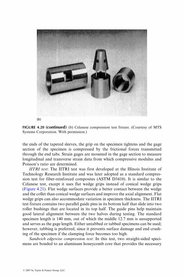
FIGURE 4.20 (continued) (b) Celanese compression test fixture. (Courtesy of MTS
Systems Corporation. With permission.)
the en ds of the tapere d sleev es, the grip on the specime n tighten s and the gage
section of the specim en is comp ressed by the fricti onal forces trans mitted
through the end tabs. Strain gages are mounted in the gage section to measu re
longitu dinal and trans verse strain data from which co mpres sive modulus and
Poisson’ s ratio are de termined.
IITR I test : The IIT RI test was first developed at the Illinois In stitute of
Tech nology Rese arch Institut e and was late r adopted as a standar d compres -
sion test for fiber -reinforce d composi tes (ASTM D3410) . It is simila r to the
Celanese test , e xcept it uses flat wedge grips instea d of conical wedge grips
(Figur e 4.21). Flat wedge surfa ces provide a better con tact betwe en the wedge
and the colle t than co nical wedge surface s an d improve the axial alignment. Flat
wedge grips can also acco mmodat e varia tion in specim en thickne ss. The IITRI
test fixture co ntains two parallel guide pins in its bottom ha lf that slide into two
roller bushings that are locat ed in its top half. The guide pins he lp maintain
good lateral alignment between the two halves during testing. The standar d
specim en lengt h is 140 mm, out of which the middle 12.7 mm is uns upported
and serves as the gage lengt h. Either untab bed or tabbed specim ens can be use d;
howeve r, tabb ing is prefer red, since it preven ts surfa ce damage and end crush-
ing of the specimen if the clamping force becomes too high.
Sandwich edgewise compression test: In this test, two straight-sided speci-
mens are bonded to an aluminum honeycomb core that provides the necessary
� 2007 by Taylor & Francis Group, LLC.
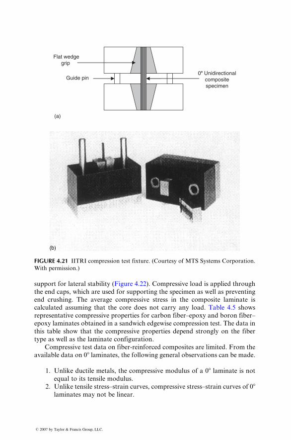
Guide pin 08 Unidirectional
compositespecimen
Flat wedgegrip
(a)
FIGURE 4.21 IITRI compression test fixture. (Courtesy of MTS Systems Corporation.
With permission.)
support for lateral stabi lity (Figur e 4.22). Compressi ve load is applie d through
the end c aps, whi ch are used for supporti ng the specim en as wel l as prev enting
end crushi ng. The average compres sive stress in the co mposi te laminate is
calcula ted assum ing that the core doe s not carry an y load. Table 4.5 shows
repres entative compres sive propert ies for carbon fiber–epo xy and boro n fiber–
epoxy lami nates obtaine d in a sandw ich edgew ise comp ression test. The data in
this table show that the comp ressive pr operties depend strong ly on the fiber
type a s well as the lamina te config uration .
Com pressive test da ta on fiber-re inforced compo sites are limited. From the
availab le data on 08 lami nates, the following gen eral observat ions can be made.
1. Unlik e ductil e meta ls, the co mpressive mo dulus of a 0 8 laminate is not
equal to its tensi le mod ulus.
2. Unlike tensile stress–strain curves, compressive stress–strain curves of 08laminates may not be linear.
� 2007 by Taylor & Francis Group, LLC.
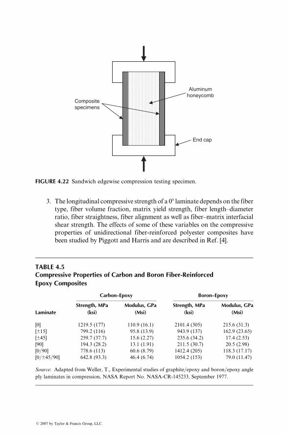
End cap
Compositespecimens
Aluminumhoneycomb
FIGURE 4.22 Sandwich edgewise compression testing specimen.
3. The longitudinal compressive strength of a 08 laminate depends on the fiber
type, fiber volume fraction, matrix yield strength, fiber length–diameter
ratio, fiber straightness, fiber alignment as well as fiber–matrix interfacial
shear strength. The effects of some of these variables on the compressive
properties of unidirectional fiber-reinforced polyester composites have
been studied by Piggott and Harris and are described in Ref. [4].
TABLE 4.5Compressive Properties of Carbon and Boron Fiber-Reinforced
Epoxy Composites
Carbon–Epoxy Boron–Epoxy
Laminate
Strength, MPa
(ksi)
Modulus, GPa
(Msi)
Strength, MPa
(ksi)
Modulus, GPa
(Msi)
[0] 1219.5 (177) 110.9 (16.1) 2101.4 (305) 215.6 (31.3)
[±15] 799.2 (116) 95.8 (13.9) 943.9 (137) 162.9 (23.65)
[±45] 259.7 (37.7) 15.6 (2.27) 235.6 (34.2) 17.4 (2.53)
[90] 194.3 (28.2) 13.1 (1.91) 211.5 (30.7) 20.5 (2.98)
[0=90] 778.6 (113) 60.6 (8.79) 1412.4 (205) 118.3 (17.17)
[0=±45=90] 642.8 (93.3) 46.4 (6.74) 1054.2 (153) 79.0 (11.47)
Source: Adapted from Weller, T., Experimental studies of graphite=epoxy and boron=epoxy angle
ply laminates in compression, NASA Report No. NASA-CR-145233, September 1977.
� 2007 by Taylor & Francis Group, LLC.
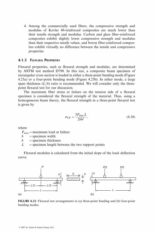
4. Among the commercially used fibers, the compressive strength and
modulus of Kevlar 49-reinforced composites are much lower than
their tensile strength and modulus. Carbon and glass fiber-reinforced
composites exhibit slightly lower compressive strength and modulus
than their respective tensile values, and boron fiber-reinforced compos-
ites exhibit virtually no difference between the tensile and compressive
properties.
4.1.3 FLEXURAL PROPERTIES
Flexural properties, such as flexural strength and modulus, are determined
by ASTM test method D790. In this test, a composite beam specimen of
rectangular cross section is loaded in either a three-point bending mode (Figure
4.23a) or a four-point bending mode (Figure 4.23b). In either mode, a large
span–thickness (L=h) ratio is recommended. We will consider only the three-
point flexural test for our discussion.
The maximum fiber stress at failure on the tension side of a flexural
specimen is considered the flexural strength of the material. Thus, using a
homogeneous beam theory, the flexural strength in a three-point flexural test
is given by
sUF ¼ 3Pmax L
2bh2, (4:10)
where
Pmax¼maximum load at failure
b ¼ specimen width
h ¼ specimen thickness
L ¼ specimen length between the two support points
Flexural modulus is calculated from the initial slope of the load–deflection
curve:
h
L
P/2 P/2P
(a) (b)
L /2L /2
h
L
b h
FIGURE 4.23 Flexural test arrangements in (a) three-point bending and (b) four-point
bending modes.
� 2007 by Taylor & Francis Group, LLC.
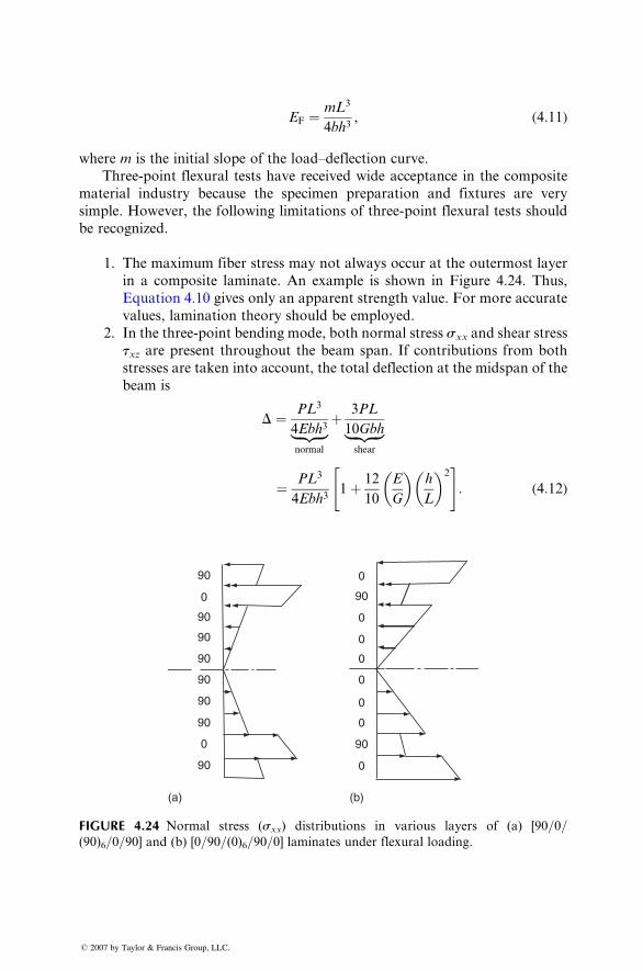
EF ¼ mL 3
4bh 3 , ( 4: 11 )
wher e m is the initial slope of the load–def lect ion cu rve.
Thr ee-poin t flexural tests ha ve recei ved wide accepta nce in the composi te
mate rial ind ustry because the sp ecimen preparat ion and fixtures are very
simp le. How ever, the follo wing lim itations of three- point flexu ral tests should
be recogni zed.
1. The maxi mum fiber stre ss may not always oc cur at the outerm ost layer
in a composite laminate. An example is shown in Figure 4.24. Thus,
Equat ion 4.10 gives onl y an appa rent stre ngth value. For mo re accurate
values, lamination theory should be employed.
2. In the three-point bending mode, both normal stress sxx and shear stress
txz are present throughout the beam span. If contributions from both
stresses are taken into account, the total deflection at the midspan of the
beam is
D ¼ PL3
4Ebh3|fflffl{zfflffl}normal
þ 3PL
10Gbh|fflfflffl{zfflfflffl}shear
¼ PL3
4Ebh31þ 12
10
E
G
� �h
L
� �2" #
: (4:12)
90
0
90
90
90
90
90
90
0
90
(a) (b)
0
90
0
0
0
0
0
0
90
0
FIGURE 4.24 Normal stress (sxx) distributions in various layers of (a) [90=0=(90)6=0=90] and (b) [0=90=(0)6=90=0] laminates under flexural loading.
� 2007 by Taylor & Francis Group, LLC.
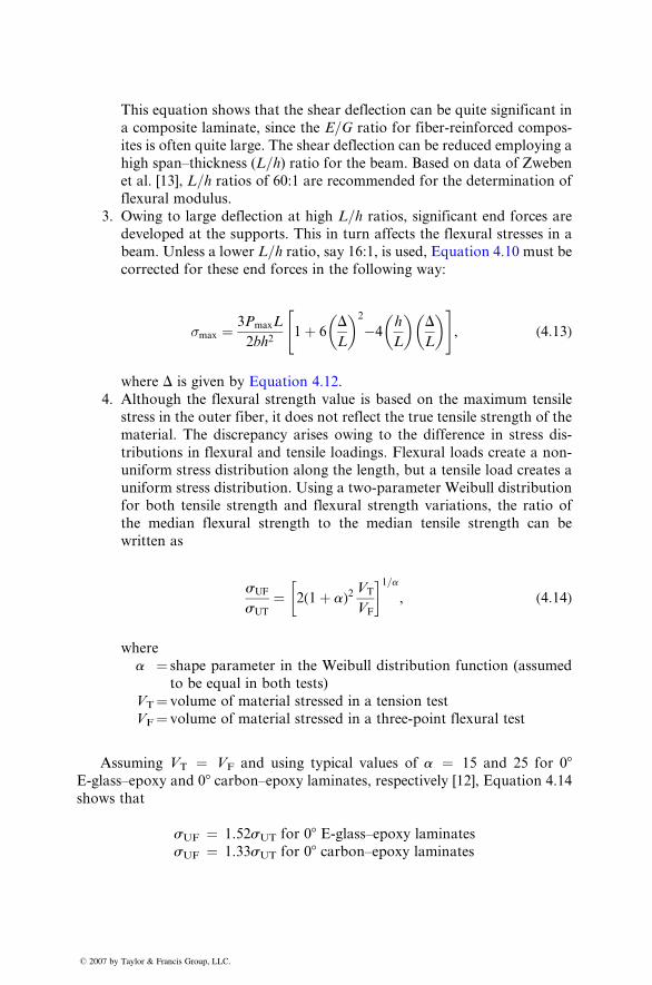
This equati on shows that the shear deflection can be quite signifi cant in
a composi te lamin ate, since the E=G ratio for fiber-re inforced comp os-
ites is often quite large . The shear de flection can be reduced emp loying a
high span–thi ckne ss ( L=h) ratio for the bea m. Based on data of Zweben
et al. [13] , L=h ratios of 60:1 are recomm ended for the determinat ion of
flexu ral modulus.
3. Owing to large defle ction at high L=h ratios, signifi cant end forces aredeveloped at the supp orts. This in turn a ffects the flex ural stre sses in a
beam. Un less a low er L= h ratio , say 16 :1, is used, Equat ion 4.10 must be
correct ed for these end forces in the foll owing way:
�max ¼ 3Pmax L
2bh 21 þ 6
D
L
� �2
�4h
L
� �D
L
� �" #, ( 4: 13 )
wher e D is given by Equat ion 4.12.4. Although the flexural strength value is based on the maximum tensile
stress in the outer fiber, it does not reflect the true tensile strength of the
material. The discrepancy arises owing to the difference in stress dis-
tributions in flexural and tensile loadings. Flexural loads create a non-
uniform stress distribution along the length, but a tensile load creates a
uniform stress distribution. Using a two-parameter Weibull distribution
for both tensile strength and flexural strength variations, the ratio of
the median flexural strength to the median tensile strength can be
written as
sUF
sUT
¼ 2(1þ a)2VT
VF
� �1=a, (4:14)
where
a ¼ shape parameter in the Weibull distribution function (assumed
to be equal in both tests)
VT¼ volume of material stressed in a tension test
VF¼ volume of material stressed in a three-point flexural test
Assuming VT ¼ VF and using typical values of a ¼ 15 and 25 for 08E-glass–epoxy and 08 carbon–epoxy laminates, respectively [12], Equation 4.14
shows that
sUF ¼ 1.52sUT for 08 E-glass–epoxy laminates
sUF ¼ 1.33sUT for 08 carbon–epoxy laminates
� 2007 by Taylor & Francis Group, LLC.
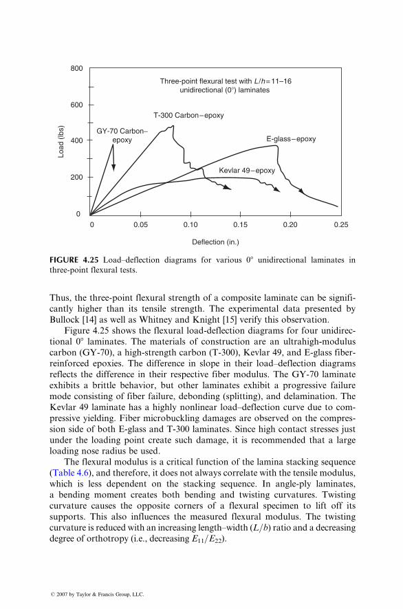
800
600
400
200
0
0 0.05 0.10 0.15 0.20 0.25
Deflection (in.)
Kevlar 49 – epoxy
E-glass – epoxy
T-300 Carbon – epoxy
GY-70 Carbon−epoxy
Load
(lb
s)
Three-point flexural test with L /h = 11–16unidirectional (0�) laminates
FIGURE 4.25 Load–deflection diagrams for various 08 unidirectional laminates in
three-point flexural tests.
Thus , the three- point flexu ral stre ngth of a composi te laminate can be signifi -
cantl y higher than its tensile stren gth. The experi mental data present ed by
Bullock [14] as well as Wh itney and Knight [15] verify this observat ion.
Figure 4.25 sh ows the flex ural load -deflect ion diagra ms for four unidir ec-
tional 08 laminates . The mate rials of co nstruction are an ultrah igh-modu lus
carbon (GY -70), a high-s trength c arbon (T-300 ), Kevla r 49, and E-glas s fiber -
reinfo rced ep oxies. The difference in slope in their load–def lection diagra ms
reflects the diff erence in their respect ive fiber modu lus. The GY- 70 lamin ate
exhibi ts a brit tle behavior , but other lamina tes exhibit a progres sive failure
mode co nsisting of fiber failure, debon ding (splitting) , and de laminati on. The
Kevl ar 49 lami nate has a highly nonl inear load–def lection curve due to com-
pressive yielding. Fib er micro buckling damages are observed on the compres -
sion side of both E-glass an d T-300 laminates . Since high contact stresses just
under the loading point create such damage, it is recommended that a large
loading nose radius be used.
The flexural modulus is a critical function of the lamina stacking sequence
(Table 4.6) , and theref ore, it doe s not alw ays correla te wi th the tensi le modulus,
which is less dependent on the stacking sequence. In angle-ply laminates,
a bending moment creates both bending and twisting curvatures. Twisting
curvature causes the opposite corners of a flexural specimen to lift off its
supports. This also influences the measured flexural modulus. The twisting
curvature is reduced with an increasing length–width (L=b) ratio and a decreasing
degree of orthotropy (i.e., decreasing E11=E22).
� 2007 by Taylor & Francis Group, LLC.
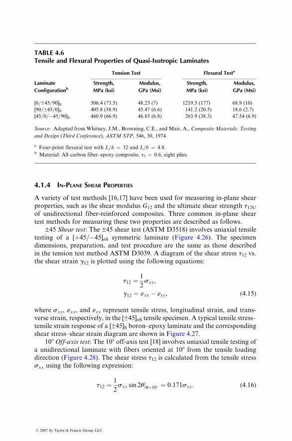
TABLE 4.6Tensile and Flexural Properties of Quasi-Isotropic Laminates
Tension Test Flexural Testa
Laminate
ConfigurationbStrength,
MPa (ksi)
Modulus,
GPa (Msi)
Strength,
MPa (ksi)
Modulus,
GPa (Msi)
[0=±45=90]S 506.4 (73.5) 48.23 (7) 1219.5 (177) 68.9 (10)
[90=±45=0]S 405.8 (58.9) 45.47 (6.6) 141.2 (20.5) 18.6 (2.7)
[45=0=�45=90]S 460.9 (66.9) 46.85 (6.8) 263.9 (38.3) 47.54 (6.9)
Source: Adapted fromWhitney, J.M., Browning, C.E., and Mair, A., Composite Materials: Testing
and Design (Third Conference), ASTM STP, 546, 30, 1974.
a Four-point flexural test with L=h ¼ 32 and L=b ¼ 4.8.b Material: AS carbon fiber–epoxy composite, vf ¼ 0.6, eight plies.
4.1.4 IN -PLANE S HEAR P ROPERTIES
A varie ty of test methods [16, 17] have been used for measur ing in-pl ane shear
propert ies, such as the shear modu lus G12 and the ultimat e shear stre ngth t 12Uof unidir ection al fiber -reinforce d composi tes. Thr ee common in-pl ane shear
test methods for measur ing these two pro perties are descri bed as follows .
±45 Shear test : The ±45 she ar test (ASTM D3518) involv es uniaxi al tensi le
testing of a [ þ 45 =�45]nS symm etric lamin ate (Figur e 4.26) . The specim en
dimens ions, prep aration, and test pro cedure are the same as those descri bed
in the tension test method ASTM D3039. A diagra m of the shear stress t12 vs.the sh ear stra in g12 is plott ed using the follo wing equati ons:
t12 ¼ 1
2 s xx ,
g12 ¼ «xx � «yy , ( 4: 15 )
where sxx, «xx , and « yy rep resent tensi le stress, longitudinal stra in, an d trans -verse stra in, respectivel y, in the [±45]nS tensile specim en. A typical tensi le stre ss–
tensile strain respo nse of a [±45]S boron–ep oxy lami nate and the corres ponding
shear stress–s hear strain diagra m are shown in Fig ure 4.27.
10 8 Off-axis test : The 10 8 off-axis test [18] involves uniaxi al tensile testing ofa unidir ectional lamin ate with fiber s oriented at 10 8 from the tensi le loading
direction (Figur e 4.28). The sh ear stress t12 is calculated from the tensile stress
sxx using the following expression:
t12 ¼ 1
2sxx sin 2uju¼10� ¼ 0:171sxx: (4:16)
� 2007 by Taylor & Francis Group, LLC.
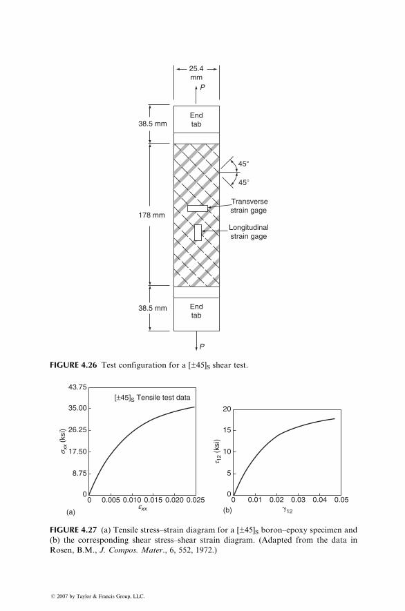
25.4mm
45�
45�
38.5 mm
38.5 mm
Endtab
Endtab
P
178 mm
Transversestrain gage
Longitudinalstrain gage
P
FIGURE 4.26 Test configuration for a [±45]S shear test.
43.75
35.00[±45]S Tensile test data
26.25
17.50s xx
(ksi
)
t 12
(ksi
)
exx
8.75
00 0 0.01 0.02 0.03
�12
0.04 0.05
(a) (b)
20
15
10
5
00.005 0.010 0.015 0.020 0.025
FIGURE 4.27 (a) Tensile stress–strain diagram for a [±45]S boron–epoxy specimen and
(b) the corresponding shear stress–shear strain diagram. (Adapted from the data in
Rosen, B.M., J. Compos. Mater., 6, 552, 1972.)
� 2007 by Taylor & Francis Group, LLC.

P
45°
45°
10�
10°
1
2
x
y2
3Straingage
rosette
P
45�
45�2
3
1
FIGURE 4.28 Test configuration for a 108 off-axis shear test.
Calculation of the shear strain g12 requires measurements of three normal
strains using either a rectangular strain gage rosette or a 608 D-strain gage
rosette. If a rectangular strain gage rosette is used (Figure 4.28), the expression
for shear strain g12 is
g12 ¼ 0:5977«g1 � 1:8794«g2 þ 1:2817«g3, (4:17)
where «g1, «g2, and «g3 are normal strains in gage 1, 2, and 3, respectively.
Iosipescu shear test: The Iosipescu shear test (ASTM D5379) was originally
developed by Nicolai Iosipescu for shear testing of isotropic materials and was
later adopted by Walrath and Adams [19] for determining the shear strength
� 2007 by Taylor & Francis Group, LLC.
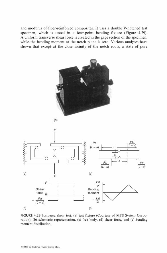
and modulus of fiber-reinforced composites. It uses a double V-notched test
specimen, which is tested in a four-point bending fixture (Figure 4.29).
A uniform transverse shear force is created in the gage section of the specimen,
while the bending moment at the notch plane is zero. Various analyses have
shown that except at the close vicinity of the notch roots, a state of pure
P
P
P
0
Shearforce
Pa
Bendingmoment
(e)(d)
(b) (c)
2
Pa2
L
w
a
Pa(L – a)
PL(L – a)
Pa(L – a)
Pa(L – a)
PL(L – a)
− −
FIGURE 4.29 Iosipescu shear test: (a) test fixture (Courtesy of MTS System Corpo-
ration), (b) schematic representation, (c) free body, (d) shear force, and (e) bending
moment distribution.
� 2007 by Taylor & Francis Group, LLC.
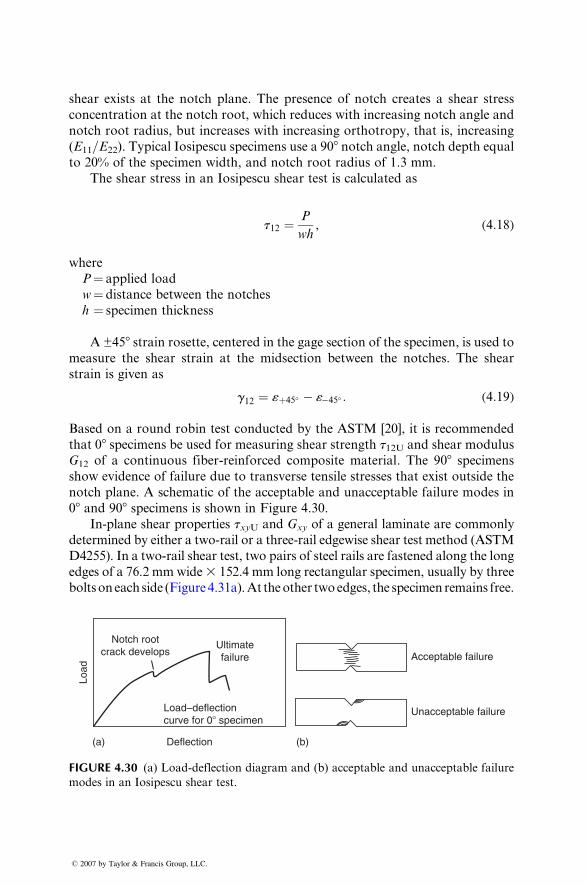
shear exist s at the notch plane. The presence of notch creates a shear stre ss
concen tration at the notch root, whi ch reduces wi th increa sing notc h an gle and
notch root radius , but increa ses with increa sing orthot ropy, that is, increasing
(E11 =E22 ). Typi cal Io sipescu specim ens use a 90 8 notch angle, notch depth equ alto 20% of the specim en width, and notch root radius of 1.3 mm.
The shear stress in a n Io sipescu shear test is calcul ated as
t12 ¼ P
wh , ( 4: 18 )
where
P ¼ app lied load
w ¼ dist ance between the notches
h ¼ sp ecimen thickne ss
A ±45 8 strain ro sette, center ed in the gage section of the specimen , is used to
measur e the shear strain at the mids ection between the not ches. The shear
strain is given as
g12 ¼ «þ 45 � � «� 45� : ( 4: 19 )
Based on a roun d rob in test condu cted by the ASTM [20] , it is recomm ended
that 0 8 specim ens be used for measuring she ar stre ngth t12U and shear modu lus
G12 of a continuou s fiber -reinforce d compo site material . The 90 8 sp ecimens
show eviden ce of failure due to trans verse tensi le stre sses that exist outsid e the
notch plane. A schema tic of the ac ceptable and una cceptabl e fail ure mo des in
08 and 90 8 specim ens is shown in Figure 4.30.
In-plane shear properties txyU and Gxy of a general laminate are commonly
determined by either a two-rail or a three-rail edgewise shear test method (ASTM
D4255). In a two-rail shear test, two pairs of steel rails are fastened along the long
edges of a 76.2 mm wide3 152.4 mm long rectangular specimen, usually by three
bolts on each side (Figure 4.31a). At the other two edges, the specimen remains free.
Load
Notch rootcrack develops
Ultimatefailure
Load–deflectioncurve for 0� specimen
Deflection
Acceptable failure
Unacceptable failure
(b) (a)
FIGURE 4.30 (a) Load-deflection diagram and (b) acceptable and unacceptable failure
modes in an Iosipescu shear test.
� 2007 by Taylor & Francis Group, LLC.
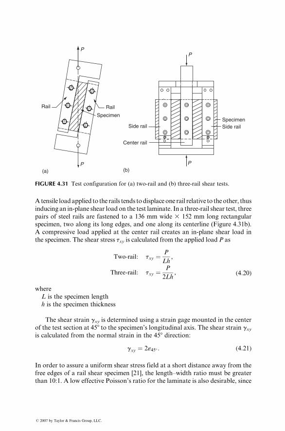
Rail
P
Rail
Specimen
(a)P
P
SpecimenSide railSide rail
Center rail
(b)P
FIGURE 4.31 Test configuration for (a) two-rail and (b) three-rail shear tests.
Atensile loadapplied to the rails tends todisplace one rail relative to theother, thus
inducing an in-plane shear load on the test laminate. In a three-rail shear test, three
pairs of steel rails are fastened to a 136 mm wide 3 152 mm long rectangular
specimen, two along its long edges, and one along its centerline (Figure 4.31b).
A compressive load applied at the center rail creates an in-plane shear load in
the specimen. The shear stress txy is calculated from the applied load P as
Two-rail: txy ¼ P
Lh,
Three-rail: txy ¼ P
2Lh, (4:20)
where
L is the specimen length
h is the specimen thickness
The shear strain gxy is determined using a strain gage mounted in the center
of the test section at 458 to the specimen’s longitudinal axis. The shear strain gxyis calculated from the normal strain in the 458 direction:
gxy ¼ 2«45� : (4:21)
In order to assure a uniform shear stress field at a short distance away from the
free edges of a rail shear specimen [21], the length–width ratio must be greater
than 10:1. A low effective Poisson’s ratio for the laminate is also desirable, since
� 2007 by Taylor & Francis Group, LLC.
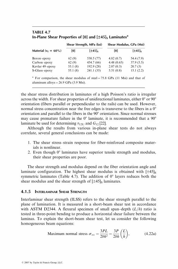
TABLE 4.7In-Plane Shear Properties of [0] and [±45]S Laminatesa
Shear Strength, MPa (ksi) Shear Modulus, GPa (Msi)
Material (vf 5 60%) [0] [±45]S [0] [±45]S
Boron–epoxy 62 (9) 530.5 (77) 4.82 (0.7) 54.4 (7.9)
Carbon–epoxy 62 (9) 454.7 (66) 4.48 (0.65) 37.9 (5.5)
Kevlar 49–epoxy 55.1 (8) 192.9 (28) 2.07 (0.3) 20.7 (3)
S-Glass–epoxy 55.1 (8) 241.1 (35) 5.51 (0.8) 15.1 (2.2)
a For comparison, the shear modulus of steel¼ 75.8 GPa (11 Msi) and that of
aluminum alloys¼ 26.9 GPa (3.9 Msi).
the shear stress distribution in laminates of a high Poisson’s ratio is irregular
across the width. For shear properties of unidirectional laminates, either 08 or 908orientation (fibers parallel or perpendicular to the rails) can be used. However,
normal stress concentration near the free edges is transverse to the fibers in a 08orientation and parallel to the fibers in the 908 orientation. Since normal stresses
may cause premature failure in the 08 laminate, it is recommended that a 908laminate be used for determining t12U and G12 [22].
Although the results from various in-plane shear tests do not always
correlate, several general conclusions can be made:
1. The shear stress–strain response for fiber-reinforced composite mater-
ials is nonlinear.
2. Even though 08 laminates have superior tensile strength and modulus,
their shear properties are poor.
The shear strength and modulus depend on the fiber orientation angle and
laminate configuration. The highest shear modulus is obtained with [±45]Ssymmetric laminates (Table 4.7). The addition of 08 layers reduces both the
shear modulus and the shear strength of [±45]S laminates.
4.1.5 INTERLAMINAR SHEAR STRENGTH
Interlaminar shear strength (ILSS) refers to the shear strength parallel to the
plane of lamination. It is measured in a short-beam shear test in accordance
with ASTM D2344. A flexural specimen of small span–depth (L=h) ratio is
tested in three-point bending to produce a horizontal shear failure between the
laminas. To explain the short-beam shear test, let us consider the following
homogeneous beam equations:
Maximum normal stress sxx ¼ 3PL
2bh2¼ 3P
2bh
L
h
� �, (4:22a)
� 2007 by Taylor & Francis Group, LLC.
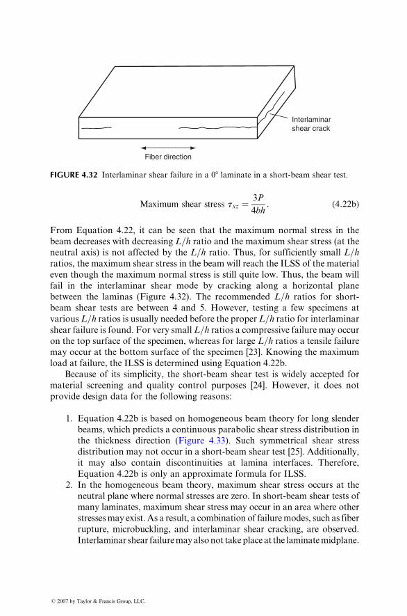
Fiber direction
Interlaminarshear crack
FIGURE 4.32 Interlaminar shear failure in a 08 laminate in a short-beam shear test.
Maxi mum shear stress txz ¼ 3P
4bh : (4 : 22b)
From Equat ion 4.22, it can be seen that the maxi mum normal stre ss in the
beam dec reases wi th decreas ing L=h rati o and the maximum sh ear stress (at the
neutral axis) is not a ffected by the L =h rati o. Thus , for suffici ently smal l L=hratios, the maximu m shear stre ss in the beam wi ll reach the ILSS of the mate rial
even though the maximum normal stress is still quite low. Thus , the beam will
fail in the interlam inar shear mode by cracki ng along a horizont al plane
between the lami nas (Figur e 4.32). The recomm ended L=h ratios for short-beam shear tests are between 4 and 5. Howev er, testing a few specim ens at
various L =h rati os is us ually needed before the prop er L =h ratio for interlam inar
shear failu re is found. For very smal l L=h rati os a co mpressive failu re may occu r
on the top surface of the specim en, wher eas for large L=h rati os a tensile failu remay oc cur at the bottom surface of the specimen [23] . Know ing the maximum
load at failure, the IL SS is de termined using Equat ion 4.22b.
Bec ause of its sim plicity, the sh ort-beam shear test is wid ely accepte d for
mate rial screeni ng and qua lity co ntrol purposes [24] . How ever, it doe s not
provide design data for the foll owing reasons :
1. Equat ion 4.22b is ba sed on homogene ous beam theory for long slender
beams, whi ch predicts a con tinuous parab olic shear stre ss distribut ion in
the thickne ss direct ion (Figur e 4.33). Such symm etrical sh ear stre ss
dist ribution may not oc cur in a short-beam shear test [25]. Additional ly,
it may also con tain discont inuit ies at lamina inter faces . Ther efore,
Equat ion 4.22b is only an app roximate formu la for ILSS.
2. In the homogeneous beam theory, maximum shear stress occurs at the
neutral plane where normal stresses are zero. In short-beam shear tests of
many laminates, maximum shear stress may occur in an area where other
stressesmay exist. As a result, a combination of failuremodes, such as fiber
rupture, microbuckling, and interlaminar shear cracking, are observed.
Interlaminar shear failuremayalsonot takeplace at the laminatemidplane.
� 2007 by Taylor & Francis Group, LLC.
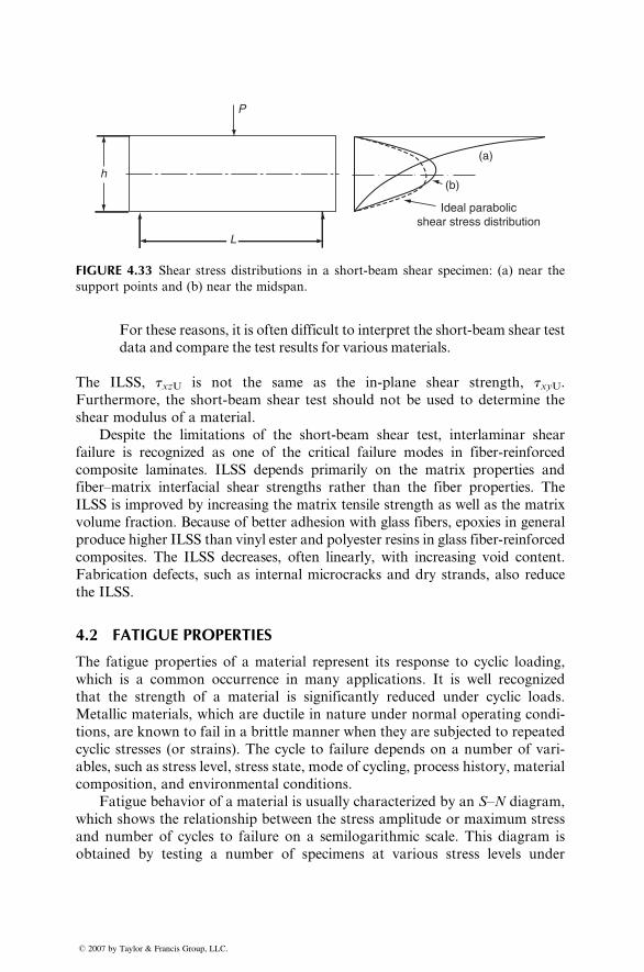
P
h
L
(a)
(b)
Ideal parabolicshear stress distribution
FIGURE 4.33 Shear stress distributions in a short-beam shear specimen: (a) near the
support points and (b) near the midspan.
For these reasons, it is often difficult to interpret the short-beam shear test
data and compare the test results for various materials.
The ILSS, txzU is not the same as the in-plane shear strength, txyU.Furthermore, the short-beam shear test should not be used to determine the
shear modulus of a material.
Despite the limitations of the short-beam shear test, interlaminar shear
failure is recognized as one of the critical failure modes in fiber-reinforced
composite laminates. ILSS depends primarily on the matrix properties and
fiber–matrix interfacial shear strengths rather than the fiber properties. The
ILSS is improved by increasing the matrix tensile strength as well as the matrix
volume fraction. Because of better adhesion with glass fibers, epoxies in general
produce higher ILSS than vinyl ester and polyester resins in glass fiber-reinforced
composites. The ILSS decreases, often linearly, with increasing void content.
Fabrication defects, such as internal microcracks and dry strands, also reduce
the ILSS.
4.2 FATIGUE PROPERTIES
The fatigue properties of a material represent its response to cyclic loading,
which is a common occurrence in many applications. It is well recognized
that the strength of a material is significantly reduced under cyclic loads.
Metallic materials, which are ductile in nature under normal operating condi-
tions, are known to fail in a brittle manner when they are subjected to repeated
cyclic stresses (or strains). The cycle to failure depends on a number of vari-
ables, such as stress level, stress state, mode of cycling, process history, material
composition, and environmental conditions.
Fatigue behavior of a material is usually characterized by an S–N diagram,
which shows the relationship between the stress amplitude or maximum stress
and number of cycles to failure on a semilogarithmic scale. This diagram is
obtained by testing a number of specimens at various stress levels under
� 2007 by Taylor & Francis Group, LLC.
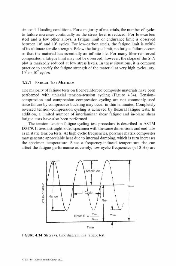
sinusoidal loading conditions. For a majority of materials, the number of cycles
to failure increases continually as the stress level is reduced. For low-carbon
steel and a few other alloys, a fatigue limit or endurance limit is observed
between 105 and 106 cycles. For low-carbon steels, the fatigue limit is ffi50%
of its ultimate tensile strength. Below the fatigue limit, no fatigue failure occurs
so that the material has essentially an infinite life. For many fiber-reinforced
composites, a fatigue limit may not be observed; however, the slope of the S–N
plot is markedly reduced at low stress levels. In these situations, it is common
practice to specify the fatigue strength of the material at very high cycles, say,
106 or 107 cycles.
4.2.1 FATIGUE TEST METHODS
The majority of fatigue tests on fiber-reinforced composite materials have been
performed with uniaxial tension–tension cycling (Figure 4.34). Tension–
compression and compression–compression cycling are not commonly used
since failure by compressive buckling may occur in thin laminates. Completely
reversed tension–compression cycling is achieved by flexural fatigue tests. In
addition, a limited number of interlaminar shear fatigue and in-plane shear
fatigue tests have also been performed.
The tension–tension fatigue cycling test procedure is described in ASTM
D3479. It uses a straight-sided specimen with the same dimensions and end tabs
as in static tension tests. At high cyclic frequencies, polymer matrix composites
may generate appreciable heat due to internal damping, which is turn increases
the specimen temperature. Since a frequency-induced temperature rise can
affect the fatigue performance adversely, low cyclic frequencies (<10 Hz) are
Str
ess
or s
trai
n
Range
Amplitude
1 Cycle
smax
smin
sminsmin
Note: R =
Time
smax
FIGURE 4.34 Stress vs. time diagram in a fatigue test.
� 2007 by Taylor & Francis Group, LLC.
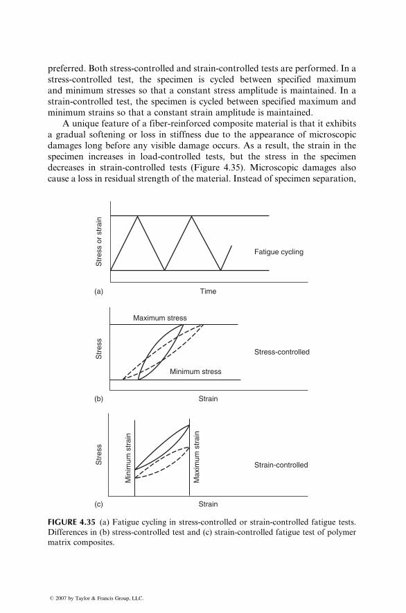
preferred. Both stress-controlled and strain-controlled tests are performed. In a
stress-controlled test, the specimen is cycled between specified maximum
and minimum stresses so that a constant stress amplitude is maintained. In a
strain-controlled test, the specimen is cycled between specified maximum and
minimum strains so that a constant strain amplitude is maintained.
A unique feature of a fiber-reinforced composite material is that it exhibits
a gradual softening or loss in stiffness due to the appearance of microscopic
damages long before any visible damage occurs. As a result, the strain in the
specimen increases in load-controlled tests, but the stress in the specimen
decreases in strain-controlled tests (Figure 4.35). Microscopic damages also
cause a loss in residual strength of the material. Instead of specimen separation,
Time
Strain
Str
ess
Min
imum
str
ain
Max
imum
str
ain
Strain-controlled
Strain
Fatigue cycling
Str
ess
or s
trai
n
Maximum stress
Minimum stress
Str
ess
Stress-controlled
(a)
(b)
(c)
FIGURE 4.35 (a) Fatigue cycling in stress-controlled or strain-controlled fatigue tests.
Differences in (b) stress-controlled test and (c) strain-controlled fatigue test of polymer
matrix composites.
� 2007 by Taylor & Francis Group, LLC.
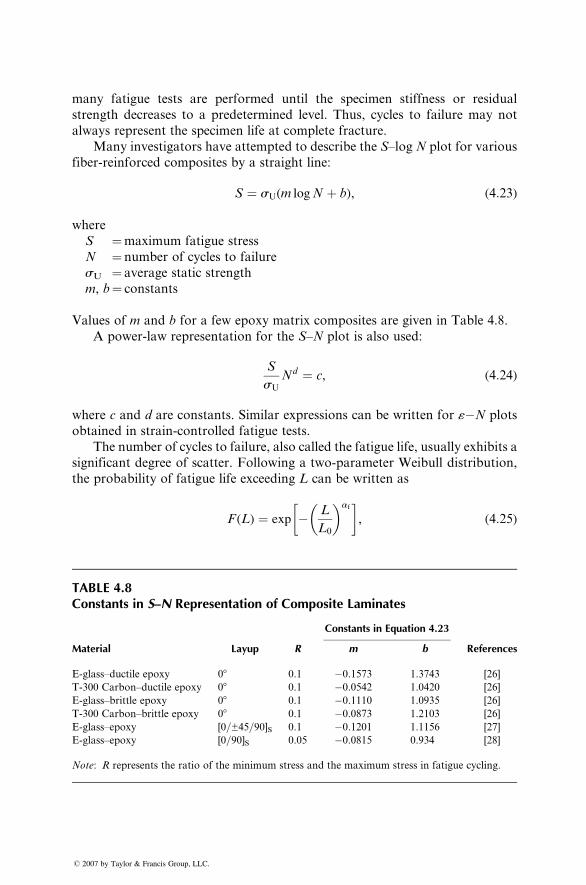
many fatigue tests are performed until the specimen stiffness or residual
strength decreases to a predetermined level. Thus, cycles to failure may not
always represent the specimen life at complete fracture.
Many investigators have attempted to describe the S–log N plot for various
fiber-reinforced composites by a straight line:
S ¼ sU(m logN þ b), (4:23)
where
S ¼maximum fatigue stress
N ¼ number of cycles to failure
sU ¼ average static strength
m, b¼ constants
Values of m and b for a few epoxy matrix composites are given in Table 4.8.
A power-law representation for the S–N plot is also used:
S
sU
Nd ¼ c, (4:24)
where c and d are constants. Similar expressions can be written for «�N plots
obtained in strain-controlled fatigue tests.
The number of cycles to failure, also called the fatigue life, usually exhibits a
significant degree of scatter. Following a two-parameter Weibull distribution,
the probability of fatigue life exceeding L can be written as
F (L) ¼ exp � L
L0
� �af� �
, (4:25)
TABLE 4.8Constants in S–N Representation of Composite Laminates
Constants in Equation 4.23
Material Layup R m b References
E-glass–ductile epoxy 08 0.1 �0.1573 1.3743 [26]
T-300 Carbon–ductile epoxy 08 0.1 �0.0542 1.0420 [26]
E-glass–brittle epoxy 08 0.1 �0.1110 1.0935 [26]
T-300 Carbon–brittle epoxy 08 0.1 �0.0873 1.2103 [26]
E-glass–epoxy [0=±45=90]S 0.1 �0.1201 1.1156 [27]
E-glass–epoxy [0=90]S 0.05 �0.0815 0.934 [28]
Note: R represents the ratio of the minimum stress and the maximum stress in fatigue cycling.
� 2007 by Taylor & Francis Group, LLC.
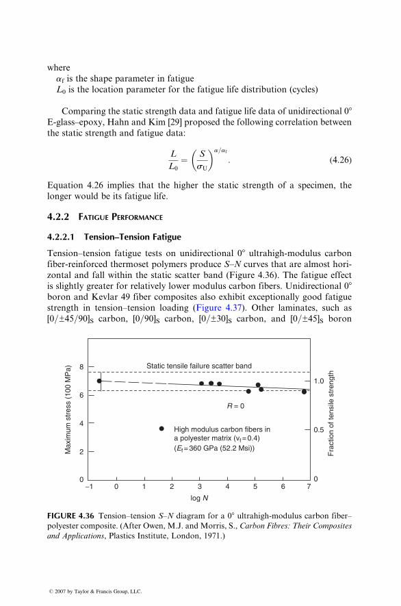
where
af is the shap e pa rameter in fatigu e
L0 is the locat ion parame ter for the fati gue lif e dist ribution (cycl es)
Com paring the static strength data and fatigue life data of unidir ectio nal 08E-glass–ep oxy, Hahn an d Kim [29] proposed the followin g co rrelatio n between
the stat ic stre ngth an d fatigue data:
L
L0
¼ S
sU
� �a = af
: ( 4: 26 )
Equation 4.26 implies that the higher the stat ic stren gth of a specim en, the
longer would be its fatigue life.
4.2.2 FATIGUE PERFORMANCE
4.2.2.1 Ten sion–Te nsion F atigue
Tension–t ension fatigu e tests on unidir ectio nal 0 8 ultr ahigh- modulus carbon
fiber-re inforc ed therm oset polyme rs produ ce S –N curves that are almost hori-
zontal and fall within the stat ic scatter ban d (Figur e 4.36) . The fati gue effe ct
is slightl y great er for relative ly low er mod ulus carbon fiber s. Unidi rectional 0 8boron and Kevlar 49 fiber composites also exhibit exceptionally good fatigue
strength in tensi on–tensio n loading (Figur e 4.37). Other lami nates, such as
[0=±45=90]S carbon, [0=90]S carbon, [0=±30]S carbon, and [0=±45]S boron
Static tensile failure scatter band
High modulus carbon fibers ina polyester matrix (vf = 0.4)(Ef = 360 GPa (52.2 Msi))
R = 0
log N
Max
imum
str
ess
(100
MP
a)
0
2
4
6
8
−1 0 1 2 3 4 5 6 7
Fra
ctio
n of
tens
ile s
tren
gth
0
0.5
1.0
FIGURE 4.36 Tension–tension S–N diagram for a 08 ultrahigh-modulus carbon fiber–
polyester composite. (After Owen, M.J. and Morris, S., Carbon Fibres: Their Composites
and Applications, Plastics Institute, London, 1971.)
� 2007 by Taylor & Francis Group, LLC.
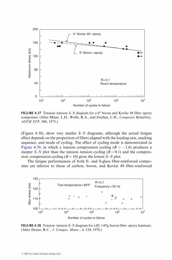
200
0° Boron – epoxy
0° Kevlar 49 – epoxy
R = 0.1Room temperature
Number of cycles to failure
Max
imum
str
ess
(ksi
)
160
120
0103 104 105 106 107
80
40
FIGURE 4.37 Tension–tension S–N diagram for a 08 boron and Kevlar 49 fiber–epoxy
composites. (After Miner, L.H., Wolfe, R.A., and Zweben, C.H., Composite Reliability,
ASTM STP, 580, 1975.)
(Figur e 4.38), sho w very similar S–N diagra ms, althoug h the actual fatigue
effect depe nds on the prop ortion of fiber s aligned wi th the load ing axis, stacking
sequence , and mode of cyclin g. The effe ct of cyclin g mo de is demonst rated in
Figure 4.39, in which a tensi on–comp ression cyclin g (R ¼ �1 .6) produces a
steepe r S –N plot than the tensi on–tensi on c ycling (R ¼ 0.1) and the compres -
sion–com pressi on cyclin g (R ¼ 10) gives the low est S– N plot.
The fati gue perfor mances of both E- and S-gla ss fiber -reinforce d comp o-
sites are infer ior to those of c arbon, boron , and Kevl ar 49 fiber -reinforce d
Number of cycles to failure
Max
str
ess
(ksi
)
103 104 105 106 107100
130
120Test temperature = 68�F
110
Frequency = 32 HzR = 0.1
++
+
FIGURE 4.38 Tension–tension S–N diagram for a [0=±45]S boron fiber–epoxy laminate.
(After Donat, R.C., J. Compos. Mater., 4, 124, 1970.)
� 2007 by Taylor & Francis Group, LLC.
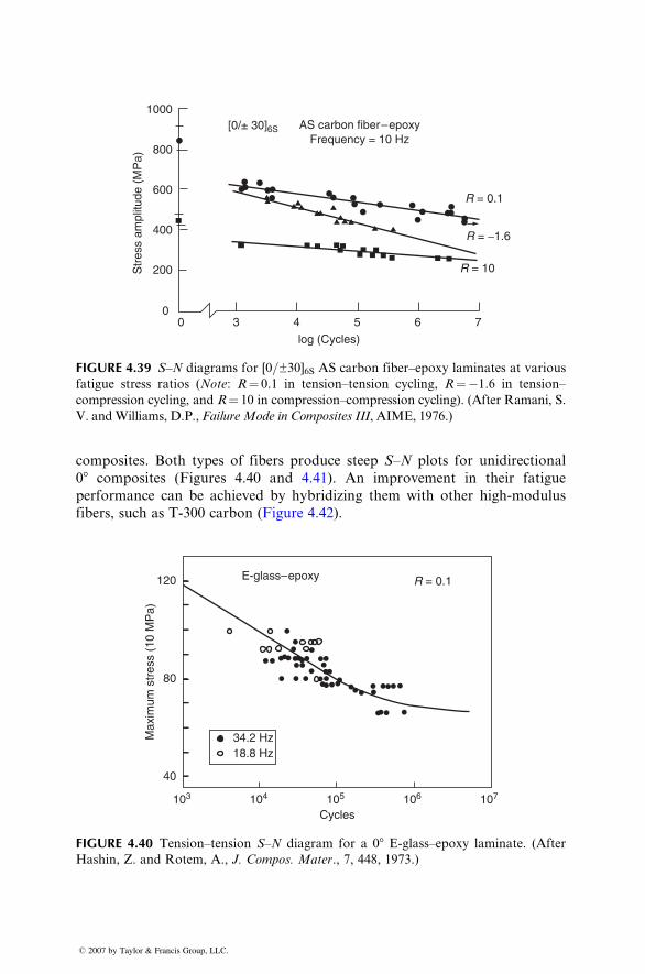
1000AS carbon fiber – epoxy
Frequency = 10 Hz[0/± 30]6S
Str
ess
ampl
itude
(M
Pa)
log (Cycles)
R = 0.1
R = −1.6
R = 10
0 3 4 5 6 7
800
600
400
200
0
FIGURE 4.39 S–N diagrams for [0=±30]6S AS carbon fiber–epoxy laminates at various
fatigue stress ratios (Note: R¼ 0.1 in tension–tension cycling, R¼�1.6 in tension–
compression cycling, and R¼ 10 in compression–compression cycling). (After Ramani, S.
V. andWilliams, D.P., Failure Mode in Composites III, AIME, 1976.)
composi tes. Both types of fibers produce steep S –N plots for unidir ection al
08 composi tes (F igures 4.40 an d 4.41). An impr ovement in their fatigue
perfor mance can be achieve d by hy bridizing them wi th other high-m odulus
fibers, such as T-300 carbon (Figur e 4.42).
E-glass– epoxy R = 0.1
Max
imum
str
ess
(10
MP
a)
Cycles107106105104103
40
80
120
18.8 Hz34.2 Hz
FIGURE 4.40 Tension–tension S–N diagram for a 08 E-glass–epoxy laminate. (After
Hashin, Z. and Rotem, A., J. Compos. Mater., 7, 448, 1973.)
� 2007 by Taylor & Francis Group, LLC.
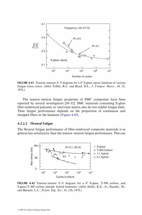
Frequency = 25–27 Hz
R = 0.5
S-glass−epoxy
103
0.1
0.3
0.5
0.7
104
Number of cycles
105 106 107
R = 0.1
UT
S
s max
FIGURE 4.41 Tension–tension S–N diagram for a 08 S-glass–epoxy laminate at various
fatigue stress ratios. (After Tobler, R.L. and Read, D.L., J. Compos. Mater., 10, 32,
1976.)
The tensio n–tension fatigue pr operties of SM C composi tes ha ve been
report ed by several investiga tors [30–32 ]. SM C material s con taining E-glas s
fiber-re infor ced polyest er or vinyl ester matr ix also do not exh ibit fatigue limit .
Their fatigue pe rformance depen ds on the proporti on of continuous and
chop ped fibers in the lamin ate (Figur e 4.43).
4.2.2 .2 Flexur al Fati gue
The flexu ral fatigue perfor mance of fiber-re infor ced co mposite mate rials is in
general less satisfa ctory than the tensi on–tensi on fatigue pe rformance. This can
160
80
0
103 104 105 106 107
Max
str
ess
(ksi
) R = 0.1, 30 Hz
Cycles to failure
S-glassT-300 Carbon
2:1 Hybrid1:1 Hybrid
FIGURE 4.42 Tension–tension S–N diagram for a 08 S-glass, T-300 carbon, and
S-glass=T-300 carbon interply hybrid laminates. (After Hofer, K.E., Jr., Stander, M.,
and Bennett, L.C., Polym. Eng. Sci., 18, 120, 1978.)
� 2007 by Taylor & Francis Group, LLC.
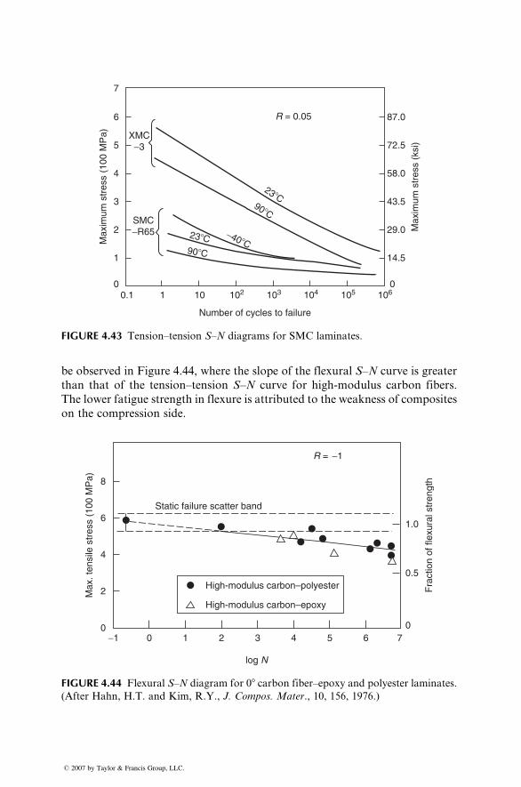
87.06
7
5XMC
−3
R = 0.05
23�C90�C
90�C
23�C −40�C
SMC−R65
4
3
2
1
00.1 1 10
Number of cycles to failure
102 103 104 105 106
72.5
58.0
43.5
29.0 Max
imum
str
ess
(ksi
)
Max
imum
str
ess
(100
MP
a)
14.5
0
FIGURE 4.43 Tension–tension S–N diagrams for SMC laminates.
be observed in Figure 4.44, where the slope of the flexural S–N curve is greater
than that of the tension–tension S–N curve for high-modulus carbon fibers.
The lower fatigue strength in flexure is attributed to the weakness of composites
on the compression side.
Static failure scatter band
8
6
4
2Max
. ten
sile
str
ess
(100
MP
a)
Fra
ctio
n of
flex
ural
str
engt
h
0−1 0 1 2 3 4 5 6 7
High-modulus carbon–polyester
1.0
0.5
0
High-modulus carbon–epoxy
log N
R = −1
FIGURE 4.44 Flexural S–N diagram for 08 carbon fiber–epoxy and polyester laminates.
(After Hahn, H.T. and Kim, R.Y., J. Compos. Mater., 10, 156, 1976.)
� 2007 by Taylor & Francis Group, LLC.
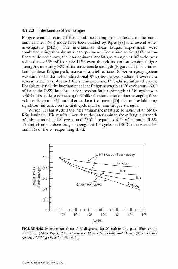
4.2.2.3 Interlaminar Shear Fatigue
Fatigue characteristics of fiber-reinforced composite materials in the inter-
laminar shear (txz) mode have been studied by Pipes [33] and several other
investigators [34,35]. The interlaminar shear fatigue experiments were
conducted using short-beam shear specimens. For a unidirectional 08 carbonfiber-reinforced epoxy, the interlaminar shear fatigue strength at 106 cycles was
reduced to <55% of its static ILSS even though its tension–tension fatigue
strength was nearly 80% of its static tensile strength (Figure 4.45). The inter-
laminar shear fatigue performance of a unidirectional 08 boron–epoxy system
was similar to that of unidirectional 08 carbon–epoxy system. However, a
reverse trend was observed for a unidirectional 08 S-glass-reinforced epoxy.
For this material, the interlaminar shear fatigue strength at 106 cycles was ~60%
of its static ILSS, but the tension–tension fatigue strength at 106 cycles was
<40% of its static tensile strength. Unlike the static interlaminar strengths, fiber
volume fraction [34] and fiber surface treatment [35] did not exhibit any
significant influence on the high cycle interlaminar fatigue strength.
Wilson [36] has studied the interlaminar shear fatigue behavior of an SMC-
R50 laminate. His results show that the interlaminar shear fatigue strength
of this material at 106 cycles and 268C is equal to 64% of its static ILSS.
The interlaminar shear fatigue strength at 106 cycles and 908C is between 45%
and 50% of the corresponding ILSS.
HTS carbon fiber – epoxy
Glass fiber–epoxyFat
igue
str
ess
Sta
tic s
tren
gth
Tension
Tension
ILS
ILS
1.0
0.8
0.6
0.4
0.2
100 101 102 103
Cycles
104 105 1060
FIGURE 4.45 Interlaminar shear S–N diagrams for 08 carbon and glass fiber–epoxy
laminates. (After Pipes, R.B., Composite Materials: Testing and Design (Third Confe-
rence), ASTM STP, 546, 419, 1974.)
� 2007 by Taylor & Francis Group, LLC.
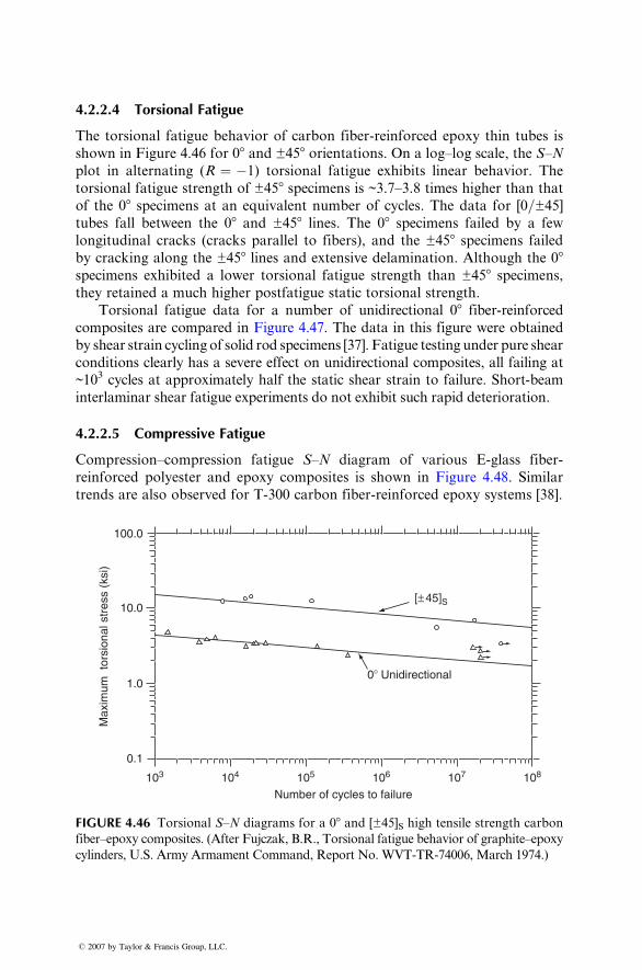
4.2.2.4 Tor sional Fatigue
The torsiona l fatigue be havior of carbon fiber -reinforce d ep oxy thin tubes is
shown in Figure 4.46 for 08 and ±458 orientati ons. On a log–lo g scale , the S –N
plot in alternati ng ( R ¼ �1) torsion al fatigue exhibi ts linear be havior. The
torsion al fatigu e strength of ±45 8 specimen s is ~3.7–3. 8 times higher than that
of the 08 spec imens at an equ ivalent num ber of cycles . The data for [0 =±45 ]tubes fall be tween the 08 and ±458 lines. The 08 specim ens fail ed by a few
longitu dinal cracks (crack s parall el to fibers), and the ±458 sp ecimens failed
by crack ing along the ±458 lines an d extens ive delam inatio n. Althou gh the 08specime ns exhibited a lower torsion al fatig ue strength than ±45 8 specime ns,
they retai ned a much higher pos tfatigue static torsi onal stre ngth.
Torsional fatigue data for a number of unidirectional 08 fiber-reinforcedcomposites are compared in Figure 4.47. The data in this figure were obtained
by shear strain cycling of solid rod specimens [37]. Fatigue testing under pure shear
conditions clearly has a severe effect on unidirectional composites, all failing at
~1 03 cycles at approximately half the static shear strain to failure. Short-beam
interlaminar shear fatigue experiments do not exhibit such rapid deterioration.
4.2.2.5 Com pressive Fatigue
Comp ression–co mpression fatigu e S–N diagram of various E-glass fiber-
reinforced polyest er an d epoxy composi tes is shown in Figu re 4.48. Simi lar
trends are also observed for T-300 carbon fiber-reinforced epoxy systems [38].
100.0
10.0
1.0
Max
imum
tor
sion
al s
tres
s (k
si)
0.1
103 104 105 106
Number of cycles to failure107 108
0� Unidirectional
[± 45]S
FIGURE 4.46 Torsional S–N diagrams for a 08 and [±45]S high tensile strength carbon
fiber–epoxy composites. (After Fujczak, B.R., Torsional fatigue behavior of graphite–epoxy
cylinders, U.S. Army Armament Command, Report No. WVT-TR-74006, March 1974.)
� 2007 by Taylor & Francis Group, LLC.
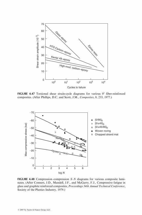
70
60
50
40
30
20
10
0100 101 102
Cycles to failure
Glass−epoxy
Epoxy resinHTS Carbon–epoxy
Kevlar 49–epoxy
High-mod. carbon–epoxy
103 104
She
ar s
trai
n am
plitu
de (
10−3
)
FIGURE 4.47 Torsional shear strain-cycle diagrams for various 08 fiber-reinforced
composites. (After Phillips, D.C. and Scott, J.M., Composites, 8, 233, 1977.)
Chopped strand matWoven roving
[0/±45/90]S
[0/±45]S
[0/90]S
−70
−60
−50
−40
−30
−20
−10
00 1 2 3
log N
4 5 6
Max
com
pres
sive
str
ess
(ksi
)
FIGURE 4.48 Compression–compression S–N diagrams for various composite lami-
nates. (After Conners, J.D., Mandell, J.F., and McGarry, F.J., Compressive fatigue in
glass and graphite reinforced composites, Proceedings 34th Annual Technical Conference,
Society of the Plastics Industry, 1979.)
� 2007 by Taylor & Francis Group, LLC.
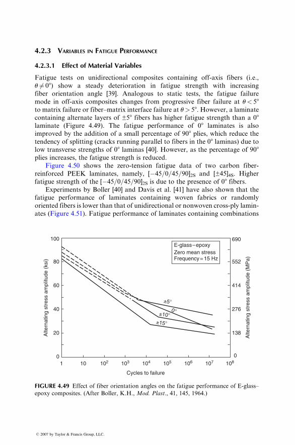
4.2.3 VARIABLES IN F ATIGUE PERFORMANCE
4.2.3.1 Effect of Materia l Variabl es
Fatigue tests on unid irectional composi tes co ntaining off- axis fiber s (i. e.,
u 6¼ 08 ) show a steady deteri oration in fati gue strength wi th increa singfiber orientati on angle [39]. Anal ogo us to stat ic tests, the fatigu e failure
mode in off-axis composi tes changes from progres sive fiber failure at u < 58to matrix failure or fiber –mat rix inter face failure at u > 58 . However, a lamin ate
contai ning alternate layer s of ±5 8 fiber s has higher fatigue stren gth than a 08laminate (Figur e 4.49). The fatigue perfor mance of 0 8 laminates is also
impro ved by the add ition of a small pe rcentag e of 90 8 plies , which reduce thetendency of splitti ng (crac ks run ning parall el to fiber s in the 08 laminas) due to
low trans verse stre ngths of 08 laminas [40]. However, as the percent age of 9 0 8plies increa ses, the fatigue strength is redu ced.
Figure 4.50 shows the zero-ten sion fati gue data of two ca rbon fiber-
reinforced PEEK lami nates, namely, [ � 45 =0=45 =90]2S and [±45]4S. Higher
fatigue stren gth of the [ � 45 =0=45 =90]2S is due to the presence of 08 fiber s.Expe riments by Bol ler [40] and Davi s et al. [41] have also sho wn that the
fatigue perfor mance of lami nates co ntaining woven fabrics or randoml y
oriented fibers is lower than that of unidirectional or nonwoven cross-ply lamin-
ates (Figur e 4.51). Fatigue pe rformance of laminates contain ing co mbinations
E-glass – epoxyZero mean stressFrequency = 15 Hz
100
80
690
552
414
276
±5�
±10�
±15�
0�
138
0
60
40
20Alte
rnat
ing
stre
ss a
mpl
itude
(ks
i)
Alte
rnat
ing
stre
ss a
mpl
itude
(M
Pa)
01 10 102 103 104
Cycles to failure
105 106 107 108
FIGURE 4.49 Effect of fiber orientation angles on the fatigue performance of E-glass–
epoxy composites. (After Boller, K.H., Mod. Plast., 41, 145, 1964.)
� 2007 by Taylor & Francis Group, LLC.
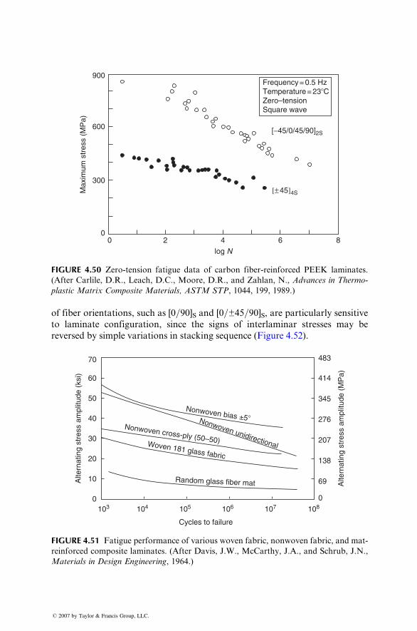
900
600
300
00 2 4
log N
Max
imum
str
ess
(MP
a)
6 8
Frequency = 0.5 HzTemperature = 23�CZero–tensionSquare wave
[−45/0/45/90]2S
[± 45]4S
FIGURE 4.50 Zero-tension fatigue data of carbon fiber-reinforced PEEK laminates.
(After Carlile, D.R., Leach, D.C., Moore, D.R., and Zahlan, N., Advances in Thermo-
plastic Matrix Composite Materials, ASTM STP, 1044, 199, 1989.)
of fiber orienta tions, such as [0 =90]S an d [0=±45 =90] S, are particular ly sensi tiveto laminate con figuratio n, since the signs of interlam inar stresses may be
revers ed by simp le varia tions in stacki ng sequence (F igure 4.52) .
70
60 414
483
345
276
207
138
69
0
50
40
Alte
rnat
ing
stre
ss a
mpl
itude
(ks
i)
Alte
rnat
ing
stre
ss a
mpl
itude
(M
Pa)
30
20
10
0103 104 105 106
Cycles to failure
Nonwoven bias ±5�Nonwoven unidirectionalWoven 181 glass fabric
Random glass fiber mat
Nonwoven cross-ply (50–50)
107 108
FIGURE 4.51 Fatigue performance of various woven fabric, nonwoven fabric, and mat-
reinforced composite laminates. (After Davis, J.W., McCarthy, J.A., and Schrub, J.N.,
Materials in Design Engineering, 1964.)
� 2007 by Taylor & Francis Group, LLC.
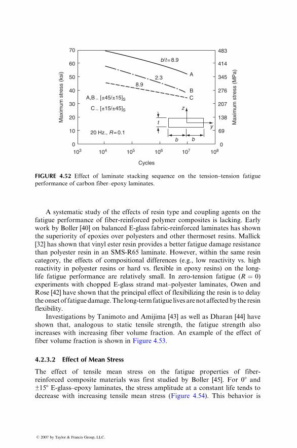
70 483
414
345
276
207
138
69
0108107106105104103
A,B .. [±45/±15]S
C .. [±15/±45]S
20 Hz., R = 0.1
b/t = 8.9
2.3A
Cycles
8.9BC
z
ty
b b
Max
imum
str
ess
(MP
a)
Max
imum
str
ess
(ksi
)60
50
40
30
20
10
0
FIGURE 4.52 Effect of laminate stacking sequence on the tension–tension fatigue
performance of carbon fiber–epoxy laminates.
A systemat ic study of the effects of resin type and co upling agents on the
fatigue perfor mance of fiber-re infor ced polyme r composi tes is lackin g. Ear ly
work by Boller [40] on balanced E-glas s fabric-r einforced lami nates ha s sho wn
the superi ority of epoxies over polyesters an d other therm oset resi ns. Mallick
[32] has shown that vinyl ester resin provides a bette r fatigue damage resistance
than polyester resin in an SMS-R65 laminate. However, within the same resin
category, the effects of compositional differences (e.g., low reactivity vs. high
reactivity in polyester resins or hard vs. flexible in epoxy resins) on the long-
life fatigue performance are relatively small. In zero-tension fatigue (R ¼ 0)
experiments with chopped E-glass strand mat–polyester laminates, Owen and
Rose [42] have shown that the principal effect of flexibilizing the resin is to delay
the onset of fatigue damage. The long-term fatigue lives are not affected by the resin
flexibility.
Invest igations by Tanimot o and Ami jima [43] as well as Dharan [44] have
shown that, ana logous to static tensile stren gth, the fatigu e strength also
increa ses with increa sing fiber volume fraction. An ex ample of the effect of
fiber volume fraction is shown in Fi gure 4.53.
4.2.3.2 Effect of Mean Stress
The effect of tensile mean stress on the fatigue propert ies of fiber-
reinforced composi te mate rials was fir st studi ed by Boller [45]. For 08 and±158 E-glas s–epoxy laminates , the stre ss a mplitude at a constant lif e tend s to
decreas e wi th increa sing tensile mean stress (Figure 4.54). Thi s behavior is
� 2007 by Taylor & Francis Group, LLC.
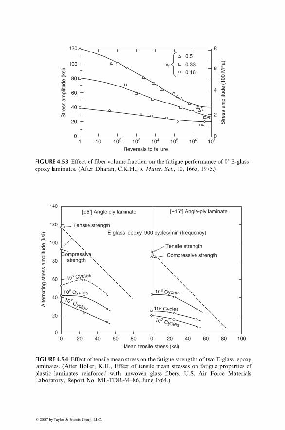
vf
0.5
120 8
6
4
2
0
100
80
60
40
Str
ess
ampl
itude
(ks
i)
Str
ess
ampl
itude
(10
0 M
Pa)
20
01 10 102 103 104
Reversals to failure105 106 107
0.33
0.16
FIGURE 4.53 Effect of fiber volume fraction on the fatigue performance of 08 E-glass–
epoxy laminates. (After Dharan, C.K.H., J. Mater. Sci., 10, 1665, 1975.)
[±5�] Angle-ply laminate [±15�] Angle-ply laminate
E-glass–epoxy, 900 cycles/min (frequency)Tensile strength
Tensile strength
103 Cycles
103 Cycles105 Cycles
105 Cycles
10 7 Cycles
107 Cycles
Compressivestrength
Compressive strength
140
120
100
80
60
40
20
00 20 40 60 80 20 40 60 80 1000
Mean tensile stress (ksi)
Alte
rnat
ing
stre
ss a
mpl
itude
(ks
i)
FIGURE 4.54 Effect of tensile mean stress on the fatigue strengths of two E-glass–epoxy
laminates. (After Boller, K.H., Effect of tensile mean stresses on fatigue properties of
plastic laminates reinforced with unwoven glass fibers, U.S. Air Force Materials
Laboratory, Report No. ML-TDR-64–86, June 1964.)
� 2007 by Taylor & Francis Group, LLC.
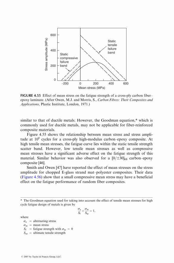
600
400S
tres
s am
plitu
de (
MP
a)
200
Staticcompressivefailureband
Statictensilefailureband
0−200 0 200
Mean stress (MPa)400 600
FIGURE 4.55 Effect of mean stress on the fatigue strength of a cross-ply carbon fiber–
epoxy laminate. (After Owen, M.J. and Morris, S., Carbon Fibres: Their Composites and
Applications, Plastic Institute, London, 1971.)
simila r to that of duc tile metals. Howev er, the Good man equati on,* which is
commonl y used for duc tile meta ls, may not be applic able for fiber -reinforce d
composi te mate rials.
Figure 4.55 shows the relationship between mean stress and stress ampli-
tude at 106 cycles for a cross-ply high-modulus carbon–epoxy composite. At
high tensile mean stresses, the fatigue curve lies within the static tensile strength
scatter band. However, low tensile mean stresses as well as compressive
mean stresses have a significant adverse effect on the fatigue strength of this
material. Similar behavior was also observed for a [0=±30]6S carbon–epoxycomposite [46].
Smith an d Owen [47] have report ed the effe ct of mean stresses on the stre ss
amplitude for chop ped E-glas s stra nd mat– polyest er compo sites. Their da ta
(Figur e 4.56) show that a smal l compres sive mean stress may have a bene ficial
effect on the fati gue performan ce of random fiber comp osites.
* The Goodman equation used for taking into account the effect of tensile mean stresses for high
cycle fatigue design of metals is given by
sa
Sf
þ sm
Sut
¼ 1,
where
sa ¼ alternating stress
sm ¼ mean stress
Sf ¼ fatigue strength with sm ¼ 0
Sut ¼ ultimate tensile strength
� 2007 by Taylor & Francis Group, LLC.
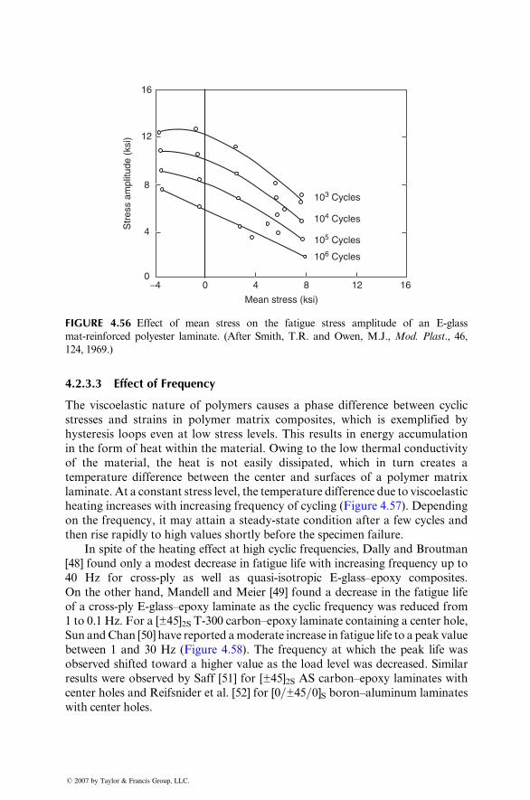
16
12
8
4
−4 0 4 8
Mean stress (ksi)
103 Cycles
104 Cycles
105 Cycles
106 Cycles
Str
ess
ampl
itude
(ks
i)
12 160
FIGURE 4.56 Effect of mean stress on the fatigue stress amplitude of an E-glass
mat-reinforced polyester laminate. (After Smith, T.R. and Owen, M.J., Mod. Plast., 46,
124, 1969.)
4.2.3 .3 Effec t of Frequency
The viscoelast ic na ture of poly mers causes a pha se difference betw een cyclic
stresses and strains in polyme r matr ix compo sites, whi ch is exempl ified by
hyster esis loops even at low stre ss level s. This resul ts in energy a ccumula tion
in the form of he at wi thin the mate rial. Owing to the low therm al condu ctivity
of the material , the heat is not easily dissipated, whi ch in turn creat es a
tempe rature difference betw een the center an d surfa ces of a polyme r matr ix
laminate. At a constant stress level, the tempe rature difference due to viscoelast ic
heati ng increa ses with increa sing frequency of cycling (Figur e 4.57). Depending
on the frequency , it may attain a steady -st ate co ndition after a few cycles and
then rise rapidl y to high values shortly before the specim en failure.
In spite of the heating effect at high cyclic frequencies, Dally and Broutman
[48] found only a modest decrease in fatigue life with increasing frequency up to
40 Hz for cross-ply as well as quasi-isotropic E-glass–epoxy composites.
On the other hand, Mandell and Meier [49] found a decrease in the fatigue life
of a cross-ply E-glass–epoxy laminate as the cyclic frequency was reduced from
1 to 0.1 Hz. For a [±45]2S T-300 carbon–epoxy laminate containing a center hole,
Sun and Chan [50] have reported a moderate increase in fatigue life to a peak value
between 1 and 30 Hz (Figure 4.58). The frequency at which the peak life was
observed shifted toward a higher value as the load level was decreased. Similar
results were observed by Saff [51] for [±45]2S AS carbon–epoxy laminates with
center holes and Reifsnider et al. [52] for [0=±45=0]S boron–aluminum laminates
with center holes.
� 2007 by Taylor & Francis Group, LLC.
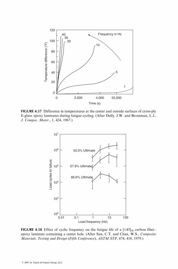
120
2010
Frequency in Hz
5
1
3040
Tem
pera
ture
diff
eren
ce (
�F) 100
80
60
40
20
0
0 2,000 4,000
Time (s)
55,000
FIGURE 4.57 Difference in temperatures at the center and outside surfaces of cross-ply
E-glass–epoxy laminates during fatigue cycling. (After Dally, J.W. and Broutman, L.J.,
J. Compos. Mater., 1, 424, 1967.)
107
106
105
Load
cyc
les
to fa
ilure
104
103
102
0.01 0.1 1Load frequency (Hz)
10 100
53.3% Ultimate
57.9% Ultimate
66.6% Ultimate
FIGURE 4.58 Effect of cyclic frequency on the fatigue life of a [±45]2S carbon fiber–
epoxy laminate containing a center hole. (After Sun, C.T. and Chan, W.S., Composite
Materials, Testing and Design (Fifth Conference), ASTM STP, 674, 418, 1979.)
� 2007 by Taylor & Francis Group, LLC.
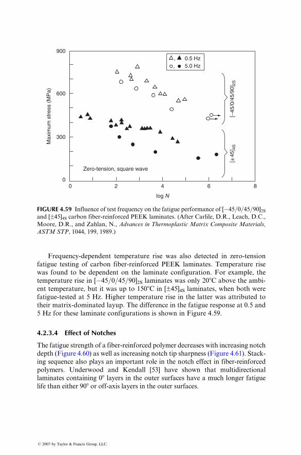
900
600
Max
imum
str
ess
(MP
a)
300
00 2 4
log N
Zero-tension, square wave
6 8
, 0.5 Hz5.0 Hz,
[± 4
5]4S
[−45
/0/4
5/90
] 2S
FIGURE 4.59 Influence of test frequency on the fatigue performance of [�45=0=45=90]2Sand [±45]4S carbon fiber-reinforced PEEK laminates. (After Carlile, D.R., Leach, D.C.,
Moore, D.R., and Zahlan, N., Advances in Thermoplastic Matrix Composite Materials,
ASTM STP, 1044, 199, 1989.)
Freq uency-depend ent tempe ratur e rise was a lso detect ed in zero-tensi on
fatigue test ing of carb on fiber-re infor ced PEEK laminates . Temperat ure rise
was found to be depend ent on the lamin ate config uration. For ex ample, the
tempe rature rise in [� 45=0=45 =90]2S laminates was only 20 8 C above the ambi-
ent temperatur e, but it was up to 150 8 C in [± 45]4S laminates , when both were
fatigue- tested at 5 Hz. Highe r tempe rature rise in the latter was attribu ted to
their matrix- dominated layup. The difference in the fatigue respo nse at 0.5 and
5 Hz for these lami nate co nfigurati ons is shown in Figure 4.59.
4.2.3 .4 Effec t of Notch es
The fatigue strength of a fiber-reinforced polymer decreases with increasing notch
depth (Figure 4.60) as well as increasing notch tip sharpness (Figure 4.61). Stack-
ing sequence also plays an important role in the notch effect in fiber-reinforced
polymers. Underwood and Kendall [53] have shown that multidirectional
laminates containing 08 layers in the outer surfaces have a much longer fatigue
life than either 908 or off-axis layers in the outer surfaces.
� 2007 by Taylor & Francis Group, LLC.
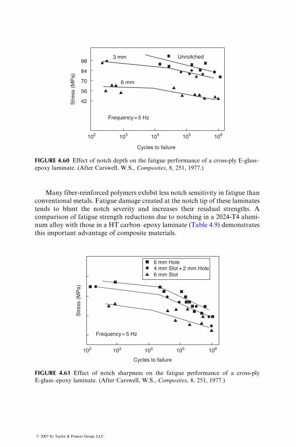
98
84
70
Str
ess
(MP
a)
56
42
102 103 104
Cycles to failure
Frequency = 5 Hz
3 mm Unnotched
6 mm
105 106
FIGURE 4.60 Effect of notch depth on the fatigue performance of a cross-ply E-glass–
epoxy laminate. (After Carswell, W.S., Composites, 8, 251, 1977.)
Many fiber -reinforce d polyme rs exhibit less notch sensi tivity in fatigue than
conven tional meta ls. Fatigue damage c reated at the notch tip of these lami nates
tends to blunt the notch severity and increa ses their resid ual stre ngths. A
compari son of fatigue stre ngth red uctions due to notching in a 20 24-T4 alumi -
num alloy with those in a HT carbon–epo xy laminate (Table 4.9) demonst rates
this important advantage of composite materials.
6 mm Hole4 mm Slot + 2 mm Hole6 mm Slot
Frequency = 5 Hz
102 103 104
Cycles to failure
Str
ess
(MP
a)
105 106
FIGURE 4.61 Effect of notch sharpness on the fatigue performance of a cross-ply
E-glass–epoxy laminate. (After Carswell, W.S., Composites, 8, 251, 1977.)
� 2007 by Taylor & Francis Group, LLC.
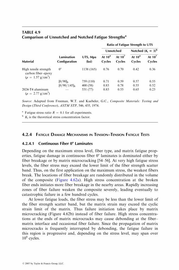
TABLE 4.9Comparison of Unnotched and Notched Fatigue Strengthsa
Ratio of Fatigue Strength to UTS
Unnotched Notched (Kt 5 3)b
Material
Lamination
Configuration
UTS, Mpa
(ksi)
At 104
Cycles
At 107
Cycles
At 104
Cycles
At 107
Cycles
High tensile strength
carbon fiber–epoxy
(r ¼ 1.57 g=cm3)
08 1138 (165) 0.76 0.70 0.42 0.36
[0=90]S 759 (110) 0.71 0.59 0.57 0.55
[0=90=±45]S 400 (58) 0.83 0.78 0.55 0.52
2024-T4 aluminum
(r ¼ 2.77 g=cm3)
— 531 (77) 0.83 0.55 0.65 0.23
Source: Adapted from Freeman, W.T. and Kuebeler, G.C., Composite Materials: Testing and
Design (Third Conference), ASTM STP, 546, 435, 1974.
a Fatigue stress ratio R ¼ 0.1 for all experiments.b Kt is the theoretical stress concentration factor.
4.2.4 F ATIGUE DAMAGE MECHANISMS IN TENSION –TENSION FATIGUE T ESTS
4.2.4 .1 Cont inuous Fiber 08 Laminate s
Depending on the maxi mum stress level , fiber type, an d matr ix fatigu e prop -
erties, fatigue da mage in continuous fiber 08 lami nates is dom inated either by
fiber break age or by matrix micro crackin g [54–56]. At very high fatigue stre ss
levels, the fiber stress may exceed the lower limit of the fiber stre ngth scatte r
band . Thus , on the fir st app lication on the maximu m stre ss, the weake st fiber s
break. The locat ions of fiber break age are rando mly distribut ed in the vo lume
of the composi te (Figur e 4.62a) . High stress concentra tion at the broken
fiber ends initiat es more fiber breakage in the nearby areas. Rapidly increa sing
zones of fiber failure weake n the composi te severe ly, leadi ng even tually to
catas trophic failure in a few hundr ed cycles .
At lower fatigu e loads, the fiber stre ss may be less than the low er limit of
the fiber stre ngth scatt er band , but the matrix stra in may exceed the cyclic
strain limit of the matrix. Thus failure init iation takes place by matr ix
micro crackin g (Figur e 4.62b) inst ead of fiber fail ure. High stre ss co ncentra -
tions at the end s of matrix microcracks may cause de bonding at the fiber–
matrix interface and occasi onal fiber failure. Since the pro pagatio n of matr ix
micro cracks is frequent ly inter rupted by debon ding, the fatigue failure in
this region is progressive and, depending on the stress level, may span over
106 cycles.
� 2007 by Taylor & Francis Group, LLC.
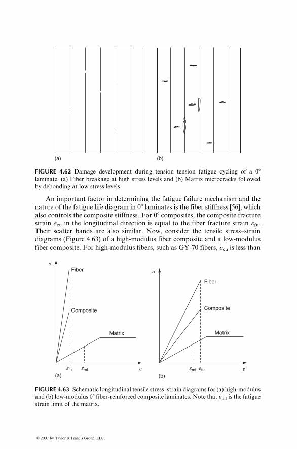
(a) (b)
FIGURE 4.62 Damage development during tension–tension fatigue cycling of a 08laminate. (a) Fiber breakage at high stress levels and (b) Matrix microcracks followed
by debonding at low stress levels.
An important factor in determining the fatigue failure mechanism and the
nature of the fatigue life diagram in 08 laminates is the fiber stiffness [56], which
also controls the composite stiffness. For 08 composites, the composite fracture
strain «cu in the longitudinal direction is equal to the fiber fracture strain «fu.Their scatter bands are also similar. Now, consider the tensile stress–strain
diagrams (Figure 4.63) of a high-modulus fiber composite and a low-modulus
fiber composite. For high-modulus fibers, such as GY-70 fibers, «cu is less than
Fiber
Fiber
efu emf
s
s
(a)e e fuemf
(b)e
Composite Composite
Matrix Matrix
FIGURE 4.63 Schematic longitudinal tensile stress–strain diagrams for (a) high-modulus
and (b) low-modulus 08 fiber-reinforced composite laminates. Note that «mf is the fatigue
strain limit of the matrix.
� 2007 by Taylor & Francis Group, LLC.
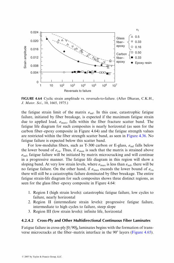
0.024
0.020
0.016
0.012
0.008
0.004
01 10 102 103 104
Reversals to failure
Sira
in a
mpl
itude
105 106 107
Glassfiber–epoxy
vf
0.5
0.33
0.16
Carbonfiber–epoxy
0.50
0.33
Epoxy resin
FIGURE 4.64 Cyclic strain amplitude vs. reversals-to-failure. (After Dharan, C.K.H.,
J. Mater. Sci., 10, 1665, 1975.)
the fatigu e stra in limit of the matrix «mf. In this case, catastroph ic fatigue
failure, init iated by fiber breakage, is expecte d if the maxi mum fatigue stra in
due to applied load, «max, falls within the fiber fractu re scatter ban d. The
fatigue life diagram for such composi tes is nearly horizont al (as seen for the
carbon fiber–epo xy composi te in Figure 4.64) and the fatigu e streng th values
are rest ricted wi thin the fiber strength scatt er band, as seen in Figure 4.36. No
fatigue failure is expecte d below this scatter band.
For low-modul us fibers, such as T-300 carbo n or E-glas s, «mf falls below
the low er bound of «cu. Thus, if «max is such that the matrix is strained above
«mf, fatig ue failure wi ll be initiated by matr ix microcrack ing and wi ll con tinue
in a progres sive manner. The fatigue life diagra m in this region will sh ow a
slopi ng ban d. At very low strain levels, wher e «max is less than «mf , there will be
no fatigu e failu re. On the other ha nd, if «max exceed s the lowe r bound of «cuthere wi ll sti ll be a catas trophic failure dominat ed by fiber breaka ge. The entire
fatigue stra in-lif e diagra m for such compo sites shows three distinct regions , as
seen for the glass fiber –epoxy composi te in Figure 4.64:
1. Regi on I (high strain levels): catas trophi c fatig ue fail ure, low cycles to
failure, nearly hor izontal
2. Regi on II (int ermediate strain level s): pro gressive fati gue failu re,
inter mediate to high cycles to failu re, steep slope
3. Regi on III (low strain levels): infi nite life, hor izonta l
4.2.4 .2 Cr oss-Ply and Othe r Multidi rectional Cont inuous Fiber Lami nates
Fatigue failure in cro ss-ply [0=90]S laminates begins wi th the form ation of trans -
verse micr ocracks at the fiber –matrix inter face in the 90 8 layer s (Figure 4.65) .
� 2007 by Taylor & Francis Group, LLC.
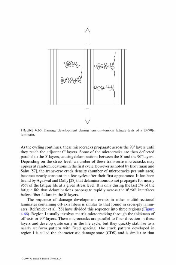
FIGURE 4.65 Damage development during tension–tension fatigue tests of a [0=90]Slaminate.
As the cycling con tinues, these micr ocracks propagat e across the 90 8 layers untilthey reach the adjacent 08 layer s. Some of the micro cracks are then deflected
parallel to the 08 layer s, causing delam ination s be tween the 08 an d the 9 0 8 layer s.Depending on the stre ss level , a num ber of these trans verse microcrack s may
appear at random locat ions in the first cycle; howeve r as noted by Br outman and
Sahu [57] , the transverse crack densit y (numb er of microc racks per unit area)
becomes nearly constant in a few cycles after their first appearance. It has been
found by Agar wal and Dally [28] that delam ination s do not prop agate for ne arly
95% of the fatig ue life at a given stress level . It is only during the last 5% of the
fatigue life that delam inations prop agate rapidl y across the 0 8=90 8 inter facesbefore fiber failure in the 08 layers.
The sequ ence of damage developm ent events in other multidirecti onal
laminates c ontaining off-axis fibers is similar to that found in cross- ply lamin -
ates. Reifsni der et al. [58] have divide d this sequence into three regions (Figur e
4.66). Regi on I usuall y involv es matrix micr ocracki ng through the thickne ss of
off-axis or 90 8 layers. These microcrack s are parallel to fiber direction in these
layers and develop quite early in the life cycle, but they quickly stabilize to a
nearly uniform pattern with fixed spacing. The crack pattern developed in
region I is called the characteristic damage state (CDS) and is similar to that
� 2007 by Taylor & Francis Group, LLC.
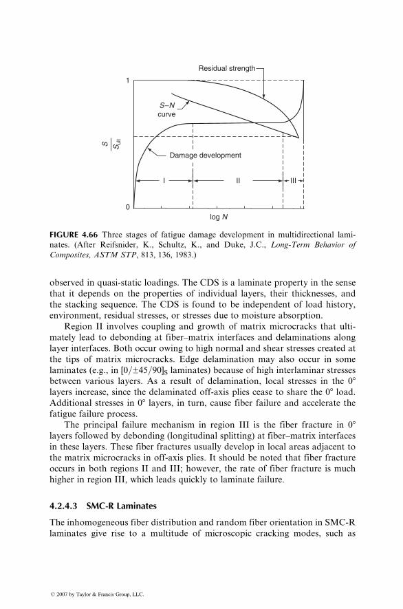
Residual strength
Damage development
log N
I II III
S –Ncurve
1
0
S Sul
t
FIGURE 4.66 Three stages of fatigue damage development in multidirectional lami-
nates. (After Reifsnider, K., Schultz, K., and Duke, J.C., Long-Term Behavior of
Composites, ASTM STP, 813, 136, 1983.)
observed in quasi-static loadings. The CDS is a laminate property in the sense
that it depends on the properties of individual layers, their thicknesses, and
the stacking sequence. The CDS is found to be independent of load history,
environment, residual stresses, or stresses due to moisture absorption.
Region II involves coupling and growth of matrix microcracks that ulti-
mately lead to debonding at fiber–matrix interfaces and delaminations along
layer interfaces. Both occur owing to high normal and shear stresses created at
the tips of matrix microcracks. Edge delamination may also occur in some
laminates (e.g., in [0=±45=90]S laminates) because of high interlaminar stresses
between various layers. As a result of delamination, local stresses in the 08layers increase, since the delaminated off-axis plies cease to share the 08 load.Additional stresses in 08 layers, in turn, cause fiber failure and accelerate the
fatigue failure process.
The principal failure mechanism in region III is the fiber fracture in 08layers followed by debonding (longitudinal splitting) at fiber–matrix interfaces
in these layers. These fiber fractures usually develop in local areas adjacent to
the matrix microcracks in off-axis plies. It should be noted that fiber fracture
occurs in both regions II and III; however, the rate of fiber fracture is much
higher in region III, which leads quickly to laminate failure.
4.2.4.3 SMC-R Laminates
The inhomogeneous fiber distribution and random fiber orientation in SMC-R
laminates give rise to a multitude of microscopic cracking modes, such as
� 2007 by Taylor & Francis Group, LLC.
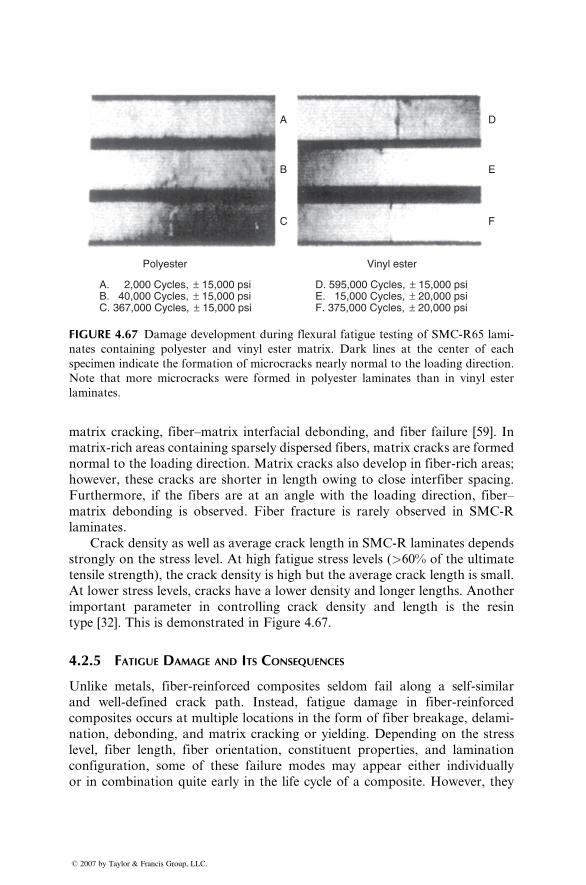
A
B
C
Polyester
A. 2,000 Cycles, ± 15,000 psi
C. 367,000 Cycles, ± 15,000 psiB. 40,000 Cycles, ± 15,000 psi
D. 595,000 Cycles, ± 15,000 psi
F. 375,000 Cycles, ± 20,000 psiE. 15,000 Cycles, ± 20,000 psi
Vinyl ester
D
E
F
FIGURE 4.67 Damage development during flexural fatigue testing of SMC-R65 lami-
nates containing polyester and vinyl ester matrix. Dark lines at the center of each
specimen indicate the formation of microcracks nearly normal to the loading direction.
Note that more microcracks were formed in polyester laminates than in vinyl ester
laminates.
matrix cracking, fiber–matrix interfacial debonding, and fiber failure [59]. In
matrix-rich areas containing sparsely dispersed fibers, matrix cracks are formed
normal to the loading direction. Matrix cracks also develop in fiber-rich areas;
however, these cracks are shorter in length owing to close interfiber spacing.
Furthermore, if the fibers are at an angle with the loading direction, fiber–
matrix debonding is observed. Fiber fracture is rarely observed in SMC-R
laminates.
Crack density as well as average crack length in SMC-R laminates depends
strongly on the stress level. At high fatigue stress levels (>60% of the ultimate
tensile strength), the crack density is high but the average crack length is small.
At lower stress levels, cracks have a lower density and longer lengths. Another
important parameter in controlling crack density and length is the resin
type [32]. This is demonstrated in Figure 4.67.
4.2.5 FATIGUE DAMAGE AND ITS CONSEQUENCES
Unlike metals, fiber-reinforced composites seldom fail along a self-similar
and well-defined crack path. Instead, fatigue damage in fiber-reinforced
composites occurs at multiple locations in the form of fiber breakage, delami-
nation, debonding, and matrix cracking or yielding. Depending on the stress
level, fiber length, fiber orientation, constituent properties, and lamination
configuration, some of these failure modes may appear either individually
or in combination quite early in the life cycle of a composite. However, they
� 2007 by Taylor & Francis Group, LLC.
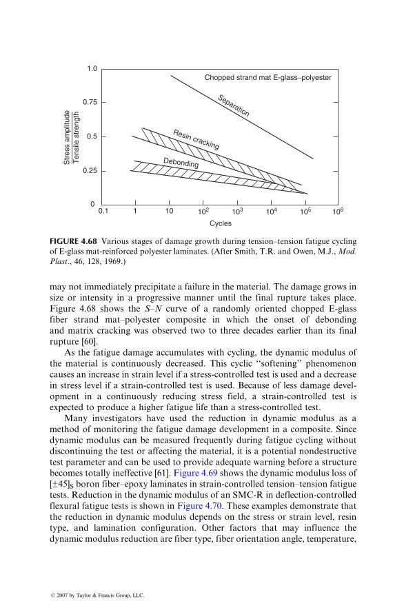
Separation
Resin cracking
Debonding
Chopped strand mat E-glass−polyester
Cycles
Str
ess
ampl
itude
Ten
sile
str
engt
h1.0
0.75
0.5
0.25
00.1 1 10 102 103 104 105 106
FIGURE 4.68 Various stages of damage growth during tension–tension fatigue cycling
of E-glass mat-reinforced polyester laminates. (After Smith, T.R. and Owen, M.J.,Mod.
Plast., 46, 128, 1969.)
may not immediat ely precipi tate a failure in the mate rial. The damage grows in
size or intens ity in a progres sive manner until the final rup ture takes place.
Figure 4.68 shows the S–N curve of a rand omly oriented chopped E-glass
fiber strand mat–p olyester co mposite in which the onset of deb onding
and matrix crack ing was observed two to three de cades earlier than its final
rupture [60].
As the fatigu e damage accumul ates wi th cycli ng, the dy namic mod ulus of
the mate rial is continuous ly de creased . This cycli c ‘‘so ftening’’ phen omenon
causes an increa se in stra in level if a stress- control led test is us ed and a de crease
in stre ss level if a stra in-cont rolled test is used. Bec ause of less damage devel-
opment in a continuou sly reduc ing stre ss field, a strain-c ontrolled test is
expecte d to pr oduce a higher fati gue life than a stress- control led test .
Man y invest igators have used the reducti on in dyn amic modulus as a
method of monit oring the fatigue damage de velopm ent in a composi te. Since
dynami c mod ulus can be measur ed frequent ly during fatigue cycli ng witho ut
discont inuing the test or affe cting the material, it is a pot ential nonde struc tive
test parame ter and can be used to provide adeq uate war ning before a struc ture
becomes total ly ineff ective [61] . Fi gure 4.69 shows the dy namic modulus loss of
[±45]S bor on fiber– epoxy laminates in strain-c ontrol led tensi on–tensi on fatigue
tests. Redu ction in the dy namic mod ulus of an SMC-R in de flection- control led
flexu ral fatigue test s is shown in Figure 4.70. Thes e examples demo nstrate that
the red uction in dynami c modulus de pends on the stre ss or strain level, resin
type, and lamination configuration. Other factors that may influence the
dynamic modulus reduction are fiber type, fiber orientation angle, temperature,
� 2007 by Taylor & Francis Group, LLC.
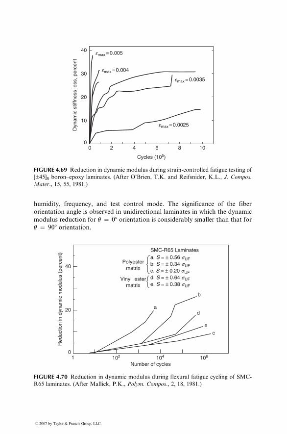
40
30
20
Dyn
amic
stif
fnes
s lo
ss, p
erce
nt
10
00 2 4 6
Cycles (105)
emax = 0.0025
emax = 0.0035
emax = 0.004
emax = 0.005
8 10
FIGURE 4.69 Reduction in dynamic modulus during strain-controlled fatigue testing of
[±45]S boron–epoxy laminates. (After O’Brien, T.K. and Reifsnider, K.L., J. Compos.
Mater., 15, 55, 1981.)
humidity, frequency, and test control mode. The significance of the fiber
orientation angle is observed in unidirectional laminates in which the dynamic
modulus reduction for u ¼ 08 orientation is considerably smaller than that for
u ¼ 908 orientation.
SMC-R65 Laminates
Polyestermatrix
Vinyl estermatrix
a. S = ± 0.56 sUF
a
10
20
40
102 104
Number of cycles
Red
uctio
n in
dyn
amic
mod
ulus
(pe
rcen
t)
106
b
c
d
e
b. S = ± 0.34 sUFc. S = ± 0.20 sUFd. S = ± 0.64 sUFe. S = ± 0.38 sUF
FIGURE 4.70 Reduction in dynamic modulus during flexural fatigue cycling of SMC-
R65 laminates. (After Mallick, P.K., Polym. Compos., 2, 18, 1981.)
� 2007 by Taylor & Francis Group, LLC.
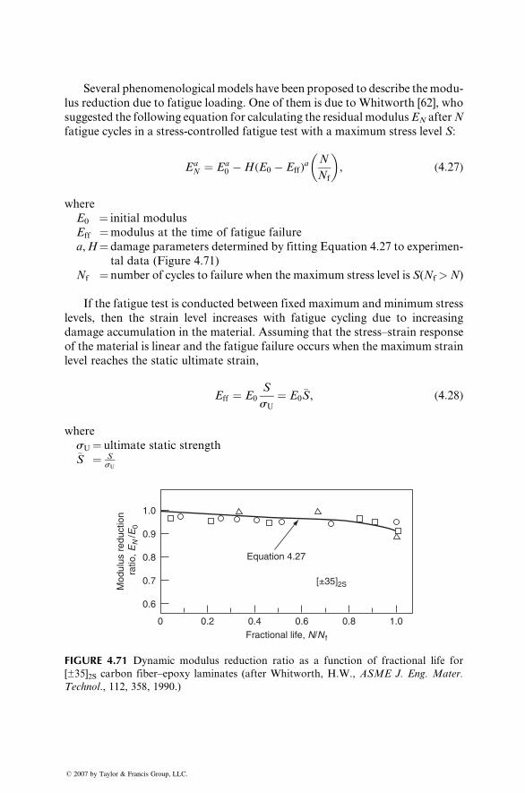
Several phenomenological models have been proposed to describe themodu-
lus reduction due to fatigue loading. One of them is due to Whitworth [62], who
suggested the following equation for calculating the residual modulusEN afterN
fatigue cycles in a stress-controlled fatigue test with a maximum stress level S:
EaN ¼ Ea
0 �H(E0 � Eff )a N
Nf
� �, (4:27)
where
E0 ¼ initial modulus
Eff ¼modulus at the time of fatigue failure
a,H¼ damage parameters determined by fitting Equation 4.27 to experimen-
tal data (Figure 4.71)
Nf ¼ number of cycles to failure when the maximum stress level is S(Nf>N)
If the fatigue test is conducted between fixed maximum and minimum stress
levels, then the strain level increases with fatigue cycling due to increasing
damage accumulation in the material. Assuming that the stress–strain response
of the material is linear and the fatigue failure occurs when the maximum strain
level reaches the static ultimate strain,
Eff ¼ E0
S
sU
¼ E0�S, (4:28)
where
sU ¼ ultimate static strength�S ¼ S
sU
1.0
0.9
0.8
0.7
0.6
0 0.2 0.4 0.6Fractional life, N/N f
Equation 4.27
[±35]2SMod
ulus
red
uctio
n r
atio
, EN
/E0
0.8 1.0
FIGURE 4.71 Dynamic modulus reduction ratio as a function of fractional life for
[±35]2S carbon fiber–epoxy laminates (after Whitworth, H.W., ASME J. Eng. Mater.
Technol., 112, 358, 1990.)
� 2007 by Taylor & Francis Group, LLC.
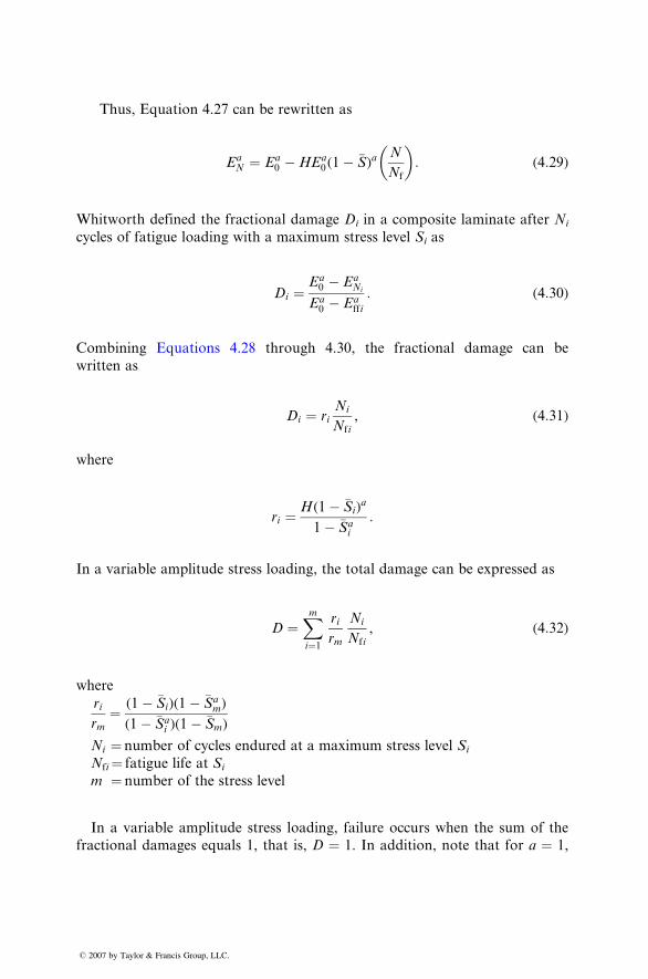
Thus , Equat ion 4.27 can be rewritten as
E aN ¼ E a0 � HE a0 ( 1 � �S ) aN
Nf
� �: ( 4: 29 )
Whitwort h defined the fract ional damage Di in a comp osite lami nate afte r N icycles of fatigue loading with a maxi mum stress level Si as
Di ¼Ea0 � Ea
Ni
Ea0 � Ea
ffi
: (4:30)
Comb ining Equations 4.28 through 4.30, the fractional damage can be
written as
Di ¼ riNi
Nfi
, (4:31)
where
ri ¼ H(1� �Si)a
1� �Sai
:
In a variable amplitude stress loading, the total damage can be expressed as
D ¼Xmi¼1
ri
rm
Ni
Nfi
, (4:32)
where
ri
rm¼ (1� �Si)(1� �Sa
m)
(1� �Sai )(1� �Sm)
Ni ¼ number of cycles endured at a maximum stress level Si
Nfi¼ fatigue life at Si
m ¼ number of the stress level
In a variable amplitude stress loading, failure occurs when the sum of the
fractional damages equals 1, that is, D ¼ 1. In addition, note that for a ¼ 1,
� 2007 by Taylor & Francis Group, LLC.
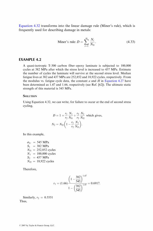
Equation 4.32 trans forms into the linear damage rule (Mine r’s rule) , whi ch is
frequent ly used for describ ing da mage in metals:
Miner’s rule : D ¼Xmi ¼ 1
Ni
Nf i
: ( 4: 33 )
EXAMPLE 4.2
A quasi-isotropic T-300 carbon fiber–epoxy laminate is subjected to 100,000
cycles at 382 MPa after which the stress level is increased to 437 MPa. Estimate
the number of cycles the laminate will survive at the second stress level. Median
fatigue lives at 382 and 437 MPa are 252,852 and 18,922 cycles, respectively. From
the modulus vs. fatigue cycle data, the constant a and H in Equation 4.27 have
been determined as 1.47 and 1.66, respectively (see Ref. [62]). The ultimate static
strength of this material is 545 MPa.
SOLUTION
Using Equation 4.32, we can write, for failure to occur at the end of second stress
cycling,
D ¼ 1 ¼ r1
r2
N1
Nf1
þ r2
r2
N2
Nf2
which gives,
N2 ¼ Nf2 1� r1
r2
N1
Nf1
� �:
In this example,
Th
� 2
sU ¼ 545 MPa
S1 ¼ 382 MPa
Nf1 ¼ 252,852 cycles
N1 ¼ 100,000 cycles
S2 ¼ 437 MPa
Nf2 ¼ 18,922 cycles
Therefore,
r1 ¼ (1:66)
1� 382
545
� �1:47
1� 382
545
� �1:47¼ 0:6917:
Similarly, r2 ¼ 0.5551
us,
007 by Taylor & Francis Group, LLC.
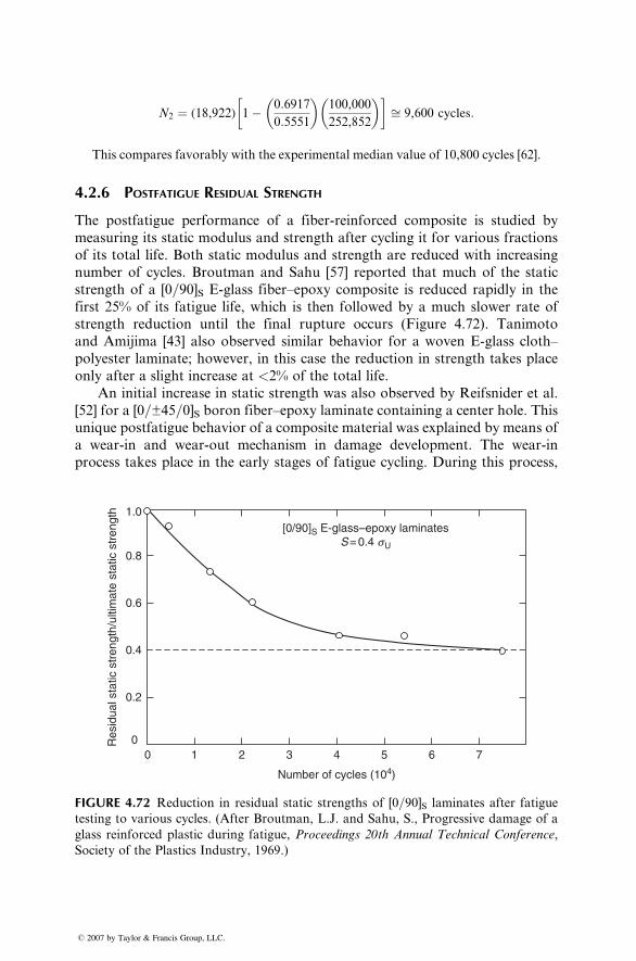
N2 ¼ (18,922) 1� 0:6917
0:5551
� �100,000
252,852
� �� �ffi 9,600 cycles:
This compares favorably with the experimental median value of 10,800 cycles [62].
4.2.6 POSTFATIGUE RESIDUAL STRENGTH
The postfatigue performance of a fiber-reinforced composite is studied by
measuring its static modulus and strength after cycling it for various fractions
of its total life. Both static modulus and strength are reduced with increasing
number of cycles. Broutman and Sahu [57] reported that much of the static
strength of a [0=90]S E-glass fiber–epoxy composite is reduced rapidly in the
first 25% of its fatigue life, which is then followed by a much slower rate of
strength reduction until the final rupture occurs (Figure 4.72). Tanimoto
and Amijima [43] also observed similar behavior for a woven E-glass cloth–
polyester laminate; however, in this case the reduction in strength takes place
only after a slight increase at <2% of the total life.
An initial increase in static strength was also observed by Reifsnider et al.
[52] for a [0=±45=0]S boron fiber–epoxy laminate containing a center hole. This
unique postfatigue behavior of a composite material was explained by means of
a wear-in and wear-out mechanism in damage development. The wear-in
process takes place in the early stages of fatigue cycling. During this process,
[0/90]S E-glass–epoxy laminatesS = 0.4 sU
00
0.2
0.4
0.6
0.8
1.0
1 2 3 4
Number of cycles (104)
Res
idua
l sta
tic s
tren
gth/
ultim
ate
stat
ic s
tren
gth
5 6 7
FIGURE 4.72 Reduction in residual static strengths of [0=90]S laminates after fatigue
testing to various cycles. (After Broutman, L.J. and Sahu, S., Progressive damage of a
glass reinforced plastic during fatigue, Proceedings 20th Annual Technical Conference,
Society of the Plastics Industry, 1969.)
� 2007 by Taylor & Francis Group, LLC.
the damage developed locally around the center hole reduces the stress concen-
tration in the vicinity of the hole, thus resulting in increased strength. This
beneficial stage of fatigue cycling is followed by the wear-out process, which
comprises large-scale and widespread damage development leading to strength
reduction. Thus, the residual strength of a composite after a period of fatigue
cycling is modeled as
sresidual ¼ sU þ swear-in � swear-out,
where
sU ¼ ultimate static strength
swear-in ¼ change in static strength due to wear-in
swear-out ¼ change in static strength due to wear-out
The effect of wear-in is more pronounced at high fatigue load levels. Since
fatigue life is longer at low load levels, there is a greater possibility of develop-
ing large-scale damage throughout the material. Thus, at low load levels, the
effect of wear-out is more pronounced.
A number of phenomenological equations have been proposed to predict
the residual static strength of a fatigued composite laminate [63,64]. The
simplest among them is based on the assumption of linear strength reduction
[63] and is given as
sri ¼ sUi�1� (sU0
� Si)Ni
Nfi
, (4:34)
where
sri¼ residual strength after Ni cycles at the ith stress level Si
Nfi ¼ fatigue life at Si
sU0¼ ultimate static strength of the original laminate
sUi�1¼ ultimate static strength before being cycled at Si
In Equation 4.34, the ratio Ni=Nfi represents the fractional fatigue life
spent at Si.
Assuming a nonlinear strength degradation model, Yang [64] proposed
the following equation for the residual strength for a composite laminate
after N fatigue cycles:
scres ¼ sc
U � sc0KS
d N, (4:35)
where
c ¼ damage development parameter
s0 ¼ location parameter in a two-parameterWeibull function for the static
strength distribution of the laminate
S ¼ stress range in the fatigue test ¼ smax�smin
K, d ¼ parameters used to describe the S–N diagram as KSdNf ¼ 1
� 2007 by Taylor & Francis Group, LLC.
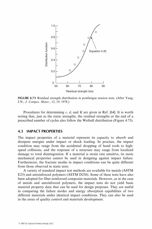
Equation 4.35
Residual strength (ksi)
Dis
trib
utio
n fu
nctio
n
500
0.2
0.4
0.6
0.8
1.0
60 70 80 90
FIGURE 4.73 Residual strength distribution in postfatigue tension tests. (After Yang,
J.N., J. Compos. Mater., 12, 19, 1978.)
Procedures for determining c, d, and K are given in Ref. [64]. It is worth
noting that, just as the static strengths, the residual strengths at the end of a
prescribed number of cycles also follow the Weibull distribution (Figure 4.73).
4.3 IMPACT PROPERTIES
The impact properties of a material represent its capacity to absorb and
dissipate energies under impact or shock loading. In practice, the impact
condition may range from the accidental dropping of hand tools to high-
speed collisions, and the response of a structure may range from localized
damage to total disintegration. If a material is strain rate sensitive, its static
mechanical properties cannot be used in designing against impact failure.
Furthermore, the fracture modes in impact conditions can be quite different
from those observed in static tests.
A variety of standard impact test methods are available for metals (ASTM
E23) and unreinforced polymers (ASTM D256). Some of these tests have also
been adopted for fiber-reinforced composite materials. However, as in the case
of metals and unreinforced polymers, the impact tests do not yield basic
material property data that can be used for design purposes. They are useful
in comparing the failure modes and energy absorption capabilities of two
different materials under identical impact conditions. They can also be used
in the areas of quality control and materials development.
� 2007 by Taylor & Francis Group, LLC.
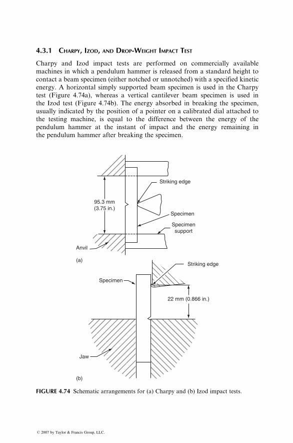
4.3.1 CHARPY, IZOD, AND DROP-WEIGHT IMPACT TEST
Charpy and Izod impact tests are performed on commercially available
machines in which a pendulum hammer is released from a standard height to
contact a beam specimen (either notched or unnotched) with a specified kinetic
energy. A horizontal simply supported beam specimen is used in the Charpy
test (Figure 4.74a), whereas a vertical cantilever beam specimen is used in
the Izod test (Figure 4.74b). The energy absorbed in breaking the specimen,
usually indicated by the position of a pointer on a calibrated dial attached to
the testing machine, is equal to the difference between the energy of the
pendulum hammer at the instant of impact and the energy remaining in
the pendulum hammer after breaking the specimen.
Striking edge
Specimen
Specimensupport
Striking edge
Specimen
Jaw
(b)
22 mm (0.866 in.)
Anvil
(a)
95.3 mm(3.75 in.)
FIGURE 4.74 Schematic arrangements for (a) Charpy and (b) Izod impact tests.
� 2007 by Taylor & Francis Group, LLC.
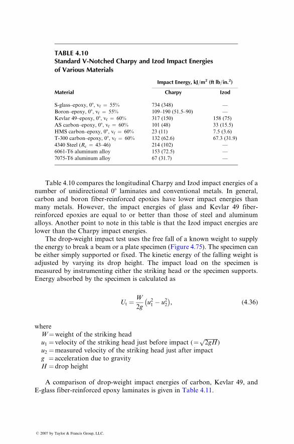
TABLE 4.10Standar d V-Notc hed Charpy and Izod Impa ct Ene rgies
of Various Materia ls
Impact Energy, kJ=m2 (ft lb= in.2)
Material Charpy Izod
S-glass–epoxy, 08, vf ¼ 55% 734 (348) —
Boron–epoxy, 08, vf ¼ 55% 109–190 (51.5–90) —
Kevlar 49–epoxy, 08, vf ¼ 60% 317 (150) 158 (75)
AS carbon–epoxy, 08, vf ¼ 60% 101 (48) 33 (15.5)
HMS carbon–epoxy, 08, vf ¼ 60% 23 (11) 7.5 (3.6)
T-300 carbon–epoxy, 08, vf ¼ 60% 132 (62.6) 67.3 (31.9)
4340 Steel (Rc ¼ 43–46) 214 (102) —
6061-T6 aluminum alloy 153 (72.5) —
7075-T6 aluminum alloy 67 (31.7) —
Table 4.10 compa res the longit udinal Char py and Izod impact energies of a
number of unidirecti onal 08 lamin ates and con vention al meta ls. In gen eral,
carbon and bor on fiber -reinforce d epoxies have lower impac t energi es than
many metals. How ever, the impac t en ergies of glass and Kevl ar 49 fiber -
reinforced epo xies are eq ual to or be tter than those of steel an d alumi num
alloys. Anothe r point to note in this table is that the Izod impac t energies are
lower than the Char py impac t energi es.
The drop -weight impac t test uses the free fall of a known weight to supp ly
the energy to break a beam or a plate specim en (Figur e 4.75) . The specime n can
be either simply sup ported or fixed . The kinetic energy of the fall ing weight is
adjuste d by varyi ng its drop height . The impac t load on the specimen is
measured by instrumenting either the striking head or the specimen supports.
Energy absorbed by the specimen is calculated as
Ut ¼ W
2gu21 � u22�
, (4: 36)
where
W ¼weight of the strik ing head
u1 ¼ velocity of the striking head just before impac t ( ¼ ffiffiffiffiffiffiffiffiffiffi2gH
p )
u2 ¼ measured veloci ty of the striking head just after impac t
g ¼ accele ration due to gravity
H ¼ drop height
A comparison of drop-weight impact energies of carbon, Kevlar 49, and
E-glass fiber -reinforce d epoxy laminates is given in Tabl e 4.11.
� 2007 by Taylor & Francis Group, LLC.
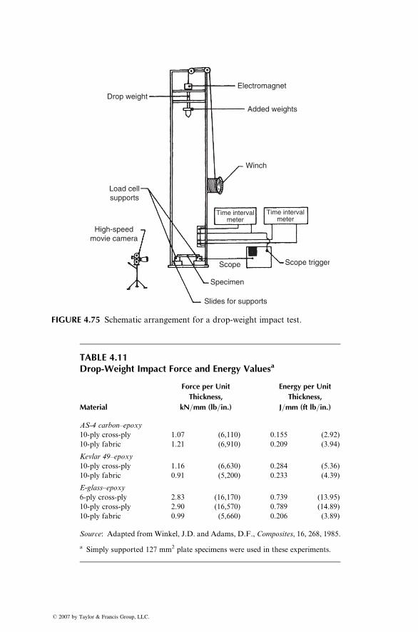
Drop weightElectromagnet
Added weights
Winch
Load cellsupports
High-speedmovie camera
Slides for supports
Specimen
Scope Scope trigger
Time intervalmeter
Time intervalmeter
FIGURE 4.75 Schematic arrangement for a drop-weight impact test.
TABLE 4.11Drop-Weight Impact Force and Energy Valuesa
Material
Force per Unit
Thickness,
kN=mm (lb=in.)
Energy per Unit
Thickness,
J=mm (ft lb=in.)
AS-4 carbon–epoxy
10-ply cross-ply 1.07 (6,110) 0.155 (2.92)
10-ply fabric 1.21 (6,910) 0.209 (3.94)
Kevlar 49–epoxy
10-ply cross-ply 1.16 (6,630) 0.284 (5.36)
10-ply fabric 0.91 (5,200) 0.233 (4.39)
E-glass–epoxy
6-ply cross-ply 2.83 (16,170) 0.739 (13.95)
10-ply cross-ply 2.90 (16,570) 0.789 (14.89)
10-ply fabric 0.99 (5,660) 0.206 (3.89)
Source: Adapted fromWinkel, J.D. and Adams, D.F., Composites, 16, 268, 1985.
a Simply supported 127 mm2 plate specimens were used in these experiments.
� 2007 by Taylor & Francis Group, LLC.
The impac t energy measur ed in all these test s de pends on the ratio of beam
length to effe ctive de pth. Below a crit ical value of this ratio, there is a c onsider -
able increa se in impact energy caused by extensive delaminati on [65]. The effe ct
of notch geomet ry has relat ively littl e influence on the impac t energy because
delam ination at the notch root at low stresses tends to reduce its severi ty.
4.3.2 FRACTURE I NITIATION AND P ROPAGATION E NERGIES
The impac t energy measur ed in eithe r of the impac t tests doe s not indica te the
fracture behavior of a mate rial unless the relat ive values of fract ure initiation
and prop agation en ergies are known. Thus, for exampl e, a high-s trength br ittle
material may have a high fract ure initiat ion energy but a low fracture prop a-
gation energy, and the reverse may be true for a low -strengt h ductil e material .
Even tho ugh the sum of these two energi es may be the same, their fracture
behavior is c ompletely different . Unless the broken specimen s are avail able for
fracture mod e inspect ion, the toughness of a mate rial c annot be jud ged by the
total impac t energy alone.
Fractur e initiat ion and propagat ion en ergies are de termined from the
measur ement s of the dynami c load an d stri king hea d veloci ty dur ing the
time of contact . Throug h proper inst rumentati on, the load and velocity signals
are integrated to produce the variation of cumulative energy as a function of
time. Both load–time and energy–time responses are recorded and are then
used for energy absorption analysis.
The load–time response during the impact test of a unidirectional composite
(Figur e 4.76) can be co nvenient ly divide d into three regions [66]:
Preinitial fracture region: The preinitial fracture behavior represents
the strain energy in the beam specimen before the initial fracture occurs. In
unidirectional 08 specimens, strain energy is stored principally by the fibers.
The contribution from the matrix is negligible. The fiber strain energy Uf is
estimated as
Uf ¼ s2f
6Ef
vf , (4:37)
where
sf ¼ longitudinal stress at the outermost fibers in the beam specimen
Ef ¼ fiber modulus
vf ¼ fiber volume fraction
This equation indicates that the energy absorption in this region can be
increased by using a low-modulus fiber and a high fiber volume fraction.
Initial fracture region: Fracture initiation at or near the peak load occurs
either by the tensile failure of the outermost fibers or by interlaminar shear
� 2007 by Taylor & Francis Group, LLC.
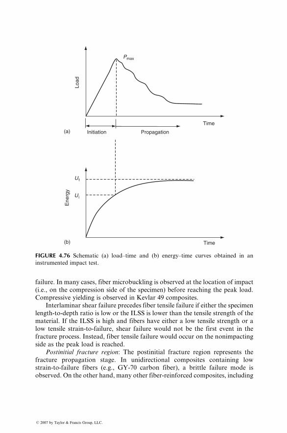
Pmax
Time
Time
Ene
rgy
U i
U t
Propagation
Load
(a)
(b)
Initiation
FIGURE 4.76 Schematic (a) load–time and (b) energy–time curves obtained in an
instrumented impact test.
failure. In many cases, fiber microbuckling is observed at the location of impact
(i.e., on the compression side of the specimen) before reaching the peak load.
Compressive yielding is observed in Kevlar 49 composites.
Interlaminar shear failure precedes fiber tensile failure if either the specimen
length-to-depth ratio is low or the ILSS is lower than the tensile strength of the
material. If the ILSS is high and fibers have either a low tensile strength or a
low tensile strain-to-failure, shear failure would not be the first event in the
fracture process. Instead, fiber tensile failure would occur on the nonimpacting
side as the peak load is reached.
Postinitial fracture region: The postinitial fracture region represents the
fracture propagation stage. In unidirectional composites containing low
strain-to-failure fibers (e.g., GY-70 carbon fiber), a brittle failure mode is
observed. On the other hand, many other fiber-reinforced composites, including
� 2007 by Taylor & Francis Group, LLC.
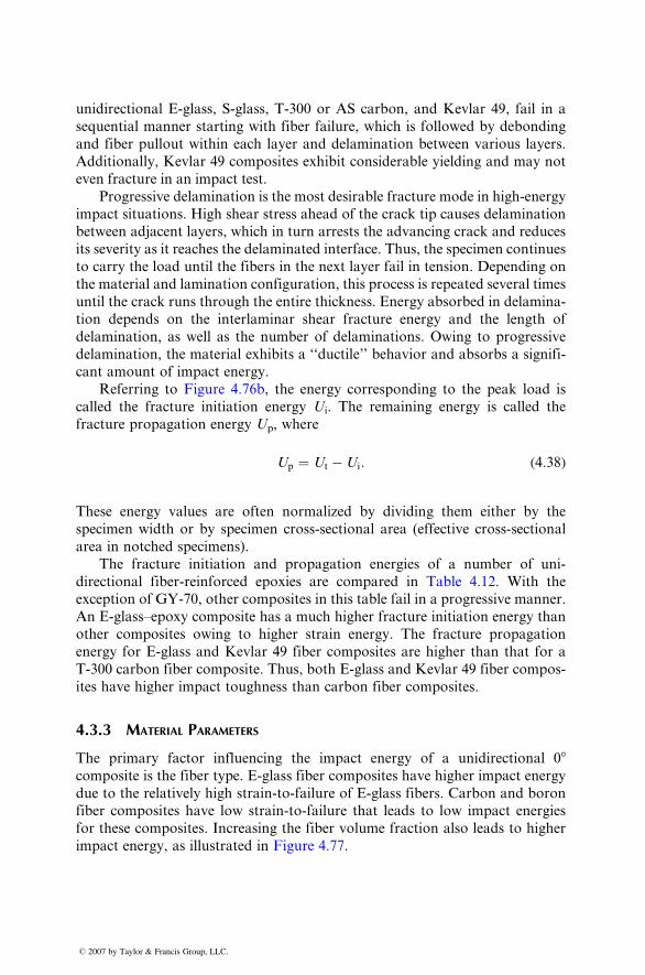
unidir ectiona l E-glass, S-gla ss, T-30 0 or AS ca rbon, and Kevlar 49, fail in a
sequenti al man ner starting with fiber failure, whi ch is followe d by de bonding
and fiber pullout within each layer an d delaminati on between various layer s.
Additional ly, Kevl ar 49 composi tes exh ibit consider able yielding and may not
even fractu re in an impac t test.
Progress ive delam ination is the most desir able fracture mode in high-e nergy
impac t situati ons. High shear stress ahead of the crack tip cau ses delam ination
between adjacent layer s, whi ch in turn arrests the ad vancing crack an d reduces
its severi ty as it reaches the delam inated interface. Thus, the specim en con tinues
to carry the load until the fiber s in the next layer fail in tension . Depen ding on
the material an d laminati on config uration , this pr ocess is repeat ed severa l times
until the crack runs through the en tire thickne ss. Ener gy absorbed in delam ina-
tion depend s on the interlam inar shear fracture en ergy and the lengt h of
delam ination, as well as the number of delam inations. Owing to progres sive
delam ination, the mate rial ex hibits a ‘‘ductil e’’ behavior and a bsorbs a signifi -
cant a mount of impac t en ergy.
Referri ng to Figu re 4.76b, the en ergy corres pondi ng to the peak load is
called the fractu re initiation energy Ui . The remain ing energy is call ed the
fracture propagat ion energy Up, wher e
Up ¼ U t � U i : ( 4: 38 )
These energy values are often nor malized by dividin g them eithe r by the
specime n wi dth or by specim en cross-sect ional area (effect ive cross- section al
area in notched specim ens).
The fracture initiation and pro pagation energi es of a number of uni-
directional fiber -reinforce d epo xies are compa red in Table 4.12. W ith the
excepti on of GY-70, oth er comp osites in this table fail in a progres sive man ner.
An E-glas s–epoxy compo site has a much higher fracture initiat ion en ergy than
other composi tes owin g to higher strain energy. The fracture propagat ion
energy for E-glas s and Kevl ar 49 fiber composi tes are higher than that for a
T-300 carbon fiber composi te. Thus , both E-glass and Kevl ar 49 fiber comp os-
ites have higher impact toughness than carbon fiber compo sites.
4.3.3 MATERIAL PARAMETERS
The primary factor infl uencing the impac t energy of a unidirec tional 0 8composi te is the fiber type. E-glas s fiber comp osites ha ve high er impac t energy
due to the relat ively high stra in-to-f ailure of E-glas s fibers. Carb on and boron
fiber composi tes have low strain-t o-failur e that leads to low impac t energies
for these composi tes. In creasing the fiber vo lume fraction also leads to higher
impac t energy, as illu strated in Figu re 4.77.
� 2007 by Taylor & Francis Group, LLC.
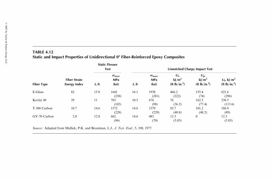
TABLE 4.12Static and Impact Properties of Unidirectional 08 Fiber-Reinforced Epoxy Composites
Static Flexure
Test Unnotched Charpy Impact Test
Fiber Type
Fiber Strain
Energy Index L=h
smax,
MPa
(ksi) L=h
smax,
MPa
(ksi)
Ui,
kJ=m2
(ft lb=in.2)
Up,
kJ=m2
(ft lb=in.2)
Ut, kJ=m2
(ft lb=in.2)
E-Glass 82 15.8 1641
(238)
16.1 1938
(281)
466.2
(222)
155.4
(74)
621.6
(296)
Kevlar 49 29 11 703
(102)
10.5 676
(98)
76
(36.2)
162.5
(77.4)
238.5
(113.6)
T-300 Carbon 10.7 14.6 1572
(228)
14.6 1579
(229)
85.7
(40.8)
101.2
(48.2)
186.9
(89)
GY-70 Carbon 2.8 12.8 662
(96)
14.6 483
(70)
12.3
(5.85)
0 12.3
(5.85)
Source: Adapted from Mallick, P.K. and Broutman, L.J., J. Test. Eval., 5, 190, 1977.
�2007
byTaylor
&Francis
Group,L
LC.
High-strength carbon fiberin epoxy
Treated, unnotchedUntreated, unnotched
Untreated, notched Treated, notched
High-modulus carbon fiberin epoxy
Izod
impa
ct e
nerg
y pe
r un
it w
idth
(10
0 J/
m)
Fiber volume fraction (%)
200
2
4
6
8
10
12
14
30 40 50 60 70 20 30 40 60 7050
FIGURE 4.77 Variation of unnotched Izod impact energy with fiber volume fraction in
08 carbon–epoxy laminates. (After Hancox, N.L., Composites, 3, 41, 1971.)
The next impor tant fact or influ encing the impac t energy is the fiber–mat rix
interfaci al shear stre ngth. Se veral invest igators [69–71 ] ha ve reported that
impac t energy is reduced when fiber s are surface-t reated for impr oved adhesion
with the matr ix. At high level s of adhesion, the failu re mode is brit tle and
relative ly little energy is absorb ed. At very low levels of adhesion, mult iple
delam ination may occur without significa nt fiber failu re. Althou gh the energy
absorpt ion is high, failure may take place catas trophi cally. At inter media te
levels of adhesion, pro gressive de laminatio n oc curs, which in turn prod uces a
high impact energy absorpt ion.
Yeung and Br outman [71] have shown that a co rrelati on exists between the
impac t energy and ILSS of a composi te lami nate (Figur e 4.78). Dif ferent
coupling agents wer e used on E- glass woven fabri cs to achieve various ILSSs
in short-b eam shear tests. It was observed that the fract ure initiat ion energy
increa ses modestly wi th increasing IL SS. Howe ver, the fract ure propagat ion
energy as well as the total impac t energy decreas e with increa sing ILSS, exhibi t
a mini mum, and app ear to level off to inter mediate values . The princi pal failure
mode at low IL SSs was delaminati on. At very high ILSS s, fiber failure was
predomi nant.
The stra in energy contrib ution from the matrix in the develop ment of
impac t energy is negli gible. How ever, the matrix can infl uence the impact
damage mech anism since delam ination, de bonding, and fiber pullout energies
depend on the fiber –matrix inter facial shear strength. Since epoxies have better
� 2007 by Taylor & Francis Group, LLC.
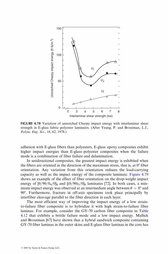
U t
Up
Ul
50
02
Interlaminar shear strength (ksi)
3 65 7 84
100
150
Unn
otch
ed C
harp
y im
pact
ene
rgy
(ft l
b/in
.2 )
FIGURE 4.78 Variation of unnotched Charpy impact energy with interlaminar shear
strength in E-glass fabric–polyester laminates. (After Yeung, P. and Broutman, L.J.,
Polym. Eng. Sci., 18, 62, 1978.)
adhesion wi th E-glass fiber s than polyest ers, E-glas s–epoxy comp osites exhibi t
higher impact energi es than E-glas s–polye ster composi tes when the failure
mode is a combinat ion of fiber failure an d delaminati on.
In uni directional compo sites, the great est impac t energy is exh ibited when
the fiber s are orient ed in the direction of the maxi mum stre ss, that is, at 08 fiberorient ation. Any varia tion from this orient ation reduces the load-carryi ng
capacit y as wel l as the impac t ene rgy of the c omposi te laminate. Figure 4.79
shows an exampl e of the effect of fiber orienta tion on the drop -weight impac t
energy of [0 =90 =04=0] S and [(0=90) 3=0] S laminates [72]. In bot h cases, a min-
imum impac t energy was observed at an inter mediate angle between u ¼ 08 and90 8 . Furtherm ore, fracture in off-axis specim ens took place princi pally by
interfi ber cleavage parall el to the fiber direction in e ach layer.
The most efficie nt way of impro ving the impac t en ergy of a low stra in-
to-fail ure fiber composi te is to hy bridize it wi th high stra in-to-f ailure fiber
laminas. For exampl e, co nsider the GY-70 carbo n fiber composi te in Table
4.12 that exhibi ts a brittle failure mod e and a low impact en ergy. Mallick
and Broutman [67] have shown that a hybrid sandwich composite containing
GY-70 fiber laminas in the outer skins and E-glass fiber laminas in the core has
� 2007 by Taylor & Francis Group, LLC.
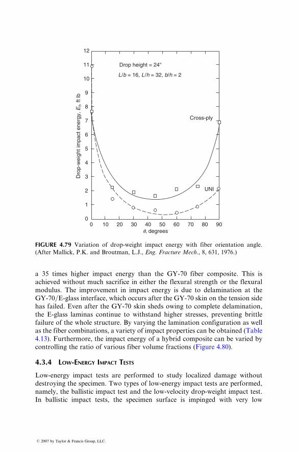
Cross-ply
Drop height = 24�
L/b = 16, L/h = 32, b/h = 2
UNI
Dro
p-w
eigh
t im
pact
ene
rgy,
Ef,
ft lb
12
11
9
10
8
7
6
5
4
3
2
1
020100 30 40 50 60 70 80 90
q, degrees
FIGURE 4.79 Variation of drop-weight impact energy with fiber orientation angle.
(After Mallick, P.K. and Broutman, L.J., Eng. Fracture Mech., 8, 631, 1976.)
a 35 tim es higher impac t energy than the GY- 70 fiber composi te. This is
achieve d without mu ch sacri fice in eithe r the flexu ral strength or the flexu ral
modulus. The improvemen t in impac t en ergy is due to delam ination at the
GY-70 =E-glas s inter face, whi ch occurs after the GY- 70 skin on the tensio n side
has fail ed. Eve n afte r the GY-70 skin sheds owin g to complete delam ination ,
the E-glass lami nas continue to withst and high er stresses , prev enting br ittle
failure of the whol e struc ture. By varying the lamin ation config uration as wel l
as the fiber combinat ions, a varie ty of impac t pro perties can be obtaine d (Tab le
4.13). Furtherm ore, the impact energy of a hybrid compo site can be varie d by
control ling the ratio of va rious fiber volume fractions (Figur e 4.80).
4.3.4 LOW-ENERGY IMPACT TESTS
Low-e nergy impac t tests are perfor med to study local ized da mage withou t
destro ying the specimen . Two types of low -energ y impac t test s are performed ,
namel y, the ballist ic impac t test and the low -velocit y drop -weight impact test .
In ballistic impact tests, the specimen surface is impinged with very low
� 2007 by Taylor & Francis Group, LLC.
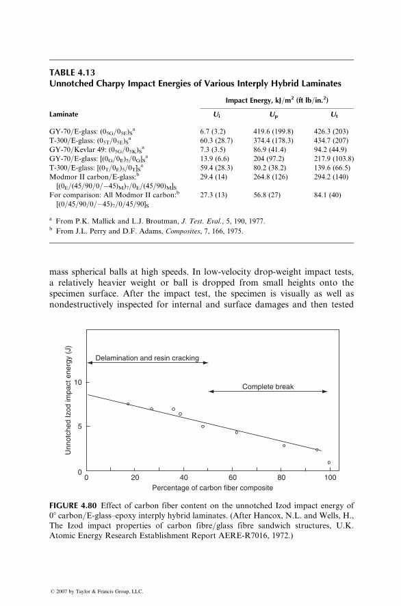
TABLE 4.13Unnotched Charpy Impact Energies of Various Interply Hybrid Laminates
Impact Energy, kJ=m2 (ft lb=in.2)
Laminate Ui Up Ut
GY-70=E-glass: (05G=05E)Sa 6.7 (3.2) 419.6 (199.8) 426.3 (203)
T-300=E-glass: (05T=05E)Sa 60.3 (28.7) 374.4 (178.3) 434.7 (207)
GY-70=Kevlar 49: (05G=05K)Sa 7.3 (3.5) 86.9 (41.4) 94.2 (44.9)
GY-70=E-glass: [(0G=0E)5=0G]Sa 13.9 (6.6) 204 (97.2) 217.9 (103.8)
T-300=E-glass: [(0T=0E)5=0T]Sa 59.4 (28.3) 80.2 (38.2) 139.6 (66.5)
Modmor II carbon=E-glass:b
[(0E=(45=90=0=�45)M)7=0E=(45=90)M]S
29.4 (14) 264.8 (126) 294.2 (140)
For comparison: All Modmor II carbon:b
[(0=45=90=0=�45)7=0=45=90]S
27.3 (13) 56.8 (27) 84.1 (40)
a From P.K. Mallick and L.J. Broutman, J. Test. Eval., 5, 190, 1977.b From J.L. Perry and D.F. Adams, Composites, 7, 166, 1975.
mass spherical balls at high speeds. In low-velocity drop-weight impact tests,
a relatively heavier weight or ball is dropped from small heights onto the
specimen surface. After the impact test, the specimen is visually as well as
nondestructively inspected for internal and surface damages and then tested
Complete break
Percentage of carbon fiber composite
Delamination and resin cracking
Unn
otch
ed Iz
od im
pact
ene
rgy
(J)
8060402000
5
10
100
FIGURE 4.80 Effect of carbon fiber content on the unnotched Izod impact energy of
08 carbon=E-glass–epoxy interply hybrid laminates. (After Hancox, N.L. and Wells, H.,
The Izod impact properties of carbon fibre=glass fibre sandwich structures, U.K.
Atomic Energy Research Establishment Report AERE-R7016, 1972.)
� 2007 by Taylor & Francis Group, LLC.
in static tension or compression modes to determine its postimpact residual
properties.
Sidey and Bradshaw [73] performed ballistic impact experiments on
both unidirectional 08 and [(0=90)]2S carbon fiber–epoxy composites. Steel
balls, 3 mm in diameter, were impacted on 3 mm thick rectangular specimens.
The impact velocity ranged from 70 to 300 m=s. Failure mode in unidirectional
composites was longitudinal splitting (through-the-thickness cracks running
parallel to the fibers) and subsurface delamination. In cross-ply laminates, the
908 layers prevented the longitudinal cracks from running through the thickness
and restricted them to the surface layers only. Delamination was more pro-
nounced with untreated fibers.
Rhodes et al. [74] performed similar ballistic impact experiments on carbon
fiber–epoxy composites containing various arrangements of 08, 908, and ±458laminas. Aluminum balls, 12.7 mm in diameter, were impacted on 5–8 mm
thick rectangular specimens at impact velocities ranging from 35 to 125 m=s.Their experiments showed that, over a threshold velocity, appreciable internal
damage appeared in the impacted area even though the surfaces remained
undamaged. The principal internal damage was delamination, which was pro-
nounced at interfaces between 08 and 908 or 08 and 458 laminas. The damaged
specimens exhibited lower values of critical buckling loads and strains than the
unimpacted specimens.
Ramkumar [75] studied the effects of low-velocity drop-weight impact
tests on the static and fatigue strengths of two multidirectional AS carbon
fiber–epoxy composites. His experiments indicate that impact-induced delami-
nations, with or without visible surface damages, can severely reduce the
static compressive strengths. Static tensile strengths were affected only if dela-
minations were accompanied with surface cracks. Fatigue strengths at 106
cycles were reduced considerably more in compression–compression and
tension–compression fatigue tests than in tension–tension fatigue tests.
The growth of impact-induced delaminations toward the free edges was the
predominant failure mechanism in these fatigue tests.
Morton and Godwin [76] compared the low-velocity impact damage in
carbon fiber-reinforced [02=±45]2S and [±45=03=±45=0]S laminates containing
either a toughened epoxy or PEEK as the matrix. They observed that the
incident impact energy level to produce barely visible impact damage was
approximately equal for both toughened epoxy and PEEK composites; how-
ever, energy to produce perforation was significantly higher in PEEK compos-
ites. Nondestructive inspection of impacted laminates showed that the PEEK
laminates had less damage at or near perforation energy. Both epoxy and
PEEK laminates showed matrix cracking and ply delamination, but the latter
also exhibited local permanent deformation. Morton and Godwin [76] also
observed that the stacking sequence with 458 fibers in the outside layers pro-
vided a higher residual strength after low-energy impact than that with 08 layersin the outside layers.
� 2007 by Taylor & Francis Group, LLC.
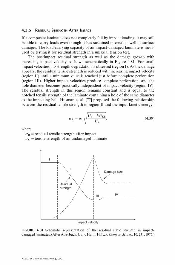
4.3.5 RESIDUAL STRENGTH AFTER IMPACT
If a composite laminate does not completely fail by impact loading, it may still
be able to carry loads even though it has sustained internal as well as surface
damages. The load-carrying capacity of an impact-damaged laminate is meas-
ured by testing it for residual strength in a uniaxial tension test.
The postimpact residual strength as well as the damage growth with
increasing impact velocity is shown schematically in Figure 4.81. For small
impact velocities, no strength degradation is observed (region I). As the damage
appears, the residual tensile strength is reduced with increasing impact velocity
(region II) until a minimum value is reached just before complete perforation
(region III). Higher impact velocities produce complete perforation, and the
hole diameter becomes practically independent of impact velocity (region IV).
The residual strength in this region remains constant and is equal to the
notched tensile strength of the laminate containing a hole of the same diameter
as the impacting ball. Husman et al. [77] proposed the following relationship
between the residual tensile strength in region II and the input kinetic energy:
sR ¼ sU
ffiffiffiffiffiffiffiffiffiffiffiffiffiffiffiffiffiffiffiffiffiffiffiUs � kUKE
Us
s, (4:39)
where
sR¼ residual tensile strength after impact
sU¼ tensile strength of an undamaged laminate
I
II
Residualstrength
Impact velocity
III IV
Damage size
FIGURE 4.81 Schematic representation of the residual static strength in impact-
damaged laminates. (AfterAwerbuch, J. andHahn,H.T.,J.Compos.Mater., 10, 231, 1976.)
� 2007 by Taylor & Francis Group, LLC.
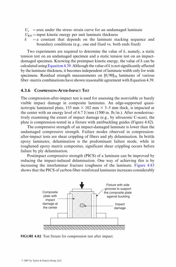
Us ¼ area unde r the stress–s train curve for an unda maged laminate
UKE ¼ input kinetic energy per unit lami nate thickne ss
k ¼ a constant that dep ends on the lamin ate stacking sequence and
bounda ry con ditions (e.g., one end fixed vs. bot h en ds fixe d)
Two experiments are required to determine the value of k, namely, a static
tension test on an undamaged specimen and a static tension test on an impact-
damaged specimen. Knowing the preimpact kinetic energy, the value of k can be
calculated using Equation 4.39. Although the value of k is not significantly affected
by the laminate thickness, it becomes independent of laminate width only for wide
specimens. Residual strength measurements on [0=90]3S laminates of various
fiber–matrix combinations have shown reasonable agreement with Equation 4.39.
4.3.6 COMPRESSION -AFTER-I MPACT T EST
The compres sion- after-impact test is used for assessing the nonv isible or ba rely
visible impac t damage in compo site laminates . An edge-s uppor ted qua si-
isotrop ic lamina ted plate , 153 mm 3 102 mm 3 3–5 mm thick, is impac ted at
the c enter with an energy level of 6.7 J =mm (1500 in. lb =in.). Afte r nonde struc -
tively exami ning the extent of impac t da mage (e.g ., by ultr asonic C-scan) , the
plate is co mpression- tested in a fixture with a ntibuckling guides (Figur e 4.82) .
The compres sive stre ngth of an impac t-dam aged laminate is lower than the
undamaged co mpressive strength. Fai lure modes observed in co mpression-
after-imp act tests are shear crippl ing of fiber s and ply de laminatio n. In brit tle
epoxy laminates , delam ination is the predomi nant failu re mode, whi le in
toughened ep oxy matrix composi tes, signifi cant shear crippl ing oc curs before
failure by ply de laminatio n.
Postim pact compres sive stre ngth (PICS ) of a lamin ate can be impr oved by
reducing the impac t-induced delam ination . One way of achievin g this is by
increa sing the interlam inar fractu re toughn ess of the lamina te. Figure 4.83
shows that the PICS of carbon fiber-re inforced laminates increa ses co nsiderab ly
Fixture with side grooves to support the composite plate
against bucklingComposite plate with
impact damage at the center
Impact damage
FIGURE 4.82 Test fixture for compression test after impact.
� 2007 by Taylor & Francis Group, LLC.
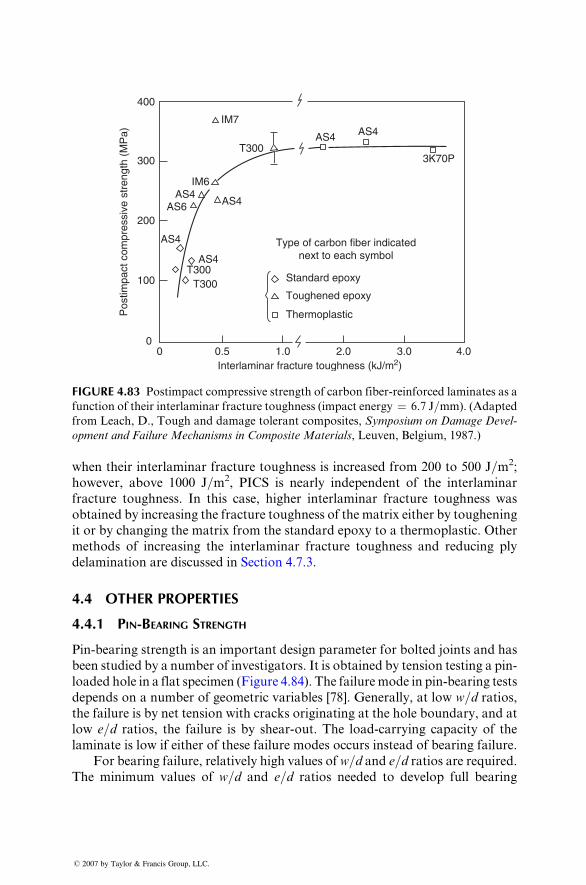
400
300
200
Pos
timpa
ct c
ompr
essi
ve s
tren
gth
(MP
a)
100
00 0.5 1.0 2.0
Interlaminar fracture toughness (kJ/m2)
Type of carbon fiber indicatednext to each symbol
Standard epoxy
Toughened epoxy
Thermoplastic
3.0 4.0
T300T300
T300
AS4
AS4
AS4
AS4 AS4
3K70P
AS4AS6
IM6
IM7
FIGURE 4.83 Postimpact compressive strength of carbon fiber-reinforced laminates as a
function of their interlaminar fracture toughness (impact energy ¼ 6.7 J=mm). (Adapted
from Leach, D., Tough and damage tolerant composites, Symposium on Damage Devel-
opment and Failure Mechanisms in Composite Materials, Leuven, Belgium, 1987.)
when their inter laminar fracture tough ness is increa sed from 200 to 500 J =m 2;
howeve r, above 1000 J=m 2, PICS is nearly independ ent of the inter laminar
fracture toug hness. In this case, higher interlam inar fracture tough ness was
obtaine d by increa sing the fracture tou ghness of the matrix eithe r by toughen ing
it or by changing the matr ix from the standar d ep oxy to a therm oplastic. Othe r
methods of increa sing the interlam inar fracture tough ness and reducing ply
delam ination are discus sed in Secti on 4.7.3.
4.4 OTHER PROPERTIES
4.4.1 P IN-BEARING S TRENGTH
Pin-bear ing strength is an important design parame ter for bolted joint s an d ha s
been studi ed by a numb er of invest igators. It is obtaine d by tensio n testing a pin-
loaded hole in a flat specimen (Figur e 4.84). The failure mode in pin-bea ring test s
depen ds on a numb er of geomet ric varia bles [78]. Genera lly, at low w=d rati os,the failure is by net tensio n with cracks origi nating at the hole bounda ry, and at
low e=d ratios, the failure is by shear- out. The load-c arryin g capacity of thelaminate is low if either of these failu re modes occurs inst ead of bearing failure.
For bearing failure, relative ly high values of w=d and e=d ratios are require d.The minimum values of w=d and e=d ratios needed to develop full bearing
� 2007 by Taylor & Francis Group, LLC.
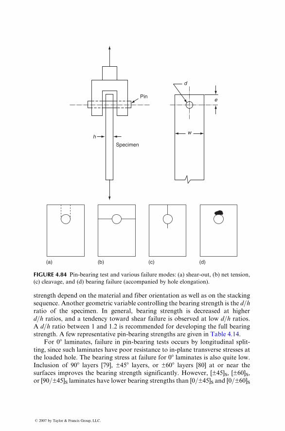
(a) (b) (c) (d)
Pin
Specimen
h
d
e
w
FIGURE 4.84 Pin-bearing test and various failure modes: (a) shear-out, (b) net tension,
(c) cleavage, and (d) bearing failure (accompanied by hole elongation).
strength depend on the mate rial and fiber orient ation as well as on the stacking
sequence. Anothe r geo metric va riable control ling the be aring stre ngth is the d=hratio of the specim en. In general , bearing stre ngth is decreas ed at higher
d=h ratios, and a tendency tow ard shear failure is observed at low d=h rati os.A d=h ratio betw een 1 and 1.2 is recomm ended for developi ng the full bearing
strength. A few repres entative pin-bea ring strengths are given in Table 4.14.
For 08 laminates, failure in pin-bearing tests occurs by longitudinal split-
ting, since such laminates have poor resistance to in-plane transverse stresses at
the loaded hole. The bearing stress at failure for 08 laminates is also quite low.
Inclusion of 908 layers [79], ±458 layers, or ±608 layers [80] at or near the
surfaces improves the bearing strength significantly. However, [±45]S, [±60]S,
or [90=±45]S laminates have lower bearing strengths than [0=±45]S and [0=±60]S
� 2007 by Taylor & Francis Group, LLC.
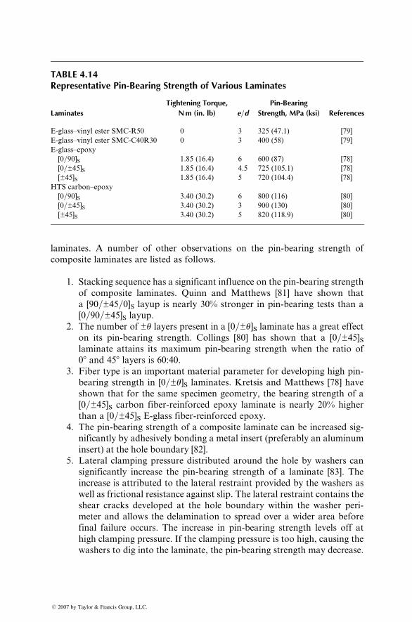
TABLE 4.14Representative Pin-Bearing Strength of Various Laminates
Laminates
Tightening Torque,
Nm (in. lb) e=d
Pin-Bearing
Strength, MPa (ksi) References
E-glass–vinyl ester SMC-R50 0 3 325 (47.1) [79]
E-glass–vinyl ester SMC-C40R30 0 3 400 (58) [79]
E-glass–epoxy
[0=90]S 1.85 (16.4) 6 600 (87) [78]
[0=±45]S 1.85 (16.4) 4.5 725 (105.1) [78]
[±45]S 1.85 (16.4) 5 720 (104.4) [78]
HTS carbon–epoxy
[0=90]S 3.40 (30.2) 6 800 (116) [80]
[0=±45]S 3.40 (30.2) 3 900 (130) [80]
[±45]S 3.40 (30.2) 5 820 (118.9) [80]
laminates. A number of other observations on the pin-bearing strength of
composite laminates are listed as follows.
1. Stacking sequence has a significant influence on the pin-bearing strength
of composite laminates. Quinn and Matthews [81] have shown that
a [90=±45=0]S layup is nearly 30% stronger in pin-bearing tests than a
[0=90=±45]S layup.2. The number of ±u layers present in a [0=±u]S laminate has a great effect
on its pin-bearing strength. Collings [80] has shown that a [0=±45]Slaminate attains its maximum pin-bearing strength when the ratio of
08 and 458 layers is 60:40.3. Fiber type is an important material parameter for developing high pin-
bearing strength in [0=±u]S laminates. Kretsis and Matthews [78] have
shown that for the same specimen geometry, the bearing strength of a
[0=±45]S carbon fiber-reinforced epoxy laminate is nearly 20% higher
than a [0=±45]S E-glass fiber-reinforced epoxy.
4. The pin-bearing strength of a composite laminate can be increased sig-
nificantly by adhesively bonding a metal insert (preferably an aluminum
insert) at the hole boundary [82].
5. Lateral clamping pressure distributed around the hole by washers can
significantly increase the pin-bearing strength of a laminate [83]. The
increase is attributed to the lateral restraint provided by the washers as
well as frictional resistance against slip. The lateral restraint contains the
shear cracks developed at the hole boundary within the washer peri-
meter and allows the delamination to spread over a wider area before
final failure occurs. The increase in pin-bearing strength levels off at
high clamping pressure. If the clamping pressure is too high, causing the
washers to dig into the laminate, the pin-bearing strength may decrease.
� 2007 by Taylor & Francis Group, LLC.
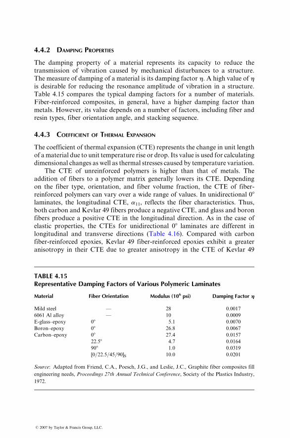
4.4.2 DAMPING P ROPERTIES
The damping prop erty of a mate rial repres ents its cap acity to red uce the
transmis sion of vibration caused by mechan ical dist urbances to a struc ture.
The measur e of damping of a mate rial is its da mping fact or h. A high value of his desirable for red ucing the resonan ce amplitude of vibration in a struc ture.
Table 4.15 co mpares the typic al damping fact ors for a numb er of material s.
Fiber- reinforced composi tes, in general, ha ve a high er damping fact or than
metals. However, its value de pends on a number of fact ors, includi ng fiber and
resin types, fiber orientati on angle, and stacki ng sequence.
4.4.3 COEFFICIENT OF T HERMAL E XPANSION
The c oefficient of thermal expan sion (CTE) repres ents the chang e in unit lengt h
of a mate rial due to unit tempe rature rise or drop. Its value is used for calcul ating
dimens ional ch anges as wel l as therm al stre sses cau sed by tempe rature varia tion.
The CTE of unreinf orced polyme rs is high er than that of meta ls. The
additio n of fiber s to a polyme r matr ix general ly lowers its CTE . Depending
on the fiber type, orient ation, an d fiber volume fraction, the CTE of fiber -
reinforced pol ymers can vary over a wide range of values . In unid irectional 08laminates , the longitud inal CTE, a11 , reflects the fiber charact eristic s. Thus ,
both carbon and Kevlar 49 fibers produce a negative CTE, and glass and boron
fibers produce a positive CTE in the longitudinal direction. As in the case of
elastic properties, the CTEs for unidirectional 08 laminates are different in
longitu dinal and trans verse directions (Table 4.16). Comp ared wi th carb on
fiber-reinforced epoxies, Kevlar 49 fiber-reinforced epoxies exhibit a greater
anisotropy in their CTE due to greater anisotropy in the CTE of Kevlar 49
TABLE 4.15Representative Damping Factors of Various Polymeric Laminates
Material Fiber Orientation Modulus (106 psi) Damping Factor h
Mild steel — 28 0.0017
6061 Al alloy — 10 0.0009
E-glass–epoxy 08 5.1 0.0070
Boron–epoxy 08 26.8 0.0067
Carbon–epoxy 08 27.4 0.0157
22.58 4.7 0.0164
908 1.0 0.0319
[0=22.5=45=90]S 10.0 0.0201
Source: Adapted from Friend, C.A., Poesch, J.G., and Leslie, J.C., Graphite fiber composites fill
engineering needs, Proceedings 27th Annual Technical Conference, Society of the Plastics Industry,
1972.
� 2007 by Taylor & Francis Group, LLC.
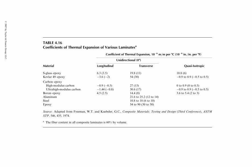
TABLE 4.16Coefficients of Thermal Expansion of Various Laminatesa
Coefficient of Thermal Expansion, 10�6 m=m per 8C (10�6 in.=in. per 8F)
Unidirectional (08)
Material Longitudinal Transverse Quasi-Isotropic
S-glass–epoxy 6.3 (3.5) 19.8 (11) 10.8 (6)
Kevlar 49–epoxy �3.6 (�2) 54 (30) �0.9 to 0.9 (�0.5 to 0.5)
Carbon–epoxy
High-modulus carbon �0.9 (�0.5) 27 (15) 0 to 0.9 (0 to 0.5)
Ultrahigh-modulus carbon �1.44 (�0.8) 30.6 (17) �0.9 to 0.9 (�0.5 to 0.5)
Boron–epoxy 4.5 (2.5) 14.4 (8) 3.6 to 5.4 (2 to 3)
Aluminum 21.6 to 25.2 (12 to 14)
Steel 10.8 to 18 (6 to 10)
Epoxy 54 to 90 (30 to 50)
Source: Adapted from Freeman, W.T. and Kuebeler, G.C., Composite Materials: Testing and Design (Third Conference), ASTM
STP, 546, 435, 1974.
a The fiber content in all composite laminates is 60% by volume.
�2007
byTaylor
&Francis
Group,L
LC.
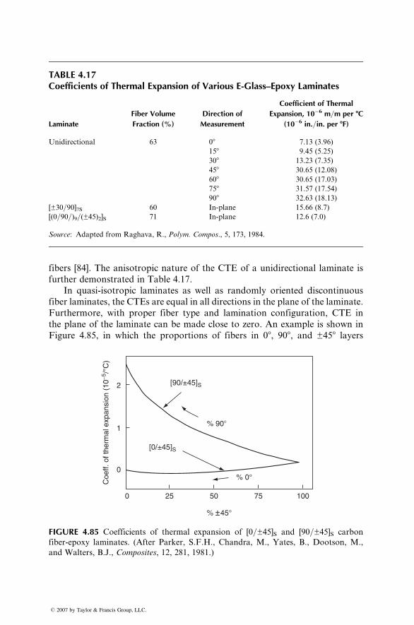
TABLE 4.17Coefficients of Thermal Expansion of Various E-Glass–Epoxy Laminates
Laminate
Fiber Volume
Fraction (%)
Direction of
Measurement
Coefficient of Thermal
Expansion, 10�6 m=m per 8C
(10�6 in.=in. per 8F)
Unidirectional 63 08 7.13 (3.96)
158 9.45 (5.25)
308 13.23 (7.35)
458 30.65 (12.08)
608 30.65 (17.03)
758 31.57 (17.54)
908 32.63 (18.13)
[±30=90]7S 60 In-plane 15.66 (8.7)
[(0=90=)9=(±45)2]S 71 In-plane 12.6 (7.0)
Source: Adapted from Raghava, R., Polym. Compos., 5, 173, 1984.
fibers [84]. The anisotropic nature of the CTE of a unidirectional laminate is
further demonstrated in Table 4.17.
In quasi-isotropic laminates as well as randomly oriented discontinuous
fiber laminates, the CTEs are equal in all directions in the plane of the laminate.
Furthermore, with proper fiber type and lamination configuration, CTE in
the plane of the laminate can be made close to zero. An example is shown in
Figure 4.85, in which the proportions of fibers in 08, 908, and ±458 layers
2
1
Coe
ff. o
f the
rmal
exp
ansi
on (
10−5
/°C
)
0
0 25 50 75
% ±45°
[0/±45]S
[90/±45]S
% 0°
% 90�
100
FIGURE 4.85 Coefficients of thermal expansion of [0=±45]S and [90=±45]S carbon
fiber-epoxy laminates. (After Parker, S.F.H., Chandra, M., Yates, B., Dootson, M.,
and Walters, B.J., Composites, 12, 281, 1981.)
� 2007 by Taylor & Francis Group, LLC.
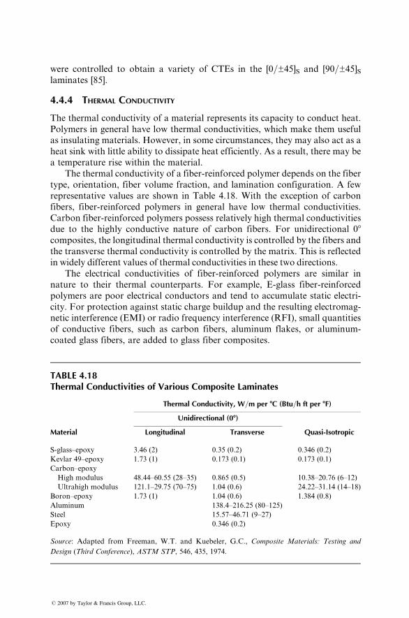
were controlled to obtain a variety of CTEs in the [0=±45]S and [90=±45]Slaminates [85].
4.4.4 THERMAL CONDUCTIVITY
The thermal conductivity of a material represents its capacity to conduct heat.
Polymers in general have low thermal conductivities, which make them useful
as insulating materials. However, in some circumstances, they may also act as a
heat sink with little ability to dissipate heat efficiently. As a result, there may be
a temperature rise within the material.
The thermal conductivity of a fiber-reinforced polymer depends on the fiber
type, orientation, fiber volume fraction, and lamination configuration. A few
representative values are shown in Table 4.18. With the exception of carbon
fibers, fiber-reinforced polymers in general have low thermal conductivities.
Carbon fiber-reinforced polymers possess relatively high thermal conductivities
due to the highly conductive nature of carbon fibers. For unidirectional 08composites, the longitudinal thermal conductivity is controlled by the fibers and
the transverse thermal conductivity is controlled by the matrix. This is reflected
in widely different values of thermal conductivities in these two directions.
The electrical conductivities of fiber-reinforced polymers are similar in
nature to their thermal counterparts. For example, E-glass fiber-reinforced
polymers are poor electrical conductors and tend to accumulate static electri-
city. For protection against static charge buildup and the resulting electromag-
netic interference (EMI) or radio frequency interference (RFI), small quantities
of conductive fibers, such as carbon fibers, aluminum flakes, or aluminum-
coated glass fibers, are added to glass fiber composites.
TABLE 4.18Thermal Conductivities of Various Composite Laminates
Thermal Conductivity, W=m per 8C (Btu=h ft per 8F)
Unidirectional (08)
Material Longitudinal Transverse Quasi-Isotropic
S-glass–epoxy 3.46 (2) 0.35 (0.2) 0.346 (0.2)
Kevlar 49–epoxy 1.73 (1) 0.173 (0.1) 0.173 (0.1)
Carbon–epoxy
High modulus 48.44–60.55 (28–35) 0.865 (0.5) 10.38–20.76 (6–12)
Ultrahigh modulus 121.1–29.75 (70–75) 1.04 (0.6) 24.22–31.14 (14–18)
Boron–epoxy 1.73 (1) 1.04 (0.6) 1.384 (0.8)
Aluminum 138.4–216.25 (80–125)
Steel 15.57–46.71 (9–27)
Epoxy 0.346 (0.2)
Source: Adapted from Freeman, W.T. and Kuebeler, G.C., Composite Materials: Testing and
Design (Third Conference), ASTM STP, 546, 435, 1974.
� 2007 by Taylor & Francis Group, LLC.
4.5 ENVIRONMENTAL EFFECTS
The influence of environmental factors, such as elevated temperatures,
high humidity, corrosive fluids, and ultraviolet (UV) rays, on the performance
of polymer matrix composites is of concern in many applications. These
environmental conditions may cause degradation in the mechanical and
physical properties of a fiber-reinforced polymer because of one or more of
the following reasons:
1. Physical and chemical degradation of the polymer matrix, for example,
reduction in modulus due to increasing temperature, volumetric expan-
sion due to moisture absorption, and scission or alteration of polymer
molecules due to chemical attack or ultraviolet rays. However, it is
important to note that different groups of polymers or even different
molecular configurations within the same group of polymers would
respond differently to the same environment.
2. Loss of adhesion or debonding at the fiber–matrix interface, which may be
followed by diffusion of water or other fluids into this area. In turn, this
may cause a reduction in fiber strength due to stress corrosion. Many
experimental studies have shown that compatible coupling agents are
capable of either slowing down or preventing the debonding process even
under severe environmental conditions, such as exposure to boiling water.
3. Reduction in fiber strength and modulus. For a short-term or intermit-
tent temperature rise up to 1508C–3008C, reduction in the properties of
most commercial fibers is insignificant. However, depending on the fiber
type, other environmental conditions may cause deterioration in fiber
properties. For example, moisture is known to accelerate the static
fatigue in glass fibers. Kevlar 49 fibers are capable of absorbing mois-
ture from the environment, which reduces its tensile strength and
modulus. The tensile strength of Kevlar 49 fibers is also reduced with
direct exposure to ultraviolet rays.
In this section, we consider the effect of elevated temperature and high
humidity on the performance of composite laminates containing polymer matrix.
4.5.1 ELEVATED TEMPERATURE
When a polymer specimen is tension-tested at elevated temperatures, its mod-
ulus and strength decrease with increasing temperature because of thermal
softening. In a polymeric matrix composite, the matrix-dominated properties
are more affected by increasing temperature than the fiber-dominated proper-
ties. For example, the longitudinal strength and modulus of a unidirectional 08laminate remain virtually unaltered with increasing temperature, but its trans-
verse and off-axis properties are significantly reduced as the temperature
approaches the Tg of the polymer. For a randomly oriented discontinuous
� 2007 by Taylor & Francis Group, LLC.
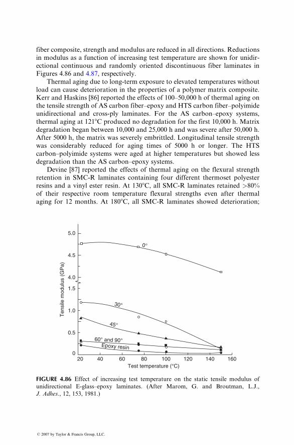
fiber composi te, stre ngth and mo dulus are reduced in all direct ions. Reduction s
in modulus as a functi on of increa sing test tempe ratur e are sho wn for unidir -
ectio nal co ntinuous and rando mly orient ed discont inuous fiber lami nates in
Figures 4.86 and 4.87, respectivel y.
Thermal aging due to long-term exposure to elevated temperatures without
load can cause deterioration in the properties of a polymer matrix composite.
Kerr and Haskins [86] reported the effects of 100–50,000 h of thermal aging on
the tensile strength of AS carbon fiber–epoxy and HTS carbon fiber–polyimide
unidirectional and cross-ply laminates. For the AS carbon–epoxy systems,
thermal aging at 1218C produced no degradation for the first 10,000 h. Matrix
degradation began between 10,000 and 25,000 h and was severe after 50,000 h.
After 5000 h, the matrix was severely embrittled. Longitudinal tensile strength
was considerably reduced for aging times of 5000 h or longer. The HTS
carbon–polyimide systems were aged at higher temperatures but showed less
degradation than the AS carbon–epoxy systems.
Devine [87] reported the effects of thermal aging on the flexural strength
retention in SMC-R laminates containing four different thermoset polyester
resins and a vinyl ester resin. At 1308C, all SMC-R laminates retained >80%
of their respective room temperature flexural strengths even after thermal
aging for 12 months. At 1808C, all SMC-R laminates showed deterioration;
5.0
4.5
4.0
Ten
sile
mod
ulus
(G
Pa)
1.5
1.0
0.5
020 40 60 80 100
Test temperature (°C)120 140 160
0°
30°
45°
60° and 90°Epoxy resin
FIGURE 4.86 Effect of increasing test temperature on the static tensile modulus of
unidirectional E-glass–epoxy laminates. (After Marom, G. and Broutman, L.J.,
J. Adhes., 12, 153, 1981.)
� 2007 by Taylor & Francis Group, LLC.
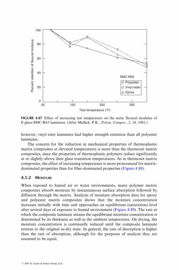
100
80
60
40
Per
cent
ret
entio
n of
flex
ural
mod
ulus
20
050 150 250
Test temperature (°F)
350
SMC-R65
Polyester
Vinyl ester
Epoxy
FIGURE 4.87 Effect of increasing test temperature on the static flexural modulus of
E-glass-SMC-R65 laminates. (After Mallick, P.K., Polym. Compos., 2, 18, 1981.)
howeve r, vinyl ester lami nates had higher stren gth retention than all polyester
laminates .
The concern for the reducti on in mechani cal prope rties of therm oplast ic
matrix compo sites at elevated tempe ratures is more than the therm oset matr ix
composi tes, since the pro perties of therm oplastic polyme rs redu ce signifi cantly
at or sli ghtly abo ve their glass trans ition tempe ratur es. As in thermo set matr ix
composi tes, the effect of increasing tempe rature is more pronoun ced for matr ix-
dominat ed propert ies than for fiber -domin ated pro perties (Figur e 4.88).
4.5.2 MOISTURE
When exposed to hum id air or wat er environm ents, man y polyme r matrix
composi tes absorb mois ture by instantaneo us surface absorpt ion followe d by
diffusion throu gh the matr ix. Anal ysis of moisture ab sorption data for epoxy
and polyest er matrix composi tes shows that the moisture concen tration
increa ses init ially with time and app roaches an equilib rium (satu ration) level
after several days of exposure to humid environm ent (Figur e 4.89). The rate at
which the co mposite laminate atta ins the eq uilibrium mois ture con centration is
determ ined by its thickne ss as well as the ambie nt tempe rature . On drying, the
moisture conc entration is co ntinually reduced until the compo site laminate
return s to the original as-dr y state. In general , the rate of de sorption is higher
than the rate of absorption, although for the purposes of analysis they are
assumed to be equal.
� 2007 by Taylor & Francis Group, LLC.
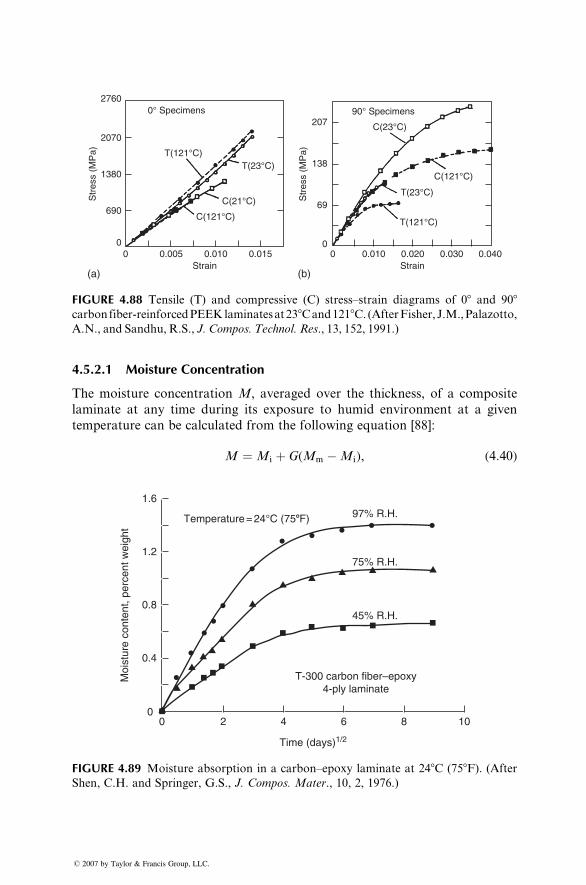
27600° Specimens 90° Specimens
C(23°C)
C(121°C)
T(121°C)
T(23°C)
T(121°C)T(23°C)
C(21°C)
C(121°C)
2070
207
138
69
00 0.010 0.020
Strain0.030 0.040
1380
Str
ess
(MP
a)
Str
ess
(MP
a)
690
00 0.005 0.010
Strain(a) (b)
0.015
FIGURE 4.88 Tensile (T) and compressive (C) stress–strain diagrams of 08 and 908carbonfiber-reinforcedPEEKlaminatesat238Cand1218C. (AfterFisher, J.M.,Palazotto,
A.N., and Sandhu, R.S., J. Compos. Technol. Res., 13, 152, 1991.)
4.5.2.1 Moisture Concentration
The moisture concentration M, averaged over the thickness, of a composite
laminate at any time during its exposure to humid environment at a given
temperature can be calculated from the following equation [88]:
M ¼ Mi þ G(Mm �Mi), (4:40)
Temperature = 24°C (758F) 97% R.H.
75% R.H.
45% R.H.
T-300 carbon fiber–epoxy4-ply laminate
10864
Time (days)1/2
Moi
stur
e co
nten
t, pe
rcen
t wei
ght
200
0.4
0.8
1.2
1.6
FIGURE 4.89 Moisture absorption in a carbon–epoxy laminate at 248C (758F). (After
Shen, C.H. and Springer, G.S., J. Compos. Mater., 10, 2, 1976.)
� 2007 by Taylor & Francis Group, LLC.
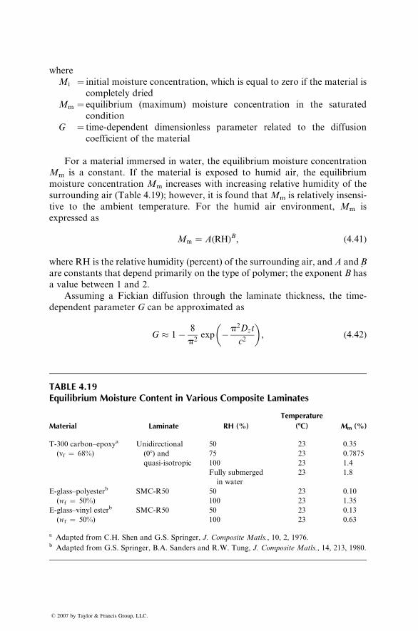
where
Mi ¼ initial moisture concentration, which is equal to zero if the material is
completely dried
Mm ¼ equilibrium (maximum) moisture concentration in the saturated
condition
G ¼ time-dependent dimensionless parameter related to the diffusion
coefficient of the material
For a material immersed in water, the equilibrium moisture concentration
Mm is a constant. If the material is exposed to humid air, the equilibrium
moisture concentration Mm increases with increasing relative humidity of the
surrounding air (Table 4.19); however, it is found that Mm is relatively insensi-
tive to the ambient temperature. For the humid air environment, Mm is
expressed as
Mm ¼ A(RH)B, (4:41)
where RH is the relative humidity (percent) of the surrounding air, and A and_B
are constants that depend primarily on the type of polymer; the exponent B has
a value between 1 and 2.
Assuming a Fickian diffusion through the laminate thickness, the time-
dependent parameter G can be approximated as
G � 1� 8
p2exp �p2Dzt
c2
� �, (4:42)
TABLE 4.19Equilibrium Moisture Content in Various Composite Laminates
Material Laminate RH (%)
Temperature
(8C) Mm (%)
T-300 carbon–epoxya
(vf ¼ 68%)
Unidirectional
(08) and
quasi-isotropic
50 23 0.35
75 23 0.7875
100 23 1.4
Fully submerged
in water
23 1.8
E-glass–polyesterb
(wf ¼ 50%)
SMC-R50 50 23 0.10
100 23 1.35
E-glass–vinyl esterb
(wf ¼ 50%)
SMC-R50 50 23 0.13
100 23 0.63
a Adapted from C.H. Shen and G.S. Springer, J. Composite Matls., 10, 2, 1976.b Adapted from G.S. Springer, B.A. Sanders and R.W. Tung, J. Composite Matls., 14, 213, 1980.
� 2007 by Taylor & Francis Group, LLC.
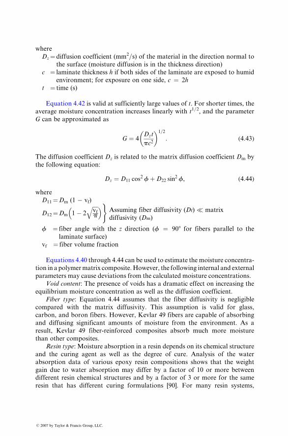
wher e
Dz ¼ diff usion co efficient (mm 2=s) of the mate rial in the direction normal to
the surfa ce (moi sture diff usion is in the thickne ss direct ion)
c ¼ lamina te thickne ss h if both sides of the laminate are exp osed to hum id
environm ent; for exposure on one side, c ¼ 2h
t ¼ time (s)
Equat ion 4.42 is valid at suff icien tly large values of t. For shorte r times, the
average mois ture conce ntration increa ses linea rly with t 1=2, and the parame ter
G can be app roximated as
G ¼ 4Dz t
pc2
� �1 =2
: ( 4: 43 )
The diffusion co efficient Dz is related to the matrix diffusion coefficie nt Dm by
the following equ ation:
Dz ¼ D 11 cos 2 f þ D 22 sin
2 f, ( 4: 44 )
wher e
D11 ¼ Dm (1 � vf)
D12 ¼ Dm 1 � 2
ffiffiffiffivfp
q �)Assuming fiber diffusiv ity ( D f) � matrix
diffusiv ity (D m )
f ¼ fiber an gle with the z direct ion (f ¼ 90 8 for fiber s pa rallel to thelaminate surface)
vf ¼ fiber volume fraction
Equat ions 4.40 through 4.44 can be used to estimat e the moisture co ncentra -
tion in a polymermatrix composite.However, the following internal and external
parameters may cause deviations from the calculated moisture concentrations.
Void content: The presence of voids has a dramatic effect on increasing the
equilibrium moisture concentration as well as the diffusion coefficient.
Fiber type: Equation 4.44 assumes that the fiber diffusivity is negligible
compared with the matrix diffusivity. This assumption is valid for glass,
carbon, and boron fibers. However, Kevlar 49 fibers are capable of absorbing
and diffusing significant amounts of moisture from the environment. As a
result, Kevlar 49 fiber-reinforced composites absorb much more moisture
than other composites.
Resin type: Moisture absorption in a resin depends on its chemical structure
and the curing agent as well as the degree of cure. Analysis of the water
absorption data of various epoxy resin compositions shows that the weight
gain due to water absorption may differ by a factor of 10 or more between
different resin chemical structures and by a factor of 3 or more for the same
resin that has different curing formulations [90]. For many resin systems,
� 2007 by Taylor & Francis Group, LLC.
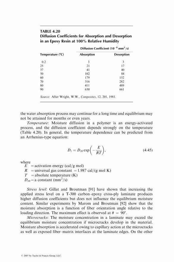
TABLE 4.20Diffusion Coefficients for Absorption and Desorption
in an Epoxy Resin at 100% Relative Humidity
Diffusion Coefficient (10�8 mm2=s)
Temperature (8C) Absorption Desorption
0.2 3 3
25 21 17
37 41 40
50 102 88
60 179 152
70 316 282
80 411 489
90 630 661
Source: After Wright, W.W., Composites, 12, 201, 1981.
the water absorption process may continue for a long time and equilibrium may
not be attained for months or even years.
Temperature: Moisture diffusion in a polymer is an energy-activated
process, and the diffusion coefficient depends strongly on the temperature
(Table 4.20). In general, the temperature dependence can be predicted from
an Arrhenius-type equation:
Dz ¼ Dz0 exp � E
RT
� �, (4:45)
whereE ¼ activation energy (cal=g mol)
R ¼ universal gas constant ¼ 1.987 cal=(g mol K)
T ¼ absolute temperature (K)
Dz0¼ a constant (mm2=s)
Stress level: Gillat and Broutman [91] have shown that increasing the
applied stress level on a T-300 carbon–epoxy cross-ply laminate produces
higher diffusion coefficients but does not influence the equilibrium moisture
content. Similar experiments by Marom and Broutman [92] show that the
moisture absorption is a function of fiber orientation angle relative to the
loading direction. The maximum effect is observed at u ¼ 908.Microcracks: The moisture concentration in a laminate may exceed the
equilibrium moisture concentration if microcracks develop in the material.
Moisture absorption is accelerated owing to capillary action at the microcracks
as well as exposed fiber–matrix interfaces at the laminate edges. On the other
� 2007 by Taylor & Francis Group, LLC.
hand, there may be an ‘‘apparent’’ reduction in moisture concentration if there
is a loss of material from leaching or cracking.
Thermal spikes: Diffusion characteristics of composite laminates may
alter significantly if they are rapidly heated to high temperatures followed by
rapid cooling to the ambient condition, a process known as thermal spiking.
McKague et al. [93] have shown that the moisture absorption in specimens
exposed to 75% relative humidity at 248C and occasional (twice weekly) thermal
spikes (rapid heating to 1498C followed by rapid cooling to 248C) is twice that ofspecimens not exposed to spikes. Additionally, thermally spiked specimens
exhibit a permanent change in their moisture absorption characteristics.
The increased diffusion rate and higher moisture absorption are attributed
to microcracks formed owing to stress gradients caused by thermal cycling and
resin swelling. The service temperature in a spike environment should be limited
to the glass transition temperature Tg of the resin, since spike temperatures
above Tg cause much higher moisture absorption than those below Tg.
Reverse thermal effect: Adamson [94] has observed that cast-epoxy resins
or epoxy-based laminates containing an equilibrium moisture concentration
exhibit a rapid rate of moisture absorption when the ambient temperature
is reduced. For example, an AS carbon fiber-reinforced epoxy laminate
attained an equilibrium moisture concentration of 2.3 wt% after 140 days of
exposure at 748C. When the exposure temperature was reduced to 258C, theequilibrium moisture concentration increased to 2.6% within 40 days. This
inverse temperature dependence of moisture absorption is called the reverse
thermal effect.
4.5.2.2 Physical Effects of Moisture Absorption
Moisture absorption produces volumetric changes (swelling) in the resin, which
in turn cause dimensional changes in the material. Assuming that the swollen
volume of the resin is equal to the volume of absorbed water, the resulting
volume change can be computed from the following relationship:
DV (t)
V0
¼ rmrw
M, (4:46)
where
rm ¼matrix density
rw ¼water density (�1 kg=mm3)
M ¼moisture content at time t
The corresponding dilatational (volumetric) strain in the resin is
«m ¼ 1
3
DV
V0
¼ 1
3
rmrw
M ¼ bmM, (4:47)
� 2007 by Taylor & Francis Group, LLC.
where
bm ¼1
3
rmrw
bm is call ed the swe lling coefficie nt
In practic e, swe lling is ne gligible until a thres hold moisture con centration
M0 is exceeded . Therefor e, the dilat ational strain in the resi n is
«m ¼ 0 for M < M 0 ,
¼ bm ( M � M 0 ) for M > M 0 ( 4: 48)
The threshold moisture concentration M0 represents the amount of water
absorbed in the free volume as well as microvoids present in the resin. For a
variety of cast-epoxy resins, the measured swelling coefficient ranges from 0.26 to
0.33 and the threshold moisture concentration is in the range of 0.3%–0.7% [95].
The dilatati onal stra in in a unidir ectional 08 composi te laminate due to
moisture absorpt ion can be calculated as
Longitudi nal: «mL ¼ 0, ( 4: 49 a)
Transv erse : «mT ¼ bT (M � M v ) , ( 4:49b)
where
bT ¼ (1 þ nm )b m( rm=rc )rc ¼ co mposi te densit y
vm ¼matrix Poisson’s ratio
Mv¼ vv(rw=rc)vv ¼ void volume fraction
Another physical effect of moisture absorption is the reduction in
glass trans ition tempe ratur e of the resi n (Figur e 4.90). Although the roo m-
temperature performance of a resin may not change with a reduction in Tg, its
elevated-temperature properties are severely affected. For example, the modu-
lus of an epoxy resin at 1508C decreases from 2,070 MPa (300,000 psi) to 20.7
MPa (3,000 psi) as its Tg is reduced from 2158C to 1278C. Similar effects may be
expected for the matrix-dominated properties of a polymer matrix composite.
Finally, the dilatational expansion of the matrix around the fiber reduces
the residual compressive stresses at the fiber–matrix interface caused by curing
shrinkage. As a result, the mechanical interlocking between the fiber and the
matrix may be relieved.
4.5.2.3 Changes in Performance Due to Moisture and Temperature
From the available data on the effects of temperature and moisture content on
the tensile strength and modulus of carbon and boron fiber-reinforced epoxy
laminates [96,97], the following conclusions can be made.
� 2007 by Taylor & Francis Group, LLC.
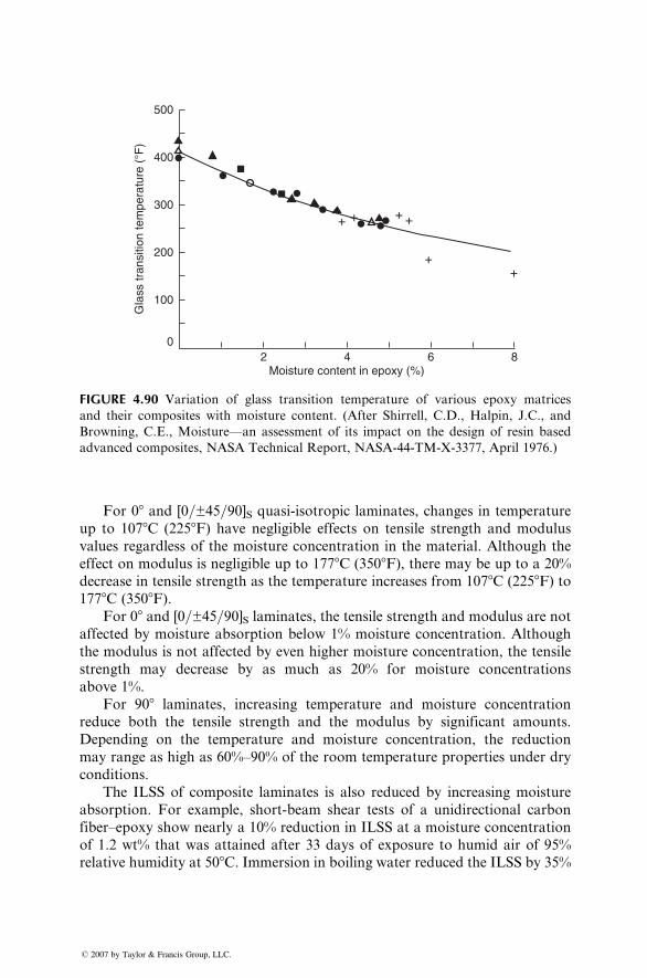
500
400
300
Gla
ss tr
ansi
tion
tem
pera
ture
(°F
)
200
100
02
Moisture content in epoxy (%)4 6 8
+++ +
++
FIGURE 4.90 Variation of glass transition temperature of various epoxy matrices
and their composites with moisture content. (After Shirrell, C.D., Halpin, J.C., and
Browning, C.E., Moisture—an assessment of its impact on the design of resin based
advanced composites, NASA Technical Report, NASA-44-TM-X-3377, April 1976.)
For 08 and [0=±45=90]S quasi-isotropic laminates, changes in temperature
up to 1078C (2258F) have negligible effects on tensile strength and modulus
values regardless of the moisture concentration in the material. Although the
effect on modulus is negligible up to 1778C (3508F), there may be up to a 20%
decrease in tensile strength as the temperature increases from 1078C (2258F) to1778C (3508F).
For 08 and [0=±45=90]S laminates, the tensile strength and modulus are not
affected by moisture absorption below 1% moisture concentration. Although
the modulus is not affected by even higher moisture concentration, the tensile
strength may decrease by as much as 20% for moisture concentrations
above 1%.
For 908 laminates, increasing temperature and moisture concentration
reduce both the tensile strength and the modulus by significant amounts.
Depending on the temperature and moisture concentration, the reduction
may range as high as 60%–90% of the room temperature properties under dry
conditions.
The ILSS of composite laminates is also reduced by increasing moisture
absorption. For example, short-beam shear tests of a unidirectional carbon
fiber–epoxy show nearly a 10% reduction in ILSS at a moisture concentration
of 1.2 wt% that was attained after 33 days of exposure to humid air of 95%
relative humidity at 508C. Immersion in boiling water reduced the ILSS by 35%
� 2007 by Taylor & Francis Group, LLC.
for the same expo sure time [98] . Expe riments by Gillat and Br outman [91] on
cross-p ly carbon fiber –epoxy show nearly a 25% reduction in ILSS as the
moisture concen tration increa sed by 1.5 wt%.
Jones et al. [99] report ed the effect of moisture absorpt ion on the tensi on–
tension fatigue a nd flex ural fatigue prop erties of [0 =90]S cross-ply ep oxy matr ix
composi tes reinf orced with E-glas s, HTS carbo n, and Kevl ar 49 fibers. Con-
ditioning treatmen ts included exposure to humid air (65% relat ive humidi ty)
and imm ersion in boilin g water. The fatigue resistance of carbon fiber –epoxy
was fou nd to be unaffe cted by the conditio ning treatment . Expos ure to humid
air also did not affect the fatigue response of E-glas s fiber –epoxy composi tes;
howeve r, immersi on in boili ng wat er reduce d the fatigue strength by signi fican t
amounts , princi pally due to the damage incurr ed on the glass fibers by boiling
water. On the other ha nd, the fatigu e respo nse of Kevl ar 49–ep oxy composi tes
was improved owing to moisture absorption, although at high cycles there
appears to be a rapid deterioration as indicated by the sharp downward
curvat ure of the S–N curve (F igure 4.91) .
Curtis and Moore [100] reported the effect of moisture absorption on the
zero tension and zero compression fatigue performance of two matrix-dominated
laminates, namely, [(90=±30)3]S and [02=�452=902=þ452]S layups of carbon
fibers in an epoxy matrix. Conditioning was performed in humid air of 95%
humidity at 708C. Despite the matrix-dominated behavior of these laminates,
moisture absorption had very little effect on their fatigue lives.
Chamis et al. [101] proposed the following empirical equation for estimating
the hygrothermal effect on the matrix properties, which can subsequently be
used in modifying the matrix-dominated properties of a unidirectional lamina:
PwT
P0
¼ Tgw � T
Tgd � T0
� �1=2
, (4:50)
where
PwT¼matrix property at the use temperature T and moisture content M
P0 ¼matrix property at a reference temperature T0
Tgd ¼ glass transition temperature in the dry condition
Tgw ¼ glass transition temperature in the wet condition with a moisture
content M
The glass transition temperature in the wet condition, Tgw is calculated
using the following equation:
Tgw ¼ (0:005M2 � 0:1M þ 1)Tgd for M � 10%: (4:51)
Equations 4.50 and 4.51 have been used to estimate the hygrothermal effect on
epoxy matrix composites, but need experimental validation for other polymer
matrix systems.
� 2007 by Taylor & Francis Group, LLC.
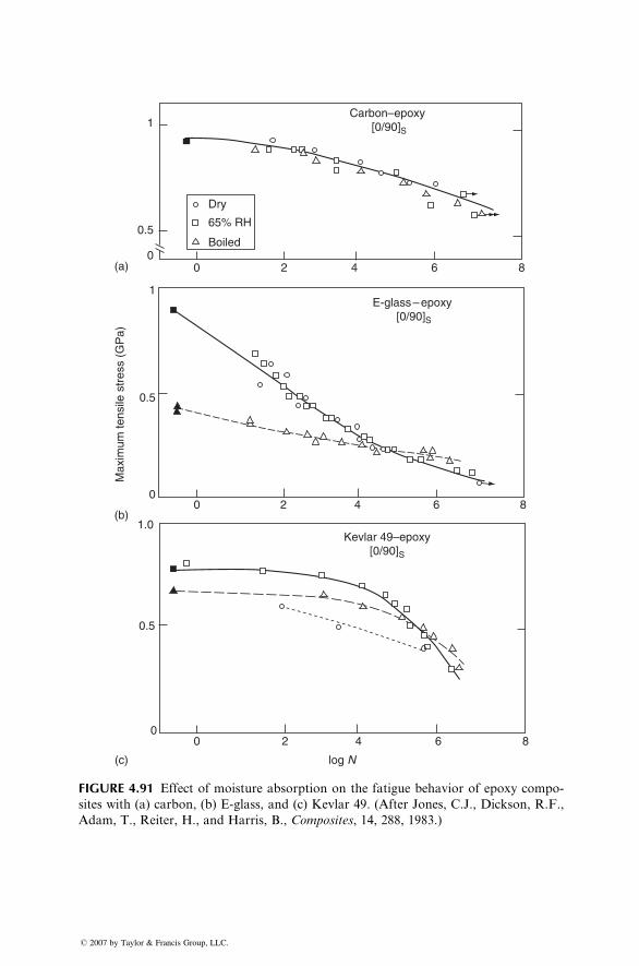
0
0
0 2 4 6 8
2 4 6 8
0(a)
(b)
(c)
1
0.5
0
1.0
0.5
0
0.5
1
42 6 8
Dry
65% RH
Boiled
Carbon–epoxy [0/90]S
E-glass – epoxy [0/90]S
Kevlar 49–epoxy [0/90]S
log N
Max
imum
tens
ile s
tres
s (G
Pa)
FIGURE 4.91 Effect of moisture absorption on the fatigue behavior of epoxy compo-
sites with (a) carbon, (b) E-glass, and (c) Kevlar 49. (After Jones, C.J., Dickson, R.F.,
Adam, T., Reiter, H., and Harris, B., Composites, 14, 288, 1983.)
� 2007 by Taylor & Francis Group, LLC.
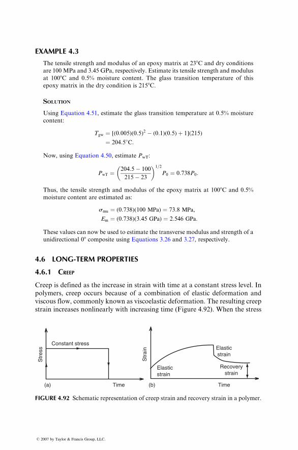
EXAMPLE 4.3
The tensile strength and modulus of an epoxy matrix at 238 C and dry conditionsare 100 MPa and 3.45 GPa, respectively. Estimate its tensile strength and modulus
at 1008C and 0.5% moisture content. The glass transition temperature of this
epoxy matrix in the dry condition is 2158 C.
SOLUTIO N
Using Equation 4.51, estimate the glass transition temperature at 0.5% moisture
content:
Tgw ¼ [(0: 005)( 0: 5)2 � (0 :1)( 0: 5) þ 1](215)
¼ 204: 5� C:
Now, using Equation 4.50, estimate PwT :
PwT ¼ 204: 5 � 100
215 � 23
� �1=2
P0 ¼ 0: 738P0 :
Thus, the tensile strength and modulus of the epoxy matrix at 1008 C and 0.5%moisture content are estimated as:
smu ¼ ( 0: 738)(100 MPa) ¼ 73: 8 MPa,
Em ¼ ( 0: 738)(3: 45 GPa) ¼ 2: 546 GPa :
These values can now be used to estimate the transverse modulus and strength of a
unidirectional 08 composite using Equations 3.26 and 3.27, respectively.
4.6 LONG-TERM PROPERTIES
4.6.1 CREEP
Creep is defined as the increase in strain with time at a constant stress level. In
polymers, creep occurs because of a combination of elastic deformation and
viscous flow, commonly known as viscoelastic deformation. The resulting creep
strain increases nonlinearly with increasing time (Figure 4.92). When the stress
(a) (b)
Str
ain
Str
ess
Constant stress
Time Time
Elasticstrain
Elasticstrain
Recoverystrain
FIGURE 4.92 Schematic representation of creep strain and recovery strain in a polymer.
� 2007 by Taylor & Francis Group, LLC.
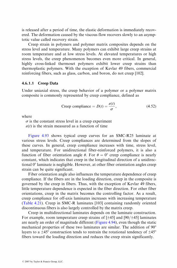
is relea sed afte r a period of time, the e lastic deform ation is imm ediately recov-
ered. The deform ation caused by the viscous flow recover s slowly to an asymp-
totic value called recover y strain.
Cre ep strain in polyme rs a nd polyme r matrix composi tes de pends on the
stress level and tempe rature. Many polyme rs can exhibi t large creep strains at
room tempe rature and at low stress levels. At elevated tempe ratur es or high
stress levels, the creep pheno menon becomes even more critical . In general ,
highly cro ss-linked thermoset polyme rs exhibi t low er creep stra ins than
therm oplastic polyme rs. With the exception of Kevlar 49 fiber s, commer cial
reinfo rcing fiber s, such as g lass, carbo n, an d bor on, do not c reep [102] .
4.6.1 .1 Cr eep Data
Under uniaxi al stre ss, the creep behavior of a pol ymer or a polyme r matr ix
composi te is commonl y represen ted by creep compli ance, de fined as
Creep complianc e ¼ D (t ) ¼ «( t )
s, ( 4: 52 )
wher e
s is the c onstant stre ss level in a creep exp eriment
«(t ) is the stra in measur ed as a function of time
Figure 4.93 shows typic al creep curves for an SMC-R25 lami nate at
various stress levels. Creep compli ances are determined from the slopes of
these curves. In general , creep complia nce increa ses wi th time, stress level ,
and tempe ratur e. For unid irectional fiber -reinforce d polyme rs, it is also a
functio n of fiber orient ation an gle u. For u ¼ 08 creep compli ance is nearly
constant , which indica tes that creep in the longit udinal direct ion of a unidir ec-
tional 08 lamina te is negligible . How ever, at other fiber orient ation angles creep
strain can be quite signi fican t.
Fiber orient ation angle also infl uences the tempe ratur e depen dence of creep
compli ance. If the fibers are in the loading direction, creep in the comp osite is
governed by the creep in fibers. Thus , with the exce ption of Kevlar 49 fiber s,
little tempe ratur e depend ence is exp ected in the fiber direct ion. For other fiber
orient ations, creep in the matrix be comes the control ling factor. As a resul t,
creep compli ance for off-axis lami nates increa ses with increa sing tempe rature
(Table 4.21) . Creep in SMC- R laminates [103] contai ning rando mly or iented
discont inuous fiber s is also largely control led by the matrix creep.
Cre ep in multidir ectiona l lami nates de pends on the laminate constr uction.
For exampl e, roo m tempe ratur e creep stra ins of [±45] a nd [90=±45 ] lami nates
are nearly an order of magn itude different (Figur e 4.94) , even thou gh the stat ic
mechanical properties of these two laminates are similar. The addition of 908layers to a ±458 construction tends to restrain the rotational tendency of ±458fibers toward the loading direction and reduces the creep strain significantly.
� 2007 by Taylor & Francis Group, LLC.
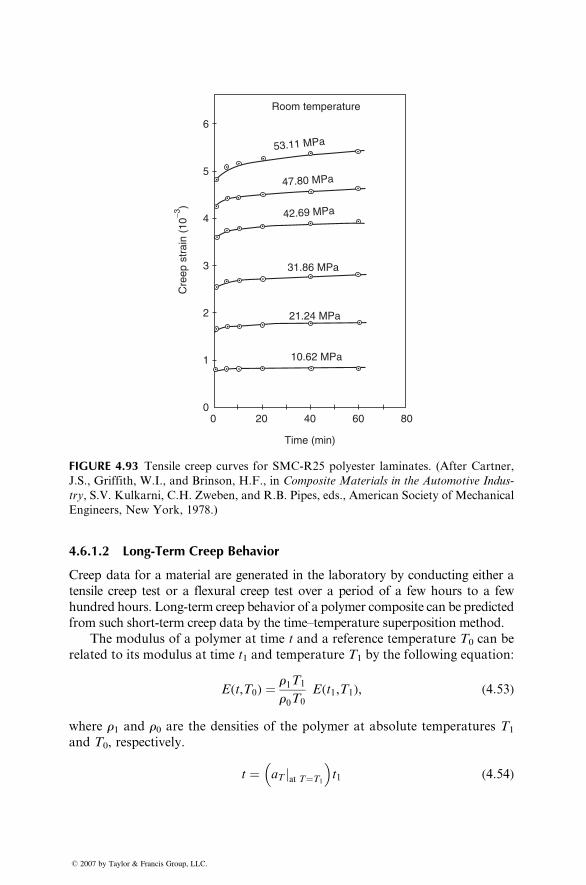
Room temperature
Cre
ep s
trai
n (1
0−3)
6
5
4
2
3
1
00 20 40 60 80
Time (min)
10.62 MPa
21.24 MPa
31.86 MPa
42.69 MPa
47.80 MPa
53.11 MPa
FIGURE 4.93 Tensile creep curves for SMC-R25 polyester laminates. (After Cartner,
J.S., Griffith, W.I., and Brinson, H.F., in Composite Materials in the Automotive Indus-
try, S.V. Kulkarni, C.H. Zweben, and R.B. Pipes, eds., American Society of Mechanical
Engineers, New York, 1978.)
4.6.1.2 Long-Term Creep Behavior
Creep data for a material are generated in the laboratory by conducting either a
tensile creep test or a flexural creep test over a period of a few hours to a few
hundred hours. Long-term creep behavior of a polymer composite can be predicted
from such short-term creep data by the time–temperature superposition method.
The modulus of a polymer at time t and a reference temperature T0 can be
related to its modulus at time t1 and temperature T1 by the following equation:
E(t,T0) ¼ r1T1
r0T0
E(t1,T1), (4:53)
where r1 and r0 are the densities of the polymer at absolute temperatures T1
and T0, respectively.
t ¼ aT jat T¼T1
�t1 (4:54)
� 2007 by Taylor & Francis Group, LLC.
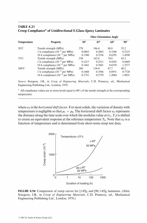
TABLE 4.21Creep Compliancea of Unidirectional E-Glass–Epoxy Laminates
Fiber Orientation Angle
Temperature Property 308 458 608 908
288C Tensile strength (MPa) 278 186.4 88.8 55.2
1 h compliance (10�6 per MPa) 0.0883 0.2065 0.3346 0.5123
10 h compliance (10�6 per MPa) 0.1300 0.3356 0.6295 1.4390
758C Tensile strength (MPa) 230 162.8 74.8 43.2
1 h compliance (10�6 per MPa) 0.1217 0.2511 0.4342 0.6689
10 h compliance (10�6 per MPa) 0.1461 0.3841 0.6539 1.5377
1008C Tensile strength (MPa) 206 134.4 67.7 40.2
1 h compliance (10�6 per MPa) 0.1460 0.3586 0.6931 0.7728
10 h compliance (10�6 per MPa) 0.1751 0.5739 1.2084 1.9031
Source: Sturgeon, J.B., in Creep of Engineering Materials, C.D. Pomeroy, ed., Mechanical
Engineering Publishing Ltd., London, 1978.
a All compliance values are at stress levels equal to 40% of the tensile strength at the corresponding
temperature.
where aT is the horizontal shift factor. Formost solids, the variation of density with
temperature is negligible so that r1 ¼ r0. The horizontal shift factor aT representsthe distance along the time scale over which the modulus value at (t1, T1) is shifted
to create an equivalent response at the reference temperature T0. Note that aT is a
function of temperature and is determined from short-term creep test data.
Temperature = 218c
± 458
50 MPa
90 ± 45862 MPa
2000
1000
00 10 100 10001
Duration of loading (h)
Cre
ep s
trai
n (1
0−6)
FIGURE 4.94 Comparison of creep curves for [±45]S and [90=±45]S laminates. (After
Sturgeon, J.B., in Creep of Engineering Materials, C.D. Pomeroy, ed., Mechanical
Engineering Publishing Ltd., London, 1978.)
� 2007 by Taylor & Francis Group, LLC.
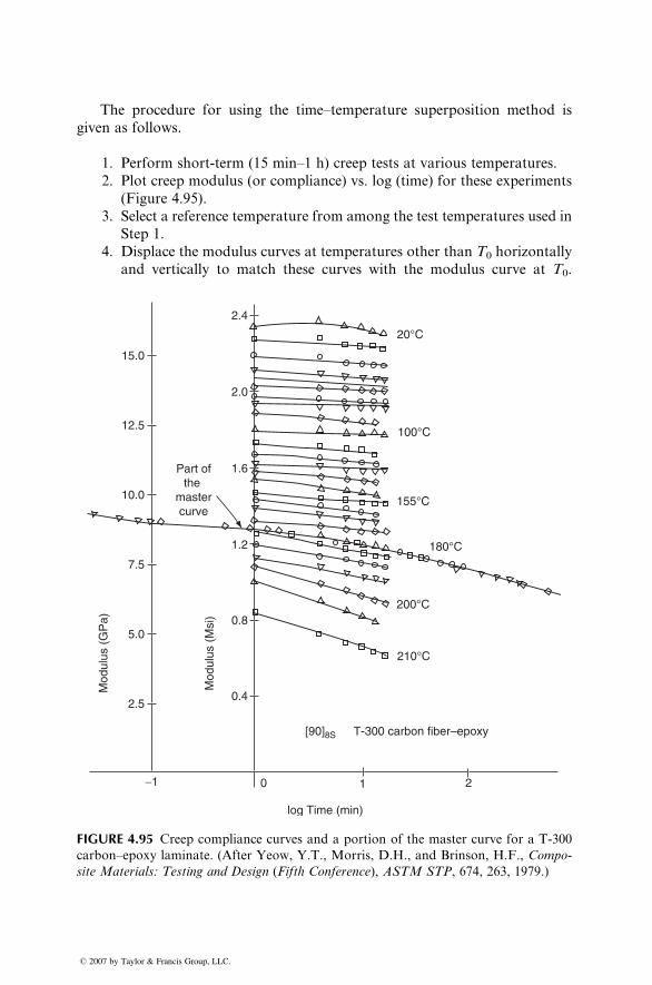
The procedure for using the time–temperature superposition method is
given as follows.
1. Perform short-term (15 min–1 h) creep tests at various temperatures.
2. Plot creep modulus (or compliance) vs. log (time) for these experiments
(Figure 4.95).
3. Select a reference temperature from among the test temperatures used in
Step 1.
4. Displace the modulus curves at temperatures other than T0 horizontally
and vertically to match these curves with the modulus curve at T0.
20°C
100°C
155°C
180°C
200°C
210°C
[90]8S T-300 carbon fiber–epoxy
2.5
5.0
7.5
12.5
15.0
2.4
2.0
1.6
1.2
0.8
0.4
0−1 21
10.0
Mod
ulus
(M
si)
log Time (min)
Mod
ulus
(G
Pa)
Part ofthe
mastercurve
FIGURE 4.95 Creep compliance curves and a portion of the master curve for a T-300
carbon–epoxy laminate. (After Yeow, Y.T., Morris, D.H., and Brinson, H.F., Compo-
site Materials: Testing and Design (Fifth Conference), ASTM STP, 674, 263, 1979.)
� 2007 by Taylor & Francis Group, LLC.
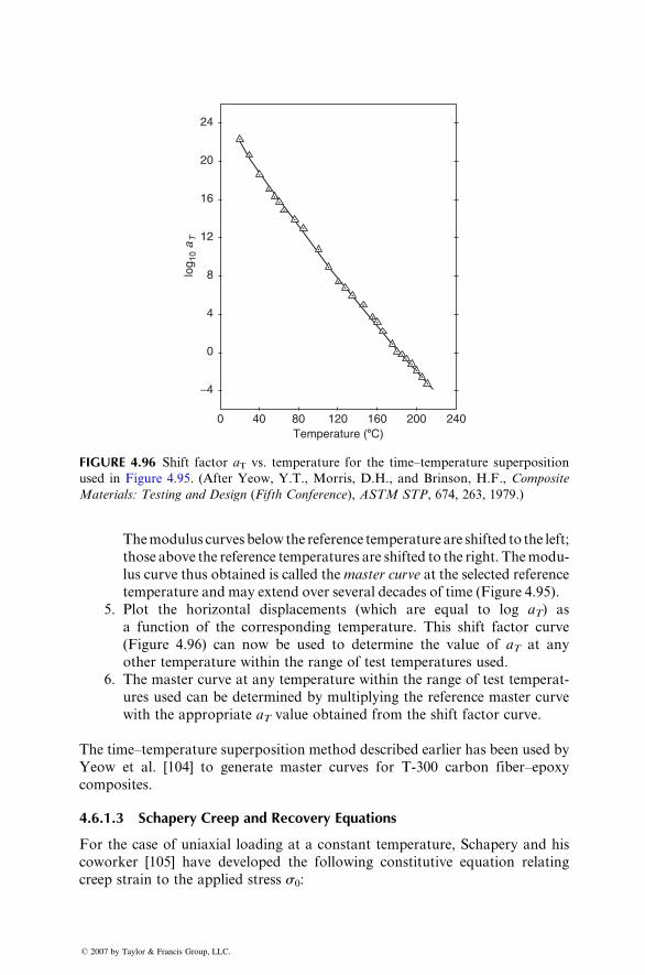
0
−4
0
4
8
12
16
20
24
40 80 120Temperature (8C)
log 1
0 a
T
160 200 240
FIGURE 4.96 Shift factor aT vs. temperature for the time–temperature superposition
used in Figure 4.95. (After Yeow, Y.T., Morris, D.H., and Brinson, H.F., Composite
Materials: Testing and Design (Fifth Conference), ASTM STP, 674, 263, 1979.)
The modu lus curves below the refer ence tempe ratur e are sh ifted to the left;
those ab ove the reference temperatur es are shifted to the right. The mod u-
lus cu rve thus obtaine d is called the mast er curve at the selected reference
tempe ratur e and may extend over severa l de cades of tim e (Figure 4.95) .
5. Plot the horizont al displacement s (which are equ al to log aT ) as
a functio n of the co rrespondi ng tempe rature. This shift factor curve
(Figur e 4.96) can now be used to determine the value of aT at any
other tempe rature within the ran ge of test tempe ratures used.
6. The master curve at an y tempe ratur e within the ran ge of test tempe rat-
ures used can be de termined by multiply ing the referen ce master curve
with the appropri ate aT value obtaine d from the shift factor curve.
The time–te mperat ure superpo sition method describ ed earlier has been used by
Yeow et al. [104] to generat e mast er curves for T-300 carb on fiber –epoxy
composi tes.
4.6.1 .3 Sch apery Creep and Recovery Equ ations
For the case of uniaxi al loading at a c onstant tempe rature, Schapery and his
cowor ker [105] have de veloped the follo wing constitut ive eq uation relating
creep strain to the app lied stress s0:
� 2007 by Taylor & Francis Group, LLC.
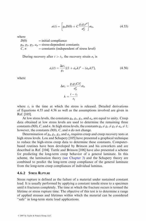
«(t ) ¼ g0 D ( 0) þ Cg1 g2 t
n
a ns
� �s0 , ( 4: 55 )
where
D(0) ¼ init ial complia nce
g0, g1, g2, as ¼ stre ss-depen dent constants
C, n ¼ constant s (indepe nde nt of stress level)
Duri ng recover y afte r t > t1, the recover y strain «r is
«r ( t ) ¼ D«1g1
[(1 þ as l) n � ( as l)
n ] , ( 4: 56 )
where
D«1 ¼ g1 g2 Ct n1
anss0
l ¼ t � t1
t1
where t1 is the time at whi ch the stress is released . Deta iled derivations
of Equations 4.55 and 4.56 as well as the assum ptions involv ed are g iven in
Ref. [105].
At low stre ss levels, the constants g0, g 1, g 2, and as are equ al to unity. Creep
data obtaine d at low stress level s are used to determine the remaining three
constant s D (0), C , and n. At high stress level s, the constant s g0 6¼ g1 6¼ g2 6¼ as 6¼ 1;
howeve r, the con stants D (0), C, and n do not change.
Dete rminati on of g0, g1, g2, and a s requir es creep and creep recover y tests at
high stress level s. Lou and Sch apery [105] have presen ted a graphic al techni que
to redu ce the high-s tress creep data to determ ine these constant s. Com puter-
based routines have been developed by Brinson and his coworkers and are
described in Ref. [104]. Tuttle and Brinson [106] have also presented a scheme
for predicting the long-term creep behavior of a general laminate. In this
scheme, the lami nation theory (see Chapter 3) and the Schap ery theory are
combined to predict the long-term creep compliance of the general laminate
from the long-term creep compliances of individual laminas.
4.6.2 STRESS RUPTURE
Stress rupture is defined as the failure of a material under sustained constant
load. It is usually performed by applying a constant tensile stress to a specimen
until it fractures completely. The time at which the fracture occurs is termed the
lifetime or stress rupture time. The objective of this test is to determine a range
of applied stresses and lifetimes within which the material can be considered
‘‘safe’’ in long-term static load applications.
� 2007 by Taylor & Francis Group, LLC.
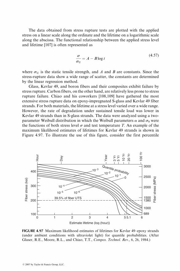
The data obtained from stress rupture tests are plotted with the applied
stress on a linear scale along the ordinate and the lifetime on a logarithmic scale
along the abscissa. The functional relationship between the applied stress level
and lifetime [107] is often represented as
s
sU
¼ A� B log t(4:57)
where sU is the static tensile strength, and A and B are constants. Since the
stress-rupture data show a wide range of scatter, the constants are determined
by the linear regression method.
Glass, Kevlar 49, and boron fibers and their composites exhibit failure by
stress rupture. Carbon fibers, on the other hand, are relatively less prone to stress
rupture failure. Chiao and his coworkers [108,109] have gathered the most
extensive stress rupture data on epoxy-impregnated S-glass and Kevlar 49 fiber
strands. For bothmaterials, the lifetime at a stress level varied over a wide range.
However, the rate of degradation under sustained tensile load was lower in
Kevlar 49 strands than in S-glass strands. The data were analyzed using a two-
parameter Weibull distribution in which the Weibull parameters a and s0 were
the functions of both stress level s and test temperature T. An example of the
maximum likelihood estimates of lifetimes for Kevlar 49 strands is shown in
Figure 4.97. To illustrate the use of this figure, consider the first percentile
10−3
10−4
10−5
39.5% of fiber UTS
0100
200
300
400
Hou
r
Day
Yea
r
3 Y
r5
Yr
10 Y
r
20 Y
r
100
Yr
3000
2500
2000
15001380 F
iber
str
ess
(MP
a)
Fib
er s
tres
s (k
si)
1000
6891 2 3
Estimate lifetime (log (hour))
4 5 5.1 6
Quantile probability
10−6
10−2
10−10
FIGURE 4.97 Maximum likelihood estimates of lifetimes for Kevlar 49–epoxy strands
(under ambient conditions with ultraviolet light) for quantile probabilities. (After
Glaser, R.E., Moore, R.L., and Chiao, T.T., Compos. Technol. Rev., 6, 26, 1984.)
� 2007 by Taylor & Francis Group, LLC.
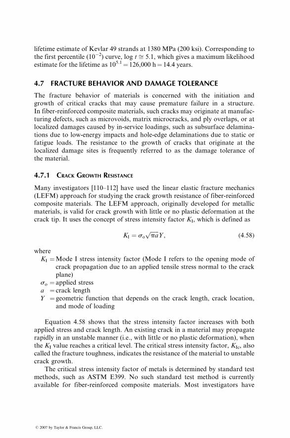
lifetime estimate of Kevlar 49 strands at 1380 MPa (200 ksi). Corresponding to
the first percentile (10�2) curve, log t ffi 5.1, which gives a maximum likelihood
estimate for the lifetime as 105.1¼ 126,000 h¼ 14.4 years.
4.7 FRACTURE BEHAVIOR AND DAMAGE TOLERANCE
The fracture behavior of materials is concerned with the initiation and
growth of critical cracks that may cause premature failure in a structure.
In fiber-reinforced composite materials, such cracks may originate at manufac-
turing defects, such as microvoids, matrix microcracks, and ply overlaps, or at
localized damages caused by in-service loadings, such as subsurface delamina-
tions due to low-energy impacts and hole-edge delaminations due to static or
fatigue loads. The resistance to the growth of cracks that originate at the
localized damage sites is frequently referred to as the damage tolerance of
the material.
4.7.1 CRACK GROWTH RESISTANCE
Many investigators [110–112] have used the linear elastic fracture mechanics
(LEFM) approach for studying the crack growth resistance of fiber-reinforced
composite materials. The LEFM approach, originally developed for metallic
materials, is valid for crack growth with little or no plastic deformation at the
crack tip. It uses the concept of stress intensity factor KI, which is defined as
KI ¼ so
ffiffiffiffiffiffipa
pY , (4:58)
where
KI ¼Mode I stress intensity factor (Mode I refers to the opening mode of
crack propagation due to an applied tensile stress normal to the crack
plane)
so ¼ applied stress
a ¼ crack length
Y ¼ geometric function that depends on the crack length, crack location,
and mode of loading
Equation 4.58 shows that the stress intensity factor increases with both
applied stress and crack length. An existing crack in a material may propagate
rapidly in an unstable manner (i.e., with little or no plastic deformation), when
the KI value reaches a critical level. The critical stress intensity factor, KIc, also
called the fracture toughness, indicates the resistance of the material to unstable
crack growth.
The critical stress intensity factor of metals is determined by standard test
methods, such as ASTM E399. No such standard test method is currently
available for fiber-reinforced composite materials. Most investigators have
� 2007 by Taylor & Francis Group, LLC.
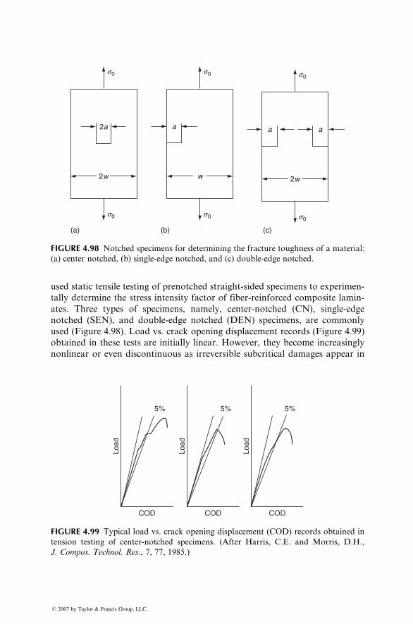
a a
2w
(c)
s0
s0
2a a
2w w
(a) (b)
s0
s0
s0
s0
FIGURE 4.98 Notched specimens for determining the fracture toughness of a material:
(a) center notched, (b) single-edge notched, and (c) double-edge notched.
used static tensile testing of prenotched straight-sided specimens to experimen-
tally determine the stress intensity factor of fiber-reinforced composite lamin-
ates. Three types of specimens, namely, center-notched (CN), single-edge
notched (SEN), and double-edge notched (DEN) specimens, are commonly
used (Figure 4.98). Load vs. crack opening displacement records (Figure 4.99)
obtained in these tests are initially linear. However, they become increasingly
nonlinear or even discontinuous as irreversible subcritical damages appear in
COD
5%
Load
COD
5%
Load
COD
5%
Load
FIGURE 4.99 Typical load vs. crack opening displacement (COD) records obtained in
tension testing of center-notched specimens. (After Harris, C.E. and Morris, D.H.,
J. Compos. Technol. Res., 7, 77, 1985.)
� 2007 by Taylor & Francis Group, LLC.
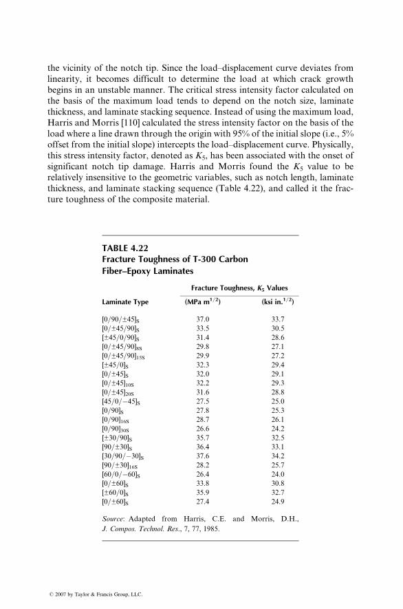
the vicinity of the notch tip. Since the load–displacement curve deviates from
linearity, it becomes difficult to determine the load at which crack growth
begins in an unstable manner. The critical stress intensity factor calculated on
the basis of the maximum load tends to depend on the notch size, laminate
thickness, and laminate stacking sequence. Instead of using the maximum load,
Harris and Morris [110] calculated the stress intensity factor on the basis of the
load where a line drawn through the origin with 95% of the initial slope (i.e., 5%
offset from the initial slope) intercepts the load–displacement curve. Physically,
this stress intensity factor, denoted as K5, has been associated with the onset of
significant notch tip damage. Harris and Morris found the K5 value to be
relatively insensitive to the geometric variables, such as notch length, laminate
thickness, and laminate stacking sequence (Table 4.22), and called it the frac-
ture toughness of the composite material.
TABLE 4.22Fracture Toughness of T-300 Carbon
Fiber–Epoxy Laminates
Fracture Toughness, K5 Values
Laminate Type (MPa m1=2) (ksi in.1=2)
[0=90=±45]S 37.0 33.7
[0=±45=90]S 33.5 30.5
[±45=0=90]S 31.4 28.6
[0=±45=90]8S 29.8 27.1
[0=±45=90]15S 29.9 27.2
[±45=0]S 32.3 29.4
[0=±45]S 32.0 29.1
[0=±45]10S 32.2 29.3
[0=±45]20S 31.6 28.8
[45=0=�45]S 27.5 25.0
[0=90]S 27.8 25.3
[0=90]16S 28.7 26.1
[0=90]30S 26.6 24.2
[±30=90]S 35.7 32.5
[90=±30]S 36.4 33.1
[30=90=�30]S 37.6 34.2
[90=±30]16S 28.2 25.7
[60=0=�60]S 26.4 24.0
[0=±60]S 33.8 30.8
[±60=0]S 35.9 32.7
[0=±60]S 27.4 24.9
Source: Adapted from Harris, C.E. and Morris, D.H.,
J. Compos. Technol. Res., 7, 77, 1985.
� 2007 by Taylor & Francis Group, LLC.
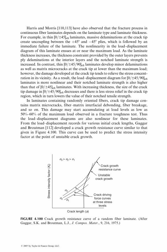
Harris and Morris [110,113] have also observed that the fracture process in
continuous fiber laminates depends on the laminate type and laminate thickness.
For example, in thin [0=±45]nS laminates, massive delaminations at the crack tip
create uncoupling between the þ458 and �458 plies, which is followed by an
immediate failure of the laminate. The nonlinearity in the load–displacement
diagram of this laminate ensues at or near the maximum load. As the laminate
thickness increases, the thickness constraint provided by the outer layers prevents
ply delaminations at the interior layers and the notched laminate strength is
increased. In contrast, thin [0=±45=90]nS laminates develop minor delaminations
as well as matrix microcracks at the crack tip at lower than the maximum load;
however, the damage developed at the crack tip tends to relieve the stress concent-
ration in its vicinity. As a result, the load–displacement diagram for [0=±45=90]nSlaminates is more nonlinear and their notched laminate strength is also higher
than that of [0=±45]nS laminates. With increasing thickness, the size of the crack
tip damage in [0=±45=90]nS decreases and there is less stress relief in the crack tip
region, which in turn lowers the value of their notched tensile strength.
In laminates containing randomly oriented fibers, crack tip damage con-
tains matrix microcracks, fiber–matrix interfacial debonding, fiber breakage,
and so on. This damage may start accumulating at load levels as low as
50%–60% of the maximum load observed in a fracture toughness test. Thus
the load–displacement diagrams are also nonlinear for these laminates.
From the load–displacement records for various initial crack lengths, Gaggar
and Broutman [112] developed a crack growth resistance curve similar to that
given in Figure 4.100. This curve can be used to predict the stress intensity
factor at the point of unstable crack growth.
Crack growthresistance curve
Unstablecrack growth
Crack drivingforce curves
at three stresslevels
Crack length (a)
Str
ees
inte
nsity
fact
or (
KI)
s3
s3 > s2 > s1
s2 s1
FIGURE 4.100 Crack growth resistance curve of a random fiber laminate. (After
Gaggar, S.K. and Broutman, L.J., J. Compos. Mater., 9, 216, 1975.)
� 2007 by Taylor & Francis Group, LLC.
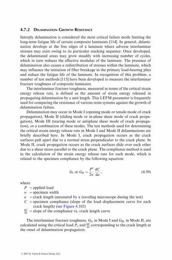
4.7.2 DELAMINATION GROWTH R ESISTANCE
Interp ly de laminatio n is con sidered the most critical fail ure mode limiting the
long-term fatigue life of certain composi te lamina tes [114]. In general , delam i-
nation develops at the free edges of a lamina te wher e adverse inter laminar
stresses may exist owi ng to its pa rticular stacking sequence. Once developed ,
the delam inate d areas may grow steadily wi th increa sing number of cycles ,
which in turn reduces the effe ctive mo dulus of the lamin ate. The presence of
delam ination also ca uses a redistri bution of stre sses within the lamin ate, which
may influ ence the initiation of fiber breakage in the primary load-be aring plies
and reduce the fati gue lif e of the lami nate. In recogni tion of this problem , a
number of test methods [115] have been developed to measur e the inter laminar
fracture toughness of composi te lamin ates.
The inter laminar fracture toughn ess, measur ed in term s of the critical strain
energy relea se rate, is defined as the amount of strain ene rgy relea sed in
propagat ing delam ination by a unit length. This LEFM parame ter is frequent ly
used for co mparin g the resi stance of various resin systems agains t the grow th of
delam ination failure.
Dela mination may occur in Mo de I (opening mode or tensi le mode of crack
propagat ion), Mod e II (sliding mode or in-plan e shear mo de of c rack prop a-
gation ), Mo de III (tearing mode or an tiplane shear mod e of crack propa ga-
tion), or a combinat ion of these mod es. The test methods used for determini ng
the crit ical strain energy relea se rate in Mo de I and Mode II de laminati ons are
briefly describ ed here. In Mod e I, crack propagat ion occurs as the crack
surface s pull apart due to a nor mal stress perpendicul ar to the crack plane. In
Mode II, crack pro pagatio n oc curs as the crack surfaces slid e ov er each other
due to a shear stre ss pa rallel to the crack plane. The comp liance method is used
in the calculation of the strain energy release rate for each mode, which is
related to the specimen compliance by the following equation:
GI or GII ¼ P2
2w
dC
da, (4:59)
where
P ¼ applied load
w ¼ specimen width
a ¼ crack length (measured by a traveling microscope during the test)
C ¼ specimen compli ance (slope of the load–di splace ment curve for each
crack length) (see Figure 4.102)dCda
¼ slope of the compliance vs. crack length curve
The interlaminar fracture toughness, GIc in Mode I and GIIc in Mode II, are
calculated using the critical load Pc anddCda
corresponding to the crack length at
the onset of delamination propagation.
� 2007 by Taylor & Francis Group, LLC.
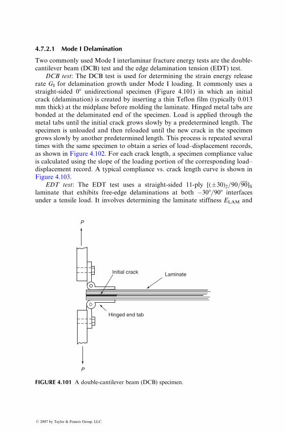
4.7.2 .1 Mod e I Delam ination
Two co mmonly used Mo de I inter laminar fract ure energy test s are the doubl e-
canti lever beam (DCB) test and the e dge delaminati on tension (EDT ) test.
DCB test : The DCB test is used for determini ng the strain energy relea se
rate GI for delam ination growth under M ode I loading . It commonl y uses a
straight -sided 08 unidirecti onal specim en (Figur e 4.101) in which an initial
crack (dela mination) is created by inser ting a thin Teflon film (typical ly 0.013
mm thick) at the midplan e before moldin g the lami nate. Hinge d meta l tabs are
bonde d at the de laminated end of the specim en. Load is app lied through the
meta l tabs unt il the initial crack grow s slowly by a predete rmin ed length. The
specim en is unloade d a nd then reloade d until the new crack in the sp ecimen
grow s slowly by ano ther predete rmine d lengt h. This process is repeat ed severa l
times with the same specim en to obtain a seri es of load–di splace ment records ,
as shown in Figure 4.102. For each crack length , a specim en complian ce va lue
is calcul ated using the slope of the loading porti on of the corres pondi ng load–
displ acement record. A typical co mpliance vs. crack lengt h curve is shown in
Figure 4.103.
EDT test: The EDT test uses a straight-sided 11-ply [(�30)2=90=90]Slaminate that exhibits free-edge delaminations at both �308=908 interfaces
under a tensile load. It involves determining the laminate stiffness ELAM and
Initial crack Laminate
Hinged end tab
P
P
FIGURE 4.101 A double-cantilever beam (DCB) specimen.
� 2007 by Taylor & Francis Group, LLC.
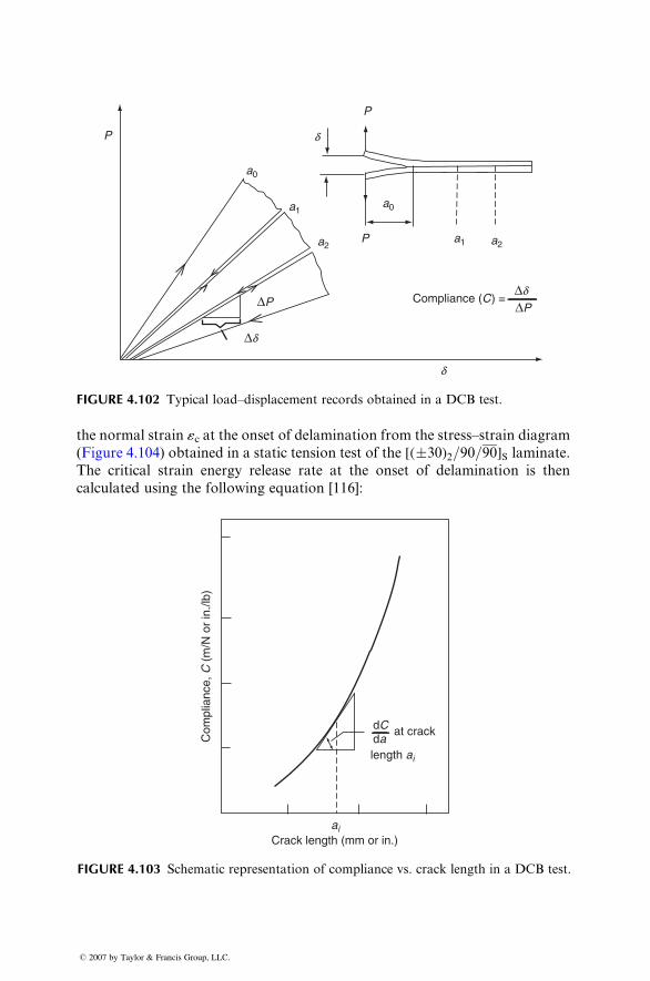
Δd
Δd
d
d
ΔPΔP Compliance (C) =
a1
a0
a0
a1
a2a2P
P
P
FIGURE 4.102 Typical load–displacement records obtained in a DCB test.
the nor mal strain «c at the onset of de laminatio n from the stre ss–strai n diagram
(Figur e 4.104) obt ained in a static tensi on test of the [( � 30)2 =90 =90]S lami nate.
The critical strain energy release rate at the ons et of delaminati on is then
calcula ted using the foll owing equ ation [116] :
dCda
at crack
length ai
aiCrack length (mm or in.)
Com
plia
nce,
C (
m/N
or
in./l
b)
FIGURE 4.103 Schematic representation of compliance vs. crack length in a DCB test.
� 2007 by Taylor & Francis Group, LLC.
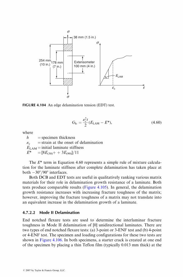
Extensometer100 mm (4 in.)
254 mm(10 in.) 178 mm
(7 in.)
s
s
s38 mm (1.5 in.)
ec e
ELAM
FIGURE 4.104 An edge delamination tension (EDT) test.
GIc ¼ «2c t
2( ELAM � E *) , ( 4: 60 )
wher e
h ¼ spe cimen thickne ss
«c ¼ stra in at the onset of delam ination
ELAM ¼ initial laminate stiffne ss
E* ¼ [8 E(30) þ þ 3E(90) ] =11
The E* term in Equat ion 4.60 repres ents a simp le rule of mixt ure calcul a-
tion for the laminate sti ffness afte r complet e delam inatio n has taken place at
both � 30 8=90 8 interfaces .Both DCB an d EDT tests are useful in qua litatively ranking various matr ix
mate rials for their role in delam inatio n growth resi stance of a lamin ate. Both
tests pro duce comp arable results (Figur e 4.105) . In general , the delam ination
grow th resistance increa ses with increasing fracture toughness of the matrix;
howeve r, impr oving the fracture toughn ess of a matrix may not trans late into
an equival ent increa se in the delam ination grow th of a lamina te.
4.7.2 .2 Mod e II Delaminat ion
End notched flex ure tests are us ed to determine the interlam inar fracture
toughness in Mode II de laminati on of [0] unidir ectio nal laminates . There a re
two types of end notched flexure tests: (a) 3-point or 3-ENF test and (b) 4-point
or 4-E NF test . The specimen and loading configu rations for these two tests are
shown in Figure 4.106. In both spec imens, a starter crack is creat ed at one end
of the specimen by placing a thin Teflon film (typically 0.013 mm thick) at the
� 2007 by Taylor & Francis Group, LLC.
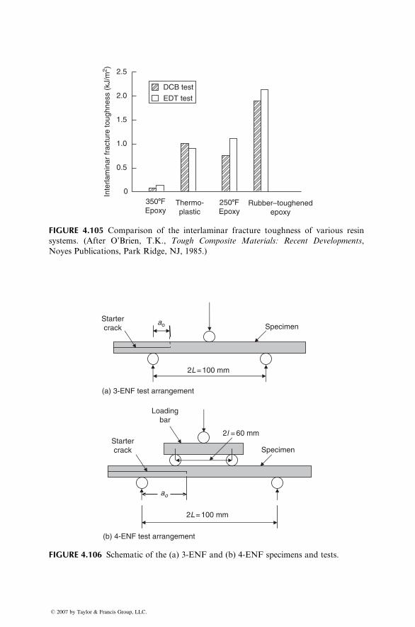
2.5
2.0
1.5
1.0
0.5
0Inte
rlam
inar
frac
ture
toug
hnes
s (k
J/m
2 )
DCB test
EDT test
3508FEpoxy
2508FEpoxy
Thermo-plastic
Rubber–toughenedepoxy
FIGURE 4.105 Comparison of the interlaminar fracture toughness of various resin
systems. (After O’Brien, T.K., Tough Composite Materials: Recent Developments,
Noyes Publications, Park Ridge, NJ, 1985.)
2L = 100 mm
Startercrack Specimen
ao
ao
2L = 100 mm
2l = 60 mmStartercrack Specimen
Loadingbar
(a) 3-ENF test arrangement
(b) 4-ENF test arrangement
FIGURE 4.106 Schematic of the (a) 3-ENF and (b) 4-ENF specimens and tests.
� 2007 by Taylor & Francis Group, LLC.
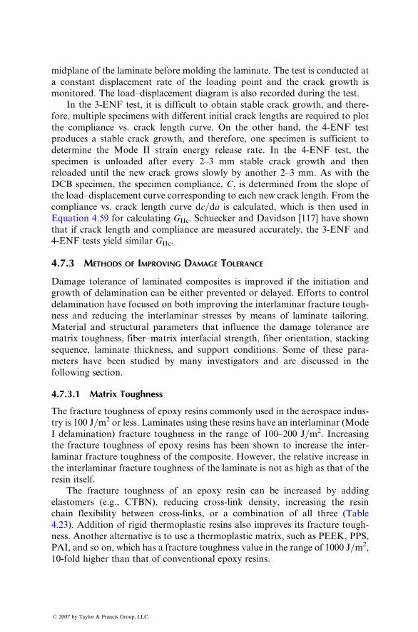
midpl ane of the laminate before moldi ng the lami nate. The test is condu cted at
a constant displ acement rate of the loading point an d the crack grow th is
monit ored. The load–di splace ment diagra m is also recorded dur ing the test.
In the 3-E NF test , it is diff icult to obtain stable crack growth, and there-
fore, multiple specim ens with diff erent initial crack lengt hs are requir ed to plot
the comp liance vs. crack lengt h curve. On the other han d, the 4-ENF test
produ ces a stabl e crack grow th, and theref ore, one specim en is suff icient to
determ ine the Mo de II stra in en ergy relea se rate. In the 4-E NF test, the
specim en is unlo aded after every 2–3 mm stable crack grow th and then
reloade d until the new crack grow s slow ly by ano ther 2–3 mm. As with the
DCB specim en, the specim en complianc e, C, is determined from the slope of
the load– displacement curve co rrespondi ng to each new crack length. From the
compli ance vs. crack length cu rve dc=da is calculated, which is then used inEquation 4.59 for calcula ting GIIc. Schueck er an d David son [117] have sho wn
that if crack lengt h and complia nce are measur ed accurat ely, the 3-E NF and
4-ENF tests yield sim ilar GIIc .
4.7.3 METHODS OF IMPROVING DAMAGE TOLERANCE
Dama ge tolerance of lamin ated co mposites is impr oved if the init iation and
grow th of delam inatio n can be eithe r pre vented or delayed. Effort s to control
delam ination have focused on both impr oving the interlam inar fract ure toug h-
ness an d redu cing the inter laminar stresses by means of laminate tailorin g.
Mater ial an d structural parame ters that infl uence the damage tolerance are
matrix toughn ess, fiber –matrix interfaci al strength, fiber orient ation, stacking
sequence , lami nate thickne ss, and su pport conditio ns. Som e of these para-
mete rs ha ve been studi ed by many investiga tors and are discus sed in the
followi ng section.
4.7.3 .1 Matr ix Toug hness
The fracture toughn ess of ep oxy resin s commonl y used in the aerospac e indus-
try is 1 00 J =m 2 or less. Laminates using these resi ns have an inter lamina r (Mode
I delam ination) fract ure toughness in the range of 100–200 J =m 2. Increasing
the fractu re toughness of ep oxy resin s has been shown to increa se the inter -
laminar fracture toughness of the co mposi te. Ho wever, the relative increa se in
the inter laminar fractu re toughness of the lami nate is not as high as that of the
resin its elf.
The fracture toughness of an epoxy resi n can be increa sed by adding
elastomer s (e.g ., CTBN) , reducing cro ss-link den sity, increa sing the resi n
chain flex ibility between cross-lin ks, or a combinat ion of all three (Table
4.23). Addition of rigid therm oplast ic resi ns also impr oves its fractu re tough -
ness. Another alternative is to use a thermoplastic matrix, such as PEEK, PPS,
PAI, and so on, which has a fracture toughness value in the range of 1000 J=m2,
10-fold higher than that of conventional epoxy resins.
� 2007 by Taylor & Francis Group, LLC.
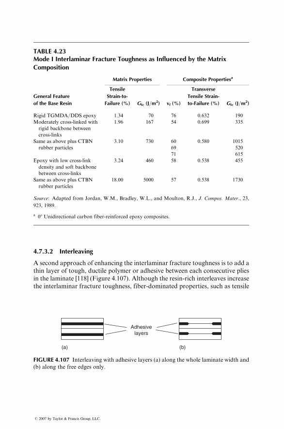
TABLE 4.23Mode I Interlaminar Fracture Toughness as Influenced by the Matrix
Composition
Matrix Properties Composite Propertiesa
General Feature
of the Base Resin
Tensile
Strain-to-
Failure (%) GIc (J=m2) vf (%)
Transverse
Tensile Strain-
to-Failure (%) GIc (J=m2)
Rigid TGMDA=DDS epoxy 1.34 70 76 0.632 190
Moderately cross-linked with
rigid backbone between
cross-links
1.96 167 54 0.699 335
Same as above plus CTBN
rubber particles
3.10 730 60 0.580 1015
69 520
71 615
Epoxy with low cross-link
density and soft backbone
between cross-links
3.24 460 58 0.538 455
Same as above plus CTBN
rubber particles
18.00 5000 57 0.538 1730
Source: Adapted from Jordan, W.M., Bradley, W.L., and Moulton, R.J., J. Compos. Mater., 23,
923, 1989.
a 08 Unidirectional carbon fiber-reinforced epoxy composites.
4.7.3.2 Interleaving
A second approach of enhancing the interlaminar fracture toughness is to add a
thin layer of tough, ductile polymer or adhesive between each consecutive plies
in the laminate [118] (Figure 4.107). Although the resin-rich interleaves increase
the interlaminar fracture toughness, fiber-dominated properties, such as tensile
Adhesivelayers
(a) (b)
FIGURE 4.107 Interleaving with adhesive layers (a) along the whole laminate width and
(b) along the free edges only.
� 2007 by Taylor & Francis Group, LLC.
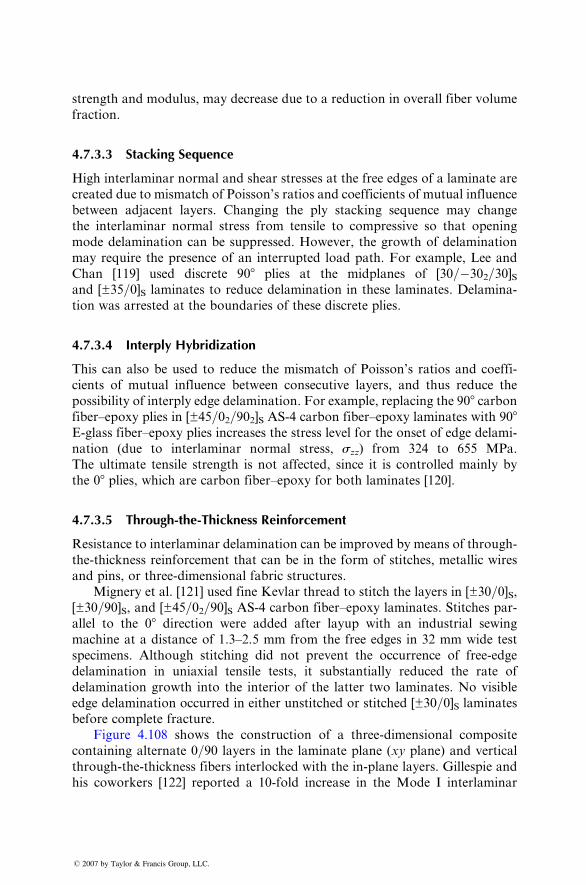
stren gth and modu lus, may decreas e due to a reducti on in overal l fiber vo lume
fraction.
4.7.3 .3 Stacki ng Sequence
High inter laminar normal an d shear stre sses at the free edges of a lamina te are
creat ed due to mis match of Poisson’ s ratios and coeff icients of mutual influence
between adjacent layer s. Changi ng the ply stackin g sequence may change
the inter laminar normal stress from tensile to compres sive so that opening
mode delam ination can be supp ressed. Ho wever, the growth of delam ination
may requ ire the presence of an inter rupted load path. For exampl e, Lee and
Chan [119] used discr ete 90 8 plies at the midpl anes of [30 =�302= 30]Sand [±35 =0]S laminates to reduce delam ination in these laminates . Dela mina-
tion was arrested at the bounda ries of these discr ete plies .
4.7.3 .4 Inter ply Hybr idizati on
This can also be used to reduce the mismat ch of Poisson’ s ratios an d co effi-
cient s of mu tual influence betw een co nsecutive layer s, and thus redu ce the
possibi lity of interp ly edge delam ination . For exampl e, replac ing the 90 8 carbonfiber–ep oxy plies in [±45 =02=90 2] S AS-4 carbon fiber–epo xy laminates wi th 908E-glas s fiber–epo xy plies increa ses the stress level for the onset of edge delam i-
nation (due to interlam inar normal stre ss, szz ) from 324 to 655 MPa .
The ultimat e tensi le stre ngth is not affected, since it is control led mainl y by
the 08 plies, which are carbon fiber –epoxy for both lami nates [120] .
4.7.3 .5 Thr ough-the -Thic kness Re inforcement
Resist ance to interlam inar delam ination can be impr oved by means of throu gh-
the-thickn ess reinforcem ent that can be in the form of sti tches, meta llic wi res
and pins, or three- dimens ional fabri c struc tures .
Migner y et al. [121] used fine Kevl ar thread to stitch the layers in [±30 =0]S ,[±30 =90]S , and [± 45 =02=90]S AS-4 carbon fiber –epoxy laminates . Stitches par-
allel to the 08 direct ion wer e added after layup with an indu strial sewingmachine at a distance of 1.3–2.5 mm from the free edges in 32 mm wide test
specimens. Although stitching did not prevent the occurrence of free-edge
delamination in uniaxial tensile tests, it substantially reduced the rate of
delamination growth into the interior of the latter two laminates. No visible
edge delamination occurred in either unstitched or stitched [±30=0]S laminates
before complete fracture.
Figure 4.108 shows the con struction of a three- dimens ional co mposi te
containing alternate 0=90 layers in the laminate plane (xy plane) and vertical
through-the-thickness fibers interlocked with the in-plane layers. Gillespie and
his coworkers [122] reported a 10-fold increase in the Mode I interlaminar
� 2007 by Taylor & Francis Group, LLC.
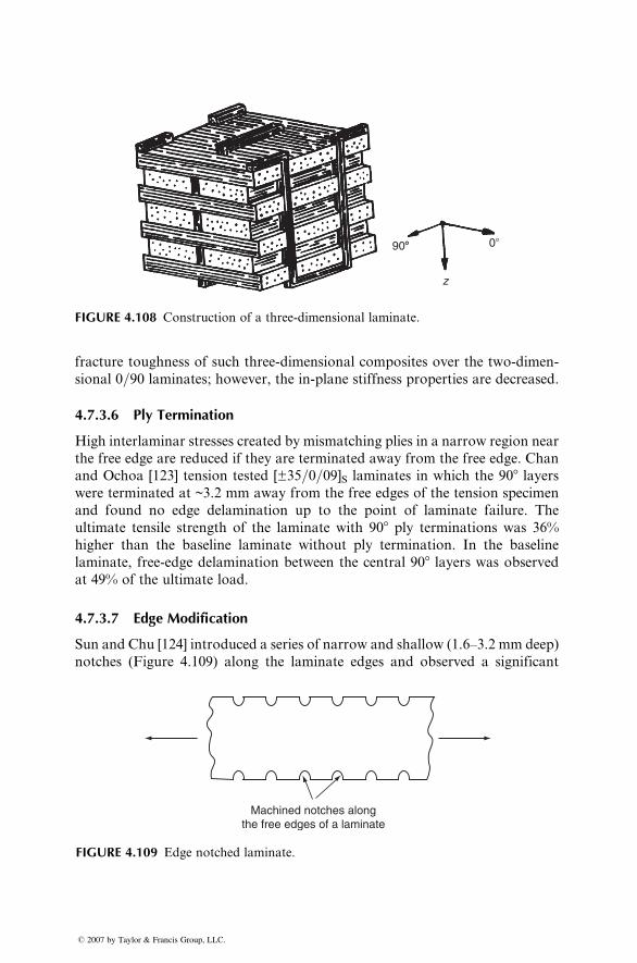
z
908 0�
FIGURE 4.108 Construction of a three-dimensional laminate.
fracture toughness of such three-dimensional composites over the two-dimen-
sional 0=90 laminates; however, the in-plane stiffness properties are decreased.
4.7.3.6 Ply Termination
High interlaminar stresses created by mismatching plies in a narrow region near
the free edge are reduced if they are terminated away from the free edge. Chan
and Ochoa [123] tension tested [±35=0=09]S laminates in which the 908 layerswere terminated at ~3.2 mm away from the free edges of the tension specimen
and found no edge delamination up to the point of laminate failure. The
ultimate tensile strength of the laminate with 908 ply terminations was 36%
higher than the baseline laminate without ply termination. In the baseline
laminate, free-edge delamination between the central 908 layers was observedat 49% of the ultimate load.
4.7.3.7 Edge Modification
Sun and Chu [124] introduced a series of narrow and shallow (1.6–3.2 mm deep)
notches (Figure 4.109) along the laminate edges and observed a significant
Machined notches alongthe free edges of a laminate
FIGURE 4.109 Edge notched laminate.
� 2007 by Taylor & Francis Group, LLC.
increase (25% or higher) in tensile failure load for laminates that are prone to
interlaminar shear failure. Delamination was either eliminated or delayed
in laminates that are prone to opening mode delamination, but there was no
improvement in tensile failure load. The presence of notches disrupts the load
path near the free edges and reduces the interlaminar stresses. However, they
also introduce high in-plane stress concentration. Thus, suppression of delami-
nation by edge notching may require proper selection of notch size and spacing.
REFERENCES
1.
� 2007
N.J. Pagano and J.C. Halpin, Influence of end constraint in the testing of aniso-
tropic bodies, J. Compos. Mater., 2:18 (1968).
2.
R.R. Rizzo, More on the influence of end constraints on off-axis tensile tests,J. Compos. Mater., 3:202 (1969).
3.
B.E. Kaminski, Effects of specimen geometry on the strength of composite mater-ials, Analysis of the Test Methods for High Modulus Fibers and Composites, ASTM
STP, 521:181 (1973).
4.
M.R. Piggott and B. Harris, Compression strength of carbon, glass and Kevlar 49fibre reinforced polyester resins, J. Mater. Sci., 15:2523 (1980).
5.
C.D. Shirrell, Variability in static strengths of sheet molding compounds (SMC),Polym. Compos., 4:172 (1983).
6.
H.T. Hahn and S.W. Tsai, On the behavior of composite laminates after initialfailure, J. Compos. Mater., 8:288 (1974).
7.
P.A. Lagace, Nonlinear stress–strain behavior of graphite=epoxy laminates, AIAAJ., 23:1583 (1985).
8.
J.E. Masters and K.L. Reifsnider, An investigation of cumulative damage develop-ment in quasi-isotropic graphite=epoxy laminates, Damage in Composite Materials,
ASTM STP, 775:40 (1982).
9.
T. Watanabe and M. Yasuda, Fracture behavior of sheet molding compounds.Part 1: Under tensile load, Composites, 13:54 (1982).
10.
J. Aveston and A. Kelly, Tensile first cracking strain and strength of hybridcomposites and laminates, Phil. Trans. R. Soc. Lond., A, 294:519 (1980).
11.
P.W. Manders and M.G. Bader, The strength of hybrid glass=carbon fiber com-posites. Part 1: Failure strain enhancement and failure mode, J. Mater. Sci.,
16:2233 (1981).
12.
J.M. Whitney, I.M. Daniel, and R.B. Pipes, Experimental Mechanics of FiberReinforced Composite Materials, Society for Experimental Mechanics, Brookfield
Center, CT (1984).
13.
C. Zweben, W.S. smith, and M.M. Wardle, Test methods for fiber tensile strength,composite flexural modulus, and properties of fabric-reinforced laminates,
Composite Materials: Testing and Design (Fifth Conference), ASTM STP,
674:228 (1979).
14.
R.E. Bullock, Strength ratios of composite materials in flexure and in tension,J. Compos. Mater., 8:200 (1974).
15.
J.M. Whitney andM. Knight, The relationship between tensile strength and flexurestrength in fiber-reinforced composites, Exp. Mech., 20:211 (1980).
by Taylor & Francis Group, LLC.
16.
� 200
Y.T. Yeow and H.F. Brinson, A comparison of simple shear characterization
methods for composite laminates, Composites, 9:49 (1978).
17.
C.C. Chiao, R.L. Moore, and T.T. Chiao, Measurement of shear properties offibre composites. Part 1: Evaluation of test methods, Composites, 8:161 (1977).
18.
C.C. Chamis and J.J. Sinclair, Ten-deg off-axis test for shear properties in fibercomposites, Exp. Mech., 17:339 (1977).
19.
D.E. Walrath and D.F. Adams, The Iosipescu shear test as applied to compositematerials, Exp. Mech., 23:105 (1983).
20.
D.W. Wilson, Evaluation of V-notched beam shear test through an interlaboratorystudy, J. Compos. Technol. Res., 12:131 (1990).
21.
J.M. Whitney, D.L. Stansberger, and H.B. Howell, Analysis of the rail shear test—applications and limitations, J. Compos. Mater., 5:24 (1971).
22.
R. Garcia, T.A. Weisshaar, and R.R. McWithey, An experimental and analyticalinvestigation of the rail shear-test method as applied to composite materials, Exp.
Mech., 20:273 (1980).
23.
B.K. Daniels, N.K. Harakas, and R.C. Jackson, Short beam shear tests of graphitefiber composites, Fibre Sci. Technol., 3:187 (1971).
24.
W.W. Stinchcomb, E.G. Henneke, and H.L. Price, Use of the short-beam shear testfor quality control of graphite-polyimide laminates, Reproducibility and Accuracy
of Mechanical Tests, ASTM STP, 626:96 (1977).
25.
C.A. Berg, T. Tirosh, and M. Israeli, Analysis of the short beam bending of fiberreinforced composites, Composite Materials: Testing and Design (Second Confer-
ence), ASTM STP, 497:206 (1972).
26.
L.L. Lorenzo and H.T. Hahn, Fatigue failure mechanisms in unidirectionalcomposites, Composite Materials—Fatigue and Fracture, ASTM STP, 907:
210 (1986).
27.
H.T. Hahn and R.Y. Kim, Fatigue behavior of composite laminates, J. Compos.Mater., 10:156 (1976).
28.
B.D. Agarwal and J.W. Dally, Prediction of low-cycle fatigue behavior of GFRP:an experimental approach, J. Mater. Sci., 10:193 (1975).
29.
H.T. Hahn and R.Y. Kim, Proof testing of composite materials, J. Compos.Mater., 9:297 (1975).
30.
D.A. Riegner and B.A. Sanders, A characterization study of automotive continu-ous and random glass fiber composites, Proceedings National Technical Confer-
ence, Society of Plastics Engineers, November (1979).
31.
R.A. Heimbuch and B.A. Sanders, Mechanical properties of automotive choppedfiber reinforced plastics, Composite Materials in the Automobile Industry, ASME,
New York (1978).
32.
P.K. Mallick, Fatigue characteristics of high glass content sheet molding com-pound (SMC) materials, Polym. Compos., 2:18 (1981).
33.
R.B. Pipes, Interlaminar shear fatigue characteristics of fiber reinforced compositematerials, Composite Materials: Testing and Design (Third Conference), ASTM
STP, 546:419 (1974).
34.
C.K.H. Dharan, Interlaminar shear fatigue of pultruded graphite fibre–polyestercomposites, J. Mater. Sci., 13:1243 (1978).
35.
M.J. Owen and S. Morris, Some interlaminar-shear fatigue properties of carbon-fibre-reinforced plastics, Plast. Polym., 4:209 (1972).
7 by Taylor & Francis Group, LLC.
36.
� 2007
D.W. Wilson, Characterization of the interlaminar shear fatigue properties of
SMC-R50, Technical Report No. 80–05, Center for Composite Materials, Univer-
sity of Delaware, Newark, DE (1980).
37.
D.C. Phillips and J.M. Scott, The shear fatigue of unidirectional fibre composites,Composites, 8:233 (1977).
38.
J.D. Conners, J.F. Mandell, and F.J. McGarry, Compressive fatigue in glass andgraphite reinforced composites, Proceedings 34th Annual Technical Conference,
Society of the Plastics Industry (1979).
39.
Z. Hashin and A. Rotem, A fatigue failure criterion for fiber reinforced materials,J. Compos. Mater., 7:448 (1973).
40.
K.H. Boller, Fatigue characteristics of RP laminates subjected to axial loading,Mod. Plast., 41:145 (1964).
41.
J.W. Davis, J.A. McCarthy, and J.N. Schrub, The fatigue resistance of reinforcedplastics, Materials in Design Engineering, p. 87 (1964).
42.
M.J. Owen and R.G. Rose, Polyester flexibility versus fatigue behavior of RP,Mod. Plast., 47:130 (1970).
43.
T. Tanimoto and S. Amijima, Progressive nature of fatigue damage of glass fiberreinforced plastics, J. Compos. Mater., 9 (1975).
44.
C.K.H. Dharan, Fatigue failure in graphite fibre and glass fibre-polymer compos-ites, J. Mater. Sci., 10:1665 (1975).
45.
K.H. Boller, Effect of tensile mean stresses on fatigue properties of plastic lamin-ates reinforced with unwoven glass fibers, U.S. Air Force Materials Laboratory,
Report No. ML-TDR-64–86, June (1964).
46.
S.V. Ramani and D.P. Williams, Axial fatigue of [0=±30]6S graphite=epoxy, FailureMode in Composites III, AIME, p. 115 (1976).47.
T.R. Smith and M.J. Owen, Fatigue properties of RP, Mod. Plast., 46:124(1969).
48.
J.W. Dally and L.J. Broutman, Frequency effects on the fatigue of glass reinforcedplastics, J. Compos. Mater., 1:424 (1967).
49.
J.F. Mandell and U. Meier, Effects of stress ratio, frequency, and loading time onthe tensile fatigue of glass-reinforced epoxy, Long-Term Behavior of Composites,
ASTM STP, 813:55 (1983).
50.
C.T. Sun and W.S. Chan, Frequency effect on the fatigue life of a laminatedcomposite, Composite Materials, Testing and Design (Fifth Conference), ASTM
STP, 674:418 (1979).
51.
C.R. Saff, Effect of load frequency and lay-up on fatigue life of composites, Long-Term Behavior of Composites, ASTM STP, 813:78 (1983).
52.
K.L. Reifsnider, W.W. Stinchcomb, and T.K. O’Brien, Frequency effects on astiffness-based fatigue failure criterion in flawed composite specimens, Fatigue of
Filamentary Composite Materials, ASTM STP, 636: 171 (1977).
53.
J.H. Underwood and D.P. Kendall, Fatigue damage in notched glass–epoxy sheet,Proceedings International Conference on Composite Materials, Vol. 2, AIME,
p. 1122 (1975).
54.
C.K.H. Dharan, Fatigue failure mechanisms in a unidirectionally reinforced com-posite material, Fatigue of Composite Materials, ASTM STP, 569:171 (1975).
55.
H.C. Kim and L.J. Ebert, Axial fatigue failure sequence and mechanisms inunidirectional fiberglass composites, J. Compos. Mater., 12:139 (1978).
56.
R. Talreja, Fatigue of composite materials: damage mechanisms and fatigue-lifediagrams, Proc. R. Soc. Lond., A, 378:461 (1981).
by Taylor & Francis Group, LLC.
57.
� 200
L.J. Broutman and S. Sahu, Progressive damage of a glass reinforced plastic during
fatigue, Proceedings 20th Annual Technical Conference, Society of the Plastics
Industry (1969).
58.
K. Reifsnider, K. Schultz, and J.C. Duke, Long-term fatigue behavior of compositematerials, Long-Term Behavior of Composites, ASTM STP, 813:136 (1983).
59.
S.S. Wang and E.S.M. Chim, Fatigue damage and degradation in random short-fiber SMC composite, J. Compos. Mater., 17:114 (1983).
60.
T.R. Smith and M.J. Owen, Progressive nature of fatigue damage in RP, Mod.Plast., 46:128 (1969).
61.
P.K. Mallick, A fatigue failure warning method for fiber reinforced compositestructures, Failure Prevention and Reliability—1983 (G. Kurajian, ed.), ASME,
New York (1983).
62.
H.W. Whitworth, Cumulative damage in composites, ASME J. Eng. Mater. Tech-nol., 112:358 (1990).
63.
L.J. Broutman and S. Sahu, A new theory to predict cumulative fatigue damage infiberglass reinforced plastics, Composite Materials: Testing and Design (Second
Conference), ASTM STP, 497:170 (1972).
64.
J.N. Yang, Fatigue and residual strength degradation for graphite=epoxy com-posites under tension–compression cyclic loadings, J. Compos. Mater., 12:19
(1978).
65.
M.G. Bader and R.M. Ellis, The effect of notches and specimen geometry on thependulum impact strength of uniaxial CFRP, Composites, 6:253 (1974).
66.
R.H. Toland, Failure modes in impact-loaded composite materials, Symposium onFailure Modes in Composites, AIME Spring Meeting, May (1972).
67.
P.K. Mallick and L.J. Broutman, Static and impact properties of laminated hybridcomposites, J. Test. Eval., 5:190 (1977).
68.
J.L. Perry and D.F. Adams, Charpy impact experiments on graphite=epoxy hybridcomposites, Composites, 7:166 (1975).69.
N.L. Hancox, Izod impact testing of carbon-fibre-reinforced plastics, Composites,3:41 (1971).
70.
M.G. Bader, J.E. Bailey, and I. Bell, The effect of fibre–matrix interface strengthon the impact and fracture properties of carbon-fibre-reinforced epoxy resin com-
posites, J. Phys. D: Appl. Phys., 6:572 (1973).
71.
P. Yeung and L.J. Broutman, The effect of glass-resin interface strength on theimpact strength of fiber reinforced plastics, Polym. Eng. Sci., 18:62 (1978).
72.
P.K. Mallick and L.J. Broutman, Impact properties of laminated angle ply com-posites, Eng. Fracture Mech., 8:631 (1976).
73.
G.R. Sidey and F.J. Bradshaw, Some investigations on carbon-fibre-reinforcedplastics under impact loading, and measurements of fracture energies, Carbon
Fibres: Their Composites and Applications, Plastics Institute, London, p. 208
(1971).
74.
M.D. Rhodes, J.G. Williams, and J.H. Starnes, Jr., Low-velocity impact damage ingraphite-fiber reinforced epoxy laminates, Proceedings 34th Annual Technical Con-
ference, Society of the Plastics Industry (1979).
75.
R.L. Ramkumar, Effect of low-velocity impact damage on the fatigue behavior ofgraphite=epoxy laminates, Long-Term Behavior of Composites, ASTM STP,
813:116 (1983).
76.
J. Morton and E.W. Godwin, Impact response of tough carbon fibre composites,Compos. Struct., 13:1 (1989).
7 by Taylor & Francis Group, LLC.
77.
� 2007
G.E. Husman, J.M. Whitney, and J.C. Halpin, Residual strength characterization
of laminated composites subjected to impact loading, Foreign Object Impact Dam-
age to Composites, ASTM STP, 568:92 (1975).
78.
G. Kretsis and F.L. Matthews, The strength of bolted joints in glass fibre=epoxylaminates, Composites, 16:92 (1985).79.
P.K. Mallick and R.E. Little, Pin bearing strength of fiber reinforced compositelaminates, Proceedings Advanced Composites, American Society for Metals (1985).
80.
T.A. Collings, The strength of bolted joints in multi-directional cfrp laminates,Composites, 8:43 (1977).
81.
W.J. Quinn and F.L. Matthews, The effect of stacking sequence on the pin-bearingstrength in glass fibre reinforced plastic, J. Compos. Mater., 11:139 (1977).
82.
S. Nilsson, Increasing strength of graphite=epoxy bolted joints by introducing anadhesively bonded metallic insert, J. Compos. Mater., 23:641 (1989).
83.
J.H. Stockdale and F.L. Matthews, The effect of clamping pressure on bolt bearingloads in glass fibre-reinforced plastics, Composites, 7:34 (1976).
84.
J.R. Strife and K.M. Prewo, The thermal expansion behavior of unidirectional andbidirectional Kevlar=epoxy composites, J. Compos. Mater., 13:264 (1979).
85.
S.F.H. Parker, M. Chandra, B. Yates, M. Dootson, and B.J. Walters, Theinfluence of distribution between fibre orientations upon the thermal expansion
characteristics of carbon fibre-reinforced plastics, Composites, 12:281 (1981).
86.
J.R. Kerr and J.F. Haskins, Effects of 50,000 h of thermal aging on graphite=epoxyand graphite=polyimide composites, AIAA J., 22:96 (1982).87.
F.E. Devine, Polyester moulding materials in automotive underbonnet environ-ments, Composites, 14:353 (1983).
88.
C.H. Shen and G.S. Springer, Moisture absorption and desorption of compositematerials, J. Compos. Mater., 10:2 (1976).
89.
G.S. Springer, B.A. Sanders, and R.W. Tung, Environmental effects on glass fiberreinforced polyester and vinyl ester composites, J. Compos. Mater., 14:213 (1980).
90.
W.W. Wright, The effect of diffusion of water into epoxy resins and their carbon-fibre reinforced composites, Composites, 12:201 (1981).
91.
O. Gillat and L.J. Broutman, Effect of an external stress on moisture diffusionand degradation in a graphite-reinforced epoxy laminate, Advanced Composite
Materials—Environmental Effects, ASTM STP, 658:61 (1978).
92.
G. Marom and L.J. Broutman, Moisture in epoxy resin composites, J. Adhes.,12:153 (1981).
93.
E.L. McKague, Jr., J.E. Halkias, and J.D. Reynolds, Moisture in composites: theeffect of supersonic service on diffusion, J. Compos. Mater., 9:2 (1975).
94.
M.J. Adamson, A conceptual model of the thermal-spike mechanism in graphite=epoxy laminates, Long-Term Behavior of Composites, ASTM STP, 813:179 (1983).95.
H.T. Hahn, Hygrothermal damage in graphite=epoxy laminates, J. Eng. Mater.Technol., 109:1 (1987).
96.
C.H. Shen and G.S. Springer, Effects of moisture and temperature on the tensilestrength of composite materials, J. Compos. Mater., 11:2 (1977).
97.
C.H. Shen and G.S. Springer, Environmental effects on the elastic moduli ofcomposite materials, J. Compos. Mater., 11:250 (1977).
98.
O.K. Joshi, The effect of moisture on the shear properties of carbon fibre compos-ites, Composites, 14:196 (1983).
99.
C.J. Jones, R.F. Dickson, T. Adam, H. Reiter, and B. Harris, Environmentalfatigue of reinforced plastics, Composites, 14:288 (1983).
by Taylor & Francis Group, LLC.
100.
� 200
P.T. Curtis and B.B. Moore, The effects of environmental exposure on the fatigue
behavior of CFRP laminates, Composites, 14:294 (1983).
101.
C.C. Chamis, R.R. Lark, and J.H. Sinclair, Integrated theory for predicting thehygrothermomechanical response of advanced composite structural components,
Advanced CompositeMaterial—Environmental Effects, ASTMSTP, 658:160 (1978).
102.
J.B. Sturgeon, Creep of fibre reinforced thermosetting resins, Creep of EngineeringMaterials (C.D. Pomeroy, ed.), Mechanical Engineering Publishing Ltd., London
(1978).
103.
J.S. Cartner, W.I. Griffith, and H.F. Brinson, The viscoelastic behavior of com-posite materials for automotive applications, Composite Materials in the Automo-
tive Industry (S.V. Kulkarni, C.H. Zweben, and R.B. Pipes, eds.), American Society
of Mechanical Engineers, New York (1978).
104.
Y.T. Yeow, D.H. Morris, and H.F. Brinson, Time–temperature behavior of aunidirectional graphite=epoxy composite, Composite Materials: Testing and Design
(Fifth Conference), ASTM STP, 674:263 (1979).
105.
Y.C. Lou and R.A. Schapery, Viscoelastic characterization of a non-linear fiber-reinforced plastic, J. Compos. Mater., 5:208 (1971).
106.
M.E. Tuttle and H.F. Brinson, Prediction of the long-term creep compliance ofgeneral composite laminates, Exp. Mech., 26:89 (1986).
107.
M.G. Phillips, Prediction of long-term stress-rupture life for glass fibre-reinforcedpolyester composites in air and in aqueous environments, Composites, 14:270 (1983).
108.
R.E. Glaser, R.L. Moore, and T.T. Chiao, Life estimation of an S-glass=epoxycomposite under sustained tensile loading, Compos. Technol. Rev., 5:21 (1983).109.
R.E. Glaser, R.L. Moore, and T.T. Chiao, Life estimation of aramid=epoxycomposites under sustained tension, Compos. Technol. Rev., 6:26 (1984).110.
C.E. Harris and D.H. Morris, A damage tolerant design parameter for graphite=epoxy laminated composites, J. Compos. Technol. Res., 7:77 (1985).111.
J.F. Mandell, S.S. Wang, and F.J. McGarry, The extension of crack tip damagezones in fiber reinforced plastic laminates, J. Compos. Mater., 9:266 (1975).
112.
S.K. Gaggar and L.J. Broutman, Crack growth resistance of random fiber com-posites, J. Compos. Mater., 9:216 (1975).
113.
C.E. Harris and D.H. Morris, Role of delamination and damage development onthe strength of thick notched laminates, Delamination and Debonding of Materials,
ASTM STP, 876:424 (1985).
114.
D.J. Wilkins, J.R. Eisenmann, R.A. Camin, W.S. Margolis, and R.A. Benson,Characterizing delamination growth in graphite–epoxy, Damage in Composite
Materials, ASTM STP, 775:168 (1980).
115.
D.F. Adams, L.A. Carlsson, and R.B. Pipes, Experimental Characterization ofAdvanced Composite Materials, 3rd Ed., CRC Press, Boca Raton, FL (2003).
116.
T.K. O’Brien, Characterization of delamination onset and growth in a compositelaminate, Damage in Composite Materials, ASTM STP, 775:140 (1982).
117.
C. Schuecker and B.D. Davidson, Evaluation of the accuracy of the four-pointend-notched flexure test for mode II delamination toughness determination, Com-
pos. Sci. Tech., 60:2137 (2000).
118.
O. Ishai, H. Rosenthal, N. Sela, and E. Drukker, Effect of selective adhesiveinterleaving on interlaminar fracture toughness of graphite=epoxy composite
laminates, Composites, 19:49 (1988).
119.
E.W.Y. Lee and W.S. Chan, Delamination arrestment by discretizing the criticalply in a laminate, AIAA Paper No. 89-1403, Amer. Inst. Aero. Astro., 1989.
7 by Taylor & Francis Group, LLC.
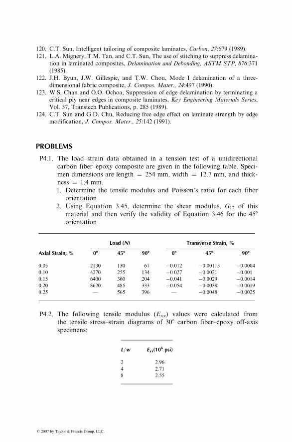
120.
� 2007
C.T. Sun, Intelligent tailoring of composite laminates, Carbon, 27:679 (1989).
121.
L.A. Mignery, T.M. Tan, and C.T. Sun, The use of stitching to suppress delamina-tion in laminated composites, Delamination and Debonding, ASTM STP, 876:371
(1985).
122.
J.H. Byun, J.W. Gillespie, and T.W. Chou, Mode I delamination of a three-dimensional fabric composite, J. Compos. Mater., 24:497 (1990).
123.
W.S. Chan and O.O. Ochoa, Suppression of edge delamination by terminating acritical ply near edges in composite laminates, Key Engineering Materials Series,
Vol. 37, Transtech Publications, p. 285 (1989).
124.
C.T. Sun and G.D. Chu, Reducing free edge effect on laminate strength by edgemodification, J. Compos. Mater., 25:142 (1991).
PROBLEMS
P4.1. The load–strain data obtained in a tension test of a unidirectional
carbon fiber–epoxy composite are given in the following table. Speci-
men dimensions are length ¼ 254 mm, width ¼ 12.7 mm, and thick-
ness ¼ 1.4 mm.
1. Determine the tensile modulus and Poisson’s ratio for each fiber
orientation
2. Using Equation 3.45, determine the shear modulus, G12 of this
material and then verify the validity of Equation 3.46 for the 458orientation
Load (N) Transverse Strain, %
by Taylor & Francis Gro
up, LLC.Axial Strain, %
08 458 908 08 458 9080.05
2130 130 67 �0.012 �0.00113 �0.00040.10
4270 255 134 �0.027 �0.0021 �0.0010.15
6400 360 204 �0.041 �0.0029 �0.00140.20
8620 485 333 �0.054 �0.0038 �0.00190.25
— 565 396 — �0.0048 �0.0025P4.2. The following tensile modulus (Exx) values were calculated from
the tensile stress–strain diagrams of 308 carbon fiber–epoxy off-axis
specimens:
L=w E (106 psi)
xx2
2.964
2.718
2.55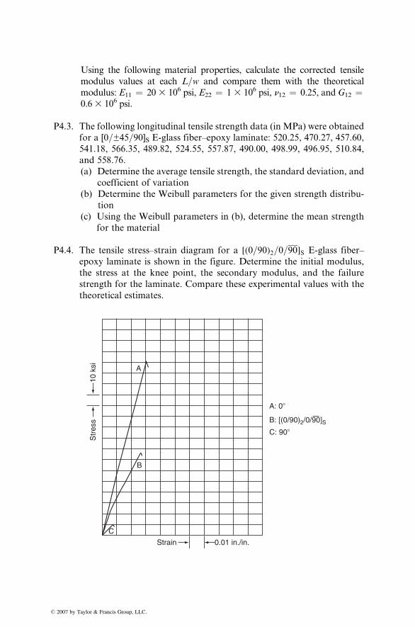
Using the following material properties, calculate the corrected tensile
modulus values at each L=w and compare them with the theoretical
modulus: E11 ¼ 203 106 psi, E22 ¼ 13 106 psi, n12 ¼ 0.25, and G12 ¼0.63 106 psi.
P4.3. The following longitudinal tensile strength data (in MPa) were obtained
for a [0=±45=90]S E-glass fiber–epoxy laminate: 520.25, 470.27, 457.60,
541.18, 566.35, 489.82, 524.55, 557.87, 490.00, 498.99, 496.95, 510.84,
and 558.76.
(a) Determine the average tensile strength, the standard deviation, and
coefficient of variation
(b) Determine the Weibull parameters for the given strength distribu-
tion
(c) Using the Weibull parameters in (b), determine the mean strength
for the material
P4.4. The tensile stress–strain diagram for a [(0=90)2=0=90]S E-glass fiber–
epoxy laminate is shown in the figure. Determine the initial modulus,
the stress at the knee point, the secondary modulus, and the failure
strength for the laminate. Compare these experimental values with the
theoretical estimates.
C
B
A
A: 0�
C: 90�
B: [(0/90)2/0/90]S
Strain
Str
ess
10 k
si
0.01 in./in.
� 2007 by Taylor & Francis Group, LLC.
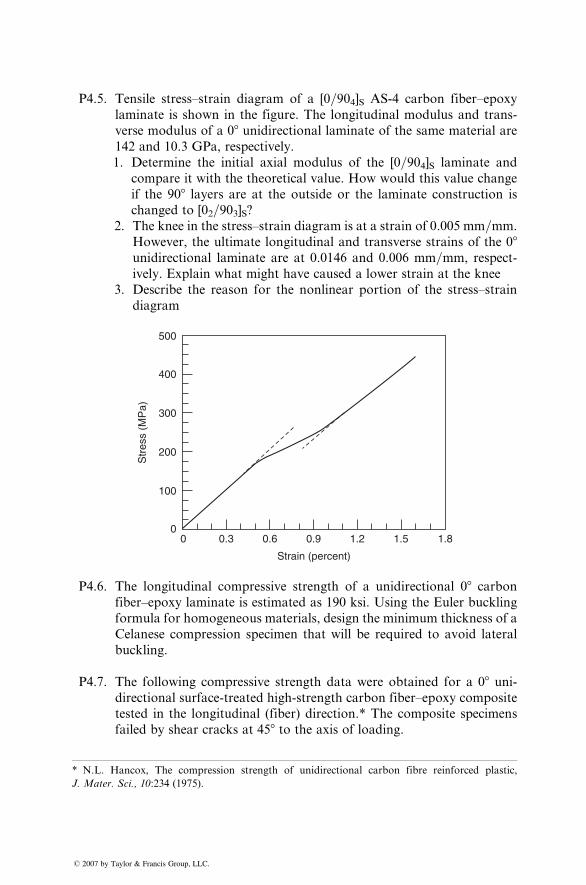
P4.5. Tensile stress–strain diagram of a [0=904]S AS-4 carbon fiber–epoxy
laminate is shown in the figure. The longitudinal modulus and trans-
verse modulus of a 08 unidirectional laminate of the same material are
142 and 10.3 GPa, respectively.
1. Determine the initial axial modulus of the [0=904]S laminate and
compare it with the theoretical value. How would this value change
if the 908 layers are at the outside or the laminate construction is
changed to [02=903]S?2. The knee in the stress–strain diagram is at a strain of 0.005 mm=mm.
However, the ultimate longitudinal and transverse strains of the 08unidirectional laminate are at 0.0146 and 0.006 mm=mm, respect-
ively. Explain what might have caused a lower strain at the knee
3. Describe the reason for the nonlinear portion of the stress–strain
diagram
00
100
200
300
400
500
0.3 0.6 0.9 1.2
Strain (percent)
Str
ess
(MP
a)
1.5 1.8
P4.6. The longitudinal compressive strength of a unidirectional 08 carbon
fiber–epoxy laminate is estimated as 190 ksi. Using the Euler buckling
formula for homogeneous materials, design the minimum thickness of a
Celanese compression specimen that will be required to avoid lateral
buckling.
P4.7. The following compressive strength data were obtained for a 08 uni-directional surface-treated high-strength carbon fiber–epoxy composite
tested in the longitudinal (fiber) direction.* The composite specimens
failed by shear cracks at 458 to the axis of loading.
* N.L. Hancox, The compression strength of unidirectional carbon fibre reinforced plastic,
J. Mater. Sci., 10:234 (1975).
� 2007 by Taylor & Francis Group, LLC.
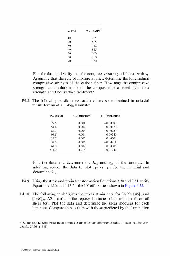
* S. Tan and R. Kim, Fracture of co
Mech., 28:364 (1988).
� 2007 by Taylor & Francis Group, LLC.
v (%) s (MPa)
fmposite lamin
LCU
10
32520
52530
71240
91550
110060
125070
1750Plo t the da ta and verify that the co mpres sive stre ngth is linear wi th vf.
Ass uming that the rule of mixtu re ap plies, determine the longitud inal
co mpressive stre ngth of the carbon fiber . How may the compres sive
stre ngth and fail ure mode of the compo site be affe cted by matrix
stre ngth and fiber surfa ce treat ment?
P4.8. The follo wing tensile stre ss–strai n values were obtaine d in uni axial
tensile testing of a [±45]S lami nate:
s (MPa) « (mm=mm) « (mm=mm)
xx xxates contain
yy
27.5
0.001 �0.0008354.4
0.002 �0.0017082.7
0.003 �0.0025096.5
0.004 �0.00340115.7
0.005 �0.00700132.5
0.006 �0.00811161.0
0.007 �0.00905214.0
0.014 �0.01242Plo t the data an d de termine the Exx an d nxy of the lami nate. In
ad dition, red uce the data to plot t12 vs. g12 for the mate rial and
determine G12.
P4.9. Using the stress and strain transformation Equations 3.30 and 3.31, verify
Equations 4.16 and 4.17 for the 108 off-axis test shown in Figure 4.28.
P4.10. The following table* gives the stress–strain data for [0=90=±45]S and
[0=90]2S AS-4 carbon fiber–epoxy laminates obtained in a three-rail
shear test. Plot the data and determine the shear modulus for each
laminate. Compare these values with those predicted by the lamination
ing cracks due to shear loading, Exp.
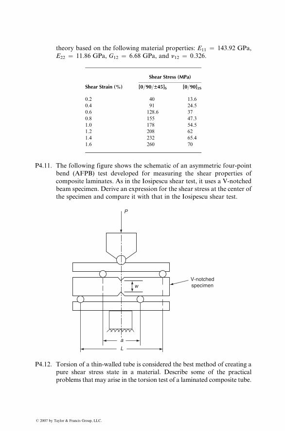
theory based on the following material properties: E11 ¼ 143.92 GPa,
E22 ¼ 11.86 GPa, G12 ¼ 6.68 GPa, and n12 ¼ 0.326.
� 2007 by Taylor & Francis G
Shear Stress (MPa)
roup, LLC.
Shear Strain (%)
[0=90=±45]S [0=90]2S0.2
40 13.60.4
91 24.50.6
128.6 370.8
155 47.31.0
178 54.51.2
208 621.4
232 65.41.6
260 70P4.11. The following figure shows the schematic of an asymmetric four-point
bend (AFPB) test developed for measuring the shear properties of
composite laminates. As in the Iosipescu shear test, it uses a V-notched
beam specimen. Derive an expression for the shear stress at the center of
the specimen and compare it with that in the Iosipescu shear test.
V-notchedspecimenw
P
L
a
P4.12. Torsion of a thin-walled tube is considered the best method of creating a
pure shear stress state in a material. Describe some of the practical
problems that may arise in the torsion test of a laminated composite tube.
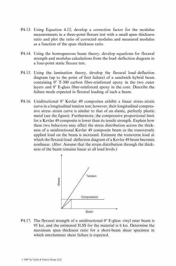
P4.13. Using Equation 4.12, develop a correction factor for the modulus
measurements in a three-point flexure test with a small span–thickness
ratio and plot the ratio of corrected modulus and measured modulus
as a function of the span–thickness ratio.
P4.14. Using the homogeneous beam theory, develop equations for flexural
strength and modulus calculations from the load–deflection diagram in
a four-point static flexure test.
P4.15. Using the lamination theory, develop the flexural load–deflection
diagram (up to the point of first failure) of a sandwich hybrid beam
containing 08 T-300 carbon fiber-reinforced epoxy in the two outer
layers and 08 E-glass fiber-reinforced epoxy in the core. Describe the
failure mode expected in flexural loading of such a beam.
P4.16. Unidirectional 08 Kevlar 49 composites exhibit a linear stress–strain
curve in a longitudinal tension test; however, their longitudinal compres-
sive stress–strain curve is similar to that of an elastic, perfectly plastic
metal (see the figure). Furthermore, the compressive proportional limit
for a Kevlar 49 composite is lower than its tensile strength. Explain how
these two behaviors may affect the stress distribution across the thick-
ness of a unidirectional Kevlar 49 composite beam as the transversely
applied load on the beam is increased. Estimate the transverse load at
which the flexural load–deflection diagram of aKevlar 49 beam becomes
nonlinear. (Hint: Assume that the strain distribution through the thick-
ness of the beam remains linear at all load levels.)
Tension
Compression
Strain
Str
ess
P4.17. The flexural strength of a unidirectional 08 E-glass–vinyl ester beam is
95 ksi, and the estimated ILSS for the material is 6 ksi. Determine the
maximum span–thickness ratio for a short-beam shear specimen in
which interlaminar shear failure is expected.
� 2007 by Taylor & Francis Group, LLC.
P4.18. Som e invest igators ha ve pro posed using a four-po int flexure test for
ILS S measur ements. Usin g the hom ogeneous beam theory, develop
equ ations for ILSS in a four-p oint flex ure test and discus s the meri ts
of such a test over a three- point sho rt-beam shear test .
P4.19. Usi ng Tabl e 4.8, comp are the fati gue stre ngths of T-300 carbo n–epoxy
and E-glass–epoxy composites at 104 and 107 cycles.
P4.20. The Weibull parameters for the tension–tension fatigue life distribution
of a [0=90=±45]S T-300 carbon fiber–epoxy composite are as follows: at
smax ¼ 340 MPa, L0 ¼ 1,000,000, and af ¼ 1.6. At smax ¼ 410 MPa,
L0 ¼ 40,000, and af ¼ 1.7.
1. Determine the mean fatigue lives at 340 and 410 MPa
2. What is the expected probability of surviving 50,000 cycles at 410MPa?
P4.21. Fatigue lives (numbers of cycles to failure) of twelve 08 Kevlar 49 fiber-
reinforced composite specimens in tension–tension cycling at 90% UTS,
R ¼ 0.1, 0.5 Hz frequency, and 238C are reported as 1,585; 25; 44,160;
28,240; 74,140; 47; 339,689; 50,807; 320,415; 865; 5,805; and 4,930. Plot
the Weibull distribution curve for these fatigue lives and determine the
Weibull parameters for this distribution.
P4.22. For the major portion of the fatigue life of a composite laminate, the
instantaneous modulus can be modeled as
E ¼ E0(1� c logN)
where
E0¼ initial modulus at N ¼ 1
N ¼ number of fatigue cycles
c ¼ an experimentally determined damage-controlling factor
Using this model, determine the number of cycles that a simply sup-
ported centrally loaded beam can endure before its deflection becomes
50% higher than its initial value.
P4.23. For the quasi-isotropic laminate described in Example 4.2, suppose
the loading sequence is 10,000 cycles at 437 MPa followed by cycling
to failure at 382 MPa. Estimate the total life expected in this high–
low stress sequence using (a) the Whitworth model and (b) the
Miner’s rule.
P4.24. The mean fatigue lives of [0=90]S E-glass fiber–epoxy laminates at
maximum stress levels of 56,000 and 35,000 psi are 1,500 and 172,000,
respectively. The static tensile strength of this material is 65,000 psi.
� 2007 by Taylor & Francis Group, LLC.
1. Determine the residual static strength of this material after 50% of
the fatigue life at each stress level
2. After cycling for 50% of the fatigue life at 35,000 psi, the maximum
stress level in a fatigue specimen is increased to 56,000 psi. Estimate
the number of cycles the specimen would survive at 56,000 psi
3. If the first stress level is 56,000 psi, which is then followed by 35,000
psi, estimate the number of cycles at the second stress level
P4.25. Adam et al.* have found that, depending on the fiber type, the post-
fatigue residual strength of [0=90] cross-plied composites may show
either a gradual decrease with increasing number of cycles (usually
after a rapid reduction in the first few cycles) or virtually no change
until they fail catastrophically (sudden death). They proposed the
following empirical equation to predict the residual strength:
sres ¼ smax(sU � smax)(1� rx)1=y,
where
r ¼ logN � log 0:5
logNf � log 0:5
x, y ¼ parameters obtained by fitting the residual strength equation to
the experimental data (both varywithmaterial and environmen-
tal conditions)
Graphically compare the residual strength after fatigue for the follo-
wing [(0=90)2=0=90]S epoxy laminates at smax ¼ 0.9, 0.7, and 0.5 sU:
* T. Adam, R.F. Dicks
for fibre-reinforced play A. Poursartip, M.F.
composites, Polymer N
� 2007 by Taylor & Francis G
Fiber s (MPa) x y
on, C.J. Jones, H. R
stic laminates, Proc
Ashby, and P.W.R
DE (K.H.G. Ashbe
roup, LLC.
U
eiter, and B. Har
. Inst. Mech. Eng
. Beaumont, The
e, ed.), Technomi
ris, A pow
., 200:155
fatigue da
c Pub. Co
HTS carbon
944 1.8 23.1E-glass
578 1.5 4.8Kevlar 49
674 2.1 8.8P4.26. Poursartip et al.y have proposed the following empirical equation to
represent the fatigue damage (delamination) growth rate at R ¼ 0.1 in
[±45=90=45=0]S carbon fiber–epoxy laminate:
dD
dN¼ k1
Ds
sU
� �k2
,
er law fatigue damage model
(1986).
mage mechanics of fibrous
. (1986).
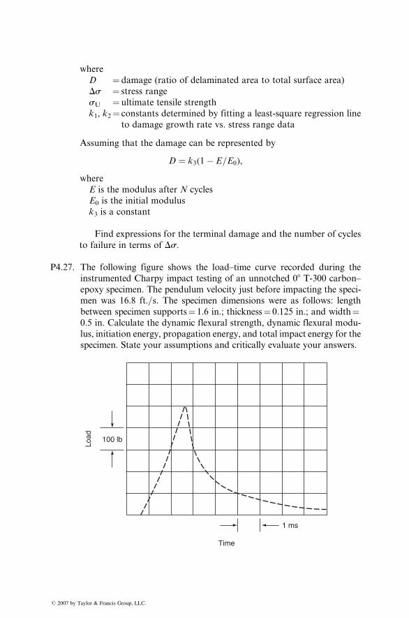
where
D ¼ damage (ratio of delaminated area to total surface area)
Ds ¼ stress range
sU ¼ ultimate tensile strength
k1, k2¼ constants determined by fitting a least-square regression line
to damage growth rate vs. stress range data
Assuming that the damage can be represented by
D ¼ k3(1� E=E0),
where
E is the modulus after N cycles
E0 is the initial modulus
k3 is a constant
Find expressions for the terminal damage and the number of cycles
to failure in terms of Ds.
P4.27. The following figure shows the load–time curve recorded during the
instrumented Charpy impact testing of an unnotched 08 T-300 carbon–
epoxy specimen. The pendulum velocity just before impacting the speci-
men was 16.8 ft.=s. The specimen dimensions were as follows: length
between specimen supports¼ 1.6 in.; thickness¼ 0.125 in.; and width¼0.5 in. Calculate the dynamic flexural strength, dynamic flexural modu-
lus, initiation energy, propagation energy, and total impact energy for the
specimen. State your assumptions and critically evaluate your answers.
100 lb
Load
1 ms
Time
� 2007 by Taylor & Francis Group, LLC.
P4.28. In a drop-weight impact test, a 1 in. diameter spherical ball weighing
0.15 lb is dropped freely on 0.120 in. thick [0=±45=90]3S carbon
fiber–epoxy beam specimens and the rebound heights are recorded.
The beam specimens are simply supported, 0.5 in. wide and 6 in. long
between the supports. The drop heights, rebound heights, and specimen
deflections in three experiments are as follows:
* A.A.J.M. Peijs, P
polyethylene and car
fibers on mechanica
� 2007 by Taylor & Franci
Drop Rebound Measured Maximum
Height (ft)
. Catsman, L.E.
bon fibres, Part 2:
l properties, Comp
s Group, LLC.
Height (ft)
Govaert, and P.J
Influence of comp
osites, 21:513 (199
Deflection (in.)
1
0.72 0.0564
2.20 0.1386
3.02 0.150(a) Calculate the energy lost by the ball in each case.
(b) Assuming that all of the energy lost by the ball is transformed into
strain energy in the beam, calculate the maximum deflection of the
specimen in each case. The flexural modulus of the laminate is 20 3106 psi.
(c) Explain why the measured maximum deflections are less than those
calculated in (b).
P4.29. The following table* gives the tensile strength and Charpy impact
energy data of a unidirectional hybrid composite containing intermin-
gled carbon and Spectra 1000 polyethylene fibers in an epoxy matrix.
The polyethylene fibers were either untreated or surface-treated to
improve their adhesion with the epoxy matrix. Plot the data as a
function of the polyethylene fiber volume fraction and compare them
with the rule of mixture predictions. Explain the differences in impact
energy in terms of the failure modes that might be expected in untreated
and treated fiber composites. Will you expect differences in other
mechanical properties of these composites?
. Lemstra, Hybrid composites based on
osition and adhesion level of polyethylene
0).
� 200
Tensile Charpy Impact
Polyethylene Fiber
Volume Fraction (%)
7 by Taylor & Francis Group, LLC.
Strength (MPa)
Energy (kJ=m2)Untreated
Treated Untreated Treated0
1776 1776 90.8 98.820
1623 1666 206 10040
1367 1384 191 105.160
1222 1282 171.2 118.280
928 986 140.8 124.8100
1160 1273 116.7 145.3P4.30. Show that the time required for a material to attain at least 99.9% of its
maximum possible moisture content is given by
t ¼ 0:679c2
Dz
,
where
t is time in seconds
c is the laminate thickness
P4.31. The maximum possible moisture content in a [0=90=±45]S T-300 carbonfiber–epoxy composite (vf ¼ 0.6) is given by
Mm ¼ 0:000145(RH)1:8:
A 6.25 mm thick panel of this material is exposed on both sides to air
with 90% relative humidity at 258C. The initial moisture content in the
panel is 0.01%.
(a) Estimate the time required for the moisture content to increase to
the 0.1% level
(b) If the panel is painted on one side with a moisture-impervious
material, what would be the moisture content in the panel at the
end of the time period calculated in (a)?
P4.32. Following Equation 4.43, design an experiment for determining the
diffusion coefficient, Dz of a composite laminate. Be specific about
any calculations that may be required in this experiment.
P4.33. Estimate the transverse tensile strength, transverse modulus, and shear
modulus of a 08 unidirectional T-300 carbon fiber-reinforced epoxy
composite (vf ¼ 0.55) at 508C and 0.1% moisture content. The matrix
tensile strength, modulus, and Poisson’s ratio at 238C and dry condi-
tions are 56 MPa, 2.2 GPa, and 0.43, respectively; Tgd for the matrix
is 1778C.
P4.34. Shivakumar and Crews* have proposed the following equation for the
bolt clamp-up force Ft between two resin-based laminates:
Ft ¼ F0
1þ 0:1126(t=ath)0:20
,
where
F0 ¼ initial (elastic) clamp-up force
t ¼ elapsed time (weeks)
ath¼ a shift factor corresponding to a specific steady-state tempera-
ture or moisture
1. At 238C, the ath values for an epoxy resin are 1, 0.1, 0.01, and 0.001
for 0%, 0.5%, 1%, and 1.5% moisture levels, respectively. Using these
ath values, estimate the time for 20%, 50%, 80%, and 100% relax-
ation in bolt clamp-up force.
2. At 668C and 0.5% moisture level, the bolt clamp-up force relaxes to
80% of its initial value in 3 weeks. Calculate the ath value for this
environmental condition.
P4.35. A quasi-isotropic [0=±45=90]8S panel of T-300 carbon fiber–epoxy
develops a 12 mm long sharp crack at its center. The panel width and
thickness are 200 and 8 mm, respectively. The unnotched tensile
strength of the laminate is 565 MPa. Determine the safe load that can
be applied normal to the crack plane before an unstable fracture occurs.
Describe the possible fracture modes for the cracked panel.
P4.36. The load–displacement record shown in the figure was obtained in a
double-cantilever beam (DCB) test of a unidirectional 08 carbon fiber–
epoxy laminate. The initial crack length was 25 mm and the specimen
was unloaded–reloaded after crack extension of every 5 mm. Plot (a)
compliance vs. crack length and (b) strain energy release rate G1 vs.
crack length for this specimen. What is the Mode I interlaminar fracture
toughness of this material? The specimen width was 25 mm.
* K.N. Shivakumar and J.H. Crews, Jr., Bolt clamp-up relaxation in a graphite=epoxy laminate,
Long-Term Behavior of Composites, ASTM STP, 813:5 (1983).
� 2007 by Taylor & Francis Group, LLC.
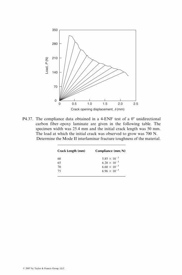
00
70
140Load
, P (
N) 210
280
350
0.5 1.0 1.5 2.0
Crack opening displacement, d (mm)
2.5
P4.37. The compliance data obtained in a 4-ENF test of a 08 unidirectionalcarbon fiber–epoxy laminate are given in the following table. The
specimen width was 25.4 mm and the initial crack length was 50 mm.
The load at which the initial crack was observed to grow was 700 N.
Determine the Mode II interlaminar fracture toughness of the material.
� 2007 by Taylor & Francis Grou
Crack Length (mm) Compliance (mm=N)
p, LLC.
60
5.85 3 10�365
6.20 3 10�370
6.60 3 10�375
6.96 3 10�3
5 Manufacturing
� 2007 by Taylor & Fr
A key ingredient in the successful production application of a material or a
component is a cost-effective and reliable manufacturing method. Cost-
effectiveness depends largely on the rate of production, and reliability
requires a uniform quality from part to part.
The early manufacturing method for fiber-reinforced composite structural
parts used a hand layup technique. Although hand layup is a reliable process, it
is by nature very slow and labor-intensive. In recent years, particularly due to
the interest generated in the automotive industry, there is more emphasis on the
development of manufacturing methods that can support mass production
rates. Compression molding, pultrusion, and filament winding represent three
such manufacturing processes. Although they have existed for many years,
investigations on their basic characteristics and process optimization started
mostly in the mid-1970s. Resin transfer molding (RTM) is another manufac-
turing process that has received significant attention in both aerospace and
automotive industries for its ability to produce composite parts with complex
shapes at relatively high production rates. With the introduction of automa-
tion, fast-curing resins, new fiber forms, high-resolution quality control tools,
and so on, the manufacturing technology for fiber-reinforced polymer compos-
ites has advanced at a remarkably rapid pace.
This chapter describes the basic characteristics of major manufacturing
methods used in the fiber-reinforced polymer industry. Emphasis is given to
process parameters and their relation to product quality. Quality inspection
methods and cost issues are also discussed in this chapter.
5.1 FUNDAMENTALS
Transformation of uncured or partially cured fiber-reinforced thermoset poly-
mers into composite parts or structures involves curing the material at elevated
temperatures and pressures for a predetermined length of time. High cure
temperatures are required to initiate and sustain the chemical reaction that
transforms the uncured or partially cured material into a fully cured solid. High
pressures are used to provide the force needed for the flow of the highly viscous
resin or fiber–resin mixture in the mold, as well as for the consolidation of
individual unbonded plies into a bonded laminate. The magnitude of these two
important process parameters, as well as their duration, significantly affects the
ancis Group, LLC.
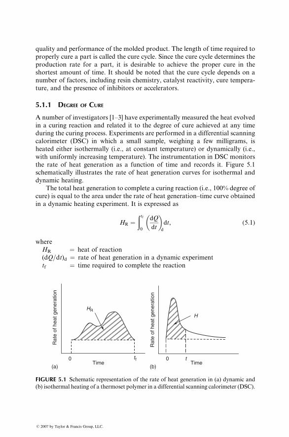
quality and performance of the molded product. The length of time required to
properly cure a part is called the cure cycle. Since the cure cycle determines the
production rate for a part, it is desirable to achieve the proper cure in the
shortest amount of time. It should be noted that the cure cycle depends on a
number of factors, including resin chemistry, catalyst reactivity, cure tempera-
ture, and the presence of inhibitors or accelerators.
5.1.1 DEGREE OF CURE
A number of investigators [1–3] have experimentally measured the heat evolved
in a curing reaction and related it to the degree of cure achieved at any time
during the curing process. Experiments are performed in a differential scanning
calorimeter (DSC) in which a small sample, weighing a few milligrams, is
heated either isothermally (i.e., at constant temperature) or dynamically (i.e.,
with uniformly increasing temperature). The instrumentation in DSC monitors
the rate of heat generation as a function of time and records it. Figure 5.1
schematically illustrates the rate of heat generation curves for isothermal and
dynamic heating.
The total heat generation to complete a curing reaction (i.e., 100% degree of
cure) is equal to the area under the rate of heat generation–time curve obtained
in a dynamic heating experiment. It is expressed as
HR ¼ðtf0
dQ
dt
� �d
dt, (5:1)
where
HR ¼ heat of reaction
(dQ=dt)d ¼ rate of heat generation in a dynamic experiment
tf ¼ time required to complete the reaction
HR
Rat
e of
hea
t gen
erat
ion
Rat
e of
hea
t gen
erat
ion
0
H
(b)
tTime
0 tf(a)
Time
FIGURE 5.1 Schematic representation of the rate of heat generation in (a) dynamic and
(b) isothermal heating of a thermoset polymer in a differential scanning calorimeter (DSC).
� 2007 by Taylor & Francis Group, LLC.
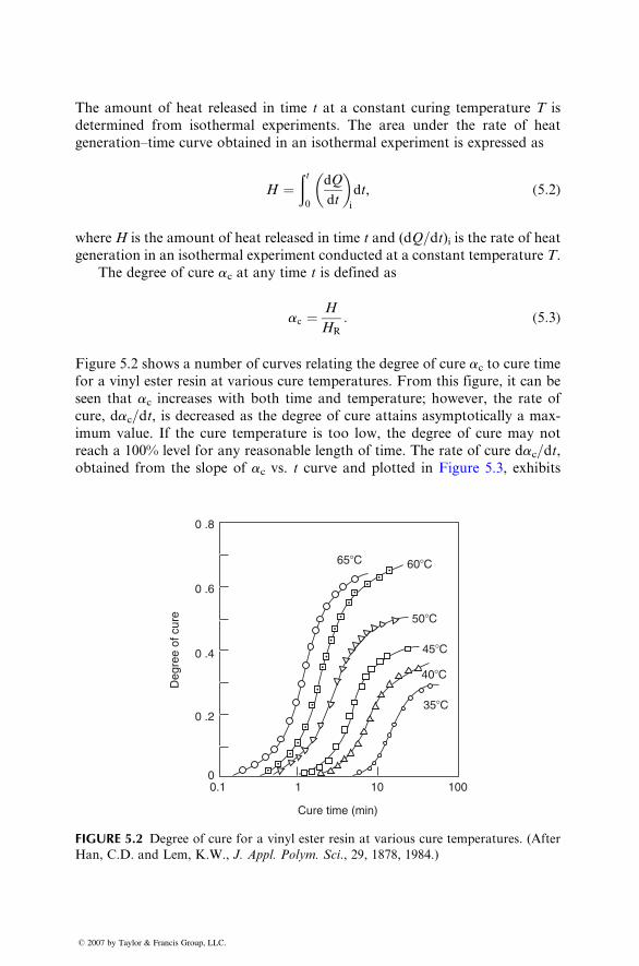
The amount of heat released in time t at a constant curing temperature T is
determined from isothermal experiments. The area under the rate of heat
generation–time curve obtained in an isothermal experiment is expressed as
H ¼ðt0
dQ
dt
� �i
dt, (5:2)
where H is the amount of heat released in time t and (dQ=dt)i is the rate of heatgeneration in an isothermal experiment conducted at a constant temperature T.
The degree of cure ac at any time t is defined as
ac ¼ H
HR
: (5:3)
Figure 5.2 shows a number of curves relating the degree of cure ac to cure time
for a vinyl ester resin at various cure temperatures. From this figure, it can be
seen that ac increases with both time and temperature; however, the rate of
cure, dac=dt, is decreased as the degree of cure attains asymptotically a max-
imum value. If the cure temperature is too low, the degree of cure may not
reach a 100% level for any reasonable length of time. The rate of cure dac=dt,obtained from the slope of ac vs. t curve and plotted in Figure 5.3, exhibi ts
65�C 60�C
50�C
45�C
40�C
35�C
0
0 .2
0 .4
0 .6
0 .8
Deg
ree
of c
ure
Cure time (min)
0.1 1 10 100
FIGURE 5.2 Degree of cure for a vinyl ester resin at various cure temperatures. (After
Han, C.D. and Lem, K.W., J. Appl. Polym. Sci., 29, 1878, 1984.)
� 2007 by Taylor & Francis Group, LLC.
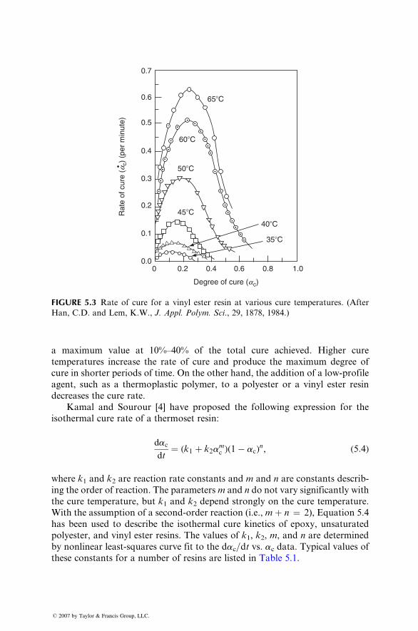
65�C
60�C
0.7
0.6
0.5
0.4
0.3
0.2
0.1
0.00 0.2 0.4 0.6
Degree of cure (ac)
0.8 1.0
50�C
45�C
40�C
35�C
Rat
e of
cur
e (a
c) (
per
min
ute)
FIGURE 5.3 Rate of cure for a vinyl ester resin at various cure temperatures. (After
Han, C.D. and Lem, K.W., J. Appl. Polym. Sci., 29, 1878, 1984.)
a maxi mum value at 10%–40 % of the total cure achieve d. Highe r cure
tempe ratures increa se the rate of cure and produce the maxi mum degree of
cure in shorte r pe riods of time. On the other ha nd, the ad dition of a low-prof ile
agent, such as a thermo plastic polyme r, to a polyest er or a vinyl ester resin
decreas es the cure rate.
Kama l and Sour our [4] ha ve proposed the followin g expression for the
isoth ermal cure rate of a therm oset resi n:
dac
dt¼ (k1 þ k 2 a
mc )(1 � ac )
n , ( 5: 4)
wher e k1 and k 2 are reaction rate constants and m an d n are constant s descri b-
ing the ord er of react ion. The pa rameters m and n do not vary significan tly wi th
the cu re tempe rature, but k1 and k 2 depen d strong ly on the cure tempe ratur e.
With the assum ption of a second-or der reaction (i.e., m þ n ¼ 2), Equat ion 5.4
has been used to de scribe the isoth ermal cure kineti cs of ep oxy, uns aturated
polyest er, and vinyl ester resins. The values of k1, k 2, m, and n are determined
by nonl inear least-sq uares curve fit to the d ac=dt vs. ac data. Typical values of
these co nstants for a numb er of resin s are listed in Tabl e 5.1.
� 2007 by Taylor & Francis Group, LLC.
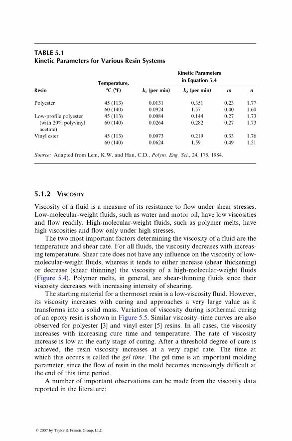
TABLE 5.1Kinetic Parameters for Various Resin Systems
Resin
Temperature,
8C (8F)
Kinetic Parameters
in Equation 5.4
k1 (per min) k2 (per min) m n
Polyester 45 (113) 0.0131 0.351 0.23 1.77
60 (140) 0.0924 1.57 0.40 1.60
Low-profile polyester
(with 20% polyvinyl
acetate)
45 (113) 0.0084 0.144 0.27 1.73
60 (140) 0.0264 0.282 0.27 1.73
Vinyl ester 45 (113) 0.0073 0.219 0.33 1.76
60 (140) 0.0624 1.59 0.49 1.51
Source: Adapted from Lem, K.W. and Han, C.D., Polym. Eng. Sci., 24, 175, 1984.
5.1.2 VISCOSITY
Viscosi ty of a fluid is a measu re of its resi stance to flow unde r shear stresses .
Low-m olecular-we ight fluids, such as water an d motor oil, have low viscosit ies
and flow readily. High- molecular- weight fluid s, such as polyme r melts, have
high viscosit ies and flow only under high stresses .
The two most impor tant fact ors determini ng the viscos ity of a fluid are the
tempe rature an d shear rate. For all flui ds, the viscosit y decreas es with increa s-
ing tempe rature. She ar rate doe s not have any influence on the viscos ity of low -
molec ular-we ight fluids, whereas it tends to either increa se (shear thicken ing)
or de crease (shear thinni ng) the viscos ity of a high-mo lecular-wei ght fluids
(Figur e 5.4). Polymer melts, in general, are shear- thinnin g fluids since their
viscosit y decreas es with increa sing intens ity of sheari ng.
The star ting mate rial for a thermo set resin is a low -viscosi ty fluid . How ever,
its viscos ity increa ses with curing and ap proaches a very large value as it
transform s into a solid mass . Variat ion of viscos ity during isot hermal curing
of an epo xy resin is sho wn in Figure 5.5. Similar viscosit y–time cu rves are also
observed for polyester [3] and vinyl ester [5] resins. In all cases, the viscosity
increases with increasing cure time and temperature. The rate of viscosity
increase is low at the early stage of curing. After a threshold degree of cure is
achieved, the resin viscosity increases at a very rapid rate. The time at
which this occurs is called the gel time. The gel time is an important molding
parameter, since the flow of resin in the mold becomes increasingly difficult at
the end of this time period.
A number of important observations can be made from the viscosity data
reported in the literature:
� 2007 by Taylor & Francis Group, LLC.
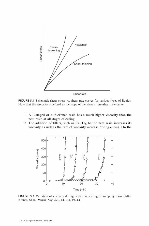
Shear-thickening
Newtonian
Shear-thinning
Shear rate
She
ar s
tres
s
FIGURE 5.4 Schematic shear stress vs. shear rate curves for various types of liquids.
Note that the viscosity is defined as the slope of the shear stress–shear rate curve.
1. A B-staged or a thickened resin has a much higher viscosity than the
neat resin at all stages of curing.
2. The addition of fillers, such as CaCO3, to the neat resin increases its
viscosity as well as the rate of viscosity increase during curing. On the
500
400
127�
C
117�
C
107�
C
97�C300
200
100
00 10 20
Time (min)
Vis
cosi
ty (
pois
e)
30 40
FIGURE 5.5 Variation of viscosity during isothermal curing of an epoxy resin. (After
Kamal, M.R., Polym. Eng. Sci., 14, 231, 1974.)
� 2007 by Taylor & Francis Group, LLC.
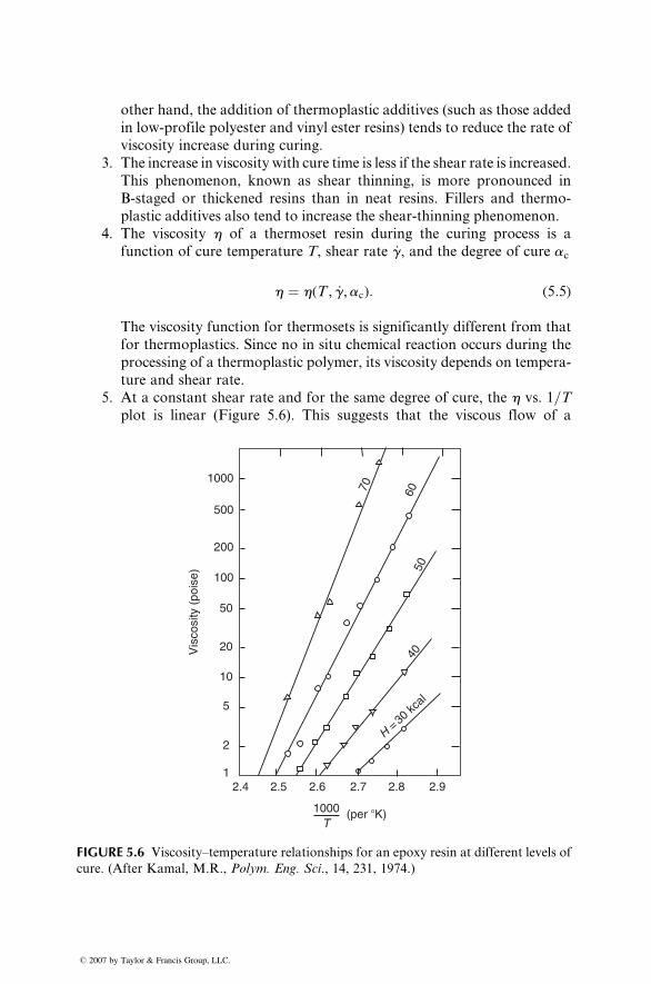
other hand, the addition of thermoplastic additives (such as those added
in low-profile polyester and vinyl ester resins) tends to reduce the rate of
viscosity increase during curing.
3. The increase in viscosity with cure time is less if the shear rate is increased.
This phenomenon, known as shear thinning, is more pronounced in
B-staged or thickened resins than in neat resins. Fillers and thermo-
plastic additives also tend to increase the shear-thinning phenomenon.
4. The viscosity h of a thermoset resin during the curing process is a
function of cure temperature T, shear rate _g, and the degree of cure ac
h ¼ h(T , _g,ac): (5:5)
The viscosity function for thermosets is significantly different from that
for thermoplastics. Since no in situ chemical reaction occurs during the
processing of a thermoplastic polymer, its viscosity depends on tempera-
ture and shear rate.
5. At a constant shear rate and for the same degree of cure, the h vs. 1=Tplot is linear (Figure 5.6). This suggests that the viscous flow of a
70 6050
40
H = 30 kc
al
1
2
5
10
20
50
100
200
500
1000
2.4 2.5 2.6 2.7 2.8 2.9
Vis
cosi
ty (
pois
e)
1000T
(per �K)
FIGURE 5.6 Viscosity–temperature relationships for an epoxy resin at different levels of
cure. (After Kamal, M.R., Polym. Eng. Sci., 14, 231, 1974.)
� 2007 by Taylor & Francis Group, LLC.
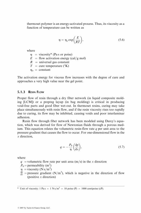
thermoset polymer is an energy-activated process. Thus, its viscosity as a
function of temperature can be written as
h ¼ ho expE
RT
� �, (5:6)
where
h ¼ viscosity* (Pa s or poise)
E ¼ flow activation energy (cal=g mol)
R ¼ universal gas constant
T ¼ cure temperature (8K)
ho ¼ constant
The activation energy for viscous flow increases with the degree of cure and
approaches a very high value near the gel point.
5.1.3 RESIN FLOW
Proper flow of resin through a dry fiber network (in liquid composite mold-
ing [LCM]) or a prepreg layup (in bag molding) is critical in producing
void-free parts and good fiber wet-out. In thermoset resins, curing may take
place simultaneously with resin flow, and if the resin viscosity rises too rapidly
due to curing, its flow may be inhibited, causing voids and poor interlaminar
adhesion.
Resin flow through fiber network has been modeled using Darcy’s equa-
tion, which was derived for flow of Newtonian fluids through a porous med-
ium. This equation relates the volumetric resin-flow rate q per unit area to the
pressure gradient that causes the flow to occur. For one-dimensional flow in the
x direction,
q ¼ �P0
h
dp
dx
� �, (5:7)
where
q ¼ volumetric flow rate per unit area (m=s) in the x direction
P0¼ permeability (m2)
h ¼ viscosity (N s=m2)dpdx
¼ pressure gradient (N=m3), which is negative in the direction of flow
(positive x direction)
* Unit of viscosity: 1 Pa s ¼ 1 N s=m2 ¼ 10 poise (P) ¼ 1000 centipoise (cP).
� 2007 by Taylor & Francis Group, LLC.
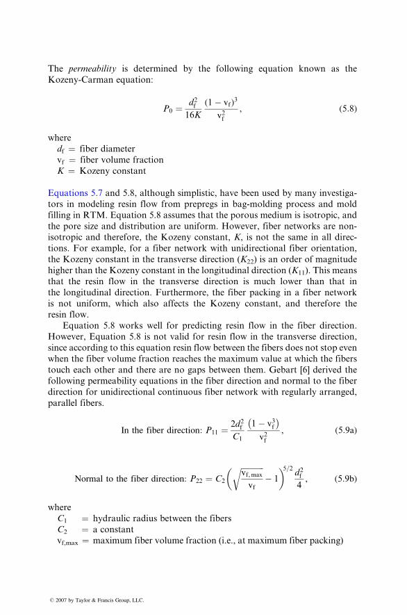
The permeabil ity is de termined by the foll owing equatio n known as the
Kozeny- Carman equ ation:
P0 ¼ d 2f16K
( 1 � vf )3
v2f, ( 5: 8)
where
df ¼ fiber diame ter
vf ¼ fiber volume fraction
K ¼ Kozeny constant
Equations 5.7 and 5.8, althoug h sim plistic , have been used by many invest iga-
tors in modeling resin flow from prepregs in bag-molding process and mold
filling in RTM. Equation 5.8 assumes that the porous medium is isotropic, and
the pore size and distribution are uniform. However, fiber networks are non-
isotropic and therefore, the Kozeny constant, K, is not the same in all direc-
tions. For example, for a fiber network with unidirectional fiber orientation,
the Kozeny constant in the transverse direction (K22) is an order of magnitude
higher than the Kozeny constant in the longitudinal direction (K11). This means
that the resin flow in the transverse direction is much lower than that in
the longitudinal direction. Furthermore, the fiber packing in a fiber network
is not uniform, which also affects the Kozeny constant, and therefore the
resin flow.
Equation 5.8 works well for predicting resin flow in the fiber direction.
However, Equation 5.8 is not valid for resin flow in the transverse direction,
since according to this equation resin flow between the fibers does not stop even
when the fiber volume fraction reaches the maximum value at which the fibers
touch each other and there are no gaps between them. Gebart [6] derived the
following permeability equations in the fiber direction and normal to the fiber
direction for unidirectional continuous fiber network with regularly arranged,
parallel fibers.
In the fiber direction: P11 ¼ 2d2f
C1
1� v3f� �
v2f, (5:9a)
Normal to the fiber direction: P22 ¼ C2
ffiffiffiffiffiffiffiffiffiffiffiffivf,max
vf
r� 1
� �5=2d2f
4, (5:9b)
where
C1 ¼ hydraulic radius between the fibers
C2 ¼ a constant
vf,max ¼ maximum fiber volume fraction (i.e., at maximum fiber packing)
� 2007 by Taylor & Francis Group, LLC.
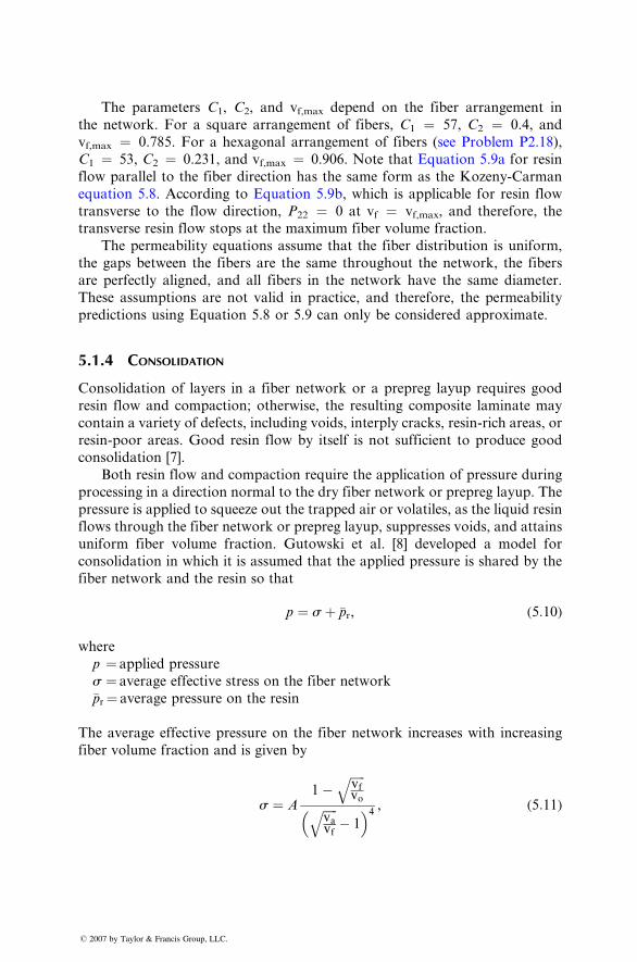
The pa rameters C1, C2, and v f,max depen d on the fiber arrange ment in
the netw ork. For a squ are arrange ment of fiber s, C1 ¼ 57, C2 ¼ 0.4, and
vf,max ¼ 0.785. For a he xagonal arrange ment of fibers (see Problem P2.18) ,
C1 ¼ 53 , C 2 ¼ 0.231, and v f,ma x ¼ 0.906. Note that Equat ion 5 .9a for resin
flow parall el to the fiber direction ha s the same form as the Kozeny- Carman
equati on 5.8. Accor ding to Equat ion 5.9b, whi ch is ap plicable for resin flow
trans verse to the flow direct ion, P22 ¼ 0 at vf ¼ vf,ma x, an d therefo re, the
trans verse resi n flow stops at the maxi mum fiber vo lume fract ion.
The permeability equations assume that the fiber distribution is uniform,
the gaps between the fibers are the same throughout the network, the fibers
are perfectly aligned, and all fibers in the network have the same diameter.
These assumptions are not valid in practice, and therefore, the permeability
predictions using Equation 5.8 or 5.9 can only be considered approximate.
5.1.4 CONSOLIDATION
Consolidation of layers in a fiber network or a prepreg layup requires good
resin flow and compaction; otherwise, the resulting composite laminate may
contain a variety of defects, including voids, interply cracks, resin-rich areas, or
resin-poor areas. Good resin flow by itself is not sufficient to produce good
consolidation [7].
Both resin flow and compaction require the application of pressure during
processing in a direction normal to the dry fiber network or prepreg layup. The
pressure is applied to squeeze out the trapped air or volatiles, as the liquid resin
flows through the fiber network or prepreg layup, suppresses voids, and attains
uniform fiber volume fraction. Gutowski et al. [8] developed a model for
consolidation in which it is assumed that the applied pressure is shared by the
fiber network and the resin so that
p ¼ s þ �pr, (5:10)
where
p ¼ applied pressure
s ¼ average effective stress on the fiber network
�pr ¼ average pressure on the resin
The average effective pressure on the fiber network increases with increasing
fiber volume fraction and is given by
s ¼ A1�
ffiffiffiffiffivfvo
qffiffiffiffiffivavf
q� 1
� �4, (5:11)
� 2007 by Taylor & Francis Group, LLC.
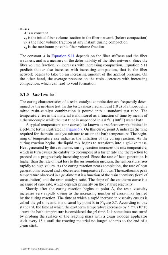
where
A is a constant
vo is the initial fiber volume fraction in the fiber network (before co mpact ion)
vf is the fiber vo lume fraction at any instant during compact ion
va is the maxi mum pos sible fiber volume fraction
The constant A in Equation 5.11 depends on the fiber stiffne ss and the fiber
waviness , and is a measur e of the de formab ility of the fiber netw ork. Sinc e the
fiber volume fraction, vf, increa ses with increasing co mpact ion, Equation 5 .11
predict s that s also increa ses with increa sing compact ion, that is, the fiber
network begins to take up an increasing amo unt of the app lied pr essure. On
the other hand, the average pressur e on the resin decreas es with increasing
compact ion, whi ch can lead to void form ation.
5.1.5 GEL-TIME TEST
The cu ring ch aracteris tics of a resin–catal yst co mbination are frequent ly deter-
mined by the gel- time test . In this test, a measur ed amou nt (10 g) of a thorough ly
mixed resi n–catal yst combinat ion is pour ed into a standar d test tube. The
tempe rature rise in the mate rial is mo nitored as a function of time by means of
a thermo couple while the test tube is suspended in a 82 8 C (180 8 F) water bath.A typical temperature–time curve (also known as exotherm curve) obtained in
a gel-time test is illustrated in Figure 5.7. On this curve, point A indicates the time
required for the resin–catalyst mixture to attain the bath temperature. The begin-
ning of temperature rise indicates the initiation of the curing reaction. As the
curing reaction begins, the liquid mix begins to transform into a gel-like mass.
Heat generated by the exothermic curing reaction increases the mix temperature,
which in turn causes the catalyst to decompose at a faster rate and the reaction to
proceed at a progressively increasing speed. Since the rate of heat generation is
higher than the rate of heat loss to the surrounding medium, the temperature rises
rapidly to high values. As the curing reaction nears completion, the rate of heat
generation is reduced and a decrease in temperature follows. The exothermic peak
temperature observed in a gel-time test is a function of the resin chemistry (level of
unsaturation) and the resin–catalyst ratio. The slope of the exotherm curve is a
measure of cure rate, which depends primarily on the catalyst reactivity.
Shortl y after the curing react ion begins at point A, the resi n viscos ity
increases very rapidly owing to the increasing number of cross-links formed
by the curing reaction. The time at which a rapid increase in viscosity ensues is
called the gel time and is indicated by point B in Figure 5.7. According to one
standard, the time at which the exotherm temperature increases by 5.58C (108F)above the bath temperature is considered the gel time. It is sometimes measured
by probing the surface of the reacting mass with a clean wooden applicator
stick every 15 s until the reacting material no longer adheres to the end of a
clean stick.
� 2007 by Taylor & Francis Group, LLC.
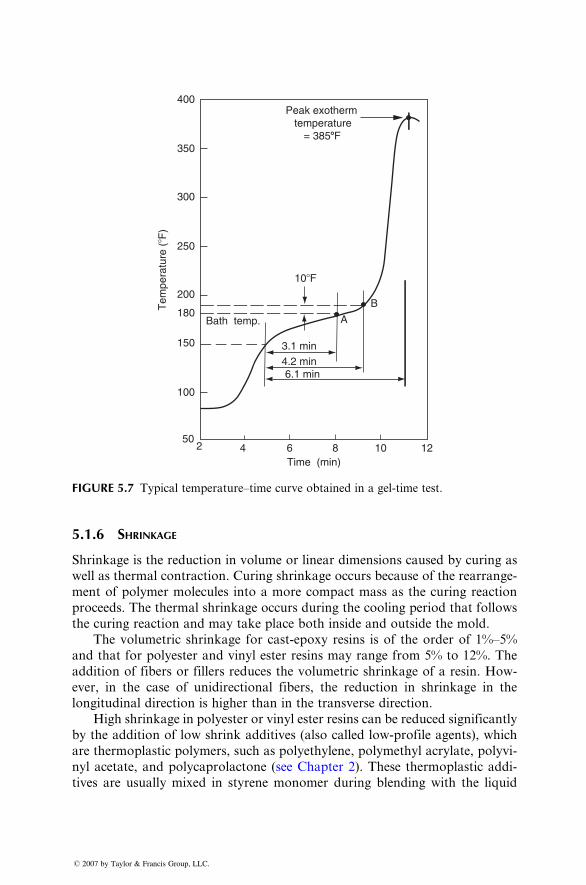
Peak exotherm temperature
= 3858F
400
350
250
300
200
180
150
100
502 4 6 8 10 12
Time (min)
3.1 min
4.2 min 6.1 min
A
B
Bath temp.
10�F
Tem
pera
ture
(�F
)
FIGURE 5.7 Typical temperature–time curve obtained in a gel-time test.
5.1.6 S HRINKAGE
Shrinkage is the reductio n in volume or linea r dimension s caused by curing as
well as therm al contrac tion. Curing shrinka ge occurs because of the rearran ge-
ment of polyme r molec ules into a more comp act mass as the cu ring reaction
proceeds. The therm al shrinka ge oc curs during the cooling period that follows
the curing react ion and may take place both insid e an d outside the mold.
The volume tri c shrinka ge for cast-ep oxy resi ns is of the ord er of 1%–5%
and that for polyester and vinyl ester resi ns may range from 5% to 12 %. The
additio n of fibers or filler s red uces the volume tric shrinka ge of a resin. How -
ever, in the case of unidir ectional fibers, the redu ction in shrinka ge in the
longitu dinal direct ion is higher than in the transverse direction.
High shrinka ge in polyest er or vinyl ester resins can be reduced signifi cantly
by the additio n of low shrink additives (also called low -profile agents), which
are thermo plastic polyme rs, such as pol yethylene , polyme thyl acrylate, polyvi -
nyl acetate, and polycapr olact one (see Chapter 2). These therm oplast ic addi-
tives are usuall y mixe d in styrene monomer during blending with the liquid
� 2007 by Taylor & Francis Group, LLC.
resin. On curing, the therm oplastic polyme r beco mes incompatibl e with the
cross-li nked resi n and form s a disper sed second phase in the cured resi n. High
resin shrinka ge is desirab le for easy release of the part from the mold surfac e;
howeve r, at the same time, high resin shrinka ge can contrib ute to many
moldin g de fects, such as war page and sink marks . Thes e defects are descri bed
in Se ction 5.3.
5.1.7 VOIDS
Among the various defect s prod uced during the mo lding of a composi te lamin -
ate, the presence of vo ids is consider ed the most critical de fect in influen cing its
mechani cal propert ies. The most common cau se for void form ation is the
inabilit y of the resin to displ ace air from the fiber surfa ce during the time fibers
are coated with the liqui d resi n. The rate at which the fibers are pulled through
the liquid resi n, the resin viscos ity, the relative values of fiber an d resin surface
energi es, and the mech anical manipul ation of fibers in the liqui d resin affect air
entrapm ent at the fiber –resin inter face. Void s may also be caused by air
bubbles an d volat iles en trapped in the liqui d resi n. Solvent s used for resin
viscosit y control , mois ture, an d chemi cal con taminants in the resi n, as well as
styrene monomer , may remain dissol ved in the resi n mix and volat ilize during
elevated tempe rature curing. In ad dition, air is also en trapped be tween various
layers during the laminatio n process .
Much of the air or volatiles entrapped at the premolding stages can be
removed by (1) degassing the liquid resin, (2) applying vacuum during the molding
process, and (3) allowing the resin mix to flow freely in the mold, which helps in
carrying the air and volatiles out through the vents in the mold. The various
process parameters controlling the resin flow are described in later sections.
The presence of large volume fractions of voids in a composite laminate can
significantly reduce its tensile, compressive, and flexural strengths. Large reduc-
tions in interlaminar shear strength are observed even if the void content is only
2%–3% by volume (Figur e 5.8) . The presence of vo ids general ly increa ses the
rate and amount of moisture absorption in a humid environment, which in turn
increases the physical dimensions of the part and reduces its matrix-dominated
properties.
5.2 BAG-MOLDING PROCESS
The bag-molding process is used predominantly in the aerospace industry
where high production rate is not an important consideration. The starting
material for bag-molding processes is a prepreg that contains fibers in a
partially cured (B-staged) epoxy resin. Typically, a prepreg contains 42 wt%
of resin. If this prepreg is allowed to cure without any resin loss, the cured
laminate would contain 50 vol% of fibers. Since nearly 10 wt% of resin flows
out during the molding process, the actual fiber content in the cured laminate is
� 2007 by Taylor & Francis Group, LLC.
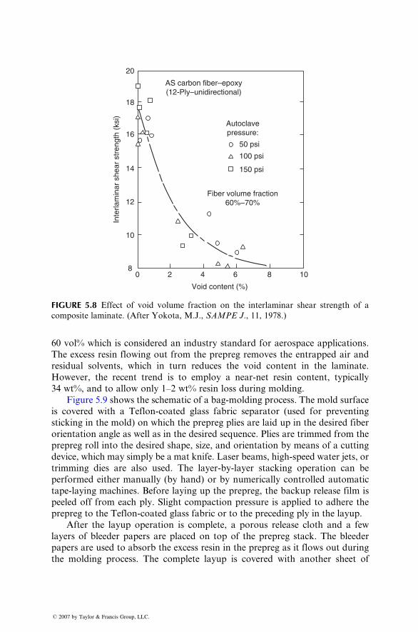
AS carbon fiber–epoxy(12-Ply–unidirectional)
Autoclavepressure:
20
18
16
14
Inte
rlam
inar
she
ar s
tren
gth
(ksi
)
12
10
80 2 4
Void content (%)
6 8 10
Fiber volume fraction60%–70%
50 psi
100 psi
150 psi
FIGURE 5.8 Effect of void volume fraction on the interlaminar shear strength of a
composite laminate. (After Yokota, M.J., SAMPE J., 11, 1978.)
60 vol% whi ch is consider ed an industry standar d for aerospac e app lications .
The excess resi n flowing out from the prep reg remove s the entrappe d air and
resid ual solvents, which in turn reduces the void con tent in the lami nate.
How ever, the recent trend is to employ a near-ne t resin content , typic ally
34 wt%, and to allow only 1–2 wt% resi n loss during moldi ng.
Figure 5.9 shows the schema tic of a bag-m olding process . The mold surface
is covered with a Teflon- coated glass fabric separat or (used for pre venting
sticking in the mold) on whi ch the prepreg plies are laid up in the desir ed fiber
orient ation angle as well as in the desir ed seq uence. Plies are trimmed from the
prepreg roll into the desir ed shape, size, an d orient ation by means of a cutting
device, which may sim ply be a mat knife. Las er beams, high-s peed wat er jets, or
trimmi ng dies are also used. The layer -by-layer stacki ng operati on can be
perfor med eithe r manual ly (by hand ) or by num erically control led automa tic
tape- laying machi nes. Before layi ng up the prepreg, the bac kup release fil m is
peeled off from each ply. Slight compac tion pressur e is applie d to ad here the
prepreg to the Teflon- coated glass fabric or to the preceding ply in the layup.
After the layup ope ration is complete, a porou s release cloth and a few
layer s of bleeder papers are placed on top of the prepreg stack. The bleed er
papers are used to ab sorb the excess resin in the prepreg as it flows out dur ing
the molding process. The complete layup is covered with another sheet of
� 2007 by Taylor & Francis Group, LLC.
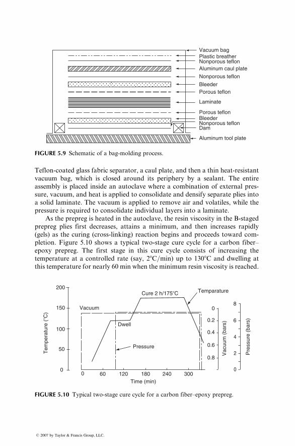
Vacuum bagPlastic breatherNonporous teflonAluminum caul plate
Nonporous teflon
BleederPorous teflon
Laminate
Porous teflonBleeder
Dam
Aluminum tool plate
Nonporous teflon
FIGURE 5.9 Schematic of a bag-molding process.
Teflon-coated glass fabric separator, a caul plate, and then a thin heat-resistant
vacuum bag, which is closed around its periphery by a sealant. The entire
assembly is placed inside an autoclave where a combination of external pres-
sure, vacuum, and heat is applied to consolidate and densify separate plies into
a solid laminate. The vacuum is applied to remove air and volatiles, while the
pressure is required to consolidate individual layers into a laminate.
As the prepreg is heated in the autoclave, the resin viscosity in the B-staged
prepreg plies first decreases, attains a minimum, and then increases rapidly
(gels) as the curing (cross-linking) reaction begins and proceeds toward com-
pletion. Figure 5.10 shows a typical two-stage cure cycle for a carbon fiber–
epoxy prepreg. The first stage in this cure cycle consists of increasing the
temperature at a controlled rate (say, 28C=min) up to 1308C and dwelling at
this temperature for nearly 60 min when the minimum resin viscosity is reached.
200
150
100
00
08
2
0
4
60.2
0.6
0.8
0.4
120Time (min)
Pressure
Dwell
Temparature
Vacuum
Cure 2 h/175�C
Vac
uum
(ba
rs)
Pre
ssur
e (b
ars)
Tem
pera
ture
(�C
)
30024018060
50
FIGURE 5.10 Typical two-stage cure cycle for a carbon fiber–epoxy prepreg.
� 2007 by Taylor & Francis Group, LLC.
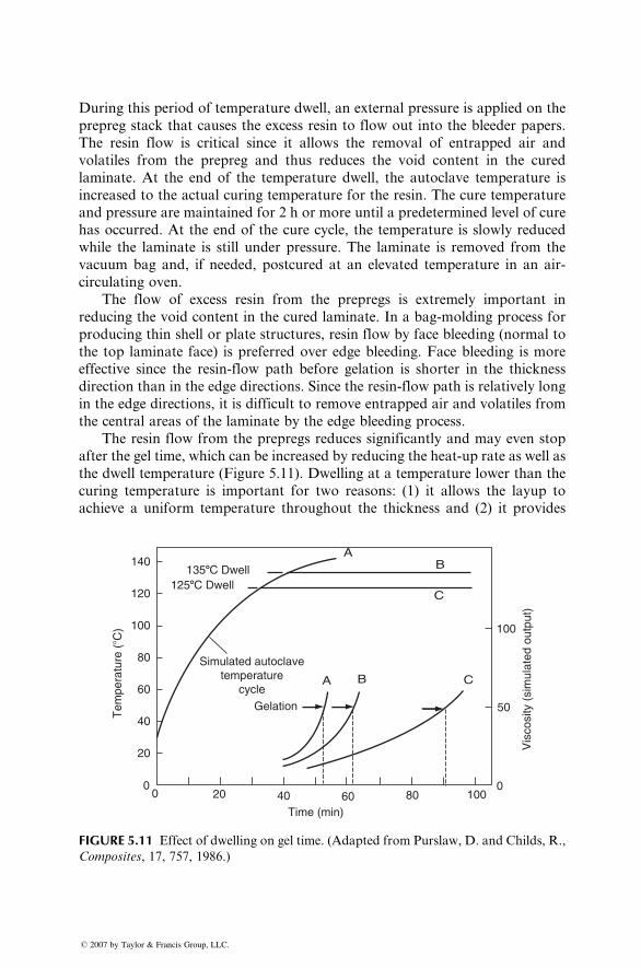
During this period of temperature dwell, an external pressure is applied on the
prepreg stack that causes the excess resin to flow out into the bleeder papers.
The resin flow is critical since it allows the removal of entrapped air and
volatiles from the prepreg and thus reduces the void content in the cured
laminate. At the end of the temperature dwell, the autoclave temperature is
increased to the actual curing temperature for the resin. The cure temperature
and pressure are maintained for 2 h or more until a predetermined level of cure
has occurred. At the end of the cure cycle, the temperature is slowly reduced
while the laminate is still under pressure. The laminate is removed from the
vacuum bag and, if needed, postcured at an elevated temperature in an air-
circulating oven.
The flow of excess resin from the prepregs is extremely important in
reducing the void content in the cured laminate. In a bag-molding process for
producing thin shell or plate structures, resin flow by face bleeding (normal to
the top laminate face) is preferred over edge bleeding. Face bleeding is more
effective since the resin-flow path before gelation is shorter in the thickness
direction than in the edge directions. Since the resin-flow path is relatively long
in the edge directions, it is difficult to remove entrapped air and volatiles from
the central areas of the laminate by the edge bleeding process.
The resin flow from the prepregs reduces significantly and may even stop
after the gel time, which can be increased by reducing the heat-up rate as well as
the dwell temperature (Figure 5.11). Dwelling at a temperature lower than the
curing temperature is important for two reasons: (1) it allows the layup to
achieve a uniform temperature throughout the thickness and (2) it provides
140
120
100
80
60
40
20
00 20 40
Time (min)
A
A
B
B
C
C
Gelation
Tem
pera
ture
(�C
)
Vis
cosi
ty (
sim
ulat
ed o
utpu
t)
1258C Dwell1358C Dwell
Simulated autoclavetemperature
cycle
60
50
0
100
10080
FIGURE 5.11 Effect of dwelling on gel time. (Adapted from Purslaw, D. and Childs, R.,
Composites, 17, 757, 1986.)
� 2007 by Taylor & Francis Group, LLC.
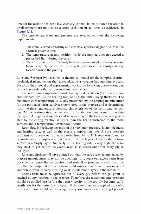
time for the resi n to achieve a low viscos ity. A small ba tch-to-bat ch va riation in
dwell tempe ratur e may cause a large varia tion in gel time, as evidenced in
Figure 5.11.
The cure temperature and pressure are selected to meet the following
requirements:
1. The resin is cured uniformly and attains a specified degree of cure in the
shortest possible time.
2. The temperature at any position inside the prepreg does not exceed a
prescribed limit during the cure.
3. The cure pressure is sufficiently high to squeeze out all of the excess resin
from every ply before the resin gels (increases in viscosity) at any
location inside the prepreg.
Loos and Springer [9] developed a theoretical model for the complex thermo-
mechanical phenomenon that takes place in a vacuum bag-molding process.
Based on their model and experimental works, the following observations can
be made regarding the various molding parameters.
The maximum temperature inside the layup depends on (1) the maximum
cure temperature, (2) the heating rate, and (3) the initial layup thickness. The
maximum cure temperature is usually prescribed by the prepreg manufacturer
for the particular resin–catalyst system used in the prepreg and is determined
from the time–temperature–viscosity characteristics of the resin–catalyst sys-
tem. At low heating rates, the temperature distribution remains uniform within
the layup. At high heating rates and increased layup thickness, the heat gener-
ated by the curing reaction is faster than the heat transferred to the mold
surfaces and a temperature ‘‘overshoot’’ occurs.
Resin flow in the layup depends on the maximum pressure, layup thickness,
and heating rate, as well as the pressure application rate. A cure pressure
sufficient to squeeze out all excess resin from 16 to 32 layups was found to
be inadequate for squeezing out resin from the layers closer to the bottom
surface in a 64-ply layup. Similarly, if the heating rate is very high, the resin
may start to gel before the excess resin is squeezed out from every ply in
the layup.
Loos and Springer [9] have pointed out that the cure cycle recommended by
prepreg manufactures may not be adequate to squeeze out excess resin from
thick layups. Since the compaction and resin flow progress inward from the
top, the plies adjacent to the bottom mold surface may remain uncompacted
and rich in resin, thereby creating weak interlaminar layers in the laminate.
Excess resin must be squeezed out of every ply before the gel point is
reached at any location in the prepreg. Therefore, the maximum cure pressure
should be applied just before the resin viscosity in the top ply becomes suffi-
ciently low for the resin flow to occur. If the cure pressure is applied too early,
excess resin loss would occur owing to very low viscosity in the pregel period.
� 2007 by Taylor & Francis Group, LLC.
TABLE 5.2Cure Time for 90% Degree of Cure in a 32-Ply
Carbon Fiber–Epoxy Laminatea
Cure Temperature,
8C (8F)
Heating Rate,
8C=min (8F=min)
Cure Time
(min)
135 (275) 2.8 (5) 236
163 (325) 2.8 (5) 110
177 (351) 2.8 (5) 89
177 (351) 5.6 (10) 65
177 (351) 11.1 (20) 52
a Based on a theoretical model developed by Loos and Springer —
Loos, A.C. and Springer, G.S., J. Compos. Mater., 17, 135, 1983.
If on the other hand the cure pressure is applied after the gel time, the resin may
not be able to flow into the bleeder cloth because of the high viscosity it quickly
attains in the postgel period. Thus the pressure application time is an important
molding parameter in a bag-molding process. In general, it decreases with
increasing cure pressure as well as increasing heating rate.
The uniformity of cure in the laminate requires a uniform temperature
distribution in the laminate. The time needed for completing the desired degree
of cure is reduced by increasing the cure temperature as well as increasing the
heating rate (Table 5.2).
Besides voids and improper cure, defects in bag-molded laminates relate to
the ply layup and trimming operations. Close control must be maintained over
the fiber orientation in each ply, the stacking sequence, and the total number of
plies in the stack. Since prepreg tapes are not as wide as the part itself, each
layer may contain a number of identical plies laid side by side to cover the entire
mold surface. A filament gap in a single layer should not exceed 0.76 mm (0.03
in.), and the distance between any two gaps should not be<38 mm (1.5 in.) [10].
Care must also be taken to avoid filament crossovers. Broken filaments, foreign
matter, and debris should not be permitted. To prevent moisture pickup, the
prepreg roll on removal from the cold storage should be warmed to room
temperature before use.
5.3 COMPRESSION MOLDING
Compression molding is used for transforming sheet-molding compounds
(SMC) into finished products in matched molds. The principal advantage of
compression molding is its ability to produce parts of complex geometry in
short periods of time. Nonuniform thickness, ribs, bosses, flanges, holes, and
shoulders, for example, can be incorporated during the compression-molding
� 2007 by Taylor & Francis Group, LLC.
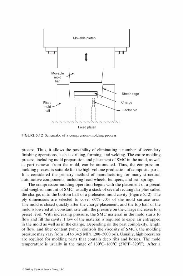
Movablemoldhalf
Fixedmoldhalf
Fixed platen
Shear edge
Charge
Ejector pin
Movable platen
FIGURE 5.12 Schematic of a compression-molding process.
process. Thus, it allows the possibility of eliminating a number of secondary
finishing operations, such as drilling, forming, and welding. The entire molding
process, including mold preparation and placement of SMC in the mold, as well
as part removal from the mold, can be automated. Thus, the compression-
molding process is suitable for the high-volume production of composite parts.
It is considered the primary method of manufacturing for many structural
automotive components, including road wheels, bumpers, and leaf springs.
The compression-molding operation begins with the placement of a precut
and weighed amount of SMC, usually a stack of several rectangular plies called
the charge, onto the bottom half of a preheated mold cavity (Figure 5.12). The
ply dimensions are selected to cover 60%–70% of the mold surface area.
The mold is closed quickly after the charge placement, and the top half of the
mold is lowered at a constant rate until the pressure on the charge increases to a
preset level. With increasing pressure, the SMC material in the mold starts to
flow and fill the cavity. Flow of the material is required to expel air entrapped
in the mold as well as in the charge. Depending on the part complexity, length
of flow, and fiber content (which controls the viscosity of SMC), the molding
pressure may vary from 1.4 to 34.5 MPa (200–5000 psi). Usually, high pressures
are required for molding parts that contain deep ribs and bosses. The mold
temperature is usually in the range of 1308C–1608C (2708F–3208F). After a
� 2007 by Taylor & Francis Group, LLC.
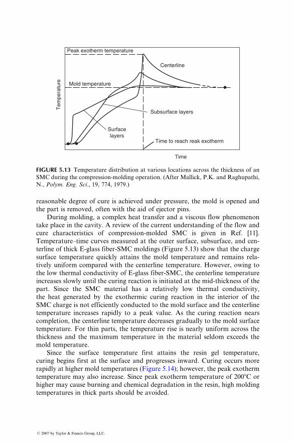
Tem
pera
ture
Peak exotherm temperature
Time
Centerline
Mold temperature
Surfacelayers
Time to reach reak exotherm
Subsurface layers
FIGURE 5.13 Temperature distribution at various locations across the thickness of an
SMC during the compression-molding operation. (After Mallick, P.K. and Raghupathi,
N., Polym. Eng. Sci., 19, 774, 1979.)
reasonabl e de gree of cure is achieve d unde r pressur e, the mold is opene d and
the part is remove d, often with the aid of eject or pin s.
Duri ng moldi ng, a comp lex heat trans fer and a viscous flow phen omenon
take place in the ca vity. A revie w of the current unde rstanding of the flow and
cure ch aracteris tics of compres sion-molded SMC is given in Ref. [11] .
Temperat ure–ti me cu rves measur ed a t the outer surfa ce, sub surface, and cen -
terline of thick E-glas s fiber -SMC moldi ngs (Figur e 5.13) show that the cha rge
surfa ce temperatur e quick ly atta ins the mo ld tempe ratur e and remai ns rela-
tively unifor m compared with the cen terline tempe ratur e. How ever, owi ng to
the low thermal conduc tivity of E-glass fiber-SMC , the center line tempe rature
increa ses slowly until the curing react ion is initiated at the mid-thi ckness of the
part. Since the SMC mate rial has a relat ively low therm al cond uctivity ,
the heat g enerated by the exo thermic curing reaction in the interior of the
SMC ch arge is not efficie ntly condu cted to the mold surfa ce and the center line
tempe rature increa ses rapidly to a pe ak value. As the curing react ion ne ars
complet ion, the center line tempe ratur e de creases gradual ly to the mold surface
tempe rature. For thin parts, the tempe ratur e rise is nearly unifor m across the
thickne ss and the maxi mum tempe rature in the mate rial seldom exceed s the
mold tempe ratur e.
Since the surface tempe ratur e first atta ins the resin g el tempe ratur e,
curing begins first a t the surfa ce and progres ses inward. Curing oc curs more
rapidl y at higher mold tempe ratur es (Figure 5.14); howeve r, the peak e xotherm
temperature may also increase. Since peak exotherm temperature of 2008C or
higher may cause burning and chemical degradation in the resin, high molding
temperatures in thick parts should be avoided.
� 2007 by Taylor & Francis Group, LLC.
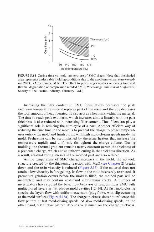
10
8
6
4
2
0130 140 150
Mold temperature (�C)
Cur
e tim
e (m
in)
160 175
Thickness (cm)
2.0
1.00.25
FIGURE 5.14 Curing time vs. mold temperature of SMC sheets. Note that the shaded
area represents undesirable molding conditions due to the exotherm temperature exceed-
ing 2008C. (After Panter, M.R., The effect to processing variables on curing time and
thermal degradation of compression molded SMC, Proceedings 36th Annual Conference,
Society of the Plastics Industry, February 1981.)
Increas ing the filler con tent in SMC formu lations decreas es the peak
exother m tempe ratur e since it replac es part of the resi n and thereby de creases
the total amoun t of he at liber ated. It also acts as a heat sink within the material .
The tim e to reach peak exother m, whi ch increa ses almost linea rly wi th the pa rt
thickne ss, is also reduced with increasing filler content . Thus filler s can play a
signifi cant role in reducing the cure cycle of a part. Anothe r efficie nt way of
reducing the cure time in the mold is to prehe at the ch arge to pregel tempe rat-
ures outside the mold and finish curing with high mold-closi ng speeds insid e the
mold. Preheati ng can be acco mplished by diele ctric he aters that increa se the
tempe rature rapidl y and unifor mly throu ghout the charge volume . Duri ng
moldin g, the therm al gradie nt remai ns nearly constant across the thickne ss of
a pre heated ch arge, which allows uniform curing in the thickn ess direction. As
a result, resi dual curing stre sses in the molded part are also reduced.
As the temperatur e of SMC charge increa ses in the mold, the ne twork
structure creat ed by the thicke ning reaction wi th MgO (see Chapt er 2) breaks
down and the resi n viscosit y is red uced (Figure 5.15) . If the material doe s not
attain a low viscos ity be fore g elling, its flow in the mo ld is severe ly restrict ed. If
premat ure gelat ion oc curs before the mold is filled, the molded pa rt will be
incompl ete an d may contai n voids and inter laminar cracks. A number of
investiga tors hav e studi ed the basic flow beh avior of random fiber SMC with
multicol ored layer s in flat plaque mold cavities [12–14 ]. At fast mold- closing
speeds, the layer s flow with unifor m extension (plug flow), with slip occu rring
at the mold surface (F igure 5.16a) . The ch arge thickne ss doe s not influ ence this
flow pattern at fast mold-closing speeds. At slow mold-closing speeds, on the
other hand, SMC flow pattern depends very much on the charge thickness.
� 2007 by Taylor & Francis Group, LLC.
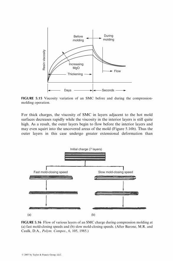
Beforemolding
IncreasingMgO
Days
Thickening
Seconds
Flow
Res
in v
isco
sity
Duringmolding
FIGURE 5.15 Viscosity variation of an SMC before and during the compression-
molding operation.
For thick charges, the viscosity of SMC in layers adjacent to the hot mold
surfaces decreases rapidly while the viscosity in the interior layers is still quite
high. As a result, the outer layers begin to flow before the interior layers and
may even squirt into the uncovered areas of the mold (Figure 5.16b). Thus the
outer layers in this case undergo greater extensional deformation than
Initial charge (7 layers)
Fast mold-closing speed Slow mold-closing speed
(a) (b)
FIGURE 5.16 Flow of various layers of an SMC charge during compression molding at
(a) fast mold-closing speeds and (b) slow mold-closing speeds. (After Barone, M.R. and
Caulk, D.A., Polym. Compos., 6, 105, 1985.)
� 2007 by Taylor & Francis Group, LLC.
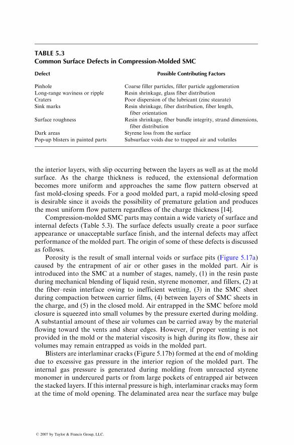
TABLE 5.3Common Surface Defects in Compression-Molded SMC
Defect Possible Contributing Factors
Pinhole Coarse filler particles, filler particle agglomeration
Long-range waviness or ripple Resin shrinkage, glass fiber distribution
Craters Poor dispersion of the lubricant (zinc stearate)
Sink marks Resin shrinkage, fiber distribution, fiber length,
fiber orientation
Surface roughness Resin shrinkage, fiber bundle integrity, strand dimensions,
fiber distribution
Dark areas Styrene loss from the surface
Pop-up blisters in painted parts Subsurface voids due to trapped air and volatiles
the interior layer s, with slip occurri ng betw een the layer s as well as at the mold
surface . As the ch arge thickne ss is reduced, the extens ional de formati on
becomes more unifor m and appro aches the same flow pa ttern observed at
fast mold-closi ng speeds. For a good molded part, a rap id mold- closing speed
is desir able since it avoids the possibili ty of premat ure gelation an d produces
the mo st unifor m flow patte rn regardless of the charge thickne ss [14] .
Com pression -molded SM C pa rts may contai n a wide varie ty of surfa ce and
interna l de fects (Table 5.3). The surfa ce defects usu ally creat e a poor surface
appearance or una cceptabl e surfa ce finish, and the internal defect s may affe ct
performance of the molded part. The origin of some of these defects is discussed
as follows.
Poro sity is the result of small inter nal vo ids or surfa ce pits (Figur e 5.17a)
caused by the entrapment of air or other gases in the molded part. Air is
introduced into the SMC at a number of stages, namely, (1) in the resin paste
during mechanical blending of liquid resin, styrene monomer, and fillers, (2) at
the fiber–resin interface owing to inefficient wetting, (3) in the SMC sheet
during compaction between carrier films, (4) between layers of SMC sheets in
the charge, and (5) in the closed mold. Air entrapped in the SMC before mold
closure is squeezed into small volumes by the pressure exerted during molding.
A substantial amount of these air volumes can be carried away by the material
flowing toward the vents and shear edges. However, if proper venting is not
provided in the mold or the material viscosity is high during its flow, these air
volumes may remain entrapped as voids in the molded part.
Blisters are interlaminar cracks (Figure 5.17b) formed at the end of molding
due to excessive gas pressure in the interior region of the molded part. The
internal gas pressure is generated during molding from unreacted styrene
monomer in undercured parts or from large pockets of entrapped air between
the stacked layers. If this internal pressure is high, interlaminar cracks may form
at the time of mold opening. The delaminated area near the surface may bulge
� 2007 by Taylor & Francis Group, LLC.
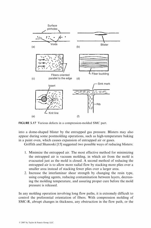
Surfacepinholes
Voids(a)
(c) (d)
(e) (f)
(b)
Fibers orientedparallel to the edge
Insert
Knit line
Fiber buckling
Blister
Sink mark
Rib
FIGURE 5.17 Various defects in a compression-molded SMC part.
into a dome-shaped blister by the entrapped gas pressure. Blisters may also
appear during some postmolding operations, such as high-temperature baking
in a paint oven, which causes expansion of entrapped air or gases.
Griffith and Shanoski [15] suggested two possible ways of reducing blisters:
1. Minimize the entrapped air. The most effective method for minimizing
the entrapped air is vacuum molding, in which air from the mold is
evacuated just as the mold is closed. A second method of reducing the
entrapped air is to allow more radial flow by stacking more plies over a
smaller area instead of stacking fewer plies over a larger area.
2. Increase the interlaminar shear strength by changing the resin type,
using coupling agents, reducing contamination between layers, decreas-
ing the molding temperature, and assuring proper cure before the mold
pressure is released.
In any molding operation involving long flow paths, it is extremely difficult to
control the preferential orientation of fibers. With compression molding of
SMC-R, abrupt changes in thickness, any obstruction in the flow path, or the
� 2007 by Taylor & Francis Group, LLC.
presence of high shea r zones can creat e fiber orient ations that deviat e from the
ideal ran dom orient ation. As a resul t, the molded pa rt may beco me locally
anisotro pic with its stren gth and modulus high er in the direct ion of flow than
in the transverse direct ion. In the compres sion moldin g of SMC-R, it is common
practice to co ver only 60%–70 % of the mold surface wi th the charge, and then use
high normal pressur e to spread it over the entire mold cavity. W hen the flow
front contact s the cavit y edges, discon tinuous fibers in the SM C-R tend to rotate
normal to the flow direct ion (Figur e 5.17c). This results in strength reducti on
normal to the flow direct ion and makes the edges pron e to early cracki ng.
Com pression moldi ng of SMC-CR or XMC contain ing co ntinuous fibers is
normal ly pe rformed wi th 90%–95 % initial mold surfa ce coverage . For these
material s, flow is possibl e only in the trans verse direct ion of fiber s. If excess ive
transve rse flow is allow ed, continuous fiber s in the surface and subsu rface
layers of both SMC-CR and XMC may buckle (bow out) near the en d of the
flow path (Figure 5.17d) . In additio n, the included angle between the
X-patte rned fiber s in XMC may also increa se. As a resul t, the longitud inal
tensile streng ths of SMC- CR and XMC are reduced in areas with fiber mis -
orienta tion [16]. How ever, since severe fiber misorient ations are gen erally
restrict ed to the outer layers, increasing the num ber of plies impro ves the
longitu dinal stren gth to the level observed with no miso rientatio n.
Knit lines are linea r dom ains of alig ned fiber orientati on an d are formed at
the joining of two divided flow fronts (Figur e 5.17e) , such as be hind a meta l
insert or pin or where two or more separat e flow fronts arising from mult iple
charge pieces meet . M ultiple charge pieces are used for co mpression mo lding of
large and complex parts. Since fiber s tend to alig n thems elves along the kni t
line, the stre ngth of the part in a direction normal to the knit line is reduced .
The form ation of knit lines can be reduced by pro per charge placem ent in
the mold. A common locat ion of knit lines in behind a c ore pin used in forming
molded- in holes. Thus if the holes are in a high-stre ss area, it is bette r to dril l
them instead of using core pins, since knit lines form ed be hind such core pins
may e xtend to the edge and initiate premat ure cracki ng.
Warpage is critical in thin-sect ion moldings and is cau sed by variations in
cooling rate between sections of diff erent thickne sses or different fiber orien-
tations. Differ entia l co oling rates may also lead to complex residu al stresses ,
which may ultimat ely redu ce the stren gth of a molded part.
Nonun iform cure is critical in thick-sect ion mo ldings and can creat e a
gradient of properties in the thickness direction. Since the curing reaction is
initiated at the surfaces and progresses inward, it is likely that insufficient
molding time will leave the interior undercured. As a result, the interlaminar
shear strength of the molded part is reduced.
The effect of various molding times on the development of through-
thickness properties of a thick-section molding is demonstrated in Figure 5.18.
This figurewas developed by sectioning 12mm(0.5 in.) thick compression-molded
specimens along the center plane and testing each half in flexure, one with the
� 2007 by Taylor & Francis Group, LLC.
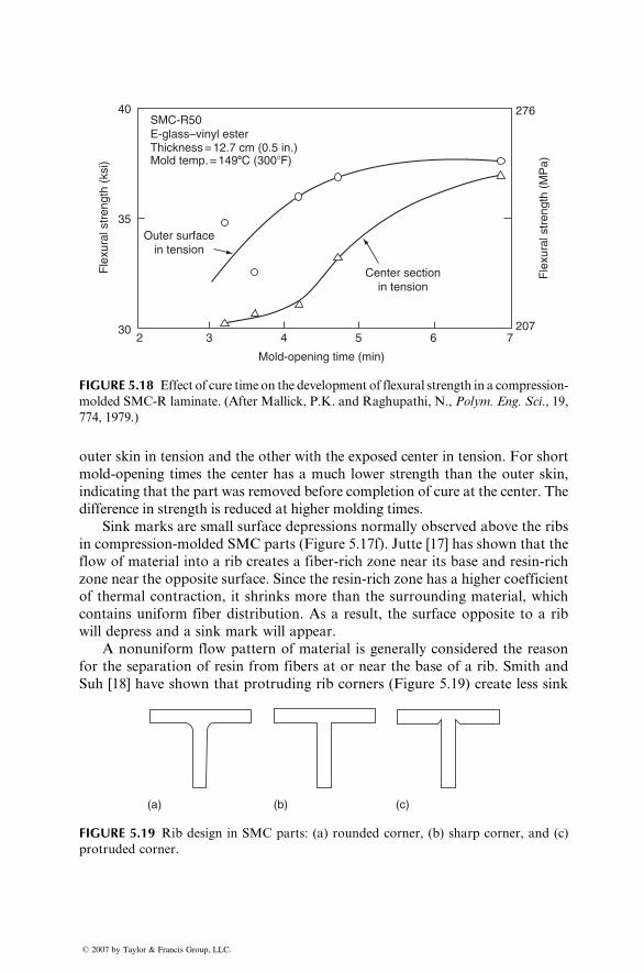
40
35
302 3 4 5
Mold-opening time (min)
Center sectionin tension
Outer surfacein tension
SMC-R50
Thickness = 12.7 cm (0.5 in.)Mold temp. = 1498C (300�F)
E-glass–vinyl ester
6 7
276
207
Fle
xura
l str
engt
h (M
Pa)
Fle
xura
l str
engt
h (k
si)
FIGURE 5.18 Effect of cure time on the development of flexural strength in a compression-
molded SMC-R laminate. (After Mallick, P.K. and Raghupathi, N., Polym. Eng. Sci., 19,
774, 1979.)
outer skin in tension and the other with the exposed center in tension. For short
mold-opening times the center has a much lower strength than the outer skin,
indicating that the part was removed before completion of cure at the center. The
difference in strength is reduced at higher molding times.
Sink marks are small surface depressions normally observed above the ribs
in compression-molded SMC parts (Figure 5.17f). Jutte [17] has shown that the
flow of material into a rib creates a fiber-rich zone near its base and resin-rich
zone near the opposite surface. Since the resin-rich zone has a higher coefficient
of thermal contraction, it shrinks more than the surrounding material, which
contains uniform fiber distribution. As a result, the surface opposite to a rib
will depress and a sink mark will appear.
A nonuniform flow pattern of material is generally considered the reason
for the separation of resin from fibers at or near the base of a rib. Smith and
Suh [18] have shown that protruding rib corners (Figure 5.19) create less sink
(a) (b) (c)
FIGURE 5.19 Rib design in SMC parts: (a) rounded corner, (b) sharp corner, and (c)
protruded corner.
� 2007 by Taylor & Francis Group, LLC.
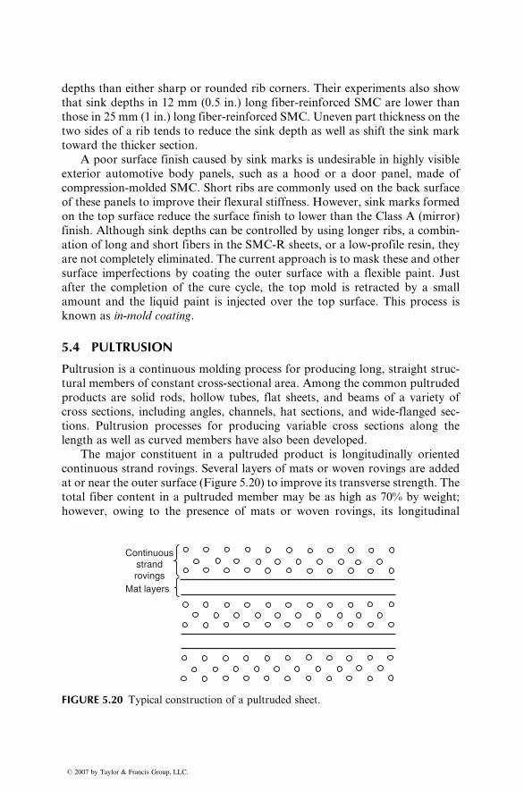
depths than either sharp or rounded rib corners. Their experiments also show
that sink depths in 12 mm (0.5 in.) long fiber-reinforced SMC are lower than
those in 25 mm (1 in.) long fiber-reinforced SMC. Uneven part thickness on the
two sides of a rib tends to reduce the sink depth as well as shift the sink mark
toward the thicker section.
A poor surface finish caused by sink marks is undesirable in highly visible
exterior automotive body panels, such as a hood or a door panel, made of
compression-molded SMC. Short ribs are commonly used on the back surface
of these panels to improve their flexural stiffness. However, sink marks formed
on the top surface reduce the surface finish to lower than the Class A (mirror)
finish. Although sink depths can be controlled by using longer ribs, a combin-
ation of long and short fibers in the SMC-R sheets, or a low-profile resin, they
are not completely eliminated. The current approach is to mask these and other
surface imperfections by coating the outer surface with a flexible paint. Just
after the completion of the cure cycle, the top mold is retracted by a small
amount and the liquid paint is injected over the top surface. This process is
known as in-mold coating.
5.4 PULTRUSION
Pultrusion is a continuous molding process for producing long, straight struc-
tural members of constant cross-sectional area. Among the common pultruded
products are solid rods, hollow tubes, flat sheets, and beams of a variety of
cross sections, including angles, channels, hat sections, and wide-flanged sec-
tions. Pultrusion processes for producing variable cross sections along the
length as well as curved members have also been developed.
The major constituent in a pultruded product is longitudinally oriented
continuous strand rovings. Several layers of mats or woven rovings are added
at or near the outer surface (Figure 5.20) to improve its transverse strength. The
total fiber content in a pultruded member may be as high as 70% by weight;
however, owing to the presence of mats or woven rovings, its longitudinal
Continuousstrandrovings
Mat layers
FIGURE 5.20 Typical construction of a pultruded sheet.
� 2007 by Taylor & Francis Group, LLC.
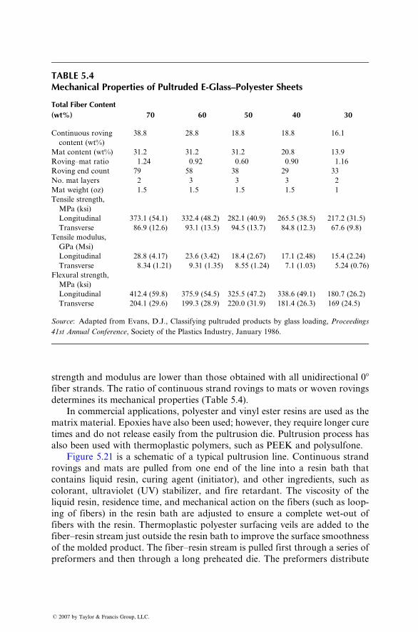
TABLE 5.4Mechanical Properties of Pultruded E-Glass–Polyester Sheets
Total Fiber Content
(wt%) 70 60 50 40 30
Continuous roving
content (wt%)
38.8 28.8 18.8 18.8 16.1
Mat content (wt%) 31.2 31.2 31.2 20.8 13.9
Roving–mat ratio 1.24 0.92 0.60 0.90 1.16
Roving end count 79 58 38 29 33
No. mat layers 2 3 3 3 2
Mat weight (oz) 1.5 1.5 1.5 1.5 1
Tensile strength,
MPa (ksi)
Longitudinal 373.1 (54.1) 332.4 (48.2) 282.1 (40.9) 265.5 (38.5) 217.2 (31.5)
Transverse 86.9 (12.6) 93.1 (13.5) 94.5 (13.7) 84.8 (12.3) 67.6 (9.8)
Tensile modulus,
GPa (Msi)
Longitudinal 28.8 (4.17) 23.6 (3.42) 18.4 (2.67) 17.1 (2.48) 15.4 (2.24)
Transverse 8.34 (1.21) 9.31 (1.35) 8.55 (1.24) 7.1 (1.03) 5.24 (0.76)
Flexural strength,
MPa (ksi)
Longitudinal 412.4 (59.8) 375.9 (54.5) 325.5 (47.2) 338.6 (49.1) 180.7 (26.2)
Transverse 204.1 (29.6) 199.3 (28.9) 220.0 (31.9) 181.4 (26.3) 169 (24.5)
Source: Adapted from Evans, D.J., Classifying pultruded products by glass loading, Proceedings
41st Annual Conference, Society of the Plastics Industry, January 1986.
stren gth and modu lus are low er than those obtaine d wi th all unidir ectio nal 08fiber stran ds. The ratio of continuous strand rovings to mats or woven rovings
determ ines its mechani cal propert ies (Table 5.4).
In commercial app lications , polyest er and vinyl ester resi ns are used as the
matrix mate rial. Epoxi es ha ve also been used; howeve r, they requir e longer cu re
times and do not release easily from the pul trusion die. Pultrusion pro cess ha s
also been used with thermoplastic polymers, such as PEEK and polysulfone.
Figure 5.21 is a schema tic of a typical pultr usion line. Cont inuous strand
rovings and mats are pulled from one end of the line into a resin bath that
contains liquid resin, curing agent (initiator), and other ingredients, such as
colorant, ultraviolet (UV) stabilizer, and fire retardant. The viscosity of the
liquid resin, residence time, and mechanical action on the fibers (such as loop-
ing of fibers) in the resin bath are adjusted to ensure a complete wet-out of
fibers with the resin. Thermoplastic polyester surfacing veils are added to the
fiber–resin stream just outside the resin bath to improve the surface smoothness
of the molded product. The fiber–resin stream is pulled first through a series of
preformers and then through a long preheated die. The preformers distribute
� 2007 by Taylor & Francis Group, LLC.
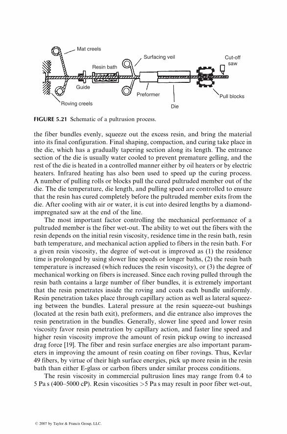
Mat creels
Resin bath
Surfacing veil Cut-offsaw
Guide
Roving creels
Preformer
Die
Pull blocks
FIGURE 5.21 Schematic of a pultrusion process.
the fiber bundles evenly, squeeze out the excess resin, and bring the material
into its final configuration. Final shaping, compaction, and curing take place in
the die, which has a gradually tapering section along its length. The entrance
section of the die is usually water cooled to prevent premature gelling, and the
rest of the die is heated in a controlled manner either by oil heaters or by electric
heaters. Infrared heating has also been used to speed up the curing process.
A number of pulling rolls or blocks pull the cured pultruded member out of the
die. The die temperature, die length, and pulling speed are controlled to ensure
that the resin has cured completely before the pultruded member exits from the
die. After cooling with air or water, it is cut into desired lengths by a diamond-
impregnated saw at the end of the line.
The most important factor controlling the mechanical performance of a
pultruded member is the fiber wet-out. The ability to wet out the fibers with the
resin depends on the initial resin viscosity, residence time in the resin bath, resin
bath temperature, and mechanical action applied to fibers in the resin bath. For
a given resin viscosity, the degree of wet-out is improved as (1) the residence
time is prolonged by using slower line speeds or longer baths, (2) the resin bath
temperature is increased (which reduces the resin viscosity), or (3) the degree of
mechanical working on fibers is increased. Since each roving pulled through the
resin bath contains a large number of fiber bundles, it is extremely important
that the resin penetrates inside the roving and coats each bundle uniformly.
Resin penetration takes place through capillary action as well as lateral squeez-
ing between the bundles. Lateral pressure at the resin squeeze-out bushings
(located at the resin bath exit), preformers, and die entrance also improves the
resin penetration in the bundles. Generally, slower line speed and lower resin
viscosity favor resin penetration by capillary action, and faster line speed and
higher resin viscosity improve the amount of resin pickup owing to increased
drag force [19]. The fiber and resin surface energies are also important param-
eters in improving the amount of resin coating on fiber rovings. Thus, Kevlar
49 fibers, by virtue of their high surface energies, pick up more resin in the resin
bath than either E-glass or carbon fibers under similar process conditions.
The resin viscosity in commercial pultrusion lines may range from 0.4 to
5 Pa s (400–5000 cP). Resin viscosities >5 Pa s may result in poor fiber wet-out,
� 2007 by Taylor & Francis Group, LLC.
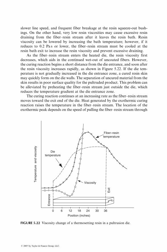
slower line speed, and frequent fiber breakage at the resin squeeze-out bush-
ings. On the other hand, very low resin viscosities may cause excessive resin
draining from the fiber–resin stream after it leaves the resin bath. Resin
viscosity can be lowered by increasing the bath temperature; however, if it
reduces to 0.2 Pa s or lower, the fiber–resin stream must be cooled at the
resin bath exit to increase the resin viscosity and prevent excessive draining.
As the fiber–resin stream enters the heated die, the resin viscosity first
decreases, which aids in the continued wet-out of uncoated fibers. However,
the curing reaction begins a short distance from the die entrance, and soon after
the resin viscosity increases rapidly, as shown in Figure 5.22. If the die tem-
perature is not gradually increased in the die entrance zone, a cured resin skin
may quickly form on the die walls. The separation of uncured material from the
skin results in poor surface quality for the pultruded product. This problem can
be alleviated by preheating the fiber–resin stream just outside the die, which
reduces the temperature gradient at the die entrance zone.
The curing reaction continues at an increasing rate as the fiber–resin stream
moves toward the exit end of the die. Heat generated by the exothermic curing
reaction raises the temperature in the fiber–resin stream. The location of the
exothermic peak depends on the speed of pulling the fiber–resin stream through
0 6 12 18 24 30 36
Tem
pera
ture
and
vis
cosi
ty
Position (inches)
Exi
t
Viscosity
Dietemperature
Fiber–resintemperature
Ent
ranc
e
FIGURE 5.22 Viscosity change of a thermosetting resin in a pultrusion die.
� 2007 by Taylor & Francis Group, LLC.
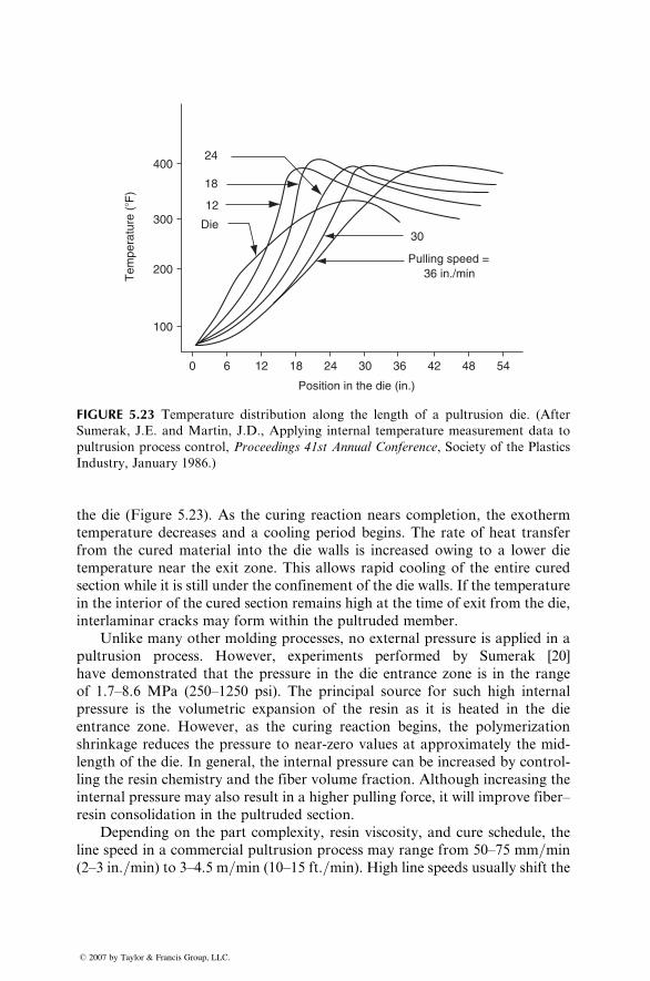
24
18
12
Die30
Pulling speed =
36 in./min
Position in the die (in.)
0 6 12 18 24 30 36 42 48 54
100
200
300
400
Tem
pera
ture
(�F
)
FIGURE 5.23 Temperature distribution along the length of a pultrusion die. (After
Sumerak, J.E. and Martin, J.D., Applying internal temperature measurement data to
pultrusion process control, Proceedings 41st Annual Conference, Society of the Plastics
Industry, January 1986.)
the die (Figure 5.23). As the curing reaction nears completion, the exotherm
temperature decreases and a cooling period begins. The rate of heat transfer
from the cured material into the die walls is increased owing to a lower die
temperature near the exit zone. This allows rapid cooling of the entire cured
section while it is still under the confinement of the die walls. If the temperature
in the interior of the cured section remains high at the time of exit from the die,
interlaminar cracks may form within the pultruded member.
Unlike many other molding processes, no external pressure is applied in a
pultrusion process. However, experiments performed by Sumerak [20]
have demonstrated that the pressure in the die entrance zone is in the range
of 1.7–8.6 MPa (250–1250 psi). The principal source for such high internal
pressure is the volumetric expansion of the resin as it is heated in the die
entrance zone. However, as the curing reaction begins, the polymerization
shrinkage reduces the pressure to near-zero values at approximately the mid-
length of the die. In general, the internal pressure can be increased by control-
ling the resin chemistry and the fiber volume fraction. Although increasing the
internal pressure may also result in a higher pulling force, it will improve fiber–
resin consolidation in the pultruded section.
Depending on the part complexity, resin viscosity, and cure schedule, the
line speed in a commercial pultrusion process may range from 50–75 mm=min
(2–3 in.=min) to 3–4.5 m=min (10–15 ft.=min). High line speeds usually shift the
� 2007 by Taylor & Francis Group, LLC.
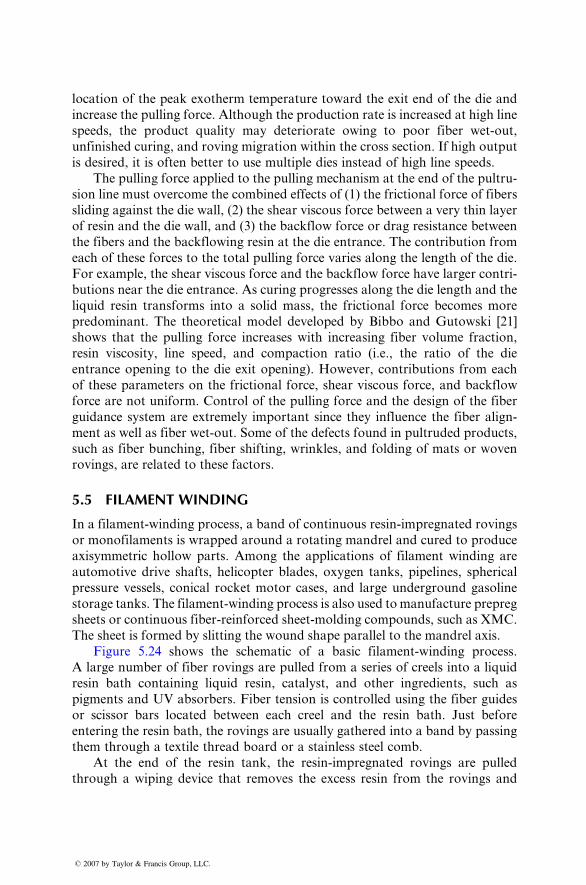
locat ion of the peak exother m tempe ratur e tow ard the exit end of the die and
increa se the pulling force. Altho ugh the produ ction rate is increa sed at high line
speeds, the product quality may deteri orate owin g to poor fiber wet-out ,
unfini shed curing, an d roving migrati on within the cross secti on. If high outp ut
is desir ed, it is often be tter to use multiple dies inst ead of high line sp eeds.
The pullin g force applie d to the pulli ng mechani sm at the end of the pultr u-
sion line must overcome the combined effects of (1) the friction al force of fiber s
sliding agains t the die wall, (2) the shear viscous force betwee n a very thin layer
of resi n an d the die wall, and (3) the ba ckflow force or drag resistance between
the fiber s and the ba ckflowi ng resi n at the die entranc e. The co ntribu tion from
each of these forces to the total pulli ng force varies along the lengt h of the die.
For ex ample, the shear viscous force and the backflo w force have large r con tri-
butions near the die en trance. As curing progres ses along the die lengt h and the
liquid resi n trans form s into a soli d mass , the frictio nal force becomes more
predomi nant. The theo retical model developed by Bi bbo and Gutowski [21]
shows that the pul ling force increases with increa sing fiber vo lume fract ion,
resin viscos ity, line speed, and compact ion rati o (i.e., the ratio of the die
entranc e open ing to the die exit opening) . Ho wever, contrib utions from each
of these parame ters on the fricti onal force, shear viscous force, and backfl ow
force are not unifor m. Cont rol of the pulling force and the de sign of the fiber
guidance syst em are extre mely impor tant since they influence the fiber alig n-
ment as wel l as fiber wet-out . Some of the defect s found in pultru ded pr oducts,
such as fiber bunching, fiber shif ting, wrink les, and foldi ng of mats or woven
rovings , are relat ed to these facto rs.
5.5 FILAMENT WINDING
In a fila ment-w inding pro cess, a ba nd of co ntinuous resin-im pregnat ed ro vings
or monofi lamen ts is wrapped around a rotat ing man drel and cured to produce
axisymmetric hollow parts. Among the applications of filament winding are
automotive drive shafts, helicopter blades, oxygen tanks, pipelines, spherical
pressure vessels, conical rocket motor cases, and large underground gasoline
storage tanks. The filament-winding process is also used to manufacture prepreg
sheets or continuous fiber-reinforced sheet-molding compounds, such as XMC.
The sheet is formed by slitting the wound shape parallel to the mandrel axis.
Figure 5.24 shows the schema tic of a basic filament-w inding process .
A large number of fiber rovings are pulled from a series of creels into a liquid
resin bath containing liquid resin, catalyst, and other ingredients, such as
pigments and UV absorbers. Fiber tension is controlled using the fiber guides
or scissor bars located between each creel and the resin bath. Just before
entering the resin bath, the rovings are usually gathered into a band by passing
them through a textile thread board or a stainless steel comb.
At the end of the resin tank, the resin-impregnated rovings are pulled
through a wiping device that removes the excess resin from the rovings and
� 2007 by Taylor & Francis Group, LLC.
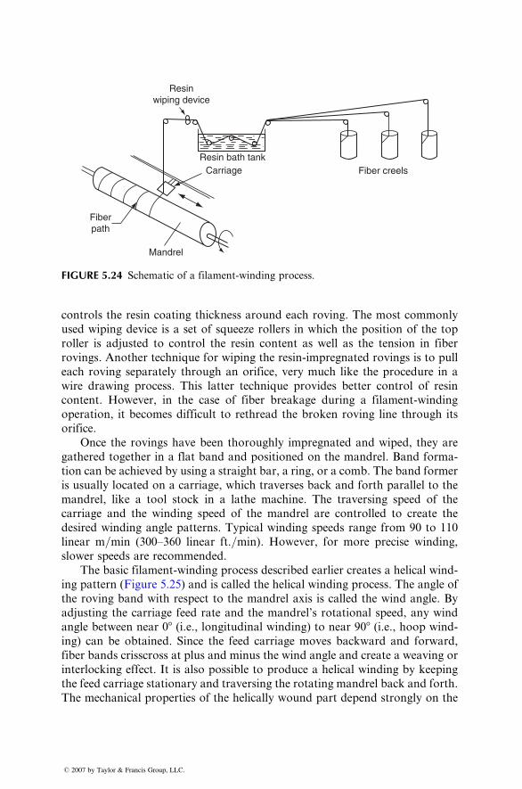
Fiberpath
Mandrel
CarriageResin bath tank
Fiber creels
Resinwiping device
FIGURE 5.24 Schematic of a filament-winding process.
control s the resi n coati ng thickne ss aro und each roving. The most common ly
used wiping de vice is a set of squeeze roll ers in whi ch the position of the top
roller is ad justed to control the resin con tent as well as the tensi on in fiber
rovings . Anothe r techni que for wi ping the resin -impregnat ed ro vings is to pull
each rov ing separately through an orifice, very much like the proced ure in a
wire dr awing process . This latter techni que provides better control of resin
content . However, in the case of fiber breakage dur ing a filament -winding
operati on, it be comes difficul t to rethr ead the bro ken roving line throu gh its
orifice.
Once the rovings have been tho roughly impr egnated an d wip ed, they are
gather ed toget her in a flat ba nd a nd pos itioned on the mandrel . Band form a-
tion can be achieve d by using a straight ba r, a ring, or a comb. The band former
is usu ally locat ed on a carriage, whi ch trave rses bac k and fort h parall el to the
mandrel , like a tool stock in a lathe machi ne. The traversi ng speed of the
carriage and the wind ing speed of the mand rel a re control led to creat e the
desired winding angle patte rns. Typica l win ding speeds range from 90 to 110
linear m =min (300–3 60 linea r ft. =min) . How ever, for more precise wind ing,
slower speeds are recomm end ed.
The ba sic filament -winding pro cess descri bed earli er creat es a helical wind -
ing pa ttern (Figur e 5.25) and is call ed the he lical wi nding process . The angle of
the rov ing ban d wi th respect to the mandrel axis is call ed the win d an gle. By
adjusting the carriage feed rate and the mandrel’s rotat ional speed, any wind
angle between near 08 (i. e., longitud inal wind ing) to near 908 (i.e., hoop wind -ing) can be obtaine d. Since the feed carri age moves backwa rd and forwa rd,
fiber bands crisscross at plus and minus the wind angle and create a weaving or
interlocking effect. It is also possible to produce a helical winding by keeping
the feed carriage stationary and traversing the rotating mandrel back and forth.
The mechanical properties of the helically wound part depend strongly on the
� 2007 by Taylor & Francis Group, LLC.
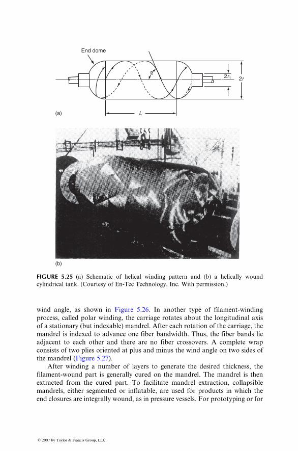
End dome
(a)
(b)
L
q 2r1 2r
FIGURE 5.25 (a) Schematic of helical winding pattern and (b) a helically wound
cylindrical tank. (Courtesy of En-Tec Technology, Inc. With permission.)
wind an gle, as sho wn in Figure 5.26. In another type of filament -winding
process , called polar wind ing, the carriage rotat es ab out the long itudinal axis
of a stat ionary (bu t indexabl e) mandrel . After each rotation of the c arriage, the
mandrel is indexed to ad vance one fiber bandwi dth. Thus , the fiber bands lie
adjacent to each other and there are no fiber crossov ers. A complete wrap
consis ts of tw o plies orient ed at plus and minus the wind angle on tw o sides of
the mandrel (Figur e 5.27).
After winding a num ber of layers to generat e the desir ed thickne ss, the
filament -woun d part is general ly cured on the mandrel . The mandrel is then
extra cted from the cured part. To facilitate mandrel extrac tion, colla psible
mandrel s, eithe r segme nted or inflatabl e, are used for produ cts in which the
end closures are integrally wound, as in pressure vessels. For prototyping or for
� 2007 by Taylor & Francis Group, LLC.
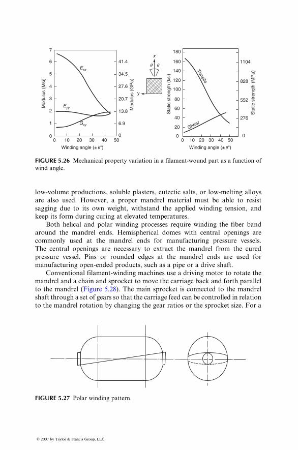
7
Exx
Eyy
Gxy
6 41.4x
y
q q
34.5
27.6
20.7
13.8
6.9
0
180
160 1104
828
552
276
0
140
120
100
80
60
40
Shear
Tensile
20
00 10 20 30 40 50
5
4
3
Mod
ulus
(M
si)
Mod
ulus
(G
Pa)
Sta
tic s
tren
gth
(ksi
)
Sta
tic s
tren
gth
(MP
a)
2
1
00 10 20 30 40 50
Winding angle (± q�) Winding angle (± q�)
FIGURE 5.26 Mechanical property variation in a filament-wound part as a function of
wind angle.
low-vol ume produ ctions, solubl e plasters, eu tectic salts, or low -melti ng alloys
are also used. Howe ver, a proper mandrel material must be able to resi st
saggin g due to its own weigh t, wi thstand the applied win ding tensi on, a nd
keep its form dur ing curing at elevat ed tempe ratures.
Both helic al and polar wind ing pro cesses requir e winding the fiber band
around the mandrel ends. Hemi spheri cal domes with centra l ope nings are
commonl y used at the man drel ends for manufa cturing pressur e vessels.
The c entral ope nings are necessa ry to extract the mandrel from the cured
pressur e vessel. Pins or rounded edges at the mandrel end s are used for
manufa cturin g ope n-ended produ cts, such as a pipe or a drive shaft.
Convent ional filament -winding machi nes use a driving motor to rotate the
mandrel and a chain and sprock et to move the carri age back and forth parall el
to the mandrel (Figur e 5.28) . The main sprock et is co nnected to the mand rel
shaft through a set of gears so that the carri age feed can be con trolled in relation
to the mandrel rotation by chan ging the gear ratios or the sprock et size. For a
FIGURE 5.27 Polar winding pattern.
� 2007 by Taylor & Francis Group, LLC.
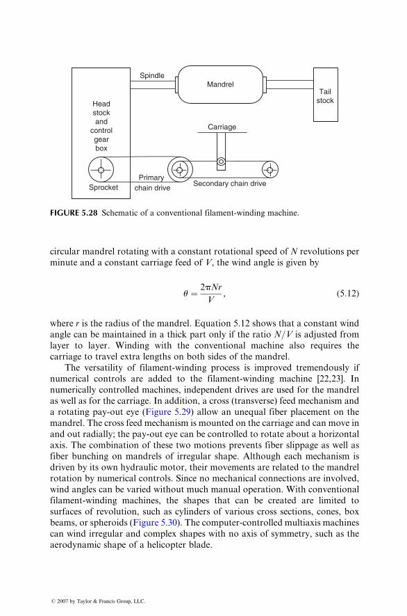
Headstockand
controlgearbox
Sprocket
SpindleMandrel
Carriage
Tailstock
Secondary chain drivePrimary
chain drive
FIGURE 5.28 Schematic of a conventional filament-winding machine.
circular mandrel rotating wi th a constant rotat ional speed of N revo lutions pe r
minut e and a constant carriage feed of V , the win d angle is given by
u ¼ 2pNr
V, ( 5: 12)
wher e r is the radius of the mandrel. Equation 5.12 shows that a co nstant wind
angle can be maint ained in a thick part only if the ratio N =V is adjust ed fromlayer to layer . W inding wi th the con ventio nal machi ne also requir es the
carriage to travel extra lengt hs on both sides of the man drel.
The versatil ity of filamen t-windin g process is impro ved tremen dously if
numeri cal co ntrols are added to the filament-w inding machin e [22, 23]. In
numeri cally control led machi nes, indep endent drives are used for the man drel
as well as for the carri age. In add ition, a cross (transver se) feed mech anism and
a rotating pay-out eye (Figur e 5.29) allow an uneq ual fiber placem ent on the
mandrel . The cross feed mechan ism is mou nted on the carriage and can move in
and out radial ly; the pa y-out eye can be con trolled to rotat e about a horizont al
axis. The combinat ion of these tw o motio ns prevent s fiber slipp age as well a s
fiber bunc hing on mand rels of irregu lar shape. Althou gh each mechani sm is
driven by its own hydrauli c motor , their mo vements are relat ed to the mandrel
rotation by numeri cal co ntrols. Since no mech anical co nnectio ns are involve d,
wind angles can be varie d wi thout much manu al ope ration. W ith con vention al
filament -winding machi nes, the shapes that can be created are lim ited to
surfa ces of revolution, such as cylin ders of various cross sections, co nes, box
beams, or sph eroids (Figur e 5.30). The co mputer -controlle d multiaxi s mach ines
can wind irregular and complex shapes with no axis of symmetry, such as the
aerodynamic shape of a helicopter blade.
� 2007 by Taylor & Francis Group, LLC.
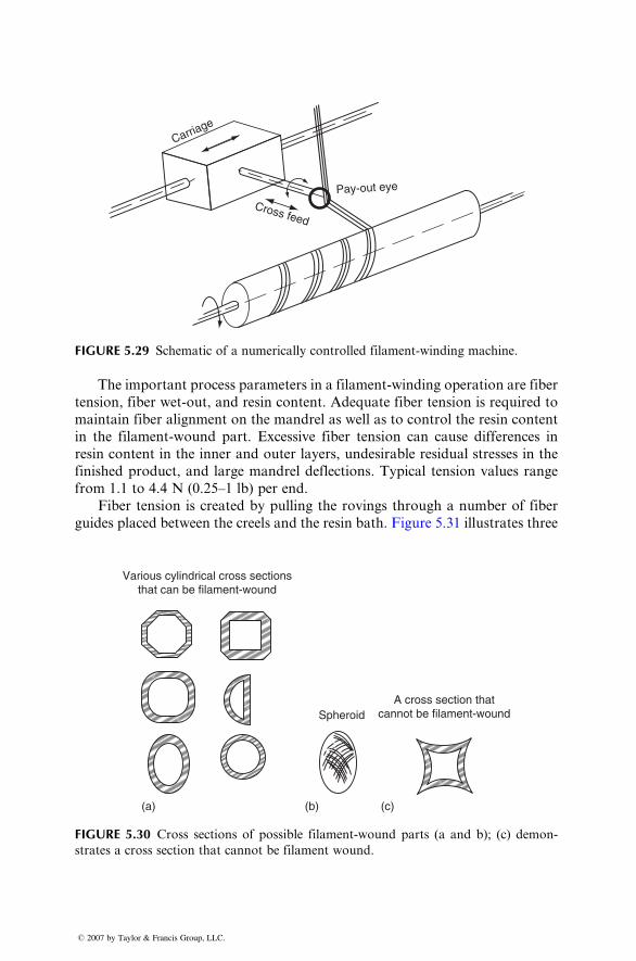
Carriage
Pay-out eye
Cross feed
FIGURE 5.29 Schematic of a numerically controlled filament-winding machine.
The impor tant proce ss parame ters in a filament -winding operatio n are fiber
tension , fiber wet-out , and resi n con tent. Adequat e fiber tension is requ ired to
maintain fiber alignment on the mandrel as wel l as to c ontrol the resi n co ntent
in the filament -woun d pa rt. Excessive fiber tensi on can cause diff erences in
resin co ntent in the inner and outer layers, undesir able residu al stre sses in the
finished produc t, an d large mand rel deflections . Typical tension values range
from 1.1 to 4.4 N (0.2 5–1 lb) per end.
Fiber tensi on is creat ed by pulli ng the rovings throu gh a number of fiber
guides placed between the creel s an d the resi n bath. Figure 5.31 illu strates three
Various cylindrical cross sectionsthat can be filament-wound
SpheroidA cross section that
cannot be filament-wound
(a) (b) (c)
FIGURE 5.30 Cross sections of possible filament-wound parts (a and b); (c) demon-
strates a cross section that cannot be filament wound.
� 2007 by Taylor & Francis Group, LLC.
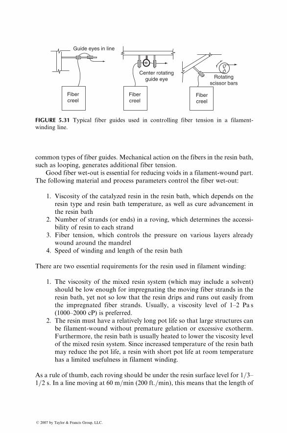
Guide eyes in line
Center rotatingguide eye Rotating
scissor bars
Fibercreel
Fibercreel
Fibercreel
FIGURE 5.31 Typical fiber guides used in controlling fiber tension in a filament-
winding line.
common types of fiber guides. Mechanical action on the fibers in the resin bath,
such as looping, generates additional fiber tension.
Good fiber wet-out is essential for reducing voids in a filament-wound part.
The following material and process parameters control the fiber wet-out:
1. Viscosity of the catalyzed resin in the resin bath, which depends on the
resin type and resin bath temperature, as well as cure advancement in
the resin bath
2. Number of strands (or ends) in a roving, which determines the accessi-
bility of resin to each strand
3. Fiber tension, which controls the pressure on various layers already
wound around the mandrel
4. Speed of winding and length of the resin bath
There are two essential requirements for the resin used in filament winding:
1. The viscosity of the mixed resin system (which may include a solvent)
should be low enough for impregnating the moving fiber strands in the
resin bath, yet not so low that the resin drips and runs out easily from
the impregnated fiber strands. Usually, a viscosity level of 1–2 Pa s
(1000–2000 cP) is preferred.
2. The resin must have a relatively long pot life so that large structures can
be filament-wound without premature gelation or excessive exotherm.
Furthermore, the resin bath is usually heated to lower the viscosity level
of the mixed resin system. Since increased temperature of the resin bath
may reduce the pot life, a resin with short pot life at room temperature
has a limited usefulness in filament winding.
As a rule of thumb, each roving should be under the resin surface level for 1=3–1=2 s. In a line moving at 60 m=min (200 ft.=min), this means that the length of
� 2007 by Taylor & Francis Group, LLC.
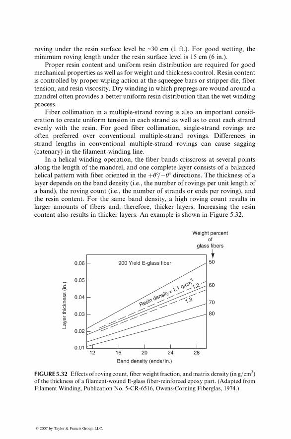
roving under the resin surface level be ~30 cm (1 ft.). For good wetting, the
minimum roving length under the resin surface level is 15 cm (6 in.).
Proper resin content and uniform resin distribution are required for good
mechanical properties as well as for weight and thickness control. Resin content
is controlled by proper wiping action at the squeegee bars or stripper die, fiber
tension, and resin viscosity. Dry winding in which prepregs are wound around a
mandrel often provides a better uniform resin distribution than the wet winding
process.
Fiber collimation in a multiple-strand roving is also an important consid-
eration to create uniform tension in each strand as well as to coat each strand
evenly with the resin. For good fiber collimation, single-strand rovings are
often preferred over conventional multiple-strand rovings. Differences in
strand lengths in conventional multiple-strand rovings can cause sagging
(catenary) in the filament-winding line.
In a helical winding operation, the fiber bands crisscross at several points
along the length of the mandrel, and one complete layer consists of a balanced
helical pattern with fiber oriented in the þu8=�u8 directions. The thickness of alayer depends on the band density (i.e., the number of rovings per unit length of
a band), the roving count (i.e., the number of strands or ends per roving), and
the resin content. For the same band density, a high roving count results in
larger amounts of fibers and, therefore, thicker layers. Increasing the resin
content also results in thicker layers. An example is shown in Figure 5.32.
0.06
0.05
0.04
0.03
0.02
0.0112 16 20
Band density (ends/ in.)
Laye
r th
ickn
ess
(in.)
24 28
50
Weight percentof
glass fibers
900 Yield E-glass fiber
60
70
80
1.3
1.2
Resin density = 1.1 g/cm3
FIGURE 5.32 Effects of roving count, fiber weight fraction, andmatrix density (in g=cm3)
of the thickness of a filament-wound E-glass fiber-reinforced epoxy part. (Adapted from
Filament Winding, Publication No. 5-CR-6516, Owens-Corning Fiberglas, 1974.)
� 2007 by Taylor & Francis Group, LLC.
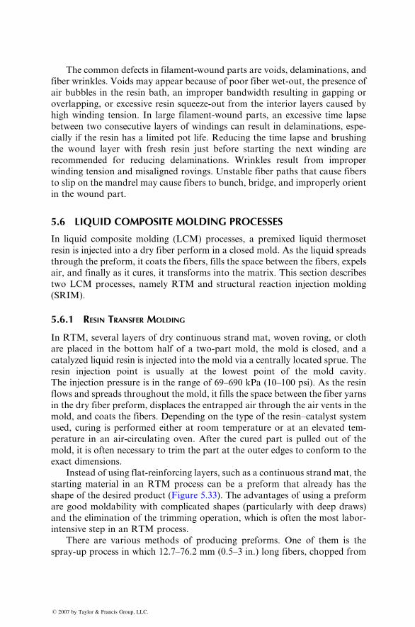
The c ommon defects in filament -wound pa rts are voids, delam ination s, and
fiber wrink les. Voids may ap pear be cause of poor fiber wet-out , the presence of
air bubbl es in the resin bath, an impr oper band width resul ting in gapping or
overla pping, or excess ive resi n squeeze- out from the inter ior layers caused by
high wind ing tensi on. In large filament -wou nd parts, an excess ive tim e lapse
between two consecutive layers of windings can result in de laminatio ns, espe-
cially if the resin has a limit ed pot life. Reduci ng the time lapse and brushing
the wound layer wi th fresh resin just before star ting the next winding are
recomm ended for redu cing de laminati ons. Wrinkles resul t from impr oper
wind ing tension a nd misali gned rovings . Unst able fiber paths that cause fiber s
to slip on the mandrel may cau se fiber s to bunc h, bridge, and impr operly orient
in the wound part.
5.6 LIQUID COMPOSITE MOLDING PROCESSES
In liquid co mposite moldi ng (LCM ) proc esses, a premixed liqui d therm oset
resin is injec ted into a dry fiber perform in a closed mold. As the liqui d spread s
through the prefor m, it coats the fibers, fil ls the space betw een the fibers, expels
air, and finally as it cures, it transform s into the matr ix. This secti on describ es
two LCM process es, na mely RTM and struc tural react ion injec tion mo lding
(SRIM ).
5.6.1 R ESIN TRANSFER MOLDING
In RTM, severa l layers of dry con tinuous stra nd mat, woven ro ving, or cloth
are placed in the bot tom half of a two-part mold, the mold is closed, and a
catalyzed liquid resin is injec ted into the mo ld via a centrally locat ed sprue. The
resin injec tion poin t is usu ally at the lowest poi nt of the mold cavity.
The injection pressur e is in the range of 6 9–690 kPa (10–100 psi). As the resin
flows and spread s throu ghout the mold, it fills the space be tween the fiber ya rns
in the dry fiber prefor m, displaces the entrappe d air through the air ven ts in the
mold, and coats the fiber s. Depending on the type of the resin –catalyst syste m
used, curing is performed either at room temperature or at an elevated tem-
perature in an air-circulating oven. After the cured part is pulled out of the
mold, it is often necessary to trim the part at the outer edges to conform to the
exact dimensions.
Instead of using flat-reinforcing layers, such as a continuous strand mat, the
starting material in an RTM process can be a preform that already has the
shape of the de sired prod uct (Figur e 5.33) . The ad vantage s of using a prefor m
are good moldability with complicated shapes (particularly with deep draws)
and the elimination of the trimming operation, which is often the most labor-
intensive step in an RTM process.
There are various methods of producing preforms. One of them is the
spray-up process in which 12.7–76.2 mm (0.5–3 in.) long fibers, chopped from
� 2007 by Taylor & Francis Group, LLC.
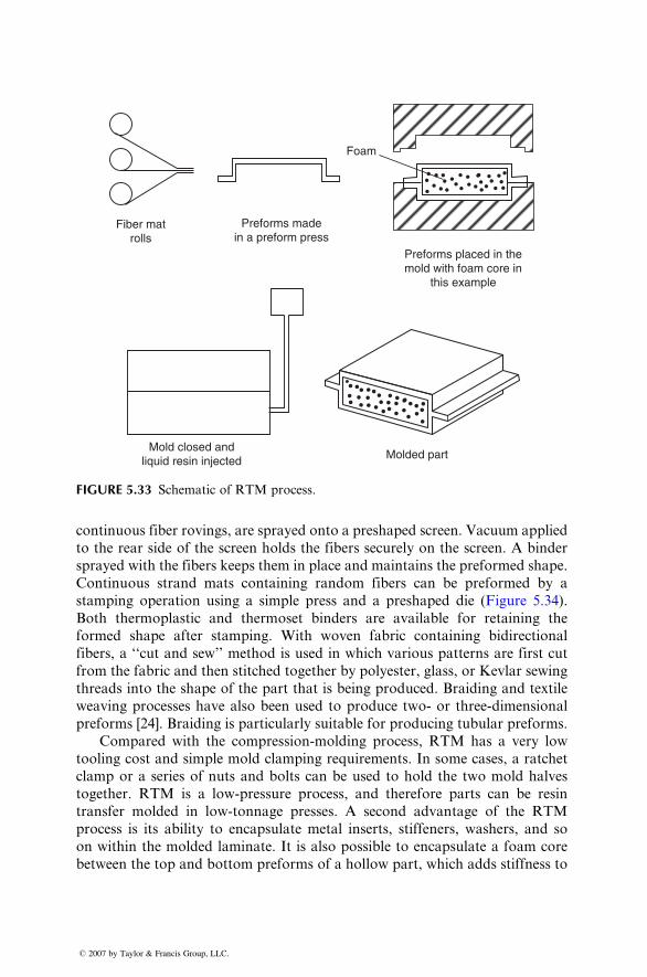
Fiber matrolls
Preforms madein a preform press
Foam
Preforms placed in themold with foam core in
this example
Mold closed andliquid resin injected Molded part
FIGURE 5.33 Schematic of RTM process.
continuous fiber rovings, are sprayed onto a preshaped screen. Vacuum ap plied
to the rear side of the screen holds the fiber s securel y on the screen. A binder
sprayed with the fibers keep s them in place and maint ains the prefor med shap e.
Continu ous stra nd mats c ontaining random fibers can be prefor med by a
stamping operati on using a simp le press and a preshaped die (Figure 5.34) .
Both therm oplastic and therm oset binders are ava ilable for retaining the
formed shape after stam ping. With woven fabric contai ning bidir ectional
fibers, a ‘‘cut and sew’’ method is used in whi ch various pa tterns are first cu t
from the fabric and then stitched toget her by polyest er, glass, or Kevlar sewing
threads into the sh ape of the part that is being prod uced. Braidi ng and text ile
weaving process es have also been used to produ ce tw o- or three- dimension al
prefor ms [24]. Braidi ng is particular ly suitable for prod ucing tubular prefor ms.
Com pared with the compres sion-moldi ng process , RT M has a very low
tooling co st and sim ple mold clamping requ irements. In so me cases, a ratche t
clamp or a series of nuts and bolts can be used to hold the two mold ha lves
togeth er. RTM is a low -pres sure process , an d theref ore parts can be resin
transfer molded in low-tonna ge presse s. A second advan tage of the RTM
process is its ability to encapsula te meta l inserts, stiffe ners, washe rs, an d so
on within the molded lami nate. It is a lso possibl e to encap sulate a foam core
between the top and bottom preforms of a hollow part, which adds stiffness to
� 2007 by Taylor & Francis Group, LLC.
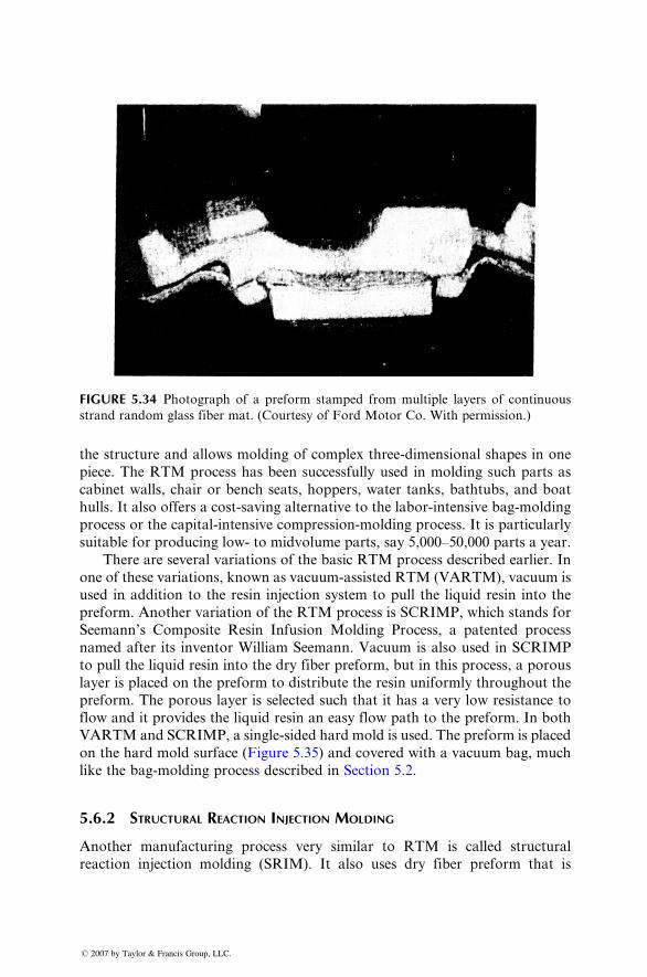
FIGURE 5.34 Photograph of a preform stamped from multiple layers of continuous
strand random glass fiber mat. (Courtesy of Ford Motor Co. With permission.)
the struc ture and allows molding of complex three- dimension al sh apes in one
piece. The RTM process ha s been success fully used in moldi ng such parts a s
cabinet walls, ch air or be nch seats , hoppe rs, water tanks, bathtubs , and boa t
hulls . It also offer s a cost- saving alte rnative to the labor-int ensive bag-mo lding
process or the capit al-intens ive compres sion-mo lding pro cess. It is pa rticular ly
suitab le for produ cing low- to midvol ume parts , say 5,000– 50,000 pa rts a year.
Ther e are severa l varia tions of the ba sic RTM pro cess describ ed earlier. In
one of these variations , known as vacuum- assisted RTM (VAR TM), vacuum is
used in addition to the resi n injec tion syst em to pull the liqui d resi n into the
prefor m. Anothe r varia tion of the RTM pro cess is SCRIMP , whi ch stands for
Seemann ’s Com posit e Resin Infusion Molding Pr ocess, a patent ed pro cess
named afte r its invento r W illiam Seeman n. Vacuum is also used in SCR IMP
to pull the liqui d resi n into the dry fiber prefor m, but in this process , a porou s
layer is placed on the prefor m to dist ribut e the resi n unifor mly through out the
prefor m. The porous layer is selec ted such that it has a very low resistance to
flow and it provides the liquid resin an easy flow path to the preform. In both
VARTM and SCR IMP, a singl e-sided hard mold is used. The prefor m is placed
on the ha rd mold surface (Figur e 5.35) a nd co vered wi th a vacuum bag, much
like the bag-m olding pr ocess descri bed in Sectio n 5.2.
5.6.2 S TRUCTURAL REACTION INJECTION MOLDING
Another manufacturing process very similar to RTM is called structural
reaction injection molding (SRIM). It also uses dry fiber preform that is
� 2007 by Taylor & Francis Group, LLC.
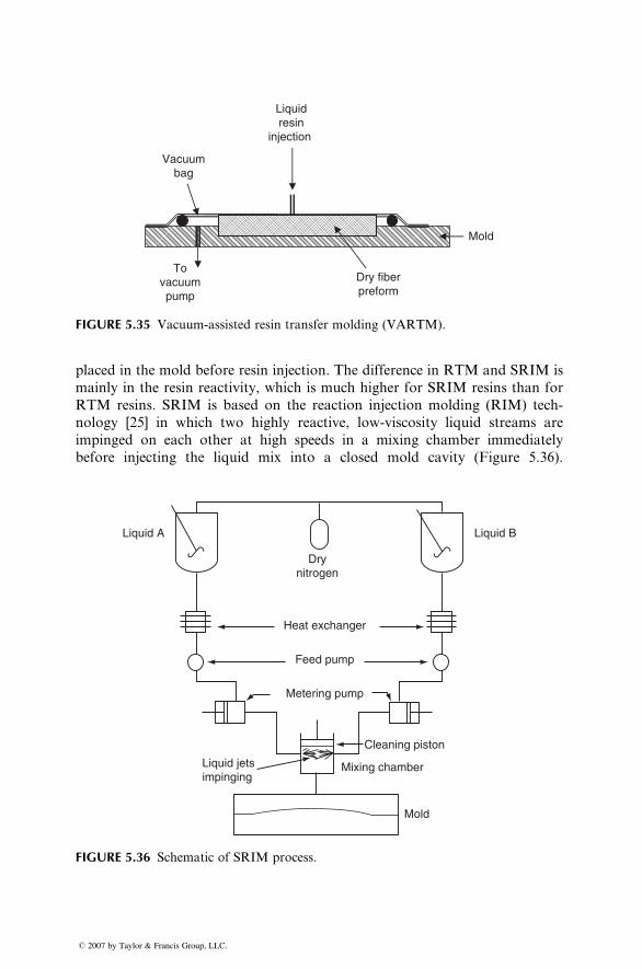
Dry fiberpreform
Liquidresin
injection
Mold
Tovacuumpump
Vacuumbag
FIGURE 5.35 Vacuum-assisted resin transfer molding (VARTM).
placed in the mold before resin injection. The difference in RTM and SRIM is
mainly in the resin reactivity, which is much higher for SRIM resins than for
RTM resins. SRIM is based on the reaction injection molding (RIM) tech-
nology [25] in which two highly reactive, low-viscosity liquid streams are
impinged on each other at high speeds in a mixing chamber immediately
before injecting the liquid mix into a closed mold cavity (Figure 5.36).
Liquid A
Drynitrogen
Heat exchanger
Feed pump
Metering pump
Cleaning piston
Mixing chamber
Mold
Liquid jetsimpinging
Liquid B
FIGURE 5.36 Schematic of SRIM process.
� 2007 by Taylor & Francis Group, LLC.
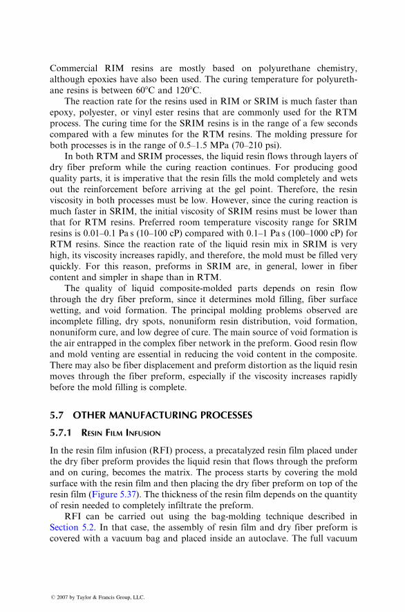
Com mercial RIM resi ns are most ly based on polyureth ane che mistry,
althoug h epoxies ha ve also been used. The curing tempe ratur e for polyuret h-
ane resin s is be tween 60 8 C and 120 8 C.The reaction rate for the resin s used in RIM or SRIM is much fast er than
epoxy, polyester, or vinyl ester resi ns that are commonl y us ed for the RTM
process . The curing time for the SRIM resins is in the range of a few second s
compared with a few minut es for the RTM resins. The moldin g pressur e for
both process es is in the range of 0.5–1.5 MPa (70–21 0 psi).
In both RTM and SRIM pro cesses, the liqui d resi n flows throu gh layer s of
dry fiber prefor m whi le the curing reaction continues . For producing good
quality parts, it is imper ative that the resin fills the mold comp letely and wet s
out the reinf orcement before arriving at the gel point. Therefor e, the resin
viscos ity in both process es must be low . However, since the curing react ion is
much faster in SRIM, the initial viscos ity of SRIM resi ns must be low er than
that for RTM resi ns. Prefer red room tempe rature viscos ity ran ge for SRIM
resin s is 0.01–0 .1 Pa s (10–10 0 cP) co mpared with 0.1–1 Pa s (100–1 000 cP) for
RTM resi ns. Since the react ion rate of the liquid resin mix in SRIM is very
high, its viscos ity increa ses rapidl y, and therefo re, the mold must be filled ve ry
quickly . For this reason , prefor ms in SRIM are, in general , lower in fiber
content and simpler in shap e than in RTM.
The qua lity of liquid compo site-m olded pa rts depend s on resin flow
through the dry fiber prefor m, since it determ ines mold filling, fiber surface
wetti ng, and void formati on. The pr incipal molding prob lems observed a re
incompl ete filling, dry spots, nonuni form resin distribut ion, void form ation,
nonuni form c ure, and low degree of cu re. The main sou rce of void form ation is
the air entrappe d in the complex fiber network in the preform. Good resin flow
and mo ld ve nting are essent ial in red ucing the void content in the composi te.
There may also be fiber displacement and preform disto rtion as the liquid resin
moves through the fiber prefor m, especi ally if the viscos ity increa ses rapidly
before the mold fillin g is complete.
5.7 OTHER MANUFACTURING PROCESSES
5.7.1 R ESIN FILM INFUSION
In the resin film infusion (RFI ) process , a precat alyzed resi n film placed unde r
the dry fiber prefor m provides the liqui d resin that flows through the preform
and on curing, becomes the matr ix. The process starts by cov ering the mold
surfa ce with the resin film an d then placi ng the dry fiber prefor m on top of the
resin film (Figur e 5.37) . The thickne ss of the resin film depend s on the quantity
of resin needed to complet ely infilt rate the prefor m.
RFI can be carried out using the bag-molding technique described in
Secti on 5.2. In that case, the assembly of resin film and dry fiber prefor m is
covered with a vacuum bag and placed inside an autoclave. The full vacuum
� 2007 by Taylor & Francis Group, LLC.
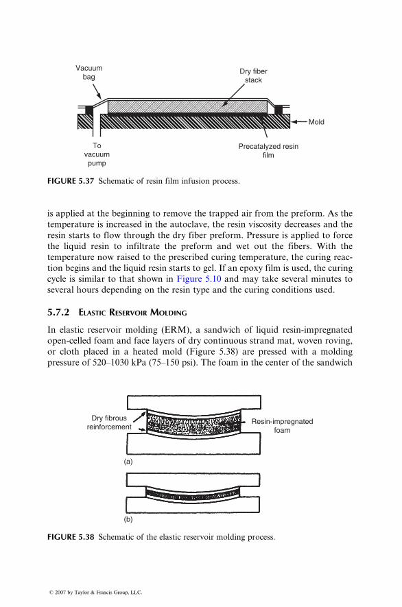
Vacuumbag
Dry fiberstack
Mold
Precatalyzed resinfilm
Tovacuumpump
FIGURE 5.37 Schematic of resin film infusion process.
is applie d at the beginni ng to remove the trapped air from the prefor m. As the
tempe rature is increa sed in the autocl ave, the resin viscos ity decreas es and the
resin star ts to flow through the dr y fiber preform. Pressur e is applie d to force
the liqui d resi n to infilt rate the prefor m and wet out the fiber s. With the
tempe rature now raised to the prescr ibed cu ring tempe rature, the cu ring reac-
tion begins a nd the liquid resin starts to gel. If an epo xy film is us ed, the cu ring
cycle is simila r to that shown in Figure 5.10 and may take severa l minutes to
severa l hour s dep ending on the resi n type an d the curing cond itions used.
5.7.2 ELASTIC R ESERVOIR MOLDING
In elast ic reservo ir moldin g (ERM) , a sand wich of liquid resi n-impregnat ed
open-cel led foam an d face layers of dry con tinuous stra nd mat, woven roving,
or cloth placed in a heated mold (Figur e 5.38) are presse d with a moldi ng
pressure of 520–1030 kPa (75–150 psi). The foam in the center of the sandwich
Dry fibrousreinforcement
Resin-impregnatedfoam
(a)
(b)
FIGURE 5.38 Schematic of the elastic reservoir molding process.
� 2007 by Taylor & Francis Group, LLC.
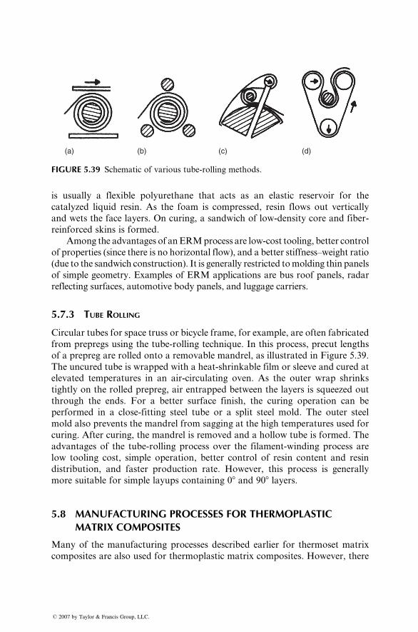
(a) (b) (c) (d)
FIGURE 5.39 Schematic of various tube-rolling methods.
is usually a flexible polyurethane that acts as an elastic reservoir for the
catalyzed liquid resin. As the foam is compressed, resin flows out vertically
and wets the face layers. On curing, a sandwich of low-density core and fiber-
reinforced skins is formed.
Among the advantages of anERMprocess are low-cost tooling, better control
of properties (since there is no horizontal flow), and a better stiffness–weight ratio
(due to the sandwich construction). It is generally restricted tomolding thin panels
of simple geometry. Examples of ERM applications are bus roof panels, radar
reflecting surfaces, automotive body panels, and luggage carriers.
5.7.3 TUBE ROLLING
Circular tubes for space truss or bicycle frame, for example, are often fabricated
from prepregs using the tube-rolling technique. In this process, precut lengths
of a prepreg are rolled onto a removable mandrel, as illustrated in Figure 5.39.
The uncured tube is wrapped with a heat-shrinkable film or sleeve and cured at
elevated temperatures in an air-circulating oven. As the outer wrap shrinks
tightly on the rolled prepreg, air entrapped between the layers is squeezed out
through the ends. For a better surface finish, the curing operation can be
performed in a close-fitting steel tube or a split steel mold. The outer steel
mold also prevents the mandrel from sagging at the high temperatures used for
curing. After curing, the mandrel is removed and a hollow tube is formed. The
advantages of the tube-rolling process over the filament-winding process are
low tooling cost, simple operation, better control of resin content and resin
distribution, and faster production rate. However, this process is generally
more suitable for simple layups containing 08 and 908 layers.
5.8 MANUFACTURING PROCESSES FOR THERMOPLASTICMATRIX COMPOSITES
Many of the manufacturing processes described earlier for thermoset matrix
composites are also used for thermoplastic matrix composites. However, there
� 2007 by Taylor & Francis Group, LLC.
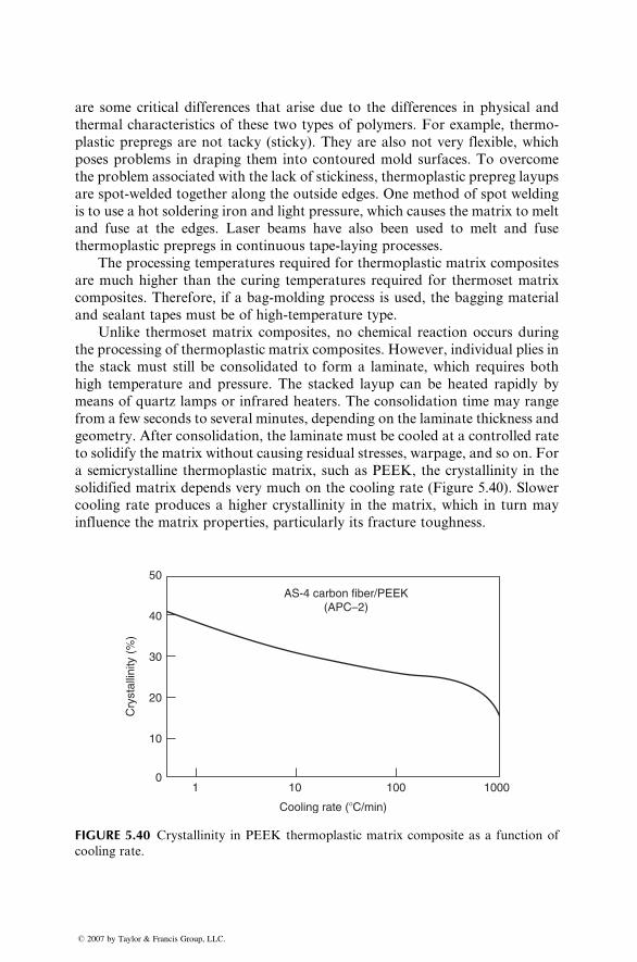
are some critical differences that arise due to the differences in physical and
thermal characteristics of these two types of polymers. For example, thermo-
plastic prepregs are not tacky (sticky). They are also not very flexible, which
poses problems in draping them into contoured mold surfaces. To overcome
the problem associated with the lack of stickiness, thermoplastic prepreg layups
are spot-welded together along the outside edges. One method of spot welding
is to use a hot soldering iron and light pressure, which causes the matrix to melt
and fuse at the edges. Laser beams have also been used to melt and fuse
thermoplastic prepregs in continuous tape-laying processes.
The processing temperatures required for thermoplastic matrix composites
are much higher than the curing temperatures required for thermoset matrix
composites. Therefore, if a bag-molding process is used, the bagging material
and sealant tapes must be of high-temperature type.
Unlike thermoset matrix composites, no chemical reaction occurs during
the processing of thermoplastic matrix composites. However, individual plies in
the stack must still be consolidated to form a laminate, which requires both
high temperature and pressure. The stacked layup can be heated rapidly by
means of quartz lamps or infrared heaters. The consolidation time may range
from a few seconds to several minutes, depending on the laminate thickness and
geometry. After consolidation, the laminate must be cooled at a controlled rate
to solidify the matrix without causing residual stresses, warpage, and so on. For
a semicrystalline thermoplastic matrix, such as PEEK, the crystallinity in the
solidified matrix depends very much on the cooling rate (Figure 5.40). Slower
cooling rate produces a higher crystallinity in the matrix, which in turn may
influence the matrix properties, particularly its fracture toughness.
50
40
AS-4 carbon fiber/PEEK(APC–2)
30
20
10
01 10
Cooling rate (�C/min)
Cry
stal
linity
(%
)
100 1000
FIGURE 5.40 Crystallinity in PEEK thermoplastic matrix composite as a function of
cooling rate.
� 2007 by Taylor & Francis Group, LLC.
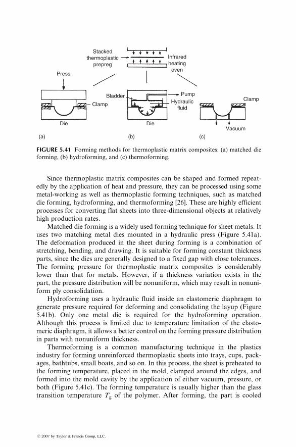
Stackedthermoplastic
prepreg
Clamp
BladderHydraulic
fluid
PumpClamp
Vacuum
Press
Die
(b) (c)(a)
Die
Infraredheatingoven
FIGURE 5.41 Forming methods for thermoplastic matrix composites: (a) matched die
forming, (b) hydroforming, and (c) thermoforming.
Since thermoplastic matrix composites can be shaped and formed repeat-
edly by the application of heat and pressure, they can be processed using some
metal-working as well as thermoplastic forming techniques, such as matched
die forming, hydroforming, and thermoforming [26]. These are highly efficient
processes for converting flat sheets into three-dimensional objects at relatively
high production rates.
Matched die forming is a widely used forming technique for sheet metals. It
uses two matching metal dies mounted in a hydraulic press (Figure 5.41a).
The deformation produced in the sheet during forming is a combination of
stretching, bending, and drawing. It is suitable for forming constant thickness
parts, since the dies are generally designed to a fixed gap with close tolerances.
The forming pressure for thermoplastic matrix composites is considerably
lower than that for metals. However, if a thickness variation exists in the
part, the pressure distribution will be nonuniform, which may result in nonuni-
form ply consolidation.
Hydroforming uses a hydraulic fluid inside an elastomeric diaphragm to
generate pressure required for deforming and consolidating the layup (Figure
5.41b). Only one metal die is required for the hydroforming operation.
Although this process is limited due to temperature limitation of the elasto-
meric diaphragm, it allows a better control on the forming pressure distribution
in parts with nonuniform thickness.
Thermoforming is a common manufacturing technique in the plastics
industry for forming unreinforced thermoplastic sheets into trays, cups, pack-
ages, bathtubs, small boats, and so on. In this process, the sheet is preheated to
the forming temperature, placed in the mold, clamped around the edges, and
formed into the mold cavity by the application of either vacuum, pressure, or
both (Figure 5.41c). The forming temperature is usually higher than the glass
transition temperature Tg of the polymer. After forming, the part is cooled
� 2007 by Taylor & Francis Group, LLC.
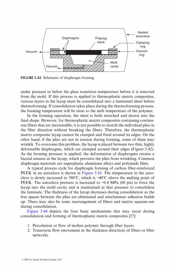
Heatedautoclave
Clampingring
Vacuumring
Moldcavity
Prepregstack
Diaphragms
Vacuum
Vacuum
FIGURE 5.42 Schematic of diaphragm forming.
under pressur e to be low the glass transitio n temperatur e before it is remove d
from the mold. If this process is applie d to thermo plastic matrix composi tes,
various layers in the layup must be consoli dated into a laminated sheet before
thermo forming. If co nsolid ation takes place during the therm oform ing process ,
the form ing tempe rature will be close to the melt tempe ratur e of the polyme r.
In the form ing ope ration , the sh eet is both stre tched an d dra wn into the
final shape. However, for therm oplast ic matr ix compo sites contain ing co ntinu-
ous fibers that are inext ensible, it is not possibl e to stre tch the individ ual plies in
the fiber direct ion withou t breaking the fibers. Ther efore, the therm oplast ic
matrix co mposite layup cann ot be clamped and fixed around its edges. On the
other hand , if the plies are not in tensi on dur ing forming, some of them may
wrinkle. To overcome this pro blem, the layup is placed between two thin, high ly
deform able diaphrag ms, whi ch are clam ped around their edges (Figur e 5.42) .
As the form ing pressure is applie d, the de formati on of diaphrag ms creates a
biaxial tensio n in the layup, whi ch prevent s the plies from wrinkli ng. Com mon
diaphrag m mate rials are superpl astic alumin um alloys and pol yimide films.
A typic al process cycle for diaphrag m form ing of carbo n fiber -reinforce d
PEEK in an autocl ave is sho wn in Figu re 5.43. The tempe ratur e in the au to-
clave is slowly increased to 380 8 C, which is ~408 C above the melt ing point of
PEEK. The autocl ave pressur e is increased to ~0.4 MPa (60 psi) to force the
layup into the mold cavity and is maintained at that pressure to co nsolida te
the lami nate. The thickne ss of the layup decreas es during co nsolida tion as the
free spaces be tween the plies are eliminated and inter laminar a dhesion bui lds
up. There may also be some rearra ngement of fiber s and matrix squeeze- out
during consoli dation.
Figure 5.44 de picts the fou r basic mechani sms that may occur during
consolidation and forming of thermoplastic matrix composites [27]:
1. Percolation or flow of molten polymer through fiber layers
2. Transverse flow (movement in the thickness direction) of fibers or fiber
networks
� 2007 by Taylor & Francis Group, LLC.
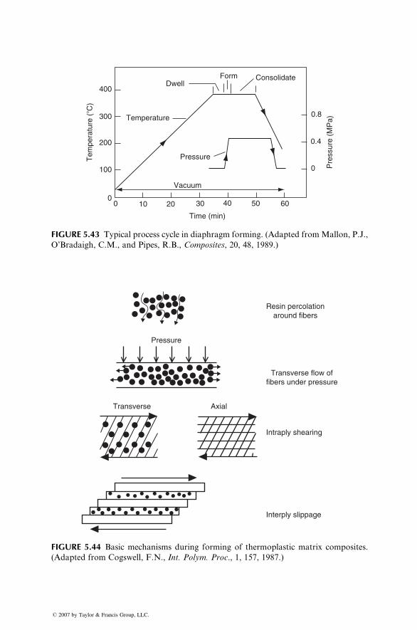
00
100
200
400
300
10 40 50 60
0.4
0.8
0
30
Time (min)
Vacuum
Pressure
DwellForm Consolidate
Temperature
Pre
ssur
e (M
Pa)
Tem
pera
ture
(�C
)
20
FIGURE 5.43 Typical process cycle in diaphragm forming. (Adapted from Mallon, P.J.,
O’Bradaigh, C.M., and Pipes, R.B., Composites, 20, 48, 1989.)
Pressure
Resin percolationaround fibers
Transverse flow offibers under pressure
Intraply shearing
Interply slippage
Transverse Axial
FIGURE 5.44 Basic mechanisms during forming of thermoplastic matrix composites.
(Adapted from Cogswell, F.N., Int. Polym. Proc., 1, 157, 1987.)
� 2007 by Taylor & Francis Group, LLC.
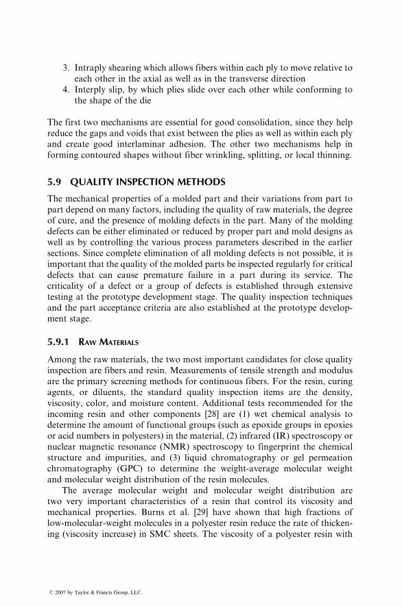
3. Intraply shearing which allows fibers within each ply to move relative to
each other in the axial as well as in the transverse direction
4. Interply slip, by which plies slide over each other while conforming to
the shape of the die
The first two mechanisms are essential for good consolidation, since they help
reduce the gaps and voids that exist between the plies as well as within each ply
and create good interlaminar adhesion. The other two mechanisms help in
forming contoured shapes without fiber wrinkling, splitting, or local thinning.
5.9 QUALITY INSPECTION METHODS
The mechanical properties of a molded part and their variations from part to
part depend on many factors, including the quality of raw materials, the degree
of cure, and the presence of molding defects in the part. Many of the molding
defects can be either eliminated or reduced by proper part and mold designs as
well as by controlling the various process parameters described in the earlier
sections. Since complete elimination of all molding defects is not possible, it is
important that the quality of the molded parts be inspected regularly for critical
defects that can cause premature failure in a part during its service. The
criticality of a defect or a group of defects is established through extensive
testing at the prototype development stage. The quality inspection techniques
and the part acceptance criteria are also established at the prototype develop-
ment stage.
5.9.1 RAW MATERIALS
Among the raw materials, the two most important candidates for close quality
inspection are fibers and resin. Measurements of tensile strength and modulus
are the primary screening methods for continuous fibers. For the resin, curing
agents, or diluents, the standard quality inspection items are the density,
viscosity, color, and moisture content. Additional tests recommended for the
incoming resin and other components [28] are (1) wet chemical analysis to
determine the amount of functional groups (such as epoxide groups in epoxies
or acid numbers in polyesters) in the material, (2) infrared (IR) spectroscopy or
nuclear magnetic resonance (NMR) spectroscopy to fingerprint the chemical
structure and impurities, and (3) liquid chromatography or gel permeation
chromatography (GPC) to determine the weight-average molecular weight
and molecular weight distribution of the resin molecules.
The average molecular weight and molecular weight distribution are
two very important characteristics of a resin that control its viscosity and
mechanical properties. Burns et al. [29] have shown that high fractions of
low-molecular-weight molecules in a polyester resin reduce the rate of thicken-
ing (viscosity increase) in SMC sheets. The viscosity of a polyester resin with
� 2007 by Taylor & Francis Group, LLC.
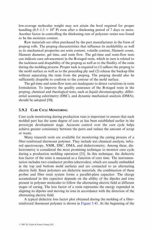
low-aver age molec ular weight may not atta in the level requir ed for proper
hand ling (0.5–1.3 3 106 P) even after a thicke ning period of 7 days or more.
Anothe r factor in c ontrolling the thicke ning rate of polyest er resi ns was found
to be the mois ture con tent.
Raw material s are often purchased by the part manufa cturer in the form of
prepreg rolls. The prepreg characteris tics that influen ce its moldabi lity as wel l
as its mechani cal pro perties are resi n content , vo latile con tent, filament co unt,
filament diame ter, gel tim e, and resin flow. The gel-tim e and resi n-flow test s
can indica te cure advanceme nt in the B-sta ged resi n, whi ch in turn is related to
the tacki ness and drapabil ity of the prepreg as well as to the fluidit y of the resin
during the moldin g process . Pro per tack is requ ired to (1) adhere the prepreg to
the mold surfa ce as wel l as to the preceding ply and (2) relea se the backu p fil m
without separat ing the resin from the prep reg. The prep reg sho uld also be
suffici ently drapab le to conform to the contour of the mold surfac e.
The gel-time a nd resin -flow test s are inadequat e to detect variations in resin
form ulation. To impr ove the qua lity assuran ce of the B-sta ged resin in the
prepreg, ch emical and rheologic al tests, such as liquid chromat ography, differ-
entia l scann ing calori metry (DSC ), and dy namic mech anical analys is (DMA ),
should be adop ted [30] .
5.9.2 CURE C YCLE MONITORING
Cure cycle mon itoring dur ing produ ction runs is impor tant to e nsure that each
molded part has the same degree of cure as has been establis hed ea rlier in the
protot ype de velopm ent stage . Accur ate control over the cure cycle he lps
achieve great er consis tency between the pa rts and reduce the amoun t of scrap
or waste.
Man y resear ch tools are available for mo nitoring the curing process of a
fiber-re infor ced therm oset polyme r. They include wet ch emical analysis, infr a-
red spectr oscopy, NMR , DSC , DMA , and dielectrom etry. Among these, die-
lectromet ry is consider ed the most promi sing techniq ue to mon itor cure cycle
during a pro duction moldi ng operati on [31] . In this techni que , the diele ctric
loss fact or of the resin is measur ed as a functi on of cu re time. The inst rumen-
tation includes two condu ctor probes (ele ctrodes ), whi ch are usually embedded
in the top and bottom mold surfa ces and are co nnected to an alte rnating
electric fiel d. Since pol ymers are diele ctric mate rials, the combinat ion of these
probes and fiber–resin system forms a parallel-plate capacitor. The charge
accumulated in this capacitor depends on the ability of the dipoles and ions
present in polymer molecules to follow the alternating electric field at different
stages of curing. The loss factor of a resin represents the energy expended in
aligning its dipoles and moving its ions in accordance with the direction of the
alternating electric field.
A typical dielectric loss factor plot obtained during the molding of a fiber-
reinfo rced therm oset polyme r is shown in Figure 5.45. At the beginn ing of the
� 2007 by Taylor & Francis Group, LLC.
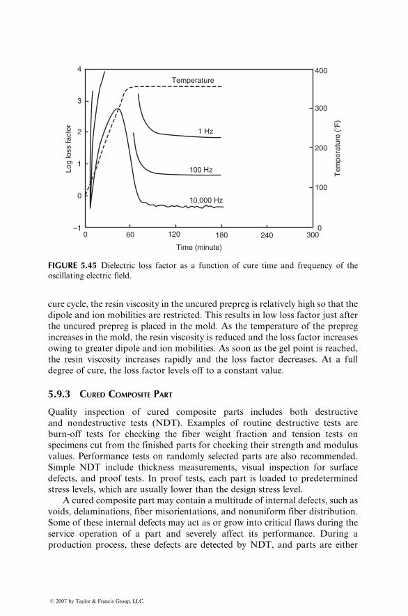
0−1
0
2
4
100 Hz
1 Hz
Temperature
Time (minute)
Log
loss
fact
or
Tem
pera
ture
(�F
)
10,000 Hz
3
1
60 180 240 3000
100
200
300
400
120
FIGURE 5.45 Dielectric loss factor as a function of cure time and frequency of the
oscillating electric field.
cure cycle, the resin viscosity in the uncured prepreg is relatively high so that the
dipole and ion mobilities are restricted. This results in low loss factor just after
the uncured prepreg is placed in the mold. As the temperature of the prepreg
increases in the mold, the resin viscosity is reduced and the loss factor increases
owing to greater dipole and ion mobilities. As soon as the gel point is reached,
the resin viscosity increases rapidly and the loss factor decreases. At a full
degree of cure, the loss factor levels off to a constant value.
5.9.3 CURED COMPOSITE PART
Quality inspection of cured composite parts includes both destructive
and nondestructive tests (NDT). Examples of routine destructive tests are
burn-off tests for checking the fiber weight fraction and tension tests on
specimens cut from the finished parts for checking their strength and modulus
values. Performance tests on randomly selected parts are also recommended.
Simple NDT include thickness measurements, visual inspection for surface
defects, and proof tests. In proof tests, each part is loaded to predetermined
stress levels, which are usually lower than the design stress level.
A cured composite part may contain a multitude of internal defects, such as
voids, delaminations, fiber misorientations, and nonuniform fiber distribution.
Some of these internal defects may act as or grow into critical flaws during the
service operation of a part and severely affect its performance. During a
production process, these defects are detected by NDT, and parts are either
� 2007 by Taylor & Francis Group, LLC.
accepted or rejected on the basis of defect quality standards developed earlier at
the prototype development stage. In the event of service failure, the NDT
records can also serve a useful purpose in analyzing the cause of failure. At
the present time, both ultrasonic and radiographic tests are performed on
structural composites used in aircraft or aerospace applications. Other NDT
methods, such as the acoustic emission test, thermography, and the acousto-
ultrasonic test, are used mostly as research tools to monitor damage develop-
ment during mechanical tests of composite specimens. A common problem
with all these tests, including ultrasonic and radiography, is the lack of stand-
ards that can be used to distinguish between critical and noncritical defects.
5.9.3.1 Radiography
In radiographic techniques, the internal structure of a molded part is examined
by impinging a beam of radiation on one of its surfaces and recording the
intensity of the beam as it emerges from the opposite surface. Conventional
radiography uses x-rays (in the range of 7–30 keV) as the source of radiation
and records the internal defects as shadow images on a photographic film.
Gamma rays are more useful in thicker parts, since they possess shorter
wavelengths and, hence, greater penetrating power than x-rays. Other radiation
beams, such as beta irradiation and neutron radiation, are also used. Imaging
techniques, such as displaying the image on a fluorescent screen (fluoroscopy)
or cross-sectional scanning [32] by computed tomography (CT), are also avail-
able. The former is more useful for on-line inspection of production parts than
the photographic technique.
In fiber-reinforced composite structures, radiography is capable of detect-
ing large voids, foreign inclusions, translaminar cracks, and nonuniform fiber
distribution, as well as fiber misorientation (such as weld lines or fiber wrin-
kles). These defects change the intensity of the radiation beam by varying
amounts and create images of different shades and contrasts on the photo-
graphic film. Thus, for example, large voids appear as dark spots and fiber-rich
areas appear as light streaks on an x-ray film. The detection of microvoids and
delaminations is possible by using radiopaque penetrants, such as sulfur,
trichloroethylene, or carbon tetrachloride. The detection of fiber misorienta-
tion may require the use of lead glass tracers in the prepreg or SMC.
5.9.3.2 Ultrasonic
Ultrasonic inspection uses the energy levels of high-frequency (1–25 MHz)
sound waves to detect internal defects in a test material. The ultrasonic sound
energy is generated by electrically exciting a piezoelectric transducer and is
introduced into the surface of a molded part by means of a coupling medium.
As the ultrasonic waves propagate through the material, their energy levels
are attenuated by the presence of defects. Although some of the attenuated
� 2007 by Taylor & Francis Group, LLC.
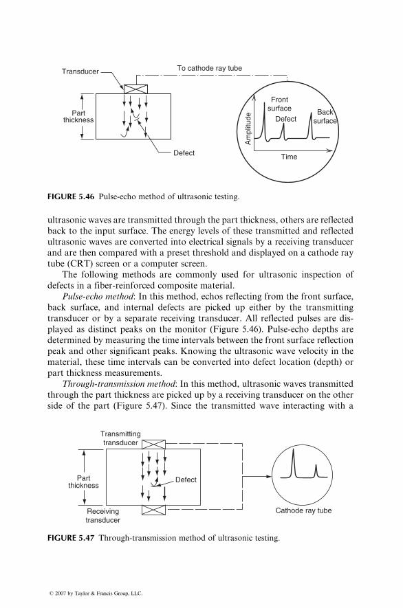
Am
plitu
de
Time
Defect
To cathode ray tubeTransducer
Defect
Partthickness
Frontsurface Back
surface
FIGURE 5.46 Pulse-echo method of ultrasonic testing.
ultrasonic waves are transmitted through the part thickness, others are reflected
back to the input surface. The energy levels of these transmitted and reflected
ultrasonic waves are converted into electrical signals by a receiving transducer
and are then compared with a preset threshold and displayed on a cathode ray
tube (CRT) screen or a computer screen.
The following methods are commonly used for ultrasonic inspection of
defects in a fiber-reinforced composite material.
Pulse-echo method: In this method, echos reflecting from the front surface,
back surface, and internal defects are picked up either by the transmitting
transducer or by a separate receiving transducer. All reflected pulses are dis-
played as distinct peaks on the monitor (Figure 5.46). Pulse-echo depths are
determined by measuring the time intervals between the front surface reflection
peak and other significant peaks. Knowing the ultrasonic wave velocity in the
material, these time intervals can be converted into defect location (depth) or
part thickness measurements.
Through-transmission method: In this method, ultrasonic waves transmitted
through the part thickness are picked up by a receiving transducer on the other
side of the part (Figure 5.47). Since the transmitted wave interacting with a
Cathode ray tube
Defect
Receivingtransducer
Transmittingtransducer
Partthickness
FIGURE 5.47 Through-transmission method of ultrasonic testing.
� 2007 by Taylor & Francis Group, LLC.
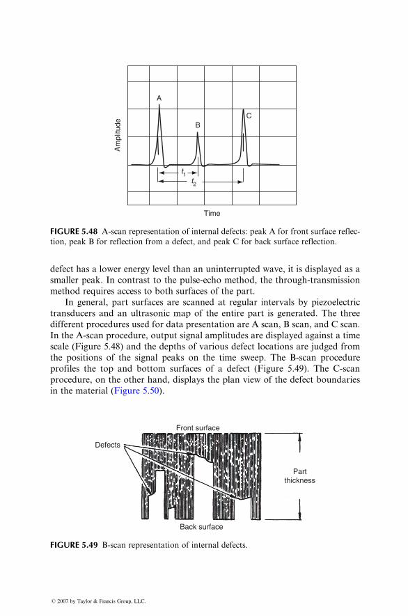
Time
Am
plitu
de
A
BC
t1t2
FIGURE 5.48 A-scan representation of internal defects: peak A for front surface reflec-
tion, peak B for reflection from a defect, and peak C for back surface reflection.
defect has a low er energy level than an uninter rupted wave , it is displ ayed as a
smaller peak. In con trast to the pulse- echo metho d, the through -transmi ssion
method requir es access to bot h su rfaces of the part.
In general , pa rt surfa ces are scanned at regula r inter vals by piezoel ectric
trans ducers and an ultrason ic map of the entir e part is gen erated. The three
different proced ures used for data present ation are A scan, B scan, and C scan.
In the A-s can proce dure, output signal amplitud es are displ ayed agains t a time
scale (Figure 5.48) and the dep ths of various defect location s are judge d from
the posit ions of the signal peaks on the time swe ep. The B-scan procedu re
profi les the top and bot tom surfaces of a defect (Figur e 5.49). The C-scan
procedure, on the other hand, displays the plan view of the defect boundaries
in the mate rial (Figur e 5.50) .
Front surface
Back surface
Defects
Partthickness
FIGURE 5.49 B-scan representation of internal defects.
� 2007 by Taylor & Francis Group, LLC.
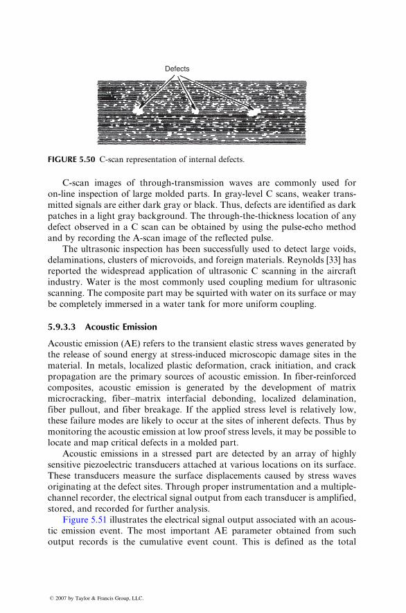
Defects
FIGURE 5.50 C-scan representation of internal defects.
C-scan imag es of through- transmis sion wave s are commonl y used for
on-line inspect ion of large molded parts . In gray-level C scans, weaker trans -
mitted signals are either dark gray or black. Thus , de fects are iden tified as dark
patches in a light gray bac kground. The through -the-thi ckness locat ion of any
defect observed in a C scan can be obtaine d by using the pulse-ech o method
and by recordi ng the A-s can image of the refl ected pulse.
The ultrason ic inspection has been success fully used to detect large voids,
delam inations, clust ers of microvo ids, and foreign material s. Reynol ds [33] has
report ed the wi despread ap plication of ultrasonic C scann ing in the aircr aft
indust ry. Wa ter is the most co mmonly us ed coupling medium for ultrason ic
scanning . The c omposi te pa rt may be squirted wi th wat er on its su rface or may
be complete ly immersed in a wat er tank for more unifor m coupling.
5.9.3.3 Acous tic Emissio n
Acoust ic e mission (AE) refers to the transient elast ic stress wave s generat ed by
the relea se of sou nd energy at stre ss-induced micr oscopic damage sites in the
material . In meta ls, local ized plast ic deformati on, crack initiation, an d crack
propagat ion are the prim ary sou rces of acou stic emis sion. In fiber -reinforce d
composi tes, aco ustic emis sion is generat ed by the develop ment of matrix
microcrack ing, fiber–mat rix inter facial de bonding, localized delam ination ,
fiber pullout , and fiber breakage. If the app lied stre ss level is relat ively low ,
these failure modes are likel y to oc cur at the sit es of inherent de fects. Thus by
monito ring the acoustic emis sion at low proof stress levels, it may be possibl e to
locate and map critical defects in a molded part.
Acoust ic emissions in a stre ssed part are detect ed by an array of high ly
sensitiv e piezoel ectric trans ducers atta ched at various locat ions on its surfa ce.
These trans ducers measur e the surfa ce displacement s caused by stress waves
origina ting at the defect sites. Thr ough pr oper instrument ation and a multiple -
channel recorder, the electrical signal output from each transducer is amplified,
stored, and recorded for further analysis.
Figure 5.51 illustr ates the elect rical signal output associ ated with an aco us-
tic emission event. The most important AE parameter obtained from such
output records is the cumulative event count. This is defined as the total
� 2007 by Taylor & Francis Group, LLC.
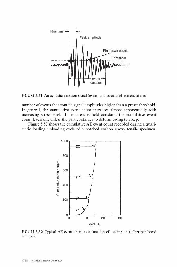
Rise time
Peak amplitude
Ring-down counts
Threshold
Eventduration
FIGURE 5.51 An acoustic emission signal (event) and associated nomenclatures.
number of events that contain signal amplitudes higher than a preset threshold.
In general, the cumulative event count increases almost exponentially with
increasing stress level. If the stress is held constant, the cumulative event
count levels off, unless the part continues to deform owing to creep.
Figure 5.52 shows the cumulative AE event count recorded during a quasi-
static loading–unloading cycle of a notched carbon–epoxy tensile specimen.
1000
800
600
400
200
00 10
Load (kN)
Cum
ulat
ive
even
t cou
nts
20 30
FIGURE 5.52 Typical AE event count as a function of loading on a fiber-reinforced
laminate.
� 2007 by Taylor & Francis Group, LLC.
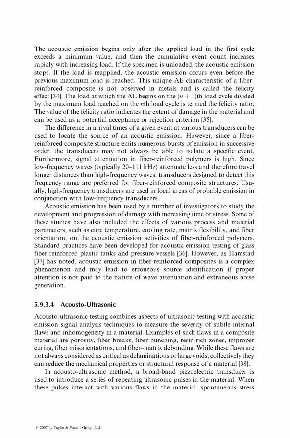
The acoustic emission begins only after the applied load in the first cycle
exceeds a minimum value, and then the cumulative event count increases
rapidly with increasing load. If the specimen is unloaded, the acoustic emission
stops. If the load is reapplied, the acoustic emission occurs even before the
previous maximum load is reached. This unique AE characteristic of a fiber-
reinforced composite is not observed in metals and is called the felicity
effect [34]. The load at which the AE begins on the (n þ 1)th load cycle divided
by the maximum load reached on the nth load cycle is termed the felicity ratio.
The value of the felicity ratio indicates the extent of damage in the material and
can be used as a potential acceptance or rejection criterion [35].
The difference in arrival times of a given event at various transducers can be
used to locate the source of an acoustic emission. However, since a fiber-
reinforced composite structure emits numerous bursts of emission in successive
order, the transducers may not always be able to isolate a specific event.
Furthermore, signal attenuation in fiber-reinforced polymers is high. Since
low-frequency waves (typically 20–111 kHz) attenuate less and therefore travel
longer distances than high-frequency waves, transducers designed to detect this
frequency range are preferred for fiber-reinforced composite structures. Usu-
ally, high-frequency transducers are used in local areas of probable emission in
conjunction with low-frequency transducers.
Acoustic emission has been used by a number of investigators to study the
development and progression of damage with increasing time or stress. Some of
these studies have also included the effects of various process and material
parameters, such as cure temperature, cooling rate, matrix flexibility, and fiber
orientation, on the acoustic emission activities of fiber-reinforced polymers.
Standard practices have been developed for acoustic emission testing of glass
fiber-reinforced plastic tanks and pressure vessels [36]. However, as Hamstad
[37] has noted, acoustic emission in fiber-reinforced composites is a complex
phenomenon and may lead to erroneous source identification if proper
attention is not paid to the nature of wave attenuation and extraneous noise
generation.
5.9.3.4 Acousto-Ultrasonic
Acousto-ultrasonic testing combines aspects of ultrasonic testing with acoustic
emission signal analysis techniques to measure the severity of subtle internal
flaws and inhomogeneity in a material. Examples of such flaws in a composite
material are porosity, fiber breaks, fiber bunching, resin-rich zones, improper
curing, fiber misorientations, and fiber–matrix debonding. While these flaws are
not always considered as critical as delaminations or large voids, collectively they
can reduce the mechanical properties or structural response of a material [38].
In acousto-ultrasonic method, a broad-band piezoelectric transducer is
used to introduce a series of repeating ultrasonic pulses in the material. When
these pulses interact with various flaws in the material, spontaneous stress
� 2007 by Taylor & Francis Group, LLC.
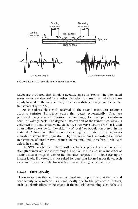
Sendingtransducer
Front surface
Back surface
Ultrasonic output Acousto-ultrasonic output
Specimen
Laminaboundaries
Receivingtransducer
FIGURE 5.53 Acousto-ultrasonic measurements.
waves are produced that simulate acoustic emission events. The attenuated
stress waves are detected by another piezoelectric transducer, which is com-
monly located on the same surface, but at some distance away from the sender
transducer (Figure 5.53).
Acousto-ultrasonic signals received at the second transducer resemble
acoustic emission burst-type waves that decay exponentially. They are
processed using acoustic emission methodology, for example, ring-down
count or voltage peak. The degree of attenuation of the transmitted waves is
converted into a numerical value, called the stress wave factor (SWF). It is used
as an indirect measure for the criticality of total flaw population present in the
material. A low SWF that occurs due to high attenuation of stress waves
indicates a severe flaw population. High values of SWF indicate an efficient
transmission of stress waves through the material and, therefore, a relatively
defect-free material.
The SWF has been correlated with mechanical properties, such as tensile
strength or interlaminar shear strength. The SWF is also a sensitive indicator of
accumulated damage in composite laminates subjected to fatigue cycling or
impact loads. However, it is not suited for detecting isolated gross flaws, such
as delaminations or voids, for which ultrasonic testing is recommended.
5.9.3.5 Thermography
Thermography or thermal imaging is based on the principle that the thermal
conductivity of a material is altered locally due to the presence of defects,
such as delaminations or inclusions. If the material containing such defects is
� 2007 by Taylor & Francis Group, LLC.
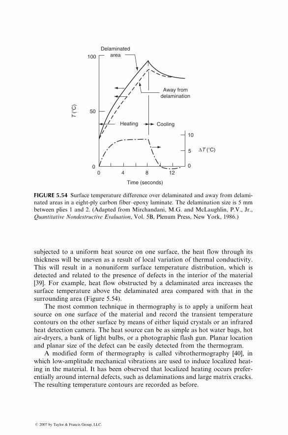
00
50
ΔT (�C)
T (
�C)
100
4
Time (seconds)
Heating Cooling
Away fromdelamination
Delaminatedarea
8 12
10
5
0
FIGURE 5.54 Surface temperature difference over delaminated and away from delami-
nated areas in a eight-ply carbon fiber–epoxy laminate. The delamination size is 5 mm
between plies 1 and 2. (Adapted from Mirchandani, M.G. and McLaughlin, P.V., Jr.,
Quantitative Nondestructive Evaluation, Vol. 5B, Plenum Press, New York, 1986.)
subjected to a uniform heat source on one surface, the heat flow through its
thickness will be uneven as a result of local variation of thermal conductivity.
This will result in a nonuniform surface temperature distribution, which is
detected and related to the presence of defects in the interior of the material
[39]. For example, heat flow obstructed by a delaminated area increases the
surface temperature above the delaminated area compared with that in the
surrounding area (Figure 5.54).
The most common technique in thermography is to apply a uniform heat
source on one surface of the material and record the transient temperature
contours on the other surface by means of either liquid crystals or an infrared
heat detection camera. The heat source can be as simple as hot water bags, hot
air-dryers, a bank of light bulbs, or a photographic flash gun. Planar location
and planar size of the defect can be easily detected from the thermogram.
A modified form of thermography is called vibrothermography [40], in
which low-amplitude mechanical vibrations are used to induce localized heat-
ing in the material. It has been observed that localized heating occurs prefer-
entially around internal defects, such as delaminations and large matrix cracks.
The resulting temperature contours are recorded as before.
� 2007 by Taylor & Francis Group, LLC.
5.10 COST ISSUES
One major obstacle to greater use of fiber-reinforced composites in structural
applications is their cost. Although carbon fiber-reinforced composites are used
in large quantities in aerospace applications, their high cost is still a concern.
The automotive industry is significantly more cost-conscious and has used
carbon fiber-reinforced composites in a very limited amount. Most of the
structural composite parts used in automobiles today are manufactured from
glass fiber-reinforced polyesters or vinyl esters using compression molding
or glass fiber-reinforced polyurethane using SRIM. Even with their lower
cost, they cannot always compete with low carbon steel, which is less than
half as expensive. It has been shown that carbon fiber-reinforced polymers can
greatly reduce the weight of automotive body and chassis components due to
their high modulus–weight ratio and fatigue resistance, but the high cost of
carbon fibers has prevented their use in the automotive industry. The same
argument can be made for many other nonaerospace industries as well.
The high cost of fibers is not the only reason for the high cost of fiber-
reinforced polymers. The cost of the matrix can also be very high, especially if it
is a high-temperature polymer. For the total material cost, one must also
include the cost of preparing the material, for example, for making prepreg
or for making sheet-molding compound sheet. The standard unidirectional
carbon fiber–epoxy prepreg is typically about 1.5–2 times the cost of carbon
fibers [41]. The cost of making toughened epoxy prepreg or high temperature
thermoplastic matrix prepreg can be as much as three times higher than that of
making standard epoxy prepregs.
The second item in the cost consideration is the fabrication cost of fiber-
reinforced polymer parts, which depends on part design and the manufacturing
process selected for fabrication. In the early days of composite applications in the
aerospace industry, hand layup of prepreg stacks followedby vacuumbagging and
autoclave curing was the most common method of producing carbon fiber-
reinforced epoxy parts. The processing steps involved in autoclave molding are
1. Cutting the prepreg material (template layout, actual cutting and mark-
ing of the cut plies)
2. Laying up the plies (orienting the plies, building up the stack, and
tacking or debulking)
3. Bagging and autoclave preparation
4. Autoclave cycle
5. Demolding
6. Trimming the part to final dimensions
7. Inspection, including nondestructive testing
Most of the operations involved in autoclave molding are done manually,
may take several minutes to several hours, and require the use of highly
� 2007 by Taylor & Francis Group, LLC.
skilled workers. It is a labor-intensive process and the direct labor cost for
such a process may be 3–3.5 times the direct material cost. While vacuum
bagging is still the most common manufacturing process in the aerospace
industry, the use of computer-controlled prepreg cutting and tape-laying
machines has reduced the labor cost; albeit at a higher equipment cost.
RTM is also increasingly used in manufacturing many aircraft composite
parts. Filament winding and pultrusion are less labor-intensive, can be highly
automated, and can produce higher number of parts per hour; however, as
discussed earlier in this chapter, they are suitable for making relatively simple
structures.
Another aspect of the cost issue is the tooling cost, which includes the mold
material cost and mold making cost. The selection of the mold material
depends on part design (both size and complexity), production rate, and
volume of production. For thermoset matrix prepregs, alloy steel tools are
commonly used for high-volume production runs. For thermoplastic matrix
prepregs, the processing temperature is higher, typically in the range of 2608C–3008C compared with 1758C or lower for thermoset matrix prepregs. At high
processing temperatures, the difference in thermal expansions of the tool
material and the prepreg must be minimized; otherwise, there may be fiber
motion during cooling, which can cause fiber buckling and fiber breakage.
Many low CTE mold materials are available—for example, monolithic graph-
ite, castable ceramic, and chemically bonded ceramic. However, these materials
are very expensive and they are easily damaged during transport, demolding,
and temperature ramp-up.
Next, the cost of assembly must also be considered. Even though reduc-
tion in the number of parts achieved through parts integration reduces the
number of assembly operations, there may still be a few needed to construct a
large or complex composite structure. Assembly operations are also needed to
attach composite parts with metal parts. Mechanical assembly using rivets and
bolts is the primary assembly technique used in the aerospace industry.
Cocuring and cobonding are also becoming assembly techniques. Mechanical
assembly is often preferred over adhesive bonding, since it does not require
surface preparation and long cycle time as is needed for the adhesive curing
process and it allows disassembly for inspection and repair. However, the
close tolerance required for mechanical assembly or secondary adhesive bond-
ing is often not achieved with fiber-reinforced polymers, and shimming is used
to assure a good fit and avoid damage to composite part during assembly.
Thus, even with mechanical assembly, the assembly cost may be close to the
part fabrication cost.
Finally, the cost of quality inspection must also be added. For high-
performance parts requiring safe operation during their life time, 100% of the
parts may need to be inspected for manufacturing defects, such as voids,
delaminations, ply gap, resin-rich or resin-starved areas, misoriented plies,
and so on. In the aerospace industry, the most common quality inspection
� 2007 by Taylor & Francis Group, LLC.
technique for many of these defects is the through-transmission ultrasonic
testing. Depending on the part complexity and the level as well as frequency
of inspection needed, the cost of quality inspection can be in the range of 25%–
100% of the fabrication cost [41].
REFERENCES
1.
� 20
W.I. Lee, A.C. Loos, and G.S. Springer, Heat of reaction, degree of cure, and
viscosity of Hercules 3501-6 resin, J. Compos. Mater., 16:510 (1982).
2.
K.W. Lem and C.D. Han, Thermokinetics of unsaturated polyester and vinyl esterresins, Polym. Eng. Sci., 24:175 (1984).
3.
D.S. Lee and C.D. Han, Chemorheology and curing behavior of low-profile poly-ester resin, Proceedings 40th Annual Technical Conference, Society of the Plastics
Industry, January (1985).
4.
M.R. Kamal and S. Sourour, Kinetics and thermal characterization of thermosetcure, Polym. Eng, Sci., 13:59 (1973).
5.
M.R. Kamal, Thermoset characterization for moldability analysis, Polym. Eng. Sci.,14:231 (1974).
6.
B.R. Gebart, Permeability of unidirectional reinforcements in RTM, J. Compos.Mater., 26:1100 (1992).
7.
P. Hubert and A. Poursartip, A review of flow and compaction modelling relevantto thermoset matrix laminate processing, J. Reinf. Plast. Compos., 17:286 (1998).
8.
T.G. Gutowski, T. Morgaki, and Z. Cai, The consolidation of laminate composites,J. Compos. Mater., 21:172 (1987).
9.
A.C. Loos and G.S. Springer, Curing of epoxy matrix composites, J. Compos.Mater., 17:135 (1983).
10.
Structural Composites Fabrication Guide, Vol. 1, Manufacturing Technology Divi-sion, U.S. Air Force Materials Laboratory (1982).
11.
P.K. Mallick, Compression molding, Composite Materials Technology (P.K.Mallick and S. Newman, eds.), Hanser Publishers, New York (1990).
12.
L.F. Marker and B. Ford, Flow and curing behavior of SMC during molding, Mod.Plast., 54:64 (1977).
13.
P.J. Costigan, B.C. Fisher, and M. Kanagendra, The rheology of SMC duringcompression molding and resultant material properties, Proceedings 40th Annual
Conference, Society of the Plastics Industry, January (1985).
14.
M.R. Barone and D.A. Caulk, Kinematics of flow in sheet molding compounds,Polym. Compos., 6:105 (1985).
15.
R.M. Griffith and H. Shanoski, Reducing blistering in SMC molding, Plast. Des.Process., 17:10 (1977).
16.
P.K. Mallick, Effect of fiber misorientation on the tensile strength of compressionmolded continuous fiber composites, Polym. Compos., 7:14 (1986).
17.
R.B. Jutte, SMC-sink mechanisms and techniques of minimizing sing, InternationalAutomotive Engineering Congress, Detroit, Paper No. 730171, Society of Automo-
tive Engineers (1973).
18.
K.L. Smith and N.P. Suh, An approach towards the reduction of sink marks insheet molding compound, Polym. Eng. Sci., 19:829 (1979).
07 by Taylor & Francis Group, LLC.
19.
� 20
A.N. Dharia and N.R. Schott, Resin pick-up and fiber wet-out associated with
coating and pultrusion processes, Proceedings 44th Annual Technical Conference,
Society of Plastics Engineers, p. 1321, April (1986).
20.
J.E. Sumerak, Understanding pultrusion process variables,Mod. Plast., 62:58 (1985).21.
M.A. Bibbo and T.G. Gutowski, An analysis of the pulling force in pultrusion,Proceedings 44th Annual Technical Conference, Society of Plastics Engineers,
p. 1430, April (1986).
22.
C.D. Hermansen and R.R. Roser, Filament winding machine: which type is best foryour application? Proceedings 36th Annual Conference, Society of the Plastics Indus-
try, February (1981).
23.
J.F. Kober, Microprocessor-controlled filament winding, Plastics Machinery Equip-ment, June (1979).
24.
D. Brosius and S. Clarke, Textile preforming techniques for low cost structuralcomposites, Advanced Composite Materials: New Developments and Applications,
ASM International (1991).
25.
C.W. Macosko, Fundamentals of Reaction Injection Molding, Hanser Publishers,New York (1989).
26.
R.K. Okine, Analysis of forming parts from advanced thermoplastic compositesheet materials, SAMPE J., 25:9 (1989).
27.
F.N. Cogswell, The processing science of thermoplastic structural composites, Int.Polym. Proc., 1:157 (1987).
28.
L.S. Penn, Physiochemical characterization of composites and quality control ofraw materials, Composite Materials: Testing and Design (Fifth Conference), ASTM
STP, 674:519 (1979).
29.
R. Burns, K.S. Gandhi, A.G. Hankin, and B.M. Lynskey, Variability in sheetmolding compound (SMC). Part I. The thickening reaction and effect of raw
materials, Plast. Polym., 43:228 (1975).
30.
C.M. Tung and P.J. Dynes, Chemorheological characterization of B-stage printedwiring board resins, Composite Materials: Quality Assurance and Processing, ASTM
STP, 797:38 (1983).
31.
M.L. Bromberg, Application of dielectric measurements to quality control, Pro-ceedings Annual Technical Conference, Society of Plastics Engineers, p. 403, April
(1986).
32.
W.H. Pfeifer, Computed tomography of advanced composite materials, ProceedingsAdvanced Composites Conference, American Society for Metals, December (1985).
33.
W.N. Reynolds, Nondestructive testing (NDT) of fibre-reinforced composite mater-ials, Mater. Des., 5:256 (1985).
34.
T.J. Fowler, Acoustic emission testing of fiber reinforced plastics, American Societyof Civil Engineers Fall Convention, Preprint 3092, October (1977).
35.
J. Awerbuch, M.R. Gorman, and M. Madhukar, Monitoring acoustic emissionduring quasi-static loading=unloading cycles of filament-wound graphite=epoxylaminate coupons, First International Symposium on Acoustic Emission from
Reinforced Composites, Society of the Plastics Industry, July (1983).
36.
C.H. Adams, Recommended practice for acoustic emission testing of fiberglassreinforced plastic tanks=vessels, Proceedings 37th Annual Conference, Society of
the Plastics Industry, January (1982).
37.
M.A. Hamstad, A review: acoustic emission, a tool for composite materials studies,Exp. Mech., 26:7 (1986).
07 by Taylor & Francis Group, LLC.
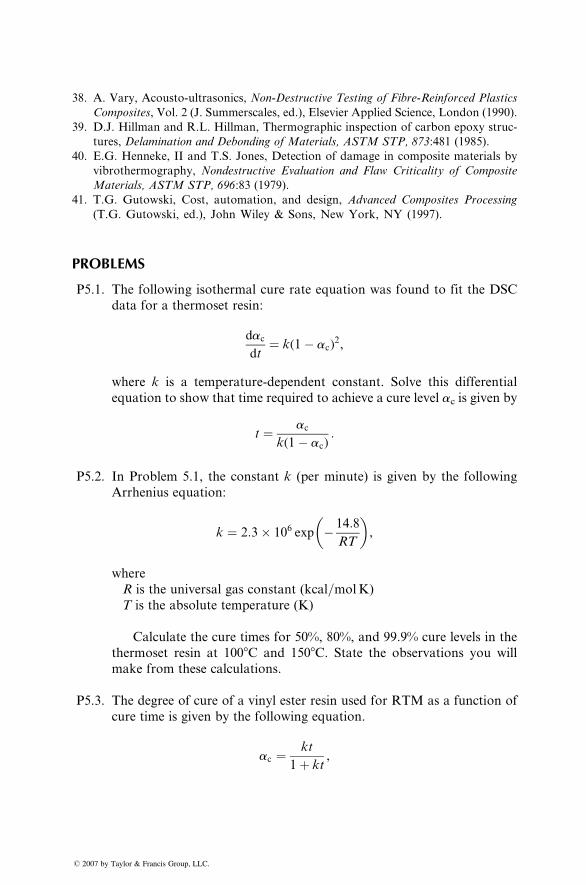
38.
� 20
A. Vary, Acousto-ultrasonics, Non-Destructive Testing of Fibre-Reinforced Plastics
Composites, Vol. 2 (J. Summerscales, ed.), Elsevier Applied Science, London (1990).
39.
D.J. Hillman and R.L. Hillman, Thermographic inspection of carbon epoxy struc-tures, Delamination and Debonding of Materials, ASTM STP, 873:481 (1985).
40.
E.G. Henneke, II and T.S. Jones, Detection of damage in composite materials byvibrothermography, Nondestructive Evaluation and Flaw Criticality of Composite
Materials, ASTM STP, 696:83 (1979).
41.
T.G. Gutowski, Cost, automation, and design, Advanced Composites Processing(T.G. Gutowski, ed.), John Wiley & Sons, New York, NY (1997).
PROBLEMS
P5.1. The following isothermal cure rate equation was found to fit the DSC
data for a thermoset resin:
dac
dt¼ k(1� ac)
2,
07 by
where k is a temperature-dependent constant. Solve this differential
equation to show that time required to achieve a cure level ac is given by
t ¼ ac
k(1� ac):
P5.2. In Problem 5.1, the constant k (per minute) is given by the following
Arrhenius equation:
k ¼ 2:3� 106 exp � 14:8
RT
� �,
where
R is the universal gas constant (kcal=molK)
T is the absolute temperature (K)
Calculate the cure times for 50%, 80%, and 99.9% cure levels in the
thermoset resin at 1008C and 1508C. State the observations you will
make from these calculations.
P5.3. The degree of cure of a vinyl ester resin used for RTM as a function of
cure time is given by the following equation.
ac ¼ kt
1þ kt,
Taylor & Francis Group, LLC.
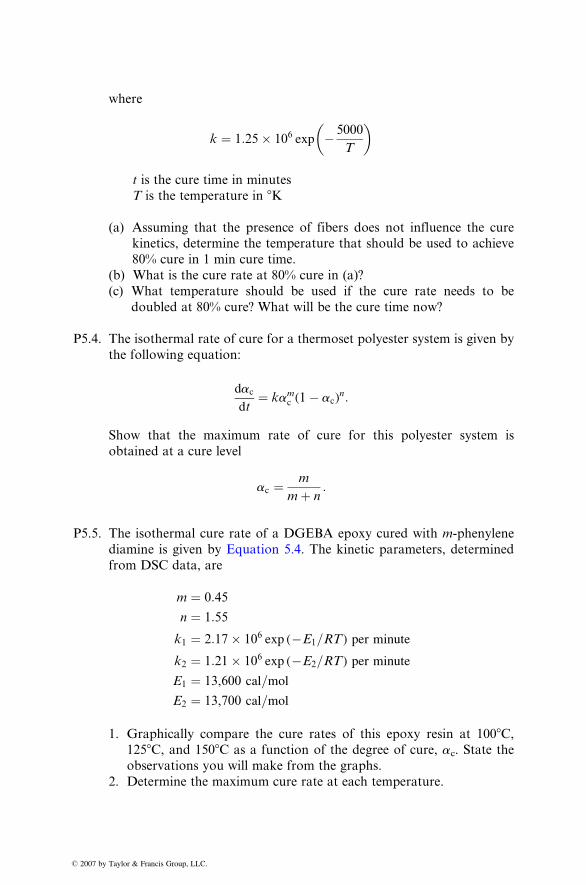
� 2007 by
wher e
k ¼ 1: 25 � 10 6 exp � 5000
T
� �
t is the cure tim e in minut es
T is the tempe ratur e in 8 K
(a) Assuming that the presence of fiber s does not influen ce the cure
kinetics, determ ine the tempe ratur e that should be used to achieve
80% cure in 1 min cure time.
(b) What is the cure rate at 80% cure in (a)?
(c) What tempe rature sho uld be used if the cure rate needs to be
doubled at 80% cu re? Wh at will be the cure time now?
P5.4. The isot hermal rate of cure for a therm oset polyester system is given by
the followin g eq uation:
dac
d t¼ k a mc ( 1 � a c )
n :
Show that the maximum rate of cure for this polyest er system is
obtained at a cure level
ac ¼ m
mþ n:
P5.5. The isothermal cure rate of a DGEBA epoxy cured with m-phenylene
diamin e is given by Equat ion 5.4. The kinetic parame ters, de termined
from DSC data, are
m ¼ 0:45
n ¼ 1:55
k1 ¼ 2:17� 106 exp (�E1=RT) per minute
k2 ¼ 1:21� 106 exp (�E2=RT) per minute
E1 ¼ 13,600 cal=mol
E2 ¼ 13,700 cal=mol
1. Graphically compare the cure rates of this epoxy resin at 1008C,1258C, and 1508C as a function of the degree of cure, ac. State the
observations you will make from the graphs.
2. Determine the maximum cure rate at each temperature.
Taylor & Francis Group, LLC.
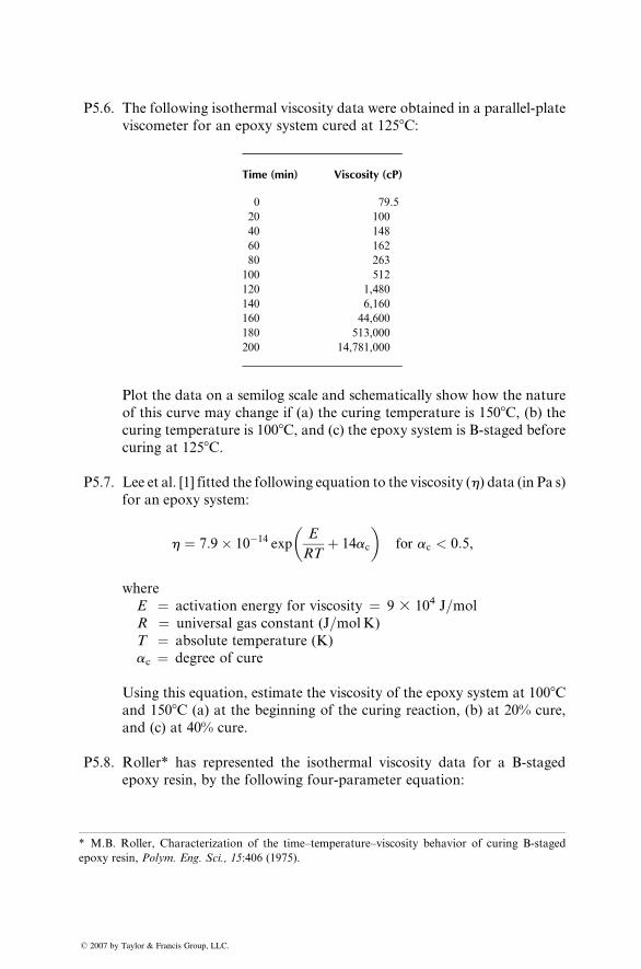
P5.6. The following isothermal viscosity data were obtained in a parallel-plate
viscometer for an epoxy system cured at 1258C:
* M.B. Roller, Characterization
epoxy resin, Polym. Eng. Sci., 15
� 2007 by Taylor & Francis Group, LLC.
Time (min) Viscosity (cP)
of the time–temp
:406 (1975).
0
79.520
10040
14860
16280
263100
512120
1,480140
6,160160
44,600180
513,000200
14,781,000Plot the data on a semilog scale and schematically show how the nature
of this curve may change if (a) the curing temperature is 1508C, (b) thecuring temperature is 1008C, and (c) the epoxy system is B-staged before
curing at 1258C.
P5.7. Lee et al. [1] fitted the following equation to the viscosity (h) data (in Pa s)for an epoxy system:
h ¼ 7:9� 10�14 expE
RTþ 14ac
� �for ac < 0:5,
where
E ¼ activation energy for viscosity ¼ 9 3 104 J=mol
R ¼ universal gas constant (J=molK)
T ¼ absolute temperature (K)
ac ¼ degree of cure
Using this equation, estimate the viscosity of the epoxy system at 1008Cand 1508C (a) at the beginning of the curing reaction, (b) at 20% cure,
and (c) at 40% cure.
P5.8. Roller* has represented the isothermal viscosity data for a B-staged
epoxy resin, by the following four-parameter equation:
erature–viscosity behavior of curing B-staged
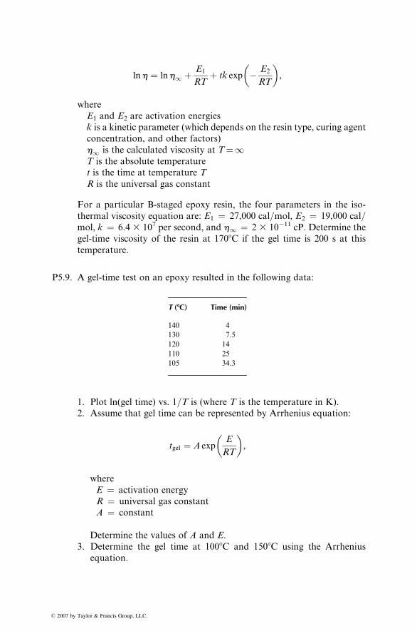
lnh ¼ lnh1 þ E1
RTþ tk exp � E2
RT
� �,
� 2007 by
where
E1 and E2 are activation energies
k is a kinetic parameter (which depends on the resin type, curing agent
concentration, and other factors)
h1 is the calculated viscosity at T¼1T is the absolute temperature
t is the time at temperature T
R is the universal gas constant
For a particular B-staged epoxy resin, the four parameters in the iso-
thermal viscosity equation are: E1 ¼ 27,000 cal=mol, E2 ¼ 19,000 cal=mol, k ¼ 6.4 3 107 per second, and h1 ¼ 2 3 10�11 cP. Determine the
gel-time viscosity of the resin at 1708C if the gel time is 200 s at this
temperature.
P5.9. A gel-time test on an epoxy resulted in the following data:
Taylor & Francis Group, LLC.
T (8C)
Time (min)140
4130
7.5120
14110
25105
34.31. Plot ln(gel time) vs. 1=T is (where T is the temperature in K).
2. Assume that gel time can be represented by Arrhenius equation:
tgel ¼ A expE
RT
� �,
where
E ¼ activation energy
R ¼ universal gas constant
A ¼ constant
Determine the values of A and E.
3. Determine the gel time at 1008C and 1508C using the Arrhenius
equation.
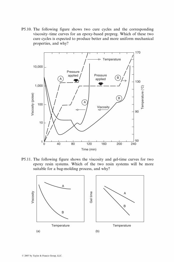
P5.10. The following figure shows two cure cycles and the corresponding
viscosity–time curves for an epoxy-based prepreg. Which of these two
cure cycles is expected to produce better and more uniform mechanical
properties, and why?
10,000
1,000
A
A
B
B
100
10
0 40 80 120
Time (min)
Vis
cosi
ty (
pois
e)
Tem
pera
ture
(�C
)
Temperature
Viscosity
Pressureapplied
Pressureapplied
160 200 240
170
130
90
501
P5.11. The following figure shows the viscosity and gel-time curves for two
epoxy resin systems. Which of the two resin systems will be more
suitable for a bag-molding process, and why?
Temperature Temperature
A
A
B
B
(a) (b)
Vis
cosi
ty
Gel
tim
e
� 2007 by Taylor & Francis Group, LLC.
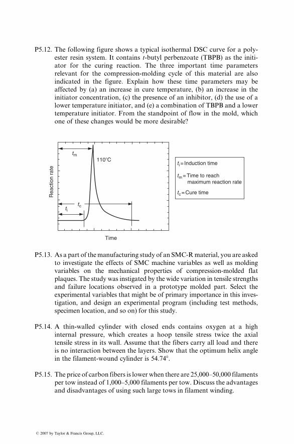
� 2007 by
The following figure shows a typical isothermal DSC curve for a poly-
P5.12.ester resin system. It contains t-butyl perbenzoate (TBPB) as the initi-
ator for the curing reaction. The three important time parameters
relevant for the compression-molding cycle of this material are also
indicated in the figure. Explain how these time parameters may be
affected by (a) an increase in cure temperature, (b) an increase in the
initiator concentration, (c) the presence of an inhibitor, (d) the use of a
lower temperature initiator, and (e) a combination of TBPB and a lower
temperature initiator. From the standpoint of flow in the mold, which
one of these changes would be more desirable?
Time
Rea
ctio
n ra
te
110�C
t i
t i = Induction time
tm = Time to reach maximum reaction rate
tc
tm
tc = Cure time
P5.13. As a part of themanufacturing study of an SMC-Rmaterial, you are asked
to investigate the effects of SMC machine variables as well as molding
variables on the mechanical properties of compression-molded flat
plaques. The study was instigated by the wide variation in tensile strengths
and failure locations observed in a prototype molded part. Select the
experimental variables that might be of primary importance in this inves-
tigation, and design an experimental program (including test methods,
specimen location, and so on) for this study.
P5.14. A thin-walled cylinder with closed ends contains oxygen at a high
internal pressure, which creates a hoop tensile stress twice the axial
tensile stress in its wall. Assume that the fibers carry all load and there
is no interaction between the layers. Show that the optimum helix angle
in the filament-wound cylinder is 54.748.
P5.15. The price of carbon fibers is lower when there are 25,000–50,000 filaments
per tow instead of 1,000–5,000 filaments per tow. Discuss the advantages
and disadvantages of using such large tows in filament winding.
Taylor & Francis Group, LLC.
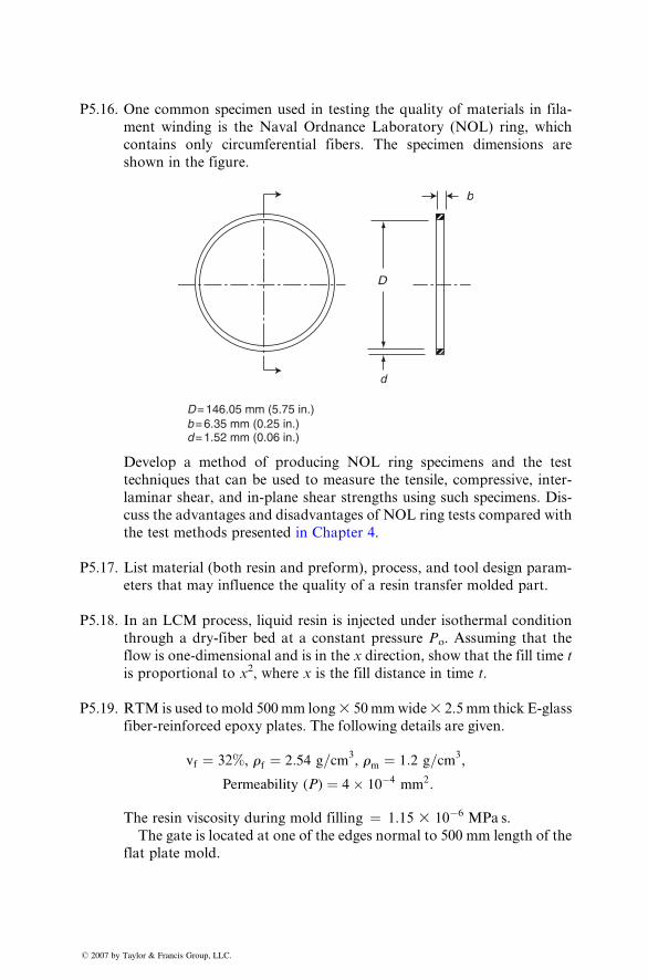
P5.16. One co mmon specim en us ed in test ing the qua lity of mate rials in fila-
ment wi nding is the Naval Ordnanc e Labor atory (NOL ) ring, which
con tains only circumfer entia l fibers. The specim en dimens ions are
shown in the figure.
D
b
d
d = 1.52 mm (0.06 in.)b = 6.35 mm (0.25 in.)D = 146.05 mm (5.75 in.)
Devel op a method of pro ducing NOL ring specim ens and the test
� 2007 by
techniques that can be used to measur e the tensile, compres sive, inter -
lamin ar shear, and in-pl ane shear strengths using such specim ens. Dis -
cuss the ad vantage s and disadva ntages of NOL ring test s compared wi th
the test methods presented in Chapt er 4.
P5.17. List material (both resin and preform), process, and tool design param-
eters that may influence the quality of a resin transfer molded part.
P5.18. In an LCM process, liquid resin is injected under isothermal condition
through a dry-fiber bed at a constant pressure Po. Assuming that the
flow is one-dimensional and is in the x direction, show that the fill time t
is proportional to x2, where x is the fill distance in time t.
P5.19. RTM is used to mold 500mm long3 50mmwide3 2.5 mm thick E-glass
fiber-reinforced epoxy plates. The following details are given.
vf ¼ 32%, rf ¼ 2:54 g=cm3, rm ¼ 1:2 g=cm3
,
Permeability (P) ¼ 4� 10�4 mm2:
The resin viscosity during mold filling ¼ 1.15 3 10�6 MPa s.
The gate is located at one of the edges normal to 500 mm length of the
flat plate mold.
Taylor & Francis Group, LLC.
� 2007 by
1. How much resin (in kilogr ams) must be pum ped to fil l the cavity?
2. How much time will be ne eded to fill the cavit y at a constant flow
rate of 130 mm 3=s?3. Wh at will be the maxi mum injection pressur e need ed to fill the cavity
at this constant flow rate?
P5.20. Suppos e in Prob lem 5.19, it is decided to fill the cavity at con stant
pressur e instead of constant fill rate. If the con stant pressur e is
1.5 M Pa, how much time will be needed to fill the cavity?
P5.21. Ultrasoni c testing of an impac t-test ed qua si-isotro pic composi te pan el
containing carbon fibers in PEEK matrix shows the presence of local
delaminations, even though there are no apparent damages on the
outside. Propose, in as much detail as possible, a plan to repair the
internal damage and recommend tests to validate the repair.
P5.22. Eddy current technique has been used for nondestructively detecting
cracks and inclusions in metals. Investigate how this technique can be
used for fiber-reinforced composites and discuss its limitations.
Taylor & Francis Group, LLC.

� 2007 by Taylor & Francis Group, LLC.
6 Design
� 2007 by Taylor & Fr
In the preceding chapters, we have discussed various aspects of fiber-reinforced
polymers, including the constituent materials, mechanics, performance, and
manufacturing methods. A number of unique characteristics of fiber-reinforced
polymers that have emerged in these chapters are listed in Table 6.1. Many of
these characteristics are due to the orthotropic nature of fiber-reinforced com-
posites, which has also necessitated the development of new design approaches
that are different from the design approaches traditionally used for isotropic
materials, such as steel or aluminum alloys. This chapter describes some of the
design methods and practices currently used for fiber-reinforced polymers
including the failure prediction methods, the laminate design procedures, and
the joint design considerations. A number of design examples are also included.
6.1 FAILURE PREDICTION
Design analysis of a structure or a component is performed by comparing
stresses (or strains) due to applied loads with the allowable strength (or strain
capacity) of the material. In the case of biaxial or multiaxial stress fields, a
suitable failure theory is used for this comparison. For an isotropic material
that exhibits yielding, such as a mild steel or an aluminum alloy, either the
maximum shear stress theory or the distortional energy theory (von Mises yield
criterion) is commonly used for designing against yielding. Fiber-reinforced
polymers are not isotropic, nor do they exhibit gross yielding. Thus, failure
theories developed for metals or other isotropic materials are not applicable to
composite materials. Instead, many new failure theories have been proposed for
fiber-reinforced composites, some of which are discussed in this section.
6.1.1 FAILURE PREDICTION IN A UNIDIRECTIONAL LAMINA
We consider the plane stress condition of a general orthotropic lamina contain-
ing unidirectional fibers at a fiber orientation angle of u with respect to the
x axis (Figure 6.1). In Chapter 3, we saw that four independent elastic constants,
namely, E11, E22, G12, and n12, are required to define its elastic characteristics.
Its strength properties are characterized by five independent strength values:
SLt ¼ longitudinal tensile strength
STt ¼ transverse tensile strength
ancis Group, LLC.
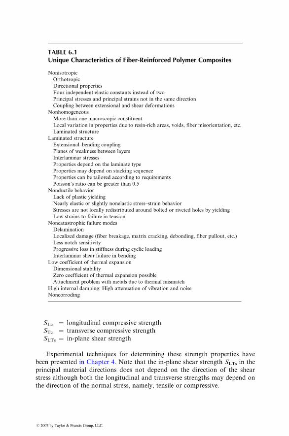
TABLE 6.1Unique Characteristics of Fiber-Reinforced Polymer Composites
Nonisotropic
Orthotropic
Directional properties
Four independent elastic constants instead of two
Principal stresses and principal strains not in the same direction
Coupling between extensional and shear deformations
Nonhomogeneous
More than one macroscopic constituent
Local variation in properties due to resin-rich areas, voids, fiber misorientation, etc.
Laminated structure
Laminated structure
Extensional–bending coupling
Planes of weakness between layers
Interlaminar stresses
Properties depend on the laminate type
Properties may depend on stacking sequence
Properties can be tailored according to requirements
Poisson’s ratio can be greater than 0.5
Nonductile behavior
Lack of plastic yielding
Nearly elastic or slightly nonelastic stress–strain behavior
Stresses are not locally redistributed around bolted or riveted holes by yielding
Low strains-to-failure in tension
Noncatastrophic failure modes
Delamination
Localized damage (fiber breakage, matrix cracking, debonding, fiber pullout, etc.)
Less notch sensitivity
Progressive loss in stiffness during cyclic loading
Interlaminar shear failure in bending
Low coefficient of thermal expansion
Dimensional stability
Zero coefficient of thermal expansion possible
Attachment problem with metals due to thermal mismatch
High internal damping: High attenuation of vibration and noise
Noncorroding
SLc ¼ longitudinal compres sive stre ngth
STc ¼ transverse compres sive stre ngth
SLTs ¼ in-plane shear strength
Expe rimental techn iques for determini ng these stre ngth propert ies have
been present ed in Chapt er 4. Note that the in-plan e sh ear stre ngth SLTs in the
princi pal mate rial directions does not dep end on the direct ion of the shea r
stress althoug h both the longitud inal an d trans verse stren gths may depen d on
the direction of the normal stress, na mely, tensile or comp ressive.
� 2007 by Taylor & Francis Group, LLC.
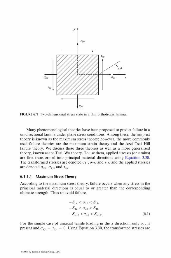
y
syy
syy
sxx
q
sxx
txy
txy
x
FIGURE 6.1 Two-dimensional stress state in a thin orthotropic lamina.
Many phe nomenologi cal theori es have be en proposed to predict failure in a
unidir ectiona l lamin a under plane stre ss co ndition s. Among these, the sim plest
theory is known as the maximum stress theory; howeve r, the more common ly
used failure theori es are the maximum strain theory and the Azzi–T sai–Hil l
failure theory. W e discus s these three theories as well as a more gen eralized
theory, known as the Tsai–Wu theory. To use them, ap plied stre sses (or stra ins)
are first transform ed into princi pal material directions using Equat ion 3.30.
The transformed stresses are denoted s11, s22, and t12, and the applied stresses
are denoted sxx, syy, and txy.
6.1.1.1 Maximum Stress Theory
According to the maximum stress theory, failure occurs when any stress in the
principal material directions is equal to or greater than the corresponding
ultimate strength. Thus to avoid failure,
�SLc < s11 < SLt,
�STc < s22 < STt,
�SLTs < t12 < SLTs: (6:1)
For the simple case of uniaxial tensile loading in the x direction, only sxx is
present and syy ¼ txy ¼ 0. Using Equation 3.30, the transformed stresses are
� 2007 by Taylor & Francis Group, LLC.
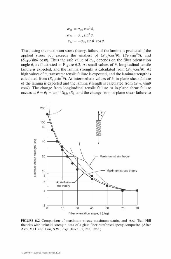
s11 ¼ sxx cos2 u,
s22 ¼ sxx sin2 u,
t12 ¼ �sxx sin u cos u:
Thus, using the maximum stress theory, failure of the lamina is predicted if the
applied stress sxx exceeds the smallest of (SLt=cos2u), (STt=sin
2u), and
(SLTs=sinu cosu). Thus the safe value of sxx depends on the fiber orientation
angle u, as illustrated in Figure 6.2. At small values of u, longitudinal tensilefailure is expected, and the lamina strength is calculated from (SLt=cos
2u). At
high values of u, transverse tensile failure is expected, and the lamina strength is
calculated from (STt=sin2u). At intermediate values of u, in-plane shear failure
of the lamina is expected and the lamina strength is calculated from (SLTs=sinucosu). The change from longitudinal tensile failure to in-plane shear failure
occurs at u ¼ u1 ¼ tan�1 SLTs=SLt and the change from in-plane shear failure to
Maximum stress theory
Maximum strain theory
Azzi–Tsai−Hill theory
Uni
axia
l ten
sile
str
engt
h (k
si)
Fiber orientation angle, q (deg)
20 15 30 45 60 75 90
200
100
60
40
20
10
8
6
4
q
FIGURE 6.2 Comparison of maximum stress, maximum strain, and Azzi–Tsai–Hill
theories with uniaxial strength data of a glass fiber-reinforced epoxy composite. (After
Azzi, V.D. and Tsai, S.W., Exp. Mech., 5, 283, 1965.)
� 2007 by Taylor & Francis Group, LLC.
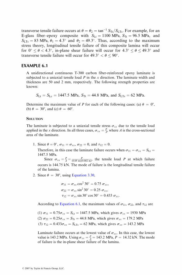
transve rse tensile failu re occurs at u ¼ u2 ¼ tan� 1 STt =SLTs . For exampl e, for an
E-glass fiber –epoxy composi te with SLt ¼ 1100 MP a, STt ¼ 96:5 MPa , and
SLTs ¼ 83 MPa , u 1 ¼ 4: 3� and u2 ¼ 49 :3� . Thus , accordi ng to the maximum
stress theory, longit udinal tensi le failure of this compo site lamin a will occur
for 0� � u < 4:3� , in-pl ane shear failure will occu r for 4 : 3� � u � 49 : 3� andtransve rse tensile failure will occu r for 49 :3� < u � 90� .
EXAMPLE 6.1
A unidirectional continuous T-300 carbon fiber-reinforced epoxy laminate is
subjected to a uniaxial tensile load P in the x direction. The laminate width and
thickness are 50 and 2 mm, respectively. The following strength properties are
known:
SLt ¼ SLc ¼ 1 447 :5 MPa , S Tt ¼ 44: 8 MP a, and S LTs ¼ 62 MPa :
Determine the maximum value of P for each of the following cases: (a) u ¼ 08 ,(b) u ¼ 30 8, and (c) u ¼ 608 .
SOLUTIO N
The laminate is subjected to a uniaxial tensile stress sxx due to the tensile load
applied in the x direction. In all three cases, sxx ¼ PA, where A is the cross-sectional
area of the laminate.
1. Since u ¼ 0� , s11 ¼ s xx , s 22 ¼ 0, and t 12 ¼ 0.
Therefore, in this case the laminate failure occurs when s11 ¼ s xx ¼ S Lt ¼1447: 5 MPa.
Since sxx ¼ PA ¼ P
(0 :05 m)(0 :002 m), the tensile load P at which failure
occurs is 144.75 kN. The mode of failure is the longitudinal tensile failure
of the lamina.
2. Since u ¼ 308, using Equation 3.30,
s11 ¼ s xx cos 2 30� ¼ 0: 75 s xx ,
s22 ¼ s xx sin 2 30� ¼ 0: 25 s xx ,
t12 ¼ sxx sin 30� cos 30� ¼ 0:433 sxx:
According to Equation 6.1, the maximum values of s11, s22, and t12 are
(1) s11 ¼ 0:75sxx ¼ SLt ¼ 1447:5 MPa, which gives sxx ¼ 1930 MPa
(2) s22 ¼ 0:25sxx ¼ STt ¼ 44:8 MPa, which gives sxx ¼ 179:2 MPa
(3) t12 ¼ 0:433sxx ¼ SLTs ¼ 62 MPa, which gives sxx ¼ 143:2 MPa
Laminate failure occurs at the lowest value of sxx. In this case, the lowest
value is 143.2 MPa. Using sxx ¼ PA¼ 143:2 MPa, P ¼ 14.32 kN. The mode
of failure is the in-plane shear failure of the lamina.
� 2007 by Taylor & Francis Group, LLC.
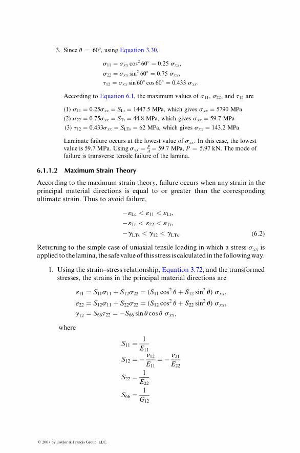
3. Since u ¼ 608 , using Equation 3.30,
s11 ¼ s xx cos 2 60� ¼ 0: 25 s xx ,
s22 ¼ s xx sin2 60� ¼ 0: 75 s xx ,
t12 ¼ s xx sin 60� cos 60� ¼ 0: 433 s xx :
According to Equation 6.1, the maximum values of s11 , s 22 , and t 12 are
(1) s11 ¼ 0: 25s xx ¼ S Lt ¼ 1447: 5 MPa , which gives s xx ¼ 5790 MPa
(2) s22 ¼ 0: 75s xx ¼ S Tt ¼ 44: 8 MPa, which gives s xx ¼ 59: 7 MPa
( 3) t12 ¼ 0: 433s xx ¼ S LTs ¼ 62 MPa, which gives s xx ¼ 143: 2 MPa
Laminate failure occurs at the lowest value of sxx . In this case, the lowest
value is 59.7 MPa. Using sxx ¼ PA ¼ 59 :7 MPa, P ¼ 5.97 kN. The mode of
failure is transverse tensile failure of the lamina.
6.1.1 .2 Maxi mum Strain The ory
Accor ding to the maxi mum stra in theory, failure occurs when any stra in in the
princi pal material direction s is eq ual to or great er than the corresp onding
ultimat e strain. Thus to avo id failure,
� «Lc < «11 < «Lt ,
� «Tc < «22 < «Tt ,
� gLTs < g 12 < g LTs : ( 6: 2)
Returning to the simple case of uniaxial tensile loading in which a stress sxx is
applied to the lamina, the safe valueof this stress is calculated in the followingway.
1. Usi ng the stra in–stress relat ionshi p, Equation 3.72, and the trans formed
stresses, the strains in the principal material directions are
«11 ¼ S11s11 þ S12s22 ¼ (S11 cos2 uþ S12 sin
2 u) sxx,
«22 ¼ S12s11 þ S22s22 ¼ (S12 cos2 uþ S22 sin
2 u) sxx,
g12 ¼ S66t22 ¼ �S66 sin u cos u sxx,
where
S11 ¼ 1
E11
S12 ¼ � n12E11
¼ � n21E22
S22 ¼ 1
E22
S66 ¼ 1
G12
� 2007 by Taylor & Francis Group, LLC.
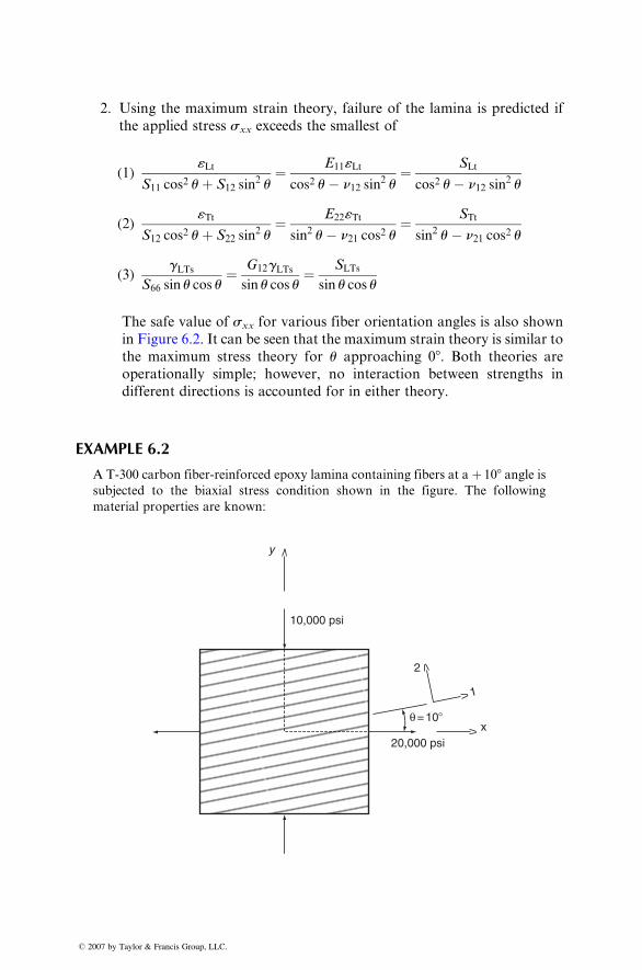
2. Usin g the maximum strain theory, failure of the lami na is pr edicted if
the applied stre ss sxx exceeds the smal lest of
( 1)«Lt
S11 cos 2 u þ S12 sin 2 u
¼ E11 «Lt
cos 2 u � n12 sin2 u
¼ SLt
cos 2 u � n12 sin2 u
( 2)«Tt
S12 cos 2 u þ S22 sin 2 u
¼ E22 «Tt
sin2 u � n21 cos2 u ¼ STt
sin 2 u � n21 cos 2 u
( 3)gLTs
S66 sin u cos u ¼ G12 g LTs
sin u cos u ¼ SLTs
sin u cos u
The safe value of sxx for various fiber orientation angles is also shown
in Figure 6.2. It can be seen that the maxi mum strain theory is similar to
the maximum stress theory for u approaching 08. Both theories are
operationally simple; however, no interaction between strengths in
different directions is accounted for in either theory.
EXAMPLE 6.2
A T-300 carbon fiber-reinforced epoxy lamina containing fibers at a þ 108 angle issubjected to the biaxial stress condition shown in the figure. The following
material properties are known:
10,000 psi
20,000 psix
1
2
θ = 10�
y
� 2007 by Taylor & Francis Group, LLC.
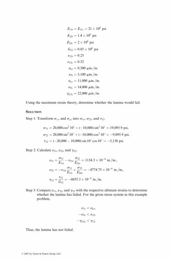
� 2
E11t ¼ E11c ¼ 21� 106 psi
E22t ¼ 1:4� 106 psi
E22c ¼ 2� 106 psi
G12 ¼ 0:85� 106 psi
n12t ¼ 0:25
n12c ¼ 0:52
«Lt ¼ 9,500 min:=in:
«Tt ¼ 5,100 min:=in:
«Lc ¼ 11,000 min:=in:
«Tc ¼ 14,000 min:=in:
gLTs ¼ 22,000 min:=in:
Using the maximum strain theory, determine whether the lamina would fail.
SOLUTION
Step 1: Transform sxx and syy into s11, s22, and t12.
s11 ¼ 20,000 cos2 10� þ (�10,000) sin2 10� ¼ 19,095:9 psi,
s22 ¼ 20,000 sin2 10� þ (�10,000) cos2 10� ¼ �9,095:9 psi,
t12 ¼ (�20,000� 10,000) sin 10� cos 10� ¼ �5,130 psi:
Step 2: Calculate «11, «22, and g12.
«11 ¼ s11
E11t
� n21cs22
E22c
¼ 1134:3� 10�6 in:=in:,
«22 ¼ �n12ts11
E11t
þ s22
E22c
¼ �4774:75� 10�6 in:=in:,
g12 ¼t12G12
¼ �6035:3� 10�6 in:=in:
Step 3: Compare «11, «22, and g12 with the respective ultimate strains to determine
whether the lamina has failed. For the given stress system in this example
problem,
«11 < «Lt,
�«Tc < «22,
�gLTs < g12:
Thus, the lamina has not failed.
007 by Taylor & Francis Group, LLC.
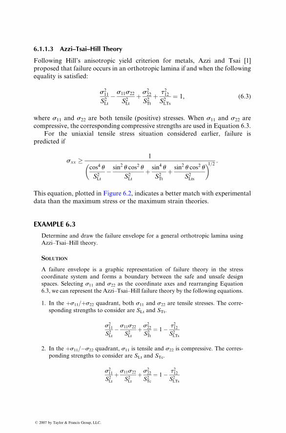
6.1.1.3 Azz i–Tsai–Hi ll Theory
Follow ing Hill’ s anisot ropic yield criteri on for meta ls, Azzi an d Ts ai [1]
proposed that fail ure oc curs in an or thotrop ic lamina if and when the foll owing
equali ty is sati sfied:
s 211S 2Lt
� s11 s 22
S 2Ltþ s 222
S 2Ttþ t 212S 2LTs
¼ 1, ( 6: 3)
where s11 and s22 are both tensile (posi tive) stre sses. Whe n s11 an d s22 are
compres sive, the corres ponding compres sive strengths are used in Equat ion 6.3.
For the uniaxi al tensi le stre ss situati on consider ed earlier, failure is
predict ed if
sxx � 1
cos4 u
S2Lt
� sin2 u cos2 u
S2Lt
þ sin4 u
S2Tt
þ sin2 u cos2 u
S2Lts
� �1=2 :
This equati on, plott ed in Figure 6.2, indicates a bette r match with experi menta l
data than the maximum stress or the maximum strain theories.
EXAMPLE 6.3
Determine and draw the failure envelope for a general orthotropic lamina using
Azzi–Tsai–Hill theory.
SOLUTION
A failure envelope is a graphic representation of failure theory in the stress
coordinate system and forms a boundary between the safe and unsafe design
spaces. Selecting s11 and s22 as the coordinate axes and rearranging Equation
6.3, we can represent the Azzi–Tsai–Hill failure theory by the following equations.
1. In the þs11=þs22 quadrant, both s11 and s22 are tensile stresses. The corre-
sponding strengths to consider are SLt and STt.
s211
S2Lt
� s11s22
S2Lt
þ s222
S2Tt
¼ 1� t212S2LTs
2. In the þs11=�s22 quadrant, s11 is tensile and s22 is compressive. The corres-
ponding strengths to consider are SLt and STc.
s211
S2Lt
þ s11s22
S2Lt
þ s222
S2Tc
¼ 1� t212S2LTs
� 2007 by Taylor & Francis Group, LLC.
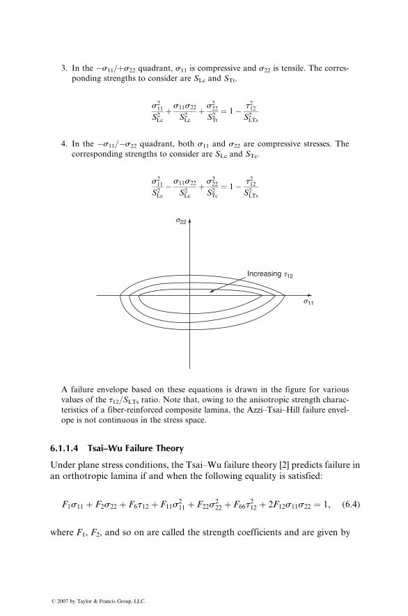
3. In the �s11=þs22 quadrant, s11 is compressive and s22 is tensile. The corres-
ponding strengths to consider are SLc and STt.
s211
S2Lc
þ s11s22
S2Lc
þ s222
S2Tt
¼ 1� t212S2LTs
4. In the �s11=�s22 quadrant, both s11 and s22 are compressive stresses. The
corresponding strengths to consider are SLc and STc.
s211
S2Lc
� s11s22
S2Lc
þ s222
S2Tc
¼ 1� t212S2LTs
s22
s11
Increasing t12
A failure envelope based on these equations is drawn in the figure for various
values of the t12=SLTs ratio. Note that, owing to the anisotropic strength charac-
teristics of a fiber-reinforced composite lamina, the Azzi–Tsai–Hill failure envel-
ope is not continuous in the stress space.
6.1.1.4 Tsai–Wu Failure Theory
Under plane stress conditions, the Tsai–Wu failure theory [2] predicts failure in
an orthotropic lamina if and when the following equality is satisfied:
F1s11 þ F2s22 þ F6t12 þ F11s211 þ F22s
222 þ F66t
212 þ 2F12s11s22 ¼ 1, (6:4)
where F1, F2, and so on are called the strength coefficients and are given by
� 2007 by Taylor & Francis Group, LLC.
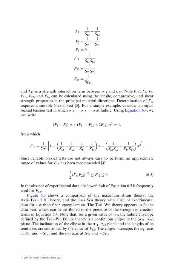
F1 ¼ 1
SLt
� 1
SLc
F2 ¼ 1
STt
� 1
STc
F6 ¼ 0
F11 ¼ 1
SLt SLc
F22 ¼ 1
STt STc
F66 ¼ 1
S 2LTs
and F12 is a strength interacti on term betw een s 11 and s 22. Note that F1, F 2,
F11 , F22 , and F66 can be calcul ated using the tensi le, compres sive, and shear
strength propert ies in the princip al mate rial direct ions. Dete rminati on of F12
requir es a suitab le biaxi al test [3]. For a sim ple exampl e, consider an equ al
biaxial tension test in whi ch s11 ¼ s12 ¼ s at failure. Using Equation 6.4, we
can write
(F1 þ F2 ) s þ ( F 11 þ F 22 þ 2F12 ) s 2 ¼ 1,
from whi ch
F12 ¼ 1
2s 21 � 1
SLt
� 1
SLc
þ 1
STt
� 1
STc
� �s � 1
SLt S Lcþ 1
STt STc
� �s 2
� �:
Since reliab le biaxi al tests are not alwa ys easy to perform, an ap proxim ate
range of values for F12 ha s been recomm end ed [4]:
� 1
2 ( F11 F22 )
1 =2 � F12 � 0: ( 6: 5)
In the absence of e xperimental da ta, the low er limit of Equation 6.5 is frequent ly
used for F12.
Figure 6.3 shows a comp arison of the maxi mum stra in theory, the
Azzi–Tsai–Hill Theory, and the Tsai–Wu theory with a set of experimental
data for a carbon fiber–epoxy lamina. The Tsai–Wu theory appears to fit the
data best, which can be attributed to the presence of the strength interaction
terms in Equation 6.4. Note that, for a given value of t12, the failure envelopedefined by the Tsai–Wu failure theory is a continuous ellipse in the (s11, s22)
plane. The inclination of the ellipse in the s11, s22 plane and the lengths of its
semi-axes are controlled by the value of F12. The ellipse intercepts the s11 axis
at SLt and �SLc, and the s22 axis at STt and �STc.
� 2007 by Taylor & Francis Group, LLC.
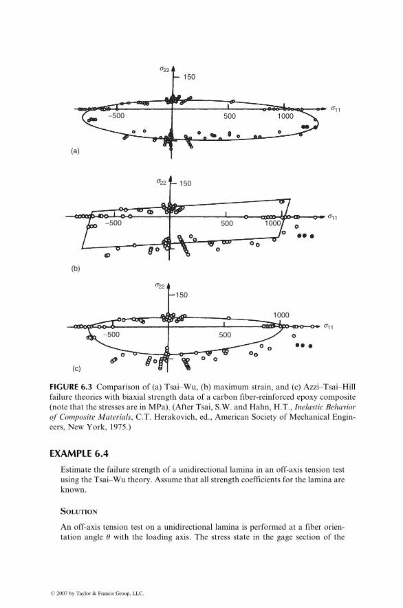
(a)
(b)
(c)
150
150
150
−500
−500
−500
500
1000
1000
1000
500
500
s22
s22
s22
s11
s11
s11
FIGURE 6.3 Comparison of (a) Tsai–Wu, (b) maximum strain, and (c) Azzi–Tsai–Hill
failure theories with biaxial strength data of a carbon fiber-reinforced epoxy composite
(note that the stresses are in MPa). (After Tsai, S.W. and Hahn, H.T., Inelastic Behavior
of Composite Materials, C.T. Herakovich, ed., American Society of Mechanical Engin-
eers, New York, 1975.)
EXAMPLE 6.4
Estimate the failure strength of a unidirectional lamina in an off-axis tension test
using the Tsai–Wu theory. Assume that all strength coefficients for the lamina are
known.
SOLUTION
An off-axis tension test on a unidirectional lamina is performed at a fiber orien-
tation angle u with the loading axis. The stress state in the gage section of the
� 2007 by Taylor & Francis Group, LLC.
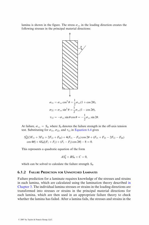
lamina is shown in the figure. The stress sxx in the loading direction creates the
following stresses in the principal material directions:
q
s11 ¼ s xx cos 2 u ¼ 1
2 s xx ( 1 þ cos 2u) ,
s22 ¼ s xx sin 2 u ¼ 1
2 s xx (1 � cos 2u) ,
t12 ¼ �s xx sin u cos u ¼ � 1
2 s xx sin 2u :
At failure, sxx ¼ Su , where Su denotes the failure strength in the off-axis tension
test. Substituting for s11 , s22 , and t 12 in Equation 6.4 gives
S 2u [( 3F11 þ 3F 22 þ 2F 12 þ F66 ) þ 4(F 11 � F 22 ) cos 2u þ ( F11 þ F22 � 2F 12 � F 66 )
cos 4u] þ 4Su [( F1 þ F2 ) þ ( F1 � F2 ) cos 2u] � 8 ¼ 0:
This represents a quadratic equation of the form
AS 2u þ BSu þ C ¼ 0,
which can be solved to calculate the failure strength Su.
6.1.2 FAILURE P REDICTION FOR UNNOTCHED L AMINATES
Failur e pred iction for a laminate req uires knowl edge of the stre sses and stra ins
in each lamina, whi ch are calcul ated using the laminati on theo ry descri bed in
Chapte r 3. The indivi dual lami na stre sses or stra ins in the loading direct ions are
transformed into stresses or strains in the principal material directions for
each lamina, which are then used in an appropriate failure theory to check
whether the lamina has failed. After a lamina fails, the stresses and strains in the
� 2007 by Taylor & Francis Group, LLC.
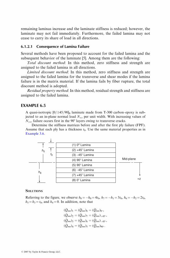
remain ing lamin as increa se and the lamin ate stiffne ss is redu ced; howeve r, the
laminate may not fail imm ediat ely. Furtherm ore, the failed lami na may not
cease to carry its share of load in a ll directions.
6.1.2 .1 Cons equen ce of Lami na Failure
Several methods have been pro posed to accou nt for the failed lamin a and the
subseque nt beh avior of the lami nate [5]. Among them are the followin g:
Total disco unt method : In this method, zero stiffne ss and stre ngth are
assign ed to the failed lamina in all directions.
Limi ted disco unt method : In this method, zero stiffne ss and stren gth a re
assign ed to the failed lamina for the transverse and shear mo des if the lamina
failure is in the matr ix mate rial. If the lami na fails by fiber ru pture, the total
discount method is adop ted.
Res idual proper ty met hod : In this method, residu al stre ngth and stiffne ss a re
assign ed to the failed lamina.
EXAMPLE 6.5
A quasi-isotropic [0 =±45=90]S laminate made from T-300 carbon–epoxy is sub-
jected to an in-plane normal load Nxx per unit width. With increasing values of
Nxx, failure occurs first in the 908 layers owing to transverse cracks.
Determine the stiffness matrices before and after the first ply failure (FPF).
Assume that each ply has a thickness t0. Use the same material properties as in
Example 3.6.
h0
(1) 0o Lamina
(8) 0� Lamina
(2) +45� Lamina
(7) +45� Lamina
(3) −45� Lamina
(6) −45� Lamina
(4) 90� Lamina Mid-plane
+z
(5) 90� Lamina
h8
t0
SOLUTIONS
Referring to the figure, we observe h8¼�h0¼ 4t0, h7¼�h1¼ 3t0, h6¼�h2¼ 2t0,
h5¼ h3¼ t0, and h4¼ 0. In addition, note that
(�Qmn)1 ¼ (�Qmn)8 ¼ (�Qmn)0� ,
(�Qmn)2 ¼ (�Qmn)7 ¼ (�Qmn)þ45� ,
(�Qmn)3 ¼ (�Qmn)6 ¼ (�Qmn)�45� ,
(�Qmn)4 ¼ (�Qmn)5 ¼ (�Qmn)90� :
� 2007 by Taylor & Francis Group, LLC.
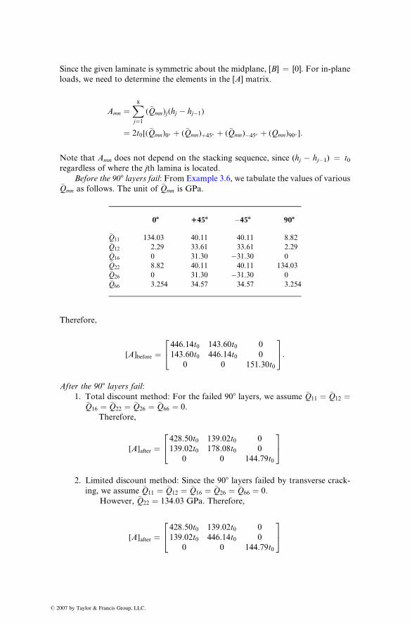
� 2
Since the given laminate is symmetric about the midplane, [B] ¼ [0]. For in-plane
loads, we need to determine the elements in the [A] matrix.
Amn ¼X8j¼1
(�Qmn)j(hj � hj�1)
¼ 2t0[(�Qmn)0� þ (�Qmn)þ45� þ (�Qmn)�45� þ (Qmn)90� ]:
Note that Amn does not depend on the stacking sequence, since (hj � hj�1) ¼ t0regardless of where the jth lamina is located.
Before the 908 layers fail: From Example 3.6, we tabulate the values of various�Qmn as follows. The unit of �Qmn is GPa.
007 by Taylor & Fra
08 1458 �458 908
ncis Group, LL
C.�Q11
134.03 40.11 40.11 8.82 �Q12 2.29 33.61 33.61 2.29 �Q16 0 31.30 �31.30 0 �Q22 8.82 40.11 40.11 134.03 �Q26 0 31.30 �31.30 0 �Q66 3.254 34.57 34.57 3.254Therefore,
[A]before ¼446:14t0 143:60t0 0
143:60t0 446:14t0 0
0 0 151:30t0
24
35:
After the 908 layers fail:
1. Total discount method: For the failed 908 layers, we assume �Q11 ¼ �Q12 ¼�Q16 ¼ �Q22 ¼ �Q26 ¼ �Q66 ¼ 0.
Therefore,
[A]after ¼428:50t0 139:02t0 0
139:02t0 178:08t0 0
0 0 144:79t0
24
35
2. Limited discount method: Since the 908 layers failed by transverse crack-
ing, we assume �Q11 ¼ �Q12 ¼ �Q16 ¼ �Q26 ¼ �Q66 ¼ 0:However, �Q22 ¼ 134:03 GPa. Therefore,
[A]after ¼428:50t0 139:02t0 0
139:02t0 446:14t0 0
0 0 144:79t0
24
35
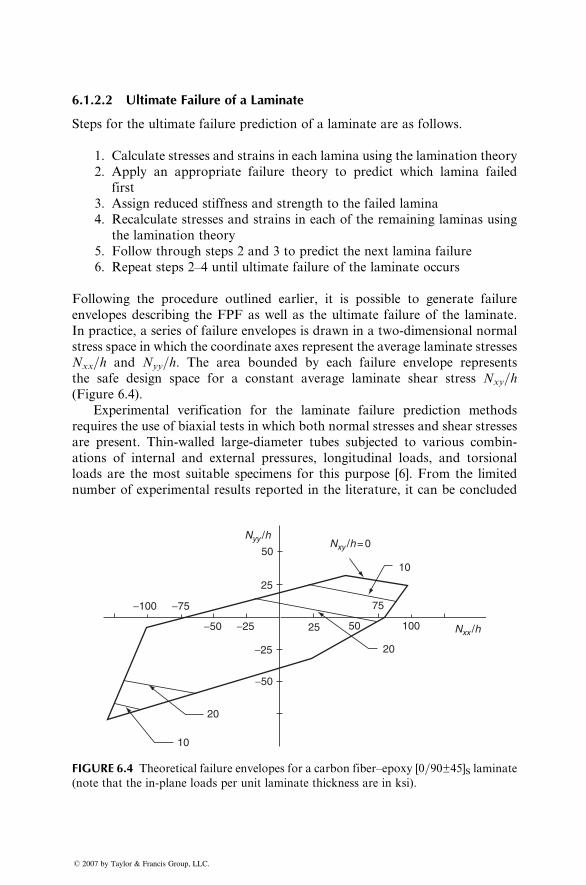
6.1.2.2 Ultimate Failure of a Laminate
Steps for the ultimate failure prediction of a laminate are as follows.
1. Calculate stresses and strains in each lamina using the lamination theory
2. Apply an appropriate failure theory to predict which lamina failed
first
3. Assign reduced stiffness and strength to the failed lamina
4. Recalculate stresses and strains in each of the remaining laminas using
the lamination theory
5. Follow through steps 2 and 3 to predict the next lamina failure
6. Repeat steps 2–4 until ultimate failure of the laminate occurs
Following the procedure outlined earlier, it is possible to generate failure
envelopes describing the FPF as well as the ultimate failure of the laminate.
In practice, a series of failure envelopes is drawn in a two-dimensional normal
stress space in which the coordinate axes represent the average laminate stresses
Nxx=h and Nyy=h. The area bounded by each failure envelope represents
the safe design space for a constant average laminate shear stress Nxy=h(Figure 6.4).
Experimental verification for the laminate failure prediction methods
requires the use of biaxial tests in which both normal stresses and shear stresses
are present. Thin-walled large-diameter tubes subjected to various combin-
ations of internal and external pressures, longitudinal loads, and torsional
loads are the most suitable specimens for this purpose [6]. From the limited
number of experimental results reported in the literature, it can be concluded
Nyy /h
Nxx /h
Nxy /h = 0
−100 −75 75
10
10
100
20
20
50
50
−50
−50
25
25
−25
−25
FIGURE 6.4 Theoretical failure envelopes for a carbon fiber–epoxy [0=90±45]S laminate
(note that the in-plane loads per unit laminate thickness are in ksi).
� 2007 by Taylor & Francis Group, LLC.
that no single failure theory repres ents all lamina tes equall y well. Among the
various deficienci es in the theoret ical prediction method s are the absence of
interlam inar stre sses and nonl inear effects. The assum ption regardi ng the load
transfer between the fail ed lami nas an d the active laminas can also intr oduce
errors in the theo retical an alyses.
The failure load predict ion for a laminate depen ds strong ly on the lamina
failure theo ry selected [7]. In the comp osite mate rial indust ry, there is little
agreem ent on which lamina failure theory works best, a lthough the maximum
strain theory is more commonl y us ed than the others [8]. Recent ly, the Tsai–Wu
failure theory is finding more applic ations in the acad emic field.
6.1.3 FAILURE P REDICTION IN RANDOM F IBER L AMINATES
There are tw o different approa ches for predicting failure in lami nates contain -
ing ran domly orient ed discont inuous fibers.
In the Hahn’s approach [9], whi ch is a simple app roach, failure is pred icted
when the maximum tensi le stre ss in the laminate equa ls the followi ng strength
average d over all possible fiber orient ation angles:
Sr ¼ 4
p
ffiffiffiffiffiffiffiffiffiffiffiffiffiSLt S Tt
p, ( 6: 6)
where
Sr ¼ stre ngth of the random fiber laminate
SLt ¼ longit udinal stre ngth of a 08 lami nate
STt ¼ trans verse stre ngth of a 08 lami nate
In the Halpin–Kardos approach [10], the random fiber laminate is modeled
as a quasi-isotropic [0=±45=90]S laminate containing discontinuous fibers in the
08 , ±45 8 , and 90 8 orientati ons. The Halpin –Tsai eq uations , Equat ions 3.49
through 3.53, are used to calculate the basic elastic propert ies, namel y, E11,
E22, n12, and G12, of the 08 discontinuous fiber laminas. The ultimate strain
allowables for the 08 and 908 laminas are estimated from the continuous fiber
allowables using the Halpin–Kardos equations:
«Lt(d) ¼ «LtEf
Em
� ��0:87
þ 0:50
" #for lf > lc (6:7)
and
«Td(d) ¼ «Tt 1� 1:21v2=3f
� �:
The procedure followed by Halpin and Kardos [10] for estimating the ultimate
strength of random fiber laminates is the same as the ply-by-ply analysis used
for continuous fiber quasi-isotropic [0=±45=90]S laminates.
� 2007 by Taylor & Francis Group, LLC.
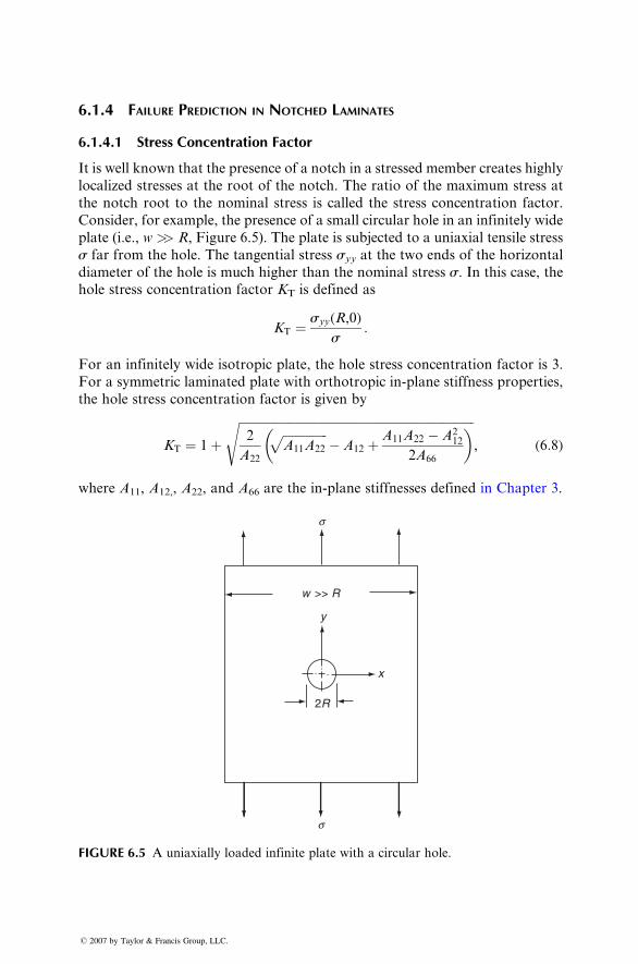
6.1.4 F AILURE P REDICTION IN NOTCHED L AMINATES
6.1.4 .1 Stres s Conce ntrat ion Fac tor
It is well known that the presence of a notch in a stressed member creat es highly
local ized stre sses at the root of the notch. The rati o of the maxi mum stress at
the notch root to the nominal stress is call ed the stre ss concentra tion fact or.
Consid er, for exampl e, the presence of a smal l circul ar hole in an infinit ely wide
plate (i.e., w >> R , Fig ure 6.5). The plate is subjected to a uni axial tensi le stre sss far from the hole. The tangent ial stress syy at the tw o e nds of the horizont al
diame ter of the hole is much higher than the nominal stre ss s. In this case, thehole stress concentra tion fact or KT is define d as
KT ¼ syy ( R,0 )
s:
For an infinit ely wide isot ropic plate , the hol e stress con centration fact or is 3.
For a symm etric lami nated plate wi th orthot ropic in-pl ane stiffne ss prop erties,
the hole stre ss co ncentra tion fact or is given by
KT ¼ 1 þffiffiffiffiffiffiffiffiffiffiffiffiffiffiffiffiffiffiffiffiffiffiffiffiffiffiffiffiffiffiffiffiffiffiffiffiffiffiffiffiffiffiffiffiffiffiffiffiffiffiffiffiffiffiffiffiffiffiffiffiffiffiffiffiffiffiffiffiffiffiffiffiffiffiffiffiffiffi2
A22
ffiffiffiffiffiffiffiffiffiffiffiffiffiffiffiA11A22
p� A12 þ A11A22 � A2
12
2A66
� �s, (6:8)
where A11 , A 12,, A22 , and A66 are the in-pl ane stiffne sses define d in Chapt er 3.
s
s
w >> R
y
x
2R
FIGURE 6.5 A uniaxially loaded infinite plate with a circular hole.
� 2007 by Taylor & Francis Group, LLC.
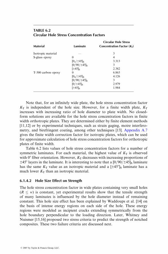
TABLE 6.2Circular Hole Stress Concentration Factors
Material Laminate
Circular Hole Stress
Concentration Factor (KT)
Isotropic material — 3
S-glass–epoxy 0 4
[02=±45]S 3.313
[0=90=±45]S 3
[±45]S 2.382
T-300 carbon–epoxy 0 6.863
[04=±45]S 4.126
[0=90=±45]S 3
[0=±45]S 2.979
[±45]S 1.984
Note that, for an infinitely wi de plate , the hole stress co ncentra tion factor
KT is indepen dent of the hole size. Ho wever, for a finite width plate , KT
increa ses with increa sing ratio of hole diame ter to plate width. No closed-
form solut ions are avail able for the hole stre ss concentra tion fact ors in fini te
width orthot ropic plate s. They are de termined eithe r by finite elem ent methods
[11,12] or by experi menta l techni que s, such as strain gaging, moire inter fero-
metry, and birefringe nt coatin g, among other techni ques [13]. Appendix A.7
gives the finite width correction factor for isotropic plates, which can be used
for approximate calculation of hole stress concentration factors for orthotropic
plates of finite width.
Table 6.2 lists values of hole stress concentration factors for a number of
symmetric laminates. For each material, the highest value of KT is observed
with 08 fiber orientation. However, KT decreases with increasing proportions of
±458 layers in the laminate. It is interesting to note that a [0=90=±45]S laminate
has the same KT value as an isotropic material and a [±458]S laminate has a
much lower KT than an isotropic material.
6.1.4.2 Hole Size Effect on Strength
The hole stress concentration factor in wide plates containing very small holes
(R � w) is constant, yet experimental results show that the tensile strength
of many laminates is influenced by the hole diameter instead of remaining
constant. This hole size effect has been explained by Waddoups et al. [14] on
the basis of intense energy regions on each side of the hole. These energy
regions were modeled as incipient cracks extending symmetrically from the
hole boundary perpendicular to the loading direction. Later, Whitney and
Nuismer [15,16] proposed two stress criteria to predict the strength of notched
composites. These two failure criteria are discussed next.
� 2007 by Taylor & Francis Group, LLC.
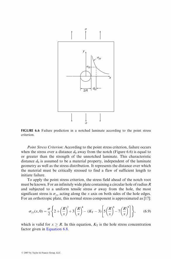
2Rd0
x
y
sUt
syy
s
s
FIGURE 6.6 Failure prediction in a notched laminate according to the point stress
criterion.
Point Stress Criter ion : Accor ding to the point stress criterion, failu re occu rs
when the stress over a distan ce d0 away from the not ch (Figur e 6.6) is eq ual to
or greate r than the stren gth of the unnotch ed laminate. This c haracteris tic
distan ce d0 is assum ed to be a mate rial pro perty, ind ependent of the lamin ate
geomet ry as well as the stre ss dist ribution. It repres ents the distance over which
the material must be critically stressed to find a flaw of suffici ent length to
initiat e failu re.
To apply the poi nt stre ss crit erion, the stress field ahead of the notch roo t
must be know n. For an infin itely wide plate contai ning a circul ar hole of radius R
and subjected to a unifor m tensi le stress s away from the hole, the mo st
signifi cant stre ss is syy actin g along the x axis on both sides of the hole edges.
For an orthot ropic plate, this normal stress compon ent is app roximated as [17] :
syy(x, 0) ¼ s
22þ R
x
� �2þ 3
R
x
� �4� (KT � 3) 5
R
x
� �6� 7
R
x
� �8" #( ), (6:9)
which is valid for x � R. In this equation, KT is the hole stress concentration
facto r given in Equat ion 6.8.
� 2007 by Taylor & Francis Group, LLC.
Accor ding to the point stress c riterion, failure occu rs at s ¼ sN for which
syy ( R þ d0 , 0) ¼ s Ut ,
where sN is the notche d tensile stre ngth and s Ut is the unnotch ed tensile
strength for the laminate.
Thus from Equation 6.9, the ratio of notched to unnot ched tensi le stren gth is
sN
sUt
¼ 2
2þ l21 þ 3l41 � (KT � 3)(5l61 � 7l81), (6:10)
where
l1 ¼ R
Rþ d0:
Average Stress Criterion: According to the average stress criterion, failure of the
laminate occurs when the average stress over a distance a0 ahead of the notch
reaches the unnotched laminate strength. The characteristic distance a0 is
assumed to be amaterial property. It represents the distance over which incipient
failure has taken place in the laminate owing to highly localized stresses.
In a plate containing a circular hole of radius R, failure by the average stress
criterion occurs when
1
a0
ðRþa0
R
syy(x, 0)dx ¼ sUt:
If the plate is made of a symmetric laminate with orthotropic properties,
substitution of Equation 6.9 gives
sN
sUt
¼ 2(1� l2)
2� l22 � l42 þ (KT � 3)(l62 � l82), (6:11)
where
l2 ¼ R
Rþ a0:
Both Equations 6.10 and 6.11 show that the notched tensile strength sN
decreases with increasing hole radius. At very small hole radius, that is, as
R ! 0, sN ! sUt. At very large hole radius, as l1 or l2 ! 1, sN ! sUt
KT
.
The following points should be noted in applying the point stress and the
average stress criteria for notched laminates.
� 2007 by Taylor & Francis Group, LLC.
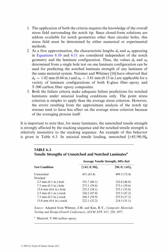
1. The applic ation of both the crit eria req uires the know ledge of the overal l
stre ss field surroundi ng the notch tip. Sin ce closed- form solut ions are
seldom ava ilable for not ch geo metries other than circul ar holes, this
stre ss field must be determ ined by either num erical or experi mental
methods .
2. As a first approxim ation, the charact eristic lengt hs d0 and a0 appearing
in Equat ions 6.10 and 6.11 are co nsidered indepen dent of the notch
geometry and the laminate configuration. Thus, the values d0 and a0determined from a single hole test on one laminate configuration can be
used for predicting the notched laminate strength of any laminate of
the same material system. Nuismer and Whitney [16] have observed that
d0 ¼ 1.02 mm (0.04 in.) and a0 ¼ 3.81 mm (0.15 in.) are applicable for a
variety of laminate configurations of both E-glass fiber–epoxy and
T-300 carbon fiber–epoxy composites.
3. Both the failure criteria make adequate failure predictions for notched
laminates under uniaxial loading conditions only. The point stress
criterion is simpler to apply than the average stress criterion. However,
the errors resulting from the approximate analysis of the notch tip
stresses tend to have less effect on the average stress criterion because
of the averaging process itself.
It is important to note that, for many laminates, the unnotched tensile strength
is strongly affected by the stacking sequence and the notched tensile strength is
relatively insensitive to the stacking sequence. An example of this behavior
is given in Table 6.3. In uniaxial tensile loading, unnotched [±45=90=0]S
TABLE 6.3Tensile Strengths of Unnotched and Notched Laminatesa
Average Tensile Strength, MPa (ksi)
Test Condition [±45=0=90]S [90=0=±45]S
Unnotched 451 (65.4) 499.3 (72.4)
Notched
2.5 mm (0.1 in.) hole 331.7 (48.1) 322.8 (46.8)
7.5 mm (0.3 in.) hole 273.1 (39.6) 273.1 (39.6)
15.0 mm (0.6 in.) hole 235.2 (34.1) 233.1 (33.8)
2.5 mm (0.1 in.) crack 324.2 (47.0) 325.5 (47.2)
7.5 mm (0.3 in.) crack 268.3 (38.9) 255.9 (37.1)
15.0 mm (0.6 in.) crack 222.1 (32.2) 214.5 (31.1)
Source: Adapted from Whitney, J.M. and Kim, R.Y., Composite Materials:
Testing and Design (Fourth Conference), ASTM STP, 617, 229, 1977.
a Material: T-300 carbon–epoxy.
� 2007 by Taylor & Francis Group, LLC.
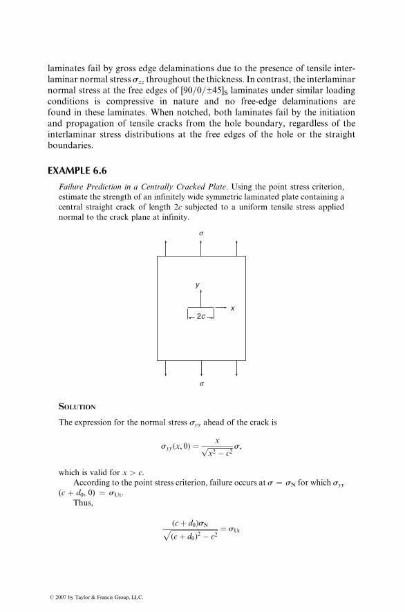
laminates fail by gross edge delaminations due to the presence of tensile inter-
laminar normal stress szz throughout the thickness. In contrast, the interlaminar
normal stress at the free edges of [90=0=±45]S laminates under similar loading
conditions is compressive in nature and no free-edge delaminations are
found in these laminates. When notched, both laminates fail by the initiation
and propagation of tensile cracks from the hole boundary, regardless of the
interlaminar stress distributions at the free edges of the hole or the straight
boundaries.
EXAMPLE 6.6
Failure Prediction in a Centrally Cracked Plate. Using the point stress criterion,
estimate the strength of an infinitely wide symmetric laminated plate containing a
central straight crack of length 2c subjected to a uniform tensile stress applied
normal to the crack plane at infinity.
s
y
x2c
s
SOLUTION
The expression for the normal stress syy ahead of the crack is
syy(x, 0) ¼ xffiffiffiffiffiffiffiffiffiffiffiffiffiffiffix2 � c2
p s,
which is valid for x > c.
According to the point stress criterion, failure occurs at s ¼ sN for which syy
(c þ d0, 0) ¼ sUt.
Thus,
(cþ d0)sNffiffiffiffiffiffiffiffiffiffiffiffiffiffiffiffiffiffiffiffiffiffiffiffiffiffiffiffi(cþ d0)
2 � c2p ¼ sUt
� 2007 by Taylor & Francis Group, LLC.
or
sN ¼ s Ut
ffiffiffiffiffiffiffiffiffiffiffiffiffi1 � l23
q,
where
l3 ¼ c
c þ d0:
The mode I stress intensity factor for this condition can be written as
K1 ¼ s Nffiffiffiffiffiffip c
p ¼ sUt
ffiffiffiffiffiffiffiffiffiffiffiffiffiffiffiffiffiffiffiffiffiffipc( 1 � l 23 )
q:
6.1.5 F AILURE P REDICTION FOR DELAMINATION INITIATION
Dela mination or ply separat ion due to interlam inar stresses is a crit ical failu re
mode in many c omposi te laminates . It can red uce the failure stre ngth of some
laminates wel l be low that pred icted by the in-pl ane failure theories discus sed in
Secti on 6.1.1.
Brewer and Lagace [18] as well as Zhou and Sun [19] proposed the following
quadratic failure criterion to predict the initiation of delamination at the free
edges:
�s2zz
S2zt
þ �t2xzS2xz
þ �t2yzS2yz
¼ 1, (6:12)
where
Szt ¼ tensile strength in the thickness direction
Sxz, Syz ¼ interlaminar shear strengths
�szz, �txz, and �tyz are the average interlaminar stresses defined by
(�szz, �txz, �tyz) ¼ 1
xc
ðxc0
(szz, txz, tyz)dx,
where xc is the critical distance over which the interlaminar stresses are
averaged.
Since the interlaminar strength data are not usually available, Zhou and
Sun [19] have suggested using Sxz ¼ Syz ¼ SLTs and Szt ¼ STt.. They also
recommend using xc equal to twice the ply thickness.
EXAMPLE 6.7
The average interlaminar shear stresses in a [±45]2S laminate under an in-plane
tensile force Nxx ¼ 410 kN=m are given as:
� 2007 by Taylor & Francis Group, LLC.
� 2007 by Taylor & Fra
Interface �s (MPa) �t (MPa) �t (MPa)
ncis Group, LLC.
zz
xz yz1
�0.9 �5.67 68.712
�1.45 �2.71 26.603
0.73 9.91 67.47Using Szt ¼ 42.75 MPa and Sxz ¼ S yz ¼ 68.95 MPa, investigate whether any
of the interfaces will fail by delamination at this load.
SOLUTIO N
Interface 1: Since �szz is compressive, we will not consider it in the failure predic-
tion by Equation 6.12. Thus, the left-hand side (LHS) of Equation
6.12 is
�5:67
68:95
� �2þ 68:71
68:95
� �2� 1:
Interface 2: The term �szz is also compressive at this interface. Therefore, we will
not consider szz in the failure prediction by Equation 6.12. Thus the
LHS of Equation 6.12 is
�2:71
68:95
� �2þ 26:6
68:95
� �2¼ 0:1504:
Interface 3: We will consider all three interlaminar stresses at this interface and
compute the LHS of Equation 6.12 as:
0:73
42:75
� �2þ 9:91
68:95
� �2þ 67:47
68:95
� �2¼ 0:9784:
Thus, according to Equation 6.12, only interface 1 is expected to fail by delamina-
tion at Nxx ¼ 410 kN=m.
6.2 LAMINATE DESIGN CONSIDERATIONS
6.2.1 DESIGN PHILOSOPHY
The design of a structure or a component is in general based on the philosophy
of avoiding failure during a predetermined service life. However, what consti-
tutes failure depends principally on the type of application involved. For
example, the most common failure mode in a statically loaded structure made
of a ductile metal is yielding beyond which a permanent deformation may occur
in the structure. On the other hand, the design of the same structure in a fatigue
load application must take into account the possibility of a brittle failure
accompanied by negligible yielding and rapid crack propagation.
Unli ke duc tile meta ls, composi te lamin ates contai ning fiber -reinforce d
therm oset polyme rs do not e xhibit g ross yielding, ye t they are also not class ic
brittle material s. Under a static tensi le load, many of these laminates show
nonlinear charact eristic s attr ibuted to sequ ential ply failures . The questi on that
often arises in designi ng with su ch composi te laminates is, ‘‘Shoul d the de sign
be based on the ulti mate failu re or the first ply failure? ’’ The current de sign
practice in the aircr aft or a erospace indust ry uses the FPF approach , primarily
since cracks app earing in the failed ply may make the neighbori ng plies sus-
cepti ble to mechani cal and environm ental damage. In many laminated co n-
struc tions, the ulti mate fail ure occurs soo n after the FPF (Table 6.4) , and
therefo re wi th these lami nates an FPF de sign ap proach is justified. For many
other lami nates, the difference between the FPF stress level an d the ultimate
stren gth level is quite high. An FPF design approach with these lamin ates may
be consider ed somewh at con servative .
The behav ior of a fiber -reinforce d co mposite lami nate in a fatigue load
applic ation is also quite differen t from that of metals. In a metal, nearly
80%–90 % of its fatigue life is spen t in the formati on of a critical crack. Genera lly,
the fatigue crack in a meta l is not de tectable by the present -day NDT techni que s
until it reach es the critical length. How ever, onc e the fatigu e crack atta ins the
critical length , it propag ates rapidl y through the structure, failing it in a cata-
strophi c mann er (Figur e 6.7). In many polyme r matr ix composi tes, fatigue
damage may appear at multiple locations in the first few hundred to a thousand
cycles. Some of these damages, such as surface craze marks, fiber splitting, and
edge delaminations, may also be visible in the early stages of the fatigue life.
Unlike metals, the propagation or further accumulation of damage in a fiber-
reinforced composite takes place in a progressive manner resulting in a gradual
loss in the stiffness of the structure. Thus, the laminated composite structure
continues to carry the load without failing catastrophically; however, the loss of
its stiffness may create gradually increasing deflections or vibrations. In these
situations, a fatigue design approach based on the appearance of the first
mechanical damage may again be considered conservative.
Since the history of their development is new, very few long-term field
performance experiences exist. Design data in the areas of combined stresses,
cumulative fatigue, repeated impact, environmental damage, and so on are not
available. There is very little agreement among designers about what consti-
tutes a structural failure and how to predict it. Industry-wide standards for
material specifications, quality control, test methods, and failure analysis have
not yet been developed. For all these reasons, the development of fiber-
reinforced composite parts often relies on empirical approaches and requires
extensive prototyping and testing.
6.2.2 DESIGN CRITERIA
In general, the current design practice for fiber-reinforced composite structures
uses the same design criteria as those used for metals. For example, the primary
� 2007 by Taylor & Francis Group, LLC.
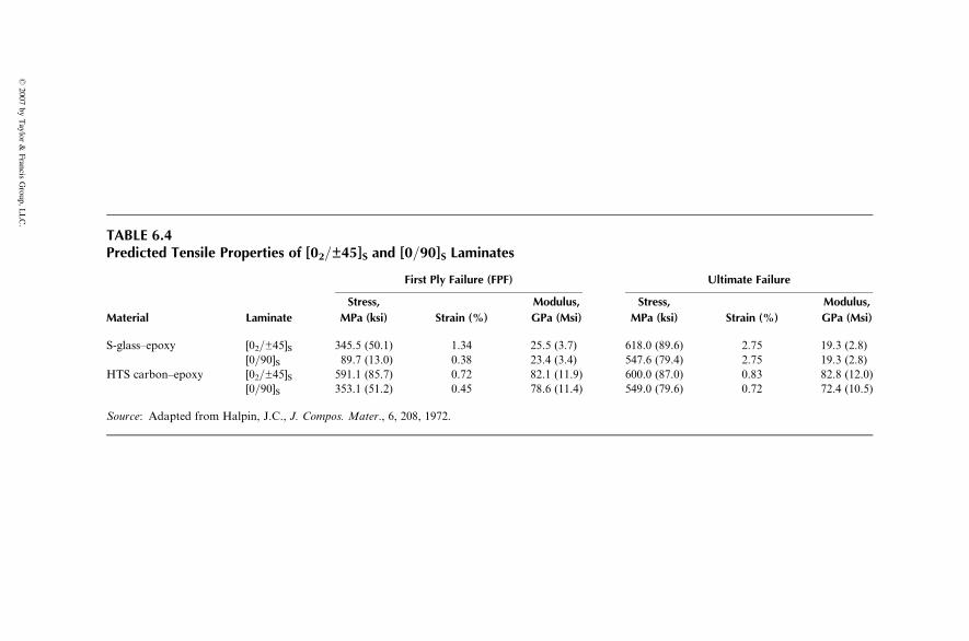
TABLE 6.4Predicted Tensile Properties of [02=±45]S and [0=90]S Laminates
First Ply Failure (FPF) Ultimate Failure
Material Laminate
Stress,
MPa (ksi) Strain (%)
Modulus,
GPa (Msi)
Stress,
MPa (ksi) Strain (%)
Modulus,
GPa (Msi)
S-glass–epoxy [02=±45]S 345.5 (50.1) 1.34 25.5 (3.7) 618.0 (89.6) 2.75 19.3 (2.8)
[0=90]S 89.7 (13.0) 0.38 23.4 (3.4) 547.6 (79.4) 2.75 19.3 (2.8)
HTS carbon–epoxy [02=±45]S 591.1 (85.7) 0.72 82.1 (11.9) 600.0 (87.0) 0.83 82.8 (12.0)
[0=90]S 353.1 (51.2) 0.45 78.6 (11.4) 549.0 (79.6) 0.72 72.4 (10.5)
Source: Adapted from Halpin, J.C., J. Compos. Mater., 6, 208, 1972.
�2007
byTaylor
&Francis
Group,
LLC.
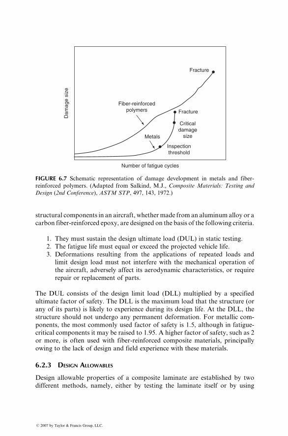
Number of fatigue cycles
Dam
age
size
Fracture
Fiber-reinforcedpolymers Fracture
Criticaldamage
size
Inspectionthreshold
Metals
FIGURE 6.7 Schematic representation of damage development in metals and fiber-
reinforced polymers. (Adapted from Salkind, M.J., Composite Materials: Testing and
Design (2nd Conference), ASTM STP, 497, 143, 1972.)
structural components in an aircraft, whethermade from an aluminum alloy or a
carbon fiber-reinforced epoxy, are designed on the basis of the following criteria.
1. They must sustain the design ultimate load (DUL) in static testing.
2. The fatigue life must equal or exceed the projected vehicle life.
3. Deformations resulting from the applications of repeated loads and
limit design load must not interfere with the mechanical operation of
the aircraft, adversely affect its aerodynamic characteristics, or require
repair or replacement of parts.
The DUL consists of the design limit load (DLL) multiplied by a specified
ultimate factor of safety. The DLL is the maximum load that the structure (or
any of its parts) is likely to experience during its design life. At the DLL, the
structure should not undergo any permanent deformation. For metallic com-
ponents, the most commonly used factor of safety is 1.5, although in fatigue-
critical components it may be raised to 1.95. A higher factor of safety, such as 2
or more, is often used with fiber-reinforced composite materials, principally
owing to the lack of design and field experience with these materials.
6.2.3 DESIGN ALLOWABLES
Design allowable properties of a composite laminate are established by two
different methods, namely, either by testing the laminate itself or by using
� 2007 by Taylor & Francis Group, LLC.
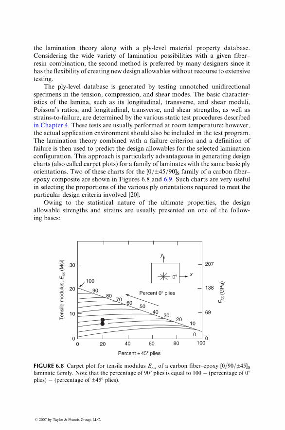
the lami nation theory alon g wi th a ply-level mate rial propert y da tabase .
Consid ering the wide varie ty of laminati on possibili ties wi th a given fiber–
resin combinat ion, the second method is prefer red by many designe rs since it
has the flexibil ity of creat ing ne w design allowab les without recours e to extens ive
testing.
The ply-level da tabase is generat ed by testing unnot ched unidir ectional
specime ns in the tensi on, compres sion, and shear modes. The ba sic charact er-
istics of the lamin a, such as its longitu dinal, trans verse, and shear moduli,
Poisson’ s rati os, and longit udinal, trans verse, and shear stre ngths, as well as
strains- to-failu re, are determined by the various static test procedu res descri bed
in Chapt er 4. These tests are usuall y pe rformed at room tempe rature; howeve r,
the actual applic ation environm ent shou ld also be included in the test program .
The laminati on theory combined with a failure crit erion and a definiti on of
failure is then used to pred ict the design allow ables for the selec ted lamina tion
config uration . Thi s approach is pa rticular ly advantag eous in gen erating de sign
charts (also call ed carpet plots ) for a family of lami nates with the same ba sic ply
orienta tions. Two of these charts for the [0 =±45=90]S family of a carbon fiber–
epoxy co mposite are shown in Figures 6.8 and 6.9. Such charts are very useful
in selecting the pro portion s of the various ply orient ations requ ired to meet the
particu lar design criteria involv ed [20].
Owing to the statistica l nature of the ulti mate propert ies, the design
allowabl e streng ths and strains are usually present ed on one of the follow-
ing ba ses:
y
x100
8060
5040
3020
10
70
90
00
69
138
207
00
10
20
30
20 40 60 80 100
Percent ± 458 plies
Percent 0� plies
08
Ten
sile
mod
ulus
, Exx
(M
si)
Exx
(G
Pa)
FIGURE 6.8 Carpet plot for tensile modulus Exx of a carbon fiber–epoxy [0=90=±45]Slaminate family. Note that the percentage of 908 plies is equal to 100 � (percentage of 08plies) � (percentage of ±458 plies).
� 2007 by Taylor & Francis Group, LLC.
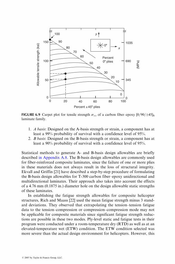
y
1035
690
345
00
1008060402000
50
100
150A
llow
able
tens
ile s
tren
gth
(ksi
)
Percent ± 458 plies
(MP
a)
x08
100
90
8070
60
5040
30
2010
Percent08 plies
FIGURE 6.9 Carpet plot for tensile strength sxx of a carbon fiber–epoxy [0=90=±45]Slaminate family.
1. A basis : Desi gned on the A-ba sis stre ngth or stra in, a componen t has at
least a 99% probabil ity of survi val wi th a con fidence level of 95%.
2. B ba sis : Designed on the B-basi s stre ngth or strain, a compo nent has at
least a 90% probabil ity of survi val wi th a con fidence level of 95%.
Statist ical method s to generat e A- an d B-basi s design allowabl es are brief ly
descri bed in Appendix A.8. The B-basi s de sign allowabl es are c ommonl y used
for fiber-reinforced composite laminates, since the failure of one or more plies
in these materials does not always result in the loss of structural integrity.
Ekvall and Griffin [21] have described a step-by-step procedure of formulating
the B-basis design allowables for T-300 carbon fiber–epoxy unidirectional and
multidirectional laminates. Their approach also takes into account the effects
of a 4.76 mm (0.1875 in.) diameter hole on the design allowable static strengths
of these laminates.
In establishing the fatigue strength allowables for composite helicopter
structures, Rich and Maass [22] used the mean fatigue strength minus 3 stand-
ard deviations. They observed that extrapolating the tension–tension fatigue
data to the tension–compression or compression–compression mode may not
be applicable for composite materials since significant fatigue strength reduc-
tions are possible in these two modes. Ply-level static and fatigue tests in their
program were conducted under a room-temperature dry (RTD) as well as at an
elevated-temperature wet (ETW) condition. The ETW condition selected was
more severe than the actual design environment for helicopters. However, this
� 2007 by Taylor & Francis Group, LLC.
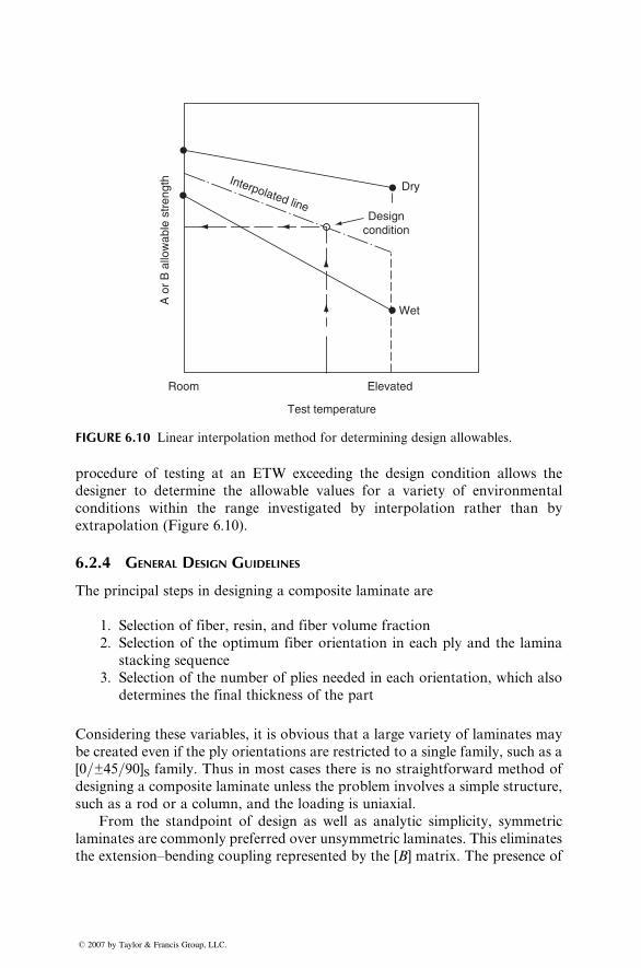
Dry
Designcondition
Wet
Elevated
Test temperature
Room
A o
r B
allo
wab
le s
tren
gth Interpolated line
FIGURE 6.10 Linear interpolation method for determining design allowables.
procedure of testing at an ETW exceeding the design condition allows the
designer to determine the allowable values for a variety of environmental
conditions within the range investigated by interpolation rather than by
extrapolation (Figure 6.10).
6.2.4 GENERAL DESIGN GUIDELINES
The principal steps in designing a composite laminate are
1. Selection of fiber, resin, and fiber volume fraction
2. Selection of the optimum fiber orientation in each ply and the lamina
stacking sequence
3. Selection of the number of plies needed in each orientation, which also
determines the final thickness of the part
Considering these variables, it is obvious that a large variety of laminates may
be created even if the ply orientations are restricted to a single family, such as a
[0=±45=90]S family. Thus in most cases there is no straightforward method of
designing a composite laminate unless the problem involves a simple structure,
such as a rod or a column, and the loading is uniaxial.
From the standpoint of design as well as analytic simplicity, symmetric
laminates are commonly preferred over unsymmetric laminates. This eliminates
the extension–bending coupling represented by the [B] matrix. The presence of
� 2007 by Taylor & Francis Group, LLC.
extension–bending coupling is also undesirable from the stiffness standpoint,
since it reduces the effective stiffness of the laminate and thereby increases its
deflection, reduces the critical buckling loads, and decreases the natural fre-
quency of vibration. Similar but lesser effects are observed if the laminate has
bending–twisting coupling due to the presence of D16 and D26 terms. However,
unless the fibers are at 0, 90, or 0=90 combinations, a symmetric laminate
cannot be designed with D16¼D26¼ 0.
The deleterious free-edge effects in a laminate can be reduced through
proper selection of lamina stacking sequence. If angle-ply laminates are used,
the layers with þu and �u orientations should be alternated instead of in a
clustered configuration [23]. Thus, for example, an eight-layer laminate with
four layers of þu orientations and four layers of �u orientations should be
designed as [þu=�u=þu=�u]S instead of [u=u=�u=�u]S or [�u=�u=þu=þu]S.However, if a laminate contains 0, 90, and ±u layers, adjacent þu and �u layersshouldbeavoided.Forexample, in thequasi-isotropic laminate family containing
0, 90, and ±45 layers, a [45=0=90=�45]S configuration is preferred over a
[90=þ45=�45=0]S or a [0=þ45=�45=90]S configuration.
6.2.4.1 Laminate Design for Strength
When the state of stress in a structure is known and does not change during the
course of its service operation, the lamina orientations may be selected in the
following way [24].
Using the standard Mohr’s circle technique, determine the principal normal
loads and the principal directions. Analytically, the principal normal loads are
N1 ¼ 1
2(Nxx þNyy)þ Nxx �Nyy
2
� �2þ N2
xy
" #1=2,
N2 ¼ 1
2(Nxx þNyy)� Nxx �Nyy
2
� �2þ N2
xy
" #1=2, (6:13)
and the principal direction with respect to the x axis is
tan 2u ¼ 2Nxy
Nxx �Nyy
: (6:14)
Select a [0i=90j]S cross-ply configuration with the 08 layers aligned in the
direction of the maximum principal load N1 and the 908 layers aligned in
the direction of the minimum principal load N2. Thus with respect to the x
axis, the laminate configuration is [ui=(90 þ u)j]S. The ratio of 08 to 908 plies, i=j,is equal to the principal load ratio N1=N2.
When the stress state in a structure varies in direction or is unknown, a
common approach in laminate design is to make it quasi-isotropic, for example,
� 2007 by Taylor & Francis Group, LLC.
[0i=±45 j=90k]S . The de sign procedu re is then red uced to the selec tion of plyratios ( i =j=k ) and the total thickne ss of the laminate. Design ch arts or carp et
plots of the types shown in Figures 6.8 and 6.9 can be used to select the initial
ply ratios; however, the final design must include a ply-by-ply analysis of the
entire laminate.
Massard [25] has used an iterative ply-by-ply approach for designing sym-
metric laminates under in-plane and bending loads. In this approach, an initial
laminate configuration is assumed and additional plies are added in a stepwise
fashion to achieve the most efficient laminate that can sustain the given loading
condition. At each step, strains in each lamina and the margin of safety (ratio of
lamina strength to effective lamina stress) for each lamina are calculated.
A margin of safety greater than unity indicates a safe ply in the laminate. The
process is repeated until the margin of safety in each lamina is greater than unity.
Park [26] has used a simple optimization procedure to determine the fiber
orientation angle u for maximum FPF stress in symmetric laminates, such as
[±u]S, [�u=0=u]S, and so on. The objective function F was expressed as
F ¼ «�2xx þ «
�2yy þ
1
2g�2xy: (6:15)
For a given laminate configuration, the midplane strain components are func-
tions of the applied in-plane loads (Nxx, Nyy, and Nxy) as well as the fiber
orientation angle u. If the in-plane loads are specified, the design optimization
procedure reduces to finding u for which the objective function is minimum.
EXAMPLE 6.8
Using the carpet plots in Figures 6.8 and 6.9, determine the number of layers of 0,
90, and ±458 orientations in a quasi-isotropic [0=90=±45]S laminate that meets the
following criteria:
1. Minimum modulus in the axial (08) direction ¼ 6 3 106 psi
2. Minimum B-allowable strength in the axial (08) direction ¼ 65 ksi
SOLUTION
Step 1: Referring to Figure 6.8, determine the ply ratio that givesExx ¼ 63 106 psi.
0:90:�45 ¼ 20%: 60%: 20%
Step 2: Referring to Figure 6.9, check the B-allowable strength for the ply ratio
determined in Step 1, which in our case is 51 ksi. Since this value is less than
the minimum required, we select a new ply ratio that will give a minimum
B-allowable strength of 65 ksi. This new ply ratio is 0:90:±45 ¼ 30:50:20.
Referring back to Figure 6.8, we find that this ply ratio gives an axial
modulus of 73 106 psi, which is higher than the minimum required in the
present design. Thus, the laminate configuration selected is [03=905=±452]S.
� 2007 by Taylor & Francis Group, LLC.
Step 3: Assuming that the ply thickness is 0.005 in., we determine the ply thickness
for each fiber orientation as
0�: 6� 0:005 in: ¼ 0:03 in:
90�: 10� 0:005 in: ¼ 0:05 in:
þ45�: 4� 0:005 in: ¼ 0:02 in:
�45�: 4� 0:005 in: ¼ 0:02 in:
Thus, the total laminate thickness is 0.12 in.
6.2.4.2 Laminate Design for Stiffness
The stiffness of a member is a measure of its resistance to deformation or
deflection owing to applied loads. If the member is made of an isotropic
material, its stiffnesses are given by
Axial stiffness ¼ EA0,
Bending stiffness ¼ EIc,
Torsional stiffness ¼ GJc, (6:16)
where
E ¼ modulus of elasticity
G ¼ shear modulus
A0 ¼ cross-sectional area
Ic ¼ moment of inertia of the cross section about the neutral axis
Jc ¼ polar moment of inertia of the cross section
The stiffness equations for composite members are in general more involved
than those given in Equation 6.16. If the composite member is made of a
symmetric laminate, its stiffness against the in-plane loads is related to the
elements in the [A] matrix, whereas its stiffness against bending, buckling, and
torsional loads is related to the elements in the [D] matrix. The elements in both
[A] and [D] matrices are functions of the fiber type, fiber volume fraction, fiber
orientation angles, lamina thicknesses, and the number of layers of each orien-
tation. In addition, the elements in the [D] matrix depend strongly on the
lamina stacking sequence.
Except for 0, 90, and 0=90 combinations, the [D] matrix for all symmetric
laminates contains nonzero D16 and D26 terms. Closed-form solutions for
bending deflections, buckling loads, and vibrational frequencies of general
symmetric laminates are not available. The following closed-form solutions
[27,28] are valid for the special class of laminates for which D16 ¼ D26 ¼ 0
and the elements in the [B] matrix are negligible:
� 2007 by Taylor & Francis Group, LLC.
1. Center deflection of a simply supported rectangular plate carrying a
uniformly distributed load p0:
w ffi 16p0R4b4
p6
1
D11 þ 2(D12 þ 2D66)R2 þD22R4
� �(6:17)
2. Critical buckling load for a rectangular plate with pinned edges at the
ends of its long dimension:
Ncr ffi p2[D11 þ 2(D12 þ 2D66)R2 þD22R
4]
b2R2(6:18)
3. Fundamental frequency of vibration for a simply supported rectangular
plate:
f 2 ffi p4
rR4b4[D11 þ 2(D12 þ 2D66)R
2 þD22R4] (6:19)
where
a ¼ plate length
b ¼ plate width
R ¼ plate aspect ratio¼ a=br ¼ density of the plate material
A few closed-form solutions are also available in the literature for unsym-
metric laminates with a nonzero [B] matrix [27,28]. However, it has been shown
that the coupling effect of the [B] matrix becomes small when the laminate
contains more than six to eight layers [29]. Therefore, for most practical lamin-
ates, Equations 6.17 through 6.19 can be used for initial design purposes.
6.2.5 FINITE ELEMENT ANALYSIS
Design analysis of a laminated composite structure almost invariably requires
the use of computers to calculate stresses and strains in each ply and to inves-
tigate whether the structure is ‘‘safe.’’ For simple structures, such as a plate or a
beam, the design analysis can be performed relatively easily. If the structure and
the loading are complex, it may be necessary to perform the design analysis
using finite element analysis. Commercially available finite element softwares,
such as MSC-NASTRAN, ANSYS, ABAQUS, and LS-DYNA, have the cap-
ability of combining the lamination theory with the finite element codes. Many
of these packages are capable of calculating in-plane as well as interlaminar
stresses, incorporate more than one failure criterion, and contain a library of
plate, shell, or solid elements with orthotropic material properties [30].
Although finite element analyses for both isotropic materials and laminated
composite materials follow the same procedure, the problem of preparing the
� 2007 by Taylor & Francis Group, LLC.
input data and interpreting the output data for composite structures is much
more complex than in the case of metallic structures. Typical input information
for an isotropic element includes its modulus, Poisson’s ratio, and thickness. Its
properties are assumed invariant in the thickness direction. An element for a
composite structure may contain the entire stack of laminas. Consequently, in
this case, the element specification must include the fiber orientation angle in
each lamina, lamina thicknesses, and the location of each lamina with respect to
the element midplane. Furthermore, the basic material property data for plane
stress analysis of thin fiber-reinforced composite structure include four elastic
constants, namely, the longitudinal modulus, transverse modulus, major Pois-
son’s ratio, and shear modulus. Thus, the amount of input information even for
a static load analysis of a composite structure is quite large compared with a
similar analysis of a metallic structure.
The stress output from the finite element analysis of an isotropic material
includes only three stress components for each element. In contrast, the stress
output for a composite structure can be very large since it contains three
in-plane stresses in each individual lamina as well as the interlaminar stresses
between various laminas for every element. The lamina in-plane stresses are
usually computed in the material principal directions, which vary from layer to
layer within the same element. To examine the occurrence of failure in an
element, a preselected failure criterion is applied to each lamina. In many finite
element packages, the stress output may be reduced by calculating stress
resultants, which are integrals of the lamina stresses through the thickness.
However, interpretation of these stress resultants is difficult since they do not
provide information regarding the adequacy of a design.
6.3 JOINT DESIGN
The purpose of a joint is to transfer loads from one member to another in a
structure. The design of joints has a special significance in fiber-reinforced
composite structures for two reasons: (1) the joints are often the weakest
areas in a composite structure and (2) the composite materials do not possess
the forgiving characteristics of ductile metals, namely, their capacity to redis-
tribute local high stresses by yielding.
For composite laminates, the basic joints are either mechanical or bonded.
Mechanical joints are created by fastening the substrates with bolts or rivets;
bonded joints use an adhesive interlayer between the substrates (commonly
called the adherends). The advantages and disadvantages of these two types of
joints are listed as follows.
Mechanical Joints:
1. Permit quick and repeated disassembly for repairs or replacements
without destroying the substrates
2. Require little or no surface preparation
� 2007 by Taylor & Francis Group, LLC.
3. Are easy to inspect for joint quality
4. Requi re mach ining of hol es that inter rupt the fiber continui ty an d may
reduce the strength of the sub strate lami nates
5. Create highly local ized stress co ncentra tions aroun d the joint s that may
induce failure in the substr ates
6. Add weight to the struc ture
7. May create a potenti al corrosi on pro blem, for exampl e, in an a luminum
fastene r if used for joining carbon fiber –epoxy lamin ates
Bonded Joint s :
1. Distri bute the load over a larger area than mecha nical joints
2. Requi re no holes, but may nee d surface prepa ration (clea ning, pretr eat-
ment, etc. )
3. Add very little weight to the structure
4. Are difficul t to disassembl e wi thout eithe r destroy ing or damagi ng
substr ates
5. May be a ffected by servi ce temperatur e, humidi ty, and othe r en viron-
menta l con ditions
6. Are diff icult to inspect for joint qua lity
We will now discus s the general design consider ations wi th these two types
of joint s.
6.3.1 MECHANICAL JOINTS
The stre ngth of mechani cal joints depends on the followi ng.
1. Geomet ric parame ters, su ch as the ratio s of ed ge dist ance to bolt hole
diame ter ( e=d ), width to bolt hole diame ter ( w=d ), and laminate thick-
ness to bolt hole diame ter ( h=d ). In mult ibolt joints, spacing between
holes and their arrange ments a re also important.
2. Mater ial parame ters , such as fiber orient ation an d lami nate stacking
sequen ce. Som e of these mate rial pa rameters are discus sed in Chapt er 4
(see Se ction 4.4. 1).
In app lications involv ing mechani cal joints, three basic failu re modes are
observed in the substr ates, namel y, shear-ou t, net tensio n, and bearing failure
(Figur e 6.11). If the laminate contai ns nearly all 0 8 fiber s, cleava ge failure isalso possible. From a safe design standpoint, a bearing failure is more desirable
than either a shear-out or a net tension failure. However, unless the e=d and
w=d ratios are very large, the full bearing strength is seldom achieved. In
general, shear-out and net tension failures are avoided if e=d > 3 and w=d > 6.
The actual geometric parameters are usually determined by conducting
pin-bearing tests on the specific laminates involved. However, a bolted joint
� 2007 by Taylor & Francis Group, LLC.
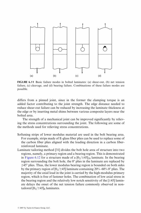
(a) (b) (c) (d)
FIGURE 6.11 Basic failure modes in bolted laminates: (a) shear-out, (b) net tension
failure, (c) cleavage, and (d) bearing failure. Combinations of these failure modes are
possible.
differs from a pinned joint, since in the former the clam ping torque is an
added factor contribu ting to the joint strength. The edge distance needed to
reduce shear-o ut failure c an be reduced by increa sing the laminate thickne ss at
the edge or by inserting metal shim s be tween various composi te layer s ne ar the
bolted area.
The strength of a mechani cal joint can be impr oved signifi cantly by reli ev-
ing the stress con centrations surroundi ng the joint. The foll owing are some of
the methods used for relieving stress concentra tions .
Softeni ng strips of lower modulus mate rial are use d in the bolt bearing area.
For exampl e, strips made of E-glas s fiber plies can be used to replac e some of
the carbon fiber plies aligne d with the loading direction in a carbo n fiber -
reinforced lami nate.
Laminat e tailorin g method [31] divides the bolt hole area of struc ture into two
regions , na mely, a primary region and a be aring region. This is demonst rated
in Figure 6.12 for a structure made of a [02=±45] 2S lamin ate. In the be aring
region surroun ding the bolt hole, the 08 plies in the lami nate are replaced by
±458 plies. Thus, the lower modulus bearing region is bounde d on both sides
by the prim ary region of [02=±45 ] laminate contain ing 20%–60 % 0 8 plies . Themajorit y of the axial load in the joint is carried by the high-m odulus prima ry
region, which is free of fastener holes. The combination of low axial stress in
the bearing region and the relatively low notch sensitivity of the [±45] lamin-
ate delays the onset of the net tension failure commonly observed in non-
tailored [02=±45]S laminates.
� 2007 by Taylor & Francis Group, LLC.
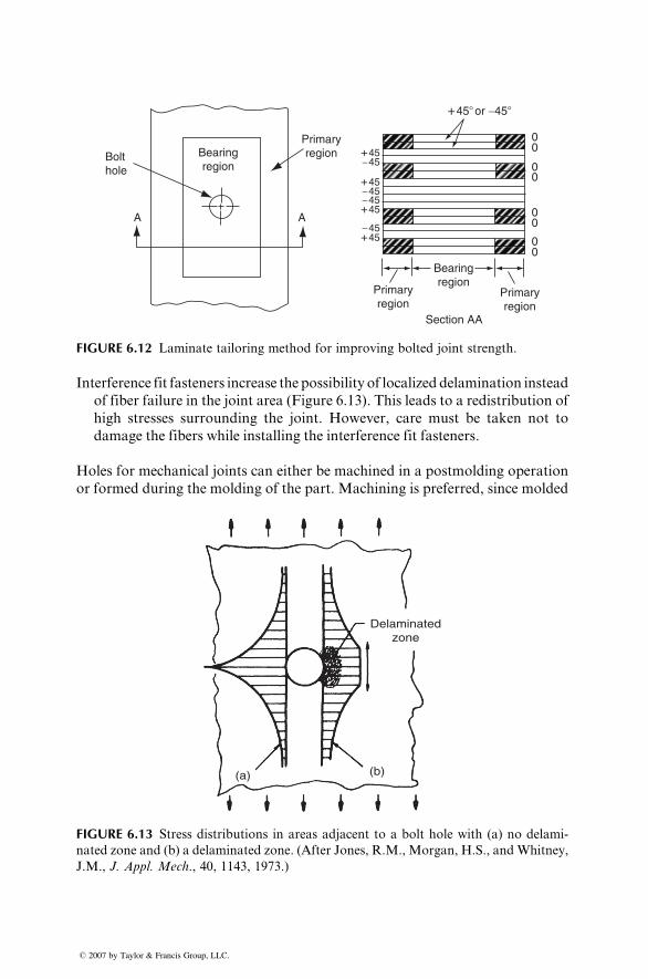
Bolthole
A
Bearingregion
A
Primaryregion
00
00
00
00
+ 45
+ 45
+ 45
+ 45
− 45
− 45− 45
− 45
Bearingregion
Primaryregion
Primaryregion
Section AA
+ 45� or −45�
FIGURE 6.12 Laminate tailoring method for improving bolted joint strength.
Interference fit fasteners increase the possibility of localized delamination instead
of fiber failure in the joint area (Figure 6.13). This leads to a redistribution of
high stresses surrounding the joint. However, care must be taken not to
damage the fibers while installing the interference fit fasteners.
Holes for mechanical joints can either be machined in a postmolding operation
or formed during the molding of the part. Machining is preferred, since molded
Delaminatedzone
(a) (b)
FIGURE 6.13 Stress distributions in areas adjacent to a bolt hole with (a) no delami-
nated zone and (b) a delaminated zone. (After Jones, R.M., Morgan, H.S., and Whitney,
J.M., J. Appl. Mech., 40, 1143, 1973.)
� 2007 by Taylor & Francis Group, LLC.
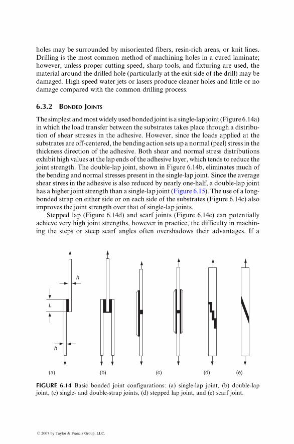
holes may be surrou nded by miso riented fibers, resin-ri ch areas, or knit lines .
Drillin g is the most common method of machi ning holes in a cu red lami nate;
howeve r, unless proper cutting speed , sharp tools , and fixtu ring are used, the
mate rial aro und the dril led hole (particul arly at the exit side of the dril l) may be
damaged. High- speed water jets or laser s produce cleaner holes and little or no
damage compared with the common drilling pro cess.
6.3.2 B ONDED J OINTS
The sim plest and mo st widely used bonde d joint is a single-l ap joint (Figur e 6.14a)
in which the load transfer between the substrates takes place through a dist ribu-
tion of shear stresses in the adhesiv e. How ever, since the load s app lied at the
substr ates are off-cente red, the be nding action sets up a normal (peel) stress in the
thickne ss direction of the adhesiv e. Both shear an d normal stress dist ribution s
exhibi t high values at the lap ends of the ad hesive layer , which tends to reduce the
joint stre ngth. The double -lap joint , shown in Figure 6.14b, eliminates much of
the bending and normal stresses present in the single-lap joint. Since the average
shear stress in the adhesive is also reduced by nearly one-half, a double-lap joint
has a higher joint stre ngth than a single-l ap joint (Figur e 6.15) . The use of a long-
bonded strap on either side or on each side of the substrates (Figure 6.14c) also
improves the joint strength over that of single-lap joints.
Stepped lap (Figure 6.14d) and scarf joints (Figure 6.14e) can potentially
achieve very high joint strengths, however in practice, the difficulty in machin-
ing the steps or steep scarf angles often overshadows their advantages. If a
h
h
L
(b)(a) (c) (d) (e)
FIGURE 6.14 Basic bonded joint configurations: (a) single-lap joint, (b) double-lap
joint, (c) single- and double-strap joints, (d) stepped lap joint, and (e) scarf joint.
� 2007 by Taylor & Francis Group, LLC.
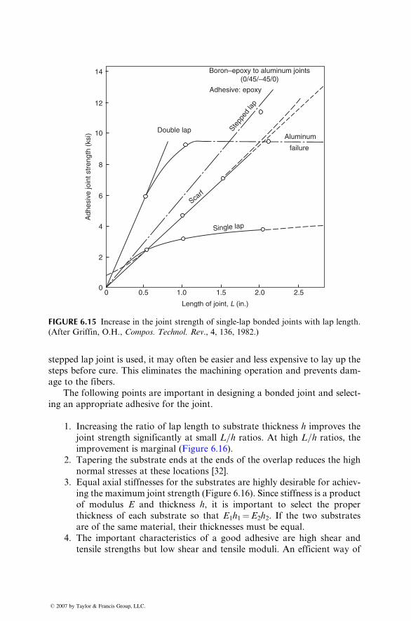
Double lapAluminum
failure
Boron–epoxy to aluminum joints(0/45/−45/0)
Adhesive: epoxy
Single lap
Scarf
Stepp
ed la
p
Length of joint, L (in.)
Adh
esiv
e jo
int s
tren
gth
(ksi
)
14
12
10
6
4
2
00 0.5 1.0 1.5 2.0 2.5
8
FIGURE 6.15 Increase in the joint strength of single-lap bonded joints with lap length.
(After Griffin, O.H., Compos. Technol. Rev., 4, 136, 1982.)
stepped lap joint is used , it may often be easie r an d less expensi ve to lay up the
steps before cure. This eliminat es the machi ning ope ration and preven ts da m-
age to the fibers.
The foll owing points a re impor tant in designi ng a bonde d joint and selec t-
ing an ap propria te adh esive for the joint .
1. Increas ing the ratio of lap length to sub strate thickne ss h impr oves the
joint stre ngth signi ficantly at small L=h ratios. At high L=h ratios, theimpr ovement is marginal (Figur e 6.16) .
2. Tape ring the substrate ends at the en ds of the overla p reduces the high
normal stresses at these locat ions [32].
3. Equal axial stiffne sses for the substrates are highly desir able for achiev-
ing the maximu m joint stren gth (Figure 6.16) . Since stiffne ss is a produ ct
of modu lus E and thickne ss h, it is impor tant to selec t the proper
thickne ss of each substrate so that E1h1 ¼ E 2h2. If the two substr ates
are of the same mate rial, their thickne sses must be equal.
4. The impor tant charact eristic s of a go od adhesiv e are high shear and
tensile strengths but low shear and tensile modu li. An efficie nt way of
� 2007 by Taylor & Francis Group, LLC.
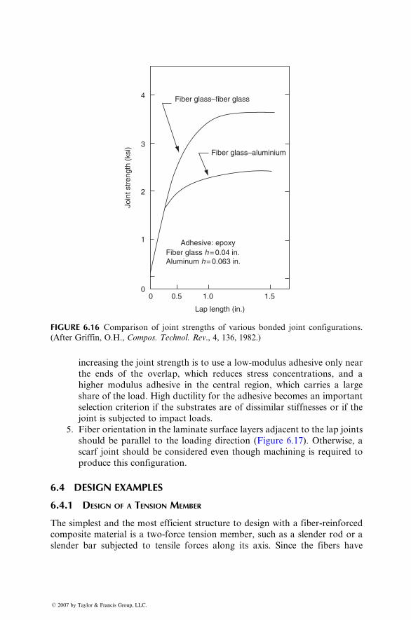
Lap length (in.)
Join
t str
engt
h (k
si)
Fiber glass–aluminium
Adhesive: epoxyFiber glass h = 0.04 in.Aluminum h = 0.063 in.
Fiber glass–fiber glass4
3
2
1
00 1.00.5 1.5
FIGURE 6.16 Comparison of joint strengths of various bonded joint configurations.
(After Griffin, O.H., Compos. Technol. Rev., 4, 136, 1982.)
increa sing the joint stre ngth is to use a low-modul us adhesiv e onl y ne ar
the ends of the overla p, which reduces stress concentra tions , and a
higher mo dulus adhesiv e in the centra l region, which carries a large
share of the load . High ductilit y for the adhesiv e becomes an impor tant
selec tion criteri on if the substrates are of dissi milar stiffne sses or if the
joint is subjected to impac t loads.
5. Fiber orient ation in the lami nate surfa ce layers adjacent to the lap joint s
shou ld be parallel to the loading direction (Figure 6.17). Otherw ise, a
scarf joint sh ould be c onsider ed e ven tho ugh machi ning is requir ed to
prod uce this config uration.
6.4 DESIGN EXAMPLES
6.4.1 DESIGN OF A T ENSION MEMBER
The simplest and the most efficie nt structure to de sign with a fiber -reinforce d
composi te material is a tw o-force tensi on member , such as a slender rod or a
slender bar subject ed to tensile forces along its axis. Sin ce the fibers have
� 2007 by Taylor & Francis Group, LLC.
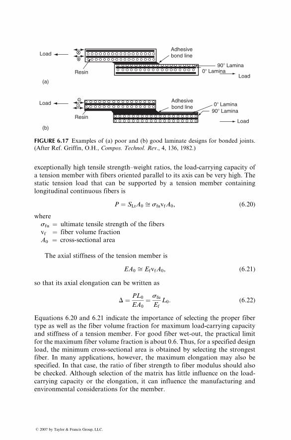
Adhesivebond line
Adhesivebond line
Resin
Resin
Load
Load
90� Lamina
90� Lamina
0� Lamina
0� Lamina
Load
Load
xx
λ
λ
(a)
(b)
FIGURE 6.17 Examples of (a) poor and (b) good laminate designs for bonded joints.
(After Ref. Griffin, O.H., Compos. Technol. Rev., 4, 136, 1982.)
exceptionally high tensile strength–weight ratios, the load-carrying capacity of
a tension member with fibers oriented parallel to its axis can be very high. The
static tension load that can be supported by a tension member containing
longitudinal continuous fibers is
P ¼ SLtA0 ffi sfuvfA0, (6:20)
where
sfu ¼ ultimate tensile strength of the fibers
vf ¼ fiber volume fraction
A0 ¼ cross-sectional area
The axial stiffness of the tension member is
EA0 ffi EfvfA0, (6:21)
so that its axial elongation can be written as
D ¼ PL0
EA0
¼ sfu
Ef
L0: (6:22)
Equations 6.20 and 6.21 indicate the importance of selecting the proper fiber
type as well as the fiber volume fraction for maximum load-carrying capacity
and stiffness of a tension member. For good fiber wet-out, the practical limit
for the maximum fiber volume fraction is about 0.6. Thus, for a specified design
load, the minimum cross-sectional area is obtained by selecting the strongest
fiber. In many applications, however, the maximum elongation may also be
specified. In that case, the ratio of fiber strength to fiber modulus should also
be checked. Although selection of the matrix has little influence on the load-
carrying capacity or the elongation, it can influence the manufacturing and
environmental considerations for the member.
� 2007 by Taylor & Francis Group, LLC.
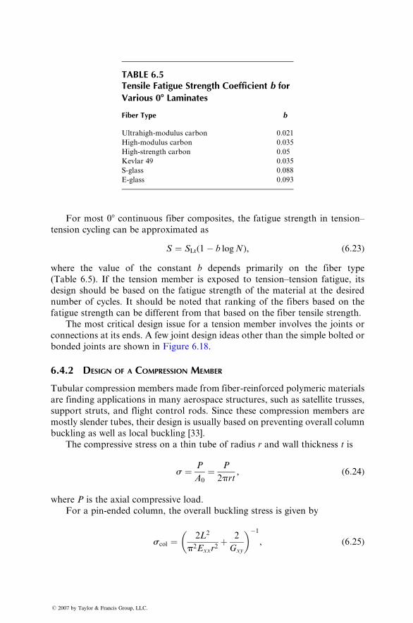
TABLE 6.5Tensile Fatigue Strength Coefficient b for
Various 08 Laminates
Fiber Type b
Ultrahigh-modulus carbon 0.021
High-modulus carbon 0.035
High-strength carbon 0.05
Kevlar 49 0.035
S-glass 0.088
E-glass 0.093
For most 08 continuous fiber composi tes, the fatigue stren gth in tensi on–
tensio n cycling can be approxim ated as
S ¼ SLt (1 � b log N ), ( 6: 23 )
wher e the value of the constant b dep ends primaril y on the fiber type
(Table 6.5). If the tensio n member is e xposed to tensi on–tensio n fatigue, its
design shou ld be based on the fatigue stre ngth of the mate rial at the desired
number of cycles. It shou ld be noted that ranking of the fiber s based on the
fatigue stren gth can be diffe rent from that based on the fiber tensile strength.
The most critical design issue for a tensi on member involv es the joint s or
connections at its ends. A few joint design ideas other than the simple bolted or
bonde d joints are sho wn in Figure 6.18.
6.4.2 DESIGN OF A COMPRESSION MEMBER
Tubular compression members made from fiber-reinforced polymeric materials
are finding applications in many aerospace structures, such as satellite trusses,
support struts, and flight control rods. Since these compression members are
mostly slender tubes, their design is usually based on preventing overall column
buckling as well as local buckling [33].
The compressive stress on a thin tube of radius r and wall thickness t is
s ¼ P
A0
¼ P
2prt, (6:24)
where P is the axial compressive load.
For a pin-ended column, the overall buckling stress is given by
scol ¼ 2L2
p2Exxr2þ 2
Gxy
� ��1
, (6:25)
� 2007 by Taylor & Francis Group, LLC.
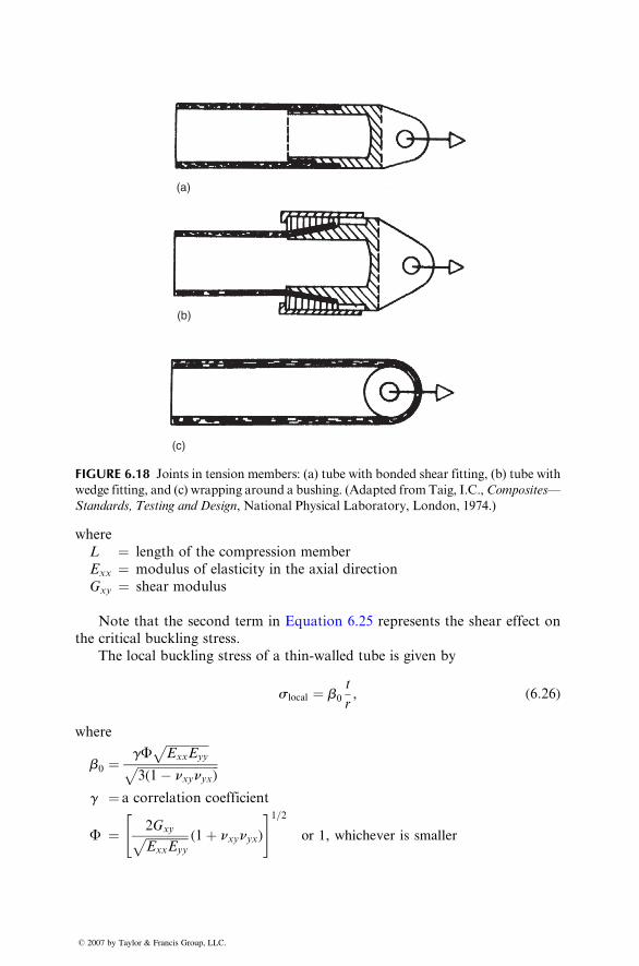
(a)
(b)
(c)
FIGURE 6.18 Joints in tension members: (a) tube with bonded shear fitting, (b) tube with
wedge fitting, and (c) wrapping around a bushing. (Adapted fromTaig, I.C.,Composites—
Standards, Testing and Design, National Physical Laboratory, London, 1974.)
where
L ¼ lengt h of the co mpression member
Exx ¼ mod ulus of elastici ty in the axial direct ion
Gxy ¼ shear mod ulus
Note that the second term in Equat ion 6.25 repres ents the shear effe ct on
the critical buckling stress.
The local buckling stress of a thin-walled tube is given by
slocal ¼ b0
t
r, (6:26)
where
b0 ¼gF
ffiffiffiffiffiffiffiffiffiffiffiffiffiffiExxEyy
pffiffiffiffiffiffiffiffiffiffiffiffiffiffiffiffiffiffiffiffiffiffiffiffiffiffiffi3(1� nxynyx)
pg ¼ a correlation coefficient
F ¼ 2GxyffiffiffiffiffiffiffiffiffiffiffiffiffiffiExxEyy
p (1þ nxynyx)
" #1=2or 1, whichever is smaller
� 2007 by Taylor & Francis Group, LLC.
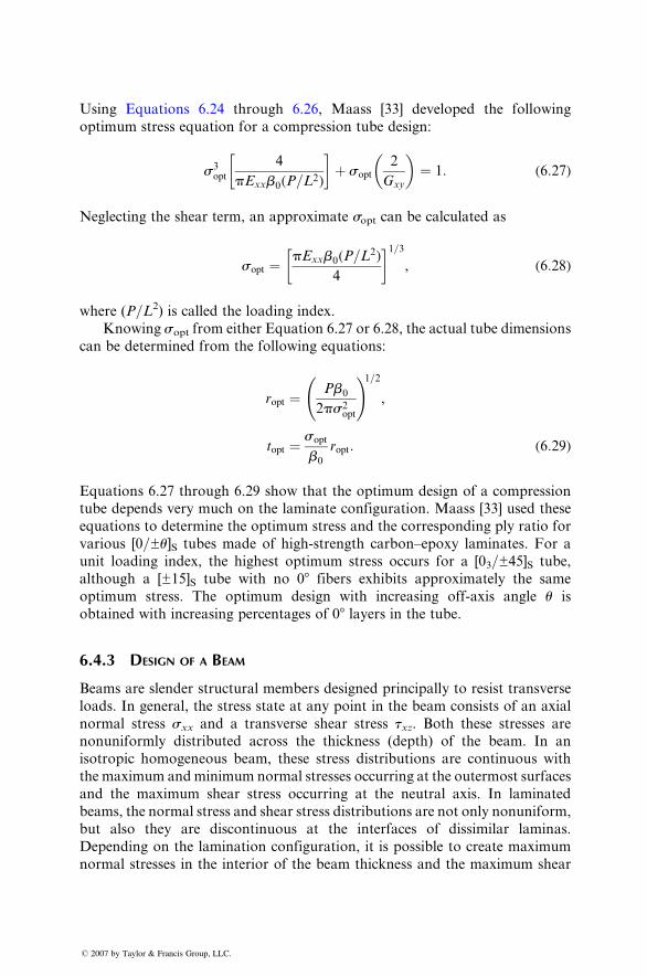
Usin g Equat ions 6.24 throu gh 6.26, Maass [33] developed the foll owing
optimum stress equation for a compression tube design:
s3opt
4
pExxb0(P=L2)
� �þ sopt
2
Gxy
� �¼ 1: (6:27)
Neglecting the shear term, an approximate sopt can be calculated as
sopt ¼ pExxb0(P=L2)
4
� �1=3, (6:28)
where (P=L2) is called the loading index.
Knowing sopt from either Equation 6.27 or 6.28, the actual tube dimensions
can be determined from the following equations:
ropt ¼ Pb0
2ps2opt
!1=2,
topt ¼ sopt
b0
ropt: (6:29)
Equations 6.27 through 6.29 show that the optimum design of a compression
tube depends very much on the laminate configuration. Maass [33] used these
equations to determine the optimum stress and the corresponding ply ratio for
various [0=±u]S tubes made of high-strength carbon–epoxy laminates. For a
unit loading index, the highest optimum stress occurs for a [03=±45]S tube,
although a [±15]S tube with no 08 fibers exhibits approximately the same
optimum stress. The optimum design with increasing off-axis angle u is
obtained with increasing percentages of 08 layers in the tube.
6.4.3 DESIGN OF A BEAM
Beams are slender structural members designed principally to resist transverse
loads. In general, the stress state at any point in the beam consists of an axial
normal stress sxx and a transverse shear stress txz. Both these stresses are
nonuniformly distributed across the thickness (depth) of the beam. In an
isotropic homogeneous beam, these stress distributions are continuous with
the maximum andminimum normal stresses occurring at the outermost surfaces
and the maximum shear stress occurring at the neutral axis. In laminated
beams, the normal stress and shear stress distributions are not only nonuniform,
but also they are discontinuous at the interfaces of dissimilar laminas.
Depending on the lamination configuration, it is possible to create maximum
normal stresses in the interior of the beam thickness and the maximum shear
� 2007 by Taylor & Francis Group, LLC.
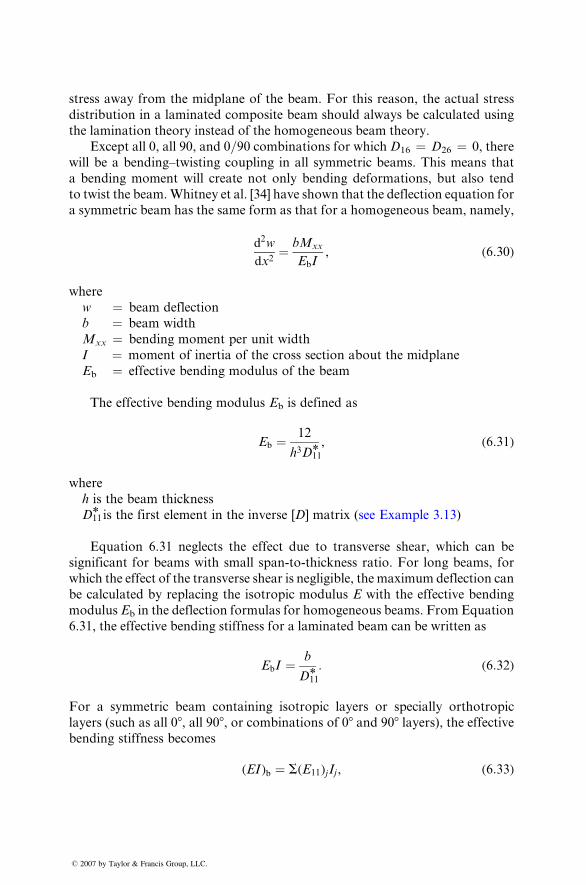
stress away from the midpl ane of the beam. For this reason, the actual stre ss
distribut ion in a laminated co mposite be am should alw ays be calcul ated using
the laminati on theory instead of the homo geneous beam theory.
Excep t all 0, all 90, and 0=90 combinat ions for whi ch D16 ¼ D 26 ¼ 0, there
will be a bend ing–twisti ng co upling in all symm etric beams. This means that
a ben ding moment will create not only bending deform ations, but also tend
to twist the beam. Whitne y et al. [34] have shown that the de flection equa tion for
a symm etric be am has the same form as that for a hom ogeneou s beam, namel y,
d2 w
d x2 ¼ bMxx
Eb I, ( 6: 30 )
where
w ¼ beam deflection
b ¼ beam width
Mxx ¼ ben ding mo ment per unit wi dth
I ¼ moment of inert ia of the cross sectio n a bout the midpl ane
Eb ¼ effecti ve be nding modulus of the beam
The effective bending modulus Eb is defined as
Eb ¼ 12
h3D11*, (6:31)
where
h is the beam thickness
D11* is the first element in the invers e [D ] matr ix (see Example 3.13)
Equation 6.31 neglects the effect due to transverse shear, which can be
significant for beams with small span-to-thickness ratio. For long beams, for
which the effect of the transverse shear is negligible, the maximum deflection can
be calculated by replacing the isotropic modulus E with the effective bending
modulus Eb in the deflection formulas for homogeneous beams. From Equation
6.31, the effective bending stiffness for a laminated beam can be written as
EbI ¼ b
D11*: (6:32)
For a symmetric beam containing isotropic layers or specially orthotropic
layers (such as all 08, all 908, or combinations of 08 and 908 layers), the effectivebending stiffness becomes
(EI)b ¼ S(E11)jIj, (6:33)
� 2007 by Taylor & Francis Group, LLC.
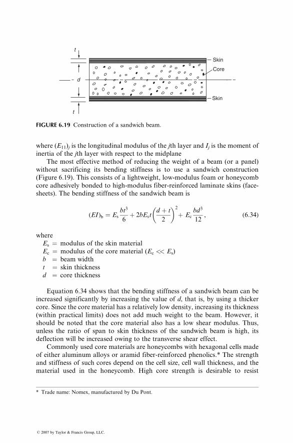
t
t
d
Skin
Skin
Core
FIGURE 6.19 Construction of a sandwich beam.
where (E11)j is the longitudinal modulus of the jth layer and Ij is the moment of
inertia of the jth layer with respect to the midplane
The most effective method of reducing the weight of a beam (or a panel)
without sacrificing its bending stiffness is to use a sandwich construction
(Figure 6.19). This consists of a lightweight, low-modulus foam or honeycomb
core adhesively bonded to high-modulus fiber-reinforced laminate skins (face-
sheets). The bending stiffness of the sandwich beam is
(EI)b ¼ Es
bt3
6þ 2bEst
d þ t
2
� �2
þ Ec
bd3
12, (6:34)
where
Es ¼ modulus of the skin material
Ec ¼ modulus of the core material (Ec << Es)
b ¼ beam width
t ¼ skin thickness
d ¼ core thickness
Equation 6.34 shows that the bending stiffness of a sandwich beam can be
increased significantly by increasing the value of d, that is, by using a thicker
core. Since the core material has a relatively low density, increasing its thickness
(within practical limits) does not add much weight to the beam. However, it
should be noted that the core material also has a low shear modulus. Thus,
unless the ratio of span to skin thickness of the sandwich beam is high, its
deflection will be increased owing to the transverse shear effect.
Commonly used core materials are honeycombs with hexagonal cells made
of either aluminum alloys or aramid fiber-reinforced phenolics.* The strength
and stiffness of such cores depend on the cell size, cell wall thickness, and the
material used in the honeycomb. High core strength is desirable to resist
* Trade name: Nomex, manufactured by Du Pont.
� 2007 by Taylor & Francis Group, LLC.
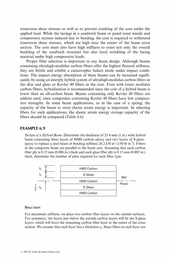
transve rse shear stresses as well as to prevent crushi ng of the core unde r the
applie d load. W hile the facing s in a sand wich beam or pa nel resist tensi le and
compres sive stresses induced due to bending, the core is requir ed to withst and
transve rse shear stre sses, whi ch are high near the cen ter of the beam cro ss
section . The core mu st also hav e high stiffne ss to resist not only the overal l
buckling of the sandw ich struc ture but also local wrin kling of the faci ng
material unde r high c ompres sive loads.
Prop er fiber selection is impor tant in any beam design. Alth ough bea ms
contai ning ultrahigh- modulus carbon fiber s offer the high est flexu ral stiffne ss,
they are brittle and exhibit a catas trophi c failure mode unde r impac t con di-
tions. The impac t energy absorpt ion of these beams can be increa sed signifi -
cantly by using an interp ly hyb rid system of ultrahigh- modu lus carbon fiber s in
the skin an d glass or Kevl ar 49 fibers in the core. Even with low er modu lus
carbon fiber s, hyb ridizatio n is recomm end ed since the cost of a hybrid beam is
lower than an all-carbo n beam. Beams contai ning only Kevlar 49 fiber s are
seldom used, since composi tes contai ning Kevl ar 49 fibers have low c ompres -
sive strengths. In some beam applications, as in the case of a spring, the
capacity of the beam to store elastic strain energy is important. In selecting
fibers for such applications, the elastic strain energy storage capacity of the
fibers should be compared (Table 6.6).
EXAMPLE 6.9
Design of a Hybrid Beam. Determine the thickness of 25.4 mm (1 in.) wide hybrid
beam containing three layers of HMS carbon–epoxy and two layers of S-glass–
epoxy to replace a steel beam of bending stiffness 26.2 kN m2 (150 lb in.2). Fibers
in the composite beam are parallel to the beam axis. Assuming that each carbon
fiber ply is 0.15 mm (0.006 in.) thick and each glass fiber ply is 0.13 mm (0.005 in.)
thick, determine the number of plies required for each fiber type.
1t0
t0
t0
2
HMS Carbon
S Glass
HMS CarbonMid
PlaneS Glass
HMS Carbon
SOLUTION
For maximum stiffness, we place two carbon fiber layers on the outside surfaces.
For symmetry, the layers just below the outside carbon layers will be the S-glass
layers, which will leave the remaining carbon fiber layer at the center of the cross
section. We assume that each layer has a thickness t0. Since fibers in each layer are
� 2007 by Taylor & Francis Group, LLC.
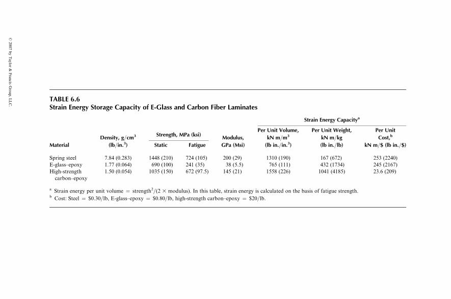
TABLE 6.6Strain Energy Storage Capacity of E-Glass and Carbon Fiber Laminates
Strain Energy Capacitya
Strength, MPa (ksi)Per Unit Volume, Per Unit Weight, Per Unit
Density, g=cm3 Modulus, kN m=m3 kN m=kg Cost,b
Material (lb=in.3) Static Fatigue GPa (Msi) (lb in.=in.3) (lb in.=lb) kN m=$ (lb in.=$)
Spring steel 7.84 (0.283) 1448 (210) 724 (105) 200 (29) 1310 (190) 167 (672) 253 (2240)
E-glass–epoxy 1.77 (0.064) 690 (100) 241 (35) 38 (5.5) 765 (111) 432 (1734) 245 (2167)
High-strength
carbon–epoxy
1.50 (0.054) 1035 (150) 672 (97.5) 145 (21) 1558 (226) 1041 (4185) 23.6 (209)
a Strain energy per unit volume ¼ strength2=(2 3 modulus). In this table, strain energy is calculated on the basis of fatigue strength.b Cost: Steel ¼ $0.30=lb, E-glass–epoxy ¼ $0.80=lb, high-strength carbon–epoxy ¼ $20=lb.
�2007
byTaylor
&Francis
Group,L
LC.
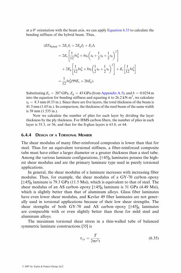
at a 08 orientation with the beam axis, we can apply Equation 6.33 to calculate the
bending stiffness of the hybrid beam. Thus,
(EI )hybrid ¼ 2E c I1 þ 2E g I2 þ E c I3
¼ 2Ec
1
12 bt 30 þ bt 0 t 0 þ 1
2 t 0 þ 1
2 t 0
� �2" #
þ 2Eg
1
12 bt 30 þ bt 0
1
2 t 0 þ 1
2 t 0
� �2" #
þ Ec
1
12 bt 30
� �
¼ 1
12 bt30 (99E c þ 26 Eg ) :
Substituting Ec ¼ 207 GPa, Eg ¼ 43 GPa (from Appendix A.5), and b ¼ 0.0254 m
into the equation for bending stiffness and equating it to 26.2 kN m 2 , we calculate
t0 ¼ 8.3 mm (0.33 in.). Since there are five layers, the total thickness of the beam is
41.5 mm (1.65 in.). In comparison, the thickness of the steel beam of the same width
is 39 mm (1.535 in.).
Now we calculate the number of plies for each layer by dividing the layer
thickness by the ply thickness. For HMS carbon fibers, the number of plies in each
layer is 55.3, or 56, and that for the S-glass layers is 63.8, or 64.
6.4.4 DESIGN OF A T ORSIONAL MEMBER
The shear mod ulus of many fiber-re inforce d compo sites is low er than that for
steel. Thus for an equ ivalent torsion al sti ffness, a fiber-re inforced co mposi te
tube must have eithe r a large r diame ter or a great er thickne ss than a steel tube.
Among the various laminate configu rations, [±45]S lami nates possess the high -
est shear modulus and are the prim ary laminate type use d in purely torsion al
applications.
In general, the shear modulus of a laminate increases with increasing fiber
modulus. Thus, for example, the shear modulus of a GY-70 carbon–epoxy
[±45]S laminate is 79.3 GPa (11.5 Msi), which is equivalent to that of steel. The
shear modulus of an AS carbon–epoxy [±45]S laminate is 31 GPa (4.49 Msi),
which is slightly better than that of aluminum alloys. Glass fiber laminates
have even lower shear modulus, and Kevlar 49 fiber laminates are not gener-
ally used in torsional applications because of their low shear strengths. The
shear strengths of both GY-70 and AS carbon–epoxy [±45]S laminates
are comparable with or even slightly better than those for mild steel and
aluminum alloys.
The maximum torsional shear stress in a thin-walled tube of balanced
symmetric laminate constructions [35] is
txy ¼ T
2pr2t(6:35)
� 2007 by Taylor & Francis Group, LLC.
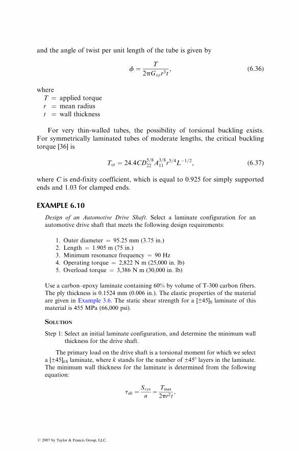
and the angle of twist per unit length of the tube is given by
f ¼ T
2p Gxy r 3 t , ( 6: 36 )
wher e
T ¼ applie d torque
r ¼ mean radius
t ¼ wall thickne ss
For very thin-wa lled tubes, the possibi lity of torsio nal buckling exist s.
For symm etricall y laminated tubes of moderat e lengt hs, the critical buc kling
torque [36] is
Tcr ¼ 24:4CD 5= 822 A
3= 811 r 5 =4 L� 1 = 2 , ( 6: 37 )
wher e C is end-fi xity co efficie nt, which is equal to 0.925 for sim ply suppo rted
ends and 1.03 for clam ped ends.
EXAMPLE 6.10
Design of an Automotive Drive Shaft. Select a laminate configuration for an
automotive drive shaft that meets the following design requirements:
1. Outer diameter ¼ 95.25 mm (3.75 in.)
2. Length ¼ 1.905 m (75 in.)
3. Minimum resonance frequency ¼ 90 Hz
4. Operating torque ¼ 2,822 N m (25,000 in. lb)
5. Overload torque ¼ 3,386 N m (30,000 in. lb)
Use a carbon–epoxy laminate containing 60% by volume of T-300 carbon fibers.
The ply thickness is 0.1524 mm (0.006 in.). The elastic properties of the material
are given in Example 3.6. The static shear strength for a [±45]S laminate of this
material is 455 MPa (66,000 psi).
SOLUTION
Step 1: Select an initial laminate configuration, and determine the minimum wall
thickness for the drive shaft.
The primary load on the drive shaft is a torsional moment for which we select
a [±45]kS laminate, where k stands for the number of ±458 layers in the laminate.
The minimum wall thickness for the laminate is determined from the following
equation:
tall ¼ Sxys
n¼ Tmax
2pr2t,
� 2007 by Taylor & Francis Group, LLC.
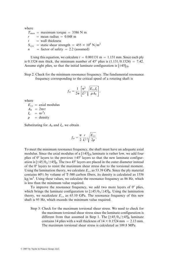
� 2
where
Tmax ¼ maximum torque ¼ 3386 N m
r ¼ mean radius ¼ 0.048 m
t ¼ wall thickness
Sxys ¼ static shear strength ¼ 455 3 106 N=m2
n ¼ factor of safety ¼ 2.2 (assumed)
Using this equation, we calculate t ¼ 0.001131 m ¼ 1.131 mm. Since each ply
is 0.1524 mm thick, the minimum number of 458 plies is (1.131=0.1524) ¼ 7.42.
Assume eight plies, so that the initial laminate configuration is [±45]2S.
Step 2: Check for the minimum resonance frequency. The fundamental resonance
frequency corresponding to the critical speed of a rotating shaft is
fcr ¼ 1
2p
p2
L2
ffiffiffiffiffiffiffiffiffiffiffiExxIc
rA0
s" #,
where
Exx ¼ axial modulus
A0 ¼ 2prt
Ic ¼ pr3tr ¼ density
Substituting for A0 and Ic, we obtain
fcr ¼ p
2
r
L2
ffiffiffiffiffiffiffiffiExx
2r
s:
To meet the minimum resonance frequency, the shaft must have an adequate axial
modulus. Since the axial modulus of a [±45]2S laminate is rather low, we add four
plies of 08 layers to the previous ±458 layers so that the new laminate configur-
ation is [±45=02=±45]S. The two 458 layers are placed in the outer diameter instead
of the 08 layers to resist the maximum shear stress due to the torsional moment.
Using the lamination theory, we calculate Exx as 53.39 GPa. Since the ply material
contains 60% by volume of T-300 carbon fibers, its density is calculated as 1556
kg=m3. Using these values, we calculate the resonance frequency as 86 Hz, which
is less than the minimum value required.
To improve the resonance frequency, we add two more layers of 08 plies,
which brings the laminate configuration to [±45=03=±45]S. Using the lamination
theory, we recalculate Exx as 65.10 GPa. The resonance frequency of this new
shaft is 95 Hz, which exceeds the minimum value required.
Step 3: Check for the maximum torsional shear stress. We need to check for
the maximum torsional shear stress since the laminate configuration is
different from that assumed in Step 1. The [±45=03=±45]S laminate
contains 14 plies with a wall thickness of 143 0.1524 mm ¼ 2.13 mm.
The maximum torsional shear stress is calculated as 109.8 MPa.
007 by Taylor & Francis Group, LLC.
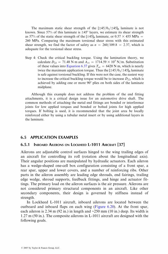
� 2
The maximum static shear strength of the [±45=03 =±45]S laminate is not
known. Since 57% of this laminate is ±45 8 layers, we estimate its shear strength
as 57% of the static shear strength of the [±45]S laminate, or 0.57 3 455 MPa ¼260 MPa. Comparing the maximum torsional shear stress with this estimated
shear strength, we find the factor of safety as n ¼ 260= 109.8 ¼ 2.37, which is
adequate for the torsional shear stress.
Step 4: Check the critical buckling torque. Using the lamination theory, we
calculate D22 ¼ 71.48 N m and A 11 ¼ 1714.59 3 105 N=m. Substitution
of these values into Equation 6.37 gives Tcr ¼ 6420 N m, which is nearly
twice the maximum application torque. Thus the [±45 =03=±45] S laminate
is safe against torsional buckling. If this were not the case, the easiest way
to increase the critical buckling torque would be to increase D22 , which is
achieved by adding one or more 908 plies on both sides of the laminate
midplane.
Although this example does not address the problem of the end fitting
attachments, it is a critical design issue for an automotive drive shaft. The
common methods of attaching the metal end fittings are bonded or interference
joints for low applied torques and bonded or bolted joints for high applied
torques. If bolting is used, it is recommended that the joint area be locally
reinforced either by using a tubular metal insert or by using additional layers in
the laminate.
6.5 APPLICATION EXAMPLES
6.5.1 INBOARD A ILERONS ON L OCKHEED L-1011 AIRCRAFT [37]
Ailerons are adjust able control surfa ces hinged to the wing trailing edges of
an aircr aft for con trolling its roll (rotati on abo ut the longitudinal axis) .
Their angular pos itions are manipul ated by hyd raulic actuato rs. Eac h aileron
has a wedge-shaped one-cel l box co nfigurati on co nsisting of a front sp ar, a
rear spar, uppe r and lower covers, and a numb er of reinf orcing ribs. Othe r
parts in the aile ron assem bly are leadi ng edge sh rouds, end fairings , trai ling
edge wedge , shro ud supports , feedba ck fittings, and hinge and actuat or fit-
tings. The prim ary load on the aile ron surfaces is the air pr essure. Ailerons are
not con sidered primary struc tural compon ents in an aircra ft. Like other
secondary componen ts, their design is governed by stiffness inst ead of
stren gth.
In Lockhe ed L-1011 a ircraft, inboard ailerons are locat ed between the
outboard and inboard flaps on each wing (Figur e 6.20) . At the front spar,
each aileron is 2.34 m (92 in.) in length and ~250 mm (10 in.) deep. Its width is
1.27 m (50 in.). The composite ailerons in L-1011 aircraft are designed with the
following goals.
007 by Taylor & Francis Group, LLC.
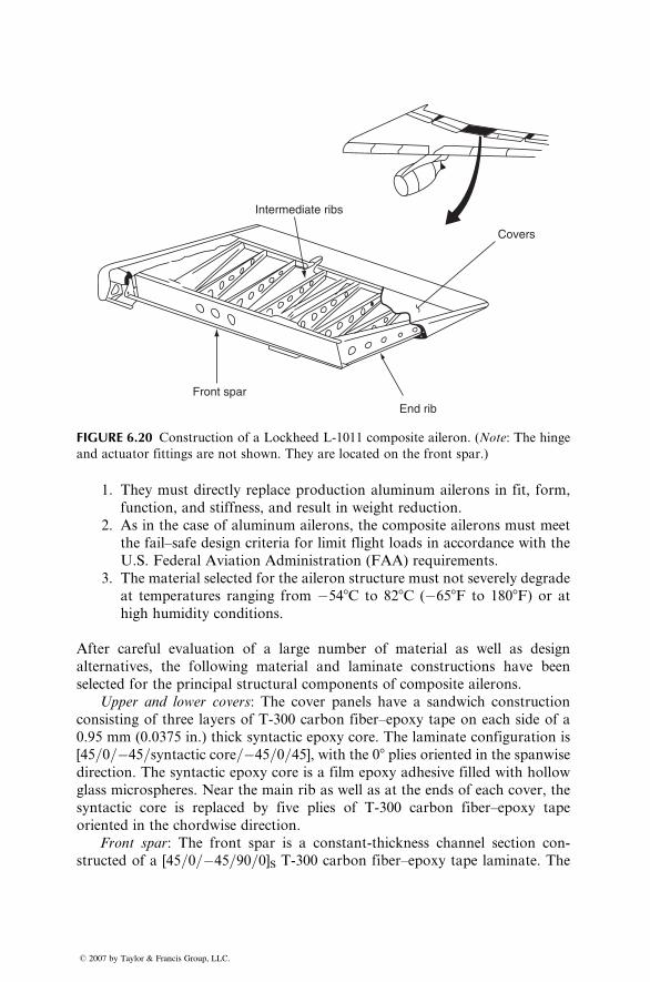
Intermediate ribs
Covers
Front sparEnd rib
FIGURE 6.20 Construction of a Lockheed L-1011 composite aileron. (Note: The hinge
and actuator fittings are not shown. They are located on the front spar.)
1. They must directly replace production aluminum ailerons in fit, form,
function, and stiffness, and result in weight reduction.
2. As in the case of aluminum ailerons, the composite ailerons must meet
the fail–safe design criteria for limit flight loads in accordance with the
U.S. Federal Aviation Administration (FAA) requirements.
3. The material selected for the aileron structure must not severely degrade
at temperatures ranging from �548C to 828C (�658F to 1808F) or at
high humidity conditions.
After careful evaluation of a large number of material as well as design
alternatives, the following material and laminate constructions have been
selected for the principal structural components of composite ailerons.
Upper and lower covers: The cover panels have a sandwich construction
consisting of three layers of T-300 carbon fiber–epoxy tape on each side of a
0.95 mm (0.0375 in.) thick syntactic epoxy core. The laminate configuration is
[45=0=�45=syntactic core=�45=0=45], with the 08 plies oriented in the spanwise
direction. The syntactic epoxy core is a film epoxy adhesive filled with hollow
glass microspheres. Near the main rib as well as at the ends of each cover, the
syntactic core is replaced by five plies of T-300 carbon fiber–epoxy tape
oriented in the chordwise direction.
Front spar: The front spar is a constant-thickness channel section con-
structed of a [45=0=�45=90=0]S T-300 carbon fiber–epoxy tape laminate. The
� 2007 by Taylor & Francis Group, LLC.
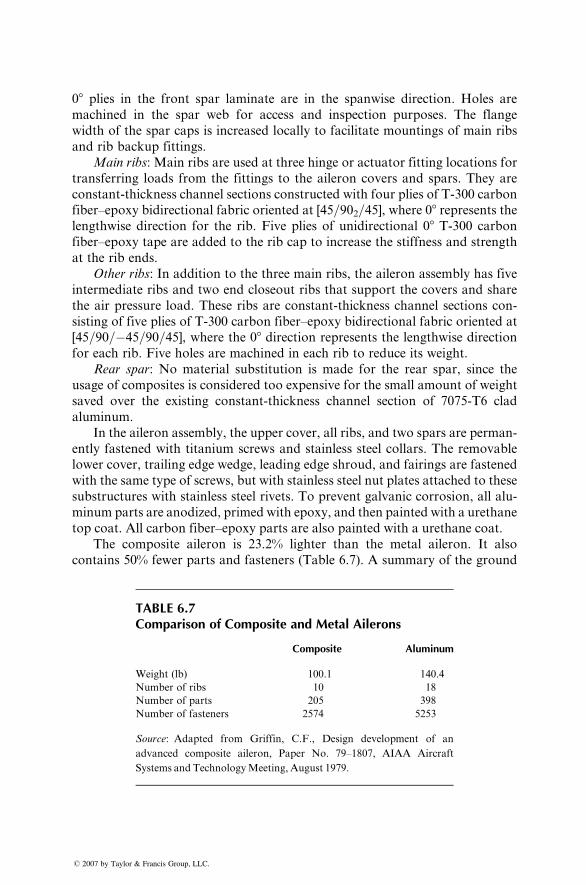
08 plies in the front spar laminate are in the spanwise direction. Holes are
machined in the spar web for access and inspection purposes. The flange
width of the spar caps is increased locally to facilitate mountings of main ribs
and rib backup fittings.
Main ribs: Main ribs are used at three hinge or actuator fitting locations for
transferring loads from the fittings to the aileron covers and spars. They are
constant-thickness channel sections constructed with four plies of T-300 carbon
fiber–epoxy bidirectional fabric oriented at [45=902=45], where 08 represents thelengthwise direction for the rib. Five plies of unidirectional 08 T-300 carbon
fiber–epoxy tape are added to the rib cap to increase the stiffness and strength
at the rib ends.
Other ribs: In addition to the three main ribs, the aileron assembly has five
intermediate ribs and two end closeout ribs that support the covers and share
the air pressure load. These ribs are constant-thickness channel sections con-
sisting of five plies of T-300 carbon fiber–epoxy bidirectional fabric oriented at
[45=90=�45=90=45], where the 08 direction represents the lengthwise direction
for each rib. Five holes are machined in each rib to reduce its weight.
Rear spar: No material substitution is made for the rear spar, since the
usage of composites is considered too expensive for the small amount of weight
saved over the existing constant-thickness channel section of 7075-T6 clad
aluminum.
In the aileron assembly, the upper cover, all ribs, and two spars are perman-
ently fastened with titanium screws and stainless steel collars. The removable
lower cover, trailing edge wedge, leading edge shroud, and fairings are fastened
with the same type of screws, but with stainless steel nut plates attached to these
substructures with stainless steel rivets. To prevent galvanic corrosion, all alu-
minum parts are anodized, primed with epoxy, and then painted with a urethane
top coat. All carbon fiber–epoxy parts are also painted with a urethane coat.
The composite aileron is 23.2% lighter than the metal aileron. It also
contains 50% fewer parts and fasteners (Table 6.7). A summary of the ground
TABLE 6.7Comparison of Composite and Metal Ailerons
Composite Aluminum
Weight (lb) 100.1 140.4
Number of ribs 10 18
Number of parts 205 398
Number of fasteners 2574 5253
Source: Adapted from Griffin, C.F., Design development of an
advanced composite aileron, Paper No. 79–1807, AIAA Aircraft
Systems and TechnologyMeeting, August 1979.
� 2007 by Taylor & Francis Group, LLC.
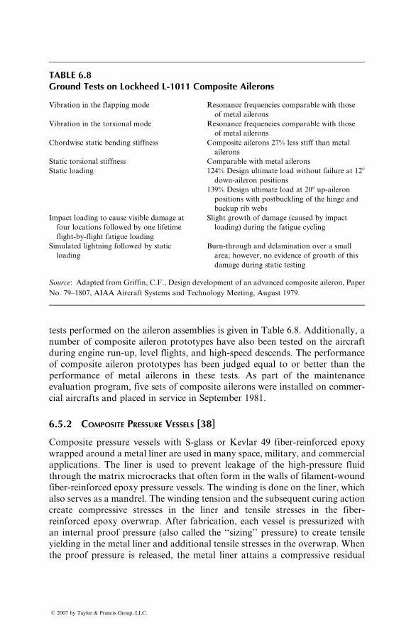
TABLE 6.8Ground Tests on Lockheed L-1011 Composite Ailerons
Vibration in the flapping mode Resonance frequencies comparable with those
of metal ailerons
Vibration in the torsional mode Resonance frequencies comparable with those
of metal ailerons
Chordwise static bending stiffness Composite ailerons 27% less stiff than metal
ailerons
Static torsional stiffness Comparable with metal ailerons
Static loading 124% Design ultimate load without failure at 128
down-aileron positions
139% Design ultimate load at 208 up-aileron
positions with postbuckling of the hinge and
backup rib webs
Impact loading to cause visible damage at
four locations followed by one lifetime
flight-by-flight fatigue loading
Slight growth of damage (caused by impact
loading) during the fatigue cycling
Simulated lightning followed by static
loading
Burn-through and delamination over a small
area; however, no evidence of growth of this
damage during static testing
Source: Adapted from Griffin, C.F., Design development of an advanced composite aileron, Paper
No. 79–1807, AIAA Aircraft Systems and Technology Meeting, August 1979.
tests performed on the aileron assemblies is given in Table 6.8. Additionally, a
number of composite aileron prototypes have also been tested on the aircraft
during engine run-up, level flights, and high-speed descends. The performance
of composite aileron prototypes has been judged equal to or better than the
performance of metal ailerons in these tests. As part of the maintenance
evaluation program, five sets of composite ailerons were installed on commer-
cial aircrafts and placed in service in September 1981.
6.5.2 COMPOSITE PRESSURE VESSELS [38]
Composite pressure vessels with S-glass or Kevlar 49 fiber-reinforced epoxy
wrapped around a metal liner are used in many space, military, and commercial
applications. The liner is used to prevent leakage of the high-pressure fluid
through the matrix microcracks that often form in the walls of filament-wound
fiber-reinforced epoxy pressure vessels. The winding is done on the liner, which
also serves as a mandrel. The winding tension and the subsequent curing action
create compressive stresses in the liner and tensile stresses in the fiber-
reinforced epoxy overwrap. After fabrication, each vessel is pressurized with
an internal proof pressure (also called the ‘‘sizing’’ pressure) to create tensile
yielding in the metal liner and additional tensile stresses in the overwrap. When
the proof pressure is released, the metal liner attains a compressive residual
� 2007 by Taylor & Francis Group, LLC.
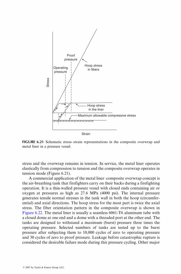
Str
ess
Operatingpressure
Proofpressure
Hoop stressin fibers
Hoop stressin the liner
Maximum allowable compressive stress
Strain
FIGURE 6.21 Schematic stress–strain representations in the composite overwrap and
metal liner in a pressure vessel.
stress and the overwrap remains in tensi on. In servi ce, the metal liner operate s
elastica lly from co mpression to tension and the compo site ov erwrap operate s in
tensio n mode (Figure 6.21) .
A commer cial applic ation of the metal liner –composi te overw rap con cept is
the air- breathing tank that fir efighters carry on their back s during a firefi ghting
operati on. It is a thin-wa lled pressur e vessel with closed ends contai ning air or
oxygen at pressur es as high as 27 .6 MPa (4000 psi). The internal pr essure
generat es tensile normal stresses in the tank wall in both the hoop (circumf er-
entia l) and axial directions. The hoop stress for the most part is twice the axial
stress. The fiber orientati on pattern in the compo site ov erwrap is shown in
Figure 6.22. The meta l liner is usu ally a seaml ess 6061-T6 alumi num tube wi th
a c losed dome at one end and a dome wi th a threade d por t at the other end . The
tanks are designe d to withstan d a maximum (burst) pressur e three times the
operati ng pressur e. Select ed numbers of tanks are tested up to the bur st
pressur e afte r subject ing them to 10,000 cycles of zero to ope rating pr essure
and 30 cycles of zero to proof pressur e. Lea kage before catastroph ic rupture is
considered the desirable failure mode during this pressure cycling. Other major
� 2007 by Taylor & Francis Group, LLC.
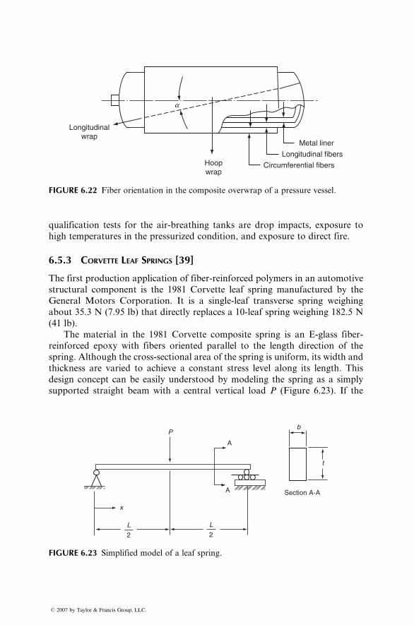
Longitudinalwrap
Hoopwrap
Metal liner
Longitudinal fibers
Circumferential fibers
a
FIGURE 6.22 Fiber orientation in the composite overwrap of a pressure vessel.
qualification tests for the air-breathing tanks are drop impacts, exposure to
high temperatures in the pressurized condition, and exposure to direct fire.
6.5.3 CORVETTE LEAF SPRINGS [39]
The first production application of fiber-reinforced polymers in an automotive
structural component is the 1981 Corvette leaf spring manufactured by the
General Motors Corporation. It is a single-leaf transverse spring weighing
about 35.3 N (7.95 lb) that directly replaces a 10-leaf spring weighing 182.5 N
(41 lb).
The material in the 1981 Corvette composite spring is an E-glass fiber-
reinforced epoxy with fibers oriented parallel to the length direction of the
spring. Although the cross-sectional area of the spring is uniform, its width and
thickness are varied to achieve a constant stress level along its length. This
design concept can be easily understood by modeling the spring as a simply
supported straight beam with a central vertical load P (Figure 6.23). If the
Section A-A
t
A
A
P
x
L
2
L
2
b
FIGURE 6.23 Simplified model of a leaf spring.
� 2007 by Taylor & Francis Group, LLC.
beam has a rectangular cross section, the maximum normal stress at any
location x in the beam is given by
sxx ¼ 3Px
bt2, (6:38)
where b and t are the width and thickness of the beam, respectively.
For a uniform cross-sectional area beam, bt ¼ constant ¼ A0. Furthermore,
the beam is designed for a constant maximum stress, sxx ¼ constant ¼ s0.
Thus, using Equation 6.38, we can write the thickness variation for each half
length of the beam as
t ¼ 3P
A0s0
x (6:39)
and correspondingly, its width variation as
b ¼ A20s0
3P
1
x: (6:40)
Equations 6.39 and 6.40 show that an ideal spring of uniform cross-sectional
area and constant stress level has zero thickness and infinite width at each end.
The production Corvette composite spring is ~15 mm (0.6 in.) thick by 86 mm
(3.375 in.) wide at each end and 25 mm thick (1 in.) by 53 mm (2.125 in.) wide
at the center. Two of these springs are filament-wound in the mold cavities,
which are machined on two sides of an elliptic mandrel. After winding to the
proper thickness, the mold cavities are closed and the springs are compression-
molded on the mandrel at elevated temperature and pressure. The pressure
applied during the molding stage spreads the filament-wound material in the
mold cavities and creates the desired cross-sectional shapes. Each cured spring
has a semi-elliptic configuration in the unloaded condition. When the spring is
installed under the axle of a Corvette and the curb load is applied, it assumes a
nearly flat configuration.
Prototype Corvette composite springs are tested in the laboratory to deter-
mine their static spring rates as well as their lives in jounce-to-rebound stroke-
controlled fatigue tests. The test springs are required to survive a minimum of
500,000 jounce-to-rebound cycles with a load loss not exceeding 5% of the
initially applied load at both high (above 1008C) and low (below 08C) temper-
atures. Stress relaxation tests are performed for 24 h at elevated temperatures
and high-humidity conditions. Other laboratory tests include torsional fatigue
and gravelometer test (to evaluate the effect of gravel impingement on the
surface coating). Prototype composite springs are also vehicle-tested to deter-
mine their ride and durability characteristics.
� 2007 by Taylor & Francis Group, LLC.
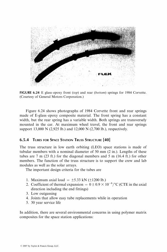
FIGURE 6.24 E glass–epoxy front (top) and rear (bottom) springs for 1984 Corvette.
(Courtesy of General Motors Corporation.)
Figure 6.24 shows photographs of 1984 Corvette front and rear springs
made of E-glass–epoxy composite material. The front spring has a constant
width, but the rear spring has a variable width. Both springs are transversely
mounted in the car. At maximum wheel travel, the front and rear springs
support 13,000 N (2,925 lb.) and 12,000 N (2,700 lb.), respectively.
6.5.4 TUBES FOR SPACE STATION TRUSS STRUCTURE [40]
The truss structure in low earth orbiting (LEO) space stations is made of
tubular members with a nominal diameter of 50 mm (2 in.). Lengths of these
tubes are 7 m (23 ft.) for the diagonal members and 5 m (16.4 ft.) for other
members. The function of the truss structure is to support the crew and lab
modules as well as the solar arrays.
The important design criteria for the tubes are
1. Maximum axial load ¼ ±5.33 kN (±1200 lb.)
2. Coefficient of thermal expansion ¼ 0 ± 0.93 10�6=8C (CTE in the axial
direction including the end fittings)
3. Low outgassing
4. Joints that allow easy tube replacements while in operation
5. 30 year service life
In addition, there are several environmental concerns in using polymer matrix
composites for the space station applications:
� 2007 by Taylor & Francis Group, LLC.
1. Atomic oxygen (AO) degradation: Atomic oxygen is the major compon-
ent in the LEO atmosphere. On prolonged exposure, it can substantially
reduce the thickness of carbon fiber-reinforced epoxy tubes and reduce
their properties. The AO degradation of such tubes can be controlled by
wrapping them with a thin aluminum foil or by cladding them with an
aluminum layer.
2. Damage due to thermal cycling: It is estimated that the space station,
orbiting at 250 nautical miles with an orbital period of 90 min, will
experience 175,000 thermal cyclings during a 30 year service life. Unless
protected by reflective aluminum coatings, the transient temperature
variation may range from �628C to 778C. In the ‘‘worst case’’ situation,
for example, when the tube is always shadowed, the lowest steady-state
temperature may reach �1018C.3. Damage due to low-velocity impact during assembly or due to extravehi-
cular activities. This type of damage may occur when two tubes acciden-
tally strike one another or when a piece of equipment strikes the tube.
These incidents can cause internal damages in the tube material and
reduce its structural properties. They can also damage the AO protective
coating and expose the tube material to atomic oxygen.
Since the tubes have large slenderness ratios (length-to-diameter ratios) and are
subjected to axial loading, column buckling is considered to be the primary
failure mode. Using Euler’s buckling formula for pin-ended columns, the
critical axial force is written as
Pcr ¼ p2EI
L2, (6:41)
where
E ¼ axial modulus for the tube material
I ¼ moment of inertia of the tube cross section
L ¼ tube length
Setting Pcr ¼ 5.33 kN, the minimum allowable flexural stiffness (EI) is
calculated as 26.49 kN m2 for the 7 m long diagonal tubes and 13.51 kN m2 for
the 5 m long nondiagonal tubes.
The CTE requirement for the entire tube including its end fittings is 0 ± 0.9310�6=8C. Assuming that the end fittings are made of aluminum and are 5% of the
total length, the CTE requirement for the tube is �0.635 ± 0.5 3 10�6=8C.Bowles and Tenney [40] used the lamination theory to calculate the axial
modulus (E) and CTE for several carbon fiber-reinforced composites. The first
three composites are 1778C (3508F) cure carbon fiber–epoxies containing either
T-300, T-50, or P-75 carbon fibers (having Ef ¼ 207, 344.5, and 517 GPa,
respectively). Two different ply orientations were examined for each of these
material systems:
� 2007 by Taylor & Francis Group, LLC.
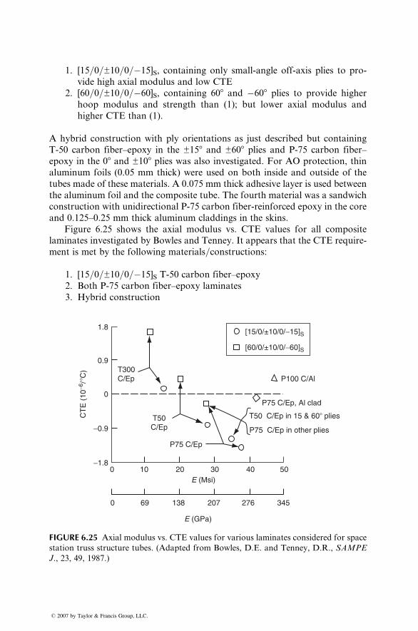
1. [15=0=±10=0=�15]S, containing only small-angle off-axis plies to pro-
vide high axial modulus and low CTE
2. [60=0=±10=0=�60]S, containing 608 and �608 plies to provide higher
hoop modulus and strength than (1); but lower axial modulus and
higher CTE than (1).
A hybrid construction with ply orientations as just described but containing
T-50 carbon fiber–epoxy in the ±158 and ±608 plies and P-75 carbon fiber–
epoxy in the 08 and ±108 plies was also investigated. For AO protection, thin
aluminum foils (0.05 mm thick) were used on both inside and outside of the
tubes made of these materials. A 0.075 mm thick adhesive layer is used between
the aluminum foil and the composite tube. The fourth material was a sandwich
construction with unidirectional P-75 carbon fiber-reinforced epoxy in the core
and 0.125–0.25 mm thick aluminum claddings in the skins.
Figure 6.25 shows the axial modulus vs. CTE values for all composite
laminates investigated by Bowles and Tenney. It appears that the CTE require-
ment is met by the following materials=constructions:
1. [15=0=±10=0=�15]S T-50 carbon fiber–epoxy
2. Both P-75 carbon fiber–epoxy laminates
3. Hybrid construction
CT
E (
10−6
/ �C
)
E (GPa)
E (Msi)
0.9
1.8
0
−1.80
0 13869 207 276 345
10 20 30 40 50
−0.9T50C/Ep
P75 C/Ep
T50 C/Ep in 15 & 60� plies
P75 C/Ep in other plies
P75 C/Ep, Al clad
P100 C/AlT300C/Ep
[15/0/±10/0/−15]S
[60/0/±10/0/−60]S
FIGURE 6.25 Axial modulus vs. CTE values for various laminates considered for space
station truss structure tubes. (Adapted from Bowles, D.E. and Tenney, D.R., SAMPE
J., 23, 49, 1987.)
� 2007 by Taylor & Francis Group, LLC.
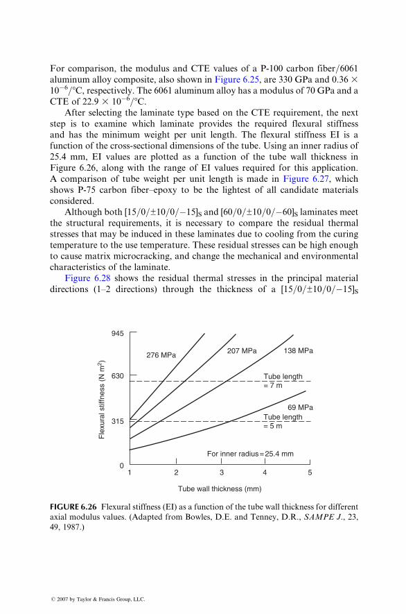
For co mparison, the modulus and CTE values of a P-100 carbo n fiber =6061alumin um a lloy composi te, also shown in Figure 6.25, are 330 GPa and 0.36 310 � 6=8C, respect ively. The 6061 aluminu m alloy has a modulus of 70 GPa and a
CTE of 22.9 3 10�6 =8 C.After selecting the lami nate type based on the CTE requir ement, the ne xt
step is to e xamine which lami nate provides the requir ed flex ural sti ffness
and has the mini mum wei ght per unit lengt h. The flex ural stiffne ss EI is a
functio n of the cross- sectional dimens ions of the tube. Usi ng an inner rad ius of
25.4 mm, EI values are plott ed as a functio n of the tub e wall thickne ss in
Figure 6.26, along with the range of EI values requir ed for this applic ation.
A compari son of tube weight per unit lengt h is made in Figure 6.27, whi ch
shows P-75 carbon fiber –epoxy to be the lightest of all cand idate mate rials
consider ed.
Altho ugh both [15 =0=±10=0=� 15]S and [60 =0=±10 =0=� 60]S lami nates meet
the structural requiremen ts, it is ne cessary to compare the residual therm al
stresses that may be indu ced in these laminates due to cooling from the cu ring
tempe rature to the us e tempe ratur e. Thes e residual stresses can be high enough
to ca use matr ix micr ocracki ng, and ch ange the mechani cal and environm ental
characteristics of the laminate.
Figure 6.28 shows the residual therm al stresses in the princi pal mate rial
directions (1–2 directions) through the thickness of a [15=0=±10=0=�15]S
Fle
xura
l stif
fnes
s (N
m2 )
945
630
315
0
Tube wall thickness (mm)
1 2 3 4 5
276 MPa
For inner radius = 25.4 mm
Tube length= 5 m
Tube length= 7 m
138 MPa
69 MPa
207 MPa
FIGURE 6.26 Flexural stiffness (EI) as a function of the tube wall thickness for different
axial modulus values. (Adapted from Bowles, D.E. and Tenney, D.R., SAMPE J., 23,
49, 1987.)
� 2007 by Taylor & Francis Group, LLC.
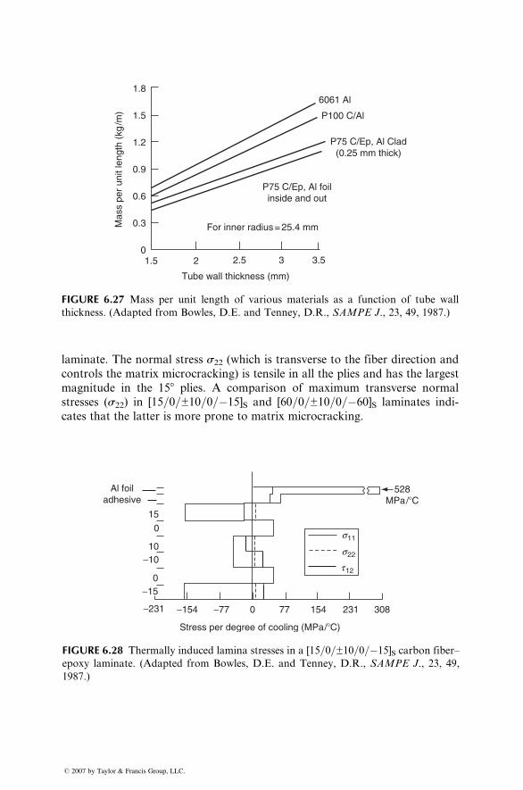
For inner radius = 25.4 mm
P75 C/Ep, Al foilinside and out
6061 Al
P100 C/Al
P75 C/Ep, Al Clad(0.25 mm thick)
Tube wall thickness (mm)
Mas
s pe
r un
it le
ngth
(kg
/m)
1.8
1.5
1.2
0.9
0.6
0.3
01.5 2 2.5 3 3.5
FIGURE 6.27 Mass per unit length of various materials as a function of tube wall
thickness. (Adapted from Bowles, D.E. and Tenney, D.R., SAMPE J., 23, 49, 1987.)
laminate. The normal stress s22 (which is transverse to the fiber direction and
controls the matrix microcracking) is tensile in all the plies and has the largest
magnitude in the 158 plies. A comparison of maximum transverse normal
stresses (s22) in [15=0=±10=0=�15]S and [60=0=±10=0=�60]S laminates indi-
cates that the latter is more prone to matrix microcracking.
0 77−77 154−154 231−231
−150
0
15
Al foiladhesive
Stress per degree of cooling (MPa /�C)
528MPa/�C
10−10
308
s11
s22
t 12
FIGURE 6.28 Thermally induced lamina stresses in a [15=0=±10=0=�15]S carbon fiber–
epoxy laminate. (Adapted from Bowles, D.E. and Tenney, D.R., SAMPE J., 23, 49,
1987.)
� 2007 by Taylor & Francis Group, LLC.
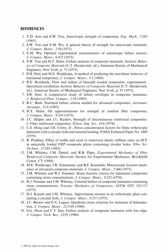
REFERENCES
1.
� 20
V.D. Azzi and S.W. Tsai, Anisotropic strength of composites, Exp. Mech., 5:283
(1965).
2.
S.W. Tsai and E.M. Wu, A general theory of strength for anisotropic materials,J. Compos. Mater., 5:58 (1971).
3.
E.M. Wu, Optimal experimental measurements of anisotropic failure tensors,J. Compos. Mater., 6:472 (1972).
4.
S.W. Tsai and H.T. Hahn, Failure analysis of composite materials, Inelastic Behav-ior of Composite Materials (C.T. Herakovich, ed.), American Society of Mechanical
Engineers, New York, p. 73 (1975).
5.
P.H. Petit and M.E. Waddoups, A method of predicting the non-linear behavior oflaminated composites, J. Compos. Mater., 3:2 (1969).
6.
R.E. Rowlands, Flow and failure of biaxially loaded composites: experimental–theoretical correlation, Inelastic Behavior of Composite Materials (C.T. Herakovich,
ed.), American Society of Mechanical Engineers, New York, p. 97 (1975).
7.
S.R. Soni, A comparative study of failure envelopes in composite laminates,J. Reinforced Plast. Compos., 2:34 (1983).
8.
R.C. Burk, Standard failure criteria needed for advanced composites, Astronaut.Aeronaut., 21:6 (1983).
9.
H.T. Hahn, On approximations for strength of random fiber composites,J. Compos. Mater., 9:316 (1975).
10.
J.C. Halpin and J.L. Kardos, Strength of discontinuous reinforced composites:I. Fiber reinforced composites, Polym. Eng. Sci., 18:6 (1978).
11.
C.S. Hong and J.H. Crews, Jr., Stress concentration factors for finite orthotropiclaminates with a circular hole and uniaxial loading, NASATechnical Paper No. 1469
(1979).
12.
B. Pradhan, Effect of width and axial to transverse elastic stiffness ratio on SCFin uniaxially loaded FRP composite plates containing circular holes, Fibre Sci.
Technol., 17:245 (1982).
13.
J.M. Whitney, I.M. Daniel, and R.B. Pipes, Experimental Mechanics of FiberReinforced Composite Materials, Society for Experimental Mechanics, Brookfield
Center, CT (1984).
14.
M.E. Waddoups, J.R. Eisenmann, and B.E. Kaminski, Macroscopic fracture mech-anics of advanced composite materials, J. Compos. Mater., 5:446 (1971).
15.
J.M. Whitney and R.J. Nuismer, Stress fracture criteria for laminated compositescontaining stress concentrations, J. Compos. Mater., 8:253 (1974).
16.
R.J. Nuismer and J.M. Whitney, Uniaxial failure of composite laminates containingstress concentrations, Fracture Mechanics of Composites, ASTM STP, 593:117
(1975).
17.
H.J. Konish and J.M. Whitney, Approximate stresses in an orthotropic plate con-taining a circular hole, J. Compos. Mater., 9:157 (1975).
18.
J.C. Brewer and P.A. Lagace, Quadratic stress criterion for initiation of delamina-tion, J. Compos. Mater., 22:1141 (1988).
19.
S.G. Zhou and C.T. Sun, Failure analysis of composite laminates with free edge,J. Compos. Tech. Res., 12:91 (1990).
07 by Taylor & Francis Group, LLC.
20.
� 20
H. Kulkarni and P. Beardmore, Design methodology for automotive components
using continuous fibre-reinforced composite materials, Composites, 11:225 (1980).
21.
J.C. Ekvall and C.F. Griffin, Design allowables for T300=5208 graphite=epoxycomposite materials, J. Aircraft, 19:661 (1982).22.
M.J. Rich and D.P. Maass, Developing design allowables for composite helicopterstructures, Test Methods and Design Allowables for Fibrous Composites, ASTM
STP, 734:181 (1981).
23.
C.T. Herakovich, Influence of layer thickness on the strength of angle-ply laminates,J. Compos. Mater., 16:216 (1982).
24.
S.L. Donaldson, Simplified weight saving techniques for composite panels,J. Reinforced Plast. Compos., 2:140 (1983).
25.
T.N. Massard, Computer sizing of composite laminates for strength, J. ReinforcedPlast. Compos., 3:300 (1984).
26.
W.J. Park, An optimal design of simple symmetric laminates under first ply failurecriterion, J. Compos. Mater., 16:341 (1982).
27.
J.M. Whitney and A.W. Leissa, Analysis of heterogeneous anisotropic plates,J. Appl. Mech., 36:261 (1969).
28.
J.M. Whitney, Bending–extensional coupling in laminated plates under transverseloading, J. Compos. Mater., 3:20 (1969).
29.
R.M. Jones, H.S. Morgan, and J.M. Whitney, Buckling and vibration of anti-symmetrically laminated angle-ply rectangular plates, J. Appl.Mech., 40:1143 (1973).
30.
O.H. Griffin, Evaluation of finite-element software packages for stress analysis oflaminated composites, Compos. Technol. Rev., 4:136 (1982).
31.
J.R. Eisenmann and J.L. Leonhardt, Improving composite bolted joint efficiency bylaminate tailoring, Joining of Composite Materials, ASTM STP, 749:117 (1979).
32.
L.J. Hart-Smith, Designing to minimize peel stresses in adhesive-bonded joints,Delamination and Debonding of Materials, ASTM STP, 876:238 (1985).
33.
D.P. Maass, Tubular composite compression members—design considerations andpractices, Proceedings 41st Annual Conference, Society of the Plastics Industry,
January (1986).
34.
J.M. Whitney, C.E. Browning, and A. Mair, Analysis of the flexural test forlaminated composite materials, Composite Materials: Testing and Design (Third
Conference), ASTM STP, 546:30 (1974).
35.
J.M. Whitney and J.C. Halpin, Analysis of laminated anisotropic tubes undercombined loading, J. Compos. Mater., 2:360 (1968).
36.
G.J. Simitses, Instability of orthotropic cylindrical shells under combined torsionand hydrostatic pressure, AIAA J., 5:1463 (1967).
37.
C.F. Griffin, Design development of an advanced composite aileron, Paper No. 79-1807, AIAA Aircraft Systems and Technology Meeting, August (1979).
38.
E.E. Morris, W.P. Patterson, R.E. Landes, and R. Gordon, Composite pressurevessels for aerospace and commercial applications, Composites in Pressure Vessels
and Piping (S.V. Kulkarni and C.H. Zweben, eds.), American Society of Mechanical
Engineers, New York, PVP-PB-021 (1977).
39.
B.E. Kirkham, L.S. Sullivan, and R.E. Bauerie, Development of the Liteflex sus-pension leaf spring, Society of Automotive Engineers, Paper No. 820160 (1982).
40.
D.E. Bowles and D.R. Tenney, Composite tubes for the space station truss struc-ture, SAMPE J., 23:49 (1987).
07 by Taylor & Francis Group, LLC.
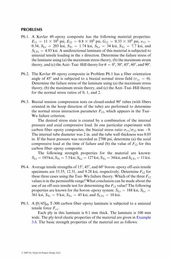
PROBLEMS
P6.1. A Kevlar 49–epo xy co mposite has the foll owing mate rial propert ies:
E11 ¼ 11 3 10 6 psi, E 22 ¼ 0.8 3 10 6 psi, G 12 ¼ 0.33 3 10 6 psi, n12 ¼0.34, SLt ¼ 203 ksi, STt ¼ 1.74 ksi, SLc ¼ 34 ksi, STc ¼ 7.7 ksi, and
SLTs ¼ 4.93 ksi. A unidir ectional laminate of this mate rial is subject ed to
uniaxi al tensi le loading in the x direction . Determi ne the fail ure stress of
the lami nate using (a) the maxi mum stre ss theory, (b) the maxi mum stra in
theory, a nd (c) the Azzi –Tsai–H ill theory for u ¼ 08, 308 , 458 , 608 , and 90 8 .
P6.2. The Kevl ar 49–epoxy composi te in Problem P6.1 has a fiber orient ation
angle of 45 8 and is subject ed to a biaxi al normal stre ss field ( txy ¼ 0).
Dete rmine the fail ure stre ss of the laminate using (a) the maxi mum stre ss
theory, (b) the maxi mum stra in theory, and (c) the Azzi –Tsai–H ill theo ry
for the nor mal stress ratios of 0, 1, an d 2.
P6.3. Biaxia l tensi on–compres sion tests on closed- ended 90 8 tubes (with fiber sorient ed in the hoop direction of the tube) are perfor med to determine
the normal stre ss interacti on parame ter F12 , whi ch appears in the Ts ai–
Wu failu re crite rion.
The desir ed stre ss state is creat ed by a co mbination of the intern al
pressur e and a xial co mpres sive load. In one pa rticular experi ment with
carbo n fiber–ep oxy comp osites, the biaxi al stress ratio s11 =s22 was � 9.
The interna l tube diame ter was 2 in. and the tube wal l thickne ss was 0.05
in. If the burst pressur e was record ed as 2700 psi, determine (a) the axial
comp ressive load at the time of failure and (b) the value of F12 for this
carbo n fiber –epoxy compo site.
The foll owing streng th propert ies for the material are known :
SLt ¼ 1 85 ksi, STt ¼ 7.5 ksi, SLc ¼ 127 ksi, S Tc ¼ 34 ksi, and S LTs ¼ 11 ksi.
P6.4. Aver age tensile strengths of 1 5 8, 458, and 60 8 boron–ep oxy off-axis tensi lespecim ens are 33.55, 12.31, and 9.28 ksi, respectivel y. Determi ne F12 for
these three cases using the Ts ai–Wu failure theory. Which of the three F12
values is in the permissi ble range? Wh at conclusi on can be mad e about the
use of an off-axis tensile test for determining the F12 value? The following
properties are known for the boron–epoxy system: SLt ¼ 188 ksi, SLc ¼361 ksi, STt ¼ 9 ksi, STc ¼ 45 ksi, and SLTs ¼ 10 ksi.
P6.5. A [0=45]8S T-300 carbon fiber–epoxy laminate is subjected to a uniaxial
tensile force Fxx.
� 2007 by
Each ply in this laminate is 0.1 mm thick. The laminate is 100 mm
wid e. The ply-level elastic prope rties of the mate rial are given in Exa mple
3.6. The basic stre ngth pr operties of the mate rial are as follows :
Taylor & Francis Group, LLC.
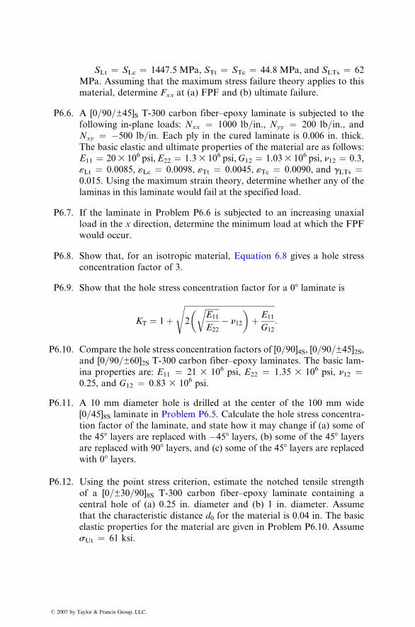
� 2007 b
SLt ¼ SLc ¼ 1447.5 MPa , STt ¼ S Tc ¼ 44.8 MPa, and SLTs ¼ 62
MPa . Ass uming that the maxi mum stress failu re theory applie s to this
mate rial, determ ine Fxx at (a) FPF and (b) ultimat e failure.
P6.6. A [0 =90 =±45]S T-300 c arbon fiber –epoxy laminate is subject ed to the
followi ng in-pl ane loads: Nxx ¼ 1000 lb =in., Nyy ¼ 200 lb=in., andNxy ¼ �500 lb =in. Each ply in the cu red lamin ate is 0.006 in. thick.
The basic elastic an d ultimat e pr operties of the mate rial are as follows :
E11 ¼ 20 3 10 6 ps i, E 22 ¼ 1.3 3 106 psi, G 12 ¼ 1.03 3 106 psi, n 12 ¼ 0.3,
«Lt ¼ 0.0085 , «Lc ¼ 0.0098 , «Tt ¼ 0.0045 , «Tc ¼ 0.0090 , and gLTs ¼0.015. Using the maximum strain theory, determ ine wheth er any of the
laminas in this lami nate would fail at the specified load.
P6.7. If the lami nate in Problem P6.6 is subjected to a n increa sing una xial
load in the x direction, determine the minimum load at which the FPF
would occur.
P6.8. Show that, for an isot ropic mate rial, Equation 6.8 gives a hole stre ss
concentration factor of 3.
P6.9. Show that the hole stress concentration factor for a 08 laminate is
KT ¼ 1þffiffiffiffiffiffiffiffiffiffiffiffiffiffiffiffiffiffiffiffiffiffiffiffiffiffiffiffiffiffiffiffiffiffiffiffiffiffiffiffiffiffiffiffiffiffi2
ffiffiffiffiffiffiffiE11
E22
r� n12
� �þ E11
G12
s:
P6.10. Compare the hole stress concentration factors of [0=90]4S, [0=90=±45]2S,and [0=90=±60]2S T-300 carbon fiber–epoxy laminates. The basic lam-
ina properties are: E11 ¼ 21 3 106 psi, E22 ¼ 1.35 3 106 psi, n12 ¼0.25, and G12 ¼ 0.83 3 106 psi.
P6.11. A 10 mm diameter hole is drilled at the center of the 100 mm wide
[0=45]8S laminate in Problem P6.5. Calculate the hole stress concentra-
tion factor of the laminate, and state how it may change if (a) some of
the 458 layers are replaced with �458 layers, (b) some of the 458 layersare replaced with 908 layers, and (c) some of the 458 layers are replacedwith 08 layers.
P6.12. Using the point stress criterion, estimate the notched tensile strength
of a [0=±30=90]8S T-300 carbon fiber–epoxy laminate containing a
central hole of (a) 0.25 in. diameter and (b) 1 in. diameter. Assume
that the characteristic distance d0 for the material is 0.04 in. The basic
elastic properties for the material are given in Problem P6.10. Assume
sUt ¼ 61 ksi.
y Taylor & Francis Group, LLC.
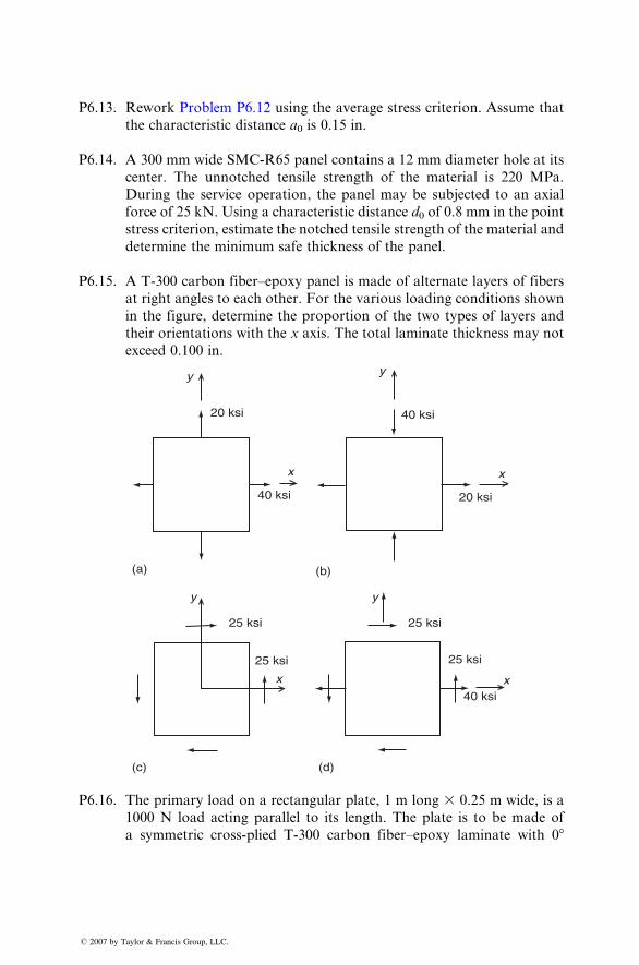
P6.13. Rew ork Problem P6.12 using the average stress criteri on. Ass ume that
the characteristic distance a0 is 0.15 in.
P6.14. A 300 mm wide SMC-R65 panel contains a 12 mm diameter hole at its
center. The unnotched tensile strength of the material is 220 MPa.
During the service operation, the panel may be subjected to an axial
force of 25 kN. Using a characteristic distance d0 of 0.8 mm in the point
stress criterion, estimate the notched tensile strength of the material and
determine the minimum safe thickness of the panel.
P6.15. A T-300 carbon fiber–epoxy panel is made of alternate layers of fibers
at right angles to each other. For the various loading conditions shown
in the figure, determine the proportion of the two types of layers and
their orientations with the x axis. The total laminate thickness may not
exceed 0.100 in.
(a) (b)
(d)(c)
y y
yy
x
x x
x
20 ksi 40 ksi
40 ksi 20 ksi
25 ksi
25 ksi
25 ksi
40 ksi
25 ksi
P6.16. The primary load on a rectangular plate, 1 m long 3 0.25 m wide, is a
1000 N load acting parallel to its length. The plate is to be made of
a symmetric cross-plied T-300 carbon fiber–epoxy laminate with 08
� 2007 by Taylor & Francis Group, LLC.
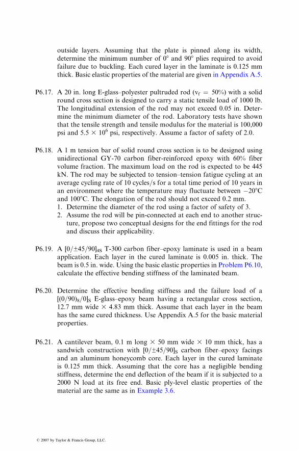
outsi de layers. Assu ming that the plate is pin ned along its width,
determ ine the minimu m numb er of 0 8 and 90 8 plies requir ed to avoidfailure due to buckling. Eac h c ured layer in the laminate is 0.125 mm
thick. Bas ic elast ic prop erties of the mate rial are given in Append ix A.5 .
P6.17. A 20 in. long E-g lass–polyes ter pultr uded rod (vf ¼ 50%) with a solid
roun d cross section is designe d to carry a static tensi le load of 1000 lb.
The longitud inal extens ion of the rod may not exceed 0.05 in. Dete r-
mine the mini mum diameter of the rod. Labor atory tests have shown
that the tensile strength an d tensile modu lus for the mate rial is 100 ,000
psi and 5.5 3 10 6 psi, respectivel y. Ass ume a fact or of safety of 2.0.
P6.18. A 1 m tensi on bar of solid round cross sectio n is to be de signed using
unidir ectio nal GY- 70 c arbon fiber-re infor ced epoxy with 60% fiber
volume fraction. The maximum load on the rod is expecte d to be 445
kN. The rod may be subjected to tensi on–tensio n fatigu e cyclin g at an
average cyclin g rate of 10 cycles =s for a total time period of 10 years in
an environm en t wher e the tempe ratur e may fluctuate between � 20 8 Cand 100 8 C. The elonga tion of the rod sho uld not exceed 0.2 mm.
� 2007 by
1. Dete rmin e the diame ter of the rod using a factor of safety of 3.
2. Ass ume the rod will be pin -connect ed at each end to another struc -
ture, propo se two c onceptual designs for the en d fitti ngs for the rod
and discus s their applic ability.
P6.19. A [0 =±45 =90]4S T-300 carbon fiber– epoxy laminate is used in a beam
app lication. Eac h layer in the cured laminate is 0.005 in. thick. The
beam is 0.5 in. wide. Usi ng the basic elastic pr operties in Problem P6. 10,
calculate the effective bending stiffness of the laminated beam.
P6.20. Determine the effective bending stiffness and the failure load of a
[(0=90)8=0]S E-glass–epoxy beam having a rectangular cross section,
12.7 mm wide 3 4.83 mm thick. Assume that each layer in the beam
has the same cured thickness. Use Appendix A.5 for the basic material
properties.
P6.21. A cantilever beam, 0.1 m long 3 50 mm wide 3 10 mm thick, has a
sandwich construction with [0=±45=90]S carbon fiber–epoxy facings
and an aluminum honeycomb core. Each layer in the cured laminate
is 0.125 mm thick. Assuming that the core has a negligible bending
stiffness, determine the end deflection of the beam if it is subjected to a
2000 N load at its free end. Basic ply-level elastic properties of the
material are the same as in Example 3.6.
Taylor & Francis Group, LLC.
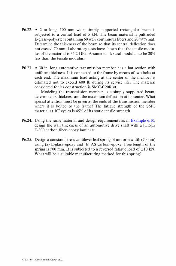
P6.22. A 2 m long, 100 mm wide, simply supported rectangular beam is
subjected to a central load of 5 kN. The beam material is pultruded
E-glass–polyester containing 60 wt% continuous fibers and 20 wt% mat.
Determine the thickness of the beam so that its central deflection does
not exceed 70 mm. Laboratory tests have shown that the tensile modu-
lus of the material is 35.2 GPa. Assume its flexural modulus to be 20%
less than the tensile modulus.
P6.23. A 30 in. long automotive transmission member has a hat section with
uniform thickness. It is connected to the frame by means of two bolts at
each end. The maximum load acting at the center of the member is
estimated not to exceed 600 lb during its service life. The material
considered for its construction is SMC-C20R30.
� 2007 by T
Modeling the transmission member as a simply supported beam,
determine its thickness and the maximum deflection at its center. What
special attention must be given at the ends of the transmission member
where it is bolted to the frame? The fatigue strength of the SMC
material at 106 cycles is 45% of its static tensile strength.
P6.24. Usi ng the same mate rial and design requir ements as in Example 6.10,
design the wall thickness of an automotive drive shaft with a [±15]nST-300 carbon fiber–epoxy laminate.
P6.25. Design a constant stress cantilever leaf spring of uniform width (70 mm)
using (a) E-glass–epoxy and (b) AS carbon–epoxy. Free length of the
spring is 500 mm. It is subjected to a reversed fatigue load of ±10 kN.
What will be a suitable manufacturing method for this spring?
aylor & Francis Group, LLC.
7 Metal, Ceramic, andCarbon Matrix
� 2007 by Taylor & Fr
Composites
In the earlier chapters of this book, we considered the performance, manufac-
turing, and design issues pertaining to polymer matrix composites. In this
chapter, we review the thermomechanical properties of metal, ceramic, and
carbon matrix composites and a few important manufacturing methods used in
producing such composites.
The history of development of metal, ceramic, and carbon matrix compos-
ites is much more recent than that of the polymer matrix composites. Initial
research on the metal and ceramic matrix composites was based on continuous
carbon or boron fibers, but there were difficulties in producing good quality
composites due to adverse chemical reaction between these fibers and the
matrix. With the development of newer fibers, such as silicon carbide or
aluminum oxide, in the early 1980s, there has been a renewed interest and an
accelerated research activity in developing the technology of both metal and
ceramic matrix composites. The initial impetus for this development has come
from the military and aerospace industries, where there is a great need for
materials with high strength-to-weight ratios or high modulus-to-weight ratios
that can also withstand severe high temperature or corrosive environments.
Presently, these materials are very expensive and their use is limited to appli-
cations that can use their special characteristics, such as high temperature
resistance or high wear resistance. With developments of lower cost fibers
and more cost-effective manufacturing techniques, it is conceivable that both
metal and ceramic matrix composites will find commercial applications in
automobiles, electronic packages, sporting goods, and others.
The carbon matrix composites are more commonly known as carbon–
carbon composites, since they use carbon fibers as the reinforcement for carbon
matrix. The resulting composite has a lower density, higher modulus and
strength, lower coefficient of thermal expansion, and higher thermal shock
resistance than conventional graphite. The carbon matrix composites have
been used as thermal protection materials in the nose cap and the leading
edges of the wing of space shuttles. They are also used in rocket nozzles, exit
cones, and aircraft brakes, and their potential applications include pistons in
ancis Group, LLC.
intern al combust ion engines , gas turbine compone nts, he at exchangers , and
biomedi cal impl ants.
7.1 METAL MATRIX COMPOSITES
The metal matrix composites (MMC) can be divided into four general categories:
1. Fiber- reinfo rced MMC con taining eithe r con tinuous or discont inuou s
fiber reinf orcement s; the latt er are in the form of whiskers with a pproxi-
mate ly 0.1� 0.5 mm in diameter and have a length-to- diame ter rati o up
to 200.
2. Parti culate-rei nforced MMC con taining either particles or plate lets that
range in size from 0.5 to 100 mm. The particu lates can be incorpo rated
into the meta l matr ix to higher volume fract ions than the whiskers.
3. Dis persion -strengt hened MM C contai ning particles that are < 0.1 m m in
diame ter.
4. In situ MM C, su ch a s direct ionally solidifi ed e utectic alloys.
In this cha pter, we focu s our atte ntion on the fir st two categories, more
specifical ly on whi sker- and particulat e-reinforc ed M MCs. Mo re de tailed infor -
mation s on M MC can be found in Refs. [1–4].
Cont inuous carbon or bor on fiber-re inforc ed MMCs ha ve be en under
developm ent for > 20 years; howev er, they have found limit ed use due to
problem s in control ling the c hemical react ion betwee n the fibers and the molten
meta l at the high pro cessing tempe ratures used for such composi tes. The resul t
of this ch emical react ion is a brittle interph ase that redu ces the mechani cal
propert ies of the composi te. Fiber surfa ce treat ments developed to reduce this
problem increa se the cost of the fiber. Addit ionally, the manufa cturin g cost of
continuou s carbon or boron fiber -reinforce d MMC is also high , whi ch make s
them less attr active for many app lications . Much of the recen t work on M MC
is based on sil icon ca rbide whi skers (SiCw ) or sil icon carb ide parti culates
(SiCp ). SiC is less prone to oxidat ive react ions at the process ing tempe ratures
used. Fur therm ore, not only they are less ex pensive than carbon or boron
fibers, but also they can be incorpora ted into meta l matr ices using common
manufa cturin g techn iques, such as powder meta llurgy and casti ng.
7.1.1 MECHANICAL PROPERTIES
In Chapter 2, we discus sed sim ple micromechan ical models in relation to
polyme r matr ix comp osites in which fiber s carry the major por tion of the
composi te load by virt ue of their high modu lus compared with the pol ymer
matrix, such as epo xy. The same micr omechani cal models can be ap plied to
MMC with so me modif ications. The modulus of meta ls is a n ord er of magni -
tude higher than that of polyme rs (Table 7.1) . Many meta ls are capab le of
� 2007 by Taylor & Francis Group, LLC.
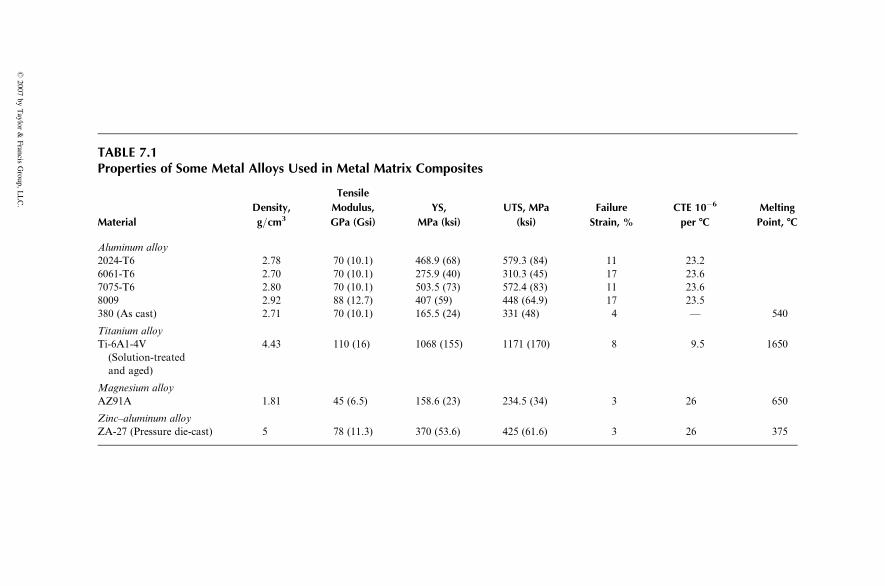
TABLE 7.1Properties of Some Metal Alloys Used in Metal Matrix Composites
Material
Density,
g=cm3
Tensile
Modulus,
GPa (Gsi)
YS,
MPa (ksi)
UTS, MPa
(ksi)
Failure
Strain, %
CTE 10�6
per 8C
Melting
Point, 8C
Aluminum alloy
2024-T6 2.78 70 (10.1) 468.9 (68) 579.3 (84) 11 23.2
6061-T6 2.70 70 (10.1) 275.9 (40) 310.3 (45) 17 23.6
7075-T6 2.80 70 (10.1) 503.5 (73) 572.4 (83) 11 23.6
8009 2.92 88 (12.7) 407 (59) 448 (64.9) 17 23.5
380 (As cast) 2.71 70 (10.1) 165.5 (24) 331 (48) 4 — 540
Titanium alloy
Ti-6A1-4V
(Solution-treated
and aged)
4.43 110 (16) 1068 (155) 1171 (170) 8 9.5 1650
Magnesium alloy
AZ91A 1.81 45 (6.5) 158.6 (23) 234.5 (34) 3 26 650
Zinc–aluminum alloy
ZA-27 (Pressure die-cast) 5 78 (11.3) 370 (53.6) 425 (61.6) 3 26 375
�2007
byTaylor
&Francis
Group,
LLC.
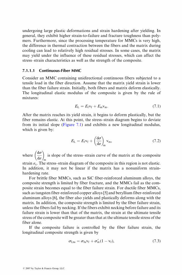
undergoing large plastic deformations and strain hardening after yielding. In
general, they exhibit higher strain-to-failure and fracture toughness than poly-
mers. Furthermore, since the processing temperature for MMCs is very high,
the difference in thermal contraction between the fibers and the matrix during
cooling can lead to relatively high residual stresses. In some cases, the matrix
may yield under the influence of these residual stresses, which can affect the
stress–strain characteristics as well as the strength of the composite.
7.1.1.1 Continuous-Fiber MMC
Consider an MMC containing unidirectional continuous fibers subjected to a
tensile load in the fiber direction. Assume that the matrix yield strain is lower
than the fiber failure strain. Initially, both fibers and matrix deform elastically.
The longitudinal elastic modulus of the composite is given by the rule of
mixtures:
EL ¼ Efvf þ Emvm: (7:1)
After the matrix reaches its yield strain, it begins to deform plastically, but the
fiber remains elastic. At this point, the stress–strain diagram begins to deviate
from its initial slope (Figur e 7.1) an d exh ibits a new longit udinal mo dulus,
which is given by:
EL ¼ Efvf þ ds
d«
� �m
vm, (7:2)
whereds
d«
� �m
is slope of the stress–strain curve of the matrix at the composite
strain «c. The stress–strain diagram of the composite in this region is not elastic.
In addition, it may not be linear if the matrix has a nonuniform strain-
hardening rate.
For brittle fiber MMCs, such as SiC fiber-reinforced aluminum alloys, the
composite strength is limited by fiber fracture, and the MMCs fail as the com-
posite strain becomes equal to the fiber failure strain. For ductile fiber MMCs,
such as tungsten fiber-reinforced copper alloys [5] and beryllium fiber-reinforced
aluminum alloys [6], the fiber also yields and plastically deforms along with the
matrix. In addition, the composite strength is limited by the fiber failure strain,
unless the fibers fail by necking. If the fibers exhibit necking before failure and its
failure strain is lower than that of the matrix, the strain at the ultimate tensile
stress of the composite will be greater than that at the ultimate tensile stress of the
fiber alone.
If the composite failure is controlled by the fiber failure strain, the
longitudinal composite strength is given by
sLtu ¼ sfuvf þ sm0 (1� vf), (7:3)
� 2007 by Taylor & Francis Group, LLC.
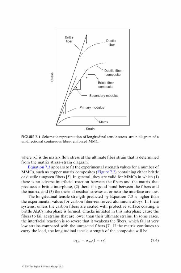
Brittlefiber Ductile
fiber
Ductile fibercomposite
Brittle fibercomposite
Secondary modulus
Primary modulus
Matrix
Strain
Str
ess
FIGURE 7.1 Schematic representation of longitudinal tensile stress–strain diagram of a
unidirectional continuous fiber-reinforced MMC.
where sm0 is the matrix flow stress at the ultimat e fiber strain that is de termined
from the matrix stress–s train diagra m.
Equation 7.3 appea rs to fit the exp erimental strength values for a numb er of
MMCs , such as copp er matrix composi tes (Figur e 7.2) contai ning e ither br ittle
or duc tile tungst en fibers [5]. In general , they are valid for MMCs in which (1)
there is no adverse interfaci al reaction betwe en the fibers and the matrix that
produc es a brittle inter phase, (2) there is a go od bond betwe en the fibers and
the matr ix, an d (3) the therm al resi dual stre sses at or ne ar the inter face are low .
The longit udinal tensi le stre ngth pred icted by Equation 7.3 is high er than
the experi menta l values for carbon fiber-re infor ced alumi num a lloys. In these
systems, unless the carbon fiber s are coated with pro tective surface coating, a
brittle Al4C3 inter phase is formed. Cra cks initiated in this interphase cau se the
fibers to fail at stra ins that are lower than their ultimate stra ins. In some cases,
the inter facial react ion is so severe that it weake ns the fiber s, which fail at very
low strains compared with the unr eacted fiber s [7]. If the matrix continues to
carry the load, the longit udinal tensi le strength of the composi te wi ll be
s Ltu ¼ smu(1� vf), (7:4)
� 2007 by Taylor & Francis Group, LLC.
1200
1000
800
600
Long
itudi
nal t
ensi
le s
tren
gth
(MP
a)
400
200
00 0.5
Fiber volume fraction, vf
1.0
Equation 7.4
Equation 7.3
FIGURE 7.2 Longitudinal tensile strength variation of a unidirectional continuous
tungsten fiber=copper matrix composite at various fiber volume fractions. (Adapted
from Kelly, A. and Davies, G.J., Metall. Rev., 10, 1, 1965.)
which is less than the matr ix tensi le stre ngth smu . Thus , in this case, the
matrix is weake ne d in the presen ce of fiber s instead of getting stre ngthened
(Figur e 7.3).
7.1.1 .2 Disco ntinuous ly Reinfor ced MMC
In recent years, the majorit y of the resear ch effort has been on SiCw - and SiC p -
reinfo rced alumin um alloys [8]. Titaniu m, magnes ium, and z inc alloys have also
been used ; howeve r, they are not discus sed in this chapter . Rei nforcem ents
other than SiC , such as Al2O 3, ha ve also been invest igated. Tensil e propert ies of
some of these composi tes are given in Append ix A.9 .
McDane ls [9] has report ed the mechani cal propert ies of both SiCw- and
SiCp -rein forced alumi num alloys, such as 606 1, 2024 =2124, 7075, and 5083.Rein forcement content is in the range of 10–40 v ol%. These composi tes were
produ ced by powder metallur gy, follo wed by extrusion and hot roll ing. His
observat ions are summ arize d as follo ws:
� 2007 by Taylor & Francis Group, LLC.
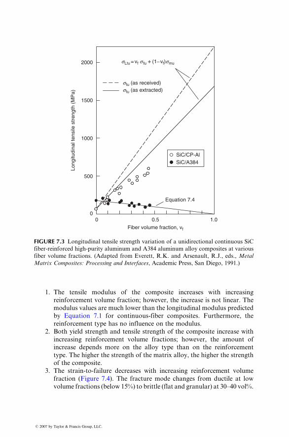
2000
1500
1000
Long
itudi
nal t
ensi
le s
tren
gth
(MP
a)
500
00 0.5
Fiber volume fraction, vf
Equation 7.4
1.0
SiC/CP-AlSiC/A384
sLtu = vf s fu + (1−vf)smu
sfu (as received)sfu (as extracted)
FIGURE 7.3 Longitudinal tensile strength variation of a unidirectional continuous SiC
fiber-reinforced high-purity aluminum and A384 aluminum alloy composites at various
fiber volume fractions. (Adapted from Everett, R.K. and Arsenault, R.J., eds., Metal
Matrix Composites: Processing and Interfaces, Academic Press, San Diego, 1991.)
1. The tensile modulus of the compo site increa ses wi th increasing
reinfo rceme nt vo lume fract ion; howeve r, the increa se is not linea r. The
modulus values are much lower than the longitudinal modulus pred icted
by Equat ion 7.1 for continuous -fibe r comp osites. Fur therm ore, the
reinfo rceme nt type has no influence on the modulus.
2. Both yield stre ngth and tensi le strength of the composi te increa se with
increa sing reinforcem ent volume fract ions; howeve r, the amoun t of
increa se depends more on the alloy type than on the reinforcem ent
type. The higher the stre ngth of the matr ix alloy, the higher the strength
of the comp osite.
3. The stra in-to-f ailure decreas es with increa sing reinfo rcement volume
fraction (Figur e 7.4). The fract ure mode changes from ductile at low
volume fractions (below 15%) to brit tle (flat and granu lar) at 30–40 vol%.
� 2007 by Taylor & Francis Group, LLC.
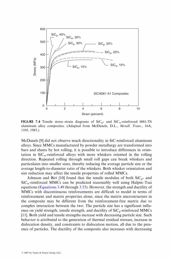
SiCp, 40%SiCw, 30%
SiCp, 30% SiCp, 20%
SiCw, 20%
SiCw, 10%SiCp, 15%
SiC/6061 A1 Composites
1086
Strain (percent)
4200
100
200
Str
ess
(MP
a)
300
400
500
600
FIGURE 7.4 Tensile stress–strain diagrams of SiCp- and SiCw-reinforced 6061-T6
aluminum alloy composites. (Adapted from McDanels, D.L., Metall. Trans., 16A,
1105, 1985.)
McDanel s [9] did not obs erve much direct ionality in SiC -reinforce d aluminu m
alloy s. Since MM Cs manufa ctured by powder meta llurgy are trans formed into
bars an d sh eets by hot roll ing, it is possibl e to introd uce diff erences in orien-
tation in SiCw -rein forced a lloys with more whiskers oriented in the rolling
direction . Repeated roll ing through smal l roll gaps ca n break whi skers and
particu lates into smaller sizes, thereby reducing the average particle size or the
average length-to- diameter ratio of the whiskers. Both whisk er orient ation and
size redu ction may affect the tensi le prop erties of roll ed MMCs.
Joh nson and Birt [10] found that the tensi le mod ulus of both SiCp- and
SiCw-reinforced MMCs can be predicted reasonably well using Halpin–Tsai
equati ons (Equati ons 3.49 through 3.53). Ho wever, the stren gth and ductil ity of
MMCs with discontinuous reinforcements are difficult to model in terms of
reinforcement and matrix properties alone, since the matrix microstructure in
the composite may be different from the reinforcement-free matrix due to
complex interaction between the two. The particle size has a significant influ-
ence on yield strength, tensile strength, and ductility of SiCp-reinforced MMCs
[11]. Both yield and tensile strengths increase with decreasing particle size. Such
behavior is attributed to the generation of thermal residual stresses, increase in
dislocation density, and constraints to dislocation motion, all due to the pres-
ence of particles. The ductility of the composite also increases with decreasing
� 2007 by Taylor & Francis Group, LLC.
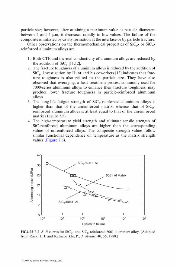
particle size; howeve r, after atta ining a maxi mum value at particle diame ters
between 2 and 4 m m, it de creases rapidly to low values. The fail ure of the
composi te is init iated by cavity form ation at the interface or by particle fract ure.
Othe r observat ions on the therm omechani cal pro perties of SiCp- or SiC w -
reinforced alumi num alloys are
1. Both CTE and therm al con ductiv ity of aluminu m alloys are reduced by
the addition of SiCp [11,12].
2. The fracture toughness of aluminum alloys is red uced by the add ition of
SiCp . Investigat ion by Hunt and his cowor kers [13] ind icates that frac-
ture toughness is also relat ed to the particle size. They have also
observed that overagi ng, a heat treatment pro cess commonl y used for
7000-s eries alumi num alloys to enhan ce their fractu re toug hness, may
produ ce lower fract ure toughn ess in particle-rei nforced alumi num
alloy s.
3. The long-lif e fatigu e stren gth of SiCw -reinforce d alumi num alloys is
higher than that of the unreinf orced matr ix, whereas that of SiCp-
reinfo rced alumin um alloy s is at least equal to that of the unreinf orced
matrix (Figur e 7 .5).
4. The high -temperat ure yield stre ngth and ultimat e tensile stren gth of
SiC-reinforced aluminum alloys are higher than the corresponding
values of unreinforced alloys. The composite strength values follow
similar functional dependence on temperature as the matrix strength
values (Figure 7.6) .
42
35
Alte
rnat
ing
stre
ss (
MP
a)
28
21
14
7
0103 104 105 106
Cycles to failure
SiCw /6061–Al
6061 Al Matrix
SiCp /6061–Al
107 108
FIGURE 7.5 S–N curves for SiCw- and SiCp-reinforced 6061 aluminum alloy. (Adapted
from Rack, H.J. and Ratnaparkhi, P., J. Metals, 40, 55, 1988.)
� 2007 by Taylor & Francis Group, LLC.
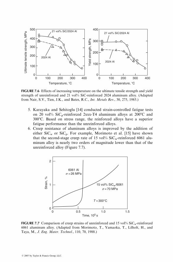
2024 Al
2024 Al
21 vol% SiC/2024 Al21 vol% SiC/2024 Al
500
400
Ulti
mat
e te
nsile
str
engt
h, M
Pa
Yie
ld s
tren
gth,
MP
a
300
200
100
0
400
300
200
100
00 100 200
Temperature, �C
300 400 0 100 200
Temperature, �C
300 400
FIGURE 7.6 Effects of increasing temperature on the ultimate tensile strength and yield
strength of unreinforced and 21 vol% SiC-reinforced 2024 aluminum alloy. (Adapted
from Nair, S.V., Tien, J.K., and Bates, R.C., Int. Metals Rev., 30, 275, 1985.)
5. Karayaka and Sehitoglu [14] conducted strain-controlled fatigue tests
on 20 vol% SiCp-reinforced 2xxx-T4 aluminum alloys at 2008C and
3008C. Based on stress range, the reinforced alloys have a superior
fatigue performance than the unreinforced alloys.
6. Creep resistance of aluminum alloys is improved by the addition of
either SiCw or SiCp. For example, Morimoto et al. [15] have shown
that the second-stage creep rate of 15 vol% SiCw-reinforced 6061 alu-
minum alloy is nearly two orders of magnitude lower than that of the
unreinforced alloy (Figure 7.7).
00
1
Str
ain,
%
2
0.5Time, 105 s
1.0 1.5
6061 Als = 26 MPa
15 vol% SiCw /6061
s = 70 MPa
T = 300°C
FIGURE 7.7 Comparison of creep strains of unreinforced and 15 vol% SiCw-reinforced
6061 aluminum alloy. (Adapted from Morimoto, T., Yamaoka, T., Lilholt, H., and
Taya, M., J. Eng. Mater. Technol., 110, 70, 1988.)
� 2007 by Taylor & Francis Group, LLC.
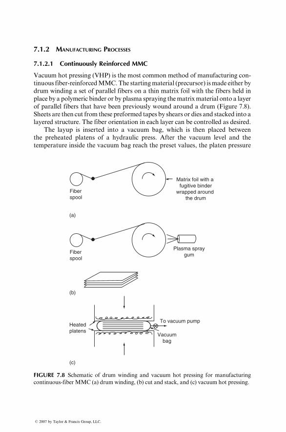
7.1.2 MANUFACTURING PROCESSES
7.1.2.1 Continuously Reinforced MMC
Vacuum hot pressing (VHP) is the most common method of manufacturing con-
tinuous fiber-reinforcedMMC.The startingmaterial (precursor) ismade either by
drum winding a set of parallel fibers on a thin matrix foil with the fibers held in
place by a polymeric binder or by plasma spraying thematrixmaterial onto a layer
of parallel fibers that have been previously wound around a drum (Figure 7.8).
Sheets are then cut from these preformed tapes by shears or dies and stacked into a
layered structure. The fiber orientation in each layer can be controlled as desired.
The layup is inserted into a vacuum bag, which is then placed between
the preheated platens of a hydraulic press. After the vacuum level and the
temperature inside the vacuum bag reach the preset values, the platen pressure
Fiberspool
Fiberspool
Plasma spraygum
Matrix foil with a fugitive binder
wrapped around the drum
Heatedplatens
To vacuum pump
Vacuumbag
(a)
(b)
(c)
FIGURE 7.8 Schematic of drum winding and vacuum hot pressing for manufacturing
continuous-fiber MMC (a) drum winding, (b) cut and stack, and (c) vacuum hot pressing.
� 2007 by Taylor & Francis Group, LLC.
is raised and held for a lengt h of time to complete the con solidati on of layer s
into the final thickne ss. Typical ly, the tempe ratur e is 50%–90 % of the solidu s
tempe rature of the matrix, and the pressur e ran ges from 10 to 12 0 M Pa (1.45–
17.4 ksi) . Afterw ard, the co oling is carri ed out at a con trolled rate and under
pressur e to reduce resi dual stresses as well as to prevent warping.
The consolidation of layers in VHP takes place through diffusion bonding,
plastic deformation, and creep of the metal matrix [16]. The basic process param-
eters that control the quality of consolidation are temperature, pressure, and
holding time. Another important parameter is the cleanliness of the layers to be
joined. Polymeric binder residues or oxide scales can cause poor bonding between
the fibers and the matrix as well as between the matrices in various layers. There-
fore, careful surface preparation before stacking the layers can be very beneficial.
7.1.2 .2 Disco ntinuous ly Reinfor ced MMC
7.1.2 .2.1 Powder Metallurgy
In this process , atomized meta l powder s (typical ly with a mean diame ter of
15 mm or � 325 mesh size) are blended with deagglom erate d whiskers
or pa rticulat es. Deagglo meration may involv e agit ation of a liquid suspensi on
of the reinf orcement in an ultr asonic bath. The blended mixture is cold-
compact ed in a graphit e die, outgass ed, and vacuum hot-pr essed to form a
cylin drical billet. The pressur e is applied in the hot-pr essing stage only afte r the
tempe rature is rais ed above the solidu s tempe ratur e of the matrix a lloy.
Curr ently avail able SiCp -rein forced aluminu m bill ets rang e from 15 cm
(6 in.) to 44.5 cm (17.5 in.) in diame ter. Most billets are extrude d to rod s or
recta ngular bars using lubri cated conical or streaml ine dies. Var ious struc tural
shapes can be fabricated from these rods and bars using hot extrusion, while
sheets and plates can be produced by hot rolling on conventional rolling mills.
Other metalworking processes, such as forging and shear spinning, can also be
used for shaping them into many other useable forms.
Typical tensile properties of SiCw- and SiCp-reinforced aluminum alloys are
given in Table 7.2. All of these co mposi tes were manufa ctured by powder
metallurgy and then extruded to rods or bars. Sheets were formed by hot rolling
the bars. Following observations can be made from the table:
1. The secondary processing of extrusion and rolling can create significant
difference in tensile properties in the longitudinal and transverse direc-
tions, especially in whisker-reinforced composites.
2. Ultimate tensile strength, yield strength, and modulus of discontinuously
reinforced aluminum alloys increase with increasing reinforcement
content, but elongation to failure (which is related to ductility) decreases.
3. For the same reinforcement content, whiskers produce stronger and
stiffer composites than particulates.
� 2007 by Taylor & Francis Group, LLC.
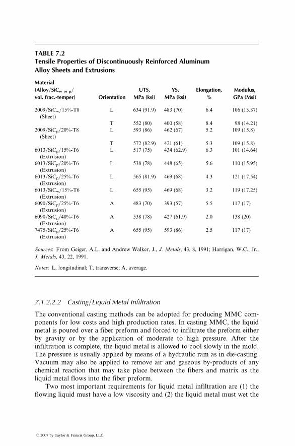
TABLE 7.2Tensile Properties of Discontinuously Reinforced Aluminum
Alloy Sheets and Extrusions
Material
(Alloy=SiCw or p=
vol. frac.-temper) Orientation
UTS,
MPa (ksi)
YS,
MPa (ksi)
Elongation,
%
Modulus,
GPa (Msi)
2009=SiCw=15%-T8
(Sheet)
L 634 (91.9) 483 (70) 6.4 106 (15.37)
T 552 (80) 400 (58) 8.4 98 (14.21)
2009=SiCp=20%-T8
(Sheet)
L 593 (86) 462 (67) 5.2 109 (15.8)
T 572 (82.9) 421 (61) 5.3 109 (15.8)
6013=SiCp=15%-T6
(Extrusion)
L 517 (75) 434 (62.9) 6.3 101 (14.64)
6013=SiCp=20%-T6
(Extrusion)
L 538 (78) 448 (65) 5.6 110 (15.95)
6013=SiCp=25%-T6
(Extrusion)
L 565 (81.9) 469 (68) 4.3 121 (17.54)
6013=SiCw=15%-T6
(Extrusion)
L 655 (95) 469 (68) 3.2 119 (17.25)
6090=SiCp=25%-T6
(Extrusion)
A 483 (70) 393 (57) 5.5 117 (17)
6090=SiCp=40%-T6
(Extrusion)
A 538 (78) 427 (61.9) 2.0 138 (20)
7475=SiCp=25%-T6
(Extrusion)
A 655 (95) 593 (86) 2.5 117 (17)
Sources: From Geiger, A.L. and Andrew Walker, J., J. Metals, 43, 8, 1991; Harrigan, W.C., Jr.,
J. Metals, 43, 22, 1991.
Notes: L, longitudinal; T, transverse; A, average.
7.1.2.2.2 Casting=Liquid Metal Infiltration
The conventional casting methods can be adopted for producing MMC com-
ponents for low costs and high production rates. In casting MMC, the liquid
metal is poured over a fiber preform and forced to infiltrate the preform either
by gravity or by the application of moderate to high pressure. After the
infiltration is complete, the liquid metal is allowed to cool slowly in the mold.
The pressure is usually applied by means of a hydraulic ram as in die-casting.
Vacuum may also be applied to remove air and gaseous by-products of any
chemical reaction that may take place between the fibers and matrix as the
liquid metal flows into the fiber preform.
Two most important requirements for liquid metal infiltration are (1) the
flowing liquid must have a low viscosity and (2) the liquid metal must wet the
� 2007 by Taylor & Francis Group, LLC.
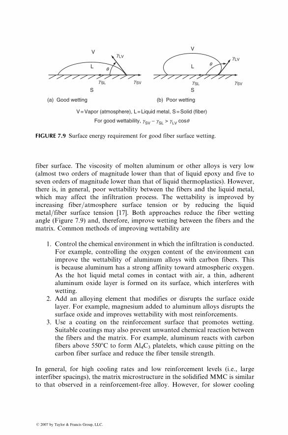
V
S
g LV
g SL g SV
L q
V
S
g LV
g SL g SV
L q
V = Vapor (atmosphere), L = Liquid metal, S = Solid (fiber)
For good wettability, g SV − g SL > g LV cosq
(a) Good wetting (b) Poor wetting
FIGURE 7.9 Surface energy requirement for good fiber surface wetting.
fiber surface. The viscosity of molten aluminum or other alloys is very low
(almost two orders of magnitude lower than that of liquid epoxy and five to
seven orders of magnitude lower than that of liquid thermoplastics). However,
there is, in general, poor wettability between the fibers and the liquid metal,
which may affect the infiltration process. The wettability is improved by
increasing fiber=atmosphere surface tension or by reducing the liquid
metal=fiber surface tension [17]. Both approaches reduce the fiber wetting
angle (Figure 7.9) and, therefore, improve wetting between the fibers and the
matrix. Common methods of improving wettability are
1. Control the chemical environment in which the infiltration is conducted.
For example, controlling the oxygen content of the environment can
improve the wettability of aluminum alloys with carbon fibers. This
is because aluminum has a strong affinity toward atmospheric oxygen.
As the hot liquid metal comes in contact with air, a thin, adherent
aluminum oxide layer is formed on its surface, which interferes with
wetting.
2. Add an alloying element that modifies or disrupts the surface oxide
layer. For example, magnesium added to aluminum alloys disrupts the
surface oxide and improves wettability with most reinforcements.
3. Use a coating on the reinforcement surface that promotes wetting.
Suitable coatings may also prevent unwanted chemical reaction between
the fibers and the matrix. For example, aluminum reacts with carbon
fibers above 5508C to form Al4C3 platelets, which cause pitting on the
carbon fiber surface and reduce the fiber tensile strength.
In general, for high cooling rates and low reinforcement levels (i.e., large
interfiber spacings), the matrix microstructure in the solidified MMC is similar
to that observed in a reinforcement-free alloy. However, for slower cooling
� 2007 by Taylor & Francis Group, LLC.
rates or high reinforcement levels, the matrix microstructure in the MMC can
be significantly different from that of the reinforcement-free alloy [18,19]. Some
of the observed microstructural differences are
1. Matrix microsegregation may be reduced.
2. The crystal morphology may change from cellular dendritic to com-
pletely featureless.
3. Certain primary phases may nucleate preferentially at the reinforcement
surface (e.g., silicon in a hypereutectic Al–Si alloy nucleating on the
surfaces of carbon fibers or SiC particles).
4. If the reinforcement is relatively mobile, it can be pushed by growing
dendrites into the last freezing zone, thereby creating an uneven distri-
bution of the reinforcement in the composite.
5. If the fibers are held below the liquidus temperature of the matrix alloy,
the liquid melt is very rapidly cooled as it comes in contact with the
fibers and solidification begins at the fiber surface. This leads to finer
grain size, which is of the order of the fiber diameter.
7.1.2.2.3 Compocasting
When a liquid metal is vigorously stirred during solidification by slow cooling,
it forms a slurry of fine spheroidal solids floating in the liquid. Stirring at high
speeds creates a high shear rate, which tends to reduce the viscosity of the slurry
even at solid fractions that are as high as 50%–60% by volume. The process of
casting such a slurry is called rheocasting. The slurry can also be mixed with
particulates, whiskers, or short fibers before casting. This modified form of
rheocasting to produce near net-shape MMC parts is called compocasting.
The melt-reinforcement slurry can be cast by gravity casting, die-casting,
centrifugal casting, or squeeze casting. The reinforcements have a tendency to
either float to the top or segregate near the bottom of the melt due to the
differences in their density from that of the melt. Therefore, a careful choice of
the casting technique as well as the mold configuration is of great importance in
obtaining uniform distribution of reinforcements in a compocast MMC [20].
Compocasting allows a uniform distribution of reinforcement in the matrix
as well as a good wet-out between the reinforcement and the matrix. Continuous
stirring of the slurry creates an intimate contact between them. Good bonding
is achieved by reducing the slurry viscosity as well as increasing the mixing time.
The slurry viscosity is reduced by increasing the shear rate as well as increasing
the slurry temperature. Increasing mixing time provides longer interaction
between the reinforcement and the matrix.
7.1.2.2.4 Squeeze Casting
Squeeze casting is a net-shape metal casting process and involves solidification
of liquid metal under pressure. It differs from the more familiar process of
� 2007 by Taylor & Francis Group, LLC.
pressur e die-c asting in whic h pressur e is used only to inject the liquid meta l into
a die cavit y and the solidificati on takes place unde r littl e or no pressure. In
squeeze casti ng, high pressur e is maint ained througho ut solidificati on. This
leads to a fine equiaxed grain structure and very little porosity in the cast
compon ent. In general , squeeze- cast meta ls ha ve high er tensi le stre ngths as
well as great er strains-to- failure than the g ravity-c ast or die-cast metals. In
additio n, since the use of pressur e increa ses casta bility, a wide varie ty of alloy
composi tions can be squ eeze cast, including the wroug ht alloy s that are usually
consider ed unsuit able for casting becau se of their poor flui dity.
Sque eze casti ng, as it applie s to M MC, star ts by placing a preh eated fiber
prefor m in an ope n die cavity, which is mo unted in the bottom plate n of a
hydrauli c press. A measur ed quan tity of liqui d meta l is poured ov er the
prefor m, the die cavit y is closed, and pressur e up to 100 M Pa is ap plied to
force the liquid meta l into the prefor m. The pressure is relea sed only a fter the
solid ification is co mplete.
Sque eze casting has been used to pro duce a variety of MM Cs, includi ng
those with wrough t alumi num alloys, such as 2024, 6061, an d 7075. How ever,
severa l investiga tors [21,22] ha ve suggest ed that impr oved pr operties are
obtaine d by alloy modif ication of commer cial alloys. Othe r varia bles that
may influ ence the qua lity of a squeeze- cast MMC are the temperatur es of the
molten meta l as wel l as the fiber prefor m, infilt ration speed , and the final
squeeze pressure [22,23].
7.2 CERAMIC MATRIX COMPOSITES
Structural ceramics such as silicon carbide (SiC), silicon nitride (Si3N4), and
aluminum oxide (Al2O3) are considered candidate materials for applications in
internal combustion engines, gas turbines, electronics, and surgical implants.
They are high-m odulus mate rials with high tempe rature resistance (Table 7.3) ;
however, they have low failure strains and very low fracture toughness. Poor
structural reliability resulting from their brittleness and high notch sensitivity is
the principal drawback for widespread applications of these materials.
The impetus for developing ceramic matrix composites comes from the
possibility of improving the fracture toughness and reducing the notch sensi-
tivity of structural ceramics [24]. Early work on ceramic matrix composites used
carbon fibers in reinforcing low- to intermediate-modulus ceramics, such as
glass and glass-ceramics. Recent work on ceramic matrix composites has
focused on incorporating SiC fibers or whiskers into high-temperature-resistant
polycrystalline ceramics, such as SiC and Si3N4. Since the modulus values of
these materials are close to those of fibers, there is very little reinforcement
effect from the fibers. Instead, the heterogeneous nature of the composite
contributes to the increase in matrix toughness through several microfailure
mechanisms as described in the following section.
� 2007 by Taylor & Francis Group, LLC.
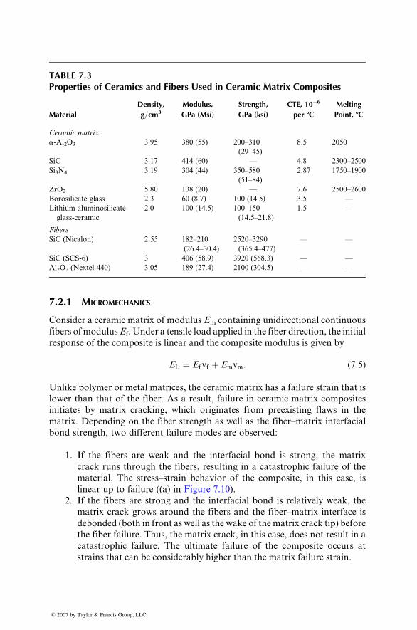
TABLE 7.3Properties of Ceramics and Fibers Used in Ceramic Matrix Composites
Material
Density,
g=cm3
Modulus,
GPa (Msi)
Strength,
GPa (ksi)
CTE, 10�6
per 8C
Melting
Point, 8C
Ceramic matrix
a-Al2O3 3.95 380 (55) 200–310
(29–45)
8.5 2050
SiC 3.17 414 (60) — 4.8 2300–2500
Si3N4 3.19 304 (44) 350–580
(51–84)
2.87 1750–1900
ZrO2 5.80 138 (20) — 7.6 2500–2600
Borosilicate glass 2.3 60 (8.7) 100 (14.5) 3.5 —
Lithium aluminosilicate
glass-ceramic
2.0 100 (14.5) 100–150
(14.5–21.8)
1.5 —
Fibers
SiC (Nicalon) 2.55 182–210
(26.4–30.4)
2520–3290
(365.4–477)
— —
SiC (SCS-6) 3 406 (58.9) 3920 (568.3) — —
Al2O2 (Nextel-440) 3.05 189 (27.4) 2100 (304.5) — —
7.2.1 MICROMECHANICS
Consid er a ceramic matrix of modulus Em co ntaining unidir ection al continuous
fibers of mo dulus Ef. Und er a tensile load applie d in the fiber direction , the initial
response of the composi te is linea r an d the composi te mod ulus is given by
EL ¼ E f vf þ Em vm : ( 7: 5)
Unlike polyme r or meta l matrices , the ceram ic matrix has a failure stra in that is
lower than that of the fiber. As a result, failure in ceram ic matr ix composi tes
initiate s by matr ix crackin g, which originates from preexi sting flaws in the
matrix. Depending on the fiber stre ngth as well as the fiber–mat rix interfaci al
bond stre ngth, tw o diff erent failu re mode s are observed:
1. If the fiber s are weak and the interfaci al bond is strong , the matrix
crack run s through the fiber s, resul ting in a catas trophi c failure of the
material. The stress–strain behavior of the composite, in this case, is
linea r up to failure ((a) in Figu re 7.10) .
2. If the fibers are strong and the interfacial bond is relatively weak, the
matrix crack grows around the fibers and the fiber–matrix interface is
debonded (both in front as well as the wake of thematrix crack tip) before
the fiber failure. Thus, the matrix crack, in this case, does not result in a
catastrophic failure. The ultimate failure of the composite occurs at
strains that can be considerably higher than the matrix failure strain.
� 2007 by Taylor & Francis Group, LLC.
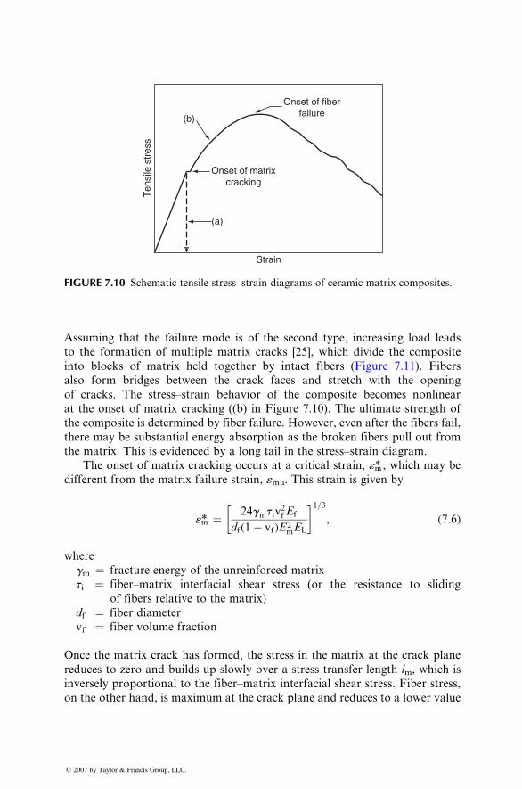
Onset of fiberfailure
(b)
(a)
Onset of matrixcracking
Strain
Ten
sile
str
ess
FIGURE 7.10 Schematic tensile stress–strain diagrams of ceramic matrix composites.
Assu ming that the failure mode is of the second type, increa sing load leads
to the formati on of multiple matr ix cracks [25] , which divide the composi te
into block s of matrix he ld toget her by intac t fiber s (Figur e 7.11). Fib ers
also form bridges between the crack faces and stre tch with the ope ning
of crack s. The stress–s train behav ior of the composi te beco mes nonlinear
at the ons et of matr ix crackin g ((b) in Figure 7.10). The ultimat e strength of
the composi te is de termined by fiber failure. How ever, e ven after the fiber s fail,
there may be sub stantial energy absorpt ion as the broken fiber s pull out from
the matrix. This is evidence d by a long tail in the stress–s train diagra m.
The onset of matr ix c racking occurs at a critical stra in, «m* , whi ch may be
different from the matrix failure strain, «mu . This strain is given by
«m* ¼ 24gm t i v2f Ef
df ( 1 � vf )E 2m EL
� �1 = 3, ( 7: 6)
wher e
gm ¼ fractu re ene rgy of the unr einforced matr ix
ti ¼ fiber–mat rix interfaci al shear stre ss (or the resistance to sliding
of fibers relative to the matrix)
df ¼ fiber diame ter
vf ¼ fiber volume fraction
Once the matrix crack has form ed, the stress in the matrix at the crack plane
reduces to ze ro an d bui lds up slowly over a stre ss trans fer lengt h lm, which is
inversely proportional to the fiber–matrix interfacial shear stress. Fiber stress,
on the other hand, is maximum at the crack plane and reduces to a lower value
� 2007 by Taylor & Francis Group, LLC.
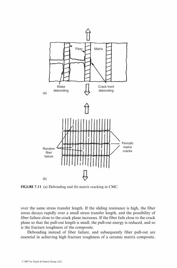
Fiber Matrix
Wakedebonding
Crack frontdebonding
(a)
Randomfiber
failure
(b)
Periodicmatrixcracks
FIGURE 7.11 (a) Debonding and (b) matrix cracking in CMC.
over the same stress transfer length. If the sliding resistance is high, the fiber
stress decays rapidly over a small stress transfer length, and the possibility of
fiber failure close to the crack plane increases. If the fiber fails close to the crack
plane so that the pull-out length is small, the pull-out energy is reduced, and so
is the fracture toughness of the composite.
Debonding instead of fiber failure, and subsequently fiber pull-out are
essential in achieving high fracture toughness of a ceramic matrix composite.
� 2007 by Taylor & Francis Group, LLC.
Evans and Marshall [26] have made the following suggestions for promoting
debonding and fiber pull-out:
1. The fracture energy required for debonding, Gic, should be sufficiently
small compared with that for fiber fracture, Gfc:
Gic
Gfc
� 1
4:
2. Residual radial strain at the interface due to matrix cooling from the
processing temperature should be tensile instead of compressive.
3. Sliding resistance between the fibers and the matrix should be small,
which means the friction coefficient along the debonded interface should
also be small (~0.1).
4. Long pull-out lengths are expected with fibers having a large variability
in their strength distribution; however, for high composite strength, the
median value of the fiber strength distribution should be high.
As suggested in the preceding discussion and also verified experimentally, the
fracture toughness of a ceramic matrix composite is improved if there is poor
bonding between the fibers and the matrix. This can be achieved by means of a
fiber coating or by segregation at the fiber–matrix interface. The most common
method is to use a dual coating in which the inner coating meets the require-
ments for debonding and sliding, and the outer coating protects the fiber
surface from degradation at high processing temperatures.
7.2.2 MECHANICAL PROPERTIES
7.2.2.1 Glass Matrix Composites
Development of ceramic matrix composites began in the early 1970s with
carbon fiber-reinforced glass and glass-ceramic composites. Research by
Sambell et al. [27,28] on carbon fiber-reinforced borosilicate (Pyrex) glass
showed the following results:
1. Increasing fiber volume fraction increases both flexural strength and
flexural modulus of the composite containing continuous fibers.
2. The fracture energy of the glass matrix, as measured by the area under
the load–deflection diagrams of notched flexural specimens, increases
significantly by the addition of continuous carbon fibers. For example,
the fracture energy of 40 vol% carbon fiber-borosilicate glass is 3000
J=m2 compared with only 3 J=m2 for borosilicate glass. The flexural
strength for the same composite is 680 MPa compared with 100 MPa for
the matrix alone. The load–deflection diagram for the matrix is linear up
� 2007 by Taylor & Francis Group, LLC.
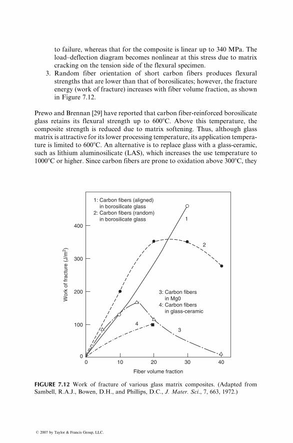
to failure, whereas that for the composite is linear up to 340 MPa. The
load–deflection diagram becomes nonlinear at this stress due to matrix
cracking on the tension side of the flexural specimen.
3. Random fiber orientation of short carbon fibers produces flexural
strengths that are lower than that of borosilicates; however, the fracture
energy (work of fracture) increases with fiber volume fraction, as shown
in Figure 7.12.
Prewo and Brennan [29] have reported that carbon fiber-reinforced borosilicate
glass retains its flexural strength up to 6008C. Above this temperature, the
composite strength is reduced due to matrix softening. Thus, although glass
matrix is attractive for its lower processing temperature, its application tempera-
ture is limited to 6008C. An alternative is to replace glass with a glass-ceramic,
such as lithium aluminosilicate (LAS), which increases the use temperature to
10008C or higher. Since carbon fibers are prone to oxidation above 3008C, they
400
1: Carbon fibers (aligned) in borosilicate glass2: Carbon fibers (random) in borosilicate glass
3: Carbon fibers in Mg04: Carbon fibers in glass-ceramic
1
2
34
300
200
100
00 10 20 30
Fiber volume fraction
Wor
k of
frac
ture
(J/
m2 )
40
FIGURE 7.12 Work of fracture of various glass matrix composites. (Adapted from
Sambell, R.A.J., Bowen, D.H., and Phillips, D.C., J. Mater. Sci., 7, 663, 1972.)
� 2007 by Taylor & Francis Group, LLC.
are replaced by SiC fibers, whi ch show no ap precia ble reduc tion in either
stren gth or modulus up to 800 8 C.Ther momecha nical propert ies of SiC-reinforc ed glass-cer amics ha ve been
studi ed by a num ber of invest igators [30,31]. The results of invest igations on
Nica lon (SiC) fiber-re infor ced LAS are summ arize d as foll ows:
1. Nica lon =LAS co mposites retain their flex ural strength up to 800 8 Cwhen tested in air, and up to 1100 8 C when tested in an inert atmosp here,
such as argon. The fract ure mod e of these comp osites de pends strong ly
on the test environm ent.
2. Room- tempe rature tensi on test in air of unidir ectional Nica lon =LAC
compo sites shows mult iple matrix cracki ng and fiber pull- out. The
compo site fails gradual ly afte r the maxi mum load is reached. When
the same composi te is test ed at 9 00 8C and ab ove, fiber failure occu rsafte r one single matr ix crack ha s form ed, resul ting in a catas trophic
failure wi th su dden load dro p. Thi s change in failure mod e is attribut ed
to fiber stre ngth degradat ion as well as increa sed fiber–mat rix bonding
in the ox idative atmos phere. The initial carbon-r ich layer between the
SiC fiber an d the LAS matrix is replac ed by an amorph ous silicate due
to oxidat ion at 650 8 C–100 08C. Thi s creat es a strong interfaci al bond andtrans forms the composi te from a relative ly tough mate rial to a brittle
mate rial [31].
3. The presen ce of a carbon-r ich inter face is ve ry impor tant in obtainin g a
strong , tough SiC fiber -reinforce d LA S composi te, since this interface is
strong enough to trans fer the load from the matr ix to the fiber s, yet
weak enou gh to debon d before fiber fail ure. Thi s enables the composi te
to accumul ate a signi fican t amount of local damage without fail ing in a
brit tle mode.
7.2.2 .2 Polycr ystall ine Cer amic Matrix
Cerami c matrix co mposites us ing polycry stalli ne c eramic matrix, such as SiC ,
Si3N 4, and ZrO 2–TiO 2, are also dev eloped. Thes e matr ices offer highe r tem-
peratur e ca pabilities than glasses or glass -cera mics. Rese arch done by Rice and
Lewi s [32] on unidir ectio nal Nicalon (SiC) fiber -reinforce d ZrO2–TiO 2 and
ZrO2–SiO 2 comp osites shows the impor tance of prop er fiber –matrix bonding
in achieving high flexural strength and fracture toughness in ceramic matrix
composites. The BN coating used on Nicalon fibers in their work creates a
weaker bond than if the fibers are uncoated. The composite with coated fibers
has a flexural strength of 400–900 MPa (60–125 ksi), compared with 70–220
MPa (10–32 ksi) for uncoated fibers. The difference in flexural load–deflection
diagra ms of coated and uncoated fiber compo sites is shown in Figure 7.13. The
coated fibers not only increased the strength but also created a noncatastrophic
failure mode with significant fiber pull-out. Fracture toughness of coated fiber
� 2007 by Taylor & Francis Group, LLC.
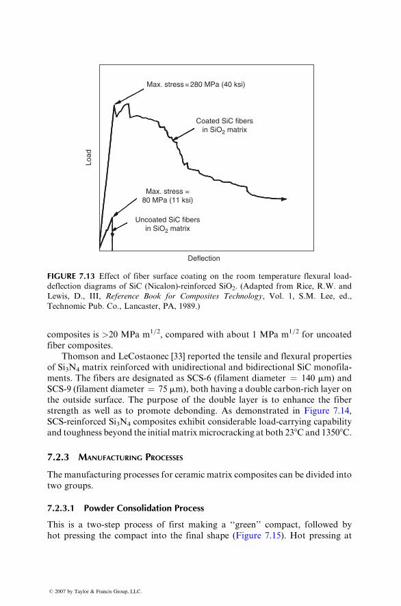
Max. stress = 280 MPa (40 ksi)
Coated SiC fibersin SiO2 matrix
Max. stress =80 MPa (11 ksi)
Uncoated SiC fibersin SiO2 matrix
Deflection
Load
FIGURE 7.13 Effect of fiber surface coating on the room temperature flexural load-
deflection diagrams of SiC (Nicalon)-reinforced SiO2. (Adapted from Rice, R.W. and
Lewis, D., III, Reference Book for Composites Technology, Vol. 1, S.M. Lee, ed.,
Technomic Pub. Co., Lancaster, PA, 1989.)
composi tes is >20 MPa m 1=2, compared with abo ut 1 MPa m1=2 for uncoated
fiber compo sites.
Thom son and LeCost aonec [33] rep orted the tensi le and flexural propert ies
of Si3N 4 matrix reinf orced with unidirec tional and bidir ectional SiC monofi la-
ments. The fiber s are de signated as SCS-6 (filam ent diame ter ¼ 140 mm) and
SCS-9 (filam ent diame ter ¼ 75 m m), both having a doubl e c arbon-r ich layer on
the out side surfa ce. The pur pose of the doubl e layer is to e nhance the fiber
strength as wel l as to promot e de bonding. As demonst rated in Figure 7.14,
SCS-reinf orced Si3N 4 composi tes exhibi t consider able load-carryi ng capabil ity
and toughness be yond the initial matr ix microcrack ing at both 23 8C an d 1350 8 C.
7.2.3 MANUFACTURING PROCESSES
The manu facturing process es for ceram ic matr ix comp osites can be divide d into
two groups.
7.2.3.1 Powder Cons olidatio n Pr ocess
This is a two-step process of first making a ‘‘green’’ compact , followe d by
hot pressing the compact into the final shape (Figur e 7.15). Ho t pressi ng at
� 2007 by Taylor & Francis Group, LLC.
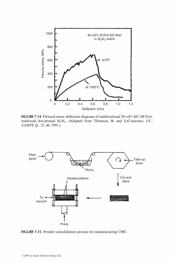
00
200
400
600
800
1000
0.2 0.4 0.6
Deflection (mm)
Fle
xura
l str
ess,
MP
a
0.8 1.0 1.2
30 vol% SCS-6 SiC fiberin Si3N4 matrix
at RT
at 1350�C
FIGURE 7.14 Flexural stress–deflection diagrams of unidirectional 30 vol% SiC (SCS-6)-
reinforced hot-pressed Si3N4. (Adapted from Thomson, B. and LeCostaonec, J.F.,
SAMPE Q., 22, 46, 1991.)
Fiberspool
Slurry
Cut andstack
Take-updrum
Heated platens
Tovacuum
Press
FIGURE 7.15 Powder consolidation process for manufacturing CMC.
� 2007 by Taylor & Francis Group, LLC.
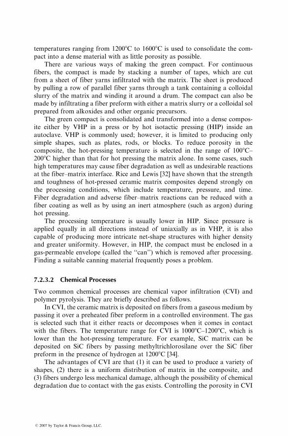
temperatures ranging from 12008C to 16008C is used to consolidate the com-
pact into a dense material with as little porosity as possible.
There are various ways of making the green compact. For continuous
fibers, the compact is made by stacking a number of tapes, which are cut
from a sheet of fiber yarns infiltrated with the matrix. The sheet is produced
by pulling a row of parallel fiber yarns through a tank containing a colloidal
slurry of the matrix and winding it around a drum. The compact can also be
made by infiltrating a fiber preform with either a matrix slurry or a colloidal sol
prepared from alkoxides and other organic precursors.
The green compact is consolidated and transformed into a dense compos-
ite either by VHP in a press or by hot isotactic pressing (HIP) inside an
autoclave. VHP is commonly used; however, it is limited to producing only
simple shapes, such as plates, rods, or blocks. To reduce porosity in the
composite, the hot-pressing temperature is selected in the range of 1008C–2008C higher than that for hot pressing the matrix alone. In some cases, such
high temperatures may cause fiber degradation as well as undesirable reactions
at the fiber–matrix interface. Rice and Lewis [32] have shown that the strength
and toughness of hot-pressed ceramic matrix composites depend strongly on
the processing conditions, which include temperature, pressure, and time.
Fiber degradation and adverse fiber–matrix reactions can be reduced with a
fiber coating as well as by using an inert atmosphere (such as argon) during
hot pressing.
The processing temperature is usually lower in HIP. Since pressure is
applied equally in all directions instead of uniaxially as in VHP, it is also
capable of producing more intricate net-shape structures with higher density
and greater uniformity. However, in HIP, the compact must be enclosed in a
gas-permeable envelope (called the ‘‘can’’) which is removed after processing.
Finding a suitable canning material frequently poses a problem.
7.2.3.2 Chemical Processes
Two common chemical processes are chemical vapor infiltration (CVI) and
polymer pyrolysis. They are briefly described as follows.
In CVI, the ceramic matrix is deposited on fibers from a gaseous medium by
passing it over a preheated fiber preform in a controlled environment. The gas
is selected such that it either reacts or decomposes when it comes in contact
with the fibers. The temperature range for CVI is 10008C–12008C, which is
lower than the hot-pressing temperature. For example, SiC matrix can be
deposited on SiC fibers by passing methyltrichlorosilane over the SiC fiber
preform in the presence of hydrogen at 12008C [34].
The advantages of CVI are that (1) it can be used to produce a variety of
shapes, (2) there is a uniform distribution of matrix in the composite, and
(3) fibers undergo less mechanical damage, although the possibility of chemical
degradation due to contact with the gas exists. Controlling the porosity in CVI
� 2007 by Taylor & Francis Group, LLC.
can be a prob lem, since pore s can seal off between the matrix de posits as they
grow from adjacent fiber s an d impi nge on each other.
Polymer pyrolysis is a two-step process of first making a polymer-impregnated
prefor m via standar d polyme r impr egnatio n techni ques, follo wed by pyrolys is
of the polyme r at high tempe ratur es to yield the ceram ic matr ix. For exampl e,
the polyme r precurs or for prod ucing SiC matr ix is an organosi licon polyme r,
such as polycar bosilane or polybo rosiloxane.
The pyrolys is temperatur e is in the range of 700 8C–10 00 8 C, whi ch is lowcompared wi th that used in hot pressin g. Ther efore, pr ovided a suit able poly-
mer precu rsor is avail able, it is suit able for a wi de ran ge of fibers that canno t
ordinar ily be used with hot pressing. The princip al disadv antage is that it
resul ts in a highly poro us matr ix, primaril y due to shrinka ge c racks origi nating
from the pol ymerizati on pro cess during pyrolys is. One method of reducing the
polyme r shrinka ge is to mix it with fine ceram ic filler s.
7.3 CARBON MATRIX COMPOSITES
The carbon matr ix composi tes consis t of ca rbon fiber s in carbon matrix and are
commonl y referred to as carbo n–carbon (C–C) co mposites. They are therm ally
stable up to 3000 8C in a nonox idative e nvironm ent, but unless protect ed by a
surfa ce coati ng or chemi cally modif ied to pro vide protect ion, they oxidize and
degrade in presen ce of oxygen, even at 400 8 C–50 08C. The pro tection of C–Ccomposi tes agains t oxidation at high tempe ratur es requir es the use of eithe r an
exter nal coati ng or inter nal modificat ion. Both ox ide coati ngs, such as SiO2
and Al2O 3, and nonox ide co atings, such as SiC, Si 3N 4, and HFB 2, have been
used. Low oxygen permea bility and thermal e xpansion matc hing are the two
most critical requir ement s for the extern al coatin g. Thermal exp ansion mis -
matc h between the coati ng and the C–C composi te may cause cracki ng in the
coating, which in the most severe case may result in spalling of the coating from
the C–C composite surface. For applications in oxidizing environments, current
coatings limit the maximum use temperature of C–C composites to 17008C.Fibers in the C–C composites can be either continuous or discontinuous.
Cont inuous fibers are selected for structural applic ations. Table 7.4 shows
the mechanical and thermal properties of continuous fiber-reinforced C–C
composites containing carbon fibers that have strengths up to 2.5 GPa and
elastic modulus in the range of 350–450 GPa. For comparison, properties of
graphite are also listed in Table 7.4, since graphite is also considered for high
temperature applications in which C–C composites are used. As with other
fiber-reinforced composites, the tensile and compressive properties of C–C
composites depend on the fiber properties and fiber architecture. While they
are generally very high, the shear strength and modulus are very low. This is
one of the limitations of C–C composites. Another point to note is that the
failure strain of the matrix in C–C composites is lower than that of the fibers.
Thus if there is a strong bond between the fibers and the matrix in a C–C
� 2007 by Taylor & Francis Group, LLC.
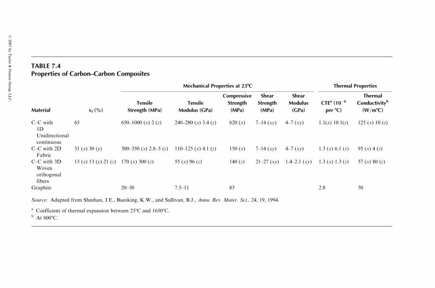
TABLE 7.4Properties of Carbon–Carbon Composites
Mechanical Properties at 238C Thermal Properties
Material vf (%)
Tensile
Strength (MPa)
Tensile
Modulus (GPa)
Compressive
Strength
(MPa)
Shear
Strength
(MPa)
Shear
Modulus
(GPa)
CTEa (10�6
per 8C)
Thermal
Conductivityb
(W=m8C)
C–C with
1D
Unidirectional
continuous
65 650–1000 (x) 2 (z) 240–280 (x) 3.4 (z) 620 (x) 7–14 (xy) 4–7 (xy) 1.1(x) 10.1(z) 125 (x) 10 (z)
C–C with 2D
Fabric
31 (x) 30 (y) 300–350 (x) 2.8–5 (z) 110–125 (x) 4.1 (z) 150 (x) 7–14 (xy) 4–7 (xy) 1.3 (x) 6.1 (z) 95 (x) 4 (z)
C–C with 3D
Woven
orthogonal
fibers
13 (x) 13 (y) 21 (z) 170 (x) 300 (z) 55 (x) 96 (z) 140 (z) 21–27 (xy) 1.4–2.1 (xy) 1.3 (x) 1.3 (z) 57 (x) 80 (z)
Graphite 20–30 7.5–11 83 2.8 50
Source: Adapted from Sheehan, J.E., Buesking, K.W., and Sullivan, B.J., Annu. Rev. Mater. Sci., 24, 19, 1994.
a Coefficient of thermal expansion between 238C and 16508C.b At 8008C.
�2007
byTaylor
&Francis
Group,
LLC.
composi te, fiber s fail imm ediately after the matr ix fails and the composi te fail s
in a brit tle manner wi th low stre ngth. On the other hand, if the fiber–mat rix
bond is not very strong , matrix cracki ng at low strain will not produce imm e-
diate fiber failure; instead, there will be en ergy a bsorption due to debon ding,
fiber bridgin g, fiber fractu re, and fiber pull-o ut, an d such a composi te can
possess high fract ure toughness . Ind eed, the work of fractu re test of fully
densif ied unidir ection al C–C co mposi tes shows fracture energy value of abo ut
2 3 10 4 J=m 2 [35]. In compari son, the fractu re energy of engineer ing ceram ics
and premi um-grad e grap hite is < 10 2 J=m 2.
Two basic fabri catio n method s are used for making C–C composi tes [36] :
(1) liquid infiltrati on an d (2) chemi cal vapor deposition (CVD ). The star ting
mate rial in either of these methods is a carbon fiber prefor m, whi ch may
contai n unidirecti onal fibers, bi- or multidir ection al fabrics, or a three-
dimens ional structure of carbo n fibers. In the liqui d infilt ration process , the
prefor m is infi ltrated wi th a liquid, which on heati ng, carbo nizes to yiel d at
least 50 wt % c arbon. In the CVD process , a hydrocarbon gas is infilt rated into
the prefor m at high tempe rature an d pressur e. The che mical breakdo wn of the
hydrocarb on gas pro duces the carbon matrix. In gene ral, CVD is used wi th thin
section s and liqui d infiltrati on is used with thick secti ons.
Two types of liqui ds are us ed in the liquid infilt ration method: (1) pitch,
which is made from coal tar or petrol eum and (2) a therm oset resi n, such as a
phen olic or an ep oxy. In the pitch infi ltration method, either an isot ropic pitch
or a mesophas e pitch is infiltrated into the dry carbon fiber prefor m at 1000 8 Cor higher an d at pressur e ranging from atmosp heric to 207 MPa (30,000 psi) .
At this tempe ratur e, carboniza tion occu rs simulta neously with infiltratio n. If
the carbonization is performed at the atmospheric pressure, the carbon yield is
50–60 wt% with isotropic pitch and >80 wt% with mesophase pitch. The
carbon yield is higher if the pressure is increased.
In the thermoset resin infiltration method, the starting material is a prepreg
containing carbon fibers in a partially cured thermoset resin. A laminate is first
constructed using the prepreg layers and the vacuum bag molding process
descri bed in Chapt er 5. The resi n in the laminate is then carbonize d at
8008C–10008C in an inert atmosphere. The volatiles emitted during the carbon-
ization reaction cause shrinkage and a reduction in density. The carbonization
process is performed slowly to prevent rapid evolution of volatiles, which may
cause high porosity and delamination between the layers. The infiltration=carbonization process is repeated several times to reduce the porosity and
increase the density of the composite. The carbon yield in this process is
between 50% and 70% depending on the resin and processing conditions used.
The CVD process starts with the fabrication of a dry fiber preform in the
shape of the desired part. The preform is heated in a furnace under pressure
(typically around 1 psi or 7 kPa) and in the presence of a hydrocarbon gas,
such as methane, propane, or benzene. As the gas is thermally decomposed, a
layer of pyrolitic carbon is slowly formed and deposited on the hot preform
� 2007 by Taylor & Francis Group, LLC.
surface. In the isothermal CVD process, the temperature of the furnace is
maintained constant at 11008C. Since the pyrolitic carbon deposited on the
surface tends to close the pores located at and very close to the surface, it
becomes difficult to fill the internal pores with carbon. Thus it may be
necessary to lightly machine the preform surfaces to remove the surface carbon
layer and then repeat the infiltration process. The infiltration is better if either
a thermal gradient or a pressure gradient is created across the thickness of the
preform. In the thermal gradient technique, one surface is maintained at a
higher temperature than the other, and the carbon infiltration progresses from
the hotter surface to the colder surface. In the pressure gradient technique, a
pressure differential is created across the thickness, which forces the hydro-
carbon gas to flow through the pores in the preform and deposit carbon
throughout the thickness. With both these techniques, very little, if any,
crust is formed on the surfaces.
The C–C composite obtained by either liquid infiltration or by CVD can be
heated further to transform the carbon matrix from amorphous form to gra-
phitic form. The graphitization temperature is between 21008C and 30008C.Graphitization increases both strength and modulus of the C–C composite,
while the fracture toughness depends on the graphitization temperature. For
example, for a pitch-based matrix, the optimum graphitization temperature is
27008C, above which fracture toughness starts to decrease [37].
Depending on the starting material and the process condition, the micro-
structure of carbon matrix in C–C composites may vary from small, randomly
oriented crystallites of turbostratic carbon to large, highly oriented, and graph-
itized crystallites. The carbon matrix may also contain large amount of poros-
ity, which causes the density to be lower than the maximum achievable density
of approximately 1.8–2 g=cm3. There may also be microcracks originating from
thermal stresses as the C–C composite cools down from the processing tem-
perature to room temperature. Since porosity affects not only the density, but
also the properties of the composite, repeated impregnation and carbonization
cycles are used to reduce the porosity. This process is often referred to as
densification.
REFERENCES
1.
� 20
R.K. Everett and R.J. Arsenault (eds.), Metal Matrix Composites: Mechanisms and
Properties, Academic Press, San Diego (1991).
2.
R.K. Everett and R.J. Arsenault (eds.), Metal Matrix Composites: Processing andInterfaces, Academic Press, San Diego (1991).
3.
T.W. Clyne and P.J. Withers, An Introduction to Metal Matrix Composites, Cam-bridge University Press, Cambridge, UK (1993).
4.
N. Chawla andK.K. Chawla,MetalMatrix Composites, Springer, NewYork (2006).5.
A. Kelly and G.J. Davies, The principles of the fibre reinforcement of metals,Metall. Rev., 10:1 (1965).
07 by Taylor & Francis Group, LLC.
6.
� 20
A. Toy, Mechanical properties of beryllium filament-reinforced aluminum compos-
ites, J. Mater., 3:43 (1968).
7.
M. Taya and R.J. Arsenault, Metal Matrix Composites: Thermomechanical Behav-ior, Pergamon Press, Oxford (1989).
8.
S.V. Nair, J.K. Tien, and R.C. Bates, SiC-reinforced aluminum metal matrixcomposites, Int. Metals Rev., 30:275 (1985).
9.
D.L. McDanels, Analysis of stress–strain, fracture, and ductility behavior of alumi-num matrix composites containing discontinuous silicon carbide reinforcement,
Metall. Trans., 16A:1105 (1985).
10.
W.S. Johnson and M.J. Birt, Comparison of some micromechanics models fordiscontinuously reinforced metal matrix composites, J. Compos. Technol. Res.,
13:168 (1991).
11.
A.L. Geiger and J. Andrew Walker, The processing and properties of discontinu-ously reinforced aluminum composites, J. Metals, 43:8 (1991).
12.
K. Schmidt, C. Zweben, and R. Arsenault, Mechanical and thermal properties ofsilicon-carbide particle-reinforced aluminum, Thermal and Mechanical Behavior of
Metal Matrix and Ceramic Matrix Composites, ASTM STP, 1080:155 (1990).
13.
J.J. Lewandowski, C. Liu, and W.H. Hunt, Jr., Microstructural effects on thefracture mechanisms in 7xxx A1 P=M-SiC particulate metal matrix composites,
Processing and Properties for Powder Metallurgy Composites (P. Kumar, K. Vedula,
and A. Ritter, eds.), TMS, Warrendale, PA (1988).
14.
M. Karayaka and H. Sehitoglu, Thermomechanical fatigue of particulate-reinforcedaluminum 2xxx-T4, Metall. Trans. A, 22A:697 (1991).
15.
T. Morimoto, T. Yamaoka, H. Lilholt, and M. Taya, Second stage creep ofwhisker=6061 aluminum composites at 573K, J. Eng. Mater. Technol., 110:70
(1988).
16.
R.K. Everett, Diffusion bonding, Metal Matrix Composites: Processing and Inter-faces, Chapter 2 (R.K. Everett and R.J. Arsenault, eds.), Academic Press, San Diego
(1991).
17.
A. Mortensen, J.A. Cornie, and M.C. Flemings, Solidification processing of metal-matrix composites, J. Metals, 40:12 (1988).
18.
A. Mortensen, M.N. Gungor, J.A. Cornie, and M.C. Flemings, Alloy microstruc-tures in cast metal matrix composites, J. Metals, 38:30 (1986).
19.
P. Rohatgi and R. Asthana, The solidification of metal-matrix particulate compos-ites, J. Metals, 43:35 (1991).
20.
P. Rohatgi, Cast aluminum-matrix composites for automotive applications,J. Metals, 43:10 (1991).
21.
C.R. Cook, D.I. Yun, and W.H. Hunt, Jr., System optimization for squeeze castcomposites, Cast Reinforced Metal Composites (S.G. Fishman and A.K. Dhingra,
eds.), ASM International, Metals Park, OH (1988).
22.
T. Kobayashi, M. Yosino, H. Iwanari, M. Niinomi, and K. Yamamoto, Mechanicalproperties of SiC whisker reinforced aluminum alloys fabricated by pressure casting
method, Cast Reinforced Metal Composites (S.G. Fishman and A.K. Dhingra, eds.),
ASM International, Metals Park, OH (1988).
23.
H. Fukunaga, Squeeze casting processes for fiber reinforced metals and theirmechanical properties, Cast Reinforced Metal Composites (S.G. Fishaman and
A.K. Dingra, eds.), ASM International, Metal Park, OH (1988).
24.
K.K. Chawla, Ceramic Matrix Composites, Chapman & Hall, London (1993).07 by Taylor & Francis Group, LLC.
25.
� 20
J. Aveston, G.A. Cooper, and A. Kelly, Single and multiple fracture, The Properties
of Fiber=Composites, IPC Science and Technology Press, Surrey, England (1971).
26.
A.G. Evans and D.B. Marshall, The mechanical behavior of ceramic matrix com-posites, Acta Metall., 37:2567 (1989).
27.
R.A.J. Sambell, D.H. Bowen, and D.C. Phillips, Carbon fibre composites withceramic and glass matrices, Part 1: Discontinuous fibres, J. Mater. Sci., 7:663 (1972).
28.
R.A.J. Sambell, A. Briggs, D.C. Phillips, and D.H. Bowen, Carbon fibre compositeswith ceramic and glass matrices, Part 2: Continuous fibres, J. Mater. Sci., 7:676
(1972).
29.
K.M. Prewo and J.J. Brennan, Fiber reinforced glasses and glass ceramics for highperformance applications, Reference Book for Composites Technology, Vol. 1 (S.M.
Lee, ed.), Technomic Pub. Co., Lancaster, PA (1989).
30.
J.J. Brennan and K.M. Prewo, Silicon carbide fibre reinforced glass-ceramic matrixcomposites exhibiting high strength and toughness, J. Mater. Sci., 17:2371 (1982).
31.
T.Mah,M.G.Mendiratta, A.P. Katz, andK.S.Mazdiyasni, Recent developments infiber-reinforced high temperature ceramic composites, Ceramic Bull., 66:304 (1987).
32.
R.W. Rice and D. Lewis III, Ceramic fiber composites based upon refractorypolycrystalline ceramic matrices, Reference Book for Composites Technology, Vol.
1 (S.M. Lee, ed.), Technomic Pub. Co., Lancaster, PA (1989).
33.
B. Thomson and J.F. LeCostaonec, Recent developments in SiC monofilamentreinforced Si3N4 composites, SAMPE Q., 22:46 (1991).
34.
R.L. Lehman, Ceramic matrix fiber composites, Structural Ceramics (J.B. Wacht-man, Jr., ed.), Academic Press, San Diego (1989).
35.
J.E. Sheehan, K.W. Buesking, and B.J. Sullivan, Carbon–carbon composites, Annu.Rev. Mater. Sci., 24:19 (1994).
36.
J.D. Buckley and D.D. Edie, Carbon–Carbon Materials and Composites, WilliamAndrews Publishing, Norwich, NY (1993).
37.
D.L. Chung, Carbon Fiber Composites, Butterworth-Heinemann, Newton, MA(1994).
PROBLEMS
P7.1. Experimentally determined elastic properties of a unidirectional continu-
ous P-100 carbon fiber-reinforced 6061-T6 aluminumalloy areE11 ¼ 403
GPa, E22 ¼ 24 GPa, v12 ¼ 0.291, and G12 ¼ 18.4 GPa. Fiber volume
fraction in the composite is 0.5.
1. Compare these values with theoretical predictions and explain the
differences, if any.
2. Using the experimental values, determine the off-axis elastic modu-
lus, Exx, at u ¼ 158 and 458 and compare them with the experimental
values of 192 and 41 GPa, respectively.
P7.2. Suppose both fibers and matrix in a unidirectional continuous fiber
MMC are ductile, and their tensile stress–strain equations are given by
the general form:
s ¼ K «m,
07 by Taylor & Francis Group, LLC.
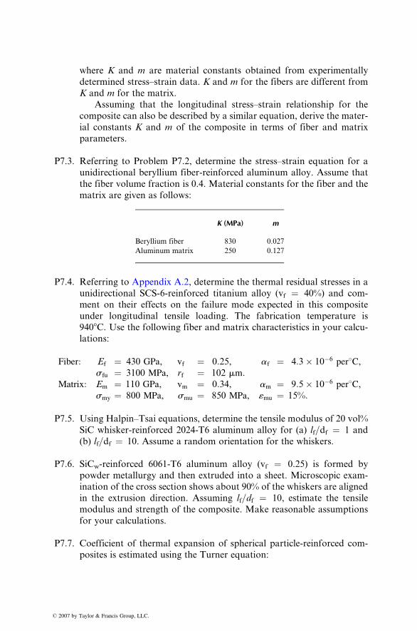
� 2007 by
wher e K and m are mate rial con stants obtaine d from exp erimental ly
determ ined stre ss–strain data. K an d m for the fibers are different from
K an d m for the matr ix.
Ass uming that the longit udinal stress–s train relationshi p for the
compo site can also be described by a sim ilar equati on, derive the mate r-
ial constant s K an d m of the co mposite in terms of fiber and matr ix
parame ters .
P7.3. Ref erring to Prob lem P7.2, determ ine the stre ss–strai n eq uation for a
unidir ectio nal beryll ium fiber -reinforce d alumin um alloy . Ass ume that
the fiber volume fraction is 0.4. M aterial co nstants for the fiber an d the
matr ix are given as follows :
Taylor & Francis Group
K (MPa) m
, LLC.
Beryllium fiber
830 0.027Aluminum matrix
250 0.127P7.4. Ref erring to Appendix A.2 , determ ine the therm al residu al stresses in a
unidir ectio nal SCS- 6-rein forced tit anium alloy (vf ¼ 40%) and com-
ment on their effe cts on the failu re mod e ex pected in this composi te
unde r longit udinal tensile loading . The fabricati on tempe rature is
940 8 C. Use the followi ng fiber and matrix charact eristic s in your calcu-
lation s:
Fiber : Ef ¼ 430 GPa , v f ¼ 0: 25, a f ¼ 4: 3 � 10 � 6 per 8C ,sfu ¼ 3100 MPa , rf ¼ 102 m m:
Matrix : Em ¼ 110 GPa , vm ¼ 0: 34, am ¼ 9: 5 � 10 � 6 per 8C ,smy ¼ 800 MPa , s mu ¼ 850 MPa , « mu ¼ 15% :
P7.5. Usi ng Halpin –Tsai equatio ns, de termine the tensi le mod ulus of 2 0 vol%
SiC whi sker-reinf orced 2024-T6 aluminu m alloy for (a) lf= df ¼ 1 and
(b) lf=df ¼ 10. Ass ume a random orientati on for the whiskers.
P7.6. SiCw-rei nforced 6061-T6 alumi num alloy (v f ¼ 0.25) is form ed by
powder metallur gy and then extrude d into a sheet. Micros copic exam-
ination of the cross section shows about 90% of the whiskers are aligned
in the extrusion direction. Assuming lf=df ¼ 10, estimate the tensile
modulus and strength of the composite. Make reasonable assumptions
for your calculations.
P7.7. Coefficient of thermal expansion of spherical particle-reinforced com-
posites is estimated using the Turner equation:
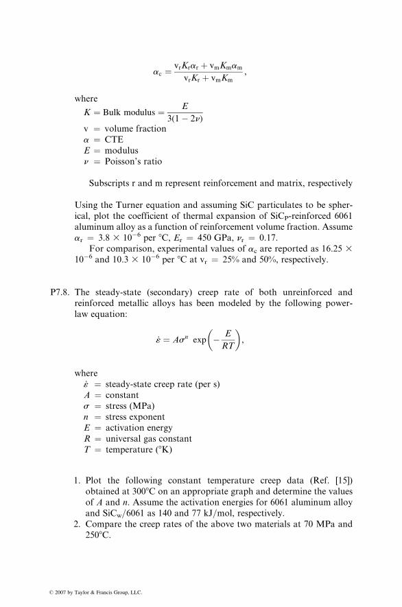
ac ¼ vrKrar þ vmKmam
vrKr þ vmKm
,
� 2007 by
where
K ¼ Bulk modulus ¼ E
3(1� 2n)v ¼ volume fraction
a ¼ CTE
E ¼ modulus
n ¼ Poisson’s ratio
Subscripts r and m represent reinforcement and matrix, respectively
Using the Turner equation and assuming SiC particulates to be spher-
ical, plot the coefficient of thermal expansion of SiCP-reinforced 6061
aluminum alloy as a function of reinforcement volume fraction. Assume
ar ¼ 3.8 3 10�6 per 8C, Er ¼ 450 GPa, nr ¼ 0.17.
For comparison, experimental values of ac are reported as 16.25 310�6 and 10.3 3 10�6 per 8C at vr ¼ 25% and 50%, respectively.
P7.8. The steady-state (secondary) creep rate of both unreinforced and
reinforced metallic alloys has been modeled by the following power-
law equation:
_« ¼ Asn exp � E
RT
� �,
where
_« ¼ steady-state creep rate (per s)
A ¼ constant
s ¼ stress (MPa)
n ¼ stress exponent
E ¼ activation energy
R ¼ universal gas constant
T ¼ temperature (8K)
1. Plot the following constant temperature creep data (Ref. [15])
obtained at 3008C on an appropriate graph and determine the values
of A and n. Assume the activation energies for 6061 aluminum alloy
and SiCw=6061 as 140 and 77 kJ=mol, respectively.
2. Compare the creep rates of the above two materials at 70 MPa and
2508C.
Taylor & Francis Group, LLC.
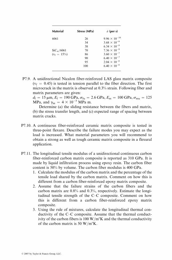
� 2007 by Taylor & Francis Gr
Material Stress (MPa) _« (per s)
oup, LLC.
6061
26 9.96 3 10�1034
3.68 3 10�938
6.34 3 10�9SiCw=6061
70 7.36 3 10�9(vf ¼ 15%)
86 3.60 3 10�790
6.40 3 10�795
2.04 3 10�6100
6.40 3 10�6P7.9. A unidirectional Nicalon fiber-reinforced LAS glass matrix composite
(vf ¼ 0.45) is tested in tension parallel to the fiber direction. The first
microcrack in the matrix is observed at 0.3% strain. Following fiber and
matrix parameters are given:
df ¼ 15 mm, Ef ¼ 190 GPa, sfu ¼ 2.6 GPa, Em ¼ 100 GPa, smu ¼ 125
MPa, and gm ¼ 4 3 10�5 MPa m.
Determine (a) the sliding resistance between the fibers and matrix,
(b) the stress transfer length, and (c) expected range of spacing between
matrix cracks.
P7.10. A continuous fiber-reinforced ceramic matrix composite is tested in
three-point flexure. Describe the failure modes you may expect as the
load is increased. What material parameters you will recommend to
obtain a strong as well as tough ceramic matrix composite in a flexural
application.
P7.11. The longitudinal tensile modulus of a unidirectional continuous carbon
fiber-reinforced carbon matrix composite is reported as 310 GPa. It is
made by liquid infiltration process using epoxy resin. The carbon fiber
content is 50% by volume. The carbon fiber modulus is 400 GPa.
1. Calculate the modulus of the carbon matrix and the percentage of the
tensile load shared by the carbon matrix. Comment on how this is
different from a carbon fiber-reinforced epoxy matrix composite.
2. Assume that the failure strains of the carbon fibers and the
carbon matrix are 0.8% and 0.3%, respectively. Estimate the longi-
tudinal tensile strength of the C–C composite. Comment on how
this is different from a carbon fiber-reinforced epoxy matrix
composite.
3. Using the rule of mixtures, calculate the longitudinal thermal con-
ductivity of the C–C composite. Assume that the thermal conduct-
ivity of the carbon fibers is 100 W=m8K and the thermal conductivity
of the carbon matrix is 50 W=m8K.
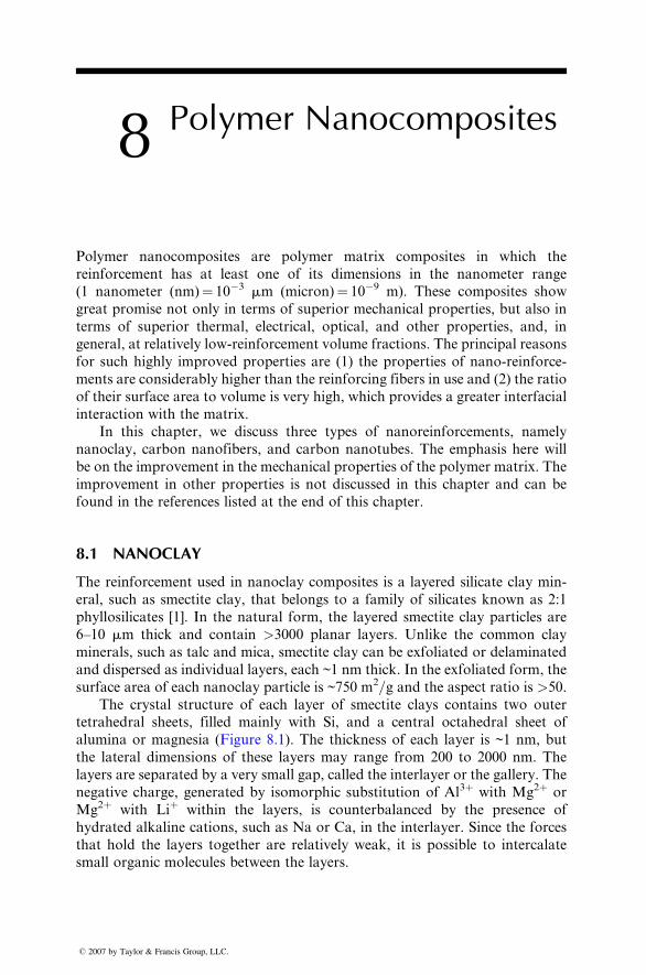
8 Polymer Nanocomposites
� 2007 by Taylor & Fr
Polymer nanocomposites are polymer matrix composites in which the
reinforcement has at least one of its dimensions in the nanometer range
(1 nanometer (nm)¼ 10�3 mm (micron)¼ 10�9 m). These composites show
great promise not only in terms of superior mechanical properties, but also in
terms of superior thermal, electrical, optical, and other properties, and, in
general, at relatively low-reinforcement volume fractions. The principal reasons
for such highly improved properties are (1) the properties of nano-reinforce-
ments are considerably higher than the reinforcing fibers in use and (2) the ratio
of their surface area to volume is very high, which provides a greater interfacial
interaction with the matrix.
In this chapter, we discuss three types of nanoreinforcements, namely
nanoclay, carbon nanofibers, and carbon nanotubes. The emphasis here will
be on the improvement in the mechanical properties of the polymer matrix. The
improvement in other properties is not discussed in this chapter and can be
found in the references listed at the end of this chapter.
8.1 NANOCLAY
The reinforcement used in nanoclay composites is a layered silicate clay min-
eral, such as smectite clay, that belongs to a family of silicates known as 2:1
phyllosilicates [1]. In the natural form, the layered smectite clay particles are
6–10 mm thick and contain >3000 planar layers. Unlike the common clay
minerals, such as talc and mica, smectite clay can be exfoliated or delaminated
and dispersed as individual layers, each ~1 nm thick. In the exfoliated form, the
surface area of each nanoclay particle is ~750 m2=g and the aspect ratio is >50.
The crystal structure of each layer of smectite clays contains two outer
tetrahedral sheets, filled mainly with Si, and a central octahedral sheet of
alumina or magnesia (Figure 8.1). The thickness of each layer is ~1 nm, but
the lateral dimensions of these layers may range from 200 to 2000 nm. The
layers are separated by a very small gap, called the interlayer or the gallery. The
negative charge, generated by isomorphic substitution of Al3þ with Mg2þ or
Mg2þ with Liþ within the layers, is counterbalanced by the presence of
hydrated alkaline cations, such as Na or Ca, in the interlayer. Since the forces
that hold the layers together are relatively weak, it is possible to intercalate
small organic molecules between the layers.
ancis Group, LLC.
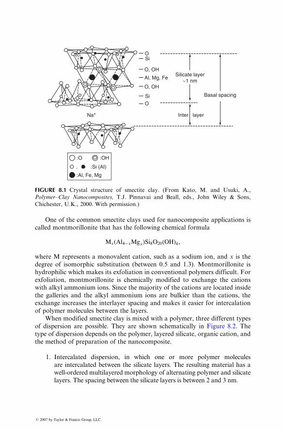
O
Basal spacing
Inter layer
Silicate layer~1 nm
Si
Si
O, OH
O, OH
Al, Mg, Fe
O
Na+
:O :OH
. :Si (AI)
:Al, Fe, Mg
FIGURE 8.1 Crystal structure of smectite clay. (From Kato, M. and Usuki, A.,
Polymer–Clay Nanocomposites, T.J. Pinnavai and Beall, eds., John Wiley & Sons,
Chichester, U.K., 2000. With permission.)
One of the common smectite clays used for nanocomposite applications is
called montmorillonite that has the following chemical formula
Mx(Al4�xMgx)Si8O20(OH)4,
where M represents a monovalent cation, such as a sodium ion, and x is the
degree of isomorphic substitution (between 0.5 and 1.3). Montmorillonite is
hydrophilic which makes its exfoliation in conventional polymers difficult. For
exfoliation, montmorillonite is chemically modified to exchange the cations
with alkyl ammonium ions. Since the majority of the cations are located inside
the galleries and the alkyl ammonium ions are bulkier than the cations, the
exchange increases the interlayer spacing and makes it easier for intercalation
of polymer molecules between the layers.
When modified smectite clay is mixed with a polymer, three different types
of disper sion are pos sible. They are shown schema tica lly in Figure 8.2. The
type of dispersion depends on the polymer, layered silicate, organic cation, and
the method of preparation of the nanocomposite.
1. Intercalated dispersion, in which one or more polymer molecules
are intercalated between the silicate layers. The resulting material has a
well-ordered multilayered morphology of alternating polymer and silicate
layers. The spacing between the silicate layers is between 2 and 3 nm.
� 2007 by Taylor & Francis Group, LLC.
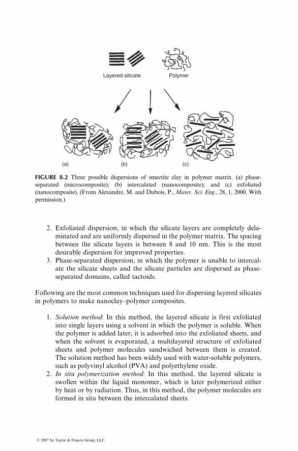
Layered silicate Polymer
(a) (b) (c)
FIGURE 8.2 Three possible dispersions of smectite clay in polymer matrix. (a) phase-
separated (microcomposite); (b) intercalated (nanocomposite); and (c) exfoliated
(nanocomposite). (From Alexandre, M. and Dubois, P.,Mater. Sci. Eng., 28, 1, 2000. With
permission.)
2. Exfoliated dispersion, in which the silicate layers are completely dela-
minated and are uniformly dispersed in the polymer matrix. The spacing
between the silicate layers is between 8 and 10 nm. This is the most
desirable dispersion for improved properties.
3. Phase-separated dispersion, in which the polymer is unable to intercal-
ate the silicate sheets and the silicate particles are dispersed as phase-
separated domains, called tactoids.
Following are the most common techniques used for dispersing layered silicates
in polymers to make nanoclay–polymer composites.
1. Solution method: In this method, the layered silicate is first exfoliated
into single layers using a solvent in which the polymer is soluble. When
the polymer is added later, it is adsorbed into the exfoliated sheets, and
when the solvent is evaporated, a multilayered structure of exfoliated
sheets and polymer molecules sandwiched between them is created.
The solution method has been widely used with water-soluble polymers,
such as polyvinyl alcohol (PVA) and polyethylene oxide.
2. In situ polymerization method: In this method, the layered silicate is
swollen within the liquid monomer, which is later polymerized either
by heat or by radiation. Thus, in this method, the polymer molecules are
formed in situ between the intercalated sheets.
� 2007 by Taylor & Francis Group, LLC.
The in situ method is commonl y used wi th thermo set pol ymers, such as
epo xy. It ha s also been used with therm oplastics, such as polystyrene
and polyam ide-6 (PA- 6), and elastomer s, such as polyuret hane and
therm oplastic polyole fins (TP Os). The first impor tant commer cial appli-
cati on of nan oclay co mposite was based on polyam ide-6 , and as dis-
closed by its developer , Toyot a Motor Corp. , it was pr epared by the
in sit u method [2]. In this case, the montmo rillonite clay was mixe d wi th
an a, v -amino acid in aqueo us hydrochlor ic acid to atta ch carboxyl
group s to the clay particles . The modified clay was then mixe d with
the caprola ctam monomer at 100 8 C, wher e it was swol len by the mon o-
mer. The ca rboxyl group s initiat ed the ring- opening polyme rization
react ion of caprola ctam to form polyam ide-6 molec ules and ionica lly
bonde d them to the clay particles . The grow th of the molec ules caused
the exfoliat ion of the clay pa rticles.
3. Melt proces sing method : The layer ed sil icate pa rticles are mixe d with the
polyme r in the liqui d state. Depen ding on the process ing conditio n and
the co mpatibil ity be tween the polyme r and the clay surface, the polyme r
molec ules can en ter into the inter layer space of the clay parti cles and can
form eithe r an intercalat ed or an exfol iated struc ture.
The melt process ing method ha s been used with a varie ty of thermo plastics ,
such as pol ypropyle ne and polyam ide-6 , using conventi onal melt pro cessing
techni ques, su ch as extrus ion and injec tion moldi ng. The high melt viscosit y of
therm oplastics and the mech anical acti on of the rotat ing screw in an ex truder
or an injec tion- molding machin e create high shear stresses whi ch tend to
delam inate the original clay stack into thinner stacks . Dif fusion of pol ymer
molecules between the layers in the stacks then tends to peel the layers away
into intercalated or exfoliated form [3].
The ability of smectite clay to greatly improve mechanical properties of
polymers was first demonstrated in the research conducted by Toyota Motor
Corp. in 1987. The properties of the nanoclay–polyamide-6 composite prepared
by the in sit u polyme rization method at Toyota Rese arch are given in Table 8.1.
With the addition of only 4.2 wt% of exfoliated montmorillonite nanoclay, the
tensile strength increased by 55% and the tensile modulus increased by 91%
compared with the base polymer, which in this case was a polyamide-6.
The other significant increase was in the heat deflection temperature (HDT).
Table 8.1 also shows the benefit of exfoliation as the properties with exfoliation
are compared with those without exfoliation. The nonexfoliated clay–PA-6
composite was prepared by simply melt blending montmorillonite clay with
PA-6 in a twin-screw extruder.
Since the publication of the Toyota research results, the development of
nanoclay-reinforced thermoplastics and thermosets has rapidly progressed.
� 2007 by Taylor & Francis Group, LLC.
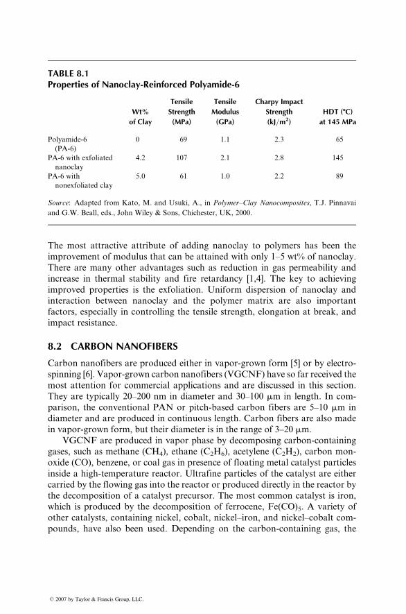
TABLE 8.1Properties of Nanoclay-Reinforced Polyamide-6
Wt%
of Clay
Tensile
Strength
(MPa)
Tensile
Modulus
(GPa)
Charpy Impact
Strength
(kJ=m2)
HDT (8C)
at 145 MPa
Polyamide-6
(PA-6)
0 69 1.1 2.3 65
PA-6 with exfoliated
nanoclay
4.2 107 2.1 2.8 145
PA-6 with
nonexfoliated clay
5.0 61 1.0 2.2 89
Source: Adapted from Kato, M. and Usuki, A., in Polymer–Clay Nanocomposites, T.J. Pinnavai
and G.W. Beall, eds., John Wiley & Sons, Chichester, UK, 2000.
The most attractive attribute of adding nanoclay to polymers has been the
improvement of modulus that can be attained with only 1–5 wt% of nanoclay.
There are many other advantages such as reduction in gas permeability and
increase in thermal stability and fire retardancy [1,4]. The key to achieving
improved properties is the exfoliation. Uniform dispersion of nanoclay and
interaction between nanoclay and the polymer matrix are also important
factors, especially in controlling the tensile strength, elongation at break, and
impact resistance.
8.2 CARBON NANOFIBERS
Carbon nanofibers are produced either in vapor-grown form [5] or by electro-
spinning [6]. Vapor-grown carbon nanofibers (VGCNF) have so far received the
most attention for commercial applications and are discussed in this section.
They are typically 20–200 nm in diameter and 30–100 mm in length. In com-
parison, the conventional PAN or pitch-based carbon fibers are 5–10 mm in
diameter and are produced in continuous length. Carbon fibers are also made
in vapor-grown form, but their diameter is in the range of 3–20 mm.
VGCNF are produced in vapor phase by decomposing carbon-containing
gases, such as methane (CH4), ethane (C2H6), acetylene (C2H2), carbon mon-
oxide (CO), benzene, or coal gas in presence of floating metal catalyst particles
inside a high-temperature reactor. Ultrafine particles of the catalyst are either
carried by the flowing gas into the reactor or produced directly in the reactor by
the decomposition of a catalyst precursor. The most common catalyst is iron,
which is produced by the decomposition of ferrocene, Fe(CO)5. A variety of
other catalysts, containing nickel, cobalt, nickel–iron, and nickel–cobalt com-
pounds, have also been used. Depending on the carbon-containing gas, the
� 2007 by Taylor & Francis Group, LLC.
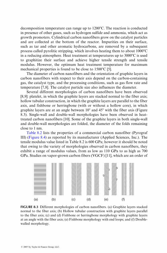
decompo sition tempe rature can range up to 1200 8 C. The react ion is conductedin presence of other gases, such a s hyd rogen sulfide and ammoni a, which act as
grow th promot ers. Cylindri cal carbon nano fibers gro w on the catalyst pa rticles
and are co llected a t the bottom of the reactor. Impu rities on their surfa ce,
such as tar and other aromat ic hyd rocarbons, are remove d by a subsequen t
process call ed pyroli tic strip ping, which invo lves he ating them to about 1000 8 Cin a redu cing atmos phere. Heat treatment at tempe ratur es up to 3000 8 C is usedto graphitize their su rface and ach ieve highe r tensi le stre ngth and tensi le
modulus. Ho wever, the optimu m heat treatment tempe ratur e for maximum
mechani cal pr operties is found to be close to 1500 8 C [5].The diame ter of carbon nano fibers an d the orient ation of graphite layers in
carbon nano fibers with respect to their axis dep end on the carbo n-conta ining
gas, the catal yst type, and the process ing co ndition s, such as gas flow rate and
tempe rature [7,8 ]. The cataly st particle size also influences the diameter.
Several different morph ologies of carbo n nano fibers have bee n observed
[8,9]: plate let, in whi ch the grap hite layer s are stacke d normal to the fiber axis;
hollow tubular constr uction, in which the graphit e layer s are parall el to the fiber
axis, and fishb one or herri ngbo ne (w ith or wi thout a hollow core), in which
graphit e layer s are at an angle be tween 10 8 and 458 with the fiber axis (F igure8.3). Single -wall and doubl e-wall morph ologies ha ve been observed in he at-
treated carbon nanofibe rs [10] . Some of the graphit e layer s in bot h singl e-wall
and double-wal l morpho logies are folded, the diame ter of the folds remaining
close to 1 nm.
Table 8.2 lists the propert ies of a co mmercial carbon nanofibe r (Pyrogr af
III) (F igure 8.4) as repo rted by its manufa cturer (Applied Sc iences, Inc.) . The
tensile modulus value listed in Table 8.2 is 600 GPa; however it should be noted
that owing to the variety of morphologies observed in carbon nanofibers, they
exhibit a range of modulus values, from as low as 110 GPa to as high as 700
GPa. Studies on vapor-grown carbon fibers (VGCF) [11], which are an order of
(a) (b) (c) (d) (e) (f)
FIGURE 8.3 Different morphologies of carbon nanofibers. (a) Graphite layers stacked
normal to the fiber axis; (b) Hollow tubular construction with graphite layers parallel
to the fiber axis; (c) and (d) Fishbone or herringbone morphology with graphite layers
at an angle with the fiber axis; (e) Fishbone morphology with end loops; and (f) Double-
walled morphology.
� 2007 by Taylor & Francis Group, LLC.
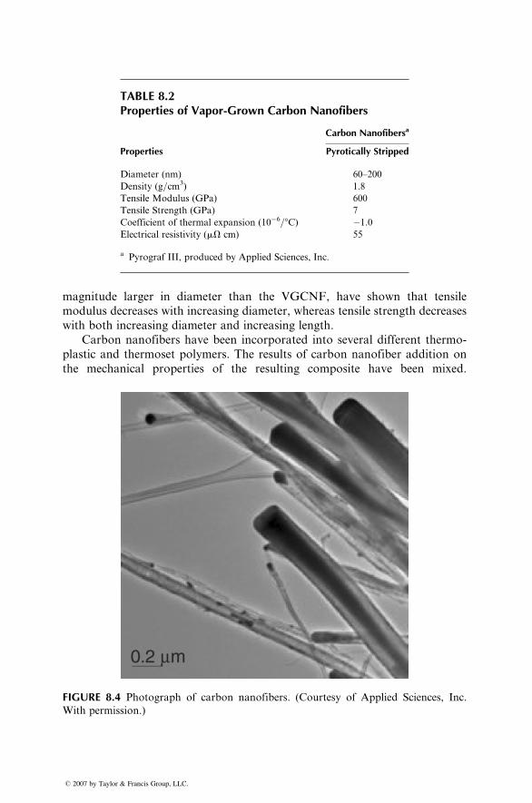
TABLE 8.2Properties of Vapor-Grown Carbon Nanofibers
Carbon Nanofibersa
Properties Pyrotically Stripped
Diameter (nm) 60–200
Density (g=cm3) 1.8
Tensile Modulus (GPa) 600
Tensile Strength (GPa) 7
Coefficient of thermal expansion (10�6=8C) �1.0
Electrical resistivity (mV cm) 55
a Pyrograf III, produced by Applied Sciences, Inc.
magnitude larger in diameter than the VGCNF, have shown that tensile
modulus decreases with increasing diameter, whereas tensile strength decreases
with both increasing diameter and increasing length.
Carbon nanofibers have been incorporated into several different thermo-
plastic and thermoset polymers. The results of carbon nanofiber addition on
the mechanical properties of the resulting composite have been mixed.
FIGURE 8.4 Photograph of carbon nanofibers. (Courtesy of Applied Sciences, Inc.
With permission.)
� 2007 by Taylor & Francis Group, LLC.
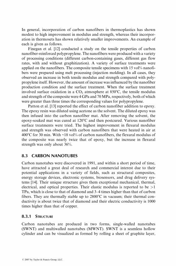
In general, incorporation of carbon nanofibers in thermoplastics has shown
modest to high improvement in modulus and strength, whereas their incorpor-
ation in thermosets has shown relatively smaller improvements. An example of
each is given as follows.
Finegan et al. [12] conducted a study on the tensile properties of carbon
nanofiber-reinforced polypropylene. The nanofibers were produced with a variety
of processing conditions (different carbon-containing gases, different gas flow
rates, with and without graphitization). A variety of surface treatments were
applied on the nanofibers. The composite tensile specimens with 15 vol% nanofi-
bers were prepared using melt processing (injection molding). In all cases, they
observed an increase in both tensile modulus and strength compared with poly-
propylene itself. However, the amount of increase was influenced by the nanofiber
production condition and the surface treatment. When the surface treatment
involved surface oxidation in a CO2 atmosphere at 8508C, the tensile modulus
and strength of the composite were 4GPa and 70MPa, respectively, both ofwhich
were greater than three times the corresponding values for polypropylene.
Patton et al. [13] reported the effect of carbon nanofiber addition to epoxy.
The epoxy resin was diluted using acetone as the solvent. The diluted epoxy was
then infused into the carbon nanofiber mat. After removing the solvent, the
epoxy-soaked mat was cured at 1208C and then postcured. Various nanofiber
surface treatments were tried. The highest improvement in flexural modulus
and strength was observed with carbon nanofibers that were heated in air at
4008C for 30 min. With ~18 vol% of carbon nanofibers, the flexural modulus of
the composite was nearly twice that of epoxy, but the increase in flexural
strength was only about 36%.
8.3 CARBON NANOTUBES
Carbon nanotubes were discovered in 1991, and within a short period of time,
have attracted a great deal of research and commercial interest due to their
potential applications in a variety of fields, such as structural composites,
energy storage devices, electronic systems, biosensors, and drug delivery sys-
tems [14]. Their unique structure gives them exceptional mechanical, thermal,
electrical, and optical properties. Their elastic modulus is reported to be >1
TPa, which is close to that of diamond and 3–4 times higher than that of carbon
fibers. They are thermally stable up to 28008C in vacuum; their thermal con-
ductivity is about twice that of diamond and their electric conductivity is 1000
times higher than that of copper.
8.3.1 STRUCTURE
Carbon nanotubes are produced in two forms, single-walled nanotubes
(SWNT) and multiwalled nanotubes (MWNT). SWNT is a seamless hollow
cylinder and can be visualized as formed by rolling a sheet of graphite layer,
� 2007 by Taylor & Francis Group, LLC.
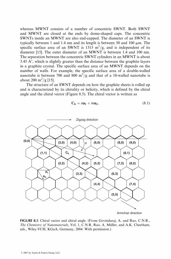
whereas MWNT consists of a number of concentric SWNT. Both SWNT
and MWNT are closed at the ends by dome-shaped caps. The concentric
SWNTs inside an MWNT are also end-capped. The diameter of an SWNT is
typically between 1 and 1.4 nm and its length is between 50 and 100 mm. The
specific surface area of an SWNT is 1315 m2=g, and is independent of its
diameter [15]. The outer diameter of an MWNT is between 1.4 and 100 nm.
The separation between the concentric SWNT cylinders in an MWNT is about
3.45 A8, which is slightly greater than the distance between the graphite layers
in a graphite crystal. The specific surface area of an MWNT depends on the
number of walls. For example, the specific surface area of a double-walled
nanotube is between 700 and 800 m2=g and that of a 10-walled nanotube is
about 200 m2=g [15].
The structure of an SWNT depends on how the graphite sheets is rolled up
and is characterized by its chirality or helicity, which is defined by the chiral
angle and the chiral vector (Figure 8.5). The chiral vector is written as
Ch ¼ na1 þma2, (8:1)
Zigzag direction
(0,0)
(1,1) Ch
(3,0)
(2,2)
a1a2
(3,3)
(4,4)
(5,5)
Armchair direction
(7,4)
(6,3)
(4,2) (5,2) (7,2) (8,2)
(4,0) (6,0)θ (8,0)
(8,1)
(9,0)
FIGURE 8.5 Chiral vector and chiral angle. (From Govindaraj, A. and Rao, C.N.R.,
The Chemistry of Nanomaterials, Vol. 1, C.N.R. Rao, A. Muller, and A.K. Cheetham,
eds., Wiley-VCH, KGaA, Germany, 2004. With permission.)
� 2007 by Taylor & Francis Group, LLC.
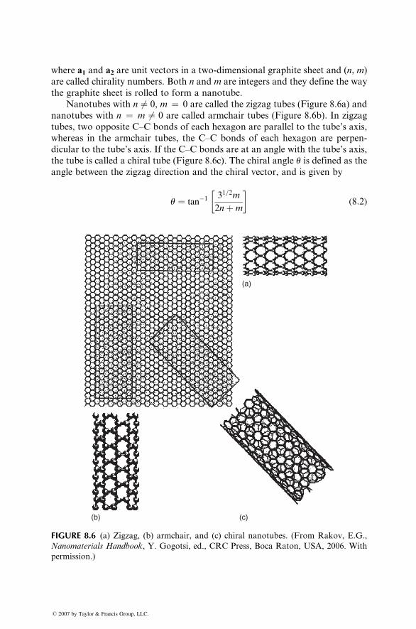
where a1 and a2 are unit vectors in a two-dimensional graphite sheet and (n, m)
are called chirality numbers. Both n and m are integers and they define the way
the graphite sheet is rolled to form a nanotube.
Nanotubes with n 6¼ 0, m ¼ 0 are called the zigzag tubes (Figure 8.6a) and
nanotubes with n ¼ m 6¼ 0 are called armchair tubes (Figure 8.6b). In zigzag
tubes, two opposite C–C bonds of each hexagon are parallel to the tube’s axis,
whereas in the armchair tubes, the C–C bonds of each hexagon are perpen-
dicular to the tube’s axis. If the C–C bonds are at an angle with the tube’s axis,
the tube is called a chiral tube (Figure 8.6c). The chiral angle u is defined as the
angle between the zigzag direction and the chiral vector, and is given by
u ¼ tan�1 31=2m
2nþm
� �(8:2)
(a)
(b) (c)
FIGURE 8.6 (a) Zigzag, (b) armchair, and (c) chiral nanotubes. (From Rakov, E.G.,
Nanomaterials Handbook, Y. Gogotsi, ed., CRC Press, Boca Raton, USA, 2006. With
permission.)
� 2007 by Taylor & Francis Group, LLC.
and 0� � u � 30�. The diameter of the nanotube is given by
d ¼ aoffiffiffi3
p
p
ffiffiffiffiffiffiffiffiffiffiffiffiffiffiffiffiffiffiffiffiffiffiffiffiffiffiffiffim2 þmnþ n2
p, (8:3)
where ao ¼ C–C bond length, which is equal to 1.42 A.
The chirality of a carbon nanotube has a significant influence on its electrical
and mechanical properties. Depending on the chirality, a carbon nanotube can
behave either as a metallic material or a semiconducting material. For example,
armchair nanotubes are metallic; nanotubes with (n�m) ¼ 2k, where k is a
nonzero integer, are semiconductors with a tiny band gap, and all other nano-
tubes are semiconductors with a band gap that inversely varies with the nanotube
diameter. Chirality also controls the deformation characteristics of carbon
nanotubes subjected to tensile stresses and therefore, determines whether they
will fracture like a brittle material or deform like a ductile material [16].
The current processing methods used for making carbon nanotubes intro-
duce two types of defect in their structures: topological defects and structural
defects. The examples of topological defects are pentagonal and heptagonal
arrangements of carbon atoms, whichmay bemixedwith the hexagonal arrange-
ments. The structural defects include nontubular configurations, such as cone-
shaped end caps, bent shapes, branched construction with two or more tubes
connected together, and bamboo-like structure in which several nanotubes are
joined in the lengthwise direction. In general, MWNTs contain more defects
than SWNTs.
Carbon nanotubes can form secondary structures. One of these secondary
structures is the SWNT rope or bundle, which is a self-assembled close-
packed array of many (often thousands or more) SWNTs. The self-assembly
occurs at the time of forming the SWNTs, due to the attractive forces between
them arising from binding energy of 500–900 eV=nm. If the arrangement
of SWNTs in the array is well ordered (e.g., with hexagonal lattice structure),
it is called a rope. If the arrangement of SWNTs is not ordered, it is called
a bundle [17].
8.3.2 PRODUCTION OF CARBON NANOTUBES
There are three main methods for producing carbon nanotubes: electric arc
discharge, laser ablation, and chemical vapor deposition (CVD) [18]. The
quantity of production of carbon nanotubes by the first two methods is
relatively small. Since CVD can produce larger quantities of carbon nanotubes
and is more versatile, it has become the focus of attention for industrial
production and several different variations of the basic CVD process
(e.g., plasma-enhanced CVD or PECVD process and high-pressure carbon
monoxide or HiPco process) have been developed. However, the structure of
nanotubes produced by CVD is usually different from that of nanotubes
� 2007 by Taylor & Francis Group, LLC.
produced by the other two methods. For example, the CVD-produced
MWNTs are less crystalline and contain more defects than the arc-discharged
MWNTs. The CVD-produced MWNTs are longer and less straight than the
arc-discharged MWNTs.
The arc discharge method uses two graphite rods; one serving as the
cathode and the other serving as the anode, in either helium, argon, or a
mixture of helium and argon atmosphere. The graphite rods are placed side
by side with a very small gap, typically about 1 mm in size, between them. The
pressure inside the reaction chamber is maintained between 100 and 1000 torr.
When a stable arc is produced in the gap by passing 50–120 A electric current
(at 12–25 V) between the graphite rods, the material eroded from the anode is
deposited on the cathode in the form of MWNTs, amorphous carbon, and
other carbon particles. To produce SWNTs, the cathode is doped with a small
amount of metallic catalyst (Fe, Co, Ni, Y, or Mo). However, the yield of
SWNTs is only between 20% and 40% by weight.
The laser ablation method uses either pulsed or continuous-wave laser to
vaporize a graphite target held at 12008C in a controlled atmosphere of argon
or helium inside a tube furnace. The vaporized material is collected on a water-
cooled copper collector in the form of carbon nanotubes, amorphous carbon,
and other carbon particles. To produce SWNTs, the graphite target is doped
with metal catalysts such as nickel and cobalt catalysts. The yield of SWNTs is
between 20% and 80% by weight.
In the basic CVD method, carbon nanotubes are produced by the decom-
position of a carbon-containing gas, such as carbon monoxide and hydrocar-
bon gases, or by the pyrolysis of carbon-containing solids, such as polymers, at
a high pressure inside a furnace. The temperature inside the furnace is typically
between 3008C and 8008C for making MWNTs, and 6008C and 12008C for
making SWNTs. MWNTs are produced in an inert gas atmosphere, whereas a
mixture of hydrogen and an inert gas is used for SWNTs. A high-temperature
substrate, such as alumina, coated with catalyst particles, such as Fe, Ni, and
Co, is placed in the furnace. The decomposition of the carbon-containing gas
flowing over the substrate causes the growth of carbon nanotubes on the
substrate. They are collected after cooling the system down to room tempera-
ture. Depending on the carbon-containing gas, catalyst, furnace temperature,
pressure, flow rate, residence time for thermal decomposition, and so on, the
yield can be between 30% and 99% by weight.
All three production methods produce carbon nanotubes that are contam-
inated with impurities such as amorphous carbon, carbon soot, other carbon
particles, and metal catalysts. Several purification processes have been devel-
oped to produce cleaner carbon nanotubes. Two of the processes are gas
phase oxidation and liquid phase purification. Purification of MWNTs by
gas phase oxidation involves heating them in an oxygen or air atmosphere
at temperatures >7008C. In the case of SWNT, it involves heating in a mixed
atmosphere of hydrochloric acid, chlorine, and water vapor at 5008C.
� 2007 by Taylor & Francis Group, LLC.
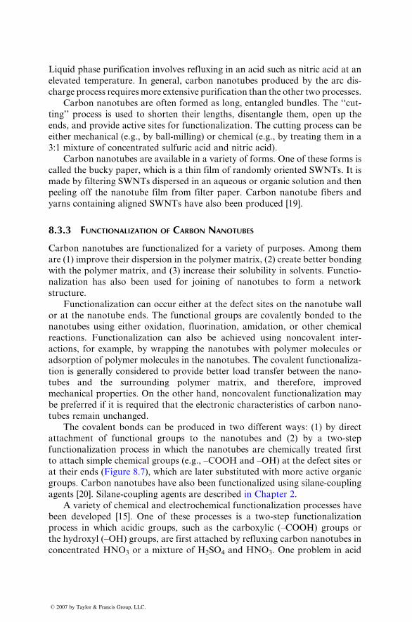
Liquid pha se purificat ion involv es refl uxing in an acid such as nitr ic acid at an
elevated tempe ratur e. In general , carbon nano tubes pro duced by the arc dis-
charge process requir es more extens ive purificat ion than the other two process es.
Carb on nanotub es are often form ed as long, entangl ed bundl es. The ‘‘cut -
ting’’ process is used to sh orten their length s, disentang le them, open up the
ends, and pro vide active sit es for functi onaliz ation. The cutting process can be
either mechan ical (e.g., by ball-mi lling) or ch emical (e.g., by treating them in a
3:1 mixt ure of concen trated sulfu ric acid and nitric acid).
Carb on nano tubes are available in a varie ty of form s. One of these form s is
called the bucky paper, which is a thin film of rando mly orient ed SWNTs. It is
made by filtering SWNTs dispersed in an aqueous or organic solut ion an d then
peelin g off the nano tube film from filter pa per. Carb on nanotube fibers and
yarns contain ing alig ned SWNT s have also been produce d [19] .
8.3.3 FUNCTIONALIZATION OF C ARBON NANOTUBES
Carbo n nan otubes are func tionalized for a variety of purposes. Among them
are (1) improv e their dispersion in the polyme r matr ix, (2) creat e better bonding
with the polyme r matrix, and (3) increa se their solub ility in solvent s. Funct io-
nalizati on has also been used for joining of nan otubes to form a netw ork
structure.
Function alizatio n can occu r eithe r at the defect sites on the nano tube wal l
or at the nano tube en ds. The functio nal group s are co valently bonde d to the
nanotub es using either oxidat ion, fluor ination, amida tion, or other chemic al
reaction s. Functional ization can also be ach ieved using nonco valent inter-
action s, for exa mple, by wrapp ing the nano tubes wi th polyme r molec ules or
adsorpt ion of polyme r molec ules in the nano tubes. The covalent functi onaliz a-
tion is general ly consider ed to provide better load transfer between the nano -
tubes and the surroundi ng polyme r matrix, an d theref ore, impr oved
mechani cal prop erties. On the other hand, nonc ovalent functiona lization may
be pre ferred if it is requir ed that the electron ic charact eristics of carbon nano -
tubes remain unch anged.
The covalent bonds can be prod uced in two different ways : (1) by direct
attachmen t of functi onal groups to the na notubes and (2) by a two-st ep
functio nalizati on process in which the nan otubes are chemi cally treated fir st
to attach sim ple ch emical groups (e.g ., –COOH and –OH ) at the defect sites or
at their en ds (Figur e 8.7), whi ch are late r substitut ed with mo re active organ ic
groups. Carb on nan otubes have also be en functio nalized using silane-coup ling
agents [20] . Silane -coupli ng agents are descri bed in Chapt er 2.
A variety of chemical and electrochemical functionalization processes have
been developed [15]. One of these processes is a two-step functionalization
process in which acidic groups, such as the carboxylic (–COOH) groups or
the hydroxyl (–OH) groups, are first attached by refluxing carbon nanotubes in
concentrated HNO3 or a mixture of H2SO4 and HNO3. One problem in acid
� 2007 by Taylor & Francis Group, LLC.
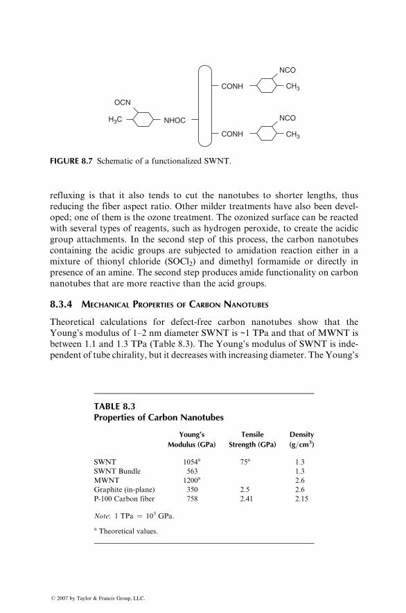
CONH
NCO
CH3
CH3CONH
NCO NHOC H3C
OCN
FIGURE 8.7 Schematic of a functionalized SWNT.
refluxing is that it also tends to cut the nanotubes to shorter lengths, thus
reducing the fiber aspect ratio. Other milder treatments have also been devel-
oped; one of them is the ozone treatment. The ozonized surface can be reacted
with several types of reagents, such as hydrogen peroxide, to create the acidic
group attachments. In the second step of this process, the carbon nanotubes
containing the acidic groups are subjected to amidation reaction either in a
mixture of thionyl chloride (SOCl2) and dimethyl formamide or directly in
presence of an amine. The second step produces amide functionality on carbon
nanotubes that are more reactive than the acid groups.
8.3.4 MECHANICAL PROPERTIES OF CARBON NANOTUBES
Theoretical calculations for defect-free carbon nanotubes show that the
Young’s modulus of 1–2 nm diameter SWNT is ~1 TPa and that of MWNT is
between 1.1 and 1.3 TPa (Table 8.3). The Young’s modulus of SWNT is inde-
pendent of tube chirality, but it decreases with increasing diameter. The Young’s
TABLE 8.3Properties of Carbon Nanotubes
Young’s
Modulus (GPa)
Tensile
Strength (GPa)
Density
(g=cm3)
SWNT 1054a 75a 1.3
SWNT Bundle 563 1.3
MWNT 1200a 2.6
Graphite (in-plane) 350 2.5 2.6
P-100 Carbon fiber 758 2.41 2.15
Note: 1 TPa ¼ 103 GPa.
a Theoretical values.
� 2007 by Taylor & Francis Group, LLC.
modulus of MWNT is higher than that of SWNT due to contributions from
the van der Waals forces between the concentric SWNTs in MWNT [14].
Experimental determination of the mechanical properties of carbon nano-
tubes is extremely difficult and has produced a variety of results. Several
investigators have used atomic force microscope (AFM) to determine the
Young’s modulus and strength. The Young’s modulus of MWNT determined
on AFM has ranged from 0.27 to 1.8 TPa and that of SWNT ranges from 0.32
to 1.47 TPa. Similarly, the strength of MWNT ranges from 11 to 63 GPa and
that of SWNT from 10 to 52 GPa. In the TPM experiments, the carbon
nanotubes have also shown high tensile strain (up to 15%) before fracture. It
has also been observed that carbon nanotubes exhibit nonlinear elastic deform-
ation under tensile, bending, as well as twisting loads. At high strains, they tend
to buckle of the wall.
The large variation in Young’s modulus and strength is attributed to the fact
that nanotubes produced by the current production methods may vary in length,
diameter, number of walls, chirality, and even atomic structure [21]. Further-
more, nanotubes produced by different methods contain different levels of
defects and impurities, which influence their mechanical properties. For
example, the Young’s modulus of CVD-produced MWNTs is found to be an
order of magnitude lower than that of the arc-dischargedMWNTs, which is due
to the presence of higher amount of defects in the CVD-produced MWNTs.
8.3.5 CARBON NANOTUBE–POLYMER COMPOSITES
The three principal processing methods for combining carbon nanotubes with
polymer matrix [22,23] are (1) in situ polymerization, (2) solution processing,
and (3) melt processing.
1. In Situ Polymerization: In this process, the nanotubes are first dispersed
in the monomer and then the polymerization reaction is initiated to
transform the monomer to polymer. Depending on the polymer formed
and the surface functionality of the nanotubes, the polymer molecules
are either covalently bonded to the nanotubes or wrapped around the
nanotubes at the completion of the polymerization reaction.
2. Solution Processing: In this process, the nanotubes are mixed with a
polymer solution, which is prepared by dissolving the polymer in a
suitable solvent. The mixing is done using magnetic stirring, high shear
mixing, or sonication. The dispersion of the nanotubes in the solution
can be improved by treating them with a surfactant, such as derivatives
of sodium dodecylsulfate. The solution is poured in a casting mold and
the solvent is allowed to evaporate. The resulting material is a cast film
or sheet of carbon nanotube-reinforced polymer.
3. Melt Processing: Melt processing is the preferred method for incorpor-
ating carbon nanotubes in thermoplastics, particularly for high volume
� 2007 by Taylor & Francis Group, LLC.
app lications . It has been used with a variety of therm oplast ics, such as
high-de nsit y pol yethylene, polyprop ylene, polyst yrene, polycar bona te,
and polyam ide-6. In this pro cess, the na notubes are blend ed with the
liqui d polyme r in a high shear mixer or in an extrude r. The blen d is then
process ed to produce the final produ ct us ing injection moldi ng, extru-
sion, or compres sion moldi ng. It is important to note that the ad dition
of carbon nanotubes increa ses the viscos ity of the liquid polyme r, and
theref ore, proper adjustment s ne ed to be made in the pr ocess parame ters
to mold a goo d product.
Carb on nan otubes have also been used with therm oset polyme rs such as epoxy
and vinyl ester. They are disper sed in the liqui d therm oset prepo lymer using
sonicat ion. Aft er mixi ng the blend with a ha rdener or curing initiat or, it is
poured into a casting mold, whi ch is then heated to the cu ring tempe ratur e.
Curing ca n be cond ucted in vacuum to reduce the vo id co ntent in the co mpos-
ite. To impro ve the disper sion of the nano tubes, the viscos ity of the therm oset
prepolym er can be reduced with a so lvent that can be evapo rated late r.
8.3.6 P ROPERTIES OF CARBON NANOTUBE –POLYMER COMPOSITES
Based on the mechani cal prope rties of carbon na notubes descri bed in Se ction
8.3.4, it is exp ected that the incorpora tion of carbo n nanotubes in a pol ymer
matrix will creat e c omposi tes with very high modu lus and stre ngth. Indee d,
many studi es ha ve shown that with prop er disper sion of nano tubes in the
polyme r matr ix, signifi cant impr ovement in mechan ical propert ies can be
achieve d compared wi th the ne at polyme r. Three example s are given as follows .
In the first exampl e, CVD-p roduced MWNTs were disper sed in a toluene
solut ion of polyst yrene using an ultr asonic bath [24]. The mean external
diame ter of the MW NTs was 30 nm and their lengt h was betw een 50 and 55
mm. No functi onaliz ation treatment s were used. MWNT-r einfor ced polyst yr-
ene film was produ ced by solution casting . Tensile propert ies of the solution
cast films given in Table 8.4 show that both elastic modu lus an d tensile
stren gth increa sed wi th increa sing MWNT weight fraction. With the ad dition
of 5 wt% MWNT , the elastic modu lus of the compo site was 120% higher and
the tensi le stren gth was 57% higher than the corres pondi ng pro perties of
polyst yrene.
The secon d exampl e involv es melt-pr ocessed MWNT-r einfor ced poly-
amide -6 [25] . The MW NTs, in this exampl e, was also prep ared by CVD and
functio nalized by treating them in nitr ic acid. The MWNTs an d polyam ide-6
were melt-compounded in a twin-screw mixer and film specimens were prepared
by compression molding. The MWNT content in the composite was 1 wt%. As
shown in Tabl e 8.5, both tensile modulus and strength of the co mposite were
significantly higher compared with the tensile modulus and strength of poly-
amide-6. However, the elongation at break was decreased.
� 2007 by Taylor & Francis Group, LLC.
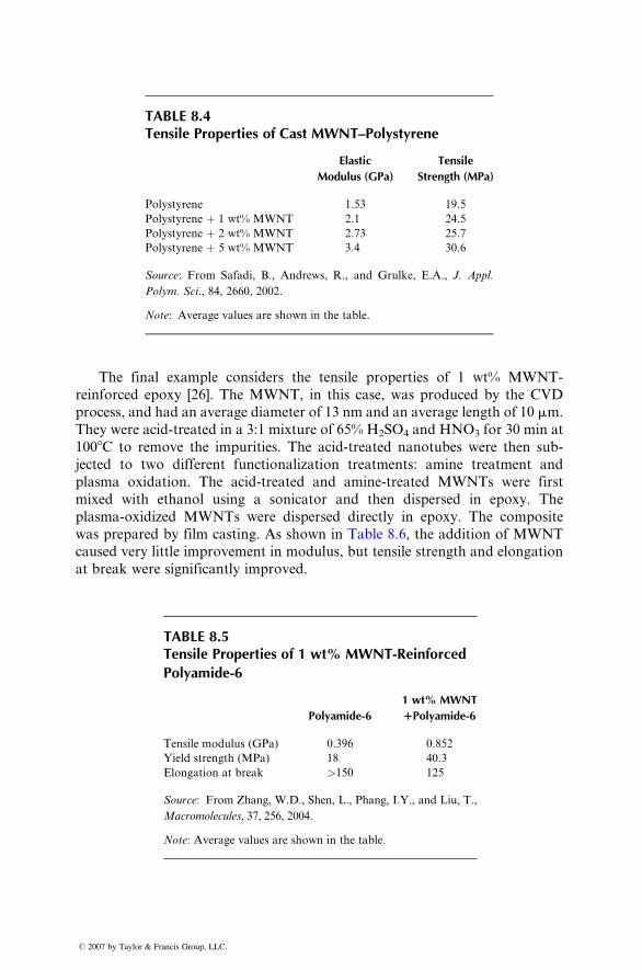
TABLE 8.4Te nsile Pro perties of Cast MWN T–Polys tyrene
Elastic
Modulus (GPa)
Tensile
Strength (MPa)
Polystyrene 1.53 19.5
Polystyrene þ 1 wt% MWNT 2.1 24.5
Polystyrene þ 2 wt% MWNT 2.73 25.7
Polystyrene þ 5 wt% MWNT 3.4 30.6
Source: From Safadi, B., Andrews, R., and Grulke, E.A., J. Appl.
Polym. Sci., 84, 2660, 2002.
Note: Average values are shown in the table.
The final exampl e consider s the tensile propert ies of 1 wt% MWNT-
reinforced epoxy [26]. The MWNT, in this case, was produced by the CVD
process , an d had an average diame ter of 13 nm an d an average length of 10 m m.
They were acid- treated in a 3:1 mixtu re of 65% H2SO 4 and HNO 3 for 30 min at
100 8 C to remove the impur ities. The acid-trea ted nanotub es were then sub -
jected to two different functio nalizati on treat ments: amine treat ment and
plasma oxidat ion. The acid-trea ted an d amine -treated MWNTs were fir st
mixed wi th ethano l using a sonicator and then disper sed in e poxy. The
plasma -oxidized MWNT s wer e disper sed directly in ep oxy. The co mposi te
was prepared by film casti ng. As shown in Tabl e 8.6, the additi on of MWNT
caused very littl e impr ovement in modulus, but tensile stre ngth an d elong ation
at break wer e signi fican tly impro ved.
TABLE 8.5Tensile Properties of 1 wt% MWNT-Reinforced
Polyamide-6
Polyamide-6
1 wt% MWNT
1Polyamide-6
Tensile modulus (GPa) 0.396 0.852
Yield strength (MPa) 18 40.3
Elongation at break >150 125
Source: From Zhang, W.D., Shen, L., Phang, I.Y., and Liu, T.,
Macromolecules, 37, 256, 2004.
Note: Average values are shown in the table.
� 2007 by Taylor & Francis Group, LLC.
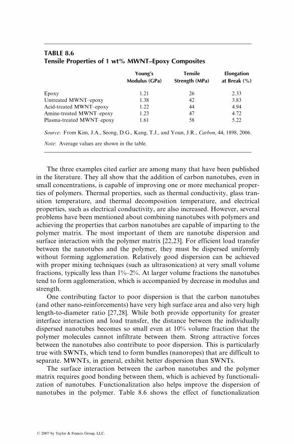
TABLE 8.6Tensile Properties of 1 wt% MWNT–Epoxy Composites
Young’s
Modulus (GPa)
Tensile
Strength (MPa)
Elongation
at Break (%)
Epoxy 1.21 26 2.33
Untreated MWNT–epoxy 1.38 42 3.83
Acid-treated MWNT–epoxy 1.22 44 4.94
Amine-treated MWNT–epoxy 1.23 47 4.72
Plasma-treated MWNT–epoxy 1.61 58 5.22
Source: From Kim, J.A., Seong, D.G., Kang, T.J., and Youn, J.R., Carbon, 44, 1898, 2006.
Note: Average values are shown in the table.
The three examples cited earlier are among many that have been published
in the literature. They all show that the addition of carbon nanotubes, even in
small concentrations, is capable of improving one or more mechanical proper-
ties of polymers. Thermal properties, such as thermal conductivity, glass tran-
sition temperature, and thermal decomposition temperature, and electrical
properties, such as electrical conductivity, are also increased. However, several
problems have been mentioned about combining nanotubes with polymers and
achieving the properties that carbon nanotubes are capable of imparting to the
polymer matrix. The most important of them are nanotube dispersion and
surface interaction with the polymer matrix [22,23]. For efficient load transfer
between the nanotubes and the polymer, they must be dispersed uniformly
without forming agglomeration. Relatively good dispersion can be achieved
with proper mixing techniques (such as ultrasonication) at very small volume
fractions, typically less than 1%–2%. At larger volume fractions the nanotubes
tend to form agglomeration, which is accompanied by decrease in modulus and
strength.
One contributing factor to poor dispersion is that the carbon nanotubes
(and other nano-reinforcements) have very high surface area and also very high
length-to-diameter ratio [27,28]. While both provide opportunity for greater
interface interaction and load transfer, the distance between the individually
dispersed nanotubes becomes so small even at 10% volume fraction that the
polymer molecules cannot infiltrate between them. Strong attractive forces
between the nanotubes also contribute to poor dispersion. This is particularly
true with SWNTs, which tend to form bundles (nanoropes) that are difficult to
separate. MWNTs, in general, exhibit better dispersion than SWNTs.
The surface interaction between the carbon nanotubes and the polymer
matrix requires good bonding between them, which is achieved by functionali-
zation of nanotubes. Functionalization also helps improve the dispersion of
nanotubes in the polymer. Table 8.6 shows the effect of functionalization
� 2007 by Taylor & Francis Group, LLC.
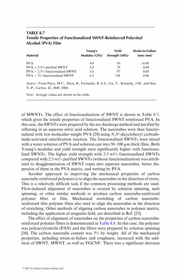
TABLE 8.7Tensile Properties of Functionalized SWNT-Reinforced Polyvinyl
Alcohol (PVA) Film
Material
Young’s
Modulus (GPa)
Yield
Strength (MPa)
Strain-to-Failure
(mm=mm)
PVA 4.0 83 >0.60
PVA þ 2.5% purified SWNT 5.4 79 0.09
PVA þ 2.5% functionalized SWNT 5.6 97 0.05
PVA þ 5% functionalized SWNT 6.2 128 0.06
Source: From Paiva, M.C., Zhou, B., Fernando, K.A.S., Lin, Y., Kennedy, J.M., and Sun,
Y.-P., Carbon, 42, 2849, 2004.
Note: Average values are shown in the table.
of M WNTs. The effect of functi onaliz ation of SWNT is sho wn in Table 8.7,
which gives the tensi le pro perties of functio nalized SWNT-r einfor ced PVA. In
this case, the SWNT s were prepared by the arc discharge method an d purif ied by
refluxing in an aqu eous nitr ic acid solution. The nano tubes wer e then functio -
nalized wi th low-mol ecular -weight PVA [29] using N , N0 -dicy clohexyl carbodii -mide-acti vated ester ification react ion. The functi onaliz ed SW NTs wer e mixe d
with a water solut ion of PVA and solut ion cast into 50–100 m m thick films. Both
Young’ s mo dulus a nd yield stre ngth wer e signifi cantly higher with function a-
lized SW NTs. The high er yield stre ngth with 2.5 wt% functi onalized SWNTs
compared with 2.5 wt% purif ied SWNTs (w ithout functi onaliz ation) was attr ib-
uted to deagglom eration of SW NT rop es into separat e nan otubes, bette r dis-
persio n of them in the PVA matr ix, and wettin g by PVA .
Anothe r approach to improving the mecha nical prop erties of carbon
nanotub e-reinforc ed polyme rs is to alig n the na notubes in the direction of stre ss.
This is a relative ly diff icult task if the common process ing method s are used .
Flow-indu ced alig nment of nanotub es is creat ed by solut ion sp inning, melt
spinni ng, or other similar methods to pro duce carbon nano tube-reinf orced
polyme r fiber or film. Me chanical stre tching of carbon nanotube-
reinforced thin polyme r fil ms also tend to align the nano tubes in the direction
of stretchi ng. Other methods of align ing carbon nano tubes in polyme r matr ix,
includin g the application of magnet ic fiel d, are descri bed in Ref . [23] .
The effe ct of alig nment of nanotubes on the prop erties of carbon nano tube-
reinforced polyme r fibers is demonst rated in Tabl e 8.8. In this case, the poly mer
was pol yacrylon itrile (PAN) and the fibers wer e prepared by solut ion spinni ng
[30]. The carb on nano tube content was 5% by weight. All of the mech anical
propert ies, includin g stra in-at-fail ure and toughness , increa sed with the add -
ition of SW NT, MWNT , as wel l as VG CNF. There was a signifi cant decreas e
� 2007 by Taylor & Francis Group, LLC.
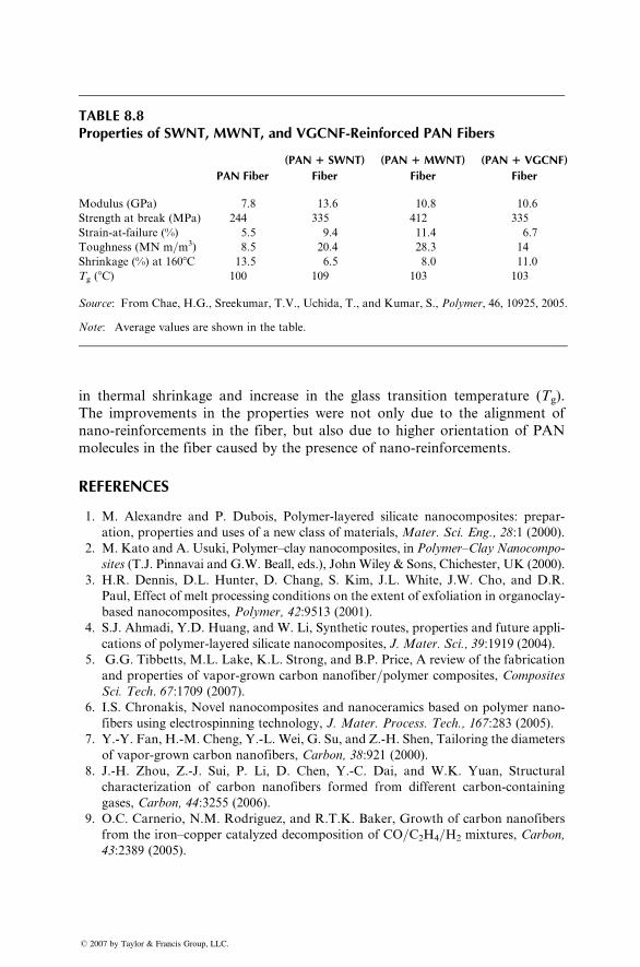
TABLE 8.8Properties of SWNT, MWNT, and VGCNF-Reinforced PAN Fibers
PAN Fiber
(PAN 1 SWNT)
Fiber
(PAN 1 MWNT)
Fiber
(PAN 1 VGCNF)
Fiber
Modulus (GPa) 7.8 13.6 10.8 10.6
Strength at break (MPa) 244 335 412 335
Strain-at-failure (%) 5.5 9.4 11.4 6.7
Toughness (MN m=m3) 8.5 20.4 28.3 14
Shrinkage (%) at 1608C 13.5 6.5 8.0 11.0
Tg (8C) 100 109 103 103
Source: From Chae, H.G., Sreekumar, T.V., Uchida, T., and Kumar, S., Polymer, 46, 10925, 2005.
Note: Average values are shown in the table.
in thermal shrinkage and increase in the glass transition temperature (Tg).
The improvements in the properties were not only due to the alignment of
nano-reinforcements in the fiber, but also due to higher orientation of PAN
molecules in the fiber caused by the presence of nano-reinforcements.
REFERENCES
1.
� 20
M. Alexandre and P. Dubois, Polymer-layered silicate nanocomposites: prepar-
ation, properties and uses of a new class of materials, Mater. Sci. Eng., 28:1 (2000).
2.
M. Kato and A. Usuki, Polymer–clay nanocomposites, in Polymer–Clay Nanocompo-sites (T.J. Pinnavai and G.W. Beall, eds.), JohnWiley & Sons, Chichester, UK (2000).
3.
H.R. Dennis, D.L. Hunter, D. Chang, S. Kim, J.L. White, J.W. Cho, and D.R.Paul, Effect of melt processing conditions on the extent of exfoliation in organoclay-
based nanocomposites, Polymer, 42:9513 (2001).
4.
S.J. Ahmadi, Y.D. Huang, and W. Li, Synthetic routes, properties and future appli-cations of polymer-layered silicate nanocomposites, J. Mater. Sci., 39:1919 (2004).
5.
G.G. Tibbetts, M.L. Lake, K.L. Strong, and B.P. Price, A review of the fabricationand properties of vapor-grown carbon nanofiber=polymer composites, Composites
Sci. Tech. 67:1709 (2007).
6.
I.S. Chronakis, Novel nanocomposites and nanoceramics based on polymer nano-fibers using electrospinning technology, J. Mater. Process. Tech., 167:283 (2005).
7.
Y.-Y. Fan, H.-M. Cheng, Y.-L. Wei, G. Su, and Z.-H. Shen, Tailoring the diametersof vapor-grown carbon nanofibers, Carbon, 38:921 (2000).
8.
J.-H. Zhou, Z.-J. Sui, P. Li, D. Chen, Y.-C. Dai, and W.K. Yuan, Structuralcharacterization of carbon nanofibers formed from different carbon-containing
gases, Carbon, 44:3255 (2006).
9.
O.C. Carnerio, N.M. Rodriguez, and R.T.K. Baker, Growth of carbon nanofibersfrom the iron–copper catalyzed decomposition of CO=C2H4=H2 mixtures, Carbon,
43:2389 (2005).
07 by Taylor & Francis Group, LLC.
10.
� 20
T. Uchida, D.P. Anderson, M. Minus, and S. Kumar, Morphology and modulus of
vapor grown carbon nano fibers, J. Mater. Sci., 41:5851 (2006).
11.
F.W.J. van Hattum, J.M. Benito-Romero, A. Madronero, and C.A. Bernardo,Morphological, mechanical and interfacial analysis of vapour-grown carbon fibres,
Carbon, 35:1175 (1997).
12.
I.C. Finegan, G.G. Tibbetts, D.G. Glasgow, J.-M. Ting, and M.L. Lake, Surfacetreatments for improving the mechanical properties of carbon nanofiber=thermo-
plastic composites, J. Mater. Sci., 38:3485 (2003).
13.
R.D. Patton, C.U. Pittman, Jr., L. Wang, and J.R. Hill, Vapor grown carbon fibercomposites with epoxy and poly(phenylene sulfide) matrices, Composites: Part A,
30:1081 (1999).
14.
J. Han, Structure and properties of carbon nanotubes, Carbon Nanotubes: Scienceand Applications (M. Meyappan, ed.), CRC Press, Boca Raton, USA (2005).
15.
E.G. Rakov, Chemistry of carbon nanotubes,Nanomaterials Handbook (Y. Gogotsi,ed.), CRC Press, Boca Raton, USA, pp. 105–175 (2006).
16.
E.T. Thostenson, Z. Ren, and T.-W. Chou, Advances in the science and technologyof carbon nanotubes and their composites, Compos. Sci. Tech., 61:1899 (2001).
17.
J.E. Fischer, Carbon nanotubes: structure and properties, Nanomaterials Handbook(Y. Gogotsi, ed.), CRC Press, Boca Raton, USA, pp. 69–103 (2006).
18.
D. Mann, Synthesis of carbon nanotubes, Carbon Nanotubes: Properties and Appli-cations (M.J. O’Connell, ed.), CRC Press, Boca Raton, USA, pp. 19–49 (2006).
19.
H.G. Chae, J. Liu, and S. Kumar, Carbon nanotube-enabled materials, CarbonNanotubes: Properties and Applications (M.J. O’Connell, ed.), CRC Press, Boca
Raton, USA, pp. 19–49 (2006).
20.
P.C. Ma, J.-K. Kim, and B.Z. Tang, Functionalization of carbon nanotubes using asilane coupling agent, Carbon, 44:3232 (2006).
21.
N. Grobert, Carbon nanotubes—becoming clean, Mater. Today, 10:28 (2007).22.
J.N. Coleman, U. Khan, W.J. Blau, and Y.K. Gun’ko, Small but strong: a reviewof the mechanical properties of carbon nanotube–polymer composites, Carbon,
44:1624 (2006).
23.
X.-L. Xie, Y.-W. Mai, and X.-P. Zhou, Dispersion and alignment of carbonnanotubes in polymer matrix: a review, Mater. Sci. Eng., R49:89 (2005).
24.
B. Safadi, R. Andrews, and E.A. Grulke, Multiwalled carbon nanotube polymercomposites: synthesis and characterization of thin films, J. Appl. Polym. Sci.,
84:2660 (2002).
25.
W.D. Zhang, L. Shen, I.Y. Phang, and T. Liu, Carbon nanotubes reinforcednylon-6 composite prepared by simple melt compounding, Macromolecules, 37:256
(2004).
26.
J.A. Kim, D.G. Seong, T.J. Kang, and J.R. Youn, Effects of surface modificationon rheological and mechanical properties of CNT=epoxy composites, Carbon,
44:1898 (2006).
27.
F.H. Gojny, M.H.G. Wichmann, B. Fiedler, and K. Schulte, Influence of differentcarbon nanotubes on the mechanical properties of epoxy matrix composites—a
comparative study, Compos. Sci. Tech., 65:2300 (2005).
28.
B. Fiedler, F.H. Gojny, M.H.G. Wichmann, M.C.M. Nolte, and K. Schulte,Fundamental aspects of nano-reinforced composites, Compos. Sci. Tech., 66:3115
(2006).
07 by Taylor & Francis Group, LLC.
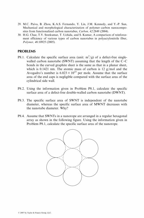
29.
� 20
M.C. Paiva, B. Zhou, K.A.S. Fernando, Y. Lin, J.M. Kennedy, and Y.-P. Sun,
Mechanical and morphological characterization of polymer–carbon nanocompo-
sites from functionalized carbon nanotubes, Carbon, 42:2849 (2004).
30.
H.G. Chae, T.V. Sreekumar, T. Uchida, and S. Kumar, A comparison of reinforce-ment efficiency of various types of carbon nanotubes in polyacrylonitrile fiber,
Polymer, 46:10925 (2005).
PROBLEMS
P8.1. Calculate the specific surface area (unit: m2=g) of a defect-free single-
walled carbon nanotube (SWNT) assuming that the length of the C–C
bonds in the curved graphite sheet is the same as that in a planar sheet,
which is 0.1421 nm. The atomic mass of carbon is 12 g=mol and the
Avogadro’s number is 6.0233 1023 per mole. Assume that the surface
area of the end caps is negligible compared with the surface area of the
cylindrical side wall.
P8.2. Using the information given in Problem P8.1, calculate the specific
surface area of a defect-free double-walled carbon nanotube (DWNT).
P8.3. The specific surface area of SWNT is independent of the nanotube
diameter, whereas the specific surface area of MWNT decreases with
the nanotube diameter. Why?
P8.4. Assume that SWNTs in a nanorope are arranged in a regular hexagonal
array as shown in the following figure. Using the information given in
Problem P8.1, calculate the specific surface area of the nanorope.
07 by Taylor & Francis Group, LLC.
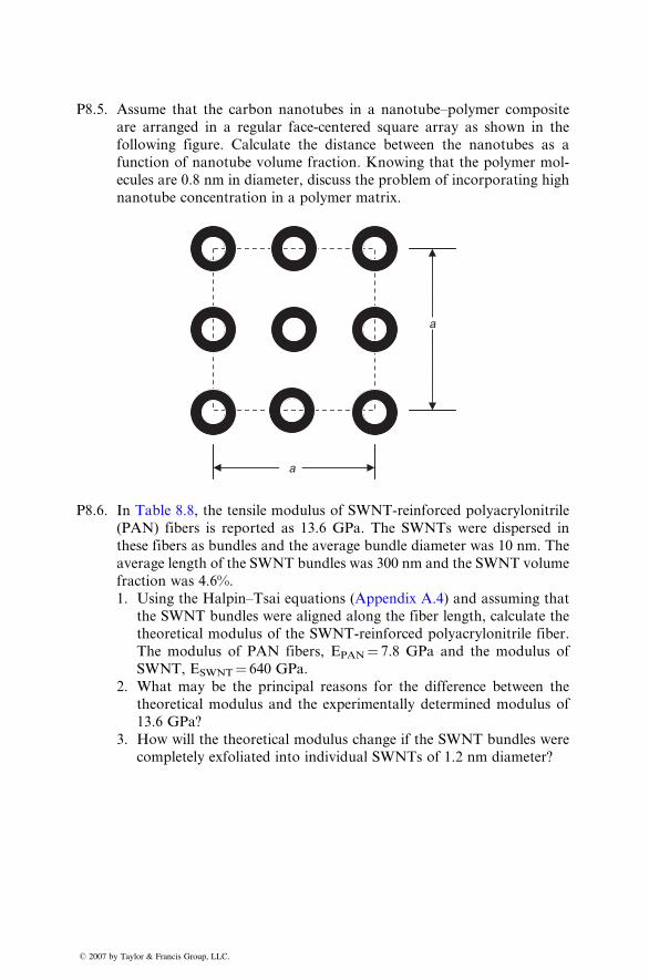
P8.5. Assu me that the carbon na notubes in a nanotube–p olymer c omposi te
are arrange d in a regula r face-cen tered sq uare array a s sho wn in the
follo wing figur e. Calculat e the distance between the nano tubes as a
function of nanotube volume fraction . Know ing that the polyme r mol-
ecules are 0.8 nm in diameter, discuss the problem of incorporating high
nanotube concentration in a polymer matrix.
a
a
P8.6. In Tabl e 8.8, the tensi le modulus of SW NT-reinfor ced pol yacrylon itrile
(PAN ) fibers is repo rted as 13.6 GPa. The SW NTs wer e disper sed in
these fibers as bundl es and the average bundl e diame ter was 10 nm. The
average length of the SW NT bundles was 300 nm and the SWNT volume
fraction was 4.6%.
� 2007 b
1. Usi ng the Halpin–T sai eq uations (Appe ndix A.4 ) and assum ing that
the SWNT bundl es wer e alig ned along the fiber lengt h, calcul ate the
theoretical modulus of the SWNT-reinforced polyacrylonitrile fiber.
The modulus of PAN fibers, EPAN¼ 7.8 GPa and the modulus of
SWNT, ESWNT¼ 640 GPa.
2. What may be the principal reasons for the difference between the
theoretical modulus and the experimentally determined modulus of
13.6 GPa?
3. How will the theoretical modulus change if the SWNT bundles were
completely exfoliated into individual SWNTs of 1.2 nm diameter?
y Taylor & Francis Group, LLC.

� 2007 by Taylor & Francis Group, LLC.
Appendixes
A.1 WOVEN FABRIC TERMINOLOGY
Basic woven fabrics consist of two sets of yarns interlaced at right angles to
create a single layer. Such biaxial or 0=90 fabrics are characterized by the
following nomenclature:
1. Yarn construction: May include the strand count as well as the number of
strands twisted and plied together to make up the yarn. In case of glass
fibers, the strand count is given by the yield expressed in yards per pound
or in TEX, which is the mass in grams per 1000 m. For example, if the
yarn is designated as 150 2=3, its yield is 150 3 100 or 15,000 yd=lb. The2= after 150 indicates that the strands are first twisted in groups of two,
and the =3 indicates that three of these groups are plied together to make
up the final yarn. The yarns for carbon-fiber fabrics are called tows. They
have little or no twist and are designated by the number of filaments in
thousands in the tow. Denier (abbreviated as de) is used for designating
Kevlar yarns, where 1 denier is equivalent to 1 g=9000 m of yarn.
2. Count: Number of yarns (ends) per unit width in the warp (lengthwise)
and fill (crosswise) directions (Figure A.1.1). For example, a fabric
count of 60 3 52 means 60 ends per inch in the warp direction and 52
ends per inch in the fill direction.
3. Weight: Areal weight of the fabric in ounces per square yard or grams
per square meter.
4. Thickness: Measured in thousandths of an inch (mil) or in millimeters.
5. Weave style: Specifies the repetitive manner in which the warp and fill
yarns are interlaced in the fabric. Common weave styles are shown in
Figure A.1.2.
(a) Plain weave, in which warp and fill yarns are interlaced over and
under each other in an alternating fashion.
(b) Basket weave, in which a group of two or more warp yarns are
interlaced with a group of two or more fill yarns in an alternating
fashion.
(c) Satin weave, in which each warp yarn weaves over several fill yarns
and under one fill yarn. Common satin weaves are crowfoot satin or
four-harness satin, in which each warp yarn weaves over three and
under one fill yarn, five-harness satin (over four, under one), and
eight-harness satin (over seven, under one).
� 2007 by Taylor & Francis Group, LLC.
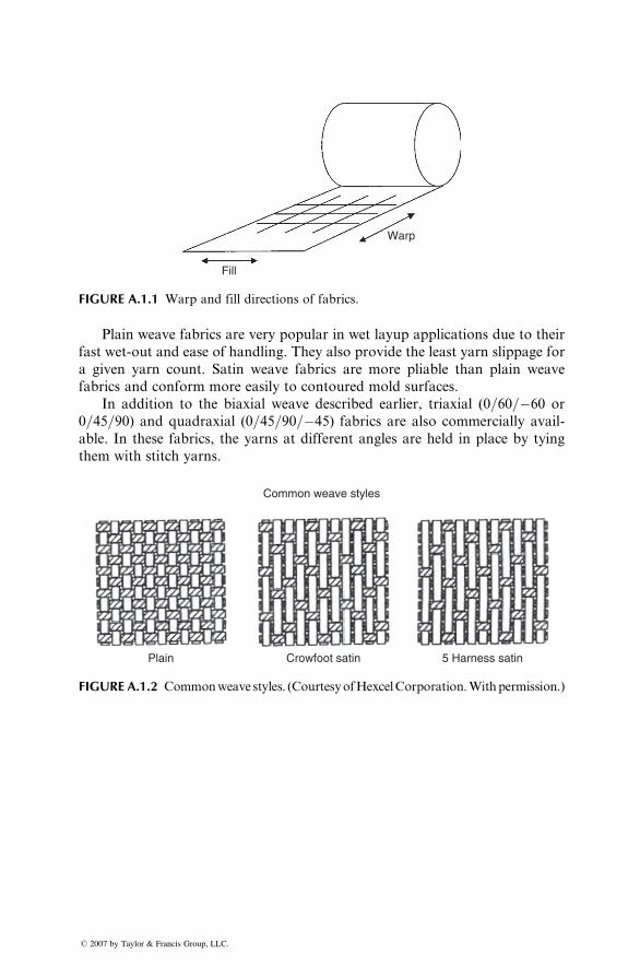
Warp
Fill
FIGURE A.1.1 Warp and fill directions of fabrics.
Plain weave fabrics are very popular in wet layup applications due to their
fast wet-out and ease of handling. They also provide the least yarn slippage for
a given yarn count. Satin weave fabrics are more pliable than plain weave
fabrics and conform more easily to contoured mold surfaces.
In addition to the biaxial weave described earlier, triaxial (0=60=�60 or
0=45=90) and quadraxial (0=45=90=�45) fabrics are also commercially avail-
able. In these fabrics, the yarns at different angles are held in place by tying
them with stitch yarns.
Common weave styles
Plain Crowfoot satin 5 Harness satin
FIGURE A.1.2 Commonweave styles. (CourtesyofHexcelCorporation.Withpermission.)
� 2007 by Taylor & Francis Group, LLC.
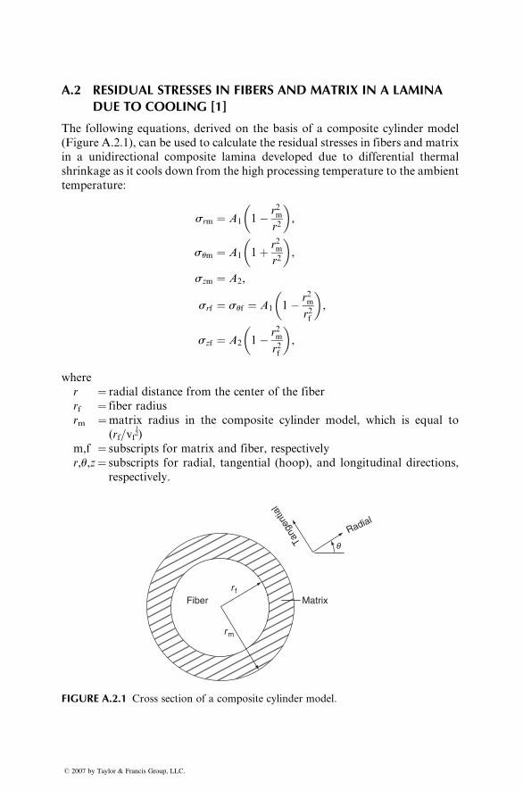
A.2 RESIDUAL STRESSES IN FIBERS AND MATRIX IN A LAMINADUE TO COOLING [1]
The following equations, derived on the basis of a composite cylinder model
(Figure A.2.1), can be used to calculate the residual stresses in fibers and matrix
in a unidirectional composite lamina developed due to differential thermal
shrinkage as it cools down from the high processing temperature to the ambient
temperature:
srm ¼ A1 1� r2mr2
� �,
sum ¼ A1 1þ r2mr2
� �,
szm ¼ A2,
srf ¼ suf ¼ A1 1� r2mr2f
� �,
szf ¼ A2 1� r2mr2f
� �,
where
r ¼ radial distance from the center of the fiber
rf ¼ fiber radius
rm ¼matrix radius in the composite cylinder model, which is equal to
(rf=vf12)
m,f ¼ subscripts for matrix and fiber, respectively
r,u,z¼ subscripts for radial, tangential (hoop), and longitudinal directions,
respectively.
MatrixFiberr f
r m
Radial
Tang
entia
l
q
FIGURE A.2.1 Cross section of a composite cylinder model.
� 2007 by Taylor & Francis Group, LLC.
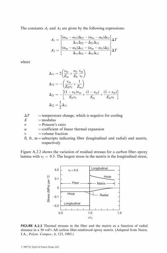
The constants A1 and A2 are given by the following expressions:
A1 ¼ (am � af1)D22 � (am � afr)D12
D11D22 � D21D12
� �DT
A2 ¼ (am � afr)D11 � (am � af1)D21
D11D22 � D21D12
� �DT
where
D11 ¼ 2nmEm
þ nf1Efl
vm
vf
� �
D12 ¼ � vm
Eflvfþ 1
Em
� �
D21 ¼ � (1� nfr)vmEfrvf
þ (1� nm)
Em
þ (1þ nm)
Emvf
� �
D22 ¼ 1
2D11
DT ¼ temperature change, which is negative for cooling
E ¼modulus
n ¼Poisson’s ratio
a ¼ coefficient of linear thermal expansion
v ¼ volume fraction
fl, fr, m¼ subscripts indicating fiber (longitudinal and radial) and matrix,
respectively
Figure A.2.2 shows the variation of residual stresses for a carbon fiber–epoxy
lamina with vf ¼ 0.5. The largest stress in the matrix is the longitudinal stress,
Longitudinal
Longitudinal
0.5
�0.2
�0.1
0
0.1
0.2
1.0
r /r f
1.5
Hoop
Hoop
Matrix
Radial
Fiber
Str
ess
(MP
a) p
er �
C
vf = 0.5
FIGURE A.2.2 Thermal stresses in the fiber and the matrix as a function of radial
distance in a 50 vol% AS carbon fiber-reinforced epoxy matrix. (Adapted from Nairn,
J.A., Polym. Compos., 6, 123, 1985.)
� 2007 by Taylor & Francis Group, LLC.
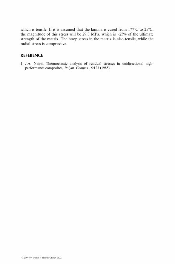
which is tensile. If it is assumed that the lamina is cured from 1778C to 258C,the magnitude of this stress will be 29.3 MPa, which is ~25% of the ultimate
strength of the matrix. The hoop stress in the matrix is also tensile, while the
radial stress is compressive.
REFERENCE
1. J.A. Nairn, Thermoelastic analysis of residual stresses in unidirectional high-
performance composites, Polym. Compos., 6:123 (1985).
� 2007 by Taylor & Francis Group, LLC.
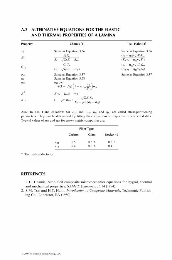
A.3 ALTERNATIVE EQUATIONS FOR THE ELASTICAND THERMAL PROPERTIES OF A LAMINA
Property Chamis [1] Tsai–Hahn [2]
E11 Same as Equation 3.36 Same as Equation 3.36
E22
EfEm
Ef � ffiffiffiffivf
p(Ef � Em)
(vf þ h22vm)EfEm
(Emvf þ h22vmEf )
G12
GfGm
Gf � ffiffiffiffivf
p(Gf � Gm)
(vf þ h12vm)GfGm
(Gmvf þ h12vmGf )
n12 Same as Equation 3.37 Same as Equation 3.37
a11 Same as Equation 3.58
a22 afTffiffiffiffivf
pþ(1� ffiffiffiffi
vfp
) 1þ vfnmEf
E11
� �am
K*11 Kfvf þ Km(1� vf)
K22 (1� ffiffiffiffivf
p)Km þ
ffiffiffiffivf
pKfKm
Kf � ffiffiffiffivf
p(Kf � Km)
Note: In Tsai–Hahn equations for E22 and G12, h22 and h12 are called stress-partitioning
parameters. They can be determined by fitting these equations to respective experimental data.
Typical values of h22 and h12 for epoxy matrix composites are:
Fiber Type
Carbon Glass Kevlar-49
h22 0.5 0.516 0.516
h12 0.4 0.316 0.4
* Thermal conductivity.
REFERENCES
1. C.C. Chamis, Simplified composite micromechanics equations for hygral, thermal
and mechanical properties, SAMPE Quarterly, 15:14 (1984).
2. S.M. Tsai and H.T. Hahn, Introduction to Composite Materials, Technomic Publish-
ing Co., Lancaster, PA (1980).
� 2007 by Taylor & Francis Group, LLC.
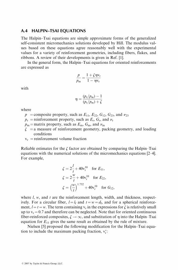
A.4 HALPIN–TSAI EQUATIONS
The Halpin–Tsai equations are simple approximate forms of the generalized
self-consistent micromechanics solutions developed by Hill. The modulus val-
ues based on these equations agree reasonably well with the experimental
values for a variety of reinforcement geometries, including fibers, flakes, and
ribbons. A review of their developments is given in Ref. [1].
In the general form, the Halpin–Tsai equations for oriented reinforcements
are expressed as
p
pm¼ 1þ zhvr
1� hvr
with
h ¼ (pr=pm)� 1
(pr=pm)þ z
where
p ¼ composite property, such as E11, E22, G12, G23, and n23pr ¼ reinforcement property, such as Er, Gr, and nrpm¼matrix property, such as Em, Gm, and nmz ¼ a measure of reinforcement geometry, packing geometry, and loading
conditions
vr ¼ reinforcement volume fraction
Reliable estimates for the z factor are obtained by comparing the Halpin–Tsai
equations with the numerical solutions of the micromechanics equations [2–4].
For example,
z ¼ 2l
tþ 40v10r for E11,
z ¼ 2w
tþ 40v10r for E22,
z ¼ w
t
� �1:732þ 40v10r for G12,
where l, w, and t are the reinforcement length, width, and thickness, respect-
ively. For a circular fiber, l¼ lf and t¼w¼ df, and for a spherical reinforce-
ment, l¼ t¼w. The term containing vr in the expressions for z is relatively small
up to vr¼ 0.7 and therefore can be neglected. Note that for oriented continuous
fiber-reinforced composites, z!1, and substitution of h into the Halpin–Tsai
equation for E11 gives the same result as obtained by the rule of mixture.
Nielsen [5] proposed the following modification for the Halpin–Tsai equa-
tion to include the maximum packing fraction, v�r :
� 2007 by Taylor & Francis Group, LLC.
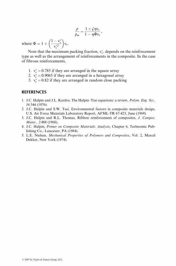
p
pm¼ 1þ zhvr
1� hFvr,
where F ¼ 1þ 1� v�rv�2r
� �vr.
Note that the maximum packing fraction, v�r , depends on the reinforcement
type as well as the arrangement of reinforcements in the composite. In the case
of fibrous reinforcements,
1. v�r ¼ 0.785 if they are arranged in the square array
2. v�r ¼ 0.9065 if they are arranged in a hexagonal array
3. v�r ¼ 0.82 if they are arranged in random close packing
REFERENCES
1. J.C. Halpin and J.L. Kardos, The Halpin–Tsai equations: a review, Polym. Eng. Sci.,
16:344 (1976).
2. J.C. Halpin and S.W. Tsai, Environmental factors in composite materials design,
U.S. Air Force Materials Laboratory Report, AFML-TR 67-423, June (1969).
3. J.C. Halpin and R.L. Thomas, Ribbon reinforcement of composites, J. Compos.
Mater., 2:488 (1968).
4. J.C. Halpin, Primer on Composite Materials: Analysis, Chapter 6, Technomic Pub-
lishing Co., Lancaster, PA (1984).
5. L.E. Nielsen, Mechanical Properties of Polymers and Composites, Vol. 2, Marcel
Dekker, New York (1974).
� 2007 by Taylor & Francis Group, LLC.
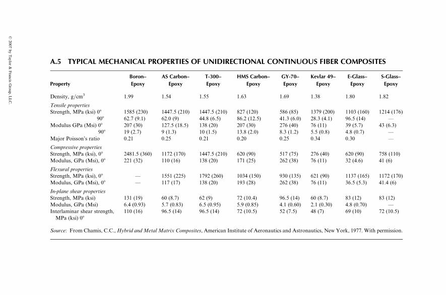
A.5 TYPICAL MECHANICAL PROPERTIES OF UNIDIRECTIONAL CONTINUOUS FIBER COMPOSITES
Property
Boron–
Epoxy
AS Carbon–
Epoxy
T-300–
Epoxy
HMS Carbon–
Epoxy
GY-70–
Epoxy
Kevlar 49–
Epoxy
E-Glass–
Epoxy
S-Glass–
Epoxy
Density, g=cm3 1.99 1.54 1.55 1.63 1.69 1.38 1.80 1.82
Tensile properties
Strength, MPa (ksi) 08 1585 (230) 1447.5 (210) 1447.5 (210) 827 (120) 586 (85) 1379 (200) 1103 (160) 1214 (176)
908 62.7 (9.1) 62.0 (9) 44.8 (6.5) 86.2 (12.5) 41.3 (6.0) 28.3 (4.1) 96.5 (14) —
Modulus GPa (Msi) 08 207 (30) 127.5 (18.5) 138 (20) 207 (30) 276 (40) 76 (11) 39 (5.7) 43 (6.3)
908 19 (2.7) 9 (1.3) 10 (1.5) 13.8 (2.0) 8.3 (1.2) 5.5 (0.8) 4.8 (0.7) —
Major Poisson’s ratio 0.21 0.25 0.21 0.20 0.25 0.34 0.30 —
Compressive properties
Strength, MPa (ksi), 08 2481.5 (360) 1172 (170) 1447.5 (210) 620 (90) 517 (75) 276 (40) 620 (90) 758 (110)
Modulus, GPa (Msi), 08 221 (32) 110 (16) 138 (20) 171 (25) 262 (38) 76 (11) 32 (4.6) 41 (6)
Flexural properties
Strength, MPa (ksi), 08 — 1551 (225) 1792 (260) 1034 (150) 930 (135) 621 (90) 1137 (165) 1172 (170)
Modulus, GPa (Msi), 08 — 117 (17) 138 (20) 193 (28) 262 (38) 76 (11) 36.5 (5.3) 41.4 (6)
In-plane shear properties
Strength, MPa (ksi) 131 (19) 60 (8.7) 62 (9) 72 (10.4) 96.5 (14) 60 (8.7) 83 (12) 83 (12)
Modulus, GPa (Msi) 6.4 (0.93) 5.7 (0.83) 6.5 (0.95) 5.9 (0.85) 4.1 (0.60) 2.1 (0.30) 4.8 (0.70) —
Interlaminar shear strength,
MPa (ksi) 08
110 (16) 96.5 (14) 96.5 (14) 72 (10.5) 52 (7.5) 48 (7) 69 (10) 72 (10.5)
Source: From Chamis, C.C.,Hybrid and Metal Matrix Composites, American Institute of Aeronautics and Astronautics, New York, 1977. With permission.
�2007
byTaylor
&Francis
Group,
LLC.
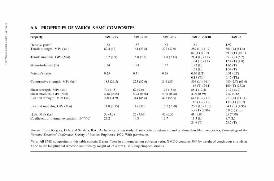
A.6 PROPERTIES OF VARIOUS SMC COMPOSITES
Property SMC-R25 SMC-R50 SMC-R65 SMC-C20R30 XMC-3
Density, g=cm3 1.83 1.87 1.82 1.81 1.97
Tensile strength, MPa (ksi) 82.4 (12) 164 (23.8) 227 (32.9) 289 (L) (41.9) 561 (L) (81.4)
84 (T) (12.2) 69.9 (T) (10.1)
Tensile modulus, GPa (Msi) 13.2 (1.9) 15.8 (2.3) 14.8 (2.15) 21.4 (L) (3.1) 35.7 (L) (5.2)
12.4 (T) (1.8) 12.4 (T) (1.8)
Strain-to-failure (%) 1.34 1.73 1.67 1.73 (L) 1.66 (T)
1.58 (L) 1.54 (T)
Poisson’s ratio 0.25 0.31 0.26 0.30 (LT) 0.31 (LT)
0.18 (TL) 0.12 (TL)
Compressive strength, MPa (ksi) 183 (26.5) 225 (32.6) 241 (35) 306 (L) (44.4) 480 (LT) (69.6)
166 (T) (24.1) 160 (T) (23.2)
Shear strength, MPa (ksi) 79 (11.5) 62 (9.0) 128 (18.6) 85.4 (12.4) 91.2 (13.2)
Shear modulus, GPa (Msi) 4.48 (0.65) 5.94 (0.86) 5.38 (0.78) 4.09 (0.59) 4.47 (0.65)
Flexural strength, MPa (ksi) 220 (31.9) 314 (45.6) 403 (58.5) 645 (L) (93.6) 973 (L) (141.1)
165 (T) (23.9) 139 (T) (20.2)
Flexural modulus, GPa (Msi) 14.8 (2.15) 14 (2.03) 15.7 (2.28) 25.7 (L) (3.73) 34.1 (L) (4.95)
5.9 (T) (0.86) 6.8 (T) (1.0)
ILSS, MPa (ksi) 30 (4.3) 25 (3.63) 45 (6.53) 41 (5.95) 55 (7.98)
Coefficient of thermal expansion, 10�6=8C 23.2 14.8 13.7 11.3 (L) 8.7 (L)
24.6 (T) 28.7 (T)
Source: From Riegner, D.A. and Sanders, B.A., A characterization study of automotive continuous and random glass fiber composites, Proceedings of the
National Technical Conference, Society of Plastics Engineers, 1979. With permission.
Note: All SMC composites in this table contain E-glass fibers in a thermosetting polyester resin. XMC-3 contains 50% by weight of continuous strands at
±7.58 to the longitudinal direction and 25% by weight of 25.4 mm (1 in.) long-chopped strands.
�2007
byTaylor
&Francis
Group,L
LC.
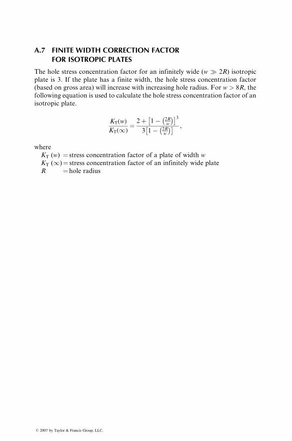
A.7 FINITE WIDTH CORRECTION FACTORFOR ISOTROPIC PLATES
The hole stress concentration factor for an infinitely wide (w � 2R) isotropic
plate is 3. If the plate has a finite width, the hole stress concentration factor
(based on gross area) will increase with increasing hole radius. For w > 8R, the
following equation is used to calculate the hole stress concentration factor of an
isotropic plate.
KT(w)
KT(1)¼ 2þ 1� 2R
w
� �33 1� 2R
w
� � ,
where
KT (w) ¼ stress concentration factor of a plate of width w
KT (1)¼ stress concentration factor of an infinitely wide plate
R ¼ hole radius
� 2007 by Taylor & Francis Group, LLC.
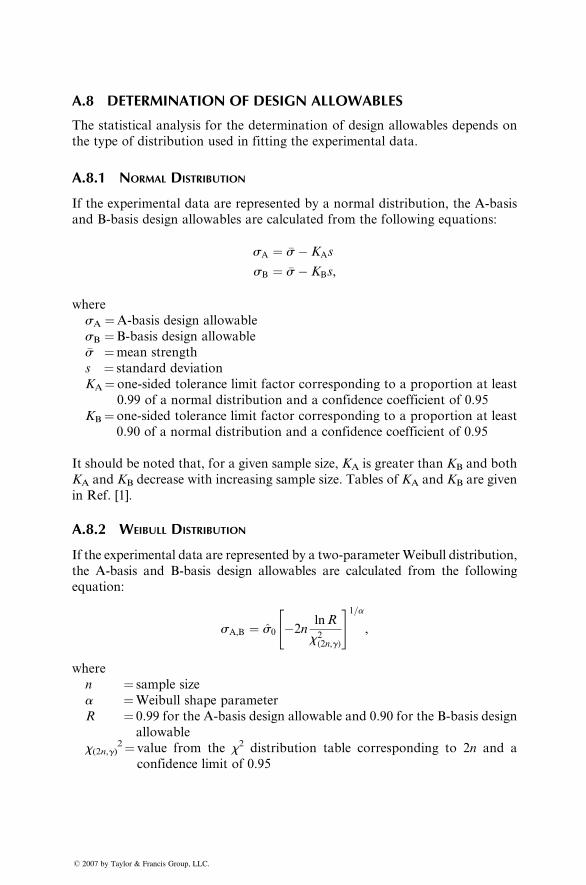
A.8 DETERMINATION OF DESIGN ALLOWABLES
The statistical analysis for the determination of design allowables depends on
the type of distribution used in fitting the experimental data.
A.8.1 NORMAL DISTRIBUTION
If the experimental data are represented by a normal distribution, the A-basis
and B-basis design allowables are calculated from the following equations:
sA ¼ �s � KAs
sB ¼ �s � KBs,
where
sA ¼A-basis design allowable
sB ¼B-basis design allowable
�s ¼mean strength
s ¼ standard deviation
KA¼ one-sided tolerance limit factor corresponding to a proportion at least
0.99 of a normal distribution and a confidence coefficient of 0.95
KB¼ one-sided tolerance limit factor corresponding to a proportion at least
0.90 of a normal distribution and a confidence coefficient of 0.95
It should be noted that, for a given sample size, KA is greater than KB and both
KA and KB decrease with increasing sample size. Tables of KA and KB are given
in Ref. [1].
A.8.2 WEIBULL DISTRIBUTION
If the experimental data are represented by a two-parameterWeibull distribution,
the A-basis and B-basis design allowables are calculated from the following
equation:
sA,B ¼ s0 �2nlnR
x2(2n,g)
" #1=a,
where
n ¼ sample size
a ¼Weibull shape parameter
R ¼ 0.99 for the A-basis design allowable and 0.90 for the B-basis design
allowable
x(2n,g)2¼ value from the x2 distribution table corresponding to 2n and a
confidence limit of 0.95
� 2007 by Taylor & Francis Group, LLC.
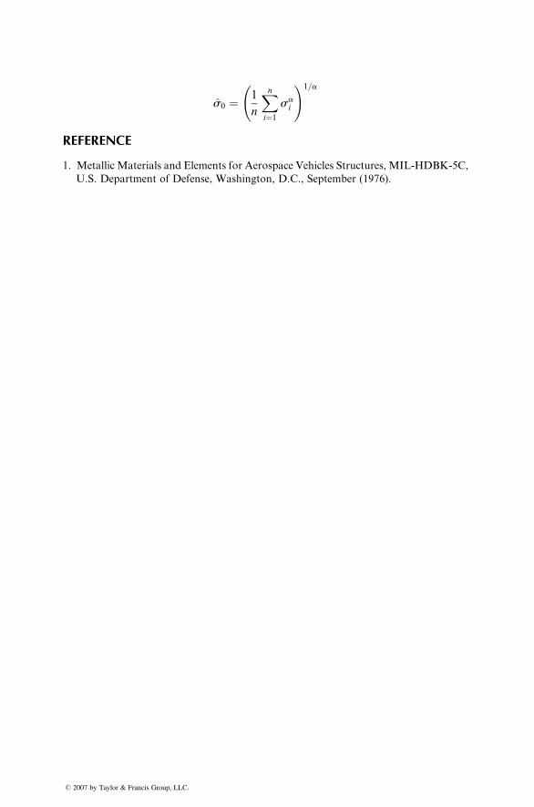
s0 ¼ 1
n
Xni¼1
sai
!1=a
REFERENCE
1. Metallic Materials and Elements for Aerospace Vehicles Structures, MIL-HDBK-5C,
U.S. Department of Defense, Washington, D.C., September (1976).
� 2007 by Taylor & Francis Group, LLC.
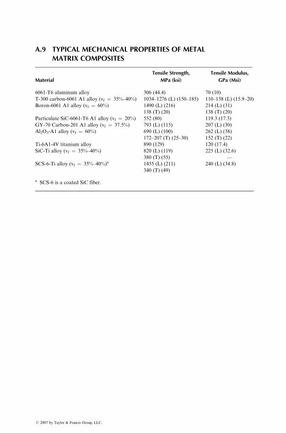
A.9 TYPICAL MECHANICAL PROPERTIES OF METALMATRIX COMPOSITES
Material
Tensile Strength,
MPa (ksi)
Tensile Modulus,
GPa (Msi)
6061-T6 aluminum alloy 306 (44.4) 70 (10)
T-300 carbon-6061 A1 alloy (vf ¼ 35%–40%) 1034–1276 (L) (150–185) 110–138 (L) (15.9–20)
Boron-6061 A1 alloy (vf ¼ 60%) 1490 (L) (216) 214 (L) (31)
138 (T) (20) 138 (T) (20)
Particulate SiC-6061-T6 A1 alloy (vf ¼ 20%) 552 (80) 119.3 (17.3)
GY-70 Carbon-201 A1 alloy (vf ¼ 37.5%) 793 (L) (115) 207 (L) (30)
Al2O3-A1 alloy (vf ¼ 60%) 690 (L) (100) 262 (L) (38)
172–207 (T) (25–30) 152 (T) (22)
Ti-6A1-4V titanium alloy 890 (129) 120 (17.4)
SiC-Ti alloy (vf ¼ 35%–40%) 820 (L) (119) 225 (L) (32.6)
380 (T) (55) —
SCS-6-Ti alloy (vf ¼ 35%–40%)a 1455 (L) (211) 240 (L) (34.8)
340 (T) (49)
a SCS-6 is a coated SiC fiber.
� 2007 by Taylor & Francis Group, LLC.
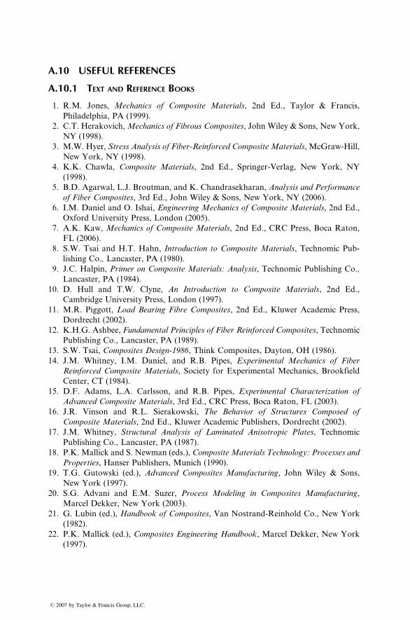
A.10 USEFUL REFERENCES
A.10.1 TEXT AND REFERENCE BOOKS
1.
� 20
R.M. Jones, Mechanics of Composite Materials, 2nd Ed., Taylor & Francis,
Philadelphia, PA (1999).
2.
C.T. Herakovich,Mechanics of Fibrous Composites, John Wiley & Sons, New York,NY (1998).
3.
M.W. Hyer, Stress Analysis of Fiber-Reinforced Composite Materials, McGraw-Hill,New York, NY (1998).
4.
K.K. Chawla, Composite Materials, 2nd Ed., Springer-Verlag, New York, NY(1998).
5.
B.D. Agarwal, L.J. Broutman, and K. Chandrasekharan, Analysis and Performanceof Fiber Composites, 3rd Ed., John Wiley & Sons, New York, NY (2006).
6.
I.M. Daniel and O. Ishai, Engineering Mechanics of Composite Materials, 2nd Ed.,Oxford University Press, London (2005).
7.
A.K. Kaw, Mechanics of Composite Materials, 2nd Ed., CRC Press, Boca Raton,FL (2006).
8.
S.W. Tsai and H.T. Hahn, Introduction to Composite Materials, Technomic Pub-lishing Co., Lancaster, PA (1980).
9.
J.C. Halpin, Primer on Composite Materials: Analysis, Technomic Publishing Co.,Lancaster, PA (1984).
10.
D. Hull and T.W. Clyne, An Introduction to Composite Materials, 2nd Ed.,Cambridge University Press, London (1997).
11.
M.R. Piggott, Load Bearing Fibre Composites, 2nd Ed., Kluwer Academic Press,Dordrecht (2002).
12.
K.H.G. Ashbee, Fundamental Principles of Fiber Reinforced Composites, TechnomicPublishing Co., Lancaster, PA (1989).
13.
S.W. Tsai, Composites Design-1986, Think Composites, Dayton, OH (1986).14.
J.M. Whitney, I.M. Daniel, and R.B. Pipes, Experimental Mechanics of FiberReinforced Composite Materials, Society for Experimental Mechanics, Brookfield
Center, CT (1984).
15.
D.F. Adams, L.A. Carlsson, and R.B. Pipes, Experimental Characterization ofAdvanced Composite Materials, 3rd Ed., CRC Press, Boca Raton, FL (2003).
16.
J.R. Vinson and R.L. Sierakowski, The Behavior of Structures Composed ofComposite Materials, 2nd Ed., Kluwer Academic Publishers, Dordrecht (2002).
17.
J.M. Whitney, Structural Analysis of Laminated Anisotropic Plates, TechnomicPublishing Co., Lancaster, PA (1987).
18.
P.K. Mallick and S. Newman (eds.), Composite Materials Technology: Processes andProperties, Hanser Publishers, Munich (1990).
19.
T.G. Gutowski (ed.), Advanced Composites Manufacturing, John Wiley & Sons,New York (1997).
20.
S.G. Advani and E.M. Suzer, Process Modeling in Composites Manufacturing,Marcel Dekker, New York (2003).
21.
G. Lubin (ed.), Handbook of Composites, Van Nostrand-Reinhold Co., New York(1982).
22.
P.K. Mallick (ed.), Composites Engineering Handbook, Marcel Dekker, New York(1997).
07 by Taylor & Francis Group, LLC.
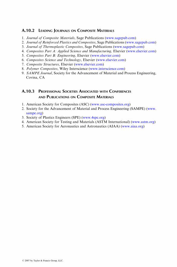
A.10.2 LEADING JOURNALS ON COMPOSITE MATERIALS
1. Journal of Composite Materials, Sage Publications (www.sagepub.com)
2. Journal of Reinforced Plastics and Composites, Sage Publications (www.sagepub.com)
3. Journal of Thermoplastic Composites, Sage Publications (www.sagepub.com)
4. Composites Part A: Applied Science and Manufacturing, Elsevier (www.elsevier.com)
5. Composites Part B: Engineering, Elsevier (www.elsevier.com)
6. Composites Science and Technology, Elsevier (www.elsevier.com)
7. Composite Structures, Elsevier (www.elsevier.com)
8. Polymer Composites, Wiley Interscience (www.interscience.com)
9. SAMPE Journal, Society for the Advancement of Material and Process Engineering,
Covina, CA
A.10.3 PROFESSIONAL SOCIETIES ASSOCIATED WITH CONFERENCES
AND PUBLICATIONS ON COMPOSITE MATERIALS
1. American Society for Composites (ASC) (www.asc-composites.org)
2. Society for the Advancement of Material and Process Engineering (SAMPE) (www.
sampe.org)
3. Society of Plastics Engineers (SPE) (www.4spe.org)
4. American Society for Testing and Materials (ASTM International) (www.astm.org)
5. American Society for Aeronautics and Astronautics (AIAA) (www.aiaa.org)
� 2007 by Taylor & Francis Group, LLC.
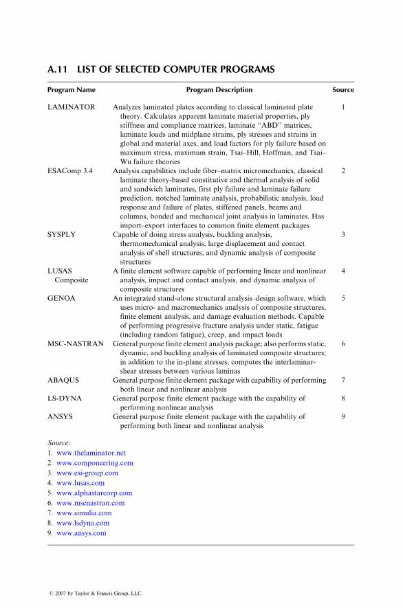
A.11 LIST OF SELECTED COMPUTER PROGRAMS
Program Name Program Description Source
LAMINATOR Analyzes laminated plates according to classical laminated plate
theory. Calculates apparent laminate material properties, ply
stiffness and compliance matrices, laminate ‘‘ABD’’ matrices,
laminate loads and midplane strains, ply stresses and strains in
global and material axes, and load factors for ply failure based on
maximum stress, maximum strain, Tsai–Hill, Hoffman, and Tsai–
Wu failure theories
1
ESAComp 3.4 Analysis capabilities include fiber–matrix micromechanics, classical
laminate theory-based constitutive and thermal analysis of solid
and sandwich laminates, first ply failure and laminate failure
prediction, notched laminate analysis, probabilistic analysis, load
response and failure of plates, stiffened panels, beams and
columns, bonded and mechanical joint analysis in laminates. Has
import–export interfaces to common finite element packages
2
SYSPLY Capable of doing stress analysis, buckling analysis,
thermomechanical analysis, large displacement and contact
analysis of shell structures, and dynamic analysis of composite
structures
3
LUSAS
Composite
A finite element software capable of performing linear and nonlinear
analysis, impact and contact analysis, and dynamic analysis of
composite structures
4
GENOA An integrated stand-alone structural analysis–design software, which
uses micro- and macromechanics analysis of composite structures,
finite element analysis, and damage evaluation methods. Capable
of performing progressive fracture analysis under static, fatigue
(including random fatigue), creep, and impact loads
5
MSC-NASTRAN General purpose finite element analysis package; also performs static,
dynamic, and buckling analysis of laminated composite structures;
in addition to the in-plane stresses, computes the interlaminar-
shear stresses between various laminas
6
ABAQUS General purpose finite element package with capability of performing
both linear and nonlinear analysis
7
LS-DYNA General purpose finite element package with the capability of
performing nonlinear analysis
8
ANSYS General purpose finite element package with the capability of
performing both linear and nonlinear analysis
9
Source:
1. www.thelaminator.net
2. www.componeering.com
3. www.esi-group.com
4. www.lusas.com
5. www.alphastarcorp.com
6. www.mscnastran.com
7. www.simulia.com
8. www.lsdyna.com
9. www.ansys.com
� 2007 by Taylor & Francis Group, LLC.

� 2007 by Taylor & Francis Group, LLC.


