Embed Size (px)
Citation preview

EEE238: Digital Signal Processing – Tutorial 1: Sampling and Quantization 1/8
1. Aliased signals

EEE238: Digital Signal Processing – Tutorial 1: Sampling and Quantization 2/8
2. Prefiltering and reconstruction

EEE238: Digital Signal Processing – Tutorial 1: Sampling and Quantization 3/8
Solution: Case (a)

EEE238: Digital Signal Processing – Tutorial 1: Sampling and Quantization 4/8
Solution: Case (b)
Solution: Case (c)

EEE238: Digital Signal Processing – Tutorial 1: Sampling and Quantization 5/8
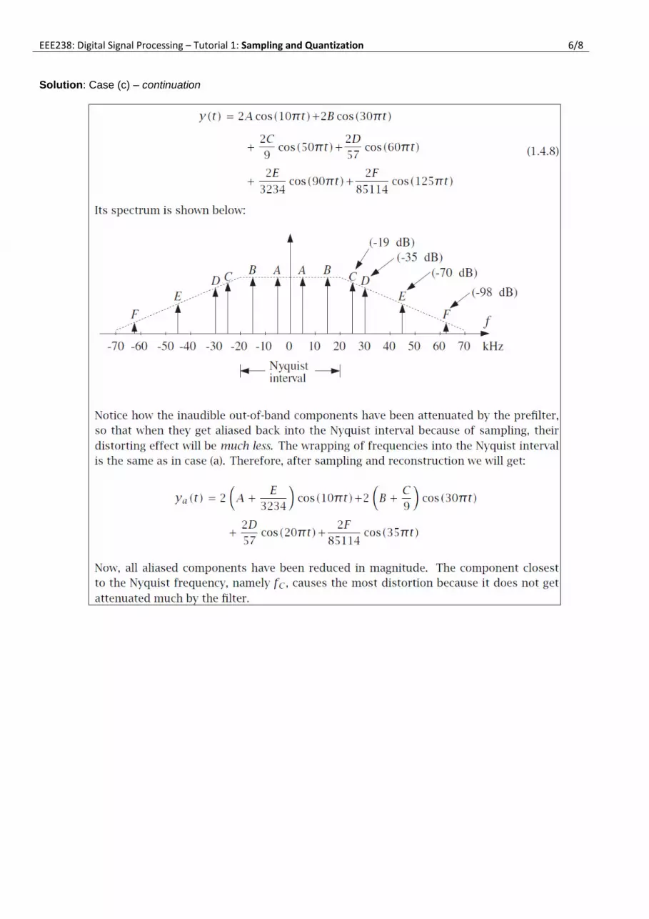
Solution: Case (c) – continuation
EEE238: Digital Signal Processing – Tutorial 1: Sampling and Quantization 6/8
Solution: Case (c) – continuation

EEE238: Digital Signal Processing – Tutorial 1: Sampling and Quantization 7/8
3. Discrete Time Fourier Transform
Calculate frequency spectrum of the sampled signal.
Solution:

EEE238: Digital Signal Processing – Tutorial 1: Sampling and Quantization 8/8
4. Quantization (specifications)
Solution:
4. Quantization (truncation)
Solution:

EEE238: Digital Signal Processing – Tutorial 2: Discrete Time Systems 1/7
1. Time invariance
Example 3.2.2: Test the time invariance of the discrete-time systems defined by
y(n)= nx(n) and the downsampler y(n)= x(2n).
EEE238: Digital Signal Processing – Tutorial 2: Discrete Time Systems 2/7
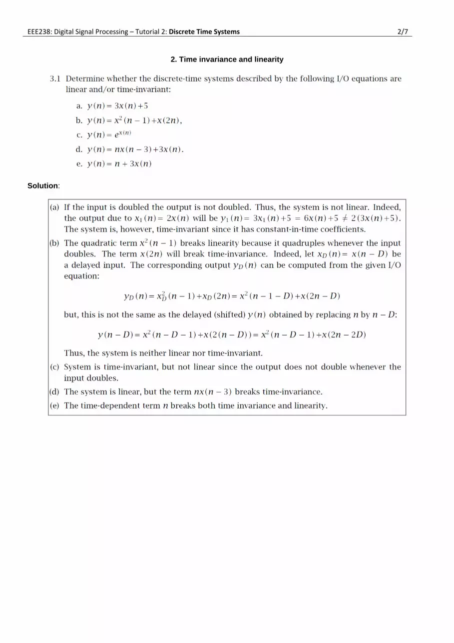
2. Time invariance and linearity
Solution:

EEE238: Digital Signal Processing – Tutorial 2: Discrete Time Systems 3/7
3. Impulse response of FIR filters

EEE238: Digital Signal Processing – Tutorial 2: Discrete Time Systems 4/7
4. Impulse response of IIR filters

EEE238: Digital Signal Processing – Tutorial 2: Discrete Time Systems 5/7
Solution:
EEE238: Digital Signal Processing – Tutorial 2: Discrete Time Systems 6/7
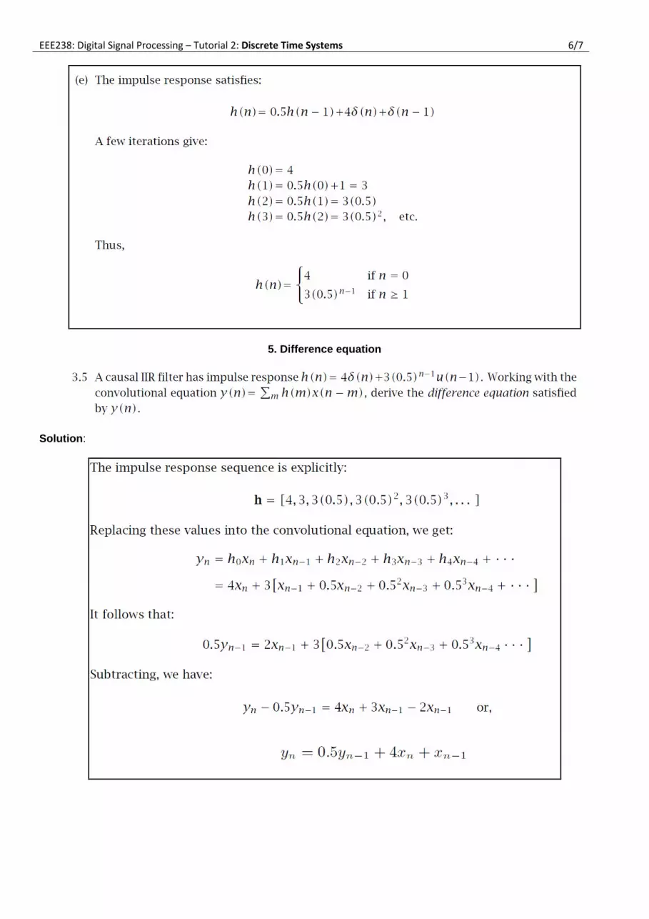
5. Difference equation
Solution:

EEE238: Digital Signal Processing – Tutorial 2: Discrete Time Systems 7/7
6. Stability
For each impulse response above determine if the LTI system is stable or not, based on
Solution:

EEE238: Digital Signal and Image Processing – Tutorial 3: FIR filtering and Convolution 1/5
1. Convolution table
Solution:
2. Sample processing (pp. 156-157)

EEE238: Digital Signal and Image Processing – Tutorial 3: FIR filtering and Convolution 2/5

EEE238: Digital Signal and Image Processing – Tutorial 3: FIR filtering and Convolution 3/5
3. Sample processing
Solution: The impulse response is read off from the coefficients of the I/O equation: h=[1,0,-1]

EEE238: Digital Signal and Image Processing – Tutorial 3: FIR filtering and Convolution 4/5
4. Convolution of infinite sequences

EEE238: Digital Signal and Image Processing – Tutorial 3: FIR filtering and Convolution 5/5
5. Index range
Solution:

EEE238: Digital Signal and Image Processing – Tutorial 4: z-Transforms 1/6
1. Transform properties
Solution:

EEE238: Digital Signal and Image Processing – Tutorial 4: z-Transforms 2/6
2. Transform and Region of Convergence (ROC)
Solution:
EEE238: Digital Signal and Image Processing – Tutorial 4: z-Transforms 3/6
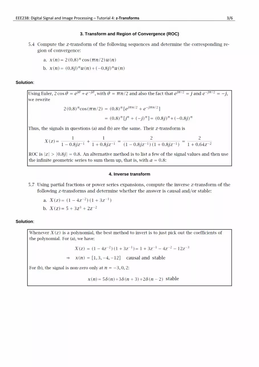
3. Transform and Region of Convergence (ROC)
Solution:
4. Inverse transform
Solution:
EEE238: Digital Signal and Image Processing – Tutorial 4: z-Transforms 4/6
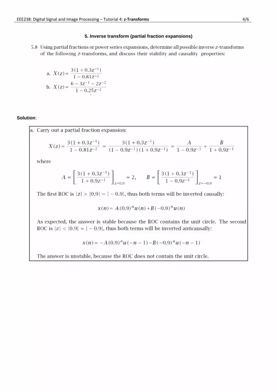
5. Inverse transform (partial fraction expansions)
Solution:

EEE238: Digital Signal and Image Processing – Tutorial 4: z-Transforms 5/6
Solution:

EEE238: Digital Signal and Image Processing – Tutorial 4: z-Transforms 6/6
6. Transform of sinusoids
Solution:

EEE238: Digital Signal and Image Processing – Tutorial 5: Transfer Functions 1/7
1. Frequency response

EEE238: Digital Signal and Image Processing – Tutorial 5: Transfer Functions 2/7

EEE238: Digital Signal and Image Processing – Tutorial 5: Transfer Functions 3/7

EEE238: Digital Signal and Image Processing – Tutorial 5: Transfer Functions 4/7
2. Transient response

EEE238: Digital Signal and Image Processing – Tutorial 5: Transfer Functions 5/7
3. Pole/Zero Design
Solution:

EEE238: Digital Signal and Image Processing – Tutorial 5: Transfer Functions 6/7

EEE238: Digital Signal and Image Processing – Tutorial 5: Transfer Functions 7/7
3. Transfer function
Solution:
EEE238: Digital Signal and Image Processing – Tutorial 6: DFT/FFT Algorithms 1/5
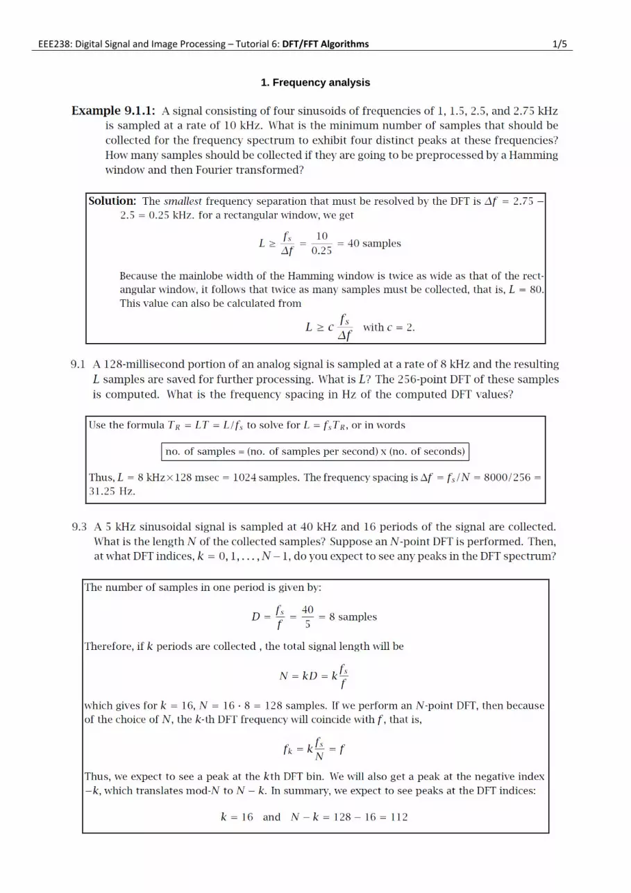
1. Frequency analysis

EEE238: Digital Signal and Image Processing – Tutorial 6: DFT/FFT Algorithms 2/5
2. Discrete Fourier Transform (DFT)
LN
LN
N
L
NN
N
NNN
NNN
WWW
WWW
WWW
A
A
)1)(1()1(0
)1(10
000
xX
with Nj
N eW
2
Solution:

EEE238: Digital Signal and Image Processing – Tutorial 6: DFT/FFT Algorithms 3/5
Solution:

EEE238: Digital Signal and Image Processing – Tutorial 6: DFT/FFT Algorithms 4/5
Solution:

EEE238: Digital Signal and Image Processing – Tutorial 6: DFT/FFT Algorithms 5/5
Solution:

EEE238: Digital Signal and Image Processing – Tutorial 7: FIR & IIR Digital Filter Design 1/3
1. FIR Digital Filter Design (impulse responses)
By performing the appropriate integrations in the inverse DTFT equation, calculate the impulse response d(k) of the bandpass, lowpass and highpass ideal filters
.

EEE238: Digital Signal and Image Processing – Tutorial 7: FIR & IIR Digital Filter Design 2/3
2. FIR Digital Filter Design (using slides 21-23 of Lecture 7)

EEE238: Digital Signal and Image Processing – Tutorial 7: FIR & IIR Digital Filter Design 3/3
3. IIR Digital Filter Design
Solution:

EEE238: Digital Signal and Image Processing – Tutorial 8: Enhancement and Mathematical Morphology 1/3
1. Consider the 3-bit image A of Figure 1. For the questions below, assume that pixel values outside
the image boundaries have a zero grey level. In addition, round the output image pixel values to
the nearest integer (nint[] operator).
132
564
213
A
Figure 1: Image A.
By processing the input image A, determine the output
(a) image B resulting from a linear contrast scaling;
031
674
103
132
564
213
:Solution
14.1nint124.1nint14.1nint
:Example
14.1nint15
7nint1
16
12nint)min(
)min()max(
1nint
:Equation
1313
3
BA
AB
AAAAAAA
LB
scalingcontrastlinear
ijijijijij
(b) image C resulting from a thresholding at standard deviation of A;
011
111
101
132
564
213
:Solution
6330.13)(because1
:Example
otherwise0
if1
1.6330
)31()33()32()35()36()34()32(31)33(33
1
1,3132564213
33
11
:Equations
)(
3232
222222222
,
2
,
CA
AC
AC
AMN
AMN
AAngthresholdi
A
Aij
ij
A
A
ji
AijA
ji
ijA

EEE238: Digital Signal and Image Processing – Tutorial 8: Enhancement and Mathematical Morphology 2/3
(c) image C resulting from a 3x3 smoothing;
222
232
222
00000
0
0
0
132
564
213
0
0
0
00000
:Solution
21.5556nint9
64013000nint
:Example
1nint
:Equation
smoothing33
11
1
1
1
1
,
CA
C
CMN
Cm n
njmiij
(d) image D resulting from a 3x3 median filtering.
020
132
020
00000
0
0
0
132
564
213
0
0
0
00000
:Solution
3)6,5,4,3,3,2,1,,1(median
:Example
filteringmedian33
22
DA
D
EEE238: Digital Signal and Image Processing – Tutorial 8: Enhancement and Mathematical Morphology 3/3
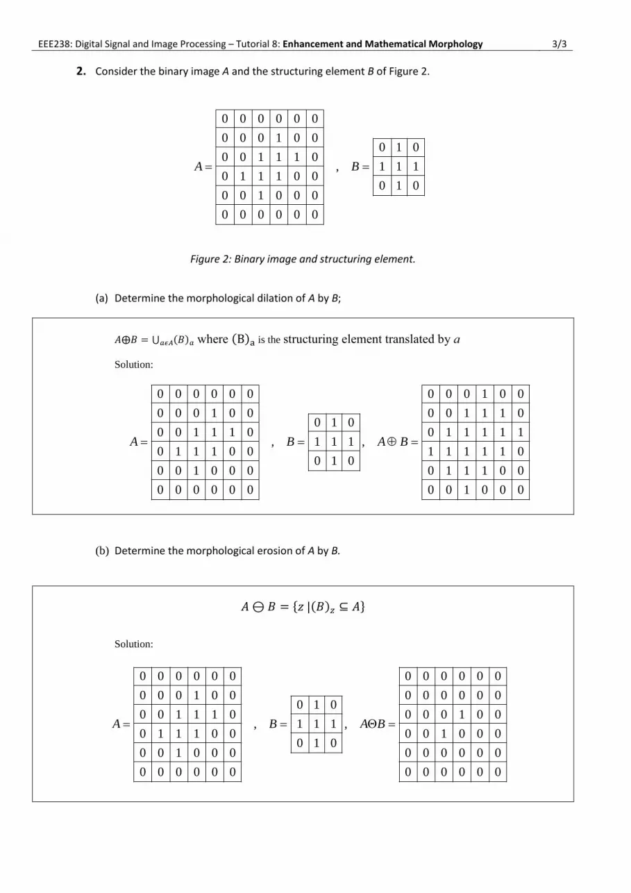
2. Consider the binary image A and the structuring element B of Figure 2.
010
111
010
,
000000
000100
001110
011100
001000
000000
BA
Figure 2: Binary image and structuring element.
(a) Determine the morphological dilation of A by B;
𝐴⨁𝐵 = ⋃ (𝐵)𝑎𝑎𝜖𝐴 where (B)a is the structuring element translated by a
Solution:
000100
001110
011111
111110
011100
001000
,
010
111
010
,
000000
000100
001110
011100
001000
000000
BABA
(b) Determine the morphological erosion of A by B.
𝐴 ⊖ 𝐵 = 𝑧 |(𝐵)𝑧 ⊆ 𝐴
Solution:
000000
000000
000100
001000
000000
000000
,
010
111
010
,
000000
000100
001110
011100
001000
000000
BABA

Midterm Examination (Lecture Section 2, Fall 2015), EEE 238 DIGITAL SIGNAL AND IMAGE PROCESSING
Page 1 of 5
NAZARBAYEV UNIVERSITY
School of Engineering
Midterm Examination
(Lecture Section 2, Fall 2015)
EEE 238 DIGITAL SIGNAL AND IMAGE PROCESSING
Date: Monday, October 19, 2015 Time: 11:00 AM – 12:50 PM
Student name:
Student ID:
All questions carry indicated marks, you can obtain a maximum of 100 marks.
Only handwritten notes are permitted.
The use of calculators approved by the School of Engineering is permitted.
PLEASE WRITE YOUR ANSWERS ON THIS EXAMINATION
QUESTION PAPER. IT WILL BE COLLECTED AT THE END OF
THIS EXAMINATION.

Midterm Examination (Lecture Section 2, Fall 2015), EEE 238 DIGITAL SIGNAL AND IMAGE PROCESSING
Page 2 of 5
1. Determine the impulse response ℎ(𝑛) of the filters:
(a) 𝑦(𝑛) = 𝑥(𝑛) + 𝑥(𝑛 − 1) [5 marks]
(b) 𝑦(𝑛) = 𝑥(𝑛) + 2𝑥(𝑛 − 1) + 4𝑥(𝑛 − 2) [5 marks]
Answers:
(a)
ℎ(𝑛) = 𝛿(𝑛) + 𝛿(𝑛 − 1)
(b)
ℎ(𝑛) = 𝛿(𝑛) + 2𝛿(𝑛 − 1) + 4𝛿(𝑛 − 2)
2. Compute the convolution, 𝐲 = 𝐡 ∗ 𝐱, of the filter impulse response 𝐡 and input signal 𝐱:
𝐡 = [3 2 1], 𝐱 = [ 1 2 1 0 1 3 ]
using the convolution table method. [10 marks]
Answer:
h\x 1 2 1 0 1 3
3 3 6 3 0 3 9
2 2 4 2 0 2 6
1 1 2 1 0 1 3
𝐲 = [3, 8, 8, 4, 4, 11, 7, 3]

Midterm Examination (Lecture Section 2, Fall 2015), EEE 238 DIGITAL SIGNAL AND IMAGE PROCESSING
Page 3 of 5
3. Determine the Discrete Time Fourier Transform (DTFT) of
(a) 𝑥(𝑛) = (0.5)𝑛 𝑢(𝑛) [10 marks]
(b) 𝑥(𝑛) = 𝛿(𝑛 − 3) [5 marks]
(c) 𝑥(𝑛) = ((0.4)𝑛 𝑢(𝑛)) ∗ 𝛿(𝑛 − 2) [5 marks]
(d) 𝑥(𝑛) = ((0.3)𝑛 𝑢(𝑛)) 𝑤(𝑛) [5 marks]
where 𝑢(𝑛) and 𝛿(𝑛) are the step function and the unit impulse function, respectively. Note
that 𝑤(𝑛) is an arbitrary window. For questions (a) and (b), justify mathematically your
answer by using the DTFT equation: 𝑋(𝜔) = ∑ 𝑥(𝑛)𝑒−𝑗𝜔𝑛∞𝑛=−∞ .
Answers:
(a)
𝑋(𝜔) = ∑ 𝑥(𝑛)𝑒−𝑗𝜔𝑛
∞
𝑛=−∞
= ∑ (0.5)𝑛𝑢(𝑛)𝑒−𝑗𝜔𝑛
∞
𝑛=−∞
𝑋(𝜔) = ∑(0.5)𝑛𝑒−𝑗𝜔𝑛 =
∞
𝑛=0
∑(0.5𝑒−𝑗𝜔)𝑛
=1
1 − 0.5𝑒−𝑗𝜔
∞
𝑛=0
(b)
𝑋(𝜔) = ∑ 𝑥(𝑛)𝑒−𝑗𝜔𝑛
∞
𝑛=−∞
= ∑ 𝛿(𝑛 − 3)𝑒−𝑗𝜔𝑛
∞
𝑛=−∞
= ∑ 𝑒−𝑗𝜔𝑛 =
3
𝑛=3
𝑒−𝑗3𝜔
(c)
𝑋(𝜔) =1
1 − 0.4𝑒−𝑗𝜔𝑒−𝑗2𝜔
(d)
𝑋(𝜔) =1
1 − 0.3𝑒−𝑗𝜔∗ 𝑊(𝜔)

Midterm Examination (Lecture Section 2, Fall 2015), EEE 238 DIGITAL SIGNAL AND IMAGE PROCESSING
Page 4 of 5
4. Determine the z-transform of
(a) 𝑥(𝑛) = 𝑒𝑗𝜔0𝑛 𝑢(𝑛) [10 marks]
(b) 𝑥(𝑛) = sin(𝜔0𝑛) 𝑢(𝑛) [15 marks]
(c) 𝑦(𝑛) = ((0.5)𝑛𝑢(𝑛)) ∗ 𝛿(𝑛 − 2) [5 marks]
where 𝑢(𝑛) and 𝛿(𝑛) are the step function and the unit impulse function, respectively. For
questions (a) and (b), justify mathematically your answers by using the z-transform equation:
𝑋(𝑧) = ∑ 𝑥(𝑛)𝑧−𝑛∞𝑛=−∞ . To simplify your result for question (b), you must use Euler’s
formula for sine and cosine.
Answers:
(a)
𝑋(𝑧) = ∑ 𝑥(𝑛)𝑧−𝑛
∞
𝑛=−∞
= ∑ 𝑒𝑗𝜔0𝑛 𝑢(𝑛)𝑧−𝑛
∞
𝑛=−∞
= ∑ 𝑒𝑗𝜔0𝑛 𝑧−𝑛
∞
𝑛=0
𝑋(𝑧) = ∑(𝑒𝑗𝜔0 𝑧−1)𝑛 =1
1 − 𝑒𝑗𝜔0 𝑧−1
∞
𝑛=0
(b)
𝑋(𝑧) = ∑ 𝑥(𝑛)𝑧−𝑛
∞
𝑛=−∞
= ∑ sin (𝜔0𝑛)𝑢(𝑛)𝑧−𝑛 =
∞
𝑛=−∞
∑𝑒𝑗𝜔0𝑛 − 𝑒−𝑗𝜔0𝑛
2𝑗
∞
𝑛=0
𝑧−𝑛
𝑋(𝑧) =1
2𝑗(∑ 𝑒𝑗𝜔0𝑛𝑧−𝑛
∞
𝑛=0
− ∑ 𝑒−𝑗𝜔0𝑛𝑧−𝑛
∞
𝑛=0
) =1
2𝑗(∑(𝑒𝑗𝜔0𝑧−1)
𝑛∞
𝑛=0
− ∑(𝑒−𝑗𝜔0𝑧−1)𝑛
∞
𝑛=0
)
𝑋(𝑧) =1
2𝑗(
1
1 − 𝑒𝑗𝜔0𝑧−1−
1
1 − 𝑒−𝑗𝜔0𝑧−1) =
1
2𝑗(
1 − 𝑒−𝑗𝜔0𝑧−1 − 1 + 𝑒𝑗𝜔0𝑧−1
(1 − 𝑒𝑗𝜔0𝑧−1)(1 − 𝑒−𝑗𝜔0𝑧−1))
𝑋(𝑧) =1
2𝑗(
(𝑒𝑗𝜔0 − 𝑒−𝑗𝜔0)𝑧−1
1 − 𝑒−𝑗𝜔0𝑧−1 − 𝑒𝑗𝜔0𝑧−1 + 𝑒𝑗𝜔0𝑒−𝑗𝜔0𝑧−2) =
𝑒𝑗𝜔0 + 𝑒−𝑗𝜔0
2𝑗 𝑧−1
1 − 2𝑒𝑗𝜔0 + 𝑒−𝑗𝜔0
2 𝑧−1 + 𝑧−2
𝑋(𝑧) =sin (𝜔0)𝑧−1
1 − 2cos (𝜔0)𝑧−1 + 𝑧−2
(c)
𝑋(𝑧) = 𝑧−2
1 − 0.5 𝑧−1

Midterm Examination (Lecture Section 2, Fall 2015), EEE 238 DIGITAL SIGNAL AND IMAGE PROCESSING
Page 5 of 5
5. Consider the filter transfer function
𝐻(𝑧) =1 − 𝑧−1
1 − 0.6 𝑧−1
(a) Determine the magnitude spectrum |𝐻(𝜔)|. [10 marks]
(b) Find the Input/Output difference equation from 𝐻(𝑧). [10 marks]
(c) Draw the block diagram realization. [5 marks]
Answers:
(a)
𝐻(𝑧) =1 − 𝑧−1
1 − 0.6 𝑧−1|
𝑧 = 𝑒𝑗𝜔
, 𝐻(𝜔) =1 − 𝑒−𝑗𝜔
1 − 0.6𝑒−𝑗𝜔
|1 − 𝑎𝑒−𝑗𝜔| = |1 − acos 𝜔 − 𝑗asin 𝜔| = √(1 − acos 𝜔)2 + (− asin 𝜔)2
|1 − 𝑎𝑒−𝑗𝜔| = √1 − 2 acos 𝜔 + 𝑎2cos2 𝜔 + 𝑎2sin2 𝜔 = √1 − 2 acos 𝜔 + 𝑎2(cos2 𝜔 + sin2 𝜔)
|1 − 𝑎𝑒−𝑗𝜔| = √1 − 2 acos 𝜔 + 𝑎2
|𝐻(𝜔)| = |1 − 𝑒−𝑗𝜔
1 − 0.6𝑒−𝑗𝜔| =
√1 − 2 cos 𝜔 + 1
√1 − 1.2 cos 𝜔 + 0.36
|𝐻(𝜔)| =√2 − 2 cos 𝜔
√1.36 − 1.2 cos 𝜔
(b)
𝐻(𝑧) =𝑌(𝑧)
𝑋(𝑧)=
1 − 𝑧−1
1 − 0.6 𝑧−1
𝑌(𝑧)(1 − 0.6𝑧−1) = 𝑋(𝑧)(1 − 𝑧−1)
𝑌(𝑧) − 0.6𝑌(𝑧) 𝑧−1 = 𝑋(𝑧) − 𝑋(𝑧)𝑧−1
𝑌(𝑧) = 0.6𝑌(𝑧) 𝑧−1 + 𝑋(𝑧) − 𝑋(𝑧)𝑧−1
𝑦(𝑛) = 0.6𝑦(𝑛 − 1) + 𝑥(𝑛) − 𝑥(𝑛 − 1)
(c)
THIS IS THE END OF THE EXAMINATION

Assignment 6
Sanzhar Askaruly
October 29, 2015
Problem 1.a. Determine the Laplace transfer function Ha(s) in terms of α and Ω0, whereα = R
Lis a coefficient and Ω0 = 1/
√LC is the angular analog cutoff frequency.
Figure 1: Analog filter circuit
Proof. I = VinR+ 1
sC+sL
Ha(s) = 1RCs+s2LC+1
= 1s2LC+sRC+1
1/LC1/LC
= 1/LCs2+Rs/L+1/LC
=Ω2
0
s2+αs+Ω20
Problem 1.b. Calculate the value of the analog cutoff frequency in hertz f0.
Proof. Ω0 = 2πf0 = 1/ 2√LC
f0 = 1
2π 2√LC= 1
2π2√
10−60.253310−3= 1
s2LC+sRC+11/LC1/LC
= 1/LCs2+Rs/L+1/LC
=Ω2
0
s2+αs+Ω20
= 10000
f0=10 kHz
Problem 1.c. Determine the analog filter magnitude spectrum |Ha(Ω)| by setting s=jΩ inHa(s), where Ω is the angular frequency.
Proof. Ha(s)=Ω2
0
s2+αs+Ω20=
Ω20
−Ω2+αΩj+Ω20
G2B=|Ha(Ω)|2=
Ω40
(Ω20−Ω2)2+(αΩ)2
|Ha(Ω)|= Ω20
2√
(Ω20−Ω2)2+(αΩ)2
Problem 1.d. Apply the bi-linear transformation by setting s=K 1−z−1
1+z−1 in Ha(s) and de-termine the coefficients b0, b1, b2, a0, a1, a2 in terms of K, α and Ω0.
1

2
Problem 1. Part D
𝐻! 𝑠 =𝛺!!
𝑠! + 𝛼𝑠 + 𝛺!!=
𝛺!!
𝐾! 1− 𝑧!!1+ 𝑧!! ! + 𝛼𝐾 1− 𝑧!!
1+ 𝑧!! + 𝛺!! 1+ 𝑧!! !
1+ 𝑧!! !
=𝛺!! 1+ 𝑧!! !
𝐾! 1− 𝑧!! ! + 𝛼𝐾 1− 𝑧!! 1+ 𝑧!! + 𝛺!! 1+ 𝑧!! ! =
=𝛺!! + 2𝛺!!𝑧!! + 𝛺!!𝑧!!
𝐾! + 𝛼𝐾 + 𝛺!! + 2 𝛺!! − 𝐾! 𝑧!! + 𝐾! − 𝛼𝐾 + 𝛺!! 𝑧!!×
1𝐾! + 𝛼𝐾 + 𝛺!!
1𝐾! + 𝛼𝐾 + 𝛺!!
=
𝛺!!𝐾! + 𝛼𝐾 + 𝛺!!
+ 2𝛺!!𝑧!!𝐾! + 𝛼𝐾 + 𝛺!!
+ 𝛺!!𝑧!!𝐾! + 𝛼𝐾 + 𝛺!!
1+ 2 𝛺!! − 𝐾!
𝐾! + 𝛼𝐾 + 𝛺!!𝑧!! + 𝐾
! − 𝛼𝐾 + 𝛺!!𝐾! + 𝛼𝐾 + 𝛺!!
𝑧!!
Therefore,
𝑏! =!!!
!!!!"!!!! 𝑏! =
!!!!
!!!!"!!!!; 𝑏! =
!!!
!!!!"!!!!
𝑎! = 2 !!!!!!
!!!!"!!!!; 𝑎! =
!!!!"!!!!
!!!!"!!!!
Problem 1. Part E
𝐾 =2𝜋𝑓!𝑐𝑜𝑡 𝜋𝑓!
𝑓!= 2𝜋10! cot 𝜋10!/10! = 1.934×10!
𝛼 =𝑅𝐿 = 78.958×10!
Ω! =1𝐿𝐶
= 62,832
𝑏! =Ω!!
𝑅 = 0.0697 = 𝑏!
𝑏! = 2𝑏! = 0.1395 𝑎! = −1.1816 𝑎! = −0.4606
Problem 1. Part F
𝐻 𝑧 =0.0697𝑧! + 0.13957𝑧 + 0.0697
𝑧! − 1.1816𝑧 + 0.4606
To find poles and zeros: Numerator (zeros):
0.0697𝑧! + 0.13957𝑧 + 0.0697 = 0 0.0697 𝑧! + 2𝑧 + 1 = 0
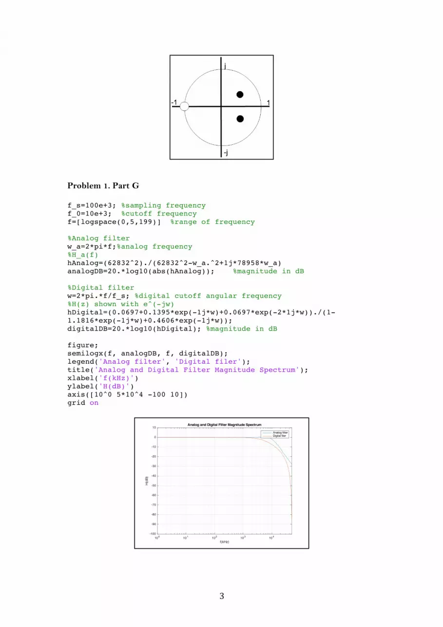
𝑧 = −1 Denominator (poles):
𝑧! − 1.1816𝑧 + 0.4606 = 0 D = 0.6680j
𝑧!,! = 0.5908± 0.3340𝑗
3
Problem 1. Part G f_s=100e+3; %sampling frequency f_0=10e+3; %cutoff frequency f=[logspace(0,5,199)] %range of frequency %Analog filter w_a=2*pi*f;%analog frequency %H_a(f) hAnalog=(62832^2)./(62832^2-w_a.^2+1j*78958*w_a) analogDB=20.*log10(abs(hAnalog)); %magnitude in dB %Digital filter w=2*pi.*f/f_s; %digital cutoff angular frequency %H(z) shown with e^(-jw) hDigital=(0.0697+0.1395*exp(-1j*w)+0.0697*exp(-2*1j*w))./(1-1.1816*exp(-1j*w)+0.4606*exp(-1j*w)); digitalDB=20.*log10(hDigital); %magnitude in dB figure; semilogx(f, analogDB, f, digitalDB); legend('Analog filter', 'Digital filer'); title('Analog and Digital Filter Magnitude Spectrum'); xlabel('f(kHz)') ylabel('H(dB)') axis([10^0 5*10^4 -100 10]) grid on
100 101 102 103 104
f(kHz)
-100
-90
-80
-70
-60
-50
-40
-30
-20
-10
0
10
H(d
B)
Analog and Digital Filter Magnitude Spectrum
Analog filterDigital filer
![1- ] 8.12.2021 Swiss German University timetable final exam](https://img.pdfslide.net/doc/110x75/6333e764a6138719eb0ad4fb/1-8122021-swiss-german-university-timetable-final-exam-.jpg)


