http://www.cambridge.org/0521810876

This page intentionally left blank

Finite Volume Methods for Hyperbolic Problems

This book contains an introduction to hyperbolic partial differential equations and a pow-erful class of numerical methods for approximating their solution, including both linearproblems and nonlinear conservation laws. These equations describe a wide range of wave-propagation and transport phenomena arising in nearly every scientific and engineeringdiscipline. Several applications are described in a self-contained manner, along with muchof the mathematical theory of hyperbolic problems. High-resolution versions of Godunov’smethod are developed, in which Riemann problems are solved to determine the local wavestructure and limiters are then applied to eliminate numerical oscillations. These meth-ods were originally designed to capture shock waves accurately, but are also useful toolsfor studying linear wave-propagation problems, particularly in heterogenous material. Themethods studied are implemented in the CLAWPACK software package. Source code for allthe examples presented can be found on the web, along with animations of many time-dependent solutions. This provides an excellent learning environment for understandingwave-propagation phenomena and finite volume methods.

Randall LeVeque is the Boeing Professor of Applied Mathematics at the University ofWashington.

Cambridge Texts in Applied Mathematics

Maximum and Minimum PrinciplesM.J. SEWELLSolitons

P.G. DRAZIN AND R.S. JOHNSONThe Kinematics of Mixing

J.M. OTTINOIntroduction to Numerical Linear Algebra and Optimisation

PHILIPPE G. CIARLETIntegral Equations

DAVID PORTER AND DAVID S.G. STIRLINGPerturbation Methods

E.J. HINCHThe Thermomechanics of Plasticity and Fracture

GERARD A. MAUGINBoundary Integral and Singularity Methods for Linearized Viscous Flow

C. POZRIKIDISNonlinear Wave Processes in AcousticsK. NAUGOLNYKH AND L. OSTROVSKY

Nonlinear SystemsP.G. DRAZIN

Stability, Instability and ChaosPAUL GLENDINNING

Applied Analysis of the Navier–Stokes EquationsC.R. DOERING AND J.D. GIBBON

Viscous FlowH. OCKENDON AND J.R. OCKENDON

Scaling, Self-Similarity and Intermediate AsymptoticsG.I. BARENBLATT

A First Course in the Numerical Analysis of Differential EquationsARIEH ISERLES

Complex Variables: Introduction and ApplicationsMARK J. ABLOWITZ AND ATHANASSIOS S. FOKASMathematical Models in the Applied Sciences

A.C. FOWLERThinking About Ordinary Differential Equations

ROBERT E. O’MALLEYA Modern Introduction to the Mathematical Theory of Water Waves

R.S. JOHNSONRarefied Gas DynamicsCARLO CERCIGNANI

Symmetry Methods for Differential EquationsPETER E. HYDONHigh Speed FlowC.J. CHAPMANWave Motion

J. BILLINGHAM AND A.C. KINGAn Introduction to Magnetohydrodynamics

P.A. DAVIDSONLinear Elastic WavesJOHN G. HARRIS

An Introduction to Symmetry AnalysisBRIAN J. CANTWELL

Introduction to Hydrodynamic StabilityP.G. DRAZIN

Finite Volume Methods for Hyperbolic ProblemsRANDALL J. LEVEQUE

Finite Volume Methods for Hyperbolic Problems

RANDALL J. LEVEQUEUniversity of Washington

The Pitt Building, Trumpington Street, Cambridge, United Kingdom

The Edinburgh Building, Cambridge CB2 2RU, UK40 West 20th Street, New York, NY 10011-4211, USA477 Williamstown Road, Port Melbourne, VIC 3207, AustraliaRuiz de Alarcón 13, 28014 Madrid, SpainDock House, The Waterfront, Cape Town 8001, South Africa

http://www.cambridge.org

First published in printed format

ISBN 0-521-81087-6 hardbackISBN 0-521-00924-3 paperback

ISBN 0-511-04219-1 eBook

Randall J. LeVeque 2004

2002

(netLibrary)

©

To Loyce and Benjamin

Contents

Preface page xvii

1 Introduction 11.1 Conservation Laws 31.2 Finite Volume Methods 51.3 Multidimensional Problems 61.4 Linear Waves and Discontinuous Media 71.5 CLAWPACK Software 81.6 References 91.7 Notation 10

Part I Linear Equations

2 Conservation Laws and Differential Equations 152.1 The Advection Equation 172.2 Diffusion and the Advection–Diffusion Equation 202.3 The Heat Equation 212.4 Capacity Functions 222.5 Source Terms 222.6 Nonlinear Equations in Fluid Dynamics 232.7 Linear Acoustics 262.8 Sound Waves 292.9 Hyperbolicity of Linear Systems 312.10 Variable-Coefficient Hyperbolic Systems 332.11 Hyperbolicity of Quasilinear and Nonlinear Systems 342.12 Solid Mechanics and Elastic Waves 352.13 Lagrangian Gas Dynamics and the p-System 412.14 Electromagnetic Waves 43

Exercises 46

3 Characteristics and Riemann Problems for LinearHyperbolic Equations 47

3.1 Solution to the Cauchy Problem 47

ix

x Contents

3.2 Superposition of Waves and Characteristic Variables 483.3 Left Eigenvectors 493.4 Simple Waves 493.5 Acoustics 493.6 Domain of Dependence and Range of Influence 503.7 Discontinuous Solutions 523.8 The Riemann Problem for a Linear System 523.9 The Phase Plane for Systems of Two Equations 553.10 Coupled Acoustics and Advection 573.11 Initial–Boundary-Value Problems 59

Exercises 62

4 Finite Volume Methods 644.1 General Formulation for Conservation Laws 644.2 A Numerical Flux for the Diffusion Equation 664.3 Necessary Components for Convergence 674.4 The CFL Condition 684.5 An Unstable Flux 714.6 The Lax–Friedrichs Method 714.7 The Richtmyer Two-Step Lax–Wendroff Method 724.8 Upwind Methods 724.9 The Upwind Method for Advection 734.10 Godunov’s Method for Linear Systems 764.11 The Numerical Flux Function for Godunov’s Method 784.12 The Wave-Propagation Form of Godunov’s Method 784.13 Flux-Difference vs. Flux-Vector Splitting 834.14 Roe’s Method 84

Exercises 85

5 Introduction to the CLAWPACK Software 875.1 Basic Framework 875.2 Obtaining CLAWPACK 895.3 Getting Started 895.4 Using CLAWPACK – a Guide through example1 915.5 Other User-Supplied Routines and Files 985.6 Auxiliary Arrays and setaux.f 985.7 An Acoustics Example 99

Exercises 99

6 High-Resolution Methods 1006.1 The Lax–Wendroff Method 1006.2 The Beam–Warming Method 1026.3 Preview of Limiters 1036.4 The REA Algorithm with Piecewise Linear Reconstruction 106

Contents xi

6.5 Choice of Slopes 1076.6 Oscillations 1086.7 Total Variation 1096.8 TVD Methods Based on the REA Algorithm 1106.9 Slope-Limiter Methods 1116.10 Flux Formulation with Piecewise Linear Reconstruction 1126.11 Flux Limiters 1146.12 TVD Limiters 1156.13 High-Resolution Methods for Systems 1186.14 Implementation 1206.15 Extension to Nonlinear Systems 1216.16 Capacity-Form Differencing 1226.17 Nonuniform Grids 123

Exercises 127

7 Boundary Conditions and Ghost Cells 1297.1 Periodic Boundary Conditions 1307.2 Advection 1307.3 Acoustics 133

Exercises 138

8 Convergence, Accuracy, and Stability 1398.1 Convergence 1398.2 One-Step and Local Truncation Errors 1418.3 Stability Theory 1438.4 Accuracy at Extrema 1498.5 Order of Accuracy Isn’t Everything 1508.6 Modified Equations 1518.7 Accuracy Near Discontinuities 155

Exercises 156

9 Variable-Coefficient Linear Equations 1589.1 Advection in a Pipe 1599.2 Finite Volume Methods 1619.3 The Color Equation 1629.4 The Conservative Advection Equation 1649.5 Edge Velocities 1699.6 Variable-Coefficient Acoustics Equations 1719.7 Constant-Impedance Media 1729.8 Variable Impedance 1739.9 Solving the Riemann Problem for Acoustics 1779.10 Transmission and Reflection Coefficients 1789.11 Godunov’s Method 1799.12 High-Resolution Methods 181

xii Contents

9.13 Wave Limiters 1819.14 Homogenization of Rapidly Varying Coefficients 183

Exercises 187

10 Other Approaches to High Resolution 18810.1 Centered-in-Time Fluxes 18810.2 Higher-Order High-Resolution Methods 19010.3 Limitations of the Lax–Wendroff (Taylor Series) Approach 19110.4 Semidiscrete Methods plus Time Stepping 19110.5 Staggered Grids and Central Schemes 198

Exercises 200

Part II Nonlinear Equations

11 Nonlinear Scalar Conservation Laws 20311.1 Traffic Flow 20311.2 Quasilinear Form and Characteristics 20611.3 Burgers’ Equation 20811.4 Rarefaction Waves 20911.5 Compression Waves 21011.6 Vanishing Viscosity 21011.7 Equal-Area Rule 21111.8 Shock Speed 21211.9 The Rankine–Hugoniot Conditions for Systems 21311.10 Similarity Solutions and Centered Rarefactions 21411.11 Weak Solutions 21511.12 Manipulating Conservation Laws 21611.13 Nonuniqueness, Admissibility, and Entropy Conditions 21611.14 Entropy Functions 21911.15 Long-Time Behavior and N-Wave Decay 222

Exercises 224

12 Finite Volume Methods for Nonlinear ScalarConservation Laws 227

12.1 Godunov’s Method 22712.2 Fluctuations, Waves, and Speeds 22912.3 Transonic Rarefactions and an Entropy Fix 23012.4 Numerical Viscosity 23212.5 The Lax–Friedrichs and Local Lax–Friedrichs Methods 23212.6 The Engquist–Osher Method 23412.7 E-schemes 23512.8 High-Resolution TVD Methods 23512.9 The Importance of Conservation Form 23712.10 The Lax–Wendroff Theorem 239

Contents xiii

12.11 The Entropy Condition 24312.12 Nonlinear Stability 244

Exercises 252

13 Nonlinear Systems of Conservation Laws 25313.1 The Shallow Water Equations 25413.2 Dam-Break and Riemann Problems 25913.3 Characteristic Structure 26013.4 A Two-Shock Riemann Solution 26213.5 Weak Waves and the Linearized Problem 26313.6 Strategy for Solving the Riemann Problem 26313.7 Shock Waves and Hugoniot Loci 26413.8 Simple Waves and Rarefactions 26913.9 Solving the Dam-Break Problem 27913.10 The General Riemann Solver for Shallow Water Equations 28113.11 Shock Collision Problems 28213.12 Linear Degeneracy and Contact Discontinuities 283

Exercises 287

14 Gas Dynamics and the Euler Equations 29114.1 Pressure 29114.2 Energy 29214.3 The Euler Equations 29314.4 Polytropic Ideal Gas 29314.5 Entropy 29514.6 Isothermal Flow 29814.7 The Euler Equations in Primitive Variables 29814.8 The Riemann Problem for the Euler Equations 30014.9 Contact Discontinuities 30114.10 Riemann Invariants 30214.11 Solution to the Riemann Problem 30214.12 The Structure of Rarefaction Waves 30514.13 Shock Tubes and Riemann Problems 30614.14 Multifluid Problems 30814.15 Other Equations of State and Incompressible Flow 309

15 Finite Volume Methods for Nonlinear Systems 31115.1 Godunov’s Method 31115.2 Convergence of Godunov’s Method 31315.3 Approximate Riemann Solvers 31415.4 High-Resolution Methods for Nonlinear Systems 32915.5 An Alternative Wave-Propagation Implementation of Approximate

Riemann Solvers 33315.6 Second-Order Accuracy 335

xiv Contents

15.7 Flux-Vector Splitting 33815.8 Total Variation for Systems of Equations 340

Exercises 348

16 Some Nonclassical Hyperbolic Problems 35016.1 Nonconvex Flux Functions 35016.2 Nonstrictly Hyperbolic Problems 35816.3 Loss of Hyperbolicity 36216.4 Spatially Varying Flux Functions 36816.5 Nonconservative Nonlinear Hyperbolic Equations 37116.6 Nonconservative Transport Equations 372

Exercises 374

17 Source Terms and Balance Laws 37517.1 Fractional-Step Methods 37717.2 An Advection–Reaction Equation 37817.3 General Formulation of Fractional-Step Methods for Linear Problems 38417.4 Strang Splitting 38717.5 Accuracy of Godunov and Strang Splittings 38817.6 Choice of ODE Solver 38917.7 Implicit Methods, Viscous Terms, and Higher-Order Derivatives 39017.8 Steady-State Solutions 39117.9 Boundary Conditions for Fractional-Step Methods 39317.10 Stiff and Singular Source Terms 39617.11 Linear Traffic Flow with On-Ramps or Exits 39617.12 Rankine–Hugoniot Jump Conditions at a Singular Source 39717.13 Nonlinear Traffic Flow with On-Ramps or Exits 39817.14 Accurate Solution of Quasisteady Problems 39917.15 Burgers Equation with a Stiff Source Term 40117.16 Numerical Difficulties with Stiff Source Terms 40417.17 Relaxation Systems 41017.18 Relaxation Schemes 415

Exercises 416

Part III Multidimensional Problems

18 Multidimensional Hyperbolic Problems 42118.1 Derivation of Conservation Laws 42118.2 Advection 42318.3 Compressible Flow 42418.4 Acoustics 42518.5 Hyperbolicity 42518.6 Three-Dimensional Systems 42818.7 Shallow Water Equations 429

Contents xv

18.8 Euler Equations 43118.9 Symmetry and Reduction of Dimension 433

Exercises 434

19 Multidimensional Numerical Methods 43619.1 Finite Difference Methods 43619.2 Finite Volume Methods and Approaches to Discretization 43819.3 Fully Discrete Flux-Differencing Methods 43919.4 Semidiscrete Methods with Runge–Kutta Time Stepping 44319.5 Dimensional Splitting 444

Exercise 446

20 Multidimensional Scalar Equations 44720.1 The Donor-Cell Upwind Method for Advection 44720.2 The Corner-Transport Upwind Method for Advection 44920.3 Wave-Propagation Implementation of the CTU Method 45020.4 von Neumann Stability Analysis 45220.5 The CTU Method for Variable-Coefficient Advection 45320.6 High-Resolution Correction Terms 45620.7 Relation to the Lax–Wendroff Method 45620.8 Divergence-Free Velocity Fields 45720.9 Nonlinear Scalar Conservation Laws 46020.10 Convergence 464

Exercises 467

21 Multidimensional Systems 46921.1 Constant-Coefficient Linear Systems 46921.2 The Wave-Propagation Approach to Accumulating Fluxes 47121.3 CLAWPACK Implementation 47321.4 Acoustics 47421.5 Acoustics in Heterogeneous Media 47621.6 Transverse Riemann Solvers for Nonlinear Systems 48021.7 Shallow Water Equations 48021.8 Boundary Conditions 485

22 Elastic Waves 49122.1 Derivation of the Elasticity Equations 49222.2 The Plane-Strain Equations of Two-Dimensional Elasticity 49922.3 One-Dimensional Slices 50222.4 Boundary Conditions 50222.5 The Plane-Stress Equations and Two-Dimensional Plates 50422.6 A One-Dimensional Rod 50922.7 Two-Dimensional Elasticity in Heterogeneous Media 509

xvi Contents

23 Finite Volume Methods on Quadrilateral Grids 51423.1 Cell Averages and Interface Fluxes 51523.2 Logically Rectangular Grids 51723.3 Godunov’s Method 51823.4 Fluctuation Form 51923.5 Advection Equations 52023.6 Acoustics 52523.7 Shallow Water and Euler Equations 53023.8 Using CLAWPACK on Quadrilateral Grids 53123.9 Boundary Conditions 534

Bibliography 535

Index 553

Preface

Hyperbolic partial differential equations arise in a broad spectrum of disciplines wherewave motion or advective transport is important: gas dynamics, acoustics, elastodynamics,optics, geophysics, and biomechanics, to name but a few. This book is intended to serveas an introduction to both the theory and the practical use of high-resolution finite volumemethods for hyperbolic problems. These methods have proved to be extremely useful inmodeling a broad set of phenomena, and I believe that there is need for a book introducingthem in a general framework that is accessible to students and researchers in many differentdisciplines.Historically, many of the fundamental ideas were first developed for the special case

of compressible gas dynamics (the Euler equations), for applications in aerodynamics,astrophysics, detonation waves, and related fields where shock waves arise. The study ofsimpler equations such as the advection equation, Burgers’ equation, and the shallow waterequations has played an important role in the development of thesemethods, but often only asmodel problems, the ultimate goal being application to the Euler equations. This orientationis still reflected in many of the texts on these methods. Of course the Euler equations remainan extremely important application, and are presented and studied in this book, but thereare also many other applications where challenging problems can be successfully tackledby understanding the basic ideas of high-resolution finite volume methods. Often it is notnecessary to understand the Euler equations in order to do so, and the complexity andpeculiarities of this particular system may obscure the more basic ideas.In particular, the Euler equations are nonlinear. This nonlinearity, and the consequent

shock formation seen in solutions, leads to many of the computational challenges that moti-vated the development of these methods. The mathematical theory of nonlinear hyperbolicproblems is also quite beautiful, and the development and analysis of finite volumemethodsrequires a rich interplay between this mathematical theory, physical modeling, and numer-ical analysis. As a result it is a challenging and satisfying field of study, and much of thisbook focuses on nonlinear problems.However, all of Part I and much of Part III (on multidimensional problems) deals en-

tirely with linear hyperbolic systems. This is partly because many of the concepts canbe introduced and understood most easily in the linear case. A thorough understandingof linear hyperbolic theory, and the development of high-resolution methods in the linearcase, is extremely useful in fully understanding the nonlinear case. In addition, I believethere are many linear wave-propagation problems (e.g., in acoustics, elastodynamics, or

xvii

xviii Preface

electromagnetics) where these methods have a great deal of potential that has not been fullyexploited, particularly for problems in heterogeneous media. I hope to encourage studentsto explore some of these areas, and researchers in these areas to learn about finite vol-ume methods. I have tried to make it possible to do so without delving into the additionalcomplications of the nonlinear theory.Studying these methods in the context of a broader set of applications has other pedagog-

ical advantages as well. Identifying the common features of various problems (as unifiedby the hyperbolic theory) often leads to a better understanding of this theory and greaterability to apply these techniques later to new problems. The finite volume approach canitself lead to greater insight into the physical phenomena and mathematical techniques. Thederivation ofmost conservation laws gives first an integral formulation that is then convertedto a differential equation. A finite volume method is based on the integral formulation, andhence is often closer to the physics than is the partial differential equation.Mastering a set of numerical methods in conjunction with learning the related mathemat-

ics and physics has a further advantage: it is possible to apply the methods immediately inorder to observe the behavior of solutions to the equations, and thereby gain intuition forhow these solutions behave. To facilitate this hands-on approach to learning, virtually everyexample in the book (and many examples not in the book) can be solved by the reader usingprograms and data that are easy to download from the web. The basis for most of these pro-grams is the CLAWPACK software package, which stands for “conservation-law-package.”This package was originally developed for my own use in teaching and so is intimatelylinked with the methods studied in this book. By having access to the source code usedto generate each figure, it is possible for the interested reader to delve more deeply intoimplementation details that aren’t presented in the text. Animations of many of the figuresare also available on the webpages, making it easier to visualize the time-dependent natureof these solutions. By downloading andmodifying the code, it is also possible to experimentwith different initial or boundary conditions, with different mesh sizes or other parameters,or with different methods on the same problem.CLAWPACK has been freely available for several years and is now extensively used for

research aswell as teaching purposes. Another function of this book is to serve as a referenceto users of the software who desire a better understanding of the methods employed and theways in which these methods can be adapted to new applications. The book is not, however,designed to be a user’s manual for the package, and it is not necessary to do any computingin order to follow the presentation.There are many different approaches to developing and implementing high-resolution

finite volume methods for hyperbolic equations. In this book I concentrate primarily on oneparticular approach, the wave-propagation algorithm that is implemented in CLAWPACK,but numerous other methods and the relation between them are discussed at least briefly.It would be impossible to survey all such methods in any detail, and instead my aim isto provide enough understanding of the underlying ideas that the reader will have a goodbasis for learning about other methods from the literature. With minor modifications of theCLAWPACK code it is possible to implement many different methods and easily comparethem on the same set of problems.This book is the result of an evolving set of lecture notes that I have used in teaching

this material over the past 15 years. An early version was published in 1989 after giving

Preface xix

the course at ETH in Zurich [281]. That version has proved popular among instructors andstudents, perhaps primarily because it is short and concise. Unfortunately, the same claimcannot be made for the present book. I have tried, however, to write the book in such away that self-contained subsets can be extracted for teaching (and learning) this material.The latter part of many chapters gets into more esoteric material that may be useful to haveavailable for reference but is not required reading. In addition, many whole chapters can beomitted without loss of continuity in a course that stresses certain aspects of the material. Inparticular, to focus on linear hyperbolic problems and heterogeneous media, a suggested setof chapters might be 1–9 and 18–21, omitting the sections in the multidimensional chaptersthat deal with nonlinearity. Other chapters may also be of interest, but can be omittedwithout loss of continuity. To focus on nonlinear conservation laws, the basic theory canbe found in Chapters 1–8, 11–15, and 18–21. Again, other topics can also be covered iftime permits, or the course can be shortened further by concentrating on scalar equationsor one-dimensional problems, for example.This book may also be useful in a course on hyperbolic problems where the focus is not

on numerical methods at all. Themathematical theory in the context of physical applicationsis developed primarily in Chapters 1–3, 9, 11, 13, 14, 16, 18, and 22, chapters that containlittle discussion of numerical issues. It may still be advantageous to use CLAWPACK tofurther explore these problems and develop physical intuition, but this can be done withouta detailed study of the numerical methods employed.Many topics in this book are closely connected to my own research. Repeatedly teach-

ing this material, writing course notes, and providing students with sample programs hasmotivated me to search for more general formulations that are easier to explain and morebroadly applicable. This work has been funded for many years by the National ScienceFoundation, the Department of Energy, and the University of Washington. Without theirsupport the present form of this book would not have been possible.I am indebted to the many students and colleagues who have taught me so much about

hyperbolic problems and numericalmethods over the years. I cannot begin to thank everyoneby name, and so will just mention a few people who had a particular impact on what ispresented in this book. Luigi Quartapelle deserves high honors for carefully reading everyword of several drafts, finding countless errors, and making numerous suggestions forsubstantial improvement. Special thanks are also due to Mike Epton, Christiane Helzel, JanOlav Langseth, Sorin Mitran, and George Turkiyyah. Along with many others, they helpedme to avoid a number of blunders and present a more polished manuscript. The remainingerrors are, of course, my own responsibility.I would also like to thank Cambridge University Press for publishing this book at a

reasonable price, especially since it is intended to be used as a textbook. Many books arepriced exorbitantly these days, and I believe it is the responsibility of authors to seek outand support publishers that serve the community well.Most importantly, I would like to thank my family for their constant encouragement and

support, particularly my wife and son. They have sacrificed many evenings and weekendsof family time for a project that, from my nine-year old’s perspective at least, has lasted alifetime.

Seattle, Washington, August, 2001

1Introduction

Hyperbolic systems of partial differential equations can be used to model a wide variety ofphenomena that involve wave motion or the advective transport of substances. This chaptercontains a brief introduction to some of the fundamental concepts and an overview of theprimary issues discussed in this book.The problems we consider are generally time-dependent, so that the solution depends

on time as well as one or more spatial variables. In one space dimension, a homogeneousfirst-order system of partial differential equations in x and t has the form

qt (x, t)+ Aqx (x, t) = 0 (1.1)

in the simplest constant-coefficient linear case. Here q :R × R → Rm is a vector with

m components representing the unknown functions (pressure, velocity, etc.) we wish todetermine, and A is a constantm×m real matrix. In order for this problem to be hyperbolic,the matrix must satisfy certain properties discussed below. Note that subscripts are used todenote partial derivatives with respect to t and x .The simplest case is the constant-coefficient scalar problem, in which m= 1 and the

matrix A reduces to a scalar value. This problem is hyperbolic provided the scalar A isreal. Already this simple equation can model either advective transport or wave motion,depending on the context.Advective transport refers to a substance being carried along with fluid motion. For ex-

ample, consider a contaminant being advected downstreamwith some fluid flowing througha one-dimensional pipe at constant velocity u. Then the concentration or density q(x, t) ofthe contaminant satisfies a scalar advection equation of the form

qt (x, t)+ uqx (x, t) = 0, (1.2)

as derived in Chapter 2. It is easy to verify that this equation admits solutions of the form

q(x, t) = q(x − ut) (1.3)

for any function q(ξ ). The concentration profile (or waveform) specified by q simply prop-agates with constant speed u and unchanged shape. In this context the equation (1.2) isgenerally called the advection equation.The phenomenon of wave motion is observed in its most basic form if we model a sound

wave traveling down a tube of gas or through an elastic solid. In this case the molecules of

1

2 1 Introduction

the gas or solid barely move, and yet a distinct wave can propagate through the materialwith its shape essentially unchanged over long distances, and at a speed c (the speed ofsound in the material) that is much larger than the velocity of material particles. We will seein Chapter 2 that a sound wave propagating in one direction (to the right with speed c > 0)can be modeled by the equation

wt (x, t)+ cwx (x, t) = 0, (1.4)

wherew(x, t) is an appropriate combination of the pressure and particle velocity. This againhas the form of a scalar first-order hyperbolic equation. In this context the equation (1.4) issometimes called the one-way wave equation because it models waves propagating in oneparticular direction.Mathematically the advection equation (1.2) and the one-way wave equation (1.4) are

identical, which suggests that advective transport and wave phenomena can be handled bysimilar mathematical and numerical techniques.Tomodel acousticwaves propagating in both directions along a one-dimensionalmedium,

we must consider the full acoustic equations derived in Chapter 2,

pt (x, t)+ Kux (x, t) = 0,ut (x, t)+ (1/ρ)px (x, t) = 0,

(1.5)

where p(x, t) is the pressure (or more properly the perturbation from some backgroundconstant pressure), and u(x, t) is the particle velocity. These are the unknown functions tobe determined. The material is described by the constants K (the bulk modulus of com-pressibility) and ρ (the density). The system (1.5) can be written as the first-order systemqt + Aqx = 0, where

q =[pu

], A =

[0 K1/ρ 0

]. (1.6)

To connect this with the one-way wave equation (1.4), let

w1(x, t) = p(x, t)+ ρcu(x, t),

where c = √K/ρ. Then it is easy to check that w1(x, t) satisfies the equation

w1t + cw1x = 0

and so we see that c can be identified as the speed of sound. On the other hand, the function

w2(x, t) = p(x, t)− ρcu(x, t)

satisfies the equation

w2t − cw2x = 0.

This is also a one-way wave equation, but with propagation speed −c. This equation hassolutions of the form q2(x, t) = q(x + ct) and models acoustic waves propagating to theleft at the speed of sound, rather than to the right.

1.1 Conservation Laws 3

The system (1.5) of two equations can thus be decomposed into two scalar equationsmodeling the two distinct acoustic waves moving in different directions. This is a funda-mental theme of hyperbolic equations and crucial to the methods developed in this book.We will see that this type of decomposition is possible more generally for hyperbolic sys-tems, and in fact the definition of “hyperbolic” is directly connected to this. We say thatthe constant-coefficient system (1.1) is hyperbolic if the matrix A has real eigenvalues anda corresponding set of m linearly independent eigenvectors. This means that any vector inRm can be uniquely decomposed as a linear combination of these eigenvectors. As we will

see in Chapter 3, this provides the decomposition into distinct waves. The correspondingeigenvalues of A give the wave speeds at which each wave propagates. For example, theacoustics matrix A of (1.6) has eigenvalues−c and+c, the speeds at which acoustic wavescan travel in this one-dimensional medium.For simple acoustic waves, some readers may be more familiar with the second-order

wave equation

ptt = c2 pxx . (1.7)

This equation for the pressure can be obtained from the system (1.5) by differentiating thefirst equation with respect to t and the second with respect to x , and then eliminating theuxt terms. The equation (1.7) is also called a hyperbolic equation according to the stan-dard classification of second-order linear equations into hyperbolic, parabolic, and ellipticequations (see [234], for example). In this book we only consider first-order hyperbolicsystems as described above. This form is more fundamental physically than the derivedsecond-order equation, and is more amenable to the development of high-resolution finitevolume methods.In practical problems there is often a coupling of advective transport and wave motion.

For example, we will see that the speed of sound in a gas generally depends on the densityand pressure of the gas. If these properties of the gas vary in space and the gas is flowing, thenthese variations will be advected with the flow. This will have an effect on any sound wavespropagating through the gas. Moreover, these variations will typically cause accelerationof the gas and have a direct effect on the fluid motion itself, which can also be modeled aswave-propagation phenomena. This coupling leads to nonlinearity in the equations.

1.1 Conservation Laws

Much of this book is concerned with an important class of homogeneous hyperbolic equa-tions called conservation laws. The simplest example of a one-dimensional conservationlaw is the partial differential equation (PDE)

qt (x, t)+ f (q(x, t))x = 0, (1.8)

where f (q) is the flux function. Rewriting this in the quasilinear form

qt + f ′(q)qx = 0 (1.9)

suggests that the equation is hyperbolic if the flux Jacobian matrix f ′(q) satisfies the con-ditions previously given for the matrix A. In fact the linear problem (1.1) is a conservation

4 1 Introduction

law with the linear flux function f (q)= Aq . Many physical problems give rise to nonli-near conservation laws in which f (q) is a nonlinear function of q, a vector of conservedquantities.

1.1.1 Integral Form

Conservation laws typically arise most naturally from physical laws in an integral form asdeveloped in Chapter 2, stating that for any two points x1 and x2,

d

dt

∫ x2

x1

q(x, t) dx = f (q(x1, t))− f (q(x2, t)). (1.10)

Each component of q measures the density of some conserved quantity, and the equation(1.10) simply states that the “total mass” of this quantity between any two points can changeonly due to the flux past the endpoints. Such conservation laws naturally hold for manyfundamental physical quantities. For example, the advection equation (1.2) for the densityof a contaminant is derived from the fact that the total mass of the contaminant is conservedas it flows down the pipe and the flux function is f (q) = uq. If the total mass of contaminantis not conserved, because of chemical reactions taking place, for example, then the con-servation law must also contain source terms as described in Section 2.5, Chapter 17, andelsewhere.The constant-coefficient linear acoustics equations (1.5) can be viewed as conservation

laws for pressure and velocity. Physically, however, these are not conserved quantitiesexcept approximately in the case of very small amplitude disturbances in uniformmedia. InSection 2.7 the acoustics equations are derived from the Euler equations of gas dynamics,the nonlinear conservation laws thatmodelmore general disturbances in a compressible gas.These equations model the conservation of mass, momentum, and energy, and the laws ofphysics determine the flux functions. See Section 2.6 and Chapter 14 for these derivations.These equations have been intensively studied and used in countless computations becauseof their importance in aerodynamics and elsewhere.There are many other systems of conservation laws that are important in various appli-

cations, and several are used in this book as examples. However, the Euler equations play aspecial role in the historical development of the techniques discussed in this book. Much ofthe mathematical theory of nonlinear conservation laws was developed with these equationsin mind, and many numerical methods were developed specifically for this system. So, al-though the theory and methods are applicable much more widely, a good knowledge of theEuler equations is required in order to read much of the available literature and benefit fromthese developments. A brief introduction is given in Chapter 14. It is a good idea to becomefamiliar with these equations even if your primary interest is far from gas dynamics.

1.1.2 Discontinuous Solutions

The differential equation (1.8) can be derived from the integral equation (1.10) by simplemanipulations (see Chapter 2) provided that q and f (q) are sufficiently smooth.This provisois important because in practice many interesting solutions are not smooth, but containdiscontinuities such as shock waves. A fundamental feature of nonlinear conservation laws

1.2 Finite Volume Methods 5

is that these discontinuities can easily develop spontaneously even from smooth initial data,and so they must be dealt with both mathematically and computationally.At a discontinuity in q , the partial differential equation (1.8) does not hold in the classical

sense and it is important to remember that the integral conservation law (1.10) is the morefundamental equation which does continue to hold. A rich mathematical theory of shock-wave solutions to conservation laws has been developed. This theory is introduced startingin Chapter 11.

1.2 Finite Volume Methods

Discontinuities lead to computational difficulties and the main subject of this book is theaccurate approximation of such solutions. Classical finite difference methods, in whichderivatives are approximated by finite differences, can be expected to break down neardiscontinuities in the solution where the differential equation does not hold. This bookconcerns finite volume methods, which are based on the integral form (1.10) instead ofthe differential equation. Rather than pointwise approximations at grid points, we breakthe domain into grid cells and approximate the total integral of q over each grid cell, oractually the cell average of q , which is this integral divided by the volume of the cell. Thesevalues are modified in each time step by the flux through the edges of the grid cells, and theprimary problem is to determine good numerical flux functions that approximate the correctfluxes reasonably well, based on the approximate cell averages, the only data available. Wewill concentrate primarily on one class of high-resolution finite volume methods that haveproved to be very effective for computing discontinuous solutions. See Section 6.3 for anintroduction to the properties of these methods.Other classes of methods have also been applied to hyperbolic equations, such as finite

element methods and spectral methods. These are not discussed directly in this book,although much of the material presented here is good background for understanding high-resolution versions.

1.2.1 Riemann Problems

A fundamental tool in the development of finite volume methods is the Riemann problem,which is simply the hyperbolic equation together with special initial data. The data ispiecewise constant with a single jump discontinuity at some point, say x = 0,

q(x, 0) ={ql if x < 0,

qr if x > 0.(1.11)

If Qi−1 and Qi are the cell averages in twoneighboring grid cells on afinite volumegrid, thenby solving the Riemann problem with ql = Qi−1 and qr = Qi , we can obtain informationthat can be used to compute a numerical flux and update the cell averages over a timestep. For hyperbolic problems the solution to the Riemann problem is typically a similaritysolution, a function of x/t alone, and consists of a finite set of waves that propagate awayfrom the origin with constant wave speeds. For linear hyperbolic systems the Riemannproblem is easily solved in terms of the eigenvalues and eigenvectors of the matrix A, as

6 1 Introduction

developed in Chapter 3. This simple structure also holds for nonlinear systems of equationsand the exact solution (or arbitrarily good approximations) to the Riemann problem can beconstructed even for nonlinear systems such as the Euler equations. The theory of nonlinearRiemann solutions for scalar problems is developed in Chapter 11 and extended to systemsin Chapter 13.Computationally, the exact Riemann solution is often too expensive to compute for non-

linear problems and approximate Riemann solvers are used in implementing numericalmethods. These techniques are developed in Section 15.3.

1.2.2 Shock Capturing vs. Tracking

Since the PDEs continue to hold away from discontinuities, one possible approach is tocombine a standard finite difference or finite volume method in smooth regions with someexplicit procedure for tracking the location of discontinuities. This is the numerical analogueof the mathematical approach in which the PDEs are supplemented by jump conditionsacross discontinuities. This approach is often called shock tracking or front tracking. Inmorethan one space dimension, discontinuities typically lie along curves (in two dimensions) orsurfaces (in three dimensions), and such algorithms typically become quite complicated.Moreover, in realistic problems theremay bemany such surfaces that interact in complicatedways as time evolves. This approach will not be discussed further in this book. For someexamples and discussion, see [41], [66], [103], [153], [154], [171], [207], [289], [290],[321], [322], [371], [372].Instead we concentrate here on shock-capturing methods, where the goal is to capture

discontinuities in the solution automatically, without explicitly tracking them. Discontinu-ities must then be smeared over one or more grid cells. Success requires that the methodimplicitly incorporate the correct jump conditions, reduce smearing to a minimum, and notintroduce nonphysical oscillations near the discontinuities. High-resolution finite volumemethods based onRiemann solutions often performwell and aremuch simpler to implementthan shock-tracking methods.

1.3 Multidimensional Problems

The Riemann problem is inherently one-dimensional, but is extensively used also in thesolution of multidimensional hyperbolic problems. A two-dimensional finite volume gridtypically consists of polygonal grid cells; quadrilaterals or triangles are most commonlyused. ARiemann problem normal to each edge of the cell can be solved in order to determinethe flux across that edge. In three dimensions each face of a finite volume cell can beapproximated by a plane, and a Riemann problem normal to this plane solved in orderto compute the flux. Multidimensional problems are discussed in the Part III of the book,starting with an introduction to the mathematical theory in Chapter 18.If the finite volume grid is rectangular, or at least logically rectangular, then the simplest

way to extend one-dimensional high-resolution methods to more dimensions is to use di-mensional splitting, a fractional-step approach in which one-dimensional problems alongeach coordinate direction are solved in turn. This approach, which is often surprisingly ef-fective in practice, is discussed in Section 19.5. In some cases amore fullymultidimensional

1.4 Linear Waves and Discontinuous Media 7

method is required, and one approach is developed starting in Chapter 20, which again reliesheavily on our ability to solve one-dimensional Riemann problems.

1.4 Linear Waves and Discontinuous Media

High-resolution methods were originally developed for nonlinear problems in order to ac-curately capture discontinuous solutions such as shock waves. Linear hyperbolic equationsoften arise from studying small-amplitude waves, where the physical nonlinearities of thetrue equations can be safely ignored. Such waves are often smooth, since shock waves canonly appear from nonlinear phenomena. The acoustic waves we are most familiar with arisefrom oscillations of materials at the molecular level and are typically well approximatedby linear combinations of sinusoidal waves at various frequencies. Similarly, most familiarelectromagnetic waves, such as visible light, are governed by the linear Maxwell equations(another hyperbolic system) and again consist of smooth sinusoidal oscillations.Formany problems in acoustics or optics the primary computational difficulty arises from

the fact that the domain of interest is many orders of magnitude larger than the wavelengthsof interest, and so it is important to use a method that can resolve smooth solutions with avery high order of accuracy in order to keep the number of grid points required manageable.For problems of this type, themethods developed in this bookmay not be appropriate. Thesefinite volume high-resolution methods are typically at best second-order accurate, resultingin the need for many points per wavelength for good accuracy. Moreover they have ahigh cost per grid cell relative to simpler finite difference methods, because of the need tosolve Riemann problems for each pair of grid cells every time step. The combination canbe disastrous if we need to compute over a domain that spans thousands of wavelengths.Instead methods with a higher order of accuracy are typically used, e.g., fourth-order finitedifference methods or spectral methods. For some problems it is hopeless to try to resolveindividual wavelengths, and instead ray-tracing methods such as geometrical optics areused to determine how rays travel without discretizing the hyperbolic equations directly.However, there are some situations in which high-resolution methods based on Riemann

solutionsmay have distinct advantages even for linear problems. Inmany applicationswave-propagation problems must be solved in materials that are not homogeneous and isotropic.The heterogeneity may be smoothly varying (e.g., acoustics in the ocean, where the soundspeed varies with density, which may vary smoothly with changes in salinity, for example).In this case high-order methods may still be applicable. In many cases, however, there aresharp interfaces between different materials. If we wish to solve for acoustic or seismicwaves in the earth, for example, the material parameters typically have jump discontinuitieswhere soilmeets rock or at the boundaries between different types of rock.Ultrasoundwavesin the human body also pass throughmany interfaces, between different organs or tissue andbone. Even in ocean acoustics there may be distinct layers of water with different salinity,and hence jump discontinuities in the sound speed, as well as the interface at the ocean floorwhere waves pass between water and earth. With wave-tracing methods it may be possibleto use reflection and transmission coefficients and Snell’s law to trace rays and reflectedrays at interfaces, but for problems with many interfaces this can be unwieldy. If we wishto model the wave motion directly by solving the hyperbolic equations, many high-ordermethods can have difficulties near interfaces, where the solution is typically not smooth.

8 1 Introduction

For these problems, high-resolution finite volume methods based on solving Riemannproblems can be an attractive alternative. Finite volume methods are a natural choice forheterogeneous media, since each grid cell can be assigned different material properties viaan appropriate averaging of the material parameters over the volume enclosed by the cell.The idea of a Riemann problem is easily extended to the case where there is a discontinuityin the medium at x = 0 as well as a discontinuity in the initial data. Solving the Riemannproblem at the interface between two cells then gives a decomposition of the data into wavesmoving into each cell, including the effects of reflection and transmission as waves movebetween different materials. Indeed, the classical reflection and transmission coefficientsfor various problems are easily derived and understood in terms of particular Riemannsolutions. Variable-coefficient linear problems are discussed in Chapter 9 and Section 21.5.Hyperbolic equations with variable coefficients may not be in conservation form, and

so the methods are developed here in a form that applies more generally. These wave-propagation methods are based directly on the waves arising from the solution of theRiemann problem rather than on numerical fluxes at cell interfaces. When applied to con-servation laws, there is a natural connection between these methods and more standardflux-differencing methods, which will be elucidated as we go along. But many of theshock-capturing ideas that have been developed in the context of conservation laws arevaluable more broadly, and one of my goals in writing this book is to present these meth-ods in a more general framework than is available elsewhere, and with more attention toapplications where they have not traditionally been applied in the past.This book is organized in such a way that all of the ideas required to apply the methods

on linear problems are introduced first, before discussing the more complicated nonlineartheory. Readerswhose primary interest is in linearwaves should be able to skip the nonlinearparts entirely by first studying Chapters 2 through 9 (on linear problems in one dimension)and then the preliminary parts of Chapters 18 through 23 (on multidimensional problems).For readers whose primary interest is in nonlinear problems, I believe that this orga-

nization is still sensible, since many of the fundamental ideas (both mathematical andalgorithmic) arise already with linear problems and are most easily understood in this con-text. Additional issues arise in the nonlinear case, but these are most easily understood ifone already has a firm foundation in the linear theory.

1.5 CLAWPACK Software

The CLAWPACK software (“conservation-laws package”) implements the various wave-propagation methods discussed in this book (in Fortran). This software was originallydeveloped as a teaching tool and is intended to be used in conjunction with this book.The use of this software is briefly described in Chapter 5, and additional documentation isavailable online, from the webpage

http://www.amath.washington.edu/~claw

Virtually all of the computational examples presented in the book were created usingCLAWPACK, and the source code used is generally available via the website

http://www.amath.washington.edu/~claw/book.html

1.6 References 9

A parenthetical remark in the text or figure captions of the form

[claw/book/chapN/examplename]

is an indication that accompanying material is available at

http://www.amath.washington.edu/~claw/book/chapN/examplename/www

often including an animation of time-dependent solutions. From this webpage it is generallypossible to download a CLAWPACK directory of the source code for the example. Down-loading the tarfile and unpacking it in your claw directory results in a subdirectory calledclaw/book/chapN/examplename. (You must first obtain the basic CLAWPACK routines asdescribed in Chapter 5.)You are encouraged to use this software actively, both to develop an intuition for the

behavior of solutions to hyperbolic equations and also to develop direct experience withthese numerical methods. It should be easy to modify the examples to experiment withdifferent parameters or initial conditions, or with the use of different methods on the sameproblem.These examples can also serve as templates for developing codes for other problems.

In addition, many problems not discussed in this book have already been solved usingCLAWPACK and are often available online. Some pointers can be found on the webpages forthe book, and others are collected within the CLAWPACK software in the applicationssubdirectory; see

http://www.amath.washington.edu/~claw/apps.html

1.6 References

Some references for particular applications and methods are given in the text. There arethousands of papers on these topics, and I have not attempted to give an exhaustive surveyof the literature by any means. The references cited have been chosen because they areparticularly relevant to the discussion here or provide a good entrance point to the broaderliterature. Listed below are a few books that may be of general interest in understandingthis material, again only a small subset of those available.An earlier version of this book appeared as a set of lecture notes [281]. This contains

a different presentation of some of the same material and may still be of interest. Mycontribution to [287] also has some overlap with this book, but is directed specificallytowards astrophysical flows and also contains some description of hyperbolic problemsarising in magnetohydrodynamics and relativistic flow, which are not discussed here.The basic theory of hyperbolic equations can be found in many texts, for example John

[229], Kevorkian [234]. The basic theory of nonlinear conservation laws is neatly presentedin the monograph of Lax [263]. Introductions to this material can also be found in manyother books, such as Liu [311], Whitham [486], or Chorin & Marsden [68]. The book ofCourant & Friedrichs [92] deals almost entirely with gas dynamics and the Euler equations,but includes much of the general theory of conservation laws in this context and is veryuseful. The books by Bressan [46], Dafermos [98], Majda [319], Serre [402], Smoller[420], and Zhang & Hsiao [499] present many more details on the mathematical theory ofnonlinear conservation laws.

10 1 Introduction

For general background on numerical methods for PDEs, the books of Iserles [211],Morton & Mayers [333], Strikwerda [427], or Tveito & Winther [461] are recommended.The book of Gustafsson, Kreiss &Oliger [174] is aimed particularly at hyperbolic problemsand contains more advanced material on well-posedness and stability of both initial- andinitial–boundary-value problems. The classic book of Richtmyer&Morton [369] contains agood description of many of the mathematical techniques used to study numerical methods,particularly for linear equations. It also includes a large section on methods for nonlinearapplications including fluid dynamics, but is out of date by now and does not discuss manyof the methods we will study.A number of books have appeared recently on numerical methods for conservation laws

that cover some of the same techniques discussed here, e.g., Godlewski & Raviart [156],Kroner [245], and Toro [450]. Several other books on computational fluid dynamics are alsouseful supplements, including Durran [117], Fletcher [137], Hirsch [198], Laney [256],Oran & Boris [348], Peyret & Taylor [359], and Tannehill, Anderson & Pletcher [445].These books discuss the fluid dynamics in more detail, generally with emphasis on specificapplications.For an excellent collection of photographs illustrating a wide variety of interesting fluid

dynamics, including shock waves, Van Dyke’s Album of Fluid Motion [463] is highly re-commended.Many more references on these topics can easily be found these days by searching on the

web. In addition to using standard web search engines, there are preprint servers that containcollections of preprints on various topics. In the field of conservation laws, the Norwegianpreprint server at

http://www.math.ntnu.no/conservation/

is of particular note.Online citation indices and bibliographic databases are extremely usefulin searching the literature, and students should be encouraged to learn to use them. Someuseful links can be found on the webpage [claw/book/chap1/].

1.7 Notation

Some nonstandard notation is used in this book that may require explanation. In general Iuse q to denote the solution to the partial differential equation under study. In the literaturethe symbol u is commonly used, so that a general one-dimensional conservation law hasthe form ut + f (u)x = 0, for example. However, most of the specific problems we willstudy involve a velocity (as in the acoustics equations (1.5)), and it is very convenientto use u for this quantity (or as the x-component of the velocity vector u= (u, v) in twodimensions).The symbol Qni (in one dimension) or Q

ni j (in two dimensions) is used to denote the

numerical approximation to the solution q . Subscripts on Q denote spatial locations (e.g.,the i th grid cell), and superscript n denotes time level tn . Often the temporal index issuppressed, since we primarily consider one-step methods where the solution at time tn+1 isdetermined entirely by data at time tn .When Q or other numerical quantities lack a temporalsuperscript it is generally clear that the current time level tn is intended.

1.7 Notation 11

For a system of m equations, q and Q are m-vectors, and superscripts are also used todenote the components of these vectors, e.g., q p for p= 1, 2, . . . ,m. It is more convenientto use superscripts than subscripts for this purpose to avoid conflicts with spatial indices.Superscripts are also used to enumerate the eigenvalues λp and eigenvectors r p of anm×mmatrix. Luckilywe generally do not need to refer to specific components of the eigenvectors.Of course superscripts must also be used for exponents at times, and this will usually beclear from context. Initial data is denoted by a circle above the variable, e.g., q◦(x), ratherthan by a subscript or superscript, in order to avoid further confusion.Several symbols play multiple roles in different contexts, since there are not enough

letters and familiar symbols to go around. For example, ψ is used in different places for theentropy flux, for source terms, and for stream functions. For the most part these differentuses are well separated and should be clear from context, but some care is needed toavoid confusion. In particular, the index p is generally used for indexing eigenvalues andeigenvectors, as mentioned above, but is also used for the pressure in acoustics and gasdynamics applications, often in close proximity. Since the pressure is never a superscript, Ihope this will be clear.One new symbol I have introduced is q∨

|(ql , qr ) (pronounced perhaps “q Riemann”) to

denote the value that arises in the similarity solution to a Riemann problem along the rayx/t = 0, when the data ql and qr is specified (see Section 1.2.1). This value is often used indefining numerical fluxes in finite volume methods, and it is convenient to have a generalsymbol for the function that yields it. This symbol is meant to suggest the spreading ofwaves from the Riemann problem, as will be explored starting in Chapter 3. Some notationspecific to multidimensional problems is introduced in Section 18.1.

Part oneLinear Equations

2Conservation Laws and Differential Equations

To see how conservation laws arise from physical principles, we will begin by consideringthe simplest possible fluid dynamics problem, in which a gas or liquid is flowing through aone-dimensional pipe with some known velocity u(x, t), which is assumed to vary only withx , the distance along the pipe, and time t . Typically in fluid dynamics problems we mustdetermine the motion of the fluid, i.e., the velocity function u(x, t), as part of the solution,but let’s assume this is already known and we wish to simply model the concentration ordensity of some chemical present in this fluid (in very small quantities that do not affectthe fluid dynamics). Let q(x, t) be the density of this chemical tracer, the function that wewish to determine.In general the density should be measured in units of mass per unit volume, e.g., grams

per cubic meter, but in studying the one-dimensional pipe with variations only in x , it ismore natural to assume that q is measured in units of mass per unit length, e.g., grams permeter. This density (which is what is denoted by q here) can be obtained by multiplying thethree-dimensional density function by the cross-sectional area of the pipe (which has unitsof square meters). Then

∫ x2

x1

q(x, t) dx (2.1)

represents the totalmass of the tracer in the section of pipe between x1 and x2 at the particulartime t , and has the units of mass. In problems where chemical kinetics is involved, it isoften necessary to measure the “mass” in terms of moles rather than grams, and the densityin moles per meter or moles per cubic meter, since the important consideration is not themass of the chemical but the number of molecules present. For simplicity we will speak interms of mass, but the conservation laws still hold in these other units.Now consider a section of the pipe x1< x < x2 and the manner in which the integral

(2.1) changes with time. If we are studying a substance that is neither created nor destroyedwithin this section, then the total mass within this section can change only due to the fluxor flow of particles through the endpoints of the section at x1 and x2. Let Fi (t) be the rateat which the tracer flows past the fixed point xi for i = 1, 2 (measured in grams per second,say). We use the convention that Fi (t)> 0 corresponds to flow to the right, while Fi (t)< 0means a leftward flux, of |Fi (t)| grams per second. Since the total mass in the section [x1, x2]

15

16 2 Conservation Laws and Differential Equations

changes only due to fluxes at the endpoints, we have

d

dt

∫ x2

x1

q(x, t) dx = F1(t)− F2(t). (2.2)

Note that +F1(t) and −F2(t) both represent fluxes into this section.The equation (2.2) is the basic integral form of a conservation law, and equations of this

type form the basis for much of what we will study. The rate of change of the total massis due only to fluxes through the endpoints – this is the basis of conservation. To proceedfurther, we need to determine how the flux functions Fj (t) are related to q(x, t), so that wecan obtain an equation that might be solvable for q . In the case of fluid flow as describedabove, the flux at any point x at time t is simply given by the product of the density q(x, t)and the velocity u(x, t):

flux at (x, t) = u(x, t)q(x, t). (2.3)

The velocity tells how rapidly particles are moving past the point x (in meters per second,say), and the density q tells how many grams of chemical a meter of fluid contains, so theproduct, measured in grams per second, is indeed the rate at which chemical is passing thispoint.Since u(x, t) is a known function, we can write this flux function as

flux = f (q, x, t) = u(x, t)q. (2.4)

In particular, if the velocity is independent of x and t , so u(x, t) = u is some constant, thenwe can write

flux = f (q) = uq. (2.5)

In this case the flux at any point and time can be determined directly from the value ofthe conserved quantity at that point, and does not depend at all on the location of the pointin space–time. In this case the equation is called autonomous. Autonomous equations willoccupy much of our attention because they arise in many applications and are simpler todeal with than nonautonomous or variable-coefficient equations, though the latter will alsobe studied.For a general autonomous flux f (q) that depends only on the value of q , we can rewrite

the conservation law (2.2) as

d

dt

∫ x2

x1

q(x, t) dx = f (q(x1, t))− f (q(x2, t)). (2.6)

The right-hand side of this equation can be rewritten using standard notation from calculus:

d

dt

∫ x2

x1

q(x, t) dx = − f (q(x, t))∣∣∣∣x2x1

. (2.7)

This shorthand will be useful in cases where the flux has a complicated form, and alsosuggests the manipulations performed below, leading to the differential equation for q.

2.1 The Advection Equation 17

Once the flux function f (q) is specified, e.g., by (2.5) for the simplest case consideredabove, we have an equation for q that we might hope to solve. This equation should holdover every interval [x1, x2] for arbitrary values of x1 and x2. It is not clear how to go aboutfinding a function q(x, t) that satisfies such a condition. Instead of attacking this problemdirectly, we generally transform it into a partial differential equation that can be handledby standard techniques. To do so, we must assume that the functions q(x, t) and f (q) aresufficiently smooth that the manipulations below are valid. This is very important to keepin mind when we begin to discuss nonsmooth solutions to these equations.If we assume that q and f are smooth functions, then this equation can be rewritten as

d

dt

∫ x2

x1

q(x, t) dx = −∫ x2

x1

∂

∂xf (q(x, t)) dx, (2.8)

or, with some further modification, as∫ x2

x1

[∂

∂tq(x, t)+ ∂

∂xf (q(x, t))

]dx = 0. (2.9)

Since this integral must be zero for all values of x1 and x2, it follows that the integrand mustbe identically zero. This gives, finally, the differential equation

∂

∂tq(x, t)+ ∂

∂xf (q(x, t)) = 0. (2.10)

This is called the differential form of the conservation laws. Partial differential equations(PDEs) of this type will be our main focus. Partial derivatives will usually be denoted bysubscripts, so this will be written as

qt (x, t)+ f (q(x, t))x = 0. (2.11)

2.1 The Advection Equation

For the flux function (2.5), the conservation law (2.10) becomes

qt + uqx = 0. (2.12)

This is called the advection equation, since it models the advection of a tracer along withthe fluid. By a tracer we mean a substance that is present in very small concentrationswithin the fluid, so that the magnitude of the concentration has essentially no effect on thefluid dynamics. For this one-dimensional problem the concentration (or density) q can bemeasured in units such as grams per meter along the length of the pipe, so that

∫ x2x1q(x, t) dx

measures the total mass (in grams) within this section of pipe. In Section 9.1 we willconsider more carefully the manner in which this is measured and the form of the resultingadvection equation in more complicated cases where the diameter of the pipe and the fluidvelocity need not be constant.Equation (2.12) is a scalar, linear, constant-coefficient PDE of hyperbolic type. The

general solution of this equation is very easy to determine. Any smooth function of the

18 2 Conservation Laws and Differential Equations

form

q(x, t) = q(x − ut) (2.13)

satisfies the differential equation (2.12), as is easily verified, and in fact any solution to(2.12) is of this form for some q . Note that q(x, t) is constant along any ray in space–timefor which x − ut = constant. For example, all along the ray X (t) = x0 + ut the value ofq(X (t), t) is equal to q(x0). Values of q simply advect (i.e., translate) with constant velocityu, as we would expect physically, since the fluid in the pipe (and hence the density oftracer moving with the fluid) is simply advecting with constant speed. These rays X (t) arecalled the characteristics of the equation. More generally, characteristic curves for a PDEare curves along which the equation simplifies in some particular manner. For the equation(2.12), we see that along X (t) the time derivative of q(X (t), t) is

d

dtq(X (t), t) = qt (X (t), t)+ X ′(t)qx (X (t), t)

= qt + uqx= 0. (2.14)

and the equation (2.12) reduces to a trivial ordinary differential equation ddt Q = 0, where

Q(t) = q(X (t), t). This again leads to the conclusion that q is constant along the charac-teristic.To find the particular solution to (2.12) of interest in a practical problem, we need more

information in order to determine the particular function q in (2.13): initial conditions andperhaps boundary conditions for the equation. First consider the case of an infinitely longpipe with no boundaries, so that (2.12) holds for−∞ < x <∞. Then to determine q(x, t)uniquely for all times t > t0 we need to know the initial condition at time t0, i.e., the initialdensity distribution at this particular time. Suppose we know

q(x, t0) = q◦(x), (2.15)

where q◦(x) is a given function. Then since the value of q must be constant on each charac-teristic, we can conclude that

q(x, t) = q◦(x − u(t − t0))

for t ≥ t0. The initial profile q◦ simply translates with speed u.If the pipe has finite length, a < x < b, then we must also specify the density of tracer

entering the pipe as a function of time, at the inflow end. For example, if u> 0 then wemust specify a boundary condition at x = a, say

q(a, t) = g0(t) for t ≥ t0

in addition to the initial condition

q(x, t) = q◦(x) for a < x < b.

2.1 The Advection Equation 19

(a)

t

a b (b)

t

a b

Fig. 2.1. The solution to the advection equation is constant along characteristics. When solving thisequation on the interval [a, b], we need boundary conditions at x = a if u > 0 as shown in (a), or atx = b if u < 0 as shown in (b).

The solution is then

q(x, t) ={g0(t − (x − a)/u) if a < x < a + u(t − t0),q◦(x − u(t − t0)) if a + u(t − t0) < x < b.

Note that we do not need to specify a boundary condition at the outflow boundary x = b(and in fact cannot, since the density there is entirely determined by the data given already).If on the other hand u< 0, then flow is to the left and we would need a boundary

condition at x = b rather than at x = a. Figure 2.1 indicates the flow of information alongcharacteristics for the two different cases. The proper specification of boundary conditionsis always an important part of the setup of a problem.From now on, we will generally take the initial time to be t = 0 to simplify notation, but

everything extends easily to general t0.

2.1.1 Variable Coefficients

If the fluid velocity u varies with x , then the flux (2.4) leads to the conservation law

qt + (u(x)q)x = 0. (2.16)

In this case the characteristic curves X (t) are solutions to the ordinary differential equations

X ′(t) = u(X (t)). (2.17)

Starting from an arbitrary initial point x0, we can solve the equation (2.17) with initialcondition X (0) = x0 to obtain a particular characteristic curve X (t). Note that these curvestrack themotion of particularmaterial particles carried along by the fluid, since their velocityat any timematches the fluid velocity. Along a characteristic curvewe find that the advection

20 2 Conservation Laws and Differential Equations

equation (2.16) simplifies:

d

dtq(X (t), t) = qt (X (t), t)+ X ′(t)qx (X (t), t)

= qt + u(X (t))qx= qt + (u(X (t))q)x − u′(X (t))q= −u′(X (t))q(X (t), t). (2.18)

Note that when u is not constant, the curves are no longer straight lines and the solution qis no longer constant along the curves, but still the original partial differential equation hasbeen reduced to solving sets of ordinary differential equations.The operator ∂t + u∂x is often called the material derivative, since it represents differen-

tiation along the characteristic curve, and hence computes the rate of change observed by amaterial particle moving with the fluid.The equation (2.16) is an advection equation in conservation form. In some applications

it is more natural to derive a nonconservative advection equation of the form

qt + u(x)qx = 0. (2.19)

Again the characteristic curves satisfy (2.17) and track the motion of material points. Forthis equation the second line of the right-hand side of (2.18) reduces to zero, so that q isnow constant along characteristic curves. Which form (2.16) or (2.19) arises often dependssimply on what units are used to measure physical quantities, e.g., whether we measureconcentration in grams per meter as was assumed above (giving (2.16)), or whether we usegrams per cubic meter, as might seem to be a more reasonable definition of concentrationin a physical fluid. The latter choice leads to (2.19), as is discussed in detail in Chapter 9,and further treatment of variable-coefficient problems is deferred until that point.

2.2 Diffusion and the Advection–Diffusion Equation

Now suppose that the fluid in the pipe is not flowing, and has zero velocity. Then accordingto the advection equation, qt = 0 and the initial profile q◦(x) does not change with time.However, if q◦ is not constant in space, then in fact it should still tend to slowly changedue to molecular diffusion. The velocity u should really be thought of as a mean velocity,the average velocity that the roughly 1023 molecules in a given drop of water have. Butindividual molecules are bouncing around in different directions, and so molecules of thesubstancewe are trackingwill tend to get spread around in thewater, as a drop of ink spreads.There will tend to be a net motion from regions where the density is large to regions whereit is smaller. Fick’s law of diffusion states that the net flux is proportional to the gradientof q, which in one space dimension is simply the derivative qx . The flux at a point x nowdepends on the value of qx at this point, rather than on the value of q, so we write

flux of q = f (qx ) = −βqx , (2.20)

where β is the diffusion coefficient. Using this flux in (2.10) gives

qt = βqxx , (2.21)

which is known as the diffusion equation.

2.3 The Heat Equation 21

In some problems the diffusion coefficient may vary with x . Then f = −β(x)qx and theequation becomes

qt = (β(x)qx )x . (2.22)

Returning to the example of fluid flow, more generally there would be both advectionand diffusion occurring simultaneously. Then the flux is f (q, qx ) = uq − βqx , giving theadvection–diffusion equation

qt + uqx = βqxx . (2.23)

The diffusion and advection–diffusion equations are examples of the general class ofPDEs called parabolic.

2.3 The Heat Equation

The equation (2.21) (or more generally (2.22)) is often called the heat equation, for heatdiffuses in much the same way as a chemical concentration. In the case of heat, there maybe no net motion of the material, but thermal vibration of molecules causes neighboringmolecules to vibrate and this internal energy diffuses through the material. Let q(x, t) nowbe the temperature of the material at point x (e.g., a metal rod, since we are in one spacedimension). The density of internal energy at point x is then given by

E(x, t) = κ(x)q(x, t),

where κ(x) is the heat capacity of thematerial at this point. It is this energy that is conserved,and hence varies in a test section [x1, x2] only due to the flux of energy past the endpoints.The heat flux is given by Fourier’s law of heat conduction,

flux = −βqx ,

where β is the coefficient of thermal conductivity. This looks identical to Fick’s law fordiffusion, but note that Fourier’s law says that the energy flux is proportional to the temper-ature gradient. If the heat capacity is identically constant, say κ ≡ 1, then this is identicalto Fick’s law, but there is a fundamental difference if κ varies. Equation (2.22) is the heatequationwhen κ ≡ 1.More generally the heat equation is derived from the conservation law

d

dt

∫ x2

x1

κ(x)q(x, t) dx = −β(x)qx (x, t)∣∣∣∣x2x1

, (2.24)

and has the differential form

(κq)t = (βqx )x . (2.25)

Typically κ does not vary with time and so this can be written as

κqt = (βqx )x . (2.26)

22 2 Conservation Laws and Differential Equations

2.4 Capacity Functions

In the previous section we saw how the heat capacity comes into the conservation law forheat conduction. There are also other situations where a “capacity” function naturally arisesin the derivation of a conservation law, where again the flux of a quantity is naturally definedin terms of one variable q, whereas it is a different quantity κq that is conserved. If the fluxfunction is f (q), then the obvious generalization of (2.24) yields the conservation law

κqt + f (q)x = 0. (2.27)

While it may be possible to incorporate κ into the definition of f (q), it is often preferablenumerically to work directly with the form (2.27). This is discussed in Section 6.16 and isuseful in many applications. In fluid flow problems, κ might represent the capacity of themedium to hold fluid. For flow through a pipe with a varying diameter, κ(x) might be thecross-sectional area, for example (see Section 9.1). For flow in porous media, κ would bethe porosity, the fraction of the medium available to fluid. On a nonuniform grid a capacityκ appears in the numerical method that is related to the size of a physical grid cell; seeSection 6.17 and Chapter 23.

2.5 Source Terms

In some situations∫ x2x1q(x, t) dx changes due to effects other than flux through the endpoints

of the section, if there is some source or sink of the substance within the section. Denotethe density function for such a source by ψ(q, x, t). (Negative values of ψ correspond to asink rather than a source.) Then the equation becomes

d

dt

∫ x2

x1

q(x, t) dx =∫ x2

x1

∂

∂xf (q(x, t)) dx +

∫ x2

x1

ψ(q(x, t), x, t) dx .

This leads to the PDE

qt (x, t)+ f (q(x, t))x = ψ(q(x, t), x, t). (2.28)

In this section we mention only a few effects that lead to source terms. Conservation lawswith source terms are more fully discussed in Chapter 17.

2.5.1 External Heat Sources

As one example, consider heat conduction in a rod as in Section 2.3, with κ ≡ 1 and β ≡constant, but now suppose there is also an external energy source distributed along the rodwith density ψ . Then we obtain the equation

qt (x, t) = βqxx (x, t)+ ψ(x, t).

This assumes the heat source is independent of the current temperature. In some casesthe strength of the source may depend on the value of q . For example, if the rod is immersedin a liquid that is held at constant temperature q0, then the flux of heat into the rod at the

2.6 Nonlinear Equations in Fluid Dynamics 23

point (x, t) is proportional to q0 − q(x, t) and the equation becomes

qt (x, t) = βqxx (x, t)+ D(q0 − q(x, t)),

where D is the conductivity coefficient between the rod and the bath.

2.5.2 Reacting Flow

As another example, consider a fluid flowing through a pipe at constant velocity as inSection 2.1, but now suppose there are several different chemical species being advectedin this flow (in minute quantities compared to the bulk fluid). If these chemicals react withone another, then the mass of each species individually will not be conserved, since it isused up or produced by the chemical reactions. We will have an advection equation for eachspecies, but these will include source terms arising from the chemical kinetics.As an extremely simple example, consider the advection of a radioactive isotope with

concentration measured by q1, which decays spontaneously at some rate α into a differentisotope with concentration q2. If this decay is taking place in a fluid moving with velocityu, then we have a system of two advection equations with source terms:

q1t + uq1x = −αq1,q2t + uq2x = +αq1.

(2.29)

This has the form qt + Aqx = ψ(q), in which the coefficient matrix A is diagonal with bothdiagonal elements equal to u. This is a hyperbolic system,with a source term.More generallywemight havem specieswith various chemical reactions occurring simultaneously betweenthem. Then we would have a system of m advection equations (with diagonal coefficientmatrix A = u I ) and source terms given by the standard kinetics equations of mass action.If there are spatial variations in concentrations, then these equations may be augmented

with diffusion terms for each species. This would lead to a system of reaction–advection–diffusion equations of the form

qt + Aqx = βqxx + ψ(q). (2.30)

The diffusion coefficient could be different for each species, in which case β would be adiagonal matrix instead of a scalar.Other types of source terms arise from external forces such as gravity or from geometric

transformations used to simplify the equations. See Chapter 17 for some other examples.

2.6 Nonlinear Equations in Fluid Dynamics

In the pipe-flowmodel discussed above, the function q(x, t) represented the density of sometracer that was carried along with the fluid but was present in such small quantities thatthe distribution of q has no effect on the fluid velocity. Now let’s consider the density ofthe fluid itself, again in grams per meter, say, for this one-dimensional problem. We willdenote the fluid density by the standard symbol ρ(x, t). If the fluid is incompressible (asmost liquids can be assumed to be for most purposes), then ρ(x, t) is constant and this

24 2 Conservation Laws and Differential Equations

one-dimensional problem is not very interesting. If we consider a gas, however, then themolecules are far enough apart that compression or expansion is possible and the densitymay vary from point to point.If we again assume that the velocity u is constant, then the density ρ will satisfy the same

advection equation as before (since the flux is simply uρ and u is constant),

ρt + uρx = 0, (2.31)

and any initial variation in density will simply translate at speed u. However, this is notwhat we would expect to happen physically. If the gas is compressed in some region (i.e.,the density is higher here than nearby) then we would expect that the gas would tend topush into the neighboring gas, spreading out, and lowering the density in this region whileraising the density nearby. (This does in fact happen provided that the pressure is also higherin this region; see below.) In order for the gas to spread out it must move relative to theneighboring gas, and hence we expect the velocity to change as a result of the variation indensity.While previously we assumed the tracer density q had no effect on the velocity, this

is no longer the case. Instead we must view the velocity u(x, t) as another unknown tobe determined along with ρ(x, t). The density flux still takes the form (2.3), and so theconservation law for ρ has the form

ρt + (ρu)x = 0, (2.32)

which agreeswith (2.31) only if u is constant. This equation is generally called the continuityequation in fluid dynamics, and models the conservation of mass.In addition to this equation we now need a second equation for the velocity. The velocity

itself is not a conserved quantity, but the momentum is. The product ρ(x, t)u(x, t) givesthe density of momentum, in the sense that the integral of ρu between any two points x1and x2 yields the total momentum in this interval, and this can change only due to the fluxof momentum through the endpoints of the interval. The momentum flux past any point xconsists of two parts. First there is momentum carried past this point along with the movingfluid. For any density function q this flux has the form qu, as we have already seen at thebeginning of this chapter, and so for the momentum q = ρu this contribution to the flux is(ρu)u = ρu2. This is essentially an advective flux, although in the case where the quantitybeing advected is the velocity or momentum of the fluid itself, the phenomenon is oftenreferred to as convection rather than advection.In addition to this macroscopic convective flux, there is also a microscopic momentum

flux due to the pressure of the fluid, as described in Section 14.1. This enters into themomentum flux, which now becomes

momentum flux = ρu2 + p.

The integral form of the conservation law (2.7) is then

d

dt

∫ x2

x1

ρ(x, t)u(x, t) dx = −[ρu2 + p]x2x1 . (2.33)

2.6 Nonlinear Equations in Fluid Dynamics 25

Note that it is only a difference in pressure between the two ends of the interval that willcause a change in the net momentum, as we would expect. We can think of this pressuredifference as a net force that causes an acceleration of the fluid, though this isn’t strictlycorrect and a better interpretation is given in Section 14.1.If we assume that ρ, u, and p are all smooth, then we obtain the differential equation

(ρu)t + (ρu2 + p)x = 0, (2.34)

modeling conservation of momentum. Combining this with the continuity equation (2.32),we have a system of two conservation laws for the conservation of mass and momentum.These are coupled equations, since ρ and ρu appear in both. They are also clearly nonlinear,since products of the unknowns appear.In developing the conservation law for ρu we have introduced a new unknown, the

pressure p(x, t). It appears that we need a third differential equation for this. Pressure is nota conserved quantity, however, and so instead we introduce a fourth variable, the energy,and an additional equation for the conservation of energy. The density of energy will bedenoted by E(x, t). This still does not determine the pressure, and to close the system wemust add an equation of state, an algebraic equation that determines the pressure at anypoint in terms of the mass, momentum, and energy at the point. The energy equation andequations of state will be discussed in detail in Chapter 14, where we will derive the fullsystem of three conservation laws.For the time being we consider special types of flowwhere we can drop the conservation-

of-energy equation and use a simpler equation of state that determines p from ρ alone. Forexample, if no shock waves are present, then it is often correct to assume that the entropy ofthe gas is constant. Such a flow is called isentropic. This is discussed further in Chapter 14.This assumption is reasonable in particular if we wish to derive the equations of linearacoustics, which we will do in the next section. In this case we look at very small-amplitudemotions (sound waves) and the flow remains isentropic. In the isentropic case the equationof state is simply

p = κργ ≡ P(ρ), (2.35)

where κ and γ are two constants (with γ ≈ 1.4 for air).More generally we could assume an equation of state of the form

p = P(ρ), (2.36)

where P(ρ) is a given function specifying the pressure in terms of density. To be physicallyrealistic we can generally assume that

P ′(ρ) > 0 for ρ > 0. (2.37)

This matches our intuition (already used above) that increasing the density of the gas willcause a corresponding increase in pressure. Note that the isentropic equation of state (2.35)has this property. We will see below that the assumption (2.37) is necessary in order toobtain a hyperbolic system.

26 2 Conservation Laws and Differential Equations

Using the equation of state (2.36) in (2.34), together with the continuity equation (2.32),gives a closed system of two equations:

ρt + (ρu)x = 0,(ρu)t + (ρu2 + P(ρ))x = 0.

(2.38)

This is a coupled system of two nonlinear conservation laws, which we can write in theform

qt + f (q)x = 0 (2.39)

if we define

q =[ρ

ρu

]=[q1

q2

], f (q) =

[ρu

ρu2 + P(ρ)

]=[

q2

(q2)2/q1 + P(q1)

]. (2.40)

More generally, a system of m conservation laws takes the form (2.39) with q ∈ Rm and

f : Rm → R

m . The components of f are the fluxes of the respective components of q , andin general each flux may depend on the values of any or all of the conserved quantities atthat point.Again it should be stressed that this differential form of the conservation law is derived

under the assumption that q is smooth, from the more fundamental integral form. Note thatwhen q is smooth, we can also rewrite (2.39) as

qt + f ′(q)qx = 0, (2.41)

where f ′(q) is the Jacobian matrix with (i, j) entry given by ∂ fi/∂q j . The form (2.41) iscalled the quasilinear form of the equation, because it resembles the linear system

qt + Aqx = 0, (2.42)

where A is a givenm×m matrix. In the linear case this matrix does not depend on q , whilein the quasilinear equation (2.41) it does. A thorough understanding of linear systems of theform (2.42) is required before tackling nonlinear systems, and the first 10 chapters concernonly linear problems. There is a close connection between these theories, and the Jacobianmatrix f ′(q) plays an important role in the nonlinear theory.

2.7 Linear Acoustics

In general one can always obtain a linear system from a nonlinear problem by linearizingabout some state. This amounts to defining A = f ′(q0) for some fixed state q0 in the linearsystem (2.42), and gives a mathematically simpler problem that is useful in some situations,particularly when the interest is in studying small perturbations about some constant state.To see how this comes about, suppose we wish to model the propagation of sound waves

in a one-dimensional tube of gas. An acoustic wave is a very small pressure disturbance thatpropagates through the compressible gas, causing infinitesimal changes in the density andpressure of the gas via small motions of the gas with infinitesimal values of the velocity u.

2.7 Linear Acoustics 27

Our eardrums are extremely sensitive to small changes in pressure and translate smalloscillations in the pressure into nerve impulses that we interpret as sound. Consequently,most sound waves are essentially linear phenomena: the magnitudes of disturbances fromthe background state are so small that products or powers of the perturbation amplitudecan be ignored. As linear phenomena, they also do not involve shock waves, and so alinearization of the isentropic equations introduced above is suitable. (An exception is the“sonic boom” caused by supersonic aircraft – this is a nonlinear shock wave, or at leastoriginates as such.)To perform the linearization of (2.40), let

q(x, t) = q0 + q(x, t), (2.43)

where q0 = (ρ0, ρ0u0) is the background state we are linearizing about and q is the pertur-bation we wish to determine. Typically u0 = 0, but it can be nonzero if we wish to studythe propagation of sound in a constant-strength wind, for example. Using (2.43) in (2.11)and discarding any terms that involve powers or products of the q variables, we obtain thelinearized equations

qt + f ′(q0)qx = 0 (2.44)

This is a constant-coefficient linear system modeling the evolution of small disturbances.To obtain the acoustics equations, we compute the Jacobian matrix for the simplified

system of gas dynamics (2.38). Differentiating the flux function from (2.40) gives

f ′(q) =[∂ f 1/∂q1 ∂ f 1/∂q2

∂ f 2/∂q1 ∂ f 2/∂q2

]

=[

0 1

−(q2)2/(q1)2 + P ′(q1) 2q2/q1

]

=[

0 1

−u2 + P ′(ρ) 2u

]. (2.45)

The equations of linear acoustics thus take the form of a constant-coefficient linear system(2.44) with

A = f ′(q0) =[

0 1−u20 + P ′(ρ0) 2u0

]. (2.46)

Note that the vector q in the system (2.44) has components ρ and ρu, the perturbation ofdensity and momentum. When written out in terms of its components, the system is

ρ t + (ρu)x = 0(ρu)t +

(−u20 + P ′(ρ0))ρx + 2u0(ρu)x = 0. (2.47)

Physically it is oftenmore natural tomodel perturbations u and p in velocity and pressure,since these can often be measured directly. To obtain such equations, first note that pressureperturbations can be related to density perturbations through the equation of state,

p0 + p = P(ρ0 + ρ) = P(ρ0)+ P ′(ρ0)ρ + · · · ,

28 2 Conservation Laws and Differential Equations

and since p0 = P(ρ0), we obtain

p ≈ P ′(ρ0)ρ.

Also we have

ρu = (ρ0 + ρ)(u0 + u) = ρ0u0 + ρu0 + ρ0u + ρu,

and so

ρu ≈ u0ρ + ρ0u.

Using these expressions in the equations (2.47) and performing some manipulations(Exercise 2.1) leads to the alternative form of the linear acoustics equations

pt + u0 px + K0ux = 0,ρ0ut + px + ρ0u0ux = 0,

(2.48)

where

K0 = ρ0P′(ρ0). (2.49)

The equations (2.48) can be written as a linear system[pu

]t

+[u0 K01/ρ0 u0

] [pu

]x

= 0. (2.50)

Here and from now on we will generally drop the tilde on p and u and use

q(x, t) =[p(x, t)u(x, t)

]to denote the pressure and velocity perturbations in acoustics.The system (2.50) can also be derived by first rewriting the conservation laws (2.38) as

a nonconservative set of equations for u and p, which is valid only for smooth solutions,and then linearizing this system; see Exercise 2.2.An important special case of these equations is obtained by setting u0 = 0, so that we

are linearizing about the motionless state. In this case the coefficient matrix A appearing inthe system (2.50) is

A =[0 K01/ρ0 0

](2.51)

and the equations reduce to

pt + K0ux = 0,ρ0ut + px = 0.

(2.52)

In Section 2.12 we will see that essentially the same set of equations can be derived forone-dimensional acoustics in an elastic solid. The parameter K0 is called the bulk modulusof compressibility of the material; see Section 22.1.2 for more about this parameter.

2.8 Sound Waves 29

2.8 Sound Waves

If we solve the equations just obtained for linear acoustics in a stationary gas, we expect thesolution to consist of sound waves propagating to the left and right. Since the equations arelinear, we should expect that the general solution consists of a linear superposition of wavesmoving in each direction, and that each wave propagates at constant speed (the speed ofsound) with its shape unchanged. This suggests looking for solutions to the system (2.52)of the form

q(x, t) = q(x − st)

for some speed s, where q(ξ ) is some function of one variable.With this Ansatzwe computethat

qt (x, t) = −sq ′(x − st), qx (x, t) = q ′(x − st),

and so the equation qt + Aqx = 0 reduces to

Aq ′(x − st) = sq ′(x − st). (2.53)

Since s is a scalar while A is a matrix, this is only possible if s is an eigenvalue of the matrixA, and q ′(ξ ) must also be a corresponding eigenvector of A for each value of ξ . Make sureyou understand why this is so, as this is a key concept in understanding the structure ofhyperbolic systems.For the matrix A in (2.51) we easily compute that the eigenvalues are

λ1 = −c0 and λ2 = +c0, (2.54)

where

c0 =√K0/ρ0, (2.55)

which must be the speed of sound in the gas. As expected, waves can propagate in eitherdirection with this speed. Recalling (2.49), we see that

c0 =√P ′(ρ0). (2.56)

The intuitively obvious assumption (2.37) (that pressure increases with density so thatP ′(ρ) > 0) turns out to be important mathematically in order for the speed of sound c0 tobe a real number.For the more general coefficient matrix A of (2.50) with u0 �= 0, the eigenvalues are

found to be

λ1 = u0 − c0 and λ2 = u0 + c0. (2.57)

When the fluid is moving with velocity u0, sound waves still propagate at speed±c0 relativeto the fluid, and at velocities λ1 and λ2 relative to a fixed observer. (See Figure 3.7.)

30 2 Conservation Laws and Differential Equations

Regardless of the value of u0, the eigenvectors of the coefficient matrix are

r1 =[−ρ0c0

1

], r2 =

[ρ0c01

]. (2.58)

Any scalar multiple of each vector would still be an eigenvector. We choose the particularnormalization of (2.58) because the quantity

Z0 ≡ ρ0c0 (2.59)

is an important parameter in acoustics, called the impedance of the medium.A sound wave propagating to the left with velocity −c0 must have the general form

q(x, t) = w1(x + c0t)r1 (2.60)

for some scalar function w1(ξ ), so that

q(x, t) = w1(x + c0t)r1 ≡ q(x + c0t)

and hence q ′(ξ ) is a scalar multiple of r1 as required by (2.53) for s = −c0. In terms of thecomponents of q this means that

p(x, t) = −Z0w1(x + c0t),u(x, t) = w1(x + c0t).

(2.61)

We see that in a left-going sound wave the pressure and velocity perturbations are alwaysrelated by p = −Z0u. Analogously, in a right-going sound wave p = +Z0u everywhereand q(x, t) = w2(x − c0t)r2 for some scalar function w2(ξ ). (See Figure 3.1.)The general solution to the acoustic equations consists of a superposition of left-going

and right-going waves, and has

q(x, t) = w1(x + c0t)r1 + w2(x − c0t)r2 (2.62)

for some scalar functions w1(ξ ) and w2(ξ ). Exactly what these functions are will dependon the initial data given for the problem. Let

q(x, 0) = q◦(x) =[p◦(x)u◦(x)

]

be the pressure and velocity perturbation at time t = 0. To compute the resulting solutionq(x, t) we need to determine the scalar functions w1 and w2 in (2.62). To do so we canevaluate (2.62) at time t = 0 and set this equal to the given data q◦, obtaining

w1(x)r1 + w2(x)r2 = q◦(x).

At each point x this gives a 2× 2 linear system of equations to solve for w1(x) and w2(x)at this particular point (since the vectors r1, r2, and q◦(x) are all known). Let

R = [r1|r2] (2.63)

2.9 Hyperbolicity of Linear Systems 31

be the 2×2 matrix with columns r1 and r2. Then this system of equations can be written as

Rw(x) = q◦(x), (2.64)

where w(x) is the vector with components w1(x) and w2(x). For acoustics the matrix R is

R =[−Z0 Z01 1

], (2.65)

which is a nonsingular matrix provided Z0 > 0 as it will be in practice. The solution to(2.64) can be found in terms of the inverse matrix

R−1 = 1

2Z0

[−1 Z01 Z0

]. (2.66)

We find that

w1(x) = 1

2Z0[−p◦(x)+ Z0u◦(x)],

w2(x) = 1

2Z0[p◦(x)+ Z0u◦(x)].

(2.67)

The solution (2.62) then becomes

p(x, t) = 1

2[p◦(x + c0t)+ p◦(x − c0t)]− Z0

2[u◦(x + c0t)− u◦(x − c0t)],

u(x, t) = − 1

2Z0[p◦(x + c0t)− p◦(x − c0t)]+ 1

2[u◦(x + c0t)+ u◦(x − c0t)].

(2.68)

2.9 Hyperbolicity of Linear Systems

The process we have just gone through to solve the acoustics equations motivates thedefinition of a first-order hyperbolic system of partial differential equations. This processgeneralizes to solve any linear constant-coefficient hyperbolic system.

Definition 2.1. A linear system of the form

qt + Aqx = 0 (2.69)

is called hyperbolic if the m × m matrix A is diagonalizable with real eigenvalues.

We denote the eigenvalues by

λ1 ≤ λ2 ≤ · · · ≤ λm .

The matrix is diagonalizable if there is a complete set of eigenvectors, i.e., if there arenonzero vectors r1, r2, . . . , rm ∈ R

m such that

Ar p = λpr p for p = 1, 2, . . . ,m, (2.70)

32 2 Conservation Laws and Differential Equations

and these vectors are linearly independent. In this case the matrix

R = [r1|r2| · · · |rm], (2.71)

formed by collecting the vectors r1, r2, . . . , rm together, is nonsingular and has an inverseR−1. We then have

R−1AR = � and A = R�R−1, (2.72)

where

� =

λ1

λ2. . .

λm

≡ diag(λ1, λ2, . . . , λm).Hence we can bring A to diagonal form by a similarity transformation, as displayed in(2.72). The importance of this from the standpoint of the PDE is that we can then rewritethe linear system (2.69) as

R−1qt + R−1ARR−1qx = 0. (2.73)

If we define w(x, t) ≡ R−1q(x, t), then this takes the form

wt +�wx = 0. (2.74)

Since� is diagonal, this system decouples into m independent advection equations for thecomponents w p of w:

wpt + λpw p

x = 0 for p = 1, 2, . . . ,m. (2.75)

Since each λp is real, these advection equations make sense physically and can be used tosolve the original system of equations (2.69). Complete details are given in the next chapter,but clearly the solution will consist of a linear combination of m “waves” traveling at thecharacteristic speeds λ1, λ2, . . . , λm . (Recall that eigenvalues are also sometimes called“characteristic values.”) These values define the characteristic curves X (t) = x0 + λptalong which information propagates in the decoupled advection equations. The functionsw p(x, t) are called the characteristic variables; see Section 3.2.There are some special classes of matrices A for which the system is certainly hyperbolic.

If A is a symmetricmatrix (A = AT ), then A is always diagonalizable with real eigenvaluesand the system is said to be symmetric hyperbolic. Also, if A has distinct real eigenvaluesλ1 < λ2 < · · · < λm , then the eigenvectors must be linearly independent and the system ishyperbolic. Such a system is called strictly hyperbolic. The equations of linear acoustics arestrictly hyperbolic, for example. The homogeneous part of the system (2.29) (i.e., settingα = 0) is symmetric hyperbolic but not strictly hyperbolic. Difficulties can arise in studyingcertain nonstrictly hyperbolic equations, as discussed briefly in Section 16.2. If A has realeigenvalues but is not diagonalizable, then the system isweakly hyperbolic; see Section 16.3.

2.10 Variable-Coefficient Hyperbolic Systems 33

2.9.1 Second-Order Wave Equations

From the acoustics equations (2.52) we can eliminate the velocity u and obtain a second-order equation for the pressure. Differentiating the pressure equation with respect to t andthe velocity equation with respect to x and then combining the results gives

ptt = −K0uxt = −K0utx = K0

(1

ρ0px

)x

= c20 pxx .

This yields the second-order wave equation of the classical form

ptt = c20 pxx (c0 ≡ constant). (2.76)

This is also a hyperbolic equation according to the standard classification of second-orderdifferential equations. In this book, however, we concentrate almost entirely on first-orderhyperbolic systems as defined at the start of Section 2.9. There is a certain equivalenceas suggested by the above transformation for acoustics. Conversely, given a second-orderequation of the type (2.76), we can derive a first-order hyperbolic system by defining newvariables

q1 = pt , q2 = −px ,

so that (2.76) becomes q1t + c20q2x = 0, while the equality of mixed partial derivatives givesq2t + q1x = 0. These two equations taken together give a system qt + Aqx = 0, with thecoefficient matrix

A =[0 c201 0

]. (2.77)

This matrix is similar to the matrix A of (2.51), meaning that there is a similarity transfor-mation A = SAS−1 relating the two matrices. The matrix S relates the two sets of variablesand leads to a corresponding change in the eigenvector matrix, while the eigenvalues of thetwo matrices are the same, ±c0.Many books take the viewpoint that the equation (2.76) is the fundamental wave equation

and a first-order system can be derived from it by introducing “artificial” variables suchas pt and px . In fact, however, it is the first-order system that follows directly from thephysics, as we have seen. Since effective numerical methods are more easily derived forthe first-order system than for the second-order scalar equation, there is no need for us toconsider the second-order equation further.

2.10 Variable-Coefficient Hyperbolic Systems

A variable-coefficient linear system of PDEs might take the form

qt + A(x)qx = 0. (2.78)

This system is hyperbolic at any point x where the coefficient matrix satisfies the conditionslaid out in Section 2.9. In Section 9.6, for example, wewill see that the equations of acousticsin a heterogeneousmedium (where the density and bulkmodulus varywith x) can bewritten

34 2 Conservation Laws and Differential Equations

as such a system which is hyperbolic everywhere, with eigenvalues given by ±c(x), wherethe sound speed c(x) varies with position depending on the material parameters.In some cases we might have a conservative system of linear equations of the form

qt + (A(x)q)x = 0, (2.79)

in which the flux function f (q, x) = A(x)q depends explicitly on x . This system could berewritten as

qt + A(x)qx = −A′(x)q (2.80)

as a system of the form (2.78) with the addition of a source term. Again the problem ishyperbolic at any point where A(x) is diagonalizable with real eigenvalues. Such problemsare discussed further in Chapter 9.

2.11 Hyperbolicity of Quasilinear and Nonlinear Systems

A quasilinear system

qt + A(q, x, t)qx = 0 (2.81)

is said to be hyperbolic at a point (q, x, t) if the matrix A(q, x, t) satisfies the hyperbolicitycondition (diagonalizable with real eigenvalues) at this point.The nonlinear conservation law (2.11) is hyperbolic if the Jacobian matrix f ′(q) appear-

ing in the quasilinear form (2.41) satisfies the hyperbolicity condition for each physicallyrelevant value of q.

Example 2.1. The nonlinear equations of isentropic gas dynamics (2.38) have the Jacobianmatrix (2.45). The eigenvalues are

λ1 = u − c, λ2 = u + c,

where the velocity u may now vary from point to point, as does the sound speed

c =√P ′(ρ). (2.82)

However, since P ′(ρ) > 0 at all points in the gas, this nonlinear system is strictly hyperbolic.(Provided we stay away from the “vacuum state” where ρ and p go to zero. For the equationof state (2.35), c→ 0 as well in this case, and the nonstrict hyperbolicity at this point causesadditional difficulties in the nonlinear analysis.)

Solutions to nonlinear hyperbolic systems also involve wave propagation, and for asystem of m equations we will often be able to find m independent waves at each point.However, since the wave speeds depend on the value of the solution q , wave shapes will typ-ically deform, and the solution procedure is greatly complicated by this nonlinear structure.Nonlinear conservation laws are discussed starting in Chapter 11.In the remainder of this chapter some other hyperbolic systems are introduced. These

sections can be skipped at this point without loss of continuity.

2.12 Solid Mechanics and Elastic Waves 35

2.12 Solid Mechanics and Elastic Waves

The equations of linear acoustics were derived in Section 2.8 by linearizing the equationsof isentropic gas dynamics. Essentially the same system of equations can be derived fromelasticity theory to obtain the equations modeling a one-dimensional acoustic wave in asolid, which again is a small-amplitude compressional disturbance in which the materialmoves back and forth in the same direction as the wave propagates, leading to small-scalechanges in density and pressure. Unlike a gas or liquid, however, a solid also supports asecond distinct type of small-amplitude waves called shear waves, in which the motion ofthe material is orthogonal to the direction of wave propagation. These two types of wavestravel at distinct speeds, as illustrated in Figure 2.2. In general these two types of waves arecoupled together and the equations of linear elasticity are a single set of hyperbolic equationsthat must be solved for all motions of the solid, which are coupled together. However, ifwe restrict our attention to one-dimensional plane waves, in which all quantities vary onlyin one direction, then these equations decouple into two independent hyperbolic systemsof two equations each. Mathematically these linear systems are not very interesting, sinceeach has the same structure as the acoustics equations we have already studied in detail.Because of this, however, some of the basic concepts of wave propagation in solids can bemost easily introduced in this context, and this foundation will be useful when we developthe multidimensional equations.Figure 2.2 shows the two distinct types of plane-wave motion in an elastic solid. Other

types of waves can also be observed in solids, such as surface waves at a free surface orinterface between different solids, but these have a truly multidimensional structure. Thestrips shown in Figure 2.2 should be viewed as taken from an infinite three-dimensional solidin which all quantities vary only with x , so the motion shown extends infinitely far in the

cpt cst

(a) (b)

Fig. 2.2. Illustration of (a) P-waves and (b) S-waves in elastic solids. Time advances going upwards.

36 2 Conservation Laws and Differential Equations

y (upward) direction and in z (normal to the page). Related one-dimensional equations canalso be used to study elastic motion in a finite elastic bar, but then additional complicationsarise in that a compression in the x-direction will typically result in some spreading in they- and z-directions, whereas in the infinite plane-wave case there is no opportunity for suchspreading; see Chapter 22.In Figure 2.2(a) the material is compressed at the left edge by a motion in the x-direction

confined to a small region in x . This compressional wave moves in the x-direction at somespeed cp and is analogous to an acoustic wave in a gas. Compressing the material leads toan increase in stress and hence to acceleration in the x-direction. These changes in stressand velocity are coupled together to result in wave motion.Figure 2.2(b) shows a different type of wave, a shear wave in which the material is

displaced in the y-direction over a small region in x . In a gas or liquid, a shear displacementof this type would not result in any restoring force or wave motion. There is no compressionor expansion of the material, and hence no stress results. Molecules of a gas or liquid maybe freely rearranged as long as there is no change in the pressure and there will be norestoring force. Of course frictional (viscous) forces will arise during a rearrangement asthe molecules move past one another, but once rearranged they are not pulled back towardstheir original locations. A solid is fundamentally different in that the constituent moleculesare attached to one another by chemical bonds that resist any deformations. The bonds willstretch slightly to allow small elastic deformations, but like tiny springs they exert a restoringforce that typically growswith themagnitude of any deformation. This operates like pressurein the case of compressional waves, but these bonds also resist shear deformations, and therestoring forces result in shear waves as illustrated in Figure 2.2(b). These waves move ata speed cs that we will see is always smaller then the speed cp of compressional waves.The two types of waves are often called P-waves and S-waves, with “P” and “S” havingtwo possible interpretations: “pressure” and “shear” waves, or alternatively “primary” and“secondary” waves in view of the fact that cp > cs and so the P-wave arising from somedisturbance always arrives at a distant observer before the S-wave.The theory of linear elasticity results from assuming that the deformations are small

enough that the restoring force is linearly related to an appropriate measure of the defor-mation of the solid. For larger deformations the response may be nonlinear. The materialis still elastic if the deformation is sufficiently small that the material can be expected toeventually return to its original configuration if all external forces are removed. If the defor-mation is too extreme, however, the material may simply fail (fracture or break), if enoughbonds are irreparably broken, or it may undergo a plastic deformation, in which bonds arebroken and reformed in a new configuration so that the resulting solid has a different restingconfiguration from that of the original solid. The theory of plasticity then applies.

2.12.1 Elastic Deformations

The mathematical notation of solid mechanics is somewhat different from that of fluiddynamics. For an elastic body we are typically concerned with small displacements aboutsome reference configuration, the location of the body at rest, for example, and so it makessense to consider the actual location of material points at some time as a function of theirreference location. For example, in two space dimensions we can let (X (x, y), Y (x, y))

2.12 Solid Mechanics and Elastic Waves 37

represent the location at time t of the material whose reference location is (x, y). Thedisplacement vector δ is then defined to be

δ(x, y, t) =[δ1(x, y, t)

δ2(x, y, t)

]=[X (x, y, t)Y (x, y, t)

]−[xy

]. (2.83)

The symbol u is often used for the displacement vector, but we reserve this for the velocityvector, which is the time derivative of the displacement,

u(x, y, t) =[u(x, y, t)v(x, y, t)

]=[δ1t (x, y, t)

δ2t (x, y, t)

]. (2.84)

Displacements of the body often lead to strainswithin the body. A strain is a deformationthat results in changes of length or shape within the body. These strains in turn lead tostress, the interior forces due to the stretching or compression of atomic bonds. Theseforces result in acceleration of the material, affecting the motion and hence the evolution ofthe strains. The equations of elasticity consist of Newton’s law relating force to accelerationtogether with stress–strain relations describing the force that results from a given strain.This constitutive relation depends on the particular material (similarly to the equation ofstate for a gas). For sufficiently small strains the stress may be assumed to vary linearlywith strain, resulting in the equations of linear elasticity.

2.12.2 Strain

Not all deformations result in a strain. Rigid-body motions (translations and rotations) inwhich the body is simply moved as a rigid entity do not lead to any internal strain or stress.Rigid translations correspond to a displacement vector δ(x, y, t) that varies only with t andis independent of spatial position. Clearly there will be a strain in the material only if δvaries in space, so that some points are displaced relative to other points in the body. Hencethe strain depends only on the displacement gradient

∇δ =[δ1x δ1y

δ2x δ2y

]=[Xx − 1 XyYx Yy − 1

], (2.85)

where the subscripts denote partial derivatives. Note that for a rigid translation ∇δ = 0.We still need to eliminate solid-body rotations, which can be done by splitting ∇δ into

the sum of a symmetric and a skew-symmetric matrix,

∇δ = ε +�, (2.86)

with

ε = 1

2[∇δ + (∇δ)T ] =

[δ1x

12

(δ1y + δ2x

)12

(δ1y + δ2x

)δ2y

](2.87)

and

� = 1

2[∇δ − (∇δ)T ] =

[0 1

2

(δ1y − δ2x

)− 12

(δ1y − δ2x

)0

]. (2.88)

38 2 Conservation Laws and Differential Equations

The rotation matrix � measures rigid rotations, whereas the symmetric matrix ε is thedesired strain matrix, which will also be written as

ε =[ε11 ε12

ε21 ε22

].

The diagonal elements ε11 and ε22 measure extensional strains in the x- and y-directions,whereas ε12 = ε21 is the shear strain.

Example 2.2. The P-wave shown in Figure 2.2 has a displacement of the form

δ(x, y, t) =[w(x − cpt)

0

]for some wave form w, and hence

ε =[w′(x − cpt) 0

0 0

]with only ε11 nonzero.The S-wave shown in Figure 2.2 has a displacement of the form

δ(x, y, t) =[

0w(x − cst)

]for some waveform w, and hence

ε =[

0 12w

′(x − cst)12w

′(x − cst) 0

]with only the shear strain nonzero.

To study one-dimensional elastic waves of the sort shown in Figure 2.2, we need onlyconsider the components ε11 and ε12 of the strain and must assume that these are functionsof (x, t) alone, independent of y and z. For two-dimensional elasticity we must considerε22 as well, with all three variables being functions of (x, y, t). For full three-dimensionalelasticity the displacement vector and strain matrix must be extended to three dimensions.The formula (2.87) still holds, and ε is now a 3× 3 symmetric matrix with six independentelements, three extensional strains on the diagonal, and three shear strains off the diagonal.See Chapter 22 for more discussion of these equations and their proper relation to three-dimensional elasticity.

2.12.3 Stress

A strain in an elastic body typically results in a restoring force called the stress. For one-dimensional elasticity as described above, we need only be concerned with two componentsof the stress: σ 11(x, t), the force in the x-direction (the normal stress), and σ 12(x, t), theforce in the y-direction (the shear stress).

2.12 Solid Mechanics and Elastic Waves 39

In one-dimensional linear elasticity there is a complete decoupling of compressional andshear effects. The normal stress σ 11 depends only on the strain ε11, while the shear stressσ 12 depends only on the shear strain ε12, and these constitutive relations are linear:

σ 11 = (λ+ 2µ)ε11 with λ+ 2µ > 0, (2.89)

σ 12 = 2µε12 with µ > 0. (2.90)

Here λ and µ are the Lame parameters characterizing the material. The parameter µ is alsocalled the shear modulus. The parameter λ does not have a simple physical meaning, but isrelated to other properties of the material in Section 22.1. It is unfortunate that the symbolλ is standard for this parameter, which should not be confused with an eigenvalue.

2.12.4 The Equations of Motion

We are now ready to write down the equations of motion for one-dimensional elastic waves.P-waves are governed by the system of equations

ε11t − ux = 0,ρut − σ 11x = 0,

(2.91)

where ρ > 0 is the density of the material. The first equation follows from the equalityXxt = Xtx , since

ε11(x, t) = Xx (x, t)− 1 =⇒ ε11t = Xxt ,

u(x, t) = Xt (x, t) =⇒ ux = Xtx .(2.92)

The second equation of (2.91) is Newton’s second law since ut is the acceleration.The system (2.91) involves both ε11 and σ 11, and one of these must be eliminated using

the constitutive relation (2.89). If we eliminate σ 11, we obtain[ε11

u

]t

+[

0 −1−(λ+ 2µ)/ρ 0

] [ε11

u

]x

= 0. (2.93)

This is a hyperbolic system, since the matrix has eigenvalues λ = ±cp with

cp =√(λ+ 2µ)/ρ. (2.94)

If we instead eliminate ε11 we obtain[σ 11

u

]t

+[

0 −(λ+ 2µ)−1/ρ 0

] [σ 11

u

]x

= 0. (2.95)

Again the coefficient matrix has eigenvalues ±cp. Note that this form is essentially equiv-alent to the acoustic equations derived in Section 2.8 if we identify

p(x, t) = −σ 11(x, t). (2.96)

Since ε11 measures the extensional stress (positive when the material is stretched, negativewhen compressed), a positive pressure corresponds to a negative value of σ 11. Note that

40 2 Conservation Laws and Differential Equations

(a)

ε

σ

(b)

p

V

Fig. 2.3. (a) A typical stress–strain relation σ = σ (ε) for the nonlinear elasticity equation (2.97).(b) The equation of state p = p(V ) for isentropic gas dynamics in a Lagrangian frame using thep-system (2.108).

the stress σ 11 can have either sign, depending on whether the material is compressed orstretched, while the pressure in a gas can only be positive. A gas that is “stretched” byallowing it to expand to a larger volume will not attempt to contract back to its originalvolume the way a solid will. This is another consequence of the fact that there are nointermolecular bonds between the gas molecules.One-dimensional nonlinear P-waves can be modeled by the more general form of (2.91)

given by

εt − ux = 0,ρut − σ (ε)x = 0,

(2.97)

where ε is the extensional strain ε11 and σ 11 = σ (ε) is a more general nonlinear constitutiverelation between stress and strain. A typical stress–strain relation might look something likewhat is shown in Figure 2.3(a). In the case shown the derivative of the stress with respectto strain decreases as the magnitude of the strain is increased. This is shown for smallvalues of |ε|, in particular for −ε� 1, since ε = −1 corresponds to a state of completecompression, Xx = 0. Elasticity theory typically breaks down long before this. For verysmall deformations ε, this nonlinear function can generally be replaced by a linearizationσ = (λ+ 2µ)ε, where (λ+ 2µ) ≡ σ ′(0). This is the relation (2.90) used in linear elasticity.The equations for a linear S-wave are essentially identical to (2.91) but involve the shear

strain, shear stress, and vertical velocity:

ε12t −1

2vx = 0,

ρvt − σ 12x = 0.(2.98)

The relationship (2.90) is now used to eliminate either ε12 or σ 12, resulting in a closedsystem of two equations, either[

ε12

v

]t

+[

0 −1/2−2µ/ρ 0

] [ε12

v

]x

= 0 (2.99)

2.13 Lagrangian Gas Dynamics and the p-System 41

if ε12 is used, or

[σ 12

v

]t

+[

0 −µ−1/ρ 0

] [σ 12

v

]x

= 0 (2.100)

if σ 12 is used. In either case, the eigenvalues of the coefficient matrix are λ = ±cs , with thewave speed

cs =√µ/ρ. (2.101)

In general, µ < λ+ 2µ and so cs < cp.We have assumed that shear-wave motion is in the y-direction. In a three-dimensional

body one could also observe a plane shear wave propagating in the x-direction for whichthe shear motion is in the z-direction. These are governed by a set of equations identical to(2.100) but involving ε13 and σ 13 in place of ε12 and σ 12, and the z-component of velocityw in place of v. Shear motion need not be aligned with either the y- or the z-axis, butcan occur in any direction perpendicular to x . Motion in any other direction is simply alinear combination of these two, however, so that there are really two decoupled systems ofequations for S-waves, alongwith the system of equations of P-waves, needed to describe allplane waves in x . Note that the systems (2.95) and (2.100) both have the samemathematicalstructure as the acoustics equations studied previously.For a general two- or three-dimensional motion of an elastic solid it is not possible

to decompose the resulting equations into independent sets of equations for P-waves andS-waves. Instead one obtains a single coupled hyperbolic system. For motions that arefully two-dimensional (but independent of the third direction), one obtains a system of fiveequations for the velocities u, v and the components of the stress tensor σ 11, σ 12, and σ 22

(or alternatively the three components of the strain tensor). Only in the case of purely one-dimensional motions do these equations decouple into independent sets. These decoupledsystems are related to the full three-dimensional equations in Chapter 22.

2.13 Lagrangian Gas Dynamics and the p-System

The fluid dynamics equations derived in Section 2.6 are in Eulerian form, meaning that xrepresents a fixed location in space, and quantities such as the velocity u(x, t) refer to thevelocity of whatever fluid particle happens to be at the point x at time t . Alternatively, theequations can be written in Lagrangian form, where fixing the coordinate ξ corresponds totracking a particular fluid particle. The Lagrangian velocity U (ξ, t) then gives the velocityof this particle at time t . Wemust then determine the mapping X (ξ, t) that gives the physicallocation of the particle labeled ξ at time t . This is more like the approach used in elasticity,as described in Section 2.12, and in one dimension a system of equations very similar to(2.97) results. (The term fluid particle refers to an infinitesimally small volume of fluid, butone that still contains a huge number of molecules so that the small-scale random variationsin velocity can be ignored.)

42 2 Conservation Laws and Differential Equations

To set up the labeling of points initially, we take an arbitrary physical location x0 (sayx0 = 0) and then at each point x assign the label

ξ =∫ x

x0

ρ◦(s) ds (2.102)

to the particle initially located at x , where ρ◦ is the initial data for the density. If the densityis positive everywhere, then this gives a one–one map. Note that ξ has units of mass andthe label ξ gives the total mass between x0 and X (ξ, t). Moreover ξ2 − ξ1 is the total massof all particles between those labeled ξ1 and ξ2 (at any time t , since particles cannot crossin this one-dimensional model).The Lagrangian velocity is related to the Eulerian velocity by

U (ξ, t) = u(X (ξ, t), t).Since X (ξ, t) tracks the location of this particle, we must have

Xt (ξ, t) = U (ξ, t).We could define a Lagrangian density function similarly, but the conservation of massequation in the Lagrangian framework is more naturally written in terms of the specificvolume

V (ξ, t) = 1

ρ(X (ξ, t), t).

This has units of volume/mass (which is just length/mass in one dimension), so it makessense to integrate this over ξ . Since integrating the specific volume over a fixed set ofparticles gives the volume occupied by these particles at time t , we must have∫ ξ2

ξ1

V (ξ, t) dξ = X (ξ2, t)− X (ξ1, t). (2.103)

Differentiating this with respect to t gives

d

dt

∫ ξ2

ξ1

V (ξ, t) dξ = U (ξ2, t)−U (ξ1, t)

=∫ ξ2

ξ1

∂

∂ξU (ξ, t) dξ. (2.104)

Rearranging this and using the fact that it must hold for all choices of ξ1 and ξ2 gives thedifferential form of the conservation law,

Vt −Uξ = 0. (2.105)

Now consider the conservation of momentum. In Eulerian form ρu is the density ofmomentum in units of momentum/volume. In Lagrangian formwe instead considerU (ξ, t),which can be interpreted as the momentum per unit mass, with∫ ξ2

ξ1

U (ξ, t) dξ

2.14 Electromagnetic Waves 43

being the total momentum of all particles between ξ1 and ξ2. By conservation ofmomentum,this integral changes only due to flux at the endpoints. Since in the Lagrangian frameworkthe endpoints are moving with the fluid, there is no “advective flux” and the only change inmomentum comes from the pressure difference between the two endpoints, so

d

dt

∫ ξ2

ξ1

U (ξ, t) dξ = p(ξ1, t)− p(ξ2, t),

which leads to the conservation law

Ut + pξ = 0. (2.106)

If we consider isentropic or isothermal flow, then we have only these two conservationlaws and the equation of state gives p in terms of V alone. Then (2.105) and (2.106) givethe system of conservation laws known as the p-system,

Vt −Uξ = 0,Ut + p(V )ξ = 0.

(2.107)

This is another simple system of two equations that is useful in understanding conservationlaws. It is slightly simpler than the corresponding Eulerian equations (2.38) in that theonly nonlinearity is in the function p(V ). This system if hyperbolic if p′(V )< 0 (seeExercise 2.7). Note that for isentropic flow we have p(V ) = κV−γ , corresponding tothe equation of state (2.35), with the shape shown in Figure 2.3(b).Frequently the p-system is written using lowercase symbols as

vt − ux = 0,ut + p(v)x = 0,

(2.108)

and we will generally use this notation when the p-system is used as a generic example of ahyperbolic system. To relate this system to the Eulerian gas dynamics equations, however,it is important to use distinct notation as derived above.The p-system (2.108) has a very similar structure to the nonlinear elasticity equation

(2.97) if we equate p with the negative stress −σ as discussed in Section 2.12. Note,however, that in the gas dynamics case we must have V > 0 and p> 0, whereas in elasticitythe stress and strain can each be either positive or negative, corresponding to extension andcompression respectively (recall Figure 2.3(a)).

2.14 Electromagnetic Waves

Electromagnetic waves are governed by Maxwell’s equations. In the simplest case this isa hyperbolic system of equations, though in materials where waves are attenuated due toinduced electric currents these are modified by additional source terms. If we assume thereis no net electric charge or current in the material through which the wave is propagating,

44 2 Conservation Laws and Differential Equations

then Maxwell’s equations reduce to

Dt − ∇ × H = 0, (2.109)

Bt + ∇ × E = 0, (2.110)

∇ · D = 0, (2.111)

∇ · B = 0. (2.112)

Here E, D, B, and H are all vectors with three spatial components. The electric field E andthe magnetic field B are related to the two other fields D and H via constitutive relationsthat characterize the medium in which the wave is propagating. These are similar to thestress–strain relations needed in elasticity theory. In general they take the form

D = ε E, (2.113)

B = µ H , (2.114)

where ε is the permittivity and µ is the magnetic permeability of the medium. In a homo-geneous isotropic material these are both scalar constants. More generally they could be3× 3 matrices and also vary in space.If the initial data satisfies the divergence-free conditions (2.111) and (2.112), then it can

be shown that these will hold for all time, and so equations (2.109) and (2.110) for Dt andBt can be taken as the time evolution equations for electromagnetic waves.If ε and µ are scalar constants, then we can eliminate D and H and rewrite the wave-

propagation equations as

Et − 1

εµ∇ × B = 0,

Bt + ∇ × E = 0.(2.115)

This is a linear hyperbolic system of equations in three dimensions.In this chapter we consider only the simplest case of a plane wave propagating in the

x-direction. The B- and E-fields then oscillate in the y–z plane, so that electromagneticwaves are somewhat like shear waves, with the oscillations orthogonal to the direction ofpropagation. However, there are now two fields, and there is an additional relationship thatthe B-field oscillations for a givenwave are orthogonal to the E-field oscillations. Figure 2.4illustrates a wave in which the E-field oscillates in y while the B-field oscillates in z. Inthis case only the y-component of E and the z-component of B are nonzero, and both varyonly with x and t . Then E and B have the form

E = 0E2(x, t)0

, B = 0

0B3(x, t)

. (2.116)

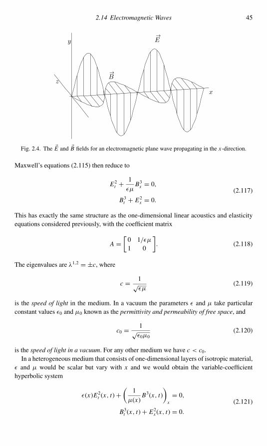
2.14 Electromagnetic Waves 45

B

E

x

y

z

↑

↑

Fig. 2.4. The E and B fields for an electromagnetic plane wave propagating in the x-direction.

Maxwell’s equations (2.115) then reduce to

E2t +1

εµB3x = 0,

B3t + E2x = 0.(2.117)

This has exactly the same structure as the one-dimensional linear acoustics and elasticityequations considered previously, with the coefficient matrix

A =[0 1/εµ1 0

]. (2.118)

The eigenvalues are λ1,2 = ±c, where

c = 1√εµ

(2.119)

is the speed of light in the medium. In a vacuum the parameters ε and µ take particularconstant values ε0 and µ0 known as the permittivity and permeability of free space, and

c0 = 1√ε0µ0

(2.120)

is the speed of light in a vacuum. For any other medium we have c < c0.In a heterogeneous medium that consists of one-dimensional layers of isotropic material,

ε and µ would be scalar but vary with x and we would obtain the variable-coefficienthyperbolic system

ε(x)E2t (x, t)+(

1

µ(x)B3(x, t)

)x

= 0,

B3t (x, t)+ E2x (x, t) = 0.(2.121)

46 2 Conservation Laws and Differential Equations

Themethods discussed in Section 9.6 for variable-coefficient acoustics could also be appliedto this system.In some media ε and/or µ may depend on the strength of the electric or magnetic field,

and hence will vary as a wave passes through. In this case the constitutive relations becomenonlinear, and Maxwell’s equations yield a nonlinear hyperbolic system of equations. Ac-tually, in most materials ε and µ do vary with the field strength, but normally the fieldsassociated with electromagnetic waves are so weak that the linearized theory is perfectlyadequate. However, in some problems with very strong fields or special materials it is nec-essary to consider nonlinear effects. The field of nonlinear optics is important, for example,in the design and study of fiber-optic cables used to transmit pulses of light over thousandsof kilometers in the telecommunications industry.

Exercises

2.1. Derive the equations (2.48) of linear acoustics from the linearized system (2.47).2.2. (a) Show that for smooth solutions the conservation laws (2.38) can be manipulated

into the following set of nonconservative nonlinear equations for the pressureand velocity:

pt + upx + ρP ′(ρ)ux = 0,ut + (1/ρ)px + uux = 0,

(2.122)

wherewe assume that the equation of state can be inverted to defineρ as a functionof p to complete this system. Note that linearizing this nonlinear system aboutsome state (ρ0, u0, p0 = P(ρ0)) again gives the acoustics system (2.47).

(b) Show that the nonlinear system (2.122) is hyperbolic provided P ′(ρ) > 0, andhas the same characteristic speeds as the conservative version (2.38).

2.3. Determine the eigenvalues and eigenvectors the matrix A in (2.77) and also the simi-larity transformation relating this to A from (2.51) when u0 = 0.

2.4. Determine the eigenvalues and eigenvectors the matrix A from (2.46), and show thatthese agree with (2.57). Determine the similarity transformation relating this matrixto A from (2.51).

2.5. Determine the condition on the function σ (ε) that is required in order for the nonlinearelasticity equation (2.91) to be hyperbolic.

2.6. Show that Xξ (ξ, t)= V (ξ, t) and hence (2.105) is simply the statement that Xξ t = Xtξ .2.7. Show that the p-system (2.108) is hyperbolic provided the function p(V ) satisfies

p′(V ) < 0 for all V .2.8. Isothermal flow ismodeled by the system (2.38)with P(ρ) = a2ρ, where a is constant;

see Section 14.6.(a) Determine the wave speeds of the linearized equations (2.50) in this case.(b) The Lagrangian form of the isothermal equations have p(V ) = a2/V . Linearize

the p-system (2.107) in this case about V0,U0, and compute the wave speedsfor Lagrangian acoustics. Verify that these are what you expect in relation to theEulerian acoustic wave speeds.

3Characteristics and Riemann Problems for Linear

Hyperbolic Equations

In this chapter we will further explore the characteristic structure of linear hyperbolic sys-tems of equations. In particular, we will study solutions to the Riemann problem, which issimply the given equation together with very special initial data consisting of a piecewiseconstant function with a single jump discontinuity. This problem and its solution are dis-cussed starting in Section 3.8, after laying some more groundwork. This simple problemplays a very important role in understanding the structure of more general solutions. It isalso a fundamental building block for the finite volume methods discussed in this book.Linear hyperbolic systems of the form

qt + Aqx = 0 (3.1)

were introduced in the last chapter. Recall that the problem is hyperbolic if A ∈ Rm×m is

diagonalizable with real eigenvalues, so that we can write

A = R�R−1, (3.2)

where R is the matrix of right eigenvectors. Then introducing the new variables

w = R−1q

allows us to reduce the system (3.1) to

wt +�wx = 0, (3.3)

which is a set of m decoupled advection equations. Note that this assumes A is constant.If A varies with x and/or t , then the problem is still linear, but R and � will typicallydepend on x and t as well and the manipulations used to obtain (3.3) are no longer valid.See Chapter 9 for discussion of variable-coefficient problems.

3.1 Solution to the Cauchy Problem

Consider the Cauchy problem for the constant-coefficient system (3.1), in which we aregiven data

q(x, 0) = q◦(x) for −∞ < x <∞.

47

48 3 Characteristics and Riemann Problems for Linear Hyperbolic Equations

From this data we can compute data

w◦(x) ≡ R−1q◦(x)

for the system (3.3). The pth equation of (3.3) is the advection equation

wpt + λpw p

x = 0 (3.4)

with solution

w p(x, t) = w p(x − λpt, 0) = w◦p(x − λpt).

Having computed all components w p(x, t) we can combine these into the vector w(x, t),and then

q(x, t) = Rw(x, t) (3.5)

gives the solution to the original problem. This is exactly the process we used to obtain thesolution (2.68) to the acoustics equations in the previous chapter.

3.2 Superposition of Waves and Characteristic Variables

Note that we can write (3.5) as

q(x, t) =m∑p=1

w p(x, t) r p, (3.6)

so that we can view the vector q(x, t) as being some linear combination of the right eigen-vectors r1, . . . , rm at each point in space–time, and hence as a superposition of wavespropagating at different velocities λp. The scalar values w p(x, t) for p = 1, . . . , m givethe coefficients of these eigenvectors at each point, and hence the strength of each wave.The requirements of hyperbolicity insure that these m vectors are linearly independent andhence every vector q has a unique representation in this form. The manipulations resultingin (3.4) show that the eigencoefficient w◦p(x) = w p(x, 0) is simply advected at constantspeed λp as time evolves, i.e.,w p(x, t) ≡ w

◦p(x0) all along the curve X (t) = x0+λpt . Thesecurves are called characteristics of the pth family, or simply p-characteristics. These arestraight lines in the case of a constant-coefficient system. Note that for a strictly hyperbolicsystem, m distinct characteristic curves pass through each point in the x–t plane.The coefficientw p(x, t) of the eigenvector r p in the eigenvector expansion (3.6) of q(x, t)

is constant along any p-characteristic. The functions w p(x, t) are called the characteristicvariables.As an example, for the acoustics equationswith A given by (2.51), we found in Section 2.8

that the characteristic variables are−p+ Z0u and p+ Z0u (or any scalar multiples of thesefunctions), where Z0 is the impedance; see (2.67).

3.5 Acoustics 49

3.3 Left Eigenvectors

Let L = R−1, and denote the rows of the matrix L by �1, �2, . . . , �m . These row vectorsare the left eigenvectors of the matrix A,

�p A = λp�p,

whereas the r p are the right eigenvectors. For example, the left eigenvectors for acousticsare given by the rows of the matrix R−1 in (2.66).Wecanwrite the characteristic variablew p(x, t),which is the pth component of R−1q(x, t)

= Lq(x, t), simply as

w p(x, t) = �pq(x, t). (3.7)

We can then rewrite the solution q(x, t) from (3.6) succinctly in terms of the initial data q◦as

q(x, t) =m∑p=1

[�p q◦(x − λpt)]r p. (3.8)

3.4 Simple Waves

We can view the solution q(x, t) as being the superposition of m waves, each of which isadvected independently with no change in shape. The pth wave has shape w◦p(x)r p andpropagateswith speedλp. This solution has a particularly simple form ifw p(x, 0) is constantin x for all but one value of p, say w◦p(x) ≡ w p for p �= i . Then the solution has the form

q(x, t) = w◦i (x − λi t)r i +

∑p �=i

w pr p (3.9)

= q◦(x − λi t)

and the initial data simply propagates with speed λi . Since m − 1 of the characteristicvariables are constant, the equation essentially reduces to qt + λi qx = 0, which governsthe behavior of the i th family. Nonlinear equations have analogous solutions, called simplewaves, in which variations occur only in one characteristic family; see Section 13.8.

3.5 Acoustics

Anarbitrary solution to the acoustics equations, as derived inSection2.8, canbedecomposedas in (3.6), [

p(x, t)u(x, t)

]= w1(x, t)

[−Z01

]+ w2(x, t)

[Z01

], (3.10)

where w1 = [−p + Z0u]/2Z0 is the strength of the left-going 1-wave, and w2 = [p +Z0u]/2Z0 is the strength of the right-going 2-wave. The functions w1(x, t) and w2(x, t)

50 3 Characteristics and Riemann Problems for Linear Hyperbolic Equations

satisfy scalar advection equations,

w1t − c0w1x = 0 and w2t + c0w2x = 0, (3.11)

so from arbitrary initial data we can compute

w1(x, t) = w1(x + c0t, 0) = w◦1(x + c0t),

w2(x, t) = w2(x − c0t, 0) = w◦2(x − c0t),

(3.12)

where w◦(x) = R−1q◦(x) is the initial data for w, and (3.6) agrees with (2.68).The advection equations (3.11) are often called the one-way wave equations, since each

one models the strength of an acoustic wave going in only one direction.If one of the characteristic variables w1 or w2 is identically constant, then the solution

(3.10) is a simple wave as defined in Section 3.4. Suppose, for example, that w1 ≡ w1 =constant, in which case

q(x, t) = w1r1 + w◦2(x − c0t) r2.

In this case it is also easy to check that the full solution q satisfies the one-waywave equationqt + c0qx = 0.Simple waves often arise in physical problems. Suppose for example that we take initial

data inwhich p= u= 0 everywhere except in some small region near the origin. Ifwe choosep and u as arbitrary functions in this region, unrelated to one another, then the solution willtypically involve a superposition of a left-going and a right-going wave. Figure 3.1 showsthe time evolution in a case where

p(x, 0) = 1

2exp(−80x2)+ S(x),

u(x, 0) = 0,(3.13)

with

S(x) ={1 if −0.3 < x < −0.1,0 otherwise.

For small time the solution changes in a seemingly haphazard way as the left-going andright-going waves superpose. But observe that eventually the two waves separate and forlarger t their individual forms are easy to distinguish. Once they have separated, each waveis a simple wave that propagates at constant velocity with its shape unchanged. In thisexample ρ0 = 1 and K0 = 0.25, so that c0 = Z0 = 1/2. Notice that the left-going wavehas p = −u/2 while the right-going wave has p = u/2, as expected from the form of theeigenvectors.

3.6 Domain of Dependence and Range of Influence

Let (X, T ) be some fixed point in space–time. We see from (3.8) that the solution q(X, T )depends only on the data q◦ at m particular points X − λpT for p = 1, 2, . . . , m. This set

3.6 Domain of Dependence and Range of Influence 51

−1 −0.8 −0.6 −0.4 −0.2 0 0.2 0.4 0.6 0.8 1−1

−0.5

0

0.5

1Pressure at time t = 0

−1 −0.8 −0.6 −0.4 −0.2 0 0.2 0.4 0.6 0.8 1−1

−0.5

0

0.5

1Velocity at time t = 0

−1 −0.8 −0.6 −0.4 −0.2 0 0.2 0.4 0.6 0.8 1−1

−0.5

0

0.5

1Pressure at time t = 0.1

−1 −0.8 −0.6 −0.4 −0.2 0 0.2 0.4 0.6 0.8 1−1

−0.5

0

0.5

1Velocity at time t = 0.1

−1 −0.8 −0.6 −0.4 −0.2 0 0.2 0.4 0.6 0.8 1−1

−0.5

0

0.5

1Pressure at time t = 0.5

−1 −0.8 −0.6 −0.4 −0.2 0 0.2 0.4 0.6 0.8 1−1

−0.5

0

0.5

1Velocity at time t = 0.5

−1 −0.8 −0.6 −0.4 −0.2 0 0.2 0.4 0.6 0.8 1−1

−0.5

0

0.5

1Pressure at time t = 1

−1 −0.8 −0.6 −0.4 −0.2 0 0.2 0.4 0.6 0.8 1−1

−0.5

0

0.5

1Velocity at time t = 1

Fig. 3.1. Evolution of an initial pressure perturbation, concentrated near the origin, into distinctsimple waves propagating with velocities −c0 and c0. The left column shows the pressure pertur-bation q1= p, and the right column shows the velocity q2= u. (Time increases going downwards.)[claw/book/chap3/acousimple]

of points,

D(X, T ) = {X − λpT : p = 1, 2, . . . , m}, (3.14)

is called the domain of dependence of the point (X, T ). See Figure 3.2(a). The value of theinitial data at other points has no influence on the value of q at (X, T ).For hyperbolic equations more generally, the domain of dependence is always a bounded

set, though for nonlinear equations the solution may depend on data over a whole intervalrather than at only a finite number of distinct points. The bounded domain of dependenceresults from the fact that information propagates at finite speed in a hyperbolic equation, aswe expect from wave motion or advection. This has important consequences in the designof numerical methods, and means that explicit methods can often be efficiently used.By contrast, for the heat equation qt = βqxx , the domain of dependence of any point

(X, T ) is the entire real line. Changing the data anywhere would in principle change thevalue of the solution at (X, T ), though the contribution dies away exponentially fast, sodata at points far away may have little effect. Nonetheless, this means that implicit numer-ical methods are often needed in solving parabolic equations. This is discussed further inSection 4.4 in relation to the CFL condition.

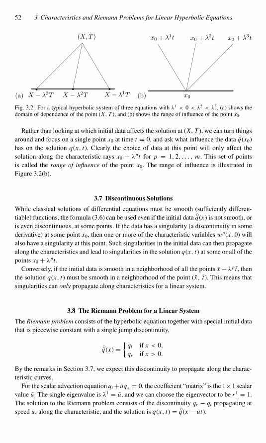
52 3 Characteristics and Riemann Problems for Linear Hyperbolic Equations

(a)

(X,T )

X − λ1TX − λ2TX − λ3T (b) x0

x0 + λ1t x0 + λ2t x0 + λ3t

Fig. 3.2. For a typical hyperbolic system of three equations with λ1 < 0 < λ2 < λ3, (a) shows thedomain of dependence of the point (X, T ), and (b) shows the range of influence of the point x0.

Rather than looking at which initial data affects the solution at (X, T ), we can turn thingsaround and focus on a single point x0 at time t = 0, and ask what influence the data q◦(x0)has on the solution q(x, t). Clearly the choice of data at this point will only affect thesolution along the characteristic rays x0 + λpt for p = 1, 2, . . . , m. This set of pointsis called the range of influence of the point x0. The range of influence is illustrated inFigure 3.2(b).

3.7 Discontinuous Solutions

While classical solutions of differential equations must be smooth (sufficiently differen-tiable) functions, the formula (3.6) can be used even if the initial data q◦(x) is not smooth, oris even discontinuous, at some points. If the data has a singularity (a discontinuity in somederivative) at some point x0, then one or more of the characteristic variables w p(x, 0) willalso have a singularity at this point. Such singularities in the initial data can then propagatealong the characteristics and lead to singularities in the solution q(x, t) at some or all of thepoints x0 + λpt .Conversely, if the initial data is smooth in a neighborhood of all the points x − λpt , then

the solution q(x, t) must be smooth in a neighborhood of the point (x, t ). This means thatsingularities can only propagate along characteristics for a linear system.

3.8 The Riemann Problem for a Linear System

The Riemann problem consists of the hyperbolic equation together with special initial datathat is piecewise constant with a single jump discontinuity,

q◦(x) ={ql if x < 0,qr if x > 0.

By the remarks in Section 3.7, we expect this discontinuity to propagate along the charac-teristic curves.For the scalar advection equation qt+ uqx = 0, the coefficient “matrix” is the 1×1 scalar

value u. The single eigenvalue is λ1 = u, and we can choose the eigenvector to be r1 = 1.The solution to the Riemann problem consists of the discontinuity qr − ql propagating atspeed u, along the characteristic, and the solution is q(x, t) = q◦(x − ut).

3.8 The Riemann Problem for a Linear System 53

For a general m × m linear system we can solve the Riemann problem explicitly usingthe information we have obtained above. It is very important to understand the structureof this solution, since we will see later that Riemann solutions for nonlinear conservationlaws have a similar structure. Moreover, many of the numerical methods we will discuss(beginning in Chapter 4) are based on using solutions to the Riemann problem to constructapproximate solutions with more general data.For the Riemann problem we can simplify the notation if we decompose ql and qr as

ql =m∑p=1

wpl r

p and qr =m∑p=1

w pr r

p. (3.15)

Then the pth advection equation (3.4) has Riemann data

w◦p(x) =

{wpl if x < 0,

wpr if x > 0,

(3.16)

and this discontinuity simply propagates with speed λp, so

w p(x, t) ={wpl if x − λpt < 0,

wpr if x − λpt > 0. (3.17)

If we let P(x, t) be the maximum value of p for which x − λpt > 0, then

q(x, t) =P(x,t)∑p=1

w pr r

p +m∑

p=P(x,t)+1wpl r

p, (3.18)

which we will write more concisely as

q(x, t) =∑

p:λp<x/t

w pr r

p +∑

p:λp>x/t

wpl r

p. (3.19)

The determination of q(x, t) at a given point (X, T ) is illustrated in Figure 3.3. In the caseshown, w1 = w1r while w

2 = w2l and w3 = w3l . The solution at the point illustrated is thus

q(X, T ) = w1r r1 + w2l r2 + w3l r3. (3.20)

Note that the solution is the same at any point in thewedge between the x = λ1t and x = λ2tcharacteristics. As we cross the pth characteristic, the value of x − λpt passes through 0and the corresponding w p jumps from w

pl to w

pr . The other coefficients wi (i �= p) remain

constant.The solution is constant in each of the wedges as shown in Figure 3.3. Across the pth

characteristic the solution jumps with the jump in q given by(w pr − w p

l

)r p ≡ α pr p. (3.21)

Note that this jump in q is an eigenvector of the matrix A (being a scalar multiple of r p).This is an extremely important fact, and a generalization of this statement is what willallow us to solve the Riemann problem for nonlinear systems of equations. This condition,

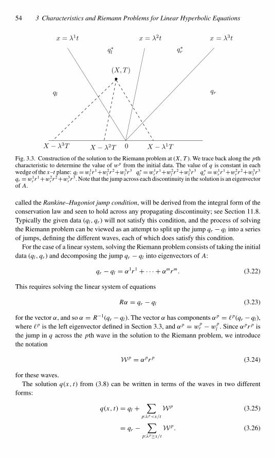
54 3 Characteristics and Riemann Problems for Linear Hyperbolic Equations

x = λ1t x = λ2t x = λ3t

X − λ3T X − λ2T X − λ1T

(X,T )

0

ql

q∗l q∗r

qr

Fig. 3.3. Construction of the solution to the Riemann problem at (X, T ). We trace back along the pthcharacteristic to determine the value of w p from the initial data. The value of q is constant in eachwedge of the x–t plane: ql =w1l r 1+w2l r 2+w3l r 3 q∗l =w1r r 1+w2l r 2+w3l r 3 q∗r =w1r r 1+w2r r 2+w3l r 3qr =w1r r 1+w2r r 2+w3r r 3. Note that the jump across each discontinuity in the solution is an eigenvectorof A.

called the Rankine–Hugoniot jump condition, will be derived from the integral form of theconservation law and seen to hold across any propagating discontinuity; see Section 11.8.Typically the given data (ql , qr ) will not satisfy this condition, and the process of solvingthe Riemann problem can be viewed as an attempt to split up the jump qr − ql into a seriesof jumps, defining the different waves, each of which does satisfy this condition.For the case of a linear system, solving the Riemann problem consists of taking the initial

data (ql , qr ) and decomposing the jump qr − ql into eigenvectors of A:

qr − ql = α1r1 + · · · + αmrm . (3.22)

This requires solving the linear system of equations

Rα = qr − ql (3.23)

for the vector α, and so α = R−1(qr − ql). The vector α has components α p = �p(qr − ql),where �p is the left eigenvector defined in Section 3.3, and α p = w

pr − w p

l . Since αpr p is

the jump in q across the pth wave in the solution to the Riemann problem, we introducethe notation

W p = α pr p (3.24)

for these waves.The solution q(x, t) from (3.8) can be written in terms of the waves in two different

forms:

q(x, t) = ql +∑

p:λp<x/t

W p (3.25)

= qr −∑

p:λp≥x/tW p. (3.26)

3.9 The Phase Plane for Systems of Two Equations 55

This can also be written as

q(x, t) = ql +m∑p=1

H (x − λpt)W p, (3.27)

where H (x) is the Heaviside function

H (x) ={0 if x < 0,1 if x > 0.

(3.28)

3.9 The Phase Plane for Systems of Two Equations

It is illuminating to view the splitting of qr − ql in state space, often called the phase planefor systems of two equations. This is simply the q1–q2 plane, where q = (q1, q2). Eachvector q(x, t) is represented by a point in this plane. In particular, ql and qr are points inthis plane, and a discontinuity with left and right states ql and qr can propagate as a singlediscontinuity only if qr −ql is an eigenvector of A, which means that the line segment fromql to qr must be parallel to the eigenvector r1 or r2. Figure 3.4 shows an example. For thestate ql illustrated there, the jump from ql to qr can propagate as a single discontinuity ifand only if qr lies on one of the two lines drawn through ql in the directions r1 and r2. Theselines give the locus of all points that can be connected to ql by a 1-wave or a 2-wave. Thisset of states is called the Hugoniot locus. We will see that there is a direct generalization ofthis to nonlinear systems in Chapter 13.Similarly, there is a Hugoniot locus through any point qr that gives the set of all points

ql that can be connected to qr by an elementary p-wave. These curves are again in thedirections r1 and r2.For a general Riemann problem with arbitrary ql and qr , the solution consists of two

discontinuities traveling with speeds λ1 and λ2, with a new constant state in between thatwe will call qm . By the discussion above,

qm = w1r r1 + w2l r2, (3.29)

so that qm −ql = (w1r −w1l )r1 and qr −qm = (w2r −w2l )r2. The location of qm in the phase

(a)

ql

q1

q2

r1r2

(b)

ql

qm

qr

0

x = λ1t x = λ2t

Fig. 3.4. (a) The Hugoniot locus of the state ql consists of all states that differ from ql by a scalarmultiple of r 1 or r 2. (b) Solution to the Riemann problem in the x–t plane.

56 3 Characteristics and Riemann Problems for Linear Hyperbolic Equations

(a)

ql

qm

qr

r1r2

(b)

ql

qm

qr

r1r2

Fig. 3.5. The new state qm arising in the solution to the Riemann problem for two different choices ofql and qr . In each case the jump from ql to qm lies in the direction of the eigenvector r 1 correspondingto the lower speed, while the jump from qm to qr lies in the direction of the eigenvector r 2.

plane must be where the 1-wave locus through ql intersects the 2-wave locus through qr .This is illustrated in Figure 3.5(a).Note that if we interchange qr and ql in this picture, the location of qm changes as

illustrated in Figure 3.5(b). In each case we travel from ql to qr by first going in thedirection r1 and then in the direction r2. This is required by the fact that λ1<λ2, sinceclearly the jump between ql and qm must travel slower than the jump between qm and qr(see Figure 3.4(b)) if we are to obtain a single-valued solution.For systemswithmore than two equations, the same interpretation is possible but becomes

harder to draw, since the state space is now m-dimensional. Since the m eigenvectors r p

are linearly independent, we can decompose any jump qr − ql into the sum of jumps inthese directions via (3.22), obtaining a piecewise linear path from ql to qr inm-dimensionalspace.

3.9.1 Acoustics

As a specific example, consider the acoustics equations discussed in Sections 2.7–2.8 withu0 = 0,

[pu

]t

+[0 K01/ρ0 0

][pu

]x

= 0. (3.30)

The eigenvalues and eigenvectors of A are given by (2.54) and (2.58). The phase plane is thep–u plane, and the eigenvectors are symmetric about the u-axis as indicated in Figure 3.6(a).Solving the general Riemann problem gives α = R−1(qr − ql) with components

α1 = �1(qr − ql) = −(pr − pl)+ Z0(ur − ul)2Z0

,

α2 = �2(qr − ql) = (pr − pl)+ Z0(ur − ul)2Z0

,

(3.31)

3.10 Coupled Acoustics and Advection 57

(a)−Z0 Z0

u

p

1r1 r2

(b)

u

ppr plpm

qm

Fig. 3.6. (a) Eigenvectors for the acoustics equations in the p–u phase plane, where Z0 is theimpedance. (b) Solution to a Riemann problem in which ul = ur = 0 and pr < pl .

and the waves areW1 = α1r1 andW2 = α2r2. The intermediate state is

qm = ql + α1r1 = 1

2

[(pl + pr )− Z0(ur − ul)(ul + ur )− (pr − pl)/Z0

]. (3.32)

Example 3.1. Consider a Riemann problem in which ul = ur = 0 and there is only a jumpin pressure with pr < pl . The phase-plane solution to the Riemann problem is sketched inFigure 3.6(b), and we compute that

α1 = pl − pr2Z0

, α2 = pr − pl2Z0

,

so that the intermediate state is

qm = ql + α1r1 = qr − α2r2 = 1

2

[pl + pr

−(pr − pl)/Z0

].

(Recall that p represents the perturbation of pressure from the constant state p0, so it is finefor it to be negative.)

3.10 Coupled Acoustics and Advection

Now consider acoustics in a fluidmoving at constant speed u0 > 0, and tomake the problemmore interesting suppose that there is also a passive tracer being advected in this fluid, withdensity denoted by φ(x, t). Then we can solve the acoustics and advection equation togetheras a system of three equations, pu

φ

t

+ u0 K0 01/ρ0 u0 00 0 u0

puφ

x

. (3.33)

Of course the acoustics and advection could be decoupled into two separate problems, butit is illuminating to solve the Riemann problem for this full system, since its structure is

58 3 Characteristics and Riemann Problems for Linear Hyperbolic Equations

closely related to what is seen in the nonlinear Euler equations of gas dynamics studiedlater, and is also important in solving two-dimensional acoustics (Section 18.4).The coefficient matrix in (3.33) has eigenvalues

λ1 = u0 − c0, λ2 = u0, λ3 = u0 + c0, (3.34)

and corresponding eigenvectors

r1 =−Z01

0

, r2 =001

, r1 = Z010

. (3.35)

The solution to the Riemann problem is easily determined: pr − plur − ulφr − φl

= α1

−Z010

+ α2001

+ α3 Z010

,where

α1 = 1

2Z0[−(pr − pl)+ Z0(ur − ul)],

α2 = φr − φl ,

α3 = 1

2Z0[(pr − pl)+ Z0(ur − ul)].

(3.36)

Note that the 1-wave and 3-wave are standard acoustic waves independent of φ, while the2-wave gives the advection of φ.Suppose φ measures the concentration of a dye in the fluid and that φr > φl , so that

at time t = 0 the fluid to the left is dark while the fluid to the right is light. Then the2-wave marks the interface between the dark and light fluids as time evolves, as indicatedin Figure 3.7. The two fluids remain in contact across this discontinuity in φ, which hasno dynamic effect, since this tracer does not affect the fluid dynamics and the pressure andvelocity are both constant across the 2-wave. This wave is called a contact discontinuity.Within each of the two fluids there is an acoustic wave moving at speed c0 (relative to the

fluid) away from the origin. The jump in pressure and/or velocity in the original Riemanndata creates a “noise,” that moves through the fluids at the speed of sound.

(a)

u0 − c0 u0 u0 + c0

0 (b)

u0 − c0 u0 u0 + c0

0

Fig. 3.7. Solution to the Riemann problem for the coupled acoustics and advection problem. Theinterface between dark and light fluid advects at the fluid velocity u0, and acoustic waves move atspeed c0 relative to the fluid. The speed of eachwave is indicated. (a) A subsonic case. (b) A supersoniccase.

3.11 Initial–Boundary-Value Problems 59

Figure 3.7 shows two different situations. In Figure 3.7(a) the fluid velocity u0 is positivebut subsonic (u0< c0), and so the left-going acoustic wave (the 1-wave) has a negativevelocity u0 − c0< 0 relative to a fixed observer. Figure 3.7(b) illustrates a supersonic flow,where u0> c0 and so u0 − c0> 0. In this case all three waves propagate to the right and noinformation can propagate upstream from the observer. This distinction is not very importantin this linear example. In nonlinear gas dynamics the distinction can be very important. Theratio M = |u0|/c0 is called the Mach number of the flow.

3.11 Initial–Boundary-Value Problems

Now consider a hyperbolic system on a bounded interval a ≤ x ≤ b. This is called theinitial–boundary-value problem, or IBVP for short, since it is a time-dependent problemfor which we need both initial data and boundary data. For a system of m equations weneed a total of m boundary conditions. Typically some conditions must be prescribed atthe left boundary x = a and some at the right boundary x = b. How many are required ateach boundary depends on the number of eigenvalues of A that are positive and negative,respectively.We considered the IBVP for the advection equation in Section 2.1 and saw that we need a

boundary condition only at x = a if u > 0 and only at x = b if u < 0. So if we diagonalizea general linear system to obtain a decoupled set of advection equations

wpt + λpw p

x = 0,

thenwe need to specify boundary data onw p(x, t) at x = a if λp > 0 and at x = b if λp < 0.(For now assume all eigenvalues are nonzero, i.e., that the boundary is noncharacteristic.)So if the system of m equations has n ≤ m negative eigenvalues and m − n positive

eigenvalues, i.e.,

λ1 ≤ λ2 ≤ · · · ≤ λn < 0 < λn+1 ≤ · · · ≤ λm,

then we need to specify m − n boundary conditions at x = a and n boundary conditions atx = b. What sort of boundary data should we impose? Partition the vector w as

w =[wI

wII

], (3.37)

where wI ∈ Rn and wII ∈ R

m−n . Then at the left boundary x = a, for example, we mustspecify the components of wII, while wI are outflow variables. It is valid to specify wII interms of wI. For example, we might use a linear boundary condition of the form

wII(a, t) = B1wI(a, t)+ g1(t), (3.38)

where B1 ∈ R(m−n)×n and g1 ∈ R

m−n . If B1 = 0, then we are simply specifying givenvalues for the inflow variables. But at a physical boundary there is often some reflection ofoutgoing waves, and this requires a nonzero B1.Boundary conditions should be specified as part of the problem and are determined by the

physical setup – generally not in terms of the characteristic variables, unfortunately. It is not

60 3 Characteristics and Riemann Problems for Linear Hyperbolic Equations

always easy to see what the correct conditions are to impose on the mathematical equation.Wemay have several pieces of information about what is happening at the boundary.Whichare the correct ones to specify at the boundary? If we specify too few or toomany conditions,or inappropriate conditions (such as trying to specify the value of an outflow characteristicvariable), then the mathematical problem is ill posed and will have no solution, or perhapsmany solutions. It often helps greatly to know what the characteristic structure is, whichreveals howmany boundary conditions we need and allows us to check that we are imposingappropriate conditions for a well-posed problem. In Chapter 7 boundary conditions arediscussed further, and we will see how to impose such boundary conditions numerically.

Example 3.2. Consider the acoustics problem (2.50) in a closed tube of gas, a ≤ x ≤ b.We expect an acoustic wave hitting either closed end to be reflected. Since the system haseigenvalues −c0 and +c0, we need to specify one condition at each end (n = m − n = 1and wI = w1, wII = w2). We do not have any information on values of the pressure at theboundary a priori, but we do know that the velocity must be zero at each end at all times,since the gas cannot flow through the solid walls (and shouldn’t flow away from the wallsor a vacuum would appear). This suggests that we should set

u(a, t) = u(b, t) = 0 (3.39)

as our two boundary conditions, and this is correct. Note that we are specifying the samething at each end, although the ingoing characteristic variable is different at the two ends.From Section 2.8 we know that the characteristic variables are

w1 = −p + Z0u, w2 = p + Z0u. (3.40)

Wecan combinew1 andw2 to see that specifyingu = 0 amounts to requiring thatw1+w2 =0 at each end. At x = a we can write this as

w2(a, t) = −w1(a, t),

which has the form (3.38)with B1= 1 and g1= 0. The outgoingwave is completely reflectedand feeds back into the incoming wave. Conversely, at x = b we can interpret the boundarycondition u = 0 as

w1(b, t) = −w2(b, t),

which sets the incoming variable at this boundary, again by complete reflection of theoutgoing variable.

Example 3.3. Supposewe set B1= 0 and g1= 0 in (3.38), so that this becomeswII(a, t)= 0.Then there is nothing flowing into the domain at the left boundary, and any left-goingwaves will simply leave the domain with no reflection. These are called outflow boundaryconditions.Figure 3.8 shows a continuation of the example shown in Figure 3.1 to later times, with

a solid wall at the left and outflow boundary conditions imposed at the right, which amountto setting w1(b, t) = 0 and hence p(b, t) = Z0u(b, t).

3.11 Initial–Boundary-Value Problems 61

−1 −0.8 −0.6 −0.4 −0.2 0 0.2 0.4 0.6 0.8 1−1

−0.5

0

0.5

1Pressure at time t = 1

−1 −0.8 −0.6 −0.4 −0.2 0 0.2 0.4 0.6 0.8 1−1

−0.5

0

0.5

1Velocity at time t = 1

−1 −0.8 −0.6 −0.4 −0.2 0 0.2 0.4 0.6 0.8 1−1

−0.5

0

0.5

1Pressure at time t = 1.5

−1 −0.8 −0.6 −0.4 −0.2 0 0.2 0.4 0.6 0.8 1−1

−0.5

0

0.5

1Velocity at time t = 1.5

−1 −0.8 −0.6 −0.4 −0.2 0 0.2 0.4 0.6 0.8 1−1

−0.5

0

0.5

1Pressure at time t = 2

−1 −0.8 −0.6 −0.4 −0.2 0 0.2 0.4 0.6 0.8 1−1

−0.5

0

0.5

1Velocity at time t = 2

−1 −0.8 −0.6 −0.4 −0.2 0 0.2 0.4 0.6 0.8 1−1

−0.5

0

0.5

1Pressure at time t = 2.5

−1 −0.8 −0.6 −0.4 −0.2 0 0.2 0.4 0.6 0.8 1−1

−0.5

0

0.5

1Velocity at time t = 2.5

−1 −0.8 −0.6 −0.4 −0.2 0 0.2 0.4 0.6 0.8 1−1

−0.5

0

0.5

1Pressure at time t = 3

−1 −0.8 −0.6 −0.4 −0.2 0 0.2 0.4 0.6 0.8 1−1

−0.5

0

0.5

1Velocity at time t = 3

Fig. 3.8. Continuation of the example shown in Figure 3.1 with a solid wall at the left and outflowboundary conditions imposed at the right. Note that the wave that strikes the left boundary is a1-wave with p=−u/2, while the reflected wave is a 2-wave with p= u/2. [claw/book/chap3/acousimple]

Example 3.4. A set of boundary conditions that is often useful mathematically is theperiodic boundary conditions

q(a, t) = q(b, t). (3.41)

This set of boundary conditions couples information at the two boundaries, and the idea isthat waves going out one end should reenter at the other end. Solving the IBVPwith periodicboundary conditions is equivalent to solving a Cauchy problem with periodic initial data,where the data given in a ≤ x ≤ b is periodically extended to the whole real line.We are specifying m coupled boundary conditions rather than m − n at one end and n at

the other, but we can reinterpret (3.41) in terms of the characteristic variables as

wII(a, t) = wII(b, t),

wI(b, t) = wI(a, t).(3.42)

62 3 Characteristics and Riemann Problems for Linear Hyperbolic Equations

The m − n incoming values wII at x = a are specified using the outgoing values at x = b,while the n incoming values wI at x = b are specified using the outgoing values at x = a.

Exercises

3.1. For each of the Riemann problems below, sketch the solution in the phase plane, andsketch q1(x, t) and q2(x, t) as functions of x at some fixed time t :

(a) A =[0 41 0

], ql =

[01

], qr =

[11

],

(b) A =[0 41 0

], ql =

[11

], qr =

[01

].

(c) A =[0 91 0

], ql =

[10

], qr =

[40

].

(d) A =[1 11 1

], ql =

[10

], qr =

[20

].

(e) A =[2 00 2

], ql =

[01

], qr =

[10

].

(f) A =[2 1

10−4 2

], ql =

[01

], qr =

[10

].

3.2. Write a script in Matlab or other convenient language that, given any 2 × 2 matrixA and states ql and qr , solves the Riemann problem and produces the plots requiredfor Exercise 3.1. Test it out on the problems of Exercise 3.1 and others.

3.3. Solve each of the Riemann problems below. In each case sketch a figure in the x–tplane similar to Figure 3.3, indicating the solution in each wedge.

(a) A =0 0 40 1 01 0 0

, ql =120

, qr =151

.(b) A =

1 0 20 2 00 0 3

, ql =111

, qr =333

.3.4. Consider the acoustics equations (3.30) with

A =[0 K01/ρ0 0

], p◦(x) =

{1 if 1 ≤ x ≤ 2,0 otherwise,

u◦(x) ≡ 0.

Find the solution for t > 0. This might model a popping balloon, for example (inone dimension).

3.5. Solve the IBVP for the acoustics equations from Exercise 3.4 on the finite domain0 ≤ x ≤ 4 with boundary conditions u(0, t) = u(4, t) = 0 (solid walls). Sketch thesolution (u and p as functions of x) at times t = 0, 0.5, 1, 1.5, 2, 3.

Exercises 63

3.6. In the problem of Exercise 3.5, what is the domain of dependence of the pointX = 1, T = 10? In this case the domain of dependence should be defined to includenot only the set of points x where the initial data affects the solution, but also the setof times on each boundary where the boundary conditions can affect the solution atthe point (X, T ).

3.7. Suppose a tube of gas is bounded by a piston at x = 0 and a solid wall at x = 1,and that the piston is very slowly pushed into the tube with constant speed ε � c,where c is the speed of sound. Then we might expect the gas in the tube to besimply compressed slowly with the pressure essentially uniform through the tubeand increasing in time like p = p0 + εt K0, where K0 is the bulk modulus. Thevelocity should be roughly linear in x , varying from u = ε at the piston to u = 0 atthe solid wall. For very small ε we can model this using linear acoustics on the fixedinterval 0 ≤ x ≤ 1 with initial data

u◦(x) = 0, p◦(x) = p0,

and boundary conditions

u(0, t) = ε, u(1, t) = 0.

The solution consists of a single acoustic wave bouncing back and forth betweenthe piston and solid wall (very rapidly relative to the wall motion), with p and upiecewise constant.Determine this solution, and show that by appropriately averagingthis rapidly varying solution one observes the expected behavior described above.This illustrates the fact that slow-scale motion is sometimes mediated by high-speedwaves.

3.8. Consider a general hyperbolic system qt + Aqx = 0 in which λ = 0 is a simple ormultiple eigenvalue. How many boundary conditions do we need to impose at eachboundary in this case? As a specific example consider the system (3.33) in the caseu0 = 0.

4Finite Volume Methods

In this chapter we begin to study finite volume methods for the solution of conservationlaws and hyperbolic systems. The fundamental concepts will be introduced, and then wewill focus on first-order accurate methods for linear equations, in particular the upwindmethod for advection and for hyperbolic systems. This is the linear version of Godunov’smethod, which is the fundamental starting point formethods for nonlinear conservation laws,discussed beginning in Chapter 15. These methods are based on the solution to Riemannproblems as discussed in the previous chapter for linear systems.Finite volume methods are closely related to finite difference methods, and a finite vol-

ume method can often be interpreted directly as a finite difference approximation to thedifferential equation. However, finite volumemethods are derived on the basis of the integralform of the conservation law, a starting point that turns out to have many advantages.

4.1 General Formulation for Conservation Laws

In one space dimension, a finite volume method is based on subdividing the spatial domaininto intervals (the “finite volumes,” also called grid cells) and keeping track of an approx-imation to the integral of q over each of these volumes. In each time step we update thesevalues using approximations to the flux through the endpoints of the intervals.Denote the i th grid cell by

Ci =(xi−1/2, xi+1/2

),

as shown in Figure 4.1. The value Qni will approximate the average value over the i thinterval at time tn:

Qni ≈1

�x

∫ xi+1/2

xi−1/2q(x, tn) dx ≡ 1

�x

∫Ciq(x, tn) dx, (4.1)

where�x = xi+1/2− xi−1/2 is the length of the cell. For simplicitywewill generally assumea uniform grid, but this is not required. (Nonuniform grids are discussed in Section 6.17.)If q(x, t) is a smooth function, then the integral in (4.1) agrees with the value of q

at the midpoint of the interval to O(�x2). By working with cell averages, however, it iseasier to use important properties of the conservation law in deriving numerical methods. Inparticular, we can insure that the numerical method is conservative in a way that mimics the

64

4.1 General Formulation for Conservation Laws 65

Qni−1 Qn

i

Qn+1i

Qni+1

Fni−1/2 Fn

i+1/2

tn

tn+1

Fig. 4.1. Illustration of a finite volume method for updating the cell average Qni by fluxes at the celledges. Shown in x–t space.

true solution, and this is extremely important in accurately calculating shock waves, as wewill see in Section 12.9. This is because

∑Ni=1 Q

ni �x approximates the integral of q over

the entire interval [a, b], and if we use a method that is in conservation form (as describedbelow), then this discrete sum will change only due to fluxes at the boundaries x = a andx = b. The total mass within the computational domain will be preserved, or at least willvary correctly provided the boundary conditions are properly imposed.The integral form of the conservation law (2.2) gives

d

dt

∫Ciq(x, t) dx = f

(q(xi−1/2, t

))− f(q(xi+1/2, t

)). (4.2)

We can use this expression to develop an explicit time-marching algorithm. Given Qni ,the cell averages at time tn , we want to approximate Q

n+1i , the cell averages at the next time

tn+1 after a time step of length �t = tn+1 − tn . Integrating (4.2) in time from tn to tn+1yields∫

Ciq(x, tn+1) dx −

∫Ciq(x, tn) dx =

∫ tn+1

tn

f(q(xi−1/2, t

))dt −

∫ tn+1

tn

f(q(xi+1/2, t

))dt.

Rearranging this and dividing by �x gives

1

�x

∫Ciq(x, tn+1) dx = 1

�x

∫Ciq(x, tn) dx

− 1

�x

[∫ tn+1

tn

f(q(xi+1/2, t

))dt −

∫ tn+1

tn

f(q(xi−1/2, t

))dt

].

(4.3)

This tells us exactly how the cell average of q from (4.1) should be updated in one timestep. In general, however, we cannot evaluate the time integrals on the right-hand side of(4.3) exactly, since q(xi±1/2, t) varies with time along each edge of the cell, and we don’thave the exact solution to work with. But this does suggest that we should study numericalmethods of the form

Qn+1i = Qni −�t

�x

(Fni+1/2 − Fni−1/2

), (4.4)

66 4 Finite Volume Methods

where Fni−1/2 is some approximation to the average flux along x = xi−1/2:

Fni−1/2 ≈1

�t

∫ tn+1

tn

f(q(xi−1/2, t

))dt. (4.5)

If we can approximate this average flux based on the values Qn , then we will have a fullydiscrete method. See Figure 4.1 for a schematic of this process.For a hyperbolic problem information propagates with finite speed, so it is reasonable

to first suppose that we can obtain Fni−1/2 based only on the values Qni−1 and Q

ni , the cell

averages on either side of this interface (see Section 4.4 for some discussion of this). Thenwe might use a formula of the form

Fni−1/2 = F(Qni−1, Qni ) (4.6)

where F is some numerical flux function. The method (4.4) then becomes

Qn+1i = Qni −�t

�x

[F(Qni , Qni+1)− F(Qni−1, Qni )]. (4.7)

The specific method obtained depends on how we choose the formula F , but in generalany method of this type is an explicit method with a three-point stencil, meaning that thevalue Qn+1i will depend on the three values Qni−1, Q

ni , and Q

ni+1 at the previous time level.

Moreover, it is said to be in conservation form, since it mimics the property (4.3) of theexact solution. Note that if we sum �xQn+1i from (4.4) over any set of cells, we obtain

�xJ∑i=I

Qn+1i = �xJ∑i=I

Qni −�t

�x

(FnJ+1/2 − FnI−1/2

). (4.8)

The sum of the flux differences cancels out except for the fluxes at the extreme edges. Overthe full domain we have exact conservation except for fluxes at the boundaries. (Numericalboundary conditions are discussed later.)The method (4.7) can be viewed as a direct finite difference approximation to the con-

servation law qt + f (q)x = 0, since rearranging it gives

Qn+1i − Qni�t

+ Fni+1/2 − Fni−1/2�x

= 0. (4.9)

Many methods can be equally well viewed as finite difference approximations to this equa-tion or as finite volume methods.

4.2 A Numerical Flux for the Diffusion Equation

The above derivation was presented for a conservation law in which the flux f (q) dependsonly on the state q . The same derivation works more generally, however, for example if theflux depends explicitly on x or if it depends on derivatives of the solution such as qx . As anexample consider the diffusion equation (2.22), where the flux (2.20) is

f (qx , x) = −β(x)qx .

4.3 Necessary Components for Convergence 67

Given two cell averages Qi−1 and Qi , the numerical flux F(Qi−1, Qi ) at the cell interfacebetween can very naturally be defined as

F(Qi−1, Qi ) = −βi−1/2(Qi − Qi−1

�x

), (4.10)

where βi−1/2≈β(xi−1/2). This numerical flux has the natural physical interpretation thatthe conserved quantity measured by q flows from one grid cell to its neighbor at a rateproportional to the difference in Q-values in the two cells, with βi−1/2 measuring theconductivity of the interface between these cells. This is a macroscopic version of Fick’slaw or Fourier’s law (or Newton’s law of cooling).Using (4.10) in (4.7) gives a standard finite difference discretization of the diffusion

equation,

Qn+1i = Qni +�t

�x2[βi+1/2

(Qni+1 − Qni

)− βi−1/2(Qni − Qni−1)]. (4.11)

If β ≡ constant, then this takes the simpler form

Qn+1i = Qni +�t

�x2β(Qni−1 − 2Qni + Qni+1

)(4.12)

and we recognize the centered approximation to qxx .For parabolic equations, explicitmethods of this type are generally not used, since they are

only stable if �t =O(�x2). Instead an implicit method is preferable, such as the standardCrank–Nicolson method,

Qn+1i = Qni +�t

2�x2[βi+1/2

(Qni+1 − Qni

)− βi−1/2(Qni − Qni−1)+ βi+1/2

(Qn+1i+1 − Qn+1i

)− βi−1/2(Qn+1i − Qn+1i−1)]. (4.13)

This can also be viewed as a finite volume method, with the flux

Fni−1/2 = −1

2�x

[βi−1/2

(Qni − Qni−1

)+ βi−1/2(Qn+1i − Qn+1i−1)].

This is a natural approximation to the time-averaged flux (4.5), and in fact has the advantageof being a second-order accurate approximation (since it is centered in both space and time)as well as giving an unconditionally stable method.The stability difficultywith explicitmethods for the diffusion equation arises from the fact

that the flux (4.10) contains�x in the denominator, leading to stability restrictions involving�t/(�x)2 after multiplying by �t/�x in (4.4). For first-order hyperbolic equations theflux function involves only q and not qx , and explicit methods are generally more efficient.However, some care must be taken to obtain stable methods in the hyperbolic case as well.

4.3 Necessary Components for Convergence

Later in this chapter we will introduce various ways to define the numerical flux functionof (4.6) for hyperbolic equations, leading to various different finite volume methods. There

68 4 Finite Volume Methods

are several considerations that go into judging how good a particular flux function is fornumerical computation. One essential requirement is that the resulting method should beconvergent, i.e., the numerical solution should converge to the true solution of the differentialequation as the grid is refined (as �x,�t → 0). This generally requires two conditions:

• The method must be consistent with the differential equation, meaning that it approxi-mates it well locally.

• Themethodmust be stable in some appropriate sense, meaning that the small errors madein each time step do not grow too fast in later time steps.

Stability and convergence theory are discussed in more detail in Chapter 8. At this stage wesimply introduce some essential ideas that are useful in discussing the basic methods.

4.3.1 Consistency

The numerical flux should approximate the integral in (4.5). In particular, if the functionq(x, t) ≡ q is constant in x , then q will not change with time and the integral in (4.5) simplyreduces to f (q). As a result, if Qni−1 = Qni = q , then we expect the numerical flux functionF of (4.6) to reduce to f (q), so we require

F(q, q) = f (q) (4.14)

for any value q. This is part of the basic consistency condition. We generally also ex-pect continuity in this function as Qi−1 and Qi vary, so that F(Qi−1, Qi )→ f (q) asQi−1, Qi → q. Typically some requirement of Lipschitz continuity is made, e.g., thereexists a constant L so that

|F(Qi−1, Qi )− f (q)| ≤ L max(|Qi − q|, |Qi−1 − q|). (4.15)

4.4 The CFL Condition

Stability analysis is considered in detail in Chapter 8. Here we mention only the CFLcondition, which is a necessary condition that must be satisfied by any finite volume orfinite difference method if we expect it to be stable and converge to the solution of thedifferential equation as the grid is refined. It simply states that the method must be used insuch a way that information has a chance to propagate at the correct physical speeds, asdetermined by the eigenvalues of the flux Jacobian f ′(q).With the explicit method (4.7) the value Qn+1i depends only on three values Qni−1, Q

ni ,

and Qni+1 at the previous time step. Suppose we apply such a method to the advectionequation qt + uqx = 0 with u > 0 so that the exact solution simply translates at speed uand propagates a distance u�t over one time step. Figure 4.2(a) shows a situation whereu�t < �x , so that information propagates less than one grid cell in a single time step.In this case it makes sense to define the flux at xi−1/2 in terms of Qni−1 and Q

ni alone. In

Figure 4.2(b), on the other hand, a larger time step is used with u�t > �x . In this case thetrue flux at xi−1/2 clearly depends on the value of Qni−2, and so should the new cell averageQn+1i . The method (4.7) would certainly be unstable when applied with such a large time

4.4 The CFL Condition 69

(a) xi−1/2Qn

iQni−1

tn

tn+1

(b) xi−1/2Qn

iQni−1Qn

i−2

tn

tn+1

Fig. 4.2. Characteristics for the advection equation, showing the information that flows into cell Ciduring a single time step. (a) For a small enough time step, the flux at xi−1/2 depends only on thevalues in the neighboring cells – only on Qni−1 in this case where u > 0. (b) For a larger time step,the flux should depend on values farther away.

step, no matter how the flux (4.6) was specified, if this numerical flux depended only onQni−1 and Q

ni .

This is a consequence of the CFL condition, named after Courant, Friedrichs, and Lewy.They wrote one of the first papers on finite difference methods for partial differentialequations [93] in 1928. (There is an English translation in [94].) They used finite differencemethods as an analytic tool for proving the existence of solutions of certain PDEs. Theidea is to define a sequence of approximate solutions (via finite difference equations), provethat they converge as the grid is refined, and then show that the limit function must satisfythe PDE, giving the existence of a solution. In the course of proving convergence of thissequence (which is precisely what we are interested in numerically), they recognized thefollowing necessary stability condition for any numerical method:

CFL Condition: A numerical method can be convergent only if its numerical domainof dependence contains the true domain of dependence of the PDE, at least in the limitas �t and �x go to zero.

It is very important to note that the CFL condition is only a necessary condition forstability (and hence convergence). It is not always sufficient to guarantee stability. In thenext section we will see a numerical flux function yielding a method that is unstable evenwhen the CFL condition is satisfied.The domain of dependence D(X, T ) for a PDE has been defined in Section 3.6. The

numerical domain of dependence of a method can be defined in a similar manner as theset of points where the initial data can possibly affect the numerical solution at the point(X, T ). This is easiest to illustrate for a finite difference method where pointwise valuesof Q are used, as shown in Figure 4.3 for a three-point method. In Figure 4.3(a) we seethat Q2i depends on Q

1i−1, Q

1i , Q

1i+1 and hence on Q

0i−2, . . . ,Q

0i+2. Only initial data in the

interval X−2�xa ≤ x ≤ X+2�xa can affect the numerical solution at (X, T ) = (xi , t2).If we now refine the grid by a factor of 2 in both space and time (�xb=�xa/2), butcontinue to focus on the same physical point (X, T ), then we see in Figure 4.3(b) thatthe numerical approximation at this point now depends on initial data at more points inthe interval X − 4�xb ≤ x ≤ X + 4�xb. But this is the same interval as before. If wecontinue to refine the grid with the ratio �t/�x ≡ r fixed, then the numerical domain ofdependence of a general point (X, T ) is X − T/r ≤ x ≤ X + T/r .

70 4 Finite Volume Methods

(a) Xt0

T = t2

(b) Xt0

T = t4

Fig. 4.3. (a) Numerical domain of dependence of a grid point when using a three-point explicit finitedifference method, with mesh spacing �xa . (b) On a finer grid with mesh spacing �xb = 1

2�xa .

Similar figures can be drawn for finite volume methods.

In order for the CFL condition to be satisfied, the domain of dependence of the truesolution must lie within this interval. For the advection equation qt + uqx = 0, for example,D(X, T ) is the single point X − uT , since q(X, T ) = q◦(X − uT ). The CFL condition thenrequires

X − T/r ≤ X − uT ≤ X + T/r

and hence

ν ≡∣∣∣∣ u�t�x

∣∣∣∣ ≤ 1. (4.16)

If this condition is not satisfied, then a change in the initial data q◦ at X − uT would changethe true solution at (X, T ) but could have no effect on the numerical solution at this point.Clearly the method cannot converge to the proper solution for all choices of initial dataunder these circumstances.The ratio ν in (4.16) is sometimes called the CFL number, or more frequently theCourant

number. Returning to the finite volumemethod illustrated in Figure 4.2, note that theCourantnumber measures the fraction of a grid cell that information propagates through in one timestep. For a hyperbolic system of equations there are generally a set of m wave speedsλ1, . . . , λm as described in Chapter 3, and the true domain of dependence is given by (3.14).In this case we define the Courant number by

ν = �t

�xmaxp|λp|. (4.17)

For a three-point method the CFL condition again leads to a necessary condition ν ≤ 1.Note that if the method has a wider stencil, then the CFL condition will lead to a more

lenient condition on the time step. For a centered five-point stencil in which Qn+1i dependsalso on Qni−2 and Q

ni+2, the CFL condition gives ν ≤ 2. Again this will only be a necessary

condition, and amore detailed analysis of stability would be required to determine the actualstability constraint needed to guarantee convergence.For hyperbolic equations we typically use explicit methods and grids for which the

Courant number is somewhat smaller than 1. This allows keeping �t/�x fixed as the gridis refined, which is sensible in that generally we wish to add more resolution at the samerate in both space and in time in order to improve the solution.

4.6 The Lax–Friedrichs Method 71

For a parabolic equation such as the diffusion equation, on the other hand, the CFLcondition places more severe constraints on an explicit method. The domain of dependenceof any point (X, T ) for T > 0 is now the whole real line, D(X, T )= (−∞,∞), and data atevery point can affect the solution everywhere. Because of this infinite propagation speed,the CFL condition requires that the numerical domain of dependence must include thewhole real line, at least in the limit as �t,�x→ 0. For an explicit method this can beaccomplished by letting�t approach zero more rapidly than�x as we refine the grid, e.g.,by taking�t = O(�x2) as required for the method (4.11). A better way to satisfy the CFLcondition in this case is to use an implicit method. In this case the numerical domain ofdependence is the entire domain, since all grid points are coupled together.

4.5 An Unstable Flux

Wenow return to the general finite volumemethod (4.4) for a hyperbolic systemand considervarious ways in which the numerical flux might be defined. In particular we consider fluxfunctions F as in (4.6). We wish to define the average flux at xi−1/2 based on the data Qni−1and Qni to the left and right of this point. A first attempt might be the simple arithmeticaverage

Fni−1/2 = F(Qni−1, Qni ) = 1

2

[f(Qni−1

)+ f(Qni)]. (4.18)

Using this in (4.4) would give

Qn+1i = Qni −�t

2�x

[f(Qni+1

)− f(Qni−1

)]. (4.19)

Unfortunately, thismethod is generally unstable for hyperbolic problems and cannot be used,even if the time step is small enough that the CFL condition is satisfied. (See Exercise 8.1.)

4.6 The Lax–Friedrichs Method

The classical Lax–Friedrichs (LxF) method has the form

Qn+1i = 1

2

(Qni−1 + Qni+1

)− �t

2�x

[f(Qni+1

)− f(Qni−1

)]. (4.20)

This is very similar to the unstable method (4.19), but the value Qni is replaced by theaverage 1

2 (Qni−1 + Qni+1). For a linear hyperbolic equation this method is stable provided

ν ≤ 1, where the Courant number ν is defined in (4.17).At first glance the method (4.20) does not appear to be of the form (4.4). However, it can

be put into this form by defining the numerical flux as

F(Qni−1, Qni ) = 1

2

[f(Qni−1

)+ f(Qni)]− �x

2�t

(Qni − Qni−1

). (4.21)

Note that this flux looks like the unstable centered flux (4.18) with the addition of anotherterm similar to the flux (4.10) of the diffusion equation. By using this flux we appear to bemodeling the advection–diffusion equation qt + f (q)x = βqxx with β = 1

2 (�x)2/�t . But

72 4 Finite Volume Methods

if we fix �t/�x , then we see that this coefficient vanishes as the grid is refined, so in thelimit the method is still consistent with the original hyperbolic equation. This additionalterm can be interpreted as numerical diffusion that damps the instabilities arising in (4.19)and gives a method that can be shown to be stable for Courant number up to 1 (which is alsothe CFL limit for this three-point method). However, the Lax–Friedrichs method introducesmuch more diffusion than is actually required, and gives numerical results that are typicallybadly smeared unless a very fine grid is used.

4.7 The Richtmyer Two-Step Lax–Wendroff Method

The Lax–Friedrichs method is only first-order accurate. Second-order accuracy can beachieved by using a better approximation to the integral in (4.5). One approach is to firstapproximate q at the midpoint in time, tn+1/2 = tn+ 1

2�t , and evaluate the flux at this point.The Richtmyer method is of this form with

Fni−1/2 = f(Qn+1/2i−1/2

), (4.22)

where

Qn+1/2i−1/2 =1

2

(Qni−1 + Qni

)− �t

2�x

[f(Qni)− f

(Qni−1

)]. (4.23)

Note that Qn+1/2i−1/2 is obtained by applying the Lax–Friedrichs method at the cell interfacewith �x and �t replaced by 1

2�x and12�t respectively.

For a linear system of equations, f (q)= Aq , the Richtmyer method reduces to the stan-dard Lax–Wendroff method, discussed further in Section 6.1. As we will see, these methodsoften lead to spurious oscillations in solutions, particularly when solving problems with dis-continuous solutions. Additional numerical diffusion (or artificial viscosity) can be addedto eliminate these oscillations, as first proposed by von Neumann and Richtmyer [477]. InChapter 6 we will study a different approach to obtaining better accuracy that allows us toavoid these oscillations more effectively.

4.8 Upwind Methods

The methods considered above have all been centered methods, symmetric about the pointwhere we are updating the solution. For hyperbolic problems, however, we expect infor-mation to propagate as waves moving along characteristics. For a system of equations wehave several waves propagating at different speeds and perhaps in different directions. Itmakes sense to try to use our knowledge of the structure of the solution to determine betternumerical flux functions. This idea gives rise to upwind methods in which the informationfor each characteristic variable is obtained by looking in the direction from which thisinformation should be coming.For the scalar advection equation there is only one speed, which is either positive or neg-

ative, and so an upwind method is typically also a one-sidedmethod, with Qn+1i determinedbased on values only to the left or only to the right. This is discussed in the next section.

4.9 The Upwind Method for Advection 73

For a system of equations there may be waves traveling in both directions, so an up-wind method must still use information from both sides, but typically uses characteristicdecomposition (often via the solution of Riemann problems) to select which information touse from each side. Upwind methods for systems of equations are discussed beginning inSection 4.10.

4.9 The Upwind Method for Advection

For the constant-coefficient advection equation qt + uqx = 0, Figure 4.2(a) indicates thatthe flux through the left edge of the cell is entirely determined by the value Qni−1 in the cellto the left of this cell. This suggests defining the numerical flux as

Fni−1/2 = uQni−1. (4.24)

This leads to the standard first-order upwind method for the advection equation,

Qn+1i = Qni −u�t

�x

(Qni − Qni−1

). (4.25)

Note that this can be rewritten as

Qn+1i − Qni�t

+ u(Qni − Qni−1

�x

)= 0,

whereas the unstable centered method (4.19) applied to the advection equation is

Qn+1i − Qni�t

+ u(Qni+1 − Qni−1

2�x

)= 0.

The upwind method uses a one-sided approximation to the derivative qx in place of thecentered approximation.Another interpretation of the upwind method is suggested by Figure 4.4(a). If we think

of the Qni as being values at grid points, Qni ≈ q(xi , tn), as is standard in a finite difference

method, then since q(x, t) is constant along characteristics we expect

Qn+1i ≈ q(xi , tn+1) = q(xi − u�t, tn).

(a) xi − u ∆t

QniQn

i−1

Qn+1i

tn

tn+1

(b) xi−1/2

QniQn

i−1

tn

tn+1

Fig. 4.4. Two interpretations of the upwind method for advection. (a) If Qni represents the value ata grid point, then we can trace the characteristic back and interpolate. (b) If Qni represents the cellaverage, then the flux at the interface is determined by the cell value on the upwind side.

74 4 Finite Volume Methods

If we approximate the value on the right by a linear interpolation between the grid valuesQni−1 and Q

ni , we obtain the method

Qn+1i = u�t

�xQni−1 +

(1− u�t

�x

)Qni . (4.26)

This is simply the upwind method, since a rearrangement gives (4.25).Note that we must have

0 ≤ u�t

�x≤ 1 (4.27)

in order for the characteristic to fall between the neighboring points so that this interpolationis sensible. In fact, (4.27) must be satisfied in order for the upwind method to be stable, andalso follows from the CFL condition. Note that if (4.27) is satisfied then (4.26) expressesQn+1i as a convex combination of Qni and Q

ni−1 (i.e., the weights are both nonnegative and

sum to 1). This is a key fact in proving stability of the method. (See Section 8.3.4.)We are primarily interested in finite volume methods, and so other interpretations of the

upwind method will be more valuable. Figure 4.4(b) and Figure 4.5 show the finite volumeviewpoint, in which the value Qni is now seen as a cell average of q over the i th grid cell Ci .We think of mixing up the tracer within this cell so that it has this average value at everypoint in the cell, at time tn . This defines a piecewise constant function at time tn with the

(a)

xi−1/2 xi+1/2

Qni

Qni−1

Qni+1

tn

tn+1

Wi−1/2

(b)

xi−1/2 xi+1/2

Qni

Qni−1

Qni+1

tn

tn+1

Wi−1/2

Fig. 4.5. Wave-propagation interpretation of the upwind method for advection. The bottom pair ofgraphs shows data at time tn , represented as a piecewise constant function. Over time�t this functionshifts by a distance u�t as indicated in the middle pair of graphs. We view the discontinuity thatoriginates at xi−1/2 as a waveWi−1/2. The top pair shows the piecewise constant function at the end ofthe time step after advecting. The new cell averages Qn+1i in each cell are then computed by averagingthis function over each cell. (a) shows a case with u > 0, while (b) shows u < 0.

4.9 The Upwind Method for Advection 75

value Qni in cell Ci . As time evolves, this piecewise constant function advects to the rightwith velocity u, and the jump between states Qni−1 and Q

ni shifts a distance u�t into cell

Ci . At the end of the time step we can compute a new cell average Qn+1i in order to repeatthis process. To compute Qn+1i we must average the piecewise constant function shownin the top of Figure 4.5 over the cell. Computing this average results in the same convexcombination (4.26) as was motivated by the characteristic-based approach of Figure 4.4(a),as the reader should verify.We can also take a wave-propagation viewpoint, which will prove useful in extending

and implementing the upwind method. The jumpWi−1/2≡ Qni − Qni−1 can be viewed as awave that is moving into cell Ci at velocity u. This wave modifies the value of q by−Wi−1/2at each point it passes. Over the time step it moves a distance u�t and passes through afraction u�t/�x of the grid cell, and hence the cell average is modified by this fraction of−Wi−1/2:

Qn+1i = Qni +u�t

�x

(−Wi−1/2). (4.28)

This again results in the upwind method (4.25).In the above discussion we have assumed that u > 0. On the other hand if u < 0 then

the upwind direction is to the right and so the numerical flux at xi−1/2 is

Fni−1/2 = uQni . (4.29)

The upwind method then has the form

Qn+1i = Qni −u�t

�x

(Qni+1 − Qni

). (4.30)

This can also be written in wave-propagation form as

Qn+1i = Qni −u�t

�xWi+1/2, (4.31)

withWi+1/2 = Qni+1 − Qni . All the interpretations presented above carry over to this caseu < 0, with the direction of flow reversed. The method (4.31) is stable provided that

−1 ≤ u�t

�x≤ 0. (4.32)

The two formulas (4.24) and (4.29) can be combined into a single upwind formula thatis valid for u of either sign,

Fni−1/2 = u−Qni + u+Qni−1, (4.33)

where

u+ = max(u, 0), u− = min(u, 0). (4.34)

76 4 Finite Volume Methods

The wave-propagation versions of the upwind method in (4.28) and (4.31) can also becombined to give the more general formula

Qn+1i = Qni −�t

�x

(u+Wi−1/2 + u−Wi+1/2

). (4.35)

This formulation will be useful in extending this method to more general hyperbolicproblems. Not all hyperbolic equations are in conservation form; consider for example thevariable-coefficient linear equation (2.78) or the quasilinear system (2.81) with suitablecoefficient matrix. Such equations do not have a flux function, and so numerical methodsof the form (4.7) cannot be applied. However, these hyperbolic problems can still be solvedusing finite volume methods that result from a simple generalization of the high-resolutionmethods developed for hyperbolic conservation laws. The unifying feature of all hyperbolicequations is that they model waves that travel at finite speeds. In particular, the solution to aRiemann problem with piecewise constant initial data (as discussed in Chapter 3) consistsof waves traveling at constant speeds away from the location of the jump discontinuity inthe initial data.In Section 4.12 we will generalize (4.35) to obtain an approach to solving hyperbolic

systems that is more general than the flux-differencing form (4.4). First, however, we seehow the upwind method can be extended to systems of equations.

4.10 Godunov’s Method for Linear Systems

The upwind method for the advection equation can be derived as a special case of thefollowing approach, which can also be applied to systems of equations. This will be referredto as the REA algorithm, for reconstruct–evolve–average. These are one-word summariesof the three steps involved.

Algorithm 4.1 (REA).

1. Reconstruct a piecewise polynomial function qn(x, tn) defined for all x, from the cellaverages Qni . In the simplest case this is a piecewise constant function that takes thevalue Qni in the i th grid cell, i.e.,

qn(x, tn) = Qni for all x ∈ Ci .

2. Evolve the hyperbolic equation exactly (or approximately) with this initial data to obtainqn(x, tn+1) a time �t later.

3. Average this function over each grid cell to obtain new cell averages

Qn+1i = 1

�x

∫Ciqn(x, tn+1) dx .

This whole process is then repeated in the next time step.In order to implement this procedure, we must be able to solve the hyperbolic equation

in step 2. Because we are starting with piecewise constant data, this can be done using the

4.10 Godunov’s Method for Linear Systems 77

theory of Riemann problems as introduced for linear problems in Chapter 3. When appliedto the advection equation, this leads to the upwind algorithm, as illustrated in Figure 4.5.The general approach of Algorithm 4.1 was originally proposed by Godunov [157] as

a method for solving the nonlinear Euler equations of gas dynamics. Application in thatcontext hinges on the fact that, even for this nonlinear system, the Riemann problem withpiecewise constant initial data can be solved and the solution consists of a finite set ofwaves traveling at constant speeds, as we will see in Chapter 13.Godunov’s method for gas dynamics revolutionized the field of computational fluid dy-

namics, by overcoming many of the difficulties that had plagued earlier numerical methodsfor compressible flow. Using the wave structure determined by the Riemann solution allowsshock waves to be handled in a properly “upwinded” manner even for systems of equationswhere information propagates in both directions. We will explore this for linear systems inthe remainder of this chapter.In step 1 we reconstruct a function qn(x, tn) from the discrete cell averages. In Godunov’s

original approach this reconstruction is a simple piecewise constant function, and for nowweconcentrate on this form of reconstruction. This leads most naturally to Riemann problems,but gives only a first-order accurate method, as we will see. To obtain better accuracy onemight consider using a better reconstruction, for example a piecewise linear function thatis allowed to have a nonzero slope σ ni in the i th grid cell. This idea forms the basis for thehigh-resolution methods that are considered starting in Chapter 6.Clearly the exact solution at time tn+1 can be constructed by piecing together the Riemann

solutions, provided that the time step �t is short enough that the waves from two adjacentRiemann problems have not yet started to interact. Figure 4.6 shows a schematic diagramof this process for the equations of linear acoustics with constant sound speed c, in whichcase this requires that

c�t ≤ 1

2�x,

so that each wave goes at most halfway through the grid cell. Rearranging gives

c�t

�x≤ 1

2. (4.36)

tn

tn+1

Qni

Qn+1i

Fig. 4.6. An illustration of the process of Algorithm 4.1 for the case of linear acoustics. The Riemannproblem is solved at each cell interface, and the wave structure is used to determine the exact solutiontime �t later. This solution is averaged over the grid cell to determine Qn+1i .

78 4 Finite Volume Methods

The quantity c�t/�x is simply the Courant number, so it appears that we are limited in(4.36) to a Courant number less than 1/2. But we will see below that this method is easilyextended to Courant numbers up to 1.

4.11 The Numerical Flux Function for Godunov’s Method

We now develop a finite volume method based on Algorithm 4.1 that can be easily imple-mented in practice. As presented, the algorithm seems cumbersome to implement. The exactsolution qn(x, tn+1) will typically contain several discontinuities and we must compute itsintegral over each grid cell in order to determine the new cell averages Qn+1i . However,it turns out to be easy to determine the numerical flux function F that corresponds toGodunov’s method.Recall the formula (4.5), which states that the numerical flux Fni−1/2 should approximate

the time average of the flux at xi−1/2 over the time step,

Fni−1/2 ≈1

�t

∫ tn+1

tn

f (q(xi−1, t)) dt.

In general the function q(xi−1/2, t) varies with t , and we certainly don’t know this variationof the exact solution. However, we can compute this integral exactly if we replace q(x, t)by the function qn(x, t) defined in Algorithm 4.1 using Godunov’s piecewise constantreconstruction. The structure of this function is shown in Figure 3.3, for example, and soclearly qn(xi−1/2, t) is constant over the time interval tn < t < tn+1. The Riemann problemcentered at xi−1/2 has a similarity solution that is constant along rays (x− xi−1/2)/(t− tn) =constant, and looking at the value along (x − xi−1/2)/t = 0 gives the value of qn(xi−1/2, t).Denote this value by Q∨

|i−1/2 = q∨

|(Qni−1, Q

ni ). This suggests defining the numerical flux

Fni−1/2 by

Fni−1/2 =1

�t

∫ tn+1

tn

f(q∨|(Qni−1, Q

ni

))dt

= f(q∨|(Qni−1, Q

ni

)). (4.37)

This gives a simple way to implement Godunov’s method for a general system of conser-vation laws:

• Solve the Riemann problem at xi−1/2 to obtain q∨| (Qni−1, Qni ).• Define the flux Fni−1/2 = F(Qni−1, Qni ) by (4.37).• Apply the flux-differencing formula (4.4).Godunov’s method is often presented in this form.

4.12 The Wave-Propagation Form of Godunov’s Method

By taking a slightly different viewpoint, we can also develop simple formulas for Godunov’smethod on linear systems of equations that are analogous to the form (4.35) for the upwind

4.12 The Wave-Propagation Form of Godunov’s Method 79

λ2∆t

W1i−1/2

W1i+1/2

W2i−1/2

W3i−1/2

Fig. 4.7. An illustration of the process of Algorithm 4.1 for the case of a linear system of threeequations. The Riemann problem is solved at each cell interface, and the wave structure is used todetermine the exact solution time�t later. The waveW2

i−1/2, for example, has moved a distance λ2�t

into the cell.

method on the advection equation. This viewpoint is particularly useful in extendingGodunov’s method to hyperbolic systems that are not in conservation form.Figure 4.7 shows a more complicated version of Figure 4.6, in which a linear system of

three equations is solved assuming λ1< 0<λ2<λ3. The function qn(x, tn+1) will typicallyhave three discontinuities in the grid cell Ci , at the points xi−1/2 + λ2�t , xi−1/2 + λ3�t ,and xi+1/2 + λ1�t .Instead of trying to work with this function directly to compute the new cell average,

recall from Section 3.8 that for a linear system the solution to the Riemann problem can beexpressed as a set of waves,

Qi − Qi−1 =m∑p=1

αpi−1/2r

p ≡m∑p=1

W pi−1/2. (4.38)

Let’s investigate what effect each wave has on the cell average. Consider the wave denotedbyW2

i−1/2 in Figure 4.7, for example. It consists of a jump in q given by

W2i−1/2 = α2i−1/2r

2,

propagating at speed λ2, and hence after time �t it has moved a distance λ2�t . This wavemodifies the value of q over a fraction of the grid cell given by λ2�t/�x . It follows thatthe effect of this wave on the cell average of q is to change the average value by the amount

−λ2�t

�xW2i−1/2.

The minus sign arises because the valueW2i−1/2 measures the jump from right to left, and

is analogous to the minus sign in (4.28).Each of the waves entering the grid cell has an analogous effect on the cell average, and

the new cell average can be found by simply adding up these independent effects. For the

80 4 Finite Volume Methods

case shown in Figure 4.7, we thus find that

Qn+1i = Qni −λ2�t

�xW2i−1/2 −

λ3�t

�xW3i−1/2 −

λ1�t

�xW1i+1/2

= Qni −�t

�x

(λ2W2

i−1/2 + λ3W3i−1/2 + λ1W1

i+1/2). (4.39)

Note that we use the 2- and the 3-wave originating from xi−1/2 and the 1-wave originat-ing from xi+1/2, based on the presumed wave speeds. This can be written in a form thatgeneralizes easily to arbitrary hyperbolic systems of m equations. Let

λ+ = max(λ, 0), λ− = min(λ, 0), (4.40)

and suppose the solution of the Riemann problem consists of m waves W p traveling atspeeds λp, each of which may be positive or negative. Then the cell average is updated by

Qn+1i = Qni −�t

�x

[m∑p=1(λp)+W p

i−1/2 +m∑p=1(λp)−W p

i+1/2

]. (4.41)

The cell average is affected by all right-going waves from xi−1/2 and by all left-going wavesfrom xi+1/2. This is a generalization of (4.35). Understanding this formulation of Godunov’smethod is crucial to understanding many of the other algorithms presented in this book.As a shorthand notation, we will also introduce the following symbols:

A−�Qi−1/2 =m∑p=1(λp)−W p

i−1/2,

A+�Qi−1/2 =m∑p=1(λp)+W p

i−1/2,

(4.42)

so that (4.41) can be rewritten as

Qn+1i = Qni −�t

�x

(A+�Qi−1/2 +A−�Qi+1/2). (4.43)

The symbol A+�Qi−1/2 should be interpreted as a single entity that measures the neteffect of all right-going waves from xi−1/2, whileA−�Qi−1/2 measures the net effect of allleft-going waves from this same interface. These net effects will also sometimes be calledfluctuations. Note that within cell Ci , it is the right-going fluctuation from the left edge,A+�Qi−1/2, and the left-going fluctuation from the right edge,A−�Qi+1/2, that affect thecell average.The notation introduced in (4.42) is motivated by the following observation. For the

constant-coefficient linear system qt + Aqx = 0, we have

W pi−1/2 = α

pi−1/2r

p,

where r p is the pth eigenvector of A, and the propagation speed is the corresponding

4.12 The Wave-Propagation Form of Godunov’s Method 81

eigenvalue λp. Define the matrices

�+ =

(λ1)+

(λ2)+

. . .

(λm)+

, �− =

(λ1)−

(λ2)−

. . .

(λm)−

.(4.44)

Thus�+ has only the positive eigenvalues on the diagonal, with negative ones replaced byzero, and conversely for �−. Now define

A+ = R�+R−1 and A− = R�−R−1, (4.45)

and note that

A+ + A− = R(�+ +�−)R−1 = R�R−1 = A. (4.46)

This gives a useful splitting of the coefficient matrix A into pieces essential for right-goingand left-going propagation. Now if we let �Qi−1/2 = Qi − Qi−1 and multiply this vectorby A+, we obtain

A+�Qi−1/2 = R�+R−1(Qi − Qi−1)= R�+αi−1/2

=m∑p=1(λp)+α pi−1/2r

p

= A+�Qi−1/2. (4.47)

Similarly, we compute that

A−�Qi−1/2 =m∑p=1(λp)−α pi−1/2r

p

= A−�Qi−1/2. (4.48)

So in the linear constant-coefficient case, each of the fluctuations A+�Qi−1/2 andA−�Qi−1/2 can be computed by simply multiplying the matrix A+ or A− by the jumpin Q. For variable-coefficient or nonlinear problems the situation is not quite so simple, andhence we introduce the more general notation (4.42) for the fluctuations, which can still becomputed by solving Riemann problems and combining the appropriate waves. We will seethat the form (4.43) of Godunov’s method can still be used.For the constant-coefficient linear problem, the wave-propagation form (4.43) of

Godunov’s method can be related directly to the numerical flux function (4.37). Notethat the value of q in the Riemann solution along x = xi−1/2 is

Q∨|i−1/2 = q∨

|(Qi−1, Qi ) = Qi−1 +

∑p:λp<0

W pi−1/2,

using the summation notation introduced in (3.19).

82 4 Finite Volume Methods

In the linear case f (Q∨|i−1/2) = AQ∨

|i−1/2 and so (4.37) gives

Fni−1/2 = AQi−1 +∑p:λp<0

AW pi−1/2.

SinceW pi−1/2 is an eigenvector of A with eigenvalue λ

p, this can be rewritten as

Fni−1/2 = AQi−1 +m∑p=1(λp)−W p

i−1/2. (4.49)

Alternatively, we could start with the formula

Q∨|i−1/2 = Qi −

∑p:λp>0

W pi−1/2

and obtain

Fni−1/2 = AQi −m∑p=1(λp)+W p

i−1/2. (4.50)

Similarly, there are two ways to express Fni+1/2. Choosing the form

Fni+1/2 = AQi +m∑p=1(λp)−W p

i+1/2

and combining this with (4.50) in the flux-differencing formula (4.4) gives

Qn+1i = Qni −�t

�x

(Fni+1/2 − Fni−1/2

)= Qni −

�t

�x

[m∑p=1(λp)−W p

i+1/2 +m∑p=1(λp)+W p

i−1/2

], (4.51)

since the AQi terms cancel out. This is exactly the same expression obtained in (4.41).For a more general conservation law qt + f (q)x = 0, we can define

Fni−1/2 = f (Qi−1)+m∑p=1(λp)−W p

i−1/2 ≡ f (Qi−1)+A−�Qi−1/2 (4.52)

or

Fni−1/2 = f (Qi )−m∑p=1(λp)+W p

i−1/2 ≡ f (Qi )−A+�Qi−1/2, (4.53)

corresponding to (4.49) and (4.50) respectively, where the speeds λp and wavesW p comeout of the solution to the Riemann problem.

4.13 Flux-Difference vs. Flux-Vector Splitting 83

4.13 Flux-Difference vs. Flux-Vector Splitting

Note that if we subtract (4.52) from (4.53) and rearrange, we obtain

f (Qi )− f (Qi−1) = A−�Qi−1/2 +A+�Qi−1/2. (4.54)

This indicates that the terms on the right-hand side correspond to a so-called flux-differencesplitting. The difference between the fluxes computed based on each of the cell averagesQi−1 and Qi is split into a left-going fluctuation that updates Qi−1 and a right-goingfluctuation that updates Qi .We can define a more general class of flux-difference splitting methods containing any

method based on some splitting of the flux difference as in (4.54), followed by applicationof the formula (4.43). Such a method is guaranteed to be conservative, and corresponds toa flux-differencing method with numerical fluxes

Fni−1/2 = f (Qi )−A+�Qi−1/2 = f (Qi−1)+A−�Qi−1/2. (4.55)

For a linear system, there are other ways to rewrite the numerical flux Fni−1/2 that giveadditional insight. Using (4.47) in (4.49), we obtain

Fni−1/2 = (A+ + A−)Qi−1 + A−(Qi − Qi−1)= A+Qi−1 + A−Qi . (4.56)

Since A+ + A− = A, the formula (4.56) gives a flux that is consistent with the correctflux in the sense of (4.14): If Qi−1= Qi = q , then (4.56) reduces to Fi−1/2= Aq = f (q).This has a very natural interpretation as a flux-vector splitting. The flux function is f (q) =Aq, and so AQi−1 and AQi give two possible approximations to the flux at xi−1/2. InSection 4.5 we considered the possibility of simply averaging these to obtain Fni−1/2 andrejected this because it gives an unstable method. The formula (4.56) suggests instead amore sophisticated average inwhichwe take the part of AQi−1 corresponding to right-goingwaves and combine it with the part of AQi corresponding to left-going waves in order toobtain the flux in between. This is the proper generalization to systems of equations of theupwind flux for the scalar advection equation given in (4.33).This is philosophically a different approach from the flux-difference splitting discussed

in relation to (4.54). What we have observed is that for a constant-coefficient linear system,the two viewpoints lead to exactly the same method. This is not typically the case fornonlinear problems, and in this book we concentrate primarily on methods that correspondto flux-difference splittings. However, note that given any flux-vector splitting, one candefine a corresponding splitting of the flux difference in the form (4.54). If we have split

f (Qi−1) = f (−)i−1 + f (+)i−1 and f (Qi ) = f (−)i + f (+)i ,

and wish to define the numerical flux as

Fni−1/2 = f (+)i−1 + f (−)i , (4.57)

84 4 Finite Volume Methods

then we can define the corresponding fluctuations as

A−�Qi−1/2 = f (−)i − f (−)i−1 ,

A+�Qi−1/2 = f (+)i − f (+)i−1 ,(4.58)

to obtain a flux-difference splitting that satisfies (4.54) and again yields Fni−1/2 via theformula (4.55). Flux-vector splittings for nonlinear problems are discussed in Section 15.7.

4.14 Roe’s Method

For a constant-coefficient linear problem there is yet another way to rewrite the flux Fni−1/2appearing in (4.49), (4.50), and (4.56), which relates it directly to the unstable naive av-eraging of AQi−1 and AQi given in (4.18). Averaging the expressions (4.49) and (4.50)gives

Fni−1/2 =1

2

[(AQi−1 + AQi )−

m∑p=1[(λp)+ − (λp)−]W p

i−1/2

]. (4.59)

Notice that λ+ − λ− = |λ|. Define the matrix |A| by

|A| = R|�|R−1, where |�| = diag(|λp|). (4.60)

Then (4.59) becomes

Fni−1/2 =1

2(AQi−1 + AQi )− 1

2|A|(Qi − Qi−1)

= 1

2[ f (Qi−1)+ f (Qi )]− 1

2|A|(Qi − Qi−1). (4.61)

This can be viewed as the arithmetic average plus a correction term that stabilizes themethod.For the constant-coefficient linear problem this is simply another way to rewrite the

Godunov or upwind flux, but this form is often seen in extensions to nonlinear problemsbased on approximate Riemann solvers, as discussed in Section 15.3. This form of the fluxis often called Roe’s method in this connection. This formulation is also useful in studyingthe numerical dissipation of the upwind method.Using the flux (4.61) in the flux-differencing formula (4.4) gives the following updating

formula for Roe’s method on a linear system:

Qn+1i = Qni −1

2

�t

�xA(Qni+1 − Qni−1

)−12

�t

�x

m∑p=1

(|λp|W pi+1/2 − |λp|W p

i−1/2). (4.62)

Exercises 85

This can also be derived directly from (4.41) by noting that another way to express (4.40) is

λ+ = 1

2(λ+ |λ|), λ− = 1

2(λ− |λ|). (4.63)

We will see in Section 12.3 that for nonlinear problems it is sometimes useful to modifythese definitions of λ±.

Exercises

4.1. (a) Determine the matrices A+ and A− as defined in (4.45) for the acoustics equa-tions (2.50).

(b) Determine the waves W1i−1/2 and W2

i−1/2 that result from arbitrary data Qi−1and Qi for this system.

4.2. If we apply the upwind method (4.25) to the advection equation qt + uqx = 0 withu > 0, and choose the time step so that u�t = �x , then the method reduces to

Qn+1i = Qni−1.

The initial data simply shifts one grid cell each time step and the exact solution isobtained, up to the accuracy of the initial data. (If the data Q0i is the exact cell averageof q◦(x), then the numerical solution will be the exact cell average for every step.)This is a nice property for a numerical method to have and is sometimes called theunit CFL condition.(a) Sketch figures analogous to Figure 4.5(a) for this case to illustrate the wave-

propagation interpretation of this result.(b) Does the Lax–Friedrichs method (4.20) satisfy the unit CFL condition? Does

the two-step Lax–Wendroff method of Section 4.7?(c) Show that the exact solution (in the same sense as above) is also obtained for

the constant-coefficient acoustics equations (2.50) with u0 = 0 if we choosethe time step so that c�t = �x and apply Godunov’s method. Determine theformulas for pn+1i and un+1i that result in this case, and show how they arerelated to the solution obtained from characteristic theory.

(d) Is it possible to obtain a similar exact result by a suitable choice of �t in thecase where u0 �= 0 in acoustics?

4.3. Consider the following method for the advection equation with u > 0:

Qn+1i = Qni −(Qni − Qni−1

)− ( u�t −�x�x

) (Qni−1 − Qni−2

)= Qni−1 −

(u�t

�x− 1

) (Qni−1 − Qni−2

). (4.64)

(a) Show that this method results from a wave-propagation algorithm of the sortillustrated in Figure 4.5(a) in the case where �x ≤ u�t ≤ 2�x , so that eachwave propagates all the way through the adjacent cell and part way through thenext.

86 4 Finite Volume Methods

(b) Give an interpretation of this method based on linear interpolation, similar towhat is illustrated in Figure 4.4(a).

(c) Show that this method is exact if u�t/�x = 1 or u�t/�x = 2.(d) For what range of Courant numbers is the CFL condition satisfied for this

method? (See also Exercise 8.6.)(e) Determine a method of this same type that works if each wave propagates

through more than two cells but less than three, i.e., if 2�x ≤ u�t ≤ 3�x .Large-time-step methods of this type can also be applied, with limited success, tononlinear problems, e.g., [42], [181], [274], [275], [279], [316].

5Introduction to the CLAWPACK Software

The basic class of finite volume methods developed in this book has been implemented inthe software package CLAWPACK. This allows these algorithms to be applied to a wide va-riety of hyperbolic systems simply by providing the appropriate Riemann solver, alongwith initial data and boundary conditions. The high-resolution methods introduced inChapter 6 are implemented, but the simple first-order Godunov method of Chapter 4 isobtained as a special case by setting the input parameters appropriately. (Specifically, setmethod(2)=1 as described below.) In this chapter an overview of the software is givenalong with examples of its application to simple problems of advection and acoustics.The software includesmore advanced features thatwill be introduced later in the book, and

can solve linear and nonlinear problems in one, two, and three space dimensions, as well asallowing the specification of capacity functions introduced in Section 2.4 (see Section 6.16)and source terms (see Chapter 17). CLAWPACK is used throughout the book to illustratethe implementation and behavior of various algorithms and their application on differentphysical systems. Nearly all the computational results presented have been obtained usingCLAWPACK with programs that can be downloaded to reproduce these results or investigatethe problems further. These samples also provide templates that can be adapted to solveother problems. See Section 1.5 for details on how to access webpages for each example.Only the one-dimensional software is introduced here. More extensive documentation,

including discussion of the multidimensional software and adaptive mesh refinement capa-bilities, can be downloaded from the webpage

http://www.amath.washington.edu/~claw/

See also the papers [283], [257] for more details about the multidimensional algorithms,and [32] for a discussion of some features of the adaptive mesh refinement code.

5.1 Basic Framework

In one space dimension, the CLAWPACK routine claw1 (or the simplified version claw1ez)can be used to solve a system of equations of the form

κ(x)qt + f (q)x = ψ(q, x, t), (5.1)

87

88 5 Introduction to the CLAWPACK Software

where q = q(x, t) ∈ Rm . The standard case of a homogeneous conservation law has κ ≡ 1

and ψ ≡ 0,

qt + f (q)x = 0. (5.2)

The flux function f (q) can also depend explicitly on x and t as well as on q . Hyperbolicsystems that are not in conservation form, e.g.,

qt + A(x, t)qx = 0, (5.3)

can also be solved.The basic requirement on the homogeneous system is that it be hyperbolic in the sense

that a Riemann solver can be specified that, for any two states Qi−1 and Qi , returns a set ofMw wavesW p

i−1/2 and speeds spi−1/2 satisfying

Mw∑p=1

W pi−1/2 = Qi − Qi−1 ≡ �Qi−1/2.

The Riemann solver must also return a left-going fluctuationA−�Qi−1/2 and a right-goingfluctuation A+�Qi−1/2. In the standard conservative case (5.2) these should satisfy

A−�Qi−1/2 +A+�Qi−1/2 = f (Qi )− f (Qi−1) (5.4)

and the fluctuations then define a flux-difference splitting as described in Section 4.13.Typically

A−�Qi−1/2 =∑p

(s pi−1/2

)−W pi−1/2, A+�Qi−1/2 =

∑p

(s pi−1/2

)+W pi−1/2, (5.5)

where s− = min(s, 0) and s+ = max(s, 0). In the nonconservative case (5.3), there is noflux function f (q), and the constraint (5.4) need not be satisfied.Only the fluctuations are used for the first-order Godunov method, which is implemented

in the form introduced in Section 4.12,

Qn+1i = Qni −�t

�x

(A+�Qi−1/2 +A−�Qi+1/2), (5.6)

assuming κ ≡ 1.The Riemann solver must be supplied by the user in the form of a subroutine rp1, as

described below. Typically the Riemann solver first computes waves and speeds and thenuses these to compute A+�Qi−1/2 and A−�Qi−1/2 internally in the Riemann solver. Thewaves and speeds must also be returned by the Riemann solver in order to use the high-resolution methods described in Chapter 6. These methods take the form

Qn+1i = Qni −�t

�x

(A+�Qi−1/2 +A−�Qi+1/2)− �t

�x

(F i+1/2 − F i−1/2

), (5.7)

where

F i−1/2 = 1

2

m∑p=1

∣∣s pi−1/2∣∣ (1− �t

�x

∣∣s pi−1/2∣∣) W pi−1/2. (5.8)

5.3 Getting Started 89

Here W pi−1/2 represents a limited version of thewaveW p

i−1/2, obtained by comparingW pi−1/2

toW pi−3/2 if s

p > 0 or toW pi+1/2 if s

p < 0.When a capacity function κ(x) is present, the Godunov method becomes

Qn+1i = Qni −�t

κi �x

(A+�Qi−1/2 +A−�Qi+1/2), (5.9)

See Section 6.16 for discussion of this algorithm and its extension to the high-resolutionmethod.If the equation has a source term, a routine src1 must also be supplied that solves the

source-term equation qt =ψ(q, κ) over a time step. A fractional-step method is used tocouple this with the homogeneous solution, as described in Chapter 17. Boundary condi-tions are imposed by setting values in ghost cells each time step, as described in Chapter 7.A few standard boundary conditions are implemented in a library routine, but this can bemodified to impose other conditions; see Section 5.4.4.

5.2 Obtaining CLAWPACK

The latest version of CLAWPACK can be downloaded from the web, at

http://www.amath.washington.edu/~claw/

Go to “download software” and select the portion you wish to obtain. At a minimum, youwill need

claw/clawpack

If you plan to use Matlab to plot results, some useful scripts are in

claw/matlab

Other plotting packages can also be used, but you will have to figure out how to properlyread in the solution produced by CLAWPACK.The basic CLAWPACK directories 1d, 2d, and 3d each contain one or two examples in

directories such as

claw/1d/example1

that illustrate the basic use of CLAWPACK. The directory

claw/book

contains drivers and data for all the examples presented in this book. You can download thisentire directory or selectively download specific examples as you need them. Some otherapplications of CLAWPACK can be found in

claw/applications

5.3 Getting Started

The discussion here assumes you are using the Unix (or Linux) operating system. The Unixprompt is denoted by unix>.

90 5 Introduction to the CLAWPACK Software

5.3.1 Creating the Directories

The files you download will be gzipped tar files. Before installing any of CLAWPACK, youshould create a directory named <path>/claw where the pathname <path> depends onwhere you want these files to reside and the local naming conventions on your computer.You should download any CLAWPACK or claw/book files to this directory. After down-loading any file of the form name.tar.gz, execute the following commands:

unix> gunzip name.tar.gz

unix> tar -xvf name.tar

This will create the appropriate subdirectories within <path>/claw.

5.3.2 Environment variables for the path

You should now set the environment variable CLAW in Unix so that the proper files can befound:

unix> setenv CLAW <path>/claw

You might want to put this line in your .cshrc file so it will automatically be executedwhen you log in or create a new window. Now you can refer to $CLAW/clawpack/1d, forexample, and reach the correct directory.

5.3.3 Compiling the code

Go to the directory claw/clawpack/1d/example1. There is a file in this directory namedcompile, which should be executable so that you can type

unix> compile

This should invoke f77 to compile all the necessary files and create an executable calledxclaw. To run the program, type

unix> xclaw

and the program should run, producing output files that start with fort. In particular,fort.q0000 contains the initial data, and fort.q0001 the solution at the first output time.The file fort.info has some information about the performance of CLAWPACK.

5.3.4 Makefiles

The compile file simply compiles all of the routines needed to run CLAWPACK on thisexample. This is simple, but if you make one small change in one routine, then everythinghas to be recompiled. Instead it is generally easier to use a Makefile, which specifies whatset of object files (ending with .o) are needed to make the executable, and which Fortranfiles (ending with .f) are needed to make the object files. If a Fortran file is changed, then itis only necessary to recompile this one rather than everything. This is done simply by typing

unix> make

5.4 Using CLAWPACK – a Guide through example1 91

A complication arises in that the example1 directory only contains a few of the necessaryFortran files, the ones specific to this particular problem. All the standard CLAWPACK filesare in the directory claw/clawpack/1d/lib. You should first go into that directory andtype make to create the object files for these library routines. This only needs to be doneonce if these files are never changed. Now go to the example1 directory and also type make.Again an executable named xclaw should be created. See the comments at the start of theMakefile for some other options.

5.3.5 Matlab Graphics

If you wish to use Matlab to view the results, you should download the directoryclaw/matlab and then set the environment variable

unix> setenv MATLABPATH ".:\$CLAW/matlab"

before starting Matlab, in order to add this directory to your Matlab search path. Thisdirectory contains the plotting routines plotclaw1.m and plotclaw2.m for plotting resultsin one and two dimensions respectively.With Matlab running in the example1 directory, type

Matlab> plotclaw1

to see the results of this computation.You should see a pulse advecting to the rightwith veloc-ity 1, and wrapping around due to the periodic boundary conditions applied in this example.

5.4 Using CLAWPACK – a Guide through example1

The program in claw/clawpack/1d/example1 solves the advection equation

qt + uqx = 0

with constant velocity u = 1 and initial data consisting of a Gaussian hump

q(x, 0) = exp(−β(x − 0.3)2). (5.10)

The parameters u = 1 and β = 200 are specified in the file setprob.data. These valuesare read in by the routine setprob.f described in Section 5.5.

5.4.1 The Main Program (driver.f)

The main program is located in the file driver.f. It simply allocates storage for the arraysneeded in CLAWPACK and then calls claw1ez, described below. Several parameters are setand used to declare these arrays. The proper values of these parameters depends on theparticular problem. They are:

maxmx: The maximum number of grid cells to be used. (The actual number mx is laterread in from the input file claw1ez.data and must satisfy mx ≤ maxmx.)

meqn: The number of equations in the hyperbolic system, e.g., meqn = 1 for a scalarequation, meqn = 2 for the acoustics equations (2.50), etc.

92 5 Introduction to the CLAWPACK Software

mwaves: The number of waves produced in each Riemann solution, called Mw in thetext. Often mwaves = meqn, but not always.

mbc: The number of ghost cells used for implementing boundary conditions, as de-scribed in Chapter 7. Setting mbc = 2 is sufficient unless changes have been made tothe CLAWPACK software resulting in a larger stencil.

mwork: A work array of dimension mwork is used internally by CLAWPACK for variouspurposes. How much space is required depends on the other parameters:

mwork≥(maxmx + 2*mbc) * (2 + 4*meqn + mwaves + meqn*mwaves)

If the value of mwork is set too small, CLAWPACKwill halt with an error message tellinghow much space is required.

maux: The number of “auxiliary” variables needed for information specifying the prob-lem, which is used in declaring the dimensions of the array aux (see below).

Three arrays are declared in driver.f:

q(1-mbc:maxmx+mbc, meqn): This array holds the approximation Qni (a vector withmeqn components) at each time tn . The value of i ranges from 1 to mx where mx<= maxmx is set at run time from the input file. The additional ghost cells numbered(1-mbc):0 and (mx+1):(mx+mbc) are used in setting boundary conditions.

work(mwork): Used as work space.aux(1-mbc:maxmx+mbc, maux): Used for auxiliary variables if maux > 0. For ex-ample, in a variable-coefficient advection problem the velocity in the i th cell might bestored in aux(i,1). See Section 5.6 for an example and more discussion. If maux = 0,then there are no auxiliary variables, and aux can simply be declared as a scalar or notdeclared at all, since this array will not be referenced.

5.4.2 The Initial Conditions (qinit.f)

The subroutine qinit.f sets the initial data in the array q. For a system with meqn com-ponents, q(i,m) should be initialized to a cell average of the mth component in the ithgrid cell. If the data is given by a smooth function, then it may be simplest to evaluate thisfunction just at the center of the cell, which agrees with the cell average to O((�x)2). Theleft edge of the cell is at xlower + (i-1)*dx, and the right edge is at xlower + i*dx. It isonly necessary to set values in cells i = 1:mx, not in the ghost cells. The values of xlower,dx, and mx are passed into qinit.f, having been set in claw1ez.

5.4.3 The claw1ez Routine

The main program driver.f sets up array storage and then calls the subroutine claw1ez,which is located in claw/clawpack/1d/lib, along with other standard CLAWPACK sub-routines described below. The claw1ez routine provides an easy way to use CLAWPACKthat should suffice for many applications. It reads input data from a file claw1ez.data,which is assumed to be in a standard form described below. It also makes other assumptionsabout what the user is providing and what type of output is desired. After checking the

5.4 Using CLAWPACK – a Guide through example1 93

inputs for consistency, claw1ez calls the CLAWPACK routine claw1 repeatedly to producethe solution at each desired output time.The claw1 routine (located in claw/clawpack/1d/lib/claw1.f) is much more gen-

eral and can be called directly by the user ifmore flexibility is needed. See the documentationin the source code for this routine.

5.4.4 Boundary Conditions

Boundary conditions must be set in every time step, and claw1 calls a subroutine bc1 inevery step to accomplish this. The manner in which this is done is described in detail inChapter 7. For many problems the choice of boundary conditions provided in the defaultroutine claw/clawpack/1d/lib/bc1.fwill be sufficient. For other boundary conditionsthe usermust provide an appropriate routine. This can be done by copying the bc1.f routineto the application directory and modifying it to insert the appropriate boundary conditionsat the points indicated.When using claw1ez, the claw1ez.data file contains parameters specifying what

boundary condition is to be used at each boundary (see Section 5.4.6, where the mthbcarray is described).

5.4.5 The Riemann Solver

The file claw/clawpack/1d/example1/rp1ad.f contains the Riemann solver, a sub-routine that should be named rp1 if claw1ez is used. (More generally the name of thesubroutine can be passed as an argument to claw1.) The Riemann solver is the crucialuser-supplied routine that specifies the hyperbolic equation being solved. The input dataconsists of two arrays ql and qr. The value ql(i,:) is the value QL

i at the left edge ofthe i th cell, while qr(i,:) is the value QR

i at the right edge of the i th cell, as indicated inFigure 5.1. Normally ql = qr and both values agree with Qni , the cell average.More flexibil-ity is allowed because in some applications, or in adapting CLAWPACK to implement differentalgorithms, it is useful to allow different values at each edge. For example, we might wantto define a piecewise linear function within the grid cell as illustrated in Figure 5.1 and

xi−1/2

Qi

Qi−1

QLi

QRi−1

Fig. 5.1. The states used in solving the Riemann problem at the interface xi−1/2.

94 5 Introduction to the CLAWPACK Software

then solve the Riemann problems between these values. This approach to high-resolutionmethods is discussed in Section 10.1.Note that the Riemann problem at the interface xi−1/2 between cells i − 1 and i has data

left state: QRi−1 = qr(i− 1, :),

right state: QLi = ql(i, :).

(5.11)

This notation is potentially confusing in that normally we use ql to denote the left state andqr to denote the right state in specifying Riemann data. The routine rp1 must solve theRiemann problem for each value of i, and return the following:

amdq(i,1:meqn), the vector A−�Qi−1/2 containing the left-going fluctuation asdescribed in Section 4.12.

apdq(i,1:meqn), the vector A+�Qi−1/2 containing the right-going fluctuation asdescribed in Section 4.12.

wave(i,1:meqn,p), the vectorW pi−1/2 representing the jump in q across the pth wave in

the Riemann solution at xi−1/2, for p = 1, 2, . . . , mwaves. (In the code mw is typicallyused in place of p.)

s(i,p), the wave speed s pi−1/2 for each wave.

For Godunov’s method, only the fluctuations amdq and apdq are actually used, and theupdate formula (5.6) is employed. The waves and speeds are only used for high-resolutioncorrection terms as described in Chapter 6.For the advection equation, the Riemann solver in example1 returns

wave(i, 1, 1) = ql(i)− qr(i− 1),

s(i, 1) = u,amdq(i, 1) = min(u, 0)∗wave(i, 1, 1),apdq(i, 1) = max(u, 0)∗wave(i, 1, 1).

Sample Riemann solvers for a variety of other applications can be found in claw/bookand claw/applications. Often these can be used directly rather than writing a newRiemann solver.

5.4.6 The Input File claw1ez.data

The claw1ez routine reads data from a file named claw1ez.data. Figure 5.2 shows the filefrom example1. Typically one value is read from each line of this file. Any text followingthis value on each line is not read and is there simply as documentation. The values read are:

mx: The number of grid cells for this computation. (Must have mx < maxmx, wheremaxmx is set in driver.f.)

nout:Number of output times at which the solution should be written out.outstyle: There are three possible ways to specify the output times. This parameterselects the desired manner to specify the times, and affects what is required next.outstyle = 1: The next line contains a single value tfinal. The computation shouldproceed to this time, and the nout outputs will be at times t0 + (tfinal -

t0)/nout, where the initial time t0 is set below.

5.4 Using CLAWPACK – a Guide through example1 95

50 mx = cells in x direction

11 nout = number of output times to print results

1 outstyle = style of specifying output times

2.2d0 tfinal = final time

0.1d0 dtv(1) = initial dt (used in all steps if method(1)=0)

1.0d99 dtv(2) = max allowable dt

1.0d0 cflv(1) = max allowable Courant number

0.9d0 cflv(2) = desired Courant number

500 nv(1) = max number of time steps per call to claw1

1 method(1) = 1 for variable dt

2 method(2) = order

0 method(3) = not used in one dimension

1 method(4) = verbosity of output

0 method(5) = source term splitting

0 method(6) = mcapa

0 method(7) = maux (should agree with parameter in driver)

1 meqn = number of equations in hyperbolic system

1 mwaves = number of waves in each Riemann solution

3 mthlim(mw) = limiter for each wave (mw=1,mwaves)

0.d0 t0 = initial time

0.0d0 xlower = left edge of computational domain

1.0d0 xupper = right edge of computational domain

2 mbc = number of ghost cells at each boundary

2 mthbc(1) = type of boundary conditions at left

2 mthbc(2) = type of boundary conditions at right

Fig. 5.2. A typical claw1ez.data file, from claw/clawpack/1d/example1 for advection.

outstyle = 2: The next line(s) contain a list of nout times at which the outputs aredesired. The computation will end when the last of these times is reached.

outstyle = 3: The next line contains two valuesnstepout, nsteps

A total of nsteps time steps will be taken, with output after every nstepout timesteps. The value of nout is ignored. This is most useful if you want to insure thattime steps of maximum length are always taken with a desired Courant number.With the other output options, the time steps are adjusted to hit the desired timesexactly. This option is also useful for debugging if you want to force the solution tobe output every time step, by setting nstepout = 1.

dtv(1): The initial value of�t used in the first time step. If method(1) = 0 below, thenfixed-size time steps are used and this is the value of �t in all steps. In this case �tmust divide the time increment between all requested outputs an integer number oftimes.

dtv(2): The maximum time step �t to be allowed in any step (in the case wheremethod(1) = 1 and variable �t is used). Variable time steps are normally chosen

96 5 Introduction to the CLAWPACK Software

based on the Courant number, and this parameter can then simply be set to some verylarge value so that it has no effect. For some problems, however, it may be necessary torestrict the time step to a smaller value based on other considerations, e.g., the behaviorof source terms in the equations.

cflv(1): The maximum Courant number to be allowed. The Courant number is calcu-lated after all the Riemann problems have been solved by determining the maximumwave speed seen. If the Courant number is no larger than cflv(1), then this step isaccepted. If the Courant number is larger, then:method(1)=0: (fixed time steps), the calculation aborts.method(1)=1: (variable time steps), the step is rejected and a smaller time step istaken.

Usually cflv(1) = 1 can be used.cflv(2): The desired Courant number for this computation. Used only if method(1)=1(variable time steps). In each time step, the next time increment �t is based on themaximum wave speed found in solving all Riemann problems in the previous timestep. If the wave speeds do not change very much, then this will lead to roughly thedesired Courant number. It’s typically best to take cflv(2) to be slightly smaller thancflv(1), say cflv(2) = 0.9.

nv(1): The maximum number of time steps allowed in any single call to claw1. Thisis provided as a precaution to avoid too lengthy runs.

method(1): Tells whether fixed or variable size time steps are to be used.method(1) = 0:A fixed time step of size dtv(1) will be used in all steps.method(1) = 1: CLAWPACKwill automatically select the time step as described above,based on the desired Courant number.

method(2): The order of the method.method(2) = 1: The first-order Godunov’s method described in Chapter 4 is used.method(2) = 2:High-resolution correction terms are also used, as described inChapter 6.

method(3): This parameter is not used in one space dimension. In two and three di-mensions it is used to further specify which high-order correction terms are applied.

method(4): This controls the amount of output printed by claw1 on the screen asCLAWPACK progresses.method(4) = 0: Information is printed only when output files are created.method(4) = 1: Every time step the value �t and Courant number are reported.

method(5): Tells whether there is a source term in the equation. If so, then a fractional-step method is used as described in Chapter 17. Time steps on the homogeneoushyperbolic equation are alternated with time steps on the source term. The solutionoperator for the source terms must be provided by the user in the routine src1.f.method(5) = 0: There is no source term. In this case the default routineclaw/clawpack/1d/lib/src1.f can be used, which does nothing, and in factthis routine will never be called.

method(5) = 1:A source term is specified in src1.f, and the first-order (Godunov)fractional-step method should be used.

method(5) = 2:A source term is specified in src1.f, and a Strang splitting is used.The Godunov splitting is generally recommended rather than the Strang splitting, forreasons discussed in Chapter 17.

5.4 Using CLAWPACK – a Guide through example1 97

method(6): Tells whether there is a “capacity function” in the equation, as introducedin Section 2.4.method(6) = 0:No capacity function; κ ≡ 1 in (2.27).method(6) = mcapa > 0: There is a capacity function, and the value of κ in the i thcell is given by aux(i,mcapa), i.e., the mcapa component of the aux array is usedto store this function. In this case capacity-form differencing is used, as describedin Section 6.16.

method(7): Tells whether there are any auxiliary variables stored in an aux array.method(7) = 0:No auxiliary variables. In this case the array aux is not referencedand can be a dummy variable.

method(7) = maux > 0: There is an aux array with maux components. In this casethe array must be properly declared in driver.f.

Note that we must always have maux ≥ mcapa. The value of method(7) specifiedhere must agree with the value of maux set in driver.f.

meqn: The number of equations in the hyperbolic system. This is also set in driver.fand the two should agree.

mwaves: The number of waves in each Riemann solution. This is often equal to meqnbut need not be. This is also set in driver.f, and the two should agree.

mthlim(1:mwaves): The limiter to be applied in each wave family as described inChapter 6. Several different limiters are provided in CLAWPACK [see (6.39)]:mthlim(mw) = 0:No limiter (Lax–Wendroff)mthlim(mw) = 1:Minmodmthlim(mw) = 2: Superbeemthlim(mw) = 3: van Leermthlim(mw) = 4:MC (monotonized centered)Other limiters can be added by modifying the routineclaw/clawpack/1d/lib/philim.f, which is called byclaw/clawpack/1d/lib/limiter.f.

t0: The initial time.xlower: The left edge of the computational domain.xupper: The right edge of the computational domain.mbc: The number of ghost cells used for setting boundary conditions. Usually mbc = 2 isused. See Chapter 7.

mthbc(1): The type of boundary condition to be imposed at the left boundary. SeeChapter 7 for more description of these and how they are implemented. The followingvalues are recognized:mthbc(1) = 0: The user will specify a boundary condition. In this case you must copythe file claw/clawpack/1d/lib/bc1.f to your application directory and modifyit to insert the proper boundary conditions in the location indicated.

mthbc(1) = 1: Zero-order extrapolation.mthbc(1) = 2: Periodic boundary conditions. In this case you must also setmthbc(2) = 2.

mthbc(1) = 3: Solid wall boundary conditions. This set of boundary conditions onlymakes sense for certain systems of equations; see Section 7.3.3.

mthbc(2): The type of boundary condition to be imposed at the right boundary. Thesame values are recognized as described above.

98 5 Introduction to the CLAWPACK Software

5.5 Other User-Supplied Routines and Files

Several other routines may be provided by the user but are not required. In each case thereis a default version provided in the library claw/clawpack/1d/lib that does nothingbut return. If you wish to provide a version, copy the library version to the applicationdirectory, modify it as required, and also modify the Makefile to point to the modifiedversion rather than to the library version.

setprob.f The claw1ez routine always calls setprob at the beginning of execution.The user can provide a subroutine that sets any problem-specific parameters or doesother initialization. For the advection problem solved in example1, this is used toset the advection velocity u. This value is stored in a common block so that it can bepassed into the Riemann solver, where it is required. The parameter beta is also set andpassed into the routine qinit.f for use in setting the initial data according to (5.10).When claw1ez is used, a setprob subroutine must always be provided. If there isnothing to be done, the default subroutine claw/clawpack/1d/lib/setprob.f canbe used, which does nothing but return.

setaux.f The claw1ez routine calls a subroutine setaux before the first call to claw1.This routine should set the array aux to contain any necessary data used in specifyingthe problem.For the example inexample1noaux array is used (maux = 0 indriver.f)and the default subroutine claw/clawpack/1d/lib/setaux.f is specified in theMakefile.

b4step1.f Within claw1 there is a call to a routine b4step1 before each call to step1(the CLAWPACK routine that actually takes a single time step). The user can supply aroutineb4step1 in place of the default routineclaw/clawpack/1d/lib/b4step1.fin order to perform additional tasks that might be required each time step. One examplemight be to modify the aux array values each time step, as described in Section 5.6.

src1.f If the equation includes a source term ψ as in (5.1), then a routine src1 mustbe provided in place of the default routine claw/clawpack/1d/lib/src1.f. Thisroutine must solve the equation qt =ψ over one time step. Often this requires solvingan ordinary differential equation in each grid cell. In some cases a partial differentialequation must be solved, for example if diffusive terms are included with ψ = qxx ,then the diffusion equation must be solved over one time step.

5.6 Auxiliary Arrays and setaux.f

The array q(i,1:meqn) contains the finite-volume solution in the i th grid cell. Oftenother arrays defined over the grid are required to specify the problem in the first place. Forexample, in a variable-coefficient advection problem

qt + u(x)qx = 0the Riemann solution at any cell interface xi−1/2 depends on the velocities ui−1 and ui .The aux array can be used to store these values and pass them into the Riemann solver.In the advection example we need only one auxiliary variable, so maux = 1 and we storethe velocity ui in aux(i,1). See Chapter 9 for more discussion of variable-coefficientproblems.

Exercises 99

Of course one could hard-wire the specific function u(x) into the Riemann solver or passit in using a common block, but the use of the auxiliary arrays gives a uniform treatment ofsuch data arrays. This is useful in particular when adaptive mesh refinement is applied, inwhich case there are many different q grids covering different portions of the computationaldomain and it is very convenient to have an associated aux array corresponding to each.The claw1ez routine always calls a subroutine setaux before beginning the compu-

tation. This routine, normally stored in setaux.f, should set the values of all auxiliaryarrays. If maux = 0 then the default routine claw/clawpack/1d/lib/setaux.f can beused, which does nothing. See Section 5.6 for an example of the use of auxiliary arrays.In some problems the values stored in the aux arrays must be time-dependent, for

example in an advection equation of the form qt + u(x, t)qx = 0. The routine setaux

is called only once at the beginning of the computation and cannot be used to mod-ify values later. The user can supply a routine b4step1 in place of the default routineclaw/clawpack/1d/lib/b4step1.f in order to modify the aux array values each timestep.

5.7 An Acoustics Example

The directory claw/clawpack/1d/example2 contains a sample code for the constant-coefficient acoustics equations (2.50). The values of the density and bulk modulus are setin setprob.f (where they are read in from a data file setprob.data). In this routinethe sound speed and impedance are also computed and passed to the Riemann solver in acommon block. The Riemann solver uses the formulas (3.31) to obtain α1 and α2, and thenthe waves areW p =α pr p. The boundary conditions are set for a reflecting wall at x =−1and nonreflecting outflow at x = 1.

Exercises

The best way to do these exercises, or more generally to use CLAWPACK on a new problem,is to copy an existing directory to a new directory with a unique name and modify theroutines in that new directory.

5.1. The example in claw/clawpack/1d/example2 has method(2)=2 set inclaw1ez.data, and hence uses a high-resolution method. Set method(2)=1 touse the upwind method instead, and compare the computed results.

5.2. Modify the data from Exercise 5.1 to take time steps for which the Courant numberis 1.1. (You must change both cflv(1) and cflv(2) in claw1ez.data.) Observethat the upwind method is unstable in this case.

5.3. The initial data in claw/clawpack/1d/example2/qinit.f has q2(x, 0) = 0 andhence the initial pressure pulse splits into left going and right going pulses. Modifyq2(x, 0) so that the initial pulse is purely left going.

6High-Resolution Methods

In Chapter 4 we developed the basic ideas of Godunov’s method, an upwind finite vol-ume method for hyperbolic systems, in the context of constant-coefficient linear systems.Godunov’s method is only first-order accurate and introduces a great deal of numericaldiffusion, yielding poor accuracy and smeared results, as can be seen in Figure 6.1(a), forexample. In this chapter wewill see how thismethod can be greatly improved by introducingcorrection terms into (4.43), to obtain a method of the form

Qn+1i = Qi − �t

�x

(A+�Qi−1/2 + A−�Qi+1/2

)− �t

�x

(F i+1/2 − F i−1/2

). (6.1)

The fluxes F i−1/2 are based on the waves resulting from the Riemann solution, which havealready been computed in the process of determining the fluctuations A±�Qi−1/2. Thebasic form of these correction terms is motivated by the Lax–Wendroff method, a standardsecond-order accurate method described in the next section. The addition of crucial limitersleads to great improvement, as discussed later in this chapter.

6.1 The Lax–Wendroff Method

The Lax–Wendroff method for the linear system qt + Aqx = 0 is based on the Taylor seriesexpansion

q(x, tn+1) = q(x, tn)+�t qt (x, tn)+ 1

2(�t)2qtt (x, tn)+ · · · . (6.2)

From the differential equation we have that qt = −Aqx , and differentiating this gives

qtt = −Aqxt = A2qxx ,

where we have used qxt = qtx = (−Aqx )x . Using these expressions for qt and qtt in (6.2)gives

q(x, tn+1) = q(x, tn)−�t Aqx (x, tn)+ 1

2(�t)2A2qxx (x, tn)+ · · · . (6.3)

100

6.1 The Lax–Wendroff Method 101

(a) 0 0.2 0.4 0.6 0.8 1−0.5

0

0.5

1

1.5Upwind at t=1

0 0.2 0.4 0.6 0.8 1−0.5

0

0.5

1

1.5Upwind at t = 5

(b) 0 0.2 0.4 0.6 0.8 1−0.5

0

0.5

1

1.5Lax–Wendroff at t = 1

0 0.2 0.4 0.6 0.8 1−0.5

0

0.5

1

1.5Lax–Wendroff at t = 5

(c) 0 0.2 0.4 0.6 0.8 1−0.5

0

0.5

1

1.5Beam–Warming at t = 1

0 0.2 0.4 0.6 0.8 1−0.5

0

0.5

1

1.5Beam–Warming at t = 5

Fig. 6.1. Tests on the advection equation with different linear methods. Results at time t = 1 and t = 5are shown, corresponding to 1 and 5 revolutions through the domain in which the equation qt+qx = 0is solved with periodic boundary conditions: (a) upwind, (b) Lax–Wendroff, (c) Beam–Warming.[claw/book/chap6/compareadv]

Keeping only the first three terms on the right-hand side and replacing the spatial derivativesby central finite difference approximations gives the Lax–Wendroff method,

Qn+1i = Qni −�t

2�xA(Qni+1 − Qni−1

)+ 1

2

(�t

�x

)2A2(Qni−1 − 2Qni + Qni+1

). (6.4)

By matching three terms in the Taylor series and using centered approximations, we obtaina second-order accurate method.This derivation of the method is based on a finite difference interpretation, with Qni

approximating the pointwise value q(xi , tn). However, we can reinterpret (6.4) as a finite

102 6 High-Resolution Methods

volume method of the form (4.4) with the flux function

Fni−1/2 =1

2A(Qni−1 + Qni

)− 1

2

�t

�xA2(Qni − Qni−1

). (6.5)

Note that this looks like the unstable averaged flux (4.18) plus a diffusive flux, but that thediffusion chosen exactly matches what appears in the Taylor series expansion (6.3). Indeed,this shows why the averaged flux (4.18) alone is unstable – the Taylor series expansion forthe true solution contains a diffusive qxx term that is missing from the numerical methodwhen the unstable flux is used.To compare the typical behavior of the upwind and Lax–Wendroff methods, Figure 6.1

shows numerical solutions to the scalar advection equation qt + qx = 0, which is solved onthe unit interval up to time t = 1 with periodic boundary conditions. Hence the solutionshould agree with the initial data, translated back to the initial location. The data, shown as asolid line in each plot, consists of both a smooth pulse and a square-wave pulse. Figure 6.1(a)shows the results when the upwind method is used. Excessive dissipation of the solutionis evident. Figure 6.1(b) shows the results when the Lax–Wendroff method is used instead.The smooth pulse is captured much better, but the square wave gives rise to an oscillatorysolution. This can be explained in terms of the Taylor series expansion (6.2) as follows.By matching the first three terms in the series expansion, the dominant error is given bythe next term, qttt = −A3qxxx . This is a dispersive term, which leads to oscillations, asexplained in more detail in Section 8.6 where modified equations are discussed. In thischapter we will see a different explanation of these oscillations, along with a cure based onlimiters.In each of these figures the results were computed using a Courant number�t/�x = 0.8.

Choosing different values gives somewhat different results, though the same basic behavior.Each method works best when the Courant number is close to 1 (and in fact is exact if theCourant number is exactly 1 for this simple problem) and less well for smaller values of�t/�x . The reader is encouraged to experiment with the CLAWPACK codes in the directoriesreferenced in the figures.

6.2 The Beam–Warming Method

The Lax–Wendroff method (6.4) is a centered three-point method. If we have a system forwhich all the eigenvalues of A are positive (e.g., the scalar advection equation with u > 0),then we might think it is preferable to use a one-sided formula. In place of the centeredformula for qx and qxx , we might use

qx (xi , tn) = 1

2�x[3q(xi , tn)− 4q(xi−1, tn)+ q(xi−2, tn)]+O(�x2),

qxx (xi , tn) = 1

(�x)2[q(xi , tn)− 2q(xi−1, tn)+ q(xi−2, tn)]+O(�x).

(6.6)

Using these in (6.3) gives a method that is again second-order accurate,

Qn+1i = Qni −�t

2�xA(3Qni − 4Qni−1 + Qni−2

)+ 1

2

(�t

�x

)2A2(Qni − 2Qni−1 + Qni−2

).

(6.7)

6.3 Preview of Limiters 103

This is known as the Beam–Warming method, and was originally introduced in [481]. It canbe written as a flux-differencing finite volume method with

Fni−1/2 = AQni−1 +1

2A

(1− �t

�xA

) (Qni−1 − Qni−2

). (6.8)

Figure 6.1(c) shows the results of the previous advection test using the Beam–Warmingmethod. The behavior is similar to that of the Lax–Wendroff method in that oscillationsappear, though the oscillations are now ahead of the discontinuities rather than behind.

6.3 Preview of Limiters

Second-order accurate methods such as the Lax–Wendroff or Beam–Warming give muchbetter accuracy on smooth solutions than the upwind method, as seen in Figure 6.1, butfail near discontinuities, where oscillations are generated. In fact, even when the solution issmooth, oscillations may appear due to the dispersive nature of these methods, as evidentin Figure 6.1. Upwind methods have the advantage of keeping the solution monotonicallyvarying in regions where the solution should be monotone, even though the accuracy is notvery good. The idea with high-resolution methods is to combine the best features of bothmethods. Second-order accuracy is obtained where possible, but we don’t insist on it inregions where the solution is not behaving smoothly (and the Taylor series expansion is noteven valid). With this approach we can achieve results like those shown in Figure 6.2.The dispersive nature of the Lax–Wendroff method also causes a slight shift in the

location of the smooth hump, a phase error, that is visible in Figure 6.1, particularlyat the later time t = 5. Another advantage of using limiters is that this phase error canbe essentially eliminated. Figure 6.3 shows a computational example where the initialdata consists of a wave packet, a high-frequency signal modulated by a Gaussian. With adispersivemethod such a packetwill typically propagate at an incorrect speed correspondingto the numerical group velocity of the method. The Lax–Wendroff method is clearly quitedispersive. The high-resolution method shown in Figure 6.3(c) performs much better. Thereis some dissipation of the wave, but much less than with the upwind method. The main goalof this chapter is to develop the class of high-resolutionmethods used to obtain these results.A hint of how this can be done is seen by rewriting the Lax-Wendroff flux (6.5) as

Fni−1/2 =(A−Qni + A+Qni−1

)+ 1

2|A|

(I − �t

�x|A|) (Qni − Qni−1

), (6.9)

using the notation A−, A+, |A| defined in Section 4.12. This now has the form of the upwindflux (4.56) with a correction term. Using this in the flux-differencing method (4.4) gives amethod of the form (6.1). Note that the correction term in (6.9) looks like a diffusive flux,since it depends on Qni − Qni−1 and has the form of (4.10), but the coefficient is positiveif the CFL condition is satisfied. Hence it corresponds to an antidiffusive flux that has theeffect of sharpening up the overly diffusive upwind approximation.The idea is now to modify the final term in (6.9) by applying some form of limiter that

changes the magnitude of the correction actually used, depending on how the solution isbehaving. The limiting process is complicated by the fact that the solution to a hyperbolicsystem typically consists of a superposition of waves in several different families. At a given

104 6 High-Resolution Methods

(a) 0 0.2 0.4 0.6 0.8 1−0.5

0

0.5

1

1.5Minmod at t = 1

0 0.2 0.4 0.6 0.8 1−0.5

0

0.5

1

1.5Minmod at t = 5

(b) 0 0.2 0.4 0.6 0.8 1−0.5

0

0.5

1

1.5Superbee at t = 1

0 0.2 0.4 0.6 0.8 1−0.5

0

0.5

1

1.5Superbee at t = 5

(c) 0 0.2 0.4 0.6 0.8 1−0.5

0

0.5

1

1.5MC limiter at t = 1

0 0.2 0.4 0.6 0.8 1−0.5

0

0.5

1

1.5MC limiter at t = 5

Fig. 6.2. Tests on the advection equation with different high-resolution methods, as in Figure 6.1:(a) minmod limiter, (b) superbee limiter, (c) MC limiter. [claw/book/chap6/compareadv]

point and time, some of thewaves passing bymay be smoothwhile others are discontinuous.Ideally we would like to apply the limiters in such a way that the discontinuous portionof the solution remains nonoscillatory while the smooth portion remains accurate. To doso we must use the characteristic structure of the solution. We will see that this is easilyaccomplishedoncewehave solved theRiemannproblemnecessary to implement theupwindGodunov method. The second-order correction terms can be computed based on the wavesarising in that Riemann solution, with each wave limited independently from the others.This process is fully described later in this chapter.More generally, one can consider combining any low-order flux formula FL (Qi−1, Qi )

(such as the upwind flux) and any higher-order formula FH (Qi−1, Qi ) (such as the

6.3 Preview of Limiters 105

(a) 0 0.2 0.4 0.6 0.8 1−1

−0.5

0

0.5

1

1.5Upwind at t = 1

0 0.2 0.4 0.6 0.8 1−1

−0.5

0

0.5

1

1.5Upwind at t = 10

(b) 0 0.2 0.4 0.6 0.8 1−1

−0.5

0

0.5

1

1.5Lax–Wendroff at t = 1

0 0.2 0.4 0.6 0.8 1−1

−0.5

0

0.5

1

1.5Lax–Wendroff at t = 10

(c) 0 0.2 0.4 0.6 0.8 1−1

−0.5

0

0.5

1

1.5Superbee at t = 1

0 0.2 0.4 0.6 0.8 1−1

−0.5

0

0.5

1

1.5Superbee at t = 10

Fig. 6.3. Tests on the advection equationwith differentmethods on awave packet. Results at time t = 1and t = 10 are shown, corresponding to 1 and 10 revolutions through the domain in which the equationqt + qx = 0 is solved with periodic boundary conditions. [claw/book/chap6/wavepacket]

Lax–Wendroff) to obtain a flux-limiter method with

Fni−1/2 = FL (Qi−1, Qi )+�ni−1/2[FH (Qi−1, Qi )− FL (Qi−1, Qi )]. (6.10)

If�ni−1/2= 0, then this reduces to the low-order method, while if�ni−1/2= 1, we obtain thehigh-order method. This idea of applying limiters to improve the behavior of high-ordermethods appeared in the early 1970s in the hybrid method of Harten and Zwas [190] andthe flux-corrected transport (FCT) method of Boris and Book [38] (see also [348], [496]).A wide variety of other methods of this form have since been developed, along with better

106 6 High-Resolution Methods

theoretical techniques to analyze them. In this chapter we combine many of these ideas todevelop a class of methods that is relatively easy to extend to harder problems.In the next section we start by giving a geometric interpretation for the scalar advection

equation, leading to slope-limitermethods of the type pioneered in van Leer’s work [464]–[468]. For the scalar advection equation there are many ways to interpret the same method,and it is illuminating to explore these. In particular we will see how this relates to flux-limiter methods of the type studied by Sweby [429], who used the algebraic total variationdiminishing (TVD) conditions of Harten [179] to derive conditions that limiter functionsshould satisfy for more general nonlinear conservation laws. We will, however, ultimatelyuse a different approach to apply these limiters to nonlinear problems, closer to the geometricapproach in Goodman & LeVeque [160]. This can be interpreted as applying the limiterfunctions to the waves resulting from the Riemann solution. Extending this to linear systemsof equations gives the algorithm introduced in Section 6.13. The method is then easilygeneralized to nonlinear systems, as described briefly in Section 6.15 and more fully inChapter 15. Multidimensional versions are discussed in Chapters 19 through 23.

6.4 The REA Algorithm with Piecewise Linear Reconstruction

Recall the reconstruct–evolve–average (REA)Algorithm4.1 introduced in Section 4.10. Forthe scalar advection equation we derived the upwind method by reconstructing a piecewiseconstant function qn(x, tn) from the cell averages Qni , solving the advection equation withthis data, and averaging the result at time tn+1 over each grid cell to obtain Qn+1i . To achievebetter thanfirst-order accuracy,wemust use a better reconstruction than a piecewise constantfunction. From the cell averages Qni we can construct a piecewise linear function of theform

qn(x, tn) = Qni + σ ni (x − xi ) for xi−1/2 ≤ x < xi+1/2, (6.11)

where

xi = 1

2

(xi−1/2 + xi+1/2

) = xi−1/2 + 1

2�x (6.12)

is the center of the i th grid cell andσ ni is the slope on the i th cell. The linear function (6.11) onthe i th cell is defined in such away that its value at the cell center xi is Qni . More importantly,the average value of qn(x, tn) over cell Ci is Qni (regardless of the slope σ ni ), so that thereconstructed function has the cell average Qni . This is crucial in developing conservativemethods for conservation laws. Note that steps 2 and 3 are conservative in general, and soAlgorithm 4.1 is conservative provided we use a conservative reconstruction in step 1, aswe have in (6.11). Later we will see how to write such methods in the standard conservationform (4.4).For the scalar advection equation qt + uqx = 0, we can easily solve the equation with this

data, and compute the new cell averages as required in step 3 of Algorithm 4.1. We have

qn(x, tn+1) = qn(x − u�t, tn).

6.5 Choice of Slopes 107

Until further notice we will assume that u > 0 and present the formulas for this particularcase. The corresponding formulas for u < 0 should be easy to derive, and in Section 6.10we will see a better way to formulate the methods in the general case.Suppose also that |u�t/�x | ≤ 1, as is required by the CFL condition. Then it is

straightforward to compute that

Qn+1i = u�t

�x

(Qni−1 +

1

2(�x − u�t)σ ni−1

)+(1− u�t

�x

)(Qni −

1

2u�t σ ni

)= Qni −

u�t

�x

(Qni − Qni−1

)− 1

2

u�t

�x(�x − u�t) (σ ni − σ ni−1). (6.13)

Again note that this is the upwind method with a correction term that depends on the slopes.

6.5 Choice of Slopes

Choosing slopes σ ni ≡ 0 gives Godunov’s method (the upwind method for the advectionequation), since the final term in (6.13) drops out. To obtain a second-order accurate methodwe want to choose nonzero slopes in such a way that σ ni approximates the derivative qxover the i th grid cell. Three obvious possibilities are

Centered slope: σ ni =Qni+1 − Qni−1

2�x(Fromm), (6.14)

Upwind slope: σ ni =Qni − Qni−1

�x(Beam–Warming), (6.15)

Downwind slope: σ ni =Qni+1 − Qni

�x(Lax–Wendroff). (6.16)

The centered slopemight seem like themost natural choice to obtain second-order accuracy,but in fact all three choices give the same formal order of accuracy, and it is the other twochoices that give methods we have already derived using the Taylor series expansion. Onlythe downwind slope results in a centered three-point method, and this choice gives theLax–Wendroff method. The upwind slope gives a fully-upwinded 3-point method, whichis simply the Beam–Warming method.The centered slope (6.14)may seem themost symmetric choice at first glance, but because

the reconstructed function is then advected in the positive direction, the final updatingformula turns out to be a nonsymmetric four-point formula,

Qn+1i = Qni −u�t

4�x

(Qni+1 + 3Qni − 5Qni−1 + Qni−2

)− u

2�t2

4�x2(Qni+1 − Qni − Qni−1 + Qni−2

). (6.17)

This method is known as Fromm’s method.

108 6 High-Resolution Methods

6.6 Oscillations

As we have seen in Figure 6.1, second-order methods such as the Lax–Wendroff or Beam–Warming (and also Fromm’s method) give oscillatory approximations to discontinuoussolutions. This can be easily understood using the interpretation of Algorithm 4.1.Consider the Lax–Wendroff method, for example, applied to piecewise constant data

with values

Qni ={1 if i ≤ J,

0 if i > J.

Choosing slopes in each grid cell based on the Lax–Wendroff prescription (6.16) gives thepiecewise linear function shown in Figure 6.4(a). The slope σ ni is nonzero only for i = J .The function qn(x, tn) has an overshoot with a maximum value of 1.5 regardless of �x .

Whenwe advect this profile a distance u�t , and then compute the average over the J th cell,we will get a value that is greater than 1 for any�t with 0 < u�t < �x . The worst case iswhen u�t = �x/2, in which case qn(x, tn+1) is shown in Figure 6.4(b) and Qn+1J = 1.125.In the next time step this overshoot will be accentuated, while in cell J − 1 we will nowhave a positive slope, leading to a value Qn+1J−1 that is less than 1. This oscillation then growswith time.The slopes proposed in the previous section were based on the assumption that the

solution is smooth. Near a discontinuity there is no reason to believe that introducing thisslope will improve the accuracy. On the contrary, if one of our goals is to avoid nonphysicaloscillations, then in the above example we must set the slope to zero in the J th cell. Anyσ nJ < 0 will lead to Q

n+1J > 1, while a positive slope wouldn’t make much sense. On the

other hand we don’t want to set all slopes to zero all the time, or we simply have thefirst-order upwind method. Where the solution is smooth we want second-order accuracy.Moreover, we will see below that even near a discontinuity, once the solution is somewhatsmeared out over more than one cell, introducing nonzero slopes can help keep the solutionfrom smearing out too far, and hence will significantly increase the resolution and keepdiscontinuities fairly sharp, as long as care is taken to avoid oscillations.This suggests that we must pay attention to how the solution is behaving near the i th

cell in choosing our formula for σ ni . (And hence the resulting updating formula will benonlinear even for the linear advection equation). Where the solution is smooth, we want tochoose something like the Lax–Wendroff slope. Near a discontinuity we may want to limitthis slope, using a value that is smaller in magnitude in order to avoid oscillations. Methodsbased on this idea are known as slope-limitermethods. This approachwas introduced by van

(a)

QnJ

(b)

Fig. 6.4. (a)Grid valuesQn and reconstructed qn(·, tn) usingLax–Wendroff slopes. (b)After advectionwith u�t = �x/2. The dots show the new cell averages Qn+1. Note the overshoot.

6.7 Total Variation 109

Leer in a series of papers, [464] through [468], where he developed the approach knownas MUSCL (monotonic upstream-centered scheme for conservation laws) for nonlinearconservation laws.

6.7 Total Variation

Howmuch shouldwe limit the slope? Ideallywewould like to have amathematical prescrip-tion that will allow us to use the Lax–Wendroff slope whenever possible, for second-orderaccuracy, while guaranteeing that no nonphysical oscillations will arise. To achieve this weneed a way to measure oscillations in the solution. This is provided by the notion of thetotal variation of a function. For a grid function Q we define

TV(Q) =∞∑

i=−∞|Qi − Qi−1|. (6.18)

For an arbitrary function q(x) we can define

TV(q) = supN∑j=1|q(ξ j )− q(ξ j−1)|, (6.19)

where the supremum is taken over all subdivisions of the real line −∞ = ξ0 < ξ1 < · · · <ξN = ∞. Note that for the total variation to be finite, Q or q must approach constant valuesq± as x →±∞.Another possible definition for functions is

TV(q) = lim supε→0

1

ε

∫ ∞

−∞|q(x)− q(x − ε)| dx . (6.20)

If q is differentiable, then this reduces to

TV(q) =∫ ∞

−∞|q ′(x)| dx . (6.21)

We can use (6.21) also for nondifferentiable functions (distributions) if we interpret q ′(x)as the distribution derivative (which includes delta functions at points where q is discon-tinuous). Note that if we define a function q(x) from a grid function Q using a piecewiseconstant approximation, then TV(q) = TV(Q).The true solution to the advection equation simply propagates at speed u with unchanged

shape, so that the total variation TV(q(·, t)) must be constant in time. A numerical solutionto the advection equation might not have constant total variation, however. If the methodintroduces oscillations, then we would expect the total variation of Qn to increase withtime. We can thus attempt to avoid oscillations by requiring that the method not increasethe total variation:

Definition 6.1. A two-level method is called total variation diminishing (TVD) if, for anyset of data Qn, the values Qn+1 computed by the method satisfy

TV(Qn+1) ≤ TV(Qn). (6.22)

110 6 High-Resolution Methods

Note that the total variation need not actually diminish in the sense of decreasing; itmay remain constant in time. A better term might be total variation nonincreasing. Infact this term (and the abbreviation TVNI) was used in the original work of Harten [179],who introduced the use of this tool in developing and analyzing numerical methods forconservation laws. It was later changed to TVD as a less cumbersome term.If a method is TVD, then in particular data that is initially monotone, say

Qni ≥ Qni+1 for all i,

will remain monotone in all future time steps. Hence if we discretize a single propagatingdiscontinuity (as in Figure 6.4), the discontinuity may become smeared in future time stepsbut cannot become oscillatory. This property is especially useful, andwemake the followingdefinition.

Definition 6.2. A method is called monotonicity-preserving if

Qni ≥ Qni+1 for all i

implies that

Qn+1i ≥ Qn+1i+1 for all i.

Any TVD method is monotonicity-preserving; see Exercise 6.3.

6.8 TVD Methods Based on the REA Algorithm

How can we derive a method that is TVD? One easy way follows from the reconstruct–evolve–average approach to deriving methods described by Algorithm 4.1. Suppose thatwe perform the reconstruction in such a way that

TV(qn(·, tn)) ≤ TV(Qn). (6.23)

Then the method will be TVD. The reason is that the evolving and averaging steps cannotpossibly increase the total variation, and so it is only the reconstruction that we need toworry about.In the evolve step we clearly have

TV(qn(·, tn+1)) = TV(qn(·, tn)) (6.24)

for the advection equation, since qn simply advects without changing shape. The totalvariation turns out to be a very useful concept in studying nonlinear problems as well;for we will see later that a wide class of nonlinear scalar conservation laws also have thisproperty, that the true solution has a nonincreasing total variation.It is a simple exercise (Exercise 6.4) to show that the averaging step gives

TV(Qn+1) ≤ TV(qn(·, tn+1)). (6.25)

Combining (6.23), (6.24), and (6.25) then shows that the method is TVD.

6.9 Slope-Limiter Methods 111

6.9 Slope-Limiter Methods

We now return to the derivation of numerical methods based on piecewise linear reconstruc-tion, and consider how to limit the slopes so that (6.23) is satisfied. Note that setting σ ni ≡ 0works, since the piecewise constant function has the same TV as the discrete data. Hencethe first-order upwind method is TVD for the advection equation. The upwind method maysmear solutions but cannot introduce oscillations.One choice of slope that gives second-order accuracy for smooth solutions while still

satisfying the TVD property is the minmod slope

σ ni = minmod(Qni − Qni−1

�x,Qni+1 − Qni

�x

), (6.26)

where the minmod function of two arguments is defined by

minmod(a, b) =

a if |a| < |b| and ab > 0,b if |b| < |a| and ab > 0,0 if ab ≤ 0.

(6.27)

If a and b have the same sign, then this selects the one that is smaller in modulus, else itreturns zero.Rather than defining the slope on the i th cell by always using the downwind difference

(which would give the Lax–Wendroff method), or by always using the upwind difference(which would give the Beam–Warming method), the minmod method compares the twoslopes and chooses the one that is smaller in magnitude. If the two slopes have differentsign, then the value Qni must be a local maximum or minimum, and it is easy to check inthis case that we must set σ ni = 0 in order to satisfy (6.23).Figure 6.2(a) shows results using the minmod method for the advection problem con-

sidered previously. We see that the minmod method does a fairly good job of maintaininggood accuracy in the smooth hump and also sharp discontinuities in the square wave, withno oscillations.Sharper resolution of discontinuities can be achieved with other limiters that do not

reduce the slope as severely as minmod near a discontinuity. Figure 6.5(a) shows somesample data representing a discontinuity smeared over two cells, along with the minmodslopes. Figure 6.5(b) shows that we can increase the slopes in these two cells to twice thevalue of the minmod slopes and still have (6.23) satisfied. This sharper reconstruction willlead to sharper resolution of the discontinuity in the next time step than we would obtainwith the minmod slopes.

(a) (b)

Fig. 6.5. Grid values Qn and reconstructed qn(·, tn) using (a) minmod slopes, (b) superbee or MCslopes. Note that these steeper slopes can be used and still have the TVD property.

112 6 High-Resolution Methods

One choice of limiter that gives the reconstruction of Figure 6.5(b), while still givingsecond order accuracy for smooth solutions, is the so-called superbee limiter introduced byRoe [378]:

σ ni = maxmod(σ(1)i , σ

(2)i

), (6.28)

where

σ(1)i = minmod

((Qni+1 − Qni

�x

), 2

(Qni − Qni−1

�x

)),

σ(2)i = minmod

(2

(Qni+1 − Qni

�x

),

(Qni − Qni−1

�x

)).

Eachone-sided slope is comparedwith twice the opposite one-sided slope.Then themaxmodfunction in (6.28) selects the argument with larger modulus. In regions where the solutionis smooth this will tend to return the larger of the two one-sided slopes, but will still begiving an approximation to qx , and hence we expect second-order accuracy. We will seelater that the superbee limiter is also TVD in general.Figure 6.2(b) shows the same test problem as before but with the superbee method. The

discontinuity stays considerably sharper. On the other hand, we see a tendency of the smoothhump to become steeper and squared off. This is sometimes a problem with superbee – bychoosing the larger of the neighboring slopes it tends to steepen smooth transitions nearinflection points.Another popular choice is themonotonized central-difference limiter (MC limiter), which

was proposed by van Leer [467]:

σ ni = minmod((Qni+1 − Qni−1

2�x

), 2

(Qni − Qni−1

�x

), 2

(Qni+1 − Qni

�x

)). (6.29)

This compares the central difference of Fromm’s method with twice the one-sided slope toeither side. In smooth regions this reduces to the centered slope of Fromm’s method andhence does not tend to artificially steepen smooth slopes to the extent that superbee does.Numerical results with this limiter are shown in Figure 6.2(c). The MC limiter appears tobe a good default choice for a wide class of problems.

6.10 Flux Formulation with Piecewise Linear Reconstruction

The slope-limiter methods described above can be written as flux-differencing methodsof the form (4.4). The updating formulas derived above can be manipulated algebraicallyto determine what the numerical flux function must be. Alternatively, we can derive thenumerical flux by computing the exact flux through the interface xi−1/2 using the piecewiselinear solution qn(x, t), by integrating uqn(xi−1/2, t) in time from tn to tn+1. For the advection

6.10 Flux Formulation with Piecewise Linear Reconstruction 113

equation this is easy to do and we find that

Fni−1/2 =1

�t

∫ tn+1

tn

uqn(xi−1/2, t

)dt

= 1

�t

∫ tn+1

tn

uqn(xi−1/2 − u(t − tn), tn

)dt

= 1

�t

∫ tn+1

tn

u[Qni−1 +

(xi−1/2 − u(t − tn)− xi−1

)σ ni−1

]dt

= uQni−1 +1

2u(�x − u�t)σ ni−1.

Using this in the flux-differencing formula (4.4) gives

Qn+1i = Qni −u�t

�x

(Qni − Qni−1

)− 1

2

u�t

�x(�x − u�t)(σ ni − σ ni−1),

which agrees with (6.13).If we also consider the case u < 0, then we will find that in general the numerical flux

for a slope-limiter method is

Fni−1/2 ={uQni−1 + 1

2 u(�x − u�t)σ ni−1 if u ≥ 0,uQni − 1

2 u(�x + u�t)σ ni if u ≤ 0,(6.30)

where σ ni is the slope in the i th cell Ci , chosen by one of the formulas discussed previously.Rather than associating a slope σ ni with the i th cell, the idea of writing the method in

terms of fluxes between cells suggests that we should instead associate our approximationto qx with the cell interface at xi−1/2 where Fni−1/2 is defined. Across the interface xi−1/2we have a jump

�Qni−1/2 = Qni − Qni−1, (6.31)

and this jump divided by�x gives an approximation to qx . This suggests that we write theflux (6.30) as

Fni−1/2 = u−Qni + u+Qni−1 +1

2|u|(1−

∣∣∣∣ u�t�x

∣∣∣∣) δni−1/2, (6.32)

where

δni−1/2 = a limited version of �Qni−1/2. (6.33)

If δni−1/2 is the jump �Qni−1/2 itself, then (6.32) gives the Lax–Wendroff method (see

Exercise 6.6). From the form (6.32), we see that the Lax–Wendroff flux can be interpretedas a modification to the upwind flux (4.33). By limiting this modification we obtain adifferent form of the high-resolution methods, as explored in the next section.

114 6 High-Resolution Methods

6.11 Flux Limiters

From the above discussion it is natural to view the Lax–Wendroff method as the basicsecond-order method based on piecewise linear reconstruction, since defining the jumpδni−1/2 in (6.33) in the most obvious way as �Q

ni−1/2 at the interface xi−1/2 results in that

method. Other second-order methods have fluxes of the form (6.32) with different choicesof δni−1/2. The slope-limiter methods can then be reinterpreted as flux-limiter methods bychoosing δni−1/2 to be a limited version of (6.31). In general we will set

δni−1/2 = φ(θni−1/2

)�Qni−1/2, (6.34)

where

θni−1/2 =�QnI−1/2�Qni−1/2

. (6.35)

The index I here is used to represent the interface on the upwind side of xi−1/2:

I ={i − 1 if u > 0,i + 1 if u < 0.

(6.36)

The ratio θni−1/2 can be thought of as a measure of the smoothness of the data near xi−1/2.Where the data is smooth we expect θni−1/2 ≈ 1 (except at extrema). Near a discontinuitywe expect that θni−1/2 may be far from 1.The function φ(θ) is the flux-limiter function, whose value depends on the smoothness.

Setting φ(θ ) ≡ 1 for all θ gives the Lax–Wendroff method, while setting φ(θ ) ≡ 0 givesupwind. More generally we might want to devise a limiter function φ that has values near1 for θ ≈ 1, but that reduces (or perhaps increases) the slope where the data is not smooth.There are many other ways one might choose to measure the smoothness of the data

besides the variable θ defined in (6.35). However, the framework proposed above results invery simple formulas for the function φ corresponding tomany standardmethods, includingall the methods discussed so far.In particular, note the nice feature that choosing

φ(θ ) = θ (6.37)

results in (6.34) becoming

δni−1/2 =(�QnI−1/2�Qni−1/2

)�Qni−1/2 = �QnI−1/2.

Hence this choice results in the jump at the interface upwind from xi−1/2 being used todefine δni−1/2 instead of the jump at this interface. As a result, the method (6.32) with thechoice of limiter (6.37) reduces to the Beam–Warming method.Since the centered difference (6.14) is the average of the one-sided slopes (6.15) and

(6.16), we also find that Fromm’s method can be obtained by choosing

φ(θ ) = 1

2(1+ θ). (6.38)

6.12 TVD Limiters 115

Also note that φ(θ ) = 2 corresponds to using δni−1/2 = 2�Qni−1/2, i.e., twice the jump atthis interface,whileφ(θ) = 2θ results in using twice the jump at the upwind interface. Recallthat these are necessary ingredients in some of the slope limiters discussed in Section 6.9.Translating the various slope limiters into flux-limiter functions, we obtain the functionsfound below for the methods previously introduced.

Linear methods:

upwind : φ(θ ) = 0,Lax–Wendroff : φ(θ ) = 1,Beam–Warming : φ(θ ) = θ,

Fromm : φ(θ ) = 1

2(1+ θ ).

(6.39a)

High-resolution limiters:

minmod : φ(θ ) = minmod(1, θ ),superbee : φ(θ ) = max(0,min(1, 2θ ),min(2, θ )),

MC : φ(θ ) = max(0,min((1+ θ )/2, 2, 2θ ))van Leer : φ(θ) = θ + |θ |

1+ |θ | .

(6.39b)

The van Leer limiter listed here was proposed in [465]. A wide variety of other limitershave also been proposed in the literature. Many of these limiters are built into CLAWPACK.The parameter mthlim in claw1ez (see Section 5.4.6) determines which limiter is used.Other limiters are easily added to the code bymodifying the file claw/clawpack/1d/lib/philim.f.The flux-limiter method has the flux (6.32) with δni−1/2 given by (6.34). Let ν = u�t/�x

be the Courant number. Then the flux-limiter method takes the form

Qn+1i = Qni − ν(Qni − Qni−1

)− 1

2ν(1− ν)[φ(θni+1/2)(Qni+1 − Qni )− φ(θni−1/2)(Qni − Qni−1)] (6.40)

if u > 0, or

Qn+1i = Qni − ν(Qni+1 − Qni

)+ 1

2ν(1+ ν)[φ(θni+1/2)(Qni+1 − Qni )− φ(θni−1/2)(Qni − Qni−1)] (6.41)

if u < 0.

6.12 TVD Limiters

For simple limiters such as minmod, it is clear from the derivation as a slope limiter(Section 6.9) that the resulting method is TVD, since it is easy to check that (6.23) issatisfied. For more complicated limiters we would like to have an algebraic proof that the

116 6 High-Resolution Methods

resulting method is TVD. A fundamental tool in this direction is the following theoremof Harten [179], which can be used to derive explicit algebraic conditions on the functionφ required for a TVD method. For some other discussions of TVD conditions, see [180],[349], [429], [435], [465].

Theorem 6.1 (Harten). Consider a general method of the form

Qn+1i = Qni − Cni−1(Qni − Qni−1

)+ Dni (Qni+1 − Qni ) (6.42)

over one time step, where the coefficients Cni−1 and Dni are arbitrary values (which in

particular may depend on values of Qn in some way, i.e., the method may be nonlinear).Then

TV(Qn+1) ≤ TV(Qn)

provided the following conditions are satisfied:

Cni−1 ≥ 0 ∀i,Dni ≥ 0 ∀i, (6.43)

Cni + Dni ≤ 1 ∀i.

Note: the updating formula for Qn+1i uses Cni−1 and Dni , but the last condition involves C

ni

and Dni .

For the proof see Exercise 8.5. We can apply this theorem to the flux-limiter method forqt + uqx = 0. We consider the case u > 0 here (see Exercise 6.7 for the case u < 0), sothat the method has the form (6.40). There are many ways to rewrite this in the form (6.42),since Cni−1 and D

ni are allowed to depend on Q

n . The obvious choice is

Cni−1 = ν − 1

2ν(1− ν)φ(θni−1/2),

Dni = −1

2ν(1− ν)φ(θni+1/2),

but this can’t be effectively used to prove themethod is TVD, as there is no hope of satisfyingthe condition (6.43) using this. If 0 ≤ ν ≤ 1 then Dni < 0 when φ is near 1.Instead note that

Qni+1 − Qni =(Qni − Qni−1

)/θni+1/2,

and so the formula (6.40) can be put into the form (6.42) with

Cni−1 = ν + 1

2ν(1− ν)

(φ(θni+1/2

)θni+1/2

− φ(θni−1/2)),

Dni = 0.

6.12 TVD Limiters 117

The conditions (6.43) are then satisfied provided that

0 ≤ Cni−1 ≤ 1.This in turn holds provided that the CFL condition 0 ≤ ν ≤ 1 holds, along with the bound∣∣∣∣φ(θ1)θ1

− φ(θ2)∣∣∣∣ ≤ 2 for all values of θ1, θ2. (6.44)

If θ ≤ 0, then we are at an extremum, and we know from our previous discussion that weshould take φ(θ )= 0 in this case to achieve a TVD method. Also, when θ > 0 we wantφ(θ ) > 0, since it generally doesn’t make sense to negate the sign of the slope in applyingthe limiter. Since θ1 and θ2 in (6.44) are independent, we then see that we must require

0 ≤ φ(θ )

θ≤ 2 and 0 ≤ φ(θ ) ≤ 2 (6.45)

for all values of θ ≥ 0 in order to guarantee that condition (6.44) is satisfied (along withφ(θ ) = 0 for θ < 0). These constraints can be rewritten concisely as

0 ≤ φ(θ) ≤ minmod(2, 2θ ). (6.46)

This defines the TVD region in the θ–φ plane: the curve φ(θ ) must lie in this region, whichis shown as the shaded region in Figure 6.6(a). This figure also shows the functions φ(θ )

(a)

θ

φ

1

1

2

2

Lax–Wendroff

Beam–Warming

Fromm

(b)

θ

φ

1

1

2

2

Minmod

(c)

θ

φ

1

1

2

2

Superbee

(d)

θ

φ

1

1

2

2

MC

31/3

Fig. 6.6. Limiter functions φ(θ ). (a) The shaded regions shows where function values must lie forthe method to be TVD. The second-order linear methods have functions φ(θ ) that leave this region.(b) The shaded region is the Sweby region of second-order TVD methods. The minmod limiter liesalong the lower boundary. (c) The superbee limiter lies along the upper boundary. (d) The MC limiteris smooth at φ = 1.

118 6 High-Resolution Methods

from (6.39a) for the Lax–Wendroff, Beam–Warming, and Fromm methods. All of thesefunctions lie outside the shaded region for some values of θ , and indeed these methods arenot TVD. This graphical analysis of φ was first presented by Sweby [429], who analyzed awide class of flux-limiter methods (for nonlinear conservation laws as well as the advectionequation).Note that for any second-order accurate method we must have φ(1)= 1. Sweby found,

moreover, that it is best to take φ to be a convex combination of φ= 1 (Lax–Wendroff)and φ= θ (Beam–Warming). Other choices apparently give too much compression, andsmooth data such as a sine wave tends to turn into a square wave as time evolves, as isalready seen to happen with the superbee limiter. Imposing this additional restriction givesthe second-order TVD region of Sweby, which is shown in Figure 6.6(b).The high-resolution limiter functions from (6.39b) are all seen to satisfy the constraints

(6.46), and these limiters all give TVDmethods. The functions φ are graphed in Figure 6.6.Note that minmod lies along the lower boundary of the Sweby region, while superbee liesalong the upper boundary. The fact that these functions are not smooth at θ = 1 correspondsto the fact that there is a switch in the choice of one-sided approximation used as θ crossesthis point. For full second-order accuracy we would like the function φ to be smooth nearθ = 1, as for the MC limiter. The van Leer limiter is an even smoother version of this.We also generally want to impose a symmetry condition on the function φ(θ). If the data

Qn is symmetric in x , then we might expect the reconstructed piecewise linear function tohave this same property. It can be shown (Exercise 6.8) that this requires that the functionφ also satisfy

φ(1/θ ) = φ(θ)

θ. (6.47)

All of the high-resolution functions listed in (6.39b) satisfy this condition.

6.13 High-Resolution Methods for Systems

The slope-limiter or flux-limiter methods can also be extended to systems of equations.This is most easily done in the flux-limiter framework. First recall that the Lax–Wendroffmethod (6.4) can be written in flux-differencing form (4.4) if we define the flux by

F(Qi−1, Qi ) = 1

2A(Qi−1 + Qi )− 1

2

�t

�xA2(Qi − Qi−1). (6.48)

Since A= A+ + A−, we can rewrite this as

F(Qi−1, Qi ) = (A+Qi−1 + A−Qi )+ 1

2|A|

(I − �t

�x|A|)(Qi − Qi−1), (6.49)

where |A| = A+ − A−.In the form (6.49), we see that the Lax–Wendroff flux can be viewed as being composed

of the upwind flux (4.56) plus a correction term, just as for the scalar advection equation. Todefine a flux-limiter method we must limit the magnitude of this correction term accordingto how the data is varying. But for a system of equations,�Qi−1/2 = Qi −Qi−1 is a vector,and it is not so clear how to compare this vector with the neighboring jump vector�Qi−3/2

6.13 High-Resolution Methods for Systems 119

or �Qi+1/2 to generalize (6.34). It is also not clear which neighboring jump to consider,since the “upwind” direction is different for each eigencomponent. The solution, of course,is that we must decompose the correction term in (6.49) into eigencomponents and limiteach scalar eigencoefficient separately, based on the algorithm for scalar advection.We can rewrite the correction term as

1

2|A|

(I − �t

�x|A|)(Qi − Qi−1) = 1

2|A|

(I − �t

�x|A|) m∑p=1

αpi−1/2r

p,

where r p are the eigenvectors of A and the coefficients α pi−1/2 are defined by (4.38). Theflux-limiter method is defined by replacing the scalar coefficient α pi−1/2 by a limited version,based on the scalar formulas of Section 6.11. We set

αpi−1/2 = α

pi−1/2φ

(θpi−1/2

), (6.50)

where

θpi−1/2 =

αpI−1/2αpi−1/2

with I ={i − 1 if λp > 0,i + 1 if λp < 0,

(6.51)

and φ is one of the limiter functions of Section 6.11. The flux function for the flux-limitermethod is then

Fi−1/2 = A+Qi−1 + A−Qi + F i−1/2, (6.52)

where the first term is the upwind flux and the correction flux F i−1/2 is defined by

F i−1/2 = 1

2|A|

(1− �t

�x|A|) m∑p=1

αpi−1/2r

p. (6.53)

Note that in the case of a scalar equation, we can take r1= 1 as the eigenvector of A= u, sothat �Qi−1/2=α1i−1/2, which is what we called δi−1/2 in Section 6.11. The formula (6.52)then reduces to (6.32). Also note that the flux F i−1/2 (and hence Fi−1/2) depends not onlyon Qi−1 and Qi , but also on Qi−2 and Qi+1 in general, because neighboring jumps areused in defining the limited values α pi−1/2 in (6.50). The flux-limiter method thus has a five-point stencil rather than the three-point stencil of the Lax–Wendroff. This is particularlyimportant in specifying boundary conditions (see Chapter 7). Note that this widening of thestencil gives a relaxation of the CFL restriction on the time step. For a five-point methodthe CFL condition requires only that the Courant number be less than 2. However, the CFLcondition gives only a necessary condition on stability, and in fact these high-resolutionmethods are generally not stable for Courant numbers between 1 and 2. The larger stencildoes not lead to a greater stability limit because the additional information is used only tolimit the second-order correction terms.Note that |A|r p = |λp|r p, so that (6.53) may be rewritten as

F i−1/2 = 1

2

m∑p=1|λp|

(1− �t

�x|λp|

)αpi−1/2r

p. (6.54)

120 6 High-Resolution Methods

This method for a system of equations can also be viewed as a slope-limiter method, ifwe think of (Qi − Qi−1)/�x as approximating the slope vector, with each element givingan approximation to the slope for the corresponding element of q in a piecewise linearreconstruction. One might be tempted to limit the slope for each element of the vectorseparately, but in fact it is much better to proceed as above and limit the eigencoefficientsobtained when the slope vector is expanded in eigenvectors of A. As a result, each wave islimited independently of other families, and the accuracy of smooth waves is not adverselyaffected by limiters being applied to other waves that may not be smooth.For these wave-propagation algorithms it is perhaps most natural to view the limiter

function as being awave limiter rather than a slope limiter or flux limiter, since it is really theindividual waves that are being limited after solving the Riemann problem. This viewpointcarries over naturally to nonlinear systems as introduced in Section 6.15 and explored morefully in Chapter 15. In the more general context, it is natural to use the notation

W pi−1/2 = α

pi−1/2r

p (6.55)

to denote the limited wave appearing in (6.54).

6.14 Implementation

For the constant-coefficient linear system, we could compute the matrices A+, A−, and |A|once and for all and compute the fluxes directly from the formulas given above. However,with limiterswemust solve theRiemann problemat each interface to obtain a decompositionof �Qi−1/2 into waves α

pi−1/2r

p and wave speeds λp, and these can be used directly in the

computation of Qn+1i without ever forming the matrices. This approach also generalizesdirectly to nonlinear systems of conservation laws, where we do not have a single matrixA, but can still solve a Riemann problem at each interface for waves and wave speeds. Thisgeneralization is discussed briefly in the next section.To accomplish this most easily, note that if we use the flux (6.52) in the flux-differencing

formula (4.4) and then rearrange the upwind terms, we can write the formula for Qn+1i as

Qn+1i = Qi − �t

�x

(A+�Qi−1/2 + A−�Qi+1/2

)− �t

�x

(F i+1/2 − F i−1/2

),

where we drop the superscript n from the current time step because we will need to usesuperscript p below to denote the wave family. Each of the terms in this expression can bewritten in terms of the wavesW p

i−1/2 = αpi−1/2r

p and wave speeds λp:

A+�Qi−1/2 =m∑p=1(λp)+W p

i−1/2,

A−�Qi−1/2 =m∑p=1(λp)−W p

i−1/2,

F i−1/2 = 1

2

m∑p=1|λp|

(1− �t

�x|λp|

)W pi−1/2.

(6.56)

6.15 Extension to Nonlinear Systems 121

6.15 Extension to Nonlinear Systems

The full extension of these methods to nonlinear problems will be discussed in Chapter 15after developing the theory of nonlinear equations. However, the main idea is easily ex-plained as a simple extension ofwhat has been done for linear systems.Given states Qi−1 andQi , the solution to the Riemann problem will be seen to yield a set of wavesW p

i−1/2 ∈ Rm

and speeds s pi−1/2 ∈ R, analogous to the linear problem, though now the speeds will varywith i , and so will the directions of the vectorsW p

i−1/2 in phase space; they will no longerall be scalar multiples of a single set of eigenvectors r p.The quantities A+�Qi−1/2 and A−�Qi−1/2 have been generalized to fluctuations in

Chapter 4, denoted by A+�Qi−1/2 and A−�Qi−1/2, with the property that

A−�Qi−1/2 +A+�Qi−1/2 = f (Qi )− f (Qi−1). (6.57)

Note that for the linear case f (Qi )− f (Qi−1) = A�Qi−1/2, and this property is satisfied.In general we can think of setting

A−�Qi−1/2 =m∑p=1

(s pi−1/2

)−W pi−1/2,

A+�Qi−1/2 =m∑p=1

(s pi−1/2

)+W pi−1/2,

(6.58)

a direct extension of (6.56). There are, however, some issues concerned with rarefactionwaves and entropy conditions that make the nonlinear case more subtle, and the properspecification of these flux differences will be discussed later. Once the waves, speeds, andflux differences have been suitably defined, the algorithm is virtually identical with whathas already been defined in the linear case. We set

Qn+1i = Qni −�t

�x

(A−�Qi+1/2 +A+�Qi−1/2)− �t

�x

(F i+1/2 − F i−1/2

), (6.59)

where

F i−1/2 = 1

2

m∑p=1

∣∣s pi−1/2∣∣ (1− �t

�x

∣∣s pi−1/2∣∣) W pi−1/2. (6.60)

Here W pi−1/2 represents a limited version of the waveW p

i−1/2, obtained by comparing thisjump with the jumpW p

I−1/2 in the same family at the neighboring Riemann problem in theupwind direction, so

I ={i − 1 if s pi−1/2 > 0,

i + 1 if s pi−1/2 < 0.(6.61)

This limiting procedure is slightly more complicated than in the constant-coefficient case,in that W p

i−1/2 and W pI−1/2 are in general no longer scalar multiples of the same vector

r p. So we cannot simply apply the scalar limiter function φ(θ ) to the ratio of these scalarcoefficients as in the constant-coefficient linear case. Instead we can, for example, project

122 6 High-Resolution Methods

the vector W pI−1/2 onto W p

i−1/2 and compare the length of this projection with the lengthofW p

i−1/2. This same issue arises for variable-coefficient linear systems and is discussed inSection 9.13.When no limiting is used, this method is formally second-order accurate provided certain

conditions are satisfied by the Riemann solution used; see Section 15.6. The methodsgenerally perform much better, however, when limiters are applied.

6.16 Capacity-Form Differencing

In many applications the system of conservation laws to be solved most naturally takes theform

κ(x)qt + f (q)x = 0, (6.62)

where κ(x) is a spatially varying capacity function as introduced in Section 2.4. In theremainder of this chapter we will see how to extend the high-resolution methods definedabove to this situation. In particular, this allows us to extend the methods to nonuniformgrids as we do in Section 6.17. This material can be skipped without loss of continuity.The equation (6.62) generally arises from an integral conservation law of the form

d

dt

∫ x2

x1

κ(x)q(x, t) dx = f (q(x1, t))− f (q(x2, t)), (6.63)

in which κ(x)q(x, t) is the conserved quantity while the flux at a point depends mostnaturally on the value of q itself. It may then be most natural to solve Riemann problemscorresponding to the flux function f (q), i.e., by solving the equation

qt + f (q)x = 0 (6.64)

locally at each cell interface, and then use the resulting wave structure to update the solutionto (6.62). This suggests a method of the form

κi Qn+1i = κi Q

ni −

�t

�x

[F(Qni , Qni+1)− F(Qni−1, Qni )]. (6.65)

Dividing by κi gives

Qn+1i = Qni −k

κi�x

[F(Qni , Qni+1)− F(Qni−1, Qni )]. (6.66)

The formof equation (6.66)will be called capacity-formdifferencing. It is a generalization ofconservation-form differencing to include the capacity function. The factor κi�x appearingin (6.66) has a natural interpretation as the effective volume of the i th grid cell if we think ofκi as a fraction of the volume available to the fluid (as in porous-media flow, for example).Note that the updating formula (6.66) has the advantage of being conservative in the propermanner for the conservation law (6.63), since computing

�x∑i

κi Qn+1i = �x

∑i

κi Qni + boundary fluxes

6.17 Nonuniform Grids 123

from (6.65) shows that all the fluxes cancel except at the boundaries, where the boundaryconditions must come into play.We can rewrite the method (6.66) in the framework of the high-resolution wave-

propagation algorithm as

Qn+1i = Qni −�t

κi�x

(A+�Qni−1/2 +A−�Qni+1/2)− �t

κi�x

(Fni+1/2 − Fni−1/2

), (6.67)

where as usual A±�Qi−1/2 are the fluctuations and F i−1/2 is the correction flux based onthe Riemann solution for (6.64) at the interface xi−1/2. We now use the correction flux

F i−1/2 = 1

2

Mw∑p=1

(1− �t

κi−1/2�x

∣∣s pi−1/2∣∣) ∣∣s pi−1/2∣∣ W pi−1/2. (6.68)

This is the general form for a system of m equations with Mw waves, as introduced inSection 6.15. The wave W p

i−1/2 is a limited version of the waveW pi−1/2, just as before, and

these waves again are obtained by solving the Riemann problem for (6.64), ignoring thecapacity function. The only modification from the formula for F i−1/2 given in (6.60) is that�x is replaced by κi−1/2�x , where

κi−1/2 = 1

2(κi−1 + κi ). (6.69)

Clearly, replacing �x by some form of κ�x is necessary on the basis of dimensionalarguments. If κ(x) is smoothly varying, then using either κi−1�x or κi �x would alsowork, and the resulting method is second-order accurate for smooth solutions with any ofthese choices.The choice κi−1/2 seems most reasonable, however, since the flux F i−1/2 is associated

with the interface between cells Ci−1 and Ci , rather than with either of the two cells. Thisterm in the correction flux gives an approximation to the 1

2�t2qtt term in the Taylor series

expansion once it is inserted in the flux-differencing term of (6.67).We compute, for smoothsolutions, that

qtt = 1

κ

(1

κ[ f ′(q)]2qx

)x

,

and centering of these terms again suggests that the inner 1/κ should be evaluated at xi±1/2.In Section 6.17.1, where nonuniform grids are discussed, we will see that this choice makesclear physical sense in that case, and is correct even if κ is not smoothly varying.

6.17 Nonuniform Grids

One natural example of a capacity function arises if we solve a standard conservation lawqt + f (q)x = 0 on a nonuniform grid such as shown on the right of Figure 6.7. There aretwo philosophically different approaches that could be taken to derive a numerical methodon this grid:

124 6 High-Resolution Methods

ξi−1/2 ξi+1/2

∆ξ

tn

tn+1

X(ξ)

tn

tn+1

xi−1/2 xi+1/2

∆xi

Fig. 6.7. The grid mapping X (ξ ) maps a uniform computational grid in ξ–t space (on the left) to thenonuniform x–t grid in physical space (on the right).

1. Work directly in the physical space (the right side of Figure 6.7), and derive a finitevolume method on the nonuniform gird for the integral form of the conservation law onthe physical-grid cells.

2. View the nonuniform grid as resulting from some coordinate mapping applied to a uni-form grid in computational space. Such a grid is illustrated on the left side of Figure 6.7,where �ξ is constant and the mapping function X (ξ ) defines xi−1/2 = X (ξi−1/2). If wecan transform the equation in x and t to an equivalent equation in ξ and t , then we cansolve the transformed equation on the uniform grid.

The first approach is generally easier to use in developing finite volume methods forconservation laws, for several reasons:

• The transformed equation in computational space includes metric terms involving X ′(ξ ),as we will see below. The mapping must be smooth in order to achieve good accuracy ifwe attempt to discretize the transformed equations directly. In practice we might want touse a highly nonuniform grid corresponding to a nonsmooth function X (ξ ).

• Even if X (ξ ) is smooth, it may not be easy to discretize the transformed equation in ξin a way that exactly conserves the correct physical quantities in x . By contrast, a finitevolume method in the physical space automatically achieves this if we write it in termsof fluxes at the cell edges.

• Using a Godunov-typemethod requires solving a Riemann problem at each cell interface,and the transformed equations lead to a transformed Riemann problem. It is often simplerto solve the original, physically meaningful Riemann problem in x .

For these reasons we will derive finite volume methods in the physical domain. However,once the method has been derived, we will see that we can then view it as a discretizationof the transformed equation. This viewpoint is useful in implementing the methods, as wecan then express the method as a finite volume method with a capacity function appliedon the uniform ξ -grid. As we will see, the capacity κi of the i th grid cell [ξi−1/2, ξi+1/2] isthen the ratio of the physical cell length �xi ≡ (xi+1/2 − xi−1/2) to �ξ , which is a naturalmeasure of the capacity of the computational cell. For a smooth mapping X (ξ ) this canbe viewed as an approximation to the capacity function κ(x) ≡ X ′(ξ ), the Jacobian of themapping, but the finite volume method remains valid and accurate even if the mapping isnot smooth.In Chapter 23, we will see that this approach extends naturally to quadrilateral grids

in more than one space dimension. Again we will derive finite volume methods in the

6.17 Nonuniform Grids 125

irregular physical grid cells, but implement the methods using capacity-form differencingon a uniform rectangular grid.We now derive a finite volume method in the physical domain. We have∫ xi+1/2

xi−1/2q(x, tn+1) dx =

∫ xi+1/2

xi−1/2q(x, tn) dx

−(∫ tn+1

tn

f(q(xi+1/2, t

))dt −

∫ tn+1

tn

f(q(xi−1/2, t

))dt

),

(6.70)

which suggests the finite volume method

Qn+1i = Qni −�t

�xi

[F(Qni , Qni+1)− F(Qni−1, Qni )], (6.71)

where �xi = xi+1/2 − xi−1/2 is the width of the i th cell and

Qni ≈1

�xi

∫ xi+1/2

xi−1/2q(x, tn) dx .

The numerical flux F(Qni−1, Qni ) should be, as usual, an approximation to1

�t

∫ tn+1

tn

f(q(xi−1/2, t

))dt.

For Godunov’s method, this is determined simply by solving the Riemann problem andevaluating the flux along x/t = 0. The fact that the grid is nonuniform is immaterial incomputing the Godunov flux. The nonuniformity of the grid does come into the second-order correction terms, however, since approximating the slopes qx with cell values requirespaying attention to the grid spacing. This is discussed in Section 6.17.1.Next we will see that the method (6.71) can be reinterpreted as a method on the uniform

computational grid. Let

κi = �xi/�ξ,

where�ξ is the uniform cell size in the computational grid shown on the left in Figure 6.7.Then the method (6.71) can be written as

Qn+1i = Qni −�t

κi�ξ

[F(Qni , Qni+1)− F(Qni−1, Qni )]. (6.72)

Let

q(ξ, t) = q(X (ξ ), t).If we now assume that the coordinate mapping X (ξ ) is differentiable, then the change ofvariables x = X (ξ ), for which dx = X ′(ξ ) dξ , gives∫ xi+1/2

xi−1/2q(x, t) dx =

∫ ξi+1/2

ξi−1/2q(X (ξ ), t) X ′(ξ ) dξ

=∫ ξi+1/2

ξi−1/2q(ξ, t)κ(ξ ) dξ,

126 6 High-Resolution Methods

where the capacity function κ(ξ ) is the Jacobian X ′(ξ ), as expected. Hence the conservationlaw

d

dt

∫ xi+1/2

xi−1/2q(x, t) dx = f

(q(xi−1/2, t

))− f(q(xi+1/2, t

))is transformed into

d

dt

∫ ξi+1/2

ξi−1/2q(ξ, t)κ(ξ ) dξ = f

(q(ξi−1/2, t

))− f(q(ξi+1/2, t

)).

This has the form of the integral conservation law (6.63) in the computational domain. Thefinite volume method (6.71), when rewritten as (6.72), can be viewed as a capacity-formdifferencing method on the uniform ξ -grid.We can also interpret Qni as an approximation to a cell average of q over the computational

domain:

Qni ≈1

�xi

∫ xi+1/2

xi−1/2q(x, tn) dx

= 1

κi�ξ

∫ ξi+1/2

ξi−1/2q(ξ, tn)κ(ξ ) dξ

≈ 1

�ξ

∫ ξi+1/2

ξi−1/2q(ξ, tn) dξ. (6.73)

6.17.1 High-Resolution Corrections

One way to derive high-resolution methods for the advection equation qt + uqx = 0 (withu > 0, say) on a nonuniform grid is to use the REA algorithm approach from Section 6.4,which is easily extended to nonuniform grids. Given cell averages, we reconstruct a piece-wise linear function on each of the grid cells, evolve the advection equation exactly byshifting this function over a distance u�t , and average onto the grid cells to obtain new cellaverages. If the slopes are all chosen to be σ ni = 0, then this reduces to the upwind method

Qn+1i = Qni −u�t

κi �ξ

(Qni − Qni−1

),

which has the form (6.72) with F(Qni−1, Qni ) = uQni−1. With nonzero slopes we obtain

Qn+1i = Qni −u�t

κi �ξ

(Qni − Qni−1

)− 1

2

u�t

κi �ξ

[(κi �ξ − u�t)σ ni − (κi−1�ξ − u�t)σ ni−1

]. (6.74)

Recall that on a uniform grid the Lax–Wendroff method is obtained by taking slopesσ ni−1= (Qni − Qni−1)/�x . On a nonuniform grid the distance between cell centers is

Exercises 127

κi−1/2�ξ , where κi−1/2 = 12 (κi−1+κi ), and the natural generalization of the Lax–Wendroff

method is obtained by setting

σ ni−1 =Qni − Qni−1κi−1/2�ξ

. (6.75)

This corresponds to a correction flux

F i−1/2 = 1

2

(κi−1κi−1/2

− u�t

κi−1/2�ξ

)u(Qni − Qni−1

). (6.76)

The natural generalization of this to systems of equations gives a correction flux similar to(6.68) but with the 1 replaced by κi/κi−1/2:

F i−1/2 = 1

2

Mw∑p=1

(κi−1κi−1/2

− �t

κi−1/2�ξ

∣∣s pi−1/2∣∣) ∣∣s pi−1/2∣∣ W pi−1/2. (6.77)

For smooth κ this is essentially the same as (6.68), but for nonsmooth κ (6.77) might givebetter accuracy.

Exercises

6.1. Verify that (6.13) results from integrating the piecewise linear solution qn(x, tn+1).6.2. Compute the total variation of the functions

(a)

q(x) =1 if x < 0,sin(πx) if 0 ≤ x ≤ 3,2 if x > 3,

(b)

q(x) =

1 if x < 0 or x = 3,1 if 0 ≤ x ≤ 1 or 2 ≤ x < 3,−1 if 1 < x < 2,2 if x > 3.

6.3. Show that any TVD method is monotonicity-preserving. (But note that the converseis not necessarily true: a monotonicity-preserving method may not be TVD on moregeneral data.)

6.4. Show that (6.25) is valid by showing that, for any function q(x), if we define discretevalues Qi by averaging q(x) over grid cells, then TV(Q) ≤ TV(q). Hint: Use thedefinition (6.19) and the fact that the average value of q lies between the maximumand minimum values on each grid cell.

6.5. Show that the minmod slope guarantees that (6.23) will be satisfied in general, andhence the minmod method is TVD.

128 6 High-Resolution Methods

6.6. Show that taking

δni−1/2 = Qni − Qni−1in (6.32) corresponds to using the downwind slope for σ in both cases u > 0 andu < 0, and that the resulting flux gives the Lax–Wendroff method.

6.7. Show that if u < 0 we can apply Theorem 6.1 to the flux-limiter method (6.41) bychoosing

Cni−1 = 0,

Dni = −ν +1

2ν(1+ ν)

(φ(θni−1/2

)− φ(θni+1/2

)θni+1/2

)

in order to show that the method is TVD provided −1≤ ν ≤ 0 and the bound (6.44)holds. Hence the same restrictions on limiter functions are found in this case asdiscussed in Section 6.12.

6.8. Verify that (6.47) is required for symmetry.6.9. Verify that (6.48) and (6.49) are equivalent and yield the Lax–Wendroff method.6.10. Plot the van Leer limiter from (6.39b), and verify that it lies in the Sweby region

shown in Figure 6.6.

7Boundary Conditions and Ghost Cells

So far we have only studied methods for updating the cell average Qni assuming that wehave neighboring cell values Qni−1 and Q

ni+1 and perhaps values further away as needed in

order to compute the fluxes Fni−1/2 and Fni+1/2. In practice we must always compute on some

finite set of grid cells covering a bounded domain, and in the first and last cells we will nothave the required neighboring information. Instead we have some set of physical boundaryconditions, as discussed in Section 3.11, that must be used in updating these cell values.One approach is to develop special formulas for use near the boundaries, which will

depend both on what type of boundary conditions are specified and on what sort of methodwe are trying to match. However, in general it is much easier to think of extending thecomputational domain to include a few additional cells on either end, called ghost cells,whose values are set at the beginning of each time step in some manner that depends on theboundary conditions and perhaps the interior solution.Figure 7.1 shows a grid with two ghost cells at each boundary. These values provide

the neighboring-cell values needed in updating the cells near the physical domain. Theupdating formula is then exactly the same in all cells, and there is no need to developa special flux-limiter method, say, that works with boundary data instead of initial data.Instead the boundary conditions must be used in deciding how to set the values of the ghostcells, but this can generally be done in a way that depends only on the boundary conditionsand is decoupled entirely from the choice of numerical method that is then applied.Suppose the problem is on the physical domain [a, b], which is subdivided into cells

C1, C2, . . . , CN with x1= a and xN+1= b, so that �x = (b − a)/N . If we use a method forwhich Fni−1/2 depends only on Q

ni−1 and Q

ni , then we need only one ghost cell on either end.

The ghost cell C0 = (a − �x, a) allows us to calculate the flux F1/2 at the left boundarywhile the ghost cell CN+1= (b, b +�x) is used to calculate FnN+1/2 at x = b. With a flux-limiter method of the type developed in Chapter 6, we will generally need two ghost cells ateach boundary, since, for example, the jump Q0 − Q−1 will be needed in limiting the fluxcorrection in F1/2. For a method with an even wider stencil, additional ghost cells would beneeded. In general we might have mBC ghost cells at each side.We will refer to the solution in the original domain [a, b] as the interior solution; it is

computed in each time step by the numerical method. At the start of each time step we havethe interior values Qn1, . . . , Q

nN obtained from the previous time step (or from the initial

conditions if n = 0), and we apply a boundary-condition procedure to fill the ghost cellswith values Qni for i = 1− mBC, . . . , 0 and i = N + 1, . . . , N + mBC before applying the

129

130 7 Boundary Conditions and Ghost Cells

....Q−1 Q0 Q1 Q2 QN QN+1 QN+2

x1/2

x = a

xN+1/2

x = b

Fig. 7.1. The computational domain [a, b] is extended to a set of ghost cells for specifying boundaryconditions.

method on the next time step. In CLAWPACK this is done in a subroutine bc1.f that is calledat the beginning of each time step. The default routine claw/clawpack/1d/lib/bc1

implements most of the particular boundary conditions discussed in this chapter. We willlook at several examples to see how the ghost-cell values might be set in order to implementvarious physical boundary conditions. In general we will discuss the boundary conditionsfor the case mBC = 2, but they can easily be extended to larger values if necessary.

7.1 Periodic Boundary Conditions

Periodic boundary conditions q(a, t) = q(b, t) are very easy to impose with any numericalmethod. In updating Q1 we need values Q0 to the left and Q2 to the right (for a three-pointmethod). By periodicity the value Q0 should agree with the value QN in the last cell. Onecould code the formula for updating Q1 specially to use QN in place of the value Qi−1that would normally be used for i > 1, but it is simpler to use the ghost-cell approach andsimply set Qn0 = QnN before computing fluxes and updating the cell values, so that the sameformula can then be used everywhere. With a five-point stencil we need to fill two ghostcells at each boundary, and we set

Qn−1 = QnN−1, Qn0 = QnN , QnN+1 = Qn1, QnN+2 = Qn2 (7.1)

at the start of each time step. These boundary conditions are implemented in theCLAWPACK routine claw/clawpack/1d/lib/bc1.f and invoked by setting mthbc(1) = 2and mthbc(2) = 2.

7.2 Advection

Consider the advection equation on [a, b] with u > 0 and the boundary condition

q(a, t) = g0(t), (7.2)

where g0(t) is a given function. Recall from Section 3.11 that we cannot specify a boundarycondition at x = b. Wemay need to specify a boundary condition at x = b for the numericalmethod, however, if the stencil for computing Qn+1i involves points to the right of xi .

7.2.1 Outflow Boundaries

First we consider the outflow boundary at x = b. If we use a one-sided method such asupwind or Beam–Warming, then we do not need any numerical boundary condition. If we

7.2 Advection 131

implement the method using ghost cells, then we can assign arbitrary values to the ghostcells on the right with no effect on the interior solution, since these values will never be used.If we use a three-point method such as Lax–Wendroff that does use values to the right,

then some numerical boundary conditions must be specified. We must in general take somecare in how we specify these to obtain a stable and accurate method.One possibility is to use a fully upwind method at the rightmost point, together with the

Lax–Wendroff method at all other points. This works quite well. Note, however, that theLax–Wendroff method allows information to propagate from right to left, even thoughthe exact solution to the advection equation does not. So there is the possibility that noisegenerated at the right boundary by this switch inmethodwill propagate back into the domainand contaminate the solution elsewhere, and perhaps even cause an instability. The Lax–Wendroff method is highly dissipative for left-going waves, and so this does not cause anoticeable problem, and one can prove that the resulting method is stable. Indeed, a similarchange in method occurs frequently with flux-limiter methods, with only slight loss inaccuracy.In general, the theory of stability for the IBVP is much more subtle and difficult than for

the Cauchy problem. See, for example, [427], [459] for an introduction to this topic.Rather than explicitly switching to a different formula at the right boundary, we can

achieve the same effect by setting ghost cell values by extrapolation from the interiorsolution. If the ghost-cell value QnN+1 is set based on Q

nN , Q

nN−1, . . . , then the new value

Qn+1N will effectively be computed on the basis of values to the left alone, even if the formuladepends on QnN+1, and hence this reduces to some sort of upwind method. The simplestapproach is to use a zero-order extrapolation, meaning extrapolation by a constant function.We simply set

QnN+1 = QnN , QnN+2 = QnN (7.3)

at the start of each time step. Then we have �QnN+1 = 0 as the value δnN+1/2 used in theflux modification to FnN+1/2 in (6.32). This flux then reduces to the upwind flux,

FnN+1/2 = uQnN ,

since u > 0. Note that the methodmay not reduce to the standard first-order upwindmethodin the last cell, however, since δnN−1/2 ( = �QnN−1/2 = QnN − QnN−1 for the Lax–Wendroffmethod) may be nonzero. But the resulting method behaves in roughly the same manner.One might also consider first-order extrapolation, based on fitting a linear function

through the interior solution. This gives

QnN+1 = QnN +(QnN − QnN−1

) = 2QnN − QnN−1. (7.4)

In this case�QnN+1/2=�QnN−1/2 and the correction terms in FnN−1/2 and FnN+1/2 will cancelout (assuming the limiter function satisfies ø(1) = 1). Now the update for Qn+1n does reduceto the standard first-order upwind method.The idea of extrapolation at outflow boundaries turns out to be extremely powerful more

generally, even for systems of equationswhere there are both incoming and outgoing charac-teristics. Oftenwe have artificial computational boundaries that arise simply becausewe canonly solve the problem on a bounded domain. At such boundaries we often want to have no

132 7 Boundary Conditions and Ghost Cells

incoming signal, though there may be outgoing waves that should leave the domain cleanlywithout generating spurious reflections at the artificial boundary. Zero-order extrapolation,coupled with the methods we are studying that perform characteristic decomposition in thesolution to each Riemann problem, is often a very effective way to accomplish this. This isdiscussed in Section 7.3.1 for linear acoustics and will be investigated later for nonlinearand multidimensional problems. First-order extrapolation might seem even better, but canlead to stability problems and is not recommended in general.Zero-order extrapolation boundary conditions are implemented in CLAWPACK as one

of the options that can be automatically invoked when using claw1ez as described inChapter 5. The ghost-cell values are set in claw/clawpack/1d/lib/bc1.f and invokedby setting mthbc(i) = 1, where i=1 for the left boundary or i=2 for the right boundary.(See Section 5.4.6.)

7.2.2 Inflow Boundary Conditions

Now consider the inflow boundary at x = a for the advection equation, where we specifythe boundary condition (7.2). One approach would be to compute the exact flux Fn1/2 byintegrating along the boundary,

Fn1/2 =1

�t

∫ tn+1

tn

uq(a, t) dt

= u

�t

∫ tn+1

tn

g0(t) dt, (7.5)

and use this in the flux-differencing formula for Qn+11 . Alternatively, a second-order accurateapproximation such as

Fn1/2 = ug0(tn +�t/2) (7.6)

could be used instead.Note that for a five-point method we also need a special formula for the flux Fn3/2, which

might be more difficult to compute by this approach.Again, for generality it is often simpler instead to find a way to set the ghost-cell values

Qn0 (and perhaps Qn−1) so that the same interior method can be used at all points. For the

advection equation we can easily compute sensible values using our knowledge of the exactsolution. We would like to set

Qn0 =1

�x

∫ a

a−�xq(x, tn) dx .

Of course the true solution isn’t even defined for x < a, but we can easily extend the solutionpast the boundary using our knowledge of characteristics, setting

q(x, tn) = q(a, tn + a − x

u

)= g0

(tn + a − x

u

). (7.7)

7.3 Acoustics 133

Then

Qn0 =1

�x

∫ a

a−�xg0

(tn + a − x

u

)dx

= u

�x

∫ tn+�x/u

tn

g0(τ ) dτ. (7.8)

Again we could approximate this integral by the second-order midpoint approximation,obtaining

Qn0 = g0(tn + �x

2u

), (7.9)

which is alsowhat wewould get if we simply evaluated the cell-center value q(a−�x/2, tn)using (7.7). Similarly, for the second ghost cell we could set

Qn−1 = g0(tn + 3�x

2u

).

Specifying such boundary conditions in CLAWPACK requires modifying the bc1 routineto set the ghost-cell values appropriately. See [claw/book/chap7/advinflow] for anexample.

7.3 Acoustics

Similar ideas can be applied to develop boundary-condition procedures for systems ofequations. The situation may be complicated by the fact that the system can have bothpositive and negative eigenvalues, so that each boundary will typically have both incomingand outgoing characteristics. Other sorts of physical boundary conditions, such as a solidwall where waves are expected to reflect, must also be studied. Many of these issues can beillustrated for the simple case of linear acoustics as developed in Section 2.7, a linear systemof two equations with one eigenvalue of each sign. The boundary-condition proceduresdeveloped here will later be seen to extend very easily to nonlinear systems such as the fullEuler equations of compressible flow.We consider the acoustics equations from (2.52),

pt + K0ux = 0ρ0ut + px = 0,

(7.10)

with a variety of different boundary conditions. The characteristic variables for this systemare

w1(x, t) = 1

2Z0(−p + Z0u),

w2(x, t) = 1

2Z0(p + Z0u),

(7.11)

where Z0 is the impedance, as derived in Section 2.8.

134 7 Boundary Conditions and Ghost Cells

7.3.1 Nonreflecting Boundary Conditions

Suppose we wish to solve theCauchy problemwith initial data u◦(x) and p◦(x) that vary withx only in some region a1 < x < b1, and are constant outside this interval, say

(p, u) ={(pL , uL ) if x < a1,(pR, uR) if x > b1.

We know from Chapter 3 that the solution to the Cauchy problem will consist of two waves,each with fixed shape depending on u◦ and p◦. One propagates to the left with speed −c0and the other to the right with speed c0. Eventually these waves will separate completelyfrom one another (certainly for times t > (b1 − a1)/c0) and leave a new constant state inbetween. Note that the characteristic variables (7.11) satisfy

w2(a1, t) = 1

2Z0(pL + Z0uL ) for all t ≥ 0,

w1(b1, t) = 1

2Z0(−pR + Z0uR) for all t ≥ 0.

(7.12)

If we nowwant to compute this solution numerically, wemust choose some finite domaina ≤ x ≤ b on which to perform the computation, and we will suppose this domain includesthe interval where the data is specified, i.e., a < a1 < b1 < b. For short times the solutionshould remain constant at the boundaries a and b, but eventually the acoustic waves shouldpass out through these boundaries. If we want to compute over longer times, then we mustspecify the boundary conditions in such a way that the waves leave the region cleanly,without generating any signal in the incoming characteristic variable propagating back intothe computational domain.The points x = a and x = b are artificial boundaries, in the sense that they are only intro-

duced to make the computational domain finite, and do not correspond to physical bound-aries. Hence we want to impose nonreflecting boundary conditions at these boundaries thatdo not introduce spurious reflections of the outgoing acoustic waves. Such boundary condi-tions are also called absorbing boundary conditions, since they are supposed to completelyabsorb any wave that hits them. Such boundary conditions are extremely important in manypractical applications. We often wish to model what is happening in a small portion ofphysical space that must be truncated artificially at some point. Consider the problem ofmodeling seismic waves in the earth, or flow around an airplane. We cannot hope to modelthe entire earth or atmosphere, nor should we need to in order to understand localized phe-nomena. We want to cut off the domain far enough away that we will have a good model,but as close in as possible to reduce the size of the computational domain and the computingtime required. Specifying good absorbing boundary conditions is often crucial in obtaininguseful results. A variety of sophisticated approaches have been developed for specifyingappropriate numerical boundary conditions. See Section 21.8.5 for some references andfurther discussion.With Godunov-type methods that involve solving the Riemann problem at each inter-

face, it turns out that simply using zero-order extrapolation often gives a reasonable setof absorbing boundary conditions that is extremely simple to implement. For the simple

7.3 Acoustics 135

one-dimensional acoustics problem, we can analyze this choice completely using the char-acteristic decomposition.In fact, one approach to solving the problem for this linear systemwould be to diagonalize

the equations, obtaining scalar advection equations for the characteristic variablesw1 andw2

from (7.11). The numerical method can also be diagonalized and yields updating formulasfor W 1 = (−Q1 + Z0Q2)/2Z0 and W 2 = (Q1 + Z0Q2)/2Z0. At the boundary x = a,for example, the variable w1 is the outgoing variable and we already know that zero-orderextrapolation can be used for this variable from Section 7.2.1. For the incoming variablew2 we want to set the value as a function g0(t), following Section 7.2.2. Since we wantto insure that no signal flows into the domain, regardless of what is flowing out in w1, thecorrect value to set is

w2(a, t) = 1

2Z0(pL + Z0uL )

for all t (recall (7.12)). Following Section 7.2.1 this would suggest setting both the ghostcell values to this value,

W 20 =

1

2Z0(pL + Z0uL ), W 2

−1 =1

2Z0(pL + Z0uL ), (7.13)

together with extrapolation of W 1. From these ghost-cell values for W we could thencompute the required ghost-cell values for Q.However, since W 2 is already constant near the point x = a, we expect that W 2

1 = (pL +Z0uL )/2Z0, and so the boundary conditions (7.13) can also be obtained by simply usingzero-order extrapolation for W 2 as well as for W 1. But now, if we extrapolate both of thecharacteristic variables and then compute Q0 and Q−1, we will find that these values aresimply what would be obtained by zero-order extrapolation of Q. So we do not need to gothrough the diagonalization at all in setting the boundary conditions, but can simply set

Qn0 = Qn1, Qn−1 = Qn1

in each time step.Note that by setting Q0 = Q1 we insure that the solution to the Riemann problem at the

interface x1/2 consists of no waves, or more properly that the wave strengths αp1/2 are all

zero. So in particular there are no waves generated at the boundary regardless of what ishappening in the interior, as desired for nonreflecting boundary conditions.There are also no outgoing waves generated at x1/2, which may be incorrect if an acoustic

wave in w1 should in fact be leaving the domain. But any outgoing waves would only beused to update the solution in the ghost cell C0, and it is not important that we update thiscell properly. In fact, the value Q0 is not updated at all by the interior algorithm. Insteadthis value is reset by extrapolation again at the start of the next time step.

7.3.2 Incoming Waves

In the previous section we assumed that we wanted incoming waves to have zero strength.In some problems we may need to specify some incoming signal. For example, we might

136 7 Boundary Conditions and Ghost Cells

wish to study what happens when a sinusoidal soundwave at some frequencyω hits a regionwith different material properties, in which case some of the energy will be reflected (seeSection 9.6). Suppose the material properties vary only in a region a1 < x < b1 and wewish to compute on a larger region a < x < b. Then we want to impose the boundarycondition

w2(a, t) = sin(ωt) (7.14)

as the incoming signal, together with nonreflection of any outgoing signal that has beengenerated within the domain. We must now apply some characteristic decomposition inthe process of applying the boundary procedure in order to impose the correct boundaryconditions. If we decompose Q1 into Q1 = W 1

1 r1 + W 2

1 r2, then the ghost cell value Q0

should be set as

Q0 = W 11 r1 + sin(ω(tn +�x/2c0)) r2.

Alternatively,we couldfirst extrapolate thewhole vector Q and then reset thew2 component,setting

Q0 = Q1 +(sin(ω(tn +�x/2c0))−W 1

1

)r2.

See [claw/book/chap7/acouinflow] for an example.For the acoustics system with only two equations, the two approaches are essentially

equivalent in terms of the work required. But if we had a larger system of m equations andwanted to impose an incoming wave in only one characteristic family, e.g.,

w j (a, t) = g0(t),

for some j (with zero-strength signal in other incoming characteristics and nonreflectionof outgoing waves), then we could set

Q0 = Q1 +[g0(tn +�x/2λ j )−W j

1

]r j ,

where W j1 = � j Q1 is the eigen-coefficient of r j in Q1 and λ j is the corresponding eigen-

value.

7.3.3 Solid Walls

Consider a tube of gas with a solid wall at one end. In this case we expect acoustic wavesto reflect at this boundary in a particular way – see Section 3.11 for the relation betweenw1 and w2. Rather than working with the characteristic variables, however, in this case it iseasier to return to the physical boundary condition itself. For a solid wall at x = a this is

u(a, t) = 0. (7.15)

7.3 Acoustics 137

The key observation is the following: Suppose we take any data (p0(x), u0(x)) defined forall x > a and extend it to x < a by setting

p0(a − ξ ) = p0(a + ξ ),u0(a − ξ ) = −u0(a + ξ ),

(7.16)

for ξ > 0. Then if we solve the Cauchy problem with this extended data, the solution weobtain for x > a will agree exactly with the solution to the half-space problem on x > awith a solid wall boundary condition (7.15) at x = a. This follows from symmetry: theconditions (7.16) will continue to hold for t > 0 and in particular u(a) = −u(a) must bezero. See also Exercise 7.2.This suggests the following formulas for ghost-cell values in each time step:

for Q0: p0 = p1, u0 = −u1,for Q−1: p−1 = p2, u−1 = −u2. (7.17)

This imposes the necessary symmetry at the start of each time step.Solid-wall boundary conditions are implemented in the CLAWPACK library routine

claw/clawpack/1d/lib/bc1.f and invoked by setting mthbc(i) = 3, where i = 1 forthe left boundary or i = 2 for the right boundary. This assumes that the solid-wall bound-ary condition can be set by reflecting all components of Q and then negating the secondcomponent, as in (7.17). This works for the acoustics equations and also for several othersystems of equations that we will study in this book, including the shallow water equationsand several forms of the gas dynamics equations. Related boundary conditions can also beused for elastic waves in solids with fixed or free boundaries; see Section 22.4.

7.3.4 Oscillating Walls

Now suppose that the solid wall at x = a is oscillating with some very small amplitude,generating an acoustic wave in the gas. This is a common situation in acoustics: small-scale molecular vibrations of solid objects give rise to many familiar sounds. For verysmall-amplitude motions we can still use the linear acoustics equations on the fixed domaina ≤ x ≤ b but with the boundary condition

u(a, t) = U (t) (7.18)

to simulate the vibrating wall. For a pure-tone oscillation we might take

U (t) = ε sin(ωt), (7.19)

for example. We can implement this by setting the following ghost-cell values:

for Q0: p0 = p1, u0 = 2U (tn)− u1,for Q−1: p−1 = p2, u−1 = 2U (tn)− u2. (7.20)

These reduce to (7.17) if U (t) ≡ 0. The rationale for this set of boundary conditions isexplored in Exercise 7.2.

138 7 Boundary Conditions and Ghost Cells

Exercises

7.1. If we use the ghost-cell value Qn0 from (7.9) in the Lax–Wendroff method, what fluxFn1/2 will be computed, and how does it compare with (7.6)? Note that if the Courantnumber is near 1, then �x/u ≈ �t .

7.2. (a) For acoustics with a solid-wall boundary, we set the ghost-cell values (7.17)and then solve a Riemann problem at x1/2 = a with data

Q0 =[

p1−u1

], Q1 =

[p1u1

].

Show that the solution to this Riemann problem has an intermediate state q∗

with u∗ = 0 along the wall, another reason why this is the sensible boundarycondition to impose.

(b) Give a similar interpretation for the oscillating-wall boundary conditions (7.20).7.3. The directory [claw/book/chap7/standing]models a standingwave. The acous-

tics equations are solved with ρ0 = K0 = 1 in a closed tube of length 1 with withinitial data p◦(x) = cos(2πx) and u◦(x) = 0. Solid-wall boundary conditions areused at each end. Modify the input data in claw1ez.data to instead use zero-orderextrapolation at the right boundary x = 1. Explain the resulting solution using thetheory of Section 3.11.

8Convergence, Accuracy, and Stability

Whenever we use a numerical method to solve a differential equation, we should be con-cerned about the accuracy and convergence properties of the method. In practice we mustapply the method on some particular discrete grid with a finite number of points, and wewish to ensure that the numerical solution obtained is a sufficiently good approximationto the true solution. For real problems we generally do not have the true solution to com-pare against, and we must rely on some combination of the following techniques to gainconfidence in our numerical results:

• Validation on test problems.Themethod (and particular implementation) should be testedon simpler problems for which the true solution is known, or on problems for which ahighly accurate comparison solution can be computed by other means. In some casesexperimental results may also be available for comparison.

• Theoretical analysis of convergence and accuracy. Ideally one would like to prove thatthe method being used converges to the correct solution as the grid is refined, and alsoobtain reasonable error estimates for the numerical error that will be observed on anyparticular finite grid.

In this chapter we concentrate on the theoretical analysis. Here we consider only the Cauchyproblem on the unbounded spatial domain, since the introduction of boundary conditionsleads to a whole new set of difficulties in analyzing the methods. We will generally assumethat the initial data has compact support, meaning that it is nonzero only over some boundedregion. Then the solution to a hyperbolic problem (which has finite propagation speeds) willhave compact support for all time, and so the integrals over the whole real line that appearbelow really reduce to finite intervals and we don’t need to worry about issues concerningthe behavior at infinity.

8.1 Convergence

In order to talk about accuracy or convergence, we first need a way to quantify the error. Weare trying to approximate a function of space and time, and there are many possible ways tomeasure the magnitude of the error. In one space dimension we have an approximation Qniat each point on space–time grid, or in each grid cell when using a finite volume method.For comparison we will let qni represent the exact value we are hoping to approximate well.

139

140 8 Convergence, Accuracy, and Stability

For a finite difference method we would probably choose the pointwise value

qni = q(xi , tn), (8.1)

while for a finite volume method we might instead want to compare Qni with

qni =1

�x

∫ xi+1/2

xi−1/2q(x, tn) dx . (8.2)

If the function q(x, t) is sufficiently smooth, then the pointwise value (8.1) evaluated atthe cell center xi agrees with the cell average (8.2) to O(�x2), and so for the methodsconsidered in this book (which are generally at most second-order accurate), comparisonwith the pointwise value can be used even for finite volume methods and is often simpler.To discuss convergence we must first pick some finite time T over which we wish to

compute. We expect errors generally to grow with time, and so it would be unreasonable toexpect that any finite grid would be capable of yielding good solutions at arbitrarily largetimes. Note that as we refine the grid, the number of time steps to reach time T will growlike T/�t and go to infinity (in the limit that must be considered in convergence theory),and so even in this case we must deal with an unbounded number of time steps. We willuse N to indicate the time level corresponding to time T = N�t . The global error at thistime will be denoted by

EN = QN − qN ,

and we wish to obtain bounds on this grid function as the grid is refined.To simplify notation we will generally assume that �t and �x are related in a fixed

manner as we refine the grid. For hyperbolic problems it is reasonable to assume that theratio�t/�x is fixed, for example. Then we can speak of letting�t → 0 to refine the grid,and speak of convergence with order s if the errors vanish likeO(�t s) or asO(�xs), whichare the same thing.

8.1.1 Choice of Norms

To quantify the error, we must choose some norm in which to measure the error at a fixedtime. The standard set of norms most commonly used are the p-norms

‖E‖p =(�x

∞∑i=−∞

|Ei |p)1/p

. (8.3)

These are discrete analogues of the function-space norms

‖E‖p =(∫ ∞

−∞|E(x)|p dx

)1/p. (8.4)

Note that the factor �x in (8.3) is very important to give the correct scaling and order ofaccuracy as the grid is refined.In particular, the 1-norm (with p= 1) is commonly used for conservation laws, since

integrals of the solution itself are of particular importance. The 2-norm is often used for

8.2 One-Step and Local Truncation Errors 141

linear problems because of the utility of Fourier analysis in this case (the classical vonNeumann analysis of linear finite difference methods; see Section 8.3.3). We will use ‖·‖without any subscript when we don’t wish to specify a particular norm. Note that for asystem of m equations, E ∈ R

m and the absolute value in (8.3) and (8.4) represents somevector norm on R

m .We say that the method is convergent at time T in the norm ‖·‖ if

lim�t→0N�t=T

‖EN‖ = 0.

The method is said to be accurate of order s if

‖EN‖ = O(�t s) as �t → 0. (8.5)

Ideally we might hope to have pointwise convergence as the grid is refined. This amountsto using the max norm (or∞-norm) to measure the error:

‖E‖∞ = max−∞<i<∞

|Ei |. (8.6)

This is the limiting case p→∞ of (8.3).If the solution q(x, t) is smooth, then it may be reasonable to expect pointwise conver-

gence. For problems with discontinuous solutions, on the other hand, there will typicallyalways be some smearing at one or more grid points in the neighborhood of the disconti-nuity. In this case we cannot expect convergence in the max norm, no matter how good themethod is. In such cases we generally don’t care about pointwise convergence, however.Convergence in the 1-norm is more relevant physically, and we may still hope to obtainthis. In general, the rate of convergence observed can depend on what norm is being used,and it is important to use an appropriate norm when measuring convergence. Differencesare typically greatest between the max norm and other choices (see Section 8.5 for anotherexample). Except in fairly rare cases, the 1-norm and 2-norm will give similar results, andthe choice of norm may depend mostly on which yields an easier mathematical analysis,e.g., the 1-norm for conservation laws and the 2-norm for linear equations.

8.2 One-Step and Local Truncation Errors

It is generally impossible to obtain a simple closed-form expression for the global errorafter hundreds or thousands of time steps. Instead of trying to obtain the error directly,the approach that is widely used in studying numerical methods for differential equationsconsists of a two-pronged attack on the problem:

• Study the error introduced in a single time step, showing that the method is consistentwith the differential equation and introduces a small error in any one step.

• Show that the method is stable, so that these local errors do not grow catastrophicallyand hence a bound on the global error can be obtained in terms of these local errors.

If we can get a bound on the local error in an appropriate sense, then stability can be usedto convert this into a bound on the global error that can be used to prove convergence.

142 8 Convergence, Accuracy, and Stability

Moreover we can generally determine the rate of convergence and perhaps even obtainreasonable error bounds. The fundamental theorem of numerical methods for differentialequations can then be summarized briefly as

consistency+ stability⇐⇒ convergence. (8.7)

This theorem appears in various forms in different contexts, e.g., the Lax equivalencetheorem for linear PDEs (Section 8.3.2) or Dahlquist’s equivalence theorem for ODEs. Theexact form of “stability” needed depends on the type of equation andmethod. In this sectionwe will study the local error, and in Section 8.3 we turn to the question of stability.A general explicit numerical method can be written as

Qn+1 = N (Qn),

whereN (·) represents the numerical operator mapping the approximate solution at one timestep to the approximate solution at the next. The one-step error is defined by applying thenumerical operator to the true solution (restricted to the grid) at some time and comparingthis with the true solution at the next time:

one-step error = N (qn)− qn+1. (8.8)

Here qn and qn+1 represent the true solution restricted to the grid by (8.1) or (8.2). Thisgives an indication of how much error is introduced in a single time step by the numericalmethod. The local truncation error is defined by dividing this by �t :

τ n = 1

�t[N (qn)− qn+1]. (8.9)

As we will see in Section 8.3, the local truncation error typically gives an indication ofthe magnitude of the global error, and particularly the order of accuracy, in cases when themethod is stable. If the local truncation error isO(�xs) as s → 0, then we expect the globalerror to have this same behavior.We say that the method is consistent with the differential equation if the local truncation

error vanishes as�t → 0 for all smooth functionsq(x, t) satisfying the differential equation.In this case we expect the method to be convergent, provided it is stable.The local truncation error is relatively easy to investigate, and for smooth solutions can

be well approximated by simple Taylor series expansions. This is illustrated very briefly inthe next example.

Example 8.1. Consider the first-order upwind method for the advection equation withu > 0,

Qn+1i = Qni −�t

�xu(Qni − Qni−1

).

Applying this method to the true solution gives the local truncation error

τ n = 1

�t

(q(xi , tn)− �t

�xu[q(xi , tn)− q(xi−1, tn)]− q(xi , tn+1)

). (8.10)

8.3 Stability Theory 143

We now expand q(xi−1, tn) and q(xi , tn+1) in Taylor series about (xi , tn) and cancel commonterms to obtain

τ n = −[qt (xi , tn)+ uqx (xi , tn)]+ 1

2�x uqxx (xi , tn)− 1

2�t qtt (xi , tn)+ · · · . (8.11)

The first term in this expression is identically zero, because we assume that q is an exactsolution to the advection equation and hence qt + uqx = 0, so we find that

Upwind: τ n = 1

2u�x qxx (xi , tn)− 1

2�t qtt (xi , tn)+O(�t2)

= 1

2u�x (1− ν) qxx (xi , tn)+O(�t2), (8.12)

where

ν ≡ u�t/�x (8.13)

is the Courant number. The truncation error is dominated by an O(�x) term, and so themethod is first-order accurate.

Similarly, one can compute the local truncation errors for other methods, e.g.,

Lax–Friedrichs: τ n = 1

2

(�x2

�t− u2�t

)qxx (xi , tn)+O(�t2) (8.14)

= 1

2u�x (1/ν − ν)qxx (xi , tn)+O(�t2), (8.15)

Lax–Wendroff: τ n = −16u(�x)2(1− ν2)qxxx (xi , tn)+O(�t3). (8.16)

Note that the Lax–Wendroff method is second-order accurate and the dominant termin the truncation error depends on the third derivative of q, whereas the upwind andLax–Friedrichs methods are both first-order accurate with the dominant error term de-pending on qxx . The relation between these errors and the diffusive or dispersive nature ofthe methods is discussed in Section 8.6.

8.3 Stability Theory

In this section we review the basic ideas of stability theory and the derivation of globalerror bounds from information on the local truncation error. The form of stability boundsdiscussed here are particularly useful in analyzing linear methods. For nonlinear methodsthey may be hard to apply, and in Section 12.12 we discuss a different approach to stabilitytheory for such methods.The essential requirements and importance of stability can be easily seen from the fol-

lowing attempt to bound the global error using a recurrence relation. In time step n supposewe have an approximation Qn with error En , so that

Qn = qn + En.

144 8 Convergence, Accuracy, and Stability

We apply the numerical method to obtain Qn+1:

Qn+1 = N (Qn) = N (qn + En),

and the global error is now

En+1 = Qn+1 − qn+1

= N (qn + En)− qn+1

= N (qn + En)−N (qn)+N (qn)− qn+1

= [N (qn + En)−N (qn)]+�t τ n. (8.17)

By introducing N (qn) we have written the new global error as the sum of two terms:• N (qn+En)−N (qn), which measures the effect of the numerical method on the previousglobal error En ,

• �t τ n , the new one-step error introduced in this time step.The study of the local truncation error allows us to bound the new one-step error. Stabilitytheory is required to bound the other term, N (qn + En)−N (qn).

8.3.1 Contractive Operators

The numerical solution operator N (·) is called contractive in some norm ‖·‖ if

‖N (P)−N (Q)‖ ≤ ‖P − Q‖ (8.18)

for any two grid functions P and Q. If the method is contractive, then it is stable in this normand we can obtain a bound on the global error from (8.17) very simply using P = qn + Enand Q = qn:

‖En+1‖ ≤ ‖N (qn + En)−N (qn)‖ +�t ‖τ n‖≤ ‖En‖ +�t ‖τ n‖. (8.19)

Applying this recursively gives

‖EN‖ ≤ ‖E0‖ +�tN−1∑n=1‖τ n‖.

Suppose the local truncation error is bounded by

‖τ‖ ≡ max0≤n≤N

‖τ n‖.

Then we have

‖EN‖ ≤ ‖E0‖ + N�t ‖τ‖≤ ‖E0‖ + T ‖τ‖ (for N�t = T ). (8.20)

8.3 Stability Theory 145

The term ‖E0‖ measures the error in the initial data on the grid, and we require that‖E0‖ → 0 as�t → 0 in order to be solving the correct initial-value problem. If the methodis consistent, then also ‖τ‖ → 0 as �t → 0 and we have proved convergence. Moreover,if ‖τ‖ = O(�t s), then the global error will have this same behavior as �t→ 0 (providedthe initial data is sufficiently accurate), and the method has global order of accuracy s.Actually a somewhat weaker requirement on the operator N is sufficient for stability.

Rather than the contractive property (8.18), it is sufficient to have

‖N (P)−N (Q)‖ ≤ (1+ α �t)‖P − Q‖ (8.21)

for all P and Q, where α is some constant independent of �t as �t→ 0. (Recall thatthe one-step operator N depends on �t even though we haven’t explicitly included thisdependence in the notation.) If (8.21) holds then the above proof still goes through with aslight modification. We now have

‖En+1‖ ≤ (1+ α �t)‖En‖ +�t ‖τ‖,

and so

‖EN‖ ≤ (1+ α �t)N‖E0‖ +�tN−1∑n=1(1+ α �t)N−1−n‖τ‖

≤ eαT (‖E0‖ + T ‖τ‖) (for N�t = T ). (8.22)

In this case the error may grow exponentially in time, but the key fact is that this growth isbounded independently of the time step �t . For fixed T we have a bound that goes to zerowith�t . This depends on the fact that any growth in error resulting from the operatorN isat most order O(�t) in one time step, which is what (8.21) guarantees.

8.3.2 Lax–Richtmyer Stability for Linear Methods

If the operator N (·) is a linear operator, then N (qn + En) = N (qn) + N (En), and soN (qn + En)−N (qn) reduces to simply N (En). In this case, the condition (8.21) reducessimply to requiring that

‖N (En)‖ ≤ (1+ α �t)‖En‖ (8.23)

for any grid function En , which is generally simpler to check. This can also be expressedas a bound on the norm of the linear operator N ,

‖N‖ ≤ 1+ α �t. (8.24)

An even looser version of this stability requirement can be formulated in the linear case.We really only need that, for each time T , there is a constant C such that

‖N n‖ ≤ C (8.25)

for all n ≤ N = T/�t , i.e., the nth power of the operatorN is uniformly bounded up to thistime, for then all the terms in (8.22) are uniformly bounded. For linear methods, this form

146 8 Convergence, Accuracy, and Stability

of stability is generally referred to as Lax–Richtmyer stability. The result (8.7) is called theLax equivalence theorem in this context. See [369] for a rigorous proof. Note that if (8.24)holds, then we can take C = eαT in (8.25).Classical methods such as the first-order upwind or the Lax–Wendroff method for the

linear advection equation are all linear methods, and this form of the stability conditioncan be used. (See Section 8.3.4 for an example.) The high-resolution methods developed inChapter 6 are not linearmethods, however, since the limiter function introduces nonlinearity.Proving stability of these methods is more subtle and is discussed briefly in Section 8.3.5and Chapter 15.

8.3.3 2-Norm Stability and von Neumann Analysis

For linear difference equations, stability analysis is often particularly easy in the 2-norm,since Fourier analysis can then be used to simplify the problem. This is the basis of vonNeumann stability analysis, which is described more completely in many books on finitedifference methods for partial differential equations (e.g., [333] or [427]).Let QnI (−∞ < I <∞) represent an arbitrary grid function for the Cauchy problem. In

this section we use I for the grid index (xI = I�x) so that i = √−1 can be used in thecomplex exponentials below.We suppose that QnI has finite norm, so that it can be expressedas a Fourier series

QnI =1√2π

∫ ∞

−∞Q(ξ ) eiξ I�x dξ. (8.26)

Applying a linear finite differencemethod to QnI andmanipulating the exponentials typicallygives an expression of the form

Qn+1I = 1√2π

∫ ∞

−∞Q(ξ ) g(ξ,�x,�t) eiξ I�x dξ, (8.27)

where g(ξ,�x,�t) is called the amplification factor for wave number ξ , since

Qn+1(ξ ) = g(ξ,�x,�t) Qn(ξ ). (8.28)

The 2-norm is now convenient because of Parseval’s relation, which states that

‖Qn‖2 = ‖Qn‖2, (8.29)

where

‖Qn‖2 =(�x

∞∑I=−∞

∣∣QnI ∣∣2)1/2

and ‖Qn‖2 =(∫ ∞

−∞|Qn(ξ )|2 dξ

)1/2.

To show that the 2-norm of Qn remains bounded it suffices to show that the 2-norm of Qn

does. But whereas all elements of Qn (as I varies) are coupled together via the differenceequations, each element of Qn (as ξ varies) satisfies an equation (8.28) that is decoupled

8.3 Stability Theory 147

from all other wave numbers. (The Fourier transform diagonalizes the linear differenceoperator.) So it suffices to consider an arbitrary single wave number ξ and data of the form

QnI = eiξ I�x . (8.30)

From this we can compute g(ξ,�x,�t). Then requiring that |g(ξ,�x,�t)| ≤ 1 for all ξgives a sufficient condition for stability. In fact it suffices to have |g(ξ,�x,�t)| ≤ 1+α �tfor some constant α independent of ξ .

Example 8.2. Consider the upwind method (4.25) for the advection equation qt+ uqx = 0with u > 0. Again use ν ≡ u�t/�x as shorthand for the Courant number, and write theupwind method (4.25) as

Qn+1I = QnI − ν(QnI − QnI−1

)= (1− ν)QnI + νQnI−1. (8.31)

We will use von Neumann analysis to demonstrate that this method is stable in the 2-normprovided that

0 ≤ ν ≤ 1 (8.32)

is satisfied, which agrees exactly with the CFL condition for this method (see Section 4.4).Using the data (8.30) yields

Qn+1I = (1− ν)eiξ I�x + νeiξ (I−1)�x= [(1− ν)+ νe−iξ�x ] eiξ I�x= g(ξ,�x,�t) QnI (8.33)

with

g(ξ,�x,�t) = (1− ν)+ νe−iξ�x . (8.34)

As ξ varies, g(ξ,�x,�t) lies on a circle of radius ν in the complex plane, centered on thereal axis at 1− ν. This circle lies entirely inside the unit circle (i.e., |g| ≤ 1 for all ξ ) if andonly if 0 ≤ ν ≤ 1, giving the stability limit (8.32) for the upwind method.

8.3.4 1-Norm Stability of the Upwind Method

For conservation laws the 1-norm is often used, particularly for nonlinear problems. Wewill demonstrate that the upwind method (4.25) considered in the previous example is alsostable in the 1-norm under the time-step restriction (8.32). We revert to the usual notationwith i as the grid index and write the upwind method (8.31) as

Qn+1i = (1− ν)Qni + νQni−1, (8.35)

148 8 Convergence, Accuracy, and Stability

where ν is again the Courant number (8.13). From this we compute

‖Qn+1‖1 = �x∑i

∣∣Qn+1i

∣∣= �x

∑i

∣∣(1− ν)Qni + νQni−1∣∣≤ �x

∑i

[(1− ν)∣∣Qni ∣∣+ ν∣∣Qni−1∣∣]. (8.36)

In the final step we have used the triangle inequality and then pulled 1 − ν and ν outsidethe absolute values, since these are both positive if (8.32) is satisfied. The sum can be splitup into two separate sums, each of which gives ‖Qn‖1, obtaining

‖Qn+1‖1 ≤ (1− ν)‖Qn‖1 + ν‖Qn‖1 = ‖Qn‖1.

This proves stability in the 1-norm. Note that this only works if (8.32) is satisfied, since weneed both 1− ν and ν to be positive.

8.3.5 Total-Variation Stability for Nonlinear Methods

For a nonlinear numerical method, showing that (8.23) holds is generally not sufficientto prove convergence. The stronger contractivity property (8.21) would be sufficient, butis generally difficult to obtain. Even for the linear advection equation, the high-resolutionmethods of Chapter 6 are nonlinear (since the limiter function depends on the data), and soa different approach to stability must be adopted to prove convergence of these methods.The total variation introduced in Section 6.7 turns out to be an effective tool for studying

stability of nonlinear problems. We make the following definition.

Definition 8.1. A numerical method is total-variation bounded (TVB) if, for any data Q0

(with TV(Q0) <∞) and time T , there is a constant R > 0 and a value �t0 > 0 such that

TV(Qn) ≤ R (8.37)

for all n�t ≤ T whenever �t < �t0.

This simply requires that we have a uniform bound on the total variation up to time T onall grids sufficiently fine (and hence as �t → 0).In Section 12.12 we will see how this can be used to prove convergence of the numerical

method (using a more subtle argument than the approach taken above for linear problems,based on the compactness of an appropriate function space). For now we just note that,in particular, a method that is TVD (see Section 6.7) is certainly TVB with R = TV(Q0)in (8.37) for any T . So the notion of a TVD method, useful in insuring that no spuriousoscillations are introduced, is also sufficient to prove convergence. In particular the high-resolution TVD methods introduced in Chapter 6 are all convergent provided the CFLcondition is satisfied (since this is required in order to be TVD).

8.4 Accuracy at Extrema 149

Of course a weaker condition than TVD is sufficient for convergence, since we only needa uniform bound of the form (8.37). For example, a method that satisfies

TV(Qn+1) ≤ (1+ α �t)TV(Qn) (8.38)

for some constant α independent of �t (at least for all �t sufficiently small) will also beTVB.

8.4 Accuracy at Extrema

Examining the results of Figure 6.1 and Figure 6.3 shows that the high-resolution methodsdeveloped in Chapter 6 give rather poor accuracy at extrema (local maxima or minima inq), even though the solution is smooth. Figure 8.1(a) gives an indication of why this occurs.All of the limiters discussed in Section 6.9 will give slopes σ = 0 in cells i − 2 and i − 1for this data. This is required in order to prove that the method is truly TVD, as any otherchoice will give a reconstructed function qn(x, tn) with TV(qn(·, tn)) > TV(Qn), allowingthe possibility that TV(Qn+1) > TV(Qn) with suitable choices of the data and time step.If the solution is smooth near the extremum, then the Lax–Wendroff slope should be closeto zero anyway, so this is perhaps not a bad approximation. However, setting the slope tozero will lead to a clipping of the solution, and the extreme value will be diminished byO(�x2) = O(�t2) in each time step. After T/�t time steps this can lead to a global errornear extrema that isO(�t), reducing the method to first-order accuracy in this region. Thiscan be observed in Figure 6.2. Osher and Chakravarthy [351] prove that TVDmethods mustin fact degenerate to first-order accuracy at extremal points.Using a better approximation to qx near extrema, as indicated in Figure 8.1(b), would give

a reconstruction that allows smooth peaks to be better represented over time, since the peaksare then reconstructed more accurately from the data. The cost is that the total variation willneed to increase slightly at times in order to reconstruct such a peak. But as indicated inSection 8.3.5, the TVD property is not strictly needed for stability. The challenge is to findlooser criteria that allow a small increase in the total variation near extremal points whilestill suppressing oscillations where necessary. This goal has led to several suggestions on

(a)

Qi

Qi−1Qi−2

(b)

Fig. 8.1. (a) A smooth maximum and cell averages. A TVD slope reconstruction will give clippingof the peak. (b) Better accuracy can be obtained with a reconstruction that is not TVD relative to thecell averages.

150 8 Convergence, Accuracy, and Stability

other ways to choose the limiter function and criteria other than strictly requiring the TVDproperty. Shu [407] has developed the theory of TVB methods for which convergence canstill be proved while better accuracy at extremal points may be obtained. The essentiallynonoscillatory (ENO) methods are another approach to obtaining high-resolution that oftengive better than second-order accuracy in smooth regions, including extrema. These arebriefly described in Section 10.4.4.

8.5 Order of Accuracy Isn’t Everything

The quality of a numerical method is often summarized by a single number, its order ofaccuracy. This is indeed an important consideration, but it can be a mistake to put too muchemphasis on this one attribute. It is not always true that a method with a higher order ofaccuracy is more accurate on a particular grid or for a particular problem.Suppose a method has order of accuracy s. Then we expect the error to behave like

‖EN‖ = C(�x)s + higher-order terms (8.39)

as the grid is refined and �x → 0. Here C is some constant that depends on the particularsolution being computed (and the time T ). The magnitude of the constant C is importantas well as the value of s. Also, note that the “higher-order” terms, which depend on higherpowers of�x , are asymptotically negligible as�x → 0, but may in fact be larger than the“dominant” term C(�x)s on the grid we wish to use in practice.As a specific example, consider the high-resolution TVDmethods developed in Chapter 6

for the scalar advection equation. Because of the nonlinear limiter function, these methodsare formally not second-order accurate, even when applied to problems with smooth solu-tions. The limiter typically leads to a clipping of the solution near extrema, as discussed inSection 8.4.For discontinuous solutions, as illustrated inFigure 6.1 andFigure 6.2, thesemethods have

clear advantages over the “second-order” Lax–Wendroff or Beam–Warming methods, eventhough for discontinuous solutions none of thesemethods exhibit second-order convergence.But suppose we compare these methods on a problem where the solution is smooth.

At least in this case one might think the second-order methods should be better than thehigh-resolution methods, which have a lower order of accuracy. This is true on a sufficientlyfine grid, but may not be at all true on the sort of grids we want to use in practice.Consider the wave-packet propagation problem illustrated in Figure 6.3. Here the data is

smooth and yet the high-resolution method shows a clear advantage over the Lax–Wendroffon the grid shown in this figure. Figure 8.2 shows the results of a mesh refinement studyfor this particular example. The true and computed solutions are compared on a sequenceof grids, and the norm of the error is plotted as a function of �x . These are shown on alog–log scale because from (8.39) we have

log |E | ≈ log |C | + s log |�x |, (8.40)

so that we expect linear behavior in this plot, with a slope given by the order of accuracys. Figure 8.2(a) shows errors in the max norm, while Figure 8.2(b) shows the errors inthe 1-norm. The Lax–Wendroff method is second-order accurate in both norms; the slope

8.6 Modified Equations 151

(a) 10−4

10−3

10−2

10−3

10−2

10−1

100

101

max-norm errors at t = 2

Slope 2

Lax--WendroffMC--limiter

(b) 10−4

10−3

10−2

10−4

10−3

10−2

10−1

100

101

1-norm errors at t = 2

Slope 2

Lax--WendroffMC--limiter

Fig. 8.2. Log–log plot of the error vs. grid size for the Lax–Wendroff and a high-resolutionmethod on the wave-packet problem of Figure 6.3: (a) max-norm errors, (b) 1-norm errors.[claw/book/chap8/wavepacket]

of the corresponding curves is about 1.999. Due to the clipping of peaks observed withTVD methods, the error with the high-resolution method is dominated by errors near thesefew locations, and so the max norm shows larger errors than the 1-norm, which averagesover the entire domain. In the max norm the observed order of accuracy is about 1.22, andon sufficiently fine grids the Lax–Wendroff method is superior. However, the crossoverpoint for this particular example is at about �x = 0.00035, meaning about 2800 grid cellsin the unit interval. This is a much finer grid than one would normally want to use forthis problem. Certainly for two- or three-dimensional analogues of this problem it wouldbe unthinkable to use this many grid points in each direction. On the coarser grids onemight use in practice, the high-resolution method is superior in spite of its lower order ofaccuracy.In the 1-norm the high-resolution method looks even better. In this norm the observed

order of accuracy is about 1.92, but the error constant C is about 5 times smaller thanwhat is observed for the Lax–Wendroff method, so that on all the grids tested the error isessentially 5 times smaller. Of course, for very small�x the Lax–Wendroff method wouldeventually prove superior, but extrapolating from the results seen in Figure 8.2(b) we findthat the crossover point in the 1-norm is around �x = 10−33.Later on we will see other examples where it is wise to look beyond order of accuracy in

comparing different methods. For example, in Chapter 17 we will see that a fractional-stepmethod for source terms that is often dismissed as being “only first-order accurate” is in factessentially identical to second-order accurate methods for many practical purposes, and isoften more efficient to use.

8.6 Modified Equations

As discussed in Section 8.2, the local truncation error of a method is determined by seeinghow well the true solution of the differential equation satisfies the difference equation. Nowwe will study a slightly different approach that can be very illuminating in that it revealsmuch more about the structure and behavior of the numerical solution in addition to theorder of the error.

152 8 Convergence, Accuracy, and Stability

The idea is to ask the following question: Is there a PDE to which our numerical ap-proximation Qni is actually the exact solution? Or, less ambitiously, can we at least find anequation that is better satisfied by Qni than the original PDE we were attempting to solve?If so, then studying the behavior of solutions to this PDE should tell us much about how thenumerical approximation is behaving. This can be advantageous because it is often easier tostudy the behavior of solutions of differential equations than of finite-difference formulas.In fact it is possible to find a PDE that is exactly satisfied by the Qni , by doing Taylor

series expansions as we do to compute the local truncation error. However, this PDE willhave an infinite number of terms involving higher and higher powers of �t and �x . Bytruncating this series at some point we will obtain a PDE that is simple enough to study andyet gives a good indication of the behavior of the Qni . If the method is accurate to order s,then this equation is generally a modification of the original PDEwith new terms of order s,and is called themodified equation for the method, or sometimes themodel equation. Gooddescriptions of the theory and use of modified equations can be found in Hedstrom [193]or Warming & Hyett [480]. See [61], [114], [126], [170] for some further discussion andother applications of this approach.

8.6.1 The Upwind Method

The derivation of a modified equation is best illustrated with an example. Consider thefirst-order upwind method for the advection equation qt + uqx = 0 in the case u > 0,

Qn+1i = Qni −u�t

�x

(Qni − Qni−1

). (8.41)

The process of deriving the modified equation is very similar to computing the local trun-cation error, only now we insert a function v(x, t) into the numerical method instead of thetrue solution q(x, t). Our goal is to determine a differential equation satisfied by v. We viewthe method as a finite difference method acting on grid-point values, and v is supposed tobe a function that agrees exactly with Qni at the grid points. So, unlike q(x, t), the functionv(x, t) satisfies (8.41) exactly:

v(x, t +�t) = v(x, t)− u�t

�x[v(x, t)− v(x −�x, t)].

Expanding these terms in Taylor series about (x, t) and simplifying gives(vt + 1

2�t vt t + 1

6(�t)2vt t t + · · ·

)+ u

(vx − 1

2�x vxx + 1

6(�x)2vxxx + · · ·

)= 0.

We can rewrite this as

vt + uvx = 1

2(u�x vxx −�t vt t )− 1

6[u(�x)2vxxx + (�t)2vt t t ]+ · · · . (8.42)

This is the PDE that v satisfies. If we take �t/�x fixed, then the terms on the right-handside areO(�t), O(�t2), etc., so that for small�t we can truncate this series to get a PDEthat is quite well satisfied by the Qni .

8.6 Modified Equations 153

If we drop all the terms on the right-hand side, we just recover the original advectionequation. Since we have then dropped terms of O(�t), we expect that Qni satisfies thisequation toO(�t), as we know to be true, since this upwind method is first-order accurate.If we keep the O(�t) terms then we get something more interesting:

vt + uvx = 1

2(u�x vxx −�t vt t ). (8.43)

This involves second derivatives in both x and t , but we can derive a slightly differentmodified equation with the same accuracy by differentiating (8.43) with respect to t toobtain

vt t = −uvxt + 1

2(u�x vxxt −�t vt t t )

and with respect to x to obtain

vt x = −uvxx + 1

2(u�x vxxx −�t vt t x ).

Combining these gives

vt t = u2vxx +O(�t).

Inserting this in (8.43) gives

vt + uvx = 1

2(u�x vxx − u2�t vxx )+O(�t2).

Since we have already decided to drop terms ofO(�t2), we can drop these terms here alsoto obtain

vt + uvx = 1

2u�x (1− ν)vxx , (8.44)

where ν = u�t/�x is the Courant number. This is now a familiar advection–diffusionequation. The grid values Qni can be viewed as giving a second-order accurate approx-imation to the true solution of this equation (whereas they only give first-order accurateapproximations to the true solution of the advection equation).For higher-order methods this elimination of t-derivatives in terms of x-derivatives can

also be done, but must be done carefully and is complicated by the need to include higher-order terms. Warming and Hyett [480] present a general procedure.The fact that the modified equation for the upwind method is an advection–diffusion

equation tells us a great deal about how the numerical solution behaves. Solutions to theadvection–diffusion equation translate at the proper speed u but also diffuse and are smearedout. This was clearly visible in Figures 6.1 and 6.3, for example.Note that the diffusion coefficient in (8.43) vanishes in the special case u�t = �x . In

this case we already know that the exact solution to the advection equation is recovered bythe upwind method; see Figure 4.4 and Exercise 4.2.Also note that the diffusion coefficient is positive only if 0< u�t/�x < 1. This is pre-

cisely the stability limit of the upwind method. If it is violated, then the diffusion coefficient

154 8 Convergence, Accuracy, and Stability

in the modified equation is negative, giving an ill-posed backward heat equation with ex-ponentially growing solutions. Hence we see that some information about stability can alsobe extracted from the modified equation.

8.6.2 Lax–Wendroff Method

If the same procedure is followed for the Lax–Wendroff method, we find that all O(�t)terms drop out of the modified equation, as is expected because this method is second-orderaccurate on the advection equation. Themodified equation obtained by retaining theO(�t2)term and then replacing time derivatives by spatial derivatives is

vt + uvx = −16u(�x)2(1− ν2)vxxx . (8.45)

The Lax–Wendroff method produces a third-order accurate solution to this equation. Thisequation has a very different character from (8.43). The vxxx term leads to dispersivebehavior rather than diffusion.This dispersion is very clearly seen in the wave-packet computation of Figure 6.3, where

the Qni computed with the Lax–Wendroff method clearly travels at the wrong speed. Dis-persive wave theory predicts that such a packet should travel at the group velocity, whichfor wavenumber ξ in the Lax–Wendroff method is

cg = u − 1

2u(�x)2(1− ν2)ξ 2.

See for example [8], [50], [298], [427], [486] for discussions of dispersive equations andgroup velocities. The utility of this concept in the study of numerical methods has beenstressed by Trefethen, in particular in relation to the stability of boundary conditions. Anice summary of some of this theory may be found in Trefethen [458].The computation shown in Figure 6.3 has ξ = 80, u = 1,�x = 1/200, and u�t/�x =

0.8, giving a group velocity of 0.9712 rather than the correct advection speed of 1. At time10 this predicts the wave packet will be lagging the correct location by a distance of about0.288, which agrees well with what is seen in the figure.For data such as that used in Figure 6.1, dispersion means that the high-frequency com-

ponents of data such as the discontinuity will travel substantially more slowly than thelower-frequency components, since the group velocity is less than u for all wave numbersand falls with increasing ξ . As a result the numerical result can be expected to develop atrain of oscillations behind the peak, with the high wave numbers lagging farthest behindthe correct location.If we retain one more term in the modified equation for the Lax–Wendroff method, we

find that the Qni are fourth-order accurate solutions to an equation of the form

vt + uvx = 1

6u(�x)2(ν2 − 1)vxxx − εvxxxx , (8.46)

where the ε in the fourth-order dissipative term is O(�x3) and positive when the stabilitybound holds. This higher-order dissipation causes the highest wave numbers to be damped,so that there is a limit to the oscillations seen in practice.

8.7 Accuracy Near Discontinuities 155

Note that the dominant new term in the modified equation corresponds to the dominantterm in the local truncation error for each of these methods. Compare (8.45) with (8.16),for example.

8.6.3 Beam–Warming Method

The second-order Beam–Warming method (6.7) has a modified equation similar to that ofthe Lax–Wendroff method,

vt + uvx = 1

6u(�x)2(2− 3ν + ν2)vxxx . (8.47)

In this case the group velocity is greater than u for all wave numbers in the case 0 < ν < 1,so that the oscillations move ahead of the main hump. This can be observed in Figure 6.1,where ν = u�t/�x = 0.8 was used. If 1 < ν < 2, then the group velocity is less than uand the oscillations will fall behind.

8.7 Accuracy Near Discontinuities

In the previous section we derived the modified equation for various numerical methods, aPDE that models the behavior of the numerical solution. This equation was derived usingTaylor series expansion, and hence is based on the assumption of smoothness, but it turnsout that the modified equation is often a good model even when the true solution of theoriginal hyperbolic problem contains discontinuities. This is because the modified equationtypically contains diffusive terms that cause the discontinuities to be immediately smearedout, as also happens with the numerical solution, and so the solution we are studying issmooth and the Taylor series expansion is valid.Figure 8.3 shows a simple example in which the upwind method has been applied to the

scalar advection equation qt + uqx = 0 with discontinuous data q◦(x) having the value 2for x < 0 and 0 for x > 0. The parameters u = 1, �x = 0.05, and �t = 0.04 were usedgiving a Courant number ν = 0.8. The dashed line is the true solution to this equation,q(x, t) = q◦(x − ut). The solid line is the exact solution to the modified equation (8.44).This advection–diffusion equation can be solved exactly to yield

v(x, t) = erfc(x − ut√4βt

), (8.48)

where

β = 1

2u�x(1− ν) (8.49)

is the diffusion coefficient from (8.44), and the complementary error function erfc is definedby

erfc(x) = 2√π

∫ ∞

xe−z

2dz. (8.50)

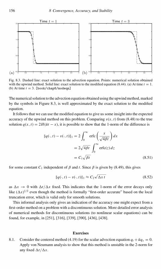
156 8 Convergence, Accuracy, and Stability

(a) 0 0.5 1 1.5 2 2.5 3 3.5 4−0.5

0

0.5

1

1.5

2

2.5Time t = 1

(b) 0 0.5 1 1.5 2 2.5 3 3.5 4−0.5

0

0.5

1

1.5

2

2.5Time t = 3

Fig. 8.3. Dashed line: exact solution to the advection equation. Points: numerical solution obtainedwith the upwind method. Solid line: exact solution to the modified equation (8.44). (a) At time t = 1.(b) At time t = 3. [book/chap8/modeqn]

The numerical solution to the advection equation obtained using the upwindmethod,markedby the symbols in Figure 8.3, is well approximated by the exact solution to the modifiedequation.It follows that we can use the modified equation to give us some insight into the expected

accuracy of the upwind method on this problem. Comparing v(x, t) from (8.48) to the truesolution q(x, t) = 2H (ut − x), it is possible to show that the 1-norm of the difference is

‖q(·, t)− v(·, t)‖1 = 2∫ ∞

0erfc

(x√4βt

)dx

= 2√4βt

∫ ∞

0erfc(z) dz

= C1√βt (8.51)

for some constant C1 independent of β and t . Since β is given by (8.49), this gives

‖q(·, t)− v(·, t)‖1 ≈ C2√�x t (8.52)

as �x → 0 with �t/�x fixed. This indicates that the 1-norm of the error decays onlylike (�x)1/2 even though the method is formally “first-order accurate” based on the localtruncation error, which is valid only for smooth solutions.This informal analysis only gives an indication of the accuracy one might expect from a

first-order method on a problem with a discontinuous solution. More detailed error analysisof numerical methods for discontinuous solutions (to nonlinear scalar equations) can befound, for example, in [251], [316], [339], [390], [436], [438].

Exercises

8.1. Consider the centered method (4.19) for the scalar advection equation qt + uqx = 0.Apply von Neumann analysis to show that this method is unstable in the 2-norm forany fixed �t/�x .

Exercises 157

8.2. Following the proof of Section 8.3.4, show that the upwind method (4.30) is stableprovided the CFL condition (4.32) is satisfied.

8.3. Consider the equation

qt + uqx = aq, q(x, 0) = q◦(x),

with solution q(x, t) = eatq◦(x − ut).(a) Show that the method

Qn+1i = Qni −u�t

�x

(Qni − Qni−1

)+�t aQniis first-order accurate for this equation by computing the local truncation error.

(b) Show that this method is Lax–Richtmyer-stable in the 1-norm provided|u�t/�x | ≤ 1, by showing that a bound of the form (8.23) holds. Note thatwhen a > 0 the numerical solution is growing exponentially in time (as is thetrue solution) but the method is stable and convergent at any fixed time.

(c) Show that this method is TVB. Is it TVD?8.4. Show that amethodQn+1 = N (Qn) that is contractive in the1-norm (L1-contractive),

so that ‖N (P)−N (Q)‖1 ≤ ‖P−Q‖1, must also be TVD, so TV(N (Q)) ≤ TV(Q).Hint: Define the grid function P by Pi = Qi−1.

8.5. Prove Harten’s Theorem 6.1. Hint: Note that

Qn+1i+1 − Qn+1i = (1− Cni − Dni

)(Qni+1 − Qni

)+ Dni+1(Qni+2 − Qni+1)+ Cni−1

(Qni − Qni−1

).

Sum |Qn+1i+1 − Qn+1i | over i and use the nonnegativity of each coefficient, as in thestability proof of Section 8.3.4.

8.6. Use themethod of Section 8.3.4 to show that themethod (4.64) is stable in the 1-normfor �x ≤ u�t ≤ 2�x .

8.7. View (8.41) as a numerical method for the equation (8.44). Compute the local trun-cation error, and verify that it is O(�t2).

8.8. Derive the modified equation (8.45) for the Lax–Wendroff method.8.9. Determine the modified equation for the centered method (4.19), and show that the

diffusion coefficient is always negative and this equation is hence ill posed. Recallthat the method (4.19) is unstable for all fixed �t/�x .

9Variable-Coefficient Linear Equations

In the preceding chapters we have primarily studied linear problems with constant co-efficients. Many interesting problems involve spatially-varying coefficients. This chapter isdevoted to exploring some of the issues that arise, both analytically and numerically, in thiscase.There are several distinct forms that a variable-coefficient hyperbolic system might take,

each of which arises naturally in some contexts. One possibility is that the coefficient matrixA multiplying qx varies with x , so the system is

qt + A(x)qx = 0. (9.1)

This system is hyperbolic in some domain if A(x) is diagonalizable with real eigenvaluesat each x in the domain. Such problems still model wave propagation, and the finite volumemethods developed in previous chapters can be applied fairly directly, in spite of the factthat this system (9.1) is not in conservation form and there is no flux function.Another form of variable-coefficient problem that often arises is

qt + (A(x)q)x = 0, (9.2)

in which the matrix A(x) appears within the x-derivative. For the constant-coefficient prob-lemwith A(x)≡ A, the two forms (9.1) and (9.2) are identical, but with variable coefficientsthey are distinct and have different solutions. The equation (9.2) is a conservation law, withthe flux function

f (q, x) = A(x)q. (9.3)

In this case the flux function depends explicitly on the location x aswell as on the value of theconserved quantities q. Again this equation is hyperbolic whenever A(x) is diagonalizablewith real eigenvalues.For a given physical problem it may be possible to derive an equation of either form (9.1)

or (9.2), depending on how the vector q is chosen. For example, in Section 9.1 we will seehow flow through a pipe can lead to an advection equation of either form, depending onhow q is defined.We can go back and forth between the forms at the expense of introducing source terms.

By applying the product rule to the x-derivative in (9.2), we could rewrite this equation in

158

9.1 Advection in a Pipe 159

the form

qt + A(x)qx = −A′(x)q,

which has the form of (9.1) with the addition of a source term. Conversely, we could rewrite(9.1) as

qt + (A(x)q)x = A′(x)q,

which now has the form of a conservation law with a source term. Normally we wish toavoid adding source terms to the equation if they can be avoided by a better choice ofvariables.Another form of variable coefficients that often arises naturally is a capacity function

κ(x), as described in the context of heat capacity in Section 2.3, giving systems of the form

κ(x)qt + (A(x)q)x = 0, (9.4)

for example. Again this could be manipulated into other forms, e.g.,

qt + κ−1(x)A(x)qx = −κ−1(x)A′(x)q,

but for problems where κq is the proper conserved quantity it may be preferable to workdirectly with the form (9.4), using the capacity-form differencing algorithms introduced inSection 6.16.

9.1 Advection in a Pipe

Consider an incompressible fluid flowing through a pipe with variable cross-sectional areaκ(x), and suppose we want to model the advection of some tracer down the length of thepipe. We denote the area by κ, since we will see that this is a natural capacity function.There are several ways we might model this, depending on how we choose our variables,leading to different forms of the variable-coefficient advection equation.We are assuming here that a one-dimensional formulation is adequate, i.e., that all quanti-

ties vary only with x (distance along the pipe) and t , and are essentially constant across anygiven cross section. In reality the flow through a pipe with varying diameter cannot be trulyone-dimensional, since there must be a velocity component in the radial direction in regionswhere the walls converge or diverge. But we will assume this is sufficiently small that it canbe safely ignored, which is true if the variation in κ is sufficiently smooth. The fluid velocityis then given by a single axial velocity u(x) that varies only with x . (See Sections 9.4.1 and9.4.2 for other contexts where this makes sense even if u is discontinuous.)Note that if κ(x) is measured in square meters and u(x) in meters per second, say, then

the product κ(x)u(x) has units of cubic meters per second and measures the volume of fluidpassing any point per unit time. Since the fluid is assumed to be incompressible, this mustbe the same at every point in the pipe, and we will denote the flow rate by U ,

U = κ(x)u(x) ≡ constant. (9.5)

160 9 Variable-Coefficient Linear Equations

If we know U and the cross-sectional area κ(x), then we can compute

u(x) = U/κ(x). (9.6)

(In Section 9.4 we consider a formulation in which κ(x)u(x) need not be constant.)Now suppose thatwe introduce a tracer into the fluid (e.g., some food coloring or chemical

contaminant into water, with very small concentration so that it does not affect the fluiddynamics). We wish to study how a given initial concentration profile advects downstream.There are two distinct ways we might choose to measure the concentration, leading todifferent forms of the advection equation.One approach would be to measure the concentration in grams per cubic meter (mass per

unit volume of fluid), which is what we would probably actually measure if we took a smallsample of fluid from the pipe and determined the concentration. Call this variable q(x, t).However, sincewe are solving a one-dimensional problemwith quantities assumed to vary

in only the x-direction, another natural possibility would be to measure the concentration inunits of mass per unit length of the pipe (grams per meter). If we call this variable q(x, t),then ∫ x2

x1

q(x, t) dx (9.7)

measures the total mass1 of tracer in the section of pipe from x1 to x2. Since this mass canonly change due to tracer moving past the endpoints, q is the proper conserved quantity forthis problem. The one-dimensional velocity u(x) measures the rate at which tracer movespast a point and the product u(x)q(x, t) is the flux in grams per second. Hence with thischoice of variables we obtain the conservative advection equation

qt + (u(x)q)x = 0. (9.8)

There is a simple relation between q and q , given by

q(x, t) = κ(x)q(x, t), (9.9)

since multiplying the mass per unit volume by the cross-sectional area gives the mass perunit length. Hence the total mass of tracer in [x1, x2], given by (9.7), can be rewritten as∫ x2

x1

κ(x)q(x, t) dx .

With this choice of variables we see that the cross-sectional area acts as a capacity function,which is quite natural in that this area clearly determines the fluid capacity of the pipe ateach point.Using the relation (9.9) in (9.8) gives an advection equation for q,

κ(x)q t + (u(x)κ(x)q)x = 0. (9.10)

1 In problems where chemical kinetics is involved, we should measure the “mass” in moles rather than grams,and the density in moles per meter or moles per cubic meter.

9.2 Finite Volume Methods 161

But now notice that applying (9.5) allows us to rewrite this as

κ(x)q t +Uqx = 0. (9.11)

Dividing by κ and using (9.6) gives

q t + u(x)q x = 0 (9.12)

as another form of the advection equation.Comparing the advection equations (9.8) and (9.12) shows that they have the form of

(9.2) and (9.1), respectively. The velocity u(x) is the same in either case, but depending onhowwemeasure the concentration, we obtain either the nonconservative or the conservativeform of the equation. The form (9.11) is a third distinct form, in which the capacity functionand flow rate appear instead of the velocity.The nonconservative form (9.12) of the advection equation is often called the transport

equation or the color equation. If we think of food coloring inwater, then it is q, themass perunit volume, that determines the color of the water. If we follow a parcel of water throughthe pipe, we expect the color to remain the same even as the area of the pipe and velocity ofthe water change. This is easily verified, since q(x, t) is constant along characteristic curves(recall the discussion of Section 2.1.1). By contrast the conserved quantity q is not constantalong characteristic curves. The mass per unit length varies with the cross-sectional areaeven if the color is constant. From (9.8) we obtain qt + u(x)qx = −u′(x)q, so that alongany characteristic curve X (t) satisfying X ′(t) = u(X (t)) we have

d

dtq(X (t), t) = −u′(X (t)) q(X (t), t). (9.13)

9.2 Finite Volume Methods

Natural upwind finite difference methods for the equations (9.8) and (9.12) are easy toderive and take the following form in the case U > 0:

Qn+1i = Qni −�t

�x

[u(xi )Q

ni − u(xi−1)Qni−1

](9.14)

and

Qn+1i = Qni −�t

�xu(xi )

(Qni − Qni−1

)(9.15)

respectively. Variations of each formula are possible in which we use u(xi−1/2) in place ofu(xi ). Either choice gives a first-order accurate approximation. In this section we will seehow to derive these methods using the finite volume framework of Godunov’s method, ina manner that allows extension to high-resolution methods.The Riemann problem at the cell interface xi−1/2 now takes the form of an advection

equation with piecewise constant coefficients as well as piecewise constant initial data. Thesolution depends on what form of the advection equation we are solving. It also dependson how we discretize the velocity u(x). Two natural possibilities are:

162 9 Variable-Coefficient Linear Equations

1. Associate a velocity ui with each grid cell. We might define ui as the pointwise valueui = u(xi ), or we could compute the cell average of u(x), or we could view the pipe ashaving a piecewise constant cross-sectional area with value κi in the i th cell, and thentake ui = U/κi .

2. Associate a velocity ui−1/2 with each cell interface xi−1/2.

There are certain advantages and disadvantages of each form, and which is chosen maydepend on the nature of the problem being solved. To begin, we will concentrate on thefirst choice. For some problems, however, it is more natural to use edge velocities ui−1/2,and this choice is discussed in Section 9.5. This is true in particular when we extend thealgorithms to more than one space dimension; see Section 18.2.

9.3 The Color Equation

In the case of the color equation (9.12), the Riemann problem models a jump in color fromQi−1 to Qi at xi−1/2. Since color is constant along particle paths, this jump in color willsimply propagate into cell Ci at the velocity ui in this cell, and so in the notation of Chapter 4we have a waveWi−1/2 (omitting the superscript 1, since there is only one wave) with jump

Wi−1/2 = Qi − Qi−1,

and speed

si−1/2 = ui .

Again we are assuming positive velocities ui in each cell Ci . If U < 0, then we would havesi−1/2 = ui−1, since the wave would enter cell i − 1. In spite of the fact that the colorequation is not in conservation form, we can still view Qni as an approximation to the cellaverage of q(x, t) at time tn . In this case Qni is simply the “average color” over this cell, and�x Qni is not the total mass of any conserved quantity. It is no longer true that the change inthis cell average is given by a flux difference, but it is true that the change can be computedfrom the wave and speed. Note that (for U > 0) only the wave Wi−1/2 enters cell Ci , andthe value of q in this cell is changed by Qi − Qi−1 at each point the wave has reached. Thewave propagates a distance si−1/2�t over the time step and hence has covered the fractionsi−1/2�t/�x of the cell. The cell average is thus modified by

Qn+1i = Qni −�t

�xsi−1/2Wi−1/2.

This gives the upwind method (9.15). Also note that this has exactly the form (4.43),

Qn+1i = Qni −�t

�x

(A+�Qi−1/2 +A−�Qi+1/2),

if we define

A+�Qi−1/2 = si−1/2Wi−1/2,

A−�Qi−1/2 = 0.(9.16)

9.3 The Color Equation 163

These formulas have been presented for the case U > 0, so that all velocities ui arepositive. The more general formulas that can also be used in the case U < 0 are

Wi−1/2 = Qni − Qni−1,

si−1/2 ={ui if U > 0,ui−1 if U < 0,

= u+i + u−i−1,A+�Qi−1/2 = s+i−1/2Wi−1/2,

A−�Qi−1/2 = s−i−1/2Wi−1/2,

(9.17)

using the notation (4.40).

9.3.1 High-Resolution Corrections

The first-order upwind method for the color equation can be greatly improved by includinghigh-resolution corrections as developed in Chapter 6. The improved method again has theform (5.7),

Qn+1i = Qni −�t

�x

(A+�Qi−1/2 +A−�Qi+1/2)− �t

�x

(F i+1/2 − F i−1/2

), (9.18)

where

F i−1/2 = 1

2

∣∣si−1/2∣∣ (1− �t

�x

∣∣si−1/2∣∣) Wi−1/2. (9.19)

Themodified wave Wi−1/2 is obtained by applying a wave limiter as described in Chapter 6.It is important to note, however, that this method is not formally second-order accu-

rate when applied to a smooth solution, even when no limiter function is used. The localtruncation error is found to be (see Exercise 9.1)

local truncation error = −12[�x − u(x)�t]u′(x)qx (x, t)+O(�x2). (9.20)

Themethod is formally second-order accurate only in the case of constant coefficients,whereu′(x) ≡ 0. However, this truncation error has a quite different form than the truncation errorfor the first-order upwind method (9.15), which is

�x u(x)qxx (x, t)+O(�x2). (9.21)

This truncation error depends on qxx and leads to substantial numerical dissipation, as withany first-order upwind method. The truncation error (9.20), on the other hand, is a multipleof qx instead. This can be viewed as corresponding to a small error in the propagation speed.The modified equation (see Section 8.6) for the high-resolution method is

qt + u(x)qx = −12[�x − u(x)�t]u′(x)qx ,

164 9 Variable-Coefficient Linear Equations

which we can rewrite (ignoring higher-order terms) as

qt + u(x + 1

2[�x − u(x)�t]

)qx = 0 (9.22)

This is again the color equation, but with the velocity evaluated at a point that is shiftedby less than a grid cell. The solution to this equation looks essentially the same as for thecorrect color equation, but slightly offset. In particular there is no diffusion or smearing ofthe solution (at least not at theO(�x) level), and hence we expect the solution obtained withthis method to look much better than what would be obtained from the first-order upwindmethod.A true second-order accurate method can be derived using the Lax–Wendroff approach

(Exercise 9.2), but results are typically similar to what is produced by the method abovewhen the solution is smooth. The high-resolution method with limiters included works verywell in practice, and much better than the formally second-order method in cases where thesolution is discontinuous.

9.3.2 Discontinuous Velocities

For flow in a pipe, reducing the problem to a one-dimensional advection equation is onlyvalid if the diameter of the pipe, and hence the velocity, is very slowly varying. Otherwisethe true fluid velocity may have a substantial radial component. This is particularly true at apoint where the diameter is discontinuous. Here the motion will be fully multidimensionaland perhaps even turbulent. However, one-dimensional approximations are frequently usedeven in this case in many engineering applications involving transport through complicatednetworks of pipes, for example.There are also other applications where a one-dimensional advection equation with

rapidly varying or even discontinuous velocities is physically relevant. One example, dis-cussed in Section 9.4.2, arises in traffic flow along a one-lane road with a discontinuousspeed limit. Another example is discussed in Section 9.4.1.An advantage of the high-resolution finite volume methods is that they typically perform

very well even when the coefficients in the equation are discontinuous. You may wish toexperiment with the examples in [claw/book/chap9/color/discontu].

9.4 The Conservative Advection Equation

Now suppose we are solving the conservative equation (9.8), qt+(u(x)q)x = 0, with veloci-ties ui given in each grid cell. Again we can use the form (5.7) after defining the fluctuationsA+�Qi−1/2 andA−�Qi−1/2 in terms of waves via the solution to the Riemann problem atxi−1/2. To do so properly wemust carefully consider the Riemann problem, which now con-sists of using piecewise constant data defined by Qi−1 and Qi and also piecewise constantcoefficients in the advection equation,

qt + ui−1qx = 0 if x < xi−1/2,

qt + uiqx = 0 if x > xi−1/2.(9.23)

9.4 The Conservative Advection Equation 165

Qi−1

Qi

Q∗i−1/2

ui−1∆t ui

t

xi−1/2

Wi−1/2

∆t

Fig. 9.1. Solution to the Riemann problem for the conservative advection equation when ui−1 > ui .

The solution is not simply a single wave propagating at velocity ui with strength Qi−Qi−1.The correct solution is indicated in Figure 9.1, and consists of two discontinuities in thesolution: a stationary one at xi−1/2 where Qi−1 jumps to some new value Q∗i−1/2, and thewave

Wi−1/2 = Qi − Q∗i−1/2 (9.24)

propagating at the expected speed

si−1/2 = ui (9.25)

(again we assume U > 0). The discontinuity at xi−1/2 arises from the fact that the jump inu at xi−1/2 corresponds to a jump in the cross-sectional area of the pipe. (A jump to a largerarea κi > κi−1 is shown in Figure 9.1, in which case ui < ui−1.) Consequently, the densityof tracer q, which is measured in the one-dimensional manner as mass per unit length, mustincrease, since there is suddenly more liquid and hence more tracer per unit length of pipe.The “color” q measured in mass per unit volume, on the other hand, does not experienceany discontinuity at xi−1/2, and so we did not have to worry about this effect in solving thecolor equation.The new value Q∗i−1/2 that arises in solving the Riemann problem can be found using the

fact that the flux f = uq must be continuous at xi−1/2 in the Riemann solution. The sameamount of tracer is leaving cell Ci−1 as entering cell Ci . This yields

ui−1Qi−1 = ui Q∗i−1/2

and hence

Q∗i−1/2 =ui−1Qi−1

ui. (9.26)

This value is used in the wave (9.24). The fluctuation is computed in terms of this wave and

166 9 Variable-Coefficient Linear Equations

the speed (9.25) as

A+�Qi−1/2 = si−1/2Wi−1/2

= ui(Qi − ui−1Qi−1

ui

)= ui Qi − ui−1Qi−1. (9.27)

Again this is for the case U > 0, and in this case we have no fluctuation to the left:

A−�Qi−1/2 = 0. (9.28)

Note that the sum of the fluctuations has the form of a flux difference, as we expect for thisconservative equation. The finite volume method

Qn+1i = Qi − �t

�x

(A+�Qi−1/2 + A−�Qi+1/2

)(9.29)

reduces to the natural upwind method (9.14).If U < 0, then we find that

Q∗i−1/2 =ui QiUi−1

,

Wi−1/2 = Q∗i−1/2 − Qi−1,si−1/2 = ui−1,

A−�Qi−1/2 = si−1/2Wi−1/2 = ui Qi − ui−1Qi−1,A+�Qi−1/2 = 0.

(9.30)

In this case (9.29) again reduces to the natural upwind method. High-resolution correctionterms can be added using (9.18) and (9.19).Since the Riemann solution now involves two jumps, one might wonder why we don’t

need two wavesW1i−1/2 andW2

i−1/2 instead of just one, as introduced above. The answer isthat the secondwavemoves at speed s = 0.Wecould include it in theRiemann solution, but itwould drop out of the expression forA+�Qi−1/2, since we sum s pW p. The correspondinghigh-resolution corrections also drop out when s = 0. So nothing would be gained byincluding this wave except additional work in applying the updating formulas.

9.4.1 Conveyer Belts

The solution illustrated in Figure 9.1 can perhaps be better understood by considering adifferent context than fluid flow in a pipe. Consider a series of conveyer belts, each going forthe length of one grid cell with velocity ui , and let q(x, t) measure the density of packagestraveling down this series of belts. See Figure 9.2. If the velocity ui is less than ui−1, thenthe density will increase at the junction xi−1/2 just as illustrated in Figure 9.1. See alsoFigure 9.3 for another interpretation, discussed in the next subsection.The structure illustrated in Figure 9.1 with two waves can also be derived by solving the

Riemann problem for a system of two conservation laws, obtained by introducing u as asecond conserved variable; see Exercise 13.11.

9.4 The Conservative Advection Equation 167

ui−1 ui

Fig. 9.2. Packages moving from a conveyer belt with speed ui−1 to a slower belt with speed ui . Thedensity of packages increases at the junction.

9.4.2 Traffic Flow

Similar advection equations arise in studying the flow of cars along a one-lane highway.To obtain a linear equation, we assume traffic is light enough that cars are always travelingat the speed limit u(x), which can vary with x , the distance along the highway. If u(x)is piecewise constant, then this is exactly the same problem as the conveyer-belt problemmentioned in Section 9.4.1, with cars replacing packages.For heavier traffic the speed typically also depends on the density of cars and the problem

becomes nonlinear. This more interesting case is examined in detail in Chapter 11.Let q(x, t) be the density of cars at point x at time t . Of course, at any particular point x

there is either a car or no car, so the concept of density at a point appears to be meaningless.What we mean should be clear, however: over a reasonably long stretch of road from x1 tox2 the number of cars present at time t should be roughly

number of cars between x1 and x2 ≈∫ x2

x1

q(x, t) dx . (9.31)

It will be convenient to measure the density in units of cars per car length, assuming allcars have the same length. Then empty highway corresponds to q = 0, bumper-to-bumpertraffic corresponds to q = 1, and in general 0 ≤ q ≤ 1. Then for (9.31) to make sense wemust measure distance x in car lengths. Also we measure the speed limit u(x) in car lengthsper time unit. The flux of cars is given by f (q) = u(x)q (in cars per time unit) and weobtain the conservation law (9.8).One way to simulate traffic flow is to track the motion of individual vehicles, assuming

a finite set of m cars on the highway. Let Xk(t) be the location of the kth car at time t . Thenthe motion of each car can be obtained by solving the ordinary differential equation

X ′k(t) = u(Xk(t))

with initial conditions corresponding to its initial location Xk(0). Note that cars move alongcharacteristics of the advection equation. (This is not true more generally if the velocitydepends on the density; see Chapter 11.)Figure 9.3 illustrates the simulation of a line of cars with an initial density variation

corresponding to a Riemann problem, traveling along a highway with a discontinuousspeed limit

u(x) ={2 if x < 0,1 if x > 0.

The paths of individual cars are plotted over time 0 ≤ t ≤ 20. The density qk(t) observedby each driver is also plotted at both the initial and final times. For this discrete simulation

168 9 Variable-Coefficient Linear Equations

−40 −30 −20 −10 0 10 20 30 40

0

0.2

0.4

0.6

0.8

1

Density at time 20

−40 −30 −20 −10 0 10 20 30 40

0

5

10

15

20

25

−40 −30 −20 −10 0 10 20 30 40

0

0.2

0.4

0.6

0.8

1

Density at time 0

Fig. 9.3. Traffic flow model corresponding to the Riemann problem of Figure 9.1, with a change inspeed limit at x = 0. Vehicle trajectories are shown, along with the density observed by each driver.We can also view the cars as representing packages moving from one conveyer belt to a slower oneas in Figure 9.2. [claw/book/chap9/traffic]

9.5 Edge Velocities 169

a discrete density is defined for each car by

qk(t) = 1

Xk+1(t)− Xk(t) , (9.32)

based on the distance to the car immediately ahead. This can be shown to be consistent withthe previous notion of density; see Exercise 9.4.The density at intermediate times can also be observed from the car paths in Figure 9.3.

Taking a slice at any fixed time, the density is inversely proportional to the distance betweenpaths.Note that the density of cars changes discontinuously at the point x = 0 where the speed

limit changes. In this simple model we assume cars and drivers can adjust speed instanta-neously in response to the speed limit. This viewpoint may help to understand Figure 9.1.Of course if ui−1/ui is sufficiently large, then Q∗i−1/2 in (9.26) may be greater than 1 evenif Qi−1 is not. Although this causes no problem mathematically, with our definition ofdensity this shouldn’t happen physically. This is a case where cars are approaching thediscontinuity in speed limit too rapidly to be accommodated in the slower region even at thebumper-to-bumper density of q = 1. In this case the linear model is definitely inadequate,and instead a nonlinear shock wave would arise in the real world. See Section 16.4.1 for adiscussion of nonlinear traffic flow with a discontinuous speed limit.For the linear traffic flow problem, the density naturally satisfies a conservative advection

equation of the form (9.8). One can, however, define a new variable q(x, t) that insteadsatisfies the color equation (9.12), by setting

q(x, t) = u(x)q(x, t).

This is simply the flux of cars. We have

q t = (uq)t = uqt = −u(uq)x = −uqx ,

and so (9.12) is satisfied. You should convince yourself that it makes sense for the flux ofcars to be constant along characteristics, as must hold for the color equation.

9.5 Edge Velocities

So far we have assumed that the variable velocity u(x) is specified by a constant value uiwithin the i th grid cell. In some cases it is more natural to instead assume that a velocityui−1/2 is specified at each cell interface. This can be viewed as a transfer rate between thecells Ci−1 and Ci .

9.5.1 The Color Equation

Solving the color equation q t + u(x)q x = 0 with edge velocities specified is very simple.We need only set

Wi−1/2 = Qi − Qi−1,si−1/2 = ui−1/2,

(9.33)

170 9 Variable-Coefficient Linear Equations

and use the usual formula

A+�Qi−1/2 =(si−1/2

)+Wi−1/2,

A−�Qi−1/2 =(si−1/2

)−Wi−1/2.(9.34)

9.5.2 The Conservative Equation

The conservative advection equation qt + (u(x)q)x = 0 can also be solved using the wavesand speeds

Wi−1/2 = Qi − Qi−1,si−1/2 = ui−1/2,

(9.35)

to define second-order corrections (perhaps modified by limiters). However, we cannot usethe expressions (9.34) to define the fluctuations. This would not lead to a conservativemethod, since (4.54) would not be satisfied. There are several different approaches that canbe used to define fluctuations that do satisfy (4.54) and lead to successful methods. Oneapproach is to notice that an upwind flux Fi−1/2 is naturally defined by

Fi−1/2 = u+i−1/2Qi−1 + u−i−1/2Qi

at the edge between the cells. Recall that the goal in defining A±�Qi−1/2 is to implementthe flux-differencing algorithm

Qn+1i = Qni −�t

�x

(Fni+1/2 − Fni−1/2

)(9.36)

via the formula

Qn+1i = Qni −�t

�x

(A+�Qi−1/2 +A−�Qi+1/2). (9.37)

We can accomplish this by setting

A+�Qi−1/2 = Fi − Fi−1/2,A−�Qi−1/2 = Fi−1/2 − Fi−1,

(9.38)

where the cell-centered flux values Fi are chosen in an arbitrary way. When inserted into(9.37) the value Fi cancels out and (9.36) results. For simplicity one could even use Fi = 0in each cell.Aesthetically it is nicer to use some approximation to the flux in cell i , for example

Fi =(u+i−1/2 + u−i+1/2

)Qi , (9.39)

so that A±�Qi−1/2 have the physical interpretation of flux differences. Note that if allvelocities are positive, then these formulas reduce to

Fi−1/2 = ui−1/2Qi−1, Fi = ui−1/2Qi ,

9.6 Variable-Coefficient Acoustics Equations 171

so that

A+�Qi−1/2 = ui−1/2(Qi − Qi−1),A−�Qi−1/2 =

(ui−1/2 − ui−3/2

)Qi−1.

(9.40)

The right-going fluctuation is si−1/2Wi−1/2 (as for the color equation), while the left-goingfluctuation accounts for the variation of u across cell Ci−1. Note that even though all flowis to the right, some information must flow to the left, since the accumulation rate in cellCi−1 depends on the outflow velocity ui−1/2 as well as the inflow velocity ui−3/2. Thesefluctuations result in the first-order method

Qn+1i = Qni −�t

�x

(ui+1/2Qni − ui−1/2Qni−1

). (9.41)

Note also that the splitting of (9.40) gives distinct approximations to the two terms thatarise when we rewrite the conservative equation in the form

qt + u(x)qx + u′(x)q = 0. (9.42)

Another way to derive the method (9.37) with the splitting (9.40) is to start with the form(9.42) and view this as the color equation with a source term−u′(x)q. ThenWi−1/2, si−1/2,and A+�Qi−1/2 all come from the color equation. The term A−�Qi−1/2 from (9.40) isdifferent from the value 0 that would be used for the color equation, and can be viewedas a device for introducing the appropriate source term into cell Ci−1 (rather than usinga fractional-step method as discussed in Chapter 17). This approach has the advantage ofmaintaining conservation, while a fractional-step method might not.If second-order correction terms are added to this algorithm using the waves and speeds

(9.35) and the formula (9.18), then it can be shown that the method is formally second-orderaccurate if no limiters are used (Exercise 9.6).

9.6 Variable-Coefficient Acoustics Equations

Previously we have studied the equations of linear acoustics in a uniform medium wherethe density ρ0 and the bulk modulus K0 are the same at every point. We now consideracoustics in a one-dimensional heterogeneous medium in which the values ρ(x) and K (x)vary with x . The theory and numerical methods developed here also apply to elasticityor electromagnetic waves in heterogeneous media, and to other hyperbolic systems withvariable coefficients.An important special case is a layered medium in which ρ and K are piecewise constant.

In applying finite volume methods we will assume the medium has this structure, at least atthe level of the grid cells. We assume the i th cell contains a uniform material with densityρi and bulk modulus Ki . Smoothly varying material parameters can be approximated wellin this manner on a sufficiently fine grid. Our discussion will focus primarily on the caseof piecewise constant media, since we need to understand this case in detail in order toimplement methods based on Riemann solvers. See Section 9.14 for discussion of how tochoose the ρi and Ki if the coefficients vary on the subgrid scale.

172 9 Variable-Coefficient Linear Equations

It is possible to solve the variable-coefficient acoustics equations in conservation formby writing them in terms of momentum and strain; see [273] for example. Here we explorethe nonconservative formulation that arises when pressure and velocity are used as thedependent variables. These are the quantities thatmust be continuous at an interface betweendifferent materials and are also physically more intuitive. This example provides a nice casestudy in solving a nonconservative variable-coefficient system, which can form a basis fordeveloping algorithms for other hyperbolic systems that perhaps cannot be rewritten inconservation form.The form (2.52) of the constant-coefficient acoustic equations generalizes naturally to

qt + A(x)qx = 0, (9.43)

where

q(x, t) =[p(x, t)

u(x, t)

], A(x) =

[0 K (x)

1/ρ(x) 0

]. (9.44)

At each point x we can diagonalize this matrix as in Section 2.8,

A(x) = R(x)�(x)R−1(x). (9.45)

If we define the sound speed

c(x) =√K (x)/ρ(x) (9.46)

and the impedance

Z (x) = ρ(x)c(x) =√K (x)ρ(x), (9.47)

then the eigenvector and eigenvalue matrix of (9.45) are

R(x) =[−Z (x) Z (x)

1 1

], �(x) =

[−c(x) 0

0 c(x)

]. (9.48)

9.7 Constant-Impedance Media

An interesting special case arises if ρ(x) and K (x) are related in such a way that Z (x) =Z0 is constant, which happens if K (x) = Z20/ρ(x) everywhere. Then the eigenvectormatrix R(x)≡ R is constant in space. In this case we can diagonalize the system (9.43) bymultiplying by R−1 to obtain

(R−1q)t + [R−1A(x)R](R−1q)x = 0.Defining

w(x, t) = R−1q(x, t)

as in Section 2.9, we can write the above system as

wt +�(x)wx = 0. (9.49)

9.8 Variable Impedance 173

This diagonal system decouples into two scalar advection equations (color equations in theterminology of Section 9.1)

w1t − c(x)w1x = 0 and w2t + c(x)w2x = 0.

Left-going and right-going sound waves propagate independently of one another with thevariable sound speed c(x).

Example 9.1. Consider a piecewise constant medium with a single discontinuity at x = 0,

ρ(x) ={ρl if x < 0,

ρr if x > 0,K (x) =

{Kl if x < 0,

Kr if x > 0.(9.50)

Take ρl = 1, ρr = 2 and Kl = 1, Kr = 0.5, so that the impedance is Z0 = 1 everywherealthough the sound speed jumps from cl = 1 to cr = 0.5. Figure 9.4 shows a right-goingacoustic wave having p(x, t) = Z0u(x, t) everywhere. As it passes through the interfacethe pulse is compressed due to the change in velocity ( just as would happen with the scalarcolor equation), but the entire wave is transmitted and there is no reflection at the interface.Compare with Figure 9.5, where there is also a jump in the impedance.

9.8 Variable Impedance

Note that the diagonalization (9.49) is possible only because R is constant in space. If R(x)varies with x then R−1(x)qx = (R−1(x)q)x − R−1x (x)q , where R

−1x (x) is the derivative of

R−1(x) with respect to x . In this case multiplying (9.43) by R−1(x) yields

wt +�(x)wx = R−1x (x)q

= B(x)w, (9.51)

where the matrix B(x) is given by B(x) = R−1x (x)R(x) and is not a diagonal matrix. In thiscase we still have advection equations for w1 and w2, but they are now coupled togetherby the source terms. The left-going and right-going acoustic waves no longer propagateindependently of one another.Rather than attempting to work with this system, we will see that the Riemann problem

can be posed and solved at a general interface between two different materials. By assumingthe medium is layered (so the impedance is piecewise constant), we can reduce the generalproblem with variable coefficients to solving such Riemann problems.Before considering the general Riemann problem, consider what happens when a wave

hits an interface in a medium of the form (9.50) if there is a jump in impedance at theinterface.

Example 9.2. Consider the medium (9.50) with ρl = 1, ρr = 4 and Kl = 1, Kr = 1. Asin Example 9.1, the velocity jumps from cl = 1 to cr = 0.5, but now the impedance is alsodiscontinuouswith Zl = 1 and Zr = 2. Figure 9.5 showswhat happens as a right-goingwavehits the interface. Part of the wave is transmitted, but part is reflected as a left-going wave.

174 9 Variable-Coefficient Linear Equations

−5 −4 −3 −2 −1 0 1 2 3 4 5−0.5

0

0.5

1

1.5q (1) at time t = 0

−5 −4 −3 −2 −1 0 1 2 3 4 5−0.5

0

0.5

1

1.5q (2) at time t = 0

−5 −4 −3 −2 −1 0 1 2 3 4 5−0.5

0

0.5

1

1.5q (1) at time t = 1

−5 −4 −3 −2 −1 0 1 2 3 4 5−0.5

0

0.5

1

1.5q (2) at time t = 1

−5 −4 −3 −2 −1 0 1 2 3 4 5−0.5

0

0.5

1

1.5q (1) at time t = 2

−5 −4 −3 −2 −1 0 1 2 3 4 5−0.5

0

0.5

1

1.5q (2) at time t = 2

−5 −4 −3 −2 −1 0 1 2 3 4 5−0.5

0

0.5

1

1.5q (1) at time t = 3

−5 −4 −3 −2 −1 0 1 2 3 4 5−0.5

0

0.5

1

1.5q (2) at time t = 3

−5 −4 −3 −2 −1 0 1 2 3 4 5−0.5

0

0.5

1

1.5q (1) at time t = 4

−5 −4 −3 −2 −1 0 1 2 3 4 5−0.5

0

0.5

1

1.5q (2) at time t = 4

−5 −4 −3 −2 −1 0 1 2 3 4 5−0.5

0

0.5

1

1.5q (1) at time t = 5

−5 −4 −3 −2 −1 0 1 2 3 4 5−0.5

0

0.5

1

1.5q (2) at time t = 5

Fig. 9.4. Right-going acoustic pulse hitting a material interface (dashed line) where the sound speedchanges from 1 to 0.5 but the impedance is the same. Left column: pressure. Right column: velocity.[claw/book/chap9/acoustics/interface]

If the incident pressure pulse has magnitude p0, then the transmitted pulse has magnitudeCT p0 and the reflected pulse has magnitude CR p0, where the transmission and reflectioncoefficients are given by

CT = 2ZrZl + Zr , CR = Zr − Zl

Zl + Zr . (9.52)

For the example in Figure 9.5, we have CT = 4/3 and CR = 1/3. Partial reflection alwaysoccurs at any interface where there is an impedance mismatch with Zl �= Zr . There areseveral ways to derive these coefficients. We will do so below by solving an appropriateRiemann problem, as motivated by the next example.

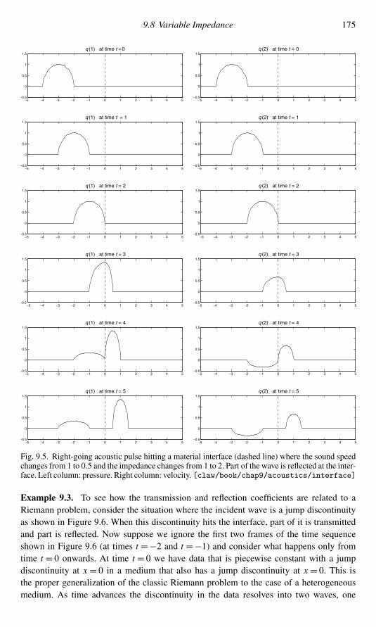
9.8 Variable Impedance 175

−5 −4 −3 −2 −1 0 1 2 3 4 5−0.5

0

0.5

1

1.5q (1) at time t = 0

−5 −4 −3 −2 −1 0 1 2 3 4 5−0.5

0

0.5

1

1.5q (2) at time t = 0

−5 −4 −3 −2 −1 0 1 2 3 4 5−0.5

0

0.5

1

1.5q (1) at time t = 1

−5 −4 −3 −2 −1 0 1 2 3 4 5−0.5

0

0.5

1

1.5q (2) at time t = 1

−5 −4 −3 −2 −1 0 1 2 3 4 5−0.5

0

0.5

1

1.5q (1) at time t = 2

−5 −4 −3 −2 −1 0 1 2 3 4 5−0.5

0

0.5

1

1.5q (2) at time t = 2

−5 −4 −3 −2 −1 0 1 2 3 4 5−0.5

0

0.5

1

1.5q (1) at time t = 3

−5 −4 −3 −2 −1 0 1 2 3 4 5−0.5

0

0.5

1

1.5q (2) at time t = 3

−5 −4 −3 −2 −1 0 1 2 3 4 5−0.5

0

0.5

1

1.5q (1) at time t = 4

−5 −4 −3 −2 −1 0 1 2 3 4 5−0.5

0

0.5

1

1.5q (2) at time t = 4

−5 −4 −3 −2 −1 0 1 2 3 4 5−0.5

0

0.5

1

1.5q (1) at time t = 5

−5 −4 −3 −2 −1 0 1 2 3 4 5−0.5

0

0.5

1

1.5q (2) at time t = 5

Fig. 9.5. Right-going acoustic pulse hitting a material interface (dashed line) where the sound speedchanges from 1 to 0.5 and the impedance changes from 1 to 2. Part of the wave is reflected at the inter-face. Left column: pressure. Right column: velocity. [claw/book/chap9/acoustics/interface]

Example 9.3. To see how the transmission and reflection coefficients are related to aRiemann problem, consider the situation where the incident wave is a jump discontinuityas shown in Figure 9.6. When this discontinuity hits the interface, part of it is transmittedand part is reflected. Now suppose we ignore the first two frames of the time sequenceshown in Figure 9.6 (at times t =−2 and t =−1) and consider what happens only fromtime t = 0 onwards. At time t = 0 we have data that is piecewise constant with a jumpdiscontinuity at x = 0 in a medium that also has a jump discontinuity at x = 0. This isthe proper generalization of the classic Riemann problem to the case of a heterogeneousmedium. As time advances the discontinuity in the data resolves into two waves, one

176 9 Variable-Coefficient Linear Equations

−5 −4 −3 −2 −1 0 1 2 3 4 5−0.5

0

0.5

1

1.5q (1) at time t = −2

−5 −4 −3 −2 −1 0 1 2 3 4 5−0.5

0

0.5

1

1.5q (2) at time t = −2

−5 −4 − 3 −2 −1 0 1 2 3 4 5−0.5

0

0.5

1

1.5q (1) at time t = −1

−5 −4 −3 −2 −1 0 1 2 3 4 5−0.5

0

0.5

1

1.5q (2) at time t = −1

−5 −4 −3 −2 −1 0 1 2 3 4 5−0.5

0

0.5

1

1.5q (1) at time t = 0

−5 −4 −3 −2 −1 0 1 2 3 4 5−0.5

0

0.5

1

1.5q (2) at time t = 0

−5 −4 −3 −2 −1 0 1 2 3 4 5−0.5

0

0.5

1

1.5q (1) at time t = 1

−5 −4 −3 −2 −1 0 1 2 3 4 5−0.5

0

0.5

1

1.5q (2) at time t = 1

−5 −4 −3 −2 −1 0 1 2 3 4 5−0.5

0

0.5

1

1.5q (1) at time t = 2

−5 −4 −3 −2 −1 0 1 2 3 4 5−0.5

0

0.5

1

1.5q (2) at time t = 2

−5 −4 −3 −2 −1 0 1 2 3 4 5−0.5

0

0.5

1

1.5q (1) at time t = 3

−5 −4 −3 −2 −1 0 1 2 3 4 5−0.5

0

0.5

1

1.5q (2) at time t = 3

Fig. 9.6. Right-going square pulse hitting a material interface (dashed line) where the sound speedchanges from 1 to 0.5 and the impedance changes from 1 to 2. The sequence from t = 0 onwardscorresponds to the Riemann problem for variable-coefficient acoustics. Left column: pressure. Rightcolumn: velocity. [claw/book/chap9/acoustics/interface]

moving to the left at the sound speed of the medium on the left and the other movingto the right at the sound speed of that medium. Determining the magnitude of these twowaves relative to the original jump will give the expressions (9.52) for the transmission andreflection coefficients. Being able to solve the general Riemann problem will also allow usto apply high-resolution finite volume methods to the general variable-coefficient acousticsproblem.

9.9 Solving the Riemann Problem for Acoustics 177

9.9 Solving the Riemann Problem for Acoustics

The general Riemann problem for acoustics in a heterogeneous medium is defined by con-sidering a piecewise constant medium of the form (9.50) together with piecewise constantinitial data

q(x, 0) ={ql if x < 0,

qr if x > 0.(9.53)

The solution to the Riemann problem consists of two acoustic waves, one moving to theleft with velocity −cl and the other to the right with velocity +cr . Each wave moves atthe sound speed of the material in which it propagates, as indicated in Figure 9.7. At theinterface x = 0 the pressure and velocity perturbations are initially discontinuous, but theyshould be continuous for t > 0, after the waves have departed. Hence there should be asingle state qm between the two waves as indicated in Figure 9.7 and as seen in Figure 9.6.We know from the theory of Section 2.8 that the jump across each wave must be an

eigenvector of the coefficient matrix from the appropriate material. Hence we must have

qm − ql = α1

[−Zl1

]and qr − qm = α2

[Zr1

](9.54)

for some scalar coefficients α1 and α2. Adding these two equations together yields

qr − ql = α1

[−Zl1

]+ α2

[Zr1

].

This leads to a linear system of equations to solve for α1 and α2,

Rlrα = qr − ql ,

−cl cr

ql qr

qm

Fig. 9.7. Structure of the solution to the Riemann problem for variable-coefficient acoustics, in thex–t plane. The dashed line shows the interface between two different materials. The waves propagateat the speed of sound in each material. Between the waves is a single state qm .

178 9 Variable-Coefficient Linear Equations

where

Rlr =[−Zl Zr1 1

]. (9.55)

This is essentially the same process used to solve the Riemann problem for constant-coefficient acoustics, but with an eigenvector matrix Rlr that is not the matrix R(x) fromeither side of the interface, but rather consists of the left-going eigenvector from the leftmedium and the right-going eigenvector from the right medium.Since

R−1lr =1

Zl + Zr

[−1 Zr1 Zl

], (9.56)

we find that

α1 = −(pr − pl)+ Zr (ur − ul)Zl + Zr ,

α2 = (pr − pl)+ Zl(ur − ul)Zl + Zr .

(9.57)

We also find that the intermediate state qm = ql + α1W1 is given by

pm = pl − α1Zl = Zr pl + Zl prZl + Zr −

(Zr ZlZl + Zr

)(ur − ul),

um = ul + α1 = Zlul + ZrurZl + Zr −

(1

Zl + Zr

)(pr − pl).

(9.58)

If Zl = Zr , then these reduce to the formulas (3.31) and (3.32) for acoustics in a constantmedium.

9.10 Transmission and Reflection Coefficients

Returning to Example 9.3, we can now compute the transmission and reflection coefficientsfor a wave hitting an interface. If the Riemann problem arises from an incident wave hittingan interface as shown in Figure 9.6, then ql and qr are not arbitrary but must be related bythe fact that qr − ql is the jump across the incident right-going wave, and hence

qr − ql = β

[Zl1

](9.59)

for some scalar β. After solving the Riemann problem at the heterogeneous interface, theoutgoing waves have strengths α1 and α2 given by

α = R−1lr (qr − ql)

= β

Zl + Zr

[−1 Zr1 Zl

][Zl1

]

= β

Zl + Zr

[Zr − Zl2Zl

]. (9.60)

9.11 Godunov’s Method 179

We thus find that the magnitudes of the reflected and transmitted waves are

α1 =(Zr − ZlZl + Zr

)β and α2 =

(2Zl

Zl + Zr

)β (9.61)

respectively. The waves are thus

reflected wave: α1

[−Zl1

]= β

(Zr − ZlZl + Zr

)[−Zl1

],

transmitted wave: α2

[Zr1

]= β

(2Zl

Zl + Zr

)[Zr1

].

Note that the pressure jump in the transmitted wave can be written as

β

(2Zl

Zl + Zr

)Zr =

(2Zr

Zl + Zr

)βZl .

Comparing thiswith thepressure jumpβZl of the incidentwave (9.59) gives the transmissioncoefficient CT of (9.52). The reflected wave has a pressure jump −CR(βZl), where CR isgiven in (9.52). The minus sign arises from the fact that we measure the pressure jump bysubtracting the value to the left of the wave from the value to the right. Since the waveis left-going, however, the gas experiences a jump in pressure of the opposite sign as thewave passes by, and it is this jump that is normally considered in defining the reflectioncoefficient CR .

9.11 Godunov’s Method

Having determined the solution to the Riemann problem for acoustics in a heterogeneousmedium, it is easy to implement Godunov’s method and other finite volume methods. Eachgrid cell is assigned a density ρi and a bulk modulus Ki , and Qni represents the cell averageof q over this cell at time tn . The Riemann problem at xi−1/2 is solved as described inSection 9.9 with ρl = ρi−1, ρr = ρi , etc. We obtain two waves

W1i−1/2 = α1i−1/2r

1i−1/2, W2

i−1/2 = α2i−1/2r2i−1/2,

where

r1i−1/2 =[−Zi−11

], r2i−1/2 =

[Zi1

].

These waves propagate at speeds s1i−1/2 = −ci−1 and s2i−1/2 = +ci . The coefficients α1i−1/2and α2i−1/2 are given by (9.57):

α1i−1/2 =−(pi − pi−1)+ Zi (ui − ui−1)

Zi−1 + Zi ,

α2i−1/2 =(pi − pi−1)+ Zi−1(ui − ui−1)

Zi−1 + Zi .

(9.62)

180 9 Variable-Coefficient Linear Equations

Godunov’s method can be implemented in the fluctuation form

Qn+1i = Qni −�t

�x

(A+�Qi−1/2 +A−�Qi+1/2)

if we define

A−�Qi−1/2 = s1i−1/2W1i−1/2, A+�Qi−1/2 = s2i−1/2W2

i−1/2, (9.63)

following the general prescription (4.42). Note that the variable-coefficient acoustic equa-tions (9.43) are not in conservation form, and so this is not a flux-difference splitting in thiscase, but it still leads to the proper updating of cell averages based on waves moving intothe grid cells.For constant-coefficient acoustics, we saw in Section 4.12 that we could interpret the

fluctuation A−�Qi−1/2 as A−(Qi − Qi−1), the “negative part” of the matrix A multipliedby the jump inQ,with A− defined in (4.45). For variable-coefficient acoustics it is interestingto note that we can make a similar interpretation in spite of the fact that the matrix A varies.In this case we haveA−�Qi−1/2 = Ai−1/2(Qi−Qi−1), where the matrix Ai−1/2 is differentthan the coefficient matrices

Ai =[0 Ki1/ρi 0

]= Ri�i R

−1i

defined in the grid cells. Define

Ri−1/2 =[−Zi−1 Zi1 1

],

analogous to Rlr in (9.55). Then the wave strengths α1i−1/2 and α2i−1/2 are determined by

αi−1/2 = R−1i−1/2(Qi − Qi−1).

The fluctuations (9.63) are thus given by

A−�Qi−1/2 = Ri−1/2�−i−1/2R−1i−1/2(Qi − Qi−1) = A−i−1/2(Qi − Qi−1),

A+�Qi−1/2 = Ri−1/2�+i−1/2R−1i−1/2(Qi − Qi−1) = A+i−1/2(Qi − Qi−1),

(9.64)

where we define

�i−1/2 =[s1i−1/2 0

0 s2i−1/2

]=[−ci−1 0

0 ci

]

and hence

Ai−1/2 = Ri−1/2�i−1/2R−1i−1/2

= 1

Zi−1 + Zi

[ci Zi − ci−1Zi−1 (ci−1 + ci )Zi−1Zi

ci−1 + ci ci Zi−1 − ci−1Zi

]. (9.65)

If Ai−1 = Ai , then Ai−1/2 also reduces to this same coefficient matrix. In general it isdifferent from the coefficient matrix on either side of the interface, and can be viewed as a

9.13 Wave Limiters 181

special average of the coefficient matrix from the two sides. If the coefficients are smoothlyvarying, then Ai−1/2 ≈ A(xi−1/2).Note that implementing the method does not require working with this matrix Ai−1/2.

We work directly with the waves and speeds. The Riemann solver is implemented in[claw/book/chap9/acoustics/interface/rp1acv.f].

9.12 High-Resolution Methods

Godunov’s method for variable-coefficient acoustics is easily extended to a high-resolutionmethod via a natural extension of the methods presented in Section 6.13, together withappropriate wave limiters. The method has the general form

Qn+1i = Qni −�t

�x

(A+�Qi+1/2 +A−�Qi−1/2)− �t

�x

(F i+1/2 − F i−1/2

), (9.66)

where

F i−1/2 = 1

2

m∑p=1

∣∣s pi−1/2∣∣ (1− �t

�x

∣∣s pi−1/2∣∣) W pi−1/2. (9.67)

Before discussing limiters, first consider the unlimited case in which W pi−1/2 = Wi−1/2.

Then a calculation shows that the method (9.66) can be rewritten as

Qn+1i = Qni −�t

2�x

[Ai−1/2(Qi − Qi−1)+ Ai+1/2(Qi+1 − Qi )

]+ �t2

2�x2[A2i+1/2(Qi+1 − Qi )− A2i−1/2(Qi − Qi−1)

]. (9.68)

This is a Lax–Wendroff-style method based on the coefficient matrices defined at the in-terface as in (9.65). As for the case of the variable-coefficient color equation discussedin Section 9.5, this method is not formally second-order accurate when A varies, be-cause the final term approximates 12�t

2(A2qx )x while the Taylor series expansion requires12�t

2qtt = 12�t

2A(Aqx )x . These differ by 12�t

2Ax Aqx . However, we have captured the12�t

2A2qxx term correctly, which is essential in eliminating the numerical diffusion of theGodunov method.This approach yields good high-resolution results in practice in spite of the lack of

formal second-order accuracy (as we’ve seen before, e.g., Section 8.5, Section 9.3.1). Sincethese high-resolution methods are of particular interest for problems where the solution orcoefficients are discontinuous, formal second-order accuracy cannot be expected in any case.If the problem is in conservation form qt + (A(x)q)x = 0, then this approach in fact givesformal second-order accuracy. See Section 16.4, where this is discussed in the more generalcontext of a conservation law with a spatially varying flux function, qt + f (q, x)x = 0.

9.13 Wave Limiters

Applying limiters to the waves W pi−1/2 is slightly more difficult for variable-coefficient

systems of equations than in the constant-coefficient case. To obtain a high-resolution

182 9 Variable-Coefficient Linear Equations

method, we wish to replace the waveW pi−1/2 by a limited version in (9.67),

W pi−1/2 = φ

(θpi−1/2

)W pi−1/2, (9.69)

as described in Chapter 6. Again θ pi−1/2 should be some measure of the smoothness ofthe pth characteristic component of the solution. When A is constant the eigenvectors r1

and r2 are the same everywhere and soW pi−1/2 = α

pi−1/2r

p can easily be compared to thecorresponding wave W p

I−1/2 = αpI−1/2r

p arising from the neighboring Riemann problemby simply comparing the two scalar wave strengths,

θpi−1/2 =

αpI−1/2αpi−1/2

. (9.70)

(Recall that I = i ± 1 as in (6.61), looking in the upwind direction as determined by thesign of s pi−1/2.) Note that in this constant-coefficient case we have

∣∣θ pi−1/2∣∣ =∥∥W p

I−1/2∥∥∥∥W p

i−1/2∥∥ (9.71)

in any vector norm.For a variable-coefficient problem, the two waves

W pi−1/2 = α

pi−1/2r

pi−1/2 =

(�pi−1/2�Qi−1/2

)r pi−1/2 (9.72)

and

W pI−1/2 = α

pI−1/2r

pI−1/2 =

(�pI−1/2�QI−1/2

)r pI−1/2 (9.73)

are typically not scalar multiples of one another, since the eigenvector matrices R(x) andL(x)= R−1(x) vary with x . In this case it may make no sense to compare α pi−1/2 withαpI−1/2, since these coefficients depend entirely on the normalization of the eigenvectors,which may vary with x . It would make more sense to compare the magnitudes of the fullwaves, using the expression (9.71) for some choice of vector norm, but some way must befound to assign a sign, which we expect to be negative near extreme points. More generally,a problem with (9.71) is that it would give |θ | ≈ 1 whenever the two waves are of similarmagnitude, regardless of whether they are actually similar vectors in phase space or not. Ifthe solution is truly smooth, then we expectW p

i−1/2≈W pI−1/2 and not just that these vectors

have nearly the same magnitude (which might be true for two vectors pointing in verydifferent directions in phase space at some discontinuity in the medium, or in the solutionfor a nonlinear problem).We would like to define θ pi−1/2 in a way that reduces to (9.70) in the constant-coefficient

case but that takes into account the degree of alignment of the wave vectors as well astheir magnitudes. This can be accomplished by projecting the vector W p

I−1/2 onto thevectorW p

i−1/2 to obtain a vector θpi−1/2W p

i−1/2 that is aligned withW pi−1/2. Using the scalar

coefficient of this projection as θ pi−1/2 gives

θpi−1/2 =

W pI−1/2 ·W p

i−1/2W pi−1/2 ·W p

i−1/2, (9.74)

9.14 Homogenization of Rapidly Varying Coefficients 183

where · is the dot product inRm . This works well in most cases, also for nonlinear problems,

and this general procedure is implemented in the limiter.f routine of CLAWPACK.Another approach has been proposed by Lax & Liu [264], [313] in defining their positive

schemes. Recall that we have used (9.72) and (9.73) to define the limiter. Lax and Liu insteaduse

W pI−1/2 = α

pI−1/2 r

pi−1/2 =

(�pi−1/2�QI−1/2

)r pi−1/2 (9.75)

in place ofW pI−1/2. The vector W p

I−1/2 is obtained by decomposing the jump�QI−1/2 intoeigenvectors of thematrix Ri−1/2 rather than into eigenvectors of RI−1/2. The vector W p

I−1/2is now a scalar multiple ofW p

i−1/2, and so we can simply use

θpi−1/2 =

αpI−1/2αpi−1/2

= W pI−1/2 ·W p

i−1/2W pi−1/2 ·W p

i−1/2. (9.76)

This is slightly more expensive to implement, but since we compute the left eigenvectorsat each cell interface in any case in order to compute theW p

i−1/2, we can also use them tocompute W p

I−1/2 at the same time if the computations are organized efficiently.For most problems the simpler expression (9.74) seems to work well, but for some prob-

lems with rapid variation in the eigenvectors the Lax–Liu limiter is superior. For example,in solving the acoustics equations in a rapidly varying periodic medium an instability at-tributed to nonlinear resonance was observed in [139] using the standard CLAWPACK limiter.A transmission-based limiter, closely related to the Lax–Liu limiter, was introduced to ad-dress this problem. This is similar to (9.76) but decomposes only the wave W p

I−1/2 intoeigenvectors r pi−1/2 rather than starting with the full jump �QI−1/2:

W pI−1/2 = α

pI−1/2r

pi−1/2 =

(�pi−1/2W p

I−1/2)r pi−1/2. (9.77)

The formula (9.76) is then used. For acoustics this has the interpretation of taking the wavefrom the neighboring Riemann problem that is approaching the interface xi−1/2 and usingonly the portion of this wave that would be transmitted through the interface in defining thelimiter. See [139] for more discussion of this and several examples where these methodsare used in periodic or random media.

9.14 Homogenization of Rapidly Varying Coefficients

If the physical parameters vary substantiallywithin a single grid cell, then itwill be necessaryto apply some sort of homogenization theory to determine appropriate averaged values touse for ρi and Ki . This might be the case in a seismology problem, for example, where eachgrid cell represents a sizable block of earth that is typically not uniform.Since ρ is the density (mass per unit length, in one dimension), the average density of

the i th cell is properly computed as the total mass in the cell divided by the length of thecell, i.e., as the arithmetic average of ρ within the cell,

ρi = 1

�x

∫ xi+1/2

xi−1/2ρ(x) dx . (9.78)

184 9 Variable-Coefficient Linear Equations

For the bulk modulus K it turns out that instead of an arithmetic average, it is necessary touse the harmonic average

Ki =(1

�x

∫ xi+1/2

xi−1/2

1

K (x)dx

)−1. (9.79)

Alternatively, we can view this as using the arithmetic average of the parameter 1/K , whichis called the coefficient of compressibility (see, e.g., [255]),

1

Ki= 1

�x

∫ xi+1/2

xi−1/2

1

K (x)dx . (9.80)

This is most easily motivated by considering the linear elasticity interpretation of acousticsfrom Section 2.12, with Lame parameters λ = K and µ = 0 and the stress–strain relation

σ = K ε (9.81)

resulting from (2.89) (dropping superscripts on σ 11 and ε11). Rewriting this as

ε = 1

Kσ (9.82)

shows that this has the form of Hooke’s law with spring constant 1/K . Recalling thatε = Xx − 1, we see that for a grid cell of homogeneous material (Ki = constant) with restlength xi−1/2 − xi+1/2 = �x , applying a force σ results in a strain[

X(xi+1/2

)− X(xi−1/2)]−�x�x

=(1

Ki

)σ. (9.83)

If the material in the cell is heterogeneous (with σ still constant), then instead we have[X(xi+1/2

)− X(xi−1/2)]−�x�x

= 1

�x

∫ xi+1/2

xi−1/2[Xx (x)− 1] dx

= 1

�x

∫ xi+1/2

xi−1/2ε(x) dx

=(1

�x

∫ xi+1/2

xi−1/2

1

K (x)dx

)σ. (9.84)

Comparing this with (9.83) motivates the averaging (9.80).Homogenization theory is often used to derive simpler systems of partial differential

equations to model the effective behavior of a medium with rapidly varying heterogeneties.As a simple example, consider a layered medium composed of thin layers of width L1 ofmaterial characterized by parameters (ρ1, K1), which alternate with thin layers of widthL2 where the parameters are (ρ2, K2). Numerically we could solve this problem usingthe high-resolution methods developed above, provided we can take �x small enough toresolve the layers. We do this in Example 9.4 below. Analytically, however, we mightlike to predict the behavior of waves propagating in this layered medium by solving somesimplified equation in place of the variable-coefficient acoustics equation. If we consider

9.14 Homogenization of Rapidly Varying Coefficients 185

(a) 0 20 40 60 80 100 120−1

−0.5

0

0.5

1Pressure at time t = 100

(b) 0 20 40 60 80 100 120−1

−0.5

0

0.5

fPressure at time t = 100

Fig. 9.8. (a) Pressure pulse in a homogeneous medium. (b) Pressure pulse in a layered medium.

waves whose wavelength is considerably longer than L1 and L2, then it turns out thatthe wave propagation can be reasonably well modeled by solving a homogenized systemof equations that is simply the constant-coefficient acoustics equation with appropriateaverages of ρ and 1/K ,

ρ = 1

L1 + L2 (L1ρ1 + L2ρ2) and K−1 = 1

L1 + L2

(L1K1+ L2K2

). (9.85)

This is illustrated in Example 9.4. More accurate homogenized equations can also be de-rived, which for this problem requires adding higher-order dispersive terms to the constant-coefficient acoustics equation, as shown by Santosa & Symes [393].In practical problems the material parameters often vary randomly, but with some slowly

varying mean values ρ(x) and K−1(x). This might be the case in a seismology problem,for example, where the basic type of rock or soil varies slowly (except for certain sharpinterfaces) but is full of randomheterogeneous structures at smaller scales. Similar problemsarise in studying ultrasound waves in biological tissue, electromagnetic waves in a hazyatmosphere, and many other applications.

Example 9.4. Figure 9.8 shows the results from twoacoustics problemswith the same initialdata and boundary conditions but different material properties. In each case the initial datais p ≡ u ≡ 0, and at the left boundary

u(0, t) ={0.2[1+ cos (π(t−15)10

)]if |t − 15| < 10,

0 otherwise.(9.86)

This in-and-out wall motion creates a pressure pulse that propagates to the right. InFigure 9.8(a) the material is uniform with ρ≡ 1 and K ≡ 1, and so the sound speed isc≡ 1. The peak pressure is generated at time t = 15, and at t = 100 is visible at x = 85, asshould be expected.

Figure 9.8(b) shows a case where the material varies periodically with

ρ = K ={3 for 2i < x < 2i + 1,1 for 2i + 1 < x < 2i + 2. (9.87)

The layers have width L1= L2= 1 as seen in the zoomed view of Figure 9.9(a), whereρ= K = 3 in the dark layers and ρ= K = 1 in the light layers. For the choice (9.87), thesound speed is c ≡ 1 in all layers. However, the pressure pulse does not propagate at

186 9 Variable-Coefficient Linear Equations

(a) 50 55 60 65 70 75 80 85 90−0.1

0

0.1

0.2

0.3

0.4

0.5

0.6

0.7

0.8

(b) 50 55 60 65 70 75 80 85 90−0.1

0

0.1

0.2

0.3

0.4

0.5

0.6

0.7

0.8

Fig. 9.9. (a) Zoom view of Figure 9.8(b) with the layers indicated. (b) The solid line is the “exact”solution. The symbols indicate the numerical solution computed with only four grid cells per layer.[claw/book/chap9/acoustics/layered]

speed 1. Instead, it propagates at the speed predicted by the homogenized acoustic equationas described above. The effective speed is

c =√K/ρ ≈ 0.866, (9.88)

based on the arithmetic average ρ = 12 (3 + 1)= 2 and the harmonic average K = ( 12 ( 13 +

1))−1= 1.5. The peak pressure generated at t = 15 is now observed at x = (85)(0.866) ≈73.6, as is clearly seen in Figure 9.9(a).What’s going on? Even though the sound speed c≡ 1 is constant everywhere, the impe-

dance Z = ρc= ρ is not, and so the eigenvectors of the coefficient matrix are different ineach layer. Recall from Section 9.8 that the wave will be partially reflected at each interfacein this case. The wave observed in Figure 9.8(a) is not a simple wave in the 2-characteristicfamily translating to the right as in the constant-coefficient case. Instead it is composed ofwaves moving in both directions that are constantly bouncing back and forth between theinterfaces, so that the energy moves more slowly to the right than we would expect from thesound speed. It is the group velocity that we are observing rather than the phase velocity.Notice from Figure 9.9(a) that the waveform is not completely smooth, but appears to

have jump discontinuities in px at each interface. This is expected, since

ut + 1

ρpx = 0.

The velocity u must be continuous at all times, from which it follows that ut and hencepx/ρ must also be continuous. This means that px will be discontinuous at points where ρis discontinuous.Figure 9.9(a) also shows dispersive oscillations beginning to form behind the propagating

pressure pulse in the periodic medium. This is not due to numerical dispersion, but rather isa correct feature of the exact solution, as predicted by the dispersive homogenized equationderived in [393].In fact, the curve shown in Figure 9.8(b) and Figure 9.9(a) is essentially the exact solution.

It was calculated on a fine grid with 2400 cells, and hence 20 grid cells in each layer.More importantly, the time step �t =�x was used. Since c≡ 1 everywhere, this means

Exercises 187

that each wave propagates through exactly one grid cell each time step, and there are nonumerical errors introducedby averagingonto the grid. In essenceweare using themethodofcharacteristics, with the Riemann solver providing the correct characteristic decompositionat each cell interface.We might now ask how accurate the high-resolution finite volume method would be

on this problem, since for practical problems it will not always be possible to choose thetime step so that c�t =�x everywhere. This can be tested by choosing �t <�x , so thatthe method no longer reduces to the method of characteristics. Now the piecewise linearreconstruction with limiter functions is being used together with averaging onto grid cells.Using �t = 0.8�x on the same grid with 2400 cells gives numerical results that are

nearly indistinguishable from the exact solution shown in Figure 9.9(a). As a much moreextreme test, the calculation was performed on a grid with only four grid cells in each layer.The results are still reasonable, as shown by the circles in Figure 9.9(b). Some accuracy islost at this resolution, but the basic structure of the solution is clearly visible, with the wavepropagating at the correct effective velocity.

Exercises

9.1. Compute the local truncation error for the method (9.18) in the case where no limiteris applied. Show that when u(x) is not constant the method fails to be formallysecond-order accurate.

9.2. Use the Lax–Wendroff approach described in Section 6.1, expanding in Taylor series,to derive a method that is formally second-order accurate for the variable-coefficientcolor equation (9.12). Compare this method with (9.18) using (9.17).

9.3. Show that if we add second-order correction terms (with no limiters) to (9.41) basedon (9.35), then we obtain a second-order accurate method for the conservative ad-vection equation.

9.4. Explain why (9.32) is consistent with the notion of density as “cars per unit length.”9.5. In the discussion of variable-coefficient advection we have assumed u(x) has the

same sign everywhere. Consider the conservative equation qt + (u(x)q)x = 0 withq(x, 0) ≡ 1 and

u(x) ={−1 if x < 0,+1 if x > 0,

or u(x) ={+1 if x < 0,−1 if x > 0.

What is the solution to each? (You might want to consider the conveyer-belt inter-pretation of Section 9.4.1.) How well will the methods presented here work for theseproblems? (See also Exercise 13.11.)

9.6. Show that the method developed in Section 9.5.2 with the correction terms (9.18)added is formally second-order accurate if no limiter is applied.

10Other Approaches to High Resolution

In this book we concentrate on one particular approach to developing high-resolution finitevolume methods, based on solving Riemann problems, using the resulting waves to definea second-order accurate method, and then applying wave limiters to achieve nonoscillatoryresults. A variety of closely related approaches have also been developed for achievinghigh-resolution results, and in this chapter a few alternatives are briefly introduced.

10.1 Centered-in-Time Fluxes

Recall the general form (4.4) of a flux-differencing method,

Qn+1i = Qni −�t

�x

(Fni+1/2 − Fni−1/2

), (10.1)

where

Fni−1/2 ≈1

�t

∫ tn+1

tn

f(q(xi−1/2, t

))dt. (10.2)

The formula (10.1) can be arbitrarily accurate if we can approximate the integral appearingin (10.2) well enough. With the approach taken in Chapter 6, we approximate this integralusing data at time tn and the Taylor series, in a manner that gives second-order accuracy.There are many ways to derive methods of this type, and the approach taken in Chapter 6is one way. Another is to first approximate

Qn+1/2i−1/2 ≈ q(xi−1/2, tn+1/2

)(10.3)

by some means and then use

Fni−1/2 = f(Qn+1/2i−1/2

)(10.4)

in (10.1). Since this is centered in time, the resulting method will be second-order accurateprovided that the approximation (10.3) is sufficiently good. Again Taylor series expansionscan be used to approximate q(xi−1/2, tn+1/2) based on the data at time tn . The Richtmyertwo-step method (4.23) gives a second-order accurate method of this form.To obtain high-resolution results we want to use the ideas of upwinding and limiting.

An approach that is often used (e.g., [80]) is to first define two edge states QL ,n+1/2i−1/2 and

188

10.1 Centered-in-Time Fluxes 189

tn

tn+1/2

tn+1

QniQn

i−1

QL,n+1/2i−1/2 Q

R,n+1/2i−1/2

Fig. 10.1. The cell averages Qn are used to obtain two approximations QL ,n+1/2i−1/2 and QR,n+1/2

i−1/2 to thestates adjacent to xi−1/2 at time tn+1/2. Solving the Riemann problem between these states gives theflux (10.5).

QR,n+1/2i−1/2 as indicated in Figure 10.1, and then solve the Riemann problem between these

states to obtain Qn+1/2i−1/2 as the value along x/t = 0 in the solution to this Riemann problem,

Qn+1/2i−1/2 = q∨|(QL ,n+1/2i−1/2 , QR,n+1/2

i−1/2). (10.5)

In order to obtain two approximate values at time tn+1/2 we can use the Taylor series,expanding from both xi and xi+1:

QL ,n+1/2i−1/2 ≈ q(xi−1/2, tn+1/2) = q(xi−1, tn)+ �x

2qx (xi−1, tn)+ �t

2qt (xi−1, tn)+ · · ·

(10.6)

and

QR,n+1/2i−1/2 ≈ q(xi−1/2, tn+1/2) = q(xi , tn)− �x

2qx (xi , tn)+ �t

2qt (xi , tn)+ · · · . (10.7)

The cell averages Qni−1 and Qni are used to approximate q(xi−1, tn) and q(xi , tn). The

qx -terms are approximated by reconstructing slopes in each cell, typically using limiterfunctions to avoid nonphysical oscillations. The time-derivative terms are replaced by spatialderivatives using the differential equation. For a general conservation law qt + f (q)x = 0we have

qt = − f ′(q)qx , (10.8)

so that the same approximations to qx can be used in these terms. For systems of equations,a characteristic decomposition of q is often used in the process of estimating qx , so that lim-iting can be done by looking in the appropriate upwind direction for each eigencomponentof qx .A disadvantage of this approach is that we must first perform some sort of character-

istic decomposition in order to estimate qx in each cell and obtain the values QL ,n+1/2i−1/2

and QR,n+1/2i−1/2 . This characteristic decomposition is similar to solving a Riemann problem,

190 10 Other Approaches to High Resolution

though it may be simplified for specific systems of equations (or qx may be approximatedby applying limiters componentwise instead on using the more expensive characteristicdecomposition). Then a Riemann problem is solved between these two states QL ,n+1/2

i−1/2 and

QR,n+1/2i−1/2 .The wave-propagation algorithm, by contrast, only solves a Riemann problem between

Qi−1 and Qi and uses the resulting structure to determine both a first-order flux and second-order correction terms. The waves coming from the Riemann solver can be viewed as aneigendecomposition of qx (since Qi−Qi−1≈�x qx ) and these are used in the Taylor seriesexpansion. The Riemann solution thus does double duty in a sense, and the methods areeasily formulated in a way that applies to arbitrary hyperbolic systems.The idea of first approximating Qn+1/2i−1/2 at the midpoint in time and then evaluating f at

these points to update Qn to Qn+1 is reminiscent of a two-stage Runge–Kutta method. InSection 10.4 we will see a more direct application of Runge–Kutta methods that also allowsthe derivation of higher-order accurate methods.

10.2 Higher-Order High-Resolution Methods

For a linear problem with a smooth (many times differentiable) solution, such as the ad-vection equation with wave-packet data as used in Figure 6.3, it is possible to obtain betteraccuracy by using a higher-order method. Fourth-order accurate methods are often used inpractice for such problems, or even spectral methods that have a formal order of accuracyhigher than any fixed power of�x . For constant-coefficient linear problems these are oftena more appropriate choice than the high-resolution methods developed in this book. How-ever, in many contexts these high-order methods are not easily or successfully applied, suchas when the solution or the coefficients of the problem are discontinuous.One might wonder, however, why we start with a second-order method and then apply

limiters to improve the behavior. Why not start with higher-order methods instead, anddevelop high-resolution versions of these? Ideally one would like to have a method thatgives a higher order of accuracy in regions where the solution is smooth together with goodresolution of discontinuities. In fact this can be done with some success, and a number ofdifferent approaches have been developed.One possible approach is to follow the REA algorithm of Section 4.10 but to use a

piecewise quadratic reconstruction of the solution in each grid cell in place of a piecewiseconstant or linear function. A popular method based on this approach is the piecewiseparabolic method (PPM). This method was originally developed in [84] for gas dynamicsand has been adapted to various other problems.Another approach that is widely used is the class of essentially nonoscillatory (ENO)

methods, which are briefly described later in this chapter. For one-dimensional linear prob-lems, methods of this class can be developed with high order of accuracy that give very niceresults on problems where the solution has both smooth regions and discontinuities.Some care is required in assessing the accuracy of these higher-order methods in gen-

eral. They are typically developed following the same general approach we used above forsecond-order methods: first for the scalar advection equation, generalizing to linear sys-tems via characteristic decomposition, and then to nonlinear problems by solving Riemannproblems, which gives a local characteristic decomposition. It is important to keep in mind

10.4 Semidiscrete Methods plus Time Stepping 191

that this decomposition is only local and that the problem cannot be decoupled into inde-pendent scalar equations except in the simplest constant-coefficient linear case. As a resultthere is a coupling between the characteristic components that can make it very difficultto maintain the formal high order of accuracy even on smooth solutions. Moreover, anylimiting that is applied to one family near a discontinuity or steep gradient can adverselyaffect the accuracy of smooth waves flowing past in other families. For these reasons, suchmethods may not exhibit higher accuracy even in regions of the solution that appear to besmooth. See [111], [113], [120], [125], [444] for some further discussion.For practical problems with interesting solutions involving shock waves, it appears diffi-

cult to formally achieve high-order accuracy in smooth regions with any method. This isnot to say that high-resolution methods based on higher-order methods are not worth using.As stressed in Section 8.5, the order of accuracy is not the only consideration and thesemethods may give better resolution of the solution even if not formally higher order. Butthe accuracy and the efficiency of a method must be carefully assessed without assuminga priori that a higher-order method will be better.

10.3 Limitations of the Lax–Wendroff (Taylor Series) Approach

The Lax–Wendroff approach to obtaining second-order accuracy (see Section 6.1) is toexpand in a Taylor series in time and replace the terms qt and qtt by expressions involvingspatial derivatives of x . The first comes directly from the PDE, whereas the expression forqtt is obtained by manipulating derivatives of the PDE. For the linear system qt + Aqx = 0one easily obtains qtt = A2qxx , but for more complicated problems this may not be so easyto do; e.g., see Section 17.2.1, where an advection equationwith a source term is considered.In Chapter 19 we will see that extending these methods to more than one space dimensionleads to cross-derivative terms that require special treatment. In spite of these limitations,methods based on second-order Taylor series expansion are successfully used in practiceand are the basis of the CLAWPACK software, for example.There are also other approaches, however. One of themost popular is described in the next

section: an approach in which the spatial and temporal discretizations are decoupled. This isparticularly useful when trying to derive methods with greater than second-order accuracy,where the Lax–Wendroff approach becomes even more cumbersome. For the linear systemabove, we easily find that qttt = −A3qxxx , but it is not so clear how this should be discretizedin order tomaintain the desired high-resolution properties near discontinuities, and this termmay be difficult to evaluate at all for other problems.

10.4 Semidiscrete Methods plus Time Stepping

The methods discussed so far have all been fully discrete methods, discretized in both spaceand time. At times it is useful to consider the discretization process in two stages, firstdiscretizing only in space, leaving the problem continuous in time. This leads to a system ofordinary differential equations in time, called the semidiscrete equations. We then discretizein time using any standard numerical method for systems of ordinary differential equations(ODEs). This approach of reducing a PDE to a system of ODEs, to which we then apply anODE solver, is often called the method of lines.

192 10 Other Approaches to High Resolution

This approach is particularly useful in developingmethods with order of accuracy greaterthan 2, since it allows us to decouple the issues of spatial and temporal accuracy. We candefine high-order approximations to the flux at a cell boundary at one instant in timeusing high-order interpolation in space, and then achieve high-order temporal accuracy byapplying any of the wide variety of high-order ODE solvers.

10.4.1 Evolution Equations for the Cell Averages

Let Qi (t) represent a discrete approximation to the cell average of q over the i th cell at timet , i.e.,

Qi (t) ≈ qi (t) ≡ 1

�x

∫ xi+1/2

xi−1/2q(x, t) dx . (10.9)

We know from the integral form of the conservation law (2.2) that the cell average qi (t)evolves according to

q ′i (t) = −1

�x

[f(q(xi+1/2, t

))− f(q(xi−1/2, t

))]. (10.10)

We now let Fi−1/2(Q(t)) represent an approximation to f (q(xi−1/2, t)), obtained from thediscrete data Q(t) = {Qi (t)}. For example, taking the Godunov approach of Section 4.11,we might solve the Riemann problem with data Qi−1(t) and Qi (t) for the intermediate stateq∨|(Qi−1(t), Qi (t)) and then set

Fi−1/2(Q(t)) = f (q∨|(Qi−1(t), Qi (t))). (10.11)

Replacing the true fluxes in (10.10) by Fi±1/2(Q(t)) and the exact cell average qi (t) byQi (t), we obtain a discrete system of ordinary differential equations for the Qi (t),

Q′i (t) = −1

�x

[Fi+1/2(Q(t))− Fi−1/2(Q(t))

]≡Li (Q(t)). (10.12)

This is the i th equation in a coupled system of equations

Q′(t) = L(Q(t)), (10.13)

since each of the fluxes Fi±1/2(t) depends on two or more of the Qi (t).We can now discretize in time. For example, if we discretize (10.12) using Euler’s method

with time step �t , and let Qni now represent our fully discrete approximation to Qi (tn),then we obtain

Qn+1i = Qni +�t Li (Qn)

= Qni −�t

�x

[Fi+1/2(Qn)− Fi−1/2(Qn)

], (10.14)

which is in the familiar form of a conservative method (4.4). In particular, if F is given by(10.11), then (10.14) is simply Godunov’s method. More generally, however, Fi−1/2(Qn)represents an approximation to the value of f (q(xi−1/2, t)) at one point in time, whereas

10.4 Semidiscrete Methods plus Time Stepping 193

the numerical flux Fni−1/2 used before has always represented an approximation to the timeaverageof f (q(xi−1/2, t)) over the time interval [tn, tn+1]. InGodunov’smethod these are thesame, since q(xi−1/2, t) is constant in time in the Riemann solution.With the Lax–Wendroffapproach the time average is approximated more accurately using approximations to timederivatives, which have been rewritten in terms of spatial derivatives. With the semidiscreteapproach we do not attempt to approximate this time average at all, but rather use onlypointwise values of the flux.To obtain higher-order accuracy, we must make two improvements: the value Fi−1/2 ob-

tained by piecewise constant approximations in (10.11) must be improved to give betterspatial accuracy at this one time, and the first-order accurate Euler method must be replacedby a higher-order time-stepping method in solving the system of ODEs (10.13). One advan-tage of themethod-of-lines approach is that the spatial and temporal accuracy are decoupledand can be considered separately. This is particularly useful in several space dimensions.One way to obtain greater spatial accuracy is to use a piecewise linear approximation in

defining Fi−1/2(Q(t)). From the data {Qi (t)} we can construct a piecewise linear functionq(x) using slope limiters as discussed in Chapter 6. Then at the interface xi−1/2 we havevalues on the left and right from the two linear approximations in each of the neighboringcells (see Figure 10.2). Denote these values by

QRi−1 = Qi−1 + �x

2σi−1 and QL

i = Qi − �x

2σi .

A second-order accurate approximation to the flux at this cell boundary at time t is thenobtained by solving the Riemann problem with left and right states given by these twovalues, and setting

Fi−1/2(Q) = f(q∨|(QRi−1, Q

Li

)). (10.15)

This type of semidiscrete MUSCL scheme is discussed in more detail by Osher [350].If we use this flux in the fully discrete method (10.14), then the method is second-order

accurate in space but only first-order accurate in time, i.e., the global error isO(�x2+�t),since the time discretization is still Euler’s method. For time-dependent problems thisimprovement in spatial accuracy alone is usually not advantageous, but for steady-state

xi−1/2

Qi

Qi−1

QLi

QRi−1

Fig. 10.2. Piecewise linear reconstruction of q(x) used to define left and right states at xi−1/2.

194 10 Other Approaches to High Resolution

problems this type of method will converge as time evolves to a second-order accurateapproximation to the steady-state solution, in spite of the fact that it is not second-orderaccurate in time along the way.To obtain amethod that is second-order accurate in time aswell as space,we can discretize

the ODEs (10.12) using a second-order accurate ODE method. One possibility is a two-stage explicit Runge–Kutta method. One standard Runge–Kutta method is the following(which is not recommended, for reasons explained in Section 10.4.2):

Q∗i = Qni −�t

2�x

[Fi+1/2(Qn)− Fi−1/2(Qn)

] = Qni +1

2�t Li (Qn),

Qn+1i = Qni −�t

�x

[Fi+1/2(Q∗)− Fi−1/2(Q∗)

] = Qni +�t Li (Q∗).(10.16)

Note that this requires solving two Riemann problems at each cell boundary in each timestep. We first solve Riemann problems based on the cell averages Qn and use these toobtain Q∗, an approximation to the cell averages at time tn+�t/2. We next solve Riemannproblems based on these cell averages in order to compute the fluxes used to advance Qn toQn+1. This second set of fluxes can now be viewed as approximations to the time integral ofthe true flux over [tn, tn+1], but it is based on estimating the pointwise flux at the midpoint intime rather than on a Taylor series expansion at time tn . This is similar in spirit to the methoddescribed in Section 10.1. But now higher-order ODE methods can be used to obtain betterapproximations based only on pointwise values rather than attempting to compute moreterms in the Taylor series. This is the basic idea behind most high-order methods for ODEs,such as Runge–Kutta methods and linear multistep methods, which are generally easierto apply than high-order Taylor series methods. (See for example [145], [177], [253] forsome general discussions of ODE methods.)

10.4.2 TVD Time Stepping

Some care must be exercised in choosing a time-stepping method for the system of ODEs(10.13). In order to obtain a high-resolution method we would wish to avoid spuriousoscillations, andwe know fromour experiencewith the Lax–Wendroffmethod that applyinghigher-order methods blindly can be disastrous. In Section 10.4.3 we will look at methodsof achieving better spatial accuracy of the pointwise fluxes in a nonoscillatory manner, butregardless of what spatial approximation is used, we must also insure that the time-steppingalgorithm does not introduce new problems. At first glance it seems that it might be verydifficult to analyze the TVD properties of methods based on this decoupling into spatialand temporal operators. The second step of the Runge–Kutta method (10.16), for example,involves updating Qn using fluxes based on Q∗. How can we hope to apply limiters to Q∗

in a way that will make the full method TVD?The development of TVD methods based on semidiscretizations is greatly simplified,

however, by the observation that certain ODE methods will be guaranteed to result in TVDmethods provided they are applied to a spatial discretization for which forward Euler timestepping is TVD. In other words, suppose we know that L(Q) is a discretization for which

10.4 Semidiscrete Methods plus Time Stepping 195

the forward Euler method

Qn+1 = Qn +�t L(Qn) (10.17)

is a TVDmethod,whichmay be easy to check. Then if we apply aTVDRunge–Kuttamethodto this operator, the resulting method will also be TVD. The Runge–Kutta method (10.16)is not one of these special methods, but the following two-stage second-order Runge–Kuttamethod is, and is equally easy to apply:

Q∗ = Qn +�t L(Qn),Q∗∗ = Q∗ +�t L(Q∗),

Qn+1 = 1

2(Qn + Q∗∗).

(10.18)

Again two applications of L, and hence two sets of Riemann problems, are required. Itis easy to verify that this method is TVD using the property (10.17), since we then haveTV(Q∗) ≤ TV(Qn) and TV(Q∗∗) ≤ TV(Q∗), and hence

TV(Qn+1) ≤ 1

2[TV(Qn)+ TV(Q∗∗)] ≤ 1

2[TV(Qn)+ TV(Qn)] = TV(Qn).

Shu & Osher [410] and Shu [408] present a number of methods of this type and alsoTVD multistep methods. See also [165], [214], [295], [409]. More recently such methodshave been called strong stability-preserving (SSP) time discretizations, e.g., [166], [423].

10.4.3 Reconstruction by Primitive Functions

To obtain high spatial accuracy we need to define Fi−1/2 in such a way that it is a good ap-proximation to f (q(xi−1/2, t)). Recall that q(t) is the vector of exact cell averages, and fromthese we want to obtain a value Qi−1/2 that approximates the pointwise value q(xi−1/2, t).One approach to this was outlined above: define QR

i−1 and QLi using slope-limited piecewise

linears, and then set

Qi−1/2 = q∨|(QRi−1, Q

Li

).

To obtain higher-order accuracy we can take the same approach but define QLi−1 and Q

Ri

via some higher-order polynomial approximation to q over the cells to the left and right ofxi−1/2.This raises the following question: Given only the cell averages qi (t), how can we con-

struct a polynomial approximation to q that is accurate pointwise to high order?A very elegant solution to this problem uses the primitive function for q(x, t). This

approach was apparently first introduced by Colella and Woodward [84] in their PPMmethod and has since been used in a variety of other methods, particularly the ENOmethodsdiscussed below.At a fixed time t , the primitive function w(x) is defined by

w(x) =∫ x

x1/2

q(ξ, t) dξ. (10.19)

196 10 Other Approaches to High Resolution

The lower limit x1/2 is arbitrary; any fixed point could be used. Changing the lower limitonly shifts w(x) by a constant, and the property of w that we will ultimately use is that

q(x, t) = w′(x), (10.20)

which is unaffected by a constant shift. Equation (10.20) allows us to obtain pointwisevalues of q if we have a good approximation to w.Now the crucial observation is that knowing cell averages of q gives us pointwise values

of w at the particular points xi+1/2. Set

Wi = w(xi+1/2

) = ∫ xi+1/2

x1/2

q(ξ, t) dξ. (10.21)

This is �x times the average of q over a collection of j cells, and hence

Wi = �xi∑j=1q j (t).

Of course this only gives us pointwise values of w at the points xi+1/2, but it gives usthe exact values at these points (assuming we start with the exact cell averages qi , as wedo in computing the truncation error). If w is sufficiently smooth (i.e., if q is sufficientlysmooth), we can then approximatew more globally to arbitrary accuracy using polynomialinterpolation. In particular, to approximate w in the i th cell Ci , we can use an interpolatingpolynomial of degree s passing through some s + 1 points Wi− j ,Wi− j+1, . . . ,Wi− j+s forsome j . (The choice of j is discussed below.) If we call this polynomial pi (x), then we have

pi (x) = w(x)+O(�xs+1) (10.22)

for x ∈ Ci , provided w ∈ Cs+1 (which requires q(·, t) ∈ Cs).Using the relation (10.20), we can obtain an approximation to q(x, t) by differentiating

pi (x). We lose one order of accuracy by differentiating the interpolating polynomial, and so

p′i (x) = q(x, t)+O(�xs) on Ci .

We can now use this to obtain approximations to q at the left and right cell interfaces, setting

QLi = p′i

(xi−1/2

),

QRi = p′i

(xi+1/2

).

Performing a similar reconstruction on the cell [xi−3/2, xi−1/2] gives pi−1(x), and we set

QRi−1 = p′i−1

(xi−1/2

)and then define Fi−1/2 as in (10.15). This gives spatial accuracy of order s for sufficientlysmooth q.

10.4 Semidiscrete Methods plus Time Stepping 197

10.4.4 ENO Methods

In the above description of the interpolation process, the value of j was left unspecified(recall that we interpolateWi− j , . . . ,Wi− j+s to approximate q on cell Ci ).When q(·, t) ∈ Csin the vicinity of xi , interpolation based on any value of j between 1 and s will give sth-orderaccuracy. However, for a high-resolution method we must be able to automatically copewith the possibility that the data is not smooth. Near discontinuities we do not expect tomaintain the high order of accuracy, but want to choose a stencil of interpolation points thatavoids introducing oscillations. It is well known that a high-degree polynomial interpolantcan be highly oscillatory even on smooth data, and certainly will be on nonsmooth data.In the piecewise linear version described initially, this was accomplished by using a

slope limiter. For example, the minmod slope compares linear interpolants based on cellsto the left and right and takes the one that is less steep. This gives a global piecewise linearapproximation that is nonoscillatory in the sense that its total variation is no greater thanthat of the discrete data.This same idea can be extended to higher-order polynomials by choosing the value of

j for each i so that the interpolant through Wi− j , . . . ,Wi− j+s has the least oscillation overall possible choices j = 1, . . . , s. This is the main idea in the ENO methods originallydeveloped by Chakravarthy, Engquist, Harten, and Osher. Complete details, along withseveral variations and additional references, can be found in the papers [182], [183], [189],[188], [410], [411].One variant uses the following procedure. Start with the linear function passing through

Wi−1 and Wi to define p(1)i (x) (where superscripts now indicate the degree of the poly-

nomial). Next compute the divided difference based on {Wi−2,Wi−1,Wi } and the divideddifference based on {Wi−1,Wi ,Wi+1}. Either of these can be used to extend p(1)i (x) to aquadratic polynomial using the Newton form of the interpolating polynomial. We definep(2)i (x) by choosing the divided difference that is smaller in magnitude.We continue recursively in this manner, adding either the next point to the left or to the

right to our stencil depending on the magnitude of the divided difference, until we have apolynomial of degree s based on some s + 1 points.Note that the first-order divided differences of W are simply the values qi ,

Wi −Wi−1�x

= qi ,

and so divided differences of W are directly related to divided differences of the cell averagesqi . In practice we need never compute theWi . (The zero-order divided difference,Wi itself,enters pi (x) only as the constant term, which drops out when we compute p′i (x).)More recently, weighted ENO (WENO) methods have been introduced, which combine

the results obtained using all possible stencils rather than choosing only one. A weightedcombination of the results from all stencils is used, where the weights are based on themagnitudes of the divided differences in such a way that smoother approximations receivegreater weight. This is more robust than placing all the weight on a single stencil, since itresponds more smoothly to changes in the data. These methods are developed in [219] and[314]. See the survey [409] for an overview and other references.

198 10 Other Approaches to High Resolution

10.5 Staggered Grids and Central Schemes

For nonlinear systems of equations, solving a Riemann problem can be an expensive oper-ation, as we will see in Chapter 13, and may not even be possible exactly. A variety of ap-proximate Riemann solvers have been developed to simplify this process (see Section 15.3),but algorithms based on Riemann problems are still typically expensive relative to ap-proaches that only require evaluating the flux function.The Lax–Friedrichs (LxF) method (Section 4.6) is one very simple method that only

uses flux evaluation and is broadly applicable. However, it is only first-order accurate andis very dissipative. Consequently a very fine grid must be used to obtain good approximatesolutions, which also leads to an expensive algorithm.Recently a class of algorithms known as central schemes have been introduced, starting

with the work of Nessyahu and Tadmor [338], which extends the LxF idea to higher-order accuracy. The basic idea is most easily explained using a staggered grid as shown inFigure 10.3(a), starting with an interpretation of the LxF method on this grid.Note that the LxF method

Qn+1i = 1

2

(Qni−1 + Qni+1

)− �t

2�x

[f(Qni+1

)− f(Qni−1

)](10.23)

computes Qn+1i based only on Qni−1 and Qni+1, so it makes sense to use a grid on which only

odd-numbered indices appear at one time and only even-numbered indices at the next. It isinteresting to note that on this grid we can view the LxF method as a variant of Godunov’smethod in which Riemann problems are solved and the resulting solution averaged overgrid cells. Figure 10.3(b) indicates how this can be done. We integrate the conservation lawover the rectangle [xi−1, xi+1]× [tn, tn+1] and obtain

Qn+1i ≈ 1

2�x

∫ xi+1

xi−1qn(x, tn+1) dx

= 1

2�x

∫ xi+1

xi−1qn(x, tn) dx

− 1

2�x

[∫ tn+1

tn

f (qn(xi+1, t)) dt −∫ tn+1

tn

f (qn(xi−1, t)) dt], (10.24)

(a)tn

tn+1

tn+2

Qni−1 Qn

i+1

Qn+1i−2 Qn+1

i+2Qn+1i

Qn+2i−1 Qn+2

i+1

(b)

Qn+1i

xi−1 xi+1xi

Fig. 10.3. Interpretation of the Lax–Friedrichs method on a staggered grid. (a) The grid labeling.(b) Integrating the conservation law over the region [xi−1, xi+1] × [tn, tn+1], which includes the fullRiemann solution at xi .

10.5 Staggered Grids and Central Schemes 199

where qn(x, t) is the exact solution to the conservation law with the piecewise constant dataQn . This is analogous to Godunov’s method as described in Section 4.10 and Section 4.11,but now implemented over a cell of width 2�x . Because of the grid staggering we have

1

�x

∫ xi+1

xi−1qn(x, tn) dx = 1

2

(Qni−1 + Qni+1

). (10.25)

As in Godunov’s method, the flux integrals in (10.24) can be calculated exactly becauseqn(xi±1, t) are constant in time. However, these are even simpler than in Godunov’s methodbecause we do not need to solve Riemann problems to find the values. The Riemannproblems are now centered at xi , xi±2, . . . , and the waves from these Riemann solutionsdo not affect the values we need at xi±1 provided the Courant number is less than 1. Wesimply have qn(xi±1, t) = Qni±1, and so evaluating the integrals in (10.24) exactly gives theLax–Friedrichs method (10.23).To obtain better accuracy we might construct approximations to qn(x, tn) in each cell

on the staggered grid by a piecewise linear function, or some higher-order polynomial,again using limiters or an ENO reconstruction to choose these functions. As the solution qn

evolves the values qn(xi±1, t)will no longer be constant and the flux integrals in (10.24)musttypically be approximated. But the large jump discontinuities in the piecewise polynomialqn(x, tn) are still at the points xi , xi±2, . . . and the solution remains smooth at xi±1 overtime �t , and so simple approximations to the flux integrals can be used.The original second-orderNessyahu–Tadmor scheme is based on using a piecewise linear

representation in each grid cell, choosing slopes σ ni−1 and σni+1 in the two cells shown in

Figure 10.3(a), for example. For a scalar problem this can be done using any standardlimiter, such as those described in Chapter 6. For systems of equations, limiting is typicallydone componentwise rather than using a characteristic decomposition, to avoid using anycharacteristic information. The updating formula takes the form

Qn+1i = Qni −�t

�x

(Fn+1/2i+1 − Fn+1/2i−1

). (10.26)

Now Qni is the cell average at time tn based on integrating the piecewise linear functionover the cell xi as in (10.25), but now taking into account the linear variation. This yields

Qni =1

2

(Qni−1 + Qni+1

)+ 1

8�x

(σ ni−1 − σ ni+1

). (10.27)

The flux Fn+1/2i−1 is computed by evaluating f at some approximation to qn(xi−1, tn+1/2)to give give second-order accuracy in time. Since qn remains smooth near xi−1, we canapproximate this well by

qn(xi−1, tn+1/2

) ≈ Qni−1 −1

2�t

∂ f

∂x

(Qni−1

). (10.28)

We use

Fn+1/2i+1 = f(Qni−1 − 1

2 �t φni−1), (10.29)

where

φni−1 ≈∂ f

∂x

(Qni−1

). (10.30)

200 10 Other Approaches to High Resolution

This can be chosen either as

φni−1 = f ′(Qni−1

)σ ni−1 (10.31)

or as a direct estimate of the slope in f (q) based on nearby cell values f (Q j ) and the samelimiting procedure used to obtain slopes σ ni−1 from the data Q j . The latter approach avoidsthe need for the Jacobian matrix f ′(q).This is just the basic idea of the high-resolution central schemes. Several different vari-

ants of this method have been developed, including nonstaggered versions, higher-ordermethods, and multidimensional generalizations. For some examples see the papers [13],[36], [206], [220], [221], [250], [294], [315], [391], and references therein.

Exercises

10.1. Show that the ENO method described in Section 10.4.4 with s= 2 (quadratic inter-polation of W ) gives a piecewise linear reconstruction of q with slopes that agreewith the minmod formula (6.26).

10.2. Derive the formula (10.27).

Part twoNonlinear Equations

11Nonlinear Scalar Conservation Laws

We begin our study of nonlinear conservation laws by considering scalar conservation lawsof the form

qt + f (q)x = 0. (11.1)

When the flux function f (q) is linear, f (q)= uq , then this is simply the advection equationwith a very simple solution. The equation becomes much more interesting if f (q) is anonlinear function of q. The solution no longer simply translates uniformly. Instead, itdeforms as it evolves, and in particular shock waves can form, across which the solution isdiscontinuous. At such points the differential equation (11.1) cannot hold in the classicalsense. We must remember that this equation is typically derived from a more fundamentalintegral conservation law that does still make sense even if q is discontinuous. In thischapter we develop the mathematical theory of nonlinear scalar equations, and then inthe next chapter we will see how to apply high-resolution finite volume methods to theseequations. In Chapter 13 we turn to the even more interesting case of nonlinear hyperbolicsystems of conservation laws.In this chapter we assume that the flux function f (q) has the property that f ′′(q) does not

change sign, i.e., that f (q) is a convex or concave function. This is often called a convex fluxin either case. The nonconvex case is somewhat trickier and is discussed in Section 16.1.For the remainder of the book we consider only conservation laws. In the linear case,

hyperbolic problems that are not in conservation form can be solved using techniques similarto those developed for conservation laws, and several examples were explored in Chapter 9.In the nonlinear case it is possible to apply similar methods to a nonconservative quasilinearhyperbolic problem qt + A(q)qx = 0, but equations of this form must be approached withcaution for reasons discussed in Section 16.5. The vast majority of physically relevantnonlinear hyperbolic problems arise from integral conservation laws, and it is generallybest to keep the equation in conservation form.

11.1 Traffic Flow

As a specific motivating example, we consider the flow of cars on a one-lane highway, asintroduced in Section 9.4.2. This is frequently used as an example of nonlinear conservationlaws, and other introductory discussions can be found in [175], [457], [486], for example.

203

204 11 Nonlinear Scalar Conservation Laws

This model provides a good introduction to the effects of nonlinearity in a familiar contextwhere the results will probably match readers’ expectations. Moreover, a good understand-ing of this example provides at least some physical intuition for the types of solutions seenin gas dynamics, an important application area for this theory. A gas is a dilute collectionof molecules that are quite far apart and hence can be compressed or expanded. The density(measured in mass or molecules per unit volume) can vary by many orders of magnitudedepending on how much space is available, and so a gas is a compressible fluid.Cars on the highway can also be thought of as a compressible fluid. The density (measured

in cars per car length, as introduced in Section 9.4.2), can vary from 0 on an empty highwayto 1 in bumper-to-bumper traffic. (We ignore the compressibility of individual cars in amajor collision)Since the flux of cars is given by uq , we obtain the conservation law

qt + (uq)x = 0. (11.2)

In Section 9.4.2 we considered the variable-coefficient linear problem in which cars alwaystravel at the speed limit u(x). This is a reasonable assumption only for very light traffic.As traffic gets heavier, it is more reasonable to assume that the speed also depends onthe density. At this point we will suppose the speed limit and road conditions are thesame everywhere, so that u depends only on q and not explicitly on x . Suppose that thevelocity is given by some specific known function u = U (q) for 0 ≤ q ≤ 1. Then (11.2)becomes

qt + (q U (q))x = 0, (11.3)

which in general is now a nonlinear conservation law since the flux function

f (q) = qU (q) (11.4)

will be nonlinear in q. This is often called the LWR model for traffic flow, after Lighthill &Whitham [299] and Richards [368]. (See Section 17.17 for a brief discussion of othermodels.)Various forms ofU (q) might be hypothesized. One simple model is to assume thatU (q)

varies linearly with q,

U (q) = umax(1− q) for 0 ≤ q ≤ 1. (11.5)

At zero density (empty road) the speed is umax, but decreases to zero as q approaches 1. Wethen have the flux function

f (q) = umaxq(1− q). (11.6)

This is a quadratic function. Note that the flux of cars is greatest when q = 1/2. As qdecreases, the flux decreases because there are few cars on the road, and as q increases, theflux decreases because traffic slows down.Before attempting to solve the nonlinear conservation law (11.3), we can develop some

intuition for how solutions behave by doing simulations of traffic flow in which we track themotion of individual vehicles Xk(t), as described in Section 9.4.2. If we define the density

11.1 Traffic Flow 205

(a) (b)

−30 −20 −10 0 10 20 30

0

0.2

0.4

0.6

0.8

1

Density at time t = 25

−30 −20 −10 0 10 20 30

0

0.2

0.4

0.6

0.8

1

Density at time t = 25

−30 −20 −10 0 10 20 30

0

5

10

15

20

25

30

−30 −20 −10 0 10 20 30

0

5

10

15

20

25

30

−30 −20 −10 0 10 20 30

0

0.2

0.4

0.6

0.8

1

Density at time t = 0

−30 −20 −10 0 10 20 30

0

0.2

0.4

0.6

0.8

1

Density at time t = 0

Fig. 11.1. Solution to the traffic flow model starting with a bulge in the density. (a) Trajectories ofindividual vehicles and the density observed by each driver. (b) The characteristic structure is shownalong with the density as computed by CLAWPACK. [claw/book/chap11/congestion]

seen by the kth driver as qk(t), as in (9.32), then the velocity of the kth car at time t will beU (qk(t)). This is a reasonable model of driver behavior: the driver chooses her speed basedonly on the distance to the car she is following. This viewpoint can be used to justify theassumption that U depends on q . The ordinary differential equations for the motion of thecars now become a coupled set of nonlinear equations:

X ′k(t) = U (qk(t)) = U ([Xk+1(t)− Xk(t)]−1) (11.7)

for k = 1, 2, . . . ,m, where m is the number of cars.Figure 11.1(a) shows an example of one such simulation. The speed limit is umax = 1,

and the cars are initially distributed so there is a Gaussian increase in the density near x = 0.Note the following:

• The disturbance in density does notmovewith the individual cars, the way it would for thelinear advection equation. Individual cars move through the congested region, slowingdown and later speeding up.

• The hump in density changes shape with time. By the end of the simulation a shock waveis visible, across which the density increases and the velocity decreases very quickly(drivers who were zipping along in light traffic must suddenly slam on their brakes).

206 11 Nonlinear Scalar Conservation Laws

(a) (b)

−40 −35 −30 −25 −20 −15 −10 −5 0 5 10

0

0.2

0.4

0.6

0.8

1

Density at time t = 36

−40 −35 −30 −25 −20 −15 −10 −5 0 5 10

0

0.2

0.4

0.6

0.8

1

Density at time t = 36

−40 −35 −30 −25 −20 −15 −10 −5 0 5 10

0

5

10

15

20

25

30

35

40

−40 −35 −30 −25 −20 −15 −10 −5 0 5 10

0

5

10

15

20

25

30

35

40

−40 −35 −30 −25 −20 −15 −10 −5 0 5 10

0

0.2

0.4

0.6

0.8

1

Density at time t = 0

−40 −35 −30 −25 −20 −15 −10 −5 0 5 10

0

0.2

0.4

0.6

0.8

1

Density at time t = 0

Fig. 11.2. Riemann problem for the traffic flow model at a red light. (a) Trajectories of individualvehicles and the density observed by each driver. (b) The characteristic structure is shown along withthe density as computed by CLAWPACK. [claw/book/chap11/redlight]

• As cars move out of the congested region, they accelerate smoothly and the densitydecreases smoothly. This is called a rarefaction wave, since the fluid is becoming morerarefied as the density decreases.

Figures 11.2 and 11.3 show two more simulations for special cases corresponding toRiemann problems in which the initial data is piecewise constant. Figure 11.2 can be in-terpreted as cars approaching a traffic jam, or a line of cars waiting for a light to change;Figure 11.3 shows how cars accelerate once the light turns green. Note that the solution tothe Riemann problem may consist of either a shock wave as in Figure 11.2 or a rarefactionwave as in Figure 11.3, depending on the data.

11.2 Quasilinear Form and Characteristics

By differentiating the flux function f (q) we obtain the quasilinear form of the conservationlaw (11.1),

qt + f ′(q)qx = 0. (11.8)

11.2 Quasilinear Form and Characteristics 207

(a) (b)

−30 −25 −20 −15 −10 −5 0 5 10 15 20

0

0.2

0.4

0.6

0.8

1

Density at time t = 18

−30 −25 −20 −15 −10 5 0 5 10 15 20

0

0.2

0.4

0.6

0.8

1

Density at time t = 18

−30 −25 −20 −15 −10 −5 0 5 10 15 20

0

2

4

6

8

10

12

14

16

18

20

−30 −25 −20 −15 −10 −5 0 5 10 15 20

0

2

4

6

8

10

12

14

16

18

20

−30 −25 −20 −15 −10 −5 0 5 10 15 20

0

0.2

0.4

0.6

0.8

1

Density at time t = 0

−30 −25 −20 −15 −10 −5 0 5 10 15 20

0

0.2

0.4

0.6

0.8

1

Density at time t = 0

Fig. 11.3. Riemann problem for the traffic flow model at a green light. (a) Trajectories of individualvehicles and the density observed by each driver. (b) The characteristic structure is shown, along withthe density as computed by CLAWPACK. [claw/book/chap11/greenlight]

It is normally preferable to work directly with the conservative form, but it is the quasilinearform that determines the characteristics of the equation. If we assume that q(x, t) is smooth,then along any curve X (t) satisfying the ODE

X ′(t) = f ′(q(X (t), t)), (11.9)

we have

d

dtq(X (t), t) = X ′(t)qx + qt

= 0 (11.10)

by (11.8) and (11.9). Hence q is constant along the curve X (t), and consequently X ′(t) isalso constant along the curve, and so the characteristic curve must be a straight line.We thus see that for a scalar conservation law, q is constant on characteristics, which are

straight lines, as long as the solution remains smooth. The structure of the characteristicsdepends on the initial data q(x, 0). Figure 11.1(b) shows the characteristics for the trafficflow problem of Figure 11.1(a). Actually, Figure 11.1(b) shows a contour plot (in x andt) of the density q as computed using CLAWPACK on a very fine grid. Since q is constant

208 11 Nonlinear Scalar Conservation Laws

on characteristics, this essentially shows the characteristic structure, as long as the solutionremains smooth. What we observe, however, is that characteristics may collide. This is anessential feature of nonlinear hyperbolic problems, giving rise to shock formation. For alinear advection equation, even one with variable coefficients, the characteristics will nevercross.Also note that the characteristic curves of Figure 11.1(b) are quite different from the

vehicle trajectories plotted in Figure 11.1(a). Only in the linear case f (q) = uq does thecharacteristic speed agree with the speed at which particles are moving, since in this casef ′(q) = u.We will explore shock waves starting in Section 11.8. For now suppose the initial data

q◦(x)= q(x, 0) is smooth and the solution remains smooth over some time period 0 ≤ t ≤ Tof interest. Constant values of q propagate along characteristic curves. Using the fact thatthese curves are straight lines, it is possible to determine the solution q(x, t) as

q(x, t) = q◦(ξ ), (11.11)

where ξ solves the equation

x = ξ + f ′(q◦(ξ ))t. (11.12)

This is generally a nonlinear equation for ξ , but will have a unique solution provided0 ≤ t ≤ T is within the period that characteristics do not cross.

11.3 Burgers’ Equation

The traffic flow model gives a scalar conservation law with a quadratic flux function. Aneven simpler scalar equation of this form is the famous Burgers equation

ut +(1

2u2)x

= 0. (11.13)

This should more properly be called the inviscid Burgers equation, since Burgers [54]actually studied the viscous equation

ut +(1

2u2)x

= εuxx . (11.14)

Rather than modeling a particular physical problem, this equation was introduced as thesimplest model equation that captures some key features of gas dynamics: the nonlinearhyperbolic term and viscosity. In the literature of hyperbolic equations, the inviscid problem(11.13) has been widely used for developing both theory and numerical methods.Around 1950,Hopf, and independently Cole, showed that the exact solution of the nonlin-

ear equation (11.14) could be found usingwhat is now called theCole–Hopf transformation.This reduces (11.14) to a linear heat equation. See Chapter 4 of Whitham [486] for detailsand Exercise 11.2 for one particular solution.

11.4 Rarefaction Waves 209

Solutions to the inviscid Burgers’ equation have the same basic structure as solutions tothe traffic flow problem considered earlier. The quasilinear form of Burgers’ equation,

ut + uux = 0, (11.15)

shows that in smooth portions of the solution the value of u is constant along characteris-tics traveling at speed u. Note that (11.15) looks like an advection equation in which thevalue of u is being carried at velocity u. This is the essential nonlinearity that appears inthe conservation-of-momentum equation of fluid dynamics: the velocity or momentum iscarried in the fluid at the fluid velocity.Detailed discussions of Burgers’ equation can be found in many sources, e.g., [281],

[486]. All of the issues illustrated below for the traffic flow equation can also be illustratedwith Burgers’ equation, and the reader is encouraged to explore this equation in the processof working through the remainder of this chapter.

11.4 Rarefaction Waves

Suppose the initial data for the traffic flow model satisfies qx (x, 0) < 0, so the density fallswith increasing x . In this case the characteristic speed

f ′(q) = U (q)+ q U ′(q) = umax(1− 2q) (11.16)

is increasing with x . Hence the characteristics are spreading out and will never cross. Thedensity observed by each car will decrease with time, and the flow is being rarefied.A special case is the Riemann problem shown in Figure 11.3. In this case the initial data is

discontinuous, but if we think of smoothing this out very slightly as in Figure 11.4(a), theneach value of q between 0 and 1 is taken on in the initial data, and each value propagateswith its characteristic speed f ′(q), as is also illustrated in Figure 11.4(a). Figure 11.3(b)shows the characteristics in the x–t plane. This is called a centered rarefaction wave, orrarefaction fan, emanating from the point (0, 0).For Burgers’ equation (11.13), the characteristics are all spreading out if ux (x, 0) > 0,

since the characteristic speed is f ′(u) = u for this equation.

(a) −30 −20 −10 0 10 20 30

0

0.2

0.4

0.6

0.8

1

(b) −30 −20 −10 0 10 20 30

0

0.2

0.4

0.6

0.8

1

Fig. 11.4. Tracing each value of q at its characteristic speed from the initial data (shown by the dashedline) to the solution at time t = 20. (a) When q is decreasing, we obtain a rarefaction wave. (b) Whenq is increasing, we obtain an unphysical triple-valued solution.

210 11 Nonlinear Scalar Conservation Laws

(a) −30 −20 −10 0 10 20 30

0

0.2

0.4

0.6

0.8

1

(b) −30 −20 −10 0 10 20 30

0

0.2

0.4

0.6

0.8

1

Fig. 11.5. Tracing each value of q at its characteristic speed from the initial data from Figure 11.1(shown by the dashed line) to the solution at two different times. (a) At t = 5 we see a compressionwave and a rarefaction wave. (b) At t = 25 we obtain an unphysical triple-valued solution.

11.5 Compression Waves

Figure 11.5(a) shows a picture similar to Figure 11.4(a) for initial data consisting of a humpof density as in the example of Figure 11.1. In this case the right half of the hump, where thedensity falls, is behaving as a rarefaction wave. The left part of the hump, where the densityis rising with increasing x , gives rise to a compression wave. A driver passing through thisregion will experience increasing density with time (this can be observed in Figure 11.1).If we try to draw a similar picture for larger times then we obtain Figure 11.5(b). As in

the case of Figure 11.4(b), this does not make physical sense. At some points x the densityappears to be triple-valued. At such points there are three characteristics reaching (x, t)from the initial data, and the equation (11.12) would have three solutions.An indication of what should instead happen physically is seen in Figure 11.1(a). Recall

that this was obtained by simulating the traffic flow directly rather than by solving a conser-vation law. The compression wave should steepen up into a discontinuous shock wave. Atsome time Tb the slope qx (x, t) will become infinite somewhere. This is called the break-ing time (by analogy with waves breaking on a beach; see Section 13.1). Beyond time Tbcharacteristics may cross and a shock wave appears. It is possible to determine Tb from theinitial data q(x, 0); see Exercise 11.1.

11.6 Vanishing Viscosity

As a differential equation, the hyperbolic conservation law (11.1) breaks down once shocksform.This is not surprising, since itwas derived from themore fundamental integral equationby manipulations that are only valid when the solution is smooth. When the solution is notsmooth, a different formulation must be used, such as the integral form or the weak formintroduced in Section 11.11.Another approach is to modify the differential equation slightly by adding a bit of

viscosity, or diffusion, obtaining

qt + f (q)x = εqxx , (11.17)

where ε > 0 is a small parameter. The term “viscosity” is motivated by fluid dynamics

11.7 Equal-Area Rule 211

(a) −50 −40 −30 −20 −10 0 10 20 30 40 500

0.1

0.2

0.3

0.4

0.5

0.6

0.7

0.8

0.9

1

(b) −50 −40 −30 −20 −10 0 10 20 30 40 500

0.1

0.2

0.3

0.4

0.5

0.6

0.7

0.8

0.9

1

A1

A2

Fig. 11.6. (a) Solutions to the viscous traffic flow equation (11.17) for two values of ε > 0, along withthe limiting shock-wave solution when ε = 0. (b) The shock wave (heavy line) can be determined byapplying the equal-area rule to the triple-valued solution of Figure 11.5(b) so that the areas A1 andA2 are equal.

equations, as discussed below. If ε is extremely small, then we might expect solutions to(11.17) to be very close to solutions of (11.1), which has ε= 0. However, the equation(11.17) is parabolic rather than hyperbolic, and it can be proved that this equation hasa unique solution for all time t > 0, for any set of initial conditions, provided only thatε > 0. Away from shock waves, qxx is bounded and this new term is negligible. If a shockbegins to form, however, the derivatives of q begin to blow up and the εqxx term becomesimportant. Figure 11.6 shows solutions to the traffic flow model from Figure 11.1 with thisnew term added, for various values of ε. As ε → 0 we approach a limiting solution that hasa discontinuity corresponding to the shock wave seen in Figure 11.1.The idea of introducing the small parameter ε and looking at the limit ε → 0 is called

the vanishing-viscosity approach to defining a sensible solution to the hyperbolic equation.To motivate this, remember that in general any mathematical equation is only a model ofreality, in which certain effects may have been modeled well but others are necessarilyneglected. In gas dynamics, for example, the hyperbolic equations (2.38) only hold if weignore thermal diffusion and the effects of viscosity in the gas, which is the frictional forceof molecules colliding and converting kinetic energy into internal energy. For a dilute gasthis is reasonable most of the time, since these forces are normally small. Including the(parabolic) viscous terms in the equations would only complicate them without changingthe solution very much. Near a shock wave, however, the viscous terms are important. Inthe real world shock waves are not sharp discontinuities but rather smooth transitions oververy narrow regions. By using the hyperbolic equation we hope to capture the big picturewithout modeling exactly how the solution behaves within this thin region.

11.7 Equal-Area Rule

From Figure 11.1 it is clear that after a shock forms, the solution contains a discontinuity,but that away from the shock the solution remains smooth and still has the property that itis constant along characteristics. This solution can be constructed by taking the unphysicalsolution of Figure 11.4(b) and eliminating the triple-valued portion by inserting a discon-tinuity at some point as indicated in Figure 11.6(b). It can be shown that the correct place

212 11 Nonlinear Scalar Conservation Laws

to insert the shock is determined by the equal-area rule: The shock is located so that thetwo regions cut off by the shock have equal areas. This is a consequence of conservation –the area under the discontinuous single-valued solution (the integral of the density) mustbe the same as the area “under” the multivalued solution, since it can be shown that the rateof change of this area is the difference between the flux at the far boundaries, even after itbecomes multivalued.

11.8 Shock Speed

As the solution evolves the shock will propagate with some speed s(t) that may change withtime. We can use the integral form of the conservation law to determine the shock speed atany time in terms of the states ql(t) and qr (t) immediately to the left and right of the shock.Suppose the shock is moving as shown in Figure 11.7, where we have zoomed in on a veryshort time increment from t1 to t1+�t over which the shock speed is essentially a constantvalue s. Then the rectangle [x1, x1 +�x]× [t1, t1 +�t] shown in Figure 11.7 is split bythe shock into two triangles and the value of q is roughly constant in each. If we apply theintegral form of the conservation law (2.6) to this region, we obtain

∫ x1+�x

x1

q(x, t1 +�t) dx −∫ x1+�x

x1

q(x, t1) dx

=∫ t1+�t

t1

f (q(x1, t)) dt −∫ t1+�t

t1

f (q(x1 +�x, t)) dt. (11.18)

Since q is essentially constant along each edge, this becomes

�x qr −�x ql = �t f (ql)−�t f (qr )+O(�t2), (11.19)

where the O(�t2) term accounts for the variation in q . If the shock speed is s, then �x =−s�t (for the case s < 0 shown in the figure). Using this in (11.19), dividing by−�t , and

Shock with speed s

x1 x1 + ∆x

t1

t1 + ∆t

q = ql

q = qr

Fig. 11.7. The Rankine–Hugoniot jump conditions are determined by integrating over an infinitesimalrectangular region in the x–t plane.

11.9 The Rankine–Hugoniot Conditions for Systems 213

taking the limit as �t → 0 gives

s(qr − ql) = f (qr )− f (ql). (11.20)

This is called the Rankine–Hugoniot jump condition. This is sometimes written simply ass[[q]] = [[ f ]], where [[·]] represents the jump across the shock.For a scalar conservation law we can divide by qr − ql and obtain the shock speed:

s = f (qr )− f (ql)

qr − ql . (11.21)

In general ql(t) and qr (t), the states just to the left and the right of the shock, vary with timeand the shock speed also varies. For the special case of a Riemann problem with piecewiseconstant data ql and qr , the resulting shock moves with constant speed, given by (11.21).Note that if ql ≈ qr , then the expression (11.21) approximates f ′(ql). A weak shock,

which is essentially an acoustic wave, thus propagates at the characteristic velocity, as weexpect from linearization.For the traffic flow flux (11.6) we find that

s = umax[1− (ql + qr )] = 1

2[ f ′(ql)+ f ′(qr )], (11.22)

since f ′(q) = umax(1 − 2q). In this case, and for any quadratic flux function, the shockspeed is simply the average of the characteristic speeds on the two sides. Another quadraticexample is Burgers’ equation (11.13), for which we find

s = 1

2(ul + ur ). (11.23)

11.9 The Rankine–Hugoniot Conditions for Systems

The derivation of (11.20) is valid for systems of conservation laws as well as for scalarequations. However, for a system of m equations, qr − ql and f (qr ) − f (ql) will both bem-vectors and wewill not be able to simply divide as in (11.21) to obtain the shock speed. Infact, for arbitrary states ql and qr there will be no scalar value s for which (11.20) is satisfied.Special relations must exist between the two states in order for them to be connected by ashock: the vector f (ql) − f (qr ) must be a scalar multiple of the vector qr − ql . We havealready seen this condition in the case of a linear system, where f (q) = Aq. In this casethe Rankine–Hugoniot condition (11.20) becomes

A(qr − ql) = s(qr − ql),

which means that qr − ql must be an eigenvector of the matrix A. The propagation speeds of the discontinuity is then the corresponding eigenvalue λ. In Chapter 3 we used thiscondition to solve the linear Riemann problem, and in Chapter 13 we will see how thistheory can be extended to nonlinear systems.

214 11 Nonlinear Scalar Conservation Laws

11.10 Similarity Solutions and Centered Rarefactions

For the special case of a Riemann problem with data

q(x, 0) ={ql if x < 0,

qr if x > 0,(11.24)

the solution to a conservation law is a similarity solution, a function of x/t alone that isself-similar at different times. The solution

q(x, t) = q(x/t) (11.25)

is constant along any ray x/t = constant through the origin, just as in the case of a linearhyperbolic system (see Chapter 3). From (11.25) we compute

qt (x, t) = − xt2q ′(x/t) and f (q)x = 1

tf ′(q(x/t)) q ′(x/t).

Inserting these in the quasilinear equation qt + f ′(q)qx = 0 shows that

f ′(q(x/t)) q ′(x/t) = x

tq ′(x/t). (11.26)

For the scalar equation we find that either q ′(x/t) = 0 (q is constant) or that

f ′(q(x/t)) = x/t. (11.27)

This allows us to determine the solution through a centered rarefaction wave explicitly.(For a system of equations we cannot simply cancel q ′(x/t) from equation (11.26). SeeSection 13.8.3 for the construction of a rarefaction wave in a nonlinear system.)Consider the traffic flow model, for example, with f given by (11.6). The solution to a

Riemann problem with ql > qr consists of a rarefaction fan. The left and right edges of thisfan propagate with the characteristic speeds f ′(ql) and f ′(qr ) respectively (see Figure 11.3),and so we have

q(x/t) ={ql for x/t ≤ f ′(ql),

qr for x/t ≥ f ′(qr ).(11.28)

In between, q varies and so (11.27) must hold, which gives

umax[1− 2q(x/t)] = x/t

and hence

q(x/t) = 1

2

(1− x

umaxt

)for f ′(ql) ≤ x/t ≤ f ′(qr ). (11.29)

Note that at any fixed time t the solution q(x, t) is linear in x as observed in Figure 11.3(b).This is a consequence of the fact that f (q) is quadratic and so f ′(q) is linear. A different fluxfunction could give rarefaction waves with more interesting structure (see Exercise 11.8).

11.11 Weak Solutions 215

11.11 Weak Solutions

We have observed that the differential equation (11.1) is not valid in the classical sensefor solutions containing shocks (though it still holds in all regions where the solution issmooth). The integral form of the conservation law (2.6) does hold, however, even whenq is discontinuous, and it was this form that we used to determine the Rankine–Hugoniotcondition (11.20) that must hold across shocks. More generally we can say that a functionq(x, t) is a solution of the conservation law if (2.2) holds for all t and any choice of x1, x2.This formulation can be difficult to work with mathematically. In this section we look at

a somewhat different integral formulation that is useful in proving results about solutions.In particular, in Section 12.10 we will investigate the convergence of finite volume methodsas the grid is refined and will need this formulation to handle discontinuous solutions.To motivate this weak form, first suppose that q(x, t) is smooth. In Chapter 2 we derived

the differential equation (11.1) by rewriting (2.7) as (2.9). Integrating this latter equation intime between t1 and t2 gives ∫ t2

t1

∫ x2

x1

[qt + f (q)x ] dx dt = 0. (11.30)

Rather than considering this integral for arbitrary choices of x1, x2, t1, and t2, we couldinstead consider ∫ ∞

0

∫ ∞

−∞[qt + f (q)x ]φ(x, t) dx dt (11.31)

for a certain set of functions φ(x, t). In particular, if φ(x, t) is chosen to be

φ(x, t) ={1 if (x, t) ∈ [x1, x2]× [t1, t2],0 otherwise,

(11.32)

then this integral reduces to the one in (11.30). We can generalize this notion by lettingφ(x, t) be any function that has compact support, meaning it is identically zero outside ofsome bounded region of the x–t plane. If we now also assume that φ is a smooth function(unlike (11.32)), then we can integrate by parts in (11.31) to obtain∫ ∞

0

∫ ∞

−∞[qφt + f (q)φx ] dx dt = −

∫ ∞

0q(x, 0)φ(x, 0) dx . (11.33)

Only one boundary term along t = 0 appears in this process, since we assume φ vanishesat infinity.A nice feature of (11.33) is that the derivatives are on φ, and no longer of q and f (q). So

(11.33) continues to make sense even if q is discontinuous. This motivates the followingdefinition.

Definition 11.1. The function q(x, t) is aweak solution of the conservation law (11.1) withgiven initial data q(x, 0) if (11.33) holds for all functions φ in C10 .

The function space C10 denotes the set of all functions that are C1 (continuously differen-

tiable) and have compact support. By assuming φ is smooth we rule out the special choice

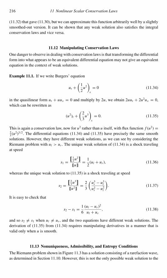
216 11 Nonlinear Scalar Conservation Laws

(11.32) that gave (11.30), but we can approximate this function arbitrarily well by a slightlysmoothed-out version. It can be shown that any weak solution also satisfies the integralconservation laws and vice versa.

11.12 Manipulating Conservation Laws

One danger to observe in dealing with conservation laws is that transforming the differentialform into what appears to be an equivalent differential equation may not give an equivalentequation in the context of weak solutions.

Example 11.1. If we write Burgers’ equation

ut +(1

2u2)x

= 0 (11.34)

in the quasilinear form ut + uux = 0 and multiply by 2u, we obtain 2uut + 2u2ux = 0,which can be rewritten as

(u2)t +(2

3u3)x

= 0. (11.35)

This is again a conservation law, now for u2 rather than u itself, with flux function f (u2) =23 (u

2)3/2. The differential equations (11.34) and (11.35) have precisely the same smoothsolutions. However, they have different weak solutions, as we can see by considering theRiemann problem with ul > ur . The unique weak solution of (11.34) is a shock travelingat speed

s1 =[[12u

2]]

[[u]]= 1

2(ul + ur ), (11.36)

whereas the unique weak solution to (11.35) is a shock traveling at speed

s2 =[[23u

3]]

[[u2]]= 2

3

(u3r − u3lu2r − u2l

). (11.37)

It is easy to check that

s2 − s1 = 1

6

(ul − ur )2ul + ur , (11.38)

and so s2 �= s1 when ul �= ur , and the two equations have different weak solutions. Thederivation of (11.35) from (11.34) requires manipulating derivatives in a manner that isvalid only when u is smooth.

11.13 Nonuniqueness, Admissibility, and Entropy Conditions

The Riemann problem shown in Figure 11.3 has a solution consisting of a rarefaction wave,as determined in Section 11.10. However, this is not the only possible weak solution to the

11.13 Nonuniqueness, Admissibility, and Entropy Conditions 217

equation with this data. Another solution is

q(x, t) ={ql if x/t < s,qr if x/t > s,

(11.39)

where the speed s is determined by the Rankine–Hugoniot condition (11.21). This functionconsists of the discontinuity propagating at speed s, the shock speed.We don’t expect a shockwave in this case, since characteristics are spreading out rather than colliding, but we didnot use any information about the characteristic structure in deriving the Rankine–Hugoniotcondition. The function (11.39) is a weak solution of the conservation law regardless ofwhether ql < qr or ql > qr . The discontinuity in the solution (11.39) is sometimes calledan expansion shock in this case.We see that the weak solution to a conservation law is not necessarily unique. This is

presumably another failing of our mathematical formulation, since physically we expectonly one thing to happen for given initial data, and hence a unique solution. Again thisresults from the fact that the hyperbolic equation is an imperfect model of reality. A bettermodel might include “viscous terms” as in Section 11.6, for example, and the resultingparabolic equation would have a unique solution for any set of data. As in the case of shockwaves, what we hope to capture with the hyperbolic equation is the correct limiting solutionas the viscosity ε vanishes. As Figure 11.4(a) suggests, if the discontinuous data is smoothedonly slightly (as would happen immediately if the equation were parabolic), then there isa unique solution determined by the characteristics. This solution clearly converges to therarefaction wave as ε → 0. So the expansion shock solution (11.39) is an artifact of ourformulation and is not physically meaningful.The existence of these spurious solution is not merely a mathematical curiosity. Under

some circumstances nonphysical solutions of this type are all too easily computed nu-merically, in spite of the fact that numerical methods typically contain some “numericalviscosity.” See Section 12.3 for a discussion of these numerical difficulties.In order to effectively use the hyperbolic equations we must impose some additional con-

dition along with the differential equation in order to insure that the problem has a uniqueweak solution that is physically correct. Often the condition we want to impose is sim-ply that the weak solution must be the vanishing-viscosity solution to the proper viscousequation. However, this condition is hard to work with directly in the context of the hy-perbolic equation. Instead, a variety of other conditions have been developed that can beapplied directly to weak solutions of hyperbolic equations to check if they are physicallyadmissible. Such conditions are sometimes called admissibility conditions, or more oftenentropy conditions. This name again comes from gas dynamics, where the second law ofthermodynamics demands that the entropy of a system must be nondecreasing with time(see Section 14.5). Across a physically admissible shock the entropy of the gas increases.Across an expansion shock, however, the entropy of the gas would decrease, which is notallowed. The entropy at each point can be computed as a simple function of the pressureand density, (2.35), and the behavior of this function can be used to test a weak solution foradmissibility. For other conservation laws it is sometimes possible to define a function η(q),called an entropy function, which has similar diagnostic properties. This approach to devel-oping entropy conditions is discussed in Section 11.14. Expansion shocks are often called

218 11 Nonlinear Scalar Conservation Laws

entropy-violating shocks, since they are weak solutions that fail to satisfy the appropriateentropy condition.First we discuss some other admissibility conditions that relate more directly to the

characteristic structure.Wediscuss only a fewpossibilities here and concentrate on the scalarcase. For some systems of equations the development of appropriate admissibility conditionsremains a challenging research question. In some cases it is not even well understood whatthe appropriate viscous regularization of the conservation law is, and it may be that differentchoices of the viscous term lead to different vanishing-viscosity solutions.For scalar equations there is an obvious condition suggested by Figures 11.2(b) and

11.3(b). A shock should have characteristics going into the shock, as time advances. Apropagating discontinuity with characteristics coming out of it would be unstable to per-turbations. Either smearing out the initial profile a little, or adding some viscosity to thesystem, will cause this to be replaced by a rarefaction fan of characteristics, as in Figure11.3(b). This gives our first version of the entropy condition:

Entropy Condition 11.1 (Lax). For a convex scalar conservation law, a discontinuity pro-pagating with speed s given by (11.21) satisfies the Lax entropy condition if

f ′(ql) > s > f ′(qr ). (11.40)

Note that f ′(q) is the characteristic speed. For convex or concave f , the Rankine–Hugoniot speed s from (11.21) must lie between f ′(ql) and f ′(qr ), so (11.40) reduces tosimply the requirement that f ′(ql)> f ′(qr ). For the traffic flow flux (11.4), this then impliesthat we need ql < qr in order for the solution to be an admissible shock since f ′′(q)< 0. Ifql > qr then the correct solution would be a rarefaction wave. For Burgers’ equation withf (u)= u2/2, on the other hand, the Lax Entropy Condition 11.1 requires ul > ur for anadmissible shock, since f ′′(u) is everywhere positive rather than negative.A more general form of (11.40), due to Oleinik, also applies to nonconvex scalar flux

functions and is given in Section 16.1.2. The generalization to systems of equations isdiscussed in Section 13.7.2.Another form of the entropy condition is based on the spreading of characteristics in a

rarefaction fan.We state this for the convex casewith f ′′(q) > 0 (such asBurgers’ equation),since this is the form usually seen in the literature. If q(x, t) is an increasing function ofx in some region, then characteristics spread out in this case. The rate of spreading can bequantified, and gives the following condition, also due to Oleinik [346].

Entropy Condition 11.2 (Oleinik). q(x, t) is the entropy solution to a scalar conservationlaw qt+ f (q)x = 0with f ′′(q) > 0 if there is a constant E > 0 such that for all a > 0, t > 0,and x ∈ R,

q(x + a, t)− q(x, t)a

<E

t. (11.41)

Note that for a discontinuity propagating with constant left and right states ql and qr ,this can be satisfied only if qr − ql ≤ 0, so this agrees with (11.40). The form of (11.41)also gives information on the rate of spreading of rarefaction waves as well as on the formof allowable jump discontinuities, and is easier to apply in some contexts. In particular,

11.14 Entropy Functions 219

this formulation has advantages in studying numerical methods, and is related to one-sidedLipschitz conditions and related stability concepts [339], [340], [437].

11.14 Entropy Functions

Another approach to the entropy condition is to define an entropy functionη(q),motivated bythermodynamic considerations in gas dynamics as described in Chapter 14. This approachoften applies to systems of equations, as in the case of gas dynamics, and is also used instudying numerical methods; see Section 12.11.1.In general an entropy function should be a function that is conserved (i.e., satisfies some

conservation law) whenever the function q(x, t) is smooth, but which has a source or asink at discontinuities in q . The entropy of a gas has this property: entropy is producedin an admissible shock but would be reduced across an expansion shock. The second lawof thermodynamics requires that the total entropy must be nondecreasing with time. Thisentropy condition rules out expansion shocks.We now restate this in mathematical form. Along with an entropy function η(q), we need

an entropy flux ψ(q) with the property that whenever q is smooth an integral conservationlaw holds, ∫ x2

x1

η(q(x, t2)) dx =∫ x2

x1

η(q(x, t1)) dx

+∫ t2

t1

ψ(q(x1, t)) dt −∫ t2

t1

ψ(q(x2, t)) dt. (11.42)

The entropy function and flux must also be chosen in such a way that if q is discontinuousin [x1, x2]× [t1, t2], then the equation (11.42) does not hold with equality, so that the totalentropy in [x1, x2] at time t2 is either less or greater than what would be predicted by thefluxes at x1 and x2. Requiring that an inequality of the form∫ x2

x1

η(q(x, t2)) dx ≤∫ x2

x1

η(q(x, t1)) dx

+∫ t2

t1

ψ(q(x1, t)) dt −∫ t2

t1

ψ(q(x2, t)) dt (11.43)

always holds gives the entropy condition. (For the physical entropy in gas dynamics onewould require an inequality of this form with ≥ in place of ≤, but in the mathematicalliterature η(q) is usually chosen to be a convex function with η′′(q)> 0, leading to theinequality (11.43).)If q(x, t) is smooth, then the conservation law (11.42) can be manipulated as in Chapter 2

to derive the differential form

η(q)t + ψ(q)x = 0. (11.44)

Moreover, if η andψ are smooth function of q , we can differentiate these to rewrite (11.44)as

η′(q)qt + ψ ′(q)qx = 0. (11.45)

220 11 Nonlinear Scalar Conservation Laws

On the other hand, the smooth function q satisfies

qt + f ′(q)qx = 0. (11.46)

Multiplying (11.46) by η′(q) and comparing with (11.45) yields

ψ ′(q) = η′(q) f ′(q) (11.47)

as a relation that should hold between the entropy function and the entropy flux. For ascalar conservation law this equation admits many solutions η(q), ψ(q). One trivial choiceof η and ψ satisfying (11.47) would be η(q) = q and ψ(q) = f (q), but then η would beconserved even across discontinuities and this would not help in defining an admissibilitycriterion. Instead we also require that η(q) be a convex function of q with η′′(q) > 0 for allq. This will give an entropy function for which the inequality (11.43) should hold.For a system of equations η and ψ are still scalar functions, but now η′(q) and ψ ′(q)

must be interpreted as the row-vector gradients of η and ψ with respect to q , e.g.,

η′(q) =[∂η

∂q1,∂η

∂q2, . . . ,

∂η

∂qm

], (11.48)

and f ′(q) is the m × m Jacobian matrix. In general (11.47) is a system of m equationsfor the two variables η and ψ . Moreover, we also require that η(q) be convex, which fora system requires that the Hessian matrix η′′(q) be positive definite. For m> 2 this mayhave no solutions. Many physical systems do have entropy functions, however, includingof course the Euler equations of gas dynamics, where the negative of physical entropy canbe used. See Exercise 13.6 for another example. For symmetric systems there is always anentropy function η(q) = qT q , as observed by Godunov [158]. Conversely, if a system has aconvex entropy, then its Hessian matrix η′′(q) symmetrizes the system [143]; see also [433].In order to see that the physically admissible weak solution should satisfy (11.43), we go

back to the more fundamental condition that the admissible q(x, t) should be the vanishing-viscosity solution. Consider the related viscous equation

qεt + f (qε)x = εqεxx (11.49)

for ε > 0. We will investigate how η(qε) behaves for solutions qε(x, t) to (11.49) and takethe limit as ε→ 0. Since solutions to the parabolic equation (11.49) are always smooth,we can derive the corresponding evolution equation for the entropy following the samemanipulations we used for smooth solutions of the inviscid equation, multiplying (11.49)by η′(qε) to obtain

η(qε)t + ψ(qε)x = εη′(qε)qεxx .

We can now rewrite the right-hand side to obtain

η(qε)t + ψ(qε)x = ε(η′(qε)qεx

)x− εη′′(qε) (qεx )2.

11.14 Entropy Functions 221

Integrating this equation over the rectangle [x1, x2]× [t1, t2] gives∫ x2

x1

η(qε(x, t2)) dx =∫ x2

x1

η(qε(x, t1)) dx

−(∫ t2

t1

ψ(qε(x2, t)) dt −∫ t2

t1

ψ(qε(x1, t)) dt

)+ ε

∫ t2

t1

[η′(qε(x2, t)) qεx (x2, t)− η′(qε(x1, t)) qεx (x1, t)

]dt

− ε

∫ t2

t1

∫ x2

x1

η′′(qε)(qεx)2dx dt. (11.50)

In addition to the flux differences, the total entropy is modified by two terms involving ε.As ε → 0, the first of these terms vanishes. (This is clearly true if the limiting functionq(x, t) is smooth at x1 and x2, and can be shown more generally.) The other term, however,involves integrating (qεx )

2 over the rectangle [x1, x2]× [t1, t2]. If the limiting weak solutionis discontinuous along a curve in this rectangle, then this term will not vanish in the limit.However, since ε > 0, (qεx )

2> 0, and η′′> 0 (by our convexity assumption), we can concludethat this term is nonpositive in the limit and hence the vanishing-viscosity weak solutionsatisfies (11.43).Just as for the conservation law, an alternative weak form of the entropy condition can be

formulated by integrating against smooth test functions φ, now required to be nonnegative,since the entropy condition involves an inequality. A weak solution q satisfies the weakform of the entropy inequality if∫ ∞

0

∫ ∞

−∞[φtη(q)+ φxψ(q)] dx dt +

∫ ∞

−∞φ(x, 0)η(q(x, 0)) dx ≥ 0 (11.51)

for all φ ∈ C10 (R×R) with φ(x, t) ≥ 0 for all x, t . In Section 12.11.1 we will see that thisform of the entropy condition is convenient to work with in proving that certain numericalmethods converge to entropy-satisfying weak solutions.The entropy inequalities (11.43) and (11.51) are often written informally as

η(q)t + ψ(q)x ≤ 0, (11.52)

with the understanding that where q is smooth (11.44) is in fact satisfied and near discon-tinuities the inequality (11.52) must be interpreted in the integral form (11.43) or the weakform (11.51).Another form that is often convenient is obtained by applying the integral inequality

(11.43) to an infinitesimal rectangle near a shock as illustrated in Figure 11.7. When theintegral form of the original conservation law was applied over this rectangle, we obtainedthe Rankine–Hugoniot jump condition (11.20),

s(qr − ql) = f (qr )− f (ql).

Going through the same steps using the inequality (11.43) leads to the inequality

s(η(qr )− η(ql)) ≥ ψ(qr )− ψ(ql). (11.53)

222 11 Nonlinear Scalar Conservation Laws

We thus see that a discontinuity propagating with speed s satisfies the entropy condition ifand only if the inequality (11.53) is satisfied.

Example 11.2. For Burgers’ equation (11.34), the discussion of Section 11.12 shows thatthe convex function η(u)= u2 can be used as an entropy function, with entropy fluxψ(u) =23u

3. Note that these satisfy (11.47). Consider a jump from ul to ur propagating with speeds = (ul + ur )/2, the shock speed for Burgers’ equation. The entropy condition (11.53)requires

1

2(ul + ur )

(u2r − u2l

) ≥ 2

3

(u3r − u3l

).

This can be rearranged to yield

1

6(ul − ur )3 ≥ 0,

and so the entropy condition is satisfied only if ul > ur , as we already found from the LaxEntropy Condition 11.1.

11.14.1 The Kruzkov Entropies

In general an entropy function should be strictly convex, with a second derivative that isstrictly positive at every point. This is crucial in the above analysis of (11.50), since the(qεx )

2 term that gives rise to the inequality in (11.51) is multiplied by η′′(qε).Rather than considering a single strictly convex function that can be used to investigate

every value of qε , a different approach was adopted by Kruzkov [248], who introduced theidea of entropy inequalities. He used a whole family of entropy functions and correspondingentropy fluxes,

ηk(q) = |q − k|, ψk(q) = sgn(q − k) [ f (q)− f (k)], (11.54)

where k is any real number. Each function ηk(q) is a piecewise linear function of q with akink at q = k, and hence η′′(q) = δ(q − k) is a delta function with support at q = k. It isa weakly convex function whose nonlinearity is concentrated at a single point, and henceit is useful only for investigating the behavior of weak solutions near the value q = k.However, it is sometimes easier to obtain entropy results by studying the simple piecewiselinear function ηk(q) than to work with an arbitrary entropy function. If it can be shown thatif a weak solution satisfies the entropy inequality (11.51) for an arbitrary choice of ηk(q)(i.e., that the entropy condition is satisfied for all the Kruzkov entropies), then (11.51) alsoholds more generally for any strictly convex entropy η(q).

11.15 Long-Time Behavior and N-Wave Decay

Figure 11.8 shows the solution to Burgers’ equation with some smooth initial data havingcompact support. As time evolves, portions of the solution where ux < 0 steepen into shockwaves while portions where ux > 0 spread out as rarefaction waves. Over time these shocks

11.15 Long-Time Behavior and N-Wave Decay 223

−8 −6 −4 −2 0 2 4 6 8−3

−2

−1

0

1

2

3

4

5

6t = 0

−6 −4 −2 0 2 4 6−1

−0.5

0

0.5

1

1.5t = 1

−8 −6 −4 −2 0 2 4 6 8−3

−2

−1

0

1

2

3

4

5

6t = 0.2

−8 −6 −4 −2 0 2 4 6 8−1

−0.5

0

0.5

1

1.5t = 2

−8 −6 −4 −2 0 2 4 6 8−3

−2

−1

0

1

2

3

4

5

6t = 0.4

−8 −6 −4 −2 0 2 4 6 8−1

−0.5

0

0.5

1

1.5t = 3

−8 −6 −4 −2 0 2 4 6 8−3

−2

−1

0

1

2

3

4

5

6t = 0.6

−8 −6 −4 −2 0 2 4 6 8−1

−0.5

0

0.5

1

1.5t = 4

−8 −6 −4 −2 0 2 4 6 8−3

−2

−1

0

1

2

3

4

5

6t = 0.8

−8 −6 −4 −2 0 2 4 6 8−1

−0.5

0

0.5

1

1.5t = 5

−8 −6 −4 −2 0 2 4 6 8−3

−2

−1

0

1

2

3

4

5

6t = 1

−8 −6 −4 −2 0 2 4 6 8−1

−0.5

0

0.5

1

1.5t = 6

Fig. 11.8. Decay of general initial data to an N-wave with Burgers’ equation. The left column showsthe initial behavior from time t = 0 to t = 1 (going down). The right column shows later times t = 1to t = 6 on a different scale. [claw/book/chap11/burgers]

and rarefactions interact. The shocks travel at different speeds, and those going in thesame direction merge into stronger shocks. Meanwhile, the rarefaction waves weaken theshocks. The most striking fact is that in the long run all the structure of the initial datacompletely disappears and the solution behaves like an N-wave: one shock propagates tothe left, another to the right, and in between the rarefactionwave is essentially linear. Similarlong-time behavior would be seen starting from any other initial data with compact support.The position and strength of the two shocks does depend on the data, but this same N-waveshape will always arise. The same is true for other nonlinear conservation laws, providedthe flux function is convex, although the shape of the rarefaction wave between the twoshocks will depend on this flux. Only for a quadratic flux (such as Burgers’ equation) will it

224 11 Nonlinear Scalar Conservation Laws

be linear. For more details about the long-time behavior of solutions, see for example [98],[308], [420].Note that this loss of structure in the solution implies that in general a nonlinear conser-

vation law models irreversible phenomena. With a linear equation, such as the advectionequation or the acoustics equations, the solution is reversible. We can start with arbi-trary data, solve the equation qt + Aqx = 0 for some time T , and then solve the equationqt − Aqx = 0 for another T time units, and the original data will be recovered. (This isequivalent to letting t run backwards in the original equation.) For a nonlinear equationqt + f (q)x = 0, we can do this only over times T for which the solution remains smooth.Over such time periods the solution is constant along the characteristics, which do not cross,and the process is reversible. Once shocks form, however, characteristics disappear into theshock and information is lost. Many different sets of data can give rise to exactly the sameshock wave. If the equation is now solved backwards in time (or, equivalently, we solveqt − f (q)x = 0) then compression at the shock becomes expansion. There are infinitelymany different weak solutions in this case. Spreading back out into the original data isone of these, but the solution at the final time contains no information about which of theinfinitely many possibilities is “correct.”The fact that information is irretrievably lost in a shock wave is directly related to the

notion that the physical entropy increases across a shock wave. Entropy is a measure of theamount of disorder in the system (see Section 14.5) and a loss of structure corresponds toan increase in entropy. Since entropy can only increase once shocks have formed, it is notpossible to recover the initial data.

Exercises

11.1. Show that in solving the scalar conservation law qt + f (q)x = 0 with smooth initialdata q(x, 0), the time at which the solution “breaks” is given by

Tb = −1minx [ f ′′(q(x, 0))qx (x, 0)]

(11.55)

if this is positive. If this is negative, then characteristics never cross. Hint: Useq(x, t) = q(ξ (x, t), 0) from (11.11), differentiate this with respect to x , and deter-mine where qx becomes infinite. To compute ξx , differentiate the equation (11.12)with respect to x .

11.2. Show that the viscous Burgers equation ut + uux = εuxx has a traveling-wavesolution of the form uε(x, t) = wε(x − st), by deriving an ODE for w and veri-fying that this ODE has solutions of the form

w(ξ ) = ur + 1

2(ul − ur )

[1− tanh

((ul − ur )ξ

4ε

)], (11.56)

when ul > ur , with the propagation speed s agreeing with the shock speed (11.23).Note thatw(ξ )→ ul as ξ →−∞, andw(ξ )→ ur as ξ →+∞. Sketch this solutionand indicate how it varies as ε → 0. What happens to this solution if ul < ur , andwhy is there no traveling-wave solution with limiting values of this form?

Exercises 225

11.3. For a general smooth scalar flux functions f (q), show by Taylor expansion of (11.21)that the shock speed is approximately the average of the characteristic speed on eachside,

s = 1

2[ f ′(ql)+ f ′(qr )]+O(|qr − ql |2).

The exercises below require determining the exact solution to a scalar conservationlaw with particular initial data. In each case you should sketch the solution at severalinstants in time as well as the characteristic structure and shock-wave locations inthe x–t plane.You may wish to solve the problem numerically by modifying the CLAWPACK

codes for this chapter in order to gain intuition for how the solution behaves and tocheck your formulas.

11.4. Determine the exact solution to Burgers’ equation ut+ ( 12u2)x = 0 for all t > 0 wheneach of the following sets of initial data is used:(a)

u◦(x) =1 if x < −1,0 if − 1 < x < 1,−1 if x > 1.

(b)

u◦(x) =−1 if x < −1,0 if − 1 < x < 1,1 if x > 1.

11.5. Determine the exact solution to Burgers’ equation for t > 0 with initial data

u◦(x) ={2 if 0 < x < 1,0 otherwise.

Note that the rarefaction wave catches up to the shock at some time Tc. For t > Tcdetermine the location of the shock by two different approaches:(a) Let xs(t) represent the shock location at time t . Determine and solve an ODE

for xs(t) by using the Rankine–Hugoniot jump condition (11.21), which musthold across the shock at each time.

(b) For t > Tc the exact solution is triangular-shaped. Use conservation to deter-mine xs(t) based on the area of this triangle. Sketch the corresponding “over-turned” solution, and illustrate the equal-area rule (as in Figure 11.6).

11.6. Repeat Exercise 11.5 with the data

u◦(x) ={2 if 0 < x < 1,4 otherwise.

Note that in this case the shock catches up with the rarefaction wave.

226 11 Nonlinear Scalar Conservation Laws

11.7. Determine the exact solution to Burgers’ equation for t > 0 with the data

u◦(x) =

12 if 0 < x,8 if 0 < x < 14,4 if 14 < x < 17,2 if 17 < x .

Note that the three shocks eventually merge into one shock.11.8. Consider the scalar conservation law ut + (eu)x = 0. Determine the exact solution

with the following sets of initial data:(a)

u◦(x) ={1 if x < 0,0 if x > 0.

(b)

u◦(x) ={0 if x < 0,1 if x > 0.

(c)

u◦(x) ={2 if 0 < x < 1,0 otherwise.

Hint: Use the approach outlined in Exercise 11.5(a).11.9. Determine an entropy function and entropy flux for the traffic flow equation with

flux (11.4). Use this to show that ql < qr is required for a shock to be admissible.

12Finite Volume Methods for Nonlinear Scalar

Conservation Laws

We now turn to the development of finite volume methods for nonlinear conservation laws.We will build directly on what has already been developed for linear systems in Chapter 4,concentrating in this chapter on scalar equations, although much of what is developed willalso apply to nonlinear systems of equations. In Chapter 15 we consider some additionalissues arising for systems of equations, particularly the need for efficient approximateRiemann solvers in Section 15.3.Nonlinearity introduces a number of new difficulties not seen for the linear problem.

Stability and convergence theory are more difficult than in the linear case, particularly inthat we are primarily interested in discontinuous solutions involving shock waves. Thistheory is taken up in Section 12.10. Moreover, we must ensure that we are converging to thecorrect weak solution of the conservation law, since the weak solution may not be unique.This requires that the numerical method be consistent with a suitable entropy condition; seeSection 12.11.For a nonlinear conservation law qt + f (q)x = 0 it is very important that the method be

in conservation form, as described in Section 4.1,

Qn+1i = Qni −�t

�x

(Fni+1/2 − Fni−1/2

), (12.1)

in order to insure that weak solutions to the conservation law are properly approximated.Recall that this form is derived directly from the integral form of the conservation laws,which is the correct equation to model when the solution is discontinuous. In Section 12.9an example is given to illustrate that methods based instead on the quasilinear form qt +f ′(q)qx = 0 may be accurate for smooth solutions but may completely fail to approximatea weak solution when the solution contains shock waves.

12.1 Godunov’s Method

Recall from Section 4.11 that Godunov’s method is obtained by solving the Riemannproblem between states Qni−1 and Q

ni in order to determine the flux F

ni−1/2 as

Fni−1/2 = f(Q∨

|i−1/2

).

227

228 12 Finite Volume Methods for Nonlinear Scalar Conservation Laws

(a) (b) (c) (d) (e)

Fig. 12.1. Five possible configurations for the solution to a scalar Riemann problem between statesQi−1 and Qi , shown in the x–t plane: (a) left-going shock, Q∨

|i−1/2= Qi ; (b) left-going rarefac-

tion, Q∨|i−1/2= Qi ; (c) transonic rarefaction, Q∨|i−1/2= qs ; (d) right-going rarefaction, Q∨|i−1/2= Qi−1;

(e) right-going shock, Q∨|i−1/2= Qi−1.

The value Q∨|i−1/2 = q∨

|(Qni−1, Q

ni ) is the value obtained along the ray x ≡ xi−1/2 in this

Riemann solution. This value is constant for t > tn , since the Riemann solution is a similaritysolution. To keep the notation less cluttered, wewill often drop the superscript n on Q below.To begin, we assume the flux function f (q) is convex (or concave), i.e., f ′′(q) does not

change sign over the range of q of interest. Then the Riemann solution consists of a singleshock or rarefaction wave. (See Section 16.1.3 for the nonconvex case.) For a scalar conser-vation law with a convex flux function there are five possible forms that the Riemann solu-tion might take, as illustrated in Figure 12.1. In most cases the solution Q∨

|i−1/2 is either Qi

(if the solution is a shock or rarefaction wavemoving entirely to the left, as in Figure 12.1(a)or (b)), or Qi−1 (if the solution is a shock or rarefaction wave moving entirely to the right,as in Figure 12.1(d) or (e)).The only case where Q∨

|i−1/2 has a different value than Qi or Qi−1 is if the solution

consists of a rarefaction wave that spreads partly to the left and partly to the right, as shownin Figure 12.1(c). Suppose for example that f ′′(q) > 0 everywhere, in which case f ′(q) isincreasing with q, so that a rarefaction wave arises if Qi−1 < Qi . In this case the situationshown in Figure 12.1(c) occurs only if

Qi−1 < qs < Qi ,

where qs is the (unique) value of q for which f ′(qs) = 0. This is called the stagnationpoint, since the value qs propagates with velocity 0. It is also called the sonic point, sincein gas dynamics the eigenvalues u ± c can take the value 0 only when the fluid speed |u|is equal to the sound speed c. The solution shown in Figure 12.1(c) is called a transonicrarefaction since in gas dynamics the fluid is accelerated from a subsonic velocity to asupersonic velocity through such a rarefaction. In a transonic rarefaction the value alongx/t = xi−1/2 is simply qs .For the case f ′′(q) > 0 we thus see that the Godunov flux function for a convex scalar

conservation law is

Fni−1/2 =

f (Qi−1) if Qi−1 > qs and s > 0,f (Qi ) if Qi < qs and s < 0,

f (qs) if Qi−1 < qs < Qi .

(12.2)

Here s = [ f (Qi )− f (Qi−1)]/(Qi − Qi−1) is the shock speed given by (11.21).Note in particular that if f ′(q)> 0 for both Qi−1 and Qi then Fni−1/2 = f (Qi−1) and

Godunov’s method reduces to the first-order upwind method

Qn+1i = Qi − �t

�x[ f (Qi )− f (Qi−1)]. (12.3)

12.2 Fluctuations, Waves, and Speeds 229

The natural upwind method is also obtained if f ′(q) < 0 for both values of Q, involvingone-sided differences in the other direction. Only in the case where f ′(q) changes signbetween Qi−1 and Qi is the formula more complicated, as we should expect, since the“upwind direction” is ambiguous in this case and information must flow both ways.The formula (12.2) can be written more compactly as

Fni−1/2 =

min

Qi−1≤q≤Qif (q) if Qi−1 ≤ Qi ,

maxQi≤q≤Qi−1

f (q) if Qi ≤ Qi−1,(12.4)

since the stagnation point qs is the global minimum or maximum of f in the convex case.This formula is valid also for the case f ′′(q)< 0 and even for nonconvex fluxes, in whichcase there may be several stagnation points at each maximum and minimum of f (seeSection 16.1).Note that there is one solution structure not illustrated in Figure 12.1, a stationary shock

with speed s = 0. In this case the value Q∨|i−1/2 is ambiguous, since the Riemann solution isdiscontinuous along x = xi−1/2. However, if s= 0 then f (Qi−1)= f (Qi ) by the Rankine–Hugoniot condition, and so Fni−1/2 is still well defined and the formula (12.4) is still valid.

12.2 Fluctuations, Waves, and Speeds

Godunov’s method can be implemented in our standard form

Qn+1i = Qi − �t

�x

(A+�Qi−1/2 +A−�Qi+1/2)

(12.5)

if we define the fluctuations A±�Qi−1/2 by

A+�Qi−1/2 = f (Qi )− f(Q∨

|i−1/2

),

A−�Qi−1/2 = f(Q∨

|i−1/2

)− f (Qi−1).(12.6)

In order to define high-resolution correction terms, we also wish to compute a waveWi−1/2and speed si−1/2 resulting from this Riemann problem. The natural choice is

Wi−1/2 = Qi − Qi−1,

si−1/2 ={[ f (Qi )− f (Qi−1)]/(Qi − Qi−1) if Qi−1 �= Qi ,

f ′(Qi ) if Qi−1 = Qi ,

(12.7)

although thevalueof si−1/2 is immaterialwhenQi−1= Qi . The speed chosen is theRankine–Hugoniot shock speed (11.21) for this data. If the Riemann solution is a shock wave, this isclearly the right thing to do. If the solution is a rarefaction wave, then the wave is not simplya jump discontinuity propagating at a single speed. However, this is still a suitable definitionof the wave and speed to use in defining correction terms that yield second-order accuracyin the smooth case. This can be verified by a truncation-error analysis of the resultingmethod; see Section 15.6. Note that when a smooth solution is being approximated, weexpect Wi−1/2=O(�x), and there is very little spreading of the rarefaction wave in anycase. Moreover, a wave consisting of this jump discontinuity propagating with speed si−1/2

230 12 Finite Volume Methods for Nonlinear Scalar Conservation Laws

does define a weak solution to the Riemann problem, although it is an expansion shock thatdoes not satisfy the entropy condition. However, provided it is not a transonic rarefaction,the same result will be obtained inGodunov’smethodwhether we use the entropy-satisfyingrarefaction wave or an expansion shock as the solution to the Riemann problem. When thewave lies entirely within one cell, the cell average is determined uniquely by conservationand does not depend on the structure of the particularweak solution chosen.We can computethe fluctuations A±�Qi−1/2 using

A+�Qi−1/2 = s+i−1/2Wi−1/2,

A−�Qi−1/2 = s−i−1/2Wi−1/2(12.8)

in place of (12.6), provided that Q∨|i−1/2= Qi−1 or Qi . Only in the case of a transonic

rarefaction is it necessary to instead use the formulas (12.6) with Q∨|i−1/2= qs .

12.3 Transonic Rarefactions and an Entropy Fix

Note that if we were to always use (12.8), even for transonic rarefactions, then we wouldstill be applying Godunov’s method using an exact solution to the Riemann problem; theRankine–Hugoniot conditions are always satisfied for the jump and speed determined in(12.7). The only problem is that the entropy condition would not be satisfied and we wouldbe using the wrong solution. For this reason the modification toA±�Qi−1/2 required in thetransonic case is often called an entropy fix.This approach is used in the Riemann solver [claw/book/chap12/efix/rp1.f]. The

wave and speed are first calculated, and the fluctuations are set using (12.8). Only in thecase of a transonic rarefaction is the entropy fix applied to modify the fluctuations. Iff ′(Qi−1) < 0 < f ′(Qi ) then the fluctuations in (12.8) are replaced by

A+�Qi−1/2 = f (Qi )− f (qs),

A−�Qi−1/2 = f (qs)− f (Qi−1).(12.9)

We will see in Section 15.3 that this approach generalizes to nonlinear systems of equa-tions in a natural way. An approximate Riemann solver can often be used that gives anapproximate solution involving a finite set of waves that are jump discontinuities W p

i−1/2propagating at some speeds s pi−1/2. These are used to define fluctuations and also high-resolution correction terms, as indicated in Section 6.15. A check is then performed to seeif any of the waves should really be transonic rarefactions, and if so, the fluctuations aremodified by performing an entropy fix.For the scalar equation this approach may seem a rather convoluted way to specify the

true Godunov flux, which is quite simple to determine directly. For nonlinear systems,however, it is generally too expensive to determine the rarefaction wave structure exactlyand this approach is usually necessary. This is discussed further in Section 15.3, wherevarious entropy fixes are presented.Dealing with transonic rarefactions properly is an important component in the develop-

ment of successfulmethods. This is illustrated in Figure 12.2,which shows several computedsolutions to Burgers’ equation (11.13) at time t = 1 for the same set of data, a Riemannproblem with ul = −1 and ur = 2. (Note that for Burgers’ equation the sonic point is at

12.3 Transonic Rarefactions and an Entropy Fix 231

(a) −3 −2 −1 0 1 2 3−1.5

−1

−0.5

0

0.5

1

1.5

2

2.5Godunov with no entropy fix

(b) −3 −2 −1 0 1 2 3−1.5

−1

−0.5

0

0.5

1

1.5

2

2.5Godunov with entropy fix

(c) −3 −2 −1 0 1 2 3−1.5

−1

−0.5

0

0.5

1

1.5

2

2.5High–resolution with no entropy fix

(d) −3 −2 −1 0 1 2 3−1.5

−1

−0.5

0

0.5

1

1.5

2

2.5High–resolution with entropy fix

Fig. 12.2. The solid line is the entropy-satisfying solution to Burgers’ equation with a transonicrarefaction wave. The circles show computed solutions. (a) Godunov’smethod using expansion-shocksolutions to each Riemann problem. This method converges to a weak solution that does not satisfy theentropy condition. (b)Godunov’smethodusing entropy-satisfying solutions to eachRiemannproblem.(c) High-resolution corrections added to the expansion-shock Godunov method. (d) High-resolutioncorrections added to the entropy-satisfying Godunov method. [claw/book/chap12/efix]

us = 0.) The top row shows results obtained with Godunov’s method and the bottom rowshows results with the high-resolution method, using the MC limiter. The plots on the leftwere obtained using (12.8) everywhere, with no entropy fix. The plots on the right wereobtained using the entropy fix, which means that the fluctuations were redefined at a singlegrid interface each time step, the one for whichUn

i−1 < 0 andUni > 0. This modification at

a single grid interface makes a huge difference in the quality of the results. In particular, theresult obtained using Godunov’s method with the expansion-shock Riemann solution looksentirely wrong. In fact it is a reasonable approximation to a weak solution to the problem,the function

u(x, t) =

−1 if x < 0,1 if 0 < x ≤ t,x/t if t ≤ x ≤ 2t,2 if x ≥ 2t.

This solution consists of an entropy-violating stationary shock at x = 0 and also a rarefactionwave. If the grid is refined, the computed solution converges nicely to this weak solution.However, this is not the physically relevant vanishing-viscosity solution that we had hopedto compute.When the correct rarefaction-wave solution to each Riemann problem is used (i.e., the

entropy fix (12.9) is employed), Godunov’s method gives a result that is much closer to theweak solution we desire. There is still a small expansion shock visible in Figure 12.2(b)

232 12 Finite Volume Methods for Nonlinear Scalar Conservation Laws

near x = 0, but this is of magnitudeO(�x) and vanishes as the grid is refined. This feature(sometimes called an entropy glitch) is a result of Godunov’s method lacking sufficientnumerical viscosity when the wave speed is very close to zero. See [160] for one analysisof this. In Section 12.11.1 we will prove that Godunov’s method converges to the correctsolution provided that transonic rarefactions are properly handled.Adding in the high-resolution correction terms (as discussed in Section 12.8) produces

better results, even when the entropy fix is not used (Figure 12.2(c)), and convergence to theproper weak solution is obtained. Even in this case, however, better results are seen if thefirst-order flux for the transonic rarefaction is properly computed, as shown inFigure 12.2(d).

12.4 Numerical Viscosity

Theweak solution seen in Figure 12.2(a), obtainedwithGodunov’smethod using the expan-sion shock solution to each Riemann problem, contains a portion of the correct rarefactionwave along with a stationary expansion shock located at x = 0. Why does it have thisparticular structure? In the first time step a Riemann problem with ul =−1 and ur = 2 issolved, resulting in an expansion shock with speed 1

2 (ul + ur )= 12 . This wave propagates

a distance 12�t and is then averaged onto the grid, resulting in some smearing of the initialdiscontinuity. The numerical viscosity causing this smearing acts similarly to the physicalviscosity of the viscous Burgers equation (11.14), and tends to produce a rarefaction wave.However, unlike the viscosity of fixed magnitude ε appearing in (11.14), the magnitude ofthe numerical viscosity depends on the local Courant number si−1/2�t/�x , since it resultsfrom the averaging process (where si−1/2 is the Rankine–Hugoniot shock speed for the dataQi−1 and Qi ). In particular, if si−1/2= 0, then there is no smearing of the discontinuity and nonumerical viscosity. For Burgers’ equation this happens whenever Qi−1 = −Qi , in whichcase the expansion-shock weak solution is stationary. The solution shown in Figure 12.2(a)has just such a stationary shock.This suggests that another way to view the entropy fix needed in the transonic case is as

the addition of extra numerical viscosity in the neighborhood of such a point. This can beexamined further by noting that the fluctuations (12.8) result in the numerical flux function

Fi−1/2 = 1

2

[f (Qi−1)+ f (Qi )−

∣∣si−1/2∣∣(Qi − Qi−1)], (12.10)

as in the derivation of (4.61). Recall from Section 4.14 that this is the central flux (4.18) withthe addition of a viscous flux term. However, when si−1/2 = 0 this viscous term disappears.This viewpoint is discussed further in Section 15.3.5 where a variety of entropy fixes fornonlinear systems are discussed.

12.5 The Lax–Friedrichs and Local Lax–Friedrichs Methods

The Lax-Friedrichs (LxF) method was introduced in Section 4.6. The flux function (4.21)for this method,

Fi−1/2 = 1

2[ f (Qi−1)+ f (Qi )− a(Qi − Qi−1)], (12.11)

12.5 The Lax–Friedrichs and Local Lax–Friedrichs Methods 233

(a)−3 −2 −1 0 1 2 3

−1.5

−1

−0.5

0

0.5

1

1.5

2

2.5Lax–Friedrichs

(b)−3 −2 −1 0 1 2 3

−1.5

−1

−0.5

0

0.5

1

1.5

2

2.5LLF method

Fig. 12.3. The solid line is the entropy-satisfying solution to Burgers’ equation with a transonicrarefaction wave. The symbols show computed solutions. (a) Lax–Friedrichs method. (b) Local Lax–Friedrichs (LLF) method. [claw/book/chap12/llf]

has a numerical viscosity a = �x/�t with a fixed magnitude that does not vanish near asonic point. As a result, this method always converges to the correct vanishing viscositysolution as the grid is refined; see Section 12.7.If the LxF method is applied to the same transonic rarefaction problem considered in

Figure 12.2, we obtain the results shown in Figure 12.3(a). Note that this method is moredissipative than Godunov’s method. It also exhibits a curious stair-step pattern in whichQ2 j = Q2 j+1 for each value of j . This results from the fact that the formula (4.20) for Qn+1i

involves only Qni−1 and Qni+1, so there is a decoupling of even and odd grid points. With

the piecewise constant initial data used in this example, the even and odd points evolvein exactly the same manner, so each solution value appears twice. (See Section 10.5 for adiscussion of the LxF method on a staggered grid in which only half the points appear. Thisviewpoint allows it to be related more directly to Godunov’s method.)An improvement to the LxF method is obtained by replacing the value a = �x/�t in

(12.11) by a locally determined value,

Fi−1/2 = 1

2

[f (Qi−1)+ f (Qi )− ai−1/2(Qi − Qi−1)

], (12.12)

where

ai−1/2 = max(| f ′(q)|) over all q between Qi−1 and Qi . (12.13)

For a convex flux function this reduces to

ai−1/2 = max(| f ′(Qi−1)|, | f ′(Qi )|).

This resulting method is Rusanov’s method [387], though recently it is often called thelocal Lax–Friedrichs (LLF) method because it has the same form as the LxF method butthe viscosity coefficient is chosen locally at each Riemann problem. It can be shown thatthis is sufficient viscosity to make the method converge to the vanishing-viscosity solution;see Section 12.7.

234 12 Finite Volume Methods for Nonlinear Scalar Conservation Laws

Note that if the CFL condition is satisfied (which is a necessary condition for stability),then | f ′(q)|�t/�x ≤ 1 for each value of q arising in the whole problem, and so

| f ′(q)| ≤ �x

�t.

Hence using a=�x/�t in the standard LxF method amounts to taking a uniform vis-cosity that is sufficient everywhere, at the expense of too much smearing in most cases.Figure 12.3(b) shows the results on the same test problem when the LLF method is used.Another related method is Murman’s method, in which (12.12) is used with (12.13)

replaced by

ai−1/2 =∣∣∣∣ f (Qi )− f (Qi−1)

Qi − Qi−1

∣∣∣∣ . (12.14)

Unlike the LLF scheme, solutions generated with this methodmay fail to satisfy the entropycondition because ai−1/2 vanishes for the case of a stationary expansion shock. In fact, thisis exactly the method (12.5) with A±�Qi−1/2 defined by (12.8), expressed in a differentform (see Exercise 12.1).Note that all these methods are easily implemented in CLAWPACK by taking

A−�Qi−1/2 = 1

2

[f (Qi )− f (Qi−1)− ai−1/2(Qi − Qi−1)

],

A+�Qi−1/2 = 1

2

[f (Qi )− f (Qi−1)+ ai−1/2(Qi − Qi−1)

],

(12.15)

as is done in [claw/book/chap12/llf/rp1.f].

12.6 The Engquist–Osher method

Wehave seen that the first-ordermethod (12.5)with the fluctuations (12.8) can be interpretedas an implementation ofGodunov’smethod inwhichwe always use the shock-wave solutionto each Riemann problem, even when this violates the entropy condition. The Engquist–Osher method [124] takes the opposite approach and always assumes the solution is a“rarefaction wave”, even when this wave must be triple-valued as in Figure 11.4(b). Thiscan be accomplished by setting

A+�Qi−1/2 =∫ Qi

Qi−1( f ′(q))+ dq,

A−�Qi−1/2 =∫ Qi

Qi−1( f ′(q))− dq.

(12.16)

Here the ± superscript on f ′(q) means the positive and negative part as in (4.40). Thesefluctuations result in an interface flux Fi−1/2 that can be expressed in any of the following

12.8 High-Resolution TVD Methods 235

ways:

Fi−1/2 = f (Qi−1)+∫ Qi

Qi−1( f ′(q))− dq

= f (Qi )−∫ Qi

Qi−1( f ′(q))+ dq

= 1

2[ f (Qi−1)+ f (Qi )]− 1

2

∫ Qi

Qi−1| f ′(q)| dq. (12.17)

If f ′(q) does not change sign between Qi−1 and Qi , then one of the fluctuations in(12.16) will be zero and these formulas reduce to the usual upwind fluxes as in (12.2). Inthe sonic rarefaction case both fluctuations are nonzero and we obtain the desired valueFi−1/2 = f (qs) as in (12.2). It is only in the transonic shock case, when f ′(Qi−1) > 0 >f ′(Qi ), that the Engquist–Osher method gives a value different from (12.2). In this caseboth fluctuations are again nonzero and we obtain

Fi−1/2 = f (Qi−1)+ f (Qi )− f (qs) (12.18)

rather than simply f (Qi−1) or f (Qi ). This is because the triple-valued solution ofFigure 11.4(b) spans the interface xi−1/2 in this case, so that the integral picks up threedifferent values of f . This flux is still consistent with the conservation law, however, and byassuming the rarefaction structure, the entropy condition is always satisfied. This approachcan be extended to systems of equations to derive approximate Riemann solvers that satisfythe entropy condition, giving the Osher scheme [349], [352].

12.7 E-schemes

Osher [349] introduced the notion of an E-scheme as one that satisfies the inequality

sgn(Qi − Qi−1)[Fi−1/2 − f (q)

] ≤ 0 (12.19)

for all q between Qi−1 and Qi . In particular, Godunov’s method with flux FGi−1/2 definedby (12.4) is clearly an E-scheme. In fact it is the limiting case, in the sense that E-schemesare precisely those for which

Fi−1/2 ≤ FGi−1/2 ifQi−1 ≤ Qi ,

Fi−1/2 ≥ FGi−1/2 ifQi−1 ≥ Qi .(12.20)

It can be shown that any E-scheme is TVD if the Courant number is sufficiently small (Exer-cise 12.3). Osher [349] proves that E-schemes are convergent to the entropy-satisfyingweaksolution. In addition to Godunov’s method, the LxF, LLF, and Engquist–Osher methods areall E-schemes. Osher also shows that E-schemes are at most first-order accurate.

12.8 High-Resolution TVD Methods

The methods described so far are only first-order accurate and not very useful in their ownright. They are, however, used as building blocks in developing certain high-resolution

236 12 Finite Volume Methods for Nonlinear Scalar Conservation Laws

methods. Godunov’s method, as described in Section 12.2, can be easily extended to ahigh-resolution method of the type developed in Chapter 6,

Qn+1i = Qi − �t

�x

(A+�Qi−1/2 + A−�Qi+1/2

)− �t

�x

(F i+1/2 − F i−1/2

). (12.21)

We set

F i−1/2 = 1

2

∣∣si−1/2∣∣ (1− �t

�x

∣∣si−1/2∣∣) Wi−1/2, (12.22)

just as we have done for the variable-coefficient advection equation in Section 9.3.1. AgainWi−1/2 is a limited version of the wave (12.7) obtained by comparing Wi−1/2 to Wi−3/2 orWi−1/2, dependingon the sign of si−1/2.Note that themethod remains conservativewith sucha modification, which is crucial in solving nonlinear conservation laws (see Section 12.9).It is also possible to prove that the resulting method will be TVD provided that one of

the TVD limiters presented in Section 6.9 is used. This is a very important result, since itmeans that these methods can be applied with confidence to nonlinear problems with shockwaves where we wish to avoid spurious oscillations. Moreover, this TVD property allowsus to prove stability and hence convergence of the methods as the grid is refined, as shownin Section 12.12. (Unfortunately, these claims are valid only for scalar conservation laws.Extending these ideas to systems of equations gives methods that are often very successfulin practice, but for which much less can be proved in general.)Here we will prove that the limiter methods are TVD under restricted conditions to

illustrate the main ideas. (See [160] for more details.) We assume that data is monotone(say nonincreasing) and that f ′(q) does not change sign over the range of the data (sayf ′(Qni ) > 0). A similar approach can be used near extreme points of Qn and sonic points,but more care is required, and the formulas are more complicated. We will also impose thetime-step restriction

�t

�xmax | f ′(q)| < 1

2, (12.23)

although this can also be relaxed to the usual CFL limit of 1 with some modification of themethod.The main idea is to again use the REA Algorithm 4.1 to interpret the high-resolution

method. The first step is to reconstruct the piecewise linear function qn(x, tn) from the cellaverages Qni . This is where the limiters come into play, and this reconstruction does notincrease the total variation of the data. The second step is to evolve the conservation lawwiththis data. If we were to solve the conservation law exactly and then average onto the grid,then the resulting method would clearly be TVD, because the exact solution operator for ascalar conservation law is TVD (and so is the averaging process). But unlike the methodswe developed in Chapter 6 for the advection equation, we are not able to solve the originalconservation law exactly in step 2 of Algorithm 4.1 (except in the case of zero slopes, whereGodunov’s method does this). In principle one could do so also for more general slopes, butthe resulting correction formula would be much more complicated than (12.22). However,the formula (12.22) can be interpreted as what results from solving a slightly differentconservation law exactly and then averaging onto the grid. Exact solutions of this modifiedconservation law also have the TVD property, and it follows that the method is TVD.

12.9 The Importance of Conservation Form 237

(a) Qni Qn

i−1Qni+1

f(q)

f(q)

(b)

Qni

Qni−1

Qni+1

xi−1/2 xi+1/2

Fig. 12.4. (a) The flux function f (q) is approximated by a piecewise linear function f (q). (b) Thepiecewise linear data qn(x, tn) is evolved by solving the conservation law with flux f (q). The resultis the heavy line. Note that a shock forms near the value Qni where the characteristic velocity f

′(q)is discontinuous.

The modified conservation law used in the time step from tn to tn+1 is obtained byreplacing the flux function f (q) by a piecewise linear function f (q) that interpolates thevalues (Qni , f (Q

ni )), as shown in Figure 12.4(a). Then in step 2 we solve the conservation

law with this flux function to evolve qn(x, tn), as shown in Figure 12.4(b). This flux isstill nonlinear, but the nonlinearity has been concentrated at the points Qni . Shocks formimmediately at the points xi (the midpoints of the grid cells), but because of the time-steprestriction (12.23), these shocks do not reach the cell boundary during the time step.Near each interface xi−1/2 the data lies between Qni−1 and Q

ni , and so the flux function

is linear with constant slope si−1/2 = [ f (Qni ) − f (Qni−1)]/(Qni − Qni−1), as arises from

the piecewise linear interpolation of f . Hence the conservation law with flux f behaveslocally like the scalar advection equation with velocity si−1/2. This is exactly the velocitythat appears in the updating formula (12.22), and it can be verified that this method producesthe correct cell averages at the end of the time step for this modified conservation law.In this informal analysis we have assumed the data is monotone near Qni . The case where

Qni is a local extreme point must be handled differently, since wewould not be able to definea single function f in the same manner. However, in this case the slope in cell Ci is zero ifa TVD limiter is used, and we can easily show that the total variation can not increase inthis case.Some more details may be found in Goodman & LeVeque [160]. Recently Morton [332]

has performed a more extensive analysis of this type of method, including also similarmethods with piecewise quadratic reconstructions as well as methods on nonuniform gridsand multidimensional versions.

12.9 The Importance of Conservation Form

In Section 4.1 we derived the conservative form of a finite volume method based on theintegral formof the conservation law.Using amethod in this formguarantees that the discretesolution will be conservative in the sense that (4.8) will be satisfied. For weak solutionsinvolving shock waves, this integral form is more fundamental than the differential equationand forms the basis for the mathematical theory of weak solutions, including the derivation

238 12 Finite Volume Methods for Nonlinear Scalar Conservation Laws

of the Rankine–Hugoniot conditions (see Section 11.8) that govern the form and speed ofshock waves. It thus makes sense that a conservative method based on the integral formmight be more successful than other methods based on the differential equation. In fact, wewill see that the use of conservative finite volume methods is essential in computing weaksolutions to conservation laws. Nonconservative methods can fail, as illustrated below.Withconservative methods, one has the satisfaction of knowing that if the method converges tosome limiting function as the grid is refined, then this function is a weak solution. This isfurther explained and proved in Section 12.10 in the form of the Lax–Wendroff theorem.In Section 12.11 we will see that similar ideas can be used to show that the limiting

function also satisfies the entropy condition, provided the numerical method satisfies anatural discrete version of the entropy condition.Consider Burgers’ equation ut + 1

2 (u2)x = 0, for example. If u> 0 everywhere, then the

conservative upwind method (Godunov’s method) takes the form

Un+1i = Un

i −�t

�x

(1

2

(Uni

)2 − 1

2

(Uni−1)2)

. (12.24)

On the other hand, using the quasilinear form ut + uux = 0, we could derive the noncon-servative upwind method

Un+1i = Un

i −�t

�xUni

(Uni −Un

i−1). (12.25)

On smooth solutions, both of these methods are first-order accurate, and they give compara-ble results.When the solution contains a shockwave, themethod (12.25) fails to converge toa weak solution of the conservation law. This is illustrated in Figure 12.5. The conservativemethod (12.24) gives a slightly smeared approximation to the shock, but it is smeared aboutthe correct location. We can easily see that it must be, since the method has the discreteconservation property (4.8). The nonconservative method (12.25), on the other hand, givesthe results shown in Figure 12.5(b). These clearly do not satisfy (4.8), and as the grid is

(a)−1 0 1 2 3 40

0.5

1

1.5

2

2.5Godunov

(b)−1 0 1 2 3 40

0.5

1

1.5

2

2.5Nonconservative method

Fig. 12.5. True and computed solutions to a Riemann problem for Burgers’ equation with data ul = 2,ur = 1, shown at time t = 2: (a) using the conservative method (12.24), (b) using the nonconservativemethod (12.25). [claw/book/chap12/nonconservative]

12.10 The Lax–Wendroff Theorem 239

refined the approximation converges to a discontinuous function that is not a weak solutionto the conservation law.This is not surprising if we recall that it is possible to derive a variety of conserva-

tion laws that are equivalent for smooth solutions but have different weak solutions. Forexample, the equations (11.34) and (11.35) have exactly the same smooth solutions, butthe Rankine–Hugoniot condition gives different shock speeds, and hence different weaksolutions. Consider a finite difference method that is consistent with one of these equations,say (11.34), using the definition of consistency introduced in Section 8.2 for linear problems(using the local truncation error derived by expanding in Taylor series). Then the method isalso consistent with (11.35), since the Taylor series expansion (which assumes smoothness)gives the same result in either case. So the method is consistent with both (11.34) and(11.35), and while we might then expect the method to converge to a function that is a weaksolution of both, that is impossible when the two weak solutions differ. Similarly, if we usea nonconservative method based on the quasilinear form, then there is no reason to expectto obtain the correct solution, except in the case of smooth solutions.Note that the nonconservative method (12.25) can be rewritten as

Un+1i = Un

i −�t

�x

(1

2

(Uni

)2 − 1

2

(Uni−1)2)+ 1

2�t �x

(Uni −Un

i−1�x

)2. (12.26)

Except for the final term, this is identical to the conservative method (12.24). The final termapproximates the time integral of 12�x (ux )

2. For smooth solutions, where ux is bounded,the effect of this term can be expected to vanish as�x → 0. For a shock wave, however, itdoes not. Just as in the derivation of the weak form of the entropy inequality (11.51), thisterm can give a finite contribution in the limit, leading to a different shock speed.The final term in (12.26) can also be viewed as a singular source term that is being added

to the conservation law, an approximation to a delta function concentrated at the shock. Thisleads to a change in the shock speed as discussed in Section 17.12. See [203] for furtheranalysis of the behavior of nonconservative methods.

12.10 The Lax–Wendroff Theorem

The fact that conservative finite volume methods are based on the integral conservation lawsuggests that we can hope to correctly approximate discontinuous weak solutions to theconservation law by using such a method. Lax and Wendroff [265] proved that this is true,at least in the sense that if the approximation converges to some function q(x, t) as the gridis refined, through some sequence �t ( j),�x ( j) → 0, then this function will in fact be aweak solution of the conservation law. The theorem does not guarantee that convergenceoccurs. For that we need some form of stability, and even then, if there is more than oneweak solution, it might be that one sequence of approximations will converge to one weaksolution, while another sequence converges to a different weak solution (and therefore athird sequence, obtained for example by merging the first two sequences, will not convergeat all!).Nonetheless, this is a very powerful and important theorem, for it says that we can

have confidence in solutions we compute. In practice we typically do not consider a whole

240 12 Finite Volume Methods for Nonlinear Scalar Conservation Laws

sequence of approximations. Instead we compute a single approximation on one fixed grid.If this solution looks reasonable and has well-resolved discontinuities (an indication thatthe method is stable and our grid is sufficiently fine), then we can believe that it is in fact agood approximation to some weak solution.Before stating the theorem, we note that it is valid for systems of conservation laws

qt + f (q)x = 0 as well as for scalar equations.

Theorem 12.1 (Lax and Wendroff [265]). Consider a sequence of grids indexed by j = 1,2, . . . , with mesh parameters �t ( j), �x ( j) → 0 as j → ∞. Let Q( j)(x, t) denote thenumerical approximation computed with a consistent and conservative method on the j thgrid. Suppose that Q( j) converges to a function q as j → ∞, in the sense made precisebelow. Then q(x, t) is a weak solution of the conservation law.

The proof of this theorem does not use smoothness of the solution, and sowe do not defineconsistency in terms of Taylor series expansions. Instead we need the form of consistencydiscussed in Section 4.3.1.In the statement of this theorem, Q( j)(x, t) denotes a piecewise constant function that

takes the value Qni on the space–time mesh cell (xi−1/2, xi+1/2) × [tn, tn+1). It is indexedby j corresponding to the particular mesh used, with�x ( j) and�t ( j) both approaching zeroas j →∞. We assume that we have convergence of the function Q( j)(x, t) to q(x, t) in thefollowing sense:

1. Over every bounded set � = [a, b]× [0, T ] in x–t space,∫ T

0

∫ b

a

∣∣Q( j)(x, t)− q(x, t)∣∣ dx dt → 0 as j →∞. (12.27)

This is the 1-norm over the set �, so we can simply write∥∥Q( j) − q∥∥1,� → 0 as j →∞. (12.28)

2. We also assume that for each T there is an R > 0 such that

TV(Q( j)(·, t)) < R for all 0 ≤ t ≤ T , j = 1, 2, . . . , (12.29)

where TV denotes the total variation function introduced in Section 6.7.

Lax and Wendroff assumed a slightly different form of convergence, namely that Q( j)

converges to q almost everywhere (i.e., except on a set of measure zero) in a uniformlybounded manner. Using the fact that each Q( j) is a piecewise constant function, it can beshown that this requirement is essentially equivalent to (12.28) and (12.29) above. Theadvantage of assuming (12.28) and (12.29) is twofold: (a) it is these properties that arereally needed in the proof, and (b) for certain important classes of methods (e.g., the totalvariation diminishing methods), it is this form of convergence that we can most directlyprove.

12.10 The Lax–Wendroff Theorem 241

Proof. We will show that the limit function q(x, t) satisfies the weak form (11.33), i.e., forall φ ∈ C10 , ∫ ∞

0

∫ +∞

−∞[φt q + φx f (q)] dx dt = −

∫ ∞

−∞φ(x, 0)q(x, 0) dx . (12.30)

Let φ be a C10 test function. On the j th grid, define the discrete version �( j) by �( j)ni =

φ(x ( j)i , t ( j)n ) where (x( j)i , t ( j)n ) is a grid point on this grid. Similarly Q

( j)ni denotes the

numerical approximation on this grid. To simplify notation, we will drop the superscript( j) below and simply use �ni and Q

ni , but remember that ( j) is implicitly present, since in

the end we must take the limit as j →∞.Multiply the conservative numerical method

Qn+1i = Qni −�t

�x

(Fni+1/2 − Fni−1/2

)by �ni to obtain

�ni Qn+1i = �ni Q

ni −

�t

�x�ni(Fni+1/2 − Fni−1/2

). (12.31)

This is true for all values of i and n on each grid j . If we now sum (12.31) over all i andn ≥ 0, we obtain

∞∑n=0

∞∑i=−∞

�ni(Qn+1i − Qni

) = −�t�x

∞∑n=0

∞∑i=−∞

�ni(Fni+1/2 − Fni−1/2

). (12.32)

We now use summation by parts, which just amounts to recombining the terms in each sum.A simple example is

m∑i=1

ai (bi − bi−1) = (a1b1 − a1b0)+ (a2b2 − a2b1)+ · · · + (ambm − ambm−1)

= −a1b0 + (a1b1 − a2b1)+ (a2b2 − a3b2)+ · · · + (am−1bm−1 − ambm−1)+ ambm

= ambm − a1b0 −m−1∑i=1(ai+1 − ai )bi . (12.33)

Note that the original sum involved the product of ai with differences of b’s, whereas thefinal sum involves the product of bi with differences of a’s. This is completely analogousto integration by parts, where the derivative is moved from one function to the other. Justas in integration by parts, there are also boundary terms ambm − a1b0 that arise.We will use this on both sides of (12.32) (for the n-sum on the left and for the i-sum on

the right). By our assumption that φ has compact support, �ni = 0 for |i | or n sufficientlylarge, and hence the boundary terms at i = ±∞, n = ∞ all drop out. The only boundaryterm that remains is at n = 0, where t0 = 0. This gives

−∞∑

i=−∞�0i Q

0i −

∞∑n=1

∞∑i=−∞

(�ni −�n−1i

)Qni =

�t

�x

∞∑n=0

∞∑i=−∞

(�ni+1 −�ni

)Fni−1/2.

242 12 Finite Volume Methods for Nonlinear Scalar Conservation Laws

Note that each of these sums is in fact a finite sum, since φ has compact support.Multiplyingby �x and rearranging this equation gives

�x �t

[ ∞∑n=1

∞∑i=−∞

(�ni −�n−1i

�t

)Qni

+∞∑n=0

∞∑i=−∞

(�ni+1 −�ni

�x

)Fni−1/2

]= −�x

∞∑i=−∞

�0i Q0i . (12.34)

This transformation using summation by parts is completely analogous to the derivation of(11.33) from (11.31).Now let j → ∞, so that �t ( j),�x ( j) → 0 in (12.34). (Recall that all of the symbols

in that equation should also be indexed by ( j) as we refine the grid.) It is reasonablystraightforward, using the 1-norm convergence of Q( j) to q and the smoothness of φ, toshow that the term on the top line of (12.34) converges to

∫∞0

∫∞−∞ φt (x, t)q(x, t) dx as

j →∞. If we define initial data Q0i by taking cell averages of the data q◦(x), for example,then the right-hand side converges to −∫∞−∞ φ(x, 0)q(x, 0) dx as well.The remaining term in (12.34), involving Fni−1/2, ismore subtle and requires the additional

assumptions on F and Q thatwe have imposed. For a three-pointmethod (such asGodunov’smethod), we have

Fni−1/2 ≡ F ( j)ni−1/2 = F(Q( j)ni−1 , Q( j)ni

),

and the consistency condition (4.15), with the choice q = Q( j)ni , gives∣∣F ( j)ni−1/2 − f(Q( j)ni

)∣∣ ≤ L∣∣Q( j)ni − Q( j)ni−1∣∣, (12.35)

where L is the Lipschitz constant for the numerical flux function. Since Q( j)n has boundedtotal variation, uniformly in j , it must be that∣∣F ( j)ni−1/2 − f

(Q( j)ni

)∣∣→ 0 as j →∞

for almost all values of i . Using this and the fact that Q( j)n converges to q, it can be shownthat

�x �t∞∑n=1

∞∑i=−∞

(�ni+1 −�ni

�x

)Fni−1/2 →

∫ ∞

0

∫ ∞

−∞φx (x, t) f (q(x, t)) dx dt

as j → ∞, which completes the demonstration that (12.34) converges to the weak form(12.30). Since this is true for any test function φ ∈ C10 , we have proved that q is in fact aweak solution. �

For simplicity we assumed the numerical flux Fni−1/2 depends only on the two neighbor-ing values Qni−1 and Q

ni . However, the proof is easily extended to methods with a wider

stencil provided a more general consistency condition holds, stating that the flux functionis uniformly Lipschitz-continuous in all values on which it depends.

12.11 The Entropy Condition 243

12.11 The Entropy Condition

The Lax–Wendroff theorem does not guarantee that weak solutions obtained using con-servative methods satisfy the entropy condition. As we have seen in Section 12.3, someadditional care is required to insure that the correct weak solution is obtained.For some numerical methods, it is possible to show that any weak solution obtained by

refining the grid will satisfy the entropy condition. Of course this supposes that we havea suitable entropy condition for the system to begin with, and the most convenient formis typically the entropy inequality introduced in Section 11.14. Recall that this requires aconvex scalar entropy function η(q) and entropy flux ψ(q) for which

∂

∂tη (q(x, t))+ ∂

∂xψ (q(x, t)) ≤ 0 (12.36)

in the weak sense, i.e., for which the inequality (11.51) holds for all φ ∈ C10 with φ(x, t) ≥ 0for all x , t :

∫ ∞

0

∫ ∞

−∞[φt (x, t)η(q(x, t))+ φx (x, t)ψ(q(x, t))] dx dt

+∫ ∞

−∞φ(x, 0)η(q(x, 0)) dx ≥ 0. (12.37)

In order to show that the weak solution q(x, t) obtained as the limit of Q( j) satisfies thisinequality, it suffices to show that a discrete entropy inequality holds, of the form

η(Qn+1i

) ≤ η(Qni)− �t

�x

("ni+1/2 −"n

i−1/2). (12.38)

Here"ni−1/2 = "(Qni−1, Q

ni ), where"(ql , qr ) is some numerical entropy flux function that

must be consistent with ψ in the same manner that we require F to be consistent withf . If we can show that (12.38) holds for a suitable ", then mimicking the proof of theLax–Wendroff theorem (i.e., multiplying (12.38) by �ni , summing over i and n, and usingsummation by parts), we can show that the limiting weak solution q(x, t) obtained as thegrid is refined satisfies the entropy inequality (12.37).

12.11.1 Entropy Consistency of Godunov’s Method

For Godunov’s method we can show that the numerical approximation will always satisfythe entropy condition provided that the Riemann solution used to define the flux at each cellinterface satisfies the entropy condition. Recall that we can interpret Godunov’s method asan implementation of the REA Algorithm 4.1. The piecewise constant function qn(x, tn)is constructed from the data Qn , and the exact solution qn(x, tn+1) to the conservation lawis then averaged on the grid to obtain Qn+1. What we now require is that the solutionqn(x, t) satisfy the entropy condition. If so, then integrating (12.36) over the rectangle

244 12 Finite Volume Methods for Nonlinear Scalar Conservation Laws

(xi−1/2, xi+1/2)× (tn, tn+1) gives∫ xi+1/2

xi−1/2η(qn(x, tn+1)) dx ≤

∫ xi+1/2

xi−1/2η(qn(x, tn)) dx

+∫ tn+1

tn

ψ(qn(xi−1/2, t

))dt −

∫ tn+1

tn

ψ(qn(xi+1/2, t

))dt.

This is almost what we need. Since qn is constant along three of the four sides of thisrectangle, all integrals on the right-hand side can be evaluated. Doing so, and dividing by�x , yields

1

�x

∫ xi+1/2

xi−1/2η(qn(x, tn+1)) dx ≤ η

(Qni)− �t

�x

[ψ(Q∨

|i+1/2

)− ψ(Q∨|i−1/2)]. (12.39)

Again Q∨|i−1/2 represents the value propagatingwith velocity 0 in the solution of theRiemann

problem. If we define the numerical entropy flux by

"ni−1/2 = ψ

(Q∨

|i−1/2

), (12.40)

then " is consistent with ψ , and the right-hand side of (12.39) agrees with that of (12.38).The left-hand side of (12.39) is not equal to η(Qn+1i ), because qn is not constant in

this interval. However, since the entropy function η is convex with η′′(q)> 0, we can useJensen’s inequality. This states that the value of η evaluated at the average value of qn isless than or equal to the average value of η(qn), i.e.,

η

(1

�x

∫ xi+1/2

xi−1/2qn(x, tn+1) dx

)≤ 1

�x

∫ xi+1/2

xi−1/2η(qn(x, tn+1)) dx . (12.41)

The left-hand side here is simply η(Qn+1i ), while the right-hand side is bounded by (12.39).Combining (12.39), (12.40), and (12.41) thus gives the desired entropy inequality (12.38).This shows that weak solutions obtained by Godunov’s method satisfy the entropy con-

dition, provided we use entropy-satisfying Riemann solutions at each cell interface. Thisresult is valid not only for scalar conservation laws. It holdsmore generally for any nonlinearsystem for which we have an entropy function.For the special case of a convex scalar conservation law, this simply means that we must

use a rarefaction wave when possible rather than an expansion shock in defining the stateQ∨

|i−1/2 used to compute the Godunov flux. However, as we have seen in Section 12.2, this

affects the value of Q∨|i−1/2 only in the case of a transonic rarefaction. So we conclude that

Godunov’s method will always produce the vanishing-viscosity solution to a convex scalarconservation law provided that transonic rarefactions are handled properly.

12.12 Nonlinear Stability

The Lax–Wendroff theorem presented in Section 12.10 does not say anything about whetherthe method converges, only that if a sequence of approximations converges, then the limitis a weak solution. To guarantee convergence, we need some form of stability, just as for

12.12 Nonlinear Stability 245

linear problems. Unfortunately, the Lax equivalence theorem mentioned in Section 8.3.2no longer holds, and we cannot use the same approach (which relies heavily on linearity)to prove convergence.The convergence proof of Section 8.3.1 can be used in the nonlinear case if the numerical

method is contractive in some norm. In particular, this is true for the class of monotonemethods. These are methods with the property that

∂Qn+1i

∂Qnj≥ 0 (12.42)

for all values of j . Thismeans that if we increase the value of any Qnj at time tn , then the value

of Qn+1i at the next time step cannot decrease as a result. This is suggested by the fact thatthe true vanishing-viscosity solution of a scalar conservation law has an analogous property:If q◦(x) and p◦(x) are two sets of initial data and q◦(x)≥ p◦(x) for all x , then q(x, t)≥ p(x, t)for all x at later times as well. Unfortunately, this monotone property holds only for certainfirst-order accurate methods, and so this approach cannot be applied to the high-resolutionmethods of greatest interest. For more details on monotone methods see, for example, [96],[156], [185], [281].In this chapter we consider a form of nonlinear stability based on total-variation bounds

that allows us to prove convergence results for a wide class of practical TVD or TVBmethods. So far, this approach has been completely successful only for scalar problems. Forgeneral systems of equationswith arbitrary initial data no numericalmethod has been provedto be stable or convergent in general, although convergence results have been obtained insome special cases (see Section 15.8.2).

12.12.1 Convergence Notions

To discuss the convergence of a grid function with discrete values Qni to a function q(x, t),it is convenient to define a piecewise-constant function Q(�t)(x, t) taking the values

Q(�t)(x, t) = Qni for (x, t) ∈ [xi−1/2, xi+1/2)× [tn, tn+1). (12.43)

We index this function by �t because it depends on the particular grid being used. Itshould really be indexed by �x as well, but to simplify notation we suppose there is afixed relation between �x and �t as we refine the grid and talk about convergence as�t → 0. In Section 12.10 a similar sequence of functions was considered and labeled Q( j),corresponding to a a grid with mesh spacing �t ( j) and �x ( j). The same notation could beused here, but it will be more convenient below to use �t as the index rather than j .One difficulty immediately presents itself when we contemplate the convergence of a

numerical method for conservation laws. The global error Q(�t)(x, t)− q(x, t) is not welldefined when the weak solution q is not unique. Instead, we measure the global error in ourapproximation by the distance from Q(�t)(x, t) to the set of all weak solutionsW ,

W = {q : q(x, t) is a weak solution to the conservation law}. (12.44)

To measure this distance we need a norm, for example the 1-norm over some finite time

246 12 Finite Volume Methods for Nonlinear Scalar Conservation Laws

interval [0, T ], denoted by

‖v‖1,T =∫ T

0‖v(·, t)‖1 dt

=∫ T

0

∫ ∞

−∞|v(x, t)| dx dt. (12.45)

The global error is then defined by

dist(Q(�t),W) = inf

w∈W∥∥Q(�t) − q∥∥1,T . (12.46)

The convergence result we would now like to prove takes the following form:If Q(�t) is generated by a numerical method in conservation form, consistent with theconservation law, and if the method is stable in some appropriate sense, then

dist(Q(�t),W)→ 0 as �t → 0.

Note that there is no guarantee that ‖Q(�t) − q‖1,T → 0 as �t → 0 for any fixed weaksolution q(x, t). The computed Q(�t) might be close to one weak solution for one value ofthe time step �t and close to a completely different weak solution for a slightly smallervalue of �t . This is of no great concern, since in practice we typically compute only onone particular grid, not a sequence of grids with �t → 0, and what the convergence resulttells us is that by taking a fine enough grid, we can be assured of being arbitrarily close tosome weak solution.Of course, in situations where there is a unique physically relevant weak solution satisfy-

ing some entropy condition, wewould ultimately like to prove convergence to this particularweak solution. This can be done if we also know that the method satisfies a discrete form ofthe entropy condition, such as (12.38). For then we know that any limiting solution obtainedby refining the grid must satisfy the entropy condition (see Section 12.11). Since the entropysolution q(x, t) to the conservation law is unique, this can be used to prove that in fact anysequence Q(�t) must converge to this function q as �t → 0.

12.12.2 Compactness

In order to prove a convergence result of the type formulated above for nonlinear problems,we must define an appropriate notion of stability. For nonlinear problems one very usefultool for proving convergence is compactness, and so we will take a slight detour to definethis concept and indicate its use.There are several equivalent definitions of a compact set within some normed space. One

definition, which describes the most important property of compact sets in relation to ourgoals of defining stability and proving convergence, is the following.

Definition 12.1. K is a compact set in some normed space if any infinite sequence ofelements of K, {κ1, κ2, κ3, . . . }, contains a subsequence that converges to an element of K.

12.12 Nonlinear Stability 247

This means that from the original sequence we can, by selecting certain elements fromthis sequence, construct a new infinite sequence

{κi1 , κi2 , κi3 , . . .

}(with i1 < i2 < i3 < · · · )

that converges to some element κ ∈ K,∥∥κi j − κ∥∥→ 0 as j →∞.

The fact that compactness guarantees the existence of convergent subsequences, combinedwith the Lax–Wendroff theorem 12.1, will give us a convergence proof of the type formu-lated above.

Example 12.1. In the spaceRwith norm given by the absolute value, any closed interval is acompact set. So, for example, any sequence of real numbers in [0, 1] contains a subsequencethat converges to a number between 0 and 1. Of course, there may be several differentsubsequences one could extract, converging perhaps to different numbers. For example, thesequence

{0, 1, 0, 1, 0, 1, . . . }

contains subsequences converging to 0 and subsequences converging to 1.

Example 12.2. In the same space as the previous example, an open interval is not compact.For example, the sequence

{1, 10−1, 10−2, 10−3, . . . }

of elements lying in the open interval (0, 1) contains no subsequences convergent to anelement of (0, 1). Of course the whole sequence, and hence every subsequence, convergesto 0, but this number is not in (0,1).

Example 12.3. An unbounded set, e.g., [0,∞), is not compact, since the sequence {1, 2,3, . . . } contains no convergent subsequence.

Generalizing these examples, it turns out that in any finite-dimensional normed linearspace, any closed and bounded set is compact. Moreover, these are the only compact sets.

Example 12.4. In the n-dimensional space Rn with any vector norm ‖·‖, the closed ball

BR = {x ∈ Rn : ‖x‖ ≤ R}

is a compact set.

248 12 Finite Volume Methods for Nonlinear Scalar Conservation Laws

12.12.3 Function Spaces

Since we are interested in proving the convergence of a sequence of functions Q(�t)(x, t),our definition of stability will require that all the functions lie within some compact setin some normed function space. Restricting our attention to the time interval [0, T ], thenatural function space is the space L1,T consisting of all functions of x and t for which thenorm (12.45) is finite,

L1,T = {v : ‖v‖1,T <∞}.

This is an infinite-dimensional space, and so it is not immediately clear what constitutesa compact set in this space. Recall that the dimension of a linear space is the number ofelements in a basis for the space, and that a basis is a linearly independent set of elementswith the property that any element can be expressed as a linear combination of the basiselements. Any space with n linearly independent elements has dimension at least n.

Example 12.5. The space of functions of x alone with finite 1-norm is denoted by L1,

L1 = {v(x) : ‖v‖1 <∞}.

This space is clearly infinite-dimensional, since the functions

v j (x) ={1 if j < x < j + 1,0 otherwise

(12.47)

for j = 0, 1, 2, . . . are linearly independent, for example.

Unfortunately, in an infinite-dimensional space, a closed and bounded set is not neces-sarily compact, as the next example shows.

Example 12.6. The sequence of functions {v1, v2, . . . } with v j defined by (12.47) all lie inthe closed and bounded unit ball

B1 = {v ∈ L1 : ‖v‖1 ≤ 1},

and yet this sequence has no convergent subsequences.

The difficulty here is that the support of these functions is nonoverlapping and marchesoff to infinity as j →∞. We might try to avoid this by considering a set of the form

{v ∈ L1 : ‖v‖1 ≤ R and Supp(v) ⊂ [−M,M]}

for some R,M > 0, where Supp(v) denotes the support of the function v, i.e., Supp(v) ⊂[−M,M] means that v(x)≡ 0 for |x |>M . However, this set is also not compact, as shownby the sequence of functions {v1, v2, . . . } with

v j (x) ={sin( j x) if |x | ≤ 1,0 if |x | > 1.

12.12 Nonlinear Stability 249

Again this sequence has no convergent subsequences, now because the functions becomemore and more oscillatory as j →∞.

12.12.4 Total-Variation Stability

In order to obtain a compact set in L1, we will put a bound on the total variation of thefunctions, a quantity already defined in (6.19) through (6.21). The set

{v ∈ L1 : TV(v) ≤ R and Supp(v) ⊂ [−M,M]} (12.48)

is a compact set, and any sequence of functions with uniformly bounded total variation andsupportmust contain convergent subsequences. (Note that the 1-normwill also be uniformlybounded as a result, with ‖v‖1 ≤ MR.)Since our numerical approximations Q(�t) are functions of x and t , we need to bound

the total variation in both space and time. We define the total variation over [0, T ] by

TVT (q) = lim supε→0

1

ε

∫ T

0

∫ ∞

−∞|q(x + ε, t)− q(x, t)| dx dt

+ lim supε→0

1

ε

∫ T

0

∫ ∞

−∞|q(x, t + ε)− q(x, t)| dx dt. (12.49)

It can be shown that the set

K = {q ∈ L1,T : TVT (q) ≤ R and Supp(q(·, t)) ⊂ [−M,M] ∀t ∈ [0, T ]} (12.50)

is a compact set in L1,T .Since our functions Q(�t)(x, t) are always piecewise constant, the definition (12.49) of

TVT reduces to simply

TVT

(Q(�t)

) = T/�t∑n=0

∞∑j=−∞

[�t∣∣Qni+1 − Qni ∣∣+�x∣∣Qn+1i − Qni

∣∣]. (12.51)

Note that we can rewrite this in terms of the one-dimensional total variation and 1-norm as

TVT

(Q(�t)

) = T/�t∑n=0

[�t TV(Qn)+ ‖Qn+1 − Qn‖1]. (12.52)

Definition 12.2. We will say that a numerical method is total-variation-stable, or simplyTV-stable, if all the approximations Q(�t) for �t <�t0 lie in some fixed set of the form(12.50) (where R and M may depend on the initial data q◦(x), the time T , and the fluxfunction f (q), but not on �t).

Note that our requirement in (12.50) that Supp(q) be uniformly bounded over [0, T ] isalways satisfied for any explicit method if the initial data q◦ has compact support and�t/�xis constant as�t → 0. This follows from the finite speed of propagation for such a method.The other requirement for TV-stability can be simplified considerably by noting the

following theorem. This says that for the special case of functions generated by conservative

250 12 Finite Volume Methods for Nonlinear Scalar Conservation Laws

numerical methods, it suffices to insure that the one-dimensional total variation at each timetn is uniformly bounded (independent of n). Uniform boundedness of TVT then follows.

Theorem 12.2. Consider a conservative method with a Lipschitz-continuous numerical fluxFni−1/2, and suppose that for each initial data q

◦ there exist some �t0, R > 0 such that

TV(Qn) ≤ R ∀n,�t with �t < �t0, n�t ≤ T . (12.53)

Then the method is TV-stable.

To prove this theorem we use the following lemma, which is proved below.

Lemma 1. If Qn is generated by a conservative method with a Lipschitz-continuous nu-merical flux function, then the bound (12.53) implies that there exists α > 0 such that

‖Qn+1 − Qn‖1 ≤ α�t ∀n,�t with �t < �t0, n�t ≤ T . (12.54)

Proof of Theorem 12.2. Using (12.53) and (12.54) in (12.52) gives

TVT

(Q(�t)

) = T/�t∑n=0

[�t TV(Qn)+ ‖Qn+1 − Qn‖1]

≤T/�t∑n=0

[�t R + α �t]

≤ �t (R + α)T/�t = (R + α)Tfor all�t < �t0, showing that TVT (Q(�t)) is uniformly bounded as�t → 0. This, togetherwith the finite-speed-of-propagation argument outlined above, shows that all Q(�t) lie in aset of the form (12.50) for all �t < �t0 and the method is TV-stable. �

Proof of Lemma 1. Recall that a method in conservation form has

Qn+1i − Qni =�t

�x

(Fni+1/2 − Fni−1/2

)and hence

‖Qn+1 − Qn‖1 = �t∞∑

j=−∞

∣∣Fni+1/2 − Fni−1/2∣∣. (12.55)

The flux Fni−1/2 depends on a finite number of values Qi−p, . . . ,Qi+r . The bound (12.53)together with the compact support of each Qn easily gives∣∣Qni ∣∣ ≤ R/2 ∀i, n with n�t ≤ T . (12.56)

This uniform bound on Qni , together with the Lipschitz continuity of the flux function,allows us to derive a bound of the form∣∣Fni+1/2 − Fni−1/2∣∣ ≤ K max

−p≤ j≤r∣∣Qni+ j − Qni+ j−1∣∣. (12.57)

12.12 Nonlinear Stability 251

It follows that ∣∣Fni+1/2 − Fni−1/2∣∣ ≤ K r∑j=−p

∣∣Qni+ j − Qni+ j−1∣∣,and so (12.55) gives

‖Qn+1 − Qn‖1 ≤ �t Kr∑

j=−p

∞∑i=−∞

∣∣Qni+ j − Qni+ j−1∣∣after interchanging sums. But now the latter sum is simply TV(Qn) for any value of j , andso

‖Qn+1 − Qn‖1 ≤ �t Kr∑

j=−pTV(Qn)

≤ �t K (p + r + 1)R,yielding the bound (12.54). �

We are now set to prove our convergence theorem, which requires TV-stability alongwith consistency.

Theorem 12.3. Suppose Q(�t) is generated by a numerical method in conservation formwith a Lipschitz continuous numerical flux, consistent with some scalar conservationlaw. If the method is TV-stable, i.e., if TV(Qn) is uniformly bounded for all n,�t with�t <�t0, n�t ≤ T , then the method is convergent, i.e., dist(Q(�t),W)→ 0 as �t → 0.

Proof. To prove this theorem we suppose that the conclusion is false, and obtain a con-tradiction. If dist(Q(�t),W) does not converge to zero, then there must be some ε > 0 andsome sequence of approximations {Q(�t1), Q(�t2), . . . } such that�t j → 0 as j →∞while

dist(Q(�t j ),W)

> ε for all j. (12.58)

Since Q(�t j ) ∈ K (the compact set of (12.50)) for all j , this sequencemust have a convergentsubsequence, converging to some function v ∈ K. Hence far enough out in this subsequence,Q(�t j ) must satisfy ∥∥Q(�t j ) − v∥∥1,T < ε for all j sufficiently large (12.59)

for the ε defined above. Moreover, since the Q(�t) are generated by a conservative andconsistent method, it follows from the Lax–Wendroff theorem (Theorem 12.1) that thelimit v must be a weak solution of the conservation law, i.e., v ∈W . But then (12.59)contradicts (12.58), and hence a sequence satisfying (12.58) cannot exist, and we concludethat dist(Q(�t),W)→ 0 as �t → 0. �

There are other ways to prove convergence of approximate solutions to nonlinear scalarproblems that do not require TV-stability. This is particularly useful inmore than one dimen-sion, where the total variation is harder to bound; see Section 20.10.2. For nonlinear systems

252 12 Finite Volume Methods for Nonlinear Scalar Conservation Laws

of equations it is impossible to bound the total variation in most cases, and convergenceresults are available only for special systems; see Section 15.8.2.

Exercises

12.1. (a) Show that the method (12.5) with A±�Qi−1/2 defined by (12.8) correspondsto the flux function (12.12) with ai−1/2 given by Murman’s formula (12.14).

(b) Show that this has entropy-violating solutions by computing the flux Fi−1/2everywhere for Burgers’ equation with Riemann data ql = − 1 and qr = 1.

12.2. Show that the LLF method (12.12) is an E-scheme.12.3. Show that any E-scheme is TVD if the Courant number is sufficiently small. Hint:

Use Theorem 6.1 with

Ci−1 = �t

�x

(f (Qi−1)− Fi−1/2Qi − Qi−1

)(12.60)

and a suitable choice for Di .12.4. Show that Jensen’s inequality (12.41) need not hold if η(q) is not convex.

13Nonlinear Systems of Conservation Laws

In Chapter 3 we developed the theory of linear systems of hyperbolic equations, in whichcase the general Riemann problem can be solved by decomposing the jump in states intoeigenvectors of the coefficient matrix. Each eigenvector corresponds to a wave travelingat one of the characteristic speeds of the system, which are given by the correspondingeigenvalues of the coefficient matrix.In Chapter 11 we explored nonlinear scalar problems, and saw that when the wave

speed depends on the solution, then waves do not propagate unchanged, but in generalwill deform as compression waves or expansion waves, and that shock waves can formfrom smooth initial data. The solution to the Riemann problem (in the simplest case wherethe flux function is convex) then consists of a single shock wave or centered rarefactionwave.In this chapter we will see that these two theories can be melded together into an elegant

general theory for nonlinear systems of equations. As in the linear case, solving the Riemannproblem for a system of m equations will typically require splitting the jump in states intom separate waves. Each of these waves, however, can now be a shock wave or a centeredrarefaction wave.We will develop this general theory using the one-dimensional shallow water equations

as a concrete example. The same theory will later be illustrated for several other systems ofequations, including the Euler equations of gas dynamics in Chapter 14. The shallow waterequations are a nice example to consider first, for several reasons. It is a system of only twoequations, and hence the simplest step up from the scalar case. The nonlinear structure ofthe equations is fairly simple, making it possible to solve the Riemann problem explicitly,and yet the structure is typical of what is seen in other important examples such as the Eulerequations. Finally, it is possible to develop intuition quite easily for how solutions to theshallow water equations should behave, and even perform simple experiments illustratingsome of the results we will see.In [281] the isothermal equations are used as the primary example. This is also a simple

system of two equations with a nonlinear structure very similar to that of the shallow waterequations. This system is discussed briefly in Section 14.6. More details and developmentof the theory of nonlinear systems based on the isothermal equations may be found in[281].

253

254 13 Nonlinear Systems of Conservation Laws

13.1 The Shallow Water Equations

To derive the one-dimensional shallow water equations, we consider fluid in a channel ofunit width and assume that the vertical velocity of the fluid is negligible and the horizontalvelocity u(x, t) is roughly constant throughout any cross section of the channel. This is trueif we consider small-amplitude waves in a fluid that is shallow relative to the wavelength.We now assume the fluid is incompressible, so the density ρ is constant. Instead we allow

the depth of the fluid to vary, and it is this depth, or height h(x, t), that we wish to determine.The total mass in [x1, x2] at time t is∫ x2

x1

ρh(x, t) dx .

The density of momentum at each point is ρu(x, t), and integrating this vertically givesthe mass flux to be ρu(x, t)h(x, t). The constant ρ drops out of the conservation-of-massequation, which then takes the familiar form (compare (2.32))

ht + (uh)x = 0. (13.1)

The quantity hu is often called the discharge in shallow water theory, since it measures theflow rate of water past a point.The conservation-of-momentum equation also takes the same form as in gas dynamics

(see (2.34)),

(ρhu)t + (ρhu2 + p)x = 0, (13.2)

but now p is determined from a hydrostatic law, stating that the pressure at distance h − ybelow the surface is ρg(h − y), where g is the gravitational constant. This pressure arisessimply from the weight of the fluid above. Integrating this vertically from y = 0 to y =h(x, t) gives the total pressure felt at (x, t), the proper pressure term in the momentum flux:

p = 1

2ρgh2. (13.3)

Using this in (13.2) and canceling ρ gives

(hu)t +(hu2 + 1

2gh2

)x

= 0. (13.4)

We can combine equations (13.1), (13.4) into the system of one-dimensional shallow waterequations [

hhu

]t

+[

uh

hu2 + 12gh

2

]x

= 0. (13.5)

Note that this is equivalent to the isentropic equations of gas dynamics (discussed inSection 2.6) with the value γ = 2, since setting P(ρ) = 1

2gρ2 in (2.38) gives the same

system.

13.1 The Shallow Water Equations 255

If we assume that h and u are smooth, then equation (13.4) can be simplified by expandingthe derivatives and using (13.1) to replace the ht term. Then several terms drop out, and(13.4) is reduced to

ut +(1

2u2 + gh

)x

= 0. (13.6)

Finally, the explicit dependence on g can be eliminated by introducing the variable ϕ = ghinto (13.1) and (13.6). The system then becomes[

uϕ

]t

+[u2/2+ ϕuϕ

]x

= 0. (13.7)

This set of equations is equivalent to the previous set (13.5) for smooth solutions, but itis important to note that the manipulations performed above depend on smoothness. Forproblems with shock waves, the two sets of conservation laws are not equivalent, and weknow from Section 12.9 that it is crucial that we use the correct set in calculating shockwaves. The form (13.5), which is derived directly from the original integral equations, isthe correct set to use.Since we will be interested in studying shock waves, we use the form (13.5) and take

q(x, t) =[hhu

]=[q1

q2

], f (q) =

[hu

hu2 + 12gh

2

]=[

q2

(q2)2/q1 + 12g(q

1)2

].

For smooth solution, these equations can equivalently be written in the quasilinear form

qt + f ′(q)qx = 0,where the Jacobian matrix f ′(q) is

f ′(q) =[

0 1−(q2/q1)2 + gq1 2q2/q1

]=[

0 1−u2 + gh 2u

]. (13.8)

The eigenvalues of f ′(q) are

λ1 = u −√gh, λ2 = u +

√gh, (13.9)

with the corresponding eigenvectors

r1 =[

1

u −√gh

], r2 =

[1

u +√gh

]. (13.10)

Note that the eigenvalues and eigenvectors are functions of q for this nonlinear system.If we wish to study waves with very small amplitude, then we can linearize these equa-

tions to obtain a linear system. Suppose the fluid is essentially at a constant depth h0> 0and moving at a constant velocity u0 (which may be zero), and let q now represent theperturbations from this constant state, so

q =[

h − h0hu − h0u0

]and q0 =

[h0h0u0

].

256 13 Nonlinear Systems of Conservation Laws

Then expanding the flux function and dropping terms of O(‖q‖2) gives the linear systemqt + Aqx = 0 where A = f ′(q0). Hence small-amplitude waves move at the characteristicvelocities λ10 = u0 − c0 and λ20 = u0 + c0, where c0 =

√gh0. These waves propagate at

speed ±c0 relative to the fluid, exactly analogous to acoustic waves in a moving fluid as inSection 2.8. These shallowwater waves should not be confused with sound waves, however.Sound does propagate in water, due to its slight compressibility, but in the shallow waterequations we are ignoring this compressibility and hence ignoring sound waves. The waveswe are modeling are often called gravity waves, since they are driven by the hydrostaticpressure resulting from gravity. They typically propagate at a speed

√gh that is much less

than the speed of sound in water.Note that λ1 and λ2 can be of either sign, depending on the magnitude of u relative to c.

In shallow water theory the ratio

Fr = |u|/c (13.11)

is called the Froude number, and is analogous to the Mach number of gas dynamics.The wave speed

√gh0 depends on the depth of the fluid; waves in deeper water move

faster. Note that within a wave the depth of the fluid varies (it is deeper at a crest than ina trough), and so we should expect the crest of a wave to propagate slightly faster thana trough. If the amplitude of the wave is very small compared to h0, then we can safelyignore this slight variation in speed, which is what we do in linearizing the equations. Thenall parts of the wave travel at the same speed based on the background depth h0, and thewave propagates with its shape unchanged. For waves with larger amplitude, however, thedeformation of the wave due to differing wave speeds may be quite noticeable. In this casethe linearized equations will not be an adequate model and the full nonlinear equations mustbe solved.The nonlinear distortion of a wave leads to a steepening of the wave in the region where

the fast-moving crest is catching upwith the slower trough ahead of it (a compressionwave),and a flattening of the wave (an expansion or rarefaction) in the region where the crest ispulling away from the following trough. This is similar to what is illustrated in Figure 11.1for the nonlinear equations of traffic flow.This behavior is familiar from watching waves break on the beach. Far from shore the

waves we normally observe have a wavelength that is very small compared to the waterdepth, and hence they are governed by surface-wave theory rather than shallow watertheory. Near the beach, however, the water depth is small enough that nonlinear shallowwater theory applies. In this shallow water, the difference in h between crests and troughsis significant and the waves steepen. In fact the crest is often observed to move beyond theposition of the preceding trough, somewhat like what is shown in Figure 11.4(b). At thispoint the assumptions of shallow water theory no longer hold, and a more complicated setof equations would have to be used to model breakers. Beyond the breaking time the depthh is triple-valued, a situation that obviously can’t occur with other systems of conservationlaws (such as traffic flow or gas dynamics) where the corresponding variable is a densitythat must be single-valued.This extreme behavior of breaking waves results from the additional complication of a

sloping beach. This leads to a continuous decrease in the fluid depth seen by the wave anda severe accentuation of the nonlinear effects. (The sloping beach, or more generally any

13.1 The Shallow Water Equations 257

variation in the bottom topography, also leads to additional source terms in the shallowwaterequations.) Shallow water waves in a domain with a flat bottom will typically not exhibitthis type of breakers. Instead the gradual steepening of the wave due to nonlinearity wouldbe counterbalanced by other effects such as surface tension (and also the vertical velocity,which is ignored in the one-dimensional model). Modeling these other effects would leadto higher-order derivatives in the equations (with small coefficients) and consequently theequations would have smooth solutions for all time, analogous to what is seen in Figure 11.6for the viscous scalar equation. When these coefficients are small, the wave can becomenearly discontinuous, and the shock-wave solution to the hyperbolic system gives a goodapproximation to such solutions. In shallow water flow, a shock wave is often called ahydraulic jump.

Example 13.1. Figure 13.1 shows the evolution of a hump of water (with initial velocity 0).As with the acoustics equations (see Figure 3.1), the hump gives rise to two waves, onemoving in each direction. If the height of the hump were very small compared to the

−5 −4 −3 −2 −1 0 1 2 3 4 50.5

1

1.5h at t = 0

−5 −4 −3 −2 −1 0 1 2 3 4 5−0.5

0

0.5hu at t = 0

−5 −4 −3 −2 −1 0 1 2 3 4 50.5

1

1.5h at t = 0.5

−5 −4 −3 −2 −1 0 1 2 3 4 5−0.5

0

0.5hu at t = 0.5

−5 −4 −3 −2 −1 0 1 2 3 4 50.5

1

1.5h at t = 1

−5 −4 −3 −2 −1 0 1 2 3 4 5−0.5

0

0.5hu at t = 1

−5 −4 −3 −2 −1 0 1 2 3 4 50.5

1

1.5h at t = 2

−5 −4 −3 −2 −1 0 1 2 3 4 5−0.5

0

0.5hu at t = 2

−5 −4 −3 −2 −1 0 1 2 3 4 50.5

1

1.5h at t = 3

−5 −4 −3 −2 −1 0 1 2 3 4 5−0.5

0

0.5hu at t = 3

Fig. 13.1. Evolution of an initial depth perturbation, concentrated near the origin, into left-going andright-going waves. The shallow water equations are solved with g = 1. The left column shows thedepth q1 = h, the right column shows the momentum q2 = hu. [claw/book/chap13/swhump]

258 13 Nonlinear Systems of Conservation Laws

0

1

2

0

1

20

0.5

1

1.5

time = 7.2

0

1

2

0

1

20

0.5

1

1.5

time = 7.6

Fig. 13.2. Shallow water sloshing in a rectangular pan that is oscillated along the diagonal.[claw/book/chap13/slosh]

background depth h0= 1, then these would propagate with their shape essentially un-changed, at the characteristic speeds ±√gh0= 1. In Figure 13.1 the variation in depthis sufficiently large that the nonlinearity plays a clear role, and each wave shows the samebehavior as the nonlinear traffic-flow example of Figure 11.1. The front of the wave (relativeto its direction of motion) steepens through a compression wave into a shock, while theback spreads out as a rarefaction wave.

Example 13.2. One can experiment with shock waves in shallow water by putting a littlewater into a shallow rectangular pan and adding some food coloring to make the wavesmore visible. Oscillate the pan slowly along one axis and you should be able to excite asingle “shock wave” propagating back and forth in the dish. Oscillate the dish along thediagonal and a pair of waves will be excited as shown in Figure 13.2.

Example 13.3. A stationary shock wave of the sort shown in Figure 13.3 is easily viewedin the kitchen sink. Turn on the faucet and hold a plate in the stream of water, a few inchesbelow the faucet. You should see a roughly circular region on the surface of the plate wherethe water flows very rapidly outwards away from the stream in a very thin layer. This

Fig. 13.3. Cartoon ofwater coming out of a faucet and hitting a horizontal surface such as the sink. Thewater expands outwards in a thin layer that suddenly thickens through a hydraulic jump (stationaryshock wave).

13.2 Dam-Break and Riemann Problems 259

region is bounded by a hydraulic jump, where the depth of the water suddenly increasesand its speed abruptly decreases. By adjusting the flow rate or angle of the plate you shouldbe able to make the location of this shock wave move around. When the conditions arefixed, the shock is stationary and has zero propagation speed. This can be modeled by thetwo-dimensional shallow water equations, or in the radially symmetric case by the one-dimensional equations with additional source terms incorporated to model the geometriceffects as described in Section 18.9.

13.2 Dam-Break and Riemann Problems

Consider the shallow water equations (13.5) with the piecewise-constant initial data

h(x, 0) ={hl if x < 0,

hr if x > 0,u(x, 0) = 0, (13.12)

where hl > hr ≥ 0. This is a special case of the Riemann problem in which ul = ur = 0,and is called the dam-break problem because it models what happens if a dam separatingtwo levels of water bursts at time t = 0. This is the shallow water equivalent of the shock-tube problem of gas dynamics (Section 14.13). We assume hr > 0.

Example 13.4. Figure 13.4 shows the evolution of the depth and fluid velocity for the dam-break problem with data hl = 3 and hr = 1. Figure 13.5 shows the structure of this solutionin the x–t plane.Water flows from left to right in awedge that expands from the dam locationx = 0. At the right edge of this wedge, moving water with some intermediate depth hm andvelocity um > 0 slams into the stationary water with h = hr , accelerating it instantaneously

−5 −4 −3 −2 −1 0 1 2 3 4 50

0.5

1

1.5

2

2.5

3

3.5h at t = 0

−5 −4 −3 −2 −1 0 1 2 3 4 5−0.5

0

0.5

1

1.5

2hu at t = 0

−5 −4 −3 −2 −1 0 1 2 3 4 50

0.5

1

1.5

2

2.5

3

3.5h at t = 0.5

−5 −4 −3 −2 −1 0 1 2 3 4 5−0.5

0

0.5

1

1.5

2hu at t = 0.5

−5 −4 −3 −2 −1 0 1 2 3 4 50

0.5

1

1.5

2

2.5

3

3.5h at t = 2

−5 −4 −3 −2 −1 0 1 2 3 4 5−0.5

0

0.5

1

1.5

2hu at t = 2

Fig. 13.4. Solution of the dam-break Riemann problem for the shallow water equations withul = ur = 0. On the left is the depth h and on the right is the momentum hu. [claw/book/chap13/dambreak]

260 13 Nonlinear Systems of Conservation Laws

−2 −1 0 1 2

1

1.5

2

2.5

3

Height

−2 −1 0 1 2

0

0.2

0.4

0.6

0.8

Velocity

−2 −1 0 1 2

1

2

3

4

Vertically integrated pressure

−2 −1 0 1 20

0.2

0.4

0.6

0.8

1Particle paths in x–t plane

Fig. 13.5. Structure of the similarity solution of the dam-break Riemann problem for the shallowwater equations with ul = ur = 0. The depth h, velocity u, and vertically integrated pressure aredisplayed as functions of x/t . The structure in the x–t plane is also shown with particle pathsindicated for a set of particles with the spacing between particles inversely proportional to the depth.[claw/book/chap13/rpsoln]

through a shock wave. This is roughly analogous to the traffic-jam shock wave studied inSection 11.1. On the left edge, the water is accelerated away from the deeper stationarywater through the structure of a centered rarefaction wave, analogous to the acceleratingtraffic situation of Section 11.1. For the scalar traffic flowmodel, we observed either a shockwave or a rarefaction wave as the Riemann solution, depending on the particular data. Theshallowwater equations are a system of two equations, and so theRiemann solution containstwo waves. For the case of the dam-break problem (ul = ur = 0), these always consist ofone shock and one rarefaction wave.Figure 13.5 shows the structure of the exact similarity solution of this Riemann problem,

along with particle paths in x–t plane. Note that the fluid is accelerated smoothly throughthe rarefaction wave and abruptly through the shock. The formulas for this solution will beworked out in Section 13.9 after developing the necessary background.

13.3 Characteristic Structure

Figure 13.6 shows the characteristic structure of the dam-break problem with data (13.12)in the case hl > hr . Figure 13.6(a) shows typical characteristic curves satisfying dX/dt =λ1 = u − √gh (called 1-characteristics), while Figure 13.6(b) shows the 2-characteristiccurves satisfying dX/dt = λ2 = u+√gh. Note that each characteristic direction is constant(the curves are straight lines) in each wedge where q is constant.

13.3 Characteristic Structure 261

−2 −1 0 1 20

0.2

0.4

0.6

0.8

11–characteristics in the x–t plane

−2 −1 0 1 20

0.2

0.4

0.6

0.8

12–characteristics in the x–t plane

(a) (b)

Fig. 13.6. Solution of the dam-break Riemann problem for the shallow water equations, shown inthe x–t plane. The dark lines show the shock wave and the edges of the rarefaction wave seen inFigure 13.4. The lighter lines show 1-characteristics and 2-characteristics.

In Figure 13.6(a) we see that the 1-characteristics behave near the 1-rarefaction wave justas we would expect from the nonlinear scalar case. They spread out through the rarefactionwave, and the edges of this wave move with the characteristic velocity in each constantregion bounding the rarefaction. Also note that the 1-characteristics cross the 2-waves inthe sense that they are approaching the 2-wave on one side (for smaller time t) and thenmoving away from the 2-wave on the other side, for larger t .On the other hand, 2-characteristics shown inFigure 13.6(b) impingeon the 2-shock, again

as wewould expect from the scalar theory. These characteristics cross the 1-rarefaction witha smooth change in velocity.This is the standard situation for many nonlinear systems of equations. For a system ofm

equations, there will bem characteristic families andm waves in the solution to the Riemannproblem. If the pth wave is a shock, then characteristics of families 1 through p − 1 willcross the shock from left to right, characteristics of family p+ 1 through m will cross fromright to left, and characteristics of family p will impinge on the shock from both sides. Thisclassical situation is observed in many physical problems, including the Euler equations ofgas dynamics, and is the case that is best understood mathematically. Such shocks are oftencalled classical Lax shocks, because much of this theory was developed by Peter Lax.In order for the classical situation to occur, certain conditions must be satisfied by the

flux function f (q). We assume the system is strictly hyperbolic, so the eigenvalues arealways distinct. The conditions of genuine nonlinearity must also be satisfied, analogousto the convexity condition for scalar equations. This as discussed further in Section 13.8.4.Otherwise the Riemann solution can be more complicated. As in the nonconvex scalarcase discussed in Section 16.1, there can be compound waves in some family consist-ing of more than a single shock or rarefaction. For systems it could also happen that thenumber of characteristics impinging on a shock is different from what has just been de-scribed, and the shock is overcompressive or undercompressive. See Section 16.2 for furtherdiscussion.

262 13 Nonlinear Systems of Conservation Laws

13.4 A Two-Shock Riemann Solution

The shallow water equations are genuinely nonlinear, and so the Riemann problem alwaysconsists of two waves, each of which is a shock or rarefaction. In Example 13.4 the solutionconsists of one of each. The following example shows that other combinations are possible.

Example 13.5. Consider the Riemann data

h(x, 0) ≡ h0, u(x, 0) ={ul if x < 0,

−ul if x > 0.(13.13)

If ul > 0, then this corresponds to two streams of water slamming into each other, withthe resulting solution shown in Figure 13.7 for the case h0 = 1 and ul = 1. The solutionis symmetric in x with h(−x, t) = h(x, t) and u(−x, t) = −u(x, t) at all times. A shockwave moves in each direction, bringing the fluid to rest, since the middle state must haveum = 0 by symmetry. The solution to this problem is computed in Section 13.7.1.The characteristic structure of this solution is shown in Figure 13.8. Note again that 1-

characteristics impinge on the 1-shockwhile crossing the 2-shock,whereas 2-characteristicsimpinge on the 2-shock.Note that if we look at only half of the domain, say x < 0, then we obtain the solution

to the problem of shallow water flowing into a wall located at x = 0 with velocity ul . Ashock wave moves out from the wall, behind which the fluid is at rest. This is now exactlyanalogous to traffic approaching a red light, as shown in Figure 11.2.

−1 −0.5 0 0.5 1

1

1.1

1.2

1.3

1.4

1.5

1.6Height

−1 −0.5 0 0.5 1

−0.4

−0.2

0

0.2

0.4

0.6Velocity

−1 −0.5 0 0.5 1

0.5

0.6

0.7

0.8

0.9

1

1.1

1.2

Vertically integrated pressure

−1 −0.5 0 0.5 10

0.2

0.4

0.6

0.8

1Particle paths in x–t plane

Fig. 13.7. Structure of the similarity solution of the two-shock Riemann problem for the shallowwater equations with ul = − ur . The depth h, velocity u, and vertically integrated pressure aredisplayed as functions of x/t . The structure in the x–t plane is also shown with particle pathsindicated for a set of particles with the spacing between particles inversely proportional to the depth.[claw/book/chap13/twoshock]

13.6 Strategy for Solving the Riemann Problem 263

−1 −0.5 0 0.5 10

0.2

0.4

0.6

0.8

11–characteristics in the x–t plane

−1 −0.5 0 0.5 10

0.2

0.4

0.6

0.8

12–characteristics in the x–t plane

Fig. 13.8. Solution of the two-shock Riemann problem for the shallow water equations, shownin the x–t plane. The dark lines show the shocks. The lighter lines show 1-characteristics and 2-characteristics.

13.5 Weak Waves and the Linearized Problem

To understand the characteristic structure of the shallow water equations, it is useful toconsider what happens in the solution to the Riemann problems discussed above in the casewhere the initial jump is so small that the linearized equation gives a good model. Considerthe data (13.12), for example, with hl = h0 + ε and hr = h0 − ε for some ε � h0. Then ifwe solve the Riemann problem for the linearized equation with u0 = 0 in (13.8), we findthat the solution consists of two acoustic waves with speeds ±√gh0, separated by a state(hm, um) with

hm = h0, um = ε√gh0.

The solution consists of two discontinuities. If we solved the nonlinear equations withthis same data, the solution would look quite similar, but the left-going wave would be aweak rarefaction wave, spreading very slightly with time, and with the 1-characteristicsspreading slightly apart rather than being parallel as in the linear problem. The right-goingwave would be a weak shock wave, with slightly converging characteristics.

13.6 Strategy for Solving the Riemann Problem

Above we have presented a few specific examples of Riemann solutions for the shallowwater equations. In order to apply Riemann-solver-based finite volume methods, we mustbe able to solve the general Riemann problem with arbitrary left and right states ql and qr .To compute the exact solution, we must do the following:

1. Determine whether each of the two waves is a shock or a rarefaction wave (perhaps usingan appropriate entropy condition).

2. Determine the intermediate state qm between the two waves.3. Determine the structure of the solution through any rarefaction waves.

The first and third of these are similar to what must be done for a nonlinear scalar equation,while the second step corresponds to the procedure for solving the Riemann problem for

264 13 Nonlinear Systems of Conservation Laws

a linear system, in which the Rankine–Hugoniot jump relations must be used to split thejump qr − ql into a set of allowable waves. In the next few chapters we will explore eachof the necessary ingredients in more detail.In practical finite volume methods, this process is often simplified by using an approxi-

mate Riemann solver as discussed in Section 15.3. Computing the exact Riemann solutioncan be expensive, and often excellent computational results are obtained with suitableapproximations.

13.7 Shock Waves and Hugoniot Loci

In this section we begin this process by studying an isolated shock wave separating twoconstant states. We will determine the relation that must hold across such a shock and itsspeed of propagation. For an arbitrary fixed state we will determine the set of all otherstates that could be connected to this one by a shock of a given family. This is a necessaryingredient in order to solve a general Riemann problem.Wewill continue to use the shallowwater equations as the primary example system. Con-

sider, for example, a shallow water 2-shock such as the right-going shock of Example 13.4or Example 13.5. This shock connects some state qm to the right state qr from the Riemanndata.Wewill view qr as being fixed and determine all possible states q that can be connectedto qr by a 2-shock. We will find that there is a one-parameter family of such states, whichtrace out a curve in state space as shown in Figure 13.9(b). Here the state space (phase plane)is the h–hu plane. This set of states is called a Hugoniot locus.Which one of these possible states corresponds to qm in the solution to the Riemann

problem depends not only on qr but also on ql . The state qm must lie on the curve shown inFigure 13.9(b), but it must also lie on an analogous curve of all states that can be connectedto ql by a 1-wave, as determined below. This is completely analogous to the manner inwhich the linear Riemann problem was solved in Chapter 3.

(a)

−0.5 0 0.5 1 1.5 2 2.5 3 3.5 4 4.5−2.5

−2

−1.5

−1

−0.5

0

0.5

1

1.5

2

2.5

h = depth

hu =

mom

entu

m

1–shocks

ql

(b)

−0.5 0 0.5 1 1.5 2 2.5 3 3.5 4 4.5−2.5

−2

−1.5

−1

−0.5

0

0.5

1

1.5

2

2.5

h = depth

hu =

mom

entu

m

2–shocks

qr

Fig. 13.9. (a) Hugoniot locus of points q in shallow water state space that can be connected to a givenstate ql by a 1-shock satisfying the Rankine–Hugoniot conditions. Only some of these states (on thesolid portion of the curves) satisfy the entropy condition; see Section 13.7.2. (b) Hugoniot locus ofpoints in shallow water state space that can be connected to a given state qr by a 2-shock satisfyingthe Rankine–Hugoniot conditions (13.15).

13.7 Shock Waves and Hugoniot Loci 265

We now consider the problem of determining all states q that can be connected to somefixed state q∗ (representing either ql or qr ) by a shock. Recall from Section 11.8 that acrossany shock the Rankine–Hugoniot condition (11.20) must be satisfied, so

s(q∗ − q) = f (q∗)− f (q). (13.14)

For the shallow water equations, this gives a system of two equations that must simultane-ously be satisfied:

s(h∗ − h) = h∗u∗ − hu,s(h∗u∗ − hu) = h∗u2∗ − hu2 +

1

2g(h2∗ − h2).

(13.15)

Recall that (h∗, u∗) is fixed and we wish to find all states (h, u) and corresponding speeds ssatisfying these relations.We thus have two equations with three unknowns, so we expect tofind a one-parameter family of solutions. In fact there are two distinct families of solutions,corresponding to 1-shocks and 2-shocks. For the time being we use the term “shock” torefer to a discontinuous weak solution satisfying the Rankine–Hugoniot condition. Laterwe will consider the additional admissibility condition that is required to ensure that sucha solution is truly a physical shock wave.There are many different ways to parameterize these families. Fairly simple formulas

result fromusing h as the parameter. For each value of hwewill determine the correspondingu and s, and plotting hu against h will give the curves shown in Figure 13.9.We first determine u by eliminating s from the system (13.15). The first equation gives

s = h∗u∗ − huh∗ − h , (13.16)

and substituting this into the second equation gives an equation relating u to h. This is aquadratic equation in u that, after simplifying somewhat, becomes

u2 − 2u∗u +[u2∗ −

g

2

(h∗h− h

h∗

)(h∗ − h)

]= 0,

with roots

u(h) = u∗ ±√g

2

(h∗h− h

h∗

)(h∗ − h). (13.17)

Note that when h = h∗ this reduces to u = u∗, as we expect, since the curves we seek mustpass through the point (h∗, u∗).For each h �= h∗ there are two different values of u, corresponding to the two families

of shocks. In the case of a very weak shock (q ≈ q∗) we expect the linearized theory tohold, and so we expect one of these curves to be tangent to the eigenvector r1(q∗) at q∗ andthe other to be tangent to r2(q∗). This allows us to distinguish which curve corresponds tothe 1-shocks and which to 2-shocks. To see this more clearly, we multiply (13.17) by h andreparameterize by a value α, with

h = h∗ + α,

266 13 Nonlinear Systems of Conservation Laws

so that h = h∗ at α = 0, to obtain

hu = h∗u∗ + α[u∗ ±

√gh∗

(1+ α

h∗

)(1+ α

2h∗

)]. (13.18)

Hence we have

q = q∗ + α[

1u∗ ±

√gh∗ +O(α)

]as α→ 0.

For α very small (as q approaches q∗), we can ignore the O(α) term and we see that thesecurves approach the point q∗ tangent to the vectors[

1u∗ ±

√gh∗

],

which are simply the eigenvectors of the Jacobian matrix (13.8) at q∗. From this we see thatchoosing the− sign in (13.18) gives the locus of 1-shocks, while the+ sign gives the locusof 2-shocks. (Note: The same is not true in (13.17), where choosing a single sign gives partof one locus and part of the other as h varies.)

13.7.1 The All-Shock Riemann Solution

Now consider a general Riemann problem with data ql and qr , and suppose we know thatthe solution consists of two shocks. We can then solve the Riemann problem by finding thestate qm that can be connected to ql by a 1-shock and also to qr by a 2-shock.We found in the previous section that through the point qr there is a curve of points q that

can be connected to qr by a 2-shock. For the shallow water equations, these points satisfy(13.18) with the plus sign and with q∗ = qr . Since qm must lie on this curve, we have

hmum = hrur + (hm − hr )[ur +

√ghr

(1+ hm − hr

hr

)(1+ hm − hr

2hr

)],

which can be simplified to give

um = ur + (hm − hr )√g

2

(1

hm+ 1

hr

). (13.19)

Similarly, there is a curve through ql of states that can be connected to ql by a 1-shock,obtained by setting q∗ = ql and taking the minus sign in (13.18). Since qm must lie on thiscurve, we find that

um = ul − (hm − hl)√g

2

(1

hm+ 1

hl

). (13.20)

We thus have a system of two equations (13.19) and (13.20) for the two unknowns hm andum . Solving this system gives the desired intermediate state in the Riemann solution. We

13.7 Shock Waves and Hugoniot Loci 267

(a)

−0.5 0 0.5 1 1.5 2 2.5 3 3.5 4 4.5−2.5

−2

−1.5

−1

−0.5

0

0.5

1

1.5

2

2.5

h = depth

hu =

mom

entu

m

ql

qr

qm

(b)

−0.5 0 0.5 1 1.5 2 2.5 3 3.5 4 4.5−2.5

−2

−1.5

−1

−0.5

0

0.5

1

1.5

2

2.5

h = depth

hu =

mom

entu

m

qlqr

qm

Fig. 13.10. All-shock solutions to the shallow water Riemann problem can be constructed by findingthe intersection of the appropriate Hugoniot loci. (a) For Example 13.6. (b) An entropy-violatingRiemann solution for Example 13.7.

can easily eliminate um from this system by noting that this appears only on the left of eachequation, and the left-hand sides are equal, so equating the right-hand sides gives a singleequation involving only the one unknown hm . This can be solved by an iterative method fornonlinear equations, such as Newton’s method.This is analogous to solving the Riemann problem for a linear hyperbolic system, as

discussed in Chapter 3, but in that case a linear system of equations results, which is moreeasily solved for the intermediate state.

Example 13.6. Consider the shallow water Riemann problem with hl = hr = 1, ul = 0.5,and ur = −0.5, as in Example 13.5. Figure 13.10(a) shows the states ql , qr , and qm in thephase plane, together with the Hugoniot loci of 1-shocks through ql and 2-shocks throughqr . In this case we could use our knowledge that um = 0 to simplify the above systemfurther, using either (13.19) or (13.20) with the left-hand side replaced by 0. We find thatthe solution is hm = 2.1701.

Example 13.7. What happens if we apply this same procedure to a Riemann problemwherethe physical solution should not consist of two shocks? For example, consider the dam-breakRiemann problem of Example 13.4, where the solution should consist of a 1-rarefactionand a 2-shock. We can still solve the problem in terms of two “shock waves” that satisfythe Rankine–Hugoniot jump conditions, as illustrated in Figure 13.10(b). This gives a weaksolution of the conservation laws, but one that does not satisfy the proper entropy conditionfor this system, as discussed in the next section. The procedure for finding the physicallycorrect solution with a rarefaction wave is given in Section 13.9.

13.7.2 The Entropy Condition

Figure 13.6 shows the characteristic structure for the physically correct solution to the dam-break Riemann problem of Example 13.4. Figure 13.11 shows the structure for the weaksolution found in Example 13.7, which consists of two discontinuities. The 1-characteristics

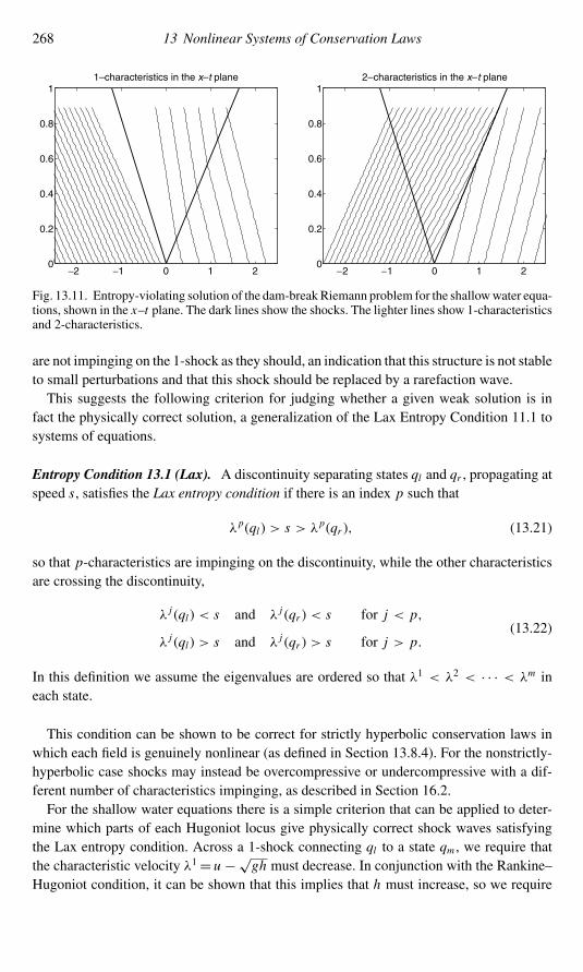
268 13 Nonlinear Systems of Conservation Laws

−2 −1 0 1 20

0.2

0.4

0.6

0.8

11–characteristics in the x–t plane

−2 −1 0 1 20

0.2

0.4

0.6

0.8

12–characteristics in the x–t plane

Fig. 13.11. Entropy-violating solution of the dam-breakRiemann problem for the shallowwater equa-tions, shown in the x–t plane. The dark lines show the shocks. The lighter lines show 1-characteristicsand 2-characteristics.

are not impinging on the 1-shock as they should, an indication that this structure is not stableto small perturbations and that this shock should be replaced by a rarefaction wave.This suggests the following criterion for judging whether a given weak solution is in

fact the physically correct solution, a generalization of the Lax Entropy Condition 11.1 tosystems of equations.

Entropy Condition 13.1 (Lax). A discontinuity separating states ql and qr , propagating atspeed s, satisfies the Lax entropy condition if there is an index p such that

λp(ql) > s > λp(qr ), (13.21)

so that p-characteristics are impinging on the discontinuity, while the other characteristicsare crossing the discontinuity,

λ j (ql) < s and λ j (qr ) < s for j < p,

λ j (ql) > s and λ j (qr ) > s for j > p.(13.22)

In this definition we assume the eigenvalues are ordered so that λ1 < λ2 < · · · < λm ineach state.

This condition can be shown to be correct for strictly hyperbolic conservation laws inwhich each field is genuinely nonlinear (as defined in Section 13.8.4). For the nonstrictly-hyperbolic case shocks may instead be overcompressive or undercompressive with a dif-ferent number of characteristics impinging, as described in Section 16.2.For the shallow water equations there is a simple criterion that can be applied to deter-

mine which parts of each Hugoniot locus give physically correct shock waves satisfyingthe Lax entropy condition. Across a 1-shock connecting ql to a state qm , we require thatthe characteristic velocity λ1= u −√gh must decrease. In conjunction with the Rankine–Hugoniot condition, it can be shown that this implies that h must increase, so we require

13.8 Simple Waves and Rarefactions 269

hm > hl . Similarly, a 2-shock connecting qm to qr satisfies the Lax entropy condition ifhm > hr . Note from Figure 13.5 and Figure 13.7 that this also means that fluid particlesexperience an increase in depth as they pass through a shock. This is similar to the phys-ical entropy condition for gas dynamics, that gas particles must experience an increase inphysical entropy as they pass through a shock wave.Figure 13.10 shows the portions of eachHugoniot locus alongwhich the entropy condition

is satisfied as solid lines. These are simply the portions along which h is increasing. Theportions indicated by dashed lines are states that can be connected by a discontinuity thatsatisfies the Rankine–Hugoniot condition, but not the entropy condition.We see from Figure 13.10(b) that the solution to the dam-break Riemann problem con-

sisting of two shocks fails to satisfy the entropy condition. Instead we must find a solutionto the Riemann problem that consists of a 1-rarefaction and a 2-shock. In the next sectionwe investigate rarefaction waves and will see that the Hugoniot locus through ql must bereplaced by a different curve, the integral curve of r1. The intersection of this curve withthe 1-shock Hugoniot locus will give the correct intermediate state qm , as described inSection 13.9.The shallow water equations also possess a convex entropy function η(q); see

Exercise 13.6. From this it follows that Godunov’s method will converge to the physi-cally correct solution, if the correct entropy solution to each Riemann problem is used; seeSection 12.11.1.

13.8 Simple Waves and Rarefactions

Solutions to a hyperbolic system of m equations are generally quite complicated, since atany point there are typically m waves passing by, moving at different speeds, and what weobserve is some superposition of these waves. In the nonlinear case the waves are constantlyinteracting with one another as well as deforming separately, leading to problems thatgenerally cannot be solved analytically. It is therefore essential to look for special situationsin which a single wave from one of the characteristic families can be studied in isolation.A shock wave consisting of piecewise constant data (satisfying the Rankine–Hugoniotconditions across the discontinuity) is one important example that was investigated in theprevious section.In this section we will investigate solutions that are smoothly varying (rather than discon-

tinuous) butwhich also have the property that they are associatedwith only one characteristicfamily of the system. Such waves are called simple waves. These have already been intro-duced for linear systems in Section 3.4. In the linear case simple waves have fixed shapeand propagate with fixed speed according to a scalar advection equation. In the nonlinearcase they will deform due to the nonlinearity, but their evolution can be modeled by scalarnonlinear equations.In particular, the centered rarefactionwaves that arise in the solution toRiemannproblems

for nonlinear systems are simple waves, but these are just one special case. They are specialin that they also have the property that they are similarity solutions of the equations andare constant along every ray x/t = constant. They arise naturally from Riemann problemsbecause of the special data used, which varies only at a single point x = 0, and hence all

270 13 Nonlinear Systems of Conservation Laws

variation in the solution flows out from the point x = t = 0. Recall from Section 11.10 thatif q(x, t) = q(x/t) then the function q(ξ ) must satisfy (11.26),

f ′(q(x/t)) q ′(x/t) =( xt

)q ′(x/t). (13.23)

For a scalar equation we could cancel q ′(x/t) from this equation. For a system of equationsq ′ is a vector and (13.23) requires that it be an eigenvector of the Jacobian matrix f ′(q(x/t)for each value of x/t . We will see how to determine this function for centered rarefactionwaves and employ it in solving the Riemann problem, but first we study some more basicideas.Again we will concentrate on the shallowwater equations to illustrate this theory. For this

system of two equations we can easily draw diagrams in the two-dimensional state spacethat help to elucidate the theory.

13.8.1 Integral Curves

Let q(ξ ) be a smooth curve through state space parameterized by a scalar parameter ξ . Wesay that this curve is an integral curve of the vector field r p if at each point q(ξ ) the tangentvector to the curve, q ′(ξ ), is an eigenvector of f ′(q(ξ )) corresponding to the eigenvalueλp(q(ξ )). If we have chosen some particular set of eigenvectors that we call r p(q), e.g.,(13.10) for the shallow water equations, then q ′(ξ ) must be some scalar multiple of theparticular eigenvector r p(q(ξ )),

q ′(ξ ) = α(ξ )r p(q(ξ )). (13.24)

The value of α(ξ ) depends on the particular parameterization of the curve and on thenormalization of r p, but the crucial idea is that the tangent to the curve is always in thedirection of the appropriate eigenvector r p evaluated at the point on the curve.

Example 13.8. Figure 13.12 shows integral curves of r1 and r2 for the shallow water equa-tions of Section 13.1, for which the eigenvectors are given by (13.10). As an example of howthese curves can be determined, consider r1 and set α(ξ )≡ 1, which selects one particularparameterization for which the formulas are relatively simple. Then (13.24) reduces to

q ′(ξ ) = r1(q(ξ )) =[

1q2/q1 −

√gq1

](13.25)

by using (13.10). This gives two ordinary differential equations for the two components ofq(ξ ):

(q1)′ = 1 (13.26)

and

(q2)′ = q2/q1 −√gq1. (13.27)

13.8 Simple Waves and Rarefactions 271

(a)

−0.5 0 0.5 1 1.5 2 2.5 3 3.5 4 4.5−2.5

−2

−1.5

−1

−0.5

0

0.5

1

1.5

2

2.5

h = depth

hu =

mom

entu

m

(b)

−0.5 0 0.5 1 1.5 2 2.5 3 3.5 4 4.5−2.5

−2

−1.5

−1

−0.5

0

0.5

1

1.5

2

2.5

h = depthhu

= m

omen

tum

Fig. 13.12. (a) Integral curves of the eigenvector field r 1 for the shallow water equations. The eigen-vector r 1(q) evaluated at any point on a curve is tangent to the curve at that point. (b) Integral curvesfor r 2.

If we set

q1(ξ ) = ξ, (13.28)

then (13.26) is satisfied. Note that since the first component of q is h, this means we areparameterizing the integral curve by depth. With this choice of q1, the second equation(13.27) becomes

(q2)′ = q2/ξ −√gξ . (13.29)

If we fix one point (h∗, u∗) on the integral curve and require that q2(h∗) = h∗u∗, thensolving the differential equation (13.29) with this initial value yields the solution

q2(ξ ) = ξu∗ + 2ξ (√gh∗ −

√gξ ). (13.30)

Plotting (q1(ξ ), q2(ξ )) from (13.28) and (13.30) gives the curves shown in Figure 13.12(a).Since ξ is just the depth h, we can also state more simply that the integral curves of r1 havethe functional form

hu = hu∗ + 2h(√gh∗ −

√gh). (13.31)

In terms of the velocity instead of the momentum, we can rewrite this as

u = u∗ + 2(√gh∗ −

√gh). (13.32)

Similarly, the integral curve of r2 passing through the point (h∗, u∗) can be shown to havethe form

u = u∗ − 2(√gh∗ −

√gh). (13.33)

272 13 Nonlinear Systems of Conservation Laws

13.8.2 Riemann Invariants

The expression (13.32) describes an integral curve of r1, where (h∗, u∗) is an arbitrary pointon the curve. This can be rewritten as

u + 2√gh = u∗ + 2

√gh∗.

Since (h∗, u∗) and (h, u) are any two points on the curve, we see that the function

w1(q) = u + 2√gh (13.34)

has the same value at all points on this curve. This function is called a Riemann invariant forthe 1-family, or simply a 1-Riemann invariant. It is a function of q whose value is invariantalong any integral curve of r1, though it will take a different value on a different integralcurve.Similarly, from (13.33) we see that

w2(q) = u − 2√gh (13.35)

is a 2-Riemann invariant, a function whose value is constant along any integral curve of r2.If q(ξ ) represents a parameterization of any integral curve of r p, then since w p(q) is

constant along q(ξ ) as ξ varies, we must have ddξ w

p(q(ξ )) = 0. Expanding this out gives

∇w p(q(ξ )) · q ′(ξ ) = 0,

where ∇w p is the gradient of w p with respect to q . By (13.24) this gives

∇w p(q(ξ )) · r p(q(ξ )) = 0. (13.36)

This relationmust hold at anypoint on every integral curve, andhence in general∇w p·r p = 0everywhere. This gives another way to characterize a p-Riemann invariant – it is a functionwhose gradient is orthogonal to the eigenvector r p at each point q.We can also view the integral curves of r p as being level sets of the function w p(q), so

that the curves in Figure 13.12(a), for example, give a contour plot of w1(q). The gradientof w1(q) is orthogonal to the contour lines, as expressed by (13.36).Note that all the integral curves shown in Figure 13.12 appear to meet at the origin

h = hu = 0. This may seem odd in that they are level sets of a function w p that takesdifferent values on each curve. But note that each w p involves the velocity u = (hu)/h,which has different limiting values depending on how the point h = hu = 0 is approached.The integral curves would look different if plotted in the h–u plane; see Exercise 13.2.For a system of m > 2 equations, the integral curves of r p will still be curves through

the m-dimensional state space, and can be determined by solving the system (13.24) withα(ξ ) ≡ 1, for example. This is now a system ofm ODEs. In general there will now bem−1distinct functions w p(ξ ) that are p-Riemann invariants for each family p.

13.8 Simple Waves and Rarefactions 273

13.8.3 Simple Waves

A simple wave is a special solution to the conservation law in which

q(x, t) = q(ξ (x, t)), (13.37)

where q(ξ ) traces out an integral curve of some family of eigenvectors r p and ξ (x, t) is asmooth mapping from (x, t) to the parameter ξ . This means that all states q(x, t) appearingin the simple wave lie on the same integral curve. Note that any p-Riemann invariant isconstant throughout the simple wave.Of course not every function of the form (13.37) will satisfy the conservation law. The

function ξ (x, t) must be chosen appropriately. We compute

qt = q ′(ξ (x, t)) ξt and qx = q ′(ξ (x, t)) ξx ,

so to satisfy qt + f (q)x = 0 we must have

ξt q′(ξ )+ ξx f ′(q(ξ )) q ′(ξ ) = 0.

Since q ′(ξ ) is always an eigenvector of f ′(q(ξ )), this yields

[ξt + ξxλp(q(ξ ))] q ′(ξ ) = 0,

and hence the function ξ (x, t) must satisfy

ξt + λp(q(ξ )) ξx = 0. (13.38)

Note that this is a scalar quasilinear hyperbolic equation for ξ .In particular, if we choose initial data q(x, 0) that is restricted entirely to this integral

curve, so that

q(x, 0) = q(ξ◦(x))

for some smooth choice of ξ◦(x), then (13.37) will be a solution to the conservation law

for t > 0 provided that ξ (x, t) solves (13.38) with initial data ξ (x, 0) = ξ◦(x), at least for

as long as the function ξ (x, t) remains smooth. In a simple wave the nonlinear system ofequations reduces to the scalar nonlinear equation (13.38) for ξ (x, t).Since (13.38) is nonlinear, the smooth solution may eventually break down at some time

Tb. At this time a shock forms in q(x, t) and the solution is in general no longer a simplewave for later times. States q that do not lie on the same integral curve will typically appearnear the shock.In the special case where λp(q(ξ (x, 0))) is monotonically increasing in x , the charac-

teristics will always be spreading out and a smooth solution will exist for all time. This isa pure rarefaction wave. If the characteristic speed λp(q(ξ (x, 0))) is decreasing in x oversome region, then a compression wave arises that will eventually break.Note that ξ (x, t) is constant along characteristic curves of the equation (13.38), curves

X (t) that satisfy X ′(t) = λp(q(ξ (X (t), t))). Since ξ is constant on this curve, so is X ′(t),and hence the characteristics are straight lines. Along these characteristics the value of

274 13 Nonlinear Systems of Conservation Laws

q(x, t) is also constant, since q(x, t) is determined by (13.37) and ξ is constant. Hence asimple wave behaves exactly like the solution to a scalar conservation law, as described inChapter 11, up to the time it breaks.For the special case of a linear hyperbolic system, simple waves satisfy scalar advection

equations (λp is constant, independent of q(ξ )), and the theory just developed agrees withwhat was presented in Section 3.4.

13.8.4 Genuine Nonlinearity and Linear Degeneracy

For the shallow water equations, the characteristic speed λp(q(ξ )) varies monotonically aswe move along an integral curve. We will verify this in Example 13.9, but it can be seenin Figure 13.13, where contours of λp are plotted along with a typical integral curve. Thismonotonicity is analogous to the situation for a scalar conservation law with a convex fluxfunction f (q), in which case the single characteristic speed λ1(q) = f ′(q) is monotonicin q. As discussed in Section 16.1, solutions to the scalar conservation law can be con-siderably more complex if f is nonconvex. The same is true for systems of equations, butfor many physical systems we have a property analogous to convexity. If λp(q(ξ )) variesmonotonically with ξ along every integral curve, then we say that the pth field is genuinelynonlinear. Note that the variation of λp along the curve can be computed as

d

dξλp(q(ξ )) = ∇λp(q(ξ )) · q ′(ξ ). (13.39)

Here ∇λp is the gradient vector obtained by differentiating the scalar λp(q) with respect toeach component of the vector q . The quantity in (13.39) must be nonzero everywhere if thefield is to be genuinely nonlinear. If the value of (13.39) is positive, then the characteristic

(a)

−0.5 0 0.5 1 1.5 2 2.5 3 3.5 4 4.5−2.5

−2

−1.5

−1

−0.5

0

0.5

1

1.5

2

2.5

h = depth

hu =

mom

entu

m

(b)

−0.5 0 0.5 1 1.5 2 2.5 3 3.5 4 4.5−2.5

−2

−1.5

−1

−0.5

0

0.5

1

1.5

2

2.5

h = depth

hu =

mom

entu

m

Fig. 13.13. (a) A typical integral curve of the eigenvector field r 1 for the shallow water equations isshown as the heavy line. The other lines are contour lines of λ1(q), curves along which λ1 is constant.The curves shown are for values λ1 = 1, 0,−1,−1.5,−2,−2.5 from top to bottom. Note that λ1

varies monotonically along the integral curve. (b) An integral curve for r 2 and contours of λ2(q) forvalues λ2 = 2.5, 2, 1.5, 1, 0,−1 from top to bottom.

13.8 Simple Waves and Rarefactions 275

speed is increasing with ξ and if it is negative the speed is decreasing. If this derivative werezero at somepoint, then the characteristic speedwould be locally constant and characteristicswould be essentially parallel as in a linear problem. The property of genuine nonlinearityinsures that this linear situation never occurs and characteristics are always compressing orexpanding as q varies.Since q ′(ξ ) is in the direction r p(q(ξ )) by (13.24), we see from (13.39) that the pth field

is genuinely nonlinear if

∇λp(q) · r p(q) �= 0 (13.40)

for all q. Note that for a scalar problem λ1(q) = f ′(q) and we can take r1(q) ≡ 1, so that(13.40) reduces to the convexity requirement f ′′(q) �= 0.At the other extreme, in some physical systems there are characteristic fields for which

the relation

∇λp(q) · r p(q) ≡ 0 (13.41)

holds for all q . This means that λp is identically constant along each integral curve. Atrivial example occurs in a constant-coefficient linear hyperbolic system, in which case λp

is constant everywhere and ∇λp(q) ≡ 0. But in nonlinear systems it may also happen thatsome field satisfies the relation (13.41) even though λp takes different values along differentintegral curves. This happens if the integral curves of r p are identical to the contour linesof λp. A field satisfying (13.41) is said to be linearly degenerate. Through a simple wave insuch a field the characteristics are parallel, as in a linear system, rather than compressing orexpanding. See Section 13.12 and Section 14.9 for examples of linearly degenerate fields.

13.8.5 Centered Rarefaction Waves

A centered rarefaction wave is a special case of a simple wave in a genuinely nonlinearfield, in which ξ (x, t) = x/t , so that the solution is constant on rays through the origin. Acentered rarefaction wave has the form

q(x, t) =

ql if x/t ≤ ξ1,

q(x/t) if ξ1 ≤ x/t ≤ ξ2,

qr if x/t ≥ ξ2,

(13.42)

where ql and qr are two points on a single integral curvewithλp(ql)<λp(qr ). This conditionis required so that characteristics spread out as time advances and the rarefactionwavemakesphysical sense. (The picture should look like Figure 11.4(a), not Figure 11.4(b).)For a centered rarefaction wave a particular parameterization of the integral curve is

forced upon us by the fact that we set ξ = x/t . Rewriting this as x = ξ t , we see that thevalue q(ξ ) observed along the ray x/t = ξ is propagating at speed ξ , which suggests thatξ at each point on the integral curve must be equal to the characteristic speed λp(q(ξ )) atthis point. This is confirmed by noting that (13.38) in this case becomes

− xt2+ λp(q(x/t))

(1

t

)= 0

276 13 Nonlinear Systems of Conservation Laws

and hence

x

t= λp(q(x/t)). (13.43)

In particular, the left edge of the rarefaction fan should be the ray x/t = λp(ql) so thatξ1= λp(ql) in (13.42), while the right edge should be the ray x/t = λp(qr ) so that ξ2 =λp(qr ). We thus have

ξ1 = λp(ql), q(ξ1) = ql ,ξ2 = λp(qr ), q(ξ2) = qr .

(13.44)

To determine how q(ξ ) varies for ξ1<ξ <ξ2 through the rarefactionwave (13.42), rewrite(13.43) as

ξ = λp(q(ξ )) (13.45)

and differentiate this with respect to ξ to obtain

1 = ∇λp(q(ξ )) · q ′(ξ ). (13.46)

Using (13.24) in (13.46) gives

1 = α(ξ )∇λp(q(ξ )) · r p(q(ξ )),

and hence

α(ξ ) = 1

∇λp(q(ξ )) · r p(q(ξ )) . (13.47)

Using this in (13.24) gives a system of ODEs for q(ξ ):

q ′(ξ ) = r p(q(ξ ))

∇λp(q(ξ )) · r p(q(ξ )) . (13.48)

This system must be solved over the interval ξ1 ≤ ξ ≤ ξ2 using either of the conditionsin (13.44) as an initial condition. Note that the denominator is nonzero provided that λp

is monotonically varying. A rarefaction wave would not make sense past a point wherethe denominator vanishes. In particular, if the pth field is genuinely nonlinear, then thedenominator is always nonzero by (13.40).

Example 13.9. For the shallow water equations we have

λ1 = u −√gh = q2/q1 −

√gq1,

∇λ1 =[−q2/(q1)2 − 1

2

√g/q1

1/q1

],

r1 =[

1q2/q1 −

√gq1

],

(13.49)

13.8 Simple Waves and Rarefactions 277

and hence

∇λ1 · r1 = −32

√g/q1, (13.50)

so that the equations (13.48) become

q ′ = −23

√q1/g

[1

q2/q1 −√gq1

]. (13.51)

The first equation of this system is

h′(ξ ) = −23

√h(ξ )/g.

The general solution is

h = 1

9g(A − ξ )2, (13.52)

for some constant A. This constant must be chosen so that (13.44) is satisfied, i.e., so thath = hl at ξ = ul −

√ghl and also h = hr at ξ = ur −

√ghr . Provided that ql and qr both

lie on an integral curve of r1, as they must if they can be joined by a centered rarefactionwave, we can satisfy both of these conditions by taking

A = ul + 2√ghl = ur + 2

√ghr . (13.53)

Recall that u + 2√gh is a 1-Riemann invariant, which has the same value at all points onthe integral curve. We see that h varies quadratically with ξ = x/t through a rarefactionwave (13.42).Once we know h as a function of ξ , we can use the formula (13.33), which holds through

any simple wave, to determine how u varies through the rarefaction wave. (i.e., we use thefact that the Riemann invariant is constant). Note that since we know the relation betweenh and u from having previously found the Riemann invariants, we do not need to solve boththe ODEs in the system (13.51). We have chosen the simpler one to solve. This trick is oftenuseful for other systems as well.Note that (13.50) is nonzero for all physically meaningful states q1 = h > 0, showing

that this field is genuinely nonlinear. The expressions for the 2-characteristic field are verysimilar (with only a few minus signs changed), and this field is also genuinely nonlinear;see Exercise 13.3.

13.8.6 The All-Rarefaction Riemann Solution

Now suppose we wish to solve a Riemann problem for which we know the solution consistsof two rarefaction waves, as in the following example.

Example 13.10. Again consider the Riemann problem for the shallow water equationswith data (13.13), but now take ul < 0. This corresponds to two streams of water that aremoving apart from one another. Again the solution will be symmetric but will consist of

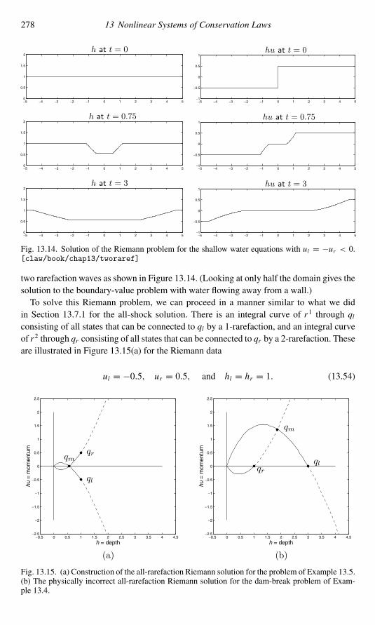
278 13 Nonlinear Systems of Conservation Laws

−5 −4 −3 −2 −1 0 1 2 3 4 50

0.5

1

1.5

2h at t = 0

−5 −4 −3 −2 −1 0 1 2 3 4 5−1

−0.5

0

0.5

1hu at t = 0

−5 −4 −3 −2 −1 0 1 2 3 4 50

0.5

1

1.5

2h at t = 0.75

−5 −4 −3 −2 −1 0 1 2 3 4 5−1

−0.5

0

0.5

1hu at t = 0.75

−5 −4 −3 −2 −1 0 1 2 3 4 50

0.5

1

1.5

2h at t = 3

−5 −4 −3 −2 −1 0 1 2 3 4 5−1

−0.5

0

0.5

1hu at t = 3

Fig. 13.14. Solution of the Riemann problem for the shallow water equations with ul = −ur < 0.[claw/book/chap13/tworaref]

two rarefaction waves as shown in Figure 13.14. (Looking at only half the domain gives thesolution to the boundary-value problem with water flowing away from a wall.)To solve this Riemann problem, we can proceed in a manner similar to what we did

in Section 13.7.1 for the all-shock solution. There is an integral curve of r1 through qlconsisting of all states that can be connected to ql by a 1-rarefaction, and an integral curveof r2 through qr consisting of all states that can be connected to qr by a 2-rarefaction. Theseare illustrated in Figure 13.15(a) for the Riemann data

ul = −0.5, ur = 0.5, and hl = hr = 1. (13.54)

(a)

−0.5 0 0.5 1 1.5 2 2.5 3 3.5 4 4.5−2.5

−2

−1.5

−1

−0.5

0

0.5

1

1.5

2

2.5

h = depth

hu =

mom

entu

m

ql

qrqm

(b)

−0.5 0 0.5 1 1.5 2 2.5 3 3.5 4 4.5−2.5

−2

−1.5

−1

−0.5

0

0.5

1

1.5

2

2.5

h = depth

hu =

mom

entu

m

qlqr

qm

Fig. 13.15. (a) Construction of the all-rarefaction Riemann solution for the problem of Example 13.5.(b) The physically incorrect all-rarefaction Riemann solution for the dam-break problem of Exam-ple 13.4.

13.9 Solving the Dam-Break Problem 279

The intermediate state qm in the Riemann solution must lie on both of these curves, andhence is at the intersection as shown in Figure 13.15(a). For this particular example qm lieson the h-axis due to symmetry. In general we can find the intersection by using the fact thatqm must lie on the curve described by (13.32) with q∗ = ql and on the curve described by(13.33) with q∗ = qr , so

um = ul + 2(√ghl −

√ghm),

um = ur − 2(√ghr −

√ghm).

(13.55)

This is a system of two nonlinear equations for hm and um . Equating the right-hand sidesgives a single equation for hm , which can be explicitly solved to obtain

hm = 1

16g[ul − ur + 2(

√ghl +

√ghr )]

2. (13.56)

This is valid provided that the expression being squared is nonnegative. When it reacheszero, the outflow is sufficiently great that the depth hm goes to zero. (See Exercise 13.2.)For the symmetric data (13.54) used in Figures 13.14 and 13.15(a), the expression (13.56)

gives hm = (4√g−1)2/16g = 9/16, sincewe use g = 1. Then either equation from (13.55)gives um = 0.

The integral curves in Figure 13.15(a) are shown partly as dashed lines. For a given stateql only some points on the integral curve of r1 can be connected to ql by a rarefaction wavethat makes physical sense, since we are assuming ql is the state on the left of the rarefactionwave. We must have λ1(ql)<λ1(q) for all states q in the rarefaction wave, and hence qmust lie on the portion of the integral curve shown as a solid line (see Figure 13.13(a)).Similarly, if qr is the state to the right of a 2-rarefaction, then states q in the rarefaction mustsatisfy λ2(q)<λ2(qr ) and must lie on the solid portion of the integral curve for r2 sketchedthrough qr in Figure 13.15(a). For the data shown in this figure, there is a state qm that canbe connected to both ql and qr by physically correct rarefaction waves, and the Riemannsolution consists of two rarefactions as illustrated in Figure 13.14.For other data this might not be the case. Figure 13.15(b) shows the data for the dam-

break Riemann problem of Example 13.4, with hl = 3, hr = 1, and ul = ur = 0. We canstill use (13.56) to compute an intermediate state qm lying at the intersection of the integralcurves, as illustrated in Figure 13.15(b), but the resulting 2-wave does not make physicalsense as a rarefaction wave, since λ2(qm) > λ2(qr ). This wave would overturn, as illustratedin Figure 13.16.Compare Figure 13.15(b) with Figure 13.10(b), where we found an all-shock solution

to this same Riemann problem. In that case the 2-shock was acceptable, but the 1-shockfailed to satisfy the entropy condition. The correct solution consists of a 1-rarefaction anda 2-shock as shown in Figure 13.5 and determined in the next section.

13.9 Solving the Dam-Break Problem

We now illustrate how to construct the general solution to a nonlinear Riemann problem,using the theory of shock waves and rarefaction waves developed above.

280 13 Nonlinear Systems of Conservation Laws

−2 −1 0 1 2

1

1.5

2

2.5

3

Height

−2 −1 0 1 2

0

0.2

0.4

0.6

0.8Velocity

−2 −1 0 1 2

1

2

3

4

Vertically integrated pressure

−2 −1 0 1 20

0.2

0.4

0.6

0.8

12–Characteristics in the x–t plane

Fig. 13.16. Unphysical solution to the dam-break Riemann problem for the shallow water equationscorresponding to the solution found in Figure 13.15(b). The 2-characteristics are shown in the lowerright plot. Note that each point in the shaded region lies on three distinct 2-characteristics.

The dam-break Riemann problem for the shallow water equations (introduced inExample 13.4) has a solution that consists of a 1-rarefaction and a 2-shock, as illustratedin Figure 13.5. In Figure 13.10 we saw how to construct a weak solution to this problemthat consists of two shock waves, one of which does not satisfy the Lax entropy condition.In Figure 13.15 we found an all-rarefaction solution to this problem that is not physicallyrealizable. To find the correct solution we must determine an intermediate state qm that isconnected to ql by a 1-rarefaction wave and simultaneously is connected to qr by a 2-shockwave. The state qm must lie on an integral curve of r1 passing through ql , so by (13.32) wemust have

um = ul + 2(√ghl −

√ghm). (13.57)

It must also lie on the Hugoniot locus of 2-shocks passing through qr , so by (13.19) it mustsatisfy

um = ur + (hm − hr )√g

2

(1

hm+ 1

hr

). (13.58)

We can easily eliminate um from these two equations and obtain a single nonlinear equation

13.10 The General Riemann Solver for Shallow Water Equations 281

(a)

−1 −0.5 0 0.5 1 1.5 2 2.5 3 3.5 4−4

−3

−2

−1

0

1

2

3

4

h = depth

hu =

mom

entu

m

qlqr

(b)

1.6 1.7 1.8 1.9 2 2.1 2.21.1

1.2

1.3

1.4

1.5

1.6

1.7

h = depth

hu =

mom

entu

m

S1(ql)

S2(qr)

R1(ql)

R2(qr)

Fig. 13.17. (a) The Hugoniot loci from Figure 13.10 together with the integral curves. (b) Close-upof the region where the curves intersect. S1: Entropy-violating 1-shocks; R1: 1-rarefactions; S2:2-shocks;R2: unphysical 2-rarefactions.

to solve for hm . The structure of the rarefaction wave connecting ql to qm can then bedetermined using the theory of Section 13.8.5.Note that the intermediate state qm resulting from this procedure will be slightly different

from that obtained in either Figure 13.10 or Figure 13.15, since the Hugoniot loci aredifferent from the integral curves. This is illustrated in Figure 13.17, where the curvesfrom Figures 13.10 and 13.15 are plotted together. Figure 13.17(b) shows a close-up nearthe points of intersection of these curves. The correct solution to the dam-break Riemannproblem has the intermediate state at the point where the two solid lines cross.Note that both sets of curves are tangent to the eigenvector r1(ql) at ql and to r2(qr )

at qr . Moreover, it can be shown that the Hugoniot locus and the integral curve througha given point have the same curvature at that point, and so the curves are really quitesimilar near that point. (See, e.g., Lax [263].) How rapidly the curves diverge from oneanother typically depends on how nonlinear the system is. For a linear system, of course,the integral curves and Hugoniot loci are identical, each being straight lines in the directionsof the constant eigenvectors. Even for nonlinear systems the Hugoniot locimay be identicalto the integral curves, though this is not the usual situation. See Exercise 13.12 for oneexample, and Temple [447] for some general discussion of such systems, which are oftencalled Temple-class systems.

13.10 The General Riemann Solver for Shallow Water Equations

For the dam-break problem we know that the 1-wave is a rarefaction while the 2-wave isa shock, leading to the system of equations (13.57) and (13.58) to solve for hm and um .For general values of ql and qr we might have any combination of shocks and rarefactionsin the two families, depending on the specific data. To find the state qm in general we candefine two functions φl and φr by

φl(h) =ul + 2(

√ghl −

√gh) if h < hl ,

ul − (h − hl)√g2

(1h + 1

hl

)if h > hl ,

282 13 Nonlinear Systems of Conservation Laws

and

φr (h) =ur − 2(

√ghr −

√gh) if h < hr ,

ur + (h − hr )√g2

(1h + 1

hr

)if h > hr .

For a given state h, the function φl(h) returns the value of u such that (h, hu) can beconnected to ql by a physically correct 1-wave, while φr (h) returns the value such that(h, hu) can be connected to qr by a physically-correct 2-wave. We want to determine hmso that φl(hm) = φr (hm). This can be accomplished by applying a nonlinear root finder tothe function φ(h) ≡ φl(h)− φr (h).

13.11 Shock Collision Problems

In a scalar equation, such a Burgers equation, when two shock waves collide, they simplymerge into a single shock wave with a larger jump. For a system of equations, the result of ashock collision is not so simple, even if the two shocks are in the same characteristic family.The result will include a stronger shock in this same family, but the collision will typicallyalso introduce waves in the other families. For example, consider initial data for the shallowwater equations consisting of the three states shown in Figure 13.18(a). These three statesall lie on the Hugoniot locus S2(q2), so there is a 2-shock connecting q1 to q2 and a slower2-shock connecting q2 to q3. (Note that the shock speed s = [[hu]]/[[h]] is given by the slopeof the line joining the two points.) If we solve the shallow water equations with data

q(x, 0) =q1 if x < x1,q2 if x1 ≤ x ≤ x2,q3 if x > x2

(13.59)

for some initial shock locations x1 < x2, then the solution consists of the these two shocks,which eventually collide at some point xc. At the time tc when they collide, the state q2

0 1 2 3 4 5 6 7

−1

0

1

2

3

4

5

6

h = depth

hu =

mom

entu

m

q1

q2

q3

S2(q2)

0 1 2 3 4 5 6 7

−1

0

1

2

3

4

5

6

h = depth

hu =

mom

entu

m

q1

q2

q3

q4

S2(q3)

R1(q1)

(a) (b)

Fig. 13.18. States arising in the collision of two 2-shocks for the shallow water equations. (a) Initialstates q1 and q3 are each connected to q2 by a 2-shock. (b) After collision, solving the Riemannproblem between q3 and q1 gives a new state q4 and a reflected 1-wave.

13.12 Linear Degeneracy and Contact Discontinuities 283

q1q2

q3

q4

Fig. 13.19. Collision of two 2-shocks giving rise to a 1-rarefaction and a 2-shock, as seen in the x–tplane.

disappears and the solution has the form

q(x, tc) ={q1 if x < xc,q3 if x > xc.

(13.60)

To determine the solution beyond this time, note that this has the form of Riemann-problem data with left state q1 and right state q3. The Riemann solution is not a single2-shock, because q1 will not lie on the Hugoniot locus S2(q3). Instead, a 1-wave must beintroduced to connect q1 to a new state q4 that lies on this Hugoniot locus, as illustratedin Figure 13.18(b). We see that the 1-wave must be a rarefaction wave, since h4< h1 andh4 is determined by the intersection of the integral curve R1(q1) with the Hugoniot locusS2(q3). (Note that q2 does lie on the Hugoniot locus S2(q3), since q3 lies on the Hugoniotlocus S2(q2).)A view of this collision in the x–t plane is seen in Figure 13.19. To view a numerical

solution of this collision, see [claw/book/chap13/collide].

13.12 Linear Degeneracy and Contact Discontinuities

The shallow water equations are a system of two equations for which both characteristicfields are genuinely nonlinear, as defined in Section 13.8.4. A smooth simple wave in one ofthese fields will always distort via compression or expansion as characteristics converge ordiverge. For the Riemann problem, each wave will be either a single shock or a rarefactionwave. Genuine nonlinearity of the pth field requires that the eigenvalue λp bemonotonicallyvarying as we move along an integral curve of r p, and hence that∇λp(q) ·r p(q) be nonzeroeverywhere.We now consider the opposite extreme, a field in which∇λp(q) ·r p(q) is identically zero

for all q, so that λp is constant along each integral curve of r p (but may take different valueson different integral curves). Such a field is called linearly degenerate, since simple wavesin which the variation of q is only in this field behave like solutions to linear hyperbolicequations. Since λp is constant throughout the wave, it simply translates with this constantspeed without distorting. If the initial data is a jump discontinuity, with ql and qr both lyingon a single integral curve of this field, then the solution will consist of this discontinuitypropagating at the constant speed λp associatedwith this integral curve. Hence theHugoniotlocus for this field agrees with the integral curve. Such a discontinuity is not a shock

284 13 Nonlinear Systems of Conservation Laws

wave, however, since the characteristic speed λp(ql)= λp(qr ) on each side agrees with thepropagation speed of the wave. Characteristics are parallel to the wave in the x–t planerather than impinging on it. Waves of this form are generally called contact discontinuities,for reasons that will become apparent after considering the simple example in the nextsection.

13.12.1 Shallow Water Equations with a Passive Tracer

Again consider the shallow water equations, but now suppose we introduce some dye intothe water in order to track its motion. Let φ(x, t) represent the concentration of this passivetracer, measured in units of mass or molarity per unit volume, so that it is a color variableas described in Chapter 9. Then values of φ move with the fluid velocity u and are constantalong particle paths, and φ satisfies the color equation (9.12),

φt + uφx = 0. (13.61)

Sinceφmeasures a passive tracer that is assumed to have no influence on the fluid dynamics,it simply satisfies this linear advection equation with the variable coefficient u(x, t), whichcan be obtained by first solving the shallow water equations. However, to illustrate linearlydegenerate fields we can couple this equation into the shallow water equations and obtainan augmented system of three conservation laws.We first rewrite (13.61) as a conservation law by instead considering the conserved

quantity hφW , where h is the depth of the water andW is the width of the channel modeledin our one-dimensional equations. This is needed solely for dimensional reasons, and wecan take W = 1 in the appropriate length units and consider hφ as the conserved quantity,measuring mass or molarity per unit length. This is conserved in one dimension with theflux uhφ, so hφ satisfies the conservation law

(hφ)t + (uhφ)x = 0. (13.62)

Note that differentiating this out gives

htφ + hφt + (hu)xφ + (hu)φx = 0,

and using ht + (hu)x = 0 allows us to relate this to the color equation (13.61). Numericallyone canworkdirectlywith (13.61) rather than (13.62) since thewave-propagation algorithmsdo not require that all equations be in conservation form, and there are often advantages todoing so (see Section 16.5).For our present purposes, however, we wish to investigate the mathematical structure of

the resulting system of conservation laws. Augmenting the shallow water equations with(13.62) gives the system qt + f (q)x = 0 with

q = hhuhφ

=q

1

q2

q3

, f (q) =

hu

hu2 + 12gh

2

uhφ

= q2

(q2)/q1 + 12g(q

1)2

q2q3/q1

. (13.63)

13.12 Linear Degeneracy and Contact Discontinuities 285

The Jacobian is now

f ′(q) =

0 1 0

−(q1)2/(q1)2 + gq1 2q2/q1 0

−q2q3/(q1)2 q3/q1 q2/q1

=

0 1 0

−u2 + gh 2u 0

−uφ φ u

. (13.64)

This is a block lower-triangular matrix, and the eigenvalues are given by those of thetwo blocks. The upper 2× 2 block is simply the Jacobian matrix (13.8) for the shallowwater equations, and has eigenvalues u±√gh. The lower 1× 1 block yields the additionaleigenvalue u. The eigenvectors are also easy to compute from those of (13.8), and we findthat

λ1 = u −√gh, λ2 = u, λ3 = u +√gh,

r1 = 1u −√gh

φ

, r2 =001

, r3 = 1u +√gh

φ

. (13.65)

The fact that the scalarφ is essentially decoupled from the shallowwater equations is clearlyapparent. Fields 1 and 3 correspond to the nonlinear waves in the shallow water equationsand involve φ only because the conserved quantity hφ has a jump discontinuity where thereis a jump in h. The tracer concentration φ is continuous across these waves. Field 2 carriesa jump in φ alone, since the first two components of r2 are 0. The speed of the 2-wave,λ2 = u, depends on the shallow water behavior, just as we expect.Ifwe considered very small variations in h and u, we could linearize this systemandobtain

a form of the acoustics equations coupled with the advection equation for φ. This linearsystem has already been considered in Section 3.10 and shows the same basic structure.For the nonlinear system, fields 1 and 3 are still genuinely nonlinear, as in the standard

shallow water equations, but field 2 is linearly degenerate, since it corresponds to the linearadvection equation. This is easily verified by computing

∇λ2 =

−u/h1/h

0

and observing that ∇λ2 · r2 ≡ 0. (Recall that ∇λ2 means the gradient of u = (hu)/h =q2/q1 with respect to q.)Any variation in φ will simply be advected with velocity u. In general the shape of φ may

distort, since u(x, t) may vary in the solution to the shallow water equations. However, ifwe consider a simple wave in Field 2, then variations in q can occur only along an integralcurve of r2. This vector always points in the φ-direction in the three-dimensional statespace, and integral curves are straight lines in this direction with no variation in h or hu.So in particular u is constant along any integral curve of r2, and simple waves consist ofarbitrary variations in φ being carried along in water of constant depth moving at constantspeed u. These are, of course, special solutions of the augmented shallow water equations.

286 13 Nonlinear Systems of Conservation Laws

13.12.2 The Riemann Problem and Contact Discontinuities

Now consider the Riemann problem for the augmented shallow water system (13.63), withpiecewise constant data having an arbitrary jump between states ql and qr (which allowsarbitrary jumps in h, u, and φ). It is clear how to solve this Riemann problem. Since φ doesnot affect h or u, the procedure of Section 13.9 can be used to determine the 1-wave and3-wave. Each is a shock or rarefaction wave, as in the standard shallow water equations,and there is no variation in φ across either of these waves. The 1-wave is moving into thefluid on the left, in which φ ≡ φl while the 3-wave is moving into the fluid on the right,in which φ ≡ φr . Between these two waves the velocity um is constant (obtained as inSection 13.9), and a 2-wave is now introduced with velocity λ2 = um . Across this wave,h = hm and u = um are constant while φ jumps from φl to φr . This wave has a simplephysical interpretation: it marks the boundary between water that was initially to the left ofthe interface and water that was initially to the right. This is clear because φ satisfies thecolor equation and hence is constant on particle paths.This 2-wave is called a contact discontinuity because it marks the point at which the

two distinct fluids (e.g., with different colors) are in contact with one another. Figure 13.20

−2 −1 0 1 2

1

1.5

2

2.5

3

Height

−2 −1 0 1 2

0

0.2

0.4

0.6

0.8

Velocity

−2 −1 0 1 2

1

2

3

4

Vertically integrated pressure

−2 −1 0 1 20

0.2

0.4

0.6

0.8

1Particle paths in x–t plane

Fig. 13.20. Structure of the similarity solution of the dam-break Riemann problem for the augmentedshallow water equations with ul = ur = 0. The depth h, velocity u, and vertically integrated pressureare displayed as functions of x/t . The value of φ is indicated by coloring the water darker whereφ = φl . The structure in the x–t plane is also shown, andparticle paths are indicated for a set of particleswith the spacing between particles inversely proportional to the depth. The contact discontinuity isnow indicated along with the rarefaction and shock.

Exercises 287

shows one example for the dam-break problem of Example 13.4. This looks exactly likeFigure 13.5 except that we have now also indicated the variation in φ by coloring the waterthat was initially behind the dam (i.e., in the region x < 0) darker. The contact discontinuityis indicated in the plot of particle paths, and it is clear that this wave separates water initiallybehind the dam from water initially downstream.Since the characteristic velocity λ2 = u agrees with the particle velocity, we can also

interpret this plot of particle paths as a plot of the 2-characteristics for the augmentedsystem. These characteristics cross the 1-wave and 3-wave and are parallel to the 2-wave,as expected because this field is linearly degenerate.The Euler equations of gas dynamics, discussed in the next chapter, also have a linearly

degenerate field corresponding to contact discontinuities. For general initial data the Rie-mann solution may contain a jump in density across the surface where the two initial gasesare in contact.

Exercises

13.1. (a) Consider an integral curve of r1 for the shallow water equations, as illustratedin Figure 13.13(a), for example. Show that the slope tangent to this curve inthe q1–q2 plane at any point is equal to λ1 at that point. (q1 = h and q2 = hu.)

(b) Consider the Hugoniot locus for 1-shocks for the shallow water equations, asillustrated in Figure 13.9(a), for example. Show that if ql and qr are two pointslying on this curve (and hence connected by a 1-shock) then the slope of thesecant line connecting these points is equal to the shock speed s.

13.2. The graphs of Figure 13.15 show the h–hu plane. The curves look somewhat dif-ferent if we instead plot them in the h–u plane.(a) Redraw Figure 13.15(a) in the h–u plane.(b) Draw a similar figure for hl = hr = 1 and −ul = ur = 1.9.(c) Draw a similar figure for hl = hr = 1 and −ul = ur = 2.1. In this case the

Riemann solution contains a region in which h = 0: dry land between the twooutgoing rarefaction waves.

13.3. Repeat the computations of Example 13.9 to determine the form of 2-rarefactionsin the shallow water equations and show that this field is genuinely nonlinear.

13.4. For the shallow water equations, show that when a 1-shock collides with a 2-shockthe result is a new pair of shocks. Exhibit the typical solution in the phase planeand the x–t plane.

13.5. In the shallow water equations, is it possible for two 2-rarefactions to collide witheach other?

13.6. For the shallow water equations, the total energy can be used as an entropy functionin the mathematical sense. This function and the associated entropy flux are givenby

η(q) = 1

2hu2 + 1

2gh2,

ψ(q) = 1

2hu3 + gh2u.

(13.66)

Verify this by showing the following.

288 13 Nonlinear Systems of Conservation Laws

(a) η(q) is convex: Show that the Hessian matrix η′′(q) is positive definite.(b) η(q)t + ψ(q)x = 0 for smooth solutions: Verify that (11.47) holds, ψ ′(q) =

η′(q) f ′(q).13.7. Consider the p-system (described in Section 2.13),

vt − ux = 0,ut + p(v)x = 0,

where p(v) is a given function of v.(a) Compute the eigenvalues of the Jacobian matrix, and show that the system is

hyperbolic provided p′(v) < 0.(b) Use the Rankine–Hugoniot condition to show that a shock connecting q =

(v, u) to some fixed state q∗ = (v∗, u∗) must satisfy

u = u∗ ±√−(p(v)− p(v∗)v − v∗

)(v − v∗). (13.67)

(c) What is the propagation speed for such a shock? How does this relate to theeigenvalues of the Jacobian matrix computed in part (a)?

(d) Plot the Hugoniot loci for the point q∗ = (1, 1) over the range −3 ≤ v ≤ 5for each of the following choices of p(v). (Note that these are not physicallyreasonable models for pressure as a function of specific volume!)(i) p(v) = −ev ,(ii) p(v) = −(2v + 0.1ev),(iii) p(v) = −2v.

(e) Determine the two-shock solution to the Riemann problem for the p-systemwith p(v) = −ev and data

ql = (1, 1), qr = (3, 4).

Do this in two ways:(i) Plot the relevant Hugoniot loci, and estimate where they intersect.(ii) Set up and solve the proper scalar nonlinear equation for vm . You might

use the Matlab command fzero or write your own Newton solver.(f) Does the Riemann solution found in the previous part satisfy the Lax entropy

condition? Sketch the structure of the solution in the x–t plane, showing alsosome sample 1-characteristics and 2-characteristics.

(g) For the given left state ql = (1, 1), in what region of the phase plane must theright state qr lie in order for the two-shock Riemann solution to satisfy theLax entropy condition?

13.8. Consider the p-system of Exercise 13.7, and take p(v) = −ev .(a) Follow the procedure of Section 13.8.1 to show that along any integral curve

of r1 the relation

u = u∗ − 2(ev∗/2 − ev/2)

Exercises 289

must hold, where (v∗, u∗) is a particular point on the integral curve. Concludethat

w1(q) = u − 2ev/2

is a 1-Riemann invariant for this system.(b) Follow the procedure of Section 13.8.5 to show that through a centered rar-

efaction wave

u(ξ ) = A − 2ξ,

where

A = ul − 2evl/2 = ur − 2evr /2,

and determine the form of v(ξ ).(c) Show that this field is genuinely nonlinear for all q .(d) Determine the 2-Riemann invariants and the form of a 2-rarefaction.(e) Suppose arbitrary states ql and qr are specified and we wish to construct a

Riemann solution consisting of two “rarefaction waves” (which might notbe physically realizable). Determine the point qm = (vm, um) where the tworelevant integral curves intersect.

(f) What conditions must be satisfied on ql and qr for this to be the physicallycorrect solution to the Riemann problem?

13.9. For the general p-system of Exercise 13.7, determine the condition on the functionp(v) that must be satisfied in order for both fields to be genuinely nonlinear for allq.

13.10. Consider the equations (2.97) modeling a one-dimensional slice of a nonlinearelastic solid. Suppose the stress–strain relation σ (ε) has the shape indicated inFigure 2.3(a). Is the system genuinely nonlinear in this case?

13.11. The variable-coefficient scalar advection equation qt + (u(x)q)x = 0 studied inSection 9.4 can be viewed as a hyperbolic system of two equations,

qt + (uq)x = 0,ut = 0,

(13.68)

where we now view u(x, t) ≡ u(x) as a second component of the system.(a) Determine the eigenvalues and eigenvectors of the Jacobian matrix for this

system.(b) Show that both fields are linearly degenerate, and that in each field the integral

curves and Hugoniot loci coincide. Plot the integral curves of each field in theq–u plane.

(c) Indicate the structure of a general Riemann solution in the q–u plane for thecase ul , ur > 0. Relate this to Figure 9.1.

(d) Note that this system fails to be strictly hyperbolic along u = 0. Can theRiemann problem be solved if ul < 0 and ur > 0? If ul > 0 and ur < 0? (SeeSection 16.4.2 for more discussion of such problems.)

290 13 Nonlinear Systems of Conservation Laws

13.12. Consider the system

vt + [vg(v, φ)]x = 0,φt + [φg(v, φ)]x = 0,

(13.69)

where g(v, φ) is a given function. Systems of this form arise in two-phase flow. Asa simple example, take g(v, φ) = φ2 and assume φ > 0.(a) Determine the eigenvalues and eigenvectors for this system and show that the

first field is linearly degenerate while the second field is genuinely nonlinear.(b) Show that the Hugoniot locus of any point q∗ consists of a pair of straight lines,

and that each line is also the integral curve of the corresponding eigenvector.(c) Obtain the general solution to the Riemann problem consisting of one shock

and one contact discontinuity. Show that this solution satisfies the Lax EntropyCondition 11.1 if and only if φl ≥ φr .

14Gas Dynamics and the Euler Equations

A brief introduction to gas dynamics was given in Section 2.6, where the equations forconservation of mass and momentum were stated. In this chapter we will consider theenergy equation and the equation of state in more detail, along with a few other quantitiesof physical (and mathematical) significance, such as the entropy. We will also look at somespecial cases, including isentropic and isothermal flows, where systems of two equationsare obtained. These provide simplified examples that can be used to illustrate the nonlineartheory.The derivations here will be very brief, with an emphasis on the main ideas without a

detailed description of the physics. More thorough introductions may be found in severalbooks on hyperbolic equations, such as [92], [156], [420], [486], or on gas dynamics, suchas [58], [70], [297], [405], [474].Recall that ρ is the density, u the velocity, E the total energy, and p the pressure of the

gas. In Section 2.6 the continuity equation

ρt + (ρu)x = 0 (14.1)

was derived from the more fundamental integral form, obtained by integrating the densityover a test section [x1, x2] and using the mass flux ρu at each end. More generally, for anyquantity z that is advected with the flow there will be a contribution to the flux for z of theform zu. Thus, the momentum equation has a contribution of the form (ρu)u = ρu2, andthe energy equation has a flux contribution Eu.

14.1 Pressure

The velocity u(x, t) used in gas dynamics is a macroscopic quantity that represents anaverage over a huge number of gas molecules in the neighborhood of the point x . Theadvective momentum flux ρu2 mentioned above is a macroscopic flux, the same as whatwould be obtained if all nearby gas molecules were moving at this same speed. In realitythey are not, however, and this microscopic variation leads to an additional microscopiccontribution to the momentum flux, which is given by the pressure. To understand this,consider a gas that is “at rest”, with macroscopic velocity u = 0. The individual moleculesare still moving, however, at least if the temperature is above absolute zero. One wayto calculate the pressure at a point x1 is to think of inserting an imaginary wall in our

291

292 14 Gas Dynamics and the Euler Equations

one-dimensional tube of gas at this point and calculate the force (per unit area) exertedon each side of this wall by the gas. These forces will normally be of equal magnitudeand opposite in sign, and arise from the molecules on each side colliding with the wall andbouncing off. Of course, if the wall is not really there, then themolecules don’t bounce off it.Instead,molecules that approach x1 from x < x1 with positivemomentummove into the testsection [x1, x2] and by doing so will increase the momentum in this section, and hencemakea positive contribution to the flux of momentum past x1. Likewise molecules that approachx1 from x > x1 must have negative momentum, so as they pass the point they are removingnegative momentum from the test section, which also makes a positive contribution to themomentum flux past this point. Note that the two contributions to momentum flux due tomolecules moving rightwards and leftwards do not cancel out, but rather add together togive a net positive flux of momentum. The momentum in the section [x1, x2] is thus alwaysincreasing due to the flux at the left boundary, resulting simply from the random movementof molecules near x1. This seems rather paradoxical, but note that if the pressure is constantover the test section then there will be an equal flux of momentum at x2, out of the section,so that the total momentum in the section remains constant (and equal to zero, since u = 0).Note that if the pressure differs between x1 and x2, then there will be a net nonzero flux ofmomentum into this section, and hence an apparent macroscopic acceleration of the gas.(Individual molecules are not actually accelerated, however – it’s just that the distributionof velocities observed in the test section is changing.)In general the pressure gives the microscopic momentum flux that must be added to the

advective flux ρu2 to obtain the total momentum flux,

momentum flux = ρu2 + p, (14.2)

leading to the integral conservation law

d

dt

∫ x2

x1

ρ(x, t)u(x, t) dx = −[ρu2 + p]x2x1 . (14.3)

The differential form of the momentum equation is

(ρu)t + (ρu2 + p)x = 0. (14.4)

There may also be external forces acting on the gas, such as gravity, that do cause theacceleration of individual molecules. In this case the external force must be integrated over[x1, x2] and this contribution added to (14.3). This leads to the addition of a source term onthe right-hand side of (14.4); see Section 2.5 and Chapter 17.

14.2 Energy

The total energy E is often decomposed as

E = ρe + 1

2ρu2. (14.5)

The term 12ρu

2 is the kinetic energy, while ρe is the internal energy. The variable e, internalenergy per unit mass, is called the specific internal energy. (In general, “specific” means

14.4 Polytropic Ideal Gas 293

“per unit mass”). Internal energy includes translational, rotational, and vibrational energyand possibly other forms of energy in more complicated situations. In the Euler equationswe assume that the gas is in local chemical and thermodynamic equilibrium and that theinternal energy is a known function of pressure and density:

e = e(p, ρ). (14.6)

This is the equation of state for the gas, which depends on the particular gas under study.The total energy advects with the flow, leading to the macroscopic energy flux term Eu.

In addition, the microscopic momentum fluxmeasured by p leads to a flux in kinetic energythat is given by pu. In the absence of outside forces, the conservation law for total energythus takes the differential form

Et + [(E + p)u]x = 0. (14.7)

If outside forces act on the gas, then a source term must be included, since the total energywill be modified by work done on the gas.

14.3 The Euler Equations

Putting these equations together gives the system of Euler equations ρ

ρuE

t

+

ρu

ρu2 + p

(E + p)u

x

= 0. (14.8)

These are a simplification of the more realisticNavier–Stokes equations, which also includeeffects of fluid viscosity and heat conduction. The terms dropped involve second-orderderivatives that would make the system parabolic rather than hyperbolic, and cause themto have smooth solutions for all time. However, when the viscosity and heat conductivityare very small, the vanishing-viscosity hyperbolic equations are a good approximation.The resulting discontinuous shock waves are good approximations to what is observed inreality – very thin regions over which the solution is rapidly varying. (In some cases viscouseffects may be nonnegligible. For example, viscous boundary layers may have a substantialeffect on the overall solution; see Section 21.8.4.)To obtain a closed system of equations, we still need to specify the equation of state

relating the internal energy to pressure and density.

14.4 Polytropic Ideal Gas

For an ideal gas, internal energy is a function of temperature alone, e = e(T ). The temper-ature T is related to p and ρ by the ideal gas law,

p = RρT (14.9)

where R is a constant obtained by dividing the universal gas constant R by the molecularweight of the gas. To good approximation, the internal energy is simply proportional to the

294 14 Gas Dynamics and the Euler Equations

temperature,

e = cvT, (14.10)

where cv is a constant known as the specific heat at constant volume. Such gases are calledpolytropic. If energy is added to a fixed volume of a polytropic gas, then the change inenergy and change in temperature are related via

de = cvdT . (14.11)

On the other hand, if the gas is allowed to expand at constant pressure, not all of theenergy goes into increasing the internal energy. The work done in expanding the volume1/ρ by d(1/ρ) is p d(1/ρ), and we obtain another relation

de + p d(1/ρ) = cp dT (14.12)

or

d(e + p/ρ) = cp dT, (14.13)

where cp is the specific heat at constant pressure. The quantity

h = e + p/ρ (14.14)

is called the (specific) enthalpy of the gas. For a polytropic gas, cp is constant, so that (14.13)yields

h = cpT, (14.15)

and the enthalpy is simply proportional to the temperature. Note that by the ideal gas law,

cp − cv = R. (14.16)

The equation of state for a polytropic gas turns out to depend only on the ratio of specificheats, usually denoted by

γ = cp/cv. (14.17)

This parameter is also often called the adiabatic exponent.Internal energy in a molecule is typically split up between various degrees of freedom

(translational, rotational, vibrational, etc.). How many degrees of freedom exist depends onthe nature of the gas. The general principle of equipartition of energy says that the averageenergy in each of these is the same. Each degree of freedom contributes an average energyof 12kT per molecule, where k is Boltzmann’s constant. This gives a total contribution ofα2 kT per molecule if there are α degrees of freedom. Multiplying this by n, the number ofmolecules per unit mass (which depends on the gas), gives

e = α

2nkT . (14.18)

14.5 Entropy 295

The product nk is precisely the gas constant R, so comparing this with (14.10) gives

cv = α

2R. (14.19)

From (14.16) we obtain

cp =(1+ α

2

)R, (14.20)

and so

γ = cp/cv = α + 2α

. (14.21)

Note that T = p/Rρ, so that

e = cvT =(cvR

) pρ= p

(γ − 1)ρ (14.22)

by (14.16) and (14.17). Using this in (14.5) gives the common form of the equation of statefor an ideal polytropic gas:

E = p

γ − 1 +1

2ρu2. (14.23)

An ideal gas with this equation of state is also sometimes called a gamma-law gas.For a monatomic gas the only degrees of freedom are the three translational degrees, so

α = 3 and γ = 5/3. For a diatomic gas there are also two rotational degrees of freedom andα = 5, so that γ = 7/5 = 1.4. Under ordinary circumstances air is composed primarily ofN2 and O2, and so γ ≈ 1.4.

14.5 Entropy

The fundamental thermodynamic quantity is the entropy. Roughly speaking, this measuresthe disorder in the system, and indicates the degree to which the internal energy is availablefor doing useful work. The greater the entropy, the less available the energy.The specific entropy s (entropy per unit mass) is given by

s = cv log (p/ργ )+ constant. (14.24)

This can be solved for p to give

p = κes/cv ργ , (14.25)

where κ is a constant.We can manipulate the Euler equations to derive the relation

st + usx = 0, (14.26)

which says that entropy is constant along particle paths in regions of smooth flow. In fact,(14.26) can be derived from fundamental principles, and this equation, together with the

296 14 Gas Dynamics and the Euler Equations

conservation of mass and momentum equations, gives an alternative formulation of theEuler equations for smooth flows (though not in conservation form):

ρt + (ρu)x = 0,(ρu)t + (ρu2 + p)x = 0, (14.27)

st + usx = 0.

The equation of state in these variables gives p as a function of ρ and s, e.g. (14.25) for apolytropic gas.From our standpoint the most important property of entropy is that in smooth flow it

remains constant on each particle path, whereas if a particle crosses a shock, then theentropy may jump, but only to a higher value. This results from the fact that the viscousprocesses (molecular collisions) in the thin physical shock profile cause the entropy toincrease. This gives the physical entropy condition for shocks. (The term “fluid particle” isused to mean an infinitesimal volume of fluid that nonetheless contains a huge number ofmolecules.)Note that along a particle path in smooth flow, since s is constant, we find by (14.25) that

p = κργ , (14.28)

where κ = κes/cv is a constant that depends only on the initial entropy of the particle. Thisexplicit relation between density and pressure along particle paths is sometimes useful. Ofcourse, if the initial entropy varies in space, then κ will be different along different particlepaths.Note that it appears we can combine the first and third equations of (14.27) to obtain a

conservation law for the entropy per unit volume, S = ρs,

St + (uS)x = 0. (14.29)

This equation does hold for smooth solutions, but it does not follow from an integralconservation law that holds more generally, and in fact entropy is not conserved acrossshocks. Hence the apparent system of conservation laws obtained by replacing the thirdequation of (14.27) by (14.29) is not equivalent to the conservative Euler equations (14.8)for weak solutions, and would result in physically incorrect shock speeds.

14.5.1 Isentropic Flow

If we consider very small smooth perturbations around some background state (as in acous-tics), then no shocks will form over reasonable time periods, and so we can use thesenonconservative equations (14.27) and obtain the same results as with the conservativeEuler equations. Moreover, since s simply advects with the flow, if s is initially uniformthroughout the gas, then s will remain constant andwe do not need to bother solving the thirdequation in (14.27). This justifies the use of the isentropic equations for small disturbances,which were presented in Section 2.3. Taking s = constant in (14.25) gives the equation of

14.5 Entropy 297

state (14.28), as was introduced earlier in (2.35). The isentropic equations again are[ρ

ρu

]t

+[

ρu

ρu2 + κργ]x

= 0. (14.30)

Recall that the sound speed c is given by

c =√γ p/ρ. (14.31)

Thiswas derived from the linearized equations using the ideal gas equation of state presentedabove. With a more general equation of state we can still study acoustics by linearizing forsmall perturbations. Assuming the entropy is constant then results in the more generalexpression for the sound speed,

c =öp

∂ρ

∣∣∣∣s=const

. (14.32)

The sound speed is computed in general from the equation of state p = p(ρ, s) by takingthe partial derivative with respect to ρ. This corresponds to the fact that within an acousticwave the density and pressure vary, but the entropy does not, and the “stiffness” of the gas(i.e., its response to compression in the form of increased pressure) dictates the velocitywith which an acoustic wave propagates.Note that the isentropic equations are still nonlinear, and so in general we expect shocks

to form if we take arbitrary data. In particular, if we look at a Riemann problem withdiscontinuous data, then we may have shocks in the solution immediately. What is thephysical meaning of these shocks, in view of the fact that across a real gas-dynamic shockwe know the entropy cannot remain constant?In reducing the Euler equations to the isentropic equations, we have dropped the conser-

vation-of-energy equation. If we study only flows for which the entropy is truly constant (noshocks), then this equation will be automatically satisfied. However, if we use the isentropicequations for a problem with shocks, then conservation of energy will not hold acrossthe shock. Mathematically such weak solutions of the isentropic equations make perfectlygood sense, but they no longer model reality properly, since they do not model conservationof energy. (However, if the shocks are weak enough, then very little entropy is producedphysically and the “isentropic” shock may be a good approximation to reality.)Another way to view this is by the following thought experiment. We could, in principle,

create a physical shock wave across which there is no increase in entropy if we could finda way to reduce the entropy of each gas particle just after it passes through the shock. Inprinciple we could accomplish this by doing some work on each fluid particle to eliminatethe “disorder” created by the trauma of passing through the shock. Doing so would requirean input of energy right at the shock. Hence across this hypothetical isentropic shock theremust be a jump in the energy of the gas, reflecting the outside work that has been done on it.Moreover, across an isentropic shock we see that the energy must jump to a higher value.

This can be used as an admissibility criterion for shocks in the weak formulation of theisentropic equations. A shock is the correct vanishing-viscosity solution to the isentropicequations only if the energy increases across the shock. The energy can thus be used as

298 14 Gas Dynamics and the Euler Equations

an “entropy function” for the isentropic system of equations, in the sense introduced inChapter 11 (though that terminology is particularly confusing here).

14.6 Isothermal Flow

Taking γ = 1 in the isentropic equations (14.30) gives a particularly simple set of equations.By (14.21), the case γ = 1 is not physically realizable but can be viewed as a limiting caseas α→∞, i.e., for very complex molecules with many degrees of freedom. Note that suchgases also have large heat capacities cv and cp, meaning that it requires a substantial input ofenergy to change the temperature verymuch. In the limit γ→ 1 the gas becomes isothermal,with constant temperature.One can also obtain the isothermal flow equations by considering an ordinary gas in a tube

that is immersed in a bath at a constant temperature T . If we assume that this bath maintainsa constant temperature within the gas, then we again obtain isothermal flow within the gas.In isothermal flow, the ideal gas law (14.9) reduces to

p = a2ρ, (14.33)

where a2 ≡ RT is a constant and a is the sound speed (which is constant in isothermal flow).Note that maintaining this constant temperature requires heat flux through the wall of thetube (to take away heat generated at a shock or supply heat to a rarefaction), and so energyis no longer conserved in the tube. But mass and momentum are still conserved, and theseequations, together with the equation of state (14.33), lead to the isothermal equations,[

ρ

ρu

]t

+[

ρu

ρu2 + a2ρ

]x

= 0. (14.34)

Isothermalflow is also an appropriatemodel for someastrophysical problems, particularlywhenmodeling shock waves traveling through low-density interstellar space. In many casesthe temperature increase caused by a shock wave leads to a radiative loss of energy viaelectromagnetic waves (at the speed of light) and very little of this energy is reabsorbed bythe gas nearby.In practice the temperature of a gas will never stay exactly constant, but it may relax

towards a constant temperature very quickly as energy flows in or out of the gas via radiationor other mechanisms. A better physical model can be obtained by considering the full Eulerequations with a source term that models the flow of heat into or out of the gas. A discussionof this relaxation system can be found in Section 17.17.3.The isothermal equations are a system of two conservation laws for which the Hugoniot

loci and integral curves are easy to compute, similarly to what was done in Chapter 13 forthe shallow water equations. These are worked out for isothermal flow in [281].

14.7 The Euler Equations in Primitive Variables

For smooth solutions it is possible to rewrite the Euler equations in various nonconservativeforms that are sometimes easier to work with or more revealing than the conservative form

14.7 The Euler Equations in Primitive Variables 299

(14.8). One example is the system (14.27), which shows that entropy is constant alongstreamlines for smooth solutions.Another form that is more comprehensible physically is obtained by working in the

primitive variables ρ, u, and p instead of the conserved variables, since the density, velocityand pressure are more intuitively meaningful. (Indeed, when we plot solutions to the theEuler equations it is generally these variables that are plotted, even if the calculation wasdone in terms of the conserved variables.)From the mass and momentum conservation equations it is easy to derive the equations

ρt + uρx + ρux = 0 (14.35)

for the density and

ut + uux + (1/ρ)px = 0 (14.36)

for the velocity. With more manipulations one can also derive the equation

pt + γ pux + upx = 0 (14.37)

for a polytropic gas. These three equations yield the quasilinear hyperbolic system ρup

t

+u ρ 00 u 1/ρ0 γ p u

ρup

x

= 0. (14.38)

This matrix has a considerably simpler form than the Jacobian matrix f ′(q) obtained fromthe conservative equations (14.8), which is given in (14.43) below. The eigenvalues andeigenvectors of the coefficient matrix in (14.38) are easily computed to be

λ1 = u − c, λ2 = u, λ3 = u + c,

r1 =−ρ/c1−ρc

, r2 =100

, r3 =ρ/c1ρc

, (14.39)

where c is the sound speed of the polytropic gas,

c =√γ p

ρ. (14.40)

We see a familiar pattern in these eigenvalues: information can advect at the fluid velocityor move as acoustic waves at speeds ±c relative to the gas. The ratio

M = |u|/c (14.41)

is called the Mach number. The flow is transonic at any point where M passes through 1.Note that linearizing these equations about a state (ρ0, u0, p0) gives a result that is easily

related to the acoustic equations derived in Section 2.7, and the eigenvectors (14.39) havebeen normalized in a manner analogous to that chosen in (2.58). (Other normalizations can

300 14 Gas Dynamics and the Euler Equations

be used instead. In particular, multiplying r1 and r3 by c and r2 by ρ would give a formwhere the physical units agree with those of the vector (ρ, u, p).)From the above expressions we see that the Euler equations are hyperbolic provided ρ

and p are positive. Moreover we can compute the gradients of the eigenvalues and findthat the first and third characteristic field are genuinely nonlinear while the second field islinearly degenerate:

∇λ1 =−∂c/∂ρ1−∂c/∂p

= c/2ρ

1−c/2p

=⇒ ∇λ1 · r1 = 12 (γ + 1),

∇λ2 =010

=⇒ ∇λ2 · r2 = 0,

∇λ3 = ∂c/∂ρ1∂c/∂p

=−c/2ρ1c/2p

=⇒ ∇λ3 · r3 = 12 (γ + 1).

(14.42)

Simple waves in the second characteristic field consist of variations in density that areadvecting with constant speed u, since u and pmust be constant in such a wave. Such wavesare often called entropy waves because the entropy satisfies the advection equation (14.26)and varies along with the density if p is constant. For the Riemann problem, the secondfield corresponds to contact discontinuities as described in Section 13.12, across which thetwo initial gases are in contact.Simple waves in the first or third family will deform, since λ1 and λ3 vary along the

integral curves of these families, sharpening into shocks or spreading out as rarefactions.

14.8 The Riemann Problem for the Euler Equations

To discuss the Riemann problem, we must return to the conservative form of the equations,which are valid across shock waves. If we compute the Jacobian matrix f ′(q) from (14.8),with the polytropic equation of state (14.23), we obtain

f ′(q) =

0 1 0

12 (γ − 3)u2 (3− γ )u γ − 1

12 (γ − 1)u3 − uH H − (γ − 1)u2 γ u

, (14.43)

where

H = E + p

ρ= h + 1

2u2 (14.44)

is the total specific enthalpy. The eigenvalues are again

λ1 = u − c, λ2 = u, λ3 = u + c, (14.45)

14.9 Contact Discontinuities 301

as for the coefficient matrix resulting from the primitive equations. They agree because thetwo forms are equivalent and should yield the same characteristic speeds. The eigenvectorswill appear different, of course, in these different variables. We have

r1 =

1u − cH − uc

, r2 =

1u12u

2

, r3 =

1u + cH + uc

. (14.46)

Note that in these variables

∇λ2(q) =

−u/ρ1/ρ

0

, (14.47)

and so we again find that ∇λ2 · r2 ≡ 0 and the second field is linearly degenerate.

14.9 Contact Discontinuities

We can have neither rarefaction waves nor shocks in the 2-characteristic field. Instead wehave contact discontinuities, which are linear discontinuities that propagate with speedequal to the characteristic speed λ2 on each side.Note that because λ2 = u is constant on the integral curves of r2, and because r2 depends

only on u, the vector r2 is itself constant on these curves, and hence the integral curves arestraight lines in phase space. Moreover, these integral curves also form the Hugoniot locifor contact discontinuities. Along these curves u and p are constant; only ρ varies.It may seem strange that this discontinuity can sustain a jump in density – it seems that

the denser gas should try to expand into the thinner gas. But that’s because our intuitiontends to equate higher density with higher pressure. It is only a pressure difference that canprovide the force for expansion, and here the pressures are equal.We can achieve twodifferent densities at the samepressure by taking gases at twodifferent

temperatures. In fact, from (14.9) it is clear that there must be a jump in temperature if thereis a jump in density but not in pressure. There must also be a jump in entropy by (14.24).This explains why contact discontinuities do not appear in solutions to the isothermal orisentropic equations considered previously. In the reduction of the Euler equations to oneof these systems of only two equations, it is this linearly degenerate characteristic field thatdisappears.Also, in the shallow water equations, where the pressure is related to the depth h by

(13.3), it is not possible to have a jump in depth without also having a jump in pressure.Hence we see contact discontinuities only if we introduce another passive tracer advectedwith the fluid, as we did in Section 13.12.Note that in all these hyperbolic systems we are ignoring diffusive effects, such as molec-

ular diffusion of a tracer or diffusion of heat in a gas. These effects would smear out contactdiscontinuities in reality. We are assuming the diffusion coefficients are sufficiently smallthat these effects are negligible over the time scales of interest.

302 14 Gas Dynamics and the Euler Equations

14.10 Riemann Invariants

Recall that for each family, the Riemann invariants are functions of q that are constant alongany integral curve of this family and hence are constant through any simple wave in thisfamily. Knowing these functions is very helpful in constructing solutions to the Riemannproblem.Since u and p are both constant across a contact discontinuity, these functions of q are

both Riemann invariants of the 2-family.The entropy s satisfies the advection equation (14.26) and hence is constant along particle

paths. It follows that s is constant through any rarefaction wave or other simple wave in the1-family or 3-family, and hence entropy is a Riemann invariant for these families. There’salso a second set of Riemann invariants for each of these families. All of the Riemanninvariants for a polytropic ideal gas are summarized below:

1-Riemann invariants: s, u + 2c

γ − 1 ,

2-Riemann invariants: u, p,

3-Riemann invariants: s, u − 2c

γ − 1 .

(14.48)

14.11 Solution to the Riemann Problem

The solution to a Riemann problem typically has a contact discontinuity and two nonlinearwaves, each of which may be either a shock or a rarefaction wave, depending on ql and qr .The structure of a typical Riemann solution is shown in Figure 14.1 (see also the examples inSection 14.13). The first and third characteristic fields for the Euler equations are genuinelynonlinear and have behavior similar to the two characteristic fields in the isothermal orisentropic equations, and also similar to what we have seen for the two fields in the shallowwater equations inChapter 13. The contact discontinuity is also sometimes called the entropywave, since it carries a jump in entropy. The first and third wave families are called acousticwaves, since in the small-disturbance limit these reduce to acoustics equations.

ρl

ul

pl

ρ∗l

u∗

p∗

ρ∗r

u∗

p∗

ρr

ur

pr

Rarefaction wave ShockContact

Fig. 14.1. Typical solution to the Riemann problem for the Euler equations.

14.11 Solution to the Riemann Problem 303

Because u and p are constant across the contact discontinuity, it is often easier to workin the primitive variables (ρ, u, p) rather than (ρ, ρu, E), although of course the jumpconditions must be determined using the conserved variables. The resulting Hugoniot locusand integral curves can be transformed into (ρ, u, p) space.If the Riemann data is (ρl , ul , pl) and (ρr , ur , pr ), then the two new constant states that

appear in the Riemann solution will be denoted by q∗l = (ρ∗l , u∗, p∗) and q∗r = (ρ∗r , u∗, p∗).(See Figure 14.1.) Note that across the 2-wave we know there is a jump only in density.Solution of the Riemann problem proceeds in principle just as in the previous chapters.

Given the states ql and qr in the phase space, we need to determine the two intermediatestates in such a way that ql and q∗l are connected by a 1-wave, q

∗l and q

∗r are connected by a

2-wave, and finally q∗r and qr are connected by a 3-wave.We need to consider three familiesof curves in the three-dimensional state space and find the appropriate intersections.This seems difficult, but we can take advantage of the fact that we know the 2-wave will

be a contact discontinuity across which u and p are constant to make the problem muchsimpler. Instead of considering the full three-dimensional (ρ, u, p) phase space, considerthe p–u plane, and project the integral curves and Hugoniot loci for the 1-waves and3-waves onto this plane. In particular, project the locus of all states that can be connectedto ql by a 1-wave (entropy satisfying shocks or rarefactions) onto this plane, and also thelocus of all states that can be connected to qr by a 3-wave. This gives Figure 14.2.We see in this example that we can go from ql (or actually, the projection of ql) to q∗ by a

1-rarefaction and from q∗ to qr by a 3-shock. The problemwith this construction, of course,is that these curves are really curves in three-space, and the mere fact that their projectionsintersect does not mean the original curves intersect. However, the curve R1(ql) must gothrough some state q∗l = (ρ∗l , u∗, p∗) for some ρ∗l (so that its projection onto the u–p planeis (u∗, p∗)). Similarly, the curve S3(qr ) must pass through some state q∗r = (ρ∗r , u

∗, p∗).But these two states differ only in ρ, and hence can be connected by a 2-wave (contactdiscontinuity). We have thus achieved our objective. Note that this technique depends onthe fact that any jump in ρ is allowed across the contact discontinuity.Based on the given state ql , we can find a function u = φl(p) that describes how u varies

as we adjust p in a state (p, u) that can be connected to ql by a 1-shock or 1-rarefaction. For

0 0.5 1 1.5 2 2.5 3 3.5 4−4

−3

−2

−1

0

1

2

3

4

p = pressure

u =

vel

ocity

(pl, ul)(pr, ur)

(p∗, u∗)

Fig. 14.2. Projection of shock and rarefaction curves onto the two-dimensional p–u plane, and de-termination of (p∗, u∗), for Sod’s Riemann problem discussed in Section 14.13.

304 14 Gas Dynamics and the Euler Equations

p < pl this function is defined by the integral curve of r1 (projected to the p–u plane), sincesuch states can be connected to ql by a 1-rarefaction. For p> pl this function is defined bythe Hugoniot locus, since these states can be connected by a shock. Similarly, for a givenstate qr we can find a function u = φr (p) that describes how u varies as we adjust p in astate (p, u) that can be connected to qr by a 3-shock or 3-rarefaction.To solve the Riemann problem we need only solve for a pressure p∗ for which φl(p∗) =

φr (p∗), which is a scalar nonlinear equation for p∗. In general this must be solved by aniterative method. Once p∗ is known, u∗, ρ∗l , and ρ

∗r are easily determined. Godunov first

proposed a numerical method based on the solution of Riemann problems and presentedone such iterative method in his paper [157] (also described in §12.15 of [369]). Chorin [67]describes an improvement of this method, and many other variants have been developedmore recently.We now briefly summarize how the functions φl(p) and φr (p) are determined. First

consider the case of 1-rarefactions through ql . Since the entropy s is a 1-Riemann invariant,we know that p/ργ is constant through any rarefaction wave. This allows us to determinehow ρ varies with p through a 1-rarefaction:

ρ = (p/pl)1/γ ρl . (14.49)

We also know that the other 1-Riemann invariant from (14.48) is constant through anyrarefaction wave, so

u + 2

γ − 1√γ p

ρ= ul + 2

γ − 1√γ plρl. (14.50)

We can use (14.49) to eliminate ρ on the left hand side and obtain

u + 2

γ − 1

√γ p

ρl

(plp

)1/γ= ul + 2

γ − 1√γ plρl

or

u + 2

γ − 1

√γ plρl

(p

pl

)(γ−1)/γ= ul + 2

γ − 1√γ plρl.

Rearranging this and using cl =√γ pl/ρl to denote the speed of sound in the left state, we

can solve this for u and obtain

u = ul + 2 clγ − 1

[1− (p/pl)(γ−1)/(2γ )

] ≡ φl(p) for p ≤ pl . (14.51)

This defines the function φl(p) for p ≤ pl .To determine this function for p > pl we need to use the Rankine–Hugoniot conditions

instead of the Riemann invariants. We omit the detailed manipulations (see [420], forexample) and just present the final formula, in which β = (γ + 1)/(γ − 1):

u = ul + 2 cl√2γ (γ − 1)

(1− p/pl√1+ βp/pl

)≡ φl(p) for p ≥ pl . (14.52)

14.12 The Structure of Rarefaction Waves 305

For each point (p, u) on the Hugoniot locus, there is a unique density ρ associated with it,given by

ρ =(1+ βp/plp/pl + β

)ρl . (14.53)

Similarly, the functionφr (p) can be determined for a given state qr by the same procedure.We obtain

u = ur −(2 crγ − 1

) (1− (p/pr )(γ−1)/(2γ )

) ≡ φr (p) for p ≤ pr , (14.54)

and

u = ur − 2 cr√2γ (γ − 1)

(1− p/pr√1+ βp/pr

)≡ φr (p) for p ≥ pr . (14.55)

The corresponding density for points on this 3-locus is given by

ρ =(1+ βp/prp/pr + β

)ρr . (14.56)

It is these functions φl(p) and φr (p) that are plotted in Figure 14.2 (for the particularcase of the Sod’s Riemann problem described in the Section 14.13). An iterative procedurecan be used to determine the intersection (p∗, u∗).Note that the formulas (14.55) and (14.56) are useful in setting initial data for numerical

tests if we wish to specify data that corresponds to a single shock wave (a 3-shock in thiscase). We can choose the right state and the pressure pl as we please, and then determineul and ρl using these formulas.

14.12 The Structure of Rarefaction Waves

In Section 14.11 we saw how to determine the Riemann solution for the Euler equations(with the polytropic equation of state) in the sense of finding the intermediate states q∗land q∗r . To fully specify the Riemann solution we must also determine the structure of anyrarefaction waves, i.e., determine ρ, u, and p as functions of ξ = x/t .Suppose there is a 1-rarefaction connecting ql to a state q∗l . Then at each point in the

rarefaction, ξ = λ1(q) = u − c, and hence the sound speed c is given by

c = u − ξ. (14.57)

We can use this expression to eliminate c = √γ p/ρ from the equality (14.50) to obtain

u + 2

γ − 1 (u − ξ ) = ul +2

γ − 1 cl . (14.58)

We can solve this for u as a function of ξ :

u(ξ ) = (γ − 1)ul + 2(cl + ξ )γ + 1 . (14.59)

306 14 Gas Dynamics and the Euler Equations

From (14.57) and (14.59) we now know how c varies with ξ :

c(ξ ) = u(ξ )− ξ. (14.60)

Next we can use the fact that p/ργ is constant to obtain the relation between c and ρ in therarefaction:

c2 = γ p/ρ

= γ (p/ργ )ργ−1

= γ(pl/ρ

γ

l

)ργ−1. (14.61)

Using (14.60), this allows us to determine how ρ varies with ξ :

ρ(ξ ) =(ργ

l [u(ξ )− ξ ]2γ pl

)1/(γ−1). (14.62)

Finally, again using the constancy of p/ργ , we obtain

p(ξ ) = (pl/ργl ) [ρ(ξ )]γ . (14.63)

The same procedure can be used for 3-rarefactions, obtaining

u(ξ ) = (γ − 1)ur − 2(cr − ξ )γ + 1 ,

ρ(ξ ) =(ργr [ξ − u(ξ )]2

γ pr

)1/(γ−1),

p(ξ ) = (pr/ργr ) [ρ(ξ )]γ .(14.64)

Having developed the formulas for the exact Riemann solution, we should note that inpractical computations all the details of this structure are generally not needed. In practicemethods based on Riemann solutions often use approximate Riemann solvers, as discussedin Section 15.3.

14.13 Shock Tubes and Riemann Problems

An experimental shock tube is filled with two different gases (or the same gas at differentpressures and perhaps densities), separated by a membrane at x = 0. Initially the gas is atrest, so u = 0 everywhere. At time t = 0 the membrane is ruptured. The problem is aspecial case of the Riemann problem (special in that ul = ur = 0), and in this case it canbe shown that the solution consists of a shock moving into the gas at lower pressure and ararefaction wave that expands into the gas at higher pressure. The interface between the twogases moves at speed u∗, and so this interface is exactly the contact discontinuity. This isvery similar to the dam-break Riemann problem for the shallow water equations describedin Section 13.2.Figure 14.3 shows particle paths in the x–t plane for one example with ρl = pl = 3 and

ρr = pr = 1. This particular problem is called the Sod problem because Sod [421] used it

14.13 Shock Tubes and Riemann Problems 307

−2 −1 0 1 2

1

1.5

2

2.5

3

Density

−2 −1 0 1 2

0

0.1

0.2

0.3

0.4

0.5

Velocity

−2 −1 0 1 2

1

1.5

2

2.5

3

Pressure

−2 −1 0 1 20

0.2

0.4

0.6

0.8

1Particle paths in x–t plane

Fig. 14.3. Solution to the Sod shock-tube problem for the Euler equations.

as a test in an influential early comparison of different numerical methods. At any fixed tthe points are spaced proportional to 1/ρ (the specific volume), so wider spacing indicateslower density. Note that there is a jump in density across the contact discontinuity whilethe velocity is the same on both sides, and equal to u∗, so particles never cross this contactsurface. Note also the decrease in density as particles go through the rarefaction wave andthe compression across the shock.By (14.9), the temperature is proportional to p/ρ. In the Sod problem the temperature is

initially uniform, but in the solution there must be a jump in temperature across the contactdiscontinuity where ρ jumps but p is constant. Although the two gases begin at the sametemperature, the gas to the left is cooled by expansion through the rarefaction wave whilethe gas to the right heats up as it crosses the shock.When the initial velocity is zero everywhere, the Riemann solution typically consists of

one shock and one rarefaction wave, along with a contact discontinuity. This is clear fromthe structure in the p–u plane shown in Figure 14.2. If the initial velocities are nonzero, thenit is possible to obtain solutions that consist of two shocks or two rarefaction waves ratherthan one of each, depending on the data. This is analogous to what was seen in Chapter 13for the shallow water equations.Figure 14.4 shows one other example of a Riemann problem for adiabatic gas dynamics,

in which the solution contains two shock waves. In this case the Riemann data is

ρl = 1, ul = 3, pl = 1

and

ρr = 2, ur = 1, pr = 1.

308 14 Gas Dynamics and the Euler Equations

−2 −1 0 1 2

1

1.5

2

2.5

3

3.5

4

4.5

Density

−2 −1 0 1 2

1

1.5

2

2.5

3

Velocity

−2 −1 0 1 2

1

1.5

2

2.5

3

3.5

Pressure

−2 −1 0 1 20

0.2

0.4

0.6

0.8

1Particle paths in x–t plane

Fig. 14.4. Solution to a Riemann problem for the Euler equations where the gas to the left has a highervelocity and the Riemann solution consists of two shock waves.

In this case the colliding gases lead to an increase in the density and pressure in the interme-diate states relative to the initial states. Note that again the contact discontinuity separatesparticle paths arising from the two initial states.

14.14 Multifluid Problems

In our discussion above, we have assumed that the Riemann problem consists of the samegas on either side of the initial discontinuity, with only a jump in the state of the gas.Many practical problems involve the interaction of more than one gas. As a starting pointfor developing algorithms for this multifluid or multicomponent situation, we might studya Riemann problem in which two different gases are in contact at x = 0 initially. In thesimplest case these might be two different ideal gamma-law gases with different valuesof γ , e.g., a shock-tube problem with the membrane initially separating air (γl ≈ 1.4) froma monatomic gas such as argon (γr = 5/3).In this case the Riemann solution still has the same structure discussed in this chapter and

seen in Figure 14.1, with the two gases always in contact at the contact discontinuity. Butnow the shock or rarefaction wave that is moving into each gas must satisfy the appropriatejump conditions or integral relations for that particular gas. The Riemann problem can stillbe solved by the procedure outlined in Section 14.11, but the function φl(p) must be definedusing γl while φr (p) is defined using γr . Setting φl(p) = φr (p) and solving for p gives theintermediate pressure p∗. Even in this more general case, the pressure and velocity must becontinuous across the contact discontinuity, and only the density has a jump.

14.15 Other Equations of State and Incompressible Flow 309

To apply a numerical method in the multifluid case we must keep track of the constituentgases so that we know what value of γ to use in each grid cell. This is further complicatedby the fact that numerically the sharp interface between the two gases will be smeareddue to numerical diffusion, and some cells will contain a mixture of gases. Approaches tohandling this with shock-capturing finite volume methods are discussed in Section 16.6.An alternative is to use a front-tracking or moving-mesh method to insure that the fluidinterface is also a grid interface, e.g., [131].

14.15 Other Equations of State and Incompressible Flow

We have considered the Riemann problem only for the simplest ideal-gas equation of state(14.23). This is valid for many problems, including aerodynamic problems at subsonicor modest supersonic speeds. In some situations it may be necessary to consider real-gaseffects, and a more complicated equation of state must be used, either a more complicatedanalytic expression or perhaps an “equation of state” that is only specified by tabulatedvalues obtained from experiments with the gas or material of interest. The use of moregeneral equations of state can complicate the Riemann solver. See [81], [91], [144], [149],[150], [208], [326], [328], [330], [396] for some discussions of more general Riemannproblems.As an example, consider what happens to a gas if we compress it to the point where

the average intermolecular distance begins to approach the size of the molecules. Then theideal-gas equation of state will no longer be valid, since it is based on a model in which eachgas molecule is viewed as a single point and the gas can be compressed indefinitely. Insteadwe must take into account the fact that the molecules themselves take up some space. Thisleads to the covolume equation of state

p = RT

v − b . (14.65)

This is written in terms of the specific volume v = 1/ρ. For b = 0 this agrees with theideal-gas equation of state (14.9), and b > 0 now represents the volume taken up by themolecules themselves.Additional corrections must be made to this equation of state as v approaches b. When

the molecules are very close together the intermolecular attractive forces (van der Waalsforces) must be considered, which tend to reduce the pressure. This leads to the van derWaals equation of state for dense polytropic gases,

p = RT

v − b −a

v2, (14.66)

along with the energy equation

e = e(T, v) = cvT − a/v. (14.67)

See, for example, [191], [192], [413]. In extreme cases, the gas undergoes a phase changeand becomes a liquid. Phase-change problems can lead to loss of hyperbolicity as describedin Section 16.3.2.

310 14 Gas Dynamics and the Euler Equations

The Euler equations of compressible flow can also be used to simulate fluid dynamics inliquids, although in most applications liquids are essentially incompressible and acousticwaves have little effect on thefluidmotion.An exception is in the studyof violent phenomenasuch as underwater explosions or cavitation, or certain other problems involving liquid–gas interfaces. For such problems the compressible equations can be used with a suitableequation of state for the liquid. See [65], [88], [138], [212], [370], [449] for some examples.In some applications acoustic waves in liquids are of interest in their own right, e.g.,

underwater acoustics, or ultrasound transmission inbiological tissue. In these cases the linearacoustic equations can often be used by assuming the liquid is stationary on the time scaleof interest in the acoustics problem. Explicit hyperbolic solvers are appropriate in this case.For most problems involving the dynamics of liquids, the incompressible Navier–Stokes

equations are used instead. Viscous terms are included, since viscosity generally cannot beignored in liquids. In these equations the pressure is typically determined by the constraintthat the divergence of the velocity field must vanish everywhere (∇ · u = 0), since the fluidis incompressible. This is a global constraint that must typically be imposed numerically bysolving an elliptic boundary-value problem over the spatial domain each time step. Note thatthis couples all points in the domain and allows information to travel at infinite speed, asmustoccur in an incompressible fluid. Applying a force to the fluid at one point will generallycause motion everywhere instantaneously. In reality, information cannot travel at infinitespeed, and this motion is in fact accomplished by acoustic waves rapidly bouncing backand forth through the domain at a much higher velocity than the observed fluid motion. SeeExercise 3.7 for a similar effect in low Mach number compressible flow, and Example 22.3for a related example in solid mechanics.In a liquid, these acoustic waves could be explicitly modeled using the compressible

Navier–Stokes equations with appropriate equations of state. However, this is generallyvery inefficient, since we would need to take extremely small time steps in order to properlyresolve these waves. The incompressible equations correctly model the fluid dynamics ofinterest by capturing the effect of the acoustic waves without explicitly modeling theirpropagation. High-resolution hyperbolic solvers are often used as a component in thesemethods for the convective terms, e.g., [9], [23], [53], [56], [266], [329]. These algorithmsmust then be coupled with implicit solvers for the viscous terms and elliptic solvers in lieuof an equation of state for the pressure. The study of incompressible Navier–Stokes andnumerical methods for these equations is a very extensive topic that will not be pursuedfurther here.The incompressible equations are also useful for gas dynamics at very lowMach numbers,

where again the acoustic waves have little effect on the fluid dynamics and the gas densityis often nearly constant. Problems in atmospheric flow and low-speed aerodynamics oftenhave this character, for example. Challenging numerical problems arise in simulating lowMach number flow in situations where compressible effects are present but very weak.Ideally one would like to use robust methods that are efficient in the zero Mach numberlimit (incompressible flow) but behave like high-resolution compressible-flow algorithmsas the Mach number increases. See [10], [173], [399], [404], [242], [386], [119] for somediscussions of this problem and possible approaches.

15Finite Volume Methods for Nonlinear Systems

15.1 Godunov’s Method

Godunov’s method has already been introduced in the context of linear systems in Chapter 4and for scalar nonlinear problems in Chapter 12. The method is easily generalized tononlinear systems if we can solve the nonlinear Riemann problem at each cell interface, andthis gives the natural generalization of the first-order upwind method to general systems ofconservation laws.Recall that Qni represents an approximation to the cell average of q(x, tn) over cell Ci ,

Qni ≈1

�x

∫ xi+1/2

xi−1/2q(x, tn) dx,

and the idea is to use the piecewise constant function defined by these cell values as initialdata qn(x, tn) for the conservation law. Solving over time�t with this data gives a functionqn(x, tn+1), which is then averaged over each cell to obtain

Qn+1i = 1

�x

∫ xi+1/2

xi−1/2qn(x, tn+1) dx . (15.1)

If the time step �t is sufficiently small, then the exact solution qn(x, t) can be determinedby piecing together the solutions to the Riemann problem arising from each cell interface,as indicated in Figure 15.1(a).Recall fromSection 4.11 thatwe donot need to perform the integration in (15.1) explicitly,

which might be difficult, since qn(x, tn+1) may be very complicated as a function of x .Instead, we can use the fact that qn(xi−1/2, t) is constant in time along each cell interface,so that the integral (4.5) can be computed exactly. Hence the cell average is updated by theformula

Qn+1i = Qni −�t

�x

(Fni+1/2 − Fni−1/2

), (15.2)

with

Fni−1/2 = F(Qni−1, Qni ) = f(q∨|(Qni−1, Q

ni

)). (15.3)

As usual, q∨|(ql , qr ) denotes the solution to the Riemann problem between states ql and qr ,

evaluated along x/t = 0.

311

312 15 Finite Volume Methods for Nonlinear Systems

(a) (b)

Fig. 15.1. Solving the Riemann problems at each interface for Godunov’s method. (a) With Courantnumber less than 1/2 there is no interaction of waves. (b) With Courant number less than 1 theinteracting waves do not reach the cell interfaces, so the fluxes are still constant in time.

In Figure 15.1(a) the time step is taken to be small enough that there is no interactionof waves from neighboring Riemann problems. This would be necessary if we wanted toconstruct the solution at qn(x, tn+1) in order to explicitly calculate the cell averages (15.1).However, in order to use the flux formula (15.3) it is only necessary that the edge valueqn(xi−1/2, t) remain constant in time over the entire time step, which allows a time steproughly twice as large, as indicated in Figure 15.1(b). If smax represents the largest wavespeed that is encountered, then on a uniform grid with the cell interfaces distance�x apart,we must require

smax�t

�x≤ 1 (15.4)

in order to insure that the formula (15.3) is valid. Note that this is precisely the CFLcondition required for stability of this three-point method, as discussed in Section 4.4. Ingeneral smax�t/�x is called the Courant number. Figure 15.1(a) shows a case for Courantnumber less than 1/2; Figure 15.1(b), for Courant number close to 1. Note that for a linearsystem of equations, smax = maxp |λp|, and this agrees with the previous definition of theCourant number in Chapter 4.To implement Godunov’s method we do not generally need to determine the full structure

of the Riemann solution at each interface, only the value Q∨|i−1/2 = q∨

|(Qni−1, Q

ni ) at the cell

interface. Normally we only need to determine the intermediate states where the relevantHugoniot loci and/or integral curves intersect, and Q∨

|i−1/2 will equal one of these states.

In particular we usually do not need to determine the structure of the solution withinrarefaction waves at all. The only exception to this is if one of the rarefactions is transonic,so that the value of Q∨

|i−1/2 falls within the rarefaction fan rather than being one of the

intermediate states. Even in this case we only need to evaluate one value from the fan, thevalue corresponding to ξ = x/t = 0 in the theory of Section 13.8.5, since this is the valuethat propagates with speed 0 and gives Q∨

|i−1/2.

15.2 Convergence of Godunov’s Method 313

Godunov’s method can again be implemented in the wave propagation form

Qn+1i = Qni −�t

�x

(A+�Qi−1/2 +A−�Qi+1/2)

(15.5)

if we define the fluctuations by

A−�Qi−1/2 = f(Q∨

|i−1/2

)− f (Qi−1),

A+�Qi−1/2 = f (Qi )− f(Q∨

|i−1/2

).

(15.6)

The fact that so little information from the Riemann solution is used in Godunov’smethod suggests that one may be able to approximate the Riemann solution and still obtainreasonable solutions. This is often done in practice, and some approaches are discussed inSection 15.3. InSection 15.4wewill see how to extendGodunov’smethod to high-resolutionmethods.

15.2 Convergence of Godunov’s Method

The Lax–Wendroff theorem of Section 12.10 applies to conservative methods for nonlinearsystems of conservation laws aswell as to scalar equations. Hence if a sequence of numericalapproximations converges in the appropriate sense to a function q(x, t) as the grid is refined,then the limit function q(x, t) must be a weak solution of the conservation law. This is apowerful and useful result, since it gives us confidence that if we compute a reasonable-looking solution on a fine grid, then it is probably close to some weak solution. In particular,we expect that shocks will satisfy the right jump conditions and be propagating at the correctspeeds. Thiswould probably not be true ifwe used a nonconservativemethod – a reasonable-looking solution might be completely wrong, as we have observed in Section 12.9.Of course we also need some additional entropy conditions on the numerical method to

conclude that the discontinuities seen are physically correct.Aswehave seen inSection 12.2,it is quite possible that a conservative method will converge to entropy-violating weaksolutions if we don’t pay attention to this point. However, if we have an entropy function forthe system, as described in Section 11.14, and if the Riemann solutions we use in Godunov’smethod all satisfy the entropy condition (11.51), then the limiting solution produced byGodunov’s method will also satisfy the entropy condition, as discussed in Section 12.11.In particular, for the Euler equations of gas dynamics the physical entropy provides anentropy function. Hence any limiting weak solution obtained via Godunov’s method willbe physically correct.The limitation of the Lax–Wendroff theorem is that it doesn’t guarantee that convergence

will occur; it only states that if a sequence converges, then the limit is a weak solution. Show-ing that convergence occurs requires some form of stability. We have seen in Section 12.12that TV-stability is one appropriate form for nonlinear problems. For scalar equationsGodunov’s method is total variation diminishing (TVD), and we could also develop high-resolution methods that can be shown to be TVD, and hence stable and convergent.Unfortunately, for nonlinear systems of equations this notion cannot easily be extended.

In general the true solution is not TVD in any reasonable sense, and so we cannot expect thenumerical solution to be. This is explored in more detail in Section 15.8. Even for classical

314 15 Finite Volume Methods for Nonlinear Systems

problems such as the shallow water equations or Euler equations, there is no proof thatGodunov’s method converges in general. In spite of the lack of rigorous results, this methodand high-resolution variants are generally successful in practice and extensively used.

15.3 Approximate Riemann Solvers

To apply Godunov’s method on a system of equations we need only determine q∨|(ql , qr ),

the state along x/t = 0 based on the Riemann data ql and qr . We do not need the entirestructure of the Riemann problem. However, to compute q∨

|we must typically determine

something about the full wave structure and wave speeds in order to determine where q∨|

lies in state space. Typically q∨|is one of the intermediate states in the Riemann solution

obtained in the process of connecting ql to qr by a sequence of shocks or rarefactions, andhence is one of the intersections of Hugoniot loci and/or integral curves. In the specialcase of a transonic rarefaction, the value of q∨

|will lie along the integral curve somewhere

between these intersections, and additional work will be required to find it.The process of solving the Riemann problem is thus often quite expensive, even though

in the end we use very little information from this solution in defining the flux. We will seelater that in order to extend the high-resolution methods of Chapter 6 to nonlinear systemsof conservation laws, wemust use more information, since all of the waves and wave speedsare used to define second-order corrections. Even so, it is often true that it is not necessaryto compute the exact solution to the Riemann problem in order to obtain good results.A wide variety of approximate Riemann solvers have been proposed that can be applied

much more cheaply than the exact Riemann solver and yet give results that in many casesare equally good when used in the Godunov or high-resolution methods. In this section wewill consider a few possibilities. For other surveys of approximate Riemann solvers, see forexample [156], [245], [450].Note that speeding up the Riemann solver can have a major impact on the efficiency of

Godunov-type methods, since we must solve a Riemann problem at every cell interfacein each time step. This will be of particular concern in more than one space dimension,where the amount of work grows rapidly. On a modest 100× 100 grid in two dimensions,for example, one must solve roughly 20,000 Riemann problems in every time step toimplement the simplest two-dimensional generalization of Godunov’s method. Methodsbased on solving Riemann problems are notoriously expensive relative to other methods.The expensemay pay off for problemswith discontinuous solutions, if it allows good resultsto be obtained with far fewer grid points than other methods would require, but it is crucialthat the Riemann solutions be computed or approximated as efficiently as possible.For given data Qi−1 and Qi , an approximate Riemann solution might define a function

Qi−1/2(x/t) that approximates the true similarity solution to the Riemann problem withdata Qi−1 and Qi . This function will typically consist of some set of Mw waves W p

i−1/2propagating at some speeds s pi−1/2, with

Qi − Qi−1 =Mw∑p=1

W pi−1/2. (15.7)

These waves and speeds will also be needed in defining high-resolution methods based onthe approximate Riemann solver in Section 15.4.

15.3 Approximate Riemann Solvers 315

To generalize Godunov’s method using this function, we might take one of two differentapproaches:

1. Define the numerical flux by

Fi−1/2 = f(Q∨

|i−1/2

),

where

Q∨|i−1/2 = Qi−1/2(0) = Qi−1 +

∑p:s pi−1/2<0

W pi−1/2 (15.8)

is the value along the cell interface. Then we proceed as in Section 15.1 and set

A−�Qi−1/2 = f(Q∨

|i−1/2

)− f (Qi−1),

A+�Qi−1/2 = f (Qi )− f(Q∨

|i−1/2

),

(15.9)

in order to use the updating formula (15.5). Note that this amounts to evaluating the trueflux function at an approximation to Q∨

|i−1/2.

2. Use the waves and speeds from the approximate Riemann solution to define

A−�Qi−1/2 =Mw∑p=1

(s pi−1/2

)−W pi−1/2,

A+�Qi−1/2 =Mw∑p=1

(s pi−1/2

)+W pi−1/2,

(15.10)

and again use the updating formula (15.5). Note that this amounts to implementing theREAAlgorithm 4.1 with the approximate Riemann solution in place of the true Riemannsolutions, averaging these solutions over the grid cells to obtain Qn+1.

If the all-shock Riemann solution is used (e.g., Section 13.7.1), then these two approachesyield the same result. This follows from the fact that the Rankine–Hugoniot condition isthen satisfied across each waveW p

i−1/2. In general this will not be true if an approximateRiemann solution is used. In fact, the second approach may not even be conservative unlessspecial care is taken in defining the approximate solution. (The first approach is alwaysconservative, since it is based on an interface flux.)

15.3.1 Linearized Riemann Solvers

One very natural approach to defining an approximate Riemann solution is to replace thenonlinear problem qt + f (q)x = 0 by some linearized problem defined locally at each cellinterface,

q t + Ai−1/2q x = 0. (15.11)

The matrix Ai−1/2 is chosen to be some approximation to f ′(q) valid in a neighborhood ofthe data Qi−1 and Qi . The matrix Ai−1/2 should satisfy the following conditions:

Ai−1/2 is diagonalizable with real eigenvalues, (15.12)

316 15 Finite Volume Methods for Nonlinear Systems

so that (15.11) is hyperbolic, and

Ai−1/2→ f ′(q) as Qi−1, Qi → q, (15.13)

so that the method is consistent with the original conservation law. The approximateRiemann solution then consists ofm waves proportional to the eigenvectors r pi−1/2 of Ai−1/2,propagating with speeds s pi−1/2= λ

pi−1/2 given by the eigenvalues. Since this is a linear prob-

lem, the Riemann problem can generally be solved more easily than the original nonlinearproblem, and often there are simple closed-form expressions for the eigenvectors and hencefor the solution, which is obtained by solving the linear system

Qi − Qi−1 =m∑p=1

αpi−1/2r

pi−1/2 (15.14)

for the coefficients α pi−1/2 and then settingW pi−1/2 = α

pi−1/2r

pi−1/2.

We might take, for example,

Ai−1/2 = f ′(Qi−1/2

), (15.15)

where Qi−1/2 is some average of Qi−1 and Qi . In particular, the Roe linearization describedin the next section has this form for the Euler or shallowwater equations, with a very specialaverage. This special averaging leads to some additional nice properties, but for problemswhere a Roe linearization is not available it is often possible to simply use Qi−1/2 =(Qi−1 + Qi )/2. Note that for any choice of Ai−1/2 satisfying (15.12) and (15.13), we canobtain a consistent and conservative method if we use the formulas (15.8) and (15.9). Theformulas (15.10) will not give a conservative method unless Ai−1/2 satisfies an additionalcondition described in the next section, since (15.10) leads to a conservative method onlyif the condition

f (Qi )− f (Qi−1) =Mw∑p=1

s pi−1/2W pi−1/2 (15.16)

is satisfied. This may not hold in general. (See Section 15.5 for an alternative approach toobtaining conservative fluctuations by directly splitting the flux difference.)Another obvious linearization is to take

Ai−1/2 = 1

2

[f ′(Qi−1)+ f ′(Qi )

], (15.17)

or some other average of the Jacobianmatrix between the two states. But note that in generalthis matrix could fail to satisfy condition (15.12) even if f ′(Qi−1) and f ′(Qi ) have realeigenvalues.Using a linearized problem can be easily motivated and justified at most cell interfaces.

The solution to a conservation law typically consists of atmost a few isolated shockwaves orcontact discontinuities separated by regions where the solution is smooth. In these regions,the variation in Q from one grid cell to the next has ‖Qi−Qi−1‖=O(�x) and the Jacobianmatrix is nearly constant, f ′(Qi−1) ≈ f ′(Qi ). Zooming in on the region of state space near

15.3 Approximate Riemann Solvers 317

(a)

−1 0 1 2 3 4 5 6 7 8−2

−1

0

1

2

3

4

5

6

7

h = depth

hu =

mom

entu

m

Qi

Qqm

(b)

−1 0 1 2 3 4 5 6 7 8−2

−1

0

1

2

3

4

5

6

7

h = depthhu

= m

omen

tum

i−1

Qi

Qi−1

Fig. 15.2. States Qi−1 and Qi are connected by a 2-shock in the shallow water equations, and lieon the same curved Hugoniot locus. The straight lines are in the directions of the eigenvectors ofan averaged Jacobian matrix of the form (15.15). (a) Using the average Qi−1/2 = (Qi−1 + Qi )/2.(b) Using the Roe average.

these points, we would find that the Hugoniot loci and integral curves needed to find theexact Riemann solution are nearly straight lines pointing in the directions of the eigenvectorsof these matrices. Defining Ai−1/2 as any reasonable approximation to these matrices willyield essentially the same eigenvectors and aRiemann solution that agrees verywell with thetrue solution. This is made more precise in Section 15.6, where we consider the truncationerror of methods based on approximate Riemann solutions.It is only near shocks that we expect Qi−1 and Qi to be far apart in state space, in which

case it is harder to justify the use of a Riemann solver that is linearized about one particularpoint such as (Qi−1+Qi )/2. The true nonlinear structure in state spacewill look very differ-ent from the eigenstructure of any one Jacobian matrix. For example, Figure 15.2(a) showstwo states Qi−1 and Qi that should be connected by a single 2-shock in the shallow waterequations, since Qi lies on the 2-Hugoniot locus of Qi−1. If instead the linearized Riemannproblem is solved using (15.15) with Qi−1/2= (Qi−1+ Qi )/2, the state qm indicated in thefigure is obtained, with a spurious 1-wave.

15.3.2 Roe Linearization

It is important to notice that even near a shock wave the Riemann problems arising atcell interfaces will typically have a large jump in at most one wave family, sayW p, with‖W j‖=O(�x) for all other waves j �= p. Most of the time a shock in one family ispropagating through smooth flow in the other families. It is only at isolated instants in timewhen two shockwaves collide that we expect to observe Riemann problemswhose solutionscontain more than one strong wave.For this reason, the situation illustrated in Figure 15.2 is the most important to consider,

along with the case where all waves are weak. This suggests the following property that wewould like a linearized matrix Ai−1/2 to possess:

318 15 Finite Volume Methods for Nonlinear Systems

If Qi−1 and Qi are connected by a single waveW p = Qi − Qi−1 in the true Riemannsolution, thenW p should also be an eigenvector of Ai−1/2.

If this holds, then the “approximate” Riemann solution will also consist of this single waveand will agree with the exact solution. This condition is easy to rewrite in a more usefulform using the Rankine–Hugoniot condition (11.21). If Qi−1 and Qi are connected by asingle wave (shock or contact discontinuity), then

f (Qi )− f (Qi−1) = s(Qi − Qi−1),

where s is the wave speed. If this is also to be a solution to the linearized Riemann problem,then we must have

Ai−1/2(Qi − Qi−1) = s(Qi − Qi−1).

Combining these, we obtain the condition

Ai−1/2(Qi − Qi−1) = f (Qi )− f (Qi−1). (15.18)

In fact this is a useful condition to impose on Ai−1/2 in general, for any Qi−1 and Qi .It guarantees that (15.10) yields a conservative method, and in fact agrees with what isobtained by (15.9). This can be confirmed by recalling that (15.10) will be conservativeprovided that (6.57) is satisfied,

A−�Qi−1/2 +A+�Qi−1/2 = f (Qi )− f (Qi−1), (15.19)

which is satisfied for the approximate Riemann solver if and only if the condition (15.18)holds.Another nice feature of (15.18) is that it states that the matrix A, which approximates the

Jacobian matrix ∂ f/∂q , should at least have the correct behavior in the one direction wherewe know the change in f that results from a change in q .The problem now is to obtain an approximate Jacobian that will satisfy (15.18) along

with (15.12) and (15.13). One way to obtain a matrix satisfying (15.18) is by integratingthe Jacobian matrix over a suitable path in state space between Qi−1 and Qi . Consider thestraight-line path parameterized by

q(ξ ) = Qi−1 + (Qi − Qi−1)ξ (15.20)

for 0 ≤ ξ ≤ 1. Then f (Qi )− f (Qi−1) can be written as the line integral

f (Qi )− f (Qi−1) =∫ 1

0

d f (q(ξ ))

dξdξ

=∫ 1

0

d f (q(ξ ))

dqq ′(ξ ) dξ

=[∫ 1

0f ′(q(ξ )) dξ

](Qi − Qi−1), (15.21)

15.3 Approximate Riemann Solvers 319

since q ′(ξ ) = Qi − Qi−1 is constant and can be pulled out of the integral. This shows thatwe can define Ai−1/2 as the average

Ai−1/2 =∫ 1

0f ′(q(ξ )) dξ. (15.22)

This average always satisfies (15.18) and (15.13), but in general there is no guarantee that(15.12) will be satisfied, even if the original problem is hyperbolic at each point q . Anadditional problem with attempting to use (15.22) is that it is generally not possible toevaluate this integral in closed form for most nonlinear problems of interest. So it cannot beused as the basis for a practical algorithm that is more efficient than using the true Riemannsolver.Roe [375] made a significant breakthrough by discovering a way to surmount this diffi-

culty for theEuler equations (for a polytropic ideal gas) by amore clever choice of integrationpath. Moreover, the resulting Ai−1/2 is of the form (15.15) and hence satisfies (15.12). Hisapproach can also be applied to other interesting systems, and will be demonstrated for theshallow water equations in the next section. See Section 15.3.4 for the Euler equations.Roe introduced a parameter vector z(q), a change of variables that leads to integrals that

are easy to evaluate. We assume this mapping is invertible so that we also know q(z). Usingthis mapping, we can also view f as a function of z, and will write f (z) as shorthand forf (q(z)).Rather than integrating on the path (15.20), we will integrate along the path

z(ξ ) = Zi−1 + (Zi − Zi−1)ξ, (15.23)

where Z j = z(Q j ) for j = i − 1, i . Then z′(ξ ) = Zi − Zi−1 is independent of ξ , and so

f (Qi )− f (Qi−1) =∫ 1

0

d f (z(ξ ))

dξdξ

=∫ 1

0

d f (z(ξ ))

dzz′(ξ ) dξ

=[∫ 1

0

d f (z(ξ ))

dzdξ

](Zi − Zi−1). (15.24)

We hope that this integral will be easy to evaluate. But even if it is, this does not yet give uswhat we need, since the right-hand side involves Zi− Zi−1 rather than Qi−Qi−1. However,we can relate these using another path integral,

Qi − Qi−1 =∫ 1

0

dq(z(ξ ))

dξdξ

=∫ 1

0

dq(z(ξ ))

dzz′(ξ ) dξ

=[∫ 1

0

dq(z(ξ ))

dzdξ

](Zi − Zi−1). (15.25)

320 15 Finite Volume Methods for Nonlinear Systems

The goal is now to find a parameter vector z(q) for which both the integral in (15.24) andthe integral in (15.25) are easy to evaluate. Then we will have

f (Qi )− f (Qi−1) = C i−1/2(Zi − Zi−1),Qi − Qi−1 = Bi−1/2(Zi − Zi−1),

(15.26)

where C i−1/2 and Bi−1/2 are these integrals. From these we can obtain the desired relation(15.18) by using

Ai−1/2 = Ci−1/2 B−1i−1/2. (15.27)

Harten and Lax (see [187]) showed that an integration procedure of this form can alwaysbe used to define amatrix A satisfying (15.12) provided that the system has a convex entropyfunction η(q) as described in Section 11.14. The choice z(q) = η′(q) then works, whereη′(q) is the gradient of η with respect to q . It is shown in [187] that the resulting matrixA HLL is then similar to a symmetric matrix and hence has real eigenvalues.To make the integrals easy to evaluate, however, we generally wish to choose z in such a

way that both ∂q/∂z and ∂ f/∂z have components that are polynomials in the componentsof z. Then they will be polynomials in ξ along the path (15.23) and hence easy to integrate.

15.3.3 Roe Solver for the Shallow Water Equations

As an example, we derive the Roe matrix for the shallow water equations. In [281] theisothermal equations, which have similar structure, are used as an example.For the shallow water equations (see Chapter 13) we have

q =[h

hu

]=[q1

q2

], f (q) =

[hu

hu2 + 12gh

2

]=[

q2

(q2)2/q1 + 12g(q

1)2

]

and

f ′(q) =[

0 1

−(q2/q1)2 + gq1 2q2/q1

]=[

0 1

−u2 + gh 2u

].

As a parameter vector we choose

z = h−1/2q, so that

[z1

z2

]=[ √

h√hu

]. (15.28)

This is analogous to the parameter vector introduced by Roe for the Euler equations (seeSection 15.3.4), in which case z = ρ−1/2q . Note that the matrix f ′(q) involves the quotientq2/q1, and hence integrating along the path (15.20) would require integrating rationalfunctions of ξ . The beauty of this choice of variables z is that the matrices we must integratein (15.24) and (15.25) involve only polynomials in ξ . We find that

q(z) =[(z1)2

z1z2

]=⇒ ∂q

∂z=[2z1 0

z2 z1

](15.29)

15.3 Approximate Riemann Solvers 321

and

f (z) =[

z1z2

(z2)2 + 12g(z

1)4

]=⇒ ∂ f

∂z=[

z2 z1

2g(z1)3 2z2

]. (15.30)

We now set

z p = Z pi−1 +(Z pi − Z pi−1

)ξ for p = 1, 2

and integrate each element of these matrices from ξ = 0 to ξ = 1. All elements are linearin ξ except the (2,1) element of ∂ f/∂z, which is cubic.Integrating the linear terms z p(ξ ) yields∫ 1

0z p(ξ ) dξ = 1

2

(Z pi−1 + Z pi

) ≡ Z p,

simply the average between the endpoints. For the cubic term we obtain∫ 1

0(z1(ξ ))3 dξ = 1

4

((Z1i)4 − (Z1i−1)4Z1i − Z1i−1

)

= 1

2

(Z1i−1 + Z1i

) · 12

[(Z1i−1

)2 + (Z1i )2]= Z1h, (15.31)

where

h = 1

2(hi−1 + hi ). (15.32)

Hence we obtain

Bi−1/2 =[2Z1 0

Z2 Z1

], C i−1/2 =

[Z2 Z1

2gZ1h 2Z2

](15.33)

and so

Ai−1/2 = C i−1/2 B−1i−1/2 =[

0 1

−(Z2/Z1)2 + gh 2Z2/Z1

]=[

0 1

−u2 + gh 2u

]. (15.34)

Here h is the arithmetic average of hi−1 and hi given in (15.32), but u is a different sort ofaverage of the velocities, the Roe average:

u = Z2

Z1=√hi−1ui−1 +

√hiui√

hi−1 +√hi

. (15.35)

Note that the matrix Ai−1/2 in (15.34) is simply the Jacobian matrix f ′(q) evaluated at thespecial state q = (h, hu). In particular, if Qi−1 = Qi then Ai−1/2 reduces to f ′(Qi ).The eigenvalues and eigenvectors of Ai−1/2 are known from (13.9) and (13.10):

λ1 = u − c, λ

2 = u + c, (15.36)

322 15 Finite Volume Methods for Nonlinear Systems

and

r1 =[

1u − c

], r2 =

[1

u + c], (15.37)

where c =√gh. To use the approximate Riemann solver we decompose Qi − Qi−1 as in

(15.14),

Qi − Qi−1= α1i−1/2r1 + α2i−1/2r2 ≡W1

i−1/2 +W2i−1/2. (15.38)

The coefficients α pi−1/2 are computed by solving this linear system, which can be doneexplicitly by inverting the matrix R of right eigenvectors to obtain

L = R−1 = 1

2c

[u + c −1−(u − c) 1

].

Multiplying this by the vector δ ≡ Qi − Qi−1 gives the vector of α-coefficients, and hence

α1i−1/2 =(u + c)δ1 − δ2

2c,

α2i−1/2 =−(u − c)δ1 + δ2

2c,

(15.39)

The fluctuations (15.10) are then used in Godunov’s method, with the speeds s given by theeigenvalues λ of (15.36).Alternatively, we could compute the numerical flux Fi−1/2 by

Fi−1/2 = f (Qi−1)+ A−i−1/2(Qi − Qi−1)

or by

Fi−1/2 = f (Qi )− A+i−1/2(Qi − Qi−1).

Averaging these two expressions gives a third version, which is symmetric in Qi−1 and Qi ,

Fi−1/2 = 1

2[ f (Qi−1)+ f (Qi )]− 1

2

∣∣ Ai−1/2∣∣(Qi − Qi−1). (15.40)

This form is often called Roe’s method (see Section 4.14) and has the form of the unstablecentered flux plus a viscous correction term.

15.3.4 Roe Solver for the Euler Equations

For the Euler equations with the equation of state (14.23), Roe [375] proposed the parametervector z = ρ−1/2q, leading to the averages

u =√ρi−1 ui−1 +√ρi ui√

ρi−1 +√ρi (15.41)

15.3 Approximate Riemann Solvers 323

for the velocity,

H =√ρi−1 Hi−1 +√ρi Hi√

ρi−1 +√ρi = (Ei−1 + pi−1)/√ρi−1 + (Ei + pi )/

√ρi√

ρi−1 +√ρi (15.42)

for the total specific enthalpy, and

c =√(γ − 1)

(H − 1

2u2)

(15.43)

for the sound speed. The eigenvalues and eigenvectors of the Roe matrix are then obtainedby evaluating (14.45) and (14.46) at this averaged state. The coefficients α pi−1/2 in the wavedecomposition

δ ≡ Qi − Qi−1 = α1r1 + α2r2 + α3r3

can be obtained by inverting the matrix of right eigenvectors, which leads to the followingformulas:

α2 = (γ − 1) (H − u2)δ1 + uδ2 − δ3c2

,

α3 = δ2 + (c − u)δ1 − cα22c

,

α1 = δ1 − α2 − α3.

(15.44)

For other equations of state and more complicated gas dynamics problems it may also bepossible to derive Roe solvers; see for example [91], [149], [172], [208], [451].

15.3.5 Sonic Entropy Fixes

One disadvantage of using a linearized Riemann solver is that the resulting approximateRiemann solution consists only of discontinuities, with no rarefaction waves. This canlead to a violation of the entropy condition, as has been observed previously for scalarconservation laws in Section 12.3.In fact, it is worth noting that in the scalar case the Roe condition (15.18) can be satisfied

by choosing the scalar Ai−1/2 as

Ai−1/2 = f (Qi )− f (Qi−1)Qi − Qi−1 , (15.45)

which is simply the shock speed resulting from the scalar Rankine–Hugoniot condition.Hence using the Roe linearization in the scalar case and solving the resulting advectionequation with velocity (15.45) is equivalent to always using the shock-wave solution to thescalar problem, as discussed in Section 12.2. In this scalar case (15.40) reduces to the fluxfor Murman’s method, (12.12) with ai−1/2 given by (12.14).Recall that in the scalar case, the use of an entropy-violating Riemann solution leads to

difficulties only in the case of a transonic rarefaction wave, in which f ′(ql) < 0 < f ′(qr ).

324 15 Finite Volume Methods for Nonlinear Systems

This is also typically true when we use Roe’s approximate Riemann solution for a systemof conservation laws. It is only for sonic rarefactions, those for which λp < 0 to the left ofthe wave while λp > 0 to the right of the wave, that entropy violation is a problem. In thecase of a sonic rarefaction wave, it is necessary to modify the approximate Riemann solverin order to obtain entropy-satisfying solutions.For the shallow water equations, a system of two equations, there is a single intermediate

state Qm in the approximate Riemann solution between Qi−1 and Qi . We can compute thecharacteristic speeds in each state as

λ1i−1 = ui−1 −√ghi−1, λ1m = um −

√ghm,

λ2m = um +√ghm, λ2i = ui +

√ghi .

(15.46)

If λ1i−1 < 0 < λ1m , then we should suspect that the 1-wave is actually a transonic rarefactionand make some adjustment to the flux, i.e., to A−�Qi−1/2 and A+�Qi−1/2, in this case.Similarly, if λ2m < 0 < λ2i , then we should fix the flux to incorporate a 2-rarefaction. Notethat at most one of these situations can hold, since λ1m < λ2m .For sufficiently simple systems, such as the shallow water equations, it may be easy

to evaluate the true intermediate state Q∨|i−1/2 that lies along the interface in the Riemann

solution at xi−1/2, once we suspect it lies on a transonic rarefaction wave in a particularfamily. If we suspect that there should be a transonic 1-rarefaction, for example, then wecan simply evaluate the state at ξ = x/t = 0 in the 1-rarefaction wave connected to Qi−1.This is easily done using the formulas in Section 13.8.5. Evaluating (13.52) at ξ = 0 andthen using (13.33) gives

h∨|i−1/2 = (ui−1 + 2

√ghi−1 )2/ 9g,

u∨|i−1/2 = ui−1 − 2

(√ghi−1 −

√gh∨|i−1/2

).

(15.47)

We can now evaluate the flux at this point and set Fi−1/2 = f (Q∨|i−1/2). Finally, the formulas

(15.9) can be used to define A±�Qi−1/2.Using the structure of the exact rarefaction wave is not always possible or desirable for

more general systems of equations where we hope to avoid determining the exact Riemannsolution. A variety of different approaches have been developed as approximate entropyfixes that work well in practice. Several of these are described below. See also [115], [349],[351], [355], [378], [382], [432], or [434] for some other discussions.

The Harten–Hyman Entropy Fix

A more general procedure was taken by Harten and Hyman [184] and modified slightly in[281]. This approach is used in many of the standard CLAWPACK solvers.Suppose there appears to be a transonic rarefaction in the k-wave, i.e., λkl < 0 < λkr ,

where λkl,r represents the kth eigenvalue of the matrix f′(q) computed in the states qkl,r just

15.3 Approximate Riemann Solvers 325

to the left and right of the k-wave in the approximate Riemann solution, i.e.,

qkl = Qi−1 +k−1∑p=1

W p, qkr = qkl +Wk . (15.48)

(We suppress the subscripts i − 1/2 here and below for clarity, since we need to addsubscripts l and r .) Then we replace the single waveWk propagating at speed λ

kby a pair

of wavesWkl = βWk andWk

r = (1− β)Wk propagating at speeds λkl and λkr . To maintain

conservation we require that

λklWkl + λkrWk

r = λkWk

and hence

β = λkr − λk

λkr − λkl. (15.49)

In practice it is simpler to leave the waveWk alone (and continue to use this single wavein the high-resolution correction terms; see Section 15.4) and instead modify the values(λk)± used in definingA±�Qi−1/2 via (15.10). The formula (15.10) can still be used (with

sk = λk) if, instead of the positive and negative parts of λ

k, we use the values

(λk)− ≡ βλkl ,

(λk)+ ≡ (1− β)λkr

(15.50)

in the kth field. These still sum to λkbut are both nonzero in the transonic case. We continue

to use the standard definitions (4.40) or (4.63) of (λk)± in any field where λkl and λkr have

the same sign.In the scalar case this entropy fix can be interpreted as using a piecewise linear approxi-

mation to the flux function f (q) in the neighborhood of the sonic point. This approximationlies below the true flux function in the convex case, a fact that is used in [281] to show thatRoe’s method with this entropy fix is an E-scheme (see Section 12.7) and hence convergesto the entropy-satisfying weak solution. See also [115] for some related results.

Numerical Viscosity

From (15.40), the flux for Roe’s method is

Fi−1/2 = 1

2[ f (Qi−1)+ f (Qi )]− 1

2

∣∣ Ai−1/2∣∣(Qi − Qi−1)= 1

2[ f (Qi−1)+ f (Qi )]− 1

2

∑p

∣∣λpi−1/2∣∣W pi−1/2. (15.51)

One way to view the need for an entropy fix is to recognize that the viscous term in this fluxis too small in the case of a transonic rarefaction. With sufficient viscosity we should notobserve entropy-violating shocks. Note that in the transonic case, where the characteristicspeeds span 0, we might expect the eigenvalue λ

pi−1/2 to be close to zero. The corresponding

term of the sum in (15.51) will then be close to zero, corresponding to no viscosity in

326 15 Finite Volume Methods for Nonlinear Systems

this field. In fact a transonic entropy-violating shock typically has speed zero, as can beobserved in Figure 12.2(a). The asymmetric portion of the rarefaction fan is moving withnonzero average speed and has positive viscosity due to the averaging process. It is onlythe symmetric part with speed 0 that remains as a stationary jump.When we implement the method using A±�Q from (15.10), we find that the numerical

flux is actually given by

Fi−1/2 = 1

2[ f (Qi−1)+ f (Qi )]− 1

2

∑p

[(λpi−1/2

)+ − (λpi−1/2)−]W pi−1/2. (15.52)

With the usual definition (4.40) of λ±, this agrees with (15.51). However, if we apply theentropy fix defined in the last section and redefine these values as in (15.50), then we haveeffectively increased the numerical viscosity specifically in the kth field when this fieldcontains a transonic rarefaction.

Harten’s Entropy Fix

Harten [179] proposed an entropy fix based on increasing the viscosity by modifying theabsolute-value function in (15.51), never allowing any eigenvalue to be too close to zero.In this simple approach one replaces each value |λpi−1/2| in (15.51) by a value φδ(λ

pi−1/2),

where φδ(λ) is a smoothed version of the absolute-value function that is always positive,staying above some value δ/2:

φδ(λ) ={|λ| if |λ| ≥ δ,

(λ2 + δ2)/(2δ) if |λ| < δ.(15.53)

A disadvantage of this approach is that the parameter δ must typically be tuned to theproblem.To implement this in the context of fluctuations A±�Qi−1/2, we can translate this mod-

ification of the absolute value into modifications of (λpi−1/2)

+ and (λpi−1/2)−. Again we can

continue to use the form (15.10) if we redefine

(λ)− ≡ 1

2[λ− φδ(λ)],

(λ)+ ≡ 1

2[λ+ φδ(λ)].

(15.54)

Note that this agrees with the usual definition (4.63) of λ± if φδ(λ) = |λ|.

The LLF Entropy Fix

Another approach to introducing more numerical viscosity is to use the approximateRiemann solver in conjunction with an extension of the local Lax–Friedrichs (LLF) methodto systems of equations. The formula (12.12) generalizes naturally to systems of equationsas

Fi−1/2 = 1

2[ f (Qi−1)+ f (Qi )]− 1

2

∑p

a pi−1/2W pi−1/2, (15.55)

15.3 Approximate Riemann Solvers 327

where

a pi−1/2 = max(∣∣λpi−1|, |λpi ∣∣). (15.56)

Here λpi−1 and λpi are eigenvalues of the Jacobians f

′(Qi−1) and f ′(Qi ) respectively, whileW pi−1/2 is the wave resulting from the Roe solver. We can implement this using

A−�Qi−1/2 = 1

2

∑p

(λpi−1/2 − a pi−1/2

)W pi−1/2,

A+�Qi−1/2 = 1

2

∑p

(λpi−1/2 + a pi−1/2

)W pi−1/2.

(15.57)

Again this can be viewed as a redefinition of λ± similar to (15.54). A disadvantage of thisapproach is that it generally adds numerical viscosity to all fields, whether or not there is atransonic rarefaction. However, wherever the solution is smooth we have λ

pi−1/2 ≈ λ

pi−1 ≈

λpi and so (15.57) essentially reduces to the standard definition of A±�Qi−1/2.

15.3.6 Failure of Linearized Solvers

In some situations linearized Riemann solvers such as those based on the Roe averagecan fail completely, giving a nonphysical solution such as negative depth in the shallowwater equation or negative pressures or density in the Euler equations. This can happen inparticular for data that is near the “vacuum state” or in situations where there is a strongexpansion.Figure 15.3 shows an example for the shallow water equation in the case of a Riemann

problem yielding two symmetric rarefaction waves, as studied in Section 13.8.6. InFigure 15.3(a) the data is hl = hr = 1 and ur = ul = 0.8 (with g= 1). The straight lines

(a)

−2 −1 0 1 2 3 4−3

−2

−1

0

1

2

3

h = depth

hu =

mom

entu

m

ql

qr

(b)

−2 −1 0 1 2 3 4−3

−2

−1

0

1

2

3

h = depth

hu =

mom

entu

m

ql

qr

Fig. 15.3. The straight lines are in the directions of the eigenvectors ofRoe-averaged JacobianmatricesA in the example of Section 15.3.6. (a) For ur = −ul = 0.8. (b) For ur = −ul = 1.8, in which casethe lines intersect at an unphysical point with hm < 0.

328 15 Finite Volume Methods for Nonlinear Systems

show the eigendirections of the Roe matrix A, which intersect at a point with um = 0 (asin the true solution) but with hm about half the correct value. The solution is still positive,however, and reasonable computational results can be obtained for this data: as the solutionsmoothes out in later time steps the Roe average gives increasingly better estimates of thetrue solution, and convergence is obtained.In Figure 15.3(b) the outflow velocity is increased to ur = −ul = 1.8. In this case the true

Riemann solution still has a positive value of hm , but in the approximate Riemann solutionthe curves intersect at a negative value of hm . The code will typically then fail when thesound speed is computed as

√gh.

Other averages give similar results. For the Euler equations it has been shown by Einfeldt,Munz, Roe,&Sjogreen [122] that for certainRiemann problems there is no linearization thatwill preserve positivity, and other approaches to approximating the Riemann solution mustbe used. They call a method positively conservative for the Euler equations if the densityand internal energy always remain positive for any physical data. They show that Godunov’smethod with the exact Riemann solver is positively conservative, and also show this formethods based on the HLLE approximate Riemann solver described in the next section.

15.3.7 The HLL and HLLE Solvers

A simple approximate Riemann solver can be based on estimating the smallest and largestwave speeds arising in the Riemann solution and then taking Q(x/t) to consist of only twowaves propagating at these speeds s1i−1/2 and s

2i−1/2. There will then be a single new state

Qi−1/2 in between, and as waves we use

W1i−1/2 = Qi−1/2 − Qi−1 and W2

i−1/2 = Qi − Qi−1/2.

We can determine the state Qi−1/2 by requiring that the approximate solution be conserva-tive, which requires

s1i−1/2(Qi−1/2 − Qi−1

)+ s2i−1/2(Qi − Qi−1/2) = f (Qi )− f (Qi−1) (15.58)

and so

Qi−1/2 =f (Qi )− f (Qi−1)− s2i−1/2Qi + s1i−1/2Qi−1

s1i−1/2 − s2i−1/2. (15.59)

Approximate Riemann solvers of this type were studied by Harten, Lax, and van Lear [187]and further developed by Einfeldt [121], who suggested a choice of s1 and s2 in the contextof gas dynamics that can be generalized to

s1i−1/2 = minp(min

(λpi , λ

pi−1/2

)),

s2i−1/2 = maxp(max

(λpi+1, λ

pi−1/2

)).

(15.60)

Here λpj is the pth eigenvalue of the Jacobian f′(Q j ), and λ

pi−1/2 is the pth eigenvalue of the

Roe average (for problemswhere this average is easily defined). In the original HLLmethodof [187], the values s1i−1/2 and s

2i−1/2 are chosen as some lower and upper bounds on all the

15.4 High-Resolution Methods for Nonlinear Systems 329

characteristic speeds that might arise in the true Riemann solution. The choice (15.60)mightnot satisfy this, but in practice gives sharper results for shock waves since the shock speedis smaller than the characteristic speed behind the shock and in this case (15.60) reduces tothe Roe approximation of the shock speed. In particular, the HLLE method shares the niceproperty of the Roe solver that for data connected by a single shock wave, the approximatesolution agrees with the true solution. In the case where the slowest or fastest wave is ararefactionwave, the formula (15.60) will use the corresponding characteristic speed, whichis faster than the Roe average speed in this case. In general it is not necessary to use an“entropy fix” when using this solver. It is also shown in [122] that this method is positivelyconservative, as discussed in the previous section, and hence may be advantageous forproblems where low densities are expected.A disadvantage of this solver is that the full Riemann solution structure is modeled by

only two waves based on approximate speeds of the fastest and slowest waves in the system.For a system of more than two equations this may lead to a loss of resolution for wavestraveling at intermediate speeds. For the Euler equations, for example, this approximationis based only on the two acoustic waves while the contact discontinuity is ignored. Theresulting numerical solutions show relatively poor resolution of the contact discontinuityas a result.A modified HLLE method (denoted by HLLEM) is proposed in [121] that attempts to

capture a contact discontinuity more accurately by introducing a piecewise linear functionas the approximate solution, where the constant intermediate state (15.59) is replaced bya linear function with the same total integral for conservation. This function is based oninformation about the contact discontinuity. The HLLEC method described in [450] isanother approach that introduces a third wave into the approximation.The introduction of a third wave and hence two intermediate states is also discussed by

Harten, Lax, and van Lear [187]. They suggest choosing the speed of this third wave as

V = [η′(Qi )− η′(Qi−1)] · [ f (Qi )− f (Qi−1)][η′(Qi )− η′(Qi−1)] · [Qi − Qi−1] (15.61)

for problems with a convex entropy function η(q). It can then be shown that V lies betweenthe smallest and largest eigenvalues of thematrix A HLL discussed at the end of Section 15.3.2.Moreover, if Qi−1 and Qi are connected by a single wave, i.e., if f (Qi ) − f (Qi−1) =s(Qi − Qi−1) for some scalar s, then V = s, and so this solver, like the Roe solver, willreproduce the exact Riemann solution in this case. Linde [300] has recently developed thisapproach further.

15.4 High-Resolution Methods for Nonlinear Systems

Godunov’s method (or one of the variants based on approximate Riemann solvers) canbe extended to high-resolution methods for nonlinear systems using essentially the sameapproach as was introduced in Section 6.13 for linear systems. The formulas have alreadybeen introduced in Section 6.15. The method takes the form

Qn+1i = Qni −�t

�x

(A−�Qi+1/2 +A+�Qi−1/2)− �t

�x

(F i+1/2 − F i−1/2

), (15.62)

330 15 Finite Volume Methods for Nonlinear Systems

where A±�Qi−1/2 are the fluctuations corresponding to Godunov’s method or one of itsvariants. The flux F i−1/2 is the high-resolution correction given by

F i−1/2 = 1

2

Mw∑p=1

∣∣s pi−1/2∣∣ (1− �t

�x

∣∣s pi−1/2∣∣) W pi−1/2. (15.63)

Recall that W pi−1/2 is the pth wave arising in the solution to the Riemann problem at

xi−1/2 and W pi−1/2 is a limited version of this wave. In the constant-coefficient linear case

this limited wave is computed by comparing the magnitude of W pi−1/2 to W p

I−1/2, thecorresponding wave from the neighboring Riemann problem in the upwind direction (I =i ± 1 depending on the sign of the wave speed s p as in (6.61)).If a linearized Riemann solver such as the Roe solver is used, then Mw =m, and we

will generally assume this case below. However, high-resolution corrections of this formcan also be applied to other Riemann solvers, for example the HLLE method for whichMw = 2. See Example 15.1 for a demonstration of the improvement this makes over theGodunov method with this solver.Several difficulties arise with nonlinear systems that are not seen with a linear system.

In the linear case each waveW p is a sharp discontinuity traveling at a single speed s p =λp. For a nonlinear system, shock waves and contact discontinuities have this form, butrarefaction waves do not. We can still define a wave strengthW p as the total jump acrossthe wave,

W p = q pr − q pl , (15.64)

where q pl and qpr are the states just to the left and right of the wave. However, there

is not a single wave speed s p to use in the formula (15.63). Instead, the characteristicspeed λp varies continuously through the rarefaction wave. In practice an average speed,e.g.,

s p = 1

2

(λpl + λpr

),

can generally be used successfully. Recall that the form of the correction terms in (15.62)guarantees that the method will be conservative regardless of the manner in which s p ischosen, so this is not an issue.Another way to deal with rarefaction waves is to simply use a discontinuous approxi-

mation instead, such as an entropy-violating shock or, more commonly, the approximatesolution obtained with a linearized Riemann solver (e.g., the Roe solver) as described inSection 15.3.2. In particular, if a linearized solver is being used to determine the fluctu-ations A±�Q, these same waves W p and the corresponding eigenvalues s p = λp can beused directly in (15.63). If an entropy fix is applied to modify A±�Q, the original wavescan generally still be used for the high-resolution correction terms with good results. Evenif the exact Riemann solver is used for the first-order fluctuations, as may be necessary forsome difficult problems where the linearized solver does not suffice, it may still be possibleto use a linearized solver to obtain the waves and speeds needed for the high-resolutioncorrections.

15.4 High-Resolution Methods for Nonlinear Systems 331

Another issue that arises for nonlinear systems is that the wavesW pi−1/2 andW p

I−1/2 aregenerally not collinear vectors in state space, and so applying a limiter based on comparingthe magnitude of these vectors is not as simple as for a constant-coefficient linear system(where the eigenvectors r p of A = f ′(q) are constant). This difficulty has already beendiscussed in the context of variable-coefficient linear systems in Section 9.13. Similarapproaches can be taken for nonlinear systems. The default approach in CLAWPACK is toproject the waveW p

I−1/2 from the neighboring Riemann problem ontoW pi−1/2 in order to

obtain a vector that can be directly compared toW pi−1/2 as described in Section 9.13.

Example 15.1. As an example we solve one standard test problem using several differentmethods. The Euler equations are solved with initial data ρ◦(x) ≡ 1, u◦(x) ≡ 0, and pressure

p◦(x) =1000 if 0 ≤ x ≤ 0.1,0.01 if 0.1 ≤ x ≤ 0.9,100 if 0.9 ≤ x ≤ 1.0.

(15.65)

This problem was first used as a test problem by Woodward & Colella [487] and is oftenreferred to as the Woodward–Colella blast-wave problem. The two discontinuities in theinitial data each have the form of a shock-tube problem and yield strong shock waves andcontact discontinuities going inwards and rarefactionwaves going outwards. The boundariesx = 0 and x = 1 are both reflecting walls and the reflected rarefaction waves interact withthe other waves.

Figure 15.4 illustrates the structure of the solution in the x–t plane, showing contourlines of both density and pressure. The two shock waves collide at about time t = 0.27and generate an additional contact discontinuity. The right-going shock then collides withthe contact discontinuity arising from the Riemann problem at x = 0.9, deflecting it to theright. Solutions are often compared at time t = 0.038, when the solution consists of contactdiscontinuities near x = 0.6, x = 0.76, and x = 0.8 and shock waves near x = 0.65 andx = 0.87. This is a challenging test problem because of the strength of the shocks involvedand the interaction of the different waves.

Fig. 15.4. Solution to the Woodward–Colella blast-wave problem in the x–t plane.

332 15 Finite Volume Methods for Nonlinear Systems

0 0.1 0.2 0.3 0.4 0.5 0.6 0.7 0.8 0.9 10

1

2

3

4

5

6

7Density

0 0.1 0.2 0.3 0.4 0.5 0.6 0.7 0.8 0.9 10

50

100

150

200

250

300

350

400

450Pressure

0 0.1 0.2 0.3 0.4 0.5 0.6 0.7 0.8 0.9 10

1

2

3

4

5

6

7Density

0 0.1 0.2 0.3 0.4 0.5 0.6 0.7 0.8 0.9 10

50

100

150

200

250

300

350

400

450Pressure

Fig. 15.5. Solution to the Woodward–Colella blast-wave problem at time t = 0.38 computed withthe Roe solver. Top: Godunov method. Bottom: High-resolution method. [claw/book/chap15/wcblast]

Figure 15.5 shows results obtained on a grid with 500 cells using the Roe solver and eitherthe first-order Godunov method (top) or the high-resolution method with the MC limiter(bottom). The solid line shows results obtained with the same method on a grid with 4000cells. Note that with the high-resolution method the shocks are captured very sharply andare in the correct locations. The contact discontinuities are considerably more smeared out,however (even in the computation on the finer grid). This is typically seen in computationswith the Euler equations. The nonlinearity that causes a shock wave to form also tends tokeep it sharp numerically. A contact discontinuity is a linearly degenerate wave for whichthe characteristics are parallel to the wave on each side. This wave simply continues tosmear further in each time step with no nonlinear sharpening effect. Notice that the pressureis continuous across the contact discontinuities and is well captured in spite of the errors inthe density.Figure 15.6 shows results obtained on a gridwith 500 cells using the simpler HLLE solver

and either the first-order Godunov method (top) or the high-resolution method with the MClimiter (bottom). Recall that this solver only uses two waves with speeds that approximatethe acoustic speeds and hence does not attempt to model the contact discontinuity at all. Inspite of this the solution has the correct structure, althoughwith considerablymore smearingof the contact discontinuities and less accuracy overall than the Roe solver provides.

15.5 An Alternative Wave-Propagation Implementation 333

0 0.1 0.2 0.3 0.4 0.5 0.6 0.7 0.8 0.9 10

1

2

3

4

5

6

7Density

0 0.1 0.2 0.3 0.4 0.5 0.6 0.7 0.8 0.9 10

50

100

150

200

250

300

350

400

450Pressure

0 0.1 0.2 0.3 0.4 0.5 0.6 0.7 0.8 0.9 10

1

2

3

4

5

6

7Density

0 0.1 0.2 0.3 0.4 0.5 0.6 0.7 0.8 0.9 10

50

100

150

200

250

300

350

400

450Pressure

Fig. 15.6. Solution to the Woodward–Colella blast-wave problem at time t = 0.38 computed withthe HLLE solver. Top: Godunov method. Bottom: High-resolution method. [claw/book/chap15/wcblast]

15.5 An Alternative Wave-Propagation Implementation of ApproximateRiemann Solvers

The high-resolution wave-propagation method (15.62) is based on the assumption thatQi − Qi−1 has been split into waves as in (15.7) and the fluctuations A±�Qi−1/2 definedusing either (15.9) or (15.10). An alternative approach is to first split the jump in f into“waves”

f (Qi )− f (Qi−1) =Mw∑p=1

Z pi−1/2 (15.66)

moving at speed s pi−1/2, and then define the fluctuations and correction terms directly fromthe Z p. This viewpoint is useful in applying some approximate Riemann solvers, and willbe used in showing the second-order accuracy of wave-propagation methods in the nextsection. It also appears to be quite useful in the context of spatially-varying flux functions(see Section 16.4), as explored in [18]. See also [288] for a more general approach wherethe jumps in both Q and f (Q) are simultaneously split into waves.If a linearized Riemann solver is used, then the vector f (Qi )− f (Qi−1) can be decom-

posed as a linear combination of the eigenvectors r pi−1/2 of the linearized matrix Ai−1/2.

334 15 Finite Volume Methods for Nonlinear Systems

Instead of solving the system (15.14), we solve

f (Qi )− f (Qi−1) =m∑p=1

βpi−1/2r

pi−1/2 (15.67)

for the coefficients β pi−1/2 and then define

Z pi−1/2 = β

pi−1/2r

pi−1/2. (15.68)

If the wave speeds are all nonzero, then we can recover wavesW pi−1/2 by setting

W pi−1/2 =

1

s pi−1/2Z pi−1/2, (15.69)

and view this as an alternative way to obtain an approximate Riemann solution in thestandard form needed for wave propagation. An advantage of this approach is that using thecondition (15.66) to define theZ p

i−1/2 guarantees that the method will be conservative whenthe fluctuations (15.10) are used. This is true for any linearization, for example the simplearithmetic average Ai−1/2 = f ′( 12 (Qi−1 + Qi )), whereas (15.16) may not be satisfied ifthe wave splitting is based on (15.14) unless Ai−1/2 is chosen to be a special average suchas the Roe average. When the Roe average is used, for which (15.18) is satisfied, the twoapproaches give exactly the same splitting, since (15.67) then yields

Ai−1/2(Qi − Qi−1) =m∑p=1

βpi−1/2r

pi−1/2

and applying Ai−1/2 to (15.14) shows that βpi−1/2 = s pi−1/2α pi−1/2.

The wave-propagation methods can be written directly in terms of the waves Z pi−1/2 in

a manner that avoids needing to form theW pi−1/2 at all, which is more satisfying in cases

where a wave speed is near zero and (15.69) might break down. The fluctuations can berewritten as

A−�Qi−1/2 =∑

p:s pi−1/2<0

Z pi−1/2,

A+�Qi−1/2 =∑

p:s pi−1/2>0

Z pi−1/2.

(15.70)

The second-order correction terms (15.63) can also be rewritten in terms of the Z pi−1/2 by

combining one factor of s pi−1/2 withW pi−1/2, at least in the case where no limiter is used so

that W pi−1/2 =W p

i−1/2 in (15.63). We obtain

F i−1/2 = 1

2

Mw∑p=1

sgn(s pi−1/2

) (1− �t

�x

∣∣s pi−1/2∣∣)Z pi−1/2. (15.71)

In Section 15.6 we will show that the resulting method is second-order accurate with areasonable consistency condition on the Riemann solver.

15.6 Second-Order Accuracy 335

To obtain high-resolution results, limiters can now be applied to the vectorsZ pi−1/2 rather

than to the W pi−1/2, using any standard limiting techniques. This appears to work as well

in practice as the standard approach and allows a broader range of linearizations to beused. If the Roe linearization is used, then the two approaches give identical methods in theunlimited case, though they will be slightly different if the limiters are applied to theZ p

i−1/2rather than to theW p

i−1/2.

15.6 Second-Order Accuracy

For smooth solutionswewould like to confirm second-order accuracy of themethod (15.62),at least if the limiters are suppressed and W p

i−1/2 is replaced byW pi−1/2 in (15.63), or the

unlimited waves Z pi−1/2 are used in the formulation of Section 15.5. Having built this

method up from Godunov’s method (based on Riemann solutions) and correction termsin each characteristic field (based on scalar theory), it is not obvious that second-orderaccuracy will be obtained for nonlinear systems, especially when approximate Riemannsolvers are used. To confirm that it is, one must compute the local truncation error or,equivalently, compare the numerical updating formula with the Taylor series expansion.For the conservation law qt + f (q)x = 0, we have

qt = − f (q)x ,qtt = −( f ′(q)qt )x =

[f ′(q) f (q)x

]x ,

(15.72)

and so

q(xi , tn+1) = q(xi , tn)−�t f (q)x + 1

2�t2

[f ′(q) f (q)x

]x+O(�t3), (15.73)

where all terms on the right are evaluated at (xi , tn).To obtain an expression that matches this to the desired order from the numerical method,

we will need to make an assumption on the accuracy of the Riemann solver. For arbitrarydata Qi−1 and Qi we assume that the method uses a flux-difference splitting of the form

f (Qi )− f (Qi−1) =m∑p=1

Z pi−1/2 (15.74)

where the vectors Z pi−1/2 are the eigenvectors of some matrix Ai−1/2= A(Qi−1, Qi ) cor-

responding to eigenvalues s pi−1/2. Either the Z pi−1/2 are computed directly as described in

Section 15.5, or else we define

Z pi−1/2 = s pi−1/2W p

i−1/2 (15.75)

in terms of the wavesW pi−1/2 computed from the decomposition (15.14).

To obtain second-order accuracy, we must make a mild assumption on the consistency ofthe matrix-valued function A(ql , qr ) with the Jacobian f ′(q). If q(x) is a smooth functionof x , then we require that

A(q(x), q(x +�x)) = f ′(q(x +�x/2))+ E(x,�x), (15.76)

336 15 Finite Volume Methods for Nonlinear Systems

where the error E(x,�x) satisfies

E(x,�x) = O(�x) as �x → 0 (15.77)

and

E(x +�x,�x)− E(x,�x)�x

= O(�x) as �x → 0. (15.78)

In particular, if

A(q(x), q(x +�x)) = f ′(q(x +�x/2))+O(�x2), (15.79)

then both of these conditions will be satisfied. Hence we can choose

A(Qi−1, Qi ) = f ′(Qi−1/2

)(15.80)

with Qi−1/2 = 12 (Qi−1 + Qi ) or with the Roe average and obtain a second-order method.

The form of the conditions (15.77) and (15.78) allows more flexibility, however. The matrixA need only be a first-order accurate approximation to f ′ at the midpoint provided that theerror is smoothly varying. This allows, for example, taking Qi−1/2 = Qi−1 or Qi in (15.80),provided the same choice is made at all grid points.To verify the second-order accuracy of a method satisfying this consistency condition,

we write out the updating formula (15.62) for Qn+1i using the fluctuations (15.70) and thecorrections (15.71). This gives

Qn+1i = Qni −�t

�x

∑p:s pi−1/2>0

Z pi−1/2 +

∑p:s pi−1/2<0

Z pi+1/2

− �t

2�x

[m∑p=1

sgn(s pi+1/2

) (1− �t

�x

∣∣s pi+1/2∣∣)Z pi+1/2

−m∑p=1

sgn(s pi−1/2

) (1− �t

�x

∣∣s pi−1/2∣∣)Z pi−1/2

]

= Qni −�t

2�x

[m∑p=1

Z pi−1/2 +

m∑p=1

Z pi+1/2

]

+ �t2

2�x2

[m∑p=1

s pi+1/2Z pi+1/2 −

m∑p=1

s pi−1/2Z pi−1/2

]

= Qni −�t

2�x

[m∑p=1

Z pi−1/2 +

m∑p=1

Z pi+1/2

]

+ �t2

2�x2

[Ai+1/2

m∑p=1

Z pi+1/2 − Ai−1/2

m∑p=1

Z pi−1/2

]. (15.81)

15.6 Second-Order Accuracy 337

To obtain the last line we have used the fact that each Z p is an eigenvector of the cor-responding A with eigenvalue s p. We can now use the assumption (15.66) to rewrite thisas

Qn+1i = Qni −�t

2�x[ f (Qi+1)− f (Qi−1)]

− �t2

2�x2{Ai+1/2[ f (Qi+1)− f (Qi )]− Ai−1/2[ f (Qi )− f (Qi−1)]

}. (15.82)

This agrees with the Taylor series expansion (15.73) to sufficient accuracy that a standardcomputation of the truncation error now shows that the method is second-order accurate,provided that A is a consistent approximation to f ′(q) as described above. This followsbecause the conditions (15.77) and (15.78) guarantee that

A(q(x), q(x +�x))(f (q(x +�x))− f (q(x))

�x

)= f ′(q(x +�x/2)) f (q(x +�x/2))x + E2(x,�x) (15.83)

with E2(x,�x) satisfying the same conditions as E(x,�x). This in turn is sufficient toshow that the final term in (15.82) agrees with theO(�t2) term in (15.73) toO(�t2�x), asrequired for second-order accuracy.Note that in place of the assumptions (15.77) and (15.78)on E(x,�x), it would be sufficient to simply assume that (15.83) holds with E2(x,�x)satisfying these conditions. This is looser in the sense that only the product of A with oneparticular vector is required to be well behaved, not the entire matrix. This proof carriesover to spatially-varying flux functions as well, as presented in [18].

15.6.1 Two-Step Lax–Wendroff Methods

It is worth noting that there are other ways to achieve second-order accuracy that do notrequire approximating the Jacobian matrix or its eigenstructure, in spite of the fact thatthe Taylor series expansion (15.73) appears to require this for the second-order terms.The need for the Jacobian can be avoided by taking a two-step approach. One exampleis the Richtmyer method of Section 4.7. When (4.23) is inserted in (4.22) and a Taylorseries expansion performed, the required Jacobian terms appear, but these are not explicitlycomputed in the implementation where only the flux f (q) is evaluated.Another popular variant is MacCormack’s method, originally introduced in [318]:

Q∗i = Qni −�t

�x

[f(Qni+1

)− f(Qni)],

Q∗∗i = Q∗i −�t

�x

[f (Q∗i )− f (Q∗i−1)

],

Qn+1i = 1

2

(Qni + Q∗∗i

).

(15.84)

Note that one-sided differencing is used twice, first to one side and then to the other. Theorder in which the two directions are used can also be switched, or one can alternate betweenthe two orderings in successive time steps, yielding amore symmetricmethod.Again, Taylor

338 15 Finite Volume Methods for Nonlinear Systems

series expansion shows that the method is second-order accurate, while the explicit use ofJacobian matrices or Riemann solvers is avoided.The problem with both the Richtmyer and MacCormack methods is that they typically

produce spurious oscillations unless artificial viscosity is explicitly added, as is done inmostpractical calculations with these methods. But adding artificial viscosity often results in theaddition of toomuchdiffusion overmost of the domain. The advantage of the high-resolutionmethods based on Riemann solvers is that we can tune this viscosity much more carefullyto the behavior of the solution. By applying limiter functions to each characteristic fieldseparately, we are in essence applying the optimal amount of artificial viscosity at each cellinterface, and only to the fieldswhere it is needed. This often results inmuch better solutions,though at some expense relative to the simpler Richtmyer or MacCormack methods.

15.7 Flux-Vector Splitting

Our focus has been onflux-difference splittingmethods for conservation laws,where thefluxdifference f (Qi ) − f (Qi−1) is split into fluctuations A−�Qi−1/2 (which modifies Qi−1)and A+�Qi−1/2 (which modifies Qi ). This splitting is typically determined by solvinga Riemann problem between the states Qi−1 and Qi . There is another related approach,already introduced in Section 4.13, where instead each flux vector f (Qi ) is split into a left-going part f (−)i and a right-going part f (+)i , so we have

f (Qi ) = f (−)i + f (+)i . (15.85)

We can then define the interface flux

Fi−1/2 = f (+)i−1 + f (−)i (15.86)

based on the portion of each cell-centered flux approaching the interface. A method of thisform is called a flux-vector splitting method, since it is the flux vector f (Qi ) that is splitinstead of the flux difference.As noted in Section 4.13, for constant-coefficient linear systems these two approaches

are identical, but for nonlinear problems they typically differ. From a flux-vector splittingmethod it is possible to define fluctuationsA±�Qi−1/2 as described in Section 4.13, so thatthese methods can also be expressed in the form (15.5) and implemented in CLAWPACK ifdesired.

15.7.1 The Steger–Warming flux

Steger andWarming [424] introduced the idea of flux-vector splitting for the Euler equationsand used a special property of this system of equations, that it is homogeneous of degree 1(at least for certain equations of state such as that of an ideal polytropic gas). This means thatf (αq) = α f (q) for any scalar α. From this it follows, by Euler’s identity for homogeneousfunctions, that

f (q) = f ′(q)q (15.87)

15.7 Flux-Vector Splitting 339

for any state q, which is not true for nonlinear functions that do not have this homogeneity.Hence if Ai is the Jacobian matrix f ′(Qi ) (or some approximation to it), then a naturalflux-vector splitting is given by

f (−)i = A−i Qi =m∑p=1

(λpi

)−ωpi r

pi ,

f (+)i = A+i Qi =m∑p=1

(λpi

)+ωpi r

pi ,

(15.88)

where the notation (4.45) is used and

Qi =m∑p=1

ωpi r

pi (15.89)

is the eigendecomposition of Qi . By (15.86) we thus have

Fi−1/2 = A+i−1Qi−1 + A−i Qi . (15.90)

This is a natural generalization of (4.56) to nonlinear systems that are homogeneous ofdegree 1. For systems that don’t have this property, we can still define a flux-vector splittingusing the eigenvectors r pi of Ai . Instead of decomposing Qi into the eigenvectors and thenusing (15.88), we can directly decompose f (Qi ) into these eigenvectors,

f (Qi ) =m∑p=1

φpi r

pi (15.91)

and then define the flux splitting by

f (−)i =m∑p=1

φp(−)i r pi , f (+)i =

m∑p=1

φp(+)i r pi , (15.92)

where

φp(−)i =

{φpi if λpi < 0,

0 if λpi ≥ 0,

φp(+)i =

{0 if λpi < 0,

φpi if λpi ≥ 0.

(15.93)

If the system is homogeneous of degree 1, then φ pi = λpi r

pi and (15.92) reduces to the

previous expression (15.88).The above splitting for the Euler equations is called Steger–Warming flux-vector split-

ting in the aerodynamics community. An equivalent method, known as the beam scheme,was introduced earlier in astrophysics [392] from a different viewpoint: each state Qi isdecomposed into distinct beams of particles traveling at the different wave speeds.For transonic flowproblems in aerodynamics, the flux-vector splitting given above suffers

from the fact that the splitting does not behave smoothly as theMach number passes through

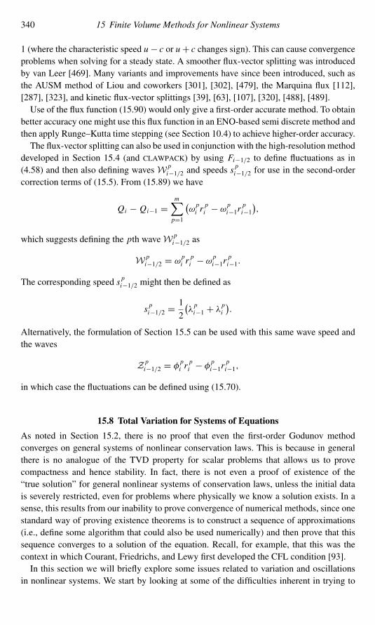
340 15 Finite Volume Methods for Nonlinear Systems

1 (where the characteristic speed u− c or u+ c changes sign). This can cause convergenceproblems when solving for a steady state. A smoother flux-vector splitting was introducedby van Leer [469]. Many variants and improvements have since been introduced, such asthe AUSM method of Liou and coworkers [301], [302], [479], the Marquina flux [112],[287], [323], and kinetic flux-vector splittings [39], [63], [107], [320], [488], [489].Use of the flux function (15.90) would only give a first-order accurate method. To obtain

better accuracy one might use this flux function in an ENO-based semi discrete method andthen apply Runge–Kutta time stepping (see Section 10.4) to achieve higher-order accuracy.The flux-vector splitting can also be used in conjunction with the high-resolution method

developed in Section 15.4 (and CLAWPACK) by using Fi−1/2 to define fluctuations as in(4.58) and then also defining wavesW p

i−1/2 and speeds spi−1/2 for use in the second-order

correction terms of (15.5). From (15.89) we have

Qi − Qi−1 =m∑p=1

(ωpi r

pi − ωpi−1r pi−1

),

which suggests defining the pth waveW pi−1/2 as

W pi−1/2 = ω

pi r

pi − ωpi−1r pi−1.

The corresponding speed s pi−1/2 might then be defined as

s pi−1/2 =1

2

(λpi−1 + λpi

).

Alternatively, the formulation of Section 15.5 can be used with this same wave speed andthe waves

Z pi−1/2 = φ

pi r

pi − φ pi−1r pi−1,

in which case the fluctuations can be defined using (15.70).

15.8 Total Variation for Systems of Equations

As noted in Section 15.2, there is no proof that even the first-order Godunov methodconverges on general systems of nonlinear conservation laws. This is because in generalthere is no analogue of the TVD property for scalar problems that allows us to provecompactness and hence stability. In fact, there is not even a proof of existence of the“true solution” for general nonlinear systems of conservation laws, unless the initial datais severely restricted, even for problems where physically we know a solution exists. In asense, this results from our inability to prove convergence of numerical methods, since onestandard way of proving existence theorems is to construct a sequence of approximations(i.e., define some algorithm that could also be used numerically) and then prove that thissequence converges to a solution of the equation. Recall, for example, that this was thecontext in which Courant, Friedrichs, and Lewy first developed the CFL condition [93].In this section we will briefly explore some issues related to variation and oscillations

in nonlinear systems. We start by looking at some of the difficulties inherent in trying to

15.8 Total Variation for Systems of Equations 341

obtain total variation bounds. For a system of m equations, we might try to define the totalvariation by

TV(q) = supN∑j=1‖q(ξ j )− q(ξ j−1)‖, (15.94)

where the supremum is taken over all subdivisions of the real line −∞ = ξ0 < ξ1 < · · · <ξN = ∞, generalizing (6.19) by replacing the absolute value by some vector norm in R

m .We will be particularly concerned with piecewise constant grid functions, in which case(15.94) reduces to

TV(Q) =∞∑

i=−∞‖Qi − Qi−1‖. (15.95)

With this definition of TV, and similar replacement of absolute value by the vector normelsewhere in the notions of convergence used in the Lax–Wendroff theorem, this theoremcontinues to hold. We might also hope that numerical methods will produce solutions thathave bounded total variation in this sense, in which case we could prove stability andconvergence.In general, however, we cannot hope to developmethods that are TVDwith this definition

of TV, because the true solution is itself not TVD. In fact, the total variation can increaseby an arbitrarily large amount over an arbitrarily short time if we choose suitable data, andso we cannot even hope to obtain a bound of the form TV(Qn+1) ≤ (1 + α �t) TV(Qn).To see this, consider the simple example in Section 13.4, the Riemann problem for theshallow water equations in which hl = hr and ul = −ur > 0 (two equal streams of watersmashing into one another). The initial data has no variation in h, and the variation inhu is 2hlul . For any time t > 0 the variation in hu is still 2hlul , but the depth nearx = 0 increases to hm > hl , and so h has total variation 2(hm − hl) > 0. By choosing ullarge enough we can make this increase in variation arbitrarily large, because hm increaseswith ul .For certain systems of equations it is possible to prove stability by measuring the total

variation in terms of wave strengths instead of using standard vector norms inRm . A simple

example is a constant-coefficient linear system, as considered in the next section.

15.8.1 Total Variation Estimates for Linear Systems

Consider a linear system qt + Aqx = 0. Note that linear systems can exhibit exactly thesame growth in TV as seen in the shallow water example above. Consider the Riemannproblem for the the acoustics equations with pl = pr and ul = −ur > 0, for example,which behaves just as described above. In spite of this, for a constant-coefficient linearsystem we can easily prove convergence of standard methods by diagonalizing the system,decoupling it into independent scalar advection equations that have the TVD property. Forexample, Godunov’s method for a linear system can be written as

Qn+1i = Qni −�t

�x

[A+(Qni − Qni−1

)+ A−(Qni+1 − Qni

)].

342 15 Finite Volume Methods for Nonlinear Systems

Multiplying by R−1 (the matrix of left eigenvectors) and definingWni = R−1Qni , we obtain

Wn+1i = Wn

i −�t

�x

[�+

(Wni −Wn

i−1)+�−(Wn

i+1 −Wni

)],

where�± = R−1A±R. This is an uncoupled set of m first-order upwind algorithms for thecharacteristic variables, each of which is TVD and convergent. It follows that Qni = RWn

i

is also convergent.This suggests that we define the total variation of Q by using a vector norm such as

‖Q‖W ≡ ‖R−1Q‖1, (15.96)

where ‖·‖1 is the standard 1-norm in Rm . Since R−1 is nonsingular, this defines a vector

norm. Then we can define the corresponding total variation by

TVW (Q) =∞∑

i=−∞‖Qi − Qi−1‖W

=∞∑

i=−∞‖R−1(Qi − Qi−1)‖1

=∞∑

i=−∞‖Wi −Wi−1‖1

=∞∑

i=−∞

m∑p=1

∣∣W pi −W p

i−1∣∣

=m∑p=1

TV(W p), (15.97)

where TV(W p) is the scalar total variation of the pth characteristic component. Since thescalar upwind method is TVD, we have

TV((W p)n+1) ≤ TV((W p)n),

and hence, with the definition (15.97) of total variation, we can show that

TVW (Qn+1) ≤ TVW (Qn). (15.98)

For the exact solution to a linear system, this same approach shows that TVW (q(·, t)) remainsconstant in time, since each scalar advection equation for the characteristic variablew p(x, t)maintains constant variation.

15.8 Total Variation for Systems of Equations 343

From this result we can also show that other forms of the total variation, such as (15.94),remain uniformly bounded even if they are not diminishing. We have

TV1(Qn) =

∑i

‖Qi − Qi−1‖1

=∑i

∥∥R(Wni −Wn

i−1)∥∥1

≤ ‖R‖1∑i

∥∥Wni −Wn

i−1∥∥1

= ‖R‖1 TVW (Qn)≤ ‖R‖1 TVW (Q0)= ‖R‖1

∑i

∥∥R−1(Q0i − Q0i−1)∥∥1≤ ‖R‖1 ‖R−1‖1 TV1(Q0). (15.99)

Hence TV1 grows by at most a factor of ‖R‖1‖R−1‖1, the condition number of the eigenvec-tor matrix, over any arbitrary time period. It is natural for this condition number to appearin the bound, since it measures how nearly linearly dependent the eigenvectors of A are.Recalling the construction of the Riemann solution from Chapter 3, we know that eigen-vectors that are nearly linearly dependent can give rise to large variation in the Riemannsolutions. (See also the example in Section 16.3.1.)Note that if we write the Riemann solution as a sum of waves,

Qi − Qi−1 =∑p

W pi−1/2 =

∑p

αpi−1/2r

p,

as introduced in Section 3.8, then we can also express TVW (Q) as

TVW (Q) =∑i

∑p

∣∣α pi−1/2∣∣. (15.100)

Recall that in defining the basis of eigenvectors r p (and hence the matrix R) we couldchoose any convenient normalization. For our present purposes it is most convenient toassume that r p is chosen to have ‖r p‖1 = 1. Then∣∣α pi−1/2∣∣ = ∥∥α pi−1/2r p∥∥1 = ∥∥W p

i−1/2∥∥1,

and we simply have

TVW (Q) =∑i

∑p

∥∥W pi−1/2

∥∥1. (15.101)

Thus another interpretation of TVW is that it is the sum of the wave strengths over all wavesarising in all Riemann problems at cell interfaces. This is illustrated in Figure 15.7. Fora linear system all waves simply pass through one another (linear superposition) with nochange in their strength as time advances. This is not true for nonlinear systems.

344 15 Finite Volume Methods for Nonlinear Systems

u

p

ql

qr

qm

W1W2

r2r1

∆u

∆p

Fig. 15.7. Illustration of TVW (Q) for Riemann-problem data in the acoustics equations. ‖qr −ql‖1 =|�p| + |�u|, whereas ‖qr − ql‖W = ‖W1‖1 + ‖W2||1.

15.8.2 Wave-Strength Estimates for Nonlinear Systems

For a linear system of equations we have just seen that we can prove the solution is totalvariation bounded by measuring the variation of a piecewise constant solution in terms ofthe metric

dW (ql , qr ) ≡∑p

‖W p‖1, (15.102)

where the W p represent waves arising in the Riemann solution between states ql and qr .Then

TVW (Q) =∑i

dW (Qi−1, Qi ). (15.103)

We can make the same definition of total variation in the case of a nonlinear hyperbolicsystem. For a linear system this metric can be rewritten in terms of a norm ‖·‖W , since thevalue of dW (ql , qr ) depends only on the value qr −ql . This is what was used in the previoussection. For a nonlinear problem this is no longer true. The wave strengths in the Riemannsolution between two states q ′l and q

′r might be quite different from those in the Riemann

solution between ql and qr even if q ′r − q ′l = qr − ql .If we attempt to use TVW as defined in (15.103) to study the stability of Godunov’s

method on nonlinear problems we run into two difficulties:

1. In general the total variation TVW may not be diminishing even in the true solution.Consider, for example, data that consists of two approaching shocks that collide andproduce two outgoing shocks. For a nonlinear problem it might happen that the outgoingshocks are stronger than the incoming shocks (with larger ‖W p‖1).

2. The averaging process in Godunov’s method introduces new states into the approximatesolution that may not appear in the true solution. Because the structure of the Hugoniotloci and integral curves can vary rapidly in state space, this may introduce additionalunphysical variation when Riemann problems are solved between these new states.

15.8 Total Variation for Systems of Equations 345

For certain special systems of equations these difficulties can be overcome and stabilityproved. For example, for certain systems of two equations the integral curves and Hugoniotloci are identical. In this case it can be shown that that these curves are in fact straight linesin state space. Such systems have been studied by Temple [448], [447], who obtained totalvariation bounds for the true solution and used these to prove existence of solutions. It isalso possible to obtain TV estimates when Godunov’s method is applied to such a system,and hence convergence can be proved [291]. Similar results have also been obtained formore general nonlinear systemswith straight-line fields [46]. For general nonlinear systems,however, such results are not currently available.

15.8.3 Glimm’s Random-Choice Method

For systems such as the Euler equations it is not possible to prove convergence of Godunov’smethod. In fact, it is not even possible to prove that weak solutions exist for all time if weallow arbitrary initial data. However, if the initial data is constrained to have sufficientlysmall total variation, then there is a famous proof of existence due to Glimm [152]. Thisproof is based on a constructive method that can also be implemented numerically, andis often called the random-choice method. Several variants of this method are describedin various sources e.g., [43], [78], [98], [307], [316], [420], [450], [499]. Here we onlysummarize the major features:

• A finite volume grid with piecewise-constant data is introduced as in Godunov’s method,and Riemann problems are solved at each cell interface to define a function qn(x, t) asin Section 4.10. However, instead of averaging the resulting solutions over grid cells, thevalue of qn(x, tn+1) at a random point x in each cell is chosen. This avoids difficulty 2mentioned in the previous subsection.

• Afunctional similar to (15.103) is used tomeasure the solution, but an additional quadraticterm is introduced that measures the potential for future interaction between each pairof waves that are approaching one another. This is necessary so as to take into accountthe potential increase in variation that can arise when two waves interact. The quadraticfunctional is the crux of Glimm’s proof, since he was able to show that a suitable choiceresults in a functional that is nonincreasing in time (for data with sufficiently smallvariation).

Computationally, the random-choice method has the advantage that shocks remain sharp,since the solution is sampled rather than averaged. Of course, the method cannot be exactlyconservative, for this same reason, but Glimm showed convergence to a weak solution withprobability 1. Another disadvantage computationally is that smooth flow is typically notvery smoothly represented. There also appear to be problems extending the method to morethan one space dimension [78], and for these reasons the method is not widely used forpractical problems, though it may be very useful for some special ones.Since Glimm’s paper, other approaches have been introduced to prove existence and

in some cases uniqueness results for certain systems of conservation laws (under suitablerestrictions on the initial data), using techniques such as compensated compactness [109],[403], [446], front tracking [44], [97], [371], and semigroup methods [35],[45], [46], [48],[49], [205], [312]. For an overview of many recent theoretical results, see Dafermos [98].

346 15 Finite Volume Methods for Nonlinear Systems

15.8.4 Oscillation in Shock Computations

Consider a simple Riemann problem in which the data lies on a Hugoniot curve, so that thesolution consists of a single shock wave. In this case the exact solution is monotonicallyvarying and has constant total variation. In this case, at least, we might hope that a sensiblenumericalmethodbasedon scalarTVD theorywould behavewell andnot introduce spuriousoscillations. In practice high-resolution methods of the type we have developed do workvery well on problems of this sort, most of the time. However, even the simplest first-orderGodunov method can produce small spurious oscillations, which can be noticeable in somecomputations. Here we briefly consider two common situations where this can arise.

Start-up Errors

Figure 15.8 shows the numerical solution to the Riemann problem for the Euler equationswith the data

ρl = 5.6698, ul = 9.0299, pl = 100 for x < 0,ρr = 1.0, ur = 0.0, pr = 1.0 for x > 0.

(15.104)

This data has been chosen to satisfy the Rankine–Hugoniot jump relations (with γ = 1.4),so that the solution is a single 3-shock propagating with speed s = 10.9636. Figure 15.8shows the computed density at time t = 1 on a grid with 400 cells, using theminmod limiter.We see in Figure 15.8(a) that the solution is resolved quite sharply, with only three pointsin the shock. The shock is in the correct location and the solution is roughly constant awayfrom it. However, some small oscillations are visible. These are seen much more clearlyin Figure 15.8(b), which shows the same solution on a different scale. Most noticeable aretwo dips in the density. These are waves that arose from the initial discontinuity at x = 0.The leftmost dip is an acoustic wave moving at speed ul − cl ≈ 4.06, and the other dipis an entropy wave moving at the fluid velocity ul ≈ 9.03. This sort of start-up error isfrequently seen when an exact discontinuity is used as initial data.

(a)−5 0 5 10 150

1

2

3

4

5

6

(b)−5 0 5 10 15

5.55

5.6

5.65

5.7

5.75

Fig. 15.8. Start-up error with Godunov’s method on a 3-shock in the Euler equations. (a) Density att = 1. (b) Magnification of the same results. [claw/book/chap15/startup]

15.8 Total Variation for Systems of Equations 347

How does this oscillation arise? The initial data is

Q0i ={ql if i < I,qr if i ≥ I

for some I. In the first time step, the Riemann problem at xI−1/2 gives rise to a singlewave that is computed exactly (even if the Roe solver is used instead of the exact solvercomputationally). However, this wave travels a distance less than�x in this time step, andthe averaging process of Godunov’s method produces a new state Q1I in one grid cell thatis a convex combination of ql and qr ,

Q1I =s�t

�xql +

(1− s�t

�x

)qr .

This state lies on the straight line connecting ql and qr in phase space. In the next time step,there will be two Riemann problems at xI−1/2 and at xI+1/2 that have nontrivial solutions.If the Hugoniot locus joining ql to qr happens to be a straight line (as in Temple-classsystems, for example; see Section 15.8.2), then each these two Riemann problems willresult in a single shock wave, since Q1I will lie on the same Hugoniot locus, and the twoshocks together make up the original shock. As in a scalar problem, the numerical solutionwill be smeared over more grid cells as time evolves, but we will still be approximating thesingle shock well, and no oscillations will appear.However, for most nonlinear systems the Hugoniot curve is not a straight line, and so

the state Q1I does not lie on the same Hugoniot curve as Q1I−1 = ql or Q1I+1 = qr . Solving

these Riemann problems then results in the generation of waves in all families, and not justa 3-wave as expected from the initial data. It is these other waves that lead to the oscillationsobserved in Figure 15.8. See [14] for more analysis and some plots showing how theseoscillations evolve in state space.

Slow-Moving Shocks

The start-up error discussed above tends to be damped by the numerical viscosity inGodunov’s method, and so is often not very visible. In situations where the numericalviscosity is small, however, the oscillations can become significant.In particular, oscillations are frequently seen if the shock is moving very slowly, in the

sense that the shock speed is very small relative to the fastest characteristic speeds in theproblem. Then it takes several time steps to cross a single grid cell even when the Courantnumber is close to one. Recall from (15.51) that the numerical viscosity of Roe’s methodvanishes as the wave speed goes to zero, and the same is true for Godunov’s method basedon the exact Riemann solver in the case where the solution is a single shock with speedclose to zero. This can be an advantage for scalar problems: nearly stationary shocks arecaptured very sharply. But for nonlinear systems this lack of viscosity can lead to increasedoscillations.

348 15 Finite Volume Methods for Nonlinear Systems

(a)−15 −10 −5 0 50

1

2

3

4

5

6

(b)−15 −10 −5 0 5

5.55

5.6

5.65

5.7

5.75

Fig. 15.9. Oscillations arising in a slow shock computed with Godunov’s method. (a) Density att = 1. (b) Magnification of the same results. [claw/book/chap15/slowshock]

As an example, suppose we take the same data (15.104) as in the previous example, butshift the velocity of ul and ur by an amount close to the previous shock speed s:

ρl = 5.6698, ul = −1.4701, pl = 100 for x < 0,ρr = 1.0, ur = −10.5, pr = 1.0 for x > 0.

(15.105)

This is simply a shift in the reference frame, and so the Riemann solution is exactly the sameas before, but with all velocities shifted by the same amount −10.5. So this again givesa single shock wave, now propagating with velocity s = 0.4636. Computational resultsare shown in Figure 15.9, illustrating the oscillations that appear in this case, again withthe first-order Godunov method. Similar oscillations arise in high-resolution methods, evenwhen limiters are used. In this case the shock continues to shed oscillations as it movesalong.For some discussions of oscillations due to slow-moving shocks, and ways to improve

the situation by introducing additional dissipation, see [14], [112], [224], [232], [343],[373]. The lack of numerical dissipation in Godunov-type methods can also lead to someother numerical problems, particularly for multidimensional computations in regions wherestrong shocks are nearly aligned with the grid. This can lead to a cross-flow instability orodd–even decoupling, and to the appearance of unphysical extrusions from the shock that areoften called carbuncles. Again the addition of more numerical dissipation may be necessaryto improve the results. For some discussions of such numerical problems and their relationto physical instabilities see, for example, [195], [287], [353], [364], [374], [487].

Exercises

15.1. Consider the p-system

vt − ux = 0,ut + p(v)x = 0.

(15.106)

Exercises 349

(a) Show that for this system the integral in (15.21) can be evaluated in order toobtain the following Roe linearization:

Ai−1/2 = 0 −1pi − pi−1Vi − Vi−1 0

.(b) In particular, determine the Roe solver for p(v) = a2/v, modeling isothermal

flow in Lagrangian coordinates, where a is the constant sound speed.(c) Implement and test this isothermal Riemann solver in CLAWPACK.(d) Does this solver require an entropy fix?

15.2. Suppose anHLLapproximateRiemann solver of the formdiscussed inSection15.3.7is used, but with s1i−1/2 = −�x/�t and s2i−1/2 = �x/�t . These are the largestspeeds that can be used with this grid spacing and still respect the CFL condition, sothese should be upper bounds on the physical speeds. Show that if this approximateRiemann solver is used in the first-order Godunov method, then the result is theLax–Friedrichs method (4.20).

16Some Nonclassical Hyperbolic Problems

In the previous chapters on nonlinear problems we have concentrated on classical systemsof conservation laws for which the wave structure is relatively simple. In particular, wehave assumed that the system is strictly hyperbolic (so that there are m distinct integralcurves through each point of phase space), and that each characteristic field is either linearlydegenerate or genuinely nonlinear (so that the eigenvalue is constant or variesmonotonicallyalong each integral curve). Many important systems of equations satisfy these conditions,including the shallow water equations and the Euler equations for an ideal gas, as well aslinear systems such as acoustics. However, there are other important applications whereone or both of these conditions fail to hold, including some problems arising in nonlinearelasticity, porous-media flow, phase transition, and magnetohydrodynamics (MHD). In thischapter we explore a few of the issues that can arise with more general systems. This is onlyan introduction to some of the difficulties, aimed primarily at explaining why the aboveassumptions lead to simplifications.We start by considering scalar conservation laws with nonconvex flux functions (which

fail to be genuinely nonlinear because f ′′(q) vanishes at one or more points). This gives agood indication of the complications that arise also in systems of more equations that fail tobe genuinely nonlinear. Then in Section 16.2 we will investigate the complications that canarise if a system is not strictly hyperbolic, i.e., if some of the wave speeds coincide at oneor more points in phase space. In Section 16.3 we go even further and see what can happenif the system fails to be (strongly) hyperbolic at some points, either because the matrix isnot diagonalizable or because the eigenvalues are not real.In Section 16.4 we consider nonlinear conservation laws with spatially varying flux func-

tions f (q, x), analogous to the variable-coefficient linear systems considered in Chapter 9.Finally, Section 16.5 contains some discussion of nonconservative nonlinear hyperbolicproblems.

16.1 Nonconvex Flux Functions

For the scalar conservation laws studied thus far, the flux function f (q) was assumed tobe a convex or concave function of q , meaning that f ′′(q) has the same sign everywhere.For the traffic flux (11.6) it is constant and negative everywhere when umax > 0. Burgers’equation is convex, since f ′′(u) ≡ 1. As shorthand we typically refer to all such genuinelynonlinear problems as convex.

350

16.1 Nonconvex Flux Functions 351

Convexity is important because it means that the characteristic speed f ′(q) is varyingmonotonically as q varies. In solving the Riemann problem with ql > qr (Figure 11.3), weobtain a smooth rarefaction wave with cars spreading out, since f ′(q) is nondecreasing as xincreases. On the other hand if ql < qr as in Figure 11.2, then the Riemann solution consistsof a shock joining these two values. If the function f (q) is not convex, then the Riemannsolution may be more complicated and can involve both shock and rarefaction waves.

16.1.1 Two-Phase Flow and the Buckley–Leverett Equation

As an example where nonconvex flux functions arise, we study a simple model for two-phase fluid flow in a porous medium. One application is to oil-reservoir simulation. Whenan underground source of oil is tapped, a certain amount of oil flows out on its own dueto high pressure in the reservoir. After the flow stops, there is typically a large amount ofoil still in the ground. One standard method of subsequent secondary recovery is to pumpwater into the oil field through some wells, forcing oil out through others. In this case thetwo phases are oil and water, and the flow takes place in a porous medium of rock or sand.We can consider a one-dimensional model problem in which oil in a tube of porous

material is displaced by water pumped in through one end. Let q(x, t) represent the fractionof fluid that is water (thewater saturation), so that 0 ≤ q ≤ 1, and 1−q(x, t) is the fractionthat is oil. If we take initial data

q(x, 0) ={1 if x < 0,0 if x > 0,

(16.1)

so that water is to the left and oil to the right, and take a positive flow rate (pumping waterin from the left), then we expect the water to displace the oil. Our first guess might be thatthe sharp interface between pure water (q = 1) and pure oil (q = 0) will be maintainedand simply advect with constant velocity. Instead, however, one observes a sharp interfacebetween pure oil and some mixed state q = q∗< 1, followed by a region in which both oiland water are present (q∗ < q < 1). Mathematically we will see that this corresponds to ashock wave followed by a rarefaction wave.Since both fluids are essentially incompressible, we expect the total flux of fluid to

be the same past any point in the tube. In regions of pure oil or pure water the velocitymust thus be the same, and we will take this value to be 1. However, in regions whereboth fluids are present, they may be moving at different average velocities. It is this be-havior that leads to the interesting mathematical structure. Physically this arises from thefact that a porous medium consists of a solid material with many pores or minute cracksthrough which the fluids slowly seep. Particles of the oil are initially bound to the solidsubstrate and must be displaced by the water molecules. The fact that oil and water donot mix (the fluids are immiscible) means that surface tension effects between the twofluids are crucial on the small length scales of the pores, and can inhibit the movementof water into the smallest pores filled with oil. Regions where 0 < q < 1 correspond toregions where some of the oil is still bound to the substrate and is stationary, so the aver-age velocity of oil molecules may be considerably less than the average velocity of watermolecules.

352 16 Some Nonclassical Hyperbolic Problems

(a)0 0.1 0.2 0.3 0.4 0.5 0.6 0.7 0.8 0.9 10

0.1

0.2

0.3

0.4

0.5

0.6

0.7

0.8

0.9

1

f(q)

fo(q)

(b)0 0.2 0.4 0.6 0.8 1

0

0.5

1

1.5

2

2.5

f ′(q)

Fig. 16.1. (a) Flux functions (16.2) for the Buckley–Leverett equation, as functions of the watersaturation q. (b) The characteristic speed f ′(q). Shown for a = 1/2 in (16.2).

Buckley and Leverett proposed a simple model for this complex situation in which theflux of water and oil are each given by expressions that depend on the saturation of the fluid:

flux of water: f (q) = q2

q2 + a(1− q)2 ;

flux of oil: fo(q) = a(1− q)2q2 + a(1− q)2 .

(16.2)

Here a< 1 is a constant. Each of the fluxes can be viewed as the product of the saturationof the phase with the average velocity of the phase. In each case the idea is that the averagevelocity approaches 0 as the saturation goes to 0 (the few molecules present are bound tothe substrate) and approaches 1 as the saturation goes to 1 (since the fluid as a whole isflowing at this rate). The fact that a< 1 arises from the fact that oil flows less easily thanwater. So if q = 1−q = 0.5, for example, we expect more water than oil to be flowing. Wetake a= 1/2 in the figures here. Note that f (q) + fo(q) ≡ 1, so that the total fluid flux isthe same everywhere, as required by incompressibility. Figure 16.1(a) shows these fluxesas a function of q.We only need to solve for q, thewater saturation, and sowe can solve a scalar conservation

law

qt + f (q)x = 0

with the flux f (q) given by (16.2). Note that this flux is nonconvex, with a single inflectionpoint. Figure 16.1(b) shows the characteristic speed

f ′(q) = 2aq(1− q)[q2 + a(1− q)2]2 ,

which has a maximum at the point of inflection.Now consider the Riemann problem with initial states ql = 1 and qr = 0. By following

characteristics, we can construct the triple-valued solution shown in Figure 16.2(a). Notethat the characteristic velocities are f ′(q), so that the profile of this bulge, seen here attime t , is simply the graph of t f ′(q) turned sideways.

16.1 Nonconvex Flux Functions 353

(a) (b) (c)

shockrarefaction

Fig. 16.2. Riemann solution for the Buckley–Leverett equation. (a) Triple-valued solution obtainedby following characteristics. (b) Insertion of an area-preserving shock. (c) Structure in the x–t plane.

Wecannowuse the equal-area rule to replace this triple-valued solutionby a correct shock.The resulting weak solution is shown in Figure 16.2(b), along with the characteristics inFigure 16.2(c). The postshock value q∗ is constant in time (Exercise 16.2), and so is theshock speed

s = f (q∗)− f (qr )

q∗ − qr = f (q∗)q∗

. (16.3)

This is to be expected, since the solution to the Riemann problem is still self-similar in thenonconvex case.Note the physical interpretation of the solution shown in Figure 16.2. As the water moves

in, it displaces a certain fraction q∗ of the oil immediately. Behind the shock, there is amixture of oil and water, with less and less oil as time goes on. At a production well (at thepoint x = 1, say), one obtains pure oil until the shock arrives, followed by a mixture of oiland water with diminishing returns as time goes on. It is impossible to recover all of the oilin finite time by this technique.Note that the Riemann solution involves both a shock and a rarefaction wave and is called

a compound wave. If f (q) had more inflection points, the solution might involve severalshocks and rarefactions (as in Example 16.1 below).Here we only consider scalar nonconvex problems. For a nonlinear system of equations,

similar behavior can arise in any nonlinear field that fails to be genuinely nonlinear (seeSection 13.8.4). This arises, for example, in the one-dimensional elasticity equations (2.97)with a nonconvex stress–strain relation. See, e.g., [483], [484].

16.1.2 Solving Nonconvex Riemann Problems

To determine the correct weak solution to a nonconvex scalar conservation law, we needan admissibility criterion for shock waves that applies in this case. A more general form ofthe entropy condition (11.40), due to Oleinik [347], applies also to nonconvex scalar fluxfunctions f :

Entropy Condition 16.1 (Oleinik). A weak solution q(x, t) is the vanishing-viscositysolution to a general scalar conservation law if all discontinuities have the property that

f (q)− f (ql)

q − ql ≥ s ≥ f (q)− f (qr )

q − qr (16.4)

for all q between ql and qr .

354 16 Some Nonclassical Hyperbolic Problems

0 0.2 0.4 0.6 0.8 1

0

0.2

0.4

0.6

0.8

1

(q∗, f(q∗))

f(q)

Shock

Rarefaction

Fig. 16.3. Convex-hull construction of the Riemann solution for the Buckley–Leverett equation withql = 1 and qr = 0. The shaded region is the convex hull of the set of points lying below the graph off (q).

For convex f , this requirement reduces to (11.40). (Note that this may not always bethe correct admissibility condition to apply; see [285] for a nonconvex traffic-flow examplewhere the vanishing-viscosity criterion would select the wrong solution.)

Convex-Hull Construction

The entropy-satisfying solution to a nonconvex Riemann problem can be determined fromthe graph of f (q) in a simple manner. If qr < ql , then construct the convex hull of the set{(q, y) : qr ≤ q ≤ ql and y ≤ f (q)}. The convex hull is the smallest convex set containingthe original set. This is shown in Figure 16.3 for the case ql = 1, qr = 0.If we look at the upper boundary of this set, we see that it is composed of a straight line

segment from (0, 0) to (q∗, f (q∗)) and then follows y = f (q) up to (1, 1). The point oftangency q∗ is precisely the postshock value. The straight line represents a shock jumpingfrom q = 0 to q = q∗, and the segment where the boundary follows f (q) is the rarefactionwave. This works more generally for any two states (provided ql > qr ) and for any f .Note that the slope of the line segment is equal to the shock speed (16.3). The fact that this

line is tangent to the curve f (q) at q∗ means that s = f ′(q∗), the shock moves at the samespeed as the characteristics at this edge of the rarefaction fan, as seen in Figure 16.2(c).If the shock were connected to some point q < q∗, then the shock speed f (q)/q would

be less than f ′(q), leading to a triple-valued solution. On the other hand, if the shock wereconnected to some point above q∗, then the entropy condition (16.4) would be violated.This explains the tangency requirement, which comes out naturally from the convex-hullconstruction. The same construction works for any qr < ql lying in [0, 1].If ql < qr , then the same idea works, but we look instead at the convex hull of the

set of points above the graph, {(q, y) : ql ≤ q ≤ qr and y ≥ f (q)}, as illustrated inExample 16.1.Note that if f is convex, then the convex hull construction gives either a single line

segment (single shock) if ql > qr or the function f itself (single rarefaction) if ql < qr .

Example 16.1. Figure 16.4(a) shows another example for the flux function f (q) = sin(q)with ql = π/4 and qr = 15π/4. The shaded region is the convex hull of the set of pointsabove this curve, since ql < qr . The lower boundary of this set shows the structure of

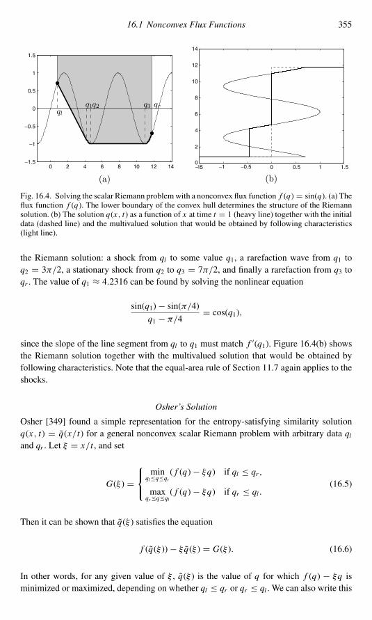
16.1 Nonconvex Flux Functions 355

0 2 4 6 8 10 12 14−1.5

−1

−0.5

0

0.5

1

1.5

q1q2 q3ql

qr

−1.5 −1 −0.5 0 0.5 1 1.50

2

4

6

8

10

12

14

(a) (b)

Fig. 16.4. Solving the scalar Riemann problemwith a nonconvex flux function f (q) = sin(q). (a) Theflux function f (q). The lower boundary of the convex hull determines the structure of the Riemannsolution. (b) The solution q(x, t) as a function of x at time t = 1 (heavy line) together with the initialdata (dashed line) and the multivalued solution that would be obtained by following characteristics(light line).

the Riemann solution: a shock from ql to some value q1, a rarefaction wave from q1 toq2 = 3π/2, a stationary shock from q2 to q3 = 7π/2, and finally a rarefaction from q3 toqr . The value of q1 ≈ 4.2316 can be found by solving the nonlinear equation

sin(q1)− sin(π/4)q1 − π/4 = cos(q1),

since the slope of the line segment from ql to q1 must match f ′(q1). Figure 16.4(b) showsthe Riemann solution together with the multivalued solution that would be obtained byfollowing characteristics. Note that the equal-area rule of Section 11.7 again applies to theshocks.

Osher’s Solution

Osher [349] found a simple representation for the entropy-satisfying similarity solutionq(x, t) = q(x/t) for a general nonconvex scalar Riemann problem with arbitrary data qland qr . Let ξ = x/t , and set

G(ξ ) =

minql≤q≤qr

( f (q)− ξq) if ql ≤ qr ,maxqr≤q≤ql

( f (q)− ξq) if qr ≤ ql .(16.5)

Then it can be shown that q(ξ ) satisfies the equation

f (q(ξ ))− ξ q(ξ ) = G(ξ ). (16.6)

In other words, for any given value of ξ , q(ξ ) is the value of q for which f (q) − ξq isminimized or maximized, depending on whether ql ≤ qr or qr ≤ ql . We can also write this

356 16 Some Nonclassical Hyperbolic Problems

as

q(ξ ) =

argminql≤q≤qr

[ f (q)− ξq] if ql ≤ qr ,

argmaxqr≤q≤ql

[ f (q)− ξq] if qr ≤ ql .(16.7)

In general the argmin function returns the argument that minimizes the expression, andsimilarly for argmax.Note that for any fixed q0 we can replace f (q) − ξq by [ f (q) − f (q0)] − ξ (q − q0) in

(16.7). Often an appropriate choice of q0 (e.g., ql or qr ) makes it easier to interpret thisexpression, since it is intimately related to the Rankine–Hugoniot jump condition (11.21).Differentiating the expression (16.6) with respect to ξ gives

[ f ′(q(ξ ))− ξ ]q ′(ξ )− q(ξ ) = G ′(ξ ). (16.8)

Along every ray x/t = ξ in the Riemann solution we have either q ′(ξ )= 0 or elsef ′(q(ξ )) = ξ (in a rarefaction wave), and hence (16.8) reduces to an expression for q(ξ ):

q(ξ ) = −G ′(ξ ). (16.9)

This gives the general solution to the Riemann problem.The equation (16.6) is particularly useful in the case ξ = 0, for which it yields the value

f (q(0)) along x/t = 0. This is the flux value f (q∨|(ql , qr )) needed in implementing Go-

dunov’s method and generalizations. When ξ = 0, (16.6) reduces to

f (q∨|(ql , qr )) = f (q(0)) = G(0) =

min

ql≤q≤qrf (q) if ql ≤ qr ,

maxqr≤q≤ql

f (q) if qr ≤ ql .(16.10)

We have already seen this formula for the special case of a convex flux function in (12.4).

16.1.3 Finite Volume Methods for Nonconvex Problems

Finite volume methods for nonconvex problems (see Section 16.1) can be developed usingthe same approach as for convex problems. To apply Godunov’s method to a scalar non-convex problem, we must compute the flux Fi−1/2 = f (Q∨

|i−1/2), where Q

∨|i−1/2 is the value

along x/t = 0 in the entropy-satisfying solution to the Riemann problem between statesQi−1 and Qi . This is easily computed using the general formula (16.10), resulting in (12.4).As usual, this flux can be converted into fluctuations A±�Qi−1/2 using (12.6).To apply a high-resolution method, we also need to define one or more waves and

corresponding speeds. Since the Riemann solution may consist of several waves in thenonconvex case, one might think it necessary to handle each wave separately. In fact itappears to be sufficient to use a single wave and the corresponding Rankine–Hugoniotspeed,

Wi−1/2 = Qi − Qi−1, si−1/2 = f (Qi )− f (Qi−1)Qi − Qi−1 .

16.1 Nonconvex Flux Functions 357

(a)−0.5 0 0.5 1 1.5

−0.2

0

0.2

0.4

0.6

0.8

1

1.2

(b)−0. 5 0 0.5 1 1.5

−0. 2

0

0.2

0.4

0.6

0.8

1

1.2

Fig. 16.5. (a) Computed solution to the Buckley–Leverett problem at time t = 1 using CLAWPACKwith sufficiently small time steps that the Courant number is less than 1. (b) Entropy-violating solutionobtained with CLAWPACK when the true Courant number is greater than 1. [claw/book/chap16/bucklev]

In computing the fluctuations an entropy fix must be included, as in the convex case, ifthe solution contains a transonic rarefaction. It is also important to insure that the Courantnumber is less than 1. Note that in computing the Courant number we must use the formula

Courant number = max

∣∣∣∣�t�x f ′(q)∣∣∣∣ ,

where we maximize over the entire range of q that appears in the solution, e.g., over [0, 1]for the Buckley–Leverett example used above. For nonconvex problems this may be largerthan values of |si−1/2|�t/�x that arise in the course of solving the problem numerically(which is how CLAWPACK estimates the Courant number). This is because the steepest partof the flux function may be in regions that are embedded in shocks and not sampled by thecell averages arising in the problem.Figure 16.5(a) shows a computed solution to the Buckley–Leverett equation using a

high-resolution method of CLAWPACK with a time step that satisfies the CFL condition.Figure 16.5(b) shows a CLAWPACK computation with the parameter values

cflv(1) = 1.0,

cflv(2) = 0.8.

This aims for a Courant number of 0.8 and forces a step to be retaken whenever the observedCourant number is greater than 1.0. Themethod fails to produce the correct solution, becausethe actual Courant number is greater than the estimate used in CLAWPACK, and the time stepsbeing used do not in fact satisfy the CFL condition. The solution obtained does approximatea weak solution, but one in which the shock jumps from q = 0 to a value greater than the q∗shown in Figure 16.3, and hence propagates at a speed that is slower than the characteristicspeed at some points in between.See[claw/book/chap16/bucklev] for theCLAWPACK implementationof theBuckley–

Leverett equation, and [claw/book/chap16/fsin] for another example, the nonconvexflux function shown in Figure 16.4(a).

358 16 Some Nonclassical Hyperbolic Problems

16.2 Nonstrictly Hyperbolic Problems

In general we have assumed that the systems we deal with are strictly hyperbolic, meaningthat the eigenvaluesλp of the Jacobianmatrix are distinct. In this sectionwewill seewhy thisis significant and briefly explore what can happen if the system fails to be strictly hyperbolic(in which case it is called nonstrictly hyperbolic). We will only scratch the surface of thisinteresting topic, which is important in many applications where some of the consequencesare still poorly understood and the subject of current research.Recall that a matrix with distinct eigenvalues must have a one-dimensional eigenspace

associated with each eigenvalue. If the Jacobian matrix f ′(q) has distinct eigenvalues atevery point q ∈ R

m , then at every point in state space there are m distinct eigendirections,which form a basis for R

m . The integral curves and Hugoniot loci are tangent to theseeigenvectors. From this it can be shownusing the implicit-function theorem that theRiemannproblemcanbeuniquely solved for any two statesql andqr that are sufficiently close together(see e.g., [263]). This does not necessarily mean that the Riemann problem can be solvedglobally for any ql and qr , but at least locally these curves foliate state space in an organizedmanner.Now suppose the system is not strictly hyperbolic and at some point q0 the Jacobian f ′(q0)

has a repeated eigenvalue. The algebraic multiplicity of this eigenvalue is the number oftimes it is repeated as a zero of the characteristic polynomial. The geometric multiplicityis the dimension of the linear space of eigenvectors associated with this eigenvalue, whichis never greater than the algebraic multiplicity but could be less. In order for the system tobe hyperbolic, the geometric multiplicity must be equal to the algebraic multiplicity, sinceonly in this case is the Jacobian matrix diagonalizable. Otherwise the matrix is defective, acase discussed in Section 16.3.1.If the system is hyperbolic but not strictly hyperbolic at q0, then for some eigenvalue the

algebraic and geometric multiplicities are equal but greater than 1. In this multidimensionaleigenspace there are infinitely many directions that are eigenvectors, and this infinitude ofeigendirections leads to some of the difficulties with nonstrictly hyperbolic systems. Even ifthis occurs only at a single point in state space, it can complicate the solution to all Riemannproblems. It is possible for infinitely many integral curves or Hugoniot loci to coalesce atsuch a point, which is often called an umbilic point because of this behavior. Here we onlyconsider some trivial examples to give an indication of how things can change. Much moreinteresting examples arise in various applications such as nonlinear elasticity, flow in porousmedia, andmagnetohydrodynamics. For some examples see [51], [142], [146], [209], [210],[227], [228], [235], [237], [238], [240], [334], [335], [372], [397], [398], [460].

16.2.1 Uncoupled Advection Equations

First it is important to note that equal eigenvalues do not always lead to difficulties. Infact some physical systems (such as one-dimensional Riemann problems arising from themultidimensional Euler equations) always have repeated eigenvalues at every point in statespace and yet require no special treatment.As a simple example, suppose we model two distinct tracers being advected in a fluid

moving at constant velocity u, with concentrations denoted by q1 and q2. Then we obtain

16.2 Nonstrictly Hyperbolic Problems 359

two uncoupled advection equations

q1t + uq1x = 0,q2t + uq2x = 0,

(16.11)

which are easily solved independently. If we view this as a system, then the coefficientmatrix is diagonal:

A =[u 00 u

]. (16.12)

This matrix has eigenvalues λ1 = λ2 = u with all ofR2 as the two-dimensional eigenspace;every direction is an eigendirection. Note that the solution to the Riemann problem betweenarbitrary states ql and qr consists of a single waveW1 = qr − ql with speed s1 = u, sincethe Rankine–Hugoniot jump condition A(qr − ql) = u(qr − ql) is satisfied for every vectorqr −ql . Every curve in state space is an integral curve of this system, but this causes no realproblems.We should note, however, that computationally it is better to use two waves

W1 =[q1r − q1l0

], W2 =

[0

q2r − q2l

],

with equal speeds s1 = s2 = u when using a high-resolution method. This way the limiteris applied separately to each component of the system. Otherwise a discontinuity in q1

in a region where the concentration q2 is smooth would lead to a loss of accuracy in theapproximation to q2.A similar sort of benign nonstrict hyperbolicity is seen in the two-dimensional Euler

equations, as discussed in Section 18.8. If we solve a one-dimensional Riemann problemin any direction then the solution consists of four waves: two nonlinear acoustic waves andtwo linearly degenerate waves moving at the intermediate fluid velocity u∗. These latterwaves form the contact discontinuity, across which the two initial gases are in contact.One of these waves carries a jump in density (as in the one-dimensional Euler equations),and the other carries a jump in the transverse velocity (see Section 18.8). As in the ad-vection example above, we could view these as a single wave carrying jumps in bothquantities, though computationally it may be best to keep them distinct. If we couple theEuler equations with the transport of different chemical species in the gases, then additionallinearly degenerate waves will arise, moving at the same speed. The fact that these wavesare linearly degenerate and the same eigenspace arises at every point in state space meansthat this loss of strict hyperbolicity does not lead to any mathematical or computationaldifficulties.

360 16 Some Nonclassical Hyperbolic Problems

16.2.2 Uncoupled Burgers’ Equations

Now consider a pair of Burgers’ equations,

ut + 1

2(u2)x = 0,

vt + 1

2(v2)x = 0,

(16.13)

for which

q =[uv

], f (q) = 1

2

[u2

v2

], f ′(q) =

[u 00 v

]. (16.14)

Again this system is easy to solve for any initial data, since the two equations are uncoupled.However, if we attempt to apply the theory developed in Chapter 13 to this system, we seethat the state-space structure has become complicated by the fact that this system fails tobe strictly hyperbolic along the line u = v. We must be careful in labeling the eigenvaluesas λ1 and λ2, since by convention we assume λ1 ≤ λ2. This requires setting

λ1 = min(u, v), λ2 = max(u, v), (16.15)

and hence there is a jump discontinuity in the directions r1 and r2 along u = v as shown inFigure 16.6:

r1 ={(1, 0)T if u < v,

(0, 1)T if u > v,r2 =

{(0, 1)T if u < v,

(1, 0)T if u > v.(16.16)

For states q on the curve u = v, every direction is an eigendirection. This allows r1 and r2

to rotate by 90◦ as we cross this curve. While it may seem that this discontinuity is simply aresult of our pedantic insistence on the ordering λ1 ≤ λ2, recall that in solving the Riemannproblem it is crucial that we first move from ql along an integral curve or Hugoniot locus

(a)

r1

r1

r2

r2

u = vλ1 = u

λ1 = v

(b)

r1

r1

r2

r2

u = v

ql

qr

q∗l

q∗r

Fig. 16.6. (a) The phase plane for a pair ofBurgers equations viewed as a nonstrictly hyperbolic systemof equations. The eigenvalues coalesce along u= v. (b) Solution to a Riemann problem consisting ofthree segments.

16.2 Nonstrictly Hyperbolic Problems 361

corresponding to the slower speed, and then along a curve corresponding to the faster speedto reach qr . Otherwise we cannot patch these waves together into a physically meaningfulsingle-valued solution. For this reason the labeling is important, and the discontinuity ineigendirections across u = v has consequences.To illustrate the effect this can have on the Riemann solution, consider the data

ql =[10

], qr =

[32

].

By solving the uncoupled Burgers equations, we see that u(x, t) consists of a rarefaction fanfor 1 ≤ x/t ≤ 3 joining ul = 1 to ur = 3, while v(x, t) is a rarefaction fan for 0 ≤ x/t ≤ 2joining vl = 0 to vr = 2. These two rarefaction fans partially overlap, so that the solutionconsists of three distinct regions:

• for 0 ≤ x/t ≤ 1, u is constant while v is varying,• for 1 ≤ x/t ≤ 2, both u and v vary together,• for 2 ≤ x/t ≤ 3, only u varies.The structure of this Riemann solution in state space is shown in Figure 16.6(b). The threedistinct waves are clear in this picture as well. We are following an integral curve of r1 fromql to q∗r = (2, 2)T , and an integral curve of r2 from q∗l = (1, 1)T to qr . The portion betweenq∗l and q

∗r is an integral curve of both eigenvector fields.

16.2.3 Undercompressive and Overcompressive Shocks

Recall the Lax Entropy Condition 13.1. For a strictly hyperbolic system of m equations,a shock in the p-family will have m + 1 characteristics impinging on it: m − p + 1from the left, since λm(ql)>λm−1(ql)> · · · >λp(ql)> s, and p from the right, sinces<λp(qr )<λp−1(qr )< · · · <λ1(qr ). This property can fail for a nonstrictly hyperbolicsystem. For example, consider the pair of Burgers equations (16.13) with data

ql =[20

], qr =

[02

]. (16.17)

The solution consists of a shock in u with speed s = 1 and a rarefaction wave in v, withspeeds ranging from 0 to 2, so that the shock is embedded in the midst of the rarefaction.The states found just to the left and right of the shock are

q∗l =[21

], q∗r =

[01

],

with eigenvalues λ1(q∗l ) = 1, λ2(q∗l ) = 2, λ1(q∗r ) = 0, and λ2(q∗r ) = 1. In this case onlythe 2-characteristic is impinging on the shock from the left, while only the 1-characteristicis impinging from the right. This shock is said to be undercompressive, because it only hastwo characteristics impinging rather than the three that one would normally expect for anonlinear systemof two equations. Note that it is also ambiguouswhetherwe should call thisa 1-shock or a 2-shock, since there is no single value of p for which λp(q∗l ) > s > λp(q∗r ) as

362 16 Some Nonclassical Hyperbolic Problems

we normally expect. This is again a consequence of the fact that the labeling of eigenvalueschanges as we cross u = v, which can only happen where two eigenvalues are equal.If we instead take the data

ql =[54

], qr =

[12

], (16.18)

then theRiemann solution is a shock in bothu andv,moving together as a single shock for thesystem at speed s= 3. This is an overcompressive shock: in this case all four characteristicsimpinge on the shock.

16.3 Loss of Hyperbolicity

In order for a first-order system qt + f (q)x = 0 to be hyperbolic in the sense that we haveused the term (more precisely, strongly hyperbolic), it is necessary that the Jacobian matrixf ′(q) be diagonalizable with real eigenvalues at each q in the physically relevant portionof state space. The system may fail to be hyperbolic at some point if the Jacobian matrixis not diagonalizable, which may happen if the eigenvalues are not distinct. Such a systemis called weakly hyperbolic if the Jacobian matrix still has real eigenvalues. An example ofthis, in the context of a linear system, is given in Section 16.3.1. See Section 16.4.2 for anonlinear example.It may also happen that the Jacobianmatrix is diagonalizable but has complex eigenvalues

and is not hyperbolic at all. In some physical problems the equations are hyperbolic formost q but there are some elliptic regions of state space where the eigenvalues are complex.This case is discussed in Section 16.3.2.

16.3.1 A Weakly-hyperbolic System

In the examples of Section 16.2, the Jacobian matrix is still diagonalizable even though theeigenvalues are not distinct. When some eigenvalues are equal, it may also happen that thematrix is defective and fails to have a full set of m linearly independent eigenvectors. Inthis case the system is only weakly hyperbolic and the theory we have developed does notapply directly. However, it is interesting to consider what goes wrong in this case, as it givesadditional insight into some aspects of the hyperbolic theory. There are also connectionswith the theory of hyperbolic equations with singular source terms, which will be studiedagain in Chapter 17.Since a small perturbation of a nondiagonalizable matrix can yield one that is diagonal-

izable, one might wonder what happens if the problem is strongly hyperbolic but the matrixA is nearly nondiagonalizable. We should expect to observe some sort of singular behavioras we approach a nondiagonalizable matrix. Consider the system of equations

q1t + uq1x + βq2x = 0,q2t + vq2x = 0,

(16.19)

16.3 Loss of Hyperbolicity 363

with the coefficient matrix

A =[u β

0 v

]. (16.20)

The eigenvalues are u and v and we assume that these are real numbers, along with thecoupling coefficient β. If u �= v, then the matrix is diagonalizable and the problem is hy-perbolic. If u = v then the problem is hyperbolic only if β = 0, in which case the systemdecouples into independent scalar advection equations for q1 and q2.Suppose that β �= 0 and that v ≤ u. We will study the case u → v. The eigenvalues and

eigenvectors of A are

λ1 = v, λ2 = u,

r1 =[

β

v − u], r2 =

[10

].

(16.21)

Note that as u → v, the eigenvector r1 becomes collinear with r2 and the eigenvector matrixR becomes singular:

R =[

β 1v − u 0

], R−1 = 1

u − v[

0 −1u − v β

]for u �= 0. (16.22)

Based on the construction of Riemann solutions presented in Section 3.9, we see thatsolving the general Riemann problem with arbitrary states ql and qr will not be possiblein the singular case u = v. Only if qr − ql = α2r2 for some scalar α2 will we be able tofind a solution. In this case q2l = q2r and so q2x ≡ 0, and the system reduces to an advectionequation for q1 alone.Now suppose u = v+ ε with ε > 0, so that the general Riemann problem can be solved

by decomposing

qr − ql = α1r1 + α2r2.

Computing α = R−1(qr − ql) yields

α1 = −1ε

(q2r − q2l

),

α2 = q1r − q1l +β

ε

(q2r − q2l

).

(16.23)

As ε → 0 the wave strengths blow up unless q2l = q2r . The intermediate state is

qm = ql + α1r1 =[q1l − β

(q2r − q2l

)/ε

q2r

], (16.24)

as illustrated inFigure 16.7(a).As ε → 0 the eigendirections becomecollinear andq1m →∞(unless q2r = q2l ). Figure 16.7(b) shows the Riemann solution in the x–t plane, with q = qmonly in the narrowwedge v < x/t < v+ ε. As the wave speeds coalesce, the solution blows

364 16 Some Nonclassical Hyperbolic Problems

(a)

ql

qr qm

q1

q2

r2

r1

(b)

ql

qr

qm

x = vtx = ut

t

0

Fig. 16.7. Riemann solution for the case ε > 0 but small: (a) in the phase plane,where the eigenvectorsare nearly collinear; (b) in the x–t plane, where the wave speeds are nearly equal.

up in the neighborhood of x = vt . In the limit the solution can be viewed as consisting ofa single jump discontinuity along with a delta-function singularity propagating at the samespeed. The exact form of this distribution solution is derived in the next section. Similarphenomena are seen in some nonlinear problems, and are often called singular shocks ordelta shocks. See [236], [239], [366], [441], [440] for some examples.

Singular-Source Interpretation

Another way to solve the Riemann problem for the system (16.19) is to note that the secondequation does not depend on q1 and can be easily solved to yield

q2(x, t) = q◦2(x − vt). (16.25)

We can then view βq2x (x, t) = βq◦2x (x − vt) as a known source term in the first equation of(16.19), resulting in

q1t + uq1x = −βq◦2x (x − vt). (16.26)

For any known function ψ(x, t), the solution to

q1t + uq1x = ψ(x, t) (16.27)

is obtained by Duhamel’s principle as

q1(x, t) = q◦1(x − ut)+∫ t

0ψ(x − u(t − τ ), τ ) dτ. (16.28)

Using ψ(x, t) = −βq◦2x (x − vt) gives

q1(x, t) = q◦1(x − ut)− β∫ t

0q◦2x (x − ut + (u − v)τ ) dτ. (16.29)

16.3 Loss of Hyperbolicity 365

If u �= v then the integral can be evaluated to give

q1(x, t) = q◦1(x − ut)− β

u − v [q◦2(x − vt)− q◦2(x − ut)]. (16.30)

If u = v, then (16.29) reduces to

q1(x, t) = q◦1(x − ut)− β∫ t

0q◦2x (x − vt) dτ

= q◦1(x − ut)− βtq◦2x (x − vt).(16.31)

This result also follows from (16.30) on letting u→v. If q◦2 is a differentiable function,then this gives the general solution and the differential equation can be solved even in thecase u = v, but note that in this case the solution grows with t in a manner unlike what wewould expect from a hyperbolic equation.Now consider the Riemann problem again, in which case q◦2 is not differentiable at x = 0.

If u �= v, then the formula (16.30) still holds. Along with (16.25) this gives the solution tothe Riemann problem, albeit in a different form than previously presented. If u = v then(16.31) still holds if we interpret q◦2x (x − vt) as a delta function. Writing the initial data interms of the Heaviside function (3.28), we have

q◦2(x) = q2l +(q2r − q2l

)H (x) =⇒ q◦2x (x − vt) =

(q2r − q2l

)δ(x − vt),

and hence

q1(x, t) = q1l +(q1r − q1l

)H (x − vt)− βt(q2r − q2l )δ(x − vt). (16.32)

Note that this same formcanbededuced from theRiemann structure shown inFigure 16.7(b),using the formula (16.24) and the observation that the solution q1 has magnitude −β(q2r −q2l )/ε over a region of width εt . As ε → 0 this approaches the delta function in (16.32).

Physical Interpretation

This Riemann problem has a simple physical interpretation if we take v = 0 and u ≥ 0.Then q2(x, t) = q◦2(x), and the equation (16.26) is an advection equation for q1 with a deltafunction source at x = 0,

q1t + uq1x = Dδ(x), (16.33)

where D = −β(q2r − q2l ). This models the advection of a tracer in a pipe filled with fluidflowing at velocity u, with an isolated source of tracer at x = 0 (e.g., a contaminant leakinginto the pipe at this point). For u> 0 the solution q1 will have a jump discontinuity at x = 0,from q1l to q

1m , since the tracer advects only downstream and not upstream. The magnitude

of the jump will depend on both D (the rate at which tracer is introduced at the source) andu (the rate at which it is carried downstream). For fixed D, larger values of u will lead to asmaller jump since the tracer is carried more rapidly away. As u decreases the magnitudeof the jump will rise. As u → 0 we approach the singular solution in which all the tracer

366 16 Some Nonclassical Hyperbolic Problems

introduced at x = 0 remains at x = 0, yielding a delta function in the solution whosemagnitude grows linearly with t , as seen in (16.32).Similar analysis applies when v �= 0, but now we must view the source location as prop-

agating with velocity v rather than being fixed. In this case it is the relative speed u− v thatdetermines the magnitude of the jump in q1, as already observed in the general Riemannsolution.

16.3.2 Equations of Mixed Type

For some physical systems there are regions of state space where f ′(q) has complex eigen-values. To see what this means, we first consider the linear system

[pu

]t

+[0 1−1 0

][pu

]x

= 0. (16.34)

This looks very similar to the acoustics equations (3.30) (with u0 = 0 and K0 = ρ0 = 1),but has a crucial change in sign of one of the elements in the coefficient matrix A, resultingin complex eigenvalues λ = ±i . The eigenvectors of A are also complex. Evidently wecannot use the techniques of Chapter 3 to solve this system, since it would not make sensephysically to decompose the data into complex-valued waves moving at speeds ±i .We can combine the two equations in (16.34) and eliminate u by differentiating to obtain

ptt = −uxt and utx = pxx , and hence

ptt + pxx = 0. (16.35)

Going through this same process for the acoustics equations (with +1 in place of −1 in(16.34)) would result in the second-order wave equation ptt = pxx , as derived inSection 2.9.1. Here we instead obtain Laplace’s equation (16.35), a second-order ellip-tic equation. From the theory of elliptic equations, it is known that this equation is wellposed only if we specify boundary conditions for p on all boundaries of the region in x–tspace where a solution is desired. This means that in order to solve the equation over somedomain [a, b] × [0, T ], we would not only have to specify initial data at time t = 0 andboundary data at x = a and x = b, but also the solution at time T. This does not have thenature of a wave-propagation problem.For a nonlinear problem it may happen that the Jacobianmatrix f ′(q) has real eigenvalues

at most points in state space but has complex eigenvalues over some relatively small region,called the elliptic region of state space. It is then an equation of mixed type. In this case itmay be that wavelike solutions exist and the initial-value problem is well posed, at least forcertain initial data, in spite of the elliptic region.Problems of this sort often arise when studying wave propagation in materials that can

undergo a phase change, for example from vapor to liquid. As discussed in Section 14.15,as a gas is compressed it is necessary eventually to consider the attractive intermolecularforces, leading to the van der Waals equation of state (14.66). If we consider the isothermalcase where T is held constant, then we obtain the p-system (2.108) with the equation

16.3 Loss of Hyperbolicity 367

v

p

α β

Fig. 16.8. The van der Waals equation of state (16.36).

of state

p(v) = RT

v − b −a

v2, (16.36)

where v= 1/ρ is the specific volume. For sufficiently large temperature, this function ismonotonically decreasing and the system is hyperbolic. If T is below the critical valueTc = 8a/(27Rb), however, then the function p(v) has the shape indicated in Figure 16.8.As the density increases (v decreases), the intermolecular forces are eventually sufficientlystrong that the gas molecules begin to weakly bind to one another, and the gas changesphase and becomes a liquid. When v is sufficiently large it is pure gas (vapor phase) and pincreases as v decreases as we expect in an ideal gas. However, as gas molecules begin tobind to one another, the gas pressure is reduced as a result, and so there is a region in whichthe pressure falls as v is decreased, the region α < v < β in Figure 16.8. For sufficientlysmall v the fluid is entirely liquid and decreasing v further leads to a strong increase inpressure.Recall that for the p-system (2.108) the Jacobian matrix is

f ′(q) =[

0 −1p′(v) 0

]. (16.37)

The eigenvalues ±√−p′(v) are real only where p′(v) < 0, and so the p–v state space hasan elliptic region consisting of the strip α < v < β, corresponding to the change of phase.We may wish to solve a Riemann problem in which the left and right states are in the twodifferent phases in order to model the motion of the interface between phases. The solutionwill consist only of states that lie below α or above β, and so the solution essentially remainsin the hyperbolic region, but it must include a phase-change jump across the elliptic region.Even if the left and right states are both in the same phase, it is possible for the Riemann

solution to involve states in the other phase. Consider, for example, the casewhere vl , vr > β

and ul > 0 while ur < 0, so that two gas streams are colliding. Then we expect the specificvolume to decrease in the intermediate region after collision, which may lead to the liquidphase forming. In this case the Riemann solution might consist of two phase boundariesmoving outward, in addition to shock waves in the gas phases. Similar equations arise instudying solids undergoing a phase transition.

368 16 Some Nonclassical Hyperbolic Problems

The theory of such problems is beyond the scope of this book. Some other examplesand further discussion may be found, for example, in [17], [26], [116], [130], [172], [200],[204], [213], [241], [269], [417], [418].

16.4 Spatially Varying Flux Functions

Chapter 9 contains a discussion of linear hyperbolic problems of the form qt + A(x)qx = 0or qt + (A(x)q)x = 0, where the coefficient matrix A(x) is spatially varying. For nonlinearproblemswehave thus far considered only the autonomous conservation lawqt+ f (q)x = 0,where the flux function f (q) depends only on the solution q and is independent of x . If theflux function varies with x , then we have a conservation law of the form

qt + f (q, x)x = 0. (16.38)

A system of this form arises, for example, when studying nonlinear elasticity in a hetero-geneous medium where the stress–strain relation σ (ε, x) varies with x . See [273] for oneapplication of a wave-propagation algorithm to this problem.The flux function can be discretized to obtain a flux function fi (q) associated with the

i th grid cell. The Riemann problem at xi−1/2 now consists of the problem

qt + fi−1(q)x = 0 if x < xi−1/2,

qt + fi (q)x = 0 if x > xi−1/2,(16.39)

together with the data Qi−1 and Qi . Often the Riemann solution is still a similarity solutionof the form q(x, t) = q(x/t) that in general consists of• left-going waves, which must be shock or rarefaction waves relative to the flux functionfi−1(q),

• right-going waves, which must be shock or rarefaction waves relative to the flux functionfi (q),

• a stationary discontinuity at x/t = 0 between states Q∨|l and Q∨|r just to the left and right

of this ray. In order for the solution to be bounded, the physical flux must be continuousacross this ray and so

fi−1(Q∨|l ) = fi (Q

∨|r ). (16.40)

Solving the Riemann problem generally consists in finding states Q∨|l and Q

∨|r satisfying

(16.40) and having the property that Qi−1 can be connected to Q∨|l using only left-going

waves, while Q∨|r can be connected to Qi using only right-going waves. This cannot always

be done, as it requires that there be a sufficient number of outgoing waves available. Asimple example where it fails is the variable-coefficient advection equation (9.8) in the casewhere ui−1 > 0 and ui < 0. All characteristics are approaching xi−1/2, and the Riemannsolution contains a delta function at this point rather than consisting only of waves.For problems where the Riemann problem can be solved in terms of waves, the wave-

propagation methods developed previously can be directly applied. Since the flux, un-like q, has no jump across xi−1/2, this is often most easily done using the formulation of

16.4 Spatially Varying Flux Functions 369

Section 15.5. This requires only splitting the flux difference into propagating waves as in(15.74),

fi (Qi )− fi−1(Qi−1) =m∑p=1

Z pi−1/2, (16.41)

and often avoids the need to explicitly compute Q∨|l and Q

∨|r . For smooth solutions, this can

be shown to be second-order accurate following the same approach as in Section 15.6. Thismethod is explored in more detail in [18]. See [147], [148], [163], [243], [270], [288], [317],[361], [453] [460] for other examples of conservation laws with spatially varying fluxesand more discussion of numerical methods.

16.4.1 Traffic Flow with a Varying Speed Limit

The Riemann solution in the spatially varying case can have more complicated structurethan in the autonomous case. As a simple scalar example, consider a traffic flow model thatincorporates changes in the speed limit or visibility along the length of the highway. Anequation of the form developed in Section 11.1 might then be used, but with a flux of theform

f (q, x) = umax(x)q(1− q) (16.42)

in place of (11.6). A linear version of this problem was discussed in Section 9.4.2. As inChapter 9, a Riemann problem can now be formulated by specifying a piecewise constantfunction umax(x) that jumps from umax,l to umax,r at x = 0, along with piecewise constantdata ql and qr .The two flux functions fl(q) and fr (q) are distinct quadratic functions as illustrated in

Figure 16.9(a) for the case umax,l = 2 and umax,r = 1. This figure also indicates the structureof the Riemann solution for ql = 0.13 and qr = 0.1. The density as a function of x is shownin Figure 16.9(b) at time t = 40. The Riemann solution consists of a stationary jump from

0 0.1 0.2 0.3 0.4 0.5 0.6 0.7 0.8 0.9 10

0.1

0.2

0.3

0.4

0.5

0.6

ql

qr

Q∨|r

−20 −10 0 10 20 30 400

0.1

0.2

0.3

0.4

0.5

0.6

0.7

0.8

0.9

1

(a) (b)

Fig. 16.9. Solution to the Riemann problem for traffic flowwith a spatially varying flux function, withql = 0.13. (a) The flux functions fl (q)= 2q(1− q) and fr (q)= q(1− q) and the states arising in theRiemann solution. In this case Q∨

|l = ql . (b) The density at t = 40. [claw/book/chap16/vctraffic]

370 16 Some Nonclassical Hyperbolic Problems

0 0.1 0.2 0.3 0.4 0.5 0.6 0.7 0.8 0.9 10

0.1

0.2

0.3

0.4

0.5

0.6

ql

qr

Q∨|l

Q∨|r

−20 −10 0 10 20 30 400

0.1

0.2

0.3

0.4

0.5

0.6

0.7

0.8

0.9

1

(a) (b)

Fig. 16.10. Solution to the Riemann problem for traffic flow with a spatially varying flux function,with ql = 0.2. (a) The flux functions fl (q) = 2q(1− q) and fr (q) = q(1− q) and the states arisingin the Riemann solution. (b) The density at t = 40. [claw/book/chap16/vctraffic]

ql = Q∨|l to a state Q

∨|r at x = 0 along with a rarefaction wave from this state to qr . In this

case there is no left-going wave. The traffic slows down abruptly at the point x = 0 wherethe speed limit umax decreases, and then speeds up again through a rarefaction wave to thestate qr . This is analogous to the example shown in Section 9.4.2, except that the right-goingdiscontinuity becomes a rarefaction wave in the nonlinear case. Note that since we require(16.40), the jump from the flux curve fl(q) to fr (q) must occur along a horizontal line inFigure 16.9(a).If the state ql is increased above 0.5(1−

√0.5) = 0.1464, however, then a solution of the

form seen in Figure 16.9(a) is no longer possible. The structure illustrated in Figure 16.10 isobserved instead, shown here for ql = 0.2. Upstream traffic is now sufficiently heavy that ashock wave forms and moves upstream, so that the Riemann solution contains a left-goingshock and a right-going rarefaction wave, along with a stationary jump in density at x = 0from Q∨

|l = 0.5(1+

√0.5) to Q∨

|r = 0.5.

16.4.2 Rewriting the Equations as an Autonomous System

Some problems with spatially varying fluxes can be rewritten as larger autonomous sys-tems of conservation laws by introducing new conserved variables that capture the spatialvariation. For example, the scalar equation (16.38) with the spatially varying flux (16.42)can be rewritten as the following autonomous system of two equations:

qt + (vq(1− q))x = 0,vt = 0.

(16.43)

The function v(x, t) has zero flux and is constant in time, so if we choose v(x, 0) = umax(x),then we are solving the original problem.The Jacobian matrix for the system (16.43) is[

v(1− 2q) q(1− q)0 0

]. (16.44)

16.5 Nonconservative Nonlinear Hyperbolic Equations 371

The eigenvalues are λ1 = v(1 − 2q) (the characteristic speed expected from the originalscalar equation) andλ2 = 0 (the speed of stationary discontinuities at x = 0). But notice thatthis system is only weakly hyperbolic at q = 0.5, since the Jacobian is not diagonalizable atthat point. This is related to the sudden change in structure of the Riemann solution shownin Figures 16.9 and 16.10 as Q∨

|r reaches the value q = 0.5 and Q∨

|l jumps from one root

of a quadratic to the other. Note that the weak hyperbolicity at the one point q = 0.5 canlead to a Riemann solution that involves three waves (Figure 16.10) even though we havean autonomous system (16.43) of only two equations. This is another example of the sort ofdifficulty that can be caused by loss of strong hyperbolicity. See Exercise 13.11 for anotherexample of this type of system.

16.5 Nonconservative Nonlinear Hyperbolic Equations

In Chapter 9 we considered nonconservative linear hyperbolic systems of the form qt +A(x)qx = 0, in the context of variable coefficient advection (the color equation, Section 9.3)and acoustics in a heterogeneous medium (Section 9.6). Solving the Riemann problem atthe cell interface xi−1/2 with matrices Ai−1 and Ai yields waves and wave speeds thatcan be used in the wave-propagation form of the high-resolution algorithms, even thoughthe equation is not in conservation form. In principle the same can be done for a generalquasilinear hyperbolic equation of the form

qt + A(q, x)qx = 0. (16.45)

If A depends explicitly on x , then we can first discretize A(q, x) as we did for spatiallyvarying flux functions in the previous section, to obtain a coefficient matrix Ai (q) in the i thcell. Then the Riemann problem at xi−1/2 consists of the data Qi−1, Qi and the equations

qt + Ai−1(q)qx = 0 if x < xi−1/2,

qt + Ai (q)qx = 0 if x > xi−1/2.(16.46)

If we can solve this Riemann problem to obtain physically meaningful waves and wavespeeds, then the wave-propagation algorithm can be applied as usual. However, in thenonlinear case it may be difficult to determine the correct Riemann solution. This is trueeven in the autonomous case where there is no explicit dependence on x and the equationis simply

qt + A(q)qx = 0. (16.47)

This differential equation only makes sense where q is differentiable. At discontinuities inq we have previously relied on the integral form of the conservation law to determine theresulting wave structure, using the Rankine–Hugoniot jump conditions. If the equation isnot in conservation form, then we cannot use this for guidance.Even for the simple Burgers equation, the quasilinear form ut + uux = 0 is compatible

with many different conservation laws, as discussed in Section 11.12. If we were only giventhe quasilinear equation to solve, it would not be clear what the correct wave speed is for a

372 16 Some Nonclassical Hyperbolic Problems

shockwave. The nonconservative upwindmethod (12.25) can be viewed a afirst-orderwave-propagation method for the quasilinear problem using the wave speed sni−1/2 = Un

i . This

gives very different results (see Figure 12.5) than are obtained using sni−1/2 = 12 (U

ni−1+Un

i ),which yields the method (12.24).If the quasilinear equation (16.47) can be rewritten as a physically meaningful conser-

vation law (in particular, if q itself should be conserved and A(q) is the Jacobian matrixof some flux function f (q)), then that conservation law should generally be solved ratherthan working with the quasilinear form numerically. However, in some applications a non-conservative equation is naturally obtained that does not have this property. In this case adetailed understanding of the physical problem is generally required in order to determinethe proper structure of the Riemann solution.Notice that if q is discontinuous at a point, then A(q) is typically discontinuous there

as well, while qx contains a delta function singularity centered at this point. The theory ofdistributions can often be used to study equations involving delta functions and Heavisidefunctions, but the classical theory only allows these distributions to be multiplied by smoothfunctions. In (16.47) we have the product of a delta function qx with a Heaviside functionA(q). Such products are generally ambiguous. If the delta function and the Heavisidefunction are each smoothed out slightly over width ε, for example by adding viscosity ordiffusion to the problem, then we have ordinary continuous functions for which the productmakes sense. But the limiting behavior as ε → 0 depends strongly on how each distributionis smoothed out. This general theory is beyond the scope of the present book. See [86],[87], [101], [194], [267], [268], [344], [345] for some further discussion and examples.

16.6 Nonconservative Transport Equations

One special nonconservative equation will be considered further here since it is easy tohandle and often arises in practice. Consider a transport equation (or color equation) of theform

φt + uφx = 0 (16.48)

for a tracer φ(x, t), and suppose that this equation is now coupled with a nonlinear systemof m conservation laws that determines the velocity u. Then the full set of m + 1 equationsis nonlinear, but is not in conservation form, because of (16.48). An example is given inSection 13.12.1, where the shallow water equations are considered along with a tracerφ used to distinguish fluid lying to the left and right of a contact discontinuity. In thatcase the equation (16.48) was rewritten in the conservation form (13.62) and a system ofconservation laws obtained. However, in some applications it may be preferable to leave thetransport equation in the nonconservative form (16.48). Otherwise one must recover φ bytaking the ratio of the two conserved quantities hφ and h. This can lead to some numericaldifficulties. In particular, if φ is expected to be piecewise constant whereas h and hφ areboth spatially varying, then numerically the ratio hφ/h may not remain constant in regionswhere φ should be constant.With the wave-propagation algorithms it is not necessary to put (16.48) into conservation

form. In addition to the waves determined from solving the conservation laws for the fluidmotion, we can simply add another wave Wm+1

i−1/2 carrying the jump φi − φi−1 at speed

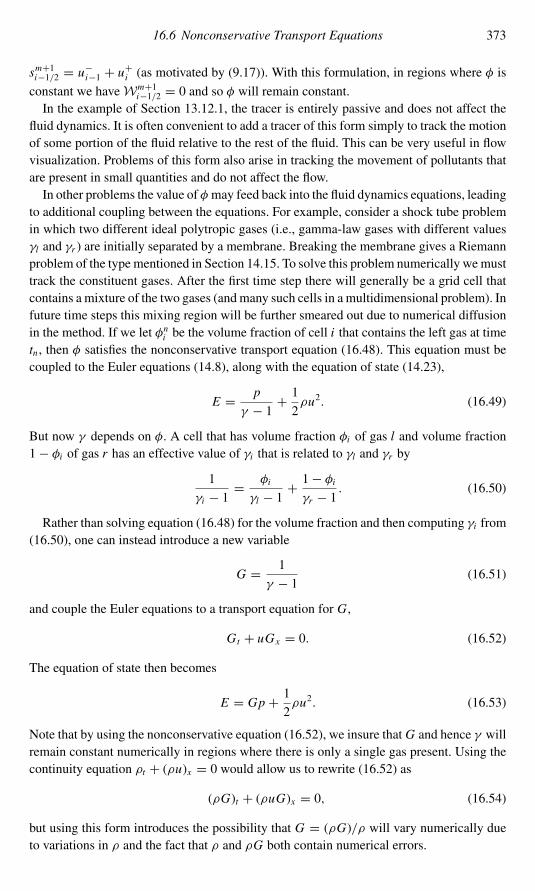
16.6 Nonconservative Transport Equations 373

sm+1i−1/2 = u−i−1 + u+i (as motivated by (9.17)). With this formulation, in regions where φ isconstant we haveWm+1

i−1/2 = 0 and so φ will remain constant.In the example of Section 13.12.1, the tracer is entirely passive and does not affect the

fluid dynamics. It is often convenient to add a tracer of this form simply to track the motionof some portion of the fluid relative to the rest of the fluid. This can be very useful in flowvisualization. Problems of this form also arise in tracking the movement of pollutants thatare present in small quantities and do not affect the flow.In other problems the value of φ may feed back into the fluid dynamics equations, leading

to additional coupling between the equations. For example, consider a shock tube problemin which two different ideal polytropic gases (i.e., gamma-law gases with different valuesγl and γr ) are initially separated by a membrane. Breaking the membrane gives a Riemannproblem of the type mentioned in Section 14.15. To solve this problem numerically wemusttrack the constituent gases. After the first time step there will generally be a grid cell thatcontains a mixture of the two gases (andmany such cells in a multidimensional problem). Infuture time steps this mixing region will be further smeared out due to numerical diffusionin the method. If we let φni be the volume fraction of cell i that contains the left gas at timetn , then φ satisfies the nonconservative transport equation (16.48). This equation must becoupled to the Euler equations (14.8), along with the equation of state (14.23),

E = p

γ − 1 +1

2ρu2. (16.49)

But now γ depends on φ. A cell that has volume fraction φi of gas l and volume fraction1− φi of gas r has an effective value of γi that is related to γl and γr by

1

γi − 1 =φi

γl − 1 +1− φiγr − 1 . (16.50)

Rather than solving equation (16.48) for the volume fraction and then computing γi from(16.50), one can instead introduce a new variable

G = 1

γ − 1 (16.51)

and couple the Euler equations to a transport equation for G,

Gt + uGx = 0. (16.52)

The equation of state then becomes

E = Gp + 1

2ρu2. (16.53)

Note that by using the nonconservative equation (16.52), we insure that G and hence γ willremain constant numerically in regions where there is only a single gas present. Using thecontinuity equation ρt + (ρu)x = 0 would allow us to rewrite (16.52) as

(ρG)t + (ρuG)x = 0, (16.54)

but using this form introduces the possibility that G = (ρG)/ρ will vary numerically dueto variations in ρ and the fact that ρ and ρG both contain numerical errors.

374 16 Some Nonclassical Hyperbolic Problems

It is also important to transport a quantity such as φ or G for which the transport equationcontinues to be valid in the context of cell averages and numerical diffusion. It is temptingto simply use the transport equation

γt + uγx = 0 (16.55)

to advect γ with the flow. This equation does hold for diffusionless gases where no mixingoccurs, since γ will then always be either γl or γr and the contact discontinuity is simplyadvected with the flow. But numerically the gases do mix, and so (16.52) must be usedinstead.If (16.55) is used numerically, then pressure oscillations will typically develop near the

interface between gases, in spite of the fact that the pressure should be constant across thecontact discontinuity. This results from using the wrong equation of state (i.e., the wrongvalue of γ ) in the mixture of gases generated by numerical diffusion. For more discussionof these issues and some numerical examples, see [4], [5], [71], [131], [132], [218], [231],[259], [362], [394], [388], [395], [412], [452].

Exercises

16.1. Determine the entropy-satisfying solution to the Riemann problem for the scalarconservation law qt + f (q)x = 0 for the following nonconvex flux functions anddata. In each case also sketch the characteristics and the structure of the Riemannsolution in the x–t plane.(a) f (q) = q3, ql = 0, qr = 2,(b) f (q) = q3, ql = 2, qr = −1,

16.2. Use the equal area rule to find an expression for the shock location in the Buckley–Leverett equation, as a function of t . Verify that the Rankine–Hugoniot condition isalways satisfied and that the shock propagates at a constant speed that agrees withthe speed f (q∗)/q∗ determined from the convex-hull construction.

16.3. For the Buckley–Leverett equation, show that (16.4) is violated if the shock goesabove q∗.

16.4. Explain why it is impossible to have a Riemann solution involving both a shockand a rarefaction when f is convex or concave.

16.5. For the nonstrictly hyperbolic system of equations (16.13) with data (16.17), plotthe following:(a) the solution to the Riemann problem in state space,(b) the 1-characteristics and 2-characteristics in the x–t plane for this solution, as

in the plots of Figure 13.6, for example.16.6. Repeat Exercise 16.5 for the data (16.18).16.7. (a) Determine the eigenvectors of the Jacobian matrix (16.44), and sketch the

integral curves of each eigenvector in state space (the q–v plane).(b) Sketch the solutions to the Riemann problems shown in Figures 16.9 and 16.10

in state space.

17Source Terms and Balance Laws

So far, we have only considered homogeneous conservation laws of the form qt+ f (q)x = 0.As mentioned briefly in Section 2.5, there are many situations in which source terms alsoappear in the equations, so that we wish to solve the system

qt + f (q)x = ψ(q). (17.1)

Note that these are generally called source terms even if physically they represent a sinkrather than a source (i.e., net loss rather than gain of the quantity q). The equation (17.1) isalso often called a balance law rather than a conservation law.We start with a few examplesshowing how source terms can arise. Others will be encountered later.

Reacting Flow

Fluid dynamics problems often involve chemically reacting fluids or gases. An examplewas mentioned in Section 2.5. An even simpler example is studied below in Section 17.2. Inthese examples the reacting species are assumed to represent a small fraction of the volume,and the chemical reactions have no effect on the fluid dynamics. More interesting problemsarise when the reactions affect the fluid motion, as in combustion problems where the heatreleased by the reactions has a pronounced effect on the dynamics of the flow. Often thechemical reactions occur on much faster time scales than the fastest wave speeds in the gas,resulting in problems with stiff source terms. Some of the issues that arise in this case arediscussed in Section 17.10.

External Forces Such as Gravity

In introducing gas dynamics in Section 2.6, we ignored external forces acting on the gas,such as gravity. External forces give source terms in themomentum equation, andwe then donot expect conservation of the initial momentum, since this force will lead to an accelerationof the fluid and a change in its net momentum.As an example, consider the equations of one-dimensional isentropic gas dynamics in the

presence of a gravitational field, pointing in the negative x-direction (so x now measuresdistance above the earth, say, in a column of gas). The gravitational force acting on thegas causes an acceleration, and hence this force enters into the integral equation for the

375

376 17 Source Terms and Balance Laws

time-derivative of momentum. The equation (2.33) is replaced by

d

dt

∫ x2

x1

ρ(x, t)u(x, t) dx = [ρ(x1, t)u2(x1, t)+ p(x1, t)]−[ρ(x2, t)u2(x2, t)+ p(x2, t)]

−∫ x2

x1

gρ(x, t) dx . (17.2)

The differential equation (2.34) becomes

(ρu)t + (ρu2 + p)x = −gρ. (17.3)

In this case the system (2.39) with q and f (q) given by (2.40) is augmented by a sourceterm with

ψ(q) =[

0−gq1

].

Geometric Source Terms

Often a physical problem in three space dimensions can be reduced to a mathematicalproblem in one or two dimensions by taking advantage of known symmetries in the solution.For example, if we wish to compute a spherically expanding acoustic wave arising from apressure perturbation at one point in space, then we can solve a one-dimensional problemin r (distance from the source) and time. However, the homogeneous conservation law inthree dimensions may acquire source terms when we reduce the dimension. This followsfrom the fact that the interval [r1, r2] now corresponds to a spherical shell, whose volumevaries with r like r2. Hence a substance whose total mass is fixed but that is spreading outradially will have a density (in mass per unit volume) that is decreasing as the substancespreads out over larger and larger spheres.As an example, in Section 18.9 we will see that with radial symmetry, the three-

dimensional acoustics equations can be reduced to the one-dimensional system

pt + K0ur = −2K0ur

,

ρ0ut + pr = 0,(17.4)

where u is now the velocity in the radial direction r . This has the same form as the one-dimensional equations of acoustics but with a geometric source term. Similar geometricsource terms arise if we consider flow in a channel or nozzle with varying cross-sectionalarea. If the variation is relatively slow, then we may be able to model this with a one-dimensional system of equations that includes source terms to model the area variation.This was discussed for a simple advection equation in Section 9.1. More generally thisleads to quasi-one-dimensional models.

Higher-Order Derivatives

Our focus is on developing methods for first-order hyperbolic systems, but many practicalproblems also involve higher-order derivatives such as small viscous or diffusive terms.Examples include the advection–diffusion equation qt + uqx = µqxx , the Navier–Stokes

17.1 Fractional-Step Methods 377

equations in which viscous terms are added to the Euler equations, or the shallow waterequations with bottom friction. Other problems may instead (or in addition) include disper-sive terms involving qxxx or other odd-order derivatives. An example is the Korteweg–deVries (KdV) equation qt + qqx = qxxx . Then the equations may be of the form (17.1) withψ(q) replaced byψ(q, qxx , qxxx , . . . ). We can still viewψ as a source term and apply someof the techniques developed in this chapter. In particular, fractional-step methods are oftenused to incorporate viscous terms in fluid dynamics problems. This is discussed briefly inthe next section and further in Section 17.7.

17.1 Fractional-Step Methods

We will primarily study problems where the homogeneous equation

qt + f (q)x = 0 (17.5)

is hyperbolic and the source terms depend only on q (and perhaps on x) but not on derivativesof q. In this case the equations

qt = ψ(q) (17.6)

reduce to independent systems of ODEs at each point x .One standard approach for such problems is to use a fractional-step or operator-splitting

method, in which we somehow alternate between solving the simpler problems (17.5) and(17.6) in order to approximate the solution to the full problem (17.1). This approach is quitesimple to use and is implemented in the CLAWPACK software (see Section 5.4.6). It allowsus to use high-resolution methods for (17.5) without change, coupling these methods withstandard ODE solvers for the equations (17.6). This approach is described in more detailand analyzed in this chapter. There are situations where a fractional-step method is notadequate, and the analysis presented in this chapter will shed some light on the errors thissplitting introduces and when it can be successfully used.There are also many situations in which the hyperbolic equation is coupled with other

terms that involve derivatives of q . For example, the advection–diffusion equation

qt + uqx = µqxx

can be viewed as an equation of the general form (17.1) in which ψ depends on qxx . Thisequation should more properly be viewed as

qt + (uq − µqx )x = 0,

in conservation form with the flux function uq −µqx (see Section 2.2). But in practice it isoften simplest and most efficient to use high-resolution explicit methods for the advectionpart and implicit methods for the diffusion equation qt = µqxx , such as the Crank–Nicolsonmethod (4.13). These two approaches can bemost easily combined by using a fractional-stepmethod. See [claw/book/chap17/advdiff] for an example.

378 17 Source Terms and Balance Laws

In Section 19.5 we will also see that it is possible to solve a two-dimensional hyperbolicequation of the form

qt + f (q)x + g(q)y = 0

by splitting it into two one-dimensional problems qt + f (q)x = 0 and qt + g(q)y = 0 andusing one-dimensional high-resolution methods for each piece. The same idea extends tothree space dimensions. In this context the fractional-step approach is called dimensionalsplitting. The theory developed in this chapter is also useful in analyzing these methods.

17.2 An Advection–Reaction Equation

To illustrate, we begin with a simple advection–reaction equation.

Example 17.1. Consider the linear equation

qt + uqx = −βq, (17.7)

with data q(x, 0) = q◦(x). This would model, for example, the transport of a radioactivematerial in a fluid flowing at constant speed u down a pipe. The material decays as itflows along, at rate β. We can easily compute the exact solution of (17.7), since along thecharacteristic dx/dt = u we have dq/dt = −βq , and hence

q(x, t) = e−βt q◦(x − ut). (17.8)

17.2.1 An Unsplit Method

Before discussing fractional-step methods in more detail, we first present an unsplitmethodfor (17.7), which more clearly models the correct equation. An obvious extension of theupwind method for advection would be (assuming u > 0)

Qn+1i = Qni −u�t

�x

(Qni − Qni−1

)−�t βQni . (17.9)

This method is first-order accurate and stable for 0 < u�t/�x ≤ 1; see Exercise 8.3.A second-order Lax–Wendroff-style method can be developed by using the Taylor series

q(x, t +�t) ≈ q(x, t)+�t qt (x, t)+ 1

2�t 2qtt (x, t). (17.10)

As in the derivation of the Lax–Wendroff method in Section 6.1, we must compute qtt fromthe PDE. Differentiating qt gives

qtt = −uqxt − βqt , qtx = −uqxx − βqx ,

and combining these, we obtain

qtt = u2qxx + 2uβqx + β2q. (17.11)

17.2 An Advection–Reaction Equation 379

Note that this is more easily obtained by using

∂t q = (−u∂x − β)q,

and hence

∂2t q = (−u∂x − β)2q =(u2∂2x + 2uβ∂x + β2

)q. (17.12)

Using this expression for qtt in (17.10) gives

q(x, t +�t) ≈ q −�t (uqx + βq)+ 1

2�t 2(u2qxx + 2uβqx + β2q)

=(1−�t β + 1

2�t 2β2

)q −�t u (1−�t β) qx + 1

2�t 2 u2qxx . (17.13)

We can now approximate x-derivatives by finite differences to obtain the second-ordermethod

Qn+1i =(1−�t β + 1

2�t 2β2

)Qni −

u�t

2�x(1−�t β) (Qni+1 − Qni−1)

+ u2�t 2

2�x2(Qni−1 − 2Qni + Qni+1

). (17.14)

In order to model the equation (17.7) correctly to second-order accuracy, we must prop-erly model the interaction between the uqx and the βq terms, which brings in the mixedterm 1

2�t2 uβqx in the Taylor series expansion.

For future use we also note that for (17.7) the full Taylor series expansion can be writtenas

q(x, t +�t) =∞∑j=0

(�t) j

j!∂jt q(x, t) =

∞∑j=0

(�t) j

j!(−u∂x − β) j q(x, t), (17.15)

which can be written formally as

q(x, t +�t) = e−�t (u∂x+β)q(x, t). (17.16)

The operator e−�t (u∂x+β), which is defined via the Taylor series in (17.15), is called thesolution operator for the equation (17.7) over a time step of length �t . Applying thisoperator to any function of x gives the evolution of this data after time �t has elapsed.Note that the second derivative qtt might be harder to compute for a more complicated

problem, making it harder to develop second-order numerical methods. It is also not clearhow to introduce limiters effectively into the unsplit method (17.14), as might be desirablein solving problems with discontinuous solutions. In some situations, it is possible to usethe ideas of high-resolution methods based on Riemann solvers and also include the effectsof source terms in the process of solving the Riemann problem. One approach of this form ispresented in Section 17.14, and some others can be found in [34], [127], [128], [151], [155],[161], [162], [167], [168], [482], [216], [217], [284], [325], [381], [471]. In many cases,

380 17 Source Terms and Balance Laws

however, the simple fractional-step approach can often be effectively used, as described inthe next section.

17.2.2 A Fractional-Step Method

A fractional-step method for (17.7) is applied by first splitting the equation into twosubproblems that can be solved independently. For the advection–reaction problem (17.7)we would take these to be:

Problem A: qt + uqx = 0, (17.17)

Problem B: qt = −βq. (17.18)

The idea of the fractional-stepmethod is to combine these by applying the twomethods in analternatingmanner. Formore complicated problems this has great advantage over attemptingto derive an unsplit method. If we split the general problem qt + f (q)x = ψ(q) into thehomogeneous conservation law and a simple ODE, then we can use standard methods foreach. In particular, the high-resolution shock-capturing methods already developed can beused directly for the homogeneous conservation law, whereas trying to derive an unsplitmethod based on the same ideas while incorporating the source term directly can be moredifficult.As a simple example of the fractional-step procedure, suppose we use the upwindmethod

for the A-step and the forward Euler for the ODE in the B-step for the advection–reactionproblem. Then the simplest fractional-step method over one time step would consist of thefollowing two stages:

A-step: Q∗i = Qni −u�t

�x

(Qni − Qni−1

), (17.19)

B-step: Qn+1i = Q∗i − β �t Q∗i . (17.20)

Note that we first take a time step of length�t with upwind, starting with initial data Qni toobtain the intermediate value Q∗i . Then we take a time step of length �t using the forwardEuler method, starting with the data Q∗ obtained from the first stage.It may seem that we have advanced the solution by time 2�t after taking these two

steps of length �t . However, in each stage we used only some of the terms in the originalPDE, and the two stages combined give a consistent approximation to solving the originalequation (17.7) over a single time step of length �t . To check this consistency, we cancombine the two stages by eliminating Q∗ to obtain a method in a more familiar form:

Qn+1i = (1− β �t)Q∗i

= (1− β �t)[Qni −

u�t

�x

(Qni − Qni−1

)]

= Qni −u�t

�x

(Qni − Qni−1

)− β �t Qni + uβ �t 2

�x

(Qni − Qni−1

). (17.21)

The first three terms on the right-hand side agree with the unsplit method (17.9). Thefinal term is O(�t 2) (since (Qni − Qni−1)/�x ≈ qx =O(1)), and so a local truncation error

17.2 An Advection–Reaction Equation 381

analysis will show that this method, though slightly different from (17.9), is also consistentand first-order accurate on the original equation (17.7).A natural question is whether we could improve the accuracy by using a more accurate

method in each step. For example, suppose we use the Lax–Wendroff method in the A-stepand the trapezoidal method, or the two-stage Runge–Kutta method, in the B-step. Wouldwe then obtain a second-order accurate method for the original equation? For this particularequation, the answer is yes. In fact if we use pth-order accurate methods for each step, theresult will be a pth-order accurate method for the full original equation. But this equationis very special in this regard, and this claim should seem surprising. One would think thatsplitting the equation into pieces in this manner would introduce some error that dependson the size of the time step �t and is independent of how well we then approximate thesubproblem in each step. In general this is true – there is a “splitting error” that in generalwould be O(�t) for the type of splitting used above, and so the resulting fractional-stepmethod will be only first-order accurate, no matter how well we then approximate eachstep. This will be analyzed in more detail below.For the case of equation (17.7) there is no splitting error. This follows from the observation

that we can solve (17.7) over any time period �t by first solving the equation (17.17) overtime �t , and then using the result as data to solve the equation (17.18) over time �t . Toverify this, let u∗(x,�t) be the exact solution to the A-problem,

q∗t + uq∗x = 0,q∗(x, 0) = q◦(x).

(17.22)

We use a different symbol q∗(x, t) for the solution to this problem rather than q(x, t), whichwe reserve for the exact solution to the original problem.Then we have

q∗(x,�t) = q◦(x − u�t).

If we now use this as data in solving the B-problem (17.18), we will be solving a differentequation,

q∗∗t = −βq∗∗ (17.23)

with initial data

q∗∗(x, 0) = q∗(x,�t) = q◦(x − u�t).

This is just an ODE at each point x , and the solution is

q∗∗(x,�t) = e−β �t q◦(x − u�t).

Comparing this with (17.8), we see that we have indeed recovered the solution to the originalproblem by this two-stage procedure.Physically we can interpret this as follows. Think of the original equation as modeling a

radioactive tracer that is advecting with constant speed u (carried along in a fluid, say) andalso decaying with rate β. Since the decay properties are independent of the position x , we

382 17 Source Terms and Balance Laws

A−R

A

R

A

R

Fig. 17.1. Illustration of a fractional-step procedure for the advection–reaction equation (17.7) whenthere is no splitting error. The pulse shown in the lower left simultaneously advects and decays asindicated by the diagonal arrow labeled A-R. The same result is obtained if the pulse first advectsto the right following the arrow A and then is allowed to decay via the reaction term, following thearrow R, or if the reaction and advection are performed in the opposite order.

can think of first advecting the tracer over time �t without allowing any decay, and thenholding the fluid and tracer stationary while we allow it to decay for time �t . We will getthe same result, and this is what we have done in the fractional-step method. Figure 17.1illustrates this.We would also get the same result if we first allowed the tracer to decay at the initial

location and then advected the decayed profile, which amounts to switching the order inwhich the two subproblems are solved (see Figure 17.1). We say that the solution operatorsfor the two subproblems commute, since we can apply them in either order and get the sameresult. In general if these operators commute, then there is no splitting error, a fact that wewill investigate more formally in Section 17.3. (Here we are only discussing the Cauchyproblem. Boundary conditions can further complicate the situation; see Section 17.9).Another way to examine the splitting error, which must be used more generally when we

do not know the exact solution to the equations involved, is to use Taylor series expansions.(This approach can be used also for nonlinear problems.) If we look at a time step of length�t , then solving the A-equation gives

q∗(x,�t) = q∗(x, 0)+�t q∗t (x, 0)+1

2�t 2q∗t t (x, 0)+ · · ·

= q∗(x, 0)− u�t q∗x (x, 0)+1

2u2�t 2q∗xx (x, 0)− · · ·

= q(x, 0)− u�t qx (x, 0)+ 1

2u2�t 2qxx (x, 0)− · · · . (17.24)

Similarly, if we solve the ODE problem (17.23) with general initial data q∗∗(x, 0), we obtain

q∗∗(x,�t) = q∗∗(x, 0)+�t q∗∗t (x, 0)+1

2�t 2q∗∗t t (x, 0)+ · · ·

=(1− β �t + 1

2β2�t 2 + · · ·

)q∗∗(x, 0). (17.25)

17.2 An Advection–Reaction Equation 383

If we now use the result from (17.24) as the initial data in (17.25), we obtain

q∗∗(x,�t) =(1−�t β + 1

2�t 2β2 − · · ·

)(q(x, 0)− u�t qx (x, 0)

+ 1

2u2�t 2qxx (x, 0)+ · · ·

)= q −�t (uqx + βq)+ 1

2�t 2(u2qxx + 2uβqx + β2q)+ · · · . (17.26)

Comparing this with the Taylor series expansion (17.13) that we used in deriving the unsplitLax–Wendroff method shows that this agrees with q(x,�t), at least for the three termsshown, and in fact to all orders.Note that the mixed term uβ �t 2qx needed in the qtt -term from (17.11) now arises

naturally from taking the product of the two Taylor series (17.24) and (17.25). In fact, wesee that for this simple equation we can write (17.25) as

q∗∗(x,�t) = e−β �t q∗∗(x, 0),

while (17.24) can be written formally as

q∗(x,�t) = e−u�t ∂x q◦(x).

If we now use q∗(x,�t) as the data q∗∗(x, 0) as we do in the fractional-step method, weobtain

q∗∗(x,�t) = e−β �t e−u�t ∂x q◦(x).

Multiplying out the Taylor series as we did in (17.26) verifies that these exponentials satisfythe usual rule, so that to compute the product we need only add the exponents, i.e.,

q∗∗(x,�t) = e−�t (u∂x+β)q◦(x).

The exponential appearing here is exactly the solution operator for the original equation,as in (17.16), and so again we see that q∗∗(x,�t) = q(x,�t) and there is no splittingerror.The fact that there is no splitting error for the problem (17.7) is a reflection of the fact that,

for this problem, the solution operator for the full problem is exactly equal to the productof the solution operators of the two subproblems (17.17) and (17.18). This is not generallytrue for other problems.

Example 17.2. Suppose we modify the equation slightly so that the decay rate β dependson x ,

qt + uqx = −β(x)q. (17.27)

Then our previous argument for the lack of a splitting error breaks down – advecting thetracer a distance u�t and then allowing it to decay, with rates given by the values of β

384 17 Source Terms and Balance Laws

A−R

A

R

A

R

Fig. 17.2. Illustration of a fractional-step procedure for the advection–reaction equation (17.27),where there is a splitting error because the decay rate β depends on x . The pulse shown in the lowerleft simultaneously advects and decays, as indicated by the diagonal arrow labeled A-R. Differentresults are obtained if the pulse first advects to the right following the arrow A and then is allowed todecay via the reaction term evaluated at the final position, following the arrow R, or if the reactionand advection are performed in the opposite order.

at the final positions, will not in general give the same result as when the decay occurscontinuously as it advects, using the instantaneous rate given by β(x) at each point passed.Figure 17.2 illustrates the fact that solution operators for the two subproblems do not

commute, shown for the case β(x) = 1 − x over 0 ≤ x ≤ 1, so that the decay rate issmaller for larger x . First advecting and then reacting gives too little decay, while firstreacting and then advecting gives too much decay. Note that this is shown for very large�t in Figure 17.2 in order to illustrate the effect clearly. With a numerical fractional-stepmethod we would be using much smaller time steps to solve the problem over this timeperiod, in each step advecting by a small amount and then reacting, so that reasonableresults could still be obtained, though formally only first-order accurate as the time step isreduced. See Section 17.5 for some numerical results.The accuracy of the fractional-step method on (17.27) can be analyzed formally using

Taylor series expansions again. Rather than developing this expansion for this particularexample, we will first examine the more general case and then apply it to that case.

17.3 General Formulation of Fractional-Step Methods for Linear Problems

Consider a more general linear PDE of the form

qt = (A+ B)q, (17.28)

where A and B may be differential operators, e.g., A=−u∂x and B=−β(x) inExample 17.2. For simplicity suppose that A and B do not depend explicitly on t , e.g.,β(x) is a function of x but not of t . Then we can compute that

qtt = (A+ B)qt = (A+ B)2q,

17.3 General Formulation of Fractional-Step Methods for Linear Problems 385

and in general

∂jt q = (A+ B) j q. (17.29)

We have used this idea before in calculating Taylor series, e.g., in (17.12).Note that if A or B do depend on t , then we would have to use the product rule, e.g.,

qtt = (A+ B)qt + (At + Bt )q,and everything would become more complicated. Also note that if the problem is nonlinearthen the Taylor series expansion can still be used if the solution is smooth, but we don’tgenerally have a simple relation of the form (17.29).In our simple case we can write the solution at time t using Taylor series as

q(x,�t) = q(x, 0)+�t(A+ B)q(x, 0)+ 1

2�t 2(A+ B)2q(x, 0)+ · · ·

=(I +�t (A+ B)+ 1

2�t 2(A+ B)2 + · · ·

)q(x, 0)

=∞∑j=0

�t j

j!(A+ B) j q(x, 0), (17.30)

which formally can be written as

q(x,�t) = e�t (A+B)q(x, 0).With the fractional-step method, we instead compute

q∗(x,�t) = e�tA q(x, 0),and then

q∗∗(x,�t) = e�t Bq∗(x,�t) = e�t Be�tA q(x, 0),and so the splitting error is

q(x,�t)− q∗∗(x,�t) = (e�t (A+B) − e�t Be�tA) q(x, 0). (17.31)

This should be calculated using the Taylor series expansions. We have (17.30) already,while

q∗∗(x,�t) =(I +�t B + 1

2�t 2B2 + · · ·

)(I +�t A+ 1

2�t 2A2 + · · ·

)q(x, 0)

=(I +�t (A+ B)+ 1

2�t 2(A2 + 2BA+ B2)+ · · ·

)q(x, 0). (17.32)

The I + �t (A + B) terms agree with (17.30). In the �t 2 term, however, the term from(17.30) is

(A+ B)2 = (A+ B)(A+ B)= A2 +AB + BA+ B2. (17.33)

386 17 Source Terms and Balance Laws

In general this is not the same as

A2 + 2BA+ B2,

and so the splitting error is

q(x,�t)− q∗∗(x,�t) = 1

2�t 2(AB − BA)q(x, 0)+O(�t 3). (17.34)

The splitting error depends on the commutator AB − BA and is zero only in the specialcase when the differential operators A and B commute (in which case it turns out that allthe higher-order terms in the splitting error also vanish).

Example 17.3. For the problem considered in Example 17.1,

A = −u∂x and B = −β.

We then have ABq = BAq = uβqx . These operators commute for β constant, and thereis no splitting error.

Example 17.4. Now suppose β = β(x) depends on x as in Example 17.2. Then we have

ABq = u∂x (β(x)q) = uβ(x)qx + uβ ′(x)q,

while

BAq = β(x)uqx .

These are not the same unless β ′(x) = 0. In general the splitting error will be

q(x,�t)− q∗∗(x,�t) = 1

2�t 2uβ ′(x)q(x, 0)+O(�t 3).

If we now design a fractional-step method based on this splitting, we will see that thesplitting error alone will introduce anO(�t 2) error in each time step, which can be expectedto accumulate to anO(�t) error after the T/�t time steps needed to reach some fixed time T(in the best case, assuming the method is stable). Hence even if we solve each subproblemexactly within the fractional-step method, the resulting method will be only first-orderaccurate. If the subproblems are actually solved with numerical methods that are sth-orderaccurate, the solution will still only be first-order accurate no matter how large s is. At leastthis is true asymptotically as the mesh spacing tends to zero. In practice results that areessentially second-order accurate are observed, for reasons described in Section 17.5.Of course this order of accuracy can only be obtained for smooth solutions. We are often

interested in problems where the solution is not smooth, in which case a lower order ofaccuracy is generally observed. In this case the ability to easily use high-resolution methodsfor the hyperbolic portion of the problem is an advantage of the fractional-step approach. Onthe other hand, it is not so clear that the method even converges in this case, since the abovearguments based on Taylor series expansions do not apply directly. For some convergenceresults, see for example [258], [442], [443].

17.4 Strang Splitting 387

17.4 Strang Splitting

The above form of fractional-step method, sometimes called the Godunov splitting, ingeneral is only first-order accurate formally. It turns out that a slight modification of thesplitting idea will yield second-order accuracy quite generally (assuming each subproblemis solved with a method of at least this accuracy). The idea is to solve the first subproblemqt =Aq over only a half time step of length �t/2. Then we use the result as data for afull time step on the second subproblem qt =Bq , and finally take another half time stepon qt =Aq . We can equally well reverse the roles of A and B here. This approach isoften called Strang splitting, as it was popularized in a paper by Strang [426] on solvingmultidimensional problems.To analyze the Strang splitting, note that we are now approximating the solution operator

e�t (A+B) by e12�tAe�t Be

12�tA. Taylor series expansion of this product shows that

e12�tAe�t Be

12�tA =

(I + 1

2�t A+ 1

8�t 2A2 + · · ·

)(I +�t B + 1

2�t 2B2 + · · ·

)×(I + 1

2�t A+ 1

8�t 2A2 + · · ·

)= I +�t (A+ B)+ 1

2�t 2(A2 +AB + BA+ B2)+O(�t 3).

(17.35)

Comparingwith (17.30), we see that theO(�t 2) term is now captured correctly. TheO(�t 3)term is not correct in general, however, unless AB = BA.Note that over several time steps we can simplify the expression obtained with the Strang

splitting. After n steps we have

Qn = (e 12�tAe�t Be 12�tA)(e 12�tAe�t Be 12�tA) · · · (e 12�tAe�t Be 12�tA)Q0 (17.36)

repeated n times. Dropping the parentheses and noting that e12�tAe

12�tA = e�tA, we obtain

Qn = e 12�tA e�t Be�tAe�t Be�tA · · · e�t B e 12 kAQ0. (17.37)

This differs from the Godunov splitting only in the fact that we start and end with a halftime step on A, rather than starting with a full step on A and ending with B.Another way to achieve this same effect is to simply take steps of length �t on each

problem, as in the first-order splitting, but to alternate the order of these steps in alternatetime steps, e.g.,

Q1 = e�t Be�tAQ0,Q2 = e�tAe�t BQ1,Q3 = e�t Be�tAQ2,Q4 = e�tAe�t BQ3,

...

388 17 Source Terms and Balance Laws

If we take an even number of time steps, then we obtain

Qn = (e�tAe�t B)(e�t Be�tA)(e�tAe�t B)(e�t Be�tA) · · · (e�tAe�t B)(e�t Be�tA)Q0

= e�tA(e�t Be�t B)(e�tAe�tA)(e�t Be�t B) · · · (e�t Be�t B)e�tAQ0.Since e�t Be�t B = e2�t B, this is essentially the same as (17.36) but with 1

2�t replaced by�t . This is generally more efficient than the approach of (17.36), since a single step with thenumerical method approximating e�tA is typically cheaper than two steps of length�t/2.On the other hand, this form is more difficult to implement with variable time steps �t , asare often used in practice. An even number of steps must be taken and the value of �t ineach pair of steps must be the same, in order to obtain the desired cancellation of errors.In CLAWPACK, either the Godunov splitting or the Strang splitting (implemented in the

form (17.36)) can be selected by setting method(5) = 1 or 2 respectively. In this case asubroutine src1.f must be provided that solves the qt = ψ(q) subproblem arising fromthe source terms.

17.5 Accuracy of Godunov and Strang Splittings

The fact that the Strang splitting is so similar to the first-order splitting suggests that thefirst-order splitting is not really so bad, and in fact it is not. While formally only first-orderaccurate, the coefficient of the O(�t) term may be much smaller than coefficients in thesecond-order terms arising from discretization of e�tA and e�t B.For this reason the simpler and more efficient Godunov splitting is often sufficient. It

is also easier to implement boundary conditions properly with the Godunov splitting, asdiscussed in Section 17.9.

Example 17.5. Figure 17.3 shows results at time t = 0.5 from solving the problem(17.27) with u= 1, β(x)= 1 − x , and initial data consisting of a Gaussian pulse cen-tered at x = 0.25. The Godunov and Strang splittings are compared, where in each case the

(a)0.5 0.6 0.7 0.8 0.9 1

0

0.2

0.4

0.6

0.8

1

1.2Upwind with Strang splitting Lax–Wendroff with Godunov splittingLax–Wendroff with Strang splitting

(b)

10−3

10−2

10−1

10−4

10−3

10−2

10−1

100

∆x

max

norm

of e

rror

Upwind with Strang splitting Lax Wendroff with Godunov splitting–Lax–Wendroff with Strang splitting

Fig. 17.3. Comparison of results with three methods applied to the problem (17.27). (a) Com-puted and true solution for �x = 0.02. (b) Log–log plot of max-norm errors vs. �x . Notethat the Godunov splitting is essentially as accurate as the Strang splitting for this problem.[claw/book/chap17/nocommute]

17.6 Choice of ODE Solver 389

Lax–Wendroff method is used for the advection equation and the second-order two-stageRunge–Kuttamethod is used for the source term.On this gridwith�x = 0.02, the results arevisually indistinguishable, even though the Godunov splitting is formally only first-orderaccurate.For contrast, Figure 17.3(a) also shows the results obtained if the first-order upwind

method is used in place of the Lax–Wendroff method in the Strang splitting. This first-ordermethod causes a substantial smearing of the solution.Figure 17.3(b) shows log–log plots of the error in the max norm for each of these three

methods as the grid is refined. For very fine grids the Godunov splitting is slightly lessaccurate and asymptotically approaches first-order, but even for the finest grid used (�x =1/400) it is only slightly less accurate than the Strang splitting. By contrast the upwindmethod is much less accurate. As in the discussion of the accuracy of limiters in Section 8.5,it is important to realize that order of accuracy is not the full story.

17.6 Choice of ODE Solver

Consider the Godunov splitting, and suppose we have already obtained Q∗ from Qn bysolving the conservation law (17.5). We now wish to advance Q∗i to Q

n+1i by solving the

ODE qt = ψ(q) over time �t in each grid cell. In some cases this equation can be solvedexactly. For the system (17.4), for example, the source terms alone yield

pt = −2K0ur

,

ut = 0.(17.38)

Since u is constant in this system, the value of pt is constant and this ODE is easily solvedexactly, yielding

pn+1i = p∗i −�t (2K0u∗i )/ri ,un+1i = u∗i .

(17.39)

For more complicated source terms, e.g., those arising from chemical kinetics with manyinteracting species, it will be necessary to use a numerical ODE solver in each grid cell.We typically want to use a method that is at least second-order accurate to maintain overallaccuracy. A wide variety of ODE solvers are available for systems of the general formy′ =ψ(y) where y(t)∈R

m . Note, however, that in general we cannot use multistep methodsthat require more than one level of data (e.g., yn−1 as well as yn) to generate the solutionyn+1 at the next time level. This is because we only have data Q∗i to use in computingQn+1i . Previous values (e.g., Qni or Q

∗i from the previous time step) are not suitable to

use in the context of multistep methods, because Q∗i is computed from Qni by solving adifferent equation (the conservation law (17.5)) than the ODE we are now attempting toapproximate.In many cases a simple explicit Runge–Kutta method can be effectively used. These

are multistage one-step methods that generate intermediate values as needed to constructhigher-order approximations. A simple second-order accurate two-stage method is often

390 17 Source Terms and Balance Laws

sufficient for use with high-resolution methods, for example the classical method

Q∗∗i = Q∗i +�t

2ψ(Q∗i ),

Qn+1i = Q∗i +�t ψ(Q∗∗i ).(17.40)

One must ensure that the explicit method is stable with the time step �t being used, orperhaps take N time steps of (17.40) using a smaller step size�t/N to advance Q∗i to Q

n+1i

stably.

17.7 Implicit Methods, Viscous Terms, and Higher-Order Derivatives

If the ODEs qt = ψ(q) are stiff, as discussed in Section 17.10, then it may be necessaryto use an implicit method in this step in order to use a reasonable time step. In this caseother numerical issues arise, and even a stable implicit method may give poor results, asillustrated in Section 17.16.A natural implicit method to consider is the trapezoidal method, a second-order accurate

one-step method that takes the form

Qn+1i = Q∗i +�t

2

[ψ(Q∗i )+ ψ

(Qn+1i

)]. (17.41)

Note, by the way, an advantage of the fractional-step approach for stiff equations. Whilethis is an implicit method, the equations obtained in the i th cell are decoupled from theequations in every other cell, and so these equations can be solved relatively easily. Thecoupling between grid cells arises only in the hyperbolic part of the equation, which canstill be solved with an explicit high-resolution method.In some cases the source term ψ may depend on derivatives of q as well as the pointwise

value, for example if wewish to solve a viscous equation qt+ f (q)x = µqxx by a fractional-step approach. In this case the derivatives will have to be discretized, bringing in values ofQ at neighboring grid cells. For example, the term ψ(Qn+1i ) in (17.41) would be replacedby

µ(Qn+1i−1 − 2Qn+1i + Qn+1i+1

)/�x2, (17.42)

and similarly for ψ(Q∗i ). The trapezoidal method (17.41) would then become the Crank–Nicolsonmethod (4.13), andwould require solving a tridiagonal linear system. It is generallynecessary to use an implicit method for source terms involving second-order derivatives,since an explicit method would require �t = O(�x2). With higher-order derivatives evensmaller time steps would be required with an explicit method. The first-order hyperbolicpart typically allows �t =O(�x), based on the CFL condition, and we generally hope totake time steps of this magnitude.Although the trapezoidal method is second-order accurate andA-stable, it is onlymargin-

ally stable in the stiff case, and this can lead to problems in the context of stiff hyperbolicequations, as illustrated in Section 17.16. For this reason the so-called TR-BDF2 methodis generally recommended as a second-order implicit method. This is a two-stage Runge–Kutta method that combines one step of the trapezoidal method over time�t/2 with a step

17.8 Steady-State Solutions 391

of the second-order BDF method, using the intermediate result as another time level. Forthe ODE qt = ψ(q) this takes the form

Q∗∗i = Q∗i +�t

2[ψ(Q∗i )+ ψ(Q∗∗i )],

Qn+1i = 1

3

[4Q∗∗i − Q∗i +�t ψ

(Qn+1i

)].

(17.43)

Ifψ represents viscous terms, sayψ = µqxx , then again thiswill have to be discretized usingterms of the form (17.42), leading to tridiagonal systems in each stage of the Runge–Kuttamethod.An example illustrating the superiority of this method over the Crank–Nicolson method

for handling a diffusion term is given in [462], for a reaction–diffusion–advection equationarising in amodel of chemotaxis in bacterial growth.Another example of how the trapezoidalmethod can fail is given in Section 17.16.

17.8 Steady-State Solutions

There are some other potential pitfalls in using a fractional-step method to handle sourceterms. In this section we consider some of these in relation to computing a steady-statesolution, one in which qt (x, t) ≡ 0 and the function q(x, t) is independent of time. Forthe homogeneous constant-coefficient linear hyperbolic equation qt + Aqx = 0, if qt = 0then qx = 0 also and the only steady-state solutions are the constant functions. When asource term is added, there can be more interesting steady-state solutions. Consider theadvection–reaction equation (17.7) from Section 17.2, qt + uqx =−βq. Setting qt = 0gives the ODE qx = −(β/u)q , and hence this has the steady-state solution

q(x, t) = Ce−(β/u)x . (17.44)

In practice we would have a finite domain and some boundary conditions that must alsobe satisfied. Consider the same PDE on the domain 0 < x < 1 with initial data q◦(x) andthe boundary condition

q(0, t) = g0(t)

at the inflow boundary. The general solution is

q(x, t) ={e−βt q◦(x − ut) if t < x/u,

e−(β/u)x g0(t − x/u) if t > x/u.(17.45)

In the special case g0(t) ≡ C , some constant, the solution q(x, t) will reach the steady state(17.44) for all t > 1/u, regardless of the initial conditions.Recall the physical interpretation of this equation as the advection at velocity u of a

radiaoactive tracer that decays at rate β. The boundary condition q(0, t) = C correspondsto inflowing fluid having concentration C at all times. Up to time t = 1/u the initial dataalso has an effect on the solution, but after this time all of the fluid (and tracer) initially

392 17 Source Terms and Balance Laws

(a)

0 0.2 0.4 0.6 0.8 10

0.2

0.4

0.6

0.8

1

1.2

(b)

0 0.2 0.4 0.6 0.8 10

0.2

0.4

0.6

0.8

1

1.2

Fig. 17.4. Balance between advection and decay in a steady state solution. (a) The steady-statesolution q(x) = e−(β/u)x is shown as the solid line. After advection by a distance u�t to the right,q∗(x) = q(x − u�t), the dashed line. (b) The advected solution decays by e−β�t , reproducingq(x) = e−β�t q∗(x).

in the domain 0 < x < 1 has flowed out the boundary at x = 1, and the steady state isreached.It is important to note that being in a steady state does not in general mean that nothing

is happening. In the above example, new tracer is constantly being introduced at x = 0,is advected downstream, and decays. The steady state results from a balance between theadvection and decay processes. The terms uqx and −βq are both nonzero but cancel out.This balance is illustrated in Figure 17.4.This suggests that we may have difficulties with a fractional-step method, where we first

solve the advection equation ignoring the reactions and then solve the reaction equationignoring the advection. Even if we start with the exact steady-state solution, each of thesesteps can be expected to make a change in the solution. In principle the two effects shouldexactly cancel out, but numerically they typically will not, since very different numericaltechniques are used in each step.In practice we generally don’t know the steady-state solution, so we cannot use this as

initial data. Instead we wish to determine the steady state by starting with some arbitraryinitial data (perhaps some approximation to the steady state) and then marching forward intime until a steady state is reached. This can be viewed as an iterative method for solvingthe steady-state problem obtained by setting qt = 0 in the equation, with each time stepbeing one iteration. If all we care about is the steady-state solution, then this may not be avery efficient iterative method to use. A method designed specifically for the steady-statesolution may be preferable. Such a method would be designed to converge as rapidly aspossible to an accurate steady-state solution without necessarily giving an accurate time-dependent solution along the way. The study of such methods is a major topic in its ownright and is not discussed further here.However, time-marching methods are often used to compute steady-state solutions. For

relatively small problemswhere computational efficiency is not an issue, itmaybemore cost-effective to use an existing time-marching code than to develop a new code specifically forthe steady-state problem. One may also be interested in related time-dependent issues such

17.9 Boundary Conditions for Fractional-Step Methods 393

as how convergence to steady state occurs in the physical system, the dynamic stability ofthe steady-state solution to small perturbations, or the solution of time-dependent problemsthat are near a steady state. Such quasisteady problems require a time-accurate approachthat can also handle steady states well. One approach is presented in Section 17.14.Fractional-step method can often be used to successfully compute steady-state or

quasisteady solutions, but several issues arise. As mentioned above, the steady state resultsfrom a balance (cancellation) between two dynamic processes that are a handled separatelyin a fractional-step method. In some cases the method may not even converge, but insteadwill oscillate in time near the correct solution. This can happen if a high-resolution methodwith limiter functions is used for the hyperbolic part, since the limiter depends on thesolution and effectively switches between different methods based on the behavior of thesolution.Even when the method converges, the numerical steady state obtained will typically

depend on the time step used. This is rather unsatisfying, since the steady solution dependsonly on x and so we would like the numerical solution generated by a particular methodto depend only on �x . By contrast, unsplit methods can often be developed in which thesteady state is independent of �t . See Exercise 17.4 for one example.

17.9 Boundary Conditions for Fractional-Step Methods

When a fractional-step method is used, we typically need to impose boundary conditions inthe hyperbolic step of the procedure.Wemay also need to impose boundary conditions in thesource term step(s) if the source terms involve spatial derivatives of q – for example, if theseare diffusion terms, then we are solving the diffusion equation, which requires boundaryconditions at each boundary. The boundary conditions for the original PDE must be usedto determine any boundary conditions needed for the fractional steps, but the connectionbetween these is often nontrivial.As a simple example, consider the advection–reaction equation (17.7) with the constant

boundary data q(0, t) = g0(t) ≡ 1, which results in the steady-state solution (17.44) forlarge t (with C = 1). Suppose we use a fractional-step method with the Godunov splitting,in which we first solve the advection equation qt + uqx = 0 over time�t and then the ODEqt = −βq over time �t . Moreover, suppose we choose �t so that u�t/�x = 1 and theadvection equation is solved exactly via

Q∗i = Qni−1, (17.46)

and then we also solve the ODE exactly via

Qn+1i = e−β �t Q∗i . (17.47)

These steps can be combined to yield

Qn+1i = e−β �t Qni−1. (17.48)

For this simple problem we observed in Section 17.2.2 that there is no splitting error, andhence this procedure should yield the exact solution. If Qni−1 is the exact cell average ofq(x, tn) over cell Ci−1, then Qn+1i will be the exact cell average of q(x, tn+1) over cell Ci .

394 17 Source Terms and Balance Laws

But to determine Qn+11 we must also use the boundary conditions. To implement the step(17.46) at i = 1 we must first specify a ghost cell value Qn0 as described in Chapter 7.(Note that the step (17.47) does not require any boundary data, since we are solving anODE within each grid cell.)As a first guess at the value Qn0, we might follow the discussion of Section 7.2.2 and use

the integral of (7.8). This would give Qn0 = 1, since the specified boundary condition isindependent of time. It appears that we have specified the exact ghost-cell value, and weknow that the method being used in the interior is exact, and yet this combination will notproduce the exact solution numerically. The value Qn+11 will not be the exact cell averageof q(t, tn+1) over the cell C1. The computed value will be

Qn+11 = e−β�t = e−(β/u)�x = 1− (β/u)�x +O(�x2), (17.49)

while the true cell average of the solution (17.44) is easily computed to be

1

�x

∫C1e−(β/u)x dx = − u

β �x

(e−(β/u)�x − 1) = 1− 1

2(β/u)�x +O(�x2). (17.50)

The numerical value (17.49) is too small by O(�x). In later time steps this error willpropagate downstream, and eventually the entire solution will have an O(�x) error.The reason for this error is made clear in Figure 17.5. Figure 17.5(a) shows the steady-

state solution, which is used as initial data, along with the function obtained after time�t ifwe solve the advection equation alone with the boundary condition g0(t)= 1. Figure 17.5(b)shows the results if we now solve the decay equation using the advected solution as data.Away from the boundary the decay exactly cancels the apparent growth due to the advection,and the exact steady-state solution is recovered. Near the boundary the use of the constantinflow boundary condition g0(t)= 1 leads to the wrong profile.It is clear how to fix this once we realize that the boundary condition q(0, t)= 1 is the

proper boundary condition for the full equation qt + uqx = − βq , but is not the properboundary condition for the pure advection equation q∗t + uq∗x = 0 that is being solved by

(a)0 0.2 0.4 0.6 0.8 1

0

0.2

0.4

0.6

0.8

1

1.2

(b)0 0.2 0.4 0.6 0.8 1

0

0.2

0.4

0.6

0.8

1

1.2

Fig. 17.5. The effect of incorrect boundary conditions in a fractional-stepmethod. (a) The steady-statesolution q(x) = e−(β/u)x is shown as the solid line. After advection by a distance u�t to the rightwith q∗(0, t) = 1, the solution is shown as the dashed line. (b) The advected solution decays by e−β�tand an error is apparent near the boundary.

17.9 Boundary Conditions for Fractional-Step Methods 395

the upwindmethod in the first step of the fractional-stepmethod. If we denote the solution tothis equation by q∗(x, t) for t ≥ tn , then this function is different from q(x, t) for t > tn andrequires different boundary conditions. Figure 17.4(b) suggests what the correct boundaryconditions are.Wewould like q∗(x, tn +�t) to be the function e−(β/u)(x−u�t)= eβ �t e−(β/u)xfor all x ≥ 0, so that after the decay step we will recover e−(β/u)x for all x ≥ 0. To obtainthis we clearly need to impose a boundary condition on q∗(0, t) that is growing with t ,

q∗(0, t) = eβ(t−tn ) ≡ g∗0 (t),

and it is this function that should be used in determining the ghost-cell value Qn0 instead ofthe original boundary condition g0(t) = 1. Note that if we evaluate the integral from (7.8)using this function g∗0 (t), we obtain

Qn0 =u

β �x

(e(β/u)�x − 1). (17.51)

Using this boundary value in the formulas (17.47) and (17.48) results in

Qn+11 = e−β �t Qn0 =u

β �x(1− e−β�x ), (17.52)

which is exactly the value (17.50).For the advection–decay equation with a more general time-dependent boundary condi-

tion q(0, t) = g0(t), the proper boundary condition to use in the advection step is

q∗(0, t) = g∗0 (t) = eβ(t−tn )g0(t).

The integral (7.8) can perhaps be evaluated exactly using this function in place of g0, or anapproximation such as (7.9) could again be used, which would result in

Qn0 = eβ �t/2g0(tn + �x

2u

). (17.53)

The proper value for the ghost-cell value Qn−1 can be found similarly if a second ghost cellis needed (for a method with a wider stencil).For the simple example considered above it was easy to determine the correct boundary

conditions for q∗ based on our knowledge of the exact solution operators for the advectionand decay problems. For other problems it may not be so easy to determine the correctboundary conditions, but an awareness of the issues raised here can often help in derivingbetter boundary conditions thanwould be obtained by simply using the boundary conditionsfrom the original equation. Since the required modification to the boundary conditions istypicallyO(�t), as in the above example, this canmake a significant difference in connectionwithmethods that are second-order accurate or better. Amore general procedure for derivingthe proper intermediate boundary conditions for a linear hyperbolic equation is discussedin [276].

396 17 Source Terms and Balance Laws

17.10 Stiff and Singular Source Terms

Most of the source terms that have appeared so far have been bounded functions corre-sponding to a source that is distributed in space. In some problems source terms naturallyarise that are concentrated at a single point, a delta function, or at least are concentratedover a very small region compared to the size of the domain. In some cases this may be anexternal source depending explicitly on x that is spatially concentrated. An example of thisnature was presented in Section 16.3.1, where we considered an advection equation with adelta function source of tracer. We consider another problem of this type in Section 17.11.In other cases the sourceψ(q) depends only on the solution and yet the solution naturally

develops structures in which the source terms are nonzero (and very large) only over verysmall regions in space. For example, this often happens if the source terms model chemicalreactions between different species (reacting flow) in cases where the reactions happen ontime scales much faster than the fluid dynamic time scales. Then solutions can developthin reaction zoneswhere the chemical-kinetics activity is concentrated. Such problems aresaid to have stiff source terms, in analogy with the classical case of stiff ODEs. Stiffnessis common in kinetics problems. Reaction rates often vary by many orders of magnitude,so that some reactions occur on time scales that are very short compared to the time periodthat must be studied. One classic example of a stiff reacting flow problem is a detonationwave; an explosion in which a flammable gas burns over a very thin reaction zone thatmoves through the unburned gas like a shock wave, but with a more complicated structure.(See, for example, [92], [136], [156].) The thin reaction zone can be idealized as a delta-function source term that moves with the detonation wave. Some simpler examples arestudied in this chapter. We will see that singular source terms lead to a modification of theRankine–Hugoniot jump conditions that determine the structure and speed of propagatingdiscontinuities.

17.11 Linear Traffic Flow with On-Ramps or Exits

As an illustration of a hyperbolic equation with a singular source term, consider traffic flowon a one-lane highway with on-ramps and exits where cars can enter or leave the highway.Then the total number of cars on the highway is not conserved, and instead there are sourcesand sinks. The corresponding source terms in the equation are delta functions with positivestrength at the locations of the on-ramps and negative strength at exits.As an example, consider a single on-ramp with a flux D at some point x0, so that the

source term is

ψ(x) = Dδ(x − x0). (17.54)

To begin with, suppose the traffic is sufficiently light that it moves at some constant speedu independent of the density q . Then the traffic flow is modeled by an advection equationas in Section 9.4.2 with the addition of the source term (17.54),

qt + uqx = Dδ(x − x0). (17.55)

This is exactly the problem considered in Section 16.3.1, and the Riemann solution hasa jump from ql to qm = ql + D/u at x = x0 (resulting from the source) and then a jump

17.12 Rankine–Hugoniot Jump Conditions at a Singular Source 397

from qm to qr at x = ut (resulting from the initial data, and moving downstream with thetraffic).

17.12 Rankine–Hugoniot Jump Conditions at a Singular Source

The jump in q at the on-ramp can be derived from a more general formula, an extension ofthe Rankine–Hugoniot jump condition to the case where there is a singular source movingwith the jump. This formula will be needed to study the nonlinear traffic flow problem.Consider a general conservation law coupled with a delta-function source term moving

at some speed s(t),

qt + f (q)x = D δ(x − X (t)), (17.56)

where X ′(t) = s(t). We will compute jump conditions at X (t) using the same procedureas in Section 11.8 for the homogeneous equation. The differential equation (17.56) resultsfrom an integral conservation law that, over a small rectangular region such as the oneshown in Figure 11.7, has the form (for s < 0 as in the figure)

∫ x1+�x

x1

q(x, t1 +�t) dx −∫ x1+�x

x1

q(x, t1) dx

=∫ t1+�t

t1

f (q(x1, t)) dt −∫ t1+�t

t1

f (q(x1 +�x, t)) dt

+∫ t1+�t

t1

∫ x1+�x

x1

D δ(x − X (t)) dx dt. (17.57)

Note that over this time interval the point X (t) always lies between x1 and x1+�x , so that∫ x1+�x

x1

D δ(x − X (t)) dx = D,

and hence the equation (17.57) can be approximated by

�x qr −�x ql = �t f (ql)−�t f (qr )+�t D +O(�t 2). (17.58)

Using �x = −s�t , dividing by −�t , and taking the limit as �t → 0 gives

s(qr − ql) = f (qr )− f (ql)− D. (17.59)

This is identical to the Rankine–Hugoniot jump condition (11.20) but with an additionalterm resulting from the singular source.Note that if the source term ψ(x, t) were a bounded function rather than a delta function,

then the source term in (17.57) would be∫ t1+�t

t1

∫ x1+�x

x1

ψ(x, t) dx dt ≈ �t�x ψ(x, t)

≈ �t 2s ψ(x1, t1). (17.60)

398 17 Source Terms and Balance Laws

After dividing by −�t this would still be O(�t) and would vanish as �t→ 0. Hence abounded source term does not change the Rankine–Hugoniot jump condition (11.20) ata discontinuity, since its contribution at any single point is negligible. A delta-functionsource term makes a nontrivial contribution at a single point and hence appears in the jumpcondition at that point.

Example 17.6. Consider again the on-ramp problem of Section 17.11, modeled by theequation (17.55). In this case s = 0 and f (q) = uq , so that at x = x0, where q jumps fromql to qm , the jump condition (17.59) yields

qm − ql = D/u.

Note that this makes sense physically: D measures the flux per unit time of cars onto thehighway, but the larger u is, the more widely spaced these cars are in the existing traffic,and hence the smaller the effect on the density.Note that this Riemann solution has a similar structure to the Riemann solution illustrated

in Figure 9.3 for the the variable-coefficient advection equation

qt + (u(x)q)x = 0 (17.61)

in the case where u(x) is discontinuous with a single jump at x0. In fact there is a connectionbetween the two, since (17.61) can be rewritten as

qt + u(x)qx = −u′(x)q.

This is the color equation with a source term. For the case described in Figure 9.3, u(x) ispiecewise constant and hence u′(x) becomes a delta function at x0.

17.13 Nonlinear Traffic Flow with On-Ramps or Exits

For larger traffic densities a nonlinear traffic model must be used, and again a source termrepresenting incoming cars at an on-ramp can be included. Figure 17.6 shows examplesusing the traffic flowmodel of Section 11.1 with velocity function (11.5). The initial densitywas q = 0.4 everywhere and a source of strength D is introduced at x0 = 0 starting at timet = 0. In Figure 17.6(a) the source strength is small enough that the structure is essentiallythe same as it would be in a linear problem: congestion is seen only downstream fromthe on-ramp, and cars speed up again through a rarefaction wave. Figure 17.6(b) showsthe same problem with a slightly larger value of D, in which case the structure is quitedifferent. Since velocity varies with density in the nonlinear model, when the flux of carsonto the highway is too large a traffic-jam shock wave forms and moves upstream from theon-ramp. Note that even if the flux at the on-ramp is now reduced or eliminated this trafficjam will continue to propagate upstream and disrupt traffic. This is one reason that someon-ramps are equipped with traffic lights allowing only “one car per green” to insure thatthe flux never rises above a certain critical value.For this model the structure of the Riemann solution can be explicitly determined (see

Exercise 17.6). Ifql > 0.5, then characteristic signals travel upstreamand a traffic-jam shock

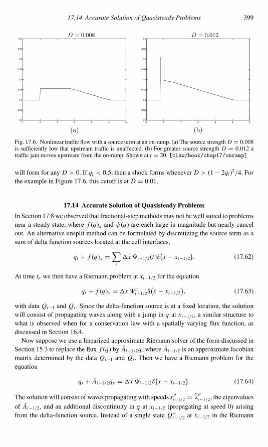
17.14 Accurate Solution of Quasisteady Problems 399

(a)−1 0 1 2 3 4 5

0.3

0.35

0.4

0.45

0.5

0.55

0.6

0.65

0.7D = 0.008

(b)−1 0 1 2 3 4 5

0.3

0.35

0.4

0.45

0.5

0.55

0.6

0.65

0.7D = 0.012

Fig. 17.6. Nonlinear traffic flowwith a source term at an on-ramp. (a) The source strength D = 0.008is sufficiently low that upstream traffic is unaffected. (b) For greater source strength D = 0.012 atraffic jam moves upstream from the on-ramp. Shown at t = 20. [claw/book/chap17/onramp]

will form for any D > 0. If ql < 0.5, then a shock forms whenever D > (1− 2ql)2/4. Forthe example in Figure 17.6, this cutoff is at D = 0.01.

17.14 Accurate Solution of Quasisteady Problems

In Section 17.8 we observed that fractional-stepmethodsmay not bewell suited to problemsnear a steady state, where f (q)x and ψ(q) are each large in magnitude but nearly cancelout. An alternative unsplit method can be formulated by discretizing the source term as asum of delta function sources located at the cell interfaces,

qt + f (q)x =∑i

�x "i−1/2(t)δ(x − xi−1/2

). (17.62)

At time tn we then have a Riemann problem at xi−1/2 for the equation

qt + f (q)x = �x "ni−1/2δ

(x − xi−1/2

), (17.63)

with data Qi−1 and Qi . Since the delta-function source is at a fixed location, the solutionwill consist of propagating waves along with a jump in q at xi−1/2, a similar structure towhat is observed when for a conservation law with a spatially varying flux function, asdiscussed in Section 16.4.Now suppose we use a linearized approximate Riemann solver of the form discussed in

Section 15.3 to replace the flux f (q) by Ai−1/2q, where Ai−1/2 is an approximate Jacobianmatrix determined by the data Qi−1 and Qi . Then we have a Riemann problem for theequation

qt + Ai−1/2qx = �x "i−1/2δ(x − xi−1/2

). (17.64)

The solution will consist of waves propagating with speeds s pi−1/2 = λpi−1/2, the eigenvalues

of Ai−1/2, and an additional discontinuity in q at xi−1/2 (propagating at speed 0) arisingfrom the delta-function source. Instead of a single state Q∨

|i−1/2 at xi−1/2 in the Riemann

400 17 Source Terms and Balance Laws

solution, there will be two states Q∨|l and Q

∨|r just to the left and right of this ray, satisfying

the Rankine–Hugoniot relation (17.59) with s = 0,

Ai−1/2Q∨|r − Ai−1/2Q∨

|l = �x "i−1/2. (17.65)

These states must be related to Qi−1 and Qi by

Ai−1/2Q∨|l − Ai−1/2Qi−1 =

∑p:s pi−1/2 < 0

s pi−1/2W pi−1/2 (17.66)

and

Ai−1/2Qi − Ai−1/2Q∨|r =

∑p:s pi−1/2>0

s pi−1/2W pi−1/2, (17.67)

whereW pi−1/2 = α

pi−1/2r

pi−1/2 is the pth wave, which is proportional to the eigenvector r

pi−1/2

of A pi−1/2. Adding (17.66) and (17.67) together and using (17.65) allows us to eliminateQ∨

|l,r and obtain

Ai−1/2(Qi − Qi−1)−�x "i−1/2 =m∑p=1

s pi−1/2W pi−1/2. (17.68)

If the Roe solver of Section 15.3.2 is used, then the matrix Ai−1/2 satisfies (15.18), andso (17.68) becomes

f (Qi )− f (Qi−1)−�x "i−1/2 =m∑p=1

s pi−1/2W pi−1/2. (17.69)

In order to determine the wavesW pi−1/2 in the Riemann solution, we need only decompose

f (Qi )− f (Qi−1)−�x"i−1/2 into eigenvectors as

f (Qi )− f (Qi−1)−�x "i−1/2 =m∑p=1

βpi−1/2r

pi−1/2, (17.70)

and then setW pi−1/2 = α

pi−1/2r

pi−1/2, where

αpi−1/2 = β

pi−1/2/s

pi−1/2 for s pi−1/2 �= 0. (17.71)

Godunov’s method and related high-resolution methods, when implemented in the wave-propagation form, only require the waves propagating at nonzero speeds, and these can allbe obtained by this procedure. Alternatively, the formulation of Section 15.5 can be used toimplement the method directly in terms of the wavesZ p

i−1/2 = βpi−1/2r

pi−1/2, with the simple

modification that these waves are now defined by solving (17.70) instead of (15.67). As inthe discussion of Section 15.5, this procedure can also be used for choices of r p other thanthe eigenvectors of the Roe matrix.This method is generally easy to implement by a simple modification of the Riemann

solver for the homogeneous equation. It is not formally second-order accurate in general,

17.15 Burgers Equation with a Stiff Source Term 401

and may not perform as well as fractional-step methods for some time-dependent problemsthat are far from steady state.The method can be greatly advantageous, however, for quasisteady problems, where

f (q)x ≈ ψ(q). In this case we expect

f (Qi )− f (Qi−1)�x

≈ "i−1/2, (17.72)

and hence the left-hand side of (17.69) will be near 0. The waves resulting from the eigen-decomposition will thus have strength near zero, and will cause little change in the solution.These waves will model the deviation from steady state, and it is precisely this informa-tion that should be propagated, and to which wave limiters should be applied. Moreover, anumerical steady-state solution computed with this method will satisfy (17.72) with equal-ity. If the source term is appropriately discretized then smooth steady-state solutions willbe computed with second-order accuracy even though the transient behavior may not beformally second-order accurate.A different wave-propagation method with similar features was proposed in [284], but

the approach just presented seems to be more robust as well as much easier to implement;see [18] for more discussion. Some other related methods can be found in the references ofSection 17.2.1.

17.15 Burgers Equation with a Stiff Source Term

In the remainder of this chapterwe consider problems having source terms that do not appearto contain delta functions, but that are typically close to zero over most of the domain whilebeing very large over thin reaction zones that dynamically evolve as part of the solution.Such source terms can often be approximated by delta functions, but their location andstrength is generally not known a priori.As a simple but illustrative example, consider the Burgers equation with a source term,

ut + 1

2(u2)x = ψ(u), (17.73)

where

ψ(u) = 1

τu(1− u)(u − β), (17.74)

with τ > 0 and 0 < β < 1. If we consider the ODE

u′(t) = ψ(u(t)) (17.75)

alone, we see that u = 0, β, 1 are equilibrium points. Themiddle point u = β is an unstableequilibrium, and from any initial data u◦ �= β, u asymptotically approaches one of the otherequilibria: u → 0 if u◦ < β or u → 1 if u◦ > β. The parameter τ determines the time scaleover which u approaches an equilibrium.For τ very small, any initial data u◦(x) supplied to the equation (17.73) will rapidly

approach a step function with values 0 and 1 (and near-discontinuous behavior where u◦(x)passes through β) on a much faster time scale than the hyperbolic wave propagation. To see

402 17 Source Terms and Balance Laws

how the solution then evolves, it suffices to consider the case of a Riemann problem withjump from value 0 to 1 or from 1 to 0.If ul = 1 and ur = 0, then theBurgers equationwith no source gives a shockwavemoving

with the Rankine–Hugoniot speed 1/2, by (11.23). The source term is then identically zeroand has no effect. More general initial data u◦(x) satisfying u◦(x)>β for x < 0 and u◦(x)<βfor x > 0 would rapidly evolve to this situation and give a shock traveling with speed 1/2for any value of β ∈ (0, 1).The situation is much more interesting in the case where ul = 0 and ur = 1, as studied

in [280]. In this case Burgers’ equation gives a rarefaction wave that spreads the initialdiscontinuity out through all intermediate values. The source term opposes this smearingand sharpens all values back towards 0 or 1. These competing effects balance out andresult in a smooth solution that rapidly approaches a traveling wave that neither smears norsharpens further, but simply propagates with some speed s:

u(x, t) = w

(x − stτ

). (17.76)

We will see below that s = β.The shape of this profile is shown in Figure 17.7(a). The width of the transition zone

in u(x, t) is O(τ ), and for small τ this appears similar to a viscous shock profile withsmall viscosity, though the competing effects that produce the steady profile are differentin that case. As we will see in the next section, computing such a solution on a grid wherethe structure is not well resolved (e.g., for �x >τ ) can be more difficult than correctlyapproximating a shock wave.The shape of the profile w and the speed s can be determined by inserting the form

(17.76) into (17.73), yielding

−sw′ + ww′ = w(1− w)(w − β), (17.77)

(a)−25 −20 −15 −10 −5 0 5 10 15 20 25

−0.2

0

0.2

0.4

0.6

0.8

1

1.2

1.4

(b)−25 −20 −15 −10 −5 0 5 10 15 20 25

−0.12

−0.1

−0.08

−0.06

−0.04

−0.02

0

0.02

Fig. 17.7. (a) Traveling-wave solution w(ξ ) to (17.73). (b) The source term ψ(w(ξ )) of (17.74).Shown for β = 0.6.

17.15 Burgers Equation with a Stiff Source Term 403

which gives the ODE

w′ = w(1− w)(w − β)w − s . (17.78)

We also require w(−∞) = 0 and w(+∞) = 1. The equation (17.78) has a solution withthese limiting values only if s = β, since otherwisew cannot cross the unstable equilibriumvalue β. When s = β we can cancel this term in (17.78) and obtain the logistic equation

w′ = w(1− w), (17.79)

with solutions of the form

w(ξ ) = eξ

1+ eξ =1

2[1+ tanh(ξ/2)], (17.80)

as shown in Figure 17.7(a).The propagation speed is s = β. Unlike the case ul = 1, ur = 0, this speed depends on

the structure of the source term. This leads to numerical difficulties if we try to solve theproblem on an underresolved grid, as discussed in the next section. More generally, if wereplace f (u) = u2/2 by a more general flux function, the propagation speed of the resultingtraveling wave will be s = f ′(β), as shown in [129].We can relate the result just found to the discussion of singular source terms earlier in

this chapter by observing that the source term ψ(w) will be essentially zero except in thetransition region, where its magnitude isO(1/τ ), as seen in Figure 17.7(b). Since this regionhas widthO(τ ), this suggests that the source terms approximate a delta function as τ → 0.Themagnitude of the limiting delta function can be found by integratingψ(w((x−st)/τ ))

over all x and taking the limit as τ → 0, although in fact this value is independent of τ forthe wave form w. We can use (17.79) to rewrite ψ(w(ξ )) as

ψ(w(ξ )) = 1

τw′(ξ )[w(ξ )− β]

= 1

τ

d

dξ

(1

2[w(ξ )− β]2

), (17.81)

and hence ∫ ∞

−∞ψ(w(x − st)/τ ) dx = τ

∫ ∞

−∞ψ(w(ξ )) dξ

= 1

2[w(ξ )− β]2

∣∣∣∣+∞−∞

= 1

2− β. (17.82)

This value is independent of τ and gives the strength D of the delta-function source observedin the limit τ → 0,

D = 1

2− β. (17.83)

404 17 Source Terms and Balance Laws

Using the modified Rankine–Hugoniot relation (17.59) results in the speed

s = 1

2− D = β

for the limiting jump discontinuity, which is consistent with the speed of the traveling wave,as we should expect. We see that the source term has a nontrivial effect even in the limitτ → 0 whenever β �= 1/2.Note from Figure 17.7(b) that the source term is negative where w<β and positive

where w > β. When β = 1/2 these two portions exactly cancel and there is no net sourceterm, so the propagation speed agrees with what is expected from the conservation lawalone. When β �= 1/2 there is a net source or sink of u in the transition zone that affectsthe speed at which the front propagates. This same effect is seen in many reacting flowproblems.

17.16 Numerical Difficulties with Stiff Source Terms

A hyperbolic equation with a source term is said to be stiff if the wave-propagation behaviorof interest occurs on a much slower time scale than the fastest times scales of the ODEqt = ψ(q) arising from the source term. An example is a detonation wave arising when gasdynamics is coupled with the chemical kinetics of combustion. Detonation waves can travelrapidly through a combustible gas, but even these fast waves are many orders of magnitudeslower than the time scales of some of the chemical reactions appearing in the kinetic sourceterms. It would often be impossible to simulate the propagation of suchwaves over distancesof physical interest if it were necessary to fully resolve the fastest reactions.As a simpler example, consider the Burgers equation (17.73) with source (17.74). As

we have seen in the previous section, when τ is very small a traveling-wave solution looksessentially like a discontinuity from ul = 0 to ur = 1 propagating at speed β = O(1).Suppose we want to approximate this with τ = 10−10, say, over a domain and time intervalthat are O(1). Then the transition from ul to ur takes place over a zone of width on theorder of 10−10. We will certainly want to use �x ! τ , and we can’t hope to resolve thestructure of the traveling wave, only the macroscopic behavior (as in shock capturing). Wealso do not want to take�t =O(τ ), but rather want to take�t =O(�x) based on the CFLrestriction for the hyperbolic problem. We hope that if the wave of interest moves less thanone grid cell each time step, we will be able to capture it accurately, with little numericalsmearing and the physically correct velocity.The classical theory of numerical methods for stiff ordinary differential equations can

be found in many sources, e.g., [145], [178], [253]. Recall that an ODE is called stiff ifwe are trying to compute a particular solution that is varying much more slowly than thefastest time scales inherent in the problem. Typically this means that the solution of interestis evolving on some slow manifold in state space and that perturbing the solution slightlyoff this manifold will result in a rapid transient response, bringing the solution back themanifold, followed by slow evolution once again. Stiff problems often arise in chemicalkinetics, where the rates of different reactions can vary by many orders of magnitude. If thefastest reactions are essentially in equilibrium, then the concentrations will vary slowly ontime scales governed by slower reactions, and the solution is evolving on a slow manifold.

17.16 Numerical Difficulties with Stiff Source Terms 405

If the system is perturbed, say by injecting additional reactants, then fast transient behaviormay result over a short period of time as the faster reactions reach a new equilibrium.A simpler example of a stiff ODE is the equation (17.75) with τ � T in (17.74), where

T is some reference time over which we are interested in the solution. For most initial datathere will be fast transient decay to one of the slow manifolds u ≡ 0 or u ≡ 1. Perturbingaway from one of these values results in a fast transient. An even simpler example is theequation

u′(t) = −u(t)/τ, (17.84)

where u ≡ 0 is the slow manifold.Numerically, stiff ODEs are problematical becausewe typicallywant to take “large” steps

whenever the solution is “slowly” evolving. However, the numerical method is not exactand hence is constantly perturbing the solution. If these perturbations take the solution offthe slow manifold, then in the next time step the solution will have a rapid transient and thedesired time step may be much too large. In particular, if an explicit method is used, thenthe stability restriction of the method will generally require choosing the time step basedon the fastest time scale present in the problem, even if we are hoping we do not need toresolve this scale. Luckily many implicitmethods have much better stability properties andallow one to choose the time step based on the behavior of the solution of interest.As we will see, solving stiff hyperbolic equations can be even more challenging than

solving stiff ODEs. This difficulty arises largely from the fact that in a stiff hyperbolicequation the fastest reactions are often not in equilibrium everywhere. In thin regions suchas the transition zone of the problem considered in Section 17.15 (see Figure 17.7(b)), orthe reaction zone of a detonation wave, there is a fast transient behavior constantly takingplace. For some problems it really appears necessary to resolve this zone in order to obtaingood solutions, in which case adaptive mesh refinement is often required to efficientlyobtain good results. In other cases we can achieve our goal of solving stiff problems onunderresolved grids. A number of techniques have been developed for various problems,and here we will primarily illustrate some of the difficulties.For stiff source terms we will again concentrate on the use of fractional-step methods

(though more sophisticated approaches may not use splitting). The Godunov splitting ap-plied to qt + f (q)x =ψ(q) would simply alternate between solving the following twoproblems over time step �t :

Problem A: qt + f (q)x = 0, (17.85)

Problem B: qt = ψ(q). (17.86)

The first thing to observe is that theODEof (17.86) is going to be stiff, and sowemust use anappropriate method for this step in going from Q∗i to Q

n+1i in the i th cell. One popular class

of stiff solvers are the BDF methods (backward differentiation formulas). These are linearmultistepmethods and require at least two previous time levels to get second-order accuracyor better. As discussed in Section 17.6, this is a problem in the context of a fractional-stepmethod, since we only have one value Q∗i that we can use.The trapezoidal method (17.41) can often be effectively used for stiff ODEs, but may

fail miserably for hyperbolic equations with stiff source terms. Figure 17.8 shows a sample

406 17 Source Terms and Balance Laws

(a)−5 −4 −3 −2 −1 0 1 2 3 4 5

−0.2

0

0.2

0.4

0.6

0.8

1

1.2

1.4Time t = 2.8

(b)−5 −4 −3 −2 −1 0 1 2 3 4 5

−0.2

0

0.2

0.4

0.6

0.8

1

1.2

1.4Time t = 2.87

Fig. 17.8. Numerical solution to the Burgers equation with a stiff source term using the trapezoidalmethod for the source term: (a) after 40 time steps, (b) after 41 time steps. [claw/book/chap17/stiffburgers]

computation on the Burgers-equation example of Section 17.15, with β = 0.8, τ = 10−5,�x = 0.1, and �t = 0.07. The initial data was u = 0 for x < 0 and u = 1 for x > 0.Figure 17.8(a) shows the solution after 40 time steps,while Figure 17.8(b) shows the solutionone time step later. The solution oscillates in time between these two different basic shapeswith a set of waves propagating at unphysical speeds.This behavior arises from the fact that the trapezoidal method is not L-stable (see [253]).

If we start on the slow manifold, this method does a good job of keeping the numericalsolution on the slowmanifold even with time steps that are large relative to the faster scales.But for initial data that has an initial fast transient, the method yields oscillations. This iseasy to see for the simple ODE (17.84). In this case the “slow manifold” is simply u ≡ 0,and starting with any other data gives exponentially fast decay of the true solution towardsthis state, with rate 1/τ . On this problem the trapezoidal method yields

Un+1 =(1− 1

2�t/τ

1+ 12�t/τ

)U ∗. (17.87)

If U ∗ = 0 then Un+1 = 0 also and we stay on the slow manifold. But if U ∗ �= 0 and�t/τ! 1 then Un+1 ≈ −U ∗. The “amplification factor” in (17.87) approaches −1 as−�t/τ → −∞. Rather than the proper decay, we obtain an oscillation in time unless thetransient is well resolved.For the Burgers equation (17.73) with a stiff source term, nonequilibrium data is con-

stantly being introduced by the averaging process in solving the conservation law near anyfront. This sets up an oscillation in time, as observed in Figure 17.8.The trapezoidal method is an A-stable method. In fact, its stability region is exactly the

left half plane. The fact that the boundary of the stability region is the imaginary axis, andhence passes through the point at infinity on the Riemann sphere, is responsible for theobserved undesirable behavior, since in solving the stiff problem we are interested in letting−�t/τ →−∞.An L-stable method is one for which the point at infinity is in the interior of the stability

region, and hence the amplification factor approaches something less than 1 in magnitude

17.16 Numerical Difficulties with Stiff Source Terms 407

as −�t/τ → −∞. (L-stability is usually defined to also require A-stability, but we usethis looser definition for convenience.) The BDF methods have this property. The one-stepBDF method is the backward Euler method, which for the equation (17.84) is simply

Un+1 = U ∗ − �t

τUn+1 =⇒ Un+1 =

(1

1+�t/τ)U ∗. (17.88)

Note that (1 + �t/τ )−1 → 0 as �t/τ → −∞, and so this method can be used on stiffproblems evenwhen the initial data is not on the slowmanifold. The backward Eulermethodis only first-order accurate. In the present context, this does not reallymatter, sincewe expectthe source terms to be active only over thin regions where there are fast transients that wecannot resolve with any accuracy anyway. What we primarily require is the L-stabilityproperty.In some situations we may want to use a second-order method that is L-stable so that

we can obtain good accuracy of source terms in regions where they are smooth (or wheretransients are well resolved) and also avoid oscillations in regions of stiffness. In the contextof a fractional-step method we must use a one-step method, and one possible choice is theTR-BDF2 method (17.43) described in Section 17.6, which is L-stable. Figure 17.9 showsresults obtained if we apply the TR-BDF2 method to the stiff source term in the Burgers-equation example. The use of this method eliminates the oscillations and unphysical statesthat were seen in Figure 17.8.However, it still produces an incorrect solution in the stiff case, as seen in Figure 17.9(a).

The wave now looks reasonable but is traveling at the wrong speed. It behaves fine if the gridis further refined, or equivalently if the value of τ is increased as shown in Figure 17.9(b).But the method still fails on underresolved grids in spite of the good behavior of the ODEsolver.This illustrates a difficulty often seen with stiff source terms. Similar behavior was

observed by Colella, Majda & Roytburd [82] for detonation waves, and the problem hasbeen discussed in many papers since. Even the simplest advection equation together withthe source term (17.74) gives similar results. An analysis of this model problem, presentedin LeVeque & Yee [293], carries over to the Burgers-equation example.

(a)−5 −4 −3 −2 −1 0 1 2 3 4 5

−0.2

0

0.2

0.4

0.6

0.8

1

1.2

1.4

(b)−5 −4 −3 −2 −1 0 1 2 3 4 5

−0.2

0

0.2

0.4

0.6

0.8

1

1.2

1.4

Fig. 17.9. Numerical solution to the Burgers equation with a stiff source term using the TR-BDF2method for the source term: (a) the stiff case τ = 10−5; (b) the nonstiff case τ = 0.1. [claw/book/chap17/stiffburgers]

408 17 Source Terms and Balance Laws

Suppose

Uni =

{0 if i < I,1 if i ≥ I,

as suggested by the result plotted in Figure 17.9(a). Then a high-resolution method for theBurgers equation will reduce to Godunov’s method (since all slopes will be limited to 0),and we will obtain

U ∗i =0 if i < I,1−�t/(2�x) if i = I,1 if i > I,

since the jump propagates at speed 1/2. For the calculation shown in Figure 17.9(a),U ∗I = 1 −�t/(2�x) = 0.65. We now solve the stiff ODE, and since U ∗I < β = 0.8, thesolution decays rapidly towards the equilibrium at 0, and so Un+1

I ≈ 0 after time�t . In allother cells the source term is zero. We thus obtain

Un+1i ≈

{0 if i < I + 1,1 if i ≥ I + 1,

and the wave has shifted over by one grid cell. The wave thus propagates at a speed of onegrid cell per time step,which is a purely numerical artifact and not the correct physical speed.Note that with a smaller time step we would haveU ∗I > β, in which caseUn+1

I ≈ 1, andso Un+1 ≈ Un . Now the numerical solution remains stationary (propagates with speed 0),again not the correct solution.This difficulty arises from the fact that the numerical method for the homogeneous hy-

perbolic equation introduces numerical diffusion, leading to a smearing of the discontinuityor steep gradient that should be observed physically. The source term is then active overthe entire region where the solution is smeared, leading to a larger contribution from thisterm than is physical. As we saw in Section 17.12, the speed at which the jump propagatesis directly related to the strength of the source concentrated at the jump, so an incorrect netsource term leads to incorrect propagation speeds.This effect has been illustrated here with a fractional-step method. Other numerical

methods, e.g., an unsplit method as in Section 17.2.1, can lead to similar difficulties. See[293] for an example. For some problems with stiff source terms it may be necessary toresolve the fastest scales (at least locally) in order to obtain good results. For a given valueof τ the methods do converge as�t,�x → 0. However, if τ is very small, then this may beimpractical and we would prefer to capture the proper behavior on an underresolved grid.For some particular problems special methods have been developed that avoid the need forsuch finely resolved grids by calculating more accurately the correct source contribution;see for example [196] for one wave-propagation approach for a simple detonation model.See [19], [33], [40], [357], [348], [494] for some other possible approaches and furtherdiscussion of these numerical difficulties.We should note that not all problems with stiff source terms lead to numerical difficulties

on underresolved grids. For some problems the correct macroscopic behavior (in particular,correct propagation speeds) is observed even if the fast time scales are not well resolved.

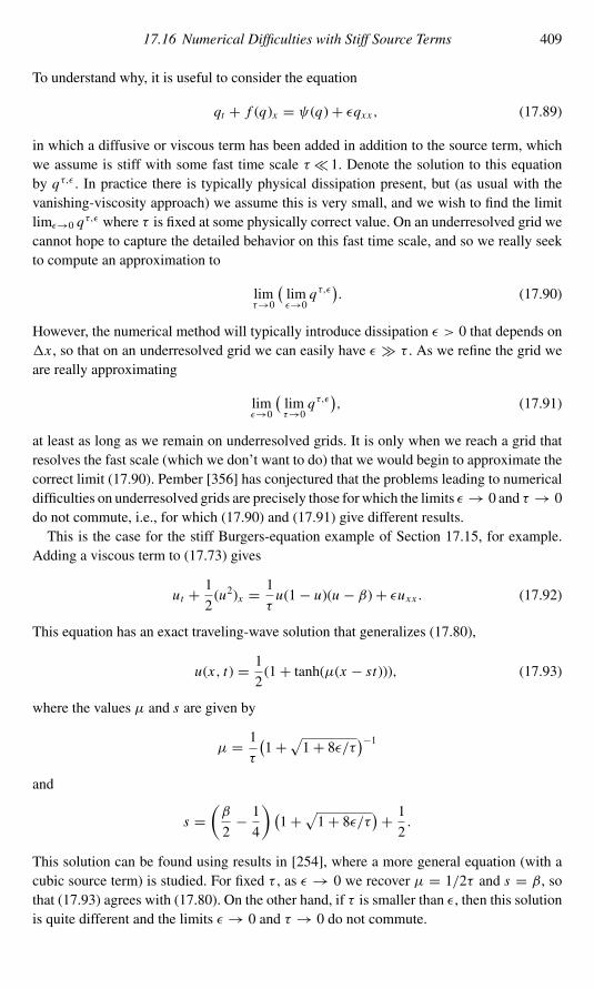
17.16 Numerical Difficulties with Stiff Source Terms 409

To understand why, it is useful to consider the equation

qt + f (q)x = ψ(q)+ εqxx , (17.89)

in which a diffusive or viscous term has been added in addition to the source term, whichwe assume is stiff with some fast time scale τ� 1. Denote the solution to this equationby qτ,ε . In practice there is typically physical dissipation present, but (as usual with thevanishing-viscosity approach) we assume this is very small, and we wish to find the limitlimε→0 qτ,ε where τ is fixed at some physically correct value. On an underresolved grid wecannot hope to capture the detailed behavior on this fast time scale, and so we really seekto compute an approximation to

limτ→0

(limε→0

qτ,ε). (17.90)

However, the numerical method will typically introduce dissipation ε > 0 that depends on�x , so that on an underresolved grid we can easily have ε ! τ . As we refine the grid weare really approximating

limε→0

(limτ→0

qτ,ε), (17.91)

at least as long as we remain on underresolved grids. It is only when we reach a grid thatresolves the fast scale (which we don’t want to do) that we would begin to approximate thecorrect limit (17.90). Pember [356] has conjectured that the problems leading to numericaldifficulties on underresolved grids are precisely those for which the limits ε → 0 and τ → 0do not commute, i.e., for which (17.90) and (17.91) give different results.This is the case for the stiff Burgers-equation example of Section 17.15, for example.

Adding a viscous term to (17.73) gives

ut + 1

2(u2)x = 1

τu(1− u)(u − β)+ εuxx . (17.92)

This equation has an exact traveling-wave solution that generalizes (17.80),

u(x, t) = 1

2(1+ tanh(µ(x − st))), (17.93)

where the values µ and s are given by

µ = 1

τ

(1+

√1+ 8ε/τ)−1

and

s =(β

2− 1

4

) (1+

√1+ 8ε/τ)+ 1

2.

This solution can be found using results in [254], where a more general equation (with acubic source term) is studied. For fixed τ , as ε → 0 we recover µ = 1/2τ and s = β, sothat (17.93) agrees with (17.80). On the other hand, if τ is smaller than ε, then this solutionis quite different and the limits ε → 0 and τ → 0 do not commute.

410 17 Source Terms and Balance Laws

In some physical problems adding additional dissipation does not substantially changethe solution, and for such problems good results can often be obtained on underresolvedgrids. In the next section we study one class of problems for which this is true.

17.17 Relaxation Systems

In many physical problems there is an equilibrium relationship between the variables thatis essentially maintained at all times. If the solution is perturbed away from this equi-librium, then it rapidly relaxes back towards the equilibrium. The problem considered inSection 17.15 has this flavor, but in that case there is a single variable u and two possiblestable equilibria u = 0 and u = 1, leading to numerical difficulties. In this section we con-sider the situation where there are several variables and perhaps many different equilibriumstates, but there is a unique equilibrium relationship between the variables.A simple model problem is the system of two equations

ut + vx = 0,

vt + aux = f (u)− vτ

(17.94)

for 0 < τ � 1, where a > 0 and f (u) is a given function. The equilibrium states are thosefor which v = f (u). If v �= f (u), then in the second equation the right-hand side dominatesthe term aux , and v is rapidly driven back towards equilibrium (except perhaps in narrowreaction zones where u has a very steep gradient).Note that if we simply assume v ≡ f (u) in (17.94), then we can discard the second

equation. Inserting this equilibrium assumption into the first equation, we then obtain thescalar conservation law

ut + f (u)x = 0. (17.95)

Thereforewemight expect solutions to the system (17.94) to bewellmodeled by the reducedequation (17.95) for small τ . In fact this is true, provided that a so-called subcharacteristiccondition is satisfied. Observe that the homogeneous part of the system (17.94) is a linearhyperbolic system. The coefficient matrix has eigenvalues λ1,2 = ±√a. Hence informationcan propagate no faster than speed

√a, and adding the source term in (17.94) does not

change this fact. On the other hand, the reduced equation (17.95) has characteristic speedf ′(u). If | f ′(u)| > √a, then we cannot expect the solution of (17.94) to behave well in thelimit τ → 0. The subcharacteristic condition for this problem is the requirement

−√a ≤ f ′(u) ≤ √a. (17.96)

Similar conditions hold for larger systems involving relaxation, and generally state thatthe characteristic speed of the reduced equation must fall within the range spanned by thecharacteristic speeds of the homogeneous part of the original system. This terminologywas introduced by Liu [310], who studied more general relaxation systems in which au isreplaced by a possibly nonlinear function σ (u) in (17.94). Such problems arise in nonlinearelasticity (see Section 2.12.4), in which case σ (u) represents the stress as a function ofstrain.

17.17 Relaxation Systems 411

Many physical systems contain rapid relaxation processes that maintain an equilibrium,and often we solve the reduced equations based on this equilibrium. In fact the Eulerequations of gas dynamics can be viewed as the reduced equations for more accurate modelsof the physics that include relaxation of vibrational or chemical nonequilibrium states thatarise from intermolecular collisions. For many practical purposes the Euler equations aresufficient, though for some problems it is necessary to consider nonequilibrium flows; seefor example [69], [70], [474], or [497]. A related example of the Euler equations relaxingtowards isothermal flow is given in Section 17.17.3.Relaxation systems are also used in modeling traffic flow. In Section 11.1 we derived a

scalar conservation law by specifying the velocity of cars as a function of density U (ρ).This assumes that drivers can react infinitely quickly to changes in density and are alwaysdriving at the resulting equilibrium velocity. In fact the velocity should relax towards thisvalue at some rate depending on the drivers’ reaction time. This can be modeled with asystem of two equations, one for the density and a second for the velocity. Such modelsare often called second-order models in traffic flow (the scalar equation is the first-ordermodel) and were first studied by Payne [354] and Whitham [486]. For more recent work,see for example [16], [99], [260], [296], [400], [498].On the theoretical side there is considerable interest in the study of quite general relaxation

systems and the conditions under which convergence of solutions occurs as τ→ 0. See forexample [64], [62], [305], [310], [336], [337], [491], [495]. Numerically it is useful tonote that these relaxation problems can typically be solved on underresolved grids, as thenext example shows. (This fact is the basis for the class of numerical relaxation schemesdiscussed in Section 17.18, in which stiff relaxation terms are intentionally introduced.)

Example 17.7. Figure 17.10 shows some solutions to the relaxation system (17.94) forf (u) = 1

2u2, a = 1, and the Riemann data

ul = 1, ur = 0, vl = f (ul) = 1

2, vr = f (ur ) = 0. (17.97)

The reduced equation is Burgers’ equation, and we expect a shock traveling with speed 1/2in the limit as τ → 0, so it should be at x = 0.4 at the time t = 0.8 shown in all figures.Numerical solutions to the system (17.94) for various values of τ are shown, obtained usinga fractional-step method. Solving the Riemann problem for the homogeneous linear systemgives two waves with speeds ±1. The state between these waves is not in equilibrium evenif the Riemann data is, and the source term relaxes this state towards equilibrium. When τis large (slow relaxation), the structure of the linear system is clearly visible, but as τ → 0we observe convergence to the solution of Burgers’ equation.Note that for this problem the numerical fractional-step method behaves well in the

limit τ → 0. The steep gradient near x/t = 0.4 (where the source term is active) is notwell resolved on the grid for the smallest value of τ used in Figure 17.10, and yet thecorrect macroscopic behavior is observed. This is a reflection of the fact that if we addO(ε)viscosity to the system (17.94), then the limits ε → 0 and τ → 0 commute, as describedin Section 17.16. The basic reason for this is that the parameter τ also acts like a viscosityin the system (though this is not clear from the form of (17.94)), and so adding additionalviscosity does not change the nature of the solution.

412 17 Source Terms and Balance Laws

−1 −0.8 −0.6 −0.4 −0.2 0 0.2 0.4 0.6 0.8 1

0

0.2

0.4

0.6

0.8

1

τ = 10

−1 −0.8 −0.6 −0.4 −0.2 0 0.2 0.4 0.6 0.8 1

0

0.2

0.4

0.6

0.8

1

τ = 10

−1 −0.8 −0.6 −0.4 −0.2 0 0.2 0.4 0.6 0.8 1

0

0.2

0.4

0.6

0.8

1

τ = 1

−1 −0.8 −0.6 −0.4 −0.2 0 0.2 0.4 0.6 0.8 1

0

0.2

0.4

0.6

0.8

1

τ = 1

−1 −0.8 −0.6 −0.4 −0.2 0 0.2 0.4 0.6 0.8 1

0

0.2

0.4

0.6

0.8

1

τ = 0.1

−1 −0.8 −0.6 −0.4 −0.2 0 0.2 0.4 0.6 0.8 1

0

0.2

0.4

0.6

0.8

1

τ = 0.1

−1 −0.8 −0.6 −0.4 −0.2 0 0.2 0.4 0.6 0.8 1

0

0.2

0.4

0.6

0.8

1

τ = 0.01

−1 −0.8 −0.6 −0.4 −0.2 0 0.2 0.4 0.6 0.8 1

0

0.2

0.4

0.6

0.8

1

τ = 0.01

−1 −0.8 −0.6 −0.4 −0.2 0 0.2 0.4 0.6 0.8 1

0

0.2

0.4

0.6

0.8

1

τ = 0.001

−1 −0.8 −0.6 −0.4 −0.2 0 0.2 0.4 0.6 0.8 1

0

0.2

0.4

0.6

0.8

1

τ = 0.001

Fig. 17.10. Solution to the relaxation system (17.94) for five different values of τ , all shown at timet = 0.8. The left column shows u, and the right column shows v.

17.17.1 Chapman–Enskog Expansion

To see that τ is like a viscosity in the relaxation system (17.94),we use a so-calledChapman–Enskog expansion,

v(x, t) = f (u(x, t))+ τv1(x, t)+ τ 2v2(x, t)+ · · · . (17.98)

The form of this expansion is motivated by the fact that v→ f (u) as τ → 0. Inserting thisin the first equation of (17.94) gives

ut + [ f (u)+ τv1 + τ 2v2 + · · · ]x = 0,

or

ut + f (u)x = −τv1x + · · · . (17.99)

To determine v1(x, t) we insert (17.98) in the second equation of (17.94), yielding

[ f ′(u)ut + τv1t + τ 2v2t + · · · ]+ aux = −(v1 + τv2 + · · · ),

17.17 Relaxation Systems 413

or by (17.99),

[ f ′(u)(− f (u)x − τv1x + · · · )+ τv1t + τ 2v2t + · · · ]+ aux = −(v1 + τv2 + · · · ).

Equating the O(1) terms for τ � 1 gives

− f ′(u) f (u)x + aux = −v1

and hence

v1 = −[a − f ′(u)2]ux .

Using this in (17.99) gives

ut + f (u)x = τ (β(u)ux )x +O(τ 2), (17.100)

where

β(u) = a − [ f ′(u)]2.

The equation (17.100) is a refined version of the reduced equation (17.95). For τ > 0 wesee that this parameter plays the role of a viscosity provided that β(u) > 0, which is trueexactly when the subcharacteristic condition (17.96) is satisfied.

17.17.2 Violating the Subcharacteristic Condition

It is interesting to ask what happens if the subcharacteristic condition is violated. If f (u) =bu is a linear function and |b| > √a, then the solution will blow up along the characteristicsgn(b)

√a as τ → 0. This case has been studied in [292]. Adding some viscosity to the

system can stabilize the solution, since then the system is parabolic and allows arbitrarypropagation speeds. If f is nonlinear, then the nonlinearity may also stabilize the solution.There are some physical problems where this is of interest, notably the case of roll wavesin shallow water theory on a sloping surface [223], [486]. However, for the vast majorityof physical problems involving relaxation the appropriate subcharacteristic condition issatisfied.

17.17.3 Thermal Relaxation and Isothermal Flow

As an example of a relaxation system we consider the Euler equations with a relaxationterm driving the temperature towards a constant value. The equations of isothermal flowwere introduced in Section 14.6, for gas in a one-dimensional tube surrounded by a bath atconstant temperature. We assume that heat flows in or out of the bath instantaneously, sothat a constant temperature is maintained in the gas (so heat is extracted from the gas justbehind a shock wave, and flows into the gas in a rarefaction wave).

414 17 Source Terms and Balance Laws

This is obviously not a perfect model of the physical situation. A better model would bethe relaxation system ρ

ρuE

t

+

ρu

ρu2 + p

(E + p)u

x

=

00

−[E − E(ρ, ρu)]/τ

(17.101)

together with an appropriate equation of state for the gas, e.g., (14.23) for a polytropic idealgas. Here E(ρ, ρu) is the energy in the gas that results if we bring T to the bath temperatureT without changing the density or momentum. According to the ideal gas law (14.9), wethen have p = RρT = a2ρ, where a =

√RT is the isothermal sound speed. Using this in

the equation of state (14.23) gives

E(ρ, ρu) = a2ρ

γ − 1 +1

2ρu2. (17.102)

The quantity τ > 0 is the time scale over which the energy E − E flows into the tube,the reciprocal of the relaxation rate. The isothermal equations (14.34),[

ρ

ρu

]t

+[

ρu

ρu2 + a2ρ

]x

= 0, (17.103)

result from letting τ → 0. These are the reduced equations corresponding to the relaxationsystem (17.101).Note that the subcharacteristic condition is satisfied for this system provided that a ≤ c,

where a is the isothermal sound speed and c = √γ p/ρ is the sound speed for the full

polytropic Euler equations. Near equilibrium we have p ≈ (γ − 1)(E − 12ρu

2) = RTρ,

and so c =√γ RT . Since γ > 1 we have c > a.

The system (17.101) has a structure similar to (17.94). We can divide the variables(ρ, ρu, E) into reduced variables (ρ, ρu) and the relaxation variable E , which relaxesquickly to an equilibrium state E , a unique value for any given (ρ, ρu). The reducedequation is obtained by assuming E ≡ E(ρ, ρu) and eliminating the relaxation variable.The system (17.94) has the same structure, with u being the reduced variable and v therelaxation variable. This structure is important in that it allows us to perform a Chapman–Enskog expansion as in Section 17.17.1 to show that the relaxation time τ plays the role ofa viscosity in the reduced equation. This in turn suggests that numerical methods will besuccessful on these relaxation systems even on underresolved grids.In particular, it is important here that there is a unique equilibrium state E corresponding

to any given values of the reduced variables (ρ, ρu). The relaxation variable E convergesto this value regardless of the initial value of E . By contrast, in the example of Burgers’equation with a stiff source term, (17.73), there is no separation into reduced and relaxationvariables, since this is a scalar equation and u plays both roles. There are two possibleequilibrium states u = 0 and u = 1, and which one we relax towards depends on the initialvalue of u. This means that a smearing of u can lead to the calculation of an incorrectequilibrium state, resulting in incorrect wave speeds, as was illustrated in Section 17.16.Note also that the example of Section 17.16 suggests that τ does not play the role of a

17.18 Relaxation Schemes 415

viscosity in the stiff Burgers example. Adding viscosity to a rarefaction wave should leaveit essentially unchanged, whereas the stiff source term of (17.73) converts the rarefactionwave into a thin reaction zone that approaches a discontinuity as τ → 0.

17.18 Relaxation Schemes

In the example of the previous section, the relaxation system is the “correct” physical modeland the reduced system is an approximation valid in the limit τ → 0. In practice one mightwant to use the reduced system (e.g., the isothermal equations) instead of solving the morecomplicated relaxation system, which involves stiff source terms as well as being a largersystem of equations. Similarly, the scalar conservation law (17.95) can be viewed as anapproximation to the relaxation system (17.94).In some situationswemaywish to turn this viewpoint around and instead viewa relaxation

system such as (17.94) as an approximation to the conservation law (17.95). Suppose wewish to solve the nonlinear conservation law ut + f (u)x = 0 numerically but for somereason don’t wish to write a nonlinear Riemann solver for f (u). Then we can artificiallyintroduce a relaxation variable v and instead solve the system (17.94) for some a and τ ,using a fractional-step method. This only requires solving a linear hyperbolic system withsimple characteristic structure in each time step. For a scalar problem this may be pointless,since the nonlinear Riemann problem is typically easy to solve, but for a nonlinear systemof m conservation laws the same idea can be applied, by using the relaxation system

ut + vx = 0,

vt + Aux = f (u)− vτ

,(17.104)

where u, v ∈ Rm and A is somem×mmatrix. The original nonlinear system ofm equations

is converted into a linear system of 2m equations with the nonlinearity concentrated in thesource terms.The coefficient matrix of (17.104) has the form

B =[0 IA 0

], (17.105)

with eigenvalues ±√λ, where λ is an eigenvalue of A. In order for the relaxation systemto be strictly hyperbolic, we require λ> 0 for each eigenvalue of A, i.e., A must be posi-tive definite. We also need the subcharacteristic condition to hold, which requires that theeigenvalues of the Jacobian matrix f ′(u) should always lie within the range of eigenvaluesof B, i.e., within the interval ±max√λp. This is a generalization of the subcharacteristiccondition (17.96) for the case m = 1.This numerical approach was introduced by Jin and Xin [225]. Methods of this type are

generally called relaxation schemes, and have since been extensively studied, e.g., [12],[60], [64], [164], [222], [226], [233], [261], [306], [439]. Jin and Xin present some theoryand numerical results for the Euler equations, taking A to be a diagonal matrix so that theRiemann problem for (17.104) is easy to solve. The choice of elements of A must be basedon estimates of the minimum and maximum wave speed that will arise in the problem so

416 17 Source Terms and Balance Laws

that the subcharacteristic condition is satisfied. In [225] the stiff source term is solved usingan implicit Runge–Kutta method with a small value of τ . In practice it seems to work aswell to simply consider the limit τ → 0, called the relaxed scheme in [225]. We can thenimplement a single step of the relaxation scheme using a fractional-step method of thefollowing form:

1. Un, V n are used as data for the homogeneous version of (17.104). Solving this linearhyperbolic system over time �t produces values U ∗, V ∗.

2. These values are used as data for the system with only the source terms, so ut = 0 andvt = [ f (u)−v]/τ . The solution of this in the limit τ → 0 has u constant and v→ f (u),so we simply set

Un+1 = U ∗,V n+1 = f (Un+1).

(17.106)

With this approach we do not need to choose a specific value of τ or solve the ODE; wesimply solve the linear hyperbolic system and then reset V to f (U ). Note that the successof relaxation schemes depends on the fact that, for relaxation systems, the stiff source termsdo not cause numerical difficulties on underresolved grids.The advantage of a relaxation scheme is that it avoids the need for a Riemann solver for

the nonlinear flux function f (u), since the hyperbolic system to be solved now involvesthe linear coefficient matrix (17.104) instead. The relaxation scheme can alternatively beviewed as a particular way of defining an approximate Riemann solver for the nonlinearproblem, as shown in [288], which results in some close connectionswith other approximateRiemann solvers introduced in Section 15.3. A particularly simple choice of A leads to theLax–Friedrichs method (4.20); see Exercise 17.9.

Exercises

17.1. Suppose β(x) varies with x in the problem of Section 17.2. Derive an unsplit second-order accurate method for this problem.

17.2. Compute the O(�t 3) term in the splitting error for the Strang splitting (17.35).17.3. Determine the splitting error for the Godunov splitting applied to the system (17.4).17.4. Suppose we wish to numerically approximate the steady-state solution to (17.7) for

the boundary-value problemwith q(0, t) = C . The exact solution is given by (17.44).(a) Consider the unsplit method (17.9), and suppose we have reached a numerical

steady state so that Qn+1i = Qni for all i . Show that this numerical steady-statesolution satisfies

Qi = Qi−11+ β �x/u .

Hence the numerical steady-state solution is accurate toO(�x) and is indepen-dent of �t .

(b) Now consider the fractional-step method (17.21), and show that the numerical

Exercises 417

steady-state solution satisfies

Qi = Qi−11+ (β �x/u)(1− β �t) .

Again this agrees with the true steady-state solution to O(�x) = O(�t), butnow the numerical steady state obtained depends on the time step �t .

17.5. Apply the approach of Section 17.14 to the advection–reaction problem (17.7), with"i−1/2 = − β

2 (Qi−1 + Qi ). Use the resulting fluctuations in (4.43) to determine afirst-order accurate unsplit method for this equation. How does this method compareto (17.9)? Is the resulting numerical steady state independent of �t?

17.6. Determine the structure of the on-ramp Riemann problem of Section 17.13. In par-ticular, show that a shock forms whenever D > (1− 2ql)2/4.

17.7. Solve the relaxation system (17.101) numerically using CLAWPACK and the Godunovsplitting for the source terms. Compare the results on a shock-tube problem withresults obtained by solving the isothermal equations. Try various values of τ andboth resolved and underresolved grids.

17.8. Determine the eigenvectors of the matrix B in (17.105) in terms of the eigenvectorsof A.

17.9. Take A = (�x/�t)2 I in the relaxation system (17.104). Show that the relaxedscheme described at the end of Section 17.18 then reduces to the Lax–Friedrichsmethod (4.20). How does the subcharacteristic condition relate to the CFL conditionin this case?

Part threeMultidimensional Problems

18Multidimensional Hyperbolic Problems

Practical problems involving conservation laws and hyperbolic systems must frequentlybe solved in more than one space dimension. Most of this book has been devoted to theone-dimensional theory and algorithms, but in the remaining chapters we will see that thisforms the basis for understanding and solving multidimensional problems as well.In two dimensions a conservation law takes the form

qt + f (q)x + g(q)y = 0, (18.1)

where q(x, y, t) is a vector of m conserved quantities, and f (q) and g(q) are flux functionsin the x- and y-directions, as described below. More generally, a quasilinear hyperbolicsystem has the form

qt + A(q, x, y, t)qx + B(q, x, y, t)qy = 0, (18.2)

where the matrices A and B satisfy certain conditions given below in Section 18.5. In threedimensions a third term would be added to each of these equations:

qt + f (q)x + g(q)y + h(q)z = 0, (18.3)

and

qt + A(q, x, y, z, t)qx + B(q, x, y, z, t)qy + C(q, x, y, z, t)qz = 0, (18.4)

respectively.

18.1 Derivation of Conservation Laws

We begin by deriving the conservation law (18.1) in two dimensions from the more funda-mental integral form. Again the integral form can be used directly in the development offinite volume methods, as we will see beginning in Chapter 19.As in one dimension (see Chapter 2), we derive the conservation law by considering an

arbitrary spatial domain � over which q is assumed to be conserved, so that the integral ofq over � varies only due to flux across the boundary of �. This boundary is denoted by

421

422 18 Multidimensional Hyperbolic Problems

∂�. We thus have

d

dt

∫∫�

q(x, y, t) dx dy = net flux across ∂�. (18.5)

The net flux is determined by integrating the flux of q normal to ∂� around this boundary.Let f (q) represent the flux of q in the x-direction (per unit length in y, per unit time).

This means that the total flux through an interval from (x0, y0) to (x0, y0 +�y) over time�t is roughly �t �y f (q(x0, y0)), for �t and �y sufficiently small.Similarly, let g(q) be the flux in the y-direction, and let f (q) = ( f (q), g(q)) be the flux

vector. Finally, let n(s) = (nx (s), ny(s)) be the outward-pointing unit normal vector to ∂�at a point (x(s), y(s)) on ∂�, where s is the arclength parameterization of ∂�. Then theflux at x(s) = (x(s), y(s)) in the direction n(s) is

n(s) · f (q(x(s), y(s), t)) = nx (s) f (q)+ ny(s)g(q), (18.6)

and (18.5) becomes

d

dt

∫∫�

q(x, y, t) dx dy = −∫∂�

n · f (q) ds. (18.7)

If q is smooth then we can use the divergence theorem to rewrite this as

d

dt

∫∫�

q(x, y, t) dx dy = −∫∫

�

∇ · f (q) dx dy, (18.8)

where the divergence of f is

∇ · f (q) = f (q)x + g(q)y .

This leads to ∫∫�

[qt + ∇ · f (q)] dx dy = 0. (18.9)

Since this must hold over any arbitrary region �, the integrand must be zero, and weobtain the conservation law (18.1) in differential form. Note that this argument is exactlyanalogous to what we did in Chapter 2 in one dimension. As in the one-dimensional case,this derivation assumes q is smooth and so the differential form holds only for smoothsolutions. To properly compute discontinuous solutions we will again use finite volumemethods based on the integral form.The same argument extends to three dimensions with the flux vector

f (q) = [ f (q), g(q), h(q)]. (18.10)

If we integrate over an arbitrary volume�, so that ∂� is the surface bounding this volume,then we obtain (18.3) for smooth solutions.In the notation above we have assumed q is a scalar. If q, f (q), g(q), h(q) ∈ R

m , then thevector f of (18.10) is a vector in R

3m , while n(s) = (nx , ny, nz) is in R3, and we interpret

18.2 Advection 423

dot products by the formula

f (q) ≡ n · f (q) = nx f (q)+ nyg(q)+ nzh(q). (18.11)

In general we use an arrow on a symbol to denote a spatial vector with components corre-sponding to each spatial dimension. In addition to n and f , we also use u = (u, v, w) forthe velocity vector and A = (A, B,C) as a vector of matrices. We will see below that weneed to investigate the linear combination

A ≡ n · A = nx A + ny B + nzC (18.12)

to determine whether the system (18.4) is hyperbolic. We use the breve accent · to denotea quantity that has been restricted to a particular direction specified by n. As a mnemonicdevice, the circular arc of the breve accent can be thought of as indicating rotation to thedesired direction. This will be heavily used in Chapter 23, where we discuss numericalmethods on general quadrilateral grids. One-dimensional Riemann problems will be solvedin the direction normal to each cell edge in order to compute the normal fluxes, and doingso requires rotating the flux function to that direction.For simplicity we will mostly restrict our attention to the case of two dimensions, but the

essential ideas extend directly to three dimensions, and this case is briefly discussed as wego along.

18.2 Advection

As a simple example, suppose a fluid is flowing with a known velocity u = (u(x, y, t),v(x, y, t)) in the plane, and let the scalar q(x, y, t) represent the concentration of a tracer,measured in units ofmass per unit area in the plane (see Section 9.1). Then the flux functionsare

f = u(x, y, t) q(x, y, t),g = v(x, y, t) q(x, y, t),

(18.13)

so that f (q) = uq and we obtain the conservation lawqt + (uq)x + (vq)y = 0. (18.14)

Note that in this case f and g may depend explicitly on (x, y, t) as well as on the value of q,and that the derivation above carries over to this situation. If in fact (u(x, y, t), v(x, y, t)) =(u, v) is constant in space and time, so the fluid is simply translating at constant speed in afixed direction, then (18.14) reduces to

qt + uqx + vqy = 0.The solution is then easily seen to be

q(x, y, t) = q◦(x − ut, y − vt), (18.15)

so that the initial density simply translates at this velocity. The solution to the more generalvariable-coefficient advection equation is discussed in Section 20.5.

424 18 Multidimensional Hyperbolic Problems

18.3 Compressible Flow

In Section 2.6 we saw the equations of compressible gas dynamics in one space dimension,in the simplest case where the equation of state relates the pressure directly to the density,

p = P(ρ). (18.16)

These equations are easily extended to two space dimensions. The conservation-of-massequation (continuity equation) for the densityρ(x, y, t) is identical to the advection equation(18.14) derived in the previous section:

ρt + (ρu)x + (ρv)y = 0. (18.17)

But now the velocities (u, v) are not known a priori. Instead the continuity equation must becoupledwith equations for the conservation of x-momentum ρu and y-momentum ρv. Eachof these momenta advects with the fluid motion, giving fluxes analogous to (18.14) with qreplaced by ρu or ρv respectively. In addition, pressure variations lead to acceleration ofthe fluid. Variation in the x-direction, measured by px , accelerates the fluid in that directionand appears in the equation for (ρu)t , while py appears in the equation for (ρv)t . Theconservation-of-momentum equations are

(ρu)t + (ρu2 + p)x + (ρuv)y = 0,(ρv)t + (ρuv)x + (ρv2 + p)y = 0.

(18.18)

These equations (18.17) and (18.18), together with the equation of state (18.16), give aclosed system of three conservation laws for mass and momentum. If the equation of stateis more complicated, then these equations will generally also have to be coupled with theequation for the conservation of energy, as discussed in Chapter 14. The simple case willsuffice for our purposes now. In particular, from these equations we can derive the linearizedequations of acoustics just as we did in Section 2.8 in one space dimension.These gas dynamics equations can be written as a system of conservation laws of the

form (18.1) with

q = ρ

ρuρv

, f (q) =

ρu

ρu2 + p

ρuv

= q2

(q2)2/q1 + P(q1)q2q3/q1

,

g(q) =

ρv

ρuv

ρv2 + p

= q3

q2q3/q1

(q3)2/q1 + P(q1)

.(18.19)

These equations can also be written in quasilinear form

qt + f ′(q)qx + g′(q)qy = 0, (18.20)

in terms of the Jacobian matrices

f ′(q) = 0 1 0−u2 + P ′(ρ) 2u 0

−uv v u

, g′(q) = 0 0 1

−uv v u−v2 + P ′(ρ) 0 2v

. (18.21)

18.5 Hyperbolicity 425

18.4 Acoustics

Linearizing the equations derived in the previous section about a constant state q0 =(ρ0, u0, v0) gives

qt + f ′(q0)qx + g′(q0)qy = 0,

where q now represents perturbations from the constant state q0. In particular, if we wish tostudy acoustics in a stationary gas, then we can take u0 = v0 = 0 and the Jacobian matricessimplify considerably:

f ′(q0) = 0 1 0P ′(ρ0) 0 00 0 0

, g′(q0) = 0 0 1

0 0 0P ′(ρ0) 0 0

. (18.22)

As in one dimension, we can now manipulate these equations to derive an equivalentlinear system in terms of perturbations in pressure and velocity, a linear system of the form

qt + Aqx + Bqy = 0, (18.23)

where (again for u0 = v0 = 0)

q = puv

, A = 0 K0 01/ρ0 0 00 0 0

, B = 0 0 K0

0 0 01/ρ0 0 0

. (18.24)

These are the equations of acoustics in two space dimensions, where again K0 = ρ0P ′(ρ0)is the bulk modulus of compressibility. More generally, for acoustics against a backgroundflow with constant velocity u0 = (u0, v0), the coefficient matrices are

A = u0 K0 01/ρ0 u0 00 0 u0

, B = v0 0 K0

0 v0 01/ρ0 0 v0

. (18.25)

18.5 Hyperbolicity

Recall that in one space dimension the linear system qt+ Aqx = 0 is said to be hyperbolic ifthe matrix A is diagonalizable with real eigenvalues. In two space dimensions we need thiscondition to hold for each of the coefficient matrices A and B, but we also need somethingmore: the same property should hold for any linear combination of these matrices. This isformalized in Definition 18.1 below after some motivation.The essence of hyperbolicity is that wavelike solutions should exist. In one space dimen-

sion a linear system of m equations generally gives rise to m waves moving at constantspeeds and unchanged shape. In two dimensions we should see this same behavior if wetake special initial data that varies only in one direction – not just the x- or y-direction, butany arbitrary direction specified by a unit vector n = (nx , ny), so that the data has the form

q(x, y, 0) = q◦(n · x) = q◦(nx x + ny y). (18.26)

426 18 Multidimensional Hyperbolic Problems

The contour lines of q(x, y, 0) are straight lines, and we expect wavemotion in the directionnormal to these lines, which is the direction given by n.In particular, there should be special initial data of this form that yields a single wave

propagating at some constant speed s, a plane wave of the form

q(x, y, t) = q(n · x − st).

This is the multidimensional analogue of the simple wave discussed in Section 3.5. If wecompute qt , qx , and qy for this Ansatz and insert them into the equation qt+ Aqx+Bqy = 0,we find that

A q ′(n · x − st) = s q ′(n · x − st),

where

A = n · A = nx A + ny B. (18.27)

Except for the trivial case q ≡ constant, (18.27) can only hold if s is an eigenvalue of thematrix A, with q ′(ξ ) a corresponding eigenvector of this matrix for each value of ξ . Thisleads to our definition of hyperbolicity in two space dimensions.

Definition18.1. The constant-coefficient systemqt+Aqx+Bqy = 0 is (strongly)hyperbolicif, for every choice of n, the matrix A = n · A is diagonalizable with real eigenvalues. Thequasilinear system (18.20) is hyperbolic in some region of state space if the Jacobian matrixf ′(q) = n · f ′(q) = nx f ′(q)+ nyg′(q) is diagonalizable with real eigenvalues for every n,for all q in this region.

Note in particular that for n = (1, 0) or n = (0, 1) we have propagation in the x- ory-direction respectively. In these cases we obtain the usual one-dimensional conditions onthe matrices A and B separately. The obvious three-dimensional extension of this definitionis given in Section 18.6.For the acoustics equations with (18.24), we have

A =

0 nx K0 nyK0nx/ρ0 0 0

ny/ρ0 0 0

. (18.28)

This matrix has eigenvalues that are independent of n:

λ1 = −c0, λ

2 = 0, λ3 = +c0,

where c0 =√K0/ρ0 is the speed of sound. This is exactly what we should expect, since

sound waves can propagate in any direction at the same speed (for the uniform isotropicmedium we are considering here, with ρ0 and K0 constant).

18.5 Hyperbolicity 427

For acoustics against a constant background flow, we expect sound waves to propagateat speed c0 relative to the moving fluid. For the matrices A and B of (18.25) we have

A =

u0 nx K0 nyK0nx/ρ0 u0 0

ny/ρ0 0 u0

, (18.29)

where u0 = n · u0 is the fluid velocity in the n-direction. Since this differs from (18.28) onlyby a multiple of the identity matrix, it has the same eigenvectors (given below in (18.33)),and the eigenvalues are simply shifted by u0:

λ1 = u0 − c0, λ

2 = u0, λ3 = u0 + c0, (18.30)

exactly as we expected.In one space dimension we can diagonalize a general linear hyperbolic equation using the

matrix of eigenvectors, decoupling it into independent scalar advection equations for eachcharacteristic variable. For a linear system in more dimensions, we can do this in generalonly for the special case of a plane-wave solution. The full system qt + Aqx + Bqy = 0with arbitrary data can be diagonalized only if the coefficient matrices commute, e.g., ifAB = BA in (18.23), in which case the matrices have the same eigenvectors. Then A andB can be simultaneously diagonalized by a common eigenvector matrix R:

A = R�x R−1, B = R�y R−1,

where �x = diag(λx1, . . . , λxm) and �y = diag(λy1, . . . , λym) contain the eigenvalues,whichmaybedifferent. The system in (18.23) can thenbediagonalizedby settingw = R−1qto obtain

wt +�xwx +�ywy = 0,

yieldingm independent advection equations. Note that in this case there are onlym distinctdirections in which information propagates. The pth characteristic variable w p propagateswith velocity (λxp, λyp). This is not what we would expect in acoustics, for example, sincesound waves can propagate in any direction.If AB �= BA, then there is no single transformation that will simultaneously diagonalize

A and B. If the system is hyperbolic, then we can diagonalize each matrix separately,

A = Rx�x (Rx )−1, B = Ry�y(Ry)−1,

but the two matrices have different eigenvectors Rx and Ry , respectively. In this case theequations are more intricately coupled. This is the usual situation physically. In the case ofacoustics, for example, the matrices A and B of (18.24) or (18.25) are not simultaneouslydiagonalizable. The matrix A of (18.25) has right eigenvectors

r x1 =−Z01

0

, r x2 =001

, r x3 = Z010

, so that Rx =−Z0 0 Z0

1 0 10 1 0

,(18.31)

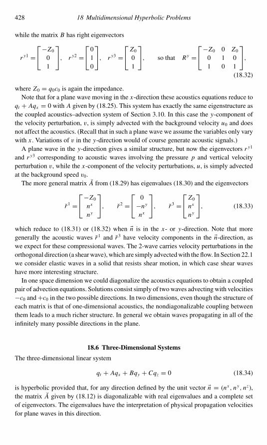
428 18 Multidimensional Hyperbolic Problems

while the matrix B has right eigenvectors

r y1 =−Z00

1

, r y2 =010

, r y3 = Z001

, so that Ry =−Z0 0 Z0

0 1 01 0 1

,(18.32)

where Z0 = q0c0 is again the impedance.Note that for a plane wave moving in the x-direction these acoustics equations reduce to

qt + Aqx = 0 with A given by (18.25). This system has exactly the same eigenstructure asthe coupled acoustics–advection system of Section 3.10. In this case the y-component ofthe velocity perturbation, v, is simply advected with the background velocity u0 and doesnot affect the acoustics. (Recall that in such a plane wave we assume the variables only varywith x . Variations of v in the y-direction would of course generate acoustic signals.)A plane wave in the y-direction gives a similar structure, but now the eigenvectors r y1

and r y3 corresponding to acoustic waves involving the pressure p and vertical velocityperturbation v, while the x-component of the velocity perturbations, u, is simply advectedat the background speed v0.The more general matrix A from (18.29) has eigenvalues (18.30) and the eigenvectors

r1 =−Z0nx

ny

, r2 = 0−nynx

, r3 = Z0nxny

, (18.33)

which reduce to (18.31) or (18.32) when n is in the x- or y-direction. Note that moregenerally the acoustic waves r1 and r3 have velocity components in the n-direction, aswe expect for these compressional waves. The 2-wave carries velocity perturbations in theorthogonal direction (a shearwave),which are simply advectedwith the flow. In Section 22.1we consider elastic waves in a solid that resists shear motion, in which case shear waveshave more interesting structure.In one space dimension we could diagonalize the acoustics equations to obtain a coupled

pair of advection equations. Solutions consist simply of twowaves advecting with velocities−c0 and+c0 in the two possible directions. In two dimensions, even though the structure ofeach matrix is that of one-dimensional acoustics, the nondiagonalizable coupling betweenthem leads to a much richer structure. In general we obtain waves propagating in all of theinfinitely many possible directions in the plane.

18.6 Three-Dimensional Systems

The three-dimensional linear system

qt + Aqx + Bqy + Cqz = 0 (18.34)

is hyperbolic provided that, for any direction defined by the unit vector n = (nx , ny, nz),the matrix A given by (18.12) is diagonalizable with real eigenvalues and a complete setof eigenvectors. The eigenvalues have the interpretation of physical propagation velocitiesfor plane waves in this direction.

18.7 Shallow Water Equations 429

The acoustics equations in three dimensions are a linear hyperbolic system for perturba-tions in the pressure and three velocity components (u, v, w). Rather than displaying thecoefficient matrices A, B, and C separately, it is more compact to just display A in anarbitrary direction n. We have

q =

puv

w

, A =

u0 nx K0 nyK0 nzK0

nx/ρ0 u0 0 0

ny/ρ0 0 u0 0

nz/ρ0 0 0 u0

, (18.35)

where

u0 = nxu0 + nyv0 + nzw0 (18.36)

is the component of the background velocity in the direction n. For any choice of direction,the eigenvalues of A are

λ1 = u0 − c0, λ

2 = λ3 = u0, λ

4 = u0 + c0. (18.37)

Note that there is a two-dimensional eigenspace corresponding to the eigenvalue λ2=

λ3= u0, since shear waves can now carry an arbitrary jump in each of the two velocitycomponents orthogonal to n.

18.7 Shallow Water Equations

In two space dimensions the shallow water equations take the form

ht + (hu)x + (hv)y = 0,

(hu)t +(hu2 + 1

2gh2

)x

+ (huv)y = 0,

(hv)t + (huv)x +(hv2 + 1

2gh2

)y

= 0,

(18.38)

where h is the depth and (u, v) the velocity vector, so that hu and hv are the momentain the two directions. These are a natural generalization of the one-dimensional equations(13.5) and are identical to the two-dimensional compressible flow equations derived inSection 18.3 if we replace ρ by h there and use the hydrostatic equation of state

p = P(h) = 1

2gh2 (18.39)

as derived in (13.3) (taking ρ = 1). From (18.21), the flux Jacobian matrices are thus

f ′(q) = 0 1 0−u2 + gh 2u 0−uv v u

, g′(q) = 0 0 1

−uv v u−v2 + gh 0 2v

. (18.40)

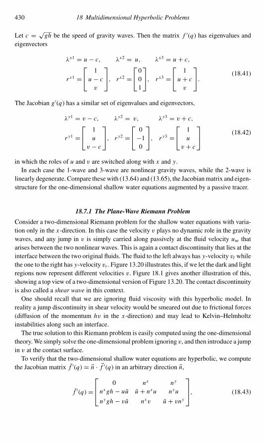
430 18 Multidimensional Hyperbolic Problems

Let c = √gh be the speed of gravity waves. Then the matrix f ′(q) has eigenvalues andeigenvectors

λx1 = u − c, λx2 = u, λx3 = u + c,

r x1 = 1u − cv

, r x2 =001

, r x3 = 1u + cv

. (18.41)

The Jacobian g′(q) has a similar set of eigenvalues and eigenvectors,

λy1 = v − c, λy2 = v, λy3 = v + c,

r y1 = 1

uv − c

, r y2 = 0−10

, r y3 = 1

uv + c

(18.42)

in which the roles of u and v are switched along with x and y.In each case the 1-wave and 3-wave are nonlinear gravity waves, while the 2-wave is

linearly degenerate. Compare these with (13.64) and (13.65), the Jacobianmatrix and eigen-structure for the one-dimensional shallow water equations augmented by a passive tracer.

18.7.1 The Plane-Wave Riemann Problem

Consider a two-dimensional Riemann problem for the shallow water equations with varia-tion only in the x-direction. In this case the velocity v plays no dynamic role in the gravitywaves, and any jump in v is simply carried along passively at the fluid velocity um thatarises between the two nonlinear waves. This is again a contact discontinuity that lies at theinterface between the two original fluids. The fluid to the left always has y-velocity vl whilethe one to the right has y-velocity vr . Figure 13.20 illustrates this, if we let the dark and lightregions now represent different velocities v. Figure 18.1 gives another illustration of this,showing a top view of a two-dimensional version of Figure 13.20. The contact discontinuityis also called a shear wave in this context.One should recall that we are ignoring fluid viscosity with this hyperbolic model. In

reality a jump discontinuity in shear velocity would be smeared out due to frictional forces(diffusion of the momentum hv in the x-direction) and may lead to Kelvin–Helmholtzinstabilities along such an interface.The true solution to this Riemann problem is easily computed using the one-dimensional

theory.We simply solve the one-dimensional problem ignoring v, and then introduce a jumpin v at the contact surface.To verify that the two-dimensional shallow water equations are hyperbolic, we compute

the Jacobian matrix f ′(q) = n · f ′(q) in an arbitrary direction n,

f ′(q) =

0 nx ny

nx gh − uu u + nxu nyu

nygh − vu nxv u + vny

, (18.43)

18.8 Euler Equations 431

u:

v:

ul = 0 ur = 0

vl vr

umum

Rarefaction Shock

Shear wave

Fig. 18.1. Solution to a Riemann problem in the x-direction for the two-dimensional shallow waterequations. The depth h and normal velocity u are as shown in Figure 13.20, and the shading in thatfigure represents v.

where u = n · u. This matrix has eigenvalues and eigenvectors given by

λ1 = u − c, λ

2 = u, λ3 = u + c,

r1 = 1u − nxcv − nyc

, r2 = 0−nynx

, r3 = 1u + nxcv + nyc

. (18.44)

The expressions (18.41) and (18.42) are special cases of this. For any direction n theeigenvalues are real and correspond to wave speeds 0, ±c relative to the moving fluid.

18.8 Euler Equations

The two-dimensionalEuler equations have the same formas the compressible flowequationspresented in Section 18.3, but with the addition of an energy equation for the general casewhere the equation of state is more complicated than (18.16):

q =

ρ

ρuρv

E

, f (q) =

ρu

ρu2 + pρuv

(E + p)u

, g(q) =

ρv

ρuv

ρv2 + p

(E + p)v

. (18.45)

432 18 Multidimensional Hyperbolic Problems

The equation of state for a γ -law polytropic gas is the obvious extension of (14.23). Thetotal energy is the sum of internal and kinetic energy,

E = p

γ − 1 +1

2ρ(u2 + v2). (18.46)

The Jacobian matrix f ′(q) has the four eigenvalues

λ1 = u − c, λ2 = u, λ3 = u, λ4 = u + c. (18.47)

As in one dimension, the sound speed is c = √γ p/ρ. The eigenvectors are

r x1 =

1

u − cv

H − uc

, r x2 =

1uv

12 (u

2 + v2)

, r x3 =

001v

, r x4 =

1

u + cv

H + uc

. (18.48)

The eigenvalues and eigenvectors in the y-direction are similar, with the roles of u and vreversed.

18.8.1 The Plane-Wave Riemann Problem

Consider a Riemann problem in which the data varies only in x . For the one-dimensionalEuler equations the density can be discontinuous across the contact discontinuity, asillustrated in Figure 14.1. In the two-dimensional extension, there can also be a jump inthe transverse velocity v across the contact discontinuity, exactly as was illustrated for thetwo-dimensional shallow water equations in Figure 18.1. The jump in density and the jumpin shear velocity are carried by two independent linearly degenerate waves that both travelat the same velocity. These two waves correspond to the two eigenvalues λ2 = λ3 = u ofthe Jacobian matrix. (The two vectors r x2 and r x3 in (18.48) are just one possible basis forthis two-diemensional eigenspace.)This two-dimensional Riemann problem is easily solved based on the one-dimensional

theory, just as in the case of the shallow water equations. We can follow the procedure ofSection 14.11, ignoring the transverse velocity v, since the primitive variables u and p arestill continuous across the contact discontinuity. We then introduce a jump in v from vl tovr at the contact discontinuity. Note that this also gives a jump in E in the eigenvector r x3,since v comes into the equation of state (18.46).

18.8.2 Three-Dimensional Euler Equations

In three spacedimensions theEuler equations are similar, butwith the additionof afifth equa-tion for the conservation of momentum ρw in the z-direction, where w is the z-component

18.9 Symmetry and Reduction of Dimension 433

of velocity. The conserved quantities and fluxes are then

q =

ρ

ρuρv

ρw

E

, f (q) =

ρu

ρu2 + pρuvρuw

(E + p)u

, g(q) =

ρv

ρuv

ρv2 + pρvw

(E + p)v

, h(q) =

ρw

ρuwρvw

ρw2 + p

(E + p)w

.(18.49)

The equation of state now includes the kinetic energy 12ρ(u

2 + v2 +w2)= 12ρu · u, where

u= (u, v, w) is the velocity vector. In any arbitrary direction n there are two nonlinearacoustic fieldswith eigenvalues (n·u)±c, and three linearly degeneratefieldswith eigenvaluen · u. These three fields correspond to jumps in the density (entropy waves), and jumps in thetwo transverse velocities (shear waves). For example, if n = (1, 0, 0), then we are lookingin the x-direction and arbitrary jumps in ρ, v, and w across the contact discontinuity canall propagate with speed u.

18.9 Symmetry and Reduction of Dimension

For some problems we may be able to reduce the complexity of the numerical problemsubstantially by taking advantage of symmetry. For example, if we are solving a problemwhere the solution is known to be radially symmetric, then we should be able to rewrite theequations in polar or spherical coordinates, obtaining a system that reduces to a problemin the single space variable r . The transformed equations will typically involve geometricsource terms.For example, when rewritten in polar r–θ coordinates, the compressible flow equations

(18.19) take the form

∂

∂t

rρrρUrρV

+ ∂

∂r

rρUrρU 2 + prρUV

+ 1

r

∂

∂θ

rρVrρUV

rρV 2 + p

= 0, (18.50)

where U (r, θ, t) is the velocity in the radial direction and V (r, θ, t) is the velocity in theθ -direction. If we assume that V (r, θ, t) ≡ 0 and there is no variation in the θ-direction,then these equations reduce to the two equations

(rρ)t + (rρU )r = 0,(rρU )t + (rρU 2 + p)r = 0.

(18.51)

This system can be rewritten as

ρt + (ρU )r = −(ρU )/r,(ρU )t + (ρU 2 + p)r = −(ρU 2)/r,

(18.52)

which has exactly the same form as the one-dimensional system of equations (2.38), butwith the addition of a geometric source term on the right-hand side.

434 18 Multidimensional Hyperbolic Problems

The full two- or three-dimensional Euler equations with radial symmetry yield

ρt + (ρU )r = −αr(ρU ),

(ρU )t + (ρU 2 + p)r = −αr(ρU 2),

Et + ((E + p)U )r = −αr((E + p)U ),

(18.53)

where α = 1 in two dimensions and α = 2 in three dimensions.Even if the real problems of interestmust be studiedmultidimensionally, radially symmet-

ric solutions are very valuable in testing and validating numerical codes. A highly accuratesolution to the one-dimensional problem can be computed on a fine grid and used to testsolutions computed with the multidimensional solver. This is useful not only in checkingthat the code gives essentially the correct answer in at least some special cases, but alsoin determining whether the numerical method is isotropic or suffers from grid-orientationeffects that lead to the results being better resolved in some directions than in others. SeeSection 21.7.1 for one such example.The D-dimensional acoustics equations with radial symmetry reduce to

pt + K0Ur = −αr(K0U ),

ρ0Ut + pr = 0,(18.54)

where again α = D − 1.

Exercises

18.1. Consider the system qt + Aqx + Bqy = 0 with

A =[3 11 3

], B =

[0 22 0

].

Show that these matrices are simultaneously diagonalizable, and determine the gen-eral solution to this system with arbitrary initial data. In particular, sketch how thesolution evolves in the x–y plane with data

q1(x, y, 0) ={1 if x2 + y2 ≤ 1,0 otherwise,

q2(x, y, 0) ≡ 0.

18.2. (a) Suppose that A and B are both symmetric matrices. Show that the systemqt + Aqx + Bqy = 0 must then be hyperbolic.

(b) Thematrices A and B are simultaneously symmetrizable if there is an invertiblematrix M such that M−1AM and M−1BM are both symmetric. Show that inthis case the system qt + Aqx + Bqy = 0 must be hyperbolic.

(c) Show that the matrices in (18.25) for the linearized acoustics equations aresimultaneously symmetrizablewith amatrixM of the formM = diag(d1, 1, 1).

Exercises 435

18.3. Consider the two-dimensional system qt + Aqx + Bqy = 0 with matrices

A =[1 100 2

], B =

[2 010 1

],

each ofwhich is diagonalizablewith real eigenvalues. Show, however, that this systemis not hyperbolic. (See also Exercise 19.1.)

18.4. Determine the eigenvectors of the three-dimensional acousticsmatrix A from (18.35).18.5. Show that the three-dimensional system (2.115) of Maxwell’s equations is hyper-

bolic.

19Multidimensional Numerical Methods

In the remainder of the book we concentrate on finite volume methods for multidimen-sional hyperbolic equations. We will begin by considering uniform Cartesian grids in twodimensions, using the notation illustrated in Figure 19.1(a). The value Qni j represents a cellaverage over the (i, j) grid cell at time tn ,

Qni j ≈1

�x �y

∫ y j+1/2

y j−1/2

∫ xi+1/2

xi−1/2q(x, y, tn) dx dy. (19.1)

As in one dimension, we can use the integral form of the equations to determine how this cellaverage varies with time, and develop finite volume methods based on numerical approx-imations to the fluxes at each cell edge. Various approaches to doing this are summarizedstarting in Section 19.2.

19.1 Finite Difference Methods

Rather than working with the cell averages and the integral form of the equations, one couldinstead view Qni j as a pointwise approximation to the value of q(xi , y j , tn) at the pointindicated in Figure 19.1(b). Discretizing the differential equations by finite differences thengives a finite difference method. As in one dimension, this approach often gives methodsthat look very similar to related finite volumemethods.Wewill concentrate on finite volumemethods, since this viewpoint allows the derivation of methods that are more robust whendiscontinuities are present, as well as being exactly conservative. However, it is sometimesuseful to think of the methods in terms of their finite difference interpretation, in particularwhen computing the local truncation error by comparing with a Taylor series expansionof the true solution at the point (xi , y j ). The flux differences arising in a finite volumemethod are often seen to give approximations to terms in this Taylor expansion, at leastwhen applied to smooth solutions.

19.1.1 Taylor Series Expansion of the Exact Solution

We develop the Taylor series expansion of the exact solution at a point after a single timestep for the constant-coefficient linear hyperbolic system

qt + Aqx + Bqy = 0. (19.2)

436

19.1 Finite Difference Methods 437

xi+1/2

yj−1/2

yj+1/2

Qij

xi−1/2

Qij

xi

yj

Fig. 19.1. (a) Finite volume grid in two space dimensions, where Qi j represents a cell average.(b) Finite difference grid in two dimensions, where Qi j represents a pointwise value.

We will require higher-order time derivatives in this expansion, which are most easily foundfrom the expression

∂jt q = [−(A∂x + B∂y)] j q. (19.3)

So, in particular,

qtt = A2qxx + ABqyx + BAqxy + B2qyy . (19.4)

Note that although qyx = qxy , in general AB �= BA, and so we cannot combine the middletwo terms.The Taylor series expansion at (xi , y j ) after time �t can be written as

q(xi , y j , tn +�t) = q +�t qt + 1

2�t2qtt + · · ·

= q −�t (Aqx + Bqy)

+ 12�t2(A2qxx + ABqyx + BAqxy + B2qyy)+ · · · . (19.5)

Note that if A and B vary with x and y, then (19.3) still holds, but (19.4) becomes

qtt = A(Aqx )x + A(Bqy)x + B(Aqx )y + B(Bqy)y . (19.6)

The expansion becomes somewhat more complicated, as would the Lax–Wendroff methoddeveloped in the next subsection.

19.1.2 The Lax–Wendroff Method

The Lax–Wendroff method for the equation (19.2) is obtained by keeping only the termsshown in (19.5) and replacing the derivatives by centered finite differences, just as in

438 19 Multidimensional Numerical Methods

one space dimension. The purely one-dimensional derivatives are approximated as in onedimension, e.g.,

qyy = 1

�y2(Qni, j−1 − 2Qni j + Qni, j+1

).

In addition, there are now cross-derivative terms, which can also be approximated to second-order with centered differences,

qxy = qyx ≈ 1

4�x �y

[(Qni+1, j+1 − Qni−1, j+1

)− (Qni+1, j−1 − Qni−1, j−1)]. (19.7)

Using these approximations in (19.5) gives

Qn+1i j = Qni j −�t

2�xA(Qni+1, j − Qni−1, j

)− �t

2�yB(Qni, j+1 − Qni, j−1

)+ �t2

2�x2A2(Qni+1, j − 2Qni j + Qni−1, j

)+ �t2

2�y2B2(Qni, j+1 − 2Qni j + Qni, j−1

)+ �t2

8�x �y(AB + BA)[(Qni+1, j+1 − Qni−1, j+1)− (Qni+1, j−1 − Qni−1, j−1)].

(19.8)

This has a nine-point stencil involving all nine of the points in Figure 19.1(b) in the updatefor Qi j . In Section 19.3.1 wewill see that this samemethod can be viewed as a finite volumemethod for updating the cell average Qi j shown in Figure 19.1(a), resulting from definingnumerical fluxes at the four edges of the cell in a natural way, based on the nine nearby cellvalues.

19.2 Finite Volume Methods and Approaches to Discretization

As in one space dimension, the two-dimensional Lax–Wendroff method suffers from prob-lems with numerical dispersion, leading to phase errors and to unphysical oscillations inproblems with discontinuities or steep gradients. By reinterpreting this method as a finitevolume method and introducing upwind biasing and flux limiting, we will see that it canbe greatly improved. We will also write the resulting methods in a more general form thatapplies also to nonlinear conservation laws and to variable-coefficient problems, by usingthe waves resulting from solving Riemann problems at each cell edge as the basis forupwinding and limiting.This goal is pursued starting in the next chapter, where we begin to focus on this approach

to developing multidimensional high-resolution methods. This is certainly not the onlyapproach, however, and a wide variety of other multidimensional algorithms have beendeveloped and successfully used. The remainder of this chapter is devoted to introducingsome general notions of multidimensional finite volume methods.Three of the most popular general approaches to obtaining multidimensional methods

are:

19.3 Fully Discrete Flux-Differencing Methods 439

• Fully discrete flux-differencing methods. In Section 19.3 we will see that the Lax–Wendroff method can be rewritten as a flux-differencing method. A numerical flux ateach edge of the grid cell is defined, based on the data at the beginning of the time step.Differencing these fluxes gives the update to the cell average over a time step. To obtainbetter than first-order accuracy it is necessary to use the Taylor series expansion devel-oped above in defining these fluxes. To obtain high-resolution nonoscillatory results it isalso necessary to introduce limiters. There are many ways in which this can be done, andone particular method of this form is developed in Chapters 20 and 21.

• Semidiscretemethodswith Runge–Kutta time stepping.Rather than using the Taylor seriesto replace time derivatives by spatial derivatives, we can focus on obtaining good accuracyof the flux at one instant in time and then use a Runge–Kutta method to perform the timestepping. This approach was introduced in one space dimension in Section 10.4. Thetwo-dimensional extension is briefly discussed in Section 19.4.

• Dimensional splitting. By far the simplest approach to obtaining a multidimensionalmethod is to apply a fractional-step method to split a multidimensional problem up into asequence of one-dimensional problems. To solve qt+ f (q)x+g(q)y = 0, for example, wemight alternate between solving qt + f (q)x = 0 and qt + g(q)y = 0, similarly to the wayfractional-step methods are used for handling source terms, as discussed in Chapter 17.This approach, which is often surprisingly effective, is discussed in Section 19.5.

Wewill concentrate onmethods that use one-dimensional Riemann solvers as a basic toolin the determination of interface fluxes. This is possible because the local problem at theedge of a grid cell is essentially one-dimensional in the direction normal to the edge. In orderto obtain better than first-order accuracy it is necessary to bring in more multidimensionalinformation, as is clear from the Taylor series expansion (19.5), but this can be done invarious ways while still only using one-dimensional Riemann solutions.One particular approach is developed starting in Chapter 20, in the form of the wave-

propagation algorithms developed in [282], [283], and [257]. These algorithms take theform of fully discrete flux-differencing methods and are implemented in CLAWPACK in sucha way that they can be applied to a wide variety of hyperbolic problems. Some relatedmethods of this form can be found, for example, in [22], [24], [80], [100], [389].Other methods have been developed that are based on a full decomposition of the data

into multidimensional waves, rather than relying on one-dimensional Riemann solvers. Forsome examples, see [3], [52], [105], [106], [134], [135], [199], [342], [414], [415], [428].

19.3 Fully Discrete Flux-Differencing Methods

In deriving the two-dimensional conservation law qt + f (q)x + g(q)y = 0 in Section 18.1,we considered an arbitrary region�. Now consider the special case where� is a rectangulargrid cell of the form Ci j = [xi−1/2, xi+1/2]×[y j−1/2, y j+1/2], as shown in Figure 19.1, wherexi+1/2 − xi−1/2 = �x and y j+1/2 − y j−1/2 = �y. In this special case, the formula (18.7)simplifies, since the normal vector always points in either the x- or the y-direction. Thenormal flux is given by f (q) along the left and right edges and by g(q) along the top and

440 19 Multidimensional Numerical Methods

bottom. Integrating around the edges as required in (18.7) then gives

d

dt

∫∫Ci jq(x, y, t) dx dy =

∫ y j+1/2

y j−1/2f(q(xi+1/2, y, t

))dy−

∫ y j+1/2

y j−1/2f(q(xi−1/2, y, t

))dy

+∫ xi+1/2

xi−1/2g(q(x, y j+1/2, t

))dx −

∫ xi+1/2

xi−1/2g(q(x, y j−1/2, t

))dx .

(19.9)

If we integrate this expression from tn to tn+1 and divide by the cell area�x �y, we are ledto a fully discrete flux-differencing method of the form

Qn+1i j = Qni j −�t

�x

[Fni+1/2, j − Fni−1/2, j

]− �t

�y

[Gni, j+1/2 − Gni, j−1/2

], (19.10)

where

Fni−1/2, j ≈1

�t �y

∫ tn+1

tn

∫ y j+1/2

y j−1/2f(q(xi−1/2, y, t

))dy dt,

Gni, j−1/2 ≈1

�t �x

∫ tn+1

tn

∫ xi+1/2

xi−1/2g(q(x, y j−1/2, t

))dx dt.

(19.11)

The numerical fluxes Fn andGn at each edge are typically computed from the data Qn at theinitial time. (As in one dimension, these methods can also be extended to nonconservativehyperbolic systems, see Section 19.3.3.)For the linear system qt+Aqx+Bqy = 0we can obtain approximations to these interface

fluxes by using the Taylor expansion (19.5), which can be rewritten as

q(x, y, tn +�t) = q − �t

(Aq − �t

2A2qx − �t

2ABqy

)x

− �t

(Bq − �t

2B2qy − �t

2BAqx

)y

+ · · · . (19.12)

This suggests that we need

Fi−1/2, j ≈ Aq(xi−1/2, y j , tn

)− �t

2A2qx

(xi−1/2, y j , tn

)− �t

2ABqy

(xi−1/2, y j , tn

),

Gi, j−1/2 ≈ Bq(xi , y j−1/2, tn

)− �t

2B2qy

(xi , y j−1/2, tn

)− �t

2BAqx

(xi , y j−1/2, tn

).

(19.13)

It can be shown that for this problem these expressions agree with the integrals in (19.11)to O(�t2).

19.3 Fully Discrete Flux-Differencing Methods 441

19.3.1 Flux-Differencing Form of the Lax–Wendroff Method

The Lax–Wendroff method (19.8) for the constant-coefficient linear system qt + Aqx +Bqy = 0 can be interpreted as a method of the form (19.10), where the fluxes are given by

Fi−1/2, j = 1

2A(Qi−1, j + Qi j )− �t

2�xA2(Qi j − Qi−1, j )

− �t

8�yAB[(Qi, j+1 − Qi j )+ (Qi−1, j+1 − Qi−1, j )

+ (Qi j − Qi, j−1)+ (Qi−1, j − Qi−1, j−1)],

Gi, j−1/2 = 1

2B(Qi, j−1 + Qi j )− �t

2�yB2(Qi j − Qi, j−1)

− �t

8�xBA[(Qi+1, j − Qi j )+ (Qi+1, j−1 − Qi, j−1)

+ (Qi j − Qi−1, j )+ (Qi, j−1 − Qi−1, j−1)].

(19.14)

These fluxes relate directly to (19.13).Note in particular that the expression ABqy in (19.13),for example, is approximated by

ABqy(xi−1/2, y j , tn)≈ 1

4�y[AB(Qi, j+1− Qi j )+ AB(Qi−1, j+1− Qi−1, j )+ AB(Qi j − Qi, j−1)+ AB(Qi−1, j − Qi−1, j−1)]. (19.15)

In Chapters 20 and 21 we will see how this method can be greatly improved by introducingan upwind bias and flux limiting into the formulas.

19.3.2 Godunov’s Method

For a general conservation law, the simplest flux-differencing method of the form (19.10)is Godunov’s method. A natural two-dimensional generalization of the method devel-oped in Section 15.1 is obtained by simply solving the normal Riemann problem at eachcell edge to find the value Q∨

|that propagates with speed 0, and then evaluating the

appropriate flux function at this value to obtain the numerical flux at this edge. Thisgives

Fi−1/2, j = f(Q∨

|i−1/2, j

),

Gi, j−1/2 = g(Q∨

|i, j−1/2

),

(19.16)

where Q∨|i−1/2, j is obtained by solving the Riemann problem for qt + f (q)x = 0 with

data Qi−1, j and Qi j , while Q∨|i, j−1/2 is obtained by solving the Riemann problem for

qt + g(q)y = 0 with data Qi, j−1 and Qi j . As in one dimension, approximate Riemannsolvers can be used in place of the exact Riemann solution.For a linear system of equations with f (q)= Aq and g(q)= Bq, we denote the eigen-

vector matrices for A and B by Rx and Ry , respectively, and the eigenvalue matrices by�x and �y , as in Section 18.5. We can then define matrices A± and B± analogous to

442 19 Multidimensional Numerical Methods

(4.45) by

A± = Rx (�x )±(Rx )−1, B± = Ry(�y)±(Ry)−1. (19.17)

In terms of this notation, we find that the Godunov fluxes for a linear problem are the naturalgeneralization of the one-dimensional flux (4.56),

Fi−1/2, j = A+Qi−1, j + A−Qi j ,

Gi, j−1/2 = B+Qi, j−1 + B−Qi j .(19.18)

This amounts to using only the first terms in the fluxes (19.13), and an upwind approximationto these. Of course, this method is only first-order accurate and moreover is typically stableonly for Courant number up to 1/2 in two dimensions. This is illustrated for the advectionequation in Section 20.4.

19.3.3 Fluctuation Form

As in one space dimension, we will develop finite volume methods in a more general formthan the flux-differencing formula (19.10), so that they are also applicable to hyperbolicequations that are not in conservation form. To make this extension we will rewrite themethod as follows, motivated by the one-dimensional method (15.62):

Qn+1i j = Qi j − �t

�x

(A+�Qi−1/2, j +A−�Qi+1/2, j)

− �t

�y

(B+�Qi, j−1/2 + B−�Qi, j+1/2)

− �t

�x

(F i+1/2, j − F i−1/2, j

)− �t

�y

(Gi, j+1/2 − Gi, j−1/2

). (19.19)

The term A+�Qi−1/2, j , for example, represents the first-order Godunov update to thecell value Qi j resulting from the Riemann problem at the edge (i − 1/2, j). The otherthree similar terms are the Godunov updates resulting from the Riemann problems at theother three edges. For the linear system discussed above, these fluctuations are simplygiven by

A±�Qi−1/2, j = A±(Qi j − Qi−1, j ),B±�Qi, j−1/2 = B±(Qi j − Qi, j−1).

(19.20)

For Godunov’s method we take F = G = 0 everywhere. Later the fluxes F and G will beused for correction terms, both those arising from introducing slopes as in one dimensionto model the A2 and B2 terms in (19.13), and also new ones modeling the cross-derivativeterms involving AB and BA in (19.13).

19.4 Semidiscrete Methods with Runge–Kutta Time Stepping 443

For a general nonlinear conservation lawwhere theGodunovfluxes are definedby (19.16),we can set

A+�Qi−1/2, j = f (Qi j )− f(Q∨

|i−1/2, j

),

A−�Qi−1/2, j = f(Q∨

|i−1/2, j

)− f (Qi−1, j ),

B+�Qi, j−1/2 = g(Qi j )− g(Q∨

|i, j−1/2

),

B−�Qi, j−1/2 = g(Q∨

|i, j−1/2

)− g(Qi, j−1).(19.21)

Godunov’s method results from using these formulas in (19.19) and setting all F = G = 0.As in one dimension, the fluctuationsA±�Q and B±�Q can also be computed in terms ofthe waves and speeds arising in the Riemann solution, using formulas analogous to (4.42).

19.4 Semidiscrete Methods with Runge–Kutta Time Stepping

As we see already from the Lax–Wendroff method with fluxes (19.14), obtaining evensecond-order accuracy with a flux-differencing method based on the time-integrated fluxes(19.11) can lead to complicated formulas. As discussed in Section 10.3 for one-dimensionalproblems, this Taylor series approach is not easily extended to obtain higher-order methods.For this reason, another popular approach is to proceed as in Section 10.4 and use theexpression (19.9) to derive ordinary differential equations for the evolution of the cellaverages

Qi j (t) =∫∫

Ci jq(x, y, t) dx dy. (19.22)

This is accomplished by defining numerical flux functions

Fi−1/2, j (Q(t)) ≈ 1

�y

∫ y j+1/2

y j−1/2f(q(xi−1/2, y, t

))dy,

Gi, j−1/2(Q(t)) ≈ 1

�x

∫ xi+1/2

xi−1/2g(q(x, y j−1/2, t

))dx

(19.23)

by some procedure based on the nearby cell averages at this instant in time. Then the systemof ODEs

d

dtQi j (t) = − 1

�x

[Fi+1/2, j (Q(t))− Fi−1/2, j (Q(t))

]− 1

�y

[Gi, j+1/2(Q(t))− Gi, j−1/2(Q(t))

](19.24)

is solved by an ODE method, typically a multistage Runge–Kutta method. In order toachieve high-order accuracy it is still necessary to use information from several grid cellsnearby in defining the fluxes (19.23), typically by some multidimensional interpolationmethod. However, since we do not attempt to also approximate the time-derivative terms,

444 19 Multidimensional Numerical Methods

this may be relatively simple. To obtain a high-resolution method, it is necessary to includesome form of upwinding and/or limiting in the process of approximating the flux, e.g., bya multidimensional version of the ENO method described in Section 10.4.4.

19.5 Dimensional Splitting

The easiest way to extend one-dimensional numerical methods to more space dimensionsis to use dimensional splitting, an application of the fractional-step procedure discussed inChapter 17. Amultidimensional problem is simply split into a sequence of one-dimensionalproblems. This is easy to apply on aCartesian grid alignedwith the coordinate axes as shownin Figure 19.1.For example, the two-dimensional linear problem

qt + Aqx + Bqy = 0

can be split into

x-sweeps : qt + Aqx = 0, (19.25)

y-sweeps : qt + Bqy = 0. (19.26)

In the x-sweeps we start with cell averages Qni j at time tn and solve one-dimensionalproblems qt + Aqx = 0 along each row of cells Ci j with j fixed, updating Qni j to Q∗i j :

Q∗i j = Qni j −�t

�x

(Fni+1/2, j − Fni−1/2, j

), (19.27)

where Fni−1/2, j is an appropriate numerical flux for the one-dimensional problem betweencells Ci−1, j and Ci j . In the y-sweeps we then use the Q∗i j values as data for solvingqt + Bqy = 0 along each column of cells with i fixed, which results in Qn+1i j :

Qn+1i j = Q∗i j −�t

�x

(G∗i, j+1/2 − G∗i, j−1/2

). (19.28)

Note that there will generally be a splitting error (see Section 17.3) unless the opera-tors A= A∂x and B= B∂y commute, i.e., unless AB= BA. Only in the case where themultidimensional problem decouples into scalar advection equations can we use dimen-sional splitting with no splitting error. Even in this case we must be careful with boundaryconditions (see Section 17.9).However, the splitting error is often no worse than the errors introduced by the numerical

methods in each sweep, and dimensional splitting can be a very effective approach. It gives asimple and relatively inexpensive way to extend one-dimensional high-resolution methodsto two or three dimensions.Note that with the dimensional-splitting approach we do not explicitly model the cross-

derivative terms involving qxy in the Taylor series expansion (19.5). In each sweep we onlymodel second derivatives in each coordinate direction, qxx and qyy , which appear in theone-dimensional algorithm. The qxy term arises automatically through the fractional-step

19.5 Dimensional Splitting 445

procedure. The intermediate solution q∗ resulting from x-sweeps involves terms modelingAqx . In the y-sweeps we compute terms modeling Bq∗y , which thus model B(Aqx )y .Instead of this Godunov splitting, one might instead use the Strang splitting

Q∗i j = Qni j −�t

2�x

(Fni+1/2, j − Fni−1/2, j

),

Q∗∗i j = Q∗i j −�t

�x

(G∗i, j+1/2 − G∗i, j−1/2

),

Qn+1i j = Qni j −�t

2�x

(F∗∗i+1/2, j − F∗∗i−1/2, j

),

(19.29)

as discussed in Section 17.4. With the Strang splitting we also obtain terms modelingA(Bqy)x from the second x-sweep, which are also needed in the Taylor series expansion.Only in the constant-coefficient case with AB = BA does the Godunov splitting give a fullysecond-order accurate method. However, in practice there is often very little difference inresults obtainedwith the two approaches, as is also the case for other fractional-stepmethodsas discussed in Section 17.5.In fact, if the Strang splitting is implemented as in (19.29), it may give worse results than

the Godunov splitting, because the x-sweeps are taken with time step�t/2 and hence willtypically have Courant number less than 1/2. This introduces more numerical smearing aswell as more work. If instead the Strang splitting is implemented by simply alternating theorder inwhich x-sweeps and y-sweeps are performed, then this is avoided (see Section 17.4).However, this is somewhat harder to implement in connection with variable-size time steps,and in CLAWPACK the form (19.29) is implemented as the Strang splitting, though theGodunov splitting is generally recommended instead.

19.5.1 CLAWPACK Implementation

In order to apply the fractional-step approach, we need to be able to solve each of the one-dimensional equations (19.25) and (19.26), and hence must have two different Riemannsolvers available. For many physical systems the equations and solution procedure areessentially the same in each direction. For example, the acoustics equations (18.25) in anisotropic medium have exactly the same form when restricted to plane waves in x or y, butwith the roles of u and v reversed. The same is true for the shallow water equations (18.38)and the Euler equations (18.45). For this reason it is often simplest to write a single Riemannsolver with a flag indicating the desired direction. This convention is used in CLAWPACK,where a single subroutine rpn2must be provided that solves the Riemann problem normalto edges of grid cells along one slice of the domain. The flag ixy indicates whether the sliceis in the x-direction or the y-direction. The other parameters of this routine are identical tothe parameters appearing in the one-dimensional Riemann solver rp1.The two-dimensional CLAWPACK code also allows a second Riemann solver rpt2 to be

provided. This must solve a different sort of Riemann problem in the transverse direction,as described in Section 21.3, and is not used in the dimensional-splitting algorithm.Dimensional splitting is invoked in CLAWPACK by setting method(3)= -1 for the

Godunov splitting, which is generally recommended, or method(3)= -2 for Strang

446 19 Multidimensional Numerical Methods

splitting. Positive values of method(3) instead invoke the unsplit methods described inlater chapters. (See Section 21.3.)

Exercise

19.1. The system given in Exercise 18.3 is hyperbolic in x and y separately, and so we canapply dimensional splitting to attempt to solve this nonhyperbolic system. Implementthis in CLAWPACK, and analyze what happens.

20Multidimensional Scalar Equations

In this chapter we will develop high-resolution methods for scalar hyperbolic equations intwo space dimensions.We begin by considering the constant-coefficient advection equationand show how the waves obtained by solving the Riemann problem at each cell interfacecan be naturally used to define high-resolution fluxes. We then extend these methods tovariable-coefficient advection and nonlinear scalar conservation laws. In the next chapterthey are extended further to hyperbolic systems of equations.We first consider the scalar advection equation

qt + uqx + vqy = 0, (20.1)

with u and v constant. In the figures illustrating these methods we will generally assumeu > 0 and v > 0, and this case will sometimes be assumed when we wish to be specific, butmost of the formulas will be presented in a manner that applies for flow in any direction.The notation u± and v± meaning the positive or negative part of the velocity will frequentlybe used, with the definition (4.40).The true solution for this equation is simply q(x, y, t) = q◦(x − ut, y − vt), but for our

present purposes the Taylor series expansion is more illuminating:

q(x, y, tn+1) = q(x, y, tn)+�t qt (x, y, tn)+ 1

2(�t)2qtt (x, y, tn)+ · · ·

= q(x, y, tn)− u�t qx − v �t qy+ 12(�t)2[u2qxx + vuqxy + uvqyx + v2qyy]+ · · · . (20.2)

This comes from (19.5) with A = u and B = v, and will be useful in identifying termsarising in finite volume approximations to the advection equation.

20.1 The Donor-Cell Upwind Method for Advection

The simplest finite volume method for the advection equation is the first-order upwindmethod, which takes the general form

Qn+1i j = Qi j − �t

�x[u+(Qi j − Qi−1, j )+ u−(Qi+1, j − Qi j )]

− �t

�y[v+(Qi j − Qi, j−1)+ v−(Qi, j+1 − Qi j )]. (20.3)

447

448 20 Multidimensional Scalar Equations

This uses an upwind approximation to the derivatives qx and qy in the O(�t) terms of theTaylor series expansion (20.2). This method has the form (19.19) with F = G = 0 andfluctuations

A±�Qi−1/2, j = u±(Qi j − Qi−1, j ),B±�Qi, j−1/2 = v±(Qi j − Qi, j−1),

(20.4)

which are a special case of (19.20).This upwind method agrees with Godunov’s method as described in Section 19.3.2 for

this scalar equation. The fluxes for the method (20.3) are

Fi−1/2, j = u+Qi−1, j + u−Qi j ,Gi, j−1/2 = v+Qi, j−1 + v−Qi j ,

(20.5)

which agree with the Godunov fluxes (19.18). In this case each Riemann solution consistsof a single wave carrying the jump in Q between the neighboring two grid cells, propagatingat speed u horizontally or at speed v vertically depending on the orientation of the two cells.The value of Q∨

|at each interface depends on whether the relevant velocity is positive or

negative.The first-order accurate method (20.3) for the advection equation is often called the

donor-cell upwind (DCU)method. Each flux in (20.5) approximates the amount of q flowingnormal to the edge, assuming that the only contribution to this flux is from the adjacent cellon the upwind side (the donor cell). This is indicated schematically in Figure 20.1(a) forthe case u, v > 0.Note that the updated value Qn+1i j depends on only the three values Qi j , Qi−1, j , and

Qi, j−1. This is clearly not correct, since the flow is really at an angle to the grid, as indicatedin Figure 20.1(b), and the value Qi−1, j−1 should also affect Qn+1i j . The CFL condition(Section 4.4) suggests that this may cause stability problems, and indeed this method doesnot have the best possible stability properties. It will be shown in Section 20.4 that this

(a) (b)

Fig. 20.1. (a) Waves moving normal to the cell interfaces give the updates for the DCU method.(b) The true velocity (u, v) is at an angle to the grid, and information from cell (i − 1, j − 1) shouldalso affect the new value in cell (i, j). This corner coupling is missing in the DCU method.

20.2 The Corner-Transport Upwind Method for Advection 449

method is stable only for �t small enough that∣∣∣∣u�t�x

∣∣∣∣+ ∣∣∣∣v �t�y

∣∣∣∣ ≤ 1. (20.6)

An improved upwind method is developed in Section 20.2, which takes account of theflow direction more fully and has the stability bound

max

(∣∣∣∣u�t�x

∣∣∣∣ , ∣∣∣∣v�t�y

∣∣∣∣) ≤ 1. (20.7)

This is better than (20.6) whenever u and v are both nonzero, i.e., when flow is at an angleto the grid.

20.2 The Corner-Transport Upwind Method for Advection

For the advection equation, a better first-order accurate upwind method can be derived bytaking the reconstruct–evolve–average approach of Algorithm 4.1, extended in the obviousway to two space dimensions:

• View the cell averages at time tn as defining a piecewise constant function qn(x, y, tn)with constant value Qni j in cell Ci j ,

• Evolve the advection equation exactly with this data over time �t ,• Average the resulting solution qn(x, y, tn+1) back onto the grid.

For the constant-coefficient advection equation this is easily done, since

qn(x, y, tn+1) = qn(x − u�t, y − v �t, tn).

The exact solution is the same piecewise constant function, simply shifted by (u �t, v �t).So we find that

Qn+1i j = 1

�x�y

∫ xi+1/2

xi−1/2

∫ y j+1/2

y j−1/2qn(x − u �t, y − v �t, tn) dx dy

= 1

�x�y

∫ xi+1/2−u�t

xi−1/2−u�t

∫ y j+1/2−v �t

y j−1/2−v �tqn(x, y, tn) dx dy. (20.8)

The new cell average Qn+1i j is given by the cell average of qn(x, y, tn) over the shadedregion shown in Figure 20.2. Since qn(x, y, tn) is constant in each grid cell, this reduces toa simple convex combination of four cell values:

Qn+1i j = 1

�x �y

[(�x − u�t)(�y − v �t)Qni j + (�x − u�t)(v �t)Qni, j−1+ (�y − v �t)(u�t)Qni−1, j + (u�t)(v �t)Qni−1, j−1

]. (20.9)

450 20 Multidimensional Scalar Equations

Fig. 20.2. The corner-transport upwind method is obtained by shifting the piecewise constant data bydistance (u�t, v �t) and averaging back on the grid. Alternatively, the new value Qn+1i j is determinedby averaging the piecewise constant function over the shaded region shown in the figure.

This can be rearranged to yield

Qn+1i j = Qi j − u�t

�x(Qi j − Qi−1, j )− v �t

�y(Qi j − Qi, j−1)

+ 12(�t)2

{u

�x

[v

�y(Qi j − Qi, j−1)− v

�y(Qi−1, j − Qi−1, j−1)

]+ v

�y

[u

�x(Qi j − Qi−1, j )− u

�x(Qi, j−1 − Qi−1, j−1)

]}. (20.10)

The top line of this expression corresponds to the donor-cell upwindmethod. The additionalterms can be arranged in several different ways. They have been displayed here in a mannerthat relates directly to the Taylor series expansion (20.2).We see that the final term in (20.10)models the cross-derivative terms uvqyx + vuqxy in the O((�t)2) term of that expansion.The method (20.10) is often called corner-transport upwind (CTU) method (following

Colella [80]), since it includes the proper transport across the corner from cell Ci−1, j−1 toCi j . It is still only first-order accurate, for two reasons: It is missing approximations to theqxx and qyy terms in (20.2), and the approximations to uqx and vqy terms are only first-order one-sided approximations. Both of these deficiencies can be addressed by introducingslopes in the x- and y-directions separately, just as we did in one dimension. Consequently ahigh-resolution version of this algorithm is easy to construct, as we will do in Section 20.6.See [25], [470] for discussion of some related algorithms.

20.3 Wave-Propagation Implementation of the CTU Method

Before discussing high-resolution corrections, we will develop a different implementationof the CTU method that will be much easier to extend to variable-coefficient advection andto other hyperbolic systems. Figure 20.3 shows the basis for a wave-propagation view ofthis method, in which all waves propagate at velocity (u, v) in the correct physical direction.To be specific we will continue to assume u > 0 and v > 0 in the figures and formulas inthis section. More general formulas are given in the next section.

20.3 Wave-Propagation Implementation of the CTU Method 451

ii− 1 i+ 1

j

j − 1

j + 1

Fig. 20.3. (a) Transverse propagation affecting the fluxes F i+1/2, j and Gi, j+1/2. (b) Transverse prop-agation affecting the fluxes F i−1/2, j and Gi, j−1/2.

From the interface between cells Ci−1, j and Ci j , for example, there is a wave that propa-gates into cells Ci j and Ci, j+1. The jump across this wave is Qi j−Qi−1, j , and this incrementaffects both cell averages Qi j and Qi, j+1. As Figure 20.3 shows, there are four distinctwavesthat affect Qni j . The effect of each wave is to modify the cell average by the jump across thewave multiplied by the fraction of the cell covered by the wave. These fractions are easilyworked out, noting that the small triangular portion of each wave moving transversely intoneighboring cells has area 12 (u�t)(v �t) = 1

2uv(�t)2. Thewave from interface (i−1/2, j),

for example, modifies Qi j by

(u�t �y − 1

2uv(�t)2

�x �y

)(Qi j − Qi−1, j ) (20.11)

and modifies Qi, j+1 by

(12uv(�t)

2

�x �y

)(Qi j − Qi−1, j ). (20.12)

Note that the update (20.11) is present in the formula (20.10), split into two parts. The latterpart, corresponding to the triangular piece, is grouped with three other term correspondingto the triangular pieces of the other three waves shown in Figure 20.3 that affect thiscell.Thuswe can view (20.10) as consisting of theDCUmethod (the first line), inwhichwaves

simply move normal to the cell interfaces as shown in Figure 20.1, combined with a set ofcorrections for the transverse propagation of the waves. These corrections can be viewed asfluxes through edges of the cell. The triangular region in cell (i, j+1) of Figure 20.3(a) hasbeen transferred from cell (i, j) and hence corresponds to a flux through edge (i, j + 1/2).This transfer can be represented by a flux Gi, j+1/2. Taking this viewpoint, we find that wecan rewrite (20.10) in the form (19.19) by definingA±�Q and B±�Q as in (20.4) and the

452 20 Multidimensional Scalar Equations

correction fluxes as

F i−1/2, j = −12

�t

�yuv(Qi−1, j − Qi−1, j−1),

F i+1/2, j = −12

�t

�yuv(Qi j − Qi, j−1),

Gi, j−1/2 = −12

�t

�xuv(Qi, j−1 − Qi−1, j−1),

Gi, j+1/2 = −12

�t

�xuv(Qi j − Qi−1, j ).

(20.13)

The CTU method has better stability properties than DCU. From the interpretation ofthe algorithm given at the beginning of Section 20.2, we expect the method to be stablefor any time step for which the piecewise constant function does not shift more than onegrid cell in the time step. This gives the stability bound (20.7), and the method is stable forCourant numbers up to 1. This can be shown formally in the 1-norm by extending the proofof Section 8.3.4 to two dimensions using the convex combination (20.9). Stability in the2-norm is demonstrated using von Neumann analysis in the next section.

20.4 von Neumann Stability Analysis

For constant-coefficient linear equations, von Neumann analysis is often the easiest way todetermine stability bounds, as discussed in Section 8.3.3 in one space dimension. As two-dimensional examples, in this section we consider the DCU method (20.3) and the CTUmethod (20.10). Similar analysis can also be performed for the Lax–Wendroff method orthe wave-propagation version (introduced in Section 20.6) provided that no limiter functionis applied. (Applying limiters makes the method nonlinear and von Neumann analysis canno longer be used.) See [282] for stability analyses of these cases and three-dimensionalgeneralizations, and also [202].To be specific wewill assume u, v > 0, although similar analysis applies to other choices

of signs. Then the DCU method (20.3) becomes

Qn+1I J = QnI J − νx(QnI J − QnI−1,J

)− ν y(QnI J − QnI,J−1), (20.14)

where νx = u�t/�x and ν y = v �t/�y. (We use I, J as the grid indices in this section,so that i = √−1 can be used in the complex exponential.) As in one dimension, Fourieranalysis decouples the constant-coefficient linear difference equation into separate equationsfor each mode, so it suffices to consider data consisting of a single arbitrary Fourier mode

QnI J = ei(ξ I �x+ηJ �y), (20.15)

where ξ and η are the wave numbers in x and y. Inserting this into (20.14) gives

Qn+1I J = g(ξ, η,�x,�y,�t) QnI J (20.16)

with amplification factor

g(ξ, η,�x,�y,�t) = (1− νx − ν y)+ νxe−iξ �x + ν ye−iη�y . (20.17)

20.5 The CTU Method for Variable-Coefficient Advection 453

The method is stable in the 2-norm provided that |g| ≤ 1 for all choices of ξ and η. Valuesof g lie a distance at most νx + ν y from the point 1 − νx − ν y in the complex plane, andhence the method is stable for 0 ≤ νx + ν y ≤ 1. By considering other choices for the signof u and v we find that in general the stability limit (20.6) is required for the DCU method.We now turn to the CTU method, which has the form (20.10) when u, v > 0. With our

current notation this becomes

Qn+1I J = QnI J − νx(QnI J − QnI−1,J

)− ν y(QnI J − QnI,J−1)+ 12νxν y

[(QnI J − QnI,J−1

)− (QnI−1,J − QnI−1,J−1)+ (QnI J − QnI−1,J )− (QnI,J−1 − QnI−1,J−1)]. (20.18)

Inserting the Fourier mode (20.15) into this again gives an expression of the form (20.16)with amplification factor

g(ξ, η,�x,�y,�t) = 1− νx (1− e−iξ �x )− ν y(1− e−iη�y)+ 12νxν y[(1− e−iη�y)− e−iξ �x (1− e−iη�y)

+ (1− e−iξ �x )− e−iη�y(1− e−iξ �x )]= [1− νx (1− e−iξ �x )][1− ν y(1− e−iη�y)]. (20.19)

Now g is the product of two one-dimensional terms. The method is stable if and only if bothterms lie in the unit circle for all choices of ξ and η, and so the method is stable providedmax(νx , ν y)≤ 1. By considering other choices for the sign of u and v we find that in generalthe stability limit (20.7) is required for the CTU method.

20.5 The CTU Method for Variable-Coefficient Advection

The formulas (20.13) are for the advection equation in the special case u, v > 0. For differentdirections of flow the fluxes must be properly specified to reflect the propagation directions.In this section we will give the general formulas based on a simple wave-propagationprocedure. We also now consider the more general context where we allow the velocitiesto vary in space, since this is equally easy to handle with the wave-propagation approach.Here we consider the color-equation form of the advection equation,

qt + u(x, y)qx + v(x, y)qy = 0, (20.20)

as discussed in Section 9.3. The conservative form of the two-dimensional advection equa-tion can be solved by extensions of the approach developed in Section 9.5.2.We assume that the velocities are specified at cell edges (see Section 9.5 for the one-

dimensional case) with ui−1/2, j specified at the edge between cells (i − 1, j) and (i, j) andvi, j−1/2 at the edge between cells (i, j−1) and (i, j). Only the normal velocity is needed ateach edge in order to determine the normal flux through that portion of the cell boundary.Ideally these should be averages of the true normal velocity along the corresponding edgeof the cell (see Section 20.8).

454 20 Multidimensional Scalar Equations

The Riemann problem at each interface leads to a single wave with speed given by theedge velocity. In the x-direction we have

Wi−1/2, j = Qi j − Qi−1, j ,si−1/2, j = ui−1/2, j ,

(20.21)

and in the y-direction

Wi, j−1/2 = Qi j − Qi, j−1,si, j−1/2 = vi, j−1/2.

(20.22)

The fluctuations needed for the DCU algorithm are the natural generalizations of (20.4),

A±�Qi−1/2, j = s±i−1/2, jWi−1/2, j = u±i−1/2, j (Qi j − Qi−1, j ),B±�Qi, j−1/2 = s±i, j−1/2Wi, j−1/2 = v±i, j−1/2(Qi j − Qi, j−1),

(20.23)

To compute the correction fluxes needed for the CTU method, we view each wave aspotentially propagating transversely into each of the neighboring cells (see Figure 20.4).Rather than giving a single expression for each correction flux, we will build up these fluxesby adding in any transverse terms arising from each Riemann problem as it is solved.At the beginning of each time step we set

F i−1/2, j := 0 and Gi, j−1/2 := 0 ∀i, j.

After solving each Riemann problem in the x-direction, at interface (i − 1/2, j), we set

v+i−1,j+1/2u

−i−1/2,j∆Q

v−i−1,j+1/2

u−i−1/2,j

∆Q

v+i,j+1/2

u+i−1/2,j

∆Q

v−i,j+1/2u+i−1/2,j∆Q

Fig. 20.4. The jump�Qi−1/2, j may propagate in any of four directions, depending on the velocities,and so four neighboring G-fluxes may need to be updated.

20.5 The CTU Method for Variable-Coefficient Advection 455

A±�Qi−1/2, j as in (20.23) and then update the nearby correction fluxes by

Gi−1, j−1/2 := Gi−1, j−1/2 − 1

2

�t

�xv−i−1, j−1/2u

−i−1/2, j (Qi j − Qi−1, j ),

Gi−1, j+1/2 := Gi−1, j+1/2 − 1

2

�t

�xv+i−1, j+1/2u

−i−1/2, j (Qi j − Qi−1, j ),

Gi, j−1/2 := Gi, j−1/2 − 1

2

�t

�xv−i, j−1/2u

+i−1/2, j (Qi j − Qi−1, j ),

Gi, j+1/2 := Gi, j+1/2 − 1

2

�t

�xv+i, j+1/2u

+i−1/2, j (Qi j − Qi−1, j ).

(20.24)

This takes into account all possible triangular regions. Normally three out of these fourupdates will be zero, as in the case where u and v are constant. At least two will alwaysbe zero, since ui−1/2, j can’t be both positive and negative. But if, for example, ui−1/2, j > 0and vi, j+1/2 > 0 while vi, j−1/2 < 0, then both Gi, j+1/2 and Gi, j−1/2 will be updated, sincethe wave is evidently flowing transversely into both the cell above and the cell below in thiscase.It may also happen that a single interface flux, say Gi, j+1/2, will be updated by more than

one flux correction arising from different Riemann problems, for example if vi, j+1/2> 0and ui−1/2, j > 0 while ui+1/2, j < 0.The unsplit algorithms are implemented in CLAWPACK using this same approach. The

correction fluxes are all initialized to zero. A Riemann problem is solved at each cellinterface, and in addition to determining the fluctuations, the appropriate nearby correctionfluxes are updated.This is implemented by means of a second transverse Riemann solver that takes the

fluctuation A+�Qi−1/2, j = u+i−1/2, j (Qi j − Qi−1, j ), for example, and produces a down-going transverse fluctuation

B−A+�Qi−1/2, j = v−i, j−1/2u+i−1/2, j (Qi j − Qi−1, j ) (20.25)

and an up-going transverse fluctuation

B+A+�Qi−1/2, j = v+i, j+1/2u+i−1/2, j (Qi j − Qi−1, j ). (20.26)

These are used to update the correction fluxes Gi, j−1/2 and Gi, j+1/2, respectively, as in(20.24). The left-going fluctuation A−�Qi−1/2, j = u−i−1/2, j (Qi j − Qi−1, j ) results in thetransverse fluctuations

B−A−�Qi−1/2, j = v−i, j−1/2u−i−1/2, j (Qi j − Qi−1, j ) (20.27)

and

B+A−�Qi−1/2, j = v+i, j+1/2u−i−1/2, j (Qi j − Qi−1, j ). (20.28)

that are used to update Gi−1, j−1/2 and Gi−1, j+1/2, respectively. This approach generalizesquite naturally to hyperbolic systems of equations and is presented in Section 21.2. The formof the Riemann solvers required in CLAWPACK is discussed in more detail in Section 21.3.

456 20 Multidimensional Scalar Equations

A similar approach is taken when sweeping in the y-direction. After solving the Riemannproblem at interface (i, j − 1/2), we set B±�Qi, j−1/2 as in (20.23) and then update thenearby correction fluxes by

F i−1/2, j−1 := F i−1/2, j−1 − 1

2

�t

�yu−i−1/2, j−1v

−i, j−1/2(Qi j − Qi, j−1),

F i+1/2, j−1 := F i+1/2, j−1 − 1

2

�t

�yu+i+1/2, j−1v

−i, j−1/2(Qi j − Qi, j−1),

F i−1/2, j := F i−1/2, j − 1

2

�t

�yu−i−1/2, jv

+i, j−1/2(Qi j − Qi, j−1),

F i+1/2, j := F i+1/2, j − 1

2

�t

�yu+i+1/2, jv

+i, j−1/2(Qi j − Qi, j−1).

(20.29)

20.6 High-Resolution Correction Terms

As noted at the end of Section 20.2, the CTU method fails to be second-order accuratebecause it is based on first-order accurate approximations to the qx and qy terms in the Taylorseries expansion, and is missing the qxx and qyy terms altogether. Both of these problemscan be fixed by adding in additional correction fluxes based entirely on the one-dimensionaltheory. In each direction we wish to replace the first-order upwind approximation by aLax–Wendroff approximation in that direction. (In two dimensions we also need the cross-derivative terms in the Taylor series expansion (20.2), but these have already been includedvia the transverse terms in the CTUmethod.) To improve the method wemake the followingupdates to the correction fluxes already defined:

F i−1/2, j := F i−1/2, j + 1

2

∣∣ui−1/2, j ∣∣ (1− �t

�x

∣∣ui−1/2, j ∣∣) Wi−1/2, j ,

Gi, j−1/2 := Gi, j−1/2 + 1

2

∣∣vi, j−1/2∣∣ (1− �t

�y

∣∣vi, j−1/2∣∣) Wi, j−1/2.

(20.30)

These have exactly the same form as the one-dimensional correction flux (6.56). In thepresent case there is only a single waveWi−1/2, j = Qi j − Qi−1, j , and as usual Wi−1/2, jrepresents a limited version of this wave, obtained by comparing this wave with the wave inthe upwind direction. If ui−1/2, j > 0 and vi, j−1/2< 0, for example, thenWi−1/2, j is comparedtoWi−3/2, j whileWi, j−1/2 is compared toWi, j+1/2.

20.7 Relation to the Lax–Wendroff Method

Suppose we apply the method just derived to the constant-coefficient advection equation(20.1) with no limiters. We might suspect this should reduce to the Lax–Wendroff methodfor the advection equation, since this is what happens in this situation in one dimension.Indeed, the pure x- and y-derivatives will be approximated as in the Lax–Wendroff method,but the cross-derivative terms are not. Instead, combining the previous expressions yields a

20.8 Divergence-Free Velocity Fields 457

flux-differencing method of the form (19.10) with fluxes

Fi−1/2, j = 12u(Qi−1, j + Qi j )− �t

2�xu2(Qi j − Qi−1, j )

− �t

2�y[u−v−(Qi, j+1 − Qi j )+ u+v−(Qi−1, j+1 − Qi−1, j )

+ u−v+(Qi j − Qi, j−1)+ u+v+(Qi−1, j − Qi−1, j−1)],

Gi, j−1/2 = 12v(Qi, j−1 + Qi j )− �t

2�yv2(Qi j − Qi, j−1)

− �t

2�x[v−u−(Qi+1, j − Qi j )+ v+u−(Qi+1, j−1 − Qi, j−1)

+ v−u+(Qi j − Qi−1, j )+ v+u+(Qi, j−1 − Qi−1, j−1)].

(20.31)

Compare this with the Lax–Wendroff method (19.14) for the case A = u, B = v. Insteadof approximating the cross-derivative term with a simple average of four nearby fluxes, asis done in (19.15) for Lax–Wendroff, the wave-propagation algorithm uses

uvqy(xi−1/2, y j ) ≈ 1

�y[u−v−(Qi, j+1 − Qi j )+ u+v−(Qi−1, j+1 − Qi−1, j )

+ u−v+(Qi j − Qi, j−1)+ u+v+(Qi−1, j − Qi−1, j−1)]. (20.32)

In this constant-coefficient case only one of these four terms will be nonzero. Rather thanaveraging four nearby approximations to qy , only one is used, taken from the upwinddirection.This leads to an improvement in the stability of the method. The Lax–Wendroff method

is generally stable only if

�t

�x

√u2 + v2 ≤ 1, (20.33)

whereas the wave-propagation version is stable up to Courant number 1 in the sense of(20.7). If u = v, then this is better by a factor of

√2. In Chapter 21 we will see that

similar improvements can be made in the Lax–Wendroff method for systems of equations,by generalizing (20.32) to systems using the matrices A± and B±.

20.8 Divergence-Free Velocity Fields

Note that the conservative advection equation

qt + (u(x, y)q)x + (v(x, y)q)y = 0 (20.34)

and the color equation

qt + u(x, y)qx + v(x, y)qy = 0 (20.35)

are mathematically equivalent if the velocity field is divergence-free,

ux (x, y)+ vy(x, y) = 0, (20.36)

458 20 Multidimensional Scalar Equations

a case that arises in many applications. In this case (20.35) is often called the advectiveform of the equation, while (20.34) is the conservative form.The constraint (20.36) holds, for example, for two-dimensional models of incompressible

flow and more generally for any flow in which the net flux through the boundary of anyarbitrary region � should be zero. For then we have

0 =∫∂�

n(s) · u(s) ds =∫∫

�

∇ · u(x, y) dx dy, (20.37)

where, as in Section 18.1, n · u is the normal velocity.If q(x, y, t) measures the density of a conserved tracer in a divergence-free flow, then

we expect the integral of q to be conserved and generally hope to achieve this numericallyeven when discretizing the color equation. Note that numerical conservation would beguaranteed if the conservative equations (20.34) were used instead, but there are otherpotential disadvantages in using this form.The methods developed in Sections 20.5 and 20.6 will be conservative on the color

equation provided that the edge velocities satisfy

1

�x

(ui+1/2, j − ui−1/2, j

)+ 1

�y

(vi, j+1/2 − vi, j−1/2

) = 0, (20.38)

as will be verified below. This is a natural discrete version of (20.36) across a grid cell.More fundamental is the integral interpretation of this condition. Since �y ui±1/2, j and�x vi, j±1/2 are supposed to approximate integrals of the normal velocity along the foursides of the grid cell, we see that multiplying (20.38) by �x �y gives a discrete form ofthe requirement (20.37). In particular, the discrete divergence-free condition (20.38) willbe satisfied if we determine the edge velocities by computing exact averages of the normalvelocities,

ui−1/2, j = 1

�y

∫ y j+1/2

y j−1/2u(xi−1/2, y

)dy,

vi, j−1/2 = − 1

�x

∫ xi+1/2

xi−1/2v(x, y j−1/2

)dx .

(20.39)

In this case (20.38) follows immediately as a special case of (20.37) for � = Ci j , the (i, j)grid cell.Unfortunately the integrals in (20.39) may be hard to evaluate exactly. If the velocities are

smooth, then simply evaluating the normal velocity at the midpoint of each edge will givevalues that are second-order accurate, but probably will not exactly satisfy the condition(20.38). In Section 20.8.1 we will see an approach to specifying these values using a streamfunction that is often quite simple to implement.First we verify that the condition (20.38) does lead to discrete conservation when the

color equation is solvedusing themethoddeveloped above.Recall that thewave-propagationmethod for the color equation can bewritten in the form (19.19)with the fluctuations (20.23)and correction fluxes F and G arising from both transverse propagation and high-resolutioncorrections, if these are included. Since these corrections are implemented by differencingthe fluxes F and G, they will maintain conservation. Thus we only need to worry about the

20.8 Divergence-Free Velocity Fields 459

fluctuations in verifying that the full method is conservative, and it is enough to considerthe DCU method

Qn+1i j = Qi j − �t

�x

[u+i−1/2, j (Qi j − Qi−1, j )+ u−i+1/2, j (Qi+1, j − Qi j )

]− �t

�y

[v+i, j−1/2(Qi j − Qi, j−1)+ v−i, j+1/2(Qi, j+1 − Qi j )

]. (20.40)

Summing this equation over all i and j and rearranging the sum on the right to collecttogether all terms involving Qi j = Qni j , we obtain∑i, j

Qn+1i j =∑i, j

Qni j

[1+ �t

�x

(ui+1/2, j − ui−1/2, j

)+ �t

�y

(vi, j+1/2 − vi, j−1/2

)]. (20.41)

We see that the method is conservative provided that (20.38) is satisfied, in the sense that∑Qn+1i j =∑ Qni j up to boundary fluxes.

20.8.1 Stream-Function Specification of Velocities

It is often easiest to define a two-dimensional divergence-free velocity field in terms of astream functionψ(x, y). Any continuous and piecewise differential scalar functionψ(x, y)can be used to define a velocity field via

u(x, y) = ψy(x, y),

v(x, y) = −ψx (x, y).(20.42)

This velocity field will be divergence-free, since

ux + vy = ψyx − ψxy = 0.

Note that the velocity field u = (u, v) is orthogonal to ∇ψ = (ψx , ψy), and hence contourlines of ψ in the x–y plane are streamlines of the flow, and are simply particle paths of theflow in the case we are considering, where ψ and hence u is independent of t .If we know the stream function ψ for a velocity field, then it is easy to compute the edge

velocities (20.39) by integrating (20.42), yielding the simple formulas

ui−1/2, j = 1

�y

[ψ(xi−1/2, y j+1/2

)− ψ(xi−1/2, y j−1/2)],vi, j−1/2 = − 1

�x

[ψ(xi+1/2, y j−1/2

)− ψ(xi−1/2, y j−1/2)]. (20.43)

We simply difference ψ between two corners to determine the total flow normal to thatedge. More generally, differencing ψ between any two points in the plane gives the totalflow normal to the line between those points, a fact that is useful in defining edge velocitieson more general curvilinear grids (see Section 23.5.2).The expressions (20.43) might also be interpreted as centered approximations to the

derivatives in (20.42), but since they are exactly equal to the integrals (20.39), the dis-crete divergence-free condition (20.38) will be satisfied. This fact can also be verified

460 20 Multidimensional Scalar Equations

directly from the formulas (20.43), since differencing the edge velocities as in (20.38)using the expressions (20.43) leads to a complete cancellation of the four corner valuesof ψ .

20.8.2 Solid-Body Rotation

As an example with circular streamlines, consider the stream function

ψ(x, y) = x2 + y2. (20.44)

The resulting velocity field

u(x, y) = 2y, v(x, y) = −2x (20.45)

corresponds to solid-body rotation.This is a nice test problem for two-dimensional advectionalgorithms, since the true solution is easily found for any initial data. In particular, thesolution at time t = Nπ agrees with the initial data for any integer N , since the flow hasthen made N complete rotations.

Example 20.1. Figure 20.5 shows the results of solid-body rotation on a 80× 80 gridwith data q = 0 except in a square region where q = 1 and a circular region where q iscone-shaped, growing to a value 1 at the center:

q(x, y, 0) =

1 if 0.1 < x < 0.6 and − 0.25 < y < 0.25,

1− r/0.35 if r ≡√(x + 0.45)2 + y2 < 0.35,

0 otherwise.

(20.46)

The results are not perfect, of course. The discontinuity in q is smeared out, and the peakof the cone is chopped off. However, this unsplit high-resolution method (using the MClimiter) gives much better results than would be obtained with more classical methods.For example, Figure 20.6 shows what we would obtain with the first-order CTU methodor the second-order method with no limiter. This figure also shows results obtained usingdimensional splitting with one-dimensional high-resolution methods, which compare verywell with the unsplit results of Figure 20.5.

20.9 Nonlinear Scalar Conservation Laws

The methods developed in Sections 20.5 and 20.6 extend easily to nonlinear scalar conser-vation laws qt + f (q)x + g(q)y = 0. The one-dimensional Riemann problem normal toeach cell edge is solved as in one dimension, resulting in waves, speeds, and fluctuations.In the x-direction we have

Wi−1/2, j = Qi j − Qi−1, j ,

si−1/2, j ={[ f (Qi j )− f (Qi−1, j )]/(Qi j − Qi−1, j ) if Qi−1, j �= Qi j ,

f ′(Qi j ) if Qi−1, j = Qi j ,

(20.47)

20.9 Nonlinear Scalar Conservation Laws 461

−1 −0.8 −0.6 −0.4 −0.2 0 0.2 0.4 0.6 0.8 1−1

−0.8

−0.6

−0.4

−0.2

0

0.2

0.4

0.6

0.8

1Time t = 0

−1

−0.5

0

0.5

1

−1

−0.5

0

0.5

10

0.2

0.4

0.6

0.8

1

−1 −0.8 −0.6 −0.4 −0.2 0 0.2 0.4 0.6 0.8 1−1

−0.8

−0.6

−0.4

−0.2

0

0.2

0.4

0.6

0.8

1Time t = 1.9635

−1

−0.5

0

0.5

1

−1

−0.5

0

0.5

10

0.2

0.4

0.6

0.8

1

−1 −0.8 −0.6 −0.4 −0.2 0 0.2 0.4 0.6 0.8 1−1

−0.8

−0.6

−0.4

−0.2

0

0.2

0.4

0.6

0.8

1Time t = 3.1416

−1

−0.5

0

0.5

1

−1

−0.5

0

0.5

10

0.2

0.4

0.6

0.8

1

Fig. 20.5. Solid-body rotation from Example 20.1. The solution computed on an 80 × 80 grid isshown at three different times. Top: t = 0; middle: t = 5π/8; bottom: t = π . At each time thesolution is shown as a contour plot (left) and a mesh plot (right). Contour lines are at the valuesq = 0.05, 0.15, 0.25, . . . , 0.95. [claw/book/chap20/rotate]

462 20 Multidimensional Scalar Equations

−1 −0.8 −0.6 −0.4 −0.2 0 0.2 0.4 0.6 0.8 1−1

−0.8

−0.6

−0.4

−0.2

0

0.2

0.4

0.6

0.8

1Time t = 3.1416

−1−0.5

00.5

1

−1

−0.5

0

0.5

10

0.2

0.4

0.6

0.8

1

−1 −0.8 −0.6 −0.4 −0.2 0 0.2 0.4 0.6 0.8 1−1

−0.8

−0.6

−0.4

−0.2

0

0.2

0.4

0.6

0.8

1Time t = 3.1416

−1−0.5

00.5

1

−1

−0.5

0

0.5

10

0.2

0.4

0.6

0.8

1

−1 −0.8 −0.6 −0.4 −0.2 0 0.2 0.4 0.6 0.8 1−1

−0.8

−0.6

−0.4

−0.2

0

0.2

0.4

0.6

0.8

1Time t = 3.1416

−1−0.5

00.5

1

−1

−0.5

0

0.5

10

0.2

0.4

0.6

0.8

1

Fig. 20.6. Solid-body rotation from Example 20.1. Results obtained with the first-order CTUmethod(top), the second-order “Lax–Wendroff” method with no limiter (middle), and dimensional splittingwith the high-resolutionmethod in each direction (bottom). Each is shown only at the final time t = π .[claw/book/chap20/rotate]

20.9 Nonlinear Scalar Conservation Laws 463

and in the y-direction

Wi, j−1/2 = Qi j − Qi, j−1,

si, j−1/2 ={[g(Qi j )− g(Qi, j−1)]/(Qi j − Qi, j−1) if Qi, j−1 �= Qi j ,

g′(Qi j ) if Qi, j−1 = Qi j .

(20.48)

The fluctuations can be defined simply as

A±�Qi−1/2, j = s±i−1/2, jWi−1/2, j ,

B±�Qi, j−1/2 = s±i, j−1/2Wi, j−1/2,(20.49)

except in the case of transonic rarefactions, where thesemust bemodified as in Section 12.3.The wave and speed can be used to compute second-order correction terms as in (20.30),

F i−1/2, j := F i−1/2, j + 1

2

∣∣si−1/2, j ∣∣ (1− �t

�x

∣∣si−1/2, j ∣∣) Wi−1/2, j ,

Gi, j−1/2 := Gi, j−1/2 + 1

2

∣∣si, j−1/2∣∣ (1− �t

�y

∣∣si, j−1/2∣∣) Wi, j−1/2.

(20.50)

The only subtle point is the determination of transverse velocities for the CTU termscorresponding to the correction fluxes developed in Section 20.5 for the advection equation.We no longer have velocities specified at nearby cell edges. Instead, the transverse velocitymust be determined by approximating g′(q) based on the data Qi−1, j and Qi j (or other datanearby). One natural approach that generalizes quite easily to systems of equations, as wewill see in the next chapter, is to choose the transverse velocity to be

vi−1/2, j ={[g(Qi j )− g(Qi−1, j )]/(Qi j − Qi−1, j ) if Qi−1, j �= Qi j ,

g′(Qi j ) if Qi−1, j = Qi j .(20.51)

We then set

Gi−1, j−1/2 := Gi−1, j−1/2 − 1

2

�t

�xv−i−1/2, j s

−i−1/2, j (Qi j − Qi−1, j ),

Gi−1, j+1/2 := Gi−1, j+1/2 − 1

2

�t

�xv+i−1/2, j s

−i−1/2, j (Qi j − Qi−1, j ),

Gi, j−1/2 := Gi, j−1/2 − 1

2

�t

�xv−i−1/2, j s

+i−1/2, j (Qi j − Qi−1, j ),

Gi, j+1/2 := Gi, j+1/2 − 1

2

�t

�xv+i−1/2, j s

+i−1/2, j (Qi j − Qi−1, j ).

(20.52)

Note that this is somewhat different from (20.24) in that a single transverse velocity vi−1/2, jis used based on the data Qi−1, j and Qi j rather than the four edge values vi, j±1/2 andvi−1, j±1/2 appearing in (20.24). Similarly, a transverse velocity ui, j−1/2 is defined in thecourse of solving Riemann problems in the y-direction and is used to update nearby F-fluxes.

464 20 Multidimensional Scalar Equations

20.9.1 Burgers Equation

The inviscid Burgers equation (11.13) can be generalized to two space dimensions as

ut + nx(1

2u2)x

+ ny(1

2u2)y

= 0 (20.53)

where n = (nx , ny) is an arbitrary unit vector. For n = (1, 0) or (0, 1), this is just the one-dimensional Burgers equation in x or y respectively. More generally this can be reduced to aone-dimensional Burgers equation at angle θ = tan−1(ny/nx ) to the x-axis. If we introducenew coordinates ξ in this direction and η in the orthogonal direction, then (20.53) reducesto

ut +(1

2u2)ξ

= 0. (20.54)

Along each slice in the ξ -direction, we can solve this one-dimensional equation to obtainthe solution u(x, y, t) along this slice.Figure 20.7 shows some sample results, using the same initial data (20.46) as for the solid-

body rotation example shown in Figure 20.5. Two different angles, θ = 0 and θ = π/4,are illustrated. These were computed on a 300× 300 grid using the high-resolution wave-propagation algorithm with the MC limiter.

20.10 Convergence

Convergence theory for multidimensional numerical methods is even more difficult thanfor one-dimensional problems. For scalar problems several results are known, however, andsome of these are summarized in this section. See [156], [245] formore detailed discussions.

20.10.1 Convergence of Dimensional Splitting

In considering the convergence of dimensionally split methods, the first natural questionis whether convergence occurs when the exact solution operator is used in each one-dimensional sweep (19.25) and (19.26). For nonlinear conservation laws this was shown byCrandall & Majda [95], even when the solution contains shock waves. Let S(t) representthe true solution operator of the full equation qt+ f (q)x+g(q)y = 0 over time t , so S(t)q◦ isthe (unique) entropy-satisfying solution at time t , (S(t)q◦)(x, t) = q(x, y, t). Similarly, letSx (t) and S y(t) be the solution operators for the one-dimensional problems qt + f (q)x = 0and qt + g(q)y = 0, respectively. Then convergence in the 1-norm of both the Godunovand Strang splitting is guaranteed by the following theorem.

Theorem 20.1 (Crandall & Majda [95]). If the exact solution operator is used in eachstep of the fractional-step procedure, then the method converges to the weak solution of thetwo-dimensional scalar conservation law, i.e.,

‖S(T )q◦ − [S y(�t)S x (�t)]nq◦‖1 → 0

20.10 Convergence 465

−1 −0.5 0 0.5 1 1.5 2−1

−0.5

0

0.5

1

1.5

2Time t = 0

−1 −0.5 0 0.5 1 1.5 2−1

−0.5

0

0.5

1

1.5

2Time t = 0

−1 −0.5 0 0.5 1 1.5 2−1

−0.5

0

0.5

1

1.5

2Time t = 0.4

−1 −0.5 0 0.5 1 1.5 2−1

−0.5

0

0.5

1

1.5

2Time t = 0.4

−1 −0.5 0 0.5 1 1.5 2−1

−0.5

0

0.5

1

1.5

2Time t = 2

−1 −0.5 0 0.5 1 1.5 2−1

−0.5

0

0.5

1

1.5

2Time t = 2

Fig. 20.7. Solution of the two-dimensional Burgers equation (20.53) at angle θ to the x-axis.Left column: θ = 0. Right column: θ = π/4. Contour lines are at u = 0.05 : 0.05 : 0.95.[claw/book/chap20/burgers]

466 20 Multidimensional Scalar Equations

and

‖S(T )q◦ − [S x (�t/2)S y(�t)S x (�t/2)]nq◦‖1 → 0

as �t → 0 and n→∞ with n�t = T .

This shows that there is hope that numerical methods based on these splittings will alsoconverge to the solution of the two-dimensional problem. If we use monotone methods (seeSection 12.12) for each one-dimensional problem, then this can in fact be shown:

Theorem 20.2 (Crandall & Majda [95]). If the exact solution operators S x (�t) andS y(�t) in the above theorem are replaced by monotone methods for the one-dimensionalconservation laws, then the results still hold.

20.10.2 Total Variation in Two Dimensions

For high-resolution methods on scalar problems, a basic tool in one dimension is the totalvariation. In two dimensions this is of more limited use, as we now explore.The true solution to a scalar conservation law is still total variation diminishing (TVD)

in two dimensions, where the total variation is now defined as

TV(q) = lim supε→0

1

ε

∫ ∞

−∞

∫ ∞

−∞|q(x + ε, y)− q(x, y)| dx dy

+ lim supε→0

1

ε

∫ ∞

−∞

∫ ∞

−∞|q(x, y + ε)− u(x, y)| dx dy. (20.55)

We can define the total variation of a discrete grid function analogously by

TV(Q) =∞∑

i=−∞

∞∑j=−∞

[�y |Qi+1, j − Qi j | +�x |Qi, j+1 − Qi j |]. (20.56)

In one space dimensionwe found that requiring amethod to be TVD for scalar problemswasa very useful requirement in developing high-resolution methods, because of the followingtwo facts:

1. It is possible to derive methods that are TVD in general and also second-order accurateon smooth solutions (at least away from extrema).

2. A TVD method guarantees approximations that all lie in some compact set (as the gridis refined), and hence convergence can be proved for nonlinear problems.

This meant that we could derive high-resolution methods that resolve discontinuities with-out spurious oscillations while also giving good accuracy on smooth solutions and beingprovably convergent.In two dimensions we might hope to do the same. Since the true solution is still TVD

and we again wish to avoid spurious oscillations, we might try to require that the numericalmethod be TVD. With the variation defined as in (20.56), this would guarantee that allapproximate solutions lie in an appropriate compact set and allow us to prove convergence,

Exercises 467

just as in onedimension. It is thennatural to look for conditions similar toHarten’s conditionsof Theorem 6.1 that might guarantee the solution is TVD and also be loose enough to allowsecond-order accuracy. Unfortunately, an attempt to do this resulted instead in the followingnegative result.

Theorem 20.3 (Goodman & LeVeque [159]). Except in certain trivial cases, any methodthat is TVD in two space dimensions is at most first-order accurate.

This does not mean, however, that it is impossible to achieve high-resolution results intwo dimensions. In fact the method described in Section 20.9 works very well in practiceand gives results that are typically as sharp and accurate as one would expect based onone-dimensional experience.Also, dimensional splitting often works very well when one-dimensional high-resolution

methods are applied in each direction separately. Note that if the second-order Strangsplitting is used, then this method is “second-order accurate” to the extent that the one-dimensional high-resolution method is. Moreover, in each sweep limiters are applied thatkeep the one-dimensional variation along that row of cells from increasing, and thus theydo a good job of insuring that no spurious oscillations arise. The problem is that this is notenough to prove that the two-dimensional variation defined by (20.56) does not increase. Arather pathological example constructed in [159] shows that the two-dimensional variationmay in fact increase. In practice this is not generally an issue, however, and Theorem 20.3simplymeans that theTVDnotion is not as useful for proving convergenceof high-resolutionmethods in two dimensions as it is in one dimension.A number of other techniques have instead been introduced for proving convergence of

numerical methods for nonlinear scalar conservation laws in more than one dimension. Oneapproach that has been quite successful is to use the theory of measure-valued solutionsof conservation laws introduced by DiPerna [110]. This requires a weaker condition thanuniformly bounded variation of the approximate solutions. Szepessy [430] used this toprove convergence of a finite element method, and Coquel & Le Floch [89], [90] applied asimilar approach to finite volume methods, as did Kroner & Rokyta [247]. See [74], [75],[76], [246], [251], [473], [485] for some other work on convergence and error estimates formultidimensional scalar problems.

Exercises

20.1. Consider the advection equation qt + qx + qy = 0 with initial data

Q0i j ={1 if i + j ≤ 0,0 if i + j > 0

for the Cauchy problem (−∞ < i, j <∞). Suppose �t = �x = �y, so that theCourant number is 1. Determine the solution Q1i j and Q

2i j after 1 and 2 time steps

when each of the following algorithms is applied:(a) The DCU algorithm of Section 20.1. Observe that there is an exponentially

growing oscillation and the method is unstable at this Courant number.

468 20 Multidimensional Scalar Equations

(b) The CTU algorithm of Section 20.2. Observe that the method is stable andproduces the exact solution at this Courant number.

20.2. Consider the Cauchy problem for the constant-coefficient advection equation withu, v > 0. Suppose we apply dimensional splitting using the Godunov splitting de-fined by (19.27) and (19.28) with the one-dimensional first-order upwind algorithmin each sweep. Eliminate Q∗ to determine how Qn+1 is defined in terms of Qn , andshow that this is equivalent to the CTU algorithm of Section 20.2. Would the samebe true for the variable-coefficient advection equation?

20.3. Verify that (20.41) follows from (20.40).20.4. Show that computing the discrete divergence (20.38) using the edge velocities

(20.43) leads to a complete cancellation of the four corner values of ψ , verifyingthat use of the stream function gives a divergence-free discrete velocity field.

20.5. Use CLAWPACK to solve the solid-body rotation problem of Section 20.8.2 on thedomain [−1, 1]× [0, 1] with q◦(x, y) ≡ 0 and boundary conditions

q(x, 0, t) ={0 if x < −0.8 or − 0.2 < x < 0,1 if − 0.8 ≤ x ≤ −0.2,

and extrapolation boundary conditions along the remainder of the boundary. Ob-serve that the solution should reach a steady state after t = π with the profilespecified along the inflow boundary being reproduced at the outflow boundary.Compare how well the various methods implemented in CLAWPACK perform onthis problem. You might also try other choices of the inflow boundary conditions,e.g., a smooth function of x .

20.6. In one space dimension the true solution to the variable-coefficient color equationqt + u(x)qx = 0 is TVD. Is the same true in two dimensions for the equationqt + u(x, y)qx + v(x, y)qy = 0 with respect to the total variation (20.56)? Hint:Consider the special case qt + u(y)qx = 0.

21Multidimensional Systems

In this chapter the high-resolution wave-propagation algorithms developed in Chapter 20for scalar problems are extended to hyperbolic systems. We start with constant-coefficientlinear systems, where the essential ingredients are most easily seen. A Riemann problemis first solved normal to each cell edge (a simple eigendecomposition in the linear case).The resulting waves are used to update cell averages on either side. The addition of cor-rection terms using wave limiters (just as in one dimension) gives high-resolution termsmodeling the pure x- and y-derivative terms in the Taylor series expansion (19.5). The cross-derivative terms are handled by simple extension of the corner-transport upwind (CTU) ideapresented for the advection equation in Sections 20.2 through 20.5. In general this requiressolving a second set of Riemann problems transverse to the interface. For a linear systemthis means performing a second eigendecomposition using the coefficient matrix in thetransverse direction. Extending the methods to variable-coefficient or nonlinear systems isthen easy, using ideas that are already familiar from one space dimension. The solutions(or approximate solutions) to the more general Riemann problems are used in place ofthe eigendecompositions, and the method is implemented in a wave-propagation form thatapplies very generally.

21.1 Constant-Coefficient Linear Systems

We again consider the constant-coefficient linear system qt + Aqx + Bqy = 0 discussed inChapter 19, where in particular the Lax–Wendroff and Godunov methods for this systemwere presented. The numerical fluxes for these twomethods are given by (19.14) and (19.18)respectively. Our goal is to create a high-resolution version of the Lax–Wendroff methodthat incorporates upwinding and limiting. In addition to upwinding the first-order term(to rewrite it as the Godunov flux plus a high-resolution correction), we also wish to upwindthe cross-derivative terms, as motivated by the CTU method for advection presented inSection 20.2. This can be accomplished by replacing the approximation (19.15) to ABqyused in the Lax-Wendroff method with

ABqy(xi−1/2, y j

) ≈ 1

�y[A−B−(Qi, j+1− Qi j )+ A+B−(Qi−1, j+1− Qi−1, j )

+ A−B+(Qi j − Qi, j−1)+ A+B+(Qi−1, j − Qi−1, j−1)], (21.1)

469

470 21 Multidimensional Systems

generalizing the expression (20.28) for theCTUmethod on the advection equation.A similarapproximation is used for the BAqx term in the G-fluxes. Here A± and B± are defined asusual by (19.17). Note the important fact that

A−B− + A+B− + A−B+ + A+B+ = (A− + B+)(A− + B+) = AB (21.2)

for arbitrary matrices A and B, which ensures that we are still using a consistent approxi-mation to the cross-derivative terms. Rather than multiplying each of the four jumps in Qby 1

4 AB as in the Lax–Wendroff method, the product AB is split into four unequal piecesbased on upwinding.In practice we do not compute these matrices or the matrix products indicated above.

Instead these terms in the flux are computed by solvingRiemann problems and accumulatingcontributions to the fluxes based on the direction of wave propagation, exactly as was donefor the advection equation in Section 20.2. This approachmakes it easy to extend themethodto variable-coefficient or nonlinear problems.In spite of the fact that we do not actually compute the fluxes in terms of these matrices, it

is useful to display them in this form for comparison with the Lax–Wendroff fluxes (19.14).We have

Fi−1/2, j = A+Qi−1, j + A−Qi j + 1

2

m∑p=1|λxp|

(1− �t

�x|λxp|

)W pi−1/2, j

− �t

2�y[A−B−(Qi, j+1 − Qi j )+ A+B−(Qi−1, j+1 − Qi−1, j )

+ A−B+(Qi j − Qi, j−1)+ A+B+(Qi−1, j − Qi−1, j−1)], (21.3)

and a similar expression for Gi, j−1/2. HereW pi−1/2, j = α

pi−1/2, j r

xp is the pth wave in the

Riemann solution, with α pi−1/2, j = (Rx )−1(Qi j − Qi−1, j ). The limited version W pi−1/2, j is

obtained by comparing this wave with W pI−1/2, j , where

I ={i − 1 if λxp > 0,i + 1 if λxp < 0.

If no limiter is used, then, as in one dimension,

m∑p=1|λxp|

(1− �t

�x|λxp|

)W pi−1/2, j = |A|

(I − �t

�x|A|)(Qi j − Qi−1, j )

and

A+Qi−1, j + A−Qi j + 1

2

m∑p=1|λxp|

(1− �t

�x|λxp|

)W pi−1/2, j

= A+Qi−1, j + A−Qi j + 1

2|A|

(I − �t

�x|A|)(Qi j − Qi−1, j )

= 1

2A(Qi−1, j + Qi j )− 1

2

�t

�xA2(Qi j − Qi−1, j ), (21.4)

21.2 The Wave-Propagation Approach to Accumulating Fluxes 471

which agrees with the corresponding terms in the Lax–Wendroff flux (19.14). On the otherhand, if all waves are fully limited so that W p

i−1/2, j = 0, then these terms in the flux reduceto the Godunov flux (19.18).

21.2 The Wave-Propagation Approach to Accumulating Fluxes

To implement the method described above, we take an approach very similar to what wasdone in Sections 20.5 and 20.6 for the advection equation. We use the form (19.19), whichmeans we need fluctuations and correction fluxes. We present the algorithm for computingeach of these in a framework that easily extends to nonlinear systems of equations by usingapproximate Riemann solvers:

1. Initialize F i−1/2, j = 0 and Gi, j−1/2 = 0 at each interface.2. Sweep through the grid, solving each Riemann problem in x . At the interface betweencells Ci−1, j and Ci j we use data Qi−1, j and Qi j to compute wavesW p

i−1/2, j and speedss pi−1/2, j . We also compute fluctuationsA−�Qi−1/2, j andA+�Qi−1/2, j exactly as in onespace dimension. For the constant-coefficient linear case theW and swill be eigenvectorsand eigenvalues of A and we will have

A−�Qi−1/2, j =m∑p=1

(s pi−1/2, j

)−W pi−1/2, j = A−�Qi−1/2, j ,

A+�Qi−1/2, j =m∑p=1

(s pi−1/2, j

)+W pi−1/2, j = A+�Qi−1/2, j .

(21.5)

3. The waves are limited to obtain W pi−1/2, j and these are used to update the correction

fluxes at this interface:

F i−1/2, j := F i−1/2, j + 1

2

m∑p=1

∣∣s pi−1/2, j ∣∣ (1− �t

�x

∣∣s pi−1/2, j ∣∣) W pi−1/2, j . (21.6)

4. The right-going fluctuationA+�Qi−1/2, j is used to compute an up-going transverse fluc-tuation B+A+�Qi−1/2, j and a down-going transverse fluctuation B−A+�Qi−1/2, j bysolving a transverse Riemann problem. We have seen an exmple of this for the advectionequationqt+uqx+vqy = 0 inSection 20.5,whereA+�Qi−1/2, j = u+i−1/2, j (Qi j−Qi−1, j )and the transverse fluctuations are defined by (20.25) and (20.26),

B±A+�Qi−1/2, j = v±i, j±1/2u+i−1/2, j (Qi j − Qi−1, j ). (21.7)

In general the symbols B+A+�Q and B−A+�Q each represent a single m-vectorobtained by some decomposition of the fluctuation A+�Q. The notation is motivatedby the linear case, in which case we want

B±A+�Qi−1/2, j = B±A+(Qi j − Qi−1, j ). (21.8)

472 21 Multidimensional Systems

In the linear system case these are computed by decomposing the fluctuationA+�Qi−1/2, j into eigenvectors of B,

A+�Qi−1/2, j =m∑p=1

β pr yp,

and then setting

B±A+�Qi−1/2, j =m∑p=1(λyp)±β pr yp. (21.9)

This wave decomposition of A+�Qi−1/2, j can be viewed as solving a second Riemannproblem in the transverse direction, even though it is not based on left and right states aswe normally interpret a Riemann solver. The net contribution of all right-going wavesis split up into up-going and down-going parts based on the eigenvectors correspondingto plane waves in the y-direction.

5. These fluctuations B±A+�Qi−1/2, j are used to update the correction fluxes above andbelow cell Ci j :

Gi, j+1/2 := Gi, j+1/2 − �t

2�xB+A+�Qi−1/2, j ,

Gi, j−1/2 := Gi, j−1/2 − �t

2�xB−A+�Qi−1/2, j .

(21.10)

6. In a similar manner, the left-going fluctuation A−�Qi−1/2, j is split into transversefluctuations B±A−�Qi−1/2, j , which are then used to update the fluxes above and belowcell Ci−1, j :

Gi−1, j+1/2 := Gi−1, j+1/2 − �t

2�xB+A−�Qi−1/2, j ,

Gi−1, j−1/2 := Gi−1, j−1/2 − �t

2�xB−A−�Qi−1/2, j .

(21.11)

Note that these updates to nearby G fluxes are exactly analogous to what was done in(20.24) for the scalar advection equation.

7. Steps 2–6 are now repeated for each Riemann problem in y, at interfaces betweencells Ci, j−1 and Ci j . The resulting waves Wi, j−1/2 are limited by comparisons in they-direction and used to update Gi, j−1/2. In solving theseRiemann problemswe also com-pute fluctuations B±�Qi, j−1/2, which are then split transversely into A±B+�Qi, j−1/2andA±B−�Qi, j−1/2. These four transverse fluctuations are used to modify four nearbyF fluxes, as was done in (20.25) for the advection equation.

8. Finally, the updating formula (19.19) is applied to advance by time �t ,

Qn+1i j = Qi j − �t

�x

(A+�Qi−1/2, j +A−�Qi+1/2, j)

− �t

�y

(B+�Qi, j−1/2 + B−�Qi, j+1/2)

− �t

�x

(F i+1/2, j − F i−1/2, j

)− �t

�y

(Gi, j+1/2 − Gi, j−1/2

). (21.12)

21.3 CLAWPACK Implementation 473

21.3 CLAWPACK Implementation

This wave-propagation algorithm is implemented in CLAWPACK by assuming that the userhas provided twoRiemann solvers. One, calledrpn2, solves theRiemann problemnormal toany cell interface and is similar to the one-dimensionalRiemann solverrp1. For dimensionalsplitting only this one Riemann solver is needed. The new Riemann solver needed for theunsplit algorithm is called rpt2 and solves Riemann problems of the sort just described inthe transverse direction.Each Riemann solver must be capable of solving the appropriate Riemann problem in

either the x-direction or the y-direction, depending onwhich edge of the cell we are workingon. The computations are organized by first taking sweeps in the x-direction along eachrow of the grid and then sweeps in the y-direction along each column. In each sweep aone-dimensional slice of the data is passed into the Riemann solver rpn2, so that ql and qrin this routine are exactly analogous to ql and qr in the one-dimensional Riemann solverrp1. A flag ixy is also passed in to indicate whether this is an x-slice (if ixy=1) or a y-slice(if ixy=2) of the data. The corresponding one-dimensional slice of the auxiliary array isalso passed in.The subroutine returns vectors offluctuations (amdq, apdq) andwaves and speeds (wave,

s) obtained by solving the one-dimensional Riemann problem at each interface along theslice, as in rp1. In order to use the dimensional-splitting methods described in Section 19.5,only this Riemann solver rpn2 is required.To perform the transverse Riemann solves required in the multidimensional wave-pro-

pagation algorithms, each of the fluctuations amdq (= A−�Q) and apdq (= A+�Q)must be passed into the transverse solver rpt2, so this routine is called twice. Within thesubroutine this parameter is called asdq (= A∗�Q), and a parameter imp indicates whichfluctuation this is (imp=1 if asdq = A−�Q, and imp=2 if asdq = A+�Q). For manyproblems the subroutine’s action may be independent of the value of imp. In particular, for aconstant-coefficient linear system the vectorA∗�Q is simply decomposed into eigenvectorsof B in either case. For a variable-coefficient problem, however, the matrix B may bedifferent to the left and right of the interface, and so the decomposition may depend onwhich direction the fluctuation is propagating.The routinerpt2 returnsbmasdq (= B−A∗�Q) andbpasdq (= B+A∗�Q), the splitting

of this fluctuation in the transverse direction. These terms are used to update the correctionfluxes G nearby.The same routine is used during the y-sweeps to split B±�Q into A±B±�Q, so when

ixy=2 it is important to realize that the input parameter asdq represents either B−�Q orB+�Q, while the outputs bmasdq and bpasdq now representA±B∗�Q. Similarly, in rpn2the parameter asdq represents A∗�Q in the x-sweeps, as described above, and representsB∗�q in the y-sweeps. It may be easiest to simply remember that in these routines “a”always refers to the normal direction and “b” to the transverse direction.For many systems of equations the Riemann solver for the x-sweeps and y-sweeps take

a very similar form, especially if the equations are isotropic and have exactly the same formin any direction (as is the case for many physical systems such as acoustics, shallow water,or gas dynamics). Then the cases ixy=1 and ixy=2 may be distinguished only by whichcomponent of q represents the normal velocity and which is the transverse velocity. This is

474 21 Multidimensional Systems

the reason that a single Riemann solver rpn2with a flag ixy is required rather than separateRiemann solvers in the x- and y-directions.The parameter values method(2) and method(3) determine what method is used in

CLAWPACK. If method(2)=1 then the first-order updates are used but the second-order cor-rections based on limited waves are not used, i.e., step 3 in the above algorithm is skipped.If method(3)=0 then no transverse propagation is done, i.e., steps 4–6 are skipped. Ifmethod(3)=1 then these steps are performed. If method(3)=2 then an additional im-provement is made to the algorithm, in which the correction terms from step 3 are also splitin the transverse direction. This is accomplished by applying the transverse solver rpt2 tothe vectors

A−�Qi−1/2, j +m∑p=1

∣∣s pi−1/2, j ∣∣ (1− �t

�x

∣∣s pi−1/2, j ∣∣) W pi−1/2, j

and

A+�Qi−1/2, j −m∑p=1

∣∣s pi−1/2, j ∣∣ (1− �t

�x

∣∣s pi−1/2, j ∣∣) W pi−1/2, j

instead of to A−�Qi−1/2, j and A+�Qi−1/2, j . The rationale for this is explained in [283].If method(3)<0 is specified, then dimensional splitting is used instead of this unsplit

algorithm, as has already been described in Section 19.5.1.See the CLAWPACK User Guide and sample programs for more description of the nor-

mal and transverse Riemann solvers. As an example we consider the acoustics equationsin the next section. The CLAWPACK Riemann solver for this system may be found in[claw/book/chap21/acoustics].

21.4 Acoustics

As an example, consider the two-dimensional acoustics equations (18.24) with no back-ground flow (u0 = v0 = 0). In this case the eigenvectors of A and B are given in (18.31)and (18.32), and the eigenvalues of each are λx1 = −c0, λx2 = 0, and λx3 = c0.The Riemann solver rpn2 must solve the Riemann problem qt + Aqx = 0 in the x-

direction when ixy=1 or qt + Bqy = 0 in the y-direction when ixy=2.If ixy=1, then we decompose �Qi−1/2, j = Qi j − Qi−1, j as

�Q = α1r x1 + α2r x2 + α3r x3, (21.13)

where the eigenvectors are given in (18.31). For clarity the subscript i − 1/2, j has beendropped from�Q and also from the coefficients α, which are different at each interface ofcourse.Solving the linear system (21.13) for α yields

α1 = −�Q1 + Z0�Q22Z0

,

α2 = �Q3,

α3 = �Q1 + Z0�Q22Z0

.

(21.14)

21.4 Acoustics 475

The waves are then given by

W1 = α1

−Z010

, W2 = α2

001

, W3 = α3

Z010

, (21.15)

and the corresponding wave speeds are s1 = −c0, s2 = 0, and s3 = c0.The fluctuations are then given by

A−�Q = s1W1, A+�Q = s3W3.

Note that the 2-wave makes no contribution to these fluctuations or to the second-ordercorrection terms, where the contribution is also weighted by s2, so the implementation canbe made slightly more efficient by propagating only the 1-wave and 3-wave. (This is donein [claw/book/chap21/acoustics], where mwaves=2 is used.) If there were a nonzerobackground flow (u0, v0), then the wave speeds would be s1 = u0 − c0, s2 = u0, ands3 = u0+ c0. In this case it would be necessary to use all three waves and consider the signof each s p in computing the fluctuations.If ixy=2 then we are sweeping in the y-direction. We then need to decompose �Q =

�Qi, j−1/2 = Qi j − Qi, j−1 as

�Q = α1r y1 + α2r y2 + α3r y3,

where the eigenvectors are given in (18.32). This yields

α1 = −�Q1 + Z0�Q32Z0

,

α2 = �Q2,

α3 = �Q1 + Z0�Q32Z0

.

(21.16)

The waves are

W1 = α1

−Z001

, W2 = α2

010

, W3 = α3

Z001

, (21.17)

and the corresponding wave speeds are s1 = −c0, s2 = 0, and s3 = c0. The fluctuationsare then

B−�Q = s1W1, B+�Q = s3W3,

but recall that in the CLAWPACK Riemann solver these are again denoted by amdq and apdq.Note that these formulas are essentially the same for each value of ixy, except that

the roles of the second and third components of Q are switched, depending on whichvelocity u or v is the velocity normal to the interface. In the CLAWPACK Riemann solver

476 21 Multidimensional Systems

[claw/book/chap21/acoustics/rpn2ac.f], this is easily accomplished by usingindices

mu ={2 if ixy = 1,

3 if ixy = 2,mv =

{3 if ixy = 1,

2 if ixy = 2(21.18)

for the normal (mu) and transverse (mv) components of Q.In fact, these formulas are easily generalized to solve a Riemann problem at any angle to

the x and y axes. This is discussed in Section 23.6, where acoustics on a general quadrilateralgrid is discussed.The transverse Riemann solver rpt2 must take a fluctuation A∗�Q and split it into

B−A∗�Q and B+A∗�Q, or take a fluctuation B∗�q and split it into A−B∗�Q andA+B∗�Q. This requires another splitting into eigenvectors of thesematrices andmultiplica-tion by the corresponding eigenvalues. This is described in the next section for themore gen-eral problem of acoustics in heterogeneousmedia. For the constant-coefficient case, see alsothe simpler transverse Riemann solver [claw/book/chap21/acoustics/rpt2ac.f].

21.5 Acoustics in Heterogeneous Media

In Section 21.4 the normal and transverse Riemann solvers for acoustics in a homogeneousmaterial were discussed. In this section we extend this to the case of a heterogeneousmaterial, where the density ρ(x, y) and the bulk modulus K (x, y) may vary in space.The one-dimensional case has been studied in Section 9.6, and here we develop the two-dimensional generalization.As in one dimension, the linear hyperbolic system can be solved in the nonconservative

form

qt + A(x, y)qx + B(x, y)qy = 0, (21.19)

where

q = puv

, A =

0 K (x, y) 0

1/ρ(x, y) 0 0

0 0 0

, B =

0 0 K (x, y)

0 0 0

1/ρ(x, y) 0 0

.(21.20)

This equation is not in conservation form, but can still be handled byhigh-resolutionmethodsif we use the fluctuation form. The solution to the Riemann problem normal to each cellinterface is computed exactly as in the one-dimensional case of Section 9.6. Let ρi j and ci jbe the density and sound speed in the (i, j) cell, where ci j =

√Ki j/ρi j . Then the Riemann

problem at the (i − 1/2, j) edge, for example, gives

W1 = α1

−Zi−1, j10

, W2 = α2

001

, W3 = α3

Zi j10

,

21.5 Acoustics in Heterogeneous Media 477

where Zi j = ρi j ci j is the impedance in the (i, j) cell, and

α1 = −�Q1 + Zi j �Q2Zi−1, j + Zi j ,

α2 = �Q3,

α3 = �Q1 + Zi−1, j �Q2Zi−1, j + Zi j .

(21.21)

The subscript i − 1/2, j has been omitted from α and �Q here for clarity.These reduce to (21.14) in the case of constant impedance. As usual, the fluctuations

A−�Q and A+�Q are given by the product of the waves and wave speeds,

A−�Qi−1/2, j = s1i−1/2, jW1i−1/2, j , A+�Qi−1/2, j = s3i−1/2, jW3

i−1/2, j ,

where s1i−1/2, j = −ci−1, j and s3i−1/2, j = ci j are the appropriate wave speeds.

21.5.1 Transverse Propagation

The right-going fluctuation A+�Q is split into up-going and down-going fluctuationsB+A+�Q and B−A+�Q that modify the fluxes Gi, j+1/2 and Gi, j−1/2 above and belowthe cell (i, j), respectively. To compute the down-going fluctuationB−A+�Q, for example,we need to decompose the vectorA+�Q into eigenvectors corresponding to up-going anddown-going waves arising from the interface at (i, j − 1/2),

A+�Qi−1/2, j = β1

−Zi, j−101

+ β2 0−10

+ β3 Zi j01

, (21.22)

with speeds −ci, j−1, 0, ci j respectively. Solving this linear system gives

β1 = −(A+�Qi−1/2, j)1 + (A+�Qi−1/2, j)3Zi jZi, j−1 + Zi j , (21.23)

where (A+�Qi−1/2, j )p is the pth element of the vector A+�Qi−1/2, j . The coefficientβ1 is the only one needed to compute the down-going fluctuation, which is obtained bymultiplying the first wave in (21.22) by the speed of this down-going wave,

B−A+�Qi−1/2, j = −ci, j−1β1−Zi, j−10

1

. (21.24)

To compute the up-goingfluctuationB−A+�Q,we insteaddecompose the vectorA+�Qinto eigenvectors corresponding to up-going and down-going waves arising from the

478 21 Multidimensional Systems

interface at (i, j + 1/2),

A+�Qi−1/2, j = β1

−Zi j01

+ β2 0−10

+ β3 Zi, j+10

1

, (21.25)

with speeds −ci j , 0, ci, j+1 respectively. Solving this linear system gives

β3 =(A+�Qi−1/2, j)1 + (A+�Qi−1/2, j)3Zi, j+1

Zi j + Zi, j+1 . (21.26)

The coefficient β3 is the only one needed to compute the up-going fluctuation, which isobtained by multiplying the third wave in (21.25) by the speed of this up-going wave,

B+A+�Qi−1/2, j = ci, j+1β3 Zi, j+10

1

. (21.27)

The left-going fluctuation A−�Qi−1/2, j must similarly be decomposed in two differentways to compute the transverse fluctuations B−A−�Qi−1/2, j and B+A−�Qi−1/2, j . Theformulas are quite similar with i replaced by i − 1 in the sound speeds c and impedances Zabove. See [claw/book/chap21/corner/rpt2acv.f].

Example 21.1. Figure 21.1(a) shows a heterogeneous medium with piecewise constantdensity andbulkmodulus. Figure 21.2 shows the calculationof an acoustic pulse propagatingin this medium. The pulse is initially a square rightward-propagating plane-wave pulse inpressure, as indicated in Figure 21.1(b). The pressure perturbation is nonzero only for

(a)−1 −0.8 −0.6 −0.4 −0.2 0 0.2 0.4 0.6 0.8 1

−1

−0.8

−0.6

−0.4

−0.2

0

0.2

0.4

0.6

0.8

1

ρl = 1

Kl = 1

cl = 1

Zl = 1ρr = 1

Kr = 0.25

cr = 0.5

Zr = 0.5

(b)−1 −0.8 −0.6 −0.4 −0.2 0 0.2 0.4 0.6 0.8 1

−1

−0.8

−0.6

−0.4

−0.2

0

0.2

0.4

0.6

0.8

1

Fig. 21.1. (a) Piecewise-constant heterogeneous material for Example 21.1. (b) Illustration of howthe interface cuts through a Cartesian grid, and the initial pressure pulse.

21.5 Acoustics in Heterogeneous Media 479

−1 −0.8 −0.6 −0.4 −0.2 0 0.2 0.4 0.6 0.8 1−1

−0.8

−0.6

−0.4

−0.2

0

0.2

0.4

0.6

0.8

1Pressure at time t = 0.4

−1 −0.8 −0.6 −0.4 −0.2 0 0.2 0.4 0.6 0.8 1−1

−0.8

−0.6

−0.4

−0.2

0

0.2

0.4

0.6

0.8

1Pressure at time t = 0.4

−1 −0.8 −0.6 −0.4 −0.2 0 0.2 0.4 0.6 0.8 1−1

−0.8

−0.6

−0.4

−0.2

0

0.2

0.4

0.6

0.8

1Pressure at time t = 0.6

−1 −0.8 −0.6 −0.4 −0.2 0 0.2 0.4 0.6 0.8 1−1

−0.8

−0.6

−

−

0.4

0.2

0

0.2

0.4

0.6

0.8

1Pressure at time t = 0.6

−1 −0.8 −0.6 −0.4 −0.2 0 0.2 0.4 0.6 0.8 1−1

−0.8

−0.6

−0.4

−0.2

0

0.2

0.4

0.6

0.8

1Pressure at time t = 1.0

−1 −0.8 −0.6 −0.4 −0.2 0 0.2 0.4 0.6 0.8 1−1

−0.8

−0.6

−0.4

−0.2

0

0.2

0.4

0.6

0.8

1Pressure at time t = 1.0

Fig. 21.2. Contours of pressure for an acoustic pulse propagating in the material shown inFigure 21.1, at three different times (from bottom to top). The calculation on the left was doneon a 100× 100 uniform Cartesian grid. [claw/book/chap21/corner] The calculation on the rightis highly resolved using adaptive mesh refinement. [claw/book/chap21/corner/amr]

−0.35 < x < −0.2. When the pulse hits the interface, it is partially reflected and partiallytransmitted. As the pulse moves up the ramp portion of the interface, observe that the usuallaw of reflection is satisfied: the angle of incidence of the original pulse is equal to the angleof reflection. The transmitted wave is also oblique to the grid, at an angle determined bySnell’s law that depends on the difference in wave speeds between the two media.

Two calculations are shown in Figure 21.2: a coarse-grid calculation on a 100× 100 gridon the left, and a highly refined adaptive mesh refinement (AMR) calculation on the right.Fine grids are used only where required near the discontinuities in pressure. To obtain the

480 21 Multidimensional Systems

same resolution on a uniform grid would require a 960× 960 grid. The AMR code used forthis computation is also part of CLAWPACK (AMRCLAW), and is described in [32].These calculations were all performed on a Cartesian grid in spite of the fact that the

interface cuts obliquely through the grid cells as illustrated in Figure 21.1(b). Values of theimpedance and sound speed in each grid cell are determined by using appropriate averagesof the density and bulk modulus in the cells and then computing Z and c from these.We firstdeterminewhat fraction of the grid cell lies in each of the twomaterials, the leftmaterial withdensity ρl and bulk modulus Kl , and the right material with density ρr and bulk modulusKr . If wl , wr is the fraction lying in each state, then we set

ρi j = wlρl + wrρr , Ki j = (wl/Kl + wr/Kr )−1. (21.28)

We use the arithmetic average of the densities and the harmonic average of the bulk moduli,as suggested by the discussion of Section 9.14. We then set

ci j =√Ki j/ρi j , Zi j = ρi j ci j . (21.29)

21.6 Transverse Riemann Solvers for Nonlinear Systems

We now consider a nonlinear conservation law qt+ f (q)x+g(q)y = 0 and will concentrateon the procedure we must perform at the interface between cells (i − 1, j) and (i, j) tosplit fluctuations A±�Qi−1/2, j into B±A±�Qi−1/2, j . For the constant-coefficient linearproblem we simply multiply by the matrices B− and B+, but for a nonlinear system thereis no single matrix B, but rather a Jacobian matrix g′(q) that depends on the data. However,if we solve Riemann problems normal to each edge by using a linearized approximateRiemann solver, as discussed in Section 15.3, then this linear approach is easily extended tothe nonlinear case. In solving the Riemann problem qt+ f (q)x = 0 we determined a matrixA so that the fluctuations are defined simply by multiplying Qi j − Qi−1, j by A− and A+.The matrix A depends on certain averaged values obtained from the states Qi−1, j and Qi j .To define the transverse Riemann solver we can now simply use these same averaged valuesto define a matrix B that approximates g′(q) near the interface. The transverse Riemannsolver then returns

B−A∗�Q = B−(A∗�Q),B+A∗�Q = B+(A∗�Q).

(21.30)

This is illustrated in the next section for the shallowwater equations. Examples for the Eulerequations can be found on the webpage [claw/book/chap21/euler].

21.7 Shallow Water Equations

The numerical methods developed above for multidimensional acoustics can be extendedeasily to nonlinear systems such as the shallow water equations. For the dimensional-splitting method we only need a normal Riemann solver (rpn2 in CLAWPACK). This isessentially identical to the one-dimensional Riemann problem for the shallow water equa-tions with a passive tracer as discussed in Section 13.12.1. In practice an approximate

21.7 Shallow Water Equations 481

Riemann solver is typically used, e.g., the Roe solver developed in Section 15.3.3. Thisis very easily extended to the two-dimensional case. In the x-direction, for example, thevelocity v does not affect the nonlinear waves, and so the Roe averages h and u are computedas in (15.32) and (15.35) respectively,

h = 1

2(hl + hr ), u =

√hl ul +

√hr ur√

hl +√hr

, (21.31)

where hl = hi−1, j , hr = hi j , etc. We also need an average value v, discussed below. TheRoe matrix is then

A =

0 1 0

−u2 + gh 2u 0

−uv v u

, (21.32)

with eigenvalues and eigenvectors

λx1 = u − c, λ

x2 = u, λx3 = u + c,

r x1 = 1u − cv

, r x2 =001

, r x3 = 1u + cv

, (21.33)

where c =√gh. Entropy fixes and limiters are applied just as in one dimension.

For the average velocity v it seems possible to simply use the Roe average

v =√hl vl +

√hr vr√

hl +√hr

(21.34)

and obtain good results in general. This does not, however, give a matrix A that satisfies theusual requirement

A(Qr − Ql) = f (Qr )− f (Ql) (21.35)

for the Roe matrix. Choosing h and u as in (21.31) insures that the first two equations ofthe system (21.35) hold, but the third equation requires

−uvδ1 + vδ2 + uδ3 = hrurvr − hlulvl ,

where δ = Qr − Ql . This equation can be used to define v, obtaining

v = (hrurvr − hlulvl)− u(hrur − hlul)(hrur − hlul)− u(hr − hl)

= alvl + arvral + ar , (21.36)

where

al = hl(u − ul), ar = hr (ur − u).

482 21 Multidimensional Systems

A difficulty with this approach is that the denominator is zero whenever ul = ur , and thiscase must be handled separately. In practice the weighting (21.34) has been successfullyused.To use the method developed in Section 21.2, we must also provide a transverse Riemann

solver, similar to the one developed in Section 18.4 for the two-dimensional acousticsequations. For the nonlinear shallow water equations we wish to take the right-going fluxA+�Qi−1/2, j , for example, and split it into an up-going part B+A+�Qi−1/2, j and a down-going part B−A+�Qi−1/2, j . As developed in Sections 21.1 through 21.6, the basic idea isto split the vector A+�Qi−1/2, j into eigenvectors of a matrix B approximating g′(q). Forthis nonlinear system the Jacobian varies with q . However, we can use the Roe-averagedquantities h, u, and v to define a natural approximatematrix B to use for this decomposition.The eigenvalues and eigenvectors are as in (18.42) but with (h, u, v) replaced by the Roeaverages. The formula (21.30) is then used to define the transverse fluctuations.Normal and transverse Riemann solvers for the shallow water equations can be found

in the directory [claw/book/chap21/radialdam]. This approach has been used in theexample shown below.

21.7.1 A Radial Dam-Break Problem

Figure 21.3 shows a radial dam-break problem for the two-dimensional shallow waterequations. The depth is initially h = 2 inside a circular dam and h = 1 outside. When thedam is removed, a shock wave travels radially outwards while a rarefaction wave movesinwards.This is similar to the structure of the one-dimensional dam-breakRiemannproblem.The fluid itself is moving outwards, and is accelerated either abruptly through the shockwave or smoothly through the rarefaction wave. Figure 21.4 shows the time evolution ofboth the depth and the radial momentum as a function of r , the distance from the origin,over a longer time period. This was computed by solving the one-dimensional equations

ht + (hU )r = −hUr,

(hU )t +(hU 2 + 1

2gh2

)r

= −hU2

r,

(21.37)

−10

1

−1

0

11

1.5

2

t = 0

−10

1

−1

0

11

1.5

2

t = 0.25

Fig. 21.3. Depth of water h for a radial dam-break problem, as computed on a 50× 50 grid.

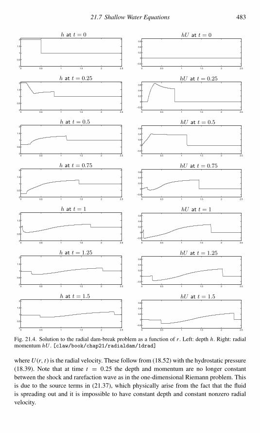
21.7 Shallow Water Equations 483

0 0.5 1 1.5 2 2.50

0.5

1

1.5

2

h at t = 0

0 0.5 1 1.5 2 2.5

−0.2

0

0.2

0.4

0.6

hU at t = 0

0 0.5 1 1.5 2 2.50

0.5

1

1.5

2

h at t = 0.25

0 0.5 1 1.5 2 2.5

−0.2

0

0.2

0.4

0.6

hU at t = 0.25

0 0.5 1 1.5 2 2.50

0.5

1

1.5

2

h at t = 0.5

0 0.5 1 1.5 2 2.5

−0.2

0

0.2

0.4

0.6

hU at t = 0.5

0 0.5 1 1.5 2 2.50

0.5

1

1.5

2

h at t = 0.75

0 0.5 1 1.5 2 2.5

−0.2

0

0.2

0.4

0.6

hU at t = 0.75

0 0.5 1 1.5 2 2.50

0.5

1

1.5

2

h at t = 1

0 0.5 1 1.5 2 2.5

−0.2

0

0.2

0.4

0.6

hU at t = 1

0 0.5 1 1.5 2 2.50

0.5

1

1.5

2

h at t = 1.25

0 0.5 1 1.5 2 2.5

−0.2

0

0.2

0.4

0.6

hU at t = 1.25

0 0.5 1 1.5 2 2.50

0.5

1

1.5

2

h at t = 1.5

0 0.5 1 1.5 2 2.5

−0.2

0

0.2

0.4

0.6

hU at t = 1.5

Fig. 21.4. Solution to the radial dam-break problem as a function of r . Left: depth h. Right: radialmomentum hU . [claw/book/chap21/radialdam/1drad]

whereU (r, t) is the radial velocity. These follow from (18.52) with the hydrostatic pressure(18.39). Note that at time t = 0.25 the depth and momentum are no longer constantbetween the shock and rarefaction wave as in the one-dimensional Riemann problem. Thisis due to the source terms in (21.37), which physically arise from the fact that the fluidis spreading out and it is impossible to have constant depth and constant nonzero radialvelocity.

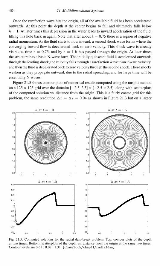
484 21 Multidimensional Systems

Once the rarefaction wave hits the origin, all of the available fluid has been acceleratedoutwards. At this point the depth at the center begins to fall and ultimately falls belowh = 1. At later times this depression in the water leads to inward acceleration of the fluid,filling this hole back in again. Note that after about t = 0.75 there is a region of negativeradial momentum. As the fluid starts to flow inward, a second shock wave forms where theconverging inward flow is decelerated back to zero velocity. This shock wave is alreadyvisible at time t = 0.75, and by t = 1 it has passed through the origin. At later timesthe structure has a basic N-wave form. The initially quiescent fluid is accelerated outwardsthrough the leading shock, the velocity falls through a rarefactionwave to an inward velocity,and then thefluid is decelerated back to zero velocity through the second shock.These shocksweaken as they propagate outward, due to the radial spreading, and for large time will beessentially N-waves.Figure 21.5 shows contour plots of numerical results computed using the unsplit method

on a 125× 125 grid over the domaim [−2.5, 2.5]× [−2.5× 2.5], along with scatterplotsof the computed solution vs. distance from the origin. This is a fairly coarse grid for thisproblem, the same resolution �x = �y = 0.04 as shown in Figure 21.3 but on a larger

−2 −1 0 1 2−2.5

−2

−1.5

−1

−0.5

0

0.5

1

1.5

2

2.5h at t = 1.0

−2 −1 0 1 2−2.5

−2

−1.5

−1

−0.5

0

0.5

1

1.5

2

2.5h at t = 1.5

0 0.5 1 1.5 2 2.50.5

0.6

0.7

0.8

0.9

1

1.1

1.2

1.3

1.4h at t = 1.0

0 0.5 1 1.5 2 2.50.5

0.6

0.7

0.8

0.9

1

1.1

1.2

1.3

1.4h at t = 1.5

Fig. 21.5. Computed solutions for the radial dam-break problem. Top: contour plots of the depthat two times. Bottom: scatterplots of the depth vs. distance from the origin at the same two times.Contour levels are 0.61 : 0.02 : 1.31. [claw/book/chap21/radialdam]

21.8 Boundary Conditions 485

domain. The depth is shown at two different times. At t = 1.0 the shock near the origincannot be resolved on this grid. The structure looks correct elsewhere, however. At t = 1.5the basic structure is captured well everywhere. Note in particular that the depth near theorigin stabilizes at a value h ≈ 0.96 that is well captured also in the two-dimensional results.

21.8 Boundary Conditions

Boundary conditions in two (or three) space dimensions can be handled in much the sameway as in one dimension. The grid on the desired computational domain consists of interiorcells that we will label by i = 1, 2, . . . ,mx and j = 1, 2, . . . ,my . This grid is extendedby introducing a set of ghost cells on all sides, for i = 1 − mBC, . . . , 0 and i = mx +1, . . . ,mx +mBC, and for j = 1−mBC, . . . , 0 and j = my + 1, . . . ,my +mBC. Figure 21.6shows a portion of such an extended grid for the case mBC = 2. At the beginning of eachtime step the ghost-cell values are filled, based on data in the interior cells and the givenboundary conditions, and then the algorithm of choice is applied over the extended domain.How many rows of ghost cells are needed depends on the stencil of the algorithm. Thehigh-resolution algorithms presented in Chapters 20 and 21 generally require two rowsof ghost cells as shown in the figure. This allows us to solve a Riemann problem at thethe boundary of the original domain and also one additional Riemann problem outside thedomain. The waves from this Riemann problem do not enter the domain and so do not affectthe solution directly, but are used to limit the waves arising from the original boundary. Inthe discussion below we assume mBC = 2, but it should be clear how to extend each of theboundary conditions for larger values of mBC.The manner in which ghost cells are filled depends on the nature of the given boundary

conditions. Periodic boundary conditions, for example, are easy to apply (as in the one-dimensional case of Section 7.1) by simply copying data from the opposite side of the grid.Belowwe will consider other standard cases, extending the approaches that were developed

−1

−1

0

0

1

1

2

2 i

j

Fig. 21.6. The lower left corner of a typical computational domain is shown as the dark line. Interiorgrid cells are labeled with i = 1, 2, . . . and j = 1, 2, . . . . The domain is extended with mBC = 2rows of ghost cells on each side.

486 21 Multidimensional Systems

in Chapter 7 to multidimensional problems. In particular, we consider solid-wall boundaryconditions and the use of extrapolation at outflow boundaries. All of these are implementedin the default CLAWPACK routine [claw/clawpack/2d/lib/bc2.f].

21.8.1 Dimensional Splitting

We will primarily concentrate on the techniques needed when unsplit methods of the form(19.10) or (19.19) are used, in which the data Qn is used to compute all fluctuations andfluxes in both the x- and y-directions. If a dimensional-splittingmethod is used, as describedin Section 19.5, then additional issues arise. If we sweep first in the x-direction to obtain Q∗

from Qn , and then sweep in the y-direction to obtain Qn+1 from Q∗ (using the Godunovsplitting), we will need to specify boundary conditions for Q∗ that may differ from thephysical boundary conditions originally given for q. Some discussion of this point was givenin Section 17.9 in the context of fractional-step methods for source terms. For dimensionalsplitting, appropriate ghost-cell values for Q∗ can often be obtained by first extending Qn

to all ghost cells and then sweeping over the rows of ghost cells along the top and bottomof the grid ( j = −1, 0 and j = my + 1,my + 2) as well as over the rows of interiorcells ( j = 1, 2, . . . ,my). This modifies the ghost-cell values by solving the same one-dimensional equation as in the interior, and gives Q∗-values in these cells that can now beused as the ghost-cell values in the y-sweeps.Note that if we wish to use the Strang splitting (19.29), then the ghost-cell values along

the left and right edges (i = −1, 0,mx + 1,mx + 2) must also be updated to Q∗ so thatwe can apply y-sweeps to these rows of cells as well as in the interior. Then we will haveQ∗∗-values in these ghost cells, which are needed in taking the final x-sweep to obtain Qn+1

from Q∗∗. To do this requires that we have twice as many ghost cells (at least along theleft and right boundaries), so that Q∗ can be obtained in the ones where Q∗∗ is ultimatelyneeded.

21.8.2 Unsplit Wave-Propagation Algorithms

Even if unsplit algorithms of the form (19.19) are used, it may be necessary to sweep overthe rows of ghost cells as well as the interior cells in order to properly implement themultidimensional algorithms. For example, the implementation of the wave-propagationalgorithm discussed in Section 21.2 uses the solution to the Riemann problem betweencells Ci−1, j and Ci j to update the fluxes Gi−1, j+1/2 and Gi, j+1/2. Referring to Figure 21.6,we see that when j = 0 we must solve the Riemann problems in this row of ghost cellsin order to obtain proper values of the fluxes Gi,1/2. These in turn are used to update theinterior values Qi1.

21.8.3 Solid Walls

In many of the problems we have considered (e.g., acoustics, shallow water equations, gasdynamics), the solution variables include velocity or momentum components in each spatialdimension. A common boundary condition is that the velocity normal to a wall should bezero, corresponding to a solid wall that fluid cannot pass through. As in one dimension, we

21.8 Boundary Conditions 487

can implement this boundary condition by a suitable extension of the solution to the ghostcells. Consider the left edge of the domain, for example, where the x-component of thevelocity should vanish. We first extrapolate all components in a symmetric manner, setting

Q0, j = Q1, j , Q−1, j = Q2, j for j = 1, 2, . . . ,my . (21.38)

We then negate the component of Qi j (for i = −1, 0) that corresponds to the x-componentof velocity or momentum. We perform a similar extension at the right boundary. At thebottom boundary we extrapolate

Qi,0 = Qi,1, Qi,−1 = Qi,2 for i = −1, 0, 1, . . . ,mx + 1,mx + 2, (21.39)

and then negate the y-component of the velocity ormomentum in these ghost cells. Note thatwe apply this procedure in the rows of ghost cells (e.g., i = −1, 0) as well as in the interiorcells in order to insure that all the ghost cells shown in Figure 21.6 are filled, includingthe four corner cells where i and j both have values 0 or −1. One should always insurethat these corner cells are properly filled, especially if combinations of different boundaryconditions are used at the two adjacent sides.Note that in the procedure just outlined, the tangential component of velocity is simply

extrapolated from the interior. For the problems we have considered (acoustics, shallowwater, gas dynamics), it really doesn’t matter what value the tangential velocity has in theghost cells, since any jump in this quantity will propagate with zero normal velocity andwillnot affect the solution in the interior cells. This is due to the symmetry of the extrapolateddata, which results in the contact discontinuity in the Riemann solution having zero velocity,properly mimicking a stationary wall. Hence any tangential velocity is allowed by theseboundary conditions.

21.8.4 No-Slip Boundary Condition

In many fluid dynamics problems there is another physical boundary condition we mightwish to impose at a solid wall. The no-slip boundary condition states that the tangentialvelocity should also vanish at the wall along with the normal velocity, so that fluid adjacentto thewall is stationary. This is expected due to friction between thewall and fluidmolecules,which keeps molecules from slipping freely along the wall. However, this friction is presentonly in viscous fluids, and hyperbolic equations only model inviscid fluids, so we are notable to impose the no-slip condition in these models. If fluid viscosity is introduced, weobtain a parabolic equation (e.g., the Navier–Stokes equations instead of the inviscid Eulerequations) that allows (in fact, requires) more boundary conditions to be specified.If the physical viscosity of the fluid is very small relative to the typical fluid velocity

away from the wall (i.e., if the Reynolds number is large), then there will often be a thinboundary layer adjacent to the wall in which the tangential velocity rapidly approachesthe zero velocity of the wall. The thickness of this layer depends on the magnitude ofthe viscosity ε and often vanishes as ε → 0. As in the case of shock waves, the inviscidhyperbolic equation attempts to model the ε = 0 limit.In some applications this is a suitable approximation. For example, inmany aerodynamics

problems the thickness of the physical boundary layer on the surface of a body is much

488 21 Multidimensional Systems

smaller than a computational cell. For this reason the inviscid Euler equations are often usedrather than the more expensive Navier–Stokes equations. However, caution must be used,since in some problems the viscous effects at the boundary do have a substantial influenceon the global solution, even when the viscosity is very small. This is particularly true if thegeometry is such that the boundary layer separates from the wall at some point (as musthappen at the trailing edge of a wing, for example). Then the vorticity generated by a no-slip boundary will move away from the wall and perhaps lead to large-scale turbulence thatpersists even when ε is extremely small, but would not be seen in an ideal inviscid fluid. Thenumerical viscosity that is inherent in any “inviscid” algorithm can lead to similar effects,but may mimic flow at the wrong Reynolds number. A full discussion of these issues isbeyond the scope of this book.

21.8.5 Extrapolation and Absorbing Boundary Conditions

For many problems we must use a computational domain that is smaller than the physicaldomain, particularly if we must cut off an essentially infinite domain at some point to obtaina finite computational domain, as already discussed in Section 7.3.1.We thenwish to imposeboundary conditions that allow us to compute on this smaller domain and obtain results thatagree well with what would be computed on a larger domain. If the computational domainis large enough for the problem of interest, then we expect that there will only be outgoingwaves at the boundary of this domain. There should not be substantial incoming wavesunless they have a known form (as from some known external source) that can be imposedas part of the boundary conditions, as was done in Section 7.3.2 in one dimension. Herewe will assume there should be no incoming waves, in which case our goal is to imposeboundary conditions on the computational domain that are nonreflecting, or absorbing, andthat allow any outgoing waves to disappear without generating spurious incoming waves.It may be that the outgoing waves should interact outside the computational domain in

such a way that incoming waves are generated, which should appear at the boundary at alater time. In general we cannot hope to model such processes via the boundary conditions,and this would be an indication that our computational domain is simply not large enoughto capture the full problem.In one space dimension, we saw in Section 7.3.1 that quite effective absorbing boundary

conditions can be obtained simply by using zero-order extrapolation. This idea can beextended easily to more dimensions as well. For example, along the left and bottom edgewe would set

Q0 j = Q1 j , Q−1, j = Q1 j for j = 1, 2, . . . ,my, (21.40)

and then

Qi0 = Qi1, Qi,−1 = Qi1 for i = −1, 0, . . . ,mx + 2. (21.41)

Note that we have filled the corner ghost cells in Figure 21.6 as well as the edge ghost cells.The value obtained in all four of the corner cells is Q11. The same value would be obtainedif we reversed the order above and first extrapolated in y and then in x .

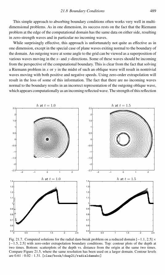
21.8 Boundary Conditions 489

This simple approach to absorbing boundary conditions often works very well in multi-dimensional problems. As in one dimension, its success rests on the fact that the Riemannproblem at the edge of the computational domain has the same data on either side, resultingin zero-strength waves and in particular no incoming waves.While surprisingly effective, this approach is unfortunately not quite as effective as in

one dimension, except in the special case of plane waves exiting normal to the boundary ofthe domain. An outgoing wave at some angle to the grid can be viewed as a superposition ofvarious waves moving in the x- and y-directions. Some of these waves should be incomingfrom the perspective of the computational boundary. This is clear from the fact that solvinga Riemann problem in x or y in the midst of such an oblique wave will result in nontrivialwaves moving with both positive and negative speeds. Using zero-order extrapolation willresult in the loss of some of this information. The fact that there are no incoming wavesnormal to the boundary results in an incorrect representation of the outgoing oblique wave,which appears computationally as an incoming reflectedwave. The strength of this reflection

−2 −1 0 1 2−2.5

−2

−1.5

−1

−0.5

0

0.5

1

1.5

2

2.5h at t = 1.0

−2 −1 0 1 2−2.5

−2

−1.5

−1

−0.5

0

0.5

1

1.5

2

2.5h at t = 1.5

0 0.5 1 1.5 2 2.50.5

0.6

0.7

0.8

0.9

1

1.1

1.2

1.3

1.4h at t = 1.0

0 0.5 1 1.5 2 2.50.5

0.6

0.7

0.8

0.9

1

1.1

1.2

1.3

1.4h at t = 1.5

Fig. 21.7. Computed solutions for the radial dam-break problem on a reduced domain [−1.1, 2.5]×[−1.5, 2.5] with zero-order extrapolation boundary conditions. Top: contour plots of the depth attwo times. Bottom: scatterplots of the depth vs. distance from the origin at the same two times.Compare Figure 21.5, where the same resolution has been used on a larger domain. Contour levelsare 0.61 : 0.02 : 1.31. [claw/book/chap21/radialdamabc]

490 21 Multidimensional Systems

generally depends on the angle of the wave to the boundary and is typically worst in corners.This is illustrated in Example 21.2 below, which shows the effects of this error. Still, theseboundary conditions are fairly effective considering their simplicity, and are often goodenough in practice.There is an extensive literature onmore sophisticated approaches to specifying absorbing

boundary conditions forwave-propagation problems. See, for example, [1], [21], [28], [117],[123], [176], [197], [230].

Example 21.2. As an example, consider the radial dam-break problem for the shallowwaterequations described in Section 21.7.1. We now solve this same problem on a 90× 100 gridin a smaller domain [−1.1, 2.5] × [−1.5, 2.5] rather than the full domain [−2.5, 2.5] ×[−2.5, 2.5] used to compute the results shown in Figure 21.5. The same mesh size �x =�y = 0.04 is used. As seen in the contour plots of Figure 21.7, small-amplitude reflectedwaves are generated as the shock wave leaves the computational domain. The effect of theseerrors is also observed in the scatterplots of depth vs. distance from the origin.

22Elastic Waves

A brief introduction to one-dimensional elasticity theory and elastic wave propagation wasgiven in Section 2.12. In this chapter we will explore the full three-dimensional elasticityequations in the context of elastic wave propagation, or elastodynamics. There are manyreferences available on the basic theory of linear and nonlinear elastodynamics (e.g., [6],[11], [141], [249], [255], [367], [422]), though often not in the first-order hyperbolic formwe need. In this chapter the equations, eigenstructure, and Riemann solutions are writtenout in detail for several different variants of the linear problem.The notation and terminology for these equations differs widely between different fields

of application. Much of the emphasis in the literature is on steady-state problems, or elas-tostatics, in which the goal is to determine the deformation of an object and the internalstresses that result from some applied force. These boundary-value problems are oftenposed as second-order or fourth-order elliptic equations. We will concentrate instead onthe hyperbolic nature of the first-order time-dependent problem, and the eigenstructureof this system. This is important in many wave-propagation applications such as seismicmodeling in the earth or the study of ultrasound waves propagating through biologicaltissue. For small deformations, linear elasticity can generally be used. But even this casecan be challenging numerically, since most practical problems involve heterogeneous ma-terials and complicated geometry. High-resolution finite volume methods are well suitedto these problems, since interfaces between different materials are handled naturally in theprocess of solving Riemann problems. This has already been explored in one dimensionin Section 9.6. These methods can also be extended to nonlinear elasticity equations byincorporating an appropriate nonlinear Riemann solver, allowing the solution of problemswith finite deformations (meaning larger than infinitesimal), in which case shock waves canform. For even larger deformations plastic behavior is observed, which can also be modeledwith hyperbolic systems in some cases. For some examples of the application of hyperbolictheory and Riemann solvers to elastic and elastic–plastic problems, see for example [8],[30], [55], [83], [85], [164], [273], [327], [360], [406], [454], [455], [456]. Here we restrictour attention to linear elastic problems.Recall from Section 2.12 that there are generally two basic types of waves that can

propagate in an elastic solid, P-waves (pressurewaves or primarywaves) and S-waves (shearwaves or secondary waves). In one dimension the P-waves and S-waves can be modeledseparately by disjoint systems of two equations each. In multidimensional problems thereis a coupling between these modes and the situation is more complicated. However, we

491

492 22 Elastic Waves

will see that a plane-wave problem in any of the three coordinate directions leads to asystem that decouples into the simple structure seen in Section 2.12.4. This means thatfinite volume methods based on Riemann solvers in the coordinate directions are easy toapply.

22.1 Derivation of the Elasticity Equations

In this section we will informally derive the full three-dimensional elasticity equations. Theclear discussion of Davis and Selvadurai [102] has largely motivated the derivation givenhere, but other derivations and discussion of elastodynamics can be found in many sources,such as those listed above.We first generalize the notation of Section 2.12.1 from two to three dimensions. The

displacement δ(x, y, z, t) now has three components, and ∇δ is a 3× 3 matrix. The straintensor ε is again defined by

ε = 1

2[∇δ + (∇δ)T ] =

ε11 ε12 ε13

ε21 ε22 ε23

ε31 ε32 ε33

. (22.1)

This symmetric matrix has six distinct elements – three extensional strains and three shearstrains – given by

ε11 = δ1x , ε22 = δ2y, ε33 = δ3z

ε12 = 12

(δ1y + δ2x

), ε13 = 1

2

(δ1z + δ3x

), ε23 = 1

2

(δ2z + δ3y

).

(22.2)

The stress tensor σ is also a 3× 3 symmetric matrix with six distinct elements,

σ =

σ11 σ 12 σ 13

σ 21 σ 22 σ 23

σ 31 σ 32 σ 33

, (22.3)

with all elements varying as functions of space and time. This is a tensorial quantity that iswritten in matrix form corresponding to x–y coordinates. At any point in space this stresstensor represents the internal forces acting at that point. If we introduce a surface throughthe point with unit normal vector n, then the traction (force per unit area) acting on thissurface is given by the vector σ · n. In particular, the three columns of σ represent the tractionacting on planes normal to the x-, y-, and z-axes respectively. Relative to these planes, thecomponents σ 11, σ 22, and σ 33 are the normal stress components, while σ 12, σ 13, and σ 23

are the shear stress components. But it is important to keep in mind that for a plane notaligned with the coordinates, the normal and shear stresses relative to that plane will eachin general have values that depend on all components of σ .

22.1 Derivation of the Elasticity Equations 493

We can derive a system of conservation laws governing wave motion as a generalizationto the systems (2.91) and (2.98) in the one-dimensional case. These equations have the form

ε11t − ux = 0,ε22t − vy = 0,ε33t − wz = 0,

ε12t −1

2(vx + uy) = 0,

ε23t −1

2(vz + wy) = 0,

ε13t −1

2(uz + wx ) = 0,

ρut − σ 11x − σ 12y − σ 13z = 0,ρvt − σ 12x − σ 22y − σ 23z = 0,ρwt − σ 13x − σ 23y − σ 33z = 0.

(22.4)

The first six equations follow directly from the definition of ε in terms of the spatial gradientof δ, whereas the velocity (u, v, w) is the time derivative of δ. (The first of these was derivedin (2.92).) The final three equations in (22.4) express the dynamic relationship between theacceleration and the net force resulting from all the stresses.The equations (22.4) must be completed by specifying a constitutive stress–strain rela-

tionship between σ and ε. In general this might be nonlinear, but for small deformations alinear stress–strain relation can be assumed, leading to the multidimensional equations oflinear elasticity derived in the next subsection.

22.1.1 Linear Elasticity

For small deformations the stress and strain can be related by a generalization of Hooke’slaw, which has the general form

σ i j =∑k,l

Ci jklεkl . (22.5)

The tensorC has 81 components, but by symmetry only 21 are independent.Wewill make aconsiderable further simplification by assuming that the material is isotropic, and hence thematerial behavior is the same in any direction. In this case the six independent componentsof σ can be related to those of ε by means of a 6× 6 matrix, which will be displayed below.If we apply a small force σ 11 in the x-direction to an elastic bar, we expect the material

to stretch by a linearly proportional small amount,

ε11 = 1

Eσ 11, (22.6)

494 22 Elastic Waves

as inHooke’s law. The parameter E is called Young’s modulus. In general we also expect thebar to contract slightly in the y- and z-directions as it is stretched in x . Since the materialis isotropic, we expect the strains ε22 and ε33 to be equal to one another and, for smalldeformations, linear in ε11:

ε22 = ε33 = −νε11.

The parameter ν is Poisson’s ratio. For most materials 0<ν < 0.5, although there arestrange materials for which ν < 0 (e.g., [252]). Thermodynamics requires −1 ≤ ν ≤ 0.5.If ν = 0.5, then the material is incompressible, a mathematical idealization in that in realityany material can be compressed if sufficient force is applied. The assumption ν < 0.5 isrequired for a hyperbolic formulation.Using (22.6), we can write

ε22 = ε33 = − ν

Eσ 11.

Similarly, a force applied in the y- or z-direction will also typically cause strains in allthree directions. More generally we can think of applying normal stresses σ 11, σ 22, andσ 33 simultaneously, resulting in strains that are a linear combination of those obtained fromeach stress separately. This leads to the extensional strains

ε11 = 1

Eσ 11 − ν

Eσ 22 − ν

Eσ 33,

ε22 = 1

Eσ 22 − ν

Eσ 11 − ν

Eσ 33,

ε33 = 1

Eσ 33 − ν

Eσ 11 − ν

Eσ 22.

(22.7)

The shear strains and shear stresses are related to one another by the simpler relations

σ 12 = 2µε12, σ 13 = 2µε13, σ 23 = 2µε23. (22.8)

whereµ ≥ 0 is the shearmodulus. For elasticmaterials the shearmodulus can be determinedin terms of E and ν as

µ = E

2(1+ ν) . (22.9)

See [102], for example, for a derivation.

22.1 Derivation of the Elasticity Equations 495

Combining (22.7) and (22.8) gives the desired stress–strain relation

ε11

ε22

ε33

ε12

ε23

ε13

=

1/E −ν/E −ν/E 0 0 0

−ν/E 1/E −ν/E 0 0 0

−ν/E −ν/E 1/E 0 0 0

0 0 0 1/2µ 0 0

0 0 0 0 1/2µ 0

0 0 0 0 0 1/2µ

σ 11

σ 22

σ 33

σ 12

σ 23

σ 13

. (22.10)

We can invert this matrix to instead determine the stress in terms of the strain,

σ 11

σ 22

σ 33

σ 12

σ 23

σ 13

=

λ+ 2µ λ λ 0 0 0

λ λ+ 2µ λ 0 0 0

λ λ λ+ 2µ 0 0 0

0 0 0 2µ 0 0

0 0 0 0 2µ 0

0 0 0 0 0 2µ

ε11

ε22

ε33

ε12

ε23

ε13

. (22.11)

Here we have introduced the parameter λ defined by

λ = νE

(1+ ν)(1− 2ν) . (22.12)

This does not have any direct physical interpretation, but is useful in that it appears in theinverse above. The relation (22.9) has also been used to simplify the form of this inverse.The parameter λ should not be confused with an eigenvalue, for which we use the symbols in this chapter. The parameters λ and µ are often called the Lame parameters for thematerial. From (22.9) and (22.12) we can also compute E and ν from λ and µ, as

E = µ(3λ+ 2µ)λ+ µ , ν = 1

2

(λ

λ+ µ). (22.13)

The relationship (22.11) can be used to convert (22.4) into a closed system of nineequations for the velocities u = (u, v, w) and either σ or ε, by eliminating the other setof six parameters (analogously to choosing (2.93) or (2.95) in the one-dimensional case).Either way we obtain a hyperbolic linear system of nine equations. The two alternativesystems are similarity transformations of one another and have the same eigenvalues, asthey must, since they model the same elastic waves.We will use u and σ , as is more common in linear elasticity. Then we need expressions

for the time derivatives of the stresses. These may be obtained by using (22.11) to write,for example,

σ 11t = (λ+ 2µ)ε11t + λε22t + λε33t

496 22 Elastic Waves

and then using the equations of motion (22.4) to evaluate the time derivatives on the right-hand side. We obtain the system

σ 11t − (λ+ 2µ)ux − λvy − λwz = 0,σ 22t − λux − (λ+ 2µ)vy − λwz = 0,σ 33t − λux − λvy − (λ+ 2µ)wz = 0,

σ 12t − µ(vx + uy) = 0,σ 23t − µ(vz + wy) = 0,σ 13t − µ(uz + wx ) = 0,

ρut − σ 11x − σ 12y − σ 13z = 0,ρvt − σ 12x − σ 22y − σ 23z = 0,ρwt − σ 13x − σ 23y − σ 33z = 0.

(22.14)

This can be written as

qt + Aqx + Bqy + Cqz = 0, (22.15)

with

q =

σ 11

σ 22

σ 33

σ 12

σ 23

σ 13

uv

w

, A =

0 0 0 0 0 0 −(λ+ 2µ) 0 0

0 0 0 0 0 0 −λ 0 0

0 0 0 0 0 0 −λ 0 0

0 0 0 0 0 0 0 µ 0

0 0 0 0 0 0 0 0 0

0 0 0 0 0 0 0 0 µ

−1/ρ 0 0 0 0 0 0 0 0

0 0 0 −1/ρ 0 0 0 0 0

0 0 0 0 0 −1/ρ 0 0 0

,

(22.16)

and similar matrices B and C with the nonzero elements shifted to different locations.The matrices A, B, and C do not commute, and so these equations are generally coupled

in the multidimensional case. This is not surprising, since we expect that elastic waves,like acoustic waves, can propagate equally well in any direction. In fact the eigenvalues ofA = nx A + ny B + nzC are the same for any unit vector n, and are given by

s1 = −cp, s2 = cp, s3 = −cs, s4 = cs,s5 = −cs, s6 = cs, s7 = s8 = s9 = 0.

(22.17)

These are not ordered monotonically, but instead the three eigenvalues with modulus 0are grouped last, since in practice we only need to propagate six waves after solving any

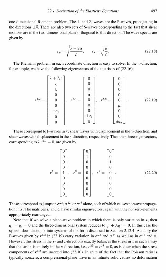
22.1 Derivation of the Elasticity Equations 497

one-dimensional Riemann problem. The 1- and 2- waves are the P-waves, propagating inthe directions ±n. There are also two sets of S-waves corresponding to the fact that shearmotions are in the two-dimensional plane orthogonal to this direction. The wave speeds aregiven by

cp =√λ+ 2µρ

, cs =õ

ρ. (22.18)

The Riemann problem in each coordinate direction is easy to solve. In the x-direction,for example, we have the following eigenvectors of the matrix A of (22.16):

r1,2 =

λ+ 2µλ

λ

000±cp00

, r3,4 =

000µ

000±cs0

, r5,6 =

00000µ

00±cs

. (22.19)

These correspond to P-waves in x , shear waves with displacement in the y-direction, andshear waves with displacement in the z-direction, respectively. The other three eigenvectors,corresponding to λ7,8,9 = 0, are given by

r7 =

000010000

, r8 =

010000000

, r9 =

001000000

. (22.20)

These correspond to jumps in σ 23, σ 22, or σ 33 alone, each of which causes nowave propaga-tion in x . The matrices B and C have similar eigenvectors, again with the nonzero elementsappropriately rearranged.Note that if we solve a plane-wave problem in which there is only variation in x , then

qy = qz = 0 and the three-dimensional system reduces to qt + Aqx = 0. In this case thesystem does decouple into systems of the form discussed in Section 2.12.4. Actually theP-waves given by r1,2 in (22.19) carry variation in σ 22 and σ 33 as well as in σ 11 and u.However, this stress in the y- and z-directions exactly balances the stress in x in such a waythat the strain is entirely in the x-direction, i.e., ε22 = ε33 = 0, as is clear when the stresscomponents of r1,2 are inserted into (22.10). In spite of the fact that the Poisson ratio istypically nonzero, a compressional plane wave in an infinite solid causes no deformation

498 22 Elastic Waves

in the orthogonal directions (as indicated in Figure 2.2). Also, since the second and thirdcolumns of A in (22.16) are identically zero, we see that the stresses σ 22 and σ 33 causeno dynamic effects and we can drop these variables from the system in deriving the one-dimensional equations (2.93). But note that these one-dimensional equations are based onthe assumption of a plane wave in an infinite three-dimensional solid, as discussed further inSection 22.3. Other “one-dimensional” situations lead to different equations. For example,the equations modeling longitudinal waves in thin elastic rod are discussed in Section 22.6.

22.1.2 The Bulk Modulus and Acoustics

The mean stress in a solid is defined to be one third the trace of the stress tensor,

1

3tr (σ ) = 1

3(σ 11 + σ 22 + σ 33). (22.21)

This is an invariant of the stress tensor, i.e., it has the same value regardless of the choiceof coordinate system used. The trace of the strain tensor is also an invariant, and this value

e ≡ tr (ε) = ε11 + ε22 + ε33, (22.22)

is called the volumetric strain. It approximates the relative change in volume in the strainedsolid. By adding together the three equations of (22.7), we find that

e = 1− 2νE

tr (σ ), (22.23)

and hence the mean stress is related to the volumetric strain by

1

3tr (σ ) = Ke, (22.24)

where the bulk modulus of compressibility K is defined by

K = E

3(1− 2ν) = λ+ 2

3µ. (22.25)

Averaging the first three equations of (22.14) gives an evolution equation for the meanstress,

1

3(σ 11 + σ 22 + σ 33)t − K (ux + vy + wz) = 0. (22.26)

We can relate the elastodynamics equations to the acoustics equations derived earlierfor gas dynamics if we make the additional assumption on that the stress is hydrostatic, asit is in a fluid. This means that there is no shear stress, σ 12 = σ 13 = σ 23 = 0, and theextensional stress components are all equal and negative,

σ 11 = σ 22 = σ 33 ≡ −p. (22.27)

The value p is called the hydrostatic pressure, and has the opposite sign from the stresses asdiscussed in Section 2.12.4. In this case the stress tensor (22.3) reduces to−pI where I is the

22.2 The Plane-Strain Equations of Two-Dimensional Elasticity 499

identity matrix. Rather than working with this tensor we can reduce the equations and dealonly with the scalar pressure p, which satisfies p = −Ke by (22.24), since p = − 1

3 tr (σ ).The equation (22.26) becomes an evolution equation for the hydrostatic pressure,

pt + K (ux + vy + wz) = 0. (22.28)

Since we now also assume that σ 12 = σ 13 = σ 23 = 0, we can drop the middle threeequations of (22.14) and the final three become

ρut + px = 0,ρvt + py = 0,ρwt + pz = 0.

(22.29)

We recognize (22.28), (22.29) as defining the three-dimensional acoustics equations fromSection 18.6. This system has wave speeds given by the “speed of sound”

c =√K

ρ=√λ+ 2

3µ

ρ. (22.30)

Note that this is different than the P-wave speed cp of (22.18), which is the sound speedactually observed in solids. However, since a fluid does not support shear stresses weshould set µ = 0, in which case (22.18) and (22.30) do agree. The acoustics equations aresometimes used as an approximate systemof equations formodeling P-waves in solidswhenshear waves are relatively unimportant, particularly in solids where µ is small comparedto λ.

22.2 The Plane-Strain Equations of Two-Dimensional Elasticity

We can reduce the three-dimensional equations (22.14) to two space dimensions by settingqz ≡ 0, for example, if we assume there is no variation in the z-direction. Note that the strainε33 = δ3z must be zero in this case, since it is the z-derivative of the z-displacement. (Wediscuss belowwhen this assumption is reasonable.) The stress σ 33 will not generally be zero,but can be determined in terms of σ 11 and σ 22 as discussed below. Dropping the equationfor σ 33 from (22.14) along with all z-derivative terms, the remaining eight equations reduceto two decoupled systems of equations,

σ 11t − (λ+ 2µ)ux − λvy = 0,σ 22t − λux − (λ+ 2µ)vy = 0,

σ 12t − µ(vx + uy) = 0,ρut − σ 11x − σ 12y = 0,ρvt − σ 12x − σ 22y = 0,

(22.31)

500 22 Elastic Waves

and

σ 23t − µwy = 0,σ 13t − µwx = 0,

ρwt − σ 13x − σ 23y = 0.(22.32)

The latter system (22.32) models shear waves with motion orthogonal to the x–y plane.Waves modeled by this system have speed cs , the S-wave speed given in (22.18).The system (22.31) is the more interesting system, and models both P-waves and S-

waves for which the motion is in the x–y plane. The S-waves modeled by this system havematerial motion orthogonal to the direction the wave is propagating, but still within thex–y plane. This system (22.31) is often called the two-dimensional plane-strain equations,since the strain is confined entirely to the x–y plane. This is a reasonable model for planewaves propagating through a three-dimensional elastic body in cases where there is novariation in the z-direction, for example, if the x–y plane is a representative slice througha three-dimensional solid with essentially infinite extent in the z-direction, as might occurin modeling large-scale seismic waves in the earth, for example. If it is correct to assumethat there is no variation in the z-direction, then it is also valid to assume that ε33 = 0.Otherwise, if ε33 had some nonzero value independent of z, then the displacement δ3 wouldhave to be of the form δ3 = ε33(z− z0) and grow without bound in z. This is not reasonablefor finite-amplitude waves. Of course, as the material is compressed in the x- or y-directionit will try to expand in z (when ν �= 0), but it will be prevented from doing so by the adjacentmaterial, which is trying equally hard to expand in the other direction. The result is a nonzerostress σ 33 while ε33 remains zero. Indeed, setting ε33 = 0 in the system (22.11) yields

σ 11 = (λ+ 2µ)ε11 + λε22, (22.33)

σ 22 = λε11 + (λ+ 2µ)ε22, (22.34)

σ 33 = λε11 + λε22. (22.35)

The first two equations of this set are all that are needed for the two-dimensional system(22.31), but the stress σ 33 can also be computed from (22.35) if desired. Alternatively wecan obtain

σ 33 = ν(σ 11 + σ 22) (22.36)

from the third equation of (22.7) by setting ε33 = 0.Note that if we invert the stress–strain relation (22.33)–(22.35) to find ε11 and ε22 in

terms of σ 11 and σ 22, we find that

Eε11 = σ 11 − νσ 22,Eε22 = σ 22 − νσ 11, (22.37)

where

E = E

1− ν2 , ν = ν

1− ν . (22.38)

22.2 The Plane-Strain Equations of Two-Dimensional Elasticity 501

The equations (22.37) have the same form as the three-dimensional stress–strain relations(22.7), but with different effective values for the Young’s modulus E and Poisson ratio ν.These relations can be derived either by inverting the 2 × 2 system given by (22.33) and(22.34), or from (22.7) by using (22.36).It is important to note that the plane-strain system (22.31) does not in general model

elastic waves in a thin plate, in spite of the fact that it might seem natural to view thisas a two-dimensional elastic medium. Wave propagation in a plate can be modeled by atwo-dimensional hyperbolic system, but (22.31) is not the correct one; see Section 22.5.We now discuss the eigenstructure of the system (22.31). Rather than displaying the

matrices A and B separately in this case, it is more compact and perhaps alsomore revealingto show the linear combination A = nx A + ny B, where n is again a unit vector in anarbitrary direction. The matrix A is then the coefficient matrix for the one-dimensionalproblem modeling the propagation of plane waves in the n-direction. Setting n = (1, 0) or(0, 1) below recovers the matrices A and B separately. We have

q =

σ 11

σ 22

σ 12

uv

, A = −

0 0 0 nx (λ+ 2µ) nyλ

0 0 0 nxλ ny(λ+ 2µ)0 0 0 nyµ nxµ

nx/ρ 0 ny/ρ 0 0

0 ny/ρ nx/ρ 0 0

. (22.39)

The eigenvalues of A are

s1 = −cp, s2 = cp, s3 = −cs, s4 = cs, s5 = 0, (22.40)

where we use s instead of λ to avoid confusion with the Lame parameter. The P-waveeigenvectors are

r1 =

λ+ 2µ(nx )2λ+ 2µ(ny)22µnxny

nxcp

nycp

, r2 =

λ+ 2µ(nx )2λ+ 2µ(ny)22µnxny

−nxcp−nycp

, (22.41)

while the S-wave eigenvectors r3,4 and the stationary wave r5 are

r3 =

−2nxnyµ2nxnyµ

[(nx )2 − (ny)2]µ−nycsnxcs

, r4 =

−2nxnyµ2nxnyµ

[(nx )2 − (ny)2]µnycs

−nxcs

, r5 =

(ny)2

(nx )2

−nxny00

.

(22.42)

Observe that P-waves r1,2 have velocity components directed in the ±n-direction, thedirection in which the plane wave propagates. The S-waves, on the other hand, have motion

502 22 Elastic Waves

in the orthogonal direction±(−ny, nx ). Note also that a P-wave in the x- or y-direction hasσ 12 = 0, but that a P-wave propagating in any other direction has σ 12 �= 0. This is becausethe elements of the stress tensor have been expressed in x–y coordinates, and represent-ing a purely extensional stress in some other direction requires all components of σ to benonzero.

22.3 One-Dimensional Slices

We can reduce the systems of equations (22.31) and (22.32) even further if we assume thatthere is no variation in the y-direction. As in our discussion of the plane-strain equationsabove, this is typically valid if we are considering a one-dimensional slice through anessentially infinite medium in cases where there is variation in only one direction (e.g., aplane wave propagating through the earth). It is not a valid model for waves in a “one-dimensional” thin elastic rod, which is discussed in Section 22.6.Setting all y-derivatives to zero in (22.31) results in the two decoupled systems

σ 11t − (λ+ 2µ)ux = 0,ρut − σ 11x = 0

(22.43)

and

σ 12t − µvx = 0,ρvt − σ 12x = 0.

(22.44)

These are the systems (2.95) and (2.100) introduced in Section 2.12.4. They model P-waveswith displacement in x and S-waves with displacement in y, respectively, with wave speedscp and cs given by (22.18).We have dropped the equation for σ 22, which is given by

σ 22 = λε11 = νσ 11. (22.45)

Note that in this case σ 33 = σ 22 by (22.36).The equations (22.32) reduce to

σ 13t − µwx = 0,ρwt − σ 13x = 0.

(22.46)

This system models an independent set of shear waves in which the displacement is in thez-direction rather than in the y-direction (and propagation still in the x-direction).

22.4 Boundary Conditions

Boundary conditions for elastic solids can be imposed inmuch the sameway as for acoustics(see Sections 7.3 and 21.8), but there are now a wider variety of physically meaningfulboundary conditions to consider. We will use the two-dimensional plane-strain equations(22.31) for illustration, and consider a point along the left edge of the domain, which we

22.4 Boundary Conditions 503

assume is at x = 0. We must then determine ghost-cell values Q0 j and Q−1, j based oninterior values and the physical boundary conditions. It should be clear how to translate thisdiscussion to other boundaries and to three dimensions.Periodic or extrapolation boundary conditions are easily imposed, as for other equations,

as discussed in Section 21.8. The more interesting cases are where either the motion of theboundary or the traction applied to the boundary is specified. These are discussed in thenext two subsections.

22.4.1 Specified Motion

Suppose the velocity of the boundary at x = 0, y = y j is known. Call the velocity at thispoint (U, V ) for brevity. Then following the discussion of Sections 7.3.4 and 21.8.3, wecan impose this by specifying the ghost-cell values as follows:

for Q0 j : σ 110 j = σ 111 j , σ 120 j = σ 121 j , σ 220 j = σ 221 j ,

u0 j = 2U − u1 j , v0 j = 2V − v1 j ;for Q−1, j : σ 11−1, j = σ 112 j , σ 12−1, j = σ 122 j , σ 22−1, j = σ 222 j ,

u−1, j = 2U − u2 j , v−1, j = 2V − v2 j .

(22.47)

When the Riemann problem is solved at x = 0 (i.e., at cell interface i = 1/2), this choiceinsures that the intermediate state Q∨

|1/2 has velocity (U, V ) and satisfies the required physical

boundary condition. An important special case isU = 0, V = 0, in which case the boundaryis fixed at this point.Note that in the case of an elastic solid we must specify both u and v. This differs from

two-dimensional acoustics or inviscid fluid dynamics, where only the normal componentof velocity is specified as discussed in Sections 21.8.3 and 21.8.4. For an inviscid fluidthere can be slip along the boundary, and so the tangential component of velocity cannotbe specified. For an elastic solid we must specify both. For a three-dimensional problemwe would also have to specify w at the boundary, e.g., w = 0 at a fixed boundary. Thestresses are not specified and must be free to react as necessary to the imposed motion. Thisis accomplished by simply reflecting σ from the interior values in (22.47), and the valuesobserved in the resulting Riemann solution Q∨

|1/2 can be used to obtain the surface traction

if this is desired as part of the solution to the problem.

22.4.2 Specified Traction

Often we wish instead to specify the traction at a point on the boundary and compute theresulting motion. At the boundary x = 0 this amounts to specifying the values of σ 11 andσ 12, say as σ 11 = S11 and σ 12 = S12 at the point x = 0, y = y j . In particular, if this is afree boundary (the edge of an elastic solid with no external force applied), then we shouldset S11 = 0 and S12 = 0. This is called a traction-free boundary. Note that we have nophysical control over σ 22 at this boundary.

504 22 Elastic Waves

The proper ghost cell values for general S11 and S12 are then given by:

for Q0 j : σ 110 j = 2S11 − σ 111 j , σ 120 j = 2S12 − σ 121 j , σ 220 j = σ 221 j ,

u0 j = u1 j , v0 j = v1 j ;

for Q−1, j : σ 11−1, j = 2S11 − σ 112 j , σ 12−1, j = 2S12 − σ 122 j , σ 22−1, j = σ 222 j ,

u−1, j = u2 j , v−1, j = v2 j .

(22.48)

For a three-dimensional problem we would also need to specify σ 13 = S13, while σ 23 andσ 33 would simply be reflected from the interior, as is done for σ 22 in (22.48).

22.5 The Plane-Stress Equations and Two-Dimensional Plates

In Section 22.2 we derived a two-dimensional hyperbolic system by using the plane-strainassumption that all displacements are confined to the x–y plane. As discussed there, thisis valid if we assume the material is essentially infinite in the z-direction and there is novariation of the solution in that direction.We now consider a different situation, in which thethree-dimensional domain is a thin plate bounded by the planes z = ±h for some small h.We wish to derive two-dimensional equations that model waves whose wavelength is longrelative to the thickness of the plate. Each surface of the plate is a free boundary and mustbe traction-free (see Section 22.4.2), so we have

σ 13 ≡ 0, σ 23 ≡ 0, σ 33 ≡ 0 (22.49)

on the boundary planes z = ±h. To derive a two-dimensional system of equations we willassume that these are identically zero throughout the plate. Then from (22.8) we also have

ε13 ≡ 0, ε23 ≡ 0. (22.50)

Note, however, that we cannot assume ε33 = 0. Instead, from (22.7) with σ 33 = 0 we obtain

ε33 = − ν

E(σ 11 + σ 22), (22.51)

along with

ε11 = 1

E(σ 11 − νσ 22),

ε22 = 1

E(−νσ 11 + σ 22).

(22.52)

Adding these last two equations together gives

ε11 + ε22 = 1− νE

(σ 11 + σ 22). (22.53)

Since ε11 + ε22 = δ1x + δ2y is the x–y divergence of the displacement, we see that ifε11 + ε22 �= 0, then there is compression or expansion in the x–y plane, and in this casefrom (22.51) there must be compensating motion in the z-direction whenever the Poisson

22.5 The Plane-Stress Equations and Two-Dimensional Plates 505

ratio ν is nonzero. No matter how thin the plate may appear, it is still three-dimensional,and stretching or compressing it in the x–y plane leads to motion in z of the same order ofmagnitude.To derive two-dimensional equations we will assume, however, that σ 11 and σ 22, and

hence ε33, are independent of z. Recall that ε33 = δ3z , so ε33 > 0 corresponds to the plate

bulging out, while ε33< 0 corresponds to the plate becoming thinner.As the plate thickens or thins, the z-velocity w must be nonzero. Moreover, it is clearly

not valid to assume that the value of w is independent of z. For example, if the plate isbulging out, then we must have w > 0 for 0 < z < h and w < 0 for −h < z < 0. Sincew = δ3t , we have wz = δ3zt = ε33t , and the assumption that ε

33 is independent of z meansthat w varies linearly in z. Although w is not zero, it is close to zero and symmetric aboutz = 0. The plate equations are most rigorously defined by integrating the three-dimensionalequations in z from −h to h and the integral of w then reduces to zero, to leading order.This justifies ignoring the effects of w in deriving the two-dimensional plate equations.Using the assumptions (22.49) and (22.50) in the system (22.4) gives the following system

of equations (after dropping the equations for ε13, ε23, ε33, and w):

ε11t − ux = 0,ε22t − vy = 0,

ε12t −1

2(vx + uy) = 0,

ρut − σ 11x − σ 12y = 0,ρvt − σ 12x − σ 22y = 0.

(22.54)

To close this system we need the constitutive relations relating σ to ε, which are given by(22.52) along with σ 12 = 2µε12 coming from (22.8). We can write these either as

ε11 = 1

E(σ 11 − νσ 22),

ε22 = 1

E(−νσ 11 + σ 22),

ε12 = 1

2µσ 12

(22.55)

or, by inverting the system, as

σ 11 =(2µ

1− ν)(ε11 + νε22),

σ 22 =(2µ

1− ν)(νε11 + ε22),

σ 12 = 2µε12.

(22.56)

As usual, we can eliminate either ε or σ from (22.54). If we eliminate ε, then we obtain the

506 22 Elastic Waves

system

σ 11t −(2µ

1− ν)ux −

(2µν

1− ν)vy = 0,

σ 22t −(2µν

1− ν)ux −

(2µ

1− ν)vy = 0,

σ 12t − µ(vx + uy) = 0,ρut − σ 11x − σ 12y = 0,ρvt − σ 12x − σ 22y = 0.

(22.57)

Note that this system has different coefficients than the plane-strain system (22.31).However, if we define

λ= 2µν

1− ν =2µλ

λ+ 2µ (22.58)

as an effective Lame parameter for the plate, then

2µ

1− ν = λ+ 2µ,

and the system (22.57) has exactly the same form as (22.31) but with λ in place of λ. Henceany method developed for the plane-strain case can also be applied to the plane-stressequations simply by changing the value of λ. In particular, the eigenstructure is the sameas that developed in Section 22.2 (with λ in place of λ), and so we see from the eigenvalues(22.40) that the characteristic wave speeds for waves in a plate are

cp =√λ+ 2µρ

=√

2µ

ρ(1− ν) =√

E

ρ(1− ν2) (22.59)

and

cs =√µ/ρ, (22.60)

respectively. The speed cs is the usual S-wave speed, but the wave speed cp is smaller thancp from (22.18) when 0 < ν < 1/2, since

λ= λ

(1− ν

1− ν)< λ. (22.61)

We will refer to waves propagating at the velocity cp as P-waves.

Example 22.1. We can investigate wave propagation in a thin plate numerically by solvingthe three-dimensional elasticity equations in a plate with finite thickness −h < z < hand imposing traction-free boundary conditions σ 13 = σ 23 = σ 33 = 0 at z = ±h. Toillustrate an isolated P-wave we can assume the wave is propagating in the x-direction

22.5 The Plane-Stress Equations and Two-Dimensional Plates 507

t = 0

t = 0.05

t = 0.1

t = 0.15

t = 0.2

t = 0.5

Fig. 22.1. Side view of a thin plate in the x–z plane. The plate is pushed inwards at the left, givingrise to a P-wave as described in the text. [claw/book/chap22/plate]

and there is no variation in y, and hence no strain in the y-direction. In this case wecan solve a two-dimensional problem in the x–z plane. The appropriate equations arenow the plane-strain equations of Section 22.2, rewritten in x and z instead of x and y.Figures 22.1 and 22.2 show results of a numerical calculation in which the traction-freeboundary conditions σ 13 = σ 33 = 0 are imposed at z = ±0.01 (see Section 22.4.2) andthe plate is initially undisturbed. Boundary conditions at x = 0 are given by specifying thevelocity (see Section 22.4.1) as

u(0, z, t) ={a sin(2π t/T ) if t ≤ T,0 if t > T,

w(0, z, t) = 0(22.62)

with T = 0.15. This corresponds to pushing the plate inward and then bringing the edgeback to its original location, slowly enough that the wavelength is long relative to thethickness.

508 22 Elastic Waves

0 0.1 0.2 0.3 0.4 0.5 0.6 0.7 0.8 0.9 1−0.01

−0.008

−0.006

−0.004

−0.002

0

0.002

0.004

0.006

0.008

0.01

0 0.1 0.2 0.3 0.4 0.5 0.6 0.7 0.8 0.9 1−0.01

−0.008

−0.006

−0.004

−0.002

0

0.002

0.004

0.006

0.008

0.01

Fig. 22.2. The stress σ 11 (top) and the vertical velocity w (bottom) at time t = 0.5 for the wave-propagation problem shown in Figure 22.1. Contour plots are shown with solid lines for positivevalues and dashed lines for negative values. [claw/book/chap22/plate]

Figure 22.1 shows the deformation of the plate at several times. This deformation hasbeen determined by integrating the velocity (u, w) in each cell over the course of thecomputation in order to compute the displacement. Points on an initially uniform grid arethen displaced by this amount to illustrate the deformed solid. For clarity these deformationsare magnified considerably over what is appropriate for linear elasticity (i.e., the constanta in the boundary data (22.62) is taken to be orders of magnitude larger than physicallyreasonable, but since the equations are linear, the solution simply scales linearly as well).Recall that the computations are always done on a fixed grid in the reference configuration,since the elasticity equations we are considering are written in the Lagrangian frame.Figure 22.2 shows contours of the computed σ 11 and w at the final time t = 0.5. We see

that σ 11 essentially varies only with x in spite of the fact that the velocityw varies linearly inthe z-direction. Moreover we observe that the leading edge of the wave has not yet reachedx = 0.9 at this time. The material parameters were chosen to be ρ = 1, λ = 2, and µ = 1so that cp = 2. Rather than traveling at this P-wave speed, the disturbance is propagatingat the velocity c p =

√3, and at time t = 0.5 has reached approximately 0.5c p = 0.866

rather than 0.5cp = 1.If this same computation were repeated but with u = w = 0 specified along z = ±h

instead of σ 13 = σ 33 = 0 (plane strain rather than a thin plate), the result would look likethe figure on the left of Figure 2.2 rather than Figure 22.1, and the disturbance would havereached x = 1 at time t = 0.5. In this case w = 0 would be exactly maintained and therewould be no deformation in the z-direction.

It may seem strange that the speed of a P-wave in a thin plate is smaller than cp. Afterall, the plate is composed of a material characterized by the Lame parameters λ and µ,and should have a characteristic propagation speed given by cp. However, a P-wave isnot simply a P-wave propagating along the plate with deformation confined to the x–yplane. Rather, it is a wave that can be viewed as a superposition of many waves propagatingtransversely through the plate, bouncing back and forth between the top and bottom surfacesand hence moving at a slower effective speed along the plate. This internal reflection at the

22.7 Two-Dimensional Elasticity in Heterogeneous Media 509

free surface is not apparent in Figure 22.2, since the zig-zagging waves effectively combineinto standing waves in the z-direction. In a thicker plate the transverse wave motion wouldbe more apparent. (A similar effect was seen in Section 9.14 for waves propagating in alayered heterogeneous material.)

22.6 A One-Dimensional Rod

Consider a thin elastic rod that is long in the x-direction and has small cross-sectionalarea, say −h≤ y≤ h and −h≤ z≤ h. If we consider compressional waves propagatingdown the rod whose wavelength is long compared to h, then these can be modeled with aone-dimensional system of equations. We can start with the plane-stress equations (22.54),which model a thin plate −h ≤ z ≤ h, and now restrict also to −h ≤ y ≤ h by imposingtraction-free boundary conditions on these surfaces: σ 12 = σ 22 = 0. As in the derivationof the plane-stress equations, we now assume that in fact σ 12 = σ 22 = 0 throughout therod, and also that v = 0 (in addition to the previous assumption that w = 0 and σ k3 = 0for k = 1, 2, 3). Then (22.54) reduces to

ε11t − ux = 0,ρut − σ 11x = 0.

(22.63)

From(22.52)wenowhave the constitutive relation ε11 = σ 11/E , and so theone-dimensionalsystem can be rewritten as

σ 11t − Eux = 0,ρut − σ 11x = 0.

(22.64)

This has the same structure as the equations (22.43) derived for a one-dimensional slice ofa three-dimensional solid. But the fact that the rod has traction-free boundaries and is freeto contract or expand in y and z leads to a different wave speed,

c rodp =√E/ρ, (22.65)

as seen by computing the eigenvalues of the coefficient matrix from (22.64).

22.7 Two-Dimensional Elasticity in Heterogeneous Media

The multidimensional elastic wave equations can be solved numerically using essentiallythe sameprocedure as for the linear acoustics equations, aswas described inChapter 21. Thisis also easily implemented for a heterogeneous medium by allowing each grid cell to havedistinct values for the density ρ and Lame parameters λ and µ. For the two-dimensionalequations discussed in Section 22.2, the Riemann solvers in [claw/book/chap22/rp]

give an implementation of the necessary eigendecompositions. These are based directly onthe eigenstructure determined in Section 22.2. Examples will be presented for the plane-strain case described there, but the same solver work also for the plane-stress equationsmodeling a thin plate if λ is replaced by λ as described in Section 22.5.

510 22 Elastic Waves

−1 −0.8 −0.6 −0.4 −0.2 0 0.2 0.4 0.6 0.8 1−1

−0.8

−0.6

−0.4

−0.2

0

0.2

0.4

0.6

0.8

1σ11 at t = 0.5

−1 −0.8 −0.6 −0.4 −0.2 0 0.2 0.4 0.6 0.8 1−1

−0.8

−0.6

−0.4

−0.2

0

0.2

0.4

0.6

0.8

1σ12 at t = 0.5

(a) (b)

Fig. 22.3. Elasticwave propagationwith initial data consisting of a P-wave as shown in Figure 21.1(b):(a) the stress σ 11; (b) the shear stress σ 12. [claw/book/chap22/corner]

Example 22.2. Figure 22.3 shows an example in the same domain indicated inFigure 21.1(a), but with the two regions now containing different elastic materials withparameters

ρl = 1, ρr = 1,λl = 4, λr = 2,µl = 0.5, µr = 1,cpl =

√5 ≈ 2.2, cpr = 2,

csl =√0.5 ≈ 0.7, csr = 1.

(22.66)

The initial data is zero everywhere, except for a perturbation as in Figure 21.1(b), in which

σ 11 = λl + 2µl , σ 22 = λl , σ 12 = 0, u = cpl , v = 0 (22.67)

for−0.35 < x < −0.2. This is an eigenvector r2 from (22.41) (with n = (1, 0)) and henceis a right-going P-wave. After hitting the interface, the transmitted P-wave moves moreslowly and there is a partial reflection, as seen in Figure 22.3(a), where a contour plot ofσ 11 is shown. In the elastic case there is also both a transmitted and reflected S-wave alongthe ramp portion of the interface. These are faintly visible in Figure 22.3(a), since S-wavesat an oblique angle have a nonzero σ 11 component (see Section 22.2). The S-waves aremuch more clearly visible in Figure 22.3(b), which shows σ 12. Note that the transmittedand reflected P-waves also contain significant components of σ 12, since they are moving atan angle to the grid.

Example 22.3. As another example of elasticwave propagation in a heterogeneousmedium,we consider a wave propagating into a solid that has embedded within it an inclusionmadeout of a stiffer material, as shown in Figure 22.4. The darker region represents material with

22.7 Two-Dimensional Elasticity in Heterogeneous Media 511

Fig. 22.4. Left column: Deformation of an elastic solid with a stiff inclusion due to compression atthe left boundary. The linear deformation is greatly exaggerated. Right column: Schlieren image ofσ 11. [claw/book/chap22/inclusion]

λ = 200, µ = 100, while the lighter-colored material has λ = 2 and µ = 1. The densityis the same everywhere, ρ = 1. The plane-strain equations are solved with traction-freeboundary conditions at y = 0, 1 and at x = 1. At x = 0 the velocity is specified as

u(0, y, t) ={ε sin(π t/0.025) if t < 0.025,0 if t ≥ 0.025, v(0, y, t) = 0. (22.68)

The solid is simply pushed over by a small amount at the left boundary. This creates

512 22 Elastic Waves

Fig. 22.5. Elastic wave propagation for the example shown in Figure 22.4. Left column: the meanstress σ 11 + σ 22. Right column: the shear stress σ 12. [claw/book/chap22/inclusion]

a compressional wave, and the resulting wave motion is illustrated in Figure 22.4. Thedeformation of the solid is computed as described in Example 22.2. Again the displacementsshown are much larger than actual linear displacements should be, and have been greatlyexaggerated so that they will be visible.

Note that the compression wave is not purely a P-wave, due to its interaction with thefree boundaries at y = ±1. At about t = 0.25 the wave hits the inclusion, which is muchstiffer and hence tends to be pushed over as a rigid unit. At later times there is very littledistortion of the inclusion, which simply shifts over slightly, launching smaller-amplitudewaves into the exterior material at the far end and also along its length due to the resistance

22.7 Two-Dimensional Elasticity in Heterogeneous Media 513

to shear. This is not really rigid motion, however. Elastic waves are rapidly bouncing backand forth in the stiff material to accomplish this motion. Note that cp = 20 and cs = 10 inthe stiff region, whereas cp = 2 and cs = 1 outside.Figure 22.5 shows the wave motion more clearly. Here the gradients of σ 11 + σ 22 and

σ 12 are plotted at various times using a schlieren image style in which a highly nonlinearcolor scale is used, so that even very small-amplitude waves show up distinctly. At timet = 0.25 we see that waves are just beginning to travel down the stiff inclusion. By timet = 0.3 they have reached the far end. As they move along the bar, they launch waves intothe surrounding material. The inclusion then begins to vibrate, giving rise to further wavesmoving vertically away from it.

23Finite Volume Methods on Quadrilateral Grids

Many multidimensional problems of practical interest involve complex geometry, and ingeneral it is not sufficient to be able to solve hyperbolic equations on a uniform Cartesiangrid in a rectangular domain. In Section 6.17 we considered a nonuniform grid in one spacedimension and sawhowhyperbolic equations can be solved on such a grid by using a uniformgrid in computational space together with a coordinate mapping and appropriate scalingof the flux differences using capacity form differencing. The capacity of the computationalcell is determined by the size of the corresponding physical cell.In this chapter we consider nonuniform finite volume grids in two dimensions, such as

those shown in Figure 23.1, and will see that similar techniques may be used. There arevarious ways to view the derivation of finite volume methods on general multidimensionalgrids. Here we will consider a direct physical interpretation in terms of fluxes normal tothe cell edges. For simplicity we restrict attention to two space dimensions. For someother discussions of finite volume methods on general grids, see for example [156], [245],[475], [476].The grids shown in Figures 23.1(a) and (b) are logically rectangular quadrilateral grids,

and we will concentrate on this case. Each cell is a quadrilateral bounded by four linearsegments. Such a grid is also often called a curvilinear grid. If we label the cells in a logicalmanner, indexing “rows” and “columns” by i and j , then cell (i, j) has the four neighbors(i ± 1, j) and (i, j ± 1). The grid can be made to wrap around the cylinder by imposingperiodic boundary conditions in one direction.The triangulation shown in Figure 23.1(c), on the other hand, gives an unstructured grid

for which there is no simple logical structure underlying the connectivity between cells.One must keep track of the neighbors of each cell explicitly. An unstructured triangulationis often easier to generate for complicated geometries than a structured grid such as the oneshown in Figure 23.1(a), but may be somewhat more difficult to work with in regard to datastructures and the development of fast and accurate solvers. See [20], [324], [385], [472]for some discussions of unstructured grids.The grids of Figure 23.1(a)–(c) are all body-fitted grids that conform to the geometry of the

problem. Figure 23.1(d) shows a different approach inwhich a uniformCartesian grid is usedover most of the domain, but with some smaller irregular cells allowed where the boundarycuts through the grid. Finite volume methods of this type are often called Cartesian-grid orembedded-boundarymethods. For problemswithmore complicated geometry this approachallows for very easy grid generation, and so it has recently become quite popular.With these

514

23.1 Cell Averages and Interface Fluxes 515

(a)−5 −4 −3 −2 −1 0 1 2 3 4 5

−5

−4

−3

−2

−1

0

1

2

3

4

5

(b)−5 −4 −3 −2 −1 0 1 2 3 4 5

−5

−4

−3

−2

−1

0

1

2

3

4

5

(c)−5 0 5

−5

−4

−3

−2

−1

0

1

2

3

4

5

(d)−5 0 5

−5

−4

−3

−2

−1

0

1

2

3

4

5

Fig. 23.1. Four possible grids for flow around a cylinder. (a) 25× 100 polar grid in r–θ . (b) 25× 104quadrilateral grid interpolating between the cylinder and a square computational domain. (c) Anunstructured triangulation. (d) A Cartesian grid with embedded boundary.

methods the main difficulty is in specifying fluxes at the edges of the small cut cells in sucha way that good accuracy is obtained and stability is preserved with reasonable-size timesteps. A variety of different approaches have been introduced; see for example [7], [31],[57], [59], [77], [104], [140], [277], [278], [358], [363], [490], [492].

23.1 Cell Averages and Interface Fluxes

With a finite volumemethodwe view each discrete value Q as a cell average over a grid cell,which is modified due to fluxes through the edges of the cell, in the case of a conservationlaw, or more generally by waves moving into the cell from each edge.We start by discussingthe case of a conservation law and will see how to extend this to nonconservative linearsystems in Section 23.4.

516 23 Finite Volume Methods on Quadrilateral Grids

The finite volume approach can be applied on any shape cell C using the integral formof the conservation law,

d

dt

∫∫Cq(x, y, t) dx dy = −

∫∂Cn(s) · f (s, t) ds, (23.1)

and hence is applicable on any of the grids of Figure 23.1 if a good numerical approximationto the interface flux can be determined. Here n(s) is the outward-pointing normal and

f (s, t) =[f (q(x(s), y(s), t))

g(q(x(s), y(s), t))

],

with the boundary (x(s), y(s)) of C parameterized by the arclength s. Then

F(s) = n(s) · f (s, t) = nx (s) f (q(x(s), y(s), t))+ ny(s) g(q(x(s), y(s), t))

gives the flux per unit length per unit time in the direction n(s). Note that for a system ofm equations f and g are vectors of length m and f is a vector of length 2m, while thenormal n(s) contains two scalar components nx and ny . (See Section 18.1 for more aboutthe multidimensional notation used here.)Integrating (23.1) from time tn to tn+1 and dividing by |C|, the area of the cell, gives

1

|C|∫∫

Cq(x, y, tn+1) dx dy = 1

|C|∫∫

Cq(x, y, tn) dx dy

− 1

|C|∫ tn+1

tn

∫∂Cn(s) · f (s, t) ds dt. (23.2)

If Qn represents the cell average over this cell at time tn , then this suggests the finite volumemethod

Qn+1 = Qn − �t

|C|N∑j=1h j F

nj , (23.3)

where Fnj represents a numerical approximation to the average normal flux across the j th

side of the cell, N is the number of sides, and h j is the length of the j th side. The factors�t and h j are introduced by taking F

nj as an approximation to the interface flux per unit

length, per unit time,

Fnj ≈

1

�t

∫ tn+1

tn

(1

h j

∫side j

n · f (s, t) ds)dt.

This agrees with the normalization used previously on Cartesian grids.

23.2 Logically Rectangular Grids 517

23.2 Logically Rectangular Grids

From now on we will consider only logically rectangular grids such as the ones shown inFigure 23.1(a) and (b). In this case we can write the finite volume method (23.3) as

Qn+1i j = Qi j − �t

|Ci j |(hi+1/2, j F i+1/2, j − hi−1/2, j F i−1/2, j

+ hi, j+1/2Gi, j+1/2 − hi, j−1/2Gi, j−1/2), (23.4)

where

|Ci j | = area of cell (i, j),hi−1/2, j = length of side between cells (i − 1, j) and (i, j),hi, j−1/2 = length of side between cells (i, j − 1) and (i, j),F i−1/2, j = flux normal to edge between cells (i − 1, j) and (i, j),

per unit time, per unit length,

Gi, j−1/2 = flux normal to edge between cells (i, j − 1) and (i, j),per unit time, per unit length.

On a uniform Cartesian grid, |Ci j | = �x �y, hi−1/2, j = �y, hi, j−1/2 = �x , and (23.4)reduces to the standard flux-differencing formula (19.10).Just as in one space dimension, we can put the general finite volume method (23.4)

into a form where it can be viewed as capacity-form differencing on a uniform grid incomputational space, whichwe now denote by ξ–η coordinates, as illustrated in Figure 23.2.The vertices (corners of grid cells) are mapped from the uniform computational grid topoints in the physical domain by two coordinate-mapping functions X (ξ, η) and Y (ξ, η).We introduce the vector hi−1/2, j as the vector connecting two corners of the grid cell, sothat hi−1/2, j is the length of this vector.

ξi−1/2 ξi+1/2

ηj−1/2

ηj+1/2

∆η (i, j)

X(ξ, η)

Y (ξ, η) �hi−1/2,j

$ni−1/2,j

Fig. 23.2. The computational grid cells shown on the left are mapped to the physical grid cells shownon the right.

518 23 Finite Volume Methods on Quadrilateral Grids

If we set

κi j = |Ci j |�ξ �η

,

Fi−1/2, j =(hi−1/2, j�η

)F i−1/2, j ,

Gi, j−1/2 =(hi, j−1/2�ξ

)Gi, j−1/2,

(23.5)

then the method (23.4) can be rewritten as

Qn+1i j = Qi j − �t

κi j �ξ

(Fi+1/2, j − Fi−1/2, j

)− �t

κi j �η

(Gi, j+1/2 − Gi, j−1/2

). (23.6)

Note that F i−1/2, j has units of flux per unit length in physical space (per unit time), so thatmultiplying by hi−1/2, j gives the total flux along the edge. Dividing by �η converts thisinto flux per unit length in computational space.The length ratios appearing in (23.5) arise in many formulas below, and we will denote

them by

γi−1/2, j = hi−1/2, j/�η,γi, j−1/2 = hi, j−1/2/�ξ.

(23.7)

These quantities relate length in physical space to length in computational space. Similarly,the capacity κi j defined in (23.5) is an area ratio, between the area of the physical gridcell and the area�ξ �η of the computational cell. If the mappings X (ξ, η) and Y (ξ, η) aresufficiently smooth functions, then these ratios can be related to derivatives of themappings.However, we do not need to assume any smoothness in the mappings or the resulting gridin order to apply the finite volume methods. The accuracy may be reduced if the grid is notsmooth, but the high-resolution methods typically perform quite well (see Example 23.2 inSection 23.8 below for an illustration of this on the grid shown in Figure 23.1(b)).Note that if q represents a density function in physical space, so that its integral over

the cell is the total mass, then the total mass in the (i, j) grid cell is roughly Qi j |Ci j | =Qi jκi j �ξ �η. Hence we see that qκ can be viewed as the “density function” in computa-tional space, where the computational cell has area �ξ �η.

23.3 Godunov’s Method

The fluxes F and G for Godunov’s method are computed by solving a Riemann problemnormal to the corresponding edge of the cell. As usual, we take the viewpoint that Qi jdefines the value everywhere in cell (i, j) of a piecewise constant function. Then at the(i − 1/2, j) side of the cell we locally have a one-dimensional Riemann problem wherethere is variation only in the direction normal to this side. Let ni−1/2, j be a unit normal inthis direction (see Figure 23.2). Then the flux function for the one-dimensional equation inthis direction is

F(q) = ni−1/2, j · f (q).

23.4 Fluctuation Form 519

Solving the Riemann problem with this flux function and data Qi−1, j and Qi j gives theGodunov flux

F i−1/2, j = ni−1/2, j · f(Q∨

|i−1/2, j

), (23.8)

where, as usual, Q∨|i−1/2, j is the solution at the interface (i.e., moving at speed zero) in the

self-similar solution to the one-dimensional Riemann problem. Multiplying F i−1/2, j byγi−1/2, j gives the numerical flux Fi−1/2, j . Similarly,

Gi, j−1/2 = ni, j−1/2 · f(Q∨

|i, j−1/2

), (23.9)

where Q∨|i, j−1/2 is obtained by solving the Riemann problem normal to the (i, j −1/2) edge

with data Qi, j−1 and Qi j .

23.4 Fluctuation Form

We derived the form (23.6) for a conservation law by considering the flux through each edgeof the grid cell. For a more general hyperbolic equation that may not be in conservationform, e.g.,

qt + A(x, y)qx + B(x, y)qy = 0, (23.10)

this approach cannot be used, and insteadwewish to use amore general fluctuation updatingformula in place of (23.6), of the form

Qn+1i j = Qi j − �t

κi j �ξ

(A+�Qi−1/2, j +A−�Qi+1/2, j)

− �t

κi j �η

(B+�Qi, j−1/2 + B−�Qi, j+1/2). (23.11)

This form can also be obtained by solving the appropriate Riemann problem normal toeach edge of the cell and seeing how the resulting waves update cell averages to either side.We will see that the formulation earlier developed in Sections 6.14–6.16 and 19.3.3 can beextended to general quadrilateral grids. High-resolution correction terms can also be addedto (23.11).We assume that we know how to solve the Riemann problem normal to each edge based

on piecewise constant initial data in the two neighboring cells and the direction of thenormal, and that the solution consists of wavesW p propagating at speeds s p. These wavesand speeds are now used to define the fluctuations, as on a uniform Cartesian grid, butthe additional scale factors γ and κ must be properly included. To see where these arise,consider the edge (i − 1/2, j). The wave W p

i−1/2, j moves a distance spi−1/2, j �t and has

width hi−1/2, j . If spi−1/2, j > 0, for example, then this wave should update Qi j by an amount

−(hi−1/2, j s

pi−1/2, j �t

|Ci j |

)W pi−1/2, j , (23.12)

520 23 Finite Volume Methods on Quadrilateral Grids

where we divide by |Ci j |, the area of the cell, since Qi j represents a cell average. Sincewe assume s pi−1/2, j > 0, this term should be part of the update arising from the term−( �t

κi j �ξ)A+�Qi−1/2, j in (23.11). Since |Ci j | = κi j �ξ �η, we can rewrite (23.12) as

−(

�t

κi j �ξ

) (hi−1/2, j�η

s pi−1/2, j

)W pi−1/2, j . (23.13)

We see that this wave’s contribution toA+�Q should be s pi−1/2, jW pi−1/2, j , where we define

s pi−1/2, j =hi−1/2, j�η

s pi−1/2, j = γi−1/2, j spi−1/2, j . (23.14)

It is this scaled speed s pi−1/2, j that must also be used in high-resolution correction terms.So, after solving the Riemann problem, the wave speeds should all be scaled as in (23.14),and then the fluctuations are

A±�Qi−1/2, j =∑p

(s pi−1/2, j

)±W pi−1/2, j , (23.15)

as usual.Similarly, at the (i, j − 1/2) edge we solve the normal Riemann problem for waves

W pi, j−1/2 and speeds s

pi, j−1/2 and then scale the speeds by γi, j−1/2 = hi, j−1/2/�ξ :

s pi, j−1/2 = γi, j−1/2 spi, j−1/2. (23.16)

The fluctuations are then

B±�Qi, j−1/2 =∑p

(s pi, j−1/2

)±W pi, j−1/2. (23.17)

23.5 Advection Equations

The constant-coefficient advection equation in two dimensions is written as

qt + uqx + vqy = 0, (23.18)

with u = (u, v) being the velocity vector. The flux vector is

f (q) = uq =[uqvq

].

The flux at the (i − 1/2, j) edge is

F i−1/2, j = ni−1/2, j · f(Q∨

|i−1/2, j

) = ui−1/2, j Q∨|i−1/2, j ,where

ui−1/2, j = unxi−1/2, j + vnyi−1/2, j

23.5 Advection Equations 521

is the velocity normal to the edge, and Q∨|i−1/2, j is the cell value from the upwind side of

the interface,

Q∨|i−1/2, j =

{Qi−1, j if ui−1/2, j > 0,Qi j if ui−1/2, j < 0.

After normalizing the flux by the ratio γi−1/2, j = hi−1/2, j/�η, we obtain

Fi−1/2, j = γi−1/2, j ui−1/2, j Q∨|i−1/2, j

= γi−1/2, j(u+i−1/2, j Qi−1, j + u−i−1/2, j Qi j

). (23.19)

Similarly, we find that

Gi, j−1/2 = γi, j−1/2(v+i, j−1/2Qi, j−1 + v−i, j−1/2Qi j

), (23.20)

where

vi, j−1/2 = nxi, j−1/2u + nyi, j−1/2v

is the velocity normal to the edge hi, j−1/2. Using these fluxes in (23.6) gives Godunov’smethod (the donor-cell upwind (DCU) method).Alternatively, we can incorporate the length ratios γ into the definitions of the velocities

at cell edges, defining edge velocities

Ui−1/2, j = γi−1/2, j ui−1/2, j ,

Vi, j−1/2 = γi, j−1/2vi, j−1/2.(23.21)

In terms of these velocities we have fluxes

Fi−1/2, j = U+i−1/2, j Qi−1, j +U−i−1/2, j Qi j ,Gi, j−1/2 = V+i, j−1/2Qi, j−1 + V−i, j−1/2Qi j .

(23.22)

This method can also be rewritten in terms of fluctuations, as shown in the next subsection.With this notation, the method looks exactly like the donor-cell method of Section 20.1 ona Cartesian grid for the variable-coefficient advection equation with velocitiesUi−1/2, j andVi, j−1/2. Indeed, the computational ξ–η grid is Cartesian, and we see that the edge velocitiesgive the appropriate velocity field in computational space. Note that in computational spacethe velocity field typically varies in space, even thoughwe startedwith a constant-coefficientvelocity in physical space.

23.5.1 Fluctuation Form

We have derived the DCU method for advection on a general quadrilateral grid in the formof conservative differencing (23.6), and obtained the numerical fluxes (23.22). We canrewrite this method in the fluctuation form (23.11) following the procedure of Section 23.4.The Riemann problem at (i − 1/2, j) gives one waveWi−1/2, j = Qi j − Qi−1, j with speeds1i−1/2, j = ui−1/2, j , the normal velocity at this edge. This speed must be scaled as in (23.14)

522 23 Finite Volume Methods on Quadrilateral Grids

to obtain the appropriate speed to be used in computing the fluctuations and later the high-resolution corrections. Doing so results again in the edge velocities defined in (23.21), i.e.,s1 = U and s2 = V . We then have the following formulas for the fluctuations:

A±�Qi−1/2, j = U±i−1/2, j (Qi j − Qi−1, j ),B±�Qi, j−1/2 = V±i, j−1/2(Qi j − Qi, j−1).

(23.23)

We have now derived two distinct approaches to solving the original equation (23.18)on a quadrilateral grid. One approach is in conservative form using fluxes (23.22), and theother is in advective form using the fluctuations (23.23). The original equation (23.18) hasconstant coefficients, and on a uniform Cartesian grid these two forms would be identical.On the quadrilateral grid, however, the edge velocities are not generally constant, and soit is not clear that the different forms will be identical. In particular, one might questionwhether the form based on advective fluctuations will yield a conservative method. In factit does, but this relies on a certain discrete divergence-free condition being automaticallysatisfied for the normal velocities at each edge,

hi+1/2, j ui+1/2, j − hi−1/2, j ui−1/2, j + hi, j+1/2vi, j+1/2 − hi, j−1/2vi, j−1/2 = 0. (23.24)

This is zero because it is exactly equal to the integral of n · u around the boundary of the(i, j) cell and the constant velocity u is divergence-free. Using this, we can verify that

�ξ �η∑i, j

κi j Qn+1i j = �ξ �η

∑i, j

κi j Qni j , (23.25)

as required for conservation, by multiplying (23.11) by κi j �ξ �η, summing over all gridcells, and rearranging the sums of the correction terms to collect together all terms involvinga singleQi j ,whose coefficient is then found to be proportional to (23.24) andhence vanishes.

23.5.2 Variable-Coefficient Advection

The constant-coefficient advection equation in physical space generally becomes a variable-coefficient problem in the computational domain, since the normal velocity at an edge varieswith the grid orientation. If the original advection equation has variable coefficients inphysical space, i.e., a nonconstant velocity field (u(x, y), v(x, y)), then we must in generaldistinguish between the conservative equation and the advective-form color equation. Eitherof the approaches outlined above (conservative form or fluctuation form) can be extended tovarying velocities simply by determining the average normal velocities ui−1/2, j and vi, j−1/2at each edge based on the varying velocity field, and then proceeding exactly as before.Ideally we would like to define these normal velocities by exactly computing the integrals

ui−1/2, j = 1

hi−1/2, j

∫ [nxi−1/2, j u(x(s), y(s))+ nyi−1/2, jv(x(s), y(s))

]ds, (23.26)

where s is arclength along the edge of the physical grid cell. In general this integral may bedifficult to compute, but in the special case where the velocity field is divergence-free anddefined by a stream function ψ(x, y) as described in Section 20.8.1, this reduces to a very

23.5 Advection Equations 523

simple formula. The velocity is related to the stream function by u = ψy and v = −ψx ,and as a result the integrand in (23.26) becomes

nxi−1/2, j u(x(s), y(s))+ nyi−1/2, jv(x(s), y(s)) = nxi−1/2, jψy − nyi−1/2, jψx ,

which is simply the derivativeψs ofψ along the edge. This is a general feature of the streamfunction: the velocity in any direction is obtained by differentiating the stream function inthe orthogonal direction. Now the fundamental theorem of calculus can be applied to theintegral in (23.26) to obtain

u1i−1/2, j =1

hi−1/2, j

∫ψs ds

= ψ(xi−1/2, j+1/2, yi−1/2, j+1/2

)− ψ(xi−1/2, j−1/2, yi−1/2, j−1/2)hi−1/2, j

, (23.27)

where the corners of the grid cells are determined by the mapping functions, e.g.,

xi−1/2, j−1/2 = X(ξi−1/2, η j−1/2

), yi−1/2, j−1/2 = Y

(ξi−1/2, η j−1/2

). (23.28)

In computing the edge velocity we multiply (23.27) by γi−1/2, j , so that the edge lengthdrops out and we obtain

Ui−1/2, j =ψ(xi−1/2, j+1/2, yi−1/2, j+1/2

)− ψ(xi−1/2, j−1/2, yi−1/2, j−1/2)�η

. (23.29)

Similarly,

Vi, j−1/2 = −ψ(xi+1/2, j−1/2, yi+1/2, j−1/2

)− ψ(xi−1/2, j−1/2, yi−1/2, j−1/2)�ξ

. (23.30)

Note that this is the standard approach for handling a stream function on the Cartesiancomputational grid, as developed in Section 20.8.1. The only new feature introduced isthe use of the grid mapping (23.28) in evaluating the stream function at the corners ofthe computational-grid cells. Differencing the stream function between two corners of thisCartesian grid and dividing by the length of the side gives the average normal velocity.

Example 23.1. We solve a problem with a constant velocity field u = 1, v = 0 (using thestream function ψ(x, y) = y) in a quarter annulus using polar coordinates, as illustrated inFigure 23.3. The mapping function is

X (ξ, η) = ξ cos(η), Y (ξ, η) = ξ sin(η) (23.31)

for 0.5 ≤ ξ ≤ 2.5 and 0 ≤ η ≤ π/2.

The initial data is q ≡ 0, and the boundary data is

q(0, y, t) ={1 if 1 < y < 1.5,0 otherwise

524 23 Finite Volume Methods on Quadrilateral Grids

0.5 1 1.5 2 2.50

0.5

1

1.5

Time t = 0.4

0 0.5 1 1.5 2 2.50

0.5

1

1.5

2

2.5Time t = 0.4

0.5 1 1.5 2 2.50

0.2

0.4

0.6

0.8

1

1.2

1.4

1.6Time t = 1.0

0 0.5 1 1.5 2 2.50

0.5

1

1.5

2

2.5Time t = 1.0

0.5 1 1.5 2 2.50

0.2

0.4

0.6

0.8

1

1.2

1.4

1.6Time t = 2.0

0 0.5 1 1.5 2 2.50

0.5

1

1.5

2

2.5Time t = 2.0

Fig. 23.3. Solution to the advection equation qt + qx = 0 in polar coordinates, as described inExample 23.1. Left column: on the computational grid. Right column: on the physical grid. Top row:on a 50× 50 grid. Later times: on a 200× 200 grid. Contour lines are at q = 0.05, 0.15, . . . , 0.95.[claw/book/chap23/advection/polar]

23.6 Acoustics 525

with extrapolation at the other boundaries. The solution consists of a band of tracer movinghorizontally inward from the left edge. The right-hand column shows the computed solutionat three times in the physical domain. The left-hand column shows the solution in thecomputational domain, where the grid is uniform but the velocity field is not constant.The top row shows that solution at time t = 0.4 on a 50 × 50 grid, along with the gridin both computational and physical space. The results at later times are from a finer-gridcomputation, on a 200× 200 grid.Note that the top boundary (η = π/2) of the computational grid is mapped to the y-axis

in the physical domain, and this is where the boundary conditions must be set. The superbeelimiter has been used for this test, and the discontinuity in q is smeared over only two orthree grid cells everywhere.

23.6 Acoustics

We now consider the constant-coefficient acoustics equations (18.24) on a quadrilateralgrid. We consider the fluctuation approach outlined in Section 23.4. Solving the acousticsequations normal to each cell edge yields two acousticwaves, which update the cell averageson either side. To obtain the proper speeds we must scale the sound speed c by the edgeratios γ as described in Section 23.4. The main new complication that arises with acoustics(and also with fluid dynamic equations such as the shallow water or Euler equations) isthat the solution q is no longer a scalar but rather a vector q = (p, u, v), which containsthe velocity as part of the solution. In each grid cell we store the Cartesian componentsof the velocity vector, i.e., Q2i j = ui j is the x-component of velocity while Q3i j = vi j isthe y-component. To solve the acoustics equations normal to an edge we need to know thecomponents of velocity normal and tangential to that edge in each of the two grid cells oneither side. The normal velocity components, alongwith the pressure in each cell, determinethe resulting acoustic waves. Any jump in the tangential velocity remains stationary at thecell edge. This jump constitutes the shear wave moving with speed zero that arises in two-dimensional acoustics (with background velocity u0 = (u0, v0) = (0, 0) in the derivationof Section 18.2) and can be ignored in the finite volume method, since it does not affect thecell average to either side. For clarity in the discussion below and consistency of notation,we include formulas for all three waves. But in an implementation only the 1-wave and3-wave need to be propagated. (If we solved the equations with nonzero u0, then the jumpin the tangential velocity would propagate at a velocity n · u0 and a third wave with thisspeed would be needed, in addition to the acoustic waves propagating at speeds (n · u0)±c.)

23.6.1 Solving the Normal Riemann Problem

To determine the waves, speeds, and fluctuations at edge (i − 1/2, j), for example, wemust solve the Riemann problem for a one-dimensional system of equations normal to theinterface, with data Qi−1, j and Qi j . Wewill consider two possible approaches to solving theRiemann problem in the direction ni−1/2, j , which give equivalent results. One approach isbased directly on the theory of Chapter 18: we solve the one-dimensional Riemann problemwith coefficient matrix A = ni−1/2, j · A and data Qi−1, j and Qi j . We first consider thisapproach.

526 23 Finite Volume Methods on Quadrilateral Grids

The second approach, illustrated for acoustics in Section 23.6.3, consists of explicitlydetermining the normal and tangential components of velocity from Qi−1, j and Qi j , re-labeling these as the “x” and “y” components, and then solving the Riemann problemqt + Aqx = 0 in the “x” direction with this modified data. The velocity components of theresulting waves must then be recombined to obtain the proper updates in physical space.This may be conceptually easier to implement in cases where a complicated Riemann solverhas already been written for Cartesian coordinates. This approach only works for isotropicequations, but applies to many physically relevant problems in fluid or solid mechanics,including the Euler and shallow water equations as well as acoustics.For the acoustics equationswe can directly solve a systemof the form qt+ Ai−1/2, j qn = 0,

where qn denotes the derivative in the normal direction and, from (18.28),

Ai−1/2, j = nxi−1/2, j A + nyi−1/2, j B

=

0 nxi−1/2, j K0 nyi−1/2, j K0

nxi−1/2, j/ρ0 0 0

nyi−1/2, j/ρ0 0 0

. (23.32)

For clarity we drop the subscript i − 1/2, j from n below, and also from the eigenvalues,eigenvectors, andα-coefficients. FromSection18.5weknow that thismatrix has eigenvaluesand eigenvectors

λ1 = −c0, λ

2 = 0, λ3 = c0,

r1 =

−Z0nx

ny

, r2 = 0−nynx

, r3 =

Z0nxny

. (23.33)

In fact we can just as easily solve the Riemann problem for the variable-coefficient casewhere the impedance Zi j and sound speed ci j have different values in each grid cell, and sothemore general formulas are presented. In this casewewish to decompose δ ≡ Qi j−Qi−1, jinto waves using

λ1 = −ci−1, j , λ

2 = 0, λ3 = ci j ,

r1 =

−Zi−1, jnx

ny

, r2 = 0−nynx

, r3 =

Zi jnxny

. (23.34)

Writing δ as a linear combination of these vectors yields the waves

W p = α pr p for p = 1, 2, 3, (23.35)

23.6 Acoustics 527

where

α1 = −δ1 + nx Zi−1, jδ2 + ny Zi−1, jδ3Zi−1, j + Zi j ,

α2 = −nyδ2 + nxδ3,

α3 = δ1 + nx Zi jδ2 + ny Zi jδ3Zi−1, j + Zi j .

(23.36)

The wave speeds are obtained by scaling λ1and λ

3as described above:

s1 = −γi−1/2, j ci−1, j ,s2 = 0,s3 = γi−1/2, j ci j .

(23.37)

The fluctuations are then given by

A−�Q = s1W1,

A+�Q = s3W3,(23.38)

since s1 < 0 while s3 > 0. All of these quantities should be indexed by i − 1/2, j . Theresulting waves and speeds are also appropriate for use in the high-resolution correctionterms, along with limiters in the usual form. This Riemann solver and an example may befound at [claw/book/chap23/acoustics].

23.6.2 Transverse Riemann Solvers

The normal Riemann solver described above is all that is needed for a dimensionally splitmethod. To use the unsplit methods developed in Chapter 21, wemust also define transverseRiemann solvers. For the acoustics equations we start with a fluctuation, sayA+�Qi−1/2, j ,andmust determineB−A+�Qi−1/2, j andB+A+�Qi−1/2, j . These correspond to the portionof this fluctuation which should be transmitted through the edges “above” and “below” thiscell, respectively. On a Cartesian grid we were able to determine both of these by simplysplitting A+�Q into up-going and down-going acoustic waves in the y-direction. On ageneral quadrilateral grid, however, the edges “above” and “below” the cell will not beparallel, and we must solve two different transverse Riemann problems in the appropriatedirections to compute the two fluctuations B+A+�Q and B−A+�Q. In the case of aheterogeneous medium we had to do this anyway, since the coefficients defining the wavespeeds and eigenvectors may be different in the cell “above” and “below,” so this is a naturalgeneralization of the transverse solver presented in Section 21.5.1 for a Cartesian grid.To compute B−A+�Q, for example, we must decompose the vector δ ≡ A+�Qi−1/2, j

into eigenvectors corresponding to a Riemann problem in the ni, j−1/2 direction at the

528 23 Finite Volume Methods on Quadrilateral Grids

interface (i, j − 1/2):

δ ≡ A+�Qi−1/2, j = β1

−Zi, j−1nxi, j−1/2

nyi, j−1/2

+ β2 0

−nyi, j−1/2nxi, j−1/2

+ β3

Zi j

nxi, j−1/2

nyi, j−1/2

. (23.39)

Solving this linear system gives

β1 = −δ1 + δ2nx Zi j + δ3ny Zi jZi, j−1 + Zi j . (23.40)

The coefficient β1 is the only one needed to compute the down-going fluctuation, which isobtained by multiplying the first wave in (23.39) by the physical speed −ci, j−1 and by thegeometric scaling factor γi, j−1/2:

B−A+�Qi−1/2, j = −γ i, j−1/2 ci, j−1 β1

−Zi, j−1nxi, j−1/2

nyi, j−1/2

. (23.41)

The up-going fluctuation B+A+�Qi−1/2, j and the fluctuations B±A−�Qi−1/2, j are ob-tained by analogous decompositions.

23.6.3 Solving the Riemann Problem by Rotating the Data

As described at the beginning of Section 23.6.1, there is an alternative approach to solvingthe normal Riemann problem in direction ni−1/2, j that may by easier to implement for somesystems. Rather than computing the eigenstructure of the Jacobian matrix in an arbitrarydirection, we can instead transform the data Qi−1, j and Qi j into new data Ql and Qr for aRiemann problem in the “x” direction of the form q t + Aqx = 0. For acoustics, the dataQl and Qr should have components

Q1l,r = pressure,

Q2l,r = normal velocity,

Q3l,r = transverse velocity.

(23.42)

We solve this one-dimensional Riemann problem and then must rotate the velocity com-ponents in the resulting waves and fluctuations back into the proper physical direction.This works because the acoustics equations are isotropic and so the Riemann problem hasexactly the same mathematical structure in any direction. It also works for systems such asthe Euler and shallow water equations; see Section 23.7.To determine the waves, speeds, and fluctuations at edge (i − 1/2, j), we must do the

following:

23.6 Acoustics 529

1. Determine Ql and Qr by rotating the velocity components:

Ql = Ri−1/2, j Qi−1, j , Qr = Ri−1/2, j Qi j ,

where

Ri−1/2, j =

1 0 0

0 nxi−1/2, j nyi−1/2, j

0 −nyi−1/2, j nxi−1/2, j

. (23.43)

This matrix leaves the pressure Q1 unchanged and rotates the velocity components ofQ into components normal and tangential to the edge.

2. Solve the one-dimensional acoustics equations with

A =

0 K 01/ρ 0 0

0 0 0

and the Riemann data Ql and Qr . As in Section 23.6.1, this can be done equally wellwith different material parameters K and ρ (and hence impedance Z ) in each grid cell.This results in the waves

W1i−1/2, j = α1

−Zi−1, j10

, W2i−1/2, j = α2

001

, W3i−1/2, j = α3

Zi j10

,with speeds λ

1i−1/2, j = −ci−1, j , λ

2i−1/2, j = 0, and λ

3i−1/2, j = ci j .

3. Scale the wave speeds,

s1i−1/2, j = −γi−1/2, j ci−1, j , s2i−1/2, j = 0, s3i−1/2, j = γi−1/2, j ci j .

4. The waves W pi−1/2, j carry jumps in the normal velocity and no jump in the tangential

velocity. To update the cell average Q properly, these must be converted into jumps in thex- and y-components of velocity, since this is what we store in Q. This is accomplishedby setting

W pi−1/2, j = R−1

i−1/2, jW pi−1/2, j

for p = 1, 2, 3, where

R−1i−1/2, j =

1 0 0

0 nxi−1/2, j −nyi−1/2, j0 nyi−1/2, j nxi−1/2, j

. (23.44)

530 23 Finite Volume Methods on Quadrilateral Grids

5. Compute the fluctuations

A−�Qi−1/2, j = s1i−1/2, jW1i−1/2, j ,

A+�Qi−1/2, j = s3i−1/2, jW3i−1/2, j ,

(23.45)

since s1< 0 while s3 > 0.

This procedure results in the samewaves, speeds, and fluctuations as the approach describedin Section 23.6.1.The transverse Riemann solver of Section 23.6.2 can also be reformulated via rotation of

the data. To computeB−A+�Q, for example, we rotate the velocity components ofA+�Qinto directions normal and tangential to the edge (i, j−1/2) by computingRi, j−1/2A+�Q.The first and second components of the resulting vector give the fluctuations in the pressureand normal velocity. These can be used to determine up-going and down-going acousticwaves, and the down-going wave is the one that is used to compute B−A+�Q.We decompose

Ri, j−1/2A+�Q = β1

−Zi, j−110

+ β2001

+ β3 Zi j10

.It is the first of these three waves that is propagating downwards. On a Cartesian gridwe would multiply this wave by the corresponding speed ci, j−1 to obtain the fluctuationB−A+�Q. On the quadrilateral grid we must first rotate the velocity components of thiswave back to x–y coordinates (multiplying byR−1

i, j−1/2), and then we must multiply by thescaled velocity γi, j−1/2ci, j−1, so we obtain

B−A+�Qi−1/2, j = γi, j−1/2ci, j−1R−1i, j−1/2β

1

−Zi, j−110

. (23.46)

To compute B+A+�Q we take a similar approach, but now must rotate using Ri, j+1/2and use the up-going wave, rotating back and scaling by γi, j+1/2. The left-going fluctuationA−�Qi−1/2, j must then be handled in a similar manner.

23.7 Shallow Water and Euler Equations

The procedure described in Section 23.6 for the acoustics equations is easily extended tononlinear systems of equations such as the two-dimensional shallowwater equations. Recallthat for these equations the components of q are (h, hu, hv), where h is the depth. As in theacoustics equations, we must rotate the momentum components at each cell interface usingthe rotation matrix (23.43). We then solve the one-dimensional Riemann problem normalto the edge just as on a Cartesian grid. An approximate Riemann solver can again be used.The waves are then rotated back into the x–y coordinate frame before using them to updateQ in the grid cells, and the wave speeds are scaled by the length ratios γ .

23.8 Using CLAWPACK on Quadrilateral Grids 531

For the unsplit algorithms of Chapter 21, we also need to define a transverse solver.As in Section 23.6.2, we need to rotate the momentum components of A+�Qi−1/2, j intodirections normal and tangential to the edge (i, j−1/2) before decomposing this vector intoeigenvectors of the transverse Jacobian matrix. In addition, we need to define this Jacobianmatrix using appropriate velocities relative to this edge. Just as we did for the Cartesian gridalgorithm described in Section 21.7, we might use the Roe averages defined from solvingthe normal Riemann problem to define the transverse Jacobian, after a suitable rotation.Sample Riemann solvers for this case may be found in [claw/book/chap23/shallow],and an example is presented in Example 23.2 below.The Euler equations can be handled in exactly the same manner. The components of q

are now (ρ, ρu, ρv, E) and the energy E is a scalar, so that rotations are again applied onlyto the momentum components of q . Sample Riemann solvers for this case may be found in[claw/book/chap23/euler].

23.8 Using CLAWPACK on Quadrilateral Grids

The sample CLAWPACK codes for this chapter all take a common form. The domain isassumed to be rectangular in the computational ξ–η plane, and it is this plane that isdiscretized with a uniform grid. So the parameters dx and dy in claw2ez.data now referto �ξ and �η, while the parameters xlower, etc., specify the range in ξ–η space.A function mapc2p.f is specified that maps a computational point (xc,yc) = (ξ, η) to

the corresponding physical point (xp,yp) = (X (ξ, η), Y (ξ, η)). This mapping is used to de-termine the physical location of the corners of grid cells, which are needed in the setaux.froutine as described below. This mapping is also typically called from the qinit.f routineto set initial data. For each grid cell we wish to set q(i,j) initially to be the cell averageof the initial data q◦(x, y). Often one can approximate this by simply evaluating q◦ at thecenter of the grid cell, and mapc2p is used to map the center of the computational grid cell,(xc,yc) = xlower + (i-0.5)*dx, ylower + (j-0.5)*dy), to the corresponding phys-ical point (xp,yp).The aux array is used to store information required for each grid cell or edge. This

can typically be set once at the start of the computation in the setaux.f routine. Exactlywhat information is required depends on the equations being solved, but we always requireκi j = |Ci j |/(�ξ �η), which must be used as a capacity function (so mcapa should be setto point to this element of the aux array). This value can be computed from the locationsof the four corners of the cell.For the advection equation as discussed in Section 23.5.2, the only other information

required is the edge velocities Ui−1/2, j and Vi, j−1/2. If a stream function is available, thenthese are easily computed by differencing the stream function between the corners. See[claw/book/chap23/advection/polar/setaux.f] for some sample formulas.For the acoustics, Euler, or shallowwater equations, we need to store enough information

to determine both the normal vector to each edge and the length ratios γ for each side. Thisrequires a minimum of two pieces of data at each side, for example the angle of the normaland the γ -value, or else the edge vector h (see Figure 23.2), from which both the normaland the length can be computed. It is more efficient, however, to store three pieces of data

532 23 Finite Volume Methods on Quadrilateral Grids

at each edge, both components of the normal vector n and also the γ value, in order tominimize the amount of computation that must be done in each time step. The CLAWPACKcodes provided for this chapter use the following convention for the aux array:

aux(i, j, 1) = nxi−1/2, j ,aux(i, j, 2) = nyi−1/2, j ,aux(i, j, 3) = γi−1/2, j ,

aux(i, j, 4) = nxi, j−1/2,aux(i, j, 5) = nyi, j−1/2,aux(i, j, 6) = γi, j−1/2,

aux(i, j, 7) = κi j .

(23.47)

For each (i, j), we store data related to the left edge and the bottom edge as well as theκ-value for this cell.

Example 23.2. As an example, we solve the two-dimensional shallow water equationsaround a circular cylinder and compare results obtained on two different types of grids, asillustrated in Figure 23.1(a) and (b). The simple polar coordinate grid of Figure 23.1(a) hasthe advantage that it is smoothly varying and orthogonal. The grid of Figure 23.1(b) waschosen to illustrate that these methods work well even on nonorthogonal grids and withabrupt changes in the orientation of grid lines.The problem we consider consists of a planar shock wave moving towards the cylinder,

with hr = 1 and ur = 0 ahead of the shock (so there is initially quiescent water around thecylinder). Behind the shock, hl = 4, and the velocity ul > 0 is determined by the Hugoniotrelation (13.17). Common experience from inserting a stick vertically into a moving streamof water leads us to expect that a bow shock will form upstream from the cylinder once theflowing water hits the cylinder. The depth jumps to a value greater than the approachingfreestream depth in this region where the flow must decelerate and go around the cylinder.

−5 −4 −3 −2 −1 0 1 2 3 4 5−5

−4

−3

−2

−1

0

1

2

3

4

5

0

5

10

−5 −4 −3 −2 −1 0 1 2 3 4 5−5

−4

−3

−2

−1

0

1

2

3

4

5

0

5

10

Fig. 23.4. A hydraulic jump in the shallow water equations hits a circular cylinder. The depth at twodifferent times is shown. Left: depth at t = 0; right: depth at t = 1.5.

23.8 Using CLAWPACK on Quadrilateral Grids 533

−5 −4 −3 −2 −1 0 1 2 3 4 5−5

−4

−3

−2

−1

0

1

2

3

4

5h at time t = 1

−5 −4 −3 −2 −1 0 1 2 3 4 5−5

−4

−3

−2

−1

0

1

2

3

4

5h at time t = 1

−5 −4 −3 −2 −1 0 1 2 3 4 5−5

−4

−3

−2

−1

0

1

2

3

4

5h at time t = 1.5

−5 −4 −3 −2 −1 0 1 2 3 4 5−5

−4

−3

−2

−1

0

1

2

3

4

5h at time t = 1.5

−5 −4 −3 −2 −1 0 1 2 3 4 5−5

−4

−3

−2

−1

0

1

2

3

4

5h at time t = 2.25

−5 −4 −3 −2 −1 0 1 2 3 4 5−5

−4

−3

−2

−1

0

1

2

3

4

5h at time t = 2.25

Fig. 23.5. Shallow water equations for a shock wave hitting a cylinder. On the left a 100 × 400polar coordinate grid of the type shown in Figure 23.1(a) is used. On the right a 100 ×416 grid of the type shown in Figure 23.1(b) is used. Contour lines are at 0.05:0.2:8.05.[claw/book/chap23/shallow/cylinder] [claw/book/chap23/shallow/sqcylinder]

In the present context this can be viewed as a reflection of the incident shock from thecylinder. Figure 23.4 shows the depth initially and at a later time.Figure 23.5 shows contour plots of computed solutions on the two grids similar to those

illustrated in Figure 23.1(a) and (b), but with greater resolution. The contour lines are

534 23 Finite Volume Methods on Quadrilateral Grids

slightly smoother and better resolved on the smooth polar grid, especially along the 45◦

lines, but the main features are captured equally well on both grids.

23.9 Boundary Conditions

Boundary conditions on quadrilateral grids can be handled in essentially the same manneras on Cartesian grids, since the computational grid is still rectangular. Ghost-cell valuesmust be determined as described in Chapter 7, so that solving the hyperbolic problem overa slightly enlarged domain automatically leads to the proper boundary behavior. Periodicand extrapolation boundary conditions are unchanged from the Cartesian case.Solid-wall boundary conditions must be modified to allow for the fact that the normal

component of velocity should be zero at thewall. In Example 23.2 above, where flow arounda cylinder is considered, the cylinder corresponds to the boundary ξ = 0 at cell interfaces(1/2, j). To determine the ghost-cell values Q0 j and Q−1, j we must use the normal vectorn1/2, j to compute the normal component of velocity.Using the rotationmatrixR1/2, j definedas in (23.43), we can compute

Q = R1/2, j Qi j for i = 1, 2,

whose components are now the depth and the velocity components normal and tangential tothe boundary. If the boundary is flat, then we can compute ghost-cell values using the sameapproach as on the Cartesian grid, reflecting the data across the boundary and negating thenormal component of velocity. We accomplish this by setting

Q1−i, j =

Q1i j

−Q2i jQ3i j

for i = 1, 2. (23.48)

These are rotated back to Cartesian components of velocity,

Q1−i, j = R−11/2, j Q1−i, j for i = 1, 2,

to obtain the desired ghost-cell values. This process yields

Q11−i, j = Qi j ,

Q21−i, j = [(ny)2 − (nx )2]Q2i j − 2nxnyQ3i j ,Q31−i, j = −2nxnyQ2i j + [(ny)2 − (nx )2]Q3i j .

(23.49)

Bibliography

[1] S. Abarbanel and D. Gottlieb, A mathematical analysis of the PML method, J. Comput. Phys.,134 (1997), pp. 357–363.

[2] R. Abgrall, Approximation of the genuinely multidimensional Riemann problem for the Eulerequations by a Roe type method (I) – the linearization, C. R. Acad. Sci. Ser. I, 319 (1994),pp. 499–504.

[3] R. Abgrall, Approximation of the genuinely multidimensional Riemann problem for theEuler equations by a Roe type method (II) – solution of the approximated Riemann problem,C. R. Acad. Sci. Ser. I, 319 (1994), pp. 625–629.

[4] R. Abgrall, How to prevent pressure oscillations in multicomponent flow calculations: A qua-siconservative approach, J. Comput. Phys., 125 (1996), pp. 150–160.

[5] R. Abgrall and S. Karni, Computations of compressible multifluids, J. Comput. Phys., 169(2001), pp. 594–623.

[6] J. D. Achenbach, Wave Propagation in Elastic Solids, North-Holland, Amsterdam, 1973.[7] M. J. Aftosmis, M. J. Berger, and J. E. Melton, Robust and efficient Cartesian mesh generation

for component-based geometry, AIAA J., 36 (1998), pp. 952–960.[8] K. Aki and P. G. Richards, Quantitative Seismology, Freeman, 1980.[9] A. S. Almgren, J. B. Bell, P. Colella, L. H. Howell, andM. L.Welcome, A conservative adaptive

projection method for the variable density incompressible Navier–Stokes equations, J. Comput.Phys., 142 (1998), pp. 1–46.

[10] A. S. Almgren, J. B. Bell, and W. Y. Crutchfield, Approximate projection methods: Part I.Inviscid analysis, SIAM J. Sci. Comput., 22 (2000), pp. 1139–1159.

[11] S. S. Antman, Nonlinear Problems of Elasticity, Springer-Verlag, New York, 1995.[12] D. Aregba-Driollet and R. Natalini, Convergence of relaxation schemes for conservation laws,

Appl. Anal., 61 (1996), pp. 163–193.[13] P. Arminjon and M.-C. Viallon, Convergence of a finite volume extension of the Nessyahu–

Tadmor scheme on unstructured grid for a two-dimensional linear hyperbolic equations, SIAMJ. Numer. Anal., 36 (1999), pp. 738–771.

[14] M. Arora and P. L. Roe, On postshock oscillations due to shock capturing schemes in unsteadyflow, J. Comput. Phys., 130 (1997), pp. 1–24.

[15] M. Asch, W. Kohler, G. Papanicolaou, M. Postel, and B.White, Frequency content of randomlyscattered signals, SIAM Rev., 33 (1991), pp. 519–625.

[16] A. Aw and M. Rascle, Resurrection of “second order” models of traffic flow, SIAM J. Appl.Math., 60 (2000), pp. 916–938.

[17] A. V. Azevedo, D. Marchesin, B. J. Plohr, and K. Zumbrun, Nonuniqueness of solutions toRiemann problems, Z. Angew. Math. Phys., 47 (1996), pp. 977–998.

[18] D. Bale, R. J. LeVeque, S. Mitran, and J. Rossmanith, A wave-propagation method for conser-vation laws and balance laws with spatially varying flux functions, submitted.

[19] W. Z. Bao and S. Jin, The random projection method for hyperbolic conservation laws withstiff reaction terms, J. Comput. Phys., 163 (2000), pp. 216–248.

[20] T. J. Barth, On Unstructured Grids and Solvers. Von Karman Institute for Fluid DynamicsLecture Series, 90-03, 1990.

535

536 Bibliography

[21] A. Bayliss and E. Turkel, Radiation boundary conditions for wave-like equations, Comm. PureAppl. Math., 33 (1980), pp. 707–725.

[22] J. Bell,M. J. Berger, J. Saltzman, andM.Welcome, Three dimensional adaptivemesh refinementfor hyperbolic conservation laws, SIAM J. Sci. Stat., 15 (1994), pp. 127–138.

[23] J. B. Bell, P. Colella, and H. M. Glaz, A second-order projection method for the incompressibleNavier–Stokes equations, J. Comput. Phys., 85 (1989), pp. 257–283.

[24] J. B. Bell, P. Colella, and J. R. Trangenstein,Higher orderGodunovmethods for general systemsof hyperbolic conservation laws, J. Comput. Phys., 82 (1989), p. 362.

[25] J. B. Bell, C. N. Dawson, and G. R. Shubin, An unsplit, higher order Godunov method forscalar conservation laws in multiple dimensions, J. Comput. Phys., 74 (1988), pp. 1–24.

[26] J. B. Bell, G. R. Shubin, and J. Trangenstein, Conservation laws of mixed type describingthree-phase flow in porous media, SIAM J. Appl. Math., 46 (1986), pp. 1000–1017.

[27] M. Ben-Artzi and J. Falcovitz, A second-order Godunov-type scheme for compressible fluiddynamics, J. Comput. Phys., 55 (1984), pp. 1–32.

[28] J.-P. Berenger, A perfectly matched layer for the absorption of electromagnetic waves,J. Comput. Phys., 114 (1994), pp. 185–200.

[29] F. Bereux and L. Sainsaulieu, ARoe-type Riemann solver for hyperbolic systems with relaxationbased on time-dependent wave decomposition, Numer. Math., 77 (1997), pp. 143–185.

[30] A. Berezovski and G. A. Maugin, Simulation of thermoelastic wave propagation by means ofa composite wave-propagation algorithm, J. Comput. Phys., 168 (2001), pp. 249–264.

[31] M. Berger and R. J. LeVeque, Stable boundary conditions for Cartesian grid calculations,Comput. Syst. Eng., 1 (1990), pp. 305–311.

[32] M. J. Berger and R. J. LeVeque, Adaptive mesh refinement using wave-propagation algorithmsfor hyperbolic systems, SIAM J. Numer. Anal., 35 (1998), pp. 2298–2316.

[33] A. C. Berkenbosch, E. F. Kaasschieter, and R. Klein, Detonation capturing for stiff combustionchemistry, Combust. Theor. Model., 2 (1998), pp. 313–348.

[34] A. Bermudez and M. Vazquez, Upwind methods for hyperbolic conservations laws with sourceterm, Comput. and Fluids, 23 (1994), pp. 1049–1071.

[35] S. Bianchini and A. Bressan, Vanishing viscosity solutions of nonlinear hyperbolic systems,Preprint 2001-050, http://www.math.ntnu.no/conservation/2001/, 2001.

[36] F. Bianco, G. Puppo, and G. Russo, High order central schemes for hyperbolic systems ofconservation laws, SIAM J. Sci. Comput., 21 (1999), pp. 294–322.

[37] S. J. Billet and E. F. Toro,OnWAF-type schemes for multidimensional hyperbolic conservationlaws, J. Comput. Phys., 130 (1997), pp. 25–40.

[38] J. P. Boris and D. L. Book, Flux corrected transport I, SHASTA, a fluid transport algorithmthat works, J. Comput. Phys., 11 (1973), pp. 38–69.

[39] F. Bouchut, Entropy satisfying flux vector splittings and kinetic BGK models. Preprint.http://www.dma.ens.fr/~fbouchut/.

[40] A. Bourlioux and A. J. Majda, Theoretical and numerical structure of unstable detonations,Phil. Trans. R. Soc. Lond. A, 350 (1995), pp. 29–68.

[41] F. Bratvedt, K. Bratvedt, C. F. Buchholz, T. Gimse, H. Holden, L. Holden, and N. H. Risebro,Frontline and frontsim: Two full scale two-phase, black oil reservoir simulators based on front-tracking, Surv. Math. Ind., 3 (1993), pp. 185–215.

[42] Y. Brenier, Averaged multivalued solutions for scalar conservation laws, SIAM J. Numer.Anal., 21 (1984), pp. 1013–1037.

[43] Y. Brenier, A variation estimate for a large time step version of the Glimm scheme using theRoe Riemann solver. Preprint, 1984.

[44] A. Bressan, Global solutions of systems of conservation laws by wave-front tracking, J. Math.Anal. Appl., 170 (1992), pp. 414–432.

[45] A. Bressan, The unique limit of the Glimm scheme, Arch. Rat. Mech. Anal., 130 (1995),pp. 205–230.

[46] A.Bressan,Hyperbolic Systems of Conservation Laws, TheOne-Dimensional CauchyProblem,Oxford University Press, 2000.

[47] A. Bressan and R. M. Colombo, The semigroup generated by 2 × 2 conservation laws, Arch.Rat. Mech. Anal., 133 (1995), pp. 1–75.

[48] A. Bressan, G. Crasta, and B. Piccoli,Well-posedness of the Cauchy problem for n× n systemsof conservation laws, Mem. Amer. Math. Soc., 694 (2000).

[49] A. Bressan, T. P. Liu, and T. Yang, L1 stability estimates for n × n conservation laws, Arch.Rat. Mech. Anal., 149 (1999), pp. 1–22.

Bibliography 537

[50] L. Brillouin, Wave Propagation and Group Velocity, Academic Press, 1960.[51] M. Brio and P. Rosenau, Evolution of the fast-intermediate shock wave in an MHD model

problem. Preprint, 1997.[52] M. Brio, A. R. Zakharian, and G. M. Webb, Two-dimensional Riemann solver for Euler equa-

tions of gas dynamics, J. Comput. Phys., 167 (2001), pp. 177–195.[53] D. L. Brown, R. Cortez, andM. L. Minion, Accurate projection methods for the incompressible

Navier–Stokes equations, J. Comput. Phys., 168 (2001), pp. 464–499.[54] J. M. Burgers, A mathematical model illustrating the theory of turbulence, Adv. Appl. Mech.,

1 (1948), pp. 171–199.[55] R. Burridge, Some Mathematical Topics in Seismology, Courant Institute of Mathematical

Sciences Lecture Notes, New York, 1976.[56] D. Calhoun, A Cartesian grid method for solving the streamfunction–vorticity equations in

irregular geometries, PhD thesis, University of Washington, 1999.[57] D.Calhoun andR. J. LeVeque, Solving the advection-diffusion equation in irregular geometries,

J. Comput. Phys., 156 (2000), pp. 1–38.[58] H. B. Callen, Thermodynamics and an Introduction to Thermostatistics, Wiley, 1985.[59] D. M. Causon, D. M. Ingram, C. G. Mingham, G. Yang, and R. V. Pearson, Calculation of

shallow water flows using a Cartesian cut cell approach, Adv. Water Res., 23 (2000), pp. 545–562.

[60] A. Chalabi, Convergence of relaxation schemes for hyperbolic conservation laws with stiffsource terms, Math. Comput., 68 (1999), pp. 955–970.

[61] S. C. Chang, A critical analysis of the modified equation technique of Warming and Hyett,J. Comput. Phys., 86 (1990), pp. 107–126.

[62] G. Chen and T. Liu, Zero relaxation and dissipation limits for hyperbolic conservation laws,Comm. Pure Appl. Math., 46 (1993), pp. 755–781.

[63] G.-Q. Chen and P. G. LeFloch, Entropy flux-splittings for hyperbolic conservation laws. Part I:General framework, Comm. Pure Appl. Math., 48 (1995), pp. 691–729.

[64] G. Q. Chen, C. D. Levermore, and T. P. Liu, Hyperbolic conservation laws with stiff relaxationterms and entropy, Comm. Pure Appl. Math., 47 (1994), pp. 787–830.

[65] T.-J. Chen and C. H. Cooke, On the Riemann problem for liquid or gas–liquid media, Int.J. Numer. Meth. Fluids, 18 (1994), pp. 529–541.

[66] I. Chern and P. Colella, A conservative front tracking method for hyperbolic conservation laws.Report UCRL-97200, LLNL, 1987.

[67] A. J. Chorin, Random choice solution of hyperbolic systems, J. Comput. Phys., 22 (1976),pp. 517–533.

[68] A. J. Chorin and J. E. Marsden, A Mathematical Introduction to Fluid Mechanics, Springer-Verlag, 1979.

[69] J. F. Clarke, Gas dynamics with relaxation effects, Rep. Prog. Phys., 41 (1978), pp. 807–863.[70] J. F. Clarke and M. McChesney, Dynamics of Relaxing Gases, Butterworths, 1976.[71] J.-P. Cocchi and R. Saurel, A Riemann problem based method for the resolution of compressible

multimaterial flows, J. Comput. Phys., 137 (1997), pp. 265–298.[72] B. Cockburn, Quasimonotone schemes for scalar conservation laws I., SIAM J. Numer. Anal.,

26 (1989), pp. 1325–1341.[73] B. Cockburn,Quasimonotone schemes for scalar conservation laws II., SIAM J. Numer. Anal.,

27 (1990), pp. 247–258.[74] B. Cockburn,Quasimonotone schemes for scalar conservation laws III., SIAM J.Numer. Anal.,

27 (1990), pp. 259–276.[75] B. Cockburn, F. Coquel, and P. G. Lefloch, An error estimate for finite volume methods for

multidimensional conservation laws, Math. Comp., 63 (1994), pp. 77–103.[76] B. Cockburn, F. Coquel, and P. G. LeFloch, Convergence of the finite volume method for

multidimensional conservation laws, SIAM J. Numer. Anal., 32 (1995), pp. 687–706.[77] W. J. Coirier and K. G. Powell, An accuracy assessment of Cartesian mesh approaches for the

Euler equations, J. Comput. Phys., 117 (1993), pp. 121–131.[78] P. Colella, Glimm’s method for gas dynamics, SIAM J. Sci. Stat. Comput., 3 (1982), pp. 76–

110.[79] P. Colella, A direct Eulerian MUSCL scheme for gas dynamics, SIAM J. Sci. Stat. Comput., 6

(1985), pp. 104–117.[80] P. Colella, Multidimensional upwind methods for hyperbolic conservation laws, J. Comput.

Phys., 87 (1990), pp. 171–200.

538 Bibliography

[81] P. Colella and H.M. Glaz, Efficient solution algorithms for the Riemann problem for real gases,J. Comput. Phys., 59 (1985), pp. 264–284.

[82] P. Colella, A. Majda, and V. Roytburd, Theoretical and numerical structure for reacting shockwaves, SIAM J. Sci. Stat. Comput., 7 (1986), pp. 1059–1080.

[83] P. Colella and J. Trangenstein, A higher-order Godunov method for modeling finite deformationin elastic-plastic solids, Comm. Pure Appl. Math., 44 (1991), pp. 41–100.

[84] P. Colella and P. Woodward, The piecewise-parabolic method (PPM) for gas-dynamical simu-lations, J. Comput. Phys., 54 (1984), pp. 174–201.

[85] J.-F. Colombeau, The elastoplastic shock problem as an example of the resolution of ambiguitiesin the multiplication of distributions, J. Math. Phys., 30 (1989), pp. 2273–2279.

[86] J.-F. Colombeau and A. Y. LeRoux, Multiplications of distributions in elasticity and hydrody-namics, J. Math. Phys., 29 (1988), pp. 315–319.

[87] J.-F. Colombeau, A. Y. LeRoux, A. Noussair, and B. Perrot, Microscopic profiles of shockwaves and ambiguities in multiplications of distributions, SIAM J. Numer. Anal., 26 (1989),pp. 871–883.

[88] C. H. Cooke and T. Chen, On shock capturing for pure water with general equation of state,Comm. Appl. Numer. Meth., 8 (1992), pp. 219–233.

[89] F. Coquel and P. Le Floch, Convergence of finite difference schemes for conservation laws inseveral space dimensions: The corrected antidiffusive flux approach, Math. Comp., 57 (1991),pp. 169–210.

[90] F. Coquel and P. Le Floch, Convergence of finite difference schemes for conservation laws inseveral space dimensions: A general theory, SIAM J. Numer. Anal., 30 (1993), pp. 675–700.

[91] F. Coquel and B. Perthame, Relaxation of energy and approximate Riemann solvers for generalpressure laws in fluid dynamics, SIAM J. Numer. Anal., 35 (1998), pp. 2223–2249.

[92] R. Courant and K. O. Friedrichs, Supersonic Flow and Shock Waves, Springer, 1948.[93] R. Courant, K. O. Friedrichs, and H. Lewy, Uber die partiellen Differenzengleichungen der

mathematischen Physik, Math. Ann., 100 (1928), pp. 32–74.[94] R. Courant, K. O. Friedrichs, and H. Lewy,On the partial difference equations of mathematical

physics, IBM J., 11 (1967), pp. 215–234.[95] M. G. Crandall and A. Majda, The method of fractional steps for conservation laws, Math.

Comp., 34 (1980), pp. 285–314.[96] M. G. Crandall and A. Majda, Monotone difference approximations for scalar conservation

laws, Math. Comp., 34 (1980), pp. 1–21.[97] C. M. Dafermos, Polygonal approximations of solutions of the initial-value problem for a

conservation law, J. Math. Anal. Appl., 38 (1972), pp. 33–41.[98] C.M. Dafermos,Hyperbolic Conservation Laws in Continuum Physics, Springer, Berlin, 2000.[99] C. F. Daganzo, Requiem for second-order fluid approximations of traffic flow, Transport. Res.

B, 29B (1995), pp. 277–286.[100] W. L. Dai and P. R. Woodward, A second-order unsplit Godunov scheme for two- and three-

dimensional Euler equations, J. Comput. Phys., 134 (1997), pp. 261–281.[101] G. Dal Maso, P. G. LeFloch, and F. Murat, Definition and weak stablity of nonconservative

products, J. Math. Pures Appl., 74 (1995), pp. 483–548.[102] R. O. Davis and A. P. S. Selvadurai, Elasticity and Geomechanics, Cambridge University

Press, 1996.[103] S. F. Davis, An interface tracking method for hyperbolic systems of conservation laws, Appl.

Numer. Math., 10 (1992), pp. 447–472.[104] D. De Zeeuw and K. Powell, An adaptively-refined Cartesian mesh solver for the Euler equa-

tions, J. Comput. Phys., 104 (1993), pp. 56–68.[105] H. Deconinck, C. Hirsch, and J. Peuteman, Characteristic decomposition methods for the

multidimensional Euler equations, in 10th Int. Conf. onNumericalMethods in Fluid Dynamics,Springer Lecture Notes in Physics 264, 1986, pp. 216–221.

[106] H. Deconinck, P. L. Roe, and R. Struijs, A multidimensional generalization of Roe’s fluxdifference splitter for the Euler equations, Comput. Fluids, 22 (1993), pp. 215–222.

[107] S. M. Deshpande, New developments in kinetic schemes, Comput. Math. Appl., 35 (1998),pp. 75–93.

[108] R. J. DiPerna, Finite difference schemes for conservation laws, Comm. Pure Appl. Math., 25(1982), pp. 379–450.

[109] R. J. DiPerna, Convergence of approximate solutions to conservation laws, Arch. Rat. Mech.Anal., 82 (1983), pp. 27–70.

Bibliography 539

[110] R. J. DiPerna, Measure-valued solutions to conservation laws, Arch. Rat. Mech. Anal., 88(1985), pp. 223–270.

[111] R. Donat, Studies on error propagation for certain nonlinear approximations to hyperbolicequations: Discontinuities in derivatives, SIAM J. Numer. Anal., 31 (1994), pp. 655–679.

[112] R. Donat and A. Marquina, Capturing shock reflections: An improved flux formula, J. Comput.Phys., 125 (1996), pp. 42–58.

[113] R. Donat and S. Osher, Propagation of error into regions of smoothness for non-linear approx-imations to hyperbolic equations, Comput. Meth. Appl. Mech. Eng., 80 (1990), pp. 59–64.

[114] J. Donea, L. Quartapelle, and V. Selmin, An analysis of time discretization in the finite elementsolution of hyperbolic problems, J. Comput. Phys., 70 (1987), pp. 463–499.

[115] G. Dubois and G. Mehlman, A non-parameterized entropy correction for Roe’s approximateRiemann solver, Numer. Math., 73 (1996), pp. 169–208.

[116] J. E. Dunn, R. Fosdick, and M. Slemrod, Shock Induced Transitions and Phase Structures inGeneral Media, IMA Vol. Math. Appl. 53, Springer-Verlag, New York, 1993.

[117] D. R. Durran, Numerical Methods for Wave Equations in Geophysical Fluid Dynamics,Springer, New York, 1999.

[118] J. R. Edwards, R. K. Franklin, and M.-S. Liou, Low-diffusion flux-splitting methods for realfluid flows with phase transitions, AIAA J., 38 (2000), pp. 1624–1633.

[119] J. R. Edwards and M.-S. Liou, Low-diffusion flux-splitting methods for flows at all speeds,AIAA J., 36 (1998), pp. 1610–1617.

[120] G. Efraimsson and G. Kreiss, A remark on numerical errors downstream of slightly viscousshocks, SIAM J. Numer. Anal., 36 (1999), pp. 853–863.

[121] B. Einfeldt, On Godunov-type methods for gas dynamics, SIAM J. Numer. Anal., 25 (1988),pp. 294–318.

[122] B. Einfeldt, C. D. Munz, P. L. Roe, and B. Sjogreen, On Godunov type methods near lowdensities, J. Comput. Phys., 92 (1991), pp. 273–295.

[123] B. Engquist and A. Majda, Absorbing boundary conditions for the numerical simulation ofwaves, Math. Comp., 31 (1977), pp. 629–651.

[124] B. Engquist and S. Osher, Stable and entropy satisfying approximations for transonic flowcalculations, Math. Comp., 34 (1980), pp. 45–75.

[125] B. Engquist and B. Sjogreen, The convergence rate of finite difference schemes in the presenceof shocks, SIAM J. Numer. Anal., 35 (1998), pp. 2464–2485.

[126] D. Estep, A modified equation for dispersive difference-schemes, Appl. Numer. Math., 17(1995), pp. 299–309.

[127] R. Eulderink and G. Mellema, General relativistic hydrodynamics with a Roe solver, Astron.Astrophys. Suppl. Ser., 110 (1995), pp. 587–623.

[128] J. Falcovitz and M. Ben-Artzi, Recent developments of the GRP method, JSME Int. J. Ser. B,38 (1995), pp. 497–517.

[129] H. Fan, S. Jin, and Z.-H. Teng, Zero reaction limit for hyperbolic conservation laws with sourceterms, J. Diff. Equations, 168 (2000), pp. 270–294.

[130] H. Fan and M. Slemrod, The Riemann problem for systems of conservation laws of mixed type,in Shock Induced Transitions and Phase Structures in General Media, J. E. Dunn, R. Fosdick,and M. Slemrod, eds., Springer, New York, 1993, pp. 61–91.

[131] R. Fazio andR. J. LeVeque,Movingmeshmethods for one-dimensional conservation laws usingCLAWPACK. Comp. Math. Appl. To appear. (http://www.math.ntnu.no/conservation/1998/).

[132] R. P. Fedkiw, T. Aslam, B. Merriman, and S. Osher, A non-oscillatory Eulerian approachto interfaces in multimaterial flows (the ghost fluid method), J. Comput. Phys., 152 (1999),pp. 457–492.

[133] R. P. Fedkiw, B.Merriman, and S.Osher,Efficient characteristic projection in upwind differenceschemes for hyperbolic systems, J. Comput. Phys., 141 (1998), pp. 22–36.

[134] M. Fey,Multidimensional upwinding I. Themethod of transport for solving the Euler equations,J. Comput. Phys., 143 (1998), pp. 159–180.

[135] M. Fey, Multidimensional upwinding II. Decomposition of the Euler equations into advectionequations, J. Comput. Phys., 143 (1998), pp. 181–199.

[136] W. Fickett, Introduction to Detonation Theory, University of California Press, Berkeley, 1985.[137] C. A. J. Fletcher, Computational Techniques for Fluid Dynamics, Springer, 1988.[138] J. Flores and M. Holt, Glimm’s method applied to underwater explosions, J. Comput. Phys., 49

(1981), pp. 377–387.

540 Bibliography

[139] T. Fogarty and R. J. LeVeque, High-resolution finite volume methods for acoustics in periodicor random media, J. Acoust. Soc. Am., 106 (1999), pp. 17–28.

[140] H. Forrer and R. Jeltsch, A higher-order boundary treatment for Cartesian-grid methods,J. Comput. Phys., 140 (1998), pp. 259–277.

[141] B. M. Fraeijs de Veubeke, A Course in Elasticity, Applied Mathematical Sciences 29, Springer,New York, 1979.

[142] H. Freistuhler, Some remarks on the structure of intermediate magnetohydrodynamic shocks,J. Geophys. Res., 96 (1991), pp. 3825–3827.

[143] K. O. Friedrichs and P. D. Lax, Systems of conservation equations with a convex extension,Proc. Nat. Acad. Sci., 68 (1971), pp. 1686–1688.

[144] T. Gallouet, J.-M. Herard, and N. Seguin, Some recent finite volume schemes to compute Eulerequations using real gas EOS. Preprint.

[145] C. W. Gear, Numerical Initial Value Problems in Ordinary Differential Equations, Prentice-Hall, 1971.

[146] P. Germain, Shock waves and shock-wave structure in magneto-fluid dynamics, Rev. Mod.Phys., 32 (1960), p. 951.

[147] T. Gimse and N. H. Risebro, Riemann problems with a discontinuous flux function, in Proc.Third Int. Conf. Hyperbolic Problems, B. Engquist and B. Gustafsson, eds., Studentlitteratur,1990, pp. 488–502.

[148] T. Gimse and N. H. Risebro, Solution of the Cauchy problem for a conservation law with adiscontinous flux function, SIAM J. Math. Anal., 23 (1992), pp. 635–648.

[149] P. Glaister, An approximate linearized Riemann solver for the Euler equations for real gases,J. Comput. Phys., 74 (1988), pp. 382–408.

[150] P. Glaister, An analysis of averaging procedures in a Riemann solver for compressible flows ofa real gas, Comput. Math. Appl., 33 (1997), pp. 105–119.

[151] H. M. Glaz and T.-P. Liu, The asymptotic analysis of wave interactions and numerical calcu-lations of transonic nozzle flow, Adv. Appl. Math., 5 (1984), pp. 111–146.

[152] J. Glimm, Solutions in the large for nonlinear hyperbolic systems of equations, Comm. PureAppl. Math., 18 (1965), pp. 695–715.

[153] J. Glimm, J. Grove, X. L. Li, K.-M. Shyue, Y. Zeng, and Q. Zhang, Three-dimensional fronttracking, SIAM J. Sci. Comput., 19 (1998), pp. 703–727.

[154] J. Glimm, E. Isaacson, D. Marchesin, and O. McBryan, Front tracking for hyperbolic systems,Adv. Appl. Math., 2 (1981), pp. 173–215.

[155] J.Glimm,G.Marshall, andB.Plohr,AgeneralizedRiemannproblem for quasi-one-dimensionalgas flows, Adv. Appl. Math., 5 (1984), pp. 1–30.

[156] E. Godlewski and P.-A. Raviart, Numerical Approximation of Hyperbolic Systems of Conser-vation Laws, Springer, New York, 1996.

[157] S. K. Godunov, A difference method for numerical calculation of discontinuous solutions ofthe equations of hydrodynamics, Mat. Sb., 47 (1959), pp. 271–306.

[158] S. K. Godunov, The problem of a generalized solution in the theory of quasi-linear equationsand in gas dynamics, Russian Math. Surv., 17 (1962), pp. 145–156.

[159] J. B.Goodman andR. J. LeVeque,On the accuracy of stable schemes for 2D scalar conservationlaws, Math. Comp., 45 (1985), pp. 15–21.

[160] J. B. Goodman and R. J. LeVeque, A geometric approach to high resolution TVD schemes,SIAM J. Numer. Anal., 25 (1988), pp. 268–284.

[161] L. Gosse, A well-balanced flux-vector splitting scheme designed for hyperbolic systems ofconservation laws with source terms, Comput. Math. Appl., 39 (2000), pp. 135–159.

[162] L. Gosse, A well-balanced scheme using non-conservative products designed for hyperbolicsystems of conservation laws with source terms, Math. Mod. Meth. Appl. Sci., 11 (2001),pp. 339–365.

[163] L. Gosse and F. James, Numerical approximations of one-dimensional linear conservationequations with discontinous coefficients, Math. Comp., 69 (2000), pp. 987–1015.

[164] L. Gosse and A. E. Tzavaras, Convergence of relaxation schemes to the equations of elasto-dynamics, Math. Comp., 70 (2000), pp. 555–577.

[165] S. Gottlieb and C.-W. Shu, Total variation diminishing Runge–Kutta schemes, Math. Comp.,67 (1998), pp. 73–85.

[166] S. Gottlieb, C.-W. Shu, and E. Tadmor, Strong stability-preserving high-order time discretiza-tion methods, SIAM Rev., 43 (2001), pp. 89–112.

Bibliography 541

[167] J. M. Greenberg and A. Y. LeRoux, A well-balanced scheme for the numerical processing ofsource terms in hyperbolic equations, SIAM J. Numer. Anal., 33 (1996), pp. 1–16.

[168] J. M. Greenberg, A. Y. LeRoux, R. Baraille, and A. Noussair, Analysis and approximation ofconservation laws with source terms, SIAM J. Numer. Anal., 34 (1997), pp. 1980–2007.

[169] M. Griebel, T. Dornseifer, and T. Neunhoeffer, Numerical Simulation in Fluid Dynamics,SIAM, Philadelphia, 1998.

[170] D. F. Griffiths and J. M. Sanz-Serna, On the scope of the method of modified equations, SIAMJ. Sci. Statist. Comput., 7 (1986), pp. 994–1008.

[171] J. Grove, Applications of front tracking to the simulation of shock refractions and unstablemixing, J. Appl. Numer. Math., 14 (1994), pp. 213–237.

[172] A. Guardone and L. Quartapelle, Exact Roe’s linearization for the van der Waals gas, GodunovMethods: Theory and Applications, E. F. Toro, ed. Kluwer/Plenum Academic Press, to appear.

[173] H. Guillard and C. Viozat, On the behaviour of upwind schemes in the low Mach number limit,Comput. & Fluids, 28 (1999), pp. 63–86.

[174] B. Gustafsson, H.-O. Kreiss, and J. Oliger, Time Dependent Problems and Difference Methods,Wiley, New York, 1995.

[175] R.Haberman,MathematicalModels: Mechanical Vibrations, PopulationDynamics, andTrafficFlow: An Introduction to Applied Mathematics, Prentice-Hall, Englewood Cliffs, N.J., 1977.

[176] T. Hagstrom, Radiation boundary conditions for the numerical simulation of waves, ActaNumer., 8 (1999), pp. 47–106.

[177] E. Hairer, S. P. Norsett, and G. Wanner, Solving Ordinary Differential Equations I. NonstiffProblems, Springer-Verlag, Berlin, Heidelberg, 1987.

[178] E. Hairer, S. P. Norsett, and G. Wanner, Solving Ordinary Differential Equations II. Stiff andDifferential-Algebraic Problems, Springer-Verlag, New York, 1993.

[179] A. Harten, High resolution schemes for hyperbolic conservation laws, J. Comput. Phys., 49(1983), pp. 357–393.

[180] A. Harten, On a class of high resolution total variation stable finite difference schemes, SIAMJ. Numer. Anal., 21 (1984), pp. 1–23.

[181] A. Harten,On a large time-step high resolution scheme, Math. Comp., 46 (1986), pp. 379–399.[182] A. Harten, ENO schemes with subcell resolution, J. Comput. Phys., 83 (1987), pp. 148–184.[183] A. Harten, B. Engquist, S. Osher, and S. Chakravarthy, Uniformly high order accurate essen-

tially nonoscillatory schemes, III, J. Comput. Phys., 71 (1987), p. 231.[184] A. Harten and J. M. Hyman, Self-adjusting grid methods for one-dimensional hyperbolic con-

servation laws, J. Comput. Phys., 50 (1983), pp. 235–269.[185] A. Harten, J. M. Hyman, and P. D. Lax, On finite-difference approximations and entropy

conditions for shocks (with appendix by Barbara Keyfitz), Comm. Pure Appl. Math., 29 (1976),pp. 297–322.

[186] A. Harten and P. D. Lax, A random choice finite difference scheme for hyperbolic conservationlaws, SIAM J. Numer. Anal., 18 (1981), pp. 289–315.

[187] A. Harten, P. D. Lax, and B. van Leer, On upstream differencing and Godunov-type schemesfor hyperbolic conservation laws, SIAM Rev., 25 (1983), pp. 35–61.

[188] A. Harten and S. Osher, Uniformly high-order accurate nonoscillatory schemes. I, SIAMJ. Numer. Anal., 24 (1987), pp. 279–309.

[189] A. Harten, S. Osher, B. Engquist, and S. Chakravarthy, Some results on uniformly high-orderaccurate essentially nonoscillatory schemes, Appl. Numer. Math., 2 (1986), pp. 347–377.

[190] A. Harten and G. Zwas, Self-adjusting hybrid schemes for shock computations, J. Comput.Phys., 9 (1972), p. 568.

[191] H. Hattori, The Riemann problem for a van der Waals fluid with entropy rate admissibilitycriterion. Isothermal case, Arch. Rat. Mech. Anal., 92 (1986), pp. 247–263.

[192] H. Hattori, The Riemann problem for a van der Waals fluid with entropy rate admissibilitycriterion. Nonisothermal case, J. Diff. Equations, 65 (1986), pp. 158–174.

[193] G. Hedstrom, Models of difference schemes for ut + ux = 0 by partial differential equations,Math. Comp., 29 (1975), pp. 969–977.

[194] A. Heibig and J. F. Colombeau, Non-conservative products in bounded variation functions,SIAM J. Math. Anal., 23 (1992), pp. 941–949.

[195] C. Helzel and D. Bale, Crossflow Instabilities in the Approximation of Detonation Waves,in Proc. 8th Int. Conf. on Hyperbolic Problems, H. Freistuhler and G. Warnecke, eds.,Birkhauser, 2000, pp. 119–128.

542 Bibliography

[196] C. Helzel, R. J. LeVeque, and G. Warnecke, A modified fractional step method for the accurateapproximation of detonation waves, SIAM J. Sci. Comput., 22 (2000), pp. 1489–1510.

[197] R. L. Higdon, Absorbing boundary conditions for difference approximations to the multi-dimensional wave equation, Math. Comp., 47 (1986), pp. 437–459.

[198] C. Hirsch, Numerical Computation of Internal and External Flows, Wiley, 1988.[199] C. Hirsch, C. Lacor, and H. Deconinck, Convection algorithms based on a diagonalization

procedure for the multidimensional Euler equations. AIAA Paper 87-1163, 1987.[200] H. Holden, On the Riemann problem for a prototype of a mixed type conservation law, Comm.

Pure Appl. Math., 40 (1987), pp. 229–264.[201] M. Holt, Numerical Methods in Fluid Dynamics, Springer-Verlag, Berlin, 1977.[202] H. Hong, R. Liska, and S. Steinberg, Testing stability by quantifier elimination, J. Symbol.

Comput., 24 (1997), pp. 161–187.[203] T. Hou and P. G. Le Floch,Why nonconservative schemes converge to wrong solutions: Error

analysis, Math. Comp., 62 (1993), pp. 497–530.[204] L. Hsiao and P. de Mottoni, Existence and uniqueness of the Riemann problem for nonlinear

system of conservation laws of mixed type, Trans. Am. Math. Soc., 322 (1990), pp. 121–158.[205] J. Hu and P. G. LeFloch, l1 continuous dependence property for systems of conservation laws,

Arch. Rat. Mech. Anal., 151 (2000), pp. 45–93.[206] H. T. Huynh, Accurate upwind methods for the Euler equations, SIAM J. Numer. Anal., 32

(1995), pp. 1565–1619.[207] J. M. Hyman, Numerical methods for tracking interfaces, Physica D, 12 (1984), pp. 396–407.[208] A. In,Numerical evaluation of an energy relaxationmethod for inviscid real fluids, SIAM J. Sci.

Comput., 21 (1999), pp. 340–365.[209] E. Isaacson, B. Plohr, and B. Temple, The Riemann problem near a hyperbolic singularity III,

SIAM J. Appl. Math., 48 (1988), pp. 1302–1318.[210] E. Isaacson and B. Temple, Analysis of a singular hyperbolic system of conservation laws,

J. Diff. Equations, 65 (1986), pp. 250–268.[211] A. Iserles, Numerical Analysis of Differential Equations, Cambridge University Press,

Cambridge, 1996.[212] M. I. Ivings, D. M. Causon, and E. F. Toro, On Riemann solvers for compressible liquids, Int.

J. Numer. Meth. Fluids, 28 (1998), pp. 395–418.[213] R. D. James, The propagation of phase boundaries in elastic bars, Arch. Rat. Mech. Anal., 73

(1980), pp. 125–158.[214] A. J. Jameson, W. Schmidt, and E. Turkel, Numerical solutions of the Euler equations by a

finite-volume method using Runge–Kutta time-stepping schemes, AIAA Paper 81-1259, 1981.[215] G. Jennings, Discrete shocks, Comm. Pure Appl. Math., 27 (1974), pp. 25–37.[216] P. Jenny and B. Muller, A new approach for a flux solver taking into account source terms,

viscous andmultidimensional effects, in Proc. 7th Int. Conf. onHyperbolic Problems, R. Jeltsch,ed., Birkhauser, 1998, pp. 503–513.

[217] P. Jenny and B. Muller, Rankine–Hugoniot–Riemann solver considering source terms andmultidimensional effects, J. Comput. Phys., 145 (1998), pp. 575–610.

[218] P. Jenny, B. Muller, and H. Thomann, Correction of conservative Euler solvers for gas mixture,J. Comput. Phys., 132 (1997), pp. 91–107.

[219] G. Jiang and C. W. Shu, Efficient implementation of weighted ENO schemes, J. Comput. Phys.,126 (1996), pp. 202–228.

[220] G.-S. Jiang, D. Levy, C.-T. Lin, S. Osher, and E. Tadmor, High-resolution non-oscillatorycentral schemes with non-staggered grids for hyperbolic conservation laws, SIAM J. Numer.Anal., 35 (1998), pp. 2147–2168.

[221] G.-S. Jiang and E. Tadmor, Non-oscillatory central schemes for multidimensional hyperbolicconservation laws, SIAM J. Sci. Comput., 19 (1998), pp. 1892–1917.

[222] S. Jin and M. A. Katsoulakis, Relaxation approximations to front propagation, J. Diff. Equa-tions, 138 (1997), pp. 380–387.

[223] S. Jin and M. A. Katsoulakis, Hyperbolic systems with supercharacteristic relaxations and rollwaves, SIAM J. Appl. Math., 61 (2000), pp. 273–292.

[224] S. Jin and J.-G. Liu, The effects of numerical viscosities: I. Slowly moving shocks, J. Comput.Phys., 126 (1996), pp. 373–389.

[225] S. Jin and Z. P. Xin, The relaxation schemes for systems of conservation laws in arbitrary spacedimensions, Comm. Pure Appl. Math., 48 (1995), pp. 235–276.

Bibliography 543

[226] S. Jin and Z. P. Xin, Numerical passage from systems of conservation laws to Hamilton–Jacobiequations, relaxation schemes, SIAM J. Numer. Anal., 35 (1998), pp. 2385–2404.

[227] T. Johansen, A. Tveito, and R. Winther, A Riemann solver for a two-phase multicomponentprocess of conservation lawsmodeling polymer flooding, SIAMJ. Sci. Stat. Comput., 10 (1989),pp. 346–879.

[228] T. Johansen and R. Winther, The solution of the Riemann problem for a hyperbolic system ofconservation laws modeling polymer flooding, SIAM J. Math. Anal., 19 (1988), pp. 541–566.

[229] F. John, Partial Differential Equations, Springer, 1971.[230] S. Karni, Far-field filtering operators for suppression of reflections from artificial boundaries,

SIAM J. Numer. Anal., 33 (1996), pp. 1014–1047.[231] S. Karni, Hybrid multifluid algorithms, SIAM J. Sci. Comput., 17 (1996), pp. 1019–1039.[232] S. Karni and S. Canic, Computation of slowly moving shocks, J. Comput. Phys., 136 (1997),

pp. 132–139.[233] M. A. Katsoulakis and A. E. Tzavaras, Contractive relaxation systems and the scalar multidi-

mensional conservation laws, Comm. Partial Diff. Equations, 22 (1997), pp. 195–223.[234] J. Kevorkian, Partial Differential Equations: Analytical Solution Techniques, Springer, New

York, 2000.[235] B. Keyfitz, A survey of nonstrictly hyperbolic conservation laws, in Nonlinear Hyperbolic

Problems, C. Carasso, P.-A. Raviart, and D. Serre, eds., Lecture Notes in Mathematics 1270,Springer-Verlag, 1986, pp. 152–162.

[236] B. Keyfitz and H. Kranzer, A viscosity approximation to a system of conservation laws withno classical Riemann solution, in Nonlinear Hyperbolic Problems, C. Carasso, P. Charrier,B. Hanouzet, and J.-L. Joly, eds., Lecture Notes in Mathematics 1402, Springer-Verlag, 1988,pp. 185–197.

[237] B. L. Keyfitz and H. C. Kranzer, A system of hyperbolic conservation laws arising in elasticitytheory, Arch. Rat. Mech. Anal., 72 (1980), pp. 219–241.

[238] B. L. Keyfitz and H. C. Kranzer, Nonstrictly Hyperbolic Conservation Laws: Proceedings ofan AMS Special Session, American Mathematical Society, Providence, R.I., 1987.

[239] B. L. Keyfitz and H. C. Kranzer, Spaces of weighted measures for conservation laws withsingular shock solutions, J. Diff. Equations, 118 (1995), pp. 420–451.

[240] B. L. Keyfitz and C. A. Mora, Prototypes for nonstrict hyperbolicity in conservation laws,Contemp. Math., 255 (2000), pp. 125–137.

[241] B. L. Keyfitz andM. Shearer, Nonlinear Evolution Equations That Change Type, Springer IMA27, 1990.

[242] R. Klein, Semiimplicit extension of a Godunov-type scheme based on lowMach number asymp-totics. 1. One-dimensional flow, J. Comput. Phys., 121 (1995), pp. 213–237.

[243] C. Klingenberg and N. H. Risebro, Convex conservation laws with discontinuous coefficients.Existence, uniqueness and asymptotic behavior, Comm. Partial Diff. Equations, 20 (1995),pp. 1959–1990.

[244] H. O. Kreiss and J. Lorenz, Initial–Boundary Value Problems and the Navier–Stokes Equations,Academic Press, 1989.

[245] D. Kroner, Numerical Schemes for Conservation Laws, Wiley-Teubner Series, 1997.[246] D.Kroner, S.Noelle, andM.Rokyta,Convergence of higher order upwindfinite volume schemes

on unstructured grids for scalar conservation laws in several space dimensions, Numer. Math.,71 (1995), pp. 527–560.

[247] D.Kroner andM.Rokyta,Convergence of upwind finite volume schemes for scalar conservationlaws in two dimensions, SIAM J. Numer. Anal., 31 (1994), pp. 324–343.

[248] S. N. Kruzkov, First order quasilinear equations in several independent variables, Math. USSRSb., 10 (1970), pp. 217–243.

[249] A. Kulikovskii and E. Sveshnikova,NonlinearWaves in ElasticMedia, CRCPress, Boca Raton,Fla., 1995.

[250] A. Kurganov and E. Tadmor, New high-resolution central schemes for nonlinear conservationlaws and convection–diffusion equations, J. Comput. Phys., 160 (2000), pp. 214–282.

[251] N. N. Kuznetsov, Accuracy of some approximate methods for computing the weak solutionsof a first-order quasi-linear equation, USSR Comput. Math. and Math. Phys., 16 (1976),pp. 105–119.

[252] R. Lakes, Foam structures with a negative Poisson’s ratio, Science, 235 (1987), pp. 1038–1040.See also http://silver.neep.wisc.edu/~lakes/sci87.html.

544 Bibliography

[253] J. D. Lambert, Computational Methods in Ordinary Differential Equations, Wiley, 1973.[254] H. Lan and K. Wang, Exact solutions for some nonlinear equations, Phys. Lett. A, 137 (1989),

pp. 369–372.[255] L. D. Landau and E. M. Lifshitz, Theory of Elasticity, Pergamon Press, 1975.[256] C. B. Laney, Computational Gasdynamics, Cambridge University Press, Cambridge, 1998.[257] J. O. Langseth andR. J. LeVeque,Awave-propagationmethod for three-dimensional hyperbolic

conservation laws, J. Comput. Phys., 165 (2000), pp. 126–166.[258] J. O. Langseth, A. Tveito, and R. Winther, On the convergence of operator splitting applied to

conservation laws with source terms, SIAM J. Numer. Anal., 33 (1996), pp. 843–863.[259] B. Larouturou,How to preserve the mass fraction positive when computing compressible multi-

component flows, J. Comput. Phys., 95 (1991), pp. 59–84.[260] C. Lattanzio and P. Marcati, The zero relaxation limit for the hydrodynamic Whitham traffic

flow model, J. Diff. Equations, 141 (1997), pp. 150–178.[261] C. Lattanzio and D. Serre, Convergence of a relaxation scheme for hyperbolic systems of

conservation laws, Numer. Math., 88 (2001), pp. 121–134.[262] P. D. Lax, Hyperbolic systems of conservation laws, II., Comm. Pure Appl. Math., 10 (1957),

pp. 537–566.[263] P. D. Lax, Hyperbolic Systems of Conservation Laws and the Mathematical Theory of Shock

Waves, SIAM Regional Conference Series in Applied Mathematics 11, 1972.[264] P. D. Lax and X. D. Liu, Solution of two dimensional Riemann problem of gas dynamics by

positive schemes, SIAM J. Sci. Comput., 19 (1998), pp. 319–340.[265] P. D. Lax and B. Wendroff, Systems of conservation laws, Comm. Pure Appl. Math., 13 (1960),

pp. 217–237.[266] L. Lee and R. J. LeVeque, An immersed interface method for incompressible Navier-Stokes

equations, submitted.[267] P. LeFloch and T.-P. Liu, Existence theory for nonlinear hyperbolic systems in nonconservative

form, Forum Math., 5 (1993), pp. 261–280.[268] P. G. LeFloch, Entropy weak solutions to nonlinear hyperbolic systems under nonconservative

form, Comm. Partial Diff. Equations, 13 (1988), pp. 669–727.[269] P. G. LeFloch, Propagating phase boundaries: Formulation of the problem and existence via

Glimm scheme, Arch. Rat. Mech. Anal., 123 (1993), pp. 153–197.[270] P. G. LeFloch and Nedelec, Explicit formulas for weighted scalar nonlinear hyperbolic

conservation laws, Trans. Amer. Math. Soc., 308 (1988), pp. 667–683.[271] B. P. Leonard, The ULTIMATE conservative difference scheme applied to unsteady one-

dimensional advection, Comput. Meth. Appl. Mech. Eng., 88 (1991), pp. 17–74.[272] B. P. Leonard, A. P. Lock, and M. K. MacVean, Conservative explicit unrestricted-time-step

multidimensional constancy-preserving advection schemes, MonthlyWeather Rev., 124 (1996),pp. 2588–2606.

[273] R. J. LeVeque, Finite volume methods for nonlinear elasticity in heterogeneous media, Int.J. Numer. Meth. Fluids, to appear.

[274] R. J. LeVeque, Large time step shock-capturing techniques for scalar conservation laws, SIAMJ. Numer. Anal., 19 (1982), pp. 1091–1109.

[275] R. J. LeVeque,A large time step generalization ofGodunov’smethod for systems of conservationlaws, SIAM J. Numer. Anal., 22 (1985), pp. 1051–1073.

[276] R. J. LeVeque, Intermediate boundary conditions for time-split methods applied to hyperbolicpartial differential equations, Math. Comp., 47 (1986), pp. 37–54.

[277] R. J. LeVeque, Cartesian grid methods for flow in irregular regions, in Numerical Methods inFluid Dynamics III, K. W. Morton and M. J. Baines, eds., Clarendon Press, 1988, pp. 375–382.

[278] R. J. LeVeque, High resolution finite volume methods on arbitrary grids via wave propagation,J. Comput. Phys., 78 (1988), pp. 36–63.

[279] R. J. LeVeque, Second order accuracy of Brenier’s time-discrete method for nonlinear systemsof conservation laws, SIAM J. Numer. Anal., 25 (1988), pp. 1–7.

[280] R. J. LeVeque, Hyperbolic Conservation Laws and Numerical Methods, Von Karman Institutefor Fluid Dynamics Lecture Series, 90-03, 1990.

[281] R. J. LeVeque, Numerical Methods for Conservation Laws, Birkhauser, 1990.[282] R. J. LeVeque, High-resolution conservative algorithms for advection in incompressible flow,

SIAM J. Numer. Anal., 33 (1996), pp. 627–665.[283] R. J. LeVeque, Wave propagation algorithms for multi-dimensional hyperbolic systems,

J. Comput. Phys., 131 (1997), pp. 327–353.

Bibliography 545

[284] R. J. LeVeque, Balancing source terms and flux gradients in high-resolution Godunov methods:The quasi-steady wave-propagation algorithm, J. Comput. Phys., 146 (1998), pp. 346–365.

[285] R. J. LeVeque, Some traffic flow models illustrating interesting hyperbolic behavior. Preprint2001-036, http://www.math.ntnu.no/conservation/2001, 2001.

[286] R. J. LeVeque and D. S. Bale, Wave-propagation methods for conservation laws with sourceterms, in Proc. 7th Int. Conf. on Hyperbolic Problems, R. Jeltsch, ed., Birkhauser, 1998,pp. 609–618.

[287] R. J. LeVeque, D. Mihalas, E. Dorfi, and E. Muller, Computational Methods for AstrophysicalFluid Flow, Saas-Fee Advanced Course 27, A. Gautschy and O. Steiner, eds., Springer, 1998.

[288] R. J. LeVeque and M. Pelanti, A class of approximate Riemann solvers and their relation torelaxation schemes, J. Comput. Phys., 172 (2001), pp. 572–591.

[289] R. J. LeVeque and K.-M. Shyue,One-dimensional front tracking based on high resolution wavepropagation methods, SIAM J. Sci. Comput., 16 (1995), pp. 348–377.

[290] R. J. LeVeque and K.-M. Shyue, Two-dimensional front tracking based on high resolution wavepropagation methods, J. Comput. Phys., 123 (1996), pp. 354–368.

[291] R. J. LeVeque and B. Temple, Stability of Godunov’s method for a class of 2 × 2 systems ofconservation laws, Trans. Amer. Math. Soc., 288 (1985), pp. 115–123.

[292] R. J. LeVeque and J. Wang, A linear hyperbolic system with stiff source terms, in Nonlinear Hy-perbolic Problems: Theoretical, Applied, andComputationalAspects, A.Donato and F.Oliveri,eds., Notes on Numerical Fluid Mechanics 43, Vieweg, 1993, pp. 401–408.

[293] R. J. LeVeque and H. C. Yee, A study of numerical methods for hyperbolic conservation lawswith stiff source terms, J. Comput. Phys., 86 (1990), pp. 187–210.

[294] D. Levy, G. Puppo, and G. Russo, Central WENO schemes for hyperbolic systems of conser-vation laws, Math. Model. Numer. Anal., 33 (1999), pp. 547–571.

[295] D. Levy and E. Tadmor, From semidiscrete to fully discrete: Stability of Runge–Kutta schemesby the energy method, SIAM Rev., 40 (1998), pp. 40–73.

[296] T. Li, Global solutions and zero relaxation limit for a traffic flow model, SIAM J. Appl. Math.,61 (2000), pp. 1042–1061.

[297] H. W. Liepmann and A. Roshko, Elements of Gas Dynamics, Wiley, 1957.[298] J. Lighthill, Waves in Fluids, Cambridge University Press, 1978.[299] M. J. Lighthill and G. B. Whitham, On kinematic waves: II. A theory of traffic flow on long

crowded roads, Proc. Roy. Soc. London, Ser. A, 229 (1955), pp. 317–345.[300] T. Linde, A practical, general-purpose, two-state HLL Riemann solver for hyperbolic conser-

vation laws, Int. J. Numer. Meth. Fluids, to appear.[301] M.-S. Liou, A sequel to AUSM: AUSM+, J. Comput. Phys., 129 (1996), pp. 364–382.[302] M.-S. Liou andC. J. Steffen Jr.,Anewflux splitting scheme, J. Comput. Phys., 107 (1993), p. 107.[303] R. Liska and B. Wendroff, Composite schemes for conservation laws, SIAM J. Numer. Anal.,

35 (1998), pp. 2250–2271.[304] R. Liska and B. Wendroff, Two-dimensional shallow water equations by composite schemes,

Int. J. Numer. Meth. Fluids, 30 (1999), pp. 461–479.[305] H. L. Liu, J. Wang, and T. Yang, Stability of a relaxation model with a nonconvex flux, SIAM

J. Math. Anal., 29 (1998), pp. 18–29.[306] H. L. Liu and G. Warnecke, Convergence rates for relaxation schemes approximating conser-

vation laws, SIAM J. Numer. Anal., 37 (2000), pp. 1316–1337.[307] T. P. Liu, The deterministic version of the Glimm scheme, Comm. Math. Phys., 57 (1977),

pp. 135–148.[308] T.-P. Liu, Large-time behavior of solutions of initial and initial–boundary value problems of

a general system of hyperbolic conservation laws, Comm. Math. Phys., 55 (1977), pp. 163–177.

[309] T. P. Liu, Admissible solutions of hyperbolic conservation laws, Amer. Math. Soc., Memoirs ofthe Amer. Math. Soc., 240 (1981).

[310] T. P. Liu, Hyperbolic conservation laws with relaxation, Comm. Math. Phys., 108 (1987),pp. 153–175.

[311] T.-P. Liu, Hyperbolic and Viscous Conservation Laws, SIAM Regional Conference Series inApplied Mathematics 72, 2000.

[312] T. P. Liu and T. Yang, Well-posedness theory for hyperbolic conservation laws, Comm. PureAppl. Math., 52 (1999), pp. 1553–1586.

[313] X. D. Liu and P. D. Lax, Positive schemes for solving multi-dimensional hyperbolic systems ofconservation laws, Comput. Fluid Dynamics J., 5 (1996), pp. 133–156.

546 Bibliography

[314] X.-D. Liu, S. Osher, and T. Chan, Weighted essentially non-oscillatory schemes, J. Comput.Phys., 115 (1994), pp. 200–212.

[315] X.-D. Liu and E. Tadmor, Third order nonoscillatory central scheme for hyperbolic conserva-tion law, Numer. Math., 79 (1998), pp. 397–425.

[316] B. J. Lucier, Error bounds for the methods of Glimm, Godunov and LeVeque, SIAM J. Numer.Anal., 22 (1985), pp. 1074–1081.

[317] W. K. Lyons, Conservation laws with sharp inhomogeneities, Quart. Appl. Math., 40 (1983),pp. 385–393.

[318] R. W. MacCormack, The effects of viscosity in hypervelocity impact cratering. AIAA Paper69-354, 1969.

[319] A. Majda, Compressible Fluid Flow and Systems of Conservation Laws in Several SpaceVariables, Appl. Math. Sci. Vol. 53, Springer, 1984.

[320] J. C. Mandal and S. M. Deshpande, Kinetic flux vector splitting for Euler equations, Comput.Fluids, 23 (1994), pp. 447–478.

[321] D.-K. Mao, A shock tracking technique based on conservation in one space dimension, SIAMJ. Numer. Anal., 32 (1995), pp. 1677–1703.

[322] D.-K.Mao, Toward front tracking based on conservation in two space dimensions, SIAM J. Sci.Comput., 22 (2000), pp. 113–151.

[323] A. Marquina, Local piecewise hyperbolic reconstruction of numerical fluxes for nonlinearscalar conservation laws, SIAM J. Sci. Comput., 15 (1994), p. 892.

[324] D. Mavriplis, Unstructured grid techniques, Annu. Rev. Fluid Mech., 29 (1997), pp. 473–514.[325] G.Mellema, F. Eulderink, andV. Icke,Hydrodynamicalmodels of aspherical planetary nebulae,

Astron. Astrophys., 252 (1991), pp. 718–732.[326] R. Menikoff and B. J. Plohr, The Riemann problem for fluid flow of real materials, Rev. Modern

Phys., 61 (1989), pp. 75–130.[327] G. H. Miller and P. Colella, A high-order Eulerian Godunov method for elastic-plastic flow in

solids, J. Comput. Phys., 167 (2001), pp. 131–176.[328] G. H. Miller and E. G. Puckett, A high-order Godunov method for multiple condensed phases,

J. Comput. Phys., 128 (1996), pp. 134–164.[329] M.L.Minion andD.L.Brown,Performance of under-resolved two-dimensional incompressible

flow simulations, II, J. Comput. Phys., 138 (1997), pp. 734–765.[330] J.-L. Montagne, H. C. Yee, and M. Vinokur, Comparative study of high-resolution shock-

capturing schemes for a real gas, in Proc. Seventh GAMM Conf. on Numerical Methodsin Fluid Mechanics, Notes on Numerical Fluid Mechanics 20, M. Deville, ed., Vieweg,Braunschweig, 1988, pp. 219–228.

[331] K. W. Morton, On the analysis of finite volume methods for evolutionary problems, SIAMJ. Numer. Anal., 35 (1998), pp. 2195–2222.

[332] K.W.Morton,Discretisation of unsteady hyperbolic conservation laws. SIAM J. Numer. Anal.,39 (2001), pp. 1556–1597.

[333] K. W. Morton and D. F. Mayers, Numerical Solution of Partial Differential Equations, Cam-bridge University Press, Cambridge, 1994.

[334] R. S. Myong and P. L. Roe, Shock waves and rarefaction waves in magnetohydrodynamics.Part I. A model system, J. Plasma Phys., 58 (1997), pp. 485–519.

[335] R. S. Myong and P. L. Roe, Shock waves and rarefaction waves in magnetohydrodynamics.Part II. The MHD system, J. Plasma Phys., 58 (1997), pp. 521–552.

[336] R. Natalini, Convergence to equilibrium for the relaxation approximations of conservationlaws, Comm. Pure Appl. Math., 49 (1996), pp. 795–823.

[337] R. Natalini, Recent mathematical results on hyperbolic relaxation problems, in Analysis ofSystems of Conservation Laws, H. Freistuhler, ed., Chapman & Hall/CRC Press Monographsand Surveys in Pure and Applied Mathematics, 1999.

[338] H. Nessyahu and E. Tadmor, Non-oscillatory central differencing for hyperbolic conservationlaws, J. Comput. Phys., 87 (1990), pp. 408–463.

[339] H. Nessyahu and E. Tadmor, The convergence rate of approximate solutions for nonlinearscalar conservation laws, SIAM J. Numer. Anal., 29 (1992), pp. 1505–1519.

[340] H. Nessyahu, E. Tadmor, and T. Tassa, The convergence rate of Godunov type schemes, SIAMJ. Numer. Anal., 31 (1994), pp. 1–16.

[341] S. Noelle, Convergence of higher order finite volume schemes on irregular grids, Adv. Comput.Math., 3 (1995), p. 197.

Bibliography 547

[342] S. Noelle, The MoT-ICE: A new high-resolution wave-propagation algorithm for multidimen-sional systems of conservation laws based on Fey’s method of transport, J. Comput. Phys., 164(2000), pp. 283–334.

[343] W. F. Noh, Errors for calculations of strong shocks using an artificial viscosity and an artificialheat flux, J. Comput. Phys., 72 (1987), p. 78.

[344] M. Oberguggenburger, Case study of a nonlinear, nonconservative, non-strictly hyperbolicsystem, Nonlinear Anal., 19 (1992), pp. 53–79.

[345] M. Oberguggenburger,Multiplication of Distributions and Applications to Partial DifferentialEquations, Longman Scientific & Technical, Harlow, and Wiley, New York, 1992.

[346] O. Oleinik, Discontinuous solutions of nonlinear differential equations, Amer. Math. Soc.Transl. Ser. 2, 26 (1957), pp. 95–172.

[347] O. Oleinik, Uniqueness and stability of the generalized solution of the Cauchy problem for aquasilinear equation, Amer. Math. Soc. Transl. Ser. 2, 33 (1964), pp. 285–290.

[348] E. S. Oran and J. P. Boris,Numerical Simulation of Reactive Flow, Cambridge University Press,second ed., 2001.

[349] S. Osher, Riemann solvers, the entropy condition, and difference approximations, SIAMJ. Numer. Anal., 21 (1984), pp. 217–235.

[350] S. Osher, Convergence of generalized MUSCL schemes, SIAM J. Numer. Anal., 22 (1985),pp. 947–961.

[351] S. Osher and S. Chakravarthy, High resolution schemes and the entropy condition, SIAMJ. Numer. Anal., 21 (1984), pp. 995–984.

[352] S. Osher and F. Solomon, Upwind difference schemes for hyperbolic systems of conservationlaws, Math. Comp., 38 (1982), pp. 339–374.

[353] M. Pandolfi and D. D’Ambrosio, Numerical instabilities in upwind methods: Analysis andcures for the “carbuncle” phenomenon, J. Comput. Phys., 166 (2001), pp. 271–301.

[354] H. J. Payne,Models of freeway traffic and control, inMathematical Models of Public Systems,Simulation Council Proc. 28, Vol. 1, 1971, pp. 51–61.

[355] M. Pelanti, L. Quartapelle, and L. Vigevano, Low dissipation entropy fix for positivity pre-serving Roe’s scheme, in Godunov Methods: Theory and Applications, E. F. Toro, ed.,Kluwer/Plenum Academic Press, to appear.

[356] R. B. Pember, Numerical methods for hyperbolic conservation laws with stiff relaxation, I.Spurious solutions, SIAM J. Appl. Math., 53 (1993), pp. 1293–1330.

[357] R. B. Pember, Numerical methods for hyperbolic conservation laws with stiff relaxation, II.Higher order Godunov methods, SIAM J. Sci. Comput., 14 (1993).

[358] R. B. Pember, J. B. Bell, P. Colella, W. Y. Crutchfield, and M. L. Welcome, An adaptiveCartesian grid method for unsteady compressible flow in complex geometries, J. Comput.Phys., 120 (1995), pp. 278–304.

[359] R. Peyret and T. D. Taylor, Computational Methods for Fluid Flow, Springer, 1983.[360] B. J. Plohr andD. Sharp, A conservative formulation for plasticity, Adv. Appl.Math., 13 (1992),

pp. 462–493.[361] F. Poupaud andM.Rascle,Measure solutions to the linearmulti-dimensional transport equation

with non-smooth coefficients, Comm. Partial Diff. Equations, 22 (1997), pp. 337–358.[362] E. G. Puckett and J. S. Saltzman, A 3D adaptive mesh refinement algorithm for multimaterial

gas dynamics, Physica D, 60 (1992), pp. 84–93.[363] J. J. Quirk, An alternative to unstructured grids for computing gas-dynamic flow around arbi-

trarily complex 2-dimensional bodies, Comput. Fluids, 23 (1994), pp. 125–142.[364] J. J. Quirk, A contribution to the great Riemann solver debate, Int. J. Numer. Methods Fluids,

18 (1994), pp. 555–574.[365] Y. B. Radvogin and N. A. Zaitsev, A locally implicit second order accurate difference scheme

for solving 2D time-dependent hyperbolic systems and Euler equations, Appl. Numer. Math.,33 (2000), pp. 525–532.

[366] J. Rauch and M. C. Read, Nonlinear superposition and absorption of delta-waves in one spacedimension, J. Funct. Anal., 73 (1987), pp. 152–178.

[367] M. Reiner, Advanced Rheology, H. K. Lewis, London, 1971.[368] P. I. Richards, Shock waves on highways, Oper. Res., 4 (1956), pp. 42–51.[369] R. D. Richtmyer and K. W. Morton, Difference Methods for Initial-Value Problems, Wiley-

Interscience, 1967.[370] S. Ridah, Shock waves in water, J. Appl. Phys., 64 (1988), pp. 152–158.

548 Bibliography

[371] N. H. Risebro, A front-tracking alternative to the random choice method, Proc. Am.Math. Soc.,117 (1993), pp. 1125–1139.

[372] N. H. Risebro and A. Tveito, Front tracking applied to a nonstrictly hyperbolic system ofconservation laws, SIAM J. Sci. Stat. Comput., 6 (1991), pp. 1401–1419.

[373] T. W. Roberts, The behavior of flux difference splitting schemes near slowly moving shockwaves, J. Comput. Phys., 90 (1990), pp. 141–160.

[374] J. Robinet, J. Gressier, G. Casalis, and J. Moschetta, Shock wave instability and the carbunclephenomenon: Same intrinsic origin?, J. Fluid Mech., 417 (2000), pp. 237–263.

[375] P. L. Roe, Approximate Riemann solvers, parameter vectors, and difference schemes, J. Com-put. Phys., 43 (1981), pp. 357–372.

[376] P. L. Roe, The use of the Riemann problem in finite-difference schemes, Lecture Notes inPhysics 141, Springer, 1981.

[377] P. L. Roe, Fluctuations and signals – a framework for numerical evolution problems, inNumerical Methods for Fluid Dynamics, K. W. Morton and M. J. Baines, eds., AcademicPress, 1982, pp. 219–257.

[378] P. L. Roe, Some contributions to the modeling of discontinuous flows, Lect. Notes Appl.Math., 22 (1985), pp. 163–193.

[379] P. L. Roe, Characteristic-based schemes for the Euler equations, Ann. Rev. Fluid Mech., 18(1986), pp. 337–365.

[380] P. L. Roe, Discrete models for the numerical analysis of time-dependent multidimensional gasdynamics, J. Comput. Phys., 63 (1986), pp. 458–476.

[381] P. L. Roe, Upwind differencing schemes for hyperbolic conservation laws with source terms,in Nonlinear Hyperbolic Problems, C. Carraso, P.-A. Raviart, and D. Serre, eds., Lecture Notesin Mathematics 1270, Springer, 1986, pp. 41–51.

[382] P. L. Roe, Sonic flux formulae, SIAM J. Sci. Stat. Comput., 13 (1992), pp. 611–630.[383] P. L. Roe, Linear bicharacteristic schemes without dissipation, SIAM J. Sci. Comput., 19

(1998), pp. 1405–1427.[384] P. L. Roe, Shock capturing, in Handbook of Shock Waves, G. Ben-Dor, O. Igra, and T. Elperin,

eds., Vol. 1, Academic Press, 2001, pp. 787–876.[385] P. L. Roe and D. Sidilkover, Optimum positive linear schemes for advection in two and three

dimensions, SIAM J. Numer. Anal., 29 (1992), pp. 1542–1568.[386] S. Roller, C.-D. Munz, K. J. Geratz, and R. Klein, The multiple pressure variables method for

weakly compressible fluids, Z. Angew. Math. Phys., Suppl. 2, 77 (1997), pp. S481–S484.[387] V. V. Rusanov, Calculation of interaction of non-steady shock waves with obstacles, J. Comput.

Math. Phys. USSR, 1 (1961), pp. 267–279.[388] L. Sainsaulieu, Finite volume approximation of two-phase fluid flows based on an approximate

Roe-type Riemann solver, J. Comput. Phys., 121 (1995), pp. 1–28.[389] J. Saltzman, An unsplit 3–D upwindmethod for hyperbolic conservation laws, J. Comput. Phys.,

115 (1994), pp. 153–168.[390] R. Sanders, On convergence of monotone finite difference schemes with variable spatial differ-

encing, Math. Comp., 40 (1983), pp. 91–106.[391] R. Sanders and A.Weiser, A high resolution staggered mesh approach for nonlinear hyperbolic

systems of conservation laws, J. Comput. Phys., 101 (1992), pp. 314–329.[392] R. H. Sanders andK. H. Prendergast, The possible relation of the 3-kiloparsec arm to explosions

in the galactic nucleus, Astrophys. J., 188 (1974), p. 489.[393] F. Santosa and W. Symes, A dispersive effective medium for wave propagation in periodic

composites, SIAM J. Appl. Math., 51 (1991), pp. 984–1005.[394] R. Saurel and R. Abgrall, A multiphase Godunov method for compressible multifluid and

multiphase flows, J. Comput. Phys., 150 (1999), pp. 425–467.[395] R. Saurel and R. Abgrall, A simple method for compressible multifluid flow, SIAM J. Sci.

Comput., 71 (1999), pp. 1115–1145.[396] R. Saurel, M. Larini, and J. C. Loraud, Exact and approximate Riemann solvers for real gases,

J. Comput. Phys., 112 (1994), pp. 126–137.[397] D. G. Schaeffer and M. Shearer, The classification of 2 × 2 systems of nonstrictly hyperbolic

conservation laws, with application to oil recovery, Comm. Pure Appl. Math., 40 (1987),pp. 141–178.

[398] D. G. Schaeffer and M. Shearer, Riemann problems for nonstrictly hyperbolic 2× 2 systems ofconservation laws, Trans. Amer. Math. Soc., 304 (1987), pp. 267–306.

Bibliography 549

[399] T. Schneider, N. Botta, K. J. Geratz, and R. Klein, Extension of finite volume compressible flowsolvers to multi-dimensional, variable density zero Mach number flows, J. Comput. Phys., 155(1999), pp. 248–286.

[400] S. Schochet, The instant-response limit in Whitham’s nonlinear traffic-flow model: Uniformwell-posedness and global existence, Asymp. Anal., 1 (1988), pp. 263–282.

[401] H.-J. Schroll, A. Tveito, and R. Winther, An L1 error bound for a semi-implicit scheme appliedto a stiff system of conservation laws, SIAM J. Numer. Anal., 34 (1997), pp. 1152–1166.

[402] D. Serre, Systems of Conservation Laws. Volume 1: Hyperbolicity, Entropies, Shock Waves,Cambridge University Press, Cambridge, 1999.

[403] D. Serre, Systems of Conservation Laws. Volume 2: Geometric Structures, Oscillation andMixed Problems, Cambridge University Press, Cambridge, 2000.

[404] J. Sesterhenn, B. Muller, and H. Thomann, On the cancellation problem in calculating com-pressible low Mach number flows, J. Comput. Phys., 151 (1999), pp. 597–615.

[405] A. H. Shapiro, The Dynamics and Thermodynamics of Compressible Fluid Flow, Ronald Press,Cambridge, Mass., 1954.

[406] R. E. Showalter and P. Shi, Dynamic plasticity models, Comput. Meth. Appl. Mech. Eng., 151(1998), pp. 501–511.

[407] C.-W. Shu, TVB uniformly high-order schemes for conservation laws, Math. Comp., 49 (1987),pp. 105–121.

[408] C.-W. Shu, Total-variation-diminishing time discretizations, SIAM J. Sci. Stat. Comput., 9(1988), pp. 1073–1084.

[409] C.-W. Shu,Essentially non-oscillatory andweighted essentially non-oscillatory schemes for hy-perbolic conservation laws, ICASE Report No. 97-65, NASA/CR-97-206253, NASA LangleyResearch Center, 1997.

[410] C.-W. Shu and S. Osher, Efficient implementation of essentially non-oscillatory shock capturingschemes, J. Comput. Phys., 77 (1988), pp. 439–471.

[411] C.-W. Shu and S. Osher, Efficient implementation of essentially non-oscillatory shock capturingschemes II, J. Comput. Phys., 83 (1989), pp. 32–78.

[412] K.-M. Shyue, An efficient shock-capturing algorithm for compressible multicomponent prob-lems, J. Comput. Phys., 142 (1998), pp. 208–242.

[413] K.-M. Shyue, A fluid-mixture type algorithm for compressible multicomponent flow with vander Waals equation of state, J. Comput. Phys., 156 (1999), pp. 43–88.

[414] D. Sidilkover, A genuinely multidimensional upwind scheme for the compressible Euler equa-tions, in Proc. Fifth Int. Conf. on Hyperbolic Problems: Theory, Numerics, Applications,J. Glimm et al., eds., World Scientific, June 1994.

[415] D. Sidilkover,Multidimensional upwinding: Unfolding themystery, inBarriers andChallengesin Computational Fluid Dynamics, ICASE/LaRC Interdiscipl. Ser. Sci. Eng., 6, 1996, pp. 371–386.

[416] D. Sidilkover, Some approaches towards constructing optimally efficient multigrid solvers forthe inviscid flow equations, Comput. Fluids, 28 (1999), pp. 551–571.

[417] M. Slemrod, Admissibility criteria for propagating phase boundaries in a van der Waals fluid,Arch. Rat. Mech. Anal., 81 (1983), pp. 301–315.

[418] M. Slemrod, A limiting “viscosity” approach to the Riemann problem for materials exhibitingchange of phase, Arch. Rat. Mech. Anal., 105 (1989), pp. 327–365.

[419] J. Smoller,On the solution of the Riemann problem with general step data for an extended classof hyperbolic systems, Mich. Math. J., 16 (1969), pp. 201–210.

[420] J. Smoller, Shock Waves and Reaction–Diffusion Equations, Springer, 1983.[421] G. Sod, A survey of several finite difference methods for systems of nonlinear hyperbolic

conservation laws, J. Comput. Phys., 27 (1978), pp. 1–31.[422] I. S. Sokolnikoff, Mathematical Theory of Elasticity, McGraw-Hill, New York, 1956.[423] R. J. Spiteri and S. J. Ruuth, A new class of optimal high-order strong-stability-preserving time

discretization methods. SIAM J. Numer. Anal., to appear.[424] J. L. Steger and R. F. Warming, Flux vector splitting of the inviscid gasdynamic equations with

applications to finite-difference methods, J. Comput. Phys., 40 (1981), p. 263.[425] G. Strang, Accurate partial differencemethods II: Nonlinear problems, Numer.Math., 6 (1964),

p. 37.[426] G. Strang, On the construction and comparison of difference schemes, SIAM J. Numer. Anal.,

5 (1968), pp. 506–517.

550 Bibliography

[427] J. C. Strikwerda, Finite Difference Schemes and Partial Differential Equations, Wadsworth &Brooks/Cole, 1989.

[428] R. Struijs, H.Deconinck, P. de Palma, P. L.Roe, andK.G. Powell,Progress onmultidimensionalupwind Euler solvers for unstructured grids, in AIAAConf. on Computational FluidDynamics,CP-91-1550, 1991.

[429] P. K. Sweby, High resolution schemes using flux limiters for hyperbolic conservation laws,SIAM J. Numer. Anal., 21 (1984), pp. 995–1011.

[430] A. Szepessy, Convergence of a shock-capturing streamline diffusion finite element method fora scalar conservation law in two space dimensions, Math. Comp., 53 (1989), pp. 527–545.

[431] E. Tadmor, The large-time behavior of the scalar, genuinely nonlinear Lax–Friedrichs scheme,Math. Comp., 43 (1984), pp. 353–368.

[432] E. Tadmor, Numerical viscosity and the entropy condition for conservative difference schemes,Math. Comp., 43 (1984), pp. 369–381.

[433] E. Tadmor, Entropy functions for symmetric systems of conservation laws, J. Math. Anal. Appl.,122 (1987), pp. 355–359.

[434] E. Tadmor, The numerical viscosity of entropy stable schemes for systems of conservation laws.I, Math. Comp., 49 (1987), pp. 91–103.

[435] E. Tadmor,Convenient total variation diminishing conditions for nonlinear difference schemes,SIAM J. Numer. Anal., 25 (1988), pp. 1002–1014.

[436] E. Tadmor, Local error estimates for discontinuous solutions of nonlinear hyperbolic equations,SIAM J. Numer. Anal., 28 (1991), pp. 891–906.

[437] E. Tadmor, Approximate solutions of nonlinear conservation laws, in Advanced NumericalApproximation of Nonlinear Hyperbolic Equations, A. Quarteroni, ed., Lecture Notes in Math-ematics 1697, Springer, 1998, pp. 1–149.

[438] E. Tadmor and T. Tang, Pointwise error estimates for scalar conservation laws with piecewisesmooth solutions, SIAM J. Numer. Anal., 36 (1999), pp. 1739–1758.

[439] E. Tadmor and T. Tang, Pointwise error estimates for relaxation approximations to conservationlaws, SIAM J. Math. Anal., 32 (2001), pp. 870–886.

[440] D. Tan, T. Zhang, and Y. Zheng, Delta-shock waves as limits of vanishing viscosity method forhyperbolic systems of conservation laws, J. Diff. Equations, 112 (1994), pp. 1–32.

[441] D. C. Tan, Riemann problem for hyperbolic systems of conservation-laws with no classicalwave solutions, Q. Appl. Math., 51 (1993), pp. 765–776.

[442] T. Tang,Convergence analysis for operator-splitting methods applied to conservation laws withstiff source terms, SIAM J. Numer. Anal., 35 (1998), pp. 1939–1968.

[443] T. Tang and Z.-H. Teng, Error bounds for fractional step methods for conservation laws withsource terms, SIAM J. Numer. Anal., 32 (1995), pp. 110–127.

[444] T. Tang and Z. H. Teng, On the regularity of approximate solutions to conservation laws withpiecewise smooth solutions, SIAM J. Numer. Anal., 38 (2000), pp. 1483–1495.

[445] J. C. Tannehill, D. A. Anderson, and R. H. Pletcher, Computational Fluid Mechanics and HeatTransfer, Taylor & Francis, Washington, D.C., 1997.

[446] L. Tartar, Compensated compactness and applications to partial differential equations, inNonlinearAnalysis andMechanics: Heriot–Watt Symposium, Vol. IV, R. J.Knops, ed., ResearchNotes in Mathematics 39, Pitman, 1979, pp. 136–192.

[447] B. Temple, Systems of conservation laws with coinciding shock and rarefaction curves, Con-temp. Math., 17 (1983), pp. 143–151.

[448] B. Temple, Systems of conservation laws with invariant submanifolds, Trans. Amer.Math. Soc.,280 (1983), pp. 781–795.

[449] P. A. Thompson, Compressible Fluid Dynamics, McGraw-Hill, New York, 1972.[450] E. F. Toro, Riemann Solvers and Numerical Methods for Fluid Dynamics, Springer, Berlin,

Heidelberg, 1997.[451] I. Toumi, A weak formulation of Roe’s approximate Riemann solver, J. Comput. Phys., 102

(1992), pp. 360–373.[452] I. Toumi and A. Kumbaro, An approximate linearized Riemann solver for a two-fluid model,

J. Comput. Phys., 124 (1996), pp. 286–300.[453] J. D. Towers, Convergence of a difference scheme for conservation laws with a discontinuous

flux, SIAM J. Numer. Anal., 38 (2000), pp. 681–698.[454] J. Trangenstein, A second-order Godunov algorithm for two-dimensional solid mechanics,

Comput. Mech., 13 (1994), pp. 343–359.

Bibliography 551

[455] J. A. Trangenstein and R. B. Pember, The Riemann problem for longitudinal motion in anelastic–plastic bar, SIAM J. Sci. Comput., 12 (1991), pp. 180–207.

[456] J. A. Trangenstein and R. B. Pember, Numerical algorithms for strong discontinuities inelastic–plastic solids, J. Comput. Phys., 103 (1992), pp. 63–89.

[457] Transportation Research Board, Revised monograph on traffic flow theory, http://www.tfhrc.gov/its/tft/tft.htm, 1998.

[458] L.N.Trefethen,Group velocity in finite difference schemes, SIAMRev., 24 (1982), pp. 113–136.[459] L. N. Trefethen, Instability of difference models for hyperbolic initial boundary value problems,

Comm. Pure Appl. Math., 37 (1984), pp. 329–367.[460] A. Tveito and R. Winther, The solution of nonstrictly hyperbolic conservation laws may be

hard to compute, SIAM J. Sci. Comput., 16 (1995), pp. 320–329.[461] A. Tveito and R. Winther, Introduction to Partial Differential Equations: A Computational

Approach, Springer, New York, 1998.[462] R. Tyson, L. G. Stern, and R. J. LeVeque, Fractional step methods applied to a chemotaxis

model, J. Math. Biol., 41 (2000), pp. 455–475.[463] M. Van Dyke, An Album of Fluid Motion, Parabolic Press, Stanford, Calif., 1982.[464] B. van Leer, Towards the ultimate conservative difference scheme I. The quest of monotonicity,

Springer Lecture Notes Phys., 18 (1973), pp. 163–168.[465] B. van Leer, Towards the ultimate conservative difference scheme II. Monotonicity and conser-

vation combined in a second order scheme, J. Comput. Phys., 14 (1974), pp. 361–370.[466] B. van Leer, Towards the ultimate conservative difference scheme III. Upstream-centered finite-

difference schemes for ideal compressible flow, J. Comput. Phys., 23 (1977), pp. 263–275.[467] B. van Leer, Towards the ultimate conservative difference scheme IV. A new approach to

numerical convection, J. Comput. Phys., 23 (1977), pp. 276–299.[468] B. van Leer, Towards the ultimate conservative difference scheme V. A second order sequel to

Godunov’s method, J. Comput. Phys., 32 (1979), pp. 101–136.[469] B. van Leer, Flux-vector splitting for the Euler equations, in Lecture Notes in Physics, Vol. 170,

E. Krause, ed., Springer-Verlag, 1982, p. 507.[470] B. van Leer, Computing Methods in Applied Sciences and Engineering VI, R. Glowinski and

J.-L. Lions, eds. North-Holland, 1984, p. 493.[471] B. van Leer, On the relation between the upwind-differencing schemes of Godunov, Engquist–

Osher, and Roe, SIAM J. Sci. Stat. Comput., 5 (1984), pp. 1–20.[472] V.Venkatakrishnan,Perspective on unstructured grid flow solvers, AIAA J., 34 (1996), pp. 533–

547.[473] J. P. Vila, Convergence and error-estimates in finite-volume schemes for general multi-

dimensional scalar conservation-laws. 1. Explicit monotone schemes, RAIRO – Math. Model.Numer. Anal., 28 (1994), pp. 267–295.

[474] W. G. Vincenti and C. H. Kruger Jr., Introduction to Physical Gas Dynamics, Wiley, 1967.[475] M.Vinokur,Conservation equations of gasdynamics in curvilinear coordinate systems, J. Com-

put. Phys., 14 (1974), pp. 105–125.[476] M. Vinokur, An analysis of finite-difference and finite-volume formulations of conservation

laws, J. Comput. Phys., 81 (1989), pp. 1–52.[477] J. von Neumann and R. D. Richtmyer, Amethod for the numerical calculation of hydrodynamic

shocks, J. Appl. Phys., 21 (1950), pp. 232–237.[478] E. V. Vorozhtsov andN.N. Yanenko,Methods for the Localization of Singularities in Numerical

Solutions of Gas Dynamics Problems, Springer-Verlag, Berlin, 1990.[479] Y. Wada and M. S. Liou, An accurate and robust flux splitting scheme for shock and contact

discontinuities, SIAM J. Sci. Comput., 18 (1997), pp. 633–657.[480] R. Warming and Hyett, The modified equation approach to the stability and accuracy analysis

of finite-difference methods, J. Comput. Phys., 14 (1974), pp. 159–179.[481] R. F. Warming and R. M. Beam, Upwind second-order difference schemes and applications

in unsteady aerodynamic flows, in Proc. AIAA 2nd Computational Fluid Dynamics Conf.,Hartford, Conn., 1975.

[482] G. Watson, D. H. Peregrine, and E. F. Toro, Numerical solution of the shallow-water equationson a beach using the weighted average flux method, in Computational Fluid Dynamics ’92,C. Hirsch et al., eds., Elsevier Science, 1992, pp. 495–502.

[483] B.Wendroff, TheRiemann problem formaterials with nonconvex equations of state I: Isentropicflow, J. Math. Anal. Appl., 38 (1972), pp. 454–466.

552 Bibliography

[484] B.Wendroff, The Riemann problem for materials with nonconvex equations of state II: Generalflow, J. Math. Anal. Appl., 38 (1972), pp. 640–658.

[485] M. Westdickenberg and S. Noelle, A new convergence proof for finite volume schemes usingthe kinetic formulation of conservation laws, SIAM J. Numer. Anal., 37 (2000), pp. 742–757.

[486] G. Whitham, Linear and Nonlinear Waves, Wiley-Interscience, 1974.[487] P.Woodward and P. Colella, The numerical simulation of two-dimensional fluid flowwith strong

shocks, J. Comput. Phys., 54 (1984), pp. 115–173.[488] K. Xu, Gas-kinetic schemes for unsteady compressible flow simulations, Von Karman Institute

for Fluid Dynamics Lecture Series 98-03, 1998.[489] K. Xu, L. Martinelli, and A. Jameson, Gas-kinetic finite volume methods, flux-vector splitting

and artificial diffusion, J. Comput. Phys., 120 (1995), pp. 48–65.[490] S. Xu, T. Aslam, andD. S. Stewart,High resolution numerical simulation of ideal and non-ideal

compressible reacting flow with embedded internal boundaries, Combust. Theory Modelling,1 (1997), pp. 113–142.

[491] W.-Q. Xu, Relaxation limit for piecewise smooth solutions to systems for conservation laws,J. Diff. Equations, 162 (2000), pp. 140–173.

[492] G. Yang, D. M. Causon, D. M. Ingram, R. Saunders, and P. Batten, A Cartesian cut cell methodfor compressible flows – part A: Static body problems, Aeronautical J., 101 (1997), pp. 47–56.

[493] H. Yee, A class of high-resolution explicit and implicit shock-capturing methods, Von KarmanInstitute for Fluid Dynamics, Lecture Series 1989-04, 1989.

[494] H. C. Yee and J. L. Shinn, Semi-implicit and fully implicit shock-capturing methods for hyper-bolic conservation laws with stiff source terms, AIAA Paper 87-1116, June 1987.

[495] W.-A. Yong, Basic aspects of hyperbolic relaxation systems, Recent Advances in the Theory ofShockWaves, Birkhauser, Progress in Nonlinear Differential Equations and their Applications,47 (2001), pp. 259–305.

[496] S. T. Zalesak, Fully multidimensional flux corrected transport algorithms for fluids, J. Comput.Phys., 31 (1979), pp. 335–362.

[497] I. B. Zeldovich and Y. P. Raizer, Physics of Shock Waves and High-Temperature HydrodynamicPhenomena, Academic Press, New York, 1966–67.

[498] H.M.Zhang,A theory of nonequilibrium traffic flow, TransportationRes.B., 32 (1998), pp. 485–498.

[499] T. Zhang and L. Hsaio, The Riemann Problem and Interaction of Waves in Gas Dynamics,Wiley, New York, 1989.

Index

acoustics, 26, 49, 56, 99boundary conditions, 133coupled with advection, 57in heterogeneous media, 171–187, 476multidimensional, 425, 474on quadrilateral grids, 525

adaptive mesh refinement (AMR), 87, 480adiabatic exponent, 294admissibility conditions, 217advection, 1, 17, 20, 73color equation, 161, 162, 169conservative form, 164, 170multidimensional, 423, 447on quadrilateral grids, 520stream function, 459, 522transport equation, 161variable coefficients, 159–171

advection–diffusion equation, 21, 155, 377advection–reaction equation, 378amplification factor, 406approximateRiemann solvers, 314–329, 333–338, 416;

see also Roe Solverarithmetic average, 183artificial viscosity, 72AUSM method, 340autonomous equations, 16, 368auxiliary arrays, 98for quadrilateral grids, 531

backward Euler method, 407balance law, 375BDF methods, 405, 407beam scheme, 339Beam–Warming method, 101, 107, 115, 118modified equation, 155

blast-wave example, 331body-fitted grids, 514Boltzmann’s constant, 294boundary conditions, 18, 59, 129–138extrapolation, 131, 488for acoustics, 133for dimensional splitting, 486for elastodynamics, 502for fractional-step methods, 393for multidimensional problems, 485in CLAWPACK, 93, 485inflow, 132

no-slip, 487nonreflecting, 134, 488on quadrilateral grids, 534oscillating walls, 137outflow, 60, 130periodic, 61, 130solid walls, 60, 136, 486traction-free, 503

boundary layer, 487breaking time, 210Buckley–Leverett equation, 351bulk modulus of compressibility, 28, 498Burgers’ equation, 208Cole–Hopf solution, 208multidimensional, 464uncoupled pair, 360viscous, 208with a stiff source term, 401

capacity functions, 22, 89, 122, 159for nonuniform grids, 124for quadrilateral grids, 531Jacobian, 518

capacity-form differencing, 122, 159, 517carbuncles, 348Cauchy problem, 47central schemes, 198–200CFL condition, 68–71for high-resolution methods, 119

change of type, 366Chapman–Enskog expansion, 412characteristiccurves, 32speeds, 32variables, 32, 48

characteristics, 18, 20, 48, 161, 206, 273for shallow water equations, 260

CLAWPACK, 8, 87–99, 445, 455, 473CLAWPACK subroutinesb4step1.f, 98bc1.f, 97, 130bc2.f, 486claw1ez.f, 87limiter.f, 97, 183mapc2p.f, 531philim.f, 97, 115qinit.f, 531

553

554 Index

CLAWPACK subroutines (contd.)rp1.f, 88rpn2.f, 445, 473rpt2.f, 445, 473setaux.f, 98, 531setprob.f, 98src1.f, 89, 98, 388

coefficient of compressibility, 184color equation, 161; see also advectioncommutator, 386compactness, 246compensated compactness, 345compound wave, 353compression wave, 210conservationof energy, 25of mass, 24of momentum, 25, 292

conservation form, 65–66, 227importance of, 237

conservation law, 3derivation, 15, 421differential form, 17integral form, 4, 16

consistency, 68, 141, 142constitutive relations, 37, 44contact discontinuity, 58, 283–284, 286–287,

300, 301continuity equation, 24, 291contractive operators, 144convection, 24convergence, 67, 139, 245of conservative methods, 239of dimensional splitting, 464of Godunov’s method, 313of multidimensional methods, 464

convex flux, 203, 228, 274convex hull, 354conveyer belts, 166corner-transport upwind (CTU) method,

449, 469Courant number, 70, 78, 312for nonconvex flux, 357

Crank–Nicolson method, 67curvilinear grids, 514

dam-break problem, 259, 279two-dimensional, 482

defective matrices, 358, 362delta shocks, 364density, 15detonation wave, 396, 404diffusion coefficient, 20diffusion equation, 66dimensional splitting, 6, 378, 439, 444–446,

486convergence, 464

discharge, 254discontinuous media, see variable coefficientsdispersion, 154displacement gradient, 37displacement vector, 37divergence-free velocities, 457, 522

domain of dependence, 51for boundary-value problem, 62numerical, 69

donor-cell upwind (DCU) method, 447

E-schemes, 235, 252edge velocities, 521in one dimension, 169

eigenvectorsfor acoustics, 58left, 49right, 31, 47

elastodynamics, 491in a heterogeneous medium, 509in a rod, 509nonlinear, 40, 491one-dimensional, 35–41, 502, 509plasticity, 36, 491

elastostatics, 491electromagnetic waves, 43elliptic region, 366energy, 25, 292Engquist–Osher method, 234ENO methods, 150, 190, 197, 444enthalpy, 294, 300entropy, 25, 295entropy conditions, 216–222, 243for gas dynamics, 296for shallow water equations, 267Lax, 268Oleinik, 353

entropy fix, 230, 323–327entropy flux, 219entropy functions, 217, 219, 298for nonlinear systems, 220, 243for shallow water equations, 287Kruzkov, 222

entropy glitch, 232entropy inequality, 219weak form, 221

entropy wave, 300, 302entropy-violating shock, 218, 267equal-area rule, 211, 353, 355equation of state, 25, 37, 293, 309covolume, 309polytropic gas, 295van der Waals, 309, 366

Euler equations, 291–310in primitive variables, 298on quadrilateral grids, 530three-dimensional, 432two-dimensional, 431, 480

Eulerian form, 41expansion shock, 217

Fick’s law, 20, 67finite difference methods, 436finite element methods, 5finite volume methods, 5, 64multidimensional, 436

fluctuations, 80, 88, 121, 229, 442on quadrilateral grids, 519

fluid particle, 41, 296

Index 555

flux, 16flux functioncentered in time, 188for Godunov’s method, 78, 81numerical, 66

flux functionsnumerical, 112

flux-corrected transport (FCT), 106flux-difference splitting, 83, 88flux-limiter method, 105, 114, 118flux-vector splitting, 83, 338kinetic, 340Marquina, 340Steger–Warming, 338

Fourier’s law of heat conduction, 21, 67fractional-step methods, 377, 380–395Fromm’s method, 107, 115, 118front tracking, 6, 309Froude number, 256fundamental theorem, 142

gamma-law gas, 295gas dynamics, 23, 291–310genuine nonlinearity, 261, 274lack of, 350, 353

ghost cells, 129, 485Glimm scheme, 345global error, 140Godunov splitting, 387, 445Godunov’s method, 64, 76, 78, 87entropy consistency, 243for acoustics in heterogeneous media, 179for nonlinear systems, 311for scalar conservation laws, 227multidimensional, 441on quadrilateral grids, 518wave-propagation form, 78

graphics, 91gravity waves, 256grid cells, 64grid-orientation effects, 434group velocity, 154, 186

harmonic average, 184Harten’s theorem, 116heat capacity, 21heat equation, 21; see also diffusion equationHeaviside function, 55heterogeneous media, see variable coefficientshigh-resolution methods, 87, 100–128, 163, 188–200,

235, 456for acoustics, 181for nonlinear systems, 329

HLLE solver, 328homogenization theory, 183Hooke’s law, 494Hugoniot locus, 55, 264hybrid methods, 106hydraulic jump, 257hydrostatic pressure, 498hyperbolicity, 3, 31, 34for multidimensional equations, 425loss of, 362

ideal gas, 293immiscible flow, 351impedance, 30, 172, 173mismatch, 174

implicit methods, 51, 67, 390incompressible elasticity, 494incompressible Navier–Stokes equation, 310initial conditions, 18, 30, 47qinit.f, 92

integral curve, 270internal energy, 292irreversibility, 224isentropic flow, 25, 296isothermal flow, 298relaxation towards, 413

isotropic materials, 493

Jacobian matrix, 26Jensen’s inequality, 244

KdV equation, 377kitchen sink, 258Kruzkov entropies, 222

L1 contractive, 157Lagrangian form, 41Lame parameters, 39, 495large-time-step methods, 86Lax equivalence theorem, 146Lax–Friedrichs method, 71, 232local truncation error, 143

Lax–Richtmyer stability, 145Lax–Wendroff method, 100, 107, 115, 118, 437,

441, 456local truncation error, 143modified equation, 154

Lax–Wendroff theorem, 238, 239, 251layered medium, 171limiters, 103for nonlinear systems, 331for systems, 181implemented in limiter.f, 97, 183Lax–Liu, 183MC, 112, 115, 117minmod, 111, 115, 117superbee, 112, 115transmission-based, 183van Leer, 115

linear degeneracy, 274–275, 283–284linearization, for acoustics, 26for shallow water equations, 263

Lipschitz continuity, 68local Lax–Friedrichs method, 232, 252local truncation error, 141, 142logistic equation, 403low Mach number flow, 310

MacCormack’s method, 337Mach number, 59, 256, 299magnetohydrodynamics (MHD), 9manipulating conservation laws, 216material derivative, 20MC limiter, see limiters

556 Index

measure-valued solutions, 467method of characteristics, 187method of lines, 191minmod limiter, see limitersmodified equations, 151–156monotone methods, 245, 466monotonicity-preserving methods, 110, 127multifluid problems, 308multiphase flow, 351multidimensional hyperbolic problems, 421–534multiplicity of eigenvalues, 358Murman’s method, 234, 252, 323MUSCL scheme, 109

N-waves, 222, 484Navier–Stokes equations, 293Nessyahu–Tadmor scheme, 199nondiagonalizable matrices, 362nonconservative equations, 161, 172nonlinear, 371

nonconvex flux, 350–357finite volume methods, 356

nonstrictly hyperbolic problems, 358–362nonuniform gridsin one dimension, 123

nonuniqueness, 216normsfor measuring error, 140

notation, unusual, 10, 422numerical diffusion, 72numerical viscosity, 217, 232, 325

odd–even decoupling, 348ODE solvers, 389one-sided method, 72one-step error, 141, 142operator splitting, 377order of accuracy, 141isn’t everything, 150near discontinuities, 155near extrema, 149of fractional-step methods, 388

oscillations, 346in time with trapezoidal method, 406numerical, 108

Osher scheme, 235Osher solution for a scalar problem, 355overcompressive shocks, 261, 361overturned waves, 279, 280

p-system, 43, 288, 348P-waves, 36, 39, 491, 497, 500, 510parameter vector, 319Parseval’s relation, 146phase change, 366phase errors, 103phase plane, 55, 264; see state spaceplane-strain equations, 499–502plane-stress equations, 504–509Poisson’s ratio, 494polytropic gas, 294, 295porous medium, 351positive schemes, 183PPM method, 190

pressure, 24, 291primitive function, 195

quadrilateral grids, 514–534quasi-one-dimensional flow, 376quasilinear form, 26, 34, 206quasisteady problems, 393

random-choice method, 345range of influence, 52Rankine–Hugoniot jump conditions, 54, 213, 264, 318,

397rarefaction wave, 206, 209, 214, 269for shallow water equations, 275for the Euler equations, 305transonic, 228, 230, 323

ray-tracing methods, 7REA (reconstruct–evolve–average) algorithm, 76, 106,

110, 126, 449reacting flow, 23, 375reaction zone, 396, 401, 405reduced equation, 410, 414reflection coefficient, 178–179reflection of outgoing waves, 59relativistic flow, 9relaxation schemes, 411, 415–416relaxation systems, 298, 410–415Reynolds number, 487Richtmyer two-step method, 72, 188, 337Riemann invariantsfor shallow water equations, 272for Euler equations, 302

Riemann problem, 5, 47for a nondiagonalizable system, 363for acoustics in heterogeneous media, 175, 177for advection, 52for linear systems, 52for shallow water equations, 259, 281for Euler equations, 300, 302, 306for traffic flow, 206, 369for variable-coefficient advection, 164strategy for nonlinear problems, 263use in Godunov’s method, 311

Riemann solutionall-rarefaction, 277all-shock, 262, 266

Riemann solversapproximate, 230, 314–329in CLAWPACK, 93

Roe average, 321Roe solver, 317–323, 481for Euler equations, 322for isothermal equations, 320, 348for p-system, 348for shallow water equations, 320

Roe’s method, 84, 322roll waves, 413Runge–Kutta methods, 389, 443Rusanov’s method, 233

S-waves, 36, 40, 491, 497, 500, 510scalar conservation law, 203–226multidimensional, 460

schlieren image, 513

Index 557

semidiscrete methods, 191–197, 439, 443semigroup methods, 345shallow water equations, 254–288dam-break problem, 259, 482on quadrilateral grids, 530two-dimensional, 429, 480with a passive tracer, 284, 286–287

shear modulus, 39, 494shear wave, 35, 428, 430, 432; see also S-wavesshock collision, 282shock speed, 213, 216incorrect, 239

shock tracking, 6shock-tube problem, 306shock wave, 4, 203, 205, 264bow shock, 532in gas dynamics, 293

similarity solutions, 214similarity transformation, 33simple waves, 49, 50, 269, 273simultaneously diagonalizable, 427singular shocks, 364singular source terms, 364slope-limiter methods, 106, 108, 111, 120slow manifold, 404, 406slow-moving shocks, 347Sod problem, 307solid-body rotation, 460, 468solid mechanics, see elastodynamicssolution operator, 379, 387, 464sonic point, 228source terms, 22, 375–417dispersive , 376geometric, 376, 433gravity, 375in CLAWPACK, 388singular, 365, 396–399stiff, 396, 401–416viscous, 376

specific, 293specific heat, 294specific volume, 42spectral methods, 5speed of light, 45speed of sound, 29, 297, 499splitting error, 381, 385, 388stability, 141, 143A-stability, 406CFL condition, 68–71L-stability, 406–407Lax–Richtmyer, 145nonlinear, 244, 313of CTU method, 452of DCU method, 452of Lax–Wendroff method, 457of upwind method, 147total variation, 148, 249von Neumann analysis, 141, 146, 452

staggered grids, 198stagnation point, 228standing wave, 138start-up errors, 346state space, 55, 264steady-state solutions, 391

stiff equations, 390stiff source terms, see source termsstrain, 37, 38Strang splitting, 387, 445stress, 37, 38relation to pressure, 40

stress–strain relations, 37, 493strictly hyperbolic, 32, 261strongly hyperbolic, 362strong stability-preserving time discretizations,

195subcharacteristic condition, 410, 413, 415violation of, 413

superbee limiter, see limiterssupersonic flow, 59Sweby region, see TVD regionsymmetric hyperbolic, 32symmetry, 433

Taylor series methods, 191temperature, 293Temple-class systems, 281, 345, 347total variation, 109, 148, 249for systems of equations, 340–348multidimensional, 466

TR-BDF2 method, 407tracer, 17, 57, 160tracer transport, 372traffic flow, 203–210linear, 167on-ramp source terms, 397, 398second-order models and relaxation, 411with varying speed limit, 369

transmission coefficient, 178–179transonic rarefaction, see rarefaction wave, transonictransport equation, 161, 372; see advectiontransverse Riemann solvers, 455, 471, 477, 480on quadrilateral grids, 527

trapezoidal method, 390traveling wave, 224TV, see total variationTVB, 148TVB methods, 150, 245TVD methods, 109, 115, 235, 245for time discretization, 194Harten’s theorem, 116

TVD region, 117

umbilic points, 358undercompressive shocks, 261, 361unit CFL condition, 85unstructured grids, 514upwind method, 72, 1151-norm stability, 1472-norm stability, 147local truncation error, 143modified equation, 152

van Leer limiter, see limitersvanishing viscosity, 210, 293, 297variable coefficients, 7, 16, 19, 33, 158–187in nonlinear flux, 368

viscous terms, 390volumetric strain, 498

558 Index

von Neumann stability analysis, 141,146, 452

wave equationone-way, 2, 50second-order, 33

wave packet, 103, 154wave-limiter methods, 120

wave-propagation methods, 8, 78, 81, 450, 471accuracy of, 335

waves, 54weak solutions, 215website, 8, 89WENO methods, 197

Young’s modulus, 494