arX

iv:1

110.

0060

v1 [

astr

o-ph

.GA

] 1

Oct

201

1

First Results from Pan-STARRS1: Faint, High Proper Motion

White Dwarfs in the Medium-Deep Fields

J. L. Tonry,1 C. W. Stubbs,2,3 M. Kilic,2,4 H. A. Flewelling,1 N .R. Deacon,1 R. Chornock,2

E. Berger,2 W. S. Burgett,1 K. C. Chambers,1 N. Kaiser,1 R-P. Kudritzki,1

K. W. Hodapp,1 E. A. Magnier,1 J. S. Morgan,1 P. A. Price,5 R. J. Wainscoat,1

ABSTRACT

The Pan-STARRS1 survey has obtained multi-epoch imaging in five bands

(Pan-STARRS1 gP1, rP1, iP1, zP1, and yP1) on twelve “Medium Deep Fields”, each

of which spans a 3.3 degree circle. For the period between Apr 2009 and Apr 2011

these fields were observed 50–200 times. Using a reduced proper motion diagram,

we have extracted a list of 47 white dwarf (WD) candidates whose Pan-STARRS1

astrometry indicates a non-zero proper motion at the 6σ level, with a typical 1σ

proper motion uncertainty of 10 mas/yr. We also used astrometry from SDSS

(when available) and USNO-B to assess our proper motion fits. None of the

WD candidates exhibits evidence of statistically significant parallaxes, with a

typical 1σ uncertainty of 8 mas. Twelve of these candidates are known WDs,

including the high proper motion (1.7′′ yr−1) WD LHS 291. We confirm three

more objects as WDs through optical spectroscopy. Based on the Pan-STARRS1

colors, ten of the stars are likely to be cool WDs with 4170 K < Teff < 5000

K and cooling ages <9 Gyr. We classify these objects as likely thick disk WDs

based on their kinematics. Our current sample represents only a small fraction of

the Pan-STARRS1 data. With continued coverage from the Medium Deep Field

Survey and the 3π survey, Pan-STARRS1 should find many more high proper

motion WDs that are part of the old thick disk and halo.

Subject headings: Galaxy: evolution – Proper Motions – White Dwarfs – Surveys:

Pan-STARRS1

1Institute for Astronomy, University of Hawaii, 2680 Woodlawn Drive, Honolulu HI 96822

2Harvard-Smithsonian Center for Astrophysics, 60 Garden Street, Cambridge, MA 02138

3Department of Physics, Harvard University, 17 Oxford Street, Cambridge MA 02138

4Homer L. Dodge Department of Physics and Astronomy, University of Oklahoma, 440 W. Brooks St.,

Norman, OK, 73019

5Department of Astrophysical Sciences, Princeton University, Princeton, NJ 08544, USA

– 2 –

1. INTRODUCTION

The oldest WDs in the Galactic disk and halo provide independent age measurements

for their parent populations (Winget et al. 1987; Liebert, Dahn & Monet 1988). The major

observational requirement for accurate age measurements is to have a large sample of cool,

old WDs. However, the intrinsic faintness of the coolest WDs make them difficult to observe,

and the previous studies of the Galactic disk and halo suffer from small samples of cool WDs.

The most commonly used sample of cool WDs in the Galactic disk includes 43 stars

and gives an age of 8 ± 1.5 Gyr (Leggett et al. 1998). Kilic et al. (2006, 2010), Harris et al.

(2006), and Rowell & Hambly (2011) significantly improved the disk WD sample based on

the SDSS + USNO-B (Munn et al. 2004) or SuperCOSMOS proper motions. However, the

≈ 19.7 mag limit of the Palomar Observatory Sky Survey and the Schmidt plates do not allow

the identification of many faint thick disk and halo WDs. In order to overcome the magnitude

limit imposed by the plate astrometry, Liebert et al. (2007) initiated a large proper motion

survey down to r = 21 mag. Kilic et al. (2010) identify several halo WD candidates in that

survey and demonstrate that deep, wide-field proper motion surveys ought to find many halo

WDs.

Classification of a WD as a halo object solely based on large proper motions can be

misleading. Oppenheimer et al. (2001) identified 38 WDs as halo objects based on Super-

COSMOS proper motions and colors. However, these claims were later rejected by kine-

matic and detailed model atmosphere analysis. Reid et al. (2001) demonstrated that the

Oppenheimer et al. (2001) sample is more consistent with the high-velocity tail of the thick

disk component. In addition, Bergeron (2003) finds that these WDs are too warm and

too young to be members of the Galactic halo. Bergeron et al. (2005) emphasize the im-

portance of determining total stellar ages in order to associate any WD with thick disk or

halo. Currently, there are only a handful of probable field halo WDs known: WD 0346+246

(Hambly et al. 1997), SDSS J1102+4113 (Hall et al. 2008), J2137+1050, and J2145+1106

with Teff ≈ 3800 K (Kilic et al. 2010).

Deep, wide-field surveys like Pan-STARRS1 provide the best opportunity to identify

significant numbers of thick disk and halo WDs. The combination of astrometry from the

SDSS and the Pan-STARRS1 3π survey can be used to identify high proper motion targets

in the >10,000 square degree overlap area. Better yet, the combination of depth (complete to

rP1∼24.5), temporal coverage (50–200 epochs over two years), colors (5 bands ranging from

400 nm to 1.1 microns) and photometric and astrometric precision over the 80 square degrees

spanned by the Pan-STARRS1 Medium-Deep fields is an excellent data set for discovering

faint WD stars.

– 3 –

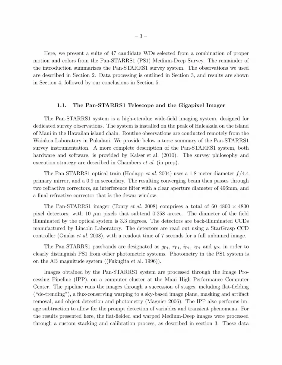
Here, we present a suite of 47 candidate WDs selected from a combination of proper

motion and colors from the Pan-STARRS1 (PS1) Medium-Deep Survey. The remainder of

the introduction summarizes the Pan-STARRS1 survey system. The observations we used

are described in Section 2. Data processing is outlined in Section 3, and results are shown

in Section 4, followed by our conclusions in Section 5.

1.1. The Pan-STARRS1 Telescope and the Gigapixel Imager

The Pan-STARRS1 system is a high-etendue wide-field imaging system, designed for

dedicated survey observations. The system is installed on the peak of Haleakala on the island

of Maui in the Hawaiian island chain. Routine observations are conducted remotely from the

Waiakoa Laboratory in Pukalani. We provide below a terse summary of the Pan-STARRS1

survey instrumentation. A more complete description of the Pan-STARRS1 system, both

hardware and software, is provided by Kaiser et al. (2010). The survey philosophy and

execution strategy are described in Chambers et al. (in prep).

The Pan-STARRS1 optical train (Hodapp et al. 2004) uses a 1.8 meter diameter f/4.4

primary mirror, and a 0.9 m secondary. The resulting converging beam then passes through

two refractive correctors, an interference filter with a clear aperture diameter of 496mm, and

a final refractive corrector that is the dewar window.

The Pan-STARRS1 imager (Tonry et al. 2008) comprises a total of 60 4800 × 4800

pixel detectors, with 10 µm pixels that subtend 0.258 arcsec. The diameter of the field

illuminated by the optical system is 3.3 degrees. The detectors are back-illuminated CCDs

manufactured by Lincoln Laboratory. The detectors are read out using a StarGrasp CCD

controller (Onaka et al. 2008), with a readout time of 7 seconds for a full unbinned image.

The Pan-STARRS1 passbands are designated as gP1, rP1, iP1, zP1 and yP1 in order to

clearly distinguish PS1 from other photometric systems. Photometry in the PS1 system is

on the AB magnitude system ((Fukugita et al. 1996)).

Images obtained by the Pan-STARRS1 system are processed through the Image Pro-

cessing Pipeline (IPP), on a computer cluster at the Maui High Performance Computer

Center. The pipeline runs the images through a succession of stages, including flat-fielding

(“de-trending”), a flux-conserving warping to a sky-based image plane, masking and artifact

removal, and object detection and photometry (Magnier 2006). The IPP also performs im-

age subtraction to allow for the prompt detection of variables and transient phenomena. For

the results presented here, the flat-fielded and warped Medium-Deep images were processed

through a custom stacking and calibration process, as described in section 3. These data

– 4 –

are collected with many dithers, permitting an outlier rejection strategy that exempts them

from the “Magic” satellite streak masking software.

1.2. The Pan-STARRS1 Photometric System

The Pan-STARRS1 observations are obtained through a set of five broadband filters,

which we have designated as gP1, rP1, iP1, zP1, and yP1. Under certain circumstances

Pan-STARRS1 observations are obtained with a sixth, “wide” filter designated as wP1 that

essentially spans gP1, rP1, and iP1. Although the filter system for Pan-STARRS1 has much in

common with that used in previous surveys, such as SDSS (York et al. 2000), there are im-

portant differences. The gP1 filter extends 20 nm redward of gSDSS, paying the price of 5577A

sky emission for greater sensitivity and lower systematics for photometric redshifts, and the

zP1 filter is cut off at 930 nm, giving it a different response than the detector response de-

fined zSDSS. SDSS has no corresponding yP1 filter. We stress that, like SDSS, Pan-STARRS1

uses the AB photometric system and there is no arbitrariness in the definition, only in how

accurately we know the bandpasses.

The details of the photometric calibration and the Pan-STARRS1 zeropoint scale will

be presented in a subsequent publication (Tonry et al. in prep), and (Magnier et al. in prep)

will provide the application to a consistent photometric catalog over the 3/4 sky observed

by Pan-STARRS1. We briefly describe the methodology used for the photometry presented

in this paper.

We have carried out extensive, in-situ measurements of the full transmission of the

Pan-STARRS1 system (Stubbs et al. 2010), as well as knowing the filter, lens, and mir-

ror characteristics from vendor’s measurements, and we have found these to be consistent.

Provisional response functions (including 1.2 airmasses of atmosphere) are available at the

project’s web site1.

Integrating the Pan-STARRS1 SDSS, and Johnson/Kron-Cousins bandpasses against

spectrophotometry of 273 stars with a wide range of temperature and surface gravity gives

us a means of transforming SDSS colors to the Pan-STARRS1 system for the stellar locus.

Table 1 relates the Pan-STARRS1 color to a corresponding SDSS color: CP1 = A+B×CSDSS,

valid over a certain range in CSDSS. Since both systems are AB the constant A is negligible,

and the relative redness of gP1 and blueness of zP1 relative to SDSS are reflected in B < 1.

The term for yP1 is purely a stellar locus extrapolation off of the SDSS system and should

1http://svn.pan-starrs.ifa.hawaii.edu/trac/ipp/wiki/PS1 Photometric System

– 5 –

be used with caution.

Table 1: Pan-STARRS1 – SDSS stellar color transformations

Cp1 CSDSS A B rms Color range

(g − r)P1 (g − r)SDSS −0.016 0.865 0.012 −0.6 – 1.6

(r − i)P1 (r − i)SDSS −0.002 1.018 0.004 −0.5 – 1.0

(i− z)P1 (i− z)SDSS +0.001 0.837 0.008 −0.5 – 1.2

(z − y)P1 (i− z)SDSS −0.004 0.400 0.022 −0.2 – 1.2

Note. — The columns contain the Pan-STARRS1 color, the SDSS color, the offset A [mag], the color

coefficient B, the rms scatter [mag] between the synthetic spectrophotometry in the Pan-STARRS1 system

and the color-transformed SDSS-band synthetic photometry, for the 273 sources used, and the color range

(SDSS) [mag] over which this RMS holds.

While the catalog of Magnier et al. (in prep) will use Pan-STARRS1 as a photometric

instrument to link observations to fundamental standards such as Vega or BD+17 4708, the

photometry presented here is based on SDSS DR7. Each Medium-Deep field observation in

a filter is brought into relative calibration with every other observation, and then overlap

with SDSS stars whose magnitudes have been transformed into the Pan-STARRS1 system

provides a single zeropoint for all. We finally use the stellar locus of Covey et al. (2007)

transformed to the Pan-STARRS1 system to provide cross-filter zero-point tweaks and create

the most consistent colors possible. The procedure is described in detail below, but it is

essential to emphasize that the photometry here is on the Pan-STARRS1 system, not on

the SDSS system, although SDSS is the basis for zeropoints and colors. Like SDSS, the

Pan-STARRS1 photometry includes 1.2 airmasses of atmospheric attenuation as a factor in

the bandpasses, although the magnitudes are corrected to the top of the atmosphere. No

correction is made for galactic extinction.

2. OBSERVATIONS

In addition to covering the entire sky at δ > −30 deg, the Pan-STARRS1 survey has

obtained multi-epoch images in the gP1, rP1, iP1, zP1 and yP1 bands of the fields listed in

Table 2, the Medium-Deep fields. MD00 is a field centered on M31 with a filter choice and

cadence designed to detect microlensing. This paper uses only the images and photometry

from the 1635 Pan-STARRS1 Medium-Deep Field survey observations acquired between Apr

– 6 –

2009 and Apr 2011. There are some 350 observations that missed IPP processing in time for

inclusion.

Table 2: Pan-STARRS1 Medium-Deep Field Centers.

Field RA (J2000) Dec (J2000)

MD00 10.675 41.267

MD01 35.875 −4.250

MD02 53.100 −27.800

MD03 130.592 44.317

MD04 150.000 2.200

MD05 161.917 58.083

MD06 185.000 47.117

MD07 213.704 53.083

MD08 242.787 54.950

MD09 334.188 0.283

MD10 352.312 −0.433

MD11 270.000 66.561

Observations of the Medium-Deep fields occur each night, cycling through the various

Pan-STARRS1 filters, during that portion of the year that the fields are accessible at less than

1.3 airmasses. A nightly “observation” in a given filter consists of 8 dithered “exposures”,

with a typical cadence as shown in Table 3. Our basic units of observation are these “nightly-

stacks” and the “stack-stack” of all nightly-stacks, although there is information available

on the timescales of individual exposures, and for other programs we assemble custom stacks

of nightly-stacks.

Table 3: Pan-STARRS1 Medium-Deep Survey, typical cadence. Observations taken 3 nights

on either side of full moon are done only in the yP1 band.

Night Filter Exposure Time

1 gP1& rP1 8×113s each

2 iP1 8×240s

3 zP1 8×240s

repeats... · · · · · ·

FM±3 yP1 8×240s

– 7 –

Table 4 provides basic information about each field and filter, including the number of

nightly-stacks available, the total exposure time, the PSF FWHM calculated by DoPhot on

the stack-stack, the median PSF of the various nightly-stacks estimated by IPP, and the 5-σ

limiting magnitude for point sources. This limiting magnitude was calculated by creating

two stacks from interleaved halves of all the nightly-stacks, comparing DoPhot photometry

between them, estimating the magnitude where the RMS difference is 0.2 mag, and from

that deriving the magnitude where the sum would have RMS uncertainty 0.2 mag. We can

relate this limiting magnitude to the RMS magnitude per 0.2′′ pixel of the background and

the PSF FWHM, w, (in arcsec). This RMS background in turn for each filter depends on

the exposure time, t, and a constant that folds together the mean system throughput, sky

background, and extinction.

RMS = (24.3, 24.1, 23.7, 23.1, 22.0) + 1.25 log(t) (1)

mlim = RMS− 5.4− 2.5 log(w), (2)

where the sequence in parentheses corresponds to gP1,rP1,iP1,zP1,yP1. The core-skirt nature

of the PSF in the stack-stack (discussed in more detail below) implies that these 5-σ limits

degrade slowly for larger apertures (e.g. for galaxy photometry).

3. DATA PROCESSING

3.1. Individual Image Processing

The Pan-STARRS1 IPP system performs flatfielding on each of the images, using white

light flatfield images from a dome screen, in combination with an illumination correction ob-

tained by rastering sources across the field of view. Bad pixel masks are applied, and carried

forward for use in the stacking stage. After determining an initial astrometric solution, the

flat-fielded images are then warped onto a tangent plane of the sky, using a flux conserving

algorithm. The plate scale for the warped images is 0.200 arcsec/pixel. The IPP removes

the sky level from the images, but at this point makes no attempt to provide a consistent

flux scale. Images obtained through clouds are included in the processing chain. We adjust

the flux scale of each image at the level of a Pan-STARRS1 “skycell”, which subtends 20

arcminutes on the sky. There is no evidence for residual spatial structure in the attenuation

from clouds in the resulting Medium-Deep field nightly stacks, each combining 8 images of

integration time over 100 seconds.

– 8 –

Table 4: Pan-STARRS1 MDF Statistics, Apr 2009–Apr 2011.

Field Filter N log t PSF 〈w〉 mlim Field Filter N log t PSF 〈w〉 mlim

MD01 gP1 42 4.7 1.25 1.55 24.5 MD06 gP1 38 4.6 1.25 1.56 24.4

MD01 rP1 42 4.7 1.15 1.35 24.4 MD06 rP1 39 4.6 1.18 1.45 24.2

MD01 iP1 41 4.9 1.05 1.27 24.4 MD06 iP1 41 4.9 1.14 1.39 24.3

MD01 zP1 41 4.9 1.03 1.24 23.9 MD06 zP1 38 4.9 1.05 1.30 23.7

MD01 yP1 21 4.6 0.95 1.17 22.4 MD06 yP1 24 4.7 1.00 1.25 22.4

MD02 gP1 30 4.5 1.31 1.79 24.2 MD07 gP1 36 4.5 1.23 1.68 24.3

MD02 rP1 29 4.5 1.20 1.74 24.1 MD07 rP1 39 4.5 1.13 1.46 24.2

MD02 iP1 30 4.8 1.11 1.50 24.2 MD07 iP1 39 4.9 1.14 1.44 24.2

MD02 zP1 33 4.8 1.06 1.30 23.6 MD07 zP1 43 4.9 1.08 1.37 23.7

MD02 yP1 16 4.5 1.14 1.42 22.1 MD07 yP1 30 4.8 1.01 1.28 22.5

MD03 gP1 38 4.6 1.18 1.44 24.5 MD08 gP1 38 4.5 1.27 1.68 24.3

MD03 rP1 37 4.6 1.09 1.28 24.4 MD08 rP1 38 4.5 1.14 1.47 24.2

MD03 iP1 41 4.9 1.06 1.31 24.4 MD08 iP1 33 4.8 1.07 1.34 24.2

MD03 zP1 42 5.0 1.03 1.27 23.9 MD08 zP1 40 4.9 1.09 1.39 23.7

MD03 yP1 20 4.6 1.00 1.36 22.4 MD08 yP1 32 4.9 0.98 1.27 22.7

MD04 gP1 35 4.6 1.17 1.52 24.5 MD09 gP1 34 4.5 1.26 1.55 24.3

MD04 rP1 37 4.6 1.09 1.46 24.3 MD09 rP1 33 4.5 1.15 1.42 24.1

MD04 iP1 35 4.9 1.07 1.35 24.3 MD09 iP1 34 4.8 1.02 1.36 24.3

MD04 zP1 28 4.8 1.03 1.32 23.6 MD09 zP1 34 4.8 1.02 1.26 23.7

MD04 yP1 8 4.3 1.03 1.21 22.0 MD09 yP1 12 4.3 0.94 1.12 22.0

MD05 gP1 42 4.6 1.24 1.58 24.4 MD10 gP1 30 4.5 1.26 1.60 24.2

MD05 rP1 40 4.6 1.17 1.46 24.3 MD10 rP1 33 4.5 1.18 1.53 24.2

MD05 iP1 34 4.8 1.06 1.44 24.3 MD10 iP1 30 4.8 1.01 1.31 24.2

MD05 zP1 27 4.8 0.99 1.27 23.6 MD10 zP1 28 4.8 1.03 1.24 23.6

MD05 yP1 17 4.6 1.02 1.33 22.3 MD10 yP1 11 4.4 0.96 1.22 22.2

MD11 gP1 1 3.0 1.17 1.45 22.4 MD00 gP1 0 · · · · · · · · · · · ·

MD11 rP1 1 3.0 1.12 1.30 22.3 MD00 rP1 101 4.9 1.03 1.30 24.8

MD11 iP1 3 3.8 1.13 1.47 22.9 MD00 iP1 66 4.6 0.96 1.25 24.0

MD11 zP1 4 3.9 1.34 1.81 22.2 MD00 zP1 0 · · · · · · · · · · · ·

MD11 yP1 5 4.0 0.96 1.21 21.6 MD00 yP1 0 · · · · · · · · · · · ·

Note. — N is the number of nights of observation, log t is the log10 of the net exposure time in sec, “PSF”

is the DoPhot FWHM of the core-skirt PSF in the stack-stacks (in arcsec), 〈w〉 is the median IPP FWHM

of the observations (in arcsec), and mlim is the 5σ detection limit for point sources.

– 9 –

3.2. Exposure combination into stacks

The images obtained from a single night in each band were typically obtained with small

dithers in boresight and at a diversity of rotator angles. The stack of 8 images per band per

night were then assembled into a “nightly stack”, using a variance-weighted combination of

individual frames, with outlier rejection. These nightly-stacked images are considered to be

that night’s image in the appropriate band. This stacking process successfully suppresses

cosmic ray artifacts, masking losses, and any sources that move a distance larger than the

PSF during the ∼ 30 minute observation interval.

Nightly-stacks are combined into “stack-stacks” by weighting each by inverse variance

times inverse PSF area. We find that this is nearly optimal for point source detection. In

principle we might do slightly better by convolution with PSF, but in practice the covariance

between warped pixels is such as to make the improvement negligible. The resulting PSF

of this stack-stack has a relatively sharp core and substantial skirt, of course, but we do

not attempt to deconvolve the skirt into a more compact PSF, even though it would be a

relatively robust operation. Instead, we always strive to match PSF models to the data, or

include skirt deconvolution as part of the normal kernel convolution required when image

subtracting the stack-stack from a nightly-stack.

3.3. Photometric and astrometric calibration

In the interim, before the Pan-STARRS1 photometric catalog of the sky is released,

we must resort to a somewhat involved procedure to bring all observations to a common

and accurate zeropoint. In brief, these steps are applied to each set of observations of each

Medium-Deep field, every 20 arcminute skycell of each field (about 70 per field), and each

filter:

1. Obtain instrumental magnitudes (fluxes) for all stars in all nightly-stacks using DoPhot

(Schechter et al. 1993).

2. By comparison of stellar instrumental magnitudes between all N(N−1)/2 pairs of ob-

servations (Tonry et al. in prep), obtain photometric and astrometric offsets for each

skycell of each nightly-stack (with indeterminate zeropoint). All instrumental magni-

tudes are corrected to an aperture magnitude within a 6 arcsec box.

3. Combine all nightly-stacks into a stack-stack using inverse variance times inverse PSF

area weighting.

– 10 –

4. Obtain instrumental magnitudes for all stars in each stack-stack.

5. Assemble a weighted combination of three estimates of photometric zeropoint by com-

paring a) SDSS stars converted to the Pan-STARRS1 system (or its extension to MD01

and MD02 using relative photometry from Pan-STARRS), b) zP1 derived from 2MASS

magnitudes and stellar locus conversions, and c) skycell-to-skycell relative zeropoints

founded on the flattening performed by the IPP with the instrumental magnitudes of

the stack-stack.

6. Create an “object catalog” from the union over all filters for each skycell; perform

forced-position photometry on each stack-stack for each object in the catalog.

7. Compare four colors for all stellar objects in five filters with the standard colors of the

stellar locus. This is derived by removing (small for MDS) SFD extinction from each ob-

ject and matching to the stellar locus (Covey et al. 2007), shifted to the Pan-STARRS1

system. Apply these (very small) offsets to the zeropoints of each filter, assuming zero

median. This corrects (High et al. 2009) for small residual effects in color-color space,

such as atmospheric extinction variations or small color terms between skycells.

This has the following features.

• All nightly-stacks and stack-stacks should have very consistent photometry, limited by

DoPhot’s ability to match the PSF and the size of the aperture box.

• Use of the flattening constraint should prevent skycell to skycell jumps in zeropoint.

• The skycell by skycell tie to a standard stellar locus should make colors more accurate

than absolute zeropoints.

• The absolute astrometry is founded on the 2MASS coordinate system that IPP cur-

rently uses to create the warps, but does remove small offsets (typically less than

∼50 mas) between nightly-stacks that have occurred as IPP evolves. This ensures that

the relative astrometry for proper motions is as accurate as we can currently make it.

Although this will eventually be superseded by the Pan-STARRS1 photometric and

astrometric system, we believe that this procedure has satisfactory accuracy for our purposes.

Figure 1 shows the stellar locus of 500,000 stars from the ten Medium-Deep fields.

The width of the locus in (r − i)P1 at (g − r)P1 = 0.6 is 0.04 mag, consistent with the

estimated uncertainties in the photometry added in quadrature to 0.02 mag, and constraining

any failure to bring skycells and Medium-Deep field photometry into color agreement to

∼ 0.02 mag.

– 11 –

Fig. 1.— Pan-STARRS1 Medium-Deep Field stellar locus of 500,000 stars in 10 MDFs. The

47 Pan-STARRS1 WD candidates are shown as square, red points. The blue extension of

the stellar locus (∼1800 stars shown in blue) are likely hot WD stars, but luminosity inferred

from proper motion is a prerequisite to identify cool WDs that overlap the stellar locus.

– 12 –

3.4. Proper motion determination

There are some 10 million objects in the 10 MD fields for which we have 50–200 ob-

servations, spread over 2 years and the five filters. We have searched these for evidence of

proper motion. The RMS astrometric residuals for sufficiently bright objects (photometric

precision of <0.05 mag) is 25–40 mas, per observation. For each object we assemble all

the detections and fit the positions for a proper motion. Objects with rP1 < 22 typically

yield an answer with uncertainty of ∼ 10mas/yr; fainter objects can be measured with cor-

respondingly greater uncertainty. For brighter objects we can find SDSS or even USNO-B

counterparts, but many are too faint.

There are some 60,000 objects that appear to have a 3σ proper motion in this 2 year data.

We further cut this by demanding a 6σ proper motion significance, and we also augment

the skycell alignment described above by a local astrometric bias correction. This consists

of finding all objects within 0.03 deg of each candidate proper motion that themselves are

more significant than 1.5σ (typically ∼40 objects), assembling a median motion and quartile-

derived RMS, subtracting this median motion from the candidate proper motion and adding

the uncertainty in quadrature to the uncertainty of the candidate’s. This has the effect of

reducing the systematic error although increasing the uncertainty, and decreasing the number

that still meet the 6σ criterion. There are about 1,000 objects that fulfill this bias-corrected,

6σ cut.

There are a number of improvements we anticipate in the near future.

• Once Pan-STARRS1 moves to its own astrometric system instead of 2MASS, the need

for this skycell adjustment and local bias correction should disappear, and we should

see significantly tighter residuals for bright enough objects.

• To date we have worked only with nightly-stacks, but of course it is possible to combine

observations to achieve better astrometric precision for faint objects at the expense of

fewer epochs.

• The present Pan-STARRS1 mission is slated to continue for at least two more years,

doubling or tripling the temporal baseline (there were far fewer observations in 2009

than in 2010).

Although the colors of the majority of the 10 million objects lie off of the stellar lo-

cus, these 1,000 objects (and 60,000 3 σ objects) lie gratifyingly close to the stellar locus;

extremely few galaxies leak past the proper motion filter.

– 13 –

Comparisons with the SIMBAD database of known proper motions show excellent agree-

ment for those objects faint enough not to be saturated for Pan-STARRS1 and bright enough

to appear in SIMBAD. At rP1∼15 only the poor seeing Pan-STARRS1 observations are un-

saturated, Pan-STARRS1 achieves its best accuracy for objects in the range of 17<rP1<21,

and without nightly-stack combination Pan-STARRS1 loses accuracy to photon statistics

fainter than rP1>22.

3.5. Parallax fits

Joint fits for parallax and proper motion over the baseline of Pan-STARRS1 observations

did not turn up any highly significant parallax: the median uncertainty is 10 mas and the

median parallax is 4 mas. There were three detections of parallax at 2.5σ at 13, 27, and

29 mas, but the covariance with proper motion make these very insecure measurements. (Of

course there are many stars in the MD fields closer than 30 pc, but they are all too bright

and saturated.) We anticipate much better performance when we have the Pan-STARRS1

astrometric grid, perhaps uncertainties as small as 3 mas for bright objects with 17<rP1<21.

Of course, the extented time baseline over the course of the Pan-STARRS1 project will also

help improve the proper motion and parallax measurements.

4. RESULTS

4.1. Selection of WDs by Reduced Proper Motion

The “reduced proper motion” (RPM) is defined as H = m+5 logµ+5 = M+5 log vtan−

3.379, where µ is measured in arcsec/yr and vtan in km/s, and is therefore a proxy for absolute

magnitude for a given transverse velocity. With accurate photometry and astrometry, these

diagrams can reveal a very clean separation of stars into main sequence, subdwarfs, and

WDs. For example, the contamination rate of the WD locus by subdwarfs is only 1-2% for

the SDSS + USNO-B RPM diagram (Kilic et al. 2006). The HgP1vs. (g − r)P1 and HrP1

vs (r − i)P1 RPM diagrams for our 1,000 proper motions are presented in Figure 2. That

the gap between subdwarfs and WDs is so clearly visible is a testament to the high accuracy

of the Pan-STARRS1 photometry and proper motions at this relatively stringent selection

criterion.

We use these RPM diagrams to identify 47 WD candidates. Astrometric and pho-

tometric data for these objects are given in Table 5 and 6, respectively. About half of

our sample has proper motion measurements available in the literature (Munn et al. 2004;

– 14 –

Fig. 2.— Pan-STARRS1 Medium Deep Field Proper Motion Diagrams. Left panel is in gP1

iP1 space, and the right panel is in rP1, iP1 space. The large clump on the right is main

sequence stars; the middle clump that separates well in (r − i)P1 are subdwarfs, and the

blue, faint objects on the left are candidate WD stars.

Fig. 3.— Pan-STARRS1 (this work) versus SDSS+USNO-B or LSPM (Munn et al. 2004;

Lepine & Shara 2005) proper motion measurements for 24 WD candidates. Objects with

unreliable SDSS+USNO-B proper motions (detected in <5 epochs) are shown as open circles.

– 15 –

Lepine & Shara 2005). Figure 3 shows a comparison of our proper motion measurements and

the literature values. Open circles mark the objects with unreliable proper motions from the

SDSS + USNO-B. Ignoring those, there is an overall agreement between our proper motion

measurements and the literature values.

– 16 –

Table 5. Pan-STARRS1 MDF White Dwarf Candidates, Astrometric Data. The columns present

Object ID designations, RA and Dec (J2000) in decimal degrees (for epoch 2010.5) the number of

valid astrometric observations per star, the measured proper motions in RA and Dec (in mas per

year), their associated uncertainties, the fitted parallax and its uncertainty, in mas. (We do not

regard any of the parallax values to be significant.)

OBJID RA(J2000) Dec(J2000) Npts µRA σµRA µ Dec σµDec π σπ

PSO J035.1219−04.4538 35.12198 -4.45385 120 49 15 -106 16 23 10

PSO J036.1807−02.7150* 36.18072 -2.71503 85 392 19 37 21 4 16

PSO J036.1820−02.7157* 36.18203 -2.71578 80 383 21 53 24 2 16

PSO J053.8940−27.1420 53.89408 -27.14205 68 49 31 -343 35 11 19

PSO J053.9285−27.4034 53.92850 -27.40348 107 51 18 102 16 29 10

PSO J128.8195+44.7108 128.81959 44.71086 131 12 13 -120 13 12 10

PSO J128.9494+44.4259 128.94944 44.42598 172 -3 7 -64 7 8 6

PSO J130.1413+43.5130 130.14136 43.51305 138 -17 10 -70 10 -8 7

PSO J130.3780+44.1562 130.37809 44.15620 157 71 9 -53 9 -6 8

PSO J130.5828+43.8370 130.58286 43.83708 158 -37 9 -52 9 -15 7

PSO J131.0677+45.8815 131.06776 45.88157 25 51 53 -253 41 -36 34

PSO J131.2406+45.6086 131.24064 45.60864 175 -54 10 -175 9 11 6

PSO J132.0255+43.9883 132.02558 43.98836 145 -86 12 -10 11 -12 9

PSO J132.2560+44.6595 132.25604 44.65954 177 -197 13 -96 12 12 6

PSO J148.6936+01.4568 148.69365 1.45680 54 149 19 -272 20 0 23

PSO J148.9818+03.1285 148.98181 3.12853 51 -14 39 -249 36 -28 48

PSO J149.3101+02.6967 149.31014 2.69677 136 -187 8 -104 8 14 10

PSO J149.3311+03.1446 149.33117 3.14463 120 45 10 -94 9 4 10

PSO J149.7106+01.7900 149.71066 1.79004 142 74 11 -6 15 13 9

PSO J149.7616+01.6465 149.76161 1.64656 140 18 9 -69 12 1 9

PSO J149.8925+02.9603 149.89256 2.96030 141 -59 12 -96 10 27 9

PSO J150.1696+03.6030 150.16966 3.60309 115 9 11 -90 11 -7 13

PSO J150.8329+02.1407 150.83292 2.14079 117 -90 12 25 11 1 15

PSO J151.3094+02.9046 151.30944 2.90467 114 -692 14 18 14 1 14

PSO J159.5163+57.6086 159.51636 57.60867 110 -10 12 -259 12 4 12

PSO J160.5173+58.5631 160.51739 58.56312 148 -99 14 -81 12 -1 8

PSO J160.6208+59.0860 160.62083 59.08602 44 -438 66 -49 65 -23 59

PSO J161.4917+59.0766 161.49173 59.07662 98 -1016 13 -1417 12 22 11

PSO J161.8956+59.2131 161.89562 59.21314 156 -32 14 -169 25 -8 7

PSO J162.2873+57.7484 162.28730 57.74848 23 -60 84 520 84 133 70

PSO J164.1738+57.2466 164.17384 57.24660 141 -13 12 -119 20 19 8

– 17 –

Table 5—Continued

OBJID RA(J2000) Dec(J2000) Npts µRA σµRA µ Dec σµDec π σπ

PSO J164.1744+58.4375 164.17447 58.43759 140 -132 19 12 15 21 9

PSO J183.8810+46.5039 183.88106 46.50397 178 -285 40 24 15 0 7

PSO J185.6294+46.1184 185.62949 46.11848 155 -63 11 -27 10 11 8

PSO J186.4406+47.1036 186.44063 47.10365 169 -143 13 22 15 -7 7

PSO J213.0478+52.6587 213.04785 52.65875 144 -51 12 72 12 -17 8

PSO J214.3502+52.8743 214.35023 52.87438 172 -55 10 57 20 -12 6

PSO J215.0267+53.3759 215.02672 53.37591 187 98 18 -89 15 13 5

PSO J241.3352+55.9465 241.33522 55.94657 172 -209 11 191 8 -1 5

PSO J242.8803+54.6275 242.88030 54.62755 97 17 16 -98 16 -3 10

PSO J333.8526−00.8187 333.85260 -0.81878 13 616 116 -411 115 11 178

PSO J334.4434−00.3065 334.44341 -0.30654 118 84 13 -58 14 0 15

PSO J334.5518−00.0227 334.55185 -0.02278 125 49 11 -97 11 7 14

PSO J334.7932+00.8453 334.79324 0.84537 136 -102 12 -10 10 18 12

PSO J334.8792+01.0115 334.87925 1.01154 137 271 12 -35 21 17 12

PSO J352.7302+00.4814 352.73028 0.48142 125 154 12 113 13 5 11

PSO J353.2230−00.5556 353.22300 -0.55562 116 65 14 62 15 10 13

Note. — * This appears to be a binary WD pair with a common proper motion.

– 18 –

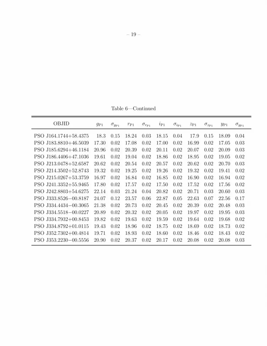
Table 6. Pan-STARRS1 MDF White Dwarf Candidates, Photometric Data. The columns

present Object ID designations, gP1,rP1,iP1,zP1,yP1 magnitudes and uncertainties.

OBJID gP1 σgP1rP1 σrP1

iP1 σiP1zP1 σzP1

yP1 σyP1

PSO J035.1219−04.4538 22.21 0.04 21.26 0.02 20.82 0.02 20.66 0.02 20.64 0.04

PSO J036.1807−02.7150 19.60 0.04 19.01 0.05 18.89 0.05 18.80 0.05 18.70 0.05

PSO J036.1820−02.7157 19.60 0.04 18.96 0.05 18.78 0.05 18.69 0.05 18.62 0.05

PSO J053.8940−27.1420 22.77 0.06 21.89 0.04 21.48 0.03 21.33 0.03 21.28 0.12

PSO J053.9285−27.4034 19.83 0.02 19.89 0.02 19.98 0.03 20.16 0.03 20.35 0.07

PSO J128.8195+44.7108 22.32 0.04 21.52 0.02 21.17 0.02 21.05 0.02 20.98 0.05

PSO J128.9494+44.4259 18.43 0.02 18.66 0.02 18.88 0.02 19.11 0.02 19.24 0.02

PSO J130.1413+43.5130 20.27 0.02 19.99 0.03 19.89 0.02 19.88 0.02 19.91 0.04

PSO J130.3780+44.1562 20.61 0.02 20.28 0.02 20.12 0.02 20.09 0.02 20.04 0.03

PSO J130.5828+43.8370 20.72 0.02 20.45 0.02 20.33 0.03 20.31 0.02 20.33 0.03

PSO J131.0677+45.8815 21.48 0.04 21.24 0.05 21.11 0.05 21.17 0.04 21.20 0.15

PSO J131.2406+45.6086 15.96 0.05 15.98 0.03 16.02 0.03 16.14 0.02 16.27 0.02

PSO J132.0255+43.9883 21.24 0.02 20.92 0.02 20.67 0.02 20.78 0.02 20.90 0.07

PSO J132.2560+44.6595 17.95 0.02 17.62 0.02 17.50 0.02 17.49 0.02 17.52 0.02

PSO J148.6936+01.4568 19.21 0.04 19.12 0.05 19.19 0.05 19.27 0.06 19.24 0.15

PSO J148.9818+03.1285 22.79 0.06 21.91 0.00 21.75 0.00 21.44 0.00 22.30 0.30

PSO J149.3101+02.6967 20.27 0.02 19.47 0.02 19.10 0.02 19.00 0.02 18.95 0.02

PSO J149.3311+03.1446 19.34 0.02 19.10 0.02 18.98 0.02 19.03 0.02 19.01 0.02

PSO J149.7106+01.7900 15.56 0.07 15.87 0.05 16.12 0.02 16.38 0.02 16.52 0.02

PSO J149.7616+01.6465 17.95 0.03 18.13 0.02 18.34 0.02 18.52 0.02 18.68 0.02

PSO J149.8925+02.9603 18.24 0.02 18.11 0.02 18.07 0.02 18.12 0.02 18.21 0.02

PSO J150.1696+03.6030 20.90 0.02 20.56 0.02 20.40 0.02 20.36 0.02 20.42 0.04

PSO J150.8329+02.1407 21.53 0.02 20.96 0.02 20.74 0.02 20.71 0.02 20.81 0.03

PSO J151.3094+02.9046 20.55 0.00 19.76 0.00 19.36 0.00 19.42 0.06 19.18 0.05

PSO J159.5163+57.6086 21.92 0.03 21.04 0.02 20.61 0.02 20.47 0.02 20.41 0.03

PSO J160.5173+58.5631 19.05 0.02 18.96 0.02 18.97 0.02 19.07 0.02 19.16 0.02

PSO J160.6208+59.0860 22.09 0.06 21.27 0.00 21.09 0.07 21.07 0.06 20.70 0.20

PSO J161.4917+59.0766 18.33 0.00 18.19 0.00 18.16 0.00 17.98 0.00 18.14 0.03

PSO J161.8956+59.2131 17.80 0.02 17.83 0.02 17.93 0.02 18.06 0.02 18.19 0.02

PSO J162.2873+57.7484 23.79 0.13 22.86 0.07 21.86 0.04 21.59 0.07 21.43 0.12

PSO J164.1738+57.2466 18.40 0.03 18.27 0.02 18.27 0.02 18.35 0.02 18.51 0.02

– 19 –

Table 6—Continued

OBJID gP1 σgP1rP1 σrP1

iP1 σiP1zP1 σzP1

yP1 σyP1

PSO J164.1744+58.4375 18.3 0.15 18.24 0.03 18.15 0.04 17.9 0.15 18.09 0.04

PSO J183.8810+46.5039 17.30 0.02 17.08 0.02 17.00 0.02 16.99 0.02 17.05 0.03

PSO J185.6294+46.1184 20.96 0.02 20.39 0.02 20.11 0.02 20.07 0.02 20.09 0.03

PSO J186.4406+47.1036 19.61 0.02 19.04 0.02 18.86 0.02 18.95 0.02 19.05 0.02

PSO J213.0478+52.6587 20.62 0.02 20.54 0.02 20.57 0.02 20.62 0.02 20.70 0.03

PSO J214.3502+52.8743 19.32 0.02 19.25 0.02 19.26 0.02 19.32 0.02 19.41 0.02

PSO J215.0267+53.3759 16.97 0.02 16.84 0.02 16.85 0.02 16.90 0.02 16.94 0.02

PSO J241.3352+55.9465 17.80 0.02 17.57 0.02 17.50 0.02 17.52 0.02 17.56 0.02

PSO J242.8803+54.6275 22.14 0.03 21.24 0.04 20.82 0.02 20.71 0.03 20.60 0.03

PSO J333.8526−00.8187 24.07 0.12 23.57 0.06 22.87 0.05 22.63 0.07 22.56 0.17

PSO J334.4434−00.3065 21.38 0.02 20.73 0.02 20.45 0.02 20.39 0.02 20.48 0.03

PSO J334.5518−00.0227 20.89 0.02 20.32 0.02 20.05 0.02 19.97 0.02 19.95 0.03

PSO J334.7932+00.8453 19.82 0.02 19.63 0.02 19.59 0.02 19.64 0.02 19.68 0.02

PSO J334.8792+01.0115 19.43 0.02 18.96 0.02 18.75 0.02 18.69 0.02 18.73 0.02

PSO J352.7302+00.4814 19.71 0.02 18.93 0.02 18.60 0.02 18.46 0.02 18.43 0.02

PSO J353.2230−00.5556 20.90 0.02 20.37 0.02 20.17 0.02 20.08 0.02 20.08 0.03

– 20 –

4.2. Optical Spectroscopy

Twelve of our candidates have optical spectroscopy available in the literature: all

of them are previously known WDs, including 6 DAs, 4 DQs, 1 DC, and 1 DZ. PSO

J161.4917+59.0766 (LHS 291) is perhaps the most interesting, with a proper motion of

1.7′′ yr−1. The identification of this object in our data demonstrates that the Pan-STARRS1

Medium Deep Field data are able to identify even the fastest moving halo objects.

We obtained spectroscopic observations of six candidates, as summarized in Table 7,

with the Hectospec instrument (Fabricant et al. 2005) on the MMT. The objects were se-

lected on the basis of field access and were part of a broader program of Pan-STARRS1

followup spectroscopy. The Hectospec fibers are 1.5′′ in diameter. We operate the spectro-

graph with the 270 lines/mm grating, providing wavelength coverage 3700–9200 A and a

spectral resolution of 5 A with a dispersion of 1.2 A per pixel. The spectra were reduced,

including flatfielding and wavelength calibration, by the Telescope Data Center pipeline

(Mink et al. 2007), at the Center for Astrophysics. Sky subtraction was performed using

the spectra from fibers placed on blank sky regions. Flux calibration was performed using

standard star observations from an earlier observing run. Therefore, the absolute flux cali-

bration, as well as the relative continuum shape, of our spectra cannot be trusted. However,

this level of resolution is sufficient to identify and separate WDs from metal-poor subdwarfs.

Table 7: Spectroscopic Observations.

PS1 ID UT Observed texp (s)

PSO J162.2873+57.7484 2011-06-08T15:36:46 4500

PSO J164.1738+57.2466 2011-06-09T16:02:41 3600

PSO J183.8810+46.5039 2011-06-13T15:47:10 4800

PSO J213.0478+52.6587 2011-06-06T15:59:53 3600

PSO J215.0267+53.3759 2011-06-06T15:34:21 3600

PSO J242.8803+54.6275 2011-06-06T15:34:23 3600

The resulting spectra are presented in Figure 4. Two of the objects with Hectospec

spectra were previously known WDs. PSO J164.1738+57.2466 is a known DZ WD with

only Ca H and K absorption visible in its optical spectrum. PSO J215.0267+53.3759 is

a known DA WD with Balmer absorption lines. One of the objects observed with Hec-

tospec, PSO J162.2873+57.7484, is too faint for the instrument and conditions, and there-

fore not included in this figure. The remaining three objects are newly confirmed WDs.

PSO J183.8810+46.5039 is a DA WD with a hydrogen atmosphere, whereas the lack of de-

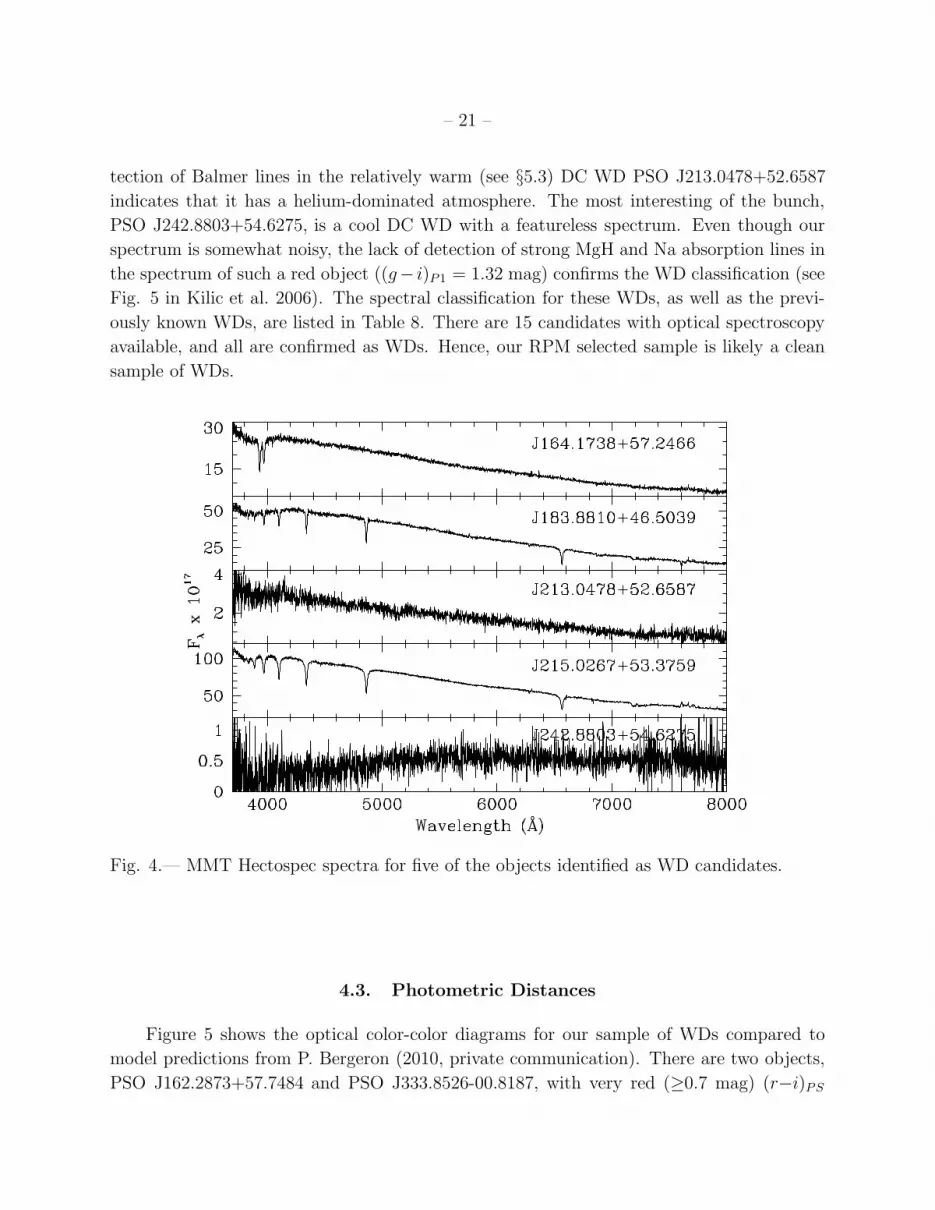
– 21 –

tection of Balmer lines in the relatively warm (see §5.3) DC WD PSO J213.0478+52.6587

indicates that it has a helium-dominated atmosphere. The most interesting of the bunch,

PSO J242.8803+54.6275, is a cool DC WD with a featureless spectrum. Even though our

spectrum is somewhat noisy, the lack of detection of strong MgH and Na absorption lines in

the spectrum of such a red object ((g− i)P1 = 1.32 mag) confirms the WD classification (see

Fig. 5 in Kilic et al. 2006). The spectral classification for these WDs, as well as the previ-

ously known WDs, are listed in Table 8. There are 15 candidates with optical spectroscopy

available, and all are confirmed as WDs. Hence, our RPM selected sample is likely a clean

sample of WDs.

Fig. 4.— MMT Hectospec spectra for five of the objects identified as WD candidates.

4.3. Photometric Distances

Figure 5 shows the optical color-color diagrams for our sample of WDs compared to

model predictions from P. Bergeron (2010, private communication). There are two objects,

PSO J162.2873+57.7484 and PSO J333.8526-00.8187, with very red (≥0.7 mag) (r−i)PS

– 22 –

colors. We classify these objects as WD + M dwarf binaries. There are also two other ob-

jects, PSO J131.0677+45.8815 and J132.0255+43.9883, with (u− g)SDSS versus (g− r)SDSS

colors similar to the known DQ WDs (bottom right panel). These objects may be DQ

WDs as well, and optical spectroscopy is needed to see if they show the C2 swan bands.

PSO J148.9818+03.1285 is the only object with a relatively blue (z−y)PS color. Hydrogen-

rich cool WDs are expected to show strong flux deficits in the infrared from collision in-

duced absorption due to molecular hydrogen (Bergeron et al. 1995; Hansen 1998). PSO

J148.9818+03.1285 may be one such WD. However, the yP1-band measurement for this ob-

ject has a large error, and therefore, the absorption may not be real. Other than these

outliers, the remaining candidates overlap with WD model predictions in various color-color

diagrams. Hence, these models can be used to derive temperatures for our targets.

We use all five Pan-STARRS1 magnitudes to fit WD models with hydrogen atmospheres

to determine the temperature, absolute magnitude, and distance of each target. Since the

Pan-STARRS1 parallax measurements for our targets are inaccurate, we assume a surface

gravity of log g = 8 which determines the radius of the star for a given value of temperature.

The mass distribution of WDs shows strong peaks at 0.61 ±0.1M⊙ for DA and 0.67 ±0.1M⊙

for DB WDs (Tremblay et al. 2011; Bergeron et al. 2011); these ranges imply log g = 8±0.3.

Hence, our assumption of log g = 8 is reasonable.

Cool WD spectral energy distributions are clearly effected by the Ly α red wing opacity

in the blue (Kowalski & Saumon 2006). Since these models do not include the Ly α opacity,

we use them to analyze only the WDs hotter than 4600 K. For cooler targets, we use the

observed colors of cool WDs from Kilic et al. (2009, 2010, analyzed using Kowalski & Saumon

(2006) models) as templates to estimate the temperatures of our targets. These templates

cover the temperature range 3730-6290 K. Based on the Pan-STARRS1 and the SDSS colors,

the temperature estimates from both the models and the templates agree to within 200 K

for stars in the temperature range 4600-6000 K.

The photometric spectral energy distributions of six of the coolest objects in our sample

are shown in Figure 6. The points with error bars show Pan-STARRS1 photometry and

the solid lines show the best-fitting templates. For example, the energy distribution of PSO

J035.1219-04.4538 (top left panel) is most similar to the WD SDSS J2222+1221 (Kilic et al.

2009), which has a temperature of 4170 K based on the Kowalski & Saumon (2006) models.

Hence, we assign a temperature of 4170 K for PSO J035.1219-04.4538. Given this temper-

ature and assuming log g = 8, we then estimate an absolute magnitude of Mg = 16.5 and a

distance of 127 pc.

One of the objects in Figure 6, PSO J148.9818+03.1285, may be a WD with a strong

yP1 flux deficit. If this absorption is real, then the best-fit pure hydrogen atmosphere WD

– 23 –

Fig. 5.— Pan-STARRS1 and SDSS (bottom right panel) color-color diagrams for our sample

of WD candidates. Spectroscopically confirmed DA (blue), DQ (magenta), DZ (green), and

DC (red) WDs are marked. The solid lines show the predicted colors for pure hydrogen

atmosphere WDs with Teff = 1500 − 110, 000 K and log g = 7, 8, and 9 (only the log g = 8

and Teff ≥ 2000 K sequence is shown in the bottom right panel).

– 24 –

model would have Teff = 3080 K and a cooling age of 11.1 Gyr. If so, PSO J148.9818+03.1285

would be a very old thick disk or halo WD. However, near-infrared photometry is required to

confirm the flux deficit in the infrared and to perform a detailed model atmosphere analysis.

Many of the infrared-faint WDs have mixed H/He atmospheres (Kilic et al. 2010), where the

effects of the collision induced absorption due to molecular hydrogen become significant at

hotter temperatures (>4000 K) compared to the pure hydrogen atmosphere counterparts.

Fig. 6.— Spectral energy distributions of six WDs with Teff = 4170 − 4570 K. Points with

error bars show the Pan-STARRS1 photometry. The solid lines show the best-fit cool WD

templates. The dotted line shows the predicted model fluxes for a Teff = 3080 K WD.

Table 8 lists the effective temperatures, distances, and tangential velocities for those

stars whose position in the RPM diagram and color-color space indicate that they are WDs.

The estimated distances and WD cooling ages for our targets range from about 50 pc to 300

pc and 0.2 Gyr to 8.6 Gyr, respectively. Two of the WD candidates, PSO J036.1807−02.7150

and PSO J036.1820−02.7157, form a common proper motion binary system. Our temper-

ature (4900 K and 5100 K) and distance (64 pc and 71 pc) estimates for these two stars

agree fairly well, confirming that these two stars are physically associated. The small differ-

ences between the temperatures and distances of the two stars can be explained by a small

difference in mass.

– 25 –

Table 8. Pan-STARRS1 MDF White Dwarf Candidates, Physical Parameters

OBJID Type Teff (K) d (pc) Vtan (km/s) Cooling Age (Gyr)

PSO J035.1219−04.4538 · · · 4170 127 70 ± 19 8.6

PSO J036.1807−02.7150 · · · 5100 71 133 ± 28 5.2

PSO J036.1820−02.7157 · · · 4900 64 117 ± 25 6.1

PSO J053.8940−27.1420 · · · 4280 178 292 ± 71 8.3

PSO J053.9285−27.4034 · · · 9670 317 171 ± 50 0.7

PSO J128.8195+44.7108 · · · 4640 177 101 ± 25 7.1

PSO J128.9494+44.4259 DA 13370 249 76 ± 19 0.3

PSO J130.1413+43.5130 · · · 6150 159 54 ± 15 2.1

PSO J130.3780+44.1562 · · · 5950 169 71 ± 17 2.3

PSO J130.5828+43.8370 · · · 6330 205 62 ± 18 2.0

PSO J131.0677+45.8815 · · · 6540 313 383 ± 125 1.8

PSO J131.2406+45.6086 DA 9110 47 41 ± 9 0.8

PSO J132.0255+43.9883 · · · 6010 231 95 ± 26 2.2

PSO J132.2560+44.6595 · · · 6100 53 55 ± 12 2.2

PSO J148.6936+01.4568 · · · 7950 165 242 ± 53 1.1

PSO J148.9818+03.1285 · · · 4350 197 233 ± 68 8.0

PSO J149.3101+02.6967 · · · 4570 67 68 ± 14 7.3

PSO J149.3311+03.1446 · · · 6480 115 57 ± 14 1.8

PSO J149.7106+01.7900 DA 15670 85 30 ± 10 0.2

PSO J149.7616+01.6465 DA 12160 183 62 ± 18 0.4

PSO J149.8925+02.9603 DA 7890 100 53 ± 13 1.1

PSO J150.1696+03.6030 · · · 5940 192 82 ± 22 2.4

PSO J150.8329+02.1407 · · · 5170 179 79 ± 21 4.8

PSO J151.3094+02.9046 · · · 4570 77 253 ± 51 7.3

PSO J159.5163+57.6086 · · · 4350 123 151 ± 32 8.0

PSO J160.5173+58.5631 DQ 10080: · · · · · · · · ·

PSO J160.6208+59.0860 · · · 5340 220 459 ± 133 4.0

PSO J161.4917+59.0766 DQ 10110: · · · · · · · · ·

PSO J161.8956+59.2131 DQ: 10150: · · · · · · · · ·

PSO J162.2873+57.7484 WD+dM? · · · · · · · · · · · ·

PSO J164.1738+57.2466 DZ* 7420 99 56 ± 16 1.3

– 26 –

Table 8—Continued

OBJID Type Teff (K) d (pc) Vtan (km/s) Cooling Age (Gyr)

PSO J164.1744+58.4375 · · · 6610 79 50 ± 13 1.8

PSO J183.8810+46.5039 DA* 6640 47 64 ± 16 1.7

PSO J185.6294+46.1184 · · · 5040 128 42 ± 12 5.5

PSO J186.4406+47.1036 DQ 6109 · · · · · · · · ·

PSO J213.0478+52.6587 DC* 7860 308 129 ± 36 1.1

PSO J214.3502+52.8743 · · · 7890 170 64 ± 22 1.1

PSO J215.0267+53.3759 DA* 8040 58 36 ± 10 1.1

PSO J241.3352+55.9465 · · · 6660 60 81 ± 17 1.7

PSO J242.8803+54.6275 DC* 4250 130 61 ± 19 8.4

PSO J333.8526−00.8187 WD+dM? · · · · · · · · · · · ·

PSO J334.4434−00.3065 · · · 4840 138 67 ± 18 6.4

PSO J334.5518−00.0227 · · · 5000 121 62 ± 15 5.7

PSO J334.7932+00.8453 · · · 6970 167 81 ± 20 1.5

PSO J334.8792+01.0115 · · · 5430 78 101 ± 22 3.5

PSO J352.7302+00.4814 DC 5130 67 61 ± 13 5.0

PSO J353.2230−00.5556 · · · 5210 137 58 ± 18 4.6

Note. — Spectral types for previously known WDs are from Eisenstein et al. (2006),

Liebert et al. (2005),Koester & Knist (2006), and Kilic et al. (2006). Asterix (*) designates

objects for which we obtained spectra.

– 27 –

Figure 7 shows the distribution of inferred ages and tangential velocities, with the as-

sumption that the distance error is 20%. The coolest WDs in our sample have temperatures

around 4200 K. Even though the individual ages for our targets cannot be trusted due to

the unknown distances and masses, the average mass for our sample should be about 0.6 M⊙

and the average age for the oldest stars in our sample should be reliable. Adding 1.4 Gyr

for the main-sequence lifetime of the 2 M⊙ solar-metallicity progenitor stars (Marigo et al.

2008) brings the total age to about 10 Gyr, entirely consistent with the oldest disk WDs

known (e.g. Table 2 of Leggett et al. 1998) and the Galactic disk age of 8 ± 1.5 Gyr. A few

of the oldest targets have large tangential velocities, and therefore they may be halo WDs.

However, the velocity errors are also relatively large for those objects. Therefore, all of our

targets are consistent with disk membership.

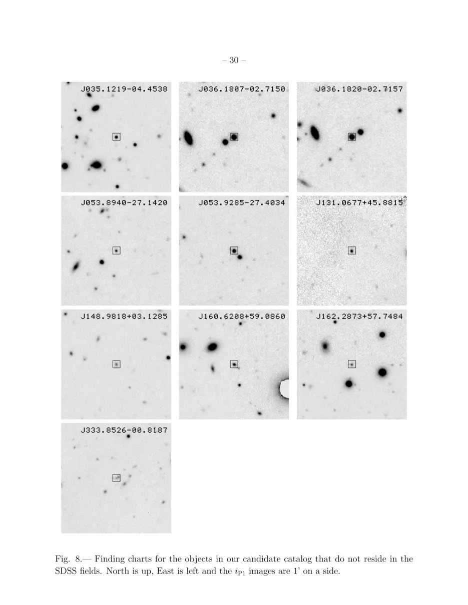
Figure 8 presents finding charts for those new objects that do not reside in the SDSS

fields.

Fig. 7.— Tangential velocities and WD cooling ages for our targets. (The high velocity,

young WD presumably have higher mass than 0.6 M⊙ and their lower luminosity for a given

temperature causes us to assign an erroneously high distance and velocity.)

– 28 –

5. DISCUSSION

Deep, wide-field surveys like Pan-STARRS1 provide an unprecedented opportunity for

the studies of different stellar populations in the Galaxy. Based on the stellar locus of

half a million stars from the ten Medium Deep Fields, we demonstrate that the systematic

uncertainty in the Pan-STARRS1 photometric zeropoints is a few percent. In addition,

the relatively high-cadence of the Pan-STARRS1 Medium Deep Field observations enable

searches for highly variable (e.g. supernovae) and/or moving objects like nearby asteroids

or high proper motion stars. Here we take advantage of the first two years of data from the

Medium Deep Field observations to select 47 WD candidates using an RPM diagram. We

are able to find objects with proper motions as large as 1.7′′ yr−1. Hence, we are sensitive

to faint halo WDs with large tangential velocities.

A comparison with WD atmosphere models and previously known cool WDs shows

that our sample contains WDs down to 4200 K, which corresponds to a main-sequence +

WD cooling age of 10 Gyr. A few of the oldest objects in our sample have large tangential

velocities that may indicate halo membership. Assuming that the halo is a single burst 12

Gyr old population with 0.4% normalization compared to the disk, Kilic et al. (2010) predict

0.14 halo WDs per square degree down to a limiting magnitude of V = 21.5 mag. Our sample

of 47 WD candidates is therefore likely to contain a few halo WDs. However, our parallaxes

as yet lack adequate accuracy to claim that they are indeed halo WDs. Pan-STARRS1 will

continue to observe the Medium Deep Fields over the course of the next two years, and the

Pan-STARRS1 astrometric catalog is imminent and will significantly improve the proper

motion and parallax precision for these targets.

For this initial project to find WDs in the Pan-STARRS1 data we concentrated on sam-

ple purity rather than completeness, and the astrometric bias correction was particularly dra-

conian. We present proper motions to a limit of 60 mas/yr and gP1∼22.5. Doubling the num-

ber of epochs should improve accuracy by 23/2 and bring us to measurements of ∼20 mas/yr

with uncertainty of ∼3 mas/yr. We used the Besancon Galaxy model (Robin et al. 2003) to

simulate the stellar populations in the Medium Deep fields. At 20 mas/yr over 70 sq. deg.,

even without co-adding to improve the nightly-stack detection limit, the model predicts we

ought to be able to find some 850 WDs. By co-adding nightly-stacks to reach a limiting

magnitude of gP1∼23.5 this number rises to about 1500. We look forward to being able to

probe the halo WD population with such a clean, large sample, and employ them to chart

the history of the Milky Way.

Facilities: Pan-STARRS1(GPC), MMT(Hectospec)

– 29 –

Support for this work was provided by National Science Foundation grant AST-1009749.

The PS1 Surveys have been made possible through contributions of the Institute for Astron-

omy, the University of Hawaii, the Pan-STARRS Project Office, the Max-Planck Society

and its participating institutes, the Max Planck Institute for Astronomy, Heidelberg and the

Max Planck Institute for Extraterrestrial Physics, Garching, The Johns Hopkins University,

Durham University, the University of Edinburgh, Queen’s University Belfast, the Harvard-

Smithsonian Center for Astrophysics, and the Las Cumbres Observatory Global Telescope

Network, Incorporated, the National Central University of Taiwan, and the National Aero-

nautics and Space Administration under Grant No. NNX08AR22G issued through the Plan-

etary Science Division of the NASA Science Mission Directorate.

The spectroscopic observations reported here were obtained at the MMT Observatory,

a joint facility of the Smithsonian Institution and the University of Arizona. This paper uses

data products produced by the OIR Telescope Data Center, supported by the Smithsonian

Astrophysical Observatory, and we have benefited from NASA’s Astrophysics Data System

Bibliographic Services and the SIMBAD database, operated at CDS, Strasbourg, France.

A. Finding Charts

– 30 –

Fig. 8.— Finding charts for the objects in our candidate catalog that do not reside in the

SDSS fields. North is up, East is left and the iP1 images are 1’ on a side.

– 31 –

REFERENCES

Bergeron, P., Saumon, D., & Wesemael, F. 1995, ApJ, 443, 764

Bergeron, P. 2003, ApJ, 586, 201

Bergeron, P., Ruiz, M. T., Hamuy, M., Leggett, S. K., Currie, M. J., Lajoie, C.-P., & Dufour,

P. 2005, ApJ, 625, 838

Bergeron, P. et al. 2011, ApJ, in press, arXiv:1105.5433

Chambers, K. C, et al., in preparation.

Covey, K. R., et al. 2007, AJ, 134, 2398

Eisenstein, D. J., et al. 2006, ApJS, 167, 40

Fabricant, D., et al. 2005, PASP, 117, 1411

Fukugita, M., et al. 1996, AJ, 111, 1748

Hall, P. B., Kowalski, P. M., Harris, H. C., Awal, A., Leggett, S. K., Kilic, M., Anderson,

S. F., & Gates, E. 2008, AJ, 136, 76

Hambly, N. C., Smartt, S. J., & Hodgkin, S. T. 1997, ApJ, 489, L157

Hansen, B. M. S. 1998, Nature, 394, 860

Harris, H. C., et al. 2006, AJ, 131, 571

High, F. W., Stubbs, C. W., Rest, A., Stalder, B., & Challis, P. 2009, AJ, 138, 110.

Hodapp, K. W., Siegmund, W. A., Kaiser, N., Chambers, K. C., Laux, U., Morgan, J., &

Mannery, E. 2004, Proc. SPIE, 5489, 667

Kaiser, N., et al. 2010, Proc. SPIE, 7733, 12K.

Kilic, M., et al. 2006, AJ, 131, 582

Kilic, M., Kowalski, P. M., & von Hippel, T. 2009, AJ, 138, 102

Kilic, M., et al. 2010, ApJ, 715, L21

Kilic, M., et al. 2010, ApJS, 190, 77

Koester, D., & Knist, S. 2006, A&A, 454, 951

– 32 –

Kowalski, P. M., & Saumon, D. 2006, ApJ, 651, L137

Kurucz, R. L. 1996, M.A.S.S., Model Atmospheres and Spectrum Synthesis, 108, 2

Lepine, S., & Shara, M. M. 2005, AJ, 129, 1483

Leggett, S. K., Ruiz, M. T., & Bergeron, P. 1998, ApJ, 497, 294

Liebert, J., Dahn, C. C., & Monet, D. G. 1988, ApJ, 332, 891

Liebert, J., Bergeron, P., & Holberg, J. B. 2005, ApJS, 156, 47

Liebert, J., Kilic, M., Williams, K. A., von Hippel, T., Winget, D. M. J., Harris, H. C.,

Levine, S., & Metcalfe, T. S. 2007, 15th European Workshop on White Dwarfs, 372,

129

Magnier, E. 2006, Proceedings of The Advanced Maui Optical and Space Surveillance Tech-

nologies Conference, Ed.: S. Ryan, The Maui Economic Development Board, p.E5

Magnier, E., et al., in preparation.

Marigo, P., Girardi, L., Bressan, A., Groenewegen, M. A. T., Silva, L., & Granato, G. L.

2008, A&A, 482, 883

Mink, D. J., Wyatt, W. F., Caldwell, N., Conroy, M. A., Furesz, G., & Tokarz, S. P. 2007,

Astronomical Data Analysis Software and Systems XVI, 376, 249

Munn, J. A., et al. 2004, AJ, 127, 3034

Onaka, P., Tonry, J. L., Isani, S., Lee, A., Uyeshiro, R., Rae, C., Robertson, L., & Ching,

G. 2008, Proc. SPIE, 7014, 12.

Oppenheimer, B. R., Hambly, N. C., Digby, A. P., Hodgkin, S. T., & Saumon, D. 2001,

Science, 292, 698

Reid, I. N., Sahu, K. C., & Hawley, S. L. 2001, ApJ, 559, 942

Robin, A. C., Reyle, C., Derriere, S., & Picaud, S. 2003, A&A, 409, 523

Rowell, N., & Hambly, N. C. 2011, MNRAS, in press, arXiv:1102.3193

Schechter, P. L., Mateo, M., & Saha, A. 1993, PASP, 105, 1342

Stubbs, C. W., Doherty, P., Cramer, C., Narayan, G., Brown, Y. J., Lykke, K. R., Woodward,

J. T., & Tonry, J. L. 2010, ApJS, 191, 376

– 33 –

Tremblay, P.-E., Bergeron, P., & Gianninas, A. 2011, ApJ, 730, 128

Tonry, J. L., Burke, B. E., Isani, S., Onaka, P. M., & Cooper, M. J. 2008, Proc. SPIE, 7021,

9.

Tonry, J. L., et al., in preparation.

Winget, D. E., Hansen, C. J., Liebert, J., Van Horn, H. M., Fontaine, G., Nather, R. E.,

Kepler, S. O., & Lamb, D. Q. 1987, ApJ, 315, L77

York, D. G., et al. 2000, AJ, 120, 1579

This preprint was prepared with the AAS LATEX macros v5.2.