Embed Size (px)
Citation preview

International Studies ProgramInternational Studies ProgramWorking Paper 09-03March 2009
Fiscal Decentralization and PublicFiscal Decentralization and Public Sector Employment: A Cross-Country Analysis
Jorge Martinez-VazquezJorge Martinez-VazquezMing-Hung Yao


International Studies Program Andrew Young School of Policy Studies Georgia State University Atlanta, Georgia 30303 United States of America Phone: (404) 651-1144 Fax: (404) 651-4449 Email: [email protected] Internet: http://isp-aysps.gsu.edu Copyright 2006, the Andrew Young School of Policy Studies, Georgia State University. No part of the material protected by this copyright notice may be reproduced or utilized in any form or by any means without prior written permission from the copyright owner.
International Studies Program Working Paper 09-03
Fiscal Decentralization and Public Sector Employment: A Cross-Country Analysis Jorge Martinez-Vazquez Ming-Hung Yao March 2009

International Studies Program Andrew Young School of Policy Studies The Andrew Young School of Policy Studies was established at Georgia State University with the objective of promoting excellence in the design, implementation, and evaluation of public policy. In addition to two academic departments (economics and public administration), the Andrew Young School houses seven leading research centers and policy programs, including the International Studies Program. The mission of the International Studies Program is to provide academic and professional training, applied research, and technical assistance in support of sound public policy and sustainable economic growth in developing and transitional economies. The International Studies Program at the Andrew Young School of Policy Studies is recognized worldwide for its efforts in support of economic and public policy reforms through technical assistance and training around the world. This reputation has been built serving a diverse client base, including the World Bank, the U.S. Agency for International Development (USAID), the United Nations Development Programme (UNDP), finance ministries, government organizations, legislative bodies and private sector institutions. The success of the International Studies Program reflects the breadth and depth of the in-house technical expertise that the International Studies Program can draw upon. The Andrew Young School's faculty are leading experts in economics and public policy and have authored books, published in major academic and technical journals, and have extensive experience in designing and implementing technical assistance and training programs. Andrew Young School faculty have been active in policy reform in over 40countries around the world. Our technical assistance strategy is not to merely provide technical prescriptions for policy reform, but to engage in a collaborative effort with the host government and donor agency to identify and analyze the issues at hand, arrive at policy solutions and implement reforms. The International Studies Program specializes in four broad policy areas: Fiscal policy, including tax reforms, public expenditure reviews, tax administration reform Fiscal decentralization, including fiscal decentralization reforms, design of intergovernmental
transfer systems, urban government finance Budgeting and fiscal management, including local government budgeting, performance-
based budgeting, capital budgeting, multi-year budgeting Economic analysis and revenue forecasting, including micro-simulation, time series
forecasting, For more information about our technical assistance activities and training programs, please visit our website at http://isp-aysps.gsu.edu or contact us by email at [email protected].

1
Fiscal Decentralization and Public Sector Employment: A Cross-Country Analysis
Jorge Martinez-Vazquez∗ Department of Economics, Georgia State University, Atlanta, Georgia
Ming-Hung Yao+
Department of Economics, Tunghai University, Taichung, Taiwan
Abstract This paper investigates the relationship between public sector employment and fiscal decentralization. We develop a theoretical framework modeling the interactions between the central and sub-national executives regarding the level of public employment at the central and sub-national government levels. In our empirical work, based on a large cross-country dataset, we find that, ceteris paribus, the level of total public sector employees in a country increases with its level of fiscal decentralization. Even though central government employment decreases with decentralization, this is more than fully offset by the increase in employment at the sub-national level accompanying decentralization. Our empirical results also indicate that the relationship between GDP per capita and public sector employment is not monotonic but quadratic, that total public sector employment is higher in unitary countries vis-à-vis federal countries, and that public employment increases with the country’s international economic openness. Keywords: fiscal decentralization; public sector employment; public sector size JEL classification: H30; H50; H77
∗ Director of International Studies Program and Regents Professor, Department of Economics, Andrew Young School of Policy Studies, Georgia State University. E-mail address: [email protected]. + Corresponding author; Assistant Professor, Department of Economics, Tunghai University, Taichung, Taiwan. E-mail address: [email protected].

2 International Studies Program Working Paper Series
Introduction
Public sector employment accounts for a considerable share of public
expenditures and it represents also a significant share of total employment in most
countries. For these reasons, trends in a public sector employment have attracted a great
deal of attention over the past two decades (Gregory & Borland, 1999). At present, it is
commonly believed that bloated bureaucracies and over-staffed public enterprises
represent a significant problem for many developing and transitional countries.
Over-staffing takes many forms, from an excessive number of agencies and ministries, to
duplications of functions at different levels of government, or even the existence of ghost
workers (Rama, 1997). Consequently, it is not surprising that retrenchment in public
sector employment has come to the forefront of the reform agenda in many countries.
In this paper we investigate what role decentralization reforms around the world
in recent times may play in the observed trends in public sector employment. Although
decentralization may be seen as a cause for the increase in public sector employment
through the proliferation of different levels of government, there are also a priori reasons
to expect that decentralization may help contain the increase in public employment. An
economic argument for decentralization is that it increases allocative efficiency in the
public sector because some public expenditure decisions can be made by a level of
government that is closer and more responsive to the needs and preferences of local
residents. This means that possibly fewer resources (including public employees) may be
needed to satisfy certain levels of needs (Martinez-Vazquez & McNab, 2003). In addition,
decentralization has the potential of improving competition of governments at the same
time that it enhances innovations, thus furthering greater efficiencies in overall
expenditures (Ford, 1999). These potential effects of decentralization suggest that fiscal

Fiscal Decentralization and Public Sector Employment: A Cross-Country Analysis 3
decentralization reform could work as therapy for the problem of bloated bureaucracies
and over-staffed public enterprises in transitional and developing countries.
In reality, over the last two decades, public sector employment has grown in some
countries but it has shrunk in others. Appendix A shows the evolution of public sector
employment as a percentage of total population for 74 countries covering the period
1985-2005.1 We can call these changes the time series variation in public employment.
The data also show that the size of public sector employment in some countries is larger
than that in other countries in any period. We can call this the cross-sectional variation in
public sector employment. As we review below, three main hypotheses have been
developed in the economics literature to explain these variations across countries and
over time in public sector employment and the size of the public sector: Wagner’s law,
the rent-seeking hypothesis, and the social insurance hypothesis. While these three
hypotheses help explain different aspects in the variation of public sector employment
levels across countries and over time, none of these hypotheses provides a clear rationale
for how public employment is affected by the level of government decentralization in a
country. In fact, to the best of our knowledge, no previous theoretical or empirical work
in the literature has examined directly the vertical structure dimension of public sector
employment.2 That is the central question addressed in this paper: do higher levels of
decentralization across countries and over time lead to higher overall public sector
employment?
1 The data on public sector employment used in this paper are obtained from the International Labor Organization (ILO) bureau of statistics, at the website http://laborsta.ilo.org/, accessed last March 26, 2009. The data are available since 1985. Before 1996, the data are available every five years. After 1996 the data are available annually. The latest year for which data are available is 2006. In order to compare the data before and after 1996, we calculate the unweighted five-year averages for the periods 1996-2000 and 2001-2005.

4 International Studies Program Working Paper Series
An essential part of fiscal decentralization reform is the transfer of expenditure
responsibilities from the central government to the sub-national governments. If we
assume that decentralization does not lead to any change in the demand for public
services, but just to a change in how (or where) the same public services are delivered, as
a result of more decentralization we would expect that the number of public sector
employees at the central government level would decrease and that this number would
increase at the sub-national level. In addition, decentralization may not leave the demand
for public services unchanged. If the efficiency of public services delivery is increased,
citizens may demand more of certain services and the overall provision of other services
may be reduced; for example, there may be less demand and spending on some national
goods or even reductions in national programs involving redistribution and so on.3 The
overall impact of fiscal decentralization on total public sector employment depends on:
(i) the relative magnitude of the two opposing substitution effects for the same level and
composition of public services, and (ii) what changes in demand and spending on public
services decentralization may bring. For example, if decentralization were to lead to an
increase in demand for labor-intensive services, such as education and health, vis-à-vis
other less labor-intensive services, total public sector employment as a result would also
experience an increase. Thus a number of scenarios may be built for both the
retrenchment and expansion in public sector employment due to decentralization.
In this paper we develop a theoretical model to analyze explicitly the relationship
between decentralization and public sector employment. The predictions of the
2 However, two previous papers reviewed below have studied in the context of a single country the evolution of sub-national public employment following changes in decentralization. 3 See, for example, Shelton (2007) and Arze del Granado et al. (2008)

Fiscal Decentralization and Public Sector Employment: A Cross-Country Analysis 5
theoretical model are tested empirically using a panel data set for a large number of
developed and developing countries over the period 1985-2005.
The rest of the paper is organized as follows. In Section 2 we review the previous
relevant literature. In Section 3 we develop the theoretical model. In Section 4 we
describe the dataset and present the empirical results. In Section 5 we conclude.
Literature Review
In this section we first review the previous economics literature on public sector
employment and then we take a look at what has been said about decentralization and
public sector employment.
Three Hypotheses on Public Sector Employment
As already mentioned above, there are three main hypotheses in the public finance
literature that were designed to understand the evolution of government size and public
sector employment. Below, we briefly outline the main features of the hypotheses while
the empirical literature and main findings under the three hypotheses are summarized in
Table 1.
Wagner’s law
The most conventional view of public sector employment is related to Wagner’s
law, which argues that economic development creates demand for new types of
government services, and that these government services will tend to rise at a faster pace

6 International Studies Program Working Paper Series
than economic development. 4 These predictions have been tested either within a
particular country or across countries, where the size of the public sector is measured in
terms of the share of government expenditures in gross domestic product (GDP) or the
share of government employees in the total population or the labor force. Some of the
recent empirical studies that have tested Wagner’s law are summarized in Table 1. An
interesting finding in this literature is that public sector employment grows with
economic development but that this relationship is not monotonic. Beyond a certain level
of development, the relationship between development level and public sector
employment becomes insignificant and Wagner’s law becomes inoperative
(Schiavo-Campo et al., 1997). In this respect, Rama (1997) estimates that the turning
point is 14,000 dollars per capita at 1985 purchasing power parity (PPP) prices.
The Rent-Seeking Hypothesis
Wagner’s law works better in explaining the levels of public employment across
countries, but it is less helpful in explaining the distribution of employment within
countries. For example, Alesina et al. (2001) find that the number of public employees in
the poorer regions of Italy (the south) is significantly larger than in the richer regions (the
north). Therefore, there would appear to be some factors other than the level of economic
development influencing the level of public employment within a country. Gelb et al.
(1991) theorize that the public sector differs from the private sector in the extent to which
it is subject to political pressures for employment and that rent seeking and rent creating
behavior can give rise to a wasteful diversion of resources into the public sector over and
4 Shelton (2007) presents a new explanation for Wagner’s law: richer countries are older and spend more on social security which boosts total public expenditure.

Fiscal Decentralization and Public Sector Employment: A Cross-Country Analysis 7
above the derived demand for resources. Robinson and Verdier (2002) further argue that
public sector employment is a good commitment device between politicians and voters
and that clientelism is a relatively attractive political strategy in situations with high
inequality and low productivity. Alesina et al. (2000), Alesina et al. (2001), and
Gimpelson and Treisman (2002) are several of the studies that have examined empirically
the rent-seeking hypothesis (see Table 1.)
[Insert TABLE 1 here]
Social Insurance and Economic Hypotheses
Rodrik (1997) suggested an alternative hypothesis to explain differences in public
sector employment: relatively safe government jobs represent partial insurance against
un-diversifiable external risk faced by the domestic economy. He argues that countries
with great exposures to external risk are likely to have higher levels of public
employment. His empirical work shows that exposure to external risk, measured as the
share of the sum of imports and exports of goods and services on GDP, is robustly
associated with levels of government employment across countries.
Public Employment and Fiscal Decentralization in the Previous Literature
With the exception of two recent papers, the discussion in the public finance
literature of the relationship between decentralization and the size of the public sector has
been in terms of overall expenditures (or revenues) and not in terms of public
employment. Nevertheless, as we review below, the impact of decentralization on the
size of public expenditures is far from settled. Much less is known about the impact of
decentralization on the size of government when size is measured by public employment.

8 International Studies Program Working Paper Series
The earliest argument to address the impact of fiscal decentralization on the public sector
size goes back to Musgrave (1959). He argued that, under a highly decentralized public
sector, we may expect a smaller budget because there is likely to be comparatively little
in the way of assistance to the poor: sorting would lead to relatively
income-homogeneous jurisdictions with less scope for redistribution and the fear of
attracting the mobile poor would also deter the adoption of redistributive programs.
Brennan and Buchanan’s (1980) Leviathan hypothesis is another classic argument
in the discussion of the relationship between decentralization and public sector size. In
their view, the decentralization of tax and spending decisions introduces competition
among governmental units seeking to attract citizens and other mobile resources, and
thereby constrains the reach and size of the Leviathan.5
However, several arguments have been made from the view point of economic
efficiency that public sector size is likely to increase with the degree of fiscal
decentralization. A first argument made by Oates (1985) is that greater decentralization
may result in the loss of certain economies of scale with the consequent increase in
administration costs.6 A second argument by Prud'homme (1995) is that the relative
poorer quality of local bureaucrats is likely to weaken public expenditure management
and result in higher supply costs of public services. From the viewpoint of political
participation, economic historian John Wallis argued that decentralization can lead to a
larger public sector because as individuals have more control over public decisions at the
5 Empirically, no consistent evidence has been found to support or reject the Leviathan hypothesis, where government size is measured as government tax revenues or expenditures as a fraction of personal income. While Oates and Wallis (1988) and Zax (1989) find supporting evidence for the Leviathan hypothesis, Giertz (1983), Oates (1985), Nelson (1987), and Forbes and Zampelli (1989) reject it. 6 See also Stein’s (1998) discussion of this point for Latin America.

Fiscal Decentralization and Public Sector Employment: A Cross-Country Analysis 9
sub-national level they may wish to empower the public sector with a wider range of
functions and responsibilities.7
Two recent papers have studied empirically the relationship between
decentralization and public employment in the context of particular countries,
Marques-Sevillano and Rossello-Villallonga (2004) for the case of Spain, and Rajaraman
and Saha (2008) for the case of India. For the case of Spain, it was found that the increase
in the number of public employees at the regional government level was 1.6 times the
reduction in the number of public employees at the central government during the period
of decentralization covering 1990-2003. For the case of India, it was found that
horizontal splintering of the federation into smaller sub-national governments (where size
is measured as population or Gross State Domestic Product) increased the total size of the
sub-national civil service across all sub-national governments. From our perspective it is
interesting to point out that these two papers discuss the impact of decentralization on
sub-national employment in a single country over time; in the current paper we are
interested in examining how decentralization affects the aggregate level of public sector
employment (at the sub-national and central levels) across countries and over time.
The Theoretical Model
With the process of fiscal decentralization, among other things, a central
government transfers some expenditure responsibilities to the sub-national governments,
which should drive to an increase in the number of sub-national government employees
and lead to a reduction in the number of central government employees. Assuming for the
7 Wallis’s argument has been quoted in Oates (1985). Oates (1985) does not provide a reference for Wallis’s hypothesis, and we have not found any other references to it except in Forbes and Zampelli (1989), who do not provide a reference either.

10 International Studies Program Working Paper Series
time being that those are the only changes brought by decentralization, its impact on total
public sector employees would depend on the relative strength of those two opposing
effects.
In this section we develop a theoretical model, building on the work by
Gimpelson and Treisman (2002), in which the level of public employment is the result of
a two-stage game played between the central government and sub-national governments.
Politicians at both levels of government are assumed to behave as utility maximization
bureaucrats (Niskanen, 1968).
The model is set up as follows. Assume there is a country composed of one
central government with an executive and n sub-national jurisdictions, ni ..., ,2 ,1= ,
each with a governor and the same number of residents. The total amount of tax resources
in the country are denoted by R , raised by a national proportional income tax, Yt ⋅ ,
where t is the fixed tax rate and Y is the real GDP. For simplicity we assume that only
the central government raises taxes, and it provides sub-national governments with
transfers. In period 1, the central government sets the degree of fiscal decentralization,
θ , which is defined as the share of R that is allocated on an equal basis to the
sub-national governments; remaining resources share, )1( θ− , is kept by the central
government.8 We denote the amount of resource allocated to jurisdiction i as ir , where
nRri ⋅= θ . Thus the budget constraints for the central and each of the sub-national
governments are R⋅− )1( θ and nR⋅θ , respectively. In period 2, the sub-national
governor in jurisdiction i receives the transfers, nR⋅θ , and sets the level of public
8 This assumption might be especially true in developing countries, where generally sub-national governments have less autonomy in revenue matters.

Fiscal Decentralization and Public Sector Employment: A Cross-Country Analysis 11
employees in its jurisdiction, denoted by im . We assume that there are two types of
public goods: local public goods and national public goods. Local public goods are only
provided to the residents in the particular jurisdiction following the decision of the
governor in this jurisdiction. National public goods are provided to all residents in the
country following the decision of the central authorities. The production functions of both
public goods are of a Cobb-Douglas form with two inputs, labor (public sector
employment) and capital, which could be represented mathematically as
βα KmKmf ⋅=),( , where m is input of public sector employment and K is capital
input.9 We further assume that the production technologies of local pubic goods in each
jurisdiction are identical across jurisdictions in the country. All public expenditures go to
pay the wages of the public employees and the capital rental costs.
The governor’s utility function in each sub-national jurisdiction is a function of
the level of local public goods provided to the residents and the sub-national government
fiscal deficit, and it is increasing the former term and decreasing with the latter. Thus, the
utility function of the sub-national governor in jurisdiction i , )( iVE , can be shown as
)()1()()( iii cmfVE πσ ⋅−−= , where im and )( imf are the number of public
employees and the production function for the local public goods, respectively, and
where the sub-national government fiscal deficit ratio in jurisdiction i , ic , is defined as
the ratio of fiscal deficit to revenue. The parameter σ captures how much of the
negative political costs of the fiscal deficit can be shifted to the central government and it
is discussed in detail below. The sub-national governor in jurisdiction i chooses to hire
the amount of im public employees to maximize his utility and provide the level of
9 In reality, the public sector might have a certain level of control over the prices of labor and capital; however, for simplicity, we assume the prices are fixed and we normalize them to 1.

12 International Studies Program Working Paper Series
)( imf local public goods to the residents in this jurisdiction. We assume the production
function is concave with 0)(' >imf and 0)(" <imf , 0>∀ im . The level of local
public goods of jurisdiction i is given by βαiiii KmKmf ⋅=),( . In equilibrium, we have
αβ⋅= **ii mK , and the total expenditure of jurisdiction i is )1(* αβ+⋅im . In addition,
the production function can be expressed solely as a function of im as
βαββα αβαβ +⋅=⋅⋅= iiii mmmmf )()()( .
In the function of the typical governor )( icπ is the political cost of running a
sub-national fiscal deficit, which is caused by over-staffing in this jurisdiction. We
assume that the sub-national governments are able to finance their fiscal deficit via other
sources, for example, borrowing from sub-national-government-own banks. Therefore
sub-national governments have so-called “soft budget” constraints.10 The fiscal deficit
ratio of jurisdiction i , ic , is equal to [ ] iii rrm −+⋅ )1( αβ , where )]1([ αβ+⋅im are
local expenditures and ir are the revenues of the jurisdiction i ; 0>ic means that
there is a fiscal deficit, 0<ic that there is a fiscal surplus, and 0=ic means in the
budget of jurisdiction i is balanced. We assume the political costs function )( icπ is
equal to zero for 0≤ic and it is a positive and a convex function for 0>ic ; that is,
0)( >icπ , 0)(' >icπ and 0)(" >icπ , 0>∀ ic .11
10 The term “soft budget” constraint was first introduced by Kornai (1992) to describe how state-owned enterprises could rely on increased subsidies even if they operated with losses. Rodden et al. (2003) describe a soft budget constraint as a situation where an entity (say, a sub-national government) can manipulate its access to funds in an undesirable way. 11 To assure the existence of a solution and to avoid a corner solution, we need several additional assumptions for this utility maximization problem: ∞→)(' imf as 0→im , 0)(' →imf as ∞→im ,
0)(' →icπ as 0→ic , and ∞→)(' icπ as ∞→ic .

Fiscal Decentralization and Public Sector Employment: A Cross-Country Analysis 13
An important implication of the soft budget constraints is that sub-national
governments can increase their expenditures without eventually facing the full costs of
these actions. Some of these costs may be shifted to the central government (Rodden, et
al., 2003). The coefficient, σ , which takes values between 0 and 1, captures the political
relationship between the central and sub-national governments in the country. This
coefficient represents the share of the political cost, )( icπ , that is shifted from the
sub-national governor to the central executive. So, )()1( icπσ ⋅− captures the political
costs that remain with the sub-national government.
The sub-national government bureaucrat’s utility function, )( iVE , shows two
properties. First, if the sub-national government provides higher level of public goods,
the sub-national governor obtains a higher level of utility. Second, hiring employees to a
high enough level leads to a fiscal deficit, which in turn decreases the utility of
sub-national governors. In our model, the penalty for profligate behavior (over-staffing)
is )()1( icπσ ⋅− . In this context, a rational governor would set *ii mm = , such that
[ ]{ } 01)1(** >−⋅+⋅⋅= Rmnc ii θαβ , where *im and *
ic are the reaction function of the
governors of jurisdiction i with respect to the central executive’s decision in period 1.12
The intuition behind this result is that since the over-staffing cost to the sub-national
government is proportionally shared by the central government, a rational sub-national
governor would choose to over-staff until the marginal benefit of providing public goods
equals the marginal cost he needs to bear which is only a part of the total costs otherwise
covered by the central executive authorities. It is quite intuitive that the level of *ic
12 The proof is shown in Appendix B.

14 International Studies Program Working Paper Series
depends on the value of σ and that the higher the value ofσ , the higher the level of
*ic .13
The coefficient σ plays an essential role in the model and so it warrants some
further discussion. Within the country the extent of the political cost to the governors
depends on whom voters blame for the sub-national government deficit. The public may
perceive the positive fiscal deficit at the sub-national level as a failure of the negotiation
and crisis management skills of the central government, even if objectively sub-national
governments are more directly to be blamed. In effect, the coefficient σ can be
interpreted as the propensity of voters to blame the central government rather than the
sub-national government for the fiscal deficit in their jurisdiction. Several institutional
factors can affect the size of the parameterσ . In particular, we can expect the value of
σ to be higher in countries where sub-national governments have less autonomous
power, especially in their ability to raise their own revenues. The lack of revenue
autonomy at the sub-national level heightens the perception that sub-national
governments only execute the expenditure policies of the central government and that
overall they act more like an agent of the central government executive. Under these
circumstances, sub-national governments can more easily shift the political costs of
sub-national fiscal deficits to the central government.
Now let us turn our attention to the central government executive’s utility
maximization problem. The central government executive’s utility depends positively on
the level of national public goods provided to all residents in the country subject to a
budget constraint and negatively on sub-national governments’ fiscal deficit. The central
13 The proof is shown in Appendix B.

Fiscal Decentralization and Public Sector Employment: A Cross-Country Analysis 15
government executive’s utility function, )( cVE , can be represented as
∑=
⋅−−=n
iic cgVE
1)()1()( πσθ . The first component on the right hand side, )1( θ−g , can
be interpreted as the production function of national public goods.14 The coefficient σ
is the share of the political cost of sub-national government fiscal deficit that the central
executive bears, and ∑=
n
iic
1
)(π is the total of the sub-national governments’ fiscal deficits
in the country. An in the case of the sub-national governments, we assume the production
function is concave with 0)'1( >−θg and 0)"1( <−θg , 1)1(0 <−<∀ θ . The central
executive chooses a degree of fiscal decentralization to maximize his utility.15 In
equilibrium, the optimal degree of fiscal decentralization can be shown as
),,,,( Rnβασθθ =∗ .16 Once *θ is determined, the optimal level of central government
employees, *cm , is also determined, and it is given by
( )[ ] ( ) ( )RnmRm cc ,,,,1 ** βασθβαα =⋅−⋅+= .
The central executive’s utility function also shows two important properties. First,
utility increases with the provision of national public goods, ( )θ−1g . Second, the central
executive suffers a decline in utility by bearing part of the political cost caused by
sub-national fiscal deficits. The share that the central government has to bear is σ for
14 We assume that there is no budget deficit problem at the central government level, and, therefore, the
total expenditure for the central government is ( ) R⋅−θ1 . Releasing and allowing the central government to
have a limited budget deficit does not change our results. 15 To assure the existence of an interior solution, we further assume that ( ) ∞→− '1 θg as 1→θ , and
( ) 0'1 →−θg as 0→θ . 16 The proof is shown in Appendix B.

16 International Studies Program Working Paper Series
each sub-national government and therefore for the entire sector too. The penalty
function for the central government is given by ∑=
⋅n
iic
1
)(πσ .
In order to investigate the interaction of hiring decisions at the two levels, we use
a game theoretic approach. The two-period-two-player game is solved by applying
backward induction.17 In period 2, the sub-national governor in jurisdiction i sets the
level of public employees in this jurisdiction at im in order to maximize his utility
function:
)()1()()( max}{ iiim
cmfVEi
πσ ⋅−−= subject to ( ) 11−
⋅+⋅⋅
=R
mnc ii θ
αβ . (1)
By solving the maximization problem, we have the following first order
condition:18
( ) ( ) ( ) ( ) ( ) 01'1' =⎥⎦⎤
⎢⎣⎡
⋅+⋅
⋅⋅−−=∂∂
=R
ncmfmVEF ii
i
i
θαβπσ . (2)
From this we can set the reaction function of the sub-national governor in
jurisdiction i as ( )Rnmm ii ,,,,, βασθ=∗ and, therefore, we have
( ) ( ) 11,,,,,*
* −⋅+⋅⋅
=R
mnRnc ii θ
αββασθ .
In period 1, the central government executive sets the degree of fiscal
decentralization, θ , to maximize his utility function:
17 Since we assume that the n sub-national jurisdictions are all identical, we can focus on one particular sub-national governor’s reaction to the central executive’s decision. Of course, this assumes that sub-national governments do not collude among themselves and that every sub-national government is too small to really affect what happens to other sub-national governments.
18 The second order condition, ( ) ( ) ( ) ( ) 21"1" ⎥⎦⎤
⎢⎣⎡
⋅+⋅
⋅⋅−−=∂∂
Rncmf
mF
iii θ
αβπσ , can be shown to be negative and
satisfied for the utility maximization problem, which assures the existence of the solution.

Fiscal Decentralization and Public Sector Employment: A Cross-Country Analysis 17
∑=
−−=n
iic cgVE
1}{)()1()( max πσθ
θ subject to ( ) 11*
* −⋅+⋅⋅
=R
mnc ii θ
αβ . (3)
Inserting the constraint into the utility function of the central government
executive’s we have:
( ) ( ) ( )∑=
⎟⎟⎠
⎞⎜⎜⎝
⎛−
⋅+⋅⋅
−−=n
i
ic R
mngVE1
*
}{111 max
θαβπσθ
θ,
with the corresponding first order condition as19
( ) ( ) ( ) 01'1'1
=⎟⎠⎞
⎜⎝⎛ −∂∂
⋅⋅+⋅
⋅−−−=∂
∂= ∑
= θθθαβπσθ
θii
n
i
c mmR
ngVEG . (4)
From the first order condition, we find the solution to the central government
executive’s utility maximization problem as ( )Rn,,,, βασθθ =∗ and, therefore, the level
of central government employment is determined
by ( )[ ] ( ) ( )RnmRm cc ,,,,,1 *** βασθθβαα =−⋅+⋅= .
The total level of public sector employment and the degree of fiscal
decentralization in the country are simultaneously determined by this system of
equations:
( ) ( ) ( )( )⎪⎩
⎪⎨⎧
=
=⋅+=⋅+=∗ Rn
RnmRnmnRnmmnmm icic
,,,,
,,,,,,,,,,,,,,, *******
σβαθθ
σβαθβασθβασθ (5)
Both the level of central and sub-national government employees in the country
are a function of fiscal decentralization. Once the degree of fiscal decentralization is
determined, the optimal level of total public sector employment is determined. Applying
the implicit function theorem to the utility maximization problem, it can be shown that
19 We assume that the second order condition is satisfied for this utility maximization problem, which
implies 0<∂∂θG . This assumption assures the existence of the solution of the central government.

18 International Studies Program Working Paper Series
the level of sub-national public employment increases and this number decreases at the
sub-national government level as the degree of fiscal decentralization grows.20 The
overall impact of fiscal decentralization on total public employment level depends on the
relative magnitude of these two opposing effects.
The Empirical Analysis
Defining Public Sector Employment
Our first task of empirical analysis is to define the term “public sector
employment”. For our empirical analysis, we use the International Labor Organization
(ILO) Public Sector Dataset. Public sector employees in the ILO dataset consist of the
employees in the general government sector and the public corporation sector. The
general government sector includes all government units,21 social security funds,22 and
other nonprofit institutions that are controlled and primarily financed by the public
authority.23 The public corporation sector comprises all of the institutional units which
produce for the market and are controlled and primarily financed by public authority.
Figure 1 shows the components of public sector employment according to the ILO.24
[Insert FIGURE 1 here]
20 The proof is shown in Appendix B. 21 The government units carry out government functions, and they include all bodies, departments, and establishments of any level of government (central, state or provincial, local) which engage in administration, defense, maintenance of public order, health, education and cultural, recreational and other social services. 22 The social security funds are social insurance schemes covering the community as a whole or large sections of the community, and are imposed, controlled, and financed by government units. They can operate at each level of government. 23 The non-profit institutions are legal entities which are autonomous from government units. They are classified under the general government only if they are non-market, as well as financed and controlled by the public authority. 24 See Hammouya (1999).

Fiscal Decentralization and Public Sector Employment: A Cross-Country Analysis 19
The International Labor Organization Public Sector Dataset covers over one
hundred countries since 1985.25 Table 2 shows the unweighted average of total public
sector employees as a percentage of total population for the Organization for Economic
Co-operation and Development (OECD hereafter) and non-OECD countries for the years
1985, 1990, 1995, 2000, and 2005.26 From Table 2, we find that the average level of
public sector employment in OECD countries is higher than that for non-OECD countries
for all periods. The average level of public sector employment for OECD countries is
quite stable over time at around 10 percent of the total population. However, for
non-OECD countries public employment as percent of total population has increased
over time, except for the period 1990-1995, from 4.88 percent of total population in 1985
to 9.31 percent in 2005. The difference in average level of public sector employment
between OECD and non-OECD countries has been decreasing over time, from a
difference of 5.08 percentage points of total population in 1985 to 1.13 percentage points
in 2005. Figure 2 depicts the time trend of average level of public sector employment for
both OECD and non-OECD countries over the 1985-2005 period.
[Insert TABLE 2 here]
[Insert FIGURE 2 here]
The Definition of Fiscal Decentralization
The second task is to define fiscal decentralization and how we measure it in
empirical analysis. Decentralization appears to be so widespread because there is often
25 Please refer to Footnote 1. 26 OECD membership information is obtained from the website, http://en.wikipedia.org/wiki/OECD, accessed March 26, 2009. Five countries, Mexico (1994), Czech Republic (1995), Hungry (1996), Poland (1996), and Slovakia (2000) in our sample became OECD members during the sample period.

20 International Studies Program Working Paper Series
confusion in terminology (Martinez-Vazquez & McNab, 1997). Three varieties of fiscal
decentralization are distinguished, corresponding to the degree of independent
decision-making exercised at the sub-national government level (Bird & Vaillancourt,
1998): (i) in the case of deconcentration, responsibilities within a central government are
dispersed to regional branch offices or sub-national administrative units; (ii) in the case
of delegation, the central government gives the sub-national governments the power to
perform functions and to raise resources but constrains that power with explicit norms
and rules; (iii) in the case of devolution, sub-national governments have discretion to
govern their own affairs with no meddling by the central authorities. In practice it is
difficult to differentiate between delegation and devolution and the measure of
decentralization used in most of the literature is the sub-national share of total
government spending or revenue. However, many authors have warned that sub-national
government expenditure or revenue shares can be misleading (see Bird (2000), Ebel &
Yilmaz (2002), and Martinez-Vazquez & McNab (2003)). Internationally comparable
data that provide the kind of information in the OECD dataset are not available from
other sources. Therefore, the sub-national government share of public expenditure or
revenue from the Government Finance Statistics Yearbook (GFS hereafter) of the
International Monetary Fund (IMF hereafter) still constitutes the only source of
cross-country data.
Table 3 presents the unweighted average of sub-national government shares of
public expenditure for OECD and non-OECD countries for five year averages between
1985 and 2005. The average of sub-national shares of expenditure for OECD countries is
higher than that for non-OECD countries in each period. However, the difference in
sub-national shares of public expenditure between OECD and non-OECD countries was

Fiscal Decentralization and Public Sector Employment: A Cross-Country Analysis 21
reduced from 21.7 percentage points in 1985 to 16.7 percentage points in 2005. Figure 3
depicts the time trend of the average of the sub-national government share of public
expenditure for both OECD and non-OECD countries since 1985. The trend in both cases
has been one of increased decentralization, something of great potential significance for
the evolution of public sector employment.
[Insert TABLE 3 here]
[Insert FIGURE 3 here]
Measuring the Political Variable
In our theoretical model, we introduce a political variable, σ , which measures
the ability of the sub-national government to shift the political cost of the fiscal deficit
incurred at the sub-national government level to the central government. The higher the
value of σ , the higher the ability of the sub-national government to shift the political
cost to the central government. In the discussion of our theoretical model we showed that
the sub-national government employee level of a country is positively correlated to the
value of σ and the central government employee level is negatively correlated to that
variable.27 The overall impact of the political variable on total public sector employment
depends on the relative importance of these two opposing effects.
Empirically, of course, there are no data on the ability of the sub-national
government to shift the political cost of sub-national fiscal deficits to the central
government. Therefore, we need to find proxy variables. One potential proxy variable
could be the pressure and extent of a “soft budget” constraint for sub-national
government but unfortunately we have no data on this either. Our proxy variable for the
27 The proof is shown in Appendix B.

22 International Studies Program Working Paper Series
ability of the sub-national governor to shift the political cost of the sub-national fiscal
deficit to the central government is a dummy variable for unitary countries versus federal
countries. Although there are exceptions, in unitary countries there is more delegation
than decentralization, and thus sub-national governments in unitary countries tend to act
more as an agent of the central government executive. For this reason we could expect
sub-national governments in unitary countries to be more likely to shift the political cost
of sub-national fiscal deficits to the central executive than sub-national governments in
federal states.28 The dummy variable will be coded as equal to one if the country is a
unitary state and zero if it is a federal state.29 Although this dummy variable has not been
used with this purpose in the previous literature, Khemani (2004) for India and
Gimpelson and Treisman (2002) for Russia use dummy variables representing political
links between the central and sub-national levels to analyze the ability of the sub-national
governments to shift the political costs of sub-national deficits to the central government.
The Empirical Approach and Estimation Results
As we saw in our theoretical model, the overall effect of fiscal decentralization on
total public sector employees depends on the magnitudes of two opposing effects: one is
the reduction in central government employment and the other one is the increase in
sub-national government employment. If the amount of the reduction in central
government employment overwhelms the increase in the sub-national government
employment, total public sector employment decreases with the degree of fiscal
28 In federal systems (as opposed to unitary systems) central and sub-national authorities are more separately identified along several dimensions: sub-national governments have a constitutionally separate source of authority from the central government; central and sub-national governments may run clearly separate election campaigns on substance issues and even on timing; budget and fiscal issues are generally more de-linked between central and sub-national authorities as are administrative and civil service issues.

Fiscal Decentralization and Public Sector Employment: A Cross-Country Analysis 23
decentralization. This would be in line with Brennan and Buchanan’s (1980) Leviathan
hypothesis, if we measure the government size as total public sector employees as a
percentage of population.
On the other hand, if the amount of the increase in the sub-national government
employment overwhelms the reduction in the central government employment, total
public sector employment would increase with the degree of fiscal decentralization, thus
supporting Oates’ (1985) and others’ points of view that the public sector tends to be
larger with more fiscal decentralization.
Estimating Specification
The particular specification of Equation System (5) in the theoretical model we
estimate is
.,,5,,4,32,10, tiititititiititi aWDECOECDOECDUNIDECPSE εββββββ ++⋅+⋅⋅+⋅+⋅+⋅+= (6)
where the dependent variable, tiPSE , , is alternatively the level of total public
sector employees as a percentage of population or the labor force, or general government
employment as a percentage of population in country i in year t. The choice of dependent
variable is discussed below. The independent variables, tiDEC , , measure the degree of
fiscal decentralization in country i in year t ; iUNI is a dummy variable for unitary
countries; tiOECD , is a dummy variable for country i being an OECD member in year t;
additionally, a slope dummy, titi DECOECD ,, ⋅ , is introduced to allow for the possible
differential impact of fiscal decentralization on public sector employment in OECD and
29 The list of federal countries, as shown in Appendix A, is based on Griffiths and Nerenberg (2005).

24 International Studies Program Working Paper Series
non-OECD countries. The vector tiW , represents a set of control variables which include
the level and the square of GDP per capita, the degree of urbanization, and the degree of
openness in the economy. The term ia is the unobserved country effect, which can be
thought of as an omitted variable and is time invariant within a country. Since the number
of time periods is small relative to the number of observations, we could include a
dummy variable for each time period to account for secular changes that are not
modeled.30 The last term, ti,ε , is the idiosyncratic error.
The most important coefficient in our estimation is that for decentralization, DEC.
But as we have seen from our model and in the review of the literature, there are multiple
effects of fiscal decentralization on public employment and therefore it is not possible to
anticipate a particular sign for 1β . For the dummy political variable iUNI , we expect
unitary countries, other things the same, to have significantly higher levels of public
employment. For the impact of GDP per capita, Wagner’s law states that economic
development creates demand for new types of government services, which leads the
public sector to hire more employees to provide these services. Consequently, from
Wagner’s law we would expect the sign of the GDP per capita coefficient to be positive.
In addition, following Rama (1997) we may expect the relationship between GDP per
capita and the level of public sector employment to be non-monotonic and to allow for
that we include GDP per capita squared in our vector of control variables. Urbanization,
which is measured as the share of the urban population in the total population, can be
expected to stimulate the demand for additional public services which, in turn, could
drive public sector employment up (Kraay & van Rijckeghem, 1995). In addition,
30 See, for example, Wooldridge (2002).

Fiscal Decentralization and Public Sector Employment: A Cross-Country Analysis 25
exposure to external risk, measured as the sum of imports and exports divided by GDP,
may lead governments to use public jobs as a partial insurance mechanism against the
risk faced by the domestic economy (Rodrik, 1997).
Data Sources
For the dependent variable we use the ILO Public Sector Dataset, which is an
unbalanced panel dataset covering 111 countries for the following years: 1985, 1990,
1995, 2000, and 2005. The data of fiscal decentralization is extracted from the GFS of the
IMF. And we use the World Development Indicators (WDI, 2007) for the data on the
control variables including, GDP per capita, degree of urbanization and the index for
openness. In Table 4 we list all the variables with their label, definition, units of
measurement, and source. Table 5 shows the descriptive statistics for the variables. Due
to problems with data availability for all the variables, we ultimately end up with a panel
dataset covering 74 countries for various years between 1985 and 2005, with a sample
size of 214 observations.
[Insert TABLE 4 here]
[Insert TABLE 5 here]
Instrumental Variables Estimation
Our estimation equation (6) is based on the system of equations in (5). Since level
of public employment *m , and, the level of decentralization, *θ are jointly determined,
there might be an endogeneity problem in regressing tiPSE , on tiDEC , . This
endogeneity problem arises from the correlation between the degree of fiscal

26 International Studies Program Working Paper Series
decentralization and the error term in (6). If endogeneity is present, then our estimators
will be biased. To address this problem, we need to find instrumental variables (IV) for
this potential endogenous variable. A suitable IV must be uncorrelated with the error term
and correlated with the endogenous variable in the model. According to Panizza (1999),
the degree of fiscal centralization is negatively correlated with ethnic fractionalization.
Empirically, three fractionalization indices are often used: besides ethnic
fractionalization, there are linguistic and religious fractionalization indices (Alesina et al.,
2003). The fractionalization index is measured by the probability of two randomly chosen
individuals belonging to different groups, and it is represented by:
∑=
⎟⎟⎠
⎞⎜⎜⎝
⎛−=
N
i T
i
POPPOPIndexizationFractional
11
where TPOP is the total population and iPOP is the number of people
belonging to group i. In our estimation, we use these three fractionalization indices as the
IVs for the degree of fiscal decentralization.
To estimate equation (6), we conduct a two-stage least squares (2SLS)
procedure.31 In the first stage using the full sample of countries, the coefficient for the
religious fractionalization index is positively and significantly associated with the degree
of fiscal decentralization, a result that is in line with that obtained by Panizza (1999). The
coefficients of the three IVs are jointly significantly different from zero at the 1% level,
which indicates that these three variables are correlated with the potentially endogenous
variable, and, therefore, are suitable IVs.32
31 See Wooldridge (2002) for the 2SLS estimation procedure. 32 Similar results are obtained in the first stage estimation when using the subsample of non-OECD countries.

Fiscal Decentralization and Public Sector Employment: A Cross-Country Analysis 27
Estimation Results
Besides the 2SLS approach we also apply the Generalized Method of Moments
(GMM) approach for the estimation of equation (6). Tables 6 and 7 present our
estimation results for the 2SLS and GMM approaches respectively using several
definitions of the dependent variable: public sector employment as a percentage of
population, and labor force and general government employees as a percentage of
population.
The issue of the quality of data is always present in doing empirical work,
especially when developing countries are included in the analysis. In order to ascertain
the robustness of our results, we run two separate sets of regressions for the groups of
OECD and non-OECD countries, and also use both definitions of decentralization: the
sub-national governments’ shares in public expenditures and revenues.
[Insert TABLE 6 here]
[Insert TABLE 7 here]
We first discuss the determinants of public sector employment as a percentage of
population. The estimation results from the 2SLS approach and the GMM approach are
consistent and show that fiscal decentralization, measured on the expenditure side, has a
significant positive impact on the level of public employment in a country. 33 A
ten-percentage point increase in the sub-national government share in public expenditures
results in an increase of 6 percentage points in public employment. In our theoretical
model, fiscal decentralization leads to an increase in sub-national government
33 With the GMM approach, fiscal decentralization on revenue side also has a positive and statistically significant result on public employment.

28 International Studies Program Working Paper Series
employment and to a reduction in the level of employment at the central government
level. Our empirical results show that for the sample of countries and the period covered
the magnitude of the increase in the sub-national government employment is greater than
that of the reduction in the central government employment. As a result, our main finding
is that total public sector employment increases with the degree of fiscal decentralization.
In the context of the previous literature on Leviathan and the size of the public sector, our
main result supports Oates’ (1985) view that the public sector (at least measured by total
public employment) tends to be larger with more fiscal decentralization.
We now turn our attention to the results for the control variables. As expected, the
political dummy variable, iUNI , is positive and significant at the 5 percent level in the
regressions based on the 2SLS approach; thus, it would appear that sub-national
governments in unitary countries have an easier time expanding public employment than
those in federal countries. The coefficients of GDP per capita are positive and significant
at the 5% level under both estimation approaches. This result is in line with the
predictions of Wagner’s law. Our result also supports Rama’s (1997) previous finding
that the relationship between GDP per capita and the level of public sector employment is
quadratic. Rama calculates that the turning point is 14,000 dollars per capita at 1985 PPP
prices; we obtain the turning point at around 27,000 dollars per capita, at 2000 PPP prices.
The difference in the two estimations is likely due to the use of a different base year for
the price index, different sample sets and different time periods.
For the other control variables, we find that the degree of openness index,
measured by the sum of exports and imports of goods and services as a share of GDP, is
positive and significant at the1% level when the sub-national share of public expenditure
is used as the measure of fiscal decentralization. This finding supports Rodrik’s (1997)

Fiscal Decentralization and Public Sector Employment: A Cross-Country Analysis 29
argument that relatively safe government jobs represent partial insurance against external
risk faced by the country. The level of urbanization is significant in the regressions for
the sub-sample of OECD countries; this means that urbanization may add to higher levels
of public employment only at certain levels of economic development.
Using public sector employment as a percentage of labor force as the dependent
variable yields quite consistent results with those where the public employment is defined
as percent of population. All the coefficients in the two sets of estimations tend to have
the same sign and similar levels of statistical significance.
When the general government employees as a percentage of population is used as
the dependent variable fiscal decentralization measured o the expenditure side is positive
and significant for the sub-sample of non-OECD countries using the GMM approach.
Several control variables remain significant in these sets of regressions, in particular,
GDP per capita and the political dummy variable, iUNI .
Summary and Conclusions
In this paper we explore the relationship between public sector employment and
fiscal decentralization. Theoretically, we develop a political economy model that sheds
light on the interactions between the central and sub-national government decisions on
their respective levels of public employment. Fiscal decentralization policy generally
shifts central government employees to the sub-national government level. The question
is whether the decrease in central government employment is more or less than the
increase in sub-national government employment. Our empirical work shows that the
increase in public employment at the sub-national government level overwhelms the
decrease in public employment at the central level. As a result, the level of total public

30 International Studies Program Working Paper Series
sector employees unambiguously increases with the degree of fiscal decentralization of a
country. Our empirical results also indicate that the relationship between GDP per capita
and public sector employment is not monotonic but quadratic. We also find that total
public sector employment is higher in unitary countries vis-à-vis federal countries and it
increases with the country’s exposure to risk.
Typically, more public employment is associated with bloated central government
bureaucracies and unresponsive and unproductive spending. On the other hand, fiscal
decentralization policy is generally thought to result in an increase in allocative
efficiency, since decisions on public expenditures made by sub-national governments are
closer and more responsive to the demands and needs of local residents. In addition,
decentralization is generally thought of as having the potential to improve competition
among governments and to facilitate technical innovations. However, decentralization
does not appear to retrench public sector employment but, rather, it seems to expand it.
This overall result could be the reflection of some wrong reasons, such as sub-national
governments not taking full responsibility for their budget decisions and being less
efficient managers. On the other hand, the overall result of an increase in employment
may reflect some more positive reasons, such as, for example, a shift in the composition
of public expenditures from decentralization toward more labor intensive public services,
such as education and health services.
However, we also provide evidence that decentralization policy can have quite
different impacts on public employment depending on the institutional environment and
the level of development in a country. The overall conclusion that decentralization
empirically leads to increases in public sector employment, of course, does not imply
anything about the final impact on welfare. In fact, if more decentralization is chosen as

Fiscal Decentralization and Public Sector Employment: A Cross-Country Analysis 31
an improved way to provide services to citizens, all our finding may imply is that the
increase in welfare produced by decentralized governance comes at the price of larger
labor inputs in the production of those services.
References
Alesina, Alberto, Reza Baqir, and William Easterly. 2000. Redistributive Public Employment. Journal of
Urban Economics 48 (2):219-41.
Alesina, Alberto, Stephan Danninger, and Massimo Rostagno. 2001. Redistribution through Public
Employment: The Case of Italy. IMF Staff Papers Vol. 48, No. 3, Washington D.C.:International
Monetary Fund.
Alesina, Alberto, Arnaud Devleeschauwer, William Easterly, Sergio Kurlat, and Romain Wacziarg. 2003.
Fractionalization. Journal of Economic Growth 8 (2):155-94.
Arze del Granado, Francisco Javier, Jorge Martinez-Vazquez, and Robert M. McNab. 2008.
Decentralization and the Composition of Public Expenditures. International Studies Program Working
Paper, Andrew Young School of Policy Studies, Georgia State University.
Bird, Richard M. 2000. Intergovernmental Fiscal Relations: Universal Principles, Local Applications:
International Studies Program Working Paper 00-2, Andrew Young School of Policy Studies, Georgia
State University.
Bird, Richard Miller, and Franðcois Vaillancourt. 1998. Fiscal Decentralization in Developing Countries.
Cambridge; New York: Cambridge University Press.
Brennan, Geoffrey, and James M. Buchanan. 1980. The Power to Tax: Analytical Foundations of a Fiscal
Constitution. Cambridge, Mass.: Cambridge University Press.
Ebel, Robert D., and Serdar Yilmaz. 2002. On the Measurement and Impact of Fiscal Decentralization.
Policy Research Working Paper 2809, Washington D.C.: World Bank Institution.
Forbes, Kevin F., and Ernest M. Zampelli. 1989. Is Leviathan a Mythical Beast? The American Economic
Review 79 (3):568-77.
Ford, James. 1999. Rationale for Decentralization. In Decentralization Briefing Notes, edited by J. Litvack
and J. Seddon. Washington, D.C.: World Bank Institute.
Gelb, A., J. B. Knight, and R. H. Sabot. 1991. Public Sector Employment, Rent Seeking and Economic
Growth. The Economic Journal 101 (408):1186-1199.
Giertz, J. Fred. 1983. State-Local Centralization and Income: A Theoretical Framework and Further
Empirical Results. Public Finance 38 (3):398-408.

32 International Studies Program Working Paper Series
Gimpelson, Vladimir, and Daniel Treisman. 2002. Fiscal Games and Public Employment: A Theory with
Evidence from Russia. World Politics 54 (2):145-83.
Gregory, R. G., and J. Borland. 1999. Recent Development in Public Sector Labor Markets. In Handbook
of Labor Economics, edited by O. Ashenfelter and D. E. Card. Amsterdam; New York: Elsevier.
Griffiths, Ann L., and Karl Nerenberg. 2005. Handbook of Federal Countries, 2005. Montreal; Ithaca
[N.Y.]: Montreal; Ithaca [N.Y.]: Published for Forum of Federations/Forum des fédérations by
McGill-Queen's University Press.
Hammouya, Messaoud. 1999. Statistics on Public Sector Employment: Methodology, Structures and
Trends. Working Papers, No. 144, Geneva: International Labor Organization.
Khemani, Stuti. 2004. Political Cycles in a Developing Economy: Effect of Elections in the Indian States.
Journal of Development Economics 73 (1):125-154.
Kraay, Aart, and Caroline van Rijckeghem. 1995. Employment and Wages in the Public Sector--A
Cross-Country Study. Working Paper No. 95/70, Washington D.C.: International Monetary Fund.
Marques-Sevillano, Jose Manuel, and Joan Rossello-Villallonga. 2004. Public Employment and Regional
Redistribution in Spain. Hacienda Publica Espanola 170:59-80.
Martinez-Vazquez, Jorge, and Robert M. McNab. 1997. Fiscal Decentralization, Economic Growth and
Democratic Goverence. International Studies Program Working Paper, Andrew Young School of
Policy Studies, Georgia State University.
Martinez-Vazquez, Jorge, and Robert M. McNab. 2003. Fiscal Decentralization and Economic Growth.
World Development 31 (9):1597-1616.
Musgrave, Richard Abel. 1959. The Theory of Public Finance; A Study in Public Economy. New York:
McGraw-Hill.
Nelson, Michael A. 1987. Searching for Leviathan: Comment and Extension. The American Economic
Review 77 (1):198-204.
Niskanen, William A. 1968. The Peculiar Economics of Bureaucracy. The American Economic Review 58
(2, Papers and Proceedings of the Eightieth Annual Meeting of the American Economic
Association):293-305.
Oates, Wallace E. 1985. Searching for Leviathan: An Empirical Study. The American Economic Review 75
(4):748-57.
Oates, Wallace E., and John Joseph Wallis. 1988. Decentralization in the Public Sector: An Empirical
Study of State and Local Government. In Fiscal Federalism: Quantitative Studies, edited by H. S.
Rosen and National Bureau of Economic Research. Chicago: University of Chicago Press.
Panizza, Ugo. 1999. On the Determinants of Fiscal Centralization: Theory and Evidence. Journal of Public
Economics 74 (1):97-139.
Prud'homme, Remy. 1995. The Dangers of Decentralization. The World Bank Research Observer 10
(2):201-220.

Fiscal Decentralization and Public Sector Employment: A Cross-Country Analysis 33
Rajaraman, Indira, and Debdatta Saha. 2008 (forthcoming). An Empirical Approach to the Optimal Size of
the Civil Service. Public Administration and Development.
Rama, Martin. 1997. Efficient Public Sector Downsizing. Policy Research Working Paper 1840,
Washington D.C.: World Bank Institution.
Rodden, Jonathan, Gunnar S. Eskeland, and Jennie I. Litvack. 2003. Fiscal Decentralization and the
Challenge of Hard Budget Constraints: Introduction and Overview. In Fiscal Decentralization and the
Challenge of Hard Budget Constraints, edited by J. Rodden, G. S. Eskeland and J. I. Litvack.
Cambridge, Mass.: MIT Press.
Rodrik, Dani. 1997. What Drives Public Employment? National Bureau of Economic Research Working
Paper No. 6141. Cambridge, MA: National Bureau of Economic Research.
Schiavo-Campo, Salvatore, Giulio de Tommaso, and Amitabha Mukherjee. 1997. An International
Statistical Survey of Government Employment and Wages. Policy Research Working Paper 1806.
Washington D.C.: World Bank Institution.
Shelton, Cameron A. 2007. The Size and Composition of Government Expenditure. Journal of Public
Economics 91 (11-12):2230-2260.
Stein, Ernesto. 1998. Fiscal Decentralizartion and Government Size in Latin America. In Democracy,
Decentralization, and Deficits in Latin America, edited by K. Fukasaku and R. Hausmann. Paris,
France: Inter-American Development Bank; Development Centre of the Organisation for Economic
Co-operation and Development.
Wooldridge, Jeffrey M. 2002. Econometric Analysis of Cross Section and Panel Data. Cambridge, Mass.:
MIT Press.
Zax, Jeffrey S. 1989. Is There a Leviathan in Your Neighborhood? The American Economic Review 79
(3):560-567.

34
Author (Year) Sample Dependent Variable Findings
Kraay and vanRijckeghem(1995)
34 developing countries and 21OECD countries from 1972-1992(Panel data estimation)
General government employees per1,000 population for OECD countriesand central government employees fordeveloping countries
Government employment is positively associated with the relaxation of resource constraints (the revenue-to-GDP ratio and foreignfinancing in the case of developing countries and GDP per capita in the case of OECD countries), urbanization, the level ofeducation, and certain countercyclical pressures for government hiring (the real effective exchange rate for developing countriesand private employment for OECD countries).
Schiavo-Campoet al. (1997)
80-100 countries in the early1990s (OLS estimation)
Government employees per 100population
Government Employment as percent of population is positively associated with per capita income and negatively with relativewages. The linkage between government employment and per capita income is not significant for the subsample of OECDcountires
Rama (1997)
90 countries for the generalgovernment employment and 41countries for the public sectoremployment in 1970s, 1980s, and1990s (Pooled OLS estimation)
(1) General government employment,and (2) public sector employment oftotal labor force
General government employment as percent of total labor force increases with per capita income, and the relationship is quadraticwith the turning point of 14,000 dollars per capita. It also increases with exposure to external risk and urbanization. Regionalfeatures may also explain some portion of the variance in government employment across countries.
Rodrik (1997)
72 countries for the generalgovernment employment and 44countries for the public sectoremployment in mid-1980s(Cross-section estimation)
(1) General government employees,and (2) public sector employment per100 population
Public employment increases with per capita income, exposure to external risk and urbanization.
Alesina et al.(2000)
U.S. cities with populationgreater than 25,000 in 1991(Cross-section estimation)
City government employment per1,000 population/working agepopulation
City government employment increases as income inequality and ethnic fragmentation increase.
Alesina et al.(2001)
Italian provinces in 1995 (Cross-section estimation)
Government employees includingnational and local employees per 100employed population at the provincialgovernment level
Estimate the public employment in the North region as the benchmark model, and conclude that public employment has been usedas a subsidy from the North to the poorer South region.
Gimpelson andTreisman (2002)
Russian regions from 1993 to1998 (Pooled OLS estimationwith panel-corrected standarderror)
(1) Public employees, (2) employeesin health, sport, social protection, (3)employees in education culture andart, (4) employees in administrationper 1,000 residents at the regionalgovernment level, and (5) publicemployees per 100 employed
The number of public employees per 1,000 regional residents decreases in the first year after a new governor was elected, and ispositively associated with larger federal transfers and loans. This number is also higher in a region with a governor in theopposition.
Marques-Sevillano andRossello-Villallonga(2004)
Spanish regions from 1990-1999(Panel data with AR(1)estimation)
(1) Regional and (2) centralgovernment employees and (3) theaggregate number per 100 employedat the regional government level
The numbers of central government employees per worker in regions where those regions receive more responsibilities from thecentral government are smaller, and the numbers of regional government employees of these regions are larger. The numbers ofcentral government employees per worker are higher in regions with lower per capita GDP. The numbers of regional governmentemployees per worker are positively associated with higher per capita GDP, higher dependency ratios and a dummy for the regionswith left-wing and region-wide oriented parties as opposed to the right-wing oriented parties. The aggregate public employees of aregion increases with dependency ratio, and decreases if there is a political shift from the coincidence of political orientation withthe ruling national party.
Rajaraman andSaha (2008)
Indian 21 states for the year of1991-1992 (OLS estimation)
General government employees per100 population
General government employees as percent of population decreases with the size of the state, measued relative to population or grossstate domestic product.
TABLE 1Summary of Empirical Studies of Public Sector Employment

Fiscal Decentralization and Public Sector Employment: A Cross-Country Analysis 35
Country 1985 1990 1995 2000 2005OECD Countries 9.97 9.92 9.35 9.82 10.44
(11) (13) (17) (22) (7)Non-OECD Countries 4.88 9.84 7.83 7.86 9.31
(16) (28) (39) (46) (15)All Countries 6.96 9.87 8.29 8.49 9.67
(27) (41) (56) (68) (22)
Source: International Labor Organization Public Sector Dataset.
Unweighted Average of Total Public Sector Employment (% of total population)
Figures in parentheses represent the number of observations.
TABLE 2
Country 1985 1990 1995 2000 2005OECD Countries 30.93 30.12 29.87 29.57 37.48
(11) (13) (17) (22) (7)Non-OECD Countries 9.23 14.25 14.56 18.72 20.79
(16) (28) (39) (46) (15)Whole Sample 18.07 19.28 19.21 22.23 26.10
(27) (41) (56) (68) (22)
Unweighted Averages of Subnational Government Shares of PublicExpenditure for OECD and Non-OECD Countries
Figures in parentheses represent the number of observations.Source: Government Finance Statistics (IMF).
TABLE 3

36 International Studies Program Working Paper Series
Variable Label Definition Units Source
Public Sector Employees PSE Total Public Sector Employees as% of Population %
International Labor OrganizationPublic Sector Dataset Websitea
Fiscal Decentralization DEC Subnational Shares of PublicExpenditures or Revenues % Government Finance Statistics
(IMF)Unitary Country UNI 1 for Unitary Countries 0/1 Griffiths and Nerenberg (2005)OECD Country OECD 1 for OECD Countries 0/1 OECD Websiteb
GDP per capita GDPPC PPP, Constant 2000 US$ 1,000World Development Indicators(2007)c
GDP per capita squared GDPPC PPP, Constant 2000 US$ 1,000,000Calculate based on WorldDevelopment Indicators (2007)c
Population Density POPDEN People per sq. km 1World Development Indicators(2007)c
Openness TRADESum of Exports and Imports ofGoods and Services Measured asa Share of GDP
%World Development Indicators(2007)c
Urbanization Ratio URB Share of Urban Population onPopulation %
World Development Indicators(2007)c
TABLE 4
b. The OECD member information is obtained on the website, http://en.wikipedia.org/wiki/OECD, accessed February 20,2009. Five countries, Mexico (1994), Czech Republic (1995), Hungry (1996), Poland (1996), and Slovakia (2000) in oursample became OECD members during the sample period.c. Variables which resource from the World Development Indicators have standard World Bank definitions.
Description of Variables
a. http://laborsta.ilo.org/, accessed March 26, 2009.
Variable Number ofObservations Mean Standard
Deviation Minimum Maximum
Public Sector Employees (%of Total Population) 214 8.63 6.48 0.41 42.40
Public Sector Employees (%of Labor Force) 214 18.68 12.83 0.93 80.49
Fiscal Decentralization 214 20.75 15.75 1.05 60.28GDP per capita 214 10.73 8.77 0.52 32.78GDP per capita squared 214 191.66 260.55 0.27 1074.46Poulation Density 214 100.84 112.44 2.00 667.00Openness 214 73.80 37.60 14.04 204.67Urbanization Ratio 214 57.50 22.15 8.94 96.98
Descriptive Statistics for the Estimation Equation (6)TABLE 5

37
0.603** - 0.412 - 0.652** - 1.072** - 0.745 - 1.190** - 0.093 - 0.348 - 0.141 -(3.41) - (1.06) - (3.09) - (2.91) - (0.96) - (2.92) - (0.57) - (1.30) - (0.77) -
- 0.141 - -0.041 - 0.971 - 0.137 - -0.241 - 1.712 - 0.043 - 0.062 - 0.050- (0.15) - (0.31) - (1.62) - (0.08) - (0.77) - (1.51) - (0.36) - (0.66) - (0.33)
0.976* 1.189** -0.595 -0.343 1.867** 2.222** 1.788* 2.386** -1.359 -0.381 3.971** 4.430** 0.2302* 0.316* -0.514 0.296 0.111 0.384(2.42) (3.24) (0.86) (0.80) (2.57) (2.66) (2.13) (3.46) (0.98) (0.50) (2.75) (2.78) (2.22) (2.10) (0.69) (1.17) (0.65) (1.88)-0.011 -0.220** 0.010 0.015 -0.050 -0.059 -0.011 -0.044** 0.022 0.018 -0.121 -0.124 -0.004 -0.004 0.009 -0.004 0.006 -0.007(0.45) (2.62) (0.92) (1.48) (1.35) (1.39) (0.21) (2.78) (0.99) (1.03) (1.65) (1.53) (1.53) (0.71) (0.70) (0.63) (0.77) (0.66)-0.005 0.007 0.006 -0.011 -0.003 0.007 -0.014 0.008 0.018 -0.021 -0.005 0.012 -0.003 -0.005 -0.001 -0.010 0.000 -0.001(0.52) (0.43) (0.44) (1.52) (0.37) (0.56) (0.67) (0.28) (0.61) (1.27) (0.35) (0.56) (0.61) (1.08) (0.12) (1.77) (0.05) (0.20)
0.056** 0.001 0.023 0.021 0.051* 0.038 0.109** -0.002 0.031 0.028 0.100* 0.067 0.001 0.010 0.026 0.002 0.010 0.011(3.43) (0.04) (0.98) (1.25) (2.21) (1.02) (3.16) (0.04) (0.69) (0.77) (2.24) (0.96) (0.19) (1.11) (0.92) (0.13) (0.82) (0.85)-0.023 0.024 0.123 0.091 -0.060 -0.084 -0.042 0.029 0.165 0.113 -0.096 -0.140 2.751 0.033 0.157 0.129* 0.018 0.031(0.41) (0.37) (1.70) (1.68) (0.92) (0.94) (0.36) (0.24) (1.16) (0.50) (0.75) (0.79) (1.64) (1.52) (1.76) (2.52) (0.49) (0.95)7.116* 8.558 9.288 3.625 10.089** 10.246* 10.812 13.711 16.768 4.626 19.505** 19.267* 2.751 2.361* 7.499 4.111** 1.105 0.821(1.97) (1.18) (1.94) (1.79) (3.18) (2.00) (1.44) (1.00) (1.75) (1.03) (3.14) (1.99) (1.56) (2.15) (1.94) (2.62) (0.71) (0.82)4.952 -10.804 - - - - 15.759 -14.942 - - - - - - - - - -(0.46) (0.56) - - - - (0.71) (0.41) - - - - - - - - - --0.635 0.391 - - - - -1.547 0.450 - - - - - - - - - -(1.04) (0.35) - - - - (1.22) (0.21) - - - - - - - - - -
-12.720 -8.045 -10.866 3.443 -17.238** -20.041 -17.350 -7.066 -8.239 18.022 -31.011** -34.056 -1.974 -1.039 -13.758 -8.295 -0.707 -0.013(1.75) (0.43) (1.01) (0.51) (2.99) (1.62) (1.15) (0.20) (0.41) (1.27) (2.77) (1.46) (0.50) (0.34) (1.61) (1.51) (0.20) (0.01)
Observations 214 186 70 62 144 124 214 186 70 62 144 124 144 126 51 44 93 82Number ofcountries 74 70 23 22 55 51 74 70 23 22 55 51 57 53 21 19 40 37
R-squared 0.277 0.174 0.453 0.330 0.297 0.258 0.209 0.137 0.277 0.113 0.276 0.235 0.484 0.526 0.529 0.546 0.224 0.382
Non-OECDCountriesOECD Countries Non-OECD
Countries All Countries OECD CountriesAll Countries OECD Countries Non-OECDCountries All Countries
TABLE 6Estimated Coefficients on Public Sector Employment by the 2SLS Approach
Dependent Variable
Public Sector Employment (% of Total Population) Public Sector Employment (% of Labor Force) General Government Employees (% of Total Population)
GDP per capita
GDP per capitasquared
Urbanization
ExpenditureDecentralizationRevenueDecentralization
Openness
PopulationDensity
Constant
The 2SLS estimation is used. The instrumental variables for decentralization and the interaction term of decentralization and OECD dummy variables are ethnic, language and religion fractionalizationindices. The first stage estimation results are not reported here, and available upon request.
OECD Country ×Decentralization
Unitary Country
OECD Country
Absolute value of z-statistics is given in parentheses.In each regression model we include a set of time dummies, but we do not report the coefficients on those dummies.* and ** denote significance at 5% and 1% level respectively.

38
0.603** - 0.200 - 0.662** - 1.072* - 0.171 - 1.215* - 0.053 - 0.069 - 0.146* -(2.92) - (1.93) - (2.77) - (2.46) - (085) - (2.49) - (0.79) - (0.81) - (2.18) -
- 0.767* - -0.007 - 0.872* - 1.300* - -0.184 - 1.611* - 0.033 - -0.057 - 0.253- (2.37) - (0.07) - (2.17) - (2.05) - (0.87) - (2.01) - (0.34) - (0.82) - (1.46)
0.976* 1.174** -0.584 -0.329 2.229** 2.758** 1.788* 2.216** -1.004 -0.523 4.731** 5.700** 0.367* 0.358* -0.343 -0.253 1.276** 1.307**(2.35) (2.62) (1.47) (0.76) (2.91) (2.63) (2.11) (2.63) (1.37) (0.59) (3.20) (2.84) (2.49) (2.15) (1.67) (0.80) (5.46) (3.52)-0.011 -0.017 0.013 0.015 -0.076* -0.108* -0.011 -0.027 0.026 0.027 -0.175** -0.235** -0.005 -0.004 0.014* 0.017* -0.046** -0.047**(0.47) (1.04) (1.48) (1.62) (2.54) (2.35) (0.22) (084) (1.61) (1.44) (2.97) (2.63) (0.85) (0.66) (2.44) (2.16) (4.58) (3.12)-0.005 -0.003 -0.002 -0.011 -0.004 0.000 -0.014 -0.011 -0.008 -0.026 -0.007 0.001 -0.003 -0.003 -0.010* -0.016** -0.001 0.002(0.57) (0.29) (0.45) (1.85) (1.18) (0.05) (0.74) (0.56) (0.75) (1.88) (1.13) (0.13) (1.14) (0.82) (2.24) (3.29) (0.76) (0.45)
0.056** 0.055* 0.036** 0.030* 0.056** 0.058** 0.109** 0.105* 0.074** 0.068* 0.107** 0.112* 0.015 0.013 0.019* 0.009 0.02** 0.026*(3.18) (2.46) (2.96) (2.23) (3.03) (2.71) (2.85) (2.24) (3.70) (2.33) (2.73) (2.47) (1.95) (1.52) (2.50) (0.79) (2.68) (2.54)-0.023 -0.033 0.134** 0.090 -0.068 -0.087 -0.042 -0.060 0.184* 0.101 -0.113 -0.151 0.013 0.013 0.124* 0.056 -0.042 -0.049(0.39) (0.55) (3.19) (1.66) (0.90) (0.93) (0.33) (0.51) (2.25) (0.87) (0.76) (0.83) (0.75) (0.79) (2.34) (0.95) (1.95) (1.27)7.116 6.328 6.469** 3.742* 12.155** 11.209* 10.812 9.043 9.112** 4.115 23.251** 21.425* 2.328** 1.939* 3.764* 1.341 2.013 1.710(1.94) (1.68) (4.42) (2.29) (2.86) (2.24) (1.41) (1.21) (3.21) (1.17) (2.76) (2.19) (3.16) (2.12) (2.73) (1.01) (1.50) (1.30)4.952 4.561 - - - - 15.759 11.286 - - - - - - - - - -(0.47) (0.89) - - - - (0.70) (1.05) - - - - - - - - - --0.635 -0.810 - - - - -1.547 -1.755 - - - - - - - - - -(1.04) (1.85) - - - - (1.18) (1.94) - - - - - - - - - -
-12.720 -12.780 -5.162 1.440 -19.849** -20.971* -17.350 -16.155 3.255 14.186 -36.029** -37.932* -1.472 -0.629 -4.642 3.660 -3.424 -4.317(1.77) (1.52) (1.14) (0.28) (3.22) (2.54) (1.15) (0.96) (0.39) (1.30) (2.91) (2.32) (0.69) (0.21) (0.78) (0.70) (1.83) (1.53)
Observations 214 186 70 62 144 124 214 186 70 62 144 124 144 126 51 44 93 82Number ofcountries 74 70 23 22 55 51 74 70 23 22 55 51 57 53 21 19 40 37
R-squared 0.651 0.593 0.954 0.935 0.557 0.437 0.657 0.632 0.960 0.931 0.612 0.516 0.885 0.887 0.957 0.927 0.845 0.748
Non-OECDCountries
Non-OECDCountries
TABLE 7Estimated Coefficients on Public Sector Employment by the GMM Approach
Dependent Variable
Public Sector Employment (% of Total Population) Public Sector Employment (% of Labor Force) General Government Employees (% of Total Population)
ExpenditureDecentralizationRevenueDecentralization
GDP per capita
OECD CountriesNon-OECDCountries All Countries All Countries OECD CountriesAll Countries OECD Countries
GDP per capitasquaredPopulationDensity
Openness
Urbanization
Unitary Country
OECD Country
OECD Country ×Decentralization
Constant
Absolute value of robust z-statistics is given in parentheses.In each regression model we include a set of time dummies, but we do not report the coefficients on those dummies.* and ** denote significance at 5% and 1% level respectively.The instrumental variables for decentralization and the interaction term of decentralization and OECD dummy variables are ethnic, language and religion fractionalization indices.

Fiscal Decentralization and Public Sector Employment: A Cross-Country Analysis 39
Employeesin
GovernmentUnits
Employeesin SocialSecurityFunds
Employees inNon-ProfitInstitutions
FIGURE 1The Main Components of Public Sector Employment According to ILO
Public Sector Employees
Employees in Central, Subnational governments
Employees in Institutions Controlled and Mainly Financed by Public Authority
Employees in the PublicCorporation Sector
Employees in the General Government Sector
Non-Market Institutions Market Insitutions
FIGURE 2Time Trend of Unwieghted Average of Total Public Sector
Employment as % of Population
0.00
2.00
4.00
6.00
8.00
10.00
12.00
1985 1990 1995 2000 2005Year
% o
f Pop
ulat
ion
OECD Countries Non-OECD Countries

40 International Studies Program Working Paper Series
FIGURE 3Time Trend of Unweighted Average Level of Subnational
Shares of Public Expenditures
0.00
5.00
10.00
15.00
20.00
25.00
30.00
35.00
40.00
1985 1990 1995 2000 2005Year
%
OECD Countries Non-OECD Countries
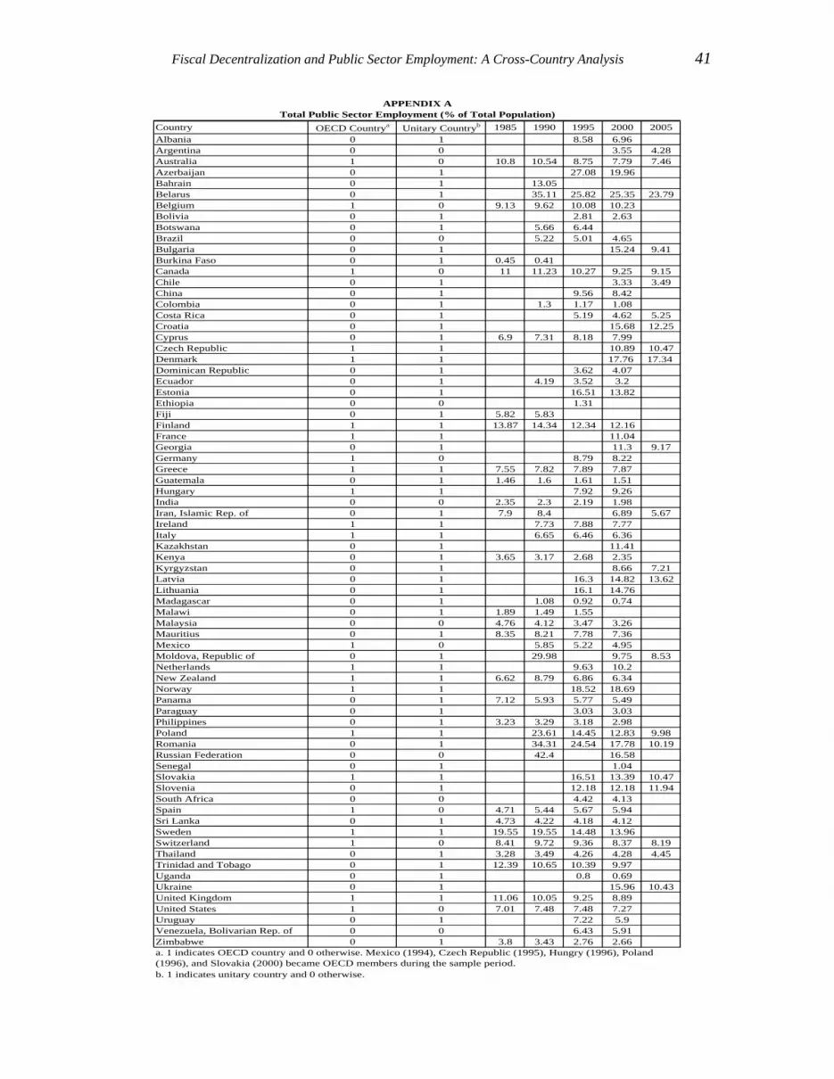
Fiscal Decentralization and Public Sector Employment: A Cross-Country Analysis 41
Country OECD Countrya Unitary Countryb 1985 1990 1995 2000 2005Albania 0 1 8.58 6.96Argentina 0 0 3.55 4.28Australia 1 0 10.8 10.54 8.75 7.79 7.46Azerbaijan 0 1 27.08 19.96Bahrain 0 1 13.05Belarus 0 1 35.11 25.82 25.35 23.79Belgium 1 0 9.13 9.62 10.08 10.23Bolivia 0 1 2.81 2.63Botswana 0 1 5.66 6.44Brazil 0 0 5.22 5.01 4.65Bulgaria 0 1 15.24 9.41Burkina Faso 0 1 0.45 0.41Canada 1 0 11 11.23 10.27 9.25 9.15Chile 0 1 3.33 3.49China 0 1 9.56 8.42Colombia 0 1 1.3 1.17 1.08Costa Rica 0 1 5.19 4.62 5.25Croatia 0 1 15.68 12.25Cyprus 0 1 6.9 7.31 8.18 7.99Czech Republic 1 1 10.89 10.47Denmark 1 1 17.76 17.34Dominican Republic 0 1 3.62 4.07Ecuador 0 1 4.19 3.52 3.2Estonia 0 1 16.51 13.82Ethiopia 0 0 1.31Fiji 0 1 5.82 5.83Finland 1 1 13.87 14.34 12.34 12.16France 1 1 11.04Georgia 0 1 11.3 9.17Germany 1 0 8.79 8.22Greece 1 1 7.55 7.82 7.89 7.87Guatemala 0 1 1.46 1.6 1.61 1.51Hungary 1 1 7.92 9.26India 0 0 2.35 2.3 2.19 1.98Iran, Islamic Rep. of 0 1 7.9 8.4 6.89 5.67Ireland 1 1 7.73 7.88 7.77Italy 1 1 6.65 6.46 6.36Kazakhstan 0 1 11.41Kenya 0 1 3.65 3.17 2.68 2.35Kyrgyzstan 0 1 8.66 7.21Latvia 0 1 16.3 14.82 13.62Lithuania 0 1 16.1 14.76Madagascar 0 1 1.08 0.92 0.74Malawi 0 1 1.89 1.49 1.55Malaysia 0 0 4.76 4.12 3.47 3.26Mauritius 0 1 8.35 8.21 7.78 7.36Mexico 1 0 5.85 5.22 4.95Moldova, Republic of 0 1 29.98 9.75 8.53Netherlands 1 1 9.63 10.2New Zealand 1 1 6.62 8.79 6.86 6.34Norway 1 1 18.52 18.69Panama 0 1 7.12 5.93 5.77 5.49Paraguay 0 1 3.03 3.03Philippines 0 1 3.23 3.29 3.18 2.98Poland 1 1 23.61 14.45 12.83 9.98Romania 0 1 34.31 24.54 17.78 10.19Russian Federation 0 0 42.4 16.58Senegal 0 1 1.04Slovakia 1 1 16.51 13.39 10.47Slovenia 0 1 12.18 12.18 11.94South Africa 0 0 4.42 4.13Spain 1 0 4.71 5.44 5.67 5.94Sri Lanka 0 1 4.73 4.22 4.18 4.12Sweden 1 1 19.55 19.55 14.48 13.96Switzerland 1 0 8.41 9.72 9.36 8.37 8.19Thailand 0 1 3.28 3.49 4.26 4.28 4.45Trinidad and Tobago 0 1 12.39 10.65 10.39 9.97Uganda 0 1 0.8 0.69Ukraine 0 1 15.96 10.43United Kingdom 1 1 11.06 10.05 9.25 8.89United States 1 0 7.01 7.48 7.48 7.27Uruguay 0 1 7.22 5.9Venezuela, Bolivarian Rep. of 0 0 6.43 5.91Zimbabwe 0 1 3.8 3.43 2.76 2.66a. 1 indicates OECD country and 0 otherwise. Mexico (1994), Czech Republic (1995), Hungry (1996), Poland(1996), and Slovakia (2000) became OECD members during the sample period.b. 1 indicates unitary country and 0 otherwise.
Total Public Sector Employment (% of Total Population)APPENDIX A

42 International Studies Program Working Paper Series
Appendix B
Footnote 12:
The utility maximization problem for the governor of jurisdiction i is defined as:
)()1()()(max}{ iiim
cmfVEi
πσ ⋅−−= subject to 1)1(−
⋅+⋅⋅
=R
mnc ii θ
αβ .
Solving the utility maximization problem, we have the following first order condition:
( ) 01)(')1()(')(=⎥⎦
⎤⎢⎣⎡
⋅+⋅
⋅⋅−−=∂
∂R
ncmfmVE
iii
i
θαβπσ .
Since 0)(' * >imf , 0)1( >−σ and α , β and ir are all positive, we have 0)(' * >icπ .
Because )( icπ is a positive and convex function for 0>ic and 0)( =icπ as 0≤ic ,
the inequality 0)(' * >icπ implies 0* >ic .
Footnote 13:
In equilibrium, we have 1)1(** −
⋅+⋅⋅
=R
mnc ii θ
αβ . Therefore, σθ
αβσ ∂
∂⋅
⋅+⋅
=∂∂ ** )1( ii m
Rnc . The
sign of σ∂∂ *
ic is determined by the sign of σ∂
∂ *im
. Let function F denotes the first order
condition of the utility maximization problem of the subnational governor in jurisdiction
i, and we have
( ) ( ) ( ) ( ) ( ) 01'1' =⎥⎦⎤
⎢⎣⎡
⋅+⋅
⋅⋅−−=∂∂
=R
ncmfmVEF ii
i
i
θαβπσ .
Applying the implicit function theorem, we have
( )
( )0
1")1("
1'
//
2
*
>
⎥⎦⎤
⎢⎣⎡
⋅+⋅
⋅⋅−−
⋅+⋅
⋅−=
∂∂∂∂
−=∂∂
Rnf
Rn
mFFm
i
i
θαβπσ
θαβπσ
σ.

Fiscal Decentralization and Public Sector Employment: A Cross-Country Analysis 43
Since 0*
>∂∂σ
im, we know 0
*
>∂∂σ
ic .
Footnote 16:
Inserting the constraint 1)1(** −
⋅+⋅⋅
=R
mnc ii θ
αβ into the central government executive’s
utility maximization objective function, we have
( ) ( ) ( )∑=
⎟⎟⎠
⎞⎜⎜⎝
⎛−
⋅+⋅⋅
−−=n
i
ic R
mngVE1
*
}{111 max
θαβπσθ
θ.
The corresponding first order condition is
( ) ( ) ( ) 01'1'1
=⎟⎠⎞
⎜⎝⎛ −∂∂
⋅⋅+⋅
⋅−−−=∂
∂ ∑= θθθ
αβπσθθ
iin
i
c mmR
ngVE
.
We assume that the second order condition is satisfied for this utility maximization
problem. The optimal degree of fiscal decentralization to the central government
executive’s utility maximization problem can be shown as ( )Rn,,,, βασθθ =∗ .
Footnote 20:
Let function F denotes the first order condition of the utility maximization
problem of the subnational governor in jurisdiction i, and we have
( ) ( ) ( ) ( ) ( ) 01'1' =⎥⎦⎤
⎢⎣⎡
⋅+⋅
⋅⋅−−=∂∂
=R
ncmfmVEF ii
i
i
θαβπσ .
Applying the implicit function theorem, we have

44 International Studies Program Working Paper Series
( ) ( ) ( ) ( )
( ).0
1")1("
1'11"1
//
2
22
*
>
⎥⎦⎤
⎢⎣⎡
⋅+⋅
⋅⋅−−
⎥⎦
⎤⎢⎣
⎡⎟⎠⎞
⎜⎝⎛
⋅+⋅
−⋅+⎟⎠⎞
⎜⎝⎛
⋅+⋅⋅
−⋅⋅+⋅
⋅⋅−−−=
∂∂∂∂
−=∂∂
Rnf
Rn
Rmn
Rn
mFFm
i
i
i
θαβπσ
θαβπ
θαβ
θαβπσ
θθ
The inequality implies the level of subnational public employment increases with the
degree of fiscal decentralization.
We assume that there is no budget deficit problem at the central government, and,
therefore, the total expenditure for the central government ( ) R⋅−θ1 . Since there are
only two inputs in the production function of public goods, the total expenditure of the
central government can be expressed as ( )αβ+⋅ 1*cm . Given the no central government
deficit problem assumption, we have ( )** 1 θβα
α−⋅
+⋅
=Rmc . From this we can see the that
level of central government employees, *cm , moves inversely with the level of fiscal
decentralization, *θ .
Footnote 27:
First, we show that the subnational government employee level of a country is
positively correlated to the value of σ . Applying implicit function theorem to the first
order condition of the utility maximization problem of the subnational governor in
jurisdiction i, we have

Fiscal Decentralization and Public Sector Employment: A Cross-Country Analysis 45
( )
( )0
1")1("
1'
//
2
*
>
⎥⎦⎤
⎢⎣⎡
⋅+⋅
⋅⋅−−
⋅+⋅
⋅−=
∂∂∂∂
−=∂∂
Rnf
Rn
mFFm
i
i
θαβπσ
θαβπσ
σ.
Next, we want to show that the central government employee level is negatively
correlated to the value of σ . Since ( )** 1 θβα
α−⋅
+⋅
=Rmc , we have
σθ
βαα
σ ∂∂⋅
+⋅
−=∂∂ ** Rmc .
By the chain rule, we have
σθ
σθ
∂∂⋅
∂∂
=∂∂ i
i
mm
.
We have shown that 0>∂∂σ
im above and 0
*
>∂∂θ
im in footnote 19, which implies that
0>∂∂σθ . Since
σθ
βαα
σ ∂∂⋅
+⋅
−=∂∂ ** Rmc , we know that 0
*
<∂∂σ
cm.


