Flow and Solute Fluxes in Integrated Wetland and Coastal Systems

by

Kumars Ebrahimi1, Roger A. Falconer2* FASCE and Binliang Lin3

Abstract

Details are given of an experimental study of the flow and tracer transport processes in an integrated

wetland and coastal basin. A novel physical model was constructed to enable observations and

measurements to be made of groundwater transport through a sand embankment between a wetland

and coastal area. This was an idealised scale model of the West Fleet Lagoon, Chesil Beach and the

adjacent coastal waters, located in Dorset, UK. An extensive set of data of the seepage fluxes

through the embankment was collected by monitoring the varying water level and velocity

distributions on both sides of the embankment. The transport behaviour of a conservative tracer was

also studied for a constant water level on the wetland side of the embankment, while running a

continuous tide on the coastal side. Time series pictures of the concentration distributions of the

tracer were filmed using a digital camcorder. An integrated surface and groundwater numerical

model was also used in this study to assist in the analysis, with the numerical model predictions

being compared with the images recorded from the experiments. Details of the physical model,

experimental procedures and the equipment used in the study are reported in this paper.

Keywords: Hydraulic Modelling; Groundwater Flow; Tidal Hydrodynamics; Solute Transport;

Numerical Modelling; Integrated Models.

1Lecturer in Hydroenvironmental Engineering, Aboureyhan Campus 39754, University of Tehran,

Tehran, Iran

2* Halcrow Professor of Water Management, School of Engineering, Cardiff University, Cardiff,

The Parade, CF64 3RJ, U.K. (Corresponding Author: FalconerRA@cf.ac.uk)

3Reader in Environmental Hydroinformatics, School of Engineering, Cardiff University, Cardiff,

The Parade, CF64 3RJ, U.K.

2

Introduction

In recent decades, increased attention has been paid to the environmental issues of interaction

between beach groundwater tables and the adjacent shallow coastal waters. Li et al. (1997)

undertook a numerical modelling study to investigate tide-induced beach water table fluctuations.

Larabi and Smedt (1997) studied seawater intrusion into unconfined aquifers and Morita and Yen

(2002) studied the rainfall-runoff processes and the interactions between surface and groundwater

flows. Similarly, wetlands and mangroves have also been studied extensively, due to their important

roles and influences on the aquatic ecosystem. The growing recognition of the values and functions

of wetlands and mangroves presents a direct challenge to the traditional objectives of water

management for specific sectorial purposes and raises questions about the meaning of better water

management (Franks and Falconer, 1999).

A large number of physical and mathematical models have been developed and deployed to study

the hydrodynamic processes involved in groundwater, surface waters and wetland systems.

Following a detailed literature review, it was found that most effort so far has been focused on

investigating individual processes within these systems. However, current knowledge on the

integrated process relating to tidal, groundwater and shallow wetland flows is rather limited. Hence,

the emphasis of this paper has been to study the interaction between wetlands and coastal waters

through shallow groundwater flows. A new approach for integrated physical modelling of

groundwater and surface water flows has been developed and is outlined herein.

According to Hughes (1995), field studies provide the best data, but they are usually expensive and

involve too many parameters. The interpretation of field measured results also often proves to be

difficult. In contrast, physical models are less expensive, generally enable data to be collected

easily, and provide controlled data; furthermore they may also include more important aspects of

the problem. Falconer (1992) not only noted that physical models could be generally used as an

3

additional engineering design tool, but added that for coastal studies the model domain often needed

to be significantly scaled down both vertically and horizontally. One disadvantage with physical

models in connection with flow and solute transport studies is a technical constraint related to

scaling. However, for modelling solute transport in porous media, Harris et al. (2000) pointed out

that physical models also offer major time-scaling advantages. For example, pore fluid seepage at

prototype scales, i.e. over a period of years, can be simulated in the model in a matter of hours.

Esposito et al. (2000) outlined that in predicting the transport of liquids containing hazardous

chemical substances in soil and groundwater bodies has proved to be an extremely challenging

exercise. They added that both mathematical and physical models have been developed to quantify

such movements.

This paper is focused on creating an idealised scale model of a wetland system and the adjacent

coastal waters. The model consists of a coastal region and a wetland region, with these being

separated by a sand embankment. A series of experiments has been undertaken to study the

influence of the coastal tidal flows on the wetland system and, in particular, the transport of a dye

tracer between the coastal region and the wetland through the embankment. The data acquired

through this study also provide a valuable database for further model calibration and validation. An

integrated surface and groundwater numerical model was also developed for this study to assist in

the analysis, with the numerical model predictions being presented together with the physical model

results.

Physical Model Details

This section details the physical model configuration, measurement devices, tidal parameter

specifications and the sand embankment properties. Details are briefly given of the features of Fleet

Lagoon and Chesil Beach, followed by details of the physical model configuration etc.

The scope of this laboratory study was not to recreate a scale model for a particular case study, but

to investigate the hydrodynamic and mixing processes in an integrated coastal, groundwater and

wetland system. For this purpose Fleet Lagoon and Chesil Beach were considered as a typical

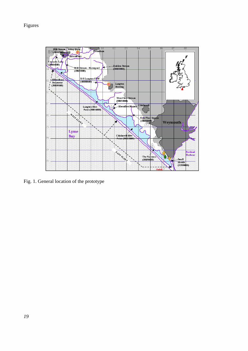
wetland – coastal site and were chosen to identify a typical prototype set up for this study. The Fleet

Lagoon is a shallow coastal lagoon, trapped behind the Chesil Beach, and sited northwest of

Portland Hill (in Dorset) along the south coast of England, see Figure 1. The flow structure within

4

the lagoon is primarily governed by tidal currents through a narrow opening to Portland Harbour,

with the lagoon being linked to the adjacent coastal waters by groundwater passage through sand

ridge, namely ‘Chesil Beach’, which is approximately 150m wide and 12.5km long, see Robinson et

al. (1983) and the UK Marine web site http://www.ukmarinesac.org.uk/activities/lagoon/14

With regard to the significance of Fleet Lagoon, Johnston and Gilliland (2000) reported that the

lagoon is one of the largest and best studied lagoons in the U.K. and has been identified as an SAC

(Special Area of Conservation). It is considered to be one of the finest examples of its physio-

graphic type in the U.K., and one of the most important sites in Europe. Generally speaking, Fleet

lagoon consists of two separate parts, namely the East and West Fleet. There is no opening to West

Bay through the beach, but the Fleet is connected to the English Channel at its south eastern end

through Portland Harbour. It is therefore tidal and saline, with a few streams draining into the

lagoon from a small catchment area of about 50km2. It is also very shallow, varying in depth from 3

to 5m in the first 2km between the tidal entrance at Smallmouth and The Narrows. Here the lagoon

is marine in character, with a strong tidal exchange to the sea. It then widens out to 2.5km in the

area known as Littlesea, where the depth is between 0 and 1.2m below chart datum, intersected by a

narrow channel of up to 4m deep. The tide is strongly attenuated in this region and penetrates only

weakly into the remaining 8km of the lagoon, known as West Fleet which has a depth of between 0

and 1.2m, see Robinson (1983). West Fleet has demonstrated a significant lack of flushing and

circulation characteristics as compared to those observed from the East Fleet, see Westwater et al.

(1999).

In establishing the dimensions and hydrodynamic characteristics of the physical model, these

characteristics were based on the tidal and geometric properties of West Fleet Lagoon and the

adjacent coastal area. However, as the main aim of the study was to get a better understanding of

the hydrodynamic and transport processes through wetlands and coastal embankments, it was

decided to set up an idealised model of an integrated wetland and coastal system. For geometric

similarity, both undistorted and distorted scale models were first considered. A distorted model was

then chosen since the laboratory tidal basin at Cardiff University’s Hyder Hydraulics Laboratory

was not able to cope with the parameters required for an undistorted model. In dimensionally

scaling the prototype, the physical model was developed upon the basis of dynamic similarity

through the Froude law, in order to maintain similar gravitational characteristics to those found in

5

the prototype. From studies undertaken by Westwater et al. (1999), Johnston and Gilliland (2000)

and Kennedy (2001) on the Fleet Lagoon, typical values of the West Fleet Lagoon were chosen and

used in the physical model design. A brief description of the model similarity and its characteristics

is presented below.

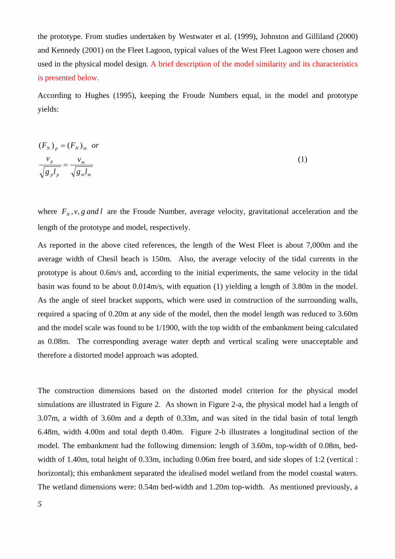
According to Hughes (1995), keeping the Froude Numbers equal, in the model and prototype

yields:

mm

m

pp

p

mNpN

lg

v

lg

v

orFF

)()(

(1)

where landgvFN ,, are the Froude Number, average velocity, gravitational acceleration and the

length of the prototype and model, respectively.

As reported in the above cited references, the length of the West Fleet is about 7,000m and the

average width of Chesil beach is 150m. Also, the average velocity of the tidal currents in the

prototype is about 0.6m/s and, according to the initial experiments, the same velocity in the tidal

basin was found to be about 0.014m/s, with equation (1) yielding a length of 3.80m in the model.

As the angle of steel bracket supports, which were used in construction of the surrounding walls,

required a spacing of 0.20m at any side of the model, then the model length was reduced to 3.60m

and the model scale was found to be 1/1900, with the top width of the embankment being calculated

as 0.08m. The corresponding average water depth and vertical scaling were unacceptable and

therefore a distorted model approach was adopted.

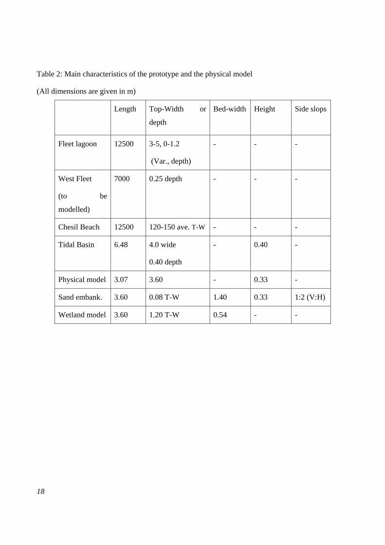
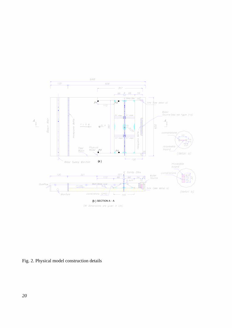
The construction dimensions based on the distorted model criterion for the physical model

simulations are illustrated in Figure 2. As shown in Figure 2-a, the physical model had a length of

3.07m, a width of 3.60m and a depth of 0.33m, and was sited in the tidal basin of total length

6.48m, width 4.00m and total depth 0.40m. Figure 2-b illustrates a longitudinal section of the

model. The embankment had the following dimension: length of 3.60m, top-width of 0.08m, bed-

width of 1.40m, total height of 0.33m, including 0.06m free board, and side slopes of 1:2 (vertical :

horizontal); this embankment separated the idealised model wetland from the model coastal waters.

The wetland dimensions were: 0.54m bed-width and 1.20m top-width. As mentioned previously, a

6

sluice gate was located in the corner of the model, to control the constant water level behind the

model embankment and also for the purpose of flushing (see Figure 2, details a and b). Table 2

summarises the main dimensions of the prototype and the physical models.

As shown in Figure 2, the physical model had a length of 3.07m, a width of 3.60m and a depth of

0.33m. It was sited in a tidal basin having a total length of 6.48m, a width of 4.00m and a depth of

0.40m. The sand embankment and the enclosed idealised wetland were sited behind the

embankment, as shown in Figure 2(a), and the coastal area was sited in front of the embankment.

Figure 2(b) illustrates a longitudinal section of the model. An embankment of length 3.60m, top-

width 0.08m, bed-width 1.40m, total height 0.33m and side slopes of 1:2 (vertical:horizontal),

separated the model wetland from the coastal region. The wetland dimensions were 0.54m bed-

width and 1.20m top-width.

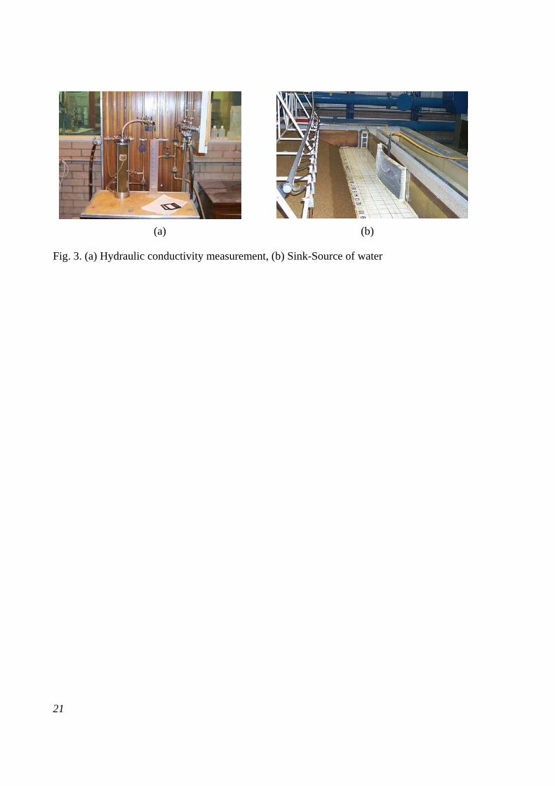
As a part of the experimental programme it was planned to study the behaviour of a conservative

dye tracer for a constant water level on the wetland side of the embankment and with a tide

operating on the coastal side. In order to create this condition, a sluice gate and a pipe were installed

behind the embankment on the far side of the model, see Figures 2 and 3-b. The combination of the

source and overflow-gate (sink) kept the water level constant, with a fluctuation of about 4mm of

the water level being measured during the experiments. It should be noted that initially it was

planed to undertake the dye tracer experiments in the same manner as for the hydrodynamic

experiments where fluctuations in the water were recorded behind the sand embankment. However,

during the tests it was found that passage of the tracer through the sand embankment, with a

fluctuating tide level downstream, took a long time. Moreover, monitoring and analysis of the

performance of the tracer movement was difficult – if not impossible – to monitor. Therefore, it

was decided to monitor the spreading of the tracer for different tides in front of the sand

embankment, while the depth of water behind the sand embankment was kept constant. Constant

amplitude and period tides were produced in the tidal basin by a vertically oscillating weir, shown

to the left end of the tidal basin, in Figure 2. The basin was fed by a water supply at a constant rate

entering through a perforated manifold. To minimise the lateral variation in the velocity and to

reduce artificial circulation in the model area, a 30mm thick honeycomb baffle was located near the

weir.

7

In this study non-cohesive sands were used to create the model embankment. The average grain

diameter of the sand was 1 mm as it was important to control the validation limits of Darcy’s law

within the sand embankment. According to Bear (1972) in practically all cases Darcy’s law is valid

as long as the Reynolds number, based on the average grain diameter, does not exceed a value of

between about 1 and 10. Calculations showed that for the sand used in this study the average

Reynolds number was about 7. A series of experiments were carried out, according to the British

Standard Methods No.BS 1377: Part 5: 1990, to determine the permeability and the specific yield of

the sand. The results showed that the average value of the sand permeability was 0.995 mm/s and

the average value of the specific yield was 29%, see Fig. 3-(a).

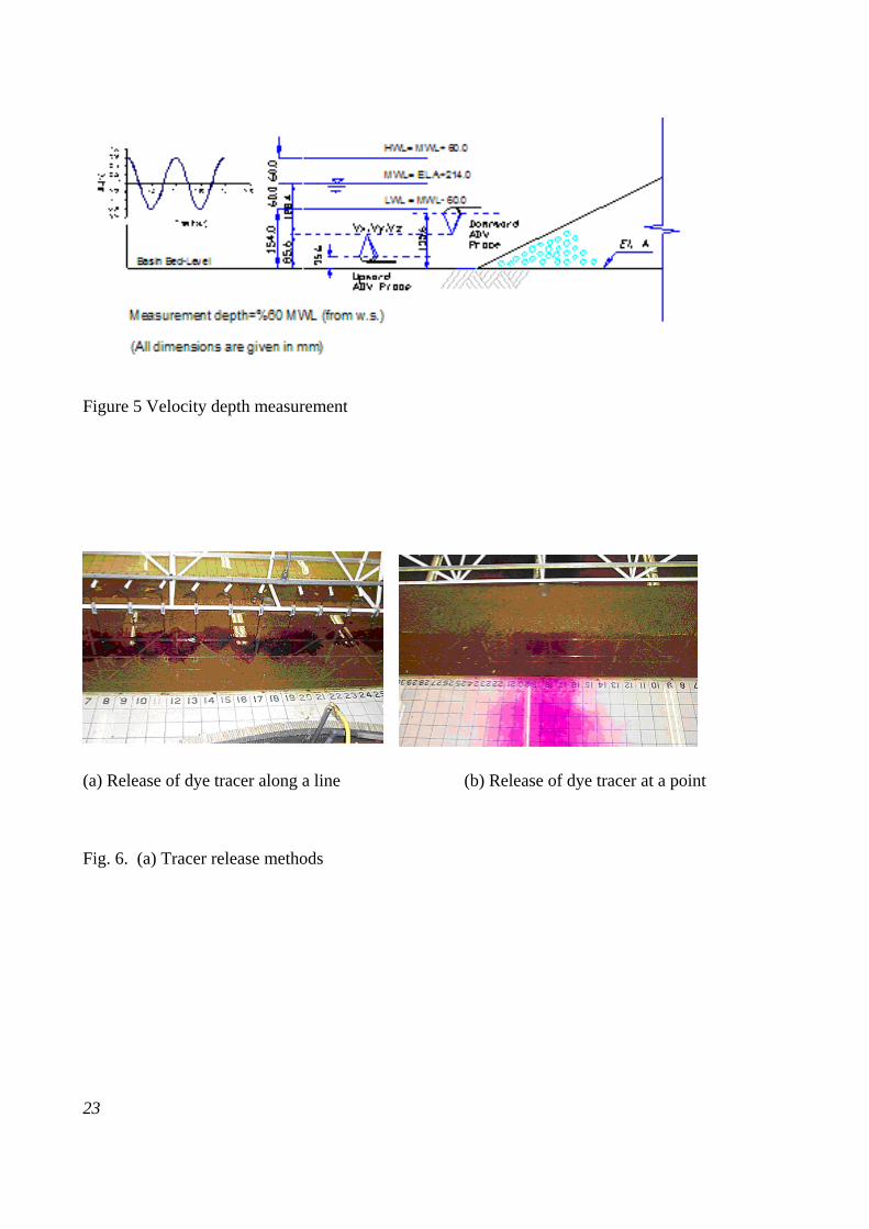
For the model tidal conditions simulated in the model the period was set to 355s, the mean water

level was set to 214mm and the tidal range set at 120mm. All tests were commenced at high tide, so

that the initial depth of water on both sides of the embankment was initially 274mm, see Figs. 4 and

5. Water levels on either side of the embankment were recorded using wave probes, which worked

on the principle of measuring the current flowing past a probe consisting of a pair of parallel

stainless steel wires.

Velocity data were acquired using a Nortek Acoustic Doppler Velocimeter (ADV). This type of

current meter uses an acoustic pulse, emitted from a central emitter, which is then retrieved through

three acoustic sensors to give the reflected Doppler shift in the reflected acoustic pulse from

particles within the flow. From these meters the data were transmitted via a conditioning module to

the PC, where the data were interpreted to give an instantaneous velocity at a specific point in the

flow and specified in Cartesian co-ordinates.

For the dye tracer monitoring studies, imaging technologies were considered as a universal tool for

visualising, digitising and analysing phenomena in experimental studies, see Allersma and Esposito

(2000). In this study the transport processes of a dye tracer were filmed using a digital camcorder,

which was equipped with a wide angle lens. The camera was positioned on the ceiling, right over

the physical model to provide optical measurements of the tracer migration through the physical

model. In Figure 2 the limits of the filmed area are highlighted by points P1, P2, P3 and P4. It

should be noted that points P2 and P4 were not fixed and they moved along the flow direction,

according to the tide levels. The use of image processing allowed non-disturbing measurements to

8

be made of the tracer plume migration. A grid pattern was painted over the physical model floor to

show the essential scale for the model calibration, see Figure 3(a). A tracer releasing device was

also developed, which comprised a wide low-depth reservoir, connected flexible tubes and 18

nozzles, see Figures 3-b and 6-a. Each nozzle had an independent valve and was drilled into the

main line at 0.20m intervals. The device was fixed on the instrumentation beam, which could be

moved along the model.

Experimental Details

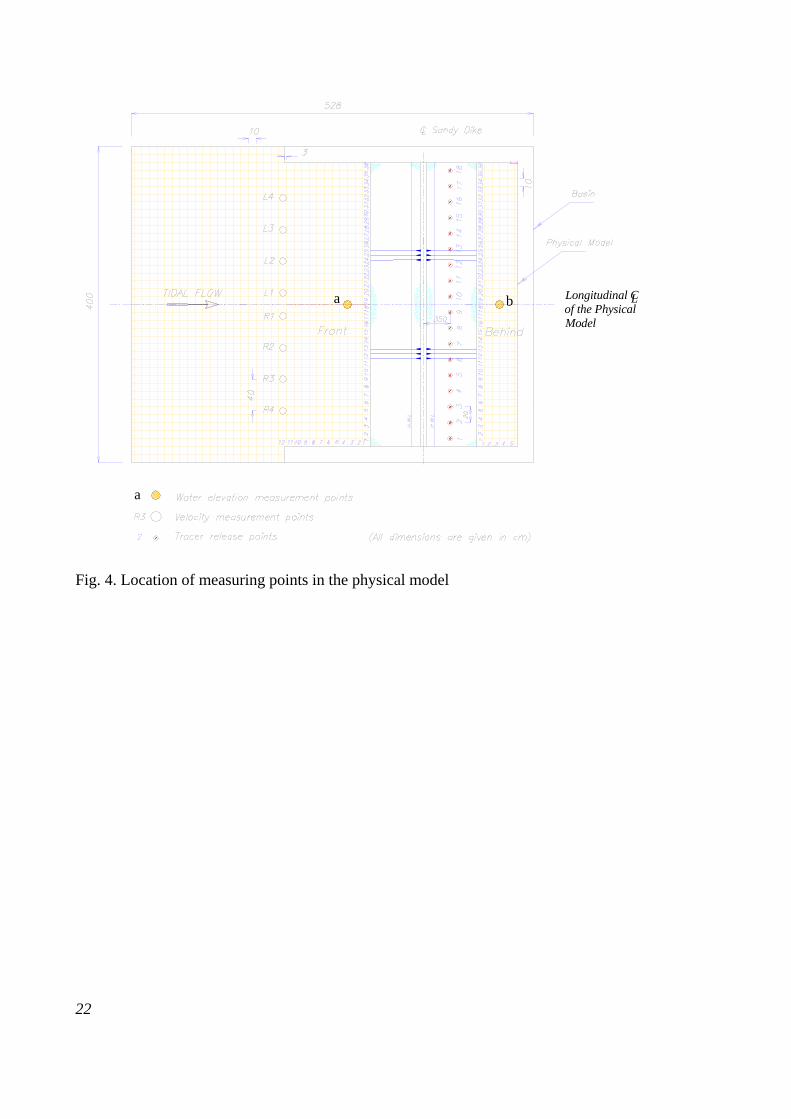
All experiments were started at high water and the initial water elevation was fixed at 274mm on

both sides of the sand embankment. Water elevations were then recorded at the middle point of the

physical model cross-section on either side of the embankment and for an average of 10 tidal

cycles. Figure 4 shows a drawing of the physical model, including the location of the sampling

points, with the water elevation data being collected and recorded at the locations a and b, shown in

Figure 4.

Velocities were collected at 8 locations, from points L1 to L4 on the left-hand side and from points

R1 to R4 on the right-hand side, over 3 tidal periods and at each location. The probe used was the

downward orientation type, and was positioned in such a manner that the x-axis was in the direction

of flow. The probe was moved from one location to the next using the access platform and the

instrumentation beam, with data being collected at elevations of 128mm below the mean water

level, see Figure 5. Based on integrating a logarithmic velocity profile, it can be shown that the

theoretical mean velocity occurs at an elevation of approximately 0.6 of the depth below the free

surface, Chow (1973).

A solute of potassium permanganate, of concentration 5g/l, was used as a tracer for the dye

concentration plume experiments. Tracer release experiments were carried out in two ways: (a) the

tracer was released at 18 points along a line, and (b) the tracer was released at one point (see Figure

4 points 1 to 18). The release device was calibrated before each experiment and the tracer was

released just behind the sand embankment in the model wetland. The transport processes were

filmed from the start of each test, using the digital camcorder, to monitor the spreading of the tracer

for different tides in the model coastal area. During these experiments the water depth within the

wetland area was kept constant at high water level and the discharge of the tracer was 1.26 ml/min.

Figure 6 shows the migration of the dye tracer within the model wetland, with the discharges

9

through the nozzles being calibrated using the nozzle valves for all cases. It should be noted that the

sand embankment and physical model tidal basin were flushed after each experiment. For this

purpose fresh water was used.

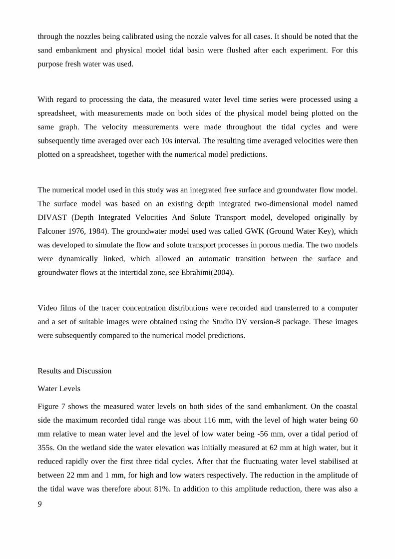
With regard to processing the data, the measured water level time series were processed using a

spreadsheet, with measurements made on both sides of the physical model being plotted on the

same graph. The velocity measurements were made throughout the tidal cycles and were

subsequently time averaged over each 10s interval. The resulting time averaged velocities were then

plotted on a spreadsheet, together with the numerical model predictions.

The numerical model used in this study was an integrated free surface and groundwater flow model.

The surface model was based on an existing depth integrated two-dimensional model named

DIVAST (Depth Integrated Velocities And Solute Transport model, developed originally by

Falconer 1976, 1984). The groundwater model used was called GWK (Ground Water Key), which

was developed to simulate the flow and solute transport processes in porous media. The two models

were dynamically linked, which allowed an automatic transition between the surface and

groundwater flows at the intertidal zone, see Ebrahimi(2004).

Video films of the tracer concentration distributions were recorded and transferred to a computer

and a set of suitable images were obtained using the Studio DV version-8 package. These images

were subsequently compared to the numerical model predictions.

Results and Discussion

Water Levels

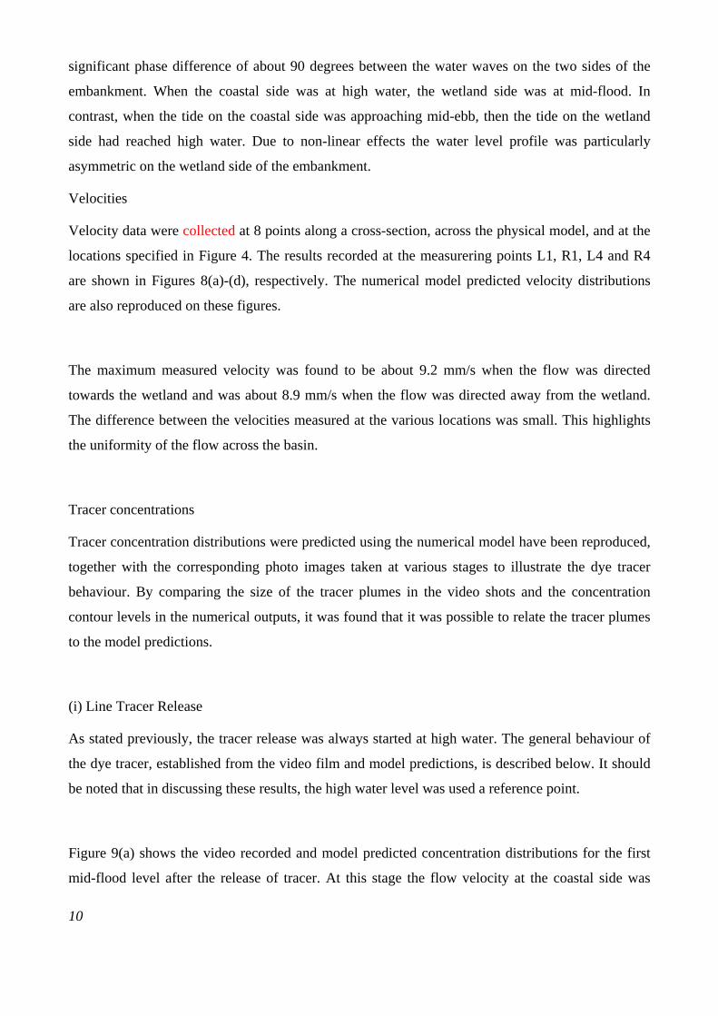
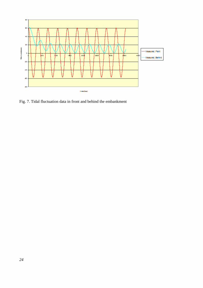
Figure 7 shows the measured water levels on both sides of the sand embankment. On the coastal

side the maximum recorded tidal range was about 116 mm, with the level of high water being 60

mm relative to mean water level and the level of low water being -56 mm, over a tidal period of

355s. On the wetland side the water elevation was initially measured at 62 mm at high water, but it

reduced rapidly over the first three tidal cycles. After that the fluctuating water level stabilised at

between 22 mm and 1 mm, for high and low waters respectively. The reduction in the amplitude of

the tidal wave was therefore about 81%. In addition to this amplitude reduction, there was also a

10

significant phase difference of about 90 degrees between the water waves on the two sides of the

embankment. When the coastal side was at high water, the wetland side was at mid-flood. In

contrast, when the tide on the coastal side was approaching mid-ebb, then the tide on the wetland

side had reached high water. Due to non-linear effects the water level profile was particularly

asymmetric on the wetland side of the embankment.

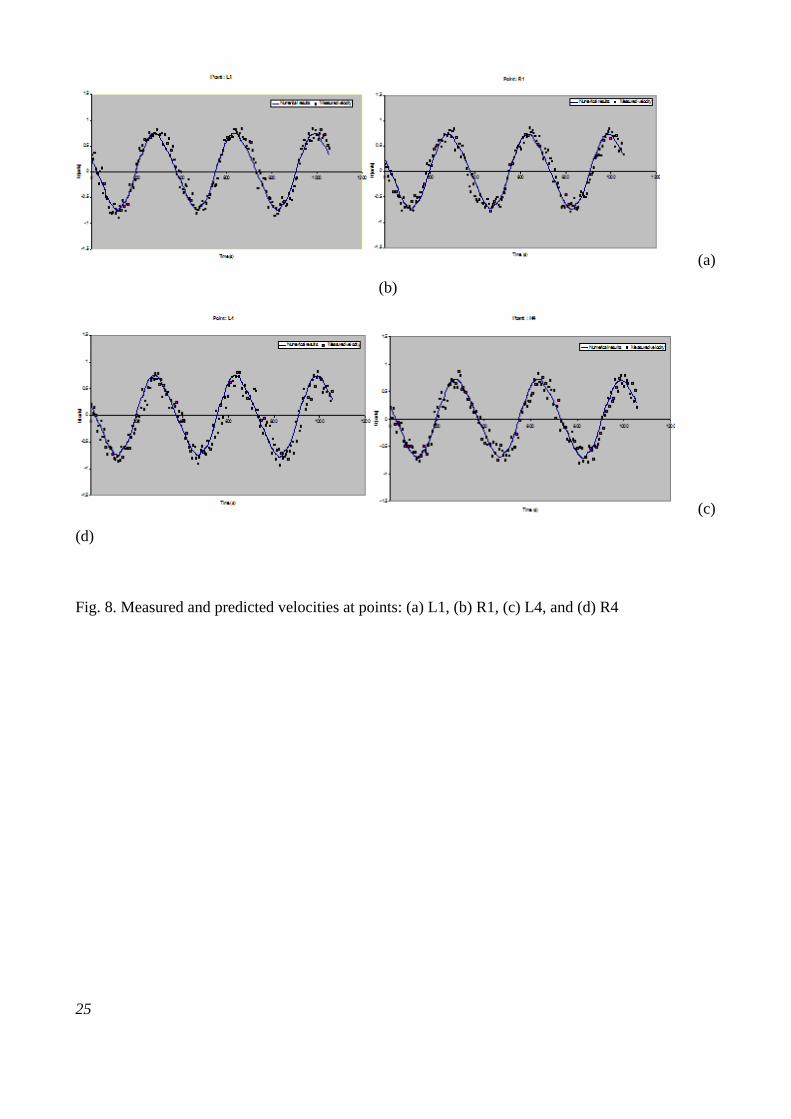
Velocities

Velocity data were collected at 8 points along a cross-section, across the physical model, and at the

locations specified in Figure 4. The results recorded at the measurering points L1, R1, L4 and R4

are shown in Figures 8(a)-(d), respectively. The numerical model predicted velocity distributions

are also reproduced on these figures.

The maximum measured velocity was found to be about 9.2 mm/s when the flow was directed

towards the wetland and was about 8.9 mm/s when the flow was directed away from the wetland.

The difference between the velocities measured at the various locations was small. This highlights

the uniformity of the flow across the basin.

Tracer concentrations

Tracer concentration distributions were predicted using the numerical model have been reproduced,

together with the corresponding photo images taken at various stages to illustrate the dye tracer

behaviour. By comparing the size of the tracer plumes in the video shots and the concentration

contour levels in the numerical outputs, it was found that it was possible to relate the tracer plumes

to the model predictions.

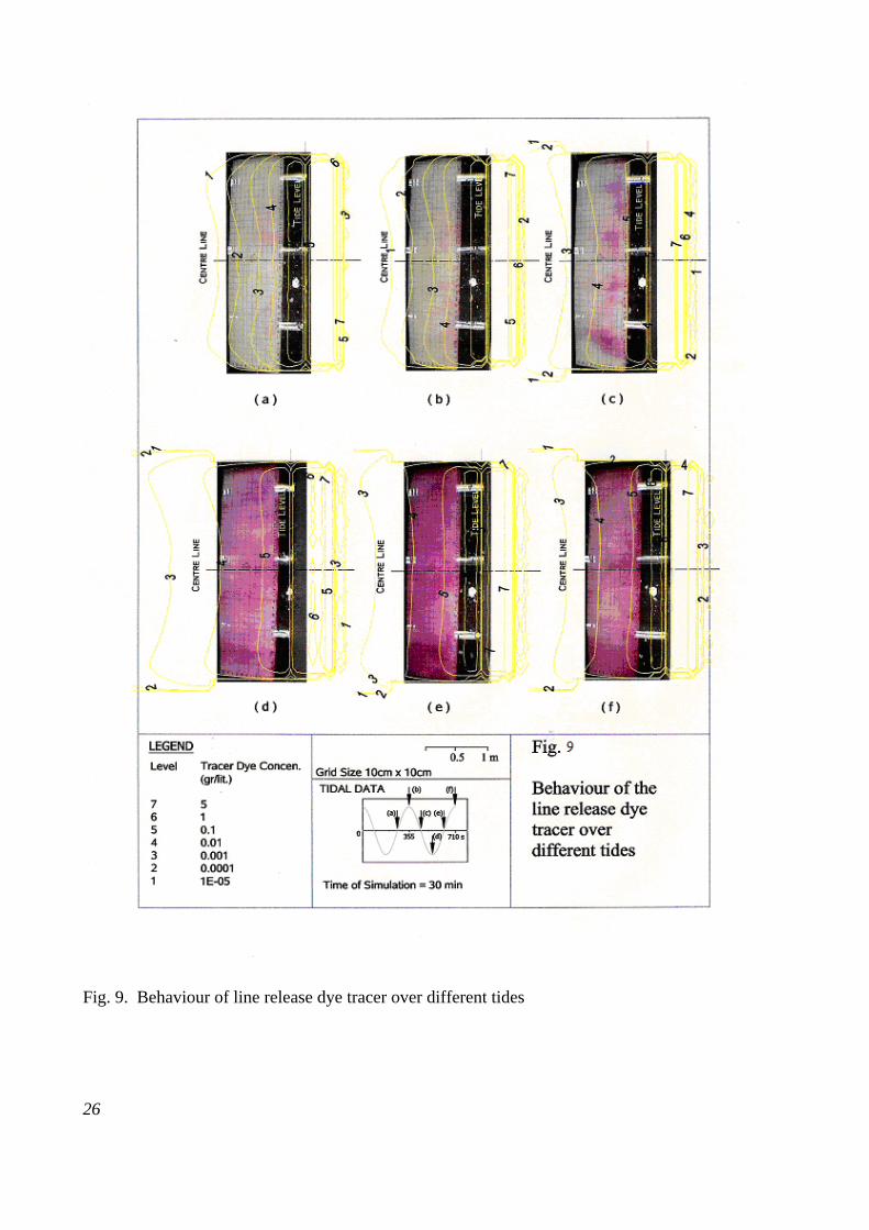
(i) Line Tracer Release

As stated previously, the tracer release was always started at high water. The general behaviour of

the dye tracer, established from the video film and model predictions, is described below. It should

be noted that in discussing these results, the high water level was used a reference point.

Figure 9(a) shows the video recorded and model predicted concentration distributions for the first

mid-flood level after the release of tracer. At this stage the flow velocity at the coastal side was

11

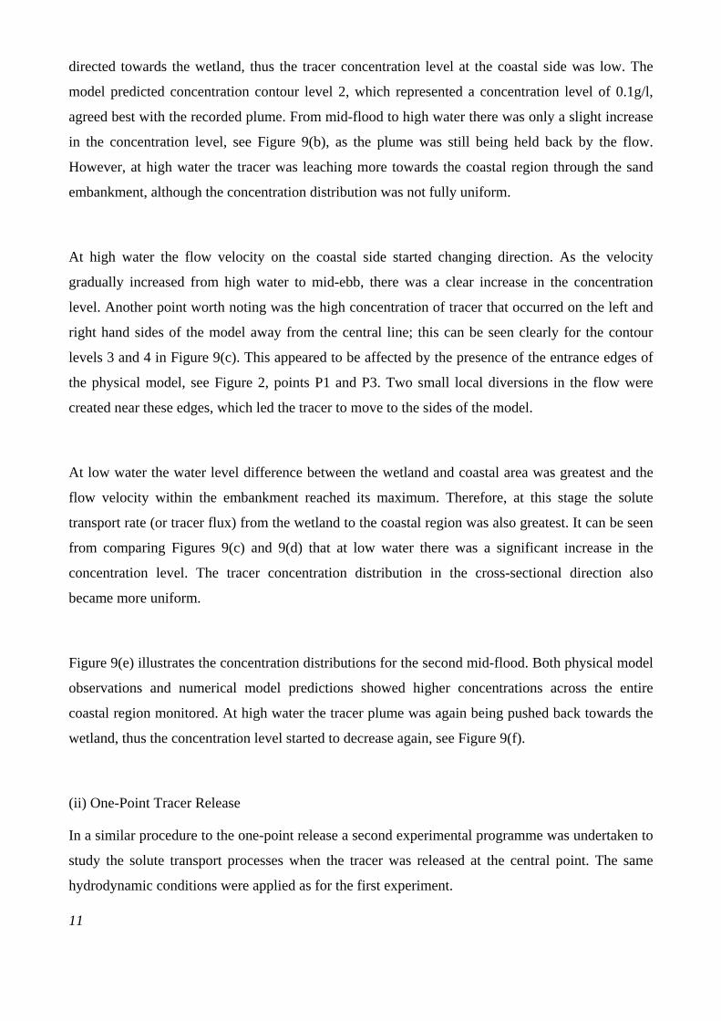
directed towards the wetland, thus the tracer concentration level at the coastal side was low. The

model predicted concentration contour level 2, which represented a concentration level of 0.1g/l,

agreed best with the recorded plume. From mid-flood to high water there was only a slight increase

in the concentration level, see Figure 9(b), as the plume was still being held back by the flow.

However, at high water the tracer was leaching more towards the coastal region through the sand

embankment, although the concentration distribution was not fully uniform.

At high water the flow velocity on the coastal side started changing direction. As the velocity

gradually increased from high water to mid-ebb, there was a clear increase in the concentration

level. Another point worth noting was the high concentration of tracer that occurred on the left and

right hand sides of the model away from the central line; this can be seen clearly for the contour

levels 3 and 4 in Figure 9(c). This appeared to be affected by the presence of the entrance edges of

the physical model, see Figure 2, points P1 and P3. Two small local diversions in the flow were

created near these edges, which led the tracer to move to the sides of the model.

At low water the water level difference between the wetland and coastal area was greatest and the

flow velocity within the embankment reached its maximum. Therefore, at this stage the solute

transport rate (or tracer flux) from the wetland to the coastal region was also greatest. It can be seen

from comparing Figures 9(c) and 9(d) that at low water there was a significant increase in the

concentration level. The tracer concentration distribution in the cross-sectional direction also

became more uniform.

Figure 9(e) illustrates the concentration distributions for the second mid-flood. Both physical model

observations and numerical model predictions showed higher concentrations across the entire

coastal region monitored. At high water the tracer plume was again being pushed back towards the

wetland, thus the concentration level started to decrease again, see Figure 9(f).

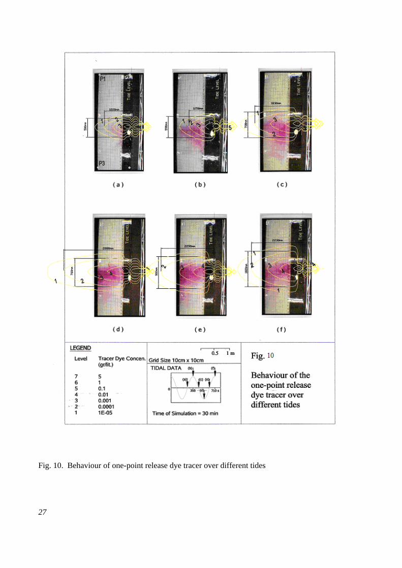
(ii) One-Point Tracer Release

In a similar procedure to the one-point release a second experimental programme was undertaken to

study the solute transport processes when the tracer was released at the central point. The same

hydrodynamic conditions were applied as for the first experiment.

12

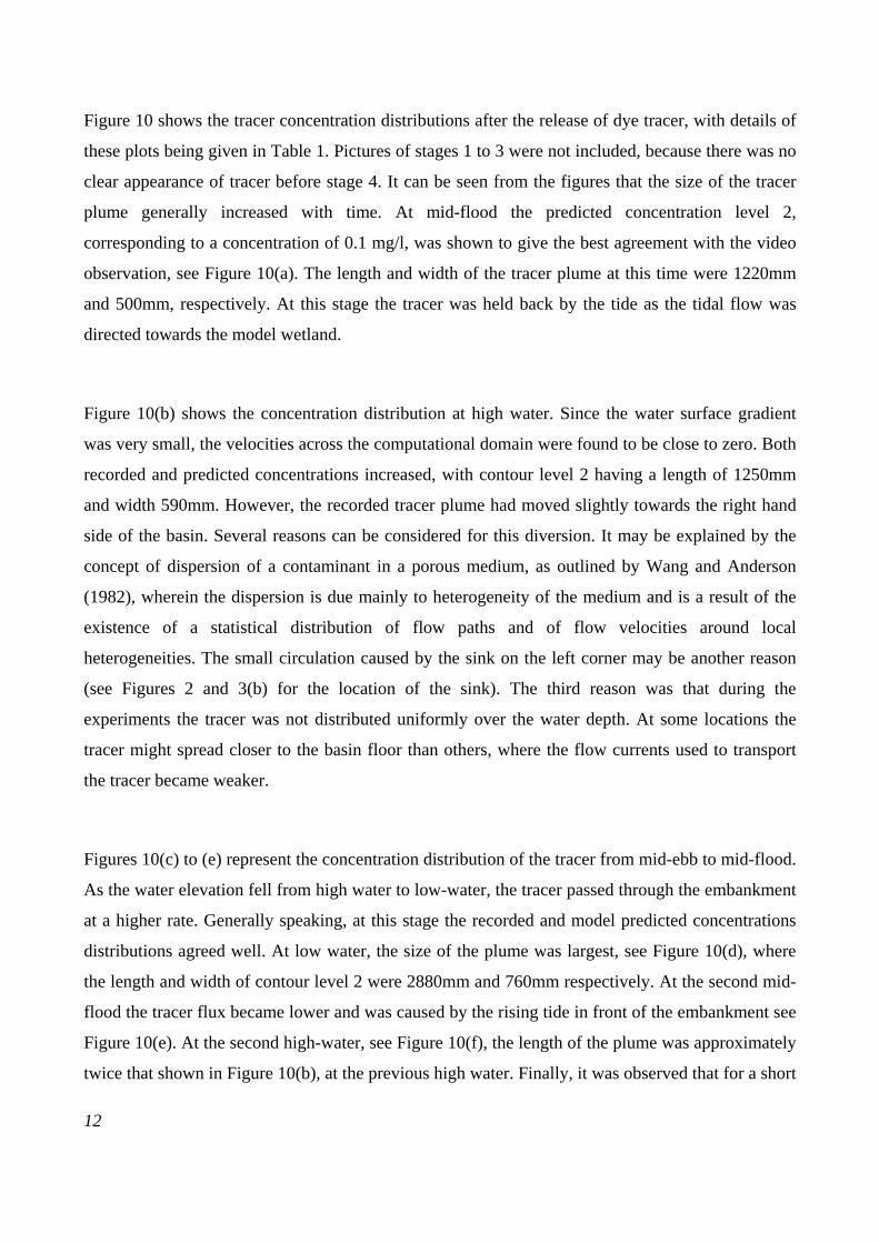
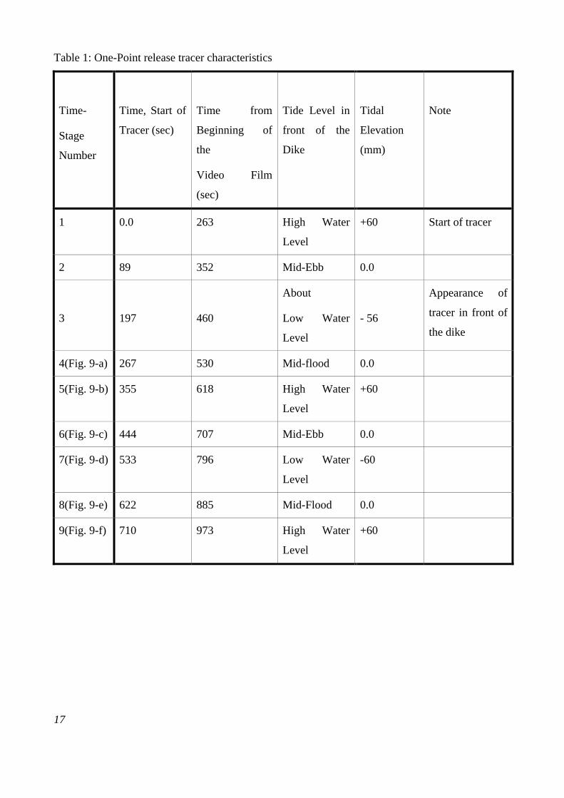
Figure 10 shows the tracer concentration distributions after the release of dye tracer, with details of

these plots being given in Table 1. Pictures of stages 1 to 3 were not included, because there was no

clear appearance of tracer before stage 4. It can be seen from the figures that the size of the tracer

plume generally increased with time. At mid-flood the predicted concentration level 2,

corresponding to a concentration of 0.1 mg/l, was shown to give the best agreement with the video

observation, see Figure 10(a). The length and width of the tracer plume at this time were 1220mm

and 500mm, respectively. At this stage the tracer was held back by the tide as the tidal flow was

directed towards the model wetland.

Figure 10(b) shows the concentration distribution at high water. Since the water surface gradient

was very small, the velocities across the computational domain were found to be close to zero. Both

recorded and predicted concentrations increased, with contour level 2 having a length of 1250mm

and width 590mm. However, the recorded tracer plume had moved slightly towards the right hand

side of the basin. Several reasons can be considered for this diversion. It may be explained by the

concept of dispersion of a contaminant in a porous medium, as outlined by Wang and Anderson

(1982), wherein the dispersion is due mainly to heterogeneity of the medium and is a result of the

existence of a statistical distribution of flow paths and of flow velocities around local

heterogeneities. The small circulation caused by the sink on the left corner may be another reason

(see Figures 2 and 3(b) for the location of the sink). The third reason was that during the

experiments the tracer was not distributed uniformly over the water depth. At some locations the

tracer might spread closer to the basin floor than others, where the flow currents used to transport

the tracer became weaker.

Figures 10(c) to (e) represent the concentration distribution of the tracer from mid-ebb to mid-flood.

As the water elevation fell from high water to low-water, the tracer passed through the embankment

at a higher rate. Generally speaking, at this stage the recorded and model predicted concentrations

distributions agreed well. At low water, the size of the plume was largest, see Figure 10(d), where

the length and width of contour level 2 were 2880mm and 760mm respectively. At the second mid-

flood the tracer flux became lower and was caused by the rising tide in front of the embankment see

Figure 10(e). At the second high-water, see Figure 10(f), the length of the plume was approximately

twice that shown in Figure 10(b), at the previous high water. Finally, it was observed that for a short

13

period around high-water, the shape of the plume changed rapidly and the plume appeared to be

dispersed quickly. From these figures it was also clear that the concentration of the tracer increased

over the tidal cycles, as the tracer colour changed from a light-red colour to a dark-red colour.

Summary and Conclusions

Details are given herein of the challenges associated with flow and solute transport interaction

between wetland basins and coastal systems. A case study was considered, namely Fleet Lagoon,

where the lagoon is separated from the coastal zone by a sand embankment. At this site salinity and

nutrient levels in the hydro-ecologically sensitive lagoon are highly dependent upon the flow and

solute transport fluxes through the sand embankment, which depends upon the water elevation in

the lagoon relative to the tidal elevation in the adjacent coastal waters.

An experimental study was undertaken to determine the hydrodynamic and solute transport

processes for an idealised linked surface and groundwater flow system, based on a scaled physical

model of the west Fleet Lagoon and the adjacent coastal waters. The main aim of the experimental

study was to investigate the seepage and the associated transport behaviour through a sand

embankment, with tidal forcing being the driving factor. Water levels and velocities were measured

at several points along a cross section within the physical model. A novel mechanical device was

developed to release dye tracer for in-line and point source release patterns within the embankment

and into the lagoon. Dye concentration levels were recorded using a digital camcorder and graphical

images at different tidal phases and the data were analysed to study the transport processes. Due to

the size of the physical model and the non–negligible sand adsorption and desorption of the tracer

into the embankment, it was difficult to generate accurate concentration distributions through the

embankment. To overcome this difficulty, numerical model predictions were therefore presented,

along with the physical model results to assist in the analysis of the flow and solute transport

processes through the embankment.

The main conclusions from the study can be summarised accordingly:

(i) Tidal forcing was the dominant factor that governed the integrated flow and solute tracer

transport processes investigated in this study. The magnitude of the tidal range was significantly

reduced when the water flowed from the model coastal region to the wetland, through the

14

embankment. There was also a large phase difference between the seaward tidal elevation and the

basin elevation in the lagoon, with the phase in the wetland being about 90 degrees behind that of

the coastal waters.

(ii) The difference between the water elevations in the coastal and wetland basins controlled the

velocity field and hence the tracer flux passing through the embankment. For a line source input, a

close relationship was identified between the tidal dynamics and the tracer transport processes. For

a point source input the study revealed that the tracer plume developed quickly in an approximate

elliptic form, passing through both the porous medium and the free surface domain. Also, as the tide

rose from low to high water, the discharge of the tracer from the wetland basin to the coastal areas

continued. The number of tidal cycles was an important parameter when considering the size and

location of the tracer plume.

(iii) The hydrodynamic and solute transport processes in a combined wetland and coastal water

system are very complex. Numeric al modelling has been shown to be an effective way in

complementing physical model experiments for developing an understanding of the processes

involved.

In numerically modelling flow and solute transport through a porous media, the inclusion of the

seepage face and simulations including the adsorption process tends to give better results due to the

importance of these factors in the modelling phenomena. Also, in the context of this study, salinity

effects were not investigated. However, this constituent may have an important impact on the

solute distribution, and to a lesser extent on the hydrodynamic parameters. Therefore, the inclusion

of salinity in the numerical model and the collection of new laboratory data with salinity included

for model validation would undoubtedly provide an improvement in the model applicability,

especially for practical case study applications. Also, in order to improve on the accuracy of the

developed model, and also to extend the applicability of this study, the application of the numerical

model to the Fleet Lagoon would be improved with the inclusion of: wind effects of wind, long

shore currents and other such hydrodynamic factors regarded as relevant at the time of field data

acquisition..

Acknowledgements

15

The first author would like to acknowledge the support of the Iranian Ministry of Science, Research

and Technology and the University of Tehran in supporting this research project at Cardiff

University.

References

Allersma, H.G.B., Esposito, G. M., 2000. Optical Analysis of Pollution Transport in Geotechnical

Centrifuge Tests. Proceedings of the International Symposium on Physical Modelling and Testing

in Environmental Geotechnics, NECER, France, 3-10.

Bear, J., 1972. Dynamics of Fluids in Porous Media. American Elsevier Publishing Company, Inc.,

New York.

Chow, V. T., 1973. Open Channel Hydraulics. McGraw Hill Book Co., Singapore.

Ebrahimi, K. 2004. Development of an Integrated Free Surface and Groundwater Flow Model. PhD

Thesis, Cardiff University.

Esposito, G., Allersma, H.G.B., Soga, K., Kechavarzi, C., Coumoulos, 2000. Centrifuge Simulation

of LNAPL Infiltration in Partially Saturated Porous Granular Medium. In: Garnier, J. et al. (eds.),

Proceedings of the International Symposium on Physical Modelling and Testing in Environmental

Geotechnics, NECER, France, 277-284.

Falconer, R. A., 1976. Mathematical Modelling of Jet-Forced Circulation in Reservoirs and

Harbours. PhD Thesis, Imperial College, University of London, London.

Falconer, R. A., 1984. A Mathematical Model Study of the Flushing Characteristics of a Shallow

Tidal Bay. Proceedings of Institution of Civil Engineers, 77, 311-332.

Falconer, R.A., 1992. Coastal Pollution Modelling, Why We Need Modelling: An Introduction.

Proceedings of the Institution of the Civil Engineers, Water Maritime and Energy, 96, 121-123.

Franks, T., Falconer, R.A. 1999. Developing Procedures for the Sustainable Use of Mangrove

Systems. Agricultural Water Management, 40, 59-64.

Harris, C., Davies, M. C. R., Depountis, N., 2000. Development of a Miniaturised Electrical

Imaging Apparatus for Monitoring Contaminant Plume Evolution During Centrifuge Modelling.

Proceedings of the International Symposium on Physical Modelling and Testing in Environmental

Geotechnics, NECER, France, 27-34.

16

Hughes, S. A., 1995. Physical Modelling and Laboratory Techniques in Coastal Engineering. World

Scientific Publishing Co. Pte. Ltd., Singapore.

Johnston, C. M., Gilliland P. M., 2000. Investigation and Managing Water Quality in Saline

Lagoons, Based on a Case Study of Nutrients in the Chesil and the Fleet European Marine Site.

Report No. ISSN 0967-876X, English Nature, The Environmental Agency U.K.

Kennedy, K., 2001. Chesil, the Fleet and the River Wey Farming Integration Study. UK Marine

SACs Project, EC Life-Nature Programme.

Larabi, A., De Smedt, F., 1997. Numerical Solution of 3-D Groundwater Flow involving Free

Boundaries by a Fixed Finite Element Method. Journal of Hydrology, 201, 161-182.

Li, L., Barry, D. A., Pattiaratchi, C. B., 1997. Numerical Modelling of Tide-Induced Beach Water

Table Fluctuations. Coastal Engineering, 30, (1-2) 105-123.

Morita, M., Yen, B. C., 2002. Modelling of Conjunctive Two-Dimensional Surface Three-

Dimensional Subsurface Flows. Journal of Hydraulic Engineering, 128(2) 84-200.

Robinson I. S., 1983. A Tidal Flushing Model of the Fleet-an English Tidal Lagoon. Estuarine,

Coastal and Shelf Science, 16, 669-688.

Robinson I. S., Warren L., Longbottom J. F., 1983. Sea-Level Fluctuations in the Fleet, an English

Tidal Lagoon. Estuarine, Coastal and Shelf Science, 16, 651-668.

Wang, H. F., Anderson, M. P., 1982. Introduction to Groundwater Modelling: Finite Differences

and Finite Element Methods. W.H. Freeman Publisher, San Francisco.

Westwater, D., Falconer, R. A., Lin, B., 1999. Modelling Tidal Currents and Solute Distributions in

Fleet Lagoon. English Nature Project No. LIF01-06-06, Cardiff School of Engineering, Cardiff.

17

Table 1: One-Point release tracer characteristics

Time-

Stage

Number

Time, Start of

Tracer (sec)

Time from

Beginning of

the

Video Film

(sec)

Tide Level in

front of the

Dike

Tidal

Elevation

(mm)

Note

1 0.0 263 High Water

Level

+60 Start of tracer

2 89 352 Mid-Ebb 0.0

3

197

460

About

Low Water

Level

- 56

Appearance of

tracer in front of

the dike

4(Fig. 9-a) 267 530 Mid-flood 0.0

5(Fig. 9-b) 355 618 High Water

Level

+60

6(Fig. 9-c) 444 707 Mid-Ebb 0.0

7(Fig. 9-d) 533 796 Low Water

Level

-60

8(Fig. 9-e) 622 885 Mid-Flood 0.0

9(Fig. 9-f) 710 973 High Water

Level

+60

18

Table 2: Main characteristics of the prototype and the physical model

(All dimensions are given in m)

Length

Top-Width or

depth

Bed-width Height Side slops

Fleet lagoon 12500 3-5, 0-1.2

(Var., depth)

- - -

West Fleet

(to be

modelled)

7000 0.25 depth - - -

Chesil Beach 12500 120-150 ave. T-W - - -

Tidal Basin 6.48 4.0 wide

0.40 depth

- 0.40 -

Physical model 3.07 3.60 - 0.33 -

Sand embank. 3.60 0.08 T-W 1.40 0.33 1:2 (V:H)

Wetland model 3.60 1.20 T-W 0.54 - -

19

Figures

Fig. 1. General location of the prototype

20

Fig. 2. Physical model construction details

SECTION A - A︵b ︶︵a ︶

21

(a) (b)

Fig. 3. (a) Hydraulic conductivity measurement, (b) Sink-Source of water

22

a b

a

Longitudinal C of the Physical Model

L

Fig. 4. Location of measuring points in the physical model

23

Figure 5 Velocity depth measurement

(a) Release of dye tracer along a line (b) Release of dye tracer at a point

Fig. 6. (a) Tracer release methods

24

Fig. 7. Tidal fluctuation data in front and behind the embankment

25

(a)

(b)

(c)

(d)

Fig. 8. Measured and predicted velocities at points: (a) L1, (b) R1, (c) L4, and (d) R4

26

Fig. 9. Behaviour of line release dye tracer over different tides

27

Fig. 10. Behaviour of one-point release dye tracer over different tides