Fluid–structure algorithms based on Steklov–Poincaré operators

Fluid-structure algorithms based on

Steklov-Poincare operators

S. Deparis∗, M. Discacciati†, G. Fourestey†‡, A. Quarteroni†§

April 25, 2005

Abstract

In this paper we review some classical algorithms for fluid-structure

interaction problems and we propose an alternative viewpoint mutuated

from the domain decomposition theory. This approach yields precondi-

tioned Richardson iterations on the Steklov-Poincare nonlinear equation

at the fluid-structure interface.

1 Introduction

Fluid-structure interaction problems are of utmost importance in applied math-ematics. They range from aeroelastic problems, such as airflows around rigidstructures, to haemodynamics, including for instance blood flow in large arteries.From the numerical viewpoint, fluid-structure interactions require the solutionof coupled fluid and structure models. In aeroelastic simulations (see [1; 2; 3]),where the inertia of the structure is much greater than the one of the fluid, thecomputation does not require sub-cycling to achieve convergence (see [4; 5; 6]).However, this is not the case in blood flow simulations: here, since the densityof the structure is comparable to the density of the fluid, the stability of numer-ical simulations of fluid-structure interactions relies heavily on the accuracy insolving the nonlinear coupled problem at each time step [7; 8; 9; 10; 11]. Con-sequently, implicit schemes must be used in order to achieve energetic balanceand stability.

An investigation of these aspects was presented in [12], where a numericalanalysis of a simplified fluid-structure interaction problems has been carried outfor implicit and staggered algorithms taking into account the so-called added-mass effect. The authors show why numerical instabilities may occur under these

∗Mechanical Engineering Department MIT, 77 Mass Ave Rm 3-264, Cambridge MA 02139,

USA, [email protected]†IACS, Chair of Modeling and Scientific Computing, Ecole Polytecnique Federale de Lau-

sanne, CH-1015, Lausanne, Switzerland, [email protected]‡[email protected]§MOX, Politecnico di Milano, P.zza Leonardo da Vinci 32, 20133 Milano, Italy,

[email protected]

1

combinations of physical parameters when using loosely coupled time advancingschemes.

Standard strategies to solve the nonlinear strongly coupled problem are fixedpoint based methods [13]. Unfortunately, these methods are very slow to con-verge (even if several acceleration strategies may improve their efficiency) andin some cases may fail to converge [10; 12; 14].

Recent advances suggest the use of Newton based methods for their fast con-vergence [14; 15; 16; 17]. They rely on the evaluation of the Jacobian associatedto the fluid-solid coupled state equations. More precisely, the critical step con-sists in the evaluation of the cross Jacobian [18], which expresses the sensitivityof the fluid state to solid motions. This differentiation can be made using finitedifference approximations (see, e.g., [18]), or by replacing the tangent operatorof the coupled system by a simpler one [19; 20; 21]. However, in both cases theseapproximations may deteriorate or prevent the overall convergence. A Newtonmethod with exact Jacobian has been investigated both mathematically andnumerically in [15].

In this paper, we present another possible strategy: to adopt numerical algo-rithms based on domain decomposition techniques, which exploit the physicallydecoupled structure of the problem itself, and allow its solution, at a given timestep, to be obtained through a sequence of independent solves involving eachsubproblem separately.

A first approach in this direction can be found in [11; 22], where the couplingbetween Stokes equations and a linearized shell model is considered. The globalproblem is reduced to a linear interface equation where the only unknown is thedisplacement of the interface separating the fluid and the structure. The analy-sis of the Steklov-Poincare operators associated to the fluid and shell models isdeveloped, and a Richardson scheme with the shell operator acting as precon-ditioner is proposed and tested.

Another instance is presented by Mok and Wall [23], who proposed an iter-ative substructuring method requiring, at each step, the independent solutionof a fluid and a structure subproblem, supplemented with suitable Dirichlet orNeumann boundary condition on the interface.

One of the advantages of such an approach is that the whole problem is re-duced to an equation involving only interface variables. In this respect, it can beregarded as a special instance of heterogeneous domain decomposition problemswhich arise whenever in the approximation of certain physical phenomena, two(or more) different kinds of boundary value problems hold within two disjointsubregions of the computational domain (see, e.g., [24]).

The outline of this paper is as follows. We will first describe the generalformulations for the fluid and the structure. Then, we will define the numericalmethods associated with these formulations. The third part will be dedicatedto the interface equations associated with the coupled problem. Finally, wewill show some numerical results produced by a 3D research code for blood-wall interaction in a simple 3D cylindrical vessel as well as in a more complexbifurcating channel representing the human carotid artery.

2

2 Problem setting

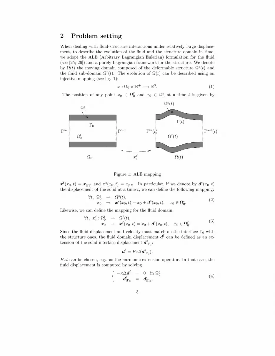
When dealing with fluid-structure interactions under relatively large displace-ment, to describe the evolution of the fluid and the structure domain in time,we adopt the ALE (Arbitrary Lagrangian Eulerian) formulation for the fluid(see [25; 26]) and a purely Lagrangian framework for the structure. We denoteby Ω(t) the moving domain composed of the deformable structure Ωs(t) andthe fluid sub-domain Ωf(t). The evolution of Ω(t) can be described using aninjective mapping (see fig. 1):

x : Ω0 × R+ −→ R

3. (1)

The position of any point x0 ∈ Ωf0 and x0 ∈ Ωs

0 at a time t is given by

PSfrag replacements

Γin Γout

Ωf0

Ωs0

Γ0

Ωf(t)

Ω0

Γin(t) Γout(t)

Ωs(t)

Γ(t)

Ωf(t)

Ω(t)xft

Figure 1: ALE mapping

xf(x0, t) = x|Ωf0

and xs(x0, t) = x|Ωs0. In particular, if we denote by ds(x0, t)

the displacement of the solid at a time t, we can define the following mapping:

∀t , Ωs0 → Ωs(t),

x0 → xs(x0, t) = x0 + ds(x0, t), x0 ∈ Ωs0.

(2)

Likewise, we can define the mapping for the fluid domain:

∀t , xft : Ωf

0 → Ωf(t),

x0 → xf(x0, t) = x0 + df(x0, t), x0 ∈ Ωf0.

(3)

Since the fluid displacement and velocity must match on the interface Γ0 withthe structure ones, the fluid domain displacement df can be defined as an ex-tension of the solid interface displacement d

s|Γ0

:

df = Ext(ds|Γ0

).

Ext can be chosen, e.g., as the harmonic extension operator. In that case, thefluid displacement is computed by solving

−κ∆df = 0 in Ωf0

df|Γ0

= ds|Γ0

,(4)

3

where κ is a properly chosen diffusion coefficient. However, we have to ensurethat the mapping xf

t is a diffeomorphism for all t and that xft(x0) is differentiable

with respect to t for all x0 in Ωf0. In other cases, different extension strategies

may be pursued see e.g., [27; 28], and [29]. Finally, we introduce the followingnotations:

wf =∂xf

t

∂t=

∂df

∂t, (5)

F =∂xf

t

∂x0, (6)

J = det F , , (7)

∂u

∂t

∣

∣

∣

∣

x0

(x, t) =d u(xf

t(x0), t)

dtwith x0 = xf

t

−1(x), (8)

which represent the velocity and the deformation gradient of the domain.We assume the fluid to be Newtonian, viscous and incompressible, so that its

behavior is described by the following fluid state problem: given the boundarydata uin, gf and f f , as well as wf and the forcing them df , the velocity field u

and the pressure p satisfy the momentum and continuity equations:

ρf

(

∂u

∂t

∣

∣

∣

∣

x0

+ (u − wf) · ∇u

)

− div[σf(u, p)] = f f in Ωf(t),

div u = 0 in Ωf(t),u = uin on Γin(t),

σf(u, p) · nf = gf on Γout(t),

(9)

where ρf is the fluid density, µ its viscosity, σf(u, p) = −pId + 2µε(u) theCauchy stress tensor (Id is the identity matrix, ε(u) = (∇u + (∇u)T )/2 thestrain rate tensor). Note that (9) does not univocally define a solution (u, p) asno boundary data are prescribed on the interface Γ(t).

Similarly, for given vector functions gs, f s, we consider the following struc-ture problem whose solution is d:

ρs∂2ds

∂t2− div|x0

(σs(ds)) = f s in Ωs

0,

σs(ds) · ns = gs on ∂Ωs

0 \ Γ0,(10)

where σs(ds) is the first Piola–Kirchoff stress tensor, γ is a coefficient account-

ing for possible viscoelastic effects, while gs represents the normal traction onexternal boundaries and nf and ns are the outward normals of respectively thefluid and the solid domain. Similarly to what we have noticed for (9), prob-lem (10) can not define univocally the unknown ds because a boundary valueon Γ0 is missing.

As a simple example, in our numerical simulations we have used the Saint-Venant Kirchhoff three-dimensional elastic model (see, e.g., [30]) where the solidstress is defined as

σs = 2µlε(ds) + λl div(ds)Id.

4

Here, ε(ds) =1

2

(

∇ds + (∇ds)T)

, µl and λl are the Lame constants. Other

models could be chosen for the structure depending on the specific problem athand. The reader may refer, e.g., to [31; 32; 33].

When coupling the two problems together, the “missing” boundary condi-tions are indeed supplemented by suitable matching conditions on the referenceinterface Γ0. More precisely, if we denote by λ(t) the interface variable corre-sponding to the displacement ds on Γ0, at any time t the coupling conditionson the reference interface Γ0 are

xft = x0 + λ

u xft =

∂λ

∂t,

(σf(u, p) · nf) xft = −σs(d

s) · ns.

(11)

The system of equations (3), (9)-(11) identifies our coupled fluid-structure prob-lem.

3 Decoupled weak formulation

We suppose the problem to be discretized in time. When the solution is availableat time tn, we look for the solution at the new time level tn+1 = tn + δt. If noambiguity occurs, all the quantities will be referred to at time t = tn+1.

If we are given a displacement of the interface λ(tn+1) at the time tn+1, wecan find its harmonic extension on the fluid domain by solving the followingvariational formulation of (4):

find dftn+1 ∈ H1

0 (Ωf0) such that

∫

Ωf0

∇dftn+1 · ∇φ = 0 ∀φ ∈ H1

0 (Ωf0)

dftn+1 = λ(tn+1) on Γ0.

(12)

Then we set wf ,n+1|Γn+1 = (df

tn+1−dftn)/δt to compute the velocity of the structure

domain and we compute the velocity and pressure of the fluid at time tn+1 bysolving:

find (un+1, pn+1) = (u(tn+1), p(tn+1)) ∈ V f(tn+1) × Qf(tn+1) such that

1

δt

∫

Ωf (tn+1)

ρfun+1vf +

∫

Ωf (tn+1)

ρf [(un+1 − wf ,n+1) · ∇un+1]vf

+µ

∫

Ωf (tn+1)

σf(un+1, pn+1)vf =

1

δt

∫

Ωf (tn+1)

ρfunvf +

∫

Γout(tn+1)

gfvf

∫

Ωf (tn+1)

qf div un+1 = 0

(13)for all (vf , qf) ∈ V f(tn+1) × Qf(tn+1), with

V f(t) =

vf |vf xft ∈ H1(Ωf

0)3, vf = 0 on Γt

,

Qf(t) =

qf | qf xft ∈ L2(Ωf

0)

,

5

and where the fluid domain Ωf(tn+1) is given by:

Ωf(tn+1) = xftn+1(Ωf

0).

We can then compute (σf(un+1, pn+1) ·nf) xf

t on Γ0, which by (11) has tobe equal to the structure normal stresses. We are assuming uin = 0, otherwisethe modification is straightforward.

On the structure side, given the same displacement λ(tn+1), we can definethe structure variational problem as:

find (ds,n+1, ws,n+1) = (ds(tn+1), ws(tn+1)) ∈ V s(tn+1) × V s(tn+1) suchthat

2

δt2

∫

Ωs0

ρsds,n+1vs −

2

δt2

∫

Ωs0

ρs(ds,n+1 + δtws,n+1)vs +

∫

Ωs0

σs(ds,n+1) · ∇vs = 0

ws,n+1 =2

δt(ds,n+1 − ds,n − ws,n)

ds,n+1 = λ(tn+1) on Γ0,(14)

for all vs ∈ V s, with V s =

vs ∈ H1(Ωs0)

3|vs = 0 on ∂Ωs0 \ Γ0

. As for thefluid, we can then compute the structure normal stresses on the interface asσs(d

s,n+1) · ns on Γ0.If for a given interface displacement λ(tn+1) the fluid and structure normal

stresses are at equilibrium, it means that the fluid-structure problem has beencorrectly solved. In general we impose the equilibrium in weak form, i.e., (fort = tn+1):

∫

Γ(t)

σf(u, p) · nfvf +

∫

Γ0

σs(ds) · nsv

s = 0 ∀(vf , vs) ∈ V f(t) × V s

such that vf xft = vs on Γ0. Both integrals can be computed as residuals of

the weak form of the equations.

4 The interface equations associated to the cou-

pled problem

We consider the coupled problem at a particular time t = tn+1. In order towrite the interface equation associated to the global fluid-structure problem, weintroduce a fluid and structure operator as follows.

Let Sf be the Dirichlet-to-Neumann (D-t-N) fluid map such that to any giveninterface displacement λ it associates the normal stress

Sf(λ) = σf := (σf(u, p) · nf) xft on Γ0,

where (u, p) is the solution of the Navier-Stokes problem (13). On the otherhand, we denote by Ss the D-t-N operator associated to the structure in Γ0 such

6

that to any given displacement λ of the interface Γ0 associates the normal stressexerted by the structure on Γ0:

Ss(λ) = σs := (σs(ds) · ns) on Γ0,

where ds is the solution of (14).

Remark that in general Sf and Ss are nonlinear and their definitions involvealso the terms due to the boundary conditions and the forcing terms.

Concerning the inverse of the solid operator, we can define S−1s as a Neumann-

to-Dirichlet (N-t-D) map that at any given normal stress σ on Γ0 it associatesthe interface displacement λ(tn+1) = ds,n+1 by solving a structure problemanalogous to (14), but with the Neumann boundary condition

σs(ds) · ns = σ on Γ0

and then computing the restriction on Γ0 of the displacement of the structuredomain.

Moreover, we denote by S ′s the tangent operator associated to the structure

problem and by (S′s)

−1 its inverse. The latter is a N-t-D map that to any givennormal stress σ on Γ0 associates the corresponding displacement λ(tn+1) of theinterface by solving the linearized structure problem with boundary conditionσs(d

s) · ns = σ on Γ0. Analogously, by (S′f)

−1 we denote the inverse of thetangent operator S ′

f . This is also a N-t-D map that for any given normal stress σon Γ0 computes the corresponding displacement λ(tn+1) of the interface throughthe solution of linearized Navier-Stokes equations with the boundary condition(σf(u, p) · nf) xf = σ on Γ0.

Using the definitions of the operators Sf and Ss and of their inverses, wecan express the coupled fluid-structure problem in terms of the solution λ of anonlinear equation defined only on Γ0. More precisely, we can envisage threepossible formulations for the interface equation which are all equivalent from amathematical point of view, but give rise to different iterative methods.

First, we have the fixed-point formulation:

find λ such that S−1s (−Sf(λ)) = λ on Γ0. (15)

This is a classical formulation in fluid-structure interaction problems, but it isworth pointing out that here the fixed point is the displacement of the sole inter-face, whereas the classical fixed point algorithm is applied to the displacementof the whole solid domain (see, e.g., [10]).

The second possible approach is a slight modification of the previous equa-tion (15):

find λ such that S−1s (−Sf(λ)) − λ = 0 on Γ0, (16)

which is more suitable for setting up a Newton iterative method. Again, this isapplied solely to the interface displacement, instead of the whole solid displace-ment (see, e.g., [15]).

Finally, we have the Steklov-Poincare equation:

find λ such that Sf(λ) + Ss(λ) = 0 on Γ0. (17)

7

4.1 Fixed point iterations

A standard algorithm to solve problem (15) is based on relaxed fixed pointiterations. One iteration of the fixed point algorithm reads: for a given λk,compute

λk+1 = λk + ωk(

λk − λk)

, (18)

whereλk = S−1

s (−Sf(λk)).

The choice of the relaxation parameter ωk is crucial for the convergence of themethod (see [12] for a recent analysis). An effective strategy for computing ωk

is given by Aitken’s method (see [13; 23; 34]).The fluid and structure problems are solved separately and sequentially. In

fact, each step k of the algorithm (18) implies:

1. apply Sf to a given displacement λk, i.e., compute the extension of λk tothe entire fluid domain, solve the fluid problem in Ωf(t) with boundary

condition u|Γ(t) xft = (λk − d

f,n|Γ(t))/δt on Γ0; then compute the stress

σkf = (σf(u

k, pk) · nf)|Γ(t) xft on the interface;

2. apply the inverse of Ss to −σkf , i.e., solve the structure problem in Ωs

0

with boundary condition σs(ds,k) · ns = −σk

f on Γ0; then compute thecorrection λk of the displacement at the iterate k.

In general, the main drawback of this method is its slow convergence rate.

4.2 Newton algorithm

The Newton algorithm exploits the formulation (16). Let J(λ) denote the Jaco-bian of S−1

s (−Sf(λ)) in λ. Given λ0, for k ≥ 0, a step of the Newton algorithmassociated to problem (16) reads:

(J(λk) − Id)µk = −(S−1s (−Sf(λ

k)) − λk),λk+1 = λk + ωkµk.

(19)

In general, the parameter ωk can be computed, e.g., by a line search technique(see [35]). Note that the Jacobian of S−1

s (−Sf(λk)) in λk has the following

expression:

J(λk) = −[

S′s

(

S−1s (−Sf(λ

k)))]−1

· S′f(λ

k) = −[

S′s

(

λk)]−1

· S′f(λ

k). (20)

The solution of the linear system (19) can be obtained using an iterative matrix-

free method such as GMRES. We remark that while the computation of[

S′s

(

λk)]−1

·δσ (for any given δσ) does only require the derivative with respect to the statevariable at the interface, the computation of S ′

f(λk)·δλ implies also shape deriva-

tives, since a variation in λ determines a variation of the fluid domain. This isa non-trivial task. In the literature, several approaches have been proposed to

8

solve exactly the tangent problem [15], or else to approximate it by either sim-pler models for the fluid [19; 21], or through finite differences schemes [9; 16; 18](however, the lack of a priori criteria for selecting optimal finite difference in-finitesimal steps may lead to a reduction of the overall convergence speed [21]).

4.3 Domain decomposition (or Steklov-Poincare) formu-lation

A common drawback of the algorithms presented so far is that their implemen-tation is purely sequential, while the domain decomposition formulation mayallow us to set up parallel algorithms to solve the interface equation (17). Letus consider for example the preconditioned Richardson method.

Since the Steklov–Poincare problem (17) is nonlinear, the Richardson methodmust be interpreted in a slightly different way than what is done in the literaturefor the linear case (see, e.g., [24]). Given λ0, for k ≥ 0, the iterative methodreads:

P(

λk+1 − λk)

= ωk(

−Sf(λk) − Ss(λ

k))

(21)

with appropriate choice of the scalar ωk. Every equation should still be intendedon Γ0. The preconditioner P , that must be chosen appropriately, maps the in-terface variable onto the space of normal stresses, and may depend on the iterateλk or more generally on the iteration step k. In these cases we will denote it byPk. The acceleration parameter ωk can be computed via the Aitken technique(see [34]). At each step k, algorithm (21) requires to solve separately the fluidand the structure problems and then to apply a preconditioner. Precisely,

1. apply Sf to λk, i.e., compute the extension of λk to the entire fluid do-main, solve the fluid problem as already illustrated for algorithm (18), andcompute the normal stress σk

f ;

2. apply Ss to λk, i.e., solve the structure problem with boundary conditiond

s,k|Γ(t) = λk on Γ(t) and compute the normal stress σk

s ;

3. apply the preconditioner P−1 to the total stress σk = σkf + σk

s on theinterface.

Note that steps (1) and (2) can be performed in parallel. The crucial issue ishow we can set up a preconditioner (more precisely, a scaling operator) in orderfor the iterative method to converge as quickly as possible. We address thisproblem in the next sections.

4.4 Preconditioners for the domain decomposition formu-lation

In this section we discuss some classical choices of the preconditioner for theRichardson method applied to the domain decomposition approach. We alsocompare the proposed preconditioners to the fixed point and Newton strategiesthat we have illustrated in Sects. 4.1 and 4.2.

9

4.4.1 Dirichlet–Neumann and Neumann–Neumann preconditioners

We define a generic linear preconditioner (more precisely, its inverse):

P−1k = αk

f S′f(λ

k)−1 + αks S′

s(λk)−1, (22)

for two given scalars αkf and αk

s . From (22) we retrieve the following specialcases:

• If αkf = 0 and αk

s = 1, then

P−1k = P−1

DN = S′s(λ

k)−1.

We call it a Dirichlet-Neumann preconditioner, and

P−1DN (σk) = S′

s(λk)−1

(


k))

;

• If αkf = 1 and αk

s = 0, then

P−1k = P−1

ND = S′f(λ

k)−1.

We call PDN a Neumann-Dirichlet preconditioner and

P−1ND(σk) = S′

f(λk)−1

(


k))

;

• If αkf + αk

s = 1, then

P−1k = P−1

NN = αkf S′

f(λk)−1 + αk

s S′s(λ

k)−1

and we call it Neumann-Neumann preconditioner.

In the Dirichlet–Neumann (or the Neumann–Dirichlet) case the computationaleffort of a Richardson step may be reduced to the solution of only one Dirichletproblem in one subdomain and one Neumann problem in the other.

It is possible to choose the parameters αkf , αk

s and ωk dynamically using ageneralized Aitken technique.

Remark 1 If we consider a linear structure model and if we choose αkf = 0 and

αks = 1, the algorithm (21) is equivalent to the fixed-point algorithm (18) (see

Sect. 4.1). Indeed, from (21)

µk = (S′s(λ

k))−1(


k))

= S−1s

(

−Sf(λk))

− λk ,

hence λk+1 = λk + ωk(λk − λk), which coincides with the last equality of (18).

10

4.5 The Newton algorithm on the Steklov-Poincare equa-tion

The genuine Newton algorithm applied to the Steklov-Poincare problem (17) isretrieved by using the algorithm (21) (with ωk = 1) and choosing at the step k

Pk = S′f(λ

k) + S′s(λ

k). (23)

Note that in order to invert Pk one must use a (preconditioned) iterative method(e.g., GMRES) and may approximate the tangent problems to accelerate thecomputations. The resolution algorithm now reads:

[

S′f(λ

k) + S′s(λ

k)]

µk = (−Sf(λk) − Ss(λ

k)) (24)

λk+1 = λk + ωkµk.

As for the classical Newton approach, µk can be computed using an itera-tive matrix-free method. Given a solid state displacement λk , the domaindecomposition-Newton method thus reads: for k ≥ 0,

1. update the residual Sf(λk) + Ss(λ

k) by solving the fluid and the structuresub-problems;

2. solve the linear system (24) via the GMRES method in order to computeµk;

3. update the displacement λk+1. In our application we take ωk = 1, but insome cases it may be necessary to adopt a linesearch or an Aitken strategy.

The GMRES solver should be preconditioned in order to accelerate the con-vergence rate. To this aim, one can use the previously defined domain de-composition preconditioners. In our numerical tests, we have considered theDirichlet-Neumann preconditioner S−1

s , so that the preconditioned matrix ofthe GMRES method becomes:

[S−1s (λk)] · [S′

f(λk) + S′s(λk)] (25)

4.5.1 Comparison with the Newton algorithm (19) on problem (16)

The Richardson algorithm (21) for the Steklov-Poincare formulation (17) withpreconditioner given by (22) (with αk

f = αks = 1) is not equivalent to the Newton

algorithm (19) applied to problem (16). In fact, the Newton algorithm (19)could be regarded as a Richardson method (21), choosing however a nonlinearpreconditioner defined as

Pk(µ) = Ss

(

S′s(λ

k)−1

·(

S′f(λ

k) + S′s(λ

k))

· µ)

, (26)

where λk = S−1s (−Sf(λ

k)).

11

In this case, for σk = −(Sf(λk) + Ss(λ

k)), we would obtain

P−1k

(

σk)

=(

S′f(λ

k) + S′s(λ

k))−1

· S′s(λ

k) · S−1s

(


k))

=(

[

S′s(λ

k)]−1

· S′f(λ

k) + Id)−1

(

S−1s (−Sf(λ

k)) − λk)

.

We see that this is equivalent to (19). In fact (20) is equal to the first bracketin the last line.

Remark 2 Note that if (only) the structure is linear, the preconditioner definedin (26) is also linear and becomes

Pk = S′f(λ

k) + S′s(λ

k),

which is exactly (23). This is a Newton method applied to (16) or (17). How-ever, we would like to remark that the domain decomposition approach allowsus to set up a completely parallel solver. In fact, the fluid and the structuresubproblems can be computed simultaneously (and independently) for both theresidual computation (operators Sf and Ss) and the application of the precondi-tioner (operators S ′

f and/or S′s).

5 Numerical results

5.1 Straight cylindrical vessel

We compare the domain decomposition algorithms with the classical fixed pointand Newton methods. We consider three different preconditioners:

1. the Dirichlet-Neumann preconditioner (here denoted as ‘Steklov-PoincareDN’), i.e., the preconditioner is equal to the structure tangent operatorS′

s;

2. the Neumann-Neumann preconditioner (here denoted ‘Steklov-PoincareNN’), i.e., a linear combination of the structure problem S ′

s and an ap-proximation of the linearized fluid problem S ′

f . In particular, the last oneis linearized by neglecting any shape derivative;

3. the domain decomposition-Newton method illustrated in Sect. 4.5 (‘DD-Newton’). The fluid tangent problem is considered as in [15] in its exactform. To invert (24) we apply the GMRES method either unprecondi-tioned, or preconditioned by ‘Steklov-Poincare DN’.

The simulations were performed on a dual 2.8 Ghz Pentium 4 Xeon with 3GB of RAM. The fluid is discretized by P1-bubble/P1 finite elements and thesolid by P1 finite elements. All the methods give the same solution up to thetolerance required.

We simulate a pressure wave in a straight cylinder of length 5cm and radius5cm at rest. The structure, whose thickness is 5mm, is considered linear and

12

clamped at both the inlet and the outlet. The fluid viscosity is set to µ = 0.03,the Lame constants to µl = 1.15 · 106 and λl = 1.73 · 106, the densities to ρf = 1and ρs = 1.2. We impose zero body forces and homogeneous Dirichlet boundaryconditions on ∂Ωs

0 \ Γ0.The fluid and the structure, both three dimensional, are initially at rest and

a pressure (a normal stress, actually) of 1.3332 · 104 dynes/cm2 is set on theinlet for a time of 3 · 10−3 s. We used two meshes:

• a coarse mesh with 1050 nodes (4680 elements) for the fluid and 1260nodes (4800 elements) for the solid (fig. 2);

• a fine mesh with 2860 nodes (14100 elements) for the fluid and 2340 nodes(9000 elements) for the solid (fig. 3).

A comparison with the classical coupling formulation have been conducted andresults are displayed in tables 1 and 2. In these tables, ‘FS evals’ stands forthe average number of evaluation per time step of either (15) or (17), while‘Tangent evals’ represents the average number of evaluations of the correspond-ing linearized system per time step. We can see that, using the preconditionedRichardson method (21), a decrease in the number of FS evaluations with respectto the classical fixed point algorithm is obtained. However, the computationaltime of the domain decomposition formulation is slightly higher than that of thefixed point formulation. The reason is that the domain decomposition formula-tion requires to solve, at each iteration, the fluid and the structure subproblems,as well as the associated tangent problems, while the latter are indeed skippedby the fixed point procedure. Furthermore, since the solid operator is linear, thetwo approaches are very similar and since our research code is sequential, theparallel structure of the Steklov-Poincare formulation (17) is not capitalized.

Figure 2: Coarse fluid (left) and structure (right) meshes

13

Figure 3: Refined fluid (left) and structure (right) meshes

Table 1: Comparison of the number of sub-iterations for the fixed point algo-rithm and the domain decomposition algorithm (coarse mesh)

Coarse mesh, ∆t = 0.001

Method FS evals Tangent evals CPU time

Fixed point 19.8 0 1h16’Steklov-Poincare DN 19.8 19.8 1h17’Steklov-Poincare NN 17.9 17.9 1h42’

∆t = 0.0005


Fixed point 32.1 0 3h27’Steklov-Poincare DN 29.2 29.2 3h50’Steklov-Poincare NN 22 22 4h20’

We compare now the Newton method (16) and the domain decomposition--Newton algorithm (see Sect. 4.5). In both cases, the Jacobians (20) and (23) arecomputed exactly (cf. [15]) and inverted by a GMRES method. The number ofNewton iterations is equivalent, although the inversion of the Jacobian in ‘DD-Newton’ needs more GMRES iterations. Preconditioning GMRES by ‘Steklov-Poincare DN’ reduces these iterations to the same as in ‘Newton’ and the CPUtime is then equivalent. As before, the reasons reside in the linearity of thestructure model and in the fact that our code is sequential.

The next steps are therefore to set up more sophisticated preconditioners forthe Jacobian system, derived either from the classical domain decomposition

14

Table 2: Comparison of the number of sub-iterations for the fixed point algo-rithm and the domain decomposition algorithm (fine mesh)

Refined mesh, ∆t = 0.001


Fixed point 19.9 0 4h28’Steklov-Poincare DN 19.5 19.5 4h40’Steklov-Poincare NN 17.7 17.7 6h12’

∆t = 0.0005


Fixed point 33 0 12h40’Steklov-Poincare DN 29.6 29.6 12h50’Steklov-Poincare NN 22.1 22.1 15h44’

theory or from lower dimensional models (in a multiscale approach, cf. [36]),and to consider a non-linear structure. The latter is of particular interest forexample in haemodynamics when dealing with complex realistic geometries withrelatively large displacements.

Table 3: Convergence time comparison between the exact Newton and the do-main decomposition-Newton methods (coarse mesh)

Coarse mesh, ∆t = 0.001

Method FS eval Tangent evals CPU time

Newton 3 12 0h56’DD-Newton 3 24 1h30’DD-Newton DN precond 3 12 0h58’

∆t = 0.0005


∆t = 0.0001



Figure 4 shows the pressure wave propagation computed on the coarse meshwith a time step of δt = 1e−3s at time t = 0.005s, 0.01s, 0.015s, and 0.02s. Thedeformation is amplified by a factor 12. We can see that, at time t = 0.01s,

15

Table 4: Convergence comparison of the computational time for the exact New-ton and domain decomposition-Newton methods (fine mesh)

Refined mesh, ∆t = 0.001



∆t = 0.0005


∆t = 0.0001



the deformation reaches the end of the tube. Afterwards, at time t = 0.015sand t = 0.02s, a backward wave propagation is observed. This phenomenoncan be explained by the fact that we clamped the structure and that we imposea vanishing fluid normal stress at the outlet. Setting proper boundary condi-tions in the case of physiological simulations is beyond the scope of this paper.The interested reader may refer, e.g., to the multiscale geometrical approachadvocated in Quarteroni and Formaggia [36].

5.2 Carotid bifurcation

We simulate a pressure wave in the carotid bifurcation using the same fluid andstructure characteristics as in the previous simulations. We solve the couplingusing our ‘DD-Newton DN precond’ algorithm. The mesh that we have used wascomputed using an original realistic geometry first proposed in [37]. The castwas produced by D. Liepsch (Fachhochschule Munchen) and the computationalmodel was developed by K. Perktold (Technische Universitat Graz) (see [37] formore details).

The fluid and the structure are initially at rest and a pressure of 1.3332 ·104dynes/cm2 is set on the inlet for a time of 3 · 10−3s. The average inflowdiameter is 0.67cm, the time step used is δt = 1e − 04 and the total numberof iterations is 200. Figure 5 displays the mesh used for the computations,Figure 6 the deformation at different time steps, while figures 7 to 10 show thedisplacement of the lower part of the carotid (the displacement is amplified 12times). In these last figures, the vectors represent the velocity of the structure.

16

Figure 4: Fluid and solid solutions at time t = 0.005s (upper left), t = 0.010s(upper right), t = 0.015s (lower left), t = 0.020s (lower right) (coarse mesh)

Figure 11 represents the inflow flux computed at each iteration. We can observethree distinct reflections: After iteration 30, i.e., after 3 · 10−3s, no pressure isimposed in the inflow, resulting in the decrease of the inflow flux. We can seethat shortly after this phase, the blood flows backward for a short period oftime. The same phenomenon is observed between iteration 108 and 150 (i.e.,at time 0.0108s and 0.015s). This happens after the pressure pulse enters thebifurcation, and the carotid wall shrinks at the intersection. The third reflectionis caused by the pressure wave leaving the computational domain. The secondreflection is physiological and is relevant in haemodynamics. The two otherscould be avoided by considering more sophisticated boundary conditions.

6 Conclusion

We have presented some new strong implicit coupled schemes to solve fluid-structure interaction problems stemming from a reformulation of the globalproblem as a Steklov-Poincare interface equation (17). With respect to the

17

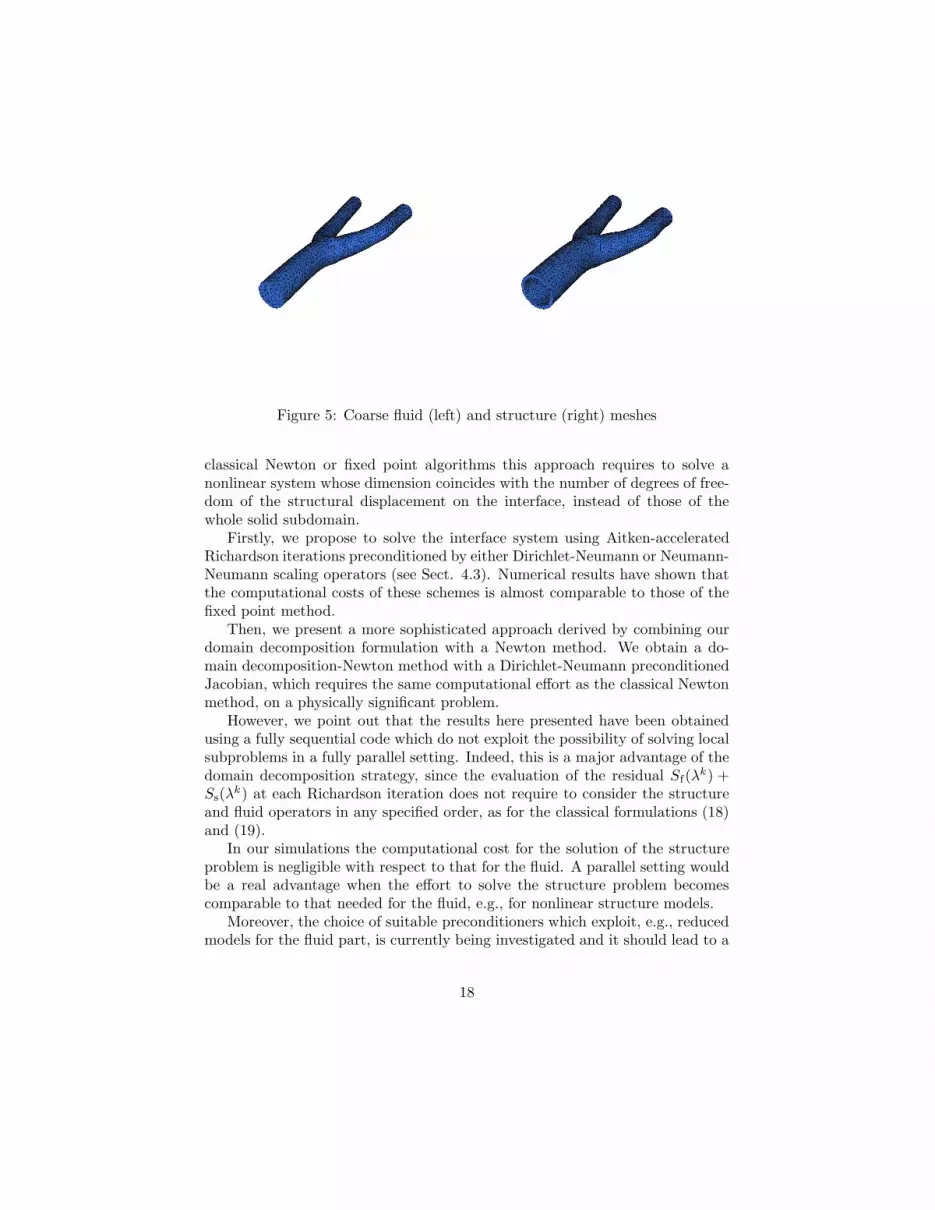
Figure 5: Coarse fluid (left) and structure (right) meshes

classical Newton or fixed point algorithms this approach requires to solve anonlinear system whose dimension coincides with the number of degrees of free-dom of the structural displacement on the interface, instead of those of thewhole solid subdomain.

Firstly, we propose to solve the interface system using Aitken-acceleratedRichardson iterations preconditioned by either Dirichlet-Neumann or Neumann-Neumann scaling operators (see Sect. 4.3). Numerical results have shown thatthe computational costs of these schemes is almost comparable to those of thefixed point method.

Then, we present a more sophisticated approach derived by combining ourdomain decomposition formulation with a Newton method. We obtain a do-main decomposition-Newton method with a Dirichlet-Neumann preconditionedJacobian, which requires the same computational effort as the classical Newtonmethod, on a physically significant problem.

However, we point out that the results here presented have been obtainedusing a fully sequential code which do not exploit the possibility of solving localsubproblems in a fully parallel setting. Indeed, this is a major advantage of thedomain decomposition strategy, since the evaluation of the residual Sf(λ

k) +Ss(λ

k) at each Richardson iteration does not require to consider the structureand fluid operators in any specified order, as for the classical formulations (18)and (19).

In our simulations the computational cost for the solution of the structureproblem is negligible with respect to that for the fluid. A parallel setting wouldbe a real advantage when the effort to solve the structure problem becomescomparable to that needed for the fluid, e.g., for nonlinear structure models.

Moreover, the choice of suitable preconditioners which exploit, e.g., reducedmodels for the fluid part, is currently being investigated and it should lead to a

18

Figure 6: Carotid deformation at time t = 0.005s (upper left), t = 0.010s (upperright), t = 0.015s (lower left), t = 0.020s (lower right)

further reduced computational cost of the preconditioning step.

Acknowledgments

All the computations in this paper were performed using a 3D research codedeveloped at the Ecole Polytechnique Federale de Lausanne, the Politecnico diMilano and INRIA Rocquencourt (www.lifev.org, project manager at EPFL:Christophe Prud’homme [email protected]).This research has been supported by the Swiss National Science Foundation(Project number 20-101-800) and by INDAM project “Integrazione di sistemicomplessi in biomedicina: modelli, simulazioni, rappresentazioni”. The authorswould also like to thank Miguel A. Fernandez for his expertize and preciousadvices on this work.

19

Figure 7: Structure deformation and velocity at time t = 0.005s

References

[1] C. Farhat, M. Lesoinne, P. L. Tallec, Load and motion transfer algorithmsfor fluid/structure interaction problems with non-matching discrete inter-faces: Momentum and energy conservation, optimal discretization and ap-plication to aeroelasticity, Comput. Methods Appl. Mech. Engrg 157 (1998)95–114.

[2] C. Farhat, G. van der Zee, P. Geuzaine, Provably second-order time-accurate loosely-coupled solution algorithms for transient nonlinear com-putational aeroelasticity, Comput. Methods Appl. Mech. Engrg. (in press).

[3] S. Piperno, C. Farhat, Partitioned procedures for the transient solution ofcoupled aeroelastic problems - Part II: Energy transfer analysis and three-dimensional applications, Comput. Methods Appl. Mech. Engrg. 190 (2001)3147–3170.

[4] G. Fourestey, S. Piperno, A second-order time-accurate ALE Lagrange-Galerkin method applied to wind engineering and control of bridge profiles,Comput. Methods Appl. Mech. Engrg. 193 (2004) 4117–4137.

20


[5] S. Piperno, Explicit/implicit fluid-structure staggered procedures with astructural predictor and fluid subcycling for 2D inviscid aeroelastic simu-lations, Int. J. Num. Meth. Fluids 25 (1997) 1207–1226.

[6] S. Piperno, Numerical simulation of aeroelastic instabilities of elementarybridge decks, Tech. Rep. 3549, INRIA (1998).

[7] S. Deparis, M. Fernandez, L. Formaggia, Acceleration of a fixed point algo-rithm for fluid-structure interaction using transpiration conditions, M2AN37 (4) (2003) 601–616.

[8] H. Matthies, J. Steindorf, Partitioned but strongly coupled iterationschemes for nonlinear fluid-structure interaction, Computer & Structures80 (2002) 1991–1999.

[9] H. Matthies, J. Steindorf, Partitioned strong coupling algorithms for fluid-structure interaction, Computer & Structures 81 (2003) 805–812.

[10] F. Nobile, Numerical Approximation of Fluid-Structure Interaction Prob-lems with Application to Haemodynamics, Ph.D. thesis, Ecole Polytech-nique Federale de Lausanne (2001).

21


[11] P. L. Tallec, J. Mouro, Fluid structure interaction with large structuraldisplacements, Comput. Methods Appl. Mech. Engrg. 190 (2001) 3039–3067.

[12] P. Causin, J.-F. Gerbeau, F. Nobile, Added-mass effect in the design of par-titioned algorithms for fluid-structure problems, Tech. Rep. 5084, INRIA(2004).

[13] M. Cervera, R. Codina, M. Galindo, On the computational efficiency andimplementation of block-iterative algorithms for nonlinear coupled prob-lems, Engrg. Comput. 13 (6) (1996) 4–30.

[14] S. Deparis, Numerical Analysis of Axisymmetric Flows and Methods forFluid-Structure Interaction Arising in Blood Flow Simulation, Ph.D. thesis,Ecole Polytechnique Federale de Lausanne (2004).

[15] M. Fernandez, M. Moubachir, A Newton method using exact jacobians forsolving fluid-structure coupling, Computers and Structures 83 (2-3) (2005)127–142.

[16] M. Heil, An efficient solver for the fully coupled solution of large-

22


-15

-10

-5

0

5

10

15

20

25

30

0 20 40 60 80 100 120 140 160 180 200

Iteration number

Inflow flux

Figure 11: Inflow flux for the carotid geometry

displacement fluid-structure interaction problems, Comput. Methods Appl.Mech. Engrg. 193 (1-2) (2004) 1–23.

23

[17] H. Matthies, J. Steindorf, Numerical efficiency of different partitionedmethods for fluid-structure interaction, Z. Angew. Math. Mech. 2 (80)(2000) 557–558.

[18] T. Tezduyar, Finite element methods for fluid dynamics with movingboundaries and interfaces, Arch. Comput. Methods Engrg. 8 (2001) 83–130.

[19] S. Deparis, J. Gerbeau, X. Vasseur, GMRES preconditioning and acceler-ated quasi-Newton algorithm and application to fluid structure interaction,in preparation (2004).

[20] J.-F. Gerbeau, V. Vidrascu, P. Frey, Fluid-structure interaction in bloodflows on geometries coming from medical imaging, Tech. Rep. 5052, INRIA(2003).

[21] J. Gerbeau, M. Vidrascu, A quasi-Newton algorithm based on a reducedmodel for fluid-structure interaction problems in blood flows, M2AN 37 (4)(2003) 663–680.

[22] J. Mouro, Interactions Fluide Structure en Grads Deplacements. ResoultionNumerique et Application aux Composants Hydrauliques Automobiles,Ph.D. thesis, Ecole Polytechnique, Paris (1996).

[23] D. P. Mok, W. A. Wall, Partitioned analysis schemes for the transientinteraction of incompressible flows and nonlinear flexible structures, in:K. Schweizerhof, W. Wall (Eds.), Trends in Computational Structural Me-chanics, K.U. Bletzinger, CIMNE, Barcelona, 2001.

[24] A. Quarteroni, A. Valli, Domain Decomposition Methods for Partial Dif-ferential Equations, Oxford Science Publications, Oxford, 1999.

[25] J. Donea, A. Huerta, J.-P. Ponthot, A. Rodrıguez-Ferran, ArbitraryLagrangian-Eulerian methods, in: The Encyclopedia of Computational Me-chanics, Vol. I, Chapt. 14, Wiley, 2004, pp. 413–437.

[26] T. Hughes, W. Liu, T. Zimmermann, Lagrangian-Eulerian finite elementformulation formulation for incompressible flows, Comp. Methods Appl.Mech. Engrg. 29 (1981) 329–349.

[27] J. Batina, Unsteady Euler airfoil solutions using unstructured dynamicmeshes, AAIA 28 (1990) 1381–1388.

[28] G. Fourestey, Simulation Numerique et Controle Optimal d’InteractionsFluide Incompressible/Structure par une Methode de Lagrange-Galerkind’Ordre 2. Applications aux Ouvrages d’Art, Ph.D. thesis, Ecole Nationaledes Ponts et Chaussees (2002).

[29] M. Lesoinne, C. Farhat, Stability analysis of dynamic meshes for transientaeroelastic computations, AIAA, Proceedings of the 11th AIAA Computa-tional Fluid Dynamics Conference, Orlando, Florida. Paper 93-3325.

24

[30] P. G. Ciarlet, Mathematical elasticity. Vol. II, Vol. 27 of Studies in Math-ematics and its Applications, North-Holland Publishing Co., Amsterdam,1997, theory of plates.

[31] D. Chapelle, K. Bathe, The Finite Element Analysis of Shells - Fundamen-tals, Springer, New York, 2003.

[32] P. L. Tallec, Introduction a la Dynamique des Structures, Ellipse, Paris,2000.

[33] A. Quarteroni, M. Tuveri, A. Veneziani, Computational vascular fluid dy-namics: problems, models and methods, Comp. Vis. Science 2 (2000) 163–197.

[34] S. Deparis, M. Discacciati, A. Quarteroni, A domain decomposition frame-work for fluid-structure interaction problems, in: Proceedings of the ThirdInternational Conference on Computational Fluid Dynamics (ICCFD3),Toronto, July 2004, 2004, submitted.

[35] A. Quarteroni, R. Sacco, F. Saleri, Numerical Mathematics, Springer, NewYork-Berlin-Heidelberg, 2000.

[36] A. Quarteroni, L. Formaggia, Modelling of Living Systems, Handbook ofNumerical Analysis, Elsevier Science, Amsterdam, 2002, Ch. Mathemat-ical Modelling and Numerical Simulation of the Cardiovascular System,submitted.

[37] G. Karner, K. Perktold, M. Hofer, D. Liepsch, Flow characteristics in ananatomically realistic compliant carotid artery bifurcation model, Com-puter Methods in Biomechanics and Biomedical Engineering (2) (1999)171–185.

25

Documents

Fluid–structure algorithms based on Steklov–Poincaré operators