Forecasting Backyard Farm Gate Hog Prices:

Evidence from the ARIMA Model

An Empirical Paper

Submitted to the Faculty of School of Economics

De La Salle University

In Partial Fulfillment Of the requirements for

Economic Forecasting and Model Buildings (ECOFORE)

Submitted by: Roca, Jayvee G.

Submitted to: Dr. Cesar Rufino

August 23, 2016

Forecasting Backyard Farm Gate Hog Prices: Evidence from the ARIMA Model

Roca, J.

Abstract

The forecasting of the price of agricultural as well as livestock and poultry products is

important to the decision making of farmers in what to produce in order to maximize

their time and profit. Comprising around 70% of the overall pig production in a market

where pork is highly regarded as valuable meat, backyard farmers play an important

role in the Philippine society. The study makes use of the state of the art TRAMO

software in order to accurately forecast future backyard farm gate prices for pigs bred

for slaughtering.

I. Introduction

1.1 What is Pork to Filipinos?

Pork is one of the major sources of protein for many Filipinos due to its relatively

cheap price and easy accessibility in “Palengkes” or wet markets and very recently, in

supermarkets across the country. All throughout history, the importance of pork in the

culture of Filipinos are readily seen from routinary ritual sacrifices for traditional

marriage ceremonies, or prayers for good harvest, up to the iconic modern day Lechon

in different festivals spread across the different regions in the country. Even before the

colonization of the Spaniards, the Filipinos have always made use of pork as staples in

their daily lives; in fact, they valued pork enough to use it as offerings to their gods in

order to gain their favor (Veneracion, 2001, as cited in Velasco, 2014). Today, the

popularity of pork in different Filipino homesteads is noticeably present, a Filipino

breakfast is not complete without tocino nor is their christmas complete without the

traditional ham, pork is much more than food to the Filipinos, it is a way of life, a

preservation of their culture and this is evident in their numerous dishes all created

with pork. In terms of actual amounts, pork really is the main staple meat for majority

of the Filipinos. Keynes (n.d.) records the consumption and production of pork at 1.9

million metric tons is significantly the highest among all meat products in the country

even compared to beef which is only produced at around 0.3 million metric tons in a

year. Equivalently, Stanton, Emms & Sia (2010) record these amounts to be around

59% of overall meat as well as poultry production in the country [See Figure 1].

Figure 1. Meat and Poultry Production in The Philippines by Product Type. Adopted

from The Philippine’s Pig Farming Sector: A Briefing for Canadian Livestock Genetics

Suppliers, by Stanton, Emms & Sia (2010)

Pork is one of the most common and most valued meat for majority of the

population in the Philippines which is also why Filipinos are generally very picky in the

freshness of their pork. Keynes (n.d.) also observes this phenomenon, wherein,

Filipinos generally tend to view imported or frozen products to be inferior substitutes

to freshly slaughtered pork found in the wet markets, which equivalently, enhances the

local hog raising industry across different regions in the country. Indeed, even the

market for hog raisers is quite unique in the Philippines where majority of the

producers, around 70%, are actually small scale backyard farmers scattered around the

different regions in the country (Keynes, n.d.; Stanton, Emms & Sia, 2010).

1.2 The Hog Raiser’s Dilemma

Similar to many goods in the market today, a typical consumer can easily observe a

gradual increase of prices of pork available to consumers over the years; however, the

opposite is true for the prices that the producers or hog raisers actually earn when they

sell off the pigs to slaughter [see Figure 2]. There is a steadily growing concern among

different hog raisers about the low prices of live meat per kilo sold; the words

“matumal” which is a Filipino term that connotes extremely low points or prices always

comes to mind. One would also hear the constant complaints of many hog raisers

concerning the low prices which they attribute mainly to the large influx of cheaper

frozen pork imports in the country. In fact, it turns out that the large amount of imports

is a legitimate concern among hog raisers in the world, important enough to threaten a

pork holiday early this year (Lim, 2016; Domingo, 2016). This phenomenon has always

been seen as a problem especially for backyard farmers, where, the country is recorded

to have people moving out of the pork industry mainly due to the high production costs

of the business and partnered with the large influx of minimally tariffed as well as

cheap imported frozen meat (Cabarles, 2007)

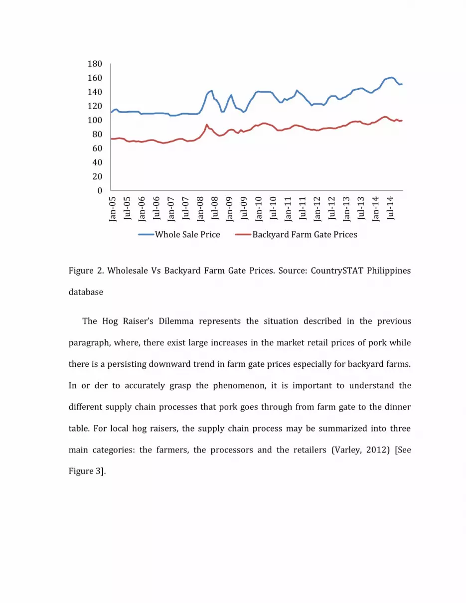
Figure 2. Wholesale Vs Backyard Farm Gate Prices. Source: CountrySTAT Philippines

database

The Hog Raiser’s Dilemma represents the situation described in the previous

paragraph, where, there exist large increases in the market retail prices of pork while

there is a persisting downward trend in farm gate prices especially for backyard farms.

In or der to accurately grasp the phenomenon, it is important to understand the

different supply chain processes that pork goes through from farm gate to the dinner

table. For local hog raisers, the supply chain process may be summarized into three

main categories: the farmers, the processors and the retailers (Varley, 2012) [See

Figure 3].

0

20

40

60

80

100

120

140

160

180

Jan

-05

Jul-

05

Jan

-06

Jul-

06

Jan

-07

Jul-

07

Jan

-08

Jul-

08

Jan

-09

Jul-

09

Jan

-10

Jul-

10

Jan

-11

Jul-

11

Jan

-12

Jul-

12

Jan

-13

Jul-

13

Jan

-14

Jul-

14

Whole Sale Price Backyard Farm Gate Prices

Figure 3. Supply Chain Process. Variables adopted from The Development of Pig

Production& Pork Markets in Asia by Varley, 2012.

. The backyard farmers either outsource their piglets from commercial farms or

have breeder pigs for themselves; the piglets are then selected and bred for

slaughtering for around 3 to 5 months depending on the growth rate of the pig. Once it

reaches its maturity, the hog raisers usually contact byaheros or caravan traders that go

around the area looking for live pigs for slaughtering; these byaheros are usually

composed of a group of people: an expert or the owner/trader itself and accompanied

with kargadors or lifters. In usual practice, hog raisers and byaheros alike follow the

market prescribed prices for live hogs which is somewhere between Php 90 to Php 130

per kilogram depending on the area, as to the accuracy the selling prices both of them

seem to follow a quasi-trust based system of determining said prices where the actual

prices are inexplicably determined by word of mouth and consensus through

neighboring hog raisers as well as other caravan traders in the area. The live pigs are

then transported to slaughter houses where they are primly chopped up at a fixed rate

of around Php 50 per head, after which they are then loaded up to be distributed to

retailers and wet markets in their respective coverage area. The retailers whether

institutional or individuals will then sell the parts to the different consumers available

in their area which then follows retail prices on the different cuts of the meat.

Farmers Processors Retailers

1.3 General Overview of the Study

Based on the facts presented in the previous section of this paper, the researcher

observe that hog raisers most especially backyard hog raisers or even pork in general

play a very important role on not just the household level but the general agricultural

sector as well. Pork itself is a multibillion dollar industry being the second most

produced agricultural product at 18.28% of total value of production, second only to the

production of rice in the country (Livestock Research Division, 2016) and as previously

mentioned, 70% of the production is attributed to local backyard farms (Stanton, Emms

& Sia, 2010). While this may be the case, in recent years the country has recorded a

drop in the farm gate prices for live pigs especially for backyard farmers which are

highly associated with large increases in the supply of cheaper imported pork.

Especially considering the currently implemented ASEAN integration, the supply of low

tariffed and lower priced pork may further drive down the already low prices for local

pork supply thereby bankrupting our local farmers in different regions all throughout

the county. Given this phenomenon, it is therefore important to look into the outlook of

backyard farm prices for pigs bred for slaughtering; which is why this study seeks to

answer the questions “How much can econometric time series modeling accurately and

consistently predict the farm gate (backyard) prices of pigs bred for slaughtering

specifically for the medium term?”

In order to answer this question, the researcher has set the following as the main

objectives of the study:

(1) To determine and describe the variation found in as well as forecast the farm

gate backyard prices of pigs bred for slaughtering using the ARIMA model.

(2) To identify the presence of time series trend and seasonality in the said prices

for the time range 1990-2016

(3) To accurately predict and forecast next period backyard farm prices for pigs

bred for slaughtering

As mentioned in the previous sections of this study, the dataset to be used in this

study is comprised of backyard farm gate prices of pigs bred for slaughtering which was

retrieved from the Philippine Statistical Authority through the Bureau of Agricultural

Statistics’ CountrySTAT Philippines database covering the time range of January1990 –

June 2016 on a monthly frequency which then amounts to a total of 318 observations.

Using both E-views and TSW software, a forecast period of 24 months is expected from the

results which will then be used to achieve the objective of the study.

II. Review of Related Literature

2.1 The Pork Industry in a Glance

The world has had an unprecedented rate of population growth especially in the end

of the 20th century, while this growth rate has been seen to gradually decrease in recent

years the fact still remains that the world population is somewhere between 8 Billion

people and counting (Ortiz-Ospina & Roser, 2016). Food security and sustainability is a

major concern in the fast changing world today, especially in countries found in Asia

where we see the largest growth rate in terms of population, even accounting for 56%

of the total world population (Asian Development Bank, 2013), as well as having large

areas where hunger is an endemic problem for majority of the population (Food and

Agriculture Organization of the United Nations, 2015). Many researchers have taken a

look into the different characteristics of consumption patterns across different regions.

Asian Development Bank (2013) records that majority of the Asian countries are

effectively switching from the basic cereals for sustenance to more complex meals such

as meat, dairy, processed foods, etc. In fact, the global consumption as well as the

production of meat products is expected to double by the year 2050 especially in

developing countries (Humane Society International, 2011). Pork is one of the main

meat groups that dominate markets across different countries in the world, it

comprises the largest share of meat consumed/produced in the world at 42% of all

meats consumed globally (Varley, 2012); the world production of pork is highly

attributed, around 50%, to the productions from developing countries especially in the

Asian continent (Food and Agriculture, 2007, as cited in Humane Society International,

2011).

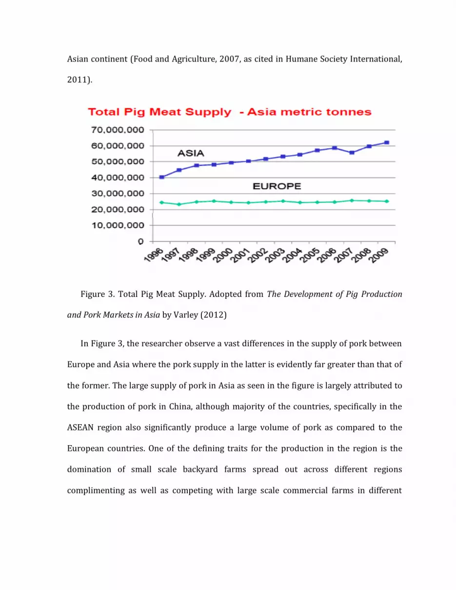
Figure 3. Total Pig Meat Supply. Adopted from The Development of Pig Production

and Pork Markets in Asia by Varley (2012)

In Figure 3, the researcher observe a vast differences in the supply of pork between

Europe and Asia where the pork supply in the latter is evidently far greater than that of

the former. The large supply of pork in Asia as seen in the figure is largely attributed to

the production of pork in China, although majority of the countries, specifically in the

ASEAN region also significantly produce a large volume of pork as compared to the

European countries. One of the defining traits for the production in the region is the

domination of small scale backyard farms spread out across different regions

complimenting as well as competing with large scale commercial farms in different

areas especially in China and the Philippines (Varley, 2012; Huynh, Aamik, Drucker &

Verstegen, 2006).

2.2 Forecasting Pork Prices

There is vast literature when it comes to forecasting the prices of agricultural

products as well as the prices of livestock and poultry. The works of Zhang, Chen and

Wang (2010), Allen (1994), Shonkwiler (1986) and Helmers and Held (1977) will be

discussed in this section of the paper. Zhang, Chen and Wang (2010) makes use of

multivariate simple regression model through the use of the SPSS software; the authors

argue that the price of pork is determined by several factors, mainly: historical, internal

and external factors. Furthermore, the authors also managed to infer that the

fluctuation of pork prices will eventually increase the prices of pork significantly

thereby affecting the CPI index itself. On the other, Allen (1994) discusses the different

developments and available approaches in the forecasting of different aspects of

agricultural as well as poultry and livestock products. The author acknowledges the

importance of the forecasting of prices to the general welfare of farmers everywhere,

where, the author points out that at the moment of commitment farmers will then be

price bargainers. Furthermore, the researchers also acknowledges how majority of the

current research made are from economists that make use of econometric models in

order to forecast said prices. Shonkwiler (1986) in a different perspective approaches

the futures prices of swine and cattle in tackling rational expectation among investors.

The author concludes that rational forecasts for said prices are rather suboptimal due

to the irrationality of the market itself. Lastly, this research looks into the work of

Helmers and Held (1977) where in the authors compares different forecasting

approaches and concluded that no one method in forecasting the prices of agricultural

product is dominant than any of the other.

This research will look into the forecasting of backyard farm gate prices for hogs

bred for slaughtering in the Philippines. To the extent of knowledge of the researcher,

this will be the first time that said variable is forecasted using the ARIMA methodology.

III. Framework and Methodology

3.1 Data Collection and Treatment

The monthly data observed in this study ranges from the periods of January 1990 up

to the latest available data of June 2016 which was obtained from the Philippine

Statistical Authority’s Bureau of Agricultural Statistics’ CountryStat Philippines

Database. The chosen data was selected by the researcher based on the availability as

well as consistency of the dataset. The given dataset contains the backyard farm gate

prices for pigs bred for slaughtering in Philippine Pesos as the base currency. Backyard

farm gate price is simply defined as the price per kilogram in which small scale hog

raisers sell their pigs bred for the purpose of slaughtering; ‘small scale farm’ in the

context of hog raising is defined by the National Statistical Coordination Board as farms

who have fewer than 21 heads adult hogs, fewer than 41 heads young hogs or in the

presence of having both adult and young hogs, it should have fewer than 10 and 22

heads respectively.

Statistically, the data used in this study is classified as a time series data (denoted as

Yt). The analysis of time series data considers four major components, mainly: (1)

Secular Trend (2) Cyclical Variation (3) Seasonal Variation (4) Irregular Variation. An

important consideration in using this form of data is the stationarity of the time series

dataset. Gujarati and Porter (2009) defines stationarity as the condition in time series

data where the mean, variance as well as covariance are not affected by time, in other

words, are time invariant. Boğaziçi University (n.d.) discusses the problems arising

from a non-stationary time series dataset, specifically the problems of spurious

regressions as well as problems in the normality of t distribution thereby decreasing

the accuracy of analysis for forecasting purposes. Statistics provide us with a wide array

of identifying the stationarity of a given time series dataset, the most popular of which

are the Augmented Dickey-Fuller Test and the Philipps-Perron Tests. If the tests

determine non stationarity in a given data set, the next step is to proceed to the first

differencing of the data until stationarity is achieved (Rufino, Lecture on Economic

Forecasting, 2016).

The dataset will then be subject to treatment as well as analysis using the TSW+

software through a program known as the TRAMO program. TRAMO is strictly defined

as “Time Series Regression with ARIMA Noise, Missing Observations, and Outliers” (Gomez

& Maravall, PROGRAMS TRAMO AND SEATS: INSTRUCTIONS FOR THE USER, 1996).

Both the software and program are top of the line statistical tools from the Bank of

Spain that are used for any number of purposes especially in identifying optimal and

non-structural model for the given data set specifically applying the Univariate Box-

Jenkins (UBJ) approach.

3.2 Box Jenkins Methodology (ARIMA Modelling)

The Box-Jenkins (BJ) methodology is powerful tool used for forecasting time series

analysis. The BJ methodology is unique and contrasted from a basic regression model

such that the approach makes use of a-theoretic modelling or modelling without

respect to economic theory which is often the case for regression based methodologies

in forecasting, furthermore, the time series model Yt for the BJ methodology are

explained by the past values of the series itself and the stochastic error terms which is

evidently different from that of the regressors based forecasting done by a common

regression methods (Gujarati & Porter, 2009). Since the study will only observe one

variable for the Autorgressive Integrated Moving Average (ARIMA) model the study will

be employing a Univariate Box Jenkins (UBJ) methodology.

3.2.1 UBJ Modelling Requirements

In using a UBJ model, as well as assuring the stationarity of the given data, it is

important to identify the optimal model processes which are categorized in to four

different processes: Autoregressive (AR), Moving Average (MA), Autogressive Moving

Average (ARMA) and Autoregressive Integrated Moving Average (ARIMA) process

(Baltagi, 2011). The most important consideration in identifying the process that the

forecasting model follows will be due to three factors p, d, q which is explained in the

succeeding paragraphs of this section.

AR(p) is an autoregressive process of the pth-order where the values are obtained

with respect to the previous time period t-p and also considers a random error term

(Lutkepohl & Kratzig, 2004). Furthermore, the forecasts computed for using AR is

simply computed as deviations from the mean with the inclusion of a random shock

value (Gujarati & Porter, 2009).

MA(q) is a moving average of the qth-order, the process makes use of random

shocks or white noise errors in order to forecast values of a given dataset; alternatively,

it also makes use of a constant value partnered with the current as well as past values of

these random shocks in order to accurately forecast a given time series dataset (Baltagi,

2011).

ARMA(p,q) is basically the presence of the characteristics for both AR(p) and MA(q)

in forecasting. The process therefore follows the same assumptions for both AR and MA

processes especially in the treatment of random shock values as well as past values for

any given dataset. It is notable that ARMA requires stationarity at level for any given

data, if the process requires differencing of any form in order to make it stationary the

model will then follow an ARIMA(p,d,q,) process where AR(p), MA(q) and d is the

number of times that the given data series was differenced in order to achieve

stationarity. The general equation for an ARIMA forecasting model is as follows:

�̂�𝑡 = μ + ϕ1 yt−1 + ⋯ + ϕp yt−p − θ1et−1 − ⋯ − θqet−q (Eq. 1)

�̂�𝑡 is the forecasted variable (dependent variable) where it is a function of its own

lagged (p) values, Yt-p. μ in this case is a constant term usually denoting the average

period to period changes. While ϕp is one of the most important variable in the

equation it is used to represent the slope of the coefficient where the analysis is largely

dependent upon the value of said equation variable; the value for the variable should

always be less than 1 if the given dataset is stationary. If ϕp is positive then the

predicted value for the given set is ϕp × (𝑌𝑡−𝑝) greater than the mean while the

opposite is true for a negative valued ϕp (Duke University, n.d.). θq in this case is

defined to be the moving average parameters of the equation while et−q is the error

term for said equation. It is worth noting that the first half of Eq. 1 is considered to be

the AR process while the latter is shown to be the MA model.

Gujarati and Porter (2009) identify four steps in order to properly execute a UBJ

Methodology which is enumerated as follows: (1) Identification (2) Estimation (3)

Diagnostic Checking (4) Forecasting.

(1) Identification

This step of the in the UBJ methodology seeks to identify the dominant process

enumerated in the previous section of this chapter. In essence, identification here

pertains to the values of p,d,q by using the different statistical tools available to

researchers in order to identify candidate models. These tools pertain to the

Autocorrelation Function (ACF), Partial Autocorrelation Function (PACF) and their

respective Correlograms. ACF denoted by 𝜌𝑘 , where k is the lagged value for the given

series, is one of the basic tests for stationarity and has a value that is between +1 and -1;

since the nature of a time series dataset is ordered it is very useful to identify the

correlation between the different time lags in a given series and this is what ACF seeks

to address. PACF on the other hand is denoted by 𝜌𝑘𝑘 where the only difference is the

control used in transitional lag values. Finally, correlograms are used in plotting the

PACF and ACF against the k lagged values of the given dataset (Gujarati & Porter, 2009).

There are certain indicators on the pattern of a correlogram that help identify the

process that the model makes use of (University of Arizona, 2015). For an AR process,

the ACF coefficient is characterized as having a gradual decline towards zero, while for

the PACF coefficient for this process reveal a straight decline to zero after a certain lag

p. MA process on the other hand sees a straight decline to zero after lag order q for its

ACF coefficient while the PACF coefficient records a gradual decrease towards zero.

Finally, for the ARMA process, since it contains both AR and MA processes, both the ACF

and PACF values are seen to decline gradually towards zero.

(2) Estimation

The estimation pertained to in this case requires that the results of the model fall in

the acceptable standard of 0.05 or at 5% level of significance. The software that the

researcher uses computes for these p-values as well as the coefficients of forecasts

automatically. Since the researcher makes use of the TSW+ software, the estimation

procedure fits the model to the data then reveals the different parameter estimates as

well as the different diagnostic statistics that pertain to the model-data fit.

(3) Diagnostic Checking

In order to accurately gauge the performance of the selected best fitting model, the

research shall compute and compare the results using the following criteria (Rufino,

Lecture on Economic Forecasting, 2016): (1) Root Mean Square Error (RMSE) (2) Mean

Absolute Error (MAE) (3) Mean Absolute Percentage Error (MAPE) (4) Theil Inequality

Coefficient (Theil’s U). The following diagnostic tests have the following equations

respectively.

𝑅𝑀𝑆𝐸 =

√∑ 𝑢𝑡2̂𝑇

𝑇=1

𝑇 (𝐸𝑞. 2)

𝑀𝐴𝐸 =∑ |𝑢�̂�|𝑇

𝑇=1

𝑇 (𝐸𝑞. 3)

𝑀𝐴𝑃𝐸 =∑ |

𝑌𝑡 − 𝑌�̂�

𝑇|𝑇

𝑇=1

𝑇 (𝐸𝑞. 4)

𝑇ℎ𝑒𝑖𝑙′𝑠 𝑈 =

√∑ 𝑢�̂�𝑇𝑇=1

𝑇

√∑ 𝑌𝑡2𝑇

𝑇=1

𝑇 +√∑ �̂�𝑡

2𝑇𝑇=1

𝑇

(𝐸𝑞 5)

The following criteria mentioned in this section make use of the past observed value of

the given data’s residuals; which means that the lower the value for these criteria the

better the given forecasts (Rufino, Lecture on Economic Forecasting, 2016).

(4) Forecasting

The forecasted values are estimated using the best model available using the

different tests and statistics discussed in the previous section of this chapter. It is worth

noting that in the best fitted model, a leveled data series makes use of an Exact

Maximum Livelihood Estimation while at logged series the Kahlman Filter Estimation

(Rufino, 2016).

IV. Results and Discussion

This section shall be discussing the results through the output of the TSW software of

the best fitted model selected based on the UBJ Criteria discussed in the previous

chapter of this paper.

4.1 Pre Test

The initial pre-test results are gathered from the TRAMO output of the TSW

software. The results show a significant Easter effect since the Easter correction was

observed; interestingly, this result coincides with the rational expectation that Filipinos

in general tend to have different meat eating patterns during the holy week, where, the

general population holds off the consumption of meat up until Easter Sunday hence the

observed Easter effect in this case (Stanton, Emms & Sia, 2010). The test whether log

values or level values are used in this model was also conducted on the same pre-test

output, where, the results show that the given data is transformed to logged values

specifically at the selection of around 1.05 logs.

4.2 Fitness of the Model

Figure 4 reveals the different criteria to determine the fitness of the model. Mq in

this instance simply describes the number of observations per year; since the data is

monthly in nature the value in this study is 12, while Nz in this study describes the

total number of observations which is at 318. The results reveal a value of Lam to be

equal to 0 which basically means that the data used in this case is logged and similarly,

the mean is also 0 suggesting that no mean correction was made in this case (Gomez &

Maravall, PROGRAMS TRAMO AND SEATS: INSTRUCTIONS FOR THE USER, 1996). The

standard errors SE(res) of the residuals are measure to be at 0.0162812 and the

Bayesian Information Criterion (BIC) is at -7.91297 which then automatically identifies

and corrects outliers on the said model.

Figure 4. Fitness of the Model.

The results further show the presence of certain outliers through the #OUT

component of the model fitness test, 16 are identified to be outliers and the effects are

already controlled for by the TSW software through the methodologies proposed by

Tsay (1989) and Chen and Liu (1993) (as cited in, Gomez and Maravall, 1997).

Furthermore, the model explicitly identifies various effects as well including the

Trading Day Effect (TD) and Easter Effect (EE) (Rufino, 2016). The model fitness test

records no TD and EE for this data set. Finally, the optimal model chosen in this case is

as observed as follows ARIMA(3,1,1)(0,1,1) suggesting the use of data with a first

differenced series [see Figure 5].

Figure 5: First Differenced Data Series. Data Source: TSW+Output

4.3 MODEL SELECTION: ARIMA

The optimal ARIMA model identified using the dataset follows ARIMA(3,1,1)(0,1,1)

which the program identified to be the best fitted model. This means that the given

model has 3 autoregressive order, 1 unit root, and 1 moving average order while the

-0.08

-0.06

-0.04

-0.02

0

0.02

0.04

0.06

0.08

Dec

-90

Feb

-92

Ap

r-9

3

Jun

-94

Au

g-9

5

Oct

-96

Dec

-97

Feb

-99

Ap

r-0

0

Jun

-01

Au

g-0

2

Oct

-03

Dec

-04

Feb

-06

Ap

r-0

7

Jun

-08

Au

g-0

9

Oct

-10

Dec

-11

Feb

-13

Ap

r-1

4

Jun

-15

seasonal component contains 0 seasonal autoregressive order, 1 seasonal unit root and

1 seasonal moving average order.

The identification of the model in the Tramo output includes the identification of

different types of outliers as identified by Gomez and Maravall (1997) as follows: (1)

Transitory Change represents a spike that eventually fades over time (2) Level Shifts

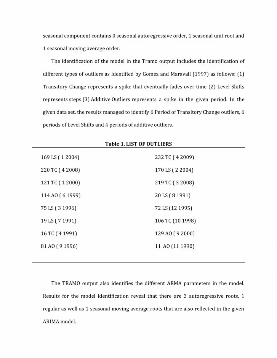
represents steps (3) Additive Outliers represents a spike in the given period. In the

given data set, the results managed to identify 6 Period of Transitory Change outliers, 6

periods of Level Shifts and 4 periods of additive outliers.

Table 1. LIST OF OUTLIERS

169 LS ( 1 2004)

220 TC ( 4 2008)

121 TC ( 1 2000)

114 AO ( 6 1999)

75 LS ( 3 1996)

19 LS ( 7 1991)

16 TC ( 4 1991)

81 AO ( 9 1996)

232 TC ( 4 2009)

170 LS ( 2 2004)

219 TC ( 3 2008)

20 LS ( 8 1991)

72 LS (12 1995)

106 TC (10 1998)

129 AO ( 9 2000)

11 AO (11 1990)

The TRAMO output also identifies the different ARMA parameters in the model.

Results for the model identification reveal that there are 3 autoregressive roots, 1

regular as well as 1 seasonal moving average roots that are also reflected in the given

ARIMA model.

Table 2. ARMA PARAMETERS

PARAMETER ESTIMATE STD ERROR T RATIO LAG

PHI1 0.62651 0.11085 5.65 1

PHI2 -0.33513 0.63509E-01 -5.28 2

PHI3 -0.26711 0.56121E-01 -4.76 3

TH1 0.53989 0.13638 3.96 1

BTH -0.87223 0.28798E-01 -30.29 12

The overall test for identifiable seasonality is seen to record seasonality in the

series. [See Table 3]

Table 3. OVERALL TEST FOR IDENTIFIABLE SEASONALITY

AUTOCORRELATION FUNCTION EVIDENCE YES

NON-PARAMETRIC EVIDENCE YES

F-TEST YES

SPECTRAL EVIDENCE YES

On the other hand, the overall test for identifiable seasonality in the residuals reveal

the opposite, where, no identifiable seasonality was found in the residuals of the given

dataset [See Table 4].

Table 4. OVERALL TEST FOR SEASONALITY IN RESIDUALS

AUTOCORRELATION FUNCTION EVIDENCE NO

NON-PARAMETRIC EVIDENCE NO

F-TEST NO

SPECTRAL EVIDENCE NO

Furthermore, in the process of the TRAMO Ouput the results reveal that the chosen

ARIMA model is “ACCEPTABLE”, however due to the number of outliers (or variability

especially in the residuals), the program cautions on some of the inferences from the

results [See Table 5].

Table 5. QUALITY ARIMA MODEL TESTS

Mean in residuals GOOD

Autocorrelation in residuals GOOD

Normality of residuals GOOD

Skewness of residuals GOOD

Kurtosis of residuals GOOD

Randomness of residual sign GOOD

Instability of residual mean GOOD

Instability of residual variance ACCEPTABLE

Seasonality in residuals GOOD

Trading day in residuals GOOD

Out-of-sample forecast errors GOOD

Number of outliers ACCEPTABLE

4.4 ACF and PACF

The model provides the autocorrelation function (ACF) and partial autocorrelation

function (PACF) in this study which is summarized in Figure 7 and Figure 8 below.

Figure 7. Autocorrelation Function of First Differenced Series

Figure 8. Partial Autocorrelation Function of First Differenced Series

4.5 Diagnostic Checking

-0.5

-0.4

-0.3

-0.2

-0.1

0

0.1

0.2

0.3

0.4

0.5

1 3 5 7 9 11 13 15 17 19 21 23 25 27 29 31 33 35

ACF

-0.4

-0.3

-0.2

-0.1

0

0.1

0.2

0.3

0.4

1 3 5 7 9 11 13 15 17 19 21 23 25 27 29 31 33 35

PACF

The first step in identifying the diagnostic checking of the forecasted value is to look

into the graphical output versus the actual values found in the data which is

represented is in Figure 9. The researchers observe that initially the forecasted and

actual values are to some degree significantly different from each other specifically

from the early periods of 1990 up until the first half of 2004 but this eventually narrows

down and become an accurate forecast from the second half 2004 onwards with the

exception of early 2008 where an obvious spike in the actual value is seen to occur in

the graph. Now, there are many possible reasons in explaining the results of the graph,

one of the standing reason mentioned in the results of the TRAMO output relate the

problems in the variability of residuals as well as the presence of multiple outliers in

the leveled series. Although it is also rightly observed that the forecasted values from

the period 2009 onwards eventually match the original series thereby ensuring that the

ex post forecast of this study is accurate enough to make further inferences.

70

75

80

85

90

95

100

105

110

Jan

-09

Jul-

09

Jan

-10

Jul-

10

Jan

-11

Jul-

11

Jan

-12

Jul-

12

Jan

-13

Jul-

13

Jan

-14

Jul-

14

Jan

-15

Jul-

15

Jan

-16

Jul-

16

Jan

-17

Jul-

17

Jan

-18

Original Series Forecasted Values

Figure 9. Original Series vs Forecasted Values

In this section of the paper, the researcher will also be discussing the different

results of the statistics computed for the purpose of diagnostic checking. The results

reveal the following statistics:

RMSE = 0.773101

MAE =0.182035

MAPE= 0.000652367

Theil’s U = 0.09367

RMSE and MAE are measures of variation in the errors of the forecast statistics, the

lesser the value for the statistics the better the result (Rufino, Lecture on Economic

Forecasting, 2016). Furthermore, it is worth noting that the greater the difference for

the RMSE and the MAE values, the greater the variability or variance in the individual

errors of the given sample. The MAPE on the other hand is a percentage value to reveal

the accuracy of the forecasted error; according to the results, the given forecast, on

average, is off by around 0.07% which is a very promising result given the forecasted

results and further supplemented by Figure 8 in the graph. Finally, the Theil’s U

identifies the accuracy of the forecasted value itself; the results of the statistics for the

given model reveal that the forecasting technique is actually better than guessing since

the values is evidently less than 1 specifically at around 0.09367 (Rufino, Lecture on

Economic Forecasting, 2016).

4.6 Ex Ante Forecast of Backyard Farm Prices for Hogs Bred for Slaughtering

The TSW+ program provides the researcher with an acceptable forecast of prices

two years (24 months) into the future as shown in Table 6 below. The ex-ante forecast

is revealed to range from July of 2016 up until June of 2018; while there still exists

variability in the forecasted values, the researchers expect the backyard price of live

pigs for slaughtering on a national scale will generally remain around the same range of

90 and above unless relevant legislation and policies are implemented to drive prices

upward in the near future.

Table 6. Forecast for Backyard Farm Gate Prices for Pigs (24 Months)

OBS DATE FORECAST STD ERROR FORECAST STD ERROR (SERIES IN

LOGS) (SERIES IN

LOGS) (SERIES IN

LEVELS) (SERIES IN

LEVELS) 319 Jul-16 4.53726 1.63E-02 93.4345 1.52162 320 Aug-16 4.5252 2.21E-02 92.3144 2.03619 321 Sep-16 4.51651 3.06E-02 91.5155 2.80117 322 Oct-16 4.52284 3.72E-02 92.097 3.42537 323 Nov-16 4.52595 4.37E-02 92.3832 4.03722 324 Dec-16 4.54236 4.96E-02 93.9124 4.6589 325 Jan-17 4.54021 5.50E-02 93.7106 5.15376 326 Feb-17 4.54902 6.01E-02 94.5398 5.68232 327 Mar-17 4.56135 6.47E-02 95.7122 6.20044 328 Apr-17 4.57549 6.92E-02 97.0756 6.72233 329 May-17 4.57657 7.33E-02 97.1807 7.13461 330 Jun-17 4.5753 7.73E-02 97.0571 7.51238 331 Jul-17 4.55973 8.17E-02 95.5581 7.82077 332 Aug-17 4.54561 8.59E-02 94.2175 8.10401 333 Sep-17 4.53654 9.01E-02 93.3674 8.42527 334 Oct-17 4.5423 9.41E-02 93.9069 8.85286 335 Nov-17 4.54509 9.80E-02 94.1688 9.2485 336 Dec-17 4.56141 0.101756 95.7188 9.7652 337 Jan-18 4.55906 0.105411 95.4938 10.0942 338 Feb-18 4.56788 0.108959 96.3398 10.5283 339 Mar-18 4.58011 0.112393 97.5249 10.9958 340 Apr-18 4.59426 0.115733 98.9152 11.4861 341 May-18 4.59531 0.118974 99.0185 11.8225 342 Jun-18 4.59404 0.122134 98.8927 12.1234

V. Conclusion and Recommendation

The study forecasted the backyard farm gate prices for hogs raised for slaughtering

using the UBJ methodology. Through the use of the program TSW+ the researchers also

managed to show the identifiable trend as well as the presence of identifiable

seasonality in the series.

The ARIMA model was used to forecast the values based on the historical prices of

said data ranging from January 1990 up to June 2016, the given data set was

differenced at first level in order to achieve stationarity. The identified optimal model

for the given data series as selected by the TRAMO program is ARIMA(3,1,1). In order to

confirm that this is indeed the best model, the researchers computed for the MAPE and

Theil’s U on the actual and forecasted values for the series which yielded highly

assuring results on the accuracy of the forecasts.

There is in fact a positive trend for the given series as well as identifiable

seasonality; however, no identifiable seasonality was recorded in the residuals. While

this may be the case, the statistics shows that the given forecast model is actually

adequate and parsimonious as required by the ARIMA framework (Rufino, Lecture on

Economic Forecasting, 2016).

The researcher recommends future researchers to look into the retail prices of pork

and compare the forecasted values in the values predicted in this series as well as

taking a look into the individual backyard farm gate prices across different regions in

the country since the prices differ from area to area.

References

Allen, P. G. (1994). Economic Forecasting in Agriculture. International Journal of

Forecasting, 81-135.

Baltagi, B. (2011). Econometrics. Springer Texts in Business and Economics.

Boğaziçi University. (n.d.). Econ 508: Lecture 1. Bebek, Istanbul, Turkey.

Cabarles, J. (2007). Effect of Industrialized Animal Production in the Livestock Industry of the

Philippines and to the Livelihood of Marginal Farmers. Retrieved from UN-FAO:

http://www.fao.org/ag/againfo/programmes/en/genetics/documents/Interlaken/

sidevent/3_3/Cabarles.pdf

Domingo, R. (2016, March 31). Hog farmers call for five-day ‘pork holiday’. Retrieved from

INQUIRER.net: http://business.inquirer.net/207804/hog-farmers-call-five-day-

pork-holiday

Duke University. (n.d.). Introduction to ARIMA: nonseasonal models. Retrieved from ARIMA

models for time series forecasting:

http://people.duke.edu/~rnau/411arim.htm#pdq

Food and Agriculture Organization of the United Nations. (2015). The FAO Hunger Map

2015. Retrieved from The State of Food Insecurity in the World 2015:

http://www.fao.org/hunger/en/

Gomez, V., & Maravall, A. (1996). PROGRAMS TRAMO AND SEATS: INSTRUCTIONS FOR

THE USER. Banco De Espana - Servicio de Estudios, 133.

Gomez, V., & Maravall, A. (1997). Programs Tramo and Seats: Instructions for the User.

Madrid: Banco De Espana.

Gujarati, D., & Porter, D. (2009). Basic Econometrics 5th Ed. New York: McGraw-Hill.

Helmers, G., & Held, L. (1977). Comparison of Livestock Price Forecasting Using Simple

Techniques, Forward Pricing and Outlook Information. Western Journal of

Agricultural Economics, 157-160.

Humane Society International. (2011). The Impact of industrial Farm Animal Production on

Food Security in the Developing World. Humane Society International.

Huynh, T., Aarnik, A., Drucker, A., & Verstegen, M. (2006). Pig Production in Cambodia,

Laos, Philippines, and Vietnam: A Review. Asian Journal of Agriculture and

Development, 22.

Keynes, V. (n.d.). On the Economics and Social Aspects of Swine Production in the Philippines.

Wisconsin: University of Wisconsin.

Lim, J. (2016, March 15). Growers threaten action as hog numbers shrink. Retrieved from

BusinessWorld Online:

http://www.bworldonline.com/content.php?section=Economy&title=growers-

threaten-action-as-hog-numbers-shrink&id=124521

Livestock Research Division. (2016, February 24). Philippine Pork to The World. Retrieved

from DOST-PCAARRD:

http://www.pcaarrd.dost.gov.ph/home/portal/index.php/quick-information-

dispatch/2681-philippine-pork-to-the-world

Lutkepohl, H., & Kratzig, M. (2004). Applied Time Series Econometrics. New York: Cambridge

University Press.

Ortiz-Ospina, E., & Roser, M. (2016). World Population Growth. Retrieved from Our World in

Data: https://ourworldindata.org/world-population-growth/#key-changes-in-

population-growth

Rufino, C. (2010). Forecasting Philippine Monthly Inflation Using TRAMO/SEATS. DLSU

Business & Economcs Review, 11.

Rufino, C. (2016). Forecasting Monthly Tourist Arrivals from ASEAN+3 Countries to the

Philippines for 2015-2016 Using SARIMA Noise Modelling. DLSU Research Congress

(p. 6). Manila : De La Salle University.

Rufino, C. (2016). Lecture on Economic Forecasting. De La Salle University, Manila,

Philippines.

Shonkwiler, J. (1986). Are Livestock Futures Prices Rational Forecasts? Western Journal of

Agricultural Economics, 123-128.

Stanton, Emms & Sia. (2010). The Philippines Pig Farming Sector:A Briefing for Canadian

Livestock Genetics Suppliers. Singapore: Embassy of Canada in the Philippines.

University of Arizona. (2015). Autoregressive Moving Average Modelling. Retrieved from

University of Arizona: http://www.ltrr.arizona.edu/~dmeko/notes_5.pdf

Varley, M. (2012). The Development of Pig Production & Pork Markets in Asia. Eurotier

2012 - International Pig Event (p. 68). The Pig Technology Company.

Velasco, G. (2014). The History of Meat in the Philippines: Why Our Markets Carry Chicken,

Beef, and Pork but Not Horse or Crocodile. Retrieved from Pepper.ph:

http://www.pepper.ph/local-meat-feature/

Veneracion, J. (2001). Philippine Agriculture During the Spanish Regime. Quezon: The

University of the Philippines Press.

Zhang, W., Chen, H., & Wang, M. (2010). A Forecast Model of Agricultural and Livestock

Products Pri. Applied Mechanics and Materials, 20-23.