Forecasting WiMAX traffic by data mining methodology

Stolojescu-Crisan and Isar EURASIP Journal on Wireless Communications andNetworking 2013, 2013:280http://jwcn.eurasipjournals.com/content/2013/1/280

RESEARCH Open Access

Forecasting WiMAX traffic by data miningmethodologyCristina Stolojescu-Crisan* and Alexandru Isar

Abstract

One of the most important objectives of wireless network service providers is to make the traffic as uniform aspossible in different sectors of the network. In this paper, we analyze the uniformity of the traffic in a WiMAX networkwith the aid of a forecasting methodology. Taking into account the high volume of data transferred in a wirelessnetwork and the requirement of real time, we propose a forecasting methodology based on data mining. Thetheoretical basis of the proposed method is explained in detail. Its implementation is highlighted by diagrams, whichexplain each step of the algorithm. The method is applied on real data and the obtained results are discussed.

Keywords: Forecasting; Data mining; Traffic; Wavelets; WiMAX

1 IntroductionWorldwide Interoperability for Microwave Access(WiMAX) technology is a modern solution for wirelessnetworks. One of the most difficult problems that appearin the exploitation of a WiMAX network is the non-uniformity of traffic developed by different base stations.This comportment is induced by the ad hoc nature ofwireless networks and concerns the service providerswho administrate the network. The amount of trafficthrough a base station (BS) should not be higher than thecapacity of that BS. If the amount of traffic approachesthe capacity of the BS, then it saturates. Due to the trafficnon-uniformity, different BS will saturate at differentfuture moments. These moments can be predicted usingtraffic forecasting methodologies.

The traces obtained by the registration of the traffic ofeach BS composing a WiMAX network are time series.Many approaches involving time series models have beenused for traffic forecasting, such as statistical models ormodels based on neural networks, [1]. For more than twodecades, Box-Jenkins autoregressive integrated movingaverage (ARIMA) technique has been used for time seriesforecasting. This class of models is used to build the timeseries model in a sequence of steps which are repeated

*Correspondence: [email protected] of Communications, “Politehnica” University of Timisoara, 2,V. Parvan, Timisoara 300223, Romania

until the optimum model is achieved. Box-Jenkins mod-els can be used to represent stationary or non-stationaryprocesses. ARIMA models are used for traffic forecast-ing in [2,3]. In [2] the authors proposed to model thetraffic evolution in an IP backbone network at large timescales. The forecasting method is accelerated by usingwavelets, taking into account the sparsity of wavelet coef-ficients. Wavelets can localize data in time scale space.At high scales, wavelets have a small time support andare able to identify discontinuities or singularities, whileat low scales wavelets have a larger time support and canidentify periodicities. The algorithm of the traffic analysismethodology proposed in [2] is presented in Figure 1.

The methodology supposes the use of ARIMA modelsin the wavelet domain to estimate the overall tendencyand the variability of the time series belonging to a wire-line network traffic database. The first block in Figure 1implements a multiresolution analysis (MRA), using thestationary wavelet transform (SWT), providing two typesof wavelet coefficients: approximation coefficients usedfor modeling the traffic overall tendency and detail coeffi-cients used for modeling the variability around the overalltendency of traffic. The second block in Figure 1 imple-ments an analysis of variance (ANOVA) procedure, whichvalidates the MRA previously implemented. The thirdblock in Figure 1 establishes the two statistical models forthe overall tendency and for the variability of traffic, usingARIMA modeling and Box-Jenkins methodology. Finally,

© 2013 Stolojescu-Crisan and Isar; licensee Springer. This is an Open Access article distributed under the terms of the CreativeCommons Attribution License (http://creativecommons.org/licenses/by/2.0), which permits unrestricted use, distribution, andreproduction in any medium, provided the original work is properly cited.

Stolojescu-Crisan and Isar EURASIP Journal on Wireless Communications and Networking 2013, 2013:280 Page 2 of 15http://jwcn.eurasipjournals.com/content/2013/1/280

Figure 1 The forecasting methodology proposed in [2].

the last block in Figure 1 estimates the risk of saturation ofthe considered server.

The first goal of the present paper is of methodologicalnature. We show that the approach presented in [2] canbe regarded as a data mining methodology. The WiMAXtraffic forecasting method proposed in this paper, inspiredby [2], is designed following the Cross Industry StandardProcess for Data Mining (CRISP-DM) methodology. Datamining is an analytic process designed to explore andto extract useful information from large data volumes.According to CRISP-DM [4], the process has several steps:business understanding, data understanding, data prepa-ration, modeling, evaluation and deployment. The suc-cession of those phases and their interdependence arerepresented in Figure 2.

The second goal of this paper is of practical nature. Wepresent the proposed forecasting algorithm, highlightingthe differences between the wireline and wireless trafficand the results obtained for a WiMAX database.

The structure of the paper is as follows. In Section 2,the phases of design are described. Section 3 is dedicatedto the implementation of the proposed forecasting sys-tem, each sub-system functionality being exemplified byfigures. The results obtained applying the proposed fore-casting methodology are presented in Section 4. Finally,Section 5 concludes the paper.

2 The WiMAX traffic forecasting methodIn the following, details about the phases of the proposedalgorithm in Figure 2 are presented.

2.1 Business understandingThe first phase of a data mining project involves under-standing the objectives and the requirements of theproject, defining the problem and designing a preliminaryplan to achieve these objectives. The objective of the pro-posed algorithm is to predict when upgrades of a given

BS must take place. We compute an aggregate demandfor each BS and we look at its evolution at time scaleslarger than 1 h. The requirement of the project is to per-form this prediction fast and precise. We have chosen theforecasting methodology proposed in [2], and our prelim-inary plan was to adapt this methodology to the case of aWiMAX network.

2.2 Data understandingData understanding phase implies collecting initial data,describing and exploring data. In our case, the data wasobtained by monitoring the traffic from 67 BS composinga WiMAX network. The duration of collection is 8 weeks.Our database is formed by numerical values represent-ing the total number of packets/bytes from uplink anddownlink channels, for each BS. The values were recordedevery 15 min and the traces are accessible in two formats:bytes per second and packets per second. Supplementarydetails about the database are presented in [5]. We willanalyze the format in packets per second, because it iseasier to handle time series with smaller values of sam-ples. For estimating the moment when the traffic of eachBS becomes comparable with the BS capacity, the down-link channel is more important. The traffic has a highervolume in downlink. Therefore, the results presented inthe following correspond to downlink channel. The risk ofsaturation of the BS in uplink is considerably smaller.

2.3 Data preparationThis phase includes selecting data to be used for analysisand data clearing, such as identification of the potentialerrors in data sets, handling missing values, and removalof noises or other unexpected results that could appearduring the acquisition process. The incomplete or miss-ing data constitute a problem. Despite the efforts made toreduce their occurrence, in most cases missing values can-not be avoided. If the number of missing values is big, the

Figure 2 Phases of a data mining project.


results are not relevant. It is therefore essential to knowhow to minimize the amount of missing values and whichstrategy to select in order to handle missing data. Thereare several strategies of handling missing data, for exam-ple delete all instances where there is at least one missingvalue, replacing missing attribute values by the attributemean, or estimating each of the missing values using thevalues that are present in the dataset (interpolation) [6].There are many different interpolation methods such aslinear, polynomial, cubic or nearest neighbor interpola-tion. We have chosen the cubic interpolation because forsome BS the missing values are situated on the first/lastposition of the vector and this fact forbids us to use, forexample, the linear interpolation.

Next, a multi-time scale analysis is proposed. The SWTis used to decompose the original signal into a range offrequency bands. The level of decomposition (n) dependson the length of the original signal. For a discrete signal,in order to be able to apply the SWT, if the decompositionat level n is needed, 2n must divide evenly the length ofthe signal. Level n of decomposition gives n + 1 signalsfor processing: one approximation signal, correspondingto the current level, and n detail sequences, correspondingto each of the n decomposition levels. The value of n givesthe maximal number of resolutions which can be used inthe MRA.

WiMAX traffic exhibits some periodicities which arebetter noticed if the sampling interval is modified from15 to 90 min. So, by temporal decimation with a factor of6, these time series can be transformed in signals with atemporal resolution of 1.5 h. This represents the highesttime resolution which is used in the proposed MRA. Fur-ther on, these temporal series will be denoted by x(t). Thederived temporal series x(2pt) have a temporal resolutionof 2p × 1.5 h.

To extract the overall trend of the traffic time series,the MRA of the temporal series x(t), using temporal res-olutions between 1.5 and 96 h, is performed. We usedShensa’s algorithm, which corresponds to the computa-tion of the SWT, with six levels of decomposition. Ateach temporal resolution, two categories of coefficientsare obtained: approximation coefficients and detail coeffi-cients. The overall trend of the traffic time series is betterhighlighted by the sequence of approximation coefficientsobtained at the time resolution of 96 h (correspondingto the sixth decomposition level), a6. In the data miningcontext, the separation of the last sequence of approxi-mation coefficients can be regarded as a data preparationoperation. The form of this sequence is appropriate formodeling the overall tendency of the traffic, using linearpredictive models. The detail sequences reflect the vari-ability of the traffic and have different energies. In thefollowing, the detail sequences corresponding to time res-olutions between 1.5 and 96 h will be denoted by d1 − d6.

The equation describing the proposed multi-time scaleanalysis is:

x(t) = a6(t) +6∑

p=1dp(t). (1)

Computing the energies of the detail sequences d1 − d6,we observed that the highest energy corresponds to d3(the time resolution of 12 h). The next detail energy valuein decreasing order corresponds to a time resolution of24 h (the detail d4), where the highest periodicities of thetime series were observed. The energy of the coefficientsa6, d3, and d4 represents a great quantity of the over-all energy of the analyzed time series. The total energycontained in x(t) will be:

E =∫ ∞

−∞|x(t)|2dt = ||x(t)||2. (2)

Hence, we have decided to ignore the detail sequenceswith small energies, to reduce the amount of computa-tion and to keep in our multi-time scale analysis only thedetails d3 and d4, which explain the deviation of the timeseries around its overall trend:

x(t) = a6(t) + βd3(t) + γ d4(t). (3)

The model in (3) represents the new statistical modelfor the traffic time series to be predicted. It reduces themultiple linear regression model in (1) to only two compo-nents: the overall trend of the traffic (described by a6) andthe variability (described by the detail coefficients d3 andd4). In order to use the new statistical model, the weightsβ and γ must be identified. First, for the identification ofthe weight β , the contribution of d4 is neglected. The newstatistical model will be expressed by:

x(t) = a6(t) + βd3(t) + e(t), (4)

where e(t) represents the error of the new statisticalmodel.

The optimal value of parameter β can be found byminimizing the mean square of e(t):

βopt = argminβ

‖x(t) − a6(t) − βd3(t)‖2. (5)

The already mentioned search procedure can be usedfor the computation of the optimal value of γ as well.This time, the contribution of the coefficient sequence, d4,is taken into account. The new statistical model will beexpressed by:

x(t) = a6(t) + βoptd3(t) + γ d4(t) + e(t). (6)

The optimal value of parameter γ can be found byminimizing the new mean square of e(t):

γopt = argminγ

‖x(t) − a6(t) − βoptd3(t)‖2. (7)


For capacity planning purposes, one only needs to knowthe traffic baseline in the future, along with possible fluc-tuations of the traffic around this particular baseline.Since our goal is not to forecast the exact amount of trafficon a particular day in the future, we calculate the weeklystandard deviation as the average of the seven values com-puted within each week. Given that the sequence a6(t)is a very smooth approximation of the original signal, wecalculate its average across each week and we create anew time series, capturing the long-term trend from oneweek to the next. Approximating the original signal, usingweekly average values for the overall long-term trend andthe daily standard deviation, results in a model whichaccurately captures the desired behavior. So, our databaseis prepared now for modeling the overall tendency of thetraffic and the variability around this tendency.

2.4 ModelingModeling phase involves the selection of the modelingtechnique and the estimation of model’s parameters. Ourgoal is to model the tendency and the variability of thetraffic using linear time series models. Let us denote theterms describing the variability with:

dt3(t) = βoptd3(t) + γoptd4(t). (8)

2.4.1 Basic stochastic models in time series analysisIn the following, some basic stochastic models in timeseries analysis are presented.

An autoregressive model of order p (AR(p)) is aweighted linear sum of the past p values [7] and it isdefined by the following equation:

Xt = Zt + φ1Xt−1 + φ2Xt−2 + . . . + φpXt−p, (9)

where Xt represent the time series which the modelmust establish, φp(.) is a pth degree polynomial and Zt isa white noise time series.

A moving average (MA) process of order q is a weightedlinear sum of the past q random shocks:

Xt = Zt + θ1Zt−1 + θ2Zt−2 + . . . + θqZt−q, (10)

where θq(.) is a qth degree polynomial and Zt is a whitenoise random process with constant variance and zeromean [7].

Being given a time series of data Xt , an autoregressivemoving average (ARMA) model is a tool for understand-ing and predicting future values in this series. The modelconsists of two parts, an AR part and a MA part. Themodel is usually then referred to as the ARMA(p,q) model,where p is the order of the autoregressive part and q is theorder of the moving average part. A time series Xt is anARMA(p,q) process if Xt is stationary and if:

φ(B)Xt = θ(B)Zt , (11)

which can be expressed as:p∑

n=1φnXt−n =

q∑n=1

θnZt−n, (12)

where φp(.) and θq(.) are pth and qth degree polynomialsand B is the backward shift operator (BjXt = Xt−j, BjZt =Zt−j , j = 0, 1, . . .).

The ARMA model fitting procedure assumes data tobe stationary. If the time series exhibits variations thatviolate the stationary assumption, then there are specificapproaches that could be used to render the time seriesstationary. Most statistical forecasting methods are basedon the assumption that the time series can be renderedapproximately stationary through the use of mathemat-ical transformations. A stationarized series is relativelyeasy to predict because its statistical properties will bethe same in the future as they have been in the past. Thepredictions for the stationarized series can then be trans-formed by reversing whatever mathematical transforma-tions were previously used, to obtain predictions for theoriginal series. Thus, finding the sequence of transforma-tions needed to stationarize a time series often providesimportant clues in the search for an appropriate forecast-ing model. One of the operations which can be used forthe stationarization of a time series is the differencingoperation. The first difference of a time series is the seriesof changes from one moment to the next. If Y (t) denotesthe value of the time series Y at time t, then the first dif-ference of Y at time t is equal to Y (t) − Y (t − 1). If thefirst difference of Y is stationary but correlated, then amore sophisticated forecasting model, such as exponentialsmoothing or ARIMA may be appropriate.

ARIMA model is a generalization of an ARMA model.In statistics and signal processing, ARIMA models, some-times called Box-Jenkins models after the iterative Box-Jenkins methodology used to estimate them, are usuallyapplied for time series data. ARIMA models are fitted totime series data, either to better understand the data orto predict future points in the series. They are applied insome cases where data show evidence of non-stationarity,when some initial differencing steps must be applied toremove the non-stationarity.

The model is generally referred to as an ARIMA(p,d,q),where p, d, and q are integers greater than or equal to zeroand refer to the order of the autoregressive, integration(number of differencing steps needed to achieve stationar-ity), and moving average parts of the model, respectively:

φ(B)(1 − B)dXt = θ(B)Zt . (13)

A generalization of standard ARIMA(p,d,q) processes isthe fractional ARIMA model, referred to as FARIMA(p,d,q) [8]. The difference between ARIMA and FARIMA


consists in the degree of differencing d, which forFARIMA models takes real values.

We have selected ARIMA modeling procedure andwe have implemented it with the aid of Box-Jenkinsmethodology.

2.4.2 Box-Jenkins methodologyThe Box-Jenkins methodology [9] applies to ARMA orARIMA models to find the best fit of a time series toits past values, in order to make forecasts. The origi-nal methodology uses an iterative three-stage modelingapproach:

• Model identification and model selection. The firstgoal is to make sure that the time series arestationary. Stationarity can be assessed from a runsequence plot. It can also be detected from anautocorrelation plot. Specifically, non-stationarity isoften indicated by an autocorrelation plot with veryslow decay. The second goal is to identify seasonalityin the dependent series. Seasonality (or periodicity)can usually be assessed from an autocorrelation plot,a seasonal sub-series plot, or a spectral plot.

• Parameter estimation. Once stationarity andseasonality have been addressed, the next step is toidentify the order (i.e., the p and q) of the AR andMA parts. The primary tools for doing this are theautocorrelation (ACF) plot and the partialautocorrelation (PACF) plot. The sample ACF plotand the sample PACF plot are compared to thetheoretical behavior of these plots, when the order isknown. Specifically, for an AR(1) process, the sampleACF should have an exponentially decreasingappearance. However, higher-order AR processes areoften a mixture of exponentially decreasing anddamped sinusoidal components. The ACF of aMA(q) process becomes zero at lag q + 1 and greater,so we examine the sample ACF to see where itessentially becomes zero.

• Model checking by testing whether the estimatedmodel conforms to the specifications of a stationaryunivariate process. In particular, the residuals shouldbe as small as possible and should not follow a model.If the estimation is inadequate, we have to go back tostep one and attempt to build a better model.

The determination of an appropriate ARMA(p,q) modelto represent an observed stationary time series involvesthe order p and q selection and estimation of the mean, thecoefficients φp and θq, and the variance of the white noise,σ 2. When p and q are known, good estimators of φ andθ can be found by imagining the data to be observationsof a stationary Gaussian time series and maximizing thelikelihood with respect to the parameters φp, θq and σ 2.The estimators obtained using this procedure are known

as maximum likelihood estimators (MLE). The aim of thismethod is to determine the parameters that maximizethe probability of observations. A detailed theoreticalapproach regarding MLE is presented in [10].

In the following, the problem of selecting appropriatevalues for the orders p and q will be discussed. Severalcriteria have been proposed in the literature, since theproblem of model selection arises frequently in statistics[11].

Developed by Akaike in 1969, final prediction error(FPE) criterion is used to select the appropriate orderof an AR process to fit to a time series X1, . . . , Xn. Themost accurate model has the smallest FPE. The FPE for anAR process of order p can be estimated according to thefollowing equation:

FPE = σ̂ 2 · n + pn − p

, (14)

where n is the number of samples and σ̂ 2 is the estimatednoise variance.

The Akaike information criterion (AIC) is a measureof the goodness of fit of an estimated statistical model.In fact, AIC is the generalization of maximum likelihoodprinciple. Given observations X1, . . . , Xn of an ARMAprocess, the AIC statistic is defined as:

AIC = −2 · ln(L) + 2(p + q + 1), (15)

where L is the likelihood function.The corrected AIC (AICC) is a bias-corrected version

of the AIC, proposed in [10]. This criterion is applied asfollows: choose p, q, φp, and θq to minimize:

AICC = −2 · lnL + 2(p + q + 1)nn − p − q − 2

, (16)

where n is the number of samples.In the case of AICC and AIC statistics, for n → ∞, the

factors 2(p+q+1)n/(n−p−q−2) respective 2(p+q+1)

are asymptotically equivalent.The Bayesian information criterion (BIC) is another cri-

terion for model selection, used to correct the overfittingnature of the AIC [10]. For a zero-mean causal invert-ible ARMA(p,q) process, BIC is defined by the followingequation:

BIC = (n − p − q) · ln[

nσ̂ 2

n − p − q

]+ n · (1 + ln

√2π)+

+ (p + q) · ln[

(∑n

t=1 X2t − nσ̂ 2)

p + q

],

(17)

where σ̂ 2 is is the maximum likelihood estimator of σ 2

(the white noise variance of the AR(p) model).The goal of the Box-Jenkins methodology is to find an

appropriate model so that the residuals are as small as


possible and exhibit no patterns [9]. The residuals repre-sent all the influences on the time series which are notexplained by other of its components (trend, seasonalcomponent, trade cycle). The steps involved to build themodel are repeated in order to find a specific multipletimes formula that copies the patterns in the series asclosely as possible and produces accurate forecasts. Theinput data must be adjusted first to form a stationaryseries and next, a basic model can be identified [9]. Theinitial model can be selected using Matlab function idpoly.

2.5 EvaluationOne of the most important phases of a data mining projectis the evaluation phase, which collaborates with all theprecedent phases. The connection with data preparationphase supposes the evaluation of the MRA, using ANOVA(see Figure 1).

2.5.1 Analysis of varianceANOVA is a statistical method used to quantify theamount of variability accounted by each term in a multi-ple linear regression model. It can be used in the reductionof a multiple linear regression model process, identifyingthose terms in the original model that explain the mostsignificant amount of variance.

The sum squared error (SSE) is defined as:

SSE =n∑

t=1e(t)2, (18)

where e(t) represents the error of the model.We denote the following sum with SSX:

SSX =n∑

t=1y(t)2, (19)

where y(t) is the observed response of the model.The total sum of squares (SST) is defined as the uncer-

tainty that would be present if one had to predict individ-ual responses without any other information:

SST =n∑

t=1

(y(t) − y(t)

)2, (20)

where y(t) represents the mean of y(t).The ANOVA methodology splits this variability into

two parts. One component is accounted for by the modeland it corresponds to the reduction in uncertainty thatoccurs when the regression model is used to predict theresponse. The remaining component is the uncertaintythat remains even after the model is used. The regressionsum of squares, SSR, is defined as the difference betweenSST and SSE. This difference represents the sum of thesquares explained by the regression.

The fraction of the variance that is explained by theregression determines the goodness of the regression andis called coefficient of determination, R2:

R2 = SSRSST

. (21)

The model is considered to be statistically significant ifit can account for a large fraction of the variability in theresponse, i.e. yields large values for R2.

2.6 DeploymentThe final stage, deployment, involves the application ofthe model to new data in order to generate predictions. Astatistical model is aggregated for each BS using the corre-sponding overall tendency and variability models and itstrajectory is established. The saturation moment can befound at the intersection of this trajectory with a horizon-tal line which represents the BS saturation threshold.

3 ImplementationWe will exemplify in the following the stages of the pro-posed forecasting method, using an example of a par-ticular trace (corresponding to BS1). We will begin withthe data preparation stage. The simple plot of the trafficcurves shows the existence of periodicities in the traffic.In Figure 3 the traffic evolution during 1 week, randomlyselected for BS1, is presented.

In order to verify the existence of periodicities, wecalculated the Fourier transform of the signal and weanalyzed the power spectral density in Figure 4. We canremark, in Figure 4, the eighth harmonic which corre-sponds to a period of 24 h. The dominant period acrossall traces is the 24 h one. The trace in Figure 4 has beenarbitrarily chosen. There are other traces in the databasefor which the eighth harmonic is dominant, being severaltimes bigger than the other harmonics and proving theperiodicity with the period of 24 h of the traffic. However,depending on the trace, the periodicity with the period of24 h can also be hidden. This periodicity has social rea-sons, reflecting a pattern of diurnal comportment of thenetwork. Such seasonal behavior is commonly observedin practical time series.

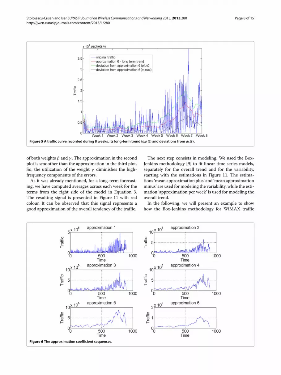
Next, we will consider a traffic curve recorded during 8weeks, represented in Figure 5 with blue.

The representation contains specific underlying overalltrend, represented in red. The other two curves representthe deviation, plus (in green)/minus (in black), from theapproximation signal. It can be observed that a large partof the traffic is contained between the green and blacklines. The red line indicates an increase of the traffic intime, suggesting the possibility of saturation of BS1.

The following step of the data preparation stage isthe multi-time scale analysis, implemented by the MRAdescribed in Equation 1. The sequences of approximation


Figure 3 A curve describing the weekly traffic evolution for a BS arbitrarily selected.

coefficients for six levels of decomposition are shown inFigure 6.

It can be observed that with a higher level of decom-position, the sequence of approximation coefficientsbecomes more smoothed. The sequences of detail coef-ficients for six levels of decomposition are depicted inFigure 7.

One of the goals of the multi-time scale analysis is toreduce the amount of data, by rejecting some detail coef-ficient sequences, without compromising the precision ofthe forecast. The result of this step is the new statistical

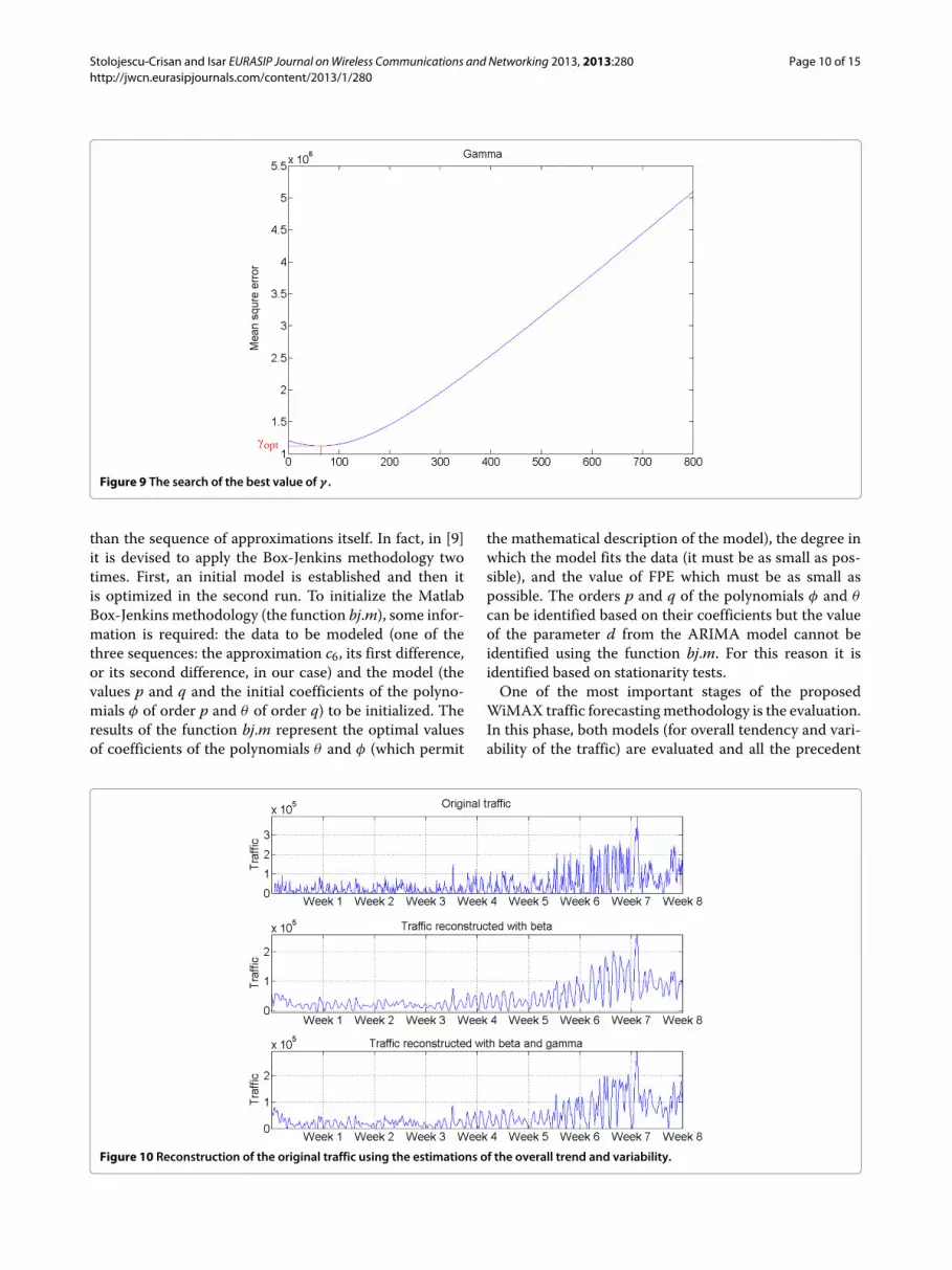
model of the traffic in Equation 3. It involves the identifi-cation of parameters β and γ , as it is shown in Equations5 and 7. In Figures 8 and 9, the minimization proceduresdescribed in Equations 5 and 7 are highlighted.

The reconstruction of the original traffic (first plot)using the estimation of the overall trend (realized usinga6) and the estimation of the variability (realized usingβd3-second plot and βd3 + γ d4-third plot) are presentedin Figure 10.

The approximation errors are higher in the second plotthan in the third plot. This remark justifies the utilization

Figure 4 The power spectral density of the signal from Figure 3. The arrow indicates the eighth harmonic.


Figure 5 A traffic curve recorded during 8 weeks, its long-term trend (a6(t)) and deviations from a6(t).

of both weights β and γ . The approximation in the secondplot is smoother than the approximation in the third plot.So, the utilization of the weight γ diminishes the high-frequency components of the errors.

As it was already mentioned, for a long-term forecast-ing, we have computed averages across each week for theterms from the right side of the model in Equation 3.The resulting signal is presented in Figure 11 with redcolour. It can be observed that this signal represents agood approximation of the overall tendency of the traffic.

The next step consists in modeling. We used the Box-Jenkins methodology [9] to fit linear time series models,separately for the overall trend and for the variability,starting with the estimations in Figure 11. The estima-tions ‘mean approximation plus’ and ‘mean approximationminus’ are used for modeling the variability, while the esti-mation ‘approximation per week’ is used for modeling theoverall trend.

In the following, we will present an example to showhow the Box-Jenkins methodology for WiMAX traffic

Figure 6 The approximation coefficient sequences.


Figure 7 The detail coefficient sequences.

prediction is applied. In Figure 12, the approximationcoefficients (a6) and their first and second differences arepresented.

The first step is to study which of these sequences arestationary, in order to establish the value of the param-eter d. The correlations of the signals in Figure 12 arerepresented in Figure 13.

The correlation of a stationary sequence must vanishafter few samples. Analyzing Figure 13, we can observethat the third sequence (from up to bottom) has the higherdecreasing speed. It has a peak in its middle. The sample

values fall rapidly at the left and the right of this pick,becoming close to zero. This decrease is faster than theone observed in the middle plot in Figure 13 or in theupper plot. The PAC of the signals in Figure 12 are repre-sented in Figure 14. They are also useful for the estimationof orders p and q.

Analyzing Figure 14, we obtain the same conclusion asin the case of Figure 13. The sequence obtained by com-puting the second difference of the sequence of approx-imations is more stationary than the sequence obtainedby computing the first difference of approximations or

Figure 8 The search of the best value of β.


Figure 9 The search of the best value of γ .

than the sequence of approximations itself. In fact, in [9]it is devised to apply the Box-Jenkins methodology twotimes. First, an initial model is established and then itis optimized in the second run. To initialize the MatlabBox-Jenkins methodology (the function bj.m), some infor-mation is required: the data to be modeled (one of thethree sequences: the approximation c6, its first difference,or its second difference, in our case) and the model (thevalues p and q and the initial coefficients of the polyno-mials φ of order p and θ of order q) to be initialized. Theresults of the function bj.m represent the optimal valuesof coefficients of the polynomials θ and φ (which permit

the mathematical description of the model), the degree inwhich the model fits the data (it must be as small as pos-sible), and the value of FPE which must be as small aspossible. The orders p and q of the polynomials φ and θ

can be identified based on their coefficients but the valueof the parameter d from the ARIMA model cannot beidentified using the function bj.m. For this reason it isidentified based on stationarity tests.

One of the most important stages of the proposedWiMAX traffic forecasting methodology is the evaluation.In this phase, both models (for overall tendency and vari-ability of the traffic) are evaluated and all the precedent

Figure 10 Reconstruction of the original traffic using the estimations of the overall trend and variability.


Figure 11 The average weekly long-term trend and the average daily standard deviation within a week.

steps are reviewed. In order to see if the new statisti-cal model in (3) is representative, we used ANOVA andwe computed the coefficient of determination. We haveobtained good results for each BS for both statistical mod-els, applying the forecasting algorithm to all the downlinktraces from the database and obtaining statistically sig-nificant ARIMA models for each traffic overall tendencyand variability of each BS. We have identified the modelparameters (p and q) using MLE. The best model was cho-sen as the one that provides the smallest AICC, BIC andFPE while offering the smallest mean square predictionerror for a number of weeks ahead.

The last stage of the proposed forecasting methodol-ogy consists in deployment. The models obtained for thelong-term trend of the downlink traces from the databaseindicate that the first difference of those time series is con-sistent with a simple MA model (p=0) with one or twoterms (q = 1 and d = 1 or q = 2 and d = 1) plus aconstant value μot . Similar results were obtained for themodels of variability of the traffic.

The moment when the saturation of the BS takes placecan be predicted comparing the trajectory of the over-all traffic forecast with the BS’s saturation threshold, asshown in Figure 15.

Figure 12 The approximation coefficients (first line) and their first (second line) and second (third line) differences.


Figure 13 Autocorrelations of sequence approximation (first line), their first (second line) and second (third line) differences.

The need for one differencing operation at lag one andthe existence of term μot across the model indicate thatthe long-term trend of the downlink traffic is a simpleexponential smoothing with growth. The trajectory forthe long-term forecasts will be a sloping line, whose slopeis equal to μot . Similar conclusions can be formulated forthe variability of the downlink traffic. The trajectory forthe variability forecast is a sloping line as well, but it hasa much smaller slope. The sum of these sloping lines isa third line, parallel with the trajectory of the long-termforecast, which represents the trajectory of the overall

forecast. Hence, the risk of saturation of a BS is propor-tional with the slope of its overall tendency. Given theestimates of μot across all models, corresponding to allBS, we can conclude, based on the positive values of thoseslopes, that all traces exhibit upward trends, but grow atdifferent rates.

4 ResultsThe slope of the overall tendency line in Figure 15 is equalto μot . Analyzing Figure 15, it can be observed that a BS

Figure 14 Partial correlations of sequence approximation (first line), their first (second line) and second (third line) differences.


Figure 15 The trajectory for the long-term forecasts.

saturates faster if μot has a higher value. Indeed, for thesame value of the saturation threshold, with the growth ofμot , the value of ts (which indicates the moment of satu-ration in Figure 15) will decrease. So, the value of μot isproportional with the saturation risk of the considered BS.

In Table 1, a classification of BS in terms of the satura-tion risk is presented. More precisely, the BS are listed indecreasing order of the slope of the overall tendency oftheir traffic. For BS50, the value of μot was estimated as

equal to 2.06 × 1016 bits/s2. The results obtained for BS50are not relevant because a lot of data are missing in thecorresponding trace, the interpolation process becomingnot reliable. The BS shown on the first column in Table 1have high values of μot . This means that these BS havea higher risk of saturation than the other ones. The BSwith the highest risk of saturation are the following: BS63,BS60, BS3, BS49, BS61. These are the BS which must beupgraded first. The moment, ts, when the upgrade must

Table 1 BS risk of saturation

BS μot (Mb/s2) BS μot (Mb/s2) BS μot (Mb/s2) BS μot (Mb/s2)

63 239.860 48 114.810 13 68.311 1 45.068

60 185.470 52 110.250 53 66.329 2 44.729

3 177.680 8 109.040 6 65.579 9 43.102

49 176.070 7 105.240 5 63.415 42 42.878

61 164.030 56 104.720 26 59.885 33 41.441

57 157.260 55 99.920 12 58.708 30 41.395

62 146.310 65 99.174 39 57.789 28 39.973

67 144.630 20 97.943 38 57.675 41 38.129

54 143.880 29 97.655 35 54.498 40 33.587

18 138.230 46 93.711 37 53.458 36 32.224

64 134.220 10 91.557 23 52.729 25 30.601

16 131.730 19 83.567 45 51.019 15 29.400

59 130.530 43 79.215 22 50.872 11 27.622

58 130.350 44 78.572 24 49.404 31 26.144

51 123.960 66 74.149 27 46.704 17 25.052

4 118.100 14 71.564 47 45.879 21 24.614

32 15.921


Figure 16 The proposed forecasting methodology.

take place can be computed using the values of μot and thevalues of the BS capacity, as it can be seen in Figure 15.

The base stations with the smallest risk of saturation areBS15, BS11, BS31, BS17 and BS21. Comparing the resultsin Table 1, it can be observed that the risk of saturationof BS63 is ten times bigger than the risk of saturationof BS21. So, the traffic of different BS is far to be uni-form. This is a significant result because it shows theexistence of some limitations in the design of WiMAXnetworks. This design is based on the Shanon commu-nications theory, which does not take into account someparticularities of the wireless networks, for example theirad hoc nature, or the effects of different social influences.The traffic analysis presented in this paper is useful fornetwork designers and administrators, being one of thefirst studies on WiMAX traffic forecasting subjects.

5 ConclusionsWe have argued that the traffic forecasting methodologyproposed in [2] can be regarded as a data mining method-ology and can be adapted for WiMAX traffic prediction.We have observed that the principal difference betweenthe wireline traffic considered in [2] and the WiMAX traf-fic consists in the higher variability of the wireless traffic.So, the adaptation of the traffic forecasting methodologypresented in Figure 1, in the case of the wireless traffic,consists in the optimization of the ANOVA procedure, ascan be seen in Figure 16 (we considered a second param-eter, γ , and we enphasized this modification using the redcircle).

This optimization is described in Equation 7. Because,in the case of WiMAX traffic, we have obtained smallerenergy values for the sequence d3 than the correspondingvalues obtained in [2], we have additionally considered thesequence d4.

The proposed forecasting methodology extracts thetraffic trends from historical measurements and can iden-tify the BS which exhibits higher growth rates and, thus,may require additional capacity in the future. It is capableof isolating the overall long trend and identifying the com-ponents that significantly contribute to its variability. Pre-dictions based on approximations of those componentsprovide accurate estimates with a minimal computationaloverhead. All our forecasts were obtained in seconds.All the procedures described are implemented as Matlabfunctions. We have found that the BS of the considered

network are more charged in downlink cycles than inuplink cycles. This unbalanced comportment gives someindications about the user needs, and its analysis can giveuseful information for the local operators, regarding thenumber of users at different locations within the network.We cannot come up with a single WiMAX network-wideforecasting model for the aggregate demand. Differentparts of the network grow at different rates (long-termtrend) and experience different types of variation (devia-tion from the long-term trend). This comportment provethat other methods must be applied to make the trafficuniform. For example, it could be possible to optimize thepositions of some BS [12].

This paper presents one of the first attempts to forecastthe traffic of a WiMAX network. Taking into account thehigh speed of traffic analysis developed by the proposedmethod (it works practically in real time), we consider thatit could be implemented by each WiMAX network serviceprovider.

Competing interestsThe authors declare that they have no competing interests.

Received: 29 July 2013 Accepted: 23 November 2013Published: 6 December 2013

References1. Z Rong, CR Qiu, X Xia, W Guoping, A case-based reasoning system for

individual demand forecasting, in Proceedings of the 4th InternationalConference on Wireless Communications, Networking and MobileComputing (WiCOM) (IEEE, Piscataway, 2008), pp. 1–6

2. K Papagiannaki, N Taft, Z Zhang, Diot C, Long-term forecasting of internetbackbone traffic: observations and initial models, in Proceedings of the IEEEINFOCOM (IEEE, Piscataway, 2003), pp. 1178–1188

3. NK Groschwitz, Polyzos G C, A time series model of long-term NSFNETbackbone traffic. Proc. IEEE Int. Conf. Commun. 3, 1400–1404 (1994)

4. P Chapman, Clinton J, Kerber R, Khabaza T, Reinartz T, Shearer C, Wirth R,CRISP-DM 1.0 Step-by-step data mining guide (2000). ftp://ftp.software.ibm.com/software/analytics/spss/support/Modeler/Documentation/14/UserManual/CRISP-DM.pdf. Accessed Nov 2013

5. Stolojescu C, Cusnir A, Moga S, Isar A, Forecasting WiMAX BS traffic bystatistical processing in the wavelet domain, in Proceedings of IEEEInternational Symposium on Signals, Circuits and Systems (Iasi, 9–10 July2009), pp. 177–180

6. L Rokach, Maimon O, The Data Mining and Knowledge Discovery Handbook:A Complete Guide for Researchers and Practitioners (Springer, New York,2005)

7. C Chatfield, Time-Series Forecasting (Chapman and Hall/CRC Press, BocaRaton, 2000)

8. HZ Moayedi, M Masnadi-Shirazi, ARIMA model for network trafficprediction and anomaly detection, in Proceedings of the InternationalSymposium on Information Technology (IEEE, Piscataway, 2008), pp. 1–6

9. GEP Box, GM Jenkins, G Reinsel, Time-Series Analysis: Forecasting andControl (Wiley, Hoboken, 2008)

ftp://ftp.software.ibm.com/software/analytics/spss/support/Modeler/Documentation/14/UserManual/CRISP-DM.pdf




10. CM Hurvich, Tsai C L, Regression and time series model selection in smallsamples. Biometrika. 76, 297–307 (1989)

11. PJ Brockwell, RA Davis, Introduction to Time Series and Forecasting(Springer, New York, 2002)

12. C Stolojescu, S Moga, P Lenca, P Isar, WiMAX traffic analysis and basestations classification in terms of LRD. J. Expert Syst. 30(4), 285–293 (2013)

doi:10.1186/1687-1499-2013-280Cite this article as: Stolojescu-Crisan and Isar: Forecasting WiMAX traffic bydata mining methodology. EURASIP Journal on Wireless Communications andNetworking 2013 2013:280.

Submit your manuscript to a journal and benefi t from:

7 Convenient online submission

7 Rigorous peer review

7 Immediate publication on acceptance

7 Open access: articles freely available online

7 High visibility within the fi eld

7 Retaining the copyright to your article

Submit your next manuscript at 7 springeropen.com

Documents

Forecasting WiMAX traffic by data mining methodology