Embed Size (px)
Citation preview
IIMB-WP No. 664/2022
WORKING PAPER NO: 664
Foreign Intermediate Inputs, Import Intermediaries, and Aggregate Productivity
Bernardo S Blum
Associate Professor of Economic Analysis and Policy, Director IIB,
Rotman School of Management, University of Toronto
Sebastian Claro Professor
Facultad de Ciencias Económicas y Empresariales, Universidad de los Andes, Chile
Kunal Dasgupta
Associate Professor of Economics and Social Sciences Indian Institute of Management Bangalore Bannerghatta Road, Bangalore – 5600 76
Ignatius J Horstmann Professor Emeritus, Economic Analysis and Policy,
Rotman School of Management University of Toronto
Marcos Rangel Associate Professor of Economics, Sanford School of Public Policy,
Duke University [email protected]
Year of Publication – May 2022
IIMB-WP No. 664/2022
Foreign Intermediate Inputs, Import Intermediaries, and Aggregate Productivity
Abstract Access to foreign intermediate inputs raises firm and aggregate productivity. This paper documents that domestic wholesalers provide such access by importing almost half of the foreign inputs used by Chilean firms. A calibrated model of trade and distribution shows that relative to the case where domestic firms can only buy directly from foreign suppliers, aggregate productivity under wholesaler importers is 7.5 percent higher. Wholesaler importers play such a large role because they allow medium and small domestic producers to buy from large (efficient) foreign suppliers. Moreover, increases in the efficiency of the wholesaler importing sector have a larger effect on aggregate productivity than similar reductions in tariffs or in the fixed cost of importing an intermediate input. Also, the presence of wholesaler importers doubles the effect of a trade liberalization on aggregate productivity. Keywords: Intermediaries, Intermediate input, Relationship costs, Productivity
Foreign Intermediate Inputs, Import Intermediaries, and
Aggregate Productivity
Bernardo S Blum* Sebastian Claro† Kunal Dasgupta‡ Ignatius J Horstmann§
Marcos Rangel¶
March 2022
Preliminary Draft
Abstract
Access to foreign intermediate inputs raises firm and aggregate productivity. This paper
documents that domestic wholesalers provide such access by importing almost half of the
foreign inputs used by Chilean firms. A calibrated model of trade and distribution shows
that relative to the case where domestic firms can only buy directly from foreign suppliers,
aggregate productivity under wholesaler importers is 7.5 percent higher. Wholesaler im-
porters play such a large role because they allow medium and small domestic producers
to buy from large (efficient) foreign suppliers. Moreover, increases in the efficiency of the
wholesaler importing sector have a larger effect on aggregate productivity than similar re-
ductions in tariffs or in the fixed cost of importing an intermediate input. Also, the presence
of wholesaler importers doubles the effect of a trade liberalization on aggregate productiv-
ity.
*Rotman School of Management, University of Toronto†Facultad de Ciencias Economicas y Empresariales, Universidad de los Andes, Chile‡Indian Institute of Management Bangalore§Rotman School of Management, University of Toronto¶Sanford School of Public Policy, Duke University
IMPORT INTERMEDIARIES AND PRODUCTIVITY 1
1. Introduction
Access to foreign intermediate inputs raises firm and aggregate productivity and, thus, can lead
to economic development. The challenge is that a multitude of trade agreements have already
reduced tariff and non-tariff barriers, with the exception of those on agricultural products, to
quite insignificant levels. It is, thus, not clear how countries can further increase firms’ access
to foreign inputs.
In this paper, we show that Chilean producers access foreign inputs in two ways. First, some
producers match directly with foreign suppliers and directly import the inputs they use. Other
firms, however, buy foreign inputs from domestic import wholesalers, who are the ones pur-
chasing the inputs from foreign suppliers. We document that both channels are empirically
important, with close to 50 percent of all foreign intermediate inputs used in Chile being traded
via wholesaler importers. This suggests that efficiency gains in the import intermediary sector
can lead to improved access to foreign inputs and, thus, to higher firm and aggregate produc-
tivity. This paper evaluates this possibility theoretically and quantitatively.
To gain insight on the way wholesaler importers facilitate intermediate input trade, we build
a unique data set matching each Chilean importer of intermediate inputs with its Argentinean
exporters. Critically, our data identify the line of business of the importer and the exporter:
manufacturer, wholesaler, retailer, etc. These data paint a sharp picture of how wholesale im-
porters facilitate intermediate input trade. First, exporters of intermediate inputs match with
few importers, and the relevant margin of adjustment for firm-level and firm-product-level ex-
ports is the amount sold per importer. Second, large exporters of intermediate inputs sell the
same intermediate input to both manufacturing firms and to wholesaler importers at the same
time. Third, large exporters of intermediate inputs maintain large trade relationships only, i.e.,
they do not engage in trade relationships that involve small trade volumes.
Motivated by these observations, we develop a model of trade and distribution that pro-
duces, in equilibrium, a trading system with the features described above. The key characteris-
tic of our model is that the main cost of selling inputs abroad is a distribution cost: the cost of
managing a trade relationship with customers. This cost includes, for instance, processing the
buyer’s orders, making sure these orders are filled correctly and on time, handling complaints
and product returns, and issuing invoices. In the management literature, this is often called
Customer Relationship Management (CRM). The challenge for foreign suppliers and domes-
tic producers is how to economize on these costs. In this context, trade intermediaries arise
endogenously as a potentially efficient technology for doing so.
A successful foreign transaction requires managing the relationship between the exporter
and the importer. This is part of the cost of doing business and includes, for instance, clarify-
ing any questions the buyer has about the product and delivery times, processing the buyer’s
2 BLUM, CLARO, DASGUPTA, HORSTMANN, RANGEL
orders, making sure these orders are filled correctly and on time, handling complaints and
product returns, issuing invoices, and making sure payment is received. In the management
literature, this is often called Customer Relationship Management (CRM).
The model allows for two distribution technologies to connect foreign suppliers to domes-
tic producers. One technology is a “direct-to-market” distribution technology, under which
suppliers and producers trade directly. This technology is essentially the one assumed by most
trade models. The alternative to selling directly is to use an “intermediated trade” distribution
technology in which foreign suppliers and domestic producers trade indirectly by pairing-up
with an import intermediary. As long as the cost of intermediation is not too large, this tech-
nology may be efficient relative to the direct-to-market selling technology, at least for some
suppliers.
Within this framework, we show that the equilibrium system of trade and distribution has,
within any class of intermediate goods, trade occurring via both direct selling and import in-
termediaries. In this equilibrium, import intermediaries allow domestic producers to access
inputs from small foreign suppliers, who would not be able to sell abroad at all if direct sell-
ing were the only option. More important, however, is that import intermediaries allow small
and medium domestic producers to access inputs from large and efficient foreign suppliers,
who otherwise would only sell to large domestic producers because of the cost of maintaining
a trade relationship.
The model produces the firm behaviors we find in the data. In particular, sales per buyer
is the relevant margin of trade expansion in the model. The reason is that, with maintaining a
trade relationship being costly, a supplier economizes on the number of producers with which
it trades by selling to an intermediary. For the same reason, large suppliers do not maintain
small trade relationships. Rather, they sell directly to large producers only, and serve small
producers via an intermediary. As a result, there is no sorting of foreign suppliers across export
mode, with large foreign suppliers selling, at the same time, to large domestic producers and to
wholesale importers.
In order to quantitatively solve the model and evaluate the role of various trade costs, we
calibrate key parameters of the model. The model is able to generate a number of the features
of the data, despite not targeting them directly. such as the empirical distribution of producers
a foreign supplier sells to.
We then go on to perform a number of counterfactual exercises. First, we ask what would
be the impact on aggregate productivity if foreign suppliers and domestic producers could only
trade directly, i.e., what is the contribution of wholesaler importers to aggregate productivity in
Chile? We find that, relative to the case where domestic producers can only buy directly from
foreign suppliers, wholesale importers raise aggregate productivity by 7.5 percent.
IMPORT INTERMEDIARIES AND PRODUCTIVITY 3
The absence of wholesaler importers studied in the first counterfactual exercise i) reduces
the the amount of imported inputs; and ii) makes firms that would optimally trade via whole-
salers trade directly instead. Our second counterfactual exercise separates these two effects. In
particular, in addition to removing the option of exporting through intermediaries, we lower
the fix cost of selling to a foreign buyer to keep input imports constant. We find that the pres-
ence of wholesale importers raises aggregate productivity by 1.5 percent, even keeping input
imports constant.
It is worth noting that, in the two counterfactual exercises just described, the presence of
wholesale importers has such a large effect not because it allows small exporters to sell in Chile
(which it does), but rather because it allows small and medium Chilean producers to import
inputs from large exporters. Without intermediaries, these large exporters would not find it
profitable to maintain a trade relationship with these small and medium importers.
The third counterfactual exercise we run studies the effect of a 10% productivity increase
in the wholesale import sector. We find that this results in a 0.8% increase in average firm
productivity. Critically, we find that this effect is eight times larger than the effect of a 10%
decrease in the cost of maintaining a customer relationship, and four times larger than a 10%
decrease in ad-valorem tariffs. This exercise highlights that an efficient import intermediary
sector can have a large effect on firms’ access to foreign inputs, with the associated gains to
productivity.
Finally, we study whether the effects of a trade liberalization episode depends on the pres-
ence and efficiency of wholesaler intermediaries. More precisely, we quantify the effect of a 10%
reduction in ad-valorem tariffs when wholesaler importers are present and when producers can
only import inputs directly from foreign suppliers (because intermediaries are too inefficient).
The effect of a trade liberalization on average firm productivity is twice as large in the presence
of wholesaler importers. The reason for this difference is that, in the presence of wholesaler
importers, a larger number of small and medium firms use foreign inputs. A decrease in tariffs
allows these firms to increase the amount of foreign inputs they use and, because these firms
were using small amounts of foreign inputs to begin with, this has a large marginal effect on
their productivity.
Our work is most closely related to two papers that use the structure of a model to quantify
the effect of access to foreign inputs on aggregate productivity. Gopinath and Neiman (2014)
shows that a large crisis increases the price of foreign inputs and leads to reductions in the
number of these inputs used by domestic producers. This, in turn, affects firm and aggregate
productivity. In their setting, domestic producers can only access foreign inputs by directly
importing them. In contrast, we show that a large share of foreign inputs is imported by do-
mestic intermediaries. This creates an extra margin of adjustment, namely switching between
4 BLUM, CLARO, DASGUPTA, HORSTMANN, RANGEL
importing inputs directly and via intermediaries. In particular, increases in the cost of a foreign
input make some producers to switch from importing it directly to buying it via domestic in-
termediaries. This attenuates the effect of the shock on productivity, as producers who would
otherwise stop using the foreign input altogether will continue to use it. But the presence of
intermediaries also magnifies the impact of the higher cost of foreign inputs on productivity.
Because intermediaries allow a larger number of small and medium domestic producers to ac-
cess foreign inputs, a shock to the price of these inputs makes these producers to substitute
away from these goods. Given that these firms tend to use small amounts of the foreign in-
put to begin with, the marginal effect of such substitution on productivity can be quite large.
We quantify these effects and find that an exogenous change in the cost of foreign inputs has
a larger effect on aggregate productivity in the presence of import intermediaries than when
firms can only import directly.
Halpern, Koren, and Szeidl (2015) study the contribution of foreign inputs to firm and ag-
gregate productivity in Hungary in the 1993-2002 period and find large effects. In their setting,
domestic producers can only access foreign inputs by importing them directly. This is justified
by the fact that only 2% of the imports of inputs into Hungary were carried out by intermedi-
aries, during the period they study. As we show, import intermediaries play a major role in Chile
in the 2000s. In general, the evidence points in the direction of trade intermediaries playing a
significant role in many, if not most countries (see Blum, Claro, and Horstmann (2018) for a
survey).
Our work is also related to a large literature that estimates the effect of foreign inputs on
firm outcomes, such as productivity and the probability of launching new products. The main
papers in this literature include Amiti and Konings (2007), Kasahara and Rodrigue (2008), Gold-
berg et al. (2010), Topalova and Khandelwal (2011), Boler, Moxnes, and Ultveit-Moe (2015),
Zhang (2017), and Fieler, Eslava, and Xu (2018). The focus of our work, in contrast to this liter-
ature, is on trade intermediaries and how they create access to foreign inputs. In order to study
the aggregate productivity effect of such access, we calibrate our model like in Gopinath and
Neiman (2014) and Halpern, Koren, and Szeidl (2015).
Another related literature studies the role of intermediaries in international trade. Blum,
Claro, and Horstmann (2018) surveys what is mostly reduced-form evidence indicating that
trade intermediaries play a meaningful role, primarily on the importing side of trade trans-
actions. In a recent paper, Defever, Imbruno, and Kneller (2020) confirms these findings by
showing that even domestic firms that do not import inputs directly benefit from tariff reduc-
tions, but only if they are in industries in which import intermediaries are important. Our work
adds to this literature in three ways. First, we show that import intermediaries play a major role
in the importation of inputs. Second, we uncover the characteristics of the technologies used
IMPORT INTERMEDIARIES AND PRODUCTIVITY 5
to trade inputs. Third, we quantify the productivity effects that import intermediaries have on
local producers.
Still in the same literature, Ahn, Khandelwal, and Wei (2011); Felbermayr and Jung (2016);
Akerman (2018); Dasgupta and Mondria (2018) develop models for the role played by interme-
diaries in international trade. A common feature of these models is that exporters sort them-
selves into selling direct or via intermediaries. We show that this is not a feature of the Chilean
data. In particular, large exporters of intermediate inputs sell a given product both directly
to domestic producers and sell to wholesaler importers. This has major implications for the
effects of trade intermediaries on aggregate productivity and welfare.
A key feature of our model is that the main cost of selling inputs abroad is the cost of main-
taining a trade relationship with a foreign buyer. We are not the first ones to study this kind of
cost. Early contributions in this area are Rauch (1999), Rauch (2001), Rauch and Watson (2004),
and Petropoulou (2011). More recent work include Bernard, Moxnes, and Ulltveit-Moe (2018),
Benguria (2021), Eaton, Kortum, and Kramarz (2022), and Eaton et al. (2022). In general, this lit-
erature finds that this cost plays an important role in explaining a number of patterns observed
in international trade data. None of these papers, however, studies trade intermediaries as a
natural way to economize on these costs. We start closing this gap and show that the presence
of a trade intermediation sector has important implications. To illustrate, with intermediaries
the effect of a trade liberalization episode in our model cannot be inferred from aggregate data
only, like in Arkolakis, Costinot, and Rodrıguez-Clare (2012). Blaum, Lelarge, and Peters (2018)
find a similar result in a model without intermediaries. In their model, firm-level data on value-
added and share of expenditures on domestic inputs are sufficient statistics for measuring the
impact of a change to the importing environment on consumer prices. This is the case in our
setting as well. However, we show that the share of firms’ expenditures on domestic (foreign)
inputs cannot be measured from imports data only, since domestic producers buy foreign in-
puts from domestic wholesalers as well.
The rest of the paper proceeds as follows.The next section describes the data and shows the
evidence on wholesaler importers. Sections 3 and 4 develop a model of trade and distribution
that captures the features of the data. Section 5 calibrates the model to Chilean data, and runs
a number of counterfactual exercises. The last section concludes.
2. Data and Evidence
2.1 Importers of intermediate inputs
The data sets used in this paper are compiled by various branches of the Chilean government.
The first data set we use comes from the Chilean Customs Office. These data contain all im-
6 BLUM, CLARO, DASGUPTA, HORSTMANN, RANGEL
port transactions into Chile, and we use this information for the year 2007. To these imports
data, we merge information produced by the Chilean Central Bank classifying each HS 8-digit
product as either a consumer good, a capital good, or an intermediate input. The classification
used by the Chilean Central Bank follows the guidelines for National Accounts published by the
United Nations so that consumer goods are those used, without any further transformation,
by households, government institutions and non-profit organizations for direct satisfaction of
their needs. In contrast, intermediate goods are ones used as intermediate inputs in produc-
tion processes, with the exception of goods that could be considered assets (used many times
to produce), which are classified as capital goods.
The third data set is obtained from Chile’s internal revenue service and identifies the main
line of business of each Chilean firm in the agency’s system. In particular, each firm is classified
as operating primarily under one of five mutually exclusive lines of business: i) Wholesalers,
ii) Retailers, iii) Manufacturers, iv) Service Providers, and v) Other. This last “catch-all” group
includes sectors not classified elsewhere, such as agriculture producers and the different levels
of government. We merge this information with the Chilean Customs data.
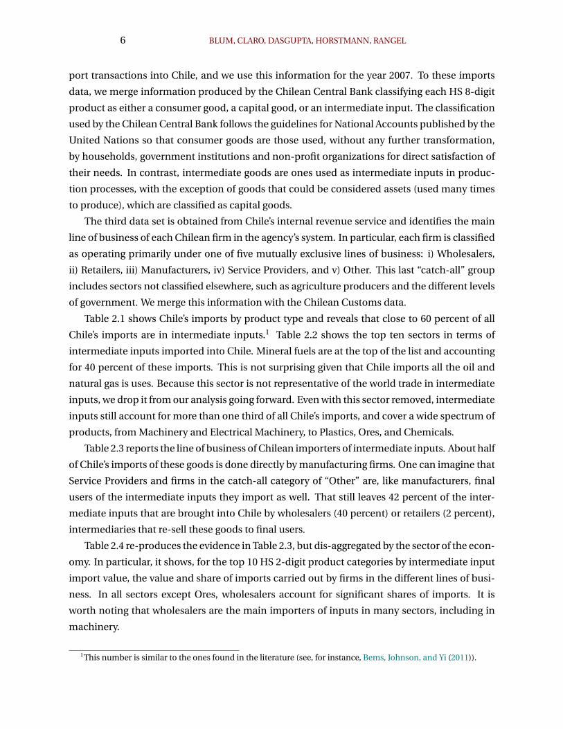
Table 2.1 shows Chile’s imports by product type and reveals that close to 60 percent of all
Chile’s imports are in intermediate inputs.1 Table 2.2 shows the top ten sectors in terms of
intermediate inputs imported into Chile. Mineral fuels are at the top of the list and accounting
for 40 percent of these imports. This is not surprising given that Chile imports all the oil and
natural gas is uses. Because this sector is not representative of the world trade in intermediate
inputs, we drop it from our analysis going forward. Even with this sector removed, intermediate
inputs still account for more than one third of all Chile’s imports, and cover a wide spectrum of
products, from Machinery and Electrical Machinery, to Plastics, Ores, and Chemicals.
Table 2.3 reports the line of business of Chilean importers of intermediate inputs. About half
of Chile’s imports of these goods is done directly by manufacturing firms. One can imagine that
Service Providers and firms in the catch-all category of “Other” are, like manufacturers, final
users of the intermediate inputs they import as well. That still leaves 42 percent of the inter-
mediate inputs that are brought into Chile by wholesalers (40 percent) or retailers (2 percent),
intermediaries that re-sell these goods to final users.
Table 2.4 re-produces the evidence in Table 2.3, but dis-aggregated by the sector of the econ-
omy. In particular, it shows, for the top 10 HS 2-digit product categories by intermediate input
import value, the value and share of imports carried out by firms in the different lines of busi-
ness. In all sectors except Ores, wholesalers account for significant shares of imports. It is
worth noting that wholesalers are the main importers of inputs in many sectors, including in
machinery.
1This number is similar to the ones found in the literature (see, for instance, Bems, Johnson, and Yi (2011)).
IMPORT INTERMEDIARIES AND PRODUCTIVITY 7
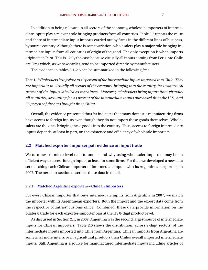
In addition to being relevant in all sectors of the economy, wholesale importers of interme-
diate inputs play a relevant role bringing products from all countries. Table 2.5 reports the value
and share of intermediate input imports carried out by firms in the different lines of business,
by source country. Although there is some variation, wholesalers play a major role bringing in-
termediate inputs from all countries of origin of the good. The only exception is when imports
originate in Peru. This is likely the case because virtually all inputs coming from Peru into Chile
are Ores which, as we saw earlier, tend to be imported directly by manufacturers.
The evidence in tables 2.1-2.5 can be summarized in the following fact:
Fact 1. Wholesalers bring close to 40 percent of the intermediate inputs imported into Chile. They
are important in virtually all sectors of the economy, bringing into the country, for instance, 50
percent of the inputs labelled as machinery. Moreover, wholesalers bring inputs from virtually
all countries, accounting for 43 percent of the intermediate inputs purchased from the U.S., and
55 percent of the ones brought from China.
Overall, the evidence presented thus far indicates that many domestic manufacturing firms
have access to foreign inputs even though they do not import these goods themselves. Whole-
salers are the ones bringing these goods into the country. Thus, access to foreign intermediate
inputs depends, at least in part, on the existence and efficiency of wholesale importers.
2.2 Matched exporter-importer pair evidence on input trade
We turn next to micro-level data to understand why using wholesaler importers may be an
efficient way to access foreign inputs, at least for some firms. For that, we developed a new data
set matching each Chilean importer of intermediate inputs with its Argentinean exporters, in
2007. The next sub-section describes these data in detail.
2.2.1 Matched Argentine exporters – Chilean Importers
For every Chilean importer that buys intermediate inputs from Argentina in 2007, we match
the importer with its Argentinean exporters. Both the import and the export data come from
the respective countries’ customs office. Combined, these data provide information on the
bilateral trade for each exporter-importer pair at the HS 8-digit product level.
As discussed in Section 2.1, in 2007, Argentina was the second largest source of intermediate
inputs for Chilean importers. Table 2.6 shows the distribution, across 2-digit sectors, of the
intermediate inputs imported into Chile from Argentina. Chilean imports from Argentina are
somewhat more intensive in agricultural products than Chile’s overall imported intermediate
inputs. Still, Argentina is a source for manufactured intermediate inputs including articles of
8 BLUM, CLARO, DASGUPTA, HORSTMANN, RANGEL
plastic, processed foods, paper and paperboard products, metals, chemicals and machinery.
Overall, Fact 1 applies to trade between Argentina and Chile as well.
As with Chilean importers, we use information from Argentina’s internal revenue service to
classify each exporter to Chile as a wholesaler, a retailer, a manufacturer, a service provider, or
other. In contrast to the evidence on importers, Argentinean manufacturers account for the
lion’s share of this country’s exports of intermediate inputs to Chile. More precisely, Argentine
manufacturers are the direct exporters of over 80 percent of the sales of intermediate inputs
to Chile. Moreover, the trade that is not exported by manufacturers is primarily in agricultural
products, cereals being the largest category. Input imports from Argentina are typical also in the
sense that the vast majority of Chilean importers intermediate inputs from Argentina are man-
ufacturing firms (32%) or wholesalers (35%). For the rest of the paper, we focus on intermediate
inputs exported by Argentinean manufacturing firms to Chilean wholesalers or manufacturing
firms.
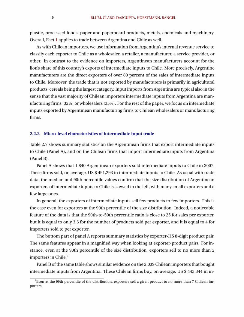
2.2.2 Micro-level characteristics of intermediate input trade
Table 2.7 shows summary statistics on the Argentinean firms that export intermediate inputs
to Chile (Panel A), and on the Chilean firms that import intermediate inputs from Argentina
(Panel B).
Panel A shows that 1,840 Argentinean exporters sold intermediate inputs to Chile in 2007.
These firms sold, on average, US $ 491,293 in intermediate inputs to Chile. As usual with trade
data, the median and 90th percentile values confirm that the size distribution of Argentinean
exporters of intermediate inputs to Chile is skewed to the left, with many small exporters and a
few large ones.
In general, the exporters of intermediate inputs sell few products to few importers. This is
the case even for exporters at the 90th percentile of the size distribution. Indeed, a noticeable
feature of the data is that the 90th-to-50th percentile ratio is close to 25 for sales per exporter,
but it is equal to only 3.5 for the number of products sold per exporter, and it is equal to 4 for
importers sold to per exporter.
The bottom part of panel A reports summary statistics by exporter-HS 8-digit product pair.
The same features appear in a magnified way when looking at exporter-product pairs. For in-
stance, even at the 90th percentile of the size distribution, exporters sell to no more than 2
importers in Chile.2
Panel B of the same table shows similar evidence on the 2,039 Chilean importers that bought
intermediate inputs from Argentina. These Chilean firms buy, on average, US $ 443,344 in in-
2Even at the 99th percentile of the distribution, exporters sell a given product to no more than 7 Chilean im-porters.
IMPORT INTERMEDIARIES AND PRODUCTIVITY 9
termediate inputs from Argentina per year, and the distribution of purchases across importers
is skewed as well, with many small importers and a few large ones. As on the exporting side,
these importers buy a relatively small number of HS 8-digit products and buy from few Argen-
tinian sellers. Even at the 90th percentile of the distribution of the number of exporters per
importer–product pair, importers buy a given product from one Argentinian seller only.3
Figure 2.1 plots the relationship between exporter size – dollar value of exports of inter-
mediate inputs to Chile – against the number of intermediate inputs traded, and against the
number of Chilean importers sold to. Figure 2.2 shows the number of Chilean importers sold
to by exporter-HS 8-digit product pairs against exporter size.4 These figures provide visual con-
firmations that, although larger exporters of intermediate inputs sell more products and sell to
more buyers, even the largest exporters tend to not sell much more than a dozen HS 8-digit
products and tend to sell to few buyers. Indeed, at the exporter-product level, even the largest
exporters sell, on average, to a hand-full of buyers only.
A formal decomposition of the variation in sales across exporters into parts due to differ-
ences in the number of products sold, in the number of buyers sold to, and in the dollar value
of sales by product and buyer, quantifies the relevance of each margin of export expansion. In
particular, we can write:
Xi = Pi ×Mi × xi,
where Xi is the dollar value of Argentine exporter i’s sales in intermediate inputs to Chile, Pi
is the number of products this exporter sells to Chile, Mi is the number of buyers this exporter
sells to in Chile, and xi is the dollar value this exporter sells per product and importer. The
above equation gives rise to the following:
V ar(lnXi) = Cov(lnPi, lnXi) + Cov(lnMi, lnXi) + Cov(lnxi, lnXi)
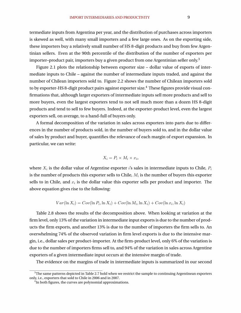
Table 2.8 shows the results of the decomposition above. When looking at variation at the
firm level, only 13% of the variation in intermediate input exports is due to the number of prod-
ucts the firm exports, and another 13% is due to the number of importers the firm sells to. An
overwhelming 74% of the observed variation in firm level exports is due to the intensive mar-
gin, i.e., dollar sales per product-importer. At the firm-product level, only 6% of the variation is
due to the number of importers firms sell to, and 94% of the variation in sales across Argentine
exporters of a given intermediate input occurs at the intensive margin of trade.
The evidence on the margins of trade in intermediate inputs is summarized in our second
3The same patterns depicted in Table 2.7 hold when we restrict the sample to continuing Argentinean exportersonly, i.e., exporters that sold to Chile in 2006 and in 2007.
4In both figures, the curves are polynomial approximations.
10 BLUM, CLARO, DASGUPTA, HORSTMANN, RANGEL
stylized fact:
Fact 2. The main margin of export expansion for Argentine exporters selling intermediate inputs
to Chile is the intensive margin of trade: dollars-per-product-per-importer.
Before we discuss the next stylized fact, we should mention that that finding that the main
margin of export expansion is dollars-per-product-per-importer is in Carballo, Ottaviano, and
Martincus (2018), for exports data from Costa Rica, Ecuador, and Uruguay (see their Table 2 of
the unpublished manuscript). In addition to confirming their finding, we show that it holds for
trade in intermediate inputs as well. Along the same lines, the finding that most exporters sell to
few, often one importer, is in all papers with data on matched exporter-importer pairs, includ-
ing Blum, Claro, and Horstmann (2010), Carballo, Ottaviano, and Martincus (2018), Bernard,
Moxnes, and Ulltveit-Moe (2018), and Benguria (2021)). Again, we confirm that this pattern
holds in our data for trade in intermediate inputs.
Figure 2.3 looks at the firms that Argentine exporters sell to in Chile. In particular, this figure
reports the share of Argentine exporters of intermediate inputs to Chile that sell to wholesaler
importers only (red line), to manufacturing firms only (blue line), and to both, wholesaler im-
porters and manufacturers (green line).
Figure 2.3 reveals that large exporters of intermediate inputs do not sort across exporting
modes; rather, they sell to both wholesaler importers and to manufacturing firms. Figure 2.4
plots the same variables for the sub-sample of exporters that sell to at least 2 importers. As
Figure 2.1 showed, the majority of exporters sell to one importer only. Among the exporters that
have multiple trade relationships, selling to both wholesaler importers and to manufacturing
firms is the norm. Figure 2.4 further reveals that hardly any exporter of inputs sells to multiple
wholesaler importers only; they either sell to one wholesaler and other manufacturers, or to
multiple manufacturers. One can see this from the fact that the curve showing the share of
exporters that sell to multiple importers and sell to at least 2 wholesalers is always very close to
zero.
It is of course possible that exporters sell different products to wholesale importers and
manufacturing firms, but do sort across export mode for any given product. Figures 2.5 and
2.6 address this question. Figure 2.5 shows the share of Argentine exporter-HS 8 product pairs
that trade with wholesaler importers only (red line), with manufacturing importers only (blue
line), and with both wholesaler importers and manufacturers (green line). A similar, although
less extreme, pattern is visible in this figure as in Figure 2.3. Large exporter-HS 8 pairs tend to
trade with both wholesalers and manufacturers at the same time. The attenuation in Figure 2.5
relative to Figure 2.3 reflects the fact that, at the exporter-HS 8 product level, it is much more
likely that an exporter sells to one importer only. Figure 6 looks at the sub-sample of exporter-
HS 8-digit product pairs sold to more than one importer, and it shows that no-sorting continues
IMPORT INTERMEDIARIES AND PRODUCTIVITY 11
to be the norm in this case as well.
These findings are summarized in the following stylized fact:
Fact 3. Large Argentine exporters of intermediate inputs do not sort across export modes, even
within HS 8-digit product. Instead, they tend to sell both directly to manufacturers and via
wholesaler importers.
Figures 3-6 reveal the export mode choices of small exporters as well. Although these ex-
porters are somewhat more likely to sell to wholesaler importers, a large share of them sell to
manufacturers only. In this sense, as a group, small exporters of inputs do not sort across export
modes either. This finding is summarized in the following stylized fact:
Fact 4. As a group, small Argentine exporters of intermediate inputs do not sort across export
modes. Although these firms are more likely to sell via wholesaler importers, there is a non-trivial
share of these exporters that sell exclusively to manufacturing firms.
Confirming the importance of both export modes, Figure 2.7 shows the share of dollars
traded directly via wholesaler importers, by exporter size. Of course, one minus this share is
traded directly to manufacturers. The figure shows that the two modes of trade account for
about half of the input trade. A similar results appears when the analysis is done at the exporter-
HS 8-digit product level.
Finally, Figure 2.8 reports, for each Argentine exporter, the dollar amount transacted with
their smallest and their largest trade partner in Chile. As established in Figure 2.1, most of the
small exporters trade with one importer only and, thus, the two curves in Figure 2.9 coincide
for these firms. Figure 2.10 shows the same metric for Argentine exporter-HS 8-digit product
pairs. Again in this case, the two curves coincide for the small exporter-product values.
The interesting feature of these figures, however, is that the smallest relationship that ex-
porters maintain grows steeply with exporter size. This is especially true at the exporter-HS
8-digit level. These figures then suggest that large exporters of an intermediate input do not
maintain small trade relationships. This is summarized in our final stylized fact:
Fact 5. Large Argentine exporters of intermediate inputs to Chile do not maintain small trade
relationships.
3. A Model of Trade and Distribution
It is natural to assume that wholesale importers arise to economize on some trade frictions.
Thus, given that standard models of intermediate goods trade have manufacturers trade di-
rectly with each other, these models fail to capture such frictions. In addition to generating
12 BLUM, CLARO, DASGUPTA, HORSTMANN, RANGEL
indirect trade as an efficient outcome, a model of trade in inputs should capture two additional
features of the data presented in the previous section. First, the intensive margin of trade is the
main margin of expansion for trade in intermediate inputs. More precisely, exporters that sell
large amounts of intermediate inputs to a country do so by selling large values per product per
importer. Second, exporters do not sort between selling direct and selling via intermediaries.
In particular, large exporters sell, at the same time, directly to manufacturers and wholesalers.
Small exporters sell either directly to manufacturers or via intermediaries but, as a group, sell
via both modes. The trade models currently in the literature featuring trade intermediaries
cannot rationalize these features of the data (Ahn, Khandelwal, and Wei, 2011; Felbermayr and
Jung, 2016; Akerman, 2018; Dasgupta and Mondria, 2018).
In this section, we develop a model of trade and distribution that produces the above fea-
tures of the data as an equilibrium outcome. In the model, the main cost of selling inputs
abroad is the cost of managing trade relationships with foreign customers. Faced with this
cost, the challenge for exporters and their foreign market customers is to develop trading ar-
rangements that economize on this cost. In equilibrium, trade intermediaries, and the mixed
trading system they induce, arise endogenously as an efficient technology for doing so.
The model has two countries, home and foreign, each with a mass of heterogeneous firms
that produce differentiated varieties. There is roundabout production: the differentiated goods
are used as intermediate inputs in production as well as consumed by final consumers. For
simplicity, we assume that home firms (producers) do not export. Furthermore, foreign firms
(suppliers) only sell intermediate inputs in the home market, i.e., foreign suppliers do not com-
pete in the home final goods market. Labor is the only factor of production in the home market
and the market for labor is perfectly competitive.
3.1 Heterogeneity
The home country has a mass of monopolistically competitive producers with exogenous pro-
ductivity j, drawn from a distribution G(j) with support [j, j]. Similarly, each foreign supplier
produces a unique input and draws productivity i from the distribution G∗ with support [i, i].
Suppliers vary in terms of their marginal cost of production, which, for simplicity, is assumed
to be 1/i. For brevity, we refer to a supplier/producer with productivity i/j simply as supplier
i/producer j, and the corresponding variety as variety i/j.
IMPORT INTERMEDIARIES AND PRODUCTIVITY 13
3.2 Preference
Consumers have standard CES preferences:
U =[ ∫
jqf (j)1−
1σ dG(j)
] σσ−1
,
where qf (j) is the final consumption of variety j, and σ > 1 is the elasticity of substitution.
These preferences give rise to the following final price index
P f =[ ∫
jp(j)1−σdG(j)
] 11−σ
,
where p(j) is the corresponding price of variety j paid by final consumers.
3.3 Technology
Producer j has the following production function:
Y (j) = j(L(j)
α
)α( Z(j)
1− α
)1−α,
where j is the total factor productivity, and L(j) and Z(j) correspond to labor and intermediate
inputs respectively. The share of labour in production, α, is assumed to be the same across
producers. Z(j), in turn, combines a bundle of domestic intermediate inputs, D(j), and foreign
intermediate inputs, R(j), in the following way:
Z(j) =[D(j)1−
1σ +R(j)1−
1σ
] σσ−1
,
where D(j) and R(j) are CES aggregates as well (Ethier, 1982):
D(j) =[ ∫j′∈ΩD(j)
qm(j′, j)1−1σ dG(j′)
] σσ−1
; R(j) =[ ∫i∈ΩR(j)
qm(i, j)1−1σ dG(i)
] σσ−1
.
qm(j′, j) and qm(i, j) are the amounts of intermediate input purchased by producer j from pro-
ducer j′ and supplier i respectively. Observe that the elasticity of substitution for domestic
varieties is assumed to be (i) the same for final consumers and producers, and (ii) the same as
foreign varieties (Krugman and Venables, 1995). ΩD(j) and ΩR(j) are the set of domestic and
foreign firms respectively that producer j buys from. Let the price of input s paid by producer
j be denoted by pm(s, j). The aggregate input price index, P (j), is given by
P (j) =[PD(j)
1−σ + PR(j)1−σ
] 11−σ
,
14 BLUM, CLARO, DASGUPTA, HORSTMANN, RANGEL
where PD(j) and PR(j) are the price indices corresponding to the domestic and the foreign
input bundles respectively:
PD(j) =[ ∫j′∈ΩD(j)
pm(j′, j)1−σdG(j′)] 1
1−σ; PR(j) =
[ ∫i∈ΩR(j)
pm(i, j)1−σdG(i)] 1
1−σ.
3.4 Cost
We assume that output of each domestic producer is also used as input by every other domes-
tic producer. The implicit assumption is that the cost of establishing a relationship within a
country is small enough to allow producers to purchase all domestic inputs. This implies that
ΩD(j) = ΩD,
where ΩD is the set of all domestic producers. Furthermore, there exists a decentralized market
for domestic varieties, resulting in a single price for every variety, i.e., pm(j′, j) = p(j′) for all
j′ ∈ ΩD.5 Consequently, the domestic input price index becomes
PD(j) = PD =[ ∫
j′∈ΩD
p(j′)1−σdG(j′)] 1
1−σ.
Given the preferences, the price charged by domestic producer j, p(j), is a constant mark-up
over marginal cost. Setting the home nominal wage as the numeraire, the marginal cost of
producer j is given by
c(j) = P (j)1−α/j.
The input cost, P (j)1−α, is j-specific. This is because, despite every producer using the same set
of domestic intermediate inputs, the set of foreign inputs, ΩR(j), could potentially vary across
j. In fact, one of the objectives of this model is to examine how the choice of multiple modes
of export could shape the availability of foreign intermediate inputs for individual domestic
producers.
3.5 Revenue
Because of the assumption of a common elasticity of substitution, P f = PD. Producer j’s rev-
enue from selling to final consumers is then
xf (j) =(p(j)PD
)1−σY,
5The price charged to the final user and intermediate user must be the same. Otherwise there are arbitrageopportunities.
IMPORT INTERMEDIARIES AND PRODUCTIVITY 15
where Y is aggregate spending and p(j) = σσ−1c(j). Similarly, producer j’s revenue from selling
to producer j′ is
xm(j, j′) = (1− α)(1− 1/σ)( p(j)
P (j′)
)1−σx(j′),
where x(j′) is total revenue of producer j′.6 One can then solve for total revenue of producer j:
x(j) =(p(j)PD
)1−σ(Y + (1− α)(1− 1/σ)
∫j′∈ΩD
λ(j′)x(j′)dG(j′)), (1)
where λ(j′) = [PD/P (j′)]1−σ ≤ 1.7 When producer j′ does not use any foreign intermediate
inputs, λ(j′) reduces to 1. At the other extreme, if domestic producers do not use any domestic
intermediate input, λ(j′) = 0 and (1) simply converges to demand from final consumers. As we
shall see later, if j′ is more productive than j′′, ΩR(j′′) ⊆ ΩR(j
′). In this case, λ(j′′) ≥ λ(j′).
3.6 Relationships
A successful foreign transaction requires managing the relationship between the exporter and
the importer. This is part of the cost of doing business and includes, for instance, clarifying any
questions the buyer has about the product and delivery times, processing the buyer’s orders,
making sure these orders are filled correctly and on time, handling complaints and product re-
turns, issuing invoices, and making sure payment is received. In the management literature,
this is often called Customer Relationship Management (CRM). Note that these costs are in-
curred every period and, thus, are different from the cost of finding customers.
We assume that there is a uniform, fixed cost, f , for adding a foreign customer to an ex-
porter’s list of customers. This cost is borne by the exporter. Specifically, an exporter incurs a
cost of f per importer that the exporter sells to. Later on, we examine how our main results
might change if we allow this cost to vary across exporters. To highlight the role played by this
per-customer cost, at this point we ignore all other standard trading costs that are assumed in
the literature.8
There are two types of domestic importers that an exporter could potentially transact with:
producers and intermediaries. The latter buys foreign intermediate inputs from the exporters
who want to sell through the intermediary, and then sells those inputs to domestic producers.
6To see this, note that we can write xm(j, j′) =(
p(j)P (j′)
)1−σ
E(j), where E(j) is total expenditure by producer j.
Because total expenditure is a fraction 1 − 1σ
of total revenue, and each producer spends a fraction 1 − α of totalexpenditure on intermediate inputs, E(j) = (1− α)(1− 1
σ)x(j).
7We have x(j) = xf (j) +∫j′ x
m(j, j′)dG(j′). Replacing the value for xm(j, j′) and re-arranging yields the expres-sion for x(j).
8Such costs might take the form of an ad-valorem cost (capturing tariffs, transportation technology, etc.), a pershipment cost (capturing bureaucracy, distribution technology, etc.) or a firm-level fixed cost (capturing one timecosts of entering foreign markets).
16 BLUM, CLARO, DASGUPTA, HORSTMANN, RANGEL
An exporter has to pay the same fixed cost f , whether matching with a producer or an interme-
diary. The intermediary, however, does not incur a per-buyer cost when selling to a domestic
producer. The intermediary does incur certain costs that that are introduced later.
4. Equilibrium
In this section, we solve for an industry equilibrium, taking aggregate spending Y as given.9
Recall that one of the key findings from the empirical section is that Argentine exporters, espe-
cially those who are large, sell the same product through multiple modes – direct and indirect
(through an intermediary). To examine the implications of such behaviour, we make a simpli-
fying assumption: a home producer is indifferent between purchasing a given input directly
or indirectly. The foreign supplier, on the other hand, optimally chooses how to sell to a given
producer. We now analyze the options facing the suppliers.
When a foreign supplier i sells directly to a domestic producer j, the supplier charges a price
that is a constant mark-up over marginal cost:
p(i, j) = p(i) =σ
σ − 1
1
i. (2)
The revenue i earns from selling to j, x(i, j), is then given by 10
x(i, j) = ξ( 1
iP (j)
)1−σx(j), (3)
where ξ = (1−α)(1− 1σ )
σ is a constant and x(j) is given by (1). The following lemma establishes
a key property of the equilibrium.
Lemma 1. x(i, j) is increasing in j.
Relative to a less productive producer, a more productive producer purchases more of every
input. If there were no imported intermediate inputs, we would have P (j) = PD and the result
in Lemma 1 would be obvious from (3).11 In an equilibrium where producers have the choice of
importing intermediate inputs, a more productive producer (higher j) has a lower input price
index, P (j). Conditional on x(j), this tends to reduce the demand for a given foreign input. At
the same time, a more productive producer also produces more, which raises x(j) and increases
the demand for all foreign inputs. Lemma 1 shows that given the assumptions on technology,
9The implicit assumption is that the industry’s share in total spending is small.10We drop the superscript m from the revenue function as foreign importers sell only intermediate inputs in the
home country.11To see this, note that with P (j) = PD, x(i, j) = ξ[(PD)αj]σ−1x(j). Because x(j) is increasing in j, the result
follows.
IMPORT INTERMEDIARIES AND PRODUCTIVITY 17
the latter force dominates. The profit earned by i when selling directly to j is then given by
π(i, j) = 1σx(i, j).
Because of the assumption that domestic producers are indifferent between importing a
given input directly or indirectly, if there are no purchasing costs (such as a fixed fee) other than
price, the intermediary must charge a price given by (2) as well. But the intermediary provides
a costly service by purchasing from exporters and selling to producers. Hence, the price that
the exporter charges to the intermediary must be less than what it charges when selling directly,
thereby allowing the intermediary to recover its cost, and possibly make a profit.
Now, producer j’s demand for input i is the same, irrespective of whether he purchases it di-
rectly or indirectly. Consequently, if producer j purchases the input from the intermediary, the
total surplus created by the exporter and the intermediary together is π(i, j). We assume that
the exporter and the intermediary engage in Nash Bargaining over the surplus with bargaining
weights β and 1 − β respectively. Specifically, the exporter offers a price to the intermediary
such that the exporter gets a share β of this surplus, leaving the remaining (1− β) for the inter-
mediary.12 The next proposition follows:
Proposition 1. Exporter i charges a price pI(i) to the intermediary, where
pI(i) = p(i)[1− 1
σ(1− β)
]. (4)
Two observations are in order. First, as long as β < 1, the exporter charges a lower price
to the intermediary relative to producers.13 As mentioned above, the lower price allows the
intermediary to recover the cost of the services that it provides.14 Second, selling indirectly
does not involve double marginalization, as the exporters endogenously reduce their mark-up
while selling to the intermediary. The extent of mark-up reduction depends on β.
Exporter i chooses how to serve each producer j: directly or indirectly. Selling directly yields
π(i, j)−f . When the exporter sells indirectly, the fixed cost per buyer, f , has to be incurred only
once. Hence, selling to j indirectly yields βπ(i, j), provided that the exporter is already selling
indirectly to some other producer j′. This is an important point that we return to below. The
exporter compares the returns from the two modes and chooses the one that yields the higher
return.12Observe that an exporter does not bargain with a producer. We justify this in the following way: because pro-
ducers use multiple inputs, measuring the surplus created by producer j and exporter i would require knowledgeof all the inputs i = i′ used by j, something that i is unlikely to have. We implicitly assume that the surplus createdby the producer and the exporter is not observed by the exporter, and hence difficult to bargain over.
13In our data, Argentinian exporters that sell the same HS 8-digit product to a Chilean manufacturing firm and toa Wholesaler charge, on average, a 3.5% lower price to the wholesaler, after controlling for transaction size.
14This result does not depend on the exporter charging a constant mark-up over marginal cost when sell-ing directly. In particular, let exporter i charge a price p′(i) when selling directly. It can then be shown thatpI(i) = p′(i)[β + (1− β) 1
i/p′(i)], where 1
iis marginal cost of supplier i. As long as p′(i) > 1
i, i.e. as long as supplier i
charges some mark-up, we have pI(i) < p′(i).
18 BLUM, CLARO, DASGUPTA, HORSTMANN, RANGEL
j
Pay-off
j
Direct
Indirect
jM (i)jD(i)
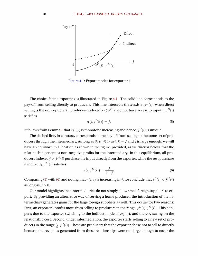
Figure 4.1: Export modes for exporter i
The choice facing exporter i is illustrated in Figure 4.1. The solid line corresponds to the
pay-off from selling directly to producers. This line intersects the x-axis at jD(i): when direct
selling is the only option, all producers indexed j < jD(i) do not have access to input i. jD(i)
satisfies
π(i, jD(i)
)= f. (5)
It follows from Lemma 1 that π(i, j) is monotone increasing and hence, jD(i) is unique.
The dashed line, in contrast, corresponds to the pay-off from selling to the same set of pro-
ducers through the intermediary. As long as βπ(i, j) > π(i, j)− f and j is large enough, we will
have an equilibrium allocation as shown in the figure, provided, as we discuss below, that the
relationship generates non-negative profits for the intermediary. In this equilibrium, all pro-
ducers indexed j > jM (i) purchase the input directly from the exporter, while the rest purchase
it indirectly. jM (i) satisfies:
π(i, jM (i)
)=
f
1− β. (6)
Comparing (5) with (6) and noting that π(i, j) is increasing in j, we conclude that jD(i) < jM (i)
as long as β > 0.
Our model highlights that intermediaries do not simply allow small foreign suppliers to ex-
port. By providing an alternative way of serving a home producer, the introduction of the in-
termediary generates gains for the large foreign suppliers as well. This occurs for two reasons:
First, an exporter i profits more from selling to producers in the range [jD(i), jM (i)]. This hap-
pens due to the exporter switching to the indirect mode of export, and thereby saving on the
relationship cost. Second, under intermediation, the exporter starts selling to a new set of pro-
ducers in the range [j, jD(i)]. These are producers that the exporter chose not to sell to directly
because the revenues generated from these relationships were not large enough to cover the
IMPORT INTERMEDIARIES AND PRODUCTIVITY 19
corresponding relationship costs.
In the literature, intermediaries have often been modelled as allowing firms to export by
incurring a lower fixed cost but higher marginal cost (Ahn, Khandelwal, and Wei, 2011; Felber-
mayr and Jung, 2016; Akerman, 2018; Dasgupta and Mondria, 2018). In such a specification, the
introduction of intermediaries benefits direct exporters at the margin: those who can barely
cover the fixed cost of exporting. These exporters switch to indirect exporting and experience
an increase in profit (ignoring possible general equilibrium effects). The largest exporters, how-
ever, are unaffected as they continue to sell directly. In our model, even the largest exporters
can potentially benefit from intermediation because they can serve a subset of home producers
indirectly while continuing to sell directly to the rest. For an allocation, such as one represented
in Figure 4.1 to be an equilibrium, it must be the case that none of the producers want to switch
the import mode. Because producers are indifferent between purchasing directly or indirectly
by assumption, this is necessarily true. But despite the producers not choosing which inputs to
import or how to import a given input, an equilibrium features variation in both the measure
of imported inputs as well as the share of directly imported inputs across producers.
How does the cutoff jM (i) vary with i? The following lemma establishes a property of jM (i)
that will be useful later.
Lemma 2. jM (i) is weakly decreasing in i.
To sell a new variety, the intermediary needs to incur some cost. We assume that the inter-
mediary incurs a cost of h per foreign variety added to its portfolio. Because intermediaries are
in the business managing customer relationships, we see h and f as measuring slightly different
things. First, we assume that the intermediary already has the capacity to manage relationships
with all Chilean customers. Thus, h is not incurred on a per customer basis. In contrast, h is
incurred on a per variety basis. The idea is that each variety a intermediary adds to its portfolio
creates some extra cost. The business literature often refers to this as the cost of complexity,
which includes not only direct costs such as materials and labor needed to handle the extra
variety, but also indirect costs to management.15 Note that h reflects the underlying productiv-
ity of the intermediary; more productive intermediaries have lower h. We also assume that the
costs h and f are incurred before the bargaining stage; this ensures that the surplus from the
relationship is simply π(i, j), as assumed earlier. For an exporter i to sell indirectly, the share of
the surplus going to the exporter must cover the fixed relationship management cost,
β
∫ jM (i)
jπ(i, j)dG(j) ≥ f,
15The notion that complexity is costly is present in areas as diverse as management (Lindemann, Maurer, andBraun (2008)) and evolutionary biology (Orr (2000)).
20 BLUM, CLARO, DASGUPTA, HORSTMANN, RANGEL
while the share of the surplus going to the intermediary must cover the fixed complexity cost,
(1− β)
∫ jM (i)
jπ(i, j)dG(j) ≥ h.
Combining the above two equations, an exporter sells indirectly if the following participation
constraint is satisfied:16 ∫ jM (i)
jπ(i, j)dG(j) ≥ max
[fβ,
h
1− β
]. (7)
The above equation gives the range of parameter values under which a foreign supplier i chooses
to export indirectly. For a given f and β, a higher h makes it less likely that i will be able to ex-
port indirectly. An increase in β, the exporter’s bargaining weight, involves a trade-off. A higher
β increases the exporter’s incentive from selling indirectly, but reduces the intermediary’s. Ac-
cordingly, a high β could prevent the exporter from selling indirectly, despite the surplus being
large enough to cover both the fixed costs (f and h).17
We define a function S(i, j) that returns the mode through which a foreign supplier i serves
home producer j:
S(i, j) =
D if i sells directly to j,
I if i sells indirectly to j,
∅ if i does not sell to j.
S(i, j) is defined for every pair (i, j). For example, if i′ does not export, S(i′, j) = ∅ for all j. Using
S(i, j), we can define the following set of foreign suppliers who export:
ΨD = i|∃j s.t. S(i, j) = D and ∄j s.t. S(i, j) = I.
ΨD is the set of suppliers who export to some home producers directly but do not use the in-
termediary, i.e. it is the set of producers who only export directly. Similarly, we define ΨI as the
set of exporters who only export indirectly and ΨM as the set of exporters who use both export
modes, i.e. mixed exporters. Finally, we define ΨNX as the set of suppliers who do not export.
We are now in a position to define an equilibrium of the model.
Definition 1. An equilibrium consists of:
1. a function S(i, j) for all i and j,
2. a set of direct exporters, ΨD, indirect exporters, ΨI , mixed exporters, ΨM , and non-exporters,
16If exporter i sells through the intermediary, he will sell indirectly to all producers j < jM (i) and not a subset ofproducers in [j, jM (i)] because the marginal cost of adding a producer through the indirect mode is zero.
17Even if∫ jM (i)
jπ(i, j)dG(j) > f + h, the relationship may not materialize if β is close to zero or close to one. In
such a situation, despite the transaction being ex-post efficient, the outcome is ex-ante inefficient.
IMPORT INTERMEDIARIES AND PRODUCTIVITY 21
ΨNX , such that
(i) suppliers maximize profits, and
(ii) the participation constraint for intermediation (equation 7) is satisfied.
Previously we had established that if supplier i is a mixed exporter, then there exists a jM (i)
such that i sells directly to all j ≥ jM (i) and indirectly to all j ≤ jM (i), i.e., the sets of producers
served directly and indirectly are connected sets. The next lemma establishes a convenient
property of the equilibrium.
Lemma 3. The sets ΨD, ΨI , ΨM and ΨNX are connected.
The above lemma implies, for example, that if supplier i1 prefers selling indirectly over di-
rectly, while supplier i2 > i1 prefers selling directly over indirectly, then all i > i2 should also
prefer selling directly over indirectly. Essentially, the pay-offs from using the different export
modes across suppliers satisfies a single-crossing property. Lemma 3 simplifies the analysis
considerably. As an example, if we want to examine how the set of suppliers with different
export modes are affected by a change in f , we simply need to consider how the thresholds
between the different sets change.
It follows from (6) that for a supplier i to only export indirectly, we must have π(i, j) < f/(1−β), provided that the participation constraint for intermediation is satisfied.18 Given the nature
of derived demand for intermediate inputs, this inequality will hold only if j is finite. In other
words, if the productivity distribution for home producers is unbounded, then every foreign
supplier will end up with a positive share of direct exports. In what follows, we assume that j
is finite. To obtain an interesting equilibrium, we furthermore make the following assumptions
about the marginal cost distribution of foreign suppliers:
Assumption 1.∫ jj π(i, j)dG(j) < f .
Assumption 2. π(i, j) > f/(1− β).
Assumption 3. π(i, j) < f .
Assumption 1 implies that the least productive supplier, i, does not find it profitable to ex-
port.19 Assumption 2 implies that the most productive supplier, i, always exports directly to
the most productive home producer, even when intermediation is feasible. Finally, Assump-
tion 3 implies that the same supplier does not find it profitable to export directly to the least
productive home producer. These three assumptions give rise to an equilibrium where (i) the
least productive foreign suppliers do not export (Bernard and Jensen, 1999), (ii) some suppliers
export directly, and (iii) even the most productive exporters might export indirectly.
18Because π(i, j) is increasing in j, if π(i, j) < f/(1− β) then π(i, j) < f/(1− β) for all j.19If the aggregate profit from exporting is less than the fixed relationship cost, exporting is not profitable, either
directly or indirectly.
22 BLUM, CLARO, DASGUPTA, HORSTMANN, RANGEL
We are now in a position to characterize the equilibrium, which depends on the relative val-
ues of the cost parameters, f and h, and the bargaining weight β. For the following discussions,
we assume that β ≥ 12 . We consider two separate cases.
4.1 Efficient intermediation
We say that intermediation is efficient when the following holds:
f
h>
( 1
β− 1
)−1,
i.e., when h is low relative to f . Because π(i, j) is continuous and decreasing in j, Assumptions
2 and 3 imply that there exists a jM (i) ∈ (j, j) where jM (i) satisfies π(i, j) = f/(1 − β).20 That
is, the most productive foreign supplier sells directly to a positive measure of home producers.
Let i be defined as
π(i, j) =f
1− β. (8)
i is the foreign supplier who is indifferent between exporting directly or indirectly to the most
productive home producer. Lemma 2 implies that we can always find such an i. Hence, all
suppliers indexed i < i will export only indirectly to a positive measure of home producers, if
exporting through an intermediary is feasible. Now, because β > 12 , (8) implies that π(i, j) >
f/β. Furthermore, f/β = max[f/β, h/(1− β)]. Accordingly,
∫ j
jπ(i, j)dG(j) > max
[fβ,
h
1− β
].
It follows that i, and by continuity some i < i, will export only indirectly. Let i be defined as
∫ j
jπ(i, j)dG(j) =
f
β.
i is the foreign supplier who is indifferent between exporting indirectly or not exporting at all.
Assumption 1 suggests that we can always find such an i. Then all producers with productivity
i < i do not export.
Finally, consider a supplier with i′ > i. For such an exporter, π(i′, jM (i′)) = f/(1− β). Using
a similar argument as above, we have
∫ jM (i′)
jπ(i′, j)dG(j) >
f
β.
20From Assumptions 2 and 3 we have π(i, j) > f/(1− β) > π(i, j). The result then follows from the IntermediateValue Theorem.
IMPORT INTERMEDIARIES AND PRODUCTIVITY 23
This suggests that every foreign supplier who exports directly also exports indirectly. We sum-
marize in the following proposition.
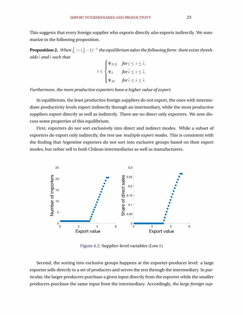
Proposition 2. When fh > ( 1β −1)−1 the equilibrium takes the following form: there exists thresh-
olds i and i such that
i ∈
ΨNX for i ≤ i ≤ i,
ΨI for i ≤ i ≤ i,
ΨM for i ≤ i ≤ i.
Furthermore, the more productive exporters have a higher value of export.
In equilibrium, the least productive foreign suppliers do not export, the ones with interme-
diate productivity levels export indirectly through an intermediary, while the most productive
suppliers export directly as well as indirectly. There are no direct only exporters. We now dis-
cuss some properties of this equilibrium.
First, exporters do not sort exclusively into direct and indirect modes. While a subset of
exporters do export only indirectly, the rest use multiple export modes. This is consistent with
the finding that Argentine exporters do not sort into exclusive groups based on their export
modes, but rather sell to both Chilean intermediaries as well as manufacturers.
Figure 4.2: Supplier-level variables (Low h)
Second, the sorting into exclusive groups happens at the exporter-producer level: a large
exporter sells directly to a set of producers and serves the rest through the intermediary. In par-
ticular, the larger producers purchase a given input directly from the exporter while the smaller
producers purchase the same input from the intermediary. Accordingly, the large foreign sup-
24 BLUM, CLARO, DASGUPTA, HORSTMANN, RANGEL
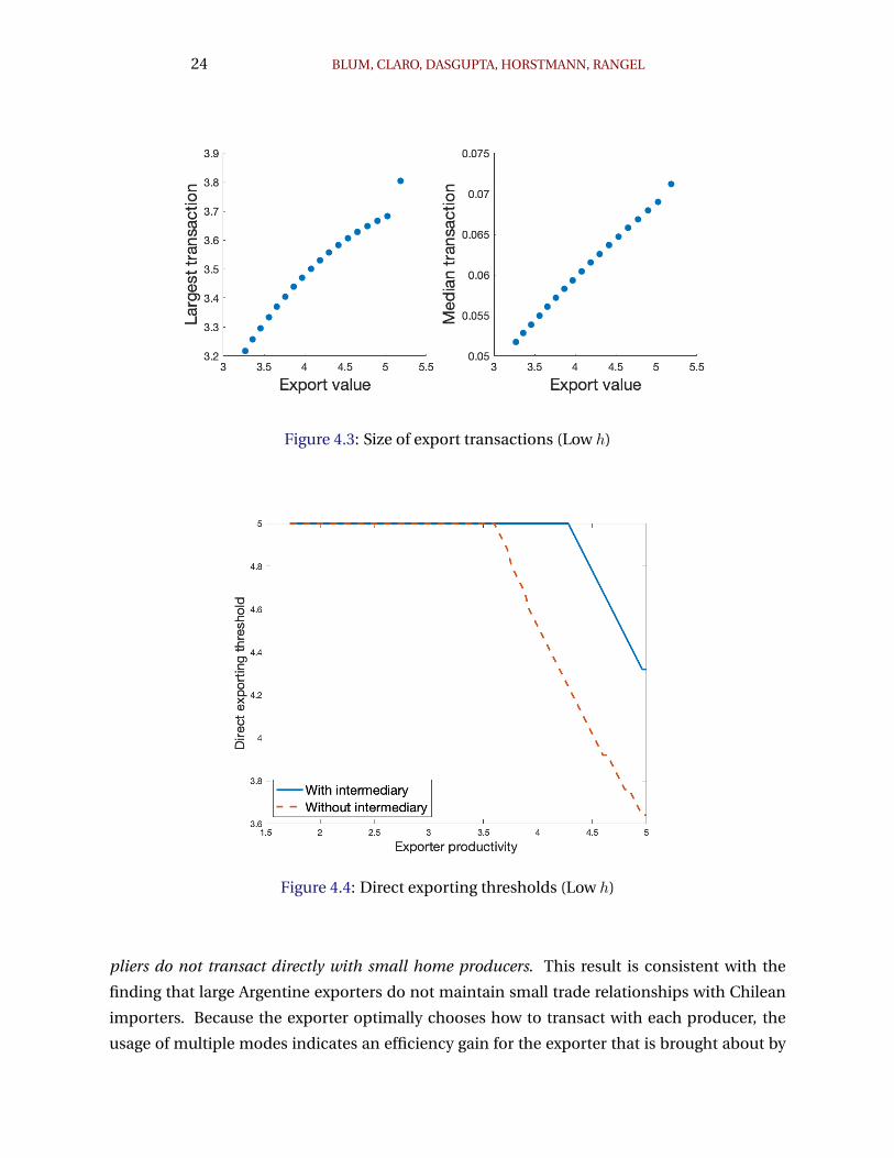
Figure 4.3: Size of export transactions (Low h)
Figure 4.4: Direct exporting thresholds (Low h)
pliers do not transact directly with small home producers. This result is consistent with the
finding that large Argentine exporters do not maintain small trade relationships with Chilean
importers. Because the exporter optimally chooses how to transact with each producer, the
usage of multiple modes indicates an efficiency gain for the exporter that is brought about by
IMPORT INTERMEDIARIES AND PRODUCTIVITY 25
the choice provided by the intermediary.
Third, consider two foreign suppliers i1 and i2 where i1 > i2 > i, i.e., both i1 and i2 are direct
exporters. Proposition 2 suggests that relative to i2, i1 has a higher value of exports (is larger).
Now, a corollary of Lemma 2 is that more productive exporters also sell directly to (weakly)
more producers. It follows that larger direct exporters also sell to more importers. Observe that
for suppliers who only export indirectly, the number of importers is just one (the intermediary).
Combining these two observations along with the sorting of exporters as stated in Proposition
2, we conclude that larger exporters also sell to more importers. This result is consistent with the
finding that relative to small Argentine exporters, large Argentine exporters sell to more Chilean
importers.
Finally, there are no exporters who only export directly (ΨD = ∅) in this equilibrium – ev-
ery exporter sells through the intermediary. Because any home producer can purchase an im-
ported input from an intermediary without having to incur any additional cost, every home
producer has access to the same set of intermediate inputs. Thus, we have an equilibrium
where every producer endogenously uses a standardized input that is an aggregate across all
individual imported inputs. Note that this feature is typically an assumption in many models
of international trade. We show that this result is obtained even when foreign suppliers opti-
mally choose which home producers to sell to; a key requirement is the presence of “efficient”
intermediaries.
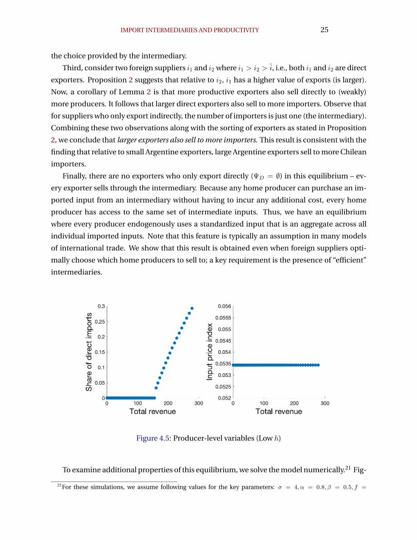
Figure 4.5: Producer-level variables (Low h)
To examine additional properties of this equilibrium, we solve the model numerically.21 Fig-
21For these simulations, we assume following values for the key parameters: σ = 4, α = 0.8, β = 0.5, f =
26 BLUM, CLARO, DASGUPTA, HORSTMANN, RANGEL
ure 4.2 and 4.3 show the correlation between export value and a number of other variables. As
already discussed above, the number of importers is weakly increasing in export value: it is one
for the indirect exporters and strictly increasing for the rest. A similar relation exists between
the share of direct sales and export value – this share is zero for all the indirect exporters and is
strictly increasing for the mixed exporters. The largest transaction of a (mixed) exporter is also
increasing in export value. Observe that the largest transaction could either be with the inter-
mediary or a producer. More importantly, the median transaction is also increasing in export
value, consistent with the sales per importer distribution being shifted to the right for larger
exporters. Each of these patterns find support in the data. Finally, Figure 4.4 shows the re-
optimization brought about the availability of intermediation. It plots the productivity of the
least productive producer a supplier sells to directly, both with and without intermediation.
In the presence of intermediation, the set of direct transactions shrinks for every supplier, as
suppliers choose to serve the less productive producers indirectly.
We can also look at producer-level variables. In Figure 4.5, we examine how the (i) share
of direct imports and (ii) the input price index, P (j), varies with producer size (total revenue).
Bigger producers are matched with more foreign exporters,22 resulting in them importing a
larger share of the foreign inputs directly. But as the set of inputs (both domestic and imported)
used is exactly the same across producers, the input price index is the same too – the difference
in producer size is driven only by the underlying exogenous productivity.
Observe that the above equilibrium configuration was obtained under the assumption of
β ≥ 12 . How do the results change if this assumption is relaxed? From (8), we see that a decline
in β causes productivity of the cut-off producer to fall. Because β determines the share of sur-
plus that a supplier obtains from the intermediary, a lower β reduces the supplier’s incentive to
export indirectly resulting in increased direct sales. Therefore, higher bargaining power of the
intermediary actually leads to lower sales through the intermediary and hence, lower profits.
The key to this result, once again, is the ability to serve the same producer through multiple
exporting modes.
4.2 Inefficient intermediation
Intermediation is inefficient whenf
h< (
1
β− 1)−1,
i.e. when h is high relative to f . Assumptions 2 and 3 continue to imply that (8) still holds:
there exists a i such that all exporters with productivity i > i export directly. But in this case,
0.005, h = 0.005. Both the supplier’s and producer’s productivity distributions are assumed to be truncated Pareto.22This follows from an exporter i selling directly to all importers in the range [jM (i), j], and jM (i) being a decreas-
ing function of i.
IMPORT INTERMEDIARIES AND PRODUCTIVITY 27
h/(1 − β) = max[f/β, h/(1 − β)]. Accordingly, one can always find a h such that the following
holds: ∫ jM (i′)
jπ(i′, j)dG(j) <
h
1− β,
for some i′ > i. In this case, the exporter i′ would like to export to every importer j < jM (i′)
through the intermediary. But the share of the surplus that accrues to the intermediary is not
enough to cover the fixed capacity cost h. As a result, in equilibrium i′ ends up exporting di-
rectly only. We summarize in the following proposition.
Proposition 3. For h large enough, the set ΨD is non-empty.
Now consider a i′′ ∈ ΨD. Assumption 2 implies that the following must be true:
π(i′′, j) < f.
Supplier i′′ does not export directly to the least productive producer j. At the same time, i′′
does not export to j through the intermediary either. We conclude that j, and by continuity,
a set of producers with low enough productivity do not use the input produced by supplier
i′′. This observation has the following implication: it is no longer the case that every home
producer uses the same standardized bundle of inputs. Rather, the less productive producers
also use fewer imported inputs – the productivity differences are magnified in the presence of
endogenous input usage.
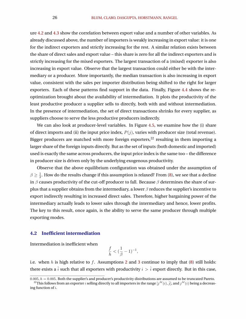
Figure 4.6: Supplier-level variables (High h)
One way to generate an equilibrium where producers have access to different imported in-
28 BLUM, CLARO, DASGUPTA, HORSTMANN, RANGEL
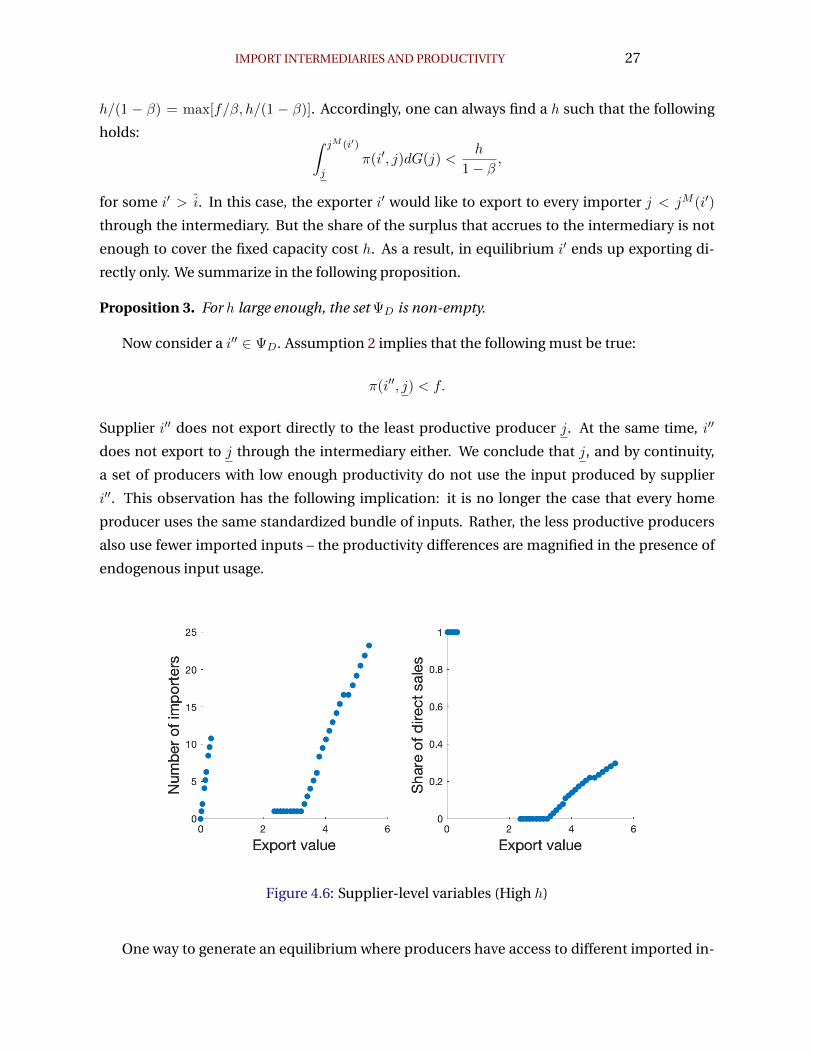
Figure 4.7: Producer-level variables (High h)
puts is to assume that producers, facing a fixed cost of importing an input, optimally choose
how many inputs to use. In such a setting, more productive producers end up using more in-
puts as their scale allows them to incur the fixed costs more often (Gopinath and Neiman, 2014;
Halpern, Koren, and Szeidl, 2015). Our model provides an alternative mechanism. Instead of
optimizing producers, we have optimizing exporters who choose which producers to sell to,
and what export mode to use. Variation in input access across producers arises when the in-
direct mode of export is not feasible for certain exporters. Accordingly, our model highlights
the role the efficiency of the intermediation sector plays in making foreign intermediate inputs
available to producers, especially the less productive ones.
The properties of one such equilibrium are shown in Figures 4.6 and 4.7. As in the sce-
nario with low h, the most productive suppliers in this equilibrium export using multiple modes
while the suppliers with lower productivity export only through intermediaries. But unlike in
the previous scenario, there now exists a third group of foreign suppliers with even lower pro-
ductivity who export directly only. While these suppliers can profitably export to a subset of
home producers, the surplus generated when they export indirectly is not large enough to cover
the capacity cost of the intermediary. Observe that direct exporting arises in this equilibrium
because importing is not profitable for the intermediary, not because direct exporting is more
profitable than indirect exporting for the foreign supplier.
It is worth discussing this last point in more detail as it explains, more generally, the lack
of sorting across distribution modes for small exporters as a group. What the model is saying
is that small exporters of intermediate inputs face a trade-off when choosing an export mode.
IMPORT INTERMEDIARIES AND PRODUCTIVITY 29
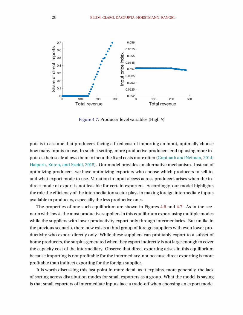
Figure 4.8: Supplier-level variables (Very high h)
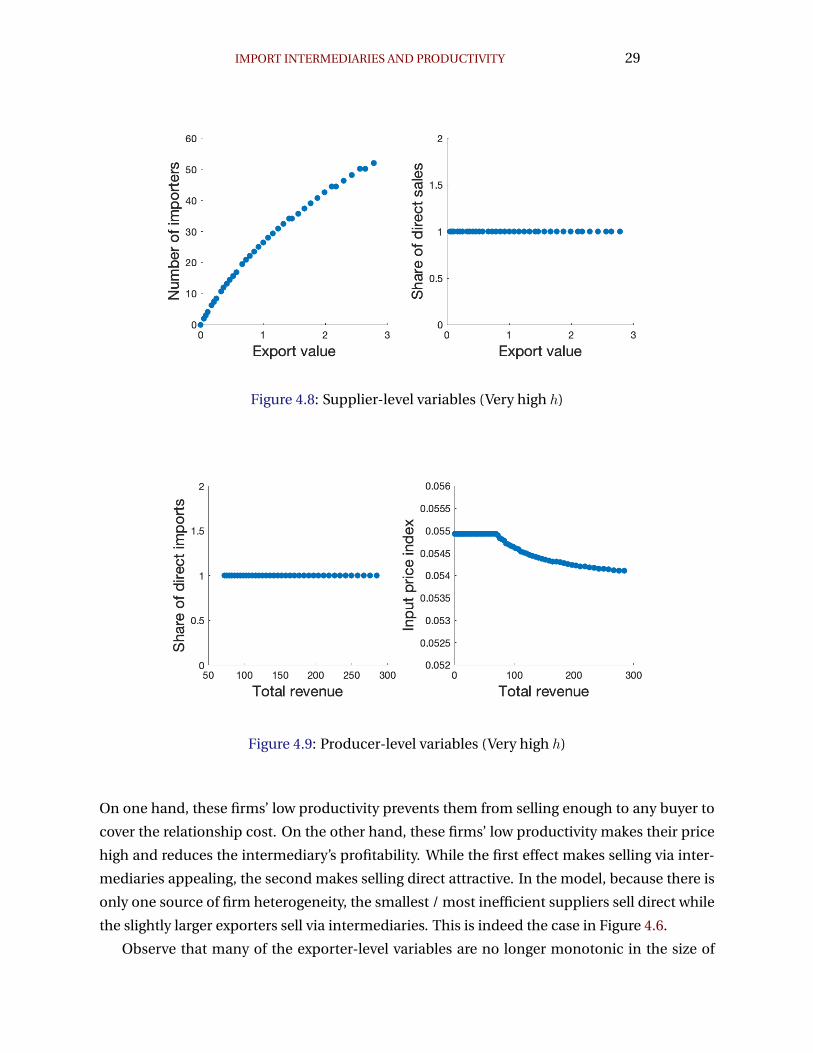
Figure 4.9: Producer-level variables (Very high h)
On one hand, these firms’ low productivity prevents them from selling enough to any buyer to
cover the relationship cost. On the other hand, these firms’ low productivity makes their price
high and reduces the intermediary’s profitability. While the first effect makes selling via inter-
mediaries appealing, the second makes selling direct attractive. In the model, because there is
only one source of firm heterogeneity, the smallest / most inefficient suppliers sell direct while
the slightly larger exporters sell via intermediaries. This is indeed the case in Figure 4.6.
Observe that many of the exporter-level variables are no longer monotonic in the size of
30 BLUM, CLARO, DASGUPTA, HORSTMANN, RANGEL
exporters. This is because the set of indirect exporters are bounded below and above by sets of
direct exporters (the latter also sell indirectly). Consequently, while the number of importers
sold to is increasing in export value for the least productive exporters, it drops to one for those
with intermediate productivity but then starts increasing again.
Moving on to the home producers, the larger and more productive producers continue to
import a greater share of their input directly as before. But as discussed earlier, the input price
index is no longer the same across producers. The direct exporters sell only to a subset of pro-
ducers and these happen to be the most productive among all the producers.23 Accordingly,
the most productive home producers face a lower aggregate input price.
Finally, we consider an equilibrium where h is so high that intermediation is not feasible
for any of the foreign producers. In such a scenario, foreign suppliers only sell directly with
the larger exporters selling to more importers (Figure 4.8). The price index also looks similar to
the one in the previous equilibrium: weakly decreasing in producer revenue. But there is a key
difference – unlike in the previous equilibrium where the least productive home producers im-
ported through the intermediary, the same set of importers do not import in this equilibrium.
This exercise once again highlights the role of intermediaries in making foreign inputs available
to the least productive home producers.
5. Quantitative Exercise
The model with intermediaries developed above illustrates how the interaction of two costs, the
per buyer relationship management cost and the intermediary’s complexity cost, can generate
a range of equilibrium configurations, both in terms of export participation by foreign suppliers
and access of domestic producers to intermediate inputs. This section studies quantitatively
the effects of these costs. More precisely, this section performs a series of counterfactual exer-
cises to quantify the importance of wholesale importers.
We begin by noting that in the model presented in Section 3, all exporters with a given pro-
ductivity level choose the same mode of export. While such one-to-one mapping between pro-
ductivity and exporting mode is analytically convenient, the data displays some heterogeneity.
In a departure from the model, we assume that every exporter-product draws a h from a distri-
bution. This is supposed to capture the fact that some product varieties are more costly for an
intermediary to handle than others. In practice, we assume that h is drawn from a log-normal
23Although we do not have information on the total output (size) of Chilean manufacturers, our data containinformation on the global imports of the Chilean importers. If we use this as a proxy for firm size, we can checkwhether the manufacturers that small Argentinean exporters sell to in Chile are, indeed, among the largest firms.Figures 11 and 12 show this evidence. More precisely, these figures show the size of the smallest and the largestmanufacturer buyer, in terms of its global imports in 2007. Both at the exporter level and at the exporter-HS 8-digitproduct, when the smallest Argentine exporters sell directly to a manufacturer importer, it is a large importer.
IMPORT INTERMEDIARIES AND PRODUCTIVITY 31
distribution with mean µh and variance vh.
One counterfactual of interest being trade liberalization, we introduce an ad-valorem cost
of trade τ into the model. To solve the model, we then need values for the following parameters:
the elasticity of substitution (σ), the labour share of output (α), the Nash bargaining weight of
the suppliers (β), the fixed relationship management cost (f ), domestic aggregate income (Y ),
parameters of the distribution cost (µh and vh) and the measure of foreign firms. Finally, we
need to parameterize the productivity distributions of both suppliers and producers.
We set σ equal to 4 (Broda and Weinstein, 2006) and α equal to 0.35 (Gopinath and Neiman,
2014). We also assume both productivity distributions to be Pareto with a shape parameter
of θ and bounded below by one (a normalization). Following Eaton, Kortum, and Kramarz
(2011), we assign a value of 7 to θ.24 Below we describe how we obtain values for the remaining
parameters.
5.1 Calibration
To calibrate the remaining six parameters, we need six moments. We make the following ob-
servations. First, aggregate domestic spending acts as a demand-shifter that changes the sales
of every foreign supplier. Accordingly, it has implications for the mean value of exports. Sec-
ond, the relationship management cost and the distribution cost, by influencing the suppliers’
decision to export and choice of export mode, determine the intensive and extensive export
margins. Finally, the measure of foreign suppliers, N∗, conditional on aggregate income and
the various costs, determines the actual number of foreign exporters. These observations in-
fluence our choice of moments to target: (i) the number of foreign exporters, (ii) mean export
value, (iii) the fraction of foreign suppliers who export, (iv) the fraction of exporters who only
sell indirectly, (v) the fraction of exporters who sell using both modes, and (vi) the share of ex-
port value that is sold through both modes. The values for all the parameters are shown in Table
5.1.
Table 5.2 shows the selected moments in the data (column 1) as well as the model (column
2).25 While we can exactly match the number and share of suppliers exporting, the model also
does well in terms of matching mean exports and the fraction of indirect-only exporters.The
model with a uniform f , however, significantly underestimates the fraction of mixed exporters
and the share of exports going through them. Accordingly, it overestimates the share of direct-
only exporters.
The resultant relationship cost, f , is 2, 400, and the mean value for the distribution cost, h,
24Eaton, Kortum, and Kramarz estimate θσ−1
to be equal to 2.4. When σ equals 4, the corresponding value of θ isaround 7.
25These moments are obtained for exporter-HS 8-digit distributions, where the HS 8-digit product is the mainproduct sold by the exporter.
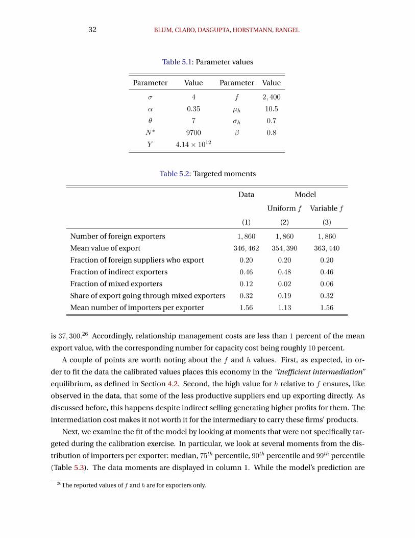
32 BLUM, CLARO, DASGUPTA, HORSTMANN, RANGEL
Table 5.1: Parameter values
Parameter Value Parameter Value
σ 4 f 2, 400
α 0.35 µh 10.5
θ 7 σh 0.7
N∗ 9700 β 0.8
Y 4.14× 10¹²
Table 5.2: Targeted moments
Data Model
Uniform f Variable f
(1) (2) (3)
Number of foreign exporters 1, 860 1, 860 1, 860
Mean value of export 346, 462 354, 390 363, 440
Fraction of foreign suppliers who export 0.20 0.20 0.20
Fraction of indirect exporters 0.46 0.48 0.46
Fraction of mixed exporters 0.12 0.02 0.06
Share of export going through mixed exporters 0.32 0.19 0.32
Mean number of importers per exporter 1.56 1.13 1.56
is 37, 300.26 Accordingly, relationship management costs are less than 1 percent of the mean
export value, with the corresponding number for capacity cost being roughly 10 percent.
A couple of points are worth noting about the f and h values. First, as expected, in or-
der to fit the data the calibrated values places this economy in the “inefficient intermediation”
equilibrium, as defined in Section 4.2. Second, the high value for h relative to f ensures, like
observed in the data, that some of the less productive suppliers end up exporting directly. As
discussed before, this happens despite indirect selling generating higher profits for them. The
intermediation cost makes it not worth it for the intermediary to carry these firms’ products.
Next, we examine the fit of the model by looking at moments that were not specifically tar-
geted during the calibration exercise. In particular, we look at several moments from the dis-
tribution of importers per exporter: median, 75th percentile, 90th percentile and 99th percentile
(Table 5.3). The data moments are displayed in column 1. While the model’s prediction are
26The reported values of f and h are for exporters only.
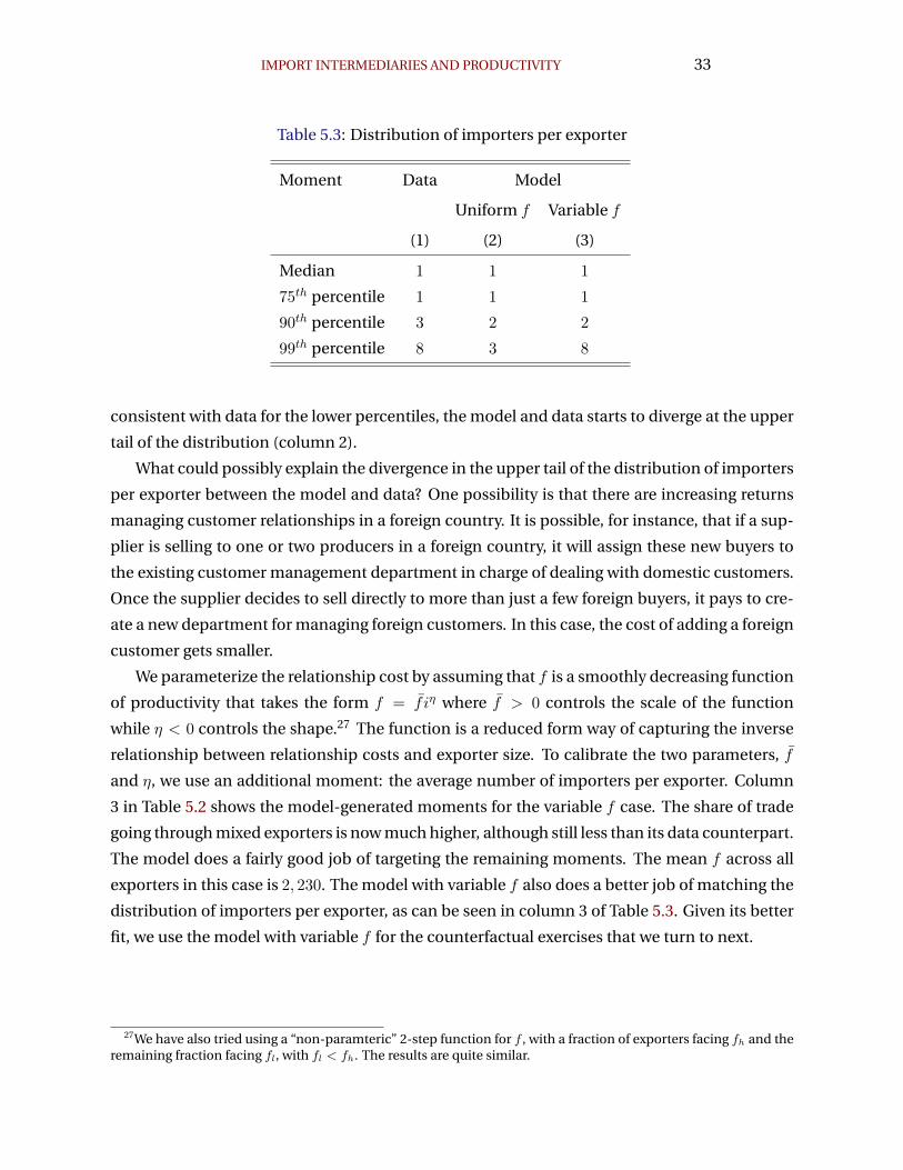
IMPORT INTERMEDIARIES AND PRODUCTIVITY 33
Table 5.3: Distribution of importers per exporter
Moment Data Model
Uniform f Variable f
(1) (2) (3)
Median 1 1 1
75th percentile 1 1 1
90th percentile 3 2 2
99th percentile 8 3 8
consistent with data for the lower percentiles, the model and data starts to diverge at the upper
tail of the distribution (column 2).
What could possibly explain the divergence in the upper tail of the distribution of importers
per exporter between the model and data? One possibility is that there are increasing returns
managing customer relationships in a foreign country. It is possible, for instance, that if a sup-
plier is selling to one or two producers in a foreign country, it will assign these new buyers to
the existing customer management department in charge of dealing with domestic customers.
Once the supplier decides to sell directly to more than just a few foreign buyers, it pays to cre-
ate a new department for managing foreign customers. In this case, the cost of adding a foreign
customer gets smaller.
We parameterize the relationship cost by assuming that f is a smoothly decreasing function
of productivity that takes the form f = f iη where f > 0 controls the scale of the function
while η < 0 controls the shape.27 The function is a reduced form way of capturing the inverse
relationship between relationship costs and exporter size. To calibrate the two parameters, f
and η, we use an additional moment: the average number of importers per exporter. Column
3 in Table 5.2 shows the model-generated moments for the variable f case. The share of trade
going through mixed exporters is now much higher, although still less than its data counterpart.
The model does a fairly good job of targeting the remaining moments. The mean f across all
exporters in this case is 2, 230. The model with variable f also does a better job of matching the
distribution of importers per exporter, as can be seen in column 3 of Table 5.3. Given its better
fit, we use the model with variable f for the counterfactual exercises that we turn to next.
27We have also tried using a “non-paramteric” 2-step function for f , with a fraction of exporters facing fh and theremaining fraction facing fl, with fl < fh. The results are quite similar.
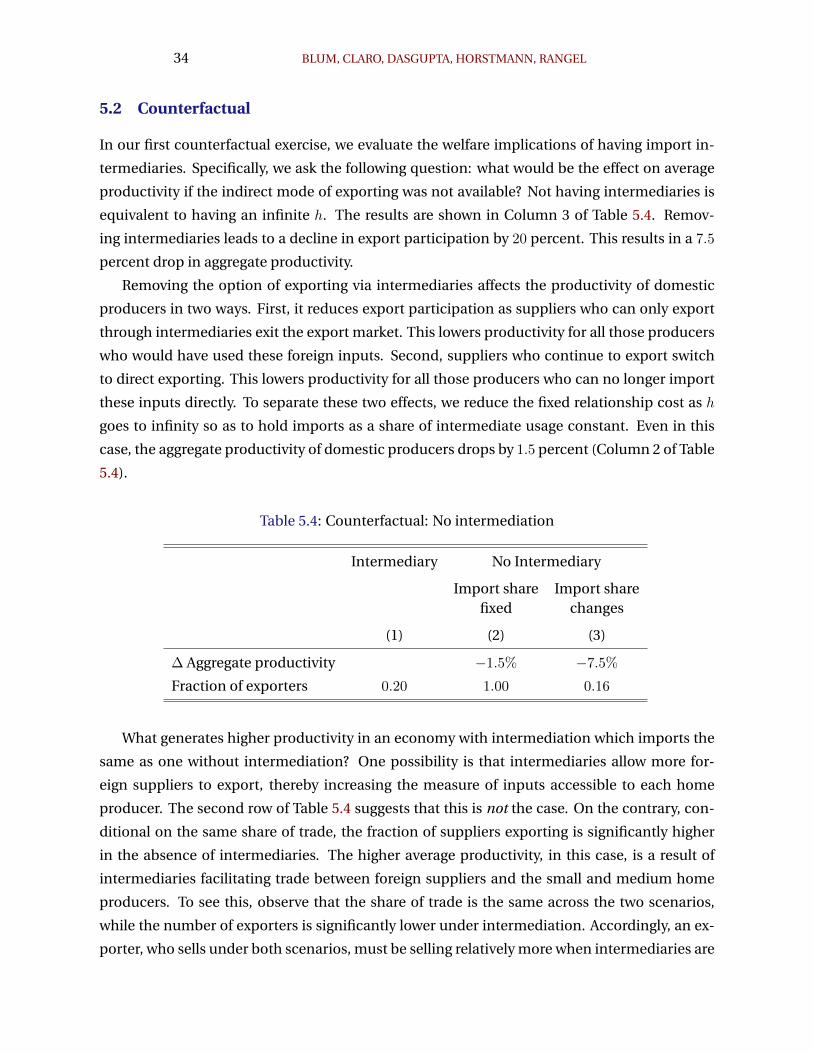
34 BLUM, CLARO, DASGUPTA, HORSTMANN, RANGEL
5.2 Counterfactual
In our first counterfactual exercise, we evaluate the welfare implications of having import in-
termediaries. Specifically, we ask the following question: what would be the effect on average
productivity if the indirect mode of exporting was not available? Not having intermediaries is
equivalent to having an infinite h. The results are shown in Column 3 of Table 5.4. Remov-
ing intermediaries leads to a decline in export participation by 20 percent. This results in a 7.5
percent drop in aggregate productivity.
Removing the option of exporting via intermediaries affects the productivity of domestic
producers in two ways. First, it reduces export participation as suppliers who can only export
through intermediaries exit the export market. This lowers productivity for all those producers
who would have used these foreign inputs. Second, suppliers who continue to export switch
to direct exporting. This lowers productivity for all those producers who can no longer import
these inputs directly. To separate these two effects, we reduce the fixed relationship cost as h
goes to infinity so as to hold imports as a share of intermediate usage constant. Even in this
case, the aggregate productivity of domestic producers drops by 1.5 percent (Column 2 of Table
5.4).
Table 5.4: Counterfactual: No intermediation
Intermediary No Intermediary
Import share Import sharefixed changes
(1) (2) (3)
∆ Aggregate productivity −1.5% −7.5%
Fraction of exporters 0.20 1.00 0.16
What generates higher productivity in an economy with intermediation which imports the
same as one without intermediation? One possibility is that intermediaries allow more for-
eign suppliers to export, thereby increasing the measure of inputs accessible to each home
producer. The second row of Table 5.4 suggests that this is not the case. On the contrary, con-
ditional on the same share of trade, the fraction of suppliers exporting is significantly higher
in the absence of intermediaries. The higher average productivity, in this case, is a result of
intermediaries facilitating trade between foreign suppliers and the small and medium home
producers. To see this, observe that the share of trade is the same across the two scenarios,
while the number of exporters is significantly lower under intermediation. Accordingly, an ex-
porter, who sells under both scenarios, must be selling relatively more when intermediaries are
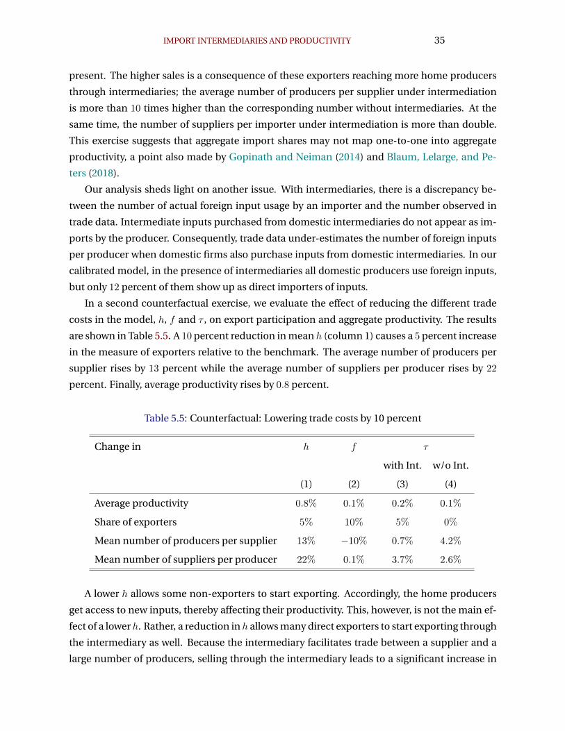
IMPORT INTERMEDIARIES AND PRODUCTIVITY 35
present. The higher sales is a consequence of these exporters reaching more home producers
through intermediaries; the average number of producers per supplier under intermediation
is more than 10 times higher than the corresponding number without intermediaries. At the
same time, the number of suppliers per importer under intermediation is more than double.
This exercise suggests that aggregate import shares may not map one-to-one into aggregate
productivity, a point also made by Gopinath and Neiman (2014) and Blaum, Lelarge, and Pe-
ters (2018).
Our analysis sheds light on another issue. With intermediaries, there is a discrepancy be-
tween the number of actual foreign input usage by an importer and the number observed in
trade data. Intermediate inputs purchased from domestic intermediaries do not appear as im-
ports by the producer. Consequently, trade data under-estimates the number of foreign inputs
per producer when domestic firms also purchase inputs from domestic intermediaries. In our
calibrated model, in the presence of intermediaries all domestic producers use foreign inputs,
but only 12 percent of them show up as direct importers of inputs.
In a second counterfactual exercise, we evaluate the effect of reducing the different trade
costs in the model, h, f and τ , on export participation and aggregate productivity. The results
are shown in Table 5.5. A 10 percent reduction in mean h (column 1) causes a 5 percent increase
in the measure of exporters relative to the benchmark. The average number of producers per
supplier rises by 13 percent while the average number of suppliers per producer rises by 22
percent. Finally, average productivity rises by 0.8 percent.
Table 5.5: Counterfactual: Lowering trade costs by 10 percent
Change in h f τ
with Int. w/o Int.
(1) (2) (3) (4)
Average productivity 0.8% 0.1% 0.2% 0.1%
Share of exporters 5% 10% 5% 0%
Mean number of producers per supplier 13% −10% 0.7% 4.2%
Mean number of suppliers per producer 22% 0.1% 3.7% 2.6%
A lower h allows some non-exporters to start exporting. Accordingly, the home producers
get access to new inputs, thereby affecting their productivity. This, however, is not the main ef-
fect of a lower h. Rather, a reduction in h allows many direct exporters to start exporting through
the intermediary as well. Because the intermediary facilitates trade between a supplier and a
large number of producers, selling through the intermediary leads to a significant increase in
36 BLUM, CLARO, DASGUPTA, HORSTMANN, RANGEL
the number of producers per supplier, on average. As more suppliers start selling through the
intermediary, each producer also has access to a larger number of inputs. Consequently, the
average number of suppliers per producer rises too.
In contrast, a similar 10 percent reduction in f (column 2) causes a much bigger increase
in the measure of exporters – 10 percent. Nevertheless, the effect on productivity is far more
modest under a lower f . This is because h and f affects trade through very different channels.
While a lower f also raises the average number of suppliers per producer, this increase is much
smaller as each existing supplier adds more producers only at the margin. The effect on the
average number of producers per supplier depends on two forces: it tends to increase as ex-
isting suppliers add more producers, but falls as the new exporters sell to fewer producers. In
this case, the latter effect dominates. The overall effect on productivity turns out to be only 0.1
percent.
Finally, we examine the effect of lowering τ . The result, it turns out, depends on whether
intermediaries are present or not. We reduce τ by 10 percent starting from the benchmark
equilibrium (column 3) and from the equilibrium without intermediaries but with the same
share of imported inputs (column 4). The increase in productivity with intermediaries is 0.2
percent, which is twice that of the increase without intermediaries. This exercise suggests that
the productivity effects of trade liberalization are enhanced in the presence of an efficient in-
termediation sector.
6. Conclusion
While economists have studied extensively the role that firms like Walmart play in allowing
domestic consumers to access foreign products (Basker and Van (2010), Holmes and Singer
(2018)), no attention has been paid to the role of trade intermediaries in providing domestic
producers access to foreign inputs. This is remarkable for two reasons. First, roughly two-thirds
of the world’s trade is in intermediate inputs (Bems, Johnson, and Yi (2011)). Second, firm-level
evidence has established that access to imported inputs raises firm and aggregate productivity
(see Amiti and Konings (2007); Gopinath and Neiman (2014) among others).
Our analysis starts closing this gap and shows that import intermediaries of foreign inputs
play a major role in a country’s aggregate productivity. Moreover, ignoring the presence of such
intermediaries can affect the measured effect of international trade in various ways. To illus-
trate, the presence of import intermediaries doubles the effect of a trade liberalization on the
country’s aggregate productivity.
Our findings open many avenues for future research. First, given the importance of the im-
port intermediary sector in Chile, it is natural to ask the extent to which the efficiency of this
IMPORT INTERMEDIARIES AND PRODUCTIVITY 37
sector varies across countries, and whether such variation contributes to the observed disparity
in countries’ productivity and per capita income. Second, while our data allowed us to study
the import intermediation sector, domestic intermediation of productive inputs may play an
important role as well. Indeed, it is possible that firms that intermediate imports also inter-
mediate domestic trade. Thus, our results may point, more generally, to the importance of the
efficiency of the intermediation sector to a country’s productivity.
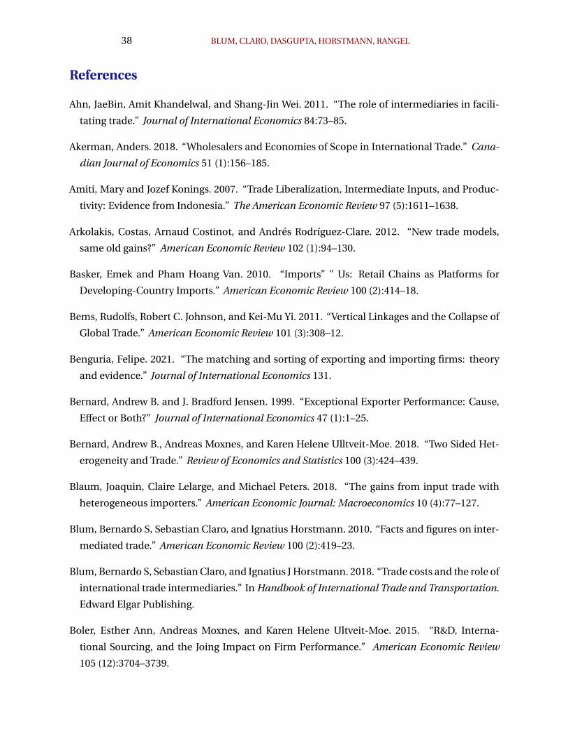
38 BLUM, CLARO, DASGUPTA, HORSTMANN, RANGEL
References
Ahn, JaeBin, Amit Khandelwal, and Shang-Jin Wei. 2011. “The role of intermediaries in facili-
tating trade.” Journal of International Economics 84:73–85.
Akerman, Anders. 2018. “Wholesalers and Economies of Scope in International Trade.” Cana-
dian Journal of Economics 51 (1):156–185.
Amiti, Mary and Jozef Konings. 2007. “Trade Liberalization, Intermediate Inputs, and Produc-
tivity: Evidence from Indonesia.” The American Economic Review 97 (5):1611–1638.
Arkolakis, Costas, Arnaud Costinot, and Andres Rodrıguez-Clare. 2012. “New trade models,
same old gains?” American Economic Review 102 (1):94–130.
Basker, Emek and Pham Hoang Van. 2010. “Imports” ” Us: Retail Chains as Platforms for
Developing-Country Imports.” American Economic Review 100 (2):414–18.
Bems, Rudolfs, Robert C. Johnson, and Kei-Mu Yi. 2011. “Vertical Linkages and the Collapse of
Global Trade.” American Economic Review 101 (3):308–12.
Benguria, Felipe. 2021. “The matching and sorting of exporting and importing firms: theory
and evidence.” Journal of International Economics 131.
Bernard, Andrew B. and J. Bradford Jensen. 1999. “Exceptional Exporter Performance: Cause,
Effect or Both?” Journal of International Economics 47 (1):1–25.
Bernard, Andrew B., Andreas Moxnes, and Karen Helene Ulltveit-Moe. 2018. “Two Sided Het-
erogeneity and Trade.” Review of Economics and Statistics 100 (3):424–439.
Blaum, Joaquin, Claire Lelarge, and Michael Peters. 2018. “The gains from input trade with
heterogeneous importers.” American Economic Journal: Macroeconomics 10 (4):77–127.
Blum, Bernardo S, Sebastian Claro, and Ignatius Horstmann. 2010. “Facts and figures on inter-
mediated trade.” American Economic Review 100 (2):419–23.
Blum, Bernardo S, Sebastian Claro, and Ignatius J Horstmann. 2018. “Trade costs and the role of
international trade intermediaries.” In Handbook of International Trade and Transportation.
Edward Elgar Publishing.
Boler, Esther Ann, Andreas Moxnes, and Karen Helene Ultveit-Moe. 2015. “R&D, Interna-
tional Sourcing, and the Joing Impact on Firm Performance.” American Economic Review
105 (12):3704–3739.
IMPORT INTERMEDIARIES AND PRODUCTIVITY 39
Broda, Christian and David E. Weinstein. 2006. “Globalization and the Gains From Variety.”
The Quarterly Journal of Economics 121 (2):541–585.
Carballo, Jeronimo, Gianmarco I.P. Ottaviano, and Christian Volpe Martincus. 2018. “The buyer
margins of firms exports.” The Journal of International Economics 112:33–49.
Dasgupta, Kunal and Jordi Mondria. 2018. “Quality uncertainty and intermediation in interna-
tional trade.” European Economic Review 104:68–91.
Defever, Fabrice, Michele Imbruno, and Richard Kneller. 2020. “Trade liberalization, input
intermediaries and firm productivity: Evidence from China.” Journal of International Eco-
nomics 126:103329.
Eaton, Jonathan, David Jinkins, James R Tybout, and Daniel Xu. 2022. “Two-sided search in
international markets.” Tech. rep., National Bureau of Economic Research.
Eaton, Jonathan, Samuel Kortum, and Francis Kramarz. 2011. “An Anatomy of International
Trade: Evidence from French Firms.” Econometrica 79 (5):1453–1498.
Eaton, Jonathan, Samuel S Kortum, and Francis Kramarz. 2022. “Firm-to-Firm Trade: Imports,
exports, and the labor market.” Tech. rep., National Bureau of Economic Research.
Ethier, Wilfred J. 1982. “National and international returns to scale in the modern theory of
international trade.” The American Economic Review 72 (3):389–405.
Felbermayr, G. and B. Jung. 2016. “Trade intermediaries and the organization of exporters.”
Review of International Economics 19 (4):634–648.
Fieler, Ana Cecilia, Marcela Eslava, and Daniel Yi Xu. 2018. “Trade, Quality Upgrading, and In-
put Linkages: Theory and Evidence from Colombia.” American Economic Review 108 (1):109–
146.
Goldberg, Pinelopi Koujianou, Amit Jumar Khandelwal, Nina Pavcnik, and Petia Topalova.
2010. “Imported Intermediate Inputs and Domestic Product Growth: Evidence from India.”
Quarterly Journal of Economics 125 (4):1727–1767.
Gopinath, Gita and Brent Neiman. 2014. “Trade Adjustment and Productivity in Large Crises.”
American Economic Review 104 (3):793–831.
Halpern, Laszlo, Miklos Koren, and Adam Szeidl. 2015. “Imported Inputs and Productivity.”
The American Economic Review 105 (12):3660–3703.
Holmes, Thomas J and Ethan Singer. 2018. “Indivisibilities in distribution.” Tech. rep., National
Bureau of Economic Research.
40 BLUM, CLARO, DASGUPTA, HORSTMANN, RANGEL
Kasahara, Hiroyuki and Joel Rodrigue. 2008. “Does the Use of Imported Intermediates Increase
Productivity? Plant-level Evidence.” The Journal of Development Economics 87 (1):106–118.
Krugman, Paul and Anthony J Venables. 1995. “Globalization and the Inequality of Nations.”
The quarterly journal of economics 110 (4):857–880.
Lindemann, Udo, Maik Maurer, and Thomas Braun. 2008. Structural complexity management:
an approach for the field of product design. Springer Science & Business Media.
Orr, H Allen. 2000. “Adaptation and the cost of complexity.” Evolution 54 (1):13–20.
Petropoulou, Dimitra. 2011. “Information Costs, Networks and Intermediation in International
Trade.” Manuscript.
Rauch, James. 1999. “Networks versus Markets in International Trade.” Journal of International
Economics 48 (1):17–35.
———. 2001. “Business and Social Networks in International Trade.” Journal of Economic Lit-
erature 39 (4):1117–1203.
Rauch, Joel and Joel Watson. 2004. “Network Intermediaries in International Trade.” Journal of
Economics & Management Strategy 13 (1):69–93.
Topalova, Petra and Amit Khandelwal. 2011. “Trade Liberalization and Firm Productivity: The
Case of India.” Review of Economic and Statistics 93 (3):995–1009.
Zhang, Hongsong. 2017. “Static and dynamic gains from costly importing of intermediate in-
puts: Evidence from Colombia.” European Economic Review 91:118–145.
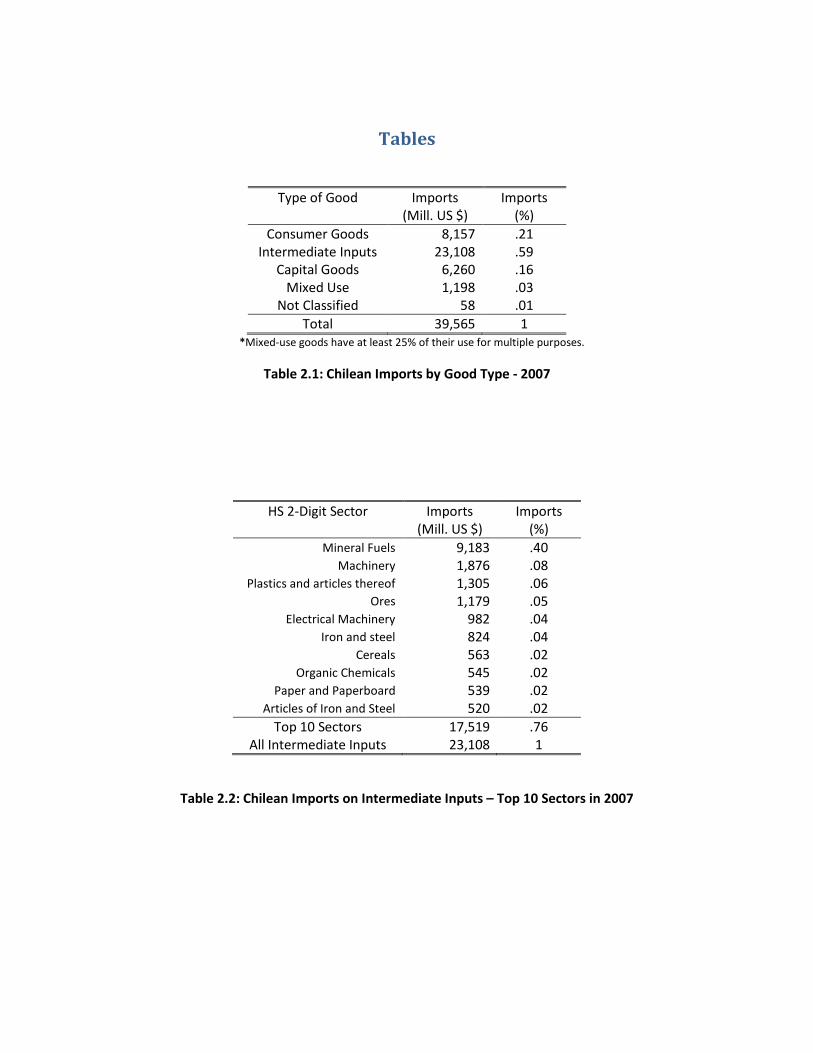
Tables
Type of Good Imports (Mill. US $)
Imports (%)
Consumer Goods 8,157 .21 Intermediate Inputs 23,108 .59
Capital Goods 6,260 .16 Mixed Use 1,198 .03
Not Classified 58 .01 Total 39,565 1
*Mixed-use goods have at least 25% of their use for multiple purposes.
Table 2.1: Chilean Imports by Good Type - 2007
HS 2-Digit Sector Imports (Mill. US $)
Imports (%)
Mineral Fuels 9,183 .40 Machinery 1,876 .08
Plastics and articles thereof 1,305 .06 Ores 1,179 .05
Electrical Machinery 982 .04 Iron and steel 824 .04
Cereals 563 .02 Organic Chemicals 545 .02
Paper and Paperboard 539 .02 Articles of Iron and Steel 520 .02
Top 10 Sectors 17,519 .76 All Intermediate Inputs 23,108 1
Table 2.2: Chilean Imports on Intermediate Inputs – Top 10 Sectors in 2007
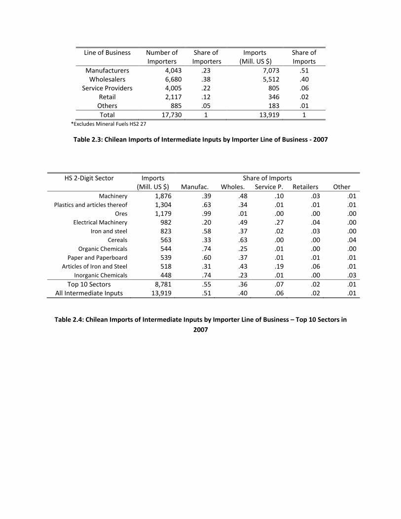
Line of Business Number of Importers
Share of Importers
Imports (Mill. US $)
Share of Imports
Manufacturers 4,043 .23 7,073 .51 Wholesalers 6,680 .38 5,512 .40
Service Providers 4,005 .22 805 .06 Retail 2,117 .12 346 .02
Others 885 .05 183 .01 Total 17,730 1 13,919 1
*Excludes Mineral Fuels HS2 27
Table 2.3: Chilean Imports of Intermediate Inputs by Importer Line of Business - 2007
Table 2.4: Chilean Imports of Intermediate Inputs by Importer Line of Business – Top 10 Sectors in 2007
HS 2-Digit Sector Imports Share of Imports (Mill. US $) Manufac. Wholes. Service P. Retailers Other
Machinery 1,876 .39 .48 .10 .03 .01 Plastics and articles thereof 1,304 .63 .34 .01 .01 .01
Ores 1,179 .99 .01 .00 .00 .00 Electrical Machinery 982 .20 .49 .27 .04 .00
Iron and steel 823 .58 .37 .02 .03 .00 Cereals 563 .33 .63 .00 .00 .04
Organic Chemicals 544 .74 .25 .01 .00 .00 Paper and Paperboard 539 .60 .37 .01 .01 .01
Articles of Iron and Steel 518 .31 .43 .19 .06 .01 Inorganic Chemicals 448 .74 .23 .01 .00 .03
Top 10 Sectors 8,781 .55 .36 .07 .02 .01 All Intermediate Inputs 13,919 .51 .40 .06 .02 .01
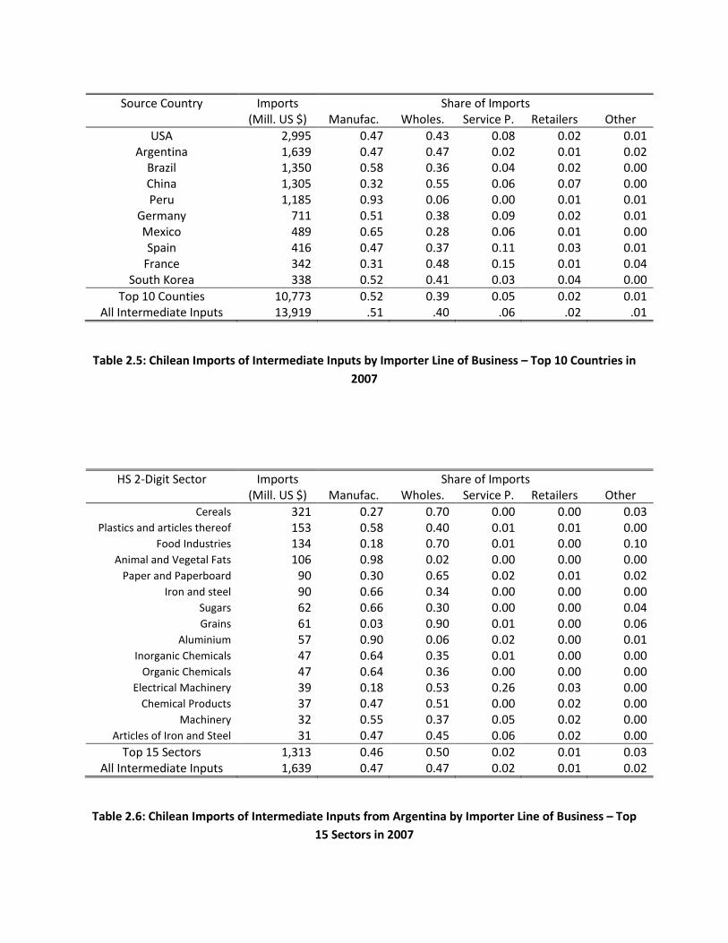
Table 2.5: Chilean Imports of Intermediate Inputs by Importer Line of Business – Top 10 Countries in 2007
Table 2.6: Chilean Imports of Intermediate Inputs from Argentina by Importer Line of Business – Top 15 Sectors in 2007
Source Country Imports Share of Imports (Mill. US $) Manufac. Wholes. Service P. Retailers Other
USA 2,995 0.47 0.43 0.08 0.02 0.01 Argentina 1,639 0.47 0.47 0.02 0.01 0.02
Brazil 1,350 0.58 0.36 0.04 0.02 0.00 China 1,305 0.32 0.55 0.06 0.07 0.00 Peru 1,185 0.93 0.06 0.00 0.01 0.01
Germany 711 0.51 0.38 0.09 0.02 0.01 Mexico 489 0.65 0.28 0.06 0.01 0.00 Spain 416 0.47 0.37 0.11 0.03 0.01
France 342 0.31 0.48 0.15 0.01 0.04 South Korea 338 0.52 0.41 0.03 0.04 0.00
Top 10 Counties 10,773 0.52 0.39 0.05 0.02 0.01 All Intermediate Inputs 13,919 .51 .40 .06 .02 .01
HS 2-Digit Sector Imports Share of Imports (Mill. US $) Manufac. Wholes. Service P. Retailers Other
Cereals 321 0.27 0.70 0.00 0.00 0.03 Plastics and articles thereof 153 0.58 0.40 0.01 0.01 0.00
Food Industries 134 0.18 0.70 0.01 0.00 0.10 Animal and Vegetal Fats 106 0.98 0.02 0.00 0.00 0.00
Paper and Paperboard 90 0.30 0.65 0.02 0.01 0.02 Iron and steel 90 0.66 0.34 0.00 0.00 0.00
Sugars 62 0.66 0.30 0.00 0.00 0.04 Grains 61 0.03 0.90 0.01 0.00 0.06
Aluminium 57 0.90 0.06 0.02 0.00 0.01 Inorganic Chemicals 47 0.64 0.35 0.01 0.00 0.00
Organic Chemicals 47 0.64 0.36 0.00 0.00 0.00 Electrical Machinery 39 0.18 0.53 0.26 0.03 0.00
Chemical Products 37 0.47 0.51 0.00 0.02 0.00 Machinery 32 0.55 0.37 0.05 0.02 0.00
Articles of Iron and Steel 31 0.47 0.45 0.06 0.02 0.00 Top 15 Sectors 1,313 0.46 0.50 0.02 0.01 0.03
All Intermediate Inputs 1,639 0.47 0.47 0.02 0.01 0.02
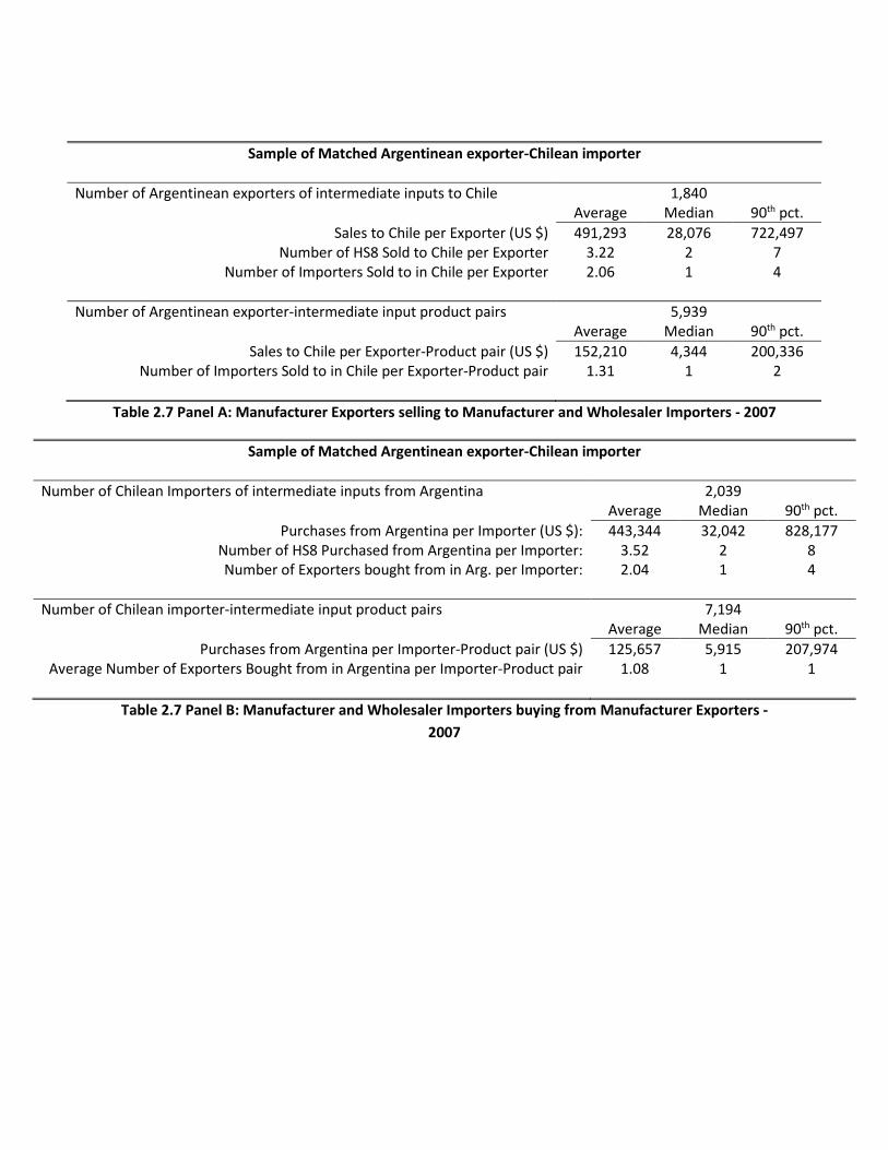
Sample of Matched Argentinean exporter-Chilean importer Number of Argentinean exporters of intermediate inputs to Chile 1,840 Average Median 90th pct.
Sales to Chile per Exporter (US $) 491,293 28,076 722,497 Number of HS8 Sold to Chile per Exporter 3.22 2 7
Number of Importers Sold to in Chile per Exporter 2.06 1 4 Number of Argentinean exporter-intermediate input product pairs 5,939 Average Median 90th pct.
Sales to Chile per Exporter-Product pair (US $) 152,210 4,344 200,336 Number of Importers Sold to in Chile per Exporter-Product pair 1.31 1 2
Table 2.7 Panel A: Manufacturer Exporters selling to Manufacturer and Wholesaler Importers - 2007
Sample of Matched Argentinean exporter-Chilean importer Number of Chilean Importers of intermediate inputs from Argentina 2,039 Average Median 90th pct.
Purchases from Argentina per Importer (US $): 443,344 32,042 828,177 Number of HS8 Purchased from Argentina per Importer: 3.52 2 8 Number of Exporters bought from in Arg. per Importer: 2.04 1 4
Number of Chilean importer-intermediate input product pairs 7,194 Average Median 90th pct.
Purchases from Argentina per Importer-Product pair (US $) 125,657 5,915 207,974 Average Number of Exporters Bought from in Argentina per Importer-Product pair 1.08 1 1
Table 2.7 Panel B: Manufacturer and Wholesaler Importers buying from Manufacturer Exporters -
2007
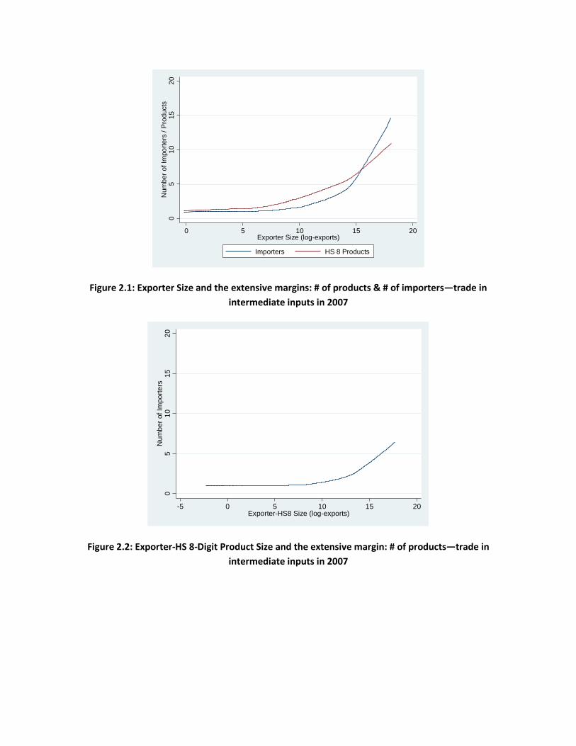
Figure 2.1: Exporter Size and the extensive margins: # of products & # of importers—trade in intermediate inputs in 2007
Figure 2.2: Exporter-HS 8-Digit Product Size and the extensive margin: # of products—trade in intermediate inputs in 2007
05
1015
20N
umbe
r of I
mpo
rters
/ Pr
oduc
ts
0 5 10 15 20Exporter Size (log-exports)
Importers HS 8 Products
05
1015
20N
umbe
r of I
mpo
rters
-5 0 5 10 15 20Exporter-HS8 Size (log-exports)
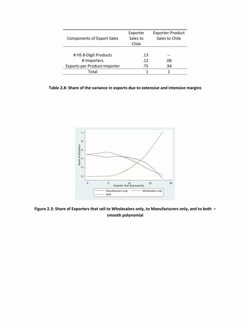
Components of Export Sales
Exporter Sales to
Chile
Exporter-Product Sales to Chile
# HS 8-Digit Products .13 --
# Importers .12 .06 Exports per Product-Importer .75 .94
Total 1 1
Table 2.8: Share of the variance in exports due to extensive and intensive margins
Figure 2.3: Share of Exporters that sell to Wholesalers only, to Manufacturers only, and to both – smooth polynomial
0.2
.4.6
.81
Shar
e of
Exp
orte
rs
0 5 10 15 20Exporter Size (log-exports)
Manufacturers only Wholesalers onlyBoth
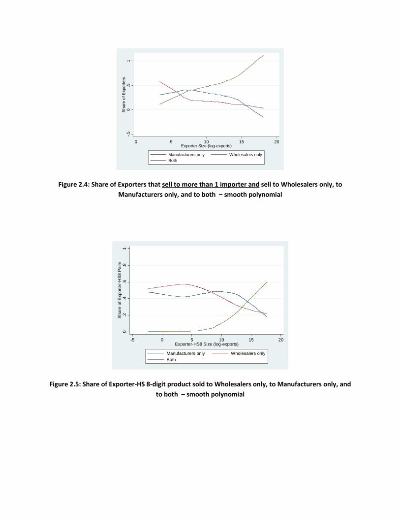
Figure 2.4: Share of Exporters that sell to more than 1 importer and sell to Wholesalers only, to Manufacturers only, and to both – smooth polynomial
Figure 2.5: Share of Exporter-HS 8-digit product sold to Wholesalers only, to Manufacturers only, and to both – smooth polynomial
-.50
.51
Shar
e of
Exp
orte
rs
0 5 10 15 20Exporter Size (log-exports)
Manufacturers only Wholesalers onlyBoth
0.2
.4.6
.81
Shar
e of
Exp
orte
r-HS8
Pai
rs
-5 0 5 10 15 20Exporter-HS8 Size (log-exports)
Manufacturers only Wholesalers onlyBoth
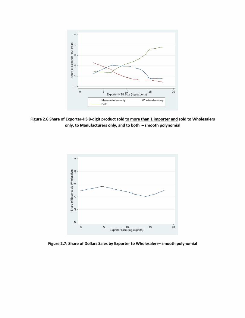
Figure 2.6 Share of Exporter-HS 8-digit product sold to more than 1 importer and sold to Wholesalers only, to Manufacturers only, and to both – smooth polynomial
Figure 2.7: Share of Dollars Sales by Exporter to Wholesalers– smooth polynomial
0.2
.4.6
.81
Shar
e of
Exp
orte
r-HS8
Pai
rs
0 5 10 15 20Exporter-HS8 Size (log-exports)
Manufacturers only Wholesalers onlyBoth
0.2
.4.6
.81
Shar
e of
Exp
orts
via
Who
lesa
lers
0 5 10 15 20Exporter Size (log-exports)
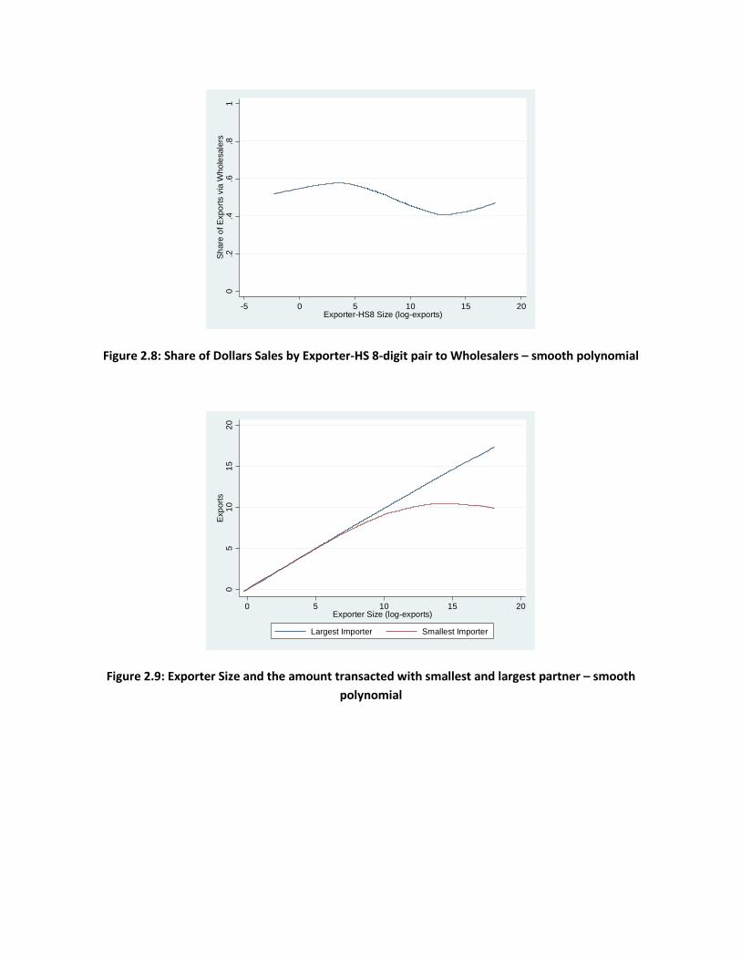
Figure 2.8: Share of Dollars Sales by Exporter-HS 8-digit pair to Wholesalers – smooth polynomial
Figure 2.9: Exporter Size and the amount transacted with smallest and largest partner – smooth polynomial
0.2
.4.6
.81
Shar
e of
Exp
orts
via
Who
lesa
lers
-5 0 5 10 15 20Exporter-HS8 Size (log-exports)
05
1015
20Ex
ports
0 5 10 15 20Exporter Size (log-exports)
Largest Importer Smallest Importer
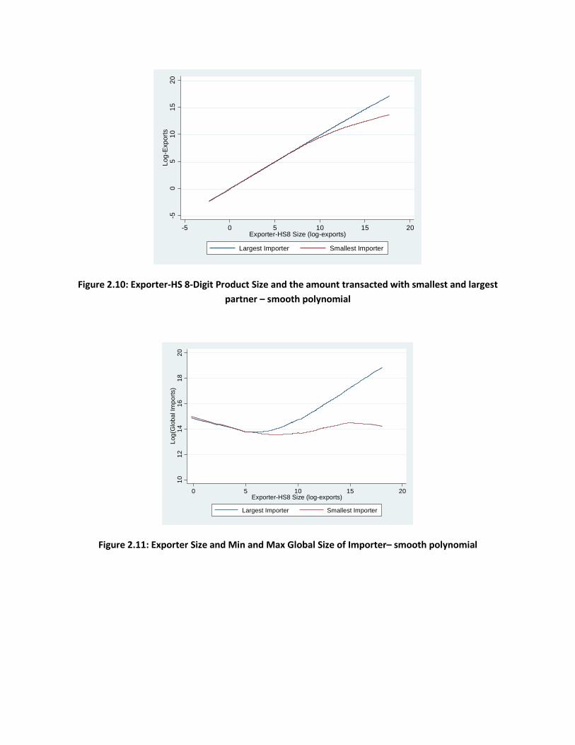
Figure 2.10: Exporter-HS 8-Digit Product Size and the amount transacted with smallest and largest partner – smooth polynomial
Figure 2.11: Exporter Size and Min and Max Global Size of Importer– smooth polynomial
-50
510
1520
Log-
Expo
rts
-5 0 5 10 15 20Exporter-HS8 Size (log-exports)
Largest Importer Smallest Importer
1012
1416
1820
Log(
Glo
bal I
mpo
rts)
0 5 10 15 20Exporter-HS8 Size (log-exports)
Largest Importer Smallest Importer
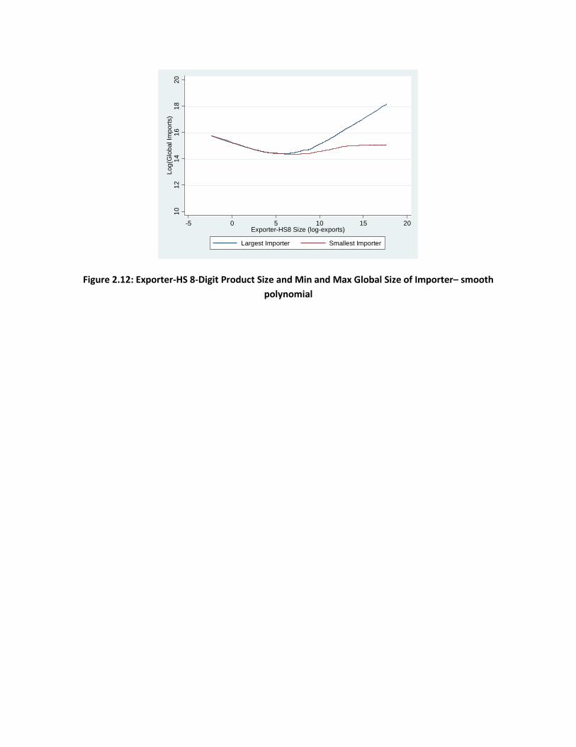
Figure 2.12: Exporter-HS 8-Digit Product Size and Min and Max Global Size of Importer– smooth polynomial
1012
1416
1820
Log(
Glo
bal I
mpo
rts)
-5 0 5 10 15 20Exporter-HS8 Size (log-exports)
Largest Importer Smallest Importer


