Embed Size (px)
Citation preview

Formal Languages and Automata Theory
D. Goswami and K. V. Krishna
November 5, 2010

Contents
1 Mathematical Preliminaries 3
2 Formal Languages 42.1 Strings . . . . . . . . . . . . . . . . . . . . . . . . . . . . . . . 52.2 Languages . . . . . . . . . . . . . . . . . . . . . . . . . . . . . 62.3 Properties . . . . . . . . . . . . . . . . . . . . . . . . . . . . . 102.4 Finite Representation . . . . . . . . . . . . . . . . . . . . . . . 13
2.4.1 Regular Expressions . . . . . . . . . . . . . . . . . . . 13
3 Grammars 183.1 Context-Free Grammars . . . . . . . . . . . . . . . . . . . . . 193.2 Derivation Trees . . . . . . . . . . . . . . . . . . . . . . . . . . 26
3.2.1 Ambiguity . . . . . . . . . . . . . . . . . . . . . . . . . 313.3 Regular Grammars . . . . . . . . . . . . . . . . . . . . . . . . 323.4 Digraph Representation . . . . . . . . . . . . . . . . . . . . . 36
4 Finite Automata 384.1 Deterministic Finite Automata . . . . . . . . . . . . . . . . . 394.2 Nondeterministic Finite Automata . . . . . . . . . . . . . . . 494.3 Equivalence of NFA and DFA . . . . . . . . . . . . . . . . . . 54
4.3.1 Heuristics to Convert NFA to DFA . . . . . . . . . . . 584.4 Minimization of DFA . . . . . . . . . . . . . . . . . . . . . . . 61
4.4.1 Myhill-Nerode Theorem . . . . . . . . . . . . . . . . . 614.4.2 Algorithmic Procedure for Minimization . . . . . . . . 65
4.5 Regular Languages . . . . . . . . . . . . . . . . . . . . . . . . 724.5.1 Equivalence of Finite Automata and Regular Languages 724.5.2 Equivalence of Finite Automata and Regular Grammars 84
4.6 Variants of Finite Automata . . . . . . . . . . . . . . . . . . . 894.6.1 Two-way Finite Automaton . . . . . . . . . . . . . . . 894.6.2 Mealy Machines . . . . . . . . . . . . . . . . . . . . . . 91
1

5 Properties of Regular Languages 945.1 Closure Properties . . . . . . . . . . . . . . . . . . . . . . . . 94
5.1.1 Set Theoretic Properties . . . . . . . . . . . . . . . . . 945.1.2 Other Properties . . . . . . . . . . . . . . . . . . . . . 97
5.2 Pumping Lemma . . . . . . . . . . . . . . . . . . . . . . . . . 104
2

Chapter 1
Mathematical Preliminaries
3

Chapter 2
Formal Languages
A language can be seen as a system suitable for expression of certain ideas,facts and concepts. For formalizing the notion of a language one must coverall the varieties of languages such as natural (human) languages and program-ming languages. Let us look at some common features across the languages.One may broadly see that a language is a collection of sentences; a sentenceis a sequence of words; and a word is a combination of syllables. If one con-siders a language that has a script, then it can be observed that a word is asequence of symbols of its underlying alphabet. It is observed that a formallearning of a language has the following three steps.
1. Learning its alphabet - the symbols that are used in the language.
2. Its words - as various sequences of symbols of its alphabet.
3. Formation of sentences - sequence of various words that follow certainrules of the language.
In this learning, step 3 is the most difficult part. Let us postpone to discussconstruction of sentences and concentrate on steps 1 and 2. For the timebeing instead of completely ignoring about sentences one may look at thecommon features of a word and a sentence to agree upon both are just se-quence of some symbols of the underlying alphabet. For example, the Englishsentence
"The English articles - a, an and the - are
categorized into two types: indefinite and definite."
may be treated as a sequence of symbols from the Roman alphabet alongwith enough punctuation marks such as comma, full-stop, colon and furtherone more special symbol, namely blank-space which is used to separate twowords. Thus, abstractly, a sentence or a word may be interchangeably used
4

for a sequence of symbols from an alphabet. With this discussion we startwith the basic definitions of alphabets and strings and then we introduce thenotion of language formally.
Further, in this chapter, we introduce some of the operations on languagesand discuss algebraic properties of languages with respect to those operations.We end the chapter with an introduction to finite representation of languagesvia regular expressions.
2.1 Strings
We formally define an alphabet as a non-empty finite set. We normally usethe symbols a, b, c, . . . with or without subscripts or 0, 1, 2, . . ., etc. for theelements of an alphabet.
A string over an alphabet Σ is a finite sequence of symbols of Σ. Althoughone writes a sequence as (a1, a2, . . . , an), in the present context, we prefer towrite it as a1a2 · · · an, i.e. by juxtaposing the symbols in that order. Thus,a string is also known as a word or a sentence. Normally, we use lower caseletters towards the end of English alphabet, namely z, y, x, w, etc., to denotestrings.
Example 2.1.1. Let Σ = {a, b} be an alphabet; then aa, ab, bba, baaba, . . .are some examples of strings over Σ.
Since the empty sequence is a finite sequence, it is also a string. Which is( ) in earlier notation; but with the notation adapted for the present contextwe require a special symbol. We use ε, to denote the empty string.
The set of all strings over an alphabet Σ is denoted by Σ∗. For example,if Σ = {0, 1}, then
Σ∗ = {ε, 0, 1, 00, 01, 10, 11, 000, 001, . . .}.
Although the set Σ∗ is infinite, it is a countable set. In fact, Σ∗ is countablyinfinite for any alphabet Σ. In order to understand some such fundamen-tal facts we introduce some string operations, which in turn are useful tomanipulate and generate strings.
One of the most fundamental operations used for string manipulation isconcatenation. Let x = a1a2 · · · an and y = b1b2 · · · bm be two strings. Theconcatenation of the pair x, y denoted by xy is the string
a1a2 · · · anb1b2 · · · bm.
5

Clearly, the binary operation concatenation on Σ∗ is associative, i.e., for allx, y, z ∈ Σ∗,
x(yz) = (xy)z.
Thus, x(yz) may simply be written as xyz. Also, since ε is the empty string,it satisfies the property
εx = xε = x
for any sting x ∈ Σ∗. Hence, Σ∗ is a monoid with respect to concatenation.The operation concatenation is not commutative on Σ∗.
For a string x and an integer n ≥ 0, we write
xn+1 = xnx with the base condition x0 = ε.
That is, xn is obtained by concatenating n copies of x. Also, whenever n = 0,the string x1 · · ·xn represents the empty string ε.
Let x be a string over an alphabet Σ. For a ∈ Σ, the number of occur-rences of a in x shall be denoted by |x|a. The length of a string x denotedby |x| is defined as
|x| =∑a∈Σ
|x|a.
Essentially, the length of a string is obtained by counting the number ofsymbols in the string. For example, |aab| = 3, |a| = 1. Note that |ε| = 0.
If we denote An to be the set of all strings of length n over Σ, then onecan easily ascertain that
Σ∗ =⋃n≥0
An.
And hence, being An a finite set, Σ∗ is a countably infinite set.We say that x is a substring of y if x occurs in y, that is y = uxv for
some strings u and v. The substring x is said to be a prefix of y if u = ε.Similarly, x is a suffix of y if v = ε.
Generalizing the notation used for number of occurrences of symbol a in astring x, we adopt the notation |y|x as the number of occurrences of a stringx in y.
2.2 Languages
We have got acquainted with the formal notion of strings that are basicelements of a language. In order to define the notion of a language in abroad spectrum, it is felt that it can be any collection of strings over analphabet.
Thus we define a language over an alphabet Σ as a subset of Σ∗.
6

Example 2.2.1.
1. The emptyset ∅ is a language over any alphabet. Similarly, {ε} is alsoa language over any alphabet.
2. The set of all strings over {0, 1} that start with 0.
3. The set of all strings over {a, b, c} having ac as a substring.
Remark 2.2.2. Note that ∅ 6= {ε}, because the language ∅ does not containany string but {ε} contains a string, namely ε. Also it is evident that |∅| = 0;whereas, |{ε}| = 1.
Since languages are sets, we can apply various well known set operationssuch as union, intersection, complement, difference on languages. The notionof concatenation of strings can be extended to languages as follows.
The concatenation of a pair of languages L1, L2 is
L1L2 = {xy | x ∈ L1 ∧ y ∈ L2}.
Example 2.2.3.
1. If L1 = {0, 1, 01} and L2 = {1, 00}, thenL1L2 = {01, 11, 011, 000, 100, 0100}.
2. For L1 = {b, ba, bab} and L2 = {ε, b, bb, abb}, we haveL1L2 = {b, ba, bb, bab, bbb, babb, baabb, babbb, bababb}.
Remark 2.2.4.
1. Since concatenation of strings is associative, so is the concatenation oflanguages. That is, for all languages L1, L2 and L3,
(L1L2)L3 = L1(L2L3).
Hence, (L1L2)L3 may simply be written as L1L2L3.
2. The number of strings in L1L2 is always less than or equal to theproduct of individual numbers, i.e.
|L1L2| ≤ |L1||L2|.
3. L1 ⊆ L1L2 if and only if ε ∈ L2.
7

Proof. The “if part” is straightforward; for instance, if ε ∈ L2, thenfor any x ∈ L1, we have x = xε ∈ L1L2. On the other hand, supposeε /∈ L2. Now, note that a string x ∈ L1 of shortest length in L1 cannotbe in L1L2. This is because, if x = yz for some y ∈ L1 and a nonemptystring z ∈ L2, then |y| < |x|. A contradiction to our assumption thatx is of shortest length in L1. Hence L1 6⊆ L1L2.
4. Similarly, ε ∈ L1 if and only if L2 ⊆ L1L2.
We write Ln to denote the language which is obtained by concatenatingn copies of L. More formally,
L0 = {ε} andLn = Ln−1L, for n ≥ 1.In the context of formal languages, another important operation is Kleene
star. Kleene star or Kleene closure of a language L, denoted by L∗, is definedas
L∗ =⋃n≥0
Ln.
Example 2.2.5.
1. Kleene star of the language {01} is{ε, 01, 0101, 010101, . . .} = {(01)n | n ≥ 0}.
2. If L = {0, 10}, then L∗ = {ε, 0, 10, 00, 010, 100, 1010, 000, . . .}Since an arbitrary string in Ln is of the form x1x2 · · ·xn, for xi ∈ L and
L∗ =⋃n≥0
Ln, one can easily observe that
L∗ = {x1x2 · · · xn | n ≥ 0 and xi ∈ L, for 1 ≤ i ≤ n}
Thus, a typical string in L∗ is a concatenation of finitely many strings of L.
Remark 2.2.6. Note that, the Kleene star of the language L = {0, 1} overthe alphabet Σ = {0, 1} is
L∗ = L0 ∪ L ∪ L2 ∪ · · ·= {ε} ∪ {0, 1} ∪ {00, 01, 10, 11} ∪ · · ·= {ε, 0, 1, 00, 01, 10, 11, · · · }= the set of all strings over Σ.
Thus, the earlier introduced notation Σ∗ is consistent with the notation ofKleene star by considering Σ as a language over Σ.
8

The positive closure of a language L is denoted by L+ is defined as
L+ =⋃n≥1
Ln.
Thus, L∗ = L+ ∪ {ε}.We often can easily describe various formal languages in English by stat-
ing the property that is to be satisfied by the strings in the respective lan-guages. It is not only for elegant representation but also to understand theproperties of languages better, describing the languages in set builder formis desired.
Consider the set of all strings over {0, 1} that start with 0. Note thateach such string can be seen as 0x for some x ∈ {0, 1}∗. Thus the languagecan be represented by
{0x | x ∈ {0, 1}∗}.
Examples
1. The set of all strings over {a, b, c} that have ac as substring can bewritten as
{xacy | x, y ∈ {a, b, c}∗}.This can also be written as
{x ∈ {a, b, c}∗ | |x|ac ≥ 1},stating that the set of all strings over {a, b, c} in which the number ofoccurrences of substring ac is at least 1.
2. The set of all strings over some alphabet Σ with even number of a′s is
{x ∈ Σ∗ | |x|a = 2n, for some n ∈ N}.Equivalently,
{x ∈ Σ∗ | |x|a ≡ 0 mod 2}.3. The set of all strings over some alphabet Σ with equal number of a′s
and b′s can be written as
{x ∈ Σ∗ | |x|a = |x|b}.
4. The set of all palindromes over an alphabet Σ can be written as
{x ∈ Σ∗ | x = xR},where xR is the string obtained by reversing x.
9

5. The set of all strings over some alphabet Σ that have an a in the 5thposition from the right can be written as
{xay | x, y ∈ Σ∗ and |y| = 4}.
6. The set of all strings over some alphabet Σ with no consecutive a′s canbe written as
{x ∈ Σ∗ | |x|aa = 0}.
7. The set of all strings over {a, b} in which every occurrence of b is notbefore an occurrence of a can be written as
{ambn | m,n ≥ 0}.
Note that, this is the set of all strings over {a, b} which do not containba as a substring.
2.3 Properties
The usual set theoretic properties with respect to union, intersection, comple-ment, difference, etc. hold even in the context of languages. Now we observecertain properties of languages with respect to the newly introduced oper-ations concatenation, Kleene closure, and positive closure. In what follows,L,L1, L2, L3 and L4 are languages.
P1 Recall that concatenation of languages is associative.
P2 Since concatenation of strings is not commutative, we have L1L2 6= L2L1,in general.
P3 L{ε} = {ε}L = L.
P4 L∅ = ∅L = ∅.
Proof. Let x ∈ L∅; then x = x1x2 for some x1 ∈ L and x2 ∈ ∅. But ∅being emptyset cannot hold any element. Hence there cannot be anyelement x ∈ L∅ so that L∅ = ∅. Similarly, ∅L = ∅ as well.
P5 Distributive Properties:
1. (L1 ∪ L2)L3 = L1L3 ∪ L2L3.
10

Proof. Suppose x ∈ (L1 ∪ L2)L3
=⇒ x = x1x2, for some x1 ∈ L1 ∪ L2), and some x2 ∈ L3
=⇒ x = x1x2, for some x1 ∈ L1 or x1 ∈ L2, and x2 ∈ L3
=⇒ x = x1x2, for some x1 ∈ L1 and x2 ∈ L3,
or x1 ∈ L2 and x2 ∈ L3
=⇒ x ∈ L1L3 or x ∈ L2L3
=⇒ x ∈ L1L3 ∪ L2L3.
Conversely, suppose x ∈ L1L3 ∪ L2L3 =⇒ x ∈ L1L3 or x ∈ L2L3.Without loos of generality, assume x 6∈ L1L3. Then x ∈ L2L3.
=⇒ x = x3x4, for some x3 ∈ L2 and x4 ∈ L3
=⇒ x = x3x4, for some x3 ∈ L1 ∪ L2, and some x4 ∈ L3
=⇒ x ∈ (L1 ∪ L2)L3.
Hence, (L1 ∪ L2)L3 = L1L3 ∪ L2L3.
2. L1(L2 ∪ L3) = L1L2 ∪ L1L3.
Proof. Similar to the above.
From these properties it is clear that the concatenation is distributiveover finite unions. Moreover, we can observe that concatenation is alsodistributive over countably infinite unions. That is,
L
(⋃i≥1
Li
)=
⋃i≥1
LLi and
(⋃i≥1
Li
)L =
⋃i≥1
LiL
P6 If L1 ⊆ L2 and L3 ⊆ L4, then L1L3 ⊆ L2L4.
P7 ∅∗ = {ε}.P8 {ε}∗ = {ε}.P9 If ε ∈ L, then L∗ = L+.
P10 L∗L = LL∗ = L+.
11

Proof. Suppose x ∈ L∗L. Then x = yz for some y ∈ L∗ and z ∈ L.But y ∈ L∗ implies y = y1 · · · yn with yi ∈ L for all i. Hence,
x = yz = (y1 · · · yn)z = y1(y2 · · · ynz) ∈ LL∗.
Converse is similar. Hence, L∗L = LL∗.
Further, when x ∈ L∗L, as above, we have x = y1 · · · ynz is clearly inL+. On the other hand, x ∈ L+ implies x = x1 · · ·xm with m ≥ 1and xi ∈ L for all i. Now write x′ = x1 · · · xm−1 so that x = x′xm.Here, note that x′ ∈ L∗; particularly, when m = 1 then x′ = ε. Thus,x ∈ L∗L. Hence, L+ = L∗L.
P11 (L∗)∗ = L∗.
P12 L∗L∗ = L∗.
P13 (L1L2)∗L1 = L1(L2L1)
∗.
Proof. Let x ∈ (L1L2)∗L1. Then x = yz, where z ∈ L1 and y =
y1 · · · yn ∈ (L1L2)∗ with yi ∈ L1L2. Now each yi = uivi, for ui ∈ L1 and
vi ∈ L2. Note that viui+1 ∈ L2L1, for all i with 1 ≤ i ≤ n− 1. Hence,x = yz = (y1 · · · yn)z = (u1v1 · · ·unvn)z = u1(v1u2 · · · vn−1unvnz) ∈L1(L2L1)
∗. Converse is similar. Hence, (L1L2)∗L1 = L1(L2L1)
∗.
P14 (L1 ∪ L2)∗ = (L∗1L
∗2)∗.
Proof. Observe that L1 ⊆ L∗1 and {ε} ⊆ L∗2. Hence, by properties P3and P6, we have L1 = L1{ε} ⊆ L∗1L
∗2. Similarly, L2 ⊆ L∗1L
∗2. Hence,
L1 ∪ L2 ⊆ L∗1L∗2. Consequently, (L1 ∪ L2)
∗ ⊆ (L∗1L∗2)∗.
For converse, observe that L∗1 ⊆ (L1 ∪L2)∗. Similarly, L∗2 ⊆ (L1 ∪L2)
∗.Thus,
L∗1L∗2 ⊆ (L1 ∪ L2)
∗(L1 ∪ L2)∗.
But, by property P12, we have (L1 ∪ L2)∗(L1 ∪ L2)
∗ = (L1 ∪ L2)∗ so
that L∗1L∗2 ⊆ (L1 ∪ L2)
∗. Hence,
(L∗1L∗2)∗ ⊆ ((L1 ∪ L2)
∗)∗ = (L1 ∪ L2)∗.
12
2.4 Finite Representation
Proficiency in a language does not expect one to know all the sentencesof the language; rather with some limited information one should be ableto come up with all possible sentences of the language. Even in case ofprogramming languages, a compiler validates a program - a sentence in theprogramming language - with a finite set of instructions incorporated in it.Thus, we are interested in a finite representation of a language - that is, bygiving a finite amount of information, all the strings of a language shall beenumerated/validated.
Now, we look at the languages for which finite representation is possible.Given an alphabet Σ, to start with, the languages with single string {x}and ∅ can have finite representation, say x and ∅, respectively. In this way,finite languages can also be given a finite representation; say, by enumeratingall the strings. Thus, giving finite representation for infinite languages is anontrivial interesting problem. In this context, the operations on languagesmay be helpful.
For example, the infinite language {ε, ab, abab, ababab, . . .} can be con-sidered as the Kleene star of the language {ab}, that is {ab}∗. Thus, usingKleene star operation we can have finite representation for some infinite lan-guages.
While operations are under consideration, to give finite representation forlanguages one may first look at the indivisible languages, namely ∅, {ε}, and{a}, for all a ∈ Σ, as basis elements.
To construct {x}, for x ∈ Σ∗, we can use the operation concatenationover the basis elements. For example, if x = aba then choose {a} and {b};and concatenate {a}{b}{a} to get {aba}. Any finite language over Σ, say{x1, . . . , xn} can be obtained by considering the union {x1} ∪ · · · ∪ {xn}.
In this section, we look at the aspects of considering operations overbasis elements to represent a language. This is one aspect of representing alanguage. There are many other aspects to give finite representations; somesuch aspects will be considered in the later chapters.
2.4.1 Regular Expressions
We now consider the class of languages obtained by applying union, con-catenation, and Kleene star for finitely many times on the basis elements.These languages are known as regular languages and the corresponding finiterepresentations are known as regular expressions.
Definition 2.4.1 (Regular Expression). We define a regular expression overan alphabet Σ recursively as follows.
13

1. ∅, ε, and a, for each a ∈ Σ, are regular expressions representing thelanguages ∅, {ε}, and {a}, respectively.
2. If r and s are regular expressions representing the languages R and S,respectively, then so are
(a) (r + s) representing the language R ∪ S,
(b) (rs) representing the language RS, and
(c) (r∗) representing the language R∗.
In a regular expression we keep a minimum number of parenthesis whichare required to avoid ambiguity in the expression. For example, we maysimply write r + st in case of (r + (st)). Similarly, r + s + t for ((r + s) + t).
Definition 2.4.2. If r is a regular expression, then the language representedby r is denoted by L(r). Further, a language L is said to be regular if thereis a regular expression r such that L = L(r).
Remark 2.4.3.
1. A regular language over an alphabet Σ is the one that can be obtainedfrom the emptyset, {ε}, and {a}, for a ∈ Σ, by finitely many applica-tions of union, concatenation and Kleene star.
2. The smallest class of languages over an alphabet Σ which contains∅, {ε}, and {a} and is closed with respect to union, concatenation,and Kleene star is the class of all regular languages over Σ.
Example 2.4.4. As we observed earlier that the languages ∅, {ε}, {a}, andall finite sets are regular.
Example 2.4.5. {an | n ≥ 0} is regular as it can be represented by theexpression a∗.
Example 2.4.6. Σ∗, the set of all strings over an alphabet Σ, is regular. Forinstance, if Σ = {a1, a2, . . . , an}, then Σ∗ can be represented as (a1 + a2 +· · ·+ an)∗.
Example 2.4.7. The set of all strings over {a, b} which contain ab as asubstring is regular. For instance, the set can be written as
{x ∈ {a, b}∗ | ab is a substring of x}= {yabz | y, z ∈ {a, b}∗}= {a, b}∗{ab}{a, b}∗
Hence, the corresponding regular expression is (a + b)∗ab(a + b)∗.
14

Example 2.4.8. The language L over {0, 1} that contains 01 or 10 as sub-string is regular.
L = {x | 01 is a substring of x} ∪ {x | 10 is a substring of x}= {y01z | y, z ∈ Σ∗} ∪ {u10v | u, v ∈ Σ∗}= Σ∗{01}Σ∗ ∪ Σ∗{10}Σ∗
Since Σ∗, {01}, and {10} are regular we have L to be regular. In fact, at thispoint, one can easily notice that
(0 + 1)∗01(0 + 1)∗ + (0 + 1)∗10(0 + 1)∗
is a regular expression representing L.
Example 2.4.9. The set of all strings over {a, b} which do not contain abas a substring. By analyzing the language one can observe that precisely thelanguage is as follows.
{bnam | m,n ≥ 0}Thus, a regular expression of the language is b∗a∗ and hence the language isregular.
Example 2.4.10. The set of strings over {a, b} which contain odd numberof a′s is regular. Although the set can be represented in set builder form as
{x ∈ {a, b}∗ | |x|a = 2n + 1, for some n},
writing a regular expression for the language is little tricky job. Hence, wepostpone the argument to Chapter 3 (see Example 3.3.6), where we constructa regular grammar for the language. Regular grammar is a tool to generateregular languages.
Example 2.4.11. The set of strings over {a, b} which contain odd numberof a′s and even number of b′s is regular. As above, a set builder form of theset is:
{x ∈ {a, b}∗ | |x|a = 2n + 1, for some n and |x|b = 2m, for some m}.
Writing a regular expression for the language is even more trickier than theearlier example. This will be handled in Chapter 4 using finite automata,yet another tool to represent regular languages.
Definition 2.4.12. Two regular expressions r1 and r2 are said to be equiv-alent if they represent the same language; in which case, we write r1 ≈ r2.
15
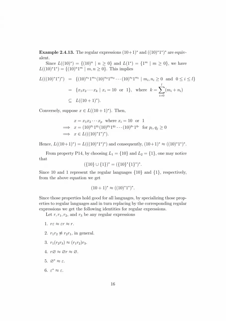
Example 2.4.13. The regular expressions (10+1)∗ and ((10)∗1∗)∗ are equiv-alent.
Since L((10)∗) = {(10)n | n ≥ 0} and L(1∗) = {1m | m ≥ 0}, we haveL((10)∗1∗) = {(10)n1m | m,n ≥ 0}. This implies
L(((10)∗1∗)∗) = {(10)n11m1(10)n21m2 · · · (10)nl1ml | mi, ni ≥ 0 and 0 ≤ i ≤ l}
= {x1x2 · · ·xk | xi = 10 or 1}, where k =l∑
i=0
(mi + ni)
⊆ L((10 + 1)∗).
Conversely, suppose x ∈ L((10 + 1)∗). Then,
x = x1x2 · · ·xp where xi = 10 or 1
=⇒ x = (10)p11q1(10)p21q2 · · · (10)pr1qr for pi, qj ≥ 0
=⇒ x ∈ L(((10)∗1∗)∗).
Hence, L((10+1)∗) = L(((10)∗1∗)∗) and consequently, (10+1)∗ ≈ ((10)∗1∗)∗.
From property P14, by choosing L1 = {10} and L2 = {1}, one may noticethat
({10} ∪ {1})∗ = ({10}∗{1}∗)∗.Since 10 and 1 represent the regular languages {10} and {1}, respectively,from the above equation we get
(10 + 1)∗ ≈ ((10)∗1∗)∗.
Since those properties hold good for all languages, by specializing those prop-erties to regular languages and in turn replacing by the corresponding regularexpressions we get the following identities for regular expressions.
Let r, r1, r2, and r3 be any regular expressions
1. rε ≈ εr ≈ r.
2. r1r2 6≈ r2r1, in general.
3. r1(r2r3) ≈ (r1r2)r3.
4. r∅ ≈ ∅r ≈ ∅.
5. ∅∗ ≈ ε.
6. ε∗ ≈ ε.
16

7. If ε ∈ L(r), then r∗ ≈ r+.
8. rr∗ ≈ r∗r ≈ r+.
9. (r1 + r2)r3 ≈ r1r3 + r2r3.
10. r1(r2 + r3) ≈ r1r2 + r1r3.
11. (r∗)∗ ≈ r∗.
12. (r1r2)∗r1 ≈ r1(r2r1)
∗.
13. (r1 + r2)∗ ≈ (r∗1r
∗2)∗.
Example 2.4.14.
1. b+(a∗b∗ + ε)b ≈ b(b∗a∗ + ε)b+ ≈ b+a∗b+.
Proof.
b+(a∗b∗ + ε)b ≈ (b+a∗b∗ + b+ε)b
≈ b+a∗b∗b + b+b
≈ b+a∗b+ + b+b
≈ b+a∗b+, since L(b+b) ⊆ L(b+a∗b+).
Similarly, one can observe that b(b∗a∗ + ε)b+ ≈ b+a∗b+.
2. (0+(01)∗0 + 0∗(10)∗)∗ ≈ (0 + 10)∗.
Proof.
(0+(01)∗0 + 0∗(10)∗)∗ ≈ (0+0(10)∗ + 0∗(10)∗)∗
≈ ((0+0 + 0∗)(10)∗)∗
≈ (0∗(10)∗)∗, since L(0+0) ⊆ L(0∗)
≈ (0 + 10)∗.
Notation 2.4.15. If L is represented by a regular expression r, i.e. L(r) = L,then we may simply use r instead of L(r) to indicated the language L. Asa consequence, for two regular expressions r and r′, r ≈ r′ and r = r′ areequivalent.
17

Chapter 3
Grammars
In this chapter, we introduce the notion of grammar called context-free gram-mar (CFG) as a language generator. The notion of derivation is instrumentalin understanding how the strings are generated in a grammar. We explainthe various properties of derivations using a graphical representation calledderivation trees. A special case of CFG, viz. regular grammar, is discussedas tool to generate to regular languages. A more general notion of grammarsis presented in Chapter 7.
In the context of natural languages, the grammar of a language is a set ofrules which are used to construct/validate sentences of the language. It hasbeen pointed out, in the introduction of Chapter 2, that this is the third stepin a formal learning of a language. Now we draw the attention of a readerto look into the general features of the grammars (of natural languages) toformalize the notion in the present context which facilitate for better under-standing of formal languages. Consider the English sentence
The students study automata theory.
In order to observe that the sentence is grammatically correct, one mayattribute certain rules of the English grammar to the sentence and validateit. For instance, the Article the followed by the Noun students form aNoun-phrase and similarly the Noun automata theory form a Noun-phrase.Further, study is a Verb. Now, choose the Sentential form “Subject VerbObject” of the English grammar. As Subject or Object can be a Noun-phraseby plugging in the above words one may conclude that the given sentenceis a grammatically correct English sentence. This verification/derivation isdepicted in Figure 3.1. The derivation can also be represented by a treestructure as shown in Figure 3.2.
18

Sentence ⇒ Subject Verb Object⇒ Noun-phrase Verb Object⇒ Article Noun Verb Object⇒ The Noun Verb Object⇒ The students Verb Object⇒ The students study Object⇒ The students study Noun-phrase⇒ The students study Noun⇒ The students study automata theory
Figure 3.1: Derivation of an English Sentence
In this process, we observe that two types of words are in the discussion.
1. The words like the, study, students.
2. The words like Article, Noun, Verb.
The main difference is, if you arrive at a stage where type (1) words areappearing, then you need not say anything more about them. In case youarrive at a stage where you find a word of type (2), then you are assumedto say some more about the word. For example, if the word Article comes,then one should say which article need to be chosen among a, an and the.Let us call the type (1) and type (2) words as terminals and nonterminals,respectively, as per their features.
Thus, a grammar should include terminals and nonterminals along with aset of rules which attribute some information regarding nonterminal symbols.
3.1 Context-Free Grammars
We now understand that a grammar should have the following components.
• A set of nonterminal symbols.
• A set of terminal symbols.
• A set of rules.
• As the grammar is to construct/validate sentences of a language, wedistinguish a symbol in the set of nonterminals to represent a sen-tence – from which various sentences of the language can be gener-ated/validated.
19

Sentence
Subject Verb Object
Noun−phraseNoun−phrase
NounArticle Noun
studentsThe study automata theory
Figure 3.2: Derivation Tree of an English Sentence
With this, we formally define the notion of grammar as below.
Definition 3.1.1. A grammar is a quadruple
G = (N, Σ, P, S)
where
1. N is a finite set of nonterminals,
2. Σ is a finite set of terminals,
3. S ∈ N is the start symbol, and
4. P is a finite subset of N × V ∗ called the set of production rules. Here,V = N ∪ Σ.
It is convenient to write A → α, for the production rule (A,α) ∈ P .
To define a formal notion of validating or deriving a sentence using agrammar, we require the following concepts.
Definition 3.1.2. Let G = (N, Σ, P, S) be a grammar with V = N ∪ Σ.
1. We define a binary relation ⇒G on V ∗ by
α ⇒G β if and only if α = α1Aα2, β = α1γα2 and A → γ ∈ P,
for all α, β ∈ V ∗.
20
2. The relation ⇒G is called one step relation on G. If α ⇒G β, then we callα yields β in one step in G.
3. The reflexive-transitive closure of ⇒G is denoted by ⇒∗G . That is, forα, β ∈ V ∗,
α ⇒∗G β if and only if
{ ∃n ≥ 0 and α0, α1, . . . , αn ∈ V ∗ such thatα = α0 ⇒G α1 ⇒G · · · ⇒G αn−1 ⇒G αn = β.
4. For α, β ∈ V ∗, if α ⇒∗G β, then we say β is derived from α or α derives
β. Further, α ⇒∗G β is called as a derivation in G.
5. If α = α0 ⇒G α1 ⇒G · · · ⇒G αn−1 ⇒G αn = β is a derivation, then the length
of the derivation is n and it may be written as α ⇒nG β.
6. In a given context, if we deal with only one grammar G, then we maysimply write ⇒, in stead of ⇒G .
7. If α ⇒∗ β is a derivation, then we say β is the yield of the derivation.
8. A string α ∈ V ∗ is said to be a sentential form in G, if α can be derivedfrom the start symbol S of G. That is, S ⇒∗ α.
9. In particular, if α ∈ Σ∗, then the sentential form α is known as asentence. In which case, we say α is generated by G.
10. The language generated by G, denoted by L(G), is the set of all sen-tences generated by G. That is,
L(G) = {x ∈ Σ∗ | S ⇒∗ x}.
Note that a production rule of a grammar is of the form A → α, whereA is a nonterminal symbol. If the nonterminal A appears in a sententialform X1 · · ·XkAXk+1 · · ·Xn, then the sentential form X1 · · ·XkαXk+1 · · ·Xn
can be obtained in one step by replacing A with α. This replacement isindependent of the neighboring symbols of A in X1 · · ·XkAXk+1 · · ·Xn. Thatis, X ′
is will not play any role in the replacement. One may call A is withinthe context of X ′
is and hence the rules A → α are said to be of context-freetype. Thus, the type of grammar that is defined here is known as context-free grammar, simply CFG. In the later chapters, we relax the constraint anddiscuss more general types of grammars.
21

Example 3.1.3. Let P = {S → ab, S → bb, S → aba, S → aab} withΣ = {a, b} and N = {S}. Then G = (N, Σ, P, S) is a context-free grammar.Since left hand side of each production rule is the start symbol S and theirright hand sides are terminal strings, every derivation in G is of length one.In fact, we precisely have the following derivation in G.
1. S ⇒ ab
2. S ⇒ bb
3. S ⇒ aba
4. S ⇒ aab
Hence, the language generated by G,
L(G) = {ab, bb, aba, aab}.
Notation 3.1.4.
1. A → α1, A → α2 can be written as A → α1 | α2.
2. Normally we use S as the start symbol of a grammar, unless otherwisespecified.
3. To give a grammar G = (N, Σ, P, S), it is sufficient to give the produc-tion rules only since one may easily find the other components N andΣ of the grammar G by looking at the rules.
Example 3.1.5. Suppose L is a finite language over an alphabet Σ, say L ={x1, x2, . . . , xn}. Then consider the finite set P = {S → x1 | x2 | · · · | xn}.Now, as discussed in Example 3.1.3, one can easily observe that the CFG({S}, Σ, P, S) generates the language L.
Example 3.1.6. Let Σ = {0, 1} and N = {S}. Consider the CFG G =(N, Σ, P, S), where P has precisely the following production rules.
1. S → 0S
2. S → 1S
3. S → ε
22

We now observe that the CFG G generates Σ∗. As every string generatedby G is a sequence of 0′s and 1′s, clearly we have L(G) ⊆ Σ∗. On the otherhand, let x ∈ Σ∗. If x = ε, then x can be generated in one step using therule S → ε. Otherwise, let x = a1a2 · · · an, where ai = 0 or 1 for all i. Now,as shown below, x can be derived in G.
S ⇒ a1S (if a1 = 0, then by rule 1; else by rule 2)⇒ a1a2S (as above)...⇒ a1a2 · · · anS (as above)⇒ a1a2 · · · anε (by rule 3)= x.
Hence, x ∈ L(G). Thus, L(G) = Σ∗.
Example 3.1.7. The language ∅ (over any alphabet Σ) can be generatedby a CFG.
Method-I. If the set of productions P is empty, then clearly the CFG G =({S}, Σ, P, S) does not generate any string and hence L(G) = ∅.
Method-II. Consider a CFG G in which each production rule has some non-terminal symbol on its right hand side. Clearly, no terminal string can begenerated in G so that L(G) = ∅.
Example 3.1.8. Consider G = ({S}, {a}, P, S) where P has the followingrules
1. S → aS
2. S → ε
Let us look at the strings that can be generated by G. Clearly, ε can begenerated in one step by using the rule S → ε. Further, if we choose rule (1)and then rule (2) we get the string a in two steps as follows:
S ⇒ aS ⇒ aε = a
If we use the rule (1), then one may notice that there will always be thenonterminal S in the resulting sentential form. A derivation can only beterminated by using rule (2). Thus, for any derivation of length k, that
23

derives some string x, we would have used rule (1) for k − 1 times and rule(2) once at the end. Precisely, the derivation will be of the form
S ⇒ aS
⇒ aaS...
⇒k−1︷ ︸︸ ︷
aa · · · a S
⇒k−1︷ ︸︸ ︷
aa · · · a ε = ak−1
Hence, it is clear that L(G) = {ak | k ≥ 0}In the following, we give some more examples of typical CFGs.
Example 3.1.9. Consider the grammar having the following productionrules:
S → aSb | ε
One may notice that the rule S → aSb should be used to derive strings otherthan ε, and the derivation shall always be terminated by S → ε. Thus, atypical derivation is of the form
S ⇒ aSb
⇒ aaSbb...
⇒ anSbn
⇒ anεbn = anbn
Hence, L(G) = {anbn | n ≥ 0}.Example 3.1.10. The grammar
S → aSa | bSb | a | b | ε
generates the set of all palindromes over {a, b}. For instance, the rules S →aSa and S → bSb will produce same terminals at the same positions towardsleft and right sides. While terminating the derivation the rules S → a | bor S → ε will produce odd or even length palindromes, respectively. Forexample, the palindrome abbabba can be derived as follows.
S ⇒ aSa
⇒ abSba
⇒ abbSbba
⇒ abbabba
24

Example 3.1.11. Consider the language L = {ambncm+n | m,n ≥ 0}. Wenow give production rules of a CFG which generates L. As given in Example3.1.9, the production rule
S → aSc
can be used to produce equal number of a′s and c′s, respectively, in left andright extremes of a string. In case, there is no b in the string, the productionrule
S → ε
can be used to terminate the derivation and produce a string of the formamcm. Note that, b′s in a string may have leading a′s; but, there will not beany a after a b. Thus, a nonterminal symbol that may be used to produceb′s must be different from S. Hence, we choose a new nonterminal symbol,say A, and define the rule
S → A
to handover the job of producing b′s to A. Again, since the number of b′sand c′s are to be equal, choose the rule
A → bAc
to produce b′s and c′s on either sides. Eventually, the rule
A → ε
can be introduced, which terminate the derivation. Thus, we have the fol-lowing production rules of a CFG, say G.
S → aSc | A | ε
A → bAc | ε
Now, one can easily observe that L(G) = L.
Example 3.1.12. For the language {ambm+ncn | m,n ≥ 0}, one may thinkin the similar lines of Example 3.1.11 and produce a CFG as given below.
S → AB
A → aAb | ε
B → bBc | ε
25

S ⇒ S ∗ S S ⇒ S ∗ S S ⇒ S + S⇒ S ∗ a ⇒ S + S ∗ S ⇒ a + S⇒ S + S ∗ a ⇒ a + S ∗ S ⇒ a + S ∗ S⇒ a + S ∗ a ⇒ a + b ∗ S ⇒ a + b ∗ S⇒ a + b ∗ a ⇒ a + b ∗ a ⇒ a + b ∗ a
(1) (2) (3)
Figure 3.3: Derivations for the string a + b ∗ a
3.2 Derivation Trees
Let us consider the CFG whose production rules are:
S → S ∗ S | S + S | (S) | a | b
Figure 3.3 gives three derivations for the string a + b ∗ a. Note that thethree derivations are different, because of application of different sequences ofrules. Nevertheless, the derivations (1) and (2) share the following feature.A nonterminal that appears at a particular common position in both thederivations derives the same substring of a + b ∗ a in both the derivations.In contrast to that, the derivations (2) and (3) are not sharing such feature.For example, the second S in step 2 of derivations (1) and (2) derives thesubstring a; whereas, the second S in step 2 of derivation (3) derives thesubstring b ∗ a. In order to distinguish this feature between the derivationsof a string, we introduce a graphical representation of a derivation calledderivation tree, which will be a useful tool for several other purposes also.
Definition 3.2.1. Let G = (N, Σ, P, S) be a CFG and V = N ∪ Σ. ForA ∈ N and α ∈ V ∗, suppose
A ⇒∗ α
is a derivation in G. A derivation tree or a parse tree of the derivation isiteratively defined as follows.
1. A is the root of the tree.
2. If the rule B → X1X2 · · ·Xk is applied in the derivation, then newnodes with labels X1, X2, . . . , Xk are created and made children to thenode B from left to right in that order.
The construction of the derivation tree of a derivation is illustrated withthe following examples.
26

Example 3.2.2. Consider the following derivation in the CFG given in Ex-ample 3.1.9.
S ⇒ aSb
⇒ aaSbb
⇒ aaεbb
= aabb
The derivation tree of the above derivation S ⇒∗ aabb is shown below.
S==
==
¢¢¢¢
a S==
==
¢¢¢¢
b
a S b
ε
Example 3.2.3. Consider the following derivation in the CFG given in Ex-ample 3.1.12.
S ⇒ AB
⇒ aAbB
⇒ aaAbbB
⇒ aaAbbB
⇒ aaAbbbBc
⇒ aaAbbbεc
= aaAbbbc
The derivation tree of the above derivation S ⇒∗ aaAbbbc is shown below.
S
NNNNNNNN
pppppppp
A==
==
¡¡¡¡
B>>
>>
¡¡¡¡
a A==
==
¡¡¡¡
b b B c
a A b ε
Note that the yield α of the derivation A ⇒∗ α can be identified in thederivation tree by juxtaposing the labels of the leaf nodes from left to right.
Example 3.2.4. Recall the derivations given in Figure 3.3. The derivationtrees corresponding to these derivations are in Figure 3.4.
27

SCC
CCC
{{{{
{S
CCCC
C
{{{{
{S
CCCC
C
{{{{
{
SCC
CCC
ÄÄÄÄ
∗ S SCC
CCC
ÄÄÄÄ
∗ S S + S??
??{{
{{{
S + S a S + S a a S ∗ S
a b a b b a
(1) (2) (3)
Figure 3.4: Derivation Trees for Figure 3.3
Now we are in a position to formalize the notion of equivalence betweenderivations, which precisely captures the feature proposed in the beginning ofthe section. Two derivations are said to be equivalent if their derivation treesare same. Thus, equivalent derivations are precisely differed by the order ofapplication of same production rules. That is, the application of productionrules in a derivation can be permuted to get an equivalent derivation. Forexample, as derivation trees (1) and (2) of Figure 3.4 are same, the derivations(1) and (2) of Figure 3.3 are equivalent. Thus, a derivation tree may representseveral equivalent derivations. However, for a given derivation tree, whoseyield is a terminal string, there is a unique special type of derivation, viz.leftmost derivation (or rightmost derivation).
Definition 3.2.5. For A ∈ N and x ∈ Σ∗, the derivation A ⇒∗ x is saidto be a leftmost derivation if the production rule applied at each step is onthe leftmost nonterminal symbol of the sentential form. In which case, thederivation is denoted by A ⇒∗
Lx.
Similarly, for A ∈ N and x ∈ Σ∗, the derivation A ⇒∗ x is said to be arightmost derivation if the production rule applied at each step is on therightmost nonterminal symbol of the sentential form. In which case, thederivation is denoted by A ⇒∗
Rx.
Because of the similarity between leftmost derivation and rightmost deriva-tion, the properties of the leftmost derivations can be imitated to get similarproperties for rightmost derivations. Now, we establish some properties ofleftmost derivations.
Theorem 3.2.6. For A ∈ N and x ∈ Σ∗, A ⇒∗ x if and only if A ⇒∗L
x.
28

Proof. “Only if” part is straightforward, as every leftmost derivation is, any-way, a derivation.
For “if” part, let
A = α0 ⇒ α1 ⇒ α2 ⇒ · · · ⇒ αn−1 ⇒ αn = x
be a derivation. If αi ⇒L αi+1, for all 0 ≤ i < n, then we are through.Otherwise, there is an i such that αi 6⇒L αi+1. Let k be the least such thatαk 6⇒L αk+1. Then, we have αi ⇒L αi+1, for all i < k, i.e. we have leftmostsubstitutions in the first k steps. We now demonstrate how to extend theleftmost substitution to (k + 1)th step. That is, we show how to convert thederivation
A = α0 ⇒L α1 ⇒L · · · ⇒L αk ⇒ αk+1 ⇒ · · · ⇒ αn−1 ⇒ αn = x
in to a derivation
A = α0 ⇒L α1 ⇒L · · · ⇒L αk ⇒L α′k+1 ⇒ α′k+2 ⇒ · · · ⇒ α′n−1 ⇒ α′n = x
in which there are leftmost substitutions in the first (k + 1) steps and thederivation is of same length of the original. Hence, by induction one canextend the given derivation to a leftmost derivation A ⇒∗
Lx.
Since αk ⇒ αk+1 but αk 6⇒L αk+1, we have
αk = yA1β1A2β2,
for some y ∈ Σ∗, A1, A2 ∈ N and β1, β2 ∈ V ∗, and A2 → γ2 ∈ P such that
αk+1 = yA1β1γ2β2.
But, since the derivation eventually yields the terminal string x, at a laterstep, say pth step (for p > k), A1 would have been substituted by some stringγ1 ∈ V ∗ using the rule A1 → γ1 ∈ P . Thus the original derivation looks asfollows.
A = α0 ⇒L α1 ⇒L · · · ⇒L αk = yA1β1A2β2
⇒ αk+1 = yA1β1γ2β2
= yA1ξ1, with ξ1 = β1γ2β2
⇒ αk+2 = yA1ξ2, ( here ξ1 ⇒ ξ2)...
⇒ αp−1 = yA1ξp−k−1
⇒ αp = yγ1ξp−k−1
⇒ αp+1
...
⇒ αn = x
29

We now demonstrate a mechanism of using the rule A1 → γ1 in (k + 1)thstep so that we get a desired derivation. Set
α′k+1 = yγ1β1A2β2
α′k+2 = yγ1β1γ2β2 = yγ1ξ1
α′k+3 = yγ1ξ2
...α′p−1 = yγ1ξp−k−2
α′p = yγ1ξp−k−1 = αp
α′p+1 = αp+1
...α′n = αn
Now we have the following derivation in which (k+1)th step has leftmostsubstitution, as desired.
A = α0 ⇒L α1 ⇒L · · · ⇒L αk = yA1β1A2β2
⇒L α′k+1 = yγ1β1A2β2
⇒ α′k+2 = yγ1β1γ2β2 = yγ1ξ1
⇒ α′k+3 = yγ1ξ2
...
⇒ α′p−1 = yγ1ξp−k−2
⇒ α′p = yγ1ξp−k−1 = αp
⇒ α′p+1 = αp+1
...
⇒ α′n = αn = x
As stated earlier, we have the theorem by induction.
Proposition 3.2.7. Two equivalent leftmost derivations are identical.
Proof. Let T be the derivation tree of two leftmost derivations D1 and D2.Note that the production rules applied at each nonterminal symbol is pre-cisely represented by its children in the derivation tree. Since the derivationtree is same for D1 and D2, the production rules applied in both the deriva-tions are same. Moreover, as D1 and D2 are leftmost derivations, the orderof application of production rules are also same; that is, each production isapplied to the leftmost nonterminal symbol. Hence, the derivations D1 andD2 are identical.
Now we are ready to establish the correspondence between derivationtrees and leftmost derivations.
30

Theorem 3.2.8. Every derivation tree, whose yield is a terminal string,represents a unique leftmost derivation.
Proof. For A ∈ N and x ∈ Σ∗, suppose T is the derivation tree of a derivationA ⇒∗ x. By Theorem 3.2.6, we can find an equivalent leftmost derivationA ⇒∗
Lx. Hence, by Proposition 3.2.7, we have a unique leftmost derivation
that is represented by T .
Theorem 3.2.9. Let G = (N, Σ, P, S) be a CFG and
κ = max{|α| | A → α ∈ P}.
For x ∈ L(G), if T is a derivation tree for x, then
|x| ≤ κh
where h is the height of the tree T .
Proof. Since κ is the maximum length of righthand side of each productionrule of G, each internal node of T is a parent of at most κ number of children.Hence, T is a κ-ary tree. Now, in the similar lines of Theorem 1.2.3 that isgiven for binary trees, one can easily prove that T has at most κh leaf nodes.Hence, |x| ≤ κh.
3.2.1 Ambiguity
Let G be a context-free grammar. It may be a case that the CFG G givestwo or more inequivalent derivations for a string x ∈ L(G). This can beidentified by their different derivation trees. While deriving the string, ifthere are multiple possibilities of application of production rules on the samesymbol, one may have a difficulty in choosing a correct rule. In the contextof compiler which is constructed based on a grammar, this difficulty will leadto an ambiguity in parsing. Thus, a grammar with such a property is saidto be ambiguous.
Definition 3.2.10. Formally, a CFG G is said to be ambiguous, if G hastwo different leftmost derivations for some string in L(G). Otherwise, thegrammar is said to be unambiguous.
Remark 3.2.11. One can equivalently say that a CFG G is ambiguous, if G hastwo different rightmost derivations or derivation trees for a string in L(G).
31

Example 3.2.12. Recall the CFG which generates arithmetic expressionswith the production rules
S → S ∗ S | S + S | (S) | a | b
As shown in Figure 3.3, the arithmetic expression a + b ∗ a has two differentleftmost derivations, viz. (2) and (3). Hence, the grammar is ambiguous.
Example 3.2.13. An unambiguous grammar which generates the arithmeticexpressions (the language generated by the CFG given in Example 3.2.12) isas follows.
S → S + T | T
T → T ∗R | R
R → (S) | a | b
In the context of constructing a compiler or similar such applications, itis desirable that the underlying grammar be unambiguous. Unfortunately,there are some CFLs for which there is no CFG which is unambiguous. Sucha CFL is known as inherently ambiguous language.
Example 3.2.14. The context-free language
{ambmcndn | m,n ≥ 1} ∪ {ambncndm | m,n ≥ 1}
is inherently ambiguous. For proof, one may refer to the Hopcroft and Ullman[1979].
3.3 Regular Grammars
Definition 3.3.1. A CFG G = (N, Σ, P, S) is said to be linear if everyproduction rule of G has at most one nonterminal symbol in its righthandside. That is,
A → α ∈ P =⇒ α ∈ Σ∗ or α = xBy, for some x, y ∈ Σ∗ and B ∈ N.
Example 3.3.2. The CFGs given in Examples 3.1.8, 3.1.9 and 3.1.11 areclearly linear. Whereas, the CFG given in Example 3.1.12 is not linear.
Remark 3.3.3. If G is a linear grammar, then every derivation in G is aleftmost derivation as well as rightmost derivation. This is because there isexactly one nonterminal symbol in the sentential form of each internal stepof the derivation.
32

Definition 3.3.4. A linear grammar G = (N, Σ, P, S) is said to be rightlinear if the nonterminal symbol in the righthand side of each production rule,if any, occurs at the right end. That is, righthand side of each productionrule is of the form – a terminal string followed by at most one nonterminalsymbol – as shown below.
A → x or A → xB
for some x ∈ Σ∗ and B ∈ N .Similarly, a left linear grammar is defined by considering the production
rules in the following form.
A → x or A → Bx
for some x ∈ Σ∗ and B ∈ N .
Because of the similarity in the definitions of left linear grammar and rightlinear grammar, every result which is true for one can be imitated to obtaina parallel result for the other. In fact, the notion of left linear grammar isequivalent right linear grammar (see Exercise ??). Here, by equivalence wemean, if L is generated by a right linear grammar, then there exists a leftlinear grammar that generates L; and vice-versa.
Example 3.3.5. The CFG given in Example 3.1.8 is a right linear grammar.For the language {ak | k ≥ 0}, an equivalent left linear grammar is given
by the following production rules.
S → Sa | ε
Example 3.3.6. We give a right linear grammar for the language
L = {x ∈ {a, b}∗ | |x|a = 2n + 1, for some n}.
We understand that the nonterminal symbols in a grammar maintain theproperties of the strings that they generate or whenever they appear in aderivation they determine the properties of the partial string that the deriva-tion so far generated.
Since we are looking for a right linear grammar for L, each productionrule will have at most one nonterminal symbol on its righthand side andhence at each internal step of a desired derivation, we will have exactly onenonterminal symbol. While, we are generating a sequence of a′s and b′s forthe language, we need not keep track of the number of b′s that are generated,so far. Whereas, we need to keep track the number of a′s; here, it need not be
33

the actual number, rather the parity (even or odd) of the number of a′s thatare generated so far. So to keep track of the parity information, we requiretwo nonterminal symbols, say O and E, respectively for odd and even. In thebeginning of any derivation, we would have generated zero number of symbols– in general, even number of a′s. Thus, it is expected that the nonterminalsymbol E to be the start symbol of the desired grammar. While E generatesthe terminal symbol b, the derivation can continue to be with nonterminalsymbol E. Whereas, if one a is generated then we change to the symbol O,as the number of a′s generated so far will be odd from even. Similarly, weswitch to E on generating an a with the symbol O and continue to be withO on generating any number of b′s. Precisely, we have obtained the followingproduction rules.
E → bE | aO
O → bO | aE
Since, our criteria is to generate a string with odd number of a′s, we canterminate a derivation while continuing in O. That is, we introduce theproduction rule
O → ε
Hence, we have the right linear grammar G = ({E, O}, {a, b}, P, E), where Phas the above defined three productions. Now, one can easily observe thatL(G) = L.
Recall that the language under discussion is stated as a regular languagein Chapter 1 (refer Example 2.4.10). Whereas, we did not supply any proofin support. Here, we could identify a right linear grammar that generatesthe language. In fact, we have the following result.
Theorem 3.3.7. The language generated by a right linear grammar is reg-ular. Moreover, for every regular language L, there exists a right lineargrammar that generates L.
An elegant proof of this theorem would require some more concepts andhence postponed to later chapters. For proof of the theorem, one may referto Chapter 4. In view of the theorem, we have the following definition.
Definition 3.3.8. Right linear grammars are also called as regular gram-mars.
Remark 3.3.9. Since left linear grammars and right linear grammars areequivalent, left linear grammars also precisely generate regular languages.Hence, left linear grammars are also called as regular grammars.
34

Example 3.3.10. The language {x ∈ {a, b}∗ | ab is a substring of x} can begenerated by the following regular grammar.
S → aS | bS | abA
A → aA | bA | ε
Example 3.3.11. Consider the regular grammar with the following produc-tion rules.
S → aA | bS | ε
A → aS | bA
Note that the grammar generates the set of all strings over {a, b} havingeven number of a′s.
Example 3.3.12. Consider the language represented by the regular expres-sion a∗b+ over {a, b}, i.e.
{ambn ∈ {a, b}∗ | m ≥ 0, n ≥ 1}
It can be easily observe that the following regular grammar generates thelanguage.
S → aS | B
B → bB | b
Example 3.3.13. The grammar with the following production rules is clearlyregular.
S → bS | aA
A → bA | aB
B → bB | aS | ε
It can be observed that the language {x ∈ {a, b}∗ | |x|a ≡ 2 mod 3} isgenerated by the grammar.
Example 3.3.14. Consider the language
L ={
x ∈ (0 + 1)∗∣∣∣ |x|0 is even ⇔ |x|1 is odd
}.
It is little tedious to construct a regular grammar to show that L is regular.However, using a better tool, we show that L is regular later (See Example5.1.3).
35

3.4 Digraph Representation
We could achieve in writing a right linear grammar for some languages. How-ever, we face difficulties in constructing a right linear grammar for some lan-guages that are known to be regular. We are now going to represent a rightlinear grammar by a digraph which shall give a better approach in writ-ing/constructing right linear grammar for languages. In fact, this digraphrepresentation motivates one to think about the notion of finite automatonwhich will be shown, in the next chapter, as an ultimate tool in understandingregular languages.
Definition 3.4.1. Given a right linear grammar G = (N, T, P, S), define thedigraph (V, E), where the vertex set V = N ∪ {$} with a new symbol $ andthe edge set E is formed as follows.
1. (A,B) ∈ E ⇐⇒ A → xB ∈ P , for some x ∈ T ∗
2. (A, $) ∈ E ⇐⇒ A → x ∈ P , for some x ∈ T ∗
In which case, the arc from A to B is labeled by x.
Example 3.4.2. The digraph for the grammar presented in Example 3.3.10is as follows.
//GFED@ABCS
a,bªª
ab //GFED@ABCA
a,bªª
ε // ?>=<89:;$
Remark 3.4.3. From a digraph one can easily give the corresponding rightlinear grammar.
Example 3.4.4. The digraph for the grammar presented in Example 3.3.12is as follows.
//GFED@ABCS
aªª
ε //GFED@ABCB
bªª
b // ?>=<89:;$
Remark 3.4.5. A derivation in a right linear grammar can be represented, inits digraph, by a path from the starting node S to the special node $; andconversely. We illustrate this through the following.
Consider the following derivation for the string aab in the grammar givenin Example 3.3.12.
S ⇒ aS ⇒ aaS ⇒ aaB ⇒ aab
The derivation can be traced by a path from S to $ in the correspondingdigraph (refer to Example 3.4.4) as shown below.
Sa // S
a // Sε // B
b // $
36

One may notice that the concatenation of the labels on the path, called labelof the path, gives the desired string. Conversely, it is easy to see that thelabel of any path from S to $ can be derived in G.
37

Chapter 4
Finite Automata
Regular grammars, as language generating devices, are intended to generateregular languages - the class of languages that are represented by regularexpressions. Finite automata, as language accepting devices, are importanttools to understand the regular languages better. Let us consider the reg-ular language - the set of all strings over {a, b} having odd number of a′s.Recall the grammar for this language as given in Example 3.3.6. A digraphrepresentation of the grammar is given below:
//GFED@ABCE
bªª
a //GFED@ABCO
bªª
a
ff
ε // ?>=<89:;$
Let us traverse the digraph via a sequence of a′s and b′s starting at the nodeE. We notice that, at a given point of time, if we are at the node E, thenso far we have encountered even number of a′s. Whereas, if we are at thenode O, then so far we have traversed through odd number of a′s. Of course,being at the node $ has the same effect as that of node O, regarding numberof a′s; rather once we reach to $, then we will not have any further move.
Thus, in a digraph that models a system which understands a language,nodes holds some information about the traversal. As each node is holdingsome information it can be considered as a state of the system and hence astate can be considered as a memory creating unit. As we are interested in thelanguages having finite representation, we restrict ourselves to those systemswith finite number of states only. In such a system we have transitionsbetween the states on symbols of the alphabet. Thus, we may call them asfinite state transition systems. As the transitions are predefined in a finitestate transition system, it automatically changes states based on the symbolsgiven as input. Thus a finite state transition system can also be called as a
38

finite state automaton or simply a finite automaton – a device that worksautomatically. The plural form of automaton is automata.
In this chapter, we introduce the notion of finite automata and show thatthey model the class of regular languages. In fact, we observe that finiteautomata, regular grammars and regular expressions are equivalent; each ofthem are to represent regular languages.
4.1 Deterministic Finite Automata
Deterministic finite automaton is a type of finite automaton in which thetransitions are deterministic, in the sense that there will be exactly one tran-sition from a state on an input symbol. Formally,
a deterministic finite automaton (DFA) is a quintuple A = (Q, Σ, δ, q0, F ),where
Q is a finite set called the set of states,Σ is a finite set called the input alphabet,q0 ∈ Q, called the initial/start state,F ⊆ Q, called the set of final/accept states, andδ : Q× Σ −→ Q is a function called the transition function or next-state
function.Note that, for every state and an input symbol, the transition function δ
assigns a unique next state.
Example 4.1.1. Let Q = {p, q, r}, Σ = {a, b}, F = {r} and δ is given bythe following table:
δ a bp q pq r pr r r
Clearly, A = (Q, Σ, δ, p, F ) is a DFA.
We normally use symbols p, q, r, . . . with or without subscripts to denotestates of a DFA.
Transition Table
Instead of explicitly giving all the components of the quintuple of a DFA, wemay simply point out the initial state and the final states of the DFA in thetable of transition function, called transition table. For instance, we use anarrow to point the initial state and we encircle all the final states. Thus, wecan have an alternative representation of a DFA, as all the components of
39

the DFA now can be interpreted from this representation. For example, theDFA in Example 4.1.1 can be denoted by the following transition table.
δ a b→ p q p
q r p©r r r
Transition Diagram
Normally, we associate some graphical representation to understand abstractconcepts better. In the present context also we have a digraph representa-tion for a DFA, (Q, Σ, δ, q0, F ), called a state transition diagram or simply atransition diagram which can be constructed as follows:
1. Every state in Q is represented by a node.
2. If δ(p, a) = q, then there is an arc from p to q labeled a.
3. If there are multiple arcs from labeled a1, . . . ak−1, and ak, one state toanother state, then we simply put only one arc labeled a1, . . . , ak−1, ak.
4. There is an arrow with no source into the initial state q0.
5. Final states are indicated by double circle.
The transition diagram for the DFA given in Example 4.1.1 is as below:
// ?>=<89:;p
b
a // ?>=<89:;q
b
bb
a // ?>=<89:;/.-,()*+ra, b
®®
Note that there are two transitions from the state r to itself on symbolsa and b. As indicated in the point 3 above, these are indicated by a singlearc from r to r labeled a, b.
Extended Transition Function
Recall that the transition function δ assigns a state for each state and an inputsymbol. This naturally can be extended to all strings in Σ∗, i.e. assigning astate for each state and an input string.
40

The extended transition function δ : Q× Σ∗ −→ Q is defined recursivelyas follows: For all q ∈ Q, x ∈ Σ∗ and a ∈ Σ,
δ(q, ε) = q and
δ(q, xa) = δ(δ(q, x), a).
For example, in the DFA given in Example 4.1.1, δ(p, aba) is q because
δ(p, aba) = δ(δ(p, ab), a)
= δ(δ(δ(p, a), b), a)
= δ(δ(δ(δ(p, ε), a), b), a)
= δ(δ(δ(p, a), b), a)
= δ(δ(q, b), a)
= δ(p, a) = q
Given p ∈ Q and x = a1a2 · · · ak ∈ Σ∗, δ(p, x) can be evaluated easilyusing the transition diagram by identifying the state that can be reached bytraversing from p via the sequence of arcs labeled a1, a2, . . . , ak.
For instance, the above case can easily be seen by the traversing throughthe path labeled aba from p to reach to q as shown below:
?>=<89:;p a // ?>=<89:;q b // ?>=<89:;p a // ?>=<89:;q
Language of a DFA
Now, we are in a position to define the notion of acceptance of a string, andconsequently acceptance of a language, by a DFA.
A string x ∈ Σ∗ is said to be accepted by a DFA A = (Q, Σ, δ, q0, F ) ifδ(q0, x) ∈ F . That is, when you apply the string x in the initial state theDFA will reach to a final state.
The set of all strings accepted by the DFA A is said to be the languageaccepted by A and is denoted by L(A ). That is,
L(A ) = {x ∈ Σ∗ | δ(q0, x) ∈ F}.Example 4.1.2. Consider the following DFA
// GFED@ABCq0
b
))SSSSSSSSSSSSSSSSSSSSSa // GFED@ABCq1
b //
a
ÂÂ??
????
???
GFED@ABC?>=<89:;q2b //
a
ÄÄÄÄÄÄ
ÄÄÄÄ
ÄGFED@ABC?>=<89:;q3
a,b
uukkkkkkkkkkkkkkkkkkkkk
?>=<89:;t
a,b
TT
41

The only way to reach from the initial state q0 to the final state q2 is throughthe string ab and it is through abb to reach another final state q3. Thus, thelanguage accepted by the DFA is
{ab, abb}.
Example 4.1.3. As shown below, let us recall the transition diagram of theDFA given in Example 4.1.1.
// ?>=<89:;p
b
a // ?>=<89:;q
b
bb
a // ?>=<89:;/.-,()*+ra, b
®®
1. One may notice that if there is aa in the input, then the DFA leads usfrom the initial state p to the final state r. Since r is also a trap state,after reaching to r we continue to be at r on any subsequent input.
2. If the input does not contain aa, then we will be shuffling between pand q but never reach the final state r.
Hence, the language accepted by the DFA is the set of all strings over {a, b}having aa as substring, i.e.
{xaay | x, y ∈ {a, b}∗}.
Description of a DFA
Note that a DFA is an abstract (computing) device. The depiction given inFigure 4.1 shall facilitate one to understand its behavior. As shown in thefigure, there are mainly three components namely input tape, reading head,and finite control. It is assumed that a DFA has a left-justified infinite tapeto accommodate an input of any length. The input tape is divided into cellssuch that each cell accommodate a single input symbol. The reading head isconnected to the input tape from finite control, which can read one symbol ata time. The finite control has the states and the information of the transitionfunction along with a pointer that points to exactly one state.
At a given point of time, the DFA will be in some internal state, say p,called the current state, pointed by the pointer and the reading head will bereading a symbol, say a, from the input tape called the current symbol. Ifδ(p, a) = q, then at the next point of time the DFA will change its internalstate from p to q (now the pointer will point to q) and the reading head willmove one cell to the right.
42

Figure 4.1: Depiction of Finite Automaton
Initializing a DFA with an input string x ∈ Σ∗ we mean x be placed onthe input tape from the left most (first) cell of the tape with the reading headplaced on the first cell and by setting the initial state as the current state.By the time the input is exhausted, if the current state of the DFA is a finalstate, then the input x is accepted by the DFA. Otherwise, x is rejected bythe DFA.
Configurations
A configuration or an instantaneous description of a DFA gives the informa-tion about the current state and the portion of the input string that is rightfrom and on to the reading head, i.e. the portion yet to be read. Formally,a configuration is an element of Q× Σ∗.
Observe that for a given input string x the initial configuration is (q0, x)and a final configuration of a DFA is of the form (p, ε).
The notion of computation in a DFA A can be described through con-figurations. For which, first we define one step relation as follows.
Definition 4.1.4. Let C = (p, x) and C ′ = (q, y) be two configurations. Ifδ(p, a) = q and x = ay, then we say that the DFA A moves from C to C ′ inone step and is denoted as C |−−
AC ′.
Clearly, |−−A
is a binary relation on the set of configurations of A .In a given context, if there is only one DFA under discussion, then we maysimply use |−− instead of |−−
A. The reflexive transitive closure of |−− may
be denoted by |−−* . That is, C |−−* C ′ if and only if there exist configurations
43

C0, C1, . . . , Cn such that
C = C0 |−− C1 |−− C2 |−− · · · |−− Cn = C ′
Definition 4.1.5. A the computation of A on the input x is of the form
C |−−* C ′
where C = (q0, x) and C ′ = (p, ε), for some p.
Remark 4.1.6. Given a DFA A = (Q, Σ, δ, q0, F ), x ∈ L(A ) if and only if(q0, x) |−−* (p, ε) for some p ∈ F .
Example 4.1.7. Consider the following DFA
// GFED@ABCq0
b
a // GFED@ABCq1
a
b // GFED@ABC?>=<89:;q2
b
a // GFED@ABC?>=<89:;q3
a
b // GFED@ABCq4
a, b
As states of a DFA are memory creating units, we demonstrate the languageof the DFA under consideration by explaining the roles of each of its states.
1. It is clear that, if the input contains only b′s, then the DFA remains inthe initial state q0 only.
2. On the other hand, if the input has an a, then the DFA transits fromq0 to q1. On any subsequent a′s, it remains in q1 only. Thus, the roleof q1 in the DFA is to understand that the input has at least one a.
3. Further, the DFA goes from q1 to q2 via a b and remains at q2 onsubsequent b′s. Thus, q2 recognizes that the input has an occurrenceof an ab.
Since q2 is a final state, the DFA accepts all those strings which haveone occurrence of ab.
4. Subsequently, if we have a number of a′s, the DFA will reach to q3,which is a final state, and remains there; so that all such strings willalso be accepted.
5. But, from then, via b the DFA goes to the trap state q4 and since it isnot a final state, all those strings will not be accepted. Here, note thatrole of q4 is to remember the second occurrence of ab in the input.
Thus, the language accepted by the DFA is the set of all strings over {a, b}which have exactly one occurrence of ab. That is,
{x ∈ {a, b}∗
∣∣∣ |x|ab = 1}
.
44

Example 4.1.8. Consider the following DFA
// GFED@ABC?>=<89:;q0
c
a,b// GFED@ABCq1
c
a,b~~}}
}}}}
}}}
GFED@ABCq2
c
TT
a,b
`AAAAAAAAA
1. First, observe that the number of occurrences of c′s in the input at anystate is simply ignored by the state by remaining in the same state.
2. Whereas, on input a or b, every state will lead the DFA to its nextstate as q0 to q1, q1 to q2 and q2 to q0.
3. It can be clearly visualized that, if the total number of a′s and b′s inthe input is a multiple of 3, then the DFA will be brought back to theinitial state q0. Since q0 is the final state those strings will be accepted.
4. On the other hand, if any string violates the above stated condition,then the DFA will either be in q1 or be in q2 and hence they will not beaccepted. More precisely, if the total number of a′s and b′s in the inputleaves the remainder 1 or 2, when it is divided by 3, then the DFA willbe in the state q1 or q2, respectively.
Hence the language of the DFA is
{x ∈ {a, b, c}∗
∣∣∣ |x|a + |x|b ≡ 0 mod 3}
.
From the above discussion, further we ascertain the following:
1. Instead of q0, if q1 is only the final state (as shown in (i), below), thenthe language will be
{x ∈ {a, b, c}∗
∣∣∣ |x|a + |x|b ≡ 1 mod 3}
2. Similarly, instead of q0, if q2 is only the final state (as shown in (ii),below), then the language will be
{x ∈ {a, b, c}∗
∣∣∣ |x|a + |x|b ≡ 2 mod 3}
45
// GFED@ABCq0
c
a,b// GFED@ABC?>=<89:;q1
c
a,b~~}}
}}}}
}}}
// GFED@ABCq0
c
a,b// GFED@ABCq1
c
a,b~~}}
}}}}
}}}
GFED@ABCq2
c
TT
a,b
`AAAAAAAAAGFED@ABC?>=<89:;q2
c
TT
a,b
`AAAAAAAAA
(i) (ii)
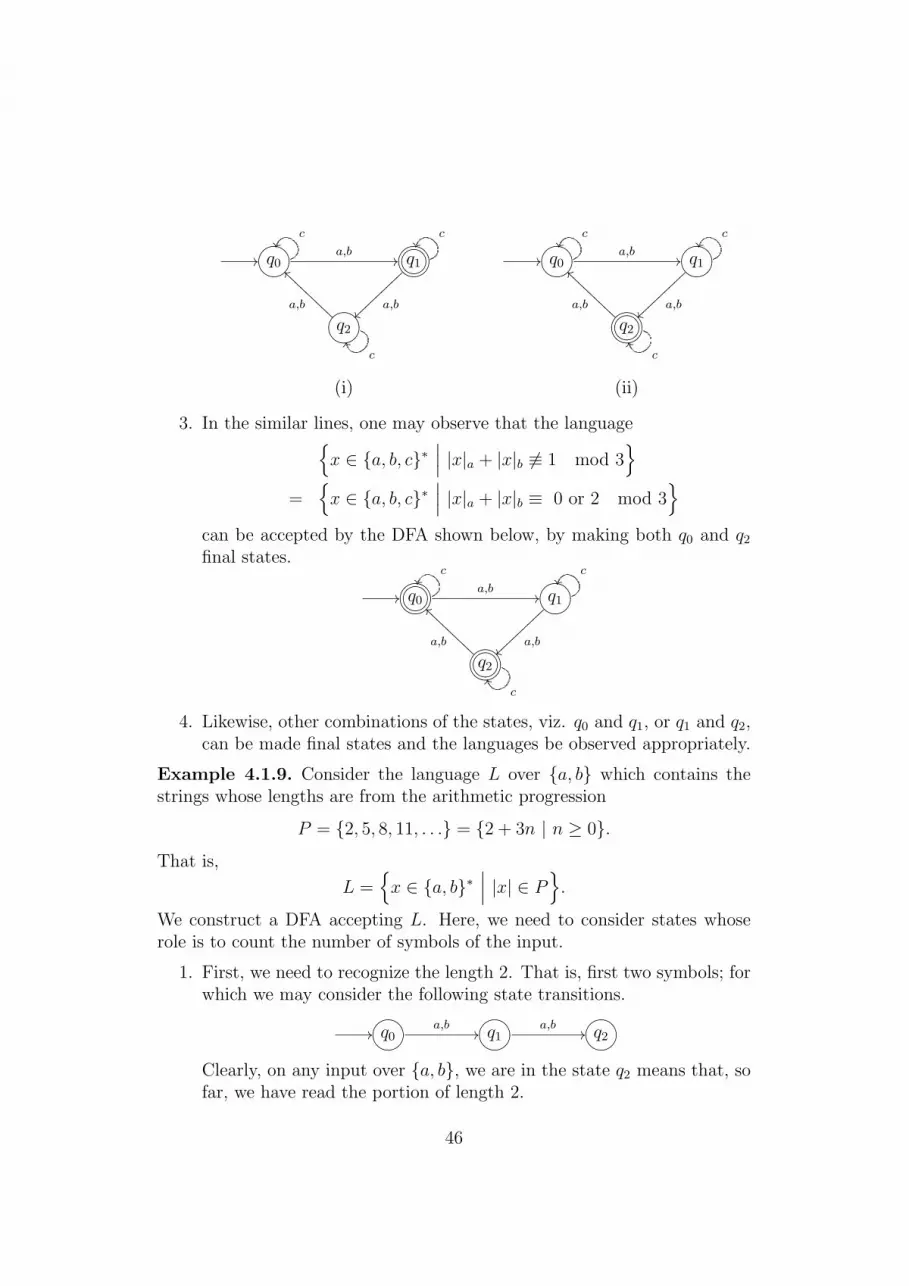
3. In the similar lines, one may observe that the language{
x ∈ {a, b, c}∗∣∣∣ |x|a + |x|b 6≡ 1 mod 3
}
={
x ∈ {a, b, c}∗∣∣∣ |x|a + |x|b ≡ 0 or 2 mod 3
}
can be accepted by the DFA shown below, by making both q0 and q2
final states.
// GFED@ABC?>=<89:;q0
c
a,b// GFED@ABCq1
c
a,b~~}}
}}}}
}}}
GFED@ABC?>=<89:;q2
c
TT
a,b
`AAAAAAAAA
4. Likewise, other combinations of the states, viz. q0 and q1, or q1 and q2,can be made final states and the languages be observed appropriately.
Example 4.1.9. Consider the language L over {a, b} which contains thestrings whose lengths are from the arithmetic progression
P = {2, 5, 8, 11, . . .} = {2 + 3n | n ≥ 0}.That is,
L ={
x ∈ {a, b}∗∣∣∣ |x| ∈ P
}.
We construct a DFA accepting L. Here, we need to consider states whoserole is to count the number of symbols of the input.
1. First, we need to recognize the length 2. That is, first two symbols; forwhich we may consider the following state transitions.
// GFED@ABCq0a,b
// GFED@ABCq1a,b
// GFED@ABCq2
Clearly, on any input over {a, b}, we are in the state q2 means that, sofar, we have read the portion of length 2.
46

2. Then, the length of rest of the string need to be a multiple of 3. Here,we borrow the idea from the Example 4.1.8 and consider the followingdepicted state transitions, further.
GFED@ABCq3
a,b
²²
// GFED@ABCq0a,b
// GFED@ABCq1a,b
// GFED@ABC?>=<89:;q2
a,b
>>}}}}}}}}}
GFED@ABCq4
a,b
`AAAAAAAAA
Clearly, this DFA accepts L.
In general, for any arithmetic progression P = {k′ + kn | n ≥ 0} withk, k′ ∈ N, if we consider the language
L ={
x ∈ Σ∗∣∣∣ |x| ∈ P
}
over an alphabet Σ, then the following DFA can be suggested for L.
ONMLHIJKqk′+1\ U K
>3
,'// GFED@ABCq0
Σ // GFED@ABCq1Σ //. . . ___ Σ // GFED@ABC?>=<89:;qk′
Σ00
pp
»
¶¯
¢tjc_^]\XYZ[q
k′+k−1Σ
SS
Example 4.1.10. Consider the language over {a, b} consisting of thosestrings that end with a. That is,
{xa | x ∈ {a, b}∗}.We observe the following to construct a DFA for the language.
1. If we assume a state q0 as the initial state, then an occurrence of a inthe input need to be distinguished. This can be done by changing thestate to some other, say q1. Whereas, we continue to be in q0 on b′s.
2. On subsequent a′s at q1 let us remain at q1. If a string ends on reachingq1, clearly it is ending with an a. By making q1 a final state, all suchstrings can be accepted.
47

3. If we encounter a b at q1, then we should go out of q1, as it is a finalstate.
4. Since again the possibilities of further occurrences of a′s need to cross-checked and q0 is already taking care of that, we may assign the tran-sition out of q1 on b to q0.
Thus, we have the following DFA which accepts the given language.
// GFED@ABCq0
b··
a // GFED@ABC?>=<89:;q1
a
b
dd
Example 4.1.11. Let us consider the following DFA
///.-,()*+a
b ///.-,()*+ a //
b
²²
/.-,()*+ÂÁÀ¿»¼½¾
b
ee
a
ww
/.-,()*+ÂÁÀ¿»¼½¾
b
a
II
Unlike the above examples, it is little tricky to ascertain the language ac-cepted by the DFA. By spending some amount of time, one may possiblyreport that the language is the set of all strings over {a, b} with last but onesymbol as b.
But for this language, if we consider the following type of finite automa-ton one can easily be convinced (with an appropriate notion of languageacceptance) that the language is so.
// ?>=<89:;p
a, b
b // ?>=<89:;q a, b// ?>=<89:;/.-,()*+r
Note that, in this type of finite automaton we are considering multiple (pos-sibly zero) number of transitions for an input symbol in a state. Thus, ifa string is given as input, then one may observe that there can be multiplenext states for the string. For example, in the above finite automaton, ifabbaba is given as input then the following two traces can be identified.
// ?>=<89:;p a // ?>=<89:;p b // ?>=<89:;p b // ?>=<89:;p a // ?>=<89:;p b // ?>=<89:;p a // ?>=<89:;p
48

// ?>=<89:;p a // ?>=<89:;p b // ?>=<89:;p b // ?>=<89:;p a // ?>=<89:;p b // ?>=<89:;q a // ?>=<89:;r
Clearly, p and r are the next states after processing the string abbaba. Sinceit is reaching to a final state, viz. r, in one of the possibilities, we maysay that the string is accepted. So, by considering this notion of languageacceptance, the language accepted by the finite automaton can be quicklyreported as the set of all strings with the last but one symbol as b, i.e.{
xb(a + b)∣∣∣ x ∈ (a + b)∗
}.
Thus, the corresponding regular expression is (a + b)∗b(a + b).
This type of automaton with some additional features is known as non-deterministic finite automaton. This concept will formally be introduced inthe following section.
4.2 Nondeterministic Finite Automata
In contrast to a DFA, where we have a unique next state for a transition froma state on an input symbol, now we consider a finite automaton with nonde-terministic transitions. A transition is nondeterministic if there are several(possibly zero) next states from a state on an input symbol or without any in-put. A transition without input is called as ε-transition. A nondeterministicfinite automaton is defined in the similar lines of a DFA in which transitionsmay be nondeterministic.
Formally, a nondeterministic finite automaton (NFA) is a quintuple N =(Q, Σ, δ, q0, F ), where Q, Σ, q0 and F are as in a DFA; whereas, the transitionfunction δ is as below:
δ : Q× (Σ ∪ {ε}) −→ ℘(Q)
is a function so that, for a given state and an input symbol (possibly ε), δassigns a set of next states, possibly empty set.
Remark 4.2.1. Clearly, every DFA can be treated as an NFA.
Example 4.2.2. Let Q = {q0, q1, q2, q3, q4}, Σ = {a, b}, F = {q1, q3} and δbe given by the following transition table.
δ a b εq0 {q1} ∅ {q4}q1 ∅ {q1} {q2}q2 {q2, q3} {q3} ∅q3 ∅ ∅ ∅q4 {q4} {q3} ∅
49

The quintuple N = (Q, Σ, δ, q0, F ) is an NFA. In the similar lines of a DFA,an NFA can be represented by a state transition diagram. For instance, thepresent NFA can be represented as follows:
// GFED@ABCq0
ε
&&LLLLLLLLLLLLLLLLLLLLLa // GFED@ABC?>=<89:;q1
b
ε // GFED@ABCq2
a
a,b// GFED@ABC?>=<89:;q3
GFED@ABCq4
a
TT
b
44hhhhhhhhhhhhhhhhhhhhhhhhhhhhhhhhhhhhhhhh
Note the following few nondeterministic transitions in this NFA.
1. There is no transition from q0 on input symbol b.
2. There are multiple (two) transitions from q2 on input symbol a.
3. There is a transition from q0 to q4 without any input, i.e. ε-transition.
Consider the traces for the string ab from the state q0. Clearly, the followingfour are the possible traces.
(i) GFED@ABCq0a // GFED@ABCq1
b // GFED@ABCq1
(ii) GFED@ABCq0ε // GFED@ABCq4
a // GFED@ABCq4b // GFED@ABCq3
(iii) GFED@ABCq0a // GFED@ABCq1
ε // GFED@ABCq2b // GFED@ABCq3
(iv) GFED@ABCq0a // GFED@ABCq1
b // GFED@ABCq1ε // GFED@ABCq2
Note that three distinct states, viz. q1, q2 and q3 are reachable from q0 viathe string ab. That means, while tracing a path from q0 for ab we considerpossible insertion of ε in ab, wherever ε-transitions are defined. For example,in trace (ii) we have included an ε-transition from q0 to q4, considering ab asεab, as it is defined. Whereas, in trace (iii) we consider ab as aεb. It is clearthat, if we process the input string ab at the state q0, then the set of nextstates is {q1, q2, q3}.Definition 4.2.3. Let N = (Q, Σ, δ, q0, F ) be an NFA. Given an input stringx = a1a2 · · · ak and a state p of N , the set of next states δ(p, x) can be easilycomputed using a tree structure, called a computation tree of δ(p, x), whichis defined in the following way:
50

1. p is the root node
2. Children of the root are precisely those nodes which are having transi-tions from p via ε or a1.
3. For any node, whose branch (from the root) is labeled a1a2 · · · ai (asa resultant string by possible insertions of ε), its children are preciselythose nodes having transitions via ε or ai+1.
4. If there is a final state whose branch from the root is labeled x (as aresultant string), then mark the node by a tick mark X.
5. If the label of the branch of a leaf node is not the full string x, i.e.some proper prefix of x, then it is marked by a cross X – indicatingthat the branch has reached to a dead-end before completely processingthe string x.
Example 4.2.4. The computation tree of δ(q0, ab) in the NFA given inExample 4.2.2 is shown in Figure 4.2
q
q q q
qq q
a
ba
bb
0
1 4
4
332
21
ε
ε
ε
✓
✓ ✓
Figure 4.2: Computation Tree of δ(q0, ab)
Example 4.2.5. The computation tree of δ(q0, abb) in the NFA given inExample 4.2.2 is shown in Figure 4.3. In which, notice that the branchq0 − q4 − q4 − q3 has the label ab, as a resultant string, and as there are nofurther transitions at q3, the branch has got terminated without completelyprocessing the string abb. Thus, it is indicated by marking a cross X at theend of the branch.
51

q
q
q
q
q
q q
b
1
21
ε
q q
a
a
bb
0
4
4
33
ε
b
1
2
ε
2 3
bε✓
✓
✕ ✕
Figure 4.3: Computation Tree of δ(q0, abb)
As the automaton given in Example 4.2.2 is nondeterministic, if a stringis processed at a state, then there may be multiple next states (unlike DFA),possibly empty. For example, if we apply the string bba at the state q0, thenthe only possible way to process the first b is going via ε-transition from q0 toq4 and then from q4 to q3 via b. As there are no transitions from q3, the stringcannot be processed further. Hence, the set of next states for the string bbaat q0 is empty.
Thus, given a string x = a1a2 · · · an and a state p, by treating x asεa1εa2ε · · · εanε and by looking at the possible complete branches starting atp, we find the set of next states for p via x. To introduce the notion of δ inan NFA, we first introduce the notion called ε-closure of a state.
Definition 4.2.6. An ε-closure of a state p, denoted by E(p) is defined asthe set of all states that are reachable from p via zero or more ε-transitions.
Example 4.2.7. In the following we enlist the ε-closures of all the states ofthe NFA given in Example 4.2.2.E(q0) = {q0, q4}; E(q1) = {q1, q2}; E(q2) = {q2}; E(q3) = {q3}; E(q4) = {q4}.
Further, for a set A of states, ε-closure of A, denoted by E(A) is definedas
E(A) =⋃p∈A
E(p).
52

Now we are ready to formally define the set of next states for a state viaa string.
Definition 4.2.8. Define the function
δ : Q× Σ∗ −→ ℘(Q)
by
1. δ(q, ε) = E(q) and
2. δ(q, xa) = E( ⋃
p∈δ(q,x)
δ(p, a))
Definition 4.2.9. A string x ∈ Σ∗ is said to be accepted by an NFA N =(Q, Σ, δ, q0, F ), if
δ(q0, x) ∩ F 6= ∅.
That is, in the computation tree of (q0, x) there should be final state amongthe nodes marked with X. Thus, the language accepted by N is
L(N ) ={
x ∈ Σ∗∣∣∣ δ(q0, x) ∩ F 6= ∅
}.
Example 4.2.10. Note that q1 and q3 are the final states for the NFA givenin Example 4.2.2.
1. The possible ways of reaching q1 from the initial state q0 is via the setof strings represented by the regular expression ab∗.
2. The are two possible ways of reaching q3 from q0 as discussed below.
(a) Via the state q1: With the strings of ab∗ we can clearly reach q1
from q0, then using the ε-transition we can reach q2. Then thestrings of a∗(a + b) will lead us from state q2 to q3. Thus, the setof string in this case can be represented by ab∗a∗(a + b).
(b) Via the state q4: Initially, we use ε-transition to reach q4 fromq0, then clearly the strings of a∗b will precisely be useful to reachfrom q4 to q3. And hence ab∗ itself represent the set of strings inthis case.
Thus, the language accepted by the NFA can be represented by thefollowing regular expression:
ab∗ + a∗b + ab∗a∗(a + b)
53

Example 4.2.11. Consider the following NFA.
// GFED@ABCq0
a
a // GFED@ABCq1ε // GFED@ABC?>=<89:;q2
b
b
ff
1. From the initial state q0 one can reach back to q0 via strings from a∗ orfrom aεb∗b, i.e. ab+, or via a string which is a mixture of strings fromthe above two sets. That is, the strings of (a + ab+)∗ will lead us fromq0 to q0.
2. Also, note that the strings of ab∗ will lead us from the initial state q0
to the final state q2.
3. Thus, any string accepted by the NFA can be of the form – a stringfrom the set (a + ab+)∗ followed by a string from the set ab∗.
Hence, the language accepted by the NFA can be represented by
(a + ab+)∗ab∗
4.3 Equivalence of NFA and DFA
Two finite automata A and A ′ are said to be equivalent if they accept thesame language, i.e. L(A ) = L(A ′). In the present context, although NFAappears more general with a lot of flexibility, we prove that NFA and DFAaccept the same class of languages.
Since every DFA can be treated as an NFA, one side is obvious. Theconverse, given an NFA there exists an equivalent DFA, is being provedthrough the following two lemmas.
Lemma 4.3.1. Given an NFA in which there are some ε-transitions, thereexists an equivalent NFA without ε-transitions.
Proof. Let N = (Q, Σ, δ, q0, F ) be a finite automaton in which there aresome ε-transitions. Set N ′ = (Q, Σ, δ′, q0, F
′), where δ′ : Q× Σ −→ ℘(Q) isgiven by
δ′(q, a) = δ(q, a) for all a ∈ Σ, q ∈ Q
and F ′ = F ∪ {q ∈ Q | E(q) ∩ F 6= ∅}. It is clear that N ′ is a finiteautomaton without ε-transitions.
54

We claim that L(N ) = L(N ′). First note that
ε ∈ L(N ) ⇐⇒ δ(q0, ε) ∩ F 6= ∅⇐⇒ E(q0) ∩ F 6= ∅⇐⇒ q0 ∈ F ′
⇐⇒ ε ∈ L(N ′).
Now, for any x ∈ Σ+, we prove that δ′(q0, x) = δ(q0, x) so that L(N ) =L(N ′). This is because, if δ′(q0, x) = δ(q0, x), then
x ∈ L(N ) ⇐⇒ δ(q0, x) ∩ F 6= ∅⇐⇒ δ′(q0, x) ∩ F 6= ∅=⇒ δ′(q0, x) ∩ F ′ 6= ∅⇐⇒ x ∈ L(N ′).
Thus, L(N ) ⊆ L(N ′).Conversely, let x ∈ L(N ′), i.e. δ′(q0, x)∩F ′ 6= ∅. If δ′(q0, x)∩F 6= ∅ then
we are through. Otherwise, there exists q ∈ δ′(q0, x) such that E(q)∩F 6= ∅.This implies that q ∈ δ(q0, x) and E(q)∩F 6= ∅. Which in turn implies thatδ(q0, x) ∩ F 6= ∅. That is, x ∈ L(N ). Hence L(N ) = L(N ′).
So, it is enough to prove that δ′(q0, x) = δ(q0, x) for each x ∈ Σ+. Weprove this by induction on |x|. If x ∈ Σ, then by definition of δ′ we have
δ′(q0, x) = δ′(q0, x) = δ(q0, x).
Assume the result for all strings of length less than or equal to m. For a ∈ Σ,let |xa| = m + 1. Since |x| = m, by inductive hypothesis,
δ′(q0, x) = δ(q0, x).
Now
δ′(q0, xa) = δ′(δ′(q0, x), a)
=⋃
p∈δ′(q0,x)
δ′(p, a)
=⋃
p∈δ(q0,x)
δ(p, a)
= δ(q0, xa).
Hence by induction we have δ′(q0, x) = δ(q0, x) ∀x ∈ Σ+. This completesthe proof.
55

Lemma 4.3.2. For every NFA N ′ without ε-transitions, there exists a DFAA such that L(N ′) = L(A ).
Proof. Let N ′ = (Q, Σ, δ′, q0, F′) be an NFA without ε-transitions. Con-
struct A = (P, Σ, µ, p0, E), where
P ={
p{i1,...,ik} | {qi1 , . . . , qik} ⊆ Q}
,
p0 = p{0},
E ={
p{i1,...,ik} ∈ P | {qi1 , . . . , qik} ∩ F ′ 6= ∅}
, and
µ : P × Σ −→ P defined by
µ(p{i1,...,ik}, a) = p{j1,...,jm} if and only if⋃
il∈{i1,...,ik}δ′(qil , a) = {qj1 , . . . , qjm}.
Clearly, A is a DFA. To show L(N ′) = L(A ), we prove that, for all x ∈ Σ∗,
µ(p0, x) = p{i1,...,ik} if and only if δ′(q0, x) = {qi1 , . . . , qik}. (?)
This suffices the result, because
x ∈ L(N ′) ⇐⇒ δ′(q0, x) ∩ F ′ 6= ∅⇐⇒ µ(p0, x) ∈ E
⇐⇒ x ∈ L(A ).
Now, we prove the statement in (?) by induction on the length of x.If |x| = 0 then δ′(q0, x) = {q0}, also µ(p0, x) = p0 = p{0} so that the
statement in (?) holds in this case. (In case x = 1 also, one may notice thatthe statement directly follows from the definition of µ.)
Assume that the statement is true for the strings whose length is lessthan or equal to n. Let x ∈ Σ∗ with |x| = n and a ∈ Σ. Then
µ(p0, xa) = µ(µ(p0, x), a).
By inductive hypothesis,
µ′(p0, x) = p{i1,...,ik} if and only if δ′(q0, x) = {qi1 , . . . , qik}.Now by definition of µ,
µ(p{i1,...,ik}, a) = p{j1,...,jm} if and only if⋃
il∈{i1,...,ik}δ′(qil , a) = {qj1 , . . . , qjm}.
56

Thus,
µ(p0, xa) = p{j1,...,jm} if and only if δ′(q0, xa) = {qj1 , . . . , qjm}.
Hence, by induction, the statement in (?) is true.
Thus, we have the following theorem.
Theorem 4.3.3. For every NFA there exists an equivalent DFA.
We illustrate the constructions for Lemma 4.3.1 and Lemma 4.3.2 throughthe following example.
Example 4.3.4. Consider the following NFA
// GFED@ABCq0
b
ε
ÃÃ@@@
@@@@
@@@@
@@@
ε, b// GFED@ABCq1
a, b
b
~~~~~~
~~~~
~~~~
~~
GFED@ABC?>=<89:;q2
That is, the transition function, say δ, can be displayed as the following table
δ a b εq0 ∅ {q0, q1} {q1, q2}q1 {q1} {q1, q2} ∅q2 ∅ ∅ ∅
In order to remove ε-transitions and obtain an equivalent finite automaton,we need to calculate δ(q, a), for all states q and for all input symbols a. Thatis given in the following table.
δ′ = δ a bq0 {q1} {q0, q1, q2}q1 {q1} {q1, q2}q2 ∅ ∅
Thus, (Q = {q0, q1, q2}, {a, b}, δ′, q0, {q0, q2}) is an equivalent NFA in whichthere are no ε-transitions. Now, to convert this to an equivalent DFA, weconsider each subset of Q as a state in the DFA and its transition functionµ assigns the union of respective transitions at each state of the above NFA
57

which are in the subset under consideration. That is, for any input symbola and a subset X of {0, 1, 2} (the index set of the states)
µ(pX , a) =⋃i∈X
δ′(qi, a).
Thus the resultant DFA is
(P, {a, b}, µ, p{0}, E)
whereP =
{pX
∣∣∣ X ⊆ {0, 1, 2}}
,
E ={
pX
∣∣∣ X ∩ {0, 2} 6= ∅}
; in fact there are six states in E, and
the transition map µ is given in the following table:
µ a bp∅ p∅ p∅p{0} p{1} p{0,1,2}p{1} p{1} p{1,2}p{2} p∅ p∅p{0,1} p{1} p{0,1,2}p{1,2} p{1} p{1,2}p{0,2} p{1} p{0,1,2}p{0,1,2} p{1} p{0,1,2}
It is observed that while converting an NFA N to an equivalent DFA A ,the number of states of A has an exponential growth compared to that ofN . In fact, if N has n states, A will have 2n states. It may also be notedthat, among these 2n states, some of the states are dead – the states whichare either inaccessible from the initial state or no final state is accessible fromthem. If there is a procedure to remove some of the dead states which donot alter the language, then we may get a DFA with lesser number of states.
In the following we provide certain heuristics to convert a given NFA withn states to an equivalent DFA with number of states less than 2n.
4.3.1 Heuristics to Convert NFA to DFA
We demonstrate certain heuristics to convert an NFA without ε-transitionsto its equivalent DFA. Nondeterminism in a finite automaton without ε-transitions is clearly because of multiple transitions at a state for an inputsymbol. That is, for a state q and an input symbol a, if δ(q, a) = P with|P | = 0 or |P | > 1, then such a situation need to be handled to avoid
58

nondeterminism at q. To do this, we propose the following techniques andillustrate them through examples.
Case 1: |P | = 0. In this case, there is no transition from q on a. Wecreate a new (trap) state t and give transition from q to t via a. For allinput symbols, the transitions from t will be assigned to itself. For all suchnondeterministic transitions in the finite automaton, creating only one newtrap state will be sufficient.
Case 2: |P | > 1. Let P = {p1, p2, . . . , pk}.If q /∈ P , then choose a new state p and assign a transition from q to
p via a. Now all the transitions from p1, p2, . . . , pk are assigned to p. Thisavoids nondeterminism at q; but, there may be an occurrence of nondeter-minism on the new state p. One may successively apply this heuristic toavoid nondeterminism further.
If q ∈ P , then the heuristic mentioned above can be applied for all thetransitions except for the one reaching to q, i.e. first remove q from P andwork as mentioned above. When there is no other loop at q, the resultantscenario with the transition from q to q is depicted as under:
?>=<89:;q a //
a
?>=<89:;p
This may be replaced by the following type of transition:
?>=<89:;q a // ?>=<89:;p
a
In case there is another loop at q, say with the input symbol b, then scenariowill be as under:
?>=<89:;q a //
a,b
?>=<89:;p
And in which case, to avoid the nondeterminism at q, we suggest the equiv-alent transitions as shown below:
?>=<89:;q
b··
a // ?>=<89:;p
a
b
bb
We illustrate these heuristics in the following examples.
Example 4.3.5. For the language over {a, b} which contains all those stringsstarting with ba, it is easy to construct an NFA as given below.
// ?>=<89:;p b // ?>=<89:;q a // ?>=<89:;/.-,()*+ra,b
®®
59

Clearly, the language accepted by the above NFA is {bax | x ∈ a, b∗}. Now,by applying the heuristics one may propose the following DFA for the samelanguage.
// ?>=<89:;p
aÁÁ
====
====
=b // ?>=<89:;q
b¡¡¢¢
¢¢¢¢
¢¢¢
a // ?>=<89:;/.-,()*+ra,b
®®
?>=<89:;t
a,b
TT
Example 4.3.6. One can construct the following NFA for the language{anxbm | x = baa, n ≥ 1 and m ≥ 0}.
///.-,()*+a
´´ a ///.-,()*+ b ///.-,()*+ a ///.-,()*+ a ///.-,()*+ÂÁÀ¿»¼½¾b
°°
By applying the heuristics, the following DFA can be constructed easily.
///.-,()*+
b**UUUUUUUUUUUUUUUUUUUUUUU a ///.-,()*+
a
´´ b ///.-,()*+ a //
b²²
/.-,()*+b
yyrrrrrrrrrrrra ///.-,()*+ÂÁÀ¿»¼½¾
attiiiiiiiiiiiiiiiiiiiiiii
b
°°
/.-,()*+
a,b
Example 4.3.7. We consider the following NFA, which accepts the language{x ∈ {a, b}∗ | bb is a substring of x}.
// ?>=<89:;p
a,b··
b // ?>=<89:;q b // ?>=<89:;/.-,()*+ra,b
®®
By applying a heuristic discussed in Case 2, as shown in the following finiteautomaton, we can remove nondeterminism at p, whereas we get nondeter-minism at q, as a result.
// ?>=<89:;p
a··
b // ?>=<89:;q
b
a
bb
b // ?>=<89:;/.-,()*+ra,b
®®
To eliminate the nondeterminism at q, we further apply the same techniqueand get the following DFA.
// ?>=<89:;p
a··
b // ?>=<89:;q
a
bb
b // ?>=<89:;/.-,()*+ra,b
®®
60

Example 4.3.8. Consider the language L over {a, b} containing those stringsx with the property that either x starts with aa and ends with b, or x startswith ab and ends with a. That is,
L = {aaxb | x ∈ {a, b}∗} ∪ {abya | y ∈ {a, b}∗}.
An NFA shown below can easily be constructed for the language L.
/.-,()*+ a ///.-,()*+a,b
°° b ///.-,()*+ÂÁÀ¿»¼½¾
///.-,()*+a
99rrrrrrrrrrrr
a%%LLLLLLLLLLLL
/.-,()*+b
///.-,()*+
a,b
QQ a///.-,()*+ÂÁÀ¿»¼½¾
By applying the heuristics on this NFA, the following DFA can be obtained,which accepts L.
/.-,()*+a
°° b ///.-,()*+ÂÁÀ¿»¼½¾b
°°
a
__
///.-,()*+ a //
b²²
/.-,()*+a
99rrrrrrrrrrrr
b%%LLLLLLLLLLLL
/.-,()*+
a,b
QQ/.-,()*+
b
QQ a///.-,()*+ÂÁÀ¿»¼½¾
a
b
ÄÄ
4.4 Minimization of DFA
In this section we provide an algorithmic procedure to convert a given DFAto an equivalent DFA with minimum number of states. In fact, this asser-tion is obtained through well-known Myhill-Nerode theorem which gives acharacterization of the languages accepted by DFA.
4.4.1 Myhill-Nerode Theorem
We start with the following basic concepts.
61

Definition 4.4.1. An equivalence relation ∼ on Σ∗ is said to be right in-variant if, for x, y ∈ Σ∗,
x ∼ y =⇒ ∀z(xz ∼ yz).
Example 4.4.2. Let L be a language over Σ. Define the relation ∼L on Σ∗
byx ∼L y if and only if ∀z(xz ∈ L ⇐⇒ yz ∈ L).
It is straightforward to observe that ∼L is an equivalence relation on Σ∗.For x, y ∈ Σ∗ assume x ∼L y. Let z ∈ Σ∗ be arbitrary. Claim: xz ∼L yz.
That is, we have to show that (∀w)(xzw ∈ L ⇐⇒ yzw ∈ L
). For w ∈ Σ∗,
write u = zw. Now, since x ∼L y, we have xu ∈ L ⇐⇒ yu ∈ L, i.e.xzw ∈ L ⇐⇒ yzw ∈ L. Hence ∼L is a right invariant equivalence on Σ∗.
Example 4.4.3. Let A = (Q, Σ, δ, q0, F ) be a DFA. Define the relation ∼A
on Σ∗ byx ∼A y if and only if δ(q0, x) = δ(q0, y).
Clearly, ∼A is an equivalence relation on Σ∗. Suppose x ∼A y, i.e. δ(q0, x) =δ(q0, y). Now, for any z ∈ Σ∗,
δ(q0, xz) = δ(δ(q0, x), z)
= δ(δ(q0, y), z)
= δ(q0, yz)
so that xz ∼A yz. Hence, ∼A is a right invariant equivalence relation.
Theorem 4.4.4 (Myhill-Nerode Theorem). Let L be a language over Σ. Thefollowing three statements regarding L are equivalent:
1. L is accepted by a DFA.
2. There exists a right invariant equivalence relation ∼ of finite index onΣ∗ such that L is the union of some the equivalence classes of ∼.
3. The equivalence relation ∼L is of finite index.
Proof. (1) ⇒ (2): Assume L is accepted by the DFA A = (Q, Σ, δ, q0, F ).First, we observe that the right invariant equivalence relation ∼A is of finiteindex. For x ∈ Σ∗, if δ(q0, x) = p, then the equivalence class containing x
[x]∼A= {y ∈ Σ∗ | δ(q0, y) = p}.
62

That is, given q ∈ Q, the set
Cq = {x ∈ Σ∗ | δ(q0, x) = q}
is an equivalence class (possibly empty, whenever q is not reachable from q0)of ∼A . Thus, the equivalence classes of ∼A are completely determined bythe states of A ; moreover, the number of equivalence classes of ∼A is lessthan or equal to the number of states of A . Hence, ∼A is of finite index.Now,
L = {x ∈ Σ∗ | δ(q0, x) ∈ F}=
⋃p∈F
{x ∈ Σ∗ | δ(q0, x) = p}
=⋃p∈F
Cp.
as desired.(2) ⇒ (3): Suppose ∼ is an equivalence with the criterion given in (2).
We show that ∼ is a refinement of ∼L so that the number of equivalenceclasses of ∼L is less than or equal to the number of equivalence classes of∼. For x, y ∈ Σ∗, suppose x ∼ y. To show x ∼L y, we have to show that∀z(xz ∈ L ⇐⇒ yz ∈ L). Since ∼ is right invariant, we have xz ∼ yz, for allz, i.e. xz and yz are in same equivalence class of ∼. As L is the union ofsome of the equivalence classes of ∼, we have
∀z(xz ∈ L ⇐⇒ yz ∈ L).
Thus, ∼L is of finite index.(3) ⇒ (1): Assume ∼L is of finite index. Construct
AL = (Q, Σ, δ, q0, F )
by setting
Q = Σ∗/∼L=
{[x]
∣∣∣ x ∈ Σ∗}
, the set of all equivalence classes of Σ∗ with
respect to ∼L,
q0 = [ε],
F ={
[x] ∈ Q∣∣∣ x ∈ L
}and
δ : Q× Σ −→ Q is defined by δ([x], a) = [xa], for all [x] ∈ Q and a ∈ Σ.
63

Since ∼L is of finite index, Q is a finite set; further, for [x], [y] ∈ Q and a ∈ Σ,
[x] = [y] =⇒ x ∼L y =⇒ xa ∼L ya =⇒ [xa] = [ya]
so that δ is well-defined. Hence AL is a DFA. We claim that L(AL) = L. Infact, we show that
δ(q0, w) = [w], ∀w ∈ Σ∗;
this serves the purpose because w ∈ L ⇐⇒ [w] ∈ F . We prove this byinduction on |w|. Induction basis is clear, because δ(q0, ε) = q0 = [ε]. Also,by definition of δ, we have δ(q0, a) = δ([ε], a) = [εa] = [a], for all a ∈ Σ.
For inductive step, consider x ∈ Σ∗ and a ∈ Σ. Now
δ(q0, xa) = δ(δ(q0, x), a)
= δ([x], a) (by inductive hypothesis)
= [xa].
This completes the proof.
Remark 4.4.5. Note that, the proof of (2) ⇒ (3) shows that the number ofstates of any DFA accepting L is greater than or equal to the index of ∼L
and the proof of (3) ⇒ (1) provides us the DFA AL with number of statesequal to the index of ∼L. Hence, AL is a minimum state DFA accepting L.
Example 4.4.6. Consider the language L = {x ∈ {a, b}∗ | ab is a substring of x}.We calculate the equivalence classes of ∼L. First observe that the strings ε,a and ab are not equivalent to each other, because of the following.
1. The string b distinguishes the pair ε and a: εb = b /∈ L, whereas ab ∈ L.
2. Any string which does not contain ab distinguishes ε and ab. For in-stance, εb = b /∈ L, whereas abb ∈ L.
3. Also, a and ab are not equivalent because, aa /∈ L, whereas aba ∈ L.
Thus, the strings ε, a and ab will be in three different equivalence classes,say [ε], [a] and [ab], respectively. Now, we show that any other x ∈ {a, b}∗will be in one of these equivalence classes.
– In case ab is a substring of x, clearly x will be in [ab].
– If ab is not a substring of x, then we discuss in the following subcases.
– For n ≥ 1, x = an: In this case, x will be in [a].
– In case x = bn, for some n ≥ 1, x will be in [ε].
64

– If x has some a’s and some b’s, then x must be of the form bnam,for n,m ≥ 1. In this case, x will be in [a].
Thus, ∼L has exactly three equivalence classes and hence it is of finite index.By Myhill-Nerode theorem, there exists a DFA accepting L.
Example 4.4.7. Consider the language L = {anbn | n ≥ 1} over the alphabet{a, b}. We show that the index of ∼L is not finite. Hence, by Myhill-Nerodetheorem, there exists no DFA accepting L. For instance, consider an, am ∈{a, b}∗, for m 6= n. They are not equivalent with respect to ∼L, because, forbn ∈ {a, b}∗, we have
anbn ∈ L, whereas ambn /∈ L.
Thus, for each n, there has to be one equivalence classes to accommodate an.Hence, the index of ∼L is not finite.
4.4.2 Algorithmic Procedure for Minimization
Given a DFA, there may be certain states which are redundant in the sensethat their roles in the language acceptance are same. Here, two states aresaid to have same role, if it will lead us to either both final states or both non-final states for every input string; so that they contribute in same mannerin language acceptance. Among such group of states, whose roles are same,only one state can be considered and others can be discarded to reduce thenumber states without affecting the language. Now, we formulate this ideaand present an algorithmic procedure to minimize the number of states ofa DFA. In fact, we obtain an equivalent DFA whose number of states isminimum.
Definition 4.4.8. Two states p and q of a DFA A are said to be equivalent,denoted by p ≡ q, if for all x ∈ Σ∗ both the states δ(p, x) and δ(q, x) areeither final states or non-final states.
Clearly, ≡ is an equivalence relation on the set of states of A . Giventwo states p and q, to test whether p ≡ q we need to check the condition forall strings in Σ∗. This is practically difficult, since Σ∗ is an infinite set. So,in the following, we introduce a notion called k-equivalence and build up atechnique to test the equivalence of states via k-equivalence.
Definition 4.4.9. For k ≥ 0, two states p and q of a DFA A are said to be
k-equivalent, denoted by pk≡ q, if for all x ∈ Σ∗ with |x| ≤ k both the states
δ(p, x) and δ(q, x) are either final states or non-final states.
65

Clearly,k≡ is also an equivalence relation on the set of states of A . Since
there are only finitely man strings of length up to k over an alphabet, one mayeasily test the k-equivalence between the states. Let us denote the partition
of Q under the relation ≡ by∏
, whereas it is∏
k under the relationk≡.
Remark 4.4.10. For any p, q ∈ Q,
p ≡ q if and only if pk≡ q for all k ≥ 0.
Also, for any k ≥ 1 and p, q ∈ Q, if pk≡ q, then p
k−1≡ q.
Given a k-equivalence relation over the set of states, the following theoremprovides us a criterion to calculate the (k + 1)-equivalence relation.
Theorem 4.4.11. For any k ≥ 0 and p, q ∈ Q,
pk+1≡ q if and only if p
0≡ q and δ(p, a)k≡ δ(q, a) ∀a ∈ Σ.
Proof. If pk+1≡ q then p
k≡ q holds (cf. Remark 4.4.10). Let x ∈ Σ∗ with |x| ≤k and a ∈ Σ be arbitrary. Then since p
k+1≡ q, δ(δ(p, a), x) and δ(δ(q, a), x)
both are either final states or non-final states, so that δ(p, a)k≡ δ(q, a).
Conversely, for k ≥ 0, suppose p0≡ q and δ(p, a)
k≡ δ(q, a) ∀a ∈ Σ. Notethat for x ∈ Σ∗ with |x| ≤ k and a ∈ Σ, δ(δ(p, a), x) and δ(δ(q, a), x) both areeither final states or non-final states, i.e. for all y ∈ Σ∗ and 1 ≤ |y| ≤ k + 1,both the states δ(p, y) and δ(q, y) are final or non-final states. But since
p0≡ q we have p
k+1≡ q.
Remark 4.4.12. Two k-equivalent states p and q will further be (k + 1)-
equivalent if δ(p, a)k≡ δ(q, a) ∀a ∈ Σ, i.e. from
∏k we can obtain
∏k+1.
Theorem 4.4.13. If∏
k =∏
k+1, for some k ≥ 0, then∏
k =∏
.
Proof. Suppose∏
k =∏
k+1. To prove that, for p, q ∈ Q,
pk+1≡ q =⇒ p
n≡ q ∀n ≥ 0
it is enough to prove that
pk+1≡ q =⇒ p
k+2≡ q.
66

Now,
pk+1≡ q =⇒ δ(p, a)
k≡ δ(q, a) ∀a ∈ Σ
=⇒ δ(p, a)k+1≡ δ(q, a) ∀a ∈ Σ
=⇒ pk+2≡ q
Hence the result follows by induction.
Using the above results, we illustrate calculating the partition∏
for thefollowing DFA.
Example 4.4.14. Consider the DFA given in following transition table.
δ a b→ q0 q3 q2
q1 q6 q2
q2 q8 q5
q307162534 q0 q1
q407162534 q2 q5
q5 q4 q3
q607162534 q1 q0
q7 q4 q6
q807162534 q2 q7
q9 q7 q10
q10 q5 q9
From the definition, two states p and q are 0-equivalent if both δ(p, x) andδ(q, x) are either final states or non-final states, for all |x| = 0. That is, bothδ(p, ε) and δ(q, ε) are either final states or non-final states. That is, both pand q are either final states or non-final states.
Thus, under the equivalence relation0≡, all final states are equivalent and
all non-final states are equivalent. Hence, there are precisely two equivalenceclasses in the partition
∏0 as given below:
∏0 =
{{q0, q1, q2, q5, q7, q9, q10}, {q3, q4, q6, q8}
}
From the Theorem 4.4.11, we know that any two 0-equivalent states, pand q, will further be 1-equivalent if
δ(p, a)0≡ δ(q, a) ∀a ∈ Σ.
67

Using this condition we can evaluate∏
1 by checking every two 0-equivalentstates whether they are further 1-equivalent or not. If they are 1-equivalentthey continue to be in the same equivalence class. Otherwise, they will be putin different equivalence classes. The following shall illustrate the computationof
∏1:
1. Consider the 0-equivalent states q0 and q1 and observe that
(i) δ(q0, a) = q3 and δ(q1, a) = q6 are in the same equivalence class of∏0; and also
(ii) δ(q0, b) = q2 and δ(q1, b) = q2 are in the same equivalence class of∏0.
Thus, q01≡ q1 so that they will continue to be in same equivalence class
in∏
1 also.
2. In contrast to the above, consider the 0-equivalent states q2 and q5 andobserve that
(i) δ(q2, a) and δ(q5, a) are, respectively, q8 and q4; which are in thesame equivalence class of
∏0.
(ii) Whereas, δ(q2, b) = q5 and δ(q5, b) = q3 are in different equiva-lences classes of
∏0.
Hence, q2 and q5 are not 1-equivalent. So, they will be in differentequivalence classes of
∏1.
3. Further, as illustrated above, one may verify whether are not q21≡ q7
and realize that q2 and q7 are not 1-equivalent. While putting q7 in a
different class that of q2, we check for q51≡ q7 to decide to put q5 and
q7 in the same equivalence class or not. As q5 and q7 are 1-equivalent,they will be put in the same equivalence of
∏1.
Since, any two states which are not k-equivalent cannot be (k+1)-equivalent,we check for those pairs belonging to same equivalence of
∏0 whether they
are further 1-equivalent. Thus, we obtain∏
1 ={{q0, q1, q2}, {q5, q7}, {q9, q10}, {q3, q4, q6, q8}
}
Similarly, we continue to compute∏
2,∏
3, etc.∏
2 ={{q0, q1, q2}, {q5, q7}, {q9, q10}, {q3, q6}, {q4, q8}
}
68

∏3 =
{{q0, q1}, {q2}, {q5, q7}, {q9, q10}, {q3, q6}, {q4, q8}
}
∏4 =
{{q0, q1}, {q2}, {q5, q7}, {q9, q10}, {q3, q6}, {q4, q8}
}
Note that the process for a DFA will always terminate at a finite stageand get
∏k =
∏k+1, for some k. This is because, there are finite number
of states and in the worst case equivalences may end up with singletons.Thereafter no further refinement is possible.
In the present context,∏
3 =∏
4. Thus it is partition∏
correspondingto ≡. Now we construct a DFA with these equivalence classes as states (byrenaming them, for simplicity) and with the induced transitions. Thus wehave an equivalent DFA with fewer number of states that of the given DFA.
The DFA with the equivalences classes as states is constructed below:Let P = {p1, . . . , p6}, where p1 = {q0, q1}, p2 = {q2}, p3 = {q5, q7},
p4 = {q9, q10}, p5 = {q3, q6}, p6 = {q4, q8}. As p1 contains the initial stateq0 of the given DFA, p1 will be the initial state. Since p5 and p6 contain thefinal states of the given DFA, these two will form the set of final states. Theinduced transition function δ′ is given in the following table.
δ′ a b→ p1 p5 p2
p2 p6 p3
p3 p6 p5
p4 p3 p4
p507162534 p1 p1
p607162534 p2 p3
Here, note that the state p4 is inaccessible from the initial state p1. This willalso be removed and the following further simplified DFA can be producedwith minimum number of states.
// GFED@ABCp1
b //
a
²²
GFED@ABCp2
a
²²
b
~~}}}}
}}}}
}}}}
}}
GFED@ABC?>=<89:;p5
a,b
EE
GFED@ABCp3boo a // GFED@ABC?>=<89:;p6
a
YY
b
ff
The following theorem confirms that the DFA obtained in this procedure,in fact, is having minimum number of states.
Theorem 4.4.15. For every DFA A , there is an equivalent minimum stateDFA A ′.
69

Proof. Let A = (Q, Σ, δ, q0, F ) be a DFA and ≡ be the state equivalence asdefined in the Definition 4.4.8. Construct
A ′ = (Q′, Σ, δ′, q′0, F′)
where
Q′ = {[q] | q is accessible from q0}, the set of equivalence classes of Qwith respect to ≡ that contain the states accessible from q0,
q′0 = [q0],
F ′ = {[q] ∈ Q′ | q ∈ F} and
δ′ : Q′ × Σ −→ Q′ is defined by δ′([q], a) = [δ(q, a)].
For [p], [q] ∈ Q′, suppose [p] = [q], i.e. p ≡ q. Now given a ∈ Σ, for eachx ∈ Σ∗, both δ(δ(p, a), x) = δ(p, ax) and δ(δ(q, a), x) = δ(q, ax) are final ornon-final states, as p ≡ q. Thus, δ(p, a) and δ(q, a) are equivalent. Hence, δ′
is well-defined and A ′ is a DFA.Claim 1: L(A ) = L(A ′).Proof of Claim 1: In fact, we show that δ′([q0], x) = [δ(q0, x)], for all
x ∈ Σ∗. This suffices because
δ′([q0], x) ∈ F ′ ⇐⇒ δ(q0, x) ∈ F.
We prove our assertion by induction on |x|. Basis for induction is clear,because δ′([q0], ε) = [q0] = [δ(q0, ε)]. For inductive step, consider x ∈ Σ∗ anda ∈ Σ. Now,
δ′([q0], xa) = δ′(δ′([q0], x), a)
= δ′([δ(q0, x)], a) (by inductive hypothesis)
= [δ(δ(q0, x), a)] (by definition of δ′)
= [δ(q0, xa)]
as desired.Claim 2: A ′ is a minimal state DFA accepting L.Proof of Claim 2: We prove that the number of states of A ′ is equal to
the number of states of AL, a minimal DFA accepting L. Since the states ofAL are the equivalence classes of ∼L, it is sufficient to prove that
the index of ∼L = the index of ∼A ′ .
Recall the proof (2) ⇒ (3) of Myhill Nerode theorem and observe that
the index of ∼L ≤ the index of ∼A ′ .
70

On the other hand, suppose there are more number of equivalence classes forA ′ then that of ∼L does. That is, there exist x, y ∈ Σ∗ such that x ∼L y,but not x ∼A ′ y.
That is, δ′([q0], x) 6= δ′([q0], y).
That is, [δ(q0, x)] 6= [δ(q0, y)].
That is, one among δ(q0, x) and δ(q0, y) is a final state and the other isa non-final state.
That is, x ∈ L ⇐⇒ y /∈ L. But this contradicts the hypothesis thatx ∼L y.
Hence, index of ∼L = index of ∼A ′ .
Example 4.4.16. Consider the DFA given in following transition table.
δ a b→ q007162534 q1 q0
q1 q0 q3
q207162534 q4 q5
q307162534 q4 q1
q407162534 q2 q6
q5 q0 q2
q6 q3 q4
We compute the partition∏
through the following:∏0 =
{{q0, q2, q3, q4}, {q1, q5, q6}
}
∏1 =
{{q0}, {q2, q3, q4}, {q1, q5, q6}
}
∏2 =
{{q0}, {q2, q3, q4}, {q1, q5}, {q6}
}
∏3 =
{{q0}, {q2, q3}, {q4}, {q1, q5}, {q6}
}
∏4 =
{{q0}, {q2, q3}, {q4}, {q1, q5}, {q6}
}
Since∏
3 =∏
4, we have∏
4 =∏
. By renaming the equivalence classesas
p0 = {q0}; p1 = {q1, q5}; p2 = {q2, q3}; p3 = {q4}; p4 = {q6}we construct an equivalent minimal DFA as shown in the following.
// GFED@ABC?>=<89:;p0a // GFED@ABCp1
b //
a
dd
GFED@ABC?>=<89:;p2a //
b
dd
GFED@ABC?>=<89:;p3b //
a
dd
GFED@ABCp4
b
dd
a
vv
71

4.5 Regular Languages
Language represented by a regular expression is defined as a regular language.Now, we are in a position to provide alternative definitions for regular lan-guages via finite automata (DFA or NFA) and also via regular grammars.That is the class of regular languages is precisely the class of languages ac-cepted by finite automata and also it is the class of languages generatedby regular grammars. These results are given in the following subsections.We also provide an algebraic method for converting a DFA to an equivalentregular expression.
4.5.1 Equivalence of Finite Automata and Regular Lan-guages
A regular expressions r is said to be equivalent to a finite automaton A , ifthe language represented by r is precisely accepted by the finite automatonA , i.e. L(r) = L(A ). In order to establish the equivalence, we prove thefollowing.
1. Given a regular expression, we construct an equivalent finite automa-ton.
2. Given a DFA A , we show that L(A ) is regular.
To prove (1), we need the following. Let r1 and r2 be two regular ex-pressions. Suppose there exist finite automata A1 = (Q1, Σ, δ1, q1, F1) andA2 = (Q2, Σ, δ2, q2, F2) which accept L(r1) and L(r2), respectively. Underthis hypothesis, we prove the following three lemmas.
Lemma 4.5.1. There exists a finite automaton accepting L(r1 + r2).
Proof. Construct A = (Q, Σ, δ, q0, F ), whereQ = Q1 ∪Q2 ∪ {q0} with a new state q0,F = F1 ∪ F2 andδ : Q× (Σ ∪ {ε}) −→ P(Q) defined by
δ(q, a) =
δ1(q, a), if q ∈ Q1, a ∈ Σ ∪ {ε};δ2(q, a), if q ∈ Q2, a ∈ Σ ∪ {ε};{q1, q2}, if q = q0, a = ε.
Then clearly, A is a finite automaton as depicted in Figure 4.4.
72

q0
q1
q2
ε
ε
A
A
A
1
2
F
F
1
2
Figure 4.4: Parallel Composition of Finite Automata
Now, for x ∈ Σ∗,
x ∈ L(A ) ⇐⇒ (δ(q0, x) ∩ F ) 6= ∅⇐⇒ (δ(q0, εx) ∩ F ) 6= ∅⇐⇒ (δ(δ(q0, ε), x) ∩ F ) 6= ∅⇐⇒ (δ({q1, q2}, x) ∩ F ) 6= ∅⇐⇒ ((δ(q1, x) ∪ δ(q2, x)) ∩ F ) 6= ∅⇐⇒ ((δ(q1, x) ∩ F ) ∪ (δ(q2, x) ∩ F )) 6= ∅⇐⇒ (δ(q1, x) ∩ F1) 6= ∅ or (δ(q2, x) ∩ F2) 6= ∅⇐⇒ x ∈ L(A1) or x ∈ L(A2)
⇐⇒ x ∈ L(A1) ∪ L(A2).
Hence, L(A ) = L(A1) ∪ L(A2).
Lemma 4.5.2. There exists a finite automaton accepting L(r1r2).
Proof. ConstructA = (Q, Σ, δ, q1, F2),
where Q = Q1 ∪Q2 and δ is defined by
δ(q, a) =
δ1(q, a), if q ∈ Q1, a ∈ Σ ∪ {ε};δ2(q, a), if q ∈ Q2, a ∈ Σ ∪ {ε};{q2}, if q ∈ F1, a = ε.
Then A is a finite automaton as shown in Figure 4.5.
73

q2
A2 F2
q1
εA
A1 F1
Figure 4.5: Series Composition of Finite Automata
We claim that L(A ) = L(A1)L(A2). Suppose x = a1a2 . . . an ∈ L(A ),i.e. δ(q1, x) ∩ F2 6= ∅. It is clear from the construction of A that the onlyway to reach from q1 to any state of F2 is via q2. Further, we have onlyε-transitions from the states of F1 to q2. Thus, while traversing through xfrom q1 to some state of F2, there exist p ∈ F1 and a number k ≤ n such that
p ∈ δ(q1, a1a2 . . . ak) and δ(q2, ak+1ak+2 . . . an) ∩ F2 6= ∅.
Then
x1 = a1a2 . . . ak ∈ L(A1) and x2 = ak+1ak+2 . . . an ∈ L(A2)
so that x = x1x2 ∈ L(A1)L(A2).Conversely, suppose x ∈ L(A1)L(A2). Then x = x1x2, for some x1 ∈
L(A1) and some x2 ∈ L(A2). That is,
δ1(q1, x1) ∩ F1 6= ∅ and δ2(q2, x2) ∩ F2 6= ∅.
Now,
(q1, x) = (q1, x1x2)
|−−* (p, x2), for some p ∈ F1
= (p, εx2)
|−− (q2, x2), since δ(p, ε) = {q2}|−−* (p′, ε), for some p′ ∈ F2
Hence, δ(q1, x) ∩ F2 6= ∅ so that x ∈ L(A ).
Lemma 4.5.3. There exists a finite automaton accepting L(r1)∗.
74

Proof. ConstructA = (Q, Σ, δ, q0, F ),
where Q = Q1 ∪ {q0, p} with new states q0 and p, F = {p} and define δ by
δ(q, a) =
{ {q1, p}, if q ∈ F1 ∪ {q0} and a = εδ1(q, a), if q ∈ Q1 and a ∈ Σ ∪ {ε}
Then A is a finite automaton as given in Figure 4.6.
q1 A1 F1
ε
ε
ε εq0
p
A
Figure 4.6: Kleene Star of a Finite Automaton
We prove that L(A ) = L(A1)∗. For x ∈ Σ∗,
x ∈ L(A ) =⇒ δ(q0, x) = {p}=⇒ either x = ε or δ(q0, x) ∩ F1 6= ∅.
If x = ε then trivially x ∈ L(A1)∗. Otherwise, there exist
p1, p2, . . . , pk ∈ F1 and x1, x2, . . . , xk
such thatp1 ∈ δ(q1, x1), p2 ∈ δ(q1, x2), . . . , pk ∈ δ(q1, xk)
with x = x1x2 . . . xk. Thus, for all 1 ≤ i ≤ k, xi ∈ L(A1) so that x ∈ L(A1)∗.
Conversely, suppose x ∈ L(A1)∗. Then x = x1x2 · · · xl with xi ∈ L(A1)
for all i and for some l ≥ 0. If l = 0, then x = ε and clearly, x ∈ L(A ).Otherwise, we have
δ1(q1, xi) ∩ F1 6= ∅ for 1 ≤ i ≤ l.
75

Now, consider the following computation of A on x:
(q0, x) = (q0, εx)
|−− (q1, x)
= (q1, x1x2 · · · xl)
|−−* (p′1, x2x3 · · · xl), for some p′1 ∈ F1
= (p′1, εx2x3 . . . xl)
|−− (q1, x2x3 . . . xl), since q1 ∈ δ(p′1, ε)...
|−−* (p′l, ε), for some p′l ∈ F1
|−− (p, ε), since p ∈ δ(p′l, ε).
As δ(q0, x) ∩ F 6= ∅ we have x ∈ L(A ).
Theorem 4.5.4. The language denoted by a regular expression can be ac-cepted by a finite automaton.
Proof. We prove the result by induction on the number of operators of aregular expression r. Suppose r has zero operators, then r must be ε,∅ or afor some a ∈ Σ.
If r = ε, then the finite automaton as depicted below serves the pur-pose.
// ?>=<89:;76540123q
If r = ∅, then (i) any finite automaton with no final state will do;or (ii) one may consider a finite automaton in which final states arenot accessible from the initial state. For instance, the following twoautomata are given for each one of the two types indicated above andserve the purpose.
// ?>=<89:;p
∀a∈Σ
// ?>=<89:;p
∀a∈Σ··
?>=<89:;76540123q∀a∈Σoo
(i) (ii)
In case r = a, for some a ∈ Σ,
// ?>=<89:;p a // ?>=<89:;76540123q
is a finite automaton which accepts r.
76
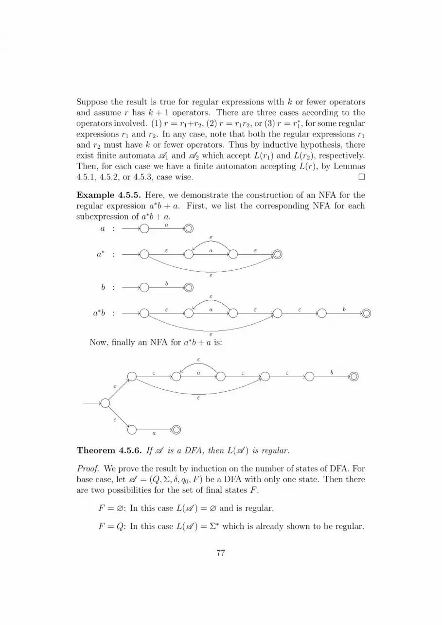
Suppose the result is true for regular expressions with k or fewer operatorsand assume r has k + 1 operators. There are three cases according to theoperators involved. (1) r = r1+r2, (2) r = r1r2, or (3) r = r∗1, for some regularexpressions r1 and r2. In any case, note that both the regular expressions r1
and r2 must have k or fewer operators. Thus by inductive hypothesis, thereexist finite automata A1 and A2 which accept L(r1) and L(r2), respectively.Then, for each case we have a finite automaton accepting L(r), by Lemmas4.5.1, 4.5.2, or 4.5.3, case wise.
Example 4.5.5. Here, we demonstrate the construction of an NFA for theregular expression a∗b + a. First, we list the corresponding NFA for eachsubexpression of a∗b + a.
a : ///.-,()*+ a ///.-,()*+ÂÁÀ¿»¼½¾
a∗ : ///.-,()*+ ε //
ε
77/.-,()*+ a ///.-,()*+ ε //
ε
ÄÄ /.-,()*+ÂÁÀ¿»¼½¾
b : ///.-,()*+ b ///.-,()*+ÂÁÀ¿»¼½¾
a∗b : ///.-,()*+ ε //
ε
77/.-,()*+ a ///.-,()*+ ε //
ε
ÄÄ /.-,()*+ ε ///.-,()*+ b ///.-,()*+ÂÁÀ¿»¼½¾
Now, finally an NFA for a∗b + a is:
/.-,()*+ ε //
ε
77/.-,()*+ a ///.-,()*+ ε //
ε
ÄÄ /.-,()*+ ε ///.-,()*+ b ///.-,()*+ÂÁÀ¿»¼½¾
///.-,()*+ε
??ÄÄÄÄÄÄÄÄ
εÂÂ
????
????
/.-,()*+a
///.-,()*+ÂÁÀ¿»¼½¾
Theorem 4.5.6. If A is a DFA, then L(A ) is regular.
Proof. We prove the result by induction on the number of states of DFA. Forbase case, let A = (Q, Σ, δ, q0, F ) be a DFA with only one state. Then thereare two possibilities for the set of final states F .
F = ∅: In this case L(A ) = ∅ and is regular.
F = Q: In this case L(A ) = Σ∗ which is already shown to be regular.
77

q does not appear on these paths0
q0
L
L
1
3
Figure 4.7: Depiction of the Language of a DFA
Assume that the result is true for all those DFA whose number of states isless than n. Now, let A = (Q, Σ, δ, q0, F ) be a DFA with |Q| = n. First notethat the language L = L(A ) can be written as
L = L∗1L2
where
L1 is the set of strings that start and end in the initial state q0
L2 is the set of strings that start in q0 and end in some final state. Weinclude ε in L2 if q0 is also a final state. Further, we add a restrictionthat q0 will not be revisited while traversing those strings. This isjustified because, the portion of a string from the initial position q0 tillthat revisits q0 at the last time will be part of L1 and the rest of theportion will be in L2.
Using the inductive hypothesis, we prove that both L1 and L2 are regular.Since regular languages are closed with respect to Kleene star and concate-nation it follows that L is regular.
The following notation shall be useful in defining the languages L1 andL2, formally, and show that they are regular. For q ∈ Q and x ∈ Σ∗, let usdenote the set of states on the path of x from q that come after q by P(q,x).That is, if x = a1 · · · an,
P(q,x) =n⋃
i=1
{δ(q, a1 · · · ai)}.
Define
L1 = {x ∈ Σ∗ | δ(q0, x) = q0}; and
L2 =
{L3, if q0 /∈ F ;L3 ∪ {ε}, if q0 ∈ F,
78

where L3 = {x ∈ Σ∗ | δ(q0, x) ∈ F, q0 /∈ P(q0,x)}. Clearly, L = L∗1L2.Claim 1: L1 is regular.Proof of Claim 1:Consider the following set
A =
(a, b) ∈ Σ× Σ
∣∣∣∣∣∣δ(q0, axb) = q0, for some x ∈ Σ∗;δ(q0, a) 6= q0;q0 /∈ P(qa,x), where qa = δ(q0, a).
and for (a, b) ∈ A, define
L(a,b) = {x ∈ Σ∗ | δ(q0, axb) = q0 and q0 /∈ P(qa,x), where qa = δ(q0, a)}.
Note that L(a,b) is the language accepted by the DFA
A(a,b) = (Q′, Σ, δ′, qa, F′)
where Q′ = Q \ {q0}, qa = δ(q0, a), F ′ = {q ∈ Q | δ(q, b) = q0} \ {q0}, and δ′
is the restriction of δ to Q′×Σ, i.e. δ′ = δ∣∣∣Q′×Σ
. For instance, if x ∈ L(A(a,b))
then, since q0 /∈ Q′, q0 /∈ P(qa,x) and δ′(qa, x) ∈ F ′. This implies,
δ(q0, axb) = δ(δ(q0, a), xb)
= δ(qa, xb)
= δ(δ(qa, x), b)
= δ(p, b), where p ∈ F ′, as δ′ = δ∣∣∣Q′×Σ
= q0,
so that x ∈ L(a,b). Converse is similar. Thus L(a,b) = L(A(a,b)). Hence, as|Q′| = n− 1, by inductive hypothesis, L(a,b) is regular. Now if we write
B = {a ∈ Σ | δ(q0, a) = q0} ∪ {ε}
then clearly,
L1 = B ∪⋃
(a,b)∈A
aL(a,b)b.
Hence L1 is regular.Claim 2: L3 is regular.Proof of Claim 2: Consider the following set
C = {a ∈ Σ | δ(q0, a) 6= q0}
79

and for a ∈ C, define
La = {x ∈ Σ∗ | δ(q0, ax) ∈ F and q0 /∈ P(qa,x), where qa = δ(q0, a)}.For a ∈ C, we set
Aa = (Q′, Σ, δ′, qa, F′′)
where Q′ = Q \ {q0}, qa = δ(q0, a), F ′′ = F \ {q0}, and δ′ is the restriction of
δ to Q′ ×Σ, i.e. δ′ = δ∣∣∣Q′×Σ
. It easy to observe that L(Aa) = La. First note
that q0 does not appear in the context of La and L(Aa). Now,
x ∈ L(Aa) ⇐⇒ δ′(qa, x) ∈ F ′′ (as q0 does not appear)
⇐⇒ δ′(qa, x) ∈ F
⇐⇒ δ(qa, x) ∈ F
⇐⇒ δ(δ(q0, a), x) ∈ F
⇐⇒ δ(q0, ax) ∈ F (as q0 does not appear)
⇐⇒ ax ∈ La.
Again, since |Q′| = n − 1, by inductive hypothesis, we have La is regular.But, clearly
L3 =⋃a∈C
aLa
so that L3 is regular. This completes the proof of the theorem.
Example 4.5.7. Consider the following DFA
// GFED@ABCq0
a··
b // GFED@ABCq1
a
zzb // GFED@ABC?>=<89:;q2
b
a
ff
1. Note that the following strings bring the DFA from q0 back to q0.
(a) a (via the path 〈q0, q0〉)(b) ba (via the path 〈q0, q1, q0〉)(c) For n ≥ 0, bbbna (via the path 〈q0, q1, q2, q2, . . . , q2, q0〉)
Thus L1 = {a, ba, bbbna | n ≥ 0} = a + ba + bbb∗a.
2. Again, since q0 is not a final state, L2 – the set of strings which takethe DFA from q0 to the final state q2 – is
{bbbn | n ≥ 0} = bbb∗.
80

Thus, as per the construction of Theorem 4.5.6, the language accepted bythe given DFA is L∗1L2 and it can be represented by the regular expression
(a + ba + bbb∗a)∗bbb∗
and hence it is regular.
Brzozowski Algebraic Method
Brzozowski algebraic method gives a conversion of DFA to its equivalent reg-ular expression. Let A = (Q, Σ, δ, q0, F ) be a DFA with Q = {q0, q2, . . . , qn}and F = {qf1 , . . . , qfk
}. For each qi ∈ Q, write
Ri = {x ∈ Σ∗ | δ(q0, x) = qi}
and note that
L(A ) =k⋃
i=1
Rfi
In order to construct a regular expression for L(A ), here we propose anunknown expression for each Ri, say ri. We are indented to observe that ri,for all i, is a regular expression so that
rf1 + rf2 + · · ·+ rfk
is a regular expression for L(A ), as desired.Suppose Σ(i,j) is the set of those symbols of Σ which take A from qi to
qj, i.e.Σ(i,j) = {a ∈ Σ | δ(qi, a) = qj}.
Clearly, as it is a finite set, Σ(i,j) is regular with the regular expression assum of its symbols. Let s(i,j) be the expression for Σ(i,j). Now, for 1 ≤ j ≤ n,since the strings of Rj are precisely taking the DFA from q0 to any state qi
then reaching qj with the symbols of Σ(i,j), we have
Rj = R0Σ(0,j) ∪ · · · ∪RiΣ(i,j) ∪ · · · ∪RnΣ(n,j).
And in case of R0, it is
R0 = R0Σ(0,0) ∪ · · · ∪RiΣ(i,0) ∪ · · · ∪RnΣ(n,0) ∪ {ε},
as ε takes the DFA from q0 to itself. Thus, for each j, we have an equation
81

j )
j ) j ) j )j )
q
q q q q q
q
i j n
j
0
10
R
RR
R
R0
1
i
j
n
(1, (
((0,
( i jn
, ,,Σ
Σ Σ ΣΣ
Figure 4.8: Depiction of the Set Rj
for rj which is depending on all ri′s, called characteristic equation of rj. The
system of characteristic equations of A is:
r0 = r0s(0,0) + r1s(1,0) + · · ·+ ris(i,0) + · · ·+ rns(n,0) + ε
r1 = r0s(0,1) + r1s(1,1) + · · ·+ ris(i,1) + · · ·+ rns(n,1)
...
rj = r0s(0,j) + r1s(1,j) + · · ·+ ris(i,j) + · · ·+ rns(n,j)
...
rn = r0s(0,n) + r1s(1,n) + · · ·+ ris(i,n) + · · ·+ rns(n,n)
The system can be solved for rfi′s, expressions for final states, via straight-
forward substitution, except the same unknown appears on the both the leftand right hand sides of a equation. This situation can be handled usingArden’s principle (see Exercise ??) which states that
Let s and t be regular expressions and r is an unknown. A equationof the form r = t + rs, where ε /∈ L(s), has a unique solution given byr = ts∗.
By successive substitutions and application of Arden’s principle we evaluatethe expressions for final states purely in terms of symbols from Σ. Since theoperations involved here are admissible for regular expression, we eventuallyobtain regular expressions for each rfi
.We demonstrate the method through the following examples.
82

Example 4.5.8. Consider the following DFA
// GFED@ABCq0
b
a // GFED@ABC?>=<89:;q1
a
dd
b
The characteristic equations for the states q0 and q1, respectively, are:
r0 = r0b + r1a + ε
r1 = r0a + r1b
Since q1 is the final state, r1 represents the language of the DFA. Hence,we need to solve for r1 explicitly in terms of a′s and b′s. Now, by Arden’sprinciple, r0 yields
r0 = (ε + r1a)b∗.
Then, by substituting r0 in r1, we get
r1 = (ε + r1a)b∗a + r1b = b∗a + r1(ab∗a + b)
Then, by applying Arden’s principle on r1, we get r1 = b∗a(ab∗a + b)∗ whichis the desired regular expression representing the language of the given DFA.
Example 4.5.9. Consider the following DFA
// GFED@ABC?>=<89:;q1
b
a // GFED@ABC?>=<89:;q2
b
dd
a // GFED@ABCq3
a, b
The characteristic equations for the states q1, q2 and q3, respectively, are:
r1 = r1b + r2b + ε
r2 = r1a
r3 = r2a + r3(a + b)
Since q1 and q2 are final states, r1 + r2 represents the language of the DFA.Hence, we need to solve for r1 and r2 explicitly in terms of a′s and b′s. Now,by substituting r2 in r1, we get
r1 = r1b + r1ab + ε = r1(b + ab) + ε.
Then, by Arden’s principle, we have r1 = ε(b + ab)∗ = (b + ab)∗. Thus,
r1 + r2 = (b + ab)∗ + (b + ab)∗a.
Hence, the regular expressions represented by the given DFA is
(b + ab)∗(ε + a).
83

4.5.2 Equivalence of Finite Automata and Regular Gram-mars
A finite automaton A is said to be equivalent to a regular grammar G, ifthe language accepted by A is precisely generated by the grammar G, i.e.L(A ) = L(G). Now, we prove that finite automata and regular grammarsare equivalent. In order to establish this equivalence, we first prove thatgiven a DFA we can construct an equivalent regular grammar. Then forconverse, given a regular grammar, we construct an equivalent generalizedfinite automaton (GFA), a notion which we introduce here as an equivalentnotion for DFA.
Theorem 4.5.10. If A is a DFA, then L(A ) can be generated by a regulargrammar.
Proof. Suppose A = (Q, Σ, δ, q0, F ) is a DFA. Construct a grammar G =(N , Σ,P , S) by setting N = Q and S = q0 and
P = {A → aB | B ∈ δ(A, a)} ∪ {A → a | δ(A, a) ∈ F}.
In addition, if the initial state q0 ∈ F , then we include S → ε in P . ClearlyG is a regular grammar. We claim that L(G) = L(A ).
From the construction of G, it is clear that ε ∈ L(A ) if and only ifε ∈ L(G). Now, for n ≥ 1, let x = a1a2 . . . an ∈ L(A ) be arbitrary. That isδ(q0, a1a2 . . . an) ∈ F . This implies, there exists a sequence of states
q1, q2, . . . , qn
such thatδ(qi−1, ai) = qi, for 1 ≤ i ≤ n, and qn ∈ F.
As per construction of G, we have
qi−1 → aiqi ∈ P , for 1 ≤ i ≤ n− 1, and qn → an ∈ P .
Using these production rules we can derive x in G as follows:
S = q0 ⇒ a1q1
⇒ a1a2q2
...
⇒ a1a2 · · · an−1qn−1
⇒ a1a2 · · · an = x.
84

Thus x ∈ L(G).
Conversely, suppose y = b1 · · · bm ∈ L(G), for m ≥ 1, i.e. S∗⇒ y in G.
Since every production rule of G is form A → aB or A → a, the derivationS
∗⇒ y has exactly m steps and first m − 1 steps are because of productionrules of the type A → aB and the last mth step is because of the rule of theform A → a. Thus, in every step of the deviation one bi of y can be producedin the sequence. Precisely, the derivation can be written as
S ⇒ b1B1
⇒ b1b2B2
...
⇒ b1b2 · · · bm−1Bm−1
⇒ b1b2 · · · bm = y.
From the construction of G, it can be observed that
δ(Bi−1, bi) = Bi, for 1 ≤ i ≤ m− 1, and B0 = S
in A . Moreover, δ(Bm−1, bm) ∈ F . Thus,
δ(q0, y) = δ(S, b1 · · · bm) = δ(δ(S, b1), b2 · · · bm)
= δ(B1, b2 · · · bm)...
= δ(Bm−1, bm)
= δ(Bm−1, bm) ∈ F
so that y ∈ L(A ). Hence L(A ) = L(G).
Example 4.5.11. Consider the DFA given in Example 4.5.8. Set N ={q0, q1}, Σ = {a, b}, S = q0 and P has the following production rules:
q0 → aq1 | bq0 | a
q1 → aq0 | bq1 | b
Now G = (N , Σ,P , S) is a regular grammar that is equivalent to the givenDFA.
Example 4.5.12. Consider the DFA given in Example 4.5.9. The regulargrammar G = (N , Σ,P , S), where N = {q1, q2, q3}, Σ = {a, b}, S = q1 andP has the following rules
q1 → aq2 | bq1 | a | b | ε
q2 → aq3 | bq1 | b
q3 → aq3 | bq3
85

is equivalent to the given DFA. Here, note that q3 is a trap state. So, theproduction rules in which q3 is involved can safely be removed to get a simplerbut equivalent regular grammar with the following production rules.
q1 → aq2 | bq1 | a | b | ε
q2 → bq1 | b
Definition 4.5.13. A generalized finite automaton (GFA) is nondetermin-istic finite automaton in which the transitions may be given via stings froma finite set, instead of just via symbols. That is, formally, GFA is a sextuple(Q, Σ, X, δ, q0, F ), where Q, Σ, q0, F are as usual in an NFA. Whereas, thetransition function
δ : Q×X −→ ℘(Q)
with a finite subset X of Σ∗.
One can easily prove that the GFA is no more powerful than an NFA.That is, the language accepted by a GFA is regular. This can be doneby converting each transition of a GFA into a transition of an NFA. Forinstance, suppose there is a transition from a state p to a state q via s stringx = a1 · · · ak, for k ≥ 2, in a GFA. Choose k − 1 new state that not alreadythere in the GFA, say p1, . . . , pk−1 and replace the transition
px−→ q
by the following new transitions via the symbols ai’s
pa1−→ p1, p1
a2−→ p2, · · · , pk−1ak−→ q
In a similar way, all the transitions via strings, of length at least 2, can bereplaced in a GFA to convert that as an NFA without disturbing its language.
Theorem 4.5.14. If L is generated by a regular grammar, then L is regular.
Proof. Let L be generated by the regular grammar G = (N , Σ,P , S). Notethat every production rule of G is either of the form A → xB or of the formA → x, for some x ∈ Σ∗ and A,B ∈ N . We construct a GFA that acceptsL, so that L is regular.
Let X be the set of all terminal strings that are on the righthand side ofproductions of G. That is,
X ={
x∣∣∣ A → xB ∈ P or A → x ∈ P
}.
86

Since P is a finite set, we have X is a finite subset of Σ∗. Now, construct aGFA
A = (Q, Σ, X, δ, q0, F )
by setting Q = N ∪ {$}, where $ is a new symbol, q0 = S, F = {$} and thetransition function δ is defied by
B ∈ δ(A, x) ⇐⇒ A → xB ∈ Pand
$ ∈ δ(A, x) ⇐⇒ A → x ∈ PWe claim that L(A ) = L.
Let w ∈ L, i.e. there is a derivation for w in G. Assume the derivationhas k steps, which is obtained by the following k− 1 production rules in thefirst k − 1 steps
Ai−1 → xiAi, for 1 ≤ i ≤ k − 1, with S = A0,
and at the end, in the kth step, the production rule
Ak−1 → xk.
Thus, w = x1x2 · · ·xk and the derivation is as shown below:
S = A0 ⇒ x1A1
⇒ x1x2A2
...
⇒ x1x2 · · · xk−1Ak−1
⇒ x1x2 · · · xk = w.
From the construction of A , it is clear that A has the following transitions:
(Ai−1, xi) |— (Ai, ε) for 1 ≤ i ≤ k,
where A0 = S and Ak = $. Using these transitions, it can be observed thatw ∈ L(A ). For instance,
(q0, w) = (S, x1 · · ·xk) = (A0, x1x2 · · ·xk)|— (A1, x2 · · · xk)...|— (Ak−1, xk)|— ($, ε).
87

Thus, L ⊆ L(A ). Converse can be shown using a similar argument as in theprevious theorem. Hence L(A ) = L.
Example 4.5.15. Consider the regular grammar given in the Example 3.3.10.Let Q = {S, A, $}, Σ = {a, b}, X = {ε, a, b, ab} and F = {$}. Set A =(Q, Σ, X, δ, S, F ), where δ : Q × X −→ ℘(Q) is defined by the followingtable.
δ ε a b abS ∅ {S} {S} {A}A {$} {A} {A} ∅$ ∅ ∅ ∅ ∅
Clearly, A is a GFA. Now, we convert the GFA A to an equivalent NFA.Consider a new symbol B and split the production rule
S → abA
of the grammar into the following two production rules
S → aB and B → bA
and replace them in place of the earlier one. Note that, in the resultantgrammar, the terminal strings that is occurring in the righthand sides ofproduction rules are of lengths at most one. Hence, in a straightforwardmanner, we have the following NFA A ′ that is equivalent to the above GFAand also equivalent to the given regular grammar. A ′ = (Q′, Σ, δ′, S, F ),where Q′ = {S,A, B, $} and δ′ : Q′×Σ −→ ℘(Q′) is defined by the followingtable.
δ ε a bS ∅ {S, B} {S}A {$} {A} {A}B ∅ ∅ {A}$ ∅ ∅ ∅
Example 4.5.16. The following an equivalent NFA for the regular grammargiven in Example 3.3.13.
δ ε a bS ∅ {A} {S}A ∅ {B} {A}B {$} {S} {B}$ ∅ ∅ ∅
88

4.6 Variants of Finite Automata
Finite state transducers, two-way finite automata and two-tape finite au-tomata are some variants of finite automata. Finite state transducers areintroduced as devices which give output for a given input; whereas, othersare language acceptors. The well-known Moore and Mealy machines are ex-amples of finite state transducers All these variants are no more powerful thanDFA; in fact, they are equivalent to DFA. In the following subsections, weintroduce two-way finite automata and Mealy machines. Some other variantsare described in Exercises.
4.6.1 Two-way Finite Automaton
In contrast to a DFA, the reading head of a two-way finite automata isallowed to move both left and right directions on the input tape. In eachtransition, the reading head can move one cell to its right or one cell to itsleft. Formally, a two-way DFA is defined as follows.
Definition 4.6.1. A two-way DFA (2DFA) is a quintuple A = (Q, Σ, δ, q0, F ),where Q, Σ, q0 and F are as in DFA, but the transition function is
δ : Q× Σ −→ Q× {L,R},
where L is indicating a left move and R is indicating a right move.
A configuration (or ID) of a 2DFA is an element of Q × Σ∗ × Σ × Σ∗
or Q × Σ∗. A configuration (q, x, a, y) ∈ Q × Σ∗ × Σ × Σ∗ indicates thatthe current state of the 2DFA is q and while the input is xay, the readinghead is scanning the symbol a. For convenience, we write (q, xay) instead of(q, x, a, y) by denoting the position of reading head with an underscore. Ifthe reading head goes beyond the input, i.e. it has just finished reading theinput, then there will not be any indication of reading head in a configuration.In which case, a configuration is of the form just (q, x) which is an elementof Q×Σ∗; this type of configurations will be at the end of a computation ofa 2DFA with input x.
As usual for an automaton, a computation of a 2DFA is also given byrelating two configurations C and C ′ with |−−* , i.e. a computation is of theform C |−−* C ′, where |−− is the one-step relation in a 2DFA which is definedas follows:
If δ(p, a) = (q, X), then the configuration C = (p, xay) gives the configu-ration C ′ in one-step, denoted by C |−− C ′, where C ′ is given by
89

Case-I: X = R.
C ′ ={
(q, xa), if y = ε;(q, xaby′), whenever y = by′, for some b ∈ Σ.
Case-II: X = L.
C ′ ={
undefined, if x = ε;(q, x′bay′), whenever x = x′b, for some b ∈ Σ.
A string x = a1a2 · · · an ∈ Σ∗ is said to be accepted by a 2DFA A if(q0, a1a2 · · · an) |−−* (p, a1a2 · · · an), for some p ∈ F . Further, the languageaccepted by A is
L(A ) = {x ∈ Σ∗ | x is accepted by A }.Example 4.6.2. Consider the language L over {0, 1} that contain all thosestrings in which every occurrence of 01 is preceded by a 0, i.e. before every 01there should be a 0. For example, 1001100010010 is in L; whereas, 101100111is not in L. The following 2DFA given in transition table representationaccepts the language L.
δ 0 1→ q007162534 (q1, R) (q0, R)
q107162534 (q1, R) (q2, L)
q2 (q3, L) (q3, L)q3 (q4, R) (q5, R)q4 (q6, R) (q6, R)q5 (q5, R) (q5, R)q6 (q0, R) (q0, R)
The following computation on 10011 shows that the string is accepted by the2DFA.
(q0, 10011) |−− (q0, 10011) |−− (q1, 10011) |−− (q1, 10011)|−− (q2, 10011) |−− (q3, 10011) |−− (q4, 10011)|−− (q6, 10011) |−− (q0, 10011) |−− (q0, 10011).
Given 1101 as input to the 2DFA, as the state component the final con-figuration of the computation
(q0, 1101) |−− (q0, 1101) |−− (q0, 1101) |−− (q1, 1101)|−− (q2, 1101) |−− (q3, 1101) |−− (q5, 1101)|−− (q5, 1101) |−− (q5, 1101).
is a non-final state, we observe that the string 1101 is not accepted by the2DFA.
90

Example 4.6.3. Consider the language over {0, 1} that contains all thosestrings with no consecutive 0′s. That is, any occurrence of two 1′s have tobe separated by at least one 0. In the following we design a 2DFA whichchecks this parameter and accepts the desired language. We show the 2DFAusing a transition diagram, where the left or right move of the reading headis indicated over the transitions.
// GFED@ABC?>=<89:;q0
(1,R)
(0,R)// GFED@ABC?>=<89:;q1
(1,R)
(0,L)~~}}
}}}}
}}}
GFED@ABC?>=<89:;q2
(1,R)
`AAAAAAAAA
(0,L)
TT
4.6.2 Mealy Machines
As mentioned earlier, Mealy machine is a finite state transducer. In orderto give output, in addition to the components of a DFA, we have a set ofoutput symbols from which the transducer produces the output through anoutput function. In case of Mealy machine, the output is associated to eachtransition, i.e. given an input symbol in a state, while changing to the nextstate, the machine emits an output symbol. Thus, formally, a Mealy machineis defined as follows.
Definition 4.6.4. A Mealy machine is a sextuple M = (Q, Σ, ∆, δ, λ, q0),where Q, Σ, δ and q0 are as in a DFA, whereas, ∆ is a finite set called outputalphabet and
λ : Q× Σ −→ ∆
is a function called output function.
In the depiction of a DFA, in addition to its components, viz. input tape,reading head and finite control, a Mealy machine has a writing head and anoutput tape. This is shown in the Figure 4.9.
Note that the output function λ assigns an output symbol for each statetransition on an input symbol. Through the natural extension of λ to strings,we determine the output string corresponding to each input string. Theextension can be formally given by the function
λ : Q× Σ∗ −→ ∆∗
that is defined by
91

Figure 4.9: Depiction of Mealy Machine
1. λ(q, ε) = ε, and
2. λ(q, xa) = λ(q, x)λ(δ(q, x), a)
for all q ∈ Q, x ∈ Σ∗ and a ∈ Σ. That is, if the input string x = a1a2 · · · an
is applied in a state q of a Mealy machine, then the output sequence
λ(q, x) = λ(q1, a1)λ(q2, a2) · · ·λ(qn, an)
where q1 = q and qi+1 = δ(qi, ai), for 1 ≤ i < n. Clearly, |x| = |λ(q, x)|.Definition 4.6.5. Let M = (Q, Σ, ∆, δ, λ, q0) be a Mealy machine. We sayλ(q0, x) is the output of M for an input string x ∈ Σ∗.
Example 4.6.6. Let Q = {q0, q1, q2}, Σ = {a, b}, ∆ = {0, 1} and define thetransition function δ and the output function λ through the following tables.
δ a bq0 q1 q0
q1 q1 q2
q2 q1 q0
λ a bq0 0 0q1 0 1q2 0 0
Clearly, M = (Q, Σ, ∆, δ, λ, q0) is a Mealy machine. By incorporating theinformation of output, following the representation of DFA, M can be rep-
92

resented by a digraph as shown below.
// GFED@ABCq0
b/0··
a/0// GFED@ABCq1
a/0
JJ
b/1// GFED@ABCq2
a/0
dd
b/0
xx
For instance, output of M for the input string baababa is 0001010. In fact,this Mealy machine prints 1 for each occurrence of ab in the input; otherwise,it prints 0.
Example 4.6.7. In the following we construct a Mealy machine that per-forms binary addition. Given two binary numbers a1 · · · an and b1 · · · bn (ifthey are different length then we put some leading 0′s to the shorter one),the input sequence will be considered as we consider in the manual addition,as shown below. (
an
bn
)(an−1
bn−1
)· · ·
(a1
b1
)
Here, we reserve a1 = b1 = 0 so as to accommodate the extra bit, if any,during addition. The expected output
cncn−1 · · · c1
is such thata1 · · · an + b1 · · · bn = c1 · · · cn.
Note that there are four input symbols, viz.(00
),
(01
),
(10
)and
(11
).
For notational convenience, let us denote the above symbols by a, b, c and d,respectively. Now, the desired Mealy machine, while it is in the initial state,say q0, if the input is d, i.e. while adding 1 + 1, it emits the output 0 andremembers the carry 1 through a new state, say q1. For other input symbols,viz. a, b and c, as there is no carry, it will continue in q0 and performs theaddition. Similarly, while the machine continues in q1, for the input a, i.e.while adding 0 + 0, it changes to the state q0, indicating that the carry is0 and emits 1 as output. Following this mechanism, the following Mealymachine is designed to perform binary addition.
GFED@ABCq0
a/0
b/1
((
c/1
JJ
d/0// GFED@ABCq1
a/1
ii
b/0··
c/0
vv
d/1
TT``@@@@@@@@
93

Chapter 5
Properties of RegularLanguages
In the previous chapters we have introduced various tools, viz. grammars,automata, to understand regular languages. Also, we have noted that theclass of regular languages is closed with respect to certain operations likeunion, concatenation, Kleene closure. Now, with this information, can wedetermine whether a given language is regular or not? If a given languageis regular, then to prove the same we need to use regular expression, regulargrammar, finite automata or Myhill-Nerode theorem. Is there any other wayto prove that a language is regular? The answer is “Yes”. If a given lan-guage can be obtained from some known regular languages by applying thoseoperations which preserve regularity, then one can ascertain that the givenlanguage is regular. If a language is not regular, although we have Myhill-Nerode theorem, a better and more practical tool viz. pumping lemma willbe introduced to ascertain that the language is not regular. If we were some-how know that some languages are not regular, then again closure propertiesmight be helpful to establish some more languages that are not regular. Thus,closure properties play important role not only in proving certain languagesare regular, but also in establishing non-regularity of languages. Hence, weare indented to explore further closure properties of regular languages.
5.1 Closure Properties
5.1.1 Set Theoretic Properties
Theorem 5.1.1. The class of regular languages is closed with respect tocomplement.
94

Proof. Let L be a regular language accepted by a DFA A = (Q, Σ, δ, q0, F ).Construct the DFA A ′ = (Q, Σ, δ, q0, Q − F ), that is, by interchanging theroles of final and nonfinal states of A . We claim that L(A ′) = Lc so thatLc is regular. For x ∈ Σ∗,
x ∈ Lc ⇐⇒ x 6∈ L
⇐⇒ δ(q0, x) 6∈ F
⇐⇒ δ(q0, x) ∈ Q− F
⇐⇒ x ∈ L(A ′).
Corollary 5.1.2. The class of regular languages is closed with respect tointersection.
Proof. If L1 and L2 are regular, then so are Lc1 and Lc
2. Then their unionLc
1 ∪ Lc2 is also regular. Hence, (Lc
1 ∪ Lc2)
c is regular. But, by De Morgan’slaw
L1 ∩ L2 = (Lc1 ∪ Lc
2)c
so that L1 ∩ L2 is regular.
Alternative Proof by Construction. For i = 1, 2, let Ai = (Qi, Σ, δi, qi, Fi) betwo DFA accepting Li. That is, L(A1) = L1 and L(A2) = L2. Set the DFA
A = (Q1 ×Q2, Σ, δ, (q1, q2), F1 × F2),
where δ is defined point-wise by
δ((p, q), a) = (δ1(p, a), δ2(q, a)),
for all (p, q) ∈ Q1 × Q2 and a ∈ Σ. We claim that L(A ) = L1 ∩ L2. Using
induction on |x|, first observe that δ((p, q), x
)=
(δ1(p, x), δ2(q, x)
), for all
x ∈ Σ∗.Now it clearly follows that
x ∈ L(A ) ⇐⇒ δ((q1, q2), x
)∈ F1 × F2
⇐⇒(δ1(q1, x), δ2(q2, x)
)∈ F1 × F2
⇐⇒ δ1(q1, x) ∈ F1 and δ2(q2, x) ∈ F2
⇐⇒ x ∈ L1 and x ∈ L2
⇐⇒ x ∈ L1 ∩ L2.
95

Example 5.1.3. Using the construction given in the above proof, we designa DFA that accepts the language
L = {x ∈ (0 + 1)∗ | |x|0 is even and |x|1 is odd}so that L is regular. Note that the following DFA accepts the languageL1 = {x ∈ (0 + 1)∗ | |x|0 is even}.
// GFED@ABC?>=<89:;q1
1
0 // GFED@ABCq2
0
gg
1
Also, the following DFA accepts the language L2 = {x ∈ (0+1)∗ | |x|1 is odd}.
// GFED@ABCp1
0
1 // GFED@ABC?>=<89:;p2
1
hh
0
Now, let s1 = (q1, p1), s2 = (q1, p2), s3 = (q2, p1) and s4 = (q2, p2) andconstruct the automaton that accepts the intersection of L1 and L2 as shownbelow.
// GFED@ABCs11
//
0²²
GFED@ABC?>=<89:;s2
1vv
0²²
GFED@ABCs31 //
0
EE
GFED@ABCs4
1
hh
0
YY
Further, we note the following regarding the automaton. If an input x takesthe automaton (from the initial state) to the state
1. s1, that means, x has even number of 0′s and even number of 1′s.
2. s2, that means, x has even number of 0′s and odd number of 1′s (asdesired in the current example).
3. s3, that means, x has odd number of 0′s and even number of 1′s.
4. s4, that means, x has odd number of 0′s and odd number of 1′s.
By choosing any combination of states among s1, s2, s3 and s4, appropri-ately, as final states we would get DFA which accept input with appropriatecombination of 0′s and 1′s. For example, to show that the language
L′ ={
x ∈ (0 + 1)∗∣∣∣ |x|0 is even ⇔ |x|1 is odd
}.
96

is regular, we choose s2 and s3 as final states and obtain the following DFAwhich accepts L′.
// GFED@ABCs11
//
0²²
GFED@ABC?>=<89:;s2
1vv
0²²
GFED@ABC?>=<89:;s31 //
0
EE
GFED@ABCs4
1
hh
0
YY
Similarly, any other combination can be considered.
Corollary 5.1.4. The class of regular languages is closed under set differ-ence.
Proof. Since L1 − L2 = L1 ∩ Lc2, the result follows.
Example 5.1.5. The language L = {an | n ≥ 5} is regular. We applyCorollary 5.1.4 with L1 = L(a∗) and L2 = {ε, a, a2, a3, a4}. Since L1 and L2
are regular, L = L1 − L2 is regular.
Remark 5.1.6. In general, one may conclude that the removal of finitely manystrings from a regular language leaves a regular language.
5.1.2 Other Properties
Theorem 5.1.7. If L is regular, then so is LR = {xR | x ∈ L}.To prove this we use the following lemma.
Lemma 5.1.8. For every regular language L, there exists a finite automatonA with a single final state such that L(A ) = L.
Proof. Let A = (Q, Σ, δ, q0, F ) be a DFA accepting L. Construct B =(Q ∪ {p}, Σ, δ′, q0, {p}), where p 6∈ Q is a new state and δ′ is given by
δ′(q, a) =
{δ(q, a), if q ∈ Q, a ∈ Σp, if q ∈ F, a = ε.
Note that B is an NFA, which is obtained by adding a new state p to A thatis connected from all the final states of A via ε-transitions. Here p is theonly final state in B and all the final states of A are made nonfinal states.It is easy to prove that L(A ) = L(B).
97

Proof of the Theorem 5.1.7. Let A be a finite automaton with the initialstate q0 and single final state qf that accepts L. Construct a finite automatonA R by reversing the arcs in A with the same labels and by interchangingthe roles of initial and final states. If x ∈ Σ∗ is accepted by A , then there isa path q0 to qf labeled x in A . Therefore, there will be a path from qf to q0
in A R labeled xR so that xR ∈ L(A R). Conversely, if x is accepted by A R,then using the similar argument one may notice that its reversal xR ∈ L(A ).Thus, L(A R) = LR so that LR is regular.
Example 5.1.9. Consider the alphabet Σ = {a0, a1, . . . , a7}, where ai =
b′ib′′ib′′′i
and b′ib
′′i b′′′i is the binary representation of decimal number i, for 0 ≤
i ≤ 7. That is, a0 =
000
, a1 =
001
, a2 =
010
, . . ., a7 =
111
.
Now a string x = ai1ai2 · · · ain over Σ is said to represent correct binaryaddition if
b′i1b′i2· · · b′in + b′′i1b
′′i2· · · b′′in = b′′′i1b
′′′i2· · · b′′′in .
For example, the string a5a1a6a5 represents correct addition, because 1011+0010 = 1101. Whereas, a5a0a6a5 does not represent a correct addition, be-cause 1011 + 0010 6= 1001.
We observe that the language L over Σ which contain all strings thatrepresent correct addition, i.e.
L = {ai1ai2 · · · ain ∈ Σ∗ | b′i1b′i2· · · b′in + b′′i1b
′′i2· · · b′′in = b′′′i1b
′′′i2· · · b′′′in},
is regular. Consider the NFA shown in the following.
?>=<89:;765401230
000
011
**
101
JJ
110 // ?>=<89:;1
001
hh
010··
100
tt
111
TT__>>>>>>>>
Note that the NFA accepts LR∪{ε}. Hence, by Remark 5.1.6, LR is regular.Now, by Theorem 5.1.7, L is regular, as desired.
Definition 5.1.10. Let L1 and L2 be two languages over Σ. Right quotientof L1 by L2, denoted by L1/L2, is the language
{x ∈ Σ∗ | ∃y ∈ L2 such that xy ∈ L1}.
98

Example 5.1.11. 1. Let L1 = {a, ab, bab, baba} and L2 = {a, ab}; thenL1/L2 = {ε, bab, b}.
2. For L3 = 10∗1 and L4 = 1, we have L3/L4 = 10∗.
3. Let L5 = 0∗10∗.
(a) L5/0∗ = L5.
(b) L5/10∗ = 0∗.
(c) L5/1 = 0∗.
4. If L6 = a∗b∗ and L7 = {(anbn)a∗ | n ≥ 0}, then L6/L7 = a∗.
Theorem 5.1.12. If L is a regular language, then so is L/L′, for any lan-guage L′.
Proof. Let L be a regular language and L′ be an arbitrary language. SupposeA = (Q, Σ, δ, q0, F ) is a DFA which accepts L. Set A ′ = (Q, Σ, δ, q0, F
′),where
F ′ = {q ∈ Q | δ(q, x) ∈ F, for some x ∈ L′},so that A ′ is a DFA. We claim that L(A ′) = L/L′. For w ∈ Σ∗,
w ∈ L(A ′) ⇐⇒ δ(q0, w) ∈ F ′
⇐⇒ δ(q0, wx) ∈ F, for some x ∈ L′
⇐⇒ w ∈ L/L′.
Hence L/L′ is regular.
Note that Σ∗ is a monoid with respect to the binary operation concate-nation. Thus, for two alphabets Σ1 and Σ2, a mapping
h : Σ∗1 −→ Σ∗
2
is a homomorphism if, for all x, y ∈ Σ∗1,
h(xy) = h(x)h(y).
One may notice that to give a homomorphism from Σ∗1 to Σ∗
2, it is enough togive images for the elements of Σ1. This is because as we are looking for ahomomorphism one can give the image of h(x) for any x = a1a2 · · · an ∈ Σ∗
1
byh(a1)h(a2) · · ·h(an).
Therefore, a homomorphism from Σ∗1 to Σ∗
2 is a mapping from Σ1 to Σ∗2.
99

Example 5.1.13. Let Σ1 = {a, b} and Σ2 = {0, 1}. Define h : Σ1 −→ Σ∗2 by
h(a) = 10 and h(b) = 010.
Then, h is a homomorphism from Σ∗1 to Σ∗
2, which for example assigns theimage 10010010 for the string abb.
We can generalize the concept of homomorphism by substituting a lan-guage instead of a string for symbols of the domain. Formally, a substitutionis a mapping from Σ1 to P(Σ∗
2).
Example 5.1.14. Let Σ1 = {a, b} and Σ2 = {0, 1}. Define h : Σ1 −→P(Σ∗
2) byh(a) = {0n | n ≥ 0}, say L1;h(b) = {1n | n ≥ 0}, say L2.
Then, h is a substitution. Now, for any string a1a2 · · · an ∈ Σ∗1, its image
under the above substitution h is
h(a1a2 · · · an) = h(a1)h(a2) · · ·h(an),
the concatenation of languages. For example, h(ab) is the language
L1L2 = {0m1n | m,n ≥ 0} = L(0∗1∗).
Given a substitution h from Σ1 to Σ2 one may naturally define h(L) fora language L over Σ1 by
h(L) =⋃x∈L
h(x).
Example 5.1.15. Consider the substitution h given in Example 5.1.14 andlet L = {anbn | n ≥ 0}. For which,
h(L) =⋃x∈L
h(x)
=⋃n≥0
h(anbn)
=⋃n≥0
n times︷ ︸︸ ︷h(a) · · ·h(a)
n times︷ ︸︸ ︷h(b) · · ·h(b)
=⋃n≥0
n times︷ ︸︸ ︷0∗ · · · 0∗
n times︷ ︸︸ ︷1∗ · · · 1∗
= {0m1n | m,n ≥ 0} = 0∗1∗.
100

Example 5.1.16. Define the substitution h : {a, b} −→ P({0, 1}∗) by
h(a) = the set of strings over {0, 1} ending with 1;h(b) = the set of strings over {0, 1} starting with 0.
For the language L = {anbm | n,m ≥ 1}, we compute h(L) through regularexpressions described below.
Note that the regular expression for L is a+b+ and that are for h(a) andh(b) are (0 + 1)∗1 and 0(0 + 1)∗. Now, write the regular expression that isobtained from the expression of L by replacing each occurrence of a by theexpression of h(a) and by replacing each occurrence of b by the expression ofh(b). That is, from a+b+, we obtain the regular expression
((0 + 1)∗1)+(0(0 + 1)∗)+.
This can be simplified as follows.
((0 + 1)∗1)+(0(0 + 1)∗)+ = ((0 + 1)∗1)∗((0 + 1)∗1)(0(0 + 1)∗)(0(0 + 1)∗)∗
= ((0 + 1)∗1)∗(0 + 1)∗10(0 + 1)∗(0(0 + 1)∗)∗
= (0 + 1)∗10(0 + 1)∗.
The following Theorem 5.1.17 confirms that the expression obtained in thisprocess represents h(L). Thus, from the expression of h(L), we can concludethat the language h(L) is the set of all strings over {0, 1} that have 10 assubstring.
Theorem 5.1.17. The class of regular languages is closed under substitu-tions by regular languages. That is, if h is a substitution on Σ such that h(a)is regular for each a ∈ Σ, then h(L) is regular for each regular language Lover Σ.
Proof. Let r be a regular expression for language L over Σ, i.e. L(r) = L,and, for each a ∈ Σ, let ra be a regular expression for h(a). Suppose r′ is theexpression obtained by replacing ra for each occurrence of a (of Σ) in r sothat r′ is a regular expression. We claim that L(r′) = h(L(r)) so that h(L)is regular. We prove our claim by induction on the number of operationsinvolved in r.
Assume that the number of operations involved in r is zero. Then thereare three possibilities for r, viz. 1. ∅, 2. ε and 3. a for some a ∈ Σ.
1. If r = ∅, then r′ = ∅ and h(L(∅)) = ∅ so that the result is straight-forward.
101

2. In case r = ε, r′ = ε and hence we have
h(L(r)) = h({ε}) = {ε} = L(r′).
3. For other case, let r = a, for some a ∈ Σ. Then, r′ = ra so that
h(L(r)) = h({a}) = L(ra) = L(r′).
Hence basis of the induction is satisfied.For inductive hypothesis, assume L(r′) = h(L(r)) for all those regular
expressions r which have k or fewer operations. Now consider a regularexpression r with k + 1 operations. Then
r = r1 + r2 or r = r1r2 or r = r∗1
for some regular expressions r1 and r2. Note that both r1 and r2 have k orfewer operations. Hence, by inductive hypothesis, we have
L(r′1) = h(L(r1)) and L(r′2) = h(L(r2)),
where r′1 and r′2 are the regular expressions which are obtained from r1 andr2 by replacing ra for each a in r1 and r2, respectively.
Consider the case where r = r1 + r2. The expression r′ (that is obtainedfrom r) is nothing else but replacing each ra in the individual r1 and r2, wehave
r′ = r′1 + r′2.
Hence,
L(r′) = L(r′1 + r′2)
= L(r′1) ∪ L(r′2)
= h(L(r1)) ∪ h(L(r2))
= h(L(r1) ∪ L(r2))
= h(L(r1 + r2))
= h(L(r))
as desired, in this case. Similarly, other two cases, viz. r = r1r2 and r = r∗1,can be handled.
Hence, the class of regular languages is closed under substitutions byregular languages.
Corollary 5.1.18. The class of regular languages is closed under homomor-phisms.
102

Theorem 5.1.19. Let h : Σ1 −→ Σ∗2 be a homomorphism and L ⊆ Σ∗
2 beregular. Then, inverse homomorphic image of L,
h−1(L) = {x ∈ Σ∗1 | h(x) ∈ L}
is regular.
Proof. Let A = (Q, Σ2, δ, q0, F ) be a DFA accepting L. We construct a DFAA ′ which accepts h−1(L). Note that, in A ′, we have to define transitions forthe symbols of Σ1 such that A ′ accepts h−1(L). We compose the homomor-phism h with the transition map δ of A to define the transition map of A ′.Precisely, we set A ′ = (Q, Σ1, δ
′, q0, F ), where the transition map
δ′ : Q× Σ1 −→ Q
is defined byδ′(q, a) = δ(q, h(a))
for all q ∈ Q and a ∈ Σ1. Note that A ′ is a DFA. Now, for all x ∈ Σ∗1, we
prove thatδ′(q0, x) = δ(q0, h(x)).
This gives us L(A ′) = h−1(L), because, for x ∈ Σ∗1,
x ∈ h−1(L) ⇐⇒ h(x) ∈ L
⇐⇒ δ(q0, h(x)) ∈ F
⇐⇒ δ′(q0, x) ∈ F
⇐⇒ x ∈ L(A ′).
We prove our assertion by induction on |x|. For basis, suppose |x| = 0. Thatis x = ε. Then clearly,
δ′(q0, x) = q0 = δ(q0, ε) = δ(q0, h(x)).
Here h(ε) = ε, because h is a homomorphism. Further, by definition of δ′,we have
δ′(q0, a) = δ′(q0, a) = δ(q0, h(a)),
for all a ∈ Σ∗1, so that the assertion is true for |x| = 1 also. For inductive
hypothesis, assumeδ′(q0, x) = δ(q0, h(x))
103

for all x ∈ Σ∗1 with |x| = k. Let x ∈ Σ∗
1 with |x| = k and a ∈ Σ1. Now,
δ′(q0, xa) = δ′(δ′(q0, x), a)
= δ′(δ(q0, h(x)), a) (by inductive hypothesis)
= δ′(δ(q0, h(x)), a)
= δ(δ(q0, h(x)), h(a)) (by definition of δ′)= δ(q0, h(x)h(a))
= δ(q0, h(xa)). (by the property of homomorphism)
Hence the result.
Example 5.1.20. Suppose L ⊆ (0 + 1)∗ is a regular language. Now weobserve that the language
L′ = {a1b1 · · · anbn ∈ (0 + 1)∗ | a1 · · · an ∈ L and ai = 0 iff bi = 1}
is regular. For instance, define
f : {0, 1} −→ {0, 1}∗
by f(0) = 01 and f(1) = 10 so that f is a homomorphism. Now note that
f(L) = {f(x) | x ∈ L}= {f(a1 · · · an) | a1 · · · an ∈ L}= {f(a1) · · · f(an) | a1 · · · an ∈ L}= {a1b1 · · · anbn | a1 · · · an ∈ L and ai = 0 iff bi = 1}= L′
Being homomorphic image of a regular language, L′ is regular.
5.2 Pumping Lemma
Theorem 5.2.1 (Pumping Lemma). If L is an infinite regular language,then there exists a number κ (associated to L) such that for all x ∈ L with|x| ≥ κ, x can be written as uvw satisfying the following:
1. v 6= ε, and
2. uviw ∈ L, for all i ≥ 0.
104

Proof. Let A = (Q, Σ, δ, q0, F ) be a DFA accepting L. Let |Q| = κ. Since Lis infinite, there exists a string x = a1a2 · · · an in L with n ≥ κ, where ai ∈ Σ.Consider the accepting sequence of x, say
q0, q1, . . . , qn
where, for 0 ≤ i ≤ n − 1, δ(qi, ai+1) = qi+1 and qn ∈ F . As there are onlyκ states in Q, by pigeon-hole principle, at least one state must be repeatedin the accepting sequence of x. Let qr = qs, for 0 ≤ r < s ≤ n. Writeu = a1 · · · ar, v = ar+1 · · · as and w = as+1 · · · an; so that x = uvw. Notethat, as r < s, we have v 6= ε. Now we will prove that uviw ∈ L, for alli ≥ 0.
q q q q q
q q
q qa
a
a a
ann−1s+1r
s−1r+1
r−110 a1
r
r+1s
s+1
n
Figure 5.1: Pumping Sequence
For a given i ≥ 0, uviw = a1 · · · ar(ar+1 · · · as)ias+1 · · · an. Since qr = qs,
we see that there is a computation for uviw in A , as given below:
(q0, uviw) |−−* (qr, viw)
|−−* (qs, vi−1w)
= (qr, vi−1w)
|−−* (qs, vi−2w)
...
|−−* (qs, w)
|−−* qn
Thus, for i ≥ 0, uviw ∈ L.
Remark 5.2.2. If L is finite, then by choosing κ = 1 + max{|x| | x ∈ L}one may notice that L vacuously satisfies the pumping lemma, as there is nostring of length greater than or equal to κ in L. Thus, the pumping lemmaholds good for all regular languages.
105

A Logical Formula. If we write
P (L) : L satisfies pumping lemma and
R(L) : L is regular,
then the pumping lemma for regular languages is R(L) =⇒ P (L). The state-ment P (L) can be elaborated by the following logical formula:
(∀L)(∃κ)(∀x)[x ∈ L and |x| ≥ κ =⇒
(∃u, v, w)(x = uvw, v 6= ε =⇒ (∀i)(uviw ∈ L)
)].
A Tool to Ascertain Non-regularity. If a language fails to satisfy thepumping lemma, then it cannot be regular. That is, ¬P (L) =⇒ ¬R(L) – thecontrapositive form of the pumping lemma. The ¬P (L) can be formulatedas below:
(∃L)(∀κ)(∃x)[x ∈ L and |x| ≥ κ and
(∀u, v, w)(x = uvw, v 6= ε and (∃i)(uviw /∈ L)
)].
This statement can be better explained via the following adversarial game.Given a language L, if we want to show that L is not regular, then we playas given in the following steps.
1. An opponent will give us an arbitrary number κ.
2. Given κ, we pickup a string x ∈ L with |x| ≥ κ.
3. Opponent will divide x into u, v and w, arbitrarily, with v 6= ε. (Herex = uvw.)
4. We pickup an i such that uviw 6∈ L.
Example 5.2.3. We wish to show that L = {anbn | n ≥ 0} is not regular. Anopponent will give us a number κ. Then, we choose a string x = ambm ∈ Lwith |x| ≥ κ. The opponent will give us u, v and w, where x = uvw andv 6= ε. Now, there are three possibilities for v, viz. (1) ap, for p ≥ 1 (2) bq,for q ≥ 1 (3) apbq, for p, q ≥ 1. In each case, we give an i such that uviw 6∈ L,as shown below.
Case-1 (v = ap, p ≥ 1). Choose i = 2. Then uviw = am+kbm which isclearly not in L.
(In fact, except for i = 1, for all i, uviw 6∈ L)
106

Case-2 (v = bq, q ≥ 1). Similar to the Case-1, one may easily observethat except for i = 1, for all i, uviw 6∈ L. As above, say i = 2, thenuv2w 6∈ L.
Case-3 (v = apbq, p, q ≥ 1). Now, again choose i = 2. Note that
uviw = am−p(apbq)2bm−q = ambqapbm.
Since p, q ≥ 1, we observe that there is an a after a b in the resultantstring. Hence uv2w 6∈ L.
Hence, we conclude that L is not regular.
Example 5.2.4. We prove that L = {ww | w ∈ (0 + 1)∗} is not regular. Oncontrary, assume that L is regular. Let κ be the pumping lemma constantassociated to L. Now, choose x = 0n1n0n1n from L with |x| ≥ κ. If x iswritten as uvw with v 6= ε, then there are ten possibilities for v. In eachcase, we observe that pumping v will result a string that is not in L. Thiscontradicts the pumping lemma so that L is not regular.
Case-1 (For p ≥ 1, v = 0p with x = 0k1v0k21n0n1n).Through the following points, in this case, we demonstrate a contra-diction to pumping lemma.
1. In this case, v is in the first block of 0′s and p < n.
2. Suppose v is pumped for i = 2.
3. If the resultant string uviw is of odd length, then clearly it is notin L.
4. Otherwise, suppose uviw = yz with |y| = |z|.5. Then, clearly, |y| = |z| = 4n+p
2= 2n + p
2.
6. Since z is the suffix of the resultant string and |z| > 2n, we havez = 1
p2 0n1n.
7. Hence, clearly, y = 0n+p1n− p2 6= z so that yz 6∈ L.
Using a similar argument as given in Case-1 and the arguments shownin Example 5.2.3, one can demonstrate contradictions to pumping lemmain each of the following remaining cases.
Case-2 (For q ≥ 1, v = 1q with x = 0n1k1v1k20n1n). That is, v is in the firstblock of 1′s.
Case-3 (For p ≥ 1, v = 0p with x = 0n1n0k1v0k21n). That is, v is in thesecond block of 0′s.
107

Case-4 (For q ≥ 1, v = 1q with x = 0n1n0n1k1v1k2). That is, v is in thesecond block of 1′s.
Case-5 (For p, q ≥ 1, v = 0p1q with x = 0k1v1k20n1n). That is, v is in thefirst block of 0n1n.
Case-6 (For p, q ≥ 1, v = 1p0q with x = 0n1k1v0k21n). That is, v is in theblock of 1n0n.
Case-7 (For p, q ≥ 1, v = 0p1q with x = 0n1n0k1v1k2). That is, v is in thesecond block of 0n1n.
Case-8 (For p, q ≥ 1, v = 0p1n0q with x = 0k1v0k21n). That is, v is in theblock of 0n1n0n.
Case-9 (For p, q ≥ 1, v = 1p0n1q with x = 0n1k1v1k2). That is, v is in theblock of 1n0n1n.
Case-10 (For p, q ≥ 1, v = 0p1n0n1q with x = 0k1v1k2). That is, v extendedover all the blocks of 0’s and 1′s.
Hence, L is not regular.
Remark 5.2.5. Although it is sufficient to choose a particular string to counterthe pumping lemma, it is often observed that depending on the string chosenthere can be several possibilities of partitions as uvw that are to be consideredas we have to check for all possibilities. For instance, in Example 5.2.3 wehave discussed three cases. On the other hand, in Example 5.2.4 instead ofchoosing a typical string we have chosen a string which reduces the numberof possibilities to discuss. Even then, there are ten possibilities to discuss.
In the following, we show how the number of possibilities, to be con-sidered, can be reduced further. In fact, we observe that it is sufficient toconsider the occurrence of v within the first κ symbols of the string underconsideration. More precisely, we state the assertion through the followingtheorem, a restricted version of pumping lemma.
Theorem 5.2.6 (Pumping Lemma – A Restricted Version). If L is an infi-nite regular language, then there exists a number κ (associated to L) such thatfor all x ∈ L with |x| ≥ κ, x can be written as uvw satisfying the following:
1. v 6= ε,
2. |uv| ≤ κ, and
3. uviw ∈ L, for all i ≥ 0.
108

Proof. The proof of the theorem is exactly same as that of Theorem 5.2.1,except that, when the pigeon-hole principle is applied to find the repetitionof states in the accepting sequence, we find the repetition of states withinthe first κ + 1 states of the sequence. As |x| ≥ κ, there will be at least κ + 1states in the sequence and since |Q| = κ, there will be repetition in the firstκ + 1 states. Hence, we have the desired extra condition |uv| ≤ κ.
Example 5.2.7. Consider that language L = {ww | w ∈ (0 + 1)∗} givenin Example 5.2.4. Using Theorem 5.2.6, we supply an elegant proof for Lis not regular. If L is regular, then let κ be the pumping lemma constantassociated to L. Now choose the string x = 0κ1κ0κ1κ from L. Using theTheorem 5.2.6, if x is written as uvw with |uv| ≤ κ and v 6= ε then there isonly one possibility for v in x, that is a substring of first block of 0′s. Hence,clearly, by pumping v we get a string that is not in the language so that wecan conclude L is not regular.
Example 5.2.8. We show that the language L = {x ∈ (a + b)∗ | x = xR} isnot regular. Consider the string x = 0κ1κ1κ0κ from L, where κ is pumpinglemma constant associated to L. If x is written as uvw with |uv| ≤ κ andv 6= ε then there is only one possibility for v in x, as in the previous example.Now, pumping v will result a string that is not a palindrome so that L is notregular.
Example 5.2.9. We show that the language
L = {xcy | x, y ∈ {a, b}∗ and |x| = |y|}
is not regular. On contrary, assume that L is regular. Then, since regularlanguages are closed with respect to intersection, L′ = L ∩ a∗cb∗ is regular.But, note that
L′ = {ancbn | n ≥ 0},because xcy ∈ a∗cb∗ and |x| = |y| implies xcy = ancbn. Now, using thehomomorphism h that is defined by
h(a) = 0, h(b) = 1, and h(c) = ε
we haveh(L′) = {0n1n | n ≥ 0}.
Since regular languages are closed under homomorphisms, h(L′) is also reg-ular. But we know that {0n1n | n ≥ 0} is not regular. Thus, we arrived at acontradiction. Hence, L is not regular.
109


