Embed Size (px)
Citation preview
HAL Id: tel-01379456https://tel.archives-ouvertes.fr/tel-01379456
Submitted on 11 Oct 2016
HAL is a multi-disciplinary open accessarchive for the deposit and dissemination of sci-entific research documents, whether they are pub-lished or not. The documents may come fromteaching and research institutions in France orabroad, or from public or private research centers.
L’archive ouverte pluridisciplinaire HAL, estdestinée au dépôt et à la diffusion de documentsscientifiques de niveau recherche, publiés ou non,émanant des établissements d’enseignement et derecherche français ou étrangers, des laboratoirespublics ou privés.
Formal reduction of differential systems :Singularly-perturbed linear differential systems andcompletely integrable Pfaffian systems with normal
crossingsSumayya Suzy Maddah
To cite this version:Sumayya Suzy Maddah. Formal reduction of differential systems : Singularly-perturbed linear differ-ential systems and completely integrable Pfaffian systems with normal crossings. Analysis of PDEs[math.AP]. Université de Limoges, 2015. English. NNT : 2015LIMO0065. tel-01379456
UNIVERSITÉ DE LIMOGES
ÉCOLE DOCTORALE no 521
FACULTÉ DES SCIENCES ET TECHNIQUES
Année : 2015 Thèse N X
Thèsepour obtenir le grade de
DOCTEUR DE L’UNIVERSITÉ DE LIMOGES
Discipline : Mathématiques et ses Applications
présentée et soutenue par
Suzy S. MADDAH
le 25 Septembre 2015
Formal Reduction of Differential Systems:Singularly-Perturbed Linear Differential Systems
and Completely Integrable Pfaffian Systems with Normal Crossings
Thèse dirigée par Moulay A. BARKATOU
JURY :
Rapporteurs:
George LABAHN Professeur, Université de Waterloo
Reinhard SCHÄFKE Professeur, Université de Strasbourg Président
Nobuki TAKAYAMA Professeur, Université de Kobe
Examinateurs (-rices):
Frédéric CHYZAK Chargé de Recherche, INRIA Saclay
Carole El BACHA Maître de Conférence, Université Libanaise
Jorge MOZO FERNÁNDEZ Professeur, Université de Valladolid
Ali WEHBE Professeur, Université Libanaise Invité
Hassan ABBAS Professeur, Université Libanaise co-Directeur
Moulay A. BARKATOU Professeur, Université de Limoges Directeur


Sumayya Suzy MADDAH
Always to my mother, my father,and my sisters, Layal, Lina, Lara, and Sally


Acknowledgements
Foremost I would like to express my deepest gratitude to Moulay Barkatou for his generous guidance in
time and knowledge, and continuous support over the course of my thesis. I was extremely lucky to have
him as an advisor. Working with him was extremely enriching on the scientific and the personal levels.
I am greatly indebted to each member in my defense jury for the privilege. I would like to thank
the president of the jury Reinhard Schäfke. I deeply appreciate his criticisms and patience which have
been indispensable to the improvement of my work. Many thanks are due to George Labahn for his
continuous encouragement and support, Carole El Bacha and Jorge Mozo Fernández for their suggestions
and attentive reading of the manusript, Nobuki Takayama for references on Pfaffian systems, and Frédéric
Chyzak for several discussions over the past two years. I am looking forward to working with him.
This thesis was “en-cotutelle” with the Lebanese University. I would like to thank all my professors in
Beirut, especially my co-advisor Hassan Abbas for his continuos support, and Ali Wehbi for participating
in my jury. I am also indebted to Ahmed Atiyya at Beirut Arab Univeristy for his encouragement.
I would like to thank all the members of DMI. My special thanks are due to Jacques-Arthur Weil, Marc
Rybowicz, Olivier Ruatta, and Thomas Cluzeau for their encouragement and advices. I am also greatly
indebted to Karim Tamine, Djamchid Ghazanfarpour, Olivier Terraz, Philippe Gaborit, and Guillaume
Gilet for giving me the opportunity to work with them. I learned immensely from them within the ATER
experience. I also take the chance to thank Sergei Abramov and Clemens Raab for discussions during
their visits to Limoges and encouragements.
I extend my gratitude to Odile Duval, Annie Nicolas, Débora Thomas, and Yolande Vieceli, for their
endless administrative help; and to Henri Massias for the technical help.
I would like to thank each of the SpecFun team at INRIA Saclay, IRMA Institute at the University of
Strasbourg, and the Graduate Center at the City University of New York for seminar invitations. A special
thanks goes to Aline Bostan, Loïc Teyssier, and Alexey Ovchinnikov. I also like to thank the organizers
and participants of the numerous conferences in which I have presented parts of this work. And I thank
Joris van der Hoeven and Gregoire Lecerf for their help and advices with Mathemagix.
My sincere thanks also goes to all my colleagues in Mathematics and Computer Science: Nora
El Amrani, Yoann Weber, Zoé Amblard, Paul Germouty, Jean-Christophe Deneuville, Nicolas Pavie,
Mohamad Akil, Gael Thomas, Charlotte Hulek, Amaury Bittmann, Georg Grasegger ... and especially my
very dear friends over these three years, Esteban Segura Ugalde, Ekatarina Ilinova, Slim Bettaieb, Sajjad
Ahmed, Georges El Nashef, Clement Potier, Karthik Poorna, and Denisse Munante, for the continuous
support in the highs and lows.
My deepest appreciation is due to Maximilian Jaroschek for what we share on the personal and
professional levels; and also to Sebastien Bouquillon and Guillaume Olivrin for charming lessons in
astronomy and artificial intelligence respectively.
I would also like to thank the very beautiful ladies Sina Zietz, Lulu Zhao, Seldag Bankir, Lina Linan,
Jasmin Hammon, and Irma Sivileviciute, for all the fun we had in Limoges. And finally, I thank all my
friends who attended or helped organize my defense, especially Fatima Saissi and Oussama Mortada.
Table of contents
Contents
Notations vii
How to read this thesis? ix
Gentle Introduction 1
Thesis Outline 4
I Singular Linear Differential Systems 8
Introduction 9
1 Formal Reduction (Computing a FFMS) 131.1 Gauge transformations . . . . . . . . . . . . . . . . . . . . . . . . . . . . . . . . . . . . . . 141.2 Equivalence between a system and an equation . . . . . . . . . . . . . . . . . . . . . . . . 151.3 A0 has at least two distinct eigenvalues . . . . . . . . . . . . . . . . . . . . . . . . . . . . . 161.4 A0 has a unique nonzero eigenvalue . . . . . . . . . . . . . . . . . . . . . . . . . . . . . . 181.5 A0 is nilpotent . . . . . . . . . . . . . . . . . . . . . . . . . . . . . . . . . . . . . . . . . . 18
1.5.1 Rank reduction . . . . . . . . . . . . . . . . . . . . . . . . . . . . . . . . . . . . . . 191.5.2 Formal exponential order ω(A) . . . . . . . . . . . . . . . . . . . . . . . . . . . . . 20
1.6 Regular systems . . . . . . . . . . . . . . . . . . . . . . . . . . . . . . . . . . . . . . . . . . 211.7 Formal reduction algorithm . . . . . . . . . . . . . . . . . . . . . . . . . . . . . . . . . . . 231.8 Remarks about the implementation . . . . . . . . . . . . . . . . . . . . . . . . . . . . . . . 231.9 Conclusion . . . . . . . . . . . . . . . . . . . . . . . . . . . . . . . . . . . . . . . . . . . . 27
2 Perturbed (Algebraic) Eigenvalue Problem 282.1 Tropicalization of A(x) . . . . . . . . . . . . . . . . . . . . . . . . . . . . . . . . . . . . . . 29
2.1.1 Application to differential systems . . . . . . . . . . . . . . . . . . . . . . . . . . . 312.2 Differential-like reduction . . . . . . . . . . . . . . . . . . . . . . . . . . . . . . . . . . . . 33
2.2.1 Integer leading exponents . . . . . . . . . . . . . . . . . . . . . . . . . . . . . . . . 332.2.2 Fractional leading exponent . . . . . . . . . . . . . . . . . . . . . . . . . . . . . . . 342.2.3 Singular case . . . . . . . . . . . . . . . . . . . . . . . . . . . . . . . . . . . . . . . 40
2.3 Conclusion . . . . . . . . . . . . . . . . . . . . . . . . . . . . . . . . . . . . . . . . . . . . 44
3 Removing Apparent Singularities 453.1 Detecting and removing apparent singularities . . . . . . . . . . . . . . . . . . . . . . . . . 473.2 Application to desingularization of scalar differential equations . . . . . . . . . . . . . . . 53
Page iv
Table of contents
3.3 Rational version of the algorithm . . . . . . . . . . . . . . . . . . . . . . . . . . . . . . . . 553.3.1 The residue matrix at p . . . . . . . . . . . . . . . . . . . . . . . . . . . . . . . . . 563.3.2 Computing the integer eigenvalues of the residue matrix . . . . . . . . . . . . . . . 583.3.3 Applications . . . . . . . . . . . . . . . . . . . . . . . . . . . . . . . . . . . . . . . . 58
3.4 Conclusion . . . . . . . . . . . . . . . . . . . . . . . . . . . . . . . . . . . . . . . . . . . . 60
II Singularly-Perturbed Linear Differential Systems 63
Introduction 64
4 Singularly-Perturbed nth-order Scalar Differential Equations 724.1 ε-Polygon . . . . . . . . . . . . . . . . . . . . . . . . . . . . . . . . . . . . . . . . . . . . . 734.2 (x, ε)-Polygon . . . . . . . . . . . . . . . . . . . . . . . . . . . . . . . . . . . . . . . . . . . 75
4.2.1 Construction of (x, ε)-polygon . . . . . . . . . . . . . . . . . . . . . . . . . . . . . . 774.2.2 Reduction of order in [D1] . . . . . . . . . . . . . . . . . . . . . . . . . . . . . . . . 794.2.3 Behavior of solutions in intermediate domains [D2] . . . . . . . . . . . . . . . . . . 82
4.3 Conclusion . . . . . . . . . . . . . . . . . . . . . . . . . . . . . . . . . . . . . . . . . . . . 84
5 Two-Fold Rank Reduction of First-Order Systems 855.1 Preliminaries . . . . . . . . . . . . . . . . . . . . . . . . . . . . . . . . . . . . . . . . . . . 86
5.1.1 Equivalent systems . . . . . . . . . . . . . . . . . . . . . . . . . . . . . . . . . . . . 875.1.2 Restraining index . . . . . . . . . . . . . . . . . . . . . . . . . . . . . . . . . . . . . 87
5.2 Basic cases . . . . . . . . . . . . . . . . . . . . . . . . . . . . . . . . . . . . . . . . . . . . 885.2.1 Case h ≤ 0 . . . . . . . . . . . . . . . . . . . . . . . . . . . . . . . . . . . . . . . . 885.2.2 The Scalar Case . . . . . . . . . . . . . . . . . . . . . . . . . . . . . . . . . . . . . . 89
5.3 ε-Block diagonalization . . . . . . . . . . . . . . . . . . . . . . . . . . . . . . . . . . . . . . 905.4 Resolution of turning points . . . . . . . . . . . . . . . . . . . . . . . . . . . . . . . . . . . 935.5 ε-Rank reduction . . . . . . . . . . . . . . . . . . . . . . . . . . . . . . . . . . . . . . . . . 99
5.5.1 ε-Reduction, h > 1 . . . . . . . . . . . . . . . . . . . . . . . . . . . . . . . . . . . . 1045.5.2 ε-Reduction, h = 1 . . . . . . . . . . . . . . . . . . . . . . . . . . . . . . . . . . . . 111
5.6 ε-Moser invariant of a scalar equation . . . . . . . . . . . . . . . . . . . . . . . . . . . . . 1145.6.1 Example of comparison with Levelt-Barkatou-LeRoux’s approach . . . . . . . . . . 118
5.7 Conclusion . . . . . . . . . . . . . . . . . . . . . . . . . . . . . . . . . . . . . . . . . . . . 120
6 Computing the ε-Formal Invariants 1216.1 Computing ε-exponential order using ε-polygon . . . . . . . . . . . . . . . . . . . . . . . . 1216.2 Formal reduction algorithm . . . . . . . . . . . . . . . . . . . . . . . . . . . . . . . . . . . 1276.3 Examples and investigations . . . . . . . . . . . . . . . . . . . . . . . . . . . . . . . . . . . 1306.4 Conclusion . . . . . . . . . . . . . . . . . . . . . . . . . . . . . . . . . . . . . . . . . . . . 142
Conclusion 143
III Completely Integrable Pfaffian Systems with Normal Crossings 145
Introduction 146
7 Computing Formal Invariants 153
Page v
Table of contents
7.1 Preliminaries . . . . . . . . . . . . . . . . . . . . . . . . . . . . . . . . . . . . . . . . . . . 1547.1.1 Compatible transformations . . . . . . . . . . . . . . . . . . . . . . . . . . . . . . . 1547.1.2 Fundamental matrix of formal solutions FMFS . . . . . . . . . . . . . . . . . . . . . 1557.1.3 Properties of the leading coefficients . . . . . . . . . . . . . . . . . . . . . . . . . . 1587.1.4 Block-diagonalization . . . . . . . . . . . . . . . . . . . . . . . . . . . . . . . . . . 1597.1.5 Eigenvalue shifting . . . . . . . . . . . . . . . . . . . . . . . . . . . . . . . . . . . . 162
7.2 Computing the formal invariants . . . . . . . . . . . . . . . . . . . . . . . . . . . . . . . . 1627.3 Formal reduction algorithm . . . . . . . . . . . . . . . . . . . . . . . . . . . . . . . . . . . 1667.4 Conclusion . . . . . . . . . . . . . . . . . . . . . . . . . . . . . . . . . . . . . . . . . . . . 168
8 Rank Reduction 1698.1 Reduction criterion . . . . . . . . . . . . . . . . . . . . . . . . . . . . . . . . . . . . . . . . 170
8.1.1 Moser’s criterion for the associated ODS systems . . . . . . . . . . . . . . . . . . . 1708.1.2 Generalized Moser’s criterion . . . . . . . . . . . . . . . . . . . . . . . . . . . . . . 171
8.2 Rank reduction algorithm . . . . . . . . . . . . . . . . . . . . . . . . . . . . . . . . . . . . 1718.3 Column reduction . . . . . . . . . . . . . . . . . . . . . . . . . . . . . . . . . . . . . . . . 1738.4 Proof of Theorem 8.1 . . . . . . . . . . . . . . . . . . . . . . . . . . . . . . . . . . . . . . . 1778.5 Conclusion . . . . . . . . . . . . . . . . . . . . . . . . . . . . . . . . . . . . . . . . . . . . 183
Conclusion and Applications 184
A Additional notions for Symbolic Resolution 191
B Software 194
List of figures 196
List of algorithms 197
Bibliography 198
Page vi
Global Notations
This is a list of global notations. Local notations will be set at the beginning of each of the three parts.
• N is the set of natural integers;
• Z is the ring of integers;
• C is the field of complex numbers;
• K is a computable commutative field of characteristic zero (Q ⊆ K ⊆ C).
• We use upper case letters for algebraic structures, matrices, and vectors (except for easily identifiedcases); the lower case letters i, j, k, l for indices; and some lower case letters (greek and latin)locally in proofs and sections, such as u, v, σ, ρ, , etc...
• We use x, t, τ as independent variables (xi, ti in the case of several variables) and ε as a parameter.
• We use n to denote the dimension of the systems considered in this thesis; R to denote the algebraicrank of specified matrices (leading coefficient matrices); p (resp. pi in case of several variables) todenote the Poincaré rank, i.e. order of pole in x (resp. xi); h to denote the order of the pole in εand ξ (also called ε-rank and ξ-rank respectively).
• We use F, G, U, W, Z for unknown n-dimensional column vectors (or n × n-matrices). We usef, g, and w in the case of scalar equations.
• We give the blocks of a matrix M with upper indices, e.g.
M =
(M11 M12
M21 M22
)
.
The size of the different blocks is dropped unless it is unclear from the context.
• Id×n (resp. In) stands for the identity matrix of dimensions d × n (resp. n × n); and Od×n (resp.On) stands for the zero matrix of dimensions d × n (resp. n × n); the dimensions are droppedwhenever confusion is not likely to arise.
• We say that A ∈ Mn(R) whenever the matrix A is a square matrix of size n whose entries lie in aring R.
• V is used to signify vector spaces of dimension n.
• GLn(R) (resp. GL(V)) is the general linear group of degree n over R (the set of n × n invertiblematrices together with the operation of matrix multiplication).
• We use ∂ to signify a derivation. x dominates this thesis and so we drop it in the derivation. Andso we write ∂ = d
dx , ∂t = ddt , ∂τ = d
dτ and ∂i =d
dxi, ∂ti =
ddti
in the case of several variables.
Page vii

• We deal mainly with three systems which are denoted throughout this thesis as follows:
– [A] represents a singular linear ordinary differential system (ODS, in short) ;
– [Aε] and [Aξ] represent a singularly-perturbed linear differential system;
– [A] represents a completely integrable Pfaffian system with normal crossings.
Page viii
How to read this thesis?
• The outline of the thesis as a whole is given at its beginning. Furthermore, each part has its own
introduction where the literature review is given, the content of individual chapters is outlined, and
the main contributions are identified.
• The list of global notations which will be used within the thesis as a whole was given. However,
each of three parts has its own notations as well which is given within their local introduction.
• In the sequel of the thesis, we suppose that the base field is C for the simplicity of the presentation.
However, the base field can be any computable commutative field K of characteristic zero (Q ⊆K ⊆ C). The algorithms presented are refined within their implementation to handle efficiently
field extensions as explained in Chapter 1 and Section 3.3.
• Chapter 1 is written in a simplified manner and serves as an introduction to the field of study. It
describes the local analysis of an ODS [A].
• Chapters 2 discusses the perturbed algebraic eigenvalue problem and can be read independently
from the other chapters of the thesis.
• Chapter 3 treats apparent singularities of linear systems with rational function entries and can be
read independently from the other chapters of the thesis.
• Part II investigates the construction of formal solutions of singularly-perturbed linear differential
systems and can be read independently.
• Part III investigates the construction of formal solutions of completely integrable Pfaffian systems
with normal crossings at the origin and can be read independently.
• The users of computer algebra systems come from a multitude of disciplines. Those who are
interested in examples of computations solely, can skip to Appendix B where the description of
the packages is adjoined.
Page ix
Background
Gentle Introduction
The study of differential equations stands out as one of the most extensive branches of mathematics,
lying at the core of modeling in natural, engineering, and increasingly social sciences. It started off in the
year 1675 with the ordinary differential equations arising naturally from the efforts to seek a solution of
physical problems. However, the quest of general methods to solve thoroughly differential equations at
hand was unfruitful except for very special cases and thus was abandoned after 100 years [117]. Since
then, diverse approaches have flourished depending on the classification of the equations.
The local analysis of nth-order linear differential equations and first-order linear differential systems
is attained via the computation of their series solutions. At ordinary points, it suffices to consider Taylor
series (power series). Any engineering student or scientist is familiar with the resolution procedure and
popular computer systems always consider a package for this goal. However, singular points are another
story and are the interest of this thesis.
In general, a singularity is a point at which a mathematical object is not defined or not well-behaved.
In the words of Harvard Theoretical physicist Andrew Strominger: “We know what a singularity is, it
is when we don’t know what to do”∗. In the second half of the twentieth century, the mathematical
knowledge has integrated with electronic computers. Computer algebra, i.e. the application of computers
to exact (“almost” exact, in contrast to numeric) mathematical computation, is a prominent outcome
of this integration and a dynamic field of contemporary research tackling a multitude of mathematical
problems (see, e.g., [62, 56]). While numerical computation involves numbers directly and their
approximations, symbolic computation involves symbols and exact values and manipulates algebraic
expressions.
∗This quote is from a BBC Horizon interview entitled “ Who’s Afraid of a Big Black Hole?” which addresses the public. Thisquote is figurative to say that classical methods are not adequate for such problems. It does not really mean that we really do notknow what to do. The interview can be accessed at:https : //www.youtube.com/playlist?list = PLAB9F4AFC3B789C74. Another way to view singularities is to consider criticalpoints, or black holes: the infinite gravity and infinite density concentrated at an infinitesimally small region. Or alternatively,consider a box of surprises: If we have sufficient information about the event, the people invited, etc..., we might guess the exactcontent of the box or an approximation to it. However, there remains a chance, inversely proportional to our information andguessing techniques, that we get really surprised. A symbolic solution is the solution to this question: What is happening? What isthe “exact” content of the box?
Page 1
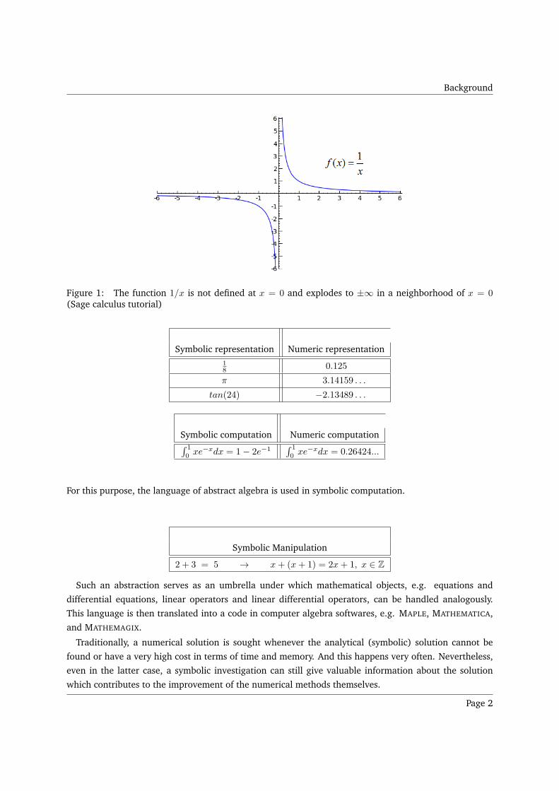
Background
Figure 1: The function 1/x is not defined at x = 0 and explodes to ±∞ in a neighborhood of x = 0(Sage calculus tutorial)
Symbolic representation Numeric representation18 0.125
π 3.14159 . . .
tan(24) −2.13489 . . .
Symbolic computation Numeric computation∫ 1
0xe−xdx = 1− 2e−1
∫ 1
0xe−xdx = 0.26424...
For this purpose, the language of abstract algebra is used in symbolic computation.
Symbolic Manipulation
2 + 3 = 5 → x+ (x+ 1) = 2x+ 1, x ∈ Z
Such an abstraction serves as an umbrella under which mathematical objects, e.g. equations and
differential equations, linear operators and linear differential operators, can be handled analogously.
This language is then translated into a code in computer algebra softwares, e.g. MAPLE, MATHEMATICA,
and MATHEMAGIX.
Traditionally, a numerical solution is sought whenever the analytical (symbolic) solution cannot be
found or have a very high cost in terms of time and memory. And this happens very often. Nevertheless,
even in the latter case, a symbolic investigation can still give valuable information about the solution
which contributes to the improvement of the numerical methods themselves.
Page 2
Background
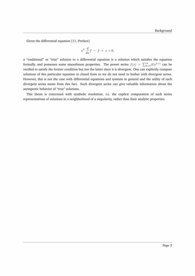
Given the differential equation [11, Preface]
x2 d
dxf − f + x = 0,
a “traditional” or “true” solution to a differential equation is a solution which satisfies the equation
formally, and possesses some smoothness properties. The power series f(x) =∑∞
k=0 k!xk+1 can be
verified to satisfy the former condition but not the latter since it is divergent. One can explicitly compute
solutions of this particular equation in closed form so we do not need to bother with divergent series.
However, this is not the case with differential equations and systems in general and the utility of such
divergent series stems from this fact. Such divergent series can give valuable information about the
asymptotic behavior of “true” solutions.
This thesis is concerned with symbolic resolution, i.e. the explicit computation of such series
representations of solutions in a neighborhood of a singularity, rather than their analytic properties.
Page 3
Thesis outline
Thesis Outline
Let K be a commutative field of characteristic zero equipped with a derivation ∂, that is a map ∂ : K → K
satisfying
∂(f + g) = ∂f + ∂g and ∂(fg) = ∂(f)g + f∂(g) for all f, g ∈ K.
We denote by K its field of constants and V an n-dimensional K-vector space. Let A be an element of
Mn(K). Setting ∆ = ∂−A , ∆ is a ∂-differential operator acting on V , that is, a K-linear endomorphism
of V satisfying the Leibniz condition:
∀f ∈ K, v ∈ V, ∆(fv) = ∂(f)v + f∆(v).
By setting ∂ = ddx and K = K((x)), the field of formal Laurent series in x over K, ∆ is associated to
the widely studied singular linear ordinary differential system (ODS). There exist several algorithms,
contributing to the formal reduction of such systems, i.e. the algorithmic procedure that computes a
change of basis w.r.t. which the matrix representation of the differential operator has a normal form.
This form allows the construction of a fundamental matrix of formal solutions (FMFS).
This thesis is mainly concerned in giving a two-fold generalization of such algorithms to treat a wider
class of systems over bivariate and multivariate fields. Namely,
• let K[[x]][[ε]] be the ring of formal power series in a parameter ε whose coefficients lie in K[[x]], the
ring of formal power series in x over K. Let K be its field of fractions and set again ∂ = ddx . We are
interested in the operator ∆ε associated to a singularly-perturbed linear differential system;
• let K[[x1, x2, . . . xm]], m ≥ 2, be the ring of formal power series in x = (x1, x2, . . . , xm) over Kand K its field of fractions. Setting ∂i =
∂∂xi
, we are interested in completely integrable Pfaffian
systems with normal crossings associated to
∆iF = 0, 1 ≤ i ≤ m,
for which the following integrability conditions are satisfied (pairwise commutativity of the
operators),
∆i ∆j = ∆j ∆i, 1 ≤ i, j ≤ m.
The systems associated to these operators are discussed in three separate parts as explained below.
Page 4
Thesis outline
Part I: Singular Linear differential systems
The first part of this thesis is devoted to topics in local and global analysis over univariate fields. It
encompasses three chapters the first of which recalls the local analysis of linear singular differential
systems. We describe the formal reduction and its underlying algorithms, leading to the construction
of solutions (e.g. uncoupling of the system into systems of lower dimensions, dropping the rank of the
singularity to its minimal integer, computing formal invariants).
The perturbed algebraic eigenvalue problem arises naturally within the discussion of the first chapter
and so it is discussed in a second chapter (∂ is set to a trivial (zero) derivation and consequently ∆ is a
linear operator). Applications to this problem arise in numerous fields as well including quantum physics
and robust control.
The third chapter is dedicated to removing apparent singularities of systems whose entries are rational
functions (∂ = ddx and K = K(x)).
Main contribution
• The formal reduction algorithm described in the Chapter 1 lead to the package MINIISOLDE [96]
written in MAPLE, and the package LINDALG [96] written in MATHEMAGIX, the open source
computer algebra and analysis system [135].
• The new algorithm for removing apparent singularities given in Chapter 3 lead to the paper [27]
with M.A. Barkatou and a MAPLE package [100] APPSING.
Part II: Singularly-perturbed linear differential systems
The second part of this thesis is dedicated to the study of the singularly-perturbed linear differential
systems. Such systems are traced back to the year 1817 [140, Historical Introduction] and are exhibited
in a myriad of problems within diverse disciplines including astronomy, hydraulics (namely the work of
Prandtl (1904) and his students [112]), and quantum physics [89, 103, 35]. Their study encompasses a
vast body of literature as well (see, e.g. [43, 140, 103] and references therein).
It was the hope of Wasow, in his 1985 treatise summing up contemporary research directions and
results on such systems, that techniques developed for the treatment of their unperturbed counterparts
be generalized to tackle their problems. The bivariate nature of such systems and the phenomenon of
turning points renders such a generalization nontrivial. The investigation in this part addresses these
obstacles.
Main contribution
• We give an algorithm to compute (outer) formal solutions in a neighborhood of a turning point. The
results of this part amount to a paper [2] with A. Barkatou and H. Abbas, a paper under redaction
with M. Barkatou [28], and a MAPLE package PARAMINT [98].
Page 5
Thesis outline
Part III: Completely Integrable Pfaffian Systems with Normal
Crossings
“Partial differential equations are the basis of all physical theorems” (Bernhard Riemann 1826-1866). In
particular, Pfaffian systems arise in many applications including the studies of aerospace and celestial
mechanics. By far, the most important for applications are those with normal crossings [111], which are
discussed in the third part of this thesis. Although it was not always stated explicitly in physical models
that one is simply applying the general theory of Pfaff forms (1-forms), such forms play a broad-ranging
role. Fundamental fields of classical physics are defined in terms of forces per unit mass, charge, etc..
And generally forces take that form†.
A univariate completely integrable Pfaffian system with normal crossings reduces to the ODS discussed
in Chapter 1, for which, unlike the multivariate case considered herein, algorithms have been developed.
Theoretical studies guarantee the existence of a change of basis which takes the system to Hukuhara-
Turrittin’s normal form from which the construction of a fundamental matrix of formal solutions is
straightforward. However, the formal reduction, that is the algorithmic procedure computing such a
change of basis, is a question of another nature and is the interest of this part.
Main contribution
• We give a formal reduction algorithm for bivariate systems which amounts to the paper [1] with
H. Abbas and M. Barkatou, and the MAPLE package [99] PFAFFINT. These results are extended
under certain conditions to multivariate systems in a submitted paper with M. Barkatou and M.
Jaroschek [25].
We conclude each of the three parts separately and give items for further research. There exist several
additional notions and approaches to treat an ODS. In this thesis, we only recall notions which correspond
to our generalizations. However, we point out in Appendix A some possible future investigations over
bivariate and multivariate fields.
A large part of this thesis is code lines. The pseudo code given for some of the algorithms within
the chapters serves the purpose of clarification only and does not coincide with the implementation.
The description of some of the functionalities of the packages and some examples of computations are
adjoined in Appendix B. The packages are available on my web page for download with their manuals.
†We refer to [49] where one can find examples from physical systems and references to early notable advances in theunderstanding of such problems
Page 6

Part I
Singular Linear Differential Systems
Page 8
Introduction to Part I
Introduction
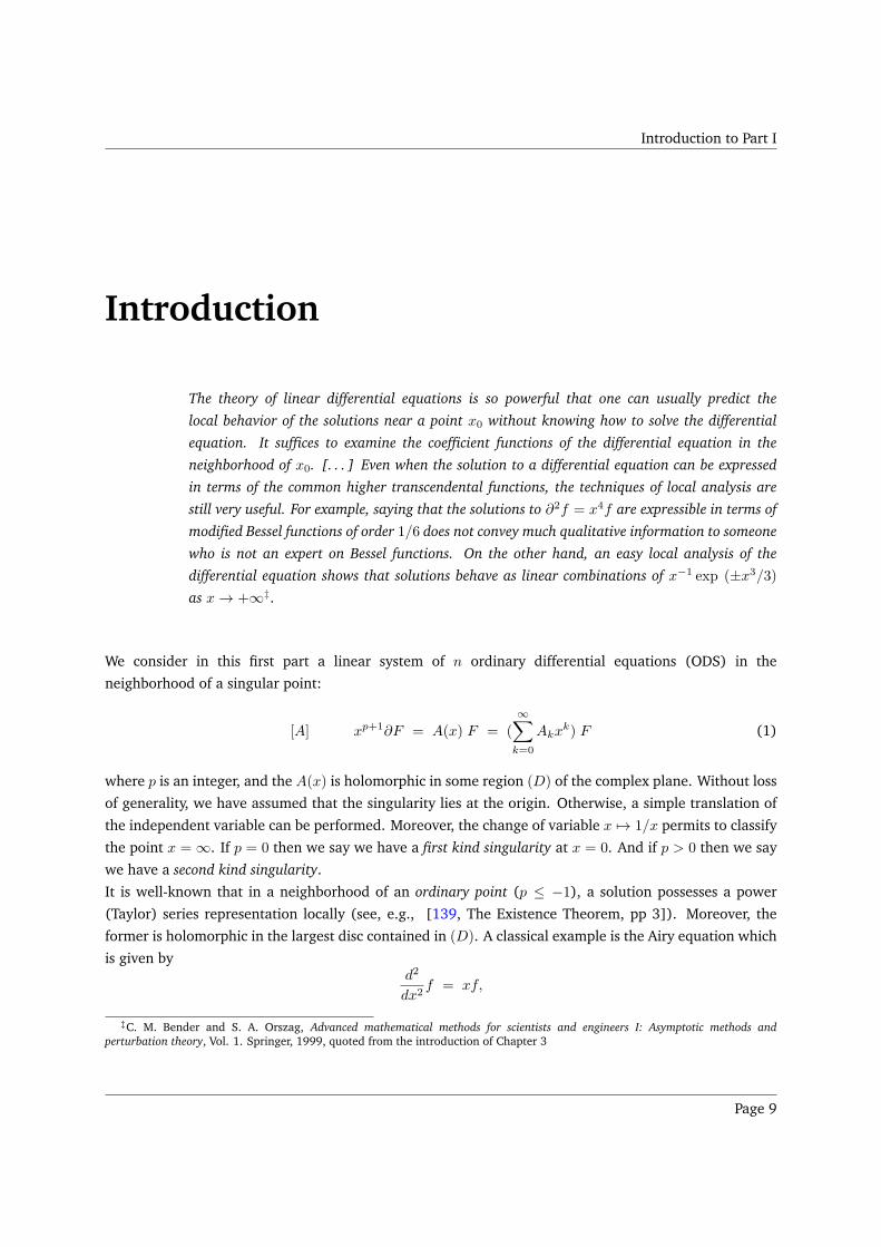
The theory of linear differential equations is so powerful that one can usually predict the
local behavior of the solutions near a point x0 without knowing how to solve the differential
equation. It suffices to examine the coefficient functions of the differential equation in the
neighborhood of x0. [. . . ] Even when the solution to a differential equation can be expressed
in terms of the common higher transcendental functions, the techniques of local analysis are
still very useful. For example, saying that the solutions to ∂2f = x4f are expressible in terms of
modified Bessel functions of order 1/6 does not convey much qualitative information to someone
who is not an expert on Bessel functions. On the other hand, an easy local analysis of the
differential equation shows that solutions behave as linear combinations of x−1 exp (±x3/3)
as x→ +∞‡.
We consider in this first part a linear system of n ordinary differential equations (ODS) in the
neighborhood of a singular point:
[A] xp+1∂F = A(x) F = (
∞∑
k=0
Akxk) F (1)
where p is an integer, and the A(x) is holomorphic in some region (D) of the complex plane. Without loss
of generality, we have assumed that the singularity lies at the origin. Otherwise, a simple translation of
the independent variable can be performed. Moreover, the change of variable x 7→ 1/x permits to classify
the point x =∞. If p = 0 then we say we have a first kind singularity at x = 0. And if p > 0 then we say
we have a second kind singularity.
It is well-known that in a neighborhood of an ordinary point (p ≤ −1), a solution possesses a power
(Taylor) series representation locally (see, e.g., [139, The Existence Theorem, pp 3]). Moreover, the
former is holomorphic in the largest disc contained in (D). A classical example is the Airy equation which
is given byd2
dx2f = xf,
‡C. M. Bender and S. A. Orszag, Advanced mathematical methods for scientists and engineers I: Asymptotic methods andperturbation theory, Vol. 1. Springer, 1999, quoted from the introduction of Chapter 3
Page 9
Introduction to Part I
and whose first-order system representation is easily obtained by setting F = (f, ∂f)T :
∂F =
[
0 1
x 0
]
F.
The general solution near x = 0 is
y(x) = c0
∞∑
k=0
x3k
9k k! Γ(k + 2/3)+ c1
∞∑
k=0
x3k+1
9k k! Γ(k + 4/3),
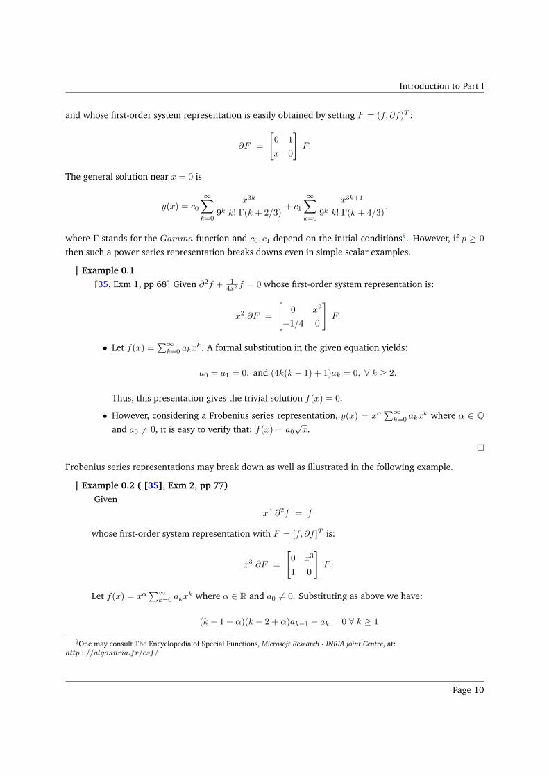
where Γ stands for the Gamma function and c0, c1 depend on the initial conditions§. However, if p ≥ 0
then such a power series representation breaks downs even in simple scalar examples.
| Example 0.1
[35, Exm 1, pp 68] Given ∂2f + 14x2 f = 0 whose first-order system representation is:
x2 ∂F =
[
0 x2
−1/4 0
]
F.
• Let f(x) =∑∞
k=0 akxk. A formal substitution in the given equation yields:
a0 = a1 = 0, and (4k(k − 1) + 1)ak = 0, ∀ k ≥ 2.
Thus, this presentation gives the trivial solution f(x) = 0.
• However, considering a Frobenius series representation, y(x) = xα∑∞
k=0 akxk where α ∈ Q
and a0 6= 0, it is easy to verify that: f(x) = a0√x.
Frobenius series representations may break down as well as illustrated in the following example.
| Example 0.2 ( [35], Exm 2, pp 77)
Given
x3 ∂2f = f
whose first-order system representation with F = [f, ∂f ]T is:
x3 ∂F =
[
0 x3
1 0
]
F.
Let f(x) = xα∑∞
k=0 akxk where α ∈ R and a0 6= 0. Substituting as above we have:
(k − 1− α)(k − 2 + α)ak−1 − ak = 0 ∀ k ≥ 1
§One may consult The Encyclopedia of Special Functions, Microsoft Research - INRIA joint Centre, at:http : //algo.inria.fr/esf/
Page 10
Introduction to Part I
and a0 = 0 which is an immediate contradiction. Hence, no Frobenius representation exists for
this example.
For a system [A] with p ≥ 0, we call p the Poincaré rank. Such systems have been studied extensively
(see, e.g., [11, 139] and references therein). It is well-known that a solution is, in general, the product
of not only a matrix of formal power series in a root of x (Airy equation at x = 0) and a matrix power of
x (Example 0.1), but also an exponential of a polynomial in a root of x−1 (Example 0.2).
Consider again Airy equation but for large |x| (x 7→ 1/x). It is known to possess two linearly independent
solutions, the Airy functions of the first and second kind, Ai(x) and Bi(x), having the following
asymptotic representation (see, e.g. [139, Ch. VI]):
Ai (x) =1
2√πx−1/4 exp (
−23x3/2
) [1 +O(|x|−3/2)],
Bi (x) =1√πx−1/4 exp (
2
3x3/2) [1 +O(|x|−3/2)].
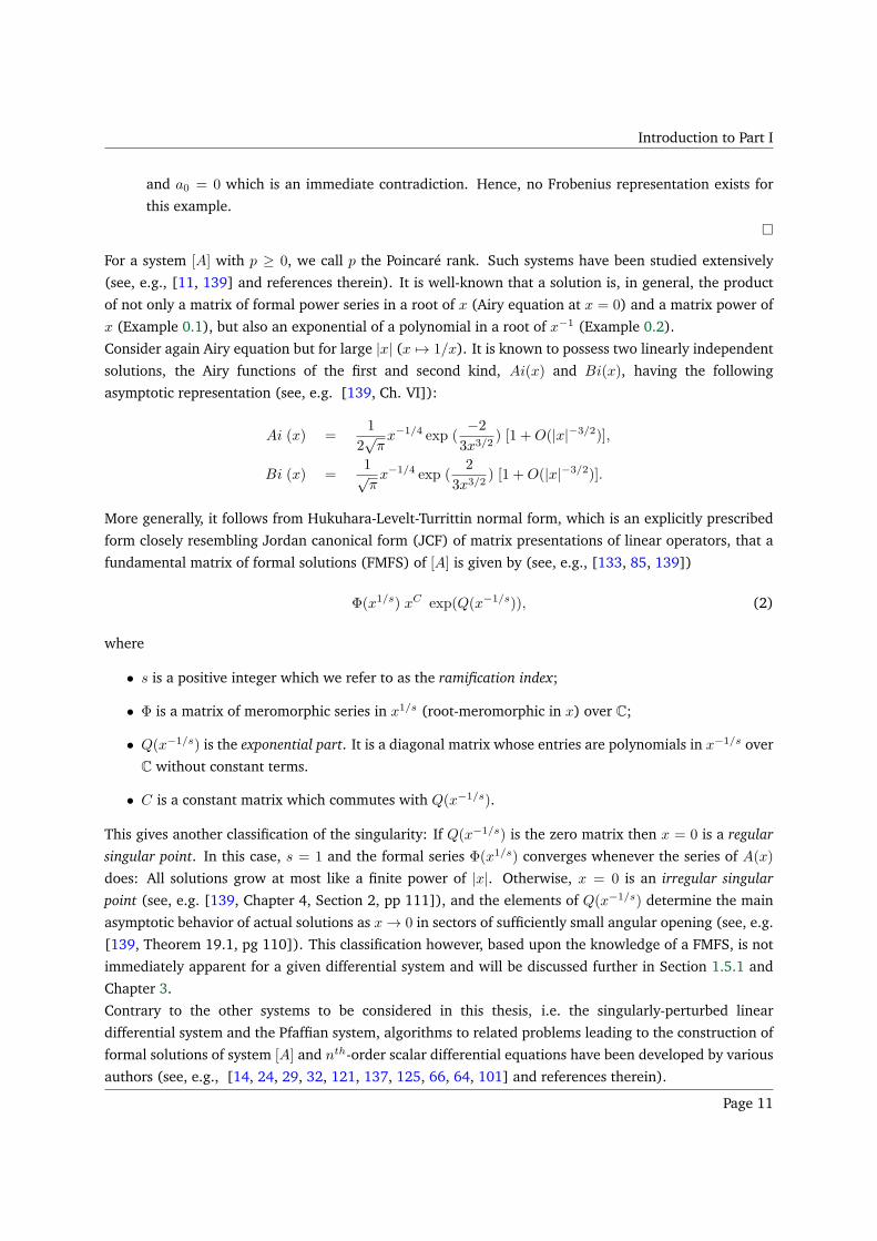
More generally, it follows from Hukuhara-Levelt-Turrittin normal form, which is an explicitly prescribed
form closely resembling Jordan canonical form (JCF) of matrix presentations of linear operators, that a
fundamental matrix of formal solutions (FMFS) of [A] is given by (see, e.g., [133, 85, 139])
Φ(x1/s) xC exp(Q(x−1/s)), (2)
where
• s is a positive integer which we refer to as the ramification index;
• Φ is a matrix of meromorphic series in x1/s (root-meromorphic in x) over C;
• Q(x−1/s) is the exponential part. It is a diagonal matrix whose entries are polynomials in x−1/s over
C without constant terms.
• C is a constant matrix which commutes with Q(x−1/s).
This gives another classification of the singularity: If Q(x−1/s) is the zero matrix then x = 0 is a regular
singular point. In this case, s = 1 and the formal series Φ(x1/s) converges whenever the series of A(x)
does: All solutions grow at most like a finite power of |x|. Otherwise, x = 0 is an irregular singular
point (see, e.g. [139, Chapter 4, Section 2, pp 111]), and the elements of Q(x−1/s) determine the main
asymptotic behavior of actual solutions as x→ 0 in sectors of sufficiently small angular opening (see, e.g.
[139, Theorem 19.1, pg 110]). This classification however, based upon the knowledge of a FMFS, is not
immediately apparent for a given differential system and will be discussed further in Section 1.5.1 and
Chapter 3.
Contrary to the other systems to be considered in this thesis, i.e. the singularly-perturbed linear
differential system and the Pfaffian system, algorithms to related problems leading to the construction of
formal solutions of system [A] and nth-order scalar differential equations have been developed by various
authors (see, e.g., [14, 24, 29, 32, 121, 137, 125, 66, 64, 101] and references therein).
Page 11
Introduction to Part I
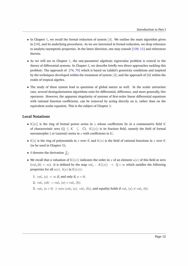
• In Chapter 1, we recall the formal reduction of system [A]. We outline the main algorithm given
in [14], and its underlying procedures. As we are interested in formal reduction, we drop reference
to analytic/asymptotic properties. In the latter direction, one may consult [139, 11] and references
therein.
• As we will see in Chapter 1, the one-parameter algebraic eigenvalue problem is central to the
theory of differential systems. In Chapter 2, we describe briefly two direct approaches tackling this
problem: The approach of [74, 75] which is based on Lidskii’s genericity conditions and inspired
by the techniques developed within the treatment of system [A]; and the approach of [4] within the
realm of tropical algebra.
• The study of these system lead to questions of global nature as well. In the scalar univariate
case, several desingularization algorithms exist for differential, difference, and more generally, Ore
operators. However, the apparent singularity of systems of first-order linear differential equations
with rational function coefficients, can be removed by acting directly on it, rather than on the
equivalent scalar equation. This is the subject of Chapter 3.
Local Notations
• K[[x]] is the ring of formal power series in x whose coefficients lie in a commutative field Kof characteristic zero (Q ⊆ K ⊆ C). K((x)) is its fraction field, namely the field of formal
meromorphic ( or Laurent) series in x with coefficients in K;
• K[x] is the ring of polynomials in x over K and K(x) is the field of rational functions in x over K(to be used in Chapter 3);
• ∂ denotes the derivation ddx ;
• We recall that a valuation of K((x)) indicates the order in x of an element a(x) of this field at zero
(valx(0) = ∞). It is defined by the map valx : K((x)) → Q ∪ ∞ which satisfies the following
properties for all a(x), b(x) in K((x)):
1. valx (a) =∞ if, and only if, a = 0;
2. valx (ab) = valx (a) + valx (b);
3. valx (a+ b) ≥ min (valx (a), valx (b)), and equality holds if valx (a) 6= valx (b);
Page 12
Chapter 1
Chapter 1
Formal Reduction (Computing a FFMS)
Contents1.1 Gauge transformations . . . . . . . . . . . . . . . . . . . . . . . . . . . . . . . . . . . 14
1.2 Equivalence between a system and an equation . . . . . . . . . . . . . . . . . . . . . 15
1.3 A0 has at least two distinct eigenvalues . . . . . . . . . . . . . . . . . . . . . . . . . . 16
1.4 A0 has a unique nonzero eigenvalue . . . . . . . . . . . . . . . . . . . . . . . . . . . . 18
1.5 A0 is nilpotent . . . . . . . . . . . . . . . . . . . . . . . . . . . . . . . . . . . . . . . . 18
1.5.1 Rank reduction . . . . . . . . . . . . . . . . . . . . . . . . . . . . . . . . . . . . . 19
1.5.2 Formal exponential order ω(A) . . . . . . . . . . . . . . . . . . . . . . . . . . . . . 20
1.6 Regular systems . . . . . . . . . . . . . . . . . . . . . . . . . . . . . . . . . . . . . . . 21
1.7 Formal reduction algorithm . . . . . . . . . . . . . . . . . . . . . . . . . . . . . . . . . 23
1.8 Remarks about the implementation . . . . . . . . . . . . . . . . . . . . . . . . . . . . 23
1.9 Conclusion . . . . . . . . . . . . . . . . . . . . . . . . . . . . . . . . . . . . . . . . . . 27
Consider again system [A] given by (1):
[A] xp+1∂F = A(x) F = (
∞∑
k=0
Akxk) F,
where p ≥ 0 and A(x) ∈ Mn(K[[x]]). As mentioned in the introduction, formal reduction is
the algorithmic procedure that constructs a fundamental matrix of formal solutions (2) of [A] (see,
e.g., [14, 114], and references therein). A recursive algorithmic procedure attaining formal reduction
was developed by Barkatou in [14]. As in the classical approach, it consists of computing at every step,
depending on the nature of the eigenvalues of the leading matrix coefficient A0, a transformation (change
of basis). Accordingly, a block-diagonalized equivalent system, an irreducible equivalent system, or the
formal exponential order are computed. These operations will be described individually in the following
sections and will be generalized in the later chapters of this thesis. Upon performing this transformation,
the resulting (uncoupled) system(s) are of either dimension(s) or Poincaré rank(s) lower than that of
[A]. Based on the former operations, the packages ISOLDE [31] and LINDALG [96] written respectively in
MAPLE and MATHEMAGIX, are dedicated to the symbolic resolution of such systems.
Page 13
1.1 Gauge transformations Chapter 1
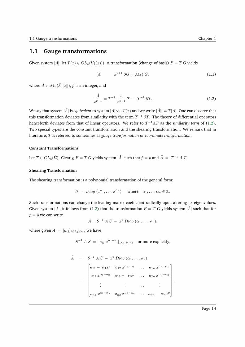
1.1 Gauge transformations
Given system [A], let T (x) ∈ GLn(K((x))). A transformation (change of basis) F = T G yields
[A] xp+1 ∂G = A(x) G, (1.1)
where A ∈Mn(K[[x]]), p is an integer, and
A
xp+1= T−1 A
xp+1T − T−1 ∂T. (1.2)
We say that system [A] is equivalent to system [A] via T (x) and we write [A] := T [A]. One can observe that
this transformation deviates from similarity with the term T−1 ∂T . The theory of differential operators
henceforth deviates from that of linear operators. We refer to T−1AT as the similarity term of (1.2).
Two special types are the constant transformation and the shearing transformation. We remark that in
literature, T is referred to sometimes as gauge transformation or coordinate transformation.
Constant Transformations
Let T ∈ GLn(K). Clearly, F = T G yields system [A] such that p = p and A = T−1 A T .
Shearing Transformation
The shearing transformation is a polynomial transformation of the general form:
S = Diag (xα1 , . . . , xαn), where α1, . . . , αn ∈ Z.
Such transformations can change the leading matrix coefficient radically upon altering its eigenvalues.
Given system [A], it follows from (1.2) that the transformation F = T G yields system [A] such that for
p = p we can write
A = S−1 A S − xp Diag (α1, . . . , αd).
where given A = [aij ]1≤i,j≤n , we have
S−1 A S = [aij xαj−αi ]1≤i,j≤n, or more explicitly,
A = S−1 A S − xp Diag (α1, . . . , αd)
=
a11 − α1xp a12 xα2−α1 . . . a1n xαn−α1
a21 xα1−α2 a22 − α2xp . . . a2n xαn−α2
...... . . .
...
an1 xα1−αn an2 xα2−αn . . . ann − αnxp
.
Page 14
1.2 Equivalence between a system and an equation Chapter 1
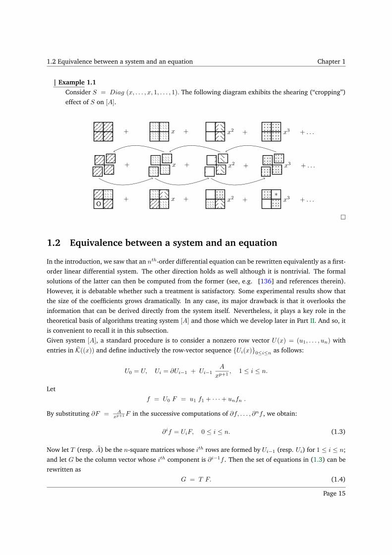
| Example 1.1
Consider S = Diag (x, . . . , x, 1, . . . , 1). The following diagram exhibits the shearing (“cropping”)
effect of S on [A].
+ x + x2 + x3 + . . .
+ x + x2 + x3 + . . .
O+ x + x2 + x3 + . . .
∗
1.2 Equivalence between a system and an equation
In the introduction, we saw that an nth-order differential equation can be rewritten equivalently as a first-
order linear differential system. The other direction holds as well although it is nontrivial. The formal
solutions of the latter can then be computed from the former (see, e.g. [136] and references therein).
However, it is debatable whether such a treatment is satisfactory. Some experimental results show that
the size of the coefficients grows dramatically. In any case, its major drawback is that it overlooks the
information that can be derived directly from the system itself. Nevertheless, it plays a key role in the
theoretical basis of algorithms treating system [A] and those which we develop later in Part II. And so, it
is convenient to recall it in this subsection.
Given system [A], a standard procedure is to consider a nonzero row vector U(x) = (u1, . . . , un) with
entries in K((x)) and define inductively the row-vector sequence Ui(x)0≤i≤n as follows:
U0 = U, Ui = ∂Ui−1 + Ui−1A
xp+1, 1 ≤ i ≤ n.
Let
f = U0 F = u1 f1 + · · ·+ unfn .
By substituting ∂F = Axp+1F in the successive computations of ∂f, . . . , ∂nf , we obtain:
∂if = UiF, 0 ≤ i ≤ n. (1.3)
Now let T (resp. A) be the n-square matrices whose ith rows are formed by Ui−1 (resp. Ui) for 1 ≤ i ≤ n;
and let G be the column vector whose ith component is ∂i−1f . Then the set of equations in (1.3) can be
rewritten as
G = T F. (1.4)
Page 15
1.3 A0 has at least two distinct eigenvalues Chapter 1
Noting that A = ∂T + T Axp+1 , (1.4) can be rewritten as
∂G = A F. (1.5)
We say that U(x) is a cyclic vector if the matrix T is invertible. Cyclic vectors always exist (see, e.g. [46]
and references therein). We can thus rewrite (1.5) and (1.4) as
F = T−1 G and ∂G = ˜A G, where ˜A(x) = AT−1 = TA
xp+1T−1 + ∂TT−1
is a companion matrix. Denoting the entries in its last row by (˜ai)0≤i≤n−1(x) ∈ K((x)), the system is
obviously equivalent to the nth-order scalar differential equation:
∂nf − ˜an−1(x) ∂n−1f − . . . ˜a1(x) ∂f − ˜a0(x) f = 0.
Another algorithm is that of [13] which computes a companion block diagonal form for system [A]. The
former can be easily adapted to singularly-perturbed linear differential systems as well to serve theoretical
purposes (Chapter 4).
In the sequel, we offer a direct treatment of the system [A], i.e. without resorting to an equivalent
nth-order scalar equation. The classical direct treatment of system [A] depends on the nature of the
eigenvalues of the leading matrix coefficient A0. For the clarity of the presentation, we can assume
without loss of generality that A0 is in Jordan canonical form (JCF, in short). This can always be achieved
by a constant transformation and efficient algorithms exist for this task [59].
1.3 A0 has at least two distinct eigenvalues
Whenever A0 has at least two distinct eigenvalues, system [A] can be uncoupled into systems of lower
dimensions via the classical Splitting lemma which we recall here with its constructive proof (see,
e.g. [139, Section 12, pp 52-54] or [11, Lemma 3, pp 42-43]).
| Theorem 1.1
Given system [A] with A(x) ∈Mn(K[[x]]). If the leading matrix coefficient is of the form
A0 =
[
A110 O
O A220
]
(1.6)
where A110 and A22
0 have no eigenvalues in common, then there exists a unique transformation T (x) ∈GLn(K[[x]]) given by
T (x) =
[
I O
O I
]
+∞∑
k=1
[
O T 12k
T 21k O
]
xi,
Page 16
1.3 A0 has at least two distinct eigenvalues Chapter 1
such that the transformation F = TG gives
xp+1 d
dxG = A(x) Z =
[
A11(x) O
O A22(x)
]
G
where A0 = A0 and A(x) ∈Mn(K[[x]]).
Proof. We have from (1.2):
xp+1∂T (x) = A(x)T (x)− T (x)A(x). (1.7)
Assume the above form for T (x), then we have for 1 ≤ 6= ς ≤ 2:
A(x)− A(x) +Aς(x) T ς(x) = O
Aς(x) +Aςς(x) T ς(x)− T ς(x) A(x) = xp+1∂T ς(x)(1.8)
Inserting the series expansions A(x) =∑∞
k=0 Akxk and A(x) =
∑∞k=0 Akx
k in (1.8), and equating the
power-like coefficients, we get recursion formulas of the form:
For k = 0 we have
A0 = A
0
Aςς0 T ς
0 − T ς0 A
0 = O
which are satisfied by settingAςς0 = Aςς
0 and T ςς0 = I, T ς
0 = O.
For k ≥ 1 we have
Aςς0 T ς
k − T ςk A
0 = −Aςk −
k−1∑
j=1
(Aςςk−jT
ςj − T ς
j Ak−j) + (k − p) T ς
k−p (1.9)
Ak = A
k +
k∑
j=1
Aςk−jT
ςj (1.10)
where T ςk−p = O for k ≤ p.
It’s clear that (1.9) is a Sylvester matrix equation that possesses a unique solution due the assumption on
the disjoint spectra of M ςς0 and M
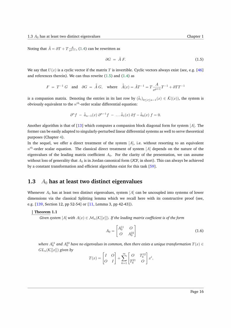
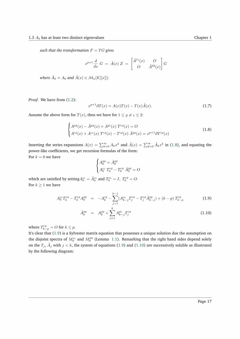
0 (Lemma 1.1). Remarking that the right hand sides depend solely
on the Tj , Aj with j < k, the system of equations (1.9) and (1.10) are successively soluble as illustrated
by the following diagram:
Page 17
1.4 A0 has a unique nonzero eigenvalue Chapter 1
O+
Ox + x2 + x3 + . . .
O+
OO
x +O
x2 + x3 + . . .
O+
OO
x +O
Ox2 +
Ox3 + . . .
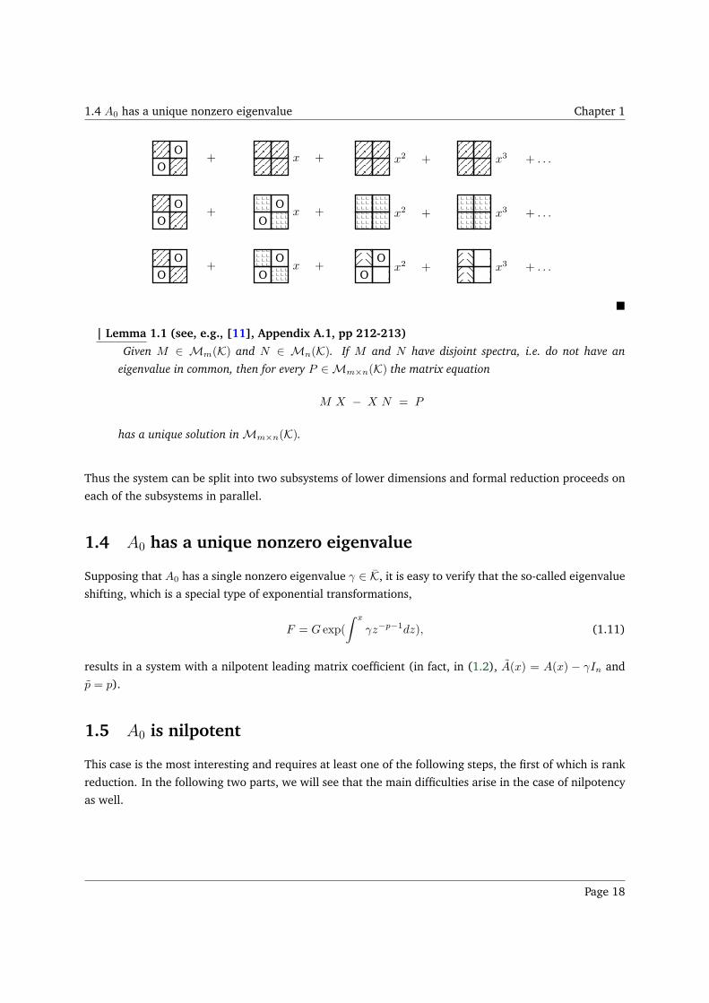
| Lemma 1.1 (see, e.g., [11], Appendix A.1, pp 212-213)
Given M ∈ Mm(K) and N ∈ Mn(K). If M and N have disjoint spectra, i.e. do not have an
eigenvalue in common, then for every P ∈Mm×n(K) the matrix equation
M X − X N = P
has a unique solution inMm×n(K).
Thus the system can be split into two subsystems of lower dimensions and formal reduction proceeds on
each of the subsystems in parallel.
1.4 A0 has a unique nonzero eigenvalue
Supposing that A0 has a single nonzero eigenvalue γ ∈ K, it is easy to verify that the so-called eigenvalue
shifting, which is a special type of exponential transformations,
F = G exp(
∫ x
γz−p−1dz), (1.11)
results in a system with a nilpotent leading matrix coefficient (in fact, in (1.2), A(x) = A(x) − γIn and
p = p).
1.5 A0 is nilpotent
This case is the most interesting and requires at least one of the following steps, the first of which is rank
reduction. In the following two parts, we will see that the main difficulties arise in the case of nilpotency
as well.
Page 18
1.5 A0 is nilpotent Chapter 1
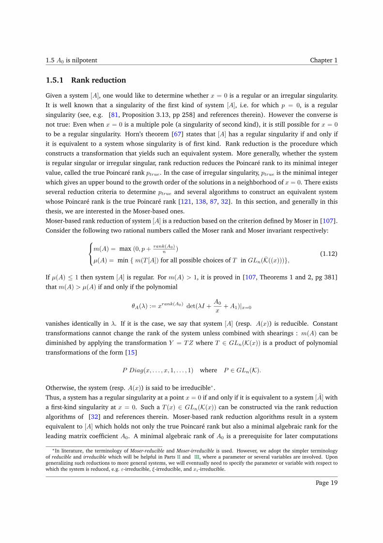
1.5.1 Rank reduction
Given a system [A], one would like to determine whether x = 0 is a regular or an irregular singularity.
It is well known that a singularity of the first kind of system [A], i.e. for which p = 0, is a regular
singularity (see, e.g. [81, Proposition 3.13, pp 258] and references therein). However the converse is
not true: Even when x = 0 is a multiple pole (a singularity of second kind), it is still possible for x = 0
to be a regular singularity. Horn’s theorem [67] states that [A] has a regular singularity if and only if
it is equivalent to a system whose singularity is of first kind. Rank reduction is the procedure which
constructs a transformation that yields such an equivalent system. More generally, whether the system
is regular singular or irregular singular, rank reduction reduces the Poincaré rank to its minimal integer
value, called the true Poincaré rank ptrue. In the case of irregular singularity, ptrue is the minimal integer
which gives an upper bound to the growth order of the solutions in a neighborhood of x = 0. There exists
several reduction criteria to determine ptrue and several algorithms to construct an equivalent system
whose Poincaré rank is the true Poincaré rank [121, 138, 87, 32]. In this section, and generally in this
thesis, we are interested in the Moser-based ones.
Moser-based rank reduction of system [A] is a reduction based on the criterion defined by Moser in [107].
Consider the following two rational numbers called the Moser rank and Moser invariant respectively:
m(A) = max (0, p+ rank(A0)n )
µ(A) = min m(T [A]) for all possible choices of T in GLn(K((x))),(1.12)
If µ(A) ≤ 1 then system [A] is regular. For m(A) > 1, it is proved in [107, Theorems 1 and 2, pg 381]
that m(A) > µ(A) if and only if the polynomial
θA(λ) := xrank(A0) det(λI +A0
x+A1)|x=0
vanishes identically in λ. If it is the case, we say that system [A] (resp. A(x)) is reducible. Constant
transformations cannot change the rank of the system unless combined with shearings : m(A) can be
diminished by applying the transformation Y = TZ where T ∈ GLn(K(x)) is a product of polynomial
transformations of the form [15]
P Diag(x, . . . , x, 1, . . . , 1) where P ∈ GLn(K).
Otherwise, the system (resp. A(x)) is said to be irreducible∗.
Thus, a system has a regular singularity at a point x = 0 if and only if it is equivalent to a system [A] with
a first-kind singularity at x = 0. Such a T (x) ∈ GLn(K(x)) can be constructed via the rank reduction
algorithms of [32] and references therein. Moser-based rank reduction algorithms result in a system
equivalent to [A] which holds not only the true Poincaré rank but also a minimal algebraic rank for the
leading matrix coefficient A0. A minimal algebraic rank of A0 is a prerequisite for later computations
∗In literature, the terminology of Moser-reducible and Moser-irreducible is used. However, we adopt the simpler terminologyof reducible and irreducible which will be helpful in Parts II and III, where a parameter or several variables are involved. Upongeneralizing such reductions to more general systems, we will eventually need to specify the parameter or variable with respect towhich the system is reduced, e.g. ε-irreducible, ξ-irreducible, and xi-irreducible.
Page 19
1.5 A0 is nilpotent Chapter 1
(Subsection 1.5.2) and from here stems our interest in such algorithms. Hence, in the rest of this thesis,
we generalize this reduction criterion and the Moser-based rank reduction algorithm of [15].
We can now suppose without any loss of generality that [A] is an irreducible system. Three possibilities
arise:
• System [A] is regular singular and so it is transformed into an equivalent system whose Poincaré
rank is zero. We proceed in the formal reduction as in Section 1.6.
• System [A] is irregular singular and the leading matrix coefficient has at least two distinct
eigenvalues (resp. unique nonzero eigenvalue). We thus retreat to Section 1.3 (resp. Section 1.4) .
• System [A] is irregular singular and the leading matrix coefficient is nilpotent. This case demands
introducing a ramification in x. This ramification (re-adjustment of the independent variable) is
not known from the outset but can be computed as we show in Subsection 1.5.2.
We remark that more recent rank reduction algorithms were given in [32] and references therein. The
transformations considered therein were optimal in the following sense: If p can be dropped by one then
the similarity transformation computed achieves this goal in one single step. Moreover, θA(λ) gives other
valuable information about the system leading to a generalized splitting lemma [114]. Roughly speaking,
the latter uncouples the system into two subsystems, one of which does not demand a ramification for
the retrieval of the leading term of the exponential parts. The former are however out of the scope of this
brief description.
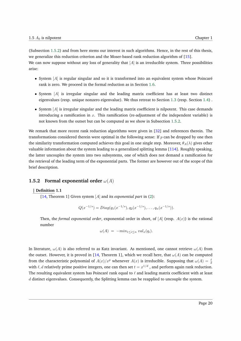
1.5.2 Formal exponential order ω(A)
| Definition 1.1
[14, Theorem 1] Given system [A] and its exponential part in (2):
Q(x−1/s) = Diag(q1(x−1/s), q2(x
−1/s), . . . , qn(x−1/s)).
Then, the formal exponential order, exponential order in short, of [A] (resp. A(x)) is the rational
number
ω(A) = −min1≤i≤n valx(qi).
In literature, ω(A) is also referred to as Katz invariant. As mentioned, one cannot retrieve ω(A) from
the outset. However, it is proved in [14, Theorem 1], which we recall here, that ω(A) can be computed
from the characteristic polynomial of A(x)/xp whenever A(x) is irreducible. Supposing that ω(A) = ℓd
with ℓ, d relatively prime positive integers, one can then set t = x1/d , and perform again rank reduction.
The resulting equivalent system has Poincaré rank equal to ℓ and leading matrix coefficient with at least
d distinct eigenvalues. Consequently, the Splitting lemma can be reapplied to uncouple the system.
Page 20
1.6 Regular systems Chapter 1
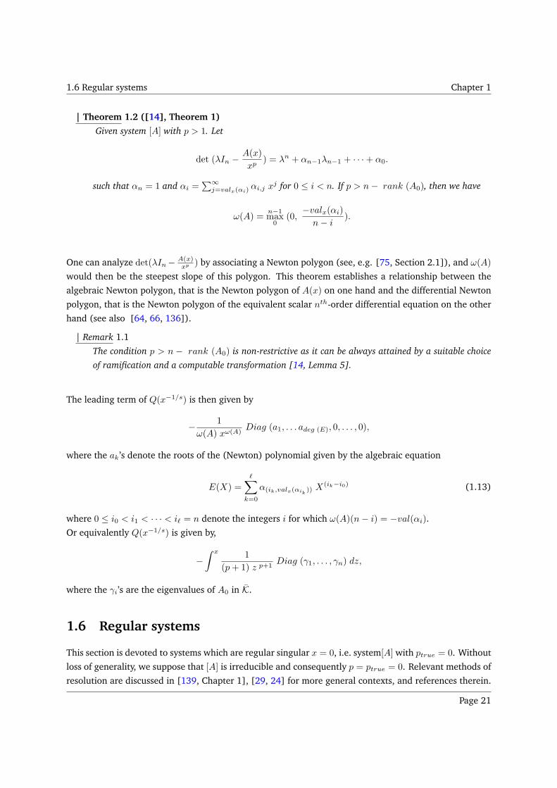
| Theorem 1.2 ([14], Theorem 1)
Given system [A] with p > 1. Let
det (λIn −A(x)
xp) = λn + αn−1λn−1 + · · ·+ α0.
such that αn = 1 and αi =∑∞
j=valx(αi)αi,j x
j for 0 ≤ i < n. If p > n− rank (A0), then we have
ω(A) =n−1max
0(0,−valx(αi)
n− i).
One can analyze det(λIn− A(x)xp ) by associating a Newton polygon (see, e.g. [75, Section 2.1]), and ω(A)
would then be the steepest slope of this polygon. This theorem establishes a relationship between the
algebraic Newton polygon, that is the Newton polygon of A(x) on one hand and the differential Newton
polygon, that is the Newton polygon of the equivalent scalar nth-order differential equation on the other
hand (see also [64, 66, 136]).
| Remark 1.1
The condition p > n − rank (A0) is non-restrictive as it can be always attained by a suitable choice
of ramification and a computable transformation [14, Lemma 5].
The leading term of Q(x−1/s) is then given by
− 1
ω(A) xω(A)Diag (a1, . . . adeg (E), 0, . . . , 0),
where the ak ’s denote the roots of the (Newton) polynomial given by the algebraic equation
E(X) =
ℓ∑
k=0
α(ik,valx(αik)) X
(ik−i0) (1.13)
where 0 ≤ i0 < i1 < · · · < iℓ = n denote the integers i for which ω(A)(n− i) = −val(αi).
Or equivalently Q(x−1/s) is given by,
−∫ x 1
(p+ 1) z p+1Diag (γ1, . . . , γn) dz,
where the γi’s are the eigenvalues of A0 in K.
1.6 Regular systems
This section is devoted to systems which are regular singular x = 0, i.e. system[A] with ptrue = 0. Without
loss of generality, we suppose that [A] is irreducible and consequently p = ptrue = 0. Relevant methods of
resolution are discussed in [139, Chapter 1], [29, 24] for more general contexts, and references therein.
Page 21
1.6 Regular systems Chapter 1
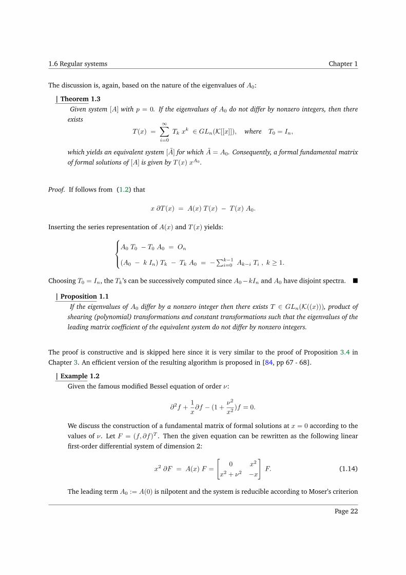
The discussion is, again, based on the nature of the eigenvalues of A0:
| Theorem 1.3
Given system [A] with p = 0. If the eigenvalues of A0 do not differ by nonzero integers, then there
exists
T (x) =
∞∑
i=0
Tk xk ∈ GLn(K[[x]]), where T0 = In,
which yields an equivalent system [A] for which A = A0. Consequently, a formal fundamental matrix
of formal solutions of [A] is given by T (x) xA0 .
Proof. If follows from (1.2) that
x ∂T (x) = A(x) T (x) − T (x) A0.
Inserting the series representation of A(x) and T (x) yields:
A0 T0 − T0 A0 = On
(A0 − k In) Tk − Tk A0 = −∑k−1i=0 Ak−i Ti , k ≥ 1.
Choosing T0 = In, the Tk ’s can be successively computed since A0−kIn and A0 have disjoint spectra.
| Proposition 1.1
If the eigenvalues of A0 differ by a nonzero integer then there exists T ∈ GLn(K((x))), product of
shearing (polynomial) transformations and constant transformations such that the eigenvalues of the
leading matrix coefficient of the equivalent system do not differ by nonzero integers.
The proof is constructive and is skipped here since it is very similar to the proof of Proposition 3.4 in
Chapter 3. An efficient version of the resulting algorithm is proposed in [84, pp 67 - 68].
| Example 1.2
Given the famous modified Bessel equation of order ν:
∂2f +1
x∂f − (1 +
ν2
x2)f = 0.
We discuss the construction of a fundamental matrix of formal solutions at x = 0 according to the
values of ν. Let F = (f, ∂f)T . Then the given equation can be rewritten as the following linear
first-order differential system of dimension 2:
x2 ∂F = A(x) F =
[
0 x2
x2 + ν2 −x
]
F. (1.14)
The leading term A0 := A(0) is nilpotent and the system is reducible according to Moser’s criterion
Page 22
1.7 Formal reduction algorithm Chapter 1
(θ(λ) = 0). The transformation F = T G where T =
[
x 0
0 1
]
yields the equivalent system:
x ∂G = A(x)G =
[
−1 1
x2 + ν2 −x
]
G.
Thus, ptrue = 0 and the system is regular singular at x = 0. The new leading matrix A0 = A(0) =[
−1 1
ν2 0
]
is not nilpotent. The difference between its two eigenvalues is given by√4ν2 + 1. We
thus distinguish two cases:
• Case 1 : If√4ν2 + 1 ∈ N∗ then Proposition 1.1 is applied to reduce.
• Case 2 : Otherwise, we proceed to constructing T (x) of Theorem 1.3 and hence a
fundamental matrix of formal solutions is given by T (x) xA0 .
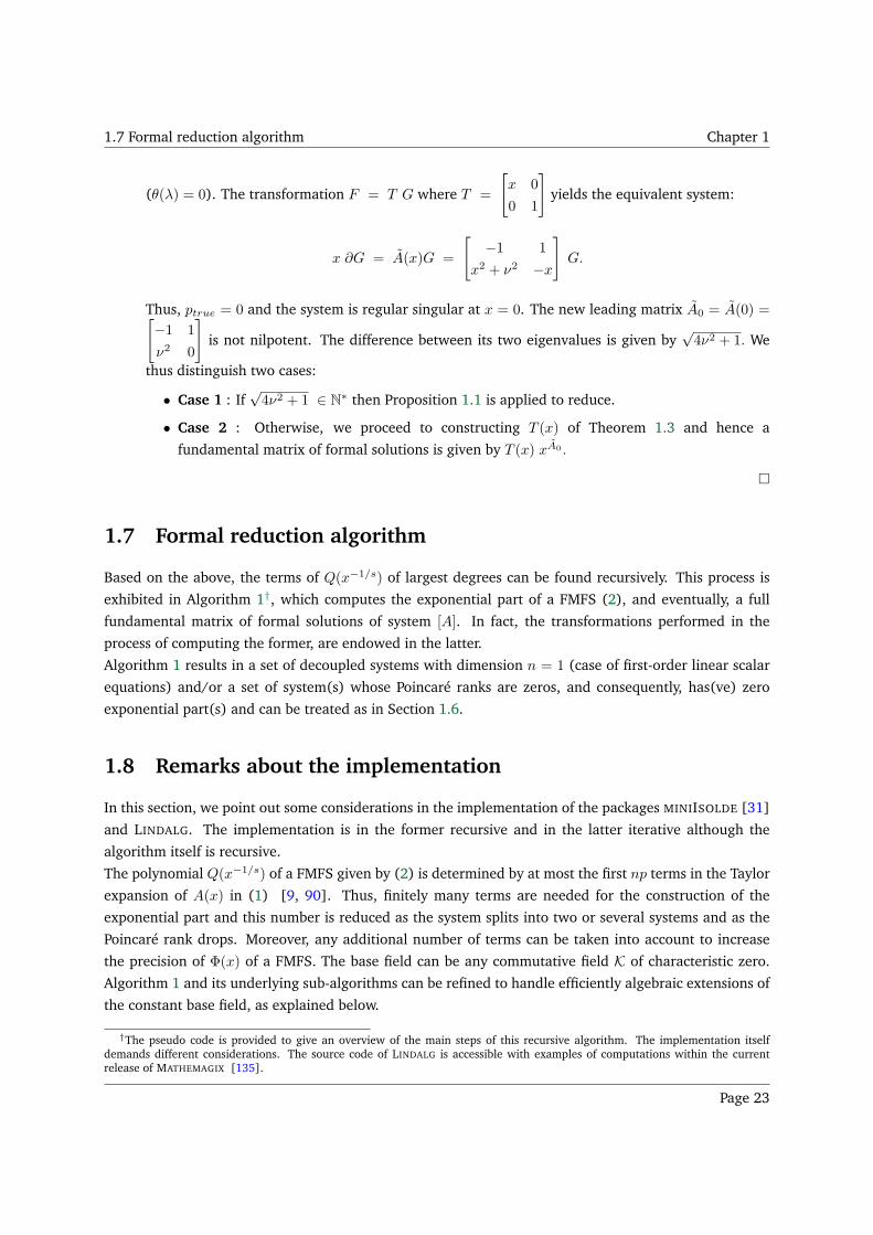
1.7 Formal reduction algorithm
Based on the above, the terms of Q(x−1/s) of largest degrees can be found recursively. This process is
exhibited in Algorithm 1†, which computes the exponential part of a FMFS (2), and eventually, a full
fundamental matrix of formal solutions of system [A]. In fact, the transformations performed in the
process of computing the former, are endowed in the latter.
Algorithm 1 results in a set of decoupled systems with dimension n = 1 (case of first-order linear scalar
equations) and/or a set of system(s) whose Poincaré ranks are zeros, and consequently, has(ve) zero
exponential part(s) and can be treated as in Section 1.6.
1.8 Remarks about the implementation
In this section, we point out some considerations in the implementation of the packages MINIISOLDE [31]
and LINDALG. The implementation is in the former recursive and in the latter iterative although the
algorithm itself is recursive.
The polynomial Q(x−1/s) of a FMFS given by (2) is determined by at most the first np terms in the Taylor
expansion of A(x) in (1) [9, 90]. Thus, finitely many terms are needed for the construction of the
exponential part and this number is reduced as the system splits into two or several systems and as the
Poincaré rank drops. Moreover, any additional number of terms can be taken into account to increase
the precision of Φ(x) of a FMFS. The base field can be any commutative field K of characteristic zero.
Algorithm 1 and its underlying sub-algorithms can be refined to handle efficiently algebraic extensions of
the constant base field, as explained below.
†The pseudo code is provided to give an overview of the main steps of this recursive algorithm. The implementation itselfdemands different considerations. The source code of LINDALG is accessible with examples of computations within the currentrelease of MATHEMAGIX [135].
Page 23
1.8 Remarks about the implementation Chapter 1
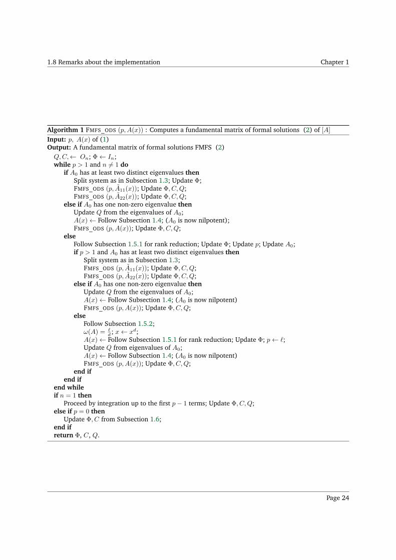
Algorithm 1 FMFS_ODS (p,A(x)) : Computes a fundamental matrix of formal solutions (2) of [A]Input: p, A(x) of (1)Output: A fundamental matrix of formal solutions FMFS (2)
Q,C,← On; Φ← In;while p > 1 and n 6= 1 do
if A0 has at least two distinct eigenvalues thenSplit system as in Subsection 1.3; Update Φ;FMFS_ODS (p, A11(x)); Update Φ, C,Q;FMFS_ODS (p, A22(x)); Update Φ, C,Q;
else if A0 has one non-zero eigenvalue thenUpdate Q from the eigenvalues of A0;A(x)← Follow Subsection 1.4; (A0 is now nilpotent);FMFS_ODS (p,A(x)); Update Φ, C,Q;
elseFollow Subsection 1.5.1 for rank reduction; Update Φ; Update p; Update A0;if p > 1 and A0 has at least two distinct eigenvalues then
Split system as in Subsection 1.3;FMFS_ODS (p, A11(x)); Update Φ, C,Q;FMFS_ODS (p, A22(x)); Update Φ, C,Q;
else if A0 has one non-zero eigenvalue thenUpdate Q from the eigenvalues of A0;A(x)← Follow Subsection 1.4; (A0 is now nilpotent)FMFS_ODS (p,A(x)); Update Φ, C,Q;
elseFollow Subsection 1.5.2;ω(A) = ℓ
d ; x← xd;A(x)← Follow Subsection 1.5.1 for rank reduction; Update Φ; p← ℓ;Update Q from eigenvalues of A0;A(x)← Follow Subsection 1.4; (A0 is now nilpotent)FMFS_ODS (p,A(x)); Update Φ, C,Q;
end ifend if
end whileif n = 1 then
Proceed by integration up to the first p− 1 terms; Update Φ, C,Q;else if p = 0 then
Update Φ, C from Subsection 1.6;end ifreturn Φ, C, Q.
Page 24
1.8 Remarks about the implementation Chapter 1
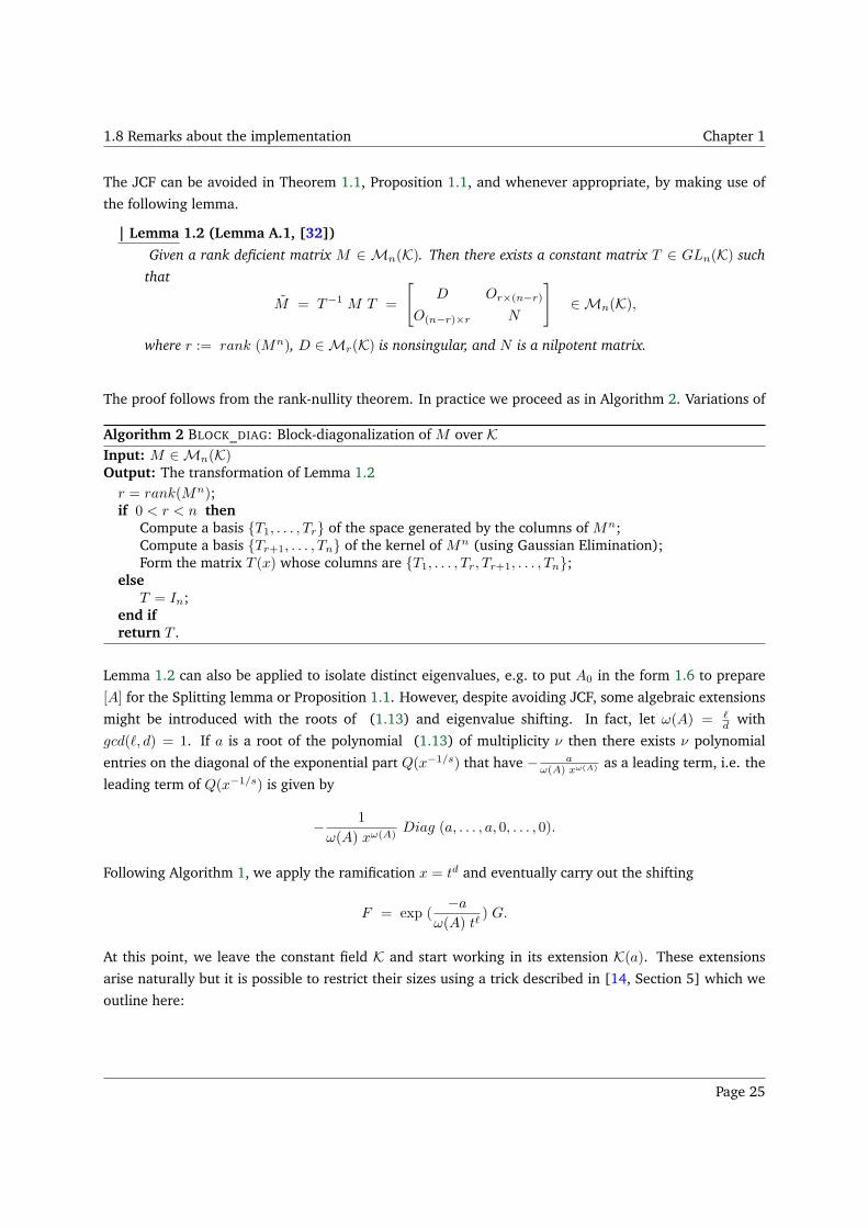
The JCF can be avoided in Theorem 1.1, Proposition 1.1, and whenever appropriate, by making use of
the following lemma.
| Lemma 1.2 (Lemma A.1, [32])
Given a rank deficient matrix M ∈ Mn(K). Then there exists a constant matrix T ∈ GLn(K) such
that
M = T−1 M T =
[
D Or×(n−r)
O(n−r)×r N
]
∈Mn(K),
where r := rank (Mn), D ∈Mr(K) is nonsingular, and N is a nilpotent matrix.
The proof follows from the rank-nullity theorem. In practice we proceed as in Algorithm 2. Variations of
Algorithm 2 BLOCK_DIAG: Block-diagonalization of M over KInput: M ∈Mn(K)Output: The transformation of Lemma 1.2r = rank(Mn);if 0 < r < n then
Compute a basis T1, . . . , Tr of the space generated by the columns of Mn;Compute a basis Tr+1, . . . , Tn of the kernel of Mn (using Gaussian Elimination);Form the matrix T (x) whose columns are T1, . . . , Tr, Tr+1, . . . , Tn;
elseT = In;
end ifreturn T .
Lemma 1.2 can also be applied to isolate distinct eigenvalues, e.g. to put A0 in the form 1.6 to prepare
[A] for the Splitting lemma or Proposition 1.1. However, despite avoiding JCF, some algebraic extensions
might be introduced with the roots of (1.13) and eigenvalue shifting. In fact, let ω(A) = ℓd with
gcd(ℓ, d) = 1. If a is a root of the polynomial (1.13) of multiplicity ν then there exists ν polynomial
entries on the diagonal of the exponential part Q(x−1/s) that have − aω(A) xω(A) as a leading term, i.e. the
leading term of Q(x−1/s) is given by
− 1
ω(A) xω(A)Diag (a, . . . , a, 0, . . . , 0).
Following Algorithm 1, we apply the ramification x = td and eventually carry out the shifting
F = exp (−a
ω(A) tℓ) G.
At this point, we leave the constant field K and start working in its extension K(a). These extensions
arise naturally but it is possible to restrict their sizes using a trick described in [14, Section 5] which we
outline here:
Page 25
1.8 Remarks about the implementation Chapter 1
Let u and v be two integers verifying uℓ + vd = 1. Let z = a−u t and b = ad. Then we have:
−aω(A) tℓ
= −auℓ+vd
ω(A) tℓ= −adv
ω(A) (a−ut)ℓ= bv
ω(A) zℓ ,
x = td = adu zd = bu zd.
One notices that if a is a root of the polynomial (1.13) then b = ad is a root of a reduced polynomial
given by Ereduced (Xd) = E(X). Hence, Algorithm 1 can then be modified as follows:
• Choose a root b of Ereduced;
• compute u and v satisfying uℓ + vd = 1;
• substitute x by bu zd;
• apply the shifting
F = G exp(−bv
ω(A) zℓ).
The new constant field is then K(b) where b is a root of a polynomial of degree equal to the degree of the
polynomial (1.13) divided by d. The computations are done up to conjugations.
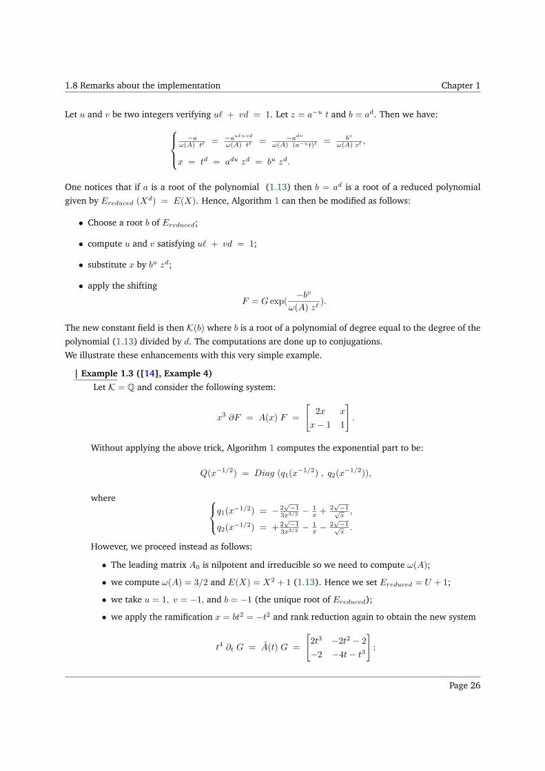
We illustrate these enhancements with this very simple example.
| Example 1.3 ([14], Example 4)
Let K = Q and consider the following system:
x3 ∂F = A(x) F =
[
2x x
x− 1 1
]
.
Without applying the above trick, Algorithm 1 computes the exponential part to be:
Q(x−1/2) = Diag (q1(x−1/2) , q2(x
−1/2)),
where
q1(x−1/2) = − 2
√−1
3x3/2 − 1x + 2
√−1√x
,
q2(x−1/2) = + 2
√−1
3x3/2 − 1x −
2√−1√x
.
However, we proceed instead as follows:
• The leading matrix A0 is nilpotent and irreducible so we need to compute ω(A);
• we compute ω(A) = 3/2 and E(X) = X2 + 1 (1.13). Hence we set Ereduced = U + 1;
• we take u = 1, v = −1, and b = −1 (the unique root of Ereduced);
• we apply the ramification x = bt2 = −t2 and rank reduction again to obtain the new system
t4 ∂t G = A(t) G =
[
2t3 −2t2 − 2
−2 −4t− t3
]
;
Page 26
1.9 Conclusion Chapter 1
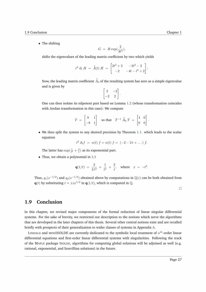
• The shifting
G = H exp(2
3t3),
shifts the eigenvalues of the leading matrix coefficient by two which yields
t4 ∂t H = ˜A(t) H =
[
2t3 + 2 −2t2 − 2
−2 −4t− t3 + 2
]
;
Now, the leading matrix coefficient ˜A0 of the resulting system has zero as a simple eigenvalue
and is given by[
2 −2−2 2
]
.
One can then isolate its nilpotent part based on Lemma 1.2 (whose transformation coincides
with Jordan transformation in this case): We compute
T =
[
8 1
−8 1
]
so that T−1 ˜A0 T =
[
4 0
0 0
]
.
• We then split the system to any desired precision by Theorem 1.1. which leads to the scalar
equation
t3 ∂tf = n(t) f = n(t) f = (−2− 2 t+ . . . ) f.
The latter has exp( 1t2 + 2
t ) as its exponential part.
• Thus, we obtain a polynomial in 1/t
q(1/t) =2
3 t3+
1
t2+
2
t, where x = −t2.
Thus, q1(x−1/2) and q2(x−1/2) obtained above by computations in Q(i) can be both obtained from
q(t) by substituting t = ±ix1/2 in q(1/t), which is computed in Q.
1.9 Conclusion
In this chapter, we revised major components of the formal reduction of linear singular differential
systems. For the sake of brevity, we restricted our description to the notions which serve the algorithms
that are developed in the later chapters of this thesis. Several other central notions exist and are recalled
briefly with prospects of their generalization to wider classes of systems in Appendix A.
LINDALG and MINIISOLDE are currently dedicated to the symbolic local treatment of nth-order linear
differential equations and first-order linear differential systems with singularities. Following the track
of the MAPLE package ISOLDE, algorithms for computing global solutions will be adjoined as well (e.g.
rational, exponential, and liouvillian solutions) in the future.
Page 27
Chapter 2
Chapter 2
Perturbed (Algebraic) Eigenvalue
Problem
Contents2.1 Tropicalization of A(x) . . . . . . . . . . . . . . . . . . . . . . . . . . . . . . . . . . . . 29
2.1.1 Application to differential systems . . . . . . . . . . . . . . . . . . . . . . . . . . . 31
2.2 Differential-like reduction . . . . . . . . . . . . . . . . . . . . . . . . . . . . . . . . . . 33
2.2.1 Integer leading exponents . . . . . . . . . . . . . . . . . . . . . . . . . . . . . . . 33
2.2.2 Fractional leading exponent . . . . . . . . . . . . . . . . . . . . . . . . . . . . . . 34
2.2.3 Singular case . . . . . . . . . . . . . . . . . . . . . . . . . . . . . . . . . . . . . . 40
2.3 Conclusion . . . . . . . . . . . . . . . . . . . . . . . . . . . . . . . . . . . . . . . . . . 44
As we have seen in Subsection 1.5.2, the formal invariants of linear singular differential system [A] given
by (1)
xp+1 d
dxF = A(x) F = (
∞∑
i=0
Akxk) F,
can be retrieved (after certain reductions) from the characteristic polynomial of its matrix A(x). We thus
turn our attention in this chapter to the algebraic eigenvalue problem.
We consider the one-parameter A(x) perturbation of an n× n constant matrix A0:
A(x) = xν∞∑
k=0
Akxk, for some ν ∈ Z, (2.1)
where the Ak ’s belong toMn(C) and A0 6= On.
It is well-known that the eigenvalues of A(x) can be expressed in some neighborhood of x = 0 as a
formal Puiseux series (see, e.g., [34, 80]), i.e. each admits a formal expansion in fractional powers of x
of the form xν∑∞
k=0 λkxk/s, where λk ∈ C (or more specifically some field extension of the base field),
s ≥ 1 is an integer, and ν ∈ Z. We suppose without loss of generality that λ0 6= 0 and we refer to it as the
leading coefficient and to ν + k/s as the leading exponent.
Page 28
2.1 Tropicalization of A(x) Chapter 2
These eigenvalue expansions can be computed by applying Newton-Puiseux algorithm to the
characteristic polynomial of A(x) (see, e.g. [50]) and there already exist computer algebra packages
for this purpose. However, this approach is indirect. A direct approach would recover leading terms from
a few low order coefficients of a matrix similar to A(x) rather than an associated scalar equation.
A direct approach to the perturbed eigenvalue problem (and more generally the perturbed eigenvalue-
eigenvector problem), is given in the linear case by the perturbation theory of Visik, Ljusternik [136], and
Lidskii [88]. For a generic matrix, the leading exponents of the eigenvalues are the inverses of the sizes
of the Jordan blocks of A0 and the leading coefficients can be obtained from certain Schur complements
constructed from the entries of A0 and A1. However, it might happen that Schur complements do not
exist or A1 has a sparse or structured pattern. The generalization of this theory to cover such cases is
the subject of profound research for both matrices and matrix pencils (see, e.g. [4, Introduction] and
references therein).
One extension of the former takes advantage of methods of min-plus algebra and is given by Akian-
Bapat-Gaubert in [4]. Another extension is given by Jeannerod-Pfluegel in [75] and relies on a
differential-like reduction inspired by Moser’s reduction criteria (Subsection 1.5.1) for linear singular
differential systems. In the latter, a direct algorithm was proposed to find the first terms of the
perturbed eigenvalues for which s = 1. In the same differential spirit, the case of s > 1 was discussed
afterwards by Jeannerod [74] based on Lidskii’s genericity conditions for perturbed eigenvalues, and
their characterization in terms of the Newton diagram of A(x) given by Moro-Burke-Overton in [105].
However, although both approaches generalize Lidskii-Visik-Ljusternik’s theory to a wider class of
matrices, both leave behind singular cases open to investigation∗. This chapter describes briefly the main
results of both approaches regarding the computation of the asymptotics of the eigenvalues of (2.1), in
Sections 2.1 and 2.2 respectively.
We aim to show the interaction between the studies of differential and linear operators: On one hand,
the techniques developed for the former turn out to be useful in the treatment of the latter; and on
the other hand, the advancements in the latter contribute directly to the former (see also [138, 108]).
Moreover, we give in Subsection 2.2.3 our partial result, in an attempt to explain the singular case in the
differential-like approach (Section 2.2), using the results of the tropical approach (Sections 2.1).
2.1 Tropicalization of A(x)
Tropical algebra (also min-plus algebra) has been initiated independently by several schools and
developed in relation with diverse mathematical fields (see, e.g. [10, 5, 92]). Let R be the ring
of real numbers. The tropical semiring Rmin is the semiring R ∪ ∞ equipped with the operations
x⊕ y : = min (x, y) and x⊙ y : = x+ y.
Tropical analogues of many classical algebraic functions exist. Let A = [vij ]1≤i,j≤n ∈ Mn(Rmin). In
∗A singular matrix herein refers to a Jordan canonical form (JCF) perturbation which cannot be treated by one or none of thetwo direct approaches discussed in this chapter. This terminology has nothing to do with the terminology of singular regular andsingular irregular points used in Chapter 1
Page 29
2.1 Tropicalization of A(x) Chapter 2
particular, the tropical characteristic polynomial of A is given by:
PA(λ) =⊕
σ∈Σn
n⊙
i=1
(λ δiσ(i) ⊕ viσ(i)) ∈ Rmin[λ],
where Σn is the set of permutations of 1, . . . , n and δiσ(i) is Kronecker’s delta. A tropical analogue
of the fundamental theorem of algebra exists and is due to Cuninhame-Green and Meijer (see, e.g. [4,
Theorem 2.9]).
An eigenvalue of A is a real number λ such that
A⊙ v = λ⊙ v, for some v ∈ Rnmin.
Although this chapter does not aim to discuss the efficiency of the approaches described, we remark that
the eigenvalues of A can be computed in polynomial time due to a result by Burkard and Betkovic [40].
We recall that A can be represented by a weighted directed graph G(A) with n nodes labeled 1, 2, ..., n as
follows: There is an arc (i, j) from node i to node j if and only if vij <∞; and the weight vij is assigned
to each arc. The normalized weight of a directed path i0, i1, ..., ik in G(A) is given by (∑k
j=1 vij−1,ij ) /k.
If ik = i0 then the path is a directed cycle (see e.g. [92, pp 127-133]). We say that a directed graph
is strongly connected if every node is reachable from every other node, i.e. one can find a directed path
connecting both nodes. Such graphs have the following interesting property (see, e.g. [92, Theorem
5.1.1, pp 128], [4, Theorem 2.1], or [10, Theorem 3.23]).
| Theorem 2.1
Let A be a tropical n × n matrix whose graph G(A) is strongly connected. Then A has a unique
eigenvalue λ(A), which is equal to the minimal length of any directed cycle in G(A).
Back to (2.1), let A(x) = [aij(x)]1≤i,j≤n ∈ Mn(C((x))). Then the tropicalization of A(x) is given by
the constant matrix A = [valx(aij)]1≤i,j≤n. Let PA(λ) =∑n
i=0 pi(x)λi ∈ C[[x]][λ] be the characteristic
polynomial of A(x). For generic entries of A(x), the tropical characteristic polynomial of A coincides with
the tropicalization of the classical characteristic polynomial of A(x) given by⊕ni=0 valx(pi)⊙λi ∈ Rmin[λ].
Supposing that the underlying digraph of A is strongly connected, we have:
| Theorem 2.2 ( [4], Theorem 3.8)
Let α = (α1, ..., αn), (α1 ≤ · · · ≤ αn), denote the sequence of the leading exponents in the expansions
of the eigenvalues of A(x) counted with their multiplicities and v = (v1, . . . , vn), v1 ≤ · · · ≤ vn) denote
the sequence of roots of the tropical characteristic polynomial of A. Then, α is weakly majorized by v,
that is( [4, Definition 3.5]),
α1 ⊙ · · · ⊙ αi ≥ v1 ⊙ · · · ⊙ vi , for all i = 1, . . . , n.
Moreover, for generic values of the aij ’s,
αi = vi, for all i = 1, . . . , n.
Page 30
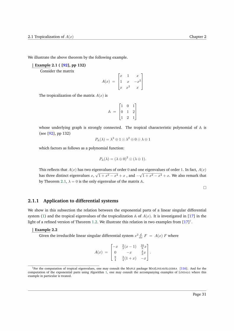
2.1 Tropicalization of A(x) Chapter 2
We illustrate the above theorem by the following example.
| Example 2.1 ( [92], pp 132)
Consider the matrix
A(x) =
x 1 x
1 x −x2
x x2 x
The tropicalization of the matrix A(x) is
A =
1 0 1
0 1 2
1 2 1
whose underlying graph is strongly connected. The tropical characteristic polynomial of A is
(see [92], pp 132)
PA(λ) = λ3 ⊕ 1⊙ λ2 ⊕ 0⊙ λ⊕ 1
which factors as follows as a polynomial function:
PA(λ) = (λ⊕ 0)2 ⊙ (λ⊕ 1).
This reflects that A(x) has two eigenvalues of order 0 and one eigenvalues of order 1. In fact, A(x)
has three distinct eigenvalues x,√1 + x2 − x4 + x , and −
√1 + x2 − x4 + x. We also remark that
by Theorem 2.1, λ = 0 is the only eigenvalue of the matrix A.
2.1.1 Application to differential systems
We show in this subsection the relation between the exponential parts of a linear singular differential
system (1) and the tropical eigenvalues of the tropicalization A of A(x). It is investigated in [17] in the
light of a refined version of Theorem 1.2. We illustrate this relation in two examples from [17]†.
| Example 2.2
Given the irreducible linear singular differential system x2 ddx F = A(x) F where
A(x) =
−x 23 (x− 1) 16
9 x
0 −x 43x
94
34 (1 + x) −x
.
†For the computation of tropical eigenvalues, one may consult the MAPLE package MAXLINEARALGEBRA [116]. And for thecomputation of the exponential parts using Algorithm 1, one may consult the accompanying examples of LINDALG where thisexample in particular is treated.
Page 31
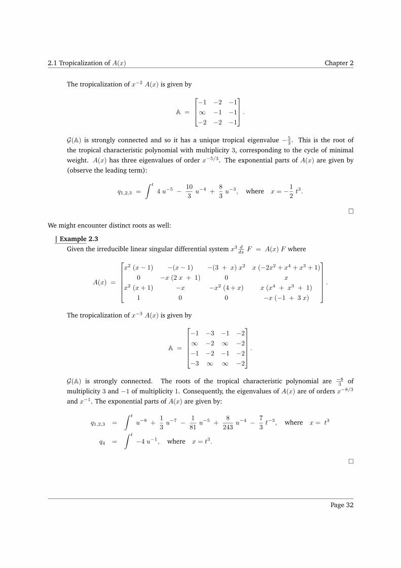
2.1 Tropicalization of A(x) Chapter 2
The tropicalization of x−2 A(x) is given by
A =
−1 −2 −1∞ −1 −1−2 −2 −1
.
G(A) is strongly connected and so it has a unique tropical eigenvalue − 53 . This is the root of
the tropical characteristic polynomial with multiplicity 3, corresponding to the cycle of minimal
weight. A(x) has three eigenvalues of order x−5/3. The exponential parts of A(x) are given by
(observe the leading term):
q1,2,3 =
∫ t
4 u−5 − 10
3u−4 +
8
3u−3, where x = −1
2t3.
We might encounter distinct roots as well:
| Example 2.3
Given the irreducible linear singular differential system x3 ddx F = A(x) F where
A(x) =
x2 (x− 1) −(x− 1) −(3 + x) x2 x (−2x2 + x4 + x3 + 1)
0 −x (2 x + 1) 0 x
x2 (x+ 1) −x −x2 (4 + x) x (x4 + x3 + 1)
1 0 0 −x (−1 + 3 x)
.
The tropicalization of x−3 A(x) is given by
A =
−1 −3 −1 −2∞ −2 ∞ −2−1 −2 −1 −2−3 ∞ ∞ −2
.
G(A) is strongly connected. The roots of the tropical characteristic polynomial are −83 of
multiplicity 3 and −1 of multiplicity 1. Consequently, the eigenvalues of A(x) are of orders x−8/3
and x−1. The exponential parts of A(x) are given by:
q1,2,3 =
∫ t
u−8 +1
3u−7 − 1
81u−5 +
8
243u−4 − 7
3t−3, where x = t3
q4 =
∫ t
−4 u−1, where x = t3.
Page 32
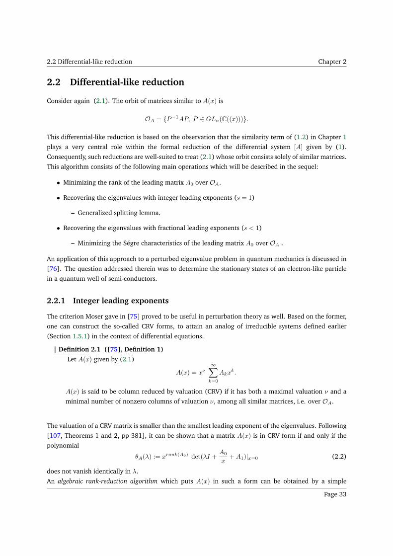
2.2 Differential-like reduction Chapter 2
2.2 Differential-like reduction
Consider again (2.1). The orbit of matrices similar to A(x) is
OA = P−1AP, P ∈ GLn(C((x))).
This differential-like reduction is based on the observation that the similarity term of (1.2) in Chapter 1
plays a very central role within the formal reduction of the differential system [A] given by (1).
Consequently, such reductions are well-suited to treat (2.1) whose orbit consists solely of similar matrices.
This algorithm consists of the following main operations which will be described in the sequel:
• Minimizing the rank of the leading matrix A0 over OA.
• Recovering the eigenvalues with integer leading exponents (s = 1)
– Generalized splitting lemma.
• Recovering the eigenvalues with fractional leading exponents (s < 1)
– Minimizing the Ségre characteristics of the leading matrix A0 over OA .
An application of this approach to a perturbed eigenvalue problem in quantum mechanics is discussed in
[76]. The question addressed therein was to determine the stationary states of an electron-like particle
in a quantum well of semi-conductors.
2.2.1 Integer leading exponents
The criterion Moser gave in [75] proved to be useful in perturbation theory as well. Based on the former,
one can construct the so-called CRV forms, to attain an analog of irreducible systems defined earlier
(Section 1.5.1) in the context of differential equations.
| Definition 2.1 ([75], Definition 1)
Let A(x) given by (2.1)
A(x) = xν∞∑
k=0
Akxk.
A(x) is said to be column reduced by valuation (CRV) if it has both a maximal valuation ν and a
minimal number of nonzero columns of valuation ν, among all similar matrices, i.e. over OA.
The valuation of a CRV matrix is smaller than the smallest leading exponent of the eigenvalues. Following
[107, Theorems 1 and 2, pp 381], it can be shown that a matrix A(x) is in CRV form if and only if the
polynomial
θA(λ) := xrank(A0) det(λI +A0
x+A1)|x=0 (2.2)
does not vanish identically in λ.
An algebraic rank-reduction algorithm which puts A(x) in such a form can be obtained by a simple
Page 33
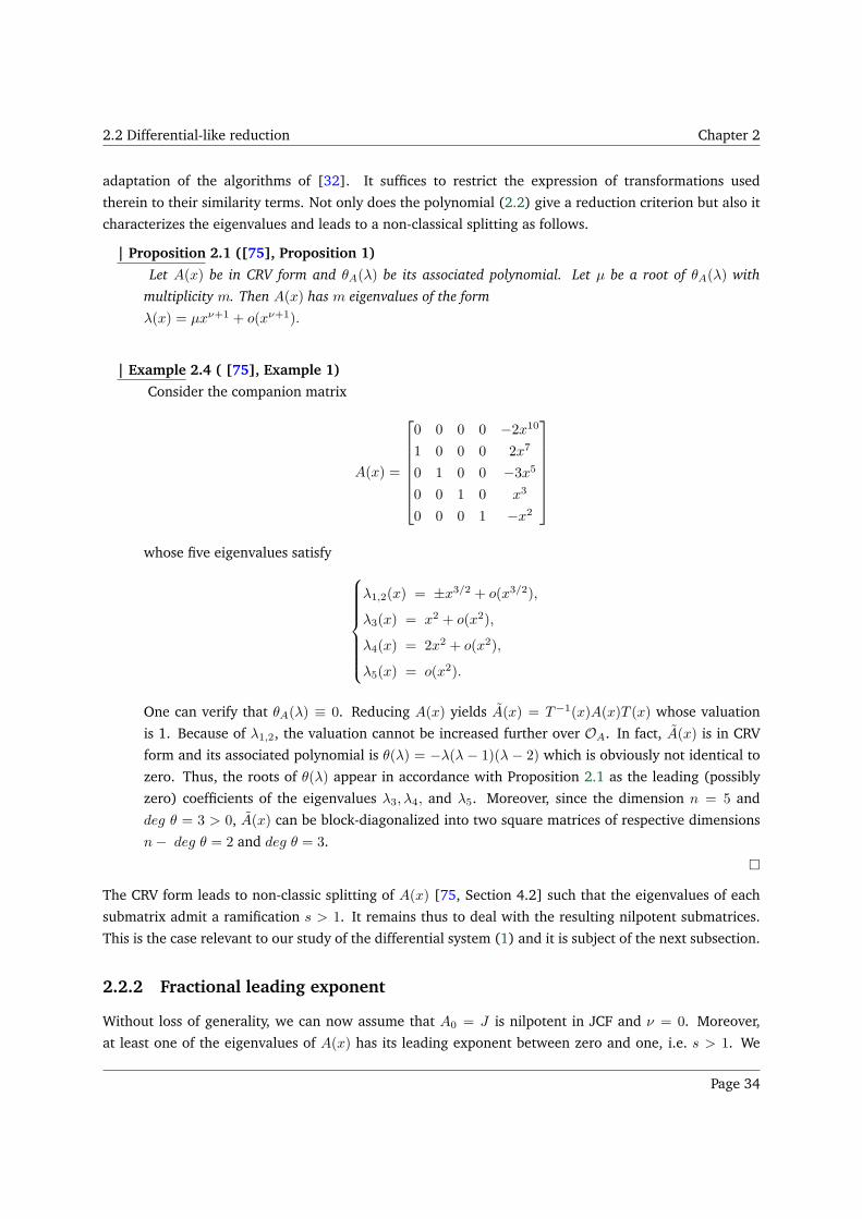
2.2 Differential-like reduction Chapter 2
adaptation of the algorithms of [32]. It suffices to restrict the expression of transformations used
therein to their similarity terms. Not only does the polynomial (2.2) give a reduction criterion but also it
characterizes the eigenvalues and leads to a non-classical splitting as follows.
| Proposition 2.1 ([75], Proposition 1)
Let A(x) be in CRV form and θA(λ) be its associated polynomial. Let µ be a root of θA(λ) with
multiplicity m. Then A(x) has m eigenvalues of the form
λ(x) = µxν+1 + o(xν+1).
| Example 2.4 ( [75], Example 1)
Consider the companion matrix
A(x) =
0 0 0 0 −2x10
1 0 0 0 2x7
0 1 0 0 −3x5
0 0 1 0 x3
0 0 0 1 −x2
whose five eigenvalues satisfy
λ1,2(x) = ±x3/2 + o(x3/2),
λ3(x) = x2 + o(x2),
λ4(x) = 2x2 + o(x2),
λ5(x) = o(x2).
One can verify that θA(λ) ≡ 0. Reducing A(x) yields A(x) = T−1(x)A(x)T (x) whose valuation
is 1. Because of λ1,2, the valuation cannot be increased further over OA. In fact, A(x) is in CRV
form and its associated polynomial is θ(λ) = −λ(λ − 1)(λ − 2) which is obviously not identical to
zero. Thus, the roots of θ(λ) appear in accordance with Proposition 2.1 as the leading (possibly
zero) coefficients of the eigenvalues λ3, λ4, and λ5. Moreover, since the dimension n = 5 and
deg θ = 3 > 0, A(x) can be block-diagonalized into two square matrices of respective dimensions
n− deg θ = 2 and deg θ = 3.
The CRV form leads to non-classic splitting of A(x) [75, Section 4.2] such that the eigenvalues of each
submatrix admit a ramification s > 1. It remains thus to deal with the resulting nilpotent submatrices.
This is the case relevant to our study of the differential system (1) and it is subject of the next subsection.
2.2.2 Fractional leading exponent
Without loss of generality, we can now assume that A0 = J is nilpotent in JCF and ν = 0. Moreover,
at least one of the eigenvalues of A(x) has its leading exponent between zero and one, i.e. s > 1. We
Page 34
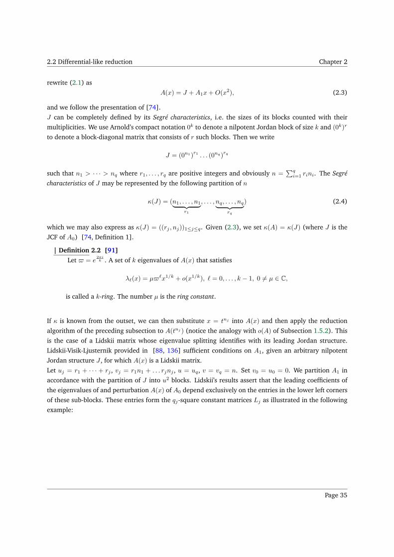
2.2 Differential-like reduction Chapter 2
rewrite (2.1) as
A(x) = J +A1x+O(x2), (2.3)
and we follow the presentation of [74].
J can be completely defined by its Segré characteristics, i.e. the sizes of its blocks counted with their
multiplicities. We use Arnold’s compact notation 0k to denote a nilpotent Jordan block of size k and (0k)r
to denote a block-diagonal matrix that consists of r such blocks. Then we write
J = (0n1)r1 . . . (0nq )
rq
such that n1 > · · · > nq where r1, . . . , rq are positive integers and obviously n =∑q
i=1 rini. The Segré
characteristics of J may be represented by the following partition of n
κ(J) = (n1, . . . , n1︸ ︷︷ ︸
r1
, . . . , nq, . . . , nq︸ ︷︷ ︸
rq
) (2.4)
which we may also express as κ(J) = ((rj , nj))1≤j≤q. Given (2.3), we set κ(A) = κ(J) (where J is the
JCF of A0) [74, Definition 1].
| Definition 2.2 [91]
Let = e2πik . A set of k eigenvalues of A(x) that satisfies
λℓ(x) = µℓx1/k + o(x1/k), ℓ = 0, . . . , k − 1, 0 6= µ ∈ C,
is called a k-ring. The number µ is the ring constant.
If κ is known from the outset, we can then substitute x = tnj into A(x) and then apply the reduction
algorithm of the preceding subsection to A(tnj ) (notice the analogy with o(A) of Subsection 1.5.2). This
is the case of a Lidskii matrix whose eigenvalue splitting identifies with its leading Jordan structure.
Lidskii-Visik-Ljusternik provided in [88, 136] sufficient conditions on A1, given an arbitrary nilpotent
Jordan structure J , for which A(x) is a Lidskii matrix.
Let uj = r1 + · · · + rj , vj = r1n1 + . . . rjnj , u = uq, v = vq = n. Set v0 = u0 = 0. We partition A1 in
accordance with the partition of J into u2 blocks. Lidskii’s results assert that the leading coefficients of
the eigenvalues of and perturbation A(x) of A0 depend exclusively on the entries in the lower left corners
of these sub-blocks. These entries form the qj-square constant matrices Lj as illustrated in the following
example:
Page 35
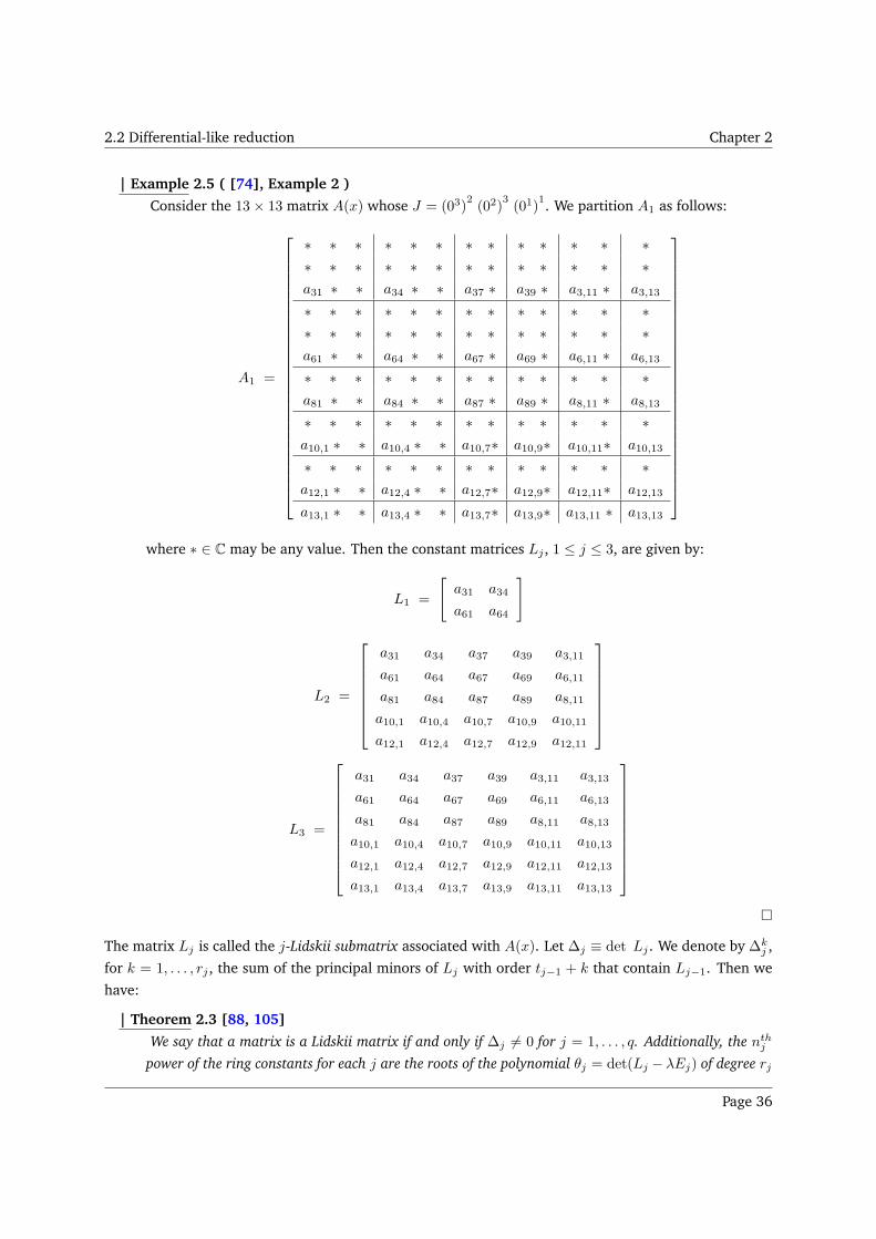
2.2 Differential-like reduction Chapter 2
| Example 2.5 ( [74], Example 2 )
Consider the 13× 13 matrix A(x) whose J = (03)2(02)
3(01)
1. We partition A1 as follows:
A1 =
∗ ∗ ∗ ∗ ∗ ∗ ∗ ∗ ∗ ∗ ∗ ∗ ∗∗ ∗ ∗ ∗ ∗ ∗ ∗ ∗ ∗ ∗ ∗ ∗ ∗a31 ∗ ∗ a34 ∗ ∗ a37 ∗ a39 ∗ a3,11 ∗ a3,13
∗ ∗ ∗ ∗ ∗ ∗ ∗ ∗ ∗ ∗ ∗ ∗ ∗∗ ∗ ∗ ∗ ∗ ∗ ∗ ∗ ∗ ∗ ∗ ∗ ∗a61 ∗ ∗ a64 ∗ ∗ a67 ∗ a69 ∗ a6,11 ∗ a6,13
∗ ∗ ∗ ∗ ∗ ∗ ∗ ∗ ∗ ∗ ∗ ∗ ∗a81 ∗ ∗ a84 ∗ ∗ a87 ∗ a89 ∗ a8,11 ∗ a8,13
∗ ∗ ∗ ∗ ∗ ∗ ∗ ∗ ∗ ∗ ∗ ∗ ∗a10,1 ∗ ∗ a10,4 ∗ ∗ a10,7∗ a10,9∗ a10,11∗ a10,13
∗ ∗ ∗ ∗ ∗ ∗ ∗ ∗ ∗ ∗ ∗ ∗ ∗a12,1 ∗ ∗ a12,4 ∗ ∗ a12,7∗ a12,9∗ a12,11∗ a12,13
a13,1 ∗ ∗ a13,4 ∗ ∗ a13,7∗ a13,9∗ a13,11 ∗ a13,13
where ∗ ∈ C may be any value. Then the constant matrices Lj , 1 ≤ j ≤ 3, are given by:
L1 =
[
a31 a34
a61 a64
]
L2 =
a31 a34 a37 a39 a3,11
a61 a64 a67 a69 a6,11
a81 a84 a87 a89 a8,11
a10,1 a10,4 a10,7 a10,9 a10,11
a12,1 a12,4 a12,7 a12,9 a12,11
L3 =
a31 a34 a37 a39 a3,11 a3,13
a61 a64 a67 a69 a6,11 a6,13
a81 a84 a87 a89 a8,11 a8,13
a10,1 a10,4 a10,7 a10,9 a10,11 a10,13
a12,1 a12,4 a12,7 a12,9 a12,11 a12,13
a13,1 a13,4 a13,7 a13,9 a13,11 a13,13
The matrix Lj is called the j-Lidskii submatrix associated with A(x). Let ∆j ≡ det Lj . We denote by ∆kj ,
for k = 1, . . . , rj , the sum of the principal minors of Lj with order tj−1 + k that contain Lj−1. Then we
have:
| Theorem 2.3 [88, 105]
We say that a matrix is a Lidskii matrix if and only if ∆j 6= 0 for j = 1, . . . , q. Additionally, the nthj
power of the ring constants for each j are the roots of the polynomial θj = det(Lj − λEj) of degree rj
Page 36
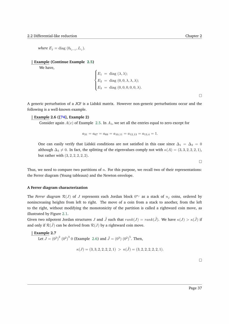
2.2 Differential-like reduction Chapter 2
where Ej = diag (0tj−1, Irj ).
| Example (Continue Example 2.5)
We have,
E1 = diag (λ, λ);
E2 = diag (0, 0, λ, λ, λ);
E3 = diag (0, 0, 0, 0, 0, λ).
A generic perturbation of a JCF is a Lidskii matrix. However non-generic perturbations occur and the
following is a well-known example.
| Example 2.6 ([74], Example 2)
Consider again A(x) of Example 2.5. In A1, we set all the entries equal to zero except for
a31 = a67 = a89 = a10,11 = a12,13 = a13,4 = 1.
One can easily verify that Lidskii conditions are not satisfied in this case since ∆1 = ∆2 = 0
although ∆3 6= 0. In fact, the splitting of the eigenvalues comply not with κ(A) = (3, 3, 2, 2, 2, 1),
but rather with (3, 2, 2, 2, 2, 2).
Thus, we need to compare two partitions of n. For this purpose, we recall two of their representations:
the Ferrer diagram (Young tableaux) and the Newton envelope.
A Ferrer diagram characterization
The Ferrer diagram R(J) of J represents each Jordan block 0nj as a stack of nj coins, ordered by
nonincreasing heights from left to right. The move of a coin from a stack to another, from the left
to the right, without modifying the monotonicity of the partition is called a rightward coin move, as
illustrated by Figure 2.1.
Given two nilpotent Jordan structures J and J such that rank(J) = rank(J). We have κ(J) > κ(J) if
and only if R(J) can be derived from R(J) by a rightward coin move.
| Example 2.7
Let J = (03)2(02)
30 (Example 2.6) and J = (03) (02)
5. Then,
κ(J) = (3, 3, 2, 2, 2, 2, 1) > κ(J) = (3, 2, 2, 2, 2, 2, 1).
Page 37
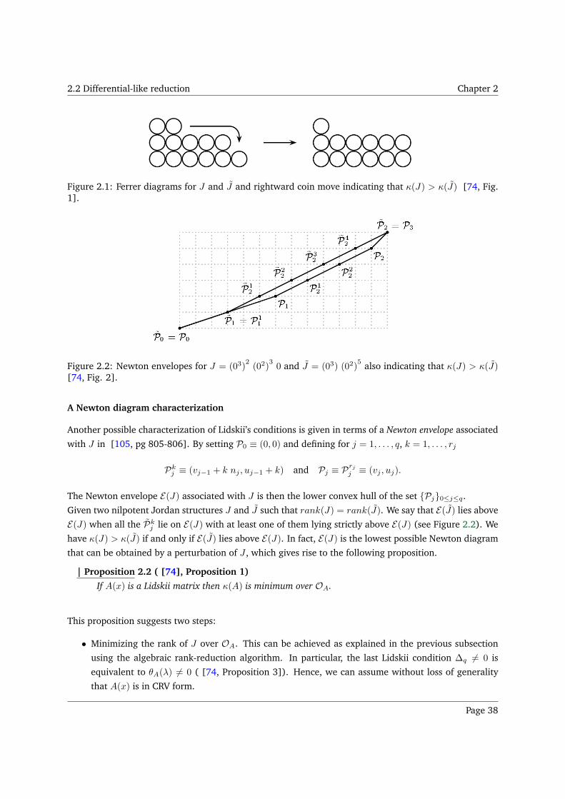
2.2 Differential-like reduction Chapter 2
Figure 2.1: Ferrer diagrams for J and J and rightward coin move indicating that κ(J) > κ(J) [74, Fig.1].
Figure 2.2: Newton envelopes for J = (03)2(02)
30 and J = (03) (02)
5 also indicating that κ(J) > κ(J)[74, Fig. 2].
A Newton diagram characterization
Another possible characterization of Lidskii’s conditions is given in terms of a Newton envelope associated
with J in [105, pg 805-806]. By setting P0 ≡ (0, 0) and defining for j = 1, . . . , q, k = 1, . . . , rj
Pkj ≡ (vj−1 + k nj , uj−1 + k) and Pj ≡ Prj
j ≡ (vj , uj).
The Newton envelope E(J) associated with J is then the lower convex hull of the set Pj0≤j≤q.
Given two nilpotent Jordan structures J and J such that rank(J) = rank(J). We say that E(J) lies above
E(J) when all the Pkj lie on E(J) with at least one of them lying strictly above E(J) (see Figure 2.2). We
have κ(J) > κ(J) if and only if E(J) lies above E(J). In fact, E(J) is the lowest possible Newton diagram
that can be obtained by a perturbation of J , which gives rise to the following proposition.
| Proposition 2.2 ( [74], Proposition 1)
If A(x) is a Lidskii matrix then κ(A) is minimum over OA.
This proposition suggests two steps:
• Minimizing the rank of J over OA. This can be achieved as explained in the previous subsection
using the algebraic rank-reduction algorithm. In particular, the last Lidskii condition ∆q 6= 0 is
equivalent to θA(λ) 6= 0 ( [74, Proposition 3]). Hence, we can assume without loss of generality
that A(x) is in CRV form.
Page 38
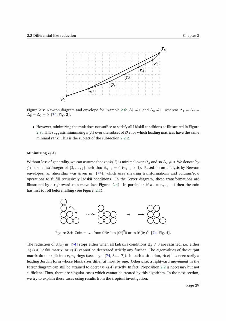
2.2 Differential-like reduction Chapter 2
Figure 2.3: Newton diagram and envelope for Example 2.6: ∆11 6= 0 and ∆3 6= 0, whereas ∆1 = ∆1
2 =∆2
2 = ∆2 = 0 [74, Fig. 3].
• However, minimizing the rank does not suffice to satisfy all Lidskii conditions as illustrated in Figure
2.3. This suggests minimizing κ(A) over the subset of OA for which leading matrices have the same
minimal rank. This is the subject of the subsection 2.2.2.
Minimizing κ(A)
Without loss of generality, we can assume that rank(J) is minimal over OA and so ∆q 6= 0. We denote by
j the smallest integer of 2, . . . , q such that ∆j−1 = 0 (nj−1 > 1). Based on an analysis by Newton
envelopes, an algorithm was given in [74], which uses shearing transformations and column/row
operations to fulfill recursively Lidskii conditions. In the Ferrer diagram, these transformations are
illustrated by a rightward coin move (see Figure 2.4). In particular, if nj = nj−1 − 1 then the coin
has first to roll before falling (see Figure 2.1).
Figure 2.4: Coin move from 04020 to (03)20 or to 03(02)
2 [74, Fig. 4].
The reduction of A(x) in [74] stops either when all Lidskii’s conditions ∆j 6= 0 are satisfied, i.e. either
A(x) a Lidskii matrix, or κ(A) cannot be decreased strictly any further. The eigenvalues of the output
matrix do not split into rj nj-rings (see. e.g. [74, Sec. 7]). In such a situation, A(x) has necessarily a
leading Jordan form whose block sizes differ at most by one. Otherwise, a rightward movement in the
Ferrer diagram can still be attained to decrease κ(A) strictly. In fact, Proposition 2.2 is necessary but not
sufficient. Thus, there are singular cases which cannot be treated by this algorithm. In the next section,
we try to explain these cases using results from the tropical investigation.
Page 39
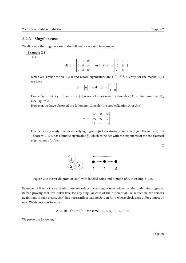
2.2 Differential-like reduction Chapter 2
2.2.3 Singular case
We illustrate the singular case in the following very simple example.
| Example 2.8
Let
A(x) =
0 1 0
0 0 x
x 0 0
and B(x) =
0 1 0
0 0 1
x2 0 0
which are similar for all x 6= 0 and whose eigenvalues are 11/3 x2/3. Clearly, for the matrix A(x)
we have
L1 =[
0]
and L2 =
[
0 1
1 0
]
.
Hence ∆1 = det L1 = 0 and so A1(x) is not a Lidskii matrix although κ(A) is minimum over OA
(see Figure 2.5).
However, we have observed the following: Consider the tropicalization A of A(x),
A =
∞ 0 ∞∞ ∞ 1
1 ∞ ∞
.
One can easily verify that its underlying digraph G(A) is strongly connected (see Figure 2.5). By
Theorem 2.1, A has a unique eigenvalue 23 , which coincides with the exponents of the the classical
eigenvalues of A(x).
Figure 2.5: Ferrer diagram of A(x) with labeled coins and digraph of A in Example 2.8.
Example 2.8 is not a particular case regarding the strong connectedness of the underlying digraph.
Before proving that this holds true for any singular case of the differential-like reduction, we remark
again that, in such a case, A(x) has necessarily a leading Jordan form whose block sizes differ at most by
one. We denote this form by
J = (0n1)r1 (0n2)
r2 for some n1 > n2, r1, r2 ∈ N∗.
We prove the following:
Page 40
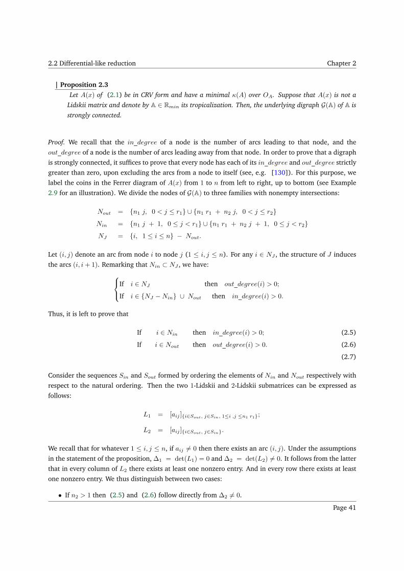
2.2 Differential-like reduction Chapter 2
| Proposition 2.3
Let A(x) of (2.1) be in CRV form and have a minimal κ(A) over OA. Suppose that A(x) is not a
Lidskii matrix and denote by A ∈ Rmin its tropicalization. Then, the underlying digraph G(A) of A is
strongly connected.
Proof. We recall that the in_degree of a node is the number of arcs leading to that node, and the
out_degree of a node is the number of arcs leading away from that node. In order to prove that a digraph
is strongly connected, it suffices to prove that every node has each of its in_degree and out_degree strictly
greater than zero, upon excluding the arcs from a node to itself (see, e.g. [130]). For this purpose, we
label the coins in the Ferrer diagram of A(x) from 1 to n from left to right, up to bottom (see Example
2.9 for an illustration). We divide the nodes of G(A) to three families with nonempty intersections:
Nout = n1 j, 0 < j ≤ r1 ∪ n1 r1 + n2 j, 0 < j ≤ r2Nin = n1 j + 1, 0 ≤ j < r1 ∪ n1 r1 + n2 j + 1, 0 ≤ j < r2NJ = i, 1 ≤ i ≤ n − Nout.
Let (i, j) denote an arc from node i to node j (1 ≤ i, j ≤ n). For any i ∈ NJ , the structure of J induces
the arcs (i, i+ 1). Remarking that Nin ⊂ NJ , we have:
If i ∈ NJ then out_degree(i) > 0;
If i ∈ NJ −Nin ∪ Nout then in_degree(i) > 0.
Thus, it is left to prove that
If i ∈ Nin then in_degree(i) > 0; (2.5)
If i ∈ Nout then out_degree(i) > 0. (2.6)
(2.7)
Consider the sequences Sin and Sout formed by ordering the elements of Nin and Nout respectively with
respect to the natural ordering. Then the two 1-Lidskii and 2-Lidskii submatrices can be expressed as
follows:
L1 = [aij ]i∈Sout, j∈Sin, 1≤i ,j ≤n1 r1;
L2 = [aij ]i∈Sout, j∈Sin.
We recall that for whatever 1 ≤ i, j ≤ n, if aij 6= 0 then there exists an arc (i, j). Under the assumptions
in the statement of the proposition, ∆1 = det(L1) = 0 and ∆2 = det(L2) 6= 0. It follows from the latter
that in every column of L2 there exists at least one nonzero entry. And in every row there exists at least
one nonzero entry. We thus distinguish between two cases:
• If n2 > 1 then (2.5) and (2.6) follow directly from ∆2 6= 0.
Page 41
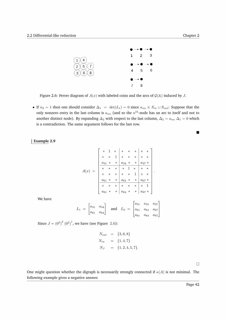
2.2 Differential-like reduction Chapter 2
Figure 2.6: Ferrer diagram of A(x) with labeled coins and the arcs of G(A) induced by J .
• If n2 = 1 then one should consider ∆1 = det(L1) = 0 since ann ∈ Sin ∪ Sout: Suppose that the
only nonzero entry in the last column is ann (and so the nth-node has an arc to itself and not to
another distinct node). By expanding ∆2 with respect to the last column, ∆2 = ann ∆1 = 0 which
is a contradiction. The same argument follows for the last row.
| Example 2.9
A(x) =
∗ 1 ∗ ∗ ∗ ∗ ∗ ∗∗ ∗ 1 ∗ ∗ ∗ ∗ ∗a31 ∗ ∗ a34 ∗ ∗ a37 ∗∗ ∗ ∗ ∗ 1 ∗ ∗ ∗∗ ∗ ∗ ∗ ∗ 1 ∗ ∗a61 ∗ ∗ a64 ∗ ∗ a67 ∗∗ ∗ ∗ ∗ ∗ ∗ ∗ 1
a81 ∗ ∗ a84 ∗ ∗ a87 ∗
.
We have
L1 =
[
a31 a34
a61 a64
]
and L2 =
a31 a34 a37
a61 a64 a67
a81 a84 a87
Since J = (03)2(02)
1, we have (see Figure 2.6):
Nout = 3, 6, 8Nin = 1, 4, 7NJ = 1, 2, 4, 5, 7.
One might question whether the digraph is necessarily strongly connected if κ(A) is not minimal. The
following example gives a negative answer.
Page 42
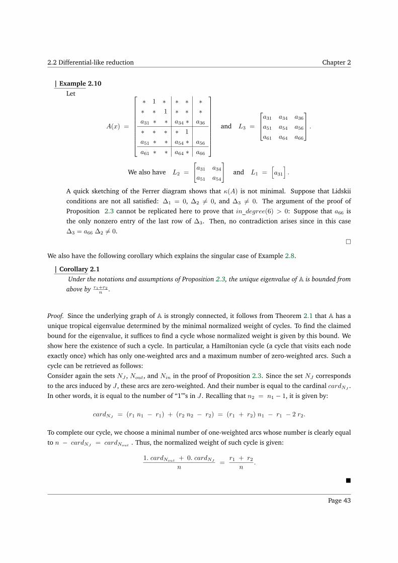
2.2 Differential-like reduction Chapter 2
| Example 2.10
Let
A(x) =
∗ 1 ∗ ∗ ∗ ∗∗ ∗ 1 ∗ ∗ ∗a31 ∗ ∗ a34 ∗ a36
∗ ∗ ∗ ∗ 1
a51 ∗ ∗ a54 ∗ a56
a61 ∗ ∗ a64 ∗ a66
and L3 =
a31 a34 a36
a51 a54 a56
a61 a64 a66
.
We also have L2 =
[
a31 a34
a51 a54
]
and L1 =[
a31
]
.
A quick sketching of the Ferrer diagram shows that κ(A) is not minimal. Suppose that Lidskii
conditions are not all satisfied: ∆1 = 0, ∆2 6= 0, and ∆3 6= 0. The argument of the proof of
Proposition 2.3 cannot be replicated here to prove that in_degree(6) > 0: Suppose that a66 is
the only nonzero entry of the last row of ∆3. Then, no contradiction arises since in this case
∆3 = a66 ∆2 6= 0.
We also have the following corollary which explains the singular case of Example 2.8.
| Corollary 2.1
Under the notations and assumptions of Proposition 2.3, the unique eigenvalue of A is bounded from
above by r1+r2n .
Proof. Since the underlying graph of A is strongly connected, it follows from Theorem 2.1 that A has a
unique tropical eigenvalue determined by the minimal normalized weight of cycles. To find the claimed
bound for the eigenvalue, it suffices to find a cycle whose normalized weight is given by this bound. We
show here the existence of such a cycle. In particular, a Hamiltonian cycle (a cycle that visits each node
exactly once) which has only one-weighted arcs and a maximum number of zero-weighted arcs. Such a
cycle can be retrieved as follows:
Consider again the sets NJ , Nout, and Nin in the proof of Proposition 2.3. Since the set NJ corresponds
to the arcs induced by J , these arcs are zero-weighted. And their number is equal to the cardinal cardNJ.
In other words, it is equal to the number of “1”’s in J . Recalling that n2 = n1 − 1, it is given by:
cardNJ= (r1 n1 − r1) + (r2 n2 − r2) = (r1 + r2) n1 − r1 − 2 r2.
To complete our cycle, we choose a minimal number of one-weighted arcs whose number is clearly equal
to n − cardNJ= cardNout
. Thus, the normalized weight of such cycle is given:
1. cardNout+ 0. cardNJ
n=
r1 + r2n
.
Page 43
2.3 Conclusion Chapter 2
In the case the bound is attained, the eigenvalues of A(x) split generically into a r1+r2n -ring by
Theorem 2.2. This gives an explanation to the exponent 23 of Example 2.8.
2.3 Conclusion
In this chapter, we discussed the interaction between the perturbation theory of JCF, the differential-like
reduction, and tropical algebra. We implemented some of the algorithms described in this chapter in the
package ALGPARAM in Maple. We conclude with various open questions regarding this interaction, the
most prevalent among which are: Do the two approaches presented here superpose so that one can cover
the singular case of the other? And what kind of interpretation does this hold for a linear differential
system‡? For example, can the genericity required in Theorem 2.2 be guaranteed for an irreducible linear
singular differential system?
‡Miyake introduced in [104] a reduction based on computing a volevic weight (due to L.R.Volevic) of the differential system (1).Roughly speaking, this weight is the minimum of normalized sums of the valuations of the system’s matrix A(x). It thus seemsplausible to attempt to interpret this weight in terms of an underlying graph of the tropicalization of A(x). Additionally, it is alsointeresting to study the relation between this weight and notion of irreducibility of the system described in Section (1.5.1)
Page 44
Chapter 3
Chapter 3
Removing Apparent Singularities
Contents3.1 Detecting and removing apparent singularities . . . . . . . . . . . . . . . . . . . . . . 47
3.2 Application to desingularization of scalar differential equations . . . . . . . . . . . . 53
3.3 Rational version of the algorithm . . . . . . . . . . . . . . . . . . . . . . . . . . . . . . 55
3.3.1 The residue matrix at p . . . . . . . . . . . . . . . . . . . . . . . . . . . . . . . . . 56
3.3.2 Computing the integer eigenvalues of the residue matrix . . . . . . . . . . . . . . . 58
3.3.3 Applications . . . . . . . . . . . . . . . . . . . . . . . . . . . . . . . . . . . . . . . 58
3.4 Conclusion . . . . . . . . . . . . . . . . . . . . . . . . . . . . . . . . . . . . . . . . . . 60
In this chapter we present a new algorithm which, given a system of first-order linear differential system
with rational function coefficients, constructs an equivalent system with rational function coefficients,
whose finite singularities are exactly the non-apparent singularities of the original system. This chapter is
an elaboration [27] and refinement of the algorithm which was first introduced in [19]. We thus consider
the following system
[A] ∂F = A(x)F
where A ∈ Mn(C(x))∗. The finite singularities of system [A] are the poles of A(x) in C. A singular
point x0 ∈ C is called an apparent singularity if there exists a fundamental matrix solution Φ(x) which is
analytic at x = x0. Consider, for example, the first-order differential system
∂F = A(x) F =
[
0 1−2x 1 + 2
x
]
F (3.1)
Clearly, this system is equivalent to the second-order scalar differential equation given by the monic
∗We remark that in this chapter we are interested in a global aspect and so we are considering A ∈ Mn(C(x)) rather thanA ∈ Mn(C[[x]]). Obviously, the absence of xp in the left hand side does not imply that the system is regular because the entries ofA(x) are rational functions.
Page 45
Chapter 3
operator L:
L := ∂2 − x+ 2
x∂ +
2
x,
for which ex and 1 + x + x2
2 form a basis of solutions. Due to this basis, one can deduce that the point
x = 0 is an apparent singularity of system (6.12). Desingularization, i.e. the problem of constructing
another operator L(f) of higher order such that the solution space of L(f) = 0 contains that of L(f) = 0,
and for which the factor x is “removed” from the denominator, is an interesting problem of research. For
instance, by the method given by Abramov-Barkatou-van Hoeij in [3] (and which we refer to as the ABH
method), one can compute a desingularization of order 4 given by the operator
L = ∂4 + (−1 + 1/4x) ∂3 + (−1/4− 3/8x) ∂2
+(1/2 + 1/8x) ∂ − 1/4.
In the scalar case, several desingularization algorithms exist for differential, difference (e.g., [3]),
and more generally, Ore operators (see, e.g. [45, 44] and references therein). However, the apparent
singularity of system (6.12) (equivalently of L) at x = 0, can be also removed by acting directly on it. In
fact, by setting [19]
F = T (x) G, T (x) =
[
1 0
1 x2
]
,
the new variable G satisfies the equivalent first-order differential system of the same size as the order of
L, given by
[A] ∂G = A G
where
A := T−1AT − T−1∂T =
[
1 x2
0 0
]
.
As in Chapter 1, we say that systems [A] and T [A] = [A] are equivalent over C(x).
In this chapter, we shall prove that, given any system [A] with rational coefficients, it can be reduced to
an equivalent system [A] with rational coefficients, such that the finite singularities of [A] coincide with
the non-apparent singularities of [A]. Our method can, in particular, be applied to the companion system
of any scalar linear differential equation with arbitrary order n. We thus have an alternative method to
the standard methods for removing apparent singularities of linear differential operators. However, it is
also interesting by its own since first-order linear differential systems with apparent singularities arise
naturally in applications (see, e.g., [77, 83, 37] and references therein for applications within Feynman
integrals and statistical physics). Moreover, such a desingularization can be very beneficial to numerical
methods.
We recall (see Section 1.5.1) that a singular point x0 ∈ C is called a regular singular point for the system
[A] if in a neighborhood of x0, there exists a fundamental matrix solution of the form Φ(x)(x−x0)C where
C ∈ Mn(C) is a constant matrix and Φ(x) is a matrix which is analytic at x0; otherwise x0 is called an
irregular singular point. The change of variable x 7→ 1/x permits to classify the point x = ∞ as an
ordinary, a regular singular, or an irregular singular point of the system [A].
Page 46
3.1 Detecting and removing apparent singularities Chapter 3
Hence apparent singularities of [A] are among regular singularities of [A]. And, as shown in
Section 1.5.1, it is proven that in the case where x0 is a regular singularity there exists a polynomial
matrix function T of x − x0 which is nonsingular for x 6= x0 such that the transformation F = TG
transforms the system [A] into an equivalent system [A] ∂G = A(x)G, for which x0 is a simple pole.
This latter system can be constructed using the so called Rational Moser algorithm developed in [15].
This algorithm, establishes partial desingularization, as it computes for a given system [A] a polynomial
transformation T (x) with det(T (x)) 6≡ 0 that leads to a system [A] such that:
(i) The finite singularities of [A] are among the finite singularities of [A].
(ii) Every finite singular point of [A] has a minimal pole order among all equivalent systems.
This chapter is organized as follows: In Section 3.1, we give our main result: We show how apparent
singularities can be detected, prove the existence of desingularizations, and develop a desingularization
algorithm over C(x). In Section 3.2, we show some examples of treating scalar linear differential
equations. In Section 3.3, we give a rational version of our algorithm. And finally, we point out items for
further investigation in Section 3.4.
3.1 Detecting and removing apparent singularities
Consider a system [A] ∂F = A(x)F with A(x) ∈Mn(C(x)).
| Definition 3.1
A system [A] ∂G = A(x) G is called a desingularization of [A] if:
(i) There exists a polynomial matrix T (x) with det(T (x)) 6≡ 0 such that [A] = T [A];
(ii) The singularities of [A] are the singularities of [A] that are not apparent.
We first prove that desingularizations do exist:
| Proposition 3.1
If x = x0 is a finite apparent singularity of [A] then there exists a polynomial matrix T (x) with
det T (x) = c(x− x0)α, c ∈ C∗, α ∈ N
such that [A] := T [A] has no pole at x = x0.
Proof. Every fundamental matrix of formal solutions Φ(x) of [A] is analytic at x0. Formally, Φ(x) ∈Mn(C[[x]]). Since C[[x]] is a principal ideal domain, one can construct unimodular transformations
P (x) ∈ GLn(C[x]), and Q(x) ∈ GLn(C[[x]]) such that (see, e.g.[107, Lemma 1] or Smith normal form)
P (x)Φ(x)Q(x) = diag((x− x0)α1 , . . . , (x− x0)
αn)
Page 47
3.1 Detecting and removing apparent singularities Chapter 3
where α1, . . . αn are nonnegative integers. We then set
T (x) = P−1(x) diag((x− x0)α1 , . . . , (x− x0)
αn).
This proof however is not constructive. In the sequel we shall develop an algorithm that produces a
desingularization of any system [A] over C(x). We start by explaining how to remove one apparent
singularity.
| Proposition 3.2
If x = x0 is a finite apparent singularity of [A] then one can construct a polynomial matrix T (x) with
det(T (x)) = c(x− x0)α, c ∈ C∗ and α ∈ N such that T [A] has at worst a simple pole at x = x0.
Proof. We have:
(i) An apparent singularity is a regular singularity, hence [A] can be reduced to an equivalent system
T [A] which has x0 as a singularity of first kind.
(ii) The transformation T can be constructed by the algorithm in [15] and hence it has the required
property (see [15, Theorem 2]).
| Proposition 3.3
Suppose that A(x) has simple pole at x = x0 and let
A(x) =A0
(x− x0)+∑
i≥1
Ai(x− x0)i−1, Ai ∈Mn(C).
If x0 is an apparent singularity then the eigenvalues of the so-called residue matrix A0, are nonnegative
integers.
Proof. Suppose that A0 possesses at least one eigenvalue which does not belong to N and let µ be an
eigenvalue of A0 such that µ ∈ C \ N with a maximal real part. Then the system [A] has a nonzero local
vectorial solution of the form:
F (x) = (x− x0)µ
+∞∑
k=0
Fk(x− x0)k
with Fk ∈ Cn and F0 6= 0, the series being convergent in a disc centered at x0 (see, e.g. [11, Chapter 2,
Theorem 6, pp 32]). Such a solution however is not analytic at x = x0 because µ /∈ N. This implies that
x0 is a singularity which is not apparent.
Page 48
3.1 Detecting and removing apparent singularities Chapter 3
| Proposition 3.4
Suppose that x = x0 is a simple pole of A(x) and that A0 has only nonnegative integer eigenvalues.
Then there exists a polynomial matrix T (x) with det(T (x)) = c(x− x0)α for some c ∈ C∗ and α ∈ N
such that [A] ∂G = A(x) G has at most a simple pole at x = x0 and A0 has a single eigenvalue:
A0 = mIn +N where m ∈ N and N is nilpotent. Moreover, x0 is an apparent singularity iff N = O.
In this case, the transformation G = (x − x0)mW leads to a system for which x = x0 is an ordinary
point.
Proof. Let m1, . . . ,ms ∈ N be the eigenvalues of A0. For i = 1, . . . , s, denote by νi the multiplicity of mi.
Suppose that m1 > m2 > . . . > ms and put ℓi = mi−mi+1 ∈ N∗, i = 1, . . . , s−1. By applying a constant
transformation we can assume that A0 is in Jordan form:
A0 =
A11
0 0
0 A220
, (3.2)
where A110 is an ν1 by ν1 matrix having one single eigenvalue m1:
A110 = m1Iν1
+N1,
N1 being a nilpotent matrix. The transformation F = PZ, where
P = diag((x− x0)Iν1 , In−ν1) (3.3)
yields the new system:
∂Z = B(x)Z,
where
B(x) = P−1A(x)P − P−1∂P.
Its residue matrix is given by:
B0 =(A0 + (x− x0)P
−1A1P − (x− x0)P−1∂P
)
|x=x0.
Let A1 be partitioned as A0 :
A1 =
A11
1 A121
A211 A22
1
, A111 ∈Mν1
(C)
Then
B0 =
A11
0 − Iν1 A121
0 A220
. (3.4)
Hence the eigenvalues of B0 are: m1 − 1,m2, . . . ,ms, each with the same initial multiplicities.
Page 49
3.1 Detecting and removing apparent singularities Chapter 3
By repeating this process ℓ1 times where m1 − ℓ1 = m2, the eigenvalues become:
m2,m2, . . . ,ms,
with the respective multiplicities ν1, ν2 . . . , νs. Thus, after ℓ1+ . . .+ ℓs−1 = m1−ms steps, let T (x) be the
product of all the transformations applied, then one gets an equivalent system [A] := T [A] ∂G = AG
of the first kind with a residue matrix A0 with a single eigenvalue ms of multiplicity ν1 + . . . + νs = n.
Hence the matrix N := A0−msIn is nilpotent. Moreover the matrix T is the product of matrices that are
either constant or of the form (3.3). Hence T is a polynomial matrix of degree at most m1 −ms and its
determinant is of the form det(T (x)) = c(x− x0)α for some c ∈ C∗ and α ∈ N.
Due to the form of A0 it follows that the system [A] has, in the neighborhood of x0, a fundamental matrix
solution of the form
G(x) = (x− x0)msΦ(x)(x− x0)
N
where
Φ(x) = In +
+∞∑
k=1
Φk(x− x0)k analytic at x = x0.
Hence x0 is an apparent singularity of [A] if and only if N is the zero matrix. Finally, if we put G =
(x − x0)msW the resulting system has the above matrix Φ(x) as a fundamental matrix solution around
x = x0. As Φ(x0) = In, the point x0 is an ordinary point for the latter system.
| Remark 3.1
One can deduce from the above proof that a necessary (but not sufficient) condition for a first-kind
singularity x0 to be an apparent singularity for [A] is that the residue matrix A0 be diagonalizable with
nonnegative integer eigenvalues. Indeed, if A0 is not diagonalizable then in (3.2) at least one of the
two blocks A110 , A22
0 has a nonzero nilpotent part. It follows from the form of (3.4) that transformation
(3.3) cannot annihilate the nilpotent part of the residue matrix. Thus if the residue matrix A0 of the
input system (or one of the intermediate systems) is not diagonalizable then the output system [A] has
a residue matrix A0 = mIn +N with N 6= O.
We thus proved the following theorem:
| Theorem 3.1
If x = x0 is a finite apparent singularity of [A] then one can construct a polynomial matrix T (x) with
det(T (x)) = c(x− x0)α, c ∈ C∗ and α ∈ N such that A(x) := T [A] has no pole at x = x0.
Due to the form of its determinant, the gauge transformation T (x) in the previous theorem does not affect
the other finite singularities of [A]. This means that the apparent singularity at x0 is removed without
introducing new finite singularities or changing the pole order of the other finite singularities of [A], as
illustrated by the following simple example.
Page 50
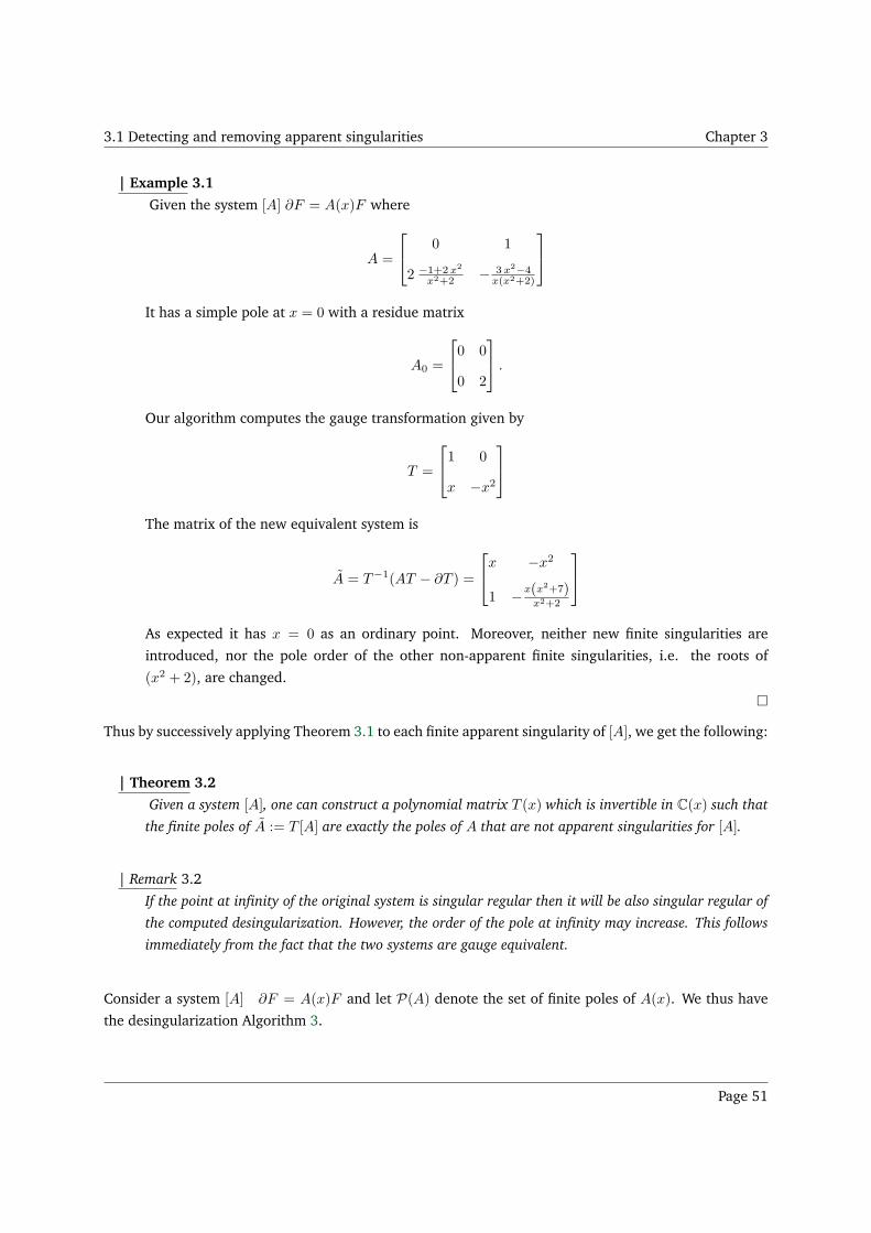
3.1 Detecting and removing apparent singularities Chapter 3
| Example 3.1
Given the system [A] ∂F = A(x)F where
A =
0 1
2 −1+2 x2
x2+2 − 3 x2−4x(x2+2)
It has a simple pole at x = 0 with a residue matrix
A0 =
0 0
0 2
.
Our algorithm computes the gauge transformation given by
T =
1 0
x −x2
The matrix of the new equivalent system is
A = T−1(AT − ∂T ) =
x −x2
1 −x(x2+7)x2+2
As expected it has x = 0 as an ordinary point. Moreover, neither new finite singularities are
introduced, nor the pole order of the other non-apparent finite singularities, i.e. the roots of
(x2 + 2), are changed.
Thus by successively applying Theorem 3.1 to each finite apparent singularity of [A], we get the following:
| Theorem 3.2
Given a system [A], one can construct a polynomial matrix T (x) which is invertible in C(x) such that
the finite poles of A := T [A] are exactly the poles of A that are not apparent singularities for [A].
| Remark 3.2
If the point at infinity of the original system is singular regular then it will be also singular regular of
the computed desingularization. However, the order of the pole at infinity may increase. This follows
immediately from the fact that the two systems are gauge equivalent.
Consider a system [A] ∂F = A(x)F and let P(A) denote the set of finite poles of A(x). We thus have
the desingularization Algorithm 3.
Page 51
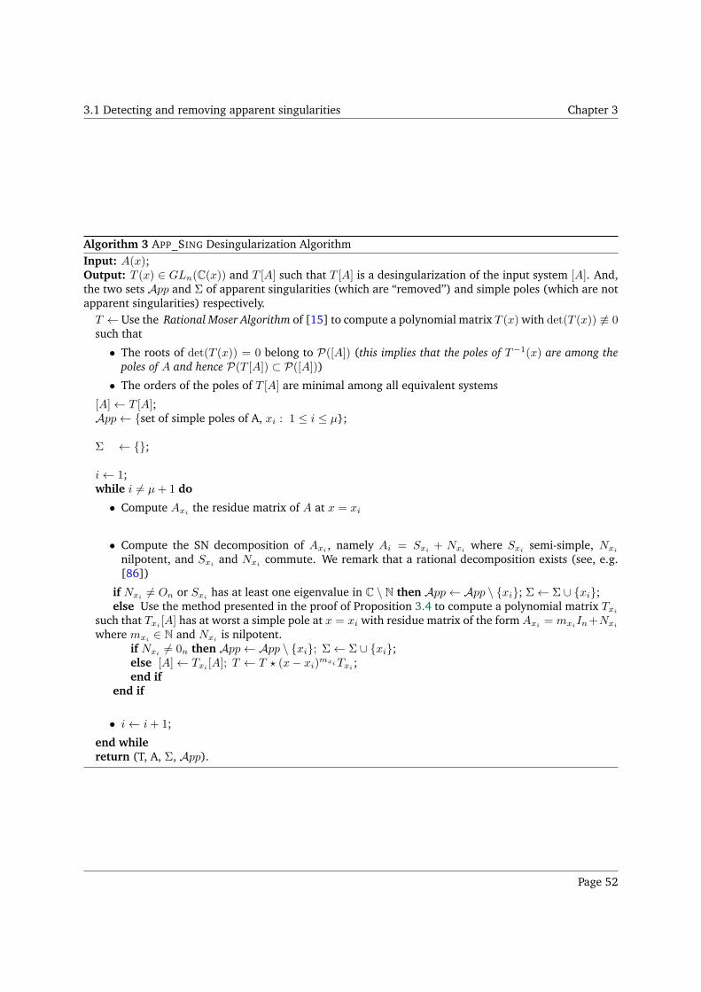
3.1 Detecting and removing apparent singularities Chapter 3
Algorithm 3 APP_SING Desingularization AlgorithmInput: A(x);Output: T (x) ∈ GLn(C(x)) and T [A] such that T [A] is a desingularization of the input system [A]. And,the two sets App and Σ of apparent singularities (which are “removed”) and simple poles (which are notapparent singularities) respectively.T ← Use the Rational Moser Algorithm of [15] to compute a polynomial matrix T (x) with det(T (x)) 6≡ 0such that
• The roots of det(T (x)) = 0 belong to P([A]) (this implies that the poles of T−1(x) are among thepoles of A and hence P(T [A]) ⊂ P([A]))
• The orders of the poles of T [A] are minimal among all equivalent systems
[A]← T [A];App← set of simple poles of A, xi : 1 ≤ i ≤ µ;
Σ ← ;
i← 1;while i 6= µ+ 1 do
• Compute Axithe residue matrix of A at x = xi
• Compute the SN decomposition of Axi, namely Ai = Sxi
+ Nxiwhere Sxi
semi-simple, Nxi
nilpotent, and Sxi and Nxi commute. We remark that a rational decomposition exists (see, e.g.[86])
if Nxi6= On or Sxi
has at least one eigenvalue in C \ N then App← App \ xi; Σ← Σ ∪ xi;else Use the method presented in the proof of Proposition 3.4 to compute a polynomial matrix Txi
such that Txi[A] has at worst a simple pole at x = xi with residue matrix of the form Axi
= mxiIn+Nxi
where mxi ∈ N and Nxi is nilpotent.if Nxi 6= 0n then App← App \ xi; Σ← Σ ∪ xi;else [A]← Txi
[A]; T ← T ⋆ (x− xi)mxiTxi
;end if
end if
• i← i+ 1;
end whilereturn (T, A, Σ, App).
Page 52
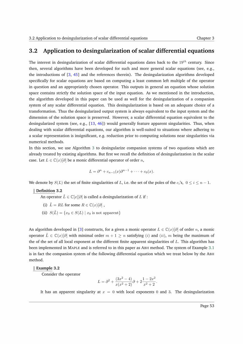
3.2 Application to desingularization of scalar differential equations Chapter 3
3.2 Application to desingularization of scalar differential equations
The interest in desingularization of scalar differential equations dates back to the 19th century. Since
then, several algorithms have been developed for such and more general scalar equations (see, e.g.,
the introductions of [3, 45] and the references therein). The desingularization algorithms developed
specifically for scalar equations are based on computing a least common left multiple of the operator
in question and an appropriately chosen operator. This outputs in general an equation whose solution
space contains strictly the solution space of the input equation. As we mentioned in the introduction,
the algorithm developed in this paper can be used as well for the desingularization of a companion
system of any scalar differential equation. This desingularization is based on an adequate choice of a
transformation. Thus the desingularized output system is always equivalent to the input system and the
dimension of the solution space is preserved. However, a scalar differential equation equivalent to the
desingularized system (see, e.g., [13, 46]) would generally feature apparent singularities. Thus, when
dealing with scalar differential equations, our algorithm is well-suited to situations where adhering to
a scalar representation is insignificant, e.g. reduction prior to computing solutions near singularities via
numerical methods.
In this section, we use Algorithm 3 to desingularize companion systems of two equations which are
already treated by existing algorithms. But first we recall the definition of desingularization in the scalar
case. Let L ∈ C(x)[∂] be a monic differential operator of order n,
L = ∂n + cn−1(x)∂n−1 + · · ·+ c0(x).
We denote by S(L) the set of finite singularities of L, i.e. the set of the poles of the ci’s, 0 ≤ i ≤ n− 1.
| Definition 3.2
An operator L ∈ C[x][∂] is called a desingularization of L if :
(i) L = RL for some R ∈ C(x)[∂] ,
(ii) S(L) = x0 ∈ S(L) | x0 is not apparent
An algorithm developed in [3] constructs, for a given a monic operator L ∈ C(x)[∂] of order n, a monic
operator L ∈ C(x)[∂] with minimal order m + 1 ≥ n satisfying (i) and (ii), m being the maximum of
the of the set of all local exponent at the different finite apparent singularities of L. This algorithm has
been implemented in MAPLE and is referred to in this paper as ABH method. The system of Example 3.1
is in fact the companion system of the following differential equation which we treat below by the ABH
method.
| Example 3.2
Consider the operator
L = ∂2 +(3x2 − 4)
x(x2 + 2)∂ + 2
1− 2x2
x2 + 2.
It has an apparent singularity at x = 0 with local exponents 0 and 3. The desingularization
Page 53
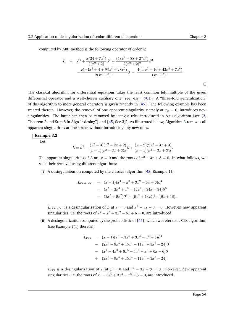
3.2 Application to desingularization of scalar differential equations Chapter 3
computed by ABH method is the following operator of order 4:
L = ∂4 +x(24 + 7x2)
2(x2 + 2)∂3 +
(58x2 + 88 + 27x4)
2(x2 + 2)2∂2
−x(−4x2 + 4 + 93x4 + 28x6)
2(x2 + 2)3∂ − 4(44x2 + 16 + 42x4 + 7x6)
(x2 + 2)3
The classical algorithm for differential equations takes the least common left multiple of the given
differential operator and a well-chosen auxiliary one (see, e.g., [70]). A “three-fold generalization”
of this algorithm to more general operators is given recently in [45]. The following example has been
treated therein. However, the removal of one apparent singularity, namely at x0 = 0, introduces new
singularities. The latter can then be removed by using a trick introduced in ABH algorithm (see [3,
Theorem 2 and Step 6 in Algo “t-desing”] and [45, Sec 3]). As illustrated below, Algorithm 3 removes all
apparent singularities at one stroke without introducing any new ones.
| Example 3.3
Let
L = ∂2 − (x2 − 3)(x2 − 2x+ 2)
(x− 1)(x2 − 3x+ 3)x∂ +
(x− 2)(2x2 − 3x+ 3)
(x− 1)(x2 − 3x+ 3)x.
The apparent singularities of L are x = 0 and the roots of x2 − 3x + 3 = 0. In what follows, we
seek their removal using different algorithms:
(i) A desingularization computed by the classical algorithm [45, Example 1]:
LCLASSICAL = (x− 1)(x4 − x3 + 3x2 − 6x+ 6)∂4
− (x5 − 2x4 + x3 − 12x2 + 24x− 24)∂3
− (3x3 + 9x2)∂2 + (6x2 + 18x)∂ − (6x+ 18).
LCLASSICAL is a desingularization of L at x = 0 and x2 − 3x + 3 = 0. However, new apparent
singularities, i.e. the roots of x4 − x3 + 3x2 − 6x+ 6 = 0, are introduced.
(ii) A desingularization computed by the probabilistic of [45], which we refer to as CKS algorithm,
(see Example 7(1) therein):
LCKS = (x− 1)(x6 − 3x5 + 3x4 − x3 + 6)∂4
− (2x6 − 9x5 + 15x4 − 11x3 + 3x2 − 24)∂3
− (x7 − 4x6 + 6x5 − 4x4 + x3 + 6x− 6)∂
+ (2x6 − 9x5 + 15x4 − 11x3 + 3x2 − 24).
LCKS is a desingularization of L at x = 0 and x2 − 3x + 3 = 0. However, new apparent
singularities, i.e. the roots of x6 − 3x5 + 3x4 − x3 + 6 = 0, are introduced.
Page 54
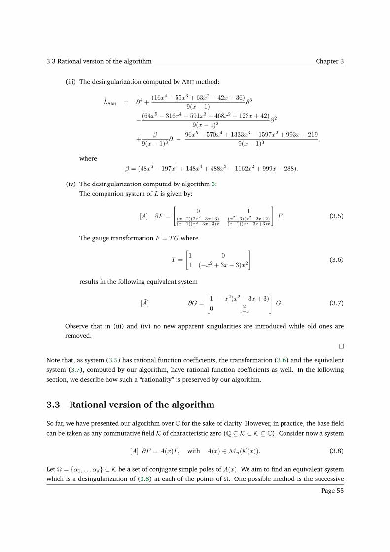
3.3 Rational version of the algorithm Chapter 3
(iii) The desingularization computed by ABH method:
LABH = ∂4 +(16x4 − 55x3 + 63x2 − 42x+ 36)
9(x− 1)∂3
− (64x5 − 316x4 + 591x3 − 468x2 + 123x+ 42)
9(x− 1)2∂2
+β
9(x− 1)3∂ − 96x5 − 570x4 + 1333x3 − 1597x2 + 993x− 219
9(x− 1)3,
where
β = (48x6 − 197x5 + 148x4 + 488x3 − 1162x2 + 999x− 288).
(iv) The desingularization computed by algorithm 3:
The companion system of L is given by:
[A] ∂F =
[
0 1(x−2)(2x2−3x+3)(x−1)(x2−3x+3)x
(x2−3)(x2−2x+2)(x−1)(x2−3x+3)x
]
F. (3.5)
The gauge transformation F = TG where
T =
[
1 0
1 (−x2 + 3x− 3)x2
]
(3.6)
results in the following equivalent system
[A] ∂G =
[
1 −x2(x2 − 3x+ 3)
0 21−x
]
G. (3.7)
Observe that in (iii) and (iv) no new apparent singularities are introduced while old ones are
removed.
Note that, as system (3.5) has rational function coefficients, the transformation (3.6) and the equivalent
system (3.7), computed by our algorithm, have rational function coefficients as well. In the following
section, we describe how such a “rationality” is preserved by our algorithm.
3.3 Rational version of the algorithm
So far, we have presented our algorithm over C for the sake of clarity. However, in practice, the base field
can be taken as any commutative field K of characteristic zero (Q ⊆ K ⊂ K ⊆ C). Consider now a system
[A] ∂F = A(x)F, with A(x) ∈Mn(K(x)). (3.8)
Let Ω = α1, . . . αd ⊂ K be a set of conjugate simple poles of A(x). We aim to find an equivalent system
which is a desingularization of (3.8) at each of the points of Ω. One possible method is the successive
Page 55
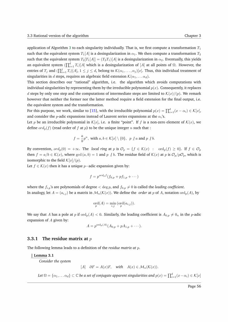
3.3 Rational version of the algorithm Chapter 3
application of Algorithm 3 to each singularity individually. That is, we first compute a transformation T1
such that the equivalent system T1[A] is a desingularization in α1. We then compute a transformation T2
such that the equivalent system T2[T1[A]] = (T2T1)[A] is a desingularization in α2. Eventually, this yields
an equivalent system (∏d
i=1 Ti)[A] which is a desingularization of [A] at all points of Ω. However, the
entries of Tj and (∏j
i=1 Ti)[A], 1 ≤ j ≤ d, belong to K(α1, . . . , αj)[x]. Thus, this individual treatment of
singularities in d steps, requires an algebraic field extension K(α1, . . . αd).
This section describes our “rational” algorithm, i.e. the algorithm which avoids computations with
individual singularities by representing them by the irreducible polynomial p(x). Consequently, it replaces
d steps by only one step and the computations of intermediate steps are limited to K(x)/(p). We remark
however that neither the former nor the latter method require a field extension for the final output, i.e.
the equivalent system and the transformation.
For this purpose, we work, similar to [15], with the irreducible polynomial p(x) =∏d
i=1(x− αi) ∈ K[x],and consider the p-adic expansions instead of Laurent series expansions at the αi’s.
Let p be an irreducible polynomial in K[x], i.e. a finite “point”. If f is a non-zero element of K(x), we
define ordp(f) (read order of f at p) to be the unique integer n such that :
f =a
bpn, with a, b ∈ K[x] \ 0, p 6 | a and p 6 | b.
By convention, ordp(0) = +∞. The local ring at p is Op = f ∈ K(x) : ordp(f) ≥ 0. If f ∈ Op
then f = a/b ∈ K(x), where gcd (a, b) = 1 and p 6 | b. The residue field of K(x) at p is Op/pOp, which is
isomorphic to the field K[x]/(p).Let f ∈ K(x) then it has a unique p−adic expansion given by:
f = pordpf (f0,p + pf1,p + · · · )
where the fi,p’s are polynomials of degree < deg p, and f0,p 6= 0 is called the leading coefficient.
In analogy, let A = (ai,j) be a matrix inMn(K(x)). We define the order at p of A, notation ordp(A), by
ordp(A) = min
i,j(ord
p(ai,j)).
We say that A has a pole at p if ordp(A) < 0. Similarly, the leading coefficient is A0,p 6= 0n in the p-adic
expansion of A given by:
A = pordp(A)(A0,p + pA1,p + · · · ).
3.3.1 The residue matrix at p
The following lemma leads to a definition of the residue matrix at p.
| Lemma 3.1
Consider the system
[A] ∂F = A(x)F, with A(x) ∈Mn(K(x)).
Let Ω = α1, . . . αd ⊂ C be a set of conjugate apparent singularities and p(x) =∏d
i=1(x−αi) ∈ K[x]
Page 56
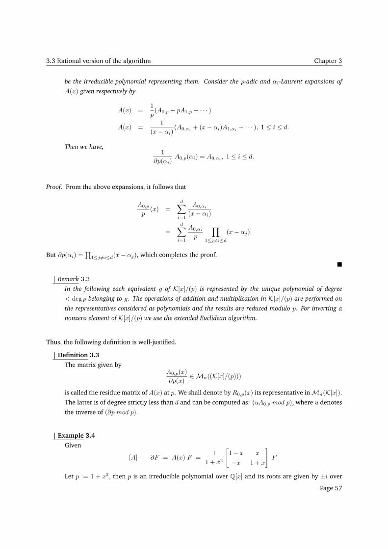
3.3 Rational version of the algorithm Chapter 3
be the irreducible polynomial representing them. Consider the p-adic and αi-Laurent expansions of
A(x) given respectively by
A(x) =1
p(A0,p + pA1,p + · · · )
A(x) =1
(x− αi)(A0,αi
+ (x− αi)A1,αi+ · · · ), 1 ≤ i ≤ d.
Then we have,1
∂p(αi)A0,p(αi) = A0,αi , 1 ≤ i ≤ d.
Proof. From the above expansions, it follows that
A0,p
p(x) =
d∑
i=1
A0,αi
(x− αi)
=
d∑
i=1
A0,αi
p
∏
1≤j 6=i≤d
(x− αj).
But ∂p(αi) =∏
1≤j 6=i≤d(x− αj), which completes the proof.
| Remark 3.3
In the following each equivalent g of K[x]/(p) is represented by the unique polynomial of degree
< deg p belonging to g. The operations of addition and multiplication in K[x]/(p) are performed on
the representatives considered as polynomials and the results are reduced modulo p. For inverting a
nonzero element of K[x]/(p) we use the extended Euclidean algorithm.
Thus, the following definition is well-justified.
| Definition 3.3
The matrix given byA0,p(x)
∂p(x)∈Mn((K[x]/(p)))
is called the residue matrix of A(x) at p. We shall denote by R0,p(x) its representative inMn(K[x]).The latter is of degree strictly less than d and can be computed as: (uA0,p mod p), where u denotes
the inverse of (∂p mod p).
| Example 3.4
Given
[A] ∂F = A(x) F =1
1 + x2
[
1− x x
−x 1 + x
]
F.
Let p := 1 + x2, then p is an irreducible polynomial over Q[x] and its roots are given by ±i over
Page 57
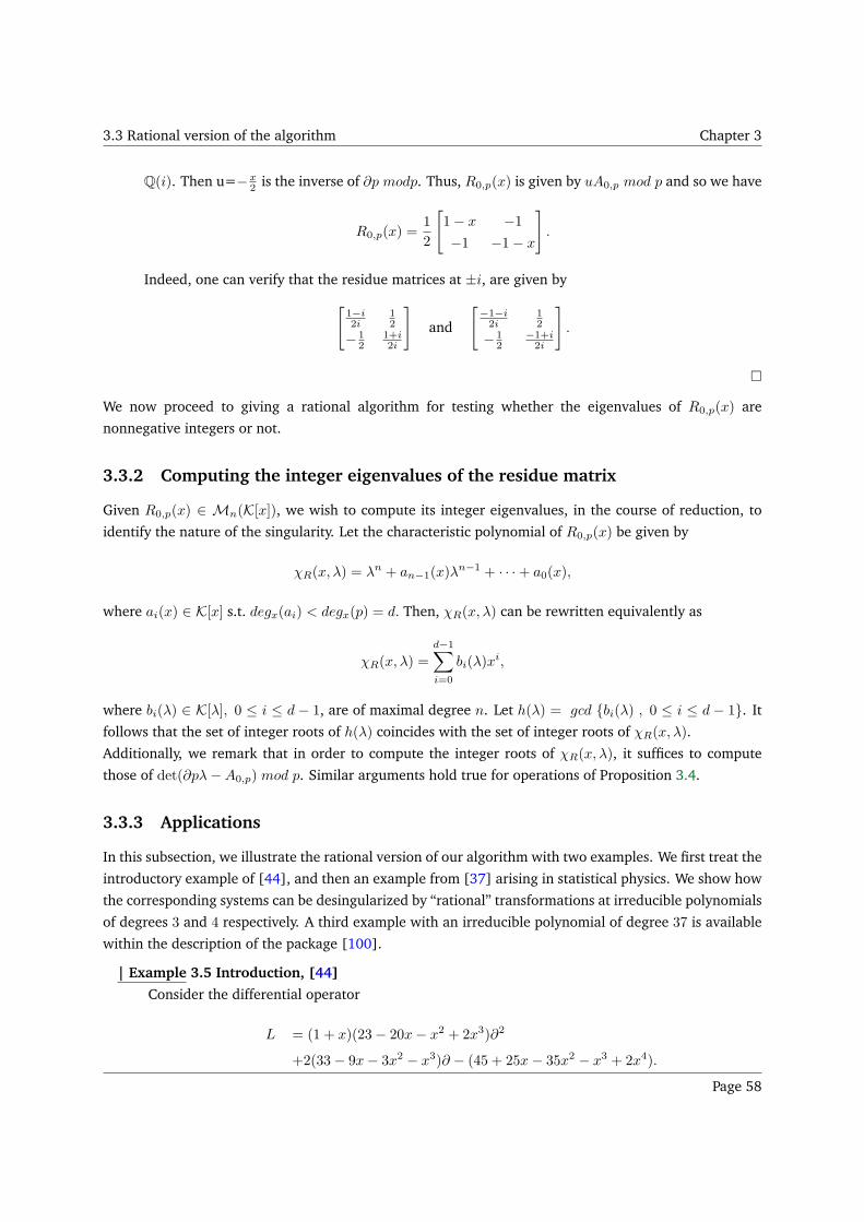
3.3 Rational version of the algorithm Chapter 3
Q(i). Then u=−x2 is the inverse of ∂p modp. Thus, R0,p(x) is given by uA0,p mod p and so we have
R0,p(x) =1
2
[
1− x −1−1 −1− x
]
.
Indeed, one can verify that the residue matrices at ±i, are given by
[1−i2i
12
− 12
1+i2i
]
and
[−1−i2i
12
− 12
−1+i2i
]
.
We now proceed to giving a rational algorithm for testing whether the eigenvalues of R0,p(x) are
nonnegative integers or not.
3.3.2 Computing the integer eigenvalues of the residue matrix
Given R0,p(x) ∈ Mn(K[x]), we wish to compute its integer eigenvalues, in the course of reduction, to
identify the nature of the singularity. Let the characteristic polynomial of R0,p(x) be given by
χR(x, λ) = λn + an−1(x)λn−1 + · · ·+ a0(x),
where ai(x) ∈ K[x] s.t. degx(ai) < degx(p) = d. Then, χR(x, λ) can be rewritten equivalently as
χR(x, λ) =d−1∑
i=0
bi(λ)xi,
where bi(λ) ∈ K[λ], 0 ≤ i ≤ d − 1, are of maximal degree n. Let h(λ) = gcd bi(λ) , 0 ≤ i ≤ d − 1. It
follows that the set of integer roots of h(λ) coincides with the set of integer roots of χR(x, λ).
Additionally, we remark that in order to compute the integer roots of χR(x, λ), it suffices to compute
those of det(∂pλ−A0,p) mod p. Similar arguments hold true for operations of Proposition 3.4.
3.3.3 Applications
In this subsection, we illustrate the rational version of our algorithm with two examples. We first treat the
introductory example of [44], and then an example from [37] arising in statistical physics. We show how
the corresponding systems can be desingularized by “rational” transformations at irreducible polynomials
of degrees 3 and 4 respectively. A third example with an irreducible polynomial of degree 37 is available
within the description of the package [100].
| Example 3.5 Introduction, [44]
Consider the differential operator
L = (1 + x)(23− 20x− x2 + 2x3)∂2
+2(33− 9x− 3x2 − x3)∂ − (45 + 25x− 35x2 − x3 + 2x4).
Page 58
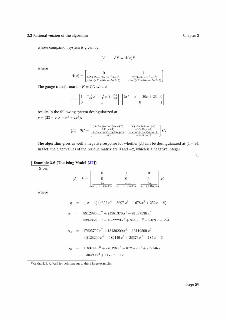
3.3 Rational version of the algorithm Chapter 3
whose companion system is given by:
[A] ∂F = A(x)F
where
A(x) =
[
0 1(45+25x−35x2−x3+2x4)(1+x)(23−20x−x2+2x3) − 2(33−9x−3x2−x3)
(1+x)(23−20x−x2+2x3)
]
.
The gauge transformation F = TG where
T =
[
1 −14143 x
2 + 311x+ 153
143
0 1
] [
2x3 − x2 − 20x+ 23 0
0 1
]
,
results in the following system desingularized at
p = (23− 20x− x2 + 2x3):
[A] ∂G =
[14x3−39x2−258x−175
143(x+1)98x2−497x−1385
−20449(x+1)2x4−x3−35x2+25x+45
x+114x3−39x2−258x+111
−143(x+1)
]
G.
The algorithm gives as well a negative response for whether [A] can be desingularized at (1 + x).
In fact, the eigenvalues of the residue matrix are 0 and −2, which is a negative integer.
| Example 3.6 (The Ising Model [37])
Given†
[A] F =
0 1 0
0 0 1−4α1
x2(−1+16x)3q−4α2
x2(−1+16x)2q−2α3
x(−1+16x)q
F,
where
q = (4x− 1)(4352x4 + 3607x3 − 1678x2 + 252x− 8
)
α1 = 89128960x7 + 74981376x6 − 97687536x5
33948640x4 − 4652220x3 + 84480x2 + 9469x− 294
α2 = 17825792x7 + 13139200x6 − 16119599x5
+5128290x4 − 689440x3 + 28373x2 − 185x− 6
α3 = 1183744x6 + 770128x5 − 872579x4 + 252146x3
−30499x2 + 1172x− 12.
†We thank J.-A. Weil for pointing out to these large examples.
Page 59
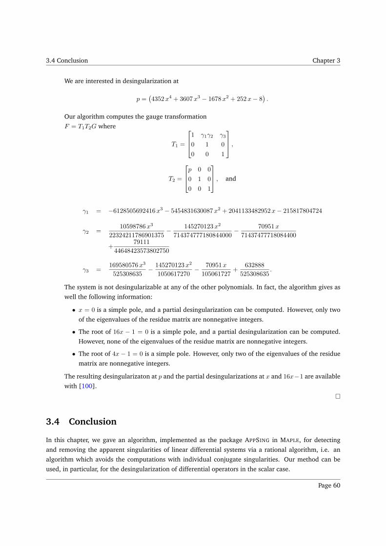
3.4 Conclusion Chapter 3
We are interested in desingularization at
p =(4352x4 + 3607x3 − 1678x2 + 252x− 8
).
Our algorithm computes the gauge transformation
F = T1T2G where
T1 =
1 γ1γ2 γ3
0 1 0
0 0 1
,
T2 =
p 0 0
0 1 0
0 0 1
, and
γ1 = −6128505692416x3 − 5454831630087x2 + 2041133482952x− 215817804724
γ2 =10598786x3
22324211786901375− 145270123x2
714374777180844000− 70951x
71437477718084400
+79111
44648423573802750
γ3 =169580576x3
525308635− 145270123x2
1050617270− 70951x
105061727+
632888
525308635.
The system is not desingularizable at any of the other polynomials. In fact, the algorithm gives as
well the following information:
• x = 0 is a simple pole, and a partial desingularization can be computed. However, only two
of the eigenvalues of the residue matrix are nonnegative integers.
• The root of 16x − 1 = 0 is a simple pole, and a partial desingularization can be computed.
However, none of the eigenvalues of the residue matrix are nonnegative integers.
• The root of 4x − 1 = 0 is a simple pole. However, only two of the eigenvalues of the residue
matrix are nonnegative integers.
The resulting desingularizaton at p and the partial desingularizations at x and 16x−1 are available
with [100].
3.4 Conclusion
In this chapter, we gave an algorithm, implemented as the package APPSING in MAPLE, for detecting
and removing the apparent singularities of linear differential systems via a rational algorithm, i.e. an
algorithm which avoids the computations with individual conjugate singularities. Our method can be
used, in particular, for the desingularization of differential operators in the scalar case.
Page 60
3.4 Conclusion Chapter 3
One field of investigation is the generalization of our algorithm to treat more general systems, e.g.
systems with parameters as well as investigating the case of difference systems. First steps in this
direction, namely reductions in the parameter and the partial desingularization, are established in [21]
and Part II respectively.
Another major field of investigation is the complexity study of the various algorithms existing for the
scalar case and comparing their efficiency, as well as studying the complexity of this new algorithm.
Partial results in this direction are already obtained in [32].
Page 61

Part II
Singularly-Perturbed Linear
Differential Systems
Page 63
Introduction to Part II
Introduction
A distinctive feature of the singularly-perturbed equations is that their solution and/or
the solution derivatives have intrinsic narrow zones (boundary and interior layers) of large
variations in which they jump from one stable state to another or to prescribed boundary values.
Such situation occurs in many physical, chemical, biological, and sociological phenomena. In
physics, for example, this happens in viscous gas flows in the zones near the boundary layers
where the viscous flow jumps from the boundary values prescribed by the condition of adhesion
to the inviscid flow or in the zones near the shock wave where the flow jumps from a subsonic
to supersonic state. In chemical reactions the rapid transition from one state to another is
typical for solution processes. In biology such sharp changes occur in population genetics.
Typical examples of rapid transitions in sociology give revolutions and corresponding changes
of political institutions‡.
In this part, we are interested in the symbolic resolution of the first-order singularly-perturbed linear
differential system given by
[Aε] εh ∂ F = A(x, ε)F, (3.9)
where ∂ = ddx , h is an integer, and A(x, ε) is an n × n matrix, in the variable x and parameter ε, in a
region of the (x, ε)-space defined by the inequalities
[D] |x| ≤ α0 , 0 < |ε| ≤ ε0, |arg ε| ≤ θ0 , (3.10)
where α0, ε0, θ0 are positive constants. We assume that A(x, ε) have an asymptotic expansion
A(x, ε) ∼∞∑
k=0
Ak(x)εk
which is valid in the given region as ε tends to zero. The Ak(x)’s are assumed to be holomorphic for
|x| ≤ α0 and we write
A0(x) = A00 + A10 x + A20 x2 + . . . .
In the case of a regular perturbation, i.e. h ≤ 0, a solution of system [Aε] can be sought by presenting
‡V. D. Liseikin, Layer resolving grids and transformations for singular perturbation problems, VSP, 2001, quoted from the preface
Page 64
Introduction to Part II
it as a power series in ε. The latter can then be inserted into (3.9) and the like powers of ε equated. This
reduces the problem of constructing solutions of [Aε] to solving recursively a set of (in)homogeneous
unperturbed singular linear differential systems over C((x)), the first of which is system [A] given by (1)
in Chapter 1 (see Section 5.2). However, singular perturbations cause major complications for their part.
As we have seen in Chapter 1, the classical formal simplification of system [A] given by (1) begins
with the reduction of its leading matrix coefficient A0 to its Jordan form. Hence, in addition to the usual
difficulties encountered within the formal reduction itself, additional ones arise for system [Aε] since its
leading matrix coefficient A0(x) is a matrix-valued function rather than a constant one. In particular,
if it has multiple eigenvalues then they might coalesce (see Section 5.4). In classical textbooks, points
where the Jordan form of A0(x) is unstable, that is to say either the multiplicity of the eigenvalues or the
degrees of the elementary divisors are not constant in a neighborhood of such points, are referred to as
turning points§. As illustrated by the following example, the behavior of solutions of the perturbed system
[Aε] around such points is far more complicated than that of system [A] around an irregular singularity.
The difficulties are exhibited by the division of the domain |x| ≤ α0 into subdomains in each of which the
solutions, which have yet to be constructed, behave quite differently [73].
| Example 3.7 ( [110], Introduction, Subsection 1.5 )
Consider the decisively simple-looking differential equation
ε2 ∂2f2 − (x3 − ε)f = 0
over the (x, ε)-region D : |x| ≤ α0 , 0 < |ε| ≤ ε0. Setting
F =
[
f
ε∂f
]
,
this equation can be rewritten as the following first-order system:
ε ∂F = A(x, ε) F =
[
0 1
x3 − ε 0
]
F. (3.11)
One can observe that the Jordan form of A0(x) is not stable in any neighborhood around x = 0.
Thereby, x = 0 might be a turning point for (3.11) and our aim is to compute a solution in a full
neighborhood of x = 0 as the parameter tends to zero.
§The definition of such points is subject to debate in literature and is refined in Definition 5.3.
Page 65
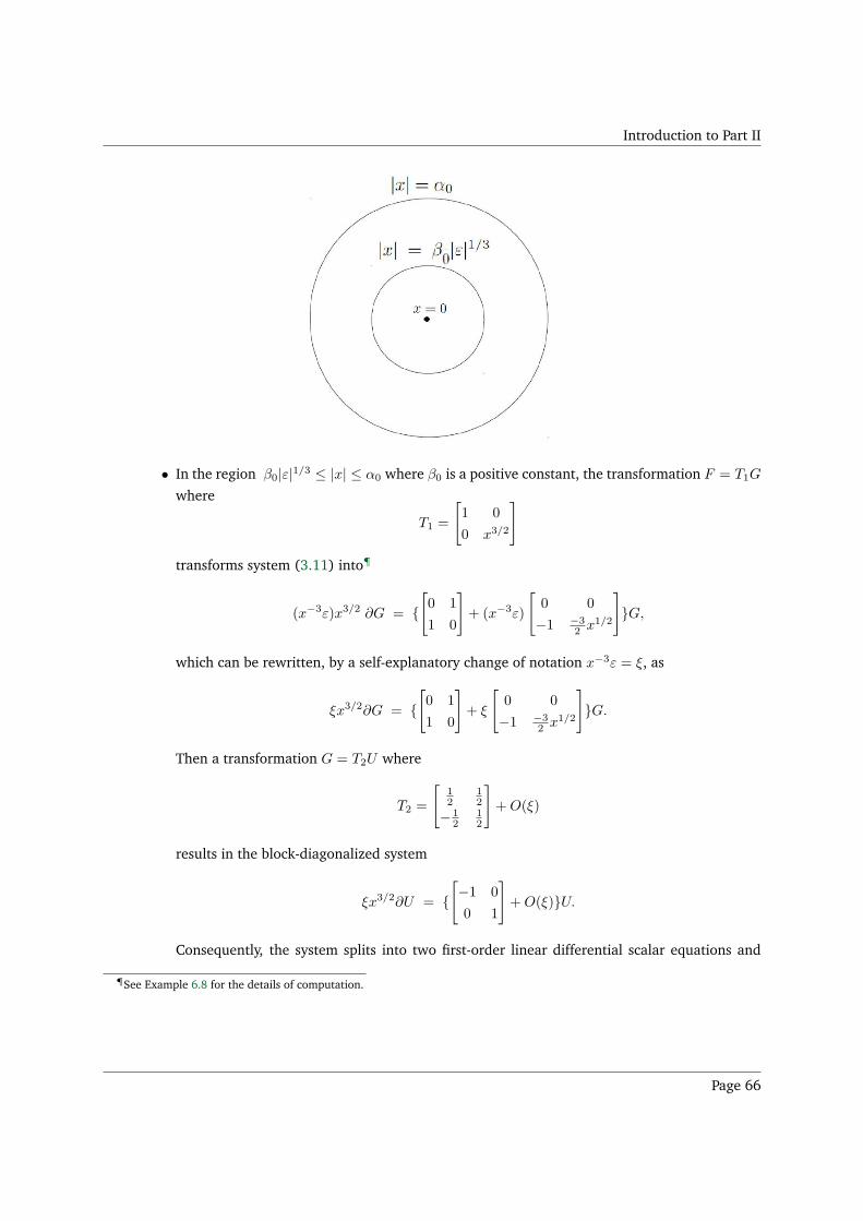
Introduction to Part II
• In the region β0|ε|1/3 ≤ |x| ≤ α0 where β0 is a positive constant, the transformation F = T1G
where
T1 =
[
1 0
0 x3/2
]
transforms system (3.11) into¶
(x−3ε)x3/2 ∂G = [
0 1
1 0
]
+ (x−3ε)
[
0 0
−1 −32 x1/2
]
G,
which can be rewritten, by a self-explanatory change of notation x−3ε = ξ, as
ξx3/2∂G = [
0 1
1 0
]
+ ξ
[
0 0
−1 −32 x1/2
]
G.
Then a transformation G = T2U where
T2 =
[12
12
− 12
12
]
+O(ξ)
results in the block-diagonalized system
ξx3/2∂U = [
−1 0
0 1
]
+O(ξ)U.
Consequently, the system splits into two first-order linear differential scalar equations and
¶See Example 6.8 for the details of computation.
Page 66
Introduction to Part II
giving rise to the following fundamental matrix of formal solution for (3.11) in this region
Fouter = T1 T2 exp(
[
− 25x
5/2ε−1 +O(x−1/2) 0
0 25x
5/2ε−1 +O(x−1/2)
]
).
• In the region |x| ≤ β0|ε|1/3, we shall perform a so-called stretching transformation. Namely,
we set τ = xǫ−1/3 and ∂τ = ddτ . Then, for all τ such as |τ | < ∞, except possibly for
neighborhoods of the roots of τ3 − 1 = 0‖, the transformation F = L1 G where
L1 =
[
1 0
0 ε1/2
]
reduces the system (3.11) to
ε1/6∂τ G =
[
0 1
τ3 − 1 0
]
G.
And the transformation G = L2 U where
L2 =
12 + 1
8 τ3 +O(τ6) 1
2 + 18 τ
3 +O(τ6)
− i2 + i
8τ3 +O(τ6) i
2 − i8τ
3 +O(τ6)
,
reduces the above system to
ε1/6∂τU = [
−i+ i2τ
3 +O(τ6) 0
0 i− i2τ
3 +O(τ6)
]
+O(ε1/6)U,
which has the following fundamental matrix of formal solution in this region:
Finner = L1 L2 exp(
[−iτ+(i/8)τ4+O(τ7)ε1/6
0
0 iτ−(i/8)τ4+O(τ7)ε1/6
]
).
We call Fouter (resp. Finner) an outer (resp. inner) solution as it is obtained in the outer (resp.
inner) region around x = 0. For less particular systems, intermediate regions might arise as well.
The formal reduction is to take place over a bivariate rather than univariate field. An immediate
consequence is the obligation to choose at each step whether to prioritize x or ε, depending on the
setting. The treatment of the singularity in x, might complicate dramatically the singularity in ε, and
vice-versa, if not handled carefully.
The methods proposed in the literature for the symbolic resolution of system [Aε] either exclude turning
points (see [43] and references therein), treat systems of dimension two, impose restrictions on the
‖The turning points other than τ = 0 do not explicitly correspond to the original turning point. They are referred to assecondary turning points [110].
Page 67
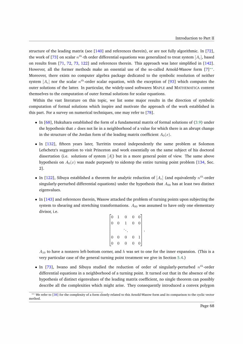
Introduction to Part II
structure of the leading matrix (see [140] and references therein), or are not fully algorithmic. In [72],
the work of [73] on scalar nth-th order differential equations was generalized to treat system [Aε], based
on results from [71, 72, 73, 122] and references therein. This approach was later simplified in [142].
However, all the former methods make an essential use of the so-called Arnold-Wasow form [7]∗∗.
Moreover, there exists no computer algebra package dedicated to the symbolic resolution of neither
system [Aε] nor the scalar nth-order scalar equation, with the exception of [93] which computes the
outer solutions of the latter. In particular, the widely-used softwares MAPLE and MATHEMATICA content
themselves to the computation of outer formal solutions for scalar equations.
Within the vast literature on this topic, we list some major results in the direction of symbolic
computation of formal solutions which inspire and motivate the approach of the work established in
this part. For a survey on numerical techniques, one may refer to [78].
• In [68], Hukuhara established the form of a fundamental matrix of formal solutions of (3.9) under
the hypothesis that x does not lie in a neighborhood of a value for which there is an abrupt change
in the structure of the Jordan form of the leading matrix coefficient A0(x).
• In [132], fifteen years later, Turrittin treated independently the same problem at Solomon
Lefschetz‘s suggestion to visit Princeton and work essentially on the same subject of his doctoral
dissertation (i.e. solutions of system [A]) but in a more general point of view. The same above
hypothesis on A0(x) was made purposely to sidestep the entire turning point problem [134, Sec.
2].
• In [122], Sibuya established a theorem for analytic reduction of [Aε] (and equivalently nth-order
singularly-perturbed differential equations) under the hypothesis that A00 has at least two distinct
eigenvalues.
• In [143] and references therein, Wasow attacked the problem of turning points upon subjecting the
system to shearing and stretching transformations. A00 was assumed to have only one elementary
divisor, i.e.
0 1 0 0 0
0 0 1 0 0
. . .
0 0 0 0 1
0 0 0 0 0
,
A10 to have a nonzero left-bottom corner, and h was set to one for the inner expansion. (This is a
very particular case of the general turning point treatment we give in Section 5.4.)
• In [73], Iwano and Sibuya studied the reduction of order of singularly-perturbed nth-order
differential equations in a neighborhood of a turning point. It turned out that in the absence of the
hypothesis of distinct eigenvalues of the leading matrix coefficient, no single theorem can possibly
describe all the complexities which might arise. They consequently introduced a convex polygon
∗∗ We refer to [38] for the complexity of a form closely-related to this Arnold-Wasow form and its comparison to the cyclic vectormethod.
Page 68
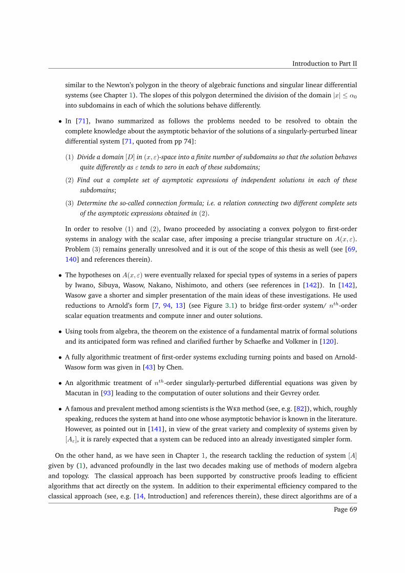
Introduction to Part II
similar to the Newton’s polygon in the theory of algebraic functions and singular linear differential
systems (see Chapter 1). The slopes of this polygon determined the division of the domain |x| ≤ α0
into subdomains in each of which the solutions behave differently.
• In [71], Iwano summarized as follows the problems needed to be resolved to obtain the
complete knowledge about the asymptotic behavior of the solutions of a singularly-perturbed linear
differential system [71, quoted from pp 74]:
(1) Divide a domain [D] in (x, ε)-space into a finite number of subdomains so that the solution behaves
quite differently as ε tends to zero in each of these subdomains;
(2) Find out a complete set of asymptotic expressions of independent solutions in each of these
subdomains;
(3) Determine the so-called connection formula; i.e. a relation connecting two different complete sets
of the asymptotic expressions obtained in (2).
In order to resolve (1) and (2), Iwano proceeded by associating a convex polygon to first-order
systems in analogy with the scalar case, after imposing a precise triangular structure on A(x, ε).
Problem (3) remains generally unresolved and it is out of the scope of this thesis as well (see [69,
140] and references therein).
• The hypotheses on A(x, ε) were eventually relaxed for special types of systems in a series of papers
by Iwano, Sibuya, Wasow, Nakano, Nishimoto, and others (see references in [142]). In [142],
Wasow gave a shorter and simpler presentation of the main ideas of these investigations. He used
reductions to Arnold’s form [7, 94, 13] (see Figure 3.1) to bridge first-order system/ nth-order
scalar equation treatments and compute inner and outer solutions.
• Using tools from algebra, the theorem on the existence of a fundamental matrix of formal solutions
and its anticipated form was refined and clarified further by Schaefke and Volkmer in [120].
• A fully algorithmic treatment of first-order systems excluding turning points and based on Arnold-
Wasow form was given in [43] by Chen.
• An algorithmic treatment of nth-order singularly-perturbed differential equations was given by
Macutan in [93] leading to the computation of outer solutions and their Gevrey order.
• A famous and prevalent method among scientists is the WKB method (see, e.g. [82]), which, roughly
speaking, reduces the system at hand into one whose asymptotic behavior is known in the literature.
However, as pointed out in [141], in view of the great variety and complexity of systems given by
[Aε], it is rarely expected that a system can be reduced into an already investigated simpler form.
On the other hand, as we have seen in Chapter 1, the research tackling the reduction of system [A]
given by (1), advanced profoundly in the last two decades making use of methods of modern algebra
and topology. The classical approach has been supported by constructive proofs leading to efficient
algorithms that act directly on the system. In addition to their experimental efficiency compared to the
classical approach (see, e.g. [14, Introduction] and references therein), these direct algorithms are of a
Page 69
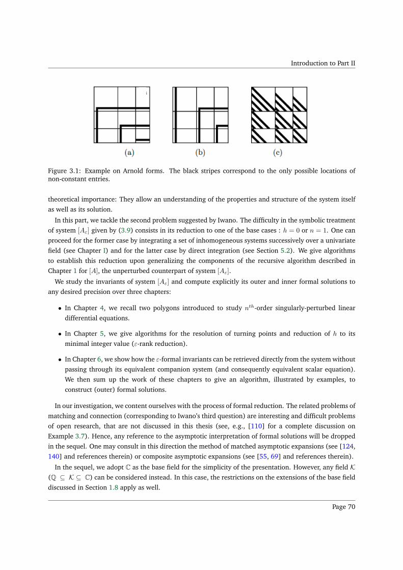
Introduction to Part II
Figure 3.1: Example on Arnold forms. The black stripes correspond to the only possible locations ofnon-constant entries.
theoretical importance: They allow an understanding of the properties and structure of the system itself
as well as its solution.
In this part, we tackle the second problem suggested by Iwano. The difficulty in the symbolic treatment
of system [Aε] given by (3.9) consists in its reduction to one of the base cases : h = 0 or n = 1. One can
proceed for the former case by integrating a set of inhomogeneous systems successively over a univariate
field (see Chapter I) and for the latter case by direct integration (see Section 5.2). We give algorithms
to establish this reduction upon generalizing the components of the recursive algorithm described in
Chapter 1 for [A], the unperturbed counterpart of system [Aε].
We study the invariants of system [Aε] and compute explicitly its outer and inner formal solutions to
any desired precision over three chapters:
• In Chapter 4, we recall two polygons introduced to study nth-order singularly-perturbed linear
differential equations.
• In Chapter 5, we give algorithms for the resolution of turning points and reduction of h to its
minimal integer value (ε-rank reduction).
• In Chapter 6, we show how the ε-formal invariants can be retrieved directly from the system without
passing through its equivalent companion system (and consequently equivalent scalar equation).
We then sum up the work of these chapters to give an algorithm, illustrated by examples, to
construct (outer) formal solutions.
In our investigation, we content ourselves with the process of formal reduction. The related problems of
matching and connection (corresponding to Iwano’s third question) are interesting and difficult problems
of open research, that are not discussed in this thesis (see, e.g., [110] for a complete discussion on
Example 3.7). Hence, any reference to the asymptotic interpretation of formal solutions will be dropped
in the sequel. One may consult in this direction the method of matched asymptotic expansions (see [124,
140] and references therein) or composite asymptotic expansions (see [55, 69] and references therein).
In the sequel, we adopt C as the base field for the simplicity of the presentation. However, any field K(Q ⊆ K ⊆ C) can be considered instead. In this case, the restrictions on the extensions of the base field
discussed in Section 1.8 apply as well.
Page 70
Introduction to Part II
Local Notations
• ∂ = ddx , ∂t = d
dt , and ∂τ = ddτ ;
• C[[x]] is the ring of formal power series in x whose coefficients lie in C; and C((x)) is its fraction
field;
• C[[ε]] is the ring of formal power series in ε whose coefficients lie in C; and C((ε)) is its fraction
field;
• C[[x]][[ε]] (resp. C[[x]]((ε))) is the ring of formal (resp. meromorphic) power series in ε whose
coefficients lie in C[[x]];
• C((x))[[ε]] (resp. C((x))((ε))) is the ring (resp. field) of formal (resp. meromorphic) power series
in ε whose coefficients lie in C((x));
• We also recall that the ε-adic valuation of C((x))((ε)) indicates the ε-order of an element of this
field and is defined by a map valε : C((x))((ε)) → Z ∪∞ which satisfies the following properties
for all a(x, ε), b(x, ε) in C((x))((ε)):
– valε (a) =∞ if, and only if, a = 0;
– valε (ab) = valε (a) + valε (b);
– valε (a+ b) ≥ min (valε (a), valε (b)).
Page 71
Chapter 4
Chapter 4
Singularly-Perturbed nth-order Scalar
Differential Equations
Contents4.1 ε-Polygon . . . . . . . . . . . . . . . . . . . . . . . . . . . . . . . . . . . . . . . . . . . 73
4.2 (x, ε)-Polygon . . . . . . . . . . . . . . . . . . . . . . . . . . . . . . . . . . . . . . . . . 75
4.2.1 Construction of (x, ε)-polygon . . . . . . . . . . . . . . . . . . . . . . . . . . . . . 77
4.2.2 Reduction of order in [D1] . . . . . . . . . . . . . . . . . . . . . . . . . . . . . . . 79
4.2.3 Behavior of solutions in intermediate domains [D2] . . . . . . . . . . . . . . . . . . 82
4.3 Conclusion . . . . . . . . . . . . . . . . . . . . . . . . . . . . . . . . . . . . . . . . . . 84
This chapter is mainly concerned with the properties and solutions of an nth-order singularly-perturbed
differential equations. We consider the singularly-perturbed linear differential equation given in [D] by
[aε] ∂n f + an−1(x, ε) ∂n−1 f + . . . + a1(x, ε) ∂f + a0(x, ε) f = 0, (4.1)
where an(x, ε) = 1 and ai(x, ε) ∈ C[[x]]((ε)) for all i ∈ 0, . . . , n− 1.In the literature, two polygons are central to the study of equations of the form [aε]: The Newton
polygon introduced in [93] and the Iwano-Sibuya characteristic polygon introduced in [73]. We use a
rather descriptive terminology and refer to these polygons as ε-polygon (Section 4.1) and (x, ε)-polygon
(Section 4.2) respectively.
As mentioned earlier, given a first-order system [Aε] of the form (3.9), a transformation F = TG where
T ∈ GLn(C[[x]]((ε))) yields
[Aε] εh ∂G = A(x, ε) G (4.2)
where h is an integer and A(x, ξ) ∈Mn(C[[x]][[ε]]) and
A(x, ε)
εh= T−1 A(x, ε)
εhT − T−1∂T. (4.3)
Page 72
4.1 ε-Polygon Chapter 4
Systems [Aε] and [Aε], given by (3.9) and (4.2) respectively, are called equivalent.
4.1 ε-Polygon
The definition of the ε-polygon and ε-polynomials is given for the nth-order singularly-perturbed scalar
differential equation [aε] in [93] upon generalizing the work of [136], which treats the unperturbed
counterpart of these equations. In fact, the definition of the ε-polygon follows the classical definition
used in [136] except that it collects the valuations with respect to ε rather than x. We first recall the basic
definitions [93, Definition 2.1]:
For (u0, v0) ∈ R2, we put
P (u0, v0) = (u, v) ∈ R2| u ≤ u0 and v ≥ v0= (−∞, u0]× [v0,∞).
Consider [aε] given by (4.1) and let Pε(a) be the union of P (i, valε (ai(x, ε)) for i ∈ 1, . . . , n. Then the
ε-polygon of [aε], denoted by Nε(a), is the intersection of R+ × R with the convex hull in R2 of the set
Pε(a). We denote the slopes of the edges of Nε(a) by e1, . . . , eℓ. These slopes are nonnegative rational
numbers.
For every j ∈ 1, . . . , ℓ, we consider the algebraic equation given by
(Ej)
ℓ∑
k=0
aik, valε(aik) (x) X
(ik−i0) = 0,
where 0 ≤ i0 < i1 < · · · < iℓ = n denote the integers i for which (i, valε(ai)) lie on the edge of slope
ej of the ε-polygon, and ai, valε(ai)(x) = ε−valε(ai) ai(x, ε)|ε=0. We say that (Ej) is the ε-polynomial∗
associated to the slope ej . We then have the following proposition:
| Proposition 4.1 ([93], Proposition 4.1)
Consider a nonzero [aε] and its ε-polygon Nε(a) of slopes e1, . . . , eℓ. Let
f(x, ε) = exp(
∫ x
q(z, ε)dz) with q(x, ε) 6= 0 ∈⋃
s∈N∗
C((x))((ε1/s)).
If f(x, ε) satisfies [aε] formally then
q(x, ε) =1
εej(X(x) +O(ε))
for some j ∈ 1, . . . , ℓ and X(x) is one of the non zero roots of the ε-polynomial (Ej) associated to
ej .
The full expansion of q(x, ε) can be obtained with the substitution f = exp(∫ x X(z)
εejdz) g [93, Proposition
∗In the literature, the slopes (resp. ε-polynomials) are also called critical indices (resp. characteristic equations).
Page 73
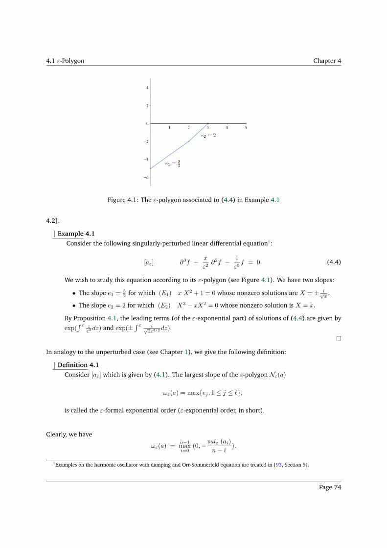
4.1 ε-Polygon Chapter 4
Figure 4.1: The ε-polygon associated to (4.4) in Example 4.1
4.2].
| Example 4.1
Consider the following singularly-perturbed linear differential equation†:
[aε] ∂3f − x
ε2∂2f − 1
ε5f = 0. (4.4)
We wish to study this equation according to its ε-polygon (see Figure 4.1). We have two slopes:
• The slope e1 = 32 for which (E1) x X2 + 1 = 0 whose nonzero solutions are X = ± i√
x.
• The slope e2 = 2 for which (E2) X3 − xX2 = 0 whose nonzero solution is X = x.
By Proposition 4.1, the leading terms (of the ε-exponential part) of solutions of (4.4) are given by
exp(∫ x z
ε2 dz) and exp(±∫ x i√
zε3/2dz).
In analogy to the unperturbed case (see Chapter 1), we give the following definition:
| Definition 4.1
Consider [aε] which is given by (4.1). The largest slope of the ε-polygon Nε(a)
ωε(a) = maxej , 1 ≤ j ≤ ℓ,
is called the ε-formal exponential order (ε-exponential order, in short).
Clearly, we have
ωε(a) =n−1maxi=0
(0,−valε (ai)
n− i).
†Examples on the harmonic oscillator with damping and Orr-Sommerfeld equation are treated in [93, Section 5].
Page 74
4.2 (x, ε)-Polygon Chapter 4
4.2 (x, ε)-Polygon
The ε-polygon gives valuable information about the ε-formal invariants of [aε], which resolves the second
item in Iwano’s reformulation of the problem, i.e. the construction of formal solutions. However, it gives
no answer to the first item which questions the division of the domain. This is the purpose of the (x, ε)-
polygon, introduced by Iwano and Sibuya in [73], and which takes into account the x-adic valuations in
addition to the ε-adic valuations considered in the ε-polygon. We follow their aforementioned paper in
the presentation of this section.
We consider again [aε] and we make use of the positive rational number ωε(a) (ωε for brevity) to
rewrite (4.1) as:
[aε] ∂n f + ε−ωε an−1(x, ε) ∂n−1 f + . . . + ε−nωε a0(x, ε) f = 0, (4.5)
where ai(x, ε) ∈ C[[x]][[ε]], for i ∈ 0, . . . , n − 1, and ai(x, ε = 0) 6≡ 0 for at least one index i. We then
turn our attention to the algebraic equation
λn + an−1(0, 0) λn−1 + . . . + a0(0, 0) = 0. (4.6)
If (4.6) has at least two distinct roots then the reduction of the order of the equation is always possible
by an analog of the splitting described in Section 1.3 (see [122, Corollary, pp 529]). We will elaborate
further this case in Section 5.3. Thus, we can assume without loss of generality that (4.6) has only one
root of order n. The transformation
g = f exp(
∫ x an−1(z, ε)
n εωεdz) (4.7)
would then reduce [aε] to
[˜aε] ∂ng + ε−2ωε ˜an−2(x, ε) ∂n−2g + . . . + ε−nωε ˜a0(x, ε)g = 0, (4.8)
which we study under the assumptions:
• ˜ai(x, ε = 0) 6≡ 0 for at least one i ∈ 0, . . . , n− 2;
• and ˜ai(x = 0, ε = 0) = 0 for all i ∈ 0, . . . , n− 2.
Consequently, the algebraic equation
λn + ˜an−2(0, 0) λn−2 + . . . + ˜a0(0, 0) = 0 (4.9)
has only one root λ = 0 of order n for x = 0, but it has at least two distinct roots for x 6= 0. Hence, x = 0
is probably a turning point.
Page 75
4.2 (x, ε)-Polygon Chapter 4
| Example 4.2 (Continue Example 4.1)
Consider again the equation (4.4) of Example 4.1 given by:
∂3 f − x
ε2∂2 f − 1
ε5f = 0.
We wish to study this equation according to the (x, ε)-polygon. We first compute ωε =
max 2, 32 = 2. Thus, (4.4) can be rewritten as
∂3 f + ε−2 (−x) ∂2 f + ε−6 (−ε) f = 0. (4.10)
One can verify that a2(x, ε = 0) = −x 6≡ 0 and the algebraic equation λ3 ≡ 0 has zero as a triple
root. The transformation (4.7) yields
∂3 g + ε−4 (−13
x2 + ε2) ∂ g + ε−6 (2
27x3 + ε) g = 0. (4.11)
So we have
• ˜a1(x, ε) = −13 x2 + ε2 and ˜a0(x, ε) = 2
27x3 + ε ;
• The algebraic equation (4.9) is given by
λ3 − 1
3x2 λ+
2
27x3 = (λ+
2
3x)(λ− 1
3x)2.
Clearly, if x = 0 then we have λ = 0 as a triple root otherwise we have two distinct roots. So
x = 0 is possibly a turning point.
Consider again [˜aε] given by (4.8). The domain |x| ≤ x0 of [D] (3.10) can be divided into a finite
number of subdomains in each of which the solution of [˜aε] behaves quite differently [73, Intro, pp 2].
To construct these subdomains, a sequence of positive rational numbers
[ρ] 0 = ρ0 < ρ1 < ρ2 < · · · < ρm. (4.12)
Page 76
4.2 (x, ε)-Polygon Chapter 4
can be employed as follows:
[D1]
βm |ε|ρm ≤ |x| ≤ αm−1 |ε|ρm−1 ,
βm−1 |ε|ρm−1 ≤ |x| ≤ αm−2 |ε|ρm−2 ,
...
β2 |ε|ρ2 ≤ |x| ≤ α1 |ε|ρ1 ,
β1 |ε|ρ1 ≤ |x| ≤ α0 ;
(4.13)
[D2]
|x| ≤ βm |ε|ρm ,
αm−1 |ε|ρm−1 ≤ |x| ≤ βm−1 |ε|ρm−1 ,
...
α1 |ε|ρ1 ≤ |x| ≤ β1 |ε|ρ1 ;
(4.14)
where the βi’s (resp. αi’s) are sufficiently large (resp. small) numbers.
The sequence [ρ] can be determined with the aid of a convex polygon which we describe in the following
subsection.
4.2.1 Construction of (x, ε)-polygon
For the simplicity of the presentation, we re-adjust our notations from [˜aε] to [aε]. Without loss of
generality, we consider
[aε] ∂nf + ε−2ωε an−2(x, ε) ∂n−2f + . . . + ε−nωε a0(x, ε)f = 0. (4.15)
with the properties of equation [˜aε]. We expand the coefficients with respect to ε:
ai(x, ε) =∑∞
k=0 ai,k(x) εk, 0 ≤ i ≤ n− 2,
ai,k(x) =∑∞
j=0 ai,k,j xj , ai,j,k ∈ C, k ≥ 0.
(4.16)
Page 77
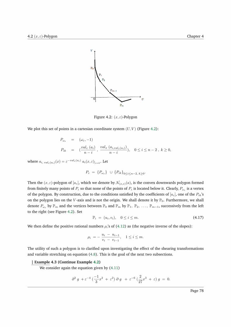
4.2 (x, ε)-Polygon Chapter 4
Figure 4.2: (x, ε)-Polygon
We plot this set of points in a cartesian coordinate system (U, V ) (Figure 4.2):
Pωε = (ωε,−1)
Pik = (valε (ai)
n− i,valx (ai,valε(ai))
n− i), 0 ≤ i ≤ n− 2 , k ≥ 0,
where ai, valε(ai)(x) = ε−valε(ai) ai(x, ε)|ε=0. Let
Pε = Pωε ∪ Pik0≤i≤n−2, k≥0.
Then the (x, ε)-polygon of [aε], which we denote by N(x,ε)(a), is the convex downwards polygon formed
from finitely many points of Pε so that none of the points of Pε is located below it. Clearly, Pωε is a vertex
of the polygon. By construction, due to the conditions satisfied by the coefficients of [aε], one of the Pik ’s
on the polygon lies on the V -axis and is not the origin. We shall denote it by P0. Furthermore, we shall
denote Pωε by Pm and the vertices between P0 and Pm by P1, P2, . . . , Pm−1, successively from the left
to the right (see Figure 4.2). Set
Pi = (ui, vi), 0 ≤ i ≤ m. (4.17)
We then define the positive rational numbers ρi’s of (4.12) as (the negative inverse of the slopes):
ρi = − ui − ui−1
vi − vi−1, 1 ≤ i ≤ m.
The utility of such a polygon is to clarified upon investigating the effect of the shearing transformations
and variable stretching on equation (4.8). This is the goal of the next two subsections.
| Example 4.3 (Continue Example 4.2)
We consider again the equation given by (4.11)
∂3 g + ε−4 (−13
x2 + ε2) ∂ g + ε−6 (2
27x3 + ε) g = 0.
Page 78
4.2 (x, ε)-Polygon Chapter 4
The (x, ε)-polygon is then defined by the following set of points: Pωε= (2,−1), P00 = (0, 1),
P01 = ( 13 , 0), P10 = (0, 1), and P12 = (1, 0). Hence, it has two slopes −3 and −1.
4.2.2 Reduction of order in [D1]
Let
F = (f, εωε ∂f, ε2 ωε ∂2 f, . . . , ε(n−1) ωε ∂n−1 f)T .
Then the equation [aε] given by (4.15) can be rewritten equivalently as the first-order system
[Aε] εωε ∂F = A(x, ε) F, (4.18)
where A(x, ε) is a companion matrix of the form
A(x, ε) =
0 1 0 . . . 0 0
0 0 1 . . . 0 0...
......
0 0 0 . . . 0 1
−a0(x, ε) −a1(x, ε) −a2(x, ε) . . . −an−2(x, ε) 0
.
In this subsection, we show that in subdomains of [D1], the system can be uncoupled into at least two
subsystems of lower dimensions (and consequently, the order of the scalar equation is reduced).
The shearing transformation F = SG (see Section 1.1), where S is of the form
S = diag(1 , εuxv , (εuxv)2, . . . , (εuxv)
n−1), (4.19)
yields the equivalent system
[Aε] εωε−u x−v ∂G = A(x, ε) G = ( B(x, ε) − v εωε−u x−v−1 C) G, (4.20)
where
B(x, ε) =
0 1 . . . 0 0
0 0 . . . 0 0...
...
0 0 . . . 0 1
−(εuxv)−n
a0(x, ε) −(εuxv)1−n
a1(x, ε) . . . −(εuxv)−2
an−2(x, ε) 0
Page 79
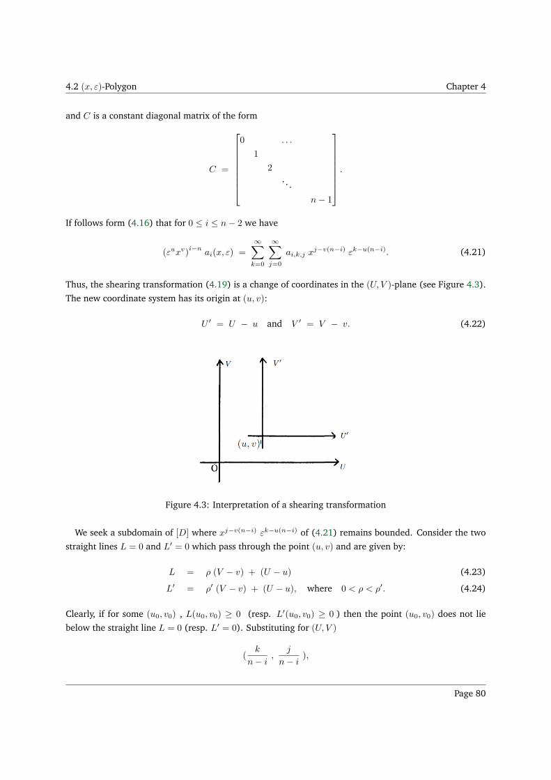
4.2 (x, ε)-Polygon Chapter 4
and C is a constant diagonal matrix of the form
C =
0 . . .
1
2
. . .
n− 1
.
If follows form (4.16) that for 0 ≤ i ≤ n− 2 we have
(εuxv)i−n
ai(x, ε) =
∞∑
k=0
∞∑
j=0
ai,k,j xj−v(n−i) εk−u(n−i). (4.21)
Thus, the shearing transformation (4.19) is a change of coordinates in the (U, V )-plane (see Figure 4.3).
The new coordinate system has its origin at (u, v):
U ′ = U − u and V ′ = V − v. (4.22)
Figure 4.3: Interpretation of a shearing transformation
We seek a subdomain of [D] where xj−v(n−i) εk−u(n−i) of (4.21) remains bounded. Consider the two
straight lines L = 0 and L′ = 0 which pass through the point (u, v) and are given by:
L = ρ (V − v) + (U − u) (4.23)
L′ = ρ′ (V − v) + (U − u), where 0 < ρ < ρ′. (4.24)
Clearly, if for some (u0, v0) , L(u0, v0) ≥ 0 (resp. L′(u0, v0) ≥ 0 ) then the point (u0, v0) does not lie
below the straight line L = 0 (resp. L′ = 0). Substituting for (U, V )
(k
n− i,
j
n− i),
Page 80
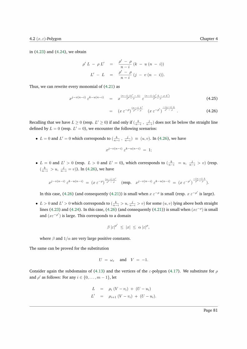
4.2 (x, ε)-Polygon Chapter 4
in (4.23) and (4.24), we obtain
ρ′ L − ρ L′ =ρ′ − ρ
n− i(k − u (n − i))
L′ − L =ρ′ − ρ
n− i(j − v (n − i)).
Thus, we can rewrite every monomial of (4.21) as
xj−v(n−i) εk−u(n−i) = x(n−i) (L′
− L)
ρ′ − ρ ε(n−i) (ρ′ L − ρ L′)
ρ′ − ρ (4.25)
= (x ε−ρ)(n−i) L′
ρ′ − ρ (x ε−ρ′
)−(n−i) L
ρ′ − ρ . (4.26)
Recalling that we have L ≥ 0 (resp. L′ ≥ 0) if and only if ( kn−i ,
jn−i ) does not lie below the straight line
defined by L = 0 (resp. L′ = 0), we encounter the following scenarios:
• L = 0 and L′ = 0 which corresponds to ( kn−i ,
jn−i ) ≡ (u, v). In (4.26), we have
xj−v(n−i) εk−u(n−i) = 1;
• L = 0 and L′ > 0 (resp. L > 0 and L′ = 0), which corresponds to ( kn−i = u, j
n−i > v) (resp.
( kn−i > u, j
n−i = v)). In (4.26), we have
xj−v(n−i) εk−u(n−i) = (x ε−ρ)(n−i) L′
ρ′ − ρ (resp. xj−v(n−i) εk−u(n−i) = (x ε−ρ′
)−(n−i) L
ρ′ − ρ ).
In this case, (4.26) (and consequently (4.21)) is small when x ε−ρ is small (resp. x ε−ρ′
is large).
• L > 0 and L′ > 0 which corresponds to ( kn−i > u, j
n−i > v) for some (u, v) lying above both straight
lines (4.23) and (4.24). In this case, (4.26) (and consequently (4.21)) is small when (xε−ρ) is small
and (xε−ρ′
) is large. This corresponds to a domain
β |ε|ρ′
≤ |x| ≤ α |ε|ρ,
where β and 1/α are very large positive constants.
The same can be proved for the substitution
U = ωε and V = −1.
Consider again the subdomains of (4.13) and the vertices of the ε-polygon (4.17). We substitute for ρ
and ρ′ as follows: For any i ∈ 0, . . . ,m− 1, let
L = ρi (V − vi) + (U − ui)
L′ = ρi+1 (V − vi) + (U − ui).
Page 81
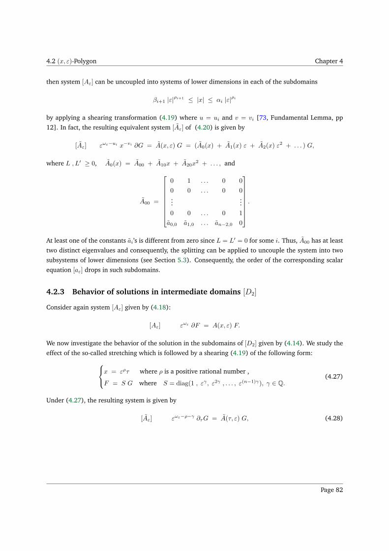
4.2 (x, ε)-Polygon Chapter 4
then system [Aε] can be uncoupled into systems of lower dimensions in each of the subdomains
βi+1 |ε|ρi+1 ≤ |x| ≤ αi |ε|ρi
by applying a shearing transformation (4.19) where u = ui and v = vi [73, Fundamental Lemma, pp
12]. In fact, the resulting equivalent system [Aε] of (4.20) is given by
[Aε] εωε−ui x−vi ∂G = A(x, ε) G = (A0(x) + A1(x) ε + A2(x) ε2 + . . . ) G,
where L ,L′ ≥ 0, A0(x) = A00 + A10x + A20x2 + . . . , and
A00 =
0 1 . . . 0 0
0 0 . . . 0 0...
...
0 0 . . . 0 1
a0,0 a1,0 . . . an−2,0 0
.
At least one of the constants ai’s is different from zero since L = L′ = 0 for some i. Thus, A00 has at least
two distinct eigenvalues and consequently, the splitting can be applied to uncouple the system into two
subsystems of lower dimensions (see Section 5.3). Consequently, the order of the corresponding scalar
equation [aε] drops in such subdomains.
4.2.3 Behavior of solutions in intermediate domains [D2]
Consider again system [Aε] given by (4.18):
[Aε] εωε ∂F = A(x, ε) F.
We now investigate the behavior of the solution in the subdomains of [D2] given by (4.14). We study the
effect of the so-called stretching which is followed by a shearing (4.19) of the following form:
x = ερτ where ρ is a positive rational number ,
F = S G where S = diag(1 , εγ , ε2γ , . . . , ε(n−1)γ), γ ∈ Q.(4.27)
Under (4.27), the resulting system is given by
[Aε] εωε−ρ−γ ∂τG = A(τ, ε) G, (4.28)
Page 82
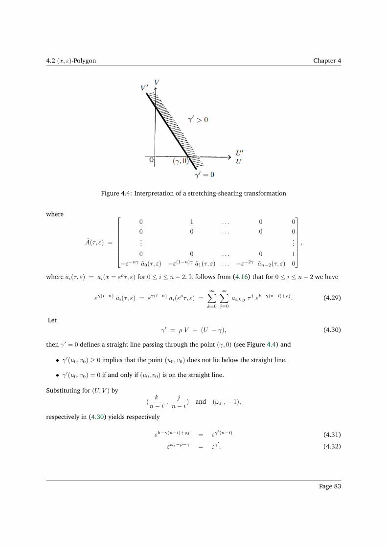
4.2 (x, ε)-Polygon Chapter 4
Figure 4.4: Interpretation of a stretching-shearing transformation
where
A(τ, ε) =
0 1 . . . 0 0
0 0 . . . 0 0...
...
0 0 . . . 0 1
−ε−nγ a0(τ, ε) −ε(1−n)γ a1(τ, ε) . . . −ε−2γ an−2(τ, ε) 0
,
where ai(τ, ε) = ai(x = ερτ, ε) for 0 ≤ i ≤ n− 2. It follows from (4.16) that for 0 ≤ i ≤ n− 2 we have
εγ(i−n) ai(τ, ε) = εγ(i−n) ai(ερτ, ε) =
∞∑
k=0
∞∑
j=0
ai,k,j τj εk−γ(n−i)+ρj . (4.29)
Let
γ′ = ρ V + (U − γ), (4.30)
then γ′ = 0 defines a straight line passing through the point (γ, 0) (see Figure 4.4) and
• γ′(u0, v0) ≥ 0 implies that the point (u0, v0) does not lie below the straight line.
• γ′(u0, v0) = 0 if and only if (u0, v0) is on the straight line.
Substituting for (U, V ) by
(k
n− i,
j
n− i) and (ωε , −1),
respectively in (4.30) yields respectively
εk−γ(n−i)+ρj = εγ′(n−i) (4.31)
εωε−ρ−γ = εγ′
. (4.32)
Page 83
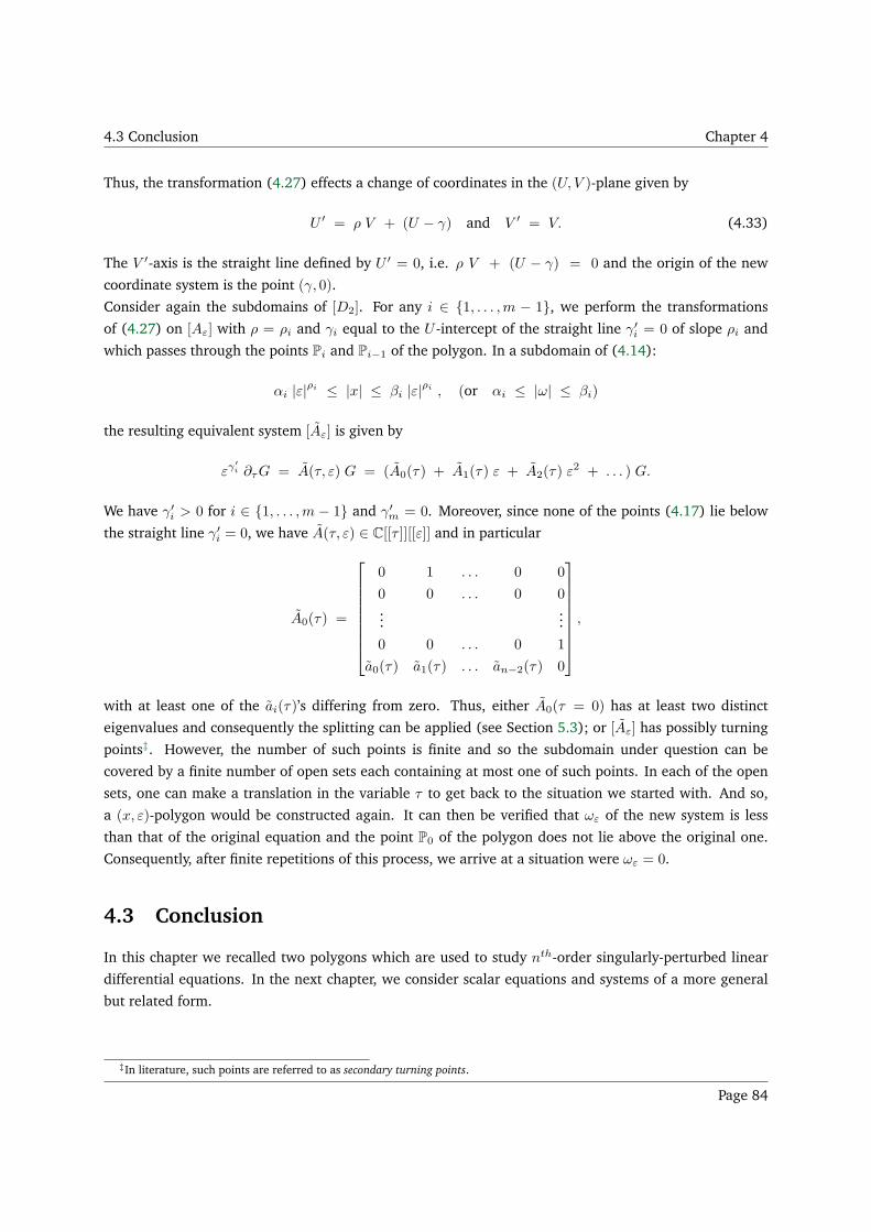
4.3 Conclusion Chapter 4
Thus, the transformation (4.27) effects a change of coordinates in the (U, V )-plane given by
U ′ = ρ V + (U − γ) and V ′ = V. (4.33)
The V ′-axis is the straight line defined by U ′ = 0, i.e. ρ V + (U − γ) = 0 and the origin of the new
coordinate system is the point (γ, 0).
Consider again the subdomains of [D2]. For any i ∈ 1, . . . ,m − 1, we perform the transformations
of (4.27) on [Aε] with ρ = ρi and γi equal to the U -intercept of the straight line γ′i = 0 of slope ρi and
which passes through the points Pi and Pi−1 of the polygon. In a subdomain of (4.14):
αi |ε|ρi ≤ |x| ≤ βi |ε|ρi , (or αi ≤ |ω| ≤ βi)
the resulting equivalent system [Aε] is given by
εγ′
i ∂τG = A(τ, ε) G = (A0(τ) + A1(τ) ε + A2(τ) ε2 + . . . ) G.
We have γ′i > 0 for i ∈ 1, . . . ,m − 1 and γ′
m = 0. Moreover, since none of the points (4.17) lie below
the straight line γ′i = 0, we have A(τ, ε) ∈ C[[τ ]][[ε]] and in particular
A0(τ) =
0 1 . . . 0 0
0 0 . . . 0 0...
...
0 0 . . . 0 1
a0(τ) a1(τ) . . . an−2(τ) 0
,
with at least one of the ai(τ)’s differing from zero. Thus, either A0(τ = 0) has at least two distinct
eigenvalues and consequently the splitting can be applied (see Section 5.3); or [Aε] has possibly turning
points‡. However, the number of such points is finite and so the subdomain under question can be
covered by a finite number of open sets each containing at most one of such points. In each of the open
sets, one can make a translation in the variable τ to get back to the situation we started with. And so,
a (x, ε)-polygon would be constructed again. It can then be verified that ωε of the new system is less
than that of the original equation and the point P0 of the polygon does not lie above the original one.
Consequently, after finite repetitions of this process, we arrive at a situation were ωε = 0.
4.3 Conclusion
In this chapter we recalled two polygons which are used to study nth-order singularly-perturbed linear
differential equations. In the next chapter, we consider scalar equations and systems of a more general
but related form.
‡In literature, such points are referred to as secondary turning points.
Page 84
Chapter 5
Chapter 5
Two-Fold Rank Reduction of
First-Order Systems
Contents5.1 Preliminaries . . . . . . . . . . . . . . . . . . . . . . . . . . . . . . . . . . . . . . . . . 86
5.1.1 Equivalent systems . . . . . . . . . . . . . . . . . . . . . . . . . . . . . . . . . . . 87
5.1.2 Restraining index . . . . . . . . . . . . . . . . . . . . . . . . . . . . . . . . . . . . 87
5.2 Basic cases . . . . . . . . . . . . . . . . . . . . . . . . . . . . . . . . . . . . . . . . . . 88
5.2.1 Case h ≤ 0 . . . . . . . . . . . . . . . . . . . . . . . . . . . . . . . . . . . . . . . . 88
5.2.2 The Scalar Case . . . . . . . . . . . . . . . . . . . . . . . . . . . . . . . . . . . . . 89
5.3 ε-Block diagonalization . . . . . . . . . . . . . . . . . . . . . . . . . . . . . . . . . . . 90
5.4 Resolution of turning points . . . . . . . . . . . . . . . . . . . . . . . . . . . . . . . . . 93
5.5 ε-Rank reduction . . . . . . . . . . . . . . . . . . . . . . . . . . . . . . . . . . . . . . . 99
5.5.1 ε-Reduction, h > 1 . . . . . . . . . . . . . . . . . . . . . . . . . . . . . . . . . . . 104
5.5.2 ε-Reduction, h = 1 . . . . . . . . . . . . . . . . . . . . . . . . . . . . . . . . . . . 111
5.6 ε-Moser invariant of a scalar equation . . . . . . . . . . . . . . . . . . . . . . . . . . 114
5.6.1 Example of comparison with Levelt-Barkatou-LeRoux’s approach . . . . . . . . . . 118
5.7 Conclusion . . . . . . . . . . . . . . . . . . . . . . . . . . . . . . . . . . . . . . . . . . 120
We consider again system (3.9) which is given by
[Aε] εh ∂F = A(x, ε)F = (
∞∑
k=0
Ak(x)ε) F,
where h is an integer and A(x, ε) has its entries in C[[x]][[ε]]. We refer to A0(x) as the leading matrix
coefficient and to A00 := A0(x = 0) as leading constant matrix.
This chapter is concerned with our contribution in the resolution of turning points and reduction of
ε-rank h to its minimal integer value. It is based on [2], where we propose algorithms to treat the turning
points of system (3.9) and uncouple it into a set of systems of lower dimensions such that each has the
Page 85
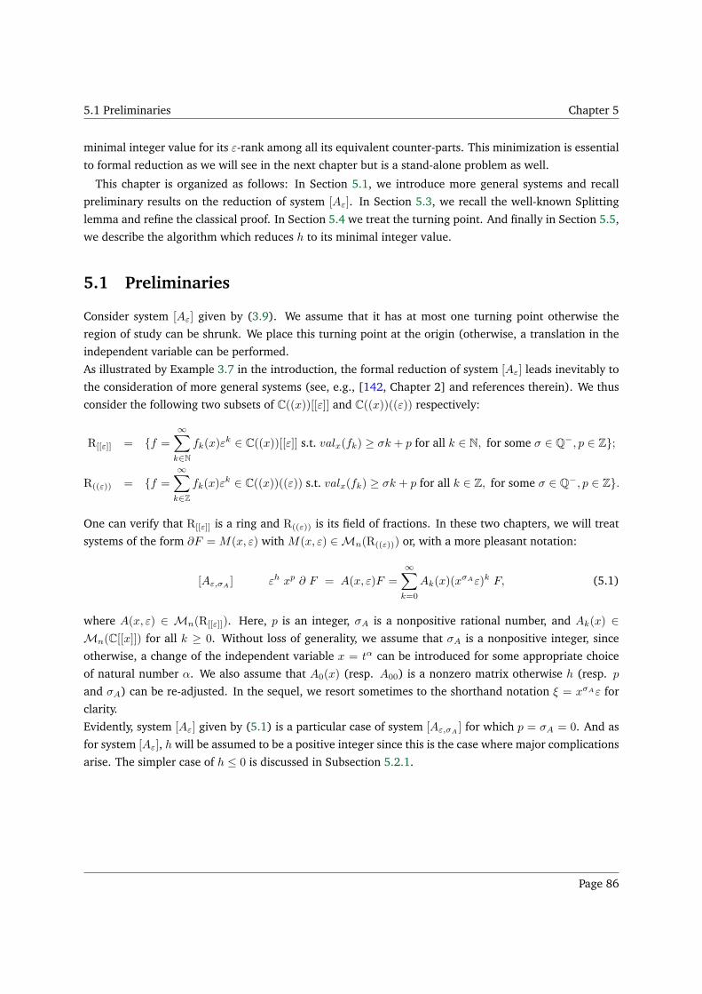
5.1 Preliminaries Chapter 5
minimal integer value for its ε-rank among all its equivalent counter-parts. This minimization is essential
to formal reduction as we will see in the next chapter but is a stand-alone problem as well.
This chapter is organized as follows: In Section 5.1, we introduce more general systems and recall
preliminary results on the reduction of system [Aε]. In Section 5.3, we recall the well-known Splitting
lemma and refine the classical proof. In Section 5.4 we treat the turning point. And finally in Section 5.5,
we describe the algorithm which reduces h to its minimal integer value.
5.1 Preliminaries
Consider system [Aε] given by (3.9). We assume that it has at most one turning point otherwise the
region of study can be shrunk. We place this turning point at the origin (otherwise, a translation in the
independent variable can be performed.
As illustrated by Example 3.7 in the introduction, the formal reduction of system [Aε] leads inevitably to
the consideration of more general systems (see, e.g., [142, Chapter 2] and references therein). We thus
consider the following two subsets of C((x))[[ε]] and C((x))((ε)) respectively:
R[[ε]] = f =
∞∑
k∈N
fk(x)εk ∈ C((x))[[ε]] s.t. valx(fk) ≥ σk + p for all k ∈ N, for some σ ∈ Q−, p ∈ Z;
R((ε)) = f =∞∑
k∈Z
fk(x)εk ∈ C((x))((ε)) s.t. valx(fk) ≥ σk + p for all k ∈ Z, for some σ ∈ Q−, p ∈ Z.
One can verify that R[[ε]] is a ring and R((ε)) is its field of fractions. In these two chapters, we will treat
systems of the form ∂F = M(x, ε) with M(x, ε) ∈Mn(R((ε))) or, with a more pleasant notation:
[Aε,σA] εh xp ∂ F = A(x, ε)F =
∞∑
k=0
Ak(x)(xσAε)k F, (5.1)
where A(x, ε) ∈ Mn(R[[ε]]). Here, p is an integer, σA is a nonpositive rational number, and Ak(x) ∈Mn(C[[x]]) for all k ≥ 0. Without loss of generality, we assume that σA is a nonpositive integer, since
otherwise, a change of the independent variable x = tα can be introduced for some appropriate choice
of natural number α. We also assume that A0(x) (resp. A00) is a nonzero matrix otherwise h (resp. p
and σA) can be re-adjusted. In the sequel, we resort sometimes to the shorthand notation ξ = xσAε for
clarity.
Evidently, system [Aε] given by (5.1) is a particular case of system [Aε,σA] for which p = σA = 0. And as
for system [Aε], h will be assumed to be a positive integer since this is the case where major complications
arise. The simpler case of h ≤ 0 is discussed in Subsection 5.2.1.
Page 86
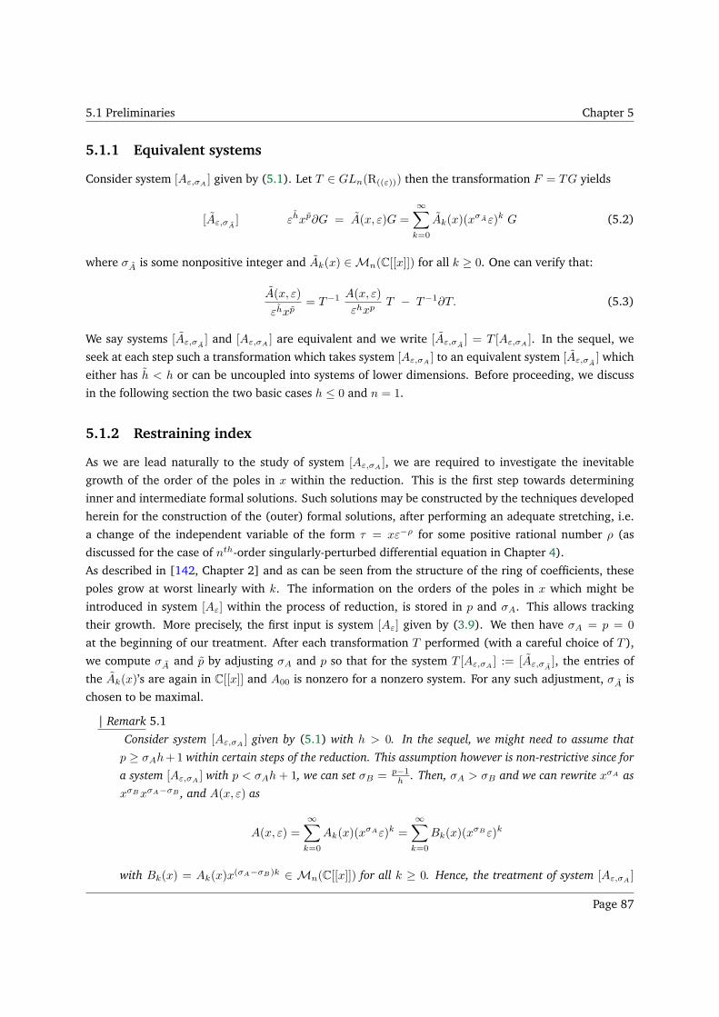
5.1 Preliminaries Chapter 5
5.1.1 Equivalent systems
Consider system [Aε,σA] given by (5.1). Let T ∈ GLn(R((ε))) then the transformation F = TG yields
[Aε,σA] εhxp∂G = A(x, ε)G =
∞∑
k=0
Ak(x)(xσAε)k G (5.2)
where σA is some nonpositive integer and Ak(x) ∈Mn(C[[x]]) for all k ≥ 0. One can verify that:
A(x, ε)
εhxp= T−1 A(x, ε)
εhxpT − T−1∂T. (5.3)
We say systems [Aε,σA] and [Aε,σA
] are equivalent and we write [Aε,σA] = T [Aε,σA
]. In the sequel, we
seek at each step such a transformation which takes system [Aε,σA] to an equivalent system [Aε,σA
] which
either has h < h or can be uncoupled into systems of lower dimensions. Before proceeding, we discuss
in the following section the two basic cases h ≤ 0 and n = 1.
5.1.2 Restraining index
As we are lead naturally to the study of system [Aε,σA], we are required to investigate the inevitable
growth of the order of the poles in x within the reduction. This is the first step towards determining
inner and intermediate formal solutions. Such solutions may be constructed by the techniques developed
herein for the construction of the (outer) formal solutions, after performing an adequate stretching, i.e.
a change of the independent variable of the form τ = xε−ρ for some positive rational number ρ (as
discussed for the case of nth-order singularly-perturbed differential equation in Chapter 4).
As described in [142, Chapter 2] and as can be seen from the structure of the ring of coefficients, these
poles grow at worst linearly with k. The information on the orders of the poles in x which might be
introduced in system [Aε] within the process of reduction, is stored in p and σA. This allows tracking
their growth. More precisely, the first input is system [Aε] given by (3.9). We then have σA = p = 0
at the beginning of our treatment. After each transformation T performed (with a careful choice of T ),
we compute σA and p by adjusting σA and p so that for the system T [Aε,σA] := [Aε,σA
], the entries of
the Ak(x)’s are again in C[[x]] and A00 is nonzero for a nonzero system. For any such adjustment, σA is
chosen to be maximal.
| Remark 5.1
Consider system [Aε,σA] given by (5.1) with h > 0. In the sequel, we might need to assume that
p ≥ σAh+1 within certain steps of the reduction. This assumption however is non-restrictive since for
a system [Aε,σA] with p < σAh+ 1, we can set σB = p−1
h . Then, σA > σB and we can rewrite xσA as
xσBxσA−σB , and A(x, ε) as
A(x, ε) =
∞∑
k=0
Ak(x)(xσAε)k =
∞∑
k=0
Bk(x)(xσBε)k
with Bk(x) = Ak(x)x(σA−σB)k ∈ Mn(C[[x]]) for all k ≥ 0. Hence, the treatment of system [Aε,σA
]
Page 87
5.2 Basic cases Chapter 5
can be substituted by the treatment of the system
[Bε,σB] ∂F = B(x, ε)F =
∞∑
k=0
Bk(x)(xσBε)kF.
5.2 Basic cases
A detailed discussion of these basic cases, whenever σA = p = 0, is given in [43, Chapter 3, Section 1, pp
52 -56]. We give here a brief discussion without any condition on σA and p.
5.2.1 Case h ≤ 0
If h ≤ 0 then the solution of system [Aε,σA] can be sought, up to any order µ, upon presenting the solution
as a power series in ξ = xσAε, i.e.
F =
∞∑
k=0
Fk(x) ξ−h+k.
The latter can then be inserted into [Aε,σA] and the like powers of ξ equated. This reduces the symbolic
resolution to solving successively a set of inhomogeneous linear singular differential systems in x solely,
the first of which is the unperturbed system [A] given by (1).
xp ∂F0 = (A0(x) + h σA xp−1I) F0
xp ∂F1 = (A0(x) + (h− 1) σA xp−1I) F1 + A1(x) F0
...
xp ∂Fµ = (A0(x) + (h− µ) σA xp−1I) Fµ +A1(x) Fµ−1 + . . . + Aµ(x) F0.
For any k ≥ 0, the solution of the homogeneous system singular in x can be sought via MINIISOLDE or
LINDALG. The solution of the inhomgeneous system can be then obtained by the method of variation of
constants (see, e.g. [11, Theorem 3, pp 11]). We remark that a transformation Fµ = x−µσAG reduces
the inhomogeneous system corresponding to Fµ to:
xp ∂G = (A0(x) + h σA xp−1I) G(x) ,
which coincides with that of F0(x). Thus we have:
Fµ(x) = x−µσA F0(x)
∫ x
0
F−10 (z) zµσA [A1(z) Fµ−1(z) + . . . + Aµ(z) F0(z)] dz.
Page 88
5.2 Basic cases Chapter 5
5.2.2 The Scalar Case
The resolution of the scalar case of a first-order system [Aε,σA] is straightforward (see, e.g., [43, pp 52-
55] or [142, page 101] ). The nth-order scalar equations with less general entries were discussed in
Chapter 4. We discuss here those with entries in R((ε)).
Equivalence with first-order systems
In Chapter 4, we have seen that a scalar equation [aε] can be expressed trivially as a first-order system [Aε].
In this section, we are interested in the reverse claim for more general systems: Given a first-order system
[Aε,σA], can we find an equivalent system which has a companion matrix form? If the answer is positive
then by denoting the entries in the last row of this companion matrix by (ai(x, ε)), 0 ≤ i ≤ n−1 ⊂ R((ε)),
the system is obviously equivalent to the singularly-perturbed scalar differential equation [aε,σa ] given by:
[aε,σa ] ∂nf − an−1(x, ε)∂n−1f − . . . a1(x, ε)∂f − a0(x, ε)f = 0.
In fact, cyclic vectors in analogy with Section 1.2 exist [46, 120]. Due to this equivalence, the formal
solutions of systems can be computed after their reduction to scalar equations. And the results of
Subsection 4.1 can be easily generalized to these more general scalar equations. However such a
treatment is computationally unsatisfactory (see e.g. [93, Conclusion]) and overlooks the information
that we can derive from the system directly. Nevertheless, it plays a key role in the theoretical basis of the
algorithm which we will develop in later chapters. In particular, it allows the definition of the ε-formal
exponential order of system [Aε,σA] as follows:
| Definition 5.1
Consider a singularly-perturbed differential system [Aε,σA] given by (5.1). The ε-polygon and ε-
polynomials of such a system are those of its equivalent nth-order singularly-perturbed differential
equation.
We denote the largest slope of the ε-polygon by ωε(A). It is called the ε-formal exponential order (ε-
exponential order in short) of system [Aε,σA]. The ε-polygon, ε-polynomials, and ωε(A) are independent
of the chosen cyclic vector (see, e.g., [46, 120]). Additionally, it follows from the equivalence under a
cyclic vector, that the ε-exponential order of system [Aε,σA] is given by
ωε(A) = max0≤i≤n
(0, (−valε (ai)
n− i)). (5.4)
Another possible approach is that of [13] which computes a companion block diagonal form for an
unperturbed system [A] given by (1). The corresponding algorithm relies on polynomial (shearing)
transformations in x and elementary row/column operations. This algorithm can be easily adapted to
the perturbed system [Aε,σA] upon using polynomial (shearing) transformations in both x and ε, and
elementary row/column operations. Such operations are discussed further in Section 5.5.
As mentioned in the introduction, a classical bridge between scalar equations and systems is Arnold’s
Page 89
5.3 ε-Block diagonalization Chapter 5
form (also called Arnold-Wasow form in this context) which can be attained by elementary row/column
operations as well [13, 7, 43, 94]. This form is “sufficiently” sparse, based on the Jordan canonical form
of the leading constant matrix coefficient (Figure 3.1), so that, roughly speaking, the techniques used for
equations can be adapted to systems. For example, given A(x, ε) in Arnold’s form, the (x, ε)-polygon is
introduced for [Aε] upon defining its vertices from the nonzero coefficients of A(x, ε) [142, Chapter 2].
In the following section, we start the process of formal reduction, acting directly on the system, with the
well-known Splitting lemma which allows uncoupling certain systems.
5.3 ε-Block diagonalization
A classical tool in perturbation theory is the so-called splitting which separates off the existing distinct
coalescence patterns. Whenever the leading constant matrix A00 := A0(0) admits at least two distinct
eigenvalues, there exists a transformation which block-diagonalizes system [Aε,σA] so that it can be
uncoupled into subsystems of lower dimensions whose leading constant matrices have a unique distinct
eigenvalue each (see, e.g., [65, Theorem XII − 4− 1, pp 381] and [142, Theorem 8.1, pp 81]).
| Theorem 5.1
Consider system [Aε,σA] given by (5.1):
[Aε,σA] εh xp ∂ F = A(x, ε)F =
∞∑
k=0
Ak(x)(xσAε)k F,
If p ≥ σAh+ 1 and A00 =
[
A1100 O
O A2200
]
and A1100 and A22
00 have no eigenvalues in common, then there
exists a unique transformation T (x, ε) =∑∞
k=0 Tk(x)(xσAε)k given by
T (x, ε) =
[
I T 120 (x)
T 210 (x) I
]
(I +
∞∑
k=1
[
O T 12k (x)
T 21k (x) O
]
(xσAε)k),
with Tk(x) ∈Mn(C[[x]]) for all k ≥ 0, such that the change of basis F = TG yields
[Aε,σA] εhxp∂G = A(x, ε) G =
∞∑
k=0
Ak(xσAε)kG =
[
A11(x, ε) O
O A22(x, ε)
]
G,
where A00 = A00 and Ak(x) ∈Mn(C[[x]]) for all k ≥ 0.
Well-known proofs (e.g. [65, pp 382- 385] and [139, pp 138 - 142]) proceed in two steps: Block-
diagionalizing A0(x), followed by the total block-diagonalization of A(x, ǫ). However, the proofs of the
first step are given only for the well-behaved case. This is the case when A0(x) have at least two distinct
eigenvalues and is holomorphically similar to its Jordan form, i.e. the eigenvalues don’t coalesce in the
region of study (see Example 5.1). We give herein a constructive proof of the first step without imposing
any restriction on the eigenvalues and eigenvectors of A0(x), as we aim to give a general discussion which
Page 90
5.3 ε-Block diagonalization Chapter 5
does not exclude turning points. The second and third steps of the proof are adaptations of [43, Chapter
3, pp 56-59] and [140, Theorem 2.3-1, pp 17], which are based on a result originally due to [122].
Proof. We proceed in three steps:
Step 1: We first block-diagonalize the leading matrix coefficient : We can construct a transformation
F = T0(x)G s.t. the leading matrix coefficient A0(x) of the equivalent system has the following block-
form in accordance with A00:
A0(x) =
[
A110 (x) O
O A220 (x)
]
.
From (5.3) we have
On = A0(x) T0(x) − T0(x) A0(x). (5.5)
Assuming that T0(x) ∈Mn(C[[x]]) is in the following form
T0(x) =
[
I T 120 (x)
T 210 (x) I
]
,
we have for 1 ≤ 6= ς ≤ 2:
A0 (x) − A
0 (x) + Aς0 (x) T ς
0 (x) = O
Aς0 (x) + Aςς
0 (x) T ς0 (x) − T ς
0 (x) A0 (x) = O
(5.6)
We inserting the series expansions A0(x) =∑∞
i=0 Ai0xi and A0(x) =
∑∞i=0 Ai0x
i in (5.6), and we
equate the power-like coefficients (Ai0 may be written conveniently as Ai,0):
For i = 0 we have
A00 = A
00
Aςς00 T ς
00 − T ς00 A
00 = O
which are satisfied by setting Aςς00 = Aςς
00 and T ςς00 = I, T ς
00 = O.
For i ≥ 1 we have
Aςς00T
ςi0 − T ς
i0 A00 = −Aς
i0 −i−1∑
j=1
(Aςςi−j,0T
ςj0 − T ς
j0 Ai−j,0) (5.7)
Ai0 = A
i0 +
i−1∑
j=1
Aςi−j,0T
ςj0 . (5.8)
It’s clear that (7.13) is a set of Sylvester matrix equations that possess a unique solution due to the
assumption on the disjoint spectra of A1100 and A22
00 (see, Lemma 1.1). Remarking that the right hand side
depends solely on the Aj0, Tj0, Aj0 with j < i, equations (7.13) and (7.15) are successively soluble.
Step 2: We can now assume without loss of generality that the leading matrix coefficient A0(x)
of [Aε,σA] has a block-diagonal form in accordance with that of A00 and we study the effect of the
Page 91
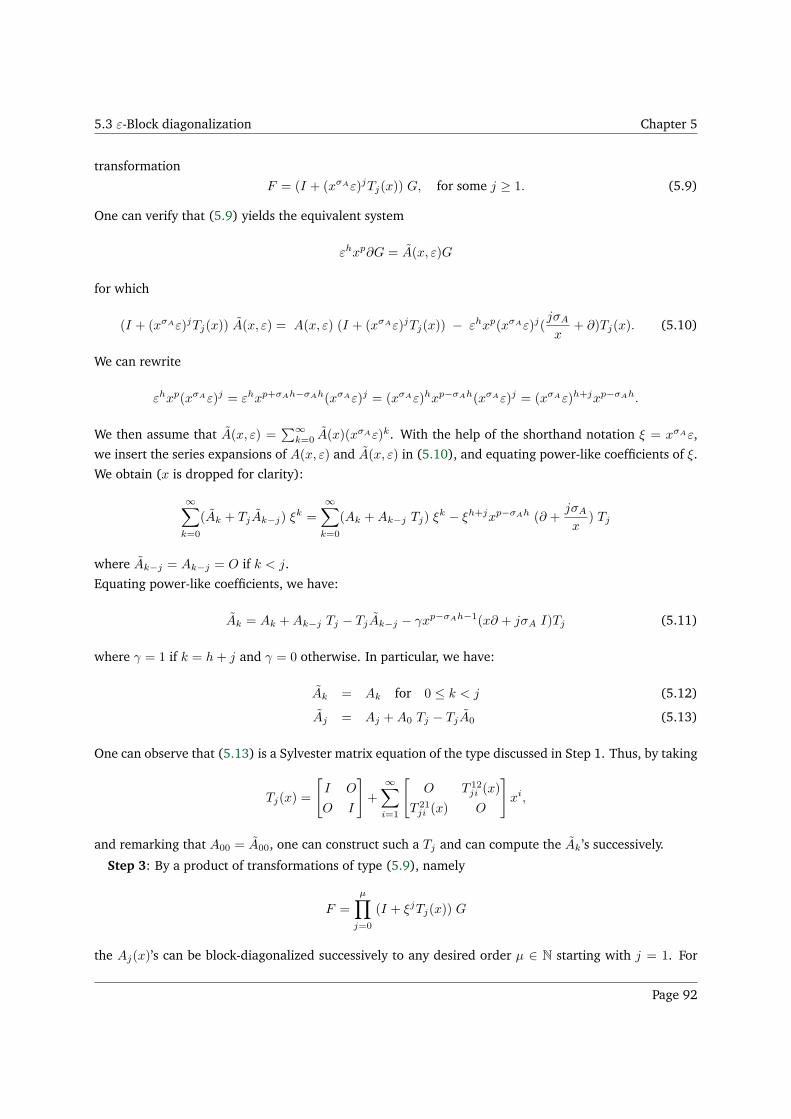
5.3 ε-Block diagonalization Chapter 5
transformation
F = (I + (xσAε)jTj(x)) G, for some j ≥ 1. (5.9)
One can verify that (5.9) yields the equivalent system
εhxp∂G = A(x, ε)G
for which
(I + (xσAε)jTj(x)) A(x, ε) = A(x, ε) (I + (xσAε)jTj(x)) − εhxp(xσAε)j(jσA
x+ ∂)Tj(x). (5.10)
We can rewrite
εhxp(xσAε)j = εhxp+σAh−σAh(xσAε)j = (xσAε)hxp−σAh(xσAε)j = (xσAε)h+jxp−σAh.
We then assume that A(x, ε) =∑∞
k=0 A(x)(xσAε)k. With the help of the shorthand notation ξ = xσAε,
we insert the series expansions of A(x, ε) and A(x, ε) in (5.10), and equating power-like coefficients of ξ.
We obtain (x is dropped for clarity):
∞∑
k=0
(Ak + TjAk−j) ξk =
∞∑
k=0
(Ak +Ak−j Tj) ξk − ξh+jxp−σAh (∂ +
jσA
x) Tj
where Ak−j = Ak−j = O if k < j.
Equating power-like coefficients, we have:
Ak = Ak +Ak−j Tj − TjAk−j − γxp−σAh−1(x∂ + jσA I)Tj (5.11)
where γ = 1 if k = h+ j and γ = 0 otherwise. In particular, we have:
Ak = Ak for 0 ≤ k < j (5.12)
Aj = Aj +A0 Tj − TjA0 (5.13)
One can observe that (5.13) is a Sylvester matrix equation of the type discussed in Step 1. Thus, by taking
Tj(x) =
[
I O
O I
]
+
∞∑
i=1
[
O T 12ji (x)
T 21ji (x) O
]
xi,
and remarking that A00 = A00, one can construct such a Tj and can compute the Ak ’s successively.
Step 3: By a product of transformations of type (5.9), namely
F =
µ∏
j=0
(I + ξjTj(x)) G
the Aj(x)’s can be block-diagonalized successively to any desired order µ ∈ N starting with j = 1. For
Page 92
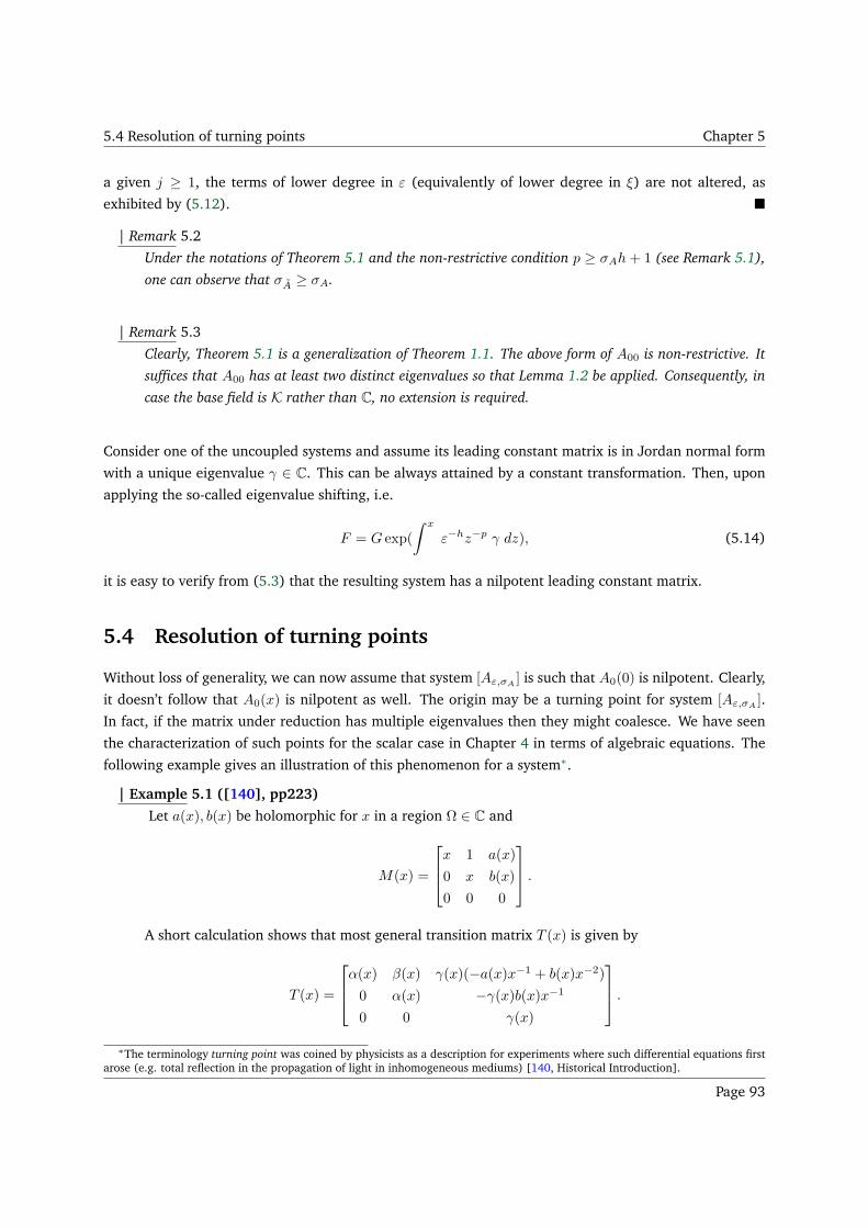
5.4 Resolution of turning points Chapter 5
a given j ≥ 1, the terms of lower degree in ε (equivalently of lower degree in ξ) are not altered, as
exhibited by (5.12).
| Remark 5.2
Under the notations of Theorem 5.1 and the non-restrictive condition p ≥ σAh+ 1 (see Remark 5.1),
one can observe that σA ≥ σA.
| Remark 5.3
Clearly, Theorem 5.1 is a generalization of Theorem 1.1. The above form of A00 is non-restrictive. It
suffices that A00 has at least two distinct eigenvalues so that Lemma 1.2 be applied. Consequently, in
case the base field is K rather than C, no extension is required.
Consider one of the uncoupled systems and assume its leading constant matrix is in Jordan normal form
with a unique eigenvalue γ ∈ C. This can be always attained by a constant transformation. Then, upon
applying the so-called eigenvalue shifting, i.e.
F = G exp(
∫ x
ε−hz−p γ dz), (5.14)
it is easy to verify from (5.3) that the resulting system has a nilpotent leading constant matrix.
5.4 Resolution of turning points
Without loss of generality, we can now assume that system [Aε,σA] is such that A0(0) is nilpotent. Clearly,
it doesn’t follow that A0(x) is nilpotent as well. The origin may be a turning point for system [Aε,σA].
In fact, if the matrix under reduction has multiple eigenvalues then they might coalesce. We have seen
the characterization of such points for the scalar case in Chapter 4 in terms of algebraic equations. The
following example gives an illustration of this phenomenon for a system∗.
| Example 5.1 ([140], pp223)
Let a(x), b(x) be holomorphic for x in a region Ω ∈ C and
M(x) =
x 1 a(x)
0 x b(x)
0 0 0
.
A short calculation shows that most general transition matrix T (x) is given by
T (x) =
α(x) β(x) γ(x)(−a(x)x−1 + b(x)x−2)
0 α(x) −γ(x)b(x)x−1
0 0 γ(x)
.
∗The terminology turning point was coined by physicists as a description for experiments where such differential equations firstarose (e.g. total reflection in the propagation of light in inhomogeneous mediums) [140, Historical Introduction].
Page 93
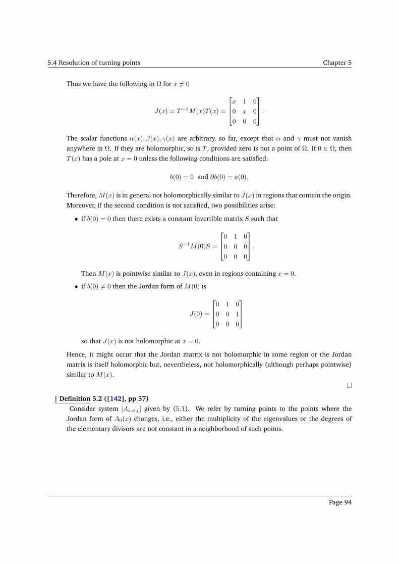
5.4 Resolution of turning points Chapter 5
Thus we have the following in Ω for x 6= 0
J(x) = T−1M(x)T (x) =
x 1 0
0 x 0
0 0 0
.
The scalar functions α(x), β(x), γ(x) are arbitrary, so far, except that α and γ must not vanish
anywhere in Ω. If they are holomorphic, so is T , provided zero is not a point of Ω. If 0 ∈ Ω, then
T (x) has a pole at x = 0 unless the following conditions are satisfied:
b(0) = 0 and ∂b(0) = a(0).
Therefore, M(x) is in general not holomorphically similar to J(x) in regions that contain the origin.
Moreover, if the second condition is not satisfied, two possibilities arise:
• if b(0) = 0 then there exists a constant invertible matrix S such that
S−1M(0)S =
0 1 0
0 0 0
0 0 0
.
Then M(x) is pointwise similar to J(x), even in regions containing x = 0.
• if b(0) 6= 0 then the Jordan form of M(0) is
J(0) =
0 1 0
0 0 1
0 0 0
so that J(x) is not holomorphic at x = 0.
Hence, it might occur that the Jordan matrix is not holomorphic in some region or the Jordan
matrix is itself holomorphic but, nevertheless, not holomorphically (although perhaps pointwise)
similar to M(x).
| Definition 5.2 ([142], pp 57)
Consider system [Aε,σA] given by (5.1). We refer by turning points to the points where the
Jordan form of A0(x) changes, i.e., either the multiplicity of the eigenvalues or the degrees of
the elementary divisors are not constant in a neighborhood of such points.
Page 94
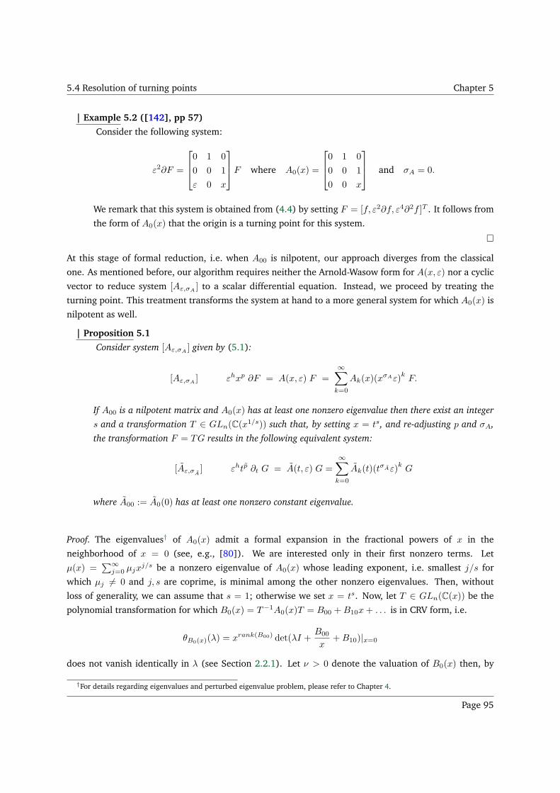
5.4 Resolution of turning points Chapter 5
| Example 5.2 ([142], pp 57)
Consider the following system:
ε2∂F =
0 1 0
0 0 1
ε 0 x
F where A0(x) =
0 1 0
0 0 1
0 0 x
and σA = 0.
We remark that this system is obtained from (4.4) by setting F = [f, ε2∂f, ε4∂2f ]T . It follows from
the form of A0(x) that the origin is a turning point for this system.
At this stage of formal reduction, i.e. when A00 is nilpotent, our approach diverges from the classical
one. As mentioned before, our algorithm requires neither the Arnold-Wasow form for A(x, ε) nor a cyclic
vector to reduce system [Aε,σA] to a scalar differential equation. Instead, we proceed by treating the
turning point. This treatment transforms the system at hand to a more general system for which A0(x) is
nilpotent as well.
| Proposition 5.1
Consider system [Aε,σA] given by (5.1):
[Aε,σA] εhxp ∂F = A(x, ε) F =
∞∑
k=0
Ak(x)(xσAε)
kF.
If A00 is a nilpotent matrix and A0(x) has at least one nonzero eigenvalue then there exist an integer
s and a transformation T ∈ GLn(C(x1/s)) such that, by setting x = ts, and re-adjusting p and σA,
the transformation F = TG results in the following equivalent system:
[Aε,σA] εhtp ∂t G = A(t, ε) G =
∞∑
k=0
Ak(t)(tσAε)
kG
where A00 := A0(0) has at least one nonzero constant eigenvalue.
Proof. The eigenvalues† of A0(x) admit a formal expansion in the fractional powers of x in the
neighborhood of x = 0 (see, e.g., [80]). We are interested only in their first nonzero terms. Let
µ(x) =∑∞
j=0 µjxj/s be a nonzero eigenvalue of A0(x) whose leading exponent, i.e. smallest j/s for
which µj 6= 0 and j, s are coprime, is minimal among the other nonzero eigenvalues. Then, without
loss of generality, we can assume that s = 1; otherwise we set x = ts. Now, let T ∈ GLn(C(x)) be the
polynomial transformation for which B0(x) = T−1A0(x)T = B00 +B10x+ . . . is in CRV form, i.e.
θB0(x)(λ) = xrank(B00) det(λI +B00
x+B10)|x=0
does not vanish identically in λ (see Section 2.2.1). Let ν > 0 denote the valuation of B0(x) then, by
†For details regarding eigenvalues and perturbed eigenvalue problem, please refer to Chapter 4.
Page 95
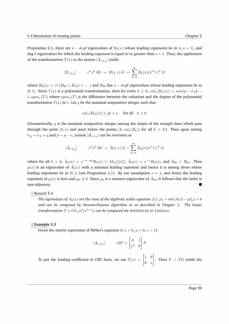
5.4 Resolution of turning points Chapter 5
Proposition 2.1, there are n − degθ eigenvalues of B0(x) whose leading exponents lie in [ν, ν + 1[, and
deg θ eigenvalues for which the leading exponent is equal to or greater than ν + 1. Then, the application
of the transformation T (x) to the system [Aε,σA] yields
[Bε,σA] εhxp ∂G = B(x, ε) G =
∞∑
k=0
Bk(x)(xσAε)k G
where B0(x) := xν(B00 + B10x+ . . . ) and B00 has n− degθ eigenvalues whose leading exponents lie in
[0, 1[. Since T (x) is a polynomial transformation, then for every k ≥ 0, valx(Bk(x)) ≥ min(p − σAh −1, spanx(T )) where spanx(T ) is the difference between the valuation and the degree of the polynomial
transformation T (x) in x. Let q be the maximal nonpositive integer such that
valx(Bk(x)) ≥ qk + ν, for all k > 0.
(Geometrically, q is the maximal nonpositive integer among the slopes of the straight lines which pass
through the point (0, ν) and stays below the points (k, valx(Bk)) for all k > 0.) Then upon setting
σA = σA + q and p = p− ν, system [Bε,σA] can be rewritten as
[Aε,σA] εhxp ∂G = A(x, ε) G =
∞∑
k=0
Ak(x)(xσAε)
kG
where for all k > 0, Ak(x) = x−ν−qkBk(x) ∈ Mn([[x]]), A0(x) = x−νB0(x), and A00 = B00. Then
µ(x) is an eigenvalue of A0(x) with a minimal leading exponent and hence it is among those whose
leading exponents lie in [0, 1[ (see Proposition 2.1). By our assumption s = 1, and hence the leading
exponent of µ(x) is zero and µ0 6= 0. Since µ0 is a nonzero eigenvalue of A00, it follows that the latter is
non-nilpotent.
| Remark 5.4
The eigenvalues of A0(x) are the roots of the algebraic scalar equation f(x, µ) = det(A(x)−µIn) = 0
and can be computed by Newton-Puiseux algorithm or as described in Chapter 2. The linear
transformation T ∈ GLn(C(x1/s)) can be computed via MINIISOLDE or LINDALG.
| Example 5.3
Given the matrix expression of Weber’s equation (σA = 0, p = 0, s = 1):
[Aε,σA] ε∂F =
[
0 1
x2 0
]
F.
To put the leading coefficient in CRV form, we use T (x) =
[
1 0
0 x
]
. Then F = TG yields the
Page 96
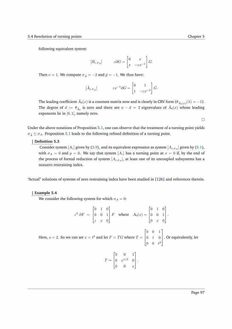
5.4 Resolution of turning points Chapter 5
following equivalent system:
[Bε,σA] ε∂G =
[
0 x
x −εx−1
]
G.
Then ν = 1. We compute σA = −2 and p = −1. We thus have:
[Aε,σA] εx−1∂G =
[
0 1
1 −εx−2
]
G.
The leading coefficient A0(x) is a constant matrix now and is clearly in CRV form (θA0(x)(λ) = −1).
The degree of d := θA0is zero and there are n − d = 2 eigenvalues of A0(x) whose leading
exponents lie in [0, 1[, namely zero.
Under the above notations of Proposition 5.1, one can observe that the treatment of a turning point yields
σA ≤ σA. Proposition 5.1 leads to the following refined definition of a turning point.
| Definition 5.3
Consider system [Aε] given by (3.9), and its equivalent expression as system [Aε,σA] given by (5.1),
with σA = 0 and p = 0. We say that system [Aε] has a turning point at x = 0 if, by the end of
the process of formal reduction of system [Aε,σA], at least one of its uncoupled subsystems has a
nonzero restraining index.
“Actual” solutions of systems of zero restraining index have been studied in [126] and references therein.
| Example 5.4
We consider the following system for which σA = 0:
ε2 ∂F =
0 1 0
0 0 1
ε x 0
F where A0(x) =
0 1 0
0 0 1
0 x 0
.
Here, s = 2. So we can set x = t2 and let F = TG where T =
0 0 1
0 t 0
0 0 t2
. Or equivalently, let
T =
0 0 1
0 x1/2 0
0 0 x
.
Page 97
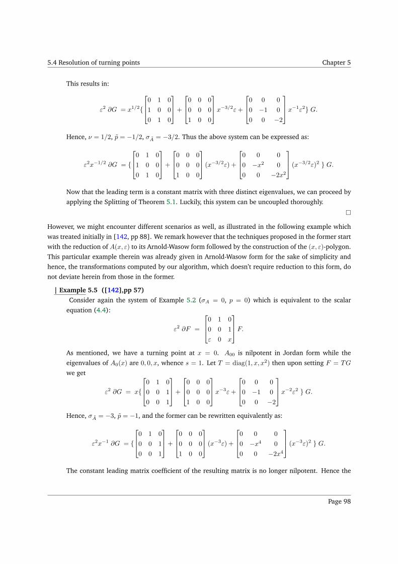
5.4 Resolution of turning points Chapter 5
This results in:
ε2 ∂G = x1/2
0 1 0
1 0 0
0 1 0
+
0 0 0
0 0 0
1 0 0
x−3/2ε+
0 0 0
0 −1 0
0 0 −2
x−1ε2 G.
Hence, ν = 1/2, p = −1/2, σA = −3/2. Thus the above system can be expressed as:
ε2x−1/2 ∂G =
0 1 0
1 0 0
0 1 0
+
0 0 0
0 0 0
1 0 0
(x−3/2ε) +
0 0 0
0 −x2 0
0 0 −2x2
(x−3/2ε)2 G.
Now that the leading term is a constant matrix with three distinct eigenvalues, we can proceed by
applying the Splitting of Theorem 5.1. Luckily, this system can be uncoupled thoroughly.
However, we might encounter different scenarios as well, as illustrated in the following example which
was treated initially in [142, pp 88]. We remark however that the techniques proposed in the former start
with the reduction of A(x, ε) to its Arnold-Wasow form followed by the construction of the (x, ε)-polygon.
This particular example therein was already given in Arnold-Wasow form for the sake of simplicity and
hence, the transformations computed by our algorithm, which doesn’t require reduction to this form, do
not deviate herein from those in the former.
| Example 5.5 ([142],pp 57)
Consider again the system of Example 5.2 (σA = 0, p = 0) which is equivalent to the scalar
equation (4.4):
ε2 ∂F =
0 1 0
0 0 1
ε 0 x
F.
As mentioned, we have a turning point at x = 0. A00 is nilpotent in Jordan form while the
eigenvalues of A0(x) are 0, 0, x, whence s = 1. Let T = diag(1, x, x2) then upon setting F = TG
we get
ε2 ∂G = x
0 1 0
0 0 1
0 0 1
+
0 0 0
0 0 0
1 0 0
x−3ε+
0 0 0
0 −1 0
0 0 −2
x−2ε2 G.
Hence, σA = −3, p = −1, and the former can be rewritten equivalently as:
ε2x−1 ∂G =
0 1 0
0 0 1
0 0 1
+
0 0 0
0 0 0
1 0 0
(x−3ε) +
0 0 0
0 −x4 0
0 0 −2x4
(x−3ε)2 G.
The constant leading matrix coefficient of the resulting matrix is no longer nilpotent. Hence the
Page 98
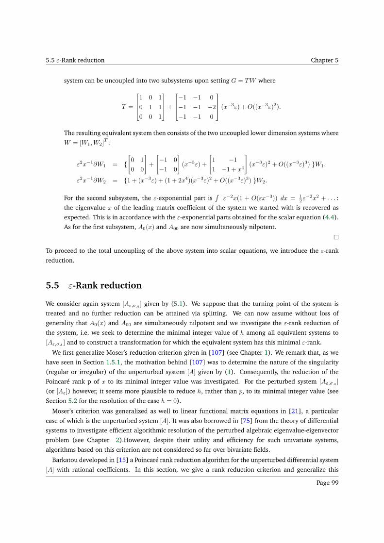
5.5 ε-Rank reduction Chapter 5
system can be uncoupled into two subsystems upon setting G = TW where
T =
1 0 1
0 1 1
0 0 1
+
−1 −1 0
−1 −1 −2−1 −1 0
(x−3ε) +O((x−3ε)2).
The resulting equivalent system then consists of the two uncoupled lower dimension systems where
W = [W1,W2]T :
ε2x−1∂W1 = [
0 1
0 0
]
+
[
−1 0
−1 0
]
(x−3ε) +
[
1 −11 −1 + x4
]
(x−3ε)2 +O((x−3ε)3) W1.
ε2x−1∂W2 = 1 + (x−3ε) + (1 + 2x4)(x−3ε)2 +O((x−3ε)3) W2.
For the second subsystem, the ε-exponential part is∫
ε−2x(1 + O(εx−3)) dx = 12ε
−2x2 + . . . :
the eigenvalue x of the leading matrix coefficient of the system we started with is recovered as
expected. This is in accordance with the ε-exponential parts obtained for the scalar equation (4.4).
As for the first subsystem, A0(x) and A00 are now simultaneously nilpotent.
To proceed to the total uncoupling of the above system into scalar equations, we introduce the ε-rank
reduction.
5.5 ε-Rank reduction
We consider again system [Aε,σA] given by (5.1). We suppose that the turning point of the system is
treated and no further reduction can be attained via splitting. We can now assume without loss of
generality that A0(x) and A00 are simultaneously nilpotent and we investigate the ε-rank reduction of
the system, i.e. we seek to determine the minimal integer value of h among all equivalent systems to
[Aε,σA] and to construct a transformation for which the equivalent system has this minimal ε-rank.
We first generalize Moser’s reduction criterion given in [107] (see Chapter 1). We remark that, as we
have seen in Section 1.5.1, the motivation behind [107] was to determine the nature of the singularity
(regular or irregular) of the unperturbed system [A] given by (1). Consequently, the reduction of the
Poincaré rank p of x to its minimal integer value was investigated. For the perturbed system [Aε,σA]
(or [Aε]) however, it seems more plausible to reduce h, rather than p, to its minimal integer value (see
Section 5.2 for the resolution of the case h = 0).
Moser’s criterion was generalized as well to linear functional matrix equations in [21], a particular
case of which is the unperturbed system [A]. It was also borrowed in [75] from the theory of differential
systems to investigate efficient algorithmic resolution of the perturbed algebraic eigenvalue-eigenvector
problem (see Chapter 2).However, despite their utility and efficiency for such univariate systems,
algorithms based on this criterion are not considered so far over bivariate fields.
Barkatou developed in [15] a Poincaré rank reduction algorithm for the unperturbed differential system
[A] with rational coefficients. In this section, we give a rank reduction criterion and generalize this
Page 99
5.5 ε-Rank reduction Chapter 5
algorithm to system [Aε,σA]‡.
Following the discussion for unperturbed systems [A] of the form (1), we define the ε-Moser rank and
ε-Moser invariant of system [Aε,σA] respectively as the rational numbers:
mε(A) = max (0, h+rank (A0(x))
n) and
µε(A) = min mε(T [Aε,σA]) for all possible choices of T in GLn(R((ε))).
| Definition 5.4
We say that system [Aε,σA] (the matrix A(x, ε) respectively) is ε-reducible if mε(A) > µε(A),
otherwise we say that is ε-irreducible.
If mε(A) ≤ 1, then h = 0. Hence, we restrict our attention to the case of mε(A) > 1.
| Remark 5.5
This definition is not to be mixed neither with the usual sense of Moser-irreducible unperturbed system
[A] given by (1), i.e. the systems whose Poincaré rank p is minimal; nor with the common sense of
reduced system in the literature, i.e. the system defined from [Aε,σA] by xp∂F = A0(x)F .
The main result of this section is the following theorem and its sufficient condition whose proof follows
after a series of intermediate results. In this section, given a system [Aε,σA], we assume, without loss of
generality due to Remark 5.1, that p− σAh− 1 ≥ 0.
| Theorem 5.2
Consider system [Aε,σA] given by (5.1):
[Aε,σA] εhxp∂F = A(x, ε)F =
∞∑
k=0
Ak(x)(xσAε)
kF.
We assume that h > 1, mε(A) > 1, and r = rank (A0(x)) < n. Suppose that there exists a
transformation F = T (x, ε)G, where T =∑∞
k=0 Tk(x)(xσAε)k is invertible, and Tk(x) ∈Mn(C[[x]])
‡Moser himself, within his numerous and diverse interests, was interested in such systems. However, he did not consider hisown approach to rank reduction of the unperturbed counterparts of such systems to treat system [Aε,σA ] as we propose in thissection. In an internal technical report [106], he investigates the formal growth order. His treatment resembles essentially that ofIwano in [71] although these works were developed independently. On another rather irrelevant note, Moser had another kind ofrelationship to researchers interested in such systems: In [112], O’Malley and Robert trace the birth of singular perturbation theoryto Gottingen with the seven-page paper of Prandtl entitled “On fluid motion with small friction”. This paper, as they quote from Tani(1977), marked on the epoch in the history of fluid dynamics, opening the way for understanding the motion of real fluids. Prandtl’slife however was characterized by his most famous student Theodore von Kármán as particularly full of overtones of naiveté. Indeed,when Prandtl decided he ought to marry in 1909, he wrote to the Foppls asking for the hand of one of their daughters, withoutspecifying one of them in particular. In a discussion whether Prandtl married the appropriate daughter of the Foppls, the authorsof [112] remark that, I quote, the tradition of marrying the daughter of one’s professor had been common in academic Germany,sometimes being suggested as the way mathematical talent was transferred between generations. Courant, for example, married Runge’sdaughter, and his daughters have also married prominent mathematicians, namely Jurgen Moser and Peter Lax, who certainly did notneed family assistance to obtain success.
Page 100
5.5 ε-Rank reduction Chapter 5
for all k ≥ 0, such that the equivalent system
[Bε,σA] εhxp∂G = B(x, ε)G =
∞∑
k=0
Bk(x)(xσAε)
kG
satisfies either (h < h) or (h = h and rank(B0(x)) < r). Then, setting ξ = xσAε, the polynomial
θA(λ) := ξr det(λI +A0(x)
ξ+A1(x))|ξ=0 (5.15)
vanishes identically in λ.
Proof. Suppose that such a T (x, ε) exists, then we can present T (x, ε) in the form (see [106, Lemma 1]):
T (x, ε) = P (x, ε) ξα Q(x, ε),
where P (x, ε), Q(x, ε) are unimodular elements ofMn(R[[ε]]), and α = diag(α1, . . . , αn) for some integers
α1 ≤ α2 ≤ · · · ≤ αn.
We then define the span s(T ) by
s := s(T ) = αn − α1 = max1≤i,j≤n (αi − αj).
Without loss of generality, one can assume that s = 1. Otherwise, T can be written as a product of s+ 1
transformations, the first of which is of span zero and the rest are of span one each, and which can be
applied successively to the system. In fact, let ek,l = 0 if k = l and ek,l = 1 otherwise. Then one can
construct§ s+ 1 sequences
β(i) = (β(i)1 , . . . , β(i)
n ), i ∈ 0, . . . , s,
§We illustrate with the following examples:
• α = (1, 2, 4) then s = 3 and the 4 sequences can be chosen as (1, 1, 1), (0, 1, 1), (0, 0, 1), (0, 0, 1);
• α = (2, 3, 3) then s = 1 and the 2 sequences can be chosen as (2, 2, 2), (0, 1, 1);
• α = (−2,−1, 3) then s = 5 and the 6 sequences can be chosen as (−2,−2,−2), (0, 1, 1), (0, 0, 1), (0, 0, 1), (0, 0, 1), (0, 0, 1).
Page 101
5.5 ε-Rank reduction Chapter 5
in the following manner
β(0) = (α1, α1, . . . , α1)
β(1) = (0, eα2,α1, . . . , eαn,α1
)
β(2) = (0, eα2,α1+1, . . . , eαn,α1+1)
...
β(i) = (0, eα2,α1+i−1, . . . , eαn,α1+i−1)
...
β(s) = (0, eα2,α1+s−1, . . . , eαn,α1+s−1)
One can then verify that for any i ∈ 1, . . . , s we have
β(i)1 ≤ · · · ≤ β(i)
n ,
β(i)n − β
(i)1 = 1, and
s∑
i=0
β(i)j = αj , j ∈ 1, . . . , n
We then proceed by defining
T (i) = Pξβ(i)
P−1, for i ∈ 0, 2, . . . , s− 1T (s) = Pξβ
(s)
Q.
We then have
T = T (0)T (1)T (2) . . . T (s)
where s(T (0)) = 0 and s(T (i)) = 1, i ∈ 1, . . . , s.We now consider A = P−1AP − ξhxp−σAhP−1∂P and B = QBQ−1 + ξhxp−σAh(∂Q)Q−1. Then we have
B = ξ−αAξα − ξhxp−σAh−1 diag(σα1, . . . , σαn).
It then follows from the unimodularity of P and Q with respect to ε (and consequently ξ) that mε(A) =
mε(A) and mε(B) = mε(B). Let ϑ(λ) = ξr det(λI + Aξ )|ξ=0, then we have:
ϑ(λ) = ξr det(λI +A
ξ)|ξ=0 = ξr det(λI +
A
ξ+ ξh−1xp−σAh−1P−1(∂P ))|ξ=0
= ξr det(λI +B
ξ+ P ) |ξ=0
where P = ξh−1xp−σAh−1(diag(σα1, . . . , σαn) + xξ−αP−1∂Pξα). Hence, P (x, ξ) has no poles in ξ since
span(T ) = 1. In other words, the pole introduced in ξ−αP−1∂Pξα is at worst a simple pole. And so, P
has no poles.
Page 102
5.5 ε-Rank reduction Chapter 5
Thus the worst pole the determinant of ϑ(λ) can have is of order µ ≤ rank(B0(x)) = rank(B0(x)) < r,
i.e.
ϑ(λ) = ξr−µ E(x, ξ, λ)|ξ=0
where E(x, ξ, λ) is a polynomial in λ whose coefficients lie in C((x))[[ξ]]. Consequently, ϑ(λ) ≡ 0. But
ϑ(λ) = ξr det(λI +A
ξ)|ξ=0 ≡ ξr det(λI +
A0(x)
ξ+A1(x) +
∞∑
k=2
Ak(x)ξk−1)|ξ=0,
and so it suffices to consider A0 and A1, which yields θA(λ) ≡ 0.
| Remark 5.6
The assumption that σA = σB = σT in the baove theorem does not restrict its generality. In fact, if
σB 6= σA or σT 6= σA then the transformation and both systems can be re-expressed with a common
restraining index equals to min(σA, σB , σT ).
In what follows, we prove constructively that the condition on (5.15) is also sufficient whenever h > 1.
We remark that the distinction between the two cases h > 1 and h = 1 is technical as explained in the
following remark and unlike for the Poincaré rank p of an unperturbed system [A], it does not lead to a
classification of regularity.
| Remark 5.7
Given system [Aε,σA] we study herein the effect of the two transformations that we will perform in the
sequel:
• Let T (x) = (In +Q(x)) ∈ GLn(C[[x]]) such that
Q(x) = [qij ]1≤i,j≤n , s.t.
qnj ∈ C[[x]] , for r + 1 ≤ j < n
qij = 0 elsewhere.
By F = TG, the resulting equivalent system is given by:
[Aε,σA] εhxp∂G = A(x, ε)G =
∞∑
k=0
Ak(x)(xσAε)k
where σA = σA and
A0(x) = (In +Q(x))−1 A0(x) (In +Q(x))
A1(x) = (In +Q(x))−1 A1(x) (In +Q(x))− γxp∂Q(x);
A2(x) = . . .
(5.16)
where γ = 1 if h = 1 and γ = 0 otherwise. But, due to (5.15), we can limit our interest to A0(x),
A1(x), A0(x), and A1(x) solely. Hence, if h > 1 then it suffices to investigate T−1 A(x, ξ) T ,
the similarity term of (5.3). However, if h = 1 then the term T−1∂T (x) should be taken into
Page 103
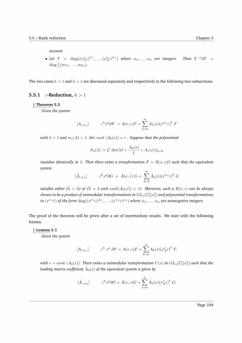
5.5 ε-Rank reduction Chapter 5
account.
• Let T = diag((xσAε)
α1 , . . . , (xσAε)
αn) where α1, . . . , αn are integers. Then T−1∂T =
diag 1x (σα1, . . . , σαn).
The two cases h > 1 and h = 1 are discussed separately and respectively in the following two subsections.
5.5.1 ε-Reduction, h > 1
| Theorem 5.3
Given the system
[Aε,σA] εhxp∂F = A(x, ε)F =
∞∑
k=0
Ak(x)(xσAε)
kF
with h > 1 and mε(A) > 1. Set rank (A0(x)) = r . Suppose that the polynomial
θA(λ) := ξr det(λI +A0(x)
ξ+A1(x))|ξ=0
vanishes identically in λ. Then there exists a transformation F = R(x, ε)G such that the equivalent
system
[Aε,σA] εhxp∂G = A(x, ε) G =
∞∑
k=0
Ak(x)(xσAε)
kG
satisfies either (h < h) or (h = h and rank(A0(x)) < r). Moreover, such a R(x, ε) can be always
chosen to be a product of unimodular transformations in GLn(C[[x]]) and polynomial transformations
in (xσAε) of the form diag((xσAε)α1 , . . . , (xσAε)αn) where α1, . . . , αn are nonnegative integers.
The proof of the theorem will be given after a set of intermediate results. We start with the following
lemma.
| Lemma 5.1
Given the system
[Aε,σA] εh xp ∂F = A(x, ε)F =
∞∑
k=0
Ak(x)(xσAε)
kF,
with r = rank (A0(x)). There exists a unimodular transformation U(x) in GLn(C[[x]]) such that the
leading matrix coefficient A0(x) of the equivalent system is given by
[Aε,σA] εhxp∂G = A(x, ε)G =
∞∑
k=0
Ak(x)(xσAε)
kG,
Page 104
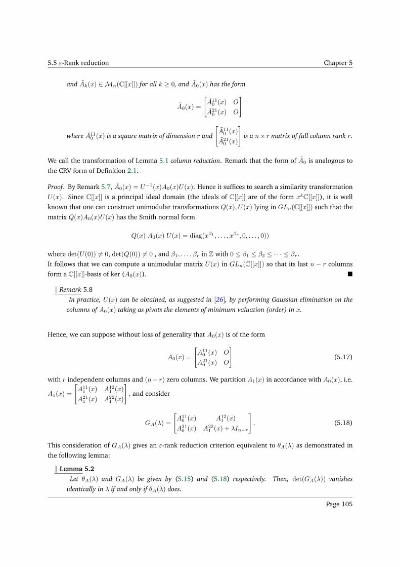
5.5 ε-Rank reduction Chapter 5
and Ak(x) ∈Mn(C[[x]]) for all k ≥ 0, and A0(x) has the form
A0(x) =
[
A110 (x) O
A210 (x) O
]
where A110 (x) is a square matrix of dimension r and
[
A110 (x)
A210 (x)
]
is a n× r matrix of full column rank r.
We call the transformation of Lemma 5.1 column reduction. Remark that the form of A0 is analogous to
the CRV form of Definition 2.1.
Proof. By Remark 5.7, A0(x) = U−1(x)A0(x)U(x). Hence it suffices to search a similarity transformation
U(x). Since C[[x]] is a principal ideal domain (the ideals of C[[x]] are of the form xkC[[x]]), it is well
known that one can construct unimodular transformations Q(x), U(x) lying in GLn(C[[x]]) such that the
matrix Q(x)A0(x)U(x) has the Smith normal form
Q(x) A0(x) U(x) = diag(xβ1 , . . . , xβr , 0, . . . , 0))
where det(U(0)) 6= 0, det(Q(0)) 6= 0 , and β1, . . . , βr in Z with 0 ≤ β1 ≤ β2 ≤ · · · ≤ βr.
It follows that we can compute a unimodular matrix U(x) in GLn(C[[x]]) so that its last n − r columns
form a C[[x]]-basis of ker (A0(x)).
| Remark 5.8
In practice, U(x) can be obtained, as suggested in [26], by performing Gaussian elimination on the
columns of A0(x) taking as pivots the elements of minimum valuation (order) in x.
Hence, we can suppose without loss of generality that A0(x) is of the form
A0(x) =
[
A110 (x) O
A210 (x) O
]
(5.17)
with r independent columns and (n− r) zero columns. We partition A1(x) in accordance with A0(x), i.e.
A1(x) =
[
A111 (x) A12
1 (x)
A211 (x) A22
1 (x)
]
, and consider
GA(λ) =
[
A110 (x) A12
1 (x)
A210 (x) A22
1 (x) + λIn−r
]
. (5.18)
This consideration of GA(λ) gives an ε-rank reduction criterion equivalent to θA(λ) as demonstrated in
the following lemma:
| Lemma 5.2
Let θA(λ) and GA(λ) be given by (5.15) and (5.18) respectively. Then, det(GA(λ)) vanishes
identically in λ if and only if θA(λ) does.
Page 105
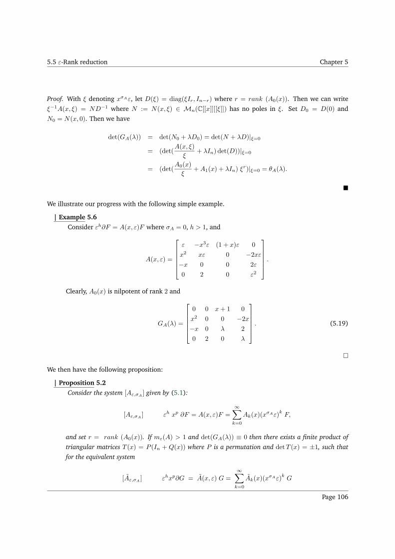
5.5 ε-Rank reduction Chapter 5
Proof. With ξ denoting xσAε, let D(ξ) = diag(ξIr, In−r) where r = rank (A0(x)). Then we can write
ξ−1A(x, ξ) = ND−1 where N := N(x, ξ) ∈ Mn(C[[x]][[ξ]]) has no poles in ξ. Set D0 = D(0) and
N0 = N(x, 0). Then we have
det(GA(λ)) = det(N0 + λD0) = det(N + λD)|ξ=0
= (det(A(x, ξ)
ξ+ λIn) det(D))|ξ=0
= (det(A0(x)
ξ+A1(x) + λIn) ξ
r)|ξ=0 = θA(λ).
We illustrate our progress with the following simple example.
| Example 5.6
Consider εh∂F = A(x, ε)F where σA = 0, h > 1, and
A(x, ε) =
ε −x3ε (1 + x)ε 0
x2 xε 0 −2xε−x 0 0 2ε
0 2 0 ε2
.
Clearly, A0(x) is nilpotent of rank 2 and
GA(λ) =
0 0 x+ 1 0
x2 0 0 −2x−x 0 λ 2
0 2 0 λ
. (5.19)
We then have the following proposition:
| Proposition 5.2
Consider the system [Aε,σA] given by (5.1):
[Aε,σA] εh xp ∂F = A(x, ε)F =
∞∑
k=0
Ak(x)(xσAε)
kF,
and set r = rank (A0(x)). If mε(A) > 1 and det(GA(λ)) ≡ 0 then there exists a finite product of
triangular matrices T (x) = P (In + Q(x)) where P is a permutation and detT (x) = ±1, such that
for the equivalent system
[Aε,σA] εhxp∂G = A(x, ε) G =
∞∑
k=0
Ak(x)(xσAε)
kG
Page 106
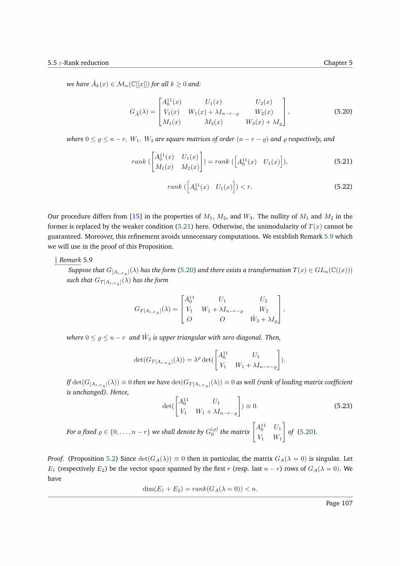
5.5 ε-Rank reduction Chapter 5
we have Ak(x) ∈Mn(C[[x]]) for all k ≥ 0 and:
GA(λ) =
A110 (x) U1(x) U2(x)
V1(x) W1(x) + λIn−r− W2(x)
M1(x) M2(x) W3(x) + λI
, (5.20)
where 0 ≤ ≤ n− r, W1, W3 are square matrices of order (n− r − ) and respectively, and
rank (
[
A110 (x) U1(x)
M1(x) M2(x)
]
) = rank ([
A110 (x) U1(x)
]
), (5.21)
rank ([
A110 (x) U1(x)
]
) < r. (5.22)
Our procedure differs from [15] in the properties of M1, M2, and W3. The nullity of M1 and M2 in the
former is replaced by the weaker condition (5.21) here. Otherwise, the unimodularity of T (x) cannot be
guaranteed. Moreover, this refinement avoids unnecessary computations. We establish Remark 5.9 which
we will use in the proof of this Proposition.
| Remark 5.9
Suppose that G[Aε,σA](λ) has the form (5.20) and there exists a transformation T (x) ∈ GLn(C((x)))
such that GT [Aε,σA](λ) has the form
GT [Aε,σA](λ) =
A110 U1 U2
V1 W1 + λIn−r− W2
O O W3 + λI
,
where 0 ≤ ≤ n− r and W3 is upper triangular with zero diagonal. Then,
det(GT [Aε,σA](λ)) = λ det(
[
A110 U1
V1 W1 + λIn−r−
]
).
If det(G[Aε,σA](λ)) ≡ 0 then we have det(GT [Aε,σA
](λ)) ≡ 0 as well (rank of leading matrix coefficient
is unchanged). Hence,
det(
[
A110 U1
V1 W1 + λIn−r−
]
) ≡ 0. (5.23)
For a fixed ∈ 0, . . . , n− r we shall denote by G()0 the matrix
[
A110 U1
V1 W1
]
of (5.20).
Proof. (Proposition 5.2) Since det(GA(λ)) ≡ 0 then in particular, the matrix GA(λ = 0) is singular. Let
E1 (respectively E2) be the vector space spanned by the first r (resp. last n− r) rows of GA(λ = 0). We
have
dim(E1 + E2) = rank(GA(λ = 0)) < n.
Page 107
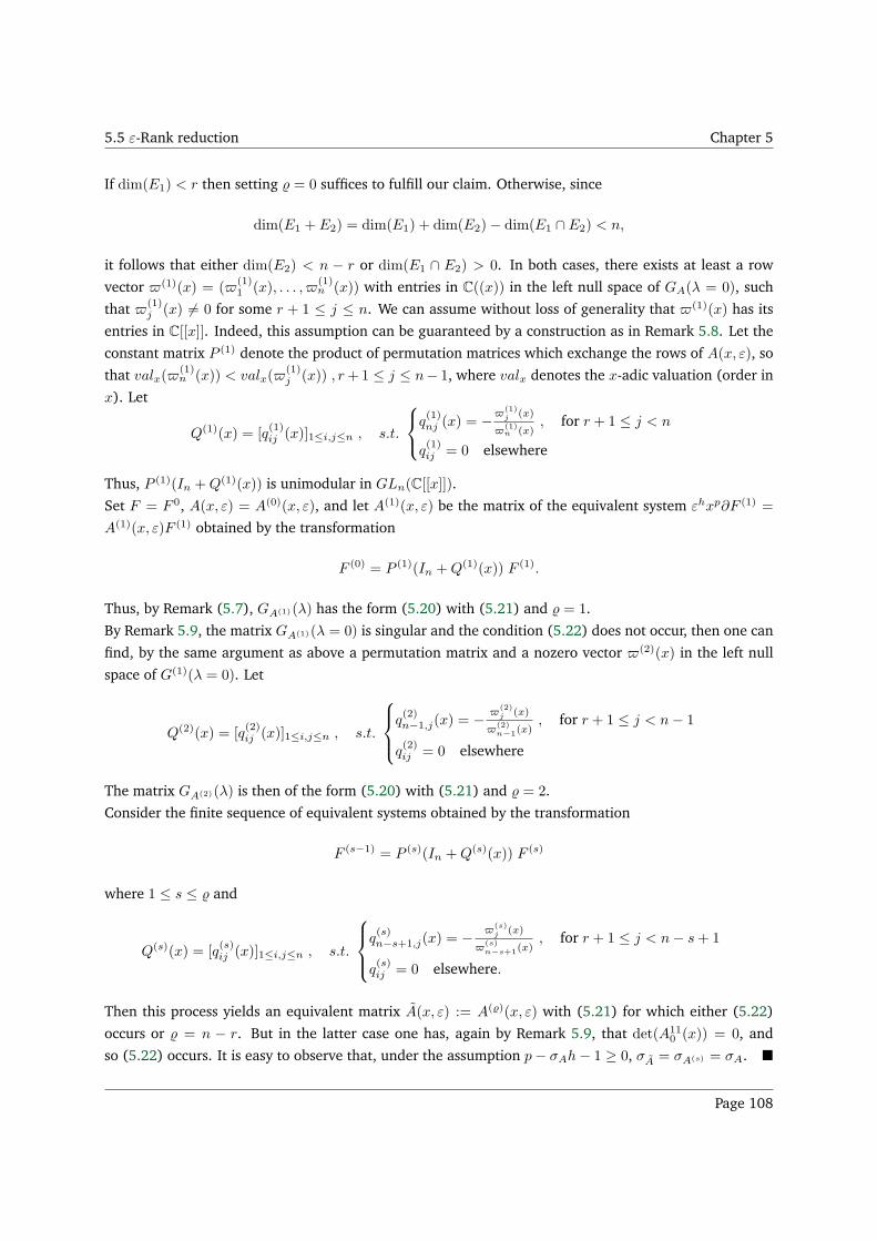
5.5 ε-Rank reduction Chapter 5
If dim(E1) < r then setting = 0 suffices to fulfill our claim. Otherwise, since
dim(E1 + E2) = dim(E1) + dim(E2)− dim(E1 ∩ E2) < n,
it follows that either dim(E2) < n − r or dim(E1 ∩ E2) > 0. In both cases, there exists at least a row
vector (1)(x) = ((1)1 (x), . . . ,
(1)n (x)) with entries in C((x)) in the left null space of GA(λ = 0), such
that (1)j (x) 6= 0 for some r + 1 ≤ j ≤ n. We can assume without loss of generality that (1)(x) has its
entries in C[[x]]. Indeed, this assumption can be guaranteed by a construction as in Remark 5.8. Let the
constant matrix P (1) denote the product of permutation matrices which exchange the rows of A(x, ε), so
that valx((1)n (x)) < valx(
(1)j (x)) , r+1 ≤ j ≤ n− 1, where valx denotes the x-adic valuation (order in
x). Let
Q(1)(x) = [q(1)ij (x)]1≤i,j≤n , s.t.
q(1)nj (x) = −
(1)j (x)
(1)n (x)
, for r + 1 ≤ j < n
q(1)ij = 0 elsewhere
Thus, P (1)(In +Q(1)(x)) is unimodular in GLn(C[[x]]).
Set F = F 0, A(x, ε) = A(0)(x, ε), and let A(1)(x, ε) be the matrix of the equivalent system εhxp∂F (1) =
A(1)(x, ε)F (1) obtained by the transformation
F (0) = P (1)(In +Q(1)(x)) F (1).
Thus, by Remark (5.7), GA(1)(λ) has the form (5.20) with (5.21) and = 1.
By Remark 5.9, the matrix GA(1)(λ = 0) is singular and the condition (5.22) does not occur, then one can
find, by the same argument as above a permutation matrix and a nozero vector (2)(x) in the left null
space of G(1)(λ = 0). Let
Q(2)(x) = [q(2)ij (x)]1≤i,j≤n , s.t.
q(2)n−1,j(x) = −
(2)j (x)
(2)n−1(x)
, for r + 1 ≤ j < n− 1
q(2)ij = 0 elsewhere
The matrix GA(2)(λ) is then of the form (5.20) with (5.21) and = 2.
Consider the finite sequence of equivalent systems obtained by the transformation
F (s−1) = P (s)(In +Q(s)(x)) F (s)
where 1 ≤ s ≤ and
Q(s)(x) = [q(s)ij (x)]1≤i,j≤n , s.t.
q(s)n−s+1,j(x) = −
(s)j (x)
(s)n−s+1(x)
, for r + 1 ≤ j < n− s+ 1
q(s)ij = 0 elsewhere.
Then this process yields an equivalent matrix A(x, ε) := A()(x, ε) with (5.21) for which either (5.22)
occurs or = n − r. But in the latter case one has, again by Remark 5.9, that det(A110 (x)) = 0, and
so (5.22) occurs. It is easy to observe that, under the assumption p− σAh− 1 ≥ 0, σA = σA(s) = σA.
Page 108
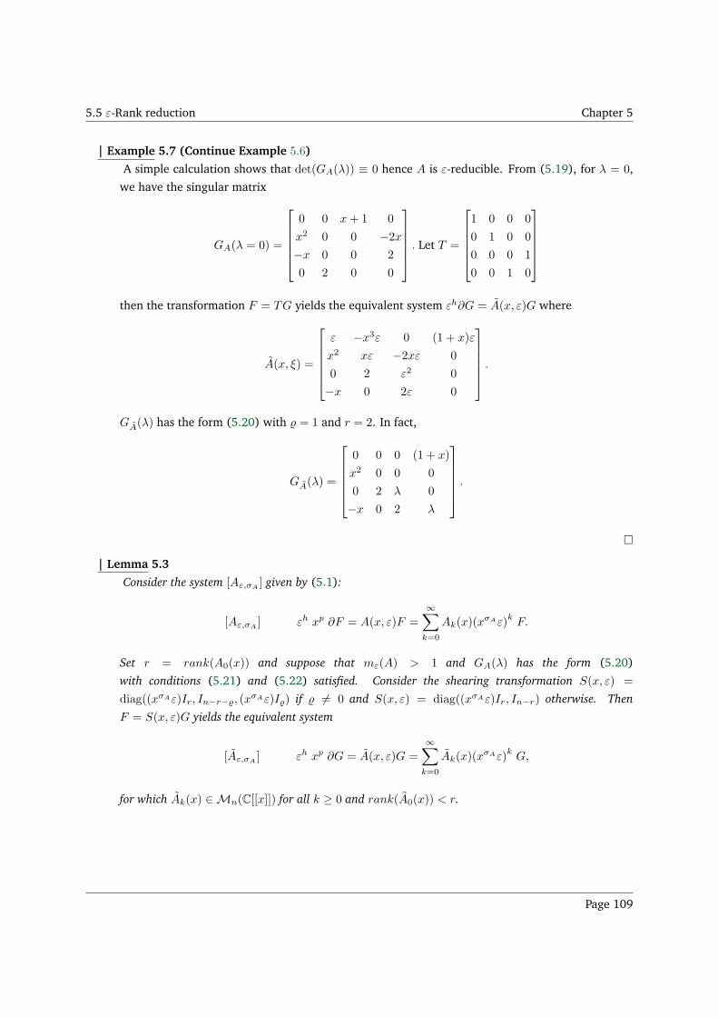
5.5 ε-Rank reduction Chapter 5
| Example 5.7 (Continue Example 5.6)
A simple calculation shows that det(GA(λ)) ≡ 0 hence A is ε-reducible. From (5.19), for λ = 0,
we have the singular matrix
GA(λ = 0) =
0 0 x+ 1 0
x2 0 0 −2x−x 0 0 2
0 2 0 0
. Let T =
1 0 0 0
0 1 0 0
0 0 0 1
0 0 1 0
then the transformation F = TG yields the equivalent system εh∂G = A(x, ε)G where
A(x, ξ) =
ε −x3ε 0 (1 + x)ε
x2 xε −2xε 0
0 2 ε2 0
−x 0 2ε 0
.
GA(λ) has the form (5.20) with = 1 and r = 2. In fact,
GA(λ) =
0 0 0 (1 + x)
x2 0 0 0
0 2 λ 0
−x 0 2 λ
.
| Lemma 5.3
Consider the system [Aε,σA] given by (5.1):
[Aε,σA] εh xp ∂F = A(x, ε)F =
∞∑
k=0
Ak(x)(xσAε)
kF.
Set r = rank(A0(x)) and suppose that mε(A) > 1 and GA(λ) has the form (5.20)
with conditions (5.21) and (5.22) satisfied. Consider the shearing transformation S(x, ε) =
diag((xσAε)Ir, In−r−, (xσAε)I) if 6= 0 and S(x, ε) = diag((xσAε)Ir, In−r) otherwise. Then
F = S(x, ε)G yields the equivalent system
[Aε,σA] εh xp ∂G = A(x, ε)G =
∞∑
k=0
Ak(x)(xσAε)
kG,
for which Ak(x) ∈Mn(C[[x]]) for all k ≥ 0 and rank(A0(x)) < r.
Page 109
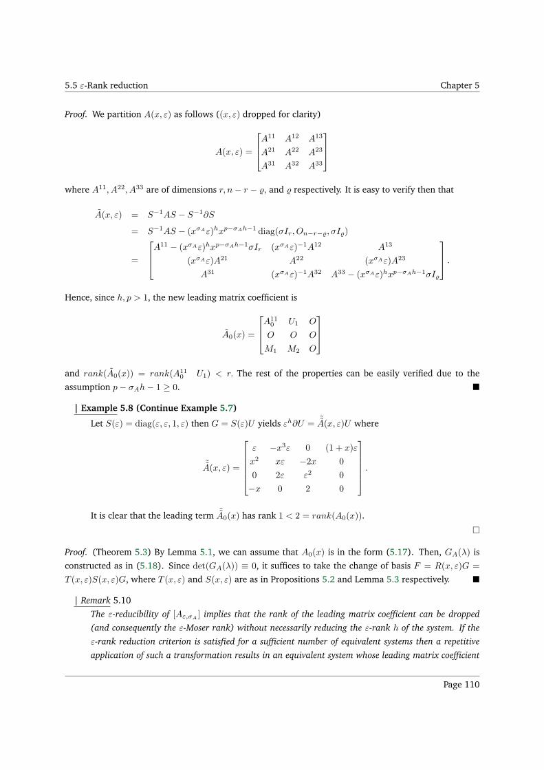
5.5 ε-Rank reduction Chapter 5
Proof. We partition A(x, ε) as follows ((x, ε) dropped for clarity)
A(x, ε) =
A11 A12 A13
A21 A22 A23
A31 A32 A33
where A11, A22, A33 are of dimensions r, n− r − , and respectively. It is easy to verify then that
A(x, ε) = S−1AS − S−1∂S
= S−1AS − (xσAε)hxp−σAh−1 diag(σIr, On−r−, σI)
=
A11 − (xσAε)hxp−σAh−1σIr (xσAε)−1A12 A13
(xσAε)A21 A22 (xσAε)A23
A31 (xσAε)−1A32 A33 − (xσAε)hxp−σAh−1σI
.
Hence, since h, p > 1, the new leading matrix coefficient is
A0(x) =
A110 U1 O
O O O
M1 M2 O
and rank(A0(x)) = rank(A110 U1) < r. The rest of the properties can be easily verified due to the
assumption p− σAh− 1 ≥ 0.
| Example 5.8 (Continue Example 5.7)
Let S(ε) = diag(ε, ε, 1, ε) then G = S(ε)U yields εh∂U = ˜A(x, ε)U where
˜A(x, ε) =
ε −x3ε 0 (1 + x)ε
x2 xε −2x 0
0 2ε ε2 0
−x 0 2 0
.
It is clear that the leading term ˜A0(x) has rank 1 < 2 = rank(A0(x)).
Proof. (Theorem 5.3) By Lemma 5.1, we can assume that A0(x) is in the form (5.17). Then, GA(λ) is
constructed as in (5.18). Since det(GA(λ)) ≡ 0, it suffices to take the change of basis F = R(x, ε)G =
T (x, ε)S(x, ε)G, where T (x, ε) and S(x, ε) are as in Propositions 5.2 and Lemma 5.3 respectively.
| Remark 5.10
The ε-reducibility of [Aε,σA] implies that the rank of the leading matrix coefficient can be dropped
(and consequently the ε-Moser rank) without necessarily reducing the ε-rank h of the system. If the
ε-rank reduction criterion is satisfied for a sufficient number of equivalent systems then a repetitive
application of such a transformation results in an equivalent system whose leading matrix coefficient
Page 110
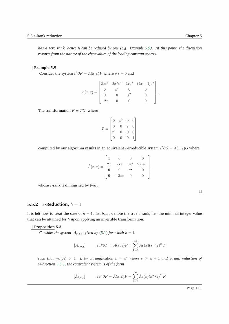
5.5 ε-Rank reduction Chapter 5
has a zero rank, hence h can be reduced by one (e.g. Example 5.9). At this point, the discussion
restarts from the nature of the eigenvalues of the leading constant matrix.
| Example 5.9
Consider the system ε4∂F = A(x, ε)F where σA = 0 and
A(x, ε) =
2xε3 3x2ε4 2xε2 (2x+ 1)ε5
0 ε4 0 0
0 0 ε2 0
−2x 0 0 0
.
The transformation F = TG, where
T =
0 ε3 0 0
0 0 ε 0
ε3 0 0 0
0 0 0 1
,
computed by our algorithm results in an equivalent ε-irreducible system ε2∂G = A(x, ε)G where
A(x, ε) =
1 0 0 0
2x 2xε 3x2 2x+ 1
0 0 ε2 0
0 −2xε 0 0
,
whose ε-rank is diminished by two .
5.5.2 ε-Reduction, h = 1
It is left now to treat the case of h = 1. Let htrue denote the true ε-rank, i.e. the minimal integer value
that can be attained for h upon applying an invertible transformation.
| Proposition 5.3
Consider the system [Aε,σA] given by (5.1) for which h = 1:
[Aε,σA] εxp∂F = A(x, ε)F =
∞∑
k=0
Ak(x)(xσAε)
kF
such that mε(A) > 1. If by a ramification ε = εs where s ≥ n + 1 and ε-rank reduction of
Subsection 5.5.1, the equivalent system is of the form
[Aε,σA] εxp∂F = A(x, ε)F =
∞∑
k=0
Ak(x)(xσA ε)
kF,
Page 111
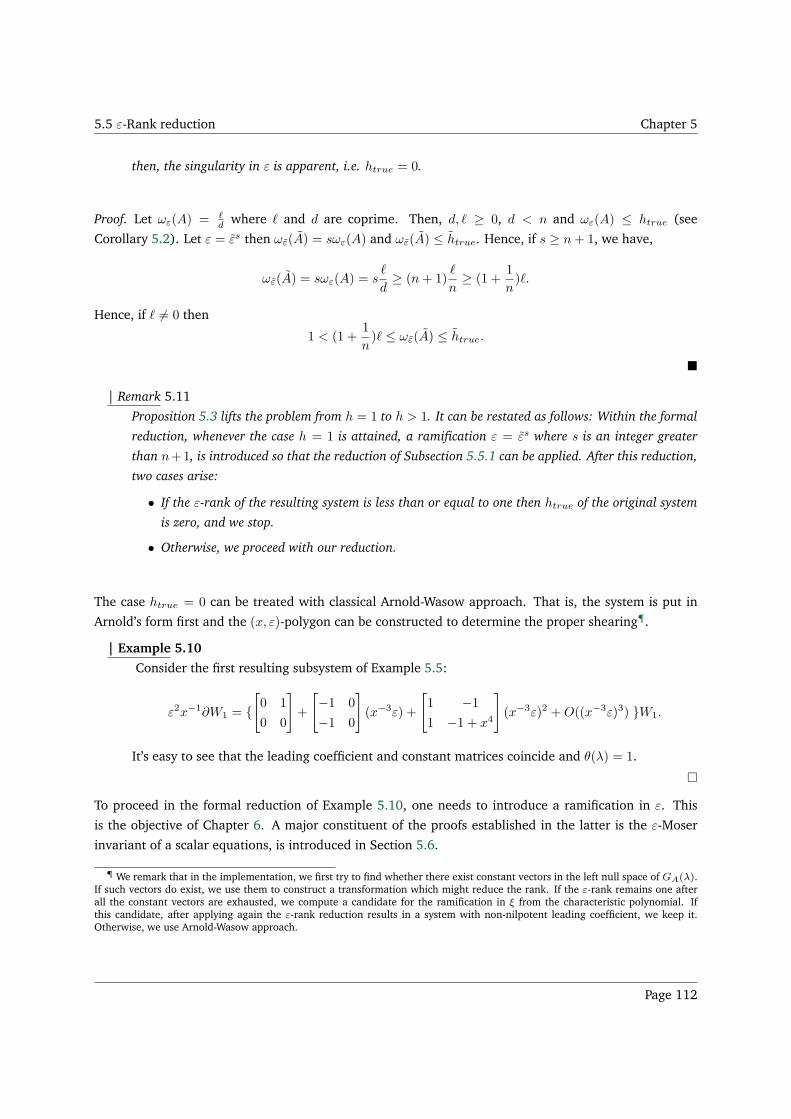
5.5 ε-Rank reduction Chapter 5
then, the singularity in ε is apparent, i.e. htrue = 0.
Proof. Let ωε(A) = ℓd where ℓ and d are coprime. Then, d, ℓ ≥ 0, d < n and ωε(A) ≤ htrue (see
Corollary 5.2). Let ε = εs then ωε(A) = sωε(A) and ωε(A) ≤ htrue. Hence, if s ≥ n+ 1, we have,
ωε(A) = sωε(A) = sℓ
d≥ (n+ 1)
ℓ
n≥ (1 +
1
n)ℓ.
Hence, if ℓ 6= 0 then
1 < (1 +1
n)ℓ ≤ ωε(A) ≤ htrue.
| Remark 5.11
Proposition 5.3 lifts the problem from h = 1 to h > 1. It can be restated as follows: Within the formal
reduction, whenever the case h = 1 is attained, a ramification ε = εs where s is an integer greater
than n+1, is introduced so that the reduction of Subsection 5.5.1 can be applied. After this reduction,
two cases arise:
• If the ε-rank of the resulting system is less than or equal to one then htrue of the original system
is zero, and we stop.
• Otherwise, we proceed with our reduction.
The case htrue = 0 can be treated with classical Arnold-Wasow approach. That is, the system is put in
Arnold’s form first and the (x, ε)-polygon can be constructed to determine the proper shearing¶.
| Example 5.10
Consider the first resulting subsystem of Example 5.5:
ε2x−1∂W1 = [
0 1
0 0
]
+
[
−1 0
−1 0
]
(x−3ε) +
[
1 −11 −1 + x4
]
(x−3ε)2 +O((x−3ε)3) W1.
It’s easy to see that the leading coefficient and constant matrices coincide and θ(λ) = 1.
To proceed in the formal reduction of Example 5.10, one needs to introduce a ramification in ε. This
is the objective of Chapter 6. A major constituent of the proofs established in the latter is the ε-Moser
invariant of a scalar equations, is introduced in Section 5.6.
¶ We remark that in the implementation, we first try to find whether there exist constant vectors in the left null space of GA(λ).If such vectors do exist, we use them to construct a transformation which might reduce the rank. If the ε-rank remains one afterall the constant vectors are exhausted, we compute a candidate for the ramification in ξ from the characteristic polynomial. Ifthis candidate, after applying again the ε-rank reduction results in a system with non-nilpotent leading coefficient, we keep it.Otherwise, we use Arnold-Wasow approach.
Page 112
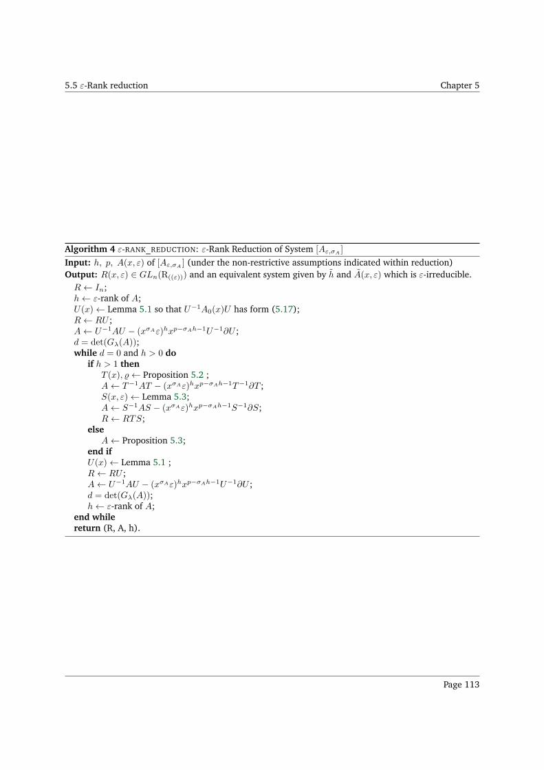
5.5 ε-Rank reduction Chapter 5
Algorithm 4 ε-RANK_REDUCTION: ε-Rank Reduction of System [Aε,σA]
Input: h, p, A(x, ε) of [Aε,σA] (under the non-restrictive assumptions indicated within reduction)
Output: R(x, ε) ∈ GLn(R((ε))) and an equivalent system given by h and A(x, ε) which is ε-irreducible.R← In;h← ε-rank of A;U(x)← Lemma 5.1 so that U−1A0(x)U has form (5.17);R← RU ;A← U−1AU − (xσAε)hxp−σAh−1U−1∂U ;d = det(Gλ(A));while d = 0 and h > 0 do
if h > 1 thenT (x), ← Proposition 5.2 ;A← T−1AT − (xσAε)hxp−σAh−1T−1∂T ;S(x, ε)← Lemma 5.3;A← S−1AS − (xσAε)hxp−σAh−1S−1∂S;R← RTS;
elseA← Proposition 5.3;
end ifU(x)← Lemma 5.1 ;R← RU ;A← U−1AU − (xσAε)hxp−σAh−1U−1∂U ;d = det(Gλ(A));h← ε-rank of A;
end whilereturn (R, A, h).
Page 113
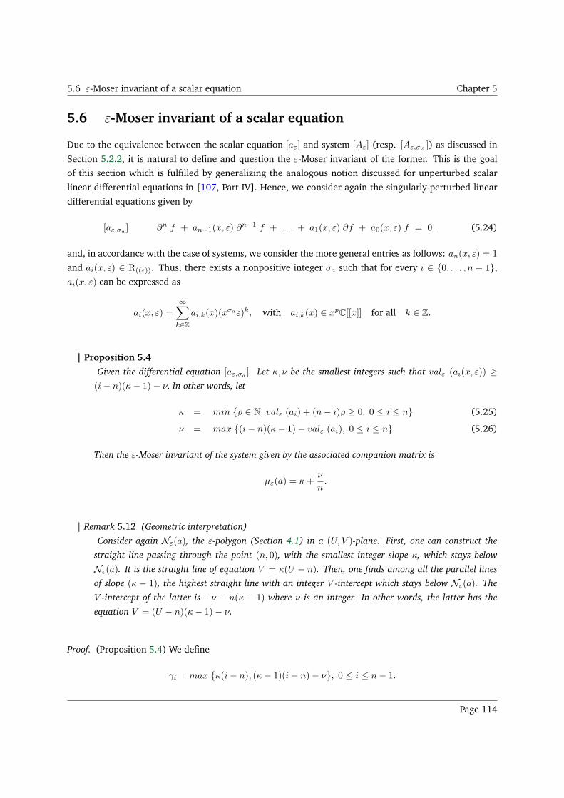
5.6 ε-Moser invariant of a scalar equation Chapter 5
5.6 ε-Moser invariant of a scalar equation
Due to the equivalence between the scalar equation [aε] and system [Aε] (resp. [Aε,σA]) as discussed in
Section 5.2.2, it is natural to define and question the ε-Moser invariant of the former. This is the goal
of this section which is fulfilled by generalizing the analogous notion discussed for unperturbed scalar
linear differential equations in [107, Part IV]. Hence, we consider again the singularly-perturbed linear
differential equations given by
[aε,σa ] ∂n f + an−1(x, ε) ∂n−1 f + . . . + a1(x, ε) ∂f + a0(x, ε) f = 0, (5.24)
and, in accordance with the case of systems, we consider the more general entries as follows: an(x, ε) = 1
and ai(x, ε) ∈ R((ε)). Thus, there exists a nonpositive integer σa such that for every i ∈ 0, . . . , n − 1,ai(x, ε) can be expressed as
ai(x, ε) =
∞∑
k∈Z
ai,k(x)(xσaε)k, with ai,k(x) ∈ xpC[[x]] for all k ∈ Z.
| Proposition 5.4
Given the differential equation [aε,σa ]. Let κ, ν be the smallest integers such that valε (ai(x, ε)) ≥(i− n)(κ− 1)− ν. In other words, let
κ = min ∈ N| valε (ai) + (n− i) ≥ 0, 0 ≤ i ≤ n (5.25)
ν = max (i− n)(κ− 1)− valε (ai), 0 ≤ i ≤ n (5.26)
Then the ε-Moser invariant of the system given by the associated companion matrix is
µε(a) = κ+ν
n.
| Remark 5.12 (Geometric interpretation)
Consider again Nε(a), the ε-polygon (Section 4.1) in a (U, V )-plane. First, one can construct the
straight line passing through the point (n, 0), with the smallest integer slope κ, which stays below
Nε(a). It is the straight line of equation V = κ(U − n). Then, one finds among all the parallel lines
of slope (κ − 1), the highest straight line with an integer V -intercept which stays below Nε(a). The
V -intercept of the latter is −ν − n(κ − 1) where ν is an integer. In other words, the latter has the
equation V = (U − n)(κ− 1)− ν.
Proof. (Proposition 5.4) We define
γi = max κ(i− n), (κ− 1)(i− n)− ν, 0 ≤ i ≤ n− 1.
Page 114
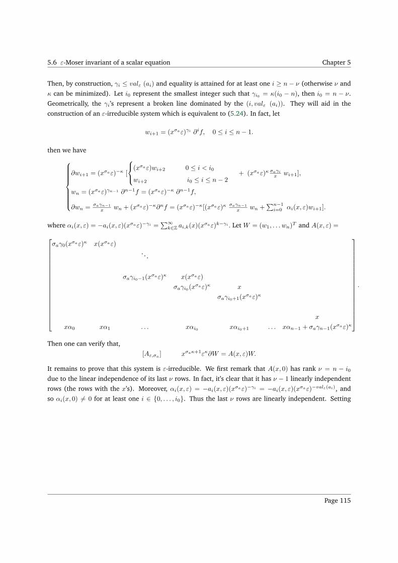
5.6 ε-Moser invariant of a scalar equation Chapter 5
Then, by construction, γi ≤ valε (ai) and equality is attained for at least one i ≥ n− ν (otherwise ν and
κ can be minimized). Let i0 represent the smallest integer such that γi0 = κ(i0 − n), then i0 = n − ν.
Geometrically, the γi’s represent a broken line dominated by the (i, valε (ai)). They will aid in the
construction of an ε-irreducible system which is equivalent to (5.24). In fact, let
wi+1 = (xσaε)γi ∂if, 0 ≤ i ≤ n− 1.
then we have
∂wi+1 = (xσaε)−κ [
(xσaε)wi+2 0 ≤ i < i0
wi+2 i0 ≤ i ≤ n− 2+ (xσaε)κ σaγi
x wi+1],
wn = (xσaε)γn−1 ∂n−1f = (xσaε)−κ ∂n−1f,
∂wn = σaγn−1
x wn + (xσaε)−κ∂nf = (xσaε)−κ[(xσaε)κ σaγn−1
x wn +∑n−1
i=0 αi(x, ε)wi+1].
where αi(x, ε) = −ai(x, ε)(xσaε)−γi =∑∞
k∈Zai,k(x)(x
σaε)k−γi . Let W = (w1, . . . wn)T and A(x, ε) =
σaγ0(xσaε)κ x(xσaε)
. . .
σaγi0−1(xσaε)κ x(xσaε)
σaγi0(xσaε)κ x
σaγi0+1(xσaε)κ
x
xα0 xα1 . . . xαi0 xαi0+1 . . . xαn−1 + σaγn−1(xσaε)κ
.
Then one can verify that,
[Aε,σa ] xσaκ+1εκ∂W = A(x, ε)W.
It remains to prove that this system is ε-irreducible. We first remark that A(x, 0) has rank ν = n − i0
due to the linear independence of its last ν rows. In fact, it’s clear that it has ν − 1 linearly independent
rows (the rows with the x’s). Moreover, αi(x, ε) = −ai(x, ε)(xσaε)−γi = −ai(x, ε)(xσaε)−valε(ai), and
so αi(x, 0) 6= 0 for at least one i ∈ 0, . . . , i0. Thus the last ν rows are linearly independent. Setting
Page 115
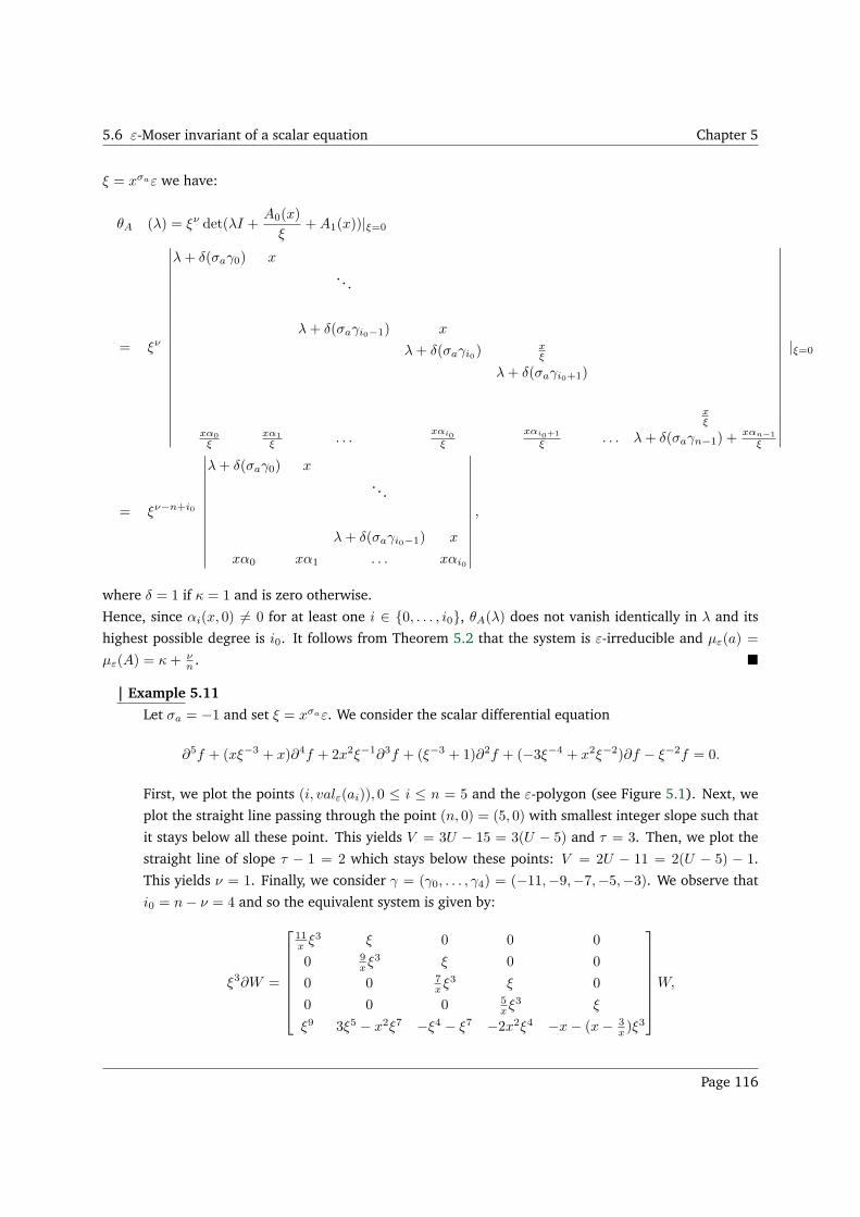
5.6 ε-Moser invariant of a scalar equation Chapter 5
ξ = xσaε we have:
θA (λ) = ξν det(λI +A0(x)
ξ+A1(x))|ξ=0
= ξν
∣∣∣∣∣∣∣∣∣∣∣∣∣∣∣∣∣∣∣∣∣∣∣
λ+ δ(σaγ0) x
. . .
λ+ δ(σaγi0−1) x
λ+ δ(σaγi0)xξ
λ+ δ(σaγi0+1)
xξ
xα0
ξxα1
ξ . . .xαi0
ξ
xαi0+1
ξ . . . λ+ δ(σaγn−1) +xαn−1
ξ
∣∣∣∣∣∣∣∣∣∣∣∣∣∣∣∣∣∣∣∣∣∣∣
|ξ=0
= ξν−n+i0
∣∣∣∣∣∣∣∣∣∣∣∣∣
λ+ δ(σaγ0) x
. . .
λ+ δ(σaγi0−1) x
xα0 xα1 . . . xαi0
∣∣∣∣∣∣∣∣∣∣∣∣∣
,
where δ = 1 if κ = 1 and is zero otherwise.
Hence, since αi(x, 0) 6= 0 for at least one i ∈ 0, . . . , i0, θA(λ) does not vanish identically in λ and its
highest possible degree is i0. It follows from Theorem 5.2 that the system is ε-irreducible and µε(a) =
µε(A) = κ+ νn .
| Example 5.11
Let σa = −1 and set ξ = xσaε. We consider the scalar differential equation
∂5f + (xξ−3 + x)∂4f + 2x2ξ−1∂3f + (ξ−3 + 1)∂2f + (−3ξ−4 + x2ξ−2)∂f − ξ−2f = 0.
First, we plot the points (i, valε(ai)), 0 ≤ i ≤ n = 5 and the ε-polygon (see Figure 5.1). Next, we
plot the straight line passing through the point (n, 0) = (5, 0) with smallest integer slope such that
it stays below all these point. This yields V = 3U − 15 = 3(U − 5) and τ = 3. Then, we plot the
straight line of slope τ − 1 = 2 which stays below these points: V = 2U − 11 = 2(U − 5) − 1.
This yields ν = 1. Finally, we consider γ = (γ0, . . . , γ4) = (−11,−9,−7,−5,−3). We observe that
i0 = n− ν = 4 and so the equivalent system is given by:
ξ3∂W =
11x ξ3 ξ 0 0 0
0 9xξ
3 ξ 0 0
0 0 7xξ
3 ξ 0
0 0 0 5xξ
3 ξ
ξ9 3ξ5 − x2ξ7 −ξ4 − ξ7 −2x2ξ4 −x− (x− 3x )ξ
3
W,
Page 116
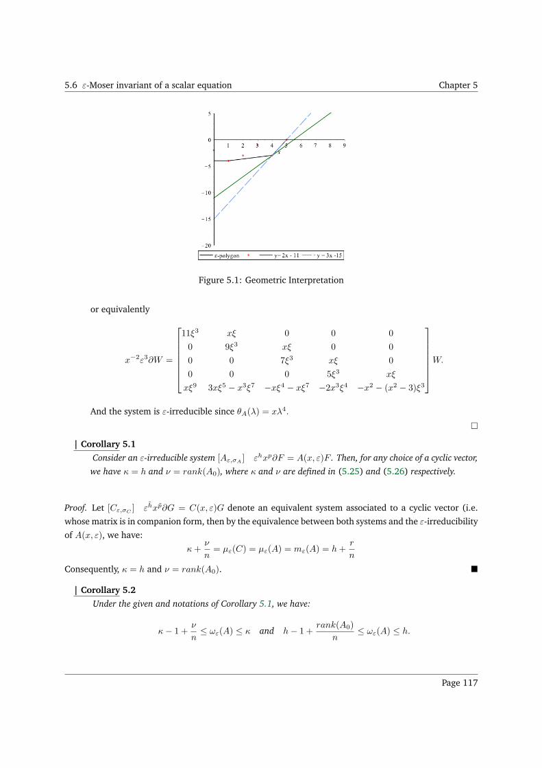
5.6 ε-Moser invariant of a scalar equation Chapter 5
Figure 5.1: Geometric Interpretation
or equivalently
x−2ε3∂W =
11ξ3 xξ 0 0 0
0 9ξ3 xξ 0 0
0 0 7ξ3 xξ 0
0 0 0 5ξ3 xξ
xξ9 3xξ5 − x3ξ7 −xξ4 − xξ7 −2x3ξ4 −x2 − (x2 − 3)ξ3
W.
And the system is ε-irreducible since θA(λ) = xλ4.
| Corollary 5.1
Consider an ε-irreducible system [Aε,σA] εhxp∂F = A(x, ε)F . Then, for any choice of a cyclic vector,
we have κ = h and ν = rank(A0), where κ and ν are defined in (5.25) and (5.26) respectively.
Proof. Let [Cε,σC] εhxp∂G = C(x, ε)G denote an equivalent system associated to a cyclic vector (i.e.
whose matrix is in companion form, then by the equivalence between both systems and the ε-irreducibility
of A(x, ε), we have:
κ+ν
n= µε(C) = µε(A) = mε(A) = h+
r
n
Consequently, κ = h and ν = rank(A0).
| Corollary 5.2
Under the given and notations of Corollary 5.1, we have:
κ− 1 +ν
n≤ ωε(A) ≤ κ and h− 1 +
rank(A0)
n≤ ωε(A) ≤ h.
Page 117
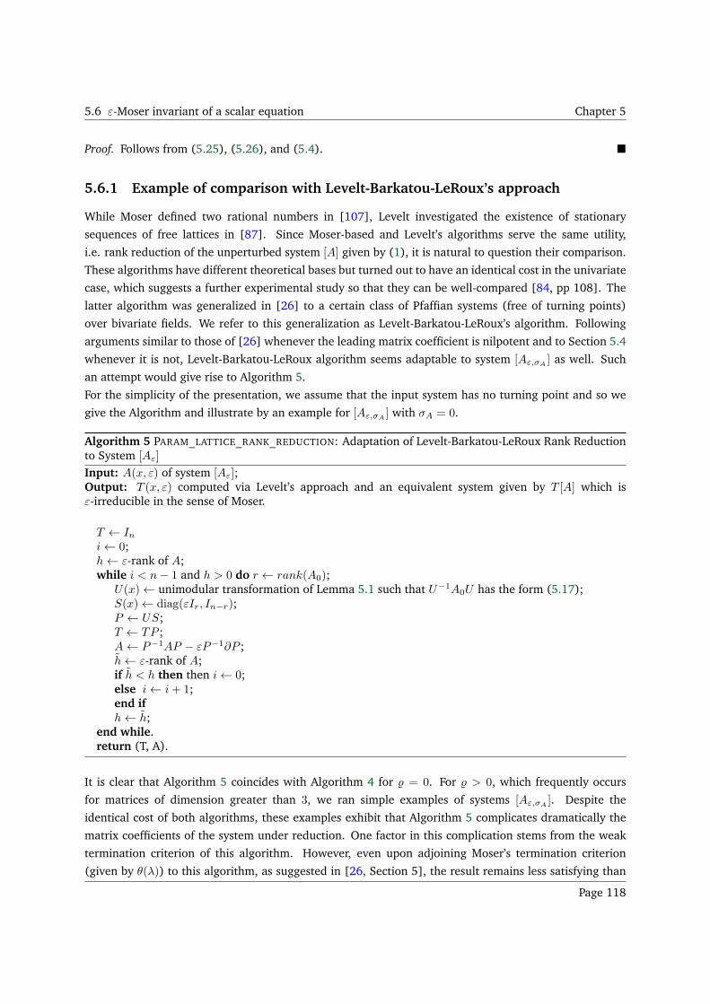
5.6 ε-Moser invariant of a scalar equation Chapter 5
Proof. Follows from (5.25), (5.26), and (5.4).
5.6.1 Example of comparison with Levelt-Barkatou-LeRoux’s approach
While Moser defined two rational numbers in [107], Levelt investigated the existence of stationary
sequences of free lattices in [87]. Since Moser-based and Levelt’s algorithms serve the same utility,
i.e. rank reduction of the unperturbed system [A] given by (1), it is natural to question their comparison.
These algorithms have different theoretical bases but turned out to have an identical cost in the univariate
case, which suggests a further experimental study so that they can be well-compared [84, pp 108]. The
latter algorithm was generalized in [26] to a certain class of Pfaffian systems (free of turning points)
over bivariate fields. We refer to this generalization as Levelt-Barkatou-LeRoux’s algorithm. Following
arguments similar to those of [26] whenever the leading matrix coefficient is nilpotent and to Section 5.4
whenever it is not, Levelt-Barkatou-LeRoux algorithm seems adaptable to system [Aε,σA] as well. Such
an attempt would give rise to Algorithm 5.
For the simplicity of the presentation, we assume that the input system has no turning point and so we
give the Algorithm and illustrate by an example for [Aε,σA] with σA = 0.
Algorithm 5 PARAM_LATTICE_RANK_REDUCTION: Adaptation of Levelt-Barkatou-LeRoux Rank Reductionto System [Aε]
Input: A(x, ε) of system [Aε];Output: T (x, ε) computed via Levelt’s approach and an equivalent system given by T [A] which isε-irreducible in the sense of Moser.
T ← Ini← 0;h← ε-rank of A;while i < n− 1 and h > 0 do r ← rank(A0);
U(x)← unimodular transformation of Lemma 5.1 such that U−1A0U has the form (5.17);S(x)← diag(εIr, In−r);P ← US;T ← TP ;A← P−1AP − εP−1∂P ;h← ε-rank of A;if h < h then then i← 0;else i← i+ 1;end ifh← h;
end while.return (T, A).
It is clear that Algorithm 5 coincides with Algorithm 4 for = 0. For > 0, which frequently occurs
for matrices of dimension greater than 3, we ran simple examples of systems [Aε,σA]. Despite the
identical cost of both algorithms, these examples exhibit that Algorithm 5 complicates dramatically the
matrix coefficients of the system under reduction. One factor in this complication stems from the weak
termination criterion of this algorithm. However, even upon adjoining Moser’s termination criterion
(given by θ(λ)) to this algorithm, as suggested in [26, Section 5], the result remains less satisfying than
Page 118
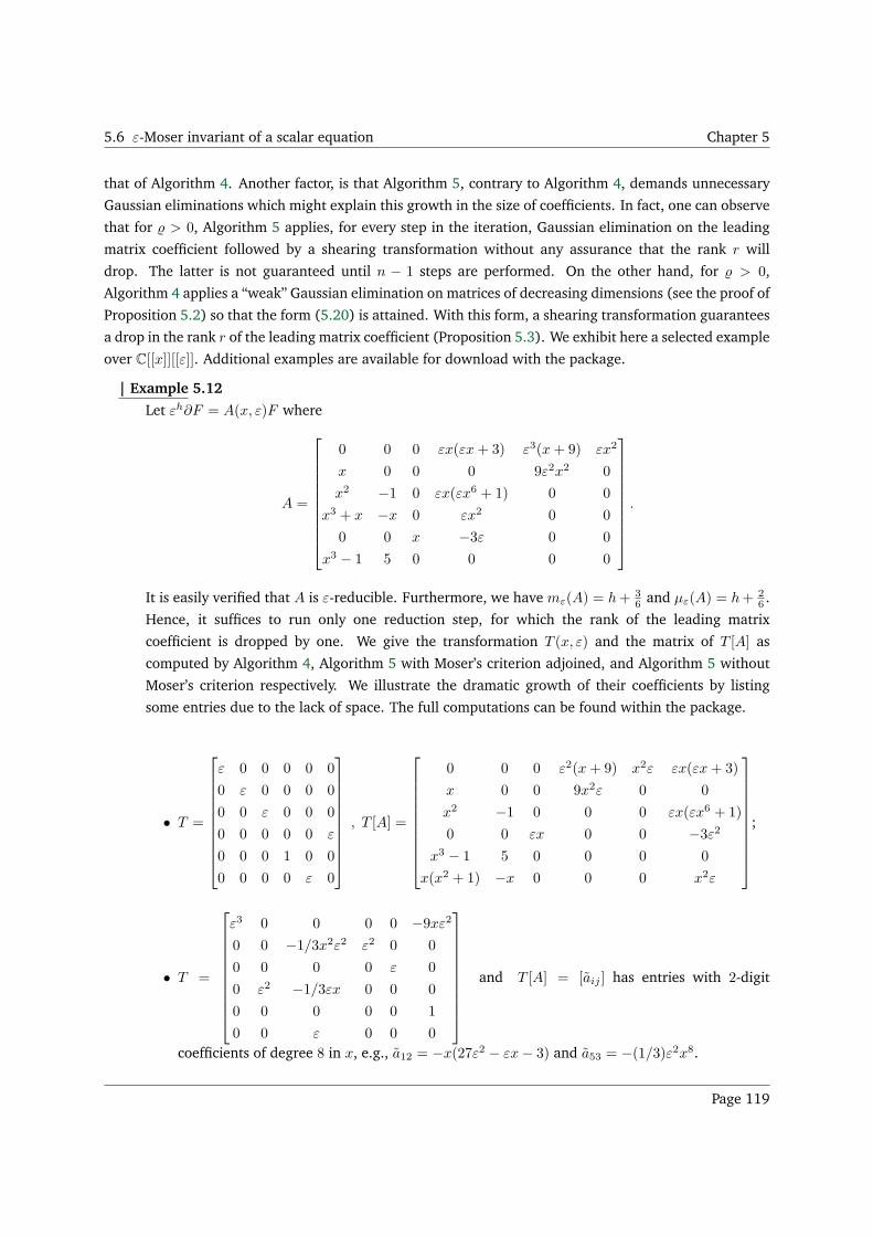
5.6 ε-Moser invariant of a scalar equation Chapter 5
that of Algorithm 4. Another factor, is that Algorithm 5, contrary to Algorithm 4, demands unnecessary
Gaussian eliminations which might explain this growth in the size of coefficients. In fact, one can observe
that for > 0, Algorithm 5 applies, for every step in the iteration, Gaussian elimination on the leading
matrix coefficient followed by a shearing transformation without any assurance that the rank r will
drop. The latter is not guaranteed until n − 1 steps are performed. On the other hand, for > 0,
Algorithm 4 applies a “weak” Gaussian elimination on matrices of decreasing dimensions (see the proof of
Proposition 5.2) so that the form (5.20) is attained. With this form, a shearing transformation guarantees
a drop in the rank r of the leading matrix coefficient (Proposition 5.3). We exhibit here a selected example
over C[[x]][[ε]]. Additional examples are available for download with the package.
| Example 5.12
Let εh∂F = A(x, ε)F where
A =
0 0 0 εx(εx+ 3) ε3(x+ 9) εx2
x 0 0 0 9ε2x2 0
x2 −1 0 εx(εx6 + 1) 0 0
x3 + x −x 0 εx2 0 0
0 0 x −3ε 0 0
x3 − 1 5 0 0 0 0
.
It is easily verified that A is ε-reducible. Furthermore, we have mε(A) = h+ 36 and µε(A) = h+ 2
6 .
Hence, it suffices to run only one reduction step, for which the rank of the leading matrix
coefficient is dropped by one. We give the transformation T (x, ε) and the matrix of T [A] as
computed by Algorithm 4, Algorithm 5 with Moser’s criterion adjoined, and Algorithm 5 without
Moser’s criterion respectively. We illustrate the dramatic growth of their coefficients by listing
some entries due to the lack of space. The full computations can be found within the package.
• T =
ε 0 0 0 0 0
0 ε 0 0 0 0
0 0 ε 0 0 0
0 0 0 0 0 ε
0 0 0 1 0 0
0 0 0 0 ε 0
, T [A] =
0 0 0 ε2(x+ 9) x2ε εx(εx+ 3)
x 0 0 9x2ε 0 0
x2 −1 0 0 0 εx(εx6 + 1)
0 0 εx 0 0 −3ε2x3 − 1 5 0 0 0 0
x(x2 + 1) −x 0 0 0 x2ε
;
• T =
ε3 0 0 0 0 −9xε20 0 −1/3x2ε2 ε2 0 0
0 0 0 0 ε 0
0 ε2 −1/3εx 0 0 0
0 0 0 0 0 1
0 0 ε 0 0 0
and T [A] = [aij ] has entries with 2-digit
coefficients of degree 8 in x, e.g., a12 = −x(27ε2 − εx− 3) and a53 = −(1/3)ε2x8.
Page 119
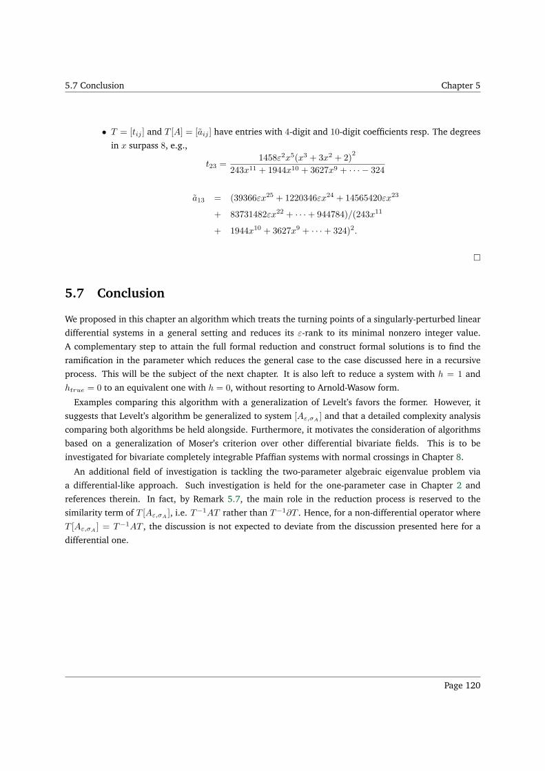
5.7 Conclusion Chapter 5
• T = [tij ] and T [A] = [aij ] have entries with 4-digit and 10-digit coefficients resp. The degrees
in x surpass 8, e.g.,
t23 =1458ε2x5(x3 + 3x2 + 2)
2
243x11 + 1944x10 + 3627x9 + · · · − 324
a13 = (39366εx25 + 1220346εx24 + 14565420εx23
+ 83731482εx22 + · · ·+ 944784)/(243x11
+ 1944x10 + 3627x9 + · · ·+ 324)2.
5.7 Conclusion
We proposed in this chapter an algorithm which treats the turning points of a singularly-perturbed linear
differential systems in a general setting and reduces its ε-rank to its minimal nonzero integer value.
A complementary step to attain the full formal reduction and construct formal solutions is to find the
ramification in the parameter which reduces the general case to the case discussed here in a recursive
process. This will be the subject of the next chapter. It is also left to reduce a system with h = 1 and
htrue = 0 to an equivalent one with h = 0, without resorting to Arnold-Wasow form.
Examples comparing this algorithm with a generalization of Levelt’s favors the former. However, it
suggests that Levelt’s algorithm be generalized to system [Aε,σA] and that a detailed complexity analysis
comparing both algorithms be held alongside. Furthermore, it motivates the consideration of algorithms
based on a generalization of Moser’s criterion over other differential bivariate fields. This is to be
investigated for bivariate completely integrable Pfaffian systems with normal crossings in Chapter 8.
An additional field of investigation is tackling the two-parameter algebraic eigenvalue problem via
a differential-like approach. Such investigation is held for the one-parameter case in Chapter 2 and
references therein. In fact, by Remark 5.7, the main role in the reduction process is reserved to the
similarity term of T [Aε,σA], i.e. T−1AT rather than T−1∂T . Hence, for a non-differential operator where
T [Aε,σA] = T−1AT , the discussion is not expected to deviate from the discussion presented here for a
differential one.
Page 120
Chapter 6
Chapter 6
Computing the ε-Formal Invariants
Contents6.1 Computing ε-exponential order using ε-polygon . . . . . . . . . . . . . . . . . . . . . 121
6.2 Formal reduction algorithm . . . . . . . . . . . . . . . . . . . . . . . . . . . . . . . . . 127
6.3 Examples and investigations . . . . . . . . . . . . . . . . . . . . . . . . . . . . . . . . 130
6.4 Conclusion . . . . . . . . . . . . . . . . . . . . . . . . . . . . . . . . . . . . . . . . . . 142
We consider again system [Aε,σA] which is given by (5.1) and which we recall here:
[Aε,σA] εh xp ∂ F = A(x, ε)F =
∞∑
k=0
Ak(x)(xσAε)k F. (6.1)
In this chapter, we adopt without loss of generality the assumptions of Section 5.1 and the additional
assumption that [Aε,σA] is ε-irreducible and h > 0. The goal of this chapter is to investigate the ε-formal
exponential order (ε-exponential order, in short) and ε-polynomials of system (6.1).
As for system [A] given by (1) in the first chapter, one cannot retrieve ωε(A) of system [Aε,σA] from the
outset. In Section 6.1, we prove that ωε(A) can be computed from the characteristic polynomial of A(x,ε)εhxp
and an associated ε-polygon whenever the system is ε-irreducible.
The ωε(A) and the corresponding ε-polynomial give indispensable information for formal reduction. In
particular, the former determines the ramification in ε which can lead to a system whose leading matrix is
non-nilpotent, so that the process of reduction can be resumed. This leads to the recursive Algorithm 6.
Eventually, we can construct fundamental matrices of formal solutions in any given subdomain. We
illustrate this algorithm by examples and motivate items for further investigation in Section 6.3.
6.1 Computing ε-exponential order using ε-polygon
Consider the ε-irreducible system [Aε,σA] given by (6.1) with h > 0 and let
det(λI − A(x, ε)
εhxp) = λn + αn−1(x, ε)λn−1 + · · ·+ α0(x, ε). (6.2)
Page 121
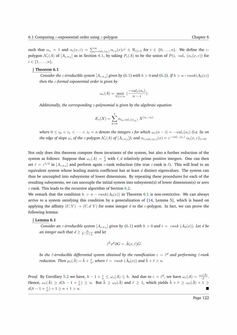
6.1 Computing ε-exponential order using ε-polygon Chapter 6
such that αn = 1 and αi(x, ε) =∑∞
j=valε(αi)αi,j(x)ε
j ∈ R((ε)) for i ∈ 0, . . . , n. We define the ε-
polygon Nε(A) of [Aε,σA] as in Section 4.1, by taking Pε(A) to be the union of P (i, valε (αi(x, ε)) for
i ∈ 1, . . . , n.
| Theorem 6.1
Consider the ε-irreducible system [Aε,σA] given by (6.1) with h > 0 and (6.2). If h > n−rank(A0(x))
then the ε-formal exponential order is given by
ωε(A) = max0≤i<n
(−valε(αi)
n− i).
Additionally, the corresponding ε-polynomial is given by the algebraic equation
Eε(X) =
ℓ∑
k=0
αik,valε(αik) X
(ik−i0)
where 0 ≤ i0 < i1 < · · · < iℓ = n denote the integers i for which ωε(n − i) = −valε(αi) (i.e. lie on
the edge of slope ωε of the ε-polygon Nε(A) of [Aε,σA]); and αi,valε(αi)(x) = ε−valε (αi) αi(x, ε)|ε=0.
Not only does this theorem compute these invariants of the system, but also a further reduction of the
system as follows: Suppose that ωε(A) = ℓd with ℓ, d relatively prime positive integers. One can then
set ε = ε1/d in [Aε,σA] and perform again ε-rank reduction (the true ε-rank is ℓ). This will lead to an
equivalent system whose leading matrix coefficient has at least d distinct eigenvalues. The system can
thus be uncoupled into subsystems of lower dimensions. By repeating these procedures for each of the
resulting subsystems, we can uncouple the initial system into subsystem(s) of lower dimension(s) or zero
ε-rank. This leads to the recursive algorithm of Section 6.2.
We remark that the condition h > n − rank(A0(x)) in Theorem 6.1 is non-restrictive. We can always
arrive to a system satisfying this condition by a generalization of [14, Lemma 5], which is based on
applying the affinity (U, V ) → (U, d V ) for some integer d to the ε-polygon. In fact, we can prove the
following lemma:
| Lemma 6.1
Consider an ε-irreducible system [Aε,σA] given by (6.1) with h > 0 and r = rank (A0(x)). Let d be
an integer such that d ≥ nh−1+ r
nand let
εhxp∂G = A(x, ε)G.
be the ε-irreducible differential system obtained by the ramification ε = εd and performing ε-rank
reduction. Then µε(A) = h+ rn , where r = rank (A0(x)) and h+ r > n.
Proof. By Corollary 5.2 we have, h − 1 + rn ≤ ωε(A) ≤ h. And due to ε = εd, we have ωε(A) =
ωε(A)d .
Hence, ωε(A) ≥ d(h − 1 + rn ) ≥ n. But h ≥ ωε(A) and r ≥ 1, which yields h + r ≥ ωε(A) + 1 ≥
d(h− 1 + rn ) + 1 ≥ n+ 1 > n.
Page 122
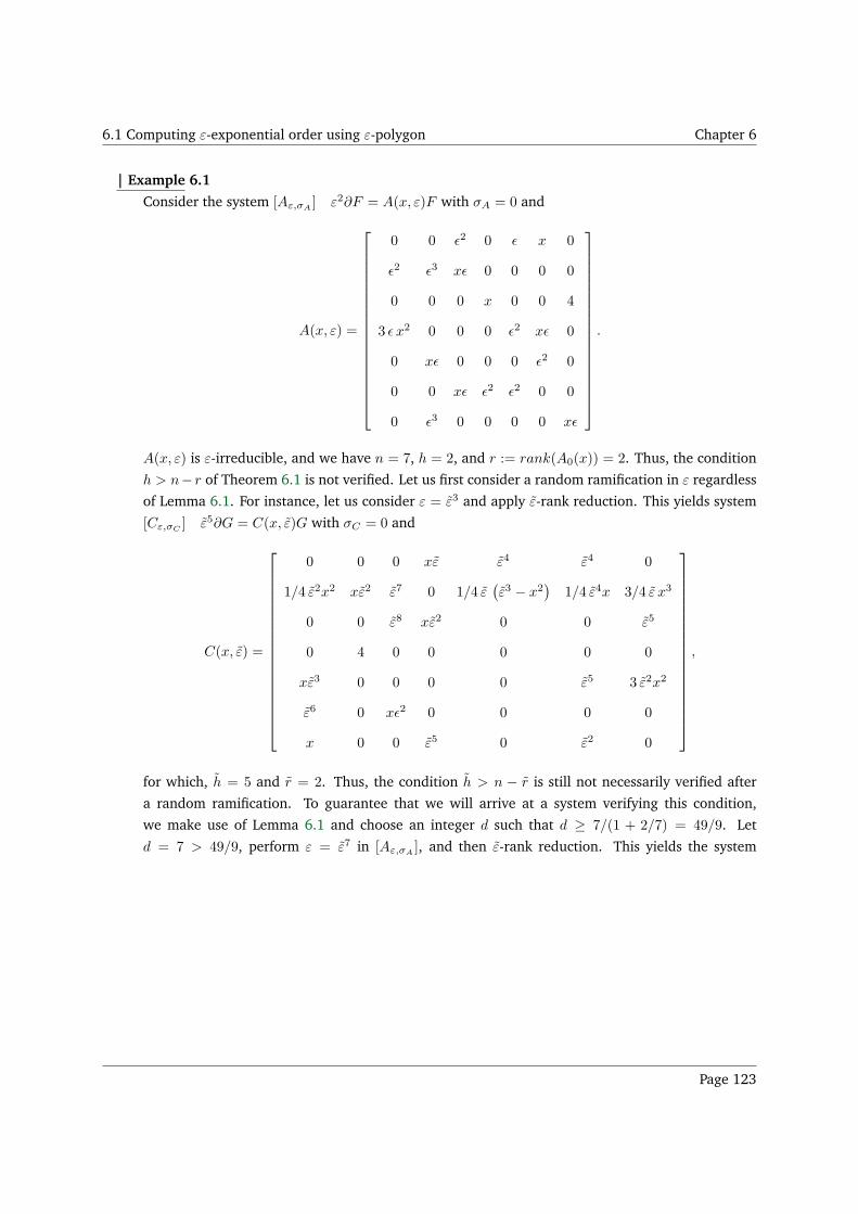
6.1 Computing ε-exponential order using ε-polygon Chapter 6
| Example 6.1
Consider the system [Aε,σA] ε2∂F = A(x, ε)F with σA = 0 and
A(x, ε) =
0 0 ǫ2 0 ǫ x 0
ǫ2 ǫ3 xǫ 0 0 0 0
0 0 0 x 0 0 4
3 ǫ x2 0 0 0 ǫ2 xǫ 0
0 xǫ 0 0 0 ǫ2 0
0 0 xǫ ǫ2 ǫ2 0 0
0 ǫ3 0 0 0 0 xǫ
.
A(x, ε) is ε-irreducible, and we have n = 7, h = 2, and r := rank(A0(x)) = 2. Thus, the condition
h > n− r of Theorem 6.1 is not verified. Let us first consider a random ramification in ε regardless
of Lemma 6.1. For instance, let us consider ε = ε3 and apply ε-rank reduction. This yields system
[Cε,σC] ε5∂G = C(x, ε)G with σC = 0 and
C(x, ε) =
0 0 0 xε ε4 ε4 0
1/4 ε2x2 xε2 ε7 0 1/4 ε(ε3 − x2
)1/4 ε4x 3/4 ε x3
0 0 ε8 xε2 0 0 ε5
0 4 0 0 0 0 0
xε3 0 0 0 0 ε5 3 ε2x2
ε6 0 xǫ2 0 0 0 0
x 0 0 ε5 0 ε2 0
,
for which, h = 5 and r = 2. Thus, the condition h > n − r is still not necessarily verified after
a random ramification. To guarantee that we will arrive at a system verifying this condition,
we make use of Lemma 6.1 and choose an integer d such that d ≥ 7/(1 + 2/7) = 49/9. Let
d = 7 > 49/9, perform ε = ε7 in [Aε,σA], and then ε-rank reduction. This yields the system
Page 123
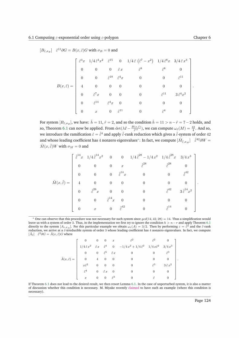
6.1 Computing ε-exponential order using ε-polygon Chapter 6
[Bε,σB] ε11∂G = B(x, ε)G with σB = 0 and
B(x, ε) =
ε4x 1/4 ε4x2 ε15 0 1/4 ε(ε7 − x2
)1/4 ε8x 3/4 ε x3
0 0 0 ε x ε8 ε8 0
0 0 ε18 ε4x 0 0 ε11
4 0 0 0 0 0 0
0 ε7x 0 0 0 ε11 3 ε4x2
0 ε14 ε4x 0 0 0 0
0 x 0 ε11 0 ε4 0
.
For system [Bε,σB], we have: h = 11, r = 2, and so the condition h = 11 > n− r = 7− 2 holds, and
so, Theorem 6.1 can now be applied. From det(λI− B(x,ε)ε11 ), we can compute ωε(M) = 42
4 . And so,
we introduce the ramification ε = ˜ε4 and apply ˜ε-rank reduction which gives a ˜ε-system of order 42
and whose leading coefficient has 4 nonzero eigenvalues∗: In fact, we compute [M˜ε,σM] ˜ε42∂W =
M(x, ˜ε)W with σM = 0 and
M(x, ˜ε) =
˜ε14x 1/4 ˜ε
14x2 0 0 1/4 ˜ε
28 − 1/4x2 1/4 ˜ε28x 3/4x3
0 0 0 x ˜ε28 ˜ε
280
0 0 0 ˜ε14x 0 0 ˜ε
42
4 0 0 0 0 0 0
0 ˜ε28x 0 0 0 ˜ε
423 ˜ε
14x2
0 0 ˜ε14x 0 0 0 0
0 x 0 ˜ε42
0 ˜ε14
0
.
∗ One can observe that this procedure was not necessary for such system since gcd(14, 42, 28) = 14. Thus a simplification wouldleave us with a system of order 3. Thus, in the implementation we first try to ignore the condition h > n−r and apply Theorem 6.1directly to the system [Aε,σA ]. For this particular example we obtain ωε(A) = 3/2. Then by performing ε = ε2 and the ε-rankreduction, we arrive at a ε-irreducible system of order 3 whose leading coefficient has 4 nonzero eigenvalues. In fact, we compute[Aε] ε3∂G = A(x, ε)G where
A(x, ε) =
0 0 0 x ε2 ε2 0
1/4 ε x2 ε x ε4 0 −1/4x2 + 1/4 ε2 1/4xε2 3/4x3
0 0 ε5 ε x 0 0 ε3
0 4 0 0 0 0 0
xε2 0 0 0 0 ε3 3 ε x2
ε4 0 ε x 0 0 0 0
x 0 0 ε3 0 ε 0
.
If Theorem 6.1 does not lead to the desired result, we then resort Lemma 6.1. In the case of unperturbed system, it is also a matterof discussion whether this condition is necessary. M. Miyake recently claimed to have such an example (where this condition isnecessary).
Page 124
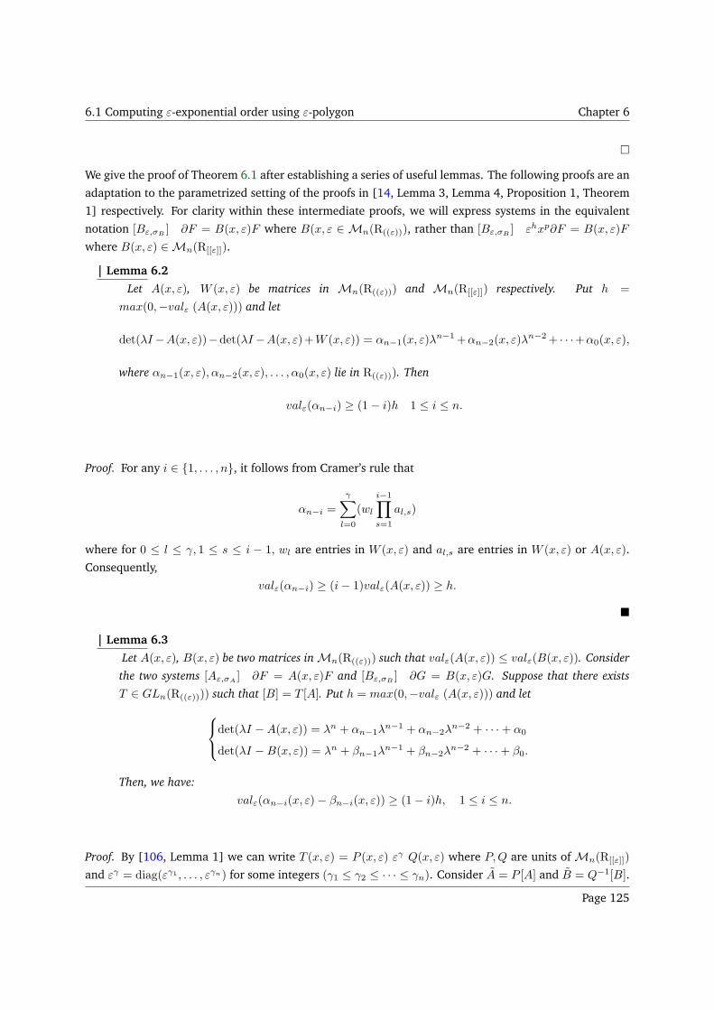
6.1 Computing ε-exponential order using ε-polygon Chapter 6
We give the proof of Theorem 6.1 after establishing a series of useful lemmas. The following proofs are an
adaptation to the parametrized setting of the proofs in [14, Lemma 3, Lemma 4, Proposition 1, Theorem
1] respectively. For clarity within these intermediate proofs, we will express systems in the equivalent
notation [Bε,σB] ∂F = B(x, ε)F where B(x, ε ∈ Mn(R((ε))), rather than [Bε,σB
] εhxp∂F = B(x, ε)F
where B(x, ε) ∈Mn(R[[ε]]).
| Lemma 6.2
Let A(x, ε), W (x, ε) be matrices in Mn(R((ε))) and Mn(R[[ε]]) respectively. Put h =
max(0,−valε (A(x, ε))) and let
det(λI−A(x, ε))−det(λI−A(x, ε)+W (x, ε)) = αn−1(x, ε)λn−1+αn−2(x, ε)λ
n−2+ · · ·+α0(x, ε),
where αn−1(x, ε), αn−2(x, ε), . . . , α0(x, ε) lie in R((ε))). Then
valε(αn−i) ≥ (1− i)h 1 ≤ i ≤ n.
Proof. For any i ∈ 1, . . . , n, it follows from Cramer’s rule that
αn−i =
γ∑
l=0
(wl
i−1∏
s=1
al,s)
where for 0 ≤ l ≤ γ, 1 ≤ s ≤ i − 1, wl are entries in W (x, ε) and al,s are entries in W (x, ε) or A(x, ε).
Consequently,
valε(αn−i) ≥ (i− 1)valε(A(x, ε)) ≥ h.
| Lemma 6.3
Let A(x, ε), B(x, ε) be two matrices inMn(R((ε))) such that valε(A(x, ε)) ≤ valε(B(x, ε)). Consider
the two systems [Aε,σA] ∂F = A(x, ε)F and [Bε,σB
] ∂G = B(x, ε)G. Suppose that there exists
T ∈ GLn(R((ε)))) such that [B] = T [A]. Put h = max(0,−valε (A(x, ε))) and let
det(λI −A(x, ε)) = λn + αn−1λn−1 + αn−2λ
n−2 + · · ·+ α0
det(λI −B(x, ε)) = λn + βn−1λn−1 + βn−2λ
n−2 + · · ·+ β0.
Then, we have:
valε(αn−i(x, ε)− βn−i(x, ε)) ≥ (1− i)h, 1 ≤ i ≤ n.
Proof. By [106, Lemma 1] we can write T (x, ε) = P (x, ε) εγ Q(x, ε) where P,Q are units ofMn(R[[ε]])
and εγ = diag(εγ1 , . . . , εγn) for some integers (γ1 ≤ γ2 ≤ · · · ≤ γn). Consider A = P [A] and B = Q−1[B].
Page 125
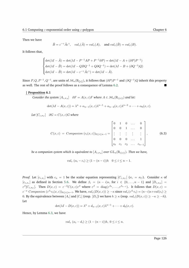
6.1 Computing ε-exponential order using ε-polygon Chapter 6
Then we have
B = ε−γAεγ , valε(A) = valε(A), and valε(B) = valε(B).
It follows that,
det(λI − A) = det(λI − P−1AP + P−1∂P ) = det(λI −A+ (∂P )P−1)
det(λI − B) = det(λI −QBQ−1 +Q∂Q−1) = det(λI −B + (∂Q−1)Q)
det(λI − B) = det(λI − ε−γAεγ) = det(λI − A).
Since P,Q, P−1, Q−1, are units ofMn(R[[ε]]), it follows that (∂P )P−1 and (∂Q−1)Q inherit this property
as well. The rest of the proof follows as a consequence of Lemma 6.2.
| Proposition 6.1
Consider the system [Aε,σA] ∂F = A(x, ε)F where A ∈Mn(R((ε))) and let:
det(λI −A(x, ε)) = λn + αn−1(x, ε)λn−1 + αn−2(x, ε)λ
n−2 + · · ·+ α0(x, ε).
Let [Cε,σC] ∂G = C(x, ε)G where
C(x, ε) = Companion (ci(x, ε))0≤i≤n−1 =
0 1 0 . . . 0
0 0 1 . . . 0...
......
......
0 0 0 . . . 1
c0 c1 c2 . . . cn−1
, (6.3)
be a companion system which is equivalent to [Aε,σA] over GLn(R((ε))). Then we have,
valε (αi − ci) ≥ (1− (n− i))h 0 ≤ i ≤ n− 1.
Proof. Let [cε,σc ] with cn = 1 be the scalar equation representing [Cε,σC] (σc = σC). Consider κ of
[cε,σc ] as defined in Section 5.6. We define βi = (n − i)κ, for i ∈ 0, . . . , n − 1 and [Dε,σD] =
εβ [Cε,σC]. Then D(x, ε) = ε−βC(x, ε)εβ where εβ = diag(εβ0 , . . . , εβn−1). It follows that D(x, ε) =
ε−κ Companion (εβici(x, ε))0≤i≤n−1. We have, valε(D(x, ε)) ≥ −κ since valε(εβici) = (n−i)κ+val(ci) ≥
0. By the equivalence between [Aε] and [Cε] (resp. [Dε]) we have h ≥ κ (resp. valε(D(x, ε)) ≥ −κ ≥ −h).
Let
det(λI −D(x, ε)) = λn + dn−1(x, ε)λn−1 + · · ·+ d0(x, ε).
Hence, by Lemma 6.3, we have
valε (αi − di) ≥ (1− (n− i))h, 0 ≤ i ≤ n.
Page 126
6.2 Formal reduction algorithm Chapter 6
Moreover, by Lemma 6.2
valε(di − ci) ≥ (1− (n− i)) max (0,− valε (D(x, ε))) ≥ (1− (n− i))κ ≥ (1− (n− i))h.
It follows that
valε(αi − ci) ≥ min (valε (αi − di), valε (di − ci)) ≥ (1− (n− i))h.
Proof. (Theorem 6.1) Let [Cε,σC] ∂G = C(x, ε)G be as in Proposition 6.1. Due to their equivalence,
[Aε,σA] and [Cε,σC
] have the same ε-exponential order and ε-polynomial. Hence, we have
ωε := ωε(A) = ωε(C) = max0≤i<n (−valε(ci)n− i
) and Eε(X) =ℓ∑
k=0
cik,valε(cik )X(ik−i0)
where 0 ≤ i0 < i1 < · · · < iℓ = n denote the integer i for which ωε(n − i) = −valε(ci). By Corollary 5.2
and Proposition 6.1 one has
valε (αi − ci) ≥ (i− n+ 1)h = (i− n)ωε + (i− n)(h− ωε) + h
≥ ωε(i− n) + (−n)(1− r
n) + h ≥ ωε(i− n) + r + h− n.
It follows from h+ r − n > 0 that valε (αi − ci) > (i− n)ωε, 0 ≤ i ≤ n.
• If i ∈ i0, . . . iℓ then ωε(i − n) = valε (ci) and valε (αi − ci) > valε (ci). Hence, valε (αi) =
valε (ci) and αi, valε (αi) = ci, val (ci).
• Else valε (αi − ci) > ωε(i− n) and valε (ci) > ωε(i− n). Thus,
valε (αi) ≥ min (valε (αi − ci), valε (ci)) > ωε(i− n).
This completes the proof.
6.2 Formal reduction algorithm
With the algorithms of uncoupling, turning point resolution, ε-rank reduction, and as can be verified by
Algorithm 6† below, one can deduce a general form for a fundamental matrix of formal outer solutions
for system [Aε] given by (3.9). In fact, it is given by
F = (
∞∑
k=0
Φk(x1/s) εk/d) exp(
∫
Q(x1/s, ε−1/d)), (6.4)
†The pseudo code of the algorithms is provided to show the sequence of steps. The implementation itself demanded differentconsiderations.
Page 127
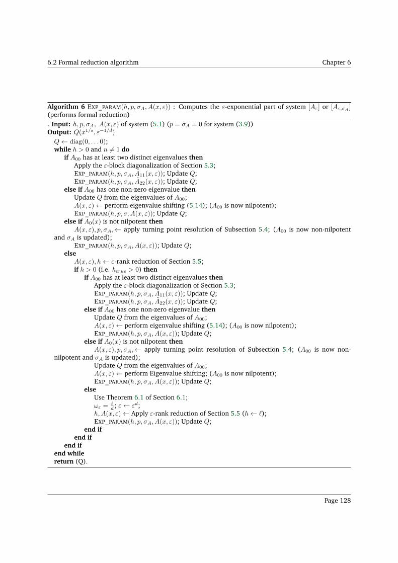
6.2 Formal reduction algorithm Chapter 6
Algorithm 6 EXP_PARAM(h, p, σA, A(x, ε)) : Computes the ε-exponential part of system [Aε] or [Aε,σA]
(performs formal reduction). Input: h, p, σA, A(x, ε) of system (5.1) (p = σA = 0 for system (3.9))Output: Q(x1/s, ε−1/d)
Q← diag(0, . . . 0);while h > 0 and n 6= 1 do
if A00 has at least two distinct eigenvalues thenApply the ε-block diagonalization of Section 5.3;EXP_PARAM(h, p, σA, A11(x, ε)); Update Q;EXP_PARAM(h, p, σA, A22(x, ε)); Update Q;
else if A00 has one non-zero eigenvalue thenUpdate Q from the eigenvalues of A00;A(x, ε)← perform eigenvalue shifting (5.14); (A00 is now nilpotent);EXP_PARAM(h, p, σ,A(x, ε)); Update Q;
else if A0(x) is not nilpotent thenA(x, ε), p, σA,← apply turning point resolution of Subsection 5.4; (A00 is now non-nilpotent
and σA is updated);EXP_PARAM(h, p, σA, A(x, ε)); Update Q;
elseA(x, ε), h← ε-rank reduction of Section 5.5;if h > 0 (i.e. htrue > 0) then
if A00 has at least two distinct eigenvalues thenApply the ε-block diagonalization of Section 5.3;EXP_PARAM(h, p, σA, A11(x, ε)); Update Q;EXP_PARAM(h, p, σA, A22(x, ε)); Update Q;
else if A00 has one non-zero eigenvalue thenUpdate Q from the eigenvalues of A00;A(x, ε)← perform eigenvalue shifting (5.14); (A00 is now nilpotent);EXP_PARAM(h, p, σA, A(x, ε)); Update Q;
else if A0(x) is not nilpotent thenA(x, ε), p, σA,← apply turning point resolution of Subsection 5.4; (A00 is now non-
nilpotent and σA is updated);Update Q from the eigenvalues of A00;A(x, ε)← perform Eigenvalue shifting; (A00 is now nilpotent);EXP_PARAM(h, p, σA, A(x, ε)); Update Q;
elseUse Theorem 6.1 of Section 6.1;ωε =
ℓd ; ε← εd;
h,A(x, ε)← Apply ε-rank reduction of Section 5.5 (h← ℓ);EXP_PARAM(h, p, σA, A(x, ε)); Update Q;
end ifend if
end ifend whilereturn (Q).
Page 128
6.2 Formal reduction algorithm Chapter 6
where s, d are positive integers; Q is a diagonal matrix whose entries are polynomials in ε−1/d with
coefficients in C((x1/s)). We refer to Q :=∫Q as the ε-exponential part (logarithms in a root of x might
arise as a result of integration); and the entries of Φi(x1/s)’s are root-meromorphic in x (see, e.g. [120,
Introduction]).
| Remark 6.1
Under the notations and statements of Theorem 6.1, the leading term of Q is given by
1
εωε(A)
∫ x
diag(X1(z), . . . , Xdeg (Eε)(z), 0, . . . , 0) dz,
where the Xi’s denote the roots of the ε-polynomial Eε(X). A similar statement can be stated in terms
of the eigenvalues of the leading matrix coefficient, xp, and εh.
We sum up our main results in Algorithm 6 which computes the ε-exponential part and consequently a
fundamental matrix of formal solutions (6.4) in a given subdomain. We recall that:
• If n = 1 then we proceed by integration up to the first h terms;
• If h ≤ 0 then we follow Subsection 5.2.1 (use MINIISOLDE or LINDALG).
Evidently, computing a FMFS over a commutative field K of characteristic zero rather than C may require
algebraic extensions of the base field. Chapter 1 describes how one can limit such extensions. One can
easily verify that a similar refinement can be applied to Algorithm 6. This is taken into consideration
within our implementations in MAPLE.
| Remark 6.2 Current Investigations
According to Section 4.2, Iwano’s first problem can be resolved with the help of a sequence of positive
rational numbers [ρ] given by (4.12):
[ρ] 0 = ρ0 < ρ1 < ρ2 < · · · < ρm.
In Section 6.3, we try to motivate the following approach to resolve the same problem for a system:
Suppose that we start the reduction with system [Aε,σA], σA = 0, given by (5.1) as an input. Then,
Algorithm 6 can determine the “true” restraining index σA,true of this system at the end of the reduction
and its outer solutions. If the restraining index is nonzero then we have a turning point and ρ1 =
−1/σA,true. We can then perform the stretching τ = xε−ρ1 for the initial system [Aε,σA], and apply
to it Algorithm 6. This determines ρ2. The same process can be repeated with ρ2 to determine ρ3, and
then with ρ3, . . . , until we reach a system with a restraining index zero. We are currently investigating
the correctness of such a process and questioning the redundancy of certain information by using the
equivalence between a system and a scalar equation, and the (x, ε)-polygon recalled in Section 4.2.
Page 129
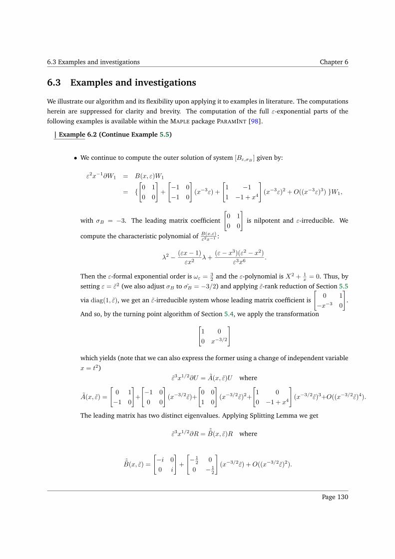
6.3 Examples and investigations Chapter 6
6.3 Examples and investigations
We illustrate our algorithm and its flexibility upon applying it to examples in literature. The computations
herein are suppressed for clarity and brevity. The computation of the full ε-exponential parts of the
following examples is available within the MAPLE package PARAMINT [98].
| Example 6.2 (Continue Example 5.5)
• We continue to compute the outer solution of system [Bε,σB] given by:
ε2x−1∂W1 = B(x, ε)W1
= [
0 1
0 0
]
+
[
−1 0
−1 0
]
(x−3ε) +
[
1 −11 −1 + x4
]
(x−3ε)2 +O((x−3ε)3) W1,
with σB = −3. The leading matrix coefficient
[
0 1
0 0
]
is nilpotent and ε-irreducible. We
compute the characteristic polynomial of B(x,ε)ε2x−1 :
λ2 − (εx− 1)
εx2λ+
(ε− x3)(ε2 − x2)
ε3x6.
Then the ε-formal exponential order is ωε = 32 and the ε-polynomial is X2 + 1
x = 0. Thus, by
setting ε = ε2 (we also adjust σB to σB = −3/2) and applying ε-rank reduction of Section 5.5
via diag(1, ε), we get an ε-irreducible system whose leading matrix coefficient is
[
0 1
−x−3 0
]
.
And so, by the turning point algorithm of Section 5.4, we apply the transformation
[
1 0
0 x−3/2
]
which yields (note that we can also express the former using a change of independent variable
x = t2)
ε3x1/2∂U = A(x, ε)U where
A(x, ε) =
[
0 1
−1 0
]
+
[
−1 0
0 0
]
(x−3/2ε)+
[
0 0
1 0
]
(x−3/2ε)2+
[
1 0
0 −1 + x4
]
(x−3/2ε)3+O((x−3/2ε)4).
The leading matrix has two distinct eigenvalues. Applying Splitting Lemma we get
ε3x1/2∂R = ˜B(x, ε)R where
˜B(x, ε) =
[
−i 0
0 i
]
+
[
− 12 0
0 − 12
]
(x−3/2ε) +O((x−3/2ε)2).
Page 130
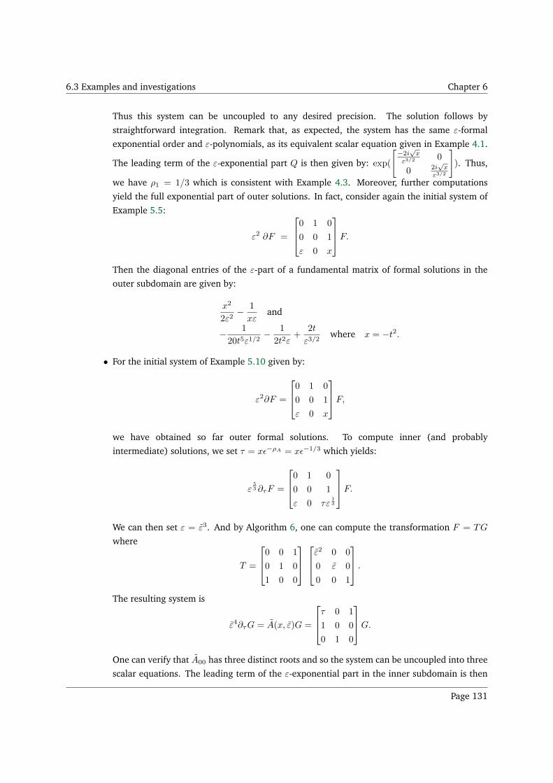
6.3 Examples and investigations Chapter 6
Thus this system can be uncoupled to any desired precision. The solution follows by
straightforward integration. Remark that, as expected, the system has the same ε-formal
exponential order and ε-polynomials, as its equivalent scalar equation given in Example 4.1.
The leading term of the ε-exponential part Q is then given by: exp(
[−2i
√x
ε3/20
0 2i√x
ε3/2
]
). Thus,
we have ρ1 = 1/3 which is consistent with Example 4.3. Moreover, further computations
yield the full exponential part of outer solutions. In fact, consider again the initial system of
Example 5.5:
ε2 ∂F =
0 1 0
0 0 1
ε 0 x
F.
Then the diagonal entries of the ε-part of a fundamental matrix of formal solutions in the
outer subdomain are given by:
x2
2ε2− 1
xεand
− 1
20t5ε1/2− 1
2t2ε+
2t
ε3/2where x = −t2.
• For the initial system of Example 5.10 given by:
ε2∂F =
0 1 0
0 0 1
ε 0 x
F,
we have obtained so far outer formal solutions. To compute inner (and probably
intermediate) solutions, we set τ = xǫ−ρA = xǫ−1/3 which yields:
ε53 ∂τF =
0 1 0
0 0 1
ε 0 τε13
F.
We can then set ε = ε3. And by Algorithm 6, one can compute the transformation F = TG
where
T =
0 0 1
0 1 0
1 0 0
ε2 0 0
0 ε 0
0 0 1
.
The resulting system is
ε4∂τG = A(x, ε)G =
τ 0 1
1 0 0
0 1 0
G.
One can verify that A00 has three distinct roots and so the system can be uncoupled into three
scalar equations. The leading term of the ε-exponential part in the inner subdomain is then
Page 131
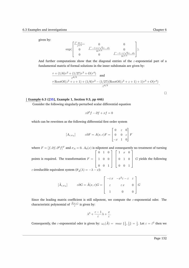
6.3 Examples and investigations Chapter 6
given by:
exp(
∫ τ dz+...
ε4/30 0
0∫ τ −1+i/
√3+...dz
2ε4/30
0 0∫ τ −1−i/
√3+...dz
2ε4/3
).
And further computations show that the diagonal entries of the ε-exponential part of a
fundamental matrix of formal solutions in the inner subdomain are given by:
τ + (1/6)τ2 + (1/27)τ3 +O(τ4)
ε4/3and
τ RootOf(z2 + z + 1) + (1/6)τ2 − (1/27)(RootOf(z2 + z + 1) + 1)τ3 +O(τ4)
ε4/3.
| Example 6.3 ([35], Example 1, Section 9.5, pp 446)
Consider the following singularly-perturbed scalar differential equation
ε∂3f − ∂f + xf = 0
which can be rewritten as the following differential first order system
[Aε,σA] ε∂F = A(x, ε)F =
0 ε 0
0 0 ε
−x 1 0
F
where F = [f, ∂f, ∂2f ]T and σA = 0. A0(x) is nilpotent and consequently no treatment of turning
points is required. The transformation F =
0 1 0
1 0 0
0 0 1
1 x 0
0 1 0
0 0 1
G yields the following
ε-irreducible equivalent system (θA(λ) = −λ− x):
[Aε,σA] ε∂G = A(x, ε)G =
−ε x −x2ε− ε ε
ε ε x 0
1 0 0
G
Since the leading matrix coefficient is still nilpotent, we compute the ε-exponential oder. The
characteristic polynomial of A(x,ε)ε is given by:
λ3 +ε− 1
ελ+
x
ε.
Consequently, the ε-exponential oder is given by: ωε(A) = max 12 , 13 = 1
2 . Let ε = ε2 then we
Page 132
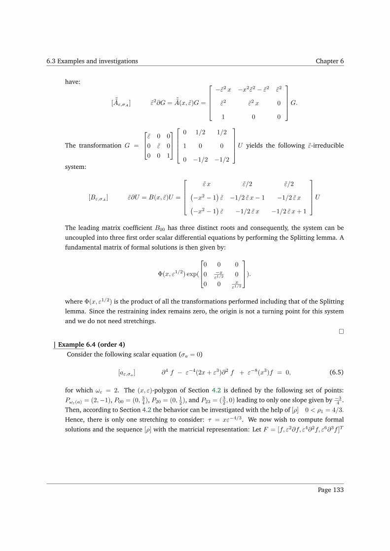
6.3 Examples and investigations Chapter 6
have:
[ ˜Aε,σA] ε2∂G = ˜A(x, ε)G =
−ε2 x −x2ε2 − ε2 ε2
ε2 ε2 x 0
1 0 0
G.
The transformation G =
ε 0 0
0 ε 0
0 0 1
0 1/2 1/2
1 0 0
0 −1/2 −1/2
U yields the following ε-irreducible
system:
[Bε,σA] ε∂U = B(x, ε)U =
ε x ε/2 ε/2
(−x2 − 1
)ε −1/2 ε x− 1 −1/2 ε x
(−x2 − 1
)ε −1/2 ε x −1/2 ε x+ 1
U
The leading matrix coefficient B00 has three distinct roots and consequently, the system can be
uncoupled into three first order scalar differential equations by performing the Splitting lemma. A
fundamental matrix of formal solutions is then given by:
Φ(x, ε1/2) exp(
0 0 0
0 −xε1/2
0
0 0 xε1/2
).
where Φ(x, ε1/2) is the product of all the transformations performed including that of the Splitting
lemma. Since the restraining index remains zero, the origin is not a turning point for this system
and we do not need stretchings.
| Example 6.4 (order 4)
Consider the following scalar equation (σa = 0)
[aε,σa] ∂4 f − ε−4(2x+ ε3)∂2 f + ε−8(x3)f = 0, (6.5)
for which ωε = 2. The (x, ε)-polygon of Section 4.2 is defined by the following set of points:
Pωε(a) = (2,−1), P00 = (0, 34 ), P20 = (0, 1
2 ), and P23 = ( 32 , 0) leading to only one slope given by −34 .
Then, according to Section 4.2 the behavior can be investigated with the help of [ρ] 0 < ρ1 = 4/3.
Hence, there is only one stretching to consider: τ = xε−4/3. We now wish to compute formal
solutions and the sequence [ρ] with the matricial representation: Let F = [f, ε2∂f, ε4∂2f, ε6∂3f ]T
Page 133
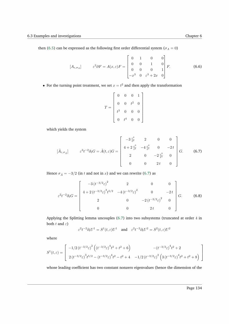
6.3 Examples and investigations Chapter 6
then (6.5) can be expressed as the following first order differential system (σA = 0)
[Aε,σA] ε2∂F = A(x, ε)F =
0 1 0 0
0 0 1 0
0 0 0 1
−x3 0 ε3 + 2x 0
F. (6.6)
• For the turning point treatment, we set x = t2 and then apply the transformation
T =
0 0 0 1
0 0 t2 0
t3 0 0 0
0 t4 0 0
which yields the system
[Aε,σA] ε2t−2∂tG = A(t, ε)G =
−3 ε2
t3 2 0 0
4 + 2 ε3
t2 −4 ε2
t3 0 −2 t
2 0 −2 ε2
t3 0
0 0 2 t 0
G. (6.7)
Hence σA = −3/2 (in t and not in x) and we can rewrite (6.7) as
ε2t−2∂tG =
−3 (t−3/2ε)2
2 0 0
4 + 2 (t−3/2ε)3t5/2 −4 (t−3/2ε)
20 −2 t
2 0 −2 (t−3/2ε)2
0
0 0 2 t 0
G. (6.8)
Applying the Splitting lemma uncouples (6.7) into two subsystems (truncated at order 4 in
both t and ε)
ε2t−2∂tU1 = S1(t, ε)U1 and ε2t−2∂tU
2 = S2(t, ε)U2
where
S1(t, ε) =
−1/2 (t−3/2ε)2(
(t−3/2ε)4t2 + t2 + 6
)
−(t−3/2ε)4t2 + 2
2 (t−3/2ε)3t5/2 − (t−3/2ε)
4t2 − t2 + 4 −1/2 (t−3/2ε)
2(
3 (t−3/2ε)4t2 + t2 + 8
)
whose leading coefficient has two constant nonzero eigenvalues (hence the dimension of the
Page 134
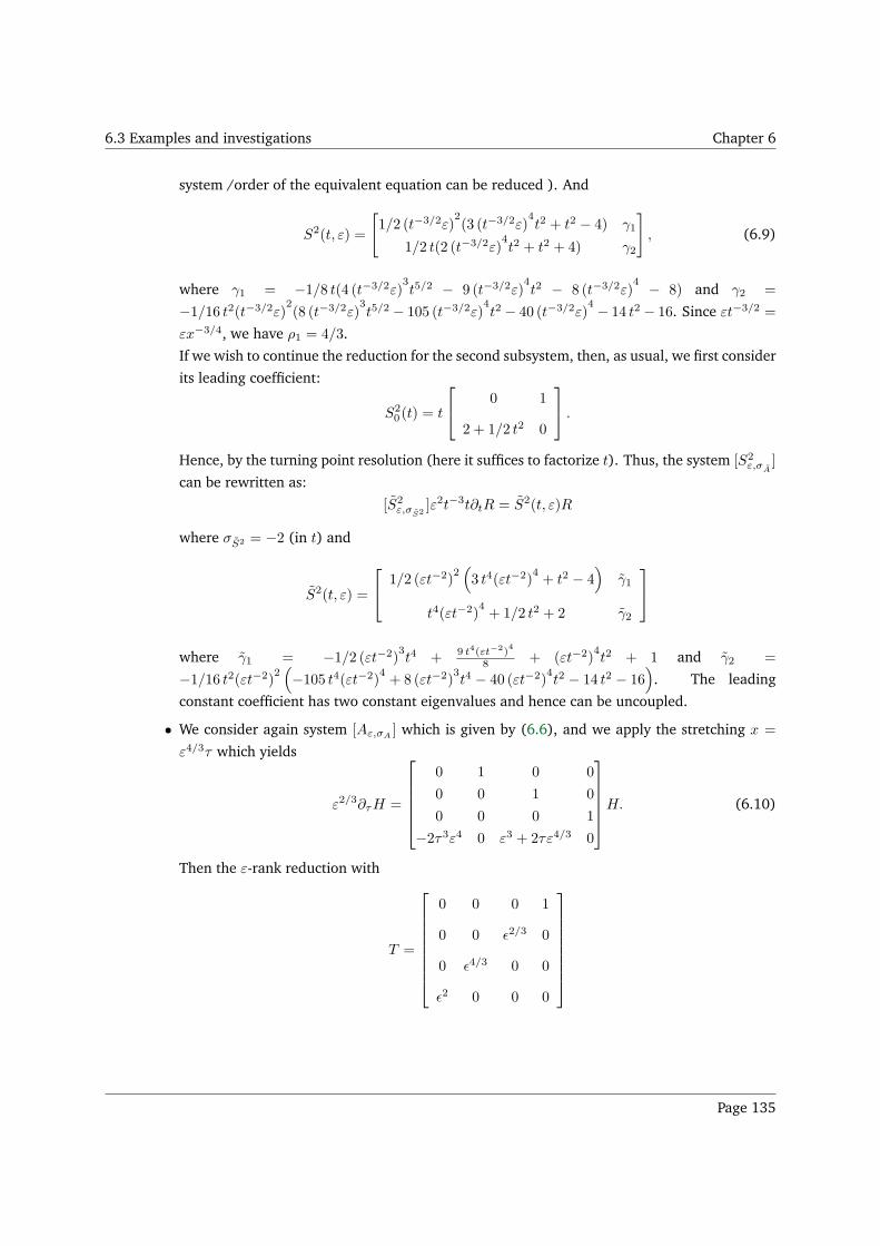
6.3 Examples and investigations Chapter 6
system /order of the equivalent equation can be reduced ). And
S2(t, ε) =
[
1/2 (t−3/2ε)2(3 (t−3/2ε)
4t2 + t2 − 4) γ1
1/2 t(2 (t−3/2ε)4t2 + t2 + 4) γ2
]
, (6.9)
where γ1 = −1/8 t(4 (t−3/2ε)3t5/2 − 9 (t−3/2ε)
4t2 − 8 (t−3/2ε)
4 − 8) and γ2 =
−1/16 t2(t−3/2ε)2(8 (t−3/2ε)
3t5/2 − 105 (t−3/2ε)
4t2 − 40 (t−3/2ε)
4 − 14 t2 − 16. Since εt−3/2 =
εx−3/4, we have ρ1 = 4/3.
If we wish to continue the reduction for the second subsystem, then, as usual, we first consider
its leading coefficient:
S20(t) = t
0 1
2 + 1/2 t2 0
.
Hence, by the turning point resolution (here it suffices to factorize t). Thus, the system [S2ε,σA
]
can be rewritten as:
[S2ε,σS2
]ε2t−3t∂tR = S2(t, ε)R
where σS2 = −2 (in t) and
S2(t, ε) =
1/2 (εt−2)2(
3 t4(εt−2)4+ t2 − 4
)
γ1
t4(εt−2)4+ 1/2 t2 + 2 γ2
where γ1 = −1/2 (εt−2)3t4 + 9 t4(εt−2)
4
8 + (εt−2)4t2 + 1 and γ2 =
−1/16 t2(εt−2)2(
−105 t4(εt−2)4+ 8 (εt−2)
3t4 − 40 (εt−2)
4t2 − 14 t2 − 16
)
. The leading
constant coefficient has two constant eigenvalues and hence can be uncoupled.
• We consider again system [Aε,σA] which is given by (6.6), and we apply the stretching x =
ε4/3τ which yields
ε2/3∂τH =
0 1 0 0
0 0 1 0
0 0 0 1
−2τ3ε4 0 ε3 + 2τε4/3 0
H. (6.10)
Then the ε-rank reduction with
T =
0 0 0 1
0 0 ǫ2/3 0
0 ǫ4/3 0 0
ǫ2 0 0 0
Page 135
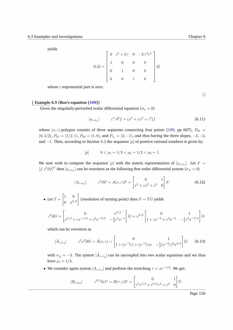
6.3 Examples and investigations Chapter 6
yields
∂τQ =
0 ǫ5 + 2 τ 0 −2 τ3ǫ4
1 0 0 0
0 1 0 0
0 0 1 0
Q
whose ε-exponential part is zero.
| Example 6.5 (Roo’s equation [109])
Given the singularly-perturbed scalar differential equation (σa = 0)
[aε,σa] ε4 ∂2f = (x5 + εx2 + ε2)f (6.11)
whose (x, ε)-polygon consists of three segments connecting four points [109, pp 607], P00 =
(0, 5/2), P01 = (1/2, 1), P02 = (1, 0), and Poε = (2,−1), and thus having the three slopes, −3,−2,
and −1. Then, according to Section 4.2 the sequence [ρ] of positive rational numbers is given by:
[ρ] 0 < ρ1 = 1/3 < ρ2 = 1/2 < ρ3 = 1.
We now wish to compute the sequence [ρ] with the matrix representation of [aε,σa]. Let F =
[f, ε2∂f ]T then [aε,σa] can be rewritten as the following first order differential system (σA = 0)
[Aε,σA] ε2∂F = A(x, ε)F =
[
0 1
x5 + εx2 + ε2 0
]
F. (6.12)
• Let T =
[
1 0
0 x5/2
]
(resolution of turning point) then F = TG yields
ε2∂G =
[
0 x5/2
x5/2 + εx−1/2 + ε2x−5/2 − 52ε
2x−1
]
G = x5/2
[
0 1
1 + εx−3 + ε2x−5 − 52ε
2x−7/2
]
G
which can be rewritten as
[Aε,σA] ε2x2∂G = A(x, ε) =
[
0 1
1 + (x−3ε) + (x−3ε)x − 52 (x
−3ε)2x5/2
]
G (6.13)
with σA = −3. The system [Aε,σA] can be uncoupled into two scalar equations and we thus
have ρ1 = 1/3.
• We consider again system [Aε,σA] and perform the stretching τ = xε−1/3. We get:
[Bε,σB] ε5/3∂τU = B(τ, ε)U =
[
0 1
τ5ε5/3 + ε5/3τ2 + ε2 0
]
U.
Page 136
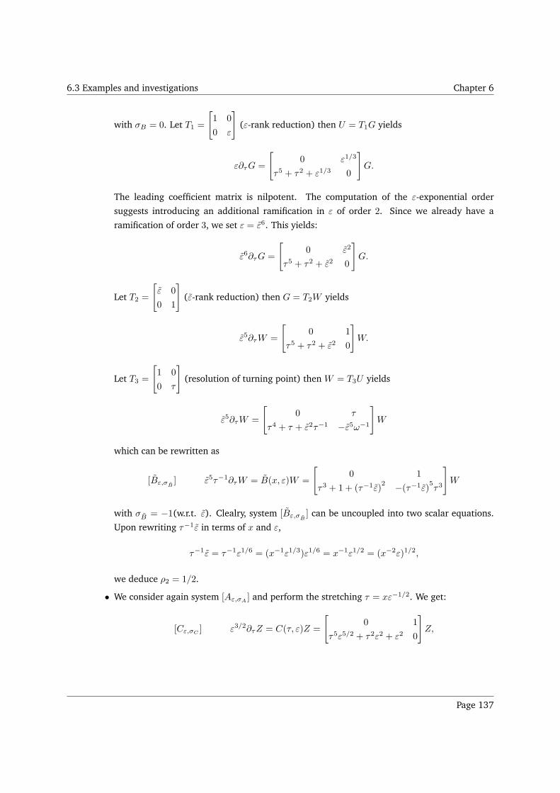
6.3 Examples and investigations Chapter 6
with σB = 0. Let T1 =
[
1 0
0 ε
]
(ε-rank reduction) then U = T1G yields
ε∂τG =
[
0 ε1/3
τ5 + τ2 + ε1/3 0
]
G.
The leading coefficient matrix is nilpotent. The computation of the ε-exponential order
suggests introducing an additional ramification in ε of order 2. Since we already have a
ramification of order 3, we set ε = ε6. This yields:
ε6∂τG =
[
0 ε2
τ5 + τ2 + ε2 0
]
G.
Let T2 =
[
ε 0
0 1
]
(ε-rank reduction) then G = T2W yields
ε5∂τW =
[
0 1
τ5 + τ2 + ε2 0
]
W.
Let T3 =
[
1 0
0 τ
]
(resolution of turning point) then W = T3U yields
ε5∂τW =
[
0 τ
τ4 + τ + ε2τ−1 −ε5ω−1
]
W
which can be rewritten as
[Bε,σB] ε5τ−1∂τW = B(x, ε)W =
[
0 1
τ3 + 1 + (τ−1ε)2 −(τ−1ε)
5τ3
]
W
with σB = −1(w.r.t. ε). Clealry, system [Bε,σB] can be uncoupled into two scalar equations.
Upon rewriting τ−1ε in terms of x and ε,
τ−1ε = τ−1ε1/6 = (x−1ε1/3)ε1/6 = x−1ε1/2 = (x−2ε)1/2,
we deduce ρ2 = 1/2.
• We consider again system [Aε,σA] and perform the stretching τ = xε−1/2. We get:
[Cε,σC] ε3/2∂τZ = C(τ, ε)Z =
[
0 1
τ5ε5/2 + τ2ε2 + ε2 0
]
Z,
Page 137
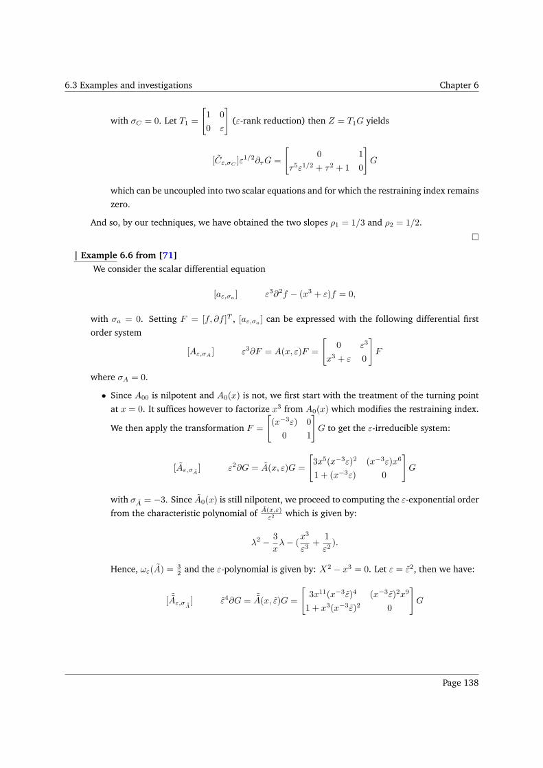
6.3 Examples and investigations Chapter 6
with σC = 0. Let T1 =
[
1 0
0 ε
]
(ε-rank reduction) then Z = T1G yields
[Cε,σC]ε1/2∂τG =
[
0 1
τ5ε1/2 + τ2 + 1 0
]
G
which can be uncoupled into two scalar equations and for which the restraining index remains
zero.
And so, by our techniques, we have obtained the two slopes ρ1 = 1/3 and ρ2 = 1/2.
| Example 6.6 from [71]
We consider the scalar differential equation
[aε,σa] ε3∂2f − (x3 + ε)f = 0,
with σa = 0. Setting F = [f, ∂f ]T , [aε,σa] can be expressed with the following differential first
order system
[Aε,σA] ε3∂F = A(x, ε)F =
[
0 ε3
x3 + ε 0
]
F
where σA = 0.
• Since A00 is nilpotent and A0(x) is not, we first start with the treatment of the turning point
at x = 0. It suffices however to factorize x3 from A0(x) which modifies the restraining index.
We then apply the transformation F =
[
(x−3ε) 0
0 1
]
G to get the ε-irreducible system:
[Aε,σA] ε2∂G = A(x, ε)G =
[
3x5(x−3ε)2 (x−3ε)x6
1 + (x−3ε) 0
]
G
with σA = −3. Since A0(x) is still nilpotent, we proceed to computing the ε-exponential order
from the characteristic polynomial of A(x,ε)ε2 which is given by:
λ2 − 3
xλ− (
x3
ε3+
1
ε2).
Hence, ωε(A) = 32 and the ε-polynomial is given by: X2 − x3 = 0. Let ε = ε2, then we have:
[ ˜Aε,σ ˜A] ε4∂G = ˜A(x, ε)G =
[
3x11(x−3ε)4 (x−3ε)2x9
1 + x3(x−3ε)2 0
]
G
Page 138
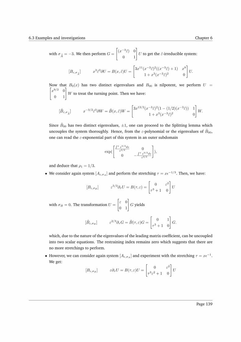
6.3 Examples and investigations Chapter 6
with σ ˜A= −3. We then perform G =
[
(x−3ε) 0
0 1
]
U to get the ε-irreducible system:
[Bε,σ ˜A] x3ε3∂U = B(x, ε)U =
[
3x11(x−3ε)2((x−3ε) + 1) x9
1 + x3(x−3ε)2 0
]
U.
Now that B0(x) has two distinct eigenvalues and B00 is nilpotent, we perform U =[
x9/2 0
0 1
]
W to treat the turning point. Then we have:
[Bε,σ ˜A] x−3/2ε3∂W = B(x, ε)W =
[
3x13/2(x−3ε)2(1− (1/2)(x−3ε)) 1
1 + x3(x−3ε)2 0
]
W.
Since B00 has two distinct eigenvalues, ±1, one can proceed to the Splitting lemma which
uncouples the system thoroughly. Hence, from the ε-polynomial or the eigenvalues of B00,
one can read the ε-exponential part of this system in an outer subdomain
exp(
[ ∫ x z3/2dz
ε3/20
0 −∫ x z3/2dz
ε3/2
]
),
and deduce that ρ1 = 1/3.
• We consider again system [Aε,σA] and perform the stretching τ = xǫ−1/3. Then, we have:
[Bε,σB] ε5/3∂τU = B(τ, ε) =
[
0 ε2
τ3 + 1 0
]
U
with σB = 0. The transformation U =
[
ε 0
0 1
]
G yields
[Bε,σB] ε2/3∂τG = B(τ, ε)G =
[
0 1
τ3 + 1 0
]
G.
which, due to the nature of the eigenvalues of the leading matrix coefficient, can be uncoupled
into two scalar equations. The restraining index remains zero which suggests that there are
no more stretchings to perform.
• However, we can consider again system [Aε,σA] and experiment with the stretching τ = xǫ−1.
We get:
[Bε,σB] ε∂τU = B(τ, ε)U =
[
0 ε2
τ3ε2 + 1 0
]
U
Page 139
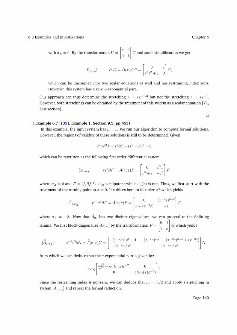
6.3 Examples and investigations Chapter 6
with σB = 0. By the transformation U =
[
ε 0
0 1
]
G and some simplification we get
[Bε,σB] ∂τG = B(τ, ε)G =
[
0 1
τ3ε2 + 1 0
]
G,
which can be uncoupled into two scalar equations as well and has restraining index zero.
However, this system has a zero ε-exponential part.
Our approach can thus determine the stretching τ = xε−1/3 but not the stretching τ = xε−1.
However, both stretchings can be obtained by the treatment of this system as a scalar equation [71,
Last section].
| Example 6.7 ([35], Example 1, Section 9.5, pp 453)
In this example, the input system has p = 1. We run our algorithm to compute formal solutions.
However, the regions of validity of these solutions is still to be determined. Given
ε3x∂2f + x2∂f − (x3 + ε)f = 0
which can be rewritten as the following first order differential system
[Aε,σA] xε3∂F = A(x, ε)F =
[
0 ε3x
x3 + ε −x2
]
F
where σA = 0 and F = [f, ∂f ]T . A00 is nilpotent while A0(x) is not. Thus, we first start with the
treatment of the turning point at x = 0. It suffices here to factorize x2 which yields
[Aε,σA] x−1ε3∂F = A(x, ε)F =
[
0 (x−2ε)3x5
x+ (x−2ε) −1
]
F
where σA = −2. Now that A00 has two distinct eigenvalues, we can proceed to the Splitting
lemma. We first block-diagonalize A0(x) by the transformation F =
[
0 1
1 x
]
G which yields
[ ˜Aε,σA] x−1ε3∂G = ˜A(x, ε)G =
[
−(x−2ε)3x6 − 1 −(x−2ε)3x7 − (x−2ε)3x5 + (x−2ε)
(x−2ε)3x5 (x−2ε)3x6
]
G,
from which we can deduce that the ε-exponential part is given by:
exp(
[−x2
2ε3 +O(ln(x)ε−2) 0
0 O(ln(x)ε−2)
]
).
Since the restraining index is nonzero, we can deduce that ρ1 = 1/2 and apply a stretching in
system [Aε,σA] and repeat the formal reduction.
Page 140
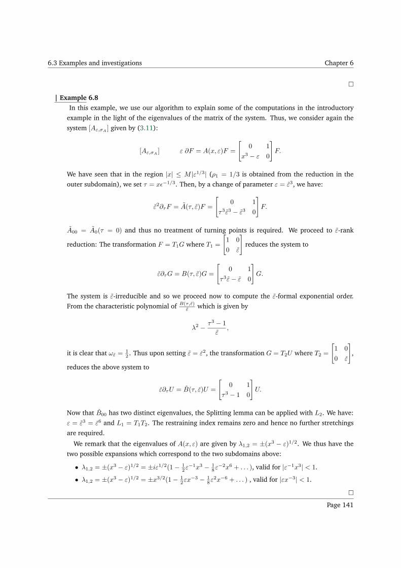
6.3 Examples and investigations Chapter 6
| Example 6.8
In this example, we use our algorithm to explain some of the computations in the introductory
example in the light of the eigenvalues of the matrix of the system. Thus, we consider again the
system [Aε,σA] given by (3.11):
[Aε,σA] ε ∂F = A(x, ε)F =
[
0 1
x3 − ε 0
]
F.
We have seen that in the region |x| ≤ M |ε1/3| (ρ1 = 1/3 is obtained from the reduction in the
outer subdomain), we set τ = xǫ−1/3. Then, by a change of parameter ε = ε3, we have:
ε2∂τF = A(τ, ε)F =
[
0 1
τ3ε3 − ε3 0
]
F.
A00 = A0(τ = 0) and thus no treatment of turning points is required. We proceed to ε-rank
reduction: The transformation F = T1G where T1 =
[
1 0
0 ε
]
reduces the system to
ε∂τG = B(τ, ε)G =
[
0 1
τ3ε− ε 0
]
G.
The system is ε-irreducible and so we proceed now to compute the ε-formal exponential order.
From the characteristic polynomial of B(τ,ε)ε which is given by
λ2 − τ3 − 1
ε,
it is clear that ωε =12 . Thus upon setting ε = ε2, the transformation G = T2U where T2 =
[
1 0
0 ε
]
,
reduces the above system to
ε∂τU = B(τ, ε)U =
[
0 1
τ3 − 1 0
]
U.
Now that B00 has two distinct eigenvalues, the Splitting lemma can be applied with L2. We have:
ε = ε3 = ε6 and L1 = T1T2. The restraining index remains zero and hence no further stretchings
are required.
We remark that the eigenvalues of A(x, ε) are given by λ1,2 = ±(x3 − ε)1/2. We thus have the
two possible expansions which correspond to the two subdomains above:
• λ1,2 = ±(x3 − ε)1/2 = ±iε1/2(1− 12ε
−1x3 − 18ε
−2x6 + . . . ), valid for |ε−1x3| < 1.
• λ1,2 = ±(x3 − ε)1/2 = ±x3/2(1− 12εx
−3 − 18ε
2x−6 + . . . ) , valid for |εx−3| < 1.
Page 141
6.4 Conclusion Chapter 6
6.4 Conclusion
In this chapter, we gave a method to compute the ε-formal invariants of the system. This result allowed
us to give an algorithm for formal reduction which resolves the second item in Iwano’s reformulation of
the problems of singularly-perturbed systems, and motivates an approach to resolve the first item in this
reformulation.
Page 142
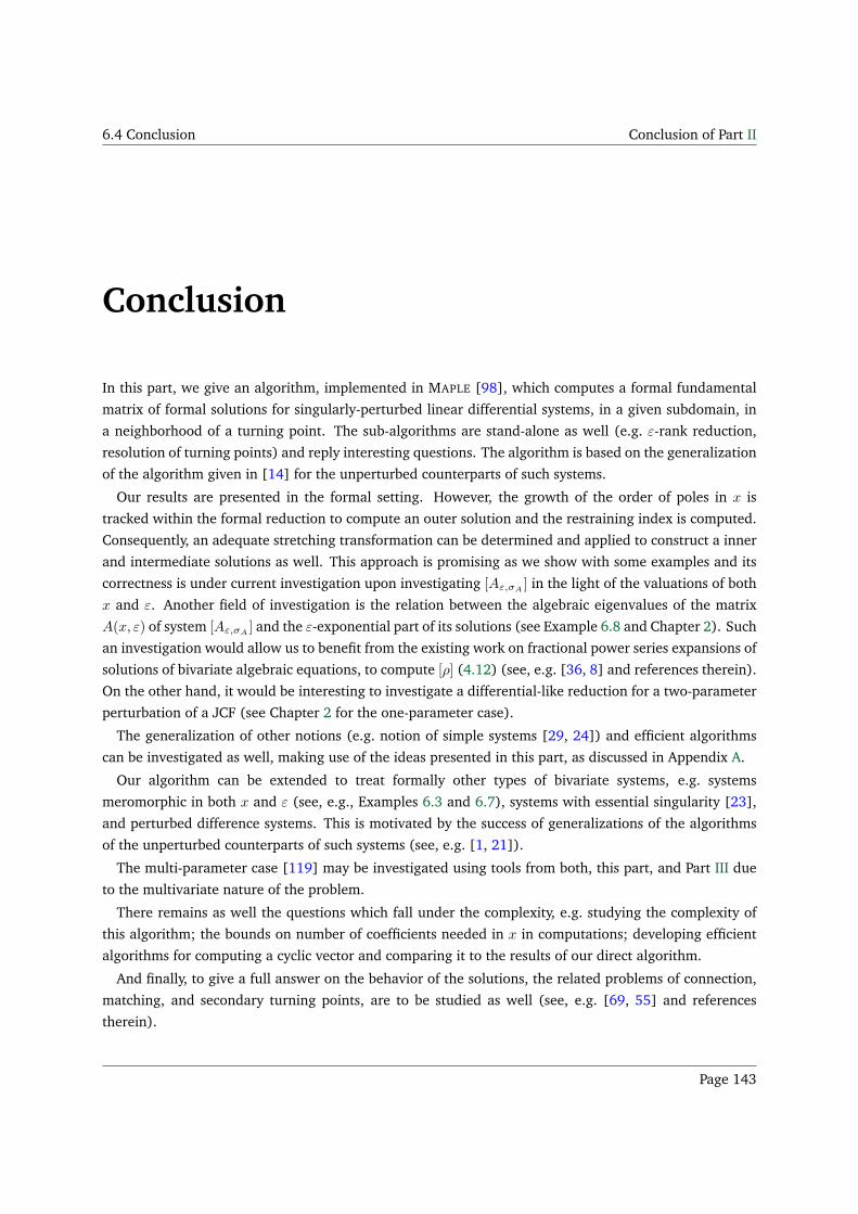
6.4 Conclusion Conclusion of Part II
Conclusion
In this part, we give an algorithm, implemented in MAPLE [98], which computes a formal fundamental
matrix of formal solutions for singularly-perturbed linear differential systems, in a given subdomain, in
a neighborhood of a turning point. The sub-algorithms are stand-alone as well (e.g. ε-rank reduction,
resolution of turning points) and reply interesting questions. The algorithm is based on the generalization
of the algorithm given in [14] for the unperturbed counterparts of such systems.
Our results are presented in the formal setting. However, the growth of the order of poles in x is
tracked within the formal reduction to compute an outer solution and the restraining index is computed.
Consequently, an adequate stretching transformation can be determined and applied to construct a inner
and intermediate solutions as well. This approach is promising as we show with some examples and its
correctness is under current investigation upon investigating [Aε,σA] in the light of the valuations of both
x and ε. Another field of investigation is the relation between the algebraic eigenvalues of the matrix
A(x, ε) of system [Aε,σA] and the ε-exponential part of its solutions (see Example 6.8 and Chapter 2). Such
an investigation would allow us to benefit from the existing work on fractional power series expansions of
solutions of bivariate algebraic equations, to compute [ρ] (4.12) (see, e.g. [36, 8] and references therein).
On the other hand, it would be interesting to investigate a differential-like reduction for a two-parameter
perturbation of a JCF (see Chapter 2 for the one-parameter case).
The generalization of other notions (e.g. notion of simple systems [29, 24]) and efficient algorithms
can be investigated as well, making use of the ideas presented in this part, as discussed in Appendix A.
Our algorithm can be extended to treat formally other types of bivariate systems, e.g. systems
meromorphic in both x and ε (see, e.g., Examples 6.3 and 6.7), systems with essential singularity [23],
and perturbed difference systems. This is motivated by the success of generalizations of the algorithms
of the unperturbed counterparts of such systems (see, e.g. [1, 21]).
The multi-parameter case [119] may be investigated using tools from both, this part, and Part III due
to the multivariate nature of the problem.
There remains as well the questions which fall under the complexity, e.g. studying the complexity of
this algorithm; the bounds on number of coefficients needed in x in computations; developing efficient
algorithms for computing a cyclic vector and comparing it to the results of our direct algorithm.
And finally, to give a full answer on the behavior of the solutions, the related problems of connection,
matching, and secondary turning points, are to be studied as well (see, e.g. [69, 55] and references
therein).
Page 143


Part III
Completely Integrable Pfaffian Systems
with Normal Crossings
Page 145
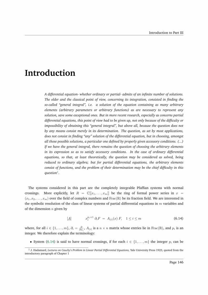
Introduction to Part III
Introduction
A differential equation- whether ordinary or partial- admits of an infinite number of solutions.
The older and the classical point of view, concerning its integration, consisted in finding the
so-called “general integral”, i.e. a solution of the equation containing as many arbitrary
elements (arbitrary parameters or arbitrary functions) as are necessary to represent any
solution, save some exceptional ones. But in more recent research, especially as concerns partial
differential equations, this point of view had to be given up, not only because of the difficulty or
impossibility of obtaining this “general integral”, but above all, because the question does not
by any means consist merely in its determination. The question, as set by most applications,
does not consist in finding “any” solution of the differential equation, but in choosing, amongst
all those possible solutions, a particular one defined by properly given accessory conditions. (...)
If we have the general integral, there remains the question of choosing the arbitrary elements
in its expression so as to satisfy accessory conditions. In the case of ordinary differential
equations, so that, at least theoretically, the question may be considered as solved, being
reduced to ordinary algebra; but for partial differential equations, the arbitrary elements
consist of functions, and the problem of their determination may be the chief difficulty in this
question‡.
The systems considered in this part are the completely integrable Pfaffian systems with normal
crossings. More explicitly, let R = C[[x1, . . . , xm]] be the ring of formal power series in x =
(x1, x2, . . . , xm) over the field of complex numbers and Frac(R) be its fraction field. We are interested in
the symbolic resolution of the class of linear systems of partial differential equations in m variables and
of the dimension n given by
[A] xpi+1i ∂iF = A(i)(x) F, 1 ≤ i ≤ m (6.14)
where, for all i ∈ 1, . . . ,m, ∂i = ∂∂xi
, A(i) is a n × n matrix whose entries lie in Frac(R), and pi is an
integer. We therefore explain the terminology:
• System (6.14) is said to have normal crossings, if for each i ∈ 1, . . . ,m the integer pi can be
‡ J. Hadamard, Lectures on Cauchy’s Problem in Linear Partial Differential Equations, Yale University Press 1923, quoted from theintroductory paragraph of Chapter 1
Page 146
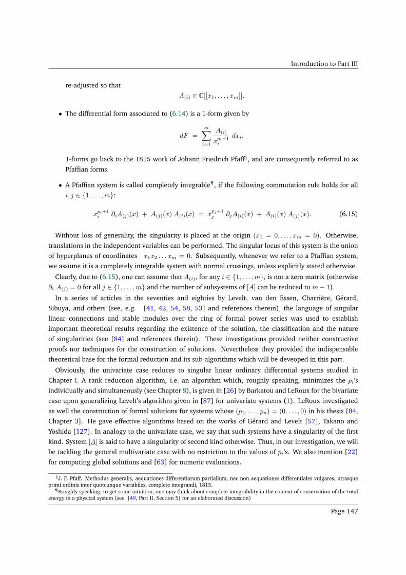
Introduction to Part III
re-adjusted so that
A(i) ∈ C[[x1, . . . , xm]].
• The differential form associated to (6.14) is a 1-form given by
dF =
m∑
i=1
A(i)
xpi+1i
dxi.
1-forms go back to the 1815 work of Johann Friedrich Pfaff§, and are consequently referred to as
Pfaffian forms.
• A Pfaffian system is called completely integrable¶, if the following commutation rule holds for all
i, j ∈ 1, . . . ,m:
xpi+1i ∂iA(j)(x) + A(j)(x) A(i)(x) = x
pj+1j ∂jA(i)(x) + A(i)(x) A(j)(x). (6.15)
Without loss of generality, the singularity is placed at the origin (x1 = 0, . . . , xm = 0). Otherwise,
translations in the independent variables can be performed. The singular locus of this system is the union
of hyperplanes of coordinates x1x2 . . . xm = 0. Subsequently, whenever we refer to a Pfaffian system,
we assume it is a completely integrable system with normal crossings, unless explicitly stated otherwise.
Clearly, due to (6.15), one can assume that A(i), for any i ∈ 1, . . . ,m, is not a zero matrix (otherwise
∂i A(j) = 0 for all j ∈ 1, . . . ,m and the number of subsystems of [A] can be reduced to m− 1).
In a series of articles in the seventies and eighties by Levelt, van den Essen, Charrière, Gérard,
Sibuya, and others (see, e.g. [41, 42, 54, 58, 53] and references therein), the language of singular
linear connections and stable modules over the ring of formal power series was used to establish
important theoretical results regarding the existence of the solution, the classification and the nature
of singularities (see [84] and references therein). These investigations provided neither constructive
proofs nor techniques for the construction of solutions. Nevertheless they provided the indispensable
theoretical base for the formal reduction and its sub-algorithms which will be deveoped in this part.
Obviously, the univariate case reduces to singular linear ordinary differential systems studied in
Chapter I. A rank reduction algorithm, i.e. an algorithm which, roughly speaking, minimizes the pi’s
individually and simultaneously (see Chapter 8), is given in [26] by Barkatou and LeRoux for the bivariate
case upon generalizing Levelt’s algorithm given in [87] for univariate systems (1). LeRoux investigated
as well the construction of formal solutions for systems whose (p1, . . . , pn) = (0, . . . , 0) in his thesis [84,
Chapter 3]. He gave effective algorithms based on the works of Gérard and Levelt [57], Takano and
Yoshida [127]. In analogy to the univariate case, we say that such systems have a singularity of the first
kind. System [A] is said to have a singularity of second kind otherwise. Thus, in our investigation, we will
be tackling the general multivariate case with no restriction to the values of pi’s. We also mention [22]
for computing global solutions and [63] for numeric evaluations.
§J. F. Pfaff. Methodus generalis, aequationes differentiarum partialium, nec non aequationes differentiales vulgares, utrasqueprimi ordinis inter quotcunque variabiles, complete integrandi, 1815.
¶Roughly speaking, to get some intuition, one may think about complete integrability in the context of conservation of the totalenergy in a physical system (see [49, Part II, Section 5] for an elaborated discussion)
Page 147
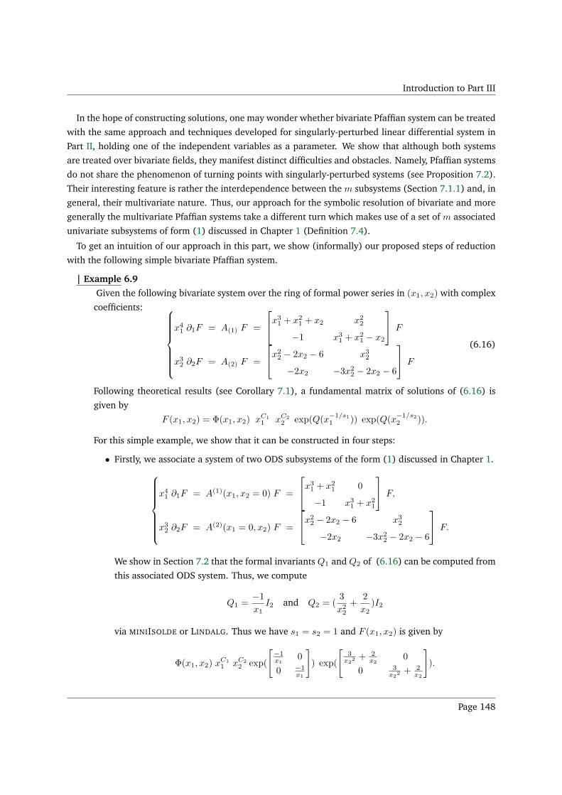
Introduction to Part III
In the hope of constructing solutions, one may wonder whether bivariate Pfaffian system can be treated
with the same approach and techniques developed for singularly-perturbed linear differential system in
Part II, holding one of the independent variables as a parameter. We show that although both systems
are treated over bivariate fields, they manifest distinct difficulties and obstacles. Namely, Pfaffian systems
do not share the phenomenon of turning points with singularly-perturbed systems (see Proposition 7.2).
Their interesting feature is rather the interdependence between the m subsystems (Section 7.1.1) and, in
general, their multivariate nature. Thus, our approach for the symbolic resolution of bivariate and more
generally the multivariate Pfaffian systems take a different turn which makes use of a set of m associated
univariate subsystems of form (1) discussed in Chapter 1 (Definition 7.4).
To get an intuition of our approach in this part, we show (informally) our proposed steps of reduction
with the following simple bivariate Pfaffian system.
| Example 6.9
Given the following bivariate system over the ring of formal power series in (x1, x2) with complex
coefficients:
x41 ∂1F = A(1) F =
x31 + x2
1 + x2 x22
−1 x31 + x2
1 − x2
F
x32 ∂2F = A(2) F =
x22 − 2x2 − 6 x3
2
−2x2 −3x22 − 2x2 − 6
F
(6.16)
Following theoretical results (see Corollary 7.1), a fundamental matrix of solutions of (6.16) is
given by
F (x1, x2) = Φ(x1, x2) xC11 xC2
2 exp(Q(x−1/s11 )) exp(Q(x
−1/s22 )).
For this simple example, we show that it can be constructed in four steps:
• Firstly, we associate a system of two ODS subsystems of the form (1) discussed in Chapter 1.
x41 ∂1F = A(1)(x1, x2 = 0) F =
x31 + x2
1 0
−1 x31 + x2
1
F,
x32 ∂2F = A(2)(x1 = 0, x2) F =
x22 − 2x2 − 6 x3
2
−2x2 −3x22 − 2x2 − 6
F.
We show in Section 7.2 that the formal invariants Q1 and Q2 of (6.16) can be computed from
this associated ODS system. Thus, we compute
Q1 =−1x1
I2 and Q2 = (3
x22
+2
x2)I2
via MINIISOLDE or LINDALG. Thus we have s1 = s2 = 1 and F (x1, x2) is given by
Φ(x1, x2) xC11 xC2
2 exp(
[−1x1
0
0 −1x1
]
) exp(
[3
x22 + 2
x20
0 3x2
2 + 2x2
]
).
Page 148
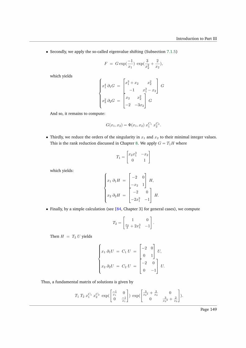
Introduction to Part III
• Secondly, we apply the so-called eigenvalue shifting (Subsection 7.1.5)
F = G exp(−1x1
) exp(3
x22
+2
x2),
which yields
x41 ∂1G =
x31 + x2 x2
2
−1 x31 − x2
G
x22 ∂2G =
x2 x2
2
−2 −3x2
G
And so, it remains to compute:
G(x1, x2) = Φ(x1, x2) xC11 xC2
2 .
• Thirdly, we reduce the orders of the singularity in x1 and x2 to their minimal integer values.
This is the rank reduction discussed in Chapter 8. We apply G = T1H where
T1 =
[
x2x31 −x2
0 1
]
which yields:
x1 ∂1H =
−2 0
−x2 1
H,
x2 ∂2H =
−2 0
−2x31 −1
H.
• Finally, by a simple calculation (see [84, Chapter 3] for general cases), we compute
T2 =
[
1 0x2
3 + 2x31 −1
]
.
Then H = T2 U yields
x1 ∂1U = C1 U =
−2 0
0 1
U,
x2 ∂2U = C2 U =
−2 0
0 −1
U.
Thus, a fundamental matrix of solutions is given by
T1 T2 xC11 xC2
2 exp(
[−1x1
0
0 −1x1
]
) exp(
[3
x22 + 2
x20
0 3x2
2 + 2x2
]
).
Page 149
Introduction to Part III
Unlike this simple example, the steps of computation can be far more evolved and demand multiple
levels of recursion. Nevertheless, we give in this part the formal reduction of such systems over three
chapters as follows:
• In Chapter 7, we show that the formal invariants of the system (6.14) can be retrieved from an
associated linear ordinary differential subsystems (ODS), each having the form [A] given by (1)
and discussed in Chapter 1. We then give a formal reduction algorithm, under the assumption that
we have at hand a rank reduction algorithm.
• In Chapter 8, we distinguish between bivariate and multivariate systems and propose rank reduction
algorithms.
We then discuss two examples which arise from applications and have different structure from the
systems considered in this thesis. Chapters 7 and 8 are based on our published paper [1] for the bivariate
case and the ongoing investigation for the multivariate case. A Maple package is also given [100].
In the sequel, we adopt C as the base field for the simplicity of the presentation. However, any other
field K (Q ⊆ K ⊆ C) can be considered instead. In this case, the restrictions on the extensions of the base
field discussed in Section 1.8 apply as well and are taken into consideration within the implementation.
Local Notations
• We use n for the dimension of each of the subsystems in accordance with the other parts. And
we use the integer m where m ≤ 1 for the number of variables. As mentioned above, for m = 1,
system (6.14) is simply an ODS.
• As mentioned in the introduction, we denote by x (resp. xi) the collection of variables x1, . . . , xm
(resp. x1, . . . , xi−1, xi+1, . . . , xm). We thus refer by R (resp. Rxi) to C[[x1, . . . , xm]] (resp.
C[[x1, . . . , xi−1, xi+1, . . . , xm]]), the ring of formal power series in x (resp. xi) over the field of
complex numbers C. And we denote its field of fractions by Frac(R) (resp. Frac(Rxi)).
• Aside from the rings R and Rxi, we will frequently have to work in other algebraic structures. Let
L be the set of monomials given by,
L = xβ = xβ1
1 xβ2
2 . . . xβmm for β = (β1, β2, . . . , βm) ∈ Nm.
Clealry, L is closed under multiplication and contains the unit element. Then, one can define
RL := L−1R, the localization of R at L, i.e. the ring of series with only finitely many terms having
monomials of strictly negative exponents. Unlike in the univariate case, Frac(R) and RL do not refer
to the same algebraic structure, e.g. (x1 + x2)−1 is an element of Frac(R) which is not an element
of RL. In fact, there exists no β ∈ N2 such that xβ(x1 + x2)−1 ∈ RL as (x1 + x2)
−1 = 1/x1
1−(−x2/x1)
whose formal expansion with respect to x2 is∑
i≥0(−1)ix−i−11 xi
2, which has infinitely many poles
in x1. For a further characterization of Frac(R), one may refer to [6].
Page 150
Introduction to Part III
• In the sequel, it will be necessary to introduce ramifications of the form xi = tαii for new variables
ti and positive integers αi (i ∈ 1, . . . ,m). And so we denote by Rt = C[[t1, . . . , tm]] the ring of
formal power series in t = (t1, t2, . . . , tm) over the field of complex numbers C and by Frac(Rt) its
field of fractions.
• We set ∂i = ∂i
∂xi and ∂ti =∂i
∂ti for all i ∈ 1, . . . ,m.
• We will have to work with some m-tuples and so we underline them so that they can be easily
identified. Let a = (a1, . . . , am) and b = (b1, . . . , bm) belong to Qm. We set 1 = (1, . . . , 1), 0 =
(0, . . . , 0), and define the order relation over Qm by
a b if and only if ai ≤ bi ∀ i ∈ 1, . . . ,m.
We also have
a = b if and only if ai = bi ∀ i ∈ 1, . . . ,m,
a ≺ b if and only if a b, and ∃ at least one index i ∈ 1, . . . ,m such that ai < bi,
and a− b = (a1 − b1, . . . , am − bm).
• In the sequel we make use of the following series representations:
– The expansion of A(i)(x) with respect to xi:
xpi+1i ∂iF = (A(i),0 +A(i),1xi +A(i),2x
2i ++ · · ·+A(i),kx
ki + . . . ) F,
where the entries of A(i),k lie in the ring Rxi; we refer to A(i),0 := A(i)(xi = 0) as the leading
matrix coefficient of the ith component [A(i)] of system [A];
– Occasionally, we need to refer to the leading matrix coefficient in the expansion of A(i)(x)
with respect to xj where i 6= j. In this case, we simply write A(i)(xj = 0) ∈ Rxjto avoid any
confusion with A(i),0, which we use to denote the leading matrix coefficient in the expansion
of A(i) with respect to xi.
– We define A(i)(xi) := A(i)(x1 = 0, . . . , xi−1 = 0, xi, xi+1 = 0, . . . , xm = 0) which has its entries
in C[[xi]]. In other words, A(i)(xi) is obtained from A(i)(x) by setting to zero all the variables
xj for which j 6= i where j ∈ 1, . . . ,m.– For the monomial expansion of M(x) ∈Mn(R), we use the lexicographical ordering (see, e.g.
[6, Section 4]) and the following short-hand notations for k = (k1, . . . , km) ∈ Nm:
|k| = k1 + · · ·+ km
xk = xk11 xk2
2 . . . xkmm
and so we write:
M(x) =
∞∑
|k|=0
Mk xk where Mk ∈Mn(C).
Page 151
Introduction to Part III
• A family of matrices is given with lower indices, e.g. (M(i),k)1≤i≤m,k≥0, and for a matrix M(i),k,
blocks are given with upper indices where the sizes of the different blocks are clear from the context.
For example, we may partition A(i),k, the kth coefficient of the matrix of the ith component, as
follows
A(i),k =
(
A11(i),k A12
(i),k
A21(i),k A22
(i),k
)
.
• We denote by pi the Poincaré rank of the ith component [A(i)] and by p = (p1, . . . , pm) the Poincaré
rank of the system [A].
• The leading matrix coefficient can be regarded as non-zero without any loss of generality, otherwise
pi can be readjusted. It will play a crucial role in our considerations. We thus adopt the following
notations:
– A(i),0 is the leading matrix coefficient of the ith component of [A] as explained above;
– A0 = (A(1),0, . . . , A(m),0) is m-tuple of the leading matrix coefficients of the system [A];
– A(i),0 = A(i)(x = 0) and A0 = (A(1),0, . . . , A(m),0) is m-tuple of the constant matrices of the
system [A].
– We also use A = (A(1), . . . ,A(m)).
Page 152
Chapter 7
Chapter 7
Computing Formal Invariants
Contents7.1 Preliminaries . . . . . . . . . . . . . . . . . . . . . . . . . . . . . . . . . . . . . . . . . 154
7.1.1 Compatible transformations . . . . . . . . . . . . . . . . . . . . . . . . . . . . . . 154
7.1.2 Fundamental matrix of formal solutions FMFS . . . . . . . . . . . . . . . . . . . . 155
7.1.3 Properties of the leading coefficients . . . . . . . . . . . . . . . . . . . . . . . . . . 158
7.1.4 Block-diagonalization . . . . . . . . . . . . . . . . . . . . . . . . . . . . . . . . . . 159
7.1.5 Eigenvalue shifting . . . . . . . . . . . . . . . . . . . . . . . . . . . . . . . . . . . 162
7.2 Computing the formal invariants . . . . . . . . . . . . . . . . . . . . . . . . . . . . . . 162
7.3 Formal reduction algorithm . . . . . . . . . . . . . . . . . . . . . . . . . . . . . . . . . 166
7.4 Conclusion . . . . . . . . . . . . . . . . . . . . . . . . . . . . . . . . . . . . . . . . . . 168
In this chapter, we are interested in the formal reduction of system [A] given by (6.14) and which we
recall here
[A] xpi+1i ∂iF = A(i)(x) F, 1 ≤ i ≤ m,
where A(i) ∈ Mn(R) and pi ≥ 0 for every i ∈ 1, . . . ,m. Let T (x) ∈ GLn(Frac(R)) then the (gauge)
transformation F = TG gives rise to
[A] xpi+1i ∂iG = A(i)(x) G, 1 ≤ i ≤ m (7.1)
where pi is an integer and
A(i)
xpi+1i
= T−1 (A(i)
xpi+1i
T − ∂iT ), 1 ≤ i ≤ m. (7.2)
We say that system (7.1) is equivalent to system (6.14) and we write [A] := T [A]. It can be easily verified
that complete integrability is inherited by an equivalent system∗. Subsequently, to stay in the same class
of systems under study, special care will be taken so that the transformations used in our considerations
∗In fact, such a transformation can be viewed as change of basis in the language of operators.
Page 153
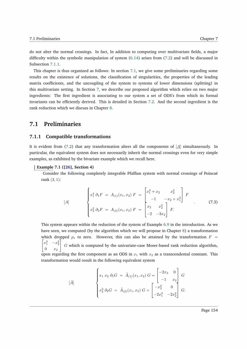
7.1 Preliminaries Chapter 7
do not alter the normal crossings. In fact, In addition to computing over multivariate fields, a major
difficulty within the symbolic manipulation of system (6.14) arises from (7.2) and will be discussed in
Subsection 7.1.1.
This chapter is thus organized as follows: In section 7.1, we give some preliminaries regarding some
results on the existence of solutions, the classification of singularities, the properties of the leading
matrix coefficients, and the uncoupling of the system to systems of lower dimensions (splitting) in
this multivariate setting. In Section 7, we describe our proposed algorithm which relies on two major
ingredients: The first ingredient is associating to our system a set of ODS’s from which its formal
invariants can be efficiently derived. This is detailed in Section 7.2. And the second ingredient is the
rank reduction which we discuss in Chapter 8.
7.1 Preliminaries
7.1.1 Compatible transformations
It is evident from (7.2) that any transformation alters all the components of [A] simultaneously. In
particular, the equivalent system does not necessarily inherit the normal crossings even for very simple
examples, as exhibited by the bivariate example which we recall here.
| Example 7.1 ([26], Section 4)
Consider the following completely integrable Pfaffian system with normal crossings of Poincaé
rank (3, 1):
[A]
x41 ∂1F = A(1)(x1, x2) F =
x31 + x2 x2
2
−1 −x2 + x31
F
x22 ∂2F = A(2)(x1, x2) F =
x2 x2
2
−2 −3x2
F.
. (7.3)
This system appears within the reduction of the system of Example 6.9 in the introduction. As we
have seen, we computed (by the algorithm which we will propose in Chapter 8) a transformation
which dropped p1 to zero. However, this can also be attained by the transformation F =[
x31 −x2
2
0 x2
]
G which is computed by the univariate-case Moser-based rank reduction algorithm,
upon regarding the first component as an ODS in x1 with x2 as a transcendental constant. This
transformation would result in the following equivalent system
[A]
x1 x2 ∂1G = A(1)(x1, x2) G =
−2x2 0
−1 x2
G
x32 ∂2G = A(2)(x1, x2) G =
−x2
2 0
−2x31 −2x2
2
G.
Page 154
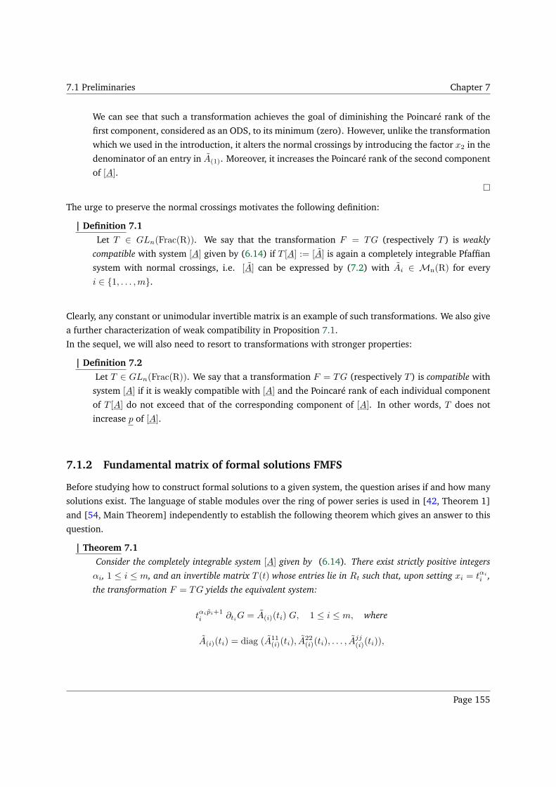
7.1 Preliminaries Chapter 7
We can see that such a transformation achieves the goal of diminishing the Poincaré rank of the
first component, considered as an ODS, to its minimum (zero). However, unlike the transformation
which we used in the introduction, it alters the normal crossings by introducing the factor x2 in the
denominator of an entry in A(1). Moreover, it increases the Poincaré rank of the second component
of [A].
The urge to preserve the normal crossings motivates the following definition:
| Definition 7.1
Let T ∈ GLn(Frac(R)). We say that the transformation F = TG (respectively T ) is weakly
compatible with system [A] given by (6.14) if T [A] := [A] is again a completely integrable Pfaffian
system with normal crossings, i.e. [A] can be expressed by (7.2) with Ai ∈ Mn(R) for every
i ∈ 1, . . . ,m.
Clearly, any constant or unimodular invertible matrix is an example of such transformations. We also give
a further characterization of weak compatibility in Proposition 7.1.
In the sequel, we will also need to resort to transformations with stronger properties:
| Definition 7.2
Let T ∈ GLn(Frac(R)). We say that a transformation F = TG (respectively T ) is compatible with
system [A] if it is weakly compatible with [A] and the Poincaré rank of each individual component
of T [A] do not exceed that of the corresponding component of [A]. In other words, T does not
increase p of [A].
7.1.2 Fundamental matrix of formal solutions FMFS
Before studying how to construct formal solutions to a given system, the question arises if and how many
solutions exist. The language of stable modules over the ring of power series is used in [42, Theorem 1]
and [54, Main Theorem] independently to establish the following theorem which gives an answer to this
question.
| Theorem 7.1
Consider the completely integrable system [A] given by (6.14). There exist strictly positive integers
αi, 1 ≤ i ≤ m, and an invertible matrix T (t) whose entries lie in Rt such that, upon setting xi = tαii ,
the transformation F = TG yields the equivalent system:
tαipi+1i ∂tiG = A(i)(ti) G, 1 ≤ i ≤ m, where
A(i)(ti) = diag (A11(i)(ti), A
22(i)(ti), . . . , A
jj(i)(ti)),
Page 155
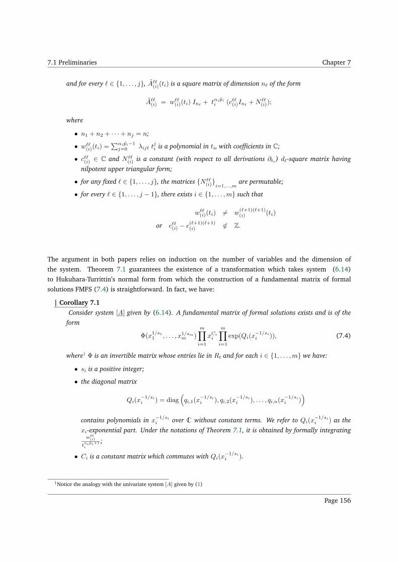
7.1 Preliminaries Chapter 7
and for every ℓ ∈ 1, . . . , j, Aℓℓ(i)(ti) is a square matrix of dimension nℓ of the form
Aℓℓ(i) = wℓℓ
(i)(ti) Inℓ+ tαipi
i (cℓℓ(i)Inℓ+N ℓℓ
(i));
where
• n1 + n2 + · · ·+ nj = n;
• wℓℓ(i)(ti) =
∑αipi−1j=0 λijℓ t
ji is a polynomial in ti, with coefficients in C;
• cℓℓ(i) ∈ C and N ℓℓ(i) is a constant (with respect to all derivations ∂ti) dℓ-square matrix having
nilpotent upper triangular form;
• for any fixed ℓ ∈ 1, . . . , j, the matrices N ℓℓ(i)i=1,...,m
are permutable;
• for every ℓ ∈ 1, . . . , j − 1, there exists i ∈ 1, . . . ,m such that
wℓℓ(i)(ti) 6= w
(ℓ+1)(ℓ+1)(i) (ti)
or cℓℓ(i) − c(ℓ+1)(ℓ+1)(i) 6∈ Z.
The argument in both papers relies on induction on the number of variables and the dimension of
the system. Theorem 7.1 guarantees the existence of a transformation which takes system (6.14)
to Hukuhara-Turrittin’s normal form from which the construction of a fundamental matrix of formal
solutions FMFS (7.4) is straightforward. In fact, we have:
| Corollary 7.1
Consider system [A] given by (6.14). A fundamental matrix of formal solutions exists and is of the
form
Φ(x1/s11 , . . . , x1/sm
m )
m∏
i=1
xCii
m∏
i=1
exp(Qi(x−1/sii )), (7.4)
where† Φ is an invertible matrix whose entries lie in Rt and for each i ∈ 1, . . . ,m we have:
• si is a positive integer;
• the diagonal matrix
Qi(x−1/sii ) = diag
(
qi,1(x−1/sii ), qi,2(x
−1/sii ), . . . , qi,n(x
−1/sii )
)
contains polynomials in x−1/sii over without constant terms. We refer to Qi(x
−1/sii ) as the
xi-exponential part. Under the notations of Theorem 7.1, it is obtained by formally integratingwℓℓ
(i)
tαipi+1
i
;
• Ci is a constant matrix which commutes with Qi(x−1/sii ).
†Notice the analogy with the univariate system [A] given by (1)
Page 156
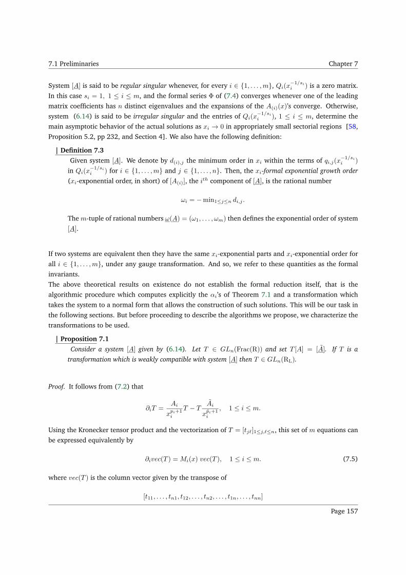
7.1 Preliminaries Chapter 7
System [A] is said to be regular singular whenever, for every i ∈ 1, . . . ,m, Qi(x−1/sii ) is a zero matrix.
In this case si = 1, 1 ≤ i ≤ m, and the formal series Φ of (7.4) converges whenever one of the leading
matrix coefficients has n distinct eigenvalues and the expansions of the A(i)(x)’s converge. Otherwise,
system (6.14) is said to be irregular singular and the entries of Qi(x−1/sii ), 1 ≤ i ≤ m, determine the
main asymptotic behavior of the actual solutions as xi → 0 in appropriately small sectorial regions [58,
Proposition 5.2, pp 232, and Section 4]. We also have the following definition:
| Definition 7.3
Given system [A]. We denote by d(i),j the minimum order in xi within the terms of qi,j(x−1/sii )
in Qi(x−1/sii ) for i ∈ 1, . . . ,m and j ∈ 1, . . . , n. Then, the xi-formal exponential growth order
(xi-exponential order, in short) of [A(i)], the ith component of [A], is the rational number
ωi = −min1≤j≤n di,j .
The m-tuple of rational numbers ω(A) = (ω1, . . . , ωm) then defines the exponential order of system
[A].
If two systems are equivalent then they have the same xi-exponential parts and xi-exponential order for
all i ∈ 1, . . . ,m, under any gauge transformation. And so, we refer to these quantities as the formal
invariants.
The above theoretical results on existence do not establish the formal reduction itself, that is the
algorithmic procedure which computes explicitly the αi’s of Theorem 7.1 and a transformation which
takes the system to a normal form that allows the construction of such solutions. This will be our task in
the following sections. But before proceeding to describe the algorithms we propose, we characterize the
transformations to be used.
| Proposition 7.1
Consider a system [A] given by (6.14). Let T ∈ GLn(Frac(R)) and set T [A] = [A]. If T is a
transformation which is weakly compatible with system [A] then T ∈ GLn(RL).
Proof. It follows from (7.2) that
∂iT =Ai
xpi+1i
T − TAi
xpi+1i
, 1 ≤ i ≤ m.
Using the Kronecker tensor product and the vectorization of T = [tjℓ]1≤j,ℓ≤n, this set of m equations can
be expressed equivalently by
∂ivec(T ) = Mi(x) vec(T ), 1 ≤ i ≤ m. (7.5)
where vec(T ) is the column vector given by the transpose of
[t11, . . . , tn1, t12, . . . , tn2, . . . , t1n, . . . , tnn]
Page 157
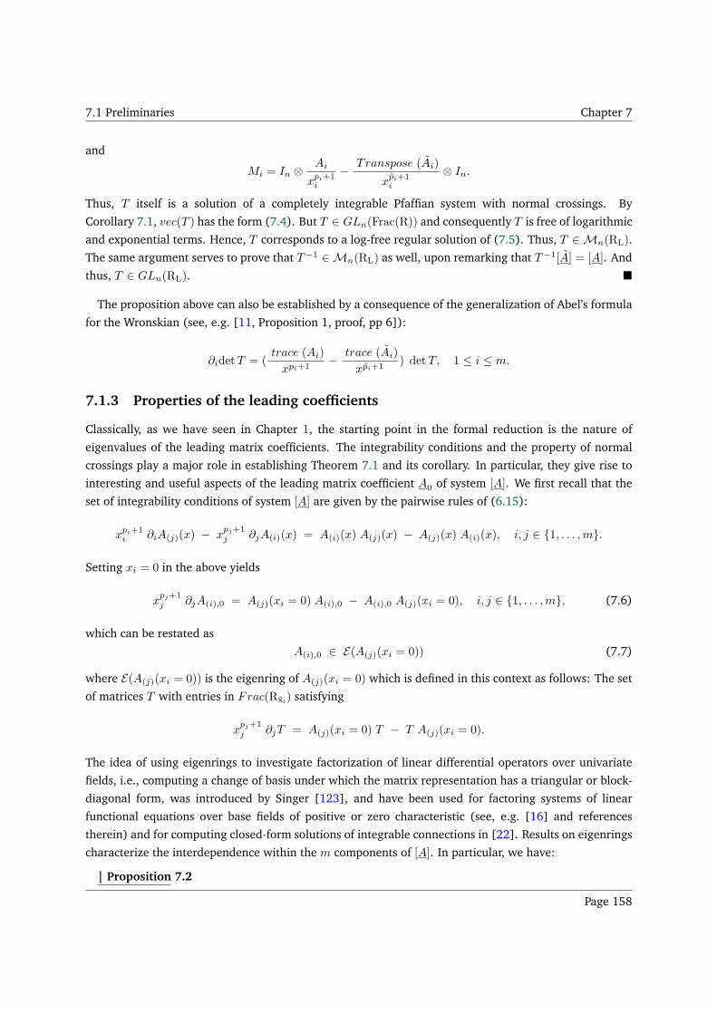
7.1 Preliminaries Chapter 7
and
Mi = In ⊗Ai
xpi+1i
− Transpose (Ai)
xpi+1i
⊗ In.
Thus, T itself is a solution of a completely integrable Pfaffian system with normal crossings. By
Corollary 7.1, vec(T ) has the form (7.4). But T ∈ GLn(Frac(R)) and consequently T is free of logarithmic
and exponential terms. Hence, T corresponds to a log-free regular solution of (7.5). Thus, T ∈Mn(RL).
The same argument serves to prove that T−1 ∈Mn(RL) as well, upon remarking that T−1[A] = [A]. And
thus, T ∈ GLn(RL).
The proposition above can also be established by a consequence of the generalization of Abel’s formula
for the Wronskian (see, e.g. [11, Proposition 1, proof, pp 6]):
∂idetT = (trace (Ai)
xpi+1− trace (Ai)
xpi+1) detT, 1 ≤ i ≤ m.
7.1.3 Properties of the leading coefficients
Classically, as we have seen in Chapter 1, the starting point in the formal reduction is the nature of
eigenvalues of the leading matrix coefficients. The integrability conditions and the property of normal
crossings play a major role in establishing Theorem 7.1 and its corollary. In particular, they give rise to
interesting and useful aspects of the leading matrix coefficient A0 of system [A]. We first recall that the
set of integrability conditions of system [A] are given by the pairwise rules of (6.15):
xpi+1i ∂iA(j)(x) − x
pj+1j ∂jA(i)(x) = A(i)(x) A(j)(x) − A(j)(x) A(i)(x), i, j ∈ 1, . . . ,m.
Setting xi = 0 in the above yields
xpj+1j ∂jA(i),0 = A(j)(xi = 0) A(i),0 − A(i),0 A(j)(xi = 0), i, j ∈ 1, . . . ,m, (7.6)
which can be restated as
A(i),0 ∈ E(A(j)(xi = 0)) (7.7)
where E(A(j)(xi = 0)) is the eigenring of A(j)(xi = 0) which is defined in this context as follows: The set
of matrices T with entries in Frac(Rxi) satisfying
xpj+1j ∂jT = A(j)(xi = 0) T − T A(j)(xi = 0).
The idea of using eigenrings to investigate factorization of linear differential operators over univariate
fields, i.e., computing a change of basis under which the matrix representation has a triangular or block-
diagonal form, was introduced by Singer [123], and have been used for factoring systems of linear
functional equations over base fields of positive or zero characteristic (see, e.g. [16] and references
therein) and for computing closed-form solutions of integrable connections in [22]. Results on eigenrings
characterize the interdependence within the m components of [A]. In particular, we have:
| Proposition 7.2
Page 158
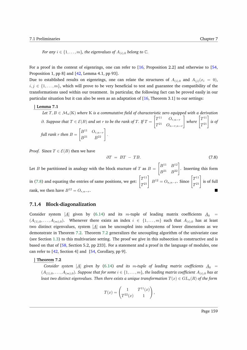
7.1 Preliminaries Chapter 7
For any i ∈ 1, . . . ,m, the eigenvalues of A(i),0 belong to C.
For a proof in the context of eigenrings, one can refer to [16, Proposition 2.2] and otherwise to [54,
Proposition 1, pp 8] and [42, Lemma 4.1, pp 93].
Due to established results on eigenrings, one can relate the structures of A(i),0 and A(j)(xi = 0),
i, j ∈ 1, . . . ,m, which will prove to be very beneficial to test and guarantee the compatibility of the
transformations used within our treatment. In particular, the following fact can be proved easily in our
particular situation but it can also be seen as an adaptation of [16, Theorem 3.1] to our settings:
| Lemma 7.1
Let T,B ∈ Mn(K) where K is a commutative field of characteristic zero equipped with a derivation
∂. Suppose that T ∈ E(B) and set r to be the rank of T . If T =
[
T 11 Or,n−r
T 21 On−r,n−r
]
where
[
T 11
T 21
]
is of
full rank r then B =
[
B11 Or,n−r
B21 B22
]
.
Proof. Since T ∈ E(B) then we have
∂T = BT − TB. (7.8)
Let B be partitioned in analogy with the block stucture of T as B =
[
B11 B12
B21 B22
]
. Inserting this form
in (7.8) and equating the entries of same positions, we get:
[
T 11
T 21
]
B12 = On,n−r. Since
[
T 11
T 21
]
is of full
rank, we then have B12 = Or,n−r.
7.1.4 Block-diagonalization
Consider system [A] given by (6.14) and its m-tuple of leading matrix coefficients A0 =
(A(1),0, . . . , A(m),0). Whenever there exists an index i ∈ 1, . . . ,m such that A(i),0 has at least
two distinct eigenvalues, system [A] can be uncoupled into subsystems of lower dimensions as we
demonstrate in Theorem 7.2. Theorem 7.2 generalizes the uncoupling algorithm of the univariate case
(see Section 1.3) to this multivariate setting. The proof we give in this subsection is constructive and is
based on that of [58, Section 5.2, pp 233]. For a statement and a proof in the language of modules, one
can refer to [42, Section 4] and [54, Corollary, pp 9].
| Theorem 7.2
Consider system [A] given by (6.14) and its m-tuple of leading matrix coefficients A0 =
(A(1),0, . . . , A(m),0). Suppose that for some i ∈ 1, . . . ,m, the leading matrix coefficient A(i),0 has at
least two distinct eigenvalues. Then there exists a unique transformation T (x) ∈ GLn(R) of the form
T (x) =
(
1 T 11(x)
T 22(x) 1
)
,
Page 159
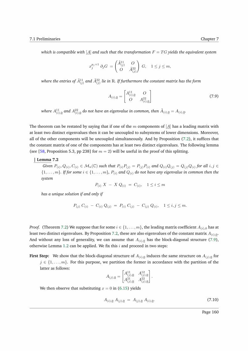
7.1 Preliminaries Chapter 7
which is compatible with [A] and such that the transformation F = TG yields the equivalent system
xpj+1j ∂jG =
(
A11(j) O
O A22(j)
)
G, 1 ≤ j ≤ m,
where the entries of A11(j) and A22
(j) lie in R. If furthermore the constant matrix has the form
A(i),0 =
[
A11(i),0 O
O A22(i),0
]
(7.9)
where A11(i),0 and A22
(i),0 do not have an eigenvalue in common, then A(i),0 = A(i),0.
The theorem can be restated by saying that if one of the m components of [A] has a leading matrix with
at least two distinct eigenvalues then it can be uncoupled to subsystems of lower dimensions. Moreover,
all of the other components will be uncoupled simultaneously. And by Proposition (7.2), it suffices that
the constant matrix of one of the components has at least two distinct eigenvalues. The following lemma
(see [58, Proposition 5.3, pp 238] for m = 2) will be useful in the proof of this splitting.
| Lemma 7.2
Given P(i), Q(i), C(i) ∈ Mn(C) such that P(i)P(j) = P(j)P(i) and Q(i)Q(j) = Q(j)Q(i) for all i, j ∈1, . . . ,m. If for some i ∈ 1, . . . ,m, P(i) and Q(i) do not have any eigenvalue in common then the
system
P(i) X − X Q(i) = C(i), 1 ≤ i ≤ m
has a unique solution if and only if
P(j) C(i) − C(i) Q(j) = P(i) C(j) − C(j) Q(i), 1 ≤ i, j ≤ m.
Proof. (Theorem 7.2) We suppose that for some i ∈ 1, . . . ,m, the leading matrix coefficient A(i),0 has at
least two distinct eigenvalues. By Proposition 7.2, these are also eigenvalues of the constant matrix A(i),0.
And without any loss of generality, we can assume that A(i),0 has the block-diagonal structure (7.9),
otherwise Lemma 1.2 can be applied. We fix this i and proceed in two steps:
First Step: We show that the block-diagonal structure of A(i),0 induces the same structure on A(j),0 for
j ∈ 1, . . . ,m. For this purpose, we partition the former in accordance with the partition of the
latter as follows:
A(j),0 =
[
A11(j),0 A12
(j),0
A21(j),0 A22
(j),0
]
.
We then observe that substituting x = 0 in (6.15) yields
A(i),0 A(j),0 = A(j),0 A(i),0. (7.10)
Page 160
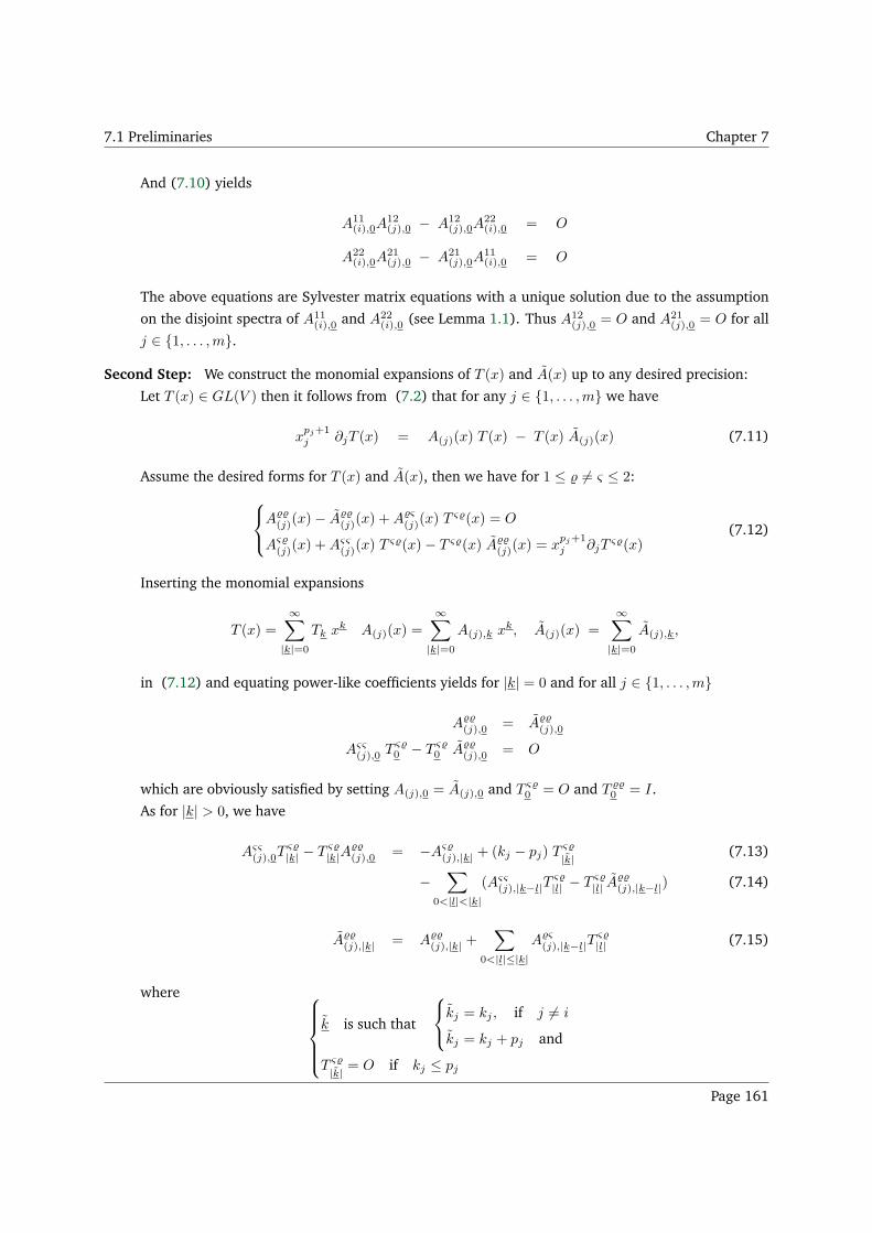
7.1 Preliminaries Chapter 7
And (7.10) yields
A11(i),0A
12(j),0 − A12
(j),0A22(i),0 = O
A22(i),0A
21(j),0 − A21
(j),0A11(i),0 = O
The above equations are Sylvester matrix equations with a unique solution due to the assumption
on the disjoint spectra of A11(i),0 and A22
(i),0 (see Lemma 1.1). Thus A12(j),0 = O and A21
(j),0 = O for all
j ∈ 1, . . . ,m.
Second Step: We construct the monomial expansions of T (x) and A(x) up to any desired precision:
Let T (x) ∈ GL(V ) then it follows from (7.2) that for any j ∈ 1, . . . ,m we have
xpj+1j ∂jT (x) = A(j)(x) T (x) − T (x) A(j)(x) (7.11)
Assume the desired forms for T (x) and A(x), then we have for 1 ≤ 6= ς ≤ 2:
A(j)(x)− A
(j)(x) +Aς(j)(x) T
ς(x) = O
Aς(j)(x) +Aςς
(j)(x) Tς(x)− T ς(x) A
(j)(x) = xpj+1j ∂jT
ς(x)(7.12)
Inserting the monomial expansions
T (x) =
∞∑
|k|=0
Tk xk A(j)(x) =
∞∑
|k|=0
A(j),k xk, A(j)(x) =
∞∑
|k|=0
A(j),k,
in (7.12) and equating power-like coefficients yields for |k| = 0 and for all j ∈ 1, . . . ,m
A(j),0 = A
(j),0
Aςς(j),0 T ς
0 − T ς0 A
(j),0 = O
which are obviously satisfied by setting A(j),0 = A(j),0 and T ς0 = O and T
0 = I.
As for |k| > 0, we have
Aςς(j),0T
ς|k| − T ς
|k|A(j),0 = −Aς
(j),|k| + (kj − pj) Tς
|k| (7.13)
−∑
0<|l|<|k|(Aςς
(j),|k−l|Tς|l| − T ς
|l| A(j),|k−l|) (7.14)
A(j),|k| = A
(j),|k| +∑
0<|l|≤|k|Aς
(j),|k−l|Tς|l| (7.15)
where
k is such that
kj = kj , if j 6= i
kj = kj + pj and
T ς
|k| = O if kj ≤ pj
Page 161
7.2 Computing the formal invariants Chapter 7
Hence, for any k ∈ Nn , j ∈ 1, . . . ,m , 1 ≤ , ς ≤ 2 , the computation of T ς|k|, and Aςς
(j),|k|, depends
solely on terms of lower order. Moreover, it can be verified by that the conditions of Lemma 7.2
are guaranteed by the monomial expansion of the integrability conditions and the disjoint spectra
of A11(i),0 and A22
(i),0. Thus, (7.15) and (7.13) can be determined uniquely and successively to any
desired precision.
We finally remark that T (x) is clearly compatible with system (6.14) since T (x = 0) = In.
Henceforth, we can assume now without loss of generality that there exists some index j ∈ 1, . . . ,m+1such that for the m-tuple of the leading matrix coefficients A0 = (A(1),0, . . . , A(m),0) we have:
• For 1 ≤ i < j, A(i),0 is nilpotent.
• For j ≤ i ≤ m, A(i),0 has a nonzero unique eigenvalue λi ∈ C,
which leads us to the next subsection.
7.1.5 Eigenvalue shifting
Let i ∈ 1, . . . ,m and suppose that A(i),0 of system [A] has a nonzero unique eigenvalue γi ∈ C. We can
then apply the so-called eigenvalue shifting
F = G exp(
∫ xi
γiz−pi−1i dzi), (7.16)
to arrive at a system [A] whose ith component has a nilpotent leading matrix coefficient. In fact we have
A(i)(x) = A(i)(x)− γiIn
A(j)(x) = A(j)(x) for all 1 ≤ j 6= i ≤ m.
Such a transformation is clearly compatible with system [A]. Henceforth, by applying to system [A]
F = G
m∏
i=j
exp(
∫ xi
γiz−pi−1i dzi),
we arrive at a system [A] with a m-tuple of nilpotent leading coefficients.
Similar to Parts I and II, with this nilpotency arises the main difficulties in formal reduction. In the next
section, we show how to compute the formal invariants of such systems.
7.2 Computing the formal invariants
One cannot retrieve ω(A) (see Definition 7.3) from the outset. In the univariate case, ω(A) reduces to
ω(A) which, as we have seen in Chapter 1, can be computed from the characteristic polynomial of A(x),
i.e. det(λI − A(x)) [14, Theorem 1], based on an analysis by a Newton’s polygon. In this section we
show that, unlike Part II, one need not search for a generalization of [14, Theorem 1] and its underlying
Page 162
7.2 Computing the formal invariants Chapter 7
set of reductions. We show that instead, the formal invariants of [A] can be obtained from a system of
associated linear singular ordinary differential systems (ODS). And so, not only we give a method to
retrieve these invariants but also we reduce computations to univariate fields. We first define these ODS
components:
| Definition 7.4
Consider system [A] given by (6.14):
[A] xpi+1i ∂i F = A(i)(x) F, 1 ≤ i ≤ m.
We call the following the associated ODS with [A]:
[A] xpi+1i ∂i F = A(i)(xi) F, 1 ≤ i ≤ m, (7.17)
where A(i)(xi) := A(x1 = 0, . . . , xi−1 = 0, xi, xi+1 = 0, . . . , xm = 0).
We then introduce the following notations:
• ω(A) = (ω(A(1)), . . . , ω(A(m))) the m-tuple of the exponential orders of the components of the
associated ODS, and
• p(A) = (p(A(1)), . . . , p(A(m))) the m-tuple of the Poincaré ranks of the components of the associated
ODS.
• ptrue
(A) = (ptrue(A(1)), . . . , ptrue(A(m))) the m-tuple of the true Poincaré ranks of the components
of the associated ODS, as defined in Section 1.5.1.
We can then establish the following theorem:
| Theorem 7.3
Given the completely integrable system with normal crossings [A] and its associated ODS system [A].
For every i ∈ 1, . . . ,m, the xi-exponential parts of the former are the exponential parts of the ith
component of the latter (see Figure 7.2). And consequently we have,
ω(A) = ω(A).
To prove this result, we rely on a triangular form weaker than the Hukuhara-Turrittin’s normal form of
Theorem 7.1. This weaker form suffices to give an insight into the computation of xi-exponential parts.
The following proposition was first given for the bivariate case in [41, Proposition 3, pp 654] and then
generalized to the multivariate general case in [42, Theorem 2.3].
| Theorem 7.4
Consider system [A] given by (6.14). There exists a positive integer α1, and a transformation T ∈GLn(Frac(Rt)) (where x1 = tα1
1 and xi = ti, 2 ≤ i ≤ m), such that the transformation F = TG
Page 163
7.2 Computing the formal invariants Chapter 7
yields the equivalent system:
[A]
tα1p1+11 ∂t1 G = A(1)(t1, x2, . . . , xm) G,
xpi+1i ∂xi
G = A(i)(x2, . . . , xm) G, 2 ≤ i ≤ m, where
(7.18)
A(1)(t1, x2, . . . , xm) = diag(A11(1), A
22(1), . . . , A
jj(1)),
A(i)(x2, . . . , xm) = diag(A11(i), A
22(i), . . . , A
jj(i)), 2 ≤ i ≤ m,
and for all ℓ ∈ 1, . . . , j and i ∈ 2, . . . ,m the entries of Aℓℓ(i) lie in Rx1
. The Aℓℓ(1)’s are of the form
Aℓℓ(1)(x2, . . . , xm) = wℓℓ
(1)(t1)Idℓ+ tα1p1
1 (N ℓℓ(1)(x2, . . . , xm) + cℓℓ(1)Inℓ
),
where
• n1 + n2 + · · ·+ nj = n;
• wℓℓ(1)(t1) and cℓℓ(1) are as in Theorem 7.1;
• If ℓ, ℓ′ ∈ 1, . . . , j − 1 and ℓ 6= ℓ′, then wℓℓ(1)(t1) 6= wℓ′ℓ′
(1) (t1) or cℓℓ(1) − cℓ′ℓ′
(1) 6∈ Z;
• N ℓℓ1 (x2, . . . , xm) is a nilpotent nℓ-square matrix whose entries lie in Rx1
.
Moreover, T can be chosen as a product of transformations in GLn(Rt) and transformations of the
form diag(tβ1
1 , . . . , tβn
1 ), where β1, . . . , βn are nonnegative integers.
Proof. (Theorem 7.3) Upon the change of independent variable x1 = tα11 , the transformation F = TG
yields system (7.18) for which the first component is given by
tα1p1+11 ∂t1 G = A(1)(t1, x2, . . . , xm) G. (7.19)
with the notations and properties as in Theorem 7.4. It then follows from (7.2) that
tα1p1+11 ∂t1T = α1 A(1)(x1 = tα1
1 ) T − T A(1). (7.20)
Due to the particular choice of T (x) characterized in Theorem 7.4, setting xi = 0, 2 ≤ i ≤ m in (7.20) is
legitimate. In particular, we are interested in the relation between the leading terms
A(1)(t1) := A(1)(x1 = tα11 , x2 = 0, . . . , xm = 0) ,
A(1)(t1) := A(1)(t1, t2 = 0, . . . , tm = 0) ,
T(t1) = T (t1, t2 = 0, . . . , tm = 0) ,
which is clearly given by
tα1p1+11 ∂t1T = α1 A(1)(x1 = tα1
1 ) T − T A(1). (7.21)
Page 164
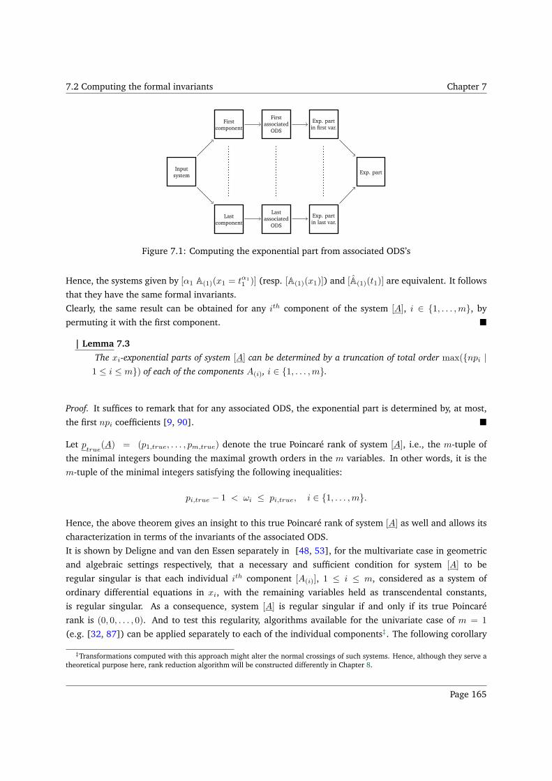
7.2 Computing the formal invariants Chapter 7
Inputsystem
Firstcomponent
Lastcomponent
Firstassociated
ODS
Lastassociated
ODS
Exp. partin first var.
Exp. partin last var.
Exp. part
Figure 7.1: Computing the exponential part from associated ODS’s
Hence, the systems given by [α1 A(1)(x1 = tα11 )] (resp. [A(1)(x1)]) and [A(1)(t1)] are equivalent. It follows
that they have the same formal invariants.
Clearly, the same result can be obtained for any ith component of the system [A], i ∈ 1, . . . ,m, by
permuting it with the first component.
| Lemma 7.3
The xi-exponential parts of system [A] can be determined by a truncation of total order max(npi |1 ≤ i ≤ m) of each of the components A(i), i ∈ 1, . . . ,m.
Proof. It suffices to remark that for any associated ODS, the exponential part is determined by, at most,
the first npi coefficients [9, 90].
Let ptrue
(A) = (p1,true, . . . , pm,true) denote the true Poincaré rank of system [A], i.e., the m-tuple of
the minimal integers bounding the maximal growth orders in the m variables. In other words, it is the
m-tuple of the minimal integers satisfying the following inequalities:
pi,true − 1 < ωi ≤ pi,true, i ∈ 1, . . . ,m.
Hence, the above theorem gives an insight to this true Poincaré rank of system [A] as well and allows its
characterization in terms of the invariants of the associated ODS.
It is shown by Deligne and van den Essen separately in [48, 53], for the multivariate case in geometric
and algebraic settings respectively, that a necessary and sufficient condition for system [A] to be
regular singular is that each individual ith component [A(i)], 1 ≤ i ≤ m, considered as a system of
ordinary differential equations in xi, with the remaining variables held as transcendental constants,
is regular singular. As a consequence, system [A] is regular singular if and only if its true Poincaré
rank is (0, 0, . . . , 0). And to test this regularity, algorithms available for the univariate case of m = 1
(e.g. [32, 87]) can be applied separately to each of the individual components‡. The following corollary
‡Transformations computed with this approach might alter the normal crossings of such systems. Hence, although they serve atheoretical purpose here, rank reduction algorithm will be constructed differently in Chapter 8.
Page 165
7.3 Formal reduction algorithm Chapter 7
follows directly from Theorem 7.3, giving a characterization of the true Poincaré rank in both the regular
and irregular cases.
| Corollary 7.2
Under the notations of this section, we have
ptrue
(A) = ptrue
(A).
For the proof, it suffices to remark that§
ptrue(A(i)) − 1 < ωi = ω(A(i)) ≤ ptrue(A(i)).
Hence, the formal exponential order, the true Poincaré rank, and most importantly the Qi’s in (7.4),
can be computed efficiently over a univariate rather than a multivariate field using the existing packages
(see Chapter 1). As mentioned in the introduction, this exponential part is of central importance in
applications since it determines the asymptotic behaviour of the solution in the neighborhood of a
singularity. However, one might also be interested in computing a full fundamental matrix of formal
solutions FMFS as given by (7.4). As we have seen in Chapter 1, the two pillars of formal reduction in
case of nilpotent leading coefficients are the formal order growth and rank reduction. So, in order to give
an algorithm to compute a fundamental matrix of formal solutions, it remains to give a compatible rank
reduction for system [A].
We assume in the next section, that we have at hand such an algorithm and we give an algorithm of
formal reduction. A rank reduction algorithm will then be investigated in Chapter 8.
7.3 Formal reduction algorithm
Given system [A], we discuss the eigenvalues of the leading matrix coefficients of its m components. If for
all of these components uncoupling is unattainable, then we fix i ∈ 1, . . . ,m and proceed to compute
the exponential order ωi from the associated ODS. Suppose that for some i, we compute ωi = ℓd with
ℓ, d coprime positive integers (see Figure 7.3 and Algorithm 7). We can then set ti = x1/di and perform
again rank reduction to get an equivalent system whose ith component has Poincaré rank equal to ℓ and
leading matrix coefficient with at least d distinct eigenvalues. Consequently, block-diagonalization can be
re-applied to uncouple the ith component. By Subsection 7.1.4, this uncoupling results in an uncoupling
for the whole system. This procedure can be repeated until we attain either a scalar system, i.e. a system
whose n components are scalar equations, or a system whose Poincaré rank is given by (0, . . . , 0). The
former is trivial and effective algorithms are given for the latter in [84, Chapter 3].
§Stronger bounds are given in [14, Remark 3]
Page 166
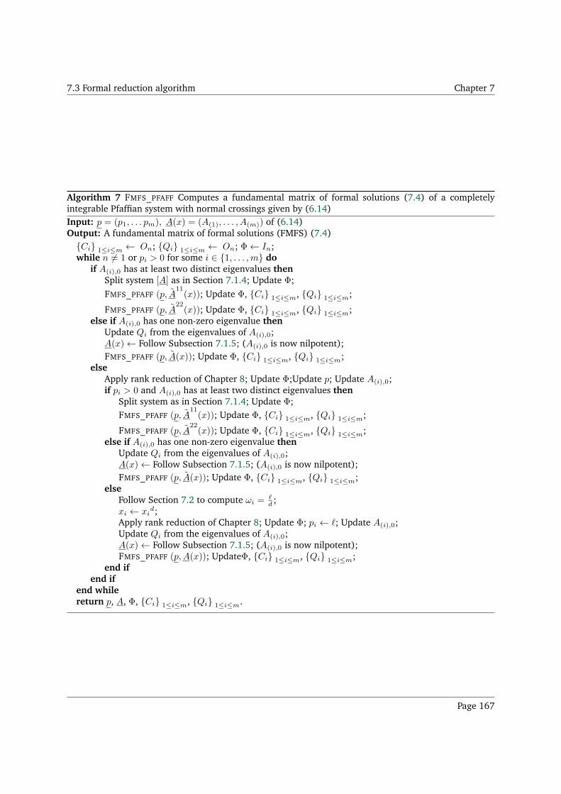
7.3 Formal reduction algorithm Chapter 7
Algorithm 7 FMFS_PFAFF Computes a fundamental matrix of formal solutions (7.4) of a completelyintegrable Pfaffian system with normal crossings given by (6.14)Input: p = (p1, . . . pm), A(x) = (A(1), . . . , A(m)) of (6.14)Output: A fundamental matrix of formal solutions (FMFS) (7.4)Ci 1≤i≤m ← On; Qi 1≤i≤m ← On; Φ← In;while n 6= 1 or pi > 0 for some i ∈ 1, . . . ,m do
if A(i),0 has at least two distinct eigenvalues thenSplit system [A] as in Section 7.1.4; Update Φ;
FMFS_PFAFF (p, A11(x)); Update Φ, Ci 1≤i≤m, Qi 1≤i≤m;
FMFS_PFAFF (p, A22(x)); Update Φ, Ci 1≤i≤m, Qi 1≤i≤m;
else if A(i),0 has one non-zero eigenvalue thenUpdate Qi from the eigenvalues of A(i),0;A(x)← Follow Subsection 7.1.5; (A(i),0 is now nilpotent);FMFS_PFAFF (p, A(x)); Update Φ, Ci 1≤i≤m, Qi 1≤i≤m;
elseApply rank reduction of Chapter 8; Update Φ;Update p; Update A(i),0;if pi > 0 and A(i),0 has at least two distinct eigenvalues then
Split system as in Section 7.1.4; Update Φ;FMFS_PFAFF (p, A
11(x)); Update Φ, Ci 1≤i≤m, Qi 1≤i≤m;
FMFS_PFAFF (p, A22(x)); Update Φ, Ci 1≤i≤m, Qi 1≤i≤m;
else if A(i),0 has one non-zero eigenvalue thenUpdate Qi from the eigenvalues of A(i),0;A(x)← Follow Subsection 7.1.5; (A(i),0 is now nilpotent);FMFS_PFAFF (p, A(x)); Update Φ, Ci 1≤i≤m, Qi 1≤i≤m;
elseFollow Section 7.2 to compute ωi =
ℓd ;
xi ← xid;
Apply rank reduction of Chapter 8; Update Φ; pi ← ℓ; Update A(i),0;Update Qi from the eigenvalues of A(i),0;A(x)← Follow Subsection 7.1.5; (A(i),0 is now nilpotent);FMFS_PFAFF (p,A(x)); UpdateΦ, Ci 1≤i≤m, Qi 1≤i≤m;
end ifend if
end whilereturn p, A, Φ, Ci 1≤i≤m, Qi 1≤i≤m.
Page 167
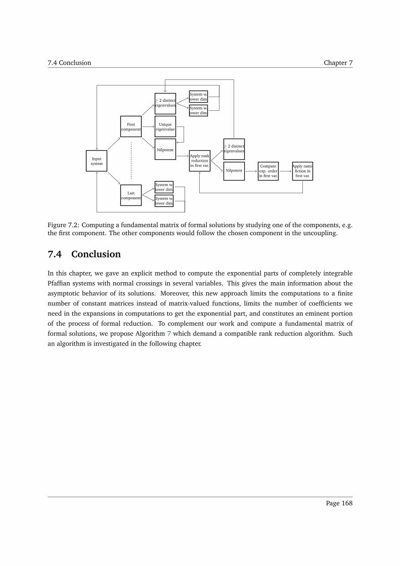
7.4 Conclusion Chapter 7
Inputsystem
Firstcomponent
Lastcomponent
System w.lower dim.
System w.lower dim.
≥ 2 distincteigenvalues
Uniqueeigenvalue
Nilpotent
System w.lower dim.
System w.lower dim.
Apply rankreductionin first var.
≥ 2 distincteigenvalues
NilpotentCompute
exp. orderin first var.
Apply rami-fiction infirst var.
Figure 7.2: Computing a fundamental matrix of formal solutions by studying one of the components, e.g.the first component. The other components would follow the chosen component in the uncoupling.
7.4 Conclusion
In this chapter, we gave an explicit method to compute the exponential parts of completely integrable
Pfaffian systems with normal crossings in several variables. This gives the main information about the
asymptotic behavior of its solutions. Moreover, this new approach limits the computations to a finite
number of constant matrices instead of matrix-valued functions, limits the number of coefficients we
need in the expansions in computations to get the exponential part, and constitutes an eminent portion
of the process of formal reduction. To complement our work and compute a fundamental matrix of
formal solutions, we propose Algorithm 7 which demand a compatible rank reduction algorithm. Such
an algorithm is investigated in the following chapter.
Page 168
Chapter 8
Chapter 8
Rank Reduction
Contents8.1 Reduction criterion . . . . . . . . . . . . . . . . . . . . . . . . . . . . . . . . . . . . . . 170
8.1.1 Moser’s criterion for the associated ODS systems . . . . . . . . . . . . . . . . . . . 170
8.1.2 Generalized Moser’s criterion . . . . . . . . . . . . . . . . . . . . . . . . . . . . . . 171
8.2 Rank reduction algorithm . . . . . . . . . . . . . . . . . . . . . . . . . . . . . . . . . . 171
8.3 Column reduction . . . . . . . . . . . . . . . . . . . . . . . . . . . . . . . . . . . . . . 173
8.4 Proof of Theorem 8.1 . . . . . . . . . . . . . . . . . . . . . . . . . . . . . . . . . . . . 177
8.5 Conclusion . . . . . . . . . . . . . . . . . . . . . . . . . . . . . . . . . . . . . . . . . . 183
Consider again system [A] given by (6.14):
[A] xpi+1i ∂i F = A(i)(x) F, 1 ≤ i ≤ m.
The Poincaré rank of the system given by p = (p1, . . . , pm) and its true Poincaré rank is given by
ptrue
(A) = (p1,true, . . . , pm,true).
In this chapter, we are interested in the rank reduction of Pfaffian systems, i.e. the explicit computation
of a transformation which, given system [A], yields an equivalent system whose Poincaré rank is the true
Poincaré rank. In other words, we show that the true Poincaré ranks of the m components of [A] can be
attained simultaneously via a transformation compatible with [A] in the bivariate case and under certain
conditions in the multivariate case.
As mentioned in the introduction, such an algorithm is developed for bivariate Pfaffian systems
in [26] upon generalizing the univariate algorithm of Levelt. Efficiency considerations aside (see
Subsection 5.6.1), the former algorithm results in an equivalent system whose Poincaré rank is minimal
but does not guarantee that the leading matrix coefficients have minimal algebraic ranks, unlike
algorithms based on Moser’s criterion. In the univariate case, the latter condition is indispensable for
the formal reduction of Algorithm 1.
This chapter is organized as follows: We first discuss two reduction criteria in Section 8.1 within
the attempt to generalize Moser’s criterion (see Section 1.5.1) and guarantee minimizing both ranks
Page 169
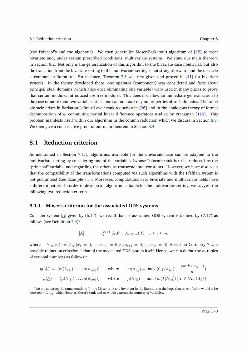
8.1 Reduction criterion Chapter 8
(the Poincaré’s and the algebraic). We then generalize Moser-Barkatou’s algorithm of [15] to treat
bivariate and, under certain prescribed conditions, multivariate systems. We state our main theorem
in Section 8.2. Not only is the generalization of this algorithm to the bivariate case nontrivial, but also
the transition from the bivariate setting to the multivariate setting is not straightforward and the obstacle
is common in literature. For instance, Theorem 7.1 was first given and proved in [41] for bivariate
systems. In the theory developed there, one operator (component) was considered and facts about
principal ideal domains (which arise once eliminating one variable) were used in many places to prove
that certain modules introduced are free modules. This does not allow an immediate generalization to
the case of more than two variables since one can no more rely on properties of such domains. The same
obstacle arises in Barkatou-LeRoux-Levelt rank reduction in [26] and in the analogous theory of formal
decomposition of m commuting partial linear difference operators studied by Praagman [115]. This
problem manifests itself within our algorithm in the column reduction which we discuss in Section 8.3.
We then give a constructive proof of our main theorem in Section 8.4.
8.1 Reduction criterion
As mentioned in Section 7.1.1, algorithms available for the univariate case can be adapted to the
multivariate setting by considering one of the variables (whose Poincaré rank is to be reduced) as the
“principal” variable and regarding the others as transcendental constants. However, we have also seen
that the compatibility of the transformations computed via such algorithms with the Pfaffian system is
not guaranteed (see Example 7.1). Moreover, computations over bivariate and multivariate fields have
a different nature. In order to develop an algorithm suitable for the multivariate setting, we suggest the
following two reduction criteria.
8.1.1 Moser’s criterion for the associated ODS systems
Consider system [A] given by (6.14), we recall that its associated ODS system is defined by (7.17) as
follows (see Definition 7.4):
[A] xpi+1i ∂i F = A(i)(xi) F, 1 ≤ i ≤ m,
where A(i)(xi) := A(i)(x1 = 0, . . . , xi−1 = 0, xi, xi+1 = 0, . . . , xm = 0). Based on Corollary 7.2, a
possible reduction criterion is that of the associated ODS system itself. Hence, we can define the m-tuples
of rational numbers as follows∗:
m(A) = (m(A(1)), . . . ,m(A(m))) where m(A(i)) = max (0, p(A(i)) +rank (A(i),0)
n)
µ(A) = (µ(A(1)), . . . , µ(A(m))) where µ(A(i)) = min m(T [A(i)]) | T ∈ GLn(RL).
∗We are adopting the same notations for the Moser rank and invariant in the literature in the hope that no confusion would arisebetween m(A(i)) which denotes Moser’s rank and m which denotes the number of variables.
Page 170
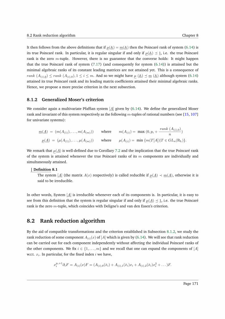
8.2 Rank reduction algorithm Chapter 8
It then follows from the above definitions that if µ(A) = m(A) then the Poincaré rank of system (6.14) is
its true Poincaré rank. In particular, it is regular singular if and only if µ(A) 1, i.e. the true Poincaré
rank is the zero m-tuple. However, there is no guarantee that the converse holds: It might happen
that the true Poincaré rank of system (7.17) (and consequently for system (6.14)) is attained but the
minimal algebraic ranks of its constant leading matrices are not attained yet. This is a consequence of
rank (A(i),0) ≤ rank (A(i),0), 1 ≤ i ≤ m. And so we might have µ (A) m (A) although system (6.14)
attained its true Poincaré rank and its leading matrix coefficients attained their minimal algebraic ranks.
Hence, we propose a more precise criterion in the next subsection.
8.1.2 Generalized Moser’s criterion
We consider again a multivariate Pfaffian system [A] given by (6.14). We define the generalized Moser
rank and invariant of this system respectively as the following m-tuples of rational numbers (see [15, 107]
for univariate systems):
m(A) = (m(A(1)), . . . ,m(A(m))) where m(A(i)) = max (0, pi +rank (A(i),0)
n)
µ(A) = (µ(A(1)), . . . , µ(A(m))) where µ(A(i)) = min m(T [A])|T ∈ GLn(RL).
We remark that µ(A) is well-defined due to Corollary 7.2 and the implication that the true Poincaré rank
of the system is attained whenever the true Poincaré ranks of its m components are individually and
simultaneously attained.
| Definition 8.1
The system [A] (the matrix A(x) respectively) is called reducible if µ(A) ≺ m(A), otherwise it is
said to be irreducible.
In other words, System [A] is irreducible whenever each of its components is. In particular, it is easy to
see from this definition that the system is regular singular if and only if µ(A) 1, i.e. the true Poincaré
rank is the zero m-tuple, which coincides with Deligne’s and van den Essen’s criterion.
8.2 Rank reduction algorithm
By the aid of compatible transformations and the criterion established in Subsection 8.1.2, we study the
rank reduction of some component A(i)(x) of [A] which is given by (6.14). We will see that rank reduction
can be carried out for each component independently without affecting the individual Poincaré ranks of
the other components. We fix i ∈ 1, . . . ,m and we recall that one can expand the components of [A]
w.r.t. xi. In particular, for the fixed index i we have,
xpi+1i ∂iF = A(i)(x)F = (A(i),0(xi) +A(i),1(xi)xi +A(i),2(xi)x
2i + . . . )F.
Page 171
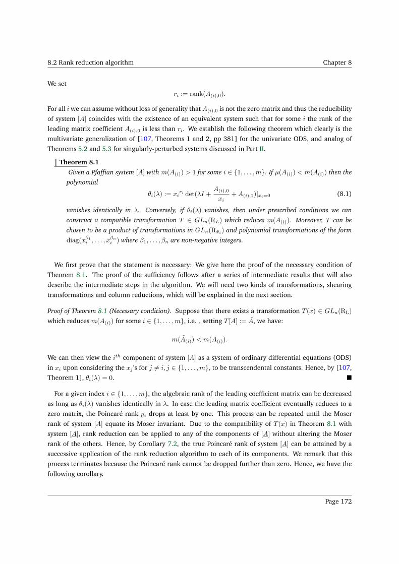
8.2 Rank reduction algorithm Chapter 8
We set
ri := rank(A(i),0).
For all i we can assume without loss of generality that A(i),0 is not the zero matrix and thus the reducibility
of system [A] coincides with the existence of an equivalent system such that for some i the rank of the
leading matrix coefficient A(i),0 is less than ri. We establish the following theorem which clearly is the
multivariate generalization of [107, Theorems 1 and 2, pp 381] for the univariate ODS, and analog of
Theorems 5.2 and 5.3 for singularly-perturbed systems discussed in Part II.
| Theorem 8.1
Given a Pfaffian system [A] with m(A(i)) > 1 for some i ∈ 1, . . . ,m. If µ(A(i)) < m(A(i)) then the
polynomial
θi(λ) := xiri det(λI +
A(i),0
xi+A(i),1)|xi=0 (8.1)
vanishes identically in λ. Conversely, if θi(λ) vanishes, then under prescribed conditions we can
construct a compatible transformation T ∈ GLn(RL) which reduces m(A(i)). Moreover, T can be
chosen to be a product of transformations in GLn(Rxi) and polynomial transformations of the form
diag(xβ1
i , . . . , xβn
i ) where β1, . . . , βn are non-negative integers.
We first prove that the statement is necessary: We give here the proof of the necessary condition of
Theorem 8.1. The proof of the sufficiency follows after a series of intermediate results that will also
describe the intermediate steps in the algorithm. We will need two kinds of transformations, shearing
transformations and column reductions, which will be explained in the next section.
Proof of Theorem 8.1 (Necessary condition). Suppose that there exists a transformation T (x) ∈ GLn(RL)
which reduces m(A(i)) for some i ∈ 1, . . . ,m, i.e. , setting T [A] := A, we have:
m(A(i)) < m(A(i)).
We can then view the ith component of system [A] as a system of ordinary differential equations (ODS)
in xi upon considering the xj ’s for j 6= i, j ∈ 1, . . . ,m, to be transcendental constants. Hence, by [107,
Theorem 1], θi(λ) = 0.
For a given index i ∈ 1, . . . ,m, the algebraic rank of the leading coefficient matrix can be decreased
as long as θi(λ) vanishes identically in λ. In case the leading matrix coefficient eventually reduces to a
zero matrix, the Poincaré rank pi drops at least by one. This process can be repeated until the Moser
rank of system [A] equate its Moser invariant. Due to the compatibility of T (x) in Theorem 8.1 with
system [A], rank reduction can be applied to any of the components of [A] without altering the Moser
rank of the others. Hence, by Corollary 7.2, the true Poincaré rank of system [A] can be attained by a
successive application of the rank reduction algorithm to each of its components. We remark that this
process terminates because the Poincaré rank cannot be dropped further than zero. Hence, we have the
following corollary.
Page 172
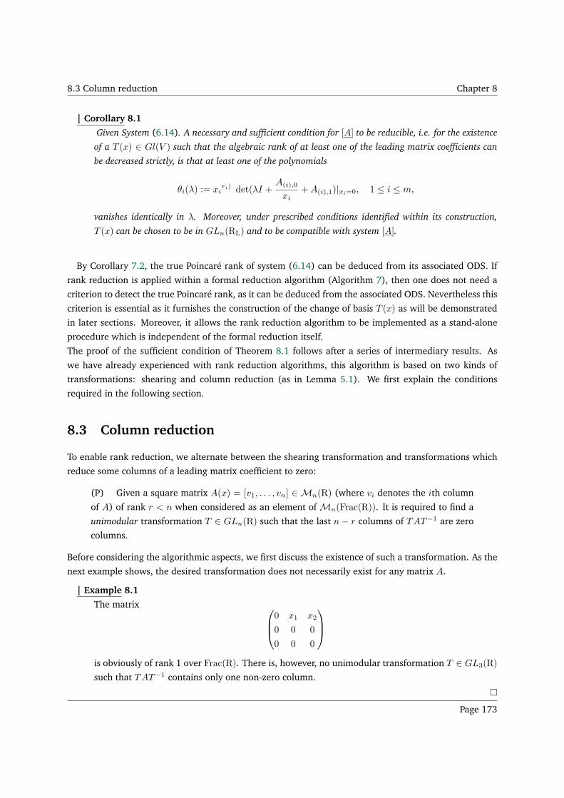
8.3 Column reduction Chapter 8
| Corollary 8.1
Given System (6.14). A necessary and sufficient condition for [A] to be reducible, i.e. for the existence
of a T (x) ∈ Gl(V ) such that the algebraic rank of at least one of the leading matrix coefficients can
be decreased strictly, is that at least one of the polynomials
θi(λ) := xiri) det(λI +
A(i),0
xi+A(i),1)|xi=0, 1 ≤ i ≤ m,
vanishes identically in λ. Moreover, under prescribed conditions identified within its construction,
T (x) can be chosen to be in GLn(RL) and to be compatible with system [A].
By Corollary 7.2, the true Poincaré rank of system (6.14) can be deduced from its associated ODS. If
rank reduction is applied within a formal reduction algorithm (Algorithm 7), then one does not need a
criterion to detect the true Poincaré rank, as it can be deduced from the associated ODS. Nevertheless this
criterion is essential as it furnishes the construction of the change of basis T (x) as will be demonstrated
in later sections. Moreover, it allows the rank reduction algorithm to be implemented as a stand-alone
procedure which is independent of the formal reduction itself.
The proof of the sufficient condition of Theorem 8.1 follows after a series of intermediary results. As
we have already experienced with rank reduction algorithms, this algorithm is based on two kinds of
transformations: shearing and column reduction (as in Lemma 5.1). We first explain the conditions
required in the following section.
8.3 Column reduction
To enable rank reduction, we alternate between the shearing transformation and transformations which
reduce some columns of a leading matrix coefficient to zero:
(P) Given a square matrix A(x) = [v1, . . . , vn] ∈ Mn(R) (where vi denotes the ith column
of A) of rank r < n when considered as an element ofMn(Frac(R)). It is required to find a
unimodular transformation T ∈ GLn(R) such that the last n− r columns of TAT−1 are zero
columns.
Before considering the algorithmic aspects, we first discuss the existence of such a transformation. As the
next example shows, the desired transformation does not necessarily exist for any matrix A.
| Example 8.1
The matrix
0 x1 x2
0 0 0
0 0 0
is obviously of rank 1 over Frac(R). There is, however, no unimodular transformation T ∈ GL3(R)
such that TAT−1 contains only one non-zero column.
Page 173
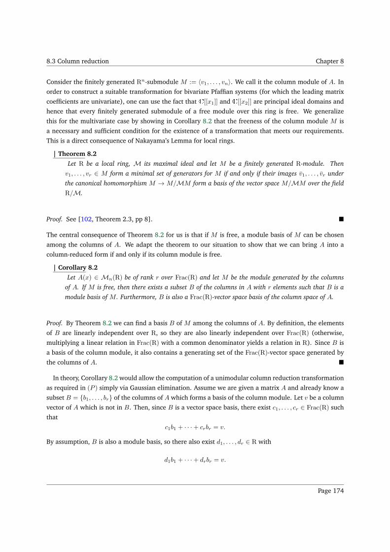
8.3 Column reduction Chapter 8
Consider the finitely generated Rn-submodule M := 〈v1, . . . , vn〉. We call it the column module of A. In
order to construct a suitable transformation for bivariate Pfaffian systems (for which the leading matrix
coefficients are univariate), one can use the fact that [[x1]] and [[x2]] are principal ideal domains and
hence that every finitely generated submodule of a free module over this ring is free. We generalize
this for the multivariate case by showing in Corollary 8.2 that the freeness of the column module M is
a necessary and sufficient condition for the existence of a transformation that meets our requirements.
This is a direct consequence of Nakayama’s Lemma for local rings.
| Theorem 8.2
Let R be a local ring, M its maximal ideal and let M be a finitely generated R-module. Then
v1, . . . , vr ∈ M form a minimal set of generators for M if and only if their images v1, . . . , vr under
the canonical homomorphism M → M/MM form a basis of the vector space M/MM over the field
R/M.
Proof. See [102, Theorem 2.3, pp 8].
The central consequence of Theorem 8.2 for us is that if M is free, a module basis of M can be chosen
among the columns of A. We adapt the theorem to our situation to show that we can bring A into a
column-reduced form if and only if its column module is free.
| Corollary 8.2
Let A(x) ∈ Mn(R) be of rank r over Frac(R) and let M be the module generated by the columns
of A. If M is free, then there exists a subset B of the columns in A with r elements such that B is a
module basis of M . Furthermore, B is also a Frac(R)-vector space basis of the column space of A.
Proof. By Theorem 8.2 we can find a basis B of M among the columns of A. By definition, the elements
of B are linearly independent over R, so they are also linearly independent over Frac(R) (otherwise,
multiplying a linear relation in Frac(R) with a common denominator yields a relation in R). Since B is
a basis of the column module, it also contains a generating set of the Frac(R)-vector space generated by
the columns of A.
In theory, Corollary 8.2 would allow the computation of a unimodular column reduction transformation
as required in (P ) simply via Gaussian elimination. Assume we are given a matrix A and already know a
subset B = b1, . . . , br of the columns of A which forms a basis of the column module. Let v be a column
vector of A which is not in B. Then, since B is a vector space basis, there exist c1, . . . , cr ∈ Frac(R) such
that
c1b1 + · · ·+ crbr = v.
By assumption, B is also a module basis, so there also exist d1, . . . , dr ∈ R with
d1b1 + · · ·+ drbr = v.
Page 174
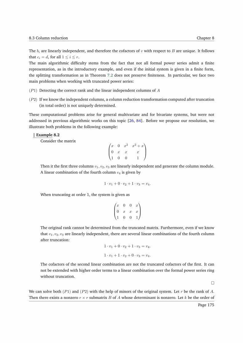
8.3 Column reduction Chapter 8
The bi are linearly independent, and therefore the cofactors of v with respect to B are unique. It follows
that ci = di for all 1 ≤ i ≤ r.
The main algorithmic difficulty stems from the fact that not all formal power series admit a finite
representation, as in the introductory example, and even if the initial system is given in a finite form,
the splitting transformation as in Theorem 7.2 does not preserve finiteness. In particular, we face two
main problems when working with truncated power series:
(P1) Detecting the correct rank and the linear independent columns of A
(P2) If we know the independent columns, a column reduction transformation computed after truncation
(in total order) is not uniquely determined.
These computational problems arise for general multivariate and for bivariate systems, but were not
addressed in previous algorithmic works on this topic [26, 84]. Before we propose our resolution, we
illustrate both problems in the following example:
| Example 8.2
Consider the matrix
x 0 x2 x2 + x
0 x x x
1 0 0 1
Then it the first three columns v1, v2, v3 are linearly independent and generate the column module.
A linear combination of the fourth column v4 is given by
1 · v1 + 0 · v2 + 1 · v3 = v4.
When truncating at order 1, the system is given as
x 0 0 x
0 x x x
1 0 0 1
The original rank cannot be determined from the truncated matrix. Furthermore, even if we know
that v1, v2, v3 are linearly independent, there are several linear combinations of the fourth column
after truncation:
1 · v1 + 0 · v2 + 1 · v3 = v4.
1 · v1 + 1 · v2 + 0 · v3 = v4.
The cofactors of the second linear combination are not the truncated cofactors of the first. It can
not be extended with higher order terms to a linear combination over the formal power series ring
without truncation.
We can solve both (P1) and (P2) with the help of minors of the original system. Let r be the rank of A.
Then there exists a nonzero r × r submatrix B of A whose determinant is nonzero. Let k be the order of
Page 175
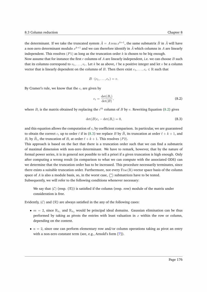
8.3 Column reduction Chapter 8
the determinant. If we take the truncated system A = A remxk+1, the same submatrix B in A will have
a non-zero determinant modulo xk+1 and we can therefore identify in A which columns in A are linearly
independent. This resolves (P1) as long as the truncation order k is chosen to be big enough.
Now assume that for instance the first r columns of A are linearly independent, i.e. we can choose B such
that its columns correspond to v1, . . . , vr. Let k be as above, ℓ be a positive integer and let v be a column
vector that is linearly dependent on the columns of B. Then there exist c1, . . . , cr ∈ R such that
B · (c1, . . . , cr) = v.
By Cramer’s rule, we know that the ci are given by
ci =det(Bi)
det(B), (8.2)
where Bi is the matrix obtained by replacing the ith column of B by v. Rewriting Equation (8.2) gives
det(B)ci − det(Bi) = 0, (8.3)
and this equation allows the computation of ci by coefficient comparison. In particular, we are guaranteed
to obtain the correct ci up to order ℓ if in (8.3) we replace B by B, its truncation at order ℓ+ k + 1, and
Bi by Bi, the truncation of Bi at order ℓ+ k + 1. This resolves (P2).
This approach is based on the fact that there is a truncation order such that we can find a submatrix
of maximal dimension with non-zero determinant. We have to remark, however, that by the nature of
formal power series, it is in general not possible to tell a priori if a given truncation is high enough. Only
after computing a wrong result (in comparison to what we can compute with the associated ODS) can
we determine that the truncation order has to be increased. This procedure necessarily terminates, since
there exists a suitable truncation order. Furthermore, not every Frac(R)-vector space basis of the column
space of A is also a module basis, so, in the worst case,(nr
)submatrices have to be tested.
Subsequently, we will refer to the following conditions whenever necessary:
We say that (C) (resp. (R)) is satisfied if the column (resp. row) module of the matrix under
consideration is free.
Evidently, (C) and (R) are always satisfied in the any of the following cases:
• m = 2, since Rx1and Rx2
would be principal ideal domains. Gaussian elimination can be thus
performed by taking as pivots the entries with least valuation in x within the row or column,
depending on the context.
• n = 2, since one can perform elementary row and/or column operations taking as pivot an entry
with a non-zero constant term (see, e.g., Arnold’s form [7]).
Page 176
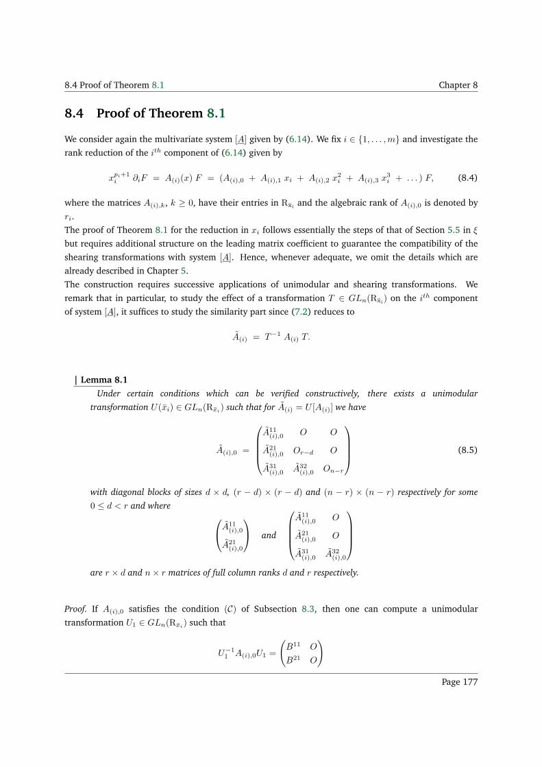
8.4 Proof of Theorem 8.1 Chapter 8
8.4 Proof of Theorem 8.1
We consider again the multivariate system [A] given by (6.14). We fix i ∈ 1, . . . ,m and investigate the
rank reduction of the ith component of (6.14) given by
xpi+1i ∂iF = A(i)(x) F = (A(i),0 + A(i),1 xi + A(i),2 x2
i + A(i),3 x3i + . . . ) F, (8.4)
where the matrices A(i),k, k ≥ 0, have their entries in Rxiand the algebraic rank of A(i),0 is denoted by
ri.
The proof of Theorem 8.1 for the reduction in xi follows essentially the steps of that of Section 5.5 in ξ
but requires additional structure on the leading matrix coefficient to guarantee the compatibility of the
shearing transformations with system [A]. Hence, whenever adequate, we omit the details which are
already described in Chapter 5.
The construction requires successive applications of unimodular and shearing transformations. We
remark that in particular, to study the effect of a transformation T ∈ GLn(Rxi) on the ith component
of system [A], it suffices to study the similarity part since (7.2) reduces to
A(i) = T−1 A(i) T.
| Lemma 8.1
Under certain conditions which can be verified constructively, there exists a unimodular
transformation U(xi) ∈ GLn(Rxi) such that for A(i) = U [A(i)] we have
A(i),0 =
A11(i),0 O O
A21(i),0 Or−d O
A31(i),0 A32
(i),0 On−r
(8.5)
with diagonal blocks of sizes d × d, (r − d) × (r − d) and (n − r) × (n − r) respectively for some
0 ≤ d < r and where
A11
(i),0
A21(i),0
and
A11(i),0 O
A21(i),0 O
A31(i),0 A32
(i),0
are r × d and n× r matrices of full column ranks d and r respectively.
Proof. If A(i),0 satisfies the condition (C) of Subsection 8.3, then one can compute a unimodular
transformation U1 ∈ GLn(Rxi) such that
U−11 A(i),0U1 =
(
B11 O
B21 O
)
Page 177
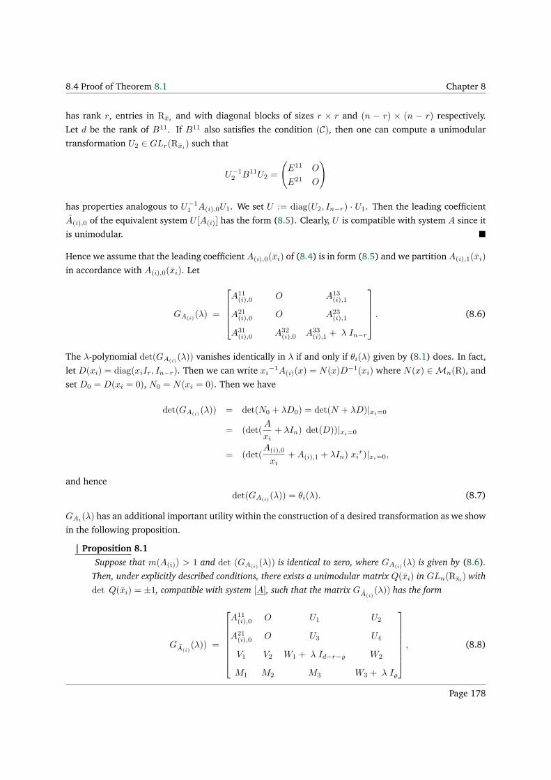
8.4 Proof of Theorem 8.1 Chapter 8
has rank r, entries in Rxiand with diagonal blocks of sizes r × r and (n − r) × (n − r) respectively.
Let d be the rank of B11. If B11 also satisfies the condition (C), then one can compute a unimodular
transformation U2 ∈ GLr(Rxi) such that
U−12 B11U2 =
(
E11 O
E21 O
)
has properties analogous to U−11 A(i),0U1. We set U := diag(U2, In−r) · U1. Then the leading coefficient
A(i),0 of the equivalent system U [A(i)] has the form (8.5). Clearly, U is compatible with system A since it
is unimodular.
Hence we assume that the leading coefficient A(i),0(xi) of (8.4) is in form (8.5) and we partition A(i),1(xi)
in accordance with A(i),0(xi). Let
GA(i)(λ) =
A11(i),0 O A13
(i),1
A21(i),0 O A23
(i),1
A31(i),0 A32
(i),0 A33(i),1 + λ In−r
. (8.6)
The λ-polynomial det(GA(i)(λ)) vanishes identically in λ if and only if θi(λ) given by (8.1) does. In fact,
let D(xi) = diag(xiIr, In−r). Then we can write xi−1A(i)(x) = N(x)D−1(xi) where N(x) ∈Mn(R), and
set D0 = D(xi = 0), N0 = N(xi = 0). Then we have
det(GA(i)(λ)) = det(N0 + λD0) = det(N + λD)|xi=0
= (det(A
xi+ λIn) det(D))|xi=0
= (det(A(i),0
xi+A(i),1 + λIn) xi
r)|xi=0,
and hence
det(GA(i)(λ)) = θi(λ). (8.7)
GAi(λ) has an additional important utility within the construction of a desired transformation as we show
in the following proposition.
| Proposition 8.1
Suppose that m(A(i)) > 1 and det (GA(i)(λ)) is identical to zero, where GA(i)
(λ) is given by (8.6).
Then, under explicitly described conditions, there exists a unimodular matrix Q(xi) in GLn(Rxi) with
det Q(xi) = ±1, compatible with system [A], such that the matrix GA(i)(λ)) has the form
GA(i)(λ)) =
A11(i),0 O U1 U2
A21(i),0 O U3 U4
V1 V2 W1 + λ Id−r− W2
M1 M2 M3 W3 + λ I
, (8.8)
Page 178
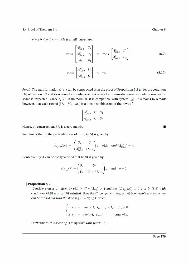
8.4 Proof of Theorem 8.1 Chapter 8
where 0 ≤ ≤ n− r, M2 is a null matrix, and
rank
A11(i),0 U1
A21(i),0 U3
M1 M3
= rank
A11
(i),0 U1
A21(i),0 U3
, (8.9)
rank
A11
(i),0 U1
A21(i),0 U3
< ri. (8.10)
Proof. The transformation Q(xi) can be constructed as in the proof of Proposition 5.2 under the condition
(R) of Section 8.3 and its weaker forms whenever necessary for intermediate matrices whose row vector
space is inspected. Since Q(xi) is unimodular, it is compatible with system [A]. It remains to remark
however, that each row of [M1 M2 M3] is a linear combination of the rows of
A11
(i),0 O U1
A21(i),0 O U3
.
Hence, by construction, M2 is a zero matrix.
We remark that in the particular case of d = 0 (8.5) is given by
A(i),0(xi) =
Or O
A32(i),0 On−r
, with rank(A32(i),0) = r.
Consequently, it can be easily verified that (8.8) is given by
GA(i)(λ) =
Or U3
V2 W1 + λIn−r
, and = 0.
| Proposition 8.2
Consider system [A] given by (6.14). If m(A(i)) > 1 and det (GA(i)(λ)) ≡ 0 is as in (8.8) with
conditions (8.9) and (8.10) satisfied, then the ith component A(i) of [A] is reducible and reduction
can be carried out with the shearing F = S(xi) G where
S(xi) = diag (xiIr, In−r−, xiI) if 6= 0
S(xi) = diag(xiIr, In−r) otherwise.
Furthermore, this shearing is compatible with system [A].
Page 179
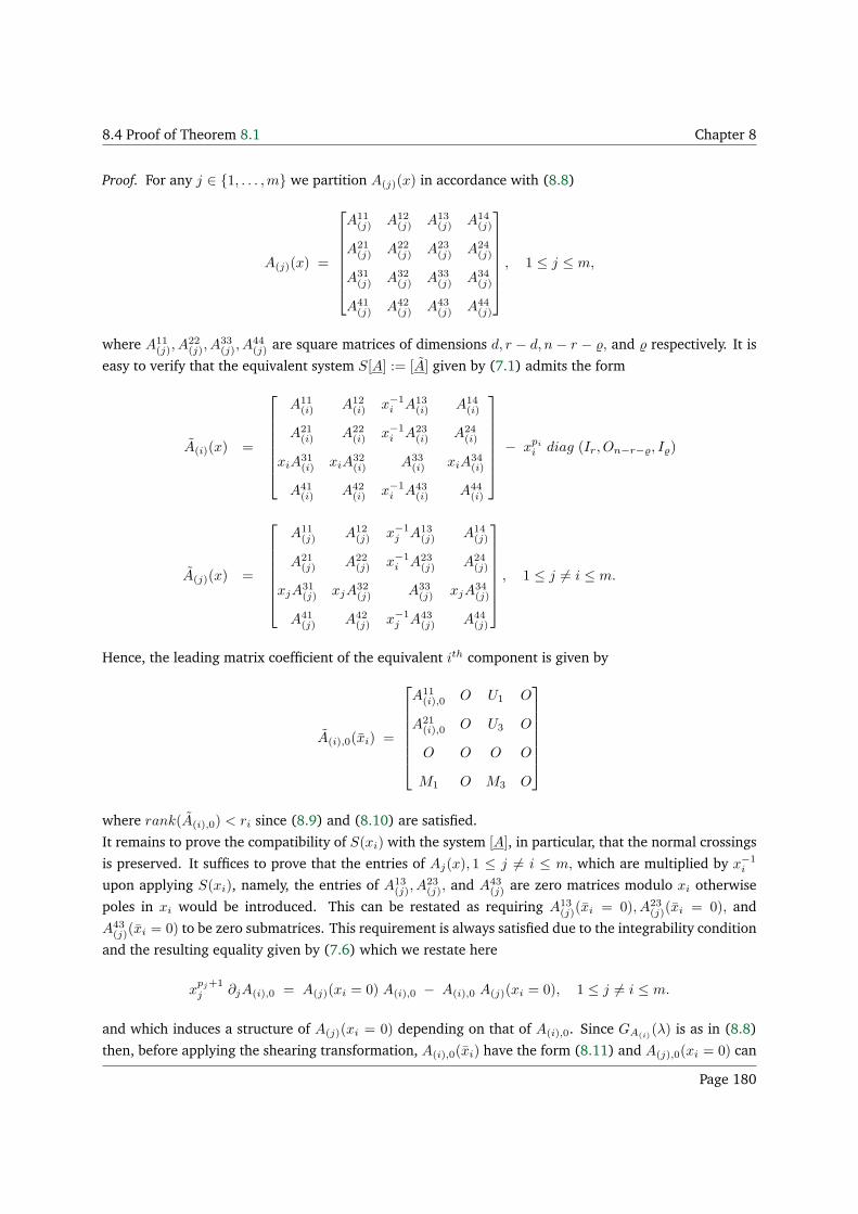
8.4 Proof of Theorem 8.1 Chapter 8
Proof. For any j ∈ 1, . . . ,m we partition A(j)(x) in accordance with (8.8)
A(j)(x) =
A11(j) A12
(j) A13(j) A14
(j)
A21(j) A22
(j) A23(j) A24
(j)
A31(j) A32
(j) A33(j) A34
(j)
A41(j) A42
(j) A43(j) A44
(j)
, 1 ≤ j ≤ m,
where A11(j), A
22(j), A
33(j), A
44(j) are square matrices of dimensions d, r − d, n − r − , and respectively. It is
easy to verify that the equivalent system S[A] := [A] given by (7.1) admits the form
A(i)(x) =
A11(i) A12
(i) x−1i A13
(i) A14(i)
A21(i) A22
(i) x−1i A23
(i) A24(i)
xiA31(i) xiA
32(i) A33
(i) xiA34(i)
A41(i) A42
(i) x−1i A43
(i) A44(i)
− xpi
i diag (Ir, On−r−, I)
A(j)(x) =
A11(j) A12
(j) x−1j A13
(j) A14(j)
A21(j) A22
(j) x−1i A23
(j) A24(j)
xjA31(j) xjA
32(j) A33
(j) xjA34(j)
A41(j) A42
(j) x−1j A43
(j) A44(j)
, 1 ≤ j 6= i ≤ m.
Hence, the leading matrix coefficient of the equivalent ith component is given by
A(i),0(xi) =
A11(i),0 O U1 O
A21(i),0 O U3 O
O O O O
M1 O M3 O
where rank(A(i),0) < ri since (8.9) and (8.10) are satisfied.
It remains to prove the compatibility of S(xi) with the system [A], in particular, that the normal crossings
is preserved. It suffices to prove that the entries of Aj(x), 1 ≤ j 6= i ≤ m, which are multiplied by x−1i
upon applying S(xi), namely, the entries of A13(j), A
23(j), and A43
(j) are zero matrices modulo xi otherwise
poles in xi would be introduced. This can be restated as requiring A13(j)(xi = 0), A23
(j)(xi = 0), and
A43(j)(xi = 0) to be zero submatrices. This requirement is always satisfied due to the integrability condition
and the resulting equality given by (7.6) which we restate here
xpj+1j ∂jA(i),0 = A(j)(xi = 0) A(i),0 − A(i),0 A(j)(xi = 0), 1 ≤ j 6= i ≤ m.
and which induces a structure of A(j)(xi = 0) depending on that of A(i),0. Since GA(i)(λ) is as in (8.8)
then, before applying the shearing transformation, A(i),0(xi) have the form (8.11) and A(j),0(xi = 0) can
Page 180
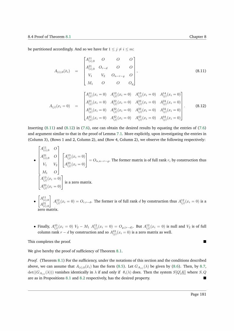
8.4 Proof of Theorem 8.1 Chapter 8
be partitioned accordingly. And so we have for 1 ≤ j 6= i ≤ m:
A(i),0(xi) =
A11(i),0 O O O
A21(i),0 Or−d O O
V1 V2 On−r− O
M1 O O O
, (8.11)
A(j)(xi = 0) =
A11(j)(xi = 0) A12
(j)(xi = 0) A13(j)(xi = 0) A14
(j)(xi = 0)
A21(j)(xi = 0) A22
(j)(xi = 0) A23(j)(xi = 0) A24
(j)(xi = 0)
A31(j)(xi = 0) A32
(j)(xi = 0) A33(j)(xi = 0) A34
(j)(xi = 0)
A41(j)(xi = 0) A42
(j)(xi = 0) A43(j)(xi = 0) A44
(j)(xi = 0)
. (8.12)
Inserting (8.11) and (8.12) in (7.6), one can obtain the desired results by equating the entries of (7.6)
and argument similar to that in the proof of Lemma 7.1. More explicitly, upon investigating the entries in
(Column 3), (Rows 1 and 2, Column 2), and (Row 4, Column 2), we observe the following respectively:
•
A11(i),0 O
A21(i),0 O
V1 V2
M1 O
A13
(j)(xi = 0)
A23(j)(xi = 0)
= On,n−r−. The former matrix is of full rank ri by construction thus
A13
(j)(xi = 0)
A23(j)(xi = 0)
is a zero matrix.
•[
A11(i),0
A21(i),0
]
A12(j)(xi = 0) = Or,r−d. The former is of full rank d by construction thus A12
(j)(xi = 0) is a
zero matrix.
• Finally, A43(j)(xi = 0) V2 −M1 A12
(j)(xi = 0) = O,(r−d). But A12(j)(xi = 0) is null and V2 is of full
column rank r − d by construction and so A43(j)(xi = 0) is a zero matrix as well.
This completes the proof.
We give hereby the proof of sufficiency of Theorem 8.1.
Proof. (Theorem 8.1) For the sufficiency, under the notations of this section and the conditions described
above, we can assume that A(i),0(xi) has the form (8.5). Let GA(i)(λ) be given by (8.6). Then, by 8.7,
det((GA(i)(λ))) vanishes identically in λ if and only if θi(λ) does. Then the system S[Q[A]] where S,Q
are as in Propositions 8.1 and 8.2 respectively, has the desired property.
Page 181
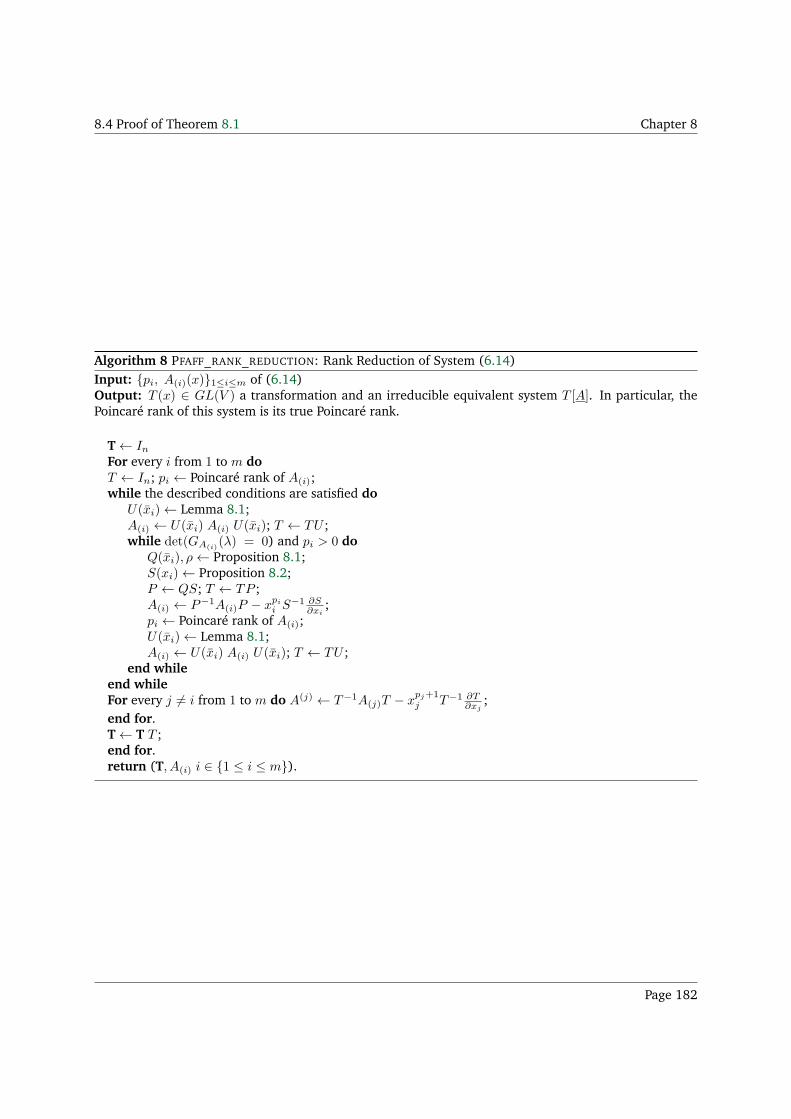
8.4 Proof of Theorem 8.1 Chapter 8
Algorithm 8 PFAFF_RANK_REDUCTION: Rank Reduction of System (6.14)Input: pi, A(i)(x)1≤i≤m of (6.14)Output: T (x) ∈ GL(V ) a transformation and an irreducible equivalent system T [A]. In particular, thePoincaré rank of this system is its true Poincaré rank.
T← InFor every i from 1 to m doT ← In; pi ← Poincaré rank of A(i);while the described conditions are satisfied do
U(xi)← Lemma 8.1;A(i) ← U(xi) A(i) U(xi); T ← TU ;while det(GA(i)
(λ) = 0) and pi > 0 doQ(xi), ρ← Proposition 8.1;S(xi)← Proposition 8.2;P ← QS; T ← TP ;A(i) ← P−1A(i)P − xpi
i S−1 ∂S∂xi
;pi ← Poincaré rank of A(i);U(xi)← Lemma 8.1;A(i) ← U(xi) A(i) U(xi); T ← TU ;
end whileend whileFor every j 6= i from 1 to m do A(j) ← T−1A(j)T − x
pj+1j T−1 ∂T
∂xj;
end for.T← T T ;end for.return (T, A(i) i ∈ 1 ≤ i ≤ m).
Page 182
8.5 Conclusion Chapter 8
| Example 8.3
Examples of dimensions two and three do not give insight to the richness of the techniques
presented. So we treat an example of dimension six. Due to the size of the system and the
number of necessary computation steps, we are not able to include it directly in this thesis. It is
available in several formats at my web page.
8.5 Conclusion
In this chapter, we gave a rank reduction criterion and an algorithm which reduces the Poincaré rank
of system [A] to its true Poincaré rank via compatible transformations of GLn(RL). Unlike the bivariate
case, the column reduction which is required in the algorithm demands imposing certain conditions in the
multivariate case. Although these conditions seem severe, the proposed algorithm gives an insight to the
obstacles encountered and resolves the problem on the linear algebra level. The same obstacle of freeness,
described in Section 8.3, arise in the attempt to generalize Levelt-Barkatou-LeRoux’s algorithm given
in [26] for bivariate systems, and in generalizing the univariate case algorithm described in Section 1.6
to construct solutions for regular-singular systems [84, Section 3.2]. An item of further investigation
is thus to investigate whether the conditions can be eliminated or weakened. We remark however that
the resolution of the linear algebra problem in Section 8.3 allows a generalization of Barkatou-LeRoux-
Levelt’s to the multivariate case under the condition (C). Hence whenever a required condition of the
form (R) do not hold anymore in Algorithm 8, such a generalization can be used as long as condition (C)holds. There remains however, the question on the equivalence of these conditions.
Page 183
8.5 Conclusion Conclusion of Part III
Conclusion and Applications
In this part, we studied completely integrable Pfaffian systems with normal crossings. We showed that
one can associate a set of univariate linear singular differential systems from which the formal invariants
of the former can be retrieved. This reduces computations to computations over a univariate field via
MINIISOLDE or LINDALG, and limits the numbers of coefficients necessary for the computations. We then
complemented our work with a rank reduction algorithm based on generalizing Moser’s criteria and the
algorithm given by Barkatou in [15]. The former is applicable to any bivariate system. However, for
multivariate systems, it demands the satisfaction of explicitly described conditions.
We obtained our results via different types of expansions:
• We used a monomial expansion to uncouple the system to systems of lower dimension in case the
leading matrix of at least one of the components has at least two distinct eigenvalues.
• To compute the formal invariants of the ith component of system [A] for any i ∈ 1, . . . ,m, we
used expansions modulo x1, . . . , xi−1, xi+1, . . . , xm.
• For rank reduction of an ith component of system [A], we used an expansion in the variable xi.
• To study the compatibility of a transformation applied to the ith component of system [A], we
expanded the other components with respect to xi.
These different series representations allowed us to retrieve information which was then patched up
together to construct formal solutions or study their behavior. In spite of the obstacles met within this
treatment, the possible approaches as well as possible series representations to such systems are not
exhausted yet due to their rich structure. For instance, one possible approach to construct a FMFS
without passing through rank reduction is to represent T (x) in the proof of Theorem 7.3 in its monomial
expansion in the light of the information about the formal invariants and construct it term by term.
We mentioned the work of [22] which computed closed form solutions of integrable connections in
m variables recursively by adapting existing algorithms handling ordinary linear differential systems.
The approach therein consists in considering m − 1 variables as transcendental constants and running
algorithms for ODS. It would be thus interesting to try instead to follow the approach developed herein
of considering the associated ODS and studying what helpful information can be derived.
Another prominent field of investigation is the analytic (asymptotic) interpretation of the formal
solutions and the recovery of “true” solutions. We mention [58, 95] in this direction and [57, 127]
for therein consists regular singularity.
Page 184
8.5 Conclusion Conclusion of Part III
One field of investigation is the formal reduction in the difference case using the approaches given
proposed herein. Praagman established in [115] a formal decomposition of m commuting partial linear
difference operators. This study was intended as an analog to that established by Levelt, van den Essen,
Gérard, Charrière, and others.
Unlike the univariate case, the algorithmic generation of examples on completely integrable Pfaffian
systems (with random or special structure) does not seem to be trivial and would be interesting to
investigate it. However, as mentioned in the introduction, Pfaffian systems arise naturally in many
applications. Systems arising from applications do not necessarily or directly fall into the class of
completely integrable Pfaffian systems with normal crossings. Our study in this thesis was restricted
to Pfaffian systems with normal crossings at the origin. But what would happen in the general case
or different locus? Investigations in this direction can be found in [111, 63, 128, 129] and references
therein.
We exhibit herein two examples to point out the obstacles encountered in adapting the techniques
developed herein but nevertheless their flexibility whenever the system at hand have a particular structure
that can be exploited. The techniques developed so far can then be modified to deal with such a system
on an individual basis. Namely, we discuss two bivariate Pfaffian systems, the first of which is perturbed
by a parameter ε, and the second lacks the normal crossings discussed in this thesis.
Since both of the systems discussed here are bivariate systems, for the clarity of the presentation, we
set m = n = 2, x = x1, y = x2, A(1)(x1, x2) = A(x, y), A(2)(x1, x2) = B(x, y), ∂1 = ∂x, and ∂2 = ∂y.
Perturbative quantum chromodynamics
The following system is a simplified version of systems arising in the field of perturbative quantum
chromodynamics†. Generally the aim is to compute certain aspects of the interaction of elementary
particles as precise as possible in order to compare it to experimental data from precision
measurements. Interactions of elementary particles can be arbitrarily complicated, involving arbitrarily
many intermediate particles, which are then called virtual particles. So one and the same interaction can
happen in many different ways internally. The parameter y below is the square of the ratio of the masses
of two of the particles involved and ranges from 0 to infinity while x ranges from 0 to 1.
Let F = (f1, . . . , f7)T denote an unknown vector and ε be a parameter. We have the following Pfaffian
system
∂xF = 1ε x (x−1) (xy+ε−y+1) A(x, y, ε) F
∂yF = 1y (y−1) (xy+ε−y+1) B(x, y, ε) F
(8.13)
where
A(x, y, ε) =
[
O4×4 O4×3
A21 A22
]
and B =
[
B11 O4×3
B21 B22
]
.
†We thank C. Raab and J.A. Weil for communicating to us this example and for discussions. At that time, C. Raab wasa postdoctoral researcher at DESY, which is a research centre whose main site lies in Hamburg. The main focus of DESY isexperimental physics in the areas of particle physics, photon science, and accelerator technology.
Page 185
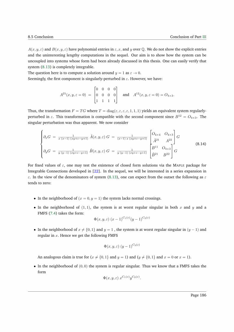
8.5 Conclusion Conclusion of Part III
A(x, y, ε) and B(x, y, ε) have polynomial entries in ε, x, and y over Q. We do not show the explicit entries
and the uninteresting lengthy computations in the sequel. Our aim is to show how the system can be
uncoupled into systems whose form had been already discussed in this thesis. One can easily verify that
system (8.13) is completely integrable.
The question here is to compute a solution around y = 1 as ε→ 0.
Seemingly, the first component is singularly-perturbed in ε. However, we have:
A21(x, y, ε = 0) =
0 0 0 0
0 0 0 0
1 1 1 1
and A12(x, y, ε = 0) = O4×3.
Thus, the transformation F = TG where T = diag(ε, ε, ε, ε, 1, 1, 1) yields an equivalent system regularly-
perturbed in ε. This transformation is compatible with the second component since B12 = O4×3. The
singular perturbation was thus apparent. We now consider
∂xG = 1x (x−1) (xy+ε−y+1) A(x, y, ε) G = 1
(x−1) x (xy+ε−y+1)
O4×4 O4×3
A21 A22
G
∂yG = 1y (y−1) (xy+ε−y+1) B(x, y, ε) G = 1
y (y−1) (xy+ε−y+1)
B11 O4×3
B21 B22
G
(8.14)
For fixed values of ε, one may test the existence of closed form solutions via the MAPLE package for
Integrable Connections developed in [22]. In the sequel, we will be interested in a series expansion in
ε. In the view of the denominators of system (8.13), one can expect from the outset the following as ε
tends to zero:
• In the neighborhood of (x = 0, y = 1) the system lacks normal crossings.
• In the neighborhood of (1, 1), the system is at worst regular singular in both x and y and a
FMFS (7.4) takes the form:
Φ(x, y, ε) (x− 1)C1(ε)(y − 1)
C2(ε)
• In the neighborhood of x 6= 0, 1 and y = 1 , the system is at worst regular singular in (y − 1) and
regular in x. Hence we get the following FMFS
Φ(x, y, ε) (y − 1)C2(ε)
An analogous claim is true for (x 6= 0, 1 and y = 1) and (y 6= 0, 1 and x = 0 or x = 1).
• In the neighborhood of (0, 0) the system is regular singular. Thus we know that a FMFS takes the
form
Φ(x, y, ε) xC1(ε)yC2(ε).
Page 186
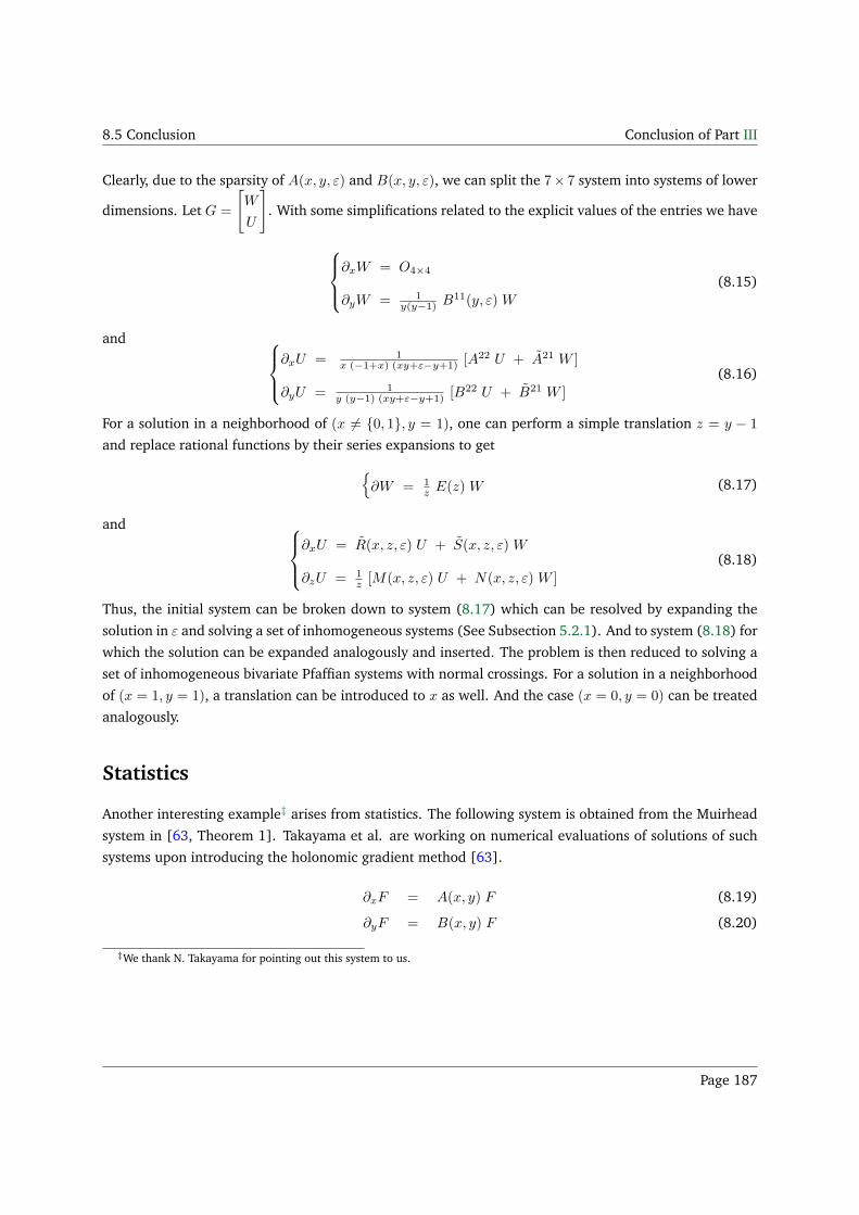
8.5 Conclusion Conclusion of Part III
Clearly, due to the sparsity of A(x, y, ε) and B(x, y, ε), we can split the 7× 7 system into systems of lower
dimensions. Let G =
[
W
U
]
. With some simplifications related to the explicit values of the entries we have
∂xW = O4×4
∂yW = 1y(y−1) B
11(y, ε) W
(8.15)
and
∂xU = 1x (−1+x) (xy+ε−y+1) [A
22 U + A21 W ]
∂yU = 1y (y−1) (xy+ε−y+1) [B
22 U + B21 W ]
(8.16)
For a solution in a neighborhood of (x 6= 0, 1, y = 1), one can perform a simple translation z = y − 1
and replace rational functions by their series expansions to get
∂W = 1z E(z) W (8.17)
and
∂xU = R(x, z, ε) U + S(x, z, ε) W
∂zU = 1z [M(x, z, ε) U + N(x, z, ε) W ]
(8.18)
Thus, the initial system can be broken down to system (8.17) which can be resolved by expanding the
solution in ε and solving a set of inhomogeneous systems (See Subsection 5.2.1). And to system (8.18) for
which the solution can be expanded analogously and inserted. The problem is then reduced to solving a
set of inhomogeneous bivariate Pfaffian systems with normal crossings. For a solution in a neighborhood
of (x = 1, y = 1), a translation can be introduced to x as well. And the case (x = 0, y = 0) can be treated
analogously.
Statistics
Another interesting example‡ arises from statistics. The following system is obtained from the Muirhead
system in [63, Theorem 1]. Takayama et al. are working on numerical evaluations of solutions of such
systems upon introducing the holonomic gradient method [63].
∂xF = A(x, y) F (8.19)
∂yF = B(x, y) F (8.20)
‡We thank N. Takayama for pointing out this system to us.
Page 187
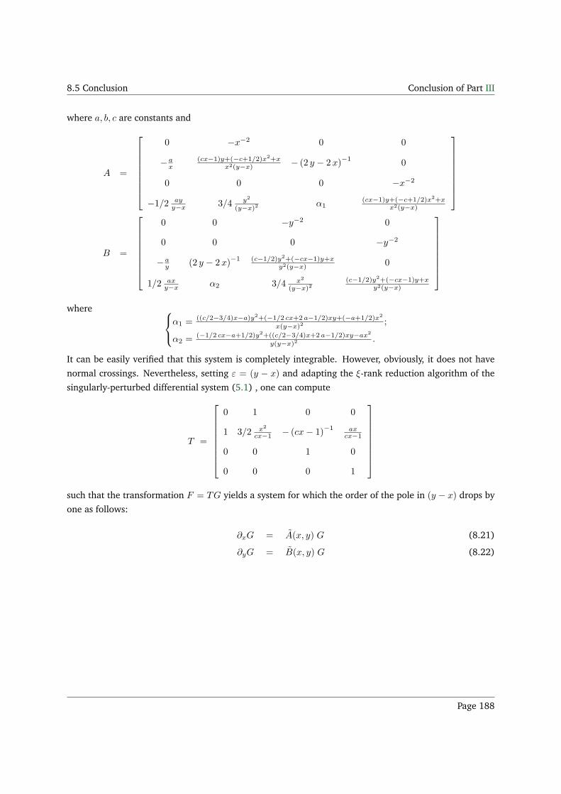
8.5 Conclusion Conclusion of Part III
where a, b, c are constants and
A =
0 −x−2 0 0
− ax
(cx−1)y+(−c+1/2)x2+xx2(y−x) − (2 y − 2x)
−10
0 0 0 −x−2
−1/2 ayy−x 3/4 y2
(y−x)2α1
(cx−1)y+(−c+1/2)x2+xx2(y−x)
B =
0 0 −y−2 0
0 0 0 −y−2
−ay (2 y − 2x)
−1 (c−1/2)y2+(−cx−1)y+xy2(y−x) 0
1/2 axy−x α2 3/4 x2
(y−x)2(c−1/2)y2+(−cx−1)y+x
y2(y−x)
where
α1 = ((c/2−3/4)x−a)y2+(−1/2 cx+2 a−1/2)xy+(−a+1/2)x2
x(y−x)2;
α2 = (−1/2 cx−a+1/2)y2+((c/2−3/4)x+2 a−1/2)xy−ax2
y(y−x)2.
It can be easily verified that this system is completely integrable. However, obviously, it does not have
normal crossings. Nevertheless, setting ε = (y − x) and adapting the ξ-rank reduction algorithm of the
singularly-perturbed differential system (5.1) , one can compute
T =
0 1 0 0
1 3/2 x2
cx−1 − (cx− 1)−1 ax
cx−1
0 0 1 0
0 0 0 1
such that the transformation F = TG yields a system for which the order of the pole in (y − x) drops by
one as follows:
∂xG = A(x, y) G (8.21)
∂yG = B(x, y) G (8.22)
Page 188

8.5 Conclusion Conclusion of Part III
where
A =
−3/2 (−y + x)−1 cx−1
(−y+x)x21
(−y+x)x2 − a(−y+x)x
−1/2 cx−1x2 0 − a
x
α3 −1/2 cxy+2 ax−2 ay−x(−y+x)x α4 1/2 ay
−y+x
0 −x−2 0 0
B =
1/2 2 cxy−2 cy2+3 y2−2 x+2 y(−y+x)y2 − yc−1
(−y+x)y2 − 1(−y+x)y2
a(−y+x)y
0 0 −y−2 0
−3/4 x2
−y+x −1/2 −cxy+2 ax−2 ay+y(−y+x)y α5 −1/2 ax
−y+x
−y+xy2 −y−2 0 0
where
α3 = 1/4 2 cx2y−2 cxy2+4 ax2−8 axy+4 ay2+3 xy2−2 x2+2 xy(−y+x)x ;
α4 = 1/2 2 cx2−2 cxy−x2−2 x+2 y(−y+x)x2 ;
α5 = 1/2 2 cxy−2 cy2+y2−2 x+2 y(−y+x)y2 .
Several questions arise:
• Can the rank reduction algorithm be generalized to such systems? And can a criterion be given to
determine whether the minimum of the singularity’s order is attained?
• A close inspection of the system reveals a kind of symmetry for this system. In particular, Let
P =
1 0 0 0
0 0 1 0
0 1 0 0
0 0 0 1
then P [A](y, x) = P−1AP = B(x, y). Consequently, one expects some kind of symmetry in the
solution which can be exploited to get the formal invariants.
One of the first consequences of the loss of the normal crossings is the instability of the JCF of the
leading constant matrix. In the case of singularly-perturbed linear differential systems, this instability
gave rise to the turning point phenomenon discussed in Part II. Thus, for a bivariate Pfaffian with
singularities of the monomial form xαyβ for some α, β ∈ N (studied e.g. by H. Majima), would it
be plausible to investigate the techniques developed in Part II to uncouple the system into systems of
lower dimensions and systems with normal crossings by holding one of the independent variables as a
parameter?
Page 189

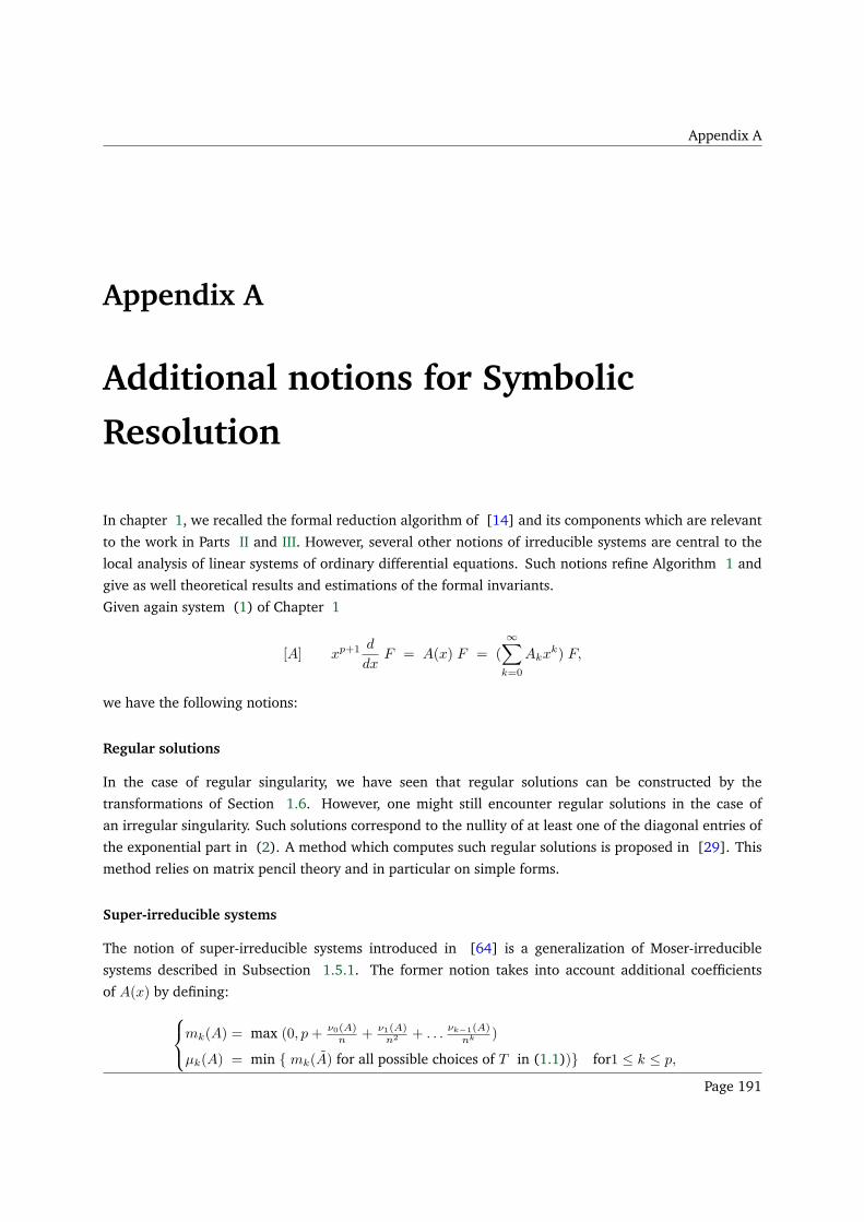
Appendix A
Appendix A
Additional notions for Symbolic
Resolution
In chapter 1, we recalled the formal reduction algorithm of [14] and its components which are relevant
to the work in Parts II and III. However, several other notions of irreducible systems are central to the
local analysis of linear systems of ordinary differential equations. Such notions refine Algorithm 1 and
give as well theoretical results and estimations of the formal invariants.
Given again system (1) of Chapter 1
[A] xp+1 d
dxF = A(x) F = (
∞∑
k=0
Akxk) F,
we have the following notions:
Regular solutions
In the case of regular singularity, we have seen that regular solutions can be constructed by the
transformations of Section 1.6. However, one might still encounter regular solutions in the case of
an irregular singularity. Such solutions correspond to the nullity of at least one of the diagonal entries of
the exponential part in (2). A method which computes such regular solutions is proposed in [29]. This
method relies on matrix pencil theory and in particular on simple forms.
Super-irreducible systems
The notion of super-irreducible systems introduced in [64] is a generalization of Moser-irreducible
systems described in Subsection 1.5.1. The former notion takes into account additional coefficients
of A(x) by defining:
mk(A) = max (0, p+ ν0(A)n + ν1(A)
n2 + . . . νk−1(A)nk )
µk(A) = min mk(A) for all possible choices of T in (1.1)) for1 ≤ k ≤ p,
Page 191
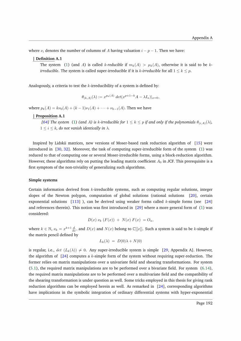
Appendix A
where νi denotes the number of columns of A having valuation i− p− 1. Then we have:
| Definition A.1
The system (1) (and A) is called k-reducible if mk(A) > µk(A), otherwise it is said to be k-
irreducible. The system is called super-irreducible if it is k-irreducible for all 1 ≤ k ≤ p.
Analogously, a criteria to test the k-irreducibility of a system is defined by:
θ(k,A)(λ) := xpk(A) det(xp+1−kA− λIn)|x=0,
where pk(A) = kν0(A) + (k − 1)ν1(A) + · · ·+ νk−1(A). Then we have
| Proposition A.1
[64] The system (1) (and A) is k-irreducible for 1 ≤ k ≤ p if and only if the polynomials θ(i,A)(λ),
1 ≤ i ≤ k, do not vanish identically in λ.
Inspired by Lidskii matrices, new versions of Moser-based rank reduction algorithm of [15] were
introduced in [30, 32]. Moreover, the task of computing super-irreducible form of the system (1) was
reduced to that of computing one or several Moser-irreducible forms, using a block-reduction algorithm.
However, these algorithms rely on putting the leading matrix coefficient A0 in JCF. This prerequisite is a
first symptom of the non-triviality of generalizing such algorithms.
Simple systems
Certain information derived from k-irreducible systems, such as computing regular solutions, integer
slopes of the Newton polygon, computation of global solutions (rational solutions [20], certain
exponential solutions [113] ), can be derived using weaker forms called k-simple forms (see [24]
and references therein). This notion was first introduced in [29] where a more general form of (1) was
considered:
D(x) νk (F (x)) + N(x) F (x) = On,
where k ∈ N, νk = xk+1 ddx , and D(x) and N(x) belong to C[[x]]. Such a system is said to be k-simple if
the matrix pencil defined by
Lk(λ) = D(0)λ+N(0)
is regular, i.e., det (Lk(λ)) 6= 0. Any super-irreducible system is simple [29, Appendix A]. However,
the algorithm of [24] computes a k-simple form of the system without requiring super-reduction. The
former relies on matrix manipulations over a univariate field and shearing transformations. For system
(5.1), the required matrix manipulations are to be performed over a bivariate field. For system (6.14),
the required matrix manipulations are to be performed over a multivariate field and the compatibility of
the shearing transformation is under question as well. Some tricks employed in this thesis for giving rank
reduction algorithms can be employed herein as well. As remarked in [24], corresponding algorithms
have implications in the symbolic integration of ordinary differential systems with hyper-exponential
Page 192
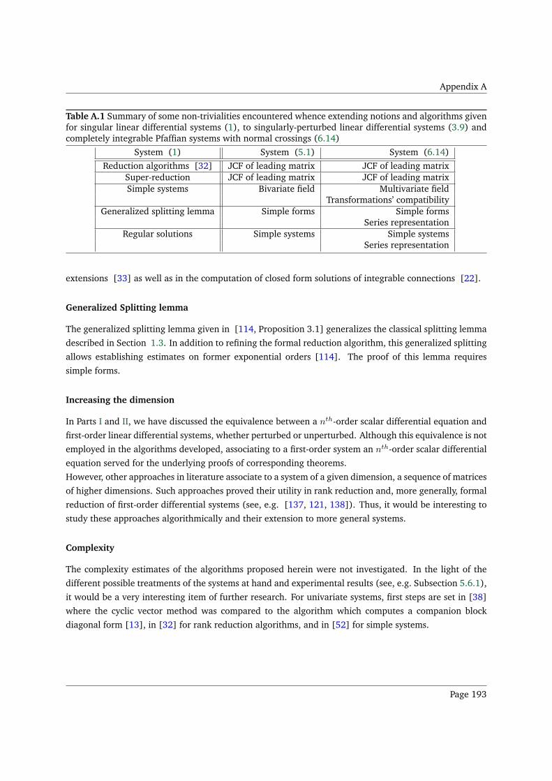
Appendix A
Table A.1 Summary of some non-trivialities encountered whence extending notions and algorithms givenfor singular linear differential systems (1), to singularly-perturbed linear differential systems (3.9) andcompletely integrable Pfaffian systems with normal crossings (6.14)
System (1) System (5.1) System (6.14)
Reduction algorithms [32] JCF of leading matrix JCF of leading matrixSuper-reduction JCF of leading matrix JCF of leading matrixSimple systems Bivariate field Multivariate field
Transformations’ compatibilityGeneralized splitting lemma Simple forms Simple forms
Series representationRegular solutions Simple systems Simple systems
Series representation
extensions [33] as well as in the computation of closed form solutions of integrable connections [22].
Generalized Splitting lemma
The generalized splitting lemma given in [114, Proposition 3.1] generalizes the classical splitting lemma
described in Section 1.3. In addition to refining the formal reduction algorithm, this generalized splitting
allows establishing estimates on former exponential orders [114]. The proof of this lemma requires
simple forms.
Increasing the dimension
In Parts I and II, we have discussed the equivalence between a nth-order scalar differential equation and
first-order linear differential systems, whether perturbed or unperturbed. Although this equivalence is not
employed in the algorithms developed, associating to a first-order system an nth-order scalar differential
equation served for the underlying proofs of corresponding theorems.
However, other approaches in literature associate to a system of a given dimension, a sequence of matrices
of higher dimensions. Such approaches proved their utility in rank reduction and, more generally, formal
reduction of first-order differential systems (see, e.g. [137, 121, 138]). Thus, it would be interesting to
study these approaches algorithmically and their extension to more general systems.
Complexity
The complexity estimates of the algorithms proposed herein were not investigated. In the light of the
different possible treatments of the systems at hand and experimental results (see, e.g. Subsection 5.6.1),
it would be a very interesting item of further research. For univariate systems, first steps are set in [38]
where the cyclic vector method was compared to the algorithm which computes a companion block
diagonal form [13], in [32] for rank reduction algorithms, and in [52] for simple systems.
Page 193

Appendix B
Appendix B
Software
The examples of computation and the description of the packages are too large to be included here.
Please refer to my web page which is, at the moment of writing this thesis, hosted by the University of
Limoges at:
http : //www.unilim.fr/pages_perso/suzy.maddah/
Page 194

List of Figures
1 The function 1/x is not defined at x = 0 and explodes to ±∞ in a neighborhood of x = 0
(Sage calculus tutorial) . . . . . . . . . . . . . . . . . . . . . . . . . . . . . . . . . . . . . . 2
2.1 Ferrer diagrams for J and J and rightward coin move indicating that κ(J) > κ(J) [74,
Fig. 1]. . . . . . . . . . . . . . . . . . . . . . . . . . . . . . . . . . . . . . . . . . . . . . . 38
2.2 Newton envelopes for J = (03)2(02)
30 and J = (03) (02)
5 also indicating that κ(J) >
κ(J) [74, Fig. 2]. . . . . . . . . . . . . . . . . . . . . . . . . . . . . . . . . . . . . . . . . . 38
2.3 Newton diagram and envelope for Example 2.6: ∆11 6= 0 and ∆3 6= 0, whereas ∆1 = ∆1
2 =
∆22 = ∆2 = 0 [74, Fig. 3]. . . . . . . . . . . . . . . . . . . . . . . . . . . . . . . . . . . . 39
2.4 Coin move from 04020 to (03)20 or to 03(02)
2 [74, Fig. 4]. . . . . . . . . . . . . . . . . . . 39
2.5 Ferrer diagram of A(x) with labeled coins and digraph of A in Example 2.8. . . . . . . . . 40
2.6 Ferrer diagram of A(x) with labeled coins and the arcs of G(A) induced by J . . . . . . . . 42
3.1 Example on Arnold forms. The black stripes correspond to the only possible locations of
non-constant entries. . . . . . . . . . . . . . . . . . . . . . . . . . . . . . . . . . . . . . . . 70
4.1 The ε-polygon associated to (4.4) in Example 4.1 . . . . . . . . . . . . . . . . . . . . . . . 74
4.2 (x, ε)-Polygon . . . . . . . . . . . . . . . . . . . . . . . . . . . . . . . . . . . . . . . . . . . 78
4.3 Interpretation of a shearing transformation . . . . . . . . . . . . . . . . . . . . . . . . . . 80
4.4 Interpretation of a stretching-shearing transformation . . . . . . . . . . . . . . . . . . . . . 83
5.1 Geometric Interpretation . . . . . . . . . . . . . . . . . . . . . . . . . . . . . . . . . . . . . 117
7.1 Computing the exponential part from associated ODS’s . . . . . . . . . . . . . . . . . . . . 165
7.2 Computing a fundamental matrix of formal solutions by studying one of the components,
e.g. the first component. The other components would follow the chosen component in
the uncoupling. . . . . . . . . . . . . . . . . . . . . . . . . . . . . . . . . . . . . . . . . . . 168
Page 196
List of Algorithms
1 FMFS_ODS (p,A(x)) : Computes a fundamental matrix of formal solutions (2) of [A] . . . 24
2 BLOCK_DIAG: Block-diagonalization of M over K . . . . . . . . . . . . . . . . . . . . . . . 25
3 APP_SING Desingularization Algorithm . . . . . . . . . . . . . . . . . . . . . . . . . . . . . 52
4 ε-RANK_REDUCTION: ε-Rank Reduction of System [Aε,σA] . . . . . . . . . . . . . . . . . . 113
5 PARAM_LATTICE_RANK_REDUCTION: Adaptation of Levelt-Barkatou-LeRoux Rank
Reduction to System [Aε] . . . . . . . . . . . . . . . . . . . . . . . . . . . . . . . . . . . . . 118
6 EXP_PARAM(h, p, σA, A(x, ε)) : Computes the ε-exponential part of system [Aε] or [Aε,σA]
(performs formal reduction) . . . . . . . . . . . . . . . . . . . . . . . . . . . . . . . . . . . 128
7 FMFS_PFAFF Computes a fundamental matrix of formal solutions (7.4) of a completely
integrable Pfaffian system with normal crossings given by (6.14) . . . . . . . . . . . . . . 167
8 PFAFF_RANK_REDUCTION: Rank Reduction of System (6.14) . . . . . . . . . . . . . . . . . 182
Page 197
Bibliography
Bibliography
[1] H. Abbas, M. A. Barkatou, and S.S. Maddah. Formal Reduction of a class of Pfaffian Systems in Two
Variables. In Proceedings of the International Symposium on Symbolic and Algebraic Computation.
ACM Press, pp 312 - 319, 2014.
[2] H. Abbas, M. A. Barkatou, and S.S. Maddah. On the Reduction of Singularly-Perturbed Linear
Differential Systems. In Proceedings of the 39th International Symposium on Symbolic and Algebraic
Computation, ACM Press, pp 320-327, 2014.
[3] S. Abramov, M. A. Barkatou, and M. van Hoeij. Apparent Singularities of Linear Difference Equations
with Polynomial Coefficients. In AAECC, 17:117-133, 2006.
[4] M. Akian, R. Bapat, and S. Gaubert. Min-Plus Methods in Eigenvalue Perturbation Theory and
Generalised Lidskii-Visik-Ljusternik Theorem. ArXiv preprint: math/0402090v3, Feb. 2004.
[5] M. Akian, R. Bapat, and S. Gaubert. Max-plus algebra. Handbook of linear algebra. Chapman and
Hall, London (2006).
[6] A. Aparicio Monforte and M. Kauers. Formal Laurent Series in Several Variables. Expositiones
Mathematicae, 31(4), pp 350–367, 2013.
[7] V. I. Arnold, On Matrices Depending on Parameters, Russian Math. Surveys, 26 (1971).
[8] F. Aroca, J. Cano, F. Jung. Power Series Solutions for Non-Linear PDE’s. In Proceedings of
International Symposium on Symbolic and Algebraic Computation, Phiadelphia, Pennsylvania, USA.
ACM, 2003.
[9] D. G. Babbitt and V. S. Varadarajan. Formal Reduction of Meromorphic Differential Equations: A
Group Theoretic View. In Pacific Journal of Mathematica, 109 (1), pp 1- 80, 1983.
[10] F. Baccelli, G. Cohen, G. J. Olsder, and J.P. Quadrat. Synchronization and Linearity: An Algebra for
Discrete Event Systems. John Wiley & Sons Ltd, 1992.
[11] W. Balser. Formal Power Series and Linear Systems of Meromorphic Ordinary Differential Equations.
Springer-Verlag, New York, 2000.
[12] M. A. Barkatou. A Rational Newton algorithm for computing formal solutions of linear differential
equations. Lecture Notes in Computer Science, Springer-Verlag, 1989.
Page 198
Bibliography
[13] M. A. Barkatou, An Algorithm for Computing a Companion Block Diagonal Form for a system of Linear
Differential Equations, AAECC, Springer-Verlag 1993.
[14] M. A. Barkatou. An Algorithm to Compute the Exponential Part of a Formal Fundamental Matrix
Solution of a Linear Differential System. Journal of App. Alg. in Eng. Comm. and Comp., 8(1): pp
1-23, 1997.
[15] M. A. Barkatou. A Rational Version of Moser’s Algorithm. In Proceedings of the International
Symposium on Symbolic and Algebraic Computation, pp 297-302. ACM Press, July 1995.
[16] M. Barkatou. Factoring systems of linear functional equations using eigenrings. In I. S. Kotsireas
and E. V. Zima, editors, Latest Advances in Symbolic Algorithms, pp 22–42. World Scientific, 2007.
[17] M.A. Barkatou. On the Exponential Parts of Singular Linear Differential Equations. Conference of
Symbolic Computations and its Applications, Aachen, May 17-20, 2012.
[18] M. A. Barkatou. On the reduction of Linear Systems of Difference Equations. In Proceedings of the
International Symposium on Symbolic and Algebraic Computation, pp 1-6. ACM Press, USA, 1989.
[19] M.A. Barkatou, Removing Apparent Singularities of Systems of Linear Differential Equations
with Rational Function Coefficients. Extended Abstract, Second Workshop Differential Equations by
Algebraic Methods (DEAM2), Linz, Austria 2011.
[20] M.A. Barkatou. On Rational Solutions of Systems of Linear Differential Equations. Journal of
Symbolic Computation, 28(4), pp 547-567, 1999.
[21] M. A. Barkatou, G. Broughton, and E. Pfluegel. Regular Systems of Linear Functional Equations and
Applications. In Proceedings of the International Symposium on Symbolic and Algebraic Computation,
pp 15-22. ACM Press, 2008.
[22] M. A. Barkatou, T. Cluzeau, C. El Bacha, and J. A. Weil. Computing closed form solutions
of integrable connections. In Proceedings of the 37th International Symposium on Symbolic and
Algebraic Computation, pp 43-50, ACM press, 2012.
[23] M. Barkatou, T. Cluzeau, A. Jalouli. Formal Solutions of Linear Differential Systems with Essential
Singularities in their Coefficients. In Proceedings of the International Symposium on Symbolic and
Algebraic Computation. ACM Press, 2015.
[24] M. A. Barkatou and C. El Bacha. On k-simple forms of first-order linear differential systems and
their computation. Journal of Sym. Comput., 54: 36-58, 2013.
[25] M. A. Barkatou, M. Jaroschek, and S.S. Maddah. Formal Solutions of Completely Integrable Pfaffian
Systems with Normal Crossings in Several Variables. Submitted, available at arXiv: 1511.00180.
[26] M. A. Barkatou and N. Le Roux. Rank Reduction of a class of Pfaffian Systems in Two Variables.
In Proceedings of the International Symposium on Symb. and Algeb. Comp., pp 204-211. ACM Press,
2006.
Page 199
Bibliography
[27] M. A. Barkatou and S.S. Maddah. Removing Apparent Singularities of Systems of Linear Differential
Equations with Rational Function Coefficients. In Proceedings of the International Symposium on
Symbolic and Algebraic Computation. ACM Press, 2015.
[28] M. Barkatou, and S.S. Maddah. Formal Solutions of Singularly-Perturbed Linear Differential
Systems. Under redaction, preliminary version available at arXiv: 1503.09075.
[29] M. A. Barkatou and E. Pfluegel. An algorithm computing the regular formal solutions of a system of
linear differential equations. Journal of Sym. Comput., 28, 569-587, 1999.
[30] M. A. Barkatou and E. Pfluegel. Computing Super-Irreducible Forms of Systems of Linear Differential
Equations via Moser-Reduction: A new Approach. In Proceedings of the International Symposium on
Symbolic and Algebraic Computation, ISSAC Waterloo, 2007.
[31] M. A. Barkatou and E. Pfluegel. ISOLDE, Integration of Systems of Ordinary Linear Differential
Equations. Available at: http://isolde.sourceforge.net/
[32] M. A. Barkatou and E. Pfluegel. On the Moser-and super-reduction algorithms of systems of linear
differential equations and their complexity. Journal of Sym. Comput., 44 (8), 1017-1036, 2009.
[33] M. A. Barkatou, and C. G. Raab. Solving linear ordinary differential systems in hyperexponential
extensions. In Proceedings of the 37th International Symposium on Symbolic and Algebraic
Computation, pp 51-58, ACM press, 2012.
[34] H. Baumgartel. Analytic Perturbation Theory for Matrices and Operators. Berkhauser Verlag. Basel,
1985.
[35] C. M. Bender and S. A. Orszag. Advanced mathematical methods for scientists and engineers I:
Asymptotic methods and perturbation theory. Vol. 1. Springer, 1999.
[36] F. Béringer and F. Jung. Multi-variate polynomials and Newton-Puiseux expansions. In Symbolic and
Numerical Scientific Computation SNSC’01, L.N.C.S 2630, 240-254, Hagenberg, Austria, september
2001. Springer 2003.
[37] A. Bostan, S. Boukraa, S. Hassani, M. van Hoeij, J.-M. Maillard, J.-A. Weil, and N. Zenine. The Ising
model: From Elliptic Curves to ModularForms and Calabi-Yau equations. J. Phys. A: Math. Theor.,
44(4):045204, 44, 2011.
[38] A. Bostan, F. Chyzak, and E. de Panafieu. Complexity Estimates for Two Uncoupling Algorithms. In
Proceedings of the International Symposium on Symbolic and Algebraic Computation, pp. 85–92, ACM
Press, 2013.
[39] R. Broucke. On Pfaff’s equations of motion in dynamics; Applications to Satellite Theory. Journal of
Celestial Mechanics, 18(3): 207-222, 1978.
[40] R. E. Burkard and P. Butkovic. Finding all Essential Terms of a Characteristic Maxpolynomial.
Discrete Applied Mathematics, 130 (3), pp 367 - 380, 2003.
Page 200
Bibliography
[41] H. Charrière. Triangulation Formelle de certains Systèmes de Pfaff Complètement Intégrables et
Application à l’etude C∞ des Systèmes non Linéaires. Annali della Scuola Normale Superiore di
Pisa-Classe di Scienze, 7(4): 625 - 714, 1980.
[42] H. Charrière and R. Gérard. Formal Reduction of Integrable Linear Connexion having a certain kind
of Irregular Singularities. Analysis, 1:85-115, 1981.
[43] G. Chen. Solutions Formelles de Systemes d’Equations Differentielles Lineaires Ordinaires
Homogenes. PhD Thesis. Université Joseph Fourier. Grenoble 1. 1990.
[44] S. Chen, M. Jaroschek, M. Kauers, and M. F. Singer. Desingularization Explains Order-Degree Curves
for Ore Operators. In Proceedings of the 38th International Symposium on Symbolic and Algebraic
Computation, pp 157-164, ACM, U.S.A. 2013.
[45] S. Chen, M. Kauers, M. F. Singer. Desingularization of Ore Operators, Available at:
arXiv:1408.5512v1, 2014.
[46] R.C. Churchill and J.J. Kovacic, Cyclic vectors, N. Rutgers University (Ed.), In Differential Algebra
and Related Topics, Proceedings of the International Workshop, pp 191- 218, World Scientific
Publishing Co., River Edge, NJ 2002.
[47] E. A. Coddington and N. Levinson. Theory of ordinary differential equations. Tata McGraw-Hill
Education, 1955.
[48] P. Deligne. Equations Différentielles à Points Singuliers Réguliers. Lecture Notes In Mathematics,
Volume 163, Springer-Verlag,1970.
[49] D. Delphenich. The role of integrability in a large class of physical systems. arXiv preprint avilable
at: arXiv:1210.4976 (2012).
[50] D. Duval. Diverses Questions Relatives au Calcul Formel avec Nombres Algébriques. Thése d’Etat,
Faculté des Sciences de Grenoble, 1987.
[51] A. Edelman, E. Elmroth, and A. B. Kagstrom. A geometric approach to perturbation theory of
matrices and matrix pencils; Part two: A stratification-enhanced staircase algorithm. SIAM Journal
on Matrix Analysis and Applications, 20(3), 667-699, 1999.
[52] C. El Bacha. Méthode Algébriques pour la Résolution d’Équations Différentielles Matricielles d’Ordre
Arbitraire. Ph.D. Thesis, University of Limoges, 2011.
[53] A. van den Essen. Regular Singularities along Normal Crossings. In Gerard Ramis, editor, Systèmes
de Pfaff et Equations Différentielles dans le Champ Complexe, volume 712 of Lecture Notes in
Mathematics, pp 88-130. Springer-Verlag, 1979.
[54] A. van den Essen and A.H.M. Levelt. Irregular Singularities in Several Variables. Memoirs of AMS,
40(270), 1982.
[55] A. Fruchard and R. Schaefke. Composite Asymptotic Expansions. Springer, 2013.
Page 201
Bibliography
[56] K. O. Geddes, S. R. Czapor, and G. Labahn. Algorithms for computer algebra. Springer Science and
Business Media, 1992.
[57] R. Gérard and A.H.M Levelt. Sur les Connexions à Singularités Régulières dans le cas de Plusieurs
Variables. In Funkcialaj Ekvacioj, 19(2), pp 149–173, 1976.
[58] R. Gérard and Y. Sibuya. Etude de certains systèmes de Pfaff avec singularités. In Gerard Ramis,
editor, Systemes de Pfaff et Equations Différentielles dans le Champ Complexe, volume 712 of Lecture
Notes in Mathematics, pp 131-288. Springer-Verlag, 1979.
[59] M. Giesbrecht and A. Storjohann. Computing rational forms of integer matrices. In Journal of
Symbolic Computations. 34 (3), pp 157 - 172, 2002.
[60] H. Gingold, On Continuous Triangularization of Matrix Functions, SIAM J. Math Anal. , Vol. 10, No
4, July 1979 .
[61] G. Golub and J. H. Wilkinson. Ill-conditioned eigensystems and the computation of the Jordan
canonical form. SIAM Review, 18(4): 578-619, 1976.
[62] J. Grabmeier, E. Kaltofen, and V. Weispfenning. Computer Algebra Handbook: Foundations,
Applications, Systems; with CD-ROM. Vol. 1. Springer, 2003.
[63] H. Hashiguchi, Y. Numata, N. Takayama, and A. Takemura. The holonomic gradient method for the
distribution function of the largest root of a Wishart matrix. In Journal of Multivariate Analysis, 117,
pp 296-312, 2013.
[64] A. Hilali and A. Wazner. Formes super-irréductibles des système différentiels linéaires. Numer.
Math.,, 50: 429-449, 1987.
[65] Hsieh and Sibuya. Basic theory of Ordinary Differential Equations. Springer1999.
[66] M. Van Hoeij. Formal Solutions and Factorization of Differential Operators with Power Series
Coefficients. Journal of Symbolic Computation, 24(1), 1-30, 1997.
[67] J. Horn. Integration linearer Differentialgleichungen durch Laplacesche Integrale und
Fakultätenreihen. Jahresbericht der Deutschen Math. Vereinigung, 24, pp. 309-329, 1915.
[68] M. Hukuhara. Sur les propriétés asymptotiques des solutions d’un système d’équations
différentielles linéaires contenant un paramètre. In Mem. Fac. Eng., Kyushu Imp. Univ 8, pp 249-
280, 1937.
[69] C. Hulek. Systémes d’ équations différentielles linéaires singuliérement perturbées et développements
asymptotiques combinés. PhD Thesis. Université de Strasbourg. 2014.
[70] E.L. Ince. Ordinary Differential Equations. Dover, 1926.
[71] M. Iwano, Asymptotic Solutions of a System of Linear Ordinary Differential Equations Containing a
Small Paramter, Part I. In Funkcialaj Ekvacioj, Vol. 5, pp 71-134, 1963.
Page 202
Bibliography
[72] M. Iwano, On the study of asymptotic solutions of a system of linear ordinary differential equations
containing a paramter. In Japan Journal of Mathematics, Vol. 35, pp 1-30, 1965.
[73] M. Iwano and Y. Sibuya. Reduction of the Order of a Linear Ordinary Differential Equation
Containing a Small Parameter. Kodai Math. Sem. Rep.15, 1–28, 1963.
[74] C.P. Jeannerod. An Algorithm for the Eigenvalue Perturbation Problem: Reduction of a κ-Matrix to a
Lidskii Matrix. In Proceedings of the International Symposium on Symbolic and Algebraic Computation.
ACM Press, 2000.
[75] C.P. Jeannerod and E. Pfluegel. A Reduction Algorithm for Matrices Depending on a Parameter. In
Proceedings of the International Sympo. on Symb. and Algeb. Comp., pp 121-128. ACM Press, 1999.
[76] C.P. Jeannerod, N. Maillard, and E. Pfluegel. An Algorithmic Approach for the Symmetric Perturbed
Eigenvalue Problem Application to the resolution of a Schr. . . odinger equation by a kp-Perturbation
Method. In Proceedings of IMACS ACA’98, 1998.
[77] Johannes M. Henn. Lectures on Differential Equations for Feynman Integrals. Prepared for
submission to JHEP, Available at arXiv:1412.2296v1, 2014.
[78] M. K. Kadalbajoo and C. P. Kailash. A survey of numerical techniques for solving singularly
perturbed ordinary differential equations. In Applied Mathematics and Computation 130, no. 2
(2002): 457-510.
[79] B. Kagstrom and A. Ruhe. An algorithm for the numerical computation of the Jordan normal form
of a complex matrix. ACM Trans. Math. Software, 6(3):389-419, 1980.
[80] T. Kato. Perturbation Theory for Linear Operators. Springer, 1980.
[81] M. Kohno. Global analysis in linear differential equations. Springer, 1999.
[82] R. E. Langer, Turning points in linear asymptotic theory. In Bol. Soc. Mat. Mexicana Vol. (2) 5, pp
1-12, 1960.
[83] R. N. Lee. Reducing differential equations for multiloop master integrals. arXiv preprint
arXiv:1411.0911, 2014.
[84] N. Le Roux. Solutions formelles déquations aux dérivées partielles. Ph.D. Thesis. University of
Limoges. 2006.
[85] A.H.M. Levelt. Jordan Decomposition for a Class of Singular Differential Operators. Arkiv for
matematik, 13 (1), pp 1-27, 1975.
[86] A.H.M. Levelt. The Semi-simple Part of a Matrix. Algoritmen In De Algebra, The Netherlands 1993.
[87] A.H.M. Levelt. Stabilizing Differential Operators: a method for Computing Invariants at Irregular
Singularities. Differential Equations and Computer Algebra, M. Singer (ed.), pp 181-228, 1991.
Page 203
Bibliography
[88] V. Lidskii. Perturbation Theory of Non-Conjugate Operators. U. S. S. R. Comput. Math. and Math.
Phys., 1:73-85, 1965.
[89] C. C. Lin, The theory of hydrodynamic stability. Cambridge Univ. Press. Cambridge, 1966.
[90] D. A. Lutz and R. Schaefke. On the Identification and Stability of Formal Invariants for Singular
Differential Equations. In Linear Algebra and its Applications, 72, pp 1- 46, 1985.
[91] Y. Ma and A. Edelman. Nongeneric perturbations of Jordan blocks. Linear Algebra Appl., 273:45-63,
1998.
[92] D. Maclagan and B. Sturmfels. Introduction to Tropical Geometry. Available on Sturmfel’s website.
[93] Y.O. Macutan. Formal Solutions of Scalar Singularly-Perturbed Linear Differential Equations. In
Proceedings of the International Symposum on Symbolic and Algebraic Computation, pp 113-120.
ACM Press, USA 1999.
[94] A. A. Mailybaev, Transformation of Families of Matrices to Normal Forms and its Application to
Stability Theory, SIAM J. Matrix Anal. Appl., Vol.21, No. 2, pp. 396-417, 1999.
[95] H. Majima. Asymptotic Analysis for Integrable Connections with Irregular Singular Points. In
Lecture Notes in Mathematics, Volume 1075, Springer-Verlag, 1984.
[96] S. S. Maddah. LINDALG : MATHEMAGIX Package for Symbolic Resolution of Linear Systems of
Differential Equations. Available at: http : //www.mathemagix.org
[97] S. S. Maddah. MINIISOLDE : MAPLE Package for Symbolic Resolution of
Linear Systems of Differential Equations. Available for download at: http :
//www.unilim.fr/pages_perso/suzy.maddah/Research_.html
[98] S. S. Maddah. PARAMINT : MAPLE Package for Symbolic Resolution of Singularly-Perturbed
Linear Differential Systems, Prototype Implementation. Available for download at: http :
//www.unilim.fr/pages_perso/suzy.maddah/Research_.html
[99] S. S. Maddah. PFAFFINT : MAPLE Package for symbolic resolution of completely integrable Pfaffian
systems with normal crossings. Prototype implementation. Available for download at: http :
//www.unilim.fr/pages_perso/suzy.maddah/Research_.html
[100] S. S. Maddah, M. A. Barkatou. APPSING : MAPLE Package for removing apparent singularities of
systems of linear differential equations with rational function coefficients. Available for download
at: http : //www.unilim.fr/pages_perso/suzy.maddah/Research_.html
[101] B. Malgrange. Sur la reduction formelle des équations diffèrentielles à singularités irrégulières.
Preprint, Institut Fourier, 1979.
[102] H. Matsumura. Commutative Ring Theory. Cambridge Studies in Advanced Mathematics,
Cambridge University Press, ISBN 9780521367646, 1989. Available at: http :
//books.google.de/books?id = yJwNrABugDEC
Page 204
Bibliography
[103] J.A.M. McHugh. An historical Survey of Ordinary Linear Differential Equations with a Large
Parameter and Turning Points. Archive for History of Exact Sciences, 7(4): pp 277-324,1971.
[104] M. Miyake. Newton Polygon and Gevrey Hierarchy in the Index Formulas for a Singular System of
Ordinary Differential Equations. Funkcialaj Ekvacioj, Vol. 55, pp 169- 237, 2012.
[105] J. Moro, J. Burke, and M. Overton. On the Lidskii- Vishik- Lyusternik Perturbation Theory for
Eigenvalues of Matrices with Arbitrary Jordan Structure. SIAM J. Matrix Anal. Appli., 18: 793-817,
1997.
[106] J. Moser. Note on Asymptotic Expansions. MRC Technical Summary Report, No. 104, University of
Wisconsin, 1959.
[107] J. Moser. The Order of a Singularity in Fuchs’ Theory. Mathematische Zeitschrift, 72:379- 398, 1960.
[108] K. Murota. Computing Puiseux-Series Solutions to Determinantal Equations via Combinatorial
Relaxation. SIAM Journal on Computing, 19(6), pp 1132-1161, 1990.
[109] M. Nakano. On the complex WKB analysis for a Schrödinger equation with a general three-segment
characteristic polygon. In Vietnam J. Math, 30, 605-625, 2002.
[110] M. Nakano and T. Nishimoto. On a Secondary Turning Point Problem. In Kodai Math. Sem. Rep.,
Vol. 22, pp 355 -384, 1970.
[111] D. Novikov, S. Yakovenko. Lectures on meromorphic flat connections. Normal forms, bifurcations
and finiteness problems in diff-l eqn., pp 387-430, 2004.
[112] Jr. O’Malley and E. Robert. Singular perturbation theory: a viscous flow out of Gottingen. Annual
Review of Fluid Mechanics, 42 , pp 1-17, 2010.
[113] E. Pfluegel. An algorithm for computing exponential solutions of first order linear differential
systems. In Proceedings of the 1997 international symposium on Symbolic and algebraic computation,
pp. 164-171, ACM press, 1997.
[114] E. Pfluegel. Effective Formal Reduction of Linear Differential Systems. Journal of App. Alg. in Eng.
Comm. and Comp., 10, 153-187, 2000.
[115] C. Praagman. Formal Decomposition of n Commuting Partial Linear Difference Operators.
Rijksuniversiteit Groningen, Mathematisch Instituut, 1983.
[116] G. Regensburger. Max-Plus linear algebra in Maple and generalized solutions for first-order
ordinary BVPs via Max-Plus interpolation. In Proceedings of MICA , pp 177-182, 2008.
[117] J. E. Sasser. Mathematical Origins of Ordinary Differential Equations: The First Hundred Years.
University of Cincinnati. In Proceedings of The Midwest Mathematics History Conferences. Miami
University, Oxford, Ohio. 1992.
[118] W. M. Seiler. Computer Algebra and Differential Equations: An Overview. Univ., Fak. für
Informatik, 1997.
Page 205
Bibliography
[119] R. Schaefke. Formal Fundamental Solutions of Irregular Singular Differential Equations Depending
Upon Parameters. Journal of Dynamical and Control Systems, Vol. 7, No. 4, pp 501-533, 2001.
[120] R. Schaefke and H. Volkmer. On the Formal Fundamental Solution of a Differential Equation
Depending on a Parameter. Funkcialaj Ekvacioj, Vol. 33, pp 1- 17, 1990.
[121] R. Schaefke and H. Volkmer. On the reduction of the Poincaré Rank of Singular Systems of Ordinary
Differential Equations. J. Reine Angew Math., Vol. 365, pp 80- 96, 1986.
[122] Sibuya. Sur Réduction Analytique d’un Système d’Équations Différentielles Ordinaires Linéaires
Contentant un Paramètre. J. Fac. Sci. Univ. Tokyo. Sect. I 7, pp 527–540, 1958.
[123] M. Singer. Testing Reducibility of Linear Differential Operators: A Group Theoretic Perspective. In
Journal of Applied Algebra in Eng. Comm. and Comp., 7(2) : pp 77- 104, 1996.
[124] L. Skinner. Singular Perturbation Theory. Springer Science and Business Media, 2011.
[125] R. Sommeling. Characteristic Classes for Irregular Singularities. In Proceedings of the international
symposium on Symbolic and algebraic computation, pp 163-168. ACM press, 1994.
[126] C. Stenger. On a conjecture of Wolfgang Wasow in linear turning point theory. In Comptes Rendus
de l’Académie des Sciences-Series I-Mathematics, 325(1), 27-32, 1997.
[127] K. Takano and M. Yoshida. On a linear system of Pfaffian equations with regular singular points.
Funkcial. Ekvac, Vol. 19, 175-189, 1976.
[128] K. Takano. A reduction theorem for a linear Pfaffian system with regular singular points. Archiv
der Mathematik, 31(1), 310-316, 1978.
[129] K. Takano. Local Equivalence of Linear Pfaffian Systems with Simple Poles. Funkcialaj Ekvacioj, 24,
373-382, 1981.
[130] R.Tarjan. Depth-first Search and Linear Graph Algorithms. SIAM Journal on Computing, 1(2), pp
146-160, 1972.
[131] H. L. Turrittin. Asymptotic Expansions of Solutions of Systems of Ordinary Differential Equations.
Contributions to the Theory of Nonlinear Oscillations II. Ann. of Math. Studies. No 29: 81-116. 1952.
[132] H.L. Turrittin. Asymptotic expansions of solutions of systems of ordinary linear differential
equations containing a parameter. In Contributions to the Theory of Nonlinear Osciallations, Vol.
II, pp. 81-116. Princeton: Princeton University Press, 1952.
[133] H.L. Turrittin. Convergent solutions of ordinary linear homogeneous differential equations in the
neighborhood of an irregular singular point. Acta Math., 93:27-66, 1955.
[134] H. L. Turrittin. My mathematical expectations. In Symposium on Ordinary Differential Equations,
pp. 1-22. Springer Berlin Heidelberg, 1973.
Page 206
Bibliography
[135] J. van der Hoeven, G. Lecerf, B. Mourrain, et al. Mathemagix, 2002. Software available from
http : //www.mathemagix.org.
[136] M. I. Visik and L. A. Ljusternik. Solution of some perturbation problems in the case of matrices and
self-adjoint or non-selfadjoint differential equations. I Russian Math. Surveys, 15(3):1–73, 1960.
[137] E. Wagenfuehrer. On the Computation of Formal Fundamental Solutions of Linear Differential
Equations at a Singular Point. Analysis, Vol. 9, pp 384- 405, 1989.
[138] E. Wagenführer. Formal Series Solutions of Singular Systems of Linear Differential Equations
and Singular Matrix Pencils. In Journal of the Faculty of Science/University of Tokyo. Sect. 1. A,
Mathematics: J. Fac. Sci. Univ. Tokyo Sect. IA Math., 36(3), pp 681-702, 1989.
[139] W. Wasow. Asymptotic Expansions for Ordinary Differential Equations. Dover Phoenix Editions,
2002.
[140] W. Wasow. Linear Turning Point Theory. Springer-Verlag. 1985.
[141] W. Wasow. Simplification of Turning Point Problems For Systems of Linear Differential Equations.
In Transactions of the American Mathematical Society, Vol. 106, No. 1, pp 100 - 114, 1963.
[142] W. Wasow. Topics in the Theory of Linear Ordinary Differential Equations Having Singularities
with respect to a Parameter. Institut de Recherche Mathématique Avancée. Université Louis Pasteur.
Strasbourg. 1979.
[143] W. Wasow. Turning Point Problems for Systems of Linear Differential Equations, Part II: The
Analytic Theory. In Communications on Pure and Applied Mathematics, Vol. XV, pp 173- 187, 1962.
[144] V. Weispfenning, T. Becker, H. Kredel. Groebner bases: a computational approach to commutative
algebra. Graduate Texts in Mathematics. Springer-Verlag, 1993.
Page 207

Réduction Formelle des Systèmes Différentiels Linéaires Singuliers:Systèmes différentiels linéaires singulièrement perturbés et systèmes de Pfaff complètement
intégrables à croisements normaux
Résumé : Dans cette thèse, nous nous sommes intéressés à l’analyse locale de systèmes différentielslinéaires singulièrement perturbés et de systèmes de Pfaff complètement intégrables et multivariés àcroisements normaux. De tels systèmes ont une vaste littérature et se retrouvent dans de nombreusesapplications. Cependant, leur résolution symbolique est toujours à l’étude. Nos approches reposentsur l’état de l’art de la réduction formelle des systèmes linéaires singuliers d’équations différentiellesordinaires univariées (ODS).
Dans le cas des systèmes différentiels linéaires singulièrement perturbés, les complications surviennentessentiellement à cause du phénomène des points tournants. Nous généralisons les notions et lesalgorithmes introduits pour le traitement des ODS afin de construire des solutions formelles. Lesalgorithmes sous-jacents sont également autonomes (par exemple la réduction de rang, la classificationde la singularité, le calcul de l’indice de restriction).
Dans le cas des systèmes de Pfaff, les complications proviennent de l’interdépendance des multiplessous-systèmes et de leur nature multivariée. Néanmoins, nous montrons que les invariants formels deces systèmes peuvent être récupérés à partir d’un ODS associé, ce qui limite donc le calcul à des corpsunivariés. De plus, nous donnons un algorithme de réduction de rang et nous discutons des obstaclesrencontrés.
Outre ces deux systèmes, nous parlons des singularités apparentes des systèmes différentiels univariésdont les coefficients sont des fonctions rationnelles et du problème des valeurs propres perturbées.
Les techniques développées au sein de cette thèse facilitent les généralisations d’autres algorithmesdisponibles pour les systèmes différentiels univariés aux cas des systèmes bivariés ou multivariés, et aussiaux systèmes d’équations fonctionnelles.
Mots clés : Calcul formel, réduction formelle, reduction de rang, singularités, points tournants,systèmes différentiels linéaires, systèmes de Pfaff complètement intégrables à croisements normaux,systèmes différentiels linéaires singulièrement perturbés, les algorithmes.
Formal Reduction of Linear Singular Differential Systems:Singularly-perturbed linear differential systems and completely integrable Pfaffian systems
with normal crossings
Abstract: In this thesis, we are interested in the local analysis of singularly-perturbed linear differentialsystems and completely integrable Pfaffian systems in several variables. Such systems have a vastliterature and arise profoundly in applications. However, their symbolic resolution is still open toinvestigation. Our approaches rely on the state of art of formal reduction of singular linear systemsof ordinary differential equations (ODS) over univariate fields.
In the case of singularly-perturbed linear differential systems, the complications arise mainly from thephenomenon of turning points. We extend notions introduced for the treatment of ODS to such systemsand generalize corresponding algorithms to construct formal solutions in a neighborhood of a singularity.The underlying components of the formal reduction proposed are stand-alone algorithms as well andserve different purposes (e.g. rank reduction, classification of singularities, computing restraining index).
In the case of Pfaffian systems, the complications arise from the interdependence of the multiplecomponents which constitute the former and the multivariate nature of the field within which reductionoccurs. However, we show that the formal invariants of such systems can be retrieved from anassociated ODS, which limits computations to univariate fields. Furthermore, we complement our workwith a rank reduction algorithm and discuss the obstacles encountered.
The techniques developed herein paves the way for further generalizations of algorithms availablefor univariate differential systems to bivariate and multivariate ones, for different types of systems offunctional equations.
In addition to proposing algorithms for these two systems, we report on apparent singularities ofdifferential systems whose coefficients lie in the univariate field of rational functions and perturbedeigenvalue problem. The main results of this thesis are summed up in three published papers [1, 2, 27],a submitted paper [25], a paper under redaction [28], and five computer algebra packages [96, 97, 98,99, 100].
Keywords: Computer algebra, formal reduction, rank reduction, singularities, turning points, lineardifferential systems, Pfaffian systems, singularly-perturbed linear differential systems, algorithms.
LABO - UMR CNRS n 7252123, avenue Albert Thomas - 87060 LIMOGES


