Microelectronics Journal 43 (2012) 818–827

Contents lists available at SciVerse ScienceDirect

Microelectronics Journal

0026-26

http://d

n Corr

E-m

agradw

journal homepage: www.elsevier.com/locate/mejo

Fractional order filter with two fractional elements of dependant orders

A. Soltan a, A.G. Radwan b,n, Ahmed M. Soliman c

a Electronics and Communications Engineering Department, Faculty of Engineering, Fayoum University, Egyptb Engineering Mathematics Department, Faculty of Engineering, Cairo University, Egyptc Electronics and Communications Engineering Department, Faculty of Engineering, Cairo University, Egypt

a r t i c l e i n f o

Article history:

Received 5 February 2012

Received in revised form

23 June 2012

Accepted 29 June 2012Available online 9 August 2012

Keywords:

Fractance

Fractional filter

Stability

Analog filter

KHN filter

92/$ - see front matter & 2012 Elsevier Ltd. A

x.doi.org/10.1016/j.mejo.2012.06.009

esponding author.

ail addresses: asa03@fayoum.edu.eg (A. Soltan

an@ieee.org (A.G. Radwan), asoliman@ieee.or

a b s t r a c t

This work is aimed at generalizing the design of continuous-time filters in the non-integer-order

(fractional-order) domain. In particular, we consider here the case where a filter is constructed using

two fractional-order elements of different orders a and b. The design equations for the filter are

generalized taking into consideration stability constraints. Also, the relations for the critical frequency

points like maximum and minimum frequency points, the half power frequency and the right phase

frequency are derived. The design technique presented here is related to a fractional order filter with

dependent orders a and b related by a ratio k. Frequency transformations from the fractional low-pass

filter to both fractional high-pass and band-pass filters are discussed. Finally, case studies of KHN active

filter design examples are illustrated and supported with numerical and ADS simulations.

& 2012 Elsevier Ltd. All rights reserved.

1. Introduction

A system which is defined by fractional order differentialequations is termed a fractional order system [1–8]. The signifi-cant advantage of fractional order systems over their counterpartinteger order systems is that they are characterized by infinitememory, whereas integer order systems are characterized by afinite memory. As a result, modeling real-world phenomena usingfractional order calculus has received great attention in the lastfew decades [6]. Literatures show a large number of naturalphenomena, which have been modeled by fractional order differ-ential equations to produce more accurate results. Many applica-tions based on fractional-order systems have been recentlydiscussed in the fields of bioengineering [9–11], chaotic systems[12], agriculture [13], electromagnetic [14], Smith-chart [15,16]and control theorems [17,18]. In addition, many fundamentals inthe conventional circuit theories and stability techniques havebeen generalized into the fractional-order domain [19,20].

Although the realization of fractional-elements has not yetbecome commercial, but there are many excellent researchpapers that have been introduced during the last three decadessuch as in the topics of fractal behavior of a metal–insulatorsolution interface, dynamic processes such as mass diffusion and

ll rights reserved.

),

g (A.M. Soliman).

heat conduction [21] Also in the analog domain where such anoperation can be called a fractance device [21–26].

A method for modeling and simulation of fractional systemsusing state space representation is proposed in [1–4]. Fractionalorder differentiators and integrators are used to compute thefractional order time derivatives and integrals of the given signal.

The Riemann–Liouville definition of a fractional derivative oforder a is given by [1,5]:

Daf ðtÞ : ¼

1Gðm�aÞ

dm

dtm

R t0

f ðtÞðt�tÞaþ 1�m dt m�1oaom,

dm

dtm f ðtÞ a¼m:

8<: ð1Þ

another approximation of fractional order derivative based onGrunwald–Letnikov is given by

Daf ðtÞ9ðDtÞ�aXm

j ¼ 0

naj f ððm�jÞDtÞ ð2Þ

where Dt is the integration step and naj ¼ ðGðj�aÞ=ðGð�aÞGðjþ1ÞÞÞ. By applying the Laplace transform to (1) assuming zeroinitial conditions yields

L 0Dat f ðtÞ

� �¼ saFðsÞ ð3Þ

The expression for the s-domain impedance of the fractancedevice is given by

ZðsÞ ¼ kosa ð4Þ

where ko is a constant and a is the fractional order. Thisimpedance is considered a generalized impedance since it covers

A. Soltan et al. / Microelectronics Journal 43 (2012) 818–827 819

the conventional passive elements (R, L, and C) where theimpedance of R, L and C are expressed as s0R, s1L, and (sC)�1 forthe values of a equal to 0, 1, and �1 respectively.

One of the most important and popular analog blocks arecontinuous time filters, which are widely used functional blocks,from simple anti-aliasing filters preceding ADCs to high-specchannel-select filters in integrated RF transceivers [27–35]. Manyrecent papers have been introduced to generalize the analysis ofthe conventional-filters in the fractional-order domain; howeverall of them assumed the same fractional-orders [4–6].

In this work, we seek to generalize the design of classical second-order filters to the fractional-order domain using two differentfractional orders a and b. Generally, the conventional and equal-order fractional filter designs are considered special cases from thisstudy. The design of a fractional order filter with different ordersincreases the degree of freedom since the design parameters can beenhanced which in turn increases the design flexibility. Moreover,fractional order filters can be controlled to obtain the exactrequirements of the delay and frequency responses in the timeand frequency domain respectively, which is a critical issue formany applications like the phase locked loop (PLL) [16–18].

This paper is organized as follows; Section 2 presents a literaturereview for the previous fractional order filter design. Section 3discusses the proposed design procedures for the fractional orderfilters using fractional elements of dependant orders. Frequencytransformation techniques from the fractional low-pass to thefractional high-pass and band-pass filter are presented in Section4. In Section 5, fractional order KHN filter design is introduced usingthe proposed procedure and simulations using ADS are also pre-sented. Finally the conclusion is introduced in Section 6.

2. Fractional-order filter design

Fractional order filters are represented by general fractional-order differential equations, and considered as the generalizedcase of the integer-order filters. Fractional order filters were firstproposed in [4], where procedures for designing all filters with asingle fractional-element were introduced. These proceduresintroduced the fractional-order low-pass (FLPF), fractional-orderhigh-pass (FHPF), fractional-order band-pass (FBPF), and fractional-order all-pass (FAPF) filters with their design equations, but it islimited to only a single fractional-element. So, a more generalizedwork was introduced in [5] to design a fractional order filter withtwo fractional elements of the same order a, which decreases thedesign degree of freedom. All the design techniques presented in[4,5] were based on using fractance devices of equal orders basedon the implementation introduced before in [21–26]. Recently, adesign procedure was presented in [6] based on using an equiva-lent transfer function on the field programmable analogue array(FPAA) by using a higher order transfer function after insertingadditional zeros and poles to obtain the same characteristic of thefractional filter.

This work aims to generalize the procedure described in [5] byusing two fractional elements but of different orders (a,b). As aresult, the degree of freedom of design and flexibility willincrease. Now it is important to review the definitions of somecritical frequencies which are required in the filter design andintroduced previously in [5] as follows:

1.

The maximum and minimum frequency (om) at which themagnitude response has a maximum or a minimum and isobtained by solving the equation ðd=doÞ9TðjoÞ9o ¼ om

¼ 0.

2. The half power frequency (oh) at which the power drops to

half the pass-band power. The bandwidth of any filter is

related to this half-power frequency, and can be calculated byusing the equation 9TðjohÞ9¼ ð1=

ffiffiffi2pÞ9Tðjopass�bandÞ9:

3.

The right phase frequency (orp) at which the phase +9T(jorp)9¼7p/2

As known from the conventional filter theory, designing thelow-pass filter with certain requirements can be enough for othertypes of filters by using some frequency transformations to obtainany transfer function. In this work, the same procedure will beused for designing fractional-order filters with two dependentorders. In the beginning, a complete study for the fractional-orderfilter with stability analysis will be discussed, then generalizedtransformations to the fractional-order high-pass and band passfilters will be introduced in a separate section. The low-pass filtertransfer function is given by

TðsÞ ¼d

saþbþasaþcð5Þ

where a, c, and d are constants and a and b are the fractional-orders of the circuit elements. Then, the characteristic equation isgiven by

Dðjo,a,bÞ ¼ oaþb cosðaþbÞp

2

� �þaoa cos

ap2

� �þc

� �

þ j oaþb sinðaþbÞp

2

� �þaoa sin

ap2

� �� �ð6Þ

So, the square of the magnitude of the characteristic equation9D(jo)92can be obtained as

Dðjo,a,bÞ 2 ¼o2ðaþbÞ þa2o2aþ2ao2aþb cosð0:5bpÞ

þ2acoa cosð0:5apÞþ2coaþb cosð0:5ðaþbÞpÞþc2

ð7Þ

3. Fractional-order filter with dependent orders

Since fractional-orders are dependent, let us assume b¼kawhere 0oa, kao2. Then, under these conditions the transferfunction will be

TðsÞ ¼d

sað1þkÞ þasaþcð8Þ

Therefore, the characteristic equation can be rewritten asfollows:

Dðjo,a,kÞ 2 ¼o2aðkþ1Þ þa2o2aþ2aoað2þkÞ cos

akp2

� �

þ2acoa cosap2

� �þ2coaðkþ1Þ cos

að1þkÞp2

� �þc2

ð9Þ

As a special case when k¼1, then a¼b and (9) will be similarto that given in [5]. As the stability represents one of the mostimportant parameters in the filter design, therefore the firstsubsection will study the stability analysis of the generalizedfractional low-pass filters of dependent orders followed by thegeneral formulas of the three critical frequencies of interestmentioned before oh,orp and om in separate subsections.

3.1. Stability analysis

To study the fractional order filter stability, a new domaincalled the fractional-domain (F-domain) defined as F¼sa wasintroduced in [3]. Hence, the physical s-plane transforms into9yF9oap and the unstable region transforms from 9ys9op/2 inthe s-plane into 9yF9oap/2 in the F-plane. So, the condition foroscillation in the s-plane is that there is a pair of complex conjugate

A. Soltan et al. / Microelectronics Journal 43 (2012) 818–827820

roots on the jo axis while all remaining roots lie in the left-halfplane. The corresponding condition in the F-plane is that at leastone root lies on the line 9yF9¼ap/2 and no roots in any of theunstable regions. Hence, the condition of stability is 9yF94ap/2.

From (8), the characteristic polynomial of the proposed frac-tional-order filter depends on four parameters which are a, c, a,and b compared to two parameters a, and c in the conventional-2nd order case which reflects the greater flexibility of design ofthese filters. So, it is required to study the effect of theseparameters (a,c) on the poles and hence stability for fixed valuesof a, and k. Fig. 1(a) and (b) display the impact of a on the poleslocations, where the system starts unstable for smaller values of a

and moves to the stable region as a increases for the same value ofc. On the other hand, Fig. 1(c) and (d) show the effect of theparameter c on the pole locations.

It is clear from Fig. 1(d) that the transfer function starts stable forsmall values of c and as c increases the filter becomes unstable sincethe poles move in the direction toward the unstable region. Asummary of the stability analysis is also presented in Table 1 wherethe filter is stable for a larger value of a but on the other handbecomes more stable for small values of c.

3.2. The maximum and minimum frequencies (om)

The maximum and minimum frequency points determine theripples behavior of the pass-band of the filter. Then, it isimportant to calculate these frequency points by solving the

Fig. 1. (a) Poles versus a for c¼5, a¼0.8 and k¼2, (b) poles versus a for c¼5, a¼1.3 and

a¼3, a¼1.3 and k¼1.

Table 1Summary of the stability analysis for the cases of interest.

a c a k Range of stability

0.01–20 5 0.8 2 aZ2.5

0.01–20 5 1.3 1 aZ1.96

0.01–20 5 0.2 7 Whole range

0.01–20 5 0.6 2 Whole range

3 0.01–50 0.8 2 cr6.6

3 0.01–50 0.2 7 cr50

3 0.01–50 0.6 2 cr50

3 0.01–50 1.3 1 cr12.7

following equation:

X2kþ1þa

kþ2

kþ1Xkþ1 cos

pka2

� �þcXk cos

ð1þkÞap2

� �

þa2

kþ1Xþ

ac

kþ1cos

ap2

� �¼ 0 ð10Þ

where X ¼oam. Therefore, if the fractional-orders a, and b¼ka are

known in addition to the other parameters a, and c which arefunctions of the circuit-elements which realize such filter as will bediscussed in the KHN section. The value of X can be calculated byusing a suitable numerical technique. Fig. 2(a) shows X versus a fordifferent values of k and a when c¼5 and Fig. 2(b) displaysX versus c for different values of a at k¼2 when a¼3. Similarly,Fig. 2(c) shows the response of X versus a for different cases.

In all cases, X has two critical values, one for the maximumfrequency point and the other for the minimum frequency point.So, it is very important to know the value of a, c, k and a todetermine the required value of X , which means that all theseparameters represent an extra degree of freedom in the designprocess. It is worthy to note that, at some values of parameters a,c, k and a, there are no visible solution for X. The number of rootsand the stability state of the solution X for different cases aresummarized in Table 2.

3.3. The half-power frequency

Similarly, by assuming Y ¼oah , the locations of half-power

frequencies (the key to finding the filter bandwidth) can beobtained by solving the following nonlinear equation.

Y2ðkþ1Þþa2Y2

þ2aY ð2þkÞ cosakp

2

� �þ2acY cos

ap2

� �

þ2cY ðkþ1Þ cosaðkþ1Þp

2

� ��c2 ¼ 0 ð11Þ

It is apparent that the half power frequency depends not onlyon the parameters a and c but it depends also on the fractionalorder a and the ratio k which increases the degree of designfreedom. Numerical analysis and simulations of Y for differentvalues of a, c, k and a are shown in Fig. 3 where there is avalid solution for any combination of all parameters. However,some of these values appear in the unstable region of thefilter such as when a¼0.8 and k¼2 the system is unstable for

k¼1, (c) poles versus c for a¼3, a¼0.6 and k¼2, and (d) poles with respect to c for

Fig. 2. (a) Change in X with a for different values of k and a at c¼5, (b) response of X with c at different values of a and k¼2 at a¼3, and (c) response of X with a at different

values of at k¼2 and c¼5.

Table 2Summary of the valid regions of X.

a c a k No. of roots

0.01–2.4 5 0.8 2 Two roots but in the unstable region

2.5–14.4 5 0.8 2 Two roots in the stable region

a414.5 5 0.8 2 X is undefined

0.01–3.08 5 0.6 2 Two roots in the stable region

a43.09 5 0.6 2 X is undefined

0.01–30 5 0.2 7 Two roots in the stable region

a430 5 0.2 7 X is undefined

3 co0.48 0.8 2 X is undefined

3 0.48rcr6.6 0.8 2 Two roots in the stable region

3 c46.6 0.8 2 Two roots but in the unstable region

3 co4.8 0.6 2 X is undefined

3 4.8rcr50 0.6 2 Two roots in the stable region

3 co0.3 0.2 7 X is undefined

3 0.48rcr50 0.2 7 Two roots in the stable region

A. Soltan et al. / Microelectronics Journal 43 (2012) 818–827 821

ao2.5. In addition, more than one solution for Y exists in theinterval 5oao6.64, where this range is immediately after theunstable region due to damping. The same is also apparent inFig. 3(b) versus c where the filter is unstable for co6.6. Moreover,the response of Y versus a gives sometimes more than onesolution at certain values of k, a and c as shown in Fig. 3(c),which means that the filter at specified values of a, c and k is notalways stable for all the values of a. Finally a summary of thesecritical points for many cases is given in Table 3.

One of the most common techniques in filter design is todesign the filter at oh¼1 rad/s (the unity half-power frequency).Then frequency scaling can be used to fulfill the requiredresponse. Consequently, (11) can be written as follows:

1þa2þ2 cosakp

2

� �þc cos

ap2

� �� �aþ2c cos

ð1þkÞap2

� ��c2 ¼ 0

ð12Þ

Figure 4, shows the relationships between the parameterswhich satisfy (12) under different cases which can be used to

design any filter under specific constraints, then by applyingfrequency scaling the required filter specification can be obtained.

3.4. Right phase frequency

The calculations of oh and om are based on the magnituderesponse, however the right-phase frequency is related to thephase response. As known from (8), the initial phase (o-0) andfinal phase (o-N) of the transfer function are zero and�0.5a(kþ1)p respectively. The right-phase frequency can beobtained by solving (13) with Z ¼oa

rp.

Z1þk cosð0:5ð1þkÞapÞþaZ cosð0:5apÞþc¼ 0 ð13Þ

dZ

da� Z cos

ap2

� � dZ

dc¼

�Z cosðap=2Þ

ðkþ1ÞZk cosðapðkþ1Þ=2Þþa cosðap=2Þð14Þ

Eq. (13) can be solved numerically to display the change of Z

and hence orp with respect to a and c for different values of k anda as shown in Fig. 5. Sometimes, (13) does not have a valid answersuch as when (kþ1)ao1 since the final phase is greater than p/2.As clear from (14), the slope of orp with respect to a is negativefor a41, whereas this slope may be positive or negative for ao1depending on the value of k and a as shown in Fig. 5(a). It is veryimportant to note that, the orp is independent on a for theconventional case (a¼1, k¼1) since the middle term in (13) willbe always zero. Therefore, the design flexibility of the fractional-order increases which gives the designers the ability to changethe value of the half power frequency oh and the maximum andminimum frequency points om without affecting the value of orp.Sometimes for big values of (kþ1)a, the fractional order filtermay have two orp values since the final phase is less than �3p/2which means the phase will pass by (�p/2) and (�3p/2) asshown in Fig. 5(a) for the case (a¼1.6, k¼1, c¼5), in addition itmay not take any values for the same case when ao3.08 wherethe filter is unstable in this range. Also, for a41 the slope of orp

with respect to c is always positive, but for ao1 the slope cannotbe predicted as shown in Fig. 5(b). Moreover, when (a¼1.6, k¼1,

Fig. 3. (a) Value of Y versus a for different values of a at c¼5,k¼2, (b) Y versus c for different values of a at a¼3,k¼2, and (c) Y versus a for different values of c and

k¼2,a¼3.

Table 3Summary of the filter response at critical cases.

a c a k No. of roots

0.01–2.4 5 0.8 2 One root in the unstable region

5–6.64 5 0.8 2 Three roots (Damping exist) in the stable region

aZ6.65 and 2.41rao5 5 0.8 2 One root in the stable region

Full range 5 0.6 2 One root in the stable region

ao1.96 5 1.3 1 One root in the unstable region

aZ1.96 5 1.3 1 One root in the stable region

3 cr1.51 and 2.41rcr6.6 0.8 2 One root in the stable region

3 1.52rcr2.41 0.8 2 Three roots (Damping exist) in the stable region

3 cZ6.7 0.8 2 One root in the unstable region

3 cr50 0.6 2 One root in the stable region

3 1.5 0.1rar0.8 2 One root in the stable region

3 1.5 0.801ra 2 Three roots (Damping exist) in the stable region

A. Soltan et al. / Microelectronics Journal 43 (2012) 818–827822

a¼3) orp does not have a value for c44.76. It is worth noting thatthe filter under these conditions will be unstable for c43.5.

Finally, the effect of the fractional order a on orp is presentedin Fig. 5(c) whereas (kþ1)ao1, there is no solution and when(kþ1)a¼1, then orp becomes infinity and tends to decrease asthe value of a increases.

3.5. Case study

The filter magnitude and phase responses of the fractional-order filter are shown in Fig. 6 after calculating the value of a

using (12) for unity frequency (oh equals 1 rad/s) with differentcases when (k, a, c, a)¼(2, 0.8, 2, 5.9094), (1, 1.3, 2, 4.0464),(2, 0.8, 5, 12.3142), and (1, 1.3, 5, 8.8311) where the calculatedcritical frequencies have been verified in all these cases.

Consequently, the frequency response presented in Fig. 7focuses on the filter response for k¼2 and a¼0.8 for two differentvalues of a where the filter response has two values for om, one atthe maximum point and the other at the minimum value of theresponse. The response of the filter at a¼6 has three values of oh

since a is very close to the unstable region, and the filter suffersfrom a damping at the pass-band as mentioned before. While thefilter response at a¼8 has very low damping compared with theresponse at a¼6.

4. Fractional-order frequency transformation

Until now, only filters using the low-pass configuration havebeen examined. The low-pass transfer function can be rewritten

Fig. 4. (a) The a versus k at different values of c and a¼0.8 at the unity frequency, (b) a versus c at different values of a and k¼2 at oh¼1 rad/s, and (c) c versus a at

different values of k and a¼3 at oh¼1 rad/s.

Fig. 5. (a) The orp response with a at different values of a, k and at c¼5, (b) the orp response with c at different values of a, k and at a¼3, and (c) the orp response with a at

different values of k and at c¼5 and a¼3.

A. Soltan et al. / Microelectronics Journal 43 (2012) 818–827 823

here as follows:

TLPF ðs,aL,cL,dL,aL,bLÞ ¼dL

saLþbLþaLsaLþcLð15Þ

In this section, the transformation from low-pass prototype intothe other configurations: high-pass and band-pass will be discussed.

4.1. Low-pass to high-pass

The low-pass prototype is converted to the high-pass filterby scaling the transfer function by 1/s. So, by using theprevious scaling with the transfer function of the low-passfilter given (15), the high-pass transfer function will be as

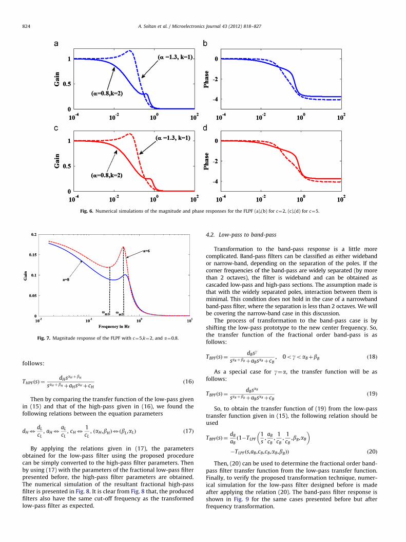
Fig. 6. Numerical simulations of the magnitude and phase responses for the FLPF (a),(b) for c¼2, (c),(d) for c¼5.

Fig. 7. Magnitude response of the FLPF with c¼5,k¼2, and a¼0.8.

A. Soltan et al. / Microelectronics Journal 43 (2012) 818–827824

follows:

THPF ðsÞ ¼dHsaH þbH

saH þbHþaHsaHþcHð16Þ

Then by comparing the transfer function of the low-pass givenin (15) and that of the high-pass given in (16), we found thefollowing relations between the equation parameters

dH3dL

cL, aH3

aL

cL, cH3

1

cL, ðaH ,bHÞ3ðbL,aLÞ ð17Þ

By applying the relations given in (17), the parametersobtained for the low-pass filter using the proposed procedurecan be simply converted to the high-pass filter parameters. Thenby using (17) with the parameters of the fractional low-pass filterpresented before, the high-pass filter parameters are obtained.The numerical simulation of the resultant fractional high-passfilter is presented in Fig. 8. It is clear from Fig. 8 that, the producedfilters also have the same cut-off frequency as the transformedlow-pass filter as expected.

4.2. Low-pass to band-pass

Transformation to the band-pass response is a little morecomplicated. Band-pass filters can be classified as either widebandor narrow-band, depending on the separation of the poles. If thecorner frequencies of the band-pass are widely separated (by morethan 2 octaves), the filter is wideband and can be obtained ascascaded low-pass and high-pass sections. The assumption made isthat with the widely separated poles, interaction between them isminimal. This condition does not hold in the case of a narrowbandband-pass filter, where the separation is less than 2 octaves. We willbe covering the narrow-band case in this discussion.

The process of transformation to the band-pass case is byshifting the low-pass prototype to the new center frequency. So,the transfer function of the fractional order band-pass is asfollows:

TBPF ðsÞ ¼dBsg

saBþbBþaBsaBþcB, 0ogoaBþbB ð18Þ

As a special case for g¼a, the transfer function will be asfollows:

TBPF ðsÞ ¼dBsaB

saBþbBþaBsaBþcBð19Þ

So, to obtain the transfer function of (19) from the low-passtransfer function given in (15), the following relation should beused

TBPF ðsÞ ¼dB

aBð1�TLPF

1

s,aB

cB,

1

cB,

1

cB,bB,aB

� �

�TLPF ðs,aB,cB,cB,aB,bBÞÞ ð20Þ

Then, (20) can be used to determine the fractional order band-pass filter transfer function from the low-pass transfer function.Finally, to verify the proposed transformation technique, numer-ical simulation for the low-pass filter designed before is madeafter applying the relation (20). The band-pass filter response isshown in Fig. 9 for the same cases presented before but afterfrequency transformation.

Fig. 9. Numerical simulations of the magnitude and phase responses for the FBPF (a),(b) for cB¼2, (c),(d) for cB¼5.

Fig. 10. (a) Approximation of a fractional capacitor via a self similar tree used in

ADS, and (b) the KHN filter using two elements of different orders.

Fig. 8. Numerical simulations of the magnitude and phase responses for the FHPF (a),(b) for cH¼1/2, (c),(d) for cH¼1/5.

A. Soltan et al. / Microelectronics Journal 43 (2012) 818–827 825

5. Circuit simulation

Now it is important to prove the reliability of the proposedalgorithm. So, the aim of this section is to apply the proposeddesign procedure on a practical filter like KHN filter. To testthe fractional order filter response, it is important first to modelthe fractional order element. A finite element approximation ofthe special case Z ¼ 1=ðC

ffiffispÞ was reported in [25]. This finite

element approximation relies on the possibility of emulating afractional-order capacitor via semi infinite RC trees [23]. Thetechnique was later developed by the authors of [21–26] for anyorder as presented in Fig. 10(a). A finite element approximationoffers a valuable tool by which the effect of a fractance device canbe simulated using a standard circuit simulator, or studiedexperimentally. However, they do not offer a simple practicaltwo-terminal device. Therefore, many practical realizations havebeen made for the fractance element by using the frequencydependent of the dielectric properties of some materials likeLiN2H5SO4 or using chemical reaction probe [22].

We investigate here some of the famous RC second-orderfilters assuming that their two normal capacitors are replacedby two fractional capacitors of different orders a and b. The finite

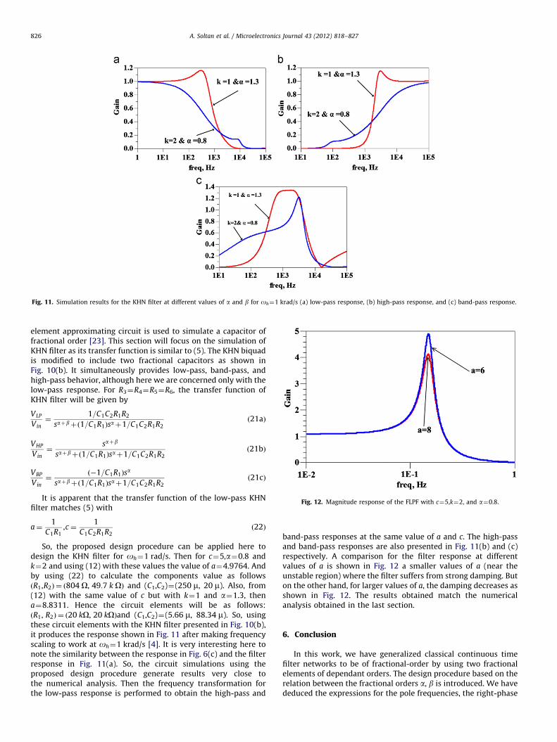
Fig. 11. Simulation results for the KHN filter at different values of a and b for oh¼1 krad/s (a) low-pass response, (b) high-pass response, and (c) band-pass response.

Fig. 12. Magnitude response of the FLPF with c¼5,k¼2, and a¼0.8.

A. Soltan et al. / Microelectronics Journal 43 (2012) 818–827826

element approximating circuit is used to simulate a capacitor offractional order [23]. This section will focus on the simulation ofKHN filter as its transfer function is similar to (5). The KHN biquadis modified to include two fractional capacitors as shown inFig. 10(b). It simultaneously provides low-pass, band-pass, andhigh-pass behavior, although here we are concerned only with thelow-pass response. For R3¼R4¼R5¼R6, the transfer function ofKHN filter will be given by

VLP

Vin¼

1=C1C2R1R2

saþbþð1=C1R1Þsaþ1=C1C2R1R2ð21aÞ

VHP

Vin¼

saþb

saþbþð1=C1R1Þsaþ1=C1C2R1R2ð21bÞ

VBP

Vin¼

ð�1=C1R1Þsa

saþbþð1=C1R1Þsaþ1=C1C2R1R2ð21cÞ

It is apparent that the transfer function of the low-pass KHNfilter matches (5) with

a¼1

C1R1,c¼

1

C1C2R1R2ð22Þ

So, the proposed design procedure can be applied here todesign the KHN filter for oh¼1 rad/s. Then for c¼5,a¼0.8 andk¼2 and using (12) with these values the value of a¼4.9764. Andby using (22) to calculate the components value as followsðR1,R2Þ ¼ ð804 O, 49:7 k OÞ and (C1,C2)¼(250 m, 20 m). Also, from(12) with the same value of c but with k¼1 and a¼1.3, thena¼8.8311. Hence the circuit elements will be as follows:ðR1, R2Þ ¼ ð20 kO, 20 kOÞand (C1,C2)¼(5.66 m, 88.34 m). So, usingthese circuit elements with the KHN filter presented in Fig. 10(b),it produces the response shown in Fig. 11 after making frequencyscaling to work at oh¼1 krad/s [4]. It is very interesting here tonote the similarity between the response in Fig. 6(c) and the filterresponse in Fig. 11(a). So, the circuit simulations using theproposed design procedure generate results very close tothe numerical analysis. Then the frequency transformation forthe low-pass response is performed to obtain the high-pass and

band-pass responses at the same value of a and c. The high-passand band-pass responses are also presented in Fig. 11(b) and (c)respectively. A comparison for the filter response at differentvalues of a is shown in Fig. 12 a smaller values of a (near theunstable region) where the filter suffers from strong damping. Buton the other hand, for larger values of a, the damping decreases asshown in Fig. 12. The results obtained match the numericalanalysis obtained in the last section.

6. Conclusion

In this work, we have generalized classical continuous timefilter networks to be of fractional-order by using two fractionalelements of dependant orders. The design procedure based on therelation between the fractional orders a, b is introduced. We havededuced the expressions for the pole frequencies, the right-phase

A. Soltan et al. / Microelectronics Journal 43 (2012) 818–827 827

frequencies, and the half-power frequencies. Also stability analy-sis of the fractional order filter is introduced. It is clear that moreflexibility in shaping the filter response can be obtained via afractional-order filter. Also, frequency transformation methods forthe low-pass fractional order filter are introduced. Besides that,a fractional order KHN filter design example is introduced toconfirm the design procedure and to prove the reliability of theproposed design procedure

References

[1] R. Caponetto, G. Dongola, L. Fortuna, I. Petras, Factional Order System—

Modeling and Control Applications, World Scientific Publishing Co. Pte. Ltd,2010, pp. 1–32.

[2] R.P. Agarwal, D. O’Regen, Ordinary and Partial Differential Equations WithSpecial Functions, Fourier Series and Boundary Value Problems, Springer,New York, 2000, pp. 64–75.

[3] A.G. Radwan, A.M. Soliman, A.S. Elwakil, A. Sedeek, On the stability of linearsystems with fractional-order elements, Chaos Solitons Fract. 40 (2009)2317–2328.

[4] A.G. Radwan, A.M. Soliman, A.S. Elwakil, First-order filters generalized to thefractional domain, J. Circuits Syst. Comput 17 (1) (2008) 55–66.

[5] A.G. Radwan, A.S. Elwakil, A.M. Soliman, On the generalization of secondorder filters to the fractional order domain, J. Circuits Syst. Comput 18 (2)(2009) 361–386.

[6] T.J. Freeborn, B. Maundy, A.S. Elwakil, Field programmable analogue arrayimplementation of fractional step filters, IET Circuits Devices Syst. 4 (6)(2010) 514–524.

[7] A.G. Radwan, A.S. Elwakil, A.M. Soliman, Fractional – order sinusoidaloscillator: design procedure and practical examples, IEEE Trans. Circuit Syst.55 (7) (2008) 2051–2063.

[8] D. Mondal, K. Biswas, Performance study of fractional order integrator usingsingle—component fractional order element, IET Circuits Devices Syst. 5 (4)(2011) 334–342.

[9] R.L. Magin, Fractional Calculus in Bioengineering, Begell House, Connecticut,2006.

[10] T.C. Doehring, A.H. Freed, E.O. Carew, I. Vesely, Fractional order viscoelasticityof the aortic valve: an alternative to QLV, J. Biomech. Eng. 127 (4) (2005)700–708.

[11] K. Moaddy, A.G. Radwan, K.N. Salama, S. Momani, I. Hashim, The fractional-order modeling and synchronization of electrically coupled neurons system,Comput. Math. Appl., http://dx.doi.org/10.1016/j.camwa.2012.01.005, in press.

[12] A.G. Radwan, K. Moddy, S. Momani, stability and nonstandard finite differ-ence method of the generalized Chua’s circuit, Comput. Math. Appl. 62 (2011)961–970.

[13] I.S. Jesus, T.J.A. Machado, B.J. Cunha, Fractional electrical impedances inbotanical elements, J. Vib. Control 14 (9) (2008) 1389–1402.

[14] M. Faryad, Q.A. Naqvi, Fractional rectangular waveguide, Prog. Electromagn.Res. 75 (2007) 384–396.

[15] A. Shamim, A.G. Radwan, K.N. Salama, Fractional smith chart theory andapplication, IEEE Microw. Wirel. Compon. Lett. 21 (3) (2011) 117–119.

[16] A.G. Radwan, A. Shamim, K.N. Salama, Theory of fractional-order elements

based impedance matching networks, IEEE Microw. Wirel. Compon. Lett. 21(3) (2011) 120–122.

[17] H. Li, Y. Luo, Y.Q. Chen, A Fractional-order proportional and derivative (FOPD)motion controller: tuning rule and experiments, IEEE Trans. Control Syst.

Technol. 18 (2) (2010) 516–520.[18] S. Mukhopadhyay, C. Coopmans, Y.Q. Chen, Purely analog fractional-order PI

control using discrete fractional capacitors (Fractals): synthesis and experi-

ments, in: Proceedings of the International Design Engineering TechnicalConferences and Computers and Information in Engineering Conference,

IDETC/CIE, USA, 2009.[19] A.G. Radwan, K.N. Salama, Passive and active elements using fractional LbCa

circuit, IEEE Trans. Circuits Syst. I 58 (10) (2011) 2388–2397.[20] A.G. Radwan, Stability analysis of the fractional-order RLC circuit, J. Fract.

Calc. Appl. (JFCA) 3 (2012).[21] M. Sugi, Y. Hirano, K. Saito, Simulation of fractal immittance by analog

circuits: an approach to the optimized circuits, IEICE Trans. Fundam E82-A

(8) (1999) 1627–1635.[22] B.T. Krishna, Studies on fractional order differentiators and integrators:

a survey, Signal Process. 91 (2011) 386–426.[23] M. Nakagawa, K. Sorimachi, Basic characteristic of fractance device, IEICE

Trans. Fundam E75-A (12) (1992) 1814–1819.[24] K. Saito, M. Sugi, Simulation of power low relaxation by analog circuits:

fractal distribution of relaxation times and non-integer exponents, IEICETrans. Fundam E76-A (2) (1993) 204–209.

[25] B.T. Krishna, K.V.V.S. Reddy, Active and passive realization of fractance deviceof order 1/2, Act. Passive Electron. Compon. (2008).

[26] A. Djouambi, A. Charef, A.V. Besancon, Optimal approximation, simulationand analog realization of the fundamental fractional order transfer function,Int. J. Appl. Math. Comput. Sci. 17 (4) (2007) 455–462.

[27] A.S. Sedra, K.C. Smith, Microelectronic Circuits, Oxford, NewYork, 1998pp. 884–963.

[28] A.S. Sedra, P.O. Brackett, Filter Theory and Design: Active and Passive, JohnWiley & Sons, Singapore, 1986, pp. 1–100.

[29] L. Thede, Practical Analog and Digital Filter Design, Artech House, 2004pp. 15–54.

[30] S. Winder, Analog and Digital Filter Design, Newnes, New York, 2002, pp. 41–122.[31] S. Butterworth, On the theory of filter amplifiers, Exp. Wireless Wireless Eng.

7 (1930) 536–541.[32] H.G. Hoang, H.D. Tuan, T.Q. Nguyen, Analog flat filter design, ICASSP (2009)

3225–3228.[33] J. Lim, D.C. Park, A modified Chebyshev bandpass filter with attenuation poles

in the stopband, IEEE Trans. Microw. Theory Tech. 45 (6) (1997) 898–904.[34] S.W. Choi, D.Y. Kim, H.K. Kim, A modified low-pass filter with progressively

diminishing ripples, Analog Integr. Circuits. Signal Process 6 (1994) 95–103.[35] A. Soltan, A.G. Radwan, A.M. Soliman, Butterworth passive filter in the

fractional-order, in: Proceedings of the 23rd International Conference onMicroelectronics, ICM, Tunis, 2011.