arX

iv:c

ond-

mat

/960

6167

v1 2

4 Ju

n 19

96

Fragmentation of Colliding Discs

Ferenc Kun1 and Hans J. Herrmann2

February 1, 2008

1Laboratoire de Physique et Mecanique des Milieux Heterogenes, C.N.R.S., U.R.A. 857Ecole Superieure de Physique et Chimie Industrielle

10 rue Vauquelin, 75231 Paris, Cedex 05, France

2ICA 1, University of Stuttgart, Pfaffenwaldring 27, 70569 Stuttgart, Germany

Abstract

We study the phenomena associated with the low-velocity impact

of two solid discs of equal size using a cell model of brittle solids. The

fragment ejection exhibits a jet-like structure the direction of which

depends on the impact parameter. We obtain the velocity and the

mass distribution of the debris. Varying the radius and the initial

velocity of the colliding particles, the velocity components of the frag-

ments show anomalous scaling. The mass distribution follows a power

law in the region of intermediate masses.

1 Introduction

Fragmentation covers a wide diversity of physical phenomena. Recently, thefragmentation of granular solids has attracted considerable scientific and in-dustrial interest. The length scales involved in this process range from thecollisional evolution of asteroids[1] to the degradation of materials comprisingsmall agglomerates employed in industrial processes[2]. On the intermediatescale there are several geophysical examples concerning to the usage of explo-sives in mining and oil shale industry, fragments from weathering, coal heapsrock fragments from chemical and nuclear explosions[1]. Most of the mea-sured fragment size distributions exhibit power law behavior with exponentsbetween 1.9 and 2.6 concentrating around 2.4[1]. Power law behavior of smallfragment masses seems to be a common characteristic of brittle fracture.

1

Comprehensive laboratory experiments were carried out applying projec-tile collision[3, 4, 5] and free fall impact with a massive plate[6, 7, 8]. Theresulting fragment size distributions show universal power law behavior. Thescaling exponents depend on the overall morphology of the objects but areindependent of the type of the materials.

Beside the size distribution of the debris, there is also particular inter-est in the energy required to achieve a certain size reduction. Collisionexperiments[4] revealed that the mass of the largest fragment normalizedby the total mass shows power law behavior as a function of the specificenergy (imparted energy normalized by the total mass). The exponents arebetween 0.6 and 1.5 depending on the geometry of the system.

On microscopic scale the fragmentation of atomic nuclei is intensivelyinvestigated[9]. In the experiments concerning the multifragmentation ofgold projectiles, a power law charge distribution of the fragments was foundindependent of the target type[10].

Several theoretical approaches were proposed to describe fragmentation.In stochastic models[11, 12, 13, 14] power law, exponential and log-normaldistributions were obtained depending on the dimensionality of the objectand the detailed breaking mechanism.

Discrete stochastic processes have also been studied as models for frag-mentation using cellular automata. In Ref. 15 two- and three - dimensionalcellular automata were proposed to model power law distributions in shearexperiments on a layer of uniformly sized fragments.

The mean - field approach describes the time evolution of the concentra-tion c(x, t) of fragments having mass x through a linear integro - differentialequation[16]:

∂c(x, t)

∂t= −a(x)c(x, t) +

∫

∞

xc(y, t)a(y)f(x|y)dy (1)

where a(x) is the overall rate at which x breaks in a time interval dt, whilef(x|y) is the relative rate at which x is produced from the break-up of y.With some further assumptions on f(x|y) exact results can be obtained butin physically interesting situations the solution is very difficult[16].

Three - dimensional impact fracture processes of random materials weremodeled based on a competitive growth of cracks[17]. A universal powerlaw fragment mass distribution was found consistent with self - organizedcriticality with an exponent of 5

3.

A two dimensional dynamic simulation of solid fracture was performedusing a cellular model material[18, 19]. The compressive failure of a rect-angular sample, the four - point shear failure of a beam and the impact ofparticles with a plate and with other particles were studied.

2

Recently, we have established[20] a two - dimensional model for a de-formable, breakable, granular solid by connecting unbreakable, undeformableelements with elastic beams, similar as in Refs. 18,19. The contacts betweenthe particles can be broken according to a physical breaking rule, which takesinto account the stretching and bending of the connections[20].

In this paper we apply the model to study the phenomena associated withlow-velocity impact of two solid discs of the same size. An advantage of ourmodel with respect to most other fragmentation models is that we can followthe trajectory of each fragment, which is often of big practical importance,and that we know how much energy each fragment carries away. Varying theimpact parameter, the size of the colliding particles and the initial velocities,we are mainly interested in the spatial distribution of the fragments, in thedistribution of the fragment velocities and the fragment size. This is im-portant to get deeper insight into the collisional evolution of asteroids, smallplanets and planetary rings. One particular interest of this experiment is thatit can be considered as a classical analog of the deeply inelastic scatteringof heavy nuclei[9]. The characteristic quantities providing collective descrip-tion of the fragmenting system (e.g. the fragment mass distribution), arescale invariant. This enables us to make also some comparison with nuclearfragmentation experiments.

2 Description of the simulation

Here we give a brief overview of the basic ideas of our model and the simu-lation technique used. For details see Ref. 20.

In order to study fragmentation of granular solids we perform MolecularDynamics (MD) simulations in two dimensions. This method calculates themotion of particles by solving Newton’s equations. In our simulation thisis done using a Predictor-Corrector scheme. The construction of our modelof a deformable, breakable, granular solid is performed in three major steps,namely, the implementation of the granular structure of the solid, the intro-duction of the elastic behavior by the cell repulsion and the beam model,and finally the breaking of the solid.

In order to take into account the complex structure of the granular solidwe use arbitrarily shaped convex polygons. To get an initial configurationof these polygons we make a special Voronoi tessellation of the plane[22].The convex polygons of this Voronoi construction are supposed to modelthe grains of the material. In this way the structure of the solid is builton a mesoscopic scale. In our simulation these polygons are the smallestparticles interacting elastically with each other. All the polygons have three

3

continuous degrees of freedom in two dimensions: the two coordinates of thepositions of the center of mass and the rotation angle. The elastic behavior ofthe solid is captured in the following way: The polygons are considered to berigid bodies. They are not breakable and not deformable. But they can over-lap when they are pressed against each other representing to some extent thelocal deformation of the grains. In order to simulate the elastic contact forcebetween touching grains we introduce a repulsive force between the overlap-ping polygons. This force is proportional to the overlapping area divided bya characteristic length of the interacting polygon pair. The proportionalityfactor is the grain bulk Young’s modulus Y [21].

In order to keep the solid together it is necessary to introduce a cohesiveforce between neighboring polygons. For this purpose we introduce beams,which were extensively used recently in crack growth models[23, 24]. Thecenters of mass of neighboring polygons are connected by elastic beams,which exert an attractive, restoring force between the grains, and can breakin order to model the fragmentation of the solid. The physical properties ofthe beams, i.e.. length, section and moment of inertia are determined by theactual realization of the Voronoi polygons. To describe their elastic behavior,the beams have a Young’s modulus E, which is in principal independent ofY , see Ref. 20.

For not too fast deformations the breaking of a beam is only caused bystretching and bending. We impose a breaking rule of the form of the vonMises plasticity criterion, which takes into account these two breaking modes,and which can reflect the fact that the longer and thinner beams are easier tobreak. The breaking rule contains two parameters tǫ and tΘ controlling therelative importance of the stretching and bending modes. In the simulationswe used the same values of tǫ and tΘ for all the beams. During all thecalculations the beams are allowed to break solely under stretching, whichtakes into account that it is much harder to break a solid under compressionthan under elongation. The breaking rule is evaluated in each iteration timestep and those beams which fulfill the breaking condition are removed fromthe calculation. The simulation stops if there is no beam breaking during300 successive iteration steps. Table 1 shows the values of the microscopicparameters of the model used in the simulations.

The calculations were performed on the CM5 of the CNCPST in Paris.We used the farming method, i.e. the same program runs on a variety ofnodes with different initial setups. In our case 32 nodes were used withdifferent seeds for the Voronoi generator, i.e. with differently shaped Voronoicells.

4

Table 1: The parameter values used in the simulations.Parameter Symbol Unit V alueDensity ρ g/cm3 5Grain bulk Young’s modulus Y dyn/cm2 1010

Beam Young’s modulus E dyn/cm2 5 · 109

Time step dt s 10−6

The failure elongation of a beam tǫ % 3The failure bending of a beam tΘ degree 4

3 Results

With the model outlined above we have already performed several numericalexperiments[20]. Namely, we studied the fragmentation of a solid disc causedby an explosion in the middle and the breaking of a rectangular solid blockdue to the impact with a projectile. Emphasis was put on the investigationof the fragment size distribution. Universal power law behavior was found,practically independent from the breaking thresholds, see Ref. 20.

In the present paper we study the collision of two solid discs of equalsize. The disc-shaped granular solid was obtained starting from the Voronoitessellation of a square and cutting out a circular window. This gives rise toa certain roughness of the surface of the particles.

The schematic representation of the experimental situation can be seenin Fig. 1. In the simulations all the microscopic parameters of the modelshown in Table 1 were fixed, only the macroscopic parameters were varied,i.e. the initial velocities ~vA, ~vB and the radii RA, RB of the colliding particlesand the impact parameter b. Only the monodisperse case RA = RB wasconsidered. The velocities of the two particles have the same magnitude andopposite direction ~vA = −~vB . The impact parameter b is defined as thedistance between the two centers of mass in the direction perpendicular tothe velocity vectors. b can vary in the interval [0, RA + RB]. The range ofthe initial velocities was chosen to be 12.5 − 50m/s, and that of the radii5 − 15cm.

In the following the results are presented concerning the time evolutionof the fragmenting system, the spatial distribution of the fragments, thedistribution of the fragment velocities and of the fragment mass.

5

3.1 Fragmentation process

In Ref. 4, based on detailed experimental studies, the low - velocity impactphenomena of solid spheres were classified into five categories: (1) elasticrebound, (2) rebound with contact damage, (3) rebound with longitudinalsplits, (4) destruction with shatter- cone like fragments, and (5) completedestruction. These categories can be well distinguished by the impartedenergy. Our simulations cover the 4th and the 5th classes varying the initialvelocities, the radii and the impact parameter. Results about the 1st casewill be presented in a forthcoming publication.

The collision initiates with the contact of the two bodies. At our velocityrange it can be assumed that the impact proceeds quasi-statically since theimpact velocity is much smaller than the velocity of the generated shock wave.Fig. 2 and Fig. 3 show representative examples of the time evolution of thecolliding system at b/d = 0 (central collision) and b/d = 0.5, respectively.Here d denotes the diameter of the particles. Due to the high compression astrongly damaged region is formed around the impact site, where practicallyall the beams are broken and all the fragments are single polygons. Since thebeam breaking dissipates energy the growth of the damage stops after sometime. The shock wave reaching the free boundary gives rise to the expansionof the particles. This overall expansion initiates crack formation which resultsin the final fragmentation of the solids. The fragments at the anti - impactsite of the particles are larger and they mainly have a shatter cone like shapein agreement with experimental observations[4]. Due to the geometry of thesystem, the fine fragments in the contact zone are confined unless the globalexpansion sets in. Thus they undergo many secondary collisions while thefragments formed in the outer region can escape without further interaction.This has an important effect on the velocity distribution of the debris in thefinal state. (See Chapter 3.2.)

Since the impact velocity is much smaller than the sound speed of thematerial, the peak stress produced by the collision around the impact site isproportional to the normal component of the impact velocity vn with respectto the contact surface. That is why the final breaking scenarios strongly de-pend on the impact parameter. In Fig. 2, in the case of a central collision thedamage is larger, i.e. the shattered zone is larger and the average fragmentsize is smaller than in Fig. 3. The larger b/d (the smaller vn), the less energyis converted into breaking and the more energy is carried away by the motionof the fragments.

In the expanding system the fragments are not isotropically distributedbut the fragment ejection has a preferred direction depending also on theimpact parameter. In Fig 4 the jet-like structure of the fragment ejection

6

can be observed, which means that most of the fragments are flying in two“cones” having a common axis and a relatively small opening angle.

To determine the jet-axis we calculated the sphericity S of the velocitydistribution:

S = min~n

2

∑

v2

T i∑

v2i

, (2)

where ~vi is the velocity of the center of mass of fragment i and vT i is itstransversal component with respect to ~n. The factor 2 scales the upperlimit of S to 1 in the case of the isotropic velocity distribution. The jet-axis~n∗ minimizes the above expression. The angle of the jet-axis and that ofthe contact surface with respect to the direction of the initial velocity as afunction of b/d are shown in Fig. 5.

Because of the low impact velocity there is enough time for stress re-arrangement inside the two bodies. Thus the stress can have a tangentialdirection to the contact surface giving rise to the jet-like ejection. (A de-tailed study of the stress field inside disc shaped particles due to an impactwill be presented in the forthcoming publication mentioned above.) Thisargument is also supported by the fact that the long cracks passing throughthe solids are either perpendicular to the contact zone or they go radially tothe surface of the solids. For the central and peripheric collisions the jet-axisis practically parallel to the contact surface (see Fig.5). The two curves differconsiderably only at intermediate b values.

The angular distribution of the fragments around the direction of theinitial velocity is shown in Fig. 6. The concentration of the debris in a smallsolid angle can be observed. The position of the peak of the distributionspractically coincides with the jet-axis.

3.2 Scaling of the velocity distribution

In order to study the velocity distribution of the fragments we performed twosets of simulations alternatively fixing the initial velocity and the radius of theparticles changing the value of the other one. Only central collisions b/d = 0were considered. In both cases the distribution of the x and y componentsof the velocity of the center of mass of the fragments was evaluated. The xaxis was chosen to be parallel to the initial velocity of the collision.

Fig. 7 and Fig. 8 show the results for fixed R = 15cm varying the initialvelocity and for fixed v = 50m/s varying the radius of the particles, respec-tively. One can observe that the distributions of both velocity componentsalways exhibit a Gaussian form. The zero mean value is a consequence ofmomentum conservation. In the x direction the fragments are slower, i.e. the

7

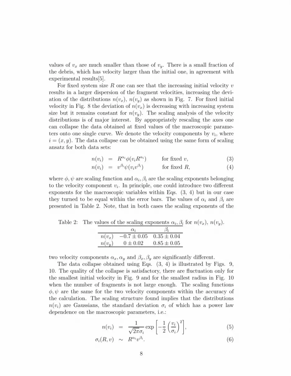
values of vx are much smaller than those of vy. There is a small fraction ofthe debris, which has velocity larger than the initial one, in agreement withexperimental results[5].

For fixed system size R one can see that the increasing initial velocity vresults in a larger dispersion of the fragment velocities, increasing the devi-ation of the distributions n(vx), n(vy) as shown in Fig. 7. For fixed initialvelocity in Fig. 8 the deviation of n(vx) is decreasing with increasing systemsize but it remains constant for n(vy). The scaling analysis of the velocitydistributions is of major interest. By appropriately rescaling the axes onecan collapse the data obtained at fixed values of the macroscopic parame-ters onto one single curve. We denote the velocity components by vi, wherei = (x, y). The data collapse can be obtained using the same form of scalingansatz for both data sets:

n(vi) = Rαiφ(viRαi) for fixed v, (3)

n(vi) = vβiψ(vivβi) for fixed R, (4)

where φ, ψ are scaling function and αi, βi are the scaling exponents belongingto the velocity component vi. In principle, one could introduce two differentexponents for the macroscopic variables within Eqs. (3, 4) but in our casethey turned to be equal within the error bars. The values of αi and βi arepresented in Table 2. Note, that in both cases the scaling exponents of the

Table 2: The values of the scaling exponents αi, βi for n(vx), n(vy).αi βi

n(vx) −0.7 ± 0.05 0.35 ± 0.04n(vy) 0 ± 0.02 0.85 ± 0.05

two velocity components αx, αy and βx, βy are significantly different.The data collapse obtained using Eqs. (3, 4) is illustrated by Figs. 9,

10. The quality of the collapse is satisfactory, there are fluctuation only forthe smallest initial velocity in Fig. 9 and for the smallest radius in Fig. 10when the number of fragments is not large enough. The scaling functionsφ, ψ are the same for the two velocity components within the accuracy ofthe calculation. The scaling structure found implies that the distributionsn(vi) are Gaussians, the standard deviation σi of which has a power lawdependence on the macroscopic parameters, i.e.:

n(vi) =1√2πσi

exp

[

−1

2

(

vi

σi

)2]

, (5)

σi(R, v) ∼ Rαivβi. (6)

8

Fig. 10 shows a representative example of the Gaussian fit too. Eq. (5) wasfitted to the scaling function φ.

The shape of the velocity distribution of the fragments is mainly deter-mined by the stress distribution in the bodies just before the breaking of thebeams. When, due to the geometry of the system, energetic fragments areconfined during some time, secondary collisions of the products can also havea considerable contribution. In our case this effect can be responsible for theGaussian shape.

The deviations of the two velocity components σx and σy can be con-sidered as the linear extensions of the fragment jet in the velocity space inthe x and y directions. Their ratio s is a characteristic quantity of the jetshape. (Note, that here we considered solely central collisions. The aboveargument can be generalized to non-central collisions choosing the x direc-tion perpendicular to the jet-axis.) Eq. (6) yields the dependence of s onthe macroscopic parameters:

s(R, v) =σy

σx

∼ Rαy−αxvβy−βx = Rγvδ (7)

The value of the new exponents characterizing the jet-shape are γ = 0.7±0.05and δ = 0.5 ± 0.05.

It is generally believed that once a solid, e.g. asteroid suffers catastrophicdestruction the pieces fly apart from each other in all directions. Howeverthis scheme is not necessarily true. From our treatment it follows that wehave anisotropic clustering of fragments, i.e. most of the fragment velocitiesare much smaller than the impact velocity and the particles fly in rathercollimated jets, the shape of which is described by γ and δ. This can haveimportant consequences for the later evolution of the fragmented system. Forinstance, in the case of the collision of asteroids fragments could recombinedue to mutual gravitation forming a cloud-like object.

3.3 The fragment mass distribution

Beside the fragment velocities, the mass distribution of the debris also haspractical importance. Fig. 2 and Fig. 3 show that the contact zone aroundthe impact site gives the main contribution to the small fragments while thelarger ones are dominated by the anti-impact site. This detachment effectbecomes more pronounced for smaller collision velocities when the type ofthe impact passes from class (5) to (4) (see Chapter 3.1).

9

The fragment mass histograms F (m) are presented in Figs. 11, 12 forfixed system size and for fixed initial velocity, respectively. Here F (m) de-notes the number of fragments with mass m divided by the total numberof fragments. In order to obtain the correct shape of the distributions atthe coarse products as well as at the finer ones logarithmic bining was used,i.e. the bining is equidistant on logarithmic scale. The histograms have twocutoffs. The lower one is due to the existence of single unbreakable poly-gons (smallest fragments) and the upper one is given by the finite size of thesystem (largest fragment).

In Fig. 11 the histogram belonging to the smallest collision velocity hastwo well distinguished local maxima, one for the fine fragments (single poly-gons and pairs) and another one for the large pieces, which are comparableto the size of the colliding particles. In between, for the “Intermediate MassFragments” (IMF) F (m) shows power law behavior, i.e. we seem to have:

F (m) ∼ m−µ. (8)

The effective exponent µ was obtained from the estimated slope of the curve,µ = 2.1 ± 0.05 for v = 12.5m/s. At low impact velocity this shape of dis-tribution is characteristic for light-fragment ejection from a heavy system[9].As the initial velocity increases the peak of the heavy fragments graduallydisappears giving rise to an increase of the contribution of IMFs, while thefraction of the shattered products hardly changes. In the IMF region theslope of F (m) depends slightly on the impact velocity, i.e. the distributionsbecome less steep with increasing v. The straight line in Figs. 11, 12 showsthe power law fitted at our highest velocity v = 50m/s and for R = 15cmwith exponent µ = 1.75 ± 0.05.

For fixed initial velocity the histograms belonging to different system sizesare characterized practically by the same exponent µ = 1.75± 0.05 as shownin Fig. 12. Only in the case of the smallest system, which suffers catastrophicdestruction shattering the particles completely, the exponent is larger.

It is important to note that in nuclear fragmentation experiments of goldprojectile with several targets, the charge distribution of the fragments showsa similar dependence on the deposited energy of the collision[25].

Beside the size distribution of the debris there is also interest in theenergy required to achieve a certain size reduction. It was revealed in collisionexperiments[4] that the mass of the largest fragment Mmax normalized by thetotal mass Mtot follows a power law as a function of the specific energy, i.e.the ratio of the imparted energy E and the total mass of the system. Theexponent characterizing the size reduction seems to be independent of thetype of the material but it is sensitive to the shape of the colliding particles.

10

For spherical bodies it was found to be around 0.7, while for cubic systemsaround 1.5 (see Ref. 4). Note, that in Fig. 12 the fixed initial velocityimplies that the specific energy is also constant. This results in more or lessthe same value of Mmax/Mtot for the different curves. In Fig. 11 for fixedsystem size the specific energy varies with the initial velocity resulting changeof Mmax/Mtot.

In order to obtain more information about the size reduction we per-formed a set of simulations on the 32 partition of the CM5 with fixedR = 15cm particle radius changing the initial velocity within the interval12.5 − 50m/s in 32 steps. In Fig. 13 Mmax/Mtot is plotted against thespecific energy E/Mtot on double logarithmic scale. Although the data arerather scattered a power law seems to be a reasonable fit with exponent 0.68in agreement with the experimental results.

4 Conclusion

We have studied the low velocity impact phenomena of two solid discs of thesame size using our cell model[20]. We focused our attention on the spatialdistribution of the debris and on the analysis of the fragment velocities andfragment mass.

Anisotropic clustering of fragments was revealed, which manifests in thejet structure of the fragment ejection. Due to the anomalous scaling of thedistributions of the velocity components the jet-shape can be characterizedby two independent exponents. The mass distribution of the intermediatemass fragments shows a power law behavior, whose exponent slightly de-creases with increasing imparted energy. We have noted that the charge dis-tributions obtained in nuclear multifragmentation experiments show a similardependence on the deposited energy of the collision. This is a manifestationof the independence of the global quantities of the fragmenting system fromthe microscopic details of the mechanism of the individual breaking.

The mass of the largest fragment normalized by the total mass also followsa power law as a function of the imparted energy density with exponent closeto the experimental observations.

Still our study makes a certain number of technical simplifications whichmight be important for a full quantitative grasp of fragmentation phenom-ena. Most important seems to us the restriction to two dimensions, whichshould be overcome in future investigations. The existence of elementary,non-breakable polygons restricts fragmentation on lower scales and hindersus from observing the formation of a powder of a shattering transition[16].

Experiments showed[4] that the relative size of the colliding bodies is an

11

important parameter describing the low velocity impact phenomena if themechanical properties of the bodies are the same. In the future our studiesshould be extended to this polydisperse case too.

Acknowledgment

We are grateful to CNCPST in Paris for the computer time on the CM5.F. Kun acknowledges the financial support of the Hungarian Academy ofSciences and the EMSPS.

References

[1] D. L. Turcotte, J. of Geophys. Res. Vol. 91 B2, 1921 (1986).

[2] C. Thornton, K. K. Yin and M. J. Adams, J. Phys. D. Appl. Phys. 29,424 (1996)

[3] N. Arbiter, C. C. Harris and G. A. Stamboltzis, Soc. of Min. Eng. 244,119 (1969).

[4] T. Matsui, T. Waza, K. Kani and S. Suzuki, J. of Geophys. Res. 87

B13, 10968 (1982).

[5] A. Fujiwara and A. Tsukamoto, Icarus 44, 142 (1980).

[6] M. Matsushita and T. Ishii, Fragmentation of long thin glass rods,Department of Physics, Chuo University (1992).

[7] L. Oddershede, P. Dimon, and J. Bohr, Phys. Rev. Lett. 71, 3107(1993).

[8] A. Meibom and I. Balslev, Phys. Rev. Lett. 76, 2492 (1996)

[9] D. Beysens, X. Campi, E. Pefferkorn (eds), Fragmentation Phenomena,World Scientific 1995.

[10] R. Botet and M. Ploszajczak, in Ref. [9]

[11] M. Matsushita and K. Sumida, How do thin glass rods break? (Stochas-tic models for one - dimensional fracture), Chuo University, Vol. 31,pp. 69-79 (1981).

[12] M. Marsili and Y. C. Zhang, preprint

12

[13] P. L. Krapivsky and E. B. Naim, Phys. Rev. E 50 3502 (1995).

[14] G. Hernandez, H. J. Herrmann, Physica A 215, 420 (1995).

[15] S. Steacy and C. Sammis, An automaton for fractal patterns of frag-mentation, Nature 353 250 (1991).

[16] S. Redner, in: Statistical Models for the Fracture of Disordered Media(North Holland, Amsterdam, 1990).

[17] H. Inaoka, H. Takayasu, preprint.

[18] A. V. Potapov, M. A. Hopkins and C. S. Campbell, Int. J. of Mod.Phys. C 6, 371 (1995).

[19] A. V. Potapov, M. A. Hopkins and C. S. Campbell, Int. J. of Mod.Phys. C 6, 399 (1995).

[20] F. Kun and H. J. Herrmann, preprint cond-mat/9512017

[21] H. J. Tillemans, H. J. Herrmann, Physica A 217, 261 (1995).

[22] K. B. Lauritsen, H. Puhl and H. J. Tillemans, Int. J. of Mod. Phys. C

5, 909 (1994).

[23] H. J. Herrmann and S. Roux (eds.) Statistical Models for the Fractureof Disordered Media (North Holland, Amsterdam, 1990).

[24] H. J. Herrmann, A. Hansen, S. Roux, Phys. Rev. B 39, 637 (1989).

[25] C. A. Ogilvie et al, Phys. Rev. Lett. 67, 1214 (1991)

13

RA

vA

RB

vB

b

Figure 1: The schematic representation of the collision experiment. In allthe simulations RA = RB and ~vA = −~vB were chosen.

14

��������������������������������������������������������������������������������������������������������������������������������������������������������������������������������������������������������������������������������������������������������������������������������������������������������������������������������������������������������������������������������������������������������������������������������������������������������������������������������������������������������������������

Figure 2: The central collision (b = 0) of two discs of equal size R = 15cmat v = 25m/s velocity. Snapshots of the evolving system present the initialconfiguration, an intermediate state and the final breaking scenario.

15

��������������������������������������������������������������������������������������������������������������������������������������������������������������������������������������������������������������������������������������������������������������������������������������������������������������������������������������������������������������������������������������������������������������������������������������������������������������������������������������������������������������������

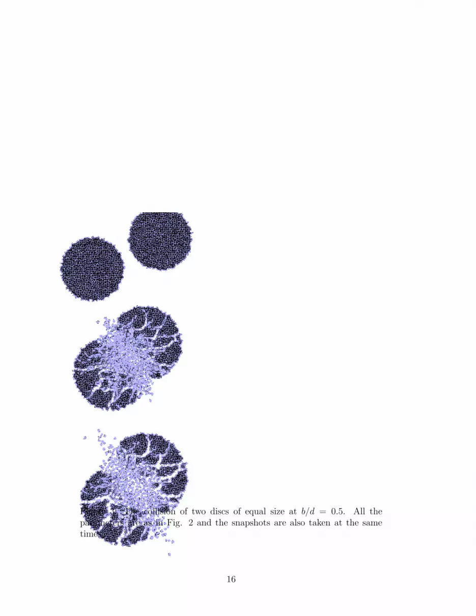
Figure 3: The collision of two discs of equal size at b/d = 0.5. All theparameters are as in Fig. 2 and the snapshots are also taken at the sametimes.

16

b/d=0 b/d=1/3 b/d=2/3

Figure 4: The velocity vectors of the center of mass of the fragments forthree different impact parameters. One can observe the jet structure of thefragment ejection. All the parameters are as in Fig. 2.

0.0 0.1 0.2 0.3 0.4 0.5 0.6 0.7 0.8 0.9 1.0

b/d

0.0

0.2

0.4

0.6

0.8

1.0

1.2

1.4

1.6

jet-axis

contact surface

Figure 5: The angle of the jet-axis and that of the contact surface withrespect to the direction of the initial velocity as a function of b/d.

17

-80 -60 -40 -20 0 20 40 60 800.0

0.05

0.1

0.15

0.2

0.25

dN

/d

b/d =0.9b/d =2/3b/d =1/2b/d =1/3b/d =1/6b/d =0

Figure 6: The angular distribution of the fragments around the direction ofthe initial velocities for different impact parameters.

18

��������������������������������������������������������������������������������������������������������������������������������������������������������������������������������������������������������������������������������������������������������������������������������������������������������������������������������������������������������������������������������������������������������������������������������������������������������������������������������������������������������������������

Figure 7: The distribution of the x and y components of the velocity of thefragments with fixed system size R = 15cm varying the initial velocity v.

19

a)

-50 -40 -30 -20 -10 0 10 20 30 40 50

vx [m/s]

0.0

0.01

0.02

0.03

0.04

0.05

0.06

0.07

n(v

x)

R=15 cm

R=12.5 cm

R=10 cm

R=5 cm

b)

-300 -200 -100 0 100 200 300

vy [m/s]

0.0

0.002

0.004

0.006

0.008

0.01

0.012

n(v

y)

R=15 cm

R=12.5 cm

R=10 cm

R=5 cm

Figure 8: The distribution of the x and y components of the velocity of thefragments with fixed initial velocity v = 50m/s varying the radius R of theparticles.

20

��������������������������������������������������������������������������������������������������������������������������������������������������������������������������������������������������������������������������������������������������������������������������������������������������������������������������������������������������������������������������������������������������������������������������������������������������������������������������������������������������������������������

Figure 9: Scaling of the velocity distributions for fixed system size R = 15cmvarying the initial velocity v.

21

-200 -150 -100 -50 0 50 100 150 200

vx R0.7

0.0

0.002

0.004

0.006

0.008

0.01

0.012

R=15 cm

R=12.5 cm

R=10 cm

R=5 cm

Figure 10: Scaling of the velocity distributions for fixed initial velocityv = 50m/s varying the radius R of the particles. The solid line shows theGaussian fit according to Eq. (5) for the scaling function φ.

5 101

2 5 102

2 5 103

2

m [g]

10-6

10-5

10-4

10-3

10-2

10-1

F(m

)

v=50 m/sv=37.5 m/sv=25 m/sv=12.5 m/s

Figure 11: The fragment mass histograms for fixed system size R = 15cmvarying the initial velocity v. The straight line shows the power law fitted tothe curve belonging to v = 50m/s.

22

5 101

2 5 102

2

m [g]

10-6

10-5

10-4

10-3

10-2

10-1

F(m

)R=15 cmR=12.5 cmR=10 cmR=5 cm

Figure 12: The fragment mass histograms for fixed initial velocity v = 50m/s,varying the system size R. The straight line is the same as in Fig. 11.

8 9106

2 3 4 5 6 7 8 9107

E/Mtot [erg/g]

3

4

5

6

7

8

9

10-1

Mm

ax/M

tot

Figure 13: The mass of the largest fragment normalized by the total mass asa function of the specific energy.

23