Embed Size (px)
Citation preview
FreeFEM DocumentationRelease 4.8
Frederic Hecht
Feb 01, 2022


In collaboration with:
i

ii
CONTENTS
1 Introduction 31.1 Version 4.5: new features . . . . . . . . . . . . . . . . . . . . . . . . . . . . . . . . . . . . . . . . 51.2 Installation guide . . . . . . . . . . . . . . . . . . . . . . . . . . . . . . . . . . . . . . . . . . . . . 61.3 Download . . . . . . . . . . . . . . . . . . . . . . . . . . . . . . . . . . . . . . . . . . . . . . . . . 181.4 History . . . . . . . . . . . . . . . . . . . . . . . . . . . . . . . . . . . . . . . . . . . . . . . . . . 191.5 Citation . . . . . . . . . . . . . . . . . . . . . . . . . . . . . . . . . . . . . . . . . . . . . . . . . . 201.6 Authors . . . . . . . . . . . . . . . . . . . . . . . . . . . . . . . . . . . . . . . . . . . . . . . . . . 211.7 Contributing . . . . . . . . . . . . . . . . . . . . . . . . . . . . . . . . . . . . . . . . . . . . . . . 22
2 Learning by Examples 252.1 Getting started . . . . . . . . . . . . . . . . . . . . . . . . . . . . . . . . . . . . . . . . . . . . . . 272.2 Classification of partial differential equations . . . . . . . . . . . . . . . . . . . . . . . . . . . . . . 322.3 Membrane . . . . . . . . . . . . . . . . . . . . . . . . . . . . . . . . . . . . . . . . . . . . . . . . 352.4 Heat Exchanger . . . . . . . . . . . . . . . . . . . . . . . . . . . . . . . . . . . . . . . . . . . . . . 402.5 Acoustics . . . . . . . . . . . . . . . . . . . . . . . . . . . . . . . . . . . . . . . . . . . . . . . . . 432.6 Thermal Conduction . . . . . . . . . . . . . . . . . . . . . . . . . . . . . . . . . . . . . . . . . . . 452.7 Irrotational Fan Blade Flow and Thermal effects . . . . . . . . . . . . . . . . . . . . . . . . . . . . 492.8 Pure Convection : The Rotating Hill . . . . . . . . . . . . . . . . . . . . . . . . . . . . . . . . . . . 532.9 The System of elasticity . . . . . . . . . . . . . . . . . . . . . . . . . . . . . . . . . . . . . . . . . 562.10 The System of Stokes for Fluids . . . . . . . . . . . . . . . . . . . . . . . . . . . . . . . . . . . . . 592.11 A projection algorithm for the Navier-Stokes equations . . . . . . . . . . . . . . . . . . . . . . . . . 602.12 Newton Method for the Steady Navier-Stokes equations . . . . . . . . . . . . . . . . . . . . . . . . 652.13 A Large Fluid Problem . . . . . . . . . . . . . . . . . . . . . . . . . . . . . . . . . . . . . . . . . . 682.14 An Example with Complex Numbers . . . . . . . . . . . . . . . . . . . . . . . . . . . . . . . . . . 732.15 Optimal Control . . . . . . . . . . . . . . . . . . . . . . . . . . . . . . . . . . . . . . . . . . . . . 772.16 A Flow with Shocks . . . . . . . . . . . . . . . . . . . . . . . . . . . . . . . . . . . . . . . . . . . 802.17 Time dependent schema optimization for heat equations . . . . . . . . . . . . . . . . . . . . . . . . 822.18 Tutorial to write a transient Stokes solver in matrix form . . . . . . . . . . . . . . . . . . . . . . . . 852.19 Wifi Propagation . . . . . . . . . . . . . . . . . . . . . . . . . . . . . . . . . . . . . . . . . . . . . 872.20 Plotting in Matlab and Octave . . . . . . . . . . . . . . . . . . . . . . . . . . . . . . . . . . . . . . 92
3 Documentation 993.1 Notations . . . . . . . . . . . . . . . . . . . . . . . . . . . . . . . . . . . . . . . . . . . . . . . . . 1003.2 Mesh Generation . . . . . . . . . . . . . . . . . . . . . . . . . . . . . . . . . . . . . . . . . . . . . 1033.3 Finite element . . . . . . . . . . . . . . . . . . . . . . . . . . . . . . . . . . . . . . . . . . . . . . 1853.4 Visualization . . . . . . . . . . . . . . . . . . . . . . . . . . . . . . . . . . . . . . . . . . . . . . . 2273.5 Algorithms & Optimization . . . . . . . . . . . . . . . . . . . . . . . . . . . . . . . . . . . . . . . 2353.6 Parallelization . . . . . . . . . . . . . . . . . . . . . . . . . . . . . . . . . . . . . . . . . . . . . . 2633.7 PETSc and SLEPc . . . . . . . . . . . . . . . . . . . . . . . . . . . . . . . . . . . . . . . . . . . . 2973.8 Plugins . . . . . . . . . . . . . . . . . . . . . . . . . . . . . . . . . . . . . . . . . . . . . . . . . . 301
iii
3.9 Developers . . . . . . . . . . . . . . . . . . . . . . . . . . . . . . . . . . . . . . . . . . . . . . . . 3073.10 ffddm . . . . . . . . . . . . . . . . . . . . . . . . . . . . . . . . . . . . . . . . . . . . . . . . . . . 324
4 Language references 3594.1 Types . . . . . . . . . . . . . . . . . . . . . . . . . . . . . . . . . . . . . . . . . . . . . . . . . . . 3604.2 Global variables . . . . . . . . . . . . . . . . . . . . . . . . . . . . . . . . . . . . . . . . . . . . . 3754.3 Quadrature formulae . . . . . . . . . . . . . . . . . . . . . . . . . . . . . . . . . . . . . . . . . . . 3804.4 Operators . . . . . . . . . . . . . . . . . . . . . . . . . . . . . . . . . . . . . . . . . . . . . . . . . 3854.5 Loops . . . . . . . . . . . . . . . . . . . . . . . . . . . . . . . . . . . . . . . . . . . . . . . . . . . 3904.6 I/O . . . . . . . . . . . . . . . . . . . . . . . . . . . . . . . . . . . . . . . . . . . . . . . . . . . . 3924.7 Functions . . . . . . . . . . . . . . . . . . . . . . . . . . . . . . . . . . . . . . . . . . . . . . . . . 3954.8 External libraries . . . . . . . . . . . . . . . . . . . . . . . . . . . . . . . . . . . . . . . . . . . . . 437
5 Mathematical Models 5235.1 Static problems . . . . . . . . . . . . . . . . . . . . . . . . . . . . . . . . . . . . . . . . . . . . . . 5235.2 Elasticity . . . . . . . . . . . . . . . . . . . . . . . . . . . . . . . . . . . . . . . . . . . . . . . . . 5455.3 Non-linear static problems . . . . . . . . . . . . . . . . . . . . . . . . . . . . . . . . . . . . . . . . 5565.4 Eigen value problems . . . . . . . . . . . . . . . . . . . . . . . . . . . . . . . . . . . . . . . . . . 5585.5 Evolution problems . . . . . . . . . . . . . . . . . . . . . . . . . . . . . . . . . . . . . . . . . . . . 5615.6 Navier-Stokes equations . . . . . . . . . . . . . . . . . . . . . . . . . . . . . . . . . . . . . . . . . 5715.7 Variational Inequality . . . . . . . . . . . . . . . . . . . . . . . . . . . . . . . . . . . . . . . . . . 5815.8 Domain decomposition . . . . . . . . . . . . . . . . . . . . . . . . . . . . . . . . . . . . . . . . . . 5845.9 Fluid-structure coupled problem . . . . . . . . . . . . . . . . . . . . . . . . . . . . . . . . . . . . . 5915.10 Transmission problem . . . . . . . . . . . . . . . . . . . . . . . . . . . . . . . . . . . . . . . . . . 5955.11 Free boundary problems . . . . . . . . . . . . . . . . . . . . . . . . . . . . . . . . . . . . . . . . . 5985.12 Non-linear elasticity . . . . . . . . . . . . . . . . . . . . . . . . . . . . . . . . . . . . . . . . . . . 6015.13 Compressible Neo-Hookean materials . . . . . . . . . . . . . . . . . . . . . . . . . . . . . . . . . . 6065.14 Whispering gallery modes . . . . . . . . . . . . . . . . . . . . . . . . . . . . . . . . . . . . . . . . 615
6 Examples 6216.1 Misc . . . . . . . . . . . . . . . . . . . . . . . . . . . . . . . . . . . . . . . . . . . . . . . . . . . 6216.2 Mesh Generation . . . . . . . . . . . . . . . . . . . . . . . . . . . . . . . . . . . . . . . . . . . . . 6286.3 Finite Element . . . . . . . . . . . . . . . . . . . . . . . . . . . . . . . . . . . . . . . . . . . . . . 6406.4 Visualization . . . . . . . . . . . . . . . . . . . . . . . . . . . . . . . . . . . . . . . . . . . . . . . 6436.5 Algorithms & Optimizations . . . . . . . . . . . . . . . . . . . . . . . . . . . . . . . . . . . . . . . 6476.6 Parallelization . . . . . . . . . . . . . . . . . . . . . . . . . . . . . . . . . . . . . . . . . . . . . . 6626.7 Developers . . . . . . . . . . . . . . . . . . . . . . . . . . . . . . . . . . . . . . . . . . . . . . . . 676
Bibliography 707
iv

FreeFEM Documentation, Release 4.8
CONTENTS 1

FreeFEM Documentation, Release 4.8
2 CONTENTS
CHAPTER
ONE
INTRODUCTION
FreeFEM is a partial differential equation solver for non-linear multi-physics systems in 1D, 2D, 3D and 3D borderdomains (surface and curve).
Problems involving partial differential equations from several branches of physics, such as fluid-structure interactions,require interpolations of data on several meshes and their manipulation within one program. FreeFEM includes a fastinterpolation algorithm and a language for the manipulation of data on multiple meshes.
FreeFEM is written in C++ and its language is a C++ idiom.
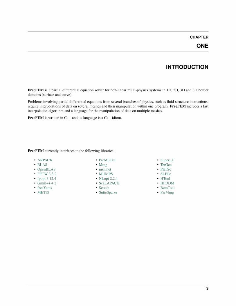
FreeFEM currently interfaces to the following libraries:
• ARPACK• BLAS• OpenBLAS• FFTW 3.3.2• Ipopt 3.12.4• Gmm++ 4.2• freeYams• METIS
• ParMETIS• Mmg• mshmet• MUMPS• NLopt 2.2.4• ScaLAPACK• Scotch• SuiteSparse
• SuperLU• TetGen• PETSc• SLEPc• HTool• HPDDM• BemTool• ParMmg
3
FreeFEM Documentation, Release 4.8
4 Chapter 1. Introduction
FreeFEM Documentation, Release 4.8
1.1 Version 4.5: new features
1.1.1 Release, binaries packages
• Since the version 4.5, the FreeFEM binary packages provides with a compiled PETSc library.
• FreeFEM is now interfaced with ParMmg.
1.1.2 New meshes and FEM border
After Surface FEM, Line FEM is possible with a new mesh type meshL, P0 P1 P2 P1dc FE, basic FEM, mesh generation.This new development allows to treat a 1d problem, such as a problem described on a 3d curve.
Abstract about Line FEM in FreeFEM.
• new meshL type, refer to the section The type meshL in 3 dimension
– new type of surface mesh: meshL
– the functionalities on the meshL type, it is necessary to load the plugin ”msh3”.
– generator of meshL segment, define multi border and buildmesh function.
– basic transformation are avalaible: movemesh, trunc, extract, checkmesh, change, AddLayers, glueof meshL.
It is possible to build the underlying meshL from a meshS with the function buildBdMesh:ThS=buildBdMesh(ThS) builds the boundary domain associated to the meshS ThS and extract it by thecommand meshL ThL=ThS. Gamma.
• new finite element space with curve finite element type
• FESpace P0 P1, P2, P1dc Lagrange finite elements and possible to add a custumed finite element with theclassical method (like a plugin).
• as in the standard 2d, 3d, surface 3d case, the variational problem associated to surface PDE can be defined byusing the keywords
– problem
– varf to access to matrix and RHS vector
– available operators are int1d, on and the operator int0d to define a Neumann boundary condition
• visualisation tools
– plot with plot of ffglut, medit meshes meshL and solutions
– 2d or 3d view, with in 3d the option to visualize the elememt Normals at element (touch ‘T’) and thedeformed domain according to it (touch ‘2’).
– loading, saving of meshes and solution at FreeFEM’s format
∗ “.mesh” mesh format file of Medit (P. Frey LJLL)
∗ “.msh” for mesh and “.sol” data solution at freefem format
1.1. Version 4.5: new features 5
FreeFEM Documentation, Release 4.8
∗ “.msh” data file of Gmsh (Mesh generator) (load “gmsh”)
∗ vtk format for meshes and solutions (load “iovtk” and use the “.vtu” extension)
1.1.3 Boundary Element Method
Allows to define and solve a 2d/3d BEM formulation and rebuild the associated potential. The document is in con-struction.
1.2 Installation guide
To use FreeFEM, two installation methods are available: user access (binary package) and access developers (from thesource code). Follow the section corresponding to your type of installation.
Note: Since the version 4.5, FreeFEM relese provides with the last version of PETSc.
1.2.1 Using binary package
First, open the following web page download page and choose your platform: Linux, MacOS or Windows.
Note: Binary packages are available for Microsoft Windows, MacOS and some Linux distributions. Since the release4.5, FreeFEM binaries provide with the current version of PETSc.
Install FreeFEM by double-clicking on the appropriate file. Under Linux and MacOS the install directory is one ofthe following /usr/local/bin, /usr/local/share/freefem++, /usr/local/lib/ff++
Windows installation
Note: The windows package is build for Window 7 64bits. The support ended for all releases under Windows 32 bitssince the V4.
First download the windows installation executable, then double click to install FreeFEM. Install MSMPI for parallelversion under window64 MS MPI V10.1.2, and install both msmpisdk.msi and MSMpiSetup.exe.
In most cases just answer yes (or type return) to all questions.
Otherwise in the Additional Task windows, check the box “Add application directory to your system path.” This isrequired otherwise the program ffglut.exe will not be found.
By now you should have two new icons on your desktop:
• FreeFem++ (VERSION).exe, the freefem++ application.
6 Chapter 1. Introduction
FreeFEM Documentation, Release 4.8
• FreeFem++ (VERSION) Examples, a link to the freefem++ examples folder.
where (VERSION) is the version of the files (for example 4.5).
By default, the installed files are in C:\Programs Files\FreeFem++. In this directory, you have all the .dll filesand other applications: FreeFem++-nw.exe, ffglut.exe, . . . The syntax for the command-line tools are the sameas those of FreeFem.exe.
To use FreeFEM binaries under Windows, two methods are possible:
• Use the FreeFEM launcher (launchff++.exe)
Warning: if you launch FreeFEM without filename script by double-clicking, your get a error due (it is bug of usageGetOpenFileName in win64).
• In shell terminal (cmd, powershell, bash, . . . ):
– To launch sequential version:
1 C:\>"Program Files (x86)\FreeFem++\FreeFem++.exe" <mySequentialScript.edp>
– To launch parallel version:
1 C:\>"Program Files\Microsoft MPI\Bin\mpiexec.exe" -n <nbProcs> C:\>"Program Files→˓(x86)\FreeFem++\FreeFem++-mpi.exe" <myParallelScript.edp>
macOS X installation
Download the macOS X binary version file, extract all the files by double clicking on the icon of the file, go the thedirectory and put the FreeFem++.app application in the /Applications directory.
If you want terminal access to FreeFEM just copy the file FreeFem++ in a directory of your $PATH shell environmentvariable.
Ubuntu installation
Note: The Debian package is built for Ubuntu 16.04
Beforehand, install the following dependances libraries using the apt tool:
1 sudo apt-get install libgsl-dev libhdf5-dev2 liblapack-dev libopenmpi-dev freeglut3-dev
Download the package FreeFEM .deb, install it by the command
1 dpkg -i FreeFEM_VERSION_Ubuntu_withPETSc_amd64.deb
FreeFEM is directly available in your terminal by the command “FreeFem++”.
1.2. Installation guide 7
FreeFEM Documentation, Release 4.8
Arch AUR package
An up-to-date package of FreeFEM for Arch is available on the Archlinux user repository.
To install it:
1 git clone https://aur.archlinux.org/freefem++-git.git2 cd freefem++-git3 makepkg -si
Note: Thanks to Stephan Husmann
Fedora installation
Packages are available in the Fedora Repositories, and they are managed by the Fedora SciTech special interest group.The packages are usually recent builds, but may not be the latest released version.
You can install them using the dnf tool, for both the serial and parallel (MPI) versions. :
1 sudo dnf install freefem++2 sudo dnf install freefem++-openmpi3 sudo dnf install freefem++-mpich
FreeFEM is directly available in your terminal by the command “FreeFem++”. To use the OpenMPI version, in yourterminal first load the OpenMPI module, for example using
1 module load mpi/openmpi-x86_64
and then the command “FreeFem++-mpi_openmpi” will be available in your terminal. To use the MPICH version, inyour terminal first load the MPICH module using
1 module load mpi/mpich-x86_64
and then the command “FreeFem++-mpi_mpich” will be available in your terminal.
1.2.2 Compiling source code
Various versions of FreeFEM are possible:• sequential and without plugins (contains in 3rdparty)
• parallel with plugins (and with PETSc).
Note: We advise you to use the package manager for macOS Homebrew to get the different packagesrequired avalaible here
8 Chapter 1. Introduction
FreeFEM Documentation, Release 4.8
Compilation on OSX (>=10.13)
1. Install Xcode, Xcode Command Line tools and Xcode Additional Tools from the Apple website
2. Install gfortran from Homebrew
1 brew cask install gfortran
Note: If you have installed gcc via brew, gfortran comes with it and you do not need this line
3. To use FreeFEM parallel version, install openmpi or mpich
1 # to install openmpi2 curl -L https://download.open-mpi.org/release/open-mpi/v4.0/openmpi-4.0.1.tar.gz --
→˓output openmpi-4.0.1.tar.gz3 tar xf openmpi-4.0.14 cd openmpi-4.0.1/5 # to install mpich6 curl -L http://www.mpich.org/static/downloads/3.3.2/mpich-3.3.2.tar.gz --output
→˓mpich-3.3.2.tar.gz7 tar xf mpich-3.3.28 cd mpich-3.3.2
4 # with brew gcc gfortran compilers5 ./configure CC=clang CXX=clang++ FC=gfortran-9 F77=gfortran-9 --prefix=/where/you/
→˓want/to/have/files/installed6
7 # with LLVM gcc and brew gfortran compilers8 ./configure CC=gcc-9 CXX=g++-9 FC=gfortran-9 F77=gfortran-9 --prefix=/where/you/
→˓want/to/have/files/installed
5 make -j<nbProcs>6 make -j<nbProcs> install
4. Install the minimal libraries for FreeFEM
1 brew install m4 git flex bison
5. If you want build your own configure according your system, install autoconf and automake from Homebrew(optional, see note in step 10)
1 brew install autoconf automake
6. To use FreeFEM with its plugins, install from Homebrew suitesparse, hdf5, cmake, wget
1 brew install suitesparse hdf5 cmake wget
7. Install gsl
1 curl -O http://mirror.cyberbits.eu/gnu/gsl/gsl-2.5.tar.gz2 tar zxvf gsl-2.5.tar.gz3 cd gsl-2.54 ./configure
(continues on next page)
1.2. Installation guide 9
FreeFEM Documentation, Release 4.8
(continued from previous page)
5 make -j<nbProcs>6 make -j<nbProcs> install --prefix=/where/you/want/to/have/files/installed
8. Download the latest Git for Mac installer git and the FreeFEM source from the repository
1 git clone https://github.com/FreeFem/FreeFem-sources.git
9. Configure your source code
1 cd FreeFem-sources2 autoreconf -i
Note: if your autoreconf version is too old, do tar zxvf AutoGeneratedFile.tar.gz
• following your compilers
3 // with brew gcc gfortran compilers4 ./configure --enable-download CC=clang CXX=clang++ F77=gfortran-95 FC=gfortran-9 --prefix=/where/you/want/to/have/files/installed6
7 // with LLVM gcc and brew gfortran compilers8 ./configure --enable-download CC=clang CXX=clang++ F77=gfortran-99 FC=gfortran-9 --prefix=/where/you/want/to/have/files/installed
10. Download the 3rd party packages to use FreeFEM plugins
1 ./3rdparty/getall -a
Note: All the third party packages have their own licence
11. If you want use PETSc/SLEPc and HPDDM (High Performance Domain Decomposition Methods)
1 cd 3rdparty/ff-petsc2 make petsc-slepc // add SUDO=sudo if your installation directory is the
→˓default /usr/local3 cd -4 ./reconfigure
12. Build your FreeFEM library and executable
1 make -j<nbProcs>2 make -j<nbProcs> check
Note: make check is optional, but advised to check the validity of your FreeFEM build
13. Install the FreeFEM apllication make install // add SUDO=sudo might be necessary
Note: it isn’t necessary to execute this last command, FreeFEM executable is avalaible here
10 Chapter 1. Introduction
FreeFEM Documentation, Release 4.8
your_installation/src/nw/FreeFem++ and mpi executable here your_installation/src/mpi/ff-mpirun.
Compilation on Ubuntu
1. Install the following packages on your system
1 sudo apt-get update && sudo apt-get upgrade2 sudo apt-get install cpp freeglut3-dev g++ gcc gfortran \3 m4 make patch pkg-config wget python unzip \4 liblapack-dev libhdf5-dev libgsl-dev \5 autoconf automake autotools-dev bison flex gdb git cmake6
7 # mpich is required for the FreeFEM parallel computing version8 sudo apt-get install mpich
Warning: In the oldest distribution of Ubuntu, libgsl-dev does not exist, use libgsl2-dev instead
2. Download FreeFEM source from the repository
1 git clone https://github.com/FreeFem/FreeFem-sources.git
3. Autoconf
1 cd FreeFem-sources2 autoreconf -i
Note: if your autoreconf version is too old, do tar zxvf AutoGeneratedFile.tar.gz
4. Configure
1 ./configure --enable-download --enable-optim2 --prefix=/where/you/want/to/have/files/installed
Note: To see all the options, type ./configure --help
5. Download the 3rd party packages
1 ./3rdparty/getall -a
Note: All the third party packages have their own licence
6. If you want use PETSc/SLEPc and HPDDM (High Performance Domain Decomposition Methods) for massivelyparallel computing
1 cd 3rdparty/ff-petsc2 make petsc-slepc // add SUDO=sudo if your installation directory is the default /
→˓usr/local(continues on next page)
1.2. Installation guide 11
FreeFEM Documentation, Release 4.8
(continued from previous page)
3 cd -4 ./reconfigure
7. Build your FreeFEM library and executable
1 make -j<nbProcs>2 make -j<nbProcs> check
Note: make check is optional, but advised to check the validity of your FreeFEM build
8. Install the executable
1 make install
Note: it isn’t necessary to execute this last command, FreeFEM executable is avalaible hereyour_installation/src/nw/FreeFem++ and mpi executable here your_installation/src/mpi/ff-mpirun
Compilation on Arch Linux
Warning: As Arch is in rolling release, the following information can be quickly outdated !
Warning: FreeFEM fails to compile using the newest version of gcc 8.1.0, use an older one instead.
1. Install the following dependencies:
1 pacman -Syu2 pacman -S git openmpi gcc-fortran wget python3 freeglut m4 make patch gmm4 blas lapack hdf5 gsl fftw arpack suitesparse5 gnuplot autoconf automake bison flex gdb6 valgrind cmake texlive-most
2. Download the FreeFEM source from the repository
1 git clone https://github.com/FreeFem/FreeFem-sources.git
3. Autoconf
1 cd FreeFem-sources2 autoreconf -i
4. Configure
1 ./configure --enable-download --enable-optim
12 Chapter 1. Introduction
FreeFEM Documentation, Release 4.8
Note: To see all the options, type ./configure --help
5. Download the packages
1 ./3rdparty/getall -a
Note: All the third party packages have their own licence
6. If you want use HPDDM (High Performance Domain Decomposition Methods) for massively parallel computing,install PETSc/SLEPc
1 cd 3rdparty/ff-petsc2 make petsc-slepc SUDO=sudo3 cd -4 ./reconfigure
7. Compile the FreeFEM source
1 make
Note: If your computer has many threads, you can run make in parallel using make -j16 for 16 threads, forexample.
Note: Optionally, check the compilation with make check
8. Install the FreeFEM application
1 sudo make install
Compilation on Fedora
1. Install the following packages on your system
1 sudo dnf update2 sudo dnf install freeglut-devel gcc-gfortran gcc-c++ gcc \3 m4 make wget python2 python3 unzip \4 lapack-devel hdf5-devel gsl gsl-devel \5 autoconf automake bison flex gdb git cmake6
7 # MPICH or OpenMPI is required for the FreeFEM parallel computing version8 sudo dnf install mpich-devel9 sudo dnf install openmpi-devel
10
11 # Then load one of the modules, for example12 module load mpi/mpich-x86_6413 # or14 module load mpi/openmpi-x86_64
1.2. Installation guide 13
FreeFEM Documentation, Release 4.8
2. Download FreeFEM source from the repository
1 git clone https://github.com/FreeFem/FreeFem-sources.git
3. Autoconf
1 cd FreeFem-sources2 autoreconf -i
Note: if your autoreconf version is too old, do tar zxvf AutoGeneratedFile.tar.gz
4. Configure
1 ./configure --enable-download --enable-optim2 --prefix=/where/you/want/to/have/files/installed
Note: To see all the options, type ./configure --help
5. Download the 3rd party packages
1 ./3rdparty/getall -a
Note: All the third party packages have their own licence
6. If you want use PETSc/SLEPc and HPDDM (High Performance Domain Decomposition Methods) for massivelyparallel computing
1 cd 3rdparty/ff-petsc2 make petsc-slepc // add SUDO=sudo if your installation directory is the default /
→˓usr/local3 cd -4 ./reconfigure
7. Build your FreeFEM library and executable
1 make -j<nbProcs>2 make -j<nbProcs> check
Note: make check is optional, but advised to check the validity of your FreeFEM build
8. Install the executable
1 make install
Note: it isn’t necessary to execute this last command, FreeFEM executable is avalaible hereyour_installation/src/nw/FreeFem++ and mpi executable here your_installation/src/mpi/ff-mpirun
14 Chapter 1. Introduction
FreeFEM Documentation, Release 4.8
Compilation on Linux with Intel software tools
Follow the guide
Compilation on Windows
Warning: The support ended for all releases under Windows 32 bits since the V4. We assume your developmentmachine is 64-bit, and you want your compiler to target 64-bit windows by default.
1. Install the Microsoft MPI v10.1.2 (archived) (msmpisdk.msi and MSMpiSetup.exe)
2. Download msys2-x86_64-latest.exe (x86_64 version) and run it.
3. Install the version control system Git for Windows
4. In the MSYS2 shell, execute the following. Hint: if you right click the title bar, go to Options -> Keys and tick“Ctrl+Shift+letter shortcuts” you can use Ctrl+Shift+V to paste in the MSYS shell.
1 pacman -Syuu
Close the MSYS2 shell once you’re asked to. There are now 3 MSYS subsystems installed: MSYS2, MinGW32and MinGW64. They can respectively be launched from C:devmsys64msys2.exe, C:devmsys64mingw32.exe andC:devmsys64mingw64.exe Reopen MSYS2 (doesn’t matter which version, since we’re merely installing packages).Repeatedly run the following command until it says there are no further updates. You might have to restart your shellagain.
1 pacman -Syuu
5. Now that MSYS2 is fully up-to-date, install the following dependancies
• for 64 bit systems:
1 pacman -S autoconf make automake-wrapper bison git \2 mingw-w64-x86_64-freeglut mingw-w64-x86_64-toolchain \3 mingw-w64-x86_64-openblas patch python perl pkg-config pkgfile \4 rebase tar time tzcode unzip which mingw-w64-x86_64-libmicroutils \5 --ignore mingw-w64-x86_64-gcc-ada --ignore mingw-w64-x86_64-gcc-objc \6 --ignore mingw-w64-x86_64-gdb mingw-w64-x86_64-cmake --noconfirm
• for 32 bit systems (FreeFEM lower than version 4):
1 pacman -S autoconf automake-wrapper bash bash-completion \2 bison bsdcpio bsdtar bzip2 coreutils curl dash file filesystem \3 findutils flex gawk gcc gcc-fortran gcc-libs grep gzip inetutils \4 info less lndir make man-db git mingw-w64-i686-freeglut \5 mingw-w64-i686-toolchain mingw-w64-i686-gsl mingw-w64-i686-hdf5 \6 mingw-w64-i686-openblas mintty msys2-keyring msys2-launcher-git \7 msys2-runtime ncurses pacman pacman-mirrors pactoys-git patch pax-git \8 perl pkg-config pkgfile rebase sed tar tftp-hpa time tzcode unzip \9 util-linux which
6. Open a MingW64 terminal (or MingW32 for old 32 bit FreeFEM version) and compile the FreeFEM source
1.2. Installation guide 15
FreeFEM Documentation, Release 4.8
1 git clone https://github.com/FreeFem/FreeFem-sources2 cd FreeFem-sources3 autoreconf -i4 ./configure --enable-generic --enable-optim \5 --enable-download --enable-maintainer-mode \6 CXXFLAGS=-mtune=generic CFLAGS=-mtune=generic \7 FFLAGS=-mtune=generic --enable-download --disable-hips8 --prefix=/where/you/want/to/have/files/installed
7. If you want use HPDDM (High Performance Domain Decomposition Methods) for massively parallel computing,install PETSc/SLEPc
1 cd 3rdparty/ff-petsc2 make petsc-slepc SUDO=sudo3 cd -4 ./reconfigure
8. Download the 3rd party packages and build your FreeFEM library and executable
1 ./3rdparty/getall -a2 make3 make check4 make install
Note: The FreeFEM executable (and some other like ffmedit, . . . ) are in C:\msys64\mingw64\bin (orC:\msys32\mingw32\bin).
1.2.3 Environment variables and init file
FreeFEM reads a user’s init file named freefem++.pref to initialize global variables: verbosity, includepath,loadpath.
Note: The variable verbosity changes the level of internal printing (0: nothing unless there are syntax errors, 1:few, 10: lots, etc. . . . ), the default value is 2.
The included files are found in the includepath list and the load files are found in the loadpath list.
The syntax of the file is:
1 verbosity = 52 loadpath += "/Library/FreeFem++/lib"3 loadpath += "/Users/hecht/Library/FreeFem++/lib"4 includepath += "/Library/FreeFem++/edp"5 includepath += "/Users/hecht/Library/FreeFem++/edp"6 # This is a comment7 load += "funcTemplate"8 load += "myfunction"9 load += "MUMPS_seq"
The possible paths for this file are
16 Chapter 1. Introduction
FreeFEM Documentation, Release 4.8
• under Unix and MacOs
1 /etc/freefem++.pref2 $(HOME)/.freefem++.pref3 freefem++.pref
• under windows
1 freefem++.pref
We can also use shell environment variables to change verbosity and the search rule before the init files.
1 export FF_VERBOSITY=502 export FF_INCLUDEPATH="dir;;dir2"3 export FF_LOADPATH="dir;;dir3"
Note: The separator between directories must be “;” and not “:” because “:” is used under Windows.
Note: To show the list of init of FreeFEM , do
1 export FF_VERBOSITY=100;2 ./FreeFem++-nw
1.2.4 Coloring Syntax FreeFem++
Atom
In order to get the syntax highlighting in Atom, you have to install the FreeFEM language support.
You can do it directly in Atom: Edit -> Preferences -> Install, and search for language-freefem-offical.
To launch scripts directly from Atom, you have to install the atom-runner package. Once installed, modify the Atomconfiguration file (Edit -> Config. . . ) to have something like that:
1 "*":2 ...3
4 runner:5 extensions:6 edp: "FreeFem++"7 scopes:8 "Freefem++": "FreeFem++"
Reboot Atom, and use Alt+R to run a FreeFem++ script.
1.2. Installation guide 17
FreeFEM Documentation, Release 4.8
Gedit
In order to get the syntax highlighting in Gedit, you have to downlaod the Gedit parser and copy it in /usr/share/gtksourceview-3.0/language-specs/.
Textmate 2, an editor under macOS
To use the coloring FreeFEM syntax with the Textmate 2 editor on Mac 10.7 or better, download from macromates.comand download the textmate freefem++ syntax here (version june 2107). To install this parser, unzip Textmate2-ff++.zipand follow the explanation given in file How_To.rtf.
rom www.freefem.org/ff++/Textmate2-ff++.zip (version june 2107) unzip Textmate2-
Notepad++,an editor under windows
Read and follow the instruction, FREEFEM++ COLOR SYNTAX OF WINDOWS .
Emacs editor
For emacs editor you can download ff++-mode.el .
1.3 Download
1.3.1 Latest binary packages
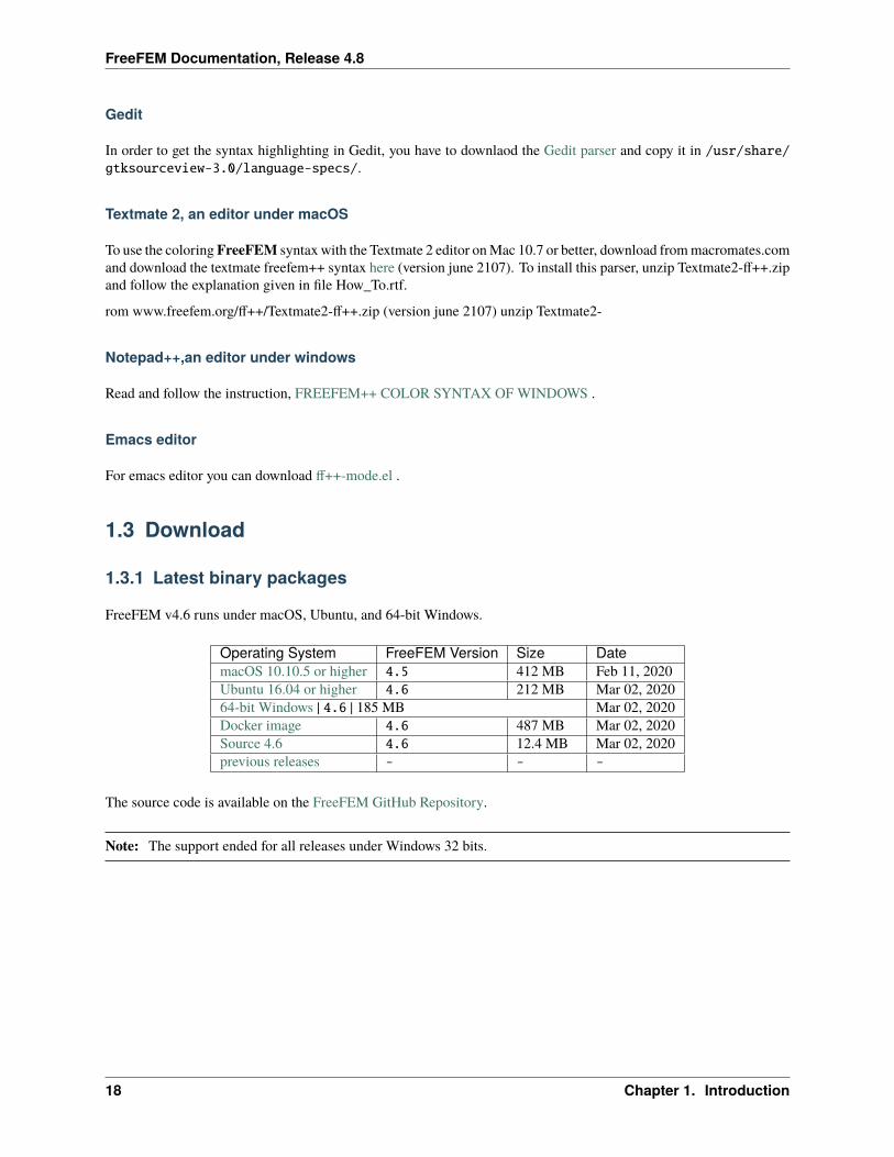
FreeFEM v4.6 runs under macOS, Ubuntu, and 64-bit Windows.
Operating System FreeFEM Version Size DatemacOS 10.10.5 or higher 4.5 412 MB Feb 11, 2020Ubuntu 16.04 or higher 4.6 212 MB Mar 02, 202064-bit Windows | 4.6 | 185 MB Mar 02, 2020Docker image 4.6 487 MB Mar 02, 2020Source 4.6 4.6 12.4 MB Mar 02, 2020previous releases - - -
The source code is available on the FreeFEM GitHub Repository.
Note: The support ended for all releases under Windows 32 bits.
18 Chapter 1. Introduction
FreeFEM Documentation, Release 4.8
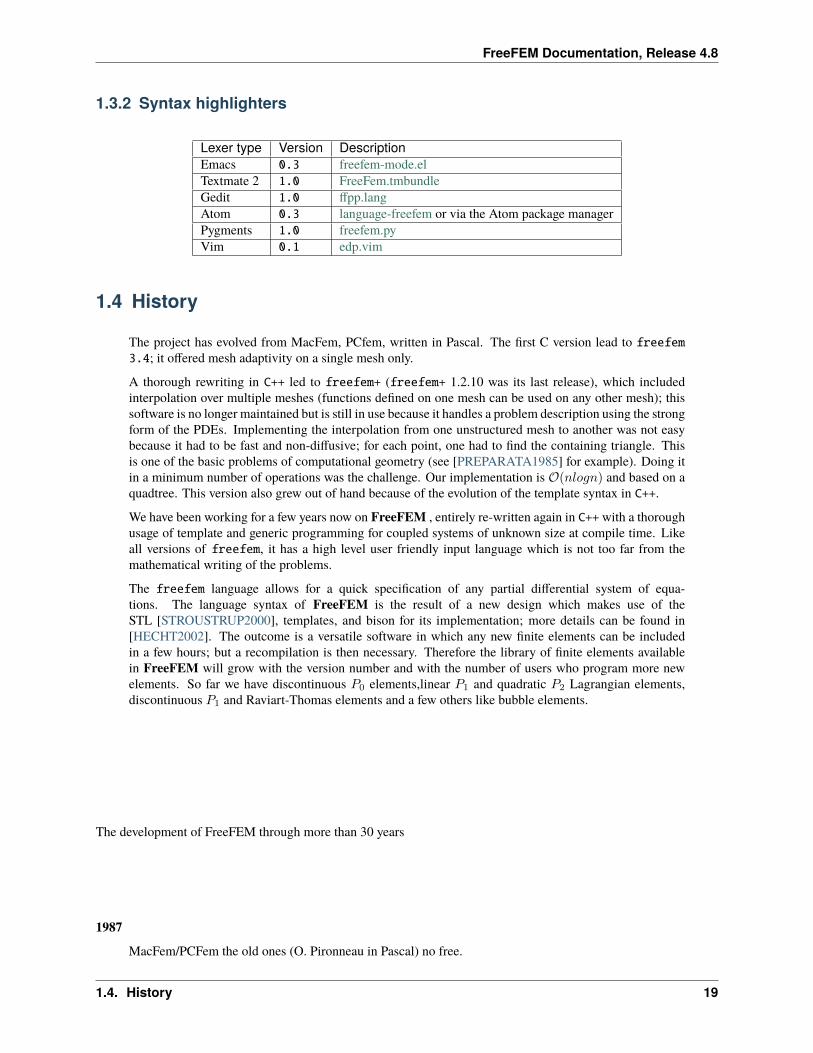
1.3.2 Syntax highlighters
Lexer type Version DescriptionEmacs 0.3 freefem-mode.elTextmate 2 1.0 FreeFem.tmbundleGedit 1.0 ffpp.langAtom 0.3 language-freefem or via the Atom package managerPygments 1.0 freefem.pyVim 0.1 edp.vim
1.4 History
The project has evolved from MacFem, PCfem, written in Pascal. The first C version lead to freefem3.4; it offered mesh adaptivity on a single mesh only.
A thorough rewriting in C++ led to freefem+ (freefem+ 1.2.10 was its last release), which includedinterpolation over multiple meshes (functions defined on one mesh can be used on any other mesh); thissoftware is no longer maintained but is still in use because it handles a problem description using the strongform of the PDEs. Implementing the interpolation from one unstructured mesh to another was not easybecause it had to be fast and non-diffusive; for each point, one had to find the containing triangle. Thisis one of the basic problems of computational geometry (see [PREPARATA1985] for example). Doing itin a minimum number of operations was the challenge. Our implementation is 𝒪(𝑛𝑙𝑜𝑔𝑛) and based on aquadtree. This version also grew out of hand because of the evolution of the template syntax in C++.
We have been working for a few years now on FreeFEM , entirely re-written again in C++ with a thoroughusage of template and generic programming for coupled systems of unknown size at compile time. Likeall versions of freefem, it has a high level user friendly input language which is not too far from themathematical writing of the problems.
The freefem language allows for a quick specification of any partial differential system of equa-tions. The language syntax of FreeFEM is the result of a new design which makes use of theSTL [STROUSTRUP2000], templates, and bison for its implementation; more details can be found in[HECHT2002]. The outcome is a versatile software in which any new finite elements can be includedin a few hours; but a recompilation is then necessary. Therefore the library of finite elements availablein FreeFEM will grow with the version number and with the number of users who program more newelements. So far we have discontinuous 𝑃0 elements,linear 𝑃1 and quadratic 𝑃2 Lagrangian elements,discontinuous 𝑃1 and Raviart-Thomas elements and a few others like bubble elements.
The development of FreeFEM through more than 30 years
1987MacFem/PCFem the old ones (O. Pironneau in Pascal) no free.
1.4. History 19
FreeFEM Documentation, Release 4.8
1992FreeFem rewrite in C++ (P1,P0 one mesh ) O. Pironneau, D. Bernardi, F.Hecht (mesh adaptation , bamg), C. Prudhomme .
1996FreeFem+ rewrite in C++ (P1,P0 more mesh) O. Pironneau, D. Bernardi, F.Hecht (algebra of function).
1998FreeFem++ rewrite with an other finite element kernel and an new language F. Hecht, O. Pironneau,K.Ohtsuka.
1999FreeFem 3d (S. Del Pino), a fist 3d version base on fictitious domaine method.
2008FreeFem++ v3 use a new finite element kernel multidimensionnels: 1d,2d,3d. . .
2014FreeFem++ v3.34 parallel version
2017FreeFem++ v3.57 parallel version
2018FreeFem++ v4: New matrix type, Surface element, New Parallel tools . . .
1.5 Citation
1.5.1 If you use FreeFEM, please cite the following reference in your work:
BibTeX
1 @articleMR3043640,2 AUTHOR = Hecht, F.,3 TITLE = New development in FreeFem++,4 JOURNAL = J. Numer. Math.,5 FJOURNAL = Journal of Numerical Mathematics,6 VOLUME = 20, YEAR = 2012,7 NUMBER = 3-4, PAGES = 251--265,8 ISSN = 1570-2820,9 MRCLASS = 65Y15,
10 MRNUMBER = 3043640,11 URL = https://freefem.org/12
20 Chapter 1. Introduction
FreeFEM Documentation, Release 4.8
APA
1 Hecht, F. (2012). New development in FreeFem++. Journal of numerical mathematics, 20(3-→˓4), 251-266.
ISO690
1 HECHT, Frédéric. New development in FreeFem++. Journal of numerical mathematics, 2012,→˓vol. 20, no 3-4, p. 251-266.
MLA
1 Hecht, Frédéric. "New development in FreeFem++." Journal of numerical mathematics 20.3-4→˓(2012): 251-266.
1.6 Authors
Frédéric HechtProfessor at Laboratoire Jacques Louis Lions (LJLL), Sorbonne University, [email protected]://www.ljll.math.upmc.fr/hecht/
Sylvain AuliacFormer PhD student at LJLL, optimization interface with nlopt, ipopt, cmaes, . . .https://www.ljll.math.upmc.fr/auliac/
Olivier PironneauProfessor of numerical analysis at the Paris VI university and at LJLL, numerical methods in fluidMember of the Institut Universitaire de France and Academie des Scienceshttps://www.ljll.math.upmc.fr/pironneau/
Jacques MoriceFormer Post-Doc at LJLL, three dimensions mesh generation and coupling with medit
Antoine Le HyaricCNRS research engineer at Laboratoire Jacques Louis Lions, expert in software engineering for scientific applica-tions, electromagnetics simulations, parallel computing and three-dimensionsal visualizationhttps://www.ljll.math.upmc.fr/lehyaric/
Kohji OhtsukaProfessor at Hiroshima Kokusai Gakuin University, Japan and chairman of the World Scientific and EngineeringAcademy and Society, Japan. Fracture dynamic, modeling and computinghttps://sites.google.com/a/comfos.org/comfos/
1.6. Authors 21
FreeFEM Documentation, Release 4.8
Pierre-Henri TournierCNRS research engineer at Laboratoire Jacques Louis Lions (LJLL), Sorbonne University, Paris
Pierre JolivetCNRS researcher, MPI interface with PETSc, HPDDM, . . .http://jolivet.perso.enseeiht.fr/
Frédéric NatafCNRS senior researcher at Laboratoire Jacques Louis Lions (LJLL), Sorbonne University, Parishttps://www.ljll.math.upmc.fr/nataf/
Simon GarnotelReasearch engineer at Airthiumhttps://github.com/sgarnotel
Karla PérezDeveloper, Airthium internshiphttps://github.com/karlaprzbr
Loan CannardWeb designer, Airthium internshiphttps://www.linkedin.com/in/loancannard
And all the dedicated Github contributors
1.7 Contributing
1.7.1 Bug report
Concerning the FreeFEM documentation
Open an Issue on FreeFem-doc repository.
Concerning the FreeFEM compilation or usage
Open an Issue on FreeFem-sources repository.
22 Chapter 1. Introduction

FreeFEM Documentation, Release 4.8
1.7.2 Improve content
Ask one of the contributors for Collaborator Access or make a Pull Request.
1.7. Contributing 23

FreeFEM Documentation, Release 4.8
24 Chapter 1. Introduction
CHAPTER
TWO
LEARNING BY EXAMPLES
The FreeFEM language is typed, polymorphic and reentrant with macro generation.
Every variable must be typed and declared in a statement, that is separated from the next by a semicolon ;.
The FreeFEM language is a C++ idiom with something that is more akin to LaTeX.
For the specialist, one key guideline is that FreeFEM rarely generates an internal finite element array, this was adoptedfor speed and consequently FreeFEM could be hard to beat in terms of execution speed, except for the time lost in theinterpretation of the language (which can be reduced by a systematic usage of varf and matrix instead of problem).
The Development Cycle: Edit–Run/Visualize–Revise
Many examples and tutorials are given there after and in the examples section. It is better to study them and learn byexample.
If you are a beginner in the finite element method, you may also have to read a book on variational formulations.
The development cycle includes the following steps:
Modeling: From strong forms of PDE to weak forms, one must know the variational formulation to use FreeFEM;one should also have an eye on the reusability of the variational formulation so as to keep the same internal matrices; atypical example is the time dependent heat equation with an implicit time scheme: the internal matrix can be factorizedonly once and FreeFEM can be taught to do so.
Programming: Write the code in FreeFEM language using a text editor such as the one provided in your integratedenvironment.
Run: Run the code (here written in file mycode.edp). That can also be done in terminal mode by :
1 FreeFem++ mycode.edp
Visualization: Use the keyword plot directly in mycode.edp to display functions while FreeFEM is running. Usethe plot-parameter wait=1 to stop the program at each plot.
Debugging: A global variable debug (for example) can help as in wait=true to wait=false.
1 bool debug = true;2
3 border a(t=0, 2.*pi)x=cos(t); y=sin(t); label=1;;4 border b(t=0, 2.*pi)x=0.8+0.3*cos(t); y=0.3*sin(t); label=2;;5
6 plot(a(50) + b(-30), wait=debug); //plot the borders to see the intersection(continues on next page)
25
FreeFEM Documentation, Release 4.8
(continued from previous page)
7 //so change (0.8 in 0.3 in b)8 //if debug == true, press Enter to continue9
10 mesh Th = buildmesh(a(50) + b(-30));11 plot(Th, wait=debug); //plot Th then press Enter12
13 fespace Vh(Th,P2);14 Vh f = sin(pi*x)*cos(pi*y);15 Vh g = sin(pi*x + cos(pi*y));16
17 plot(f, wait=debug); //plot the function f18 plot(g, wait=debug); //plot the function g
Changing debug to false will make the plots flow continuously. Watching the flow of graphs on the screen (whiledrinking coffee) can then become a pleasant experience.
Error management
Error messages are displayed in the console window. They are not always very explicit because of the template structureof the C++ code (we did our best!). Nevertheless they are displayed at the right place. For example, if you forgetparenthesis as in:
1 bool debug = true;2 mesh Th = square(10,10;3 plot(Th);
then you will get the following message from FreeFEM:
1 2 : mesh Th = square(10,10;2 Error line number 2, in file bb.edp, before token ;3 parse error4 current line = 25 syntax error6 current line = 27 Compile error : syntax error8 line number :2, ;9 error Compile error : syntax error
10 line number :2, ;11 code = 1 mpirank: 0
If you use the same symbol twice as in:
1 real aaa = 1;2 real aaa;
then you will get the message:
1 2 : real aaa; The identifier aaa exists2 the existing type is <Pd>3 the new type is <Pd>
If you find that the program isn’t doing what you want you may also use cout to display in text format on the consolewindow the value of variables, just as you would do in C++.
The following example works:
26 Chapter 2. Learning by Examples
FreeFEM Documentation, Release 4.8
1 ...2 fespace Vh(Th, P1);3 Vh u;4 cout << u;5 matrix A = a(Vh, Vh);6 cout << A;
Another trick is to comment in and out by using // as in C++. For example:
1 real aaa =1;2 // real aaa;
2.1 Getting started
For a given function 𝑓(𝑥, 𝑦), find a function 𝑢(𝑥, 𝑦) satisfying :
−∆𝑢(𝑥, 𝑦) = 𝑓(𝑥, 𝑦) for all (𝑥, 𝑦) in Ω𝑢(𝑥, 𝑦) = 0 for all (𝑥, 𝑦) on 𝜕Ω
(2.1)
Here 𝜕Ω is the boundary of the bounded open set Ω ⊂ R2 and ∆𝑢 = 𝜕2𝑢𝜕𝑥2 + 𝜕2𝑢
𝜕𝑦2 .
We will compute 𝑢 with 𝑓(𝑥, 𝑦) = 𝑥𝑦 and Ω the unit disk. The boundary 𝐶 = 𝜕Ω is defined as:
𝐶 = (𝑥, 𝑦)| 𝑥 = cos(𝑡), 𝑦 = sin(𝑡), 0 ≤ 𝑡 ≤ 2𝜋
Note: In FreeFEM, the domain Ω is assumed to be described by the left side of its boundary.
The following is the FreeFEM program which computes 𝑢:
1 // Define mesh boundary2 border C(t=0, 2*pi)x=cos(t); y=sin(t);3
4 // The triangulated domain Th is on the left side of its boundary5 mesh Th = buildmesh(C(50));6
7 // The finite element space defined over Th is called here Vh8 fespace Vh(Th, P1);9 Vh u, v;// Define u and v as piecewise-P1 continuous functions
10
11 // Define a function f12 func f= x*y;13
14 // Get the clock in second15 real cpu=clock();16
17 // Define the PDE18 solve Poisson(u, v, solver=LU)19 = int2d(Th)( // The bilinear part20 dx(u)*dx(v)21 + dy(u)*dy(v)
(continues on next page)
2.1. Getting started 27
FreeFEM Documentation, Release 4.8
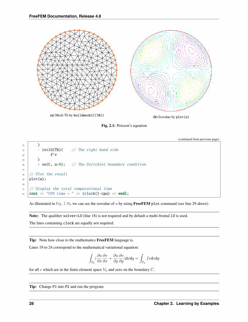
(a) Mesh Th by buildmesh(C(50)) (b) Isovalue by plot(u)
Fig. 2.1: Poisson’s equation
(continued from previous page)
22 )23 - int2d(Th)( // The right hand side24 f*v25 )26 + on(C, u=0); // The Dirichlet boundary condition27
28 // Plot the result29 plot(u);30
31 // Display the total computational time32 cout << "CPU time = " << (clock()-cpu) << endl;
As illustrated in Fig. 2.1b, we can see the isovalue of 𝑢 by using FreeFEM plot command (see line 29 above).
Note: The qualifier solver=LU (line 18) is not required and by default a multi-frontal LU is used.
The lines containing clock are equally not required.
Tip: Note how close to the mathematics FreeFEM language is.
Lines 19 to 24 correspond to the mathematical variational equation:∫𝑇ℎ
(𝜕𝑢
𝜕𝑥
𝜕𝑣
𝜕𝑥+𝜕𝑢
𝜕𝑦
𝜕𝑣
𝜕𝑦)d𝑥d𝑦 =
∫𝑇ℎ
𝑓𝑣d𝑥d𝑦
for all 𝑣 which are in the finite element space 𝑉ℎ and zero on the boundary 𝐶.
Tip: Change P1 into P2 and run the program.
28 Chapter 2. Learning by Examples
FreeFEM Documentation, Release 4.8
This first example shows how FreeFEM executes with no effort all the usual steps required by the finite element method(FEM). Let’s go through them one by one.
On the line 2:
The boundary Γ is described analytically by a parametric equation for 𝑥 and for 𝑦. When Γ =∑𝐽𝑗=0 Γ𝑗 then each
curve Γ𝑗 must be specified and crossings of Γ𝑗 are not allowed except at end points.
The keyword label can be added to define a group of boundaries for later use (boundary conditions for instance).Hence the circle could also have been described as two half circle with the same label:
1 border Gamma1(t=0, pi)x=cos(t); y=sin(t); label=C;2 border Gamma2(t=pi, 2.*pi)x=cos(t); y=sin(t); label=C;
Boundaries can be referred to either by name (Gamma1 for example) or by label (C here) or even by its internal numberhere 1 for the first half circle and 2 for the second (more examples are in Meshing Examples).
On the line 5The triangulation 𝒯ℎ of Ω is automatically generated by buildmesh(C(50)) using 50 points on C as in Fig. 2.1a.
The domain is assumed to be on the left side of the boundary which is implicitly oriented by the parametrization. Soan elliptic hole can be added by typing:
1 border C(t=2.*pi, 0)x=0.1+0.3*cos(t); y=0.5*sin(t);;
If by mistake one had written:
1 border C(t=0, 2.*pi)x=0.1+0.3*cos(t); y=0.5*sin(t);;
then the inside of the ellipse would be triangulated as well as the outside.
Note: Automatic mesh generation is based on the Delaunay-Voronoi algorithm. Refinement of the mesh are done byincreasing the number of points on Γ, for example buildmesh(C(100)), because inner vertices are determined by thedensity of points on the boundary.
Mesh adaptation can be performed also against a given function f by calling adaptmesh(Th,f).
Now the name 𝒯ℎ (Th in FreeFEM) refers to the family 𝑇𝑘𝑘=1,··· ,𝑛𝑡 of triangles shown in Fig. 2.1a.
Traditionally ℎ refers to the mesh size, 𝑛𝑡 to the number of triangles in 𝒯ℎ and 𝑛𝑣 to the number of vertices, but it isseldom that we will have to use them explicitly.
If Ω is not a polygonal domain, a “skin” remains between the exact domain Ω and its approximation Ωℎ = ∪𝑛𝑡
𝑘=1𝑇𝑘.However, we notice that all corners of Γℎ = 𝜕Ωℎ are on Γ.
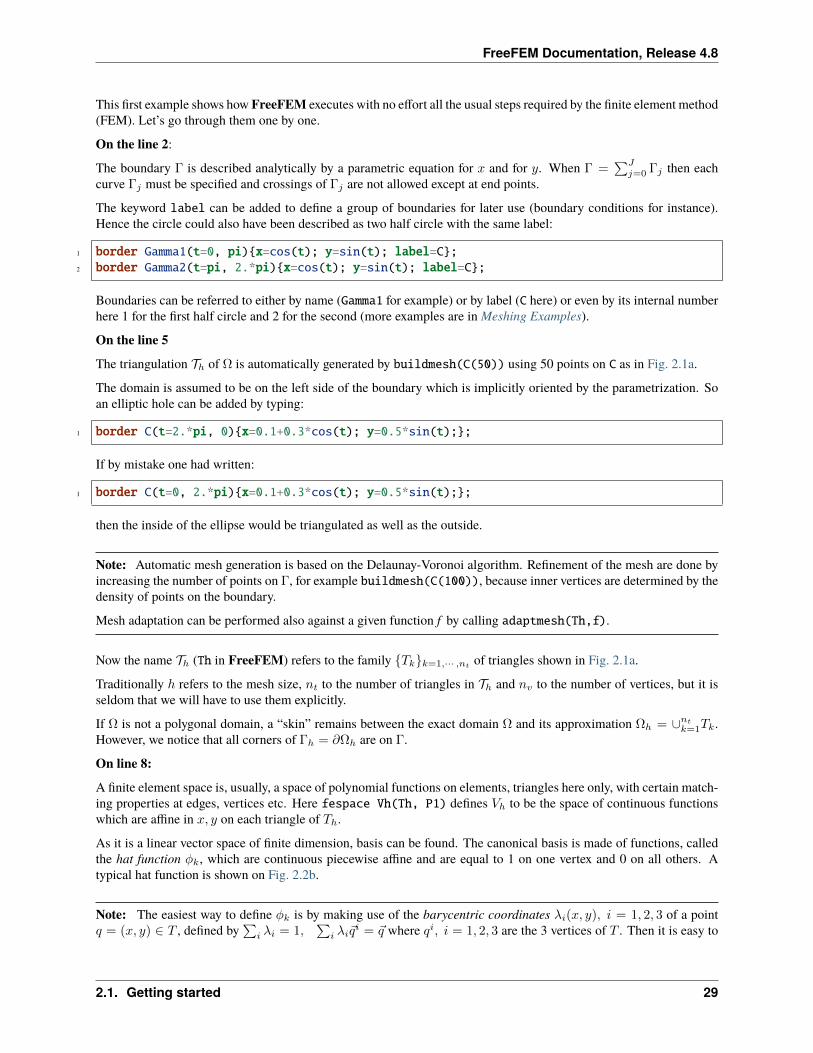
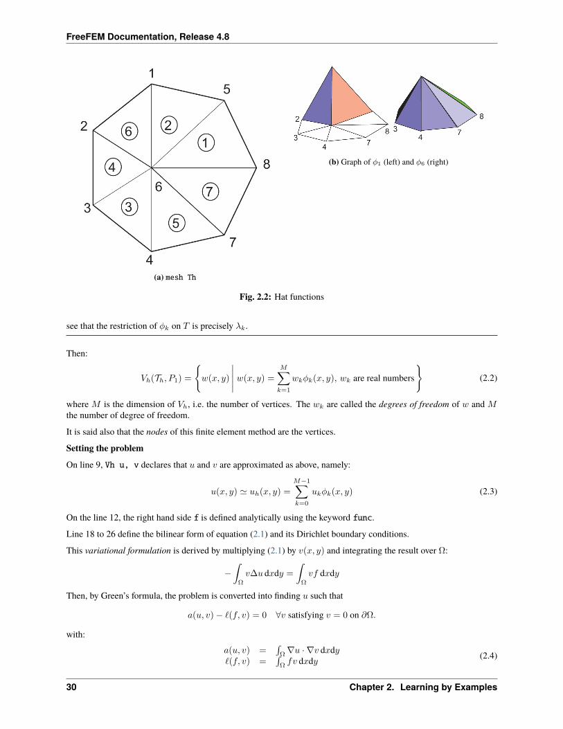
On line 8:A finite element space is, usually, a space of polynomial functions on elements, triangles here only, with certain match-ing properties at edges, vertices etc. Here fespace Vh(Th, P1) defines 𝑉ℎ to be the space of continuous functionswhich are affine in 𝑥, 𝑦 on each triangle of 𝑇ℎ.
As it is a linear vector space of finite dimension, basis can be found. The canonical basis is made of functions, calledthe hat function 𝜑𝑘, which are continuous piecewise affine and are equal to 1 on one vertex and 0 on all others. Atypical hat function is shown on Fig. 2.2b.
Note: The easiest way to define 𝜑𝑘 is by making use of the barycentric coordinates 𝜆𝑖(𝑥, 𝑦), 𝑖 = 1, 2, 3 of a point𝑞 = (𝑥, 𝑦) ∈ 𝑇 , defined by
∑𝑖 𝜆𝑖 = 1,
∑𝑖 𝜆𝑖
𝑖 = where 𝑞𝑖, 𝑖 = 1, 2, 3 are the 3 vertices of 𝑇 . Then it is easy to
2.1. Getting started 29
FreeFEM Documentation, Release 4.8
(a) mesh Th
(b) Graph of 𝜑1 (left) and 𝜑6 (right)
Fig. 2.2: Hat functions
see that the restriction of 𝜑𝑘 on 𝑇 is precisely 𝜆𝑘.
Then:
𝑉ℎ(𝒯ℎ, 𝑃1) =
𝑤(𝑥, 𝑦)
𝑤(𝑥, 𝑦) =
𝑀∑𝑘=1
𝑤𝑘𝜑𝑘(𝑥, 𝑦), 𝑤𝑘 are real numbers
(2.2)
where 𝑀 is the dimension of 𝑉ℎ, i.e. the number of vertices. The 𝑤𝑘 are called the degrees of freedom of 𝑤 and 𝑀the number of degree of freedom.
It is said also that the nodes of this finite element method are the vertices.
Setting the problemOn line 9, Vh u, v declares that 𝑢 and 𝑣 are approximated as above, namely:
𝑢(𝑥, 𝑦) ≃ 𝑢ℎ(𝑥, 𝑦) =
𝑀−1∑𝑘=0
𝑢𝑘𝜑𝑘(𝑥, 𝑦) (2.3)
On the line 12, the right hand side f is defined analytically using the keyword func.
Line 18 to 26 define the bilinear form of equation (2.1) and its Dirichlet boundary conditions.
This variational formulation is derived by multiplying (2.1) by 𝑣(𝑥, 𝑦) and integrating the result over Ω:
−∫Ω
𝑣∆𝑢 d𝑥d𝑦 =
∫Ω
𝑣𝑓 d𝑥d𝑦
Then, by Green’s formula, the problem is converted into finding 𝑢 such that
𝑎(𝑢, 𝑣)− ℓ(𝑓, 𝑣) = 0 ∀𝑣 satisfying 𝑣 = 0 on 𝜕Ω.
with:
𝑎(𝑢, 𝑣) =∫Ω∇𝑢 · ∇𝑣 d𝑥d𝑦
ℓ(𝑓, 𝑣) =∫Ω𝑓𝑣 d𝑥d𝑦 (2.4)
30 Chapter 2. Learning by Examples
FreeFEM Documentation, Release 4.8
In FreeFEM the Poisson problem can be declared only as in:
1 Vh u,v; problem Poisson(u,v) = ...
and solved later as in:
1 Poisson; //the problem is solved here
or declared and solved at the same time as in:
1 Vh u,v; solve Poisson(u,v) = ...
and (2.4) is written with dx(u) = 𝜕𝑢/𝜕𝑥, dy(u) = 𝜕𝑢/𝜕𝑦 and:∫Ω
∇𝑢 · ∇𝑣 d𝑥d𝑦 −→ int2d(Th)( dx(u)*dx(v) + dy(u)*dy(v) )∫Ω
𝑓𝑣 d𝑥d𝑦 −→ int2d(Th)( f*v ) (Notice here, 𝑢 is unused)
Warning: In FreeFEM bilinear terms and linear terms should not be under the same integral indeed toconstruct the linear systems FreeFEM finds out which integral contributes to the bilinear form by checking if bothterms, the unknown (here u) and test functions (here v) are present.
Solution and visualizationOn line 15, the current time in seconds is stored into the real-valued variable cpu.
Line 18, the problem is solved.
Line 29, the visualization is done as illustrated in Fig. 2.1b.
(see Plot for zoom, postscript and other commands).Line 32, the computing time (not counting graphics) is written on the console. Notice the C++-like syntax; the userneeds not study C++ for using FreeFEM, but it helps to guess what is allowed in the language.
Access to matrices and vectorsInternally FreeFEM will solve a linear system of the type
𝑀−1∑𝑗=0
𝐴𝑖𝑗𝑢𝑗 − 𝐹𝑖 = 0, 𝑖 = 0, · · · ,𝑀 − 1; 𝐹𝑖 =
∫Ω
𝑓𝜑𝑖 d𝑥d𝑦 (2.5)
which is found by using (2.3) and replacing 𝑣 by 𝜑𝑖 in (2.4). The Dirichlet conditions are implemented by penalty,namely by setting 𝐴𝑖𝑖 = 1030 and 𝐹𝑖 = 1030 * 0 if 𝑖 is a boundary degree of freedom.
Note: The number 1030 is called tgv (très grande valeur or very high value in english) and it is generally possible tochange this value, see the item :freefem`solve, tgv=`
The matrix𝐴 = (𝐴𝑖𝑗) is called stiffness matrix. If the user wants to access𝐴 directly he can do so by using (see sectionVariational form, Sparse matrix, PDE data vector for details).
1 varf a(u,v)2 = int2d(Th)(3 dx(u)*dx(v)
(continues on next page)
2.1. Getting started 31
FreeFEM Documentation, Release 4.8
(continued from previous page)
4 + dy(u)*dy(v)5 )6 + on(C, u=0)7 ;8 matrix A = a(Vh, Vh); //stiffness matrix
The vector 𝐹 in (2.5) can also be constructed manually:
1 varf l(unused,v)2 = int2d(Th)(3 f*v4 )5 + on(C, unused=0)6 ;7 Vh F;8 F[] = l(0,Vh); //F[] is the vector associated to the function F
The problem can then be solved by:
1 u[] = A^-1*F[]; //u[] is the vector associated to the function u
Note: Here u and F are finite element function, and u[] and F[] give the array of value associated (u[] ≡(𝑢𝑖)𝑖=0,...,𝑀−1 and F[] ≡ (𝐹𝑖)𝑖=0,...,𝑀−1).
So we have:
u(𝑥, 𝑦) =
𝑀−1∑𝑖=0
u[][𝑖]𝜑𝑖(𝑥, 𝑦), F(𝑥, 𝑦) =
𝑀−1∑𝑖=0
F[][𝑖]𝜑𝑖(𝑥, 𝑦)
where 𝜑𝑖, 𝑖 = 0..., ,𝑀 − 1 are the basis functions of Vh like in equation :eq: equation3, and 𝑀 = Vh.ndof is thenumber of degree of freedom (i.e. the dimension of the space Vh).
The linear system (2.5) is solved by UMFPACK unless another option is mentioned specifically as in:
1 Vh u, v;2 problem Poisson(u, v, solver=CG) = int2d(...
meaning that Poisson is declared only here and when it is called (by simply writing Poisson;) then (2.5) will besolved by the Conjugate Gradient method.
2.2 Classification of partial differential equations
Summary : It is usually not easy to determine the type of a system. Yet the approximations and algorithms suited tothe problem depend on its type:
• Finite Elements compatible (LBB conditions) for elliptic systems
• Finite difference on the parabolic variable and a time loop on each elliptic subsystem of parabolic systems; betterstability diagrams when the schemes are implicit in time.
• Upwinding, Petrov-Galerkin, Characteristics-Galerkin, Discontinuous-Galerkin, Finite Volumes for hyperbolicsystems plus, possibly, a time loop.
32 Chapter 2. Learning by Examples
FreeFEM Documentation, Release 4.8
When the system changes type, then expect difficulties (like shock discontinuities) !
Elliptic, parabolic and hyperbolic equationsA partial differential equation (PDE) is a relation between a function of several variables and its derivatives.
𝐹
(𝜙(𝑥),
𝜕𝜙
𝜕𝑥1(𝑥), · · · , 𝜕𝜙
𝜕𝑥𝑑(𝑥),
𝜕2𝜙
𝜕𝑥21(𝑥), · · · , 𝜕
𝑚𝜙
𝜕𝑥𝑚𝑑(𝑥)
)= 0, ∀𝑥 ∈ Ω ⊂ R𝑑
The range of 𝑥 over which the equation is taken, here Ω, is called the domain of the PDE. The highest derivation index,here 𝑚, is called the order. If 𝐹 and 𝜙 are vector valued functions, then the PDE is actually a system of PDEs.
Unless indicated otherwise, here by convention one PDE corresponds to one scalar valued 𝐹 and 𝜙. If 𝐹 is linear withrespect to its arguments, then the PDE is said to be linear.
The general form of a second order, linear scalar PDE is
𝛼𝜙+ 𝑎 · ∇𝜙+𝐵 : ∇(∇𝜙) = 𝑓 in Ω ⊂ R𝑑,
where 𝜕2𝜙𝜕𝑥𝑖𝜕𝑥𝑗
and 𝐴 : 𝐵 means∑𝑑𝑖,𝑗=1 𝑎𝑖𝑗𝑏𝑖𝑗 ., 𝑓(𝑥), 𝛼(𝑥) ∈ R, 𝑎(𝑥) ∈ R𝑑, 𝐵(𝑥) ∈ R𝑑×𝑑 are the PDE coefficients.
If the coefficients are independent of 𝑥, the PDE is said to have constant coefficients.
To a PDE we associate a quadratic form, by replacing 𝜙 by 1, 𝜕𝜙/𝜕𝑥𝑖 by 𝑧𝑖 and 𝜕2𝜙/𝜕𝑥𝑖𝜕𝑥𝑗 by 𝑧𝑖𝑧𝑗 , where 𝑧 is avector in R𝑑:
𝛼+𝐴 · 𝑧 + 𝑧𝑇𝐵𝑧 = 𝑓.
If it is the equation of an ellipse (ellipsoid if 𝑑 ≥ 2), the PDE is said to be elliptic; if it is the equation of a parabola ora hyperbola, the PDE is said to be parabolic or hyperbolic.
If 𝐵 ≡ 0, the degree is no longer 2 but 1, and for reasons that will appear more clearly later, the PDE is still said to behyperbolic.
These concepts can be generalized to systems, by studying whether or not the polynomial system 𝑃 (𝑧) associated withthe PDE system has branches at infinity (ellipsoids have no branches at infinity, paraboloids have one, and hyperboloidshave several).
If the PDE is not linear, it is said to be non-linear. These are said to be locally elliptic, parabolic, or hyperbolic accordingto the type of the linearized equation.
For example, for the non-linear equation
𝜕2𝜙
𝜕𝑡2− 𝜕𝜙
𝜕𝑥
𝜕2𝜙
𝜕𝑥2= 1
we have 𝑑 = 2, 𝑥1 = 𝑡, 𝑥2 = 𝑥 and its linearized form is:
𝜕2𝑢
𝜕𝑡2− 𝜕𝑢
𝜕𝑥
𝜕2𝜙
𝜕𝑥2− 𝜕𝜙
𝜕𝑥
𝜕2𝑢
𝜕𝑥2= 0
which for the unknown 𝑢 is locally elliptic if 𝜕𝜙𝜕𝑥 < 0 and locally hyperbolic if 𝜕𝜙𝜕𝑥 > 0.
Tip: Laplace’s equation is elliptic:
∆𝜙 ≡ 𝜕2𝜙
𝜕𝑥21+𝜕2𝜙
𝜕𝑥22+ · · ·+ 𝜕2𝜙
𝜕𝑥2𝑑= 𝑓, ∀𝑥 ∈ Ω ⊂ R𝑑
Tip: The heat equation is parabolic in 𝑄 = Ω×]0, 𝑇 [⊂ R𝑑+1:
𝜕𝜙
𝜕𝑡− 𝜇∆𝜙 = 𝑓 ∀𝑥 ∈ Ω ⊂ R𝑑, ∀𝑡 ∈]0, 𝑇 [
2.2. Classification of partial differential equations 33
FreeFEM Documentation, Release 4.8
Tip: If 𝜇 > 0, the wave equation is hyperbolic:
𝜕2𝜙
𝜕𝑡2− 𝜇∆𝜙 = 𝑓 in 𝑄.
Tip: The convection diffusion equation is parabolic if 𝜇 = 0 and hyperbolic otherwise:
𝜕𝜙
𝜕𝑡+ 𝑎∇𝜙− 𝜇∆𝜙 = 𝑓
Tip: The biharmonic equation is elliptic:
∆(∆𝜙) = 𝑓 in Ω.
Boundary conditionsA relation between a function and its derivatives is not sufficient to define the function. Additional information on theboundary Γ = 𝜕Ω of Ω, or on part of Γ is necessary. Such information is called a boundary condition.
For example:
𝜙(𝑥) given, ∀𝑥 ∈ Γ,
is called a Dirichlet boundary condition. The Neumann condition is
𝜕𝜙
𝜕𝑛(𝑥) given on Γ (or 𝑛 ·𝐵∇𝜙, given on Γ for a general second order PDE)
where 𝑛 is the normal at 𝑥 ∈ Γ directed towards the exterior of Ω (by definition 𝜕𝜙𝜕𝑛 = ∇𝜙 · 𝑛).
Another classical condition, called a Robin (or Fourier) condition is written as:
𝜙(𝑥) + 𝛽(𝑥)𝜕𝜙
𝜕𝑛(𝑥) given on Γ.
Finding a set of boundary conditions that defines a unique 𝜙 is a difficult art.
In general, an elliptic equation is well posed (i.e. 𝜙 is unique) with one Dirichlet, Neumann or Robin condition on thewhole boundary.
Thus, Laplace’s equation is well posed with a Dirichlet or Neumann condition but also with :
𝜙 given on Γ1,𝜕𝜙
𝜕𝑛given on Γ2, Γ1 ∪ Γ2 = Γ, Γ1 ∩ Γ2 = ∅.
Parabolic and hyperbolic equations rarely require boundary conditions on all of Γ×]0, 𝑇 [. For instance, the heat equa-tion is well posed with :
𝜙 given at 𝑡 = 0 and Dirichlet or Neumann or mixed conditions on 𝜕Ω.
Here 𝑡 is time so the first condition is called an initial condition. The whole set of conditions is also called Cauchycondition.
The wave equation is well posed with :
𝜙 and𝜕𝜙
𝜕𝑡given at 𝑡 = 0 and Dirichlet or Neumann or mixed conditions on 𝜕Ω.
34 Chapter 2. Learning by Examples
FreeFEM Documentation, Release 4.8
2.3 Membrane
Summary : Here we shall learn how to solve a Dirichlet and/or mixed Dirichlet Neumann problem for the Laplaceoperator with application to the equilibrium of a membrane under load. We shall also check the accuracy of the methodand interface with other graphics packages
An elastic membrane Ω is attached to a planar rigid support Γ, and a force 𝑓(𝑥)𝑑𝑥 is exerted on each surface elementd𝑥 = d𝑥1d𝑥2. The vertical membrane displacement, 𝜙(𝑥), is obtained by solving Laplace’s equation:
−∆𝜙 = 𝑓 in Ω
As the membrane is fixed to its planar support, one has:
𝜙|Γ = 0
If the support wasn’t planar but had an elevation 𝑧(𝑥1, 𝑥2) then the boundary conditions would be of non-homogeneousDirichlet type.
𝜙|Γ = 𝑧
If a part Γ2 of the membrane border Γ is not fixed to the support but is left hanging, then due to the membrane’s rigiditythe angle with the normal vector 𝑛 is zero; thus the boundary conditions are:
𝜙|Γ1= 𝑧,
𝜕𝜙
𝜕𝑛|Γ2
= 0
where Γ1 = Γ− Γ2; recall that 𝜕𝜙𝜕𝑛 = ∇𝜙 · 𝑛 Let us recall also that the Laplace operator ∆ is defined by:
∆𝜙 =𝜕2𝜙
𝜕𝑥21+𝜕2𝜙
𝜕𝑥22
Todo: Check references
With such “mixed boundary conditions” the problem has a unique solution (see Dautray-Lions (1988), Strang (1986)and Raviart-Thomas (1983)). The easiest proof is to notice that 𝜙 is the state of least energy, i.e.
𝐸(𝜑) = min𝜙−𝑧∈𝑉
𝐸(𝑣), with 𝐸(𝑣) =
∫Ω
(1
2|∇𝑣|2 − 𝑓𝑣)
and where 𝑉 is the subspace of the Sobolev space 𝐻1(Ω) of functions which have zero trace on Γ1. Recall that(𝑥 ∈ R𝑑, 𝑑 = 2 here):
𝐻1(Ω) = 𝑢 ∈ 𝐿2(Ω) : ∇𝑢 ∈ (𝐿2(Ω))𝑑
Calculus of variation shows that the minimum must satisfy, what is known as the weak form of the PDE or its variationalformulation (also known here as the theorem of virtual work)∫
Ω
∇𝜙 · ∇𝑤 =
∫Ω
𝑓𝑤 ∀𝑤 ∈ 𝑉
Next an integration by parts (Green’s formula) will show that this is equivalent to the PDE when second derivativesexist.
2.3. Membrane 35
FreeFEM Documentation, Release 4.8
Warning: Unlike the previous version Freefem+ which had both weak and strong forms, FreeFEM implementsonly weak formulations. It is not possible to go further in using this software if you don’t know the weak form(i.e. variational formulation) of your problem: either you read a book, or ask help form a colleague or drop thematter. Now if you want to solve a system of PDE like 𝐴(𝑢, 𝑣) = 0, 𝐵(𝑢, 𝑣) = 0 don’t close this manual, becausein weak form it is
∫Ω
(𝐴(𝑢, 𝑣)𝑤1 +𝐵(𝑢, 𝑣)𝑤2) = 0 ∀𝑤1, 𝑤2...
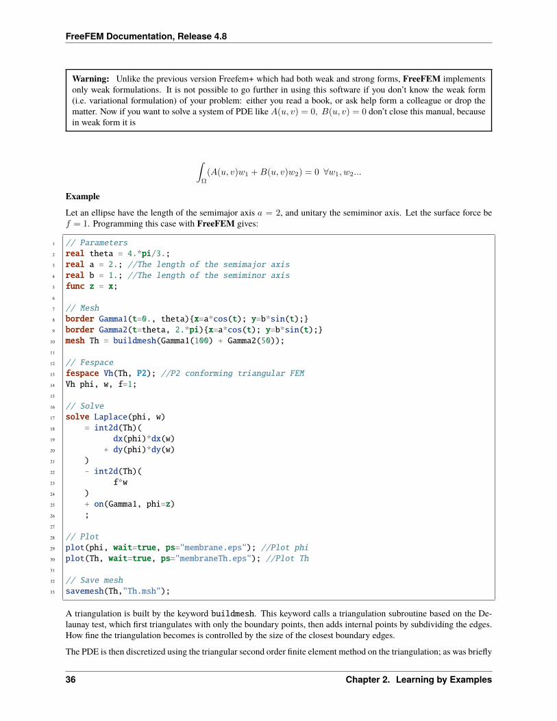
ExampleLet an ellipse have the length of the semimajor axis 𝑎 = 2, and unitary the semiminor axis. Let the surface force be𝑓 = 1. Programming this case with FreeFEM gives:
1 // Parameters2 real theta = 4.*pi/3.;3 real a = 2.; //The length of the semimajor axis4 real b = 1.; //The length of the semiminor axis5 func z = x;6
7 // Mesh8 border Gamma1(t=0., theta)x=a*cos(t); y=b*sin(t);9 border Gamma2(t=theta, 2.*pi)x=a*cos(t); y=b*sin(t);
10 mesh Th = buildmesh(Gamma1(100) + Gamma2(50));11
12 // Fespace13 fespace Vh(Th, P2); //P2 conforming triangular FEM14 Vh phi, w, f=1;15
16 // Solve17 solve Laplace(phi, w)18 = int2d(Th)(19 dx(phi)*dx(w)20 + dy(phi)*dy(w)21 )22 - int2d(Th)(23 f*w24 )25 + on(Gamma1, phi=z)26 ;27
28 // Plot29 plot(phi, wait=true, ps="membrane.eps"); //Plot phi30 plot(Th, wait=true, ps="membraneTh.eps"); //Plot Th31
32 // Save mesh33 savemesh(Th,"Th.msh");
A triangulation is built by the keyword buildmesh. This keyword calls a triangulation subroutine based on the De-launay test, which first triangulates with only the boundary points, then adds internal points by subdividing the edges.How fine the triangulation becomes is controlled by the size of the closest boundary edges.
The PDE is then discretized using the triangular second order finite element method on the triangulation; as was briefly
36 Chapter 2. Learning by Examples
FreeFEM Documentation, Release 4.8
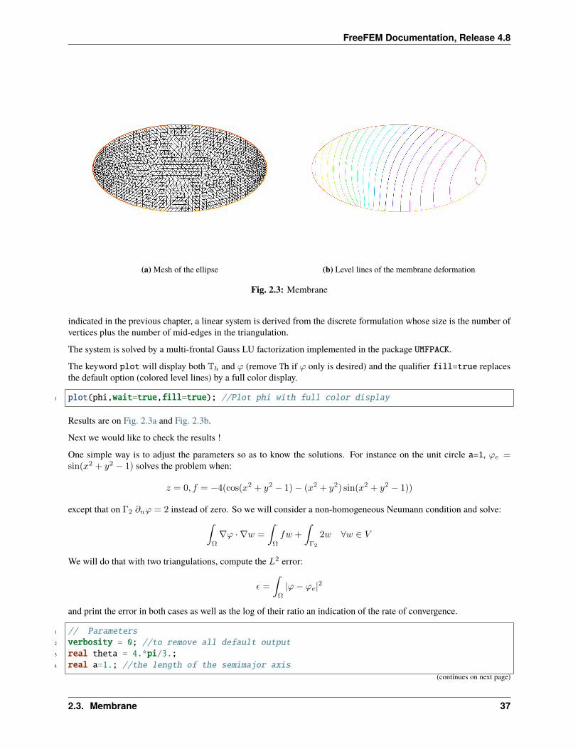
(a) Mesh of the ellipse (b) Level lines of the membrane deformation
Fig. 2.3: Membrane
indicated in the previous chapter, a linear system is derived from the discrete formulation whose size is the number ofvertices plus the number of mid-edges in the triangulation.
The system is solved by a multi-frontal Gauss LU factorization implemented in the package UMFPACK.
The keyword plot will display both Tℎ and 𝜙 (remove Th if 𝜙 only is desired) and the qualifier fill=true replacesthe default option (colored level lines) by a full color display.
1 plot(phi,wait=true,fill=true); //Plot phi with full color display
Results are on Fig. 2.3a and Fig. 2.3b.
Next we would like to check the results !
One simple way is to adjust the parameters so as to know the solutions. For instance on the unit circle a=1, 𝜙𝑒 =sin(𝑥2 + 𝑦2 − 1) solves the problem when:
𝑧 = 0, 𝑓 = −4(cos(𝑥2 + 𝑦2 − 1)− (𝑥2 + 𝑦2) sin(𝑥2 + 𝑦2 − 1))
except that on Γ2 𝜕𝑛𝜙 = 2 instead of zero. So we will consider a non-homogeneous Neumann condition and solve:∫Ω
∇𝜙 · ∇𝑤 =
∫Ω
𝑓𝑤 +
∫Γ2
2𝑤 ∀𝑤 ∈ 𝑉
We will do that with two triangulations, compute the 𝐿2 error:
𝜖 =
∫Ω
|𝜙− 𝜙𝑒|2
and print the error in both cases as well as the log of their ratio an indication of the rate of convergence.
1 // Parameters2 verbosity = 0; //to remove all default output3 real theta = 4.*pi/3.;4 real a=1.; //the length of the semimajor axis
(continues on next page)
2.3. Membrane 37
FreeFEM Documentation, Release 4.8
(continued from previous page)
5 real b=1.; //the length of the semiminor axis6 func f = -4*(cos(x^2+y^2-1) - (x^2+y^2)*sin(x^2+y^2-1));7 func phiexact = sin(x^2 + y^2 - 1);8
9 // Mesh10 border Gamma1(t=0., theta)x=a*cos(t); y=b*sin(t);11 border Gamma2(t=theta, 2.*pi)x=a*cos(t); y=b*sin(t);12
13 // Error loop14 real[int] L2error(2); //an array of two values15 for(int n = 0; n < 2; n++)16 // Mesh17 mesh Th = buildmesh(Gamma1(20*(n+1)) + Gamma2(10*(n+1)));18
19 // Fespace20 fespace Vh(Th, P2);21 Vh phi, w;22
23 // Solve24 solve Laplace(phi, w)25 = int2d(Th)(26 dx(phi)*dx(w)27 + dy(phi)*dy(w)28 )29 - int2d(Th)(30 f*w31 )32 - int1d(Th, Gamma2)(33 2*w34 )35 + on(Gamma1,phi=0)36 ;37
38 // Plot39 plot(Th, phi, wait=true, ps="membrane.eps");40
41 // Error42 L2error[n] = sqrt(int2d(Th)((phi-phiexact)^2));43 44
45 // Display loop46 for(int n = 0; n < 2; n++)47 cout << "L2error " << n << " = " << L2error[n] << endl;48
49 // Convergence rate50 cout << "convergence rate = "<< log(L2error[0]/L2error[1])/log(2.) << endl;
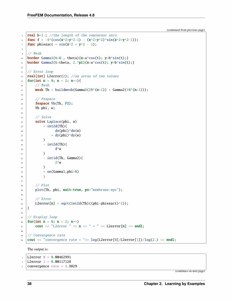
The output is:
1 L2error 0 = 0.004629912 L2error 1 = 0.001171283 convergence rate = 1.9829
(continues on next page)
38 Chapter 2. Learning by Examples
FreeFEM Documentation, Release 4.8
(continued from previous page)
4 times: compile 0.02s, execution 6.94s
We find a rate of 1.98 , which is not close enough to the 3 predicted by the theory.
The Geometry is always a polygon so we lose one order due to the geometry approximation in 𝑂(ℎ2).
Now if you are not satisfied with the .eps plot generated by FreeFEM and you want to use other graphic facilities,then you must store the solution in a file very much like in C++. It will be useless if you don’t save the triangulation aswell, consequently you must do
1 2 ofstream ff("phi.txt");3 ff << phi[];4 5 savemesh(Th,"Th.msh");
For the triangulation the name is important: the extension determines the format.
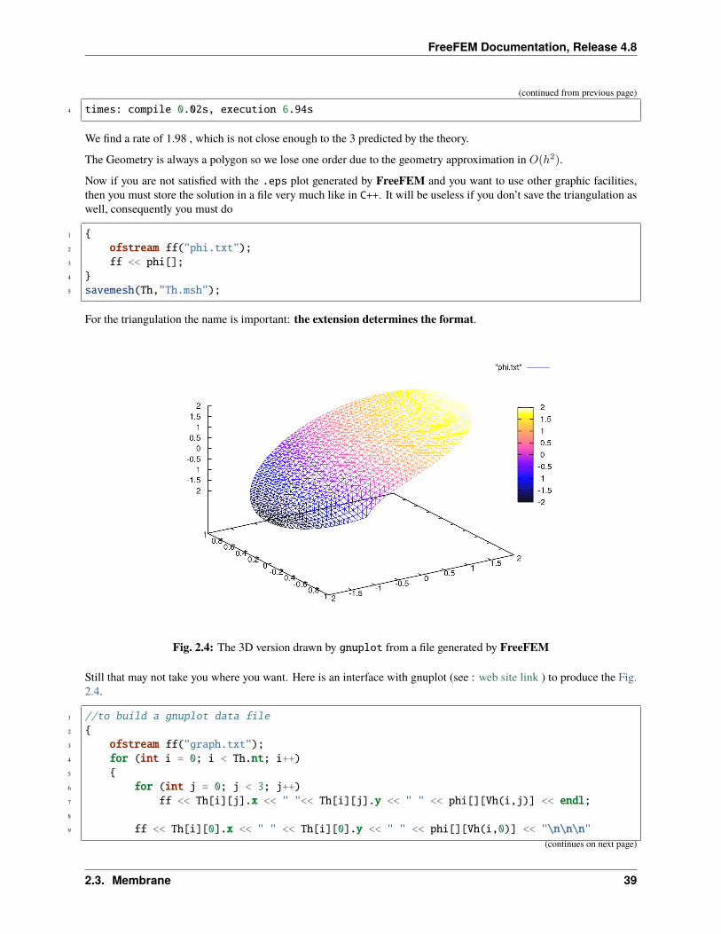
Fig. 2.4: The 3D version drawn by gnuplot from a file generated by FreeFEM
Still that may not take you where you want. Here is an interface with gnuplot (see : web site link ) to produce the Fig.2.4.
1 //to build a gnuplot data file2 3 ofstream ff("graph.txt");4 for (int i = 0; i < Th.nt; i++)5 6 for (int j = 0; j < 3; j++)7 ff << Th[i][j].x << " "<< Th[i][j].y << " " << phi[][Vh(i,j)] << endl;8
9 ff << Th[i][0].x << " " << Th[i][0].y << " " << phi[][Vh(i,0)] << "\n\n\n"(continues on next page)
2.3. Membrane 39
FreeFEM Documentation, Release 4.8
(continued from previous page)
10 11
We use the finite element numbering, where Wh(i,j) is the global index of 𝑗𝑇ℎ degrees of freedom of triangle number𝑖.
Then open gnuplot and do:
1 set palette rgbformulae 30,31,322 splot "graph.txt" w l pal
This works with P2 and P1, but not with P1nc because the 3 first degrees of freedom of P2 or P2 are on vertices andnot with P1nc.
2.4 Heat Exchanger
Summary: Here we shall learn more about geometry input and triangulation files, as well as read and write operations.
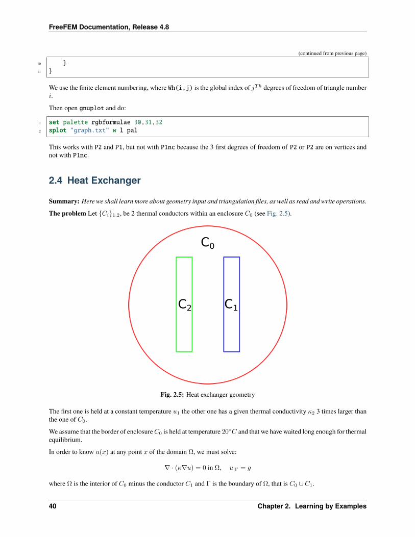
The problem Let 𝐶𝑖1,2, be 2 thermal conductors within an enclosure 𝐶0 (see Fig. 2.5).
Fig. 2.5: Heat exchanger geometry
The first one is held at a constant temperature 𝑢1 the other one has a given thermal conductivity 𝜅2 3 times larger thanthe one of 𝐶0.
We assume that the border of enclosure𝐶0 is held at temperature 20∘𝐶 and that we have waited long enough for thermalequilibrium.
In order to know 𝑢(𝑥) at any point 𝑥 of the domain Ω, we must solve:
∇ · (𝜅∇𝑢) = 0 in Ω, 𝑢|Γ = 𝑔
where Ω is the interior of 𝐶0 minus the conductor 𝐶1 and Γ is the boundary of Ω, that is 𝐶0 ∪ 𝐶1.
40 Chapter 2. Learning by Examples
FreeFEM Documentation, Release 4.8
Here 𝑔 is any function of 𝑥 equal to 𝑢𝑖 on 𝐶𝑖.
The second equation is a reduced form for:
𝑢 = 𝑢𝑖 on 𝐶𝑖, 𝑖 = 0, 1.
The variational formulation for this problem is in the subspace 𝐻10 (Ω) ⊂ 𝐻1(Ω) of functions which have zero traces
on Γ.
𝑢− 𝑔 ∈ 𝐻10 (Ω) :
∫Ω
∇𝑢∇𝑣 = 0∀𝑣 ∈ 𝐻10 (Ω)
Let us assume that𝐶0 is a circle of radius 5 centered at the origin,𝐶𝑖 are rectangles,𝐶1 being at the constant temperature𝑢1 = 60∘𝐶 (so we can only consider its boundary).
1 // Parameters2 int C1=99;3 int C2=98; //could be anything such that !=0 and C1!=C24
5 // Mesh6 border C0(t=0., 2.*pi)x=5.*cos(t); y=5.*sin(t);7
8 border C11(t=0., 1.)x=1.+t; y=3.; label=C1;9 border C12(t=0., 1.)x=2.; y=3.-6.*t; label=C1;
10 border C13(t=0., 1.)x=2.-t; y=-3.; label=C1;11 border C14(t=0., 1.)x=1.; y=-3.+6.*t; label=C1;12
13 border C21(t=0., 1.)x=-2.+t; y=3.; label=C2;14 border C22(t=0., 1.)x=-1.; y=3.-6.*t; label=C2;15 border C23(t=0., 1.)x=-1.-t; y=-3.; label=C2;16 border C24(t=0., 1.)x=-2.; y=-3.+6.*t; label=C2;17
18 plot( C0(50) //to see the border of the domain19 + C11(5)+C12(20)+C13(5)+C14(20)20 + C21(-5)+C22(-20)+C23(-5)+C24(-20),21 wait=true, ps="heatexb.eps");22
23 mesh Th=buildmesh(C0(50)24 + C11(5)+C12(20)+C13(5)+C14(20)25 + C21(-5)+C22(-20)+C23(-5)+C24(-20));26
27 plot(Th,wait=1);28
29 // Fespace30 fespace Vh(Th, P1);31 Vh u, v;32 Vh kappa=1 + 2*(x<-1)*(x>-2)*(y<3)*(y>-3);33
34 // Solve35 solve a(u, v)36 = int2d(Th)(37 kappa*(38 dx(u)*dx(v)39 + dy(u)*dy(v)40 )
(continues on next page)
2.4. Heat Exchanger 41
FreeFEM Documentation, Release 4.8
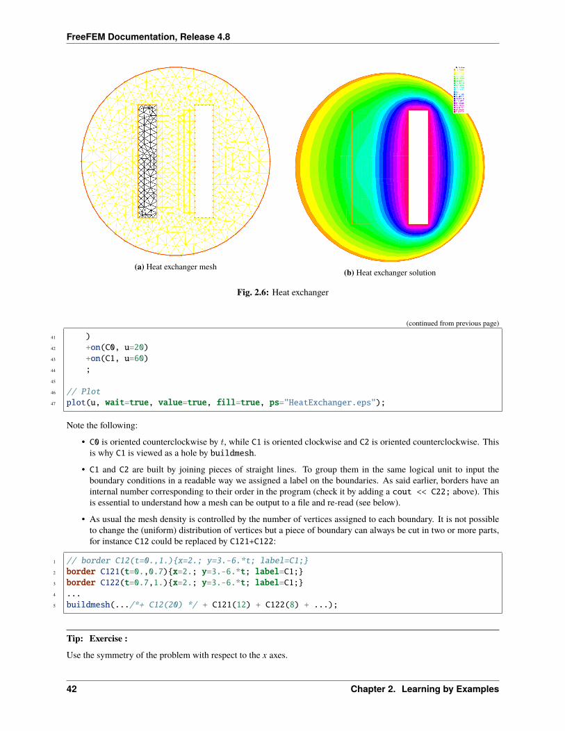
(a) Heat exchanger mesh (b) Heat exchanger solution
Fig. 2.6: Heat exchanger
(continued from previous page)
41 )42 +on(C0, u=20)43 +on(C1, u=60)44 ;45
46 // Plot47 plot(u, wait=true, value=true, fill=true, ps="HeatExchanger.eps");
Note the following:
• C0 is oriented counterclockwise by 𝑡, while C1 is oriented clockwise and C2 is oriented counterclockwise. Thisis why C1 is viewed as a hole by buildmesh.
• C1 and C2 are built by joining pieces of straight lines. To group them in the same logical unit to input theboundary conditions in a readable way we assigned a label on the boundaries. As said earlier, borders have aninternal number corresponding to their order in the program (check it by adding a cout << C22; above). Thisis essential to understand how a mesh can be output to a file and re-read (see below).
• As usual the mesh density is controlled by the number of vertices assigned to each boundary. It is not possibleto change the (uniform) distribution of vertices but a piece of boundary can always be cut in two or more parts,for instance C12 could be replaced by C121+C122:
1 // border C12(t=0.,1.)x=2.; y=3.-6.*t; label=C1;2 border C121(t=0.,0.7)x=2.; y=3.-6.*t; label=C1;3 border C122(t=0.7,1.)x=2.; y=3.-6.*t; label=C1;4 ...5 buildmesh(.../*+ C12(20) */ + C121(12) + C122(8) + ...);
Tip: Exercise :Use the symmetry of the problem with respect to the x axes.
42 Chapter 2. Learning by Examples
FreeFEM Documentation, Release 4.8
Triangulate only one half of the domain, and set homogeneous Neumann conditions on the horizontal axis.
Writing and reading triangulation files Suppose that at the end of the previous program we added the line
1 savemesh(Th, "condensor.msh");
and then later on we write a similar program but we wish to read the mesh from that file. Then this is how the condensershould be computed:
1 // Mesh2 mesh Sh = readmesh("condensor.msh");3
4 // Fespace5 fespace Wh(Sh, P1);6 Wh us, vs;7
8 // Solve9 solve b(us, vs)
10 = int2d(Sh)(11 dx(us)*dx(vs)12 + dy(us)*dy(vs)13 )14 +on(1, us=0)15 +on(99, us=1)16 +on(98, us=-1)17 ;18
19 // Plot20 plot(us);
Note that the names of the boundaries are lost but either their internal number (in the case of C0) or their label number(for C1 and C2) are kept.
2.5 Acoustics
Summary : Here we go to grip with ill posed problems and eigenvalue problems
Pressure variations in air at rest are governed by the wave equation:
𝜕2𝑢
𝜕𝑡2− 𝑐2∆𝑢 = 0
When the solution wave is monochromatic (and that depends on the boundary and initial conditions), 𝑢 is of the form𝑢(𝑥, 𝑡) = 𝑅𝑒(𝑣(𝑥)𝑒𝑖𝑘𝑡) where 𝑣 is a solution of Helmholtz’s equation:
𝑘2𝑣 + 𝑐2∆𝑣 = 0 in Ω𝜕𝑣𝜕𝑛 |Γ = 𝑔
where 𝑔 is the source.
Note the “+” sign in front of the Laplace operator and that 𝑘 > 0 is real. This sign may make the problem ill posed forsome values of 𝑐
𝑘 , a phenomenon called “resonance”.
At resonance there are non-zero solutions even when 𝑔 = 0. So the following program may or may not work:
2.5. Acoustics 43
FreeFEM Documentation, Release 4.8
1 // Parameters2 real kc2 = 1.;3 func g = y*(1.-y);4
5 // Mesh6 border a0(t=0., 1.)x=5.; y=1.+2.*t;7 border a1(t=0., 1.)x=5.-2.*t; y=3.;8 border a2(t=0., 1.)x=3.-2.*t; y=3.-2.*t;9 border a3(t=0., 1.)x=1.-t; y=1.;
10 border a4(t=0., 1.)x=0.; y=1.-t;11 border a5(t=0., 1.)x=t; y=0.;12 border a6(t=0., 1.)x=1.+4.*t; y=t;13
14 mesh Th = buildmesh(a0(20) + a1(20) + a2(20)15 + a3(20) + a4(20) + a5(20) + a6(20));16
17 // Fespace18 fespace Vh(Th, P1);19 Vh u, v;20
21 // Solve22 solve sound(u, v)23 = int2d(Th)(24 u*v * kc225 - dx(u)*dx(v)26 - dy(u)*dy(v)27 )28 - int1d(Th, a4)(29 g * v30 )31 ;32
33 // Plot34 plot(u, wait=1, ps="Sound.eps");
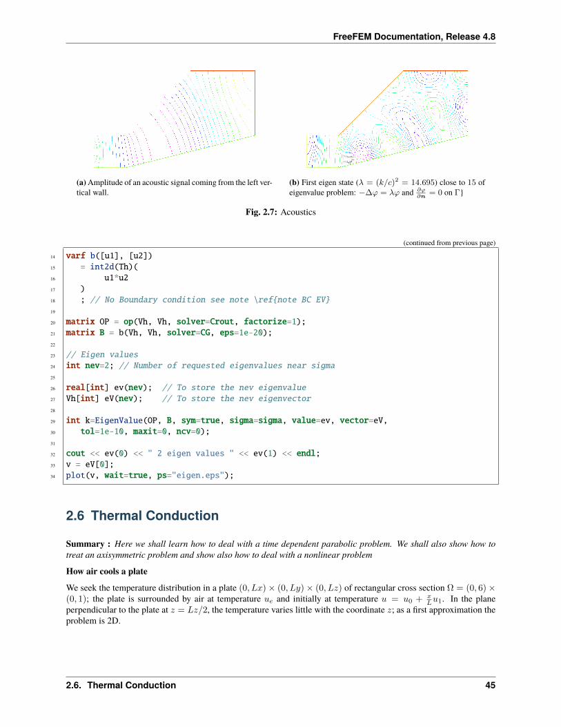
Results are on Fig. 2.7a. But when 𝑘𝑐2 is an eigenvalue of the problem, then the solution is not unique:
• if 𝑢𝑒 = 0 is an eigen state, then for any given solution 𝑢+ 𝑢𝑒 is another solution.
To find all the 𝑢𝑒 one can do the following :
1 // Parameters2 real sigma = 20; //value of the shift3
4 // Problem5 // OP = A - sigma B ; // The shifted matrix6 varf op(u1, u2)7 = int2d(Th)(8 dx(u1)*dx(u2)9 + dy(u1)*dy(u2)
10 - sigma* u1*u211 )12 ;13
(continues on next page)
44 Chapter 2. Learning by Examples
FreeFEM Documentation, Release 4.8
(a) Amplitude of an acoustic signal coming from the left ver-tical wall.
(b) First eigen state (𝜆 = (𝑘/𝑐)2 = 14.695) close to 15 ofeigenvalue problem: −Δ𝜙 = 𝜆𝜙 and 𝜕𝜙
𝜕𝑛= 0 on Γ
Fig. 2.7: Acoustics
(continued from previous page)
14 varf b([u1], [u2])15 = int2d(Th)(16 u1*u217 )18 ; // No Boundary condition see note \refnote BC EV19
20 matrix OP = op(Vh, Vh, solver=Crout, factorize=1);21 matrix B = b(Vh, Vh, solver=CG, eps=1e-20);22
23 // Eigen values24 int nev=2; // Number of requested eigenvalues near sigma25
26 real[int] ev(nev); // To store the nev eigenvalue27 Vh[int] eV(nev); // To store the nev eigenvector28
29 int k=EigenValue(OP, B, sym=true, sigma=sigma, value=ev, vector=eV,30 tol=1e-10, maxit=0, ncv=0);31
32 cout << ev(0) << " 2 eigen values " << ev(1) << endl;33 v = eV[0];34 plot(v, wait=true, ps="eigen.eps");
2.6 Thermal Conduction
Summary : Here we shall learn how to deal with a time dependent parabolic problem. We shall also show how totreat an axisymmetric problem and show also how to deal with a nonlinear problem
How air cools a plateWe seek the temperature distribution in a plate (0, 𝐿𝑥)× (0, 𝐿𝑦)× (0, 𝐿𝑧) of rectangular cross section Ω = (0, 6)×(0, 1); the plate is surrounded by air at temperature 𝑢𝑒 and initially at temperature 𝑢 = 𝑢0 + 𝑥
𝐿𝑢1. In the planeperpendicular to the plate at 𝑧 = 𝐿𝑧/2, the temperature varies little with the coordinate 𝑧; as a first approximation theproblem is 2D.
2.6. Thermal Conduction 45
FreeFEM Documentation, Release 4.8
We must solve the temperature equation in Ω in a time interval (0,T).
𝜕𝑡𝑢−∇ · (𝜅∇𝑢) = 0 in Ω× (0, 𝑇 )𝑢(𝑥, 𝑦, 0) = 𝑢0 + 𝑥𝑢1
𝜅 𝜕𝑢𝜕𝑛 + 𝛼(𝑢− 𝑢𝑒) = 0 on Γ× (0, 𝑇 )
Here the diffusion 𝜅 will take two values, one below the middle horizontal line and ten times less above, so as tosimulate a thermostat.
The term 𝛼(𝑢− 𝑢𝑒) accounts for the loss of temperature by convection in air. Mathematically this boundary conditionis of Fourier (or Robin, or mixed) type.
The variational formulation is in 𝐿2(0, 𝑇 ;𝐻1(Ω)); in loose terms and after applying an implicit Euler finite differenceapproximation in time; we shall seek 𝑢𝑛(𝑥, 𝑦) satisfying for all 𝑤 ∈ 𝐻1(Ω):∫
Ω
(𝑢𝑛 − 𝑢𝑛−1
𝛿𝑡𝑤 + 𝜅∇𝑢𝑛∇𝑤) +
∫Γ
𝛼(𝑢𝑛 − 𝑢𝑢𝑒)𝑤 = 0
1 // Parameters2 func u0 = 10. + 90.*x/6.;3 func k = 1.8*(y<0.5) + 0.2;4 real ue = 25.;5 real alpha=0.25;6 real T=5.;7 real dt=0.1 ;8
9 // Mesh10 mesh Th = square(30, 5, [6.*x,y]);11
12 // Fespace13 fespace Vh(Th, P1);14 Vh u=u0, v, uold;15
16 // Problem17 problem thermic(u, v)18 = int2d(Th)(19 u*v/dt20 + k*(21 dx(u) * dx(v)22 + dy(u) * dy(v)23 )24 )25 + int1d(Th, 1, 3)(26 alpha*u*v27 )28 - int1d(Th, 1, 3)(29 alpha*ue*v30 )31 - int2d(Th)(32 uold*v/dt33 )34 + on(2, 4, u=u0)35 ;36
37 // Time iterations(continues on next page)
46 Chapter 2. Learning by Examples
FreeFEM Documentation, Release 4.8
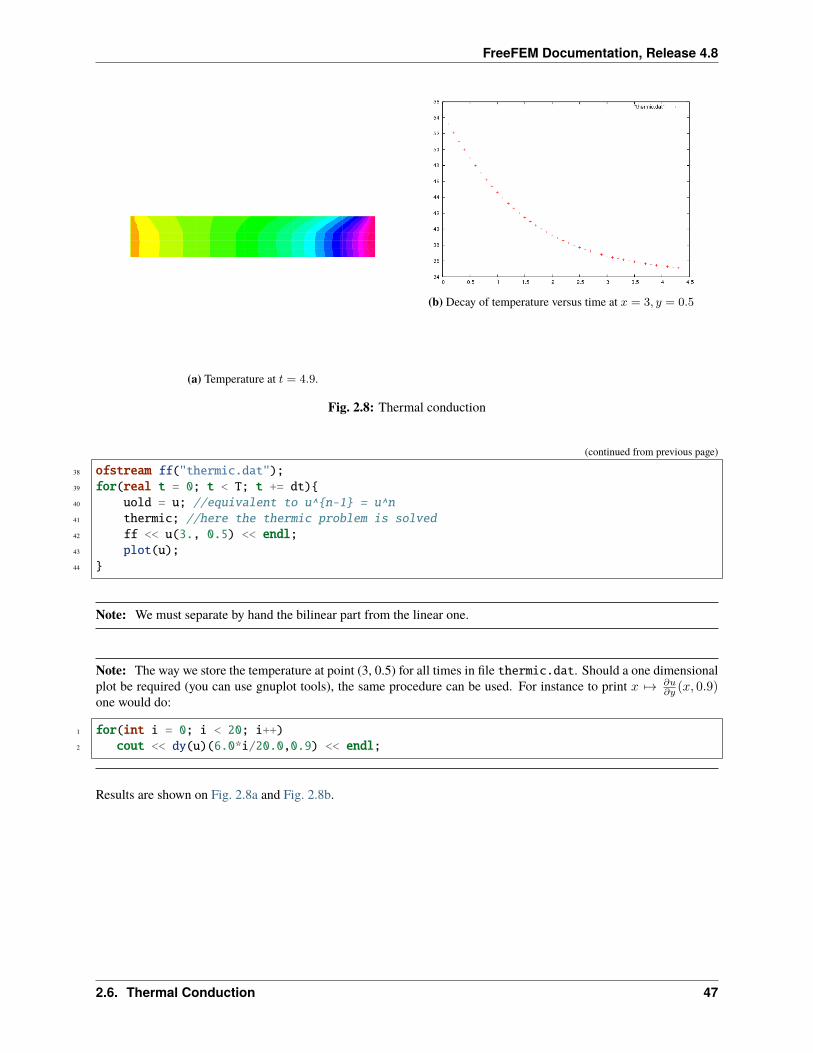
(a) Temperature at 𝑡 = 4.9.
(b) Decay of temperature versus time at 𝑥 = 3, 𝑦 = 0.5
Fig. 2.8: Thermal conduction
(continued from previous page)
38 ofstream ff("thermic.dat");39 for(real t = 0; t < T; t += dt)40 uold = u; //equivalent to u^n-1 = u^n41 thermic; //here the thermic problem is solved42 ff << u(3., 0.5) << endl;43 plot(u);44
Note: We must separate by hand the bilinear part from the linear one.
Note: The way we store the temperature at point (3, 0.5) for all times in file thermic.dat. Should a one dimensionalplot be required (you can use gnuplot tools), the same procedure can be used. For instance to print 𝑥 ↦→ 𝜕𝑢
𝜕𝑦 (𝑥, 0.9)one would do:
1 for(int i = 0; i < 20; i++)2 cout << dy(u)(6.0*i/20.0,0.9) << endl;
Results are shown on Fig. 2.8a and Fig. 2.8b.
2.6. Thermal Conduction 47
FreeFEM Documentation, Release 4.8
2.6.1 Axisymmetry: 3D Rod with circular section
Let us now deal with a cylindrical rod instead of a flat plate. For simplicity we take 𝜅 = 1.
In cylindrical coordinates, the Laplace operator becomes (𝑟 is the distance to the axis, 𝑧 is the distance along the axis,𝜃 polar angle in a fixed plane perpendicular to the axis):
∆𝑢 =1
𝑟𝜕𝑟(𝑟𝜕𝑟𝑢) +
1
𝑟2𝜕2𝜃𝜃𝑢+ 𝜕2𝑧𝑧.
Symmetry implies that we loose the dependence with respect to 𝜃; so the domain Ω is again a rectangle ]0, 𝑅[×]0, |[. We take the convention of numbering of the edges as in square() (1 for the bottom horizontal . . . ); the problem isnow:
𝑟𝜕𝑡𝑢− 𝜕𝑟(𝑟𝜕𝑟𝑢)− 𝜕𝑧(𝑟𝜕𝑧𝑢) = 0 in Ω𝑢(𝑡 = 0) = 𝑢0 + 𝑧
𝐿𝑧(𝑢1 − 𝑢)
𝑢|Γ4 = 𝑢0𝑢|Γ2
= 𝑢1𝛼(𝑢− 𝑢𝑒) + 𝜕𝑢
𝜕𝑛 |Γ1∪Γ3= 0
Note that the PDE has been multiplied by 𝑟.
After discretization in time with an implicit scheme, with time steps dt, in the FreeFEM syntax 𝑟 becomes 𝑥 and 𝑧becomes 𝑦 and the problem is:
1 problem thermaxi(u, v)2 = int2d(Th)(3 (u*v/dt + dx(u)*dx(v) + dy(u)*dy(v))*x4 )5 + int1d(Th, 3)(6 alpha*x*u*v7 )8 - int1d(Th, 3)(9 alpha*x*ue*v
10 )11 - int2d(Th)(12 uold*v*x/dt13 )14 + on(2, 4, u=u0);
Note: The bilinear form degenerates at 𝑥 = 0. Still one can prove existence and uniqueness for 𝑢 and because of thisdegeneracy no boundary conditions need to be imposed on Γ1.
2.6.2 A Nonlinear Problem : Radiation
Heat loss through radiation is a loss proportional to the absolute temperature to the fourth power (Stefan’s Law). Thisadds to the loss by convection and gives the following boundary condition:
𝜅𝜕𝑢
𝜕𝑛+ 𝛼(𝑢− 𝑢𝑒) + 𝑐[(𝑢+ 273)4 − (𝑢𝑒 + 273)4] = 0
The problem is nonlinear, and must be solved iteratively with fixed-point iteration where𝑚 denotes the iteration index,a semi-linearization of the radiation condition gives
𝜕𝑢𝑚+1
𝜕𝑛+ 𝛼(𝑢𝑚+1 − 𝑢𝑒) + 𝑐(𝑢𝑚+1 − 𝑢𝑒)(𝑢𝑚 + 𝑢𝑒 + 546)((𝑢𝑚 + 273)2 + (𝑢𝑒 + 273)2) = 0,
48 Chapter 2. Learning by Examples
FreeFEM Documentation, Release 4.8
because we have the identity 𝑎4 − 𝑏4 = (𝑎− 𝑏)(𝑎+ 𝑏)(𝑎2 + 𝑏2).
The iterative process will work with 𝑣 = 𝑢− 𝑢𝑒.
1 ...2 // Mesh3 fespace Vh(Th, P1);4 Vh vold, w, v=u0-ue, b,vp;5
6 // Problem7 problem thermradia(v, w)8 = int2d(Th)(9 v*w/dt
10 + k*(dx(v) * dx(w) + dy(v) * dy(w))11 )12 + int1d(Th, 1, 3)(13 b*v*w14 )15 - int2d(Th)(16 vold*w/dt17 )18 + on(2, 4, v=u0-ue)19 ;20
21 verbosity=0; // to remove spurious FREEfem print22 for (real t=0;t<T;t+=dt)23 vold[] = v[];// just copy DoF's, faster than interpolation pv=v;24 for (int m = 0; m < 5; m++) 25 vp[]=v[];// save previous state of commute error26 b = alpha + rad * (v + 2*uek) * ((v+uek)^2 + uek^2);27 thermradia;28 vp[]-=v[];29 real err = vp[].linfty;// error value30 cout << " time " << t << " iter " << m << " err = "<< vp[].linfty << endl;31 if( err < 1e-5) break; // if error is enough small break fixed-point loop32 33 34 v[] += ue;// add a constant to all DoF's of v35
36 plot(v);
2.7 Irrotational Fan Blade Flow and Thermal effects
Summary : Here we will learn how to deal with a multi-physics system of PDEs on a complex geometry, with multiplemeshes within one problem. We also learn how to manipulate the region indicator and see how smooth is the projectionoperator from one mesh to another.
Incompressible flowWithout viscosity and vorticity incompressible flows have a velocity given by:
𝑢 =
(𝜕𝜓𝜕𝑥
−𝜕𝜓𝜕𝑦
), where 𝜓 is solution of ∆𝜓 = 0
2.7. Irrotational Fan Blade Flow and Thermal effects 49
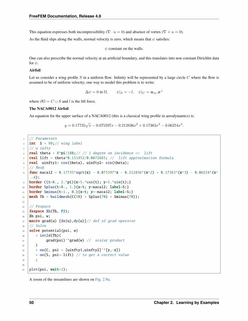
FreeFEM Documentation, Release 4.8
This equation expresses both incompressibility (∇ · 𝑢 = 0) and absence of vortex (∇× 𝑢 = 0).
As the fluid slips along the walls, normal velocity is zero, which means that 𝜓 satisfies:
𝜓 constant on the walls.
One can also prescribe the normal velocity at an artificial boundary, and this translates into non constant Dirichlet datafor 𝜓.
AirfoilLet us consider a wing profile 𝑆 in a uniform flow. Infinity will be represented by a large circle 𝐶 where the flow isassumed to be of uniform velocity; one way to model this problem is to write:
∆𝜓 = 0 in Ω, 𝜓|𝑆 = −𝑙, 𝜓|𝐶 = 𝑢∞.𝑥⊥
where 𝜕Ω = 𝐶 ∪ 𝑆 and 𝑙 is the lift force.
The NACA0012 AirfoilAn equation for the upper surface of a NACA0012 (this is a classical wing profile in aerodynamics) is:
𝑦 = 0.17735√𝑥− 0.075597𝑥− 0.212836𝑥2 + 0.17363𝑥3 − 0.06254𝑥4.
1 // Parameters2 int S = 99;// wing label3 // u infty4 real theta = 8*pi/180;// // 1 degree on incidence => lift5 real lift = theta*0.151952/0.0872665; // lift approximation formula6 real uinfty1= cos(theta), uinfty2= sin(theta);7 // Mesh8 func naca12 = 0.17735*sqrt(x) - 0.075597*x - 0.212836*(x^2) + 0.17363*(x^3) - 0.06254*(x^
→˓4);9 border C(t=0., 2.*pi)x=5.*cos(t); y=5.*sin(t);
10 border Splus(t=0., 1.)x=t; y=naca12; label=S;11 border Sminus(t=1., 0.)x=t; y=-naca12; label=S;12 mesh Th = buildmesh(C(50) + Splus(70) + Sminus(70));13
14 // Fespace15 fespace Xh(Th, P2);16 Xh psi, w;17 macro grad(u) [dx(u),dy(u)]// def of grad operator18 // Solve19 solve potential(psi, w)20 = int2d(Th)(21 grad(psi)'*grad(w) // scalar product22 )23 + on(C, psi = [uinfty1,uinfty2]'*[y,-x])24 + on(S, psi=-lift) // to get a correct value25 ;26
27 plot(psi, wait=1);
A zoom of the streamlines are shown on Fig. 2.9a.
50 Chapter 2. Learning by Examples
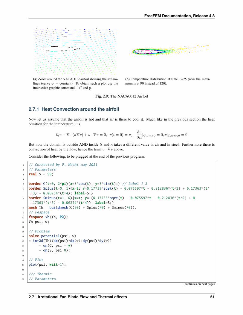
FreeFEM Documentation, Release 4.8
(a) Zoom around the NACA0012 airfoil showing the stream-lines (curve 𝜓 = constant). To obtain such a plot use theinteractive graphic command: “+” and p.
(b) Temperature distribution at time T=25 (now the maxi-mum is at 90 instead of 120).
Fig. 2.9: The NACA0012 Airfoil
2.7.1 Heat Convection around the airfoil
Now let us assume that the airfoil is hot and that air is there to cool it. Much like in the previous section the heatequation for the temperature 𝑣 is
𝜕𝑡𝑣 −∇ · (𝜅∇𝑣) + 𝑢 · ∇𝑣 = 0, 𝑣(𝑡 = 0) = 𝑣0,𝜕𝑣
𝜕𝑛|𝐶,𝑢·𝑛>0 = 0, 𝑣|𝐶,𝑢·𝑛<0 = 0
But now the domain is outside AND inside 𝑆 and 𝜅 takes a different value in air and in steel. Furthermore there isconvection of heat by the flow, hence the term 𝑢 · ∇𝑣 above.
Consider the following, to be plugged at the end of the previous program:
1 // Corrected by F. Hecht may 20212 // Parameters3 real S = 99;4
5 border C(t=0, 2*pi)x=3*cos(t); y=3*sin(t); // Label 1,26 border Splus(t=0, 1)x=t; y=0.17735*sqrt(t) - 0.075597*t - 0.212836*(t^2) + 0.17363*(t^
→˓3) - 0.06254*(t^4); label=S;7 border Sminus(t=1, 0)x=t; y=-(0.17735*sqrt(t) - 0.075597*t - 0.212836*(t^2) + 0.
→˓17363*(t^3) - 0.06254*(t^4)); label=S;8 mesh Th = buildmesh(C(50) + Splus(70) + Sminus(70));9 // Fespace
10 fespace Vh(Th, P2);11 Vh psi, w;12
13 // Problem14 solve potential(psi, w)15 = int2d(Th)(dx(psi)*dx(w)+dy(psi)*dy(w))16 + on(C, psi = y)17 + on(S, psi=0);18
19 // Plot20 plot(psi, wait=1);21
22 /// Thermic23 // Parameters
(continues on next page)
2.7. Irrotational Fan Blade Flow and Thermal effects 51
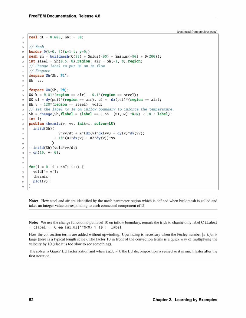
FreeFEM Documentation, Release 4.8
(continued from previous page)
24 real dt = 0.005, nbT = 50;25
26 // Mesh27 border D(t=0, 2)x=1+t; y=0;28 mesh Sh = buildmesh(C(25) + Splus(-90) + Sminus(-90) + D(200));29 int steel = Sh(0.5, 0).region, air = Sh(-1, 0).region;30 // Change label to put BC on In flow31 // Fespace32 fespace Wh(Sh, P1);33 Wh vv;34
35 fespace W0(Sh, P0);36 W0 k = 0.01*(region == air) + 0.1*(region == steel);37 W0 u1 = dy(psi)*(region == air), u2 = -dx(psi)*(region == air);38 Wh v = 120*(region == steel), vold;39 // set the label to 10 on inflow boundary to inforce the temperature.40 Sh = change(Sh,flabel = (label == C && [u1,u2]'*N<0) ? 10 : label);41 int i;42 problem thermic(v, vv, init=i, solver=LU)43 = int2d(Sh)(44 v*vv/dt + k*(dx(v)*dx(vv) + dy(v)*dy(vv))45 + 10*(u1*dx(v) + u2*dy(v))*vv46 )47 - int2d(Sh)(vold*vv/dt)48 + on(10, v= 0);49
50
51 for(i = 0; i < nbT; i++) 52 vold[]= v[];53 thermic;54 plot(v);55
Note: How steel and air are identified by the mesh parameter region which is defined when buildmesh is called andtakes an integer value corresponding to each connected component of Ω;
Note: We use the change function to put label 10 on inflow boundary, remark the trick to chanhe only label C flabel= (label == C && [u1,u2]'*N<0) ? 10 : label
How the convection terms are added without upwinding. Upwinding is necessary when the Pecley number |𝑢|𝐿/𝜅 islarge (here is a typical length scale), The factor 10 in front of the convection terms is a quick way of multiplying thevelocity by 10 (else it is too slow to see something).
The solver is Gauss’ LU factorization and when init = 0 the LU decomposition is reused so it is much faster after thefirst iteration.
52 Chapter 2. Learning by Examples
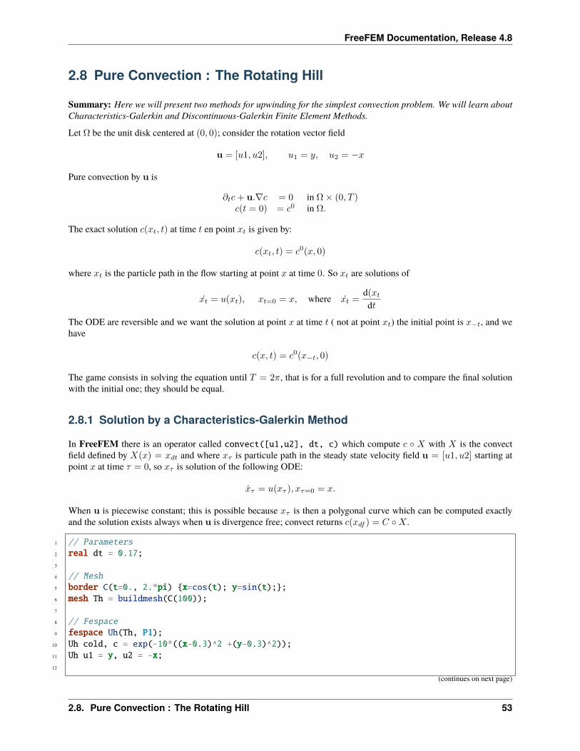
FreeFEM Documentation, Release 4.8
2.8 Pure Convection : The Rotating Hill
Summary: Here we will present two methods for upwinding for the simplest convection problem. We will learn aboutCharacteristics-Galerkin and Discontinuous-Galerkin Finite Element Methods.
Let Ω be the unit disk centered at (0, 0); consider the rotation vector field
u = [𝑢1, 𝑢2], 𝑢1 = 𝑦, 𝑢2 = −𝑥
Pure convection by u is
𝜕𝑡𝑐+ u.∇𝑐 = 0 in Ω× (0, 𝑇 )𝑐(𝑡 = 0) = 𝑐0 in Ω.
The exact solution 𝑐(𝑥𝑡, 𝑡) at time 𝑡 en point 𝑥𝑡 is given by:
𝑐(𝑥𝑡, 𝑡) = 𝑐0(𝑥, 0)
where 𝑥𝑡 is the particle path in the flow starting at point 𝑥 at time 0. So 𝑥𝑡 are solutions of
𝑥𝑡 = 𝑢(𝑥𝑡), 𝑥𝑡=0 = 𝑥, where 𝑥𝑡 =d(𝑥𝑡d𝑡
The ODE are reversible and we want the solution at point 𝑥 at time 𝑡 ( not at point 𝑥𝑡) the initial point is 𝑥−𝑡, and wehave
𝑐(𝑥, 𝑡) = 𝑐0(𝑥−𝑡, 0)
The game consists in solving the equation until 𝑇 = 2𝜋, that is for a full revolution and to compare the final solutionwith the initial one; they should be equal.
2.8.1 Solution by a Characteristics-Galerkin Method
In FreeFEM there is an operator called convect([u1,u2], dt, c) which compute 𝑐 ∘ 𝑋 with 𝑋 is the convectfield defined by 𝑋(𝑥) = 𝑥𝑑𝑡 and where 𝑥𝜏 is particule path in the steady state velocity field u = [𝑢1, 𝑢2] starting atpoint 𝑥 at time 𝜏 = 0, so 𝑥𝜏 is solution of the following ODE:
𝜏 = 𝑢(𝑥𝜏 ), 𝑥𝜏=0 = 𝑥.
When u is piecewise constant; this is possible because 𝑥𝜏 is then a polygonal curve which can be computed exactlyand the solution exists always when u is divergence free; convect returns 𝑐(𝑥𝑑𝑓 ) = 𝐶 ∘𝑋 .
1 // Parameters2 real dt = 0.17;3
4 // Mesh5 border C(t=0., 2.*pi) x=cos(t); y=sin(t);;6 mesh Th = buildmesh(C(100));7
8 // Fespace9 fespace Uh(Th, P1);
10 Uh cold, c = exp(-10*((x-0.3)^2 +(y-0.3)^2));11 Uh u1 = y, u2 = -x;12
(continues on next page)
2.8. Pure Convection : The Rotating Hill 53
FreeFEM Documentation, Release 4.8
(continued from previous page)
13 // Time loop14 real t = 0;15 for (int m = 0; m < 2.*pi/dt; m++)16 t += dt;17 cold = c;18 c = convect([u1, u2], -dt, cold);19 plot(c, cmm=" t="+t +", min="+c[].min+", max="+c[].max);20
Note: 3D plots can be done by adding the qualifyer dim=3 to the plot instruction.
The method is very powerful but has two limitations:
• it is not conservative
• it may diverge in rare cases when |u| is too small due to quadrature error.
2.8.2 Solution by Discontinuous-Galerkin FEM
Discontinuous Galerkin methods take advantage of the discontinuities of 𝑐 at the edges to build upwinding. There aremay formulations possible. We shall implement here the so-called dual-𝑃𝐷𝐶1 formulation (see [ERN2006]):∫
Ω
(𝑐𝑛+1 − 𝑐𝑛
𝛿𝑡+ 𝑢 · ∇𝑐)𝑤 +
∫𝐸
(𝛼|𝑛 · 𝑢| − 1
2𝑛 · 𝑢)[𝑐]𝑤 =
∫𝐸−
Γ
|𝑛 · 𝑢|𝑐𝑤 ∀𝑤
where 𝐸 is the set of inner edges and 𝐸−Γ is the set of boundary edges where 𝑢 · 𝑛 < 0 (in our case there is no such
edges). Finally [𝑐] is the jump of 𝑐 across an edge with the convention that 𝑐+ refers to the value on the right of theoriented edge.
1 // Parameters2 real al=0.5;3 real dt = 0.05;4
5 // Mesh6 border C(t=0., 2.*pi) x=cos(t); y=sin(t);;7 mesh Th = buildmesh(C(100));8
9 // Fespace10 fespace Vh(Th,P1dc);11 Vh w, ccold, v1 = y, v2 = -x, cc = exp(-10*((x-0.3)^2 +(y-0.3)^2));12
13 // Macro14 macro n() (N.x*v1 + N.y*v2) // Macro without parameter15
16 // Problem17 problem Adual(cc, w)18 = int2d(Th)(19 (cc/dt+(v1*dx(cc)+v2*dy(cc)))*w20 )21 + intalledges(Th)(22 (1-nTonEdge)*w*(al*abs(n)-n/2)*jump(cc)
(continues on next page)
54 Chapter 2. Learning by Examples
FreeFEM Documentation, Release 4.8
(continued from previous page)
23 )24 - int2d(Th)(25 ccold*w/dt26 )27 ;28
29 // Time iterations30 for (real t = 0.; t < 2.*pi; t += dt)31 ccold = cc;32 Adual;33 plot(cc, fill=1, cmm="t="+t+", min="+cc[].min+", max="+ cc[].max);34 35
36 // Plot37 real [int] viso = [-0.2, -0.1, 0., 0.1, 0.2, 0.3, 0.4, 0.5, 0.6, 0.7, 0.8, 0.9, 1., 1.1];38 plot(cc, wait=1, fill=1, ps="ConvectCG.eps", viso=viso);39 plot(cc, wait=1, fill=1, ps="ConvectDG.eps", viso=viso);
Note: New keywords: intalledges to integrate on all edges of all triangles
intalledges(Th) ≡∑𝑇∈Th
∫𝜕𝑇
(so all internal edges are see two times), nTonEdge which is one if the triangle has a boundary edge and two otherwise,jump to implement [𝑐].
Results of both methods are shown on Fig. 2.10a nad Fig. 2.10b with identical levels for the level line; this is done withthe plot-modifier viso.
Notice also the macro where the parameter u is not used (but the syntax needs one) and which ends with a //; it simplyreplaces the name n by (N.x*v1+N.y*v2). As easily guessed N.x,N.y is the normal to the edge.
Now if you think that DG is too slow try this:
1 // Mesh2 border C(t=0., 2.*pi) x=cos(t); y=sin(t);;3 mesh Th = buildmesh(C(100));4
5 fespace Vh(Th,P1);//P1,P2,P0,P1dc,P2dc, uncond stable6
7 Vh vh,vo,u1 = y, u2 = -x, v = exp(-10*((x-0.3)^2 +(y-0.3)^2));8 real dt = 0.03,t=0, tmax=2*pi, al=0.5, alp=200;9
10 problem A(v,vh) = int2d(Th)(v*vh/dt-v*(u1*dx(vh)+u2*dy(vh)))11 + intalledges(Th)(vh*(mean(v)*(N.x*u1+N.y*u2)12 +alp*jump(v)*abs(N.x*u1+N.y*u2)))13 + int1d(Th,1)(((N.x*u1+N.y*u2)>0)*(N.x*u1+N.y*u2)*v*vh)14 - int2d(Th)(vo*vh/dt);15
16 varf Adual(v,vh) = int2d(Th)((v/dt+(u1*dx(v)+u2*dy(v)))*vh)17 + intalledges(Th)((1-nTonEdge)*vh*(al*abs(N.x*u1+N.y*u2)18 -(N.x*u1+N.y*u2)/2)*jump(v));
(continues on next page)
2.8. Pure Convection : The Rotating Hill 55
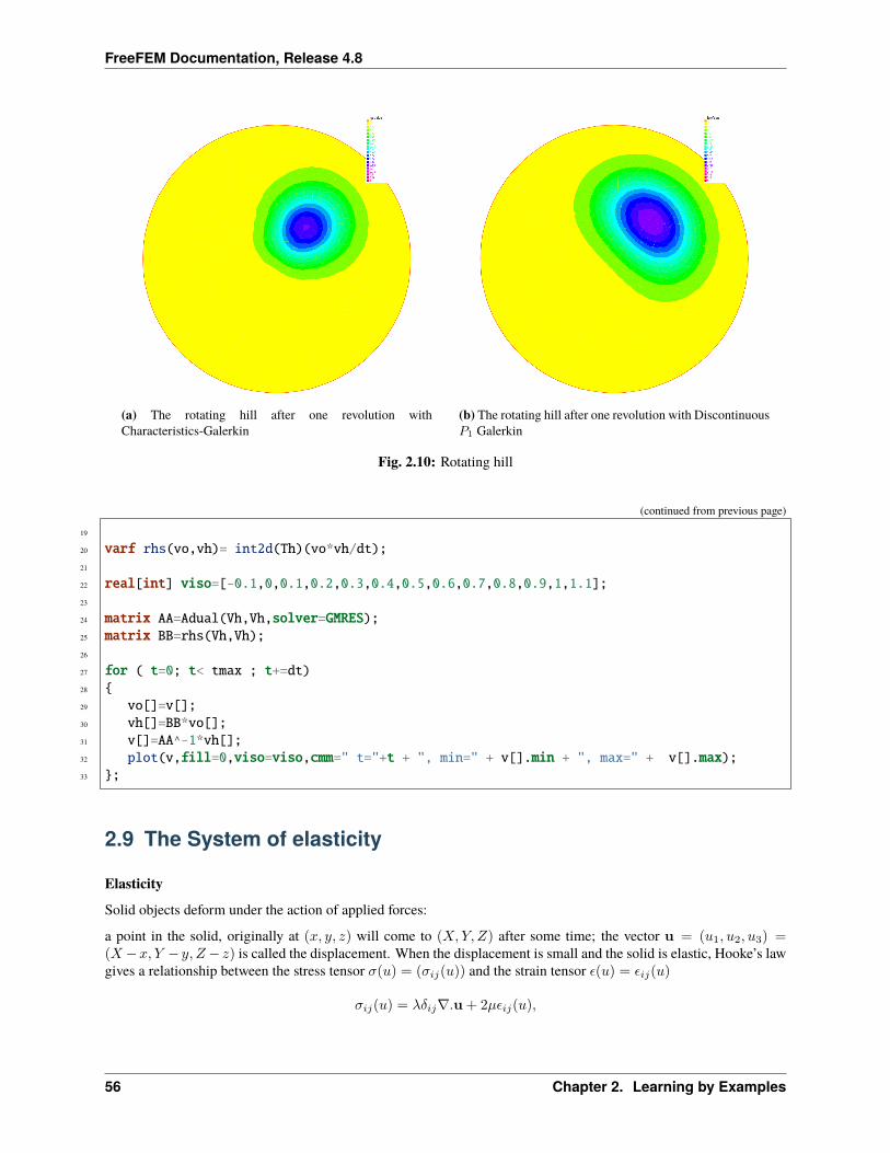
FreeFEM Documentation, Release 4.8
(a) The rotating hill after one revolution withCharacteristics-Galerkin
(b) The rotating hill after one revolution with Discontinuous𝑃1 Galerkin
Fig. 2.10: Rotating hill
(continued from previous page)
19
20 varf rhs(vo,vh)= int2d(Th)(vo*vh/dt);21
22 real[int] viso=[-0.1,0,0.1,0.2,0.3,0.4,0.5,0.6,0.7,0.8,0.9,1,1.1];23
24 matrix AA=Adual(Vh,Vh,solver=GMRES);25 matrix BB=rhs(Vh,Vh);26
27 for ( t=0; t< tmax ; t+=dt)28 29 vo[]=v[];30 vh[]=BB*vo[];31 v[]=AA^-1*vh[];32 plot(v,fill=0,viso=viso,cmm=" t="+t + ", min=" + v[].min + ", max=" + v[].max);33 ;
2.9 The System of elasticity
ElasticitySolid objects deform under the action of applied forces:
a point in the solid, originally at (𝑥, 𝑦, 𝑧) will come to (𝑋,𝑌, 𝑍) after some time; the vector u = (𝑢1, 𝑢2, 𝑢3) =(𝑋−𝑥, 𝑌 − 𝑦, 𝑍− 𝑧) is called the displacement. When the displacement is small and the solid is elastic, Hooke’s lawgives a relationship between the stress tensor 𝜎(𝑢) = (𝜎𝑖𝑗(𝑢)) and the strain tensor 𝜖(𝑢) = 𝜖𝑖𝑗(𝑢)
𝜎𝑖𝑗(𝑢) = 𝜆𝛿𝑖𝑗∇.u + 2𝜇𝜖𝑖𝑗(𝑢),
56 Chapter 2. Learning by Examples
FreeFEM Documentation, Release 4.8
where the Kronecker symbol 𝛿𝑖𝑗 = 1 if 𝑖 = 𝑗, 0 otherwise, with
𝜖𝑖𝑗(𝑢) =1
2(𝜕𝑢𝑖𝜕𝑥𝑗
+𝜕𝑢𝑗𝜕𝑥𝑖
),
and where 𝜆, 𝜇 are two constants that describe the mechanical properties of the solid, and are themselves related to thebetter known constants 𝐸, Young’s modulus, and 𝜈, Poisson’s ratio:
𝜇 =𝐸
2(1 + 𝜈), 𝜆 =
𝐸𝜈
(1 + 𝜈)(1− 2𝜈).
Lamé’s systemLet us consider a beam with axis 𝑂𝑧 and with perpendicular section Ω. The components along 𝑥 and 𝑦 of the strainu(𝑥) in a section Ω subject to forces f perpendicular to the axis are governed by:
−𝜇∆u− (𝜇+ 𝜆)∇(∇.u) = f in Ω,
where 𝜆 ,𝜇 are the Lamé coefficients introduced above.
Remark, we do not use this equation because the associated variational form does not give the right boundary condition,we simply use:
−𝑑𝑖𝑣(𝜎) = f in Ω
where the corresponding variational form is:∫Ω
𝜎(𝑢) : 𝜖(v) 𝑑𝑥−∫Ω
v𝑓 𝑑𝑥 = 0;
where : denotes the tensor scalar product, i.e. 𝑎 : 𝑏 =∑𝑖,𝑗 𝑎𝑖𝑗𝑏𝑖𝑗 .
So the variational form can be written as :∫Ω
𝜆∇.𝑢∇.𝑣 + 2𝜇𝜖(u) : 𝜖(v) 𝑑𝑥−∫Ω
v𝑓 𝑑𝑥 = 0;
Tip: Consider an elastic plate with the undeformed rectangle shape [0, 20]× [−1, 1].
The body force is the gravity force f and the boundary force g is zero on lower, upper and right sides. The left verticalside of the beam is fixed. The boundary conditions are:
𝜎.n = g = 0 on Γ1,Γ4,Γ3,u = 0 on Γ2
Here u = (𝑢, 𝑣) has two components.
The above two equations are strongly coupled by their mixed derivatives, and thus any iterative solution on each of thecomponents is risky. One should rather use FreeFEM’s system approach and write:
1 // Parameters2 real E = 21e5;3 real nu = 0.28;4
5 real f = -1;6
7 // Mesh(continues on next page)
2.9. The System of elasticity 57
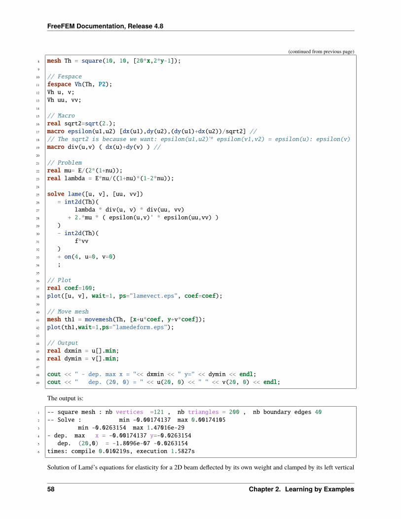
FreeFEM Documentation, Release 4.8
(continued from previous page)
8 mesh Th = square(10, 10, [20*x,2*y-1]);9
10 // Fespace11 fespace Vh(Th, P2);12 Vh u, v;13 Vh uu, vv;14
15 // Macro16 real sqrt2=sqrt(2.);17 macro epsilon(u1,u2) [dx(u1),dy(u2),(dy(u1)+dx(u2))/sqrt2] //18 // The sqrt2 is because we want: epsilon(u1,u2)'* epsilon(v1,v2) = epsilon(u): epsilon(v)19 macro div(u,v) ( dx(u)+dy(v) ) //20
21 // Problem22 real mu= E/(2*(1+nu));23 real lambda = E*nu/((1+nu)*(1-2*nu));24
25 solve lame([u, v], [uu, vv])26 = int2d(Th)(27 lambda * div(u, v) * div(uu, vv)28 + 2.*mu * ( epsilon(u,v)' * epsilon(uu,vv) )29 )30 - int2d(Th)(31 f*vv32 )33 + on(4, u=0, v=0)34 ;35
36 // Plot37 real coef=100;38 plot([u, v], wait=1, ps="lamevect.eps", coef=coef);39
40 // Move mesh41 mesh th1 = movemesh(Th, [x+u*coef, y+v*coef]);42 plot(th1,wait=1,ps="lamedeform.eps");43
44 // Output45 real dxmin = u[].min;46 real dymin = v[].min;47
48 cout << " - dep. max x = "<< dxmin << " y=" << dymin << endl;49 cout << " dep. (20, 0) = " << u(20, 0) << " " << v(20, 0) << endl;
The output is:
1 -- square mesh : nb vertices =121 , nb triangles = 200 , nb boundary edges 402 -- Solve : min -0.00174137 max 0.001741053 min -0.0263154 max 1.47016e-294 - dep. max x = -0.00174137 y=-0.02631545 dep. (20,0) = -1.8096e-07 -0.02631546 times: compile 0.010219s, execution 1.5827s
Solution of Lamé’s equations for elasticity for a 2D beam deflected by its own weight and clamped by its left vertical
58 Chapter 2. Learning by Examples
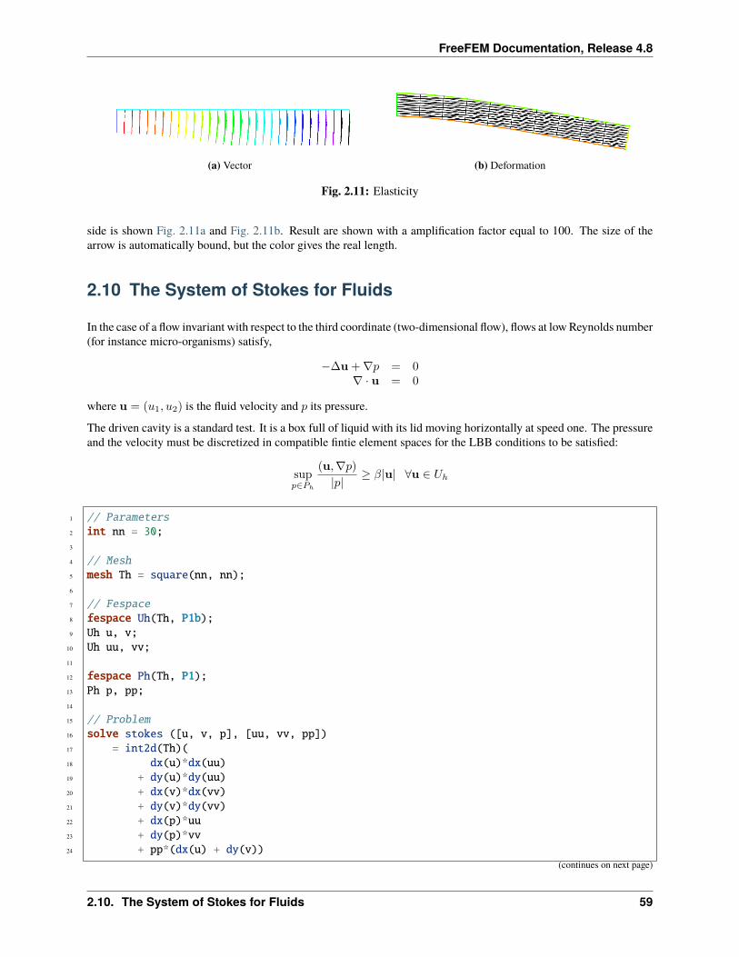
FreeFEM Documentation, Release 4.8
(a) Vector (b) Deformation
Fig. 2.11: Elasticity
side is shown Fig. 2.11a and Fig. 2.11b. Result are shown with a amplification factor equal to 100. The size of thearrow is automatically bound, but the color gives the real length.
2.10 The System of Stokes for Fluids
In the case of a flow invariant with respect to the third coordinate (two-dimensional flow), flows at low Reynolds number(for instance micro-organisms) satisfy,
−∆u +∇𝑝 = 0∇ · u = 0
where u = (𝑢1, 𝑢2) is the fluid velocity and 𝑝 its pressure.
The driven cavity is a standard test. It is a box full of liquid with its lid moving horizontally at speed one. The pressureand the velocity must be discretized in compatible fintie element spaces for the LBB conditions to be satisfied:
sup𝑝∈𝑃ℎ
(u,∇𝑝)|𝑝|
≥ 𝛽|u| ∀u ∈ 𝑈ℎ
1 // Parameters2 int nn = 30;3
4 // Mesh5 mesh Th = square(nn, nn);6
7 // Fespace8 fespace Uh(Th, P1b);9 Uh u, v;
10 Uh uu, vv;11
12 fespace Ph(Th, P1);13 Ph p, pp;14
15 // Problem16 solve stokes ([u, v, p], [uu, vv, pp])17 = int2d(Th)(18 dx(u)*dx(uu)19 + dy(u)*dy(uu)20 + dx(v)*dx(vv)21 + dy(v)*dy(vv)22 + dx(p)*uu23 + dy(p)*vv24 + pp*(dx(u) + dy(v))
(continues on next page)
2.10. The System of Stokes for Fluids 59
FreeFEM Documentation, Release 4.8
(continued from previous page)
25 - 1e-10*p*pp26 )27 + on(1, 2, 4, u=0, v=0)28 + on(3, u=1, v=0)29 ;30
31 // Plot32 plot([u, v], p, wait=1);
Note: We add a stabilization term −10e− 10 * p * pp to fix the constant part of the pressure.
Results are shown on Fig. 2.12.
2.11 A projection algorithm for the Navier-Stokes equations
Summary : Fluid flows require good algorithms and good triangultions. We show here an example of a complexalgorithm and or first example of mesh adaptation.
An incompressible viscous fluid satisfies:
𝜕𝑡u + u · ∇u +∇𝑝− 𝜈∆u = 0 in Ω×]0, 𝑇 [∇ · u = 0 in Ω×]0, 𝑇 [u|𝑡=0 = u0
u|Γ = uΓ
A possible algorithm, proposed by Chorin, is:
1𝛿𝑡 [u
𝑚+1 − u𝑚𝑜X𝑚] +∇𝑝𝑚 − 𝜈∆u𝑚 = 0u|Γ = uΓ
𝜈𝜕𝑛u|Γ𝑜𝑢𝑡 = 0
−∆𝑝𝑚+1 = −∇ · u𝑚𝑜X𝑚
𝜕𝑛𝑝𝑚+1 = 0 on Γ𝑝𝑚+1 = 0 on Γ𝑜𝑢𝑡
where u𝑜X(𝑥) = u(x − u(x)𝛿𝑡) since 𝜕𝑡u + u · ∇u is approximated by the method of characteristics, as in theprevious section.
We use the Chorin’s algorithm with free boundary condition at outlet (i.e. 𝑝 = 0, 𝜈𝜕𝑛𝑢 = 0), to compute a correction,q, to the pressure.
−∆𝑞 = ∇ · u𝑞 = 0 on Γ𝑜𝑢𝑡
and define
u𝑚+1 = u + 𝑃∇𝑞𝛿𝑡𝑝𝑚+1 = 𝑝𝑚 − 𝑞
where u is the (u𝑚+1, 𝑣𝑚+1) of Chorin’s algorithm, and where 𝑃 is the 𝐿2 projection with mass lumping ( a sparsematrix).
The backward facing step
60 Chapter 2. Learning by Examples
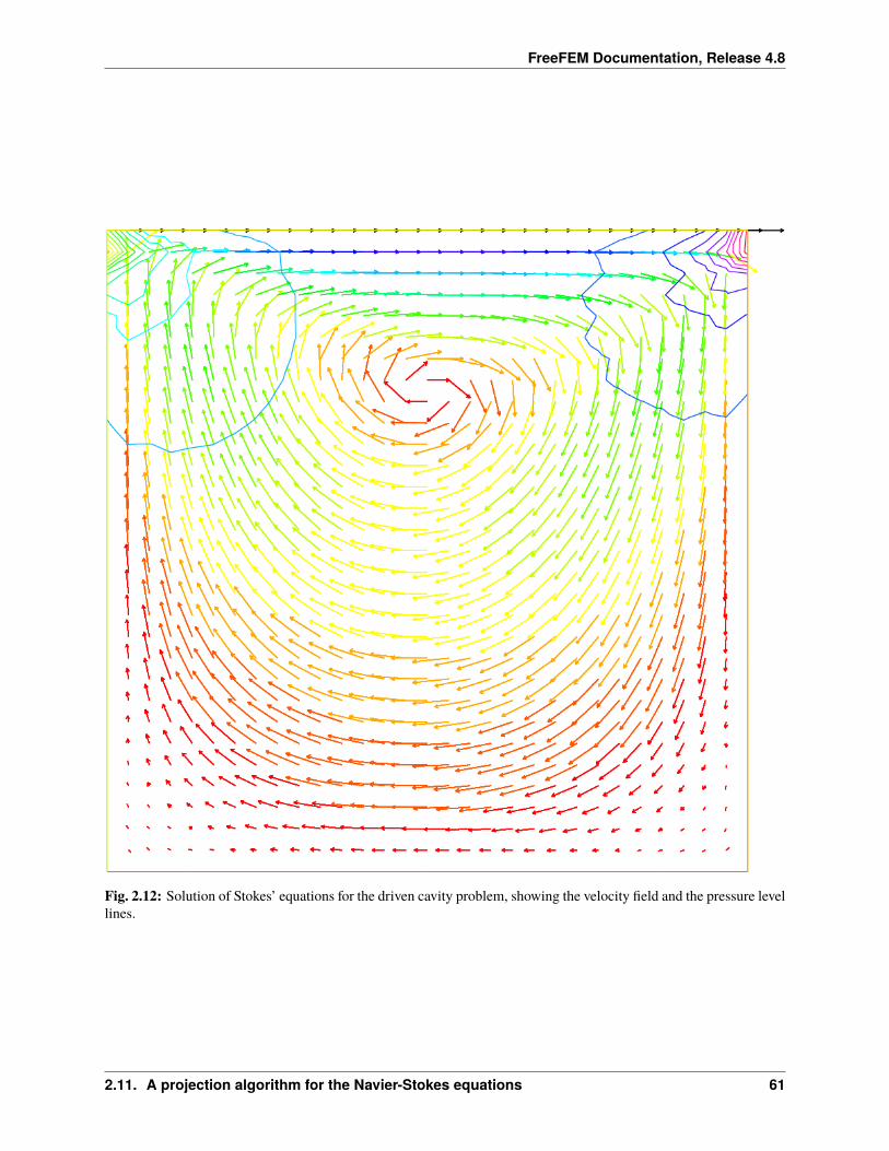
FreeFEM Documentation, Release 4.8
Fig. 2.12: Solution of Stokes’ equations for the driven cavity problem, showing the velocity field and the pressure levellines.
2.11. A projection algorithm for the Navier-Stokes equations 61
FreeFEM Documentation, Release 4.8
The geometry is that of a channel with a backward facing step so that the inflow section is smaller than the outflowsection. This geometry produces a fluid recirculation zone that must be captured correctly.
This can only be done if the triangulation is sufficiently fine, or well adapted to the flow.
Note: There is a technical difficulty in the example: the output B.C. Here we put 𝑝 = 0 and 𝜈𝜕𝑛𝑢 = 0.
1 // Parameters2 verbosity = 0;3 int nn = 1;4 real nu = 0.0025;5 real dt = 0.2;6 real epsv = 1e-6;7 real epsu = 1e-6;8 real epsp = 1e-6;9
10 // Mesh11 border a0(t=1, 0)x=-2; y=t; label=1;12 border a1(t=-2, 0)x=t; y=0; label=2;13 border a2(t=0, -0.5)x=0; y=t; label=2;14 border a3(t=0, 1)x=18*t^1.2; y=-0.5; label=2;15 border a4(t=-0.5, 1)x=18; y=t; label=3;16 border a5(t=1, 0)x=-2+20*t; y=1; label=4;17
18 mesh Th = buildmesh(a0(3*nn) + a1(20*nn) + a2(10*nn) + a3(150*nn) + a4(5*nn) +→˓a5(100*nn));
19 plot(Th);20
21 // Fespace22 fespace Vh(Th, P1);23 Vh w;24 Vh u=0, v=0;25 Vh p=0;26 Vh q=0;27
28 // Definition of Matrix dtMx and dtMy29 matrix dtM1x, dtM1y;30
31 // Macro32 macro BuildMat()33 /* for memory managenemt */34 varf vM(unused, v) = int2d(Th)(v);35 varf vdx(u, v) = int2d(Th)(v*dx(u)*dt);36 varf vdy(u, v) = int2d(Th)(v*dy(u)*dt);37
38 real[int] Mlump = vM(0, Vh);39 real[int] one(Vh.ndof); one = 1;40 real[int] M1 = one ./ Mlump;41 matrix dM1 = M1;42 matrix Mdx = vdx(Vh, Vh);43 matrix Mdy = vdy(Vh, Vh);44 dtM1x = dM1*Mdx;
(continues on next page)
62 Chapter 2. Learning by Examples
FreeFEM Documentation, Release 4.8
(continued from previous page)
45 dtM1y = dM1*Mdy;46 //47
48 // Build matrices49 BuildMat50
51 // Time iterations52 real err = 1.;53 real outflux = 1.;54 for(int n = 0; n < 300; n++)55 // Update56 Vh uold=u, vold=v, pold=p;57
58 // Solve59 solve pb4u (u, w, init=n, solver=CG, eps=epsu)60 = int2d(Th)(61 u*w/dt62 + nu*(dx(u)*dx(w) + dy(u)*dy(w))63 )64 -int2d(Th)(65 convect([uold, vold], -dt, uold)/dt*w66 - dx(p)*w67 )68 + on(1, u=4*y*(1-y))69 + on(2, 4, u=0)70 ;71
72 plot(u);73
74 solve pb4v (v, w, init=n, solver=CG, eps=epsv)75 = int2d(Th)(76 v*w/dt77 + nu*(dx(v)*dx(w) + dy(v)*dy(w))78 )79 -int2d(Th)(80 convect([uold,vold],-dt,vold)/dt*w81 - dy(p)*w82 )83 +on(1, 2, 3, 4, v=0)84 ;85
86 solve pb4p (q, w, solver=CG, init=n, eps=epsp)87 = int2d(Th)(88 dx(q)*dx(w)+dy(q)*dy(w)89 )90 - int2d(Th)(91 (dx(u)+ dy(v))*w/dt92 )93 + on(3, q=0)94 ;95
96 //to have absolute epsilon in CG algorithm.
(continues on next page)
2.11. A projection algorithm for the Navier-Stokes equations 63
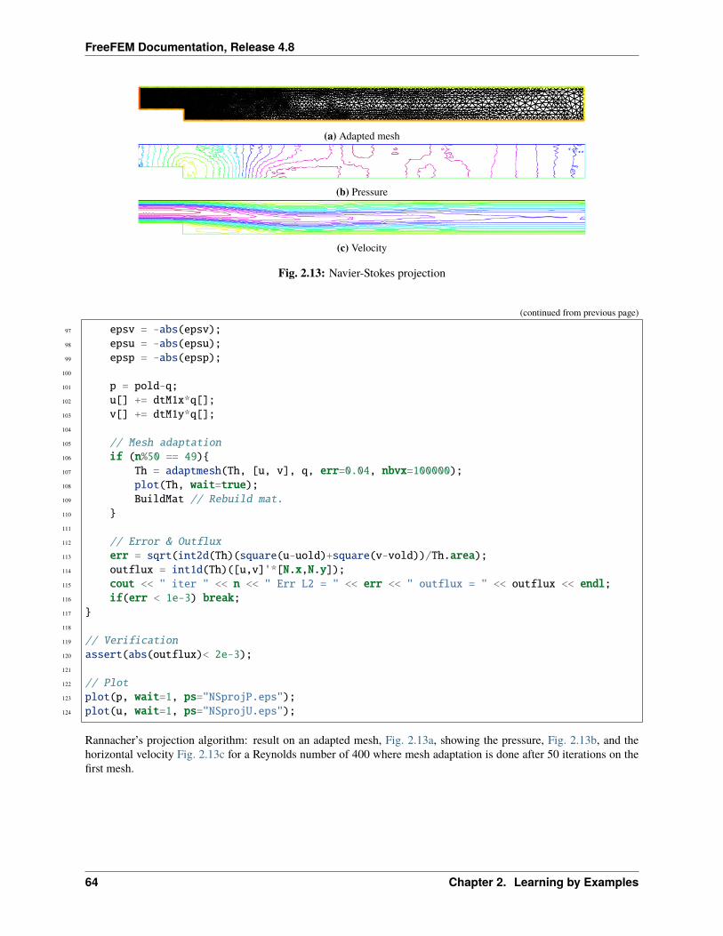
FreeFEM Documentation, Release 4.8
(a) Adapted mesh
(b) Pressure
(c) Velocity
Fig. 2.13: Navier-Stokes projection
(continued from previous page)
97 epsv = -abs(epsv);98 epsu = -abs(epsu);99 epsp = -abs(epsp);
100
101 p = pold-q;102 u[] += dtM1x*q[];103 v[] += dtM1y*q[];104
105 // Mesh adaptation106 if (n%50 == 49)107 Th = adaptmesh(Th, [u, v], q, err=0.04, nbvx=100000);108 plot(Th, wait=true);109 BuildMat // Rebuild mat.110 111
112 // Error & Outflux113 err = sqrt(int2d(Th)(square(u-uold)+square(v-vold))/Th.area);114 outflux = int1d(Th)([u,v]'*[N.x,N.y]);115 cout << " iter " << n << " Err L2 = " << err << " outflux = " << outflux << endl;116 if(err < 1e-3) break;117 118
119 // Verification120 assert(abs(outflux)< 2e-3);121
122 // Plot123 plot(p, wait=1, ps="NSprojP.eps");124 plot(u, wait=1, ps="NSprojU.eps");
Rannacher’s projection algorithm: result on an adapted mesh, Fig. 2.13a, showing the pressure, Fig. 2.13b, and thehorizontal velocity Fig. 2.13c for a Reynolds number of 400 where mesh adaptation is done after 50 iterations on thefirst mesh.
64 Chapter 2. Learning by Examples

FreeFEM Documentation, Release 4.8
2.12 Newton Method for the Steady Navier-Stokes equations
The problem is find the velocity field u = (𝑢𝑖)𝑑𝑖=1 and the pressure 𝑝 of a Flow satisfying in the domain Ω ⊂ R𝑑(𝑑 =
2, 3):
(u · ∇)u− 𝜈∆u +∇𝑝 = 0∇ · u = 0
where 𝜈 is the viscosity of the fluid, ∇ = (𝜕𝑖)𝑑𝑖=1, the dot product is ·, and ∆ = ∇ · ∇ with the same boundary
conditions (u is given on Γ).
The weak form is find u, 𝑝 such that for ∀v (zero on Γ), and ∀𝑞:∫Ω
((u · ∇)u).v + 𝜈∇u : ∇v − 𝑝∇ · v − 𝑞∇ · u = 0
The Newton Algorithm to solve nonlinear problem is:
Find 𝑢 ∈ 𝑉 such that 𝐹 (𝑢) = 0 where 𝐹 : 𝑉 ↦→ 𝑉 .
1. choose 𝑢0 ∈ R𝑛 , ;
2. for ( 𝑖 = 0; 𝑖 < niter; 𝑖 = 𝑖+ 1)
1. solve 𝐷𝐹 (𝑢𝑖)𝑤𝑖 = 𝐹 (𝑢𝑖);
2. 𝑢𝑖+1 = 𝑢𝑖 − 𝑤𝑖;
break ||𝑤𝑖|| < 𝜀.
Where 𝐷𝐹 (𝑢) is the differential of 𝐹 at point 𝑢, this is a linear application such that:
𝐹 (𝑢+ 𝛿) = 𝐹 (𝑢) +𝐷𝐹 (𝑢)𝛿 + 𝑜(𝛿)
For Navier Stokes, 𝐹 and 𝐷𝐹 are:
𝐹 (u, 𝑝) =∫Ω
((u · ∇)u).v + 𝜈∇u : ∇v − 𝑝∇ · v − 𝑞∇ · u𝐷𝐹 (u, 𝑝)(𝛿u, 𝛿𝑝) =
∫Ω
((𝛿u · ∇)u).v + ((u · ∇)𝛿u).v+ 𝜈∇𝛿u : ∇v − 𝛿𝑝∇ · v − 𝑞∇ · 𝛿u
So the Newton algorithm become:
1 // Parameters2 real R = 5.;3 real L = 15.;4
5 real nu = 1./50.;6 real nufinal = 1/200.;7 real cnu = 0.5;8
9 real eps = 1e-6;10
11 verbosity = 0;12
13 // Mesh14 border cc(t=0, 2*pi)x=cos(t)/2.; y=sin(t)/2.; label=1;15 border ce(t=pi/2, 3*pi/2)x=cos(t)*R; y=sin(t)*R; label=1;16 border beb(tt=0, 1)real t=tt^1.2; x=t*L; y=-R; label=1;
(continues on next page)
2.12. Newton Method for the Steady Navier-Stokes equations 65
FreeFEM Documentation, Release 4.8
(continued from previous page)
17 border beu(tt=1, 0)real t=tt^1.2; x=t*L; y=R; label=1;18 border beo(t=-R, R)x=L; y=t; label=0;19 border bei(t=-R/4, R/4)x=L/2; y=t; label=0;20 mesh Th = buildmesh(cc(-50) + ce(30) + beb(20) + beu(20) + beo(10) + bei(10));21 plot(Th);22
23 //bounding box for the plot24 func bb = [[-1,-2],[4,2]];25
26 // Fespace27 fespace Xh(Th, P2);28 Xh u1, u2;29 Xh v1,v2;30 Xh du1,du2;31 Xh u1p,u2p;32
33 fespace Mh(Th,P1);34 Mh p;35 Mh q;36 Mh dp;37 Mh pp;38
39 // Macro40 macro Grad(u1,u2) [dx(u1), dy(u1), dx(u2),dy(u2)] //41 macro UgradV(u1,u2,v1,v2) [[u1,u2]'*[dx(v1),dy(v1)],42 [u1,u2]'*[dx(v2),dy(v2)]] //43 macro div(u1,u2) (dx(u1) + dy(u2)) //44
45 // Initialization46 u1 = (x^2+y^2) > 2;47 u2 = 0;48
49 // Viscosity loop50 while(1)51 int n;52 real err=0;53 // Newton loop54 for (n = 0; n < 15; n++)55 // Newton56 solve Oseen ([du1, du2, dp], [v1, v2, q])57 = int2d(Th)(58 nu * (Grad(du1,du2)' * Grad(v1,v2))59 + UgradV(du1,du2, u1, u2)' * [v1,v2]60 + UgradV( u1, u2,du1,du2)' * [v1,v2]61 - div(du1,du2) * q62 - div(v1,v2) * dp63 - 1e-8*dp*q //stabilization term64 )65 - int2d(Th) (66 nu * (Grad(u1,u2)' * Grad(v1,v2))67 + UgradV(u1,u2, u1, u2)' * [v1,v2]68 - div(u1,u2) * q
(continues on next page)
66 Chapter 2. Learning by Examples
FreeFEM Documentation, Release 4.8
(continued from previous page)
69 - div(v1,v2) * p70 )71 + on(1, du1=0, du2=0)72 ;73
74 u1[] -= du1[];75 u2[] -= du2[];76 p[] -= dp[];77
78 real Lu1=u1[].linfty, Lu2=u2[].linfty, Lp=p[].linfty;79 err = du1[].linfty/Lu1 + du2[].linfty/Lu2 + dp[].linfty/Lp;80
81 cout << n << " err = " << err << " " << eps << " rey = " << 1./nu << endl;82 if(err < eps) break; //converge83 if( n>3 && err > 10.) break; //blowup84 85
86 if(err < eps) //converge: decrease $\nu$ (more difficult)87 // Plot88 plot([u1, u2], p, wait=1, cmm=" rey = " + 1./nu , coef=0.3, bb=bb);89
90 // Change nu91 if( nu == nufinal) break;92 if( n < 4) cnu = cnu^1.5; //fast converge => change faster93 nu = max(nufinal, nu* cnu); //new viscosity94
95 // Update96 u1p = u1;97 u2p = u2;98 pp = p;99
100 else //blowup: increase $\nu$ (more simple)101 assert(cnu< 0.95); //the method finally blowup102
103 // Recover nu104 nu = nu/cnu;105 cnu= cnu^(1./1.5); //no conv. => change lower106 nu = nu* cnu; //new viscosity107 cout << " restart nu = " << nu << " Rey = " << 1./nu << " (cnu = " << cnu << " )
→˓\n";108
109 // Recover a correct solution110 u1 = u1p;111 u2 = u2p;112 p = pp;113 114
Note: We use a trick to make continuation on the viscosity 𝜈, because the Newton method blowup owe start with thefinal viscosity 𝜈.
2.12. Newton Method for the Steady Navier-Stokes equations 67
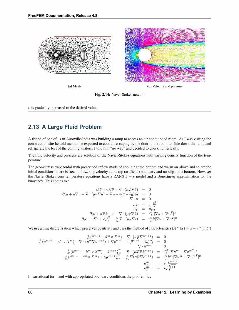
FreeFEM Documentation, Release 4.8
(a) Mesh (b) Velocity and pressure
Fig. 2.14: Naver-Stokes newton
𝜈 is gradually increased to the desired value.
2.13 A Large Fluid Problem
A friend of one of us in Auroville-India was building a ramp to access an air conditioned room. As I was visiting theconstruction site he told me that he expected to cool air escaping by the door to the room to slide down the ramp andrefrigerate the feet of the coming visitors. I told him “no way” and decided to check numerically.
The fluid velocity and pressure are solution of the Navier-Stokes equations with varying density function of the tem-perature.
The geometry is trapezoidal with prescribed inflow made of cool air at the bottom and warm air above and so are theinitial conditions; there is free outflow, slip velocity at the top (artificial) boundary and no-slip at the bottom. Howeverthe Navier-Stokes cum temperature equations have a RANS 𝑘 − 𝜖 model and a Boussinesq approximation for thebuoyancy. This comes to :
𝜕𝑡𝜃 + 𝑢∇𝜃 −∇ · (𝜅𝑚𝑇 ∇𝜃) = 0𝜕𝑡𝑢+ 𝑢∇𝑢−∇ · (𝜇𝑇∇𝑢) +∇𝑝+ 𝑒(𝜃 − 𝜃0)2 = 0
∇ · 𝑢 = 0
𝜇𝑇 = 𝑐𝜇𝑘2
𝜖𝜅𝑇 = 𝜅𝜇𝑇
𝜕𝑡𝑘 + 𝑢∇𝑘 + 𝜖−∇ · (𝜇𝑇∇𝑘) = 𝜇𝑇
2 |∇𝑢+∇𝑢𝑇 |2
𝜕𝑡𝜖+ 𝑢∇𝜖+ 𝑐2𝜖2
𝑘 −𝑐𝜖𝑐𝜇∇ · (𝜇𝑇∇𝜖) = 𝑐1
2 𝑘|∇𝑢+∇𝑢𝑇 |2
We use a time discretization which preserves positivity and uses the method of characteristics (𝑋𝑚(𝑥) ≈ 𝑥−𝑢𝑚(𝑥)𝛿𝑡)
1𝛿𝑡 (𝜃
𝑚+1 − 𝜃𝑚 ∘𝑋𝑚)−∇ · (𝜅𝑚𝑇 ∇𝜃𝑚+1) = 01𝛿𝑡 (𝑢
𝑚+1 − 𝑢𝑚 ∘𝑋𝑚)−∇ · (𝜇𝑚𝑇 ∇𝑢𝑚+1) +∇𝑝𝑚+1 + 𝑒(𝜃𝑚+1 − 𝜃0)2 = 0∇ · 𝑢𝑚+1 = 0
1𝛿𝑡 (𝑘
𝑚+1 − 𝑘𝑚 ∘𝑋𝑚) + 𝑘𝑚+1 𝜖𝑚
𝑘𝑚 −∇ · (𝜇𝑚𝑇 ∇𝑘𝑚+1) =
𝜇𝑚𝑇
2 |∇𝑢𝑚 +∇𝑢𝑚𝑇 |2
1𝛿𝑡 (𝜖
𝑚+1 − 𝜖𝑚 ∘𝑋𝑚) + 𝑐2𝜖𝑚+1 𝜖𝑚
𝑘𝑚 −𝑐𝜖𝑐𝜇∇(𝜇𝑚𝑇 ∇𝜖𝑚+1) = 𝑐1
2 𝑘𝑚|∇𝑢𝑚 +∇𝑢𝑚𝑇 |2
𝜇𝑚+1𝑇 = 𝑐𝜇
𝑘𝑚+12
𝜖𝑚+1
𝜅𝑚+1𝑇 = 𝜅𝜇𝑚+1
𝑇
In variational form and with appropriated boundary conditions the problem is :
68 Chapter 2. Learning by Examples
FreeFEM Documentation, Release 4.8
1 load "iovtk"2
3 verbosity=0;4
5 // Parameters6 int nn = 15;7 int nnPlus = 5;8 real l = 1.;9 real L = 15.;
10 real hSlope = 0.1;11 real H = 6.;12 real h = 0.5;13
14 real reylnods =500;15 real beta = 0.01;16
17 real eps = 9.81/303.;18 real nu = 1;19 real numu = nu/sqrt(0.09);20 real nuep = pow(nu,1.5)/4.1;21 real dt = 0.;22
23 real Penalty = 1.e-6;24
25 // Mesh26 border b1(t=0, l)x=t; y=0;27 border b2(t=0, L-l)x=1.+t; y=-hSlope*t;28 border b3(t=-hSlope*(L-l), H)x=L; y=t;29 border b4(t=L, 0)x=t; y=H;30 border b5(t=H, h)x=0; y=t;31 border b6(t=h, 0)x=0; y=t;32
33 mesh Th=buildmesh(b1(nnPlus*nn*l) + b2(nn*sqrt((L-l)^2+(hSlope*(L-l))^2)) + b3(nn*(H +→˓hSlope*(L-l))) + b4(nn*L) + b5(nn*(H-h)) + b6(nnPlus*nn*h));
34 plot(Th);35
36 // Fespaces37 fespace Vh2(Th, P1b);38 Vh2 Ux, Uy;39 Vh2 Vx, Vy;40 Vh2 Upx, Upy;41
42 fespace Vh(Th,P1);43 Vh p=0, q;44 Vh Tp, T=35;45 Vh k=0.0001, kp=k;46 Vh ep=0.0001, epp=ep;47
48 fespace V0h(Th,P0);49 V0h muT=1;50 V0h prodk, prode;51 Vh kappa=0.25e-4, stress;52
(continues on next page)
2.13. A Large Fluid Problem 69
FreeFEM Documentation, Release 4.8
(continued from previous page)
53 // Macro54 macro grad(u) [dx(u), dy(u)] //55 macro Grad(U) [grad(U#x), grad(U#y)] //56 macro Div(U) (dx(U#x) + dy(U#y)) //57
58 // Functions59 func g = (x) * (1-x) * 4;60
61 // Problem62 real alpha = 0.;63
64 problem Temperature(T, q)65 = int2d(Th)(66 alpha * T * q67 + kappa* grad(T)' * grad(q)68 )69 + int2d(Th)(70 - alpha*convect([Upx, Upy], -dt, Tp)*q71 )72 + on(b6, T=25)73 + on(b1, b2, T=30)74 ;75
76 problem KineticTurbulence(k, q)77 = int2d(Th)(78 (epp/kp + alpha) * k * q79 + muT* grad(k)' * grad(q)80 )81 + int2d(Th)(82 prodk * q83 - alpha*convect([Upx, Upy], -dt, kp)*q84 )85 + on(b5, b6, k=0.00001)86 + on(b1, b2, k=beta*numu*stress)87 ;88
89 problem ViscosityTurbulence(ep, q)90 = int2d(Th)(91 (1.92*epp/kp + alpha) * ep * q92 + muT * grad(ep)' * grad(q)93 )94 + int1d(Th, b1, b2)(95 T * q * 0.00196 )97 + int2d(Th)(98 prode * q99 - alpha*convect([Upx, Upy], -dt, epp)*q
100 )101 + on(b5, b6, ep=0.00001)102 + on(b1, b2, ep=beta*nuep*pow(stress,1.5))103 ;104
(continues on next page)
70 Chapter 2. Learning by Examples
FreeFEM Documentation, Release 4.8
(continued from previous page)
105 // Initialization with stationary solution106 solve NavierStokes ([Ux, Uy, p], [Vx, Vy, q])107 = int2d(Th)(108 alpha * [Ux, Uy]' * [Vx, Vy]109 + muT * (Grad(U) : Grad(V))110 + p * q * Penalty111 - p * Div(V)112 - Div(U) * q113 )114 + int1d(Th, b1, b2, b4)(115 Ux * Vx * 0.1116 )117 + int2d(Th)(118 eps * (T-35) * Vx119 - alpha*convect([Upx, Upy], -dt, Upx)*Vx120 - alpha*convect([Upx, Upy], -dt, Upy)*Vy121 )122 + on(b6, Ux=3, Uy=0)123 + on(b5, Ux=0, Uy=0)124 + on(b1, b4, Uy=0)125 + on(b2, Uy=-Upx*N.x/N.y)126 + on(b3, Uy=0)127 ;128
129 plot([Ux, Uy], p, value=true, coef=0.2, cmm="[Ux, Uy] - p");130
131 132 real[int] xx(21), yy(21), pp(21);133 for (int i = 0 ; i < 21; i++)134 yy[i] = i/20.;135 xx[i] = Ux(0.5,i/20.);136 pp[i] = p(i/20.,0.999);137 138 cout << " " << yy << endl;139 plot([xx, yy], wait=true, cmm="Ux x=0.5 cup");140 plot([yy, pp], wait=true, cmm="p y=0.999 cup");141 142
143 // Initialization144 dt = 0.1; //probably too big145 int nbiter = 3;146 real coefdt = 0.25^(1./nbiter);147 real coefcut = 0.25^(1./nbiter);148 real cut = 0.01;149 real tol = 0.5;150 real coeftol = 0.5^(1./nbiter);151 nu = 1./reylnods;152
153 T = T - 10*((x<1)*(y<0.5) + (x>=1)*(y+0.1*(x-1)<0.5));154
155 // Convergence loop156 real T0 = clock();
(continues on next page)
2.13. A Large Fluid Problem 71
FreeFEM Documentation, Release 4.8
(continued from previous page)
157 for (int iter = 1; iter <= nbiter; iter++)158 cout << "Iteration " << iter << " - dt = " << dt << endl;159 alpha = 1/dt;160
161 // Time loop162 real t = 0.;163 for (int i = 0; i <= 500; i++)164 t += dt;165 cout << "Time step " << i << " - t = " << t << endl;166
167 // Update168 Upx = Ux;169 Upy = Uy;170 kp = k;171 epp = ep;172 Tp = max(T, 25); //for beauty only should be removed173 Tp = min(Tp, 35); //for security only should be removed174 kp = max(k, 0.0001); epp = max(ep, 0.0001); // to be secure: should not be active175 muT = 0.09*kp*kp/epp;176
177 // Solve NS178 NavierStokes;179
180 // Update181 prode = -0.126*kp*(pow(2*dx(Ux),2)+pow(2*dy(Uy),2)+2*pow(dx(Uy)+dy(Ux),2))/2;182 prodk = -prode*kp/epp*0.09/0.126;183 kappa = muT/0.41;184 stress = abs(dy(Ux));185
186 // Solve k-eps-T187 KineticTurbulence;188 ViscosityTurbulence;189 Temperature;190
191 // Plot192 plot(T, value=true, fill=true);193 plot([Ux, Uy], p, coef=0.2, cmm=" [Ux, Uy] - p", WindowIndex=1);194
195 // Time196 cout << "\tTime = " << clock()-T0 << endl;197 198
199 // Check200 if (iter >= nbiter) break;201
202 // Adaptmesh203 Th = adaptmesh(Th, [dx(Ux), dy(Ux), dx(Ux), dy(Uy)], splitpbedge=1, abserror=0,
→˓cutoff=cut, err=tol, inquire=0, ratio=1.5, hmin=1./1000);204 plot(Th);205
206 // Update207 dt = dt * coefdt;
(continues on next page)
72 Chapter 2. Learning by Examples
FreeFEM Documentation, Release 4.8
(continued from previous page)
208 tol = tol * coeftol;209 cut = cut * coefcut;210 211 cout << "Total Time = " << clock()-T0 << endl;
2.14 An Example with Complex Numbers
In a microwave oven heat comes from molecular excitation by an electromagnetic field. For a plane monochromaticwave, amplitude is given by Helmholtz’s equation:
𝛽𝑣 + ∆𝑣 = 0.
We consider a rectangular oven where the wave is emitted by part of the upper wall. So the boundary of the domain is
made up of a part Γ1 where 𝑣 = 0 and of another part Γ2 = [𝑐, 𝑑] where for instance 𝑣 = sin
(𝜋𝑦 − 𝑐𝑐− 𝑑
).
Within an object to be cooked, denoted by 𝐵, the heat source is proportional to 𝑣2. At equilibrium, one has :
−∆𝜃 = 𝑣2𝐼𝐵𝜃Γ = 0
where 𝐼𝐵 is 1 in the object and 0 elsewhere.
In the program below 𝛽 = 1/(1− 𝑖/2) in the air and 2/(1− 𝑖/2) in the object (𝑖 =√−1):
1 // Parameters2 int nn = 2;3 real a = 20.;4 real b = 20.;5 real c = 15.;6 real d = 8.;7 real e = 2.;8 real l = 12.;9 real f = 2.;
10 real g = 2.;11
12 // Mesh13 border a0(t=0, 1)x=a*t; y=0; label=1;14 border a1(t=1, 2)x=a; y=b*(t-1); label=1;15 border a2(t=2, 3) x=a*(3-t); y=b; label=1;16 border a3(t=3, 4)x=0; y=b-(b-c)*(t-3); label=1;17 border a4(t=4, 5)x=0; y=c-(c-d)*(t-4); label=2;18 border a5(t=5, 6)x=0; y=d*(6-t); label=1;19
20 border b0(t=0, 1)x=a-f+e*(t-1); y=g; label=3;21 border b1(t=1, 4)x=a-f; y=g+l*(t-1)/3; label=3;22 border b2(t=4, 5)x=a-f-e*(t-4); y=l+g; label=3;23 border b3(t=5, 8)x=a-e-f; y=l+g-l*(t-5)/3; label=3;24
25 mesh Th = buildmesh(a0(10*nn) + a1(10*nn) + a2(10*nn) + a3(10*nn) +a4(10*nn) + a5(10*nn)26 + b0(5*nn) + b1(10*nn) + b2(5*nn) + b3(10*nn));27 real meat = Th(a-f-e/2, g+l/2).region;
(continues on next page)
2.14. An Example with Complex Numbers 73
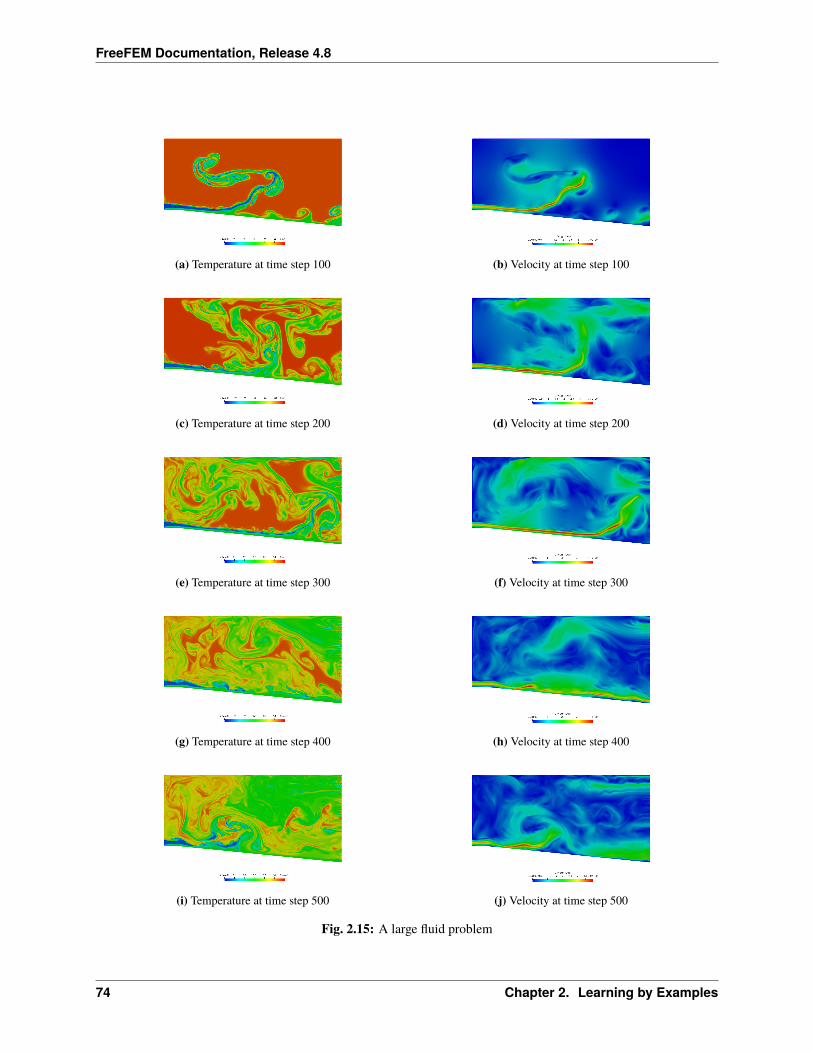
FreeFEM Documentation, Release 4.8
(a) Temperature at time step 100 (b) Velocity at time step 100
(c) Temperature at time step 200 (d) Velocity at time step 200
(e) Temperature at time step 300 (f) Velocity at time step 300
(g) Temperature at time step 400 (h) Velocity at time step 400
(i) Temperature at time step 500 (j) Velocity at time step 500
Fig. 2.15: A large fluid problem
74 Chapter 2. Learning by Examples
FreeFEM Documentation, Release 4.8
(continued from previous page)
28 real air= Th(0.01,0.01).region;29 plot(Th, wait=1);30
31 // Fespace32 fespace Vh(Th, P1);33 Vh R=(region-air)/(meat-air);34 Vh<complex> v, w;35 Vh vr, vi;36
37 fespace Uh(Th, P1);38 Uh u, uu, ff;39
40 // Problem41 solve muwave(v, w)42 = int2d(Th)(43 v*w*(1+R)44 - (dx(v)*dx(w) + dy(v)*dy(w))*(1 - 0.5i)45 )46 + on(1, v=0)47 + on(2, v=sin(pi*(y-c)/(c-d)))48 ;49
50 vr = real(v);51 vi = imag(v);52
53 // Plot54 plot(vr, wait=1, ps="rmuonde.ps", fill=true);55 plot(vi, wait=1, ps="imuonde.ps", fill=true);56
57 // Problem (temperature)58 ff=1e5*(vr^2 + vi^2)*R;59
60 solve temperature(u, uu)61 = int2d(Th)(62 dx(u)* dx(uu)+ dy(u)* dy(uu)63 )64 - int2d(Th)(65 ff*uu66 )67 + on(1, 2, u=0)68 ;69
70 // Plot71 plot(u, wait=1, ps="tempmuonde.ps", fill=true);
Results are shown on Fig. 2.16a, Fig. 2.16b and Fig. 2.16c.
2.14. An Example with Complex Numbers 75
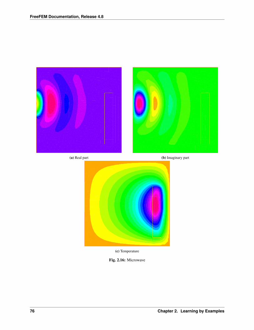
FreeFEM Documentation, Release 4.8
(a) Real part (b) Imaginary part
(c) Temperature
Fig. 2.16: Microwave
76 Chapter 2. Learning by Examples
FreeFEM Documentation, Release 4.8
2.15 Optimal Control
Thanks to the function BFGS it is possible to solve complex nonlinear optimization problem within FreeFEM. Forexample consider the following inverse problem
min𝑏,𝑐,𝑑∈𝑅 𝐽 =∫𝐸
(𝑢− 𝑢𝑑)2−∇(𝜅(𝑏, 𝑐, 𝑑) · ∇𝑢) = 0
𝑢|Γ = 𝑢Γ
where the desired state 𝑢𝑑, the boundary data 𝑢Γ and the observation set 𝐸 ⊂ Ω are all given. Furthermore let usassume that:
𝜅(𝑥) = 1 + 𝑏𝐼𝐵(𝑥) + 𝑐𝐼𝐶(𝑥) + 𝑑𝐼𝐷(𝑥) ∀𝑥 ∈ Ω
where 𝐵,𝐶,𝐷 are separated subsets of Ω.
To solve this problem by the quasi-Newton BFGS method we need the derivatives of 𝐽 with respect to 𝑏, 𝑐, 𝑑. We selfexplanatory notations, if 𝛿𝑏, 𝛿𝑐, 𝛿𝑑 are variations of 𝑏, 𝑐, 𝑑 we have:
𝛿𝐽 ≈ 2∫𝐸
(𝑢− 𝑢𝑑)𝛿𝑢−∇(𝜅 · ∇𝛿𝑢) ≈ ∇(𝛿𝜅 · ∇𝑢)
𝛿𝑢|Γ = 0
Obviously 𝐽 ′𝑏 is equal to 𝛿𝐽 when 𝛿𝑏 = 1, 𝛿𝑐 = 0, 𝛿𝑑 = 0, and so on for 𝐽 ′
𝑐 and 𝐽 ′𝑑.
All this is implemented in the following program:
1 // Mesh2 border aa(t=0, 2*pi)x=5*cos(t); y=5*sin(t);;3 border bb(t=0, 2*pi)x=cos(t); y=sin(t);;4 border cc(t=0, 2*pi)x=-3+cos(t); y=sin(t);;5 border dd(t=0, 2*pi)x=cos(t); y =-3+sin(t);;6
7 mesh th = buildmesh(aa(70) + bb(35) + cc(35) + dd(35));8
9 // Fespace10 fespace Vh(th, P1);11 Vh Ib=((x^2+y^2)<1.0001),12 Ic=(((x+3)^2+ y^2)<1.0001),13 Id=((x^2+(y+3)^2)<1.0001),14 Ie=(((x-1)^2+ y^2)<=4),15 ud, u, uh, du;16
17 // Problem18 real[int] z(3);19 problem A(u, uh)20 = int2d(th)(21 (1+z[0]*Ib+z[1]*Ic+z[2]*Id)*(dx(u)*dx(uh) + dy(u)*dy(uh))22 )23 + on(aa, u=x^3-y^3)24 ;25
26 // Solve27 z[0]=2; z[1]=3; z[2]=4;28 A;
(continues on next page)
2.15. Optimal Control 77
FreeFEM Documentation, Release 4.8
(continued from previous page)
29 ud = u;30
31 ofstream f("J.txt");32 func real J(real[int] & Z)33 for (int i = 0; i < z.n; i++)34 z[i] =Z[i];35 A;36 real s = int2d(th)(Ie*(u-ud)^2);37 f << s << " ";38 return s;39 40
41 // Problem BFGS42 real[int] dz(3), dJdz(3);43 problem B (du, uh)44 = int2d(th)(45 (1+z[0]*Ib+z[1]*Ic+z[2]*Id)*(dx(du)*dx(uh) + dy(du)*dy(uh))46 )47 + int2d(th)(48 (dz[0]*Ib+dz[1]*Ic+dz[2]*Id)*(dx(u)*dx(uh) + dy(u)*dy(uh))49 )50 +on(aa, du=0)51 ;52
53 func real[int] DJ(real[int] &Z)54 for(int i = 0; i < z.n; i++)55 for(int j = 0; j < dz.n; j++)56 dz[j] = 0;57 dz[i] = 1;58 B;59 dJdz[i] = 2*int2d(th)(Ie*(u-ud)*du);60 61 return dJdz;62 63
64 real[int] Z(3);65 for(int j = 0; j < z.n; j++)66 Z[j]=1;67
68 BFGS(J, DJ, Z, eps=1.e-6, nbiter=15, nbiterline=20);69 cout << "BFGS: J(z) = " << J(Z) << endl;70 for(int j = 0; j < z.n; j++)71 cout << z[j] << endl;72
73 // Plot74 plot(ud, value=1, ps="u.eps");
In this example the sets 𝐵,𝐶,𝐷,𝐸 are circles of boundaries 𝑏𝑏, 𝑐𝑐, 𝑑𝑑, 𝑒𝑒 and the domain Ω is the circle of boundary𝑎𝑎.
The desired state 𝑢𝑑 is the solution of the PDE for 𝑏 = 2, 𝑐 = 3, 𝑑 = 4. The unknowns are packed into array 𝑧.
78 Chapter 2. Learning by Examples
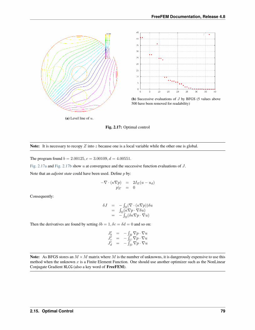
FreeFEM Documentation, Release 4.8
(a) Level line of 𝑢.
(b) Successive evaluations of 𝐽 by BFGS (5 values above500 have been removed for readability)
Fig. 2.17: Optimal control
Note: It is necessary to recopy 𝑍 into 𝑧 because one is a local variable while the other one is global.
The program found 𝑏 = 2.00125, 𝑐 = 3.00109, 𝑑 = 4.00551.
Fig. 2.17a and Fig. 2.17b show 𝑢 at convergence and the successive function evaluations of 𝐽 .
Note that an adjoint state could have been used. Define 𝑝 by:
−∇ · (𝜅∇𝑝) = 2𝐼𝐸(𝑢− 𝑢𝑑)𝑝|Γ = 0
Consequently:
𝛿𝐽 = −∫Ω
(∇ · (𝜅∇𝑝))𝛿𝑢=
∫Ω
(𝜅∇𝑝 · ∇𝛿𝑢)= −
∫Ω
(𝛿𝜅∇𝑝 · ∇𝑢)
Then the derivatives are found by setting 𝛿𝑏 = 1, 𝛿𝑐 = 𝛿𝑑 = 0 and so on:
𝐽 ′𝑏 = −
∫𝐵∇𝑝 · ∇𝑢
𝐽 ′𝑐 = −
∫𝐶∇𝑝 · ∇𝑢
𝐽 ′𝑑 = −
∫𝐷∇𝑝 · ∇𝑢
Note: As BFGS stores an𝑀 ×𝑀 matrix where𝑀 is the number of unknowns, it is dangerously expensive to use thismethod when the unknown 𝑥 is a Finite Element Function. One should use another optimizer such as the NonLinearConjugate Gradient NLCG (also a key word of FreeFEM).
2.15. Optimal Control 79
FreeFEM Documentation, Release 4.8
2.16 A Flow with Shocks
Compressible Euler equations should be discretized with Finite Volumes or FEM with flux up-winding scheme but theseare not implemented in FreeFEM. Nevertheless acceptable results can be obtained with the method of characteristicsprovided that the mean values 𝑓 =
1
2
(𝑓+ + 𝑓−
)are used at shocks in the scheme, and finally mesh adaptation.
𝜕𝑡𝜌+ ∇𝜌+ 𝜌∇ · 𝑢 = 0
𝜌(𝜕𝑡𝑢+ 𝜌𝑢𝜌 ∇𝑢+∇𝑝 = 0
𝜕𝑡𝑝+ ∇𝑝+ (𝛾 − 1)𝑝∇ · 𝑢 = 0
One possibility is to couple 𝑢, 𝑝 and then update 𝜌, i.e.:1
(𝛾−1)𝛿𝑡𝑝𝑚 (𝑝𝑚+1 − 𝑝𝑚 ∘𝑋𝑚) +∇ · 𝑢𝑚+1 = 0𝜌𝑚
𝛿𝑡 (𝑢𝑚+1 − 𝑢𝑚 ∘ 𝑚) +∇𝑝𝑚+1 = 0
𝜌𝑚+1 = 𝜌𝑚 ∘𝑋𝑚 + 𝜌𝑚
(𝛾−1)𝑝𝑚 (𝑝𝑚+1 − 𝑝𝑚 ∘𝑋𝑚)
A numerical result is given on Fig. 2.18 and the FreeFEM script is
1 // Parameters2 verbosity = 1;3 int anew = 1;4 int m = 5;5 real x0 = 0.5;6 real y0 = 0.;7 real rr = 0.2;8 real dt = 0.01;9 real u0 = 2.;
10 real err0 = 0.00625;11 real pena = 2.;12
13 // Mesh14 border ccc(t=0, 2)x=2-t; y=1;;15 border ddd(t=0, 1)x=0; y=1-t;;16 border aaa1(t=0, x0-rr)x=t; y=0;;17 border cercle(t=pi, 0)x=x0+rr*cos(t); y=y0+rr*sin(t);18 border aaa2(t=x0+rr, 2)x=t; y=0;;19 border bbb(t=0, 1)x=2; y=t;;20
21 mesh Th;22 if(anew)23 Th = buildmesh (ccc(5*m) + ddd(3*m) + aaa1(2*m) + cercle(5*m) + aaa2(5*m) + bbb(2*m));24 else25 Th = readmesh("Th_circle.mesh"); plot(Th);26
27 // fespace28 fespace Wh(Th, P1);29 Wh u, v;30 Wh u1, v1;31 Wh uh, vh;32
33 fespace Vh(Th, P1);34 Vh r, rh, r1;35
(continues on next page)
80 Chapter 2. Learning by Examples
FreeFEM Documentation, Release 4.8
(continued from previous page)
36 // Macro37 macro dn(u) (N.x*dx(u)+N.y*dy(u)) //38
39 // Initialization40 if(anew)41 u1 = u0;42 v1 = 0;43 r1 = 1;44 45 else46 ifstream g("u.txt"); g >> u1[];47 ifstream gg("v.txt"); gg >> v1[];48 ifstream ggg("r.txt"); ggg >> r1[];49 plot(u1, ps="eta.eps", value=1, wait=1);50 err0 = err0/10;51 dt = dt/10;52 53
54 // Problem55 problem euler(u, v, r, uh, vh, rh)56 = int2d(Th)(57 (u*uh + v*vh + r*rh)/dt58 + ((dx(r)*uh + dy(r)*vh) - (dx(rh)*u + dy(rh)*v))59 )60 + int2d(Th)(61 - (62 rh*convect([u1,v1],-dt,r1)63 + uh*convect([u1,v1],-dt,u1)64 + vh*convect([u1,v1],-dt,v1)65 )/dt66 )67 +int1d(Th, 6)(68 rh*u69 )70 + on(2, r=0)71 + on(2, u=u0)72 + on(2, v=0)73 ;74
75 // Iterations76 int j = 80;77 for(int k = 0; k < 3; k++)78 if(k==20)79 err0 = err0/10;80 dt = dt/10;81 j = 5;82 83
84 // Solve85 for(int i = 0; i < j; i++)86 euler;87 u1=u;
(continues on next page)
2.16. A Flow with Shocks 81
FreeFEM Documentation, Release 4.8
(continued from previous page)
88 v1=v;89 r1=abs(r);90 cout << "k = " << k << " E = " << int2d(Th)(u^2+v^2+r) << endl;91 plot(r, value=1);92 93
94 // Mesh adaptation95 Th = adaptmesh (Th, r, nbvx=40000, err=err0, abserror=1, nbjacoby=2, omega=1.8,
→˓ratio=1.8, nbsmooth=3, splitpbedge=1, maxsubdiv=5, rescaling=1);96 plot(Th);97 u = u;98 v = v;99 r = r;
100
101 // Save102 savemesh(Th, "Th_circle.mesh");103 ofstream f("u.txt"); f << u[];104 ofstream ff("v.txt"); ff << v[];105 ofstream fff("r.txt"); fff << r[];106 r1 = sqrt(u*u+v*v);107 plot(r1, ps="mach.eps", value=1);108 r1 = r;109
2.17 Time dependent schema optimization for heat equations
First, it is possible to define variational forms, and use this forms to build matrix and vector to make very fast script (4times faster here).
For example solve the ThermalConduction problem, we must solve the temperature equation in Ω in a time interval(0,T).
𝜕𝑡𝑢−∇ · (𝜅∇𝑢) = 0 in Ω× (0, 𝑇 )𝑢(𝑥, 𝑦, 0) = 𝑢0 + 𝑥𝑢1
𝑢 = 30 on Γ24 × (0, 𝑇 )𝜅 𝜕𝑢𝜕𝑛 + 𝛼(𝑢− 𝑢𝑒) = 0 on Γ× (0, 𝑇 )
The variational formulation is in 𝐿2(0, 𝑇 ;𝐻1(Ω)); we shall seek 𝑢𝑛 satisfying:
∀𝑤 ∈ 𝑉0;
∫Ω
𝑢𝑛 − 𝑢𝑛−1
𝛿𝑡𝑤 + 𝜅∇𝑢𝑛∇𝑤) +
∫Γ
𝛼(𝑢𝑛 − 𝑢𝑢𝑒)𝑤 = 0
where 𝑉0 = 𝑤 ∈ 𝐻1(Ω)/𝑤|Γ24= 0.
So, to code the method with the matrices 𝐴 = (𝐴𝑖𝑗), 𝑀 = (𝑀𝑖𝑗), and the vectors 𝑢𝑛, 𝑏𝑛, 𝑏′, 𝑏”, 𝑏𝑐𝑙 (notation if 𝑤 is avector then 𝑤𝑖 is a component of the vector).
𝑢𝑛 = 𝐴−1𝑏𝑛, 𝑏′ = 𝑏0 +𝑀𝑢𝑛−1, 𝑏” =1
𝜀𝑏𝑐𝑙, 𝑏𝑛𝑖 =
𝑏′′𝑖 if 𝑖 ∈ Γ24
𝑏′𝑖 else
82 Chapter 2. Learning by Examples
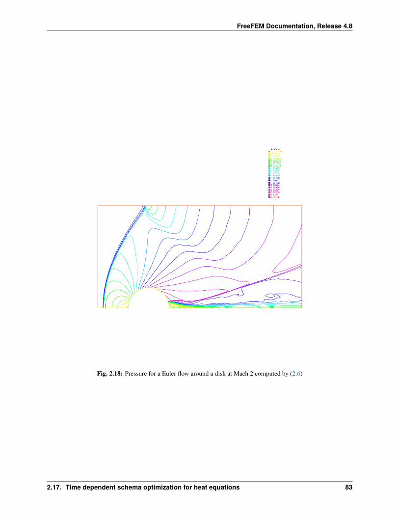
FreeFEM Documentation, Release 4.8
Fig. 2.18: Pressure for a Euler flow around a disk at Mach 2 computed by (2.6)
2.17. Time dependent schema optimization for heat equations 83
FreeFEM Documentation, Release 4.8
Where with 1𝜀 = tgv = 1030:
𝐴𝑖𝑗 =
⎧⎨⎩1𝜀 if 𝑖 ∈ Γ24, and 𝑗 = 𝑖∫
Ω
𝑤𝑗𝑤𝑖/𝑑𝑡+ 𝑘(∇𝑤𝑗 .∇𝑤𝑖) +
∫Γ13
𝛼𝑤𝑗𝑤𝑖 else
𝑀𝑖𝑗 =
⎧⎨⎩1𝜀 if 𝑖 ∈ Γ24, and 𝑗 = 𝑖
𝑛
∫Ω
𝑤𝑗𝑤𝑖/𝑑𝑡 else
𝑏0,𝑖 = 𝑛∫Γ13
𝛼𝑢𝑢𝑒𝑤𝑖𝑏𝑐𝑙 = 𝑢0 the initial data
The Fast version script:
1 ...2 Vh u0=fu0, u=u0;
Create three variational formulation, and build the matrices 𝐴,𝑀 .
1 varf vthermic (u, v)2 = int2d(Th)(3 u*v/dt4 + k*(dx(u)*dx(v) + dy(u)*dy(v))5 )6 + int1d(Th, 1, 3)(7 alpha*u*v8 )9 + on(2,4,u=1)
10 ;11
12 varf vthermic0 (u, v)13 = int1d(Th, 1, 3)(14 alpha*ue*v15 )16 ;17 varf vMass (u,v)18 = int2d(Th)(19 u*v/dt20 )21 + on(2, 4, u=1)22 ;23
24 real tgv = 1e30;25 matrix A = vthermic(Vh, Vh, tgv=tgv, solver=CG);26 matrix M = vMass(Vh, Vh);
Now, to build the right hand size; we need 4 vectors.
1 real[int] b0 = vthermic0(0,Vh); //constant part of RHS2 real[int] bcn = vthermic(0,Vh); //tgv on Dirichlet part3 real[int] bcl = tgv*u0[]; //the Dirichlet B.C. part4
5 // The fast loop6 for(real t = 0; t < T; t += dt)7 real[int] b = b0; //the RHS
(continues on next page)
84 Chapter 2. Learning by Examples
FreeFEM Documentation, Release 4.8
(continued from previous page)
8 b += M*u[]; //add the the time dependent part9 b = bcn ? bcl : b; //do $\forall i$: b[i] = bcn[i] ? bcl[i] : b[i];
10 u[] = A^-1*b; //solve linear problem11 plot(u);12
2.18 Tutorial to write a transient Stokes solver in matrix form
Consider the following script to solve a time dependent Stokes problem in a cavity
1 // Parameters2 real nu = 0.1;3 real T=1.;4 real dt = 0.1;5
6 // Mesh7 mesh Th = square(10, 10);8
9 // Fespace10 fespace Vh(Th, P2)11 Vh u, v;12 Vh uu, vv;13 Vh uold=0, vold=0;14
15 fespace Qh(Th, P1);16 Qh p;17 Qh pp;18
19 // Problem20 problem stokes (u, v, p, uu, vv, pp)21 = int2d(Th)(22 (u*uu+v*vv)/dt23 + nu*(dx(u)*dx(uu) + dy(u)*dy(uu) + dx(v)*dx(vv) + dy(v)*dy(vv))24 - p*pp*1.e-625 - p*(dx(uu) + dy(vv))26 - pp*(dx(u) + dy(v))27 )28 - int2d(Th)(29 (uold*uu+vold*vv)/dt30 )31 + on(1, 2, 4, u=0, v=0)32 + on(3, u=1, v=0)33 ;34
35 // Time loop36 int m, M = T/dt;37 for(m = 0; m < M; m++)38 stokes;39 uold = u;40 vold = v;
(continues on next page)
2.18. Tutorial to write a transient Stokes solver in matrix form 85
FreeFEM Documentation, Release 4.8
(continued from previous page)
41 42
43 // Plot44 plot(p, [u, v], value=true, wait=true, cmm="t="+m*dt);
Every iteration is in fact of the form 𝐴[𝑢, 𝑣, 𝑝] = 𝐵[𝑢𝑜𝑙𝑑, 𝑣𝑜𝑙𝑑, 𝑝𝑜𝑙𝑑] + 𝑏 where 𝐴,𝐵 are matrices and 𝑏 is a vectorcontaining the boundary conditions. 𝐴,𝐵, 𝑏 are constructed by:
1 fespace Xh(Th, [P2, P2, P1]);2 varf aa ([u, v, p], [uu, vv, pp])3 = int2d(Th)(4 (u*uu+v*vv)/dt5 + nu*(dx(u)*dx(uu) + dy(u)*dy(uu) + dx(v)*dx(vv) + dy(v)*dy(vv))6 - p*pp*1.e-67 - p*(dx(uu) + dy(vv))8 - pp*(dx(u) + dy(v))9 )
10 + on(1, 2, 4, u=0, v=0)11 + on(3, u=1, v=0)12 ;13
14 varf bb ([uold, vold, pold], [uu, vv, pp])15 = int2d(Th)(16 (uold*uu+vold*vv)/dt17 )18 //+ on(1, 2, 4, uold=0, vold=0)19 //+ on(3, uold=1, vold=0)20 ;21
22 varf bcl ([uold, vold, pold], [uu, vv, pp])23 = on(1, 2, 4, uold=0, vold=0)24 + on(3, uold=1, vold=0)25 ;26
27 matrix A = aa(Xh, Xh, solver=UMFPACK);28 matrix B = bb(Xh, Xh);29 real[int] b = bcl(0, Xh);
Note that the boundary conditions are not specified in 𝑏𝑏. Removing the comment // would cause the compiler tomultiply the diagonal terms corresponding to a Dirichlet degree of freedom by a very large term (tgv); if so 𝑏 wouldnot be needed, on the condition that 𝑢𝑜𝑙𝑑 = 1 on boundary 3 initially. Note also that b has a tgv on the Dirichlet nodes,by construction, and so does A.
The loop will then be:
1 real[int] sol(Xh.ndof), aux(Xh.ndof);2 for (m = 0; m < M; m++)3 aux = B*sol; aux += b;4 sol = A^-1 * aux;5
There is yet a difficulty with the initialization of sol and with the solution from sol. For this we need a temporaryvector in 𝑋ℎ and here is a solution:
86 Chapter 2. Learning by Examples
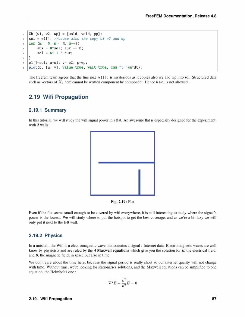
FreeFEM Documentation, Release 4.8
1 Xh [w1, w2, wp] = [uold, vold, pp];2 sol = w1[]; //cause also the copy of w2 and wp3 for (m = 0; m < M; m++)4 aux = B*sol; aux += b;5 sol = A^-1 * aux;6 7 w1[]=sol; u=w1; v= w2; p=wp;8 plot(p, [u, v], value=true, wait=true, cmm="t="+m*dt);
The freefem team agrees that the line sol=w1[]; is mysterious as it copies also w2 and wp into sol. Structured datasuch as vectors of 𝑋ℎ here cannot be written component by component. Hence w1=u is not allowed.
2.19 Wifi Propagation
2.19.1 Summary
In this tutorial, we will study the wifi signal power in a flat. An awesome flat is especially designed for the experiment,with 2 walls:
Fig. 2.19: Flat
Even if the flat seems small enough to be covered by wifi everywhere, it is still interesting to study where the signal’spower is the lowest. We will study where to put the hotspot to get the best coverage, and as we’re a bit lazy we willonly put it next to the left wall.
2.19.2 Physics
In a nutshell, the Wifi is a electromagnetic wave that contains a signal : Internet data. Electromagnetic waves are wellknow by physicists and are ruled by the 4 Maxwell equations which give you the solution for E, the electrical field,and B, the magnetic field, in space but also in time.
We don’t care about the time here, because the signal period is really short so our internet quality will not changewith time. Without time, we’re looking for stationaries solutions, and the Maxwell equations can be simplified to oneequation, the Helmholtz one :
∇2𝐸 +𝑘2
𝑛2𝐸 = 0
2.19. Wifi Propagation 87
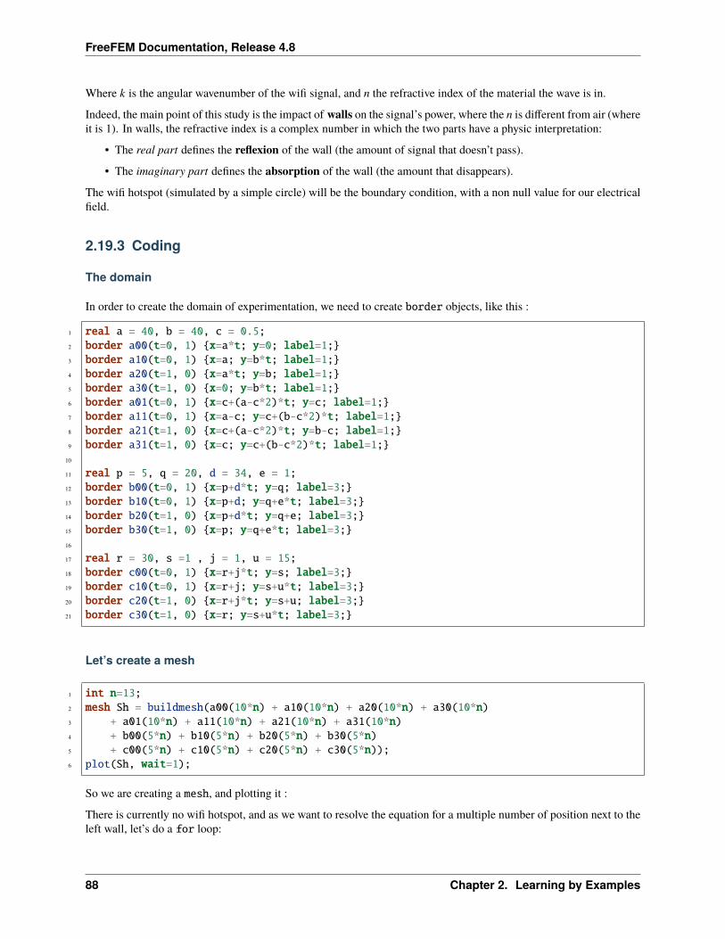
FreeFEM Documentation, Release 4.8
Where k is the angular wavenumber of the wifi signal, and n the refractive index of the material the wave is in.
Indeed, the main point of this study is the impact of walls on the signal’s power, where the n is different from air (whereit is 1). In walls, the refractive index is a complex number in which the two parts have a physic interpretation:
• The real part defines the reflexion of the wall (the amount of signal that doesn’t pass).
• The imaginary part defines the absorption of the wall (the amount that disappears).
The wifi hotspot (simulated by a simple circle) will be the boundary condition, with a non null value for our electricalfield.
2.19.3 Coding
The domain
In order to create the domain of experimentation, we need to create border objects, like this :
1 real a = 40, b = 40, c = 0.5;2 border a00(t=0, 1) x=a*t; y=0; label=1;3 border a10(t=0, 1) x=a; y=b*t; label=1;4 border a20(t=1, 0) x=a*t; y=b; label=1;5 border a30(t=1, 0) x=0; y=b*t; label=1;6 border a01(t=0, 1) x=c+(a-c*2)*t; y=c; label=1;7 border a11(t=0, 1) x=a-c; y=c+(b-c*2)*t; label=1;8 border a21(t=1, 0) x=c+(a-c*2)*t; y=b-c; label=1;9 border a31(t=1, 0) x=c; y=c+(b-c*2)*t; label=1;
10
11 real p = 5, q = 20, d = 34, e = 1;12 border b00(t=0, 1) x=p+d*t; y=q; label=3;13 border b10(t=0, 1) x=p+d; y=q+e*t; label=3;14 border b20(t=1, 0) x=p+d*t; y=q+e; label=3;15 border b30(t=1, 0) x=p; y=q+e*t; label=3;16
17 real r = 30, s =1 , j = 1, u = 15;18 border c00(t=0, 1) x=r+j*t; y=s; label=3;19 border c10(t=0, 1) x=r+j; y=s+u*t; label=3;20 border c20(t=1, 0) x=r+j*t; y=s+u; label=3;21 border c30(t=1, 0) x=r; y=s+u*t; label=3;
Let’s create a mesh
1 int n=13;2 mesh Sh = buildmesh(a00(10*n) + a10(10*n) + a20(10*n) + a30(10*n)3 + a01(10*n) + a11(10*n) + a21(10*n) + a31(10*n)4 + b00(5*n) + b10(5*n) + b20(5*n) + b30(5*n)5 + c00(5*n) + c10(5*n) + c20(5*n) + c30(5*n));6 plot(Sh, wait=1);
So we are creating a mesh, and plotting it :
There is currently no wifi hotspot, and as we want to resolve the equation for a multiple number of position next to theleft wall, let’s do a for loop:
88 Chapter 2. Learning by Examples
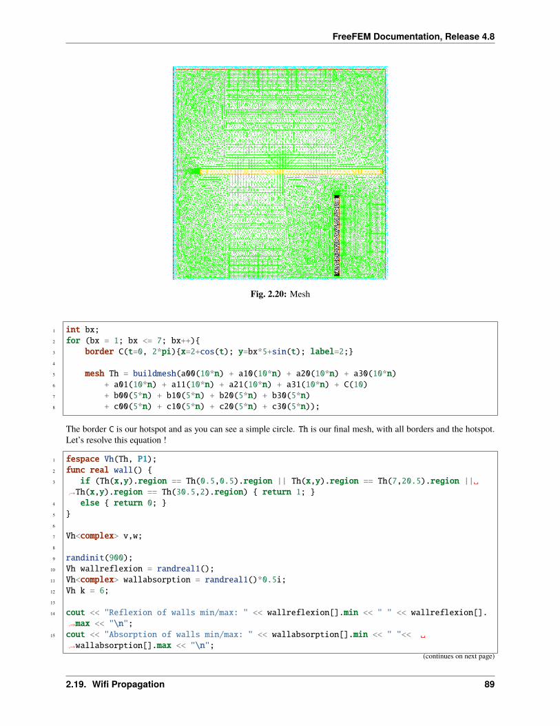
FreeFEM Documentation, Release 4.8
Fig. 2.20: Mesh
1 int bx;2 for (bx = 1; bx <= 7; bx++)3 border C(t=0, 2*pi)x=2+cos(t); y=bx*5+sin(t); label=2;4
5 mesh Th = buildmesh(a00(10*n) + a10(10*n) + a20(10*n) + a30(10*n)6 + a01(10*n) + a11(10*n) + a21(10*n) + a31(10*n) + C(10)7 + b00(5*n) + b10(5*n) + b20(5*n) + b30(5*n)8 + c00(5*n) + c10(5*n) + c20(5*n) + c30(5*n));
The border C is our hotspot and as you can see a simple circle. Th is our final mesh, with all borders and the hotspot.Let’s resolve this equation !
1 fespace Vh(Th, P1);2 func real wall() 3 if (Th(x,y).region == Th(0.5,0.5).region || Th(x,y).region == Th(7,20.5).region ||
→˓Th(x,y).region == Th(30.5,2).region) return 1; 4 else return 0; 5 6
7 Vh<complex> v,w;8
9 randinit(900);10 Vh wallreflexion = randreal1();11 Vh<complex> wallabsorption = randreal1()*0.5i;12 Vh k = 6;13
14 cout << "Reflexion of walls min/max: " << wallreflexion[].min << " " << wallreflexion[].→˓max << "\n";
15 cout << "Absorption of walls min/max: " << wallabsorption[].min << " "<< →˓wallabsorption[].max << "\n";
(continues on next page)
2.19. Wifi Propagation 89
FreeFEM Documentation, Release 4.8
(continued from previous page)
16
17 problem muwave(v,w) =18 int2d(Th)(19 (v*w*k^2)/(1+(wallreflexion+wallabsorption)*wall())^220 - (dx(v)*dx(w)+dy(v)*dy(w))21 )22 + on(2, v=1)23 ;24
25 muwave;26 Vh vm = log(real(v)^2 + imag(v)^2);27 plot(vm, wait=1, fill=true, value=0, nbiso=65);28
A bit of understanding here :
• The fespace keyword defines a finite elements space, no need to know more here.
• The function wall return 0 if in air and 1 if in a wall (x and y are global variables).
• For this example, random numbers are used for the reflexion and the absorption.
• The problem is defined with problem and we solve it by calling it.
Finally, I plotted the log of the module of the solution v to see the signal’s power, and here we are :
Fig. 2.21: Solution
Beautiful isn’t it ? This is the first position for the hotspot, but there are 6 others, and the electrical field is evolvingdepending on the position. You can see the other positions here :
90 Chapter 2. Learning by Examples
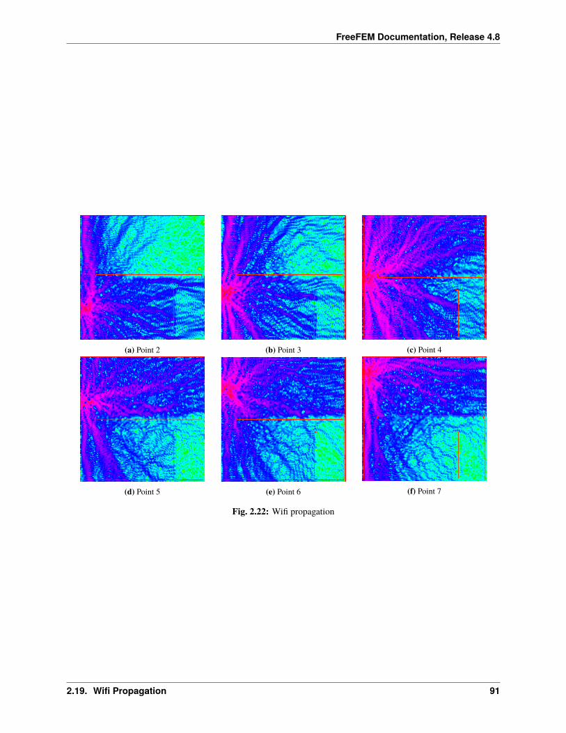
FreeFEM Documentation, Release 4.8
(a) Point 2 (b) Point 3 (c) Point 4
(d) Point 5 (e) Point 6 (f) Point 7
Fig. 2.22: Wifi propagation
2.19. Wifi Propagation 91
FreeFEM Documentation, Release 4.8
2.20 Plotting in Matlab and Octave
2.20.1 Overview
In order to create a plot of a FreeFEM simulation in Matlab© or Octave two steps are necessary:
• The mesh, the finite element space connectivity and the simulation data must be exported into files
• The files must be imported into the Matlab / Octave workspace. Then the data can be visualized with the ffmatliblibrary
The steps are explained in more detail below using the example of a stripline capacitor.
Note: Finite element variables must be in P1 or P2. The simulation data can be 2D or 3D.
2.20.2 2D Problem
Consider a stripline capacitor problem which is also shown in Fig. 2.23. On the two boundaries (the electrodes) 𝐶𝐴,𝐶𝐾 a Dirichlet condition and on the enclosure 𝐶𝐵 a Neumann condition is set. The electrostatic potential 𝑢 betweenthe two electrodes is given by the Laplace equation
∆𝑢(𝑥, 𝑦) = 0
and the electrostatic field E is calculated by
E = −∇𝑢
1 int CA=3, CK=4, CB=5;2 real w2=1.0, h=0.4, d2=0.5;3
4 border bottomA(t=-w2,w2) x=t; y=d2; label=CA;;5 border rightA(t=d2,d2+h) x=w2; y=t; label=CA;;6 border topA(t=w2,-w2) x=t; y=d2+h; label=CA;;7 border leftA(t=d2+h,d2) x=-w2; y=t; label=CA;;8
9 border bottomK(t=-w2,w2) x=t; y=-d2-h; label=CK;;10 border rightK(t=-d2-h,-d2) x=w2; y=t; label=CK;;11 border topK(t=w2,-w2) x=t; y=-d2; label=CK;;12 border leftK(t=-d2,-d2-h) x=-w2; y=t; label=CK;;13
14 border enclosure(t=0,2*pi)x=5*cos(t); y=5*sin(t); label=CB;15
16 int n=15;17 mesh Th = buildmesh(enclosure(3*n)+18 bottomA(-w2*n)+topA(-w2*n)+rightA(-h*n)+leftA(-h*n)+19 bottomK(-w2*n)+topK(-w2*n)+rightK(-h*n)+leftK(-h*n));20
21 fespace Vh(Th,P1);22
23 Vh u,v;24 real u0=2.0;
(continues on next page)
92 Chapter 2. Learning by Examples
FreeFEM Documentation, Release 4.8
(continued from previous page)
25
26 problem Laplace(u,v,solver=LU) =27 int2d(Th)(dx(u)*dx(v) + dy(u)*dy(v))28 + on(CA,u=u0)+on(CK,u=0);29
30 real error=0.01;31 for (int i=0;i<1;i++)32 Laplace;33 Th=adaptmesh(Th,u,err=error);34 error=error/2.0;35 36 Laplace;37
38 Vh Ex, Ey;39 Ex = -dx(u);40 Ey = -dy(u);41
42 plot(u,[Ex,Ey],wait=true);
2.20.3 Exporting Data
The mesh is stored with the FreeFEM command savemesh(), while the connectivity of the finite element space andthe simulation data are stored with the macro commands ffSaveVh() and ffSaveData(). These two commands arelocated in the ffmatlib.idp file which is included in the ffmatlib. Therefore, to export the stripline capacitor datathe following statement sequence must be added to the FreeFEM code:
1 include "ffmatlib.idp"2
3 //Save mesh4 savemesh(Th,"capacitor.msh");5 //Save finite element space connectivity6 ffSaveVh(Th,Vh,"capacitor_vh.txt");7 //Save some scalar data8 ffSaveData(u,"capacitor_potential.txt");9 //Save a 2D vector field
10 ffSaveData2(Ex,Ey,"capacitor_field.txt");
2.20.4 Importing Data
The mesh file can be loaded into the Matlab / Octave workspace using the ffreadmesh() command. A mesh fileconsists of three main sections:
1. The mesh points as nodal coordinates
2. A list of boundary edges including boundary labels
3. List of triangles defining the mesh in terms of connectivity
The three data sections mentioned are returned in the variables p, b and t. The finite element space connectivity and thesimulation data can be loaded using the ffreaddata() command. Therefore, to load the example data the followingstatement sequence must be executed in Matlab / Octave:
2.20. Plotting in Matlab and Octave 93
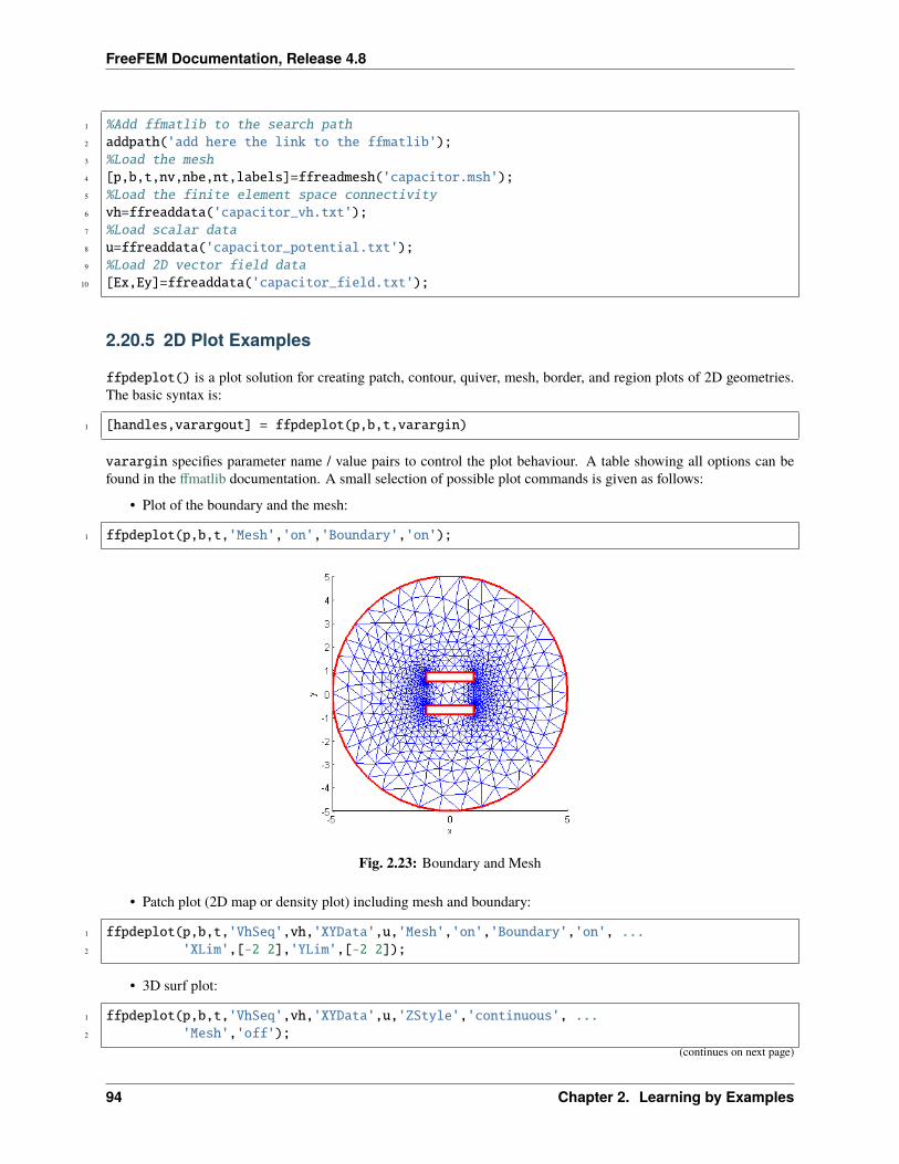
FreeFEM Documentation, Release 4.8
1 %Add ffmatlib to the search path2 addpath('add here the link to the ffmatlib');3 %Load the mesh4 [p,b,t,nv,nbe,nt,labels]=ffreadmesh('capacitor.msh');5 %Load the finite element space connectivity6 vh=ffreaddata('capacitor_vh.txt');7 %Load scalar data8 u=ffreaddata('capacitor_potential.txt');9 %Load 2D vector field data
10 [Ex,Ey]=ffreaddata('capacitor_field.txt');
2.20.5 2D Plot Examples
ffpdeplot() is a plot solution for creating patch, contour, quiver, mesh, border, and region plots of 2D geometries.The basic syntax is:
1 [handles,varargout] = ffpdeplot(p,b,t,varargin)
varargin specifies parameter name / value pairs to control the plot behaviour. A table showing all options can befound in the ffmatlib documentation. A small selection of possible plot commands is given as follows:
• Plot of the boundary and the mesh:
1 ffpdeplot(p,b,t,'Mesh','on','Boundary','on');
Fig. 2.23: Boundary and Mesh
• Patch plot (2D map or density plot) including mesh and boundary:
1 ffpdeplot(p,b,t,'VhSeq',vh,'XYData',u,'Mesh','on','Boundary','on', ...2 'XLim',[-2 2],'YLim',[-2 2]);
• 3D surf plot:
1 ffpdeplot(p,b,t,'VhSeq',vh,'XYData',u,'ZStyle','continuous', ...2 'Mesh','off');
(continues on next page)
94 Chapter 2. Learning by Examples
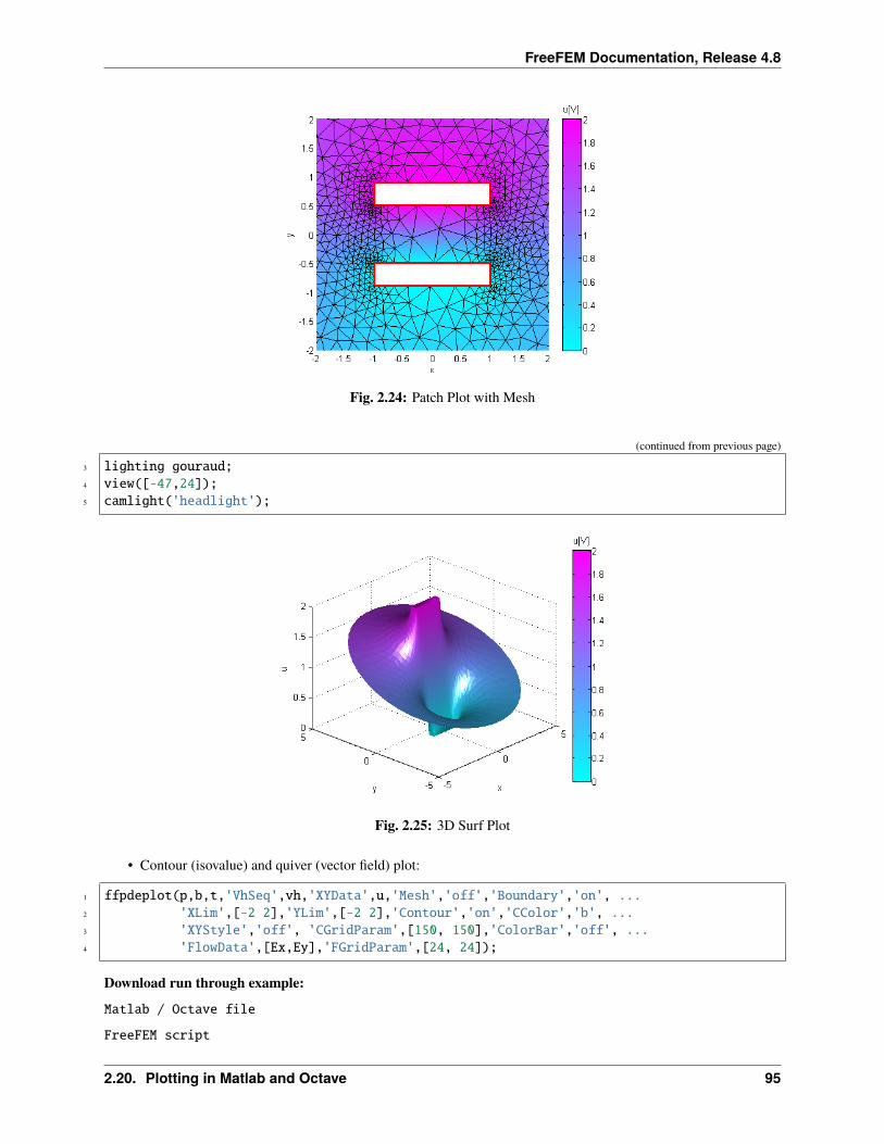
FreeFEM Documentation, Release 4.8
Fig. 2.24: Patch Plot with Mesh
(continued from previous page)
3 lighting gouraud;4 view([-47,24]);5 camlight('headlight');
Fig. 2.25: 3D Surf Plot
• Contour (isovalue) and quiver (vector field) plot:
1 ffpdeplot(p,b,t,'VhSeq',vh,'XYData',u,'Mesh','off','Boundary','on', ...2 'XLim',[-2 2],'YLim',[-2 2],'Contour','on','CColor','b', ...3 'XYStyle','off', 'CGridParam',[150, 150],'ColorBar','off', ...4 'FlowData',[Ex,Ey],'FGridParam',[24, 24]);
Download run through example:Matlab / Octave file
FreeFEM script
2.20. Plotting in Matlab and Octave 95
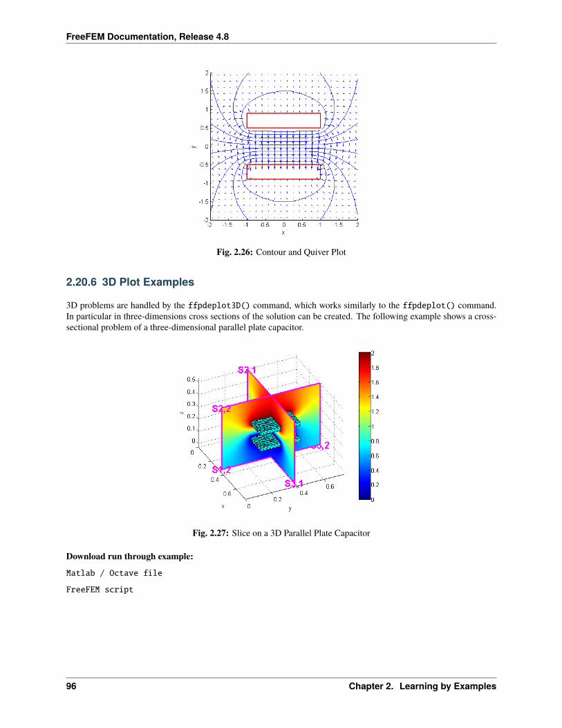
FreeFEM Documentation, Release 4.8
Fig. 2.26: Contour and Quiver Plot
2.20.6 3D Plot Examples
3D problems are handled by the ffpdeplot3D() command, which works similarly to the ffpdeplot() command.In particular in three-dimensions cross sections of the solution can be created. The following example shows a cross-sectional problem of a three-dimensional parallel plate capacitor.
Fig. 2.27: Slice on a 3D Parallel Plate Capacitor
Download run through example:Matlab / Octave file
FreeFEM script
96 Chapter 2. Learning by Examples

FreeFEM Documentation, Release 4.8
2.20.7 References
• Octave
• Matlab
• ffmatlib
2.20. Plotting in Matlab and Octave 97
FreeFEM Documentation, Release 4.8
98 Chapter 2. Learning by Examples
CHAPTER
THREE
DOCUMENTATION
The fruit of a long maturing process, freefem, in its last avatar, FreeFEM , is a high level integrated developmentenvironment (IDE) for numerically solving partial differential equations (PDE) in dimension 1,2 3 and surface and line3D. It is the ideal tool for teaching the finite element method but it is also perfect for research to quickly test new ideasor multi-physics and complex applications.
FreeFEM has an advanced automatic mesh generator, capable of a posteriori mesh adaptation; it has a general purposeelliptic solver interfaced with fast algorithms, such as the multi-frontal method UMFPACK, SuperLU, MUMPS. Hy-perbolic and parabolic problems are solved by iterative algorithms prescribed by the user with the high level language ofFreeFEM. It has several triangular finite elements, including discontinuous elements. Everything is there in FreeFEMto prepare research quality reports with online color display, zooming and other features as well as postscript printouts.
This manual is meant for students at a Masters level, for researchers at any level, and for engineers (including financialengineering) with some understanding of variational methods for partial differential equations.
Introduction
A partial differential equation is a relation between a function of several variables and its (partial) derivatives. Manyproblems in physics, engineering, mathematics and even banking are modeled by one or several partial differentialequations.
FreeFEM is a software to solve these equations numerically. As its name implies, it is a free software (see the copyrightsfor full detail) based on the Finite Element Method; it is not a package, it is an integrated product with its own highlevel programming language. This software runs on all UNIX OS (with g++ 3.3 or later, and OpenGL), on WindowXP, Vista and 7, 8, 10 and on MacOS 10 intel.
Moreover FreeFEM is highly adaptive. Many phenomena involve several coupled systems. Fluid-structure interac-tions, Lorentz forces for aluminum casting and ocean-atmosphere problems are three such systems. These requiredifferent finite element approximations and polynomial degrees, possibly on different meshes. Some algorithms likethe Schwarz’ domain decomposition method also requires data interpolation on multiple meshes within one program.FreeFEM can handle these difficulties, i.e. arbitrary finite element spaces on arbitrary unstructured and adapted bi-dimensional meshes.
The characteristics of FreeFEM are:
• Problem description (real or complex valued) by their variational formulations, with access to the internal vectorsand matrices if needed.
• Multi-variables, multi-equations, bi-dimensional and three-dimensional static or time dependent, linear or non-linear coupled systems; however the user is required to describe the iterative procedures which reduce the problemto a set of linear problems.
• Easy geometric input by analytic description of boundaries by pieces; however this part is not a CAD system; forinstance when two boundaries intersect, the user must specify the intersection points.
• Automatic mesh generator, based on the Delaunay-Voronoi algorithm; the inner point density is proportional tothe density of points on the boundaries [GEORGE1996].
99
FreeFEM Documentation, Release 4.8
• Metric-based anisotropic mesh adaptation. The metric can be computed automatically from the Hessian of anyFreeFEM function [HECHT1998].
• High level user friendly typed input language with an algebra of analytic and finite element functions.
• Multiple finite element meshes within one application with automatic interpolation of data on different meshesand possible storage of the interpolation matrices.
• A large variety of triangular finite elements: linear, quadratic Lagrangian elements and more, discontinuous P1and Raviart-Thomas elements, elements of a non-scalar type, the mini-element,. . . (but no quadrangles).
• Tools to define discontinuous Galerkin finite element formulations P0, P1dc, P2dc and keywords: jump, mean,intalledges.
• A large variety of linear direct and iterative solvers (LU, Cholesky, Crout, CG, GMRES, UMFPACK, MUMPS,SuperLU, . . . ) and eigenvalue and eigenvector solvers (ARPARK) .
• Near optimal execution speed (compared with compiled C++ implementations programmed directly).
• Online graphics, generation of ,.txt,.eps,.gnu, mesh files for further manipulations of input and output data.
• Many examples and tutorials: elliptic, parabolic and hyperbolic problems, Navier-Stokes flows, elasticity, fluidstructure interactions, Schwarz’s domain decomposition method, eigenvalue problem, residual error indicator,. . .
• A parallel version using MPI
3.1 Notations
Here mathematical expressions and corresponding FreeFEM commands are explained.
3.1.1 Generalities
• [𝛿𝑖𝑗] Kronecker delta (0 if 𝑖 = 𝑗, 1 if 𝑖 = 𝑗 for integers 𝑖, 𝑗)
• [∀] for all
• [∃] there exists
• [i.e.] that is
• [PDE] partial differential equation (with boundary conditions)
• [∅] the empty set
• [N] the set of integers (𝑎 ∈ N⇔ int a), int means long int inside FreeFEM• [R] the set of real numbers (𝑎 ∈ R⇔ real a), double inside FreeFEM• [C] the set of complex numbers (𝑎 ∈ C⇔ complex a), complex<double>
• [R𝑑] 𝑑-dimensional Euclidean space
100 Chapter 3. Documentation
FreeFEM Documentation, Release 4.8
3.1.2 Sets, Mappings, Matrices, Vectors
Let 𝐸, 𝐹, 𝐺 be three sets and 𝐴 the subset of 𝐸.
• [𝑥 ∈ 𝐸| 𝑃] the subset of 𝐸 consisting of the elements possessing the property 𝑃
• [𝐸 ∪ 𝐹 ] the set of elements belonging to 𝐸 or 𝐹
• [𝐸 ∩ 𝐹 ] the set of elements belonging to 𝐸 and 𝐹
• [𝐸 ∖𝐴] the set 𝑥 ∈ 𝐸| 𝑥 ∈ 𝐴
• [𝐸 + 𝐹 ] 𝐸 ∪ 𝐹 with 𝐸 ∩ 𝐹 = ∅
• [𝐸 × 𝐹 ] the Cartesian product of 𝐸 and 𝐹
• [𝐸𝑛] the 𝑛-th power of 𝐸 (𝐸2 = 𝐸 × 𝐸, 𝐸𝑛 = 𝐸 × 𝐸𝑛−1)
• [𝑓 : 𝐸 → 𝐹 ] the mapping form 𝐸 into 𝐹 , i.e., 𝐸 ∋ 𝑥 ↦→ 𝑓(𝑥) ∈ 𝐹
• [𝐼𝐸 or 𝐼] the identity mapping in 𝐸,i.e., 𝐼(𝑥) = 𝑥 ∀𝑥 ∈ 𝐸
• [𝑓 ∘ 𝑔] for 𝑓 : 𝐹 → 𝐺 and 𝑔 : 𝐸 → 𝐹 , 𝐸 ∋ 𝑥 ↦→ (𝑓 ∘ 𝑔)(𝑥) = 𝑓(𝑔(𝑥)) ∈ 𝐺 (see Elementary function)
• [𝑓 |𝐴] the restriction of 𝑓 : 𝐸 → 𝐹 to the subset 𝐴 of 𝐸
• [𝑎𝑘] column vector with components 𝑎𝑘• [(𝑎𝑘)] row vector with components 𝑎𝑘• [(𝑎𝑘)𝑇 ] denotes the transpose of a matrix (𝑎𝑘), and is 𝑎𝑘
• [𝑎𝑖𝑗] matrix with components 𝑎𝑖𝑗 , and (𝑎𝑖𝑗)𝑇 = (𝑎𝑗𝑖)
3.1.3 Numbers
For two real numbers 𝑎, 𝑏
• [𝑎, 𝑏] is the interval 𝑥 ∈ R| 𝑎 ≤ 𝑥 ≤ 𝑏
• ]𝑎, 𝑏] is the interval 𝑥 ∈ R| 𝑎 < 𝑥 ≤ 𝑏
• [𝑎, 𝑏[ is the interval 𝑥 ∈ R| 𝑎 ≤ 𝑥 < 𝑏
• ]𝑎, 𝑏[ is the interval 𝑥 ∈ R| 𝑎 < 𝑥 < 𝑏
3.1.4 Differential Calculus
• [𝜕𝑓/𝜕𝑥] the partial derivative of 𝑓 : R𝑑 → R with respect to 𝑥 (dx(f))
• [∇𝑓 ] the gradient of 𝑓 : Ω→ R,i.e., ∇𝑓 = (𝜕𝑓/𝜕𝑥, 𝜕𝑓/𝜕𝑦)
• [div(f) or ∇.f ] the divergence of f : Ω→ R𝑑, i.e., div(f) = 𝜕𝑓1/𝜕𝑥+ 𝜕𝑓2/𝜕𝑦
• [∆𝑓 ] the Laplacian of 𝑓 : Ω→ R, i.e., ∆𝑓 = 𝜕2𝑓/𝜕𝑥2 + 𝜕2𝑓/𝜕𝑦2
3.1. Notations 101
FreeFEM Documentation, Release 4.8
3.1.5 Meshes
• [Ω] usually denotes a domain on which PDE is defined
• [Γ] denotes the boundary of Ω,i.e., Γ = 𝜕Ω (keyword border, see Border)
• [𝒯ℎ] the triangulation of Ω, i.e., the set of triangles 𝑇𝑘, where ℎ stands for mesh size (keyword mesh, buildmesh,see Mesh Generation)
• [𝑛𝑡] the number of triangles in 𝒯ℎ (get by Th.nt)
• [Ωℎ] denotes the approximated domain Ωℎ = ∪𝑛𝑡
𝑘=1𝑇𝑘 of Ω. If Ω is polygonal domain, then it will be Ω = Ωℎ
• [Γℎ] the boundary of Ωℎ
• [𝑛𝑣] the number of vertices in 𝒯ℎ (get by Th.nv)
• [𝑛𝑏𝑒] the number of boundary element in 𝒯ℎ (get by Th.nbe)
• [|Ωℎ|] the measure (area or volume) in 𝒯ℎ (get by Th.measure)
• [|𝜕Ωℎ|] the measure of the border (length or area) in 𝒯ℎ (get by Th.bordermeasure)
• [ℎ𝑚𝑖𝑛] the minimum edge size of 𝒯ℎ (get by Th.hmin)
• [ℎ𝑚𝑎𝑥] the maximum edge size of 𝒯ℎ (get by Th.hmax)
• [[𝑞𝑖𝑞𝑗]] the segment connecting 𝑞𝑖 and 𝑞𝑗
• [𝑞𝑘1 , 𝑞𝑘2 , 𝑞𝑘3 ] the vertices of a triangle 𝑇𝑘 with anti-clock direction (get the coordinate of 𝑞𝑘𝑗 by(Th[k-1][j-1].x, Th[k-1][j-1].y))
• [𝐼Ω] the set 𝑖 ∈ N| 𝑞𝑖 ∈ Γℎ
3.1.6 Functional Spaces
• [𝐿2(Ω)] the set𝑤(𝑥, 𝑦)
∫Ω
|𝑤(𝑥, 𝑦)|2d𝑥d𝑦 <∞
norm: ‖𝑤‖0,Ω =
(∫Ω
|𝑤(𝑥, 𝑦)|2d𝑥d𝑦)1/2
scalar product: (𝑣, 𝑤) =
∫Ω
𝑣𝑤
• [𝐻1(Ω)] the set𝑤 ∈ 𝐿2(Ω)
∫Ω
(|𝜕𝑤/𝜕𝑥|2 + |𝜕𝑤/𝜕𝑦|2
)d𝑥d𝑦 <∞
norm: ‖𝑤‖1,Ω =(‖𝑤‖20,Ω + ‖∇𝑢‖20.Ω
)1/2• [𝐻𝑚(Ω)] the set
𝑤 ∈ 𝐿2(Ω)
∫Ω
𝜕|𝛼|𝑤
𝜕𝑥𝛼1𝜕𝑦𝛼2∈ 𝐿2(Ω) ∀𝛼 = (𝛼1, 𝛼2) ∈ N2, |𝛼| = 𝛼1 + 𝛼2
scalar product: (𝑣, 𝑤)1,Ω =∑
|𝛼|≤𝑚
∫Ω
𝐷𝛼𝑣𝐷𝛼𝑤
• [𝐻10 (Ω)] the set
𝑤 ∈ 𝐻1(Ω) | 𝑢 = 0 on Γ
[𝐿2(Ω)2] denotes 𝐿2(Ω)× 𝐿2(Ω), and also 𝐻1(Ω)2 = 𝐻1(Ω)×𝐻1(Ω)
102 Chapter 3. Documentation
FreeFEM Documentation, Release 4.8
3.1.7 Finite Element Spaces
• [𝑉ℎ] denotes the finite element space created by fespace Vh(Th, *) in FreeFEM (see Finite Elements for *)
• [Πℎ𝑓 ] the projection of the function 𝑓 into 𝑉ℎ (func f=x^2*y^3; Vh v = f;) means 𝑣 = 𝑃𝑖ℎ(𝑓) * [𝑣] forFE-function 𝑣 in 𝑉ℎ means the column vector (𝑣1, · · · , 𝑣𝑀 )𝑇 if 𝑣 = 𝑣1𝜑1 + · · · + 𝑣𝑀𝜑𝑀 , which is shown byfespace Vh(Th, P2); Vh v; cout << v[] << endl;
3.2 Mesh Generation
In this section, operators and tools on meshes are presented.
FreeFEM type for mesh variable:
• 1D mesh: meshL
• 2D mesh: mesh
• 3D volume mesh: mesh3
• 3D border meshes– 3D surface meshS
– 3D curve meshL
Through this presentation, the principal commands for the mesh generation and links between mesh - mesh3 - meshS- meshL are described.
3.2.1 The type mesh in 2 dimension
Commands for 2d mesh Generation
The FreeFEM type to define a 2d mesh object is mesh.
The command square
The command square triangulates the unit square.
The following generates a 4 × 5 grid in the unit square [0, 1]2. The labels of the boundaries are shown in Fig. 3.1.
1 mesh Th = square(4, 5);
To construct a 𝑛×𝑚 grid in the rectangle [𝑥0, 𝑥1]× [𝑦0, 𝑦1], proceed as follows:
1 real x0 = 1.2;2 real x1 = 1.8;3 real y0 = 0;4 real y1 = 1;5 int n = 5;6 real m = 20;7 mesh Th = square(n, m, [x0+(x1-x0)*x, y0+(y1-y0)*y]);
Note: Adding the named parameter flags=icase with icase:
3.2. Mesh Generation 103

FreeFEM Documentation, Release 4.8
Fig. 3.1: Boundary labels of the mesh by square(10,10)
0. will produce a mesh where all quads are split with diagonal 𝑥− 𝑦 = 𝑐𝑜𝑛𝑠𝑡𝑎𝑛𝑡
1. will produce a Union Jack flag type of mesh
2. will produce a mesh where all quads are split with diagonal 𝑥+ 𝑦 = 𝑐𝑜𝑛𝑠𝑡𝑎𝑛𝑡
3. same as in case 0, except two corners where the triangles are the same as case 2, to avoid having 3 vertices onthe boundary
4. same as in case 2, except two corners where the triangles are the same as case 0, to avoid having 3 vertices onthe boundary
1 mesh Th = square(n, m, [x0+(x1-x0)*x, y0+(y1-y0)*y], flags=icase);
Note: Adding the named parameter label=labs will change the 4 default label numbers to labs[i-1], for exampleint[int] labs=[11, 12, 13, 14], and adding the named parameter region=10 will change the region numberto 10, for instance (v 3.8).
To see all of these flags at work, check Square mesh example:
1 for (int i = 0; i < 5; ++i)2 int[int] labs = [11, 12, 13, 14];3 mesh Th = square(3, 3, flags=i, label=labs, region=10);4 plot(Th, wait=1, cmm="square flags = "+i );5
104 Chapter 3. Documentation
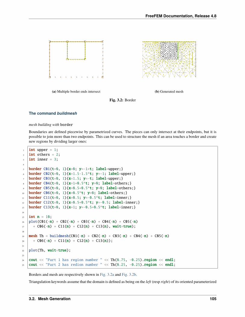
FreeFEM Documentation, Release 4.8
(a) Multiple border ends intersect (b) Generated mesh
Fig. 3.2: Border
The command buildmesh
mesh building with border
Boundaries are defined piecewise by parametrized curves. The pieces can only intersect at their endpoints, but it ispossible to join more than two endpoints. This can be used to structure the mesh if an area touches a border and createnew regions by dividing larger ones:
1 int upper = 1;2 int others = 2;3 int inner = 3;4
5 border C01(t=0, 1)x=0; y=-1+t; label=upper;6 border C02(t=0, 1)x=1.5-1.5*t; y=-1; label=upper;7 border C03(t=0, 1)x=1.5; y=-t; label=upper;8 border C04(t=0, 1)x=1+0.5*t; y=0; label=others;9 border C05(t=0, 1)x=0.5+0.5*t; y=0; label=others;
10 border C06(t=0, 1)x=0.5*t; y=0; label=others;11 border C11(t=0, 1)x=0.5; y=-0.5*t; label=inner;12 border C12(t=0, 1)x=0.5+0.5*t; y=-0.5; label=inner;13 border C13(t=0, 1)x=1; y=-0.5+0.5*t; label=inner;14
15 int n = 10;16 plot(C01(-n) + C02(-n) + C03(-n) + C04(-n) + C05(-n)17 + C06(-n) + C11(n) + C12(n) + C13(n), wait=true);18
19 mesh Th = buildmesh(C01(-n) + C02(-n) + C03(-n) + C04(-n) + C05(-n)20 + C06(-n) + C11(n) + C12(n) + C13(n));21
22 plot(Th, wait=true);23
24 cout << "Part 1 has region number " << Th(0.75, -0.25).region << endl;25 cout << "Part 2 has redion number " << Th(0.25, -0.25).region << endl;
Borders and mesh are respectively shown in Fig. 3.2a and Fig. 3.2b.
Triangulation keywords assume that the domain is defined as being on the left (resp right) of its oriented parameterized
3.2. Mesh Generation 105
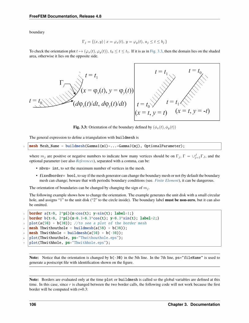
FreeFEM Documentation, Release 4.8
boundary
Γ𝑗 = (𝑥, 𝑦) | 𝑥 = 𝜙𝑥(𝑡), 𝑦 = 𝜙𝑦(𝑡), 𝑎𝑗 ≤ 𝑡 ≤ 𝑏𝑗
To check the orientation plot 𝑡 ↦→ (𝜙𝑥(𝑡), 𝜙𝑦(𝑡)), 𝑡0 ≤ 𝑡 ≤ 𝑡1. If it is as in Fig. 3.3, then the domain lies on the shadedarea, otherwise it lies on the opposite side.
Fig. 3.3: Orientation of the boundary defined by (𝜑𝑥(𝑡), 𝜑𝑦(𝑡))
The general expression to define a triangulation with buildmesh is
1 mesh Mesh_Name = buildmesh(Gamma1(m1)+...+GammaJ(mj), OptionalParameter);
where 𝑚𝑗 are positive or negative numbers to indicate how many vertices should be on Γ𝑗 , Γ = ∪𝐽𝑗=1Γ𝐽 , and theoptional parameter (see also References), separated with a comma, can be:
• nbvx= int, to set the maximum number of vertices in the mesh.
• fixedborder= bool, to say if the mesh generator can change the boundary mesh or not (by default the boundarymesh can change; beware that with periodic boundary conditions (see. Finite Element), it can be dangerous.
The orientation of boundaries can be changed by changing the sign of 𝑚𝑗 .
The following example shows how to change the orientation. The example generates the unit disk with a small circularhole, and assigns “1” to the unit disk (“2” to the circle inside). The boundary label must be non-zero, but it can alsobe omitted.
1 border a(t=0, 2*pi)x=cos(t); y=sin(t); label=1;2 border b(t=0, 2*pi)x=0.3+0.3*cos(t); y=0.3*sin(t); label=2;3 plot(a(50) + b(30)); //to see a plot of the border mesh4 mesh Thwithouthole = buildmesh(a(50) + b(30));5 mesh Thwithhole = buildmesh(a(50) + b(-30));6 plot(Thwithouthole, ps="Thwithouthole.eps");7 plot(Thwithhole, ps="Thwithhole.eps");
Note: Notice that the orientation is changed by b(-30) in the 5th line. In the 7th line, ps="fileName" is used togenerate a postscript file with identification shown on the figure.
Note: Borders are evaluated only at the time plot or buildmesh is called so the global variables are defined at thistime. In this case, since 𝑟 is changed between the two border calls, the following code will not work because the firstborder will be computed with r=0.3:
106 Chapter 3. Documentation
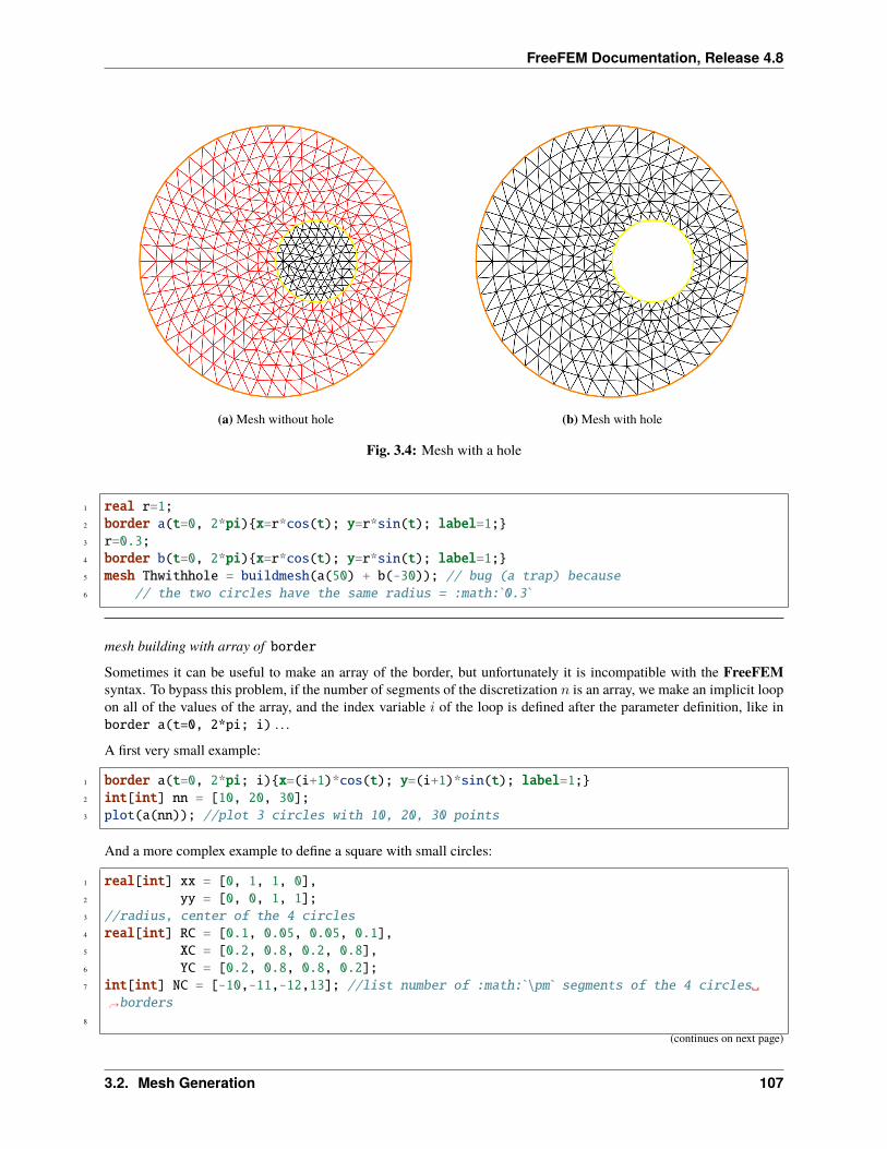
FreeFEM Documentation, Release 4.8
(a) Mesh without hole (b) Mesh with hole
Fig. 3.4: Mesh with a hole
1 real r=1;2 border a(t=0, 2*pi)x=r*cos(t); y=r*sin(t); label=1;3 r=0.3;4 border b(t=0, 2*pi)x=r*cos(t); y=r*sin(t); label=1;5 mesh Thwithhole = buildmesh(a(50) + b(-30)); // bug (a trap) because6 // the two circles have the same radius = :math:`0.3`
mesh building with array of border
Sometimes it can be useful to make an array of the border, but unfortunately it is incompatible with the FreeFEMsyntax. To bypass this problem, if the number of segments of the discretization 𝑛 is an array, we make an implicit loopon all of the values of the array, and the index variable 𝑖 of the loop is defined after the parameter definition, like inborder a(t=0, 2*pi; i) . . .
A first very small example:
1 border a(t=0, 2*pi; i)x=(i+1)*cos(t); y=(i+1)*sin(t); label=1;2 int[int] nn = [10, 20, 30];3 plot(a(nn)); //plot 3 circles with 10, 20, 30 points
And a more complex example to define a square with small circles:
1 real[int] xx = [0, 1, 1, 0],2 yy = [0, 0, 1, 1];3 //radius, center of the 4 circles4 real[int] RC = [0.1, 0.05, 0.05, 0.1],5 XC = [0.2, 0.8, 0.2, 0.8],6 YC = [0.2, 0.8, 0.8, 0.2];7 int[int] NC = [-10,-11,-12,13]; //list number of :math:`\pm` segments of the 4 circles
→˓borders8
(continues on next page)
3.2. Mesh Generation 107
FreeFEM Documentation, Release 4.8
(continued from previous page)
9 border bb(t=0, 1; i)10 11 // i is the index variable of the multi border loop12 int ii = (i+1)%4;13 real t1 = 1-t;14 x = xx[i]*t1 + xx[ii]*t;15 y = yy[i]*t1 + yy[ii]*t;16 label = 0;17 18
19 border cc(t=0, 2*pi; i)20 21 x = RC[i]*cos(t) + XC[i];22 y = RC[i]*sin(t) + YC[i];23 label = i + 1;24 25 int[int] nn = [4, 4, 5, 7]; //4 border, with 4, 4, 5, 7 segment respectively26 plot(bb(nn), cc(NC), wait=1);27 mesh th = buildmesh(bb(nn) + cc(NC));28 plot(th, wait=1);
Mesh Connectivity and data
The following example explains methods to obtain mesh information.
1 // Mesh2 mesh Th = square(2, 2);3
4 cout << "// Get data of the mesh" << endl;5 6 int NbTriangles = Th.nt;7 real MeshArea = Th.measure;8 real BorderLength = Th.bordermeasure;9
10 cout << "Number of triangle(s) = " << NbTriangles << endl;11 cout << "Mesh area = " << MeshArea << endl;12 cout << "Border length = " << BorderLength << endl;13
14 // Th(i) return the vextex i of Th15 // Th[k] return the triangle k of Th16 // Th[k][i] return the vertex i of the triangle k of Th17 for (int i = 0; i < NbTriangles; i++)18 for (int j = 0; j < 3; j++)19 cout << i << " " << j << " - Th[i][j] = " << Th[i][j]20 << ", x = " << Th[i][j].x21 << ", y= " << Th[i][j].y22 << ", label=" << Th[i][j].label << endl;23 24
25 cout << "// Hack to get vertex coordinates" << endl;26
(continues on next page)
108 Chapter 3. Documentation
FreeFEM Documentation, Release 4.8
(continued from previous page)
27 fespace femp1(Th, P1);28 femp1 Thx=x,Thy=y;29
30 int NbVertices = Th.nv;31 cout << "Number of vertices = " << NbVertices << endl;32
33 for (int i = 0; i < NbVertices; i++)34 cout << "Th(" << i << ") : " << Th(i).x << " " << Th(i).y << " " << Th(i).label35 << endl << "\told method: " << Thx[][i] << " " << Thy[][i] << endl;36 37
38 cout << "// Method to find information of point (0.55,0.6)" << endl;39 40 int TNumber = Th(0.55, 0.6).nuTriangle; //the triangle number41 int RLabel = Th(0.55, 0.6).region; //the region label42
43 cout << "Triangle number in point (0.55, 0.6): " << TNumber << endl;44 cout << "Region label in point (0.55, 0.6): " << RLabel << endl;45 46
47 cout << "// Information of triangle" << endl;48 49 int TNumber = Th(0.55, 0.6).nuTriangle;50 real TArea = Th[TNumber].area; //triangle area51 real TRegion = Th[TNumber].region; //triangle region52 real TLabel = Th[TNumber].label; //triangle label, same as region for triangles53
54 cout << "Area of triangle " << TNumber << ": " << TArea << endl;55 cout << "Region of triangle " << TNumber << ": " << TRegion << endl;56 cout << "Label of triangle " << TNumber << ": " << TLabel << endl;57 58
59 cout << "// Hack to get a triangle containing point x, y or region number (old method)" <→˓< endl;
60 61 fespace femp0(Th, P0);62 femp0 TNumbers; //a P0 function to get triangle numbering63 for (int i = 0; i < Th.nt; i++)64 TNumbers[][i] = i;65 femp0 RNumbers = region; //a P0 function to get the region number66
67 int TNumber = TNumbers(0.55, 0.6); // Number of the triangle containing (0.55, 0,6)68 int RNumber = RNumbers(0.55, 0.6); // Number of the region containing (0.55, 0,6)69
70 cout << "Point (0.55,0,6) :" << endl;71 cout << "\tTriangle number = " << TNumber << endl;72 cout << "\tRegion number = " << RNumber << endl;73 74
75 cout << "// New method to get boundary information and mesh adjacent" << endl;76 77 int k = 0;
(continues on next page)
3.2. Mesh Generation 109
FreeFEM Documentation, Release 4.8
(continued from previous page)
78 int l=1;79 int e=1;80
81 // Number of boundary elements82 int NbBoundaryElements = Th.nbe;83 cout << "Number of boundary element = " << NbBoundaryElements << endl;84 // Boundary element k in 0, ..., Th.nbe85 int BoundaryElement = Th.be(k);86 cout << "Boundary element " << k << " = " << BoundaryElement << endl;87 // Vertice l in 0, 1 of boundary element k88 int Vertex = Th.be(k)[l];89 cout << "Vertex " << l << " of boundary element " << k << " = " << Vertex << endl;90 // Triangle containg the boundary element k91 int Triangle = Th.be(k).Element;92 cout << "Triangle containing the boundary element " << k << " = " << Triangle <<
→˓endl;93 // Triangle egde nubmer containing the boundary element k94 int Edge = Th.be(k).whoinElement;95 cout << "Triangle edge number containing the boundary element " << k << " = " <<
→˓Edge << endl;96 // Adjacent triangle of the triangle k by edge e97 int Adjacent = Th[k].adj(e); //The value of e is changed to the corresponding edge
→˓in the adjacent triangle98 cout << "Adjacent triangle of the triangle " << k << " by edge " << e << " = " <<
→˓Adjacent << endl;99 cout << "\tCorresponding edge = " << e << endl;
100 // If there is no adjacent triangle by edge e, the same triangle is returned101 //Th[k] == Th[k].adj(e)102 // Else a different triangle is returned103 //Th[k] != Th[k].adj(e)104 105
106 cout << "// Print mesh connectivity " << endl;107 108 int NbTriangles = Th.nt;109 for (int k = 0; k < NbTriangles; k++)110 cout << k << " : " << int(Th[k][0]) << " " << int(Th[k][1])111 << " " << int(Th[k][2])112 << ", label " << Th[k].label << endl;113
114 for (int k = 0; k < NbTriangles; k++)115 for (int e = 0, ee; e < 3; e++)116 //set ee to e, and ee is change by method adj,117 cout << k << " " << e << " <=> " << int(Th[k].adj((ee=e))) << " " << ee118 << ", adj: " << (Th[k].adj((ee=e)) != Th[k]) << endl;119
120 int NbBoundaryElements = Th.nbe;121 for (int k = 0; k < NbBoundaryElements; k++)122 cout << k << " : " << Th.be(k)[0] << " " << Th.be(k)[1]123 << " , label " << Th.be(k).label124 << ", triangle " << int(Th.be(k).Element)125 << " " << Th.be(k).whoinElement << endl;
(continues on next page)
110 Chapter 3. Documentation
FreeFEM Documentation, Release 4.8
(continued from previous page)
126
127 real[int] bb(4);128 boundingbox(Th, bb);129 // bb[0] = xmin, bb[1] = xmax, bb[2] = ymin, bb[3] =ymax130 cout << "boundingbox:" << endl;131 cout << "xmin = " << bb[0]132 << ", xmax = " << bb[1]133 << ", ymin = " << bb[2]134 << ", ymax = " << bb[3] << endl;135
The output is:
1 // Get data of the mesh2 Number of triangle = 83 Mesh area = 14 Border length = 45 0 0 - Th[i][j] = 0, x = 0, y= 0, label=46 0 1 - Th[i][j] = 1, x = 0.5, y= 0, label=17 0 2 - Th[i][j] = 4, x = 0.5, y= 0.5, label=08 1 0 - Th[i][j] = 0, x = 0, y= 0, label=49 1 1 - Th[i][j] = 4, x = 0.5, y= 0.5, label=0
10 1 2 - Th[i][j] = 3, x = 0, y= 0.5, label=411 2 0 - Th[i][j] = 1, x = 0.5, y= 0, label=112 2 1 - Th[i][j] = 2, x = 1, y= 0, label=213 2 2 - Th[i][j] = 5, x = 1, y= 0.5, label=214 3 0 - Th[i][j] = 1, x = 0.5, y= 0, label=115 3 1 - Th[i][j] = 5, x = 1, y= 0.5, label=216 3 2 - Th[i][j] = 4, x = 0.5, y= 0.5, label=017 4 0 - Th[i][j] = 3, x = 0, y= 0.5, label=418 4 1 - Th[i][j] = 4, x = 0.5, y= 0.5, label=019 4 2 - Th[i][j] = 7, x = 0.5, y= 1, label=320 5 0 - Th[i][j] = 3, x = 0, y= 0.5, label=421 5 1 - Th[i][j] = 7, x = 0.5, y= 1, label=322 5 2 - Th[i][j] = 6, x = 0, y= 1, label=423 6 0 - Th[i][j] = 4, x = 0.5, y= 0.5, label=024 6 1 - Th[i][j] = 5, x = 1, y= 0.5, label=225 6 2 - Th[i][j] = 8, x = 1, y= 1, label=326 7 0 - Th[i][j] = 4, x = 0.5, y= 0.5, label=027 7 1 - Th[i][j] = 8, x = 1, y= 1, label=328 7 2 - Th[i][j] = 7, x = 0.5, y= 1, label=329 // Hack to get vertex coordinates30 Number of vertices = 931 Th(0) : 0 0 432 old method: 0 033 Th(1) : 0.5 0 134 old method: 0.5 035 Th(2) : 1 0 236 old method: 1 037 Th(3) : 0 0.5 438 old method: 0 0.539 Th(4) : 0.5 0.5 0
(continues on next page)
3.2. Mesh Generation 111
FreeFEM Documentation, Release 4.8
(continued from previous page)
40 old method: 0.5 0.541 Th(5) : 1 0.5 242 old method: 1 0.543 Th(6) : 0 1 444 old method: 0 145 Th(7) : 0.5 1 346 old method: 0.5 147 Th(8) : 1 1 348 old method: 1 149 // Method to find the information of point (0.55,0.6)50 Triangle number in point (0.55, 0.6): 751 Region label in point (0.55, 0.6): 052 // Information of a triangle53 Area of triangle 7: 0.12554 Region of triangle 7: 055 Label of triangle 7: 056 // Hack to get a triangle containing point x, y or region number (old method)57 Point (0.55,0,6) :58 Triangle number = 759 Region number = 060 // New method to get boundary information and mesh adjacent61 Number of boundary element = 862 Boundary element 0 = 063 Vertex 1 of boundary element 0 = 164 Triangle containing the boundary element 0 = 065 Triangle edge number containing the boundary element 0 = 266 Adjacent triangle of the triangle 0 by edge 1 = 167 Corresponding edge = 268 // Print mesh connectivity69 0 : 0 1 4, label 070 1 : 0 4 3, label 071 2 : 1 2 5, label 072 3 : 1 5 4, label 073 4 : 3 4 7, label 074 5 : 3 7 6, label 075 6 : 4 5 8, label 076 7 : 4 8 7, label 077 0 0 <=> 3 1, adj: 178 0 1 <=> 1 2, adj: 179 0 2 <=> 0 2, adj: 080 1 0 <=> 4 2, adj: 181 1 1 <=> 1 1, adj: 082 1 2 <=> 0 1, adj: 183 2 0 <=> 2 0, adj: 084 2 1 <=> 3 2, adj: 185 2 2 <=> 2 2, adj: 086 3 0 <=> 6 2, adj: 187 3 1 <=> 0 0, adj: 188 3 2 <=> 2 1, adj: 189 4 0 <=> 7 1, adj: 190 4 1 <=> 5 2, adj: 191 4 2 <=> 1 0, adj: 1
(continues on next page)
112 Chapter 3. Documentation
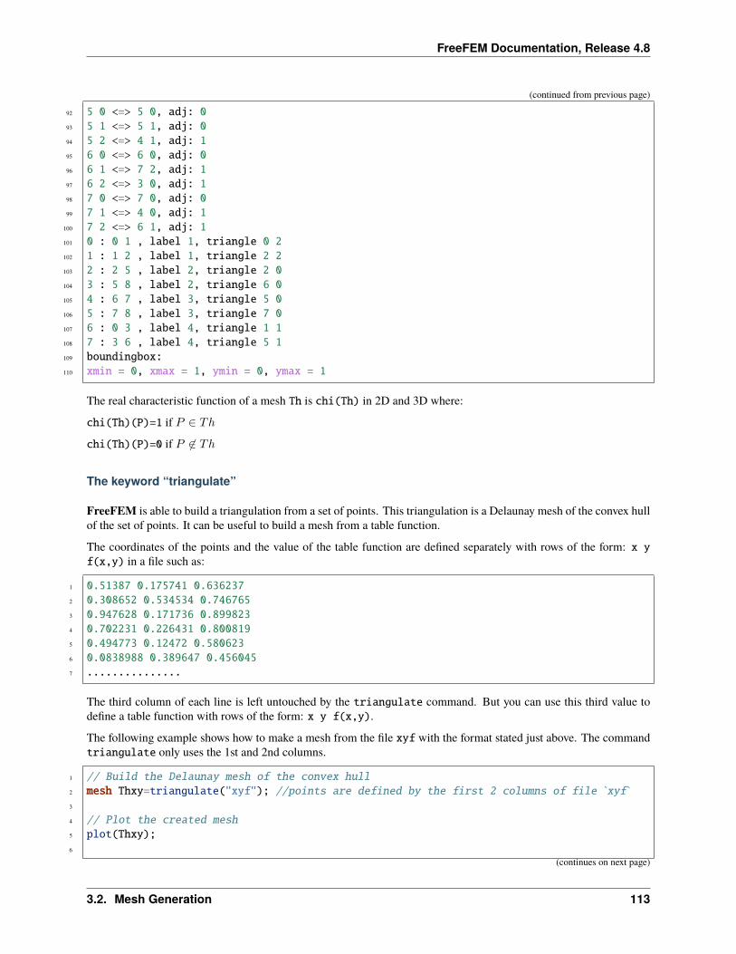
FreeFEM Documentation, Release 4.8
(continued from previous page)
92 5 0 <=> 5 0, adj: 093 5 1 <=> 5 1, adj: 094 5 2 <=> 4 1, adj: 195 6 0 <=> 6 0, adj: 096 6 1 <=> 7 2, adj: 197 6 2 <=> 3 0, adj: 198 7 0 <=> 7 0, adj: 099 7 1 <=> 4 0, adj: 1
100 7 2 <=> 6 1, adj: 1101 0 : 0 1 , label 1, triangle 0 2102 1 : 1 2 , label 1, triangle 2 2103 2 : 2 5 , label 2, triangle 2 0104 3 : 5 8 , label 2, triangle 6 0105 4 : 6 7 , label 3, triangle 5 0106 5 : 7 8 , label 3, triangle 7 0107 6 : 0 3 , label 4, triangle 1 1108 7 : 3 6 , label 4, triangle 5 1109 boundingbox:110 xmin = 0, xmax = 1, ymin = 0, ymax = 1
The real characteristic function of a mesh Th is chi(Th) in 2D and 3D where:
chi(Th)(P)=1 if 𝑃 ∈ 𝑇ℎ
chi(Th)(P)=0 if 𝑃 ∈ 𝑇ℎ
The keyword “triangulate”
FreeFEM is able to build a triangulation from a set of points. This triangulation is a Delaunay mesh of the convex hullof the set of points. It can be useful to build a mesh from a table function.
The coordinates of the points and the value of the table function are defined separately with rows of the form: x yf(x,y) in a file such as:
1 0.51387 0.175741 0.6362372 0.308652 0.534534 0.7467653 0.947628 0.171736 0.8998234 0.702231 0.226431 0.8008195 0.494773 0.12472 0.5806236 0.0838988 0.389647 0.4560457 ...............
The third column of each line is left untouched by the triangulate command. But you can use this third value todefine a table function with rows of the form: x y f(x,y).
The following example shows how to make a mesh from the file xyf with the format stated just above. The commandtriangulate only uses the 1st and 2nd columns.
1 // Build the Delaunay mesh of the convex hull2 mesh Thxy=triangulate("xyf"); //points are defined by the first 2 columns of file `xyf`3
4 // Plot the created mesh5 plot(Thxy);6
(continues on next page)
3.2. Mesh Generation 113
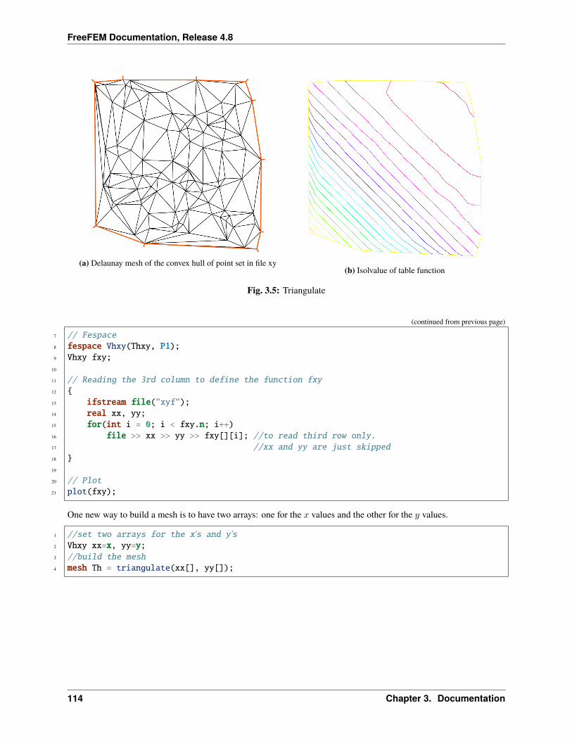
FreeFEM Documentation, Release 4.8
(a) Delaunay mesh of the convex hull of point set in file xy(b) Isolvalue of table function
Fig. 3.5: Triangulate
(continued from previous page)
7 // Fespace8 fespace Vhxy(Thxy, P1);9 Vhxy fxy;
10
11 // Reading the 3rd column to define the function fxy12 13 ifstream file("xyf");14 real xx, yy;15 for(int i = 0; i < fxy.n; i++)16 file >> xx >> yy >> fxy[][i]; //to read third row only.17 //xx and yy are just skipped18 19
20 // Plot21 plot(fxy);
One new way to build a mesh is to have two arrays: one for the 𝑥 values and the other for the 𝑦 values.
1 //set two arrays for the x's and y's2 Vhxy xx=x, yy=y;3 //build the mesh4 mesh Th = triangulate(xx[], yy[]);
114 Chapter 3. Documentation
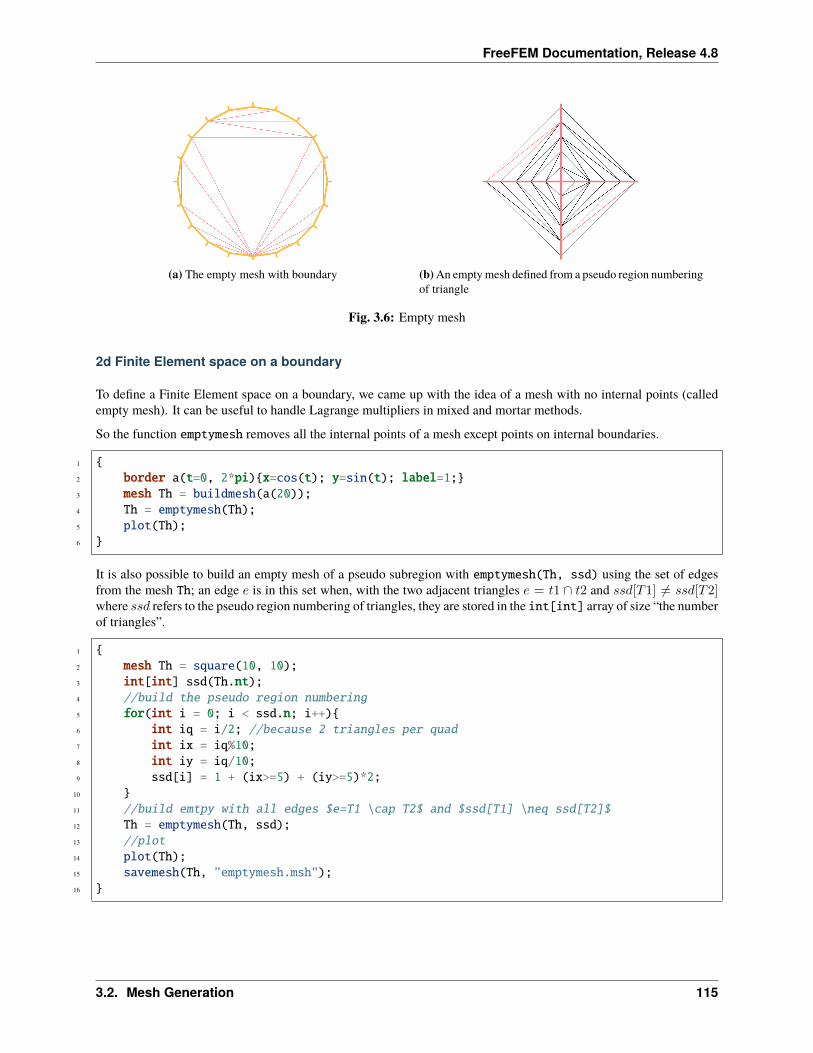
FreeFEM Documentation, Release 4.8
(a) The empty mesh with boundary (b) An empty mesh defined from a pseudo region numberingof triangle
Fig. 3.6: Empty mesh
2d Finite Element space on a boundary
To define a Finite Element space on a boundary, we came up with the idea of a mesh with no internal points (calledempty mesh). It can be useful to handle Lagrange multipliers in mixed and mortar methods.
So the function emptymesh removes all the internal points of a mesh except points on internal boundaries.
1 2 border a(t=0, 2*pi)x=cos(t); y=sin(t); label=1;3 mesh Th = buildmesh(a(20));4 Th = emptymesh(Th);5 plot(Th);6
It is also possible to build an empty mesh of a pseudo subregion with emptymesh(Th, ssd) using the set of edgesfrom the mesh Th; an edge 𝑒 is in this set when, with the two adjacent triangles 𝑒 = 𝑡1 ∩ 𝑡2 and 𝑠𝑠𝑑[𝑇1] = 𝑠𝑠𝑑[𝑇2]where 𝑠𝑠𝑑 refers to the pseudo region numbering of triangles, they are stored in the int[int] array of size “the numberof triangles”.
1 2 mesh Th = square(10, 10);3 int[int] ssd(Th.nt);4 //build the pseudo region numbering5 for(int i = 0; i < ssd.n; i++)6 int iq = i/2; //because 2 triangles per quad7 int ix = iq%10;8 int iy = iq/10;9 ssd[i] = 1 + (ix>=5) + (iy>=5)*2;
10 11 //build emtpy with all edges $e=T1 \cap T2$ and $ssd[T1] \neq ssd[T2]$12 Th = emptymesh(Th, ssd);13 //plot14 plot(Th);15 savemesh(Th, "emptymesh.msh");16
3.2. Mesh Generation 115
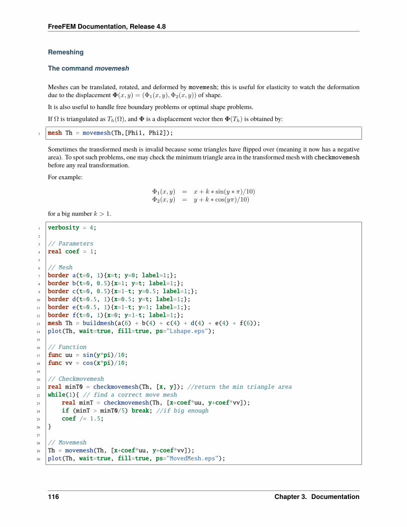
FreeFEM Documentation, Release 4.8
Remeshing
The command movemesh
Meshes can be translated, rotated, and deformed by movemesh; this is useful for elasticity to watch the deformationdue to the displacement Φ(𝑥, 𝑦) = (Φ1(𝑥, 𝑦),Φ2(𝑥, 𝑦)) of shape.
It is also useful to handle free boundary problems or optimal shape problems.
If Ω is triangulated as 𝑇ℎ(Ω), and Φ is a displacement vector then Φ(𝑇ℎ) is obtained by:
1 mesh Th = movemesh(Th,[Phi1, Phi2]);
Sometimes the transformed mesh is invalid because some triangles have flipped over (meaning it now has a negativearea). To spot such problems, one may check the minimum triangle area in the transformed mesh with checkmovemeshbefore any real transformation.
For example:
Φ1(𝑥, 𝑦) = 𝑥+ 𝑘 * sin(𝑦 * 𝜋)/10)Φ2(𝑥, 𝑦) = 𝑦 + 𝑘 * cos(𝑦𝜋)/10)
for a big number 𝑘 > 1.
1 verbosity = 4;2
3 // Parameters4 real coef = 1;5
6 // Mesh7 border a(t=0, 1)x=t; y=0; label=1;;8 border b(t=0, 0.5)x=1; y=t; label=1;;9 border c(t=0, 0.5)x=1-t; y=0.5; label=1;;
10 border d(t=0.5, 1)x=0.5; y=t; label=1;;11 border e(t=0.5, 1)x=1-t; y=1; label=1;;12 border f(t=0, 1)x=0; y=1-t; label=1;;13 mesh Th = buildmesh(a(6) + b(4) + c(4) + d(4) + e(4) + f(6));14 plot(Th, wait=true, fill=true, ps="Lshape.eps");15
16 // Function17 func uu = sin(y*pi)/10;18 func vv = cos(x*pi)/10;19
20 // Checkmovemesh21 real minT0 = checkmovemesh(Th, [x, y]); //return the min triangle area22 while(1) // find a correct move mesh23 real minT = checkmovemesh(Th, [x+coef*uu, y+coef*vv]);24 if (minT > minT0/5) break; //if big enough25 coef /= 1.5;26 27
28 // Movemesh29 Th = movemesh(Th, [x+coef*uu, y+coef*vv]);30 plot(Th, wait=true, fill=true, ps="MovedMesh.eps");
116 Chapter 3. Documentation
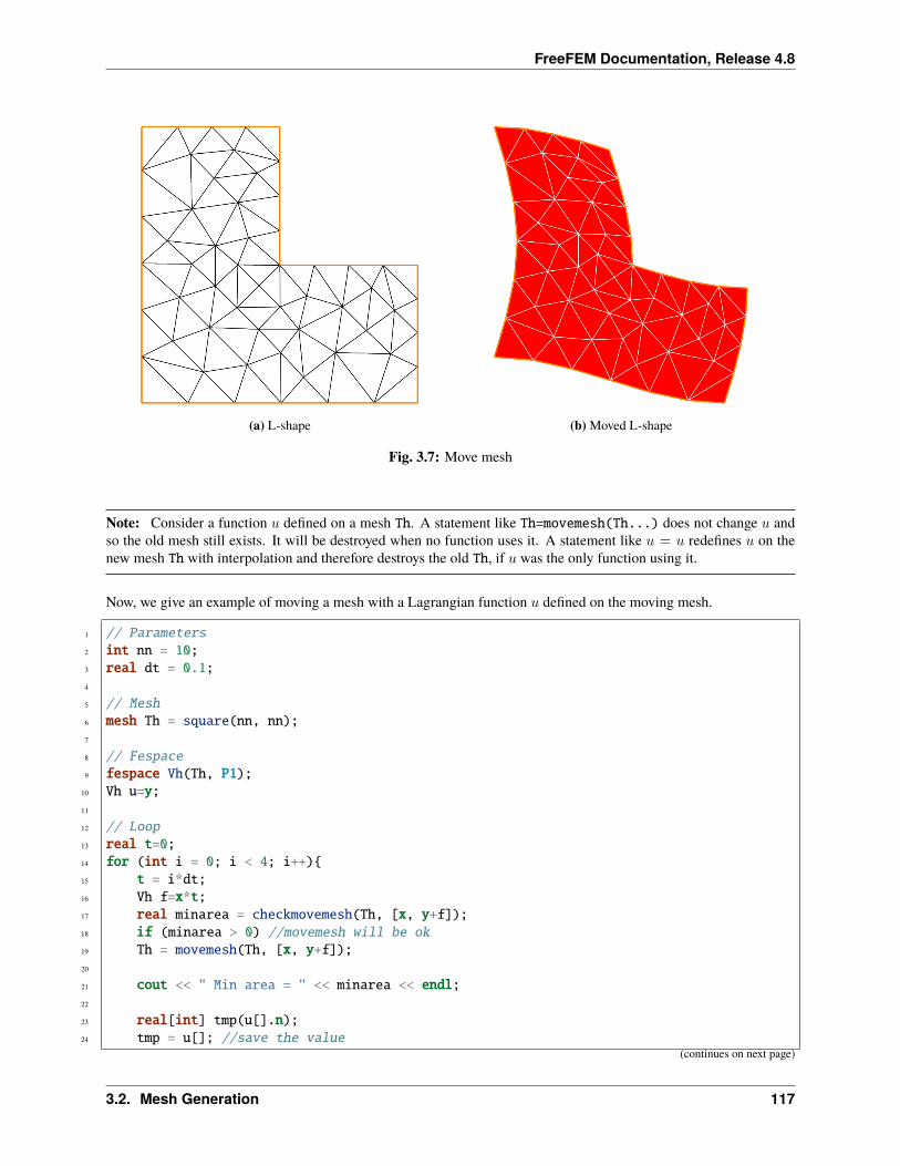
FreeFEM Documentation, Release 4.8
(a) L-shape (b) Moved L-shape
Fig. 3.7: Move mesh
Note: Consider a function 𝑢 defined on a mesh Th. A statement like Th=movemesh(Th...) does not change 𝑢 andso the old mesh still exists. It will be destroyed when no function uses it. A statement like 𝑢 = 𝑢 redefines 𝑢 on thenew mesh Th with interpolation and therefore destroys the old Th, if 𝑢 was the only function using it.
Now, we give an example of moving a mesh with a Lagrangian function 𝑢 defined on the moving mesh.
1 // Parameters2 int nn = 10;3 real dt = 0.1;4
5 // Mesh6 mesh Th = square(nn, nn);7
8 // Fespace9 fespace Vh(Th, P1);
10 Vh u=y;11
12 // Loop13 real t=0;14 for (int i = 0; i < 4; i++)15 t = i*dt;16 Vh f=x*t;17 real minarea = checkmovemesh(Th, [x, y+f]);18 if (minarea > 0) //movemesh will be ok19 Th = movemesh(Th, [x, y+f]);20
21 cout << " Min area = " << minarea << endl;22
23 real[int] tmp(u[].n);24 tmp = u[]; //save the value
(continues on next page)
3.2. Mesh Generation 117
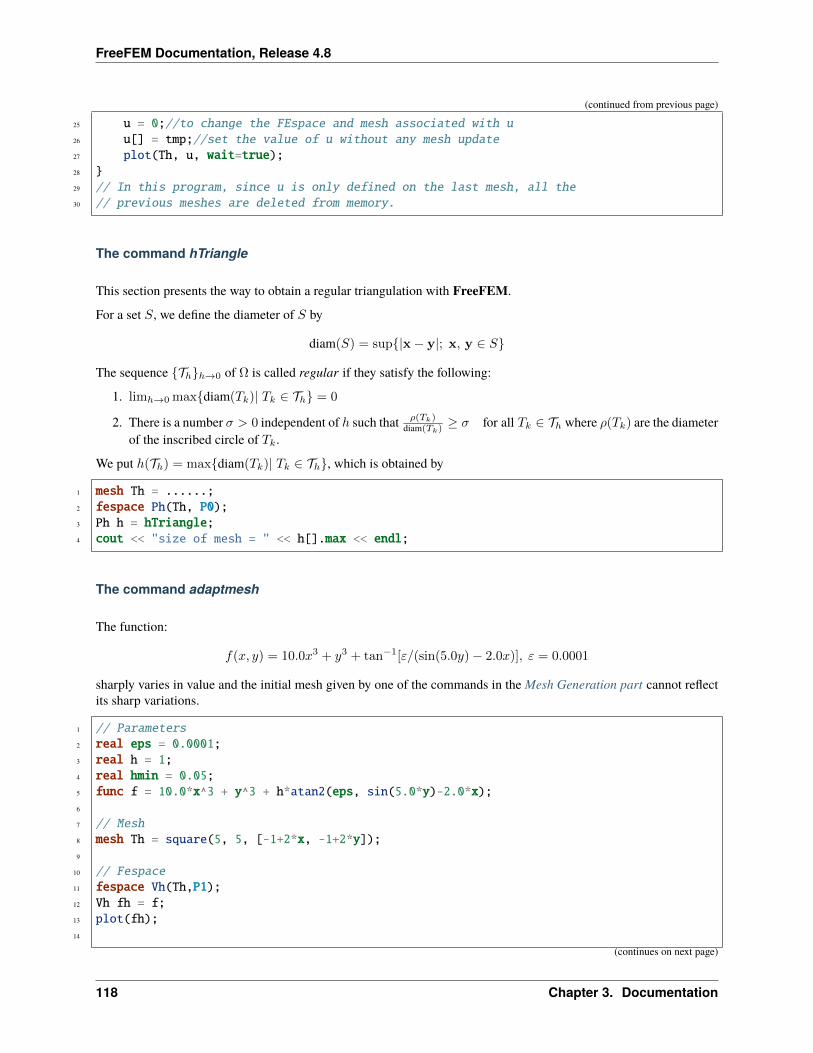
FreeFEM Documentation, Release 4.8
(continued from previous page)
25 u = 0;//to change the FEspace and mesh associated with u26 u[] = tmp;//set the value of u without any mesh update27 plot(Th, u, wait=true);28 29 // In this program, since u is only defined on the last mesh, all the30 // previous meshes are deleted from memory.
The command hTriangle
This section presents the way to obtain a regular triangulation with FreeFEM.
For a set 𝑆, we define the diameter of 𝑆 by
diam(𝑆) = sup|x− y|; x, y ∈ 𝑆
The sequence 𝒯ℎℎ→0 of Ω is called regular if they satisfy the following:
1. limℎ→0 maxdiam(𝑇𝑘)| 𝑇𝑘 ∈ 𝒯ℎ = 0
2. There is a number 𝜎 > 0 independent of ℎ such that 𝜌(𝑇𝑘)diam(𝑇𝑘)
≥ 𝜎 for all 𝑇𝑘 ∈ 𝒯ℎ where 𝜌(𝑇𝑘) are the diameterof the inscribed circle of 𝑇𝑘.
We put ℎ(𝒯ℎ) = maxdiam(𝑇𝑘)| 𝑇𝑘 ∈ 𝒯ℎ, which is obtained by
1 mesh Th = ......;2 fespace Ph(Th, P0);3 Ph h = hTriangle;4 cout << "size of mesh = " << h[].max << endl;
The command adaptmesh
The function:
𝑓(𝑥, 𝑦) = 10.0𝑥3 + 𝑦3 + tan−1[𝜀/(sin(5.0𝑦)− 2.0𝑥)], 𝜀 = 0.0001
sharply varies in value and the initial mesh given by one of the commands in the Mesh Generation part cannot reflectits sharp variations.
1 // Parameters2 real eps = 0.0001;3 real h = 1;4 real hmin = 0.05;5 func f = 10.0*x^3 + y^3 + h*atan2(eps, sin(5.0*y)-2.0*x);6
7 // Mesh8 mesh Th = square(5, 5, [-1+2*x, -1+2*y]);9
10 // Fespace11 fespace Vh(Th,P1);12 Vh fh = f;13 plot(fh);14
(continues on next page)
118 Chapter 3. Documentation
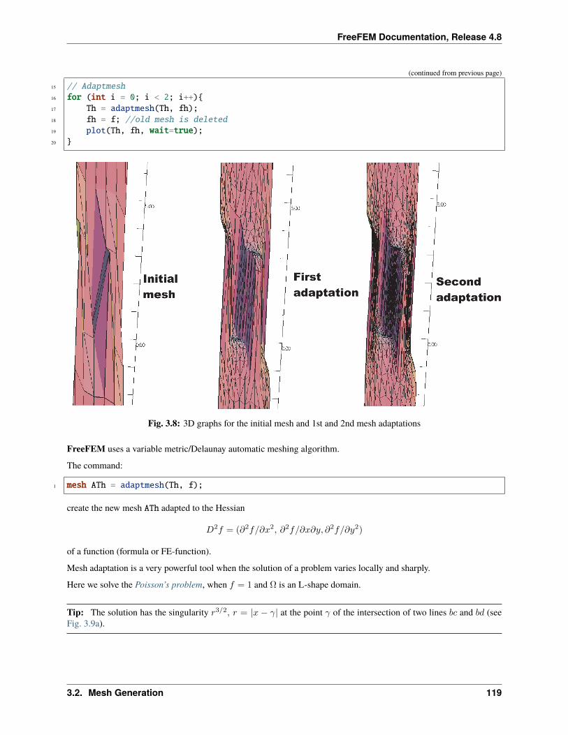
FreeFEM Documentation, Release 4.8
(continued from previous page)
15 // Adaptmesh16 for (int i = 0; i < 2; i++)17 Th = adaptmesh(Th, fh);18 fh = f; //old mesh is deleted19 plot(Th, fh, wait=true);20
Fig. 3.8: 3D graphs for the initial mesh and 1st and 2nd mesh adaptations
FreeFEM uses a variable metric/Delaunay automatic meshing algorithm.
The command:
1 mesh ATh = adaptmesh(Th, f);
create the new mesh ATh adapted to the Hessian
𝐷2𝑓 = (𝜕2𝑓/𝜕𝑥2, 𝜕2𝑓/𝜕𝑥𝜕𝑦, 𝜕2𝑓/𝜕𝑦2)
of a function (formula or FE-function).
Mesh adaptation is a very powerful tool when the solution of a problem varies locally and sharply.
Here we solve the Poisson’s problem, when 𝑓 = 1 and Ω is an L-shape domain.
Tip: The solution has the singularity 𝑟3/2, 𝑟 = |𝑥 − 𝛾| at the point 𝛾 of the intersection of two lines 𝑏𝑐 and 𝑏𝑑 (seeFig. 3.9a).
3.2. Mesh Generation 119
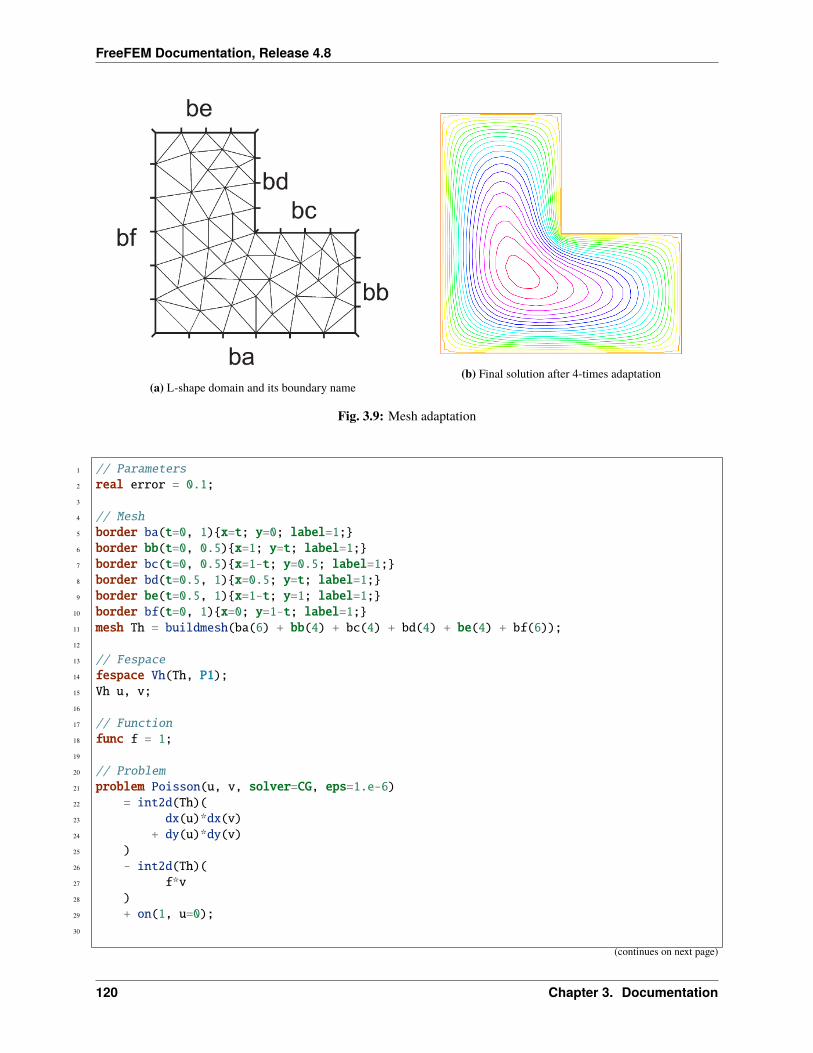
FreeFEM Documentation, Release 4.8
(a) L-shape domain and its boundary name(b) Final solution after 4-times adaptation
Fig. 3.9: Mesh adaptation
1 // Parameters2 real error = 0.1;3
4 // Mesh5 border ba(t=0, 1)x=t; y=0; label=1;6 border bb(t=0, 0.5)x=1; y=t; label=1;7 border bc(t=0, 0.5)x=1-t; y=0.5; label=1;8 border bd(t=0.5, 1)x=0.5; y=t; label=1;9 border be(t=0.5, 1)x=1-t; y=1; label=1;
10 border bf(t=0, 1)x=0; y=1-t; label=1;11 mesh Th = buildmesh(ba(6) + bb(4) + bc(4) + bd(4) + be(4) + bf(6));12
13 // Fespace14 fespace Vh(Th, P1);15 Vh u, v;16
17 // Function18 func f = 1;19
20 // Problem21 problem Poisson(u, v, solver=CG, eps=1.e-6)22 = int2d(Th)(23 dx(u)*dx(v)24 + dy(u)*dy(v)25 )26 - int2d(Th)(27 f*v28 )29 + on(1, u=0);30
(continues on next page)
120 Chapter 3. Documentation
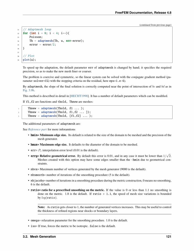
FreeFEM Documentation, Release 4.8
(continued from previous page)
31 // Adaptmesh loop32 for (int i = 0; i < 4; i++)33 Poisson;34 Th = adaptmesh(Th, u, err=error);35 error = error/2;36 37
38 // Plot39 plot(u);
To speed up the adaptation, the default parameter err of adaptmesh is changed by hand; it specifies the requiredprecision, so as to make the new mesh finer or coarser.
The problem is coercive and symmetric, so the linear system can be solved with the conjugate gradient method (pa-rameter solver=CG) with the stopping criteria on the residual, here eps=1.e-6).
By adaptmesh, the slope of the final solution is correctly computed near the point of intersection of 𝑏𝑐 and 𝑏𝑑 as inFig. 3.9b.
This method is described in detail in [HECHT1998]. It has a number of default parameters which can be modified.
If f1,f2 are functions and thold, Thnew are meshes:
1 Thnew = adaptmesh(Thold, f1 ... );2 Thnew = adaptmesh(Thold, f1,f2 ... ]);3 Thnew = adaptmesh(Thold, [f1,f2] ... );
The additional parameters of adaptmesh are:
See Reference part for more inforamtions
• hmin=Minimum edge size. Its default is related to the size of the domain to be meshed and the precision of themesh generator.
• hmax=Maximum edge size. It defaults to the diameter of the domain to be meshed.
• err= 𝑃1 interpolation error level (0.01 is the default).
• errg= Relative geometrical error. By default this error is 0.01, and in any case it must be lower than 1/√
2.Meshes created with this option may have some edges smaller than the -hmin due to geometrical con-straints.
• nbvx= Maximum number of vertices generated by the mesh generator (9000 is the default).
• nbsmooth= number of iterations of the smoothing procedure (5 is the default).
• nbjacoby= number of iterations in a smoothing procedure during the metric construction, 0 means no smoothing,6 is the default.
• ratio= ratio for a prescribed smoothing on the metric. If the value is 0 or less than 1.1 no smoothing isdone on the metric. 1.8 is the default. If ratio > 1.1, the speed of mesh size variations is boundedby 𝑙𝑜𝑔(ratio).
Note: As ratio gets closer to 1, the number of generated vertices increases. This may be useful to controlthe thickness of refined regions near shocks or boundary layers.
• omega= relaxation parameter for the smoothing procedure. 1.0 is the default.
• iso= If true, forces the metric to be isotropic. false is the default.
3.2. Mesh Generation 121
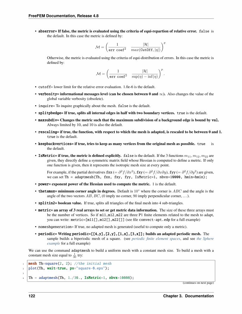
FreeFEM Documentation, Release 4.8
• abserror= If false, the metric is evaluated using the criteria of equi-repartion of relative error. false isthe default. In this case the metric is defined by:
ℳ =
(1
err coef2|ℋ|
𝑚𝑎𝑥(CutOff, |𝜂|)
)𝑝Otherwise, the metric is evaluated using the criteria of equi-distribution of errors. In this case the metric isdefined by:
ℳ =
(1
err coef2|ℋ|
sup(𝜂)− inf(𝜂)
)𝑝.
• cutoff= lower limit for the relative error evaluation. 1.0e-6 is the default.
• verbosity= informational messages level (can be chosen between 0 and∞). Also changes the value of theglobal variable verbosity (obsolete).
• inquire= To inquire graphically about the mesh. false is the default.
• splitpbedge= If true, splits all internal edges in half with two boundary vertices. true is the default.
• maxsubdiv= Changes the metric such that the maximum subdivision of a background edge is bound by val.Always limited by 10, and 10 is also the default.
• rescaling= if true, the function, with respect to which the mesh is adapted, is rescaled to be between 0 and 1.true is the default.
• keepbackvertices= if true, tries to keep as many vertices from the original mesh as possible. true isthe default.
• IsMetric= if true, the metric is defined explicitly. false is the default. If the 3 functions𝑚11,𝑚12,𝑚22 aregiven, they directly define a symmetric matrix field whose Hessian is computed to define a metric. If onlyone function is given, then it represents the isotropic mesh size at every point.
For example, if the partial derivatives fxx (= 𝜕2𝑓/𝜕𝑥2), fxy (= 𝜕2𝑓/𝜕𝑥𝜕𝑦), fyy (= 𝜕2𝑓/𝜕𝑦2) are given,we can set Th = adaptmesh(Th, fxx, fxy, fyy, IsMetric=1, nbvx=10000, hmin=hmin);
• power= exponent power of the Hessian used to compute the metric. 1 is the default.
• thetamax= minimum corner angle in degrees. Default is 10∘ where the corner is 𝐴𝐵𝐶 and the angle is theangle of the two vectors 𝐴𝐵,𝐵𝐶, (0 imply no corner, 90 imply perpendicular corner, . . . ).
• splitin2= boolean value. If true, splits all triangles of the final mesh into 4 sub-triangles.
• metric= an array of 3 real arrays to set or get metric data information. The size of these three arrays mustbe the number of vertices. So if m11,m12,m22 are three P1 finite elements related to the mesh to adapt,you can write: metric=[m11[],m12[],m22[]] (see file convect-apt.edp for a full example)
• nomeshgeneration= If true, no adapted mesh is generated (useful to compute only a metric).
• periodic=Writing periodic=[[4,y],[2,y],[1,x],[3,x]]; builds an adapted periodic mesh. Thesample builds a biperiodic mesh of a square. (see periodic finite element spaces, and see the Sphereexample for a full example)
We can use the command adaptmesh to build a uniform mesh with a constant mesh size. To build a mesh with aconstant mesh size equal to 1
30 try:
1 mesh Th=square(2, 2); //the initial mesh2 plot(Th, wait=true, ps="square-0.eps");3
4 Th = adaptmesh(Th, 1./30., IsMetric=1, nbvx=10000);(continues on next page)
122 Chapter 3. Documentation
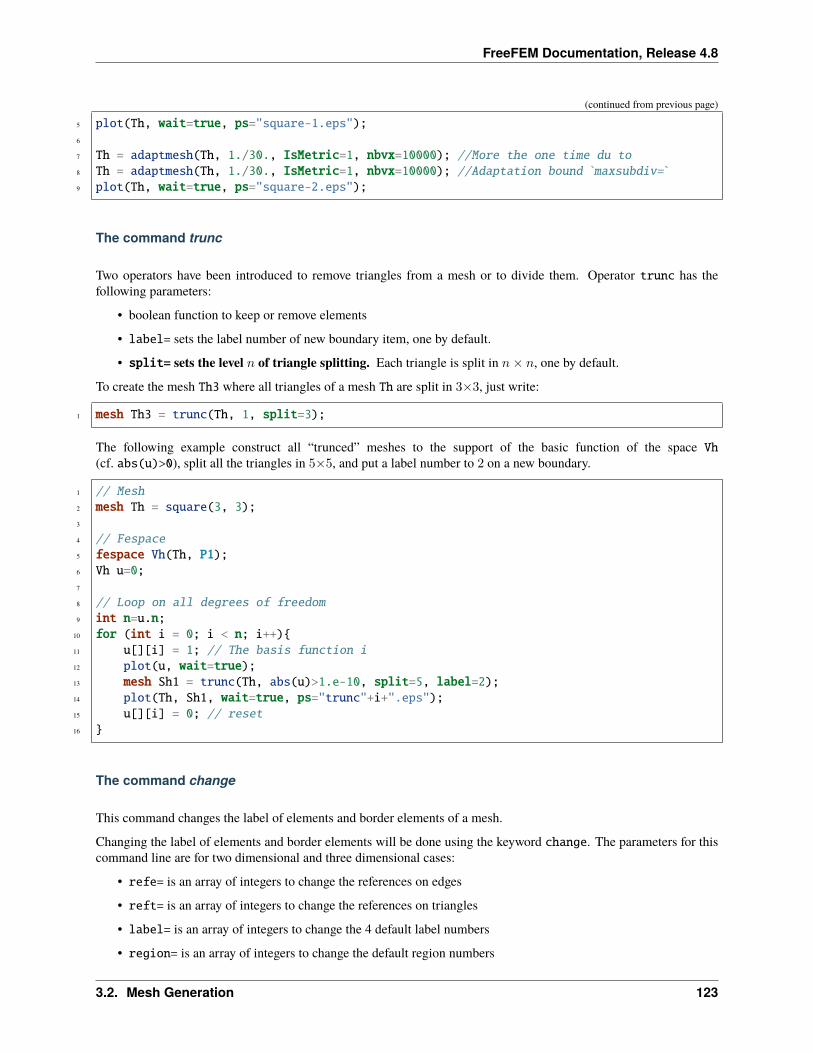
FreeFEM Documentation, Release 4.8
(continued from previous page)
5 plot(Th, wait=true, ps="square-1.eps");6
7 Th = adaptmesh(Th, 1./30., IsMetric=1, nbvx=10000); //More the one time du to8 Th = adaptmesh(Th, 1./30., IsMetric=1, nbvx=10000); //Adaptation bound `maxsubdiv=`9 plot(Th, wait=true, ps="square-2.eps");
The command trunc
Two operators have been introduced to remove triangles from a mesh or to divide them. Operator trunc has thefollowing parameters:
• boolean function to keep or remove elements
• label= sets the label number of new boundary item, one by default.
• split= sets the level 𝑛 of triangle splitting. Each triangle is split in 𝑛× 𝑛, one by default.
To create the mesh Th3 where all triangles of a mesh Th are split in 3×3, just write:
1 mesh Th3 = trunc(Th, 1, split=3);
The following example construct all “trunced” meshes to the support of the basic function of the space Vh(cf. abs(u)>0), split all the triangles in 5×5, and put a label number to 2 on a new boundary.
1 // Mesh2 mesh Th = square(3, 3);3
4 // Fespace5 fespace Vh(Th, P1);6 Vh u=0;7
8 // Loop on all degrees of freedom9 int n=u.n;
10 for (int i = 0; i < n; i++)11 u[][i] = 1; // The basis function i12 plot(u, wait=true);13 mesh Sh1 = trunc(Th, abs(u)>1.e-10, split=5, label=2);14 plot(Th, Sh1, wait=true, ps="trunc"+i+".eps");15 u[][i] = 0; // reset16
The command change
This command changes the label of elements and border elements of a mesh.
Changing the label of elements and border elements will be done using the keyword change. The parameters for thiscommand line are for two dimensional and three dimensional cases:
• refe= is an array of integers to change the references on edges
• reft= is an array of integers to change the references on triangles
• label= is an array of integers to change the 4 default label numbers
• region= is an array of integers to change the default region numbers
3.2. Mesh Generation 123
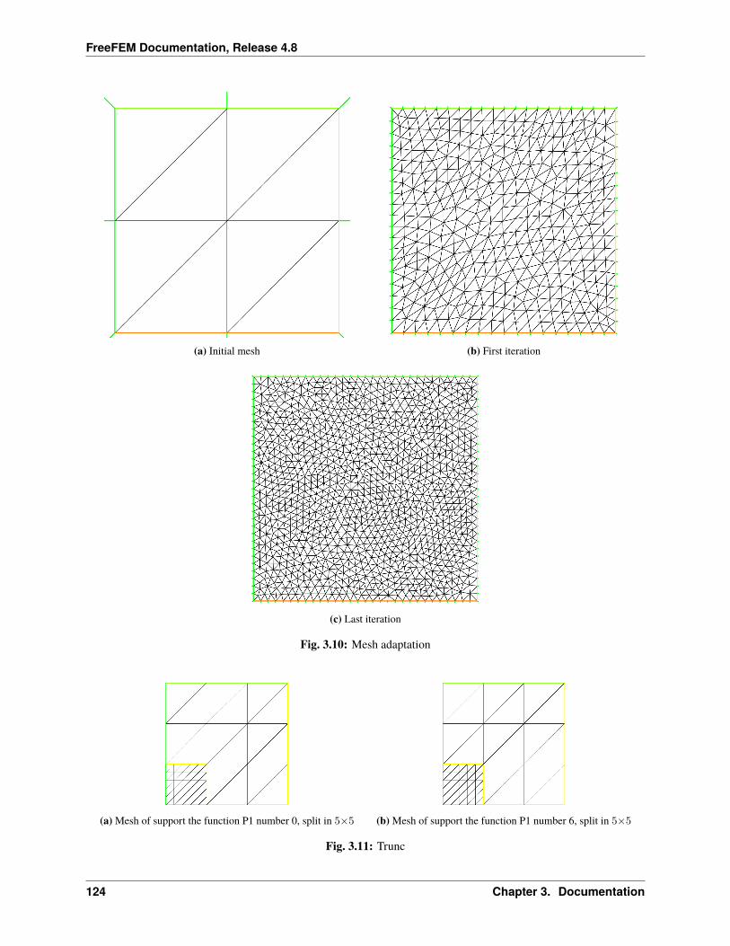
FreeFEM Documentation, Release 4.8
(a) Initial mesh (b) First iteration
(c) Last iteration
Fig. 3.10: Mesh adaptation
(a) Mesh of support the function P1 number 0, split in 5×5 (b) Mesh of support the function P1 number 6, split in 5×5
Fig. 3.11: Trunc
124 Chapter 3. Documentation
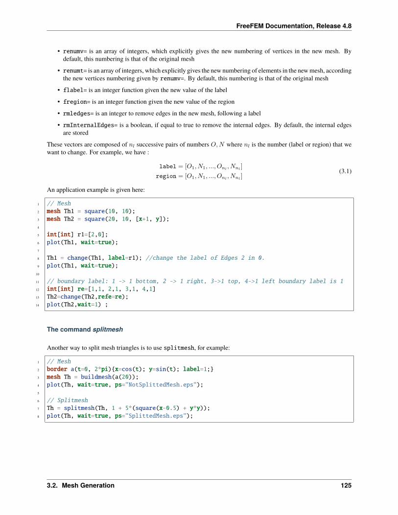
FreeFEM Documentation, Release 4.8
• renumv= is an array of integers, which explicitly gives the new numbering of vertices in the new mesh. Bydefault, this numbering is that of the original mesh
• renumt= is an array of integers, which explicitly gives the new numbering of elements in the new mesh, accordingthe new vertices numbering given by renumv=. By default, this numbering is that of the original mesh
• flabel= is an integer function given the new value of the label
• fregion= is an integer function given the new value of the region
• rmledges= is an integer to remove edges in the new mesh, following a label
• rmInternalEdges= is a boolean, if equal to true to remove the internal edges. By default, the internal edgesare stored
These vectors are composed of 𝑛𝑙 successive pairs of numbers 𝑂,𝑁 where 𝑛𝑙 is the number (label or region) that wewant to change. For example, we have :
label = [𝑂1, 𝑁1, ..., 𝑂𝑛𝑙, 𝑁𝑛𝑙
]
region = [𝑂1, 𝑁1, ..., 𝑂𝑛𝑙, 𝑁𝑛𝑙
](3.1)
An application example is given here:
1 // Mesh2 mesh Th1 = square(10, 10);3 mesh Th2 = square(20, 10, [x+1, y]);4
5 int[int] r1=[2,0];6 plot(Th1, wait=true);7
8 Th1 = change(Th1, label=r1); //change the label of Edges 2 in 0.9 plot(Th1, wait=true);
10
11 // boundary label: 1 -> 1 bottom, 2 -> 1 right, 3->1 top, 4->1 left boundary label is 112 int[int] re=[1,1, 2,1, 3,1, 4,1]13 Th2=change(Th2,refe=re);14 plot(Th2,wait=1) ;
The command splitmesh
Another way to split mesh triangles is to use splitmesh, for example:
1 // Mesh2 border a(t=0, 2*pi)x=cos(t); y=sin(t); label=1;3 mesh Th = buildmesh(a(20));4 plot(Th, wait=true, ps="NotSplittedMesh.eps");5
6 // Splitmesh7 Th = splitmesh(Th, 1 + 5*(square(x-0.5) + y*y));8 plot(Th, wait=true, ps="SplittedMesh.eps");
3.2. Mesh Generation 125
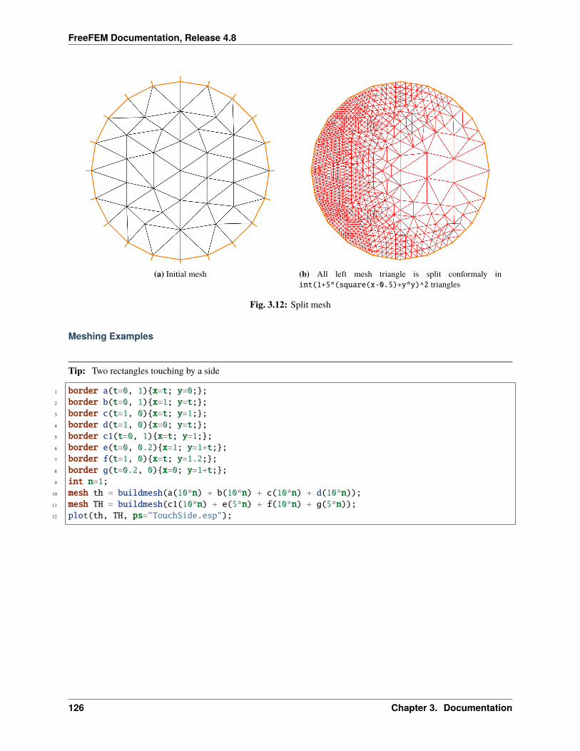
FreeFEM Documentation, Release 4.8
(a) Initial mesh (b) All left mesh triangle is split conformaly inint(1+5*(square(x-0.5)+y*y)^2 triangles
Fig. 3.12: Split mesh
Meshing Examples
Tip: Two rectangles touching by a side
1 border a(t=0, 1)x=t; y=0;;2 border b(t=0, 1)x=1; y=t;;3 border c(t=1, 0)x=t; y=1;;4 border d(t=1, 0)x=0; y=t;;5 border c1(t=0, 1)x=t; y=1;;6 border e(t=0, 0.2)x=1; y=1+t;;7 border f(t=1, 0)x=t; y=1.2;;8 border g(t=0.2, 0)x=0; y=1+t;;9 int n=1;
10 mesh th = buildmesh(a(10*n) + b(10*n) + c(10*n) + d(10*n));11 mesh TH = buildmesh(c1(10*n) + e(5*n) + f(10*n) + g(5*n));12 plot(th, TH, ps="TouchSide.esp");
126 Chapter 3. Documentation
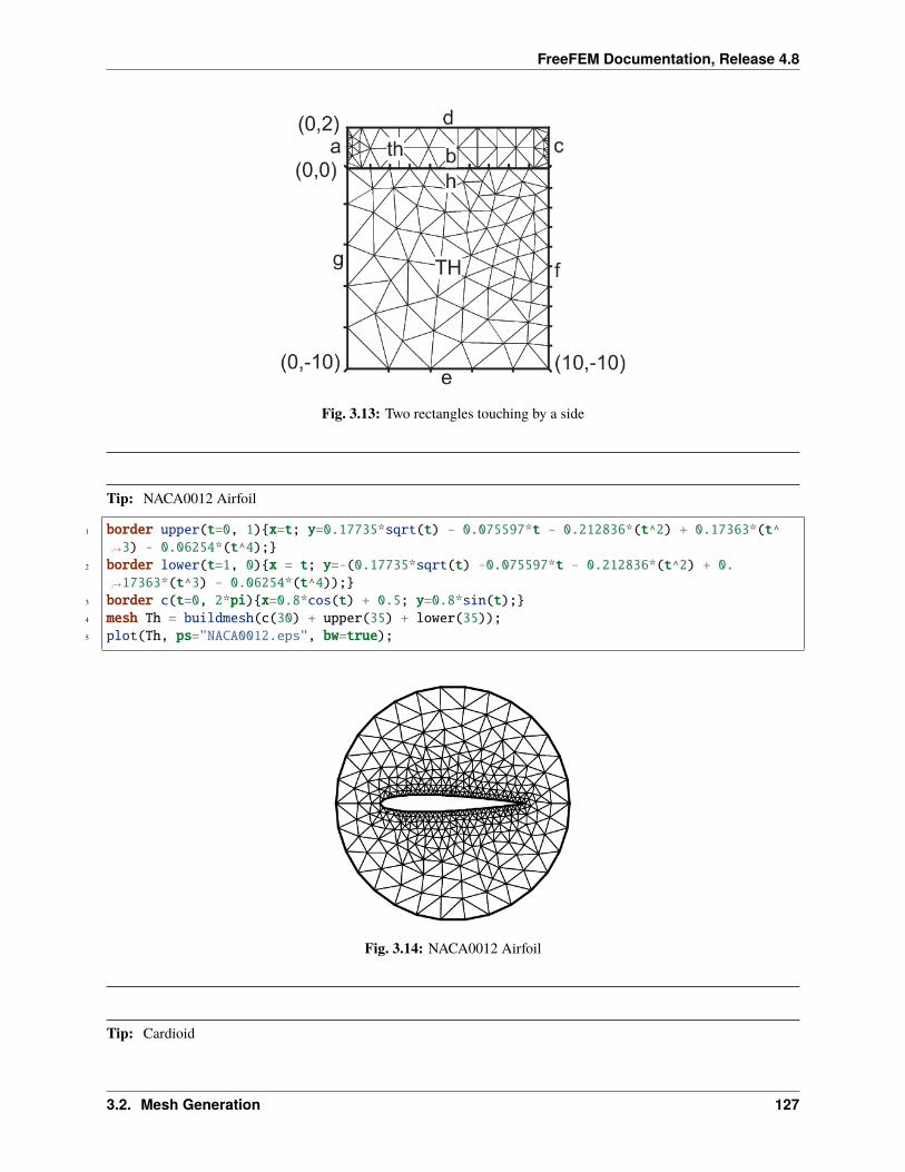
FreeFEM Documentation, Release 4.8
Fig. 3.13: Two rectangles touching by a side
Tip: NACA0012 Airfoil
1 border upper(t=0, 1)x=t; y=0.17735*sqrt(t) - 0.075597*t - 0.212836*(t^2) + 0.17363*(t^→˓3) - 0.06254*(t^4);
2 border lower(t=1, 0)x = t; y=-(0.17735*sqrt(t) -0.075597*t - 0.212836*(t^2) + 0.→˓17363*(t^3) - 0.06254*(t^4));
3 border c(t=0, 2*pi)x=0.8*cos(t) + 0.5; y=0.8*sin(t);4 mesh Th = buildmesh(c(30) + upper(35) + lower(35));5 plot(Th, ps="NACA0012.eps", bw=true);
Fig. 3.14: NACA0012 Airfoil
Tip: Cardioid
3.2. Mesh Generation 127
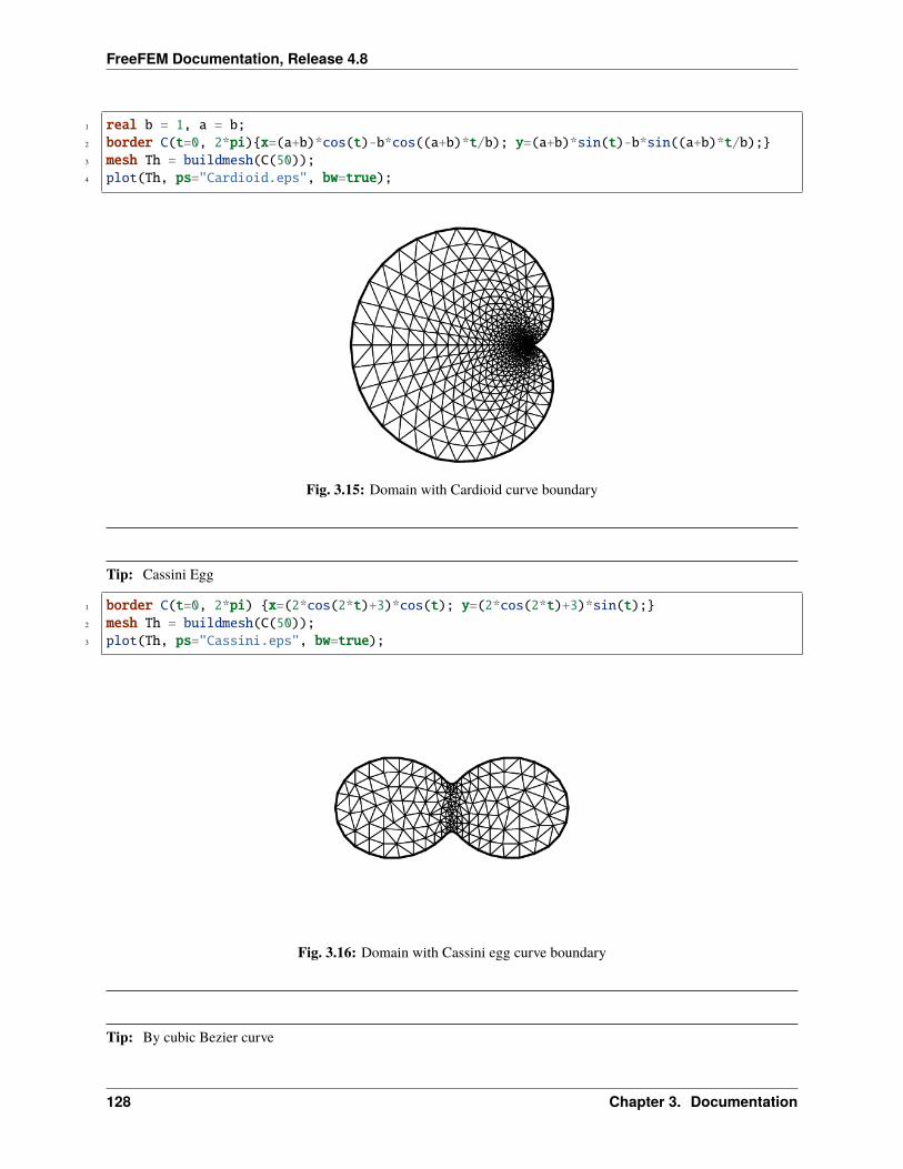
FreeFEM Documentation, Release 4.8
1 real b = 1, a = b;2 border C(t=0, 2*pi)x=(a+b)*cos(t)-b*cos((a+b)*t/b); y=(a+b)*sin(t)-b*sin((a+b)*t/b);3 mesh Th = buildmesh(C(50));4 plot(Th, ps="Cardioid.eps", bw=true);
Fig. 3.15: Domain with Cardioid curve boundary
Tip: Cassini Egg
1 border C(t=0, 2*pi) x=(2*cos(2*t)+3)*cos(t); y=(2*cos(2*t)+3)*sin(t);2 mesh Th = buildmesh(C(50));3 plot(Th, ps="Cassini.eps", bw=true);
Fig. 3.16: Domain with Cassini egg curve boundary
Tip: By cubic Bezier curve
128 Chapter 3. Documentation
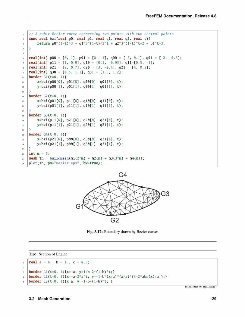
FreeFEM Documentation, Release 4.8
1 // A cubic Bezier curve connecting two points with two control points2 func real bzi(real p0, real p1, real q1, real q2, real t)3 return p0*(1-t)^3 + q1*3*(1-t)^2*t + q2*3*(1-t)*t^2 + p1*t^3;4 5
6 real[int] p00 = [0, 1], p01 = [0, -1], q00 = [-2, 0.1], q01 = [-2, -0.5];7 real[int] p11 = [1,-0.9], q10 = [0.1, -0.95], q11=[0.5, -1];8 real[int] p21 = [2, 0.7], q20 = [3, -0.4], q21 = [4, 0.5];9 real[int] q30 = [0.5, 1.1], q31 = [1.5, 1.2];
10 border G1(t=0, 1)11 x=bzi(p00[0], p01[0], q00[0], q01[0], t);12 y=bzi(p00[1], p01[1], q00[1], q01[1], t);13 14 border G2(t=0, 1)15 x=bzi(p01[0], p11[0], q10[0], q11[0], t);16 y=bzi(p01[1], p11[1], q10[1], q11[1], t);17 18 border G3(t=0, 1)19 x=bzi(p11[0], p21[0], q20[0], q21[0], t);20 y=bzi(p11[1], p21[1], q20[1], q21[1], t);21 22 border G4(t=0, 1)23 x=bzi(p21[0], p00[0], q30[0], q31[0], t);24 y=bzi(p21[1], p00[1], q30[1], q31[1], t);25 26 int m = 5;27 mesh Th = buildmesh(G1(2*m) + G2(m) + G3(3*m) + G4(m));28 plot(Th, ps="Bezier.eps", bw=true);
Fig. 3.17: Boundary drawn by Bezier curves
Tip: Section of Engine
1 real a = 6., b = 1., c = 0.5;2
3 border L1(t=0, 1)x=-a; y=1+b-2*(1+b)*t;4 border L2(t=0, 1)x=-a+2*a*t; y=-1-b*(x/a)*(x/a)*(3-2*abs(x)/a );5 border L3(t=0, 1)x=a; y=-1-b+(1+b)*t;
(continues on next page)
3.2. Mesh Generation 129
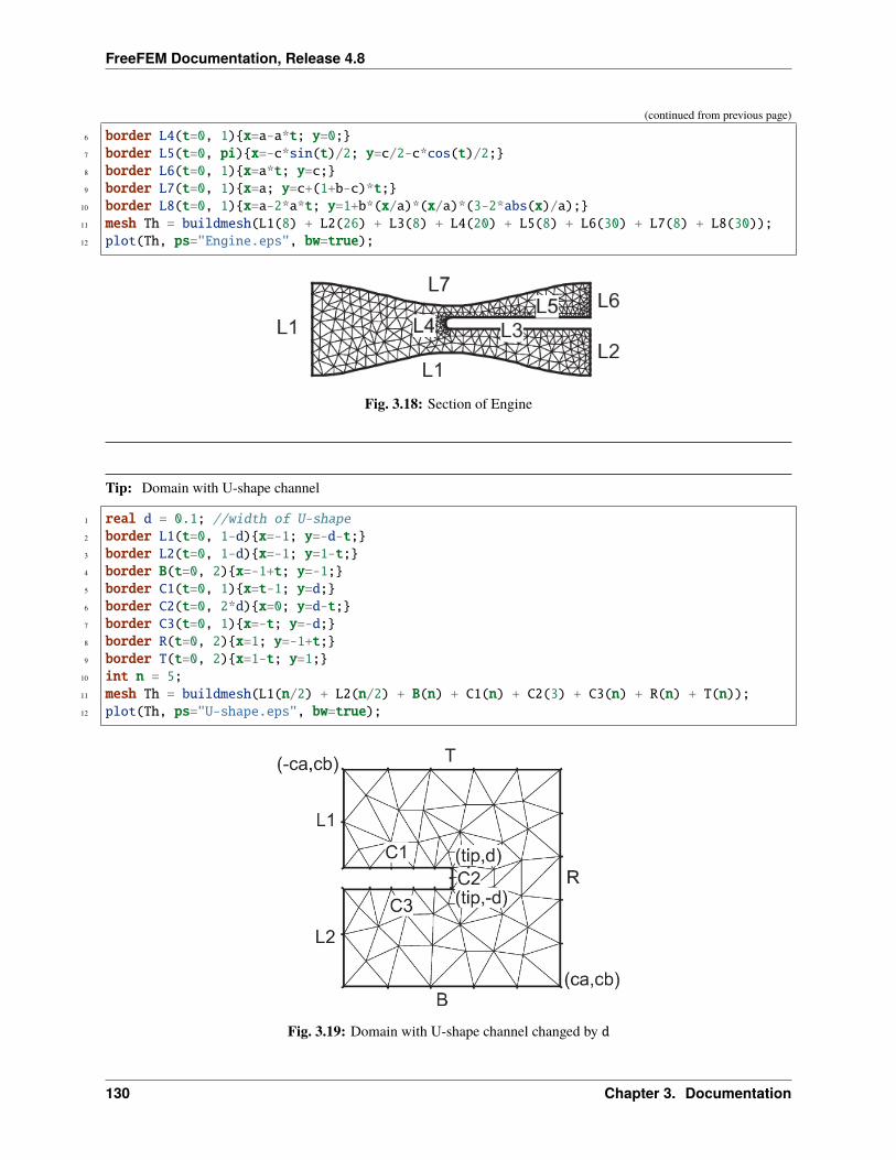
FreeFEM Documentation, Release 4.8
(continued from previous page)
6 border L4(t=0, 1)x=a-a*t; y=0;7 border L5(t=0, pi)x=-c*sin(t)/2; y=c/2-c*cos(t)/2;8 border L6(t=0, 1)x=a*t; y=c;9 border L7(t=0, 1)x=a; y=c+(1+b-c)*t;
10 border L8(t=0, 1)x=a-2*a*t; y=1+b*(x/a)*(x/a)*(3-2*abs(x)/a);11 mesh Th = buildmesh(L1(8) + L2(26) + L3(8) + L4(20) + L5(8) + L6(30) + L7(8) + L8(30));12 plot(Th, ps="Engine.eps", bw=true);
Fig. 3.18: Section of Engine
Tip: Domain with U-shape channel
1 real d = 0.1; //width of U-shape2 border L1(t=0, 1-d)x=-1; y=-d-t;3 border L2(t=0, 1-d)x=-1; y=1-t;4 border B(t=0, 2)x=-1+t; y=-1;5 border C1(t=0, 1)x=t-1; y=d;6 border C2(t=0, 2*d)x=0; y=d-t;7 border C3(t=0, 1)x=-t; y=-d;8 border R(t=0, 2)x=1; y=-1+t;9 border T(t=0, 2)x=1-t; y=1;
10 int n = 5;11 mesh Th = buildmesh(L1(n/2) + L2(n/2) + B(n) + C1(n) + C2(3) + C3(n) + R(n) + T(n));12 plot(Th, ps="U-shape.eps", bw=true);
Fig. 3.19: Domain with U-shape channel changed by d
130 Chapter 3. Documentation
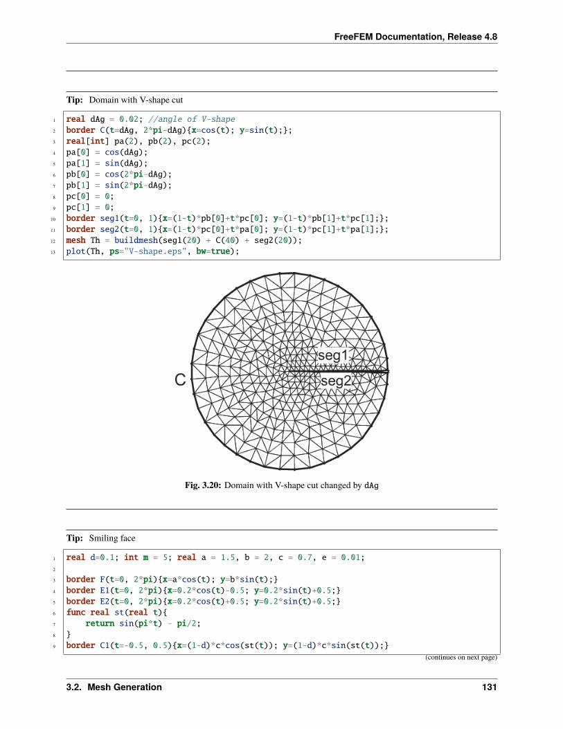
FreeFEM Documentation, Release 4.8
Tip: Domain with V-shape cut
1 real dAg = 0.02; //angle of V-shape2 border C(t=dAg, 2*pi-dAg)x=cos(t); y=sin(t);;3 real[int] pa(2), pb(2), pc(2);4 pa[0] = cos(dAg);5 pa[1] = sin(dAg);6 pb[0] = cos(2*pi-dAg);7 pb[1] = sin(2*pi-dAg);8 pc[0] = 0;9 pc[1] = 0;
10 border seg1(t=0, 1)x=(1-t)*pb[0]+t*pc[0]; y=(1-t)*pb[1]+t*pc[1];;11 border seg2(t=0, 1)x=(1-t)*pc[0]+t*pa[0]; y=(1-t)*pc[1]+t*pa[1];;12 mesh Th = buildmesh(seg1(20) + C(40) + seg2(20));13 plot(Th, ps="V-shape.eps", bw=true);
Fig. 3.20: Domain with V-shape cut changed by dAg
Tip: Smiling face
1 real d=0.1; int m = 5; real a = 1.5, b = 2, c = 0.7, e = 0.01;2
3 border F(t=0, 2*pi)x=a*cos(t); y=b*sin(t);4 border E1(t=0, 2*pi)x=0.2*cos(t)-0.5; y=0.2*sin(t)+0.5;5 border E2(t=0, 2*pi)x=0.2*cos(t)+0.5; y=0.2*sin(t)+0.5;6 func real st(real t)7 return sin(pi*t) - pi/2;8 9 border C1(t=-0.5, 0.5)x=(1-d)*c*cos(st(t)); y=(1-d)*c*sin(st(t));
(continues on next page)
3.2. Mesh Generation 131
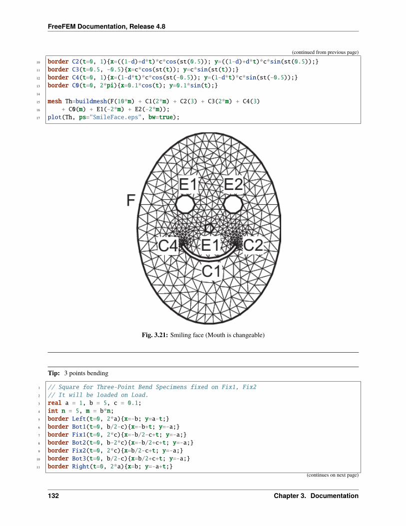
FreeFEM Documentation, Release 4.8
(continued from previous page)
10 border C2(t=0, 1)x=((1-d)+d*t)*c*cos(st(0.5)); y=((1-d)+d*t)*c*sin(st(0.5));11 border C3(t=0.5, -0.5)x=c*cos(st(t)); y=c*sin(st(t));12 border C4(t=0, 1)x=(1-d*t)*c*cos(st(-0.5)); y=(1-d*t)*c*sin(st(-0.5));13 border C0(t=0, 2*pi)x=0.1*cos(t); y=0.1*sin(t);14
15 mesh Th=buildmesh(F(10*m) + C1(2*m) + C2(3) + C3(2*m) + C4(3)16 + C0(m) + E1(-2*m) + E2(-2*m));17 plot(Th, ps="SmileFace.eps", bw=true);
Fig. 3.21: Smiling face (Mouth is changeable)
Tip: 3 points bending
1 // Square for Three-Point Bend Specimens fixed on Fix1, Fix22 // It will be loaded on Load.3 real a = 1, b = 5, c = 0.1;4 int n = 5, m = b*n;5 border Left(t=0, 2*a)x=-b; y=a-t;6 border Bot1(t=0, b/2-c)x=-b+t; y=-a;7 border Fix1(t=0, 2*c)x=-b/2-c+t; y=-a;8 border Bot2(t=0, b-2*c)x=-b/2+c+t; y=-a;9 border Fix2(t=0, 2*c)x=b/2-c+t; y=-a;
10 border Bot3(t=0, b/2-c)x=b/2+c+t; y=-a;11 border Right(t=0, 2*a)x=b; y=-a+t;
(continues on next page)
132 Chapter 3. Documentation
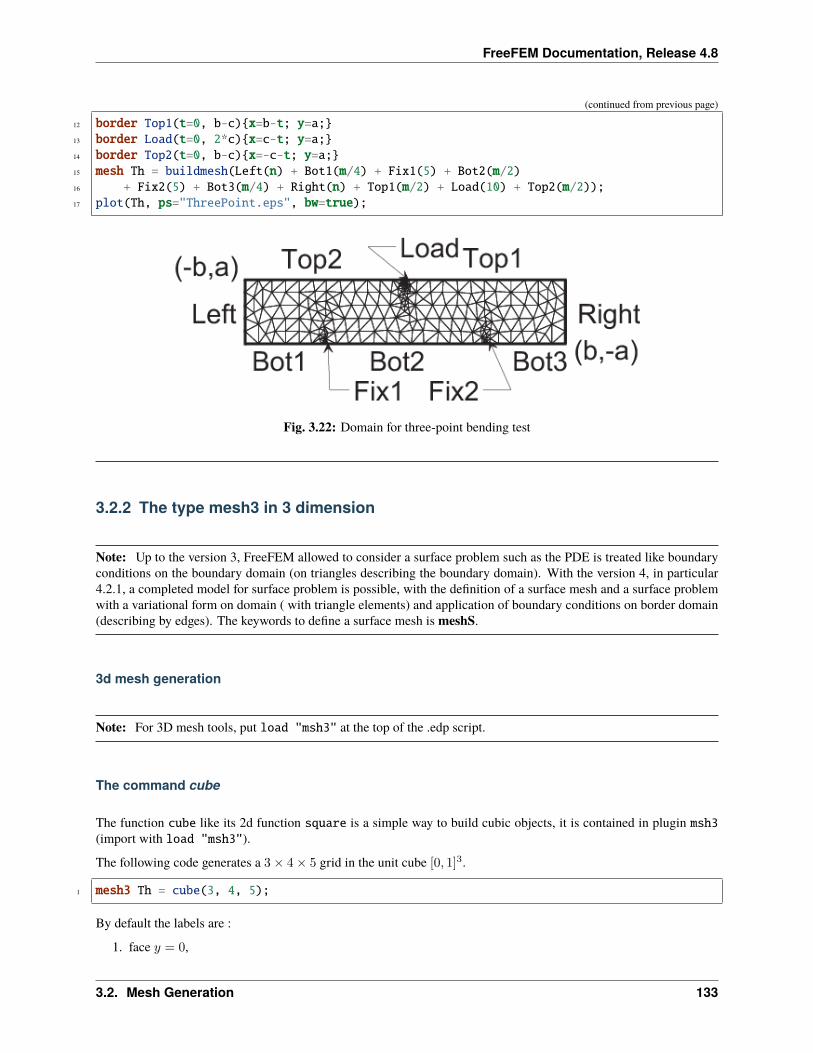
FreeFEM Documentation, Release 4.8
(continued from previous page)
12 border Top1(t=0, b-c)x=b-t; y=a;13 border Load(t=0, 2*c)x=c-t; y=a;14 border Top2(t=0, b-c)x=-c-t; y=a;15 mesh Th = buildmesh(Left(n) + Bot1(m/4) + Fix1(5) + Bot2(m/2)16 + Fix2(5) + Bot3(m/4) + Right(n) + Top1(m/2) + Load(10) + Top2(m/2));17 plot(Th, ps="ThreePoint.eps", bw=true);
Fig. 3.22: Domain for three-point bending test
3.2.2 The type mesh3 in 3 dimension
Note: Up to the version 3, FreeFEM allowed to consider a surface problem such as the PDE is treated like boundaryconditions on the boundary domain (on triangles describing the boundary domain). With the version 4, in particular4.2.1, a completed model for surface problem is possible, with the definition of a surface mesh and a surface problemwith a variational form on domain ( with triangle elements) and application of boundary conditions on border domain(describing by edges). The keywords to define a surface mesh is meshS.
3d mesh generation
Note: For 3D mesh tools, put load "msh3" at the top of the .edp script.
The command cube
The function cube like its 2d function square is a simple way to build cubic objects, it is contained in plugin msh3(import with load "msh3").
The following code generates a 3× 4× 5 grid in the unit cube [0, 1]3.
1 mesh3 Th = cube(3, 4, 5);
By default the labels are :
1. face 𝑦 = 0,
3.2. Mesh Generation 133
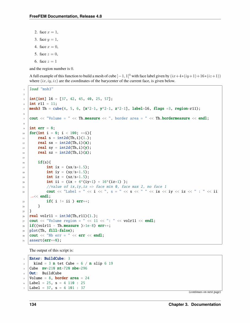
FreeFEM Documentation, Release 4.8
2. face 𝑥 = 1,
3. face 𝑦 = 1,
4. face 𝑥 = 0,
5. face 𝑧 = 0,
6. face 𝑧 = 1
and the region number is 0.
A full example of this function to build a mesh of cube ]−1, 1[3 with face label given by (𝑖𝑥+4*(𝑖𝑦+1)+16*(𝑖𝑧+1))where (𝑖𝑥, 𝑖𝑦, 𝑖𝑧) are the coordinates of the barycenter of the current face, is given below.
1 load "msh3"2
3 int[int] l6 = [37, 42, 45, 40, 25, 57];4 int r11 = 11;5 mesh3 Th = cube(4, 5, 6, [x*2-1, y*2-1, z*2-1], label=l6, flags =3, region=r11);6
7 cout << "Volume = " << Th.measure << ", border area = " << Th.bordermeasure << endl;8
9 int err = 0;10 for(int i = 0; i < 100; ++i)11 real s = int2d(Th,i)(1.);12 real sx = int2d(Th,i)(x);13 real sy = int2d(Th,i)(y);14 real sz = int2d(Th,i)(z);15
16 if(s)17 int ix = (sx/s+1.5);18 int iy = (sy/s+1.5);19 int iz = (sz/s+1.5);20 int ii = (ix + 4*(iy+1) + 16*(iz+1) );21 //value of ix,iy,iz => face min 0, face max 2, no face 122 cout << "Label = " << i << ", s = " << s << " " << ix << iy << iz << " : " << ii
→˓<< endl;23 if( i != ii ) err++;24 25 26 real volr11 = int3d(Th,r11)(1.);27 cout << "Volume region = " << 11 << ": " << volr11 << endl;28 if((volr11 - Th.measure )>1e-8) err++;29 plot(Th, fill=false);30 cout << "Nb err = " << err << endl;31 assert(err==0);
The output of this script is:
1 Enter: BuildCube: 32 kind = 3 n tet Cube = 6 / n slip 6 193 Cube nv=210 nt=720 nbe=2964 Out: BuildCube5 Volume = 8, border area = 246 Label = 25, s = 4 110 : 257 Label = 37, s = 4 101 : 37
(continues on next page)
134 Chapter 3. Documentation
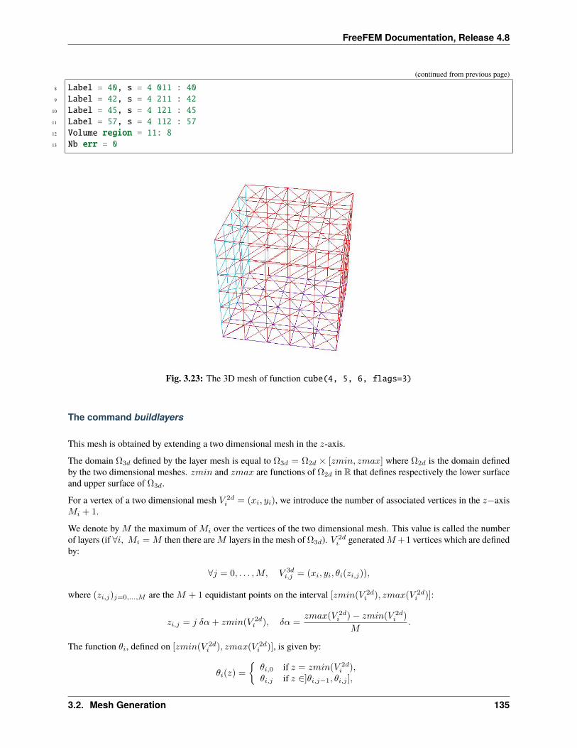
FreeFEM Documentation, Release 4.8
(continued from previous page)
8 Label = 40, s = 4 011 : 409 Label = 42, s = 4 211 : 42
10 Label = 45, s = 4 121 : 4511 Label = 57, s = 4 112 : 5712 Volume region = 11: 813 Nb err = 0
Fig. 3.23: The 3D mesh of function cube(4, 5, 6, flags=3)
The command buildlayers
This mesh is obtained by extending a two dimensional mesh in the 𝑧-axis.
The domain Ω3𝑑 defined by the layer mesh is equal to Ω3𝑑 = Ω2𝑑 × [𝑧𝑚𝑖𝑛, 𝑧𝑚𝑎𝑥] where Ω2𝑑 is the domain definedby the two dimensional meshes. 𝑧𝑚𝑖𝑛 and 𝑧𝑚𝑎𝑥 are functions of Ω2𝑑 in R that defines respectively the lower surfaceand upper surface of Ω3𝑑.
For a vertex of a two dimensional mesh 𝑉 2𝑑𝑖 = (𝑥𝑖, 𝑦𝑖), we introduce the number of associated vertices in the 𝑧−axis
𝑀𝑖 + 1.
We denote by 𝑀 the maximum of 𝑀𝑖 over the vertices of the two dimensional mesh. This value is called the numberof layers (if ∀𝑖, 𝑀𝑖 = 𝑀 then there are𝑀 layers in the mesh of Ω3𝑑). 𝑉 2𝑑
𝑖 generated𝑀+1 vertices which are definedby:
∀𝑗 = 0, . . . ,𝑀, 𝑉 3𝑑𝑖,𝑗 = (𝑥𝑖, 𝑦𝑖, 𝜃𝑖(𝑧𝑖,𝑗)),
where (𝑧𝑖,𝑗)𝑗=0,...,𝑀 are the 𝑀 + 1 equidistant points on the interval [𝑧𝑚𝑖𝑛(𝑉 2𝑑𝑖 ), 𝑧𝑚𝑎𝑥(𝑉 2𝑑
𝑖 )]:
𝑧𝑖,𝑗 = 𝑗 𝛿𝛼+ 𝑧𝑚𝑖𝑛(𝑉 2𝑑𝑖 ), 𝛿𝛼 =
𝑧𝑚𝑎𝑥(𝑉 2𝑑𝑖 )− 𝑧𝑚𝑖𝑛(𝑉 2𝑑
𝑖 )
𝑀.
The function 𝜃𝑖, defined on [𝑧𝑚𝑖𝑛(𝑉 2𝑑𝑖 ), 𝑧𝑚𝑎𝑥(𝑉 2𝑑
𝑖 )], is given by:
𝜃𝑖(𝑧) =
𝜃𝑖,0 if 𝑧 = 𝑧𝑚𝑖𝑛(𝑉 2𝑑
𝑖 ),𝜃𝑖,𝑗 if 𝑧 ∈]𝜃𝑖,𝑗−1, 𝜃𝑖,𝑗 ],
3.2. Mesh Generation 135
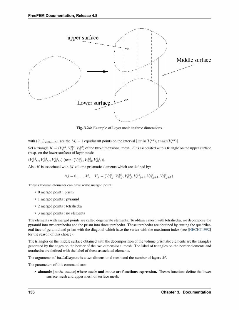
FreeFEM Documentation, Release 4.8
Fig. 3.24: Example of Layer mesh in three dimensions.
with (𝜃𝑖,𝑗)𝑗=0,...,𝑀𝑖are the 𝑀𝑖 + 1 equidistant points on the interval [𝑧𝑚𝑖𝑛(𝑉 2𝑑
𝑖 ), 𝑧𝑚𝑎𝑥(𝑉 2𝑑𝑖 )].
Set a triangle𝐾 = (𝑉 2𝑑𝑖1 , 𝑉 2𝑑
𝑖2 , 𝑉 2𝑑𝑖3 ) of the two dimensional mesh. 𝐾 is associated with a triangle on the upper surface
(resp. on the lower surface) of layer mesh:
(𝑉 3𝑑𝑖1,𝑀 , 𝑉
3𝑑𝑖2,𝑀 , 𝑉
3𝑑𝑖3,𝑀 ) (resp. (𝑉 3𝑑
𝑖1,0, 𝑉3𝑑𝑖2,0, 𝑉
3𝑑𝑖3,0)).
Also 𝐾 is associated with 𝑀 volume prismatic elements which are defined by:
∀𝑗 = 0, . . . ,𝑀, 𝐻𝑗 = (𝑉 3𝑑𝑖1,𝑗 , 𝑉
3𝑑𝑖2,𝑗 , 𝑉
3𝑑𝑖3,𝑗 , 𝑉
3𝑑𝑖1,𝑗+1, 𝑉
3𝑑𝑖2,𝑗+1, 𝑉
3𝑑𝑖3,𝑗+1).
Theses volume elements can have some merged point:
• 0 merged point : prism
• 1 merged points : pyramid
• 2 merged points : tetrahedra
• 3 merged points : no elements
The elements with merged points are called degenerate elements. To obtain a mesh with tetrahedra, we decompose thepyramid into two tetrahedra and the prism into three tetrahedra. These tetrahedra are obtained by cutting the quadrilat-eral face of pyramid and prism with the diagonal which have the vertex with the maximum index (see [HECHT1992]for the reason of this choice).
The triangles on the middle surface obtained with the decomposition of the volume prismatic elements are the trianglesgenerated by the edges on the border of the two dimensional mesh. The label of triangles on the border elements andtetrahedra are defined with the label of these associated elements.
The arguments of buildlayers is a two dimensional mesh and the number of layers 𝑀 .
The parameters of this command are:
• zbound= [𝑧𝑚𝑖𝑛, 𝑧𝑚𝑎𝑥] where 𝑧𝑚𝑖𝑛 and 𝑧𝑚𝑎𝑥 are functions expression. Theses functions define the lowersurface mesh and upper mesh of surface mesh.
136 Chapter 3. Documentation
FreeFEM Documentation, Release 4.8
• coef= A function expression between [0,1]. This parameter is used to introduce degenerate element in mesh.
The number of associated points or vertex 𝑉 2𝑑𝑖 is the integer part of 𝑐𝑜𝑒𝑓(𝑉 2𝑑
𝑖 )𝑀 .
• region= This vector is used to initialize the region of tetrahedra.
This vector contains successive pairs of the 2d region number at index 2𝑖 and the corresponding 3d region numberat index 2𝑖+ 1, like change.
• labelmid= This vector is used to initialize the 3d labels number of the vertical face or mid face from the 2dlabel number.
This vector contains successive pairs of the 2d label number at index 2𝑖 and the corresponding 3d label numberat index 2𝑖+ 1, like change.
• labelup= This vector is used to initialize the 3d label numbers of the upper/top face from the 2d region number.
This vector contains successive pairs of the 2d region number at index 2𝑖 and the corresponding 3d label numberat index 2𝑖+ 1, like change.
• labeldown= Same as the previous case but for the lower/down face label.
Moreover, we also add post processing parameters that allow to moving the mesh. These parameters correspond toparameters transfo, facemerge and ptmerge of the command line movemesh.
The vector region, labelmid, labelup and labeldownThese vectors are composed of 𝑛𝑙 successive pairs of number𝑂𝑖, 𝑁𝑙 where 𝑛𝑙 is the number (label or region) that we want to get.
An example of this command is given in the Build layer mesh example.
Tip: Cube
1 //Cube.idp2 load "medit"3 load "msh3"4
5 func mesh3 Cube (int[int] &NN, real[int, int] &BB, int[int, int] &L)6 real x0 = BB(0,0), x1 = BB(0,1);7 real y0 = BB(1,0), y1 = BB(1,1);8 real z0 = BB(2,0), z1 = BB(2,1);9
10 int nx = NN[0], ny = NN[1], nz = NN[2];11
12 // 2D mesh13 mesh Thx = square(nx, ny, [x0+(x1-x0)*x, y0+(y1-y0)*y]);14
15 // 3D mesh16 int[int] rup = [0, L(2,1)], rdown=[0, L(2,0)];17 int[int] rmid=[1, L(1,0), 2, L(0,1), 3, L(1,1), 4, L(0,0)];18 mesh3 Th = buildlayers(Thx, nz, zbound=[z0,z1],19 labelmid=rmid, labelup = rup, labeldown = rdown);20
21 return Th;22
Tip: Unit cube
3.2. Mesh Generation 137
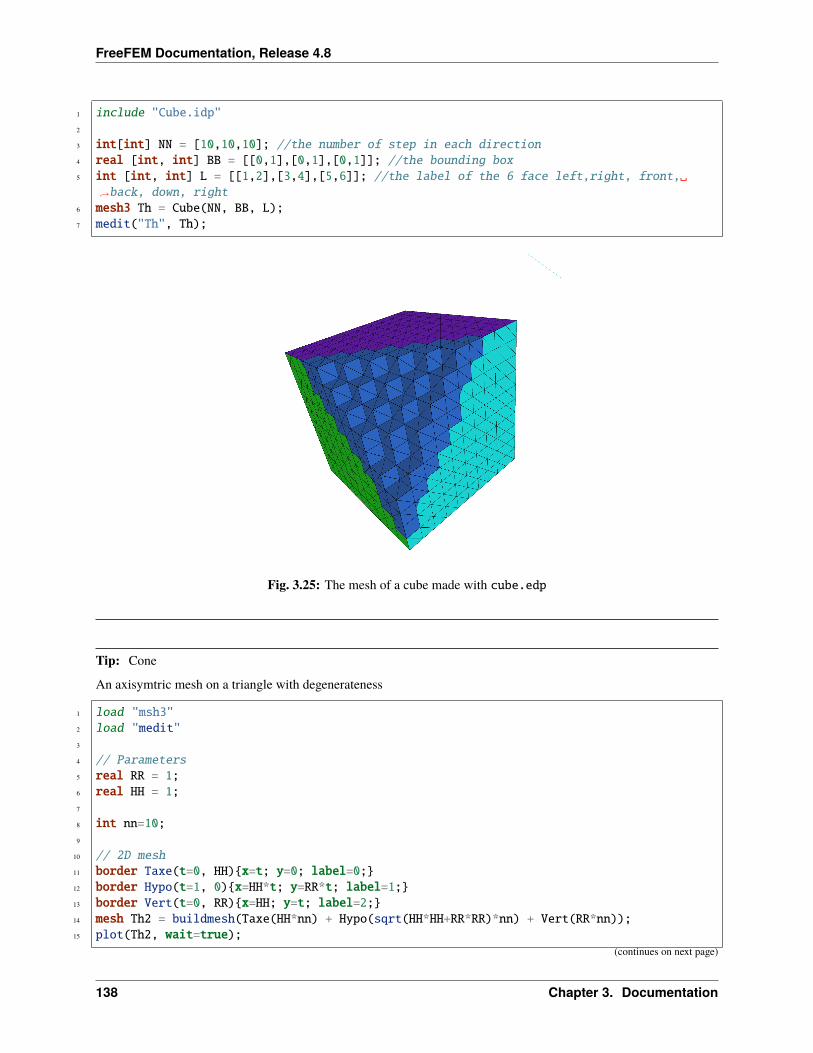
FreeFEM Documentation, Release 4.8
1 include "Cube.idp"2
3 int[int] NN = [10,10,10]; //the number of step in each direction4 real [int, int] BB = [[0,1],[0,1],[0,1]]; //the bounding box5 int [int, int] L = [[1,2],[3,4],[5,6]]; //the label of the 6 face left,right, front,
→˓back, down, right6 mesh3 Th = Cube(NN, BB, L);7 medit("Th", Th);
Fig. 3.25: The mesh of a cube made with cube.edp
Tip: Cone
An axisymtric mesh on a triangle with degenerateness
1 load "msh3"2 load "medit"3
4 // Parameters5 real RR = 1;6 real HH = 1;7
8 int nn=10;9
10 // 2D mesh11 border Taxe(t=0, HH)x=t; y=0; label=0;12 border Hypo(t=1, 0)x=HH*t; y=RR*t; label=1;13 border Vert(t=0, RR)x=HH; y=t; label=2;14 mesh Th2 = buildmesh(Taxe(HH*nn) + Hypo(sqrt(HH*HH+RR*RR)*nn) + Vert(RR*nn));15 plot(Th2, wait=true);
(continues on next page)
138 Chapter 3. Documentation
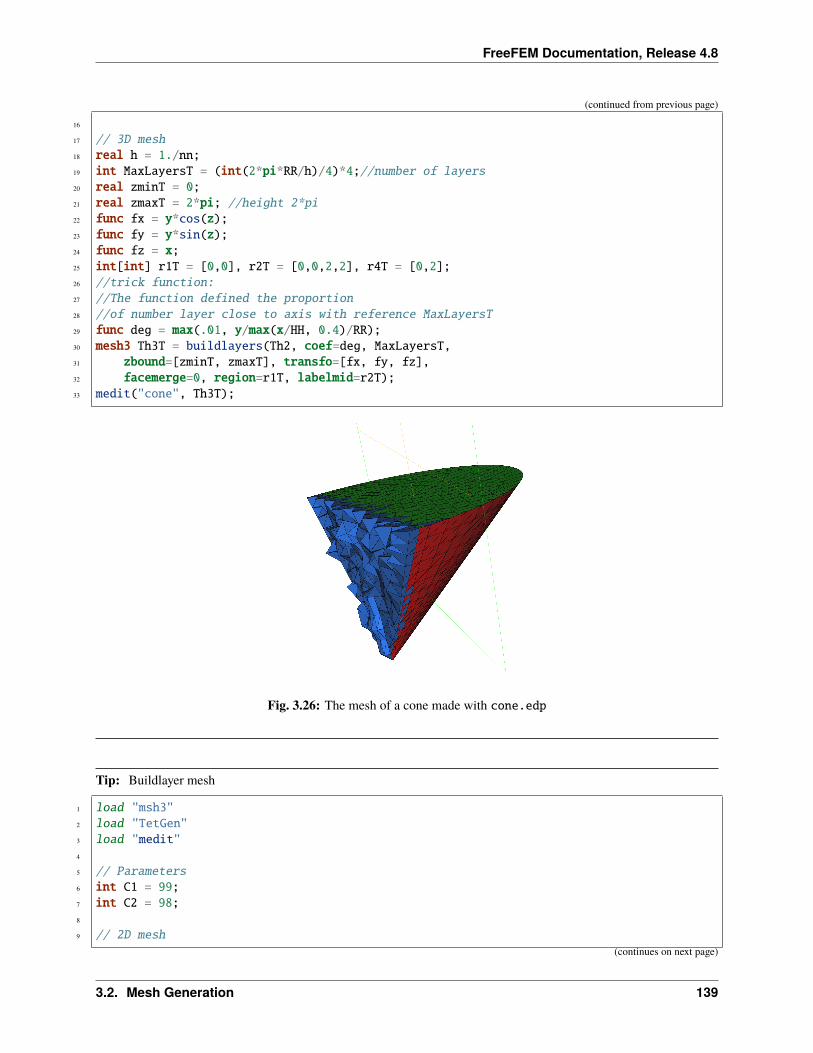
FreeFEM Documentation, Release 4.8
(continued from previous page)
16
17 // 3D mesh18 real h = 1./nn;19 int MaxLayersT = (int(2*pi*RR/h)/4)*4;//number of layers20 real zminT = 0;21 real zmaxT = 2*pi; //height 2*pi22 func fx = y*cos(z);23 func fy = y*sin(z);24 func fz = x;25 int[int] r1T = [0,0], r2T = [0,0,2,2], r4T = [0,2];26 //trick function:27 //The function defined the proportion28 //of number layer close to axis with reference MaxLayersT29 func deg = max(.01, y/max(x/HH, 0.4)/RR);30 mesh3 Th3T = buildlayers(Th2, coef=deg, MaxLayersT,31 zbound=[zminT, zmaxT], transfo=[fx, fy, fz],32 facemerge=0, region=r1T, labelmid=r2T);33 medit("cone", Th3T);
Fig. 3.26: The mesh of a cone made with cone.edp
Tip: Buildlayer mesh
1 load "msh3"2 load "TetGen"3 load "medit"4
5 // Parameters6 int C1 = 99;7 int C2 = 98;8
9 // 2D mesh(continues on next page)
3.2. Mesh Generation 139
FreeFEM Documentation, Release 4.8
(continued from previous page)
10 border C01(t=0, pi)x=t; y=0; label=1;11 border C02(t=0, 2*pi) x=pi; y=t; label=1;12 border C03(t=0, pi) x=pi-t; y=2*pi; label=1;13 border C04(t=0, 2*pi) x=0; y=2*pi-t; label=1;14
15 border C11(t=0, 0.7)x=0.5+t; y=2.5; label=C1;16 border C12(t=0, 2)x=1.2; y=2.5+t; label=C1;17 border C13(t=0, 0.7)x=1.2-t; y=4.5; label=C1;18 border C14(t=0, 2)x=0.5; y=4.5-t; label=C1;19
20 border C21(t=0, 0.7)x=2.3+t; y=2.5; label=C2;21 border C22(t=0, 2)x=3; y=2.5+t; label=C2;22 border C23(t=0, 0.7)x=3-t; y=4.5; label=C2;23 border C24(t=0, 2)x=2.3; y=4.5-t; label=C2;24
25 mesh Th = buildmesh(C01(10) + C02(10) + C03(10) + C04(10)26 + C11(5) + C12(5) + C13(5) + C14(5)27 + C21(-5) + C22(-5) + C23(-5) + C24(-5));28
29 mesh Ths = buildmesh(C01(10) + C02(10) + C03(10) + C04(10)30 + C11(5) + C12(5) + C13(5) + C14(5));31
32 // Construction of a box with one hole and two regions33 func zmin = 0.;34 func zmax = 1.;35 int MaxLayer = 10;36
37 func XX = x*cos(y);38 func YY = x*sin(y);39 func ZZ = z;40
41 int[int] r1 = [0, 41], r2 = [98, 98, 99, 99, 1, 56];42 int[int] r3 = [4, 12]; //the triangles of uppper surface mesh43 //generated by the triangle in the 2D region44 //of mesh Th of label 4 as label 1245 int[int] r4 = [4, 45]; //the triangles of lower surface mesh46 //generated by the triangle in the 2D region47 //of mesh Th of label 4 as label 45.48
49 mesh3 Th3 = buildlayers(Th, MaxLayer, zbound=[zmin, zmax], region=r1,50 labelmid=r2, labelup=r3, labeldown=r4);51 medit("box 2 regions 1 hole", Th3);52
53 // Construction of a sphere with TetGen54 func XX1 = cos(y)*sin(x);55 func YY1 = sin(y)*sin(x);56 func ZZ1 = cos(x);57
58 real[int] domain = [0., 0., 0., 0, 0.001];59 string test = "paACQ";60 cout << "test = " << test << endl;61 mesh3 Th3sph = tetgtransfo(Ths, transfo=[XX1, YY1, ZZ1],
(continues on next page)
140 Chapter 3. Documentation
FreeFEM Documentation, Release 4.8
(continued from previous page)
62 switch=test, nbofregions=1, regionlist=domain);63 medit("sphere 2 regions", Th3sph);
Remeshing
Note: if an operation on a mesh3 is performed then the same operation is applyed on its surface part (its meshSassociated)
The command change
This command changes the label of elements and border elements of a mesh. It’s the equivalent command in 2d meshcase.
Changing the label of elements and border elements will be done using the keyword change. The parameters for thiscommand line are for two dimensional and three dimensional cases:
• reftet= is a vector of integer that contains successive pairs of the old label number to the new label number.
• refface= is a vector of integer that contains successive pairs of the old region number to new region number.
• flabel= is an integer function given the new value of the label.
• fregion= is an integer function given the new value of the region.
• rmInternalFaces= is a boolean, equal true to remove the internal faces.
• rmlfaces= is a vector of integer, where triangle’s label given are remove of the mesh
These vectors are composed of 𝑛𝑙 successive pairs of numbers 𝑂,𝑁 where 𝑛𝑙 is the number (label or region) that wewant to change. For example, we have:
label = [𝑂1, 𝑁1, ..., 𝑂𝑛𝑙, 𝑁𝑛𝑙
]
region = [𝑂1, 𝑁1, ..., 𝑂𝑛𝑙, 𝑁𝑛𝑙
]
An example of use:
1 // Mesh2 mesh3 Th1 = cube(10, 10);3 mesh3 Th2 = cube(20, 10, [x+1, y,z]);4
5 int[int] r1=[2,0];6 plot(Th1, wait=true);7
8 Th1 = change(Th1, label=r1); //change the label of Edges 2 in 0.9 plot(Th1, wait=true);
10
11 // boundary label: 1 -> 1 bottom, 2 -> 1 right, 3->1 top, 4->1 left boundary label is 112 int[int] re=[1,1, 2,1, 3,1, 4,1]13 Th2=change(Th2,refe=re);14 plot(Th2,wait=1) ;
3.2. Mesh Generation 141
FreeFEM Documentation, Release 4.8
The command trunc
This operator have been introduce to remove a piece of mesh or/and split all element or for a particular label elementThe three named parameter - boolean function to keep or remove elements - split= sets the level n of triangle splitting.each triangle is splitted in n × n ( one by default) - freefem:label= sets the label number of new boundary item (1 bydefault)
An example of use
1 load "msh3"2 load "medit"3 int nn=8;4 mesh3 Th=cube(nn,nn,nn);5 // remove the small cube $]1/2,1[^2$6 Th= trunc(Th,((x<0.5) |(y< 0.5)| (z<0.5)), split=3, label=3);7 medit("cube",Th);
The command movemesh
3D meshes can be translated, rotated, and deformed using the command line movemesh as in the 2D case (see sectionmovemesh). If Ω is tetrahedrized as 𝑇ℎ(Ω), and Φ(𝑥, 𝑦) = (Φ1(𝑥, 𝑦, 𝑧),Φ2(𝑥, 𝑦, 𝑧),Φ3(𝑥, 𝑦, 𝑧)) is the transformationvector then Φ(𝑇ℎ) is obtained by:
1 mesh3 Th = movemesh(Th, [Phi1, Phi2, Phi3], ...);2 mesh3 Th = movemesh3(Th, transfo=[Phi1, Phi2, Phi3], ...); (syntax with transfo=)
The parameters of movemesh in three dimensions are:
• transfo= sets the geometric transformation Φ(𝑥, 𝑦) = (Φ1(𝑥, 𝑦, 𝑧),Φ2(𝑥, 𝑦, 𝑧),Φ3(𝑥, 𝑦, 𝑧))
• region= sets the integer labels of the tetrahedra. 0 by default.
• label= sets the labels of the border faces. This parameter is initialized as the label for the keyword change.
• facemerge= An integer expression. When you transform a mesh, some faces can be merged. This parameterequals to one if the merges’ faces is considered. Otherwise it equals to zero. By default, this parameter isequal to 1.
• ptmerge = A real expression. When you transform a mesh, some points can be merged. This parameter is thecriteria to define two merging points. By default, we use
𝑝𝑡𝑚𝑒𝑟𝑔𝑒 = 1𝑒− 7 𝑉 𝑜𝑙(𝐵),
where 𝐵 is the smallest axis parallel boxes containing the discretion domain of Ω and 𝑉 𝑜𝑙(𝐵) is the volume ofthis box.
• orientation = An integer expression equal 1, give the oientation of the triangulation, elements must be in thereference orientation (counter clock wise) equal -1 reverse the orientation of the tetrahedra
Note: The orientation of tetrahedra are checked by the positivity of its area and automatically corrected during thebuilding of the adjacency.
An example of this command can be found in the Poisson’s equation 3D example.
142 Chapter 3. Documentation
FreeFEM Documentation, Release 4.8
1 load "medit"2 include "cube.idp"3 int[int] Nxyz=[20,5,5];4 real [int,int] Bxyz=[[0.,5.],[0.,1.],[0.,1.]];5 int [int,int] Lxyz=[[1,2],[2,2],[2,2]];6 real E = 21.5e4;7 real sigma = 0.29;8 real mu = E/(2*(1+sigma));9 real lambda = E*sigma/((1+sigma)*(1-2*sigma));
10 real gravity = -0.05;11 real sqrt2=sqrt(2.);12
13 mesh3 Th=Cube(Nxyz,Bxyz,Lxyz);14 fespace Vh(Th,[P1,P1,P1]);15 Vh [u1,u2,u3], [v1,v2,v3];16
17 macro epsilon(u1,u2,u3) [dx(u1),dy(u2),dz(u3),(dz(u2)+dy(u3))/sqrt2,(dz(u1)+dx(u3))/→˓sqrt2,(dy(u1)+dx(u2))/sqrt2] // EOM
18 macro div(u1,u2,u3) ( dx(u1)+dy(u2)+dz(u3) ) // EOM19
20 solve Lame([u1,u2,u3],[v1,v2,v3])=21 int3d(Th)(22 lambda*div(u1,u2,u3)*div(v1,v2,v3)23 +2.*mu*( epsilon(u1,u2,u3)'*epsilon(v1,v2,v3) )24 )25 - int3d(Th) (gravity*v3)26 + on(1,u1=0,u2=0,u3=0);27
28 real dmax= u1[].max;29 real coef= 0.1/dmax;30
31 int[int] ref2=[1,0,2,0]; // array32 mesh3 Thm=movemesh(Th,[x+u1*coef,y+u2*coef,z+u3*coef],label=ref2);33 // mesh3 Thm=movemesh3(Th,transfo=[x+u1*coef,y+u2*coef,z+u3*coef],label=ref2); older
→˓syntax34 Thm=change(Thm,label=ref2);35 plot(Th,Thm, wait=1,cmm="coef amplification = "+coef );
movemesh doesn’t use the prefix tranfo= [.,.,.], the geometric transformation is directly given by [.,.,.] in the argumentslist
The command extract
This command offers the possibility to extract a boundary part of a mesh3
• refface , is a vector of integer that contains a list of triangle face references, where the extract function mustbe apply.
• label , is a vector of integer that contains a list of tetrahedra label
1 load"msh3"2 int nn = 30;3 int[int] labs = [1, 2, 2, 1, 1, 2]; // Label numbering
(continues on next page)
3.2. Mesh Generation 143
FreeFEM Documentation, Release 4.8
(continued from previous page)
4 mesh3 Th = cube(nn, nn, nn, label=labs);5 // extract the surface (boundary) of the cube6 int[int] llabs = [1, 2];7 meshS ThS = extract(Th,label=llabs);
The command buildSurface
This new function allows to build the surface mesh of a volume mesh, under the condition the surface is the boundary ofthe volume. By definition, a mesh3 is defined by a list of vertices, tetrahedron elements and triangle border elements.buildSurface function create the meshS corresponding, given the list vertices which are on the border domain, thetriangle elements and build the list of edges. Remark, for a closed surface mesh, the edges list is empty.
The command movemesh23
A simple method to tranform a 2D mesh in 3D Surface mesh. The principe is to project a two dimensional domain ina three dimensional space, 2d surface in the (x,y,z)-space to create a surface mesh 3D, meshS.
Warning: Since the release 4.2.1, the FreeFEM function movemesh23 returns a meshS type.
This corresponds to translate, rotate or deforme the domain by a displacement vector of this form Φ(x,y) =(Φ1(𝑥, 𝑦),Φ2(𝑥, 𝑦),Φ3(𝑥, 𝑦)).
The result of moving a two dimensional mesh Th2 by this three dimensional displacement is obtained using:
1 **meshS** Th3 = movemesh23(Th2, transfo=[Phi(1), Phi(2), Phi(3)]);
The parameters of this command line are:
• transfo= [Φ1, Φ2, Φ3] sets the displacement vector of transformation Φ(x,y) =[Φ1(𝑥, 𝑦),Φ2(𝑥, 𝑦),Φ3(𝑥, 𝑦)].
• label= sets an integer label of triangles.
• orientation= sets an integer orientation to give the global orientation of the surface of mesh. Equal 1, give atriangulation in the reference orientation (counter clock wise) equal -1 reverse the orientation of the triangles
• ptmerge= A real expression. When you transform a mesh, some points can be merged. This parameter is thecriteria to define two merging points. By default, we use
𝑝𝑡𝑚𝑒𝑟𝑔𝑒 = 1𝑒− 7 𝑉 𝑜𝑙(𝐵),
where 𝐵 is the smallest axis, parallel boxes containing the discretized domain of Ω and 𝑉 𝑜𝑙(𝐵) is the volumeof this box.
We can do a “gluing” of surface meshes using the process given in Change section. An example to obtain a threedimensional mesh using the command line tetg and movemesh23 is given below.
1 load "msh3"2 load "tetgen"3
4 // Parameters(continues on next page)
144 Chapter 3. Documentation
FreeFEM Documentation, Release 4.8
(continued from previous page)
5 real x10 = 1.;6 real x11 = 2.;7 real y10 = 0.;8 real y11 = 2.*pi;9
10 func ZZ1min = 0;11 func ZZ1max = 1.5;12 func XX1 = x;13 func YY1 = y;14
15 real x20 = 1.;16 real x21 = 2.;17 real y20=0.;18 real y21=1.5;19
20 func ZZ2 = y;21 func XX2 = x;22 func YY2min = 0.;23 func YY2max = 2*pi;24
25 real x30=0.;26 real x31=2*pi;27 real y30=0.;28 real y31=1.5;29
30 func XX3min = 1.;31 func XX3max = 2.;32 func YY3 = x;33 func ZZ3 = y;34
35 // Mesh36 mesh Thsq1 = square(5, 35, [x10+(x11-x10)*x, y10+(y11-y10)*y]);37 mesh Thsq2 = square(5, 8, [x20+(x21-x20)*x, y20+(y21-y20)*y]);38 mesh Thsq3 = square(35, 8, [x30+(x31-x30)*x, y30+(y31-y30)*y]);39
40 // Mesh 2D to 3D surface41 meshS Th31h = movemesh23(Thsq1, transfo=[XX1, YY1, ZZ1max], orientation=1);42 meshS Th31b = movemesh23(Thsq1, transfo=[XX1, YY1, ZZ1min], orientation=-1);43
44 meshS Th32h = movemesh23(Thsq2, transfo=[XX2, YY2max, ZZ2], orientation=-1);45 meshS Th32b = movemesh23(Thsq2, transfo=[XX2, YY2min, ZZ2], orientation=1);46
47 meshS Th33h = movemesh23(Thsq3, transfo=[XX3max, YY3, ZZ3], orientation=1);48 meshS Th33b = movemesh23(Thsq3, transfo=[XX3min, YY3, ZZ3], orientation=-1);49
50 // Gluing surfaces51 meshS Th33 = Th31h + Th31b + Th32h + Th32b + Th33h + Th33b;52 plot(Th33, cmm="Th33");53
54 // Tetrahelize the interior of the cube with TetGen55 real[int] domain =[1.5, pi, 0.75, 145, 0.0025];56 meshS Thfinal = tetg(Th33, switch="paAAQY", regionlist=domain);
(continues on next page)
3.2. Mesh Generation 145
FreeFEM Documentation, Release 4.8
(continued from previous page)
57 plot(Thfinal, cmm="Thfinal");58
59 // Build a mesh of a half cylindrical shell of interior radius 1, and exterior radius 2→˓and a height of 1.5
60 func mv2x = x*cos(y);61 func mv2y = x*sin(y);62 func mv2z = z;63 meshS Thmv2 = movemesh(Thfinal, transfo=[mv2x, mv2y, mv2z], facemerge=0);64 plot(Thmv2, cmm="Thmv2");
3d Meshing examples
Tip: Lake
1 load "msh3"2 load "medit"3
4 // Parameters5 int nn = 5;6
7 // 2D mesh8 border cc(t=0, 2*pi)x=cos(t); y=sin(t); label=1;9 mesh Th2 = buildmesh(cc(100));
10
11 // 3D mesh12 int[int] rup = [0, 2], rlow = [0, 1];13 int[int] rmid = [1, 1, 2, 1, 3, 1, 4, 1];14 func zmin = 2-sqrt(4-(x*x+y*y));15 func zmax = 2-sqrt(3.);16
17 mesh3 Th = buildlayers(Th2, nn,18 coef=max((zmax-zmin)/zmax, 1./nn),19 zbound=[zmin,zmax],20 labelmid=rmid,21 labelup=rup,22 labeldown=rlow);23
24 medit("Th", Th);
Tip: Hole region
1 load "msh3"2 load "TetGen"3 load "medit"4
5 // 2D mesh6 mesh Th = square(10, 20, [x*pi-pi/2, 2*y*pi]); // ]-pi/2, pi/2[X]0,2pi[7
(continues on next page)
146 Chapter 3. Documentation
FreeFEM Documentation, Release 4.8
(continued from previous page)
8 // 3D mesh9 //parametrization of a sphere
10 func f1 = cos(x)*cos(y);11 func f2 = cos(x)*sin(y);12 func f3 = sin(x);13 //partial derivative of the parametrization14 func f1x = sin(x)*cos(y);15 func f1y = -cos(x)*sin(y);16 func f2x = -sin(x)*sin(y);17 func f2y = cos(x)*cos(y);18 func f3x = cos(x);19 func f3y = 0;20 //M = DF^t DF21 func m11 = f1x^2 + f2x^2 + f3x^2;22 func m21 = f1x*f1y + f2x*f2y + f3x*f3y;23 func m22 = f1y^2 + f2y^2 + f3y^2;24
25 func perio = [[4, y], [2, y], [1, x], [3, x]];26 real hh = 0.1;27 real vv = 1/square(hh);28 verbosity = 2;29 Th = adaptmesh(Th, m11*vv, m21*vv, m22*vv, IsMetric=1, periodic=perio);30 Th = adaptmesh(Th, m11*vv, m21*vv, m22*vv, IsMetric=1, periodic=perio);31 plot(Th, wait=true);32
33 //construction of the surface of spheres34 real Rmin = 1.;35 func f1min = Rmin*f1;36 func f2min = Rmin*f2;37 func f3min = Rmin*f3;38
39 meshS ThSsph = movemesh23(Th, transfo=[f1min, f2min, f3min]);40
41 real Rmax = 2.;42 func f1max = Rmax*f1;43 func f2max = Rmax*f2;44 func f3max = Rmax*f3;45
46 meshS ThSsph2 = movemesh23(Th, transfo=[f1max, f2max, f3max]);47
48 //gluing meshes49 meshS ThS = ThSsph + ThSsph2;50
51 cout << " TetGen call without hole " << endl;52 real[int] domain2 = [1.5, 0., 0., 145, 0.001, 0.5, 0., 0., 18, 0.001];53 mesh3 Th3fin = tetg(ThS, switch="paAAQYY", nbofregions=2, regionlist=domain2);54 medit("Sphere with two regions", Th3fin);55
56 cout << " TetGen call with hole " << endl;57 real[int] hole = [0.,0.,0.];58 real[int] domain = [1.5, 0., 0., 53, 0.001];59 mesh3 Th3finhole = tetg(ThS, switch="paAAQYY",
(continues on next page)
3.2. Mesh Generation 147
FreeFEM Documentation, Release 4.8
(continued from previous page)
60 nbofholes=1, holelist=hole, nbofregions=1, regionlist=domain);61 medit("Sphere with a hole", Th3finhole);
Tip: Build a 3d mesh of a cube with a balloon
1 load "msh3"2 load "TetGen"3 load "medit"4 include "MeshSurface.idp"5
6 // Parameters7 real hs = 0.1; //mesh size on sphere8 int[int] N = [20, 20, 20];9 real [int,int] B = [[-1, 1], [-1, 1], [-1, 1]];
10 int [int,int] L = [[1, 2], [3, 4], [5, 6]];11
12 // Meshes13 meshS ThH = SurfaceHex(N, B, L, 1);14 meshS ThS = Sphere(0.5, hs, 7, 1);15
16 meshS ThHS = ThH + ThS;17 medit("Hex-Sphere", ThHS);18
19 real voltet = (hs^3)/6.;20 cout << "voltet = " << voltet << endl;21 real[int] domain = [0, 0, 0, 1, voltet, 0, 0, 0.7, 2, voltet];22 mesh3 Th = tetg(ThHS, switch="pqaAAYYQ", nbofregions=2, regionlist=domain);23 medit("Cube with ball", Th);
3.2.3 The type meshS in 3 dimension
Warning: Since the release 4.2.1, the surface mesh3 object (list of vertices and border elements, without tetahedraelements) is remplaced by meshS type.
Commands for 3d surface mesh generation
The command square3
The function square3 like the function square in 2d is the simple way to a build the unit square plan in the spaceR3. To use this command, it is necessary to load the pluging msh3 (need load "msh3"). A square in 3d consists inbuilding a 2d square which is projected from R2 to R3. The parameters of this command line are:
• n,m generates a n×m grid in the unit square
• [.,.,.] is [ Φ1, Φ2, Φ3 ] is the geometric transformation from R2 to R3. By default, [ Φ1, Φ2, Φ3 ] = [x,y,0]
• orientation= equal 1, gives the orientation of the triangulation, elements are in the reference orientation(counter clock wise) equal -1 reverse the orientation of the triangles it’s the global orientation of the surface
148 Chapter 3. Documentation
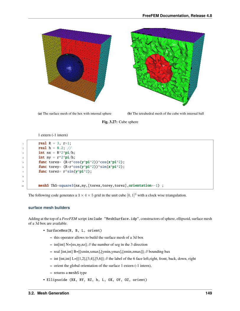
FreeFEM Documentation, Release 4.8
(a) The surface mesh of the hex with internal sphere (b) The tetrahedral mesh of the cube with internal ball
Fig. 3.27: Cube sphere
1 extern (-1 intern)
1 real R = 3, r=1;2 real h = 0.2; //3 int nx = R*2*pi/h;4 int ny = r*2*pi/h;5 func torex= (R+r*cos(y*pi*2))*cos(x*pi*2);6 func torey= (R+r*cos(y*pi*2))*sin(x*pi*2);7 func torez= r*sin(y*pi*2);8
9
10 meshS ThS=square3(nx,ny,[torex,torey,torez],orientation=-1) ;
The following code generates a 3× 4× 5 grid in the unit cube [0, 1]3 with a clock wise triangulation.
surface mesh builders
Adding at the top of a FreeFEM script include "MeshSurface.idp", constructors of sphere, ellipsoid, surface meshof a 3d box are available.
• SurfaceHex(N, B, L, orient)
– this operator allows to build the surface mesh of a 3d box
– int[int] N=[nx,ny,nz]; // the number of seg in the 3 direction
– real [int,int] B=[[xmin,xmax],[ymin,ymax],[zmin,zmax]]; // bounding bax
– int [int,int] L=[[1,2],[3,4],[5,6]]; // the label of the 6 face left,right, front, back, down, right
– orient the global orientation of the surface 1 extern (-1 intern),
– returns a meshS type
• Ellipsoide (RX, RY, RZ, h, L, OX, OY, OZ, orient)
3.2. Mesh Generation 149
FreeFEM Documentation, Release 4.8
– h is the mesh size
– L is the label
– orient the global orientation of the surface 1 extern (-1 intern)
– OX, OY, OZ are real numbers to give the Ellipsoide center ( optinal, by default is (0,0,0) )
– where RX, RY, RZ are real numbers such as the parametric equations of the ellipsoid is:
– returns a meshS type
∀𝑢 ∈ [−𝜋2,𝜋
2[ and 𝑣 ∈ [0, 2𝜋],
𝑥=Rx 𝑐𝑜𝑠(𝑢)𝑐𝑜𝑠(𝑣)+Ox𝑦=Ry 𝑐𝑜𝑠(𝑢)𝑠𝑖𝑛(𝑣)+Oy
𝑧=Rz 𝑠𝑖𝑛(𝑣)+Oz
• Sphere(R, h, L, OX, OY, OZ, orient)
– where R is the raduis of the sphere,
– OX, OY, OZ are real numbers to give the Ellipsoide center ( optinal, by default is (0,0,0) )
– h is the mesh size of the shpere
– L is the label the the sphere
– orient the global orientation of the surface 1 extern (-1 intern)
– returns a meshS type
1 func meshS SurfaceHex(int[int] & N,real[int,int] &B ,int[int,int] & L,int orientation)2 real x0=B(0,0),x1=B(0,1);3 real y0=B(1,0),y1=B(1,1);4 real z0=B(2,0),z1=B(2,1);5
6 int nx=N[0],ny=N[1],nz=N[2];7
8 mesh Thx = square(ny,nz,[y0+(y1-y0)*x,z0+(z1-z0)*y]);9 mesh Thy = square(nx,nz,[x0+(x1-x0)*x,z0+(z1-z0)*y]);
10 mesh Thz = square(nx,ny,[x0+(x1-x0)*x,y0+(y1-y0)*y]);11
12 int[int] refx=[0,L(0,0)],refX=[0,L(0,1)]; // Xmin, Ymax faces labels renumbering13 int[int] refy=[0,L(1,0)],refY=[0,L(1,1)]; // Ymin, Ymax faces labesl renumbering14 int[int] refz=[0,L(2,0)],refZ=[0,L(2,1)]; // Zmin, Zmax faces labels renumbering15
16 meshS Thx0 = movemesh23(Thx,transfo=[x0,x,y],orientation=-orientation,label=refx);17 meshS Thx1 = movemesh23(Thx,transfo=[x1,x,y],orientation=+orientation,label=refX);18 meshS Thy0 = movemesh23(Thy,transfo=[x,y0,y],orientation=+orientation,label=refy);19 meshS Thy1 = movemesh23(Thy,transfo=[x,y1,y],orientation=-orientation,label=refY);20 meshS Thz0 = movemesh23(Thz,transfo=[x,y,z0],orientation=-orientation,label=refz);21 meshS Thz1 = movemesh23(Thz,transfo=[x,y,z1],orientation=+orientation,label=refZ);22 meshS Th= Thx0+Thx1+Thy0+Thy1+Thz0+Thz1;23
24 return Th;25 26
27 func meshS Ellipsoide (real RX,real RY,real RZ,real h,int L,real Ox,real Oy,real Oz,int→˓orientation)
28 mesh Th=square(10,20,[x*pi-pi/2,2*y*pi]); // $]\frac-pi2,frac-pi2[\→˓times]0,2\pi[ $
(continues on next page)
150 Chapter 3. Documentation
FreeFEM Documentation, Release 4.8
(continued from previous page)
29 // a parametrization of a sphere30 func f1 =RX*cos(x)*cos(y);31 func f2 =RY*cos(x)*sin(y);32 func f3 =RZ*sin(x);33 // partiel derivative34 func f1x= -RX*sin(x)*cos(y);35 func f1y= -RX*cos(x)*sin(y);36 func f2x= -RY*sin(x)*sin(y);37 func f2y= +RY*cos(x)*cos(y);38 func f3x=-RZ*cos(x);39 func f3y=0;40 // the metric on the sphere $ M = DF^t DF $41 func m11=f1x^2+f2x^2+f3x^2;42 func m21=f1x*f1y+f2x*f2y+f3x*f3y;43 func m22=f1y^2+f2y^2+f3y^2;44 func perio=[[4,y],[2,y],[1,x],[3,x]]; // to store the periodic condition45 real hh=h;// hh mesh size on unite sphere46 real vv= 1/square(hh);47 Th=adaptmesh(Th,m11*vv,m21*vv,m22*vv,IsMetric=1,periodic=perio);48 Th=adaptmesh(Th,m11*vv,m21*vv,m22*vv,IsMetric=1,periodic=perio);49 Th=adaptmesh(Th,m11*vv,m21*vv,m22*vv,IsMetric=1,periodic=perio);50 Th=adaptmesh(Th,m11*vv,m21*vv,m22*vv,IsMetric=1,periodic=perio);51 int[int] ref=[0,L];52 meshS ThS=movemesh23(Th,transfo=[f1,f2,f3],orientation=orientation,refface=ref);53 ThS=mmgs(ThS,hmin=h,hmax=h,hgrad=2.);54 return ThS;55 56
57 func meshS Ellipsoide (real RX,real RY,real RZ,real h,int L,int orientation) 58 return Ellipsoide (RX,RY,RZ,h,L,0.,0.,0.,orientation);59 60 func meshS Sphere(real R,real h,int L,int orientation) 61 return Ellipsoide(R,R,R,h,L,orientation);62 63 func meshS Sphere(real R,real h,int L,real Ox,real Oy,real Oz,int orientation) 64 return Ellipsoide(R,R,R,h,L,Ox,Oy,Oz,orientation);65
2D mesh generators combined with movemesh23
FreeFEM ‘s meshes can be built by the composition of the movemesh23 command from a 2d mesh generation. Theoperation is a projection of a 2d plane in R3 following the geometric transformation [ Φ1, Φ2, Φ3 ].
1 load "msh3"2 real l = 3;3 border a(t=-l,l)x=t; y=-l;label=1;;4 border b(t=-l,l)x=l; y=t;label=1;;5 border c(t=l,-l)x=t; y=l;label=1;;6 border d(t=l,-l)x=-l; y=t;label=1;;7 int n = 100;8 border i(t=0,2*pi)x=1.1*cos(t);y=1.1*sin(t);label=5;;
(continues on next page)
3.2. Mesh Generation 151
FreeFEM Documentation, Release 4.8
(continued from previous page)
9 mesh th= buildmesh(a(n)+b(n)+c(n)+d(n)+i(-n));10 meshS Th= movemesh23(th,transfo=[x,y,cos(x)^2+sin(y)^2]);
Remeshing
The command trunc
This operator allows to define a meshS by truncating another one, i.e. by removing triangles, and/or by splitting eachtriangle by a given positive integer s. In a FreeFEM script, this function must be called as follows:
meshS TS2= trunc (TS1, boolean function to keep or remove elements, split = s, label = . . . )
The command has the following arguments:
• boolean function to keep or remove elements
• split= sets the level n of triangle splitting. each triangle is splitted in n × n ( one by default)
• label= sets the label number of new boundary item (1 by default)
An example of how to call the function
1 real R = 3, r=1;2 real h = 0.2; //3 int nx = R*2*pi/h;4 int ny = r*2*pi/h;5 func torex= (R+r*cos(y*pi*2))*cos(x*pi*2);6 func torey= (R+r*cos(y*pi*2))*sin(x*pi*2);7 func torez= r*sin(y*pi*2);8 // build a tore9 meshS ThS=square3(nx,ny,[torex,torey,torez]) ;
10 ThS=trunc(ThS, (x < 0.5) | (y < 0.5) | (z > 1.), split=4);
The command movemesh
Like 2d and 3d type meshes in FreeFEM, meshS can be translated, rotated or deformated by an application [Φ1, Φ2,Φ3]. The image 𝑇ℎ(Ω) is obtained by the command movemeshS.
The parameters of movemeshS are:
• transfo= sets the geometric transformation Φ(𝑥, 𝑦) = (Φ1(𝑥, 𝑦, 𝑧),Φ2(𝑥, 𝑦, 𝑧),Φ3(𝑥, 𝑦, 𝑧))
• region= sets the integer labels of the triangles. 0 by default.
• label= sets the labels of the border edges. This parameter is initialized as the label for the keyword change.
• edgemerge= An integer expression. When you transform a mesh, some triangles can be merged and fix theparameter to 1, else 0 By default, this parameter is equal to 1.
• ptmerge = A real expression. When you transform a mesh, some points can be merged. This parameter is thecriteria to define two merging points. By default, we use
𝑝𝑡𝑚𝑒𝑟𝑔𝑒 = 1𝑒− 7 𝑉 𝑜𝑙(𝐵),
152 Chapter 3. Documentation
FreeFEM Documentation, Release 4.8
where 𝐵 is the smallest axis parallel boxes containing the discretion domain of Ω and 𝑉 𝑜𝑙(𝐵) isthe volume of this box.
• orientation = An integer expression equal 1, give the oientation of the triangulation, elements must be inthe reference orientation (counter clock wise) equal -1 reverse the orientation of the triangles. It’s the globalorientation of the normals at the surface 1 extern (-1 intern)
Example of using
1 meshS Th1 = square3(n,n,[2*x,y,1],orientation=-1);2 meshS Th2=movemeshS(Th1, transfo=[x,y,z]);3 meshS Th3=movemesh(Th1, [x,y,z]);
The command change
Equivalent for a 2d or 3d mesh, the command change changes the label of elements and border elements of a meshS.
The parameters for this command line are:
• reftri= is a vector of integer that contains successive pairs of the old label number to the new label number forelements.
• refedge= is a vector of integer that contains successive pairs of the old region number to new region numberfor boundary elements.
• flabel= is an integer function given the new value of the label.
• fregion= is an integer function given the new value of the region.
• rmledges= is a vector of integer, where edge’s label given are remove of the mesh
These vectors are composed of 𝑛𝑙 successive pairs of numbers 𝑂,𝑁 where 𝑛𝑙 is the number (label or region) that wewant to change. For example, we have:
label = [𝑂1, 𝑁1, ..., 𝑂𝑛𝑙, 𝑁𝑛𝑙
]
region = [𝑂1, 𝑁1, ..., 𝑂𝑛𝑙, 𝑁𝑛𝑙
]
Link with a mesh3
In topology and mathematics, the boundary of a subset S of a topological space X is the set of points which can beapproached both from S and from the outside of S. The general definitions to the boundary of a subset S of a topologicalspace X are:
• the closure of S without the interior of S 𝜕𝑆 = 𝑆∖𝑆.
• the intersection of the closure of S with the closure of its complement 𝜕𝑆 = 𝑆 ∩ (𝑋∖𝑆).
• the set of points p of X such that every neighborhood of p contains at least one point of S and at least one pointnot of S.
More concretely in FreeFEM, the gestion of a 3D mesh is as follows. Let be Ω a subset of R3 and 𝜕Ω is boundary, thefinite element discretization Ωℎ of this domain gives:
• a mesh3 type, denotes Th3, meshing the volume domain. It contains all the nodes, the tetrahedrons Ω𝑖 such asΩℎ = ∪𝑖Ω𝑖 and the list of triangles describing the boundary domain
• a meshS type, denotes ThS, meshing the boundary of the volume domain. Typically, containing the nodes be-longing to the boundary of Th3 and, if it exists the boundary triangles and the edges.
Remark: Condition of meshS existence | In FreeFEM, a meshS can be defined in 2 cases such as:
3.2. Mesh Generation 153
FreeFEM Documentation, Release 4.8
• Th3 ⊂ ThS where it exactly describes the bounder of Th3.
• a mehS is an explicite surface mesh given by a list of vertices, triangle finite elements and boundary edge elements(can be optional follows the geometry domain)
Note: Hence, if an input mesh (.msh freefem or .mesh format) contains a list of vertices, tetrahedra, triangles andedges, FreeFEM builds a mesh3 whitch contains explicitly a surface mesh type meshS.
The command Gamma
The command Gamma allows to build and manipulate the border mesh independly of a volume mesh such as the surfaceis described by triangle elements and edges border elements in 3d. Use this function, suppose that the mesh3 objecteven contains the geometric description of its surface. That means, the input mesh explicitly contains the list of vertices,tetrahedra, triangles and edges. In case where the surface mesh doesn’t exist, before calling Gamma, must build it bycalling the buildSurface function (see the next function description).
1 load "msh3"2 int n= 10;3 int nvb = (n+1)^3 - (n-1)^3;// Nb boundary vertices4 int ntb = n*n*12; // Nb of Boundary triangle5 mesh3 Th=cube(n,n,n);6 Th = buildBdMesh(Th); // build the surface mesh7 // build Th1, the surface of Th, defined by triangles elements and edges border
→˓elements list8 meshS Th1 = Th.Gamma;
The command buildBdMesh
Let Th3 a volume mesh (mesh3 type) ; such as the geometry description is a list of vertices, tetrahedra elementsand triangle border elements. FreeFEM can generate the surface mesh associated to Th3. The intern mechanism ofFreeFEM created directly the meshS associated to Th3 and accessible by the command meshS ThS = Th3.Gamma;.
The command savesurfacemesh
Available for 3d meshes, the command savesurfacemesh saves the entire surface of a 3d volume mesh3 at the format.mesh. Two possibilies about the mesh3 surface:
• the geometric surface isn’t explicite, that means the mesh3 doesn’t contain surface elements (triangles) and bordersurface elements (edge). The surface is defined by the border of the volume. Hence, savesurfacemesh returnsthe list of vertices and faces of the volume mesh, according to a local numbring at the border mesh.
• the geometric surface is explicite and known by the mesh3 type. This may be due to the nature of the datamesh (list of vertices, tetrahedra, triangles, edges) or a surface building by FreeFEM with the calling ofbuildSurface operator. In this case, savesurfacemesh allows to save the real geometry of the surface 3dmesh (list of vertices, triangles, edges)
Example of use
1 load "msh3"2 mesh3 Th3=cube(10,15,5);3 savemesh(Th3, "surf.mesh");
(continues on next page)
154 Chapter 3. Documentation
FreeFEM Documentation, Release 4.8
(continued from previous page)
4 savesurfacemesh(Th3, "surfreal.mesh");5 mesh3 ThS3 = trunc(Th3, 1, split=3);6 meshS ThSS = ThS3.Gamma;7 savesurfacemesh(ThS3, "surfacesplit.mesh");8 savemesh(ThSS,"GammaSplit.mesh" );
volume mesh and meshS=NULL
savesurfmesh(Th,filename_mesh) write in the file the vertices list and the triangle list (face of the volum mesh) accord-ing to a numbering in local surface
savesurfmesh(Th,filename_points,filename_faces) The operation does the same thing that the first exept to
Glue of meshS meshes
A surface 3d mesh can be the result of the generation of several assembled meshes, with caution of the right orientationat the merged interfaces.
1 meshS Th1 = square3(n,n,[2*x,y,1],orientation=-1);2 meshS Th2 = square3(n,n,[2*x,y,0],orientation=1);3 meshS Th11 = square3(n,n,[2*x,1,y],orientation=1);4 meshS Th22 = square3(n,n,[2*x,0,y],orientation=-1);5 meshS Th5 = square3(n,n,[1,y,x]);6 meshS Th6 = square3(n,n,[2,y,x],orientation=1);7 meshS Th = Th1+Th2+Th11+Th22+Th5+Th6;8 assert(Th.nbnomanifold==40);
Warning: For the moment, the case of no manifold mesh are not considered in FreeFEM. To check if the meshScontains no manifold elements, the command nbnomanifold.
3.2.4 The type meshL in 3 dimension
Commands for 3d curve mesh generation
The command segment
The function segment is a basic command to define a curve in 3D space.
The parameters of this command line are:
• n generates a n subsegments from the unit line
• [.,.,.] is [ Φ1, Φ2, Φ3 ] is the geometric transformation from R1 to R3. By default, [ Φ1, Φ2,Φ3 ] = [x,0,0]
• orientation= equal 1, gives the orientation of the triangulation, elements are in the reference orien-tation (counter clock wise) equal -1 reverse the orientation of the triangles it’s the global orientationof the surface 1 extern (-1 intern)
• cleanmesh= is a boolean, allowing remove the duplicated nodes
• removeduplicate= is a boolean, allowing remove the duplicated elements and border elements
3.2. Mesh Generation 155
FreeFEM Documentation, Release 4.8
• precismesh this parameter is the criteria to define two merging points. By default, it value is1e-7 and define the smallest axis parallel boxes containing the discretion domain of Ω
By defaut, the border points are marked by label 1 and 2.
1 real R = 3, r=1;2 real h = 0.1; //3 int nx = R*2*pi/h;4 func torex= (R+r*cos(y*pi*2))*cos(x*pi*2);5 func torey= (R+r*cos(y*pi*2))*sin(x*pi*2);6 func torez= r*sin(y*pi*2);7 meshL Th=segment(nx,[torex,torey,torez],removeduplicate=true) ;
The following code generates a 10 subsegments from the unit line with a clock wise triangulation, according to thegeometric transformation [torex,torey,torez] and removing the duplicated points/elements
The command buildmesh
This operator allows to define a curve mesh from multi-borders. The domain can be defined by a parametrized curve(keyword border), such as Th1 in the following example or piecewise by parametrized curves, such as the constructionof the mesh Th2.
The pieces can only intersect at their endpoints, but it is possible to join more than two endpoints.
1 load "msh3"2
3 // conical helix4 border E1(t=0, 10.*pi)x=(1.)*t*cos(t); y=-(1.)*t*sin(t); z=t;5 meshL Th1=buildmeshL(E1(1000));6
7 int upper = 1, others = 2, inner = 3, n = 10;8 border D01(t=0, 1) x=0; y=-1+t; 9 border D02(t=0, 1)x=1.5-1.5*t; y=-1; z=3;label=upper;
10 border D03(t=0, 1)x=1.5; y=-t; z=3;label=upper;11 border D04(t=0, 1)x=1+0.5*t; y=0; z=3;label=others;12 border D05(t=0, 1)x=0.5+0.5*t; y=0; z=3;label=others;13 border D06(t=0, 1)x=0.5*t; y=0; z=3;label=others;14 border D11(t=0, 1)x=0.5; y=-0.5*t; z=3;label=inner;15 border D12(t=0, 1)x=0.5+0.5*t; y=-0.5; z=3;label=inner;16 border D13(t=0, 1)x=1; y=-0.5+0.5*t; z=3;label=inner;17
18 meshL Th2=buildmeshL(D01(-n) + D02(-n) + D03(-n) + D04(-n) + D05(-n)19 + D06(-n) + D11(n) + D12(n) + D13(n));
156 Chapter 3. Documentation
FreeFEM Documentation, Release 4.8
Remeshing
The command trunc
This operator allows to define a meshL by truncating another one, i.e. by removing segments, and/or by splitting eachelement by a given positive integer s. Here, an example to use this function:
meshL ThL2= trunc (ThL1, boolean function to keep or remove elements, split = s, label = . . . )
The command has the following arguments:
• boolean function to keep or remove elements
• split= sets the level n of edge splitting, each edge is splitted in n subpart( one by default)
• label= sets the label number of new boundary item (1 by default)
• new2old
• old2new
• renum
• orientation= equal 1, gives the orientation of the triangulation, elements are in the reference orientation(counter clock wise) equal -1 reverse the orientation of the triangles it’s the global orientation of the surface1 extern (-1 intern)
• cleanmesh= is a boolean, allowing remove the duplicated nodes
• removeduplicate= is a boolean, allowing remove the duplicated elements and border elements
• precismesh this parameter is the criteria to define two merging points. By default, it value is 1e-7 and de-fine the smallest axis parallel boxes containing the discretion domain of Ω
An example of how to call this function
1 int nx=10;2 meshL Th=segment(nx,[5.*x,cos(pi*x),sin(pi*x)]);3 Th=trunc(Th, (x < 0.5) | (y < 0.5) | (z > 1.), split=4);
The command movemesh
This is the classical mesh transformation FreeFEM function, meshL can be deformed by an application [ Φ1, Φ2, Φ3]. The image 𝑇ℎ(Ω) is obtained by the command movemeshL.
The parameters of movemesh are:
• transfo= sets the geometric transformation Φ(𝑥, 𝑦) = (Φ1(𝑥, 𝑦, 𝑧),Φ2(𝑥, 𝑦, 𝑧),Φ3(𝑥, 𝑦, 𝑧))
• refedge= sets the integer labels of the triangles. 0 by default.
• refpoint= sets the labels of the border points. This parameter is initialized as the label for the keywordchange.
• precismesh this parameter is the criteria to define two merging points. By default, it value is 1e-7 and de-fine the smallest axis parallel boxes containing the discretion domain of Ω
• orientation = An integer expression equal 1, give the oientation of the triangulation, elements must be inthe reference orientation (counter clock wise) equal -1 reverse the orientation of the triangles. It’s the globalorientation of the normals at the surface 1 extern (-1 intern)
• cleanmesh= is a boolean, allowing remove the duplicated nodes
3.2. Mesh Generation 157
FreeFEM Documentation, Release 4.8
• removeduplicate= is a boolean, allowing remove the duplicated elements and border elements
Note: The definition of the geometric transformation depends on the space dimension of the studied problem. It meansthat, with curve FEM, it’s possible to treat a real 1D problem (space coordinate is x) then the transformation is givenby x: ->F(x), that means [F_x] and F_y=F_z=0 in FreeFEM function.
Example of using
1 int nx=100;2 meshL Th=Sline(nx);3 meshL Th31=movemesh(Th, [x]);4 meshL Th32=movemesh(Th, [x,-x*(x-1)]);5 meshL Th3=Th31+Th32;
The command change
The command change changes the label of elements and border elements of a meshL.
The parameters for this command line are:
• refedge= is a vector of integer that contains successive pairs of the old label number to the new label numberfor elements.
• refpoint= is a vector of integer that contains successive pairs of the old region number to new region numberfor boundary elements.
• flabel= is an integer function given the new value of the label.
• fregion= is an integer function given the new value of the region.
• rmlpoint= is a vector of integer, where edge’s label given are remove of the mesh
These vectors are composed of 𝑛𝑙 successive pairs of numbers 𝑂,𝑁 where 𝑛𝑙 is the number (label or region) that wewant to change. For example, we have:
label = [𝑂1, 𝑁1, ..., 𝑂𝑛𝑙, 𝑁𝑛𝑙
]
region = [𝑂1, 𝑁1, ..., 𝑂𝑛𝑙, 𝑁𝑛𝑙
]
The commands buildBdMesh and Gamma
The command Gamma allows to extract the border mesh independly of a surface mesh. With this function, the con-structed border mesh contains the full geometric description of th eboundary surface. In case where the border meshdoesn’t exist, before calling Gamma, must build it by calling the buildBdMesh function (see the next function descrip-tion).
1 load "msh3"2 int n= 10;3 meshS Th=square3(n,n);4 Th = buildBdMesh(Th); // build the border mesh5 // build Th1, the border of Th, defined by edges elements and point border elements6 meshL Th1 = Th.Gamma;
158 Chapter 3. Documentation
FreeFEM Documentation, Release 4.8
Glue of meshL meshes
An assembling of meshL is possible thanks to the operator +. The result returns a meshL, with caution of the rightorientation at the merged interfaces. Here, the function checkmesh can be called.
1 int n=10;2 meshL Th1 = segment(n);3 meshL Th2 = segment(n,[0,x,0],orientation=1);4 meshL Th3 = segment(n,[x,0,1],orientation=1);5 meshL Th4 = segment(n,[0,0,x],orientation=-1);6
7 meshL Th = Th1+Th2+Th3+Th4;8 Th=rebuildBorder(Th, ridgeangledetection=pi/2.+0.0001);
Warning: For the moment, the case of no manifold mesh are not considered in FreeFEM. To check if the meshLcontains no manifold elements, the command nbnomanifold.
The command extract
This operator allows to extract a labeled piece or the entire border of a 2D mesh and project it in 3D. Optionally, ageometic transformation can be applied.
1 mesh Th=square(10,10);2 int[int] ll=[4];3 meshL ThL = extract(Th,[x+2,y*5],refedge=ll);
The commands rebuildBorder
This operator, used in the last example, allows to reconstruted the border elements following a special criteriaridgeangledetection. By default, it value is 8
9 * 𝑎𝑟𝑐𝑡𝑎𝑛(1) ≈ 40, the diedral angle for a decahedron.
The commands checkmesh
This function is avalaible for all 3D meshes. It checkes and validates the a given mesh, allows to remove duplicatevertices and/or elements and border elements. The possible arguments are
• precismesh= this parameter is the criteria to define two merging points. By default, it value is 1e-7 anddefine the smallest axis parallel boxes containing the discretion domain of Ω
• removeduplicate= is a boolean, allowing remove the duplicated elements and border elements
• rebuildboundary= is a boolean, allowing rebuild the border elements (in case of incomplete list given by themesh)
Example:
1 mesh3 Th = checkmesh(Th);
3.2. Mesh Generation 159
FreeFEM Documentation, Release 4.8
TetGen: A tetrahedral mesh generator
TetGen is a software developed by Dr. Hang Si of Weierstrass Institute for Applied Analysis and Stochastics in Berlin,Germany [HANG2006]. TetGen is free for research and non-commercial use. For any commercial license utilization,a commercial license is available upon request to Hang Si.
This software is a tetrahedral mesh generator of a three dimensional domain defined by its boundary (a surface). Theinput domain takes into account a polyhedral or a piecewise linear complex. This tetrahedralization is a constrainedDelaunay tetrahedralization.
The method used in TetGen to control the quality of the mesh is a Delaunay refinement due to Shewchuk[SHEWCHUK1998]. The quality measure of this algorithm is the Radius-Edge Ratio (see Section 1.3.1 [HANG2006]for more details). A theoretical bound of this ratio of the Shewchuk algorithm is obtained for a given complex ofvertices, constrained segments and facets of surface mesh, with no input angle less than 90 degrees. This theoreticalbound is 2.0.
The launch of TetGen is done with the keyword tetg. The parameters of this command line is:
• reftet= sets the label of tetrahedra.
• label= is a vector of integers that contains the old labels number at index 2𝑖 and the new labels number at index 2𝑖+ 1 of Triangles.This parameter is initialized as a label for the keyword change.
• switch= A string expression. This string corresponds to the command line switch of TetGen see Section 3.2of [HANG2006].
• nbofholes= Number of holes (default value: “size of holelist / 3”).
• holelist= This array corresponds to holelist of TetGenio data structure [HANG2006]. A real vectorof size 3 * nbofholes. In TetGen, each hole is associated with a point inside this domain. This vec-tor is 𝑥ℎ1 , 𝑦ℎ1 , 𝑧ℎ1 , 𝑥ℎ2 , 𝑦ℎ2 , 𝑧ℎ2 , · · · , where 𝑥ℎ𝑖 , 𝑦ℎ𝑖 , 𝑧ℎ𝑖 is the associated point with the 𝑖th hole.
• nbofregions= Number of regions (default value: “size of regionlist / 5”).
• regionlist= This array corresponds to regionlist of TetGenio data structure [HANG2006].
The attribute and the volume constraint of region are given in this real vector of size 5 * nbofregions. The𝑖th region is described by five elements: 𝑥−coordinate, 𝑦−coordinate and 𝑧−coordinate of a point inside thisdomain (𝑥𝑖, 𝑦𝑖, 𝑧𝑖); the attribute (𝑎𝑡𝑖) and the maximum volume for tetrahedra (𝑚𝑣𝑜𝑙𝑖) for this region.
The regionlist vector is: 𝑥1, 𝑦1, 𝑧1, 𝑎𝑡1,𝑚𝑣𝑜𝑙1, 𝑥2, 𝑦2, 𝑧2, 𝑎𝑡2,𝑚𝑣𝑜𝑙2, · · ·.
• nboffacetcl= Number of facets constraints “size of facetcl / 2”).
• facetcl= This array corresponds to facetconstraintlist of TetGenio data structure [HANG2006].
The 𝑖𝑡ℎ facet constraint is defined by the facet marker 𝑅𝑒𝑓𝑓𝑐𝑖 and the maximum area for faces 𝑚𝑎𝑟𝑒𝑎𝑓𝑐𝑖 . Thefacetcl array is: 𝑅𝑒𝑓𝑓𝑐1 ,𝑚𝑎𝑟𝑒𝑎𝑓𝑐1 , 𝑅𝑒𝑓
𝑓𝑐2 ,𝑚𝑎𝑟𝑒𝑎𝑓𝑐2 , · · ·.
This parameters has no effect if switch q is not selected.
Principal switch parameters in TetGen:
• p Tetrahedralization of boundary.
• q Quality mesh generation. The bound of Radius-Edge Ratio will be given after the option q. By default, thisvalue is 2.0.
• a Constructs with the volume constraints on tetrahedra. These volumes constraints are defined with thebound of the previous switch q or in the parameter regionlist.
• A Attributes reference to region given in the regionlist. The other regions have label 0.
The option AA gives a different label at each region. This switch works with the option p. If option r is used,this switch has no effect.
160 Chapter 3. Documentation
FreeFEM Documentation, Release 4.8
• r Reconstructs and Refines a previously generated mesh. This character is only used with the command linetetgreconstruction.
• Y This switch preserves the mesh on the exterior boundary.
This switch must be used to ensure a conformal mesh between two adjacent meshes.
• YY This switch preserves the mesh on the exterior and interior boundary.
• C The consistency of the result’s mesh is testing by TetGen.
• CC The consistency of the result’s mesh is testing by TetGen and also constrained checks of Delaunay mesh (ifp switch is selected) or the consistency of Conformal Delaunay (if q switch is selected).
• V Give information of the work of TetGen. More information can be obtained in specified VV or VVV.
• Q Quiet: No terminal output except errors
• M The coplanar facets are not merging.
• T Sets a tolerance for coplanar test. The default value is 1𝑒− 8.
• d Intersections of facets are detected.
To obtain a tetrahedral mesh with TetGen, we need the surface mesh of a three dimensional domain. We now give thecommand line in FreeFEM to construct these meshes.
The keyword tetgtransfoThis keyword corresponds to a composition of command line tetg and movemesh23.
1 tetgtransfo(Th2, transfo=[Phi(1), Phi(2), Phi(3)]), ...) = tetg(Th3surf, ...),
where Th3surf = movemesh23(Th2, transfo=[Phi(1), Phi(2), Phi(3)]) and Th2 is the input two dimen-sional mesh of tetgtransfo.
The parameters of this command line are, on one hand, the parameters label, switch, regionlist, nboffacetcl,facetcl of keyword tetg and on the other hand, the parameter ptmerge of keyword movemesh23.
Note: To use tetgtransfo, the result’s mesh of movemesh23 must be a closed surface and define one region only.Therefore, the parameter regionlist is defined for one region.
An example of this keyword can be found in line 61 of the Build layer mesh example.
The keyword tetgconvexhullFreeFEM, using TetGen, is able to build a tetrahedralization from a set of points. This tetrahedralization is a Delaunaymesh of the convex hull of the set of points.
The coordinates of the points can be initialized in two ways. The first is a file that contains the coordinate of points𝑋𝑖 = (𝑥𝑖, 𝑦𝑖, 𝑧𝑖). This file is organized as follows:
𝑛𝑣𝑥1 𝑦1 𝑧1𝑥2 𝑦2 𝑧2...
......
𝑥𝑛𝑣 𝑦𝑛𝑣 𝑧𝑛𝑣
The second way is to give three arrays that correspond respectively to the 𝑥−coordinates, 𝑦−coordinates and𝑧−coordinates.
The parameters of this command line are :
3.2. Mesh Generation 161
FreeFEM Documentation, Release 4.8
• switch= A string expression. This string corresponds to the command line switch of TetGen see Section 3.2of [HANG2006].
• reftet= An integer expression. Set the label of tetrahedra.
• label= An integer expression. Set the label of triangles.
In the string switch, we can’t used the option p and q of TetGen.
Reconstruct/Refine a 3d mesh with TetGen
Meshes in three dimension can be refined using TetGen with the command line tetgreconstruction.
The parameter of this keyword are
• region= an integer array that changes the region number of tetrahedra. This array is defined as the pa-rameter reftet in the keyword change.
• label= an integer array that changes the label of boundary triangles. This array is defined as the parameterlabel in the keyword change.
• sizeofvolume= a reel function. This function constraints the volume size of the tetrahedra in the domain (seeIsotrope mesh adaption section to build a 3d adapted mesh).
The parameters switch, nbofregions, regionlist, nboffacetcl and facetcl of the command line which callTetGen (tetg) is used for tetgrefine.
In the parameter switch=, the character r should be used without the character p.
For instance, see the manual of TetGen [HANG2006] for effect of r to other character.
The parameter regionlist defines a new volume constraint in the region. The label in the regionlist will be theprevious label of region.
This parameter and nbofregions can’t be used with the parameter sizeofvolume.
**Example refinesphere.edp**
1 load "msh3"2 load "tetgen"3 load "medit"4
5 mesh Th=square(10,20,[x*pi-pi/2,2*y*pi]); // $]\frac-pi2,frac-pi2[\times]0,2\→˓pi[ $
6 // a parametrization of a sphere7 func f1 =cos(x)*cos(y);8 func f2 =cos(x)*sin(y);9 func f3 = sin(x);
10 // partiel derivative of the parametrization DF11 func f1x=sin(x)*cos(y);12 func f1y=-cos(x)*sin(y);13 func f2x=-sin(x)*sin(y);14 func f2y=cos(x)*cos(y);15 func f3x=cos(x);16 func f3y=0;17 // $ M = DF^t DF $18 func m11=f1x^2+f2x^2+f3x^2;19 func m21=f1x*f1y+f2x*f2y+f3x*f3y;20 func m22=f1y^2+f2y^2+f3y^2;
(continues on next page)
162 Chapter 3. Documentation
FreeFEM Documentation, Release 4.8
(continued from previous page)
21
22 func perio=[[4,y],[2,y],[1,x],[3,x]];23 real hh=0.1;24 real vv= 1/square(hh);25 verbosity=2;26 Th=adaptmesh(Th,m11*vv,m21*vv,m22*vv,IsMetric=1,periodic=perio);27 Th=adaptmesh(Th,m11*vv,m21*vv,m22*vv,IsMetric=1,periodic=perio);28 plot(Th,wait=1);29
30 verbosity=2;31
32 // construction of the surface of spheres33 real Rmin = 1.;34 func f1min = Rmin*f1;35 func f2min = Rmin*f2;36 func f3min = Rmin*f3;37
38 meshS ThS=movemesh23(Th,transfo=[f1min,f2min,f3min]);39
40 real[int] domain = [0.,0.,0.,145,0.01];41 mesh3 Th3sph=tetg(ThS,switch="paAAQYY",nbofregions=1,regionlist=domain);42
43 int[int] newlabel = [145,18];44 real[int] domainrefine = [0.,0.,0.,145,0.0001];45 mesh3 Th3sphrefine=tetgreconstruction(Th3sph,switch="raAQ",region=newlabel,nbofregions=1,
→˓regionlist=domainrefine,sizeofvolume=0.0001);46
47 int[int] newlabel2 = [145,53];48 func fsize = 0.01/(( 1 + 5*sqrt( (x-0.5)^2+(y-0.5)^2+(z-0.5)^2) )^3);49 mesh3 Th3sphrefine2=tetgreconstruction(Th3sph,switch="raAQ",region=newlabel2,
→˓sizeofvolume=fsize);50
51 medit("sphere",Th3sph,wait=1);52 medit("sphererefinedomain",wait=1,Th3sphrefine);53 medit("sphererefinelocal",wait=1,Th3sphrefine2);54
55 // FFCS: testing 3d plots56 plot(Th3sph);57 plot(Th3sphrefine);58 plot(Th3sphrefine2);
3.2.5 Read/Write Statements for meshes
2d case
format of mesh data
Users who want to read a triangulation made elsewhere should see the structure of the file generated below:
3.2. Mesh Generation 163
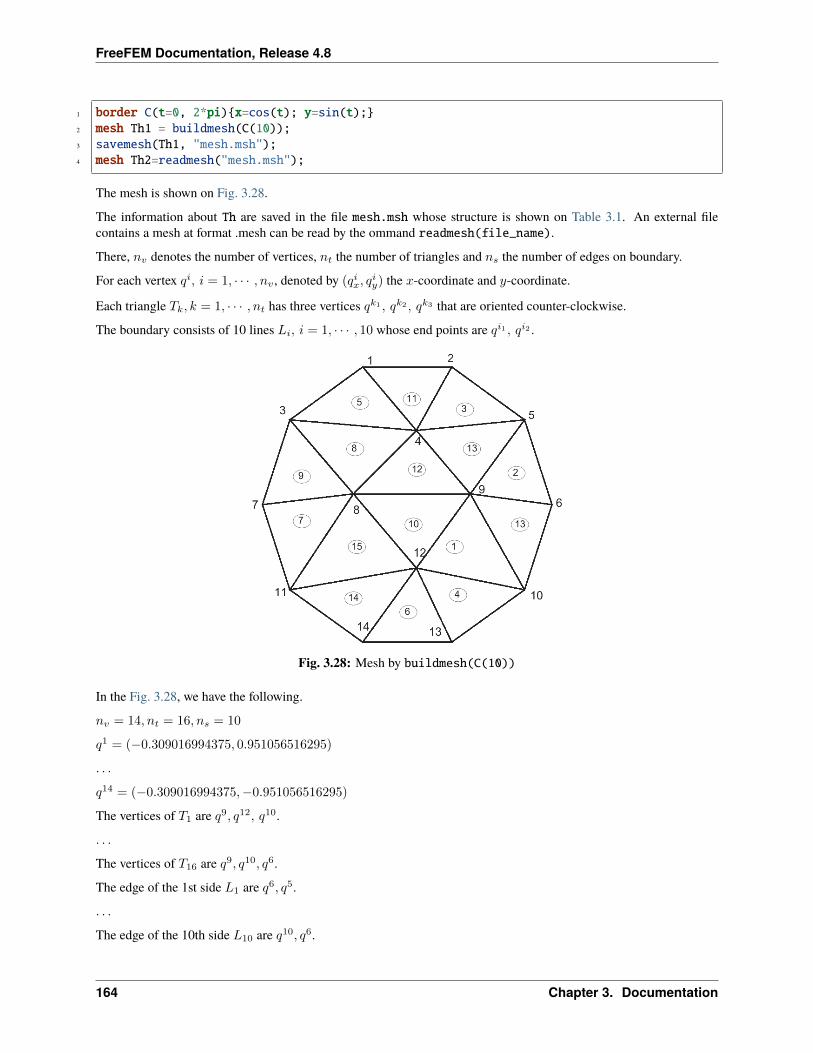
FreeFEM Documentation, Release 4.8
1 border C(t=0, 2*pi)x=cos(t); y=sin(t);2 mesh Th1 = buildmesh(C(10));3 savemesh(Th1, "mesh.msh");4 mesh Th2=readmesh("mesh.msh");
The mesh is shown on Fig. 3.28.
The information about Th are saved in the file mesh.msh whose structure is shown on Table 3.1. An external filecontains a mesh at format .mesh can be read by the ommand readmesh(file_name).
There, 𝑛𝑣 denotes the number of vertices, 𝑛𝑡 the number of triangles and 𝑛𝑠 the number of edges on boundary.
For each vertex 𝑞𝑖, 𝑖 = 1, · · · , 𝑛𝑣 , denoted by (𝑞𝑖𝑥, 𝑞𝑖𝑦) the 𝑥-coordinate and 𝑦-coordinate.
Each triangle 𝑇𝑘, 𝑘 = 1, · · · , 𝑛𝑡 has three vertices 𝑞𝑘1 , 𝑞𝑘2 , 𝑞𝑘3 that are oriented counter-clockwise.
The boundary consists of 10 lines 𝐿𝑖, 𝑖 = 1, · · · , 10 whose end points are 𝑞𝑖1 , 𝑞𝑖2 .
Fig. 3.28: Mesh by buildmesh(C(10))
In the Fig. 3.28, we have the following.
𝑛𝑣 = 14, 𝑛𝑡 = 16, 𝑛𝑠 = 10
𝑞1 = (−0.309016994375, 0.951056516295)
. . .
𝑞14 = (−0.309016994375,−0.951056516295)
The vertices of 𝑇1 are 𝑞9, 𝑞12, 𝑞10.
. . .
The vertices of 𝑇16 are 𝑞9, 𝑞10, 𝑞6.
The edge of the 1st side 𝐿1 are 𝑞6, 𝑞5.
. . .
The edge of the 10th side 𝐿10 are 𝑞10, 𝑞6.
164 Chapter 3. Documentation
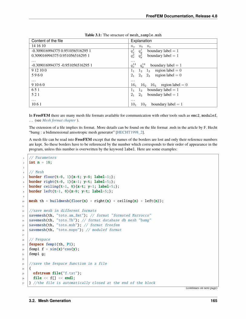
FreeFEM Documentation, Release 4.8
Table 3.1: The structure of mesh_sample.mshContent of the file Explanation14 16 10 𝑛𝑣 𝑛𝑡 𝑛𝑒-0.309016994375 0.951056516295 10.309016994375 0.951056516295 1. . .-0.309016994375 -0.951056516295 1
𝑞1𝑥 𝑞1𝑦 boundary label = 1𝑞2𝑥 𝑞2𝑦 boundary label = 1. . .𝑞14𝑥 𝑞14𝑦 boundary label = 1
9 12 10 05 9 6 0. . .9 10 6 0
11 12 13 region label = 021 22 23 region label = 0. . .161 162 163 region label = 0
6 5 15 2 1. . .10 6 1
11 12 boundary label = 121 22 boundary label = 1. . .101 102 boundary label = 1
In FreeFEM there are many mesh file formats available for communication with other tools such as emc2, modulef,. . . (see Mesh format chapter ).
The extension of a file implies its format. More details can be found on the file format .msh in the article by F. Hecht“bamg : a bidimensional anisotropic mesh generator” [HECHT1998_2].
A mesh file can be read into FreeFEM except that the names of the borders are lost and only their reference numbersare kept. So these borders have to be referenced by the number which corresponds to their order of appearance in theprogram, unless this number is overwritten by the keyword label. Here are some examples:
1 // Parameters2 int n = 10;3
4 // Mesh5 border floor(t=0, 1)x=t; y=0; label=1;;6 border right(t=0, 1)x=1; y=t; label=5;;7 border ceiling(t=1, 0)x=t; y=1; label=5;;8 border left(t=1, 0)x=0; y=t; label=5;;9
10 mesh th = buildmesh(floor(n) + right(n) + ceiling(n) + left(n));11
12 //save mesh in different formats13 savemesh(th, "toto.am_fmt"); // format "formated Marrocco"14 savemesh(th, "toto.Th"); // format database db mesh "bamg"15 savemesh(th, "toto.msh"); // format freefem16 savemesh(th, "toto.nopo"); // modulef format17
18 // Fespace19 fespace femp1(th, P1);20 femp1 f = sin(x)*cos(y);21 femp1 g;22
23 //save the fespace function in a file24 25 ofstream file("f.txt");26 file << f[] << endl;27 //the file is automatically closed at the end of the block
(continues on next page)
3.2. Mesh Generation 165
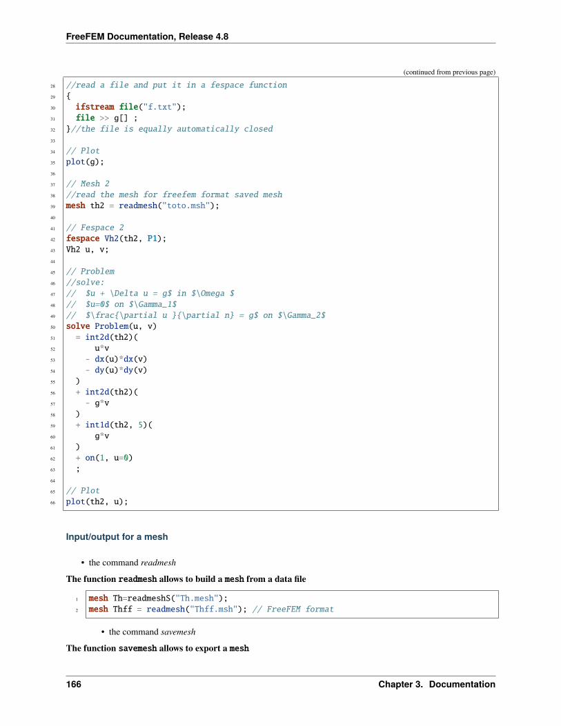
FreeFEM Documentation, Release 4.8
(continued from previous page)
28 //read a file and put it in a fespace function29 30 ifstream file("f.txt");31 file >> g[] ;32 //the file is equally automatically closed33
34 // Plot35 plot(g);36
37 // Mesh 238 //read the mesh for freefem format saved mesh39 mesh th2 = readmesh("toto.msh");40
41 // Fespace 242 fespace Vh2(th2, P1);43 Vh2 u, v;44
45 // Problem46 //solve:47 // $u + \Delta u = g$ in $\Omega $48 // $u=0$ on $\Gamma_1$49 // $\frac\partial u \partial n = g$ on $\Gamma_2$50 solve Problem(u, v)51 = int2d(th2)(52 u*v53 - dx(u)*dx(v)54 - dy(u)*dy(v)55 )56 + int2d(th2)(57 - g*v58 )59 + int1d(th2, 5)(60 g*v61 )62 + on(1, u=0)63 ;64
65 // Plot66 plot(th2, u);
Input/output for a mesh
• the command readmesh
The function readmesh allows to build a mesh from a data file
1 mesh Th=readmeshS("Th.mesh");2 mesh Thff = readmesh("Thff.msh"); // FreeFEM format
• the command savemesh
The function savemesh allows to export a mesh
166 Chapter 3. Documentation
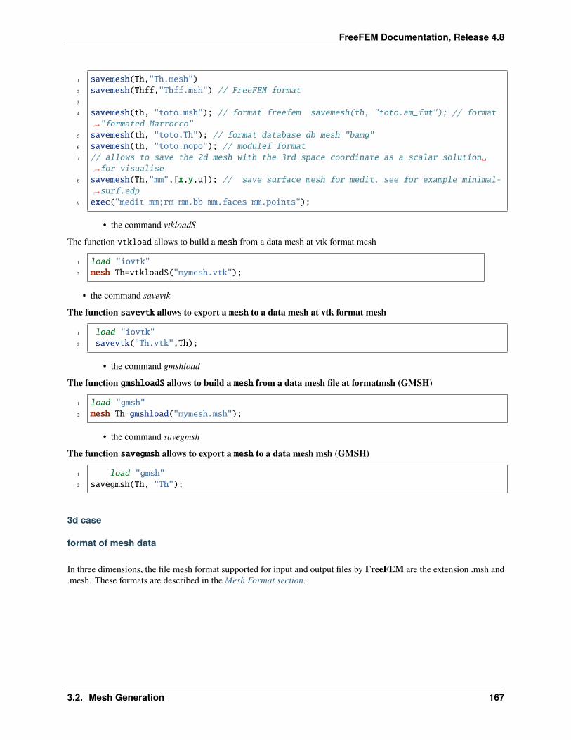
FreeFEM Documentation, Release 4.8
1 savemesh(Th,"Th.mesh")2 savemesh(Thff,"Thff.msh") // FreeFEM format3
4 savemesh(th, "toto.msh"); // format freefem savemesh(th, "toto.am_fmt"); // format→˓"formated Marrocco"
5 savemesh(th, "toto.Th"); // format database db mesh "bamg"6 savemesh(th, "toto.nopo"); // modulef format7 // allows to save the 2d mesh with the 3rd space coordinate as a scalar solution
→˓for visualise8 savemesh(Th,"mm",[x,y,u]); // save surface mesh for medit, see for example minimal-
→˓surf.edp9 exec("medit mm;rm mm.bb mm.faces mm.points");
• the command vtkloadS
The function vtkload allows to build a mesh from a data mesh at vtk format mesh
1 load "iovtk"2 mesh Th=vtkloadS("mymesh.vtk");
• the command savevtk
The function savevtk allows to export a mesh to a data mesh at vtk format mesh
1 load "iovtk"2 savevtk("Th.vtk",Th);
• the command gmshload
The function gmshloadS allows to build a mesh from a data mesh file at formatmsh (GMSH)
1 load "gmsh"2 mesh Th=gmshload("mymesh.msh");
• the command savegmsh
The function savegmsh allows to export a mesh to a data mesh msh (GMSH)
1 load "gmsh"2 savegmsh(Th, "Th");
3d case
format of mesh data
In three dimensions, the file mesh format supported for input and output files by FreeFEM are the extension .msh and.mesh. These formats are described in the Mesh Format section.
3.2. Mesh Generation 167
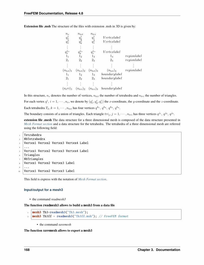
FreeFEM Documentation, Release 4.8
Extension file .msh The structure of the files with extension .msh in 3D is given by:
𝑛𝑣 𝑛𝑡𝑒𝑡 𝑛𝑡𝑟𝑖𝑞1𝑥 𝑞1𝑦 𝑞1𝑧 𝑉 𝑒𝑟𝑡𝑒𝑥𝑙𝑎𝑏𝑒𝑙𝑞2𝑥 𝑞2𝑦 𝑞2𝑧 𝑉 𝑒𝑟𝑡𝑒𝑥𝑙𝑎𝑏𝑒𝑙...
......
...𝑞𝑛𝑣𝑥 𝑞𝑛𝑣
𝑦 𝑞𝑛𝑣𝑧 𝑉 𝑒𝑟𝑡𝑒𝑥𝑙𝑎𝑏𝑒𝑙
11 12 13 14 𝑟𝑒𝑔𝑖𝑜𝑛𝑙𝑎𝑏𝑒𝑙21 22 23 24 𝑟𝑒𝑔𝑖𝑜𝑛𝑙𝑎𝑏𝑒𝑙...
......
......
(𝑛𝑡𝑒𝑡)1 (𝑛𝑡𝑒𝑡)2 (𝑛𝑡𝑒𝑡)3 (𝑛𝑡𝑒𝑡)4 𝑟𝑒𝑔𝑖𝑜𝑛𝑙𝑎𝑏𝑒𝑙11 12 13 𝑏𝑜𝑢𝑛𝑑𝑎𝑟𝑦𝑙𝑎𝑏𝑒𝑙21 22 23 𝑏𝑜𝑢𝑛𝑑𝑎𝑟𝑦𝑙𝑎𝑏𝑒𝑙...
......
...(𝑛𝑡𝑟𝑖)1 (𝑛𝑡𝑟𝑖)2 (𝑛𝑡𝑟𝑖)3 𝑏𝑜𝑢𝑛𝑑𝑎𝑟𝑦𝑙𝑎𝑏𝑒𝑙
In this structure, 𝑛𝑣 denotes the number of vertices, 𝑛𝑡𝑒𝑡 the number of tetrahedra and 𝑛𝑡𝑟𝑖 the number of triangles.
For each vertex 𝑞𝑖, 𝑖 = 1, · · · , 𝑛𝑣 , we denote by (𝑞𝑖𝑥, 𝑞𝑖𝑦, 𝑞
𝑖𝑧) the 𝑥-coordinate, the 𝑦-coordinate and the 𝑧-coordinate.
Each tetrahedra 𝑇𝑘, 𝑘 = 1, · · · , 𝑛𝑡𝑒𝑡 has four vertices 𝑞𝑘1 , 𝑞𝑘2 , 𝑞𝑘3 , 𝑞𝑘4 .
The boundary consists of a union of triangles. Each triangle 𝑡𝑟𝑖𝑗 , 𝑗 = 1, · · · , 𝑛𝑡𝑟𝑖 has three vertices 𝑞𝑗1 , 𝑞𝑗2 , 𝑞𝑗3 .
extension file .mesh The data structure for a three dimensional mesh is composed of the data structure presented inMesh Format section and a data structure for the tetrahedra. The tetrahedra of a three dimensional mesh are referredusing the following field:
1 Tetrahedra2 NbTetrahedra3 Vertex1 Vertex2 Vertex3 Vertex4 Label4 ...5 Vertex1 Vertex2 Vertex3 Vertex4 Label6 Triangles7 NbTriangles8 Vertex1 Vertex2 Vertex3 Label9 ...
10 Vertex1 Vertex2 Vertex3 Label
This field is express with the notation of Mesh Format section.
Input/output for a mesh3
• the command readmesh3
The function readmesh3 allows to build a mesh3 from a data file
1 mesh3 Th3=readmesh3("Th3.mesh");2 mesh3 Th3ff = readmesh3("Th3ff.msh"); // FreeFEM format
• the command savemesh
The function savemesh allows to export a mesh3
168 Chapter 3. Documentation
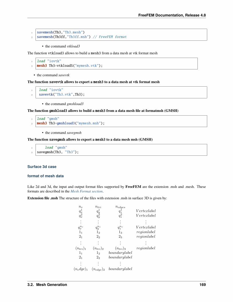
FreeFEM Documentation, Release 4.8
1 savemesh(Th3,"Th3.mesh")2 savemesh(Th3ff,"Th3ff.msh") // FreeFEM format
• the command vtkload3
The function vtkload3 allows to build a mesh3 from a data mesh at vtk format mesh
1 load "iovtk"2 mesh3 Th3=vtkloadS("mymesh.vtk");
• the command savevtk
The function savevtk allows to export a mesh3 to a data mesh at vtk format mesh
1 load "iovtk"2 savevtk("Th3.vtk",Th3);
• the command gmshload3
The function gmshload3 allows to build a mesh3 from a data mesh file at formatmsh (GMSH)
1 load "gmsh"2 mesh3 Th3=gmshload3("mymesh.msh");
• the command savegmsh
The function savegmsh allows to export a mesh3 to a data mesh msh (GMSH)
1 load "gmsh"2 savegmsh(Th3, "Th3");
Surface 3d case
format of mesh data
Like 2d and 3d, the input and output format files supported by FreeFEM are the extension .msh and .mesh. Theseformats are described in the Mesh Format section.
Extension file .msh The structure of the files with extension .msh in surface 3D is given by:
𝑛𝑣 𝑛𝑡𝑟𝑖 𝑛𝑒𝑑𝑔𝑒𝑠𝑞1𝑥 𝑞1𝑦 𝑞1𝑧 𝑉 𝑒𝑟𝑡𝑒𝑥𝑙𝑎𝑏𝑒𝑙𝑞2𝑥 𝑞2𝑦 𝑞2𝑧 𝑉 𝑒𝑟𝑡𝑒𝑥𝑙𝑎𝑏𝑒𝑙...
......
...𝑞𝑛𝑣𝑥 𝑞𝑛𝑣
𝑦 𝑞𝑛𝑣𝑧 𝑉 𝑒𝑟𝑡𝑒𝑥𝑙𝑎𝑏𝑒𝑙
11 12 13 𝑟𝑒𝑔𝑖𝑜𝑛𝑙𝑎𝑏𝑒𝑙21 22 23 𝑟𝑒𝑔𝑖𝑜𝑛𝑙𝑎𝑏𝑒𝑙...
......
...(𝑛𝑡𝑟𝑖)1 (𝑛𝑡𝑟𝑖)2 (𝑛𝑡𝑟𝑖)3 𝑟𝑒𝑔𝑖𝑜𝑛𝑙𝑎𝑏𝑒𝑙
11 12 𝑏𝑜𝑢𝑛𝑑𝑎𝑟𝑦𝑙𝑎𝑏𝑒𝑙21 22 𝑏𝑜𝑢𝑛𝑑𝑎𝑟𝑦𝑙𝑎𝑏𝑒𝑙...
......
(𝑛𝑒𝑑𝑔𝑒)1 (𝑛𝑒𝑑𝑔𝑒)2 𝑏𝑜𝑢𝑛𝑑𝑎𝑟𝑦𝑙𝑎𝑏𝑒𝑙
3.2. Mesh Generation 169
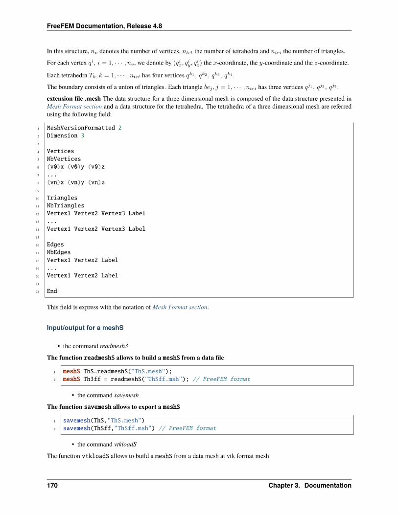
FreeFEM Documentation, Release 4.8
In this structure, 𝑛𝑣 denotes the number of vertices, 𝑛𝑡𝑒𝑡 the number of tetrahedra and 𝑛𝑡𝑟𝑖 the number of triangles.
For each vertex 𝑞𝑖, 𝑖 = 1, · · · , 𝑛𝑣 , we denote by (𝑞𝑖𝑥, 𝑞𝑖𝑦, 𝑞
𝑖𝑧) the 𝑥-coordinate, the 𝑦-coordinate and the 𝑧-coordinate.
Each tetrahedra 𝑇𝑘, 𝑘 = 1, · · · , 𝑛𝑡𝑒𝑡 has four vertices 𝑞𝑘1 , 𝑞𝑘2 , 𝑞𝑘3 , 𝑞𝑘4 .
The boundary consists of a union of triangles. Each triangle 𝑏𝑒𝑗 , 𝑗 = 1, · · · , 𝑛𝑡𝑟𝑖 has three vertices 𝑞𝑗1 , 𝑞𝑗2 , 𝑞𝑗3 .
extension file .mesh The data structure for a three dimensional mesh is composed of the data structure presented inMesh Format section and a data structure for the tetrahedra. The tetrahedra of a three dimensional mesh are referredusing the following field:
1 MeshVersionFormatted 22 Dimension 33
4 Vertices5 NbVertices6 (v0)x (v0)y (v0)z7 ...8 (vn)x (vn)y (vn)z9
10 Triangles11 NbTriangles12 Vertex1 Vertex2 Vertex3 Label13 ...14 Vertex1 Vertex2 Vertex3 Label15
16 Edges17 NbEdges18 Vertex1 Vertex2 Label19 ...20 Vertex1 Vertex2 Label21
22 End
This field is express with the notation of Mesh Format section.
Input/output for a meshS
• the command readmesh3
The function readmeshS allows to build a meshS from a data file
1 meshS ThS=readmeshS("ThS.mesh");2 meshS Th3ff = readmeshS("ThSff.msh"); // FreeFEM format
• the command savemesh
The function savemesh allows to export a meshS
1 savemesh(ThS,"ThS.mesh")2 savemesh(ThSff,"ThSff.msh") // FreeFEM format
• the command vtkloadS
The function vtkloadS allows to build a meshS from a data mesh at vtk format mesh
170 Chapter 3. Documentation
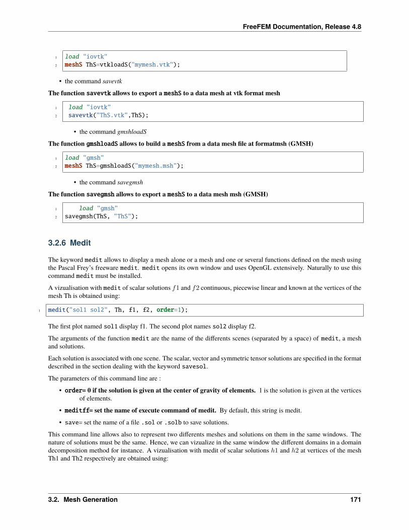
FreeFEM Documentation, Release 4.8
1 load "iovtk"2 meshS ThS=vtkloadS("mymesh.vtk");
• the command savevtk
The function savevtk allows to export a meshS to a data mesh at vtk format mesh
1 load "iovtk"2 savevtk("ThS.vtk",ThS);
• the command gmshloadS
The function gmshloadS allows to build a meshS from a data mesh file at formatmsh (GMSH)
1 load "gmsh"2 meshS ThS=gmshloadS("mymesh.msh");
• the command savegmsh
The function savegmsh allows to export a meshS to a data mesh msh (GMSH)
1 load "gmsh"2 savegmsh(ThS, "ThS");
3.2.6 Medit
The keyword medit allows to display a mesh alone or a mesh and one or several functions defined on the mesh usingthe Pascal Frey’s freeware medit. medit opens its own window and uses OpenGL extensively. Naturally to use thiscommand medit must be installed.
A vizualisation with medit of scalar solutions 𝑓1 and 𝑓2 continuous, piecewise linear and known at the vertices of themesh Th is obtained using:
1 medit("sol1 sol2", Th, f1, f2, order=1);
The first plot named sol1 display f1. The second plot names sol2 display f2.
The arguments of the function medit are the name of the differents scenes (separated by a space) of medit, a meshand solutions.
Each solution is associated with one scene. The scalar, vector and symmetric tensor solutions are specified in the formatdescribed in the section dealing with the keyword savesol.
The parameters of this command line are :
• order= 0 if the solution is given at the center of gravity of elements. 1 is the solution is given at the verticesof elements.
• meditff= set the name of execute command of medit. By default, this string is medit.
• save= set the name of a file .sol or .solb to save solutions.
This command line allows also to represent two differents meshes and solutions on them in the same windows. Thenature of solutions must be the same. Hence, we can vizualize in the same window the different domains in a domaindecomposition method for instance. A vizualisation with medit of scalar solutions ℎ1 and ℎ2 at vertices of the meshTh1 and Th2 respectively are obtained using:
3.2. Mesh Generation 171
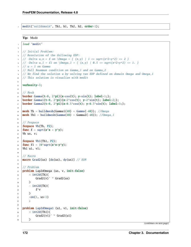
FreeFEM Documentation, Release 4.8
1 medit("sol2domain", Th1, h1, Th2, h2, order=1);
Tip: Medit
1 load "medit"2
3 // Initial Problem:4 // Resolution of the following EDP:5 // -Delta u_s = f on \Omega = (x,y) | 1 <= sqrt(x^2+y^2) <= 2 6 // -Delta u_1 = f1 on \Omega_1 = (x,y) | 0.5 <= sqrt(x^2+y^2) <= 1. 7 // u = 1 on Gamma8 // Null Neumman condition on Gamma_1 and on Gamma_29 // We find the solution u by solving two EDP defined on domain Omega and Omega_1
10 // This solution is visualize with medit11
12 verbosity=3;13
14 // Mesh15 border Gamma(t=0, 2*pi)x=cos(t); y=sin(t); label=1;;16 border Gamma1(t=0, 2*pi)x=2*cos(t); y=2*sin(t); label=2;;17 border Gamma2(t=0, 2*pi)x=0.5*cos(t); y=0.5*sin(t); label=3;;18
19 mesh Th = buildmesh(Gamma1(40) + Gamma(-40)); //Omega20 mesh Th1 = buildmesh(Gamma(40) + Gamma2(-40)); //Omega_121
22 // Fespace23 fespace Vh(Th, P2);24 func f = sqrt(x*x + y*y);25 Vh us, v;26
27 fespace Vh1(Th1, P2);28 func f1 = 10*sqrt(x*x+y*y);29 Vh1 u1, v1;30
31 // Macro32 macro Grad2(us) [dx(us), dy(us)] // EOM33
34 // Problem35 problem Lap2dOmega (us, v, init=false)36 = int2d(Th)(37 Grad2(v)' * Grad2(us)38 )39 - int2d(Th)(40 f*v41 )42 +on(1, us=1)43 ;44
45 problem Lap2dOmega1 (u1, v1, init=false)46 = int2d(Th1)(47 Grad2(v1)' * Grad2(u1)48 )
(continues on next page)
172 Chapter 3. Documentation
FreeFEM Documentation, Release 4.8
(continued from previous page)
49 - int2d(Th1)(50 f1*v151 )52 + on(1, u1=1)53 ;54
55 // Solve56 Lap2dOmega;57 Lap2dOmega1;58
59 // Plot with medit60 medit("solution", Th, us, Th1, u1, order=1, save="testsavemedit.solb");
3.2.7 Mshmet
Mshmet is a software developed by P. Frey that allows to compute an anisotropic metric based on solutions (i.e. Hessian-based). This software can return also an isotropic metric. Moreover, mshmet can also construct a metric suitable forlevelset interface capturing. The solution can be defined on 2D or 3D structured/unstructured meshes. For example,the solution can be an error estimate of a FE solution.
Solutions for mshmet are given as an argument. The solution can be a func, a vector func, a symmetric tensor, afespace function, a fespace vector function and a fespace symmetric tensor. The symmetric tensor argument isdefined as this type of data for datasol argument. This software accepts more than one solution.
For example, the metric 𝑀 computed with mshmet for the solution 𝑢 defined on the mesh 𝑇ℎ is obtained by writing:
1 fespace Vh(Th, P1);2 Vh u; //a scalar fespace function3 real[int] M = mshmet(Th, u);
The parameters of the keyword mshmet are :
• normalization = (b) do a normalization of all solution in [0, 1].
• aniso = (b) build anisotropic metric if 1 (default 0: isotropic)
• levelset = (b) build metric for levelset method (default: false)
• verbosity = (l) level of verbosity
• nbregul = (l) number of regularization’s iteration of solutions given (default 0).
• hmin = (d)
• hmax = (d)
• err = (d) level of error.
• width = (d) the width
• metric = a vector of double. This vector contains an initial metric given to mshmet. The structure of themetric vector is described in the next paragraph.
• loptions = a vector of integer of size 7. This vector contains the integer parameters of mshmet (for expertonly).
– loptions(0): normalization (default 1).
3.2. Mesh Generation 173
FreeFEM Documentation, Release 4.8
– loptions(1): isotropic parameters (default 0). 1 for isotropic metric results otherwise 0.
– loptions(2): level set parameters (default 0). 1 for building level set metric otherwise 0.
– loptions(3): debug parameters (default 0). 1 for turning on debug mode otherwise 0.
– loptions(4): level of verbosity (default 10).
– loptions(5): number of regularization’s iteration of solutions given (default 0).
– loptions(6): previously metric parameter (default 0). 1 for using previous metric otherwise 0.
• doptions= a vector of double of size 4. This vector contains the real parameters of mshmet (for expert only).
– doptions(0): hmin : min size parameters (default 0.01).
– doptions(1): hmax : max size parameters (default 1.0).
– doptions(2): eps : tolerance parameters (default 0.01).
– doptions(2): width : relative width for Level Set (0 < 𝑤 < 1) (default 0.05).
The result of the keyword mshmet is a real[int] which contains the metric computed by mshmet at the differentvertices 𝑉𝑖 of the mesh.
With 𝑛𝑣 is the number of vertices, the structure of this vector is:
𝑀𝑖𝑠𝑜 = (𝑚(𝑉0),𝑚(𝑉1), . . . ,𝑚(𝑉𝑛𝑣))𝑡
for a isotropic metric 𝑚. For a symmetric tensor metric ℎ =
⎛⎝ 𝑚11 𝑚12 𝑚13
𝑚21 𝑚22 𝑚23
𝑚31 𝑚32 𝑚33
⎞⎠ , the parameters metric is:
𝑀𝑎𝑛𝑖𝑠𝑜 = (𝐻(𝑉0), . . . ,𝐻(𝑉𝑛𝑣))𝑡
where 𝐻(𝑉𝑖) is the vector of size 6 defined by [𝑚11,𝑚21,𝑚22,𝑚31,𝑚32,𝑚33]
Tip: mshmet
1 load "mshmet"2 load "medit"3 load "msh3"4
5 // Parameters6 real error = 0.01;7 func zmin = 0;8 func zmax = 1;9 int MaxLayer = 10;
10
11 // Mesh12 border a(t=0, 1.0)x=t; y=0; label=1;;13 border b(t=0, 0.5)x=1; y=t; label=2;;14 border c(t=0, 0.5)x=1-t; y=0.5; label=3;;15 border d(t=0.5, 1)x=0.5; y=t; label=4;;16 border e(t=0.5, 1)x=1-t; y=1; label=5;;17 border f(t=0.0, 1)x=0; y=1-t; label=6;;18 mesh Th = buildmesh(a(6) + b(4) + c(4) + d(4) + e(4) + f(6));19 mesh3 Th3 = buildlayers(Th, MaxLayer, zbound=[zmin, zmax]);20
(continues on next page)
174 Chapter 3. Documentation
FreeFEM Documentation, Release 4.8
(continued from previous page)
21 // Fespace22 fespace Vh3(Th3, P2);23 Vh3 u3, v3;24
25 fespace Vh3P1(Th3, P1);26 Vh3P1 usol;27
28 // Problem29 problem Problem2(u3, v3, solver=sparsesolver)30 = int3d(Th3)(31 u3*v3*1.0e-1032 + dx(u3)*dx(v3)33 + dy(u3)*dy(v3)34 + dz(u3)*dz(v3)35 )36 - int3d(Th3)(37 v338 )39 +on(0, 1, 2, 3, 4, 5, 6, u3=0)40 ;41
42 // Solve43 Problem2;44 cout << u3[].min << " " << u3[].max << endl;45
46 medit("Sol", Th3, u3);47
48 real[int] bb = mshmet(Th3,u3);49 cout << "Metric:" << bb << endl;50 for (int ii = 0; ii < Th3.nv; ii++)51 usol[][ii] = bb[ii];52
53 medit("Metric", Th3, usol);
3.2.8 FreeYams
FreeYams is a surface mesh adaptation software which is developed by P. Frey. This software is a new version ofyams. The adapted surface mesh is constructed with a geometric metric tensor field. This field is based on the intrinsicproperties of the discrete surface.
Also, this software allows to construct a simplification of a mesh. This decimation is based on the Hausdorff distancebetween the initial and the current triangulation. Compared to the software yams, FreeYams can be used also to produceanisotropic triangulations adapted to levelset simulations. A technical report on freeYams documentation is availablehere.
To call FreeYams in FreeFEM, we used the keyword freeyams. The arguments of this function are the initial meshand/or metric. The metric with freeyams are a func, a fespace function, a symmetric tensor function, a symmetrictensor fespace function or a vector of double (real[int]). If the metric is a vector of double, this data must be givenin metric parameter. Otherwise, the metric is given in the argument.
For example, the adapted mesh of Thinit defined by the metric 𝑢 defined as fespace function is obtained by writing:
3.2. Mesh Generation 175
FreeFEM Documentation, Release 4.8
1 fespace Vh(Thinit, P1);2 Vh u;3 mesh3 Th = freeyams(Thinit, u);
The symmetric tensor argument for freeyams keyword is defined as this type of data for datasol argument.
• aniso= (b) aniso or iso metric (default 0, iso)
• mem= (l) memory of for freeyams in Mb (default -1, freeyams choose)
• hmin= (d)
• hmax= (d)
• gradation= (d)
• option= (l)
– 0 : mesh optimization (smoothing+swapping)
– 1 : decimation+enrichment adaptated to a metric map. (default)
– -1 : decimation adaptated to a metric map.
– 2 : decimation+enrichment with a Hausdorff-like method
– -2 : decimation with a Hausdorff-like method
– 4 : split triangles recursively.
– 9 : No-Shrinkage Vertex Smoothing
• ridgeangle= (d)
• absolute= (b)
• verbosity= (i)
• metric= vector expression. This parameters contains the metric at the different vertices on the initial mesh.With 𝑛𝑣 is the number of vertices, this vector is:
𝑀𝑖𝑠𝑜 = (𝑚(𝑉0),𝑚(𝑉1), . . . ,𝑚(𝑉𝑛𝑣))𝑡
for a scalar metric 𝑚. For a symmetric tensor metric ℎ =
⎛⎝ 𝑚11 𝑚12 𝑚13
𝑚21 𝑚22 𝑚23
𝑚31 𝑚32 𝑚33
⎞⎠, the parameters metric is:
𝑀𝑎𝑛𝑖𝑠𝑜 = (𝐻(𝑉0), . . . ,𝐻(𝑉𝑛𝑣))𝑡
where 𝐻(𝑉𝑖) is the vector of size 6 defined by [𝑚11,𝑚21,𝑚22,𝑚31,𝑚32,𝑚33]
• loptions= a vector of integer of size 13. This vectors contains the integer options of FreeYams. (just for theexpert)
– loptions(0): anisotropic parameter (default 0). If you give an anisotropic metric 1 otherwise 0.
– loptions(1): Finite Element correction parameter (default 0). 1 for no Finite Element correctionotherwise 0.
– loptions(2): Split multiple connected points parameter (default 1). 1 for splitting multiple con-nected points otherwise 0.
– loptions(3): maximum value of memory size in Mbytes (default -1: the size is given by freeyams).
176 Chapter 3. Documentation
FreeFEM Documentation, Release 4.8
– loptions(4): set the value of the connected component which we want to obtain. (Remark:freeyams give an automatic value at each connected component).
– loptions(5): level of verbosity
– loptions(6): Create point on straight edge (no mapping) parameter (default 0). 1 for creatingpoint on straight edge otherwise 0.
– loptions(7): validity check during smoothing parameter. This parameter is only used with No-Shrinkage Vertex Smoothing optimization (optimization option parameter 9). 1 for No validitychecking during smoothing otherwise 0.
– loptions(8): number of desired’s vertices (default -1).
– loptions(9): number of iteration of optimizations (default 30).
– loptions(10): no detection parameter (default 0). 1 for detecting the ridge on the mesh otherwise0. The ridge definition is given in the parameter doptions(12).
– loptions(11): no vertex smoothing parameter (default 0). 1 for smoothing the vertices otherwise 0.
– loptions(12): Optimization level parameter (default 0).
– 0 : mesh optimization (smoothing+swapping)
– 1 : decimation+enrichment adaptated to a metric map.
– -1: decimation adaptated to a metric map.
– 2 : decimation+enrichment with a Hausdorff-like method
– -2: decimation with a Hausdorff-like method
– 4 : split triangles recursively.
– 9 : No-Shrinkage Vertex Smoothing
• doptions= a vector of double of size 11. This vectors contains the real options of freeyams.
– doptions(0): Set the geometric approximation (Tangent plane deviation) (default 0.01).
– doptions(1): Set the lamda parameter (default -1).
– doptions(2): Set the mu parmeter (default -1).
– doptions(3): Set the gradation value (Mesh density control) (default 1.3).
– doptions(4): Set the minimal size(hmin) (default -2.0: the size is automatically computed).
– doptions(5): Set the maximal size(hmax) (default -2.0: the size is automatically computed).
– doptions(6): Set the tolerance of the control of Chordal deviation (default -2.0).
– doptions(7): Set the quality of degradation (default 0.599).
– doptions(8): Set the declic parameter (default 2.0).
– doptions(9): Set the angular walton limitation parameter (default 45 degree).
– doptions(10): Set the angular ridge detection (default 45 degree).
Tip: freeyams
1 load "msh3"2 load "medit"3 load "freeyams"
(continues on next page)
3.2. Mesh Generation 177
FreeFEM Documentation, Release 4.8
(continued from previous page)
4
5 // Parameters6 int nn = 20;7 real zmin = 0;8 real zmax = 1;9
10 // Mesh11 mesh Th2 = square(nn, nn);12 int[int] rup = [0, 2], rdown = [0, 1];13 int[int] rmid = [1, 1, 2, 1, 3, 1, 4, 1];14 mesh3 Th = buildlayers(Th2, nn, zbound=[zmin, zmax], reffacemid=rmid, reffaceup=rup,
→˓reffacelow=rdown);15 mesh3 Th3 = freeyams(Th);16
17 medit("SurfaceMesh", Th3);
3.2.9 mmg3d
Todo: mmg3d-v4.0
Mmg3d is a 3D remeshing software developed by C. Dobrzynski and P. Frey.
This software allows to remesh an initial mesh made of tetrahedra. This initial mesh is adapted to a geometric metrictensor field or to a displacement vector (moving rigid body). The metric can be obtained with mshmet.
Note:• If no metric is given, an isotropic metric is computed by analyzing the size of the edges in the initial mesh.
• If a displacement is given, the vertices of the surface triangles are moved without verifying the geometricalstructure of the new surface mesh.
The parameters of mmg3d are :
• options= vector expression. This vector contains the option parameters of mmg3d. It is a vector of 6 values,with the following meaning:
– Optimization parameters : (default 1)
0 : mesh optimization.
1 : adaptation with metric (deletion and insertion vertices) and optimization.
-1 : adaptation with metric (deletion and insertion vertices) without optimization.
4 : split tetrahedra (be careful modify the surface).
9 : moving mesh with optimization.
-9 : moving mesh without optimization.
– Debug mode : (default 0)
1 : turn on debug mode.
178 Chapter 3. Documentation
FreeFEM Documentation, Release 4.8
0 : otherwise.
– Specify the size of bucket per dimension (default 64)
– Swapping mode : (default 0)
1 : no edge or face flipping.
0 : otherwise.
– Insert points mode : (default 0)
1 : no edge splitting or collapsing and no insert points.
0 : otherwise.
5. Verbosity level (default 3)
• memory= integer expression. Set the maximum memory size of new mesh in Mbytes. By default the numberof maximum vertices, tetrahedra and triangles are respectively 500 000, 3000 000, 100000 which representapproximately a memory of 100 Mo.
• metric= vector expression. This vector contains the metric given at mmg3d. It is a vector of size 𝑛𝑣 or 6 𝑛𝑣respectively for an isotropic and anisotropic metric where 𝑛𝑣 is the number of vertices in the initial mesh.The structure of metric vector is described in the mshmet.
• displacement= [Φ1,Φ2,Φ3] set the displacement vector of the initial mesh Φ(x,y) =[Φ1(𝑥, 𝑦),Φ2(𝑥, 𝑦),Φ3(𝑥, 𝑦)].
• displVect= sets the vector displacement in a vector expression. This vector contains the displacement ateach point of the initial mesh. It is a vector of size 3 𝑛𝑣.
Tip: mmg3d
1 load "msh3"2 load "medit"3 load "mmg3d"4 include "Cube.idp"5
6 // Parameters7 int n = 6;8 int[int] Nxyz = [12, 12, 12];9 real [int, int] Bxyz = [[0., 1.], [0., 1.], [0., 1.]];
10 int [int, int] Lxyz = [[1, 1], [2, 2], [2, 2]];11
12 // Mesh13 mesh3 Th = Cube(Nxyz, Bxyz, Lxyz);14
15 real[int] isometric(Th.nv);16 for (int ii = 0; ii < Th.nv; ii++)17 isometric[ii] = 0.17;18
19 mesh3 Th3 = mmg3d(Th, memory=100, metric=isometric);20
21 // Plot22 medit("Initial", Th);23 medit("Isometric", Th3);
3.2. Mesh Generation 179
FreeFEM Documentation, Release 4.8
Tip: Falling spheres
1 load "msh3"2 load "TetGen"3 load "medit"4 load "mmg3d"5 include "MeshSurface.idp"6
7 // Parameters8 real hs = 0.8;9 int[int] N = [4/hs, 8/hs, 11.5/hs];
10 real [int, int] B = [[-2, 2], [-2, 6], [-10, 1.5]];11 int [int, int] L = [[311, 311], [311, 311], [311, 311]];12
13 int[int] opt = [9, 0, 64, 0, 0, 3];14 real[int] vit=[0, 0, -0.3];15 func zero = 0.;16 func dep = vit[2];17
18 // Meshes19 meshS ThH = SurfaceHex(N, B, L, 1);20 meshS ThSg = Sphere(1, hs, 300, -1);21 meshS ThSd = Sphere(1, hs, 310, -1);22 ThSd = movemesh(ThSd, [x, 4+y, z]);23 meshS ThHS = ThH + ThSg + ThSd;24 medit("ThHS", ThHS);25
26 real voltet = (hs^3)/6.;27 real[int] domain = [0, 0, -4, 1, voltet];28 real [int] holes = [0, 0, 0, 0, 4, 0];29 mesh3 Th = tetg(ThHS, switch="pqaAAYYQ", nbofregions=1, regionlist=domaine, nbofholes=2,
→˓holelist=holes);30 medit("Box-With-two-Ball", Th);31
32 // Fespace33 fespace Vh(Th, P1);34 Vh uh,vh;35
36 // Macro37 macro Grad(u) [dx(u),dy(u),dz(u)]38
39 // Problem40 problem Lap (uh, vh, solver=CG)41 = int3d(Th)(42 Grad(uh)' * Grad(vh)43 )44 + on(310, 300, uh=dep)45 + on(311, uh=0.)46 ;47
48 // Falling loop49 for(int it = 0; it < 29; it++)
(continues on next page)
180 Chapter 3. Documentation
FreeFEM Documentation, Release 4.8
(continued from previous page)
50 cout << " ITERATION " << it << endl;51
52 // Solve53 Lap;54
55 // Plot56 plot(Th, uh);57
58 // Sphere falling59 Th = mmg3d(Th, options=opt, displacement=[zero, zero, uh], memory=1000);60
3.2.10 A first 3d isotrope mesh adaptation process
Tip: Adaptation 3D
1 load "msh3"2 load "TetGen"3 load "mshmet"4 load "medit"5
6 // Parameters7 int nn = 6;8 int[int] l1111 = [1, 1, 1, 1]; //labels9 int[int] l01 = [0, 1];
10 int[int] l11 = [1, 1];11
12 real errm = 1e-2; //level of error13
14 // Mesh15 mesh3 Th3 = buildlayers(square(nn, nn, region=0, label=l1111),16 nn, zbound=[0, 1], labelmid=l11, labelup=l01, labeldown=l01);17
18 Th3 = trunc(Th3, (x<0.5) | (y < 0.5) | (z < 0.5), label=1); //remove the ]0.5,1[^3 cube19
20 // Fespace21 fespace Vh(Th3, P1);22 Vh u, v, usol, h;23
24 // Macro25 macro Grad(u) [dx(u), dy(u), dz(u)] // EOM26
27 // Problem28 problem Poisson (u, v, solver=CG)29 = int3d(Th3)(30 Grad(u)' * Grad(v)31 )32 - int3d(Th3)(33 1*v
(continues on next page)
3.2. Mesh Generation 181
FreeFEM Documentation, Release 4.8
(continued from previous page)
34 )35 + on(1, u=0)36 ;37
38 // Loop39 for (int ii = 0; ii < 5; ii++)40 // Solve41 Poisson;42 cout << "u min, max = " << u[].min << " "<< u[].max << endl;43
44 h=0.; //for resizing h[] because the mesh change45 h[] = mshmet(Th3, u, normalization=1, aniso=0, nbregul=1, hmin=1e-3, hmax=0.3,
→˓err=errm);46 cout << "h min, max = " << h[].min << " "<< h[].max << " " << h[].n << " " << Th3.nv
→˓<< endl;47 plot(u, wait=true);48
49 errm *= 0.8; //change the level of error50 cout << "Th3 " << Th3.nv < " " << Th3.nt << endl;51 Th3 = tetgreconstruction(Th3, switch="raAQ", sizeofvolume=h*h*h/6.); //rebuild mesh52 medit("U-adap-iso-"+ii, Th3, u, wait=true);53
3.2.11 Build a 2d mesh from an isoline
The idea is to get the discretization of an isoline of fluid meshes, this tool can be useful to construct meshes from image.First, we give an example of the isovalue meshes 0.2 of analytical function
√(𝑥− 1/2)2 + (𝑦 − 1/2)2, on unit square.
1 load "isoline"2
3 real[int,int] xy(3, 1); //to store the isoline points4 int[int] be(1); //to store the begin, end couple of lines5 6 mesh Th = square(10, 10);7 fespace Vh(Th, P1);8 Vh u = sqrt(square(x-0.5) + square(y-0.5));9 real iso = 0.2 ;
10 real[int] viso = [iso];11 plot(u, viso=viso,Th);//to see the iso line12
13 int nbc = isoline(Th, u, xy, close=1, iso=iso, beginend=be, smoothing=0.1);
The isoline parameters are Th the mesh, the expression 𝑢, the bidimentionnal array xy to store the list coordinate ofthe points. The list of named parameter are :
• iso= value of the isoline to compute (0 is the default value)
• close= close the isoline with the border (default true), we add the part of the mesh border such the value isless than the isovalue
• smoothing= number of smoothing process is the 𝑙𝑟𝑠 where 𝑙 is the length of the current line component, 𝑟 theratio, 𝑠 is smoothing value. The smoothing default value is 0.
182 Chapter 3. Documentation
FreeFEM Documentation, Release 4.8
• ratio= the ratio (1 by default).
• eps= relative 𝜀 (default 1e-10)
• beginend= array to get begin, end couple of each of sub line (resize automatically)
• file= to save the data curve in data file for gnuplot
In the array xy you get the list of vertices of the isoline, each connex line go from 𝑖 = 𝑖𝑐0, . . . , 𝑖𝑐1−1 with 𝑖𝑐0 = 𝑏𝑒(2* 𝑐)
𝑖𝑐1 = 𝑏𝑒(2 * 𝑐+ 1), and where 𝑥𝑖 = 𝑥𝑦(0, 𝑖), 𝑦𝑖 = 𝑦𝑥(1, 𝑖), 𝑙𝑖 = 𝑥𝑦(2, 𝑖).
Here 𝑙𝑖 is the length of the line (the origin of the line is point 𝑖𝑐0).
The sense of the isoline is such that the upper part is at the left size of the isoline. So here : the minimum is a point0.5, 05 so the curve 1 turn in the clockwise sense, the order of each component are sort such that the number of pointby component is decreasing.
1 cout << "Number of the line component = " << nbc << endl;2 cout << "Number of points = " << xy.m << endl;3 cout << "be = " << be << endl;4
5 // shows the lines component6 for (int c = 0; c < nbc; ++c)7 int i0 = be[2*c], i1 = be[2*c+1]-1;8 cout << "Curve " << c << endl;9 for(int i = i0; i <= i1; ++i)
10 cout << "x= " << xy(0,i) << " y= " << xy(1,i) << " s= " << xy(2, i) << endl;11 plot([xy(0, i0:i1), xy(1, i0:i1)], wait=true, viso=viso, cmm=" curve "+c);12 13 14
15 cout << "length of last curve = " << xy(2, xy.m-1) << endl;
We also have a new function to easily parametrize a discrete curve defined by the couple 𝑏𝑒, 𝑥𝑦.
1 border Curve0(t=0, 1)2 int c=0; //component 03 int i0=be[2*c], i1=be[2*c+1]-1;4 P=Curve(xy, i0, i1, t); //Curve 05 label=1;6 7
8 border Curve1(t=0, 1)9 int c=1; //component 1
10 int i0=be[2*c], i1=be[2*c+1]-1;11 P=Curve(xy, i0, i1, t); //Curve 112 label=1;13 14
15 plot(Curve1(100)); //show curve16 mesh Th = buildmesh(Curve1(-100));17 plot(Th, wait=true);
Secondly, we use this idea to build meshes from an image, we use the plugins ppm2rnm to read pgm a gray scale imageand then we extract the gray contour at level 0.25.
Tip: Leman lake
3.2. Mesh Generation 183
FreeFEM Documentation, Release 4.8
1 load "ppm2rnm"2 load "isoline"3
4 // Parameters5 string leman = "LemanLake.pgm";6 real AreaLac = 580.03; //in km^27 real hsize = 5;8 real[int, int] Curves(3, 1);9 int[int] be(1);
10 int nc; //nb of curve11 12 real[int, int] ff1(leman); //read image13 //and set it in a rect. array14 int nx = ff1.n, ny = ff1.m;15 //build a Cartesian mesh such that the origin is in the right place.16 mesh Th = square(nx-1, ny-1, [(nx-1)*(x), (ny-1)*(1-y)]);17 //warning the numbering of the vertices (x,y) is18 //given by $i = x/nx + nx* y/ny $19 fespace Vh(Th, P1);20 Vh f1;21 f1[] = ff1; //transform array in finite element functions.22 nc = isoline(Th, f1, iso=0.25, close=1, Curves, beginend=be, smoothing=.1, ratio=0.
→˓5);23 24
25 //The longest isoline: the lake26 int ic0 = be(0), ic1 = be(1)-1;27 plot([Curves(0, ic0:ic1), Curves(1, ic0:ic1)], wait=true);28
29 int NC = Curves(2, ic1)/hsize;30 real xl = Curves(0, ic0:ic1).max - 5;31 real yl = Curves(1, ic0:ic1).min + 5;32 border G(t=0, 1)P=Curve(Curves, ic0, ic1, t); label=1+(x>xl)*2+(y<yl);33 plot(G(-NC), wait=true);34
35 mesh Th = buildmesh(G(-NC));36 plot(Th, wait=true);37
38 real scale = sqrt(AreaLac/Th.area);39 Th = movemesh(Th, [x*scale, y*scale]);40 cout << "Th.area = " << Th.area << " Km^2 " << " == " << AreaLac << " Km^2 " << endl;41 plot(Th, wait=true, ps="leman.eps");
184 Chapter 3. Documentation
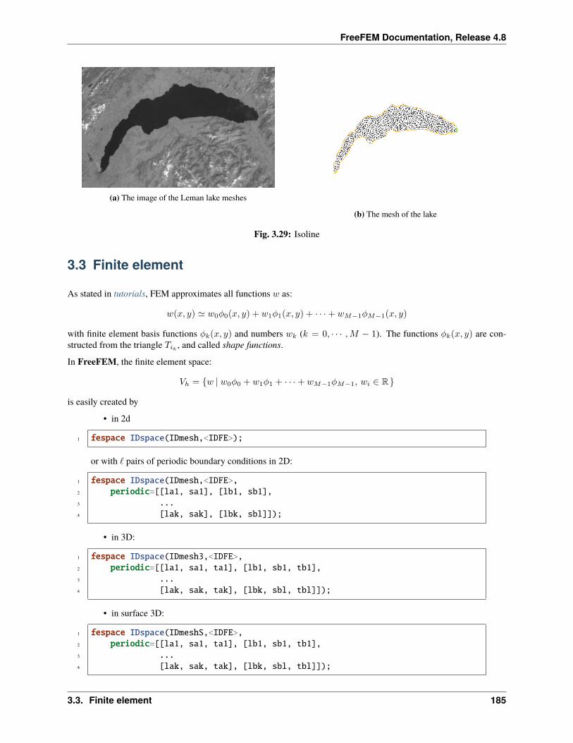
FreeFEM Documentation, Release 4.8
(a) The image of the Leman lake meshes
(b) The mesh of the lake
Fig. 3.29: Isoline
3.3 Finite element
As stated in tutorials, FEM approximates all functions 𝑤 as:
𝑤(𝑥, 𝑦) ≃ 𝑤0𝜑0(𝑥, 𝑦) + 𝑤1𝜑1(𝑥, 𝑦) + · · ·+ 𝑤𝑀−1𝜑𝑀−1(𝑥, 𝑦)
with finite element basis functions 𝜑𝑘(𝑥, 𝑦) and numbers 𝑤𝑘 (𝑘 = 0, · · · ,𝑀 − 1). The functions 𝜑𝑘(𝑥, 𝑦) are con-structed from the triangle 𝑇𝑖𝑘 , and called shape functions.
In FreeFEM, the finite element space:
𝑉ℎ = 𝑤 | 𝑤0𝜑0 + 𝑤1𝜑1 + · · ·+ 𝑤𝑀−1𝜑𝑀−1, 𝑤𝑖 ∈ R
is easily created by
• in 2d
1 fespace IDspace(IDmesh,<IDFE>);
or with ℓ pairs of periodic boundary conditions in 2D:
1 fespace IDspace(IDmesh,<IDFE>,2 periodic=[[la1, sa1], [lb1, sb1],3 ...4 [lak, sak], [lbk, sbl]]);
• in 3D:
1 fespace IDspace(IDmesh3,<IDFE>,2 periodic=[[la1, sa1, ta1], [lb1, sb1, tb1],3 ...4 [lak, sak, tak], [lbk, sbl, tbl]]);
• in surface 3D:
1 fespace IDspace(IDmeshS,<IDFE>,2 periodic=[[la1, sa1, ta1], [lb1, sb1, tb1],3 ...4 [lak, sak, tak], [lbk, sbl, tbl]]);
3.3. Finite element 185
FreeFEM Documentation, Release 4.8
where IDspace is the name of the space (e.g. Vh), IDmesh IDmesh3 IDmeshS `is respectly the name of theassociated :freefem:`mesh, mesh3, meshS and <IDFE> is an identifier of finite element type.
In 2D we have a pair of periodic boundary conditions, if [𝑙𝑎𝑖, 𝑠𝑎𝑖], [𝑙𝑏𝑖, 𝑠𝑏𝑖] is a pair of int, and the 2 labels 𝑙𝑎𝑖 and𝑙𝑏𝑖 refer to 2 pieces of boundary to be in equivalence.
If [𝑙𝑎𝑖, 𝑠𝑎𝑖], [𝑙𝑏𝑖, 𝑠𝑏𝑖] is a pair of real, then 𝑠𝑎𝑖 and 𝑠𝑏𝑖 give two common abscissa on the two boundary curves, andtwo points are identified as one if the two abscissa are equal.
In 2D, we have a pair of periodic boundary conditions, if [𝑙𝑎𝑖, 𝑠𝑎𝑖, 𝑡𝑎𝑖], [𝑙𝑏𝑖, 𝑠𝑏𝑖, 𝑡𝑏𝑖] is a pair of int, the 2 labels 𝑙𝑎𝑖and 𝑙𝑏𝑖 define the 2 pieces of boundary to be in equivalence.
If [𝑙𝑎𝑖, 𝑠𝑎𝑖, 𝑡𝑎𝑖], [𝑙𝑏𝑖, 𝑠𝑏𝑖, 𝑡𝑏𝑖] is a pair of real, then 𝑠𝑎𝑖, 𝑡𝑎𝑖 and 𝑠𝑏𝑖, 𝑡𝑏𝑖 give two common parameters on the twoboundary surfaces, and two points are identified as one if the two parameters are equal.
Note: The 2D mesh of the two identified borders must be the same, so to be sure, use the parameterfixedborder=true in buildmesh command (see fixedborder).
3.3.1 List of the types of finite elements
As of today, the known types of finite elements are:
• [P0] piecewise constant discontinuous finite element (2d, 3d, surface 3d), the degrees of freedom are thebarycenter element value.
P0ℎ =
𝑣 ∈ 𝐿2(Ω)
for all 𝐾 ∈ 𝒯ℎ there is 𝛼𝐾 ∈ R : 𝑣|𝐾 = 𝛼𝐾
(3.2)
• [P1] piecewise linear continuous finite element (2d, 3d, surface 3d), the degrees of freedom are the verticesvalues.
P1ℎ =
𝑣 ∈ 𝐻1(Ω)
∀𝐾 ∈ 𝒯ℎ, 𝑣|𝐾 ∈ 𝑃1
(3.3)
• [P1dc] piecewise linear discontinuous finite element (2d, 3d with load”Element_P1dc1”)
P1𝑑𝑐|ℎ =
𝑣 ∈ 𝐿2(Ω)
∀𝐾 ∈ 𝒯ℎ, 𝑣|𝐾 ∈ 𝑃1
(3.4)
Warning: Due to an interpolation problem, the degree of freedom is not the vertices but three vertices whichmove inside 𝑇 (𝑋) = 𝐺+ .99(𝑋 −𝐺) where 𝐺 is the barycenter.
• [P1b] piecewise linear continuous finite element plus bubble (2d, 3d)
The 2D Case:
P1𝑏|ℎ =
𝑣 ∈ 𝐻1(Ω)
∀𝐾 ∈ 𝒯ℎ, 𝑣|𝐾 ∈ 𝑃1 ⊕ Span𝜆𝐾0 𝜆𝐾1 𝜆𝐾2
(3.5)
The 3D Case:
186 Chapter 3. Documentation
FreeFEM Documentation, Release 4.8
P1𝑏|ℎ =
𝑣 ∈ 𝐻1(Ω)
∀𝐾 ∈ 𝒯ℎ, 𝑣|𝐾 ∈ 𝑃1 ⊕ Span𝜆𝐾0 𝜆𝐾1 𝜆𝐾2 𝜆𝐾3
(3.6)
where 𝜆𝐾𝑖 , 𝑖 = 0, .., 𝑑 are the 𝑑 + 1 barycentric coordinate functions of the element 𝐾 (triangle ortetrahedron).
• P1bl,P1bl3d piecewise linear continuous finite element plus linear bubble (with load”Element_P1bl” 2d, 3d).
The bubble is built by splitting the 𝐾, a barycenter in 𝑑+ 1 sub element. (need load "Element_P1bl")
• [P2, P2] piecewise 𝑃2 continuous finite element (2d, 3d, surface 3d)
P2ℎ =
𝑣 ∈ 𝐻1(Ω)
∀𝐾 ∈ 𝒯ℎ, 𝑣|𝐾 ∈ 𝑃2
where 𝑃2 is the set of polynomials of R2 of degrees ≤ 2.
• [P2b, P2b3d] piecewise 𝑃2 continuous finite element plus bubble (2d, 3d with load”Element_P2bulle3”)
The 2D Case:
P2ℎ =
𝑣 ∈ 𝐻1(Ω)
∀𝐾 ∈ 𝒯ℎ, 𝑣|𝐾 ∈ 𝑃2 ⊕ Span𝜆𝐾0 𝜆𝐾1 𝜆𝐾2
The 3D Case:
P2ℎ =
𝑣 ∈ 𝐻1(Ω)
∀𝐾 ∈ 𝒯ℎ, 𝑣|𝐾 ∈ 𝑃2 ⊕ Span𝜆𝐾0 𝜆𝐾1 𝜆𝐾2 𝜆𝐾3
• [P2dc] piecewise 𝑃2 discontinuous finite element (2d)
P2𝑑𝑐|ℎ =
𝑣 ∈ 𝐿2(Ω)
∀𝐾 ∈ 𝒯ℎ, 𝑣|𝐾 ∈ 𝑃2
Warning: Due to an interpolation problem, the degree of freedom is not the six P2 nodes but six nodeswhich move inside 𝑇 (𝑋) = 𝐺+ .99(𝑋 −𝐺) where 𝐺 is the barycenter.
• [P2h] quadratic homogeneous continuous (without P1).
• [P3] piecewise 𝑃3 continuous finite element (2d) (needs load "Element_P3")
P3ℎ =
𝑣 ∈ 𝐻1(Ω)
∀𝐾 ∈ 𝒯ℎ, 𝑣|𝐾 ∈ 𝑃3
where 𝑃3 is the set of polynomials of R2 of degrees ≤ 3.
• [P3dc] piecewise 𝑃3 discontinuous finite element (2d) (needs load "Element_P3dc")
P3𝑑𝑐|ℎ =
𝑣 ∈ 𝐿2(Ω)
∀𝐾 ∈ 𝒯ℎ, 𝑣|𝐾 ∈ 𝑃3
where 𝑃3 is the set of polynomials of R2 of degrees ≤ 3.
3.3. Finite element 187
FreeFEM Documentation, Release 4.8
• [P4] piecewise 𝑃4 continuous finite element (2d) (needs load "Element_P4")
P4ℎ =
𝑣 ∈ 𝐻1(Ω)
∀𝐾 ∈ 𝒯ℎ, 𝑣|𝐾 ∈ 𝑃4
where 𝑃4 is the set of polynomials of R2 of degrees ≤ 4.
• [P4dc] piecewise 𝑃4 discontinuous finite element (2d) (needs load "Element_P4dc")
P4𝑑𝑐|ℎ =
𝑣 ∈ 𝐿2(Ω)
∀𝐾 ∈ 𝒯ℎ, 𝑣|𝐾 ∈ 𝑃3
where 𝑃4 is the set of polynomials of R2 of degrees ≤ 3.
• [P0Edge] piecewise 𝑃0 discontinuous finite element (2d) contained on each edge of the mesh.
• [P1Edge] piecewise 𝑃1 discontinuous finite element (2d) (needs load "Element_PkEdge") 𝑃1 on each edgeof the mesh.
• [P2Edge] piecewise 𝑃2 discontinuous finite element (2d) (needs load "Element_PkEdge") 𝑃2 on each edgeof the mesh.
• [P3Edge] piecewise 𝑃3 discontinuous finite element (2d) (needs load "Element_PkEdge") 𝑃3 on each edgeof the mesh.
• [P4Edge] piecewise 𝑃4 discontinuous finite element (2d) (needs load "Element_PkEdge") 𝑃4 on each edgeof the mesh.
• [P5Edge] piecewise 𝑃5 discontinuous finite element (2d) (needs load "Element_PkEdge") 𝑃5 on each edgeof the mesh.
• [P2Morley] piecewise 𝑃2 non conform finite element (2d) (needs load "Morley")
P2ℎ =
𝑣 ∈ 𝐿2(Ω)
∀𝐾 ∈ 𝒯ℎ, 𝑣|𝐾 ∈ 𝑃3,
𝑣 continuous at vertices,
𝜕𝑛𝑣 continuous at middle of edge,
where 𝑃2 is the set of polynomials of R2 of degrees ≤ 2.
Warning: To build the interplant of a function 𝑢 (scalar) for this finite element, we need the func-tion and 2 partial derivatives (𝑢, 𝑢𝑥, 𝑢𝑦), creating this vectorial finite element with 3 components(𝑢, 𝑢𝑥, 𝑢𝑦).
See our example for solving the BiLaplacien problem:
1 load "Morley"2
3 // Parameters4 int nn = 10;5 real h = 0.01;6
7 real f = 1;8
9 // Mesh10 mesh Th = square(nn, nn);
(continues on next page)
188 Chapter 3. Documentation
FreeFEM Documentation, Release 4.8
(continued from previous page)
11 Th = adaptmesh(Th, h, IsMetric=1);12
13 // Fespace14 fespace Vh(Th, P2Morley); //The Morley finite element space15 Vh [u, ux, uy], [v, vx, vy];16
17 // Macro18 macro bilaplacien(u, v) (dxx(u)*dxx(v) + dyy(u)*dyy(v) + 2.*dxy(u)*dxy(v)) /
→˓/19
20 // Problem21 solve bilap ([u, ux, uy], [v, vx, vy])22 = int2d(Th)(23 bilaplacien(u, v)24 )25 - int2d(Th)(26 f*v27 )28 + on(1, 2, 3, 4, u=0, ux=0, uy=0)29 ;30
31 // Plot32 plot(u, cmm="u");
• [HCT] 𝑃3 𝐶1 conforms finite element (2d) (needs load "Element_HCT") one 3 sub triangles.
Lets call 𝒯 ℎ the sub mesh of 𝒯ℎ where all triangles are split in 3 at the barycenter.
P𝐻𝐶𝑇ℎ =𝑣 ∈ 𝐶1(Ω)
∀𝐾 ∈ 𝒯
ℎ , 𝑣|𝐾 ∈ 𝑃3
where 𝑃3 is the set of polynomials of R2 of degrees ≤ 3.
The degrees of freedom are the values of the normal derivative at the mid-point of each edge[BERNADOU1980].
Warning: To build the interplant of a function 𝑢 (scalar) for this finite element, we need the func-tion and 2 partial derivatives (𝑢, 𝑢𝑥, 𝑢𝑦), creating this vectorial finite element with 3 components(𝑢, 𝑢𝑥, 𝑢𝑦) like in previous finite element.
• [P2BR] (needs load "BernadiRaugel") the Bernadi Raugel Finite Element is a Vectorial element (2d) with2 components, see [BERNARDI1985].
It is a 2D coupled Finite Element, where the Polynomial space is 𝑃 21 with 3 normal bubble edge
functions (𝑃2). There are 9 degrees of freedom:
– 2 components at each of the 3 vertices and
– the 3 flux on the 3 edges.
• [RT0, RT03d] Raviart-Thomas finite element of degree 0.
The 2D Case:
𝑅𝑇0ℎ =v ∈ 𝐻(div)
∀𝐾 ∈ 𝒯ℎ, v|𝐾(𝑥, 𝑦) =
𝛼1
𝐾
𝛼2𝐾
+ 𝛽𝐾 | 𝑥𝑦
(3.7)
3.3. Finite element 189
FreeFEM Documentation, Release 4.8
The 3D Case:
𝑅𝑇0ℎ =
v ∈ 𝐻(div)
∀𝐾 ∈ 𝒯ℎ, v|𝐾(𝑥, 𝑦, 𝑧) =
𝛼
1𝐾
𝛼2𝐾
𝛼3𝐾
+ 𝛽𝐾
𝑥𝑦𝑧
(3.8)
where by writing div w =∑𝑑𝑖=1 𝜕𝑤𝑖/𝜕𝑥𝑖 with w = (𝑤𝑖)
𝑑𝑖=1:
𝐻(div) =w ∈ 𝐿2(Ω)𝑑
div w ∈ 𝐿2(Ω)
and where 𝛼1
𝐾 , 𝛼2𝐾 , 𝛼3
𝐾 , 𝛽𝐾 are real numbers.
• [RT0Ortho] Raviart-Thomas Orthogonal, or Nedelec finite element type I of degree 0 in dimension 2
𝑅𝑇0𝑂𝑟𝑡ℎ𝑜ℎ =v ∈ 𝐻(curl)
∀𝐾 ∈ 𝒯ℎ, v|𝐾(𝑥, 𝑦) =
𝛼1
𝐾
𝛼2𝐾
+ 𝛽𝐾 |−𝑦𝑥
(3.9)
• [Edge03d] 3d Nedelec finite element or Edge Element of degree 0.
𝐸𝑑𝑔𝑒0ℎ =
v ∈ 𝐻(Curl)
∀𝐾 ∈ 𝒯ℎ, v|𝐾(𝑥, 𝑦, 𝑧) =
𝛼
1𝐾
𝛼2𝐾
𝛼3𝐾
+
𝛽
1𝐾
𝛽2𝐾
𝛽3𝐾
×𝑥𝑦𝑧
: 𝑙𝑎𝑏𝑒𝑙 : 𝑒𝑞 : 𝐸𝑑𝑔𝑒03𝑑
where by writing curlw =
𝜕𝑤2/𝜕𝑥3−𝜕𝑤3/𝜕𝑥2
𝜕𝑤3/𝜕𝑥1−𝜕𝑤1/𝜕𝑥3
𝜕𝑤1/𝜕𝑥2−𝜕𝑤2/𝜕𝑥1
with w = (𝑤𝑖)𝑑𝑖=1:
𝐻(curl) =w ∈ 𝐿2(Ω)𝑑
curl w ∈ 𝐿2(Ω)𝑑
and 𝛼1
𝐾 , 𝛼2𝐾 , 𝛼
3𝐾 , 𝛽
1𝐾 , 𝛽
2𝐾 , 𝛽
3𝐾 are real numbers.
• [Edge13d] (needs load "Element_Mixte3d") 3d Nedelec finite element or Edge Element of degree 1.
• [Edge23d] (needs load "Element_Mixte3d") 3d Nedelec finite element or Edge Element of degree 2.
• [P1nc] piecewise linear element continuous at the mid-point of the edge only in 2D (Crouzeix-Raviart FiniteElement 2D).
• [P2pnc] piecewise quadratic plus a P3 bubble element with the continuity of the 2 moments on each edge (needsload "Element_P2pnc")
• [RT1] (needs load "Element_Mixte")
𝑅𝑇1ℎ =v ∈ 𝐻(div)
∀𝐾 ∈ 𝒯ℎ, 𝛼1
𝐾 , 𝛼2𝐾 , 𝛽𝐾 ∈ 𝑃 2
1 , 𝑃0,v|𝐾(𝑥, 𝑦) =𝛼1
𝐾
𝛼2𝐾
+ 𝛽𝐾 | 𝑥𝑦
(3.10)
• [RT1Ortho] (needs load "Element_Mixte")
𝑅𝑇1ℎ =v ∈ 𝐻(curl)
∀𝐾 ∈ 𝒯ℎ, 𝛼1
𝐾 , 𝛼2𝐾 , 𝛽𝐾 ∈ 𝑃 2
1 , 𝑃0,v|𝐾(𝑥, 𝑦) =𝛼1
𝐾
𝛼2𝐾
+ 𝛽𝐾 |−𝑦𝑥(3.11)
• [RT2] (needs load "Element_Mixte")
𝑅𝑇2ℎ =v ∈ 𝐻(div)
∀𝐾 ∈ 𝒯ℎ, 𝛼1
𝐾 , 𝛼2𝐾 , 𝛽𝐾 ∈ 𝑃 2
2 , 𝑃1,v|𝐾(𝑥, 𝑦) =𝛼1
𝐾
𝛼2𝐾
+ 𝛽𝐾 | 𝑥𝑦
(3.12)
190 Chapter 3. Documentation
FreeFEM Documentation, Release 4.8
• [RT2Ortho] (needs load "Element_Mixte")
𝑅𝑇2ℎ =v ∈ 𝐻(curl)
∀𝐾 ∈ 𝒯ℎ, 𝛼1
𝐾 , 𝛼2𝐾 , 𝛽𝐾 ∈ 𝑃 2
2 , 𝑃1, v|𝐾(𝑥, 𝑦) =𝛼1
𝐾
𝛼2𝐾
+ 𝛽𝐾 |−𝑦𝑥(3.13)
• [BDM1] (needs load "Element_Mixte") the Brezzi-Douglas-Marini finite element:
𝐵𝐷𝑀1ℎ =v ∈ 𝐻(div)
∀𝐾 ∈ 𝒯ℎ, v|𝐾 ∈ 𝑃 2
1
(3.14)
• [BDM1Ortho] (needs load "Element_Mixte") the Brezzi-Douglas-Marini Orthogonal also call Nedelec oftype II , finite element
𝐵𝐷𝑀1𝑂𝑟𝑡ℎ𝑜ℎ =v ∈ 𝐻(curl)
∀𝐾 ∈ 𝒯ℎ, v|𝐾 ∈ 𝑃 2
1
(3.15)
• [FEQF] (needs load "Element_QF") the finite element to store functions at default quadrature points (so thequadrature is qf5pT in 2D and is qfV5 in 3d).
For over quadrature you have the following corresponding finite element’s quadrature formula.
– FEQF1 ↦→ qf1pT,
– FEQF2 ↦→ qf2pT,
– FEQF5 ↦→ qf5pT,
– FEQF7 ↦→ qf7pT,
– FEQF9 ↦→ qf9pT,
– FEQF13d ↦→ qfV1,
– FEQF23d ↦→ qfV2,
– FEQF53d ↦→ qfV5
You can use this element to optimize the storage and reuse of functions with a long formula inside an integral for nonlinear processes.
3.3.2 Use of fespace in 2D
With the 2D finite element spaces
𝑋ℎ =𝑣 ∈ 𝐻1(]0, 1[2)| ∀𝐾 ∈ 𝒯ℎ 𝑣|𝐾 ∈ 𝑃1
𝑋𝑝ℎ = 𝑣 ∈ 𝑋ℎ| 𝑣 (| 0. ) = 𝑣 (| 1. ) , 𝑣 (| .0 ) = 𝑣 (| .1 )
𝑀ℎ =𝑣 ∈ 𝐻1(]0, 1[2)| ∀𝐾 ∈ 𝒯ℎ 𝑣|𝐾 ∈ 𝑃2
𝑅ℎ =
v ∈ 𝐻1(]0, 1[2)2| ∀𝐾 ∈ 𝒯ℎ v|𝐾(𝑥, 𝑦) =
𝛼𝐾
𝛽𝐾+ 𝛾𝐾 | 𝑥𝑦
when 𝒯ℎ is a mesh 10× 10 of the unit square ]0, 1[2, we only write in FreeFEM:
3.3. Finite element 191
FreeFEM Documentation, Release 4.8
1 mesh Th = square(10, 10);2 fespace Xh(Th, P1); //scalar FE3 fespace Xph(Th,P1,4 periodic=[[2, y], [4, y], [1, x], [3, x]]); //bi-periodic FE5 fespace Mh(Th, P2); //scalar FE6 fespace Rh(Th, RT0); //vectorial FE
where Xh, Mh, Rh expresses finite element spaces (called FE spaces) 𝑋ℎ, 𝑀ℎ, 𝑅ℎ, respectively.
To use FE-functions 𝑢ℎ, 𝑣ℎ ∈ 𝑋ℎ, 𝑝ℎ, 𝑞ℎ ∈𝑀ℎ and 𝑈ℎ, 𝑉ℎ ∈ 𝑅ℎ, we write:
1 Xh uh, vh;2 Xph uph, vph;3 Mh ph, qh;4 Rh [Uxh, Uyh], [Vxh, Vyh];5 Xh[int] Uh(10); //array of 10 functions in Xh6 Rh[int] [Wxh, Wyh](10); //array of 10 functions in Rh7 Wxh[5](0.5,0.5); //the 6th function at point (0.5, 0.5)8 Wxh[5][]; //the array of the degree of freedom of the 6th function
The functions 𝑈ℎ, 𝑉ℎ have two components so we have
𝑈ℎ =𝑈𝑥ℎ𝑈𝑦ℎ and 𝑉ℎ =
𝑉 𝑥ℎ𝑉 𝑦ℎ
3.3.3 Use of fespace in 3D
With the 3D finite element spaces
𝑋ℎ = 𝑣 ∈ 𝐻1(]0, 1[3)| ∀𝐾 ∈ 𝒯ℎ 𝑣|𝐾 ∈ 𝑃1
𝑋𝑝ℎ =𝑣 ∈ 𝑋ℎ| 𝑣
(0..
)= 𝑣
(1..
), 𝑣( .
0.
)= 𝑣
( .1.
), 𝑣( ..0
)= 𝑣
( ..1
)𝑀ℎ = 𝑣 ∈ 𝐻1(]0, 1[3)| ∀𝐾 ∈ 𝒯ℎ 𝑣|𝐾 ∈ 𝑃2
𝑅ℎ =v ∈ 𝐻1(]0, 1[3)2| ∀𝐾 ∈ 𝒯ℎ v|𝐾(𝑥, 𝑦, 𝑧) =
𝛼𝐾
𝛽𝐾𝛾𝐾
+ 𝛿𝐾
𝑥𝑦𝑧
when 𝒯ℎ is a mesh 10× 10× 10 of the unit cubic ]0, 1[2, we write in FreeFEM:
1 //label: 0 up, 1 down, 2 front, 3 left, 4 back, 5 right2 int nn=10;3 mesh3 Th=buildlayers(square(nn,nn,region=0),nn,4 zbound=[zmin,zmax], labelmid=rmid, reffaceup = rup,5 reffacelow = rdown);6
7 fespace Xh(Th, P1); //scalar FE8 // a FE space with full periodic condition in 3 axes9 fespace Xph(Th,P1,periodic=[[1,y,z],[2,y,z],
10 [3,x,z],[4,x,z],[5,x,y],[6,x,y]]);11 fespace Mh(Th, P2); //scalar FE12 fespace Rh(Th, RT03d); //vectorial FE
where Xh, Mh, Rh expresses finite element spaces (called FE spaces) 𝑋ℎ, 𝑀ℎ, 𝑅ℎ, respectively.
The functions 𝑈ℎ, 𝑉ℎ have two components so we have
192 Chapter 3. Documentation
FreeFEM Documentation, Release 4.8
3.3.4 Use of fespace in surface 3D
With the 3D finite element spaces
𝑋ℎ = 𝑣 ∈ 𝐻1(]0, 1[3)| ∀𝐾 ∈ 𝒯ℎ 𝑣|𝐾 ∈ 𝑃1
1 meshS Th = square3(10, 10);2 fespace Xh(Th, P1); //scalar FE
where Xh expresses finite element spaces (called FE spaces) 𝑋ℎ, respectively.
To use FE-functions 𝑢ℎ, 𝑣ℎ ∈ 𝑋ℎ, 𝑝ℎ, 𝑞ℎ ∈𝑀ℎ and 𝑈ℎ, 𝑉ℎ ∈ 𝑅ℎ, we write:
1 Xh uh, vh;2 Xh[int] Uh(10); //array of 10 functions in Xh
3.3.5 Finite Element functions
To define and use FE-functions 𝑢ℎ, 𝑣ℎ ∈ 𝑋ℎ, 𝑝ℎ, 𝑞ℎ ∈𝑀ℎ and 𝑈ℎ, 𝑉ℎ ∈ 𝑅ℎ, we write:
1 Xh uh, vh;2 Xph uph, vph;3 Mh ph, qh;4 Rh [Uxh, Uyh, Uyzh], [Vxh, Vyh, Vyzh];5 Xh[int] Uh(10); //array of 10 functions in Xh6 Rh[int] [Wxh,Wyh,Wzh](10); // array of 10 functions in Rh7 Wxh[5](0.5,0.5,0.5); //the 6th function at point (0.5, 0.5, 0.5)8 Wxh[5][]; //the array of the degree of freedom of the 6th function
The functions 𝑈ℎ, 𝑉ℎ have three components, so we have:
𝑈ℎ =
(𝑈ℎ)𝑥(𝑈ℎ)𝑦(𝑈ℎ)𝑧
and 𝑉ℎ =
(𝑉ℎ)𝑥(𝑉ℎ)𝑦(𝑉ℎ)𝑧
Note: One challenge of the periodic boundary condition is that the mesh must have equivalent faces.
The buildlayers mesh generator splits each quadrilateral face with the diagonal passing through the vertex withmaximum number, so to be sure to have the same mesh one both face periodic the 2D numbering in correspondingedges must be compatible (for example the same variation).
By Default, the numbering of square vertex is correct.
To change the mesh numbering you can use the change function like:
1 2 int[int] old2new(0:Th.nv-1); //array set on 0, 1, .., nv-13 fespace Vh2(Th, P1);4 Vh2 sorder = x+y; //choose an order increasing on 4 square borders with x or y5 sort(sorder[], old2new); //build the inverse permutation6 int[int] new2old = old2new^-1; //inverse the permutation7 Th = change(Th, renumv=new2old);8
The full example is in examples.
3.3. Finite element 193
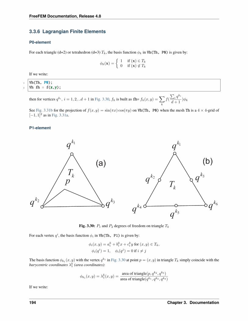
FreeFEM Documentation, Release 4.8
3.3.6 Lagrangian Finite Elements
P0-element
For each triangle (d=2) or tetrahedron (d=3) 𝑇𝑘, the basis function 𝜑𝑘 in Vh(Th, P0) is given by:
𝜑𝑘(x) =
1 if (x) ∈ 𝑇𝑘0 if (x) ∈ 𝑇𝑘
If we write:
1 Vh(Th, P0);2 Vh fh = f(x,y);
then for vertices 𝑞𝑘𝑖 , 𝑖 = 1, 2, ..𝑑+ 1 in Fig. 3.30, 𝑓ℎ is built as fh= 𝑓ℎ(𝑥, 𝑦) =∑𝑘
𝑓(
∑𝑖 𝑞𝑘𝑖
𝑑+ 1)𝜑𝑘
See Fig. 3.31b for the projection of 𝑓(𝑥, 𝑦) = sin(𝜋𝑥) cos(𝜋𝑦) on Vh(Th, P0) when the mesh Th is a 4 × 4-grid of[−1, 1]2 as in Fig. 3.31a.
P1-element
Fig. 3.30: 𝑃1 and 𝑃2 degrees of freedom on triangle 𝑇𝑘
For each vertex 𝑞𝑖, the basis function 𝜑𝑖 in Vh(Th, P1) is given by:
𝜑𝑖(𝑥, 𝑦) = 𝑎𝑘𝑖 + 𝑏𝑘𝑖 𝑥+ 𝑐𝑘𝑖 𝑦 for (𝑥, 𝑦) ∈ 𝑇𝑘,𝜑𝑖(𝑞
𝑖) = 1, 𝜑𝑖(𝑞𝑗) = 0 if 𝑖 = 𝑗
The basis function 𝜑𝑘1(𝑥, 𝑦) with the vertex 𝑞𝑘1 in Fig. 3.30 at point 𝑝 = (𝑥, 𝑦) in triangle 𝑇𝑘 simply coincide with thebarycentric coordinates 𝜆𝑘1 (area coordinates):
𝜑𝑘1(𝑥, 𝑦) = 𝜆𝑘1(𝑥, 𝑦) =area of triangle(𝑝, 𝑞𝑘2 , 𝑞𝑘3)
area of triangle(𝑞𝑘1 , 𝑞𝑘2 , 𝑞𝑘3)
If we write:
194 Chapter 3. Documentation
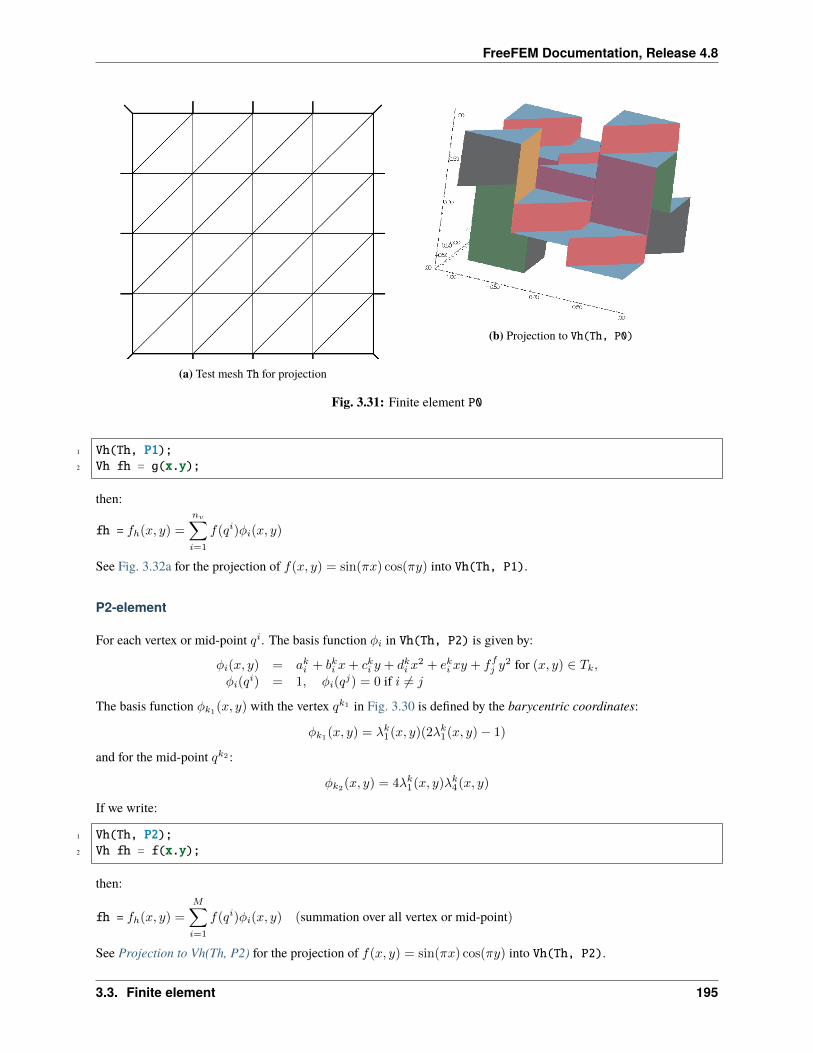
FreeFEM Documentation, Release 4.8
(a) Test mesh Th for projection
(b) Projection to Vh(Th, P0)
Fig. 3.31: Finite element P0
1 Vh(Th, P1);2 Vh fh = g(x.y);
then:
fh = 𝑓ℎ(𝑥, 𝑦) =
𝑛𝑣∑𝑖=1
𝑓(𝑞𝑖)𝜑𝑖(𝑥, 𝑦)
See Fig. 3.32a for the projection of 𝑓(𝑥, 𝑦) = sin(𝜋𝑥) cos(𝜋𝑦) into Vh(Th, P1).
P2-element
For each vertex or mid-point 𝑞𝑖. The basis function 𝜑𝑖 in Vh(Th, P2) is given by:
𝜑𝑖(𝑥, 𝑦) = 𝑎𝑘𝑖 + 𝑏𝑘𝑖 𝑥+ 𝑐𝑘𝑖 𝑦 + 𝑑𝑘𝑖 𝑥2 + 𝑒𝑘𝑖 𝑥𝑦 + 𝑓𝑓𝑗 𝑦
2 for (𝑥, 𝑦) ∈ 𝑇𝑘,𝜑𝑖(𝑞
𝑖) = 1, 𝜑𝑖(𝑞𝑗) = 0 if 𝑖 = 𝑗
The basis function 𝜑𝑘1(𝑥, 𝑦) with the vertex 𝑞𝑘1 in Fig. 3.30 is defined by the barycentric coordinates:
𝜑𝑘1(𝑥, 𝑦) = 𝜆𝑘1(𝑥, 𝑦)(2𝜆𝑘1(𝑥, 𝑦)− 1)
and for the mid-point 𝑞𝑘2 :
𝜑𝑘2(𝑥, 𝑦) = 4𝜆𝑘1(𝑥, 𝑦)𝜆𝑘4(𝑥, 𝑦)
If we write:
1 Vh(Th, P2);2 Vh fh = f(x.y);
then:
fh = 𝑓ℎ(𝑥, 𝑦) =
𝑀∑𝑖=1
𝑓(𝑞𝑖)𝜑𝑖(𝑥, 𝑦) (summation over all vertex or mid-point)
See Projection to Vh(Th, P2) for the projection of 𝑓(𝑥, 𝑦) = sin(𝜋𝑥) cos(𝜋𝑦) into Vh(Th, P2).
3.3. Finite element 195
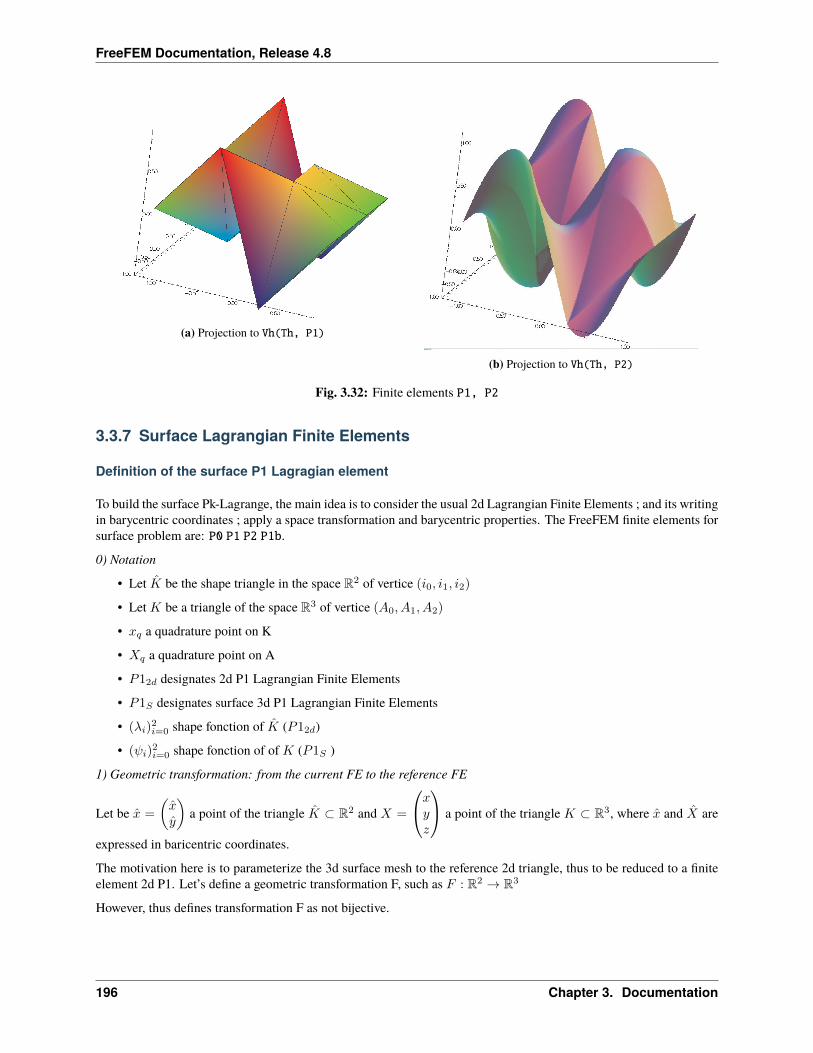
FreeFEM Documentation, Release 4.8
(a) Projection to Vh(Th, P1)
(b) Projection to Vh(Th, P2)
Fig. 3.32: Finite elements P1, P2
3.3.7 Surface Lagrangian Finite Elements
Definition of the surface P1 Lagragian element
To build the surface Pk-Lagrange, the main idea is to consider the usual 2d Lagrangian Finite Elements ; and its writingin barycentric coordinates ; apply a space transformation and barycentric properties. The FreeFEM finite elements forsurface problem are: P0 P1 P2 P1b.
0) Notation
• Let be the shape triangle in the space R2 of vertice (𝑖0, 𝑖1, 𝑖2)
• Let 𝐾 be a triangle of the space R3 of vertice (𝐴0, 𝐴1, 𝐴2)
• 𝑥𝑞 a quadrature point on K
• 𝑋𝑞 a quadrature point on A
• 𝑃12𝑑 designates 2d P1 Lagrangian Finite Elements
• 𝑃1𝑆 designates surface 3d P1 Lagrangian Finite Elements
• (𝜆𝑖)2𝑖=0 shape fonction of (𝑃12𝑑)
• (𝜓𝑖)2𝑖=0 shape fonction of of 𝐾 (𝑃1𝑆 )
1) Geometric transformation: from the current FE to the reference FE
Let be =
(𝑦
)a point of the triangle ⊂ R2 and 𝑋 =
⎛⎝𝑥𝑦𝑧
⎞⎠ a point of the triangle 𝐾 ⊂ R3, where and are
expressed in baricentric coordinates.
The motivation here is to parameterize the 3d surface mesh to the reference 2d triangle, thus to be reduced to a finiteelement 2d P1. Let’s define a geometric transformation F, such as 𝐹 : R2 → R3
However, thus defines transformation F as not bijective.
196 Chapter 3. Documentation
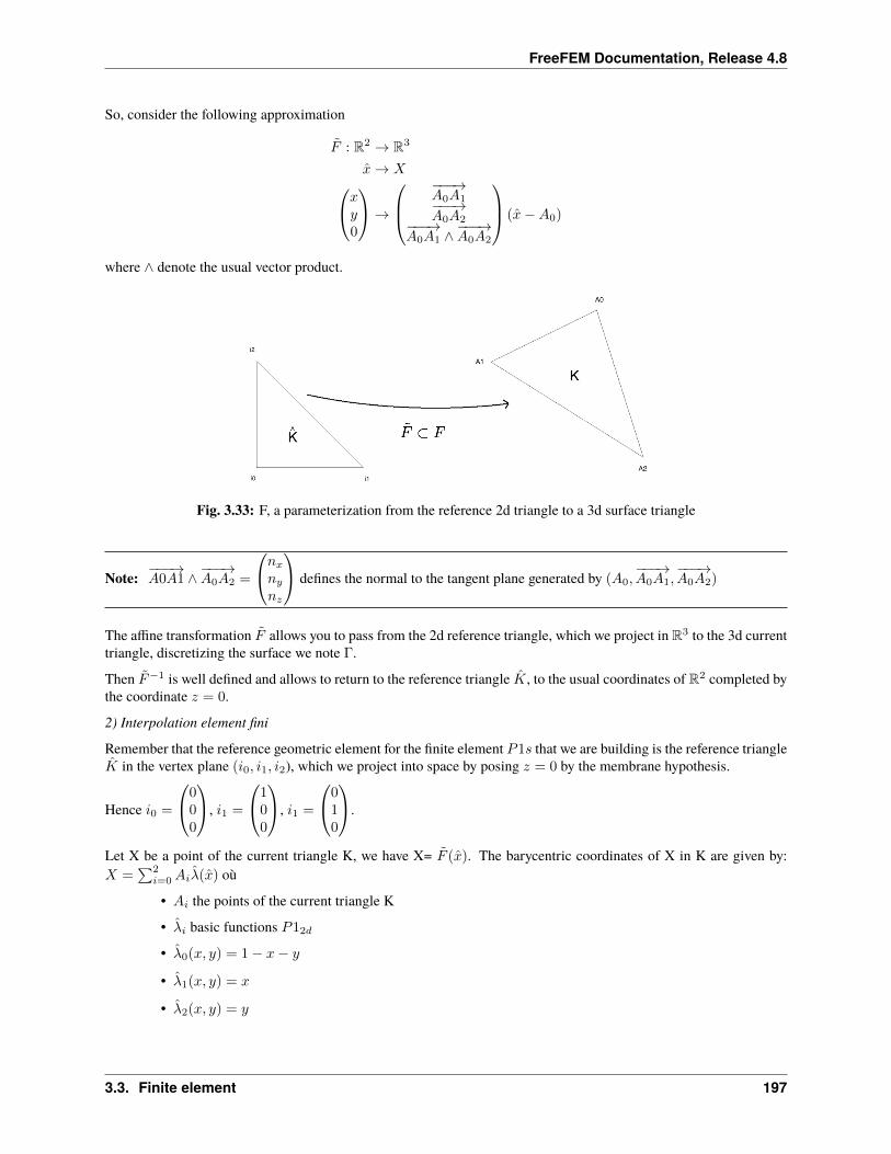
FreeFEM Documentation, Release 4.8
So, consider the following approximation
𝐹 : R2 → R3
→ 𝑋⎛⎝𝑥𝑦0
⎞⎠→⎛⎜⎝
−−−→𝐴0𝐴1−−−→𝐴0𝐴2−−−→
𝐴0𝐴1 ∧−−−→𝐴0𝐴2
⎞⎟⎠ (−𝐴0)
where ∧ denote the usual vector product.
Fig. 3.33: F, a parameterization from the reference 2d triangle to a 3d surface triangle
Note: −−−→𝐴0𝐴1 ∧−−−→𝐴0𝐴2 =
⎛⎝𝑛𝑥𝑛𝑦𝑛𝑧
⎞⎠ defines the normal to the tangent plane generated by (𝐴0,−−−→𝐴0𝐴1,
−−−→𝐴0𝐴2)
The affine transformation 𝐹 allows you to pass from the 2d reference triangle, which we project in R3 to the 3d currenttriangle, discretizing the surface we note Γ.
Then 𝐹−1 is well defined and allows to return to the reference triangle , to the usual coordinates of R2 completed bythe coordinate 𝑧 = 0.
2) Interpolation element fini
Remember that the reference geometric element for the finite element 𝑃1𝑠 that we are building is the reference triangle in the vertex plane (𝑖0, 𝑖1, 𝑖2), which we project into space by posing 𝑧 = 0 by the membrane hypothesis.
Hence 𝑖0 =
⎛⎝000
⎞⎠, 𝑖1 =
⎛⎝100
⎞⎠, 𝑖1 =
⎛⎝010
⎞⎠.
Let X be a point of the current triangle K, we have X= 𝐹 (). The barycentric coordinates of X in K are given by:𝑋 =
∑2𝑖=0𝐴𝑖() où
• 𝐴𝑖 the points of the current triangle K
• 𝑖 basic functions 𝑃12𝑑
• 0(𝑥, 𝑦) = 1− 𝑥− 𝑦
• 1(𝑥, 𝑦) = 𝑥
• 2(𝑥, 𝑦) = 𝑦
3.3. Finite element 197
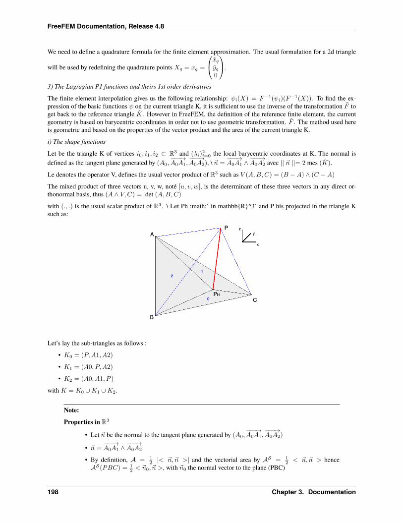
FreeFEM Documentation, Release 4.8
We need to define a quadrature formula for the finite element approximation. The usual formulation for a 2d triangle
will be used by redefining the quadrature points 𝑋𝑞 = 𝑥𝑞 =
⎛⎝𝑞𝑦𝑞0
⎞⎠.
3) The Lagragian P1 functions and theirs 1st order derivatives
The finite element interpolation gives us the following relationship: 𝜓𝑖(𝑋) = 𝐹−1(𝜓𝑖)(𝐹−1(𝑋)). To find the ex-
pression of the basic functions 𝜓 on the current triangle K, it is sufficient to use the inverse of the transformation 𝐹 toget back to the reference triangle . However in FreeFEM, the definition of the reference finite element, the currentgeometry is based on barycentric coordinates in order not to use geometric transformation. 𝐹 . The method used hereis geometric and based on the properties of the vector product and the area of the current triangle K.
i) The shape functions
Let be the triangle K of vertices 𝑖0, 𝑖1, 𝑖2 ⊂ R3 and (𝜆𝑖)2𝑖=0 the local barycentric coordinates at K. The normal is
defined as the tangent plane generated by (𝐴0,−−−→𝐴0𝐴1,
−−−→𝐴0𝐴2), \ =
−−−→𝐴0𝐴1 ∧
−−−→𝐴0𝐴2 avec || ||= 2 mes ().
Le denotes the operator V, defines the usual vector product of R3 such as 𝑉 (𝐴,𝐵,𝐶) = (𝐵 −𝐴) ∧ (𝐶 −𝐴)
The mixed product of three vectors u, v, w, noté [𝑢, 𝑣, 𝑤], is the determinant of these three vectors in any direct or-thonormal basis, thus (𝐴 ∧ 𝑉,𝐶) = det (𝐴,𝐵,𝐶)
with (., .) is the usual scalar product of R3. \ Let Ph :math:` in mathbbR^3` and P his projected in the triangle Ksuch as:
Let’s lay the sub-triangles as follows :
• 𝐾0 = (𝑃,𝐴1, 𝐴2)
• 𝐾1 = (𝐴0, 𝑃,𝐴2)
• 𝐾2 = (𝐴0, 𝐴1, 𝑃 )
with 𝐾 = 𝐾0 ∪𝐾1 ∪𝐾2.
Note:Properties in R3
• Let be the normal to the tangent plane generated by (𝐴0,−−−→𝐴0𝐴1,
−−−→𝐴0𝐴2)
• =−−−→𝐴0𝐴1 ∧
−−−→𝐴0𝐴2
• By definition, 𝒜 = 12 |< , >| and the vectorial area by 𝒜𝒮 = 1
2 < , > hence𝒜𝒮(𝑃𝐵𝐶) = 1
2 < 0, >, with 0 the normal vector to the plane (PBC)
198 Chapter 3. Documentation
FreeFEM Documentation, Release 4.8
Let’s define the respective vector areas
• 0(𝑃 ) = 𝑉 (𝑃,𝐴1, 𝐴2) the vectorial area of K0
• 1(𝑃 ) = 𝑉 (𝐴0, 𝑃,𝐴2) the vectorial area of K1
• 2(𝑃 ) = 𝑉 (𝐴0, 𝐴1, 𝑃 ) the vectorial area of K2
By definition, in 3d, the barycentric coordinates are given by algebraic area ratio: :math:` lambda_i(P) = frac (vecN_i(P),vec N)(vec N,vec N)labelbasisfunc`
Note that (𝑖(𝑃 ), ) = 2 sign mes (𝐾𝑖) || || and ( , ) = 2 sign mes (𝐾) || ||, avec 𝑠𝑖𝑔𝑛 the orientation ofthe current triangle compared to the reference triangle.
We find the finite element interpolation, 𝑃 =∑2𝑖=0 𝜆𝑖(𝑃 )𝐴𝑖.
ii) 1st order derivatives of Lagrangian P1 FE
Let be any vector of ∈ R3.
(2(𝑃 ), ) = ((𝐴1 −𝐴0) ∧ (𝑃 −𝐴0), 𝑌 )
= det(𝐴1 −𝐴0, 𝑃 −𝐴0, 𝑌 )
= det(𝐴1 −𝐴0, 𝑃, 𝑌 )− det(𝐴1 −𝐴0, 𝐴0, 𝑌 )
Let’s calculate the differential of (2(𝑃 ), 𝑌 ),∀𝑌
𝐷𝑃 (2(𝑃 ), ) = det(𝐴1 −𝐴0, 𝑃′, 𝑌 )𝑑𝑃
∇𝑃 (2(𝑃 ), ) = det (𝐴1 −𝐴0, 𝑃′, )
= −𝑑𝑒𝑡(𝐴1 −𝐴0, , 𝑃′)
= −(𝐴1 −𝐴0) ∧ .𝑃 ′
= ∧ (𝐴1 −𝐴0)
Consider in particular = , then
∇𝑃 (2(𝑃 ), ) = ∧ (𝐴1 −𝐴0)
= ∧ 𝐸2 = −det(𝐴1 −𝐴0, , 𝑃′)
This leads to :math:` nabla_P lambda_2(P) = frac (vec N wedge E_2)(vec N,vec N) `
By similar calculations for 0(𝑃 ) et 1(𝑃 )
∇𝑃𝜆𝑖(𝑃 ) = (∧𝐸𝑖)
(,)
Note: With the definition of the surface gradient and the 2d Pk-Lagrange FE used barycentric coordinates, surfacePk-Langrange FE are trivial.
3.3. Finite element 199
FreeFEM Documentation, Release 4.8
3.3.8 P1 Nonconforming Element
Refer to [THOMASSET2012] for details; briefly, we now consider non-continuous approximations so we will lose theproperty:
𝑤ℎ ∈ 𝑉ℎ ⊂ 𝐻1(Ω)
If we write:
1 Vh(Th, P1nc);2 Vh fh = f(x.y);
then:
fh = 𝑓ℎ(𝑥, 𝑦) =
𝑛𝑣∑𝑖=1
𝑓(𝑚𝑖)𝜑𝑖(𝑥, 𝑦) (summation over all midpoint)
Here the basis function 𝜑𝑖 associated with the mid-point 𝑚𝑖 = (𝑞𝑘𝑖 + 𝑞𝑘𝑖+1)/2 where 𝑞𝑘𝑖 is the 𝑖-th point in 𝑇𝑘, andwe assume that 𝑗 + 1 = 0 if 𝑗 = 3:
𝜑𝑖(𝑥, 𝑦) = 𝑎𝑘𝑖 + 𝑏𝑘𝑖 𝑥+ 𝑐𝑘𝑖 𝑦 for (𝑥, 𝑦) ∈ 𝑇𝑘,𝜑𝑖(𝑚
𝑖) = 1, 𝜑𝑖(𝑚𝑗) = 0 if 𝑖 = 𝑗
Strictly speaking 𝜕𝜑𝑖/𝜕𝑥, 𝜕𝜑𝑖/𝜕𝑦 contain Dirac distribution 𝜌𝛿𝜕𝑇𝑘.
The numerical calculations will automatically ignore them. In [THOMASSET2012], there is a proof of the estimation(𝑛𝑣∑𝑘=1
∫𝑇𝑘
|∇𝑤 −∇𝑤ℎ|2𝑡𝑒𝑥𝑡𝑑𝑥𝑡𝑒𝑥𝑡𝑑𝑦
)1/2
= 𝑂(ℎ)
The basis functions 𝜑𝑘 have the following properties.
1. For the bilinear form 𝑎 defined in Fig. 3.34a satisfy:
𝑎(𝜑𝑖, 𝜑𝑖) > 0, 𝑎(𝜑𝑖, 𝜑𝑗) ≤ 0 if 𝑖 = 𝑗∑𝑛𝑣
𝑘=1 𝑎(𝜑𝑖, 𝜑𝑘) ≥ 0
2. 𝑓 ≥ 0⇒ 𝑢ℎ ≥ 0
3. If 𝑖 = 𝑗, the basis function 𝜑𝑖 and 𝜑𝑗 are 𝐿2-orthogonal:
∫Ω
𝜑𝑖𝜑𝑗 𝑡𝑒𝑥𝑡𝑑𝑥𝑡𝑒𝑥𝑡𝑑𝑦 = 0 if 𝑖 = 𝑗
which is false for 𝑃1-element.
See Fig. 3.34a for the projection of 𝑓(𝑥, 𝑦) = sin(𝜋𝑥) cos(𝜋𝑦) into Vh(Th, P1nc).
200 Chapter 3. Documentation
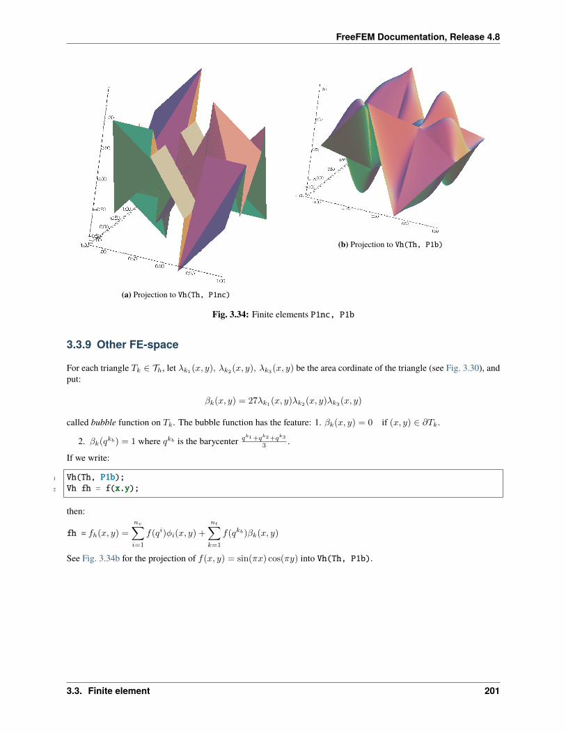
FreeFEM Documentation, Release 4.8
(a) Projection to Vh(Th, P1nc)
(b) Projection to Vh(Th, P1b)
Fig. 3.34: Finite elements P1nc, P1b
3.3.9 Other FE-space
For each triangle 𝑇𝑘 ∈ 𝒯ℎ, let 𝜆𝑘1(𝑥, 𝑦), 𝜆𝑘2(𝑥, 𝑦), 𝜆𝑘3(𝑥, 𝑦) be the area cordinate of the triangle (see Fig. 3.30), andput:
𝛽𝑘(𝑥, 𝑦) = 27𝜆𝑘1(𝑥, 𝑦)𝜆𝑘2(𝑥, 𝑦)𝜆𝑘3(𝑥, 𝑦)
called bubble function on 𝑇𝑘. The bubble function has the feature: 1. 𝛽𝑘(𝑥, 𝑦) = 0 if (𝑥, 𝑦) ∈ 𝜕𝑇𝑘.
2. 𝛽𝑘(𝑞𝑘𝑏) = 1 where 𝑞𝑘𝑏 is the barycenter 𝑞𝑘1+𝑞𝑘2+𝑞𝑘3
3 .
If we write:
1 Vh(Th, P1b);2 Vh fh = f(x.y);
then:
fh = 𝑓ℎ(𝑥, 𝑦) =
𝑛𝑣∑𝑖=1
𝑓(𝑞𝑖)𝜑𝑖(𝑥, 𝑦) +
𝑛𝑡∑𝑘=1
𝑓(𝑞𝑘𝑏)𝛽𝑘(𝑥, 𝑦)
See Fig. 3.34b for the projection of 𝑓(𝑥, 𝑦) = sin(𝜋𝑥) cos(𝜋𝑦) into Vh(Th, P1b).
3.3. Finite element 201
FreeFEM Documentation, Release 4.8
3.3.10 Vector Valued FE-function
Functions from R2 to R𝑁 with𝑁 = 1 are called scalar functions and called vector valued when𝑁 > 1. When𝑁 = 2
1 fespace Vh(Th, [P0, P1]) ;
makes the space
𝑉ℎ = w = (𝑤1, 𝑤2)| 𝑤1 ∈ 𝑉ℎ(𝒯ℎ, 𝑃0), 𝑤2 ∈ 𝑉ℎ(𝒯ℎ, 𝑃1)
Raviart-Thomas Element
In the Raviart-Thomas finite element 𝑅𝑇0ℎ, the degrees of freedom are the fluxes across edges 𝑒 of the mesh, wherethe flux of the function f : R2 −→ R2 is
∫𝑒f .𝑛𝑒, 𝑛𝑒 is the unit normal of edge 𝑒.
This implies an orientation of all the edges of the mesh, for example we can use the global numbering of the edgevertices and we just go from small to large numbers.
To compute the flux, we use a quadrature with one Gauss point, the mid-point of the edge.
Consider a triangle 𝑇𝑘 with three vertices (a,b, c).
Lets denote the vertices numbers by 𝑖𝑎, 𝑖𝑏, 𝑖𝑐, and define the three edge vectors e1, e2, e3 by 𝑠𝑔𝑛(𝑖𝑏 − 𝑖𝑐)(b − c),𝑠𝑔𝑛(𝑖𝑐 − 𝑖𝑎)(c− a), 𝑠𝑔𝑛(𝑖𝑎 − 𝑖𝑏)(a− b).
We get three basis functions:
𝜑𝑘1 =𝑠𝑔𝑛(𝑖𝑏 − 𝑖𝑐)
2|𝑇𝑘|(x− a), 𝜑𝑘2 =
𝑠𝑔𝑛(𝑖𝑐 − 𝑖𝑎)
2|𝑇𝑘|(x− b), 𝜑𝑘3 =
𝑠𝑔𝑛(𝑖𝑎 − 𝑖𝑏)2|𝑇𝑘|
(x− c),
where |𝑇𝑘| is the area of the triangle 𝑇𝑘. If we write:
1 Vh(Th, RT0);2 Vh [f1h, f2h] = [f1(x, y), f2(x, y)];
then:
fh = fℎ(𝑥, 𝑦) =
𝑛𝑡∑𝑘=1
6∑𝑙=1
𝑛𝑖𝑙𝑗𝑙 |eil |𝑓𝑗𝑙(𝑚𝑖𝑙)𝜑𝑖𝑙𝑗𝑙
where 𝑛𝑖𝑙𝑗𝑙 is the 𝑗𝑙-th component of the normal vector n𝑖𝑙 ,
𝑚1,𝑚2,𝑚3 =
b + c
2,a + c
2,b + a
2
and 𝑖𝑙 = 1, 1, 2, 2, 3, 3, 𝑗𝑙 = 1, 2, 1, 2, 1, 2 with the order of 𝑙.
1 // Mesh2 mesh Th = square(2, 2);3
4 // Fespace5 fespace Xh(Th, P1);6 Xh uh = x^2 + y^2, vh;7
8 fespace Vh(Th, RT0);9 Vh [Uxh, Uyh] = [sin(x), cos(y)]; //vectorial FE function
10
(continues on next page)
202 Chapter 3. Documentation
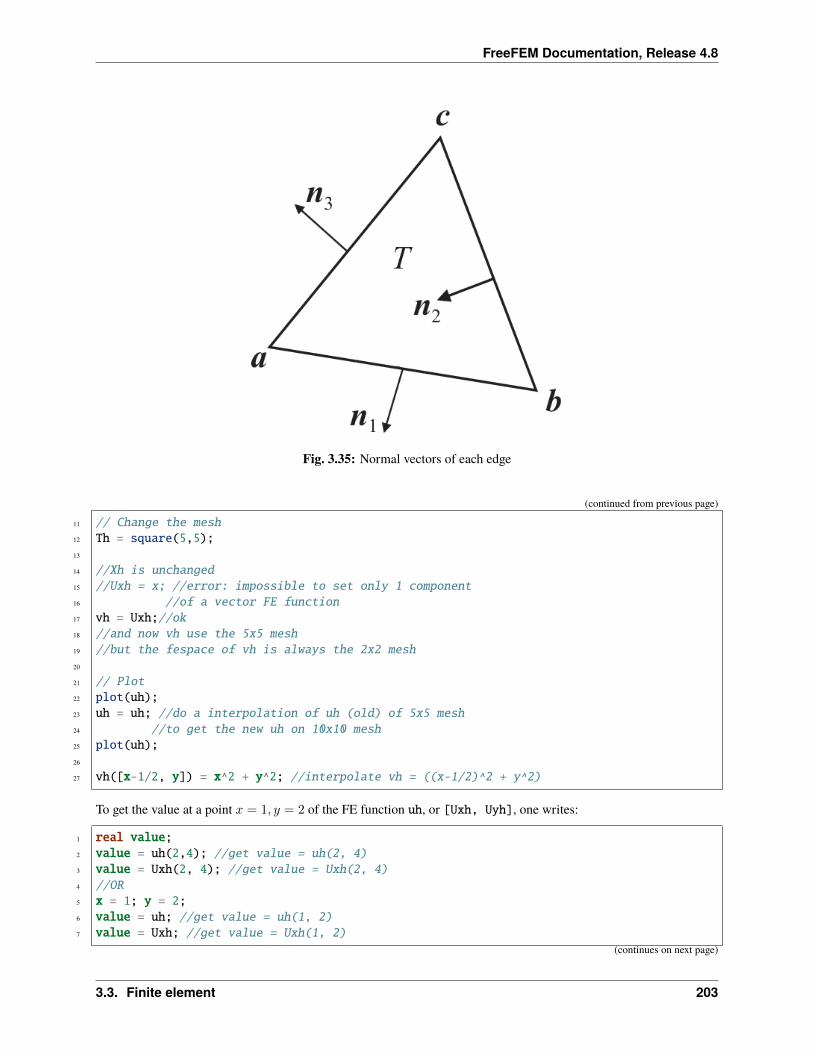
FreeFEM Documentation, Release 4.8
Fig. 3.35: Normal vectors of each edge
(continued from previous page)
11 // Change the mesh12 Th = square(5,5);13
14 //Xh is unchanged15 //Uxh = x; //error: impossible to set only 1 component16 //of a vector FE function17 vh = Uxh;//ok18 //and now vh use the 5x5 mesh19 //but the fespace of vh is always the 2x2 mesh20
21 // Plot22 plot(uh);23 uh = uh; //do a interpolation of uh (old) of 5x5 mesh24 //to get the new uh on 10x10 mesh25 plot(uh);26
27 vh([x-1/2, y]) = x^2 + y^2; //interpolate vh = ((x-1/2)^2 + y^2)
To get the value at a point 𝑥 = 1, 𝑦 = 2 of the FE function uh, or [Uxh, Uyh], one writes:
1 real value;2 value = uh(2,4); //get value = uh(2, 4)3 value = Uxh(2, 4); //get value = Uxh(2, 4)4 //OR5 x = 1; y = 2;6 value = uh; //get value = uh(1, 2)7 value = Uxh; //get value = Uxh(1, 2)
(continues on next page)
3.3. Finite element 203
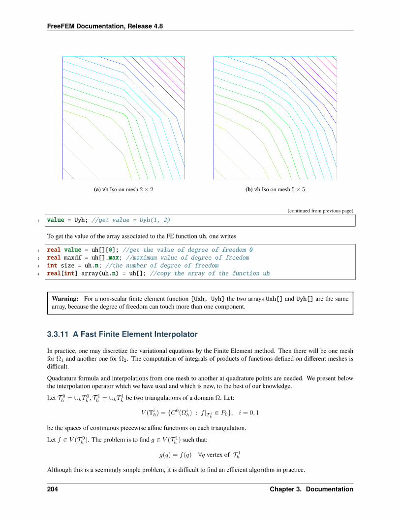
FreeFEM Documentation, Release 4.8
(a) vh Iso on mesh 2× 2 (b) vh Iso on mesh 5× 5
(continued from previous page)
8 value = Uyh; //get value = Uyh(1, 2)
To get the value of the array associated to the FE function uh, one writes
1 real value = uh[][0]; //get the value of degree of freedom 02 real maxdf = uh[].max; //maximum value of degree of freedom3 int size = uh.n; //the number of degree of freedom4 real[int] array(uh.n) = uh[]; //copy the array of the function uh
Warning: For a non-scalar finite element function [Uxh, Uyh] the two arrays Uxh[] and Uyh[] are the samearray, because the degree of freedom can touch more than one component.
3.3.11 A Fast Finite Element Interpolator
In practice, one may discretize the variational equations by the Finite Element method. Then there will be one meshfor Ω1 and another one for Ω2. The computation of integrals of products of functions defined on different meshes isdifficult.
Quadrature formula and interpolations from one mesh to another at quadrature points are needed. We present belowthe interpolation operator which we have used and which is new, to the best of our knowledge.
Let 𝒯 0ℎ = ∪𝑘𝑇 0
𝑘 , 𝒯 1ℎ = ∪𝑘𝑇 1
𝑘 be two triangulations of a domain Ω. Let:
𝑉 (T𝑖ℎ) = 𝐶0(Ω𝑖ℎ) : 𝑓 |𝑇 𝑖𝑘∈ 𝑃0, 𝑖 = 0, 1
be the spaces of continuous piecewise affine functions on each triangulation.
Let 𝑓 ∈ 𝑉 (𝒯 0ℎ ). The problem is to find 𝑔 ∈ 𝑉 (𝒯 1
ℎ ) such that:
𝑔(𝑞) = 𝑓(𝑞) ∀𝑞 vertex of 𝒯 1ℎ
Although this is a seemingly simple problem, it is difficult to find an efficient algorithm in practice.
204 Chapter 3. Documentation
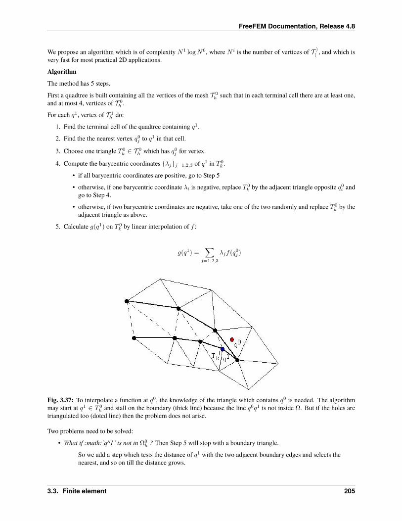
FreeFEM Documentation, Release 4.8
We propose an algorithm which is of complexity 𝑁1 log𝑁0, where 𝑁 𝑖 is the number of vertices of 𝒯 ⟩⟨ , and which is
very fast for most practical 2D applications.
AlgorithmThe method has 5 steps.
First a quadtree is built containing all the vertices of the mesh 𝒯 0ℎ such that in each terminal cell there are at least one,
and at most 4, vertices of 𝒯 0ℎ .
For each 𝑞1, vertex of 𝒯 1ℎ do:
1. Find the terminal cell of the quadtree containing 𝑞1.
2. Find the the nearest vertex 𝑞0𝑗 to 𝑞1 in that cell.
3. Choose one triangle 𝑇 0𝑘 ∈ 𝒯 0
ℎ which has 𝑞0𝑗 for vertex.
4. Compute the barycentric coordinates 𝜆𝑗𝑗=1,2,3 of 𝑞1 in 𝑇 0𝑘 .
• if all barycentric coordinates are positive, go to Step 5
• otherwise, if one barycentric coordinate 𝜆𝑖 is negative, replace 𝑇 0𝑘 by the adjacent triangle opposite 𝑞0𝑖 and
go to Step 4.
• otherwise, if two barycentric coordinates are negative, take one of the two randomly and replace 𝑇 0𝑘 by the
adjacent triangle as above.
5. Calculate 𝑔(𝑞1) on 𝑇 0𝑘 by linear interpolation of 𝑓 :
𝑔(𝑞1) =∑
𝑗=1,2,3
𝜆𝑗𝑓(𝑞0𝑗 )
Fig. 3.37: To interpolate a function at 𝑞0, the knowledge of the triangle which contains 𝑞0 is needed. The algorithmmay start at 𝑞1 ∈ 𝑇 0
𝑘 and stall on the boundary (thick line) because the line 𝑞0𝑞1 is not inside Ω. But if the holes aretriangulated too (doted line) then the problem does not arise.
Two problems need to be solved:
• What if :math:`q^1` is not in Ω0ℎ ? Then Step 5 will stop with a boundary triangle.
So we add a step which tests the distance of 𝑞1 with the two adjacent boundary edges and selects thenearest, and so on till the distance grows.
3.3. Finite element 205
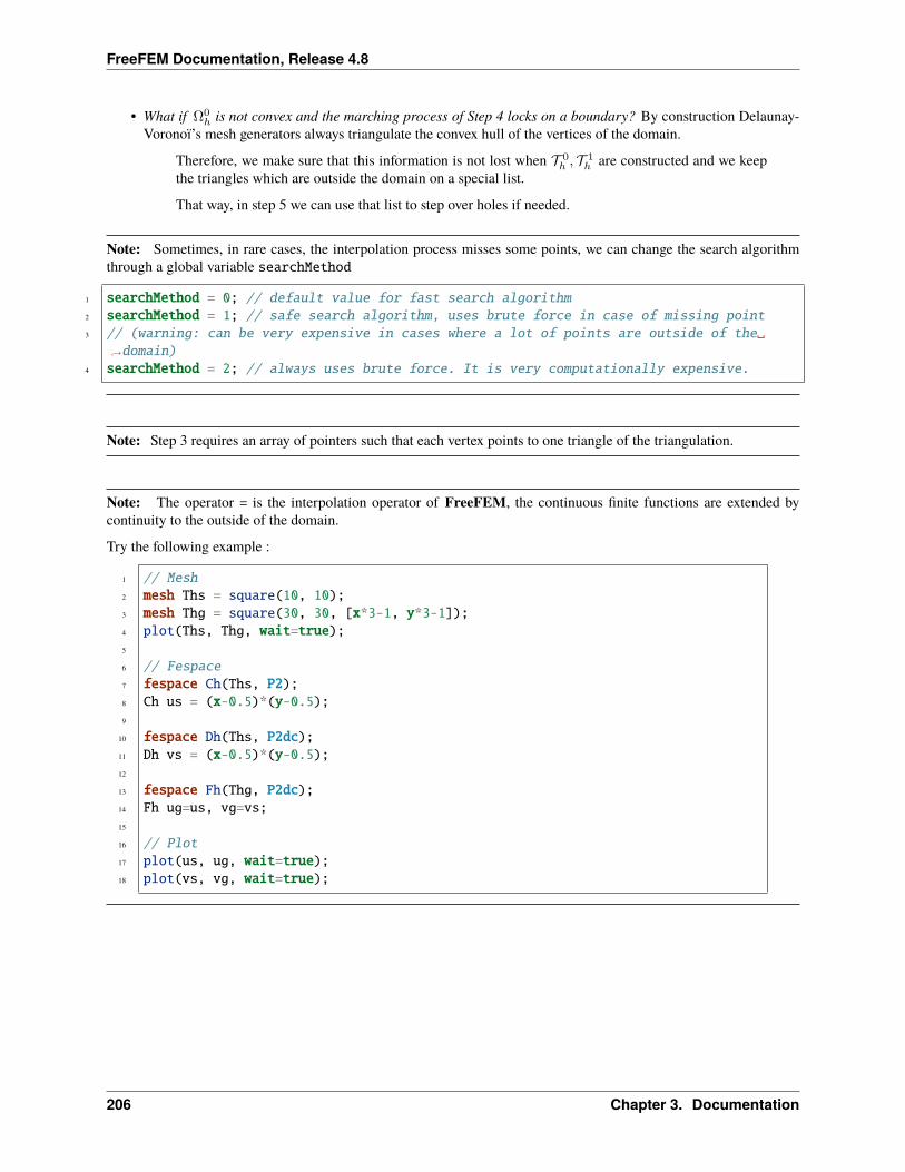
FreeFEM Documentation, Release 4.8
• What if Ω0ℎ is not convex and the marching process of Step 4 locks on a boundary? By construction Delaunay-
Voronoï’s mesh generators always triangulate the convex hull of the vertices of the domain.
Therefore, we make sure that this information is not lost when 𝒯 0ℎ , 𝒯 1
ℎ are constructed and we keepthe triangles which are outside the domain on a special list.
That way, in step 5 we can use that list to step over holes if needed.
Note: Sometimes, in rare cases, the interpolation process misses some points, we can change the search algorithmthrough a global variable searchMethod
1 searchMethod = 0; // default value for fast search algorithm2 searchMethod = 1; // safe search algorithm, uses brute force in case of missing point3 // (warning: can be very expensive in cases where a lot of points are outside of the
→˓domain)4 searchMethod = 2; // always uses brute force. It is very computationally expensive.
Note: Step 3 requires an array of pointers such that each vertex points to one triangle of the triangulation.
Note: The operator = is the interpolation operator of FreeFEM, the continuous finite functions are extended bycontinuity to the outside of the domain.
Try the following example :
1 // Mesh2 mesh Ths = square(10, 10);3 mesh Thg = square(30, 30, [x*3-1, y*3-1]);4 plot(Ths, Thg, wait=true);5
6 // Fespace7 fespace Ch(Ths, P2);8 Ch us = (x-0.5)*(y-0.5);9
10 fespace Dh(Ths, P2dc);11 Dh vs = (x-0.5)*(y-0.5);12
13 fespace Fh(Thg, P2dc);14 Fh ug=us, vg=vs;15
16 // Plot17 plot(us, ug, wait=true);18 plot(vs, vg, wait=true);
206 Chapter 3. Documentation
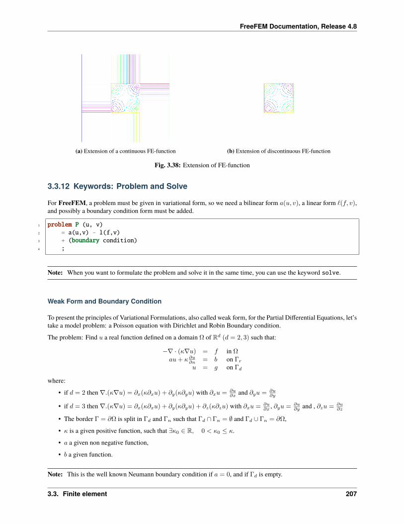
FreeFEM Documentation, Release 4.8
(a) Extension of a continuous FE-function (b) Extension of discontinuous FE-function
Fig. 3.38: Extension of FE-function
3.3.12 Keywords: Problem and Solve
For FreeFEM, a problem must be given in variational form, so we need a bilinear form 𝑎(𝑢, 𝑣), a linear form ℓ(𝑓, 𝑣),and possibly a boundary condition form must be added.
1 problem P (u, v)2 = a(u,v) - l(f,v)3 + (boundary condition)4 ;
Note: When you want to formulate the problem and solve it in the same time, you can use the keyword solve.
Weak Form and Boundary Condition
To present the principles of Variational Formulations, also called weak form, for the Partial Differential Equations, let’stake a model problem: a Poisson equation with Dirichlet and Robin Boundary condition.
The problem: Find 𝑢 a real function defined on a domain Ω of R𝑑 (𝑑 = 2, 3) such that:
−∇ · (𝜅∇𝑢) = 𝑓 in Ω𝑎𝑢+ 𝜅 𝜕𝑢𝜕𝑛 = 𝑏 on Γ𝑟
𝑢 = 𝑔 on Γ𝑑
where:
• if 𝑑 = 2 then ∇.(𝜅∇𝑢) = 𝜕𝑥(𝜅𝜕𝑥𝑢) + 𝜕𝑦(𝜅𝜕𝑦𝑢) with 𝜕𝑥𝑢 = 𝜕𝑢𝜕𝑥 and 𝜕𝑦𝑢 = 𝜕𝑢
𝜕𝑦
• if 𝑑 = 3 then ∇.(𝜅∇𝑢) = 𝜕𝑥(𝜅𝜕𝑥𝑢) + 𝜕𝑦(𝜅𝜕𝑦𝑢) + 𝜕𝑧(𝜅𝜕𝑧𝑢) with 𝜕𝑥𝑢 = 𝜕𝑢𝜕𝑥 , 𝜕𝑦𝑢 = 𝜕𝑢
𝜕𝑦 and , 𝜕𝑧𝑢 = 𝜕𝑢𝜕𝑧
• The border Γ = 𝜕Ω is split in Γ𝑑 and Γ𝑛 such that Γ𝑑 ∩ Γ𝑛 = ∅ and Γ𝑑 ∪ Γ𝑛 = 𝜕Ω,
• 𝜅 is a given positive function, such that ∃𝜅0 ∈ R, 0 < 𝜅0 ≤ 𝜅.
• 𝑎 a given non negative function,
• 𝑏 a given function.
Note: This is the well known Neumann boundary condition if 𝑎 = 0, and if Γ𝑑 is empty.
3.3. Finite element 207
FreeFEM Documentation, Release 4.8
In this case the function appears in the problem just by its derivatives, so it is defined only up to a constant (if 𝑢 is asolution then 𝑢+ 𝑐 is also a solution).
Let 𝑣, a regular test function, null on Γ𝑑, by integration by parts we get:
−∫Ω
∇ · (𝜅∇𝑢) 𝑣 𝑑𝜔 =
∫Ω
𝜅∇𝑣 · ∇𝑢 𝑑𝜔 −∫Γ
𝑣𝜅𝜕𝑢
𝜕n𝑑𝛾,=
∫Ω
𝑓𝑣 𝑑𝜔
where if 𝑑 = 2 the ∇𝑣.∇𝑢 = (𝜕𝑢𝜕𝑥𝜕𝑣𝜕𝑥 + 𝜕𝑢
𝜕𝑦𝜕𝑣𝜕𝑦 ),
where if 𝑑 = 3 the ∇𝑣.∇𝑢 = (𝜕𝑢𝜕𝑥𝜕𝑣𝜕𝑥 + 𝜕𝑢
𝜕𝑦𝜕𝑣𝜕𝑦 + 𝜕𝑢
𝜕𝑧𝜕𝑣𝜕𝑧 ),
and where n is the unitary outer-pointing normal of the Γ.
Now we note that 𝜅 𝜕𝑢𝜕𝑛 = −𝑎𝑢+ 𝑏 on Γ𝑟 and 𝑣 = 0 on Γ𝑑 and Γ = Γ𝑑 ∪ Γ𝑛 thus:
−∫Γ
𝑣𝜅𝜕𝑢
𝜕𝑛=
∫Γ𝑟
𝑎𝑢𝑣 −∫Γ𝑟
𝑏𝑣
The problem becomes:
Find 𝑢 ∈ 𝑉𝑔 = 𝑤 ∈ 𝐻1(Ω)/𝑤 = 𝑔 on Γ𝑑 such that:∫Ω
𝜅∇𝑣.∇𝑢 𝑑𝜔 +
∫Γ𝑟
𝑎𝑢𝑣 𝑑𝛾 =
∫Ω
𝑓𝑣 𝑑𝜔 +
∫Γ𝑟
𝑏𝑣 𝑑𝛾, ∀𝑣 ∈ 𝑉0 (3.16)
where 𝑉0 = 𝑣 ∈ 𝐻1(Ω)/𝑣 = 0 on Γ𝑑
Except in the case of Neumann conditions everywhere, the problem (3.16) is well posed when 𝜅 ≥ 𝜅0 > 0.
Note: If we have only the Neumann boundary condition, linear algebra tells us that the right hand side must beorthogonal to the kernel of the operator for the solution to exist.
One way of writing the compatibility condition is:∫Ω
𝑓 𝑑𝜔 +
∫Γ
𝑏 𝑑𝛾 = 0
and a way to fix the constant is to solve for 𝑢 ∈ 𝐻1(Ω) such that:∫Ω
(𝜀𝑢𝑣 + 𝜅∇𝑣.∇𝑢) 𝑑𝜔 =
∫Ω
𝑓𝑣 𝑑𝜔 +
∫Γ𝑟
𝑏𝑣 𝑑𝛾, ∀𝑣 ∈ 𝐻1(Ω)
where 𝜀 is a small parameter (∼ 𝜅 10−10|Ω| 2𝑑 ).
Remark that if the solution is of order 1𝜀 then the compatibility condition is unsatisfied, otherwise we get the solution
such that∫Ω𝑢 = 0, you can also add a Lagrange multiplier to solve the real mathematical problem like in the Lagrange
multipliers example.
In FreeFEM, the bidimensional problem (3.16) becomes:
1 problem Pw (u, v)2 = int2d(Th)( //int_Omega kappa nabla v . nabla u3 kappa*(dx(u)*dx(v) + dy(u)*dy(v))4 )5 + int1d(Th, gn)( //int_Gamma_r a u v6 a * u*v
(continues on next page)
208 Chapter 3. Documentation
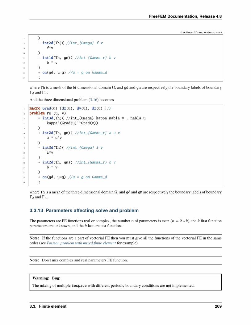
FreeFEM Documentation, Release 4.8
(continued from previous page)
7 )8 - int2d(Th)( //int_Omega f v9 f*v
10 )11 - int1d(Th, gn)( //int_Gamma_r b v12 b * v13 )14 + on(gd, u=g) //u = g on Gamma_d15 ;
where Th is a mesh of the bi-dimensional domain Ω, and gd and gn are respectively the boundary labels of boundaryΓ𝑑 and Γ𝑛.
And the three dimensional problem (3.16) becomes
1 macro Grad(u) [dx(u), dy(u), dz(u) ]//2 problem Pw (u, v)3 = int3d(Th)( //int_Omega kappa nabla v . nabla u4 kappa*(Grad(u)'*Grad(v))5 )6 + int2d(Th, gn)( //int_Gamma_r a u v7 a * u*v8 )9 - int3d(Th)( //int_Omega f v
10 f*v11 )12 - int2d(Th, gn)( //int_Gamma_r b v13 b * v14 )15 + on(gd, u=g) //u = g on Gamma_d16 ;
where Th is a mesh of the three dimensional domain Ω, and gd and gn are respectively the boundary labels of boundaryΓ𝑑 and Γ𝑛.
3.3.13 Parameters affecting solve and problem
The parameters are FE functions real or complex, the number 𝑛 of parameters is even (𝑛 = 2 * 𝑘), the 𝑘 first functionparameters are unknown, and the 𝑘 last are test functions.
Note: If the functions are a part of vectorial FE then you must give all the functions of the vectorial FE in the sameorder (see Poisson problem with mixed finite element for example).
Note: Don’t mix complex and real parameters FE function.
Warning: Bug:The mixing of multiple fespace with different periodic boundary conditions are not implemented.
3.3. Finite element 209
FreeFEM Documentation, Release 4.8
So all the finite element spaces used for tests or unknown functions in a problem, must have the same type ofperiodic boundary conditions or no periodic boundary conditions.
No clean message is given and the result is unpredictable.
The parameters are:
• solver= LU, CG, Crout, Cholesky, GMRES, sparsesolver, UMFPACK . . .
The default solver is sparsesolver (it is equal to UMFPACK if no other sparse solver is defined) or isset to LU if no direct sparse solver is available.
The storage mode of the matrix of the underlying linear system depends on the type of solver chosen;for LU the matrix is sky-line non symmetric, for Crout the matrix is sky-line symmetric, for Choleskythe matrix is sky-line symmetric positive definite, for CG the matrix is sparse symmetric positive, andfor GMRES, sparsesolver or UMFPACK the matrix is just sparse.
• eps= a real expression.
𝜀 sets the stopping test for the iterative methods like CG.
Note that if 𝜀 is negative then the stopping test is:
||𝐴𝑥− 𝑏|| < |𝜀|
if it is positive, then the stopping test is:
||𝐴𝑥− 𝑏|| < |𝜀|||𝐴𝑥0 − 𝑏||
• init= boolean expression, if it is false or 0 the matrix is reconstructed.
Note that if the mesh changes the matrix is reconstructed too.
• precon= name of a function (for example P) to set the preconditioner.
The prototype for the function P must be:
1 func real[int] P(real[int] & xx);
• tgv= Huge value (1030) used to implement Dirichlet boundary conditions.
• tolpivot= sets the tolerance of the pivot in UMFPACK (10−1) and, LU, Crout, Cholesky factorisation (10−20).
• tolpivotsym= sets the tolerance of the pivot sym in UMFPACK
• strategy= sets the integer UMFPACK strategy (0 by default).
3.3.14 Problem definition
Below v is the unknown function and w is the test function.
After the “=” sign, one may find sums of:
• Identifier(s); this is the name given earlier to the variational form(s) (type varf ) for possible reuse.
Remark, that the name in the varf of the unknown test function is forgotten, we use the order in theargument list to recall names as in a C++ function,
• The terms of the bilinear form itself: if 𝐾 is a given function,
210 Chapter 3. Documentation
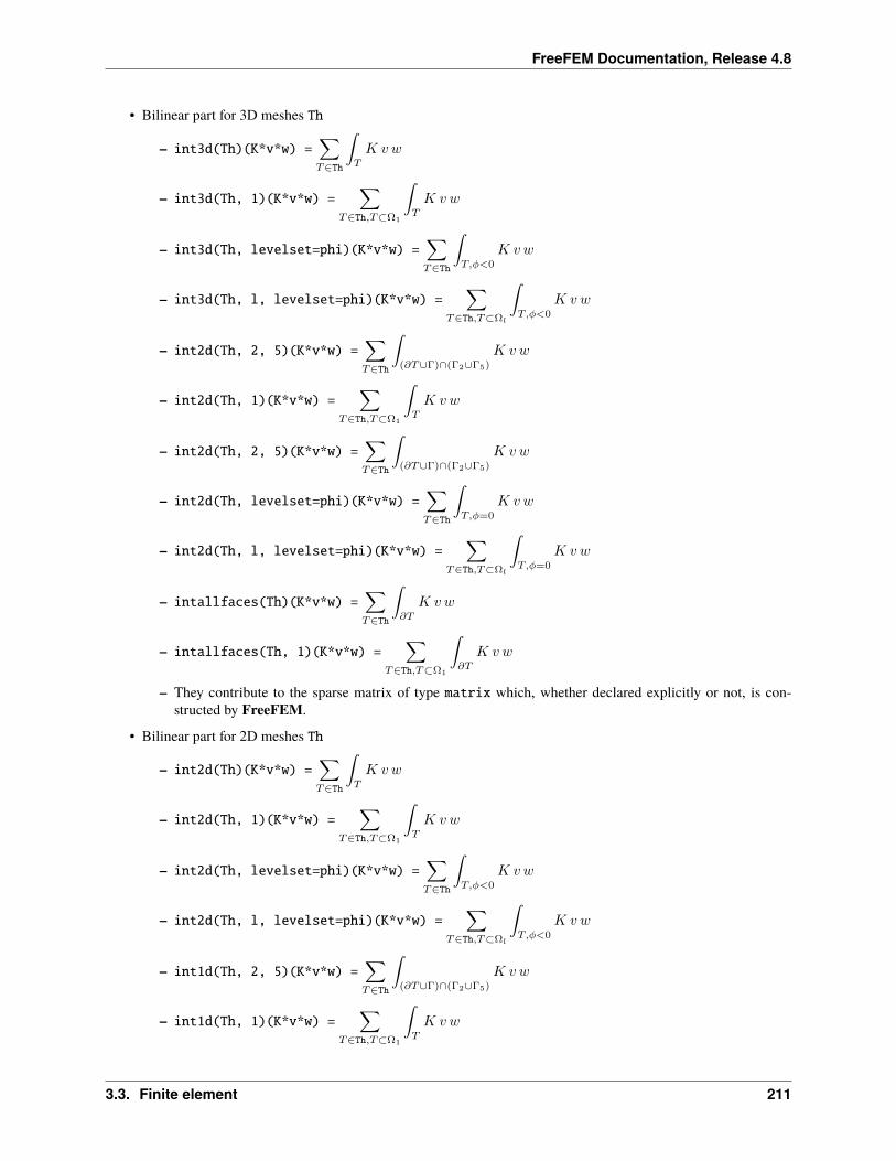
FreeFEM Documentation, Release 4.8
• Bilinear part for 3D meshes Th
– int3d(Th)(K*v*w) =∑𝑇∈Th
∫𝑇
𝐾 𝑣𝑤
– int3d(Th, 1)(K*v*w) =∑
𝑇∈Th,𝑇⊂Ω1
∫𝑇
𝐾 𝑣𝑤
– int3d(Th, levelset=phi)(K*v*w) =∑𝑇∈Th
∫𝑇,𝜑<0
𝐾 𝑣𝑤
– int3d(Th, l, levelset=phi)(K*v*w) =∑
𝑇∈Th,𝑇⊂Ω𝑙
∫𝑇,𝜑<0
𝐾 𝑣𝑤
– int2d(Th, 2, 5)(K*v*w) =∑𝑇∈Th
∫(𝜕𝑇∪Γ)∩(Γ2∪Γ5)
𝐾 𝑣𝑤
– int2d(Th, 1)(K*v*w) =∑
𝑇∈Th,𝑇⊂Ω1
∫𝑇
𝐾 𝑣𝑤
– int2d(Th, 2, 5)(K*v*w) =∑𝑇∈Th
∫(𝜕𝑇∪Γ)∩(Γ2∪Γ5)
𝐾 𝑣𝑤
– int2d(Th, levelset=phi)(K*v*w) =∑𝑇∈Th
∫𝑇,𝜑=0
𝐾 𝑣𝑤
– int2d(Th, l, levelset=phi)(K*v*w) =∑
𝑇∈Th,𝑇⊂Ω𝑙
∫𝑇,𝜑=0
𝐾 𝑣𝑤
– intallfaces(Th)(K*v*w) =∑𝑇∈Th
∫𝜕𝑇
𝐾 𝑣𝑤
– intallfaces(Th, 1)(K*v*w) =∑
𝑇∈Th,𝑇⊂Ω1
∫𝜕𝑇
𝐾 𝑣𝑤
– They contribute to the sparse matrix of type matrix which, whether declared explicitly or not, is con-structed by FreeFEM.
• Bilinear part for 2D meshes Th
– int2d(Th)(K*v*w) =∑𝑇∈Th
∫𝑇
𝐾 𝑣𝑤
– int2d(Th, 1)(K*v*w) =∑
𝑇∈Th,𝑇⊂Ω1
∫𝑇
𝐾 𝑣𝑤
– int2d(Th, levelset=phi)(K*v*w) =∑𝑇∈Th
∫𝑇,𝜑<0
𝐾 𝑣𝑤
– int2d(Th, l, levelset=phi)(K*v*w) =∑
𝑇∈Th,𝑇⊂Ω𝑙
∫𝑇,𝜑<0
𝐾 𝑣𝑤
– int1d(Th, 2, 5)(K*v*w) =∑𝑇∈Th
∫(𝜕𝑇∪Γ)∩(Γ2∪Γ5)
𝐾 𝑣𝑤
– int1d(Th, 1)(K*v*w) =∑
𝑇∈Th,𝑇⊂Ω1
∫𝑇
𝐾 𝑣𝑤
3.3. Finite element 211
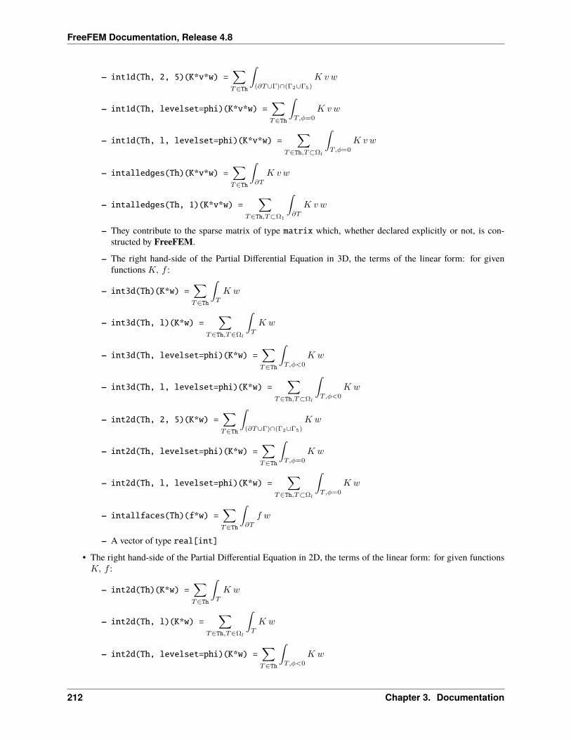
FreeFEM Documentation, Release 4.8
– int1d(Th, 2, 5)(K*v*w) =∑𝑇∈Th
∫(𝜕𝑇∪Γ)∩(Γ2∪Γ5)
𝐾 𝑣𝑤
– int1d(Th, levelset=phi)(K*v*w) =∑𝑇∈Th
∫𝑇,𝜑=0
𝐾 𝑣𝑤
– int1d(Th, l, levelset=phi)(K*v*w) =∑
𝑇∈Th,𝑇⊂Ω𝑙
∫𝑇,𝜑=0
𝐾 𝑣𝑤
– intalledges(Th)(K*v*w) =∑𝑇∈Th
∫𝜕𝑇
𝐾 𝑣𝑤
– intalledges(Th, 1)(K*v*w) =∑
𝑇∈Th,𝑇⊂Ω1
∫𝜕𝑇
𝐾 𝑣𝑤
– They contribute to the sparse matrix of type matrix which, whether declared explicitly or not, is con-structed by FreeFEM.
– The right hand-side of the Partial Differential Equation in 3D, the terms of the linear form: for givenfunctions 𝐾, 𝑓 :
– int3d(Th)(K*w) =∑𝑇∈Th
∫𝑇
𝐾 𝑤
– int3d(Th, l)(K*w) =∑
𝑇∈Th,𝑇∈Ω𝑙
∫𝑇
𝐾 𝑤
– int3d(Th, levelset=phi)(K*w) =∑𝑇∈Th
∫𝑇,𝜑<0
𝐾 𝑤
– int3d(Th, l, levelset=phi)(K*w) =∑
𝑇∈Th,𝑇⊂Ω𝑙
∫𝑇,𝜑<0
𝐾 𝑤
– int2d(Th, 2, 5)(K*w) =∑𝑇∈Th
∫(𝜕𝑇∪Γ)∩(Γ2∪Γ5)
𝐾 𝑤
– int2d(Th, levelset=phi)(K*w) =∑𝑇∈Th
∫𝑇,𝜑=0
𝐾 𝑤
– int2d(Th, l, levelset=phi)(K*w) =∑
𝑇∈Th,𝑇⊂Ω𝑙
∫𝑇,𝜑=0
𝐾 𝑤
– intallfaces(Th)(f*w) =∑𝑇∈Th
∫𝜕𝑇
𝑓 𝑤
– A vector of type real[int]
• The right hand-side of the Partial Differential Equation in 2D, the terms of the linear form: for given functions𝐾, 𝑓 :
– int2d(Th)(K*w) =∑𝑇∈Th
∫𝑇
𝐾 𝑤
– int2d(Th, l)(K*w) =∑
𝑇∈Th,𝑇∈Ω𝑙
∫𝑇
𝐾 𝑤
– int2d(Th, levelset=phi)(K*w) =∑𝑇∈Th
∫𝑇,𝜑<0
𝐾 𝑤
212 Chapter 3. Documentation
FreeFEM Documentation, Release 4.8
– int2d(Th, l, levelset=phi)(K*w) =∑
𝑇∈Th,𝑇⊂Ω𝑙
∫𝑇,𝜑<0
𝐾 𝑤
– int1d(Th, 2, 5)(K*w) =∑𝑇∈Th
∫(𝜕𝑇∪Γ)∩(Γ2∪Γ5)
𝐾 𝑤
– int1d(Th, levelset=phi)(K*w) =∑𝑇∈Th
∫𝑇,𝜑=0
𝐾 𝑤
– int1d(Th, l, levelset=phi)(K*w) =∑
𝑇∈Th,𝑇⊂Ω𝑙
∫𝑇,𝜑=0
𝐾 𝑤
– intalledges(Th)(f*w) =∑𝑇∈Th
∫𝜕𝑇
𝑓 𝑤
– a vector of type real[int]
• The boundary condition terms:
– An “on” scalar form (for Dirichlet) : on(1, u=g)
Used for all degrees of freedom 𝑖 of the boundary referred by “1”, the diagonal term of the matrix𝑎𝑖𝑖 = 𝑡𝑔𝑣 with the terrible giant value tgv (= 1030 by default), and the right hand side 𝑏[𝑖] =”(Πℎ𝑔)[𝑖]” × 𝑡𝑔𝑣, where the ”(Πℎ𝑔)𝑔[𝑖]” is the boundary node value given by the interpolationof 𝑔.
– A linear form on Γ (for Neumann in 2d) -int1d(Th)(f*w) or -int1d(Th, 3)(f*w)
– A bilinear form on Γ or Γ2 (for Robin in 2d) int1d(Th)(K*v*w) or int1d(Th,2)(K*v*w)
– A linear form on Γ (for Neumann in 3d) -int2d(Th)(f*w) or -int2d(Th, 3)(f*w)
– A bilinear form on Γ or Γ2 (for Robin in 3d) int2d(Th)(K*v*w) or int2d(Th,2)(K*v*w)
Note:• An “on” vectorial form (for Dirichlet): on(1, u1=g1, u2=g2)
If you have vectorial finite element like RT0, the 2 components are coupled, and so you have : 𝑏[𝑖] = ”(Πℎ(𝑔1, 𝑔2))[𝑖]”×𝑡𝑔𝑣, where Πℎ is the vectorial finite element interpolant.
• An “on” vectorial form (for Dirichlet): on(u=g, tgv= none positive value ) ,
if the value is equal to -2 (i.e tgv == -2 `) then we put to :math:`0 all term of the line andcolomn 𝑖 in the matrix, except diagonal term 𝑎𝑖𝑖 = 1, and 𝑏[𝑖] = ”(Πℎ𝑔)[𝑖]” else if the value is equalto -20 (i.e tgv == -20 `) then we put to :math:`0 all term of the line and colomn 𝑖 in the matrix,and 𝑏[𝑖] = ”(Πℎ𝑔)[𝑖]”
else if the value is equal to -10 (i.e tgv == -10 `) then we put to :math:`0 all term of the line thematrix, and 𝑏[𝑖] = ”(Πℎ𝑔)[𝑖]”
else (i.e tgv == -1 `) we put to :math:`0 all term of the line 𝑖 in the matrix, except diagonal term𝑎𝑖𝑖 = 1, and 𝑏[𝑖] = ”(Πℎ𝑔)[𝑖]”.
• If needed, the different kind of terms in the sum can appear more than once.
• The integral mesh and the mesh associated to test functions or unknown functions can be different in the case ofvarf form.
• N.x, N.y and N.z are the normal’s components.
• Ns.x, Ns.y and Ns.z are the normal’s components of the suface in case of meshS integral
3.3. Finite element 213
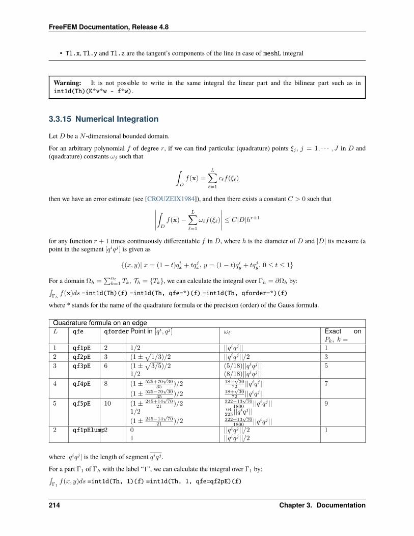
FreeFEM Documentation, Release 4.8
• Tl.x, Tl.y and Tl.z are the tangent’s components of the line in case of meshL integral
Warning: It is not possible to write in the same integral the linear part and the bilinear part such as inint1d(Th)(K*v*w - f*w).
3.3.15 Numerical Integration
Let 𝐷 be a 𝑁 -dimensional bounded domain.
For an arbitrary polynomial 𝑓 of degree 𝑟, if we can find particular (quadrature) points 𝜉𝑗 , 𝑗 = 1, · · · , 𝐽 in 𝐷 and(quadrature) constants 𝜔𝑗 such that ∫
𝐷
𝑓(x) =
𝐿∑ℓ=1
𝑐ℓ𝑓(𝜉ℓ)
then we have an error estimate (see [CROUZEIX1984]), and then there exists a constant 𝐶 > 0 such that∫𝐷
𝑓(x)−𝐿∑ℓ=1
𝜔ℓ𝑓(𝜉ℓ)
≤ 𝐶|𝐷|ℎ𝑟+1
for any function 𝑟 + 1 times continuously differentiable 𝑓 in 𝐷, where ℎ is the diameter of 𝐷 and |𝐷| its measure (apoint in the segment [𝑞𝑖𝑞𝑗 ] is given as
(𝑥, 𝑦)| 𝑥 = (1− 𝑡)𝑞𝑖𝑥 + 𝑡𝑞𝑗𝑥, 𝑦 = (1− 𝑡)𝑞𝑖𝑦 + 𝑡𝑞𝑗𝑦, 0 ≤ 𝑡 ≤ 1
For a domain Ωℎ =∑𝑛𝑡
𝑘=1 𝑇𝑘, 𝒯ℎ = 𝑇𝑘, we can calculate the integral over Γℎ = 𝜕Ωℎ by:∫Γℎ𝑓(x)𝑑𝑠 =int1d(Th)(f) =int1d(Th, qfe=*)(f) =int1d(Th, qforder=*)(f)
where * stands for the name of the quadrature formula or the precision (order) of the Gauss formula.
Quadrature formula on an edge𝐿 qfe qforder Point in [𝑞𝑖, 𝑞𝑗 ] 𝜔ℓ Exact on
𝑃𝑘, 𝑘 =1 qf1pE 2 1/2 ||𝑞𝑖𝑞𝑗 || 1
2 qf2pE 3 (1±√
1/3)/2 ||𝑞𝑖𝑞𝑗 ||/2 3
3 qf3pE 6 (1±√
3/5)/21/2
(5/18)||𝑞𝑖𝑞𝑗 ||(8/18)||𝑞𝑖𝑞𝑗 ||
5
4 qf4pE 8 (1± 525+70√30
35 )/2
(1± 525−70√30
35 )/2
18−√30
72 ||𝑞𝑖𝑞𝑗 ||18+
√30
72 ||𝑞𝑖𝑞𝑗 ||7
5 qf5pE 10 (1± 245+14√70
21 )/21/2
(1± 245−14√70
21 )/2
322−13√70
1800 ||𝑞𝑖𝑞𝑗 ||64225 ||𝑞
𝑖𝑞𝑗 ||322+13
√70
1800 ||𝑞𝑖𝑞𝑗 ||
9
2 qf1pElump2 01
||𝑞𝑖𝑞𝑗 ||/2||𝑞𝑖𝑞𝑗 ||/2
1
where |𝑞𝑖𝑞𝑗 | is the length of segment 𝑞𝑖𝑞𝑗 .
For a part Γ1 of Γℎ with the label “1”, we can calculate the integral over Γ1 by:∫Γ1𝑓(𝑥, 𝑦)𝑑𝑠 =int1d(Th, 1)(f) =int1d(Th, 1, qfe=qf2pE)(f)
214 Chapter 3. Documentation
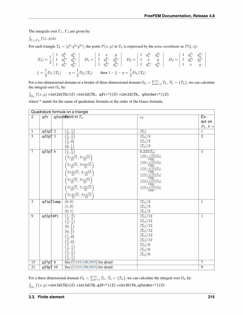
FreeFEM Documentation, Release 4.8
The integrals over Γ1, Γ3 are given by:∫Γ1∪Γ3
𝑓(𝑥, 𝑦)𝑑𝑠
For each triangle 𝑇𝑘 = [𝑞𝑘1𝑞𝑘2𝑞𝑘3 ], the point 𝑃 (𝑥, 𝑦) in 𝑇𝑘 is expressed by the area coordinate as 𝑃 (𝜉, 𝜂):
|𝑇𝑘| =1
2
1 𝑞𝑘1𝑥 𝑞𝑘1𝑦
1 𝑞𝑘2𝑥 𝑞𝑘2𝑦1 𝑞𝑘3𝑥 𝑞𝑘3𝑦
𝐷1 =
1 𝑥 𝑦
1 𝑞𝑘2𝑥 𝑞𝑘2𝑦1 𝑞𝑘3𝑥 𝑞𝑘3𝑦
𝐷2 =
1 𝑞𝑘1𝑥 𝑞𝑘1𝑦
1 𝑥 𝑦1 𝑞𝑘3𝑥 𝑞𝑘3𝑦
𝐷3 =
1 𝑞𝑘1𝑥 𝑞𝑘1𝑦
1 𝑞𝑘2𝑥 𝑞𝑘2𝑦1 𝑥 𝑦
𝜉 =1
2𝐷1/|𝑇𝑘| 𝜂 =
1
2𝐷2/|𝑇𝑘| then 1− 𝜉 − 𝜂 =
1
2𝐷3/|𝑇𝑘|
For a two dimensional domain or a border of three dimensional domain Ωℎ =∑𝑛𝑡
𝑘=1 𝑇𝑘, 𝒯ℎ = 𝑇𝑘, we can calculatethe integral over Ωℎ by:∫Ωℎ𝑓(𝑥, 𝑦) =int2d(Th)(f) =int2d(Th, qft=*)(f) =int2d(Th, qforder=*)(f)
where * stands for the name of quadrature formula or the order of the Gauss formula.
Quadrature formula on a triangle𝐿 qft qforderPoint in 𝑇𝑘 𝜔ℓ Ex-
act on𝑃𝑘, 𝑘 =
1 qf1pT 2(13 ,
13
)|𝑇𝑘| 1
3 qf2pT 3(12 ,
12
)(12 , 0)(
0, 12) |𝑇𝑘|/3
|𝑇𝑘|/3|𝑇𝑘|/3
2
7 qf5pT 6(13 ,
13
)(6−
√15
21 , 6−√15
21
)(
6−√15
21 , 9+2√15
21
)(
9+2√15
21 , 6−√15
21
)(
6+√15
21 , 6+√15
21
)(
6+√15
21 , 9−2√15
21
)(
9−2√15
21 , 6+√15
21
)
0.225|𝑇𝑘|(155−
√15)|𝑇𝑘|
1200(155−
√15)|𝑇𝑘|
1200(155−
√15)|𝑇𝑘|
1200(155+
√15)|𝑇𝑘|
1200(155+
√15)|𝑇𝑘|
1200(155+
√15)|𝑇𝑘|
1200
5
3 qf1pTlump (0, 0)(1, 0)(0, 1)
|𝑇𝑘|/3|𝑇𝑘|/3|𝑇𝑘|/3
1
9 qf2pT4P1(14 ,
34
)(34 ,
14
)(0, 14
)(0, 34
)(14 , 0)(
34 , 0)(
14 ,
14
)(14 ,
12
)(12 ,
14
)
|𝑇𝑘|/12|𝑇𝑘|/12|𝑇𝑘|/12|𝑇𝑘|/12|𝑇𝑘|/12|𝑇𝑘|/12|𝑇𝑘|/6|𝑇𝑘|/6|𝑇𝑘|/6
1
15 qf7pT 8 See [TAYLOR2005] for detail 721 qf9pT 10 See [TAYLOR2005] for detail 9
For a three dimensional domain Ωℎ =∑𝑛𝑡
𝑘=1 𝑇𝑘, 𝒯ℎ = 𝑇𝑘, we can calculate the integral over Ωℎ by:∫Ωℎ𝑓(𝑥, 𝑦) =int3d(Th)(f) =int3d(Th,qfV=*)(f) =int3D(Th,qforder=*)(f)
3.3. Finite element 215
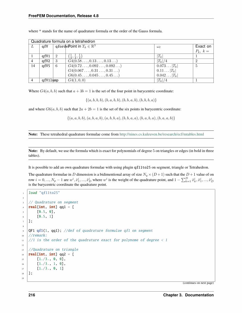
FreeFEM Documentation, Release 4.8
where * stands for the name of quadrature formula or the order of the Gauss formula.
Quadrature formula on a tetrahedron𝐿 qfV qforderPoint in 𝑇𝑘 ∈ R3 𝜔ℓ Exact on
𝑃𝑘, 𝑘 =
1 qfV1 2(14 ,
14 ,
14
)|𝑇𝑘| 1
4 qfV2 3 𝐺4(0.58 . . . , 0.13 . . . , 0.13 . . .) |𝑇𝑘|/4 214 qfV5 6 𝐺4(0.72 . . . , 0.092 . . . , 0.092 . . .)
𝐺4(0.067 . . . , 0.31 . . . , 0.31 . . .)𝐺6(0.45 . . . , 0.045 . . . , 0.45 . . .)
0.073 . . . |𝑇𝑘|0.11 . . . |𝑇𝑘|0.042 . . . |𝑇𝑘|
5
4 qfV1lump 𝐺4(1, 0, 0) |𝑇𝑘|/4 1
Where 𝐺4(𝑎, 𝑏, 𝑏) such that 𝑎+ 3𝑏 = 1 is the set of the four point in barycentric coordinate:
(𝑎, 𝑏, 𝑏, 𝑏), (𝑏, 𝑎, 𝑏, 𝑏), (𝑏, 𝑏, 𝑎, 𝑏), (𝑏, 𝑏, 𝑏, 𝑎)
and where 𝐺6(𝑎, 𝑏, 𝑏) such that 2𝑎+ 2𝑏 = 1 is the set of the six points in barycentric coordinate:
(𝑎, 𝑎, 𝑏, 𝑏), (𝑎, 𝑏, 𝑎, 𝑏), (𝑎, 𝑏, 𝑏, 𝑎), (𝑏, 𝑏, 𝑎, 𝑎), (𝑏, 𝑎, 𝑏, 𝑎), (𝑏, 𝑎, 𝑎, 𝑏)
Note: These tetrahedral quadrature formulae come from http://nines.cs.kuleuven.be/research/ecf/mtables.html
Note: By default, we use the formula which is exact for polynomials of degree 5 on triangles or edges (in bold in threetables).
It is possible to add an own quadrature formulae with using plugin qf11to25 on segment, triangle or Tetrahedron.
The quadrature formulae in𝐷 dimension is a bidimentional array of size𝑁𝑞× (𝐷+ 1) such that the𝐷+ 1 value of onrow 𝑖 = 0, ..., 𝑁𝑝 − 1 are 𝑤𝑖, 𝑖1, ..., 𝑖𝐷 where 𝑤𝑖 is the weight of the quadrature point, and 1−
∑𝐷𝑘=1
𝑖𝑘,
𝑖1, ...,
𝑖𝐷
is the barycentric coordinate the quadrature point.
1 load "qf11to25"2
3 // Quadrature on segment4 real[int, int] qq1 = [5 [0.5, 0],6 [0.5, 1]7 ];8
9 QF1 qf1(1, qq1); //def of quadrature formulae qf1 on segment10 //remark:11 //1 is the order of the quadrature exact for polynome of degree < 112
13 //Quadrature on triangle14 real[int, int] qq2 = [15 [1./3., 0, 0],16 [1./3., 1, 0],17 [1./3., 0, 1]18 ];19
(continues on next page)
216 Chapter 3. Documentation
FreeFEM Documentation, Release 4.8
(continued from previous page)
20 QF2 qf2(1, qq2); //def of quadrature formulae qf2 on triangle21 //remark:22 //1 is the order of the quadrature exact for polynome of degree < 123 //so must have sum w^i = 124
25 // Quadrature on tetrahedron26 real[int, int] qq3 = [27 [1./4., 0, 0, 0],28 [1./4., 1, 0, 0],29 [1./4., 0, 1, 0],30 [1./4., 0, 0, 1]31 ];32
33 QF3 qf3(1, qq3); //def of quadrature formulae qf3 on get34 //remark:35 //1 is the order of the quadrature exact for polynome of degree < 1)36
37 // Verification in 1d and 2d38 mesh Th = square(10, 10);39
40 real I1 = int1d(Th, qfe=qf1)(x^2);41 real I1l = int1d(Th, qfe=qf1pElump)(x^2);42
43 real I2 = int2d(Th, qft=qf2)(x^2);44 real I2l = int2d(Th, qft=qf1pTlump)(x^2);45
46 cout << I1 << " == " << I1l << endl;47 cout << I2 << " == " << I2l << endl;48 assert( abs(I1-I1l) < 1e-10 );49 assert( abs(I2-I2l) < 1e-10 );
The output is
1 1.67 == 1.672 0.335 == 0.335
3.3.16 Variational Form, Sparse Matrix, PDE Data Vector
In FreeFEM it is possible to define variational forms, and use them to build matrices and vectors, and store them tospeed-up the script (4 times faster here).
For example let us solve the Thermal Conduction problem.
The variational formulation is in 𝐿2(0, 𝑇 ;𝐻1(Ω)); we shall seek 𝑢𝑛 satisfying:
∀𝑤 ∈ 𝑉0;
∫Ω
𝑢𝑛 − 𝑢𝑛−1
𝛿𝑡𝑤 + 𝜅∇𝑢𝑛∇𝑤) +
∫Γ
𝛼(𝑢𝑛 − 𝑢𝑢𝑒)𝑤 = 0
where 𝑉0 = 𝑤 ∈ 𝐻1(Ω)/𝑤|Γ24= 0.
So to code the method with the matrices 𝐴 = (𝐴𝑖𝑗), 𝑀 = (𝑀𝑖𝑗), and the vectors 𝑢𝑛, 𝑏𝑛, 𝑏′, 𝑏”, 𝑏𝑐𝑙 (notation if 𝑤 is avector then 𝑤𝑖 is a component of the vector).
𝑢𝑛 = 𝐴−1𝑏𝑛, 𝑏′ = 𝑏0 +𝑀𝑢𝑛−1, 𝑏” =1
𝜀𝑏𝑐𝑙, 𝑏𝑛𝑖 =
𝑏”𝑖 if 𝑖 ∈ Γ24
𝑏′𝑖 else if ∈ Γ24
3.3. Finite element 217
FreeFEM Documentation, Release 4.8
Where with 1𝜀 = tgv = 1030:
𝐴𝑖𝑗 =
⎧⎨⎩1𝜀 if 𝑖 ∈ Γ24, and𝑗 = 𝑖∫
Ω
𝑤𝑗𝑤𝑖/𝑑𝑡+ 𝑘(∇𝑤𝑗 .∇𝑤𝑖) +
∫Γ13
𝛼𝑤𝑗𝑤𝑖 else if 𝑖 ∈ Γ24, or𝑗 = 𝑖
𝑀𝑖𝑗 =
⎧⎨⎩1𝜀 if 𝑖 ∈ Γ24, and𝑗 = 𝑖∫
Ω
𝑤𝑗𝑤𝑖/𝑑𝑡 else if 𝑖 ∈ Γ24, or𝑗 = 𝑖
𝑏0,𝑖 =∫Γ13
𝛼𝑢𝑢𝑒𝑤𝑖𝑏𝑐𝑙 = 𝑢0 the initial data
1 // Parameters2 func fu0 = 10 + 90*x/6;3 func k = 1.8*(y<0.5) + 0.2;4 real ue = 25.;5 real alpha = 0.25;6 real T = 5;7 real dt = 0.1 ;8
9 // Mesh10 mesh Th = square(30, 5, [6*x, y]);11
12 // Fespace13 fespace Vh(Th, P1);14 Vh u0 = fu0, u = u0;
Create three variational formulation, and build the matrices 𝐴,𝑀 .
1 // Problem2 varf vthermic (u, v)3 = int2d(Th)(4 u*v/dt5 + k*(dx(u)*dx(v) + dy(u)*dy(v))6 )7 + int1d(Th, 1, 3)(8 alpha*u*v9 )
10 + on(2, 4, u=1)11 ;12
13 varf vthermic0 (u, v)14 = int1d(Th, 1, 3)(15 alpha*ue*v16 )17 ;18
19 varf vMass (u, v)20 = int2d(Th)(21 u*v/dt22 )23 + on(2, 4, u=1)24 ;25
(continues on next page)
218 Chapter 3. Documentation
FreeFEM Documentation, Release 4.8
(continued from previous page)
26 real tgv = 1e30;27 matrix A = vthermic(Vh, Vh, tgv=tgv, solver=CG);28 matrix M = vMass(Vh, Vh);
Now, to build the right hand size we need 4 vectors.
1 real[int] b0 = vthermic0(0, Vh); //constant part of the RHS2 real[int] bcn = vthermic(0, Vh); //tgv on Dirichlet boundary node ( !=0 )3 //we have for the node i : i in Gamma_24 -> bcn[i] != 04 real[int] bcl = tgv*u0[]; //the Dirichlet boundary condition part
Note: The boundary condition is implemented by penalization and vector bcn contains the contribution of the bound-ary condition 𝑢 = 1, so to change the boundary condition, we have just to multiply the vector bcn[] by the currentvalue f of the new boundary condition term by term with the operator .*.
Uzawa model gives a real example of using all this features.
And the new version of the algorithm is now:
1 // Time loop2 ofstream ff("thermic.dat");3 for(real t = 0; t < T; t += dt)4 // Update5 real[int] b = b0; //for the RHS6 b += M*u[]; //add the the time dependent part7 //lock boundary part:8 b = bcn ? bcl : b; //do forall i: b[i] = bcn[i] ? bcl[i] : b[i]9
10 // Solve11 u[] = A^-1*b;12
13 // Save14 ff << t << " " << u(3, 0.5) << endl;15
16 // Plot17 plot(u);18 19
20 // Display21 for(int i = 0; i < 20; i++)22 cout << dy(u)(6.0*i/20.0, 0.9) << endl;23
24 // Plot25 plot(u, fill=true, wait=true);
Note: The functions appearing in the variational form are formal and local to the varf definition, the only importantthing is the order in the parameter list, like in:
1 varf vb1([u1, u2], q) = int2d(Th)((dy(u1) + dy(u2))*q) + int2d(Th)(1*q);2 varf vb2([v1, v2], p) = int2d(Th)((dy(v1) + dy(v2))*p) + int2d(Th)(1*p);
3.3. Finite element 219
FreeFEM Documentation, Release 4.8
To build matrix 𝐴 from the bilinear part the variational form 𝑎 of type varf simply write:
1 A = a(Vh, Wh , []...]);2 // where3 //Vh is "fespace" for the unknown fields with a correct number of component4 //Wh is "fespace" for the test fields with a correct number of component
Possible named parameters in , [...] are
• solver= LU, CG, Crout, Cholesky, GMRES, sparsesolver, UMFPACK . . .
The default solver is GMRES.
The storage mode of the matrix of the underlying linear system depends on the type of solver chosen;for LU the matrix is sky-line non symmetric, for Crout the matrix is sky-line symmetric, for Choleskythe matrix is sky-line symmetric positive definite, for CG the matrix is sparse symmetric positive, andfor GMRES, sparsesolver or UMFPACK the matrix is just sparse.
• factorize = If true then do the matrix factorization for LU, Cholesky or Crout, the default value is false.
• eps= A real expression.
𝜀 sets the stopping test for the iterative methods like CG.
Note that if 𝜀 is negative then the stopping test is:
||𝐴𝑥− 𝑏|| < |𝜀|
if it is positive then the stopping test is
||𝐴𝑥− 𝑏|| < |𝜀|||𝐴𝑥0 − 𝑏||
• precon= Name of a function (for example P) to set the preconditioner.
The prototype for the function P must be:
1 func real[int] P(real[int] & xx) ;
• tgv= Huge value (1030) used to implement Dirichlet boundary conditions.
• tolpivot= Set the tolerance of the pivot in UMFPACK (10−1) and, LU, Crout, Cholesky factorization (10−20).
• tolpivotsym= Set the tolerance of the pivot sym in UMFPACK
• strategy= Set the integer UMFPACK strategy (0 by default).
Note: The line of the matrix corresponding to the space Wh and the column of the matrix corresponding to the spaceVh.
To build the dual vector b (of type real[int]) from the linear part of the variational form a do simply:
1 real b(Vh.ndof);2 b = a(0, Vh);
A first example to compute the area of each triangle 𝐾 of mesh 𝑇ℎ, just do:
220 Chapter 3. Documentation
FreeFEM Documentation, Release 4.8
1 fespace Nh(Th, P0); //the space function constant / triangle2 Nh areaK;3 varf varea (unused, chiK) = int2d(Th)(chiK);4 etaK[] = varea(0, Ph);
Effectively, the basic functions of space 𝑁ℎ, are the characteristic function of the element of Th, and the numbering isthe numeration of the element, so by construction:
etaK[𝑖] =
∫1|𝐾𝑖
=
∫𝐾𝑖
1;
Now, we can use this to compute error indicators like in example Adaptation using residual error indicator.
First to compute a continuous approximation to the function ℎ “density mesh size” of the mesh 𝑇ℎ.
1 fespace Vh(Th, P1);2 Vh h ;3 real[int] count(Th.nv);4 varf vmeshsizen (u, v) = intalledges(Th, qfnbpE=1)(v);5 varf vedgecount (u, v) = intalledges(Th, qfnbpE=1)(v/lenEdge);6
7 // Computation of the mesh size8 count = vedgecount(0, Vh); //number of edge / vertex9 h[] = vmeshsizen(0, Vh); //sum length edge / vertex
10 h[] = h[]./count; //mean length edge / vertex
To compute error indicator for Poisson equation:
𝜂𝐾 =
∫𝐾
ℎ2𝐾 |(𝑓 + ∆𝑢ℎ)|2 +
∫𝜕𝐾
ℎ𝑒|[𝜕𝑢ℎ𝜕𝑛
]|2
where ℎ𝐾 is size of the longest edge (hTriangle), ℎ𝑒 is the size of the current edge (lenEdge), 𝑛 the normal.
1 fespace Nh(Th, P0); // the space function constant / triangle2 Nh etak;3 varf vetaK (unused, chiK)4 = intalledges(Th)(5 chiK*lenEdge*square(jump(N.x*dx(u) + N.y*dy(u)))6 )7 + int2d(Th)(8 chiK*square(hTriangle*(f + dxx(u) + dyy(u)))9 )
10 ;11
12 etak[] = vetaK(0, Ph);
We add automatic expression optimization by default, if this optimization creates problems, it can be removed with thekeyword optimize as in the following example:
1 varf a (u1, u2)2 = int2d(Th, optimize=0)(3 dx(u1)*dx(u2)4 + dy(u1)*dy(u2)5 )6 + on(1, 2, 4, u1=0)
(continues on next page)
3.3. Finite element 221
FreeFEM Documentation, Release 4.8
(continued from previous page)
7 + on(3, u1=1)8 ;
or you can also do optimization and remove the check by setting optimize=2.
Remark, it is all possible to build interpolation matrix, like in the following example:
1 mesh TH = square(3, 4);2 mesh th = square(2, 3);3 mesh Th = square(4, 4);4
5 fespace VH(TH, P1);6 fespace Vh(th, P1);7 fespace Wh(Th, P1);8
9 matrix B = interpolate(VH, Vh); //build interpolation matrix Vh->VH10 matrix BB = interpolate(Wh, Vh); //build interpolation matrix Vh->Wh
and after some operations on sparse matrices are available for example:
1 int N = 10;2 real [int, int] A(N, N); //a full matrix3 real [int] a(N), b(N);4 A = 0;5 for (int i = 0; i < N; i++)6 A(i, i) = 1+i;7 if (i+1 < N) A(i, i+1) = -i;8 a[i] = i;9
10 b = A*b;11 matrix sparseA = A;12 cout << sparseA << endl;13 sparseA = 2*sparseA + sparseA';14 sparseA = 4*sparseA + sparseA*5;15 matrix sparseB = sparseA + sparseA + sparseA; ;16 cout << "sparseB = " << sparseB(0,0) << endl;
3.3.17 Interpolation matrix
It is also possible to store the matrix of a linear interpolation operator from a finite element space 𝑉ℎ to another 𝑊ℎ tointerpolate(𝑊ℎ,𝑉ℎ,. . . ) a function.
Note that the continuous finite functions are extended by continuity outside of the domain.
The named parameters of function interpolate are:
• inside= set true to create zero-extension.
• t= set true to get the transposed matrix
• op= set an integer written below
– 0 the default value and interpolate of the function
– 1 interpolate the 𝜕𝑥
222 Chapter 3. Documentation
FreeFEM Documentation, Release 4.8
– 2 interpolate the 𝜕𝑦– 3 interpolate the 𝜕𝑧
• U2Vc= set the which is the component of 𝑊ℎ come in 𝑉ℎ in interpolate process in a int array so the size of thearray is number of component of 𝑊ℎ, if the put −1 then component is set to 0, like in the following example:(by default the component number is unchanged).
1 fespace V4h(Th4, [P1, P1, P1, P1]);2 fespace V3h(Th, [P1, P1, P1]);3 int[int] u2vc = [1, 3, -1]; //-1 -> put zero on the component4 matrix IV34 = interpolate(V3h, V4h, inside=0, U2Vc=u2vc); //V3h <- V4h5 V4h [a1, a2, a3, a4] = [1, 2, 3, 4];6 V3h [b1, b2, b3] = [10, 20, 30];7 b1[] = IV34*a1[];
So here we have: freefem b1 == 2, b2 == 4, b3 == 0 ...
Tip: Matrix interpolation
1 // Mesh2 mesh Th = square(4, 4);3 mesh Th4 = square(2, 2, [x*0.5, y*0.5]);4 plot(Th, Th4, wait=true);5
6 // Fespace7 fespace Vh(Th, P1);8 Vh v, vv;9 fespace Vh4(Th4, P1);
10 Vh4 v4=x*y;11
12 fespace Wh(Th, P0);13 fespace Wh4(Th4, P0);14
15 // Interpolation16 matrix IV = interpolate(Vh, Vh4); //here the function is exended by continuity17 cout << "IV Vh<-Vh4 " << IV << endl;18
19 v=v4;20 vv[]= IV*v4[]; //here v == vv21
22 real[int] diff= vv[] - v[];23 cout << "|| v - vv || = " << diff.linfty << endl;24 assert( diff.linfty<= 1e-6);25
26 matrix IV0 = interpolate(Vh, Vh4, inside=1); //here the function is exended by zero27 cout << "IV Vh<-Vh4 (inside=1) " << IV0 << endl;28
29 matrix IVt0 = interpolate(Vh, Vh4, inside=1, t=1);30 cout << "IV Vh<-Vh4^t (inside=1) " << IVt0 << endl;31
32 matrix IV4t0 = interpolate(Vh4, Vh);33 cout << "IV Vh4<-Vh^t " << IV4t0 << endl;34
(continues on next page)
3.3. Finite element 223
FreeFEM Documentation, Release 4.8
(continued from previous page)
35 matrix IW4 = interpolate(Wh4, Wh);36 cout << "IV Wh4<-Wh " << IW4 << endl;37
38 matrix IW4V = interpolate(Wh4, Vh);39 cout << "IV Wh4<-Vh " << IW4 << endl;
Build interpolation matrix 𝐴 at a array of points (𝑥𝑥[𝑗], 𝑦𝑦[𝑗]), 𝑖 = 0, 2 here:
𝑎𝑖𝑗 = 𝑑𝑜𝑝(𝑤𝑖𝑐(𝑥𝑥[𝑗], 𝑦𝑦[𝑗]))
where 𝑤𝑖 is the basic finite element function, 𝑐 the component number, 𝑑𝑜𝑝 the type of diff operator like in op def.
1 real[int] xx = [.3, .4], yy = [.1, .4];2 int c = 0, dop = 0;3 matrix Ixx = interpolate(Vh, xx, yy, op=dop, composante=c);4 cout << Ixx << endl;5 Vh ww;6 real[int] dd = [1, 2];7 ww[] = Ixx*dd;
Tip: Schwarz
The following shows how to implement with an interpolation matrix a domain decomposition algorithm based onSchwarz method with Robin conditions.
Given a non-overlapping partition Ω = Ω0 ∪ Ω1 with Ω0 ∩ Ω1 = ∅, Σ := Ω0 ∩ Ω1 the algorithm is:
−∆𝑢𝑖 = 𝑓 in Ω𝑖, 𝑖 = 0, 1,
𝜕(𝑢1 − 𝑢0)
𝜕𝑛+ 𝛼(𝑢1 − 𝑢0) = 0 on Σ.
The same in variational form is: ∫Ω𝑖∇𝑢𝑖 · ∇𝑣 +
∫Σ𝛼𝑢𝑖𝑣 =
∫Ω𝑖𝑓𝑣
−∫Ω𝑗
(∇𝑢𝑗 · ∇𝑣 − 𝑓𝑣) +∫Σ𝛼𝑢𝑗𝑣, ∀𝑣 ∈ 𝐻1
0 (Ω), 𝑖, 𝑗 = [0, 1] ∪ [1, 0]
To discretized with the 𝑃 1 triangular Lagrangian finite element space 𝑉ℎ simply replace 𝐻10 (Ω) by 𝑉ℎ(Ω0)∪ 𝑉ℎ(Ω1).
Then difficulty is to compute∫Ω𝑗∇𝑢𝑗 · ∇𝑣 when 𝑣 is a basis function of 𝑉ℎ(Ω𝑖), 𝑖 = 𝑗.
It is done as follows (with Γ = 𝜕Ω):
1 // Parameters2 int n = 30;3 int Gamma = 1;4 int Sigma = 2;5
6 func f = 1.;7 real alpha = 1.;8
9 int Niter = 50;10
11 // Mesh(continues on next page)
224 Chapter 3. Documentation
FreeFEM Documentation, Release 4.8
(continued from previous page)
12 mesh[int] Th(2);13 int[int] reg(2);14
15 border a0(t=0, 1)x=t; y=0; label=Gamma;16 border a1(t=1, 2)x=t; y=0; label=Gamma;17 border b1(t=0, 1)x=2; y=t; label=Gamma;18 border c1(t=2, 1)x=t; y=1; label=Gamma;19 border c0(t=1, 0)x=t; y=1; label=Gamma;20 border b0(t=1, 0)x=0; y=t; label=Gamma;21 border d(t=0, 1)x=1; y=t; label=Sigma;22 plot(a0(n) + a1(n) + b1(n) + c1(n) + c0(n) + b0(n) + d(n));23 mesh TH = buildmesh(a0(n) + a1(n) + b1(n) + c1(n) + c0(n) + b0(n) + d(n));24
25 reg(0) = TH(0.5, 0.5).region;26 reg(1) = TH(1.5, 0.5).region;27
28 for(int i = 0; i < 2; i++) Th[i] = trunc(TH, region==reg(i));29
30 // Fespace31 fespace Vh0(Th[0], P1);32 Vh0 u0 = 0;33
34 fespace Vh1(Th[1], P1);35 Vh1 u1 = 0;36
37 // Macro38 macro grad(u) [dx(u), dy(u)] //39
40 // Problem41 int i;42 varf a (u, v)43 = int2d(Th[i])(44 grad(u)'*grad(v)45 )46 + int1d(Th[i], Sigma)(47 alpha*u*v48 )49 + on(Gamma, u=0)50 ;51
52 varf b (u, v)53 = int2d(Th[i])(54 f*v55 )56 + on(Gamma, u=0)57 ;58
59 varf du1dn (u, v)60 =-int2d(Th[1])(61 grad(u1)'*grad(v)62 - f*v63 )
(continues on next page)
3.3. Finite element 225
FreeFEM Documentation, Release 4.8
(continued from previous page)
64 + int1d(Th[1], Sigma)(65 alpha*u1*v66 )67 +on(Gamma, u=0)68 ;69
70 varf du0dn (u, v)71 =-int2d(Th[0])(72 grad(u0)'*grad(v)73 - f*v74 )75 + int1d(Th[0], Sigma)(76 alpha*u0*v77 )78 +on(Gamma, u=0)79 ;80
81 matrix I01 = interpolate(Vh1, Vh0);82 matrix I10 = interpolate(Vh0, Vh1);83
84 matrix[int] A(2);85 i = 0; A[i] = a(Vh0, Vh0);86 i = 1; A[i] = a(Vh1, Vh1);87
88 // Solving loop89 for(int iter = 0; iter < Niter; iter++)90 // Solve on Th[0]91 92 i = 0;93 real[int] b0 = b(0, Vh0);94 real[int] Du1dn = du1dn(0, Vh1);95 real[int] Tdu1dn(Vh0.ndof); Tdu1dn = I01'*Du1dn;96 b0 += Tdu1dn;97 u0[] = A[0]^-1*b0;98 99 // Solve on Th[1]
100 101 i = 1;102 real[int] b1 = b(0, Vh1);103 real[int] Du0dn = du0dn(0, Vh0);104 real[int] Tdu0dn(Vh1.ndof); Tdu0dn = I10'*Du0dn;105 b1 += Tdu0dn;106 u1[] = A[1]^-1*b1;107 108 plot(u0, u1, cmm="iter="+iter);109
226 Chapter 3. Documentation
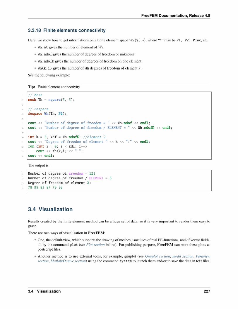
FreeFEM Documentation, Release 4.8
3.3.18 Finite elements connectivity
Here, we show how to get informations on a finite element space 𝑊ℎ(𝒯𝑛, *), where “*” may be P1, P2, P1nc, etc.
• Wh.nt gives the number of element of 𝑊ℎ
• Wh.ndof gives the number of degrees of freedom or unknown
• Wh.ndofK gives the number of degrees of freedom on one element
• Wh(k,i) gives the number of 𝑖th degrees of freedom of element 𝑘.
See the following example:
Tip: Finite element connectivity
1 // Mesh2 mesh Th = square(5, 5);3
4 // Fespace5 fespace Wh(Th, P2);6
7 cout << "Number of degree of freedom = " << Wh.ndof << endl;8 cout << "Number of degree of freedom / ELEMENT = " << Wh.ndofK << endl;9
10 int k = 2, kdf = Wh.ndofK; //element 211 cout << "Degree of freedom of element " << k << ":" << endl;12 for (int i = 0; i < kdf; i++)13 cout << Wh(k,i) << " ";14 cout << endl;
The output is:
1 Number of degree of freedom = 1212 Number of degree of freedom / ELEMENT = 63 Degree of freedom of element 2:4 78 95 83 87 79 92
3.4 Visualization
Results created by the finite element method can be a huge set of data, so it is very important to render them easy tograsp.
There are two ways of visualization in FreeFEM:
• One, the default view, which supports the drawing of meshes, isovalues of real FE-functions, and of vector fields,all by the command plot (see Plot section below). For publishing purpose, FreeFEM can store these plots aspostscript files.
• Another method is to use external tools, for example, gnuplot (see Gnuplot section, medit section, Paraviewsection, Matlab/Octave section) using the command system to launch them and/or to save the data in text files.
3.4. Visualization 227
FreeFEM Documentation, Release 4.8
3.4.1 Plot
With the command plot, meshes, isovalues of scalar functions, and vector fields can be displayed.
The parameters of the plot command can be meshes, real FE functions, arrays of 2 real FE functions, arrays of twodouble arrays, to plot respectively a mesh, a function, a vector field, or a curve defined by the two double arrays.
Note: The length of an arrow is always bound to be in [5‰, 5%] of the screen size in order to see something.
The plot command parameters are listed in the Reference part.
The keyboard shortcuts are:
• enter tries to show plot
• p previous plot (10 plots saved)
• ? shows this help
• +,- zooms in/out around the cursor 3/2 times
• = resets the view
• r refreshes plot
• up, down, left, right special keys to tanslate
• 3 switches 3d/2d plot keys :
– z,Z focal zoom and zoom out
– H,h increases or decreases the Z scale of the plot
• mouse motion:
– left button rotates
– right button zooms (ctrl+button on mac)
– right button +alt tanslates (alt+ctrl+button on mac)
• a,A increases or decreases the arrow size
• B switches between showing the border meshes or not
• i,I updates or not: the min/max bound of the functions to the window
• n,N decreases or increases the number of iso value arrays
• b switches between black and white or color plotting
• g switches between grey or color plotting
• f switches between filling iso or iso line
• l switches between lighting or not
• v switches between show or not showing the numerical value of colors
• m switches between show or not showing the meshes
• w window dump in file ffglutXXXX.ppm
• * keep/drop viewpoint for next plot
• k complex data / change view type
• ESC closes the graphics process before version 3.22, after no way to close
228 Chapter 3. Documentation
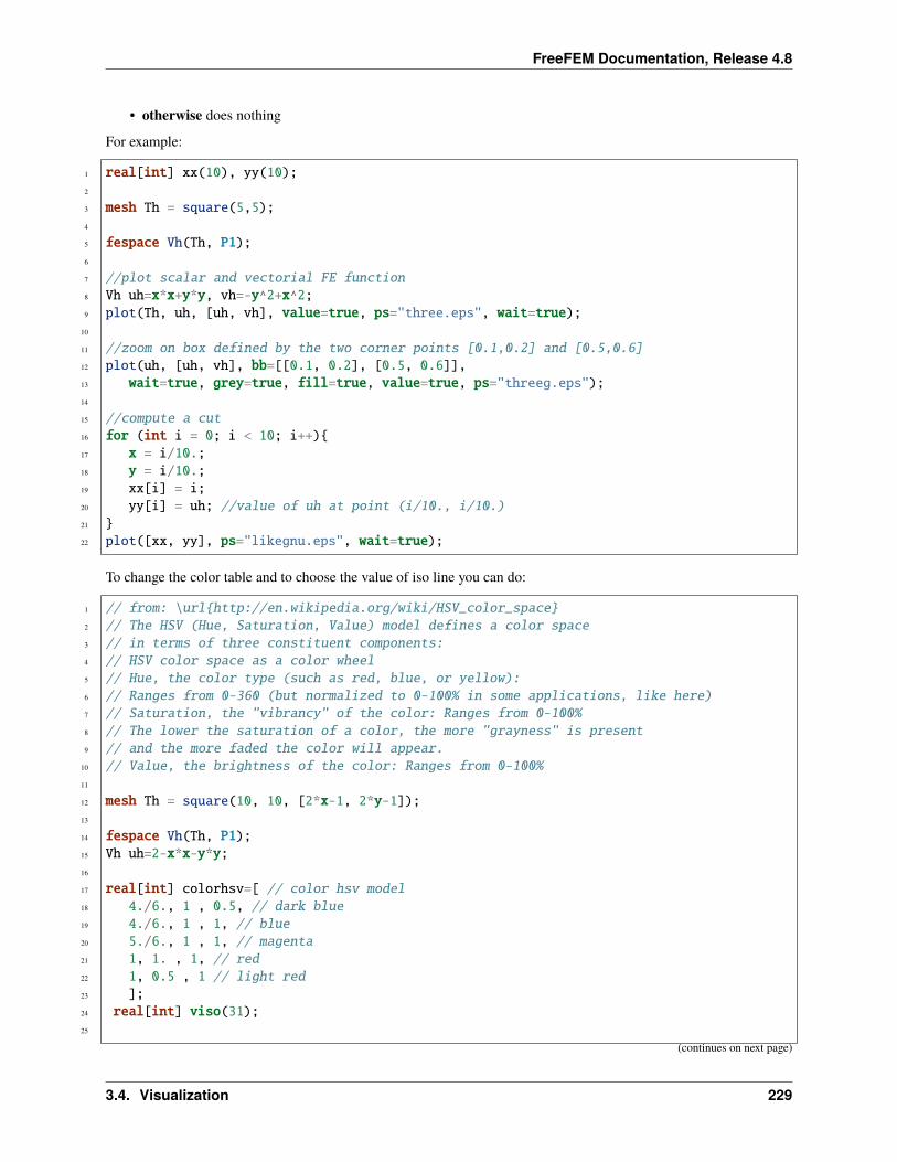
FreeFEM Documentation, Release 4.8
• otherwise does nothing
For example:
1 real[int] xx(10), yy(10);2
3 mesh Th = square(5,5);4
5 fespace Vh(Th, P1);6
7 //plot scalar and vectorial FE function8 Vh uh=x*x+y*y, vh=-y^2+x^2;9 plot(Th, uh, [uh, vh], value=true, ps="three.eps", wait=true);
10
11 //zoom on box defined by the two corner points [0.1,0.2] and [0.5,0.6]12 plot(uh, [uh, vh], bb=[[0.1, 0.2], [0.5, 0.6]],13 wait=true, grey=true, fill=true, value=true, ps="threeg.eps");14
15 //compute a cut16 for (int i = 0; i < 10; i++)17 x = i/10.;18 y = i/10.;19 xx[i] = i;20 yy[i] = uh; //value of uh at point (i/10., i/10.)21 22 plot([xx, yy], ps="likegnu.eps", wait=true);
To change the color table and to choose the value of iso line you can do:
1 // from: \urlhttp://en.wikipedia.org/wiki/HSV_color_space2 // The HSV (Hue, Saturation, Value) model defines a color space3 // in terms of three constituent components:4 // HSV color space as a color wheel5 // Hue, the color type (such as red, blue, or yellow):6 // Ranges from 0-360 (but normalized to 0-100% in some applications, like here)7 // Saturation, the "vibrancy" of the color: Ranges from 0-100%8 // The lower the saturation of a color, the more "grayness" is present9 // and the more faded the color will appear.
10 // Value, the brightness of the color: Ranges from 0-100%11
12 mesh Th = square(10, 10, [2*x-1, 2*y-1]);13
14 fespace Vh(Th, P1);15 Vh uh=2-x*x-y*y;16
17 real[int] colorhsv=[ // color hsv model18 4./6., 1 , 0.5, // dark blue19 4./6., 1 , 1, // blue20 5./6., 1 , 1, // magenta21 1, 1. , 1, // red22 1, 0.5 , 1 // light red23 ];24 real[int] viso(31);25
(continues on next page)
3.4. Visualization 229
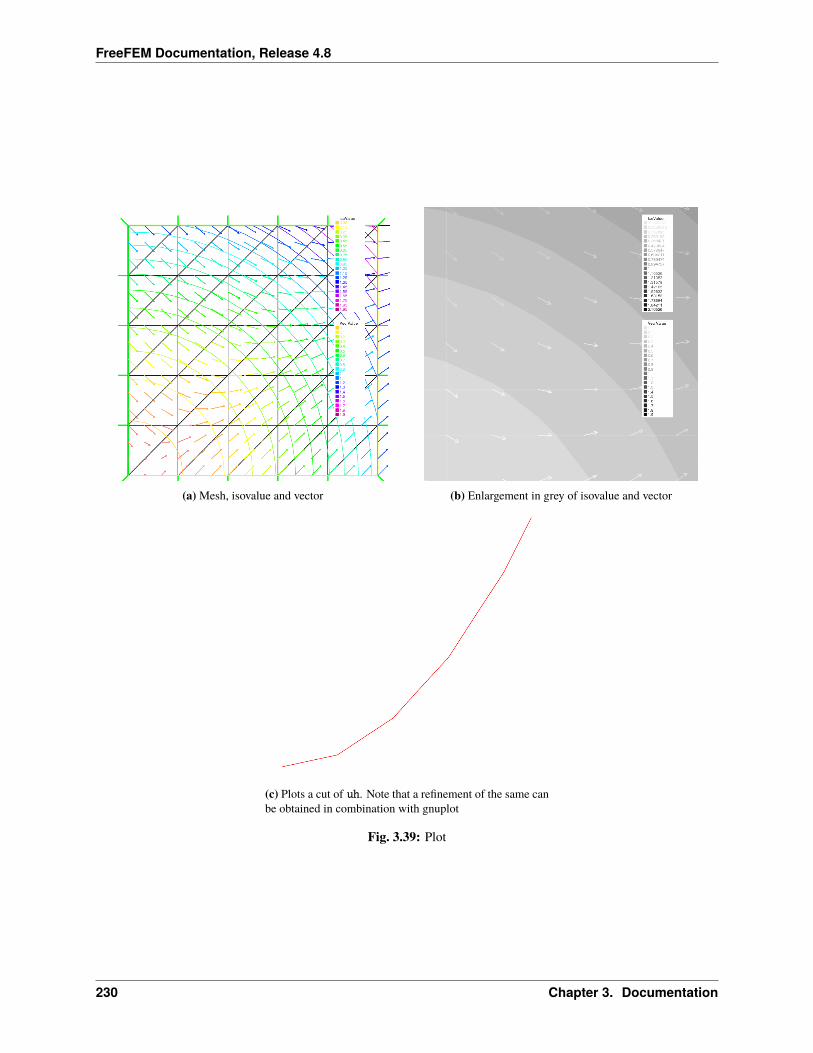
FreeFEM Documentation, Release 4.8
(a) Mesh, isovalue and vector (b) Enlargement in grey of isovalue and vector
(c) Plots a cut of uh. Note that a refinement of the same canbe obtained in combination with gnuplot
Fig. 3.39: Plot
230 Chapter 3. Documentation
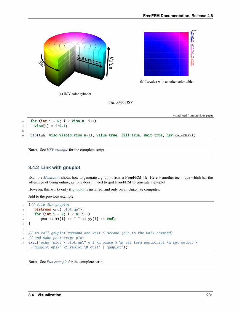
FreeFEM Documentation, Release 4.8
(a) HSV color cylinder
(b) Isovalue with an other color table
Fig. 3.40: HSV
(continued from previous page)
26 for (int i = 0; i < viso.n; i++)27 viso[i] = i*0.1;28
29 plot(uh, viso=viso(0:viso.n-1), value=true, fill=true, wait=true, hsv=colorhsv);
Note: See HSV example for the complete script.
3.4.2 Link with gnuplot
Example Membrane shows how to generate a gnuplot from a FreeFEM file. Here is another technique which has theadvantage of being online, i.e. one doesn’t need to quit FreeFEM to generate a gnuplot.
However, this works only if gnuplot is installed, and only on an Unix-like computer.
Add to the previous example:
1 // file for gnuplot2 ofstream gnu("plot.gp");3 for (int i = 0; i < n; i++)4 gnu << xx[i] << " " << yy[i] << endl;5 6
7 // to call gnuplot command and wait 5 second (due to the Unix command)8 // and make postscript plot9 exec("echo 'plot \"plot.gp\" w l \n pause 5 \n set term postscript \n set output \
→˓"gnuplot.eps\" \n replot \n quit' | gnuplot");
Note: See Plot example for the complete script.
3.4. Visualization 231
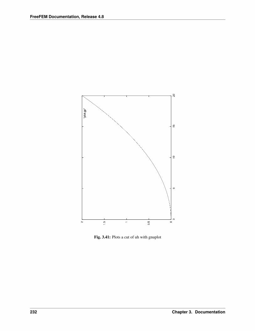
FreeFEM Documentation, Release 4.8
Fig. 3.41: Plots a cut of uh with gnuplot
232 Chapter 3. Documentation
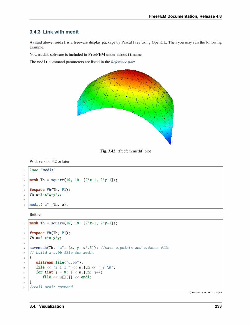
FreeFEM Documentation, Release 4.8
3.4.3 Link with medit
As said above, medit is a freeware display package by Pascal Frey using OpenGL. Then you may run the followingexample.
Now medit software is included in FreeFEM under ffmedit name.
The medit command parameters are listed in the Reference part.
Fig. 3.42: :freefem:medit` plot
With version 3.2 or later
1 load "medit"2
3 mesh Th = square(10, 10, [2*x-1, 2*y-1]);4
5 fespace Vh(Th, P1);6 Vh u=2-x*x-y*y;7
8 medit("u", Th, u);
Before:
1 mesh Th = square(10, 10, [2*x-1, 2*y-1]);2
3 fespace Vh(Th, P1);4 Vh u=2-x*x-y*y;5
6 savemesh(Th, "u", [x, y, u*.5]); //save u.points and u.faces file7 // build a u.bb file for medit8 9 ofstream file("u.bb");
10 file << "2 1 1 " << u[].n << " 2 \n";11 for (int j = 0; j < u[].n; j++)12 file << u[][j] << endl;13 14 //call medit command
(continues on next page)
3.4. Visualization 233
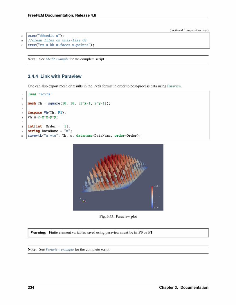
FreeFEM Documentation, Release 4.8
(continued from previous page)
15 exec("ffmedit u");16 //clean files on unix-like OS17 exec("rm u.bb u.faces u.points");
Note: See Medit example for the complete script.
3.4.4 Link with Paraview
One can also export mesh or results in the .vtk format in order to post-process data using Paraview.
1 load "iovtk"2
3 mesh Th = square(10, 10, [2*x-1, 2*y-1]);4
5 fespace Vh(Th, P1);6 Vh u=2-x*x-y*y;7
8 int[int] Order = [1];9 string DataName = "u";
10 savevtk("u.vtu", Th, u, dataname=DataName, order=Order);
Fig. 3.43: Paraview plot
Warning: Finite element variables saved using paraview must be in P0 or P1
Note: See Paraview example for the complete script.
234 Chapter 3. Documentation
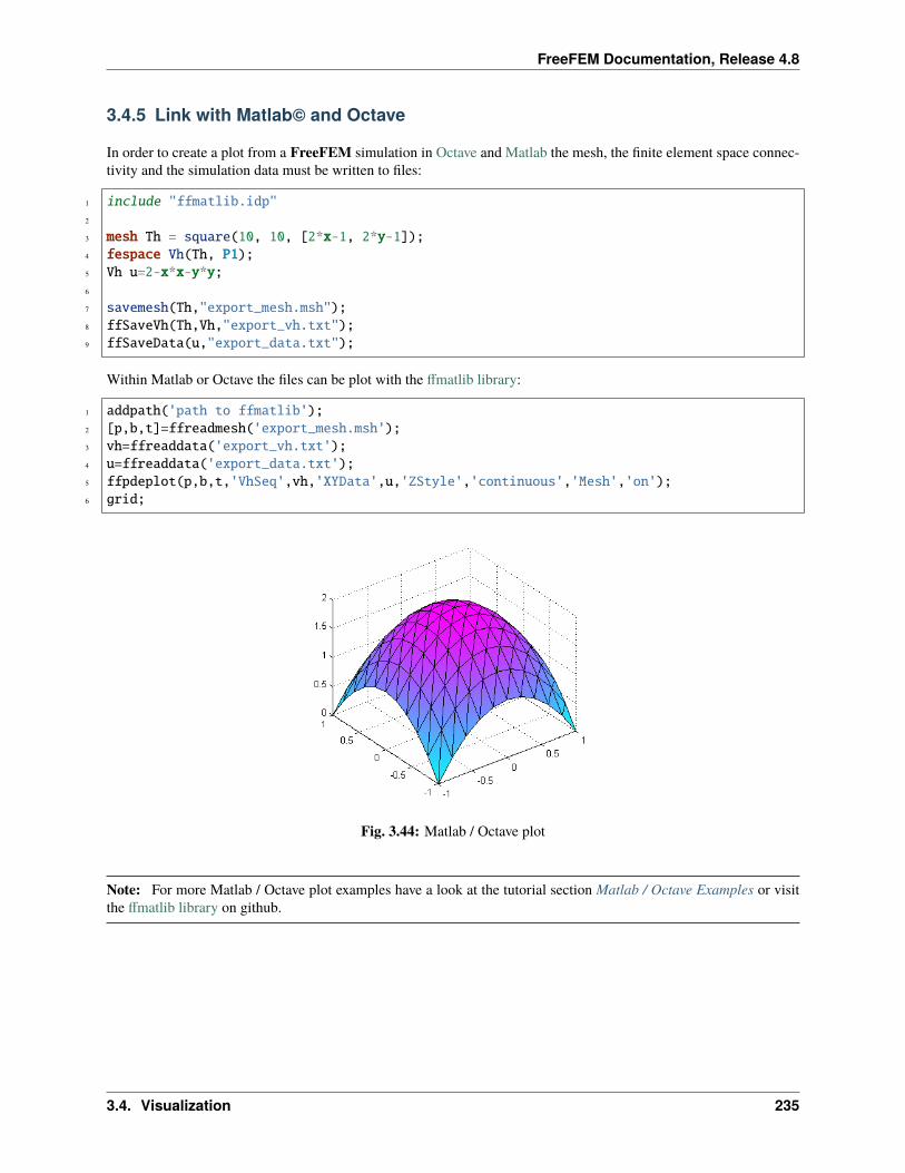
FreeFEM Documentation, Release 4.8
3.4.5 Link with Matlab© and Octave
In order to create a plot from a FreeFEM simulation in Octave and Matlab the mesh, the finite element space connec-tivity and the simulation data must be written to files:
1 include "ffmatlib.idp"2
3 mesh Th = square(10, 10, [2*x-1, 2*y-1]);4 fespace Vh(Th, P1);5 Vh u=2-x*x-y*y;6
7 savemesh(Th,"export_mesh.msh");8 ffSaveVh(Th,Vh,"export_vh.txt");9 ffSaveData(u,"export_data.txt");
Within Matlab or Octave the files can be plot with the ffmatlib library:
1 addpath('path to ffmatlib');2 [p,b,t]=ffreadmesh('export_mesh.msh');3 vh=ffreaddata('export_vh.txt');4 u=ffreaddata('export_data.txt');5 ffpdeplot(p,b,t,'VhSeq',vh,'XYData',u,'ZStyle','continuous','Mesh','on');6 grid;
Fig. 3.44: Matlab / Octave plot
Note: For more Matlab / Octave plot examples have a look at the tutorial section Matlab / Octave Examples or visitthe ffmatlib library on github.
3.4. Visualization 235
FreeFEM Documentation, Release 4.8
3.5 Algorithms & Optimization
3.5.1 Conjugate Gradient/GMRES
Suppose we want to solve the Euler problem (here 𝑥 has nothing to do with the reserved variable for the first coordinatein FreeFEM):
find 𝑥 ∈ R𝑛 such that
∇𝐽(𝑥) =
(𝜕𝐽
𝜕𝑥𝑖(x)
)= 0 (3.17)
where 𝐽 is a function (to minimize for example) from R𝑛 to R.
If the function is convex we can use the conjugate gradient algorithm to solve the problem, and we just need the function(named dJ for example) which computes ∇𝐽 , so the parameters are the name of that function with prototype funcreal[int] dJ(real[int] &xx); which computes ∇𝐽 , and a vector x of type (of course the number 20 can bechanged) real[int] x(20); to initialize the process and get the result.
Given an initial value x(0), a maximum number 𝑖max of iterations, and an error tolerance 0 < 𝜖 < 1:
Put x = x(0) and write
1 NLCG(dJ, x, precon=M, nbiter=imax, eps=epsilon, stop=stopfunc);
will give the solution of x of ∇𝐽(x) = 0. We can omit parameters precon, nbiter, eps, stop. Here 𝑀 is thepreconditioner whose default is the identity matrix.
The stopping test is
‖∇𝐽(x)‖𝑃 ≤ 𝜖‖∇𝐽(x(0))‖𝑃
Writing the minus value in eps=, i.e.,
1 NLCG(dJ, x, precon=M, nbiter=imax, eps=-epsilon);
We can use the stopping test:
‖∇𝐽(x)‖2𝑃 ≤ 𝜖
The parameters of these three functions are:
• nbiter= set the number of iteration (by default 100)
• precon= set the preconditioner function (P for example) by default it is the identity, note the prototype is funcreal[int] P(real[int] &x).
• eps= set the value of the stop test 𝜀 (= 10−6 by default) if positive then relative test ||∇𝐽(𝑥)||𝑃 ≤ 𝜀||∇𝐽(𝑥0)||𝑃 ,otherwise the absolute test is ||∇𝐽(𝑥)||2𝑃 ≤ |𝜀|.
• veps= set and return the value of the stop test, if positive, then relative test is ||∇𝐽(𝑥)||𝑃 ≤ 𝜀||∇𝐽(𝑥0)||𝑃 ,otherwise the absolute test is ||∇𝐽(𝑥)||2𝑃 ≤ |𝜀|. The return value is minus the real stop test (remark: it is usefulin loop).
• stop= stopfunc add your test function to stop before the eps criterion. The prototype for the function stopfuncis
1 func bool stopfunc(int iter, real[int] u, real[int] g)
where u is the current solution, and g, the current gradient, is not preconditioned.
236 Chapter 3. Documentation
FreeFEM Documentation, Release 4.8
Tip: Algorithms.edp
For a given function 𝑏, let us find the minimizer 𝑢 of the function
𝐽(𝑢) = 12
∫Ω𝑓(|∇𝑢|2)−
∫Ω𝑢𝑏
𝑓(𝑥) = 𝑎𝑥+ 𝑥− ln(1 + 𝑥), 𝑓 ′(𝑥) = 𝑎+ 𝑥1+𝑥 , 𝑓 ′′(𝑥) = 1
(1+𝑥)2
under the boundary condition 𝑢 = 0 on 𝜕Ω.
1 fespace Ph(Th, P0);2 Ph alpha; //store df(|nabla u|^2)3
4 // The function J5 //J(u) = 1/2 int_Omega f(|nabla u|^2) - int_Omega u b6 func real J (real[int] & u)7 Vh w;8 w[] = u;9 real r = int2d(Th)(0.5*f(dx(w)*dx(w) + dy(w)*dy(w)) - b*w);
10 cout << "J(u) = " << r << " " << u.min << " " << u.max << endl;11 return r;12 13
14 // The gradient of J15 func real[int] dJ (real[int] & u)16 Vh w;17 w[] = u;18 alpha = df(dx(w)*dx(w) + dy(w)*dy(w));19 varf au (uh, vh)20 = int2d(Th)(21 alpha*(dx(w)*dx(vh) + dy(w)*dy(vh))22 - b*vh23 )24 + on(1, 2, 3, 4, uh=0)25 ;26
27 u = au(0, Vh);28 return u; //warning: no return of local array29
We also want to construct a preconditioner 𝐶 with solving the problem:
find 𝑢ℎ ∈ 𝑉0ℎ such that:
∀𝑣ℎ ∈ 𝑉0ℎ,∫Ω
𝛼∇𝑢ℎ.∇𝑣ℎ =
∫Ω
𝑏𝑣ℎ
where 𝛼 = 𝑓 ′(|∇𝑢|2).
1 alpha = df(dx(u)*dx(u) + dy(u)*dy(u));2 varf alap (uh, vh)3 = int2d(Th)(4 alpha*(dx(uh)*dx(vh) + dy(uh)*dy(vh))5 )6 + on(1, 2, 3, 4, uh=0)7 ;
(continues on next page)
3.5. Algorithms & Optimization 237
FreeFEM Documentation, Release 4.8
(continued from previous page)
8
9 varf amass(uh, vh)10 = int2d(Th)(11 uh*vh12 )13 + on(1, 2, 3, 4, uh=0)14 ;15
16 matrix Amass = amass(Vh, Vh, solver=CG);17 matrix Alap= alap(Vh, Vh, solver=Cholesky, factorize=1);18
19 // Preconditionner20 func real[int] C(real[int] & u)21 real[int] w = u;22 u = Alap^-1*w;23 return u; //warning: no return of local array variable24
To solve the problem, we make 10 iterations of the conjugate gradient, recompute the preconditioner and restart theconjugate gradient:
1 int conv=0;2 for(int i = 0; i < 20; i++)3 conv = NLCG(dJ, u[], nbiter=10, precon=C, veps=eps, verbosity=5);4 if (conv) break;5
6 alpha = df(dx(u)*dx(u) + dy(u)*dy(u));7 Alap = alap(Vh, Vh, solver=Cholesky, factorize=1);8 cout << "Restart with new preconditionner " << conv << ", eps =" << eps << endl;9
10
11 // Plot12 plot (u, wait=true, cmm="solution with NLCG");
For a given symmetric positive matrix 𝐴, consider the quadratic form
𝐽(x) =1
2x𝑇𝐴x− b𝑇x
then 𝐽(x) is minimized by the solution x of 𝐴x = b. In this case, we can use the function AffineCG
1 AffineCG(A, x, precon=M, nbiter=imax, eps=epsilon, stop=stp);
If 𝐴 is not symmetric, we can use GMRES(Generalized Minimum Residual) algorithm by
1 AffineGMRES(A, x, precon=M, nbiter=imax, eps=epsilon);
Also, we can use the non-linear version of GMRES algorithm (the function 𝐽 is just convex)
1 AffineGMRES(dJ, x, precon=M, nbiter=imax, eps=epsilon);
For the details of these algorithms, refer to [PIRONNEAU1998], Chapter IV, 1.3.
238 Chapter 3. Documentation
FreeFEM Documentation, Release 4.8
3.5.2 Algorithms for Unconstrained Optimization
Two algorithms of COOOL package are interfaced with the Newton Raphson method (called Newton) and the BFGSmethod. These two are directly available in FreeFEM (no dynamical link to load). Be careful with these algorithms,because their implementation uses full matrices. We also provide several optimization algorithms from the NLoptlibrary as well as an interface for Hansen’s implementation of CMAES (a MPI version of this one is also available).
Example of usage for BFGS or CMAES
Tip: BFGS
1 real[int] b(10), u(10);2
3 //J4 func real J (real[int] & u)5 real s = 0;6 for (int i = 0; i < u.n; i++)7 s += (i+1)*u[i]*u[i]*0.5 - b[i]*u[i];8 if (debugJ)9 cout << "J = " << s << ", u = " << u[0] << " " << u[1] << endl;
10 return s;11 12
13 //the gradient of J (this is a affine version (the RHS is in)14 func real[int] DJ (real[int] &u)15 for (int i = 0; i < u.n; i++)16 u[i] = (i+1)*u[i];17 if (debugdJ)18 cout << "dJ: u = " << u[0] << " " << u[1] << " " << u[2] << endl;19 u -= b;20 if (debugdJ)21 cout << "dJ-b: u = " << u[0] << " " << u[1] << " " << u[2] << endl;22 return u; //return of global variable ok23 24
25 b=1;26 u=2;27 BFGS(J, DJ, u, eps=1.e-6, nbiter=20, nbiterline=20);28 cout << "BFGS: J(u) = " << J(u) << ", err = " << error(u, b) << endl;
It is almost the same a using the CMA evolution strategy except, that since it is a derivative free optimizer, the dJargument is omitted and there are some other named parameters to control the behavior of the algorithm. With thesame objective function as above, an example of utilization would be (see CMAES Variational inequality for a completeexample):
1 load "ff-cmaes"2 //define J, u, ...3 real min = cmaes(J, u, stopTolFun=1e-6, stopMaxIter=3000);4 cout << "minimum value is " << min << " for u = " << u << endl;
This algorithm works with a normal multivariate distribution in the parameters space and tries to adapt its covariancematrix using the information provided by the successive function evaluations (see NLopt documentation for more
3.5. Algorithms & Optimization 239
FreeFEM Documentation, Release 4.8
details). Therefore, some specific parameters can be passed to control the starting distribution, size of the samplegenerations, etc. . . Named parameters for this are the following:
• seed= Seed for random number generator (val is an integer). No specified value will lead to a clock based seedinitialization.
• initialStdDev= Value for the standard deviations of the initial covariance matrix ( val is a real). If the value𝜎 is passed, the initial covariance matrix will be set to 𝜎𝐼 . The expected initial distance between initial 𝑋 andthe 𝑎𝑟𝑔𝑚𝑖𝑛 should be roughly initialStdDev. Default is 0.3.
• initialStdDevs= Same as above except that the argument is an array allowing to set a value of the initialstandard deviation for each parameter. Entries differing by several orders of magnitude should be avoided (if itcan’t be, try rescaling the problem).
• stopTolFun= Stops the algorithm if function value differences are smaller than the passed one, default is 10−12.
• stopTolFunHist= Stops the algorithm if function value differences from the best values are smaller than thepassed one, default is 0 (unused).
• stopTolX= Stopping criteria is triggered if step sizes in the parameters space are smaller than this real value,default is 0.
• stopTolXFactor= Stopping criteria is triggered when the standard deviation increases more than this value.The default value is 103.
• stopMaxFunEval= Stops the algorithm when stopMaxFunEval function evaluations have been done. Set to900(𝑛+ 3)2 by default, where 𝑛 is the parameters space dimension.
• stopMaxIter= Integer stopping the search when stopMaxIter generations have been sampled. Unused bydefault.
• popsize= Integer value used to change the sample size. The default value is 4 + ⌊3 ln(𝑛)⌋. Increasing thepopulation size usually improves the global search capabilities at the cost of, at most, a linear reduction of theconvergence speed with respect to popsize.
• paramFile= This string type parameter allows the user to pass all the parameters using an extern file, as inHansen’s original code. More parameters related to the CMA-ES algorithm can be changed with this file. Notethat the parameters passed to the CMAES function in the FreeFEM script will be ignored if an input parametersfile is given.
3.5.3 IPOPT
The ff-Ipopt package is an interface for the IPOPT [WÄCHTER2006] optimizer. IPOPT is a software library forlarge scale, non-linear, constrained optimization. It implements a primal-dual interior point method along with filtermethod based line searches.
IPOPT needs a direct sparse symmetric linear solver. If your version of FreeFEM has been compiled with the--enable-downlad tag, it will automatically be linked with a sequential version of MUMPS. An alternative toMUMPS would be to download the HSL subroutines (see Compiling and Installing the Java Interface JIPOPT) andplace them in the /ipopt/Ipopt-3.10.2/ThirdParty/HSL directory of the FreeFEM downloads folder beforecompiling.
240 Chapter 3. Documentation
FreeFEM Documentation, Release 4.8
Short description of the algorithm
In this section, we give a very brief glimpse at the underlying mathematics of IPOPT. For a deeper introduction oninterior methods for nonlinear smooth optimization, one may consult [FORSGREN2002], or [WÄCHTER2006] formore IPOPT specific elements. IPOPT is designed to perform optimization for both equality and inequality constrainedproblems. However, nonlinear inequalities are rearranged before the beginning of the optimization process in order torestrict the panel of nonlinear constraints to those of the equality kind. Each nonlinear inequality is transformed into apair of simple bound inequalities and nonlinear equality constraints by the introduction of as many slack variables asis needed : 𝑐𝑖(𝑥) ≤ 0 becomes 𝑐𝑖(𝑥) + 𝑠𝑖 = 0 and 𝑠𝑖 ≤ 0, where 𝑠𝑖 is added to the initial variables of the problems𝑥𝑖. Thus, for convenience, we will assume that the minimization problem does not contain any nonlinear inequalityconstraint. It means that, given a function 𝑓 : R𝑛 ↦→ R, we want to find:
𝑥0 = argmin𝑥∈𝑉
𝑓(𝑥)
with 𝑉 = 𝑥 ∈ R𝑛 | 𝑐(𝑥) = 0 and 𝑥𝑙 ≤ 𝑥 ≤ 𝑥𝑢(3.18)
Where 𝑐 : R𝑛 → R𝑚 and 𝑥𝑙, 𝑥𝑢 ∈ R𝑛 and inequalities hold componentwise. The 𝑓 function as well as the constraints𝑐 should be twice-continuously differentiable.
As a barrier method, interior points algorithms try to find a Karush-Kuhn-Tucker point for (3.18) by solving a sequenceof problems, unconstrained with respect to the inequality constraints, of the form:
for a given 𝜇 > 0, find 𝑥𝜇 = argmin𝑥∈R𝑛 | 𝑐(𝑥)=0
𝐵(𝑥, 𝜇) (3.19)
Where 𝜇 is a positive real number and
𝐵(𝑥, 𝜇) = 𝑓(𝑥)− 𝜇𝑛∑𝑖=1
ln(𝑥𝑢,𝑖 − 𝑥𝑖)− 𝜇𝑚∑𝑖=1
ln(𝑥𝑖 − 𝑥𝑙,𝑖)
The remaining equality constraints are handled with the usual Lagrange multipliers method. If the sequence of barrierparameters 𝜇 converge to 0, intuition suggests that the sequence of minimizers of (3.19) converge to a local constrainedminimizer of (3.18). For a given 𝜇, (3.19) is solved by finding (𝑥𝜇, 𝜆𝜇) ∈ R𝑛 × R𝑚 such that:
∇𝐵(𝑥𝜇, 𝜇) +
𝑚∑𝑖=1
𝜆𝜇,𝑖∇𝑐𝑖(𝑥𝜇) = ∇𝐵(𝑥𝜇, 𝜇) + 𝐽𝑐(𝑥𝜇)𝑇𝜆𝜇 = 0
𝑐(𝑥𝜇) = 0
(3.20)
The derivations for ∇𝐵 only holds for the 𝑥 variables, so that:
∇𝐵(𝑥, 𝜇) = ∇𝑓(𝑥) +
⎛⎜⎝𝜇/(𝑥𝑢,1 − 𝑥1)...
𝜇/(𝑥𝑢,𝑛 − 𝑥𝑛)
⎞⎟⎠−⎛⎜⎝𝜇/(𝑥1 − 𝑥𝑙,1)
...𝜇/(𝑥𝑛 − 𝑥𝑙,𝑛)
⎞⎟⎠If we respectively call 𝑧𝑢(𝑥, 𝜇) = (𝜇/(𝑥𝑢,1 − 𝑥1), . . . , 𝜇/(𝑥𝑢,𝑛 − 𝑥𝑛)) and 𝑧𝑙(𝑥, 𝜇) the other vector appearing in theabove equation, then the optimum (𝑥𝜇, 𝜆𝜇) satisfies:
∇𝑓(𝑥𝜇) + 𝐽𝑐(𝑥𝜇)𝑇𝜆𝜇 + 𝑧𝑢(𝑥𝜇, 𝜇)− 𝑧𝑙(𝑥𝜇, 𝜇) = 0 and 𝑐(𝑥𝜇) = 0 (3.21)
In this equation, the 𝑧𝑙 and 𝑧𝑢 vectors seem to play the role of Lagrange multipliers for the simple bound inequalities,and indeed, when 𝜇→ 0, they converge toward some suitable Lagrange multipliers for the KKT conditions, providedsome technical assumptions are fulfilled (see [FORSGREN2002]).
Equation (3.21) is solved by performing a Newton method in order to find a solution of (3.20) for each of the decreas-ing values of 𝜇. Some order 2 conditions are also taken into account to avoid convergence to local maximizers, see[FORSGREN2002] for details about them. In the most classic IP algorithms, the Newton method is directly applied to
3.5. Algorithms & Optimization 241
FreeFEM Documentation, Release 4.8
(3.20). This is in most case inefficient due to frequent computation of infeasible points. These difficulties are avoidedin Primal-Dual interior point methods where (3.20) is transformed into an extended system where 𝑧𝑢 and 𝑧𝑙 are treatedas unknowns and the barrier problems are finding (𝑥, 𝜆, 𝑧𝑢, 𝑧𝑙) ∈ R𝑛 × R𝑚 × R𝑛 × R𝑛 such that:⎧⎪⎪⎨⎪⎪⎩
∇𝑓(𝑥) + 𝐽𝑐(𝑥)𝑇𝜆+ 𝑧𝑢 − 𝑧𝑙 = 0𝑐(𝑥) = 0
(𝑋𝑢 −𝑋)𝑧𝑢 − 𝜇𝑒 = 0(𝑋 −𝑋𝑙)𝑧𝑙 − 𝜇𝑒 = 0
(3.22)
Where if 𝑎 is a vector of R𝑛, 𝐴 denotes the diagonal matrix 𝐴 = (𝑎𝑖𝛿𝑖𝑗)1≤𝑖,𝑗≤𝑛 and 𝑒 ∈ R𝑛 = (1, 1, . . . , 1). Solvingthis nonlinear system by the Newton method is known as being the primal-dual interior point method. Here again,more details are available in [FORSGREN2002]. Most actual implementations introduce features in order to globalizethe convergence capability of the method, essentially by adding some line-search steps to the Newton algorithm, or byusing trust regions. For the purpose of IPOPT, this is achieved by a filter line search methods, the details of which canbe found in [WÄCHTER2006].
More IPOPT specific features or implementation details can be found in [WÄCHTER2006]. We will just retain thatIPOPT is a smart Newton method for solving constrained optimization problems, with global convergence capabilitiesdue to a robust line search method (in the sense that the algorithm will converge no matter the initializer). Due to theunderlying Newton method, the optimization process requires expressions of all derivatives up to the order 2 of thefitness function as well as those of the constraints. For problems whose Hessian matrices are difficult to compute orlead to high dimensional dense matrices, it is possible to use a BFGS approximation of these objects at the cost of amuch slower convergence rate.
IPOPT in FreeFEM
Calling the IPOPT optimizer in a FreeFEM script is done with the IPOPT function included in the ff-Ipopt dynamiclibrary. IPOPT is designed to solve constrained minimization problems in the form:
find𝑥0 = argmin𝑥∈R𝑛
𝑓(𝑥)
s.t.
∀𝑖 ≤ 𝑛, 𝑥lb𝑖 ≤ 𝑥𝑖 ≤ 𝑥ub𝑖 (simple bounds)∀𝑖 ≤ 𝑚, 𝑐lb𝑖 ≤ 𝑐𝑖(𝑥) ≤ 𝑐ub𝑖 (constraints functions)
Where ub and lb stand for “upper bound” and “lower bound”. If for some 𝑖, 1 ≤ 𝑖 ≤ 𝑚 we have 𝑐lb𝑖 = 𝑐ub𝑖 , it meansthat 𝑐𝑖 is an equality constraint, and an inequality one if 𝑐lb𝑖 < 𝑐ub𝑖 .
There are different ways to pass the fitness function and constraints. The more general one is to define the functionsusing the keyword func. Any returned matrix must be a sparse one (type matrix, not a real[int,int]):
1 func real J (real[int] &X) ... //Fitness Function, returns a scalar2 func real[int] gradJ (real[int] &X) ... //Gradient is a vector3
4 func real[int] C (real[int] &X) ... //Constraints5 func matrix jacC (real[int] &X) ... //Constraints Jacobian
Warning: In the current version of FreeFEM, returning a matrix object that is local to a function block leads toundefined results. For each sparse matrix returning function you define, an extern matrix object has to be declared,whose associated function will overwrite and return on each call. Here is an example for jacC:
1 matrix jacCBuffer; //just declare, no need to define yet2 func matrix jacC (real[int] &X)3 ...//fill jacCBuffer4 return jacCBuffer;5
242 Chapter 3. Documentation
FreeFEM Documentation, Release 4.8
Warning: IPOPT requires the structure of each matrix at the initialization of the algorithm. Some errors may occurif the matrices are not constant and are built with the matrix A = [I,J,C] syntax, or with an intermediary fullmatrix (real[int,int]), because any null coefficient is discarded during the construction of the sparse matrix.It is also the case when making matrices linear combinations, for which any zero coefficient will result in thesuppression of the matrix from the combination. Some controls are available to avoid such problems. Check thenamed parameter descriptions (checkindex, structhess and structjac can help). We strongly advice to usevarf as much as possible for the matrix forging.
The Hessian returning function is somewhat different because it has to be the Hessian of the Lagrangian function:
(𝑥, 𝜎𝑓 , 𝜆) ↦→ 𝜎𝑓∇2𝑓(𝑥) +
𝑚∑𝑖=1
𝜆𝑖∇2𝑐𝑖(𝑥) where 𝜆 ∈ R𝑚 and 𝜎 ∈ R
Your Hessian function should then have the following prototype:
1 matrix hessianLBuffer; //Just to keep it in mind2 func matrix hessianL (real[int] &X, real sigma, real[int] &lambda)...
If the constraints functions are all affine, or if there are only simple bound constraints, or no constraint at all, theLagrangian Hessian is equal to the fitness function Hessian, one can then omit the sigma and lambda parameters:
1 matrix hessianJBuffer;2 func matrix hessianJ (real[int] &X)... //Hessian prototype when constraints are affine
When these functions are defined, IPOPT is called this way:
1 real[int] Xi = ... ; //starting point2 IPOPT(J, gradJ, hessianL, C, jacC, Xi, /*some named parameters*/);
If the Hessian is omitted, the interface will tell IPOPT to use the (L)BFGS approximation (it can also be enabled witha named parameter, see further). Simple bound or unconstrained problems do not require the constraints part, so thefollowing expressions are valid:
1 IPOPT(J, gradJ, C, jacC, Xi, ... ); //IPOPT with BFGS2 IPOPT(J, gradJ, hessianJ, Xi, ... ); //Newton IPOPT without constraints3 IPOPT(J, gradJ, Xi, ... ); //BFGS, no constraints
Simple bounds are passed using the lb and ub named parameters, while constraint bounds are passed with the clband cub ones. Unboundedness in some directions can be achieved by using the 1𝑒19 and −1𝑒19 values that IPOPTrecognizes as +∞ and −∞:
1 real[int] xlb(n), xub(n), clb(m), cub(m);2 //fill the arrays...3 IPOPT(J, gradJ, hessianL, C, jacC, Xi, lb=xlb, ub=xub, clb=clb, cub=cub, /*some other
→˓named parameters*/);
P2 fitness function and affine constraints function : In the case where the fitness function or constraints functioncan be expressed respectively in the following forms:
∀𝑥 ∈ R𝑛, 𝑓(𝑥) = 12 ⟨𝐴𝑥, 𝑥⟩+ ⟨𝑏, 𝑥⟩ (𝐴, 𝑏) ∈ℳ𝑛,𝑛(R)× R𝑛
or, 𝐶(𝑥) = 𝐴𝑥+ 𝑏 (𝐴, 𝑏) ∈ℳ𝑚,𝑛(R)× R𝑚
where 𝐴 and 𝑏 are constant, it is possible to directly pass the (𝐴, 𝑏) pair instead of defining 3 (or 2) functions. It alsoindicates to IPOPT that some objects are constant and that they have to be evaluated only once, thus avoiding multiplecopies of the same matrix. The syntax is:
3.5. Algorithms & Optimization 243
FreeFEM Documentation, Release 4.8
1 // Affine constraints with "standard" fitness function2 matrix A = ... ; //linear part of the constraints3 real[int] b = ... ; //constant part of constraints4 IPOPT(J, gradJ, hessianJ, [A, b], Xi, /*bounds and named parameters*/);5 //[b, A] would work as well.
Note that if you define the constraints in this way, they don’t contribute to the Hessian, so the Hessian should only takeone real[int] as an argument.
1 // Affine constraints and P2 fitness func2 matrix A = ... ; //bilinear form matrix3 real[int] b = ... ; //linear contribution to f4 matrix Ac = ... ; //linear part of the constraints5 real[int] bc = ... ; //constant part of constraints6 IPOPT([A, b], [Ac, bc], Xi, /*bounds and named parameters*/);
If both objective and constraint functions are given this way, it automatically activates the IPOPTmehrotra_algorithm option (better for linear and quadratic programming according to the documentation).Otherwise, this option can only be set through the option file (see the named parameters section).
A false case is the one of defining 𝑓 in this manner while using standard functions for the constraints:
1 matrix A = ... ; //bilinear form matrix2 real[int] b = ... ; //linear contribution to f3 func real[int] C(real[int] &X)... //constraints4 func matrix jacC(real[int] &X)... //constraints Jacobian5 IPOPT([A, b], C, jacC, Xi, /*bounds and named parameters*/);
Indeed, when passing [A, b] in order to define 𝑓 , the Lagrangian Hessian is automatically built and has the constant𝑥 ↦→ 𝐴 function, with no way to add possible constraint contributions, leading to incorrect second order derivatives.So, a problem should be defined like that in only two cases:
1. constraints are nonlinear but you want to use the BFGS mode (then add bfgs=1 to the named parameter),
2. constraints are affine, but in this case, compatible to pass in the same way
Here are some other valid definitions of the problem (cases when 𝑓 is a pure quadratic or linear form, or𝐶 a pure linearfunction, etc. . . ):
1 // Pure quadratic f - A is a matrix2 IPOPT(A, /*constraints arguments*/, Xi, /*bound and named parameters*/);3 // Pure linear f - b is a real[int]4 IPOPT(b, /*constraints arguments*/, Xi, /*bound and named parameters*/);5 // Linear constraints - Ac is a matrix6 IPOPT(/*fitness function arguments*/, Ac, Xi, /*bound and named parameters*/);
Returned Value : The IPOPT function returns an error code of type int. A zero value is obtained when the algorithmsucceeds and positive values reflect the fact that IPOPT encounters minor troubles. Negative values reveal more prob-lematic cases. The associated IPOPT return tags are listed in the table below. The IPOPT pdf documentation providesa more accurate description of these return statuses:
244 Chapter 3. Documentation
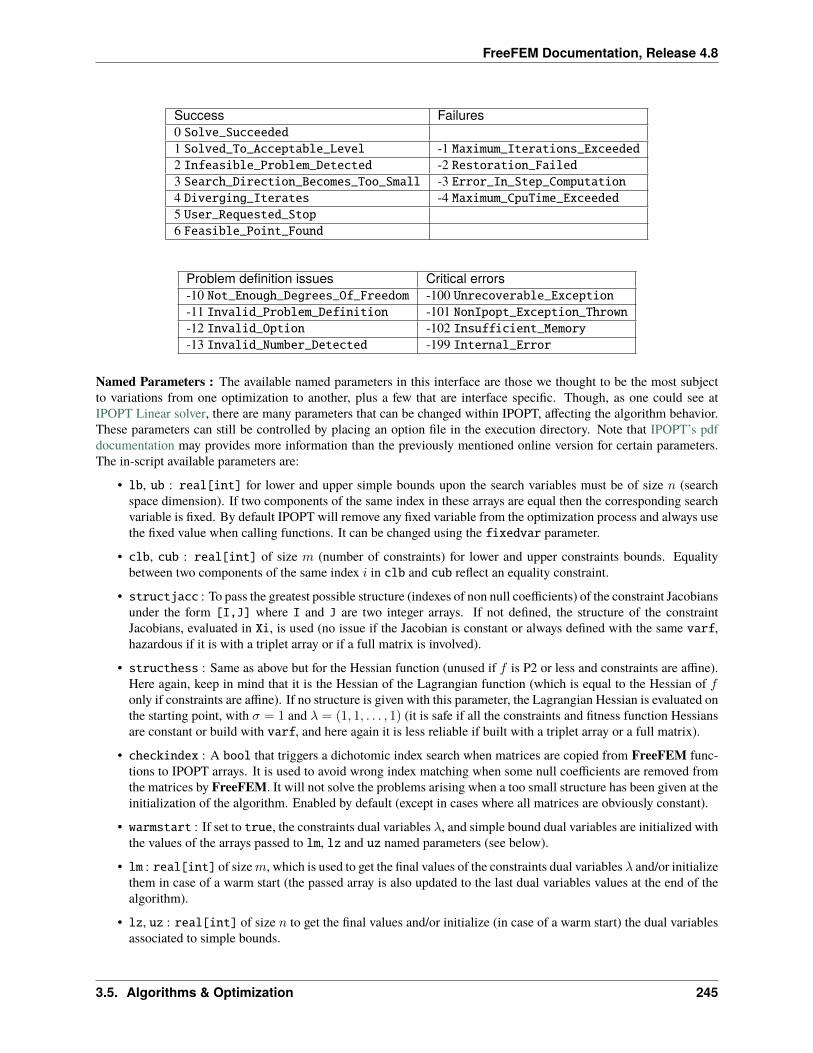
FreeFEM Documentation, Release 4.8
Success Failures0 Solve_Succeeded1 Solved_To_Acceptable_Level -1 Maximum_Iterations_Exceeded2 Infeasible_Problem_Detected -2 Restoration_Failed3 Search_Direction_Becomes_Too_Small -3 Error_In_Step_Computation4 Diverging_Iterates -4 Maximum_CpuTime_Exceeded5 User_Requested_Stop6 Feasible_Point_Found
Problem definition issues Critical errors-10 Not_Enough_Degrees_Of_Freedom -100 Unrecoverable_Exception-11 Invalid_Problem_Definition -101 NonIpopt_Exception_Thrown-12 Invalid_Option -102 Insufficient_Memory-13 Invalid_Number_Detected -199 Internal_Error
Named Parameters : The available named parameters in this interface are those we thought to be the most subjectto variations from one optimization to another, plus a few that are interface specific. Though, as one could see atIPOPT Linear solver, there are many parameters that can be changed within IPOPT, affecting the algorithm behavior.These parameters can still be controlled by placing an option file in the execution directory. Note that IPOPT’s pdfdocumentation may provides more information than the previously mentioned online version for certain parameters.The in-script available parameters are:
• lb, ub : real[int] for lower and upper simple bounds upon the search variables must be of size 𝑛 (searchspace dimension). If two components of the same index in these arrays are equal then the corresponding searchvariable is fixed. By default IPOPT will remove any fixed variable from the optimization process and always usethe fixed value when calling functions. It can be changed using the fixedvar parameter.
• clb, cub : real[int] of size 𝑚 (number of constraints) for lower and upper constraints bounds. Equalitybetween two components of the same index 𝑖 in clb and cub reflect an equality constraint.
• structjacc : To pass the greatest possible structure (indexes of non null coefficients) of the constraint Jacobiansunder the form [I,J] where I and J are two integer arrays. If not defined, the structure of the constraintJacobians, evaluated in Xi, is used (no issue if the Jacobian is constant or always defined with the same varf,hazardous if it is with a triplet array or if a full matrix is involved).
• structhess : Same as above but for the Hessian function (unused if 𝑓 is P2 or less and constraints are affine).Here again, keep in mind that it is the Hessian of the Lagrangian function (which is equal to the Hessian of 𝑓only if constraints are affine). If no structure is given with this parameter, the Lagrangian Hessian is evaluated onthe starting point, with 𝜎 = 1 and 𝜆 = (1, 1, . . . , 1) (it is safe if all the constraints and fitness function Hessiansare constant or build with varf, and here again it is less reliable if built with a triplet array or a full matrix).
• checkindex : A bool that triggers a dichotomic index search when matrices are copied from FreeFEM func-tions to IPOPT arrays. It is used to avoid wrong index matching when some null coefficients are removed fromthe matrices by FreeFEM. It will not solve the problems arising when a too small structure has been given at theinitialization of the algorithm. Enabled by default (except in cases where all matrices are obviously constant).
• warmstart : If set to true, the constraints dual variables 𝜆, and simple bound dual variables are initialized withthe values of the arrays passed to lm, lz and uz named parameters (see below).
• lm : real[int] of size𝑚, which is used to get the final values of the constraints dual variables 𝜆 and/or initializethem in case of a warm start (the passed array is also updated to the last dual variables values at the end of thealgorithm).
• lz, uz : real[int] of size 𝑛 to get the final values and/or initialize (in case of a warm start) the dual variablesassociated to simple bounds.
3.5. Algorithms & Optimization 245
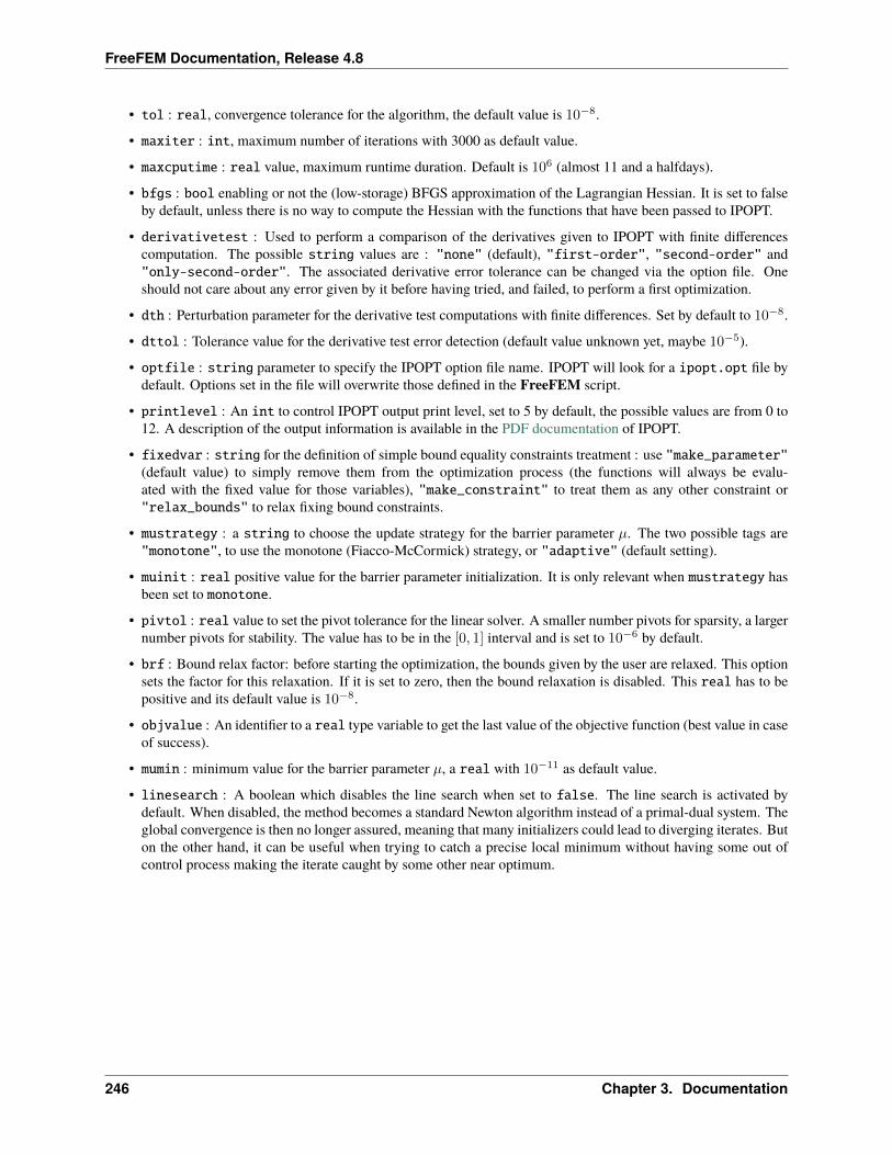
FreeFEM Documentation, Release 4.8
• tol : real, convergence tolerance for the algorithm, the default value is 10−8.
• maxiter : int, maximum number of iterations with 3000 as default value.
• maxcputime : real value, maximum runtime duration. Default is 106 (almost 11 and a halfdays).
• bfgs : bool enabling or not the (low-storage) BFGS approximation of the Lagrangian Hessian. It is set to falseby default, unless there is no way to compute the Hessian with the functions that have been passed to IPOPT.
• derivativetest : Used to perform a comparison of the derivatives given to IPOPT with finite differencescomputation. The possible string values are : "none" (default), "first-order", "second-order" and"only-second-order". The associated derivative error tolerance can be changed via the option file. Oneshould not care about any error given by it before having tried, and failed, to perform a first optimization.
• dth : Perturbation parameter for the derivative test computations with finite differences. Set by default to 10−8.
• dttol : Tolerance value for the derivative test error detection (default value unknown yet, maybe 10−5).
• optfile : string parameter to specify the IPOPT option file name. IPOPT will look for a ipopt.opt file bydefault. Options set in the file will overwrite those defined in the FreeFEM script.
• printlevel : An int to control IPOPT output print level, set to 5 by default, the possible values are from 0 to12. A description of the output information is available in the PDF documentation of IPOPT.
• fixedvar : string for the definition of simple bound equality constraints treatment : use "make_parameter"(default value) to simply remove them from the optimization process (the functions will always be evalu-ated with the fixed value for those variables), "make_constraint" to treat them as any other constraint or"relax_bounds" to relax fixing bound constraints.
• mustrategy : a string to choose the update strategy for the barrier parameter 𝜇. The two possible tags are"monotone", to use the monotone (Fiacco-McCormick) strategy, or "adaptive" (default setting).
• muinit : real positive value for the barrier parameter initialization. It is only relevant when mustrategy hasbeen set to monotone.
• pivtol : real value to set the pivot tolerance for the linear solver. A smaller number pivots for sparsity, a largernumber pivots for stability. The value has to be in the [0, 1] interval and is set to 10−6 by default.
• brf : Bound relax factor: before starting the optimization, the bounds given by the user are relaxed. This optionsets the factor for this relaxation. If it is set to zero, then the bound relaxation is disabled. This real has to bepositive and its default value is 10−8.
• objvalue : An identifier to a real type variable to get the last value of the objective function (best value in caseof success).
• mumin : minimum value for the barrier parameter 𝜇, a real with 10−11 as default value.
• linesearch : A boolean which disables the line search when set to false. The line search is activated bydefault. When disabled, the method becomes a standard Newton algorithm instead of a primal-dual system. Theglobal convergence is then no longer assured, meaning that many initializers could lead to diverging iterates. Buton the other hand, it can be useful when trying to catch a precise local minimum without having some out ofcontrol process making the iterate caught by some other near optimum.
246 Chapter 3. Documentation
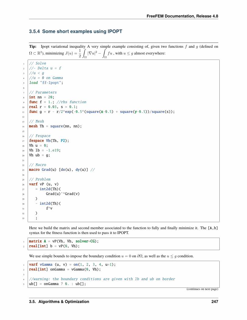
FreeFEM Documentation, Release 4.8
3.5.4 Some short examples using IPOPT
Tip: Ipopt variational inequality A very simple example consisting of, given two functions 𝑓 and 𝑔 (defined on
Ω ⊂ R2), minimizing 𝐽(𝑢) =1
2
∫Ω
|∇𝑢|2 −∫Ω
𝑓𝑢 , with 𝑢 ≤ 𝑔 almost everywhere:
1 // Solve2 //- Delta u = f3 //u < g4 //u = 0 on Gamma5 load "ff-Ipopt";6
7 // Parameters8 int nn = 20;9 func f = 1.; //rhs function
10 real r = 0.03, s = 0.1;11 func g = r - r/2*exp(-0.5*(square(x-0.5) + square(y-0.5))/square(s));12
13 // Mesh14 mesh Th = square(nn, nn);15
16 // Fespace17 fespace Vh(Th, P2);18 Vh u = 0;19 Vh lb = -1.e19;20 Vh ub = g;21
22 // Macro23 macro Grad(u) [dx(u), dy(u)] //24
25 // Problem26 varf vP (u, v)27 = int2d(Th)(28 Grad(u)'*Grad(v)29 )30 - int2d(Th)(31 f*v32 )33 ;
Here we build the matrix and second member associated to the function to fully and finally minimize it. The [A,b]syntax for the fitness function is then used to pass it to IPOPT.
1 matrix A = vP(Vh, Vh, solver=CG);2 real[int] b = vP(0, Vh);
We use simple bounds to impose the boundary condition 𝑢 = 0 on 𝜕Ω, as well as the 𝑢 ≤ 𝑔 condition.
1 varf vGamma (u, v) = on(1, 2, 3, 4, u=1);2 real[int] onGamma = vGamma(0, Vh);3
4 //warning: the boundary conditions are given with lb and ub on border5 ub[] = onGamma ? 0. : ub[];
(continues on next page)
3.5. Algorithms & Optimization 247
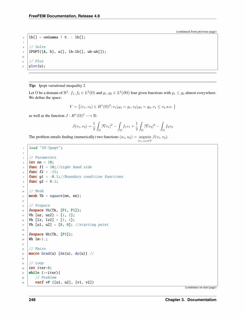
FreeFEM Documentation, Release 4.8
(continued from previous page)
6 lb[] = onGamma ? 0. : lb[];7
8 // Solve9 IPOPT([A, b], u[], lb=lb[], ub=ub[]);
10
11 // Plot12 plot(u);
Tip: Ipopt variational inequality 2
Let Ω be a domain of R2. 𝑓1, 𝑓2 ∈ 𝐿2(Ω) and 𝑔1, 𝑔2 ∈ 𝐿2(𝜕Ω) four given functions with 𝑔1 ≤ 𝑔2 almost everywhere.We define the space:
𝑉 =
(𝑣1, 𝑣2) ∈ 𝐻1(Ω)2; 𝑣1|𝜕Ω = 𝑔1, 𝑣2|𝜕Ω = 𝑔2, 𝑣1 ≤ 𝑣2 a.e.
as well as the function 𝐽 : 𝐻1(Ω)2 −→ R:
𝐽(𝑣1, 𝑣2) =1
2
∫Ω
|∇𝑣1|2 −∫Ω
𝑓1𝑣1 +1
2
∫Ω
|∇𝑣2|2 −∫Ω
𝑓2𝑣2
The problem entails finding (numerically) two functions (𝑢1, 𝑢2) = argmin(𝑣1,𝑣2)∈𝑉
𝐽(𝑣1, 𝑣2).
1 load "ff-Ipopt";2
3 // Parameters4 int nn = 10;5 func f1 = 10;//right hand side6 func f2 = -15;7 func g1 = -0.1;//Boundary condition functions8 func g2 = 0.1;9
10 // Mesh11 mesh Th = square(nn, nn);12
13 // Fespace14 fespace Vh(Th, [P1, P1]);15 Vh [uz, uz2] = [1, 1];16 Vh [lz, lz2] = [1, 1];17 Vh [u1, u2] = [0, 0]; //starting point18
19 fespace Wh(Th, [P1]);20 Wh lm=1.;21
22 // Macro23 macro Grad(u) [dx(u), dy(u)] //24
25 // Loop26 int iter=0;27 while (++iter)28 // Problem29 varf vP ([u1, u2], [v1, v2])
(continues on next page)
248 Chapter 3. Documentation
FreeFEM Documentation, Release 4.8
(continued from previous page)
30 = int2d(Th)(31 Grad(u1)'*Grad(v1)32 + Grad(u2)'*Grad(v2)33 )34 - int2d(Th)(35 f1*v136 + f2*v237 )38 ;39
40 matrix A = vP(Vh, Vh); //fitness function matrix41 real[int] b = vP(0, Vh); //and linear form42
43 int[int] II1 = [0], II2 = [1];//Constraints matrix44 matrix C1 = interpolate (Wh, Vh, U2Vc=II1);45 matrix C2 = interpolate (Wh, Vh, U2Vc=II2);46 matrix CC = -1*C1 + C2; // u2 - u1 > 047 Wh cl = 0; //constraints lower bounds (no upper bounds)48
49 //Boundary conditions50 varf vGamma ([u1, u2], [v1, v2]) = on(1, 2, 3, 4, u1=1, u2=1);51 real[int] onGamma = vGamma(0, Vh);52 Vh [ub1, ub2] = [g1, g2];53 Vh [lb1, lb2] = [g1, g2];54 ub1[] = onGamma ? ub1[] : 1e19; //Unbounded in interior55 lb1[] = onGamma ? lb1[] : -1e19;56
57 Vh [uzi, uzi2] = [uz, uz2], [lzi, lzi2] = [lz, lz2];58 Wh lmi = lm;59 Vh [ui1, ui2] = [u1, u2];60
61 // Solve62 IPOPT([b, A], CC, ui1[], lb=lb1[], clb=cl[], ub=ub1[], warmstart=iter>1, uz=uzi[],
→˓lz=lzi[], lm=lmi[]);63
64 // Plot65 plot(ui1, ui2, wait=true, nbiso=60, dim=3);66
67 if(iter > 1) break;68
69 // Mesh adpatation70 Th = adaptmesh(Th, [ui1, ui2], err=0.004, nbvx=100000);71 [uz, uz2] = [uzi, uzi2];72 [lz, lz2] = [lzi, lzi2];73 [u1, u2] = [ui1, ui2];74 lm = lmi;75
3.5. Algorithms & Optimization 249
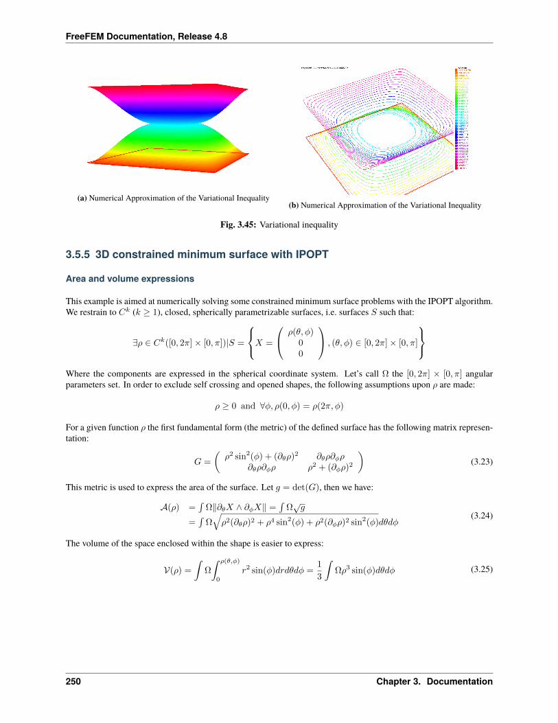
FreeFEM Documentation, Release 4.8
(a) Numerical Approximation of the Variational Inequality(b) Numerical Approximation of the Variational Inequality
Fig. 3.45: Variational inequality
3.5.5 3D constrained minimum surface with IPOPT
Area and volume expressions
This example is aimed at numerically solving some constrained minimum surface problems with the IPOPT algorithm.We restrain to 𝐶𝑘 (𝑘 ≥ 1), closed, spherically parametrizable surfaces, i.e. surfaces 𝑆 such that:
∃𝜌 ∈ 𝐶𝑘([0, 2𝜋]× [0, 𝜋])|𝑆 =
⎧⎨⎩𝑋 =
⎛⎝ 𝜌(𝜃, 𝜑)00
⎞⎠ , (𝜃, 𝜑) ∈ [0, 2𝜋]× [0, 𝜋]
⎫⎬⎭Where the components are expressed in the spherical coordinate system. Let’s call Ω the [0, 2𝜋] × [0, 𝜋] angularparameters set. In order to exclude self crossing and opened shapes, the following assumptions upon 𝜌 are made:
𝜌 ≥ 0 and ∀𝜑, 𝜌(0, 𝜑) = 𝜌(2𝜋, 𝜑)
For a given function 𝜌 the first fundamental form (the metric) of the defined surface has the following matrix represen-tation:
𝐺 =
(𝜌2 sin2(𝜑) + (𝜕𝜃𝜌)2 𝜕𝜃𝜌𝜕𝜑𝜌
𝜕𝜃𝜌𝜕𝜑𝜌 𝜌2 + (𝜕𝜑𝜌)2
)(3.23)
This metric is used to express the area of the surface. Let 𝑔 = det(𝐺), then we have:
𝒜(𝜌) =∫
Ω‖𝜕𝜃𝑋 ∧ 𝜕𝜑𝑋‖ =∫
Ω√𝑔
=∫
Ω√𝜌2(𝜕𝜃𝜌)2 + 𝜌4 sin2(𝜑) + 𝜌2(𝜕𝜑𝜌)2 sin2(𝜑)𝑑𝜃𝑑𝜑
(3.24)
The volume of the space enclosed within the shape is easier to express:
𝒱(𝜌) =
∫Ω
∫ 𝜌(𝜃,𝜑)
0
𝑟2 sin(𝜑)𝑑𝑟𝑑𝜃𝑑𝜑 =1
3
∫Ω𝜌3 sin(𝜑)𝑑𝜃𝑑𝜑 (3.25)
250 Chapter 3. Documentation
FreeFEM Documentation, Release 4.8
Derivatives
In order to use a Newton based interior point optimization algorithm, one must be able to evaluate the derivatives of𝒜and 𝒱 with respect to 𝑟ℎ𝑜. Concerning the area, we have the following result:
∀𝑣 ∈ 𝐶1(Ω) , ⟨𝑑𝒜(𝜌), 𝑣⟩ =
∫Ω
1
2
𝑑𝑔(𝜌)(𝑣)√𝑔
𝑑𝜃𝑑𝜑
Where 𝑔 is the application mapping the (𝜃, 𝜑) ↦→ 𝑔(𝜃, 𝜑) scalar field to 𝜌. This leads to the following expression, easyto transpose in a freefem script using:
∀𝑣 ∈ 𝐶1(Ω)⟨𝑑𝒜(𝜌), 𝑣⟩ =
∫Ω(2𝜌3 sin2(𝜑) + 𝜌(𝜕𝜃𝜌)2 + 𝜌(𝜕𝜑𝜌)2 sin2(𝜑)
)𝑣
+∫
Ω 𝜌2𝜕𝜃𝜌𝜕𝜃𝑣 + 𝜌2𝜕𝜑𝜌 sin2(𝜑)𝜕𝜑𝑣(3.26)
With a similar approach, one can derive an expression for second order derivatives. However, comporting no specificdifficulties, the detailed calculus are tedious, the result is that these derivatives can be written using a 3× 3 matrix Bwhose coefficients are expressed in term of 𝜌 and its derivatives with respect to 𝜃 and 𝜑, such that:
∀(𝑤, 𝑣) ∈ 𝐶1(Ω) , 𝑑2𝒜(𝜌)(𝑤, 𝑣) =
∫Ω(𝑤 𝜕𝜃𝑤 𝜕𝜑𝑤
)B
⎛⎝ 𝑣𝜕𝜃𝑣𝜕𝜑𝑣
⎞⎠ 𝑑𝜃𝑑𝜑 (3.27)
Deriving the volume function derivatives is again an easier task. We immediately get the following expressions:
∀𝑣 , ⟨𝑑𝒱(𝜌), 𝑣⟩ =∫
Ω𝜌2 sin(𝜑)𝑣 𝑑𝜃𝑑𝜑∀𝑤, 𝑣 , 𝑑2𝒱(𝜌)(𝑤, 𝑣) =
∫Ω2𝜌 sin(𝜑)𝑤𝑣 𝑑𝜃𝑑𝜑
(3.28)
The problem and its script
The whole code is available in IPOPT minimal surface & volume example. We propose to solve the following problem:
Tip: Given a positive function 𝜌object piecewise continuous, and a scalar 𝒱max > 𝒱(𝜌object), find 𝜌0 such that:
𝜌0 = argmin𝜌∈𝐶1(Ω)
𝒜(𝜌) , s.t. 𝜌0 ≥ 𝜌object and 𝒱(𝜌0) ≤ 𝒱max
If 𝜌object is the spherical parametrization of the surface of a 3-dimensional object (domain) 𝒪, it can be interpretedas finding the surface with minimum area enclosing the object with a given maximum volume. If 𝒱max is close to𝒱(𝜌object), so should be 𝜌0 and 𝜌object. With higher values of 𝒱max, 𝜌 should be closer to the unconstrained minimumsurface surrounding 𝒪 which is obtained as soon as 𝒱max ≥ 4
3𝜋‖𝜌object‖3∞ (sufficient but not necessary).
It also could be interesting to solve the same problem with the constraint 𝒱(𝜌0) ≥ 𝒱min which leads to a sphere when𝒱min ≥ 1
6𝜋diam(𝒪)3 and moves toward the solution of the unconstrained problem as 𝒱min decreases.
We start by meshing the domain [0, 2𝜋]× [0, 𝜋], then a periodic P1 finite elements space is defined.
1 load "msh3";2 load "medit";3 load "ff-Ipopt";4
5 // Parameters6 int nadapt = 3;7 real alpha = 0.9;8 int np = 30;
(continues on next page)
3.5. Algorithms & Optimization 251
FreeFEM Documentation, Release 4.8
(continued from previous page)
9 real regtest;10 int shapeswitch = 1;11 real sigma = 2*pi/40.;12 real treshold = 0.1;13 real e = 0.1;14 real r0 = 0.25;15 real rr = 2-r0;16 real E = 1./(e*e);17 real RR = 1./(rr*rr);18
19 // Mesh20 mesh Th = square(2*np, np, [2*pi*x, pi*y]);21
22 // Fespace23 fespace Vh(Th, P1, periodic=[[2, y], [4, y]]);24 //Initial shape definition25 //outside of the mesh adaptation loop to initialize with the previous optimial shape
→˓found on further iterations26 Vh startshape = 5;
We create some finite element functions whose underlying arrays will be used to store the values of dual variablesassociated to all the constraints in order to reinitialize the algorithm with it in the case where we use mesh adaptation.Doing so, the algorithm will almost restart at the accuracy level it reached before mesh adaptation, thus saving manyiterations.
1 Vh uz = 1., lz = 1.;2 rreal[int] lm = [1];
Then, follows the mesh adaptation loop, and a rendering function, Plot3D, using 3D mesh to display the shape it ispassed with medit (the movemesh23 procedure often crashes when called with ragged shapes).
1 for(int kkk = 0; kkk < nadapt; ++kkk)2 int iter=0;3 func sin2 = square(sin(y));4
5 // A function which transform Th in 3d mesh (r=rho)6 //a point (theta,phi) of Th becomes ( r(theta,phi)*cos(theta)*sin(phi) , r(theta,
→˓phi)*sin(theta)*sin(phi) , r(theta,phi)*cos(phi) )7 //then displays the resulting mesh with medit8 func int Plot3D (real[int] &rho, string cmm, bool ffplot)9 Vh rhoo;
10 rhoo[] = rho;11 //mesh sTh = square(np, np/2, [2*pi*x, pi*y]);12 //fespace sVh(sTh, P1);13 //Vh rhoplot = rhoo;14 try15 mesh3 Sphere = movemesh23(Th, transfo=[rhoo(x,y)*cos(x)*sin(y), rhoo(x,
→˓y)*sin(x)*sin(y), rhoo(x,y)*cos(y)]);16 if(ffplot)17 plot(Sphere);18 else19 medit(cmm, Sphere);
(continues on next page)
252 Chapter 3. Documentation
FreeFEM Documentation, Release 4.8
(continued from previous page)
20 21 catch(...)22 cout << "PLOT ERROR" << endl;23 24 return 1;25 26
Here are the functions related to the area computation and its shape derivative, according to equations (3.24) and (3.26):
1 // Surface computation2 //Maybe is it possible to use movemesh23 to have the surface function less complicated3 //However, it would not simplify the gradient and the hessian4 func real Area (real[int] &X)5 Vh rho;6 rho[] = X;7 Vh rho2 = square(rho);8 Vh rho4 = square(rho2);9 real res = int2d(Th)(sqrt(rho4*sin2 + rho2*square(dx(rho)) +
→˓rho2*sin2*square(dy(rho))));10 ++iter;11 if(1)12 plot(rho, value=true, fill=true, cmm="rho(theta,phi) on [0,2pi]x[0,pi] - S="+res,
→˓dim=3);13 else14 Plot3D(rho[], "shape_evolution", 1);15 return res;16 17
18 func real[int] GradArea (real[int] &X)19 Vh rho, rho2;20 rho[] = X;21 rho2[] = square(X);22 Vh sqrtPsi, alpha;23 24 Vh dxrho2 = dx(rho)*dx(rho), dyrho2 = dy(rho)*dy(rho);25 sqrtPsi = sqrt(rho2*rho2*sin2 + rho2*dxrho2 + rho2*dyrho2*sin2);26 alpha = 2.*rho2*rho*sin2 + rho*dxrho2 + rho*dyrho2*sin2;27 28 varf dArea (u, v)29 = int2d(Th)(30 1./sqrtPsi * (alpha*v + rho2*dx(rho)*dx(v) + rho2*dy(rho)*sin2*dy(v))31 )32 ;33
34 real[int] grad = dArea(0, Vh);35 return grad;36
The function returning the hessian of the area for a given shape is a bit blurry, thus we won’t show here all of equation(3.27) coefficients definition, they can be found in the edp file.
3.5. Algorithms & Optimization 253
FreeFEM Documentation, Release 4.8
1 matrix hessianA;2 func matrix HessianArea (real[int] &X)3 Vh rho, rho2;4 rho[] = X;5 rho2 = square(rho);6 Vh sqrtPsi, sqrtPsi3, C00, C01, C02, C11, C12, C22, A;7 8 Vh C0, C1, C2;9 Vh dxrho2 = dx(rho)*dx(rho), dyrho2 = dy(rho)*dy(rho);
10 sqrtPsi = sqrt( rho2*rho2*sin2 + rho2*dxrho2 + rho2*dyrho2*sin2);11 sqrtPsi3 = (rho2*rho2*sin2 + rho2*dxrho2 + rho2*dyrho2*sin2)*sqrtPsi;12 C0 = 2*rho2*rho*sin2 + rho*dxrho2 + rho*dyrho2*sin2;13 C1 = rho2*dx(rho);14 C2 = rho2*sin2*dy(rho);15 C00 = square(C0);16 C01 = C0*C1;17 C02 = C0*C2;18 C11 = square(C1);19 C12 = C1*C2;20 C22 = square(C2);21 A = 6.*rho2*sin2 + dxrho2 + dyrho2*sin2;22 23 varf d2Area (w, v)24 =int2d(Th)(25 1./sqrtPsi * (26 A*w*v27 + 2*rho*dx(rho)*dx(w)*v28 + 2*rho*dx(rho)*w*dx(v)29 + 2*rho*dy(rho)*sin2*dy(w)*v30 + 2*rho*dy(rho)*sin2*w*dy(v)31 + rho2*dx(w)*dx(v)32 + rho2*sin2*dy(w)*dy(v)33 )34 + 1./sqrtPsi3 * (35 C00*w*v36 + C01*dx(w)*v37 + C01*w*dx(v)38 + C02*dy(w)*v39 + C02*w*dy(v)40 + C11*dx(w)*dx(v)41 + C12*dx(w)*dy(v)42 + C12*dy(w)*dx(v)43 + C22*dy(w)*dy(v)44 )45 )46 ;47 hessianA = d2Area(Vh, Vh);48 return hessianA;49
And the volume related functions:
1 // Volume computation(continues on next page)
254 Chapter 3. Documentation
FreeFEM Documentation, Release 4.8
(continued from previous page)
2 func real Volume (real[int] &X)3 Vh rho;4 rho[] = X;5 Vh rho3 = rho*rho*rho;6 real res = 1./3.*int2d(Th)(rho3*sin(y));7 return res;8 9
10 func real[int] GradVolume (real[int] &X)11 Vh rho;12 rho[] = X;13 varf dVolume(u, v) = int2d(Th)(rho*rho*sin(y)*v);14 real[int] grad = dVolume(0, Vh);15 return grad;16 17
18 matrix hessianV;19 func matrix HessianVolume(real[int] &X)20 Vh rho;21 rho[] = X;22 varf d2Volume(w, v) = int2d(Th)(2*rho*sin(y)*v*w);23 hessianV = d2Volume(Vh, Vh);24 return hessianV;25
If we want to use the volume as a constraint function we must wrap it and its derivatives in some FreeFEM functionsreturning the appropriate types. It is not done in the above functions in cases where one wants to use it as a fitnessfunction. The lagrangian hessian also has to be wrapped since the Volume is not linear with respect to 𝜌, it has somenon-null second order derivatives.
1 func real[int] ipVolume (real[int] &X) real[int] vol = [Volume(X)]; return vol; 2 matrix mdV;3 func matrix ipGradVolume (real[int] &X) real[int,int] dvol(1,Vh.ndof); dvol(0,:) =
→˓GradVolume(X); mdV = dvol; return mdV; 4 matrix HLagrangian;5 func matrix ipHessianLag (real[int] &X, real objfact, real[int] &lambda)6 HLagrangian = objfact*HessianArea(X) + lambda[0]*HessianVolume(X);7 return HLagrangian;8
The ipGradVolume function could pose some troubles during the optimization process because the gradient vector istransformed in a sparse matrix, so any null coefficient will be discarded. Here we create the IPOPT structure manuallyand use the checkindex named-parameter to avoid bad indexing during copies. This gradient is actually dense, thereis no reason for some components to be constantly zero:
1 int[int] gvi(Vh.ndof), gvj=0:Vh.ndof-1;2 gvi = 0;
These two arrays will be passed to IPOPT with structjacc=[gvi,gvj]. The last remaining things are the bounddefinitions. The simple lower bound must be equal to the components of the P1 projection of 𝜌𝑜𝑏𝑗𝑒𝑐𝑡. And we choose𝛼 ∈ [0, 1] to set 𝒱max to (1− 𝛼)𝒱(𝜌𝑜𝑏𝑗𝑒𝑐𝑡) + 𝛼 4
3𝜋‖𝜌object‖3∞:
3.5. Algorithms & Optimization 255
FreeFEM Documentation, Release 4.8
1 func disc1 = sqrt(1./(RR+(E-RR)*cos(y)*cos(y)))*(1+0.1*cos(7*x));2 func disc2 = sqrt(1./(RR+(E-RR)*cos(x)*cos(x)*sin2));3
4 if(1)5 lb = r0;6 for (int q = 0; q < 5; ++q)7 func f = rr*Gaussian(x, y, 2*q*pi/5., pi/3.);8 func g = rr*Gaussian(x, y, 2*q*pi/5.+pi/5., 2.*pi/3.);9 lb = max(max(lb, f), g);
10 11 lb = max(lb, rr*Gaussian(x, y, 2*pi, pi/3));12 13 lb = max(lb, max(disc1, disc2));14 real Vobj = Volume(lb[]);15 real Vnvc = 4./3.*pi*pow(lb[].linfty,3);16
17 if(1)18 Plot3D(lb[], "object_inside", 1);19 real[int] clb = 0., cub = [(1-alpha)*Vobj + alpha*Vnvc];
Calling IPOPT:
1 int res = IPOPT(Area, GradArea, ipHessianLag, ipVolume, ipGradVolume,2 rc[], ub=ub[], lb=lb[], clb=clb, cub=cub, checkindex=1, maxiter=kkk<nadapt-1 ? 40:150,3 warmstart=kkk, lm=lm, uz=uz[], lz=lz[], tol=0.00001, structjacc=[gvi,gvj]);4 cout << "IPOPT: res =" << res << endl ;5
6 // Plot7 Plot3D(rc[], "Shape_at_"+kkk, 1);8 Plot3D(GradArea(rc[]), "ShapeGradient", 1);
Finally, before closing the mesh adaptation loop, we have to perform the said adaptation. The mesh is adaptated withrespect to the 𝑋 = (𝜌, 0, 0) (in spherical coordinates) vector field, not directly with respect to 𝜌, otherwise the truecurvature of the 3D-shape would not be well taken into account.
1 if (kkk < nadapt-1)2 Th = adaptmesh(Th, rc*cos(x)*sin(y), rc*sin(x)*sin(y), rc*cos(y),3 nbvx=50000, periodic=[[2, y], [4, y]]);4 plot(Th, wait=true);5 startshape = rc;6 uz = uz;7 lz = lz;8
Here are some pictures of the resulting surfaces obtained for decreasing values of 𝛼 (and a slightly more complicatedobject than two orthogonal discs). We return to the enclosed object when 𝛼 = 0:
256 Chapter 3. Documentation
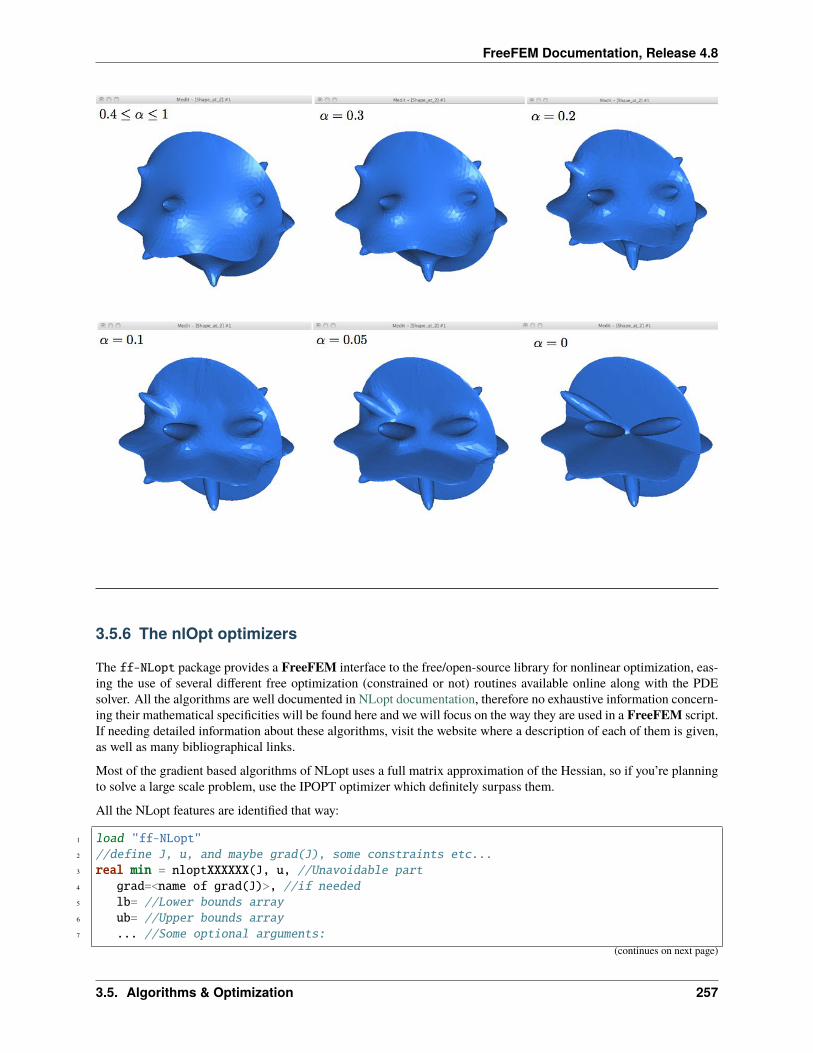
FreeFEM Documentation, Release 4.8
3.5.6 The nlOpt optimizers
The ff-NLopt package provides a FreeFEM interface to the free/open-source library for nonlinear optimization, eas-ing the use of several different free optimization (constrained or not) routines available online along with the PDEsolver. All the algorithms are well documented in NLopt documentation, therefore no exhaustive information concern-ing their mathematical specificities will be found here and we will focus on the way they are used in a FreeFEM script.If needing detailed information about these algorithms, visit the website where a description of each of them is given,as well as many bibliographical links.
Most of the gradient based algorithms of NLopt uses a full matrix approximation of the Hessian, so if you’re planningto solve a large scale problem, use the IPOPT optimizer which definitely surpass them.
All the NLopt features are identified that way:
1 load "ff-NLopt"2 //define J, u, and maybe grad(J), some constraints etc...3 real min = nloptXXXXXX(J, u, //Unavoidable part4 grad=<name of grad(J)>, //if needed5 lb= //Lower bounds array6 ub= //Upper bounds array7 ... //Some optional arguments:
(continues on next page)
3.5. Algorithms & Optimization 257
FreeFEM Documentation, Release 4.8
(continued from previous page)
8 //Constraints functions names,9 //Stopping criteria,
10 //Algorithm specific parameters,11 //Etc...12 );
XXXXXX refers to the algorithm tag (not necessarily 6 characters long). u is the starting position (a real[int] typearray) which will be overwritten by the algorithm, the value at the end being the found 𝑎𝑟𝑔𝑚𝑖𝑛. And as usual, J isa function taking a real[int] type array as argument and returning a real. grad, lb and ub are “half-optional”arguments, in the sense that they are obligatory for some routines but not all.
The possible optionally named parameters are the following, note that they are not used by all algorithms (some donot support constraints, or a type of constraints, some are gradient-based and others are derivative free, etc. . . ). Onecan refer to the table after the parameters description to check which are the named parameters supported by a specificalgorithm. Using an unsupported parameter will not stop the compiler work, seldom breaks runtime, and will justbe ignored. When it is obvious you are missing a routine, you will get a warning message at runtime (for example ifyou pass a gradient to a derivative free algorithm, or set the population of a non-genetic one, etc. . . ). In the followingdescription, 𝑛 stands for the dimension of the search space.
Half-optional parameters :• grad= The name of the function which computes the gradient of the cost function (prototype should bereal[int] → real[int], both argument and result should have the size 𝑛). This is needed as soon as agradient-based method is involved, which is ignored if defined in a derivative free context.
• lb/ub = Lower and upper bounds arrays ( real[int] type) of size 𝑛. Used to define the bounds within whichthe search variable is allowed to move. Needed for some algorithms, optional, or unsupported for others.
• subOpt : Only enabled for the Augmented Lagrangian and MLSL methods who need a sub-optimizer in orderto work. Just pass the tag of the desired local algorithm with a string.
Constraints related parameters (optional - unused if not specified):• IConst/EConst : Allows to pass the name of a function implementing some inequality (resp. equality) con-
straints on the search space. The function type must be real[int]→ real[int] where the size of the returnedarray is equal to the number of constraints (of the same type - it means that all of the constraints are computedin one vectorial function). In order to mix inequality and equality constraints in a same minimization attempt,two vectorial functions have to be defined and passed. See example (3.29) for more details about how theseconstraints have to be implemented.
• gradIConst/gradEConst : Use to provide the inequality (resp. equality) constraints gradient. These arereal[int] → real[int,int] type functions. Assuming we have defined a constraint function (either in-equality or equality) with 𝑝 constraints, the size of the matrix returned by its associated gradient must be 𝑝× 𝑛(the 𝑖-th line of the matrix is the gradient of the 𝑖-th constraint). It is needed in a gradient-based context as soonas an inequality or equality constraint function is passed to the optimizer and ignored in all other cases.
• tolIConst/tolEConst : Tolerance values for each constraint. This is an array of size equal to the number ofinequality (resp. equality) constraints. Default value is set to 10−12 for each constraint of any type.
Stopping criteria :• stopFuncValue : Makes the algorithm end when the objective function reaches this real value.
• stopRelXTol : Stops the algorithm when the relative moves in each direction of the search space is smaller thanthis real value.
• stopAbsXTol : Stops the algorithm when the moves in each direction of the search space is smaller than thecorresponding value in this real[int] array.
258 Chapter 3. Documentation
FreeFEM Documentation, Release 4.8
• stopRelFTol : Stops the algorithm when the relative variation of the objective function is smaller than thisreal value.
• stopAbsFTol : Stops the algorithm when the variation of the objective function is smaller than this real value.
• stopMaxFEval : Stops the algorithm when the number of fitness evaluations reaches this integer value.
• stopTime : Stops the algorithm when the optimization time in seconds exceeds this real value. This is not astrict maximum: the time may exceed it slightly, depending upon the algorithm and on how slow your functionevaluation is.
Note that when an AUGLAG or MLSL method is used, the meta-algorithm and the sub-algorithm may havedifferent termination criteria. Thus, for algorithms of this kind, the following named parameters has been defined(just adding the SO prefix - for Sub-Optimizer) to set the ending condition of the sub-algorithm (the meta oneuses the ones above): SOStopFuncValue, SOStopRelXTol, and so on. . . If these are not used, the sub-optimizerwill use those of the master routine.
Other named parameters :• popSize : integer used to change the size of the sample for stochastic search methods. Default value is a
peculiar heuristic to the chosen algorithm.
• SOPopSize : Same as above, but when the stochastic search is passed to a meta-algorithm.
• nGradStored : The number (integer type) of gradients to “remember” from previous optimization steps:increasing this increases the memory requirements but may speed convergence. It is set to a heuristic value bydefault. If used with AUGLAG or MLSL, it will only affect the given subsidiary algorithm.
The following table sums up the main characteristics of each algorithm, providing the more important information aboutwhich features are supported by which algorithm and what are the unavoidable arguments they need. More details canbe found in NLopt documentation.
Tip: Variational inequality
Let Ω be a domain of R2, 𝑓1, 𝑓2 ∈ 𝐿2(Ω) and 𝑔1, 𝑔2 ∈ 𝐿2(𝜕Ω) four given functions with 𝑔1 ≤ 𝑔2 almost everywhere.
We define the space:
𝑉 =
(𝑣1, 𝑣2) ∈ 𝐻1(Ω)2; 𝑣1|𝜕Ω = 𝑔1, 𝑣2|𝜕Ω = 𝑔2, 𝑣1 ≤ 𝑣2 a.e.
as well as the function 𝐽 : 𝐻1(Ω)2 −→ R:
𝐽(𝑣1, 𝑣2) =1
2
∫Ω
|∇𝑣1|2 −∫Ω
𝑓1𝑣1 +1
2
∫Ω
|∇𝑣2|2 −∫Ω
𝑓2𝑣2 (3.29)
The problem consists in finding (numerically) two functions (𝑢1, 𝑢2) = argmin(𝑣1,𝑣2)∈𝑉
𝐽(𝑣1, 𝑣2).
This can be interpreted as finding 𝑢1, 𝑢2 as close as possible (in a certain sense) to the solutions of the Laplace equationwith respectively 𝑓1, 𝑓2 second members and 𝑔1, 𝑔2 Dirichlet boundary conditions with the 𝑢1 ≤ 𝑢2 almost everywhereconstraint.
Here is the corresponding script to treat this variational inequality problem with one of the NLOpt algorithms.
1 //A brief script to demonstrate how to use the freefemm interfaced nlopt routines2 //The problem consist in solving a simple variational inequality using one of the3 //optimization algorithm of nlopt. We restart the algorithlm a few times after4 //performing some mesh adaptation to get a more precise output5
6 load "ff-NLopt"7
(continues on next page)
3.5. Algorithms & Optimization 259
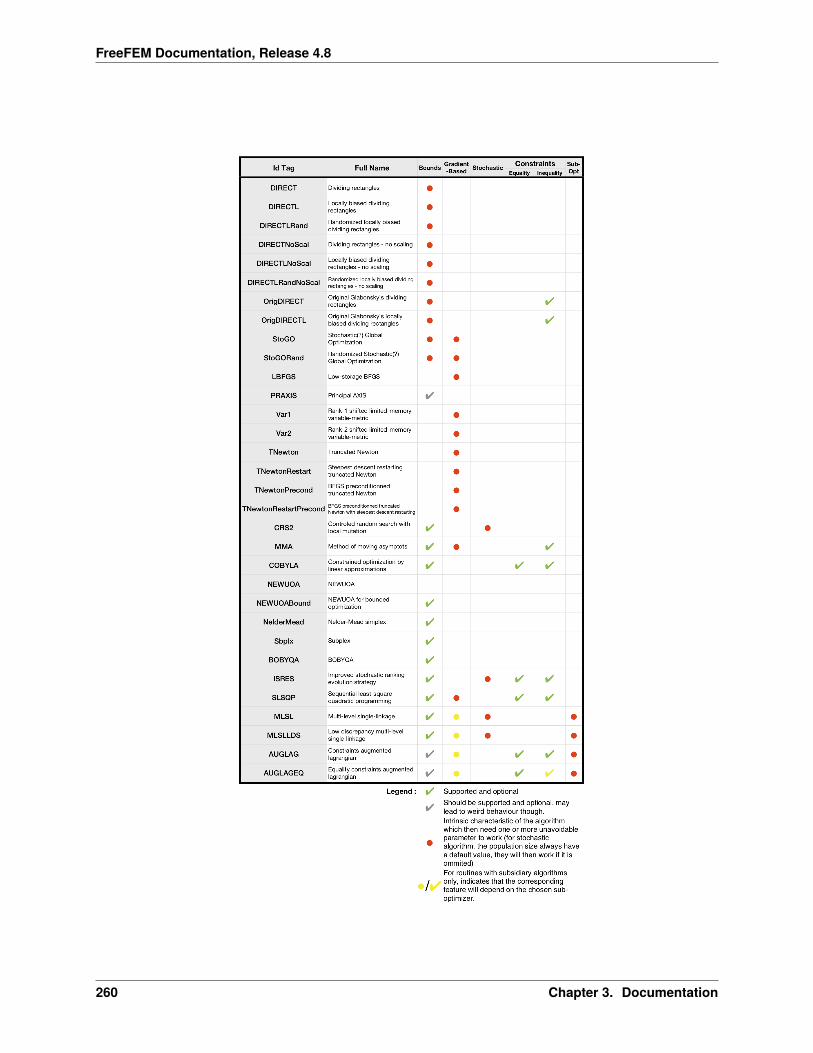
FreeFEM Documentation, Release 4.8
260 Chapter 3. Documentation
FreeFEM Documentation, Release 4.8
(continued from previous page)
8 // Parameters9 int kas = 3; //choose of the algorithm
10 int NN = 10;11 func f1 = 1.;12 func f2 = -1.;13 func g1 = 0.;14 func g2 = 0.1;15 int iter = 0;16 int nadapt = 2;17 real starttol = 1e-6;18 real bctol = 6.e-12;19
20 // Mesh21 mesh Th = square(NN, NN);22
23 // Fespace24 fespace Vh(Th, P1);25 Vh oldu1, oldu2;26
27 // Adaptation loop28 for (int al = 0; al < nadapt; ++al)29 varf BVF (v, w) = int2d(Th)(0.5*dx(v)*dx(w) + 0.5*dy(v)*dy(w));30 varf LVF1 (v, w) = int2d(Th)(f1*w);31 varf LVF2 (v, w) = int2d(Th)(f2*w);32 matrix A = BVF(Vh, Vh);33 real[int] b1 = LVF1(0, Vh), b2 = LVF2(0, Vh);34
35 varf Vbord (v, w) = on(1, 2, 3, 4, v=1);36
37 Vh In, Bord;38 Bord[] = Vbord(0, Vh, tgv=1);39 In[] = Bord[] ? 0:1;40 Vh gh1 = Bord*g1, gh2 = Bord*g2;41
42 func real J (real[int] &X)43 Vh u1, u2;44 u1[] = X(0:Vh.ndof-1);45 u2[] = X(Vh.ndof:2*Vh.ndof-1);46 iter++;47 real[int] Au1 = A*u1[], Au2 = A*u2[];48 Au1 -= b1;49 Au2 -= b2;50 real val = u1[]'*Au1 + u2[]'*Au2;51 if (iter%10 == 9)52 plot(u1, u2, nbiso=30, fill=1, dim=3, cmm="adapt level "+al+" - iteration
→˓"+iter+" - J = "+val, value=1);53 return val;54 55
56 varf dBFV (v, w) = int2d(Th)(dx(v)*dx(w)+dy(v)*dy(w));57 matrix dA = dBFV(Vh, Vh);58 func real[int] dJ (real[int] &X)
(continues on next page)
3.5. Algorithms & Optimization 261
FreeFEM Documentation, Release 4.8
(continued from previous page)
59 Vh u1, u2;60 u1[] = X(0:Vh.ndof-1);61 u2[] = X(Vh.ndof:2*Vh.ndof-1);62
63 real[int] grad1 = dA*u1[], grad2 = dA*u2[];64 grad1 -= b1;65 grad2 -= b2;66 real[int] Grad(X.n);67 Grad(0:Vh.ndof-1) = grad1;68 Grad(Vh.ndof:2*Vh.ndof-1) = grad2;69 return Grad;70 71
72 func real[int] IneqC (real[int] &X)73 real[int] constraints(Vh.ndof);74 for (int i = 0; i < Vh.ndof; ++i) constraints[i] = X[i] - X[i+Vh.ndof];75 return constraints;76 77
78 func real[int,int] dIneqC (real[int] &X)79 real[int, int] dconst(Vh.ndof, 2*Vh.ndof);80 dconst = 0;81 for(int i = 0; i < Vh.ndof; ++i)82 dconst(i, i) = 1.;83 dconst(i, i+Vh.ndof) = -1.;84 85 return dconst;86 87
88 real[int] BordIndex(Th.nbe); //Indexes of border d.f.89 90 int k = 0;91 for (int i = 0; i < Bord.n; ++i) if (Bord[][i]) BordIndex[k] = i; ++k; 92 93
94 func real[int] BC (real[int] &X)95 real[int] bc(2*Th.nbe);96 for (int i = 0; i < Th.nbe; ++i)97 int I = BordIndex[i];98 bc[i] = X[I] - gh1[][I];99 bc[i+Th.nbe] = X[I+Th.nv] - gh2[][I];
100 101 return bc;102 103
104 func real[int, int] dBC(real[int] &X)105 real[int, int] dbc(2*Th.nbe,2*Th.nv);106 dbc = 0.;107 for (int i = 0; i < Th.nbe; ++i)108 int I = BordIndex[i];109 dbc(i, I) = 1.;110 dbc(i+Th.nbe, I+Th.nv) = 1.;
(continues on next page)
262 Chapter 3. Documentation
FreeFEM Documentation, Release 4.8
(continued from previous page)
111 112 return dbc;113 114
115 real[int] start(2*Vh.ndof), up(2*Vh.ndof), lo(2*Vh.ndof);116
117 if (al == 0)118 start(0:Vh.ndof-1) = 0.;119 start(Vh.ndof:2*Vh.ndof-1) = 0.01;120 121 else122 start(0:Vh.ndof-1) = oldu1[];123 start(Vh.ndof:2*Vh.ndof-1) = oldu2[];124 125
126 up = 1000000;127 lo = -1000000;128 for (int i = 0; i < Vh.ndof; ++i)129 if (Bord[][i])130 up[i] = gh1[][i] + bctol;131 lo[i] = gh1[][i] - bctol;132 up[i+Vh.ndof] = gh2[][i] + bctol;133 lo[i+Vh.ndof] = gh2[][i] - bctol;134 135 136
137 real mini = 1e100;138 if (kas == 1)139 mini = nloptAUGLAG(J, start, grad=dJ, lb=lo,140 ub=up, IConst=IneqC, gradIConst=dIneqC,141 subOpt="LBFGS", stopMaxFEval=10000, stopAbsFTol=starttol);142 else if (kas == 2)143 mini = nloptMMA(J, start, grad=dJ, lb=lo, ub=up, stopMaxFEval=10000,
→˓stopAbsFTol=starttol);144 else if (kas == 3)145 mini = nloptAUGLAG(J, start, grad=dJ, IConst=IneqC,146 gradIConst=dIneqC, EConst=BC, gradEConst=dBC,147 subOpt="LBFGS", stopMaxFEval=200, stopRelXTol=1e-2);148 else if (kas == 4)149 mini = nloptSLSQP(J, start, grad=dJ, IConst=IneqC,150 gradIConst=dIneqC, EConst=BC, gradEConst=dBC,151 stopMaxFEval=10000, stopAbsFTol=starttol);152 Vh best1, best2;153 best1[] = start(0:Vh.ndof-1);154 best2[] = start(Vh.ndof:2*Vh.ndof-1);155
156 Th = adaptmesh(Th, best1, best2);157 oldu1 = best1;158 oldu2 = best2;159
3.5. Algorithms & Optimization 263
FreeFEM Documentation, Release 4.8
3.5.7 Optimization with MPI
The only quick way to use the previously presented algorithms on a parallel architecture lies in parallelizing the usedcost function (which is in most real life cases, the expensive part of the algorithm). Somehow, we provide a parallelversion of the CMA-ES algorithm. The parallelization principle is the trivial one of evolving/genetic algorithms: ateach iteration the cost function has to be evaluated 𝑁 times without any dependence at all, these 𝑁 calculus are thenequally distributed to each process. Calling the MPI version of CMA-ES is nearly the same as calling its sequentialversion (a complete example of use can be found in the CMAES MPI variational inequality example):
1 load "mpi-cmaes"2 ... // Define J, u and all here3 real min = cmaesMPI(J, u, stopTolFun=1e-6, stopMaxIter=3000);4 cout << "minimum value is " << min << " for u = " << u << endl;
If the population size is not changed using the popsize parameter, it will use the heuristic value slightly changedto be equal to the closest greatest multiple of the size of the communicator used by the optimizer. The FreeFEMmpicommworld is used by default. The user can specify his own MPI communicator with the named parameter comm=,see the MPI section of this manual for more information about communicators in FreeFEM.
3.6 Parallelization
A first attempt of parallelization of FreeFEM is made here with MPI. An extended interface with MPI has been addedto FreeFEM version 3.5, (see the MPI documentation for the functionality of the language).
3.6.1 MPI
MPI Keywords
The following keywords and concepts are used:
• mpiComm to defined a communication world
• mpiGroup to defined a group of processors in the communication world
• mpiRequest to defined a request to wait for the end of the communication
MPI Constants
• mpisize The total number of processes,
• mpirank the id-number of my current process in 0, ..., mpisize-1,
• mpiUndefined The MPI_Undefined constant,
• mpiAnySource The MPI_ANY_SOURCE constant,
• mpiCommWorld The MPI_COMM_WORLD constant,
• [ . . . ] and all the keywords of MPI_Op for the reduce operator: mpiMAX, mpiMIN, mpiSUM, mpiPROD, mpiLAND,mpiLOR, mpiLXOR, mpiBAND, mpiBXOR.
264 Chapter 3. Documentation
FreeFEM Documentation, Release 4.8
MPI Constructor
1 // Parameters2 int[int] proc1 = [1, 2], proc2 = [0, 3];3 int color = 1;4 int key = 1;5
6 // MPI ranks7 cout << "MPI rank = " << mpirank << endl;8
9 // MPI10 mpiComm comm(mpiCommWorld, 0, 0); //set a MPI_Comm to MPI_COMM_WORLD11
12 mpiGroup grp(proc1); //set MPI_Group to proc 1,2 in MPI_COMM_WORLD13 mpiGroup grp1(comm, proc1); //set MPI_Group to proc 1,2 in comm14
15 mpiComm ncomm1(mpiCommWorld, grp); //set the MPI_Comm form grp16
17 mpiComm ncomm2(comm, color, key); //MPI_Comm_split(MPI_Comm comm, int color, int key,→˓MPI_Comm *ncomm)
18
19 mpiRequest rq; //defined an MPI_Request20 mpiRequest[int] arq(10); //defined an array of 10 MPI_Request
MPI Functions
1 mpiComm Comm(mpiCommWorld, 0, 0);2
3 int MPICommSize = mpiSize(Comm);4 int MPIRank = mpiRank(Comm);5
6 if (MPIRank == 0) cout << "MPI Comm size = " << MPICommSize << endl;7 cout << "MPI rank in Comm = " << mpiRank(Comm) << endl;8
9 mpiRequest Req;10 mpiRequest[int] ReqArray(10);11
12 for (int i = 0; i < MPICommSize; i++)13 //return processor i with no Resquest in MPI_COMM_WORLD14 processor(i);15 //return processor any source with no Resquest in MPI_COMM_WORLD16 processor(mpiAnySource);17 //return processor i with no Resquest in Comm18 processor(i, Comm);19 //return processor i with no Resquest in Comm20 processor(Comm, i);21 //return processor i with Resquest rq in Comm22 /* processor(i, Req, Comm);23 //return processor i with Resquest rq in MPI_COMM_WORLD24 processor(i, Req); */25 //return processor i in MPI_COMM_WORLD in block mode for synchronously communication
(continues on next page)
3.6. Parallelization 265
FreeFEM Documentation, Release 4.8
(continued from previous page)
26 processorblock(i);27 //return processor any source in MPI_COMM_WORLD in block mode for synchronously
→˓communication28 processorblock(mpiAnySource);29 //return processor i in in Comm in block mode30 processorblock(i, Comm);31 32
33 mpiBarrier(Comm); //do a MPI_Barrier on communicator Comm34 mpiWaitAny(ReqArray); //wait add of Request array,35 mpiWait(Req); //wait on a Request36 real t = mpiWtime(); //return MPIWtime in second37 real tick = mpiWtick(); //return MPIWTick in second
where a processor is just a integer rank, pointer to a MPI_comm and pointer to a MPI_Request, and processorblockwith a special MPI_Request.
MPI Communicator operator
1 int status; //to get the MPI status of send / recv2 real a, b;3
4 mpiComm comm(mpiCommWorld, 0, 0);5 mpiRequest req;6
7 //send a,b asynchronously to the process 18 processor(1) << a << b;9 //receive a,b synchronously from the process 10
10 processor(10) >> a >> b;11
12 //broadcast from processor of comm to other comm processor13 // broadcast(processor(10, comm), a);14 //send synchronously to the process 10 the data a15 status = Send(processor(10, comm), a);16 //receive synchronously from the process 10 the data a17 status = Recv(processor(10, comm), a);18
19 //send asynchronously to the process 10 the data a without request20 status = Isend(processor(10, comm), a);21 //send asynchronously to the process 10 the data a with request22 status = Isend(processor(10, comm, req), a);23 //receive asynchronously from the process 10 the data a24 status = Irecv(processor(10, req), a);25 //Error asynchronously without request.26 // status = Irecv(processor(10), a);
where the data type of a can be of type of int, real, complex, int[int], real[int], complex[int],int[int,int], double[int,int], complex[int,int], mesh, mesh3, mesh[int], mesh3[int], matrix,matrix<complex>
266 Chapter 3. Documentation
FreeFEM Documentation, Release 4.8
1 //send asynchronously to the process 10 the data a with request2 processor(10, req) << a ;3 //receive asynchronously from the process 10 the data a with request4 processor(10, req) >> a ;
If a, b are arrays or full matrices of int, real, or complex, we can use the following MPI functions:
1 mpiAlltoall(a, b, [comm]);2 mpiAllgather(a, b, [comm]);3 mpiGather(a, b, processor(..) );4 mpiScatter(a, b, processor(..));5 mpiReduce(a, b, processor(..), mpiMAX);6 mpiAllReduce(a, b, comm, mpiMAX);
Thank you to Guy-Antoine Atenekeng Kahou for his help to code this interface.
Schwarz example in parallel
This example is a rewritting of example Schwarz overlapping.
1 ff-mpirun -np 2 SchwarzParallel.edp2 # OR3 mpirun -np 2 FreeFem++-mpi SchwarzParallel.edp
1 if (mpisize != 2)2 cout << " sorry, number of processors !=2 " << endl;3 exit(1);4 5
6 // Parameters7 verbosity = 0;8 int interior = 2;9 int exterior = 1;
10 int n = 4;11
12 // Mesh13 border a(t=1, 2)x=t; y=0; label=exterior;14 border b(t=0, 1)x=2; y=t; label=exterior;15 border c(t=2, 0)x=t; y=1; label=exterior;16 border d(t=1, 0)x=1-t; y=t; label=interior;17 border e(t=0, pi/2)x=cos(t); y=sin(t); label=interior;18 border e1(t=pi/2, 2*pi)x=cos(t); y=sin(t); label=exterior;19 mesh[int] Th(mpisize);20 if (mpirank == 0)21 Th[0] = buildmesh(a(5*n) + b(5*n) + c(10*n) + d(5*n));22 else23 Th[1] = buildmesh(e(5*n) + e1(25*n));24
25 broadcast(processor(0), Th[0]);26 broadcast(processor(1), Th[1]);27
28 // Fespace(continues on next page)
3.6. Parallelization 267
FreeFEM Documentation, Release 4.8
(continued from previous page)
29 fespace Vh(Th[mpirank], P1);30 Vh u = 0, v;31
32 fespace Vhother(Th[1-mpirank], P1);33 Vhother U = 0;34
35 //Problem36 int i = 0;37 problem pb (u, v, init=i, solver=Cholesky)38 = int2d(Th[mpirank])(39 dx(u)*dx(v)40 + dy(u)*dy(v)41 )42 - int2d(Th[mpirank])(43 v44 )45 + on(interior, u=U)46 + on(exterior, u= 0 )47 ;48
49 // Loop50 for (i = 0; i < 20; i++)51 cout << mpirank << " - Loop " << i << endl;52
53 // Solve54 pb;55 //send u to the other proc, receive in U56 processor(1-mpirank) << u[];57 processor(1-mpirank) >> U[];58
59 // Error60 real err0, err1;61 err0 = int1d(Th[mpirank],interior)(square(U - u));62 // send err0 to the other proc, receive in err163 processor(1-mpirank) << err0;64 processor(1-mpirank) >> err1;65 real err = sqrt(err0 + err1);66 cout << " err = " << err << " - err0 = " << err0 << " - err1 = " << err1 << endl;67 if (err < 1e-3) break;68 69 if (mpirank == 0)70 plot(u, U);
Todo: script freeze in the loop
268 Chapter 3. Documentation
FreeFEM Documentation, Release 4.8
True parallel Schwarz example
Thank you to F. Nataf
This is a explanation of the two examples MPI-GMRES 2D and MPI-GMRES 3D, a Schwarz parallel with a complexityalmost independent of the number of process (with a coarse grid preconditioner).
To solve the following Poisson problem on domain Ω with boundary Γ in 𝐿2(Ω) :
−∆𝑢 = 𝑓 in Ω𝑢 = 𝑔 on Γ
where 𝑓 and 𝑔 are two given functions of 𝐿2(Ω) and of 𝐻 12 (Γ),
Lets introduce (𝜋𝑖)𝑖=1,..,𝑁𝑝 a regular partition of the unity of Ω, q-e-d:
𝜋𝑖 ∈ 𝒞0(Ω) : 𝜋𝑖 ≥ 0 and𝑁𝑝∑𝑖=1
𝜋𝑖 = 1.
Denote Ω𝑖 the sub domain which is the support of 𝜋𝑖 function and also denote Γ𝑖 the boundary of Ω𝑖.
The parallel Schwarz method is:
Let ℓ = 0 the iterator and a initial guest 𝑢0 respecting the boundary condition (i.e. 𝑢0|Γ = 𝑔).
∀𝑖 = 1.., 𝑁𝑝 :
−∆𝑢ℓ𝑖 = 𝑓 in Ω𝑖𝑢ℓ𝑖 = 𝑢ℓ on Γ𝑖 ∖ Γ𝑢ℓ𝑖 = 𝑔 on Γ𝑖 ∩ Γ
𝑢ℓ+1 =
𝑁𝑝∑𝑖=1
𝜋𝑖𝑢ℓ𝑖 (3.30)
After discretization with the Lagrange finite element method, with a compatible mesh 𝒯ℎ𝑖 of Ω𝑖, i. e., the exist a globalmesh 𝒯ℎ such that 𝒯ℎ𝑖 is include in 𝒯ℎ.
Let us denote:
• 𝑉ℎ𝑖 the finite element space corresponding to domain Ω𝑖,
• 𝒩ℎ𝑖 is the set of the degree of freedom 𝜎𝑘𝑖 ,
• 𝒩Γ𝑖
ℎ𝑖 is the set of the degree of freedom of 𝑉ℎ𝑖 on the boundary Γ𝑖 of Ω𝑖,
• 𝜎𝑘𝑖 (𝑣ℎ) is the value the degree of freedom 𝑘,
• 𝑉0ℎ𝑖 = 𝑣ℎ ∈ 𝑉ℎ𝑖 : ∀𝑘 ∈ 𝒩Γ𝑖
ℎ𝑖 , 𝜎𝑘𝑖 (𝑣ℎ) = 0,
• The conditional expression 𝑎 ? 𝑏 : 𝑐 is defined like in :c`C` of C++ language by
𝑎?𝑏 : 𝑐 ≡
if 𝑎 is true then return belse return 𝑐 .
Note: We never use finite element space associated to the full domain Ω because it is too expensive.
We have to defined to operator to build the previous algorithm:
3.6. Parallelization 269
FreeFEM Documentation, Release 4.8
We denote 𝑢ℓℎ|𝑖 the restriction of 𝑢ℓℎ on 𝑉ℎ𝑖, so the discrete problem on Ω𝑖 of problem (3.30) is find 𝑢ℓℎ𝑖 ∈ 𝑉ℎ𝑖 suchthat:
∀𝑣ℎ𝑖 ∈ 𝑉0𝑖 :
∫Ω𝑖
∇𝑣ℎ𝑖 · ∇𝑢ℎℓ𝑖 =
∫Ω𝑖
𝑓𝑣ℎ𝑖, ∀𝑘 ∈ 𝒩Γ𝑖
ℎ𝑖 : 𝜎𝑘𝑖 (𝑢ℎℓ𝑖) = (𝑘 ∈ Γ) ? 𝑔𝑘𝑖 : 𝜎𝑘𝑖 (𝑢ℎ
ℓ|𝑖)
where 𝑔𝑘𝑖 is the value of 𝑔 associated to the degree of freedom 𝑘 ∈ 𝒩Γ𝑖
ℎ𝑖 .
In FreeFEM, it can be written has with U is the vector corresponding to 𝑢ℓℎ|𝑖 and the vector U1 is the vector corre-sponding to 𝑢ℓℎ𝑖 is the solution of:
1 real[int] U1(Ui.n);2 real[int] b = onG .* U;3 b = onG ? b : Bi ;4 U1 = Ai^-1*b;
where onG[𝑖] = (𝑖 ∈ Γ𝑖 ∖ Γ)?1 : 0, and Bi the right of side of the problem, are defined by
1 // Fespace2 fespace Whi(Thi, P2);3
4 // Problem5 varf vPb (U, V)6 = int3d(Thi)(7 grad(U)'*grad(V)8 )9 + int3d(Thi)(
10 F*V11 )12 + on(1, U=g)13 + on(10, U=G)14 ;15
16 varf vPbon (U, V) = on(10, U=1) + on(1, U=0);17
18 matrix Ai = vPb (Whi, Whi, solver=sparsesolver);19 real[int] onG = vPbon(0, Whi);20 real[int] Bi=vPb(0, Whi);
where the FreeFEM label of Γ is 1 and the label of Γ𝑖 ∖ Γ is 10.
To build the transfer/update part corresponding to (3.30) equation on process 𝑖, let us call njpart the number theneighborhood of domain of Ω𝑖 (i.e: 𝜋𝑗 is none 0 of Ω𝑖), we store in an array jpart of size njpart all this neighborhood.
Let us introduce two array of matrix, Smj[j] to defined the vector to send from 𝑖 to 𝑗 a neighborhood process, and thematrix 𝑟𝑀𝑗[𝑗] to after to reduce owith neighborhood 𝑗 domain.
So the tranfert and update part compute 𝑣𝑖 = 𝜋𝑖𝑢𝑖 +∑𝑗∈𝐽𝑖 𝜋𝑗𝑢𝑗 and can be write the FreeFEM function Update:
1 func bool Update (real[int] &ui, real[int] &vi)2 int n = jpart.n;3 for (int j = 0; j < njpart; ++j) Usend[j][] = sMj[j]*ui;4 mpiRequest[int] rq(n*2);5 for (int j = 0; j < n; ++j) Irecv(processor(jpart[j], comm,rq[j]), Ri[j][]);6 for (int j = 0; j < n; ++j) Isend(processor(jpart[j], comm, rq[j+n]), Si[j][]);7 for (int j = 0; j < n*2; ++j) int k = mpiWaitAny(rq);
(continues on next page)
270 Chapter 3. Documentation
FreeFEM Documentation, Release 4.8
(continued from previous page)
8 // apply the unity local partition9 vi = Pii*ui; //set to pi_i u_i
10 for (int j = 0; j < njpart; ++j) vi += rMj[j]*Vrecv[j][]; //add pi_j u_j11 return true;12
where the buffer are defined by:
1 InitU(njpart, Whij, Thij, aThij, Usend) //defined the send buffer2 InitU(njpart, Whij, Thij, aThij, Vrecv) //defined the revc buffer
with the following macro definition:
1 macro InitU(n, Vh, Th, aTh, U) Vh[int] U(n); for (int j = 0; j < n; ++j)Th = aTh[j];→˓U[j] = 0;
First GMRES algorithm: you can easily accelerate the fixed point algorithm by using a parallel GMRES algorithmafter the introduction the following affine 𝒜𝑖 operator sub domain Ω𝑖.
1 func real[int] DJ0 (real[int]& U)2 real[int] V(U.n), b = onG .* U;3 b = onG ? b : Bi ;4 V = Ai^-1*b;5 Update(V, U);6 V -= U;7 return V;8
Where the parallel MPIGMRES or MPICG algorithm is just a simple way to solve in parallel the following 𝐴𝑖𝑥𝑖 = 𝑏𝑖, 𝑖 =1, .., 𝑁𝑝 by just changing the dot product by reduce the local dot product of all process with the following MPI code:
1 template<class R> R ReduceSum1(R s, MPI_Comm *comm)2 R r = 0;3 MPI_Allreduce(&s, &r, 1, MPI_TYPE<R>::TYPE(), MPI_SUM, *comm );4 return r;5
This is done in MPIGC dynamics library tool.
Second GMRES algorithm: Use scharwz algorithm as a preconditioner of basic GMRES method to solving the parallelproblem.
1 func real[int] DJ (real[int]& U) //the original problem2 ++kiter;3 real[int] V(U.n);4 V = Ai*U;5 V = onGi ? 0.: V; //remove boundary term6 return V;7 8
9 func real[int] PDJ (real[int]& U) //the preconditioner10 real[int] V(U.n);11 real[int] b = onG ? 0. : U;
(continues on next page)
3.6. Parallelization 271
FreeFEM Documentation, Release 4.8
(continued from previous page)
12 V = Ai^-1*b;13 Update(V, U);14 return U;15
Third GMRES algorithm: Add a coarse solver to the previous algorithm
First build a coarse grid on processor 0, and the
1 matrix AC, Rci, Pci;2 if (mpiRank(comm) == 0)3 AC = vPbC(VhC, VhC, solver=sparsesolver); //the coarse problem4
5 Pci = interpolate(Whi, VhC); //the projection on coarse grid6 Rci = Pci'*Pii; //the restriction on Process i grid with the partition pi_i7
8 func bool CoarseSolve (real[int]& V, real[int]& U, mpiComm& comm)9 // solving the coarse problem
10 real[int] Uc(Rci.n), Bc(Uc.n);11 Uc = Rci*U;12 mpiReduce(Uc, Bc, processor(0, comm), mpiSUM);13 if (mpiRank(comm) == 0)14 Uc = AC^-1*Bc;15 broadcast(processor(0, comm), Uc);16 V = Pci*Uc;17
The New preconditionner
1 func real[int] PDJC (real[int]& U)2 // Idea: F. Nataf.3 // 0 ~ (I C1A)(I-C2A) => I ~ - C1AC2A +C1A +C2A4 // New Prec P= C1+C2 - C1AC2 = C1(I- A C2) +C25 // ( C1(I- A C2) +C2 ) Uo6 // V = - C2*Uo7 // ....8 real[int] V(U.n);9 CoarseSolve(V, U, comm);
10 V = -V; //-C2*Uo11 U += Ai*V; //U = (I-A C2) Uo12 real[int] b = onG ? 0. : U;13 U = Ai^-1*b; //C1( I -A C2) Uo14 V = U - V;15 Update(V, U);16 return U;17
The code of the 4 algorithms:
1 real epss = 1e-6;2 int rgmres = 0;3 if (gmres == 1)4 rgmres = MPIAffineGMRES(DJ0, u[], veps=epss, nbiter=300,
(continues on next page)
272 Chapter 3. Documentation
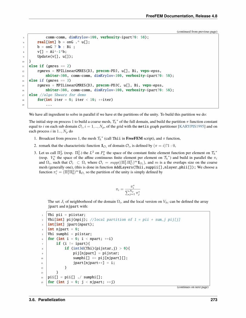
FreeFEM Documentation, Release 4.8
(continued from previous page)
5 comm=comm, dimKrylov=100, verbosity=ipart?0: 50);6 real[int] b = onG .* u[];7 b = onG ? b : Bi ;8 v[] = Ai^-1*b;9 Update(v[], u[]);
10 11 else if (gmres == 2)12 rgmres = MPILinearGMRES(DJ, precon=PDJ, u[], Bi, veps=epss,13 nbiter=300, comm=comm, dimKrylov=100, verbosity=ipart?0: 50);14 else if (gmres == 3)15 rgmres = MPILinearGMRES(DJ, precon=PDJC, u[], Bi, veps=epss,16 nbiter=300, comm=comm, dimKrylov=100, verbosity=ipart?0: 50);17 else //algo Shwarz for demo18 for(int iter = 0; iter < 10; ++iter)19 ...
We have all ingredient to solve in parallel if we have et the partitions of the unity. To build this partition we do:
The initial step on process 1 to build a coarse mesh, 𝒯ℎ* of the full domain, and build the partition 𝜋 function constantequal to 𝑖 on each sub domain 𝒪𝑖, 𝑖 = 1, .., 𝑁𝑝, of the grid with the metis graph partitioner [KARYPIS1995] and oneach process 𝑖 in 1.., 𝑁𝑝 do
1. Broadcast from process 1, the mesh 𝒯ℎ* (call Thii in FreeFEM script), and 𝜋 function,
2. remark that the characteristic function 1I𝒪𝑖of domain 𝒪𝑖, is defined by (𝜋 = 𝑖)?1 : 0,
3. Let us call Π2𝑃 (resp. Π2
𝑉 ) the 𝐿2 on 𝑃 *ℎ the space of the constant finite element function per element on 𝒯ℎ*
(resp. 𝑉 *ℎ the space of the affine continuous finite element per element on 𝒯ℎ*) and build in parallel the 𝜋𝑖
and Ω𝑖, such that 𝒪𝑖 ⊂ Ω𝑖 where 𝒪𝑖 = 𝑠𝑢𝑝𝑝((Π2𝑉 Π2
𝐶)𝑚1I𝑂𝑖), and 𝑚 is a the overlaps size on the coarse
mesh (generally one), (this is done in function AddLayers(Thii,suppii[],nlayer,phii[]); We choose afunction 𝜋*
𝑖 = (Π21Π2
0)𝑚1I𝒪𝑖so the partition of the unity is simply defined by
𝜋𝑖 =𝜋*𝑖∑𝑁𝑝
𝑗=1 𝜋*𝑗
The set 𝐽𝑖 of neighborhood of the domain Ω𝑖, and the local version on 𝑉ℎ𝑖 can be defined the arrayjpart and njpart with:
1 Vhi pii = piistar;2 Vhi[int] pij(npij); //local partition of 1 = pii + sum_j pij[j]3 int[int] jpart(npart);4 int njpart = 0;5 Vhi sumphi = piistar;6 for (int i = 0; i < npart; ++i)7 if (i != ipart)8 if (int3d(Thi)(pijstar,j) > 0)9 pij[njpart] = pijstar;
10 sumphi[] += pij[njpart][];11 jpart[njpart++] = i;12 13 14 pii[] = pii[] ./ sumphi[];15 for (int j = 0; j < njpart; ++j)
(continues on next page)
3.6. Parallelization 273
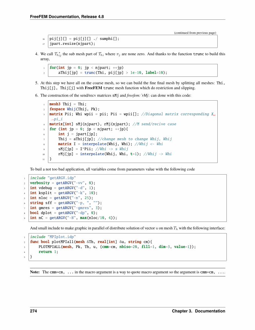
FreeFEM Documentation, Release 4.8
(continued from previous page)
16 pij[j][] = pij[j][] ./ sumphi[];17 jpart.resize(njpart);
4. We call 𝒯ℎ*𝑖𝑗 the sub mesh part of 𝒯ℎ𝑖 where 𝜋𝑗 are none zero. And thanks to the function trunc to build thisarray,
1 for(int jp = 0; jp < njpart; ++jp)2 aThij[jp] = trunc(Thi, pij[jp] > 1e-10, label=10);
5. At this step we have all on the coarse mesh, so we can build the fine final mesh by splitting all meshes: Thi,Thij[j], Thij[j] with FreeFEM trunc mesh function which do restriction and slipping.
6. The construction of the send/recv matrices sMj and freefem:`rMj: can done with this code:
1 mesh3 Thij = Thi;2 fespace Whij(Thij, Pk);3 matrix Pii; Whi wpii = pii; Pii = wpii[]; //Diagonal matrix corresponding X
→˓pi_i4 matrix[int] sMj(njpart), rMj(njpart); //M send/recive case5 for (int jp = 0; jp < njpart; ++jp)6 int j = jpart[jp];7 Thij = aThij[jp]; //change mesh to change Whij, Whij8 matrix I = interpolate(Whij, Whi); //Whij <- Whi9 sMj[jp] = I*Pii; //Whi -> s Whij
10 rMj[jp] = interpolate(Whij, Whi, t=1); //Whij -> Whi11
To buil a not too bad application, all variables come from parameters value with the following code
1 include "getARGV.idp"2 verbosity = getARGV("-vv", 0);3 int vdebug = getARGV("-d", 1);4 int ksplit = getARGV("-k", 10);5 int nloc = getARGV("-n", 25);6 string sff = getARGV("-p, ", "");7 int gmres = getARGV("-gmres", 3);8 bool dplot = getARGV("-dp", 0);9 int nC = getARGV("-N", max(nloc/10, 4));
And small include to make graphic in parallel of distribute solution of vector 𝑢 on mesh 𝑇ℎ with the following interface:
1 include "MPIplot.idp"2 func bool plotMPIall(mesh &Th, real[int] &u, string cm)3 PLOTMPIALL(mesh, Pk, Th, u, cmm=cm, nbiso=20, fill=1, dim=3, value=1);4 return 1;5
Note: The cmm=cm, ... in the macro argument is a way to quote macro argument so the argument is cmm=cm, ....
274 Chapter 3. Documentation
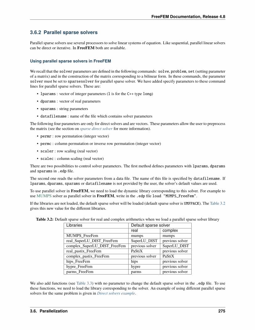
FreeFEM Documentation, Release 4.8
3.6.2 Parallel sparse solvers
Parallel sparse solvers use several processors to solve linear systems of equation. Like sequential, parallel linear solverscan be direct or iterative. In FreeFEM both are available.
Using parallel sparse solvers in FreeFEM
We recall that the solver parameters are defined in the following commands: solve, problem, set (setting parameterof a matrix) and in the construction of the matrix corresponding to a bilinear form. In these commands, the parametersolver must be set to sparsesolver for parallel sparse solver. We have added specify parameters to these commandlines for parallel sparse solvers. These are:
• lparams : vector of integer parameters (l is for the C++ type long)
• dparams : vector of real parameters
• sparams : string parameters
• datafilename : name of the file which contains solver parameters
The following four parameters are only for direct solvers and are vectors. These parameters allow the user to preprocessthe matrix (see the section on sparse direct solver for more information).
• permr : row permutation (integer vector)
• permc : column permutation or inverse row permutation (integer vector)
• scaler : row scaling (real vector)
• scalec : column scaling (real vector)
There are two possibilities to control solver parameters. The first method defines parameters with lparams, dparamsand sparams in .edp file.
The second one reads the solver parameters from a data file. The name of this file is specified by datafilename. Iflparams, dparams, sparams or datafilename is not provided by the user, the solver’s default values are used.
To use parallel solver in FreeFEM, we need to load the dynamic library corresponding to this solver. For example touse MUMPS solver as parallel solver in FreeFEM, write in the .edp file load "MUMPS_FreeFem".
If the libraries are not loaded, the default sparse solver will be loaded (default sparse solver is UMFPACK). The Table 3.2gives this new value for the different libraries.
Table 3.2: Default sparse solver for real and complex arithmetics when we load a parallel sparse solver libraryLibraries Default sparse solver
real complexMUMPS_FreeFem mumps mumpsreal_SuperLU_DIST_FreeFem SuperLU_DIST previous solvercomplex_SuperLU_DIST_FreeFem previous solver SuperLU_DISTreal_pastix_FreeFem PaStiX previous solvercomplex_pastix_FreeFem previous solver PaStiXhips_FreeFem hips previous solverhypre_FreeFem hypre previous solverparms_FreeFem parms previous solver
We also add functions (see Table 3.3) with no parameter to change the default sparse solver in the .edp file. To usethese functions, we need to load the library corresponding to the solver. An example of using different parallel sparsesolvers for the same problem is given in Direct solvers example.
3.6. Parallelization 275
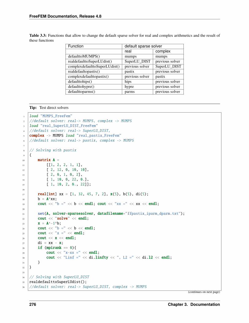
FreeFEM Documentation, Release 4.8
Table 3.3: Functions that allow to change the default sparse solver for real and complex arithmetics and the result ofthese functions
Function default sparse solverreal complex
defaulttoMUMPS() mumps mumpsrealdefaulttoSuperLUdist() SuperLU_DIST previous solvercomplexdefaulttoSuperLUdist() previous solver SuperLU_DISTrealdefaultopastix() pastix previous solvercomplexdefaulttopastix() previous solver pastixdefaulttohips() hips previous solverdefaulttohypre() hypre previous solverdefaulttoparms() parms previous solver
Tip: Test direct solvers
1 load "MUMPS_FreeFem"2 //default solver: real-> MUMPS, complex -> MUMPS3 load "real_SuperLU_DIST_FreeFem"4 //default solver: real-> SuperLU_DIST,5 complex -> MUMPS load "real_pastix_FreeFem"6 //default solver: real-> pastix, complex -> MUMPS7
8 // Solving with pastix9
10 matrix A =11 [[1, 2, 2, 1, 1],12 [ 2, 12, 0, 10, 10],13 [ 2, 0, 1, 0, 2],14 [ 1, 10, 0, 22, 0.],15 [ 1, 10, 2, 0., 22]];16
17 real[int] xx = [1, 32, 45, 7, 2], x(5), b(5), di(5);18 b = A*xx;19 cout << "b =" << b << endl; cout << "xx =" << xx << endl;20
21 set(A, solver=sparsesolver, datafilename="ffpastix_iparm_dparm.txt");22 cout << "solve" << endl;23 x = A^-1*b;24 cout << "b =" << b << endl;25 cout << "x =" << endl;26 cout << x << endl;27 di = xx - x;28 if (mpirank == 0)29 cout << "x-xx =" << endl;30 cout << "Linf =" << di.linfty << ", L2 =" << di.l2 << endl;31 32 33
34 // Solving with SuperLU_DIST35 realdefaulttoSuperLUdist();36 //default solver: real-> SuperLU_DIST, complex -> MUMPS
(continues on next page)
276 Chapter 3. Documentation
FreeFEM Documentation, Release 4.8
(continued from previous page)
37 38 matrix A =39 [[1, 2, 2, 1, 1],40 [ 2, 12, 0, 10, 10],41 [ 2, 0, 1, 0, 2],42 [ 1, 10, 0, 22, 0.],43 [ 1, 10, 2, 0., 22]];44
45 real[int] xx = [1, 32, 45, 7, 2], x(5), b(5), di(5);46 b = A*xx;47 cout << "b =" << b << endl;48 cout << "xx =" << xx << endl;49
50 set(A, solver=sparsesolver, datafilename="ffsuperlu_dist_fileparam.txt");51 cout << "solve" << endl;52 x = A^-1*b;53 cout << "b =" << b << endl;54 cout << "x =" << endl;55 cout << x << endl;56 di = xx - x;57 if (mpirank == 0)58 cout << "x-xx =" << endl;59 cout << "Linf =" << di.linfty << ", L2 =" << di.l2 << endl;60 61 62
63 // Solving with MUMPS64 defaulttoMUMPS();65 //default solver: real-> MUMPS, complex -> MUMPS66 67 matrix A =68 [[1, 2, 2, 1, 1],69 [ 2, 12, 0, 10, 10],70 [ 2, 0, 1, 0, 2],71 [ 1, 10, 0, 22, 0.],72 [ 1, 10, 2, 0., 22]];73
74 real[int] xx = [1, 32, 45, 7, 2], x(5), b(5), di(5);75 b = A*xx;76 cout << "b =" << b << endl;77 cout << "xx =" << xx << endl;78
79 set(A, solver=sparsesolver, datafilename="ffmumps_fileparam.txt");80 cout << "solving solution" << endl;81 x = A^-1*b;82 cout << "b =" << b << endl;83 cout << "x =" << endl;84 cout << x << endl;85 di = xx - x;86 if (mpirank == 0)87 cout << "x-xx =" << endl;88 cout << "Linf =" << di.linfty << ", L2" << di.l2 << endl;
(continues on next page)
3.6. Parallelization 277
FreeFEM Documentation, Release 4.8
(continued from previous page)
89 90
Sparse direct solver
In this section, we present the sparse direct solvers interfaced with FreeFEM.
MUMPS solver
MUltifrontal Massively Parallel Solver (MUMPS) is an open-source library.
This package solves linear system of the form 𝐴 𝑥 = 𝑏 where 𝐴 is a square sparse matrix with a direct method. Thesquare matrix considered in MUMPS can be either unsymmetric, symmetric positive definite or general symmetric.
The method implemented in MUMPS is a direct method based on a multifrontal approach. It constructs a directfactorization 𝐴 = 𝐿 𝑈 , 𝐴 = 𝐿𝑡 𝐷 𝐿 depending of the symmetry of the matrix 𝐴.
MUMPS uses the following libraries :• BLAS,
• BLACS,
• ScaLAPACK.
Warning: MUMPS does not solve linear system with a rectangular matrix.
MUMPS parameters:There are four input parameters in MUMPS. Two integers SYM and PAR, a vector of integer of size 40 INCTL and avector of real of size 15 CNTL.
The first parameter gives the type of the matrix: 0 for unsymmetric matrix, 1 for symmetric positive matrix and 2 forgeneral symmetric.
The second parameter defined if the host processor work during the factorization and solves steps : PAR=1 host processorworking and PAR=0 host processor not working.
The parameter INCTL and CNTL is the control parameter of MUMPS. The vectors ICNTL and CNTL in MUMPS becomeswith index 1 like vector in Fortran. For more details see the MUMPS user’s guide.
We describe now some elements of the main parameters of ICNTL for MUMPS.
• Input matrix parameter The input matrix is controlled by parameters ICNTL(5) and ICNTL(18). Thematrix format (resp. matrix pattern and matrix entries) are controlled by INCTL(5) (resp. INCTL(18)).
The different values of ICNTL(5) are 0 for assembled format and 1 for element format. In the currentrelease of FreeFEM, we consider that FE matrix or matrix is storage in assembled format. Therefore,INCTL(5) is treated as 0 value.
The main option for ICNTL(18): INCLTL(18)=0 centrally on the host processor, ICNTL(18)=3 dis-tributed the input matrix pattern and the entries (recommended option for distributed matrix by developerof MUMPS). For other values of ICNTL(18) see the MUMPS user’s guide. These values can be used alsoin FreeFEM.
The default option implemented in FreeFEM are ICNTL(5)=0 and ICNTL(18)=0.
278 Chapter 3. Documentation
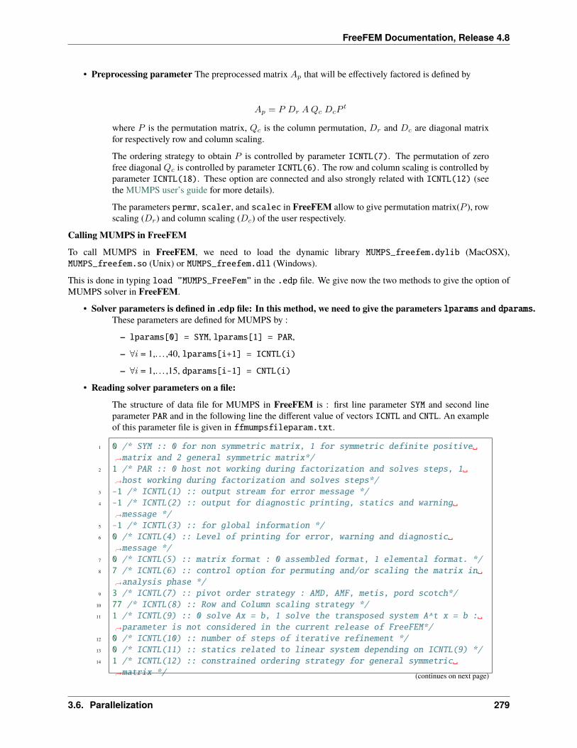
FreeFEM Documentation, Release 4.8
• Preprocessing parameter The preprocessed matrix 𝐴𝑝 that will be effectively factored is defined by
𝐴𝑝 = 𝑃 𝐷𝑟 𝐴𝑄𝑐 𝐷𝑐𝑃𝑡
where 𝑃 is the permutation matrix, 𝑄𝑐 is the column permutation, 𝐷𝑟 and 𝐷𝑐 are diagonal matrixfor respectively row and column scaling.
The ordering strategy to obtain 𝑃 is controlled by parameter ICNTL(7). The permutation of zerofree diagonal 𝑄𝑐 is controlled by parameter ICNTL(6). The row and column scaling is controlled byparameter ICNTL(18). These option are connected and also strongly related with ICNTL(12) (seethe MUMPS user’s guide for more details).
The parameters permr, scaler, and scalec in FreeFEM allow to give permutation matrix(𝑃 ), rowscaling (𝐷𝑟) and column scaling (𝐷𝑐) of the user respectively.
Calling MUMPS in FreeFEMTo call MUMPS in FreeFEM, we need to load the dynamic library MUMPS_freefem.dylib (MacOSX),MUMPS_freefem.so (Unix) or MUMPS_freefem.dll (Windows).
This is done in typing load "MUMPS_FreeFem" in the .edp file. We give now the two methods to give the option ofMUMPS solver in FreeFEM.
• Solver parameters is defined in .edp file: In this method, we need to give the parameters lparams and dparams.These parameters are defined for MUMPS by :
– lparams[0] = SYM, lparams[1] = PAR,
– ∀𝑖 = 1,. . . ,40, lparams[i+1] = ICNTL(i)
– ∀𝑖 = 1,. . . ,15, dparams[i-1] = CNTL(i)
• Reading solver parameters on a file:The structure of data file for MUMPS in FreeFEM is : first line parameter SYM and second lineparameter PAR and in the following line the different value of vectors ICNTL and CNTL. An exampleof this parameter file is given in ffmumpsfileparam.txt.
1 0 /* SYM :: 0 for non symmetric matrix, 1 for symmetric definite positive→˓matrix and 2 general symmetric matrix*/
2 1 /* PAR :: 0 host not working during factorization and solves steps, 1→˓host working during factorization and solves steps*/
3 -1 /* ICNTL(1) :: output stream for error message */4 -1 /* ICNTL(2) :: output for diagnostic printing, statics and warning
→˓message */5 -1 /* ICNTL(3) :: for global information */6 0 /* ICNTL(4) :: Level of printing for error, warning and diagnostic
→˓message */7 0 /* ICNTL(5) :: matrix format : 0 assembled format, 1 elemental format. */8 7 /* ICNTL(6) :: control option for permuting and/or scaling the matrix in
→˓analysis phase */9 3 /* ICNTL(7) :: pivot order strategy : AMD, AMF, metis, pord scotch*/
10 77 /* ICNTL(8) :: Row and Column scaling strategy */11 1 /* ICNTL(9) :: 0 solve Ax = b, 1 solve the transposed system A^t x = b :
→˓parameter is not considered in the current release of FreeFEM*/12 0 /* ICNTL(10) :: number of steps of iterative refinement */13 0 /* ICNTL(11) :: statics related to linear system depending on ICNTL(9) */14 1 /* ICNTL(12) :: constrained ordering strategy for general symmetric
→˓matrix */ (continues on next page)
3.6. Parallelization 279
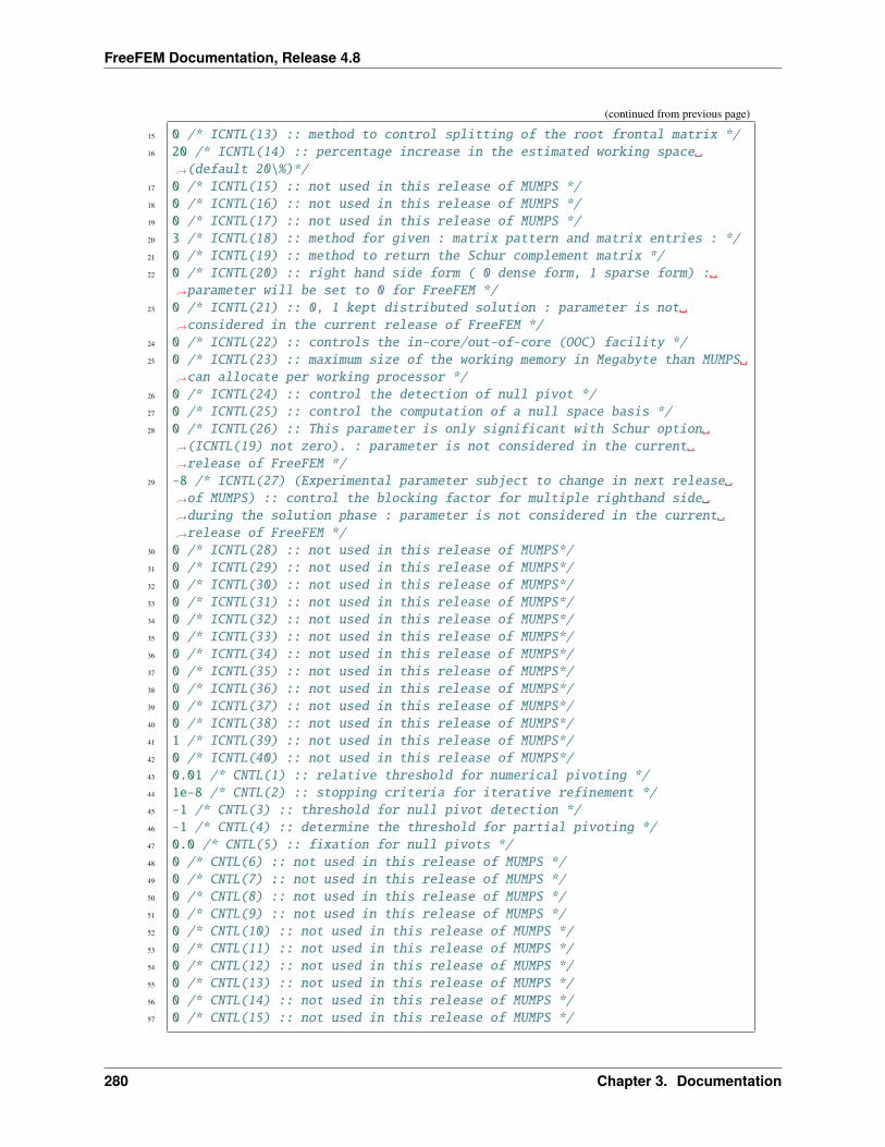
FreeFEM Documentation, Release 4.8
(continued from previous page)
15 0 /* ICNTL(13) :: method to control splitting of the root frontal matrix */16 20 /* ICNTL(14) :: percentage increase in the estimated working space
→˓(default 20\%)*/17 0 /* ICNTL(15) :: not used in this release of MUMPS */18 0 /* ICNTL(16) :: not used in this release of MUMPS */19 0 /* ICNTL(17) :: not used in this release of MUMPS */20 3 /* ICNTL(18) :: method for given : matrix pattern and matrix entries : */21 0 /* ICNTL(19) :: method to return the Schur complement matrix */22 0 /* ICNTL(20) :: right hand side form ( 0 dense form, 1 sparse form) :
→˓parameter will be set to 0 for FreeFEM */23 0 /* ICNTL(21) :: 0, 1 kept distributed solution : parameter is not
→˓considered in the current release of FreeFEM */24 0 /* ICNTL(22) :: controls the in-core/out-of-core (OOC) facility */25 0 /* ICNTL(23) :: maximum size of the working memory in Megabyte than MUMPS
→˓can allocate per working processor */26 0 /* ICNTL(24) :: control the detection of null pivot */27 0 /* ICNTL(25) :: control the computation of a null space basis */28 0 /* ICNTL(26) :: This parameter is only significant with Schur option
→˓(ICNTL(19) not zero). : parameter is not considered in the current→˓release of FreeFEM */
29 -8 /* ICNTL(27) (Experimental parameter subject to change in next release→˓of MUMPS) :: control the blocking factor for multiple righthand side→˓during the solution phase : parameter is not considered in the current→˓release of FreeFEM */
30 0 /* ICNTL(28) :: not used in this release of MUMPS*/31 0 /* ICNTL(29) :: not used in this release of MUMPS*/32 0 /* ICNTL(30) :: not used in this release of MUMPS*/33 0 /* ICNTL(31) :: not used in this release of MUMPS*/34 0 /* ICNTL(32) :: not used in this release of MUMPS*/35 0 /* ICNTL(33) :: not used in this release of MUMPS*/36 0 /* ICNTL(34) :: not used in this release of MUMPS*/37 0 /* ICNTL(35) :: not used in this release of MUMPS*/38 0 /* ICNTL(36) :: not used in this release of MUMPS*/39 0 /* ICNTL(37) :: not used in this release of MUMPS*/40 0 /* ICNTL(38) :: not used in this release of MUMPS*/41 1 /* ICNTL(39) :: not used in this release of MUMPS*/42 0 /* ICNTL(40) :: not used in this release of MUMPS*/43 0.01 /* CNTL(1) :: relative threshold for numerical pivoting */44 1e-8 /* CNTL(2) :: stopping criteria for iterative refinement */45 -1 /* CNTL(3) :: threshold for null pivot detection */46 -1 /* CNTL(4) :: determine the threshold for partial pivoting */47 0.0 /* CNTL(5) :: fixation for null pivots */48 0 /* CNTL(6) :: not used in this release of MUMPS */49 0 /* CNTL(7) :: not used in this release of MUMPS */50 0 /* CNTL(8) :: not used in this release of MUMPS */51 0 /* CNTL(9) :: not used in this release of MUMPS */52 0 /* CNTL(10) :: not used in this release of MUMPS */53 0 /* CNTL(11) :: not used in this release of MUMPS */54 0 /* CNTL(12) :: not used in this release of MUMPS */55 0 /* CNTL(13) :: not used in this release of MUMPS */56 0 /* CNTL(14) :: not used in this release of MUMPS */57 0 /* CNTL(15) :: not used in this release of MUMPS */
280 Chapter 3. Documentation
FreeFEM Documentation, Release 4.8
If no solver parameter is given, we used default option of MUMPS solver.
Tip: MUMPS example
A simple example of calling MUMPS in FreeFEM with this two methods is given in the Test solver MUMPS example.
SuperLU distributed solver
The package SuperLU_DIST solves linear systems using LU factorization. It is a free scientific library
This library provides functions to handle square or rectangular matrix in real and complex arithmetics. The methodimplemented in SuperLU_DIST is a supernodal method. New release of this package includes a parallel symbolicfactorization. This scientific library is written in C and MPI for communications.
SuperLU_DIST parameters:We describe now some parameters of SuperLU_DIST. The SuperLU_DIST library use a 2D-logical process group.This process grid is specified by 𝑛𝑝𝑟𝑜𝑤 (process row) and 𝑛𝑝𝑐𝑜𝑙 (process column) such that 𝑁𝑝 = 𝑛𝑝𝑟𝑜𝑤 𝑛𝑝𝑐𝑜𝑙where 𝑁𝑝 is the number of all process allocated for SuperLU_DIST.
The input matrix parameters is controlled by “matrix=” in sparams for internal parameter or in the third line of pa-rameters file. The different value are
• matrix=assembled global matrix are available on all process
• matrix=distributedglobal The global matrix is distributed among all the process
• matrix=distributed The input matrix is distributed (not yet implemented)
The option arguments of SuperLU_DIST are described in the section Users-callable routine of the SuperLU users’guide.
The parameter Fact and TRANS are specified in FreeFEM interfaces to SuperLU_DIST during the different steps. Forthis reason, the value given by the user for this option is not considered.
The factorization LU is calculated in SuperLU_DIST on the matrix 𝐴𝑝.
𝐴𝑝 = 𝑃𝑐 𝑃𝑟 𝐷𝑟 𝐴𝐷𝑐 𝑃𝑡𝑐
where𝑃𝑐 and𝑃𝑟 is the row and column permutation matrix respectively,𝐷𝑟 and𝐷𝑐 are diagonal matrix for respectivelyrow and column scaling.
The option argument RowPerm (resp. ColPerm) control the row (resp. column) permutation matrix. 𝐷𝑟 and 𝐷𝑐 iscontrolled by the parameter DiagScale.
The parameter permr, permc, scaler, and scalec in FreeFEM is provided to give row permutation, column permu-tation, row scaling and column scaling of the user respectively.
The other parameters for LU factorization are ParSymFact and ReplaceTinyPivot. The parallel symbolic factor-ization works only on a power of two processes and need the ParMetis ordering. The default option argument ofSuperLU_DIST are given in the file ffsuperlu_dist_fileparam.txt.
Calling SuperLU_DIST in FreeFEMTo call SuperLU_DIST in FreeFEM, we need to load the library dynamic correspond to interface. This done bythe following line load "real_superlu _DIST_FreeFem" (resp. load "complex_superlu_DIST_FreeFem")for real (resp. complex) arithmetics in the file .edp.
Solver parameters is defined in .edp file:
3.6. Parallelization 281
FreeFEM Documentation, Release 4.8
To call SuperLU_DIST with internal parameter, we used the parameters sparams. The value of parameters of Su-perLU_DIST in sparams are defined by :
• nprow=1,
• npcol=1,
• matrix= distributedgloba,
• Fact= DOFACT,
• Equil=NO,
• ParSymbFact=NO,
• ColPerm= MMD_AT_PLUS_A,
• RowPerm= LargeDiag,
• DiagPivotThresh=1.0,
• IterRefine=DOUBLE,
• Trans=NOTRANS,
• ReplaceTinyPivot=NO,
• SolveInitialized=NO,
• PrintStat=NO,
• DiagScale=NOEQUIL
This value correspond to the parameter in the file ffsuperlu_dist_fileparam.txt. If one parameter is not specifiedby the user, we take the default value of SuperLU_DIST.
Reading solver parameters on a file: The structure of data file for SuperLU_DIST in FreeFEM is given in the fileffsuperlu_dist_fileparam.txt (default value of the FreeFEM interface).
1 1 /* nprow : integer value */2 1 /* npcol : integer value */3 distributedglobal /* matrix input : assembled, distributedglobal, distributed */4 DOFACT /* Fact : DOFACT, SamePattern, SamePattern_SameRowPerm, FACTORED */5 NO /* Equil : NO, YES */6 NO /* ParSymbFact : NO, YES */7 MMD_AT_PLUS_A /* ColPerm : NATURAL, MMD_AT_PLUS_A, MMD_ATA, METIS_AT_PLUS_A, PARMETIS,
→˓MY_PERMC */8 LargeDiag /* RowPerm : NOROWPERM, LargeDiag, MY_PERMR */9 1.0 /* DiagPivotThresh : real value */
10 DOUBLE /* IterRefine : NOREFINE, SINGLE, DOUBLE, EXTRA */11 NOTRANS /* Trans : NOTRANS, TRANS, CONJ*/12 NO /* ReplaceTinyPivot : NO, YES*/13 NO /* SolveInitialized : NO, YES*/14 NO /* RefineInitialized : NO, YES*/15 NO /* PrintStat : NO, YES*/16 NOEQUIL /* DiagScale : NOEQUIL, ROW, COL, BOTH*/
If no solver parameter is given, we used default option of SuperLU_DIST solver.
Tip: A simple example of calling SuperLU_DIST in FreeFEM with this two methods is given in the Solver su-perLU_DIST example.
282 Chapter 3. Documentation
FreeFEM Documentation, Release 4.8
PaStiX solver
PaStiX (Parallel Sparse matrix package) is a free scientific library under CECILL-C license. This package solves sparselinear system with a direct and block ILU(k) iterative methods. his solver can be applied to a real or complex matrixwith a symmetric pattern.
PaStiX parameters:The input matrix parameter of FreeFEM depend on PaStiX interface. matrix = assembled for non distributedmatrix. It is the same parameter for SuperLU_DIST.
There are four parameters in PaStiX : iparm, dparm, perm and invp. These parameters are respectively the integerparameters (vector of size 64), real parameters (vector of size 64), permutation matrix and inverse permutation matrixrespectively. iparm and dparm vectors are described in PaStiX RefCard.
The parameters permr and permc in FreeFEM are provided to give permutation matrix and inverse permutation matrixof the user respectively.
Solver parameters defined in .edp file:To call PaStiX in FreeFEM in this case, we need to specify the parameters lparams and dparams. These parametersare defined by :
∀𝑖 = 0,. . . ,63, lparams[i] = iparm[i].
∀𝑖 = 0,. . . ,63, dparams[i] = dparm[i].
Reading solver parameters on a file:The structure of data file for PaStiX parameters in FreeFEM is: first line structure parameters of the matrix and in thefollowing line the value of vectors iparm and dparm in this order.
1 assembled /* matrix input :: assembled, distributed global and distributed */2 iparm[0]3 iparm[1]4 ...5 ...6 iparm[63]7 dparm[0]8 dparm[1]9 ...
10 ...11 dparm[63]
An example of this file parameter is given in ffpastix_iparm_dparm.txt with a description of these parameters.This file is obtained with the example file iparm.txt and dparm.txt including in the PaStiX package.
If no solver parameter is given, we use the default option of PaStiX solver.
Tip: A simple example of calling PaStiX in FreeFEM with this two methods is given in the Solver PaStiX example.
In Table 3.4, we recall the different matrix considering in the different direct solvers.
Table 3.4: Type of matrix used by the different direct sparse solver
3.6. Parallelization 283
FreeFEM Documentation, Release 4.8
direct solver square matrix rectangular matrixsym sym pattern unsym sym sym pattern unsym
SuperLU_DIST yes yes yes yes yes yesMUMPS yes yes yes no no noPastix yes yes no no no no
Parallel sparse iterative solver
Concerning iterative solvers, we have chosen pARMS, HIPS and Hypre.
Each software implements a different type of parallel preconditioner.
So, pARMS implements algebraic domain decomposition preconditioner type such as additive Schwartz [CAI1989]and interface method; while HIPS implement hierarchical incomplete factorization and finally HYPRE implementsmultilevel preconditioner are AMG(Algebraic MultiGrid) and parallel approximated inverse.
To use one of these programs in FreeFEM, you have to install it independently of FreeFEM. It is also necessary toinstall the MPI communication library which is essential for communication between the processors and, in some cases,software partitioning graphs like METIS or Scotch.
All this preconditioners are used with Krylov subspace methods accelerators.
Krylov subspace methods are iterative methods which consist in finding a solution 𝑥 of linear system 𝐴𝑥 = 𝑏 insidethe affine space 𝑥0 + 𝐾𝑚 by imposing that 𝑏 − 𝐴𝑥⊥ℒ𝑚, where 𝐾𝑚 is Krylov subspace of dimension 𝑚 defined by𝐾𝑚 = 𝑟0, 𝐴𝑟0, 𝐴2𝑟0, ..., 𝐴
𝑚−1𝑟0 and ℒ𝑚 is another subspace of dimension 𝑚 which depends on type of Krylovsubspace. For example in GMRES, ℒ𝑚 = 𝐴𝐾𝑚.
We realized an interface which is easy to use, so that the call of these different softwares in FreeFEM is done in thesame way. You just have to load the solver and then specify the parameters to apply to the specific solvers. In the restof this chapter, when we talk about Krylov subspace methods we mean one among GMRES, CG and BICGSTAB.
pARMS solver
pARMS (parallel Algebraic Multilevel Solver) is a software developed by Youssef Saad and al at University of Min-nesota.
This software is specialized in the resolution of large sparse non symmetric linear systems of equation. Solvers devel-oped in pARMS are of type “Krylov’s subspace”.
It consists of variants of GMRES like FGMRES (Flexible GMRES), DGMRES (Deflated GMRES) [SAAD2003] andBICGSTAB. pARMS also implements parallel preconditioner like RAS (Restricted Additive Schwarz) [CAI1989] andSchur Complement type preconditioner.
All these parallel preconditioners are based on the principle of domain decomposition. Thus, the matrix𝐴 is partitionedinto sub matrices 𝐴𝑖(𝑖 = 1, ..., 𝑝) where p represents the number of partitions one needs. The union of 𝐴𝑖 forms theoriginal matrix. The solution of the overall system is obtained by solving the local systems on 𝐴𝑖 (see [SMITH1996]).Therefore, a distinction is made between iterations on 𝐴 and the local iterations on 𝐴𝑖.
To solve the local problem on 𝐴𝑖 there are several preconditioners as ilut (Incomplete LU with threshold), iluk (In-complete LU with level of fill in) and ARMS (Algebraic Recursive Multilevel Solver).
Tip: Default parameters
1 load "parms_FreeFem" //Tell FreeFem that you will use pARMS2
3 // Mesh(continues on next page)
284 Chapter 3. Documentation
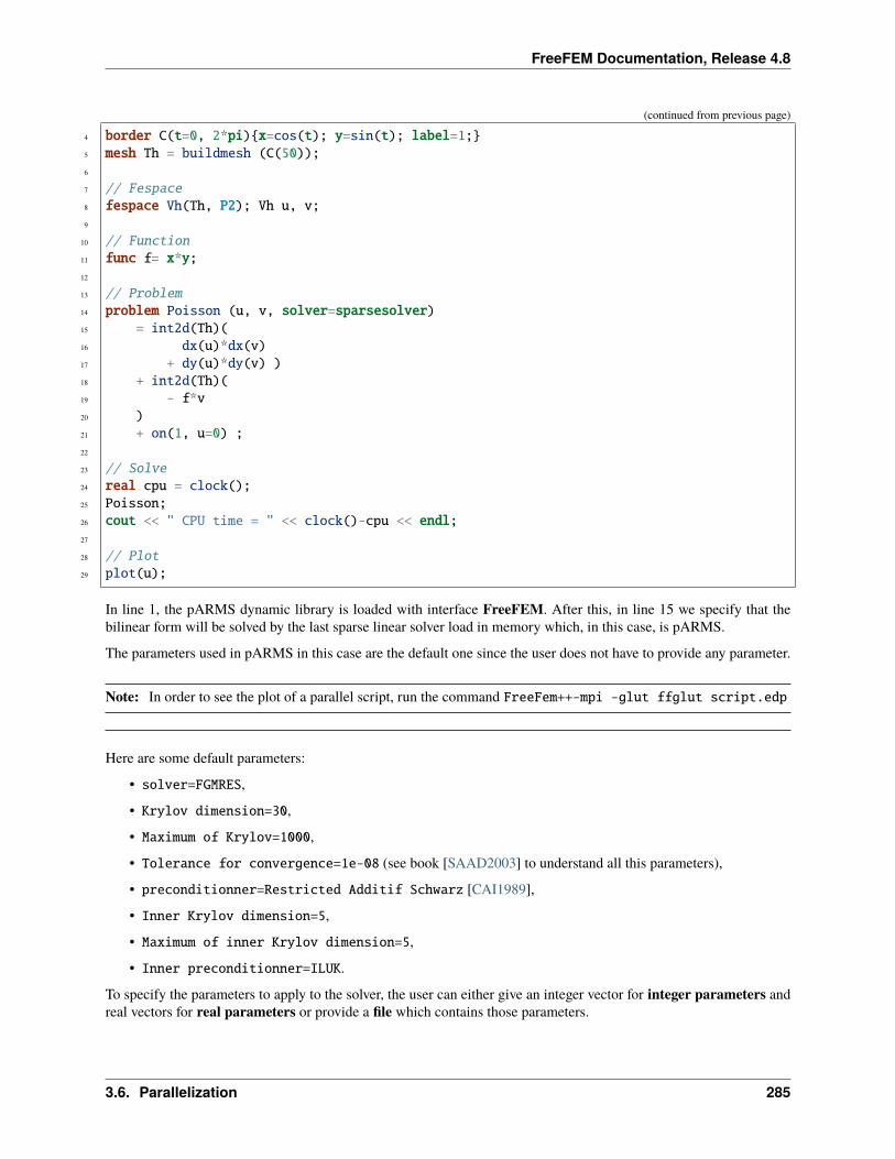
FreeFEM Documentation, Release 4.8
(continued from previous page)
4 border C(t=0, 2*pi)x=cos(t); y=sin(t); label=1;5 mesh Th = buildmesh (C(50));6
7 // Fespace8 fespace Vh(Th, P2); Vh u, v;9
10 // Function11 func f= x*y;12
13 // Problem14 problem Poisson (u, v, solver=sparsesolver)15 = int2d(Th)(16 dx(u)*dx(v)17 + dy(u)*dy(v) )18 + int2d(Th)(19 - f*v20 )21 + on(1, u=0) ;22
23 // Solve24 real cpu = clock();25 Poisson;26 cout << " CPU time = " << clock()-cpu << endl;27
28 // Plot29 plot(u);
In line 1, the pARMS dynamic library is loaded with interface FreeFEM. After this, in line 15 we specify that thebilinear form will be solved by the last sparse linear solver load in memory which, in this case, is pARMS.
The parameters used in pARMS in this case are the default one since the user does not have to provide any parameter.
Note: In order to see the plot of a parallel script, run the command FreeFem++-mpi -glut ffglut script.edp
Here are some default parameters:
• solver=FGMRES,
• Krylov dimension=30,
• Maximum of Krylov=1000,
• Tolerance for convergence=1e-08 (see book [SAAD2003] to understand all this parameters),
• preconditionner=Restricted Additif Schwarz [CAI1989],
• Inner Krylov dimension=5,
• Maximum of inner Krylov dimension=5,
• Inner preconditionner=ILUK.
To specify the parameters to apply to the solver, the user can either give an integer vector for integer parameters andreal vectors for real parameters or provide a file which contains those parameters.
3.6. Parallelization 285
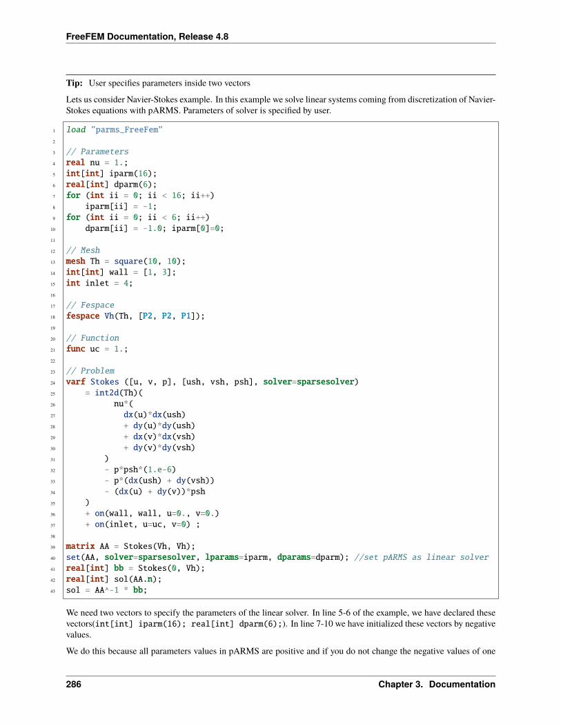
FreeFEM Documentation, Release 4.8
Tip: User specifies parameters inside two vectors
Lets us consider Navier-Stokes example. In this example we solve linear systems coming from discretization of Navier-Stokes equations with pARMS. Parameters of solver is specified by user.
1 load "parms_FreeFem"2
3 // Parameters4 real nu = 1.;5 int[int] iparm(16);6 real[int] dparm(6);7 for (int ii = 0; ii < 16; ii++)8 iparm[ii] = -1;9 for (int ii = 0; ii < 6; ii++)
10 dparm[ii] = -1.0; iparm[0]=0;11
12 // Mesh13 mesh Th = square(10, 10);14 int[int] wall = [1, 3];15 int inlet = 4;16
17 // Fespace18 fespace Vh(Th, [P2, P2, P1]);19
20 // Function21 func uc = 1.;22
23 // Problem24 varf Stokes ([u, v, p], [ush, vsh, psh], solver=sparsesolver)25 = int2d(Th)(26 nu*(27 dx(u)*dx(ush)28 + dy(u)*dy(ush)29 + dx(v)*dx(vsh)30 + dy(v)*dy(vsh)31 )32 - p*psh*(1.e-6)33 - p*(dx(ush) + dy(vsh))34 - (dx(u) + dy(v))*psh35 )36 + on(wall, wall, u=0., v=0.)37 + on(inlet, u=uc, v=0) ;38
39 matrix AA = Stokes(Vh, Vh);40 set(AA, solver=sparsesolver, lparams=iparm, dparams=dparm); //set pARMS as linear solver41 real[int] bb = Stokes(0, Vh);42 real[int] sol(AA.n);43 sol = AA^-1 * bb;
We need two vectors to specify the parameters of the linear solver. In line 5-6 of the example, we have declared thesevectors(int[int] iparm(16); real[int] dparm(6);). In line 7-10 we have initialized these vectors by negativevalues.
We do this because all parameters values in pARMS are positive and if you do not change the negative values of one
286 Chapter 3. Documentation
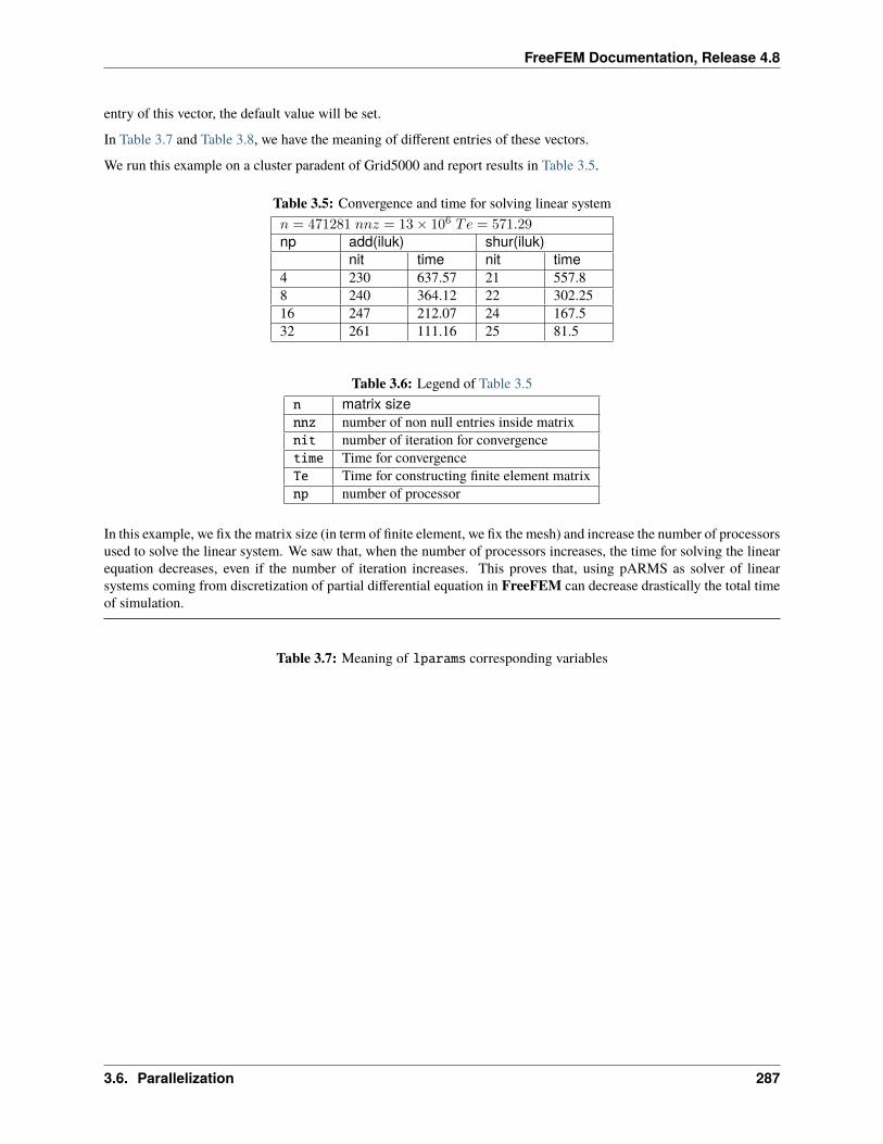
FreeFEM Documentation, Release 4.8
entry of this vector, the default value will be set.
In Table 3.7 and Table 3.8, we have the meaning of different entries of these vectors.
We run this example on a cluster paradent of Grid5000 and report results in Table 3.5.
Table 3.5: Convergence and time for solving linear system𝑛 = 471281 𝑛𝑛𝑧 = 13× 106 𝑇𝑒 = 571.29np add(iluk) shur(iluk)
nit time nit time4 230 637.57 21 557.88 240 364.12 22 302.2516 247 212.07 24 167.532 261 111.16 25 81.5
Table 3.6: Legend of Table 3.5n matrix sizennz number of non null entries inside matrixnit number of iteration for convergencetime Time for convergenceTe Time for constructing finite element matrixnp number of processor
In this example, we fix the matrix size (in term of finite element, we fix the mesh) and increase the number of processorsused to solve the linear system. We saw that, when the number of processors increases, the time for solving the linearequation decreases, even if the number of iteration increases. This proves that, using pARMS as solver of linearsystems coming from discretization of partial differential equation in FreeFEM can decrease drastically the total timeof simulation.
Table 3.7: Meaning of lparams corresponding variables
3.6. Parallelization 287
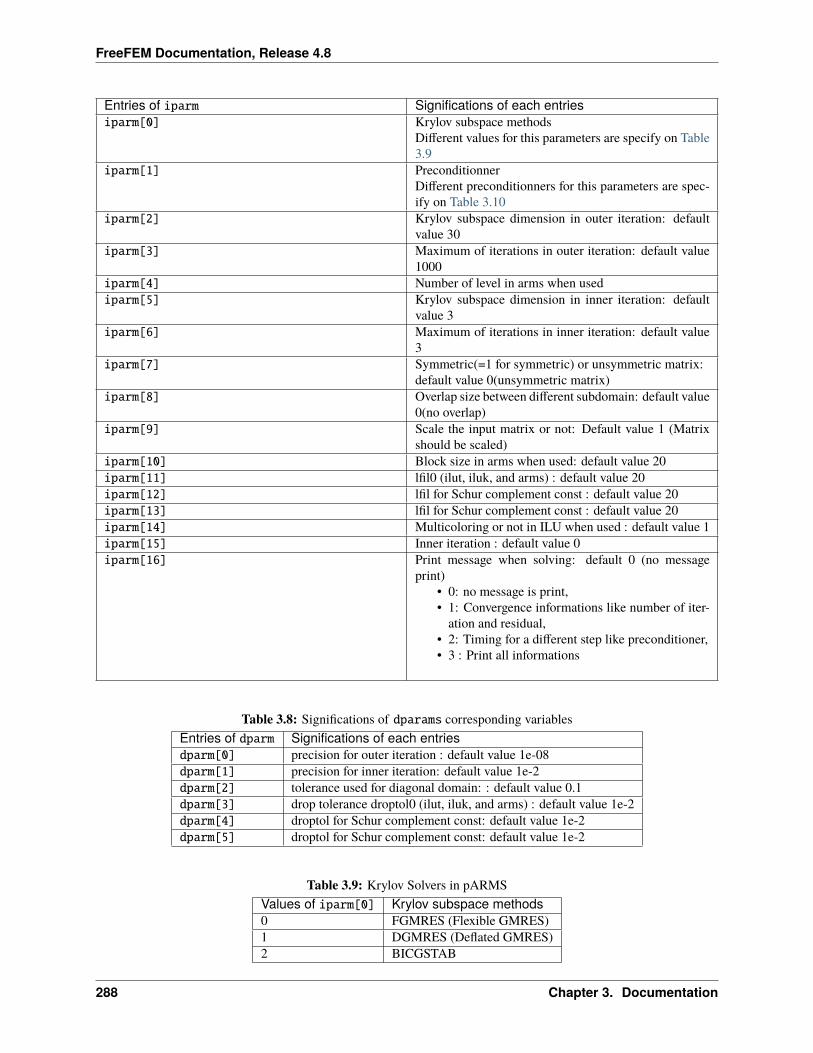
FreeFEM Documentation, Release 4.8
Entries of iparm Significations of each entriesiparm[0] Krylov subspace methods
Different values for this parameters are specify on Table3.9
iparm[1] PreconditionnerDifferent preconditionners for this parameters are spec-ify on Table 3.10
iparm[2] Krylov subspace dimension in outer iteration: defaultvalue 30
iparm[3] Maximum of iterations in outer iteration: default value1000
iparm[4] Number of level in arms when usediparm[5] Krylov subspace dimension in inner iteration: default
value 3iparm[6] Maximum of iterations in inner iteration: default value
3iparm[7] Symmetric(=1 for symmetric) or unsymmetric matrix:
default value 0(unsymmetric matrix)iparm[8] Overlap size between different subdomain: default value
0(no overlap)iparm[9] Scale the input matrix or not: Default value 1 (Matrix
should be scaled)iparm[10] Block size in arms when used: default value 20iparm[11] lfil0 (ilut, iluk, and arms) : default value 20iparm[12] lfil for Schur complement const : default value 20iparm[13] lfil for Schur complement const : default value 20iparm[14] Multicoloring or not in ILU when used : default value 1iparm[15] Inner iteration : default value 0iparm[16] Print message when solving: default 0 (no message
print)• 0: no message is print,• 1: Convergence informations like number of iter-
ation and residual,• 2: Timing for a different step like preconditioner,• 3 : Print all informations
Table 3.8: Significations of dparams corresponding variablesEntries of dparm Significations of each entriesdparm[0] precision for outer iteration : default value 1e-08dparm[1] precision for inner iteration: default value 1e-2dparm[2] tolerance used for diagonal domain: : default value 0.1dparm[3] drop tolerance droptol0 (ilut, iluk, and arms) : default value 1e-2dparm[4] droptol for Schur complement const: default value 1e-2dparm[5] droptol for Schur complement const: default value 1e-2
Table 3.9: Krylov Solvers in pARMSValues of iparm[0] Krylov subspace methods0 FGMRES (Flexible GMRES)1 DGMRES (Deflated GMRES)2 BICGSTAB
288 Chapter 3. Documentation
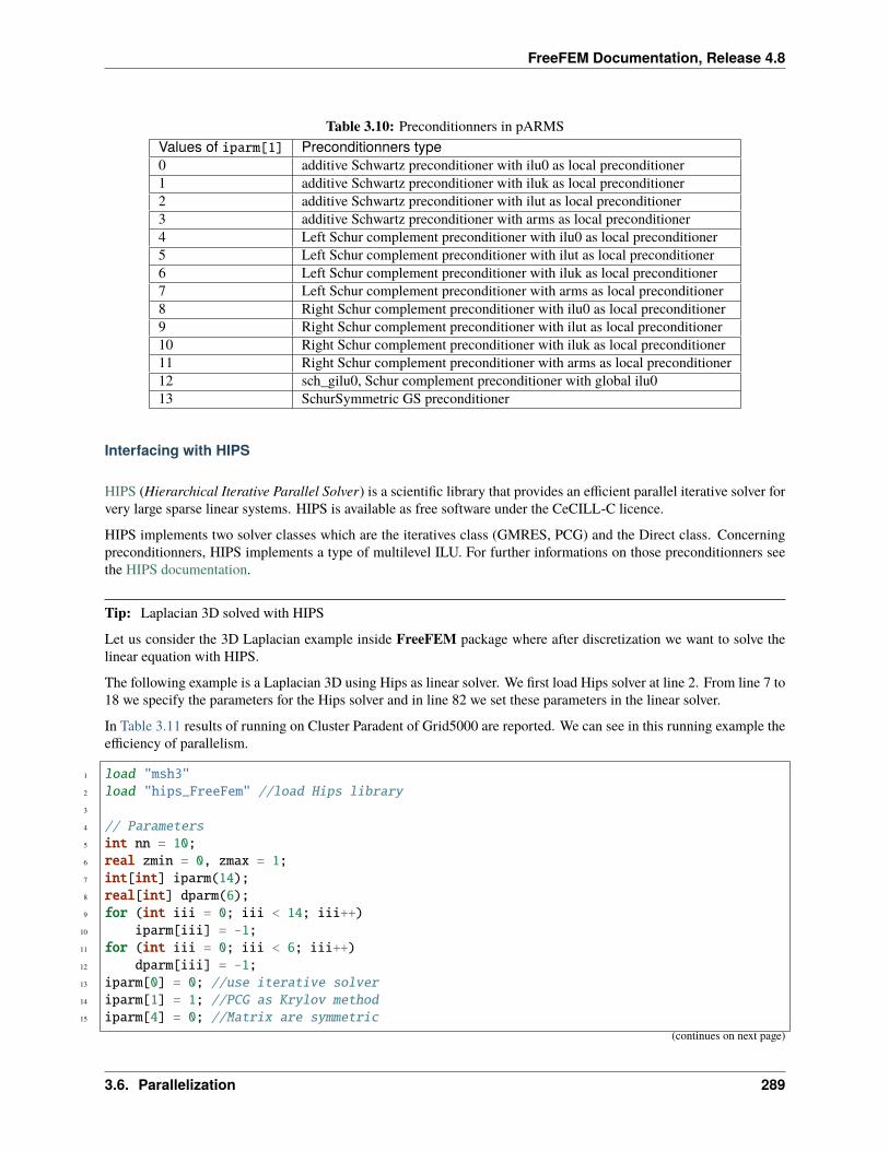
FreeFEM Documentation, Release 4.8
Table 3.10: Preconditionners in pARMSValues of iparm[1] Preconditionners type0 additive Schwartz preconditioner with ilu0 as local preconditioner1 additive Schwartz preconditioner with iluk as local preconditioner2 additive Schwartz preconditioner with ilut as local preconditioner3 additive Schwartz preconditioner with arms as local preconditioner4 Left Schur complement preconditioner with ilu0 as local preconditioner5 Left Schur complement preconditioner with ilut as local preconditioner6 Left Schur complement preconditioner with iluk as local preconditioner7 Left Schur complement preconditioner with arms as local preconditioner8 Right Schur complement preconditioner with ilu0 as local preconditioner9 Right Schur complement preconditioner with ilut as local preconditioner10 Right Schur complement preconditioner with iluk as local preconditioner11 Right Schur complement preconditioner with arms as local preconditioner12 sch_gilu0, Schur complement preconditioner with global ilu013 SchurSymmetric GS preconditioner
Interfacing with HIPS
HIPS (Hierarchical Iterative Parallel Solver) is a scientific library that provides an efficient parallel iterative solver forvery large sparse linear systems. HIPS is available as free software under the CeCILL-C licence.
HIPS implements two solver classes which are the iteratives class (GMRES, PCG) and the Direct class. Concerningpreconditionners, HIPS implements a type of multilevel ILU. For further informations on those preconditionners seethe HIPS documentation.
Tip: Laplacian 3D solved with HIPS
Let us consider the 3D Laplacian example inside FreeFEM package where after discretization we want to solve thelinear equation with HIPS.
The following example is a Laplacian 3D using Hips as linear solver. We first load Hips solver at line 2. From line 7 to18 we specify the parameters for the Hips solver and in line 82 we set these parameters in the linear solver.
In Table 3.11 results of running on Cluster Paradent of Grid5000 are reported. We can see in this running example theefficiency of parallelism.
1 load "msh3"2 load "hips_FreeFem" //load Hips library3
4 // Parameters5 int nn = 10;6 real zmin = 0, zmax = 1;7 int[int] iparm(14);8 real[int] dparm(6);9 for (int iii = 0; iii < 14; iii++)
10 iparm[iii] = -1;11 for (int iii = 0; iii < 6; iii++)12 dparm[iii] = -1;13 iparm[0] = 0; //use iterative solver14 iparm[1] = 1; //PCG as Krylov method15 iparm[4] = 0; //Matrix are symmetric
(continues on next page)
3.6. Parallelization 289
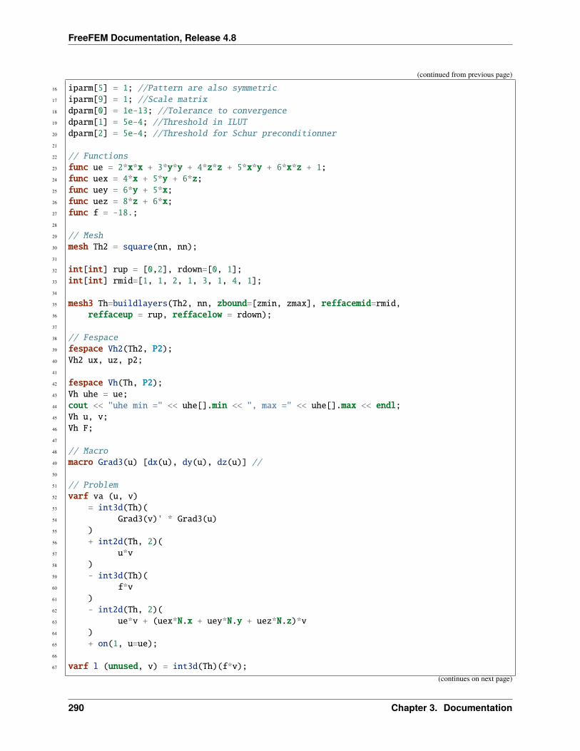
FreeFEM Documentation, Release 4.8
(continued from previous page)
16 iparm[5] = 1; //Pattern are also symmetric17 iparm[9] = 1; //Scale matrix18 dparm[0] = 1e-13; //Tolerance to convergence19 dparm[1] = 5e-4; //Threshold in ILUT20 dparm[2] = 5e-4; //Threshold for Schur preconditionner21
22 // Functions23 func ue = 2*x*x + 3*y*y + 4*z*z + 5*x*y + 6*x*z + 1;24 func uex = 4*x + 5*y + 6*z;25 func uey = 6*y + 5*x;26 func uez = 8*z + 6*x;27 func f = -18.;28
29 // Mesh30 mesh Th2 = square(nn, nn);31
32 int[int] rup = [0,2], rdown=[0, 1];33 int[int] rmid=[1, 1, 2, 1, 3, 1, 4, 1];34
35 mesh3 Th=buildlayers(Th2, nn, zbound=[zmin, zmax], reffacemid=rmid,36 reffaceup = rup, reffacelow = rdown);37
38 // Fespace39 fespace Vh2(Th2, P2);40 Vh2 ux, uz, p2;41
42 fespace Vh(Th, P2);43 Vh uhe = ue;44 cout << "uhe min =" << uhe[].min << ", max =" << uhe[].max << endl;45 Vh u, v;46 Vh F;47
48 // Macro49 macro Grad3(u) [dx(u), dy(u), dz(u)] //50
51 // Problem52 varf va (u, v)53 = int3d(Th)(54 Grad3(v)' * Grad3(u)55 )56 + int2d(Th, 2)(57 u*v58 )59 - int3d(Th)(60 f*v61 )62 - int2d(Th, 2)(63 ue*v + (uex*N.x + uey*N.y + uez*N.z)*v64 )65 + on(1, u=ue);66
67 varf l (unused, v) = int3d(Th)(f*v);
(continues on next page)
290 Chapter 3. Documentation
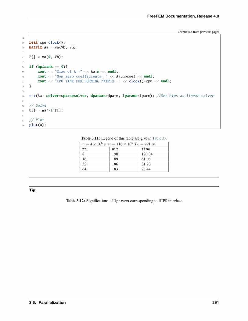
FreeFEM Documentation, Release 4.8
(continued from previous page)
68
69 real cpu=clock();70 matrix Aa = va(Vh, Vh);71
72 F[] = va(0, Vh);73
74 if (mpirank == 0)75 cout << "Size of A =" << Aa.n << endl;76 cout << "Non zero coefficients =" << Aa.nbcoef << endl;77 cout << "CPU TIME FOR FORMING MATRIX =" << clock()-cpu << endl;78 79
80 set(Aa, solver=sparsesolver, dparams=dparm, lparams=iparm); //Set hips as linear solver81
82 // Solve83 u[] = Aa^-1*F[];84
85 // Plot86 plot(u);
Table 3.11: Legend of this table are give in Table 3.6𝑛 = 4× 10⁶ 𝑛𝑛𝑧 = 118× 106 𝑇𝑒 = 221.34np nit time8 190 120.3416 189 61.0832 186 31.7064 183 23.44
Tip:
Table 3.12: Significations of lparams corresponding to HIPS interface
3.6. Parallelization 291
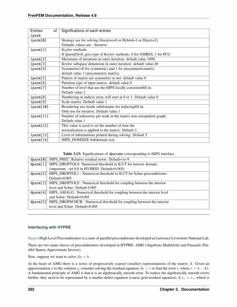
FreeFEM Documentation, Release 4.8
Entries ofiparm
Significations of each entries
iparm[0] Strategy use for solving (Iterative=0 or Hybrid=1 or Direct=2).Defaults values are : Iterative
iparm[1] Krylov methods.If iparm[0]=0, give type of Krylov methods: 0 for GMRES, 1 for PCG
iparm[2] Maximum of iterations in outer iteration: default value 1000iparm[3] Krylov subspace dimension in outer iteration: default value 40iparm[4] Symmetric(=0 for symmetric) and 1 for unsymmetricmatrix:
default value 1 (unsymmetric matrix)iparm[5] Pattern of matrix are symmetric or not: default value 0iparm[6] Partition type of input matrix: default value 0iparm[7] Number of level that use the HIPS locally consistentfill-in:
Default value 2iparm[8] Numbering in indices array will start at 0 or 1: Default value 0iparm[9] Scale matrix. Default value 1iparm[10] Reordering use inside subdomains for reducingfill-in:
Only use for iterative. Default value 1iparm[11] Number of unknowns per node in the matrix non-zeropattern graph:
Default value 1iparm[12] This value is used to set the number of time the
normalization is applied to the matrix: Default 2.iparm[13] Level of informations printed during solving: Default 5.iparm[14] HIPS_DOMSIZE Subdomain size
Table 3.13: Significations of dparams corresponding to HIPS interfacedparm[0] HIPS_PREC: Relative residual norm: Default=1e-9dparm[1] HIPS_DROPTOL0: Numerical threshold in ILUT for interior domain
(important : set 0.0 in HYBRID: Default=0.005)dparm[2] HIPS_DROPTOL1 : Numerical threshold in ILUT for Schur preconditioner:
Default=0.005dparm[3] HIPS_DROPTOLE : Numerical threshold for coupling between the interior
level and Schur: Default 0.005dparm[4] HIPS_AMALG : Numerical threshold for coupling between the interior level
and Schur: Default=0.005dparm[5] HIPS_DROPSCHUR : Numerical threshold for coupling between the interior
level and Schur: Default=0.005
Interfacing with HYPRE
Hypre (High Level Preconditioner) is a suite of parallel preconditioner developed at Lawrence Livermore National Lab.
There are two main classes of preconditioners developed in HYPRE: AMG (Algebraic MultiGrid) and Parasails (Par-allel Sparse Approximate Inverse).
Now, suppose we want to solve 𝐴𝑥 = 𝑏.
At the heart of AMG there is a series of progressively coarser (smaller) representations of the matrix 𝐴. Given anapproximation to the solution 𝑥, consider solving the residual equation𝐴𝑒 = 𝑟 to find the error 𝑒, where 𝑟 = 𝑏−𝐴.A fundamental principle of AMG is that it is an algebraically smooth error. To reduce the algebraically smooth errorsfurther, they need to be represented by a smaller defect equation (coarse grid residual equation) 𝐴𝑐𝑒𝑐 = 𝑟𝑐, which is
292 Chapter 3. Documentation
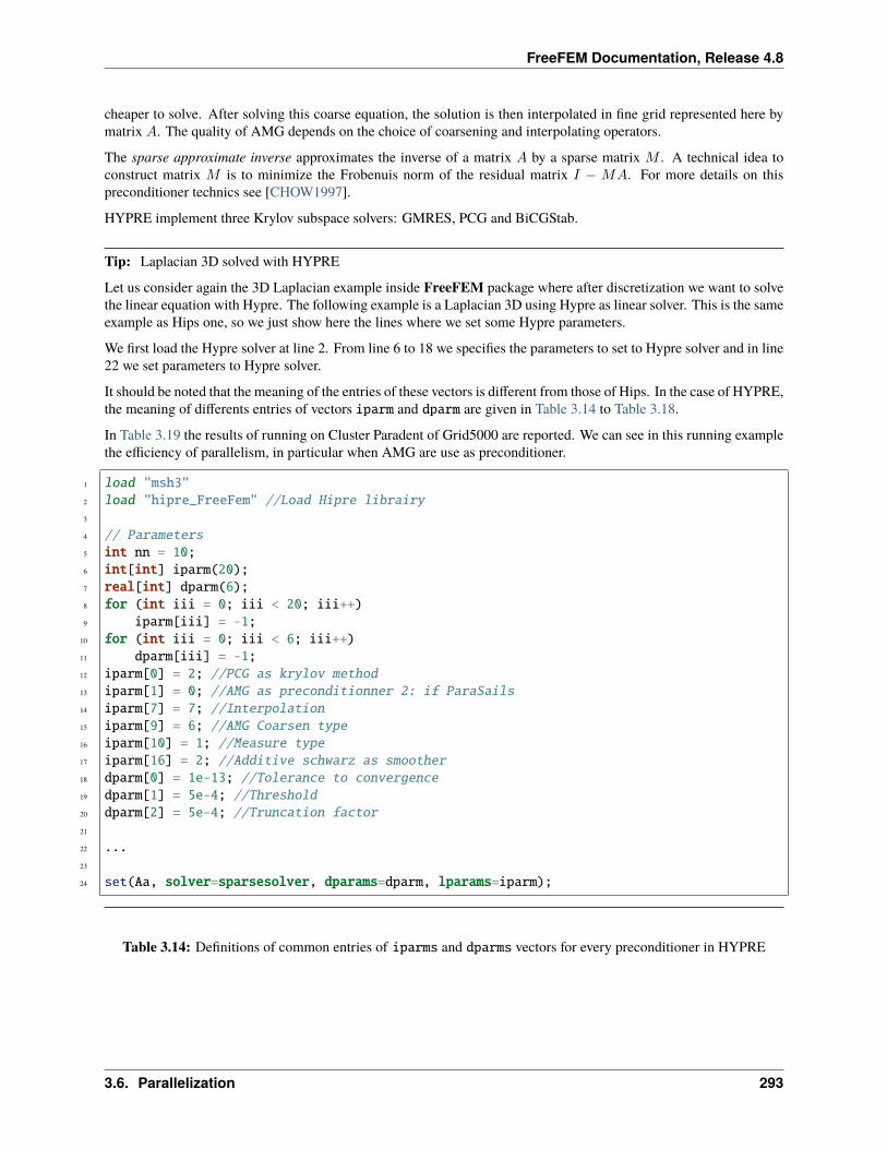
FreeFEM Documentation, Release 4.8
cheaper to solve. After solving this coarse equation, the solution is then interpolated in fine grid represented here bymatrix 𝐴. The quality of AMG depends on the choice of coarsening and interpolating operators.
The sparse approximate inverse approximates the inverse of a matrix 𝐴 by a sparse matrix 𝑀 . A technical idea toconstruct matrix 𝑀 is to minimize the Frobenuis norm of the residual matrix 𝐼 − 𝑀𝐴. For more details on thispreconditioner technics see [CHOW1997].
HYPRE implement three Krylov subspace solvers: GMRES, PCG and BiCGStab.
Tip: Laplacian 3D solved with HYPRE
Let us consider again the 3D Laplacian example inside FreeFEM package where after discretization we want to solvethe linear equation with Hypre. The following example is a Laplacian 3D using Hypre as linear solver. This is the sameexample as Hips one, so we just show here the lines where we set some Hypre parameters.
We first load the Hypre solver at line 2. From line 6 to 18 we specifies the parameters to set to Hypre solver and in line22 we set parameters to Hypre solver.
It should be noted that the meaning of the entries of these vectors is different from those of Hips. In the case of HYPRE,the meaning of differents entries of vectors iparm and dparm are given in Table 3.14 to Table 3.18.
In Table 3.19 the results of running on Cluster Paradent of Grid5000 are reported. We can see in this running examplethe efficiency of parallelism, in particular when AMG are use as preconditioner.
1 load "msh3"2 load "hipre_FreeFem" //Load Hipre librairy3
4 // Parameters5 int nn = 10;6 int[int] iparm(20);7 real[int] dparm(6);8 for (int iii = 0; iii < 20; iii++)9 iparm[iii] = -1;
10 for (int iii = 0; iii < 6; iii++)11 dparm[iii] = -1;12 iparm[0] = 2; //PCG as krylov method13 iparm[1] = 0; //AMG as preconditionner 2: if ParaSails14 iparm[7] = 7; //Interpolation15 iparm[9] = 6; //AMG Coarsen type16 iparm[10] = 1; //Measure type17 iparm[16] = 2; //Additive schwarz as smoother18 dparm[0] = 1e-13; //Tolerance to convergence19 dparm[1] = 5e-4; //Threshold20 dparm[2] = 5e-4; //Truncation factor21
22 ...23
24 set(Aa, solver=sparsesolver, dparams=dparm, lparams=iparm);
Table 3.14: Definitions of common entries of iparms and dparms vectors for every preconditioner in HYPRE
3.6. Parallelization 293
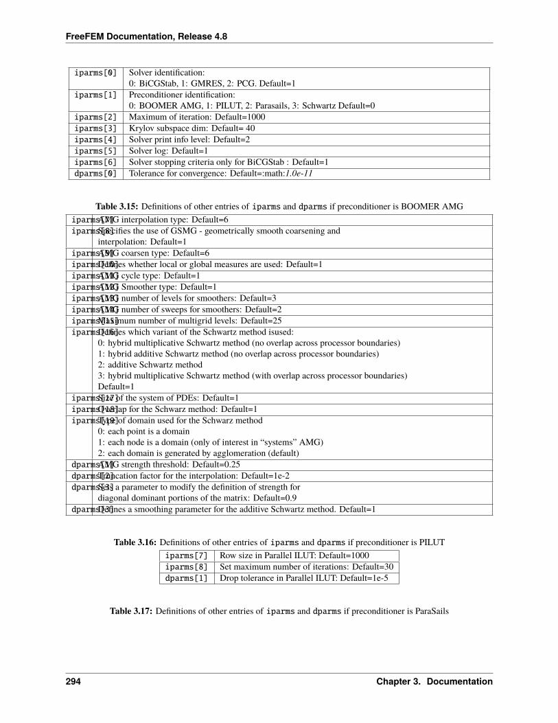
FreeFEM Documentation, Release 4.8
iparms[0] Solver identification:0: BiCGStab, 1: GMRES, 2: PCG. Default=1
iparms[1] Preconditioner identification:0: BOOMER AMG, 1: PILUT, 2: Parasails, 3: Schwartz Default=0
iparms[2] Maximum of iteration: Default=1000iparms[3] Krylov subspace dim: Default= 40iparms[4] Solver print info level: Default=2iparms[5] Solver log: Default=1iparms[6] Solver stopping criteria only for BiCGStab : Default=1dparms[0] Tolerance for convergence: Default=:math:1.0e-11
Table 3.15: Definitions of other entries of iparms and dparms if preconditioner is BOOMER AMGiparms[7]AMG interpolation type: Default=6iparms[8]Specifies the use of GSMG - geometrically smooth coarsening and
interpolation: Default=1iparms[9]AMG coarsen type: Default=6iparms[10]Defines whether local or global measures are used: Default=1iparms[11]AMG cycle type: Default=1iparms[12]AMG Smoother type: Default=1iparms[13]AMG number of levels for smoothers: Default=3iparms[14]AMG number of sweeps for smoothers: Default=2iparms[15]Maximum number of multigrid levels: Default=25iparms[16]Defines which variant of the Schwartz method isused:
0: hybrid multiplicative Schwartz method (no overlap across processor boundaries)1: hybrid additive Schwartz method (no overlap across processor boundaries)2: additive Schwartz method3: hybrid multiplicative Schwartz method (with overlap across processor boundaries)Default=1
iparms[17]Size of the system of PDEs: Default=1iparms[18]Overlap for the Schwarz method: Default=1iparms[19]Type of domain used for the Schwarz method
0: each point is a domain1: each node is a domain (only of interest in “systems” AMG)2: each domain is generated by agglomeration (default)
dparms[1]AMG strength threshold: Default=0.25dparms[2]Truncation factor for the interpolation: Default=1e-2dparms[3]Sets a parameter to modify the definition of strength for
diagonal dominant portions of the matrix: Default=0.9dparms[3]Defines a smoothing parameter for the additive Schwartz method. Default=1
Table 3.16: Definitions of other entries of iparms and dparms if preconditioner is PILUTiparms[7] Row size in Parallel ILUT: Default=1000iparms[8] Set maximum number of iterations: Default=30dparms[1] Drop tolerance in Parallel ILUT: Default=1e-5
Table 3.17: Definitions of other entries of iparms and dparms if preconditioner is ParaSails
294 Chapter 3. Documentation
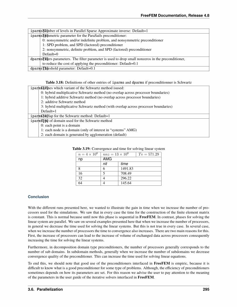
FreeFEM Documentation, Release 4.8
iparms[7]Number of levels in Parallel Sparse Approximate inverse: Default=1iparms[8]Symmetric parameter for the ParaSails preconditioner:
0: nonsymmetric and/or indefinite problem, and nonsymmetric preconditioner1: SPD problem, and SPD (factored) preconditioner2: nonsymmetric, definite problem, and SPD (factored) preconditionerDefault=0
dparms[1]Filters parameters. The filter parameter is used to drop small nonzeros in the preconditioner,to reduce the cost of applying the preconditioner: Default=0.1
dparms[2]Threshold parameter: Default=0.1
Table 3.18: Definitions of other entries of iparms and dparms if preconditionner is Schwartziparms[7]Defines which variant of the Schwartz method isused:
0: hybrid multiplicative Schwartz method (no overlap across processor boundaries)1: hybrid additive Schwartz method (no overlap across processor boundaries)2: additive Schwartz method3: hybrid multiplicative Schwartz method (with overlap across processor boundaries)Default=1
iparms[8]Overlap for the Schwartz method: Default=1iparms[9]Type of domain used for the Schwartz method
0: each point is a domain1: each node is a domain (only of interest in “systems” AMG)2: each domain is generated by agglomeration (default)
Table 3.19: Convergence and time for solving linear system𝑛 = 4× 10⁶ 𝑛𝑛𝑧 = 13× 106 𝑇𝑒 = 571.29np AMG
nit time8 6 1491.8316 5 708.4932 4 296.2264 4 145.64
Conclusion
With the different runs presented here, we wanted to illustrate the gain in time when we increase the number of pro-cessors used for the simulations. We saw that in every case the time for the construction of the finite element matrixis constant. This is normal because until now this phase is sequential in FreeFEM. In contrast, phases for solving thelinear system are parallel. We saw on several examples presented here that when we increase the number of processors,in general we decrease the time used for solving the linear systems. But this is not true in every case. In several case,when we increase the number of processors the time to convergence also increases. There are two main reasons for this.First, the increase of processors can lead to the increase of volume of exchanged data across processors consequentlyincreasing the time for solving the linear systems.
Furthermore, in decomposition domain type preconditioners, the number of processors generally corresponds to thenumber of sub domains. In subdomain methods, generally when we increase the number of subdomains we decreaseconvergence quality of the preconditioner. This can increase the time used for solving linear equations.
To end this, we should note that good use of the preconditioners interfaced in FreeFEM is empiric, because it isdifficult to know what is a good preconditioner for some type of problems. Although, the efficiency of preconditionerssometimes depends on how its parameters are set. For this reason we advise the user to pay attention to the meaningof the parameters in the user guide of the iterative solvers interfaced in FreeFEM.
3.6. Parallelization 295
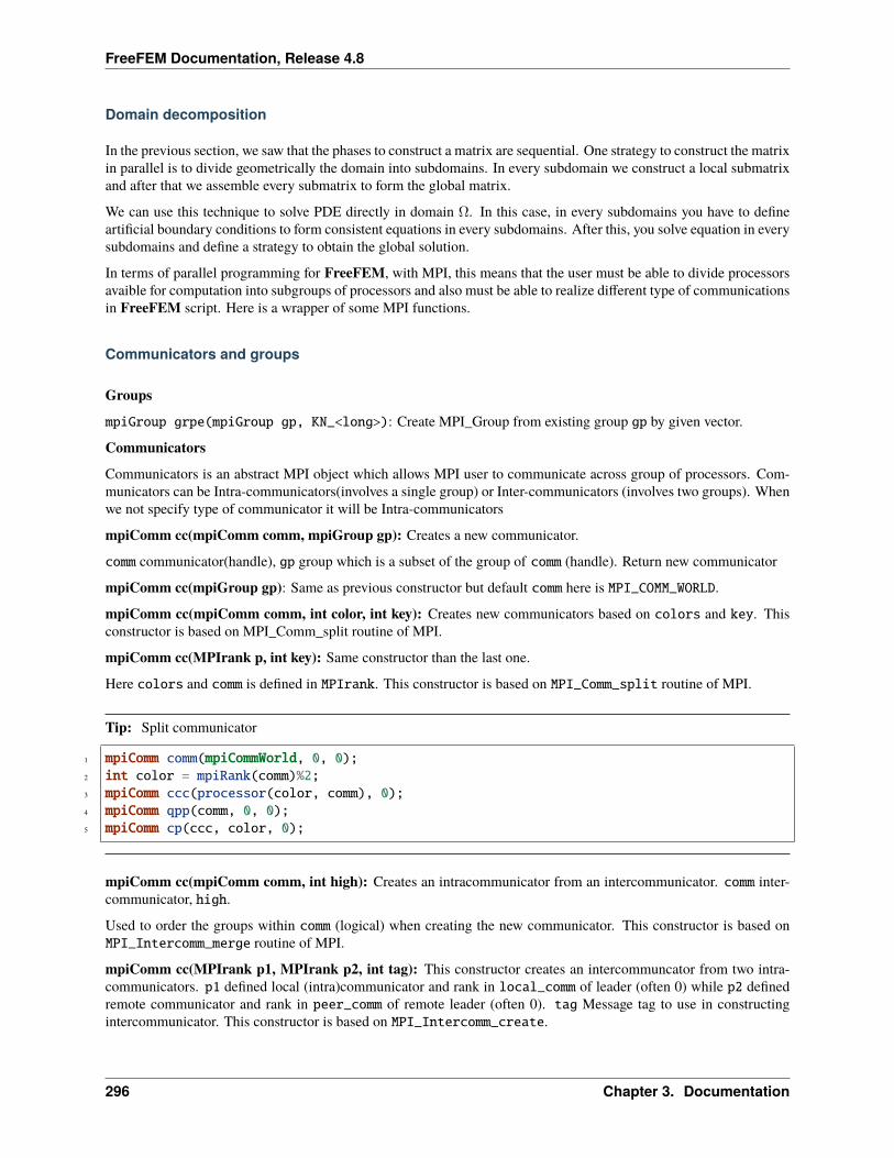
FreeFEM Documentation, Release 4.8
Domain decomposition
In the previous section, we saw that the phases to construct a matrix are sequential. One strategy to construct the matrixin parallel is to divide geometrically the domain into subdomains. In every subdomain we construct a local submatrixand after that we assemble every submatrix to form the global matrix.
We can use this technique to solve PDE directly in domain Ω. In this case, in every subdomains you have to defineartificial boundary conditions to form consistent equations in every subdomains. After this, you solve equation in everysubdomains and define a strategy to obtain the global solution.
In terms of parallel programming for FreeFEM, with MPI, this means that the user must be able to divide processorsavaible for computation into subgroups of processors and also must be able to realize different type of communicationsin FreeFEM script. Here is a wrapper of some MPI functions.
Communicators and groups
GroupsmpiGroup grpe(mpiGroup gp, KN_<long>): Create MPI_Group from existing group gp by given vector.
CommunicatorsCommunicators is an abstract MPI object which allows MPI user to communicate across group of processors. Com-municators can be Intra-communicators(involves a single group) or Inter-communicators (involves two groups). Whenwe not specify type of communicator it will be Intra-communicators
mpiComm cc(mpiComm comm, mpiGroup gp): Creates a new communicator.
comm communicator(handle), gp group which is a subset of the group of comm (handle). Return new communicator
mpiComm cc(mpiGroup gp): Same as previous constructor but default comm here is MPI_COMM_WORLD.
mpiComm cc(mpiComm comm, int color, int key): Creates new communicators based on colors and key. Thisconstructor is based on MPI_Comm_split routine of MPI.
mpiComm cc(MPIrank p, int key): Same constructor than the last one.
Here colors and comm is defined in MPIrank. This constructor is based on MPI_Comm_split routine of MPI.
Tip: Split communicator
1 mpiComm comm(mpiCommWorld, 0, 0);2 int color = mpiRank(comm)%2;3 mpiComm ccc(processor(color, comm), 0);4 mpiComm qpp(comm, 0, 0);5 mpiComm cp(ccc, color, 0);
mpiComm cc(mpiComm comm, int high): Creates an intracommunicator from an intercommunicator. comm inter-communicator, high.
Used to order the groups within comm (logical) when creating the new communicator. This constructor is based onMPI_Intercomm_merge routine of MPI.
mpiComm cc(MPIrank p1, MPIrank p2, int tag): This constructor creates an intercommuncator from two intra-communicators. p1 defined local (intra)communicator and rank in local_comm of leader (often 0) while p2 definedremote communicator and rank in peer_comm of remote leader (often 0). tag Message tag to use in constructingintercommunicator. This constructor is based on MPI_Intercomm_create.
296 Chapter 3. Documentation
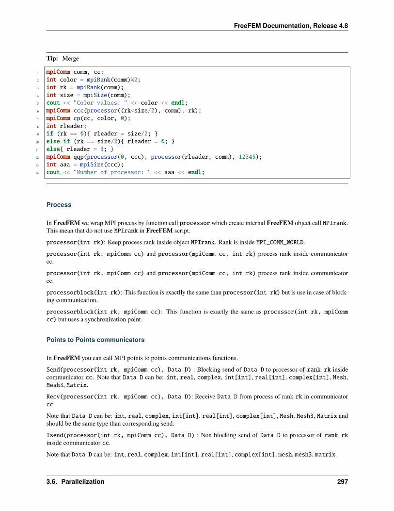
FreeFEM Documentation, Release 4.8
Tip: Merge
1 mpiComm comm, cc;2 int color = mpiRank(comm)%2;3 int rk = mpiRank(comm);4 int size = mpiSize(comm);5 cout << "Color values: " << color << endl;6 mpiComm ccc(processor((rk<size/2), comm), rk);7 mpiComm cp(cc, color, 0);8 int rleader;9 if (rk == 0) rleader = size/2;
10 else if (rk == size/2) rleader = 0; 11 else rleader = 3; 12 mpiComm qqp(processor(0, ccc), processor(rleader, comm), 12345);13 int aaa = mpiSize(ccc);14 cout << "Number of processor: " << aaa << endl;
Process
In FreeFEM we wrap MPI process by function call processor which create internal FreeFEM object call MPIrank.This mean that do not use MPIrank in FreeFEM script.
processor(int rk): Keep process rank inside object MPIrank. Rank is inside MPI_COMM_WORLD.
processor(int rk, mpiComm cc) and processor(mpiComm cc, int rk) process rank inside communicatorcc.
processor(int rk, mpiComm cc) and processor(mpiComm cc, int rk) process rank inside communicatorcc.
processorblock(int rk): This function is exactlly the same than processor(int rk) but is use in case of block-ing communication.
processorblock(int rk, mpiComm cc): This function is exactly the same as processor(int rk, mpiCommcc) but uses a synchronization point.
Points to Points communicators
In FreeFEM you can call MPI points to points communications functions.
Send(processor(int rk, mpiComm cc), Data D) : Blocking send of Data D to processor of rank rk insidecommunicator cc. Note that Data D can be: int, real, complex, int[int], real[int], complex[int], Mesh,Mesh3, Matrix.
Recv(processor(int rk, mpiComm cc), Data D): Receive Data D from process of rank rk in communicatorcc.
Note that Data D can be: int, real, complex, int[int], real[int], complex[int], Mesh, Mesh3, Matrix andshould be the same type than corresponding send.
Isend(processor(int rk, mpiComm cc), Data D) : Non blocking send of Data D to processor of rank rkinside communicator cc.
Note that Data D can be: int, real, complex, int[int], real[int], complex[int], mesh, mesh3, matrix.
3.6. Parallelization 297
FreeFEM Documentation, Release 4.8
Recv(processor(int rk, mpiComm cc), Data D): Receive corresponding to send.
Global operations
In FreeFEM you can call MPI global communication functions.
broadcast(processor(int rk, mpiComm cc), Data D): Process rk Broadcast Data D to all process insidecommunicator cc. Note that Data D can be: int, real, complex, int[int], real[int], complex[int], Mesh,Mesh3, Matrix.
broadcast(processor(int rk), Data D): Process rkBroadcast Data D to all process inside MPI_COMM_WORLD.Note that Data D can be: int, real, complex, int[int], real[int], complex[int], Mesh, Mesh3, Matrix.
mpiAlltoall(Data a, Data b): Sends data a from all to all processes. Receive buffer is Data b. This is doneinside communicator MPI_COMM_WORLD.
mpiAlltoall(Data a, Data b, mpiComm cc): Sends data a from all to all processes. Receive buffer is Datab. This is done inside communicator cc.
mpiGather(Data a, Data b, processor(mpiComm, int rk): Gathers together values Data a from a group ofprocesses. Process of rank rk get data on communicator rk. This function is like MPI_Gather.
mpiAllgather(Data a, Data b): Gathers Data a from all processes and distribute it to all in Data b. This isdone inside communicator MPI_COMM_WORLD. This function is like MPI_Allgather.
mpiAllgather(Data a, Data b, mpiComm cc): Gathers Data a from all processes and distribute it to all in Datab. This is done inside communicator cc. This function is like MPI_Allgather.
mpiScatter(Data a,Data b,processor(int rk, mpiComm cc)): Sends Data a from one process whith rankrk to all other processes in group represented by communicator mpiComm cc.
mpiReduce(Data a, Data b, processor(int rk, mpiComm cc), MPI_Op op) Reduces values Data a onall processes to a single value Data b on process of rank rk and communicator cc.
Operation use in reduce is: MPI_Op op which can be: mpiMAX, mpiMIN, mpiSUM, mpiPROD, mpiLAND, mpiLOR,mpiLXOR, mpiBAND, mpiBXOR, mpiMAXLOC, mpiMINLOC.
Note that, for all global operations, only int[int] and real[int] are data type take in account in FreeFEM.
3.7 PETSc and SLEPc
FreeFEM is interfaced with PETSc and SLEPc which offer a wide range of sequential or parallel linear or nonlinearsolvers, time steppers, optimizers, and eigensolvers. In particular, it gives access transparently (without much changesto user code) to: distributed and multithreaded direct solvers (PARDISO, MUMPS, SuperLU), multigrid solvers (hypre,GAMG), domain decomposition methods (block Jacobi, ASM, HPDDM). For a detailed introduction to these tools,interested readers are referred to the tutorial Introduction to FreeFEM with an emphasis on parallel computing.
In most of the scripts listed below, the following standard procedure is used.• Load an initial sequential mesh (in 2D or 3D).
• Partition the mesh and generate connectivity information according to the number of processes.
• Provide these information to PETSc so that subsequent computations may be done in a distributed fashion.
Combining the power and flexibility of PETSc with the ease-of-use of FreeFEM may help design multiphysics solvers,e.g., for Navier–Stokes equations, advanced matrix-free discretizations, and such.
298 Chapter 3. Documentation
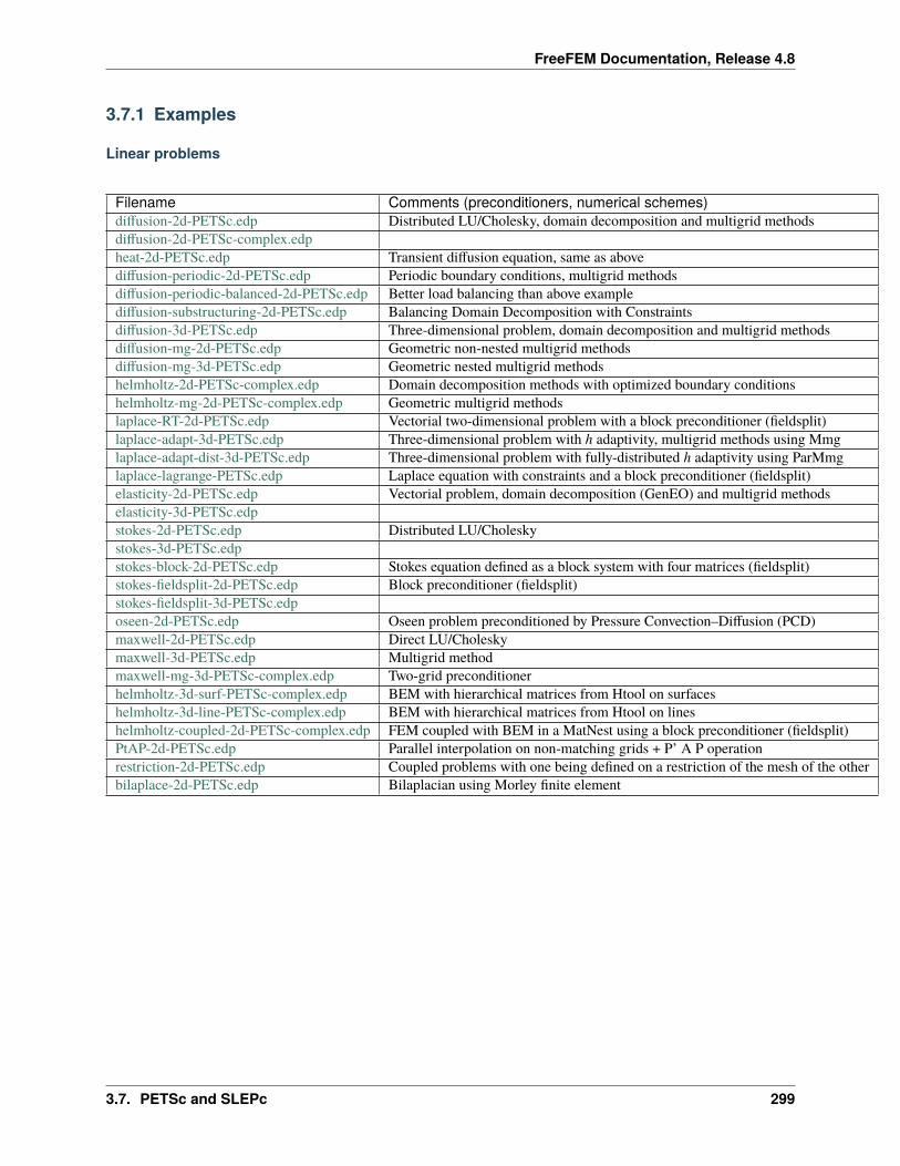
FreeFEM Documentation, Release 4.8
3.7.1 Examples
Linear problems
Filename Comments (preconditioners, numerical schemes)diffusion-2d-PETSc.edp Distributed LU/Cholesky, domain decomposition and multigrid methodsdiffusion-2d-PETSc-complex.edpheat-2d-PETSc.edp Transient diffusion equation, same as abovediffusion-periodic-2d-PETSc.edp Periodic boundary conditions, multigrid methodsdiffusion-periodic-balanced-2d-PETSc.edp Better load balancing than above examplediffusion-substructuring-2d-PETSc.edp Balancing Domain Decomposition with Constraintsdiffusion-3d-PETSc.edp Three-dimensional problem, domain decomposition and multigrid methodsdiffusion-mg-2d-PETSc.edp Geometric non-nested multigrid methodsdiffusion-mg-3d-PETSc.edp Geometric nested multigrid methodshelmholtz-2d-PETSc-complex.edp Domain decomposition methods with optimized boundary conditionshelmholtz-mg-2d-PETSc-complex.edp Geometric multigrid methodslaplace-RT-2d-PETSc.edp Vectorial two-dimensional problem with a block preconditioner (fieldsplit)laplace-adapt-3d-PETSc.edp Three-dimensional problem with h adaptivity, multigrid methods using Mmglaplace-adapt-dist-3d-PETSc.edp Three-dimensional problem with fully-distributed h adaptivity using ParMmglaplace-lagrange-PETSc.edp Laplace equation with constraints and a block preconditioner (fieldsplit)elasticity-2d-PETSc.edp Vectorial problem, domain decomposition (GenEO) and multigrid methodselasticity-3d-PETSc.edpstokes-2d-PETSc.edp Distributed LU/Choleskystokes-3d-PETSc.edpstokes-block-2d-PETSc.edp Stokes equation defined as a block system with four matrices (fieldsplit)stokes-fieldsplit-2d-PETSc.edp Block preconditioner (fieldsplit)stokes-fieldsplit-3d-PETSc.edposeen-2d-PETSc.edp Oseen problem preconditioned by Pressure Convection–Diffusion (PCD)maxwell-2d-PETSc.edp Direct LU/Choleskymaxwell-3d-PETSc.edp Multigrid methodmaxwell-mg-3d-PETSc-complex.edp Two-grid preconditionerhelmholtz-3d-surf-PETSc-complex.edp BEM with hierarchical matrices from Htool on surfaceshelmholtz-3d-line-PETSc-complex.edp BEM with hierarchical matrices from Htool on lineshelmholtz-coupled-2d-PETSc-complex.edp FEM coupled with BEM in a MatNest using a block preconditioner (fieldsplit)PtAP-2d-PETSc.edp Parallel interpolation on non-matching grids + P’ A P operationrestriction-2d-PETSc.edp Coupled problems with one being defined on a restriction of the mesh of the otherbilaplace-2d-PETSc.edp Bilaplacian using Morley finite element
3.7. PETSc and SLEPc 299
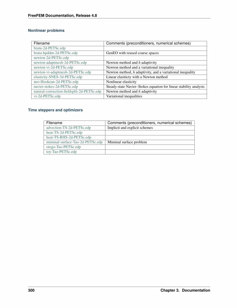
FreeFEM Documentation, Release 4.8
Nonlinear problems
Filename Comments (preconditioners, numerical schemes)bratu-2d-PETSc.edpbratu-hpddm-2d-PETSc.edp GenEO with reused coarse spacesnewton-2d-PETSc.edpnewton-adaptmesh-2d-PETSc.edp Newton method and h adaptivitynewton-vi-2d-PETSc.edp Newton method and a variational inequalitynewton-vi-adaptmesh-2d-PETSc.edp Newton method, h adaptivity, and a variational inequalityelasticity-SNES-3d-PETSc.edp Linear elasiticty with a Newton methodneo-Hookean-2d-PETSc.edp Nonlinear elasticitynavier-stokes-2d-PETSc.edp Steady-state Navier–Stokes equation for linear stability analysisnatural-convection-fieldsplit-2d-PETSc.edp Newton method and h adaptivityvi-2d-PETSc.edp Variational inequalities
Time steppers and optimizers
Filename Comments (preconditioners, numerical schemes)advection-TS-2d-PETSc.edp Implicit and explicit schemesheat-TS-2d-PETSc.edpheat-TS-RHS-2d-PETSc.edpminimal-surface-Tao-2d-PETSc.edp Minimal surface problemorego-Tao-PETSc.edptoy-Tao-PETSc.edp
300 Chapter 3. Documentation
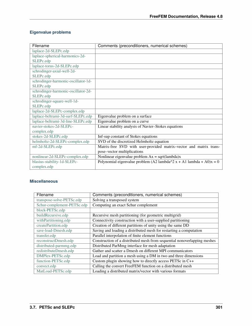
FreeFEM Documentation, Release 4.8
Eigenvalue problems
Filename Comments (preconditioners, numerical schemes)laplace-2d-SLEPc.edplaplace-spherical-harmonics-2d-SLEPc.edplaplace-torus-2d-SLEPc.edpschrodinger-axial-well-2d-SLEPc.edpschrodinger-harmonic-oscillator-1d-SLEPc.edpschrodinger-harmonic-oscillator-2d-SLEPc.edpschrodinger-square-well-1d-SLEPc.edplaplace-2d-SLEPc-complex.edplaplace-beltrami-3d-surf-SLEPc.edp Eigenvalue problem on a surfacelaplace-beltrami-3d-line-SLEPc.edp Eigenvalue problem on a curvenavier-stokes-2d-SLEPc-complex.edp
Linear stability analysis of Navier–Stokes equations
stokes-2d-SLEPc.edp Inf-sup constant of Stokes equationshelmholtz-2d-SLEPc-complex.edp SVD of the discretized Helmholtz equationmf-2d-SLEPc.edp Matrix-free SVD with user-provided matrix–vector and matrix trans-
pose–vector multiplicationsnonlinear-2d-SLEPc-complex.edp Nonlinear eigenvalue problem Ax = sqrt(lambda)xblasius-stability-1d-SLEPc-complex.edp
Polynomial eigenvalue problem (A2 lambda^2 x + A1 lambda + A0)x = 0
Miscellaneous
Filename Comments (preconditioners, numerical schemes)transpose-solve-PETSc.edp Solving a transposed systemSchur-complement-PETSc.edp Computing an exact Schur complementblock-PETSc.edpbuildRecursive.edp Recursive mesh partitioning (for geometric multigrid)withPartitioning.edp Connectivity construction with a user-supplied partitioningcreatePartition.edp Creation of different partitions of unity using the same DDsave-load-Dmesh.edp Saving and loading a distributed mesh for restarting a computationtransfer.edp Parallel interpolation of finite element functionsreconstructDmesh.edp Construction of a distributed mesh from sequential nonoverlapping meshesdistributed-parmmg.edp Distributed ParMmg interface for mesh adaptationredistributeDmesh.edp Gather and scatter a Dmesh on different MPI communicatorsDMPlex-PETSc.edp Load and partition a mesh using a DM in two and three dimensionsfunction-PETSc.edp Custom plugin showing how to directly access PETSc in C++convect.edp Calling the convert FreeFEM function on a distributed meshMatLoad-PETSc.edp Loading a distributed matrix/vector with various formats
3.7. PETSc and SLEPc 301
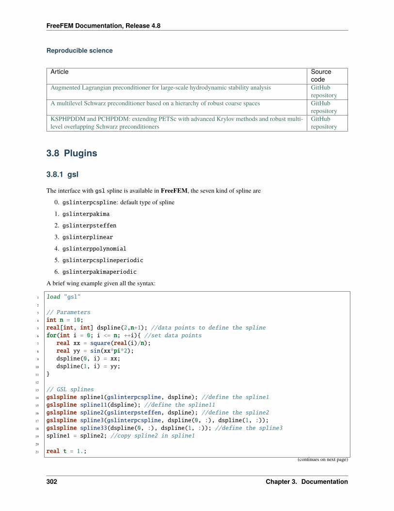
FreeFEM Documentation, Release 4.8
Reproducible science
Article Sourcecode
Augmented Lagrangian preconditioner for large-scale hydrodynamic stability analysis GitHubrepository
A multilevel Schwarz preconditioner based on a hierarchy of robust coarse spaces GitHubrepository
KSPHPDDM and PCHPDDM: extending PETSc with advanced Krylov methods and robust multi-level overlapping Schwarz preconditioners
GitHubrepository
3.8 Plugins
3.8.1 gsl
The interface with gsl spline is available in FreeFEM, the seven kind of spline are
0. gslinterpcspline: default type of spline
1. gslinterpakima
2. gslinterpsteffen
3. gslinterplinear
4. gslinterppolynomial
5. gslinterpcsplineperiodic
6. gslinterpakimaperiodic
A brief wing example given all the syntax:
1 load "gsl"2
3 // Parameters4 int n = 10;5 real[int, int] dspline(2,n+1); //data points to define the spline6 for(int i = 0; i <= n; ++i) //set data points7 real xx = square(real(i)/n);8 real yy = sin(xx*pi*2);9 dspline(0, i) = xx;
10 dspline(1, i) = yy;11 12
13 // GSL splines14 gslspline spline1(gslinterpcspline, dspline); //define the spline115 gslspline spline11(dspline); //define the spline1116 gslspline spline2(gslinterpsteffen, dspline); //define the spline217 gslspline spline3(gslinterpcspline, dspline(0, :), dspline(1, :));18 gslspline spline33(dspline(0, :), dspline(1, :)); //define the spline319 spline1 = spline2; //copy spline2 in spline120
21 real t = 1.;(continues on next page)
302 Chapter 3. Documentation
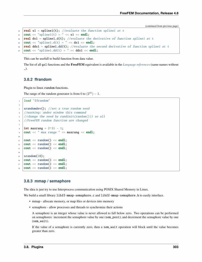
FreeFEM Documentation, Release 4.8
(continued from previous page)
22 real s1 = spline1(t); //evaluate the function spline1 at t23 cout << "spline1(t) = " << s1 << endl;24 real ds1 = spline1.d(t); //evaluate the derivative of function spline1 at t25 cout << "spline1.d(t) = " << ds1 << endl;26 real dds1 = spline1.dd(t); //evaluate the second derivative of function spline1 at t27 cout << "spline1.dd(t) = " << dds1 << endl;
This can be usefull to build function from data value.
The list of all gsl functions and the FreeFEM equivalent is available in the Language references (same names without_).
3.8.2 ffrandom
Plugin to linux random functions.
The range of the random generator is from 0 to (231)− 1.
1 load "ffrandom"2
3 srandomdev(); //set a true random seed4 //warning: under window this command5 //change the seed by randinit(random())) so all6 //FreeFEM random function are changed7
8 int maxrang = 2^31 - 1;9 cout << " max range " << maxrang << endl;
10
11 cout << random() << endl;12 cout << random() << endl;13 cout << random() << endl;14
15 srandom(10);16 cout << random() << endl;17 cout << random() << endl;18 cout << random() << endl;
3.8.3 mmap / semaphore
The idea is just try to use Interprocess communication using POSIX Shared Memory in Linux.
We build a small library libff-mmap-semaphore.c and libff-mmap-semaphore.h to easily interface.
• mmap - allocate memory, or map files or devices into memory
• semaphore - allow processes and threads to synchronize their actions
A semaphore is an integer whose value is never allowed to fall below zero. Two operations can be performedon semaphores: increment the semaphore value by one (sem_post); and decrement the semaphore value by one(sem_wait).
If the value of a semaphore is currently zero, then a sem_wait operation will block until the value becomesgreater than zero.
3.8. Plugins 303
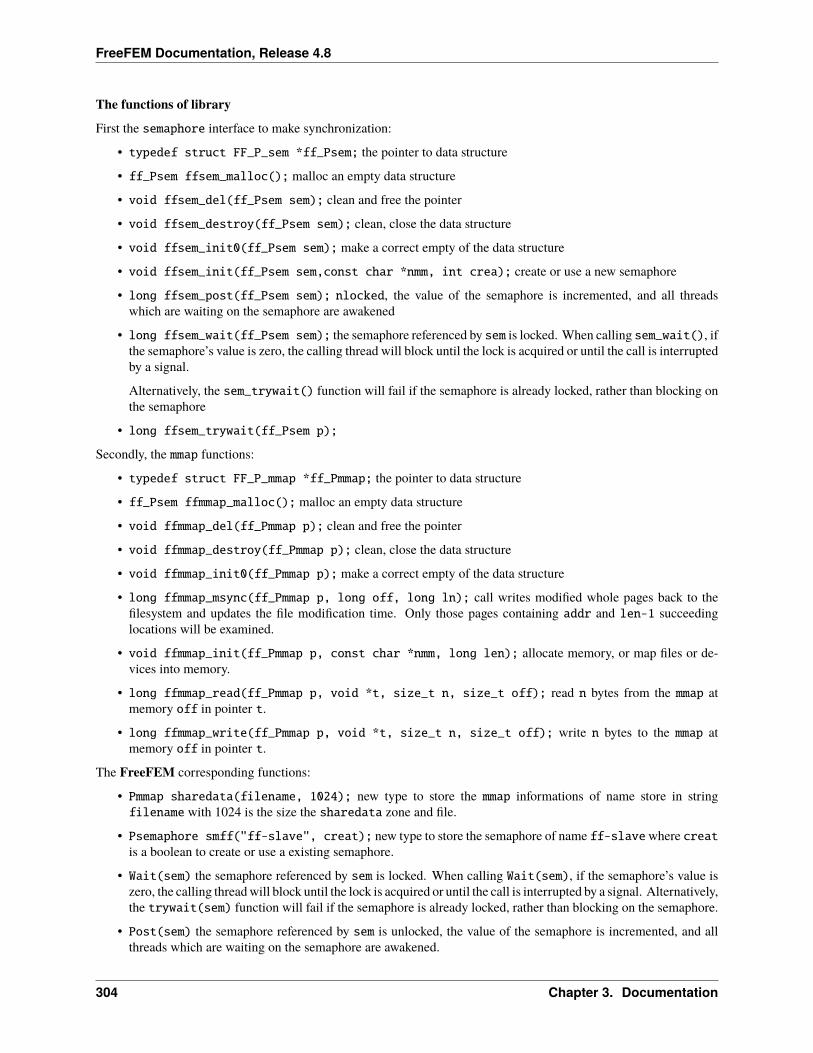
FreeFEM Documentation, Release 4.8
The functions of libraryFirst the semaphore interface to make synchronization:
• typedef struct FF_P_sem *ff_Psem; the pointer to data structure
• ff_Psem ffsem_malloc(); malloc an empty data structure
• void ffsem_del(ff_Psem sem); clean and free the pointer
• void ffsem_destroy(ff_Psem sem); clean, close the data structure
• void ffsem_init0(ff_Psem sem); make a correct empty of the data structure
• void ffsem_init(ff_Psem sem,const char *nmm, int crea); create or use a new semaphore
• long ffsem_post(ff_Psem sem); nlocked, the value of the semaphore is incremented, and all threadswhich are waiting on the semaphore are awakened
• long ffsem_wait(ff_Psem sem); the semaphore referenced by sem is locked. When calling sem_wait(), ifthe semaphore’s value is zero, the calling thread will block until the lock is acquired or until the call is interruptedby a signal.
Alternatively, the sem_trywait() function will fail if the semaphore is already locked, rather than blocking onthe semaphore
• long ffsem_trywait(ff_Psem p);
Secondly, the mmap functions:
• typedef struct FF_P_mmap *ff_Pmmap; the pointer to data structure
• ff_Psem ffmmap_malloc(); malloc an empty data structure
• void ffmmap_del(ff_Pmmap p); clean and free the pointer
• void ffmmap_destroy(ff_Pmmap p); clean, close the data structure
• void ffmmap_init0(ff_Pmmap p); make a correct empty of the data structure
• long ffmmap_msync(ff_Pmmap p, long off, long ln); call writes modified whole pages back to thefilesystem and updates the file modification time. Only those pages containing addr and len-1 succeedinglocations will be examined.
• void ffmmap_init(ff_Pmmap p, const char *nmm, long len); allocate memory, or map files or de-vices into memory.
• long ffmmap_read(ff_Pmmap p, void *t, size_t n, size_t off); read n bytes from the mmap atmemory off in pointer t.
• long ffmmap_write(ff_Pmmap p, void *t, size_t n, size_t off); write n bytes to the mmap atmemory off in pointer t.
The FreeFEM corresponding functions:
• Pmmap sharedata(filename, 1024); new type to store the mmap informations of name store in stringfilename with 1024 is the size the sharedata zone and file.
• Psemaphore smff("ff-slave", creat); new type to store the semaphore of name ff-slavewhere creatis a boolean to create or use a existing semaphore.
• Wait(sem) the semaphore referenced by sem is locked. When calling Wait(sem), if the semaphore’s value iszero, the calling thread will block until the lock is acquired or until the call is interrupted by a signal. Alternatively,the trywait(sem) function will fail if the semaphore is already locked, rather than blocking on the semaphore.
• Post(sem) the semaphore referenced by sem is unlocked, the value of the semaphore is incremented, and allthreads which are waiting on the semaphore are awakened.
304 Chapter 3. Documentation
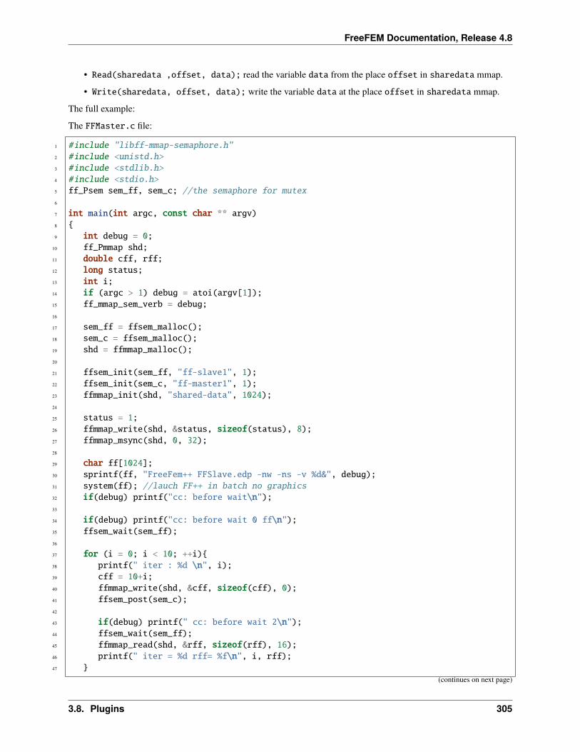
FreeFEM Documentation, Release 4.8
• Read(sharedata ,offset, data); read the variable data from the place offset in sharedata mmap.
• Write(sharedata, offset, data); write the variable data at the place offset in sharedata mmap.
The full example:
The FFMaster.c file:
1 #include "libff-mmap-semaphore.h"2 #include <unistd.h>3 #include <stdlib.h>4 #include <stdio.h>5 ff_Psem sem_ff, sem_c; //the semaphore for mutex6
7 int main(int argc, const char ** argv)8 9 int debug = 0;
10 ff_Pmmap shd;11 double cff, rff;12 long status;13 int i;14 if (argc > 1) debug = atoi(argv[1]);15 ff_mmap_sem_verb = debug;16
17 sem_ff = ffsem_malloc();18 sem_c = ffsem_malloc();19 shd = ffmmap_malloc();20
21 ffsem_init(sem_ff, "ff-slave1", 1);22 ffsem_init(sem_c, "ff-master1", 1);23 ffmmap_init(shd, "shared-data", 1024);24
25 status = 1;26 ffmmap_write(shd, &status, sizeof(status), 8);27 ffmmap_msync(shd, 0, 32);28
29 char ff[1024];30 sprintf(ff, "FreeFem++ FFSlave.edp -nw -ns -v %d&", debug);31 system(ff); //lauch FF++ in batch no graphics32 if(debug) printf("cc: before wait\n");33
34 if(debug) printf("cc: before wait 0 ff\n");35 ffsem_wait(sem_ff);36
37 for (i = 0; i < 10; ++i)38 printf(" iter : %d \n", i);39 cff = 10+i;40 ffmmap_write(shd, &cff, sizeof(cff), 0);41 ffsem_post(sem_c);42
43 if(debug) printf(" cc: before wait 2\n");44 ffsem_wait(sem_ff);45 ffmmap_read(shd, &rff, sizeof(rff), 16);46 printf(" iter = %d rff= %f\n", i, rff);47
(continues on next page)
3.8. Plugins 305
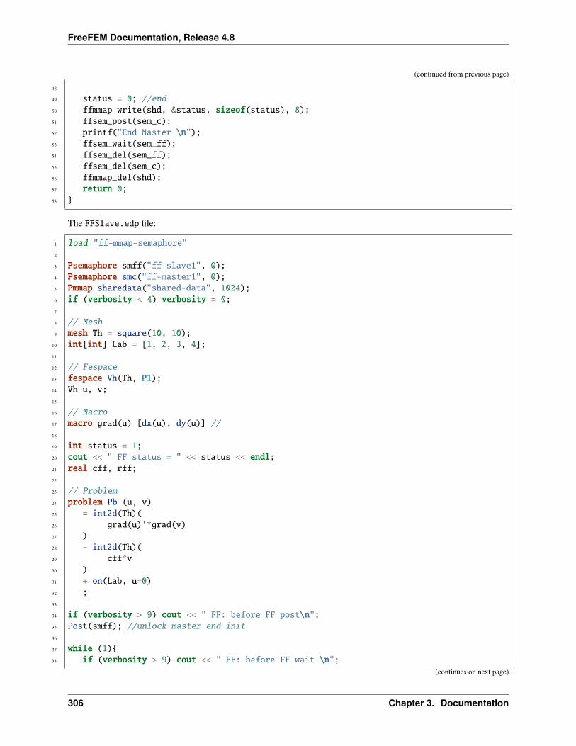
FreeFEM Documentation, Release 4.8
(continued from previous page)
48
49 status = 0; //end50 ffmmap_write(shd, &status, sizeof(status), 8);51 ffsem_post(sem_c);52 printf("End Master \n");53 ffsem_wait(sem_ff);54 ffsem_del(sem_ff);55 ffsem_del(sem_c);56 ffmmap_del(shd);57 return 0;58
The FFSlave.edp file:
1 load "ff-mmap-semaphore"2
3 Psemaphore smff("ff-slave1", 0);4 Psemaphore smc("ff-master1", 0);5 Pmmap sharedata("shared-data", 1024);6 if (verbosity < 4) verbosity = 0;7
8 // Mesh9 mesh Th = square(10, 10);
10 int[int] Lab = [1, 2, 3, 4];11
12 // Fespace13 fespace Vh(Th, P1);14 Vh u, v;15
16 // Macro17 macro grad(u) [dx(u), dy(u)] //18
19 int status = 1;20 cout << " FF status = " << status << endl;21 real cff, rff;22
23 // Problem24 problem Pb (u, v)25 = int2d(Th)(26 grad(u)'*grad(v)27 )28 - int2d(Th)(29 cff*v30 )31 + on(Lab, u=0)32 ;33
34 if (verbosity > 9) cout << " FF: before FF post\n";35 Post(smff); //unlock master end init36
37 while (1)38 if (verbosity > 9) cout << " FF: before FF wait \n";
(continues on next page)
306 Chapter 3. Documentation
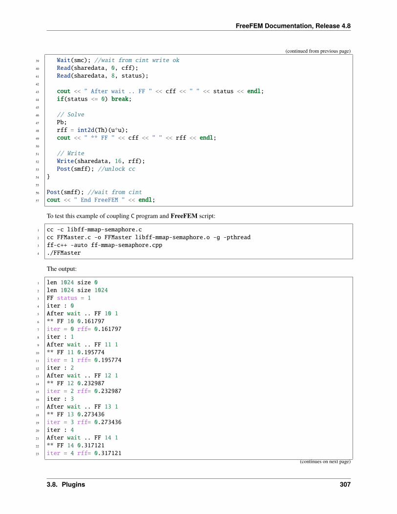
FreeFEM Documentation, Release 4.8
(continued from previous page)
39 Wait(smc); //wait from cint write ok40 Read(sharedata, 0, cff);41 Read(sharedata, 8, status);42
43 cout << " After wait .. FF " << cff << " " << status << endl;44 if(status <= 0) break;45
46 // Solve47 Pb;48 rff = int2d(Th)(u*u);49 cout << " ** FF " << cff << " " << rff << endl;50
51 // Write52 Write(sharedata, 16, rff);53 Post(smff); //unlock cc54 55
56 Post(smff); //wait from cint57 cout << " End FreeFEM " << endl;
To test this example of coupling C program and FreeFEM script:
1 cc -c libff-mmap-semaphore.c2 cc FFMaster.c -o FFMaster libff-mmap-semaphore.o -g -pthread3 ff-c++ -auto ff-mmap-semaphore.cpp4 ./FFMaster
The output:
1 len 1024 size 02 len 1024 size 10243 FF status = 14 iter : 05 After wait .. FF 10 16 ** FF 10 0.1617977 iter = 0 rff= 0.1617978 iter : 19 After wait .. FF 11 1
10 ** FF 11 0.19577411 iter = 1 rff= 0.19577412 iter : 213 After wait .. FF 12 114 ** FF 12 0.23298715 iter = 2 rff= 0.23298716 iter : 317 After wait .. FF 13 118 ** FF 13 0.27343619 iter = 3 rff= 0.27343620 iter : 421 After wait .. FF 14 122 ** FF 14 0.31712123 iter = 4 rff= 0.317121
(continues on next page)
3.8. Plugins 307
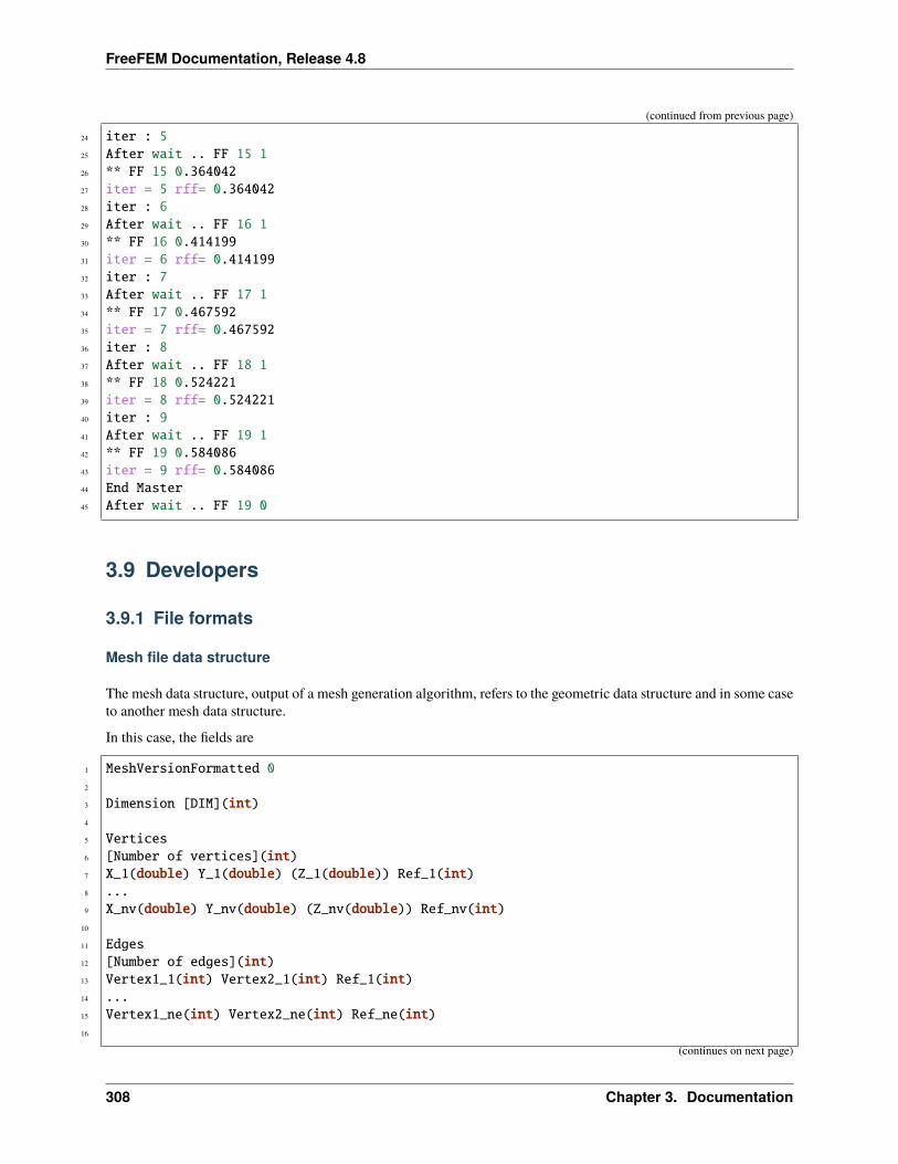
FreeFEM Documentation, Release 4.8
(continued from previous page)
24 iter : 525 After wait .. FF 15 126 ** FF 15 0.36404227 iter = 5 rff= 0.36404228 iter : 629 After wait .. FF 16 130 ** FF 16 0.41419931 iter = 6 rff= 0.41419932 iter : 733 After wait .. FF 17 134 ** FF 17 0.46759235 iter = 7 rff= 0.46759236 iter : 837 After wait .. FF 18 138 ** FF 18 0.52422139 iter = 8 rff= 0.52422140 iter : 941 After wait .. FF 19 142 ** FF 19 0.58408643 iter = 9 rff= 0.58408644 End Master45 After wait .. FF 19 0
3.9 Developers
3.9.1 File formats
Mesh file data structure
The mesh data structure, output of a mesh generation algorithm, refers to the geometric data structure and in some caseto another mesh data structure.
In this case, the fields are
1 MeshVersionFormatted 02
3 Dimension [DIM](int)4
5 Vertices6 [Number of vertices](int)7 X_1(double) Y_1(double) (Z_1(double)) Ref_1(int)8 ...9 X_nv(double) Y_nv(double) (Z_nv(double)) Ref_nv(int)
10
11 Edges12 [Number of edges](int)13 Vertex1_1(int) Vertex2_1(int) Ref_1(int)14 ...15 Vertex1_ne(int) Vertex2_ne(int) Ref_ne(int)16
(continues on next page)
308 Chapter 3. Documentation
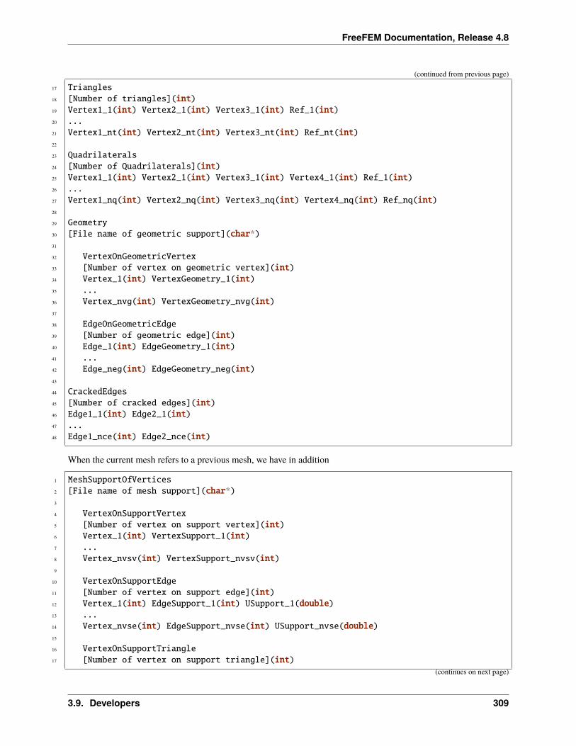
FreeFEM Documentation, Release 4.8
(continued from previous page)
17 Triangles18 [Number of triangles](int)19 Vertex1_1(int) Vertex2_1(int) Vertex3_1(int) Ref_1(int)20 ...21 Vertex1_nt(int) Vertex2_nt(int) Vertex3_nt(int) Ref_nt(int)22
23 Quadrilaterals24 [Number of Quadrilaterals](int)25 Vertex1_1(int) Vertex2_1(int) Vertex3_1(int) Vertex4_1(int) Ref_1(int)26 ...27 Vertex1_nq(int) Vertex2_nq(int) Vertex3_nq(int) Vertex4_nq(int) Ref_nq(int)28
29 Geometry30 [File name of geometric support](char*)31
32 VertexOnGeometricVertex33 [Number of vertex on geometric vertex](int)34 Vertex_1(int) VertexGeometry_1(int)35 ...36 Vertex_nvg(int) VertexGeometry_nvg(int)37
38 EdgeOnGeometricEdge39 [Number of geometric edge](int)40 Edge_1(int) EdgeGeometry_1(int)41 ...42 Edge_neg(int) EdgeGeometry_neg(int)43
44 CrackedEdges45 [Number of cracked edges](int)46 Edge1_1(int) Edge2_1(int)47 ...48 Edge1_nce(int) Edge2_nce(int)
When the current mesh refers to a previous mesh, we have in addition
1 MeshSupportOfVertices2 [File name of mesh support](char*)3
4 VertexOnSupportVertex5 [Number of vertex on support vertex](int)6 Vertex_1(int) VertexSupport_1(int)7 ...8 Vertex_nvsv(int) VertexSupport_nvsv(int)9
10 VertexOnSupportEdge11 [Number of vertex on support edge](int)12 Vertex_1(int) EdgeSupport_1(int) USupport_1(double)13 ...14 Vertex_nvse(int) EdgeSupport_nvse(int) USupport_nvse(double)15
16 VertexOnSupportTriangle17 [Number of vertex on support triangle](int)
(continues on next page)
3.9. Developers 309
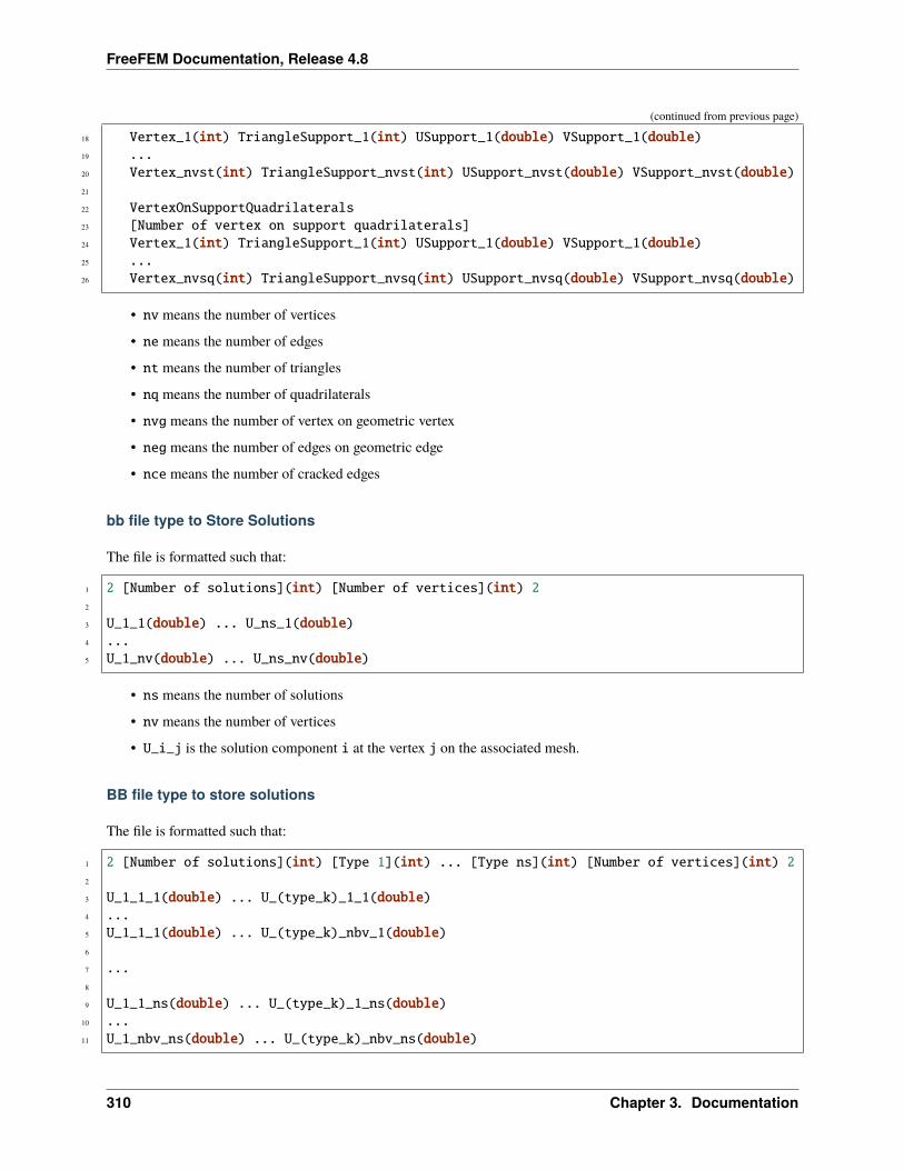
FreeFEM Documentation, Release 4.8
(continued from previous page)
18 Vertex_1(int) TriangleSupport_1(int) USupport_1(double) VSupport_1(double)19 ...20 Vertex_nvst(int) TriangleSupport_nvst(int) USupport_nvst(double) VSupport_nvst(double)21
22 VertexOnSupportQuadrilaterals23 [Number of vertex on support quadrilaterals]24 Vertex_1(int) TriangleSupport_1(int) USupport_1(double) VSupport_1(double)25 ...26 Vertex_nvsq(int) TriangleSupport_nvsq(int) USupport_nvsq(double) VSupport_nvsq(double)
• nv means the number of vertices
• ne means the number of edges
• nt means the number of triangles
• nq means the number of quadrilaterals
• nvg means the number of vertex on geometric vertex
• neg means the number of edges on geometric edge
• nce means the number of cracked edges
bb file type to Store Solutions
The file is formatted such that:
1 2 [Number of solutions](int) [Number of vertices](int) 22
3 U_1_1(double) ... U_ns_1(double)4 ...5 U_1_nv(double) ... U_ns_nv(double)
• ns means the number of solutions
• nv means the number of vertices
• U_i_j is the solution component i at the vertex j on the associated mesh.
BB file type to store solutions
The file is formatted such that:
1 2 [Number of solutions](int) [Type 1](int) ... [Type ns](int) [Number of vertices](int) 22
3 U_1_1_1(double) ... U_(type_k)_1_1(double)4 ...5 U_1_1_1(double) ... U_(type_k)_nbv_1(double)6
7 ...8
9 U_1_1_ns(double) ... U_(type_k)_1_ns(double)10 ...11 U_1_nbv_ns(double) ... U_(type_k)_nbv_ns(double)
310 Chapter 3. Documentation
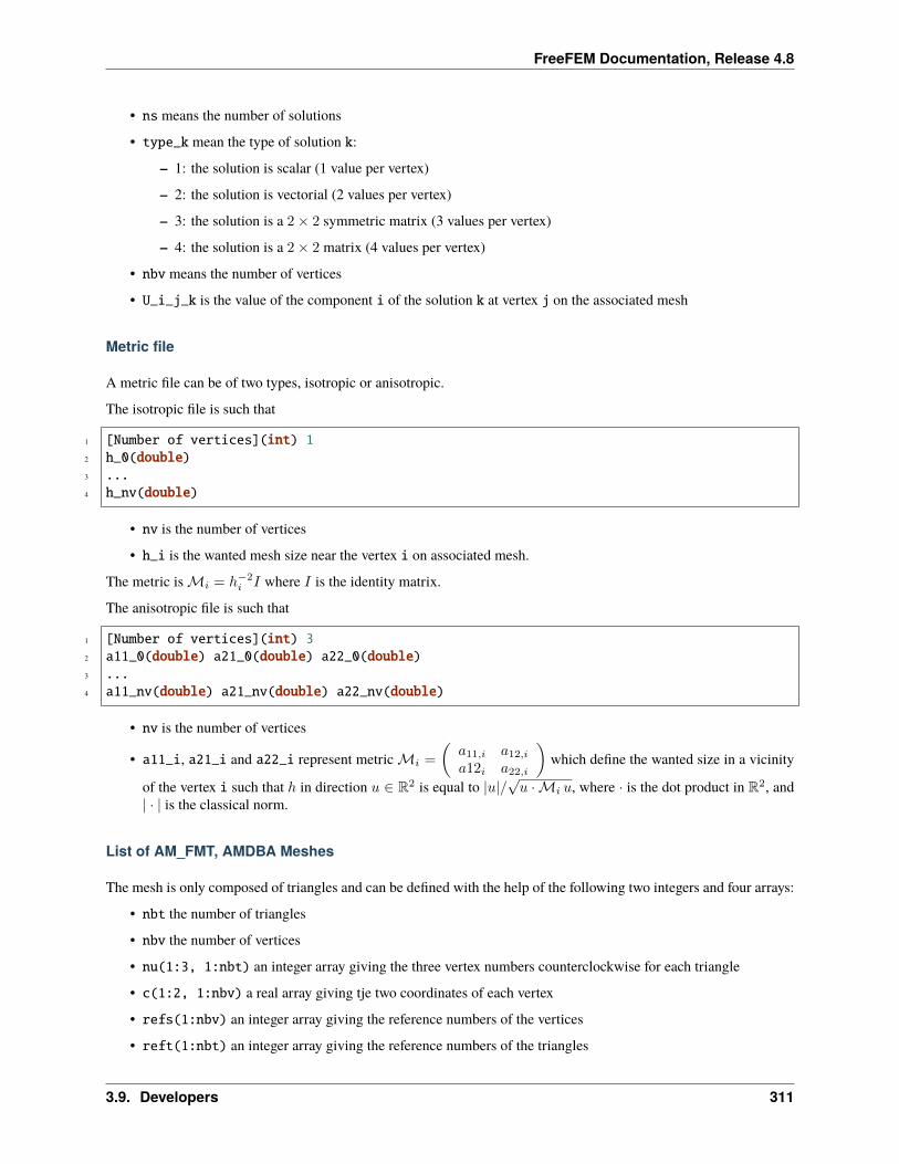
FreeFEM Documentation, Release 4.8
• ns means the number of solutions
• type_k mean the type of solution k:
– 1: the solution is scalar (1 value per vertex)
– 2: the solution is vectorial (2 values per vertex)
– 3: the solution is a 2× 2 symmetric matrix (3 values per vertex)
– 4: the solution is a 2× 2 matrix (4 values per vertex)
• nbv means the number of vertices
• U_i_j_k is the value of the component i of the solution k at vertex j on the associated mesh
Metric file
A metric file can be of two types, isotropic or anisotropic.
The isotropic file is such that
1 [Number of vertices](int) 12 h_0(double)3 ...4 h_nv(double)
• nv is the number of vertices
• h_i is the wanted mesh size near the vertex i on associated mesh.
The metric isℳ𝑖 = ℎ−2𝑖 𝐼 where 𝐼 is the identity matrix.
The anisotropic file is such that
1 [Number of vertices](int) 32 a11_0(double) a21_0(double) a22_0(double)3 ...4 a11_nv(double) a21_nv(double) a22_nv(double)
• nv is the number of vertices
• a11_i, a21_i and a22_i represent metricℳ𝑖 =
(𝑎11,𝑖 𝑎12,𝑖𝑎12𝑖 𝑎22,𝑖
)which define the wanted size in a vicinity
of the vertex i such that ℎ in direction 𝑢 ∈ R2 is equal to |𝑢|/√𝑢 · ℳ𝑖 𝑢, where · is the dot product in R2, and
| · | is the classical norm.
List of AM_FMT, AMDBA Meshes
The mesh is only composed of triangles and can be defined with the help of the following two integers and four arrays:
• nbt the number of triangles
• nbv the number of vertices
• nu(1:3, 1:nbt) an integer array giving the three vertex numbers counterclockwise for each triangle
• c(1:2, 1:nbv) a real array giving tje two coordinates of each vertex
• refs(1:nbv) an integer array giving the reference numbers of the vertices
• reft(1:nbt) an integer array giving the reference numbers of the triangles
3.9. Developers 311
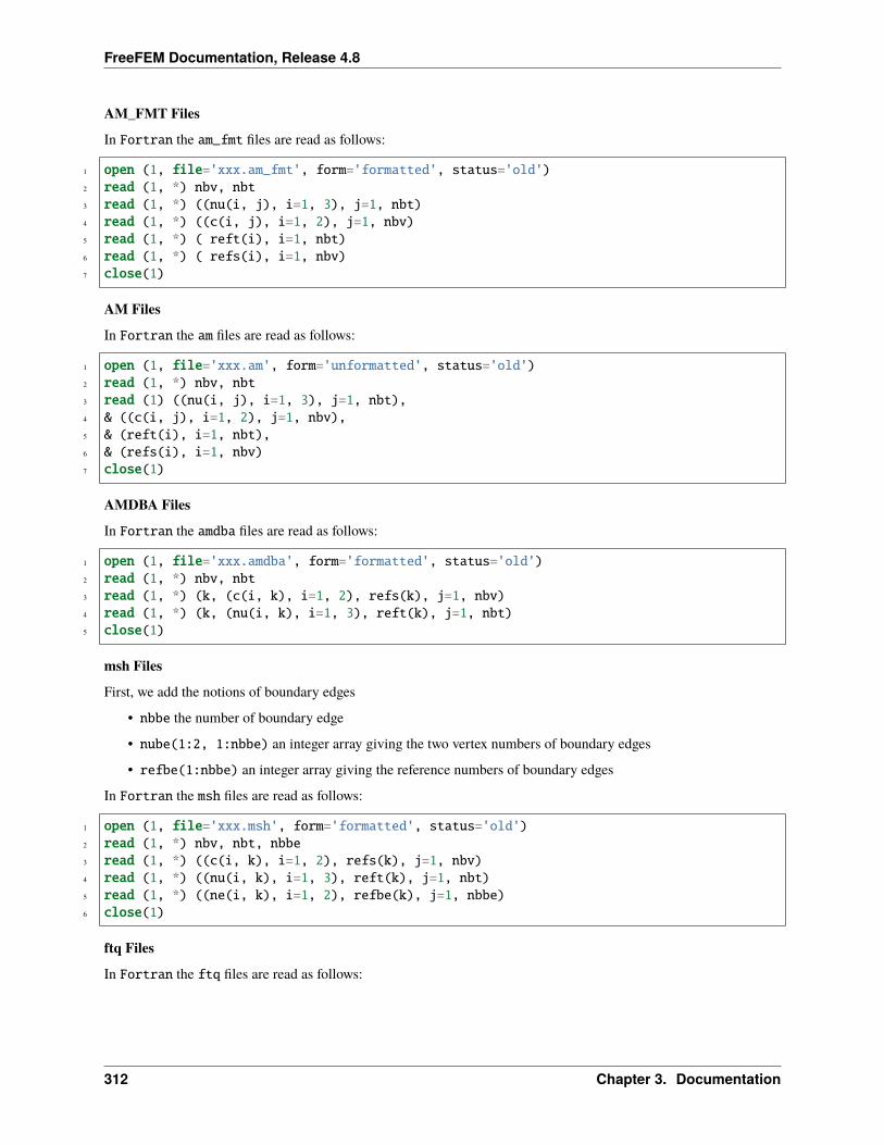
FreeFEM Documentation, Release 4.8
AM_FMT FilesIn Fortran the am_fmt files are read as follows:
1 open (1, file='xxx.am_fmt', form='formatted', status='old')2 read (1, *) nbv, nbt3 read (1, *) ((nu(i, j), i=1, 3), j=1, nbt)4 read (1, *) ((c(i, j), i=1, 2), j=1, nbv)5 read (1, *) ( reft(i), i=1, nbt)6 read (1, *) ( refs(i), i=1, nbv)7 close(1)
AM FilesIn Fortran the am files are read as follows:
1 open (1, file='xxx.am', form='unformatted', status='old')2 read (1, *) nbv, nbt3 read (1) ((nu(i, j), i=1, 3), j=1, nbt),4 & ((c(i, j), i=1, 2), j=1, nbv),5 & (reft(i), i=1, nbt),6 & (refs(i), i=1, nbv)7 close(1)
AMDBA FilesIn Fortran the amdba files are read as follows:
1 open (1, file='xxx.amdba', form='formatted', status='old')2 read (1, *) nbv, nbt3 read (1, *) (k, (c(i, k), i=1, 2), refs(k), j=1, nbv)4 read (1, *) (k, (nu(i, k), i=1, 3), reft(k), j=1, nbt)5 close(1)
msh FilesFirst, we add the notions of boundary edges
• nbbe the number of boundary edge
• nube(1:2, 1:nbbe) an integer array giving the two vertex numbers of boundary edges
• refbe(1:nbbe) an integer array giving the reference numbers of boundary edges
In Fortran the msh files are read as follows:
1 open (1, file='xxx.msh', form='formatted', status='old')2 read (1, *) nbv, nbt, nbbe3 read (1, *) ((c(i, k), i=1, 2), refs(k), j=1, nbv)4 read (1, *) ((nu(i, k), i=1, 3), reft(k), j=1, nbt)5 read (1, *) ((ne(i, k), i=1, 2), refbe(k), j=1, nbbe)6 close(1)
ftq FilesIn Fortran the ftq files are read as follows:
312 Chapter 3. Documentation
FreeFEM Documentation, Release 4.8
1 open(1,file='xxx.ftq',form='formatted',status='old')2 read (1,*) nbv,nbe,nbt,nbq3 read (1,*) (k(j),(nu(i,j),i=1,k(j)),reft(j),j=1,nbe)4 read (1,*) ((c(i,k),i=1,2),refs(k),j=1,nbv)5 close(1)
where if k(j) = 3 when the element j is a triangle and k(j) = 4 when the the element j is a quadrilateral.
sol and solb files
With the keyword savesol, we can store a scalar functions, a scalar finite element functions, a vector fields, a vectorfinite element fields, a symmetric tensor and a symmetric finite element tensor.
Such format is used in medit.
Extension file .solThe first two lines of the file are :
• MeshVersionFormatted 0
• Dimension [DIM](int)
The following fields begin with one of the following keyword: SolAtVertices, SolAtEdges, SolAtTriangles,SolAtQuadrilaterals, SolAtTetrahedra, SolAtPentahedra, SolAtHexahedra.
In each field, we give then in the next line the number of elements in the solutions (SolAtVertices: number ofvertices, SolAtTriangles: number of triangles, . . . ). In other lines, we give the number of solutions, the type ofsolution (1: scalar, 2: vector, 3: symmetric tensor). And finally, we give the values of the solutions on the elements.
The file must be ended with the keyword End.
The real element of symmetric tensor :
𝑆𝑇 3𝑑 =
⎛⎝ 𝑆𝑇 3𝑑𝑥𝑥 𝑆𝑇 3𝑑
𝑥𝑦 𝑆𝑇 3𝑑𝑥𝑧
𝑆𝑇 3𝑑𝑦𝑥 𝑆𝑇 3𝑑
𝑦𝑦 𝑆𝑇 3𝑑𝑦𝑧
𝑆𝑇 3𝑑𝑧𝑥 𝑆𝑇 3𝑑
𝑧𝑦 𝑆𝑇 3𝑑𝑧𝑧
⎞⎠ 𝑆𝑇 2𝑑 =
(𝑆𝑇 2𝑑
𝑥𝑥 𝑆𝑇 2𝑑𝑥𝑦
𝑆𝑇 2𝑑𝑦𝑥 𝑆𝑇 2𝑑
𝑦𝑦
)(3.31)
stored in the extension .sol are respectively 𝑆𝑇 3𝑑𝑥𝑥 , 𝑆𝑇
3𝑑𝑦𝑥 , 𝑆𝑇
3𝑑𝑦𝑦 , 𝑆𝑇
3𝑑𝑧𝑥 , 𝑆𝑇
3𝑑𝑧𝑦 , 𝑆𝑇
3𝑑𝑧𝑧 and 𝑆𝑇 2𝑑
𝑥𝑥 , 𝑆𝑇2𝑑𝑦𝑥 , 𝑆𝑇
2𝑑𝑦𝑦
An example of field with the keyword SolAtTetrahedra:
1 SolAtTetrahedra2 [Number of tetrahedra](int)3 [Number of solutions](int) [Type of solution 1](int) ... [Type of soution nt](int)4
5 U_1_1_1(double) ... U_nrs_1_1(double)6 ...7 U_1_ns_1(double) ... U_(nrs_k)_ns_1(double)8
9 ...10
11 U_1_1_nt(double) ... U_nrs_1_nt(double)12 ...13 U_1_ns_nt(double) ... U_(nrs_k)_ns_nt(double)
• ns is the number of solutions
• typesol_k, type of the solution number k
3.9. Developers 313
FreeFEM Documentation, Release 4.8
– typesol_k = 1 the solution k is scalar
– typesol_k = 2 the solution k is vectorial
– typesol_k = 3 the solution k is a symmetric tensor or symmetric matrix
• nrs_k is the number of real to describe solution k
– nrs_k = 1 if the solution k is scalar
– nrs_k = dim if the solution k is vectorial (dim is the dimension of the solution)
– nrs_k = dim*(dim+1)/2 if the solution k is a symmetric tensor or symmetric matrix
• U_i_j_^k is a real equal to the value of the component i of the solution k at tetrahedron j on the associatedmesh
The format .solb is the same as format .sol but in binary (read/write is faster, storage is less).
A real scalar functions 𝑓1, a vector fields Φ = [Φ1,Φ2,Φ3] and a symmetric tensor 𝑆𝑇 3𝑑 (3.31) at the vertices of thethree dimensional mesh Th3 is stored in the file f1PhiTh3.sol using :
1 savesol("f1PhiST3dTh3.sol", Th3, f1, [Phi(1), Phi(2), Phi(3)], VV3, order=1);
where 𝑉 𝑉 3 = [𝑆𝑇 3𝑑𝑥𝑥 , 𝑆𝑇
3𝑑𝑦𝑥 , 𝑆𝑇
3𝑑𝑦𝑦 , 𝑆𝑇
3𝑑𝑧𝑥 , 𝑆𝑇
3𝑑𝑧𝑦 , 𝑆𝑇
3𝑑𝑧𝑧 ].
For a two dimensional mesh Th, A real scalar functions 𝑓2, a vector fields Ψ = [Ψ1,Ψ2] and a symmetric tensor 𝑆𝑇 2𝑑
(3.31) at triangles is stored in the file f2PsiST2dTh3.solb using :
1 savesol("f2PsiST2dTh3.solb", Th, f2, [Psi(1), Psi(2)], VV2, order=0);
where 𝑉 𝑉 2 = [𝑆𝑇 2𝑑𝑥𝑥 , 𝑆𝑇
2𝑑𝑦𝑥 , 𝑆𝑇
2𝑑𝑦𝑦 ]
The arguments of savesol functions are the name of a file, a mesh and solutions. These arguments must be given inthis order.
The parameters of this keyword are :
• order = 0 is the solution is given at the center of gravity of elements. 1 is the solution is given at the verticesof elements.
In the file, solutions are stored in this order : scalar solutions, vector solutions and finally symmetric tensor solutions.
3.9.2 Adding a new finite element
Some notations
For a function 𝑓 taking value in R𝑁 , 𝑁 = 1, 2, · · ·, we define the finite element approximation Πℎ𝑓 of 𝑓 .
Let us denote the number of the degrees of freedom of the finite element by 𝑁𝑏𝐷𝑜𝐹 . Then the 𝑖-th base 𝜔𝐾𝑖 (𝑖 =0, · · · , 𝑁𝑏𝐷𝑜𝐹 − 1) of the finite element space has the 𝑗-th component 𝜔𝐾𝑖𝑗 for 𝑗 = 0, · · · , 𝑁 − 1.
The operator Πℎ is called the interpolator of the finite element.
We have the identity 𝜔𝐾𝑖 = Πℎ𝜔𝐾𝑖 .
Formally, the interpolator Πℎ is constructed by the following formula:
Πℎ𝑓 =
kPi−1∑𝑘=0
𝛼𝑘𝑓 𝑗𝑘(𝑃𝑝𝑘)𝜔𝐾𝑖𝑘 (3.32)
where 𝑃𝑝 is a set of 𝑛𝑝𝑃𝑖 points,
314 Chapter 3. Documentation
FreeFEM Documentation, Release 4.8
In the formula (3.32), the list 𝑝𝑘, 𝑗𝑘, 𝑖𝑘 depend just on the type of finite element (not on the element), but the coefficient𝛼𝑘 can be depending on the element.
Tip: Classical scalar Lagrange finite element
With the classical scalar Lagrange finite element, we have kPi = npPi = NbOfNode and
• 𝑃𝑝 is the point of the nodal points.
• the 𝛼𝑘 = 1, because we take the value of the function at the point 𝑃𝑘.
• 𝑝𝑘 = 𝑘 , 𝑗𝑘 = 𝑘 because we have one node per function.
• 𝑗𝑘 = 0 because 𝑁 = 1.
Tip: The Raviart-Thomas finite element
𝑅𝑇0ℎ = v ∈ 𝐻(𝑑𝑖𝑣)/∀𝐾 ∈ 𝒯ℎ v|𝐾(𝑥, 𝑦) = 𝛼𝐾
𝛽𝐾+ 𝛾𝐾 | 𝑥𝑦 (3.33)
The degrees of freedom are the flux through an edge 𝑒 of the mesh, where the flux of the function f : R2 −→ R2 is∫𝑒f .𝑛𝑒, 𝑛𝑒 is the unit normal of edge 𝑒 (this implies a orientation of all the edges of the mesh, for example we can use
the global numbering of the edge vertices and we just go to small to large number).
To compute this flux, we use a quadrature formula with one point, the middle point of the edge. Consider a triangle 𝑇with three vertices (a,b, c).
Let denote the vertices numbers by 𝑖𝑎, 𝑖𝑏, 𝑖𝑐, and define the three edge vectors e0, e1, e2 by 𝑠𝑔𝑛(𝑖𝑏 − 𝑖𝑐)(b − c),𝑠𝑔𝑛(𝑖𝑐 − 𝑖𝑎)(c− a), 𝑠𝑔𝑛(𝑖𝑎 − 𝑖𝑏)(a− b).
The three basis functions are:
𝜔𝐾0 =𝑠𝑔𝑛(𝑖𝑏 − 𝑖𝑐)
2|𝑇 |(𝑥− 𝑎), 𝜔𝐾1 =
𝑠𝑔𝑛(𝑖𝑐 − 𝑖𝑎)
2|𝑇 |(𝑥− 𝑏), 𝜔𝐾2 =
𝑠𝑔𝑛(𝑖𝑎 − 𝑖𝑏)2|𝑇 |
(𝑥− 𝑐),
where |𝑇 | is the area of the triangle 𝑇 .
So we have 𝑁 = 2, kPi = 6; npPi = 3; and:
• 𝑃𝑝 =
b+c2 , a+c
2 , b+a2
• 𝛼0 = −e02, 𝛼1 = e01, 𝛼2 = −e12, 𝛼3 = e11, 𝛼4 = −e22, 𝛼5 = e21 (effectively, the vector (−e𝑚2 , e𝑚1 ) is orthogonal
to the edge e𝑚 = (𝑒𝑚1 , 𝑒𝑚2 ) with a length equal to the side of the edge or equal to
∫𝑒𝑚
1).
• 𝑖𝑘 = 0, 0, 1, 1, 2, 2,
• 𝑝𝑘 = 0, 0, 1, 1, 2, 2 , 𝑗𝑘 = 0, 1, 0, 1, 0, 1, 0, 1.
Which class to add?
Add file FE_ADD.cpp in directory FreeFem-sources/src/femlib for example first to initialize :
1 #include "error.hpp"2 #include "rgraph.hpp"3 using namespace std;4 #include "RNM.hpp"5 #include "fem.hpp"6 #include "FESpace.hpp"
(continues on next page)
3.9. Developers 315
FreeFEM Documentation, Release 4.8
(continued from previous page)
7 #include "AddNewFE.h"8
9 namespace Fem2D ...
Then add a class which derive for public TypeOfFE like:
1 class TypeOfFE_RTortho : public TypeOfFE public:2 static int Data[]; //some numbers3 TypeOfFE_RTortho():4 TypeOfFE(5 0+3+0, //nb degree of freedom on element6 2, //dimension N of vectorial FE (1 if scalar FE)7 Data, //the array data8 1, //nb of subdivision for plotting9 1, //nb of sub finite element (generaly 1)
10 6, //number kPi of coef to build the interpolator11 3, //number npPi of integration point to build interpolator12 0 //an array to store the coef \alpha_k to build interpolator13 //here this array is no constant so we have14 //to rebuilt for each element15 )16 17 const R2 Pt[] = R2(0.5, 0.5), R2(0.0, 0.5), R2(0.5, 0.0) ;18 // the set of Point in hatK19 for (int p = 0, kk = 0; p < 3; p++)20 P_Pi_h[p] = Pt[p];21 for (int j = 0; j < 2; j++)22 pij_alpha[kk++] = IPJ(p, p, j);23 24 //definition of i_k, p_k, j_k in interpolator25
26 void FB(const bool *watdd, const Mesh &Th, const Triangle &K,27 const R2 &PHat, RNMK_ &val) const;28
29 void Pi_h_alpha(const baseFElement &K, KN_<double> &v) const;30 ;
where the array data is formed with the concatenation of five array of size NbDoF and one array of size N.
This array is:
1 int TypeOfFE_RTortho::Data[] = 2 //for each df 0, 1, 3:3 3, 4, 5, //the support of the node of the df4 0, 0, 0, //the number of the df on the node5 0, 1, 2, //the node of the df6 0, 0, 0, //the df come from which FE (generally 0)7 0, 1, 2, //which are the df on sub FE8 0, 09 ; //for each component j=0, N-1 it give the sub FE associated
where the support is a number 0, 1, 2 for vertex support, 3, 4, 5 for edge support, and finally 6 for element support.
The function to defined the function 𝜔𝐾𝑖 , this function return the value of all the basics function or this derivatives in
316 Chapter 3. Documentation
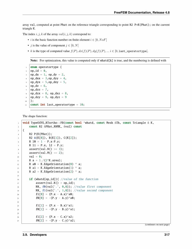
FreeFEM Documentation, Release 4.8
array val, computed at point Phat on the reference triangle corresponding to point R2 P=K(Phat); on the currenttriangle K.
The index 𝑖, 𝑗, 𝑘 of the array 𝑣𝑎𝑙(𝑖, 𝑗, 𝑘) correspond to:
• 𝑖 is the basic function number on finite element 𝑖 ∈ [0, 𝑁𝑜𝐹 [
• 𝑗 is the value of component 𝑗 ∈ [0, 𝑁 [
• 𝑘 is the type of computed value 𝑓(𝑃 ), 𝑑𝑥(𝑓)(𝑃 ), 𝑑𝑦(𝑓)(𝑃 ), ... 𝑖 ∈ [0, last_operatortype[.
Note: For optimization, this value is computed only if whatd[k] is true, and the numbering is defined with
1 enum operatortype 2 op_id = 0,3 op_dx = 1, op_dy = 2,4 op_dxx = 3,op_dyy = 4,5 op_dyx = 5,op_dxy = 5,6 op_dz = 6,7 op_dzz = 7,8 op_dzx = 8, op_dxz = 8,9 op_dzy = 9, op_dyz = 9
10 ;11 const int last_operatortype = 10;
The shape function:
1 void TypeOfFE_RTortho::FB(const bool *whatd, const Mesh &Th, const Triangle & K,2 const R2 &PHat,RNMK_ &val) const3 4 R2 P(K(PHat));5 R2 A(K[0]), B(K[1]), C(K[2]);6 R l0 = 1 - P.x-P.y;7 R l1 = P.x, l2 = P.y;8 assert(val.N() >= 3);9 assert(val.M() == 2);
10 val = 0;11 R a = 1./(2*K.area);12 R a0 = K.EdgeOrientation(0) * a;13 R a1 = K.EdgeOrientation(1) * a;14 R a2 = K.EdgeOrientation(2) * a;15
16 if (whatd[op_id]) //value of the function17 assert(val.K() > op_id);18 RN_ f0(val('.', 0,0)); //value first component19 RN_ f1(val('.', 1,0)); //value second component20 f1[0] = (P.x - A.x)*a0;21 f0[0] = -(P.y - A.y)*a0;22
23 f1[1] = (P.x - B.x)*a1;24 f0[1] = -(P.y - B.y)*a1;25
26 f1[2] = (P.x - C.x)*a2;27 f0[2] = -(P.y - C.y)*a2;
(continues on next page)
3.9. Developers 317
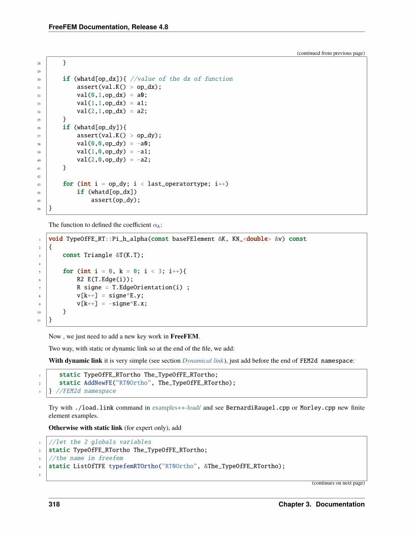
FreeFEM Documentation, Release 4.8
(continued from previous page)
28 29
30 if (whatd[op_dx]) //value of the dx of function31 assert(val.K() > op_dx);32 val(0,1,op_dx) = a0;33 val(1,1,op_dx) = a1;34 val(2,1,op_dx) = a2;35 36 if (whatd[op_dy])37 assert(val.K() > op_dy);38 val(0,0,op_dy) = -a0;39 val(1,0,op_dy) = -a1;40 val(2,0,op_dy) = -a2;41 42
43 for (int i = op_dy; i < last_operatortype; i++)44 if (whatd[op_dx])45 assert(op_dy);46
The function to defined the coefficient 𝛼𝑘:
1 void TypeOfFE_RT::Pi_h_alpha(const baseFElement &K, KN_<double> &v) const2 3 const Triangle &T(K.T);4
5 for (int i = 0, k = 0; i < 3; i++)6 R2 E(T.Edge(i));7 R signe = T.EdgeOrientation(i) ;8 v[k++] = signe*E.y;9 v[k++] = -signe*E.x;
10 11
Now , we just need to add a new key work in FreeFEM.
Two way, with static or dynamic link so at the end of the file, we add:
With dynamic link it is very simple (see section Dynamical link), just add before the end of FEM2d namespace:
1 static TypeOfFE_RTortho The_TypeOfFE_RTortho;2 static AddNewFE("RT0Ortho", The_TypeOfFE_RTortho);3 //FEM2d namespace
Try with ./load.link command in examples++-load/ and see BernardiRaugel.cpp or Morley.cpp new finiteelement examples.
Otherwise with static link (for expert only), add
1 //let the 2 globals variables2 static TypeOfFE_RTortho The_TypeOfFE_RTortho;3 //the name in freefem4 static ListOfTFE typefemRTOrtho("RT0Ortho", &The_TypeOfFE_RTortho);5
(continues on next page)
318 Chapter 3. Documentation
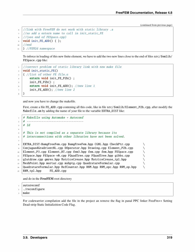
FreeFEM Documentation, Release 4.8
(continued from previous page)
6 //link with FreeFEM do not work with static library .a7 //so add a extern name to call in init_static_FE8 //(see end of FESpace.cpp)9 void init_FE_ADD() ;
10 //end11 //FEM2d namespace
To inforce in loading of this new finite element, we have to add the two new lines close to the end of files src/femlib/FESpace.cpp like:
1 //correct problem of static library link with new make file2 void init_static_FE()3 //list of other FE file.o4 extern void init_FE_P2h() ;5 init_FE_P2h() ;6 extern void init_FE_ADD(); //new line 17 init_FE_ADD(); //new line 28
and now you have to change the makefile.
First, create a file FE_ADD.cpp contening all this code, like in file src/femlib/Element_P2h.cpp, after modify theMakefile.am by adding the name of your file to the variable EXTRA_DIST like:
1 # Makefile using Automake + Autoconf2 # ----------------------------------3 # Id4
5 # This is not compiled as a separate library because its6 # interconnections with other libraries have not been solved.7
8 EXTRA_DIST=BamgFreeFem.cpp BamgFreeFem.hpp CGNL.hpp CheckPtr.cpp \9 ConjuguedGradrientNL.cpp DOperator.hpp Drawing.cpp Element_P2h.cpp \
10 Element_P3.cpp Element_RT.cpp fem3.hpp fem.cpp fem.hpp FESpace.cpp \11 FESpace.hpp FESpace-v0.cpp FQuadTree.cpp FQuadTree.hpp gibbs.cpp \12 glutdraw.cpp gmres.hpp MatriceCreuse.hpp MatriceCreuse_tpl.hpp \13 MeshPoint.hpp mortar.cpp mshptg.cpp QuadratureFormular.cpp \14 QuadratureFormular.hpp RefCounter.hpp RNM.hpp RNM_opc.hpp RNM_op.hpp \15 RNM_tpl.hpp FE_ADD.cpp
and do in the FreeFEM root directory
1 autoreconf2 ./reconfigure3 make
For codewarrior compilation add the file in the project an remove the flag in panal PPC linker FreeFm++ SettingDead-strip Static Initializition Code Flag.
3.9. Developers 319
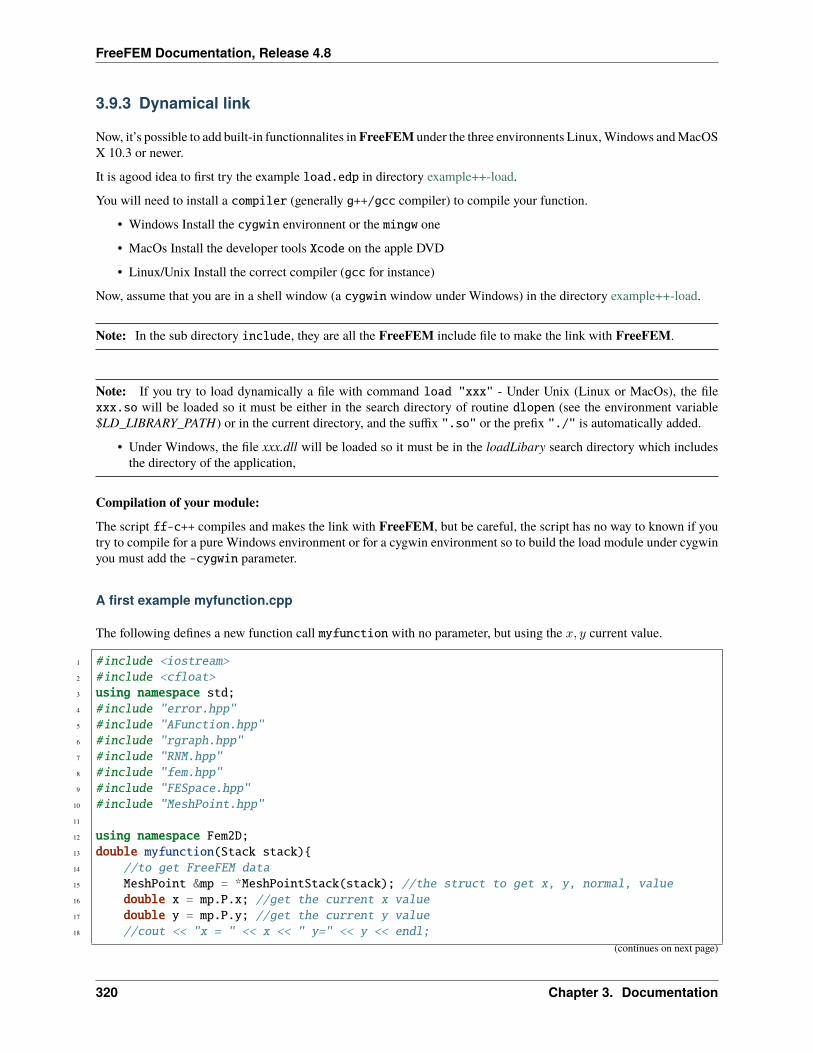
FreeFEM Documentation, Release 4.8
3.9.3 Dynamical link
Now, it’s possible to add built-in functionnalites in FreeFEM under the three environnents Linux, Windows and MacOSX 10.3 or newer.
It is agood idea to first try the example load.edp in directory example++-load.
You will need to install a compiler (generally g++/gcc compiler) to compile your function.
• Windows Install the cygwin environnent or the mingw one
• MacOs Install the developer tools Xcode on the apple DVD
• Linux/Unix Install the correct compiler (gcc for instance)
Now, assume that you are in a shell window (a cygwin window under Windows) in the directory example++-load.
Note: In the sub directory include, they are all the FreeFEM include file to make the link with FreeFEM.
Note: If you try to load dynamically a file with command load "xxx" - Under Unix (Linux or MacOs), the filexxx.so will be loaded so it must be either in the search directory of routine dlopen (see the environment variable$LD_LIBRARY_PATH) or in the current directory, and the suffix ".so" or the prefix "./" is automatically added.
• Under Windows, the file xxx.dll will be loaded so it must be in the loadLibary search directory which includesthe directory of the application,
Compilation of your module:The script ff-c++ compiles and makes the link with FreeFEM, but be careful, the script has no way to known if youtry to compile for a pure Windows environment or for a cygwin environment so to build the load module under cygwinyou must add the -cygwin parameter.
A first example myfunction.cpp
The following defines a new function call myfunction with no parameter, but using the 𝑥, 𝑦 current value.
1 #include <iostream>2 #include <cfloat>3 using namespace std;4 #include "error.hpp"5 #include "AFunction.hpp"6 #include "rgraph.hpp"7 #include "RNM.hpp"8 #include "fem.hpp"9 #include "FESpace.hpp"
10 #include "MeshPoint.hpp"11
12 using namespace Fem2D;13 double myfunction(Stack stack)14 //to get FreeFEM data15 MeshPoint &mp = *MeshPointStack(stack); //the struct to get x, y, normal, value16 double x = mp.P.x; //get the current x value17 double y = mp.P.y; //get the current y value18 //cout << "x = " << x << " y=" << y << endl;
(continues on next page)
320 Chapter 3. Documentation
FreeFEM Documentation, Release 4.8
(continued from previous page)
19 return sin(x)*cos(y);20
Now the Problem is to build the link with FreeFEM, to do that we need two classes, one to call the functionmyfunction.
All FreeFEM evaluable expression must be a C++ struct/classwhich derivate from E_F0. By default this expressiondoes not depend of the mesh position, but if they derivate from E_F0mps the expression depends of the mesh position,and for more details see [HECHT2002].
1 //A class build the link with FreeFEM2 //generaly this class are already in AFunction.hpp3 //but unfortunatly, I have no simple function with no parameter4 //in FreeFEM depending of the mesh5 template<class R>6 class OneOperator0s : public OneOperator 7 //the class to define and evaluate a new function8 //It must devive from E_F0 if it is mesh independent9 //or from E_F0mps if it is mesh dependent
10 class E_F0_F :public E_F0mps 11 public:12 typedef R (*func)(Stack stack);13 func f; //the pointeur to the fnction myfunction14 E_F0_F(func ff) : f(ff) 15 //the operator evaluation in FreeFEM16 AnyType operator()(Stack stack) const return SetAny<R>(f(stack));17 ;18 typedef R (*func)(Stack);19 func f;20 public:21 //the function which build the FreeFEM byte code22 E_F0 *code(const basicAC_F0 &) const return new E_F0_F(f); 23 //the constructor to say ff is a function without parameter24 //and returning a R25 OneOperator0s(func ff) : OneOperator(map_type[typeid(R).name()]),f(ff)26 ;
To finish we must add this new function in FreeFEM table, to do that include :
1 void init()2 Global.Add("myfunction", "(", new OneOperator0s<double>(myfunction));3 4 LOADFUNC(init);
It will be called automatically at load module time.
To compile and link, use the ff-c++ script :
1 ff-c++ myfunction.cpp2 g++ -c -g -Iinclude myfunction.cpp3 g++ -bundle -undefined dynamic_lookup -g myfunction.o -o ./myfunction.dylib
To try the simple example under Linux or MacOS, do FreeFem++-nw load.edp
The output must be:
3.9. Developers 321
FreeFEM Documentation, Release 4.8
1 -- FreeFem++ v *.****** (date *** ** *** ****, **:**:** (UTC+0*00))2 Load: lg_fem lg_mesh lg_mesh3 eigenvalue3 1 : // Example of dynamic function load4 2 : // --------------------------------5 3 : // $Id$6 4 :7 5 : load "myfunction"8 6 : // dumptable(cout);9 7 : mesh Th=square(5,5);
10 8 : fespace Vh(Th,P1);11 9 : Vh uh= myfunction(); // warning do not forget ()12 10 : cout << uh[].min << " " << uh[].max << endl;13 11 : cout << " test io ( " << endl;14 12 : testio();15 13 : cout << " ) end test io .. " << endl; sizestack + 1024 =1416 ( 392 )16
17 -- Square mesh : nb vertices =36 , nb triangles = 50 , nb boundary edges 2018 0 0.84147119 test io (20 test cout 3.1415921 test cout 51222 test cerr 3.1415923 test cerr 51224 ) end test io ..25 times: compile 0.012854s, execution 0.000313s, mpirank:026 CodeAlloc : nb ptr 2715, size :371104 mpirank: 027 Ok: Normal End
Under Windows, launch FreeFEM with the mouse (or ctrl O) on the example.
Example: Discrete Fast Fourier Transform
This will add FFT to FreeFEM, taken from FFTW. To download and install under download/include just go indownload/fftw and try make.
The 1D dfft (fast discret fourier transform) for a simple array 𝑓 of size 𝑛 is defined by the following formula:
dfft(𝑓, 𝜀)𝑘 =
𝑛−1∑𝑗=0
𝑓𝑖𝑒𝜀2𝜋𝑖𝑘𝑗/𝑛
The 2D DFFT for an array of size 𝑁 = 𝑛×𝑚 is:
dfft(𝑓,𝑚, 𝜀)𝑘+𝑛𝑙 =
𝑚−1∑𝑗′=0
𝑛−1∑𝑗=0
𝑓𝑖+𝑛𝑗𝑒𝜀2𝜋𝑖(𝑘𝑗/𝑛+𝑙𝑗′/𝑚)
Note: The value 𝑛 is given by 𝑠𝑖𝑧𝑒(𝑓)/𝑚, and the numbering is row-major order.
So the classical discrete DFFT is 𝑓 = dfft(𝑓,−1)/√𝑛 and the reverse dFFT 𝑓 = dfft(𝑓, 1)/
√𝑛
Note: The 2D Laplace operator is
322 Chapter 3. Documentation
FreeFEM Documentation, Release 4.8
𝑓(𝑥, 𝑦) = 1/√𝑁
𝑚−1∑𝑗′=0
𝑛−1∑𝑗=0
𝑓𝑖+𝑛𝑗𝑒𝜀2𝜋𝑖(𝑥𝑗+𝑦𝑗′)
and we have
𝑓𝑘+𝑛𝑙 = 𝑓(𝑘/𝑛, 𝑙/𝑚)
So
∆𝑓𝑘𝑙 = −((2𝜋)2((𝑘)2 + ()2))𝑓𝑘𝑙where 𝑘 = 𝑘 if 𝑘 ≤ 𝑛/2 else 𝑘 = 𝑘 − 𝑛 and = 𝑙 if 𝑙 ≤ 𝑚/2 else = 𝑙 −𝑚.
And to have a real function we need all modes to be symmetric around zero, so 𝑛 and 𝑚 must be odd.
Compile to build a new library
1 ff-c++ dfft.cpp ../download/install/lib/libfftw3.a -I../download/install/include2 export MACOSX_DEPLOYMENT_TARGET=10.33 g++ -c -Iinclude -I../download/install/include dfft.cpp4 g++ -bundle -undefined dynamic_lookup dfft.o -o ./dfft.dylib ../download/install/lib/
→˓libfftw3.a
To test, try FFT example.
Load Module for Dervieux P0-P1 Finite Volume Method
The associed edp file is examples++-load/convect_dervieux.edp.
See mat_dervieux.cpp.
More on Adding a new finite element
First read the Adding a new finite element section, we add two new finite elements examples in the directory examples++-load.
The Bernardi-Raugel Element
The Bernardi-Raugel finite element is meant to solve the Navier Stokes equations in 𝑢, 𝑝 formulation; the velocity space𝑃 𝑏𝑟𝐾 is minimal to prove the inf-sup condition with piecewise constant pressure by triangle.
The finite element space 𝑉ℎ is
𝑉ℎ = 𝑢 ∈ 𝐻1(Ω)2; ∀𝐾 ∈ 𝑇ℎ, 𝑢|𝐾 ∈ 𝑃 𝑏𝑟𝐾
where
𝑃 𝑏𝑟𝐾 = 𝑠𝑝𝑎𝑛𝜆𝐾𝑖 𝑒𝑘𝑖=1,2,3,𝑘=1,2 ∪ 𝜆𝐾𝑖 𝜆𝐾𝑖+1𝑛𝐾𝑖+2𝑖=1,2,3
with notation 4 = 1, 5 = 2 and where 𝜆𝐾𝑖 are the barycentric coordinates of the triangle 𝐾, (𝑒𝑘)𝑘=1,2 the canonicalbasis of R2 and 𝑛𝐾𝑘 the outer normal of triangle 𝐾 opposite to vertex 𝑘.
See BernardiRaugel.cpp.
A way to check the finite element
3.9. Developers 323
FreeFEM Documentation, Release 4.8
1 load "BernardiRaugel"2
3 // Macro4 //a macro the compute numerical derivative5 macro DD(f, hx, hy) ( (f(x1+hx, y1+hy) - f(x1-hx, y1-hy))/(2*(hx+hy)) ) //6
7 // Mesh8 mesh Th = square(1, 1, [10*(x+y/3), 10*(y-x/3)]);9
10 // Parameters11 real x1 = 0.7, y1 = 0.9, h = 1e-7;12 int it1 = Th(x1, y1).nuTriangle;13
14 // Fespace15 fespace Vh(Th, P2BR);16 Vh [a1, a2], [b1, b2], [c1, c2];17
18
19 for (int i = 0; i < Vh.ndofK; ++i)20 cout << i << " " << Vh(0,i) << endl;21
22 for (int i = 0; i < Vh.ndofK; ++i)23 24 a1[] = 0;25 int j = Vh(it1, i);26 a1[][j] = 1;27 plot([a1, a2], wait=1);28 [b1, b2] = [a1, a2]; //do the interpolation29
30 c1[] = a1[] - b1[];31 cout << " ---------" << i << " " << c1[].max << " " << c1[].min << endl;32 cout << " a = " << a1[] <<endl;33 cout << " b = " << b1[] <<endl;34 assert(c1[].max < 1e-9 && c1[].min > -1e-9); //check if the interpolation is correct35
36 // check the derivative and numerical derivative37 cout << " dx(a1)(x1, y1) = " << dx(a1)(x1, y1) << " == " << DD(a1, h, 0) << endl;38 assert( abs(dx(a1)(x1, y1) - DD(a1, h, 0) ) < 1e-5);39 assert( abs(dx(a2)(x1, y1) - DD(a2, h, 0) ) < 1e-5);40 assert( abs(dy(a1)(x1, y1) - DD(a1, 0, h) ) < 1e-5);41 assert( abs(dy(a2)(x1, y1) - DD(a2, 0, h) ) < 1e-5);42
A real example using this finite element, just a small modification of the Navier-Stokes P2-P1 example, just the begen-ning is change to
1 load "BernardiRaugel"2
3 real s0 = clock();4 mesh Th = square(10, 10);5 fespace Vh2(Th, P2BR);6 fespace Vh(Th, P0);7 Vh2 [u1, u2], [up1, up2];
(continues on next page)
324 Chapter 3. Documentation
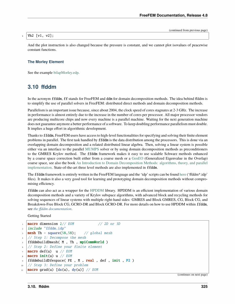
FreeFEM Documentation, Release 4.8
(continued from previous page)
8 Vh2 [v1, v2];
And the plot instruction is also changed because the pressure is constant, and we cannot plot isovalues of peacewiseconstant functions.
The Morley Element
See the example bilapMorley.edp.
3.10 ffddm
In the acronym ffddm, ff stands for FreeFEM and ddm for domain decomposition methods. The idea behind ffddm isto simplify the use of parallel solvers in FreeFEM: distributed direct methods and domain decomposition methods.
Parallelism is an important issue because, since about 2004, the clock speed of cores stagnates at 2-3 GHz. The increasein performance is almost entirely due to the increase in the number of cores per processor. All major processor vendorsare producing multicore chips and now every machine is a parallel machine. Waiting for the next generation machinedoes not guarantee anymore a better performance of a software. To keep doubling performance parallelism must double.It implies a huge effort in algorithmic development.
Thanks to ffddm, FreeFEM users have access to high-level functionalities for specifying and solving their finite elementproblems in parallel. The first task handled by ffddm is the data distribution among the processors. This is done via anoverlapping domain decomposition and a related distributed linear algebra. Then, solving a linear system is possibleeither via an interface to the parallel MUMPS solver or by using domain decomposition methods as preconditionersto the GMRES Krylov method. The ffddm framework makes it easy to use scalable Schwarz methods enhancedby a coarse space correction built either from a coarse mesh or a GenEO (Generalized Eigenvalue in the Overlap)coarse space, see also the book An Introduction to Domain Decomposition Methods: algorithms, theory, and parallelimplementation. State-of-the-art three level methods are also implemented in ffddm.
The ffddm framework is entirely written in the FreeFEM language and the ‘idp’ scripts can be found here (‘ffddm*.idp’files). It makes it also a very good tool for learning and prototyping domain decomposition methods without compro-mising efficiency.
ffddm can also act as a wrapper for the HPDDM library. HPDDM is an efficient implementation of various domaindecomposition methods and a variety of Krylov subspace algorithms, with advanced block and recycling methods forsolving sequences of linear systems with multiple right-hand sides: GMRES and Block GMRES, CG, Block CG, andBreakdown-Free Block CG, GCRO-DR and Block GCRO-DR. For more details on how to use HPDDM within ffddm,see the ffddm documentation.
Getting Started
1 macro dimension 2// EOM // 2D or 3D2 include "ffddm.idp"3 mesh Th = square(50,50); // global mesh4 // Step 1: Decompose the mesh5 ffddmbuildDmesh( M , Th , mpiCommWorld )6 // Step 2: Define your finite element7 macro def(u) u // EOM8 macro init(u) u // EOM9 ffddmbuildDfespace( FE , M , real , def , init , P2 )
10 // Step 3: Define your problem11 macro grad(u) [dx(u), dy(u)] // EOM
(continues on next page)
3.10. ffddm 325
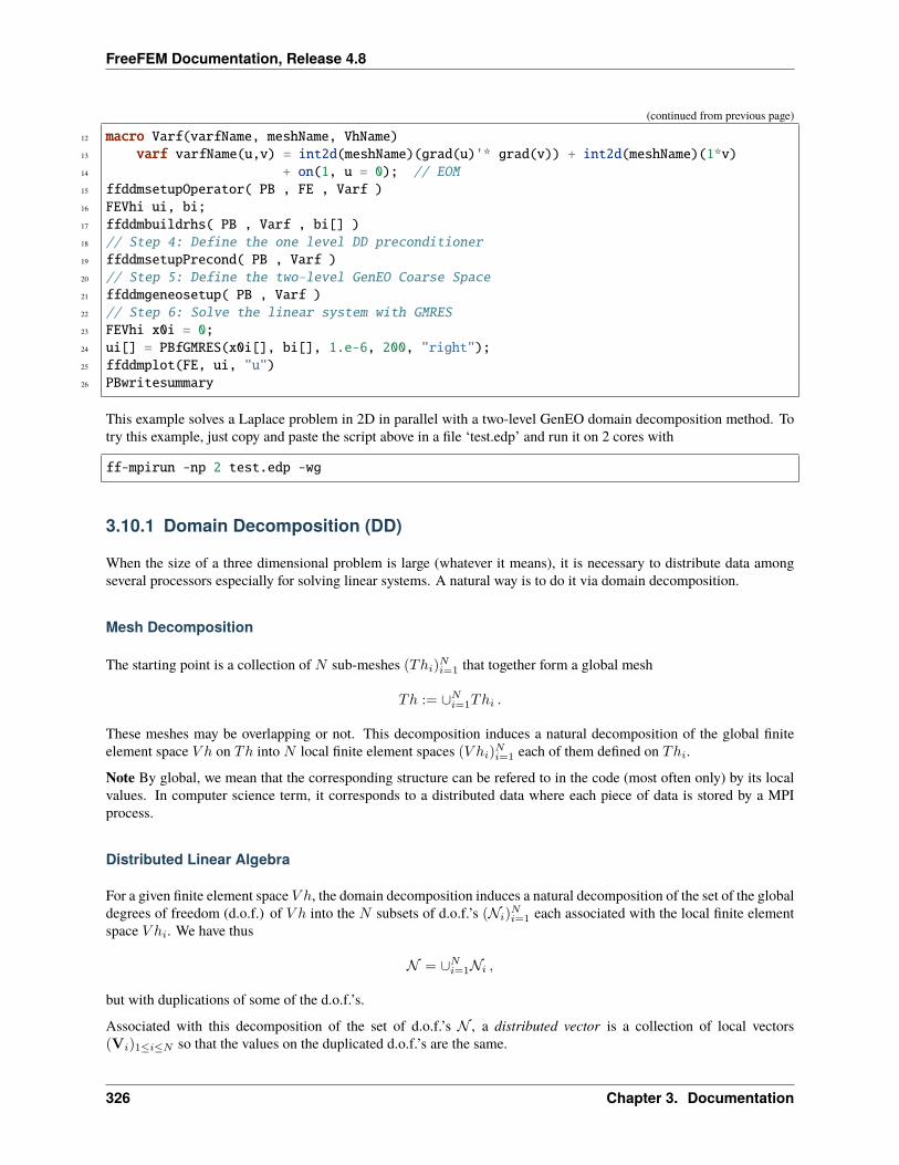
FreeFEM Documentation, Release 4.8
(continued from previous page)
12 macro Varf(varfName, meshName, VhName)13 varf varfName(u,v) = int2d(meshName)(grad(u)'* grad(v)) + int2d(meshName)(1*v)14 + on(1, u = 0); // EOM15 ffddmsetupOperator( PB , FE , Varf )16 FEVhi ui, bi;17 ffddmbuildrhs( PB , Varf , bi[] )18 // Step 4: Define the one level DD preconditioner19 ffddmsetupPrecond( PB , Varf )20 // Step 5: Define the two-level GenEO Coarse Space21 ffddmgeneosetup( PB , Varf )22 // Step 6: Solve the linear system with GMRES23 FEVhi x0i = 0;24 ui[] = PBfGMRES(x0i[], bi[], 1.e-6, 200, "right");25 ffddmplot(FE, ui, "u")26 PBwritesummary
This example solves a Laplace problem in 2D in parallel with a two-level GenEO domain decomposition method. Totry this example, just copy and paste the script above in a file ‘test.edp’ and run it on 2 cores with
ff-mpirun -np 2 test.edp -wg
3.10.1 Domain Decomposition (DD)
When the size of a three dimensional problem is large (whatever it means), it is necessary to distribute data amongseveral processors especially for solving linear systems. A natural way is to do it via domain decomposition.
Mesh Decomposition
The starting point is a collection of 𝑁 sub-meshes (𝑇ℎ𝑖)𝑁𝑖=1 that together form a global mesh
𝑇ℎ := ∪𝑁𝑖=1𝑇ℎ𝑖 .
These meshes may be overlapping or not. This decomposition induces a natural decomposition of the global finiteelement space 𝑉 ℎ on 𝑇ℎ into 𝑁 local finite element spaces (𝑉 ℎ𝑖)
𝑁𝑖=1 each of them defined on 𝑇ℎ𝑖.
Note By global, we mean that the corresponding structure can be refered to in the code (most often only) by its localvalues. In computer science term, it corresponds to a distributed data where each piece of data is stored by a MPIprocess.
Distributed Linear Algebra
For a given finite element space 𝑉 ℎ, the domain decomposition induces a natural decomposition of the set of the globaldegrees of freedom (d.o.f.) of 𝑉 ℎ into the 𝑁 subsets of d.o.f.’s (𝒩𝑖)𝑁𝑖=1 each associated with the local finite elementspace 𝑉 ℎ𝑖. We have thus
𝒩 = ∪𝑁𝑖=1𝒩𝑖 ,
but with duplications of some of the d.o.f.’s.
Associated with this decomposition of the set of d.o.f.’s 𝒩 , a distributed vector is a collection of local vectors(V𝑖)1≤𝑖≤𝑁 so that the values on the duplicated d.o.f.’s are the same.
326 Chapter 3. Documentation
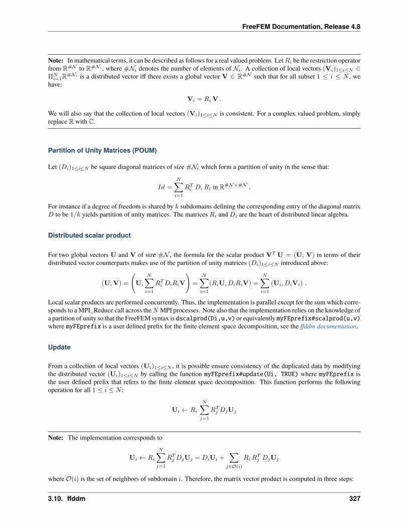
FreeFEM Documentation, Release 4.8
Note: In mathematical terms, it can be described as follows for a real valued problem. Let𝑅𝑖 be the restriction operatorfrom R#𝒩 to R#𝒩𝑖 , where #𝒩𝑖 denotes the number of elements of 𝒩𝑖. A collection of local vectors (V𝑖)1≤𝑖≤𝑁 ∈Π𝑁𝑖=1R#𝒩𝑖 is a distributed vector iff there exists a global vector V ∈ R#𝒩 such that for all subset 1 ≤ 𝑖 ≤ 𝑁 , we
have:
V𝑖 = 𝑅𝑖V .
We will also say that the collection of local vectors (V𝑖)1≤𝑖≤𝑁 is consistent. For a complex valued problem, simplyreplace R with C.
Partition of Unity Matrices (POUM)
Let (𝐷𝑖)1≤𝑖≤𝑁 be square diagonal matrices of size #𝒩𝑖 which form a partition of unity in the sense that:
𝐼𝑑 =𝑁∑𝑖=1
𝑅𝑇𝑖 𝐷𝑖𝑅𝑖 in R#𝒩×#𝒩 .
For instance if a degree of freedom is shared by 𝑘 subdomains defining the corresponding entry of the diagonal matrix𝐷 to be 1/𝑘 yields partition of unity matrices. The matrices 𝑅𝑖 and 𝐷𝑖 are the heart of distributed linear algebra.
Distributed scalar product
For two global vectors U and V of size #𝒩 , the formula for the scalar product V𝑇 U = (U, V) in terms of theirdistributed vector counterparts makes use of the partition of unity matrices (𝐷𝑖)1≤𝑖≤𝑁 introduced above:
(U,V) =
(U,
𝑁∑𝑖=1
𝑅𝑇𝑖 𝐷𝑖𝑅𝑖V
)=
𝑁∑𝑖=1
(𝑅𝑖U, 𝐷𝑖𝑅𝑖V) =
𝑁∑𝑖=1
(U𝑖, 𝐷𝑖V𝑖) .
Local scalar products are performed concurrently. Thus, the implementation is parallel except for the sum which corre-sponds to a MPI_Reduce call across the𝑁 MPI processes. Note also that the implementation relies on the knowledge ofa partition of unity so that the FreeFEM syntax is dscalprod(Di,u,v) or equivalently myFEprefix#scalprod(u,v)where myFEprefix is a user defined prefix for the finite element space decomposition, see the ffddm documentation.
Update
From a collection of local vectors (U𝑖)1≤𝑖≤𝑁 , it is possible ensure consistency of the duplicated data by modifyingthe distributed vector (U𝑖)1≤𝑖≤𝑁 by calling the function myFEprefix#update(Ui, TRUE) where myFEprefix isthe user defined prefix that refers to the finite element space decomposition. This function performs the followingoperation for all 1 ≤ 𝑖 ≤ 𝑁 :
U𝑖 ← 𝑅𝑖
𝑁∑𝑗=1
𝑅𝑇𝑗 𝐷𝑗U𝑗
Note: The implementation corresponds to
U𝑖 ← 𝑅𝑖
𝑁∑𝑗=1
𝑅𝑇𝑗 𝐷𝑗U𝑗 = 𝐷𝑖U𝑖 +∑𝑗∈𝒪(𝑖)
𝑅𝑖𝑅𝑇𝑗 𝐷𝑗U𝑗
where 𝒪(𝑖) is the set of neighbors of subdomain 𝑖. Therefore, the matrix vector product is computed in three steps:
3.10. ffddm 327
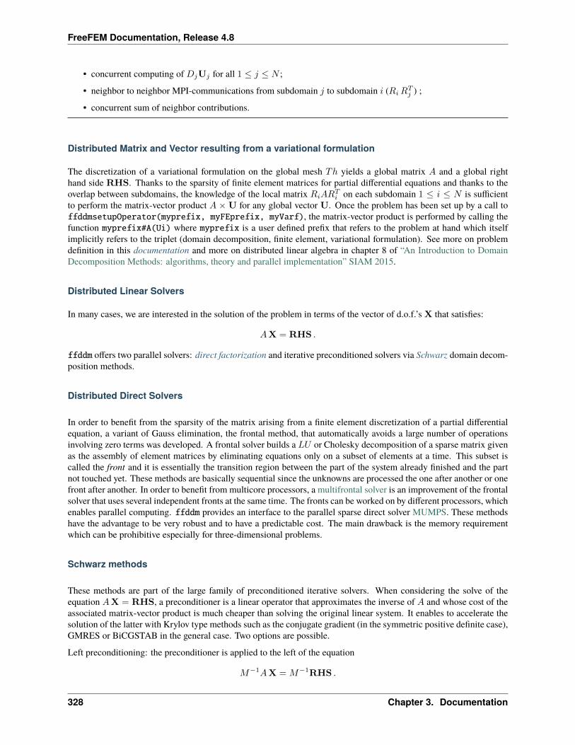
FreeFEM Documentation, Release 4.8
• concurrent computing of 𝐷𝑗U𝑗 for all 1 ≤ 𝑗 ≤ 𝑁 ;
• neighbor to neighbor MPI-communications from subdomain 𝑗 to subdomain 𝑖 (𝑅𝑖𝑅𝑇𝑗 ) ;
• concurrent sum of neighbor contributions.
Distributed Matrix and Vector resulting from a variational formulation
The discretization of a variational formulation on the global mesh 𝑇ℎ yields a global matrix 𝐴 and a global righthand side RHS. Thanks to the sparsity of finite element matrices for partial differential equations and thanks to theoverlap between subdomains, the knowledge of the local matrix 𝑅𝑖𝐴𝑅𝑇𝑖 on each subdomain 1 ≤ 𝑖 ≤ 𝑁 is sufficientto perform the matrix-vector product 𝐴 ×U for any global vector U. Once the problem has been set up by a call toffddmsetupOperator(myprefix, myFEprefix, myVarf), the matrix-vector product is performed by calling thefunction myprefix#A(Ui) where myprefix is a user defined prefix that refers to the problem at hand which itselfimplicitly refers to the triplet (domain decomposition, finite element, variational formulation). See more on problemdefinition in this documentation and more on distributed linear algebra in chapter 8 of “An Introduction to DomainDecomposition Methods: algorithms, theory and parallel implementation” SIAM 2015.
Distributed Linear Solvers
In many cases, we are interested in the solution of the problem in terms of the vector of d.o.f.’s X that satisfies:
𝐴X = RHS .
ffddm offers two parallel solvers: direct factorization and iterative preconditioned solvers via Schwarz domain decom-position methods.
Distributed Direct Solvers
In order to benefit from the sparsity of the matrix arising from a finite element discretization of a partial differentialequation, a variant of Gauss elimination, the frontal method, that automatically avoids a large number of operationsinvolving zero terms was developed. A frontal solver builds a 𝐿𝑈 or Cholesky decomposition of a sparse matrix givenas the assembly of element matrices by eliminating equations only on a subset of elements at a time. This subset iscalled the front and it is essentially the transition region between the part of the system already finished and the partnot touched yet. These methods are basically sequential since the unknowns are processed the one after another or onefront after another. In order to benefit from multicore processors, a multifrontal solver is an improvement of the frontalsolver that uses several independent fronts at the same time. The fronts can be worked on by different processors, whichenables parallel computing. ffddm provides an interface to the parallel sparse direct solver MUMPS. These methodshave the advantage to be very robust and to have a predictable cost. The main drawback is the memory requirementwhich can be prohibitive especially for three-dimensional problems.
Schwarz methods
These methods are part of the large family of preconditioned iterative solvers. When considering the solve of theequation 𝐴X = RHS, a preconditioner is a linear operator that approximates the inverse of 𝐴 and whose cost of theassociated matrix-vector product is much cheaper than solving the original linear system. It enables to accelerate thesolution of the latter with Krylov type methods such as the conjugate gradient (in the symmetric positive definite case),GMRES or BiCGSTAB in the general case. Two options are possible.
Left preconditioning: the preconditioner is applied to the left of the equation
𝑀−1𝐴X = 𝑀−1RHS .
328 Chapter 3. Documentation
FreeFEM Documentation, Release 4.8
and the Krylov method is applied to the left preconditioned system with a residual that is preconditioner dependent.
Right preconditioning: the preconditioner is inserted on the right of the operator:
𝐴𝑀−1Y = RHS where X = 𝑀−1Y.
and the Krylov method is applied to the right preconditioned system with a residual that is preconditioner independent.
In both cases, if the preconditioner is efficient the number of iterations to get a converged solution is much smallerthan the number of iterations of the Krylov method applied to the original equation 𝐴X = RHS. Although rightpreconditioning seems more intricate, it is much safer to use since the convergence is checked on a residual that doesnot depend on the preconditioner.
In the sequel, we consider the solution of the equation𝐴X = RHS preconditioned by domain decomposition methodsand with a flexible GMRES Krylov method which is thus necessarily right preconditioned.
Restricted Additive Schwarz (RAS)
The RAS preconditioner reads:
𝑀−1𝑅𝐴𝑆 :=
𝑁∑𝑗=1
𝑅𝑇𝑗 𝐷𝑗(𝑅𝑗 𝐴𝑅𝑇𝑗 )−1𝑅𝑗 ,
where for each subdomain 𝑗 the restriction matrix 𝑅𝑗 and the partition of unity matrix 𝐷𝑗 to a global right hand sideRHS is detailed below. Recall that this global vector is distributed among processes via the local vectors (RHS𝑖)
𝑁𝑖=1.
Let 𝐴𝑗 denote the local matrix (𝑅𝑗 𝐴𝑅𝑇𝑗 ). The local vector in subdomain 𝑖 resulting from the matrix vector product
𝑀−1𝑅𝐴𝑆RHS consists in computing:
𝑅𝑖
𝑁∑𝑗=1
𝑅𝑇𝑗 𝐷𝑗 𝐴−1𝑗 RHS𝑗 = 𝐷𝑖𝐴
−1𝑖 RHS𝑖 +
∑𝑗∈𝒪(𝑖)
(𝑅𝑖𝑅𝑇𝑗 )𝐷𝑗 𝐴
−1𝑗 RHS𝑗 .
This task is performed by first solving concurrently on all subdomains a linear system for Y𝑗 for all 1 ≤ 𝑗 ≤ 𝑁 :
𝐴𝑗Y𝑗 = RHS𝑗 .
Each local vector Y𝑗 is weighted by the partition of unity matrix 𝐷𝑗 . Then data transfers between neighboring sub-domains implement the 𝑅𝑖𝑅𝑇𝑗 𝐷𝑗Y𝑗 formula. The contribution from neighboring subdomains are summed locally.This pattern is very similar to that of the update procedure.
Optimized Restricted Additive Schwarz (ORAS)
The ORAS preconditioner may be seen as a variant of the RAS preconditioner. It reads:
𝑀−1𝑅𝐴𝑆 :=
𝑁∑𝑗=1
𝑅𝑇𝑗 𝐷𝑗 𝐵−1𝑗 𝑅𝑗
where 𝐵𝑗 are local matrices of size #𝒩𝑗 × #𝒩𝑗 for 1 ≤ 𝑗 ≤ 𝑁 . This variant is very useful when dealing withwave propagation phenomena such as Helmholtz problems in acoustics or Maxwell system in the frequency domainfor electromagnetism. Defining 𝐵𝑗 as the discretization of the physical equation with impedance conditions on theboundary of the subdomain has been proved to be a good choice.
3.10. ffddm 329
FreeFEM Documentation, Release 4.8
Two level methods
The RAS and ORAS methods are called a one-level method in the sense that sub-domains only interact with theirdirect neighbors. For some problems such as Darcy problems or static elasticity problems and when the number ofsubdomains is large, such one-level methods may suffer from a slow convergence. The fix is to add to the preconditioneran auxiliary coarse problem that couples all subdomains at each iteration and is inexpensive to calculate.
In mathematical terms, we first choose a full rank rectangular matrix 𝑍 ∈ R#𝒩×𝑁𝐶 where 𝑁𝐶 ≪ #𝒩 denotes thedimension of the coarse space spanned by the columns of 𝑍. We also pick a coarse matrix 𝐴𝐶 ∈ R𝑁𝐶×𝑁𝐶 . A genericone-level method preconditioner 𝑀−1
1 is enriched by a solve on the coarse space. The simplest correction formula isadditive:
𝑀−12 := 𝑍 𝐴−1
𝐶 𝑍𝑇 +𝑀−11
Other correction formulas are given in documentation.
We consider two ways to build 𝑍 and thus the coarse space and the coarse problem 𝐴𝐶 , see below Coarse Mesh andGenEO
Coarse Mesh
A first possibility is to discretize the problem on a coarse mesh, following the same principle as multi-grid methods.For 3-D problems, a coarsening of the mesh size by a factor 2, reduces by a factor 23 = 8 the size of the coarse problemwhich is then easier to solve by a direct method. Then, 𝑍 is the interpolation matrix from the coarse finite elementspace to the fine one.
GenEO
For highly heterogeneous or anisotropic problems, two level methods based on coarse meshes might fail and a moresophisticated construction must be used. A provable robust coarse space called GenEO is built by first solving thefollowing local generalized eigenvalue problem in parallel for each subdomain 1 ≤ 𝑖 ≤ 𝑁 , where 𝐴Neu
𝑖 denotes thelocal matrix resulting from the variational formulation:
𝐷𝑖𝐴𝑖𝐷𝑖 𝑉𝑖,𝑘 = 𝜆𝑖,𝑘 𝐴Neu𝑖 𝑉𝑖,𝑘
The eigenvectors selected to enter the coarse space correspond to eigenvalues 𝜆𝑖,𝑘 ≥ 𝜏 , where the threshold parameter𝜏 is user-defined. The precise formulas are given in this documentation. From a mathematical point of view, it has beenproved that for a symmetric positive definite matrix𝐴, the spectrum of the preconditioned by the two-level method witha GenEO coarse space lies in the interval [
1
1 + 𝑘1 𝜏, 𝑘0].
Note A heuristic that justifies this construction is as follows. We first introduce the Additive Schwarz method (ASM)which can be seen as a symmetrized variant of the RAS preconditioner:
𝑀−1𝐴𝑆𝑀 :=
𝑁∑𝑗=1
𝑅𝑇𝑗 𝐴−1𝑗 𝑅𝑗 .
It can be proved that the lower bound for the eigenvalue of 𝑀−1𝐴𝑆𝑀 𝐴 is close to zero (which is bad for convergence)
whereas the upper bound depends only on the number of neigbors of a subdomain (which is good for convergence).
Second, we also introduce the following preconditioner 𝑀−1𝑁𝑁 :
𝑀−1𝑁𝑁 :=
∑1≤𝑗≤𝑁
𝐷𝑖 (𝐴Neu𝑗 )−1𝐷𝑗 .
330 Chapter 3. Documentation
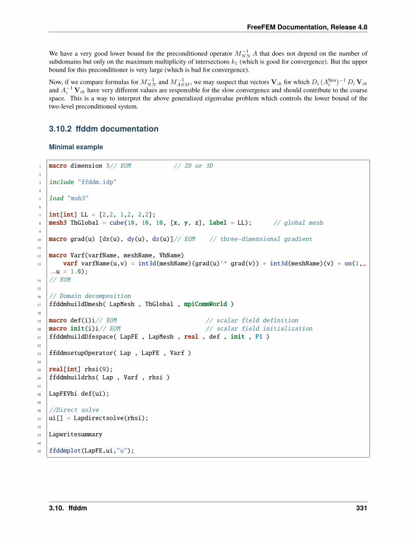
FreeFEM Documentation, Release 4.8
We have a very good lower bound for the preconditioned operator 𝑀−1𝑁𝑁 𝐴 that does not depend on the number of
subdomains but only on the maximum multiplicity of intersections 𝑘1 (which is good for convergence). But the upperbound for this preconditioner is very large (which is bad for convergence).
Now, if we compare formulas for 𝑀−1𝑁𝑁 and 𝑀−1
𝐴𝑆𝑀 , we may suspect that vectors V𝑖𝑘 for which 𝐷𝑖 (𝐴Neu𝑖 )−1𝐷𝑖V𝑖𝑘
and 𝐴−1𝑖 V𝑖𝑘 have very different values are responsible for the slow convergence and should contribute to the coarse
space. This is a way to interpret the above generalized eigenvalue problem which controls the lower bound of thetwo-level preconditioned system.
3.10.2 ffddm documentation
Minimal example
1 macro dimension 3// EOM // 2D or 3D2
3 include "ffddm.idp"4
5 load "msh3"6
7 int[int] LL = [2,2, 1,2, 2,2];8 mesh3 ThGlobal = cube(10, 10, 10, [x, y, z], label = LL); // global mesh9
10 macro grad(u) [dx(u), dy(u), dz(u)]// EOM // three-dimensional gradient11
12 macro Varf(varfName, meshName, VhName)13 varf varfName(u,v) = int3d(meshName)(grad(u)'* grad(v)) + int3d(meshName)(v) + on(1,
→˓u = 1.0);14 // EOM15
16 // Domain decomposition17 ffddmbuildDmesh( LapMesh , ThGlobal , mpiCommWorld )18
19 macro def(i)i// EOM // scalar field definition20 macro init(i)i// EOM // scalar field initialization21 ffddmbuildDfespace( LapFE , LapMesh , real , def , init , P1 )22
23 ffddmsetupOperator( Lap , LapFE , Varf )24
25 real[int] rhsi(0);26 ffddmbuildrhs( Lap , Varf , rhsi )27
28 LapFEVhi def(ui);29
30 //Direct solve31 ui[] = Lapdirectsolve(rhsi);32
33 Lapwritesummary34
35 ffddmplot(LapFE,ui,"u");
3.10. ffddm 331
FreeFEM Documentation, Release 4.8
Overlapping mesh decomposition
1 ffddmbuildDmesh(prmesh,Th,comm)
decomposes the mesh Th into overlapping submeshes. The mesh will be distributed over the mpi ranks of commu-nicator comm. This will create and expose variables whose names will be prefixed by prmesh, see below (# is theconcatenation operator). The way the initial mesh Th is partitioned depends on the value of ffddmpartitioner.
The size of the overlap between subdomains (its width in terms of number of mesh elements) is given by ffddmoverlap.
The level of refinement of the resulting submeshes with respect to the input mesh Th is given by ffddmsplit.
If ffddmexclude = 0, the first ffddmpCS mpi ranks of comm will be excluded from the spatial domain decomposition,in order to dedicate them later to the coarse problem (for two-level preconditioners).
The label of the new border of the submeshes (the interface between the subdomains) is given by ffddminterfacelabel.
defines:• int prmesh#npart number of subdomains for this decomposition; should be equal to mpiSize(comm) - ffd-
dmexclude * ffddmpCS
• int prmesh#pCS equal to ffddmpCS
• int prmesh#exclude equal to ffddmexclude
• int prmesh#excluded true if ffddmexclude is true (= 0) and mpiRank(comm) < prmesh#pCS. In this case,this mpi rank will be excluded from the spatial domain decomposition and will only work on the coarse problem.
• mpiComm prmesh#commddm mpi communicator for ranks participating in the spatial domain decom-position (ranks 0 to prmesh#npart-1 in comm if prmesh#exclude is false, ranks prmesh#pCS toprmesh#pCS+prmesh#npart-1 otherwise)
• mpiComm prmesh#commCS mpi communicator for ranks participating in the assembly and resolution of thecoarse problem for two-level preconditioners (ranks 0 to prmesh#pCS - 1 in comm)
• mpiComm prmesh#commself self mpi communicator (this mpi rank only), used for factorizing local matrices
• meshN[int] prmesh#aTh array (size prmesh#npart) of local meshes of the subdomains. In the standard par-allel case, only the local mesh for this mpi rank prmesh#aTh[mpiRank(prmesh#commddm)] is defined (unlessthis mpi rank is excluded from the spatial domain decomposition, i.e. prmesh#excluded = 1, see below). Inthe sequential case, all local meshes are defined.
• meshN prmesh#Thi the local mesh of the subdomain for this mpi rank, i. e.prmesh#aTh[mpiRank(prmesh#commddm)] in the parallel case
• int prmesh#numberIntersection the number of neighbors for this mpi rank
• int[int] prmesh#arrayIntersection the list of neighbor ranks in prmesh#commddm for this mpi rank
Remark for sequential use (see -seqddm):• meshN[int] prmesh#aTh array (size prmesh#npart) of local meshes of the subdomains
332 Chapter 3. Documentation
FreeFEM Documentation, Release 4.8
Local finite element spaces
1 ffddmbuildDfespace(prfe,prmesh,scalar,def,init,Pk)
builds the local finite element spaces and associated distributed operators on top of the mesh decomposition prmesh.This will create and expose variables whose names will be prefixed by prfe, see below. It is assumed that ffddmbuild-Dmesh has already been called with prefix prmesh in order to build the mesh decomposition.
The local finite element spaces of type Pk (where Pk is the type of finite element: P1, [P2,P2,P1], . . . ) are defined onthe local meshes of the subdomains based on the mesh decomposition previously created with prefix prmesh.
scalar determines the type of data for this finite element: real or complex.
Two macros, def and init, are needed: def specifies how to define a finite element function in the finite element spacePk, and init specifies how to interpolate a scalar function onto the (possibly multiple) components of Pk. Two examplesare given below:
For scalar P2 finite elements and complex-valued problems:
1 macro def(u) u// EOM2 macro init(u) u// EOM3 ffddmbuildDfespace(myFEprefix,mymeshprefix,complex,def,init,P2)
For vectorial [P2,P2,P1] finite elements and real-valued problems:
1 macro def(u) [u, u#B, u#C]// EOM2 macro init(u) [u, u, u]// EOM3 ffddmbuildDfespace(myFEprefix,mymeshprefix,real,def,init,[P2,P2,P1])
In practice, this builds the necessary distributed operators associated to the finite element space: the local partition ofunity functions (𝐷𝑖)𝑖=1,...,𝑁 (see prfe#Dk and prfe#Dih below) as well as the function prfe#update (see below)which synchronizes local vectors (𝑢𝑖)𝑖=1,...,𝑁 between neighboring subdomains, performing the equivalent of 𝑢𝑖 =
𝑅𝑖(∑𝑁𝑗=1𝑅
𝑇𝑗 𝑢𝑗) or 𝑢𝑖 = 𝑅𝑖(
∑𝑁𝑗=1𝑅
𝑇𝑗 𝐷𝑗𝑢𝑗) in a distributed parallel environment.
prfe#scalprod (see below) performs the parallel scalar product for vectors defined on this finite element.
defines:• prfe#prmesh macro, saves the parent prefix prmesh of the mesh decomposition
• prfe#K macro, saves the type of data scalar for this finite element space (real or complex)
• func prfe#fPk saves the type of finite element Pk, e.g. P1, [P2,P2,P1], . . .
• fespace prfe#Vhi the local finite element space for this mpi rank, defined on the local mesh prmesh#Thi
• int prfe#Ndofglobal the total number of degrees of freedom 𝑛 for this finite element discretization
• prfe#mdef macro, saves the macro def giving the definition of a finite element function in the finite elementspace Pk
• prfe#minit macro, saves the macro init specifying how to interpolate a scalar function onto the (possiblymultiple) components of a finite element function of Pk. This is used to create the local partition of unity functionin prfe#Vhi, by interpolating the local P1 partition of unity function onto the components of prfe#Vhi. Fornon Lagrange finite element spaces (e.g. RT0, Edge03d, . . . ), see ffddmbuildDfespaceEdge.
• prfe#K[int][int] prfe#Dk array (size prmesh#npart) of local partition of unity vectors in the subdomains,equivalent to (𝐷𝑖)𝑖=1,...,𝑁 . In the standard parallel case, only the local partition of unity vector for this mpi rankprfe#Dk[mpiRank(prmesh#commddm)] is defined (unless this mpi rank is excluded from the spatial domaindecomposition, i. e. prmesh#excluded = 1). In the sequential case, all local partition of unity vectors aredefined.
3.10. ffddm 333
FreeFEM Documentation, Release 4.8
• matrix<prfe#K>[int] prfe#Dih array (size prmesh#npart) similar to prfe#Dk but in matrix form, allow-ing for easier matrix-matrix multiplications. prfe#Dih[i] is a diagonal matrix, with the diagonal equal toprfe#Dk[i].
• fespace prfe#Vhglob the global finite element space defined on the global mesh prmesh#Thglob. Definedonly if -noGlob is not used.
• matrix<prfe#K>[int] prfe#Rih array (size prmesh#npart) of restriction matrices from the global finiteelement space to the local finite element spaces on the local submeshes of the subdomains. In the standardparallel case, only the restriction matrix for this mpi rank prfe#Rih[mpiRank(prmesh#commddm)] is defined(unless this mpi rank is excluded from the spatial domain decomposition, i. e. prmesh#excluded = 1). Inthe sequential case, all restriction matrices are defined. The restriction matrices prfe#Rih are defined only if-noGlob is not used.
• func int prfe#update(scalar[int] ui, bool scale)The function prfe#update synchronizes the lo-cal vector ui between subdomains by exchanging the values of ui shared with neighboring subdomains (in theoverlap region) using point-to-point MPI communications. If scale is true, ui is multiplied by the local partition ofunity beforehand. This is equivalent to 𝑢𝑖 = 𝑅𝑖(
∑𝑁𝑗=1𝑅
𝑇𝑗 𝑢𝑗) when scale is false and 𝑢𝑖 = 𝑅𝑖(
∑𝑁𝑗=1𝑅
𝑇𝑗 𝐷𝑗𝑢𝑗)
when scale is true.
• func scalar prfe#scalprod(scalar[int] ai, scalar[int] bi) The function prfe#scalprod com-putes the global scalar product of two vectors whose local restriction to the subdomain of this mpi rank are aiand bi. The result is computed as
∑𝑁𝑗=1(𝐷𝑗𝑎𝑗 , 𝑏𝑗).
Define the problem to solve
1 ffddmsetupOperator(pr,prfe,Varf)
builds the distributed operator associated to the variational problem given by Varf, on top of the distributed finiteelement space prfe. This will create and expose variables whose names will be prefixed by pr, see below. It is assumedthat ffddmbuildDfespace has already been called with prefix prfe in order to define the distributed finite element space.
In practice, this builds the so-called local ‘Dirichlet’ matrices 𝐴𝑖 = 𝑅𝑖𝐴𝑅𝑇𝑖 , the restrictions of the global operator 𝐴
to the subdomains (see pr#aRdbelow). The matrices correspond to the discretization of the bilinear form given by themacro Varf, which represents the abstract variational form of the problem. These matrices are then used to implementthe action of the global operator 𝐴 on a local vector (the parallel matrix-vector product with 𝐴), see pr#A below.
At this point, we already have the necessary data to be able to solve the problem with a parallel direct solver (MUMPS),which is the purpose of the function pr#directsolve (see below). See ffddmbuildrhs for building the right-hand side.
The macro Varf is required to have three parameters: the name of the variational form, the mesh, and the finite elementspace. The variational form given in this ‘abstract’ format will then be used by ffddm to assemble the discrete operatorsby setting the appropriate mesh and finite element space as parameters. An example is given below:
1 macro myVarf(varfName, meshName, VhName)2 varf varfName(u,v) = int3d(meshName)(grad(u)''* grad(v)) + on(1, u = 1.0);3 // EOM4
5 ffddmsetupOperator(myprefix,myFEprefix,myVarf)
Remark In this simple example, the third parameter VhName is not used. However, for more complex cases such asnon-linear or time dependent problems where the problem depends on a solution computed at a previous step, it isuseful to know for which discrete finite element space the variational form is being used. See for example TODO
defines:• pr#prfe macro, saves the parent prefix prfe of the finite element space
334 Chapter 3. Documentation
FreeFEM Documentation, Release 4.8
• int pr#verbosity the level of verbosity for this problem, initialized with the value of ffddmverbosity
• pr#writesummary macro, prints a summary of timings for this problem, such as the time spent to assemblelocal matrices or solve the linear system.
• matrix<prfe#K> pr#Aglobal the global matrix 𝐴 corresponding to the discretization of the variational formgiven by the macro Varf on the global finite element space prfe#Vhglob. Defined only in the sequential case.
• matrix<prfe#K>[int] pr#aRd array (size prfe#prmesh#npart) of so-called local ‘Dirichlet’ matrices inthe subdomains; these are the restrictions of the global operator to the subdomains, equivalent to 𝐴𝑖 = 𝑅𝑖𝐴𝑅
𝑇𝑖
with 𝐴 the global matrix corresponding to the discretization of the variational form given by the macro Varfon the global finite element space. In the standard parallel case, only the local matrix for this mpi rankpr#aRd[mpiRank(prmesh#commddm)] is defined (unless this mpi rank is excluded from the spatial domaindecomposition, i. e. prmesh#excluded = 1). In the sequential case, all local matrices are defined.
• func prfe#K[int] pr#A(prfe#K[int] &ui) The function pr#A computes the parallel matrix-vector prod-uct, i.e. the action of the global operator 𝐴 on the local vector 𝑢𝑖. The computation is equivalent to𝑅𝑖(∑𝑁𝑗=1𝑅
𝑇𝑗 𝐷𝑗𝐴𝑗𝑢𝑗) and is performed in parallel using local matrices pr#aRd and the function prfe#update.
In the sequential case, the global matrix pr#Aglobal is used instead.
• func prfe#K[int] pr#AT(prfe#K[int] &ui) Similarly to pr#A, The function pr#AT computes the actionof 𝐴𝑇 , the transpose of the global operator 𝐴, on 𝑢𝑖.
• func prfe#K[int] pr#directsolve(prfe#K[int]& rhsi) The function pr#directsolve allows tosolve the linear system 𝐴𝑥 = 𝑏 in parallel using the parallel direct solver MUMPS. The matrix is given toMUMPS in distributed form through the local matrices pr#aRd. The input rhsi is given as a distributed vector(rhsi is the restriction of the global right-hand side 𝑏 to the subdomain of this mpi rank, see ffddmbuildrhs) andthe returned vector is local as well.
Remark: rectangular operatorsIt is possible to define a non-square distributed operator where the variational form takes two different finite elementspaces of unknown and test functions. This is done through macro ffddmsetupOperatorRect which takes two FEprefixes (which must be defined on the same mesh prefix), see below:
1 macro myVarf(varfName, meshName, VhName)2 varf varfName([u, uB, uC], [q]) = int3d(meshName)(div(u) * q);3 // EOM4
5 ffddmsetupOperatorRect(myprefix,myFEprefixV,myFEprefixP,myVarf)
1 ffddmbuildrhs(pr,Varfrhs,rhs)
builds the right-hand side associated to the variational form given by Varfrhs for the problem corresponding to prefixpr. The resulting right-hand side vector rhs corresponds to the discretization of the abstract linear form given by themacro Varfrhs (see ffddmsetupOperator for more details on how to define the abstract variational form as a macro).
The input vector rhs is resized and contains the resulting local right-hand side 𝑅𝑖𝑏, the restriction of the global right-hand side 𝑏 to the subdomain of this mpi rank. In the sequential case, the global right-hand side vector 𝑏 is assembledinstead.
An example is given below:
1 macro myVarfrhs(varfName, meshName, VhName)2 varf varfName(u,v) = intN(meshName)(v) + on(1, u = 1.0);3 // EOM4
(continues on next page)
3.10. ffddm 335
FreeFEM Documentation, Release 4.8
(continued from previous page)
5 real[int] rhsi(0);6 ffddmbuildrhs(myprefix,myVarfrhs,rhsi)
One level preconditioners
1 ffddmsetupPrecond(pr,VarfPrec)
builds the one level preconditioner for problem pr. This will create and expose variables whose names will be prefixedby pr, see below. It is assumed that ffddmsetupOperator has already been called with prefix pr in order to define theproblem to solve.
In practice, this builds and performs the factorization of the local matrices used in the one level preconditioner. Thelocal matrices depend on the choice of ffddmprecond and VarfPrec, see pr#aRbelow.
defines:• string pr#prec equal to ffddmprecond. Sets the type of one level preconditioner 𝑀−1
1 to be used: “asm”(Additive Schwarz), “ras” (Restricted Additive Schwarz), “oras” (Optimized Restricted Additive Schwarz), “soras”(Symmetric Optimized Restricted Additive Schwarz) or “none” (no preconditioner).
• matrix<pr#prfe#K>[int] pr#aR array (size prfe#prmesh#npart) of local matrices used for the one levelpreconditioner. Each mpi rank of the spatial domain decomposition performs the 𝐿𝑈 (or 𝐿𝐷𝐿𝑇 ) factorizationof the local matrix corresponding to its subdomain using the direct solver MUMPS.
– If VarfPrec is not a previously defined macro (just put null for example), the matrices pr#aR are setto be equal to the so-called local ‘Dirichlet’ matrices pr#aRd (see ffddmsetupOperator). This is for theclassical ASM preconditioner𝑀−1
1 = 𝑀−1ASM =
∑𝑁𝑖=1𝑅
𝑇𝑖 𝐴
−1𝑖 𝑅𝑖 or classical RAS preconditioner𝑀−1
1 =
𝑀−1RAS =
∑𝑁𝑖=1𝑅
𝑇𝑖 𝐷𝑖𝐴
−1𝑖 𝑅𝑖 (it is assumed that ffddmprecond is equal to “asm” or “ras”).
– If VarfPrec is a macro, it is assumed that VarfPrec defines an abstract bilinear form (see ffddmsetupOp-erator for more details on how to define the abstract variational form as a macro).
∗ If ffddmprecond is equal to “asm” or “ras”, the matrices pr#aR will be assembled as local ‘Dirichlet’matrices in the same manner as pr#aRd, but using the bilinear form defined by VarfPrec instead. Thisdefines the ASM preconditioner as 𝑀−1
1 = 𝑀−1ASM =
∑𝑁𝑖=1𝑅
𝑇𝑖 (𝐴Prec
𝑖 )−1𝑅𝑖 and the RAS precondi-
tioner as 𝑀−11 = 𝑀−1
RAS =∑𝑁𝑖=1𝑅
𝑇𝑖 𝐷𝑖(𝐴
Prec𝑖 )
−1𝑅𝑖, where 𝐴Prec
𝑖 = 𝑅𝑖𝐴Prec𝑅𝑇𝑖 .
∗ If ffddmprecond is equal to “oras” or “soras”, the matrices pr#aR will correspond to the discretizationof the variational form VarfPrec in the subdomains Ω𝑖. In particular, various boundary conditions canbe imposed at the interface between subdomains (corresponding to mesh boundary of label ffddminter-facelabel set by the parent call to ffddmbuildDmesh), such as Optimized Robin boundary conditions.We note the ORAS preconditioner as 𝑀−1
1 = 𝑀−1ORAS =
∑𝑁𝑖=1𝑅
𝑇𝑖 𝐷𝑖(𝐵
Prec𝑖 )
−1𝑅𝑖 and the SORAS
preconditioner as 𝑀−11 = 𝑀−1
SORAS =∑𝑁𝑖=1𝑅
𝑇𝑖 𝐷𝑖(𝐵
Prec𝑖 )
−1𝐷𝑖𝑅𝑖.
• func pr#prfe#K[int] pr#PREC1(pr#prfe#K[int] &ui) The function pr#PREC1 computes the parallelapplication of the one level preconditioner 𝑀−1
1 , i.e. the action of 𝑀−11 on the local vector 𝑢𝑖. In the sequential
case, it computes the action of 𝑀−11 on a global vector. The action of the inverse of local matrices pr#aRd is
computed by forward-backward substitution using their 𝐿𝑈 (or 𝐿𝐷𝐿𝑇 ) decomposition.
• func pr#prfe#K[int] pr#PREC(pr#prfe#K[int] &ui) The function pr#PREC corresponds to the actionof the preconditioner 𝑀−1 for problem pr. It coincides with the one level preconditioner pr#PREC1 after thecall to ffddmsetupPrecond. If a second level is subsequently added (see the next section about Two level precon-ditioners), it will then coincide with the two level preconditioner 𝑀−1
2 (see pr#PREC2level).
• func pr#prfe#K[int] pr#fGMRES(pr#prfe#K[int]& x0i, pr#prfe#K[int]& bi, real eps, intnbiter, string sprec) The function pr#fGMRES allows to solve the linear system 𝐴𝑥 = 𝑏 in parallel using
336 Chapter 3. Documentation
FreeFEM Documentation, Release 4.8
the flexible GMRES method preconditioned by 𝑀−1. The action of the global operator 𝐴 is given by pr#A, theaction of the preconditioner 𝑀−1 is given by pr#PREC and the scalar products are computed by pr#scalprod.More details are given in the section Solving the linear system.
Two level preconditioners
The main ingredient of a two level preconditioner is the so-called ‘coarse space’ matrix 𝑍.
𝑍 is a rectangular matrix of size 𝑛× 𝑛𝑐, where usually 𝑛𝑐 ≪ 𝑛.
𝑍 is used to build the ‘coarse space operator’ 𝐸 = 𝑍𝑇𝐴𝑍, a square matrix of size 𝑛𝑐 × 𝑛𝑐. We can then define the‘coarse space correction operator’ 𝑄 = 𝑍𝐸−1𝑍𝑇 = 𝑍(𝑍𝑇𝐴𝑍)−1𝑍𝑇 , which can then be used to enrich the one levelpreconditioner through a correction formula. The simplest one is the additive coarse correction: 𝑀−1
2 = 𝑀−11 + 𝑄.
See pr#corr below for all other available correction formulas.
There are multiple ways to define a relevant coarse space 𝑍 for different classes of problems. ffddmgeneosetup definesa coarse space correction operator by building the GenEO coarse space, while ffddmcoarsemeshsetup builds the coarsespace using a coarse mesh.
After a call to either ffddmgeneosetup or ffddmcoarsemeshsetup, the following variables and functions are set up:
• int pr#ncoarsespace the size of the coarse space 𝑛𝑐.
• string pr#corr initialized with the value of ffddmcorrection. Specifies the type of coarse correction formulato use for the two level preconditioner. The possible values are:
"AD" : Additive, 𝑀−1 = 𝑀−12 = 𝑀−1
1 +𝑄"BNN" : Balancing Neumann-Neumann, 𝑀−1 = 𝑀−1
2 = (𝐼 −𝑄𝐴)𝑀−11 (𝐼 −𝐴𝑄) +𝑄
"ADEF1" : Adapted Deflation Variant 1, 𝑀−1 = 𝑀−12 = 𝑀−1
1 (𝐼 −𝐴𝑄) +𝑄"ADEF2" : Adapted Deflation Variant 2, 𝑀−1 = 𝑀−1
2 = (𝐼 −𝑄𝐴)𝑀−11 +𝑄
"RBNN1" : Reduced Balancing Variant 1, 𝑀−1 = 𝑀−12 = (𝐼 −𝑄𝐴)𝑀−1
1 (𝐼 −𝐴𝑄)"RBNN2" : Reduced Balancing Variant 2, 𝑀−1 = 𝑀−1
2 = (𝐼 −𝑄𝐴)𝑀−11
"none" : no coarse correction, 𝑀−1 = 𝑀−12 = 𝑀−1
1
• Note that AD, ADEF1 and RBNN2 only require one application of 𝑄, while BNN, ADEF2 and RBNN1 requiretwo. The default coarse correction is ADEF1, which is cheaper and generally as robust as BNN or ADEF2.
• func pr#prfe#K[int] pr#Q(pr#prfe#K[int] &ui) The function pr#Q computes the parallel applicationof the coarse correction operator 𝑄, i.e. the action of 𝑄 = 𝑍𝐸−1𝑍𝑇 on the local vector 𝑢𝑖. In the sequentialcase, it computes the action of 𝑄 on a global vector. The implementation differs depending on the method usedto build the coarse space (with GenEO or using a coarse mesh), but the idea is the same: the action of thetranspose of the distributed operator 𝑍 on the distributed vector 𝑢𝑖 is computed in parallel, with the contributionof all subdomains being gathered in a vector of size 𝑛𝑐 in the mpi process of rank 0. The action of the inverseof the coarse space operator 𝐸 is then computed by forward-backward substitution using its 𝐿𝑈 (or 𝐿𝐷𝐿𝑇 )decomposition previously computed by the first pr#prfe#prmesh#pCS ranks of the mpi communicator. Theresult is then sent back to all subdomains to perform the last application of 𝑍 and obtain the resulting local vectorin each subdomain.
• func pr#prfe#K[int] pr#PREC2level(pr#prfe#K[int] &ui) The function pr#PREC2level computesthe parallel application of the two level preconditioner 𝑀−1
2 , i.e. the action of 𝑀−12 on the local vector 𝑢𝑖. In
the sequential case, it computes the action of 𝑀−12 on a global vector. The two level preconditioner depends on
the choice of the coarse correction formula which is determined by pr#corr, see above.
3.10. ffddm 337
FreeFEM Documentation, Release 4.8
Building the GenEO coarse space
1 ffddmgeneosetup(pr,Varf)
This builds the GenEO coarse space for problem pr. This will create and expose variables whose names will be prefixedby pr, see below. It is assumed that ffddmsetupPrecond has already been called for prefix pr in order to define the onelevel preconditioner for problem pr. The GenEO coarse space is𝑍 = (𝑅𝑇𝑖 𝐷𝑖𝑉𝑖,𝑘)𝑖=1,...,𝑁
𝜆𝑖,𝑘≥𝜏 , where 𝑉𝑖,𝑘 are eigenvectorscorresponding to eigenvalues 𝜆𝑖,𝑘 of the following local generalized eigenvalue problem in subdomain 𝑖:
𝐷𝑖𝐴𝑖𝐷𝑖𝑉𝑖,𝑘 = 𝜆𝑖,𝑘𝐴Neu𝑖 𝑉𝑖,𝑘,
where 𝐴Neu𝑖 is the local Neumann matrix of subdomain 𝑖 (with Neumann boundary conditions at the subdomain inter-
face).
In practice, this builds and factorizes the local Neumann matrices𝐴Neu𝑖 corresponding to the abstract bilinear form given
by the macro Varf (see ffddmsetupOperator for more details on how to define the abstract variational form as a macro).In the GenEO method, the abstract bilinear form Varf is assumed to be the same as the one used to define the problempr through the previous call to ffddmsetupOperator. The local generalized eigenvalue problem is then solved in eachsubdomain to find the eigenvectors 𝑉𝑖,𝑘 corresponding to the largest eigenvalues 𝜆𝑖,𝑘 (see pr#Z below). The numberof computed eigenvectors 𝜈 is given by ffddmnu. The eigenvectors selected to enter 𝑍 correspond to eigenvalues 𝜆𝑖,𝑘larger than 𝜏 , where the threshold parameter 𝜏 is given by ffddmtau. If ffddmtau = 0, all ffddmnu eigenvectors areselected. Finally, the coarse space operator 𝐸 = 𝑍𝑇𝐴𝑍 is assembled and factorized (see pr#E below).
defines:• pr#prfe#K[int][int] pr#Z array of local eigenvectors 𝑍𝑖,𝑘 = 𝐷𝑖𝑉𝑖,𝑘 obtained by solving the local gener-
alized eigenvalue problem above in the subdomain of this mpi rank using Arpack. The number of computedeigenvectors 𝜈 is given by ffddmnu. The eigenvectors selected to enter 𝑍 correspond to eigenvalues 𝜆𝑖,𝑘 largerthan 𝜏 , where the threshold parameter 𝜏 is given by ffddmtau. If ffddmtau = 0, all ffddmnu eigenvectors areselected.
• matrix<pr#prfe#K> pr#E the coarse space operator 𝐸 = 𝑍𝑇𝐴𝑍. The matrix pr#E is assembled in paralleland is factorized by the parallel direct solver MUMPS using the first pr#prfe#prmesh#pCS ranks of the mpicommunicator, with mpi rank 0 as the master process. The number of mpi processes dedicated to the coarseproblem is set by the underlying mesh decomposition of problem pr, which also specifies if these mpi ranks areexcluded from the spatial decomposition or not. These parameters are set by ffddmpCS and ffddmexclude whencalling ffddmbuildDmesh (see ffddmbuildDmesh for more details).
Building the coarse space from a coarse mesh
1 ffddmcoarsemeshsetup(pr,Thc,VarfEprec,VarfAprec)
builds the coarse space for problem pr from a coarse problem which corresponds to the discretization of a variationalform on a coarser mesh Thc of Ω. This will create and expose variables whose names will be prefixed by pr, see below.It is assumed that ffddmsetupPrecond has already been called for prefix pr in order to define the one level preconditionerfor problem pr. The abstract variational form for the coarse problem can differ from the original problem pr and isgiven by macro VarfEprec (see ffddmsetupOperator for more details on how to define the abstract variational form asa macro). For example, absorption can be added in the preconditioner for wave propagation problems, see examplesfor Helmholtz and Maxwell equations in the Examples section.
The coarse space 𝑍 corresponds to the interpolation operator from the coarse finite element space to the original finiteelement space of the problem. Thus, the coarse space operator 𝐸 = 𝑍𝑇𝐴Eprec𝑍 corresponds to the matrix of theproblem given by VarfEprec discretized on the coarse mesh Thc and is assembled as such.
Similarly, VarfAprec specifies the global operator involved in multiplicative coarse correction formulas. For example,𝑀−1
2,ADEF1 = 𝑀−11 (𝐼 −𝐴Aprec𝑄) +𝑄 (where 𝑄 = 𝑍𝐸−1𝑍𝑇 ). 𝐴Aprec defaults to 𝐴 if VarfAprec is not a valid macro
338 Chapter 3. Documentation
FreeFEM Documentation, Release 4.8
(you can put null for example).
defines:• meshN pr#ThCoarse the coarse mesh Thc• fespace pr#VhCoarse the coarse finite element space of type pr#prfe#fPk defined on the coarse meshpr#ThCoarse
• matrix<pr#prfe#K> pr#AglobEprec the global matrix𝐴Aprec corresponding to the discretization of the vari-ational form given by the macro VarfAprec on the global finite element space pr#prfe#Vhglob. Defined onlyin the sequential case. pr#AglobEprec is equal to pr#Aglobal if VarfAprec is not a valid macro.
• matrix<pr#prfe#K> pr#aRdEprec the local ‘Dirichlet’ matrix corresponding to VarfAprec; it is the localrestriction of the global operator 𝐴Aprec to the subdomain, equivalent to 𝐴Aprec
𝑖 = 𝑅𝑖𝐴Aprec𝑅𝑇𝑖 with 𝐴Aprec the
global matrix corresponding to the discretization of the variational form given by the macro VarfAprec on theglobal finite element space. Defined only if this mpi rank is not excluded from the spatial domain decomposition,i. e. prmesh#excluded = 0. pr#aRdEprec is equal to pr#aRd[mpiRank(prmesh#commddm)] if VarfAprecis not a valid macro.
• func pr#prfe#K[int] pr#AEprec(pr#prfe#K[int] &ui)The function pr#AEprec computes the parallelmatrix-vector product, i.e. the action of the global operator 𝐴Aprec on the local vector 𝑢𝑖. The computation isequivalent to𝑅𝑖(
∑𝑁𝑗=1𝑅
𝑇𝑗 𝐷𝑗𝐴
Aprec𝑗 𝑢𝑗) and is performed in parallel using local matrices pr#aRdEprec and the
function pr#prfe#update. In the sequential case, the global matrix pr#AglobEprec is used instead.
• matrix<pr#prfe#K> pr#ZCM the interpolation operator 𝑍 from the coarse finite element space pr#VhCoarseto the global finite element space pr#prfe#Vhglob. Defined only in the sequential case.
• matrix<pr#prfe#K> pr#ZCMi the local interpolation operator 𝑍𝑖 from the coarse finite element spacepr#VhCoarse to the local finite element space pr#prfe#Vhi. Defined only if this mpi rank is not excludedfrom the spatial domain decomposition, i. e. prmesh#excluded = 0. pr#ZCMi is used for the parallel applica-tion of 𝑍 and 𝑍𝑇 .
• matrix<pr#prfe#K> pr#ECM the coarse space operator 𝐸 = 𝑍𝑇𝐴Eprec𝑍. The matrix pr#ECM is assembledby discretizing the variational form given by VarfEprec on the coarse mesh and factorized by the parallel directsolver MUMPS using the first pr#prfe#prmesh#pCS ranks of the mpi communicator, with mpi rank 0 as themaster process. The number of mpi processes dedicated to the coarse problem is set by the underlying meshdecomposition of problem pr, which also specifies if these mpi ranks are excluded from the spatial decom-position or not. These parameters are set by ffddmpCS and ffddmexclude when calling ffddmbuildDmesh (seeffddmbuildDmesh for more details).
Solving the linear system
1 func pr#prfe#K[int] pr#fGMRES(pr#prfe#K[int]& x0i, pr#prfe#K[int]& bi, real eps, int→˓itmax, string sp)
solves the linear system for problem pr using the flexible GMRES algorithm with preconditioner𝑀−1 (correspondingto pr#PREC). Returns the local vector corresponding to the restriction of the solution to pr#prfe#Vhi. x0i and bi arelocal distributed vectors corresponding respectively to the initial guess and the right-hand side (see ffddmbuildrhs). epsis the stopping criterion in terms of the relative decrease in residual norm. If eps < 0, the residual norm itself is usedinstead. itmax sets the maximum number of iterations. sp selects between the "left" or "right" preconditioningvariants: left preconditioned GMRES solves𝑀−1𝐴𝑥 = 𝑀−1𝑏, while right preconditioned GMRES solves𝐴𝑀−1𝑦 =𝑏 for 𝑦, with 𝑥 = 𝑀−1𝑦.
3.10. ffddm 339
FreeFEM Documentation, Release 4.8
Using HPDDM within ffddm
ffddm allows you to use HPDDM to solve your problem, effectively replacing the ffddm implementation of all parallellinear algebra computations. ffddm can then be viewed as a finite element interface for HPDDM.
You can use HPDDM features unavailable in ffddm such as advanced Krylov subspace methods implementing blockand recycling techniques.
To switch to HPDDM, simply define the macro pr#withhpddm before using ffddmsetupOperator. You can then passHPDDM options with command-line arguments or directly to the underlying HPDDM operator pr#hpddmOP. Optionsneed to be prefixed by the operator prefix:
1 macro PBwithhpddm()1 // EOM2 ffddmsetupOperator( PB , FE , Varf )3 set(PBhpddmOP,sparams="-hpddm_PB_krylov_method gcrodr -hpddm_PB_recycle 10");
You can also choose to replace only the Krylov solver, by defining the macro pr#withhpddmkrylov before usingffddmsetupOperator. Doing so, a call to pr#fGMRES will call the HPDDM Krylov solver, with ffddm providing theoperator and preconditioner through pr#A and pr#PREC. You can then pass HPDDM options to the Krylov solverthrough command-line arguments:
1 macro PBwithhpddmkrylov()1 // EOM2 ffddmsetupOperator( PB , FE , Varf )
For example, using restarted GCRO-DR(40) and recycling 10 Ritz vectors at each restart:
1 ff-mpirun -np 4 test.edp -wg -hpddm_krylov_method gcrodr -hpddm_recycle 10 -ffddm_gmres_→˓restart 40
An example can be found in Helmholtz-2d-HPDDM-BGMRES.edp, see the Examples section.
Advanced use
Interpolation between two distributed finite element spaces
The parallel interpolation of a distributed finite element function to another distributed finite element space can becomputed using the prfe#transferfromVhi macro. Internally, it uses the transfer macro from the macro_ddm.idp script. The macro is prefixed by the source finite element prefix prfe and is used a follows:
1 prfe#transferfromVhi(us,Vht,Pkt,rest)
where us is distributed source FE function defined on prfe#Vhi, Vht is the target local finite element space, Pkt isthe approximation space corresponding to Vht and rest is the target local FE function defined on Vht. You can findan example below:
1 macro dimension()2//2
3 include "ffddm.idp"4
5 mesh Ths = square(10,10);6
7 mesh Tht = square(30,20);8
9 ffddmbuildDmesh(Ms,Ths,mpiCommWorld)(continues on next page)
340 Chapter 3. Documentation
FreeFEM Documentation, Release 4.8
(continued from previous page)
10
11 ffddmbuildDmesh(Mt,Tht,mpiCommWorld)12
13 func Pk = [P2,P2];14
15 macro def(u)[u,u#2]//16 macro init(u)[u,u]//17 ffddmbuildDfespace(FEs,Ms,real,def,init,Pk)18 ffddmbuildDfespace(FEt,Mt,real,def,init,Pk)19
20 FEsVhi def(us) = [cos(x^2+y),sin(x^2+y)];21
22 FEtVhi def(ut);23
24 FEstransferfromVhi(us,FEtVhi,Pk,ut)25
26 ffddmplot(FEs,us,"u source");27 ffddmplot(FEt,ut,"u target");
Local finite element spaces for non Lagrange finite elements
For Lagrange finite elements, the partition of unity (𝐷𝑖)𝑖=1,...,𝑁 (see prfe#Dk and prfe#Dih) is built by interpolatingthe local P1 partition of unity function onto the components of the Pk finite element space prfe#Vhi. For non Lagrangefinite element spaces, such as Raviart–Thomas or Nédélec edge elements, the definition of the degrees of freedom canbe more involved, and interpolating the P1 partition of unity functions directly is inappropriate. The idea is then to usea “pseudo” finite element Pkpart derived from Pk which is suitable for interpolating the P1 partition of unity, in thesense that it will produce a partition of unity for Pk.
For example, for first-order Nédélec edge elements (Edge03d), whose degrees of freedom are the circulations alongthe edges, we define the “pseudo” finite element Edge03ds0 which can be seen as a scalar Lagrange counterpart: thenumbering of the degrees of freedom is the same, but they correspond to the value at the edge midpoints.
For Lagrange finite elements, the distributed finite element spaces are built using ffddmbuildDfespace. Here you mustuse ffddmbuildDfespaceEdge, which builds the distributed finite element space using a “pseudo” finite element tobuild the partition of unity:
1 ffddmbuildDfespaceEdge(prfe,prmesh,scalar,def,init,Pk,defpart,initpart,Pkpart)
where macros defpart and initpart specify how to define and interpolate a function in the ‘pseudo’ finite elementspace Pkpart, similar to def and init for Pk.
An example with first-order Nédélec edge elements (Edge03d + Edge03ds0) for Maxwell equations can be found inMaxwell-3d-simple.edp, see the Examples section.
3.10. ffddm 341
FreeFEM Documentation, Release 4.8
Inexact coarse solves for two level methods
We have seen in the Two level preconditioners section that two level methods produce a ‘coarse space operator’ 𝐸 thatneeds to be inverted at each iteration. By default the coarse space operator matrix is factorized by the direct solverMUMPS. This can become a bottleneck and hinder scalability for large problems, where 𝐸 can become too large to befactorized efficiently. To remedy this, we can instead opt to use an iterative method to solve the coarse problem at eachiteration. Moreover, in order to retain robustness, a DD preconditioner can be used to solve the inner coarse problemmore efficiently.
Coarse mesh and inexact coarse solve
When the coarse problem comes from a coarse mesh discretization, a natural way to do inexact coarse solve is to use aone level domain decomposition method on the coarse problem, with the same subdomain partitioning for the coarseand fine meshes. This means that each processor is associated to one spatial subdomain and hosts the two local (nested)coarse and fine submeshes corresponding to this subdomain, as well as the corresponding local matrices for the twodiscretizations. This natural choice offers interesting benefits:
• We naturally recover a load-balanced parallel implementation, provided that the initial partitioning is balanced.
• The communication pattern between neighboring subdomains is the same for the coarse and fine discretizations.
• The assembly and the application of the interpolation operator𝑍 (and𝑍𝑇 ) between the fine and the coarse spacescan be computed locally in each subdomain and require no communication.
In ffddm, the first step is to build the two nested mesh decompositions using ffddmbuildDmeshNested:
1 ffddmbuildDmeshNested(prmesh,Thc,s,comm)
decomposes the coarse mesh Thc into overlapping submeshes and creates the fine decomposition by locally refiningsubmeshes by a factor of s, i.e. splitting each mesh element into 𝑠𝑑 elements, 𝑠 ≥ 1. This will create and exposevariables corresponding to both decompositions, prefixed by prmesh for the fine mesh and by prmesh#Coarse for thecoarse mesh (see ffddmbuildDmesh). It also sets the integer variable prmesh#binexactCS to 1, which specifies thatany two level method defined on mesh prefix prmesh will use inexact coarse solves.
The distributed finite element spaces, operators and preconditioners can then be defined for both decompositions. Hereis an example where the coarse problem is solved using a one level method:
1 ffddmbuildDmeshNested(M, Thc, 3, mpiCommWorld)2
3 ffddmbuildDfespace(FE, M, real, def, init, Pk)4 ffddmbuildDfespace(FECoarse, MCoarse, real, def, init, Pk)5
6 // coarse operator (Varf of E):7 ffddmsetupOperator(PBCoarse, FECoarse, VarfEprec)8 // one level preconditioner for the coarse problem:9 ffddmsetupPrecond(PBCoarse, VarfPrecC)
10
11 // operator for the fine problem:12 ffddmsetupOperator(PB, FE, Varf)13 // one level preconditioner for the fine problem:14 ffddmsetupPrecond(PB, VarfPrec)15
16 // add the second level:17 ffddmcoarsemeshsetup(PB, Thc, VarfEprec, null)18
(continues on next page)
342 Chapter 3. Documentation
FreeFEM Documentation, Release 4.8
(continued from previous page)
19 [...]20 u[] = PBfGMRES(x0, rhs, 1.e-6, 200, "right");
Remarks:• Note that the different prefixes need to match: prefixes for the coarse decomposition have to be those of the fine
decomposition, appended with Coarse.
• The operator and preconditioner for the coarse problem have to be defined before those of the fine problem,because the pr#Q function is actually defined by ffddmsetupPrecond and involves a call to pr#CoarsefGMRES(which is defined by ffddmsetupPrecond for the coarse problem) for the iterative solution of the coarse problemif pr#prfe#prmesh#binexactCS = 0.
• In this case, ffddmcoarsemeshsetup does not use Thc or VarfEprec and only builds the local interpolationmatrices between fine and coarse local finite element spaces pr#prfe#Vhi and pr#prfe#CoarseVhi to be ableto apply 𝑍 and 𝑍𝑇 .
• The GMRES tolerance for the inner solution of the coarse problem is set by ffddminexactCStol and is equal to0.1 by default.
In practice, these methods can give good results for wave propagation problems, where the addition of artificial ab-sorption in the preconditioner helps with the convergence of the one level method for the inner solution of the coarseproblem. You can find an example for Maxwell equations in Maxwell_Cobracavity.edp, see the Examples section.More details can be found here and in
M. Bonazzoli, V. Dolean, I. G. Graham, E. A. Spence, P.-H. Tournier. Domain decomposition precondi-tioning for the high-frequency time-harmonic Maxwell equations with absorption. Mathematics of Com-putation, 2019. DOI: https://doi.org/10.1090/mcom/3447
3.10.3 Parameters
Command-line arguments
• -ffddm_verbosity N, the level of verbosity of ffddm, see ffddmverbosity (default 3).
• -seqddm N use ffddm in sequential mode, with N the number of subdomains.
• -noGlob if present, do not define any global quantity (such as saving the global mesh for plotting or buildingthe global restriction matrices). Cannot be used in sequential mode or with plotting.
• -ffddm_partitioner N specifies how to partition the initial domain, see ffddmpartitioner (default 1, metis).
• -ffddm_overlap N specifies the width of the overlap region between subdomains, see ffddmoverlap (default1).
• -ffddm_master_p N, number of master processes for the coarse problem (for two level preconditioners), seeffddmpCS (default 1).
• -ffddm_master_exclude 0|1 exclude master processes from the domain decomposition, see ffddmexclude(default 0).
• -ffddm_split N, level of refinement of the local submeshes with respect to the initial global mesh, see ffddm-split (default 1).
• -ffddm_schwarz_method S, specifies the type of one level preconditioner 𝑀−11 : “asm” (Additive Schwarz),
“ras” (Restricted Additive Schwarz), “oras” (Optimized Restricted Additive Schwarz), “soras” (Symmetric Opti-mized Restricted Additive Schwarz) or “none” (no preconditioner), see ffddmprecond (default “ras”).
3.10. ffddm 343
FreeFEM Documentation, Release 4.8
• -ffddm_geneo_nu N, number of local eigenvectors to compute in each subdomain when solving the local gen-eralized eigenvalue problem for the GenEO method, see ffddmnu (default 20).
• -ffddm_geneo_threshold R, threshold parameter for selecting local eigenvectors when solving the local gen-eralized eigenvalue problems for the GenEO method, see ffddmtau (default 0.5). If the command-line parameter-ffddm_geneo_nu N is used, then ffddmtau is initialized to 0.
• -ffddm_schwarz_coarse_correction S, specifies the coarse correction formula to use for the two levelpreconditioner: “AD” (Additive), “BNN” (Balancing Neumann-Neumann), “ADEF1” (Adapted Deflation Variant1), “ADEF2” (Adapted Deflation Variant 2), “RBNN1” (Reduced Balancing Variant 1), “RBNN2” (ReducedBalancing Variant 2) or “none” (no coarse correction), see ffddmcorrection (default “ADEF1”).
• -ffddm_inexactCS_tol R, specifies the GMRES tolerance for the inner solution of the coarse problem whenusing a two level method with approximate coarse solves, see ffddminexactCStol (default 0.1).
Global parameters
• ffddmverbosity initialized by command-line argument -ffddm_verbosity N, specifies the level of verbosityof ffddm (default 3).
• ffddmpartitioner initialized by command-line argument -ffddm_partitioner N, specifies how to partitionthe initial domain:
– N=0: user-defined partition through the definition of a macro, see ffddmbuildDmesh
– N=1: use the automatic graph partitioner metis (default)
– N=2: use the automatic graph partitioner scotch
• ffddmoverlap initialized by command-line argument -ffddm_overlap N, specifies the number of layers of meshelements in the overlap region between subdomains N >= 1 (default 1). Remark The actual width of the overlapregion between subdomains is 2N, since each subdomain is extended by N layers of elements in a symmetricway.
• ffddminterfacelabel the label of the new border of the subdomain meshes (the interface between the sub-domains) (default 10). Used for imposing problem-dependent boundary conditions at the interface betweensubdomains for the preconditioner, for example optimized Robin boundary conditions (see ORAS).
• ffddmpCS initialized by command-line argument -ffddm_master_p N, number of mpi processes used for theassembly and resolution of the coarse problem for two level preconditioners (default 1).
• ffddmexclude initialized by command-line argument -ffddm_master_exclude, 0 or 1 (default 0). If true, mpiranks participating in the assembly and resolution of the coarse problem for two level preconditioners will beexcluded from the spatial domain decomposition and will only work on the coarse problem.
• ffddmsplit initialized by command-line argument ffddm_split N, level of refinement of the local submesheswith respect to the initial global mesh (default 1). This is useful for large problems, where we want to avoidworking with a very large global mesh. The idea is to start from a coarser global mesh, and generate finer localmeshes in parallel during the mesh decomposition step in order to reach the desired level of refinement for thesubdomains. For example, calling ffddmbuildDmesh with ffddmsplit = 3 will generate local submeshes whereeach mesh element of the initial mesh is split into 3𝑑 elements.
• ffddmprecond initialized by command-line argument -ffddm_schwarz_method S, specifies the type of onelevel preconditioner𝑀−1
1 to build when calling ffddmsetupPrecond: “asm” (Additive Schwarz), “ras” (RestrictedAdditive Schwarz), “oras” (Optimized Restricted Additive Schwarz), “soras” (Symmetric Optimized RestrictedAdditive Schwarz) or “none” (no preconditioner). Default is “ras”. See ffddmsetupPrecond for more details.
• ffddmnu initialized by command-line argument -ffddm_geneo_nu N, number of local eigenvectors to computein each subdomain when solving the local generalized eigenvalue problem for the GenEO method (default 20).See ffddmgeneosetup for more details.
344 Chapter 3. Documentation
FreeFEM Documentation, Release 4.8
• ffddmtau initialized by command-line argument -ffddm_geneo_threshold R, threshold parameter for selectinglocal eigenvectors when solving the local generalized eigenvalue problems for the GenEO method (default 0.5). Ifthe command-line parameter -ffddm_geneo_nu N is used, then ffddmtau is initialized to 0. See ffddmgeneosetupfor more details.
• ffddmcorrection initialized by command-line argument -ffddm_schwarz_coarse_correction S, specifies thecoarse correction formula to use for the two level preconditioner: “AD” (Additive), “BNN” (Balancing Neumann-Neumann), “ADEF1” (Adapted Deflation Variant 1), “ADEF2” (Adapted Deflation Variant 2), “RBNN1” (Re-duced Balancing Variant 1), “RBNN2” (Reduced Balancing Variant 2) or “none” (no coarse correction). Defaultis “ADEF1”. See the section about Two level preconditioners for more details.
• ffddminexactCStol initialized by command-line argument -ffddm_inexactCS_tol R, GMRES tolerance forthe inner solution of the coarse problem when using a two level method with approximate coarse solves (default0.1). See the section about Approximate coarse solves for two level methods for more details.
3.10.4 Tutorial
Authors: Pierre-Henri Tournier - Frédéric Nataf - Pierre Jolivet
What is ffddm ?
• ffddm implements a class of parallel solvers in FreeFEM: overlapping Schwarz domain decomposition methods
• The entire ffddm framework is written in the FreeFEM language ffddm aims at simplifying the use of parallel solvers in FreeFEMYou can find the ffddm scripts here (‘ffddm*.idp’ files) and examples here
• ffddm provides a set of high-level macros and functions to– handle data distribution: distributed meshes and linear algebra
– build DD preconditioners for your variational problems
– solve your problem using preconditioned Krylov methods
• ffddm implements scalable two level Schwarz methods, with a coarse space correction built either from a coarsemesh or a GenEO coarse space Ongoing research: approximate coarse solves and three level methods
• ffddm can also act as a wrapper for the HPDDM library. HPDDM is an efficient C++11 implementation ofvarious domain decomposition methods and Krylov subspace algorithms with advanced block and recyclingtechniques More details on how to use HPDDM within ffddm here
Why Domain Decomposition Methods ?
How can we solve a large sparse linear system 𝐴𝑢 = 𝑏 ∈ R𝑛 ?
3.10. ffddm 345
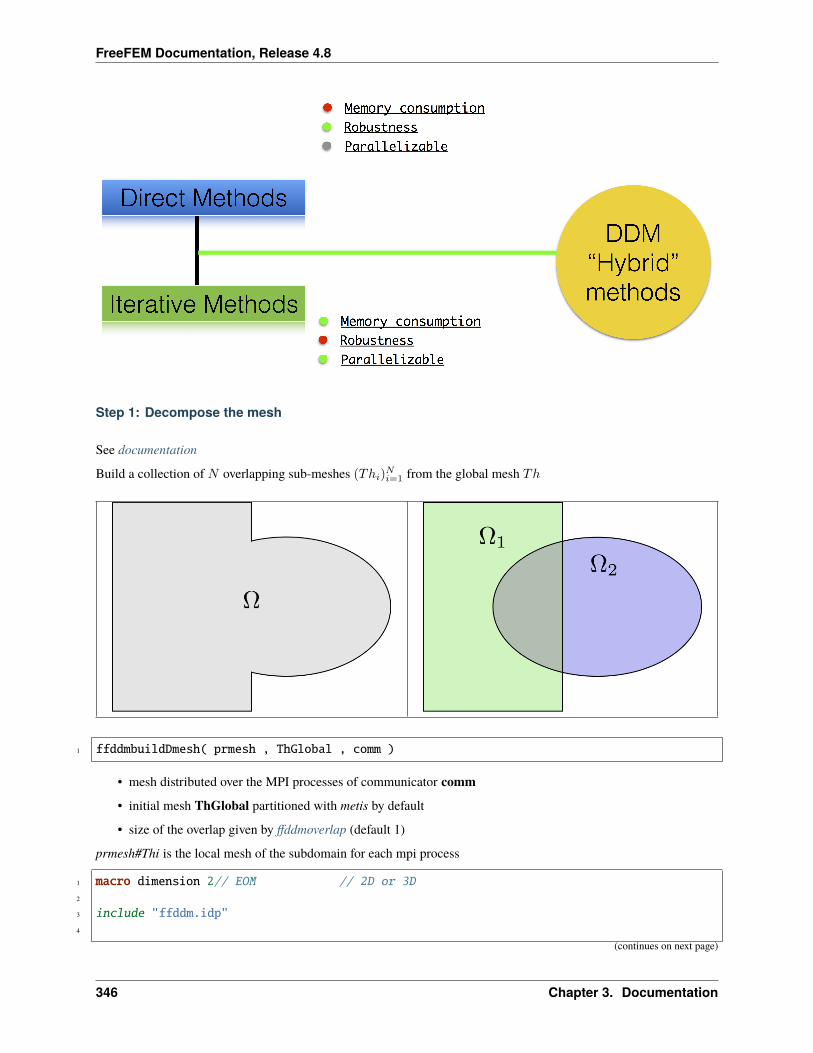
FreeFEM Documentation, Release 4.8
Step 1: Decompose the mesh
See documentation
Build a collection of 𝑁 overlapping sub-meshes (𝑇ℎ𝑖)𝑁𝑖=1 from the global mesh 𝑇ℎ
1 ffddmbuildDmesh( prmesh , ThGlobal , comm )
• mesh distributed over the MPI processes of communicator comm• initial mesh ThGlobal partitioned with metis by default
• size of the overlap given by ffddmoverlap (default 1)
prmesh#Thi is the local mesh of the subdomain for each mpi process
1 macro dimension 2// EOM // 2D or 3D2
3 include "ffddm.idp"4
(continues on next page)
346 Chapter 3. Documentation
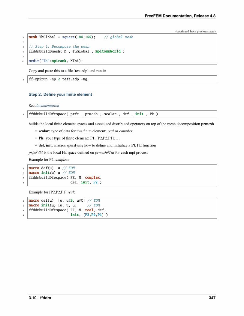
FreeFEM Documentation, Release 4.8
(continued from previous page)
5 mesh ThGlobal = square(100,100); // global mesh6
7 // Step 1: Decompose the mesh8 ffddmbuildDmesh( M , ThGlobal , mpiCommWorld )9
10 medit("Th"+mpirank, MThi);
Copy and paste this to a file ‘test.edp’ and run it:
1 ff-mpirun -np 2 test.edp -wg
Step 2: Define your finite element
See documentation
1 ffddmbuildDfespace( prfe , prmesh , scalar , def , init , Pk )
builds the local finite element spaces and associated distributed operators on top of the mesh decomposition prmesh• scalar: type of data for this finite element: real or complex
• Pk: your type of finite element: P1, [P2,P2,P1], . . .
• def, init: macros specifying how to define and initialize a Pk FE function
prfe#Vhi is the local FE space defined on prmesh#Thi for each mpi process
Example for P2 complex:
1 macro def(u) u // EOM2 macro init(u) u // EOM3 ffddmbuildDfespace( FE, M, complex,4 def, init, P2 )
Example for [P2,P2,P1] real:
1 macro def(u) [u, u#B, u#C] // EOM2 macro init(u) [u, u, u] // EOM3 ffddmbuildDfespace( FE, M, real, def,4 init, [P2,P2,P1] )
3.10. ffddm 347
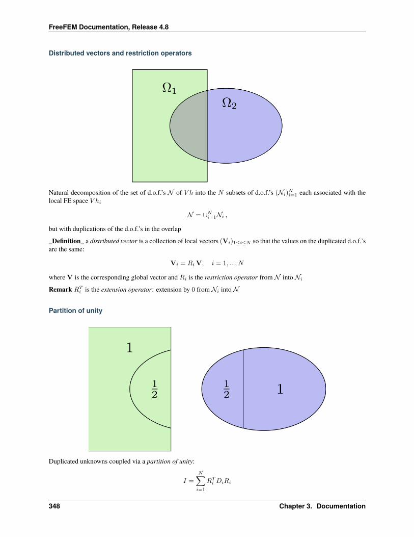
FreeFEM Documentation, Release 4.8
Distributed vectors and restriction operators
Natural decomposition of the set of d.o.f.’s 𝒩 of 𝑉 ℎ into the 𝑁 subsets of d.o.f.’s (𝒩𝑖)𝑁𝑖=1 each associated with thelocal FE space 𝑉 ℎ𝑖
𝒩 = ∪𝑁𝑖=1𝒩𝑖 ,
but with duplications of the d.o.f.’s in the overlap
_Definition_ a distributed vector is a collection of local vectors (V𝑖)1≤𝑖≤𝑁 so that the values on the duplicated d.o.f.’sare the same:
V𝑖 = 𝑅𝑖V, 𝑖 = 1, ..., 𝑁
where V is the corresponding global vector and 𝑅𝑖 is the restriction operator from 𝒩 into 𝒩𝑖Remark 𝑅𝑇𝑖 is the extension operator: extension by 0 from 𝒩𝑖 into 𝒩
Partition of unity
Duplicated unknowns coupled via a partition of unity:
𝐼 =
𝑁∑𝑖=1
𝑅𝑇𝑖 𝐷𝑖𝑅𝑖
348 Chapter 3. Documentation
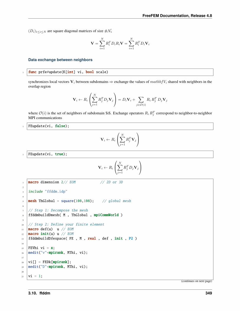
FreeFEM Documentation, Release 4.8
(𝐷𝑖)1≤𝑖≤𝑁 are square diagonal matrices of size #𝒩𝑖
V =
𝑁∑𝑖=1
𝑅𝑇𝑖 𝐷𝑖𝑅𝑖V =
𝑁∑𝑖=1
𝑅𝑇𝑖 𝐷𝑖V𝑖
Data exchange between neighbors
1 func prfe#update(K[int] vi, bool scale)
synchronizes local vectors V𝑖 between subdomains⇒ exchange the values of 𝑚𝑎𝑡ℎ𝑏𝑓𝑉𝑖 shared with neighbors in theoverlap region
V𝑖 ← 𝑅𝑖
⎛⎝ 𝑁∑𝑗=1
𝑅𝑇𝑗 𝐷𝑗V𝑗
⎞⎠ = 𝐷𝑖V𝑖 +∑𝑗∈𝒪(𝑖)
𝑅𝑖𝑅𝑇𝑗 𝐷𝑗V𝑗
where 𝒪(𝑖) is the set of neighbors of subdomain $i$. Exchange operators 𝑅𝑖𝑅𝑇𝑗 correspond to neighbor-to-neighborMPI communications
1 FEupdate(vi, false);
V𝑖 ← 𝑅𝑖
⎛⎝ 𝑁∑𝑗=1
𝑅𝑇𝑗 V𝑗
⎞⎠1 FEupdate(vi, true);
V𝑖 ← 𝑅𝑖
⎛⎝ 𝑁∑𝑗=1
𝑅𝑇𝑗 𝐷𝑗V𝑗
⎞⎠1 macro dimension 2// EOM // 2D or 3D2
3 include "ffddm.idp"4
5 mesh ThGlobal = square(100,100); // global mesh6
7 // Step 1: Decompose the mesh8 ffddmbuildDmesh( M , ThGlobal , mpiCommWorld )9
10 // Step 2: Define your finite element11 macro def(u) u // EOM12 macro init(u) u // EOM13 ffddmbuildDfespace( FE , M , real , def , init , P2 )14
15 FEVhi vi = x;16 medit("v"+mpirank, MThi, vi);17
18 vi[] = FEDk[mpirank];19 medit("D"+mpirank, MThi, vi);20
21 vi = 1;(continues on next page)
3.10. ffddm 349
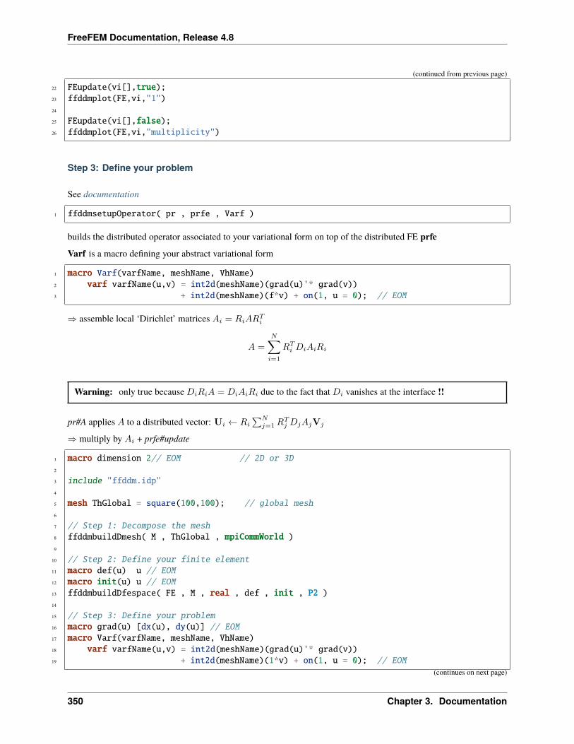
FreeFEM Documentation, Release 4.8
(continued from previous page)
22 FEupdate(vi[],true);23 ffddmplot(FE,vi,"1")24
25 FEupdate(vi[],false);26 ffddmplot(FE,vi,"multiplicity")
Step 3: Define your problem
See documentation
1 ffddmsetupOperator( pr , prfe , Varf )
builds the distributed operator associated to your variational form on top of the distributed FE prfeVarf is a macro defining your abstract variational form
1 macro Varf(varfName, meshName, VhName)2 varf varfName(u,v) = int2d(meshName)(grad(u)'* grad(v))3 + int2d(meshName)(f*v) + on(1, u = 0); // EOM
⇒ assemble local ‘Dirichlet’ matrices 𝐴𝑖 = 𝑅𝑖𝐴𝑅𝑇𝑖
𝐴 =
𝑁∑𝑖=1
𝑅𝑇𝑖 𝐷𝑖𝐴𝑖𝑅𝑖
Warning: only true because 𝐷𝑖𝑅𝑖𝐴 = 𝐷𝑖𝐴𝑖𝑅𝑖 due to the fact that 𝐷𝑖 vanishes at the interface !!
pr#A applies 𝐴 to a distributed vector: U𝑖 ← 𝑅𝑖∑𝑁𝑗=1𝑅
𝑇𝑗 𝐷𝑗𝐴𝑗V𝑗
⇒ multiply by 𝐴𝑖 + prfe#update
1 macro dimension 2// EOM // 2D or 3D2
3 include "ffddm.idp"4
5 mesh ThGlobal = square(100,100); // global mesh6
7 // Step 1: Decompose the mesh8 ffddmbuildDmesh( M , ThGlobal , mpiCommWorld )9
10 // Step 2: Define your finite element11 macro def(u) u // EOM12 macro init(u) u // EOM13 ffddmbuildDfespace( FE , M , real , def , init , P2 )14
15 // Step 3: Define your problem16 macro grad(u) [dx(u), dy(u)] // EOM17 macro Varf(varfName, meshName, VhName)18 varf varfName(u,v) = int2d(meshName)(grad(u)'* grad(v))19 + int2d(meshName)(1*v) + on(1, u = 0); // EOM
(continues on next page)
350 Chapter 3. Documentation
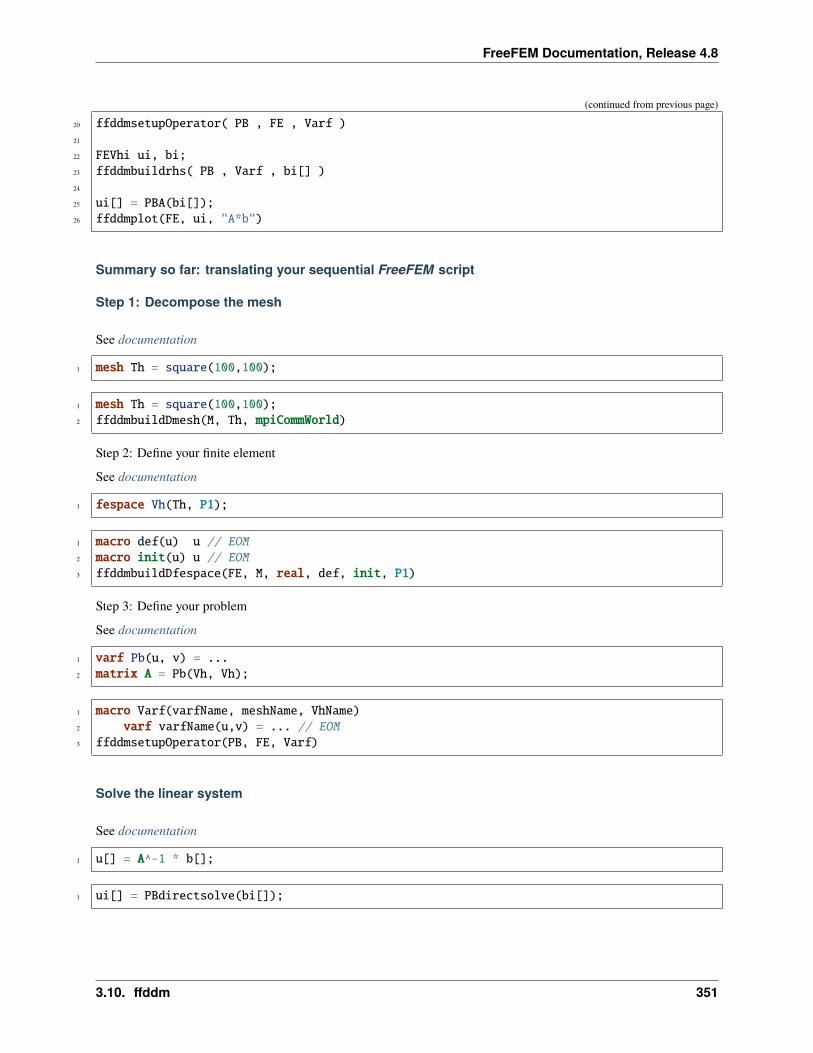
FreeFEM Documentation, Release 4.8
(continued from previous page)
20 ffddmsetupOperator( PB , FE , Varf )21
22 FEVhi ui, bi;23 ffddmbuildrhs( PB , Varf , bi[] )24
25 ui[] = PBA(bi[]);26 ffddmplot(FE, ui, "A*b")
Summary so far: translating your sequential FreeFEM script
Step 1: Decompose the mesh
See documentation
1 mesh Th = square(100,100);
1 mesh Th = square(100,100);2 ffddmbuildDmesh(M, Th, mpiCommWorld)
Step 2: Define your finite element
See documentation
1 fespace Vh(Th, P1);
1 macro def(u) u // EOM2 macro init(u) u // EOM3 ffddmbuildDfespace(FE, M, real, def, init, P1)
Step 3: Define your problem
See documentation
1 varf Pb(u, v) = ...2 matrix A = Pb(Vh, Vh);
1 macro Varf(varfName, meshName, VhName)2 varf varfName(u,v) = ... // EOM3 ffddmsetupOperator(PB, FE, Varf)
Solve the linear system
See documentation
1 u[] = A^-1 * b[];
1 ui[] = PBdirectsolve(bi[]);
3.10. ffddm 351
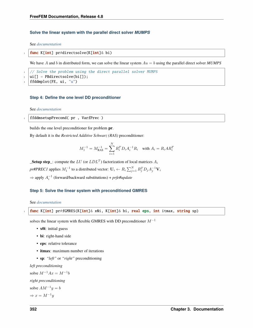
FreeFEM Documentation, Release 4.8
Solve the linear system with the parallel direct solver MUMPS
See documentation
1 func K[int] pr#directsolve(K[int]& bi)
We have 𝐴 and 𝑏 in distributed form, we can solve the linear system 𝐴𝑢 = 𝑏 using the parallel direct solver MUMPS
1 // Solve the problem using the direct parallel solver MUMPS2 ui[] = PBdirectsolve(bi[]);3 ffddmplot(FE, ui, "u")
Step 4: Define the one level DD preconditioner
See documentation
1 ffddmsetupPrecond( pr , VarfPrec )
builds the one level preconditioner for problem pr.
By default it is the Restricted Additive Schwarz (RAS) preconditioner:
𝑀−11 = 𝑀−1
RAS =
𝑁∑𝑖=1
𝑅𝑇𝑖 𝐷𝑖𝐴−1𝑖 𝑅𝑖 with 𝐴𝑖 = 𝑅𝑖𝐴𝑅
𝑇𝑖
_Setup step_: compute the 𝐿𝑈 (or 𝐿𝐷𝐿𝑇 ) factorization of local matrices 𝐴𝑖pr#PREC1 applies 𝑀−1
1 to a distributed vector: U𝑖 ← 𝑅𝑖∑𝑁𝑗=1𝑅
𝑇𝑗 𝐷𝑗𝐴
−1𝑗 V𝑖
⇒ apply 𝐴−1𝑖 (forward/backward substitutions) + prfe#update
Step 5: Solve the linear system with preconditioned GMRES
See documentation
1 func K[int] pr#fGMRES(K[int]& x0i, K[int]& bi, real eps, int itmax, string sp)
solves the linear system with flexible GMRES with DD preconditioner 𝑀−1
• x0i: initial guess
• bi: right-hand side
• eps: relative tolerance
• itmax: maximum number of iterations
• sp: “left” or “right” preconditioning
left preconditioning
solve 𝑀−1𝐴𝑥 = 𝑀−1𝑏
right preconditioning
solve 𝐴𝑀−1𝑦 = 𝑏
⇒ 𝑥 = 𝑀−1𝑦
352 Chapter 3. Documentation
FreeFEM Documentation, Release 4.8
1 macro dimension 2// EOM // 2D or 3D2 include "ffddm.idp"3
4 mesh ThGlobal = square(100,100); // global mesh5 // Step 1: Decompose the mesh6 ffddmbuildDmesh( M , ThGlobal , mpiCommWorld )7 // Step 2: Define your finite element8 macro def(u) u // EOM9 macro init(u) u // EOM
10 ffddmbuildDfespace( FE , M , real , def , init , P2 )11 // Step 3: Define your problem12 macro grad(u) [dx(u), dy(u)] // EOM13 macro Varf(varfName, meshName, VhName)14 varf varfName(u,v) = int2d(meshName)(grad(u)'* grad(v))15 + int2d(meshName)(1*v) + on(1, u = 0); // EOM16 ffddmsetupOperator( PB , FE , Varf )17
18 FEVhi ui, bi;19 ffddmbuildrhs( PB , Varf , bi[] )20
21 // Step 4: Define the one level DD preconditioner22 ffddmsetupPrecond( PB , Varf )23
24 // Step 5: Solve the linear system with GMRES25 FEVhi x0i = 0;26 ui[] = PBfGMRES(x0i[], bi[], 1.e-6, 200, "right");27
28 ffddmplot(FE, ui, "u")29 PBwritesummary
Define a two level DD preconditioner
See documentation
Goal improve scalability of the one level method
⇒ enrich the one level preconditioner with a coarse problem coupling all subdomains
Main ingredient is a rectangular matrix 𝑍 of size 𝑛× 𝑛𝑐, where 𝑛𝑐 ≪ 𝑛 𝑍 is the coarse space matrix
The coarse space operator 𝐸 = 𝑍𝑇𝐴𝑍 is a square matrix of size 𝑛𝑐 × 𝑛𝑐The simplest way to enrich the one level preconditioner is through the additive coarse correction formula:
𝑀−12 = 𝑀−1
1 + 𝑍𝐸−1𝑍𝑇
How to choose 𝑍 ?
3.10. ffddm 353
FreeFEM Documentation, Release 4.8
Build the GenEO coarse space
See documentation
1 ffddmgeneosetup( pr , Varf )
The GenEO method builds a robust coarse space for highly heterogeneous or anisotropic SPD problems
⇒ solve a local generalized eigenvalue problem in each subdomain
𝐷𝑖𝐴𝑖𝐷𝑖 𝑉𝑖,𝑘 = 𝜆𝑖,𝑘 𝐴Neu𝑖 𝑉𝑖,𝑘
with 𝐴Neu𝑖 the local Neumann matrices built from Varf (same Varf as Step 3)
The GenEO coarse space is 𝑍 = (𝑅𝑇𝑖 𝐷𝑖𝑉𝑖,𝑘)𝑖=1,...,𝑁𝜆𝑖,𝑘≥𝜏 The eigenvectors 𝑉𝑖,𝑘 selected to enter the coarse space corre-
spond to eigenvalues 𝜆𝑖,𝑘 ≥ 𝜏 , where 𝜏 is a threshold parameter
Theorem the spectrum of the preconditioned operator lies in the interval [1
1 + 𝑘1𝜏, 𝑘0] where 𝑘0 − 1 is
the # of neighbors and 𝑘1 is the multiplicity of intersections⇒ 𝑘0 and 𝑘1 do not depend on 𝑁 nor on thePDE
1 macro dimension 2// EOM // 2D or 3D2 include "ffddm.idp"3
4 mesh ThGlobal = square(100,100); // global mesh5 // Step 1: Decompose the mesh6 ffddmbuildDmesh( M , ThGlobal , mpiCommWorld )7 // Step 2: Define your finite element8 macro def(u) u // EOM9 macro init(u) u // EOM
10 ffddmbuildDfespace( FE , M , real , def , init , P2 )11 // Step 3: Define your problem12 macro grad(u) [dx(u), dy(u)] // EOM13 macro Varf(varfName, meshName, VhName)14 varf varfName(u,v) = int2d(meshName)(grad(u)'* grad(v))15 + int2d(meshName)(1*v) + on(1, u = 0); // EOM16 ffddmsetupOperator( PB , FE , Varf )17
18 FEVhi ui, bi;19 ffddmbuildrhs( PB , Varf , bi[] )20
21 // Step 4: Define the one level DD preconditioner22 ffddmsetupPrecond( PB , Varf )23
24 // Build the GenEO coarse space25 ffddmgeneosetup( PB , Varf )26
27 // Step 5: Solve the linear system with GMRES28 FEVhi x0i = 0;29 ui[] = PBfGMRES(x0i[], bi[], 1.e-6, 200, "right");
354 Chapter 3. Documentation
FreeFEM Documentation, Release 4.8
Build the coarse space from a coarse mesh
See documentation
1 ffddmcoarsemeshsetup( pr , Thc , VarfEprec , VarfAprec )
For non SPD problems, an alternative is to build the coarse space by discretizing the PDE on a coarser mesh Thc𝑍 will be the interpolation matrix from the coarse FE space 𝑉 ℎ𝑐 to the original FE space 𝑉 ℎ
⇒ 𝐸 = 𝑍𝑇𝐴𝑍 is the matrix of the problem discretized on the coarse mesh
The variational problem to be discretized on Thc is given by macro VarfEprecVarfEprec can differ from the original Varf of the problem
Example: added absorption for wave propagation problems
Similarly, VarfAprec specifies the global operator involved in multiplicative coarse correction formulas. It defaults to𝐴 if VarfAprec is not defined
1 macro dimension 2// EOM // 2D or 3D2 include "ffddm.idp"3
4 mesh ThGlobal = square(100,100); // global mesh5 // Step 1: Decompose the mesh6 ffddmbuildDmesh( M , ThGlobal , mpiCommWorld )7 // Step 2: Define your finite element8 macro def(u) u // EOM9 macro init(u) u // EOM
10 ffddmbuildDfespace( FE , M , real , def , init , P2 )11 // Step 3: Define your problem12 macro grad(u) [dx(u), dy(u)] // EOM13 macro Varf(varfName, meshName, VhName)14 varf varfName(u,v) = int2d(meshName)(grad(u)'* grad(v))15 + int2d(meshName)(1*v) + on(1, u = 0); // EOM16 ffddmsetupOperator( PB , FE , Varf )17
18 FEVhi ui, bi;19 ffddmbuildrhs( PB , Varf , bi[] )20
21 // Step 4: Define the one level DD preconditioner22 ffddmsetupPrecond( PB , Varf )23
24 // Build the coarse space from a coarse mesh25 mesh Thc = square(10,10);26 ffddmcoarsemeshsetup( PB , Thc , Varf , null )27
28 // Step 5: Solve the linear system with GMRES29 FEVhi x0i = 0;30 ui[] = PBfGMRES(x0i[], bi[], 1.e-6, 200, "right");
3.10. ffddm 355
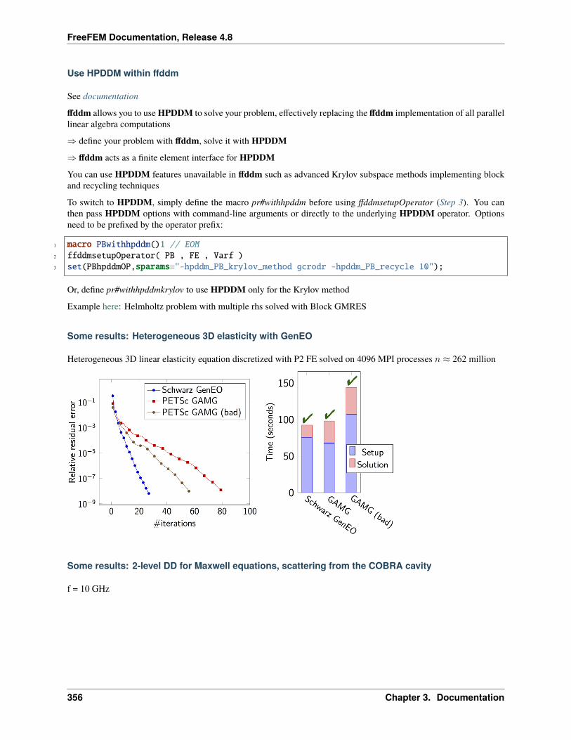
FreeFEM Documentation, Release 4.8
Use HPDDM within ffddm
See documentation
ffddm allows you to use HPDDM to solve your problem, effectively replacing the ffddm implementation of all parallellinear algebra computations
⇒ define your problem with ffddm, solve it with HPDDM⇒ ffddm acts as a finite element interface for HPDDMYou can use HPDDM features unavailable in ffddm such as advanced Krylov subspace methods implementing blockand recycling techniques
To switch to HPDDM, simply define the macro pr#withhpddm before using ffddmsetupOperator (Step 3). You canthen pass HPDDM options with command-line arguments or directly to the underlying HPDDM operator. Optionsneed to be prefixed by the operator prefix:
1 macro PBwithhpddm()1 // EOM2 ffddmsetupOperator( PB , FE , Varf )3 set(PBhpddmOP,sparams="-hpddm_PB_krylov_method gcrodr -hpddm_PB_recycle 10");
Or, define pr#withhpddmkrylov to use HPDDM only for the Krylov method
Example here: Helmholtz problem with multiple rhs solved with Block GMRES
Some results: Heterogeneous 3D elasticity with GenEO
Heterogeneous 3D linear elasticity equation discretized with P2 FE solved on 4096 MPI processes 𝑛 ≈ 262 million
Some results: 2-level DD for Maxwell equations, scattering from the COBRA cavity
f = 10 GHz
356 Chapter 3. Documentation
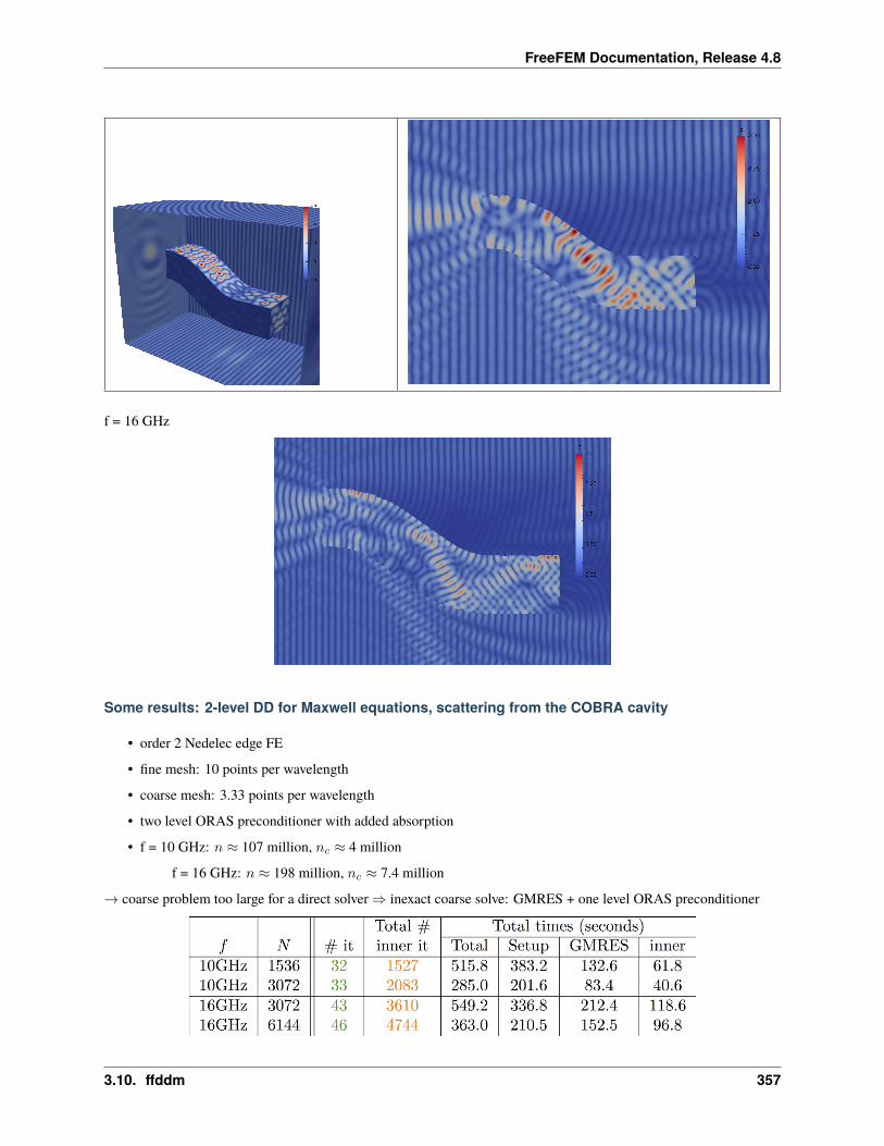
FreeFEM Documentation, Release 4.8
f = 16 GHz
Some results: 2-level DD for Maxwell equations, scattering from the COBRA cavity
• order 2 Nedelec edge FE
• fine mesh: 10 points per wavelength
• coarse mesh: 3.33 points per wavelength
• two level ORAS preconditioner with added absorption
• f = 10 GHz: 𝑛 ≈ 107 million, 𝑛𝑐 ≈ 4 million
f = 16 GHz: 𝑛 ≈ 198 million, 𝑛𝑐 ≈ 7.4 million
→ coarse problem too large for a direct solver⇒ inexact coarse solve: GMRES + one level ORAS preconditioner
3.10. ffddm 357
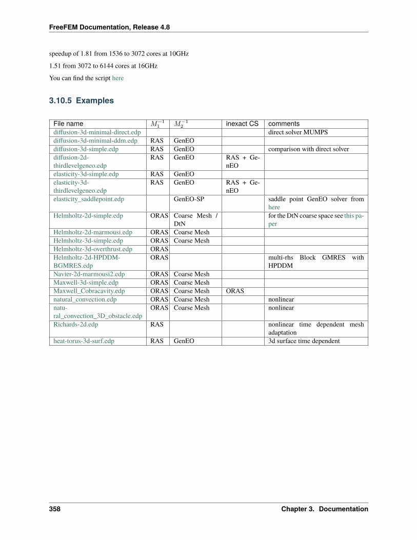
FreeFEM Documentation, Release 4.8
speedup of 1.81 from 1536 to 3072 cores at 10GHz
1.51 from 3072 to 6144 cores at 16GHz
You can find the script here
3.10.5 Examples
File name 𝑀−11 𝑀−1
2 inexact CS commentsdiffusion-3d-minimal-direct.edp direct solver MUMPSdiffusion-3d-minimal-ddm.edp RAS GenEOdiffusion-3d-simple.edp RAS GenEO comparison with direct solverdiffusion-2d-thirdlevelgeneo.edp
RAS GenEO RAS + Ge-nEO
elasticity-3d-simple.edp RAS GenEOelasticity-3d-thirdlevelgeneo.edp
RAS GenEO RAS + Ge-nEO
elasticity_saddlepoint.edp GenEO-SP saddle point GenEO solver fromhere
Helmholtz-2d-simple.edp ORAS Coarse Mesh /DtN
for the DtN coarse space see this pa-per
Helmholtz-2d-marmousi.edp ORAS Coarse MeshHelmholtz-3d-simple.edp ORAS Coarse MeshHelmholtz-3d-overthrust.edp ORASHelmholtz-2d-HPDDM-BGMRES.edp
ORAS multi-rhs Block GMRES withHPDDM
Navier-2d-marmousi2.edp ORAS Coarse MeshMaxwell-3d-simple.edp ORAS Coarse MeshMaxwell_Cobracavity.edp ORAS Coarse Mesh ORASnatural_convection.edp ORAS Coarse Mesh nonlinearnatu-ral_convection_3D_obstacle.edp
ORAS Coarse Mesh nonlinear
Richards-2d.edp RAS nonlinear time dependent meshadaptation
heat-torus-3d-surf.edp RAS GenEO 3d surface time dependent
358 Chapter 3. Documentation
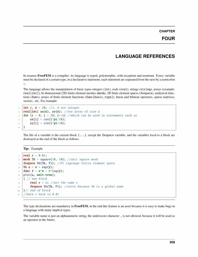
CHAPTER
FOUR
LANGUAGE REFERENCES
In essence FreeFEM is a compiler: its language is typed, polymorphic, with exception and reentrant. Every variablemust be declared of a certain type, in a declarative statement; each statement are separated from the next by a semicolon;.
The language allows the manipulation of basic types integers (int), reals (real), strings (string), arrays (example:real[int]), bi-dimensional (2D) finite element meshes (mesh), 2D finite element spaces (fespace), analytical func-tions (func), arrays of finite element functions (func[basic_type]), linear and bilinear operators, sparse matrices,vectors , etc. For example:
1 int i, n = 20; //i, n are integer2 real[int] xx(n), yy(n); //two array of size n3 for (i = 0; i < 20; i++) //which can be used in statements such as4 xx[i] = cos(i*pi/10);5 yy[i] = sin(i*pi/10);6
The life of a variable is the current block ..., except the fespace variable, and the variables local to a block aredestroyed at the end of the block as follows.
Tip: Example
1 real r = 0.01;2 mesh Th = square(10, 10); //unit square mesh3 fespace Vh(Th, P1); //P1 Lagrange finite element space4 Vh u = x + exp(y);5 func f = z*x + r*log(y);6 plot(u, wait=true);7 // new block8 real r = 2; //not the same r9 fespace Vh(Th, P1); //error because Vh is a global name
10 // end of block11 //here r back to 0.01
The type declarations are mandatory in FreeFEM; in the end this feature is an asset because it is easy to make bugs ina language with many implicit types.
The variable name is just an alphanumeric string, the underscore character _ is not allowed, because it will be used asan operator in the future.
359
FreeFEM Documentation, Release 4.8
4.1 Types
4.1.1 Standard types
int
Integer value (equivalent to long in C++).
1 int i = 0;
bool
Boolean value.
1 bool b = true;
Tip: The result of a comparison is a boolean
bool b = (1 < 2);
real
Real value (equivalent to double in C++).
1 real r = 0.;
complex
Complex value (equivalent to two double or complex<double> in C++).
1 complex c = 0. + 1i;
The imaginary number 𝑖 is defined as 1i
Tip: Example
1 complex a = 1i, b = 2 + 3i;2 cout << "a + b = " << a + b << endl;3 cout << "a - b = " << a - b << endl;4 cout << "a*b = " << a*b << endl;5 cout << "a/b = " << a/b << endl;
The output of this script is:
a + b = (2,4)a - b = (-2,-2)a*b = (-3,2)a/b = (0.230769,0.153846)
360 Chapter 4. Language references
FreeFEM Documentation, Release 4.8
Note: See Complex example for a detailed example.
string
String value.
1 string s = "this is a string";
Note: string value is enclosed within double quotes.
Other types can be concatenate to a string, like:
1 int i = 1;2 real r = 1.;3 string s = "the int i = " + i +", the real r = " + r + ", the complex z = " + (1. + 1i);
To append a string in a string at position 4:
1 s(4:3) = "+++";
To copy a substring in an other string:
1 string s2 = s1(5:10);
See String Example for a complete example.
4.1.2 Mesh design
border
Border type.
1 border b(t=0., 1.)x=cos(2.*pi*t); y=sin(2.*pi*t);
Define the 2D geometrical border in parametric coordinates.
Note: Label
A label can be defined with the border:
1 border b(t=0., 1.)x=cos(2.*pi*t); y=sin(2.*pi*t); label=1;
Note: Inner variable
An inner variable can be defined inside a border:
4.1. Types 361
FreeFEM Documentation, Release 4.8
1 border b(t=0., 1.)real tt=2.*pi*t; x=cos(tt); y=sin(tt);
Note: From vector
A border can be defined from two vectors using P.x and P.y:
1 border b(t=0, vectorX.n-1)P.x=vectorX[t]; P.y=vectorY[t];
mesh
2D Mesh type (see Mesh Generation).
1 mesh Th;
mesh3
3D mesh type (see Mesh Generation).
1 mesh3 Th;
4.1.3 Finite element space design
fespace
Finite element space type (see Finite Element).
1 fespace Uh(Th, P1);2 fespace UPh(Th, [P2, P2, P1]);
A finite element space is based on a mesh (Th) with an element definition, scalar (P1) or vector ([P2, P2, P1]).
Available finite element space:Generic:
• P0 / P03d
• P0Edge
• P1 / P13d
• P1dc
• P1b / P1b3d
• P1bl / P1bl3d
• P1nc
• P2 / P23d
• P2b
• P2dc
362 Chapter 4. Language references
FreeFEM Documentation, Release 4.8
• P2h
• RT0 / RT03d
• RT0Ortho
• Edge03d
Using Element_P3:
• P3
Using Element_P3dc:
• P3dc
Using Element_P4:
• P4
Using Element_P4dc:
• P4dc
Using Element_PkEdge:
• P1Edge
• P2Edge
• P3Edge
• P4Edge
• P5Edge
Using Morlay:
• P2Morley
Using HCT :
• HCT
Using BernardiRaugel:
• P2BR
Using Element_Mixte:
• RT1
• RT1Ortho
• RT2
• RT2Ortho
• BDM1
• BDM1Ortho
Using Element_Mixte3d:
• Edge13d
• Edge23d
Using Element_QF:
• FEQF
4.1. Types 363
FreeFEM Documentation, Release 4.8
A finite element function is defined as follow:
1 fespace Uh(Th, P1);2 Uh u;3
4 fespace UPh(Th, [P2, P2, P1]);5 UPh [Ux, Uy, p];
4.1.4 Macro design
macro
Macro type.
1 macro vU() [Ux, Uy] //2 macro grad(u) [dx(u), dy(u)] //
Macro ends with //.
Note: Macro concatenation
You can use the C concatenation operator ## inside a macro using #.
If Ux and Uy are defined as finite element function, you can define:
1 macro Grad(U) [grad(U#x), grad(U#y)] // End of macro
See Macro example
NewMacro / EndMacro
Warning: In developement - Not tested
Set and end a macro
1 NewMacro grad(u) [dx(u), dy(u)] EndMacro
IFMACRO
Check if a macro exists and check its value.
1 IFMACRO(AA) //check if macro AA exists2 ...3 ENDIFMACRO4
5 IFMACRO(AA, tt) //check if amcro exists and is equall to tt6 ...7 ENDIFMACRO
364 Chapter 4. Language references
FreeFEM Documentation, Release 4.8
ENDIFMACRO
4.1.5 Functions design
func
Function type.
Function without parameters (𝑥, 𝑦 and 𝑧 are implicitly considered):
1 func f = x^2 + y^2;
Note: Function’s type is defined by the expression’s type.
Function with parameters:
1 func real f (real var)2 return x^2 + y^2 + var^2;3
Elementary functions
Class of basic functions (polynomials, exponential, logarithmic, trigonometric, circular) and the functions obtainedfrom those by the four arithmetic operations
𝑓(𝑥) + 𝑔(𝑥), 𝑓(𝑥)− 𝑔(𝑥), 𝑓(𝑥)𝑔(𝑥), 𝑓(𝑥)/𝑔(𝑥)
and by composition 𝑓(𝑔(𝑥)), each applied a finite number of times.
In FreeFEM, all elementary functions can thus be created. The derivative of an elementary function is also an ele-mentary function; however, the indefinite integral of an elementary function cannot always be expressed in terms ofelementary functions.
See Elementary function example for a complete example.
Random functions
FreeFEM includes the Mersenne Twister random number generator. It is a very fast and accurate random numbergenerator of period 2219937 − 1.
See randint32(), randint31(), randreal1(), randreal2(), randreal3(), randres53(), randinit(seed).
In addition, the ffrandom plugin interface random, srandom and srandomdev functions of the Unix libc library.The range is 0−−231 − 1.
Note: If srandomdev is not defined, a seed based on the current time is used.
gsl plugin equally allows usage of all random functions of the gsllib, see gsl external library.
4.1. Types 365
FreeFEM Documentation, Release 4.8
FE-functions
Finite element functions are also constructed like elementary functions by an arithmetic formula involving elementaryfunctions.
The difference is that they are evaluated at declaration time and FreeFEM stores the array of its values at the placesassociated with he degree of freedom of the finite element type. By opposition, elementary functions are evaluated onlywhen needed. Hence FE-functions are not defined only by their formula but also by the mesh and the finite elementwhich enter in their definitions.
If the value of a FE-function is requested at a point which is not a degree of freedom, an interpolation is used, leadingto an interpolation error, while by contrast, an elementary function can be evaluated at any point exactly.
1 func f = x^2*(1+y)^3 + y^2;2 mesh Th = square(20, 20, [-2+4*x, -2+4*y]); // ]-2, 2[^23 fespace Vh(Th, P1);4 Vh fh=f; //fh is the projection of f to Vh (real value)5 func zf = (x^2*(1+y)^3 + y^2)*exp(x + 1i*y);6 Vh<complex> zh = zf; //zh is the projection of zf to complex value Vh space
The construction of fh = f is explained in Finite Element.
Warning: The plot command only works for real or complex FE-functions, not for elementary functions.
4.1.6 Problem design
problem
Problem type.
1 problem Laplacian (u, uh) = ...
FreeFEM needs the variational form in the problem definition.
In order to solve the problem, just call:
1 Laplacian;
Note: Solver
A solver can be specified in the problem definition:
1 problem Laplacian(u, uh, solver=CG) = ...
The default solver is sparsesolver or LU if any direct sparse solver is available.
Solvers are listed in the Global variables section.
Note: Stop test
A criterion 𝜀 can be defined for iterative methods, like CG for example:
366 Chapter 4. Language references
FreeFEM Documentation, Release 4.8
1 problem Laplacian(u, uh, solver=CG, eps=1.e-6) = ...
If 𝜀 > 0, the stop test is:
||𝐴𝑥− 𝑏|| < 𝜀
Else, the stop test is:
||𝐴𝑥− 𝑏|| < |𝜀|||𝐴𝑥0 − 𝑏||
Note: Reconstruction
The keyword init controls the reconstruction of the internal problem matrix.
If init is set to false or 0, the matrix is reconstructed et each problem calls (or after a mesh modification), else thepreviously constructed matrix is used.
1 problem Laplacian(u, uh, init=1) = ...
Note: Preconditioning
A preconditioner can be specified in the problem definition:
1 problem Laplacian(u, uh, precon=P) = ...
The preconditioning function must have a prototype like:
1 func real[int] P(real[int] &xx);
Note: “Très grande valeur”
The “Très grand valeur” tgv (or Terrible giant value) used to implement the Dirichlet conditions can be modified inthe problem definition:
1 problem Laplacian(u, uh, tgv=1e30) = ...
Refere to Problem definition for a description of the Dirichlet condition implementation.
Note: Pivot tolerance
The tolerance of the pivot in UMFPACK, LU, Crout, Cholesky factorization can be modified in the problem definition:
1 problem Laplacian(u, uh, solver=LU, tolpivot=1e-20) = ...
Note: UMFPACK
Two specific parameters for the UMFPACK can be modifed:
4.1. Types 367
FreeFEM Documentation, Release 4.8
• Tolerance of the pivot sym
• strategy
1 problem Laplacian(u, uh, solver=LU, tolpivotsym=1e-1, strategy=0) = ...
Refer to the UMFPACK website for more informations.
Note: dimKrylov
Dimension of the Krylov space
Usage of problem is detailled in the tutorials.
solve
Solve type.
Identical to problem but automatically solved.
Usage of solve is detailled in the tutorials.
varf
Variational form type.
1 varf vLaplacian (u, uh) = ...
Directly define a variational form.
This is the other way to define a problem in order to directly manage matrix and right hang side.
Usage of varf is detailed in the tutorial.
4.1.7 Array
An array stores multiple objects, and there are 2 kinds of arrays:
• the first is similar to vector, i.e. array with integer indices
• the second is array with string indices
In the first case, the size of the array must be known at execution time, and implementation is done with the KN<> classand all the vector operator of KN<> are implemented.
Arrays can be set like in Matlab or Scilab with the operator ::, the array generator of a:c is equivalent to a:1:c, andthe array set by a:b:c is set to size ⌊|(𝑏− 𝑎)/𝑐|+ 1⌋ and the value 𝑖 is set by 𝑎+ 𝑖(𝑏− 𝑎)/𝑐.
There are int,real, complex array with, in the third case, two operators (.im, .re) to generate the real and imagi-nary real array from the complex array (without copy).
Note: Quantiles are points taken at regular intervals from the cumulative distribution function of a random variable.Here the array values are random.
368 Chapter 4. Language references
FreeFEM Documentation, Release 4.8
This statistical function a.quantile(q) computes 𝑣 from an array 𝑎 of size 𝑛 for a given number 𝑞 ∈]0, 1[ such that:
#𝑖/𝑎[𝑖] < 𝑣 ∼ 𝑞 * 𝑛
it is equivalent to 𝑣 = 𝑎[𝑞 * 𝑛] when the array 𝑎 is sorted.
For example, to declare, fill and display an array of real of size n:
1 int n = 5;2 real[int] Ai(n);3 for (int i = 0; i < n; i++)4 Ai[i] = i;5 cout << Ai << endl;
The output of this script is:
50 1 2 3 4
See the Array example for a complete example.
Array index
Array index can be int or string:
1 real[int] Ai = [1, 1, 0, 0];2 real[string] As = [1, 1, 0, 0];
Array size
The size of an array is obtained using the keyword n:
1 int ArraySize = Ai.n;
Array sort
To sort an array:
1 Ai.sort;
Double array
A double array (matrix) can be defined using two indexes:
1 real[int, int] Aii = [[1, 1], [0, 0]];
The two sizes are obtained using the keywords n and m:
1 int ArraySize1 = Aii.n;2 int ArraySize2 = Aii.m;
4.1. Types 369
FreeFEM Documentation, Release 4.8
The minimum and maximum values of an array (simple or double) can be obtained using:
1 real ArrayMin = Aii.min;2 real ArrayMax = Aii.max;
Th minimum and maximum position of an array can be obtained using:
1 int mini = Aii.imin;2 int minj = Aii.jmin;3
4 int maxi = Aii.imax;5 int maxj = Aii.jmax;
Tip: An array can be obtained from a finite element function using:
1 real[int] aU = U[];
where U is a finite element function.
Array of FE functions
It is also possible to make an array of FE functions, with the same syntax, and we can treat them as vector valuedfunction if we need them.
The syntax for space or vector finite function is
1 int n = 100; //size of the array.2 Vh[int] wh(n); //real scalar case3 Wh[int] [uh,vh](n); //real vectorial case4 Vh<complex>[int] cwh(n); //complex scalar case5 Wh<complex>[int] [cuh, cvh](n); //complex vectorial case6 [cuh[2], cvh[2]] = [x, y]; //set interpolation of index 27
8 // Array of Array9 real [int][int] V(10);
10 matrix[int] B(10);11 real [int, int][int] A(10);
Tip: Example
In the following example, Poisson’s equation is solved for 3 different given functions 𝑓 = 1, sin(𝜋𝑥) cos(𝜋𝑦), |𝑥 −1||𝑦 − 1|, whose solutions are stored in an array of FE function.
1 // Mesh2 mesh Th = square(20, 20, [2*x, 2*y]);3
4 // Fespace5 fespace Vh(Th, P1);6 Vh u, v, f;7
8 // Problem(continues on next page)
370 Chapter 4. Language references
FreeFEM Documentation, Release 4.8
(continued from previous page)
9 problem Poisson (u, v)10 = int2d(Th)(11 dx(u)*dx(v)12 + dy(u)*dy(v)13 )14 + int2d(Th)(15 - f*v16 )17 + on(1, 2, 3, 4, u=0)18 ;19
20 Vh[int] uu(3); //an array of FE function21 // Solve problem 122 f = 1;23 Poisson;24 uu[0] = u;25 // Solve problem 226 f = sin(pi*x)*cos(pi*y);27 Poisson;28 uu[1] = u;29 // Solve problem 330 f = abs(x-1)*abs(y-1);31 Poisson;32 uu[2] = u;33
34 // Plot35 for (int i = 0; i < 3; i++)36 plot(uu[i], wait=true);
See FE array example.
Map arrays
1 real[string] map; //a dynamic array2
3 map["1"] = 2.0;4 map[2] = 3.0; //2 is automatically cast to the string "2"5
6 cout << "map[\"1\"] = " << map["1"] << endl;7 cout << "map[2] = " << map[2] << endl;
It is just a map of the standard template library so no operations on vector are allowed, except the selection of an item.
4.1. Types 371
FreeFEM Documentation, Release 4.8
4.1.8 matrix
Defines a sparse matrix.
Matrices can be defined like vectors:
1 matrix A = [[1, 2, 3],2 [4, 5, 6],3 [7, 8, 9]];
or using a variational form type (see Finite Element):
1 matrix Laplacian = vLaplacian(Uh, Uh);
or from block of matrices:
1 matrix A1, ..., An;2 matrix A = [[A1, ...], ..., [..., An]];
or using sparse matrix set:
1 A = [I, J, C];
Note: I and J are int[int] and C is real[int]. The matrix is defined as:
𝐴 =∑𝑘
𝐶[𝑘]𝑀𝐼[𝑘],𝐽[𝑘]
where 𝑀𝑎,𝑏 = (𝛿𝑖𝑎𝛿𝑗𝑏)𝑖𝑗
I, J and C can be retrieved using [I, J, C] = A (arrays are automatically resized).
The size of the matrix is n = I.max;, m = J.max;.
Matrices are designed using templates, so they can be real or complex:
1 matrix<real> A = ...2 matrix<complex> Ai = ...
Note: Solver
See problem.
The default solver is GMRES.
1 matrix A = vLaplacian(Uh, Uh, solver=sparsesolver);
or
1 set(A , solver=sparsesolver);
Note: Factorize
If true, the factorization is done for LU, Cholesky or Crout.
372 Chapter 4. Language references
FreeFEM Documentation, Release 4.8
1 matrix A = vLaplacian(Uh, Uh, solver=LU, factorize=1);
or
1 set(A , solver=LU, factorize=1);
Note: Stop test
See problem.
Note: Très grande valeur
See problem.
Note: Preconditioning
See problem.
Note: Pivot tolerance
See problem.
Note: UMFPACK
See problem.
Note: dimKrylov
See problem.
Note: datafilename
Name of the file containing solver parameters, see Parallel sparse solvers
Note: lparams
Vector of integer parameters for the solver, see Parallel sparse solvers
Note: dparams
Vector of real parameters for the solver, see Parallel sparse solvers
Note: sparams
4.1. Types 373
FreeFEM Documentation, Release 4.8
String parameters for the solver, see Parallel sparse solvers
Tip: To modify the solver, the stop test,. . . after the matrix construction, use the set keyword.
Matrix size
The size of a matrix is obtain using:
1 int NRows = A.n;2 int NColumns = A.m;
Matrix resize
To resize a matrix, use:
1 A.resize(n, m);
Warning: When resizing, all new terms are set to zero.
Matrix diagonal
The diagonal of the matrix is obtained using:
1 real[int] Aii = A.diag;
Matrix renumbering
1 int[int] I(15), J(15);2 matrix B = A;3 B = A(I, J);4 B = A(I^-1, J^-1);
Complex matrix
Use .im and .re to get the imaginary and real part of a complex matrix, respectively:
1 matrix<complex> C = ...2 matrix R = C.re;3 matrix I = C.im;
374 Chapter 4. Language references
FreeFEM Documentation, Release 4.8
Dot product / Outer product
The dot product of two matrices is realized using:
1 real d = A' * B;
The outer product of two matrices is realized using:
1 matrix C = A * B'
See Matrix operations example for a complete example.
Matrix inversion
See Matrix inversion example.
4.2 Global variables
4.2.1 area
Area of the current triangle.
1 fespace Vh0(Th, P0);2 Vh0 A = area;
4.2.2 ARGV
Array that contains all the command line arguments.
1 for (int i = 0; i < ARGV.n; i++)2 cout << ARGV[i] << endl;
See Command line arguments example for a complete example.
4.2.3 BoundaryEdge
Return 1 if the current edge is on a boundary, 0 otherwise.
1 real B = int2d(Th)(BoundaryEdge);
4.2. Global variables 375
FreeFEM Documentation, Release 4.8
4.2.4 CG
Conjugate gradient solver.
Usable in problem and solve definition
1 problem Laplacian (U, V, solver=CG) = ...
Or in matrix construction
1 matrix A = vLaplacian(Uh, Uh, solver=CG);
Or in set function
1 set(A, solver=CG);
4.2.5 Cholesky
Cholesky solver.
4.2.6 Crout
Crout solver.
4.2.7 edgeOrientation
Sign of 𝑖− 𝑗 if the current edge is [𝑞𝑖, 𝑞𝑗 ].
1 real S = int1d(Th, 1)(edgeOrientation);
4.2.8 false
False boolean value.
1 bool b = false;
4.2.9 GMRES
GMRES solver (Generalized minimal residual method).
376 Chapter 4. Language references
FreeFEM Documentation, Release 4.8
4.2.10 hTriangle
Size of the current triangle.
1 fespace Vh(Th, P0);2 Vh h = hTriangle;
4.2.11 include
Include an external library.
1 include "iovtk"
4.2.12 InternalEdge
Return 0 if the current edge is on a boundary, 1 otherwise.
1 real I = int2d(Th)(InternalEdge);
4.2.13 label
Label number of a boundary if the current point is on a boundary, 0 otherwise.
1 int L = Th(xB, yB).label;
4.2.14 lenEdge
Length of the current edge.
For an edge [𝑞𝑖, 𝑔𝑗 ], return |𝑞𝑖 − 𝑞𝑗 |.
1 real L = int1d(Th, 1)(lenEdge);
4.2.15 load
Load a script.
1 load "Element_P3"
4.2. Global variables 377

FreeFEM Documentation, Release 4.8
4.2.16 LU
LU solver.
4.2.17 N
Outward unit normal at the current point if it is on a curve defined by a border. N.x, N.y, N.z are respectively the𝑥, 𝑦 and 𝑧 components of the normal.
1 func Nx = N.x;2 func Ny = N.y;3 func Nz = N.z;
4.2.18 nTonEdge
Number of adjacent triangles of the current edge.
1 real nTE = int2d(Th)(nTonEdge);
4.2.19 nuEdge
Index of the current edge in the triangle.
1 real nE = int2d(Th)(nuEdge);
4.2.20 nuTriangle
Index of the current triangle.
1 fespace Vh(Th, P0);2 Vh n = nuTriangle;
4.2.21 P
Current point.
1 real cx = P.x;2 real cy = P.y;3 real cz = P.z;
378 Chapter 4. Language references
FreeFEM Documentation, Release 4.8
4.2.22 pi
Pi = 3.14159.
1 real Pi = pi;
This is a real value.
4.2.23 region
Region number of the current point. If the point is outside, then region == notaregion where notaregion is aFreeFEM integer constant.
1 int R = Th(xR, yR).region;
4.2.24 sparsesolver
Sparse matrix solver.
4.2.25 true
True boolean value.
1 bool b = true;
4.2.26 verbosity
Verbosity level.
1 int Verbosity = verbosity;2 verbosity = 0;
0 = nothing, 1 = little information, 10 = a lot of information, . . .
This is an integer value.
4.2.27 version
FreeFEM version.
1 cout << version << endl;
4.2. Global variables 379
FreeFEM Documentation, Release 4.8
4.2.28 volume
Volume of the current tetrahedra.
1 fespace Vh0(Th, P0);2 Vh0 V = volume;
4.2.29 x
The 𝑥 coordinate at the current point.
1 real CurrentX = x;
This is a real value.
4.2.30 y
The 𝑦 coordinate at the current point.
1 real CurrentY = y;
This is a real value.
4.2.31 z
The 𝑧 coordinate at the current point.
1 real CurrentZ = z;
This is a real value.
4.3 Quadrature formulae
The quadrature formula is like the following: ∫𝐷
𝑓(x) ≈𝐿∑ℓ=1
𝜔ℓ𝑓(𝜉ℓ)
4.3.1 int1d
Quadrature formula on an edge.
380 Chapter 4. Language references
FreeFEM Documentation, Release 4.8
Notations
|𝐷| is the measure of the edge 𝐷.
For a shake of simplicity, we denote:
𝑓(x) = 𝑔(𝑡)
with 0 ≤ 𝑡 ≤ 1; x = (1− 𝑡)x0 + 𝑡x1.
qf1pE
1 int1d(Th, qfe=qf1pE)( ... )
or
1 int1d(Th, qforder=2)( ... )
This quadrature formula is exact on P1. ∫𝐷
𝑓(x) ≈ |𝐷|𝑔(
1
2
)
qf2pE
1 int1d(Th, qfe=qf2pE)( ... )
or
1 int1d(Th, qforder=3)( ... )
This quadrature formula is exact on P3.∫𝐷
𝑓(x) ≈ |𝐷|2
(𝑔
(1 +
√1/3
2
)+ 𝑔
(1−
√1/3
2
))
qf3pE (default)
1 int1d(Th, qfe=qf3pE)( ... )
or
1 int1d(Th, qforder=6)( ... )
This quadrature formula is the default one and be exact on P5.∫𝐷
𝑓(x) ≈ |𝐷|18
(5𝑔
(1 +
√3/5
2
)+ 8𝑔
(1
2
)+ 5𝑔
(1−
√3/5
2
))
4.3. Quadrature formulae 381
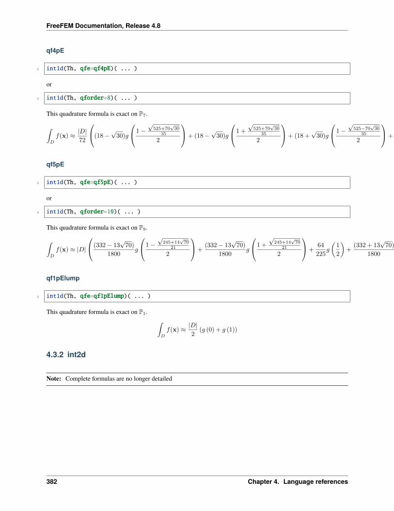
FreeFEM Documentation, Release 4.8
qf4pE
1 int1d(Th, qfe=qf4pE)( ... )
or
1 int1d(Th, qforder=8)( ... )
This quadrature formula is exact on P7.
∫𝐷
𝑓(x) ≈ |𝐷|72
⎛⎝(18−√
30)𝑔
⎛⎝1−√
525+70√30
35
2
⎞⎠+ (18−√
30)𝑔
⎛⎝1 +
√525+70
√30
35
2
⎞⎠+ (18 +√
30)𝑔
⎛⎝1−√
525−70√30
35
2
⎞⎠+ (18 +√
30)𝑔
⎛⎝1 +
√525−70
√30
35
2
⎞⎠⎞⎠
qf5pE
1 int1d(Th, qfe=qf5pE)( ... )
or
1 int1d(Th, qforder=10)( ... )
This quadrature formula is exact on P9.
∫𝐷
𝑓(x) ≈ |𝐷|
⎛⎝ (332− 13√
70)
1800𝑔
⎛⎝1−√
245+14√70
21
2
⎞⎠+(332− 13
√70)
1800𝑔
⎛⎝1 +
√245+14
√70
21
2
⎞⎠+64
225𝑔
(1
2
)+
(332 + 13√
70)
1800𝑔
⎛⎝1−√
245−14√70
21
2
⎞⎠+(332 + 13
√70)
1800𝑔
⎛⎝1 +
√245−14
√70
21
2
⎞⎠⎞⎠
qf1pElump
1 int1d(Th, qfe=qf1pElump)( ... )
This quadrature formula is exact on P1. ∫𝐷
𝑓(x) ≈ |𝐷|2
(𝑔 (0) + 𝑔 (1))
4.3.2 int2d
Note: Complete formulas are no longer detailed
382 Chapter 4. Language references
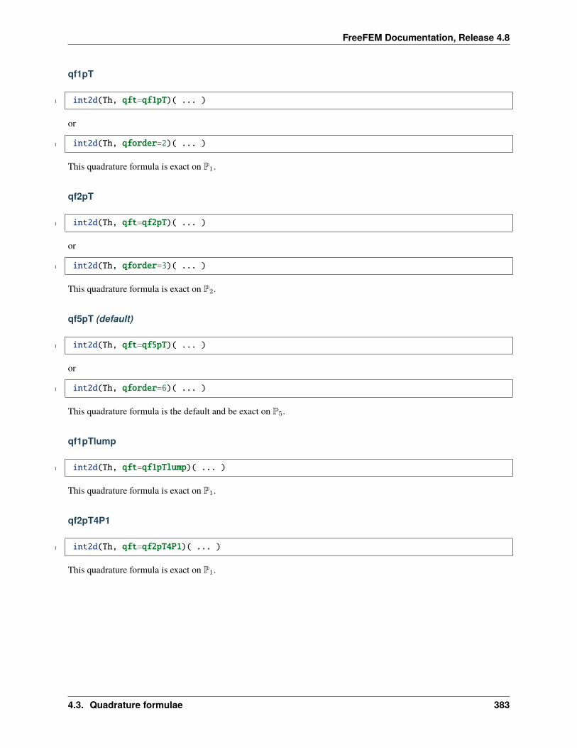
FreeFEM Documentation, Release 4.8
qf1pT
1 int2d(Th, qft=qf1pT)( ... )
or
1 int2d(Th, qforder=2)( ... )
This quadrature formula is exact on P1.
qf2pT
1 int2d(Th, qft=qf2pT)( ... )
or
1 int2d(Th, qforder=3)( ... )
This quadrature formula is exact on P2.
qf5pT (default)
1 int2d(Th, qft=qf5pT)( ... )
or
1 int2d(Th, qforder=6)( ... )
This quadrature formula is the default and be exact on P5.
qf1pTlump
1 int2d(Th, qft=qf1pTlump)( ... )
This quadrature formula is exact on P1.
qf2pT4P1
1 int2d(Th, qft=qf2pT4P1)( ... )
This quadrature formula is exact on P1.
4.3. Quadrature formulae 383
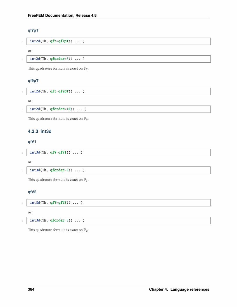
FreeFEM Documentation, Release 4.8
qf7pT
1 int2d(Th, qft=qf7pT)( ... )
or
1 int2d(Th, qforder=8)( ... )
This quadrature formula is exact on P7.
qf9pT
1 int2d(Th, qft=qf9pT)( ... )
or
1 int2d(Th, qforder=10)( ... )
This quadrature formula is exact on P9.
4.3.3 int3d
qfV1
1 int3d(Th, qfV=qfV1)( ... )
or
1 int3d(Th, qforder=2)( ... )
This quadrature formula is exact on P1.
qfV2
1 int3d(Th, qfV=qfV2)( ... )
or
1 int3d(Th, qforder=3)( ... )
This quadrature formula is exact on P2.
384 Chapter 4. Language references
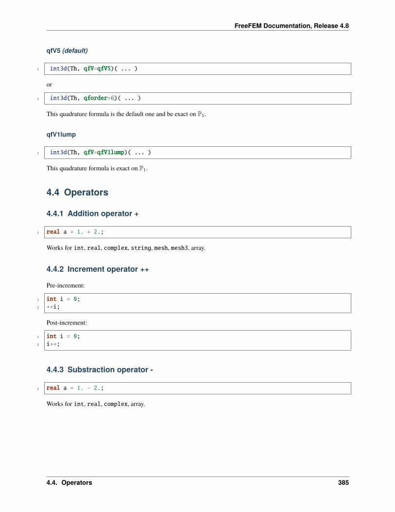
FreeFEM Documentation, Release 4.8
qfV5 (default)
1 int3d(Th, qfV=qfV5)( ... )
or
1 int3d(Th, qforder=6)( ... )
This quadrature formula is the default one and be exact on P5.
qfV1lump
1 int3d(Th, qfV=qfV1lump)( ... )
This quadrature formula is exact on P1.
4.4 Operators
4.4.1 Addition operator +
1 real a = 1. + 2.;
Works for int, real, complex, string, mesh, mesh3, array.
4.4.2 Increment operator ++
Pre-increment:
1 int i = 0;2 ++i;
Post-increment:
1 int i = 0;2 i++;
4.4.3 Substraction operator -
1 real a = 1. - 2.;
Works for int, real, complex, array.
4.4. Operators 385
FreeFEM Documentation, Release 4.8
4.4.4 Decrement operator –
Pre-decrement:
1 int i = 0;2 --i;
Post-decrement:
1 int i = 0;2 i--;
4.4.5 Multiplication operator *
1 real[int] b;2 matrix A3 real[int] x = A^-1*b;
Works for int, real, complex, array, matrix.
4.4.6 Equal operator =
1 real a = 1.;
4.4.7 Comparison operator ==
1 real a = 1.;2 real b = 1.;3
4 cout << (a == b) << endl;
4.4.8 Comparison operator !=
1 real a = 1.;2 real b = 2.;3
4 cout << (a != b) << endl;
386 Chapter 4. Language references
FreeFEM Documentation, Release 4.8
4.4.9 Comparison operator <, <=
1 real a = 1.;2 real b = 2.;3
4 cout << (a < b) << endl;5 cout << (a <= b) << endl;
4.4.10 Comparison operator >, >=
1 real a = 3.;2 real b = 2.;3
4 cout << (a > b) << endl;5 cout << (a >= b) << endl;
4.4.11 Compound operator +=, -=, *=, /=
1 real a = 1;2 a += 2.;3 a -= 1.;4 a *= 3.;5 a /= 2.;
4.4.12 Term by term multiplication .*
1 matrix A = B .* C;
4.4.13 Division operator /
1 real a = 1. / 2.;
Works for int, real, complex.
4.4.14 Term by term division ./
1 matrix A = B ./ C;
4.4. Operators 387
FreeFEM Documentation, Release 4.8
4.4.15 Remainder from the division %
1 int a = 1 % 2;
Works for int, real.
4.4.16 Power operator ^
1 real a = 2.^2;
Works for int, real, complex, matrix.
4.4.17 Inverse of a matrix ^-1
1 real[int] Res = A^-1 * b;
Warning: This operator can not be used to directly create a matrix, see Matrix inversion.
4.4.18 Transpose operator ‘
1 real[int] a = b';
Works for array and matrix.
Note: For matrix<complex>, the ::freefem`’` operator return the Hermitian tranpose.
4.4.19 Tensor scalar product :
𝐴 : 𝐵 =∑𝑖,𝑗
𝐴𝑖𝑗𝐵𝑖𝑗
4.4.20 C++ arithmetical if expression ? :
a ? b : c is equal to b if the a is true, c otherwise.
Tip: Example with int
1 int a = 12; int b = 5;2
3 cout << a << " + " << b << " = " << a + b << endl;4 cout << a << " - " << b << " = " << a - b << endl;5 cout << a << " * " << b << " = " << a * b << endl;6 cout << a << " / " << b << " = " << a / b << endl;7 cout << a << " % " << b << " = " << a % b << endl;
(continues on next page)
388 Chapter 4. Language references
FreeFEM Documentation, Release 4.8
(continued from previous page)
8 cout << a << " ^ " << b << " = " << a ^ b << endl;9 cout << "( " << a << " < " << b << " ? " << a << " : " << b << ") = " << (a < b ? a : b)
→˓<< endl;
The output of this script is:
12 + 5 = 1712 - 5 = 712 * 5 = 6012 / 5 = 212 % 5 = 212 ^ 5 = 248832( 12 < 5 ? 12 : 5) = 5
Tip: Example with real
1 real a = qsrt(2.); real b = pi;2
3 cout << a << " + " << b << " = " << a + b << endl;4 cout << a << " - " << b << " = " << a - b << endl;5 cout << a << " * " << b << " = " << a * b << endl;6 cout << a << " / " << b << " = " << a / b << endl;7 cout << a << " % " << b << " = " << a % b << endl;8 cout << a << " ^ " << b << " = " << a ^ b << endl;9 cout << "( " << a << " < " << b << " ? " << a << " : " << b << ") = " << (a < b ? a : b)
→˓<< endl;
The output of this script is:
1.41421 + 3.14159 = 4.555811.41421 - 3.14159 = -1.727381.41421 * 3.14159 = 4.442881.41421 / 3.14159 = 0.4501581.41421 % 3.14159 = 11.41421 ^ 3.14159 = 2.97069
4.4. Operators 389
FreeFEM Documentation, Release 4.8
4.5 Loops
See Loop example.
4.5.1 for
For loop.
1 for (int i = 0; i < N; ++i)2 ...3
4.5.2 if
If condition.
1 if (condition)2 ...3 4 else5 ...6
4.5.3 else
See if .
4.5.4 while
While loop.
1 while (condition)2 ...3
4.5.5 continue
Continue a loop.
1 for (int i = 0; i < N; ++i)2 ...3 if (condition) continue;4 ...5
390 Chapter 4. Language references
FreeFEM Documentation, Release 4.8
4.5.6 break
Break a loop.
1 while (condition1)2 ...3 if (condition) break;4 ...5
4.5.7 try
Try a part of code.
1 try2 ...3 4 catch(...)5 ...6
See Basic error handling example and Error handling example.
4.5.8 catch
Catch an error, see try
4.5.9 Implicit loop
Array with one index:
1 for [i, ai : a]
If real[int] a(10), then i=0:9 and ai is a reference to a[i].
Array with two indices or matrix:
1 for [i, j, aij : a]
If real[int] a(10, 11), then i=0:9, j=1:10 and aij is a reference to a(i, j).
See Implicit loop example.
4.5. Loops 391
FreeFEM Documentation, Release 4.8
4.6 I/O
See I/O example
See File stream example.
4.6.1 cout
Standard C++ output device (default: console).
1 cout << "Some text" << endl;
4.6.2 cin
Standard C++ input device (default: keyboard).
1 cin >> var;
4.6.3 endl
End of line.
1 cout << "Some text" << endl;
4.6.4 ifstream
Open a file in read mode.
1 ifstream file("file.txt");
Note: A file is closed at the end of a block.
4.6.5 ofstream
Open a file in write mode.
1 ofstream file("file.txt");
Note: A file is closed at the end of a block.
392 Chapter 4. Language references
FreeFEM Documentation, Release 4.8
4.6.6 append
Append data to an existing file.
1 ofstream file("file.txt", append);
4.6.7 binary
Write a file in binary.
1 ofstream file("file.btxt", binary);
4.6.8 seekg
Set the file position.
1 file.seekg(Pos);
4.6.9 tellg
Get the file position.
1 int Pos = file.tellg();
4.6.10 flush
Flush the buffer of the file.
1 file.flush
4.6.11 getline
Get the current line.
1 string s;2 getline(file, s);
4.6.12 Output format
In the descriptions below, f is an output stream, for example cout or a ofstream.
All this methods, excepted the first, return a stream, so they can be chained:
1 cout.scientific.showpos << 3 << endl;
4.6. I/O 393
FreeFEM Documentation, Release 4.8
precision
Set the number of digits printed to the right of the decimal point. This applies to all subsequent floating point numberswritten to that output stream. However, this won’t make floating-point “integers” print with a decimal point. It’snecessary to use fixed for that effect.
1 int np = f.precision(n)
scientific
Formats floating-point numbers in scientific notation
1 f.scientific
fixed
Used fixed point notation for floating-point numbers. Opposite of scientific.
1 f.fixed
showbase
Converts insertions to an external form that can be read according to the C++ lexical conventions for integral constants.By default, showbase is not set.
1 f.showbase
noshowbase
Unset showbase flags.
1 f.noshowbase
showpos
Inserts a plus sign (+) into a decimal conversion of a positive integral value.
1 f.showpos
394 Chapter 4. Language references
FreeFEM Documentation, Release 4.8
noshowpos
Unset showpos flags.
1 f.noshowpos
default
Reset all the previous flags to the default expect precision.
1 f.default
setw
Behaves as if member width were called with n as argument on the stream on which it is inserted as a manipulator (itcan be inserted on output streams).
1 f.setw(n)
4.7 Functions
4.7.1 abs
Return the absolute value.
1 real a = abs(b);
Parameters:
• b (int, real, complex, fespace function, real[int] or real[int, int])
Output:
• a (int, real, real[int] or real[int, int])
4.7.2 acos
arccos function.
1 real theta = acos(x);
Parameter:
• x (real, real[int] or real[int, int])
Output:
• theta (real, real[int] or real[int, int])
4.7. Functions 395
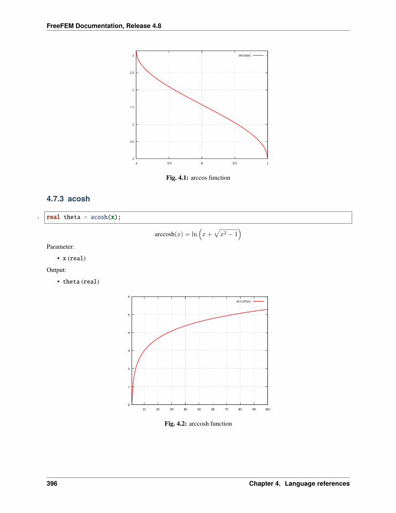
FreeFEM Documentation, Release 4.8
Fig. 4.1: arccos function
4.7.3 acosh
1 real theta = acosh(x);
arccosh(𝑥) = ln(𝑥+
√𝑥2 − 1
)Parameter:
• x (real)
Output:
• theta (real)
Fig. 4.2: arccosh function
396 Chapter 4. Language references
FreeFEM Documentation, Release 4.8
4.7.4 adaptmesh
Mesh adaptation function.
1 mesh Thnew = adaptmesh(Th, [fx, fy], hmin=HMin, hmax=HMax, err=Err, errg=ErrG, nbvx=NbVx,→˓ nbsmooth=NbSmooth, nbjacoby=NbJacoby, ratio=Ratio, omega=Omega, iso=Iso,→˓abserror=AbsError, cutoff=CutOff, verbosity=Verbosity, inquire=Inquire,→˓splitpbedge=SplitPbEdge, maxsubdiv=MaxSubdiv, rescaling=Rescaling,→˓keepbackvertices=KeepBackVertices, IsMetric=isMetric, power=Power, thetamax=ThetaMax,→˓splitin2=SplitIn2, metric=Metric, nomeshgeneration=NoMeshGeneration,→˓periodic=Periodic);
Parameters:
• Th (mesh) Mesh to refine
• [fx, fy] (func or fespace function), scalar or vectorial Function to follow for the mesh adaptation
• hmin= (real) Minimum edge size
• hmax= (real) Maximum edge size
• err= (real) Error level (P1 interpolation)
• errg= (real) Relative geometrical error
• nbvx= (int) Maximum number of vertices
• nbsmooth= (int) Number of smoothing iterations
• nbjacoby= (int) Number of iterations for the smoothing procedure
• ratio= (real) Ratio of the triangles
• omega= (real) Relaxation parameter for the smoothing procedure
• iso= (bool) Isotropic adaptation (if true)
• abserror= (bool) Error (if true) - Relative error (if false)
• cutoff= (real) Lower limit of the relative error evaluation
• verbosity= (real) Verbosity level
• inquire= (bool) If true, inquire graphically
• splitpbedge= (bool) If true, split all internal edges in half
• maxsubdiv= (int) Bound the maximum subdivisions
• rescaling= (bool) Rescale the function in [0, 1]
• keepbackvertices= (bool) If true, try to keep vertices of the original mesh
• IsMetric= (bool) If true, the metric is defined explicitly
• power= (int) Exponent of the Hessian
• thetamax= (int) Minimum corner angle (in degree)
• splitin2= (bool) Split all triangles into 4 sub-triangles if true
• metric= ([real[int], real[int], real[int]]) Array of 3 real arrays defining the metric
• nomeshgeneration= (bool) If true, the mesh is not generated
• periodic= (real[int, int]) Build an adapted periodic mesh
4.7. Functions 397
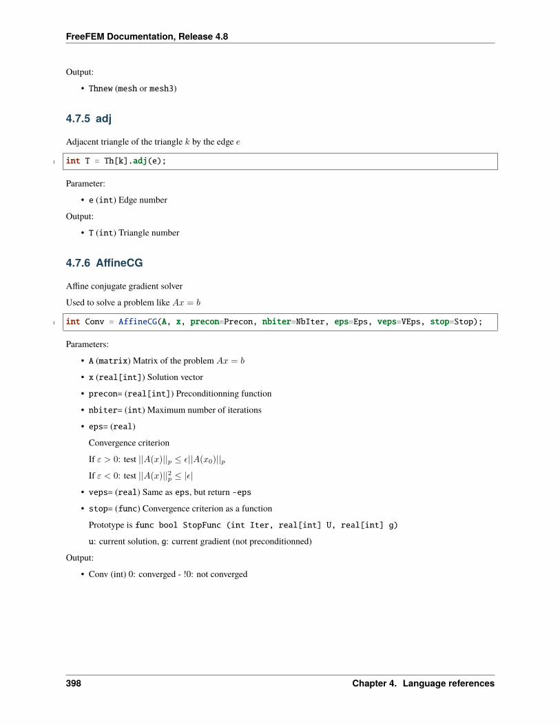
FreeFEM Documentation, Release 4.8
Output:
• Thnew (mesh or mesh3)
4.7.5 adj
Adjacent triangle of the triangle 𝑘 by the edge 𝑒
1 int T = Th[k].adj(e);
Parameter:
• e (int) Edge number
Output:
• T (int) Triangle number
4.7.6 AffineCG
Affine conjugate gradient solver
Used to solve a problem like 𝐴𝑥 = 𝑏
1 int Conv = AffineCG(A, x, precon=Precon, nbiter=NbIter, eps=Eps, veps=VEps, stop=Stop);
Parameters:
• A (matrix) Matrix of the problem 𝐴𝑥 = 𝑏
• x (real[int]) Solution vector
• precon= (real[int]) Preconditionning function
• nbiter= (int) Maximum number of iterations
• eps= (real)
Convergence criterion
If 𝜀 > 0: test ||𝐴(𝑥)||𝑝 ≤ 𝜖||𝐴(𝑥0)||𝑝If 𝜀 < 0: test ||𝐴(𝑥)||2𝑝 ≤ |𝜖|
• veps= (real) Same as eps, but return -eps
• stop= (func) Convergence criterion as a function
Prototype is func bool StopFunc (int Iter, real[int] U, real[int] g)
u: current solution, g: current gradient (not preconditionned)
Output:
• Conv (int) 0: converged - !0: not converged
398 Chapter 4. Language references
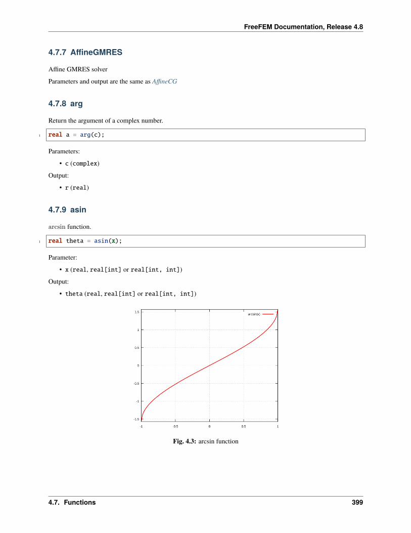
FreeFEM Documentation, Release 4.8
4.7.7 AffineGMRES
Affine GMRES solver
Parameters and output are the same as AffineCG
4.7.8 arg
Return the argument of a complex number.
1 real a = arg(c);
Parameters:
• c (complex)
Output:
• r (real)
4.7.9 asin
arcsin function.
1 real theta = asin(x);
Parameter:
• x (real, real[int] or real[int, int])
Output:
• theta (real, real[int] or real[int, int])
Fig. 4.3: arcsin function
4.7. Functions 399
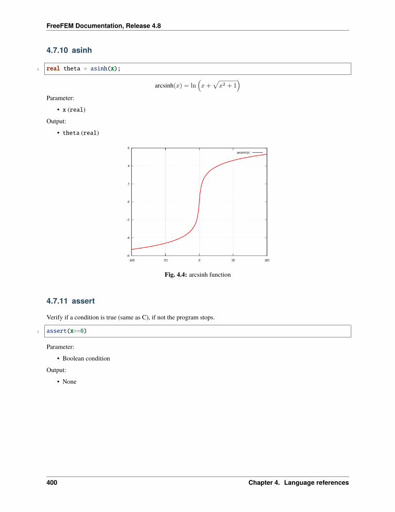
FreeFEM Documentation, Release 4.8
4.7.10 asinh
1 real theta = asinh(x);
arcsinh(𝑥) = ln(𝑥+
√𝑥2 + 1
)Parameter:
• x (real)
Output:
• theta (real)
Fig. 4.4: arcsinh function
4.7.11 assert
Verify if a condition is true (same as C), if not the program stops.
1 assert(x==0)
Parameter:
• Boolean condition
Output:
• None
400 Chapter 4. Language references
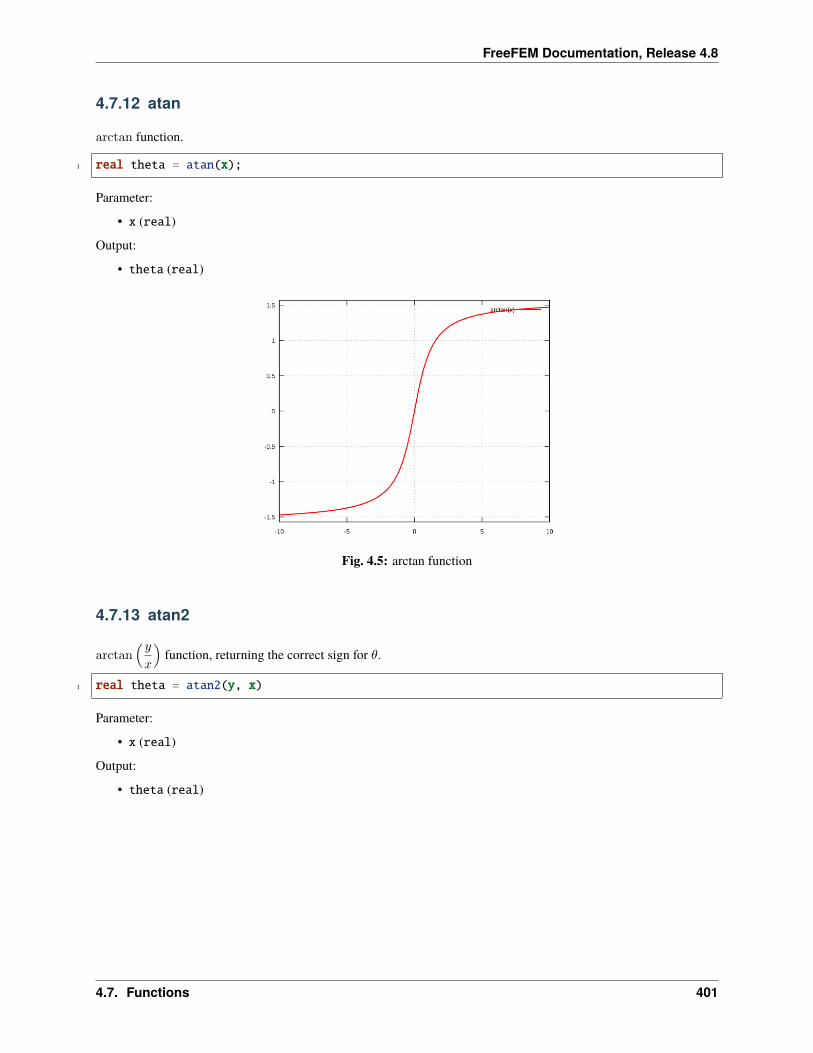
FreeFEM Documentation, Release 4.8
4.7.12 atan
arctan function.
1 real theta = atan(x);
Parameter:
• x (real)
Output:
• theta (real)
Fig. 4.5: arctan function
4.7.13 atan2
arctan(𝑦𝑥
)function, returning the correct sign for 𝜃.
1 real theta = atan2(y, x)
Parameter:
• x (real)
Output:
• theta (real)
4.7. Functions 401
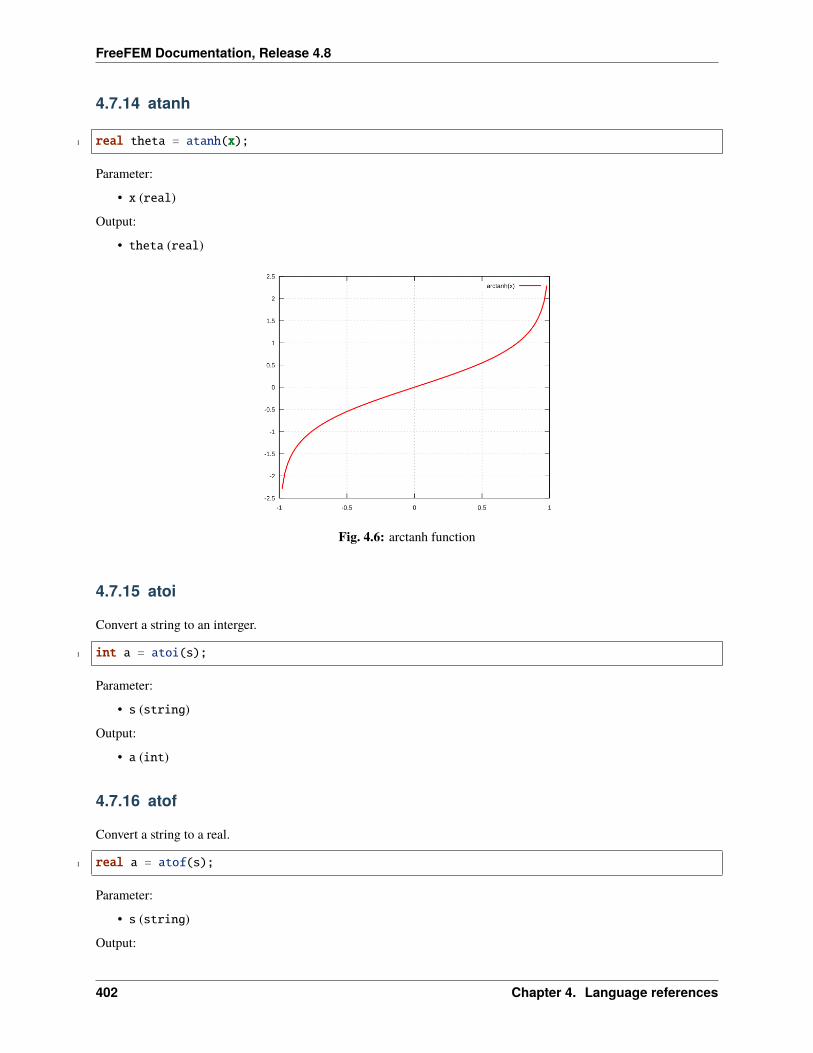
FreeFEM Documentation, Release 4.8
4.7.14 atanh
1 real theta = atanh(x);
Parameter:
• x (real)
Output:
• theta (real)
Fig. 4.6: arctanh function
4.7.15 atoi
Convert a string to an interger.
1 int a = atoi(s);
Parameter:
• s (string)
Output:
• a (int)
4.7.16 atof
Convert a string to a real.
1 real a = atof(s);
Parameter:
• s (string)
Output:
402 Chapter 4. Language references
FreeFEM Documentation, Release 4.8
• a (real)
4.7.17 BFGS
Todo: todo
4.7.18 buildmesh
Build a 2D mesh using border elements.
1 mesh Th = buildmesh(b1(nn) + b2(nn) + b3(nn) + b4(nn),[points=Points], ][nbvx=Nbvx],→˓[fixedborder=FixedBorder]);
Parameters:
• b1, b2, b3, b4 (border)
Geometry border, b1(nn) means b1 border discretized by nn vertices
• points (real[int, int]) [Optional]
Specify a set of points
The size of Points array is (nbp, 2), containing a set of nbp points with x and y coordinates
• nbvx= (int) [Optional]
Maximum number of vertices Default: 9000
• fixedborder= (bool) [Optional]
If true, mesh generator cannot change the boundary mesh
Default: false
Output:
• Th (mesh) Resulting mesh
4.7.19 ceil
Round fractions up of 𝑥.
1 int c = ceil(x);
Parameter:
• x (real)
Output:
• c (int)
4.7. Functions 403
FreeFEM Documentation, Release 4.8
4.7.20 change
Change a property of a mesh.
1 int[int] L = [0, 1];2 Thnew = change(Th, label=L);
Parameters:
• Th (mesh) Original mesh
• label= L (int[int]) Pair of old and new label
• region= R (int[int]) Pair of old and new region
• flabel= l (func int) Function of int given the new label
• fregion= r (func int) Function of int given the new region
Output:
• Thnew (mesh) Mesh with changed parameters
4.7.21 checkmovemesh
Check a movemesh without mesh generation.
1 real minT = checkmovemesh(Th, [Dx, Dy]);
Parameters:
Same as movemesh
Output:
• minT (real) Minimum triangle area
4.7.22 chi
Characteristic function of a mesh.
1 int IsInMesh = chi(Th)(x, y);
Parameters:
• Th (mesh or mesh3)
• x (real) Position 𝑥
• y (real) Position 𝑦
Output:
• IsInMesh (int) 1 if (𝑥, 𝑦) ∈ Th 0 if (𝑥, 𝑦) ∈ Th
404 Chapter 4. Language references
FreeFEM Documentation, Release 4.8
4.7.23 clock
Get the clock in second.
1 real t = clock();
Parameter:
• None
Output:
• t (real) Current CPU time
4.7.24 complexEigenValue
Same as EigenValue for complex problems.
4.7.25 conj
Caculate the conjuguate of a complex number.
1 complex C1 = 1 + 1i;2 complex C2 = conj(C1);
Parameter:
• C1 (complex) Complex number
Output:
• C2 (complex) Conjuguate of C1
4.7.26 convect
Characteristics Galerkin method.
1 real cgm = convect([Ux, Uy], dt, c);2 real cgm = convect([Ux, Uy, Uz], dt, c);
Compute 𝑐 ∘X with X(x) = x𝜏 and x𝜏 is the solution of:
x𝜏 = u(x𝜏 )x𝜏 = x
Parameters:
• ux (fespace function) Velocity: 𝑥 component
• uy (fespace function) Velocity: 𝑦 component
• uz (fespace function) 3D onlyVelocity: 𝑧 component
• dt (real) Time step
• c (fespace function) Function to convect
4.7. Functions 405
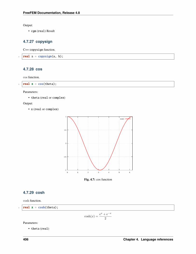
FreeFEM Documentation, Release 4.8
Output:
• cgm (real) Result
4.7.27 copysign
C++ copysign function.
1 real s = copysign(a, b);
4.7.28 cos
cos function.
1 real x = cos(theta);
Parameters:
• theta (real or complex)
Output:
• x (real or complex)
Fig. 4.7: cos function
4.7.29 cosh
cosh function.
1 real x = cosh(theta);
cosh(𝑥) =𝑒𝑥 + 𝑒−𝑥
2
Parameters:
• theta (real)
406 Chapter 4. Language references
FreeFEM Documentation, Release 4.8
Output:
• x (real)
4.7.30 diffnp
Arithmetic useful function.
1 diffnp(a, b) = (a<0)&(0<b) ? (b-a) : 0;
4.7.31 diffpos
Arithmetic useful function.
1 diffpos(a, b) = max(b-a, 0);
4.7.32 dist
Arithmetic useful function.
1 dist(a, b) = sqrt(a^2 + b^2);2 dist(a, b, c) = sqrt(a^2 + b^2 + c^2);
4.7.33 dumptable
Show all types, operators and functions in FreeFEM.
1 dumptable(out);
Parameters:
• out (ostream) cout of ofstream file.
Output:
• None
4.7.34 dx
𝑥 derivative.
1 Uh up = dx(u);
𝜕𝑢
𝜕𝑥
Parameters:
• u (fespace function)
Output:
• up (fespace function)
4.7. Functions 407
FreeFEM Documentation, Release 4.8
4.7.35 dxx
𝑥 double derivative.
1 Uh upp = dxx(u);
𝜕2𝑢
𝜕𝑥2
Parameters:
• u (fespace function)
Output:
• upp (fespace function)
4.7.36 dxy
𝑥𝑦 derivative.
1 Uh upp = dxy(u);
𝜕2𝑢
𝜕𝑥𝜕𝑦
Parameters:
• u (fespace function)
Output:
• upp (fespace function)
4.7.37 dxz
𝑥𝑧 derivative.
1 Uh upp = dxz(u);
𝜕2𝑢
𝜕𝑥𝜕𝑧
Parameters:
• u (fespace function)
Output:
• upp (fespace function)
408 Chapter 4. Language references
FreeFEM Documentation, Release 4.8
4.7.38 dy
𝑦 derivative.
1 Uh up = dy(u);
𝜕𝑢
𝜕𝑦
Parameters:
• u (fespace function)
Output:
• upp (fespace function)
4.7.39 dyx
𝑦𝑥 derivative.
1 Uh upp = dyx(u);
𝜕2𝑢
𝜕𝑦𝜕𝑥
Parameters:
• u (fespace function)
Output:
• upp (fespace function)
4.7.40 dyy
𝑦 double derivative.
1 Uh upp = dyy(u);
𝜕2𝑢
𝜕𝑥2
Parameters:
• u (fespace function)
Output:
• upp (fespace function)
4.7. Functions 409
FreeFEM Documentation, Release 4.8
4.7.41 dyz
𝑦𝑧 derivative.
1 Uh upp = dyz(u);
𝜕2𝑢
𝜕𝑦𝜕𝑧
Parameters:
• u (fespace function)
Output:
• upp (fespace function)
4.7.42 dz
𝑧 derivative.
1 Uh up = dz(u);
𝜕𝑢
𝜕𝑧
Parameters:
• u (fespace function)
Output:
• upp (fespace function)
4.7.43 dzx
𝑧𝑥 derivative.
1 Uh upp = dzx(u);
𝜕2𝑢
𝜕𝑧𝜕𝑥
Parameters:
• u (fespace function)
Output:
• upp (fespace function)
410 Chapter 4. Language references
FreeFEM Documentation, Release 4.8
4.7.44 dzy
𝑧𝑦 derivative.
1 Uh upp = dzy(u);
𝜕2𝑢
𝜕𝑧𝜕𝑦
Parameters:
• u (fespace function)
Output:
• upp (fespace function)
4.7.45 dzz
𝑧 double derivative.
1 Uh upp = dzz(u);
𝜕2𝑢
𝜕𝑧2
Parameters:
• u (fespace function)
Output:
• upp (fespace function)
4.7.46 EigenValue
Compute the generalized eigenvalue of 𝐴𝑢 = 𝜆𝐵𝑢. The shifted-inverse method is used by default with sigma=𝜎, theshift of the method. The function EigenValue can be used for either matrices or functions returning a matrix vectorproduct. The use of the matrix version is shown below.
1 int k = EigenValue(A,B,nev= , sigma= );
Parameters:
• A, B: matrices of same size
• nev=n: number of desired eigenvalues given by an integer n
• sym=: the problem is symmetric or not
• tol=: the relative accuracy to which eigenvalues are to be determined
• value=: an array to store the real part of the eigenvalues
• ivalue=: an array to store the imaginary part of the eigenvalues
• vector=: a Finite Element function array to store the eigenvectors
• sigma=: the shift value
• Other parameters are available for more advanced use: see the ARPACK documentation.
4.7. Functions 411
FreeFEM Documentation, Release 4.8
Output: The output is the number of converged eigenvalues, which can be different than the number of requestedeigenvalues given by nev=. Note that the eigenvalues and the eigenvectors are stored for further purposes using theparameters value= and vector=.
4.7.47 emptymesh
Build an empty mesh.
Useful to handle Lagrange multipliers in mixed and Mortar methods.
1 mesh eTh = emptymesh(Th, ssd);
Parameters:
• Th (mesh) Mesh to empty
• ssd (int[int]) Pseudo subregion label
Output:
• eTh (mesh) Empty mesh
4.7.48 erf
The error function:
𝑒𝑟𝑓(𝑥) =2√𝑝𝑖
∫ 𝑥
0
exp(−𝑡2)𝑑𝑡
1 real err = erf(x);
Parameters:
• x (real)
Output:
• err (real)
4.7.49 erfc
Complementary of the error function:
𝑒𝑟𝑓𝑐(𝑥) = 1− 𝑒𝑟𝑓(𝑥)
1 real errc = erfc(x);
Parameters:
• x (real)
Output:
• err (real)
412 Chapter 4. Language references
FreeFEM Documentation, Release 4.8
4.7.50 exec
Execute an external command.
1 int v = exec(command);
Parameters:
• command (string) Command to execute
Output:
• v (int) Value returned by the command
4.7.51 exit
Exit function, equivalent to return.
1 exit(N);
Parameters:
• N (int) Return value
Output:
• None
4.7.52 exp
Exponential function.
1 real a = exp(b);
Parameters:
• b (real or complex)
Output:
• a (real or complex)
4.7.53 fdim
Positive difference (cmath function).
1 real fd = fdim(a, b);
Parameters:
• a (real)
• b (real)
Output:
• fd (real) If 𝑥 > 𝑦, return 𝑥− 𝑦If 𝑥 ≤ 𝑦, return 0
4.7. Functions 413
FreeFEM Documentation, Release 4.8
4.7.54 floor
Floor function.
1 real a = floor(b);
Return the largest integer value not greater than b.
Parameters:
• b (real)
Output:
• a (real)
4.7.55 fmax
Maximum (cmath function).
1 real Max = fmax(a, b);
Parameters:
• a (real)
• b (real)
Output:
• Max (real)
4.7.56 fmin
Minimum (cmath function).
1 real Min = fmin(a, b);
Parameters:
• a (real)
• b (real)
Output:
• Min (real)
4.7.57 fmod
Remainder of 𝑎/𝑏 (cmath function).
1 real Mod = fmod(a, b);
Parameters:
• a (real)
• b (real)
414 Chapter 4. Language references
FreeFEM Documentation, Release 4.8
Output:
• Mod (real)
4.7.58 imag
Imaginary part of a complex number.
1 complex c = 1. + 1i;2 real Im = imag(c);
4.7.59 int1d
1D integral.
1 int1d(Th, [Label], [qfe=Qfe], [qforder=Qforder])(2 ...3 )
Used in problem, solve or varf definition to impose a boundary condition only (FreeFEM does not support 1D simu-lation), or outside to calculate a quantity.
Parameters:
• Th (mesh) Mesh where the integral is calculated
• Label (int) [Optional]
Label of the 1D border Default: all borders of the mesh
• qfe= (quadrature formula) [Optional] (qf3E by default)
Quadrature formula, see quadrature formulae
• qforder= (quadrature formula) [Optional]
Quadrature order, see quadrature formulae
Output:
• Depending on the situation: In a problem, solve or varf definition: Non relevant.
Outside: real (example: real l = int1d(Th, 1)(1.);).
Warning: In a problem, solve or varf definition, the content of int1d must be a linear or bilinear form.
4.7.60 int2d
2D integral.
1 int2d(Th, [Region], [qft=Qft], [qforder=Qforder])(2 ...3 )
Or
4.7. Functions 415
FreeFEM Documentation, Release 4.8
1 int2d(Th, [Label], [qft=Qft], [qforder=Qforder])(2 ...3 )
Used in problem, solve or varf definition to: - Calculate integral in 2D simulation - Impose a boundary condition in3D simulation Or outside to calculate a quantity.
Parameters:
• Th (mesh, mesh3 , meshS`or :freefem:`meshL) Mesh where the integral is calculated
• Region (int) [Optional] Label of the 2D region (2D simulation or Surface simulation) Default: all regions ofthe mesh
• Label (int) [Optional] Label of the 2D border (3D simulation) Default: all borders of the mesh
• qft= (quadrature formula) [Optional] (qf5T by default)
Quadrature formula, see quadrature formulae
• qforder= (quadrature formula) [Optional]
Quadrature order, see quadrature formulae
Output:
• Depending on the situation: In a problem, solve or varf definition: Non relevant. Outside: real (example:real s = int2d(Th, 1)(1.);).
Warning: In a problem, solve or varf definition, the content of the int2d must be a linear or bilinear form.
4.7.61 int3d
3D integral.
1 int3d(Th, [Region], [qfV=QfV], [qforder=Qforder])(2 ...3 )
Used in problem, solve or varf definition to calculate integral in 3D simulation, or outside to calculate a quantity.
Parameters:
• Th (mesh3) Mesh where the integral is calculated
• Region (int) [Optional]
Label of the 3D region
Default: all regions of the mesh
• qfV= (quadrature formula) [Optional] (qf5V by default)
Quadrature formula, see quadrature formulae
• qforder= (quadrature formula) [Optional]
Quadrature order, see quadrature formulae
Output:
416 Chapter 4. Language references
FreeFEM Documentation, Release 4.8
• Depending on the situation: In a problem, solve or varf definition: Non relevant. Outside: real (example:real v = int3d(Th, 1)(1.);).
Warning: In a problem, solve or varf definition, the content of the int3d must be a linear or bilinear form.
4.7.62 intalledges
Integral on all edges.
1 intalledges(Th, [Region])(2 ...3 )
Parameters:
• Th (mesh) Mesh where the integral is calculated
• Region (int) [Optional]
Label of the region
Default: all regions of the mesh
Output:
• Non relevant
4.7.63 intallfaces
Intergal on all faces.
Same as intalledges for mesh3.
4.7.64 interpolate
Interpolation operator from a finite element space to another.
1 matrix I = interpolate(Wh, Vh, [inside=Inside], [t=T], [op=Op], [U2Vc=U2VC]);
Parameters:
• Wh (fespace) Target finite element space
• Vh (fespace) Original finite element space
• inside= (bool) If true, create a zero extension outside the Vh domain
• t= (bool) If true, return the transposed matrix
• op= (int) 0: interpolate the function (default value) 1: interpolate 𝜕𝑥 2: interpolate 𝜕𝑦 3: interpolate 𝜕𝑧• U2Vc= (int[int]) Array of the same size of Wh describing which component of Vhis interpolated in Wh
Output:
• I (matrix) Interpolation matrix operator
4.7. Functions 417
FreeFEM Documentation, Release 4.8
4.7.65 invdiff
Arithmetic useful function.
1 invdiff(a, b) = (abs(a-b) < 10^(-30)) ? (a-b) : 1/(a-b)2 invdiff(a, b, e) = (abs(a-b) < e) ? (a-b) : 1/(a-b)
4.7.66 invdiffnp
Arithmetic useful function.
1 invdiffnp(a, b) = (a<0)&(0<b) ? 1/(b-a) : 0
4.7.67 invdiffpos
Arithmetic useful function.
1 invdiffpos(a, b) = (a<b) ? 1./(b-a) : 0
4.7.68 isInf
The C++ isInf function.
1 bool b = isInf(a);
4.7.69 isNaN
The C++ isNan function.
1 bool b = isNaN(a);
4.7.70 isNormal
The C++ isNormal function.
4.7.71 j0
Bessel function of first kind, order 0.
1 real b = j0(x);
Parameters:
• x (real)
Output:
• b (real)
418 Chapter 4. Language references
FreeFEM Documentation, Release 4.8
4.7.72 j1
Bessel function of first kind, order 1.
1 real b = j1(x);
Parameters:
• x (real)
Output:
• b (real)
4.7.73 jn
Bessel function of first kind, order n.
1 real b = jn(n, x);
𝐽𝑛(𝑥) =
∞∑𝑝=0
(1)𝑝
𝑝!(𝑛+ 𝑝)!
(𝑥2
)2𝑝+𝑛Parameters:
• n (int)
• x (real)
Output:
• b (real)
4.7.74 jump
Jump function across an edge.
1 intalledges(2 ... jump(c) ...3 )
Parameters:
• c (fespace function) Discontinuous function
Output:
• Non relevant
4.7. Functions 419
FreeFEM Documentation, Release 4.8
4.7.75 LinearCG
Linear CG solver
Parameters and output are the same as AffineCG
4.7.76 LinearGMRES
Linear GMRES solver
Parameters and output are the same as AffineCG
4.7.77 lgamma
Natural logarithm of the absolute value of the Γ function of 𝑥.
1 real lg = lgamma(x);
Parameters:
• x (real)
Output:
• lg (real)
4.7.78 log
Natural logarithm.
1 real l = log(x);
Parameters:
• x (real or complex)
Output:
• l (real or complex)
Note: Complex value
For complex value, the log function is defined as:
log(𝑧) = log(|𝑧|) + 𝑖 arg(𝑧)
420 Chapter 4. Language references
FreeFEM Documentation, Release 4.8
4.7.79 log10
Common logarithm.
1 real l = log10(x);
Parameters:
• x (real)
Output:
• l (real)
4.7.80 lrint
Integer value nearest to 𝑥.
1 int l = lrint(a);
Parameters:
• a (real)
Output:
• l (int)
4.7.81 lround
Round a value, and return an integer value.
1 int l = lround(a);
Parameters:
• a (real)
Output:
• l (int)
4.7.82 ltime
Return the current time since the Epcoh.
1 int t = ltime();
Parameter:
• None
Output:
• t (int)
4.7. Functions 421
FreeFEM Documentation, Release 4.8
4.7.83 max
Maximum value of two, three or four values.
1 real m = max(a, b);2 real m = max(a, b, c);3 real m = max(a, b, c, d);
Parameters:
• a (int or real)
• b (int or real)
• c (int or real) [Optional]
• d (int or real) [Optional]
Output:
• b (int or real)
4.7.84 min
Minimum value of two, three or four values.
1 real m = min(a, b);2 real m = min(a, b, c);3 real m = min(a, b, c, d);
Parameters:
• a (int or real)
• b (int or real)
• c (int or real) [Optional]
• d (int or real) [Optional]
Output:
• b (int or real)
4.7.85 movemesh
Move a mesh.
1 mesh MovedTh = movemesh(Th, [Dx, Dy]);2 mesh3 MovedTh = movemesh(Th, [Dx, Dy, Dz], [region=Region], [label=Label],
→˓[facemerge=FaceMerge], [ptmerge=PtMerge], [orientation=Orientation]);
Parameters:
• Th (mesh of mesh3) Mesh to move
• Dx (fespace function) Displacement along 𝑥
• Dy (fespace function) Displacement along 𝑦
422 Chapter 4. Language references
FreeFEM Documentation, Release 4.8
• Dz (fespace function) 3D onlyDisplacement along 𝑧
• region= (int) [Optional] 3D onlySet label to tetrahedra
• label= (int[int]) [Optional] 3D onlySet label of faces (see change for more information)
• facemerge= (int) [Optional] 3D onlyIf equal to 1, some faces can be merged during the mesh moving Default: 1
• ptmerge= (real) [Optional] 3D onlyCriteria to define when two points merge
• orientation= (int) [Optional] 3D onlyIf equal to 1, allow orientation reverse if tetrahedra is not positive Default: 1
Output:
• MovedTh (mesh or mesh3) Moved mesh
4.7.86 NaN
C++ nan function.
1 real n = NaN([String]);
Parameters:
• String (string) Default: ""
4.7.87 NLCG
Non-linear conjugate gradient.
Parameters and output are the same as AffineCG
4.7.88 on
Dirichlet condition function.
1 problem (u, v)2 ...3 + on(Label, u=uD)4 ...
Warning: Used only in problem, solve and varf
Parameters:
4.7. Functions 423
FreeFEM Documentation, Release 4.8
• Label (int or border in 2D)
Boundary reference where to impose the Dirichlet condition
• uD (fespace function, func or real or int)
Dirichlet condition (u is an unknown of the problem)
Output:
• Non relevant
4.7.89 plot
Plot meshes and results.
1 plot([Th], [u], [[Ux, Uy, Uz]], [wait=Wait], [ps=PS], [coef=Coef], [fill=Fill],→˓cmm=[Cmm], [value=Value], [aspectratio=AspectRatio], [bb=Bb], [nbiso=NbIso],→˓[nbarrow=NbArrow], [viso=VIso], [varrow=VArrow], [bw=Bw], [grey=Grey], [hsv=Hsv],→˓[boundary=Boundary], [dim=Dim], [prev=Prev], [WindowIndex=WI]);
Note: Only one of Th, u or [Ux, Uy] / [Ux, Uy, Uz] is needed for the plot command.
Parameters:
• Th (mesh or mesh3) Mesh to display
• u (fespace function) Scalar fespace function to display
• [Ux, Uy] / [Ux, Uy, Uz] (fespace function array) Vectorial fespace function to display
• [Ux, Uy] ([real[int], real[int]]) Couple a real array to display a curve
• wait= (bool) If true, wait before continue
• ps= (string) Name of the file to save the plot (.ps or .eps format)
• coef= (real) Arrow size
• fill= (bool) If true, fill color between isovalue (usable with scalar fespace function only)
• cmm= (string) Text comment in the graphic window
• value= (bool) If true, show the value scale
• aspectratio= (bool) If true, preserve the aspect ratio
• bb= ([real[int], real[int]]) Specify a bounding box using two corner points
• nbiso= (int) Number of isovalues
• nbarrow= (int) Number of colors of arrows values
• viso= (real[int]) Specify an array of isovalues
• varrow= (real[int]) Specify an array of arrows values color
• bw= (bool) If true, the plot is in black and white
• grey= (bool) If true, the plot is in grey scale
• hsv= (real[int]) Array of 3× 𝑛 values defining HSV color model [ℎ1, 𝑠1, 𝑣1, ..., ℎ𝑛, 𝑠𝑛, 𝑣𝑛]
• boundary= (bool) If true, display the boundary of the domain
424 Chapter 4. Language references
FreeFEM Documentation, Release 4.8
• dim= (int) Set the dimension of the plot: 2 or 3
• prev= (bool) Use the graphic state of the previous state
• WindowIndex= (int) Specify window index for multiple windows graphics
Output:
• None
See the plot section for in-graphic commands.
4.7.90 polar
Polar coordinates.
1 complex p = polar(a, b);
Parameters:
• a (real)
• b (real)
Output:
• p (complex)
4.7.91 pow
Power function.
1 real p = pow(a, b);
𝑝 = 𝑎𝑏
Parameters:
• a (real)
• b (real)
Output:
• p (real)
4.7.92 projection
Arithmetic useful function.
1 real p = projection(a, b, x);
Projection is equivalent to:
1 projection(a, b, x) = min(max(a, x), b)*(a < b) + min(max(b, x), a)*(1-(a < b));
Parameters:
• a (real)
4.7. Functions 425
FreeFEM Documentation, Release 4.8
• b (real)
• x (real)
Output:
• p (real)
4.7.93 randinit
Initialize the state vector by using a seed.
1 randinit(seed);
Parameters:
• seed (int)
Output:
• None
4.7.94 randint31
Generate unsigned int (31 bits) random number.
1 int r = randint31();
Parameters:
• None
Output:
• r (int)
4.7.95 randint32
Generate unsigned int (32 bits) random number.
1 int r = randint32();
Parameters:
• None
Output:
• r (int)
426 Chapter 4. Language references
FreeFEM Documentation, Release 4.8
4.7.96 randreal1
Generate uniform real in [0, 1] (32 bits).
1 real r = randreal1();
Parameters:
• None
Output:
• r (real)
4.7.97 randreal2
Generate uniform real in [0, 1) (32 bits).
1 real r = randreal2();
Parameters:
• None
Output:
• r (real)
4.7.98 randreal3
Generate uniform real in (0, 1) (32 bits).
1 real r = randreal3();
Parameters:
• None
Output:
• r (real)
4.7.99 randres53
Generate uniform real in [0, 1) (53 bits).
1 real r = randres53();
Parameters:
• None
Output:
• r (real)
4.7. Functions 427
FreeFEM Documentation, Release 4.8
4.7.100 readmesh
Read a 2D mesh file at different formats (see Mesh Generation).
1 mesh Th = readmesh(MeshFileName);
Parameters:
• MeshFileName (string)
Output:
• Th (mesh)
4.7.101 readmesh3
Read a 3D mesh file at different formats (see Mesh Generation).
1 mesh3 Th = readmesh3(MeshFileName);
Parameters:
• MeshFileName (string)
Output:
• Th (mesh3)
4.7.102 real
Return the real part of a complex number.
1 real r = real(c);
Parameters:
• c (complex)
Output:
• r (real)
4.7.103 rint
Integer value nearest to 𝑥 (real value).
1 real r = rint(a);
Parameters:
• a (real)
Output:
• r (real)
428 Chapter 4. Language references
FreeFEM Documentation, Release 4.8
4.7.104 round
Round a value (real value).
1 real r = round(a);
Parameters:
• a (real)
Output:
• r (real)
4.7.105 savemesh
Save a 2D or 3D mesh in different formats (see Mesh Generation 2D and Mesh Generation 3D).
1 savemesh(Th, MeshFileName);
Parameters:
• Th (mesh or mesh3)
• MeshFileName (string)
Output:
• None
4.7.106 set
Set a property to a matrix. See matrix.
4.7.107 sign
Sign of a value.
1 int s = sign(a);
Parameters:
• a (real or int)
Output:
• s (int)
4.7. Functions 429
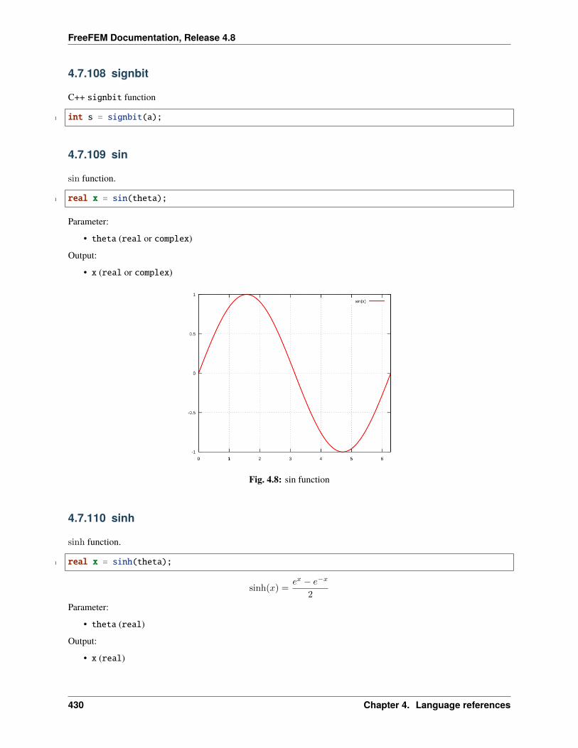
FreeFEM Documentation, Release 4.8
4.7.108 signbit
C++ signbit function
1 int s = signbit(a);
4.7.109 sin
sin function.
1 real x = sin(theta);
Parameter:
• theta (real or complex)
Output:
• x (real or complex)
Fig. 4.8: sin function
4.7.110 sinh
sinh function.
1 real x = sinh(theta);
sinh(𝑥) =𝑒𝑥 − 𝑒−𝑥
2
Parameter:
• theta (real)
Output:
• x (real)
430 Chapter 4. Language references
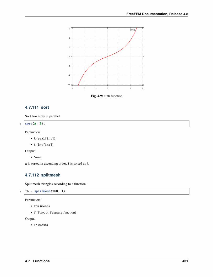
FreeFEM Documentation, Release 4.8
Fig. 4.9: sinh function
4.7.111 sort
Sort two array in parallel
1 sort(A, B);
Parameters:
• A (real[int])
• B (int[int])
Output:
• None
A is sorted in ascending order, B is sorted as A.
4.7.112 splitmesh
Split mesh triangles according to a function.
1 Th = splitmesh(Th0, f);
Parameters:
• Th0 (mesh)
• f (func or fespace function)
Output:
• Th (mesh)
4.7. Functions 431
FreeFEM Documentation, Release 4.8
4.7.113 sqrt
Square root
1 real s = sqrt(a);
Parameter:
• a (real)
Output:
• s (real)
4.7.114 square
1. Square of a number.
1 real S = square(a);
Parameter:
• a (real)
Output:
• S (real)
2. Build a structured square mesh.
1 mesh Th = square(nnX, nnY, [[L*x, H*y]], [flags=Flags], [label=Labels], [region=Region]);
Parameters:
• nnX (int) Discretization along 𝑥
• nnY (int) Discretization along 𝑦
• L (real) [Optional] Length along 𝑥
• H (real) [Optional] Height along 𝑦
• flags= (int) [Optional]
• label= (int[int]) [Optional]
• region= (int) [Optional]
Structured mesh type, see Mesh Generation chapter for more information
Output:
• Th (mesh)
432 Chapter 4. Language references
FreeFEM Documentation, Release 4.8
4.7.115 storagetotal
1 int total = storagetotal();
4.7.116 storageused
1 int used = storageused();
4.7.117 strtod
C++ strtod function
1 string text = "10.5";2 real number = strtod(text);
Parameter:
• text (string)
Output:
• number (real)
4.7.118 strtol
C++ strtol function
1 string text = "10";2 int number = strtol(text);3
4 int base = 16;5 int number = strtol(text, base);
Parameter:
• text (string)
• base (int) Base [Optional]
Output:
• number (int)
4.7.119 swap
Swap values.
1 swap(a, b);
Parameters:
• a (real)
• b (real)
4.7. Functions 433
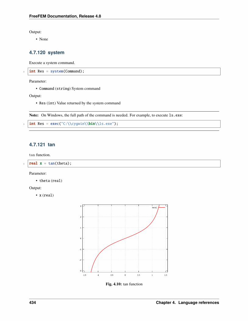
FreeFEM Documentation, Release 4.8
Output:
• None
4.7.120 system
Execute a system command.
1 int Res = system(Command);
Parameter:
• Command (string) System command
Output:
• Res (int) Value returned by the system command
Note: On Windows, the full path of the command is needed. For example, to execute ls.exe:
1 int Res = exec("C:\\cygwin\\bin\\ls.exe");
4.7.121 tan
tan function.
1 real x = tan(theta);
Parameter:
• theta (real)
Output:
• x (real)
Fig. 4.10: tan function
434 Chapter 4. Language references
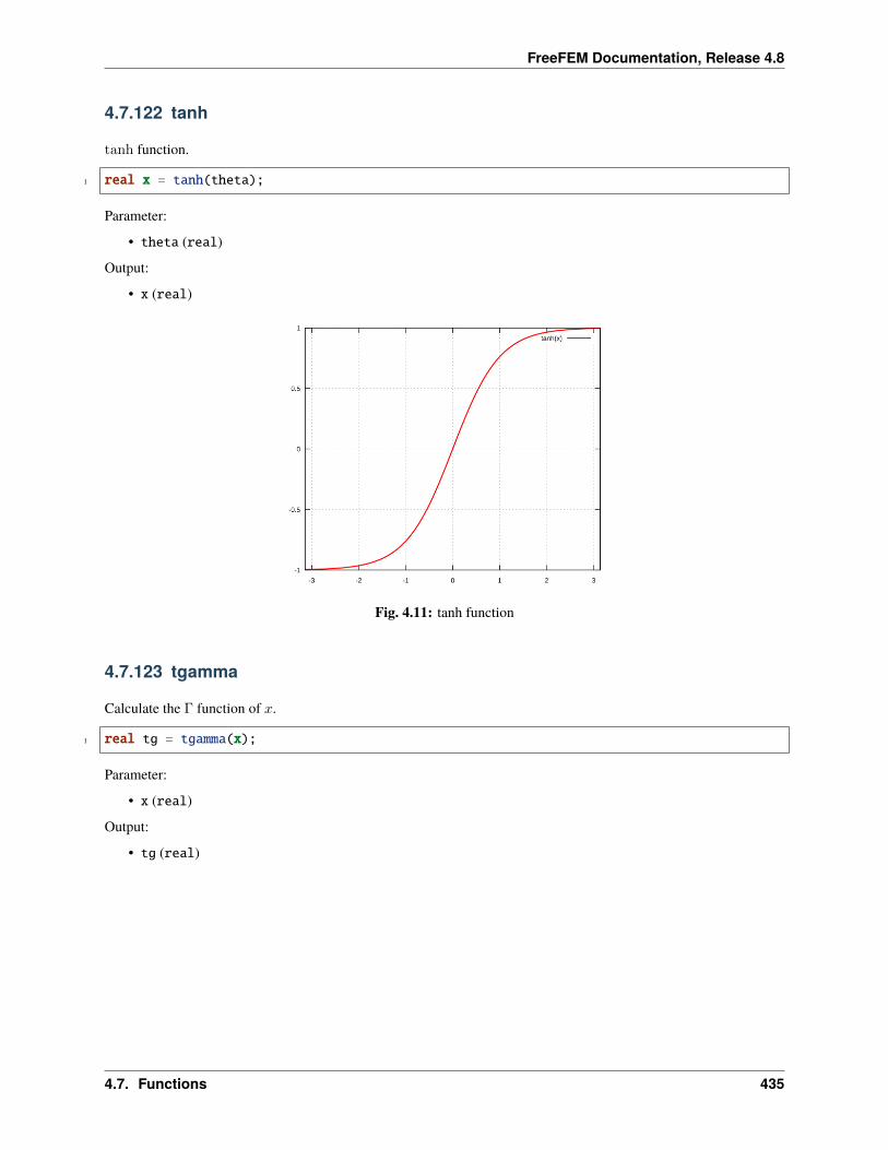
FreeFEM Documentation, Release 4.8
4.7.122 tanh
tanh function.
1 real x = tanh(theta);
Parameter:
• theta (real)
Output:
• x (real)
Fig. 4.11: tanh function
4.7.123 tgamma
Calculate the Γ function of 𝑥.
1 real tg = tgamma(x);
Parameter:
• x (real)
Output:
• tg (real)
4.7. Functions 435
FreeFEM Documentation, Release 4.8
4.7.124 time
Return the current time (C++ function).
1 real t = time();
Parameter:
• None
Output:
• t (real)
4.7.125 trace
Matrix trace
1 real tr = trace([[1, 2], [3, 4]]);
Parameters:
• Matrix
Output:
• Trace of the matrix (real)
4.7.126 trunc
Split triangle of a mesh.
1 mesh Th = trunc(Th0, R, [split=Split], [label=Label]);
Parameters:
• Th0 (mesh)
• R (bool or int) Split triangles where R is true or different from 0
• split= (int) [Optional]
Level of splitting Default: 1
• label= (int) [Optional]
Label number of new boundary item Default: 1
Output:
• Th (mesh)
436 Chapter 4. Language references
FreeFEM Documentation, Release 4.8
4.7.127 y0
Bessel function of second kind, order 0.
1 real B = y0(x);
Parameters:
• x (real)
Output:
• b (real)
4.7.128 y1
Bessel function of second kind, order 1.
1 real B = y1(x);
Parameters:
• x (real)
Output:
• b (real)
4.7.129 yn
Bessel function of second kind, order n.
1 real B = yn(n, x);
𝑌𝑛(𝑥) = lim𝜆→𝑛
𝐽𝜆(𝑥) cos(𝜆𝜋)− 𝐽−𝜆(𝑥)
sin(𝜆𝜋)
Parameters:
• n (int)
• x (real)
Output:
• b (real)
4.8 External libraries
4.8.1 aniso
boundaniso
Todo: todo
4.8. External libraries 437
FreeFEM Documentation, Release 4.8
4.8.2 BEC
BECtrap
Todo: todo
GPvortex
Todo: todo
dxGPVortex
Todo: todo
dyGPVortex
Todo: todo
4.8.3 Binary I/O
LoadVec
Todo: todo
LoadFlag
Todo: todo
438 Chapter 4. Language references
FreeFEM Documentation, Release 4.8
SaveVec
Todo: todo
flag
Todo: todo
4.8.4 buildlayer
buildlayers
Todo: todo
4.8.5 ClosePoints
radiusSearch
Todo: todo
Voisinage
Todo: todo
neighborhood
Todo: todo
4.8. External libraries 439
FreeFEM Documentation, Release 4.8
ClosePoints2
Todo: todo
ClosePoint
Todo: todo
ClosePoints1
Todo: todo
4.8.6 Curvature
extractborder
Extract a border of a mesh.
1 int Res = extractborder(Th, Label, Points);
Parameters:
• Th (mesh or mesh3)
• Label (int) Label of the border to extract
• Points (real[int, int]) Extracted points Must be allocated as real[int, int] Points(3, 1);
Output:
• Res (real) Length of the extracted border
curvature
Todo: todo
440 Chapter 4. Language references
FreeFEM Documentation, Release 4.8
raxicurvature
Todo: todo
curves
Todo: todo
setecurveabcisse
Todo: todo
equiparameter
Todo: todo
Tresca
Todo: todo
VonMises
Todo: todo
4.8.7 dfft
Refer to the FFTW documentation for more informations.
4.8. External libraries 441
FreeFEM Documentation, Release 4.8
plandfft
Todo: todo
execute
Todo: todo
delete
Todo: todo
dfft
Todo: todo
map
Todo: todo
4.8.8 distance
Need
1 load "distance"
distance
1 distance(Th, d, dist, [distmax=DistMax]);
Parameters:
• Th (mesh)
• d
• dist (real[int])
Output:
•
442 Chapter 4. Language references
FreeFEM Documentation, Release 4.8
Todo: todo
checkdist
Todo: todo
4.8.9 DxWriter
Dxaddmesh
Todo: todo
Dxaddtimeseries
Todo: todo
Dxaddsol2ts
Todo: todo
4.8.10 Element_P1bl
expert
Todo: todo
4.8.11 exactpartition
exactpartition
Todo: todo
4.8. External libraries 443
FreeFEM Documentation, Release 4.8
4.8.12 ff-AiryBiry
airy
Todo: todo
biry
Todo: todo
4.8.13 ff-cmaes
cmaes
Todo: todo
4.8.14 ff_gsl_awk
Refer to the GSL documentation for more informations
gslcdfugaussianP
Link to:
1 gsl_cdf_ugaussian_P(a)
gslcdfugaussianQ
Link to:
1 gsl_cdf_ugaussian_Q(a)
gslcdfugaussianPinv
Link to:
1 gsl_cdf_ugaussian_Pinv(a)
444 Chapter 4. Language references
FreeFEM Documentation, Release 4.8
gslcdfugaussianQinv
Link to:
1 gsl_cdf_ugaussian_Qinv(a)
gslcdfgaussianP
Link to:
1 gsl_cdf_gaussian_P(a, b)
gslcdfgaussianQ
Link to:
1 gsl_cdf_gaussian_Q(a, b)
gslcdfgaussianPinv
Link to:
1 gsl_cdf_gaussian_Pinv(a, b)
gslcdfgaussianQinv
Link to:
1 gsl_cdf_gaussian_Qinv(a, b)
gslcdfgammaP
Link to:
1 gsl_cdf_gamma_P(a, b, c)
gslcdfgammaQ
Link to:
1 gsl_cdf_gamma_Q(a, b, c)
4.8. External libraries 445
FreeFEM Documentation, Release 4.8
gslcdfgammaPinv
Link to:
1 gsl_cdf_gamma_Pinv(a, b, c)
gslcdfgammaQinv
Link to:
1 gsl_cdf_gamma_Pinv(a, b, c)
gslcdfcauchyP
Link to:
1 gsl_cdf_cauchy_P(a, b)
gslcdfcauchyQ
Link to:
1 gsl_cdf_cauchy_Q(a, b)
gslcdfcauchyPinv
Link to:
1 gsl_cdf_cauchy_Pinv(a, b)
gslcdfcauchyQinv
Link to:
1 gsl_cdf_cauchy_Qinv(a, b)
gslcdflaplaceP
Link to:
1 gsl_cdf_lapalce_P(a, b)
446 Chapter 4. Language references
FreeFEM Documentation, Release 4.8
gslcdflaplaceQ
Link to:
1 gsl_cdf_lapalce_Q(a, b)
gslcdflaplacePinv
Link to:
1 gsl_cdf_lapalce_Pinv(a, b)
gslcdflaplaceQinv
Link to:
1 gsl_cdf_lapalce_Qinv(a, b)
gslcdfrayleighP
Link to:
1 gsl_cdf_rayleigh_P(a, b)
gslcdfrayleighQ
Link to:
1 gsl_cdf_rayleigh_Q(a, b)
gslcdfrayleighPinv
Link to:
1 gsl_cdf_rayleigh_Pinv(a, b)
gslcdfrayleighQinv
Link to:
1 gsl_cdf_rayleigh_Qinv(a, b)
4.8. External libraries 447
FreeFEM Documentation, Release 4.8
gslcdfchisqP
Link to:
1 gsl_cdf_chisq_P(a, b)
gslcdfchisqQ
Link to:
1 gsl_cdf_chisq_Q(a, b)
gslcdfchisqPinv
Link to:
1 gsl_cdf_chisq_Pinv(a, b)
gslcdfchisqQinv
Link to:
1 gsl_cdf_chisq_Qinv(a, b)
gslcdfexponentialP
Link to:
1 gsl_cdf_exponential_P(a, b)
gslcdfexponentialQ
Link to:
1 gsl_cdf_exponential_Q(a, b)
gslcdfexponentialPinv
Link to:
1 gsl_cdf_exponential_Pinv(a, b)
448 Chapter 4. Language references

FreeFEM Documentation, Release 4.8
gslcdfexponentialQinv
Link to:
1 gsl_cdf_exponential_Qinv(a, b)
gslcdfexppowP
Link to:
1 gsl_cdf_exppow_P(a, b, c)
gslcdfexppowQ
Link to:
1 gsl_cdf_exppow_Q(a, b, c)
gslcdftdistP
Link to:
1 gsl_cdf_t_dist_P(a, b)
gslcdftdistQ
Link to:
1 gsl_cdf_t_dist_Q(a, b)
gslcdftdistPinv
Link to:
1 gsl_cdf_t_dist_Pinv(a, b)
gslcdftdistQinv
Link to:
1 gsl_cdf_t_dist_Qinv(a, b)
4.8. External libraries 449
FreeFEM Documentation, Release 4.8
gslcdffdistP
Link to:
1 gsl_cdf_fdist_P(a, b, c)
gslcdffdistQ
Link to:
1 gsl_cdf_fdist_Q(a, b, c)
gslcdffdistPinv
Link to:
1 gsl_cdf_fdist_Pinv(a, b, c)
gslcdffdistQinv
Link to:
1 gsl_cdf_fdist_Qinv(a, b, c)
gslcdfbetaP
Link to:
1 gsl_cdf_beta_P(a, b, c)
gslcdfbetaQ
Link to:
1 gsl_cdf_beta_Q(a, b, c)
gslcdfbetaPinv
Link to:
1 gsl_cdf_beta_Pinv(a, b, c)
450 Chapter 4. Language references
FreeFEM Documentation, Release 4.8
gslcdfbetaQinv
Link to:
1 gsl_cdf_beta_Qinv(a, b, c)
gslcdfflatP
Link to:
1 gsl_cdf_flat_P(a, b, c)
gslcdfflatQ
Link to:
1 gsl_cdf_flat_Q(a, b, c)
gslcdfflatPinv
Link to:
1 gsl_cdf_flat_Pinv(a, b, c)
gslcdfflatQinv
Link to:
1 gsl_cdf_flat_Qinv(a, b, c)
gslcdflognormalP
Link to:
1 gsl_cdf_lognormal_P(a, b, c)
gslcdflognormalQ
Link to:
1 gsl_cdf_lognormal_Q(a, b, c)
4.8. External libraries 451
FreeFEM Documentation, Release 4.8
gslcdflognormalPinv
Link to:
1 gsl_cdf_lognormal_Pinv(a, b, c)
gslcdflognormalQinv
Link to:
1 gsl_cdf_lognormal_Qinv(a, b, c)
gslcdfgumbel1P
Link to:
1 gsl_cdf_gumbel1_P(a, b, c)
gslcdfgumbel1Q
Link to:
1 gsl_cdf_gumbel1_Q(a, b, c)
gslcdfgumbel1Pinv
Link to:
1 gsl_cdf_gumbel1_Pinv(a, b, c)
gslcdfgumbel1Qinv
Link to:
1 gsl_cdf_gumbel1_Qinv(a, b, c)
gslcdfgumbel2P
Link to:
1 gsl_cdf_gumbel2_P(a, b, c)
452 Chapter 4. Language references
FreeFEM Documentation, Release 4.8
gslcdfgumbel2Q
Link to:
1 gsl_cdf_gumbel2_Q(a, b, c)
gslcdfgumbel2Pinv
Link to:
1 gsl_cdf_gumbel2_Pinv(a, b, c)
gslcdfgumbel2Qinv
Link to:
1 gsl_cdf_gumbel2_Qinv(a, b, c)
gslcdfweibullP
Link to:
1 gsl_cdf_weibull_P(a, b, c)
gslcdfweibullQ
Link to:
1 gsl_cdf_weibull_Q(a, b, c)
gslcdfweibullPinv
Link to:
1 gsl_cdf_weibull_Pinv(a, b, c)
gslcdfweibullQinv
Link to:
1 gsl_cdf_weibull_Qinv(a, b, c)
4.8. External libraries 453
FreeFEM Documentation, Release 4.8
gslcdfparetoP
Link to:
1 gsl_cdf_pareto_P(a, b, c)
gslcdfparetoQ
Link to:
1 gsl_cdf_pareto_Q(a, b, c)
gslcdfparetoPinv
Link to:
1 gsl_cdf_pareto_Pinv(a, b, c)
gslcdfparetoQinv
Link to:
1 gsl_cdf_pareto_Qinv(a, b, c)
gslcdflogisticP
Link to:
1 gsl_cdf_logistic_P(a, b)
gslcdflogisticQ
Link to:
1 gsl_cdf_logistic_Q(a, b)
gslcdflogisticPinv
Link to:
1 gsl_cdf_logistic_Pinv(a, b)
454 Chapter 4. Language references
FreeFEM Documentation, Release 4.8
gslcdflogisticQinv
Link to:
1 gsl_cdf_logistic_Qinv(a, b)
gslcdfbinomialP
Link to:
1 gsl_cdf_binomial_P(a, b, c)
gslcdfbinomialQ
Link to:
1 gsl_cdf_binomial_Q(a, b, c)
gslcdfpoissonP
Link to:
1 gsl_cdf_poisson_P(a, b)
gslcdfpoissonQ
Link to:
1 gsl_cdf_poisson_Q(a, b)
gslcdfgeometricP
Link to:
1 gsl_cdf_geometric_P(a, b)
gslcdfgeometricQ
Link to:
1 gsl_cdf_geometric_Q(a, b)
4.8. External libraries 455
FreeFEM Documentation, Release 4.8
gslcdfnegativebinomialP
Link to:
1 gsl_cdf_negative_binomial_P(a, b, c)
gslcdfnegativebinomialQ
Link to:
1 gsl_cdf_negative_binomial_Q(a, b, c)
gslcdfpascalP
Link to:
1 gsl_cdf_pascal_P(a, b, c)
gslcdfpascalQ
Link to:
1 gsl_cdf_pascal_Q(a, b, c)
gslranbernoullipdf
Link to:
1 gsl_ran_bernoulli_pdf(a, b)
gslranbeta
Link to:
1 gsl_ran_beta(a, b, c)
gslranbetapdf
Link to:
1 gsl_ran_beta_pdf(a, b, c)
456 Chapter 4. Language references

FreeFEM Documentation, Release 4.8
gslranbinomialpdf
Link to:
1 gsl_ran_binomial_pdf(a, b, c)
gslranexponential
Link to:
1 gsl_ran_exponential(a, b)
gslranexponentialpdf
Link to:
1 gsl_ran_exponential_pdf(a, b)
gslranexppow
Link to:
1 gsl_ran_exppow(a, b, c)
gslranexppowpdf
Link to:
1 gsl_ran_exppow_pdf(a, b, c)
gslrancauchy
Link to:
1 gsl_ran_cauchy(a, b)
gslrancauchypdf
Link to:
1 gsl_ran_cauchy_pdf(a, b)
4.8. External libraries 457
FreeFEM Documentation, Release 4.8
gslranchisq
Link to:
1 gsl_ran_chisq(a, b)
gslranchisqpdf
Link to:
1 gsl_ran_chisq_pdf(a, b)
gslranerlang
Link to:
1 gsl_ran_erlang(a, b, c)
gslranerlangpdf
Link to:
1 gsl_ran_erlang_pdf(a, b, c)
gslranfdist
Link to:
1 gsl_ran_fdist(a, b, c)
gslranfdistpdf
Link to:
1 gsl_ran_fdist_pdf(a, b, c)
gslranflat
Link to:
1 gsl_ran_flat(a, b, c)
458 Chapter 4. Language references
FreeFEM Documentation, Release 4.8
gslranflatpdf
Link to:
1 gsl_ran_flat_pdf(a, b, c)
gslrangamma
Link to:
1 gsl_ran_gamma(a, b, c)
gslrangammaint
Link to:
1 gsl_ran_gamma_int(a, b, c)
gslrangammapdf
Link to:
1 gsl_ran_gamma_pdf(a, b, c)
gslrangammamt
Link to:
1 gsl_ran_gamma_mt(a, b, c)
gslrangammaknuth
Link to:
1 gsl_ran_gamma_knuth(a, b, c)
gslrangaussian
Link to:
1 gsl_ran_gaussian(a, b)
4.8. External libraries 459
FreeFEM Documentation, Release 4.8
gslrangaussianratiomethod
Link to:
1 gsl_ran_gaussian_ratio_method(a, b)
gslrangaussianziggurat
Link to:
1 gsl_ran_gaussian_ziggurat(a, b)
gslrangaussianpdf
Link to:
1 gsl_ran_gaussian_pdf(a, b)
gslranugaussian
Link to:
1 gsl_ran_ugaussian(a)
gslranugaussianratiomethod
Link to:
1 gsl_ran_ugaussian_ratio_method(a)
gslranugaussianpdf
Link to:
1 gsl_ran_ugaussian_pdf(a)
gslrangaussiantail
Link to:
1 gsl_ran_gaussian_tail(a, b, c)
460 Chapter 4. Language references
FreeFEM Documentation, Release 4.8
gslrangaussiantailpdf
Link to:
1 gsl_ran_gaussian_tail_pdf(a, b, c)
gslranugaussiantail
Link to:
1 gsl_ran_ugaussian_tail(a, b)
gslranugaussiantailpdf
Link to:
1 gsl_ran_ugaussian_tail_pdf(a, b)
gslranlandau
Link to:
1 gsl_ran_landau(a)
gslranlandaupdf
Link to:
1 gsl_ran_landau_pdf(a)
gslrangeometricpdf
Link to:
1 gsl_ran_geometric_pdf(a, b)
gslrangumbel1
Link to:
1 gsl_ran_gumbel1(a, b, c)
4.8. External libraries 461
FreeFEM Documentation, Release 4.8
gslrangumbel1pdf
Link to:
1 gsl_ran_gumbel1_pdf(a, b, c)
gslrangumbel2
Link to:
1 gsl_ran_gumbel2(a, b, c)
gslrangumbel2pdf
Link to:
1 gsl_ran_gumbel2_pdf(a, b, c)
gslranlogistic
Link to:
1 gsl_ran_logistic(a, b)
gslranlogisticpdf
Link to:
1 gsl_ran_logistic_pdf(a, b)
gslranlognormal
Link to:
1 gsl_ran_lognormal(a, b, c)
gslranlognormalpdf
Link to:
1 gsl_ran_lognormal_pdf(a, b, c)
462 Chapter 4. Language references
FreeFEM Documentation, Release 4.8
gslranlogarithmicpdf
Link to:
1 gsl_ran_logarithmic_pdf(a, b)
gslrannegativebinomialpdf
Link to:
1 gsl_ran_negative_binomial_pdf(a, b, c)
gslranpascalpdf
Link to:
1 gsl_ran_pascal_pdf(a, b, c)
gslranpareto
Link to:
1 gsl_ran_pareto(a, b, c)
gslranparetopdf
Link to:
1 gsl_ran_pareto_pdf(a, b, c)
gslranpoissonpdf
Link to:
1 gsl_ran_poisson_pdf(a, b)
gslranrayleigh
Link to:
1 gsl_ran_rayleigh(a, b)
4.8. External libraries 463
FreeFEM Documentation, Release 4.8
gslranrayleighpdf
Link to:
1 gsl_ran_rayleigh_pdf(a, b)
gslranrayleightail
Link to:
1 gsl_ran_rayleigh_tail(a, b, c)
gslranrayleightailpdf
Link to:
1 gsl_ran_rayleigh_tail_pdf(a, b, c)
gslrantdist
Link to:
1 gsl_ran_tdsit(a, b)
gslrantdistpdf
Link to:
1 gsl_ran_tdsit_pdf(a, b)
gslranlaplace
Link to:
1 gsl_ran_laplace(a, b)
gslranlaplacepdf
Link to:
1 gsl_ran_laplace_pdf(a, b)
464 Chapter 4. Language references
FreeFEM Documentation, Release 4.8
gslranlevy
Link to:
1 gsl_ran_levy(a, b, c)
gslranweibull
Link to:
1 gsl_ran_weibull(a, b, c)
gslranweibullpdf
Link to:
1 gsl_ran_weibull_pdf(a, b, c)
gslsfairyAi
Link to:
1 gsl_sf_airy_Ai(a, b)
gslsfairyBi
Link to:
1 gsl_sf_airy_Bi(a, b)
gslsfairyAiscaled
Link to:
1 gsl_sf_airy_Ai_scaled(a, b)
gslsfairyBiscaled
Link to:
1 gsl_sf_airy_Bi_scaled(a, b)
4.8. External libraries 465
FreeFEM Documentation, Release 4.8
gslsfairyAideriv
Link to:
1 gsl_sf_airy_Ai_deriv(a, b)
gslsfairyBideriv
Link to:
1 gsl_sf_airy_Bi_deriv(a, b)
gslsfairyAiderivscaled
Link to:
1 gsl_sf_airy_Ai_deriv_scaled(a, b)
gslsfairyBiderivscaled
Link to:
1 gsl_sf_airy_Bi_deriv_scaled(a, b)
gslsfairyzeroAi
Link to:
1 gsl_sf_airy_Ai(a, b)
gslsfairyzeroBi
Link to:
1 gsl_sf_airy_aero_Bi(a)
gslsfairyzeroAideriv
Link to:
1 gsl_sf_airy_aero_Ai_deriv(a)
466 Chapter 4. Language references
FreeFEM Documentation, Release 4.8
gslsfairyzeroBideriv
Link to:
1 gsl_sf_airy_aero_Bi_deriv(a)
gslsfbesselJ0
Link to:
1 gsl_sf_bessel_J0(a)
gslsfbesselJ1
Link to:
1 gsl_sf_bessel_J1(a)
gslsfbesselJn
Link to:
1 gsl_sf_bessel_Jn(a, b)
gslsfbesselY0
Link to:
1 gsl_sf_bessel_Y0(a)
gslsfbesselY1
Link to:
1 gsl_sf_bessel_Y1(a)
gslsfbesselYn
Link to:
1 gsl_sf_bessel_Yn(a, b)
4.8. External libraries 467
FreeFEM Documentation, Release 4.8
gslsfbesselI0
Link to:
1 gsl_sf_bessel_I0(a)
gslsfbesselI1
Link to:
1 gsl_sf_bessel_I1(a)
gslsfbesselIn
Link to:
1 gsl_sf_bessel_In(a, b)
gslsfbesselI0scaled
Link to:
1 gsl_sf_bessel_I0_scaled(a)
gslsfbesselI1scaled
Link to:
1 gsl_sf_bessel_I1_scaled(a)
gslsfbesselInscaled
Link to:
1 gsl_sf_bessel_In_scaled(a, b)
gslsfbesselK0
Link to:
1 gsl_sf_bessel_K0(a)
468 Chapter 4. Language references
FreeFEM Documentation, Release 4.8
gslsfbesselK1
Link to:
1 gsl_sf_bessel_K1(a)
gslsfbesselKn
Link to:
1 gsl_sf_bessel_Kn(a, b)
gslsfbesselK0scaled
Link to:
1 gsl_sf_bessel_K0_scaled(a)
gslsfbesselK1scaled
Link to:
1 gsl_sf_bessel_K1_scaled(a)
gslsfbesselKnscaled
Link to:
1 gsl_sf_bessel_Kn_scaled(a, b)
gslsfbesselj0
Link to:
1 gsl_sf_bessel_j0(a)
gslsfbesselj1
Link to:
1 gsl_sf_bessel_j1(a)
4.8. External libraries 469
FreeFEM Documentation, Release 4.8
gslsfbesselj2
Link to:
1 gsl_sf_bessel_j2(a)
gslsfbesseljl
Link to:
1 gsl_sf_bessel_jl(a, b)
gslsfbessely0
Link to:
1 gsl_sf_bessel_y0(a)
gslsfbessely1
Link to:
1 gsl_sf_bessel_y0(a)
gslsfbessely2
Link to:
1 gsl_sf_bessel_y0(a)
gslsfbesselyl
Link to:
1 gsl_sf_bessel_jl(a, b)
gslsfbesseli0scaled
Link to:
1 gsl_sf_bessel_i0_scaled(a)
470 Chapter 4. Language references

FreeFEM Documentation, Release 4.8
gslsfbesseli1scaled
Link to:
1 gsl_sf_bessel_i1_scaled(a)
gslsfbesseli2scaled
Link to:
1 gsl_sf_bessel_i2_scaled(a)
gslsfbesselilscaled
Link to:
1 gsl_sf_bessel_il_scaled(a, b)
gslsfbesselk0scaled
Link to:
1 gsl_sf_bessel_k0_scaled(a)
gslsfbesselk1scaled
Link to:
1 gsl_sf_bessel_k1_scaled(a)
gslsfbesselk2scaled
Link to:
1 gsl_sf_bessel_k2_scaled(a)
gslsfbesselklscaled
Link to:
1 gsl_sf_bessel_kl_scaled(a, b)
4.8. External libraries 471
FreeFEM Documentation, Release 4.8
gslsfbesselJnu
Link to:
1 gsl_sf_bessel_Jnu(a, b)
gslsfbesselYnu
Link to:
1 gsl_sf_bessel_Ynu(a, b)
gslsfbesselInuscaled
Link to:
1 gsl_sf_bessel_Inu_scaled(a, b)
gslsfbesselInu
Link to:
1 gsl_sf_bessel_Inu(a, b)
gslsfbesselKnuscaled
Link to:
1 gsl_sf_bessel_Knu_scaled(a, b)
gslsfbesselKnu
Link to:
1 gsl_sf_bessel_Knu(a, b)
gslsfbessellnKnu
Link to:
1 gsl_sf_bessel_lnKnu(a, b)
472 Chapter 4. Language references
FreeFEM Documentation, Release 4.8
gslsfbesselzeroJ0
Link to:
1 gsl_sf_bessel_zero_J0(a)
gslsfbesselzeroJ1
Link to:
1 gsl_sf_bessel_zero_J1(a)
gslsfbesselzeroJnu
Link to:
1 gsl_sf_bessel_zero_Jnu(a, b)
gslsfclausen
Link to:
1 gsl_sf_clausen(a)
gslsfhydrogenicR1
Link to:
1 gsl_sf_hydrogenicR_1(a, b)
gslsfdawson
Link to:
1 gsl_sf_dawnson(a)
gslsfdebye1
Link to:
1 gsl_sf_debye_1(a)
4.8. External libraries 473
FreeFEM Documentation, Release 4.8
gslsfdebye2
Link to:
1 gsl_sf_debye_2(a)
gslsfdebye3
Link to:
1 gsl_sf_debye_3(a)
gslsfdebye4
Link to:
1 gsl_sf_debye_4(a)
gslsfdebye5
Link to:
1 gsl_sf_debye_5(a)
gslsfdebye6
Link to:
1 gsl_sf_debye_6(a)
gslsfdilog
Link to:
1 gsl_sf_dilog(a)
gslsfmultiply
Link to:
1 gsl_sf_multiply(a, b)
474 Chapter 4. Language references
FreeFEM Documentation, Release 4.8
gslsfellintKcomp
Link to:
1 gsl_sf_ellint_Kcomp(a, b)
gslsfellintEcomp
Link to:
1 gsl_sf_ellint_Ecomp(a, b)
gslsfellintPcomp
Link to:
1 gsl_sf_ellint_Pcomp(a, b, c)
gslsfellintDcomp
Link to:
1 gsl_sf_ellint_Dcomp(a, b)
gslsfellintF
Link to:
1 gsl_sf_ellint_F(a, b, c)
gslsfellintE
Link to:
1 gsl_sf_ellint_E(a, b, c)
gslsfellintRC
Link to:
1 gsl_sf_ellint_RC(a, b, c)
4.8. External libraries 475
FreeFEM Documentation, Release 4.8
gslsferfc
Link to:
1 gsl_sf_erfc(a)
gslsflogerfc
Link to:
1 gsl_sf_log_erfc(a)
gslsferf
Link to:
1 gsl_sf_erf(a)
gslsferfZ
Link to:
1 gsl_sf_erf_Z(a)
gslsferfQ
Link to:
1 gsl_sf_erf_Q(a)
gslsfhazard
Link to:
1 gsl_sf_hazard(a)
gslsfexp
Link to:
1 gsl_sf_exp(a)
476 Chapter 4. Language references
FreeFEM Documentation, Release 4.8
gslsfexpmult
Link to:
1 gsl_sf_exp_mult(a, b)
gslsfexpm1
Link to:
1 gsl_sf_expm1(a)
gslsfexprel
Link to:
1 gsl_sf_exprel(a)
gslsfexprel2
Link to:
1 gsl_sf_exprel_2(a)
gslsfexpreln
Link to:
1 gsl_sf_exprel_n(a, b)
gslsfexpintE1
Link to:
1 gsl_sf_expint_E1(a)
gslsfexpintE2
Link to:
1 gsl_sf_expint_E2(a)
4.8. External libraries 477
FreeFEM Documentation, Release 4.8
gslsfexpintEn
Link to:
1 gsl_sf_expint_En(a, b)
gslsfexpintE1scaled
Link to:
1 gsl_sf_expint_E1_scaled(a)
gslsfexpintE2scaled
Link to:
1 gsl_sf_expint_E1_scaled(a)
gslsfexpintEnscaled
Link to:
1 gsl_sf_expint_En_scaled(a, b)
gslsfexpintEi
Link to:
1 gsl_sf_expint_Ei(a)
gslsfexpintEiscaled
Link to:
1 gsl_sf_expint_Ei_scaled(a)
gslsfShi
Link to:
1 gsl_sf_Shi(a)
478 Chapter 4. Language references
FreeFEM Documentation, Release 4.8
gslsfChi
Link to:
1 gsl_sf_Chi(a)
gslsfexpint3
Link to:
1 gsl_sf_expint_3(a)
gslsfSi
Link to:
1 gsl_sf_Si(a)
gslsfCi
Link to:
1 gsl_sf_Ci(a)
gslsfatanint
Link to:
1 gsl_sf_atanint(a)
gslsffermidiracm1
Link to:
1 gsl_sf_fermi_dirac_m1(a)
gslsffermidirac0
Link to:
1 gsl_sf_fermi_dirac_0(a)
4.8. External libraries 479
FreeFEM Documentation, Release 4.8
gslsffermidirac1
Link to:
1 gsl_sf_fermi_dirac_1(a)
gslsffermidirac2
Link to:
1 gsl_sf_fermi_dirac_2(a)
gslsffermidiracint
Link to:
1 gsl_sf_fermi_dirac_int(a, b)
gslsffermidiracmhalf
Link to:
1 gsl_sf_fermi_dirac_mhalf(a)
gslsffermidirachalf
Link to:
1 gsl_sf_fermi_dirac_half(a)
gslsffermidirac3half
Link to:
1 gsl_sf_fermi_dirac_3half(a)
gslsffermidiracinc0
Link to:
1 gsl_sf_fermi_dirac_inc_0(a, b)
480 Chapter 4. Language references
FreeFEM Documentation, Release 4.8
gslsflngamma
Link to:
1 gsl_sf_lngamma(a)
gslsfgamma
Link to:
1 gsl_sf_gamma(a)
gslsfgammastar
Link to:
1 gsl_sf_gammastar(a)
gslsfgammainv
Link to:
1 gsl_sf_gammainv(a)
gslsftaylorcoeff
Link to:
1 gsl_sf_taylorcoeff(a, b)
gslsffact
Link to:
1 gsl_sf_fact(a)
gslsfdoublefact
Link to:
1 gsl_sf_doublefact(a)
4.8. External libraries 481
FreeFEM Documentation, Release 4.8
gslsflnfact
Link to:
1 gsl_sf_lnfact(a)
gslsflndoublefact
Link to:
1 gsl_sf_lndoublefact(a)
gslsflnchoose
Link to:
1 gsl_sf_lnchoose(a, b)
gslsfchoose
Link to:
1 gsl_sf_choose(a, b)
gslsflnpoch
Link to:
1 gsl_sf_lnpoch(a, b)
gslsfpoch
Link to:
1 gsl_sf_poch(a, b)
gslsfpochrel
Link to:
1 gsl_sf_pochrel(a, b)
482 Chapter 4. Language references
FreeFEM Documentation, Release 4.8
gslsfgammaincQ
Link to:
1 gsl_sf_gamma_inc_Q(a, b)
gslsfgammaincP
Link to:
1 gsl_sf_gamma_inc_P(a, b)
gslsfgammainc
Link to:
1 gsl_sf_gamma_inc(a, b)
gslsflnbeta
Link to:
1 gsl_sf_lnbeta(a, b)
gslsfbeta
Link to:
1 gsl_sf_beta(a, b)
gslsfbetainc
Link to:
1 gsl_sf_betaçinc(a, b, c)
gslsfgegenpoly1
Link to:
1 gsl_sf_gegenpoly_1(a, b)
4.8. External libraries 483
FreeFEM Documentation, Release 4.8
gslsfgegenpoly2
Link to:
1 gsl_sf_gegenpoly_2(a, b)
gslsfgegenpoly3
Link to:
1 gsl_sf_gegenpoly_3(a, b)
gslsfgegenpolyn
Link to:
1 gsl_sf_gegenpoly_n(a, b, c)
gslsfhyperg0F1
Link to:
1 gsl_sf_hyperg_0F1(a, b)
gslsfhyperg1F1int
Link to:
1 gsl_sf_hyperg_1F1_inc(a, b, c)
gslsfhyperg1F1
Link to:
1 gsl_sf_hyperg_1F1(a, b, c)
gslsfhypergUint
Link to:
1 gsl_sf_hyperg_U_inc(a, b, c)
484 Chapter 4. Language references
FreeFEM Documentation, Release 4.8
gslsfhypergU
Link to:
1 gsl_sf_hyperg_U(a, b, c)
gslsfhyperg2F0
Link to:
1 gsl_sf_hyperg_U_2F0(a, b, c)
gslsflaguerre1
Link to:
1 gsl_sf_laguerre_1(a, b)
gslsflaguerre2
Link to:
1 gsl_sf_laguerre_2(a, b)
gslsflaguerre3
Link to:
1 gsl_sf_laguerre_3(a, b)
gslsflaguerren
Link to:
1 gsl_sf_laguerre_n(a, b, c)
gslsflambertW0
Link to:
1 gsl_sf_lambert_W0(a)
4.8. External libraries 485

FreeFEM Documentation, Release 4.8
gslsflambertWm1
Link to:
1 gsl_sf_lambert_Wm1(a)
gslsflegendrePl
Link to:
1 gsl_sf_legendre_Pl(a, b)
gslsflegendreP1
Link to:
1 gsl_sf_legendre_P1(a)
gslsflegendreP2
Link to:
1 gsl_sf_legendre_P2(a)
gslsflegendreP3
Link to:
1 gsl_sf_legendre_P3(a)
gslsflegendreQ0
Link to:
1 gsl_sf_legendre_Q0(a)
gslsflegendreQ1
Link to:
1 gsl_sf_legendre_Q1(a)
486 Chapter 4. Language references
FreeFEM Documentation, Release 4.8
gslsflegendreQl
Link to:
1 gsl_sf_legendre_Ql(a, b)
gslsflegendrePlm
Link to:
1 gsl_sf_legendre_Plm(a, b, c)
gslsflegendresphPlm
Link to:
1 gsl_sf_legendre_sphP1m(a, b, c)
gslsflegendrearraysize
Link to:
1 gsl_sf_legendre_array_size(a, b)
gslsfconicalPhalf
Link to:
1 gsl_sf_conicalP_half(a, b)
gslsfconicalPmhalf
Link to:
1 gsl_sf_conicalP_mhalf(a, b)
gslsfconicalP0
Link to:
1 gsl_sf_conicalP_0(a, b)
4.8. External libraries 487
FreeFEM Documentation, Release 4.8
gslsfconicalP1
Link to:
1 gsl_sf_conicalP_1(a, b)
gslsfconicalPsphreg
Link to:
1 gsl_sf_conicalP_sph_reg(a, b, c)
gslsfconicalPcylreg
Link to:
1 gsl_sf_conicalP_cyl_reg(a, b, c)
gslsflegendreH3d0
Link to:
1 gsl_sf_legendre_H3d_0(a, b)
gslsflegendreH3d1
Link to:
1 gsl_sf_legendre_H3d_1(a, b)
gslsflegendreH3d
Link to:
1 gsl_sf_legendre_H3d(a, b, c)
gslsflog
Link to:
1 gsl_sf_log(a)
488 Chapter 4. Language references
FreeFEM Documentation, Release 4.8
gslsflogabs
Link to:
1 gsl_sf_log_abs(a)
gslsflog1plusx
Link to:
1 gsl_sf_log_1plusx(a)
gslsflog1plusxmx
Link to:
1 gsl_sf_log_1plusx_mx(a)
gslsfpowint
Link to:
1 gsl_sf_pow_int(a, b)
gslsfpsiint
Link to:
1 gsl_sf_psi_int(a)
gslsfpsi
Link to:
1 gsl_sf_psi(a)
gslsfpsi1piy
Link to:
1 gsl_sf_psi_1piy(a)
4.8. External libraries 489
FreeFEM Documentation, Release 4.8
gslsfpsi1int
Link to:
1 gsl_sf_psi_1_int(a)
gslsfpsi1
Link to:
1 gsl_sf_psi_1(a)
gslsfpsin
Link to:
1 gsl_sf_psi_n(a, b)
gslsfsynchrotron1
Link to:
1 gsl_sf_synchrotron_1(a)
gslsfsynchrotron2
Link to:
1 gsl_sf_synchrotron_2(a)
gslsftransport2
Link to:
1 gsl_sf_transport_2(a)
gslsftransport3
Link to:
1 gsl_sf_transport_3(a)
490 Chapter 4. Language references
FreeFEM Documentation, Release 4.8
gslsftransport4
Link to:
1 gsl_sf_transport_4(a)
gslsftransport5
Link to:
1 gsl_sf_transport_5(a)
gslsfsin
Link to:
1 gsl_sf_sin(a)
gslsfcos
Link to:
1 gsl_sf_cos(a)
gslsfhypot
Link to:
1 gsl_sf_hypot(a, b)
gslsfsinc
Link to:
1 gsl_sf_sinc(a)
gslsflnsinh
Link to:
1 gsl_sf_lnsinh(a)
4.8. External libraries 491
FreeFEM Documentation, Release 4.8
gslsflncosh
Link to:
1 gsl_sf_lncosh(a)
gslsfanglerestrictsymm
Link to:
1 gsl_sf_andle_restrict_symm(a)
gslsfanglerestrictpos
Link to:
1 gsl_sf_angle_restrict_pos(a)
gslsfzetaint
Link to:
1 gsl_sf_zeta_int(a)
gslsfzeta
Link to:
1 gsl_sf_zeta(a)
gslsfzetam1
Link to:
1 gsl_sf_zetam1(a)
gslsfzetam1int
Link to:
1 gsl_sf_zetam1_int(a)
492 Chapter 4. Language references
FreeFEM Documentation, Release 4.8
gslsfhzeta
Link to:
1 gsl_sf_hzeta(a, b)
gslsfetaint
Link to:
1 gsl_sf_eta_int(a)
gslsfeta
Link to:
1 gsl_sf_eta(a)
4.8.15 ff-Ipopt
Refer to the Ipopt documentation for more informations.
IPOPT
Todo: todo
4.8.16 fflapack
Refer to the LAPACK documentation for more informations.
inv
Todo: todo
dgeev
Todo: todo
4.8. External libraries 493
FreeFEM Documentation, Release 4.8
zgeev
Todo: todo
geev
Todo: todo
geev
Todo: todo
dggev
Todo: todo
zggev
Todo: todo
dsygvd
Todo: todo
dgesdd
Todo: todo
494 Chapter 4. Language references
FreeFEM Documentation, Release 4.8
zhegv
Todo: todo
dsyev
Todo: todo
zheev
Todo: todo
4.8.17 ff-mmap-semaphore
Wait
Todo: todo
trywait
Todo: todo
Post
Todo: todo
msync
Todo: todo
4.8. External libraries 495

FreeFEM Documentation, Release 4.8
Read
Todo: todo
Write
Todo: todo
4.8.18 ffnewuoa
newuoa
Todo: todo
4.8.19 ff-NLopt
Refer to the NLOPT documentation for more informations.
nloptDIRECT
Todo: todo
nloptDIRECTL
Todo: todo
nloptDIRECTLRand
Todo: todo
496 Chapter 4. Language references
FreeFEM Documentation, Release 4.8
nloptDIRECTScal
Todo: todo
nloptDIRECTNoScal
Todo: todo
nloptDIRECTLNoScal
Todo: todo
nloptDIRECTLRandNoScal
Todo: todo
nloptOrigDIRECT
Todo: todo
nloptOrigDIRECTL
Todo: todo
nloptStoGO
Todo: todo
4.8. External libraries 497

FreeFEM Documentation, Release 4.8
nloptStoGORand
Todo: todo
nloptLBFGS
Todo: todo
nloptPRAXIS
Todo: todo
nloptVar1
Todo: todo
nloptVar2
Todo: todo
nloptTNewton
Todo: todo
nloptTNewtonRestart
Todo: todo
498 Chapter 4. Language references
FreeFEM Documentation, Release 4.8
nloptTNewtonPrecond
Todo: todo
nloptTNewtonPrecondRestart
Todo: todo
nloptCRS2
Todo: todo
nloptMMA
Todo: todo
nloptCOBYLA
Todo: todo
nloptNEWUOA
Todo: todo
nloptNEWUOABound
Todo: todo
4.8. External libraries 499

FreeFEM Documentation, Release 4.8
nloptNelderMead
Todo: todo
nloptSbplx
Todo: todo
nloptBOBYQA
Todo: todo
nloptISRES
Todo: todo
nloptSLSQP
Todo: todo
nloptMLSL
Todo: todo
nloptMLSLLDS
Todo: todo
500 Chapter 4. Language references
FreeFEM Documentation, Release 4.8
nloptAUGLAG
Todo: todo
nloptAUGLAGEQ
Todo: todo
4.8.20 ffrandom
srandomdev
Todo: todo
srandom
Todo: todo
random
Todo: todo
4.8.21 FreeFemQA
MeshGenQA
Todo: todo
4.8. External libraries 501
FreeFEM Documentation, Release 4.8
4.8.22 freeyams
freeyams
Todo: todo
4.8.23 gmsh
Need
1 load "gmsh"
The gmsh software is available here
gmshload
Load a 2D mesh build with Gmsh.
1 mesh Th = gmshload(MeshFile, [reftri=RefTri], [renum=Renum]);
Parameters:
• MeshFile (string) Mesh file name
• reftri= (.. todo:: todo)
• renum= (.. todo:: todo)
Output:
• Th (mesh)
gmshload3
Load a 3D mesh build with Gmsh.
1 mesh3 Th = gmshload3(MeshFile, [reftet=RefTet], [renum=Renum]);
Parameters:
• MeshFile (string) Mesh file name
• reftet= (.. todo:: todo)
• renum= (.. todo:: todo)
Output:
• Th (mesh3)
502 Chapter 4. Language references
FreeFEM Documentation, Release 4.8
savegmsh
Todo: todo
4.8.24 gsl
gslpolysolvequadratic
Todo: todo
gslpolysolvecubic
Todo: todo
gslpolycomplexsolve
Todo: todo
gslrnguniform
Todo: todo
gslrnguniformpos
Todo: todo
gslname
Todo: todo
4.8. External libraries 503
FreeFEM Documentation, Release 4.8
gslrngget
Todo: todo
gslrngmin
Todo: todo
gslrngmax
Todo: todo
gslrngset
Todo: todo
gslrngtype
Todo: todo
4.8.25 ilut
applyIlutPrecond
Todo: todo
makeIlutPrecond
Todo: todo
504 Chapter 4. Language references
FreeFEM Documentation, Release 4.8
4.8.26 iohdf5
savehdf5sol
Todo: todo
4.8.27 iovtk
savevtk
Save mesh or solution in vtk/vtu format.
1 savevtk(FileName, Th, [Ux, Uy, Uz], p, [dataname=DataName],→˓[withsurfacemesh=WithSurfaceMesh], [order=Order], [floatmesh=FloatMesh],→˓[floatsol=FloatSol], [bin=Bin], [swap=Swap]);
Parameters:
• FileName (string) File name: *.vtk or *.vtu
• Th (mesh or mesh3)
• [Ux, Uy, Uz], p (fespace function of vector of fespace functions) Solutions to save, as much as wanted
• dataname= (string) Name of solutions, seprated by a space
• withsurfacemesh= (bool) .. todo:: todo
• order= (int[int]) Order of solutions.
Available: 0 or 1
• floatmesh= (bool) .. todo:: todo
• floatsol= (bool) .. todo:: todo
• bin= (bool) If true, save file in binary format
• swap (bool) .. todo:: todo
Output:
• None
vtkload
Todo: todo
4.8. External libraries 505
FreeFEM Documentation, Release 4.8
vtkload3
Todo: todo
4.8.28 isoline
Need
1 load "isoline"
isoline
1 int N = isoline(Th, u, xy, iso=Iso, close=Close, smoothing=Smoothing, ratio=Ratio,→˓eps=Eps, beginend=BeginEnd, file=File);
Todo: todo
Curve
Todo: todo
Area
Todo: todo
findallocalmin
Todo: todo
4.8.29 lapack
inv
Todo: todo
506 Chapter 4. Language references
FreeFEM Documentation, Release 4.8
dgeev
Todo: todo
zgeev
Todo: todo
geev
Todo: todo
dggev
Todo: todo
zggev
Todo: todo
dsygvd
Todo: todo
dgesdd
Todo: todo
4.8. External libraries 507
FreeFEM Documentation, Release 4.8
zhegv
Todo: todo
dsyev
Todo: todo
zheev
Todo: todo
dgelsy
Todo: todo
4.8.30 lgbmo
bmo
Todo: todo
4.8.31 mat_dervieux
MatUpWind1
Todo: todo
508 Chapter 4. Language references
FreeFEM Documentation, Release 4.8
4.8.32 mat_psi
MatUpWind0
Todo: todo
4.8.33 medit
medit
Todo: todo
savesol
Todo: todo
readsol
Todo: todo
4.8.34 metis
metisnodal
Todo: todo
metisdual
Todo: todo
4.8. External libraries 509
FreeFEM Documentation, Release 4.8
4.8.35 MetricKuate
MetricKuate
Todo: todo
4.8.36 MetricPk
MetricPk
Todo: todo
4.8.37 mmg3d
mmg3d
Todo: todo
4.8.38 mmg3d-v4.0
mmg3d
Todo: todo
4.8.39 msh3
change
Todo: todo
510 Chapter 4. Language references
FreeFEM Documentation, Release 4.8
movemesh23
Todo: todo
movemesh2D3Dsurf
Todo: todo
movemesh3
Todo: todo
movemesh
Todo: todo
movemesh3D
Todo: todo
deplacement
Todo: todo
checkbemesh
Todo: todo
4.8. External libraries 511
FreeFEM Documentation, Release 4.8
buildlayers
Todo: todo
bcube
Todo: todo
cube
Construct a cubic mesh.
1 mesh3 Th = cube(nnX, nnY, nnZ, [X(x), Y(y), Z(z)], [label=Label], [flags=Flags],→˓[region=Region]);
Parameters:
• nnX (int) Number of discretization point along 𝑥
• nnY (int) Number of discretization point along 𝑦
• nnZ (int) Number of discretization point along 𝑧
• X(x) (func) [Optional] Affine function of 𝑥 to define the length Default: x
• Y(y) (func) [Optional] Affine function of 𝑦 to define the width Default: y
• Z(z) (func) [Optional] Affine function of 𝑧 to define the height Default: z
• label= (int[int]) [Optional]
List of surface labels Default: [1, 2, 3, 4, 5, 6]
• flags= (int) [Optional]
Refer to square
• region= (int) [Optional]
Region number of the cube volume Default: 0
Output:
• Th (mesh3) Cube mesh
trunc
Todo: todo
512 Chapter 4. Language references
FreeFEM Documentation, Release 4.8
gluemesh
Todo: todo
extract
Todo: todo
showborder
Todo: todo
getborder
Todo: todo
AddLayers
Todo: todo
4.8.40 mshmet
mshmet
Todo: todo
4.8.41 MUMPS
defaulttoMUMPSseq
Todo: todo
4.8. External libraries 513
FreeFEM Documentation, Release 4.8
4.8.42 MUMPS_seq
defaulttoMUMPSseq
Todo: todo
4.8.43 netgen
netg
Todo: todo
netgstl
Todo: todo
netgload
Todo: todo
4.8.44 NewSolver
defaulttoUMFPACK
Todo: todo
4.8.45 PARDISO
defaulttoPARDISO
Todo: todo
514 Chapter 4. Language references
FreeFEM Documentation, Release 4.8
ompsetnumthreads
Todo: todo
ompgetnumthreads
Todo: todo
ompgetmaxthreads
Todo: todo
4.8.46 pcm2rnm
readpcm
Todo: todo
4.8.47 pipe
flush
Todo: todo
sleep
Todo: todo
4.8. External libraries 515
FreeFEM Documentation, Release 4.8
usleep
Todo: todo
4.8.48 qf11to25
QF1d
Todo: todo
QF2d
Todo: todo
QF3d
Todo: todo
tripleQF
4.8.49 scotch
scotch
Todo: todo
4.8.50 shell
readdir
Todo: todo
516 Chapter 4. Language references
FreeFEM Documentation, Release 4.8
unlink
Todo: todo
rmdir
Todo: todo
cddir
Todo: todo
chdir
Todo: todo
basename
Todo: todo
dirname
Todo: todo
mkdir
Todo: todo
4.8. External libraries 517
FreeFEM Documentation, Release 4.8
chmod
Todo: todo
cpfile
Todo: todo
stat
Todo: todo
isdir
Todo: todo
getenv
Todo: todo
setenv
Todo: todo
unsetenv
Todo: todo
518 Chapter 4. Language references
FreeFEM Documentation, Release 4.8
4.8.51 splitedges
SplitedgeMesh
Todo: todo
4.8.52 splitmesh12
splitmesh12
Todo: todo
4.8.53 splitmesh3
splitmesh3
Todo: todo
4.8.54 splitmesh4
splimesh4
Todo: todo
4.8.55 splitmesh6
splitmesh6
Todo: todo
4.8. External libraries 519
FreeFEM Documentation, Release 4.8
4.8.56 SuperLu
defaulttoSuperLu
Todo: todo
4.8.57 symmetrizeCSR
symmetrizeCSR
Todo: todo
4.8.58 tetgen
Refer to the Tetgen documentation for more informations.
tetgconvexhull
Todo: todo
tetgtransfo
Todo: todo
tetg
Build a 3D mesh from a surface.
1 mesh3 Th = tetg(Th0, [reftet=RefTet], [label=Label], [switch=Switch],→˓[nbofholes=NbOfHoles], [holelist=HoleList], [nbofregions=NbOfRegions],→˓[regionlist=RegionList], [nboffacetcl=NbOfFaceTcl], [facetcl=FaceTcl])
Todo: todo
520 Chapter 4. Language references
FreeFEM Documentation, Release 4.8
tetgreconstruction
Todo: todo
4.8.59 UMFPACK64
defaulttoUMFPACK64
Todo: todo
4.8.60 VTK_writer_3d
Vtkaddmesh
Todo: todo
Vtkaddscalar
Todo: todo
4.8.61 VTK_writer
Vtkaddmesh
Todo: todo
Vtkaddscalar
4.8. External libraries 521

FreeFEM Documentation, Release 4.8
522 Chapter 4. Language references
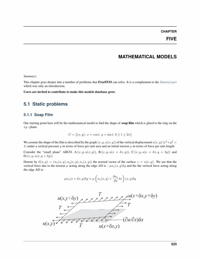
CHAPTER
FIVE
MATHEMATICAL MODELS
Summary:
This chapter goes deeper into a number of problems that FreeFEM can solve. It is a complement to the Tutorial partwhich was only an introduction.
Users are invited to contribute to make this models database grow.
5.1 Static problems
5.1.1 Soap Film
Our starting point here will be the mathematical model to find the shape of soap film which is glued to the ring on the𝑥𝑦−plane:
𝐶 = (𝑥, 𝑦); 𝑥 = cos 𝑡, 𝑦 = sin 𝑡, 0 ≤ 𝑡 ≤ 2𝜋
We assume the shape of the film is described by the graph (𝑥, 𝑦, 𝑢(𝑥, 𝑦)) of the vertical displacement 𝑢(𝑥, 𝑦) (𝑥2+𝑦2 <1) under a vertical pressure 𝑝 in terms of force per unit area and an initial tension 𝜇 in terms of force per unit length.
Consider the “small plane” ABCD, A:(𝑥, 𝑦, 𝑢(𝑥, 𝑦)), B:(𝑥, 𝑦, 𝑢(𝑥 + 𝛿𝑥, 𝑦)), C:(𝑥, 𝑦, 𝑢(𝑥 + 𝛿𝑥, 𝑦 + 𝛿𝑦)) andD:(𝑥, 𝑦, 𝑢(𝑥, 𝑦 + 𝛿𝑦)).
Denote by (𝑥, 𝑦) = (𝑛𝑥(𝑥, 𝑦), 𝑛𝑦(𝑥, 𝑦), 𝑛𝑧(𝑥, 𝑦)) the normal vector of the surface 𝑧 = 𝑢(𝑥, 𝑦). We see that thevertical force due to the tension 𝜇 acting along the edge AD is −𝜇𝑛𝑥(𝑥, 𝑦)𝛿𝑦 and the the vertical force acting alongthe edge AD is:
𝜇𝑛𝑥(𝑥+ 𝛿𝑥, 𝑦)𝛿𝑦 ≃ 𝜇(𝑛𝑥(𝑥, 𝑦) +
𝜕𝑛𝑥𝜕𝑥
𝛿𝑥
)(𝑥, 𝑦)𝛿𝑦
523
FreeFEM Documentation, Release 4.8
Similarly, for the edges AB and DC we have:
−𝜇𝑛𝑦(𝑥, 𝑦)𝛿𝑥, 𝜇 (𝑛𝑦(𝑥, 𝑦) + 𝜕𝑛𝑦/𝜕𝑦) (𝑥, 𝑦)𝛿𝑥
The force in the vertical direction on the surface ABCD due to the tension 𝜇 is given by:
𝜇 (𝜕𝑛𝑥/𝜕𝑥) 𝛿𝑥𝛿𝑦 + 𝑇 (𝜕𝑛𝑦/𝜕𝑦) 𝛿𝑦𝛿𝑥
Assuming small displacements, we have:
𝜈𝑥 = (𝜕𝑢/𝜕𝑥)/√
1 + (𝜕𝑢/𝜕𝑥)2 + (𝜕𝑢/𝜕𝑦)2 ≃ 𝜕𝑢/𝜕𝑥,
𝜈𝑦 = (𝜕𝑢/𝜕𝑦)/√
1 + (𝜕𝑢/𝜕𝑥)2 + (𝜕𝑢/𝜕𝑦)2 ≃ 𝜕𝑢/𝜕𝑦
Letting 𝛿𝑥→ 𝑑𝑥, 𝛿𝑦 → 𝑑𝑦, we have the equilibrium of the vertical displacement of soap film on ABCD by 𝑝:
𝜇𝑑𝑥𝑑𝑦𝜕2𝑢/𝜕𝑥2 + 𝜇𝑑𝑥𝑑𝑦𝜕2𝑢/𝜕𝑦2 + 𝑝𝑑𝑥𝑑𝑦 = 0
Using the Laplace operator ∆ = 𝜕2/𝜕𝑥2 + 𝜕2/𝜕𝑦2, we can find the virtual displacement write the following:
−∆𝑢 = 𝑓 in Ω
where 𝑓 = 𝑝/𝜇, Ω = (𝑥, 𝑦); 𝑥2 + 𝑦2 < 1.
Poisson’s equation appears also in electrostatics taking the form of 𝑓 = 𝜌/𝜖 where 𝜌 is the charge density, 𝜖 thedielectric constant and 𝑢 is named as electrostatic potential.
The soap film is glued to the ring 𝜕Ω = 𝐶, then we have the boundary condition:
𝑢 = 0 on 𝜕Ω
If the force is gravity, for simplify, we assume that 𝑓 = −1.
1 // Parameters2 int nn = 50;3 func f = -1;4 func ue = (x^2+y^2-1)/4; //ue: exact solution5
6 // Mesh7 border a(t=0, 2*pi)x=cos(t); y=sin(t); label=1;8 mesh disk = buildmesh(a(nn));9 plot(disk);
10
11 // Fespace12 fespace femp1(disk, P1);13 femp1 u, v;14
15 // Problem16 problem laplace (u, v)17 = int2d(disk)( //bilinear form18 dx(u)*dx(v)19 + dy(u)*dy(v)20 )21 - int2d(disk)( //linear form22 f*v23 )24 + on(1, u=0) //boundary condition
(continues on next page)
524 Chapter 5. Mathematical Models
FreeFEM Documentation, Release 4.8
(continued from previous page)
25 ;26
27 // Solve28 laplace;29
30 // Plot31 plot (u, value=true, wait=true);32
33 // Error34 femp1 err = u - ue;35 plot(err, value=true, wait=true);36
37 cout << "error L2 = " << sqrt( int2d(disk)(err^2) )<< endl;38 cout << "error H10 = " << sqrt( int2d(disk)((dx(u)-x/2)^2) + int2d(disk)((dy(u)-y/2)^2) )
→˓<< endl;39
40 /// Re-run with a mesh adaptation ///41
42 // Mesh adaptation43 disk = adaptmesh(disk, u, err=0.01);44 plot(disk, wait=true);45
46 // Solve47 laplace;48 plot (u, value=true, wait=true);49
50 // Error51 err = u - ue; //become FE-function on adapted mesh52 plot(err, value=true, wait=true);53
54 cout << "error L2 = " << sqrt( int2d(disk)(err^2) )<< endl;55 cout << "error H10 = " << sqrt( int2d(disk)((dx(u)-x/2)^2) + int2d(disk)((dy(u)-y/2)^2) )
→˓<< endl;
In the 37th line, the 𝐿2-error estimation between the exact solution 𝑢𝑒,
‖𝑢ℎ − 𝑢𝑒‖0,Ω =
(∫Ω
|𝑢ℎ − 𝑢𝑒|2 𝑡𝑒𝑥𝑡𝑑𝑥𝑡𝑒𝑥𝑡𝑑𝑦)1/2
and in the following line, the 𝐻1-error seminorm estimation:
|𝑢ℎ − 𝑢𝑒|1,Ω =
(∫Ω
|∇𝑢ℎ −∇𝑢𝑒|2 𝑡𝑒𝑥𝑡𝑑𝑥𝑡𝑒𝑥𝑡𝑑𝑦)1/2
are done on the initial mesh. The results are ‖𝑢ℎ − 𝑢𝑒‖0,Ω = 0.000384045, |𝑢ℎ − 𝑢𝑒|1,Ω = 0.0375506.
After the adaptation, we have ‖𝑢ℎ − 𝑢𝑒‖0,Ω = 0.000109043, |𝑢ℎ − 𝑢𝑒|1,Ω = 0.0188411. So the numerical solution isimproved by adaptation of mesh.
5.1. Static problems 525
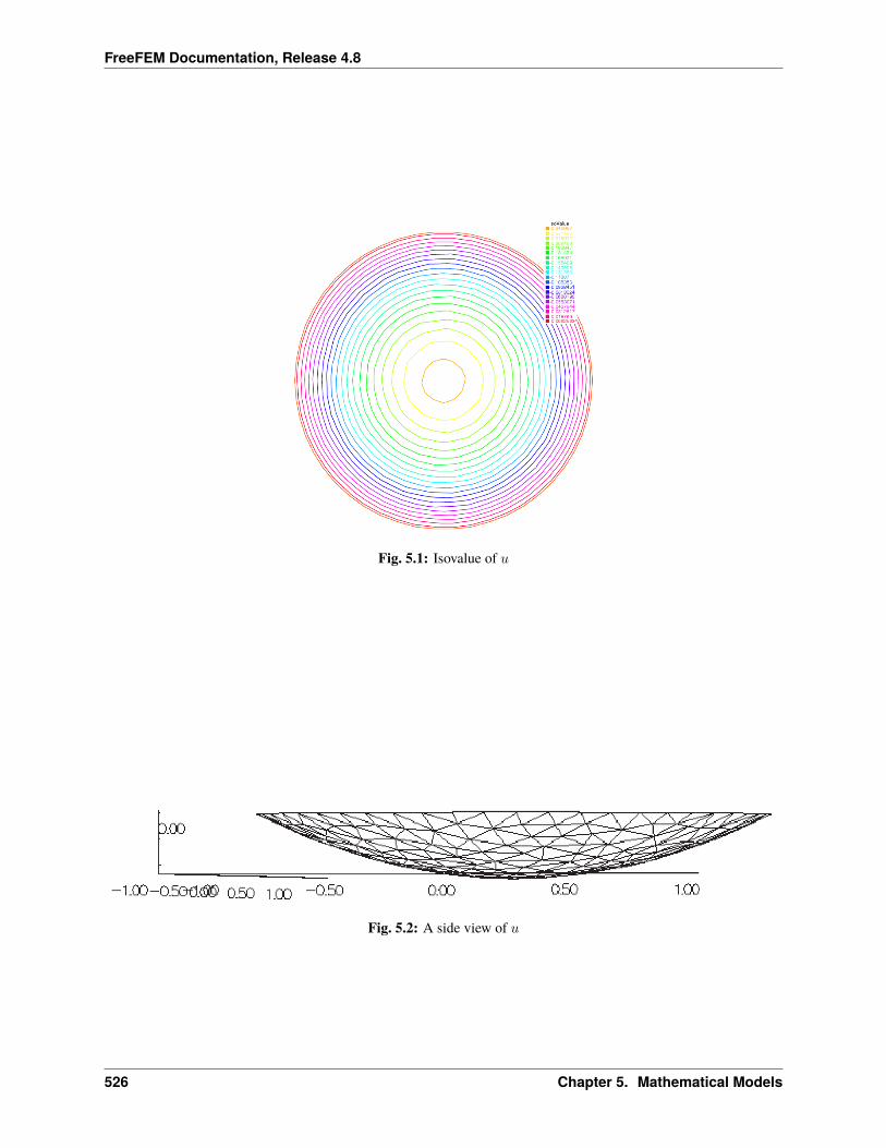
FreeFEM Documentation, Release 4.8
Fig. 5.1: Isovalue of 𝑢
Fig. 5.2: A side view of 𝑢
526 Chapter 5. Mathematical Models
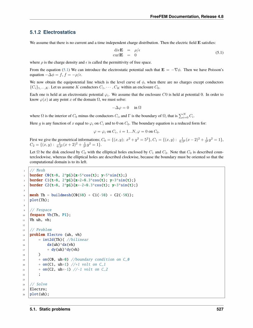
FreeFEM Documentation, Release 4.8
5.1.2 Electrostatics
We assume that there is no current and a time independent charge distribution. Then the electric field E satisfies:
divE = 𝜌/𝜖curlE = 0
(5.1)
where 𝜌 is the charge density and 𝜖 is called the permittivity of free space.
From the equation (5.1) We can introduce the electrostatic potential such that E = −∇𝜑. Then we have Poisson’sequation −∆𝜑 = 𝑓 , 𝑓 = −𝜌/𝜖.
We now obtain the equipotential line which is the level curve of 𝜑, when there are no charges except conductors𝐶𝑖1,··· ,𝐾 . Let us assume 𝐾 conductors 𝐶1, · · · , 𝐶𝐾 within an enclosure 𝐶0.
Each one is held at an electrostatic potential 𝜙𝑖. We assume that the enclosure 𝐶0 is held at potential 0. In order toknow 𝜙(𝑥) at any point 𝑥 of the domain Ω, we must solve:
−∆𝜙 = 0 in Ω
where Ω is the interior of 𝐶0 minus the conductors 𝐶𝑖, and Γ is the boundary of Ω, that is∑𝑁𝑖=0 𝐶𝑖.
Here 𝑔 is any function of 𝑥 equal to 𝜙𝑖 on 𝐶𝑖 and to 0 on 𝐶0. The boundary equation is a reduced form for:
𝜙 = 𝜙𝑖 on 𝐶𝑖, 𝑖 = 1...𝑁, 𝜙 = 0 on 𝐶0.
First we give the geometrical informations; 𝐶0 = (𝑥, 𝑦); 𝑥2 + 𝑦2 = 52, 𝐶1 = (𝑥, 𝑦) : 10.32 (𝑥− 2)2 + 1
32 𝑦2 = 1,
𝐶2 = (𝑥, 𝑦) : 10.32 (𝑥+ 2)2 + 1
32 𝑦2 = 1.
Let Ω be the disk enclosed by 𝐶0 with the elliptical holes enclosed by 𝐶1 and 𝐶2. Note that 𝐶0 is described coun-terclockwise, whereas the elliptical holes are described clockwise, because the boundary must be oriented so that thecomputational domain is to its left.
1 // Mesh2 border C0(t=0, 2*pi)x=5*cos(t); y=5*sin(t);3 border C1(t=0, 2*pi)x=2+0.3*cos(t); y=3*sin(t);4 border C2(t=0, 2*pi)x=-2+0.3*cos(t); y=3*sin(t);5
6 mesh Th = buildmesh(C0(60) + C1(-50) + C2(-50));7 plot(Th);8
9 // Fespace10 fespace Vh(Th, P1);11 Vh uh, vh;12
13 // Problem14 problem Electro (uh, vh)15 = int2d(Th)( //bilinear16 dx(uh)*dx(vh)17 + dy(uh)*dy(vh)18 )19 + on(C0, uh=0) //boundary condition on C_020 + on(C1, uh=1) //+1 volt on C_121 + on(C2, uh=-1) //-1 volt on C_222 ;23
24 // Solve25 Electro;26 plot(uh);
5.1. Static problems 527
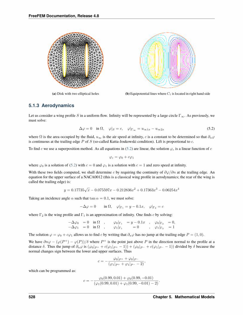
FreeFEM Documentation, Release 4.8
(a) Disk with two elliptical holes (b) Equipotential lines where𝐶1 is located in right hand side
5.1.3 Aerodynamics
Let us consider a wing profile 𝑆 in a uniform flow. Infinity will be represented by a large circle Γ∞. As previously, wemust solve:
∆𝜙 = 0 in Ω, 𝜙|𝑆 = 𝑐, 𝜙|Γ∞ = 𝑢∞1𝑥 − 𝑢∞2𝑥 (5.2)
where Ω is the area occupied by the fluid, 𝑢∞ is the air speed at infinity, 𝑐 is a constant to be determined so that 𝜕𝑛𝜙is continuous at the trailing edge 𝑃 of 𝑆 (so-called Kutta-Joukowski condition). Lift is proportional to 𝑐.
To find 𝑐 we use a superposition method. As all equations in (5.2) are linear, the solution 𝜙𝑐 is a linear function of 𝑐
𝜙𝑐 = 𝜙0 + 𝑐𝜙1
where 𝜙0 is a solution of (5.2) with 𝑐 = 0 and 𝜙1 is a solution with 𝑐 = 1 and zero speed at infinity.
With these two fields computed, we shall determine 𝑐 by requiring the continuity of 𝜕𝜙/𝜕𝑛 at the trailing edge. Anequation for the upper surface of a NACA0012 (this is a classical wing profile in aerodynamics; the rear of the wing iscalled the trailing edge) is:
𝑦 = 0.17735√𝑥− 0.075597𝑥− 0.212836𝑥2 + 0.17363𝑥3 − 0.06254𝑥4
Taking an incidence angle 𝛼 such that tan𝛼 = 0.1, we must solve:
−∆𝜙 = 0 in Ω, 𝜙|Γ1= 𝑦 − 0.1𝑥, 𝜙|Γ2
= 𝑐
where Γ2 is the wing profile and Γ1 is an approximation of infinity. One finds 𝑐 by solving:
−∆𝜙0 = 0 in Ω , 𝜙0|Γ1= 𝑦 − 0.1𝑥 , 𝜙0|Γ2
= 0,−∆𝜙1 = 0 in Ω , 𝜙1|Γ1
= 0 , 𝜙1|Γ2= 1
The solution 𝜙 = 𝜙0 + 𝑐𝜙1 allows us to find 𝑐 by writing that 𝜕𝑛𝜙 has no jump at the trailing edge 𝑃 = (1, 0).
We have 𝜕𝑛𝜙 − (𝜙(𝑃+) − 𝜙(𝑃 ))/𝛿 where 𝑃+ is the point just above 𝑃 in the direction normal to the profile at adistance 𝛿. Thus the jump of 𝜕𝑛𝜙 is (𝜙0|𝑃+ + 𝑐(𝜙1|𝑃+ − 1)) + (𝜙0|𝑃− + 𝑐(𝜙1|𝑃− − 1)) divided by 𝛿 because thenormal changes sign between the lower and upper surfaces. Thus
𝑐 = − 𝜙0|𝑃+ + 𝜙0|𝑃−
(𝜙1|𝑃+ + 𝜙1|𝑃− − 2),
which can be programmed as:
𝑐 = − 𝜙0(0.99, 0.01) + 𝜙0(0.99,−0.01)
(𝜙1(0.99, 0.01) + 𝜙1(0.99,−0.01)− 2).
528 Chapter 5. Mathematical Models
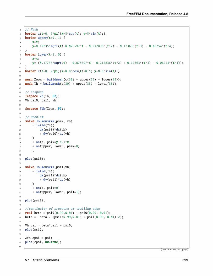
FreeFEM Documentation, Release 4.8
1 // Mesh2 border a(t=0, 2*pi)x=5*cos(t); y=5*sin(t);3 border upper(t=0, 1) 4 x=t;5 y=0.17735*sqrt(t)-0.075597*t - 0.212836*(t^2) + 0.17363*(t^3) - 0.06254*(t^4);6 7 border lower(t=1, 0) 8 x=t;9 y=-(0.17735*sqrt(t) - 0.075597*t - 0.212836*(t^2) + 0.17363*(t^3) - 0.06254*(t^4));
10 11 border c(t=0, 2*pi)x=0.8*cos(t)+0.5; y=0.8*sin(t);12
13 mesh Zoom = buildmesh(c(30) + upper(35) + lower(35));14 mesh Th = buildmesh(a(30) + upper(35) + lower(35));15
16 // Fespace17 fespace Vh(Th, P2);18 Vh psi0, psi1, vh;19
20 fespace ZVh(Zoom, P2);21
22 // Problem23 solve Joukowski0(psi0, vh)24 = int2d(Th)(25 dx(psi0)*dx(vh)26 + dy(psi0)*dy(vh)27 )28 + on(a, psi0=y-0.1*x)29 + on(upper, lower, psi0=0)30 ;31
32 plot(psi0);33
34 solve Joukowski1(psi1,vh)35 = int2d(Th)(36 dx(psi1)*dx(vh)37 + dy(psi1)*dy(vh)38 )39 + on(a, psi1=0)40 + on(upper, lower, psi1=1);41
42 plot(psi1);43
44 //continuity of pressure at trailing edge45 real beta = psi0(0.99,0.01) + psi0(0.99,-0.01);46 beta = -beta / (psi1(0.99,0.01) + psi1(0.99,-0.01)-2);47
48 Vh psi = beta*psi1 + psi0;49 plot(psi);50
51 ZVh Zpsi = psi;52 plot(Zpsi, bw=true);53
(continues on next page)
5.1. Static problems 529
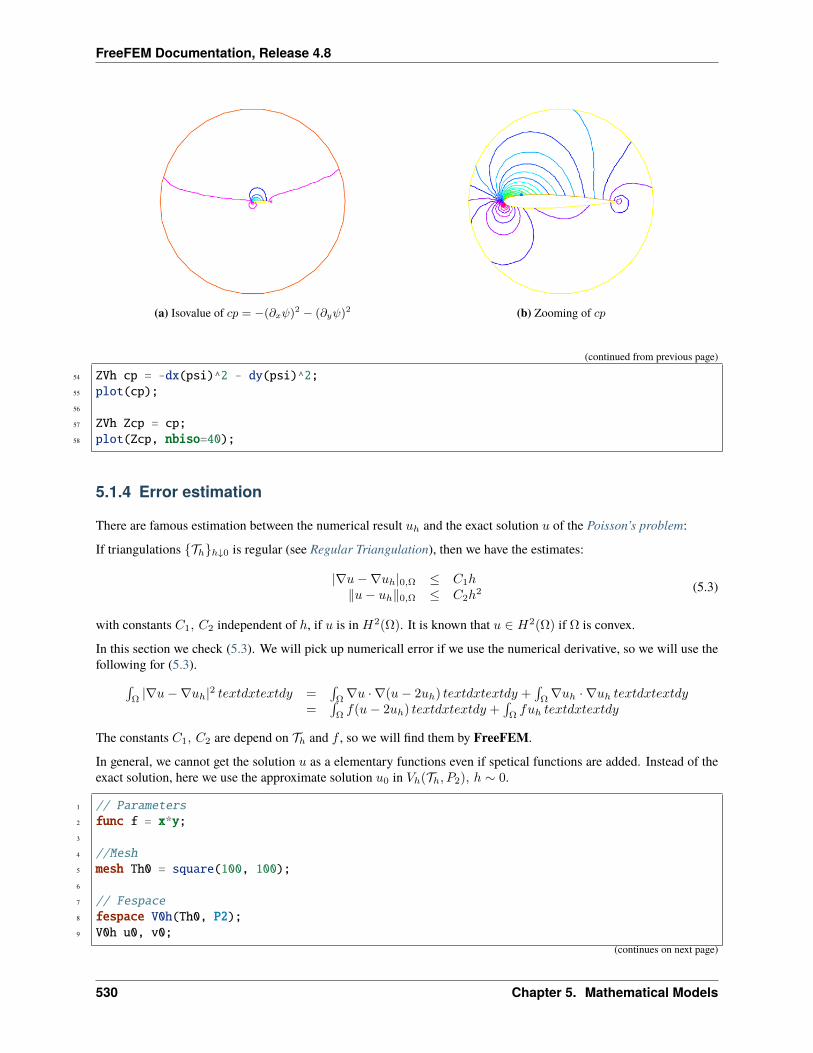
FreeFEM Documentation, Release 4.8
(a) Isovalue of 𝑐𝑝 = −(𝜕𝑥𝜓)2 − (𝜕𝑦𝜓)
2 (b) Zooming of 𝑐𝑝
(continued from previous page)
54 ZVh cp = -dx(psi)^2 - dy(psi)^2;55 plot(cp);56
57 ZVh Zcp = cp;58 plot(Zcp, nbiso=40);
5.1.4 Error estimation
There are famous estimation between the numerical result 𝑢ℎ and the exact solution 𝑢 of the Poisson’s problem:
If triangulations 𝒯ℎℎ↓0 is regular (see Regular Triangulation), then we have the estimates:
|∇𝑢−∇𝑢ℎ|0,Ω ≤ 𝐶1ℎ‖𝑢− 𝑢ℎ‖0,Ω ≤ 𝐶2ℎ
2 (5.3)
with constants 𝐶1, 𝐶2 independent of ℎ, if 𝑢 is in 𝐻2(Ω). It is known that 𝑢 ∈ 𝐻2(Ω) if Ω is convex.
In this section we check (5.3). We will pick up numericall error if we use the numerical derivative, so we will use thefollowing for (5.3).∫
Ω|∇𝑢−∇𝑢ℎ|2 𝑡𝑒𝑥𝑡𝑑𝑥𝑡𝑒𝑥𝑡𝑑𝑦 =
∫Ω∇𝑢 · ∇(𝑢− 2𝑢ℎ) 𝑡𝑒𝑥𝑡𝑑𝑥𝑡𝑒𝑥𝑡𝑑𝑦 +
∫Ω∇𝑢ℎ · ∇𝑢ℎ 𝑡𝑒𝑥𝑡𝑑𝑥𝑡𝑒𝑥𝑡𝑑𝑦
=∫Ω𝑓(𝑢− 2𝑢ℎ) 𝑡𝑒𝑥𝑡𝑑𝑥𝑡𝑒𝑥𝑡𝑑𝑦 +
∫Ω𝑓𝑢ℎ 𝑡𝑒𝑥𝑡𝑑𝑥𝑡𝑒𝑥𝑡𝑑𝑦
The constants 𝐶1, 𝐶2 are depend on 𝒯ℎ and 𝑓 , so we will find them by FreeFEM.
In general, we cannot get the solution 𝑢 as a elementary functions even if spetical functions are added. Instead of theexact solution, here we use the approximate solution 𝑢0 in 𝑉ℎ(𝒯ℎ, 𝑃2), ℎ ∼ 0.
1 // Parameters2 func f = x*y;3
4 //Mesh5 mesh Th0 = square(100, 100);6
7 // Fespace8 fespace V0h(Th0, P2);9 V0h u0, v0;
(continues on next page)
530 Chapter 5. Mathematical Models
FreeFEM Documentation, Release 4.8
(continued from previous page)
10
11 // Problem12 solve Poisson0 (u0, v0)13 = int2d(Th0)(14 dx(u0)*dx(v0)15 + dy(u0)*dy(v0)16 )17 - int2d(Th0)(18 f*v019 )20 + on(1, 2, 3, 4, u0=0)21 ;22 plot(u0);23
24 // Error loop25 real[int] errL2(10), errH1(10);26 for (int i = 1; i <= 10; i++)27 // Mesh28 mesh Th = square(5+i*3,5+i*3);29
30 // Fespace31 fespace Vh(Th, P1);32 Vh u, v;33 fespace Ph(Th, P0);34 Ph h = hTriangle; //get the size of all triangles35
36 // Problem37 solve Poisson (u, v)38 = int2d(Th)(39 dx(u)*dx(v)40 + dy(u)*dy(v)41 )42 - int2d(Th)(43 f*v44 )45 + on(1, 2, 3, 4, u=0)46 ;47
48 // Error49 V0h uu = u; //interpolate solution on first mesh50 errL2[i-1] = sqrt( int2d(Th0)((uu - u0)^2) )/h[].max^2;51 errH1[i-1] = sqrt( int2d(Th0)(f*(u0 - 2*uu + uu)) )/h[].max;52 53
54 // Display55 cout << "C1 = " << errL2.max << "("<<errL2.min<<")" << endl;56 cout << "C2 = " << errH1.max << "("<<errH1.min<<")" << endl;
We can guess that 𝐶1 = 0.0179253(0.0173266) and 𝐶2 = 0.0729566(0.0707543), where the numbers inside theparentheses are minimum in calculation.
5.1. Static problems 531
FreeFEM Documentation, Release 4.8
5.1.5 Periodic Boundary Conditions
We now solve the Poisson equation:
−∆𝑢 = 𝑠𝑖𝑛(𝑥+ 𝜋/4.) * 𝑐𝑜𝑠(𝑦 + 𝜋/4.)
on the square ]0, 2𝜋[2 under bi-periodic boundary condition 𝑢(0, 𝑦) = 𝑢(2𝜋, 𝑦) for all 𝑦 and 𝑢(𝑥, 0) = 𝑢(𝑥, 2𝜋) for all𝑥.
These boundary conditions are achieved from the definition of the periodic finite element space.
1 // Parameters2 func f = sin(x+pi/4.)*cos(y+pi/4.); //right hand side3
4 // Mesh5 mesh Th = square(10, 10, [2*x*pi, 2*y*pi]);6
7 // Fespace8 //defined the fespace with periodic condition9 //label: 2 and 4 are left and right side with y the curve abscissa
10 // 1 and 2 are bottom and upper side with x the curve abscissa11 fespace Vh(Th, P2, periodic=[[2, y], [4, y], [1, x], [3, x]]);12 Vh uh, vh;13
14 // Problem15 problem laplace (uh, vh)16 = int2d(Th)(17 dx(uh)*dx(vh)18 + dy(uh)*dy(vh)19 )20 + int2d(Th)(21 - f*vh22 )23 ;24
25 // Solve26 laplace;27
28 // Plot29 plot(uh, value=true);
The periodic condition does not necessarily require parallel boundaries. The following example give such example.
Tip: Periodic boundary conditions - non-parallel boundaries
1 // Parameters2 int n = 10;3 real r = 0.25;4 real r2 = 1.732;5 func f = (y+x+1)*(y+x-1)*(y-x+1)*(y-x-1);6
7 // Mesh8 border a(t=0, 1)x=-t+1; y=t; label=1;;9 border b(t=0, 1)x=-t; y=1-t; label=2;;
(continues on next page)
532 Chapter 5. Mathematical Models
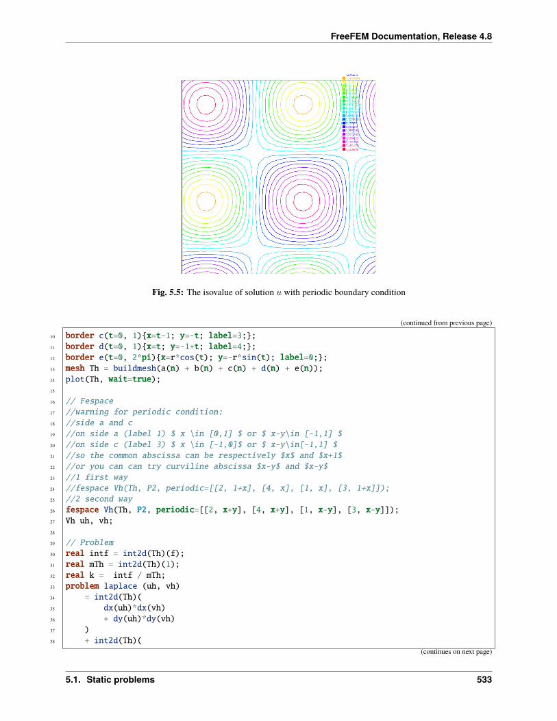
FreeFEM Documentation, Release 4.8
Fig. 5.5: The isovalue of solution 𝑢 with periodic boundary condition
(continued from previous page)
10 border c(t=0, 1)x=t-1; y=-t; label=3;;11 border d(t=0, 1)x=t; y=-1+t; label=4;;12 border e(t=0, 2*pi)x=r*cos(t); y=-r*sin(t); label=0;;13 mesh Th = buildmesh(a(n) + b(n) + c(n) + d(n) + e(n));14 plot(Th, wait=true);15
16 // Fespace17 //warning for periodic condition:18 //side a and c19 //on side a (label 1) $ x \in [0,1] $ or $ x-y\in [-1,1] $20 //on side c (label 3) $ x \in [-1,0]$ or $ x-y\in[-1,1] $21 //so the common abscissa can be respectively $x$ and $x+1$22 //or you can can try curviline abscissa $x-y$ and $x-y$23 //1 first way24 //fespace Vh(Th, P2, periodic=[[2, 1+x], [4, x], [1, x], [3, 1+x]]);25 //2 second way26 fespace Vh(Th, P2, periodic=[[2, x+y], [4, x+y], [1, x-y], [3, x-y]]);27 Vh uh, vh;28
29 // Problem30 real intf = int2d(Th)(f);31 real mTh = int2d(Th)(1);32 real k = intf / mTh;33 problem laplace (uh, vh)34 = int2d(Th)(35 dx(uh)*dx(vh)36 + dy(uh)*dy(vh)37 )38 + int2d(Th)(
(continues on next page)
5.1. Static problems 533
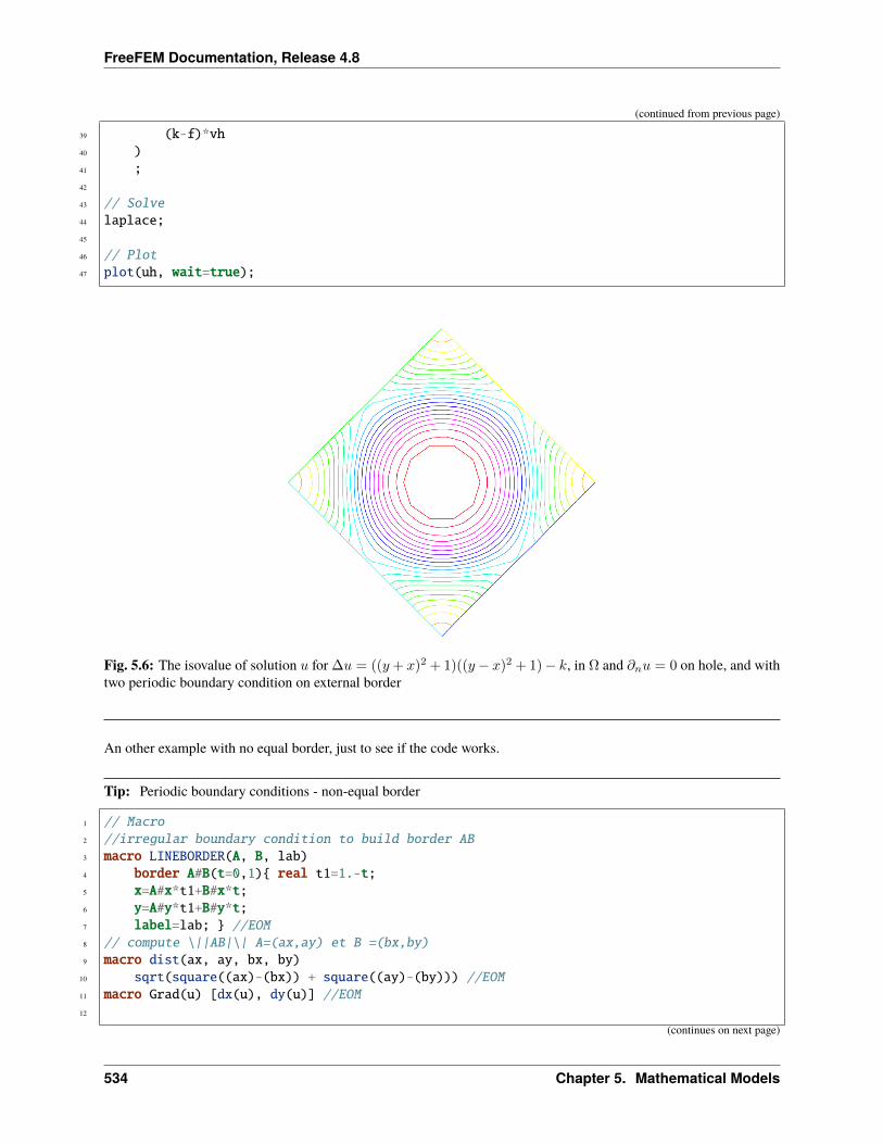
FreeFEM Documentation, Release 4.8
(continued from previous page)
39 (k-f)*vh40 )41 ;42
43 // Solve44 laplace;45
46 // Plot47 plot(uh, wait=true);
Fig. 5.6: The isovalue of solution 𝑢 for ∆𝑢 = ((𝑦 + 𝑥)2 + 1)((𝑦− 𝑥)2 + 1)− 𝑘, in Ω and 𝜕𝑛𝑢 = 0 on hole, and withtwo periodic boundary condition on external border
An other example with no equal border, just to see if the code works.
Tip: Periodic boundary conditions - non-equal border
1 // Macro2 //irregular boundary condition to build border AB3 macro LINEBORDER(A, B, lab)4 border A#B(t=0,1) real t1=1.-t;5 x=A#x*t1+B#x*t;6 y=A#y*t1+B#y*t;7 label=lab; //EOM8 // compute \||AB|\| A=(ax,ay) et B =(bx,by)9 macro dist(ax, ay, bx, by)
10 sqrt(square((ax)-(bx)) + square((ay)-(by))) //EOM11 macro Grad(u) [dx(u), dy(u)] //EOM12
(continues on next page)
534 Chapter 5. Mathematical Models
FreeFEM Documentation, Release 4.8
(continued from previous page)
13 // Parameters14 int n = 10;15 real Ax = 0.9, Ay = 1;16 real Bx = 2, By = 1;17 real Cx = 2.5, Cy = 2.5;18 real Dx = 1, Dy = 2;19 real gx = (Ax+Bx+Cx+Dx)/4.;20 real gy = (Ay+By+Cy+Dy)/4.;21
22 // Mesh23 LINEBORDER(A,B,1)24 LINEBORDER(B,C,2)25 LINEBORDER(C,D,3)26 LINEBORDER(D,A,4)27 mesh Th=buildmesh(AB(n)+BC(n)+CD(n)+DA(n),fixedborder=1);28
29 // Fespace30 real l1 = dist(Ax,Ay,Bx,By);31 real l2 = dist(Bx,By,Cx,Cy);32 real l3 = dist(Cx,Cy,Dx,Dy);33 real l4 = dist(Dx,Dy,Ax,Ay);34 func s1 = dist(Ax,Ay,x,y)/l1; //absisse on AB = ||AX||/||AB||35 func s2 = dist(Bx,By,x,y)/l2; //absisse on BC = ||BX||/||BC||36 func s3 = dist(Cx,Cy,x,y)/l3; //absisse on CD = ||CX||/||CD||37 func s4 = dist(Dx,Dy,x,y)/l4; //absisse on DA = ||DX||/||DA||38 verbosity = 6; //to see the abscisse value of the periodic condition39 fespace Vh(Th, P1, periodic=[[1, s1], [3, s3], [2, s2], [4, s4]]);40 verbosity = 1; //reset verbosity41 Vh u, v;42
43 real cc = 0;44 cc = int2d(Th)((x-gx)*(y-gy)-cc)/Th.area;45 cout << "compatibility = " << int2d(Th)((x-gx)*(y-gy)-cc) <<endl;46
47 // Problem48 solve Poisson (u, v)49 = int2d(Th)(50 Grad(u)'*Grad(v)51 + 1e-10*u*v52 )53 -int2d(Th)(54 10*v*((x-gx)*(y-gy)-cc)55 )56 ;57
58 // Plot59 plot(u, value=true);
Tip: Periodic boundry conditions - Poisson cube-balloon
5.1. Static problems 535
FreeFEM Documentation, Release 4.8
1 load "msh3" load "tetgen" load "medit"2
3 // Parameters4 real hs = 0.1; //mesh size on sphere5 int[int] N = [20, 20, 20];6 real [int,int] B = [[-1, 1], [-1, 1], [-1, 1]];7 int [int,int] L = [[1, 2], [3, 4], [5, 6]];8
9 real x0 = 0.3, y0 = 0.4, z0 = 06;10 func f = sin(x*2*pi+x0)*sin(y*2*pi+y0)*sin(z*2*pi+z0);11
12 // Mesh13 bool buildTh = 0;14 mesh3 Th;15 try //a way to build one time the mesh or read it if the file exist16 Th = readmesh3("Th-hex-sph.mesh");17 18 catch (...)19 buildTh = 1;20 21
22 if (buildTh)23 include "MeshSurface.idp"24
25 // Surface Mesh26 mesh3 ThH = SurfaceHex(N, B, L, 1);27 mesh3 ThS = Sphere(0.5, hs, 7, 1);28
29 mesh3 ThHS = ThH + ThS;30
31 real voltet = (hs^3)/6.;32 real[int] domain = [0, 0, 0, 1, voltet, 0, 0, 0.7, 2, voltet];33 Th = tetg(ThHS, switch="pqaAAYYQ", nbofregions=2, regionlist=domain);34
35 savemesh(Th, "Th-hex-sph.mesh");36 37
38 // Fespace39 fespace Ph(Th, P0);40 Ph reg = region;41 cout << " centre = " << reg(0,0,0) << endl;42 cout << " exterieur = " << reg(0,0,0.7) << endl;43
44 verbosity = 50;45 fespace Vh(Th, P1, periodic=[[3, x, z], [4, x, z], [1, y, z], [2, y, z], [5, x, y], [6,
→˓x, y]]);46 verbosity = 1;47 Vh uh,vh;48
49 // Macro50 macro Grad(u) [dx(u),dy(u),dz(u)] // EOM51
52 // Problem(continues on next page)
536 Chapter 5. Mathematical Models
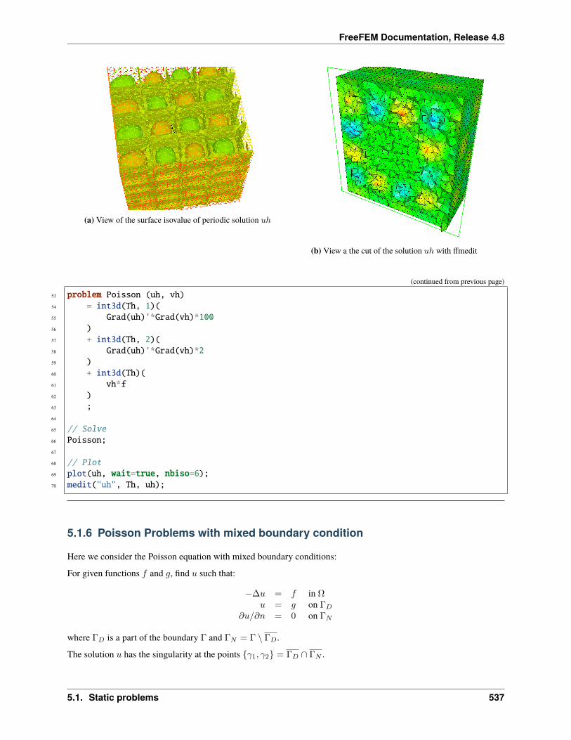
FreeFEM Documentation, Release 4.8
(a) View of the surface isovalue of periodic solution 𝑢ℎ
(b) View a the cut of the solution 𝑢ℎ with ffmedit
(continued from previous page)
53 problem Poisson (uh, vh)54 = int3d(Th, 1)(55 Grad(uh)'*Grad(vh)*10056 )57 + int3d(Th, 2)(58 Grad(uh)'*Grad(vh)*259 )60 + int3d(Th)(61 vh*f62 )63 ;64
65 // Solve66 Poisson;67
68 // Plot69 plot(uh, wait=true, nbiso=6);70 medit("uh", Th, uh);
5.1.6 Poisson Problems with mixed boundary condition
Here we consider the Poisson equation with mixed boundary conditions:
For given functions 𝑓 and 𝑔, find 𝑢 such that:
−∆𝑢 = 𝑓 in Ω𝑢 = 𝑔 on Γ𝐷
𝜕𝑢/𝜕𝑛 = 0 on Γ𝑁
where Γ𝐷 is a part of the boundary Γ and Γ𝑁 = Γ ∖ Γ𝐷.
The solution 𝑢 has the singularity at the points 𝛾1, 𝛾2 = Γ𝐷 ∩ Γ𝑁 .
5.1. Static problems 537
FreeFEM Documentation, Release 4.8
When Ω = (𝑥, 𝑦); −1 < 𝑥 < 1, 0 < 𝑦 < 1, Γ𝑁 = (𝑥, 𝑦); −1 ≤ 𝑥 < 0, 𝑦 = 0, Γ𝐷 = 𝜕Ω ∖ Γ𝑁 , the singularitywill appear at 𝛾1 = (0, 0), 𝛾2(−1, 0), and 𝑢 has the expression:
𝑢 = 𝐾𝑖𝑢𝑆 + 𝑢𝑅, 𝑢𝑅 ∈ 𝐻2(near 𝛾𝑖), 𝑖 = 1, 2
with a constants 𝐾𝑖.
Here 𝑢𝑆 = 𝑟1/2𝑗 sin(𝜃𝑗/2) by the local polar coordinate (𝑟𝑗 , 𝜃𝑗 at 𝛾𝑗 such that (𝑟1, 𝜃1) = (𝑟, 𝜃).
Instead of polar coordinate system (𝑟, 𝜃), we use that 𝑟 = sqrt (𝑥2 + 𝑦2) and 𝜃 = atan2 (𝑦, 𝑥) in FreeFEM.
Assume that 𝑓 = −2 × 30(𝑥2 + 𝑦2) and 𝑔 = 𝑢𝑒 = 10(𝑥2 + 𝑦2)1/4 sin([tan−1(𝑦/𝑥)]/2
)+ 30(𝑥2𝑦2), where 𝑢𝑒S is
the exact solution.
1 // Parameters2 func f = -2*30*(x^2+y^2); //given function3 //the singular term of the solution is K*us (K: constant)4 func us = sin(atan2(y,x)/2)*sqrt( sqrt(x^2+y^2) );5 real K = 10.;6 func ue = K*us + 30*(x^2*y^2);7
8 // Mesh9 border N(t=0, 1)x=-1+t; y=0; label=1;;
10 border D1(t=0, 1)x=t; y=0; label=2;;11 border D2(t=0, 1)x=1; y=t; label=2;;12 border D3(t=0, 2)x=1-t; y=1; label=2;;13 border D4(t=0, 1)x=-1; y=1-t; label=2;;14
15 mesh T0h = buildmesh(N(10) + D1(10) + D2(10) + D3(20) + D4(10));16 plot(T0h, wait=true);17
18 // Fespace19 fespace V0h(T0h, P1);20 V0h u0, v0;21
22 //Problem23 solve Poisson0 (u0, v0)24 = int2d(T0h)(25 dx(u0)*dx(v0)26 + dy(u0)*dy(v0)27 )28 - int2d(T0h)(29 f*v030 )31 + on(2, u0=ue)32 ;33
34 // Mesh adaptation by the singular term35 mesh Th = adaptmesh(T0h, us);36 for (int i = 0; i < 5; i++)37 mesh Th = adaptmesh(Th, us);38
39 // Fespace40 fespace Vh(Th, P1);41 Vh u, v;
(continues on next page)
538 Chapter 5. Mathematical Models
FreeFEM Documentation, Release 4.8
(continued from previous page)
42
43 // Problem44 solve Poisson (u, v)45 = int2d(Th)(46 dx(u)*dx(v)47 + dy(u)*dy(v)48 )49 - int2d(Th)(50 f*v51 )52 + on(2, u=ue)53 ;54
55 // Plot56 plot(Th);57 plot(u, wait=true);58
59 // Error in H1 norm60 Vh uue = ue;61 real H1e = sqrt( int2d(Th)(dx(uue)^2 + dy(uue)^2 + uue^2) );62 Vh err0 = u0 - ue;63 Vh err = u - ue;64 Vh H1err0 = int2d(Th)(dx(err0)^2 + dy(err0)^2 + err0^2);65 Vh H1err = int2d(Th)(dx(err)^2 + dy(err)^2 + err^2);66 cout << "Relative error in first mesh = "<< int2d(Th)(H1err0)/H1e << endl;67 cout << "Relative error in adaptive mesh = "<< int2d(Th)(H1err)/H1e << endl;
From line 35 to 37, mesh adaptations are done using the base of singular term.
In line 61, H1e = |𝑢𝑒|1,Ω is calculated.
In lines 64 and 65, the relative errors are calculated, that is:
‖𝑢0ℎ − 𝑢𝑒‖1,Ω/𝐻1𝑒 = 0.120421‖𝑢𝑎ℎ − 𝑢𝑒‖1,Ω/𝐻1𝑒 = 0.0150581
where 𝑢0ℎ is the numerical solution in T0h and 𝑢𝑎ℎ is u in this program.
5.1.7 Poisson with mixed finite element
Here we consider the Poisson equation with mixed boundary value problems:
For given functions 𝑓 , 𝑔𝑑, 𝑔𝑛, find 𝑝 such that
−∆𝑝 = 1 in Ω𝑝 = 𝑔𝑑 on Γ𝐷
𝜕𝑝/𝜕𝑛 = 𝑔𝑛 on Γ𝑁
where Γ𝐷 is a part of the boundary Γ and Γ𝑁 = Γ ∖ Γ𝐷.
The mixed formulation is: find 𝑝 and u such that:
∇𝑝+ u = 0 in Ω∇.u = 𝑓 in Ω𝑝 = 𝑔𝑑 on Γ𝐷
𝜕𝑢.𝑛 = g𝑛.𝑛 on Γ𝑁
5.1. Static problems 539
FreeFEM Documentation, Release 4.8
where g𝑛 is a vector such that g𝑛.𝑛 = 𝑔𝑛.
The variational formulation is:
∀v ∈ V0 :∫Ω𝑝∇.𝑣 + vv =
∫Γ𝑑𝑔𝑑v.𝑛
∀𝑞 ∈ P :∫Ω𝑞∇.𝑢 =
∫Ω𝑞𝑓
𝜕𝑢.𝑛 = g𝑛.𝑛 on Γ𝑁
where the functional space are:
P = 𝐿2(Ω), V = 𝐻(𝑑𝑖𝑣) = v ∈ 𝐿2(Ω)2,∇.v ∈ 𝐿2(Ω)
and:
V0 = v ∈ V; v.𝑛 = 0 on Γ𝑁
To write the FreeFEM example, we have just to choose the finites elements spaces.
Here V space is discretize with Raviart-Thomas finite element RT0 and P is discretize by constant finite element P0.
Example 9.10 LaplaceRT.edp
1 // Parameters2 func gd = 1.;3 func g1n = 1.;4 func g2n = 1.;5
6 // Mesh7 mesh Th = square(10, 10);8
9 // Fespace10 fespace Vh(Th, RT0);11 Vh [u1, u2];12 Vh [v1, v2];13
14 fespace Ph(Th, P0);15 Ph p, q;16
17 // Problem18 problem laplaceMixte ([u1, u2, p], [v1, v2, q], solver=GMRES, eps=1.0e-10, tgv=1e30,
→˓dimKrylov=150)19 = int2d(Th)(20 p*q*1e-15 //this term is here to be sure21 // that all sub matrix are inversible (LU requirement)22 + u1*v123 + u2*v224 + p*(dx(v1)+dy(v2))25 + (dx(u1)+dy(u2))*q26 )27 + int2d(Th) (28 q29 )30 - int1d(Th, 1, 2, 3)(31 gd*(v1*N.x +v2*N.y)32 )33 + on(4, u1=g1n, u2=g2n)
(continues on next page)
540 Chapter 5. Mathematical Models
FreeFEM Documentation, Release 4.8
(continued from previous page)
34 ;35
36 // Solve37 laplaceMixte;38
39 // Plot40 plot([u1, u2], coef=0.1, wait=true, value=true);41 plot(p, fill=1, wait=true, value=true);
5.1.8 Metric Adaptation and residual error indicator
We do metric mesh adaption and compute the classical residual error indicator 𝜂𝑇 on the element 𝑇 for the Poissonproblem.
First, we solve the same problem as in a previous example.
1 // Parameters2 real[int] viso(21);3 for (int i = 0; i < viso.n; i++)4 viso[i] = 10.^(+(i-16.)/2.);5 real error = 0.01;6 func f = (x-y);7
8 // Mesh9 border ba(t=0, 1.0)x=t; y=0; label=1;
10 border bb(t=0, 0.5)x=1; y=t; label=2;11 border bc(t=0, 0.5)x=1-t; y=0.5; label=3;12 border bd(t=0.5, 1)x=0.5; y=t; label=4;13 border be(t=0.5, 1)x=1-t; y=1; label=5;14 border bf(t=0.0, 1)x=0; y=1-t; label=6;15 mesh Th = buildmesh(ba(6) + bb(4) + bc(4) + bd(4) + be(4) + bf(6));16
17 // Fespace18 fespace Vh(Th, P2);19 Vh u, v;20
21 fespace Nh(Th, P0);22 Nh rho;23
24 // Problem25 problem Probem1 (u, v, solver=CG, eps=1.0e-6)26 = int2d(Th, qforder=5)(27 u*v*1.0e-1028 + dx(u)*dx(v)29 + dy(u)*dy(v)30 )31 + int2d(Th, qforder=5)(32 - f*v33 )34 ;
5.1. Static problems 541
FreeFEM Documentation, Release 4.8
Now, the local error indicator 𝜂𝑇 is:
𝜂𝑇 =
(ℎ2𝑇 ||𝑓 + ∆𝑢ℎ||2𝐿2(𝑇 ) +
∑𝑒∈ℰ𝐾
ℎ𝑒 || [𝜕𝑢ℎ𝜕𝑛𝑘
] ||2𝐿2(𝑒)
) 12
where ℎ𝑇 is the longest edge of 𝑇 , ℰ𝑇 is the set of 𝑇 edge not on Γ = 𝜕Ω, 𝑛𝑇 is the outside unit normal to 𝐾, ℎ𝑒 isthe length of edge 𝑒, [𝑔] is the jump of the function 𝑔 across edge (left value minus right value).
Of course, we can use a variational form to compute 𝜂2𝑇 , with test function constant function in each triangle.
1 // Error2 varf indicator2 (uu, chiK)3 = intalledges(Th)(4 chiK*lenEdge*square(jump(N.x*dx(u) + N.y*dy(u)))5 )6 + int2d(Th)(7 chiK*square(hTriangle*(f + dxx(u) + dyy(u)))8 )9 ;
10
11 // Mesh adaptation loop12 for (int i = 0; i < 4; i++)13 // Solve14 Probem1;15 cout << u[].min << " " << u[].max << endl;16 plot(u, wait=true);17
18 // Error19 rho[] = indicator2(0, Nh);20 rho = sqrt(rho);21 cout << "rho = min " << rho[].min << " max=" << rho[].max << endl;22 plot(rho, fill=true, wait=true, cmm="indicator density", value=true, viso=viso,
→˓nbiso=viso.n);23
24 // Mesh adaptation25 plot(Th, wait=true, cmm="Mesh (before adaptation)");26 Th = adaptmesh(Th, [dx(u), dy(u)], err=error, anisomax=1);27 plot(Th, wait=true, cmm="Mesh (after adaptation)");28 u = u;29 rho = rho;30 error = error/2;31
If the method is correct, we expect to look the graphics by an almost constant function 𝜂 on your computer as in Fig.5.8a and Fig. 5.8b.
542 Chapter 5. Mathematical Models
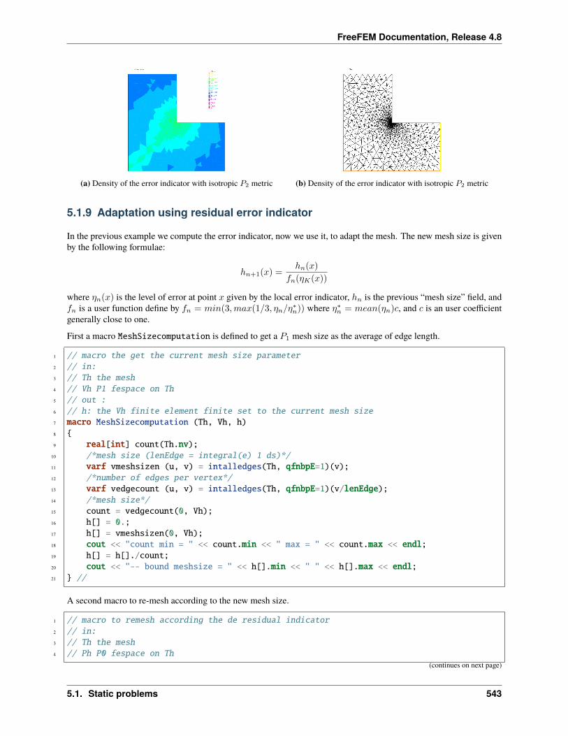
FreeFEM Documentation, Release 4.8
(a) Density of the error indicator with isotropic 𝑃2 metric (b) Density of the error indicator with isotropic 𝑃2 metric
5.1.9 Adaptation using residual error indicator
In the previous example we compute the error indicator, now we use it, to adapt the mesh. The new mesh size is givenby the following formulae:
ℎ𝑛+1(𝑥) =ℎ𝑛(𝑥)
𝑓𝑛(𝜂𝐾(𝑥))
where 𝜂𝑛(𝑥) is the level of error at point 𝑥 given by the local error indicator, ℎ𝑛 is the previous “mesh size” field, and𝑓𝑛 is a user function define by 𝑓𝑛 = 𝑚𝑖𝑛(3,𝑚𝑎𝑥(1/3, 𝜂𝑛/𝜂
*𝑛)) where 𝜂*𝑛 = 𝑚𝑒𝑎𝑛(𝜂𝑛)𝑐, and 𝑐 is an user coefficient
generally close to one.
First a macro MeshSizecomputation is defined to get a 𝑃1 mesh size as the average of edge length.
1 // macro the get the current mesh size parameter2 // in:3 // Th the mesh4 // Vh P1 fespace on Th5 // out :6 // h: the Vh finite element finite set to the current mesh size7 macro MeshSizecomputation (Th, Vh, h)8 9 real[int] count(Th.nv);
10 /*mesh size (lenEdge = integral(e) 1 ds)*/11 varf vmeshsizen (u, v) = intalledges(Th, qfnbpE=1)(v);12 /*number of edges per vertex*/13 varf vedgecount (u, v) = intalledges(Th, qfnbpE=1)(v/lenEdge);14 /*mesh size*/15 count = vedgecount(0, Vh);16 h[] = 0.;17 h[] = vmeshsizen(0, Vh);18 cout << "count min = " << count.min << " max = " << count.max << endl;19 h[] = h[]./count;20 cout << "-- bound meshsize = " << h[].min << " " << h[].max << endl;21 //
A second macro to re-mesh according to the new mesh size.
1 // macro to remesh according the de residual indicator2 // in:3 // Th the mesh4 // Ph P0 fespace on Th
(continues on next page)
5.1. Static problems 543
FreeFEM Documentation, Release 4.8
(continued from previous page)
5 // Vh P1 fespace on Th6 // vindicator the varf to evaluate the indicator7 // coef on etameam8 macro ReMeshIndicator (Th, Ph, Vh, vindicator, coef)9
10 Vh h=0;11 /*evaluate the mesh size*/12 MeshSizecomputation(Th, Vh, h);13 Ph etak;14 etak[] = vindicator(0, Ph);15 etak[] = sqrt(etak[]);16 real etastar= coef*(etak[].sum/etak[].n);17 cout << "etastar = " << etastar << " sum = " << etak[].sum << " " << endl;18
19 /*etaK is discontinous*/20 /*we use P1 L2 projection with mass lumping*/21 Vh fn, sigma;22 varf veta(unused, v) = int2d(Th)(etak*v);23 varf vun(unused, v) = int2d(Th)(1*v);24 fn[] = veta(0, Vh);25 sigma[] = vun(0, Vh);26 fn[] = fn[]./ sigma[];27 fn = max(min(fn/etastar,3.),0.3333);28
29 /*new mesh size*/30 h = h / fn;31 /*build the mesh*/32 Th = adaptmesh(Th, IsMetric=1, h, splitpbedge=1, nbvx=10000);33 //
1 // Parameters2 real hinit = 0.2; //initial mesh size3 func f=(x-y);4
5 // Mesh6 border ba(t=0, 1.0)x=t; y=0; label=1;7 border bb(t=0, 0.5)x=1; y=t; label=2;8 border bc(t=0, 0.5)x=1-t; y=0.5; label=3;9 border bd(t=0.5, 1)x=0.5; y=t; label=4;
10 border be(t=0.5, 1)x=1-t; y=1; label=5;11 border bf(t=0.0, 1)x=0; y=1-t; label=6;12 mesh Th = buildmesh(ba(6) + bb(4) + bc(4) + bd(4) + be(4) + bf(6));13
14 // Fespace15 fespace Vh(Th, P1); //for the mesh size and solution16 Vh h = hinit; //the FE function for the mesh size17 Vh u, v;18
19 fespace Ph(Th, P0); //for the error indicator20
21 //Build a mesh with the given mesh size hinit22 Th = adaptmesh(Th, h, IsMetric=1, splitpbedge=1, nbvx=10000);
(continues on next page)
544 Chapter 5. Mathematical Models
FreeFEM Documentation, Release 4.8
(continued from previous page)
23 plot(Th, wait=1);24
25 // Problem26 problem Poisson (u, v)27 = int2d(Th, qforder=5)(28 u*v*1.0e-1029 + dx(u)*dx(v)30 + dy(u)*dy(v)31 )32 - int2d(Th, qforder=5)(33 f*v34 )35 ;36
37 varf indicator2 (unused, chiK)38 = intalledges(Th)(39 chiK*lenEdge*square(jump(N.x*dx(u) + N.y*dy(u)))40 )41 + int2d(Th)(42 chiK*square(hTriangle*(f + dxx(u) + dyy(u)))43 )44 ;45
46 // Mesh adaptation loop47 for (int i = 0; i < 10; i++)48 u = u;49
50 // Solve51 Poisson;52 plot(Th, u, wait=true);53
54 real cc = 0.8;55 if (i > 5) cc=1;56 ReMeshIndicator(Th, Ph, Vh, indicator2, cc);57 plot(Th, wait=true);58
5.2 Elasticity
Consider an elastic plate with undeformed shape Ω×]− ℎ, ℎ[ in R3, Ω ⊂ R2.
By the deformation of the plate, we assume that a point 𝑃 (𝑥1, 𝑥2, 𝑥3) moves to 𝒫(𝜉1, 𝜉2, 𝜉3). The vector u =(𝑢1, 𝑢2, 𝑢3) = (𝜉1 − 𝑥1, 𝜉2 − 𝑥2, 𝜉3 − 𝑥3) is called the displacement vector.
By the deformation, the line segment x,x + 𝜏∆x moves approximately to x + u(x),x + 𝜏∆x + u(x + 𝜏∆x) forsmall 𝜏 , where x = (𝑥1, 𝑥2, 𝑥3), ∆x = (∆𝑥1,∆𝑥2,∆𝑥3).
We now calculate the ratio between two segments:
𝜂(𝜏) = 𝜏−1|∆x|−1 (|u(x + 𝜏∆x)− u(x) + 𝜏∆x| − 𝜏 |∆x|)
5.2. Elasticity 545
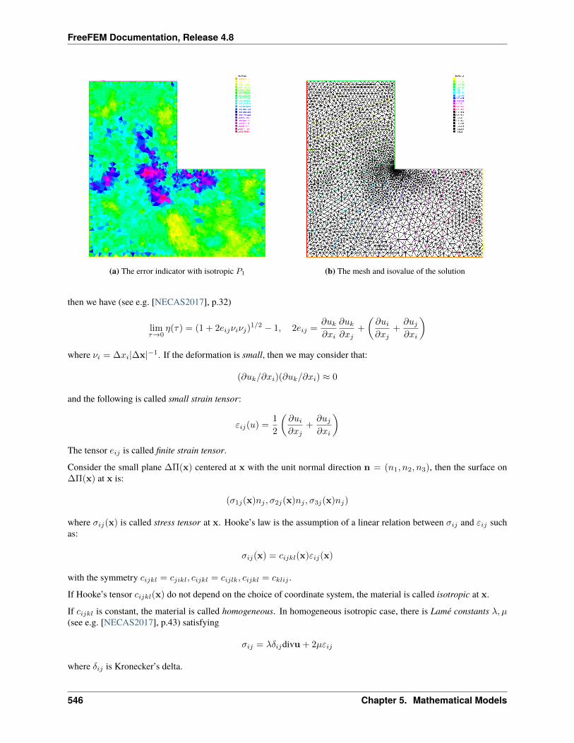
FreeFEM Documentation, Release 4.8
(a) The error indicator with isotropic 𝑃1 (b) The mesh and isovalue of the solution
then we have (see e.g. [NECAS2017], p.32)
lim𝜏→0
𝜂(𝜏) = (1 + 2𝑒𝑖𝑗𝜈𝑖𝜈𝑗)1/2 − 1, 2𝑒𝑖𝑗 =
𝜕𝑢𝑘𝜕𝑥𝑖
𝜕𝑢𝑘𝜕𝑥𝑗
+
(𝜕𝑢𝑖𝜕𝑥𝑗
+𝜕𝑢𝑗𝜕𝑥𝑖
)where 𝜈𝑖 = ∆𝑥𝑖|∆x|−1. If the deformation is small, then we may consider that:
(𝜕𝑢𝑘/𝜕𝑥𝑖)(𝜕𝑢𝑘/𝜕𝑥𝑖) ≈ 0
and the following is called small strain tensor:
𝜀𝑖𝑗(𝑢) =1
2
(𝜕𝑢𝑖𝜕𝑥𝑗
+𝜕𝑢𝑗𝜕𝑥𝑖
)The tensor 𝑒𝑖𝑗 is called finite strain tensor.
Consider the small plane ∆Π(x) centered at x with the unit normal direction n = (𝑛1, 𝑛2, 𝑛3), then the surface on∆Π(x) at x is:
(𝜎1𝑗(x)𝑛𝑗 , 𝜎2𝑗(x)𝑛𝑗 , 𝜎3𝑗(x)𝑛𝑗)
where 𝜎𝑖𝑗(x) is called stress tensor at x. Hooke’s law is the assumption of a linear relation between 𝜎𝑖𝑗 and 𝜀𝑖𝑗 suchas:
𝜎𝑖𝑗(x) = 𝑐𝑖𝑗𝑘𝑙(x)𝜀𝑖𝑗(x)
with the symmetry 𝑐𝑖𝑗𝑘𝑙 = 𝑐𝑗𝑖𝑘𝑙, 𝑐𝑖𝑗𝑘𝑙 = 𝑐𝑖𝑗𝑙𝑘, 𝑐𝑖𝑗𝑘𝑙 = 𝑐𝑘𝑙𝑖𝑗 .
If Hooke’s tensor 𝑐𝑖𝑗𝑘𝑙(x) do not depend on the choice of coordinate system, the material is called isotropic at x.
If 𝑐𝑖𝑗𝑘𝑙 is constant, the material is called homogeneous. In homogeneous isotropic case, there is Lamé constants 𝜆, 𝜇(see e.g. [NECAS2017], p.43) satisfying
𝜎𝑖𝑗 = 𝜆𝛿𝑖𝑗divu + 2𝜇𝜀𝑖𝑗
where 𝛿𝑖𝑗 is Kronecker’s delta.
546 Chapter 5. Mathematical Models
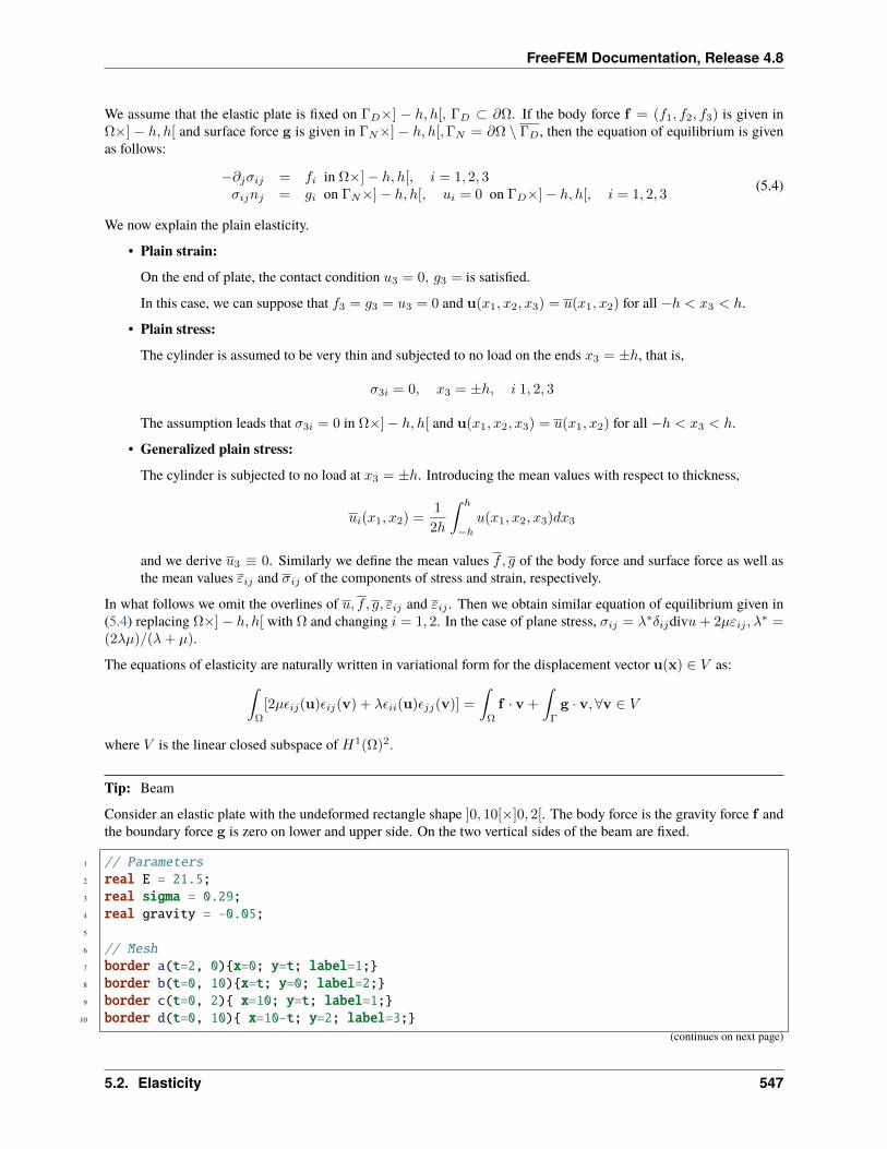
FreeFEM Documentation, Release 4.8
We assume that the elastic plate is fixed on Γ𝐷×] − ℎ, ℎ[, Γ𝐷 ⊂ 𝜕Ω. If the body force f = (𝑓1, 𝑓2, 𝑓3) is given inΩ×] − ℎ, ℎ[ and surface force g is given in Γ𝑁×] − ℎ, ℎ[,Γ𝑁 = 𝜕Ω ∖ Γ𝐷, then the equation of equilibrium is givenas follows:
−𝜕𝑗𝜎𝑖𝑗 = 𝑓𝑖 in Ω×]− ℎ, ℎ[, 𝑖 = 1, 2, 3𝜎𝑖𝑗𝑛𝑗 = 𝑔𝑖 on Γ𝑁×]− ℎ, ℎ[, 𝑢𝑖 = 0 on Γ𝐷×]− ℎ, ℎ[, 𝑖 = 1, 2, 3
(5.4)
We now explain the plain elasticity.
• Plain strain:On the end of plate, the contact condition 𝑢3 = 0, 𝑔3 = is satisfied.
In this case, we can suppose that 𝑓3 = 𝑔3 = 𝑢3 = 0 and u(𝑥1, 𝑥2, 𝑥3) = 𝑢(𝑥1, 𝑥2) for all −ℎ < 𝑥3 < ℎ.
• Plain stress:The cylinder is assumed to be very thin and subjected to no load on the ends 𝑥3 = ±ℎ, that is,
𝜎3𝑖 = 0, 𝑥3 = ±ℎ, 𝑖 1, 2, 3
The assumption leads that 𝜎3𝑖 = 0 in Ω×]− ℎ, ℎ[ and u(𝑥1, 𝑥2, 𝑥3) = 𝑢(𝑥1, 𝑥2) for all −ℎ < 𝑥3 < ℎ.
• Generalized plain stress:The cylinder is subjected to no load at 𝑥3 = ±ℎ. Introducing the mean values with respect to thickness,
𝑢𝑖(𝑥1, 𝑥2) =1
2ℎ
∫ ℎ
−ℎ𝑢(𝑥1, 𝑥2, 𝑥3)𝑑𝑥3
and we derive 𝑢3 ≡ 0. Similarly we define the mean values 𝑓, 𝑔 of the body force and surface force as well asthe mean values 𝜀𝑖𝑗 and 𝜎𝑖𝑗 of the components of stress and strain, respectively.
In what follows we omit the overlines of 𝑢, 𝑓, 𝑔, 𝜀𝑖𝑗 and 𝜀𝑖𝑗 . Then we obtain similar equation of equilibrium given in(5.4) replacing Ω×]− ℎ, ℎ[ with Ω and changing 𝑖 = 1, 2. In the case of plane stress, 𝜎𝑖𝑗 = 𝜆*𝛿𝑖𝑗div𝑢+ 2𝜇𝜀𝑖𝑗 , 𝜆
* =(2𝜆𝜇)/(𝜆+ 𝜇).
The equations of elasticity are naturally written in variational form for the displacement vector u(x) ∈ 𝑉 as:∫Ω
[2𝜇𝜖𝑖𝑗(u)𝜖𝑖𝑗(v) + 𝜆𝜖𝑖𝑖(u)𝜖𝑗𝑗(v)] =
∫Ω
f · v +
∫Γ
g · v,∀v ∈ 𝑉
where 𝑉 is the linear closed subspace of 𝐻1(Ω)2.
Tip: Beam
Consider an elastic plate with the undeformed rectangle shape ]0, 10[×]0, 2[. The body force is the gravity force f andthe boundary force g is zero on lower and upper side. On the two vertical sides of the beam are fixed.
1 // Parameters2 real E = 21.5;3 real sigma = 0.29;4 real gravity = -0.05;5
6 // Mesh7 border a(t=2, 0)x=0; y=t; label=1;8 border b(t=0, 10)x=t; y=0; label=2;9 border c(t=0, 2) x=10; y=t; label=1;
10 border d(t=0, 10) x=10-t; y=2; label=3;(continues on next page)
5.2. Elasticity 547
FreeFEM Documentation, Release 4.8
(continued from previous page)
11 mesh th = buildmesh(b(20) + c(5) + d(20) + a(5));12
13 // Fespace14 fespace Vh(th, [P1, P1]);15 Vh [uu, vv];16 Vh [w, s];17
18 // Macro19 real sqrt2 = sqrt(2.);20 macro epsilon(u1, u2) [dx(u1), dy(u2), (dy(u1)+dx(u2))/sqrt2] //21 macro div(u,v) (dx(u) + dy(v)) //22
23 // Problem24 real mu = E/(2*(1+sigma));25 real lambda = E*sigma/((1+sigma)*(1-2*sigma));26 solve Elasticity ([uu, vv], [w, s])27 = int2d(th)(28 lambda*div(w,s)*div(uu,vv)29 + 2.*mu*( epsilon(w,s)'*epsilon(uu,vv) )30 )31 + int2d(th)(32 - gravity*s33 )34 + on(1, uu=0, vv=0)35 ;36
37 // Plot38 plot([uu, vv], wait=true);39 plot([uu,vv], wait=true, bb=[[-0.5, 2.5], [2.5, -0.5]]);40
41 // Movemesh42 mesh th1 = movemesh(th, [x+uu, y+vv]);43 plot(th1, wait=true);
Tip: Beam 3D
Consider elastic box with the undeformed parallelepiped shape ]0, 5[×]0, 1[×]0, 1[. The body force is the gravity forcef and the boundary force g is zero on all face except one the one vertical left face where the beam is fixed.
1 include "cube.idp"2
3 // Parameters4 int[int] Nxyz = [20, 5, 5];5 real [int, int] Bxyz = [[0., 5.], [0., 1.], [0., 1.]];6 int [int, int] Lxyz = [[1, 2], [2, 2], [2, 2]];7
8 real E = 21.5e4;9 real sigma = 0.29;
10 real gravity = -0.05;11
12 // Mesh(continues on next page)
548 Chapter 5. Mathematical Models
FreeFEM Documentation, Release 4.8
(continued from previous page)
13 mesh3 Th = Cube(Nxyz, Bxyz, Lxyz);14
15 // Fespace16 fespace Vh(Th, [P1, P1, P1]);17 Vh [u1, u2, u3], [v1, v2, v3];18
19 // Macro20 real sqrt2 = sqrt(2.);21 macro epsilon(u1, u2, u3) [22 dx(u1), dy(u2), dz(u3),23 (dz(u2) + dy(u3))/sqrt2,24 (dz(u1) + dx(u3))/sqrt2,25 (dy(u1) + dx(u2))/sqrt2] //26 macro div(u1, u2, u3) (dx(u1) + dy(u2) + dz(u3)) //27
28 // Problem29 real mu = E/(2*(1+sigma));30 real lambda = E*sigma/((1+sigma)*(1-2*sigma));31
32 solve Lame ([u1, u2, u3], [v1, v2, v3])33 = int3d(Th)(34 lambda*div(u1, u2, u3)*div(v1, v2, v3)35 + 2.*mu*( epsilon(u1, u2, u3)'*epsilon(v1, v2, v3) )36 )37 - int3d(Th)(38 gravity*v339 )40 + on(1, u1=0, u2=0, u3=0)41 ;42
43 // Display44 real dmax = u1[].max;45 cout << "max displacement = " << dmax << endl;46
47 // Movemesh48 real coef = 0.1/dmax;49 int[int] ref2 = [1, 0, 2, 0];50 mesh3 Thm = movemesh3(Th, transfo=[x+u1*coef, y+u2*coef, z+u3*coef], label=ref2);51 Thm = change(Thm, label=ref2);52
53 // Plot54 plot(Th, Thm, wait=true, cmm="coef amplification = "+coef);
5.2. Elasticity 549
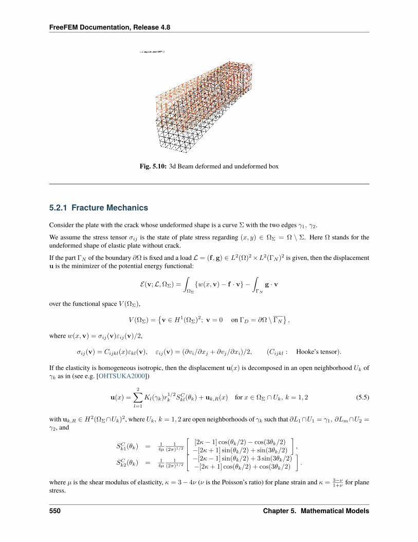
FreeFEM Documentation, Release 4.8
Fig. 5.10: 3d Beam deformed and undeformed box
5.2.1 Fracture Mechanics
Consider the plate with the crack whose undeformed shape is a curve Σ with the two edges 𝛾1, 𝛾2.
We assume the stress tensor 𝜎𝑖𝑗 is the state of plate stress regarding (𝑥, 𝑦) ∈ ΩΣ = Ω ∖ Σ. Here Ω stands for theundeformed shape of elastic plate without crack.
If the part Γ𝑁 of the boundary 𝜕Ω is fixed and a load ℒ = (f ,g) ∈ 𝐿2(Ω)2×𝐿2(Γ𝑁 )2 is given, then the displacementu is the minimizer of the potential energy functional:
ℰ(v;ℒ,ΩΣ) =
∫ΩΣ
𝑤(𝑥,v)− f · v −∫Γ𝑁
g · v
over the functional space 𝑉 (ΩΣ),
𝑉 (ΩΣ) =v ∈ 𝐻1(ΩΣ)2; v = 0 on Γ𝐷 = 𝜕Ω ∖ Γ𝑁
,
where 𝑤(𝑥,v) = 𝜎𝑖𝑗(v)𝜀𝑖𝑗(v)/2,
𝜎𝑖𝑗(v) = 𝐶𝑖𝑗𝑘𝑙(𝑥)𝜀𝑘𝑙(v), 𝜀𝑖𝑗(v) = (𝜕𝑣𝑖/𝜕𝑥𝑗 + 𝜕𝑣𝑗/𝜕𝑥𝑖)/2, (𝐶𝑖𝑗𝑘𝑙 : Hooke’s tensor).
If the elasticity is homogeneous isotropic, then the displacement u(𝑥) is decomposed in an open neighborhood 𝑈𝑘 of𝛾𝑘 as in (see e.g. [OHTSUKA2000])
u(𝑥) =
2∑𝑙=1
𝐾𝑙(𝛾𝑘)𝑟1/2𝑘 𝑆𝐶𝑘𝑙(𝜃𝑘) + u𝑘,𝑅(𝑥) for 𝑥 ∈ ΩΣ ∩ 𝑈𝑘, 𝑘 = 1, 2 (5.5)
with u𝑘,𝑅 ∈ 𝐻2(ΩΣ∩𝑈𝑘)2, where𝑈𝑘, 𝑘 = 1, 2 are open neighborhoods of 𝛾𝑘 such that 𝜕𝐿1∩𝑈1 = 𝛾1, 𝜕𝐿𝑚∩𝑈2 =𝛾2, and
𝑆𝐶𝑘1(𝜃𝑘) = 14𝜇
1(2𝜋)1/2
[[2𝜅− 1] cos(𝜃𝑘/2)− cos(3𝜃𝑘/2)−[2𝜅+ 1] sin(𝜃𝑘/2) + sin(3𝜃𝑘/2)
],
𝑆𝐶𝑘2(𝜃𝑘) = 14𝜇
1(2𝜋)1/2
[−[2𝜅− 1] sin(𝜃𝑘/2) + 3 sin(3𝜃𝑘/2)−[2𝜅+ 1] cos(𝜃𝑘/2) + cos(3𝜃𝑘/2)
].
where 𝜇 is the shear modulus of elasticity, 𝜅 = 3− 4𝜈 (𝜈 is the Poisson’s ratio) for plane strain and 𝜅 = 3−𝜈1+𝜈 for plane
stress.
550 Chapter 5. Mathematical Models
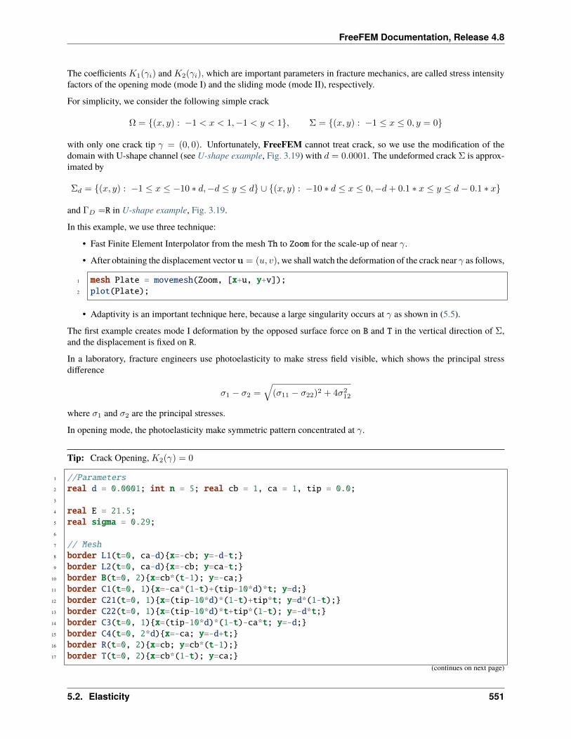
FreeFEM Documentation, Release 4.8
The coefficients 𝐾1(𝛾𝑖) and 𝐾2(𝛾𝑖), which are important parameters in fracture mechanics, are called stress intensityfactors of the opening mode (mode I) and the sliding mode (mode II), respectively.
For simplicity, we consider the following simple crack
Ω = (𝑥, 𝑦) : −1 < 𝑥 < 1,−1 < 𝑦 < 1, Σ = (𝑥, 𝑦) : −1 ≤ 𝑥 ≤ 0, 𝑦 = 0
with only one crack tip 𝛾 = (0, 0). Unfortunately, FreeFEM cannot treat crack, so we use the modification of thedomain with U-shape channel (see U-shape example, Fig. 3.19) with 𝑑 = 0.0001. The undeformed crack Σ is approx-imated by
Σ𝑑 = (𝑥, 𝑦) : −1 ≤ 𝑥 ≤ −10 * 𝑑,−𝑑 ≤ 𝑦 ≤ 𝑑 ∪ (𝑥, 𝑦) : −10 * 𝑑 ≤ 𝑥 ≤ 0,−𝑑+ 0.1 * 𝑥 ≤ 𝑦 ≤ 𝑑− 0.1 * 𝑥
and Γ𝐷 =R in U-shape example, Fig. 3.19.
In this example, we use three technique:
• Fast Finite Element Interpolator from the mesh Th to Zoom for the scale-up of near 𝛾.
• After obtaining the displacement vectoru = (𝑢, 𝑣), we shall watch the deformation of the crack near 𝛾 as follows,
1 mesh Plate = movemesh(Zoom, [x+u, y+v]);2 plot(Plate);
• Adaptivity is an important technique here, because a large singularity occurs at 𝛾 as shown in (5.5).
The first example creates mode I deformation by the opposed surface force on B and T in the vertical direction of Σ,and the displacement is fixed on R.
In a laboratory, fracture engineers use photoelasticity to make stress field visible, which shows the principal stressdifference
𝜎1 − 𝜎2 =√
(𝜎11 − 𝜎22)2 + 4𝜎212
where 𝜎1 and 𝜎2 are the principal stresses.
In opening mode, the photoelasticity make symmetric pattern concentrated at 𝛾.
Tip: Crack Opening, 𝐾2(𝛾) = 0
1 //Parameters2 real d = 0.0001; int n = 5; real cb = 1, ca = 1, tip = 0.0;3
4 real E = 21.5;5 real sigma = 0.29;6
7 // Mesh8 border L1(t=0, ca-d)x=-cb; y=-d-t;9 border L2(t=0, ca-d)x=-cb; y=ca-t;
10 border B(t=0, 2)x=cb*(t-1); y=-ca;11 border C1(t=0, 1)x=-ca*(1-t)+(tip-10*d)*t; y=d;12 border C21(t=0, 1)x=(tip-10*d)*(1-t)+tip*t; y=d*(1-t);13 border C22(t=0, 1)x=(tip-10*d)*t+tip*(1-t); y=-d*t;14 border C3(t=0, 1)x=(tip-10*d)*(1-t)-ca*t; y=-d;15 border C4(t=0, 2*d)x=-ca; y=-d+t;16 border R(t=0, 2)x=cb; y=cb*(t-1);17 border T(t=0, 2)x=cb*(1-t); y=ca;
(continues on next page)
5.2. Elasticity 551
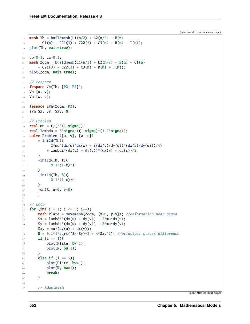
FreeFEM Documentation, Release 4.8
(continued from previous page)
18 mesh Th = buildmesh(L1(n/2) + L2(n/2) + B(n)19 + C1(n) + C21(3) + C22(3) + C3(n) + R(n) + T(n));20 plot(Th, wait=true);21
22 cb=0.1; ca=0.1;23 mesh Zoom = buildmesh(L1(n/2) + L2(n/2) + B(n) + C1(n)24 + C21(3) + C22(3) + C3(n) + R(n) + T(n));25 plot(Zoom, wait=true);26
27 // Fespace28 fespace Vh(Th, [P2, P2]);29 Vh [u, v];30 Vh [w, s];31
32 fespace zVh(Zoom, P2);33 zVh Sx, Sy, Sxy, N;34
35 // Problem36 real mu = E/(2*(1+sigma));37 real lambda = E*sigma/((1+sigma)*(1-2*sigma));38 solve Problem ([u, v], [w, s])39 = int2d(Th)(40 2*mu*(dx(u)*dx(w) + ((dx(v)+dy(u))*(dx(s)+dy(w)))/4)41 + lambda*(dx(u) + dy(v))*(dx(w) + dy(s))/242 )43 -int1d(Th, T)(44 0.1*(1-x)*s45 )46 +int1d(Th, B)(47 0.1*(1-x)*s48 )49 +on(R, u=0, v=0)50 ;51
52 // Loop53 for (int i = 1; i <= 5; i++)54 mesh Plate = movemesh(Zoom, [x+u, y+v]); //deformation near gamma55 Sx = lambda*(dx(u) + dy(v)) + 2*mu*dx(u);56 Sy = lambda*(dx(u) + dy(v)) + 2*mu*dy(v);57 Sxy = mu*(dy(u) + dx(v));58 N = 0.1*1*sqrt((Sx-Sy)^2 + 4*Sxy^2); //principal stress difference59 if (i == 1)60 plot(Plate, bw=1);61 plot(N, bw=1);62 63 else if (i == 5)64 plot(Plate, bw=1);65 plot(N, bw=1);66 break;67 68
69 // Adaptmesh
(continues on next page)
552 Chapter 5. Mathematical Models
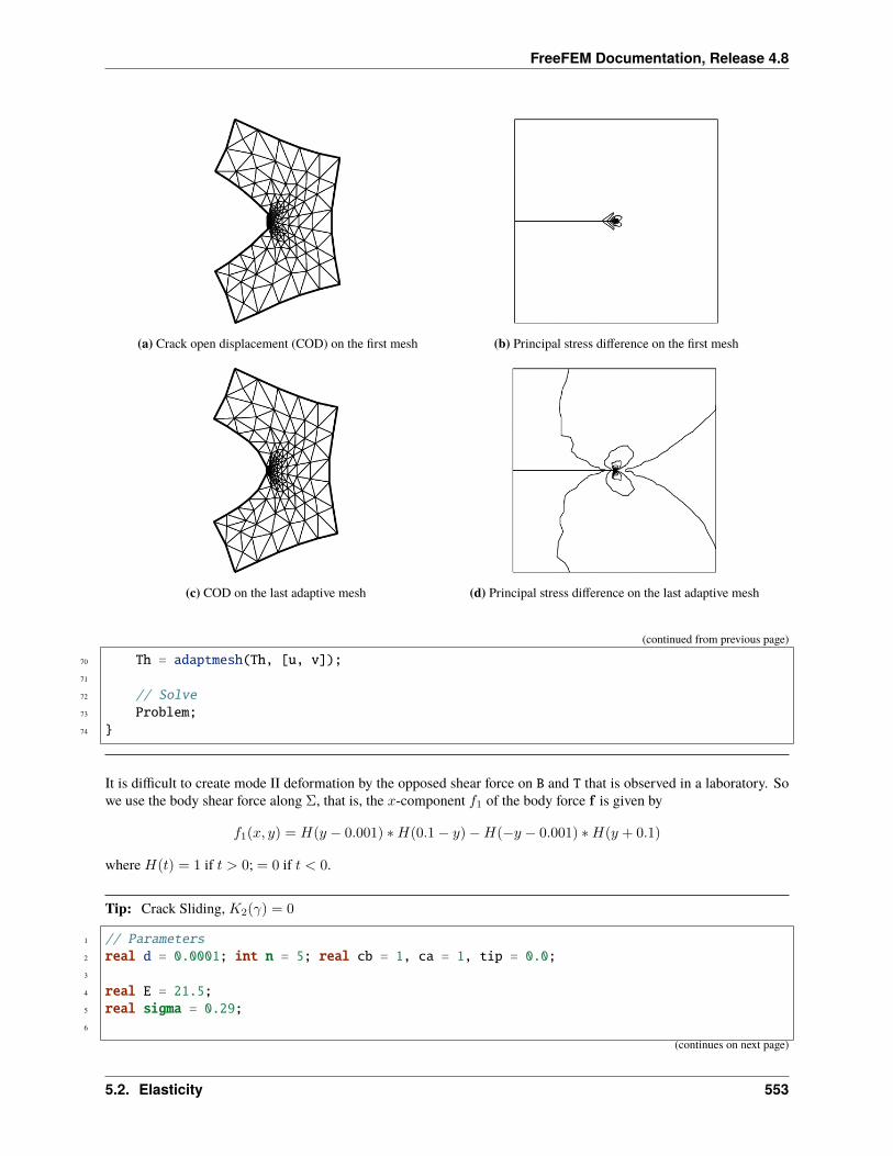
FreeFEM Documentation, Release 4.8
(a) Crack open displacement (COD) on the first mesh (b) Principal stress difference on the first mesh
(c) COD on the last adaptive mesh (d) Principal stress difference on the last adaptive mesh
(continued from previous page)
70 Th = adaptmesh(Th, [u, v]);71
72 // Solve73 Problem;74
It is difficult to create mode II deformation by the opposed shear force on B and T that is observed in a laboratory. Sowe use the body shear force along Σ, that is, the 𝑥-component 𝑓1 of the body force f is given by
𝑓1(𝑥, 𝑦) = 𝐻(𝑦 − 0.001) *𝐻(0.1− 𝑦)−𝐻(−𝑦 − 0.001) *𝐻(𝑦 + 0.1)
where 𝐻(𝑡) = 1 if 𝑡 > 0; = 0 if 𝑡 < 0.
Tip: Crack Sliding, 𝐾2(𝛾) = 0
1 // Parameters2 real d = 0.0001; int n = 5; real cb = 1, ca = 1, tip = 0.0;3
4 real E = 21.5;5 real sigma = 0.29;6
(continues on next page)
5.2. Elasticity 553
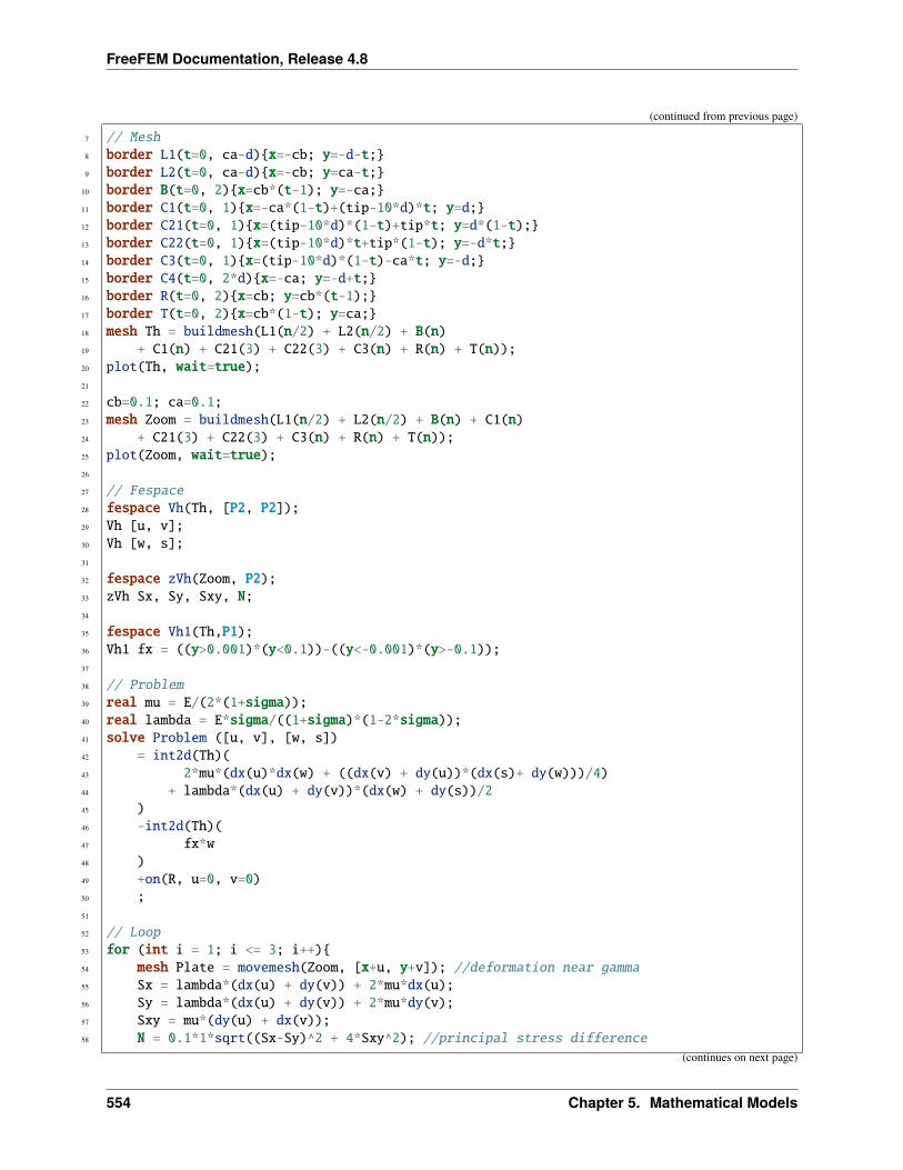
FreeFEM Documentation, Release 4.8
(continued from previous page)
7 // Mesh8 border L1(t=0, ca-d)x=-cb; y=-d-t;9 border L2(t=0, ca-d)x=-cb; y=ca-t;
10 border B(t=0, 2)x=cb*(t-1); y=-ca;11 border C1(t=0, 1)x=-ca*(1-t)+(tip-10*d)*t; y=d;12 border C21(t=0, 1)x=(tip-10*d)*(1-t)+tip*t; y=d*(1-t);13 border C22(t=0, 1)x=(tip-10*d)*t+tip*(1-t); y=-d*t;14 border C3(t=0, 1)x=(tip-10*d)*(1-t)-ca*t; y=-d;15 border C4(t=0, 2*d)x=-ca; y=-d+t;16 border R(t=0, 2)x=cb; y=cb*(t-1);17 border T(t=0, 2)x=cb*(1-t); y=ca;18 mesh Th = buildmesh(L1(n/2) + L2(n/2) + B(n)19 + C1(n) + C21(3) + C22(3) + C3(n) + R(n) + T(n));20 plot(Th, wait=true);21
22 cb=0.1; ca=0.1;23 mesh Zoom = buildmesh(L1(n/2) + L2(n/2) + B(n) + C1(n)24 + C21(3) + C22(3) + C3(n) + R(n) + T(n));25 plot(Zoom, wait=true);26
27 // Fespace28 fespace Vh(Th, [P2, P2]);29 Vh [u, v];30 Vh [w, s];31
32 fespace zVh(Zoom, P2);33 zVh Sx, Sy, Sxy, N;34
35 fespace Vh1(Th,P1);36 Vh1 fx = ((y>0.001)*(y<0.1))-((y<-0.001)*(y>-0.1));37
38 // Problem39 real mu = E/(2*(1+sigma));40 real lambda = E*sigma/((1+sigma)*(1-2*sigma));41 solve Problem ([u, v], [w, s])42 = int2d(Th)(43 2*mu*(dx(u)*dx(w) + ((dx(v) + dy(u))*(dx(s)+ dy(w)))/4)44 + lambda*(dx(u) + dy(v))*(dx(w) + dy(s))/245 )46 -int2d(Th)(47 fx*w48 )49 +on(R, u=0, v=0)50 ;51
52 // Loop53 for (int i = 1; i <= 3; i++)54 mesh Plate = movemesh(Zoom, [x+u, y+v]); //deformation near gamma55 Sx = lambda*(dx(u) + dy(v)) + 2*mu*dx(u);56 Sy = lambda*(dx(u) + dy(v)) + 2*mu*dy(v);57 Sxy = mu*(dy(u) + dx(v));58 N = 0.1*1*sqrt((Sx-Sy)^2 + 4*Sxy^2); //principal stress difference
(continues on next page)
554 Chapter 5. Mathematical Models
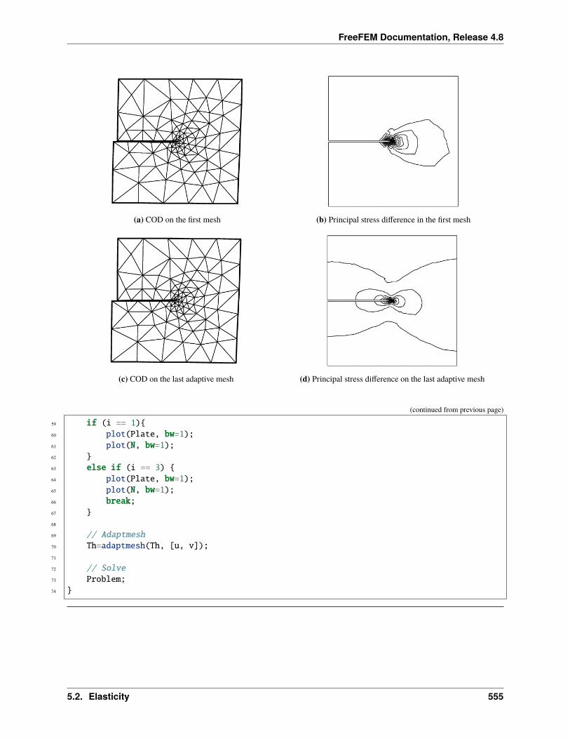
FreeFEM Documentation, Release 4.8
(a) COD on the first mesh (b) Principal stress difference in the first mesh
(c) COD on the last adaptive mesh (d) Principal stress difference on the last adaptive mesh
(continued from previous page)
59 if (i == 1)60 plot(Plate, bw=1);61 plot(N, bw=1);62 63 else if (i == 3) 64 plot(Plate, bw=1);65 plot(N, bw=1);66 break;67 68
69 // Adaptmesh70 Th=adaptmesh(Th, [u, v]);71
72 // Solve73 Problem;74
5.2. Elasticity 555
FreeFEM Documentation, Release 4.8
5.3 Non-linear static problems
Here we propose to solve the following non-linear academic problem of minimization of a functional:
𝐽(𝑢) =
∫Ω
1
2𝑓(|∇𝑢|2)− 𝑢 * 𝑏
where 𝑢 is function of 𝐻10 (Ω) and 𝑓 defined by:
𝑓(𝑥) = 𝑎 * 𝑥+ 𝑥− 𝑙𝑛(1 + 𝑥), 𝑓 ′(𝑥) = 𝑎+𝑥
1 + 𝑥, 𝑓 ′′(𝑥) =
1
(1 + 𝑥)2
5.3.1 Newton-Raphson algorithm
Now, we solve the Euler problem ∇𝐽(𝑢) = 0 with Newton-Raphson algorithm, that is:
𝑢𝑛+1 = 𝑢𝑛 − (∇2𝐽(𝑢𝑛))−1 * ∇𝐽(𝑢𝑛)
1 // Parameters2 real a = 0.001;3 func b = 1.;4
5 // Mesh6 mesh Th = square(10, 10);7 Th = adaptmesh(Th, 0.05, IsMetric=1, splitpbedge=1);8 plot(Th, wait=true);9
10 // Fespace11 fespace Vh(Th, P1);12 Vh u=0;13 Vh v, w;14
15 fespace Ph(Th, P1dc);16 Ph alpha; //to store |nabla u|^217 Ph dalpha ; //to store 2f''(|nabla u|^2)18
19 // Function20 func real f (real u)21 return u*a + u - log(1.+u);22 23 func real df (real u)24 return a +u/(1.+u);25 26 func real ddf (real u)27 return 1. / ((1.+u)*(1.+u));28 29
30 // Problem31 //the variational form of evaluate dJ = nabla J32 //dJ = f'()*(dx(u)*dx(vh) + dy(u)*dy(vh))33 varf vdJ (uh, vh)34 = int2d(Th)(
(continues on next page)
556 Chapter 5. Mathematical Models
FreeFEM Documentation, Release 4.8
(continued from previous page)
35 alpha*(dx(u)*dx(vh) + dy(u)*dy(vh))36 - b*vh37 )38 + on(1, 2, 3, 4, uh=0)39 ;40
41 //the variational form of evaluate ddJ = nabla^2 J42 //hJ(uh,vh) = f'()*(dx(uh)*dx(vh) + dy(uh)*dy(vh))43 // + 2*f''()(dx(u)*dx(uh) + dy(u)*dy(uh)) * (dx(u)*dx(vh) + dy(u)*dy(vh))44 varf vhJ (uh, vh)45 = int2d(Th)(46 alpha*(dx(uh)*dx(vh) + dy(uh)*dy(vh))47 + dalpha*(dx(u)*dx(vh) + dy(u)*dy(vh))*(dx(u)*dx(uh) + dy(u)*dy(uh))48 )49 + on(1, 2, 3, 4, uh=0)50 ;51
52 // Newton algorithm53 for (int i = 0; i < 100; i++)54 // Compute f' and f''55 alpha = df(dx(u)*dx(u) + dy(u)*dy(u));56 dalpha = 2*ddf(dx(u)*dx(u) + dy(u)*dy(u));57
58 // nabla J59 v[]= vdJ(0, Vh);60
61 // Residual62 real res = v[]'*v[];63 cout << i << " residu^2 = " << res << endl;64 if( res < 1e-12) break;65
66 // HJ67 matrix H = vhJ(Vh, Vh, factorize=1, solver=LU);68
69 // Newton70 w[] = H^-1*v[];71 u[] -= w[];72 73
74 // Plot75 plot (u, wait=true, cmm="Solution with Newton-Raphson");
5.3. Non-linear static problems 557
FreeFEM Documentation, Release 4.8
5.4 Eigen value problems
This section depends on your installation of FreeFEM; you need to have compiled ARPACK. This tool is available inFreeFEM if the word eigenvalue appears in line Load:, like:
1 -- FreeFem++ v*.** (date *** *** ** **:**:** CET ****)2 file : ***.edp3 Load: lg_fem lg_mesh eigenvalue
This tool is based on arpack++, the object-oriented version of ARPACK eigenvalue package [LEHOUCQ1998].
The function EigenValue computes the generalized eigenvalue of 𝐴𝑢 = 𝜆𝐵𝑢. The Shift-invert method is used bydefault, with sigma =𝜎 the shift of the method.
The matrix 𝑂𝑃 is defined with 𝐴− 𝜎𝐵.
The return value is the number of converged eigenvalues (can be greater than the number of requested eigenvaluesnev=)
1 int k = EigenValue(OP, B, nev=Nev, sigma=Sigma);
where the matrix 𝑂𝑃 = 𝐴− 𝜎𝐵 with a solver and boundary condition, and the matrix 𝐵.
There is also a functional interface:
1 int k = EigenValue(n, FOP1, FB, nev=Nev, sigma=Sigma);
where 𝑛 is the size of the problem, and the operators are now defined through functions, defining respectively the matrixproduct of 𝑂𝑃−1 and 𝐵, as in
1 int n = OP1.n;2 func real[int] FOP1(real[int] & u) real[int] Au = OP^-1*u; return Au; 3 func real[int] FB(real[int] & u) real[int] Au = B*u; return Au;
If you want finer control over the method employed in ARPACK, you can specify which mode ARPACK will work with(mode= , see ARPACK documentation [LEHOUCQ1998]). The operators necessary for the chosen mode can be passedthrough the optional parameters A=, A1=, B=, B1=, (see below).
• mode=1: Regular mode for solving 𝐴𝑢 = 𝜆𝑢
1 int k = EigenValue(n, A=FOP, mode=1, nev=Nev);
where the function FOP defines the matrix product of A
• mode=2: Regular inverse mode for solving 𝐴𝑢 = 𝜆𝐵𝑢
1 int k = EigenValue(n, A=FOP, B=FB, B1=FB1, mode=2, nev=Nev);
where the functions FOP, FB and FB1 define respectively the matrix product of 𝐴, 𝐵 and 𝐵−1
• mode=3: Shift-invert mode for solving 𝐴𝑢 = 𝜆𝐵𝑢
1 int k = EigenValue(n, A1=FOP1, B=FB, mode=3, sigma=Sigma, nev=Nev);
where the functions FOP1 and FB define respectively the matrix product of 𝑂𝑃−1 = (𝐴− 𝜎𝐵)−1 and 𝐵
You can also specify which subset of eigenvalues you want to compute (which=). The default value is which="LM",for eigenvalues with largest magnitude. "SM" is for smallest magnitude, "LA" for largest algebraic value, "SA" forsmallest algebraic value, and "BE" for both ends of the spectrum.
558 Chapter 5. Mathematical Models
FreeFEM Documentation, Release 4.8
Remark: For complex problems, you need to use the keyword complexEigenValue instead of EigenValue whenpassing operators through functions.
Note: Boundary condition and Eigenvalue Problems
The locking (Dirichlet) boundary condition is make with exact penalization so we put 1e30=tgv on the diagonal termof the locked degree of freedom (see Finite element chapter). So take Dirichlet boundary condition just on 𝐴 and noton 𝐵 because we solve 𝑤 = 𝑂𝑃−1 *𝐵 * 𝑣.
If you put locking (Dirichlet) boundary condition on 𝐵 matrix (with key work on) you get small spurious modes(10−30), due to boundary condition, but if you forget the locking boundary condition on 𝐵 matrix (no keywork on)you get huge spurious (1030) modes associated to these boundary conditons. We compute only small mode, so we getthe good one in this case.
• sym= The problem is symmetric (all the eigen value are real)
• nev= The number desired eigenvalues (nev) close to the shift.
• value= The array to store the real part of the eigenvalues
• ivalue= The array to store the imaginary part of the eigenvalues
• vector= The FE function array to store the eigenvectors
• rawvector= An array of type real[int,int] to store eigenvectors by column.
For real non symmetric problems, complex eigenvectors are given as two consecutive vectors, so if eigenvalue 𝑘and 𝑘+ 1 are complex conjugate eigenvalues, the 𝑘th vector will contain the real part and the 𝑘+ 1th vector theimaginary part of the corresponding complex conjugate eigenvectors.
• tol= The relative accuracy to which eigenvalues are to be determined;
• sigma= The shift value;
• maxit= The maximum number of iterations allowed;
• ncv= The number of Arnoldi vectors generated at each iteration of ARPACK;
• mode= The computational mode used by ARPACK (see above);
• which= The requested subset of eigenvalues (see above).
Tip: Laplace eigenvalue
In the first example, we compute the eigenvalues and the eigenvectors of the Dirichlet problem on square Ω =]0, 𝜋[2.
The problem is to find: 𝜆, and ∇𝑢𝜆 in R×𝐻10 (Ω)∫
Ω
∇𝑢𝜆∇𝑣 = 𝜆
∫Ω
𝑢𝑣 ∀𝑣 ∈ 𝐻10 (Ω)
The exact eigenvalues are 𝜆𝑛,𝑚 = (𝑛2 + 𝑚2), (𝑛,𝑚) ∈ N*2 with the associated eigenvectors are 𝑢𝑚,𝑛 = sin(𝑛𝑥) *
sin(𝑚𝑦).
We use the generalized inverse shift mode of the arpack++ library, to find 20 eigenvalues and eigenvectors close to theshift value 𝜎 = 20.
1 // Parameters2 verbosity=0;3 real sigma = 20; //value of the shift4 int nev = 20; //number of computed eigen value close to sigma
(continues on next page)
5.4. Eigen value problems 559
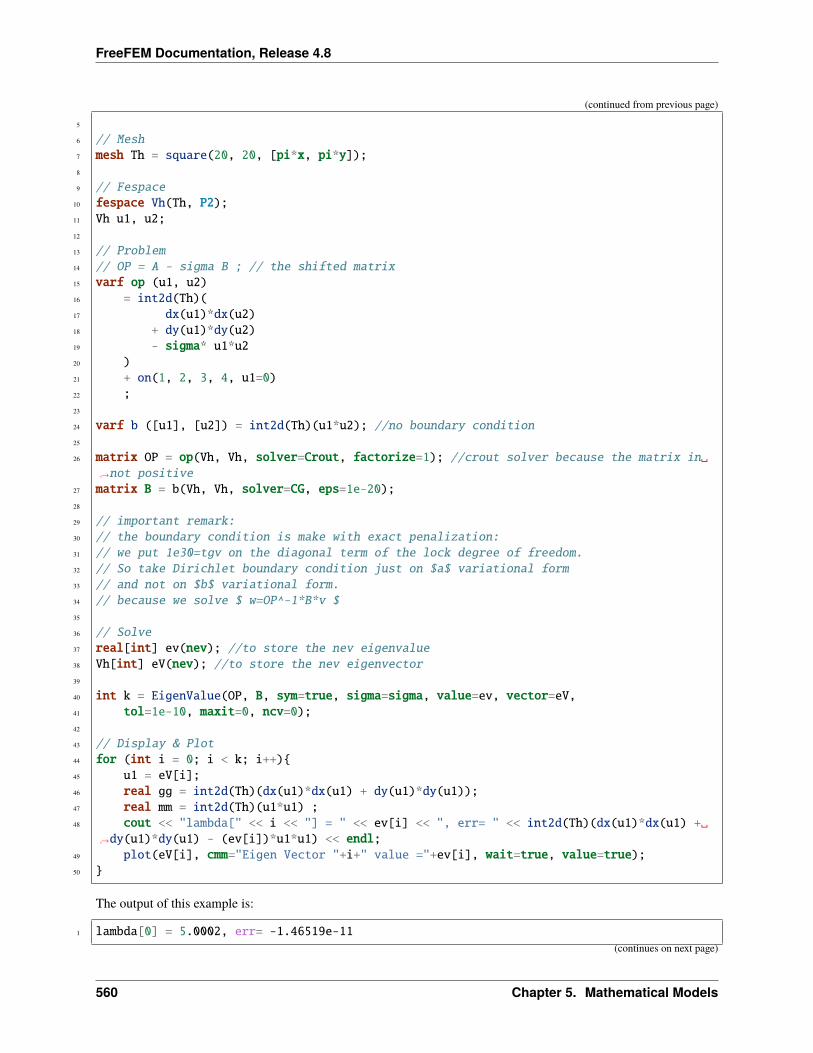
FreeFEM Documentation, Release 4.8
(continued from previous page)
5
6 // Mesh7 mesh Th = square(20, 20, [pi*x, pi*y]);8
9 // Fespace10 fespace Vh(Th, P2);11 Vh u1, u2;12
13 // Problem14 // OP = A - sigma B ; // the shifted matrix15 varf op (u1, u2)16 = int2d(Th)(17 dx(u1)*dx(u2)18 + dy(u1)*dy(u2)19 - sigma* u1*u220 )21 + on(1, 2, 3, 4, u1=0)22 ;23
24 varf b ([u1], [u2]) = int2d(Th)(u1*u2); //no boundary condition25
26 matrix OP = op(Vh, Vh, solver=Crout, factorize=1); //crout solver because the matrix in→˓not positive
27 matrix B = b(Vh, Vh, solver=CG, eps=1e-20);28
29 // important remark:30 // the boundary condition is make with exact penalization:31 // we put 1e30=tgv on the diagonal term of the lock degree of freedom.32 // So take Dirichlet boundary condition just on $a$ variational form33 // and not on $b$ variational form.34 // because we solve $ w=OP^-1*B*v $35
36 // Solve37 real[int] ev(nev); //to store the nev eigenvalue38 Vh[int] eV(nev); //to store the nev eigenvector39
40 int k = EigenValue(OP, B, sym=true, sigma=sigma, value=ev, vector=eV,41 tol=1e-10, maxit=0, ncv=0);42
43 // Display & Plot44 for (int i = 0; i < k; i++)45 u1 = eV[i];46 real gg = int2d(Th)(dx(u1)*dx(u1) + dy(u1)*dy(u1));47 real mm = int2d(Th)(u1*u1) ;48 cout << "lambda[" << i << "] = " << ev[i] << ", err= " << int2d(Th)(dx(u1)*dx(u1) +
→˓dy(u1)*dy(u1) - (ev[i])*u1*u1) << endl;49 plot(eV[i], cmm="Eigen Vector "+i+" value ="+ev[i], wait=true, value=true);50
The output of this example is:
1 lambda[0] = 5.0002, err= -1.46519e-11(continues on next page)
560 Chapter 5. Mathematical Models
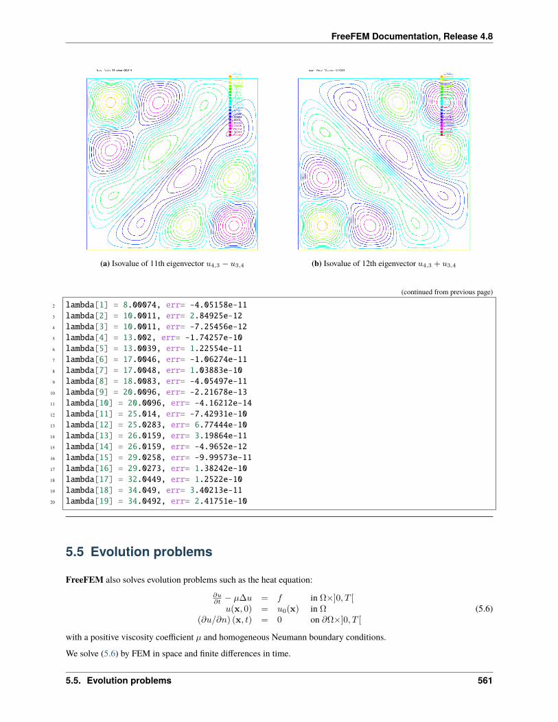
FreeFEM Documentation, Release 4.8
(a) Isovalue of 11th eigenvector 𝑢4,3 − 𝑢3,4 (b) Isovalue of 12th eigenvector 𝑢4,3 + 𝑢3,4
(continued from previous page)
2 lambda[1] = 8.00074, err= -4.05158e-113 lambda[2] = 10.0011, err= 2.84925e-124 lambda[3] = 10.0011, err= -7.25456e-125 lambda[4] = 13.002, err= -1.74257e-106 lambda[5] = 13.0039, err= 1.22554e-117 lambda[6] = 17.0046, err= -1.06274e-118 lambda[7] = 17.0048, err= 1.03883e-109 lambda[8] = 18.0083, err= -4.05497e-11
10 lambda[9] = 20.0096, err= -2.21678e-1311 lambda[10] = 20.0096, err= -4.16212e-1412 lambda[11] = 25.014, err= -7.42931e-1013 lambda[12] = 25.0283, err= 6.77444e-1014 lambda[13] = 26.0159, err= 3.19864e-1115 lambda[14] = 26.0159, err= -4.9652e-1216 lambda[15] = 29.0258, err= -9.99573e-1117 lambda[16] = 29.0273, err= 1.38242e-1018 lambda[17] = 32.0449, err= 1.2522e-1019 lambda[18] = 34.049, err= 3.40213e-1120 lambda[19] = 34.0492, err= 2.41751e-10
5.5 Evolution problems
FreeFEM also solves evolution problems such as the heat equation:𝜕𝑢𝜕𝑡 − 𝜇∆𝑢 = 𝑓 in Ω×]0, 𝑇 [
𝑢(x, 0) = 𝑢0(x) in Ω(𝜕𝑢/𝜕𝑛) (x, 𝑡) = 0 on 𝜕Ω×]0, 𝑇 [
(5.6)
with a positive viscosity coefficient 𝜇 and homogeneous Neumann boundary conditions.
We solve (5.6) by FEM in space and finite differences in time.
5.5. Evolution problems 561
FreeFEM Documentation, Release 4.8
We use the definition of the partial derivative of the solution in the time derivative:
𝜕𝑢
𝜕𝑡(𝑥, 𝑦, 𝑡) = lim
𝜏→0
𝑢(𝑥, 𝑦, 𝑡)− 𝑢(𝑥, 𝑦, 𝑡− 𝜏)
𝜏
which indicates that 𝑢𝑚(𝑥, 𝑦) = 𝑢(𝑥, 𝑦,𝑚𝜏) will satisfy approximatively:
𝜕𝑢
𝜕𝑡(𝑥, 𝑦,𝑚𝜏) ≃ 𝑢𝑚(𝑥, 𝑦)− 𝑢𝑚−1(𝑥, 𝑦)
𝜏
The time discretization of heat equation (5.6) is as follows, ∀𝑚 = 0, · · · , [𝑇/𝜏 ]:
𝑢𝑚+1−𝑢𝑚
𝜏 − 𝜇∆𝑢𝑚+1 = 𝑓𝑚+1 in Ω𝑢0(x) = 𝑢0(x) in Ω
𝜕𝑢𝑚+1/𝜕𝑛(x) = 0 on 𝜕Ω
which is so-called backward Euler method for (5.6).
To obtain the variational formulation, multiply with the test function 𝑣 both sides of the equation:∫Ω
𝑢𝑚+1𝑣 − 𝜏∆𝑢𝑚+1𝑣 =
∫Ω
𝑢𝑚 + 𝜏𝑓𝑚+1𝑣
By the divergence theorem, we have:∫Ω
𝑢𝑚+1𝑣 + 𝜏∇𝑢𝑚+1 · ∇𝑣 −∫𝜕Ω
𝜏(𝜕𝑢𝑚+1/𝜕𝑛
)𝑣 =
∫Ω
𝑢𝑚𝑣 + 𝜏𝑓𝑚+1𝑣
By the boundary condition 𝜕𝑢𝑚+1/𝜕𝑛 = 0, it follows that:∫Ω
𝑢𝑚+1𝑣 + 𝜏∇𝑢𝑚+1 · ∇𝑣 −∫Ω
𝑢𝑚𝑣 + 𝜏𝑓𝑚+1𝑣 = 0 (5.7)
Using the identity just above, we can calculate the finite element approximation 𝑢𝑚ℎ of 𝑢𝑚 in a step-by-step mannerwith respect to 𝑡.
Tip: Example
We now solve the following example with the exact solution 𝑢(𝑥, 𝑦, 𝑡) = 𝑡𝑥4, Ω =]0, 1[2.
𝜕𝑢𝜕𝑡 − 𝜇∆𝑢 = 𝑥4 − 𝜇12𝑡𝑥2 in Ω×]0, 3[𝑢(𝑥, 𝑦, 0) = 0 on Ω
𝑢|𝜕Ω = 𝑡 * 𝑥4
1 // Parameters2 real dt = 0.1;3 real mu = 0.01;4
5 // Mesh6 mesh Th = square(16, 16);7
8 // Fespace9 fespace Vh(Th, P1);
10 Vh u, v, uu, f, g;11
12 // Problem13 problem dHeat (u, v)
(continues on next page)
562 Chapter 5. Mathematical Models
FreeFEM Documentation, Release 4.8
(continued from previous page)
14 = int2d(Th)(15 u*v16 + dt*mu*(dx(u)*dx(v) + dy(u)*dy(v))17 )18 + int2d(Th)(19 - uu*v20 - dt*f*v21 )22 + on(1, 2, 3, 4, u=g)23 ;24
25 // Time loop26 real t = 0;27 uu = 0;28 for (int m = 0; m <= 3/dt; m++)29 // Update30 t = t+dt;31 f = x^4 - mu*t*12*x^2;32 g = t*x^4;33 uu = u;34
35 // Solve36 dHeat;37
38 // Plot39 plot(u, wait=true);40 cout << "t=" << t << " - L^2-Error=" << sqrt(int2d(Th)((u-t*x^4)^2)) << endl;41
In the last statement, the 𝐿2-error(∫
Ω
𝑢− 𝑡𝑥4
2)1/2 is calculated at 𝑡 = 𝑚𝜏, 𝜏 = 0.1. At 𝑡 = 0.1, the error is0.000213269. The errors increase with 𝑚 and 0.00628589 at 𝑡 = 3.
The iteration of the backward Euler (5.7) is made by for loop.
Note: The stiffness matrix in the loop is used over and over again. FreeFEM support reuses of stiffness matrix.
5.5.1 Mathematical Theory on Time Difference Approximations.
In this section, we show the advantage of implicit schemes. Let 𝑉,𝐻 be separable Hilbert space and 𝑉 is dense in 𝐻 .Let 𝑎 be a continuous bilinear form over 𝑉 × 𝑉 with coercivity and symmetry.
Then√𝑎(𝑣, 𝑣) become equivalent to the norm ‖𝑣‖ of 𝑉 .
Problem Ev(f,Omega): For a given 𝑓 ∈ 𝐿2(0, 𝑇 ;𝑉 ′), 𝑢0 ∈ 𝐻
𝑑𝑑𝑡 (𝑢(𝑡), 𝑣) + 𝑎(𝑢(𝑡), 𝑣) = (𝑓(𝑡), 𝑣) ∀𝑣 ∈ 𝑉, 𝑎.𝑒. 𝑡 ∈ [0, 𝑇 ]
𝑢(0) = 𝑢0
where 𝑉 ′ is the dual space of 𝑉 .
Then, there is an unique solution 𝑢 ∈ 𝐿∞(0, 𝑇 ;𝐻) ∩ 𝐿2(0, 𝑇 ;𝑉 ).
5.5. Evolution problems 563
FreeFEM Documentation, Release 4.8
Let us denote the time step by 𝜏 > 0, 𝑁𝑇 = [𝑇/𝜏 ]. For the discretization, we put 𝑢𝑛 = 𝑢(𝑛𝜏) and consider the timedifference for each 𝜃 ∈ [0, 1]
1𝜏
(𝑢𝑛+1ℎ − 𝑢𝑛ℎ, 𝜑𝑖
)+ 𝑎
(𝑢𝑛+𝜃ℎ , 𝜑𝑖
)= ⟨𝑓𝑛+𝜃, 𝜑𝑖⟩
𝑖 = 1, · · · ,𝑚, 𝑛 = 0, · · · , 𝑁𝑇𝑢𝑛+𝜃ℎ = 𝜃𝑢𝑛+1
ℎ + (1− 𝜃)𝑢𝑛ℎ,𝑓𝑛+𝜃 = 𝜃𝑓𝑛+1 + (1− 𝜃)𝑓𝑛
Formula (5.8) is the forward Euler scheme if 𝜃 = 0, Crank-Nicolson scheme if 𝜃 = 1/2, the backward Euler scheme if𝜃 = 1.
Unknown vectors 𝑢𝑛 = (𝑢1ℎ, · · · , 𝑢𝑀ℎ )𝑇 in
𝑢𝑛ℎ(𝑥) = 𝑢𝑛1𝜑1(𝑥) + · · ·+ 𝑢𝑛𝑚𝜑𝑚(𝑥), 𝑢𝑛1 , · · · , 𝑢𝑛𝑚 ∈ R
are obtained from solving the matrix
(𝑀 + 𝜃𝜏𝐴)𝑢𝑛+1 = 𝑀 − (1− 𝜃)𝜏𝐴𝑢𝑛 + 𝜏𝜃𝑓𝑛+1 + (1− 𝜃)𝑓𝑛
𝑀 = (𝑚𝑖𝑗), 𝑚𝑖𝑗 = (𝜑𝑗 , 𝜑𝑖), 𝐴 = (𝑎𝑖𝑗), 𝑎𝑖𝑗 = 𝑎(𝜑𝑗 , 𝜑𝑖)
Refer [TABATA1994], pp.70–75 for solvability of (5.8). The stability of (5.8) is in [TABATA1994], Theorem 2.13:
Let 𝒯ℎℎ↓0 be regular triangulations (see Regular Triangulation). Then there is a number 𝑐0 > 0 independent of ℎsuch that,
|𝑢𝑛ℎ|2 ≤
1𝛿
|𝑢0ℎ|2 + 𝜏
∑𝑛−1𝑘=0 ‖𝑓𝑘+𝜃‖2𝑉 ′
ℎ
𝜃 ∈ [0, 1/2)
|𝑢0ℎ|2 + 𝜏∑𝑛−1𝑘=0 ‖𝑓𝑘+𝜃‖2𝑉 ′
ℎ𝜃 ∈ [1/2, 1]
if the following are satisfied:
1. When 𝜃 ∈ [0, 1/2), then we can take a time step 𝜏 in such a way that
𝜏 <2(1− 𝛿)
(1− 2𝜃)𝑐20ℎ2
for arbitrary 𝛿 ∈ (0, 1).
2. When 1/2 ≤ 𝜃 ≤ 1, we can take 𝜏 arbitrary.
Tip: Example
1 // Parameters2 real tau = 0.1; real3 theta = 0.;4
5 // Mesh6 mesh Th = square(12, 12);7
8 // Fespace9 fespace Vh(Th, P1);
10 Vh u, v, oldU;11 Vh f1, f0;12
13 fespace Ph(Th, P0);14 Ph h = hTriangle; // mesh sizes for each triangle
(continues on next page)
564 Chapter 5. Mathematical Models
FreeFEM Documentation, Release 4.8
(continued from previous page)
15
16 // Function17 func real f (real t)18 return x^2*(x-1)^2 + t*(-2 + 12*x - 11*x^2 - 2*x^3 + x^4);19 20
21 // File22 ofstream out("err02.csv"); //file to store calculations23 out << "mesh size = " << h[].max << ", time step = " << tau << endl;24 for (int n = 0; n < 5/tau; n++)25 out << n*tau << ",";26 out << endl;27
28 // Problem29 problem aTau (u, v)30 = int2d(Th)(31 u*v32 + theta*tau*(dx(u)*dx(v) + dy(u)*dy(v) + u*v)33 )34 - int2d(Th)(35 oldU*v36 - (1-theta)*tau*(dx(oldU)*dx(v) + dy(oldU)*dy(v) + oldU*v)37 )38 - int2d(Th)(39 tau*(theta*f1 + (1-theta)*f0)*v40 )41 ;42
43 // Theta loop44 while (theta <= 1.0)45 real t = 0;46 real T = 3;47 oldU = 0;48 out << theta << ",";49 for (int n = 0; n < T/tau; n++)50 // Update51 t = t + tau;52 f0 = f(n*tau);53 f1 = f((n+1)*tau);54
55 // Solve56 aTau;57 oldU = u;58
59 // Plot60 plot(u);61
62 // Error63 Vh uex = t*x^2*(1-x)^2; //exact solution = tx^2(1-x)^264 Vh err = u - uex; // err = FE-sol - exact65 out << abs(err[].max)/abs(uex[].max) << ",";66
(continues on next page)
5.5. Evolution problems 565
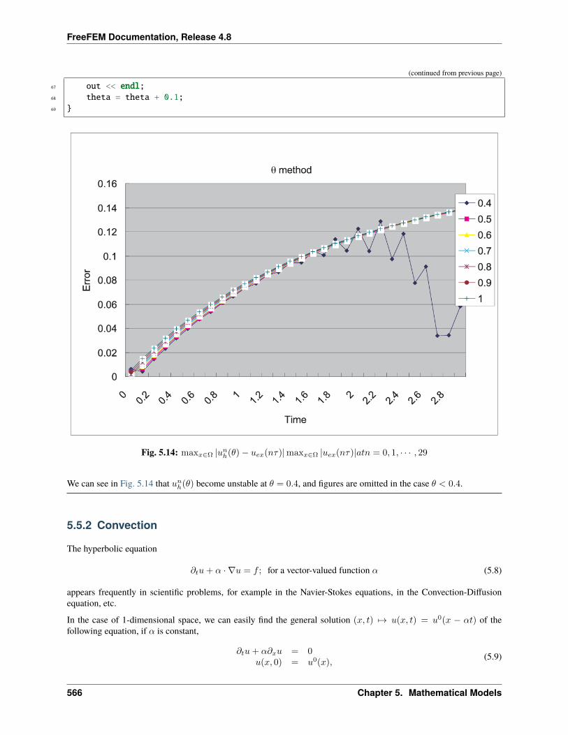
FreeFEM Documentation, Release 4.8
(continued from previous page)
67 out << endl;68 theta = theta + 0.1;69
Fig. 5.14: max𝑥∈Ω |𝑢𝑛ℎ(𝜃)− 𝑢𝑒𝑥(𝑛𝜏)|max𝑥∈Ω |𝑢𝑒𝑥(𝑛𝜏)|𝑎𝑡𝑛 = 0, 1, · · · , 29
We can see in Fig. 5.14 that 𝑢𝑛ℎ(𝜃) become unstable at 𝜃 = 0.4, and figures are omitted in the case 𝜃 < 0.4.
5.5.2 Convection
The hyperbolic equation
𝜕𝑡𝑢+ 𝛼 · ∇𝑢 = 𝑓 ; for a vector-valued function 𝛼 (5.8)
appears frequently in scientific problems, for example in the Navier-Stokes equations, in the Convection-Diffusionequation, etc.
In the case of 1-dimensional space, we can easily find the general solution (𝑥, 𝑡) ↦→ 𝑢(𝑥, 𝑡) = 𝑢0(𝑥 − 𝛼𝑡) of thefollowing equation, if 𝛼 is constant,
𝜕𝑡𝑢+ 𝛼𝜕𝑥𝑢 = 0𝑢(𝑥, 0) = 𝑢0(𝑥),
(5.9)
566 Chapter 5. Mathematical Models
FreeFEM Documentation, Release 4.8
because 𝜕𝑡𝑢+ 𝛼𝜕𝑥𝑢 = −𝛼0 + 𝑎0 = 0, where 0 = 𝑑𝑢0(𝑥)/𝑑𝑥.
Even if 𝛼 is not constant, the construction works on similar principles. One begins with the ordinary differentialequation (with the convention that 𝛼 is prolonged by zero apart from (0, 𝐿)× (0, 𝑇 )):
(𝜏) = +𝛼(𝑋(𝜏), 𝜏), 𝜏 ∈ (0, 𝑡) 𝑋(𝑡) = 𝑥
In this equation 𝜏 is the variable and 𝑥, 𝑡 are parameters, and we denote the solution by𝑋𝑥,𝑡(𝜏). Then it is noticed that(𝑥, 𝑡)→ 𝑣(𝑋(𝜏), 𝜏) in 𝜏 = 𝑡 satisfies the equation
𝜕𝑡𝑣 + 𝛼𝜕𝑥𝑣 = 𝜕𝑡𝑋 + 𝑎𝜕𝑥𝑋 = 0
and by the definition 𝜕𝑡𝑋 = = +𝛼 and 𝜕𝑥𝑋 = 𝜕𝑥𝑥 in 𝜏 = 𝑡, because if 𝜏 = 𝑡 we have 𝑋(𝜏) = 𝑥.
The general solution of (5.9) is thus the value of the boundary condition in𝑋𝑥,𝑡(0), that is to say 𝑢(𝑥, 𝑡) = 𝑢0(𝑋𝑥,𝑡(0))where 𝑋𝑥,𝑡(0) is on the 𝑥 axis, 𝑢(𝑥, 𝑡) = 𝑢0(𝑋𝑥,𝑡(0)) if 𝑋𝑥,𝑡(0) is on the axis of 𝑡.
In higher dimension Ω ⊂ 𝑅𝑑, 𝑑 = 2, 3, the equation for the convection is written
𝜕𝑡𝑢+ 𝛼 · ∇𝑢 = 0 in Ω× (0, 𝑇 )
where a(𝑥, 𝑡) ∈ R𝑑.
FreeFEM implements the Characteristic-Galerkin method for convection operators. Recall that the equation (5.8) canbe discretized as
𝐷𝑢
𝐷𝑡= 𝑓 i.e.
𝑑𝑢
𝑑𝑡(𝑋(𝑡), 𝑡) = 𝑓 (𝑋(𝑡), 𝑡) where
𝑑𝑋
𝑑𝑡(𝑡) = 𝛼(𝑋(𝑡), 𝑡)
where 𝐷 is the total derivative operator. So a good scheme is one step of backward convection by the method ofCharacteristics-Galerkin
1
𝜏
(𝑢𝑚+1(𝑥)− 𝑢𝑚(𝑋𝑚(𝑥))
)= 𝑓𝑚(𝑥) (5.10)
where 𝑋𝑚(𝑥) is an approximation of the solution at 𝑡 = 𝑚𝜏 of the ordinary differential equation
𝑑X
𝑑𝑡(𝑡) = 𝛼𝑚(X(𝑡)),X((𝑚+ 1)𝜏) = 𝑥.
where 𝛼𝑚(𝑥) = (𝛼1(𝑥,𝑚𝜏), 𝛼2(𝑥,𝑚𝜏)). Because, by Taylor’s expansion, we have
𝑢𝑚(X(𝑚𝜏)) = 𝑢𝑚(X((𝑚+ 1)𝜏))− 𝜏∑𝑑𝑖=1
𝜕𝑢𝑚
𝜕𝑥𝑖(X((𝑚+ 1)𝜏))𝜕𝑋𝑖
𝜕𝑡 ((𝑚+ 1)𝜏) + 𝑜(𝜏)
= 𝑢𝑚(𝑥)− 𝜏𝛼𝑚(𝑥) · ∇𝑢𝑚(𝑥) + 𝑜(𝜏)
where 𝑋𝑖(𝑡) are the i-th component of X(𝑡), 𝑢𝑚(𝑥) = 𝑢(𝑥,𝑚𝜏) and we used the chain rule and 𝑥 = X((𝑚 + 1)𝜏).From (5.11), it follows that
𝑢𝑚(𝑋𝑚(𝑥)) = 𝑢𝑚(𝑥)− 𝜏𝛼𝑚(𝑥) · ∇𝑢𝑚(𝑥) + 𝑜(𝜏)
Also we apply Taylor’s expansion for 𝑡→ 𝑢𝑚(𝑥− 𝛼𝑚(𝑥)𝑡), 0 ≤ 𝑡 ≤ 𝜏 , then
𝑢𝑚(𝑥− 𝛼𝜏) = 𝑢𝑚(𝑥)− 𝜏𝛼𝑚(𝑥) · ∇𝑢𝑚(𝑥) + 𝑜(𝜏).
Putting
convect(𝛼,−𝜏, 𝑢𝑚) ≈ 𝑢𝑚 (𝑥− 𝛼𝑚𝜏)
we can get the approximation
𝑢𝑚 (𝑋𝑚(𝑥)) ≈ convect ([𝑎𝑚1 , 𝑎𝑚2 ],−𝜏, 𝑢𝑚) by 𝑋𝑚 ≈ 𝑥 ↦→ 𝑥− 𝜏 [𝑎𝑚1 (𝑥), 𝑎𝑚2 (𝑥)]
5.5. Evolution problems 567
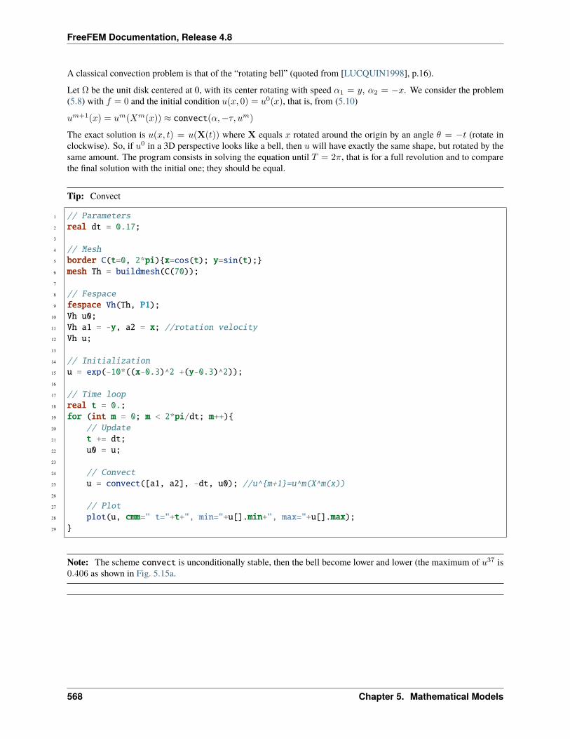
FreeFEM Documentation, Release 4.8
A classical convection problem is that of the “rotating bell” (quoted from [LUCQUIN1998], p.16).
Let Ω be the unit disk centered at 0, with its center rotating with speed 𝛼1 = 𝑦, 𝛼2 = −𝑥. We consider the problem(5.8) with 𝑓 = 0 and the initial condition 𝑢(𝑥, 0) = 𝑢0(𝑥), that is, from (5.10)
𝑢𝑚+1(𝑥) = 𝑢𝑚(𝑋𝑚(𝑥)) ≈ convect(𝛼,−𝜏, 𝑢𝑚)
The exact solution is 𝑢(𝑥, 𝑡) = 𝑢(X(𝑡)) where X equals 𝑥 rotated around the origin by an angle 𝜃 = −𝑡 (rotate inclockwise). So, if 𝑢0 in a 3D perspective looks like a bell, then 𝑢 will have exactly the same shape, but rotated by thesame amount. The program consists in solving the equation until 𝑇 = 2𝜋, that is for a full revolution and to comparethe final solution with the initial one; they should be equal.
Tip: Convect
1 // Parameters2 real dt = 0.17;3
4 // Mesh5 border C(t=0, 2*pi)x=cos(t); y=sin(t);6 mesh Th = buildmesh(C(70));7
8 // Fespace9 fespace Vh(Th, P1);
10 Vh u0;11 Vh a1 = -y, a2 = x; //rotation velocity12 Vh u;13
14 // Initialization15 u = exp(-10*((x-0.3)^2 +(y-0.3)^2));16
17 // Time loop18 real t = 0.;19 for (int m = 0; m < 2*pi/dt; m++)20 // Update21 t += dt;22 u0 = u;23
24 // Convect25 u = convect([a1, a2], -dt, u0); //u^m+1=u^m(X^m(x))26
27 // Plot28 plot(u, cmm=" t="+t+", min="+u[].min+", max="+u[].max);29
Note: The scheme convect is unconditionally stable, then the bell become lower and lower (the maximum of 𝑢37 is0.406 as shown in Fig. 5.15a.
568 Chapter 5. Mathematical Models
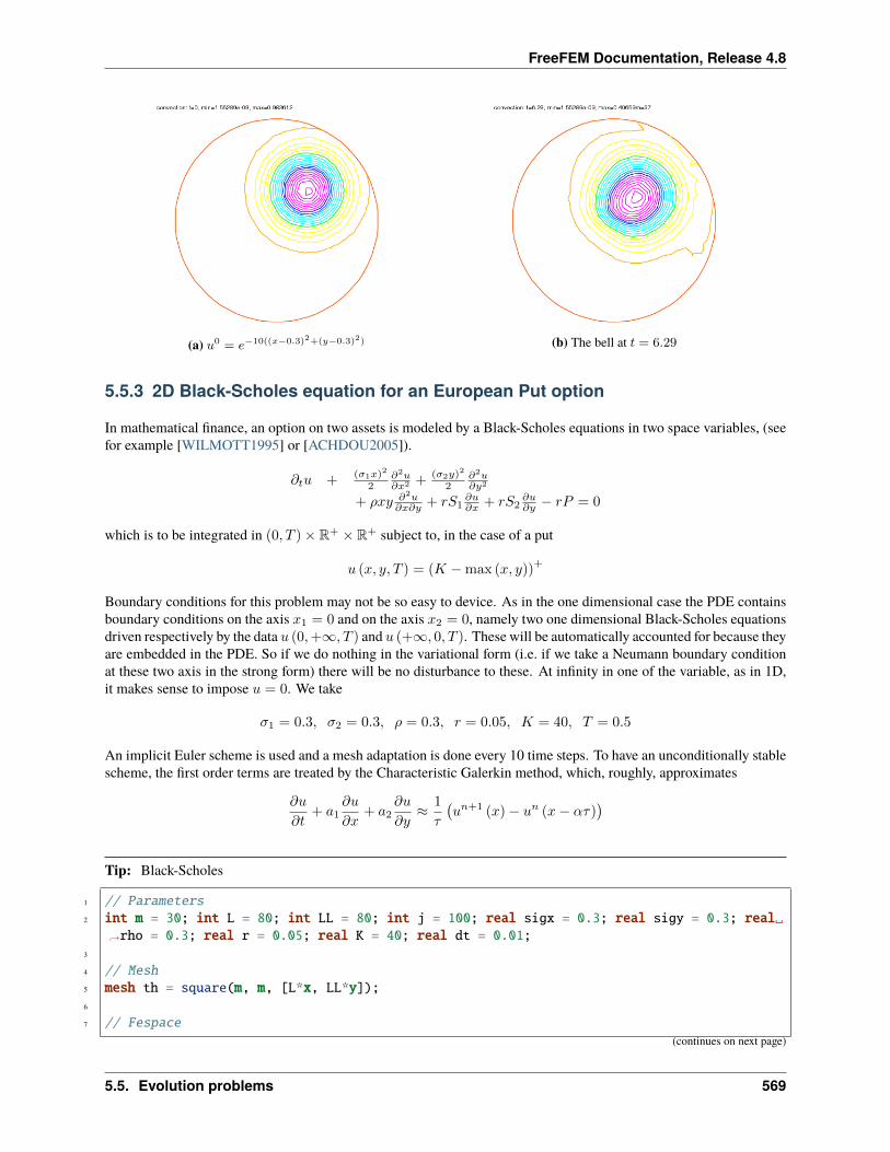
FreeFEM Documentation, Release 4.8
(a) 𝑢0 = 𝑒−10((𝑥−0.3)2+(𝑦−0.3)2) (b) The bell at 𝑡 = 6.29
5.5.3 2D Black-Scholes equation for an European Put option
In mathematical finance, an option on two assets is modeled by a Black-Scholes equations in two space variables, (seefor example [WILMOTT1995] or [ACHDOU2005]).
𝜕𝑡𝑢 + (𝜎1𝑥)2
2𝜕2𝑢𝜕𝑥2 + (𝜎2𝑦)
2
2𝜕2𝑢𝜕𝑦2
+ 𝜌𝑥𝑦 𝜕2𝑢𝜕𝑥𝜕𝑦 + 𝑟𝑆1
𝜕𝑢𝜕𝑥 + 𝑟𝑆2
𝜕𝑢𝜕𝑦 − 𝑟𝑃 = 0
which is to be integrated in (0, 𝑇 )× R+ × R+ subject to, in the case of a put
𝑢 (𝑥, 𝑦, 𝑇 ) = (𝐾 −max (𝑥, 𝑦))+
Boundary conditions for this problem may not be so easy to device. As in the one dimensional case the PDE containsboundary conditions on the axis 𝑥1 = 0 and on the axis 𝑥2 = 0, namely two one dimensional Black-Scholes equationsdriven respectively by the data 𝑢 (0,+∞, 𝑇 ) and 𝑢 (+∞, 0, 𝑇 ). These will be automatically accounted for because theyare embedded in the PDE. So if we do nothing in the variational form (i.e. if we take a Neumann boundary conditionat these two axis in the strong form) there will be no disturbance to these. At infinity in one of the variable, as in 1D,it makes sense to impose 𝑢 = 0. We take
𝜎1 = 0.3, 𝜎2 = 0.3, 𝜌 = 0.3, 𝑟 = 0.05, 𝐾 = 40, 𝑇 = 0.5
An implicit Euler scheme is used and a mesh adaptation is done every 10 time steps. To have an unconditionally stablescheme, the first order terms are treated by the Characteristic Galerkin method, which, roughly, approximates
𝜕𝑢
𝜕𝑡+ 𝑎1
𝜕𝑢
𝜕𝑥+ 𝑎2
𝜕𝑢
𝜕𝑦≈ 1
𝜏
(𝑢𝑛+1 (𝑥)− 𝑢𝑛 (𝑥− 𝛼𝜏)
)
Tip: Black-Scholes
1 // Parameters2 int m = 30; int L = 80; int LL = 80; int j = 100; real sigx = 0.3; real sigy = 0.3; real
→˓rho = 0.3; real r = 0.05; real K = 40; real dt = 0.01;3
4 // Mesh5 mesh th = square(m, m, [L*x, LL*y]);6
7 // Fespace(continues on next page)
5.5. Evolution problems 569
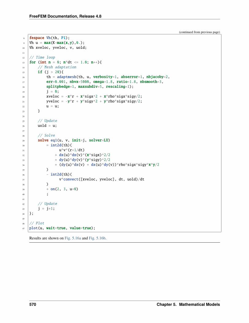
FreeFEM Documentation, Release 4.8
(continued from previous page)
8 fespace Vh(th, P1);9 Vh u = max(K-max(x,y),0.);
10 Vh xveloc, yveloc, v, uold;11
12 // Time loop13 for (int n = 0; n*dt <= 1.0; n++)14 // Mesh adaptation15 if (j > 20)16 th = adaptmesh(th, u, verbosity=1, abserror=1, nbjacoby=2,17 err=0.001, nbvx=5000, omega=1.8, ratio=1.8, nbsmooth=3,18 splitpbedge=1, maxsubdiv=5, rescaling=1);19 j = 0;20 xveloc = -x*r + x*sigx^2 + x*rho*sigx*sigy/2;21 yveloc = -y*r + y*sigy^2 + y*rho*sigx*sigy/2;22 u = u;23 24
25 // Update26 uold = u;27
28 // Solve29 solve eq1(u, v, init=j, solver=LU)30 = int2d(th)(31 u*v*(r+1/dt)32 + dx(u)*dx(v)*(x*sigx)^2/233 + dy(u)*dy(v)*(y*sigy)^2/234 + (dy(u)*dx(v) + dx(u)*dy(v))*rho*sigx*sigy*x*y/235 )36 - int2d(th)(37 v*convect([xveloc, yveloc], dt, uold)/dt38 )39 + on(2, 3, u=0)40 ;41
42 // Update43 j = j+1;44 ;45
46 // Plot47 plot(u, wait=true, value=true);
Results are shown on Fig. 5.16a and Fig. 5.16b.
570 Chapter 5. Mathematical Models
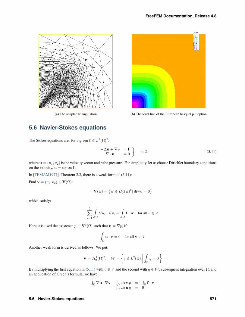
FreeFEM Documentation, Release 4.8
(a) The adapted triangulation (b) The level line of the European basquet put option
5.6 Navier-Stokes equations
The Stokes equations are: for a given f ∈ 𝐿2(Ω)2:
−∆u +∇𝑝 = f∇ · u = 0
in Ω (5.11)
whereu = (𝑢1, 𝑢2) is the velocity vector and 𝑝 the pressure. For simplicity, let us choose Dirichlet boundary conditionson the velocity, u = uΓ on Γ.
In [TEMAM1977], Theorem 2.2, there is a weak form of (5.11):
Find v = (𝑣1, 𝑣2) ∈ V(Ω):
V(Ω) = w ∈ 𝐻10 (Ω)2| divw = 0
which satisfy:
2∑𝑖=1
∫Ω
∇𝑢𝑖 · ∇𝑣𝑖 =
∫Ω
f ·w for all 𝑣 ∈ 𝑉
Here it is used the existence 𝑝 ∈ 𝐻1(Ω) such that u = ∇𝑝, if:∫Ω
u · v = 0 for all v ∈ 𝑉
Another weak form is derived as follows: We put:
V = 𝐻10 (Ω)2; 𝑊 =
𝑞 ∈ 𝐿2(Ω)
∫Ω
𝑞 = 0
By multiplying the first equation in (5.11) with 𝑣 ∈ 𝑉 and the second with 𝑞 ∈𝑊 , subsequent integration over Ω, andan application of Green’s formula, we have:∫
Ω∇u · ∇v −
∫Ω
divv 𝑝 =∫Ωf · v∫
Ωdivu 𝑞 = 0
5.6. Navier-Stokes equations 571
FreeFEM Documentation, Release 4.8
This yields the weak form of (5.11):
Find (u, 𝑝) ∈ V ×𝑊 such that:
𝑎(u,v) + 𝑏(v, 𝑝) = (f ,v)𝑏(u, 𝑞) = 0
for all (v, 𝑞) ∈ 𝑉 ×𝑊 , where:
𝑎(u,v) =∫Ω∇u · ∇v =
∑2𝑖=1
∫Ω∇𝑢𝑖 · ∇𝑣𝑖
𝑏(u, 𝑞) = −∫Ω
divu 𝑞
Now, we consider finite element spaces Vℎ ⊂ V and 𝑊ℎ ⊂𝑊 , and we assume the following basis functions:
Vℎ = 𝑉ℎ × 𝑉ℎ, 𝑉ℎ = 𝑣ℎ| 𝑣ℎ = 𝑣1𝜑1 + · · ·+ 𝑣𝑀𝑉𝜑𝑀𝑉
,𝑊ℎ = 𝑞ℎ| 𝑞ℎ = 𝑞1𝜙1 + · · ·+ 𝑞𝑀𝑊
𝜙𝑀𝑊
The discrete weak form is: Find (uℎ, 𝑝ℎ) ∈ Vℎ ×𝑊ℎ such that:
𝑎(uℎ,vℎ) + 𝑏(vℎ, 𝑝) = (f ,vℎ), ∀vℎ ∈ Vℎ
𝑏(uℎ, 𝑞ℎ) = 0, ∀𝑞ℎ ∈𝑊ℎ(5.12)
Note: Assume that:
1. There is a constant 𝛼ℎ > 0 such that:
𝑎(vℎ,vℎ) ≥ 𝛼‖vℎ‖21,Ω for all vℎ ∈ 𝑍ℎ
where:
𝑍ℎ = vℎ ∈ Vℎ| 𝑏(wℎ, 𝑞ℎ) = 0 for all 𝑞ℎ ∈𝑊ℎ
2. There is a constant 𝛽ℎ > 0 such that:
supvℎ∈Vℎ
𝑏(vℎ, 𝑞ℎ)
‖vℎ‖1,Ω≥ 𝛽ℎ‖𝑞ℎ‖0,Ω for all 𝑞ℎ ∈𝑊ℎ
Then we have an unique solution (uℎ, 𝑝ℎ) of (5.12) satisfying:
‖u− uℎ‖1,Ω + ‖𝑝− 𝑝ℎ‖0,Ω ≤ 𝐶(
infvℎ∈Vℎ
‖𝑢− 𝑣ℎ‖1,Ω + inf𝑞ℎ∈𝑊ℎ
‖𝑝− 𝑞ℎ‖0,Ω)
with a constant 𝐶 > 0 (see e.g. [ROBERTS1993], Theorem 10.4).
Let us denote that:
𝐴 = (𝐴𝑖𝑗), 𝐴𝑖𝑗 =∫Ω∇𝜑𝑗 · ∇𝜑𝑖 𝑖, 𝑗 = 1, · · · ,𝑀V
B = (𝐵𝑥𝑖𝑗 , 𝐵𝑦𝑖𝑗), 𝐵𝑥𝑖𝑗 = −∫Ω𝜕𝜑𝑗/𝜕𝑥𝜙𝑖 𝐵𝑦𝑖𝑗 = −
∫Ω𝜕𝜑𝑗/𝜕𝑦 𝜙𝑖
𝑖 = 1, · · · ,𝑀𝑊 ; 𝑗 = 1, · · · ,𝑀𝑉
then (5.12) is written by: (A B*
B 0
)(Uℎ
𝑝ℎ
)=
(Fℎ0
)
572 Chapter 5. Mathematical Models
FreeFEM Documentation, Release 4.8
where:
A =
(𝐴 00 𝐴
)B* =
𝐵𝑥𝑇
𝐵𝑦𝑇
Uℎ =
𝑢1,ℎ𝑢2,ℎ
Fℎ =
∫Ω𝑓1𝜑𝑖
∫Ω𝑓2𝜑𝑖
Penalty method: This method consists of replacing (5.12) by a more regular problem:
Find (v𝜖ℎ, 𝑝𝜖ℎ) ∈ Vℎ × ℎ satisfying:
𝑎(u𝜖ℎ,vℎ) + 𝑏(vℎ, 𝑝𝜖ℎ) = (f ,vℎ), ∀vℎ ∈ Vℎ
𝑏(u𝜖ℎ, 𝑞ℎ)− 𝜖(𝑝𝜖ℎ, 𝑞ℎ) = 0, ∀𝑞ℎ ∈ ℎ(5.13)
where ℎ ⊂ 𝐿2(Ω). Formally, we have:
divu𝜖ℎ = 𝜖𝑝𝜖ℎ
and the corresponding algebraic problem:(A 𝐵*
𝐵 −𝜖𝐼
)(U𝜖ℎ
𝑝𝜖ℎ
)=
(Fℎ0
)
Note: We can eliminate 𝑝𝜖ℎ = (1/𝜖)𝐵𝑈 𝜖ℎ to obtain:
(𝐴+ (1/𝜖)𝐵*𝐵)U𝜖ℎ = F𝜖ℎ (5.14)
Since the matrix 𝐴+ (1/𝜖)𝐵*𝐵 is symmetric, positive-definite, and sparse, (5.14) can be solved by known technique.There is a constant 𝐶 > 0 independent of 𝜖 such that:
‖uℎ − u𝜖ℎ‖1,Ω + ‖𝑝ℎ − 𝑝𝜖ℎ‖0,Ω ≤ 𝐶𝜖
(see e.g. [ROBERTS1993], 17.2)
Tip: Cavity
The driven cavity flow problem is solved first at zero Reynolds number (Stokes flow) and then at Reynolds 100. Thevelocity pressure formulation is used first and then the calculation is repeated with the stream function vorticity formu-lation.
We solve the driven cavity problem by the penalty method (5.13) where uΓ ·n = 0 and uΓ · s = 1 on the top boundaryand zero elsewhere (n is the unit normal to Γ, and s the unit tangent to Γ).
The mesh is constructed by:
1 mesh Th = square(8, 8);
We use a classical Taylor-Hood element technique to solve the problem:
The velocity is approximated with the 𝑃2 FE (𝑋ℎ space), and the pressure is approximated with the 𝑃1 FE (𝑀ℎ space),where:
𝑋ℎ =v ∈ 𝐻1(]0, 1[2)
∀𝐾 ∈ 𝒯ℎ 𝑣|𝐾 ∈ 𝑃2
and:
𝑀ℎ =𝑣 ∈ 𝐻1(]0, 1[2)
∀𝐾 ∈ 𝒯ℎ 𝑣|𝐾 ∈ 𝑃1
The FE spaces and functions are constructed by:
5.6. Navier-Stokes equations 573
FreeFEM Documentation, Release 4.8
1 fespace Xh(Th, P2); //definition of the velocity component space2 fespace Mh(Th, P1); //definition of the pressure space3 Xh u2, v2;4 Xh u1, v1;5 Mh p, q;
The Stokes operator is implemented as a system-solve for the velocity (𝑢1, 𝑢2) and the pressure 𝑝. The test functionfor the velocity is (𝑣1, 𝑣2) and 𝑞 for the pressure, so the variational form (5.12) in freefem language is:
1 solve Stokes (u1, u2, p, v1, v2, q, solver=Crout)2 = int2d(Th)(3 (4 dx(u1)*dx(v1)5 + dy(u1)*dy(v1)6 + dx(u2)*dx(v2)7 + dy(u2)*dy(v2)8 )9 - p*q*(0.000001)
10 - p*dx(v1) - p*dy(v2)11 - dx(u1)*q - dy(u2)*q12 )13 + on(3, u1=1, u2=0)14 + on(1, 2, 4, u1=0, u2=0)15 ;
Each unknown has its own boundary conditions.
If the streamlines are required, they can be computed by finding 𝜓 such that 𝑟𝑜𝑡𝜓 = 𝑢 or better:
−∆𝜓 = ∇× 𝑢
1 Xh psi, phi;2
3 solve streamlines (psi, phi)4 = int2d(Th)(5 dx(psi)*dx(phi)6 + dy(psi)*dy(phi)7 )8 + int2d(Th)(9 - phi*(dy(u1) - dx(u2))
10 )11 + on(1, 2, 3, 4, psi=0)12 ;
Now the Navier-Stokes equations are solved:
𝜕𝑢
𝜕𝑡+ 𝑢 · ∇𝑢− 𝜈∆𝑢+∇𝑝 = 0,∇ · 𝑢 = 0
with the same boundary conditions and with initial conditions 𝑢 = 0.
This is implemented by using the convection operator convect for the term 𝜕𝑢𝜕𝑡 + 𝑢 · ∇𝑢, giving a discretization in
time1𝜏 (𝑢𝑛+1 − 𝑢𝑛 ∘𝑋𝑛)− 𝜈∆𝑢𝑛+1 +∇𝑝𝑛+1 = 0,
∇ · 𝑢𝑛+1 = 0
574 Chapter 5. Mathematical Models
FreeFEM Documentation, Release 4.8
The term 𝑢𝑛 ∘𝑋𝑛(𝑥) ≈ 𝑢𝑛(𝑥− 𝑢𝑛(𝑥)𝜏) will be computed by the operator convect, so we obtain:
1 int i=0;2 real alpha=1/dt;3 problem NS (u1, u2, p, v1, v2, q, solver=Crout, init=i)4 = int2d(Th)(5 alpha*(u1*v1 + u2*v2)6 + nu * (7 dx(u1)*dx(v1) + dy(u1)*dy(v1)8 + dx(u2)*dx(v2) + dy(u2)*dy(v2)9 )
10 - p*q*(0.000001)11 - p*dx(v1) - p*dy(v2)12 - dx(u1)*q - dy(u2)*q13 )14 + int2d(Th)(15 - alpha*convect([up1,up2],-dt,up1)*v116 - alpha*convect([up1,up2],-dt,up2)*v217 )18 + on(3, u1=1, u2=0)19 + on(1, 2, 4,u1=0, u2=0)20 ;21
22 // Time loop23 for (i = 0; i <= 10; i++)24 // Update25 up1 = u1;26 up2 = u2;27
28 // Solve29 NS;30
31 // Plot32 if (!(i % 10))33 plot(coef=0.2, cmm="[u1,u2] and p", p, [u1, u2]);34
Notice that the stiffness matrices are reused (keyword init=i)
The complete script is available in cavity example.
5.6.1 Uzawa Algorithm and Conjugate Gradients
We solve Stokes problem without penalty. The classical iterative method of Uzawa is described by the algorithm (seee.g. [ROBERTS1993], 17.3, [GLOWINSKI1979], 13 or [GLOWINSKI1985], 13):
• Initialize: Let 𝑝0ℎ be an arbitrary chosen element of 𝐿2(Ω).
• Calculate :math:`mathbfu_h`: Once 𝑝𝑛ℎ is known, v𝑛ℎ is the solution of:
u𝑛ℎ = 𝐴−1(fℎ −B*𝑝𝑛ℎ)
• Advance :math:`p_h`: Let 𝑝𝑛+1ℎ be defined by;
5.6. Navier-Stokes equations 575
FreeFEM Documentation, Release 4.8
𝑝𝑛+1ℎ = 𝑝𝑛ℎ + 𝜌𝑛Bu𝑛ℎ
There is a constant 𝛼 > 0 such that 𝛼 ≤ 𝜌𝑛 ≤ 2 for each 𝑛, then u𝑛ℎ converges to the solution uℎ, and then 𝐵v𝑛ℎ → 0as 𝑛→∞ from the Advance 𝑝ℎ. This method in general converges quite slowly.
First we define mesh, and the Taylor-Hood approximation. So 𝑋ℎ is the velocity space, and 𝑀ℎ is the pressure space.
Tip: Stokes Uzawa
1 // Mesh2 mesh Th = square(10, 10);3
4 // Fespace5 fespace Xh(Th, P2);6 Xh u1, u2;7 Xh bc1, bc2;8 Xh b;9
10 fespace Mh(Th, P1);11 Mh p;12 Mh ppp; //ppp is a working pressure13
14 // Problem15 varf bx (u1, q) = int2d(Th)(-(dx(u1)*q));16 varf by (u1, q) = int2d(Th)(-(dy(u1)*q));17 varf a (u1, u2)18 = int2d(Th)(19 dx(u1)*dx(u2)20 + dy(u1)*dy(u2)21 )22 + on(3, u1=1)23 + on(1, 2, 4, u1=0) ;24 //remark: put the on(3,u1=1) before on(1,2,4,u1=0)25 //because we want zero on intersection26
27 matrix A = a(Xh, Xh, solver=CG);28 matrix Bx = bx(Xh, Mh); //B=(Bx, By)29 matrix By = by(Xh, Mh);30
31 bc1[] = a(0,Xh); //boundary condition contribution on u132 bc2 = 0; //no boundary condition contribution on u233
34 //p_h^n -> B A^-1 - B^* p_h^n = -div u_h35 //is realized as the function divup36 func real[int] divup (real[int] & pp)37 //compute u1(pp)38 b[] = Bx'*pp;39 b[] *= -1;40 b[] += bc1[];41 u1[] = A^-1*b[];42 //compute u2(pp)
(continues on next page)
576 Chapter 5. Mathematical Models
FreeFEM Documentation, Release 4.8
(continued from previous page)
43 b[] = By'*pp;44 b[] *= -1;45 b[] += bc2[];46 u2[] = A^-1*b[];47 //u^n = (A^-1 Bx^T p^n, By^T p^n)^T48 ppp[] = Bx*u1[]; //ppp = Bx u_149 ppp[] += By*u2[]; //+ By u_250
51 return ppp[] ;52 53
54 // Initialization55 p=0; //p_h^0 = 056 LinearCG(divup, p[], eps=1.e-6, nbiter=50); //p_h^n+1 = p_h^n + B u_h^n57 // if n> 50 or |p_h^n+1 - p_h^n| <= 10^-6, then the loop end58 divup(p[]); //compute the final solution59
60 plot([u1, u2], p, wait=1, value=true, coef=0.1);
5.6.2 NSUzawaCahouetChabart.edp
In this example we solve the Navier-Stokes equation past a cylinder with the Uzawa algorithm preconditioned by theCahouet-Chabart method (see [GLOWINSKI2003] for all the details).
The idea of the preconditioner is that in a periodic domain, all differential operators commute and the Uzawa algorithmcomes to solving the linear operator ∇.((𝛼𝐼𝑑 + 𝜈∆)−1∇, where 𝐼𝑑 is the identity operator. So the preconditionersuggested is 𝛼∆−1 + 𝜈𝐼𝑑.
To implement this, we do:
Tip: NS Uzawa Cahouet Chabart
1 // Parameters2 verbosity = 0;3 real D = 0.1;4 real H = 0.41;5 real cx0 = 0.2;6 real cy0 = 0.2; //center of cylinder7 real xa = 0.15;8 real ya = 0.2;9 real xe = 0.25;
10 real ye = 0.2;11 int nn = 15;12
13 //TODO14 real Um = 1.5; //max velocity (Rey 100)15 real nu = 1e-3;16
17 func U1 = 4.*Um*y*(H-y)/(H*H); //Boundary condition18 func U2 = 0.;
(continues on next page)
5.6. Navier-Stokes equations 577
FreeFEM Documentation, Release 4.8
(continued from previous page)
19 real T=2;20 real dt = D/nn/Um; //CFL = 121 real epspq = 1e-10;22 real eps = 1e-6;23
24 // Variables25 func Ub = Um*2./3.;26 real alpha = 1/dt;27 real Rey = Ub*D/nu;28 real t = 0.;29
30 // Mesh31 border fr1(t=0, 2.2)x=t; y=0; label=1;32 border fr2(t=0, H)x=2.2; y=t; label=2;33 border fr3(t=2.2, 0)x=t; y=H; label=1;34 border fr4(t=H, 0)x=0; y=t; label=1;35 border fr5(t=2*pi, 0)x=cx0+D*sin(t)/2; y=cy0+D*cos(t)/2; label=3;36 mesh Th = buildmesh(fr1(5*nn) + fr2(nn) + fr3(5*nn) + fr4(nn) + fr5(-nn*3));37
38 // Fespace39 fespace Mh(Th, [P1]);40 Mh p;41
42 fespace Xh(Th, [P2]);43 Xh u1, u2;44
45 fespace Wh(Th, [P1dc]);46 Wh w; //vorticity47
48 // Macro49 macro grad(u) [dx(u), dy(u)] //50 macro div(u1, u2) (dx(u1) + dy(u2)) //51
52 // Problem53 varf von1 ([u1, u2, p], [v1, v2, q])54 = on(3, u1=0, u2=0)55 + on(1, u1=U1, u2=U2)56 ;57
58 //remark : the value 100 in next varf is manualy fitted, because free outlet.59 varf vA (p, q) =60 int2d(Th)(61 grad(p)' * grad(q)62 )63 + int1d(Th, 2)(64 100*p*q65 )66 ;67
68 varf vM (p, q)69 = int2d(Th, qft=qf2pT)(70 p*q
(continues on next page)
578 Chapter 5. Mathematical Models
FreeFEM Documentation, Release 4.8
(continued from previous page)
71 )72 + on(2, p=0)73 ;74
75 varf vu ([u1], [v1])76 = int2d(Th)(77 alpha*(u1*v1)78 + nu*(grad(u1)' * grad(v1))79 )80 + on(1, 3, u1=0)81 ;82
83 varf vu1 ([p], [v1]) = int2d(Th)(p*dx(v1));84 varf vu2 ([p], [v1]) = int2d(Th)(p*dy(v1));85
86 varf vonu1 ([u1], [v1]) = on(1, u1=U1) + on(3, u1=0);87 varf vonu2 ([u1], [v1]) = on(1, u1=U2) + on(3, u1=0);88
89 matrix pAM = vM(Mh, Mh, solver=UMFPACK);90 matrix pAA = vA(Mh, Mh, solver=UMFPACK);91 matrix AU = vu(Xh, Xh, solver=UMFPACK);92 matrix B1 = vu1(Mh, Xh);93 matrix B2 = vu2(Mh, Xh);94
95 real[int] brhs1 = vonu1(0, Xh);96 real[int] brhs2 = vonu2(0, Xh);97
98 varf vrhs1(uu, vv) = int2d(Th)(convect([u1, u2], -dt, u1)*vv*alpha) + vonu1;99 varf vrhs2(v2, v1) = int2d(Th)(convect([u1, u2], -dt, u2)*v1*alpha) + vonu2;
100
101 // Uzawa function102 func real[int] JUzawa (real[int] & pp)103 real[int] b1 = brhs1; b1 += B1*pp;104 real[int] b2 = brhs2; b2 += B2*pp;105 u1[] = AU^-1 * b1;106 u2[] = AU^-1 * b2;107 pp = B1'*u1[];108 pp += B2'*u2[];109 pp = -pp;110 return pp;111 112
113 // Preconditioner function114 func real[int] Precon (real[int] & p)115 real[int] pa = pAA^-1*p;116 real[int] pm = pAM^-1*p;117 real[int] pp = alpha*pa + nu*pm;118 return pp;119 120
121 // Initialization122 p = 0;
(continues on next page)
5.6. Navier-Stokes equations 579
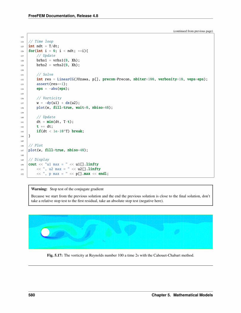
FreeFEM Documentation, Release 4.8
(continued from previous page)
123
124 // Time loop125 int ndt = T/dt;126 for(int i = 0; i < ndt; ++i)127 // Update128 brhs1 = vrhs1(0, Xh);129 brhs2 = vrhs2(0, Xh);130
131 // Solve132 int res = LinearCG(JUzawa, p[], precon=Precon, nbiter=100, verbosity=10, veps=eps);133 assert(res==1);134 eps = -abs(eps);135
136 // Vorticity137 w = -dy(u1) + dx(u2);138 plot(w, fill=true, wait=0, nbiso=40);139
140 // Update141 dt = min(dt, T-t);142 t += dt;143 if(dt < 1e-10*T) break;144 145
146 // Plot147 plot(w, fill=true, nbiso=40);148
149 // Display150 cout << "u1 max = " << u1[].linfty151 << ", u2 max = " << u2[].linfty152 << ", p max = " << p[].max << endl;
Warning: Stop test of the conjugate gradient
Because we start from the previous solution and the end the previous solution is close to the final solution, don’ttake a relative stop test to the first residual, take an absolute stop test (negative here).
Fig. 5.17: The vorticity at Reynolds number 100 a time 2s with the Cahouet-Chabart method.
580 Chapter 5. Mathematical Models
FreeFEM Documentation, Release 4.8
5.7 Variational Inequality
We present, a classical example of variational inequality.
Let us denote 𝒞 = 𝑢 ∈ 𝐻10 (Ω), 𝑢 ≤ 𝑔
The problem is:
𝑢 = 𝑎𝑟𝑔min𝑢∈𝒞
𝐽(𝑢) =1
2
∫Ω
∇𝑢.∇𝑢−∫Ω
𝑓𝑢
where 𝑓 and 𝑔 are given function.
The solution is a projection on the convex 𝒞 of 𝑓⋆ for the scalar product ((𝑣, 𝑤)) =∫Ω∇𝑣.∇𝑤 of 𝐻1
0 (Ω) where 𝑓⋆ issolution of:
(𝑓⋆, 𝑣) =
∫Ω
𝑓𝑣, ∀𝑣 ∈ 𝐻10 (‘Ω)
The projection on a convex satisfy clearly ∀𝑣 ∈ 𝒞, ((𝑢 − 𝑣, 𝑢 − 𝑓)) ≤ 0, and after expanding, we get the classicalinequality:
∀𝑣 ∈ 𝒞,∫Ω
∇(𝑢− 𝑣)∇𝑢 ≤∫Ω
(𝑢− 𝑣)𝑓
We can also rewrite the problem as a saddle point problem:
Find 𝜆, 𝑢 such that:
max𝜆∈𝐿2(Ω),𝜆≥0
min𝑢∈𝐻1
0 (Ω)ℒ(𝑢, 𝜆) =
1
2
∫Ω
∇𝑢.∇𝑢−∫Ω
𝑓𝑢+
∫Ω
𝜆(𝑢− 𝑔)+
where ((𝑢− 𝑔)+ = 𝑚𝑎𝑥(0, 𝑢− 𝑔).
This saddle point problem is equivalent to find 𝑢, 𝜆 such that:⎧⎪⎨⎪⎩∫Ω
∇𝑢.∇𝑣 + 𝜆𝑣+ 𝑑𝜔 =
∫Ω
𝑓𝑢, ∀𝑣 ∈ 𝐻10 (Ω)∫
Ω
𝜇(𝑢− 𝑔)+ = 0, ∀𝜇 ∈ 𝐿2(Ω), 𝜇 ≥ 0, 𝜆 ≥ 0,
An algorithm to solve the previous problem is:
1. k=0, and choose 𝜆0 belong 𝐻−1(Ω)
2. Loop on 𝑘 = 0, .....
• set ℐ𝑘 = 𝑥 ∈ Ω/𝜆𝑘 + 𝑐 * (𝑢𝑘+1 − 𝑔) ≤ 0
• 𝑉𝑔,𝑘+1 = 𝑣 ∈ 𝐻10 (Ω)/𝑣 = 𝑔 on 𝐼𝑘,
• 𝑉0,𝑘+1 = 𝑣 ∈ 𝐻10 (Ω)/𝑣 = 0 on 𝐼𝑘,
• Find 𝑢𝑘+1 ∈ 𝑉𝑔,𝑘+1 and 𝜆𝑘+1 ∈ 𝐻−1(Ω) such that⎧⎪⎨⎪⎩∫Ω
∇𝑢𝑘+1.∇𝑣𝑘+1 𝑑𝜔 =
∫Ω
𝑓𝑣𝑘+1, ∀𝑣𝑘+1 ∈ 𝑉0,𝑘+1
< 𝜆𝑘+1, 𝑣 >=
∫Ω
∇𝑢𝑘+1.∇𝑣 − 𝑓𝑣 𝑑𝜔
where<,> is the duality bracket between𝐻10 (Ω) and𝐻−1(Ω), and 𝑐 is a penalty constant (large enough).
5.7. Variational Inequality 581
FreeFEM Documentation, Release 4.8
You can find all the mathematics about this algorithm in [ITO2003] [HINTERMULLER2002].
Now how to do that in FreeFEM? The full example is:
Tip: Variational inequality
1 load "medit"2
3 // Parameters4 real eps = 1e-5;5 real c = 1000; //penalty parameter of the algoritm6 real tgv = 1e30; //a huge value for exact penalization7 func f = 1; //right hand side function8 func fd = 0; //Dirichlet boundary condition function9
10 // Mesh11 mesh Th = square(20, 20);12
13 // Fespace14 fespace Vh(Th, P1);15 int n = Vh.ndof; //number of degree of freedom16 Vh uh, uhp; //u^n+1 and u^n17 Vh Ik; //to define the set where the containt is reached.18 Vh g = 0.05; //discret function g19 Vh lambda = 0;20
21 // Problem22 varf a (uh, vh)23 = int2d(Th)(24 dx(uh)*dx(vh)25 + dy(uh)*dy(vh)26 )27 - int2d(Th)(28 f*vh29 )30 + on(1, 2, 3, 4, uh=fd)31 ;32
33 //the mass Matrix construction34 varf vM (uh, vh) = int2d(Th)(uh*vh);35
36 //two versions of the matrix of the problem37 matrix A = a(Vh, Vh, tgv=tgv, solver=CG); //one changing38 matrix AA = a(Vh, Vh, solver=CG); //one for computing residual39
40 matrix M = vM(Vh, Vh); //to do a fast computing of L^2 norm : sqrt(u'*(w=M*u))41
42 real[int] Aiin(n);43 real[int] Aii = A.diag; //get the diagonal of the matrix44 real[int] rhs = a(0, Vh, tgv=tgv);45
46 // Initialization47 Ik = 0;
(continues on next page)
582 Chapter 5. Mathematical Models

FreeFEM Documentation, Release 4.8
(continued from previous page)
48 uhp = -tgv;49
50 // Loop51 for(int iter = 0; iter < 100; ++iter)52 // Update53 real[int] b = rhs; //get a copy of the Right hand side54 real[int] Ak(n); //the complementary of Ik ( !Ik = (Ik-1))55 Ak = 1.; Ak -= Ik[];56 //adding new locking condition on b and on the diagonal if (Ik ==1 )57 b = Ik[] .* g[]; b *= tgv; b -= Ak .* rhs;58 Aiin = Ik[] * tgv; Aiin += Ak .* Aii; //set Aii= tgv i in Ik59 A.diag = Aiin; //set the matrix diagonal60 set(A, solver=CG); //important to change preconditioning for solving61
62 // Solve63 uh[] = A^-1* b; //solve the problem with more locking condition64
65 // Residual66 lambda[] = AA * uh[]; //compute the residual (fast with matrix)67 lambda[] += rhs; //remark rhs = -\int f v68
69 Ik = (lambda + c*( g- uh)) < 0.; //the new locking value70
71 // Plot72 plot(Ik, wait=true, cmm=" lock set ", value=true, fill=true);73 plot(uh, wait=true, cmm="uh");74
75 // Error76 //trick to compute L^2 norm of the variation (fast method)77 real[int] diff(n), Mdiff(n);78 diff = uh[] - uhp[];79 Mdiff = M*diff;80 real err = sqrt(Mdiff'*diff);81 cout << "|| u_k=1 - u_k ||_2 = " << err << endl;82
83 // Stop test84 if(err < eps) break;85
86 // Update87 uhp[] = uh[];88 89
90 // Plot91 medit("uh", Th, uh);
Note: As you can see on this example, some vector, or matrix operator are not implemented so a way is to skip theexpression and we use operator +=, -= to merge the result.
5.7. Variational Inequality 583
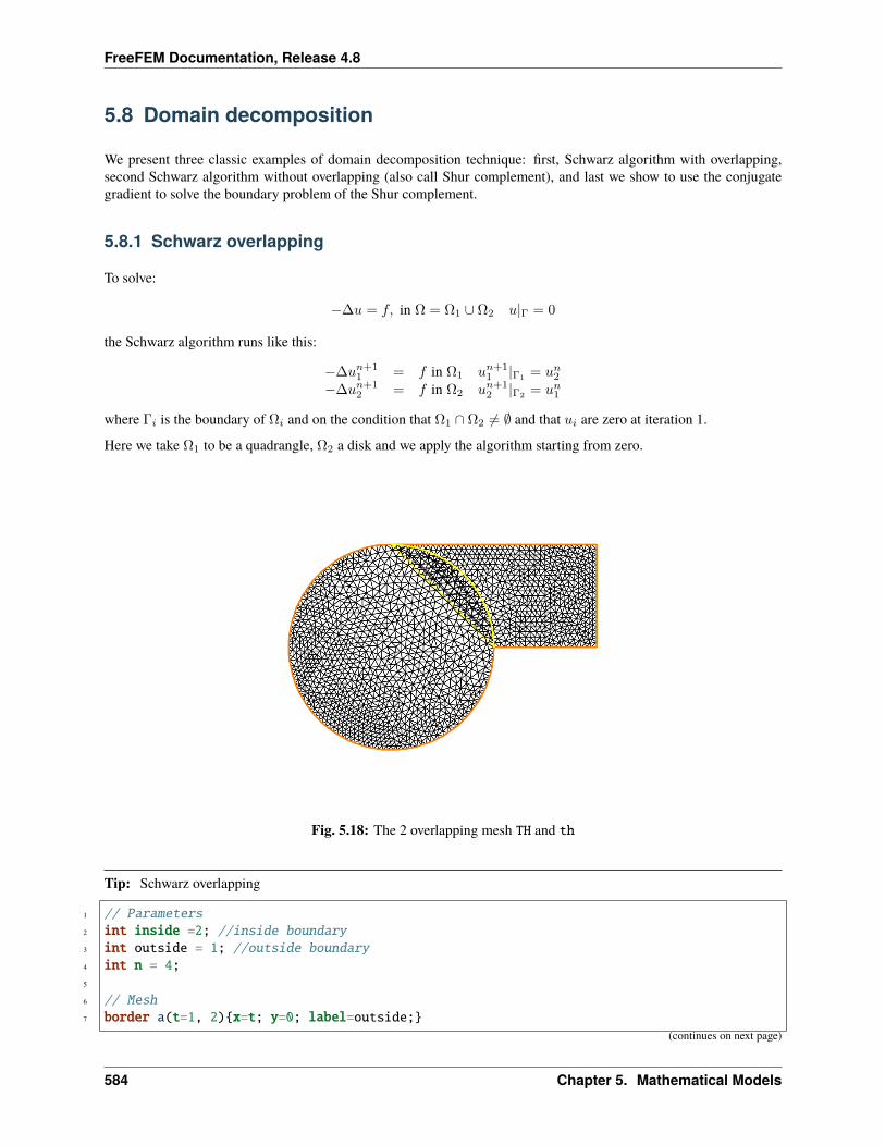
FreeFEM Documentation, Release 4.8
5.8 Domain decomposition
We present three classic examples of domain decomposition technique: first, Schwarz algorithm with overlapping,second Schwarz algorithm without overlapping (also call Shur complement), and last we show to use the conjugategradient to solve the boundary problem of the Shur complement.
5.8.1 Schwarz overlapping
To solve:
−∆𝑢 = 𝑓, in Ω = Ω1 ∪ Ω2 𝑢|Γ = 0
the Schwarz algorithm runs like this:
−∆𝑢𝑛+11 = 𝑓 in Ω1 𝑢𝑛+1
1 |Γ1= 𝑢𝑛2
−∆𝑢𝑛+12 = 𝑓 in Ω2 𝑢𝑛+1
2 |Γ2= 𝑢𝑛1
where Γ𝑖 is the boundary of Ω𝑖 and on the condition that Ω1 ∩ Ω2 = ∅ and that 𝑢𝑖 are zero at iteration 1.
Here we take Ω1 to be a quadrangle, Ω2 a disk and we apply the algorithm starting from zero.
Fig. 5.18: The 2 overlapping mesh TH and th
Tip: Schwarz overlapping
1 // Parameters2 int inside =2; //inside boundary3 int outside = 1; //outside boundary4 int n = 4;5
6 // Mesh7 border a(t=1, 2)x=t; y=0; label=outside;
(continues on next page)
584 Chapter 5. Mathematical Models
FreeFEM Documentation, Release 4.8
(continued from previous page)
8 border b(t=0, 1)x=2; y=t; label=outside;9 border c(t=2, 0)x=t; y=1; label=outside;
10 border d(t=1, 0)x=1-t; y=t; label=inside;11 border e(t=0, pi/2)x=cos(t); y=sin(t); label=inside;12 border e1(t=pi/2, 2*pi)x=cos(t); y=sin(t); label=outside;13 mesh th = buildmesh(a(5*n) + b(5*n) + c(10*n) + d(5*n));14 mesh TH = buildmesh(e(5*n) + e1(25*n));15 plot(th, TH, wait=true); //to see the 2 meshes16
17 // Fespace18 fespace vh(th, P1);19 vh u=0, v;20
21 fespace VH(TH, P1);22 VH U, V;23
24 // Problem25 int i = 0;26 problem PB (U, V, init=i, solver=Cholesky)27 = int2d(TH)(28 dx(U)*dx(V)29 + dy(U)*dy(V)30 )31 + int2d(TH)(32 - V33 )34 + on(inside, U=u)35 + on(outside, U=0)36 ;37
38 problem pb (u, v, init=i, solver=Cholesky)39 = int2d(th)(40 dx(u)*dx(v)41 + dy(u)*dy(v)42 )43 + int2d(th)(44 - v45 )46 + on(inside, u=U)47 + on(outside, u=0)48 ;49
50 // Calculation loop51 for (i = 0 ; i < 10; i++)52 // Solve53 PB;54 pb;55
56 // Plot57 plot(U, u, wait=true);58
5.8. Domain decomposition 585
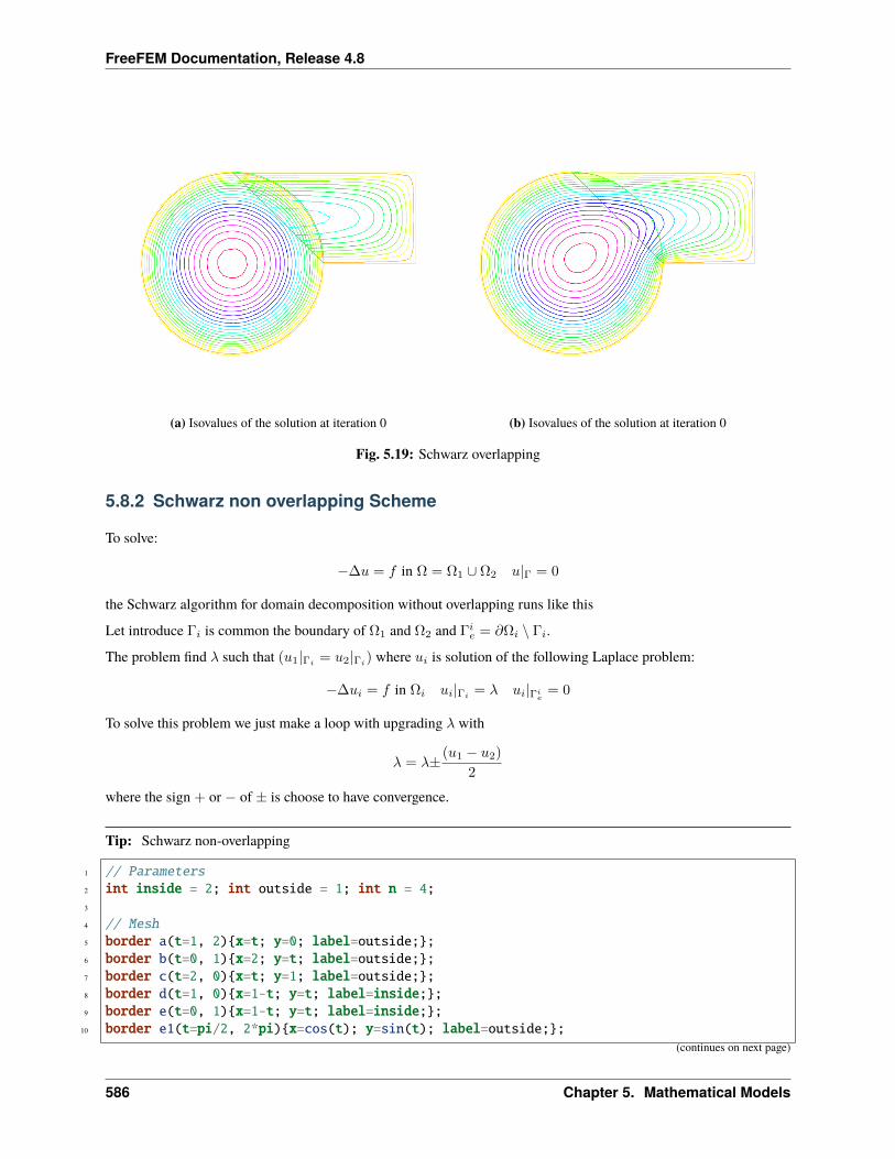
FreeFEM Documentation, Release 4.8
(a) Isovalues of the solution at iteration 0 (b) Isovalues of the solution at iteration 0
Fig. 5.19: Schwarz overlapping
5.8.2 Schwarz non overlapping Scheme
To solve:
−∆𝑢 = 𝑓 in Ω = Ω1 ∪ Ω2 𝑢|Γ = 0
the Schwarz algorithm for domain decomposition without overlapping runs like this
Let introduce Γ𝑖 is common the boundary of Ω1 and Ω2 and Γ𝑖𝑒 = 𝜕Ω𝑖 ∖ Γ𝑖.
The problem find 𝜆 such that (𝑢1|Γ𝑖 = 𝑢2|Γ𝑖) where 𝑢𝑖 is solution of the following Laplace problem:
−∆𝑢𝑖 = 𝑓 in Ω𝑖 𝑢𝑖|Γ𝑖 = 𝜆 𝑢𝑖|Γ𝑖𝑒
= 0
To solve this problem we just make a loop with upgrading 𝜆 with
𝜆 = 𝜆± (𝑢1 − 𝑢2)
2
where the sign + or − of ± is choose to have convergence.
Tip: Schwarz non-overlapping
1 // Parameters2 int inside = 2; int outside = 1; int n = 4;3
4 // Mesh5 border a(t=1, 2)x=t; y=0; label=outside;;6 border b(t=0, 1)x=2; y=t; label=outside;;7 border c(t=2, 0)x=t; y=1; label=outside;;8 border d(t=1, 0)x=1-t; y=t; label=inside;;9 border e(t=0, 1)x=1-t; y=t; label=inside;;
10 border e1(t=pi/2, 2*pi)x=cos(t); y=sin(t); label=outside;;(continues on next page)
586 Chapter 5. Mathematical Models
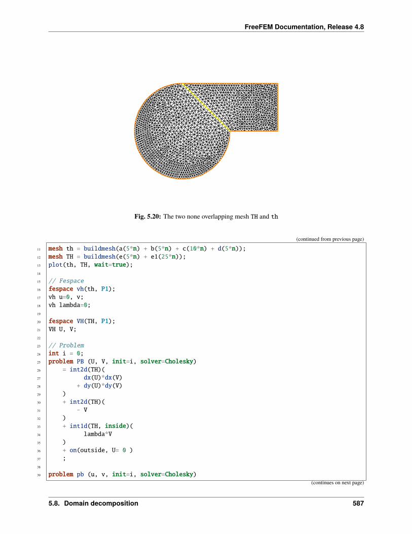
FreeFEM Documentation, Release 4.8
Fig. 5.20: The two none overlapping mesh TH and th
(continued from previous page)
11 mesh th = buildmesh(a(5*n) + b(5*n) + c(10*n) + d(5*n));12 mesh TH = buildmesh(e(5*n) + e1(25*n));13 plot(th, TH, wait=true);14
15 // Fespace16 fespace vh(th, P1);17 vh u=0, v;18 vh lambda=0;19
20 fespace VH(TH, P1);21 VH U, V;22
23 // Problem24 int i = 0;25 problem PB (U, V, init=i, solver=Cholesky)26 = int2d(TH)(27 dx(U)*dx(V)28 + dy(U)*dy(V)29 )30 + int2d(TH)(31 - V32 )33 + int1d(TH, inside)(34 lambda*V35 )36 + on(outside, U= 0 )37 ;38
39 problem pb (u, v, init=i, solver=Cholesky)(continues on next page)
5.8. Domain decomposition 587
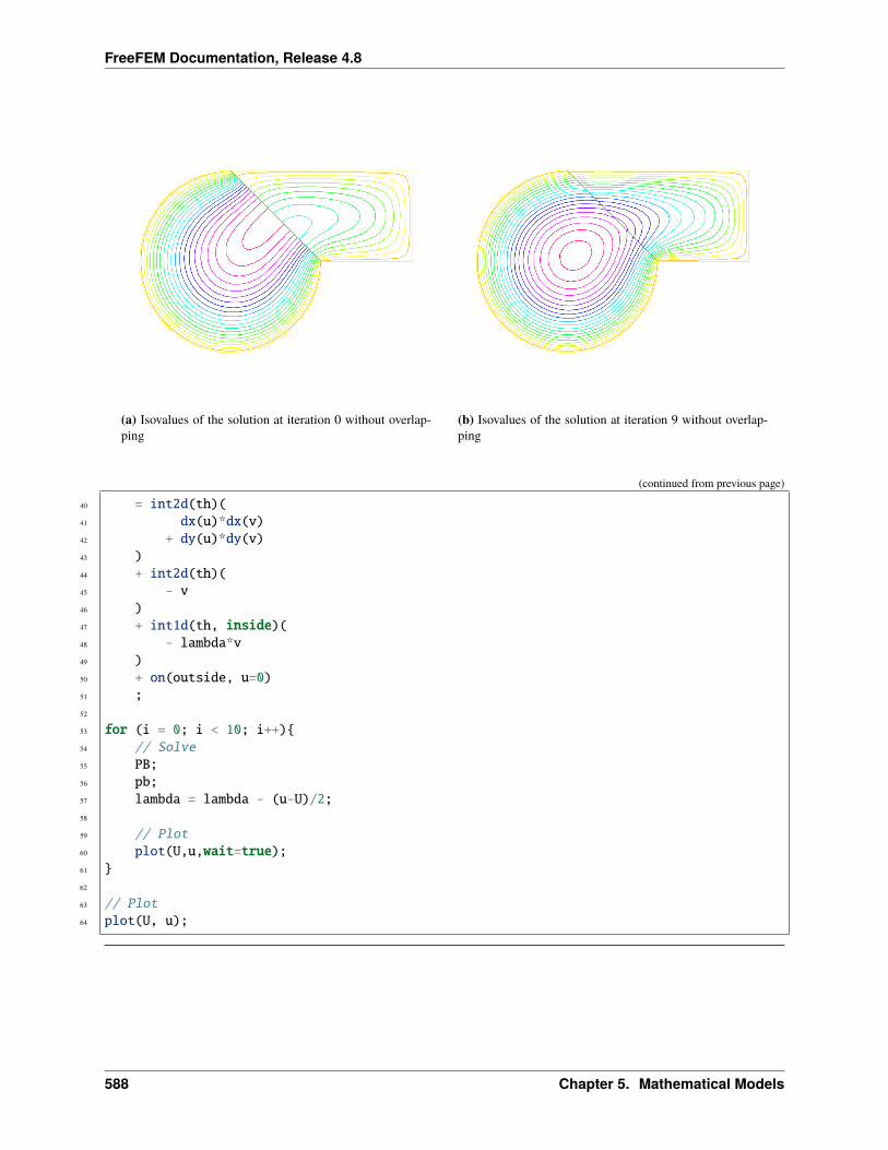
FreeFEM Documentation, Release 4.8
(a) Isovalues of the solution at iteration 0 without overlap-ping
(b) Isovalues of the solution at iteration 9 without overlap-ping
(continued from previous page)
40 = int2d(th)(41 dx(u)*dx(v)42 + dy(u)*dy(v)43 )44 + int2d(th)(45 - v46 )47 + int1d(th, inside)(48 - lambda*v49 )50 + on(outside, u=0)51 ;52
53 for (i = 0; i < 10; i++)54 // Solve55 PB;56 pb;57 lambda = lambda - (u-U)/2;58
59 // Plot60 plot(U,u,wait=true);61 62
63 // Plot64 plot(U, u);
588 Chapter 5. Mathematical Models
FreeFEM Documentation, Release 4.8
5.8.3 Schwarz conjuguate gradient
To solve −∆𝑢 = 𝑓 in Ω = Ω1 ∪Ω2 𝑢|Γ = 0 the Schwarz algorithm for domain decomposition without overlappingruns like this
Let introduce Γ𝑖 is common the boundary of Ω1 and Ω2 and Γ𝑖𝑒 = 𝜕Ω𝑖 ∖ Γ𝑖.
The problem find 𝜆 such that (𝑢1|Γ𝑖 = 𝑢2|Γ𝑖) where 𝑢𝑖 is solution of the following Laplace problem:
−∆𝑢𝑖 = 𝑓 in Ω𝑖 𝑢𝑖|Γ𝑖= 𝜆 𝑢𝑖|Γ𝑖
𝑒= 0
The version of this example uses the Shur complement. The problem on the border is solved by a conjugate gradientmethod.
Tip: Schwarz conjugate gradient
First, we construct the two domains:
1 // Parameters2 int inside = 2; int outside = 1; int n = 4;3
4 // Mesh5 border Gamma1(t=1, 2)x=t; y=0; label=outside;6 border Gamma2(t=0, 1)x=2; y=t; label=outside;7 border Gamma3(t=2, 0)x=t; y=1; label=outside;8 border GammaInside(t=1, 0)x=1-t; y=t; label=inside;9 border GammaArc(t=pi/2, 2*pi)x=cos(t); y=sin(t); label=outside;
10 mesh Th1 = buildmesh(Gamma1(5*n) + Gamma2(5*n) + GammaInside(5*n) + Gamma3(5*n));11 mesh Th2 = buildmesh(GammaInside(-5*n) + GammaArc(25*n));12 plot(Th1, Th2);
Now, define the finite element spaces:
1 // Fespace2 fespace Vh1(Th1, P1);3 Vh1 u1, v1;4 Vh1 lambda;5 Vh1 p=0;6
7 fespace Vh2(Th2,P1);8 Vh2 u2, v2;
Note: It is impossible to define a function just on a part of boundary, so the 𝜆 function must be defined on the alldomain Ω1 such as:
1 Vh1 lambda;
The two Poisson’s problems:
1 problem Pb1 (u1, v1, init=i, solver=Cholesky)2 = int2d(Th1)(3 dx(u1)*dx(v1)4 + dy(u1)*dy(v1)
(continues on next page)
5.8. Domain decomposition 589
FreeFEM Documentation, Release 4.8
(continued from previous page)
5 )6 + int2d(Th1)(7 - v18 )9 + int1d(Th1, inside)(
10 lambda*v111 )12 + on(outside, u1=0)13 ;14
15 problem Pb2 (u2, v2, init=i, solver=Cholesky)16 = int2d(Th2)(17 dx(u2)*dx(v2)18 + dy(u2)*dy(v2)19 )20 + int2d(Th2)(21 - v222 )23 + int1d(Th2, inside)(24 - lambda*v225 )26 + on(outside, u2=0)27 ;
And, we define a border matrix, because the 𝜆 function is none zero inside the domain Ω1:
1 varf b(u2, v2, solver=CG) = int1d(Th1, inside)(u2*v2);2 matrix B = b(Vh1, Vh1, solver=CG);
The boundary problem function,
𝜆 −→∫Γ𝑖
(𝑢1 − 𝑢2)𝑣1
1 // Boundary problem function2 func real[int] BoundaryProblem (real[int] &l)3 lambda[] = l; //make FE function form l4 Pb1;5 Pb2;6 i++; //no refactorization i != 07 v1 = -(u1-u2);8 lambda[] = B*v1[];9 return lambda[];
10
Note: The difference between the two notations v1 and v1[] is: v1 is the finite element function and v1[] is thevector in the canonical basis of the finite element function v1.
1 // Solve2 real cpu=clock();
(continues on next page)
590 Chapter 5. Mathematical Models
FreeFEM Documentation, Release 4.8
(continued from previous page)
3 LinearCG(BoundaryProblem, p[], eps=1.e-6, nbiter=100);4 //compute the final solution, because CG works with increment5 BoundaryProblem(p[]); //solve again to have right u1, u26
7 // Display & Plot8 cout << " -- CPU time schwarz-gc:" << clock()-cpu << endl;9 plot(u1, u2);
5.9 Fluid-structure coupled problem
This problem involves the Lamé system of elasticity and the Stokes system for viscous fluids with velocity u andpressure 𝑝:
−∆u +∇𝑝 = 0 in Ω∇ · u = 0 in Ω
u = uΓ on Γ = 𝜕Ω
where 𝑢Γ is the velocity of the boundaries. The force that the fluid applies to the boundaries is the normal stress
h = (∇u +∇u𝑇 )n− 𝑝n
Elastic solids subject to forces deform: a point in the solid at (x,y) goes to (X,Y) after. When the displacement vectorv = (𝑣1, 𝑣2) = (𝑋 − 𝑥, 𝑌 − 𝑦) is small, Hooke’s law relates the stress tensor 𝜎 inside the solid to the deformationtensor 𝜖:
𝜎𝑖𝑗 = 𝜆𝛿𝑖𝑗∇.v + 2𝜇𝜖𝑖𝑗 , 𝜖𝑖𝑗 =1
2(𝜕𝑣𝑖𝜕𝑥𝑗
+𝜕𝑣𝑗𝜕𝑥𝑖
)
where 𝛿 is the Kronecker symbol and where 𝜆, 𝜇 are two constants describing the material mechanical properties interms of the modulus of elasticity, and Young’s modulus.
The equations of elasticity are naturally written in variational form for the displacement vector 𝑣(𝑥) ∈ 𝑉 as:∫Ω
[2𝜇𝜖𝑖𝑗(v)𝜖𝑖𝑗(w) + 𝜆𝜖𝑖𝑖(𝑣)𝜖𝑗𝑗(w)] =
∫Ω
g ·w +
∫Γ
h ·w,∀w ∈ 𝑉
The data are the gravity force g and the boundary stress h.
Tip: Fluide-structure In our example, the Lamé system and the Stokes system are coupled by a common boundaryon which the fluid stress creates a displacement of the boundary and hence changes the shape of the domain where theStokes problem is integrated. The geometry is that of a vertical driven cavity with an elastic lid. The lid is a beam withweight so it will be deformed by its own weight and by the normal stress due to the fluid reaction. The cavity is the10× 10 square and the lid is a rectangle of height 𝑙 = 2.
A beam sits on a box full of fluid rotating because the left vertical side has velocity one. The beam is bent by its ownweight, but the pressure of the fluid modifies the bending.
The bending displacement of the beam is given by (𝑢𝑢, 𝑣𝑣) whose solution is given as follows.
1 // Parameters2 int bottombeam = 2; //label of bottombeam3 real E = 21.5;
(continues on next page)
5.9. Fluid-structure coupled problem 591
FreeFEM Documentation, Release 4.8
(continued from previous page)
4 real sigma = 0.29;5 real gravity = -0.05;6 real coef = 0.2;7
8 // Mesh (solid)9 border a(t=2, 0)x=0; y=t; label=1;
10 border b(t=0, 10)x=t; y=0; label=bottombeam;11 border c(t=0, 2)x=10; y=t; label=1;12 border d(t=0, 10)x=10-t; y=2; label=3;13 mesh th = buildmesh(b(20) + c(5) + d(20) + a(5));14
15 // Fespace (solid)16 fespace Vh(th, P1);17 Vh uu, w, vv, s;18
19 // Macro20 real sqrt2 = sqrt(2.);21 macro epsilon(u1, u2) [dx(u1), dy(u2), (dy(u1)+dx(u2))/sqrt2] //22 macro div(u1, u2) (dx(u1) + dy(u2)) //23
24 // Problem (solid)25 real mu = E/(2*(1+sigma));26 real lambda = E*sigma/((1+sigma)*(1-2*sigma));27 solve Elasticity([uu, vv], [w, s])28 = int2d(th)(29 lambda*div(w,s)*div(uu,vv)30 + 2.*mu*(epsilon(w,s)'*epsilon(uu,vv))31 )32 + int2d(th)(33 - gravity*s34 )35 + on(1, uu=0, vv=0)36 ;37
38 plot([uu, vv], wait=true);39 mesh th1 = movemesh(th, [x+uu, y+vv]);40 plot(th1, wait=true);
Then Stokes equation for fluids at low speed are solved in the box below the beam, but the beam has deformed the box(see border h):
1 // Mesh (fluid)2 border e(t=0, 10)x=t; y=-10; label= 1;3 border f(t=0, 10)x=10; y=-10+t ; label= 1;4 border g(t=0, 10)x=0; y=-t; label= 2;5 border h(t=0, 10)x=t; y=vv(t,0)*( t>=0.001 )*(t <= 9.999); label=3;6 mesh sh = buildmesh(h(-20) + f(10) + e(10) + g(10));7 plot(sh, wait=true);
We use the Uzawa conjugate gradient to solve the Stokes problem like in Navier-Stokes equations.
1 // Fespace (fluid)(continues on next page)
592 Chapter 5. Mathematical Models
FreeFEM Documentation, Release 4.8
(continued from previous page)
2 fespace Xh(sh, P2);3 Xh u1, u2;4 Xh bc1;5 Xh brhs;6 Xh bcx=0, bcy=1;7
8 fespace Mh(sh, P1);9 Mh p, ppp;
10
11 // Problem (fluid)12 varf bx (u1, q) = int2d(sh)(-(dx(u1)*q));13 varf by (u1, q) = int2d(sh)(-(dy(u1)*q));14 varf Lap (u1, u2)15 = int2d(sh)(16 dx(u1)*dx(u2)17 + dy(u1)*dy(u2)18 )19 + on(2, u1=1)20 + on(1, 3, u1=0)21 ;22
23 bc1[] = Lap(0, Xh);24
25 matrix A = Lap(Xh, Xh, solver=CG);26 matrix Bx = bx(Xh, Mh);27 matrix By = by(Xh, Mh);28
29
30 func real[int] divup (real[int] & pp)31 int verb = verbosity;32 verbosity = 0;33 brhs[] = Bx'*pp;34 brhs[] += bc1[] .*bcx[];35 u1[] = A^-1*brhs[];36 brhs[] = By'*pp;37 brhs[] += bc1[] .*bcy[];38 u2[] = A^-1*brhs[];39 ppp[] = Bx*u1[];40 ppp[] += By*u2[];41 verbosity = verb;42 return ppp[];43
do a loop on the two problems
1 // Coupling loop2 for(int step = 0; step < 10; ++step)3 // Solve (fluid)4 LinearCG(divup, p[], eps=1.e-3, nbiter=50);5 divup(p[]);
Now the beam will feel the stress constraint from the fluid:
5.9. Fluid-structure coupled problem 593
FreeFEM Documentation, Release 4.8
1 // Forces2 Vh sigma11, sigma22, sigma12;3 Vh uu1=uu, vv1=vv;4
5 sigma11([x+uu, y+vv]) = (2*dx(u1) - p);6 sigma22([x+uu, y+vv]) = (2*dy(u2) - p);7 sigma12([x+uu, y+vv]) = (dx(u1) + dy(u2));
which comes as a boundary condition to the PDE of the beam:
1 // Solve (solid)2 solve Elasticity2 ([uu, vv], [w, s], init=step)3 = int2d(th)(4 lambda*div(w,s)*div(uu,vv)5 + 2.*mu*(epsilon(w,s)'*epsilon(uu,vv))6 )7 + int2d(th)(8 - gravity*s9 )
10 + int1d(th, bottombeam)(11 - coef*(sigma11*N.x*w + sigma22*N.y*s + sigma12*(N.y*w+N.x*s))12 )13 + on(1, uu=0, vv=0)14 ;15
16 // Plot17 plot([uu, vv], wait=1);18
19 // Error20 real err = sqrt(int2d(th)((uu-uu1)^2 + (vv-vv1)^2));21 cout << "Erreur L2 = " << err << endl;
Notice that the matrix generated by Elasticity2 is reused (see init=i). Finally we deform the beam:
1 // Movemesh2 th1 = movemesh(th, [x+0.2*uu, y+0.2*vv]);3 plot(th1, wait=true);
Fluid velocity and pressure, displacement vector of the structure and displaced geometry in the fluid-structure interac-tion of a soft side and a driven cavity are shown Fig. 5.22, Fig. 5.23a and Fig. 5.23b
594 Chapter 5. Mathematical Models
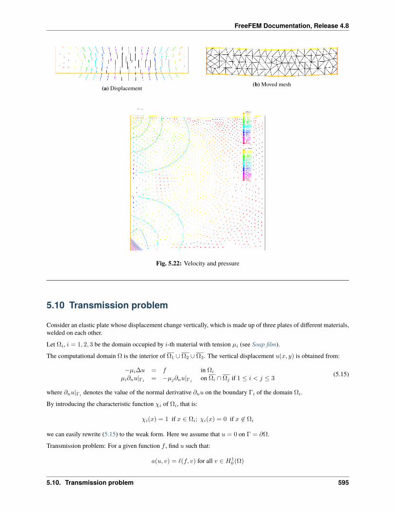
FreeFEM Documentation, Release 4.8
(a) Displacement(b) Moved mesh
Fig. 5.22: Velocity and pressure
5.10 Transmission problem
Consider an elastic plate whose displacement change vertically, which is made up of three plates of different materials,welded on each other.
Let Ω𝑖, 𝑖 = 1, 2, 3 be the domain occupied by 𝑖-th material with tension 𝜇𝑖 (see Soap film).
The computational domain Ω is the interior of Ω1 ∪ Ω2 ∪ Ω3. The vertical displacement 𝑢(𝑥, 𝑦) is obtained from:
−𝜇𝑖∆𝑢 = 𝑓 in Ω𝑖𝜇𝑖𝜕𝑛𝑢|Γ𝑖
= −𝜇𝑗𝜕𝑛𝑢|Γ𝑗on Ω𝑖 ∩ Ω𝑗 if 1 ≤ 𝑖 < 𝑗 ≤ 3
(5.15)
where 𝜕𝑛𝑢|Γ𝑖denotes the value of the normal derivative 𝜕𝑛𝑢 on the boundary Γ𝑖 of the domain Ω𝑖.
By introducing the characteristic function 𝜒𝑖 of Ω𝑖, that is:
𝜒𝑖(𝑥) = 1 if 𝑥 ∈ Ω𝑖; 𝜒𝑖(𝑥) = 0 if 𝑥 ∈ Ω𝑖
we can easily rewrite (5.15) to the weak form. Here we assume that 𝑢 = 0 on Γ = 𝜕Ω.
Transmission problem: For a given function 𝑓 , find 𝑢 such that:
𝑎(𝑢, 𝑣) = ℓ(𝑓, 𝑣) for all 𝑣 ∈ 𝐻10 (Ω)
5.10. Transmission problem 595
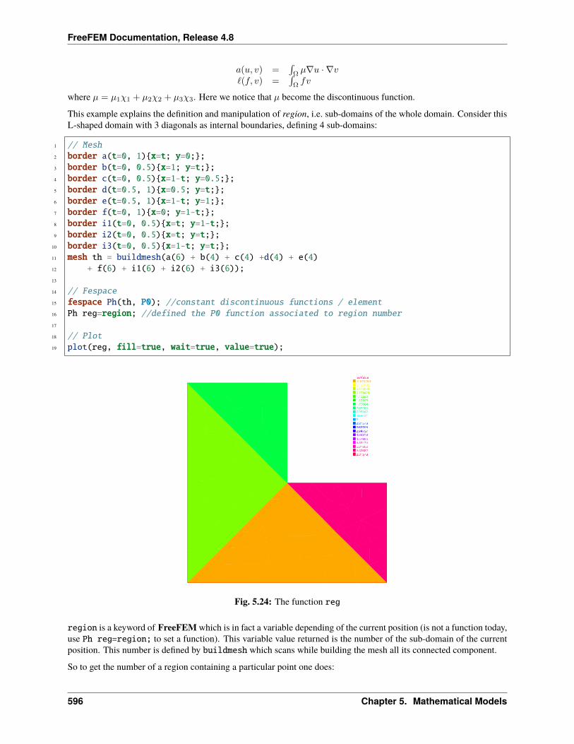
FreeFEM Documentation, Release 4.8
𝑎(𝑢, 𝑣) =∫Ω𝜇∇𝑢 · ∇𝑣
ℓ(𝑓, 𝑣) =∫Ω𝑓𝑣
where 𝜇 = 𝜇1𝜒1 + 𝜇2𝜒2 + 𝜇3𝜒3. Here we notice that 𝜇 become the discontinuous function.
This example explains the definition and manipulation of region, i.e. sub-domains of the whole domain. Consider thisL-shaped domain with 3 diagonals as internal boundaries, defining 4 sub-domains:
1 // Mesh2 border a(t=0, 1)x=t; y=0;;3 border b(t=0, 0.5)x=1; y=t;;4 border c(t=0, 0.5)x=1-t; y=0.5;;5 border d(t=0.5, 1)x=0.5; y=t;;6 border e(t=0.5, 1)x=1-t; y=1;;7 border f(t=0, 1)x=0; y=1-t;;8 border i1(t=0, 0.5)x=t; y=1-t;;9 border i2(t=0, 0.5)x=t; y=t;;
10 border i3(t=0, 0.5)x=1-t; y=t;;11 mesh th = buildmesh(a(6) + b(4) + c(4) +d(4) + e(4)12 + f(6) + i1(6) + i2(6) + i3(6));13
14 // Fespace15 fespace Ph(th, P0); //constant discontinuous functions / element16 Ph reg=region; //defined the P0 function associated to region number17
18 // Plot19 plot(reg, fill=true, wait=true, value=true);
Fig. 5.24: The function reg
region is a keyword of FreeFEM which is in fact a variable depending of the current position (is not a function today,use Ph reg=region; to set a function). This variable value returned is the number of the sub-domain of the currentposition. This number is defined by buildmesh which scans while building the mesh all its connected component.
So to get the number of a region containing a particular point one does:
596 Chapter 5. Mathematical Models
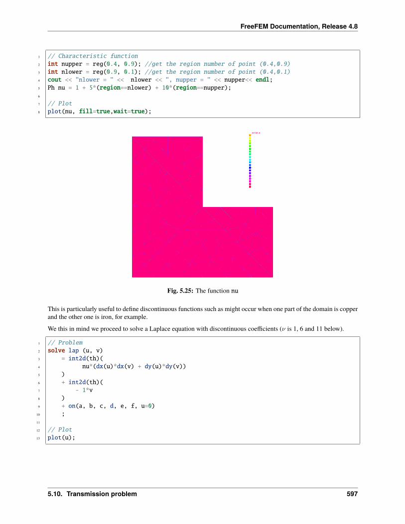
FreeFEM Documentation, Release 4.8
1 // Characteristic function2 int nupper = reg(0.4, 0.9); //get the region number of point (0.4,0.9)3 int nlower = reg(0.9, 0.1); //get the region number of point (0.4,0.1)4 cout << "nlower = " << nlower << ", nupper = " << nupper<< endl;5 Ph nu = 1 + 5*(region==nlower) + 10*(region==nupper);6
7 // Plot8 plot(nu, fill=true,wait=true);
Fig. 5.25: The function nu
This is particularly useful to define discontinuous functions such as might occur when one part of the domain is copperand the other one is iron, for example.
We this in mind we proceed to solve a Laplace equation with discontinuous coefficients (𝜈 is 1, 6 and 11 below).
1 // Problem2 solve lap (u, v)3 = int2d(th)(4 nu*(dx(u)*dx(v) + dy(u)*dy(v))5 )6 + int2d(th)(7 - 1*v8 )9 + on(a, b, c, d, e, f, u=0)
10 ;11
12 // Plot13 plot(u);
5.10. Transmission problem 597
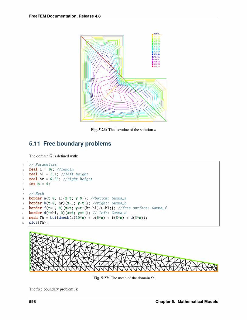
FreeFEM Documentation, Release 4.8
Fig. 5.26: The isovalue of the solution 𝑢
5.11 Free boundary problems
The domain Ω is defined with:
1 // Parameters2 real L = 10; //length3 real hl = 2.1; //left height4 real hr = 0.35; //right height5 int n = 4;6
7 // Mesh8 border a(t=0, L)x=t; y=0;; //bottom: Gamma_a9 border b(t=0, hr)x=L; y=t;; //right: Gamma_b
10 border f(t=L, 0)x=t; y=t*(hr-hl)/L+hl;; //free surface: Gamma_f11 border d(t=hl, 0)x=0; y=t;; // left: Gamma_d12 mesh Th = buildmesh(a(10*n) + b(6*n) + f(8*n) + d(3*n));13 plot(Th);
Fig. 5.27: The mesh of the domain Ω
The free boundary problem is:
598 Chapter 5. Mathematical Models
FreeFEM Documentation, Release 4.8
Find 𝑢 and Ω such that: ⎧⎪⎪⎪⎪⎨⎪⎪⎪⎪⎩−∆𝑢 = 0 in Ω
𝑢 = 𝑦 on Γ𝑏𝜕𝑢𝜕𝑛 = 0 on Γ𝑑 ∪ Γ𝑎𝜕𝑢𝜕𝑛 = 𝑞
𝐾𝑛𝑥 on Γ𝑓𝑢 = 𝑦 on Γ𝑓
We use a fixed point method;
Ω0 = Ω
In two step, fist we solve the classical following problem:⎧⎪⎪⎨⎪⎪⎩−∆𝑢 = 0 in Ω𝑛
𝑢 = 𝑦 on Γ𝑛𝑏𝜕𝑢𝜕𝑛 = 0 on Γ𝑛𝑑 ∪ Γ𝑛𝑎𝑢 = 𝑦 on Γ𝑛𝑓
The variational formulation is:
Find 𝑢 on 𝑉 = 𝐻1(Ω𝑛), such than 𝑢 = 𝑦 on Γ𝑛𝑏 and Γ𝑛𝑓∫Ω𝑛
∇𝑢∇𝑢′ = 0, ∀𝑢′ ∈ 𝑉 with 𝑢′ = 0 on Γ𝑛𝑏 ∪ Γ𝑛𝑓
And secondly to construct a domain deformation ℱ(𝑥, 𝑦) = [𝑥, 𝑦 − 𝑣(𝑥, 𝑦)] where 𝑣 is solution of the followingproblem: ⎧⎪⎪⎨⎪⎪⎩
−∆𝑣 = 0 in Ω𝑛
𝑣 = 0 on Γ𝑛𝑎𝜕𝑣𝜕𝑛 = 0 on Γ𝑛𝑏 ∪ Γ𝑛𝑑𝜕𝑣𝜕𝑛 = 𝜕𝑢
𝜕𝑛 −𝑞𝐾𝑛𝑥 on Γ𝑛𝑓
The variational formulation is:
Find 𝑣 on 𝑉 , such than 𝑣 = 0 on Γ𝑛𝑎 :∫Ω𝑛
∇𝑣∇𝑣′ =
∫Γ𝑛𝑓
(𝜕𝑢
𝜕𝑛− 𝑞
𝐾𝑛𝑥)𝑣′, ∀𝑣′ ∈ 𝑉 with 𝑣′ = 0 on Γ𝑛𝑎
Finally the new domain Ω𝑛+1 = ℱ(Ω𝑛)
Tip: Free boundary
The FreeFEM implementation is:
1 // Parameters2 real L = 10; //length3 real hr = 2.1; //left height4 real hl = 0.35; //right height5 int n = 4;6
7 real q = 0.02; //incoming flow8 real K = 0.5; //permeability9
10 // Mesh(continues on next page)
5.11. Free boundary problems 599
FreeFEM Documentation, Release 4.8
(continued from previous page)
11 border a(t=0, L)x=t; y=0;; //bottom: Gamma_a12 border b(t=0, hr)x=L; y=t;; //right: Gamma_b13 border f(t=L, 0)x=t; y=t*(hr-hl)/L+hl;; //free surface: Gamma_f14 border d(t=hl, 0)x=0; y=t;; // left: Gamma_d15 mesh Th = buildmesh(a(10*n) + b(6*n) + f(8*n) + d(3*n));16 plot(Th);17
18 // Fespace19 fespace Vh(Th, P1);20 Vh u, v;21 Vh uu, vv;22
23 // Problem24 problem Pu (u, uu, solver=CG)25 = int2d(Th)(26 dx(u)*dx(uu)27 + dy(u)*dy(uu)28 )29 + on(b, f, u=y)30 ;31
32 problem Pv (v, vv, solver=CG)33 = int2d(Th)(34 dx(v)*dx(vv)35 + dy(v)*dy(vv)36 )37 + on(a, v=0)38 + int1d(Th, f)(39 vv*((q/K)*N.y - (dx(u)*N.x + dy(u)*N.y))40 )41 ;42
43 // Loop44 int j = 0;45 real errv = 1.;46 real erradap = 0.001;47 while (errv > 1e-6)48 // Update49 j++;50
51 // Solve52 Pu;53 Pv;54
55 // Plot56 plot(Th, u, v);57
58 // Error59 errv = int1d(Th, f)(v*v);60
61 // Movemesh62 real coef = 1.;
(continues on next page)
600 Chapter 5. Mathematical Models
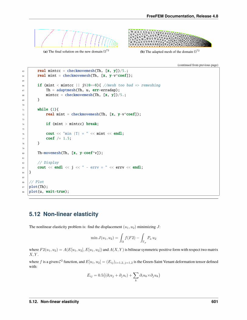
FreeFEM Documentation, Release 4.8
(a) The final solution on the new domain Ω72 (b) The adapted mesh of the domain Ω72
(continued from previous page)
63 real mintcc = checkmovemesh(Th, [x, y])/5.;64 real mint = checkmovemesh(Th, [x, y-v*coef]);65
66 if (mint < mintcc || j%10==0) //mesh too bad => remeshing67 Th = adaptmesh(Th, u, err=erradap);68 mintcc = checkmovemesh(Th, [x, y])/5.;69 70
71 while (1)72 real mint = checkmovemesh(Th, [x, y-v*coef]);73
74 if (mint > mintcc) break;75
76 cout << "min |T| = " << mint << endl;77 coef /= 1.5;78 79
80 Th=movemesh(Th, [x, y-coef*v]);81
82 // Display83 cout << endl << j << " - errv = " << errv << endl;84 85
86 // Plot87 plot(Th);88 plot(u, wait=true);
5.12 Non-linear elasticity
The nonlinear elasticity problem is: find the displacement (𝑢1, 𝑢2) minimizing 𝐽 :
min 𝐽(𝑢1, 𝑢2) =
∫Ω
𝑓(𝐹2)−∫Γ𝑝
𝑃𝑎 𝑢2
where𝐹2(𝑢1, 𝑢2) = 𝐴(𝐸[𝑢1, 𝑢2], 𝐸[𝑢1, 𝑢2]) and𝐴(𝑋,𝑌 ) is bilinear symmetric positive form with respect two matrix𝑋,𝑌 .
where 𝑓 is a given 𝒞2 function, and𝐸[𝑢1, 𝑢2] = (𝐸𝑖𝑗)𝑖=1,2, 𝑗=1,2 is the Green-Saint Venant deformation tensor definedwith:
𝐸𝑖𝑗 = 0.5((𝜕𝑖𝑢𝑗 + 𝜕𝑗𝑢𝑖) +
∑𝑘
𝜕𝑖𝑢𝑘×𝜕𝑗𝑢𝑘)
5.12. Non-linear elasticity 601
FreeFEM Documentation, Release 4.8
Denote u = (𝑢1, 𝑢2), v = (𝑣1, 𝑣2), w = (𝑤1, 𝑤2). So, the differential of 𝐽 is:
𝐷𝐽(u)(v) =
∫𝐷𝐹2(u)(v) 𝑓 ′(𝐹2(u)))−
∫Γ𝑝
𝑃𝑎𝑣2
where 𝐷𝐹2(u)(v) = 2 𝐴(𝐷𝐸[u](v), 𝐸[u]) and 𝐷𝐸 is the first differential of 𝐸.
The second order differential is:
𝐷2𝐽(u)((v), (w)) =
∫𝐷𝐹2(u)(v) 𝐷𝐹2(u)(w) 𝑓 ′′(𝐹2(u)))
+
∫𝐷2𝐹2(u)(v,w) 𝑓 ′(𝐹2(u)))
where:
𝐷2𝐹2(u)(v,w) = 2 𝐴( 𝐷2𝐸[u](v,w) , 𝐸[u] ) + 2 𝐴( 𝐷𝐸[u](v) , 𝐷𝐸[u](w) ).
and 𝐷2𝐸 is the second differential of 𝐸.
So all notations can be define with macro:
1 macro EL(u, v) [dx(u), (dx(v)+dy(u)), dy(v)] //is [epsilon_11, 2epsilon_12, epsilon_22]2
3 macro ENL(u, v) [4 (dx(u)*dx(u) + dx(v)*dx(v))*0.5,5 (dx(u)*dy(u) + dx(v)*dy(v)),6 (dy(u)*dy(u) + dy(v)*dy(v))*0.57 ] //8
9 macro dENL(u, v, uu, vv) [10 (dx(u)*dx(uu) + dx(v)*dx(vv)),11 (dx(u)*dy(uu) + dx(v)*dy(vv) + dx(uu)*dy(u) + dx(vv)*dy(v)),12 (dy(u)*dy(uu) + dy(v)*dy(vv))13 ] //14
15 macro E(u, v) (EL(u,v) + ENL(u,v)) //is [E_11, 2E_12, E_22]16 macro dE(u, v, uu, vv) (EL(uu, vv) + dENL(u, v, uu, vv)) //17 macro ddE(u, v, uu, vv, uuu, vvv) dENL(uuu, vvv, uu, vv) //18 macro F2(u, v) (E(u, v)'*A*E(u, v)) //19 macro dF2(u, v, uu, vv) (E(u, v)'*A*dE(u, v, uu, vv)*2.) //20 macro ddF2(u, v, uu, vv, uuu, vvv) (21 (dE(u, v, uu, vv)'*A*dE(u, v, uuu, vvv))*2.22 + (E(u, v)'*A*ddE(u, v, uu, vv, uuu, vvv))*2.23 ) //
The Newton Method is:
choose 𝑛 = 0,and 𝑢0, 𝑣0 the initial displacement
• loop:
– find (𝑑𝑢, 𝑑𝑣) : solution of
𝐷2𝐽(𝑢𝑛, 𝑣𝑛)((𝑤, 𝑠), (𝑑𝑢, 𝑑𝑣)) = 𝐷𝐽(𝑢𝑛, 𝑣𝑛)(𝑤, 𝑠), ∀𝑤, 𝑠
– 𝑢𝑛 = 𝑢𝑛− 𝑑𝑢, 𝑣𝑛 = 𝑣𝑛− 𝑑𝑣
– until (𝑑𝑢, 𝑑𝑣) small is enough
602 Chapter 5. Mathematical Models
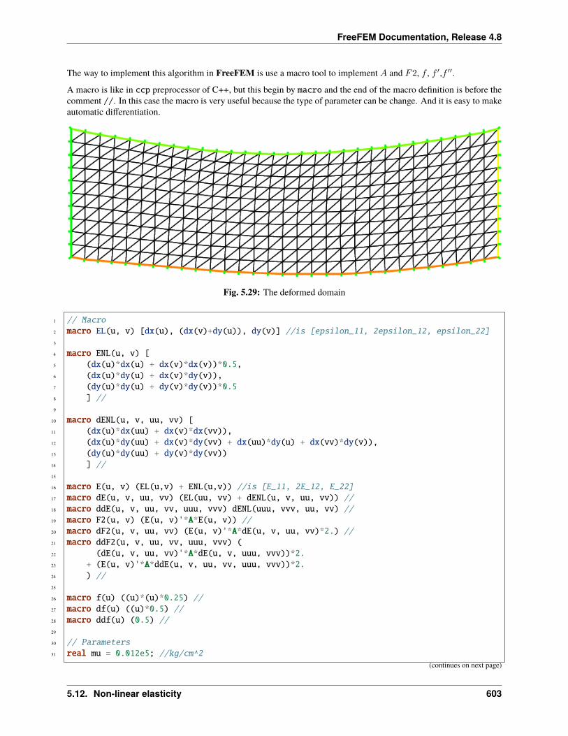
FreeFEM Documentation, Release 4.8
The way to implement this algorithm in FreeFEM is use a macro tool to implement 𝐴 and 𝐹2, 𝑓 , 𝑓 ′,𝑓 ′′.
A macro is like in ccp preprocessor of C++, but this begin by macro and the end of the macro definition is before thecomment //. In this case the macro is very useful because the type of parameter can be change. And it is easy to makeautomatic differentiation.
Fig. 5.29: The deformed domain
1 // Macro2 macro EL(u, v) [dx(u), (dx(v)+dy(u)), dy(v)] //is [epsilon_11, 2epsilon_12, epsilon_22]3
4 macro ENL(u, v) [5 (dx(u)*dx(u) + dx(v)*dx(v))*0.5,6 (dx(u)*dy(u) + dx(v)*dy(v)),7 (dy(u)*dy(u) + dy(v)*dy(v))*0.58 ] //9
10 macro dENL(u, v, uu, vv) [11 (dx(u)*dx(uu) + dx(v)*dx(vv)),12 (dx(u)*dy(uu) + dx(v)*dy(vv) + dx(uu)*dy(u) + dx(vv)*dy(v)),13 (dy(u)*dy(uu) + dy(v)*dy(vv))14 ] //15
16 macro E(u, v) (EL(u,v) + ENL(u,v)) //is [E_11, 2E_12, E_22]17 macro dE(u, v, uu, vv) (EL(uu, vv) + dENL(u, v, uu, vv)) //18 macro ddE(u, v, uu, vv, uuu, vvv) dENL(uuu, vvv, uu, vv) //19 macro F2(u, v) (E(u, v)'*A*E(u, v)) //20 macro dF2(u, v, uu, vv) (E(u, v)'*A*dE(u, v, uu, vv)*2.) //21 macro ddF2(u, v, uu, vv, uuu, vvv) (22 (dE(u, v, uu, vv)'*A*dE(u, v, uuu, vvv))*2.23 + (E(u, v)'*A*ddE(u, v, uu, vv, uuu, vvv))*2.24 ) //25
26 macro f(u) ((u)*(u)*0.25) //27 macro df(u) ((u)*0.5) //28 macro ddf(u) (0.5) //29
30 // Parameters31 real mu = 0.012e5; //kg/cm^2
(continues on next page)
5.12. Non-linear elasticity 603
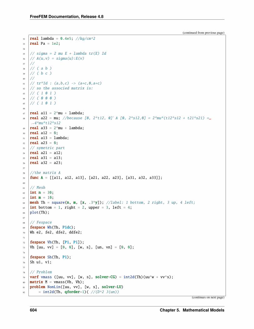
FreeFEM Documentation, Release 4.8
(continued from previous page)
32 real lambda = 0.4e5; //kg/cm^233 real Pa = 1e2;34
35 // sigma = 2 mu E + lambda tr(E) Id36 // A(u,v) = sigma(u):E(v)37 //38 // ( a b )39 // ( b c )40 //41 // tr*Id : (a,b,c) -> (a+c,0,a+c)42 // so the associed matrix is:43 // ( 1 0 1 )44 // ( 0 0 0 )45 // ( 1 0 1 )46
47 real a11 = 2*mu + lambda;48 real a22 = mu; //because [0, 2*t12, 0]' A [0, 2*s12,0] = 2*mu*(t12*s12 + t21*s21) =
→˓4*mu*t12*s1249 real a33 = 2*mu + lambda;50 real a12 = 0;51 real a13 = lambda;52 real a23 = 0;53 // symetric part54 real a21 = a12;55 real a31 = a13;56 real a32 = a23;57
58 //the matrix A59 func A = [[a11, a12, a13], [a21, a22, a23], [a31, a32, a33]];60
61 // Mesh62 int n = 30;63 int m = 10;64 mesh Th = square(n, m, [x, .3*y]); //label: 1 bottom, 2 right, 3 up, 4 left;65 int bottom = 1, right = 2, upper = 3, left = 4;66 plot(Th);67
68 // Fespace69 fespace Wh(Th, P1dc);70 Wh e2, fe2, dfe2, ddfe2;71
72 fespace Vh(Th, [P1, P1]);73 Vh [uu, vv] = [0, 0], [w, s], [un, vn] = [0, 0];74
75 fespace Sh(Th, P1);76 Sh u1, v1;77
78 // Problem79 varf vmass ([uu, vv], [w, s], solver=CG) = int2d(Th)(uu*w + vv*s);80 matrix M = vmass(Vh, Vh);81 problem NonLin([uu, vv], [w, s], solver=LU)82 = int2d(Th, qforder=1)( //(D^2 J(un))
(continues on next page)
604 Chapter 5. Mathematical Models
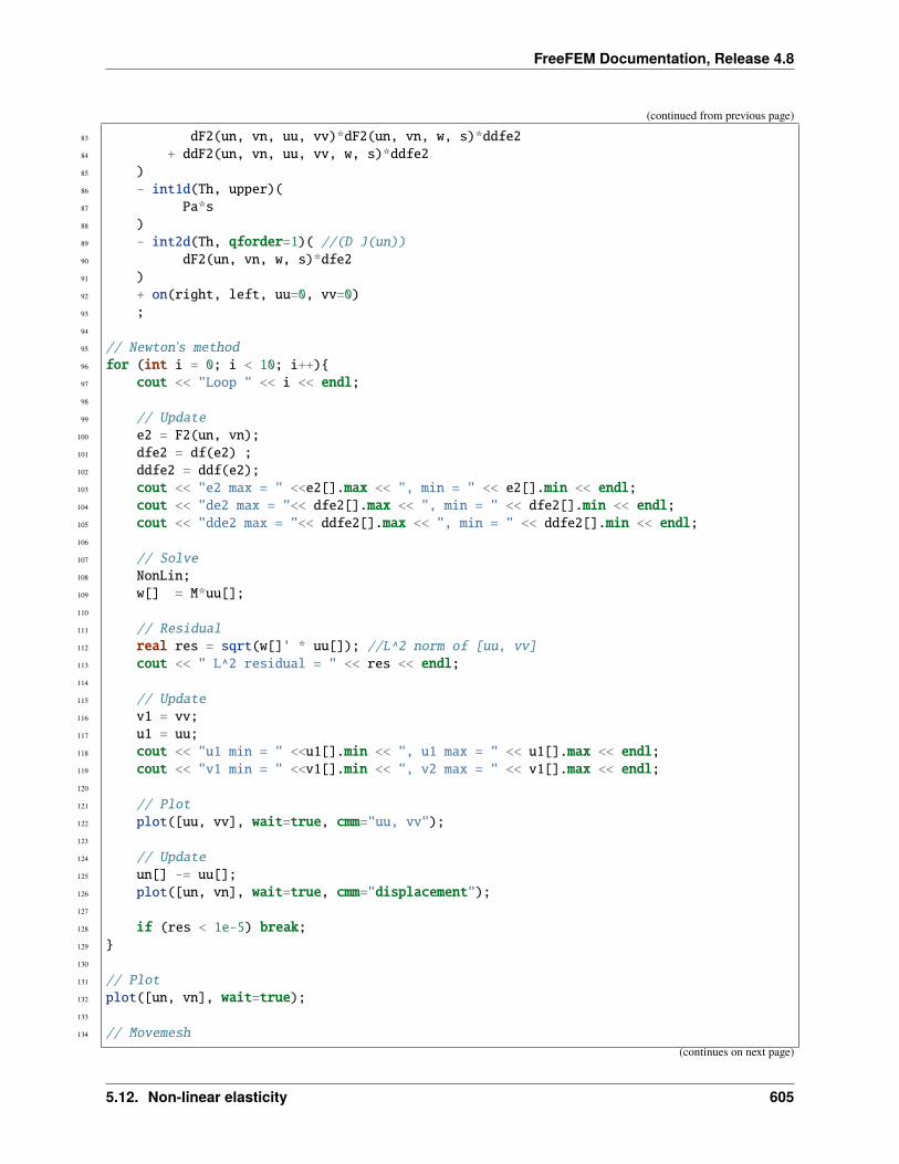
FreeFEM Documentation, Release 4.8
(continued from previous page)
83 dF2(un, vn, uu, vv)*dF2(un, vn, w, s)*ddfe284 + ddF2(un, vn, uu, vv, w, s)*ddfe285 )86 - int1d(Th, upper)(87 Pa*s88 )89 - int2d(Th, qforder=1)( //(D J(un))90 dF2(un, vn, w, s)*dfe291 )92 + on(right, left, uu=0, vv=0)93 ;94
95 // Newton's method96 for (int i = 0; i < 10; i++)97 cout << "Loop " << i << endl;98
99 // Update100 e2 = F2(un, vn);101 dfe2 = df(e2) ;102 ddfe2 = ddf(e2);103 cout << "e2 max = " <<e2[].max << ", min = " << e2[].min << endl;104 cout << "de2 max = "<< dfe2[].max << ", min = " << dfe2[].min << endl;105 cout << "dde2 max = "<< ddfe2[].max << ", min = " << ddfe2[].min << endl;106
107 // Solve108 NonLin;109 w[] = M*uu[];110
111 // Residual112 real res = sqrt(w[]' * uu[]); //L^2 norm of [uu, vv]113 cout << " L^2 residual = " << res << endl;114
115 // Update116 v1 = vv;117 u1 = uu;118 cout << "u1 min = " <<u1[].min << ", u1 max = " << u1[].max << endl;119 cout << "v1 min = " <<v1[].min << ", v2 max = " << v1[].max << endl;120
121 // Plot122 plot([uu, vv], wait=true, cmm="uu, vv");123
124 // Update125 un[] -= uu[];126 plot([un, vn], wait=true, cmm="displacement");127
128 if (res < 1e-5) break;129 130
131 // Plot132 plot([un, vn], wait=true);133
134 // Movemesh
(continues on next page)
5.12. Non-linear elasticity 605
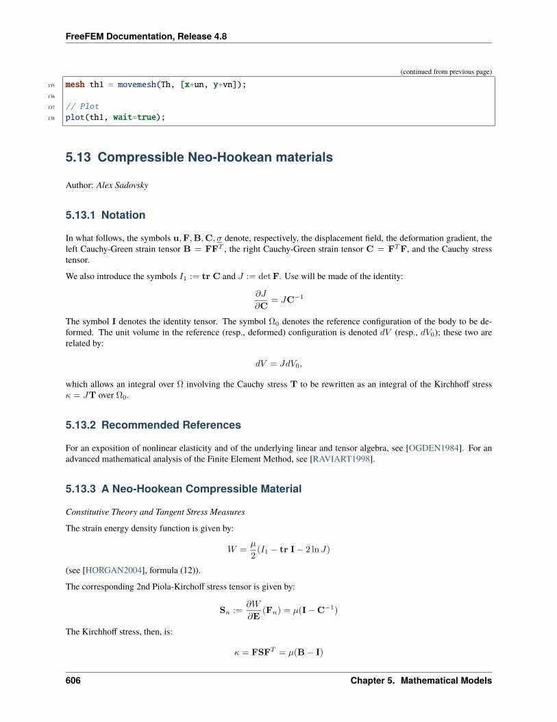
FreeFEM Documentation, Release 4.8
(continued from previous page)
135 mesh th1 = movemesh(Th, [x+un, y+vn]);136
137 // Plot138 plot(th1, wait=true);
5.13 Compressible Neo-Hookean materials
Author: Alex Sadovsky
5.13.1 Notation
In what follows, the symbols u,F,B,C, 𝜎 denote, respectively, the displacement field, the deformation gradient, theleft Cauchy-Green strain tensor B = FF𝑇 , the right Cauchy-Green strain tensor C = F𝑇F, and the Cauchy stresstensor.
We also introduce the symbols 𝐼1 := tr C and 𝐽 := detF. Use will be made of the identity:
𝜕𝐽
𝜕C= 𝐽C−1
The symbol I denotes the identity tensor. The symbol Ω0 denotes the reference configuration of the body to be de-formed. The unit volume in the reference (resp., deformed) configuration is denoted 𝑑𝑉 (resp., 𝑑𝑉0); these two arerelated by:
𝑑𝑉 = 𝐽𝑑𝑉0,
which allows an integral over Ω involving the Cauchy stress T to be rewritten as an integral of the Kirchhoff stress𝜅 = 𝐽T over Ω0.
5.13.2 Recommended References
For an exposition of nonlinear elasticity and of the underlying linear and tensor algebra, see [OGDEN1984]. For anadvanced mathematical analysis of the Finite Element Method, see [RAVIART1998].
5.13.3 A Neo-Hookean Compressible Material
Constitutive Theory and Tangent Stress Measures
The strain energy density function is given by:
𝑊 =𝜇
2(𝐼1 − tr I− 2 ln𝐽)
(see [HORGAN2004], formula (12)).
The corresponding 2nd Piola-Kirchoff stress tensor is given by:
S𝑛 :=𝜕𝑊
𝜕E(F𝑛) = 𝜇(I−C−1)
The Kirchhoff stress, then, is:
𝜅 = FSF𝑇 = 𝜇(B− I)
606 Chapter 5. Mathematical Models
FreeFEM Documentation, Release 4.8
The tangent Kirchhoff stress tensor at F𝑛 acting on 𝛿F𝑛+1 is, consequently:
𝜕𝜅
𝜕F(F𝑛)𝛿F𝑛+1 = 𝜇
[F𝑛(𝛿F𝑛+1)𝑇 + 𝛿F𝑛+1(F𝑛)𝑇
]The Weak Form of the BVP in the Absence of Body (External) Forces
The Ω0 we are considering is an elliptical annulus, whose boundary consists of two concentric ellipses (each allowedto be a circle as a special case), with the major axes parallel. Let 𝑃 denote the dead stress load (traction) on a portion𝜕Ω𝑡0 (= the inner ellipse) of the boundary 𝜕Ω0. On the rest of the boundary, we prescribe zero displacement.
The weak formulation of the boundary value problem is:
0 =∫Ω0𝜅[F] :
(∇⊗w)(F)−1
−
∫𝜕Ω𝑡
0𝑃 · 0
For brevity, in the rest of this section we assume 𝑃 = 0. The provided FreeFEM code, however, does not rely on thisassumption and allows for a general value and direction of 𝑃 .
Given a Newton approximation u𝑛 of the displacement field u satisfying the BVP, we seek the correction 𝛿u𝑛+1 toobtain a better approximation:
u𝑛+1 = u𝑛 + 𝛿u𝑛+1
by solving the weak formulation:
0 =∫Ω0𝜅[F𝑛 + 𝛿F𝑛+1] :
(∇⊗w)(F𝑛 + 𝛿F𝑛+1)−1
−∫𝜕Ω0
𝑃 · 0
=∫Ω0
𝜅[F𝑛] + 𝜕𝜅
𝜕F [F𝑛]𝛿F𝑛+1
:
(∇⊗w)(F𝑛 + 𝛿F𝑛+1)−1
=∫Ω0
𝜅[F𝑛] + 𝜕𝜅
𝜕F [F𝑛]𝛿F𝑛+1
:
(∇⊗w)(F−1𝑛 + F−2
𝑛 𝛿F𝑛+1)
=∫Ω0𝜅[F𝑛] :
(∇⊗w)F−1
𝑛
−
∫Ω0𝜅[F𝑛] :
(∇⊗w)(F−2
𝑛 𝛿F𝑛+1)
+∫Ω0
𝜕𝜅𝜕F [F𝑛]𝛿F𝑛+1
:
(∇⊗w)F−1𝑛
⎫⎪⎪⎪⎪⎪⎪⎪⎪⎪⎬⎪⎪⎪⎪⎪⎪⎪⎪⎪⎭for all test functionsw,
where we have taken:
𝛿F𝑛+1 = ∇⊗ 𝛿u𝑛+1
Note: Contrary to standard notational use, the symbol 𝛿 here bears no variational context. By 𝛿 we mean simply anincrement in the sense of Newton’s Method. The role of a variational virtual displacement here is played by w.
5.13.4 An Approach to Implementation in FreeFEM
Introducing the code-like notation, where a string in <>’s is to be read as one symbol, the individual components ofthe tensor:
< 𝑇𝑎𝑛𝐾 >:=𝜕𝜅
𝜕F[F𝑛]𝛿F𝑛+1
will be implemented as the macros < 𝑇𝑎𝑛𝐾11 >, < 𝑇𝑎𝑛𝐾12 >, . . .
The individual components of the tensor quantities:
D1 := F𝑛(𝛿F𝑛+1)𝑇 + 𝛿F𝑛+1(F𝑛)𝑇 ,
5.13. Compressible Neo-Hookean materials 607
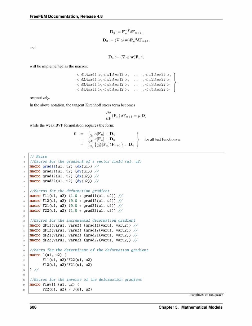
FreeFEM Documentation, Release 4.8
D2 := F−𝑇𝑛 𝛿F𝑛+1,
D3 := (∇⊗w)F−2𝑛 𝛿F𝑛+1,
and
D4 := (∇⊗w)F−1𝑛 ,
will be implemented as the macros:
< 𝑑1𝐴𝑢𝑥11 >,< 𝑑1𝐴𝑢𝑥12 >, . . . , < 𝑑1𝐴𝑢𝑥22 >,< 𝑑2𝐴𝑢𝑥11 >,< 𝑑2𝐴𝑢𝑥12 >, . . . , < 𝑑2𝐴𝑢𝑥22 >< 𝑑3𝐴𝑢𝑥11 >,< 𝑑3𝐴𝑢𝑥12 >, . . . , < 𝑑3𝐴𝑢𝑥22 >< 𝑑4𝐴𝑢𝑥11 >,< 𝑑4𝐴𝑢𝑥12 >, . . . , < 𝑑4𝐴𝑢𝑥22 >
⎫⎪⎪⎬⎪⎪⎭ ,
respectively.
In the above notation, the tangent Kirchhoff stress term becomes
𝜕𝜅
𝜕F(F𝑛) 𝛿F𝑛+1 = 𝜇D1
while the weak BVP formulation acquires the form:
0 =∫Ω0𝜅[F𝑛] : D4
−∫Ω0𝜅[F𝑛] : D3
+∫Ω0
𝜕𝜅𝜕F [F𝑛]𝛿F𝑛+1
: D4
⎫⎬⎭ for all test functionsw
1 // Macro2 //Macros for the gradient of a vector field (u1, u2)3 macro grad11(u1, u2) (dx(u1)) //4 macro grad21(u1, u2) (dy(u1)) //5 macro grad12(u1, u2) (dx(u2)) //6 macro grad22(u1, u2) (dy(u2)) //7
8 //Macros for the deformation gradient9 macro F11(u1, u2) (1.0 + grad11(u1, u2)) //
10 macro F12(u1, u2) (0.0 + grad12(u1, u2)) //11 macro F21(u1, u2) (0.0 + grad21(u1, u2)) //12 macro F22(u1, u2) (1.0 + grad22(u1, u2)) //13
14 //Macros for the incremental deformation gradient15 macro dF11(varu1, varu2) (grad11(varu1, varu2)) //16 macro dF12(varu1, varu2) (grad12(varu1, varu2)) //17 macro dF21(varu1, varu2) (grad21(varu1, varu2)) //18 macro dF22(varu1, varu2) (grad22(varu1, varu2)) //19
20 //Macro for the determinant of the deformation gradient21 macro J(u1, u2) (22 F11(u1, u2)*F22(u1, u2)23 - F12(u1, u2)*F21(u1, u2)24 ) //25
26 //Macros for the inverse of the deformation gradient27 macro Finv11 (u1, u2) (28 F22(u1, u2) / J(u1, u2)
(continues on next page)
608 Chapter 5. Mathematical Models
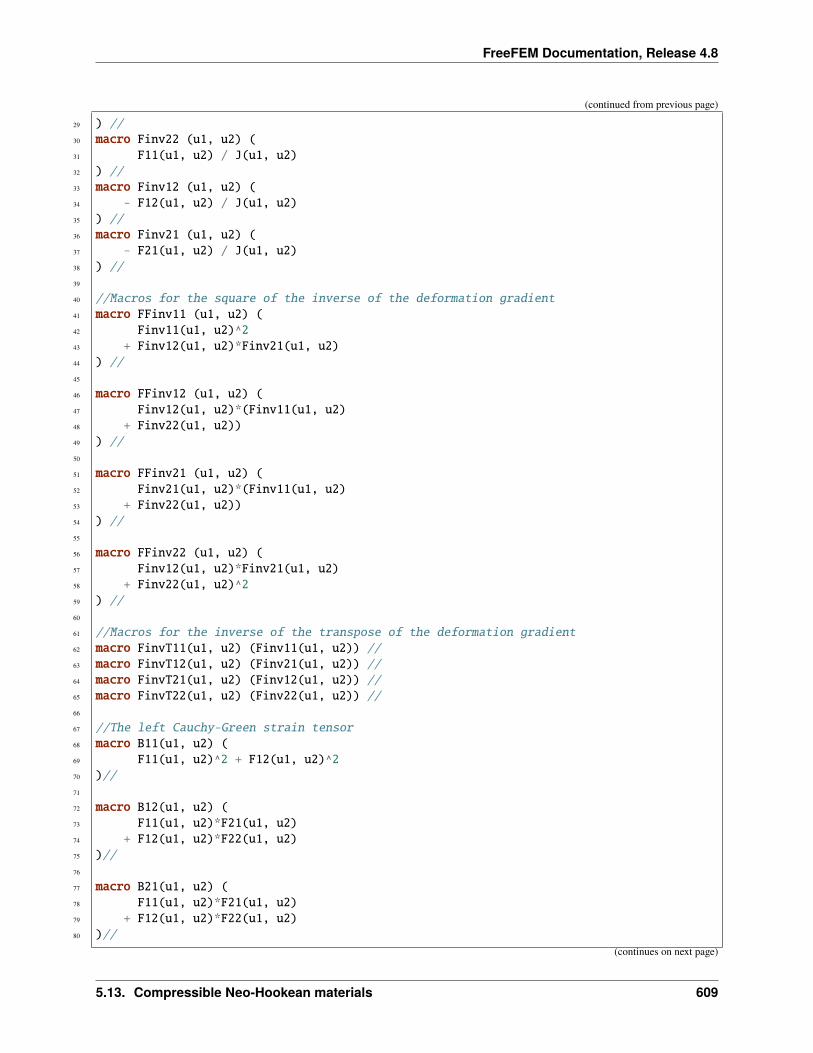
FreeFEM Documentation, Release 4.8
(continued from previous page)
29 ) //30 macro Finv22 (u1, u2) (31 F11(u1, u2) / J(u1, u2)32 ) //33 macro Finv12 (u1, u2) (34 - F12(u1, u2) / J(u1, u2)35 ) //36 macro Finv21 (u1, u2) (37 - F21(u1, u2) / J(u1, u2)38 ) //39
40 //Macros for the square of the inverse of the deformation gradient41 macro FFinv11 (u1, u2) (42 Finv11(u1, u2)^243 + Finv12(u1, u2)*Finv21(u1, u2)44 ) //45
46 macro FFinv12 (u1, u2) (47 Finv12(u1, u2)*(Finv11(u1, u2)48 + Finv22(u1, u2))49 ) //50
51 macro FFinv21 (u1, u2) (52 Finv21(u1, u2)*(Finv11(u1, u2)53 + Finv22(u1, u2))54 ) //55
56 macro FFinv22 (u1, u2) (57 Finv12(u1, u2)*Finv21(u1, u2)58 + Finv22(u1, u2)^259 ) //60
61 //Macros for the inverse of the transpose of the deformation gradient62 macro FinvT11(u1, u2) (Finv11(u1, u2)) //63 macro FinvT12(u1, u2) (Finv21(u1, u2)) //64 macro FinvT21(u1, u2) (Finv12(u1, u2)) //65 macro FinvT22(u1, u2) (Finv22(u1, u2)) //66
67 //The left Cauchy-Green strain tensor68 macro B11(u1, u2) (69 F11(u1, u2)^2 + F12(u1, u2)^270 )//71
72 macro B12(u1, u2) (73 F11(u1, u2)*F21(u1, u2)74 + F12(u1, u2)*F22(u1, u2)75 )//76
77 macro B21(u1, u2) (78 F11(u1, u2)*F21(u1, u2)79 + F12(u1, u2)*F22(u1, u2)80 )//
(continues on next page)
5.13. Compressible Neo-Hookean materials 609
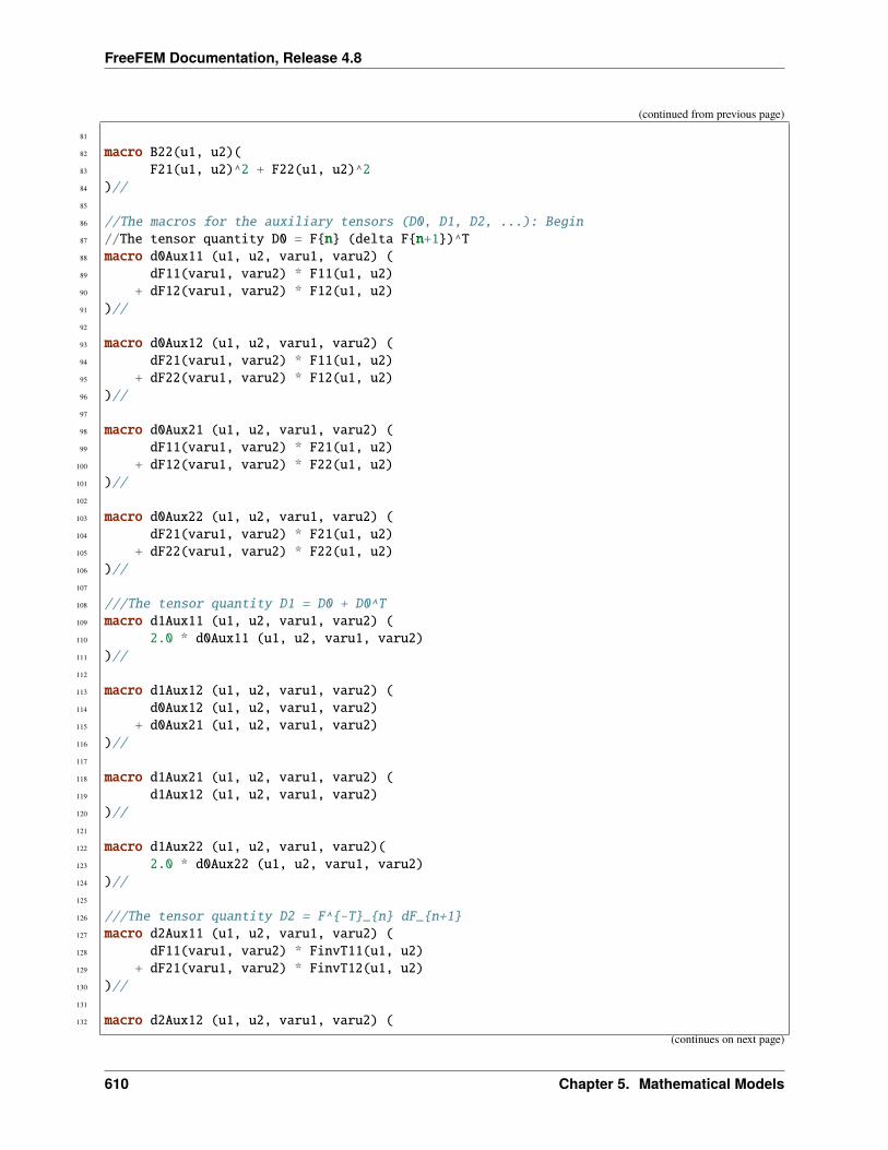
FreeFEM Documentation, Release 4.8
(continued from previous page)
81
82 macro B22(u1, u2)(83 F21(u1, u2)^2 + F22(u1, u2)^284 )//85
86 //The macros for the auxiliary tensors (D0, D1, D2, ...): Begin87 //The tensor quantity D0 = Fn (delta Fn+1)^T88 macro d0Aux11 (u1, u2, varu1, varu2) (89 dF11(varu1, varu2) * F11(u1, u2)90 + dF12(varu1, varu2) * F12(u1, u2)91 )//92
93 macro d0Aux12 (u1, u2, varu1, varu2) (94 dF21(varu1, varu2) * F11(u1, u2)95 + dF22(varu1, varu2) * F12(u1, u2)96 )//97
98 macro d0Aux21 (u1, u2, varu1, varu2) (99 dF11(varu1, varu2) * F21(u1, u2)
100 + dF12(varu1, varu2) * F22(u1, u2)101 )//102
103 macro d0Aux22 (u1, u2, varu1, varu2) (104 dF21(varu1, varu2) * F21(u1, u2)105 + dF22(varu1, varu2) * F22(u1, u2)106 )//107
108 ///The tensor quantity D1 = D0 + D0^T109 macro d1Aux11 (u1, u2, varu1, varu2) (110 2.0 * d0Aux11 (u1, u2, varu1, varu2)111 )//112
113 macro d1Aux12 (u1, u2, varu1, varu2) (114 d0Aux12 (u1, u2, varu1, varu2)115 + d0Aux21 (u1, u2, varu1, varu2)116 )//117
118 macro d1Aux21 (u1, u2, varu1, varu2) (119 d1Aux12 (u1, u2, varu1, varu2)120 )//121
122 macro d1Aux22 (u1, u2, varu1, varu2)(123 2.0 * d0Aux22 (u1, u2, varu1, varu2)124 )//125
126 ///The tensor quantity D2 = F^-T_n dF_n+1127 macro d2Aux11 (u1, u2, varu1, varu2) (128 dF11(varu1, varu2) * FinvT11(u1, u2)129 + dF21(varu1, varu2) * FinvT12(u1, u2)130 )//131
132 macro d2Aux12 (u1, u2, varu1, varu2) (
(continues on next page)
610 Chapter 5. Mathematical Models
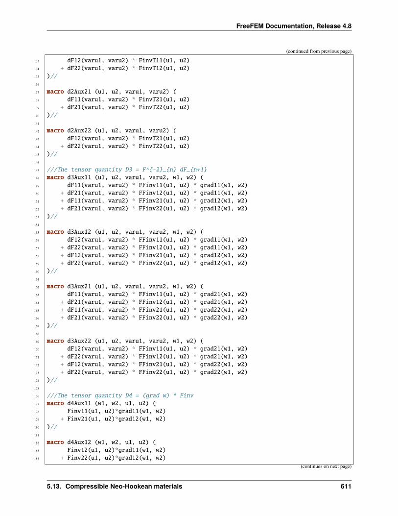
FreeFEM Documentation, Release 4.8
(continued from previous page)
133 dF12(varu1, varu2) * FinvT11(u1, u2)134 + dF22(varu1, varu2) * FinvT12(u1, u2)135 )//136
137 macro d2Aux21 (u1, u2, varu1, varu2) (138 dF11(varu1, varu2) * FinvT21(u1, u2)139 + dF21(varu1, varu2) * FinvT22(u1, u2)140 )//141
142 macro d2Aux22 (u1, u2, varu1, varu2) (143 dF12(varu1, varu2) * FinvT21(u1, u2)144 + dF22(varu1, varu2) * FinvT22(u1, u2)145 )//146
147 ///The tensor quantity D3 = F^-2_n dF_n+1148 macro d3Aux11 (u1, u2, varu1, varu2, w1, w2) (149 dF11(varu1, varu2) * FFinv11(u1, u2) * grad11(w1, w2)150 + dF21(varu1, varu2) * FFinv12(u1, u2) * grad11(w1, w2)151 + dF11(varu1, varu2) * FFinv21(u1, u2) * grad12(w1, w2)152 + dF21(varu1, varu2) * FFinv22(u1, u2) * grad12(w1, w2)153 )//154
155 macro d3Aux12 (u1, u2, varu1, varu2, w1, w2) (156 dF12(varu1, varu2) * FFinv11(u1, u2) * grad11(w1, w2)157 + dF22(varu1, varu2) * FFinv12(u1, u2) * grad11(w1, w2)158 + dF12(varu1, varu2) * FFinv21(u1, u2) * grad12(w1, w2)159 + dF22(varu1, varu2) * FFinv22(u1, u2) * grad12(w1, w2)160 )//161
162 macro d3Aux21 (u1, u2, varu1, varu2, w1, w2) (163 dF11(varu1, varu2) * FFinv11(u1, u2) * grad21(w1, w2)164 + dF21(varu1, varu2) * FFinv12(u1, u2) * grad21(w1, w2)165 + dF11(varu1, varu2) * FFinv21(u1, u2) * grad22(w1, w2)166 + dF21(varu1, varu2) * FFinv22(u1, u2) * grad22(w1, w2)167 )//168
169 macro d3Aux22 (u1, u2, varu1, varu2, w1, w2) (170 dF12(varu1, varu2) * FFinv11(u1, u2) * grad21(w1, w2)171 + dF22(varu1, varu2) * FFinv12(u1, u2) * grad21(w1, w2)172 + dF12(varu1, varu2) * FFinv21(u1, u2) * grad22(w1, w2)173 + dF22(varu1, varu2) * FFinv22(u1, u2) * grad22(w1, w2)174 )//175
176 ///The tensor quantity D4 = (grad w) * Finv177 macro d4Aux11 (w1, w2, u1, u2) (178 Finv11(u1, u2)*grad11(w1, w2)179 + Finv21(u1, u2)*grad12(w1, w2)180 )//181
182 macro d4Aux12 (w1, w2, u1, u2) (183 Finv12(u1, u2)*grad11(w1, w2)184 + Finv22(u1, u2)*grad12(w1, w2)
(continues on next page)
5.13. Compressible Neo-Hookean materials 611
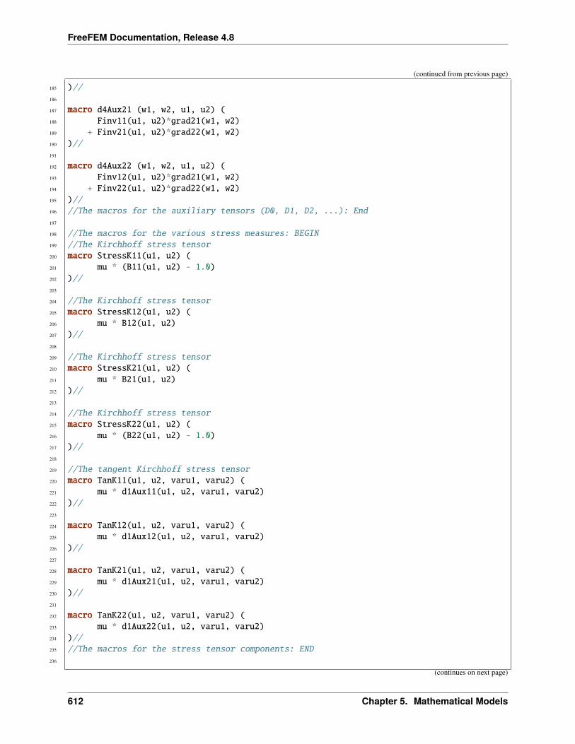
FreeFEM Documentation, Release 4.8
(continued from previous page)
185 )//186
187 macro d4Aux21 (w1, w2, u1, u2) (188 Finv11(u1, u2)*grad21(w1, w2)189 + Finv21(u1, u2)*grad22(w1, w2)190 )//191
192 macro d4Aux22 (w1, w2, u1, u2) (193 Finv12(u1, u2)*grad21(w1, w2)194 + Finv22(u1, u2)*grad22(w1, w2)195 )//196 //The macros for the auxiliary tensors (D0, D1, D2, ...): End197
198 //The macros for the various stress measures: BEGIN199 //The Kirchhoff stress tensor200 macro StressK11(u1, u2) (201 mu * (B11(u1, u2) - 1.0)202 )//203
204 //The Kirchhoff stress tensor205 macro StressK12(u1, u2) (206 mu * B12(u1, u2)207 )//208
209 //The Kirchhoff stress tensor210 macro StressK21(u1, u2) (211 mu * B21(u1, u2)212 )//213
214 //The Kirchhoff stress tensor215 macro StressK22(u1, u2) (216 mu * (B22(u1, u2) - 1.0)217 )//218
219 //The tangent Kirchhoff stress tensor220 macro TanK11(u1, u2, varu1, varu2) (221 mu * d1Aux11(u1, u2, varu1, varu2)222 )//223
224 macro TanK12(u1, u2, varu1, varu2) (225 mu * d1Aux12(u1, u2, varu1, varu2)226 )//227
228 macro TanK21(u1, u2, varu1, varu2) (229 mu * d1Aux21(u1, u2, varu1, varu2)230 )//231
232 macro TanK22(u1, u2, varu1, varu2) (233 mu * d1Aux22(u1, u2, varu1, varu2)234 )//235 //The macros for the stress tensor components: END236
(continues on next page)
612 Chapter 5. Mathematical Models
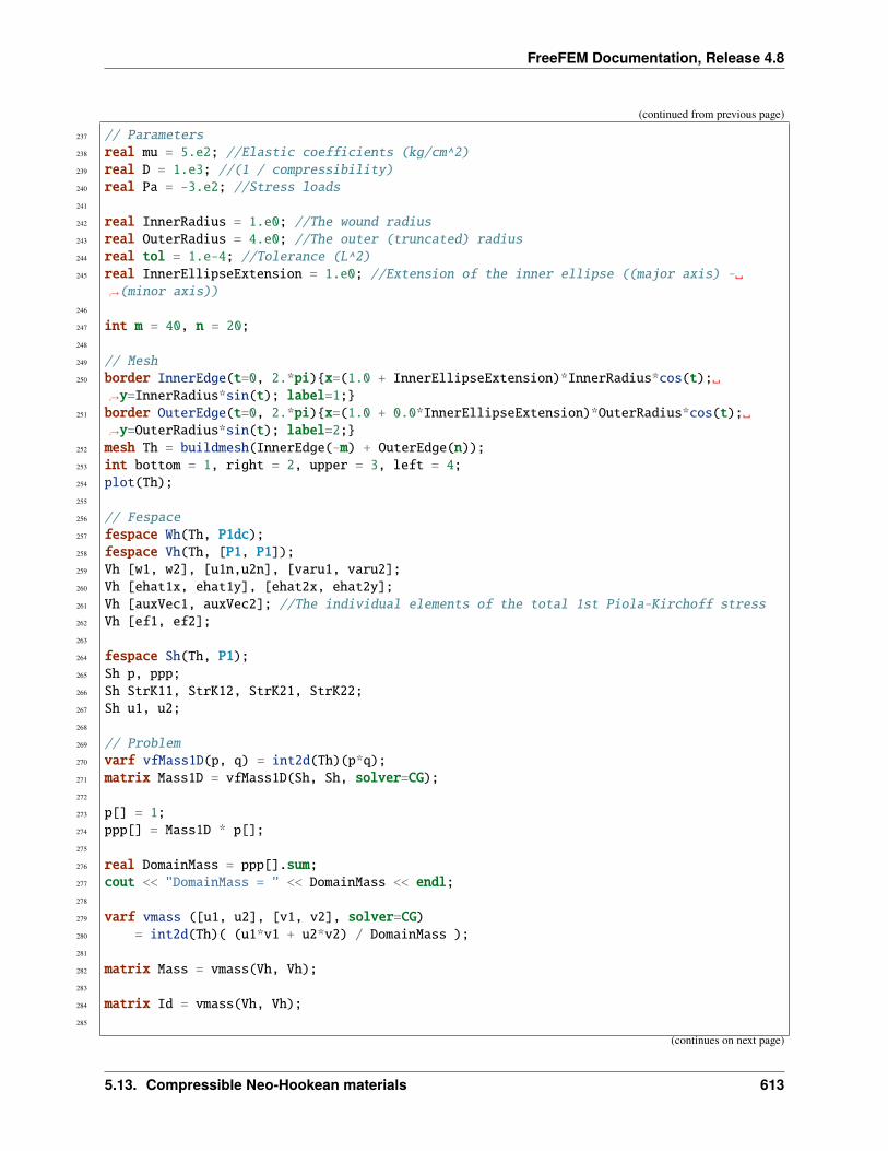
FreeFEM Documentation, Release 4.8
(continued from previous page)
237 // Parameters238 real mu = 5.e2; //Elastic coefficients (kg/cm^2)239 real D = 1.e3; //(1 / compressibility)240 real Pa = -3.e2; //Stress loads241
242 real InnerRadius = 1.e0; //The wound radius243 real OuterRadius = 4.e0; //The outer (truncated) radius244 real tol = 1.e-4; //Tolerance (L^2)245 real InnerEllipseExtension = 1.e0; //Extension of the inner ellipse ((major axis) -
→˓(minor axis))246
247 int m = 40, n = 20;248
249 // Mesh250 border InnerEdge(t=0, 2.*pi)x=(1.0 + InnerEllipseExtension)*InnerRadius*cos(t);
→˓y=InnerRadius*sin(t); label=1;251 border OuterEdge(t=0, 2.*pi)x=(1.0 + 0.0*InnerEllipseExtension)*OuterRadius*cos(t);
→˓y=OuterRadius*sin(t); label=2;252 mesh Th = buildmesh(InnerEdge(-m) + OuterEdge(n));253 int bottom = 1, right = 2, upper = 3, left = 4;254 plot(Th);255
256 // Fespace257 fespace Wh(Th, P1dc);258 fespace Vh(Th, [P1, P1]);259 Vh [w1, w2], [u1n,u2n], [varu1, varu2];260 Vh [ehat1x, ehat1y], [ehat2x, ehat2y];261 Vh [auxVec1, auxVec2]; //The individual elements of the total 1st Piola-Kirchoff stress262 Vh [ef1, ef2];263
264 fespace Sh(Th, P1);265 Sh p, ppp;266 Sh StrK11, StrK12, StrK21, StrK22;267 Sh u1, u2;268
269 // Problem270 varf vfMass1D(p, q) = int2d(Th)(p*q);271 matrix Mass1D = vfMass1D(Sh, Sh, solver=CG);272
273 p[] = 1;274 ppp[] = Mass1D * p[];275
276 real DomainMass = ppp[].sum;277 cout << "DomainMass = " << DomainMass << endl;278
279 varf vmass ([u1, u2], [v1, v2], solver=CG)280 = int2d(Th)( (u1*v1 + u2*v2) / DomainMass );281
282 matrix Mass = vmass(Vh, Vh);283
284 matrix Id = vmass(Vh, Vh);285
(continues on next page)
5.13. Compressible Neo-Hookean materials 613
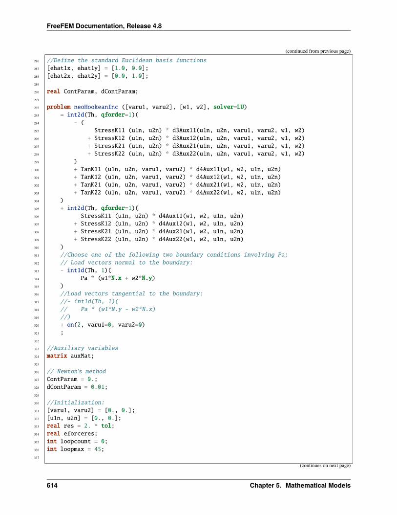
FreeFEM Documentation, Release 4.8
(continued from previous page)
286 //Define the standard Euclidean basis functions287 [ehat1x, ehat1y] = [1.0, 0.0];288 [ehat2x, ehat2y] = [0.0, 1.0];289
290 real ContParam, dContParam;291
292 problem neoHookeanInc ([varu1, varu2], [w1, w2], solver=LU)293 = int2d(Th, qforder=1)(294 - (295 StressK11 (u1n, u2n) * d3Aux11(u1n, u2n, varu1, varu2, w1, w2)296 + StressK12 (u1n, u2n) * d3Aux12(u1n, u2n, varu1, varu2, w1, w2)297 + StressK21 (u1n, u2n) * d3Aux21(u1n, u2n, varu1, varu2, w1, w2)298 + StressK22 (u1n, u2n) * d3Aux22(u1n, u2n, varu1, varu2, w1, w2)299 )300 + TanK11 (u1n, u2n, varu1, varu2) * d4Aux11(w1, w2, u1n, u2n)301 + TanK12 (u1n, u2n, varu1, varu2) * d4Aux12(w1, w2, u1n, u2n)302 + TanK21 (u1n, u2n, varu1, varu2) * d4Aux21(w1, w2, u1n, u2n)303 + TanK22 (u1n, u2n, varu1, varu2) * d4Aux22(w1, w2, u1n, u2n)304 )305 + int2d(Th, qforder=1)(306 StressK11 (u1n, u2n) * d4Aux11(w1, w2, u1n, u2n)307 + StressK12 (u1n, u2n) * d4Aux12(w1, w2, u1n, u2n)308 + StressK21 (u1n, u2n) * d4Aux21(w1, w2, u1n, u2n)309 + StressK22 (u1n, u2n) * d4Aux22(w1, w2, u1n, u2n)310 )311 //Choose one of the following two boundary conditions involving Pa:312 // Load vectors normal to the boundary:313 - int1d(Th, 1)(314 Pa * (w1*N.x + w2*N.y)315 )316 //Load vectors tangential to the boundary:317 //- int1d(Th, 1)(318 // Pa * (w1*N.y - w2*N.x)319 //)320 + on(2, varu1=0, varu2=0)321 ;322
323 //Auxiliary variables324 matrix auxMat;325
326 // Newton's method327 ContParam = 0.;328 dContParam = 0.01;329
330 //Initialization:331 [varu1, varu2] = [0., 0.];332 [u1n, u2n] = [0., 0.];333 real res = 2. * tol;334 real eforceres;335 int loopcount = 0;336 int loopmax = 45;337
(continues on next page)
614 Chapter 5. Mathematical Models
FreeFEM Documentation, Release 4.8
(continued from previous page)
338 // Iterations339 while (loopcount <= loopmax && res >= tol)340 loopcount ++;341 cout << "Loop " << loopcount << endl;342
343 // Solve344 neoHookeanInc;345
346 // Update347 u1 = varu1;348 u2 = varu2;349
350 // Residual351 w1[] = Mass*varu1[];352 res = sqrt(w1[]' * varu1[]); //L^2 norm of [varu1, varu2]353 cout << " L^2 residual = " << res << endl;354
355 // Newton356 u1n[] += varu1[];357
358 // Plot359 plot([u1n,u2n], cmm="displacement");360 361
362 // Plot363 plot(Th, wait=true);364
365 // Movemesh366 mesh Th1 = movemesh(Th, [x+u1n, y+u2n]);367
368 // Plot369 plot(Th1, wait=true);370 plot([u1n,u2n]);
5.14 Whispering gallery modes
Author: I. S. Grudinin
In whispering gallery mode (WGM) resonators, which are typically spheres or disks, electromagnetic field is trappedby total internal reflections from the boundary. Modes of such resonators are distinguished by compact volume andrecord high quality factors (Q) in a broad range of frequencies.
Modern applications of such resonators include microwave and optical cavities for atomic clocks, cavity optomechanics,nonlinear and quantum optics. Analytical solutions for WG modes are only available for a limited number of idealizedgeometries, such as sphere or ellipsoid. Since resonator dimensions are typically much larger than optical wavelength,direct application of numerical 3D finite difference time domain (FDTD) or finite element methods (FEM) is notpractical. It’s possible to solve the vectorial wave equation by reducing it to a two dimensional case by taking axialsymmetry into account.
Such reduction leads to a system of 3 equations to be solved in a 2D “𝜌 − 𝑧” section of a resonator. Please refer to[OXBORROW2007] for a detailed derivation and to [GRUDININ2012] for an example of using FreeFEM to computeWGMs.
5.14. Whispering gallery modes 615
FreeFEM Documentation, Release 4.8
5.14.1 Wave equation for the WGMs
Since electric field is discontinuous on the surface of a dielectric and magnetic field is typically not, we derive ourequations for the magnetic field. The electric field can be easily derived at a later stage from = 𝑖
𝜔𝜖0𝜖−1∇ × .
Following a standard procedure starting with Maxwell equations we derive a wave equation in a single-axis anisotropicmedium such as an optical crystal:
∇×(𝜖−1∇×
)− 𝑘20 − 𝛼∇
(∇ ·
)= 0 (5.16)
Here 𝑘0 = 𝜔/𝑐 is the wavenumber, 𝛼 is the penalty term added to fight spurious FEM solutions. For anisotropicsingle-axis medium with 𝜕𝜖/𝜕𝜑 = 0 in cylindrical system of coordinates we have:
𝜖 =
⎛⎝𝜖𝜌 0 00 𝜖𝜌 00 0 𝜖𝑧
⎞⎠ .
We now assume axial symmetry of our electromagnetic fields and insert an imaginary unity in front of the 𝐻𝜑 toallow all field components to be real numbers and also to account for the phase shift of this component (𝜌, 𝜑, 𝑧) =𝐻𝜌(𝜌, 𝑧), 𝑖𝐻𝜑(𝜌, 𝑧), 𝐻𝑧(𝜌, 𝑧) × 𝑒𝑖𝑚𝜑.
We write the wave equation (5.16) explicitly in cylindrical coordinates, thus obtaining a set of three differential equa-tions for the domain Ω given by the resonator’s cross section and some space outside:
𝐴1𝐻𝑡𝜌, 𝐻
𝑡𝜑, 𝐻
𝑡𝑧 = 0
𝐴2𝐻𝑡𝜌, 𝐻
𝑡𝜑, 𝐻
𝑡𝑧 = 0
𝐴3𝐻𝑡𝜌, 𝐻
𝑡𝜑, 𝐻
𝑡𝑧 = 0
The numerical solutions of these equations and boundary conditions can be found with FreeFEM if we write the systemin the weak, or integral form.
5.14.2 Weak formulation
In general, to obtain the integral or “weak” statements equivalent to system (5.17) and boundary conditions we forma scalar dot product between an arbitrary magnetic field test function H𝑡 = 𝐻𝑡
𝜌, 𝐻𝑡𝜑, 𝐻
𝑡𝑧 and the components of
our vectorial equation 𝐴1, 𝐴2, 𝐴3, and integrate over the resonator’s cross section domain Ω (and its boundary for theboundary conditions): ∫
Ω
(𝐻𝑡𝜌𝐴1 +𝐻𝑡
𝜑𝐴2 +𝐻𝑡𝑧𝐴3)𝑑Ω
We can reduce the order of partial derivatives in this integral by using the Green’s formula for integration by parts. Forexample: ∫
Ω
𝐻𝑡𝑧
𝜕2𝐻𝑧
𝜕𝜌2𝑑Ω = −
∫Ω
𝜕𝐻𝑡𝑧
𝜕𝜌
𝜕𝐻𝑧
𝜕𝜌𝑑Ω +
∮𝐻𝑡𝑧
𝜕𝐻𝑧
𝜕𝜌𝑛𝜌𝑑Γ
Thus converting equations (5.17) we obtain a large expression for the weak form.
616 Chapter 5. Mathematical Models
FreeFEM Documentation, Release 4.8
5.14.3 A dielectric sphere example with FreeFEM
We now compute the fundamental mode frequency for a fused silica sphere. The sphere is 36 micrometer in diameter,the refractive index is 1.46, the boundary condition is the magnetic wall (which can actually be omitted as it holdsautomatically).
1 // Parameters2 real radius = 36; //approximate radius of the cavity3 real yb = -10, yt = -yb; //window yb=bottom and yt=top coordinates4 real xl = radius-5, xr = radius+3; //window xl=left and xr=right coordinates5 real angle = asin((yt)/radius); //angle of the sphere segment to model in radians6 int Nm = 60; //number of mesh vertices per border7 real ne = 1.46; //n_e-extraordinary refractive index (root of permittivity parallel to z-
→˓axis, epara)8 real no = 1.46; //n_o-ordinary refractive index (root of permittivity orthogonal to z-
→˓axis, eorto)9 real nm = 1; //refractive index of surrounding medium (air)
10
11 int nev = 4; // number of eigen values to find12
13 int M = 213; //azimuthal mode order ~ 2Pi*n*R/lambda14 real alpha = 1; //penalty term15
16 // Mesh17 border W1l(t=0, 1)x=xl+(radius*cos(angle)-xl)*(1-t); y=yt; label=1;18 border W1r(t=0, 1)x=xr-(xr-radius*cos(angle))*(t); y=yt; label=1;19 border W2(t=0, 1)x=xr; y=yb+(yt-yb)*t; label=1;20 border W3l(t=0, 1)x=xl+(radius*cos(angle)-xl)*(t); y=yb; label=1;21 border W3r(t=0, 1)x=xr-(xr-radius*cos(angle))*(1-t); y=yb; label=1;22 border W4(t=0, 1)x=xl; y=yt-(yt-yb)*t; label=1;23 border S(t=0, 1)x=radius*cos((t-0.5)*2*angle); y=radius*sin((t-0.5)*2*angle); label=2;24 mesh Th = buildmesh(W1r(Nm/4) + W1l(Nm/4) + W4(Nm) + W3l(Nm/4) + W3r(Nm/4) + W2(Nm) +
→˓S(Nm));25 plot(Th, WindowIndex=0);26
27 // Fespace28 fespace Ph(Th, P0);29 Ph reg = region;30
31 int ncav = reg(xl+1, 0); // cavity32 int nair = reg(xr-1, 0); //air33 Ph eorto = no^2*(region==ncav) + nm^2*(region==nair); //subdomains for epsilon values
→˓inside and outside the resonators34 Ph epara = ne^2*(region==ncav) + nm^2*(region==nair); //subdomains for epsilon values
→˓inside and outside the resonators35
36 //supplementary variables to store eigenvectors, defined on mesh Th with P2 elements -→˓Largange quadratic.
37 fespace Supp(Th, P2);38 Supp eHsqr;39
40 //3d vector FE space41 fespace Vh(Th, [P2, P2, P2]);
(continues on next page)
5.14. Whispering gallery modes 617
FreeFEM Documentation, Release 4.8
(continued from previous page)
42 Vh [Hr, Hphi, Hz], [vHr, vHphi, vHz]; //magnetic field components on Vh space and test→˓functions vH
43
44 // Macro45 //boundary condition macros46 macro EWall(Hr, Hphi, Hz) (47 dy(Hr) - dx(Hz) + Hr*N.x + Hz*N.y48 - epara*(Hz*M - dy(Hphi)*x)*N.y49 + eorto*(Hphi - Hr*M+dx(Hphi)*x)*N.x) //50 macro MWall(Hr, Hphi, Hz) (51 Hphi + Hz*N.x - Hr*N.y52 + epara*(Hz*M - dy(Hphi)*x)*N.x53 + eorto*(Hphi - Hr*M+dx(Hphi)*x)*N.y ) //54
55 // Problem56 real sigma =(M/(ne*radius))^2+2; // value of the shift (k^2), where the modes will be
→˓found57 varf b ([Hr, Hphi, Hz], [vHr, vHphi, vHz])58 = int2d(Th)(59 x*(Hr*vHr+Hphi*vHphi+Hz*vHz)60 )61 ;62 // OP = A - sigma B ; // the shifted matrix63 varf op ([Hr, Hphi, Hz], [vHr, vHphi, vHz])=64 int2d(Th)(65 (66 (eorto*(vHphi*Hphi - M*(vHphi*Hr + Hphi*vHr) + M^2*vHr*Hr) + epara*M^
→˓2*vHz*Hz)/x //A/r67 + eorto*(dx(vHphi)*(Hphi - M*Hr) + dx(Hphi)*(vHphi - M*vHr)) -
→˓epara*M*(vHz*dy(Hphi) + Hz*dy(vHphi)) //B68 + x*(eorto*dx(vHphi)*dx(Hphi) + epara*((dx(vHz) - dy(vHr))*(dx(Hz) - dy(Hr))
→˓+ dy(vHphi)*dy(Hphi))) //C69 )/(eorto*epara)70 + alpha*(71 (vHr*Hr - M*(vHphi*Hr + Hphi*vHr) + M^2*vHphi*Hphi)/x //D/r72 + (dx(vHr) + dy(vHz))*(Hr - M*Hphi) + (vHr - M*vHphi)*(dx(Hr) + dy(Hz)) //E73 + x*(dx(vHr) + dy(vHz))*(dx(Hr) + dy(Hz)) //F74 )75 -sigma*x*(vHr*Hr + vHphi*Hphi + vHz*Hz)76 )77 //electric wall boundary condition on the boundary of computation domain78 +int1d(Th, 1)(79 EWall(Hr, Hphi, Hz)*EWall(vHr, vHphi, vHz)80 )81 ;82 //setting sparce matrices and assigning the solver UMFPACK to solve eigenvalue problem83 matrix B = b(Vh, Vh, solver=UMFPACK);84 matrix OP = op(Vh, Vh, solver=UMFPACK);85
86 // Solve87 real[int] ev(nev); //to store the nev eigenvalue88 Vh[int] [eHr, eHphi, eHz](nev); //to store the nev eigenvector
(continues on next page)
618 Chapter 5. Mathematical Models
FreeFEM Documentation, Release 4.8
(continued from previous page)
89 //calling ARPACK on sparce matrices with the assigned solver UMFPACK:90 int k = EigenValue(OP, B, sym=true, sigma=sigma, value=ev, vector=eHr, tol=1e-10,
→˓maxit=0, ncv=0);91
92 k = min(k, nev); //sometimes the number of converged eigen values93 //can be greater than nev94
95 //file to output mode values96 ofstream f("modes.txt");97 //setting number of digits in the file output98 int nold = f.precision(11);99
100 // Plot & Save101 for (int i = 0; i < k; i++)102 real lambda = 2*pi/sqrt(ev[i]);103 eHsqr = (sqrt(eHr[i]^2 + eHphi[i]^2 + eHz[i]^2)); //intensity from magnetic field
→˓components104 plot(eHsqr, WindowIndex=i, value=1, nbiso=20,LabelColors=1, aspectratio=1, cmm="Mode
→˓"+i+", lambda="+lambda+", F="+(299792.458/lambda));105 f << "Mode "<< i << ", ka=" << sqrt(ev[i])*radius << endl;106
5.14. Whispering gallery modes 619

FreeFEM Documentation, Release 4.8
620 Chapter 5. Mathematical Models
CHAPTER
SIX
EXAMPLES
6.1 Misc
6.1.1 Poisson’s Equation
1 // Parameters2 int nn = 20;3 real L = 1.;4 real H = 1.;5 real l = 0.5;6 real h = 0.5;7
8 func f = 1.;9 func g = 0.;
10
11 int NAdapt = 10;12
13 // Mesh14 border b1(t=0, L)x=t; y=0;;15 border b2(t=0, h)x=L; y=t;;16 border b3(t=L, l)x=t; y=h;;17 border b4(t=h, H)x=l; y=t;;18 border b5(t=l, 0)x=t; y=H;;19 border b6(t=H, 0)x=0; y=t;;20
21 mesh Th = buildmesh(b1(nn*L) + b2(nn*h) + b3(nn*(L-l)) + b4(nn*(H-h)) + b5(nn*l) +→˓b6(nn*H));
22
23 // Fespace24 fespace Vh(Th, P1); // Change P1 to P2 to test P2 finite element25 Vh u, v;26
27 // Macro28 macro grad(u) [dx(u), dy(u)] //29
30 // Problem31 problem Poisson (u, v, solver=CG, eps=-1.e-6)32 = int2d(Th)(33 grad(u)' * grad(v)34 )
(continues on next page)
621
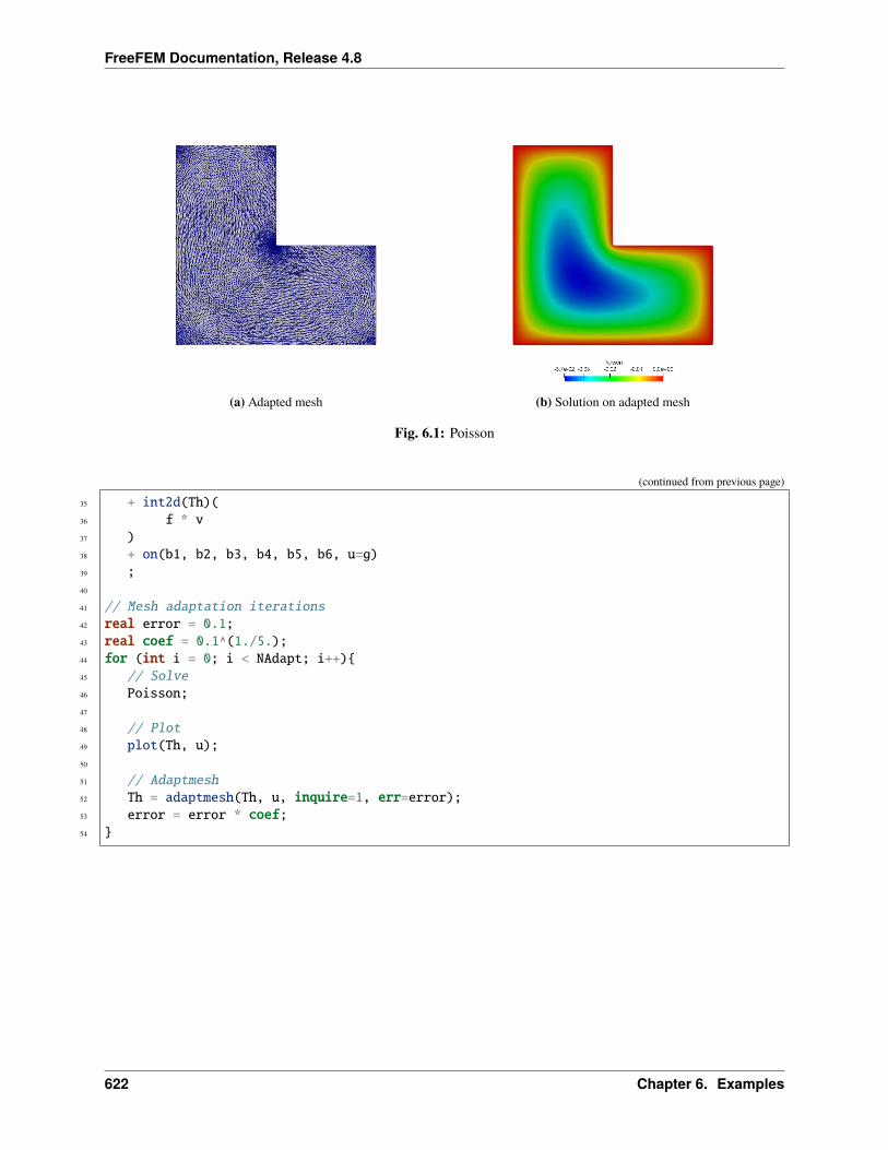
FreeFEM Documentation, Release 4.8
(a) Adapted mesh (b) Solution on adapted mesh
Fig. 6.1: Poisson
(continued from previous page)
35 + int2d(Th)(36 f * v37 )38 + on(b1, b2, b3, b4, b5, b6, u=g)39 ;40
41 // Mesh adaptation iterations42 real error = 0.1;43 real coef = 0.1^(1./5.);44 for (int i = 0; i < NAdapt; i++)45 // Solve46 Poisson;47
48 // Plot49 plot(Th, u);50
51 // Adaptmesh52 Th = adaptmesh(Th, u, inquire=1, err=error);53 error = error * coef;54
622 Chapter 6. Examples
FreeFEM Documentation, Release 4.8
6.1.2 Poisson’s equation 3D
1 load "tetgen"2
3 // Parameters4 real hh = 0.1;5 func ue = 2.*x*x + 3.*y*y + 4.*z*z + 5.*x*y + 6.*x*z + 1.;6 func f= -18.;7
8 // Mesh9 mesh Th = square(10, 20, [x*pi-pi/2, 2*y*pi]); // ]-pi/2, pi/2[X]0,2pi[
10 func f1 = cos(x)*cos(y);11 func f2 = cos(x)*sin(y);12 func f3 = sin(x);13 func f1x = sin(x)*cos(y);14 func f1y = -cos(x)*sin(y);15 func f2x = -sin(x)*sin(y);16 func f2y = cos(x)*cos(y);17 func f3x = cos(x);18 func f3y = 0;19 func m11 = f1x^2 + f2x^2 + f3x^2;20 func m21 = f1x*f1y + f2x*f2y + f3x*f3y;21 func m22 = f1y^2 + f2y^2 + f3y^2;22 func perio = [[4, y], [2, y], [1, x], [3, x]];23 real vv = 1/square(hh);24 Th = adaptmesh(Th, m11*vv, m21*vv, m22*vv, IsMetric=1, periodic=perio);25 Th = adaptmesh(Th, m11*vv, m21*vv, m22*vv, IsMetric=1, periodic=perio);26 plot(Th);27
28 real[int] domain = [0., 0., 0., 1, 0.01];29 mesh3 Th3 = tetgtransfo(Th, transfo=[f1, f2, f3], nbofregions=1, regionlist=domain);30 plot(Th3);31
32 border cc(t=0, 2*pi)x=cos(t); y=sin(t); label=1;33 mesh Th2 = buildmesh(cc(50));34
35 // Fespace36 fespace Vh(Th3, P23d);37 Vh u, v;38 Vh uhe = ue;39 cout << "uhe min: " << uhe[].min << " - max: " << uhe[].max << endl;40 cout << uhe(0.,0.,0.) << endl;41
42 fespace Vh2(Th2, P2);43 Vh2 u2, u2e;44
45 // Macro46 macro Grad3(u) [dx(u), dy(u), dz(u)] //47
48 // Problem49 problem Lap3d (u, v, solver=CG)50 = int3d(Th3)(51 Grad3(v)' * Grad3(u)
(continues on next page)
6.1. Misc 623
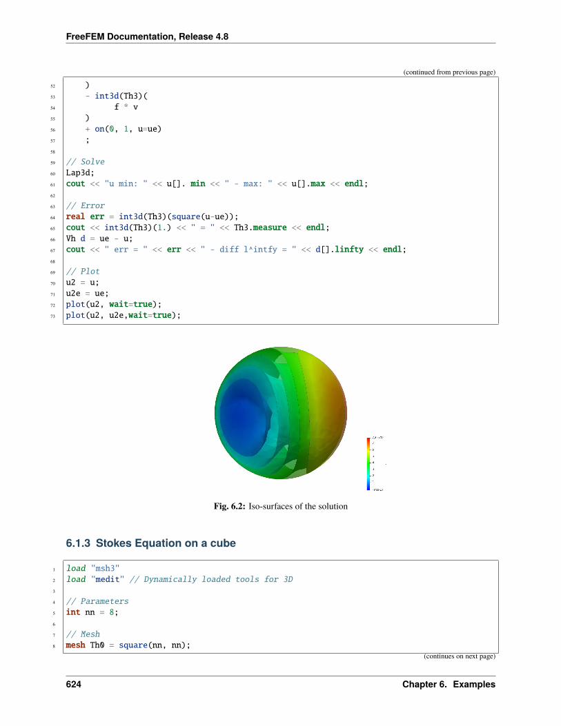
FreeFEM Documentation, Release 4.8
(continued from previous page)
52 )53 - int3d(Th3)(54 f * v55 )56 + on(0, 1, u=ue)57 ;58
59 // Solve60 Lap3d;61 cout << "u min: " << u[]. min << " - max: " << u[].max << endl;62
63 // Error64 real err = int3d(Th3)(square(u-ue));65 cout << int3d(Th3)(1.) << " = " << Th3.measure << endl;66 Vh d = ue - u;67 cout << " err = " << err << " - diff l^intfy = " << d[].linfty << endl;68
69 // Plot70 u2 = u;71 u2e = ue;72 plot(u2, wait=true);73 plot(u2, u2e,wait=true);
Fig. 6.2: Iso-surfaces of the solution
6.1.3 Stokes Equation on a cube
1 load "msh3"2 load "medit" // Dynamically loaded tools for 3D3
4 // Parameters5 int nn = 8;6
7 // Mesh8 mesh Th0 = square(nn, nn);
(continues on next page)
624 Chapter 6. Examples
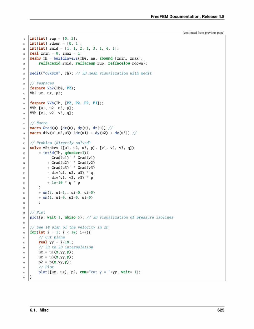
FreeFEM Documentation, Release 4.8
(continued from previous page)
9 int[int] rup = [0, 2];10 int[int] rdown = [0, 1];11 int[int] rmid = [1, 1, 2, 1, 3, 1, 4, 1];12 real zmin = 0, zmax = 1;13 mesh3 Th = buildlayers(Th0, nn, zbound=[zmin, zmax],14 reffacemid=rmid, reffaceup=rup, reffacelow=rdown);15
16 medit("c8x8x8", Th); // 3D mesh visualization with medit17
18 // Fespaces19 fespace Vh2(Th0, P2);20 Vh2 ux, uz, p2;21
22 fespace VVh(Th, [P2, P2, P2, P1]);23 VVh [u1, u2, u3, p];24 VVh [v1, v2, v3, q];25
26 // Macro27 macro Grad(u) [dx(u), dy(u), dz(u)] //28 macro div(u1,u2,u3) (dx(u1) + dy(u2) + dz(u3)) //29
30 // Problem (directly solved)31 solve vStokes ([u1, u2, u3, p], [v1, v2, v3, q])32 = int3d(Th, qforder=3)(33 Grad(u1)' * Grad(v1)34 + Grad(u2)' * Grad(v2)35 + Grad(u3)' * Grad(v3)36 - div(u1, u2, u3) * q37 - div(v1, v2, v3) * p38 + 1e-10 * q * p39 )40 + on(2, u1=1., u2=0, u3=0)41 + on(1, u1=0, u2=0, u3=0)42 ;43
44 // Plot45 plot(p, wait=1, nbiso=5); // 3D visualization of pressure isolines46
47 // See 10 plan of the velocity in 2D48 for(int i = 1; i < 10; i++)49 // Cut plane50 real yy = i/10.;51 // 3D to 2D interpolation52 ux = u1(x,yy,y);53 uz = u3(x,yy,y);54 p2 = p(x,yy,y);55 // Plot56 plot([ux, uz], p2, cmm="cut y = "+yy, wait= 1);57
6.1. Misc 625
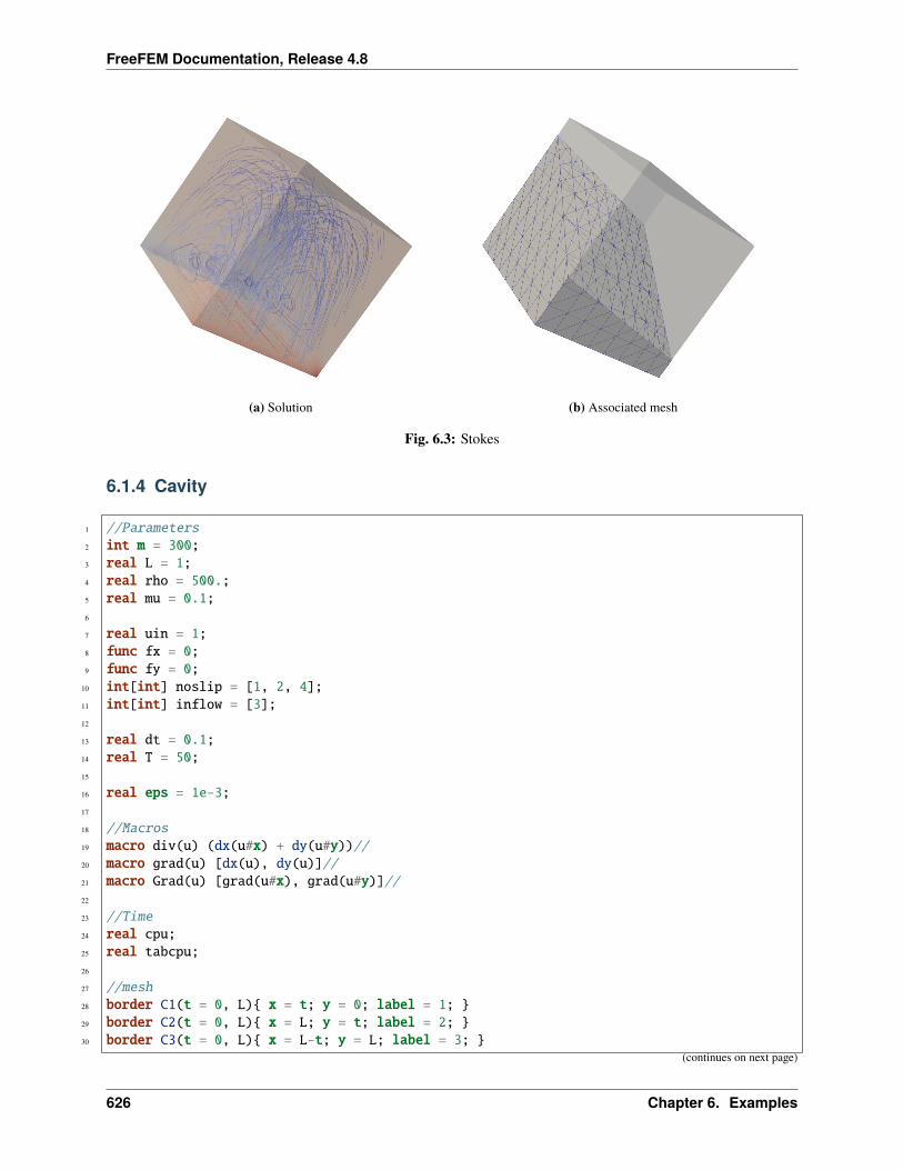
FreeFEM Documentation, Release 4.8
(a) Solution (b) Associated mesh
Fig. 6.3: Stokes
6.1.4 Cavity
1 //Parameters2 int m = 300;3 real L = 1;4 real rho = 500.;5 real mu = 0.1;6
7 real uin = 1;8 func fx = 0;9 func fy = 0;
10 int[int] noslip = [1, 2, 4];11 int[int] inflow = [3];12
13 real dt = 0.1;14 real T = 50;15
16 real eps = 1e-3;17
18 //Macros19 macro div(u) (dx(u#x) + dy(u#y))//20 macro grad(u) [dx(u), dy(u)]//21 macro Grad(u) [grad(u#x), grad(u#y)]//22
23 //Time24 real cpu;25 real tabcpu;26
27 //mesh28 border C1(t = 0, L) x = t; y = 0; label = 1; 29 border C2(t = 0, L) x = L; y = t; label = 2; 30 border C3(t = 0, L) x = L-t; y = L; label = 3;
(continues on next page)
626 Chapter 6. Examples
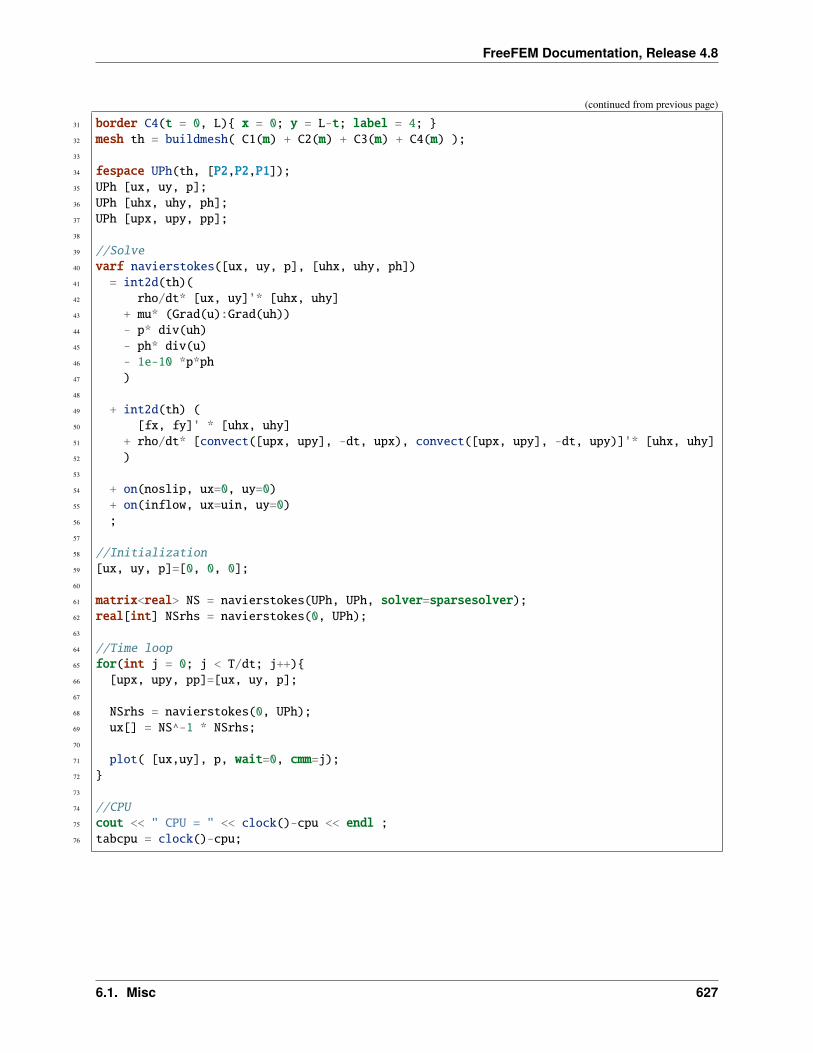
FreeFEM Documentation, Release 4.8
(continued from previous page)
31 border C4(t = 0, L) x = 0; y = L-t; label = 4; 32 mesh th = buildmesh( C1(m) + C2(m) + C3(m) + C4(m) );33
34 fespace UPh(th, [P2,P2,P1]);35 UPh [ux, uy, p];36 UPh [uhx, uhy, ph];37 UPh [upx, upy, pp];38
39 //Solve40 varf navierstokes([ux, uy, p], [uhx, uhy, ph])41 = int2d(th)(42 rho/dt* [ux, uy]'* [uhx, uhy]43 + mu* (Grad(u):Grad(uh))44 - p* div(uh)45 - ph* div(u)46 - 1e-10 *p*ph47 )48
49 + int2d(th) (50 [fx, fy]' * [uhx, uhy]51 + rho/dt* [convect([upx, upy], -dt, upx), convect([upx, upy], -dt, upy)]'* [uhx, uhy]52 )53
54 + on(noslip, ux=0, uy=0)55 + on(inflow, ux=uin, uy=0)56 ;57
58 //Initialization59 [ux, uy, p]=[0, 0, 0];60
61 matrix<real> NS = navierstokes(UPh, UPh, solver=sparsesolver);62 real[int] NSrhs = navierstokes(0, UPh);63
64 //Time loop65 for(int j = 0; j < T/dt; j++)66 [upx, upy, pp]=[ux, uy, p];67
68 NSrhs = navierstokes(0, UPh);69 ux[] = NS^-1 * NSrhs;70
71 plot( [ux,uy], p, wait=0, cmm=j);72 73
74 //CPU75 cout << " CPU = " << clock()-cpu << endl ;76 tabcpu = clock()-cpu;
6.1. Misc 627
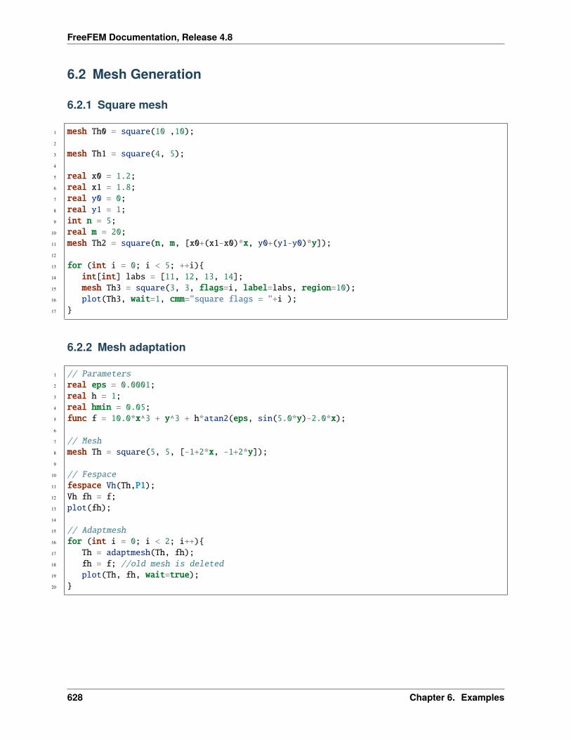
FreeFEM Documentation, Release 4.8
6.2 Mesh Generation
6.2.1 Square mesh
1 mesh Th0 = square(10 ,10);2
3 mesh Th1 = square(4, 5);4
5 real x0 = 1.2;6 real x1 = 1.8;7 real y0 = 0;8 real y1 = 1;9 int n = 5;
10 real m = 20;11 mesh Th2 = square(n, m, [x0+(x1-x0)*x, y0+(y1-y0)*y]);12
13 for (int i = 0; i < 5; ++i)14 int[int] labs = [11, 12, 13, 14];15 mesh Th3 = square(3, 3, flags=i, label=labs, region=10);16 plot(Th3, wait=1, cmm="square flags = "+i );17
6.2.2 Mesh adaptation
1 // Parameters2 real eps = 0.0001;3 real h = 1;4 real hmin = 0.05;5 func f = 10.0*x^3 + y^3 + h*atan2(eps, sin(5.0*y)-2.0*x);6
7 // Mesh8 mesh Th = square(5, 5, [-1+2*x, -1+2*y]);9
10 // Fespace11 fespace Vh(Th,P1);12 Vh fh = f;13 plot(fh);14
15 // Adaptmesh16 for (int i = 0; i < 2; i++)17 Th = adaptmesh(Th, fh);18 fh = f; //old mesh is deleted19 plot(Th, fh, wait=true);20
628 Chapter 6. Examples
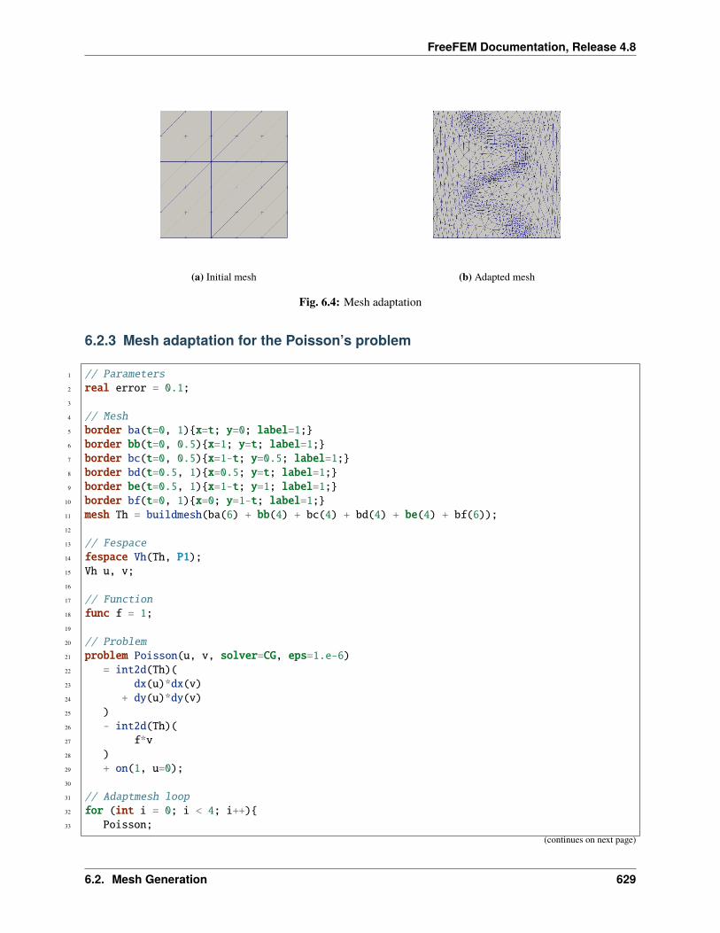
FreeFEM Documentation, Release 4.8
(a) Initial mesh (b) Adapted mesh
Fig. 6.4: Mesh adaptation
6.2.3 Mesh adaptation for the Poisson’s problem
1 // Parameters2 real error = 0.1;3
4 // Mesh5 border ba(t=0, 1)x=t; y=0; label=1;6 border bb(t=0, 0.5)x=1; y=t; label=1;7 border bc(t=0, 0.5)x=1-t; y=0.5; label=1;8 border bd(t=0.5, 1)x=0.5; y=t; label=1;9 border be(t=0.5, 1)x=1-t; y=1; label=1;
10 border bf(t=0, 1)x=0; y=1-t; label=1;11 mesh Th = buildmesh(ba(6) + bb(4) + bc(4) + bd(4) + be(4) + bf(6));12
13 // Fespace14 fespace Vh(Th, P1);15 Vh u, v;16
17 // Function18 func f = 1;19
20 // Problem21 problem Poisson(u, v, solver=CG, eps=1.e-6)22 = int2d(Th)(23 dx(u)*dx(v)24 + dy(u)*dy(v)25 )26 - int2d(Th)(27 f*v28 )29 + on(1, u=0);30
31 // Adaptmesh loop32 for (int i = 0; i < 4; i++)33 Poisson;
(continues on next page)
6.2. Mesh Generation 629
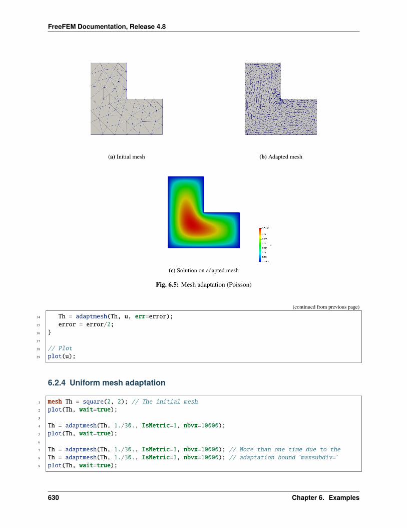
FreeFEM Documentation, Release 4.8
(a) Initial mesh (b) Adapted mesh
(c) Solution on adapted mesh
Fig. 6.5: Mesh adaptation (Poisson)
(continued from previous page)
34 Th = adaptmesh(Th, u, err=error);35 error = error/2;36 37
38 // Plot39 plot(u);
6.2.4 Uniform mesh adaptation
1 mesh Th = square(2, 2); // The initial mesh2 plot(Th, wait=true);3
4 Th = adaptmesh(Th, 1./30., IsMetric=1, nbvx=10000);5 plot(Th, wait=true);6
7 Th = adaptmesh(Th, 1./30., IsMetric=1, nbvx=10000); // More than one time due to the8 Th = adaptmesh(Th, 1./30., IsMetric=1, nbvx=10000); // adaptation bound `maxsubdiv=`9 plot(Th, wait=true);
630 Chapter 6. Examples
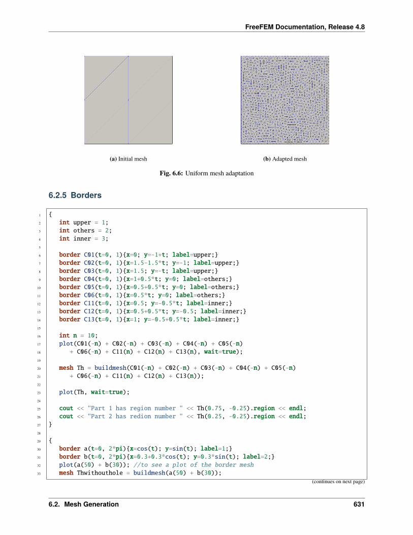
FreeFEM Documentation, Release 4.8
(a) Initial mesh (b) Adapted mesh
Fig. 6.6: Uniform mesh adaptation
6.2.5 Borders
1 2 int upper = 1;3 int others = 2;4 int inner = 3;5
6 border C01(t=0, 1)x=0; y=-1+t; label=upper;7 border C02(t=0, 1)x=1.5-1.5*t; y=-1; label=upper;8 border C03(t=0, 1)x=1.5; y=-t; label=upper;9 border C04(t=0, 1)x=1+0.5*t; y=0; label=others;
10 border C05(t=0, 1)x=0.5+0.5*t; y=0; label=others;11 border C06(t=0, 1)x=0.5*t; y=0; label=others;12 border C11(t=0, 1)x=0.5; y=-0.5*t; label=inner;13 border C12(t=0, 1)x=0.5+0.5*t; y=-0.5; label=inner;14 border C13(t=0, 1)x=1; y=-0.5+0.5*t; label=inner;15
16 int n = 10;17 plot(C01(-n) + C02(-n) + C03(-n) + C04(-n) + C05(-n)18 + C06(-n) + C11(n) + C12(n) + C13(n), wait=true);19
20 mesh Th = buildmesh(C01(-n) + C02(-n) + C03(-n) + C04(-n) + C05(-n)21 + C06(-n) + C11(n) + C12(n) + C13(n));22
23 plot(Th, wait=true);24
25 cout << "Part 1 has region number " << Th(0.75, -0.25).region << endl;26 cout << "Part 2 has redion number " << Th(0.25, -0.25).region << endl;27 28
29 30 border a(t=0, 2*pi)x=cos(t); y=sin(t); label=1;31 border b(t=0, 2*pi)x=0.3+0.3*cos(t); y=0.3*sin(t); label=2;32 plot(a(50) + b(30)); //to see a plot of the border mesh33 mesh Thwithouthole = buildmesh(a(50) + b(30));
(continues on next page)
6.2. Mesh Generation 631
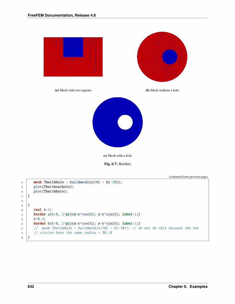
FreeFEM Documentation, Release 4.8
(a) Mesh with two regions (b) Mesh without a hole
(c) Mesh with a hole
Fig. 6.7: Borders
(continued from previous page)
34 mesh Thwithhole = buildmesh(a(50) + b(-30));35 plot(Thwithouthole);36 plot(Thwithhole);37 38
39 40 real r=1;41 border a(t=0, 2*pi)x=r*cos(t); y=r*sin(t); label=1;42 r=0.3;43 border b(t=0, 2*pi)x=r*cos(t); y=r*sin(t); label=1;44 // mesh Thwithhole = buildmesh(a(50) + b(-30)); // do not do this because the two45 // circles have the same radius = $0.3$46
632 Chapter 6. Examples
FreeFEM Documentation, Release 4.8
6.2.6 Change
1 verbosity=3;2
3 // Mesh4 mesh Th1 = square(10, 10);5 mesh Th2 = square(20, 10, [x+1, y]);6
7 int[int] r1=[2, 0];8 plot(Th1, wait=true);9
10 Th1 = change(Th1, label=r1); // Change edges' label from 2 to 011 plot(Th1, wait=true);12
13 int[int] r2=[4, 0];14 Th2 = change(Th2, label=r2); // Change edges' label from 4 to 015 plot(Th2, wait=true);16
17 mesh Th = Th1 + Th2; // 'gluing together' Th1 and Th2 meshes18 cout << "nb lab = " << int1d(Th1,1,3,4)(1./lenEdge)+int1d(Th2,1,2,3)(1./lenEdge)19 << " == " << int1d(Th,1,2,3,4)(1./lenEdge) << " == " << ((10+20)+10)*2 << endl;20 plot(Th, wait=true);21
22 fespace Vh(Th, P1);23 Vh u, v;24
25 macro Grad(u) [dx(u),dy(u)] // Definition of a macro26
27 solve P(u, v)28 = int2d(Th)(29 Grad(u)'*Grad(v)30 )31 -int2d(Th)(32 v33 )34 + on(1, 3, u=0)35 ;36
37 plot(u, wait=1);
6.2.7 Cube
1 load "msh3"2
3 int[int] l6 = [37, 42, 45, 40, 25, 57];4 int r11 = 11;5 mesh3 Th = cube(4, 5, 6, [x*2-1, y*2-1, z*2-1], label=l6, flags =3, region=r11);6
7 cout << "Volume = " << Th.measure << ", border area = " << Th.bordermeasure << endl;8
9 int err = 0;(continues on next page)
6.2. Mesh Generation 633
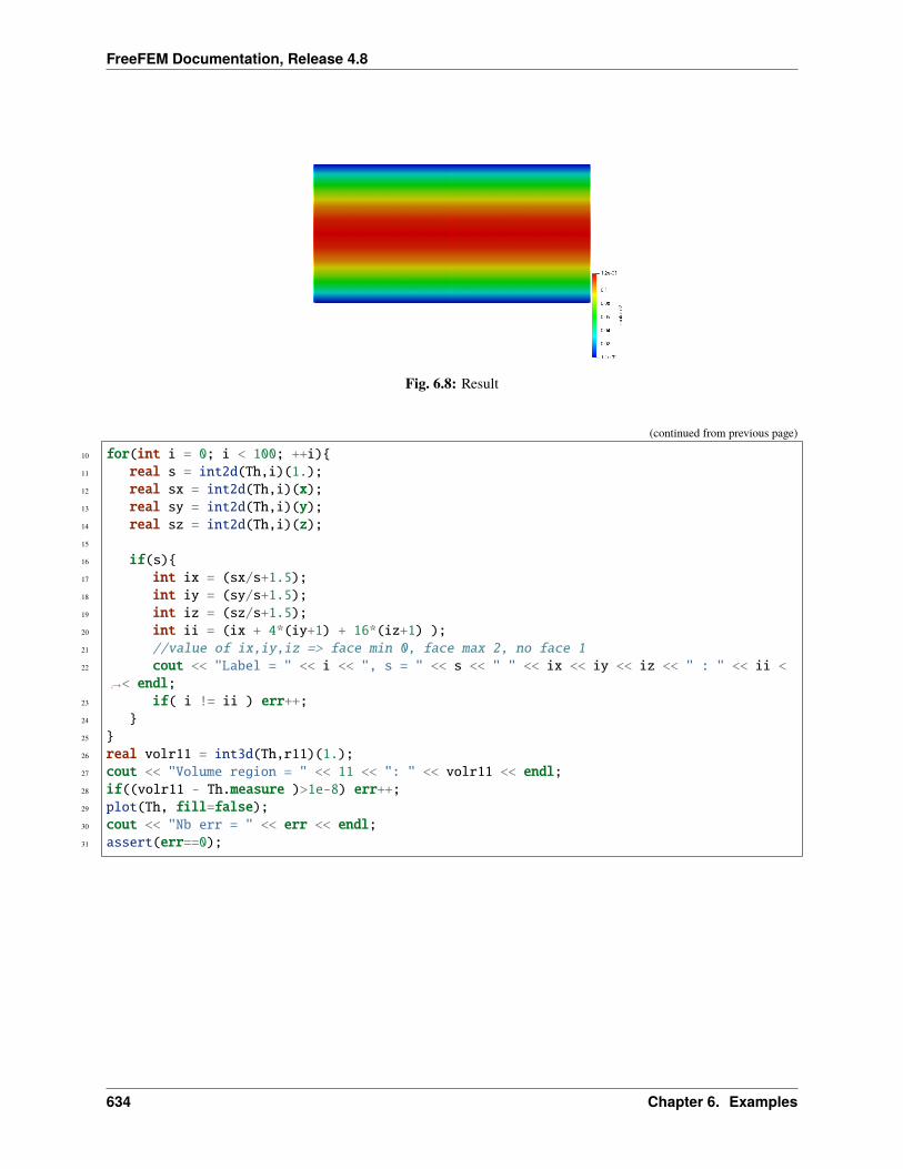
FreeFEM Documentation, Release 4.8
Fig. 6.8: Result
(continued from previous page)
10 for(int i = 0; i < 100; ++i)11 real s = int2d(Th,i)(1.);12 real sx = int2d(Th,i)(x);13 real sy = int2d(Th,i)(y);14 real sz = int2d(Th,i)(z);15
16 if(s)17 int ix = (sx/s+1.5);18 int iy = (sy/s+1.5);19 int iz = (sz/s+1.5);20 int ii = (ix + 4*(iy+1) + 16*(iz+1) );21 //value of ix,iy,iz => face min 0, face max 2, no face 122 cout << "Label = " << i << ", s = " << s << " " << ix << iy << iz << " : " << ii <
→˓< endl;23 if( i != ii ) err++;24 25 26 real volr11 = int3d(Th,r11)(1.);27 cout << "Volume region = " << 11 << ": " << volr11 << endl;28 if((volr11 - Th.measure )>1e-8) err++;29 plot(Th, fill=false);30 cout << "Nb err = " << err << endl;31 assert(err==0);
634 Chapter 6. Examples
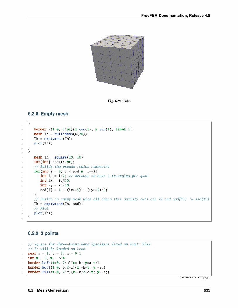
FreeFEM Documentation, Release 4.8
Fig. 6.9: Cube
6.2.8 Empty mesh
1 2 border a(t=0, 2*pi)x=cos(t); y=sin(t); label=1;3 mesh Th = buildmesh(a(20));4 Th = emptymesh(Th);5 plot(Th);6 7 8 mesh Th = square(10, 10);9 int[int] ssd(Th.nt);
10 // Builds the pseudo region numbering11 for(int i = 0; i < ssd.n; i++)12 int iq = i/2; // Because we have 2 triangles per quad13 int ix = iq%10;14 int iy = iq/10;15 ssd[i] = 1 + (ix>=5) + (iy>=5)*2;16 17 // Builds an emtpy mesh with all edges that satisfy e=T1 cap T2 and ssd[T1] != ssd[T2]18 Th = emptymesh(Th, ssd);19 // Plot20 plot(Th);21
6.2.9 3 points
1 // Square for Three-Point Bend Specimens fixed on Fix1, Fix22 // It will be loaded on Load3 real a = 1, b = 5, c = 0.1;4 int n = 5, m = b*n;5 border Left(t=0, 2*a)x=-b; y=a-t;6 border Bot1(t=0, b/2-c)x=-b+t; y=-a;7 border Fix1(t=0, 2*c)x=-b/2-c+t; y=-a;
(continues on next page)
6.2. Mesh Generation 635
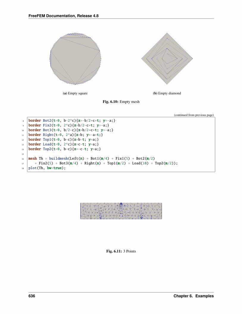
FreeFEM Documentation, Release 4.8
(a) Empty square (b) Empty diamond
Fig. 6.10: Empty mesh
(continued from previous page)
8 border Bot2(t=0, b-2*c)x=-b/2+c+t; y=-a;9 border Fix2(t=0, 2*c)x=b/2-c+t; y=-a;
10 border Bot3(t=0, b/2-c)x=b/2+c+t; y=-a;11 border Right(t=0, 2*a)x=b; y=-a+t;12 border Top1(t=0, b-c)x=b-t; y=a;13 border Load(t=0, 2*c)x=c-t; y=a;14 border Top2(t=0, b-c)x=-c-t; y=a;15
16 mesh Th = buildmesh(Left(n) + Bot1(m/4) + Fix1(5) + Bot2(m/2)17 + Fix2(5) + Bot3(m/4) + Right(n) + Top1(m/2) + Load(10) + Top2(m/2));18 plot(Th, bw=true);
Fig. 6.11: 3 Points
636 Chapter 6. Examples
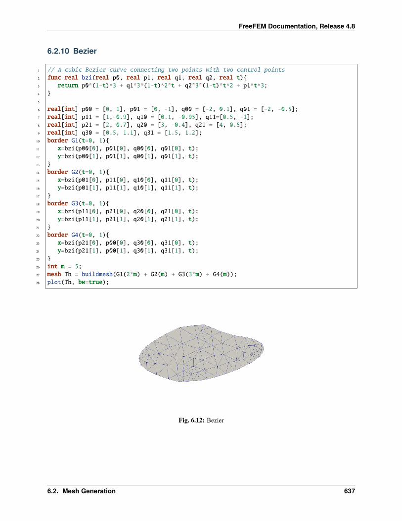
FreeFEM Documentation, Release 4.8
6.2.10 Bezier
1 // A cubic Bezier curve connecting two points with two control points2 func real bzi(real p0, real p1, real q1, real q2, real t)3 return p0*(1-t)^3 + q1*3*(1-t)^2*t + q2*3*(1-t)*t^2 + p1*t^3;4 5
6 real[int] p00 = [0, 1], p01 = [0, -1], q00 = [-2, 0.1], q01 = [-2, -0.5];7 real[int] p11 = [1,-0.9], q10 = [0.1, -0.95], q11=[0.5, -1];8 real[int] p21 = [2, 0.7], q20 = [3, -0.4], q21 = [4, 0.5];9 real[int] q30 = [0.5, 1.1], q31 = [1.5, 1.2];
10 border G1(t=0, 1)11 x=bzi(p00[0], p01[0], q00[0], q01[0], t);12 y=bzi(p00[1], p01[1], q00[1], q01[1], t);13 14 border G2(t=0, 1)15 x=bzi(p01[0], p11[0], q10[0], q11[0], t);16 y=bzi(p01[1], p11[1], q10[1], q11[1], t);17 18 border G3(t=0, 1)19 x=bzi(p11[0], p21[0], q20[0], q21[0], t);20 y=bzi(p11[1], p21[1], q20[1], q21[1], t);21 22 border G4(t=0, 1)23 x=bzi(p21[0], p00[0], q30[0], q31[0], t);24 y=bzi(p21[1], p00[1], q30[1], q31[1], t);25 26 int m = 5;27 mesh Th = buildmesh(G1(2*m) + G2(m) + G3(3*m) + G4(m));28 plot(Th, bw=true);
Fig. 6.12: Bezier
6.2. Mesh Generation 637
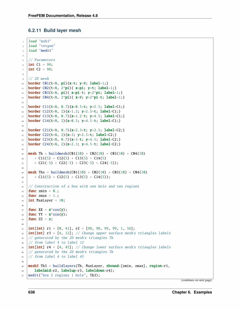
FreeFEM Documentation, Release 4.8
6.2.11 Build layer mesh
1 load "msh3"2 load "tetgen"3 load "medit"4
5 // Parameters6 int C1 = 99;7 int C2 = 98;8
9 // 2D mesh10 border C01(t=0, pi)x=t; y=0; label=1;11 border C02(t=0, 2*pi) x=pi; y=t; label=1;12 border C03(t=0, pi) x=pi-t; y=2*pi; label=1;13 border C04(t=0, 2*pi) x=0; y=2*pi-t; label=1;14
15 border C11(t=0, 0.7)x=0.5+t; y=2.5; label=C1;16 border C12(t=0, 2)x=1.2; y=2.5+t; label=C1;17 border C13(t=0, 0.7)x=1.2-t; y=4.5; label=C1;18 border C14(t=0, 2)x=0.5; y=4.5-t; label=C1;19
20 border C21(t=0, 0.7)x=2.3+t; y=2.5; label=C2;21 border C22(t=0, 2)x=3; y=2.5+t; label=C2;22 border C23(t=0, 0.7)x=3-t; y=4.5; label=C2;23 border C24(t=0, 2)x=2.3; y=4.5-t; label=C2;24
25 mesh Th = buildmesh(C01(10) + C02(10) + C03(10) + C04(10)26 + C11(5) + C12(5) + C13(5) + C14(5)27 + C21(-5) + C22(-5) + C23(-5) + C24(-5));28
29 mesh Ths = buildmesh(C01(10) + C02(10) + C03(10) + C04(10)30 + C11(5) + C12(5) + C13(5) + C14(5));31
32 // Construction of a box with one hole and two regions33 func zmin = 0.;34 func zmax = 1.;35 int MaxLayer = 10;36
37 func XX = x*cos(y);38 func YY = x*sin(y);39 func ZZ = z;40
41 int[int] r1 = [0, 41], r2 = [98, 98, 99, 99, 1, 56];42 int[int] r3 = [4, 12]; // Change upper surface mesh's triangles labels43 // generated by the 2D mesh's triangles Th44 // from label 4 to label 1245 int[int] r4 = [4, 45]; // Change lower surface mesh's triangles labels46 // generated by the 2D mesh's triangles Th47 // from label 4 to label 4548
49 mesh3 Th3 = buildlayers(Th, MaxLayer, zbound=[zmin, zmax], region=r1,50 labelmid=r2, labelup=r3, labeldown=r4);51 medit("box 2 regions 1 hole", Th3);
(continues on next page)
638 Chapter 6. Examples
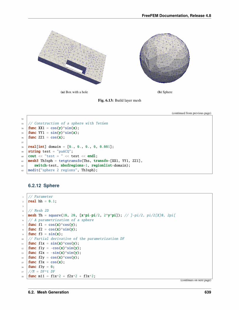
FreeFEM Documentation, Release 4.8
(a) Box with a hole (b) Sphere
Fig. 6.13: Build layer mesh
(continued from previous page)
52
53 // Construction of a sphere with TetGen54 func XX1 = cos(y)*sin(x);55 func YY1 = sin(y)*sin(x);56 func ZZ1 = cos(x);57
58 real[int] domain = [0., 0., 0., 0, 0.001];59 string test = "paACQ";60 cout << "test = " << test << endl;61 mesh3 Th3sph = tetgtransfo(Ths, transfo=[XX1, YY1, ZZ1],62 switch=test, nbofregions=1, regionlist=domain);63 medit("sphere 2 regions", Th3sph);
6.2.12 Sphere
1 // Parameter2 real hh = 0.1;3
4 // Mesh 2D5 mesh Th = square(10, 20, [x*pi-pi/2, 2*y*pi]); // ]-pi/2, pi/2[X]0, 2pi[6 // A parametrization of a sphere7 func f1 = cos(x)*cos(y);8 func f2 = cos(x)*sin(y);9 func f3 = sin(x);
10 // Partial derivative of the parametrization DF11 func f1x = sin(x)*cos(y);12 func f1y = -cos(x)*sin(y);13 func f2x = -sin(x)*sin(y);14 func f2y = cos(x)*cos(y);15 func f3x = cos(x);16 func f3y = 0;17 //M = DF^t DF18 func m11 = f1x^2 + f2x^2 + f3x^2;
(continues on next page)
6.2. Mesh Generation 639
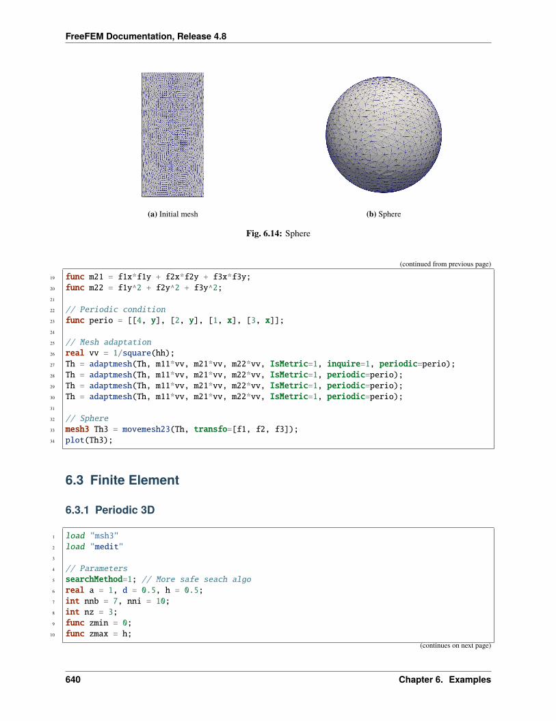
FreeFEM Documentation, Release 4.8
(a) Initial mesh (b) Sphere
Fig. 6.14: Sphere
(continued from previous page)
19 func m21 = f1x*f1y + f2x*f2y + f3x*f3y;20 func m22 = f1y^2 + f2y^2 + f3y^2;21
22 // Periodic condition23 func perio = [[4, y], [2, y], [1, x], [3, x]];24
25 // Mesh adaptation26 real vv = 1/square(hh);27 Th = adaptmesh(Th, m11*vv, m21*vv, m22*vv, IsMetric=1, inquire=1, periodic=perio);28 Th = adaptmesh(Th, m11*vv, m21*vv, m22*vv, IsMetric=1, periodic=perio);29 Th = adaptmesh(Th, m11*vv, m21*vv, m22*vv, IsMetric=1, periodic=perio);30 Th = adaptmesh(Th, m11*vv, m21*vv, m22*vv, IsMetric=1, periodic=perio);31
32 // Sphere33 mesh3 Th3 = movemesh23(Th, transfo=[f1, f2, f3]);34 plot(Th3);
6.3 Finite Element
6.3.1 Periodic 3D
1 load "msh3"2 load "medit"3
4 // Parameters5 searchMethod=1; // More safe seach algo6 real a = 1, d = 0.5, h = 0.5;7 int nnb = 7, nni = 10;8 int nz = 3;9 func zmin = 0;
10 func zmax = h;(continues on next page)
640 Chapter 6. Examples
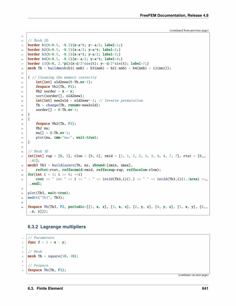
FreeFEM Documentation, Release 4.8
(continued from previous page)
11
12 // Mesh 2D13 border b1(t=0.5, -0.5)x=a*t; y=-a/2; label=1;14 border b2(t=0.5, -0.5)x=a/2; y=a*t; label=2;15 border b3(t=0.5, -0.5)x=a*t; y=a/2; label=3;16 border b4(t=0.5, -0.5)x=-a/2; y=a*t; label=4;17 border i1(t=0, 2.*pi)x=d/2*cos(t); y=-d/2*sin(t); label=7;18 mesh Th = buildmesh(b1(-nnb) + b3(nnb) + b2(-nnb) + b4(nnb) + i1(nni));19
20 // Cleaning the memory correctly21 int[int] old2new(0:Th.nv-1);22 fespace Vh2(Th, P1);23 Vh2 sorder = x + y;24 sort(sorder[], old2new);25 int[int] new2old = old2new^-1; // Inverse permutation26 Th = change(Th, renumv=new2old);27 sorder[] = 0:Th.nv-1;28 29 30 fespace Vh2(Th, P1);31 Vh2 nu;32 nu[] = 0:Th.nv-1;33 plot(nu, cmm="nu=", wait=true);34 35
36 // Mesh 3D37 int[int] rup = [0, 5], rlow = [0, 6], rmid = [1, 1, 2, 2, 3, 3, 4, 4, 7, 7], rtet = [0,
→˓41];38 mesh3 Th3 = buildlayers(Th, nz, zbound=[zmin, zmax],39 reftet=rtet, reffacemid=rmid, reffaceup=rup, reffacelow=rlow);40 for(int i = 1; i <= 6; ++i)41 cout << " int " << i << " : " << int2d(Th3,i)(1.) << " " << int2d(Th3,i)(1./area) <<
→˓endl;42
43 plot(Th3, wait=true);44 medit("Th3", Th3);45
46 fespace Vh(Th3, P2, periodic=[[1, x, z], [3, x, z], [2, y, z], [4, y, z], [5, x, y], [6,→˓x, y]]);
6.3.2 Lagrange multipliers
1 // Parameters2 func f = 1 + x - y;3
4 // Mesh5 mesh Th = square(10, 10);6
7 // Fespace8 fespace Vh(Th, P1);
(continues on next page)
6.3. Finite Element 641
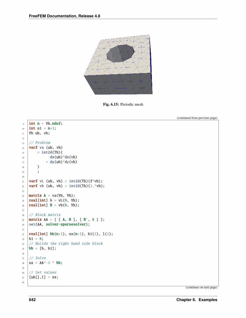
FreeFEM Documentation, Release 4.8
Fig. 6.15: Periodic mesh
(continued from previous page)
9 int n = Vh.ndof;10 int n1 = n+1;11 Vh uh, vh;12
13 // Problem14 varf va (uh, vh)15 = int2d(Th)(16 dx(uh)*dx(vh)17 + dy(uh)*dy(vh)18 )19 ;20
21 varf vL (uh, vh) = int2d(Th)(f*vh);22 varf vb (uh, vh) = int2d(Th)(1.*vh);23
24 matrix A = va(Vh, Vh);25 real[int] b = vL(0, Vh);26 real[int] B = vb(0, Vh);27
28 // Block matrix29 matrix AA = [ [ A, B ], [ B', 0 ] ];30 set(AA, solver=sparsesolver);31
32 real[int] bb(n+1), xx(n+1), b1(1), l(1);33 b1 = 0;34 // Builds the right hand side block35 bb = [b, b1];36
37 // Solve38 xx = AA^-1 * bb;39
40 // Set values41 [uh[],l] = xx;42
(continues on next page)
642 Chapter 6. Examples
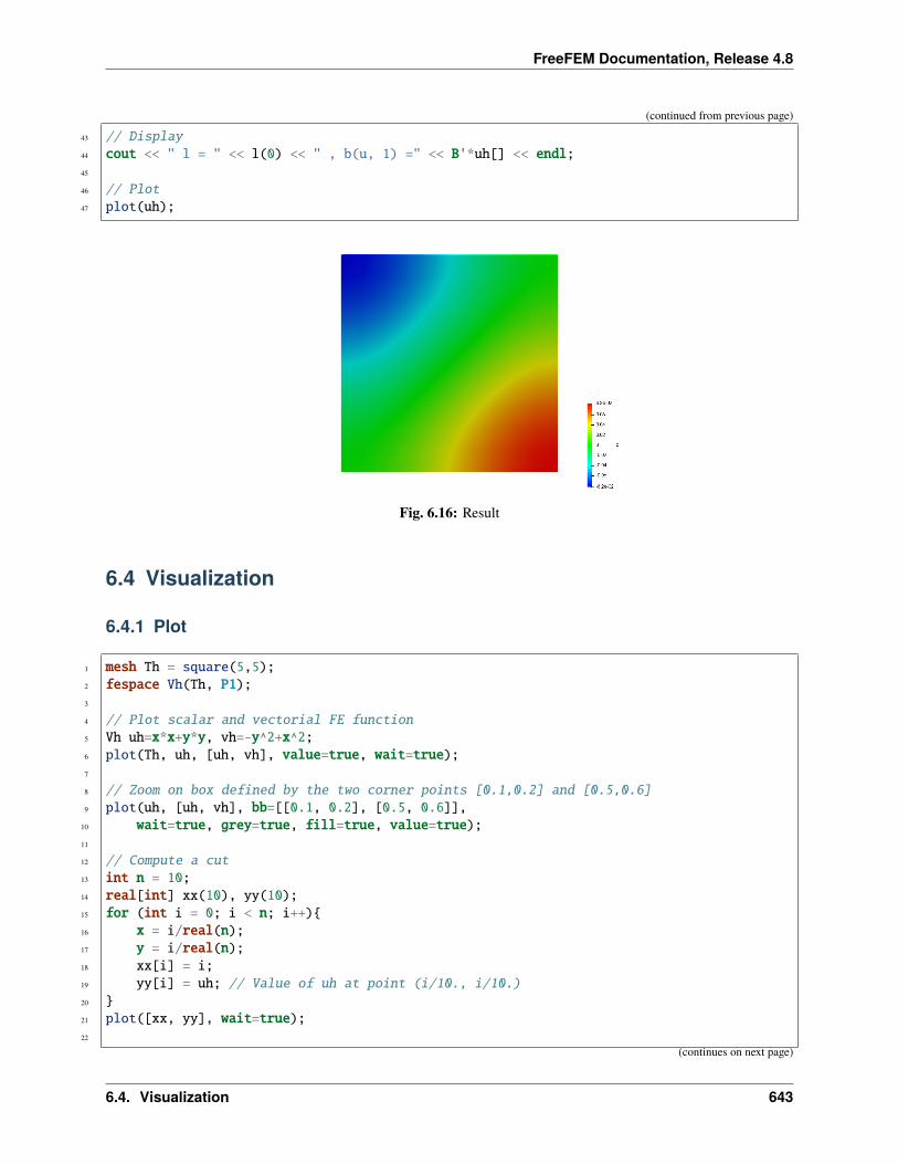
FreeFEM Documentation, Release 4.8
(continued from previous page)
43 // Display44 cout << " l = " << l(0) << " , b(u, 1) =" << B'*uh[] << endl;45
46 // Plot47 plot(uh);
Fig. 6.16: Result
6.4 Visualization
6.4.1 Plot
1 mesh Th = square(5,5);2 fespace Vh(Th, P1);3
4 // Plot scalar and vectorial FE function5 Vh uh=x*x+y*y, vh=-y^2+x^2;6 plot(Th, uh, [uh, vh], value=true, wait=true);7
8 // Zoom on box defined by the two corner points [0.1,0.2] and [0.5,0.6]9 plot(uh, [uh, vh], bb=[[0.1, 0.2], [0.5, 0.6]],
10 wait=true, grey=true, fill=true, value=true);11
12 // Compute a cut13 int n = 10;14 real[int] xx(10), yy(10);15 for (int i = 0; i < n; i++)16 x = i/real(n);17 y = i/real(n);18 xx[i] = i;19 yy[i] = uh; // Value of uh at point (i/10., i/10.)20 21 plot([xx, yy], wait=true);22
(continues on next page)
6.4. Visualization 643
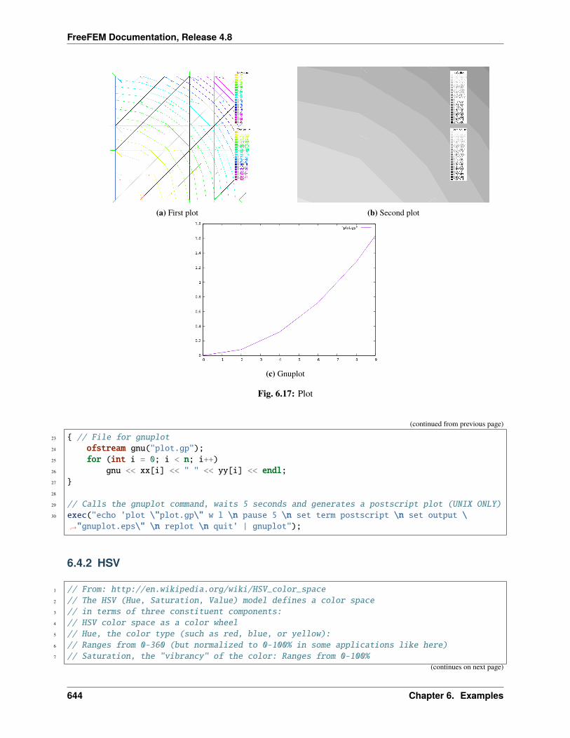
FreeFEM Documentation, Release 4.8
(a) First plot (b) Second plot
(c) Gnuplot
Fig. 6.17: Plot
(continued from previous page)
23 // File for gnuplot24 ofstream gnu("plot.gp");25 for (int i = 0; i < n; i++)26 gnu << xx[i] << " " << yy[i] << endl;27 28
29 // Calls the gnuplot command, waits 5 seconds and generates a postscript plot (UNIX ONLY)30 exec("echo 'plot \"plot.gp\" w l \n pause 5 \n set term postscript \n set output \
→˓"gnuplot.eps\" \n replot \n quit' | gnuplot");
6.4.2 HSV
1 // From: http://en.wikipedia.org/wiki/HSV_color_space2 // The HSV (Hue, Saturation, Value) model defines a color space3 // in terms of three constituent components:4 // HSV color space as a color wheel5 // Hue, the color type (such as red, blue, or yellow):6 // Ranges from 0-360 (but normalized to 0-100% in some applications like here)7 // Saturation, the "vibrancy" of the color: Ranges from 0-100%
(continues on next page)
644 Chapter 6. Examples
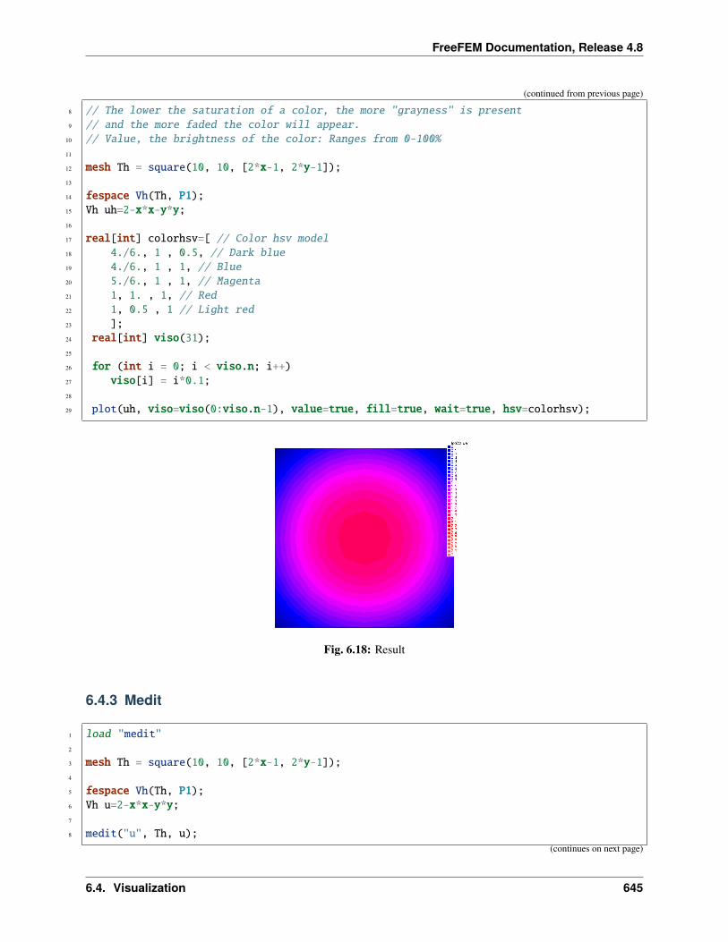
FreeFEM Documentation, Release 4.8
(continued from previous page)
8 // The lower the saturation of a color, the more "grayness" is present9 // and the more faded the color will appear.
10 // Value, the brightness of the color: Ranges from 0-100%11
12 mesh Th = square(10, 10, [2*x-1, 2*y-1]);13
14 fespace Vh(Th, P1);15 Vh uh=2-x*x-y*y;16
17 real[int] colorhsv=[ // Color hsv model18 4./6., 1 , 0.5, // Dark blue19 4./6., 1 , 1, // Blue20 5./6., 1 , 1, // Magenta21 1, 1. , 1, // Red22 1, 0.5 , 1 // Light red23 ];24 real[int] viso(31);25
26 for (int i = 0; i < viso.n; i++)27 viso[i] = i*0.1;28
29 plot(uh, viso=viso(0:viso.n-1), value=true, fill=true, wait=true, hsv=colorhsv);
Fig. 6.18: Result
6.4.3 Medit
1 load "medit"2
3 mesh Th = square(10, 10, [2*x-1, 2*y-1]);4
5 fespace Vh(Th, P1);6 Vh u=2-x*x-y*y;7
8 medit("u", Th, u);(continues on next page)
6.4. Visualization 645
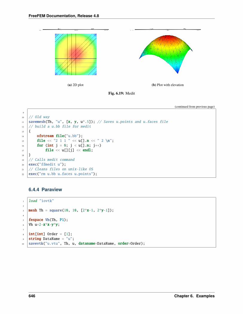
FreeFEM Documentation, Release 4.8
(a) 2D plot (b) Plot with elevation
Fig. 6.19: Medit
(continued from previous page)
9
10 // Old way11 savemesh(Th, "u", [x, y, u*.5]); // Saves u.points and u.faces file12 // build a u.bb file for medit13 14 ofstream file("u.bb");15 file << "2 1 1 " << u[].n << " 2 \n";16 for (int j = 0; j < u[].n; j++)17 file << u[][j] << endl;18 19 // Calls medit command20 exec("ffmedit u");21 // Cleans files on unix-like OS22 exec("rm u.bb u.faces u.points");
6.4.4 Paraview
1 load "iovtk"2
3 mesh Th = square(10, 10, [2*x-1, 2*y-1]);4
5 fespace Vh(Th, P1);6 Vh u=2-x*x-y*y;7
8 int[int] Order = [1];9 string DataName = "u";
10 savevtk("u.vtu", Th, u, dataname=DataName, order=Order);
646 Chapter 6. Examples
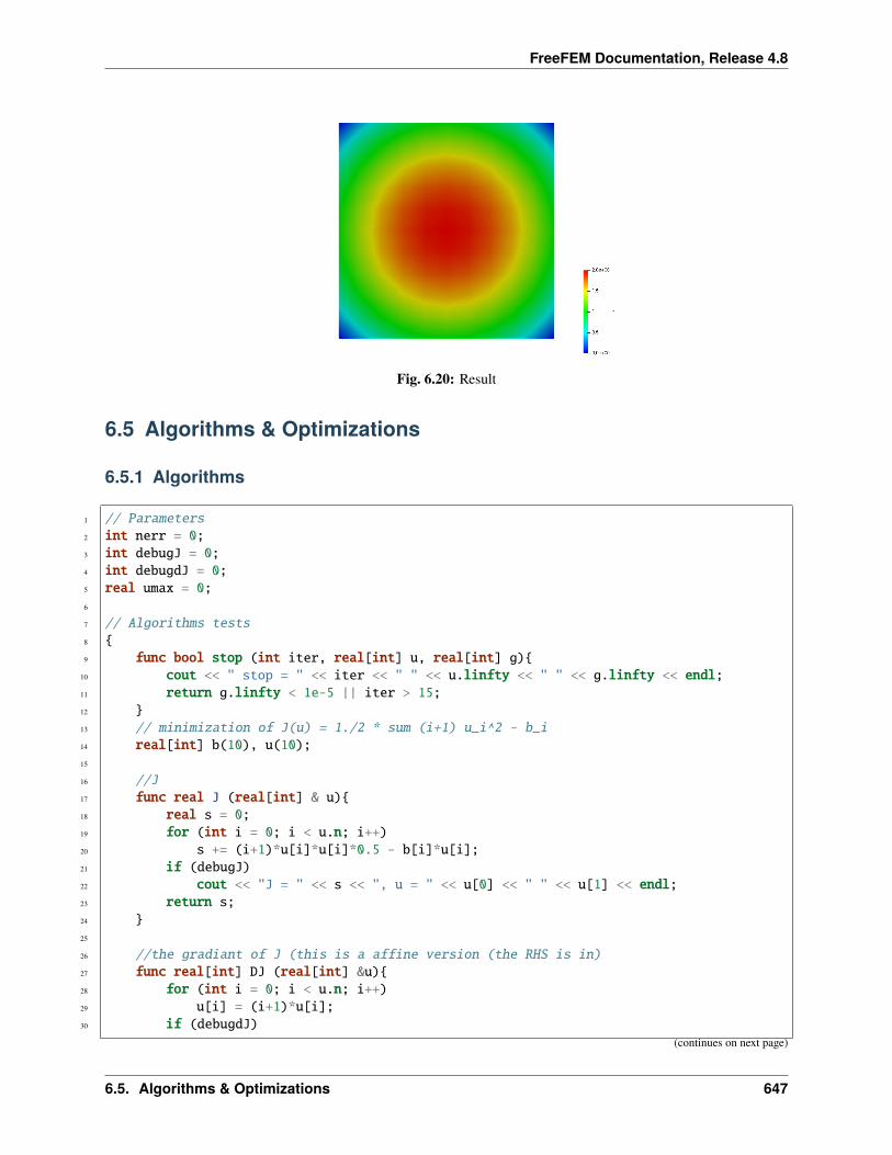
FreeFEM Documentation, Release 4.8
Fig. 6.20: Result
6.5 Algorithms & Optimizations
6.5.1 Algorithms
1 // Parameters2 int nerr = 0;3 int debugJ = 0;4 int debugdJ = 0;5 real umax = 0;6
7 // Algorithms tests8 9 func bool stop (int iter, real[int] u, real[int] g)
10 cout << " stop = " << iter << " " << u.linfty << " " << g.linfty << endl;11 return g.linfty < 1e-5 || iter > 15;12 13 // minimization of J(u) = 1./2 * sum (i+1) u_i^2 - b_i14 real[int] b(10), u(10);15
16 //J17 func real J (real[int] & u)18 real s = 0;19 for (int i = 0; i < u.n; i++)20 s += (i+1)*u[i]*u[i]*0.5 - b[i]*u[i];21 if (debugJ)22 cout << "J = " << s << ", u = " << u[0] << " " << u[1] << endl;23 return s;24 25
26 //the gradiant of J (this is a affine version (the RHS is in)27 func real[int] DJ (real[int] &u)28 for (int i = 0; i < u.n; i++)29 u[i] = (i+1)*u[i];30 if (debugdJ)
(continues on next page)
6.5. Algorithms & Optimizations 647
FreeFEM Documentation, Release 4.8
(continued from previous page)
31 cout << "dJ: u = " << u[0] << " " << u[1] << " " << u[2] << endl;32 u -= b;33 if (debugdJ)34 cout << "dJ-b: u = " << u[0] << " " << u[1] << " " << u[2] << endl;35 return u; //return of global variable ok36 37
38 //the gradiant of the bilinear part of J (the RHS is remove)39 func real[int] DJ0 (real[int] &u)40 for (int i = 0 ; i < u.n; i++)41 u[i] = (i+1)*u[i];42 if(debugdJ)43 cout << "dJ0: u =" << u[0] << " " << u[1] << " " << u[2] << endl;44 return u; //return of global variable ok45 46
47 //erro calculation48 func real error (real[int] & u, real[int] & b)49 real s = 0;50 for (int i = 0; i < u.n; i++)51 s += abs((i+1)*u[i] - b[i]);52 return s;53 54
55 func real[int] matId (real[int] &u) return u; 56
57 int verb=5; //verbosity58 b = 1.; //set right hand side59 u = 0.; //set initial gest60
61 LinearCG(DJ, u, eps=1.e-6, nbiter=20, precon=matId, verbosity=verb);62 cout << "LinearGC (Affine) : J(u) = " << J(u) << ", err = " << error(u, b) << endl;63 nerr += !(error(u,b) < 1e-5);64 if(nerr) cout << "sol: u = " << u[0] << " " << u[1] << " " << u[2] << endl;65
66 b = 1;67 u = 0;68 LinearCG(DJ, u, eps=1.e-15, nbiter=20, precon=matId, verbosity=verb, stop=stop);69 cout << "LinearGC (Affine with stop) : J(u) = " << J(u) << ", err = " << error(u, b)
→˓<< endl;70 nerr += !(error(u,b) < 1e-5);71 if(nerr) cout << "sol: u = " << u[0] << " " << u[1] << " " << u[2] << endl;72
73 b = 1;74 u = 0;75 LinearCG(DJ0, u, b, eps=1.e-6, nbiter=20, precon=matId, verbosity=verb);76 cout << "LinearGC (Linear) : J(u) = " << J(u) << ", err = " << error(u, b) << endl;77 nerr += !(error(u,b) < 1e-5);78 if(nerr) cout << "sol: u = " << u[0] << " " << u[1] << " " << u[2] << endl;79
80
81 b = 1;
(continues on next page)
648 Chapter 6. Examples
FreeFEM Documentation, Release 4.8
(continued from previous page)
82 u = 0;83 AffineGMRES(DJ, u, eps=1.e-6, nbiter=20, precon=matId, verbosity=verb);84 cout << "AffineGMRES (Affine) : J(u) = " << J(u) << ", err = " << error(u, b) <<
→˓endl;85 nerr += !(error(u,b) < 1e-5);86 if(nerr) cout << "sol: u = " << u[0] << " " << u[1] << " " << u[2] << endl;87
88 b=1;89 u=0;90 LinearGMRES(DJ0, u, b, eps=1.e-6, nbiter=20, precon=matId, verbosity=verb);91 cout << "LinearGMRES (Linear) : J(u) = " << J(u) << ", err = " << error(u, b) <<
→˓endl;92 nerr += !(error(u,b) < 1e-5);93 if(nerr) cout << "sol: u = " << u[0] << " " << u[1] << " " << u[2] << endl;94
95
96 b=1;97 u=0;98 NLCG(DJ, u, eps=1.e-6, nbiter=20, precon=matId, verbosity=verb);99 cout << "NLCG: J(u) = " << J(u) << ", err = " << error(u, b) << endl;
100 nerr += !(error(u,b) < 1e-5);101 if(nerr) cout << "sol: u =" << u[0] << " " << u[1] << " " << u[2] << endl;102
103
104 //warning: BFGS use a full matrix of size nxn (where n=u.n)105 b=1;106 u=2;107 BFGS(J, DJ, u, eps=1.e-6, nbiter=20, nbiterline=20);108 cout << "BFGS: J(u) = " << J(u) << ", err = " << error(u, b) << endl;109 assert(error(u,b) < 1e-5);110 if(nerr) cout << "sol: u =" << u[0] << " " << u[1] << " " << u[2] << endl;111
112 assert(nerr==0);113 114
115 // A real non linear test116 // Parameters117 real a = 0.001;118 real eps = 1e-6;119 //f(u) = a*u + u-ln(1+u), f'(u) = a+ u/(1+u), f''(u) = 1/(1+u)^2120 func real f(real u) return u*a+u-log(1+u); 121 func real df(real u) return a+u/(1+u); 122 func real ddf(real u) return 1/((1+u)*(1+u)); 123
124 // Mesh125 mesh Th = square(20, 20);126
127 // Fespace128 fespace Vh(Th, P1);129 Vh b = 1;130 Vh u = 0;131
(continues on next page)
6.5. Algorithms & Optimizations 649
FreeFEM Documentation, Release 4.8
(continued from previous page)
132 fespace Ph(Th, P0);133 Ph alpha; //store df(|nabla u|^2)134
135 // The functionnal J136 //J(u) = 1/2 int_Omega f(|nabla u|^2) - int_Omega u b137 func real J (real[int] & u)138 Vh w;139 w[] = u;140 real r = int2d(Th)(0.5*f(dx(w)*dx(w) + dy(w)*dy(w)) - b*w);141 cout << "J(u) = " << r << " " << u.min << " " << u.max << endl;142 return r;143 144
145 // The gradiant of J146 func real[int] dJ (real[int] & u)147 Vh w;148 w[] = u;149 alpha = df(dx(w)*dx(w) + dy(w)*dy(w));150 varf au (uh, vh)151 = int2d(Th)(152 alpha*(dx(w)*dx(vh) + dy(w)*dy(vh))153 - b*vh154 )155 + on(1, 2, 3, 4, uh=0)156 ;157
158 u = au(0, Vh);159 return u; //warning: no return of local array160 161
162 // Problem163 alpha = df(dx(u)*dx(u) + dy(u)*dy(u));164 varf alap (uh, vh)165 = int2d(Th)(166 alpha*(dx(uh)*dx(vh) + dy(uh)*dy(vh))167 )168 + on(1, 2, 3, 4, uh=0)169 ;170
171 varf amass(uh, vh)172 = int2d(Th)(173 uh*vh174 )175 + on(1, 2, 3, 4, uh=0)176 ;177
178 matrix Amass = amass(Vh, Vh, solver=CG);179 matrix Alap= alap(Vh, Vh, solver=Cholesky, factorize=1);180
181 // Preconditionner182 func real[int] C(real[int] & u)183 real[int] w = u;
(continues on next page)
650 Chapter 6. Examples
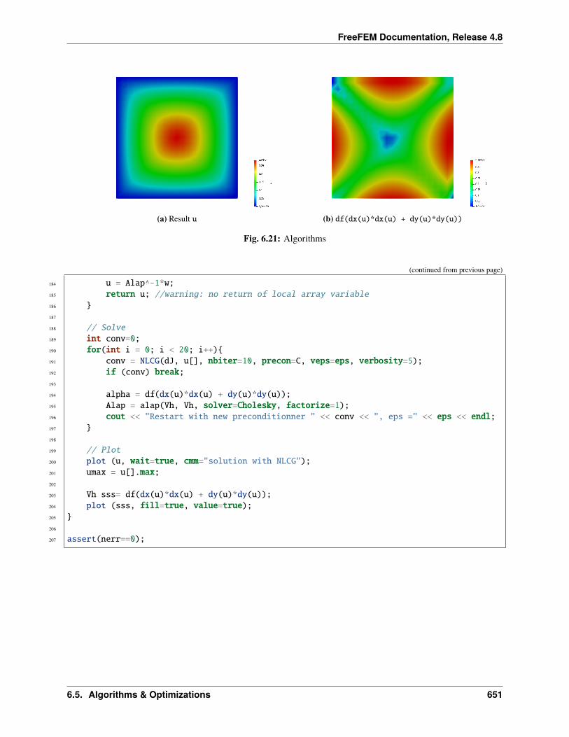
FreeFEM Documentation, Release 4.8
(a) Result u (b) df(dx(u)*dx(u) + dy(u)*dy(u))
Fig. 6.21: Algorithms
(continued from previous page)
184 u = Alap^-1*w;185 return u; //warning: no return of local array variable186 187
188 // Solve189 int conv=0;190 for(int i = 0; i < 20; i++)191 conv = NLCG(dJ, u[], nbiter=10, precon=C, veps=eps, verbosity=5);192 if (conv) break;193
194 alpha = df(dx(u)*dx(u) + dy(u)*dy(u));195 Alap = alap(Vh, Vh, solver=Cholesky, factorize=1);196 cout << "Restart with new preconditionner " << conv << ", eps =" << eps << endl;197 198
199 // Plot200 plot (u, wait=true, cmm="solution with NLCG");201 umax = u[].max;202
203 Vh sss= df(dx(u)*dx(u) + dy(u)*dy(u));204 plot (sss, fill=true, value=true);205 206
207 assert(nerr==0);
6.5. Algorithms & Optimizations 651
FreeFEM Documentation, Release 4.8
6.5.2 CMAES variational inequality
1 load "ff-cmaes"2
3 // Parameters4 int NN = 7;5 func f1 = 1.;6 func f2 = -1.;7 func g1 = 0.;8 func g2 = 0.1;9 int iter = 0;
10 int nadapt = 1;11 real starttol = 1e-10;12 real bctol = 6.e-12;13 real pena = 1000.;14
15 // Mesh16 mesh Th = square(NN, NN);17
18 // Fespace19 fespace Vh(Th, P1);20 Vh ou1, ou2;21
22 // Mesh adaptation loops23 for (int al = 0; al < nadapt; ++al)24 // Problem25 varf BVF (v, w)26 = int2d(Th)(27 0.5*dx(v)*dx(w)28 + 0.5*dy(v)*dy(w)29 )30 ;31 varf LVF1 (v, w) = int2d(Th)(f1*w);32 varf LVF2 (v, w) = int2d(Th)(f2*w);33
34 matrix A = BVF(Vh, Vh);35 real[int] b1 = LVF1(0, Vh);36 real[int] b2 = LVF2(0, Vh);37
38 varf Vbord (v, w) = on(1, 2, 3, 4, v=1);39
40 Vh In, Bord;41 Bord[] = Vbord(0, Vh, tgv=1);42 In[] = Bord[] ? 0:1;43 Vh gh1 = Bord*g1;44 Vh gh2 = Bord*g2;45
46 // Function which creates a vector of the search space type from47 // two finite element functions48 func int FEFToSSP (real[int] &fef1, real[int] &fef2, real[int] &ssp)49 int kX = 0;50 for (int i = 0; i < Vh.ndof; ++i)51 if (In[][i])
(continues on next page)
652 Chapter 6. Examples
FreeFEM Documentation, Release 4.8
(continued from previous page)
52 ssp[kX] = fef1[i];53 ssp[kX+In[].sum] = fef2[i];54 ++kX;55 56 57 return 1;58 59
60 // Splits a vector from the search space and fills61 // two finite element functions with it62 func int SSPToFEF (real[int] &fef1, real[int] &fef2, real[int] &ssp)63 int kX = 0;64 for (int i = 0; i < Vh.ndof; ++i)65 if (In[][i])66 fef1[i] = ssp[kX];67 fef2[i] = ssp[kX+In[].sum];68 ++kX;69 70 else71 fef1[i] = gh1[][i];72 fef2[i] = gh2[][i];73 74 75 return 1;76 77
78 func real IneqC (real[int] &X)79 real[int] constraints(In[].sum);80 for (int i = 0; i < In[].sum; ++i)81 constraints[i] = X[i] - X[i+In[].sum];82 constraints[i] = constraints[i] <= 0 ? 0. : constraints[i];83 84 return constraints.l2;85 86
87 func real J (real[int] &X)88 Vh u1, u2;89 SSPToFEF(u1[], u2[], X);90 iter++;91 real[int] Au1 = A*u1[], Au2 = A*u2[];92 Au1 -= b1;93 Au2 -= b2;94 real val = u1[]'*Au1 + u2[]'*Au2;95 val += pena * IneqC(X);96 if (iter%200 == 199)97 plot(u1, u2, nbiso=30, fill=1, dim=3, cmm="adapt level "+al+" - iteration
→˓"+iter+" - J = "+val, value=1);98 return val ;99
100
101 // Solve102 real[int] start(2*In[].sum);
(continues on next page)
6.5. Algorithms & Optimizations 653
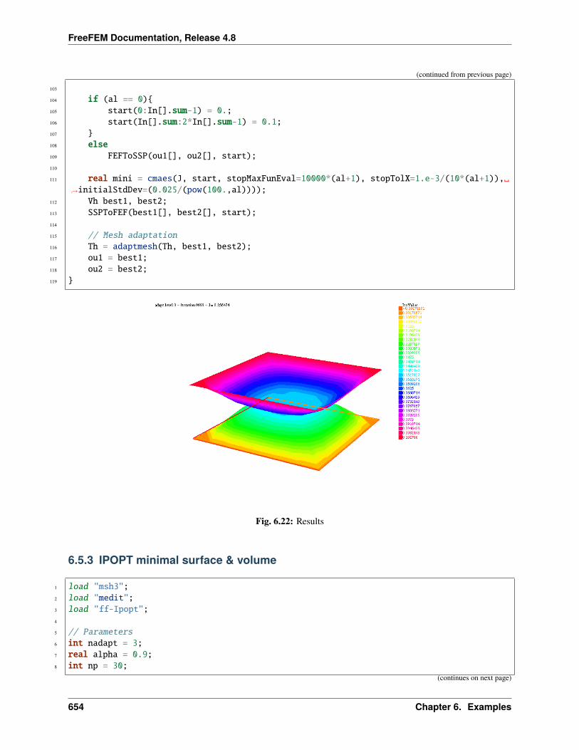
FreeFEM Documentation, Release 4.8
(continued from previous page)
103
104 if (al == 0)105 start(0:In[].sum-1) = 0.;106 start(In[].sum:2*In[].sum-1) = 0.1;107 108 else109 FEFToSSP(ou1[], ou2[], start);110
111 real mini = cmaes(J, start, stopMaxFunEval=10000*(al+1), stopTolX=1.e-3/(10*(al+1)),→˓initialStdDev=(0.025/(pow(100.,al))));
112 Vh best1, best2;113 SSPToFEF(best1[], best2[], start);114
115 // Mesh adaptation116 Th = adaptmesh(Th, best1, best2);117 ou1 = best1;118 ou2 = best2;119
Fig. 6.22: Results
6.5.3 IPOPT minimal surface & volume
1 load "msh3";2 load "medit";3 load "ff-Ipopt";4
5 // Parameters6 int nadapt = 3;7 real alpha = 0.9;8 int np = 30;
(continues on next page)
654 Chapter 6. Examples
FreeFEM Documentation, Release 4.8
(continued from previous page)
9 real regtest;10 int shapeswitch = 1;11 real sigma = 2*pi/40.;12 real treshold = 0.1;13 real e = 0.1;14 real r0 = 0.25;15 real rr = 2-r0;16 real E = 1./(e*e);17 real RR = 1./(rr*rr);18
19 // Mesh20 mesh Th = square(2*np, np, [2*pi*x, pi*y]);21
22 // Fespace23 fespace Vh(Th, P1, periodic=[[2, y], [4, y]]);24 //Initial shape definition25 //outside of the mesh adaptation loop to initialize with the previous optimial shape
→˓found on further iterations26 Vh startshape = 5;27 Vh uz = 1., lz = 1.;28
29 // Mesh adaptation loop30 real[int] lm = [1];31 for(int kkk = 0; kkk < nadapt; ++kkk)32 int iter=0;33 func sin2 = square(sin(y));34
35 // A function which transform Th in 3d mesh (r=rho)36 //a point (theta,phi) of Th becomes ( r(theta,phi)*cos(theta)*sin(phi) , r(theta,
→˓phi)*sin(theta)*sin(phi) , r(theta,phi)*cos(phi) )37 //then displays the resulting mesh with medit38 func int Plot3D (real[int] &rho, string cmm, bool ffplot)39 Vh rhoo;40 rhoo[] = rho;41 //mesh sTh = square(np, np/2, [2*pi*x, pi*y]);42 //fespace sVh(sTh, P1);43 //Vh rhoplot = rhoo;44 try45 mesh3 Sphere = movemesh23(Th, transfo=[rhoo(x,y)*cos(x)*sin(y), rhoo(x,
→˓y)*sin(x)*sin(y), rhoo(x,y)*cos(y)]);46 if(ffplot)47 plot(Sphere);48 else49 medit(cmm, Sphere);50 51 catch(...)52 cout << "PLOT ERROR" << endl;53 54 return 1;55 56
57 // Surface computation
(continues on next page)
6.5. Algorithms & Optimizations 655
FreeFEM Documentation, Release 4.8
(continued from previous page)
58 //Maybe is it possible to use movemesh23 to have the surface function less→˓complicated
59 //However, it would not simplify the gradient and the hessian60 func real Area (real[int] &X)61 Vh rho;62 rho[] = X;63 Vh rho2 = square(rho);64 Vh rho4 = square(rho2);65 real res = int2d(Th)(sqrt(rho4*sin2 + rho2*square(dx(rho)) +
→˓rho2*sin2*square(dy(rho))));66 ++iter;67 if(1)68 plot(rho, value=true, fill=true, cmm="rho(theta,phi) on [0,2pi]x[0,pi] - S=
→˓"+res, dim=3);69 else70 Plot3D(rho[], "shape_evolution", 1);71 return res;72 73
74 func real[int] GradArea (real[int] &X)75 Vh rho, rho2;76 rho[] = X;77 rho2[] = square(X);78 Vh sqrtPsi, alpha;79 80 Vh dxrho2 = dx(rho)*dx(rho), dyrho2 = dy(rho)*dy(rho);81 sqrtPsi = sqrt(rho2*rho2*sin2 + rho2*dxrho2 + rho2*dyrho2*sin2);82 alpha = 2.*rho2*rho*sin2 + rho*dxrho2 + rho*dyrho2*sin2;83 84 varf dArea (u, v)85 = int2d(Th)(86 1./sqrtPsi * (alpha*v + rho2*dx(rho)*dx(v) + rho2*dy(rho)*sin2*dy(v))87 )88 ;89
90 real[int] grad = dArea(0, Vh);91 return grad;92 93
94 matrix hessianA;95 func matrix HessianArea (real[int] &X)96 Vh rho, rho2;97 rho[] = X;98 rho2 = square(rho);99 Vh sqrtPsi, sqrtPsi3, C00, C01, C02, C11, C12, C22, A;
100 101 Vh C0, C1, C2;102 Vh dxrho2 = dx(rho)*dx(rho), dyrho2 = dy(rho)*dy(rho);103 sqrtPsi = sqrt( rho2*rho2*sin2 + rho2*dxrho2 + rho2*dyrho2*sin2);104 sqrtPsi3 = (rho2*rho2*sin2 + rho2*dxrho2 + rho2*dyrho2*sin2)*sqrtPsi;105 C0 = 2*rho2*rho*sin2 + rho*dxrho2 + rho*dyrho2*sin2;106 C1 = rho2*dx(rho);
(continues on next page)
656 Chapter 6. Examples
FreeFEM Documentation, Release 4.8
(continued from previous page)
107 C2 = rho2*sin2*dy(rho);108 C00 = square(C0);109 C01 = C0*C1;110 C02 = C0*C2;111 C11 = square(C1);112 C12 = C1*C2;113 C22 = square(C2);114 A = 6.*rho2*sin2 + dxrho2 + dyrho2*sin2;115 116 varf d2Area (w, v)117 =int2d(Th)(118 1./sqrtPsi * (119 A*w*v120 + 2*rho*dx(rho)*dx(w)*v121 + 2*rho*dx(rho)*w*dx(v)122 + 2*rho*dy(rho)*sin2*dy(w)*v123 + 2*rho*dy(rho)*sin2*w*dy(v)124 + rho2*dx(w)*dx(v)125 + rho2*sin2*dy(w)*dy(v)126 )127 + 1./sqrtPsi3 * (128 C00*w*v129 + C01*dx(w)*v130 + C01*w*dx(v)131 + C02*dy(w)*v132 + C02*w*dy(v)133 + C11*dx(w)*dx(v)134 + C12*dx(w)*dy(v)135 + C12*dy(w)*dx(v)136 + C22*dy(w)*dy(v)137 )138 )139 ;140 hessianA = d2Area(Vh, Vh);141 return hessianA;142 143
144 // Volume computation145 func real Volume (real[int] &X)146 Vh rho;147 rho[] = X;148 Vh rho3 = rho*rho*rho;149 real res = 1./3.*int2d(Th)(rho3*sin(y));150 return res;151 152
153 func real[int] GradVolume (real[int] &X)154 Vh rho;155 rho[] = X;156 varf dVolume(u, v) = int2d(Th)(rho*rho*sin(y)*v);157 real[int] grad = dVolume(0, Vh);158 return grad;
(continues on next page)
6.5. Algorithms & Optimizations 657
FreeFEM Documentation, Release 4.8
(continued from previous page)
159 160 matrix hessianV;161 func matrix HessianVolume(real[int] &X)162 Vh rho;163 rho[] = X;164 varf d2Volume(w, v) = int2d(Th)(2*rho*sin(y)*v*w);165 hessianV = d2Volume(Vh, Vh);166 return hessianV;167 168
169 //if we want to use the volume as a constraint function170 //we must wrap it in some freefem functions returning the appropriate type171 //The lagrangian hessian also have to be wrapped since the Volume is not linear with172 //respect to rho, it will constribbute to the hessian.173 func real[int] ipVolume (real[int] &X) real[int] vol = [Volume(X)]; return vol; 174 matrix mdV;175 func matrix ipGradVolume (real[int] &X) real[int,int] dvol(1,Vh.ndof); dvol(0,:) =
→˓GradVolume(X); mdV = dvol; return mdV; 176 matrix HLagrangian;177 func matrix ipHessianLag (real[int] &X, real objfact, real[int] &lambda)178 HLagrangian = objfact*HessianArea(X) + lambda[0]*HessianVolume(X);179 return HLagrangian;180 181
182 //building struct for GradVolume183 int[int] gvi(Vh.ndof), gvj=0:Vh.ndof-1;184 gvi = 0;185
186 Vh rc = startshape; //the starting value187 Vh ub = 1.e19; //bounds definition188 Vh lb = 0;189
190 func real Gaussian (real X, real Y, real theta, real phi)191 real deltax2 = square((X-theta)*sin(Y)), deltay2 = square(Y-phi);192 return exp(-0.5 * (deltax2 + deltay2) / (sigma*sigma));193 194
195 func disc1 = sqrt(1./(RR+(E-RR)*cos(y)*cos(y)))*(1+0.1*cos(7*x));196 func disc2 = sqrt(1./(RR+(E-RR)*cos(x)*cos(x)*sin2));197
198 if(1)199 lb = r0;200 for (int q = 0; q < 5; ++q)201 func f = rr*Gaussian(x, y, 2*q*pi/5., pi/3.);202 func g = rr*Gaussian(x, y, 2*q*pi/5.+pi/5., 2.*pi/3.);203 lb = max(max(lb, f), g);204 205 lb = max(lb, rr*Gaussian(x, y, 2*pi, pi/3));206 207 lb = max(lb, max(disc1, disc2));208 real Vobj = Volume(lb[]);209 real Vnvc = 4./3.*pi*pow(lb[].linfty,3);
(continues on next page)
658 Chapter 6. Examples
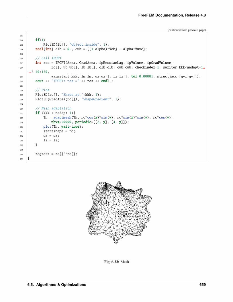
FreeFEM Documentation, Release 4.8
(continued from previous page)
210
211 if(1)212 Plot3D(lb[], "object_inside", 1);213 real[int] clb = 0., cub = [(1-alpha)*Vobj + alpha*Vnvc];214
215 // Call IPOPT216 int res = IPOPT(Area, GradArea, ipHessianLag, ipVolume, ipGradVolume,217 rc[], ub=ub[], lb=lb[], clb=clb, cub=cub, checkindex=1, maxiter=kkk<nadapt-1
→˓? 40:150,218 warmstart=kkk, lm=lm, uz=uz[], lz=lz[], tol=0.00001, structjacc=[gvi,gvj]);219 cout << "IPOPT: res =" << res << endl ;220
221 // Plot222 Plot3D(rc[], "Shape_at_"+kkk, 1);223 Plot3D(GradArea(rc[]), "ShapeGradient", 1);224
225 // Mesh adaptation226 if (kkk < nadapt-1)227 Th = adaptmesh(Th, rc*cos(x)*sin(y), rc*sin(x)*sin(y), rc*cos(y),228 nbvx=50000, periodic=[[2, y], [4, y]]);229 plot(Th, wait=true);230 startshape = rc;231 uz = uz;232 lz = lz;233 234
235 regtest = rc[]'*rc[];236
Fig. 6.23: Mesh
6.5. Algorithms & Optimizations 659
FreeFEM Documentation, Release 4.8
6.5.4 CMAES MPI variational inequality
Command:
1 ff-mpirun -np 4 CMAESMPIVariationalInequality.edp -glut ffglut
1 load "mpi-cmaes"2
3 // Parameters4 int NN = 10;5 func f1 = 1.;6 func f2 = -1.;7 func g1 = 0.;8 func g2 = 0.1;9 int iter = 0;
10 int nadapt = 1;11 real starttol = 1e-10;12 real bctol = 6.e-12;13 real pena = 1000;14
15 // Mesh16 mesh Th = square(NN, NN);17
18 // Fespace19 fespace Vh(Th, P1);20 Vh ou1, ou2;21
22 // Mehs adaptation loop23 for (int al = 0; al < nadapt; ++al)24 // Problem25 varf BVF (v, w)26 = int2d(Th)(27 0.5*dx(v)*dx(w)28 + 0.5*dy(v)*dy(w)29 )30 ;31 varf LVF1 (v, w) = int2d(Th)(f1*w);32 varf LVF2 (v, w) = int2d(Th)(f2*w);33 matrix A = BVF(Vh, Vh);34 real[int] b1 = LVF1(0, Vh);35 real[int] b2 = LVF2(0, Vh);36
37 varf Vbord (v, w) = on(1, 2, 3, 4, v=1);38
39 Vh In, Bord;40 Bord[] = Vbord(0, Vh, tgv=1);41 In[] = Bord[] ? 0:1;42 Vh gh1 = Bord*g1, gh2 = Bord*g2;43
44 //Function which create a vector of the search space type from45 //two finite element functions46 func int FEFToSSP (real[int] &fef1, real[int] &fef2, real[int] &ssp)47 int kX = 0;
(continues on next page)
660 Chapter 6. Examples
FreeFEM Documentation, Release 4.8
(continued from previous page)
48 for (int i = 0; i < Vh.ndof; ++i)49 if (In[][i])50 ssp[kX] = fef1[i];51 ssp[kX+In[].sum] = fef2[i];52 ++kX;53 54 55 return 1;56 57
58 //Function spliting a vector from the search space and fills59 //two finite element functions with it60 func int SSPToFEF (real[int] &fef1, real[int] &fef2, real[int] &ssp)61 int kX = 0;62 for (int i = 0; i < Vh.ndof; ++i)63 if (In[][i])64 fef1[i] = ssp[kX];65 fef2[i] = ssp[kX+In[].sum];66 ++kX;67 68 else69 fef1[i] = gh1[][i];70 fef2[i] = gh2[][i];71 72 73 return 1;74 75
76 func real IneqC (real[int] &X)77 real[int] constraints(In[].sum);78 for (int i = 0; i < In[].sum; ++i)79 constraints[i] = X[i] - X[i+In[].sum];80 constraints[i] = constraints[i] <= 0 ? 0. : constraints[i];81 82 return constraints.l2;83 84
85 func real J (real[int] &X)86 Vh u1, u2;87 SSPToFEF(u1[], u2[], X);88 iter++;89 real[int] Au1 = A*u1[], Au2 = A*u2[];90 Au1 -= b1;91 Au2 -= b2;92 real val = u1[]'*Au1 + u2[]'*Au2;93 val += pena * IneqC(X);94 plot(u1, u2, nbiso=30, fill=1, dim=3, cmm="adapt level "+al+" - iteration "+iter+
→˓" - J = "+val, value=1);95 return val ;96 97
98 // Solve
(continues on next page)
6.5. Algorithms & Optimizations 661
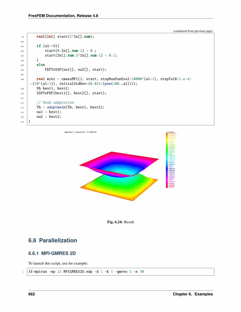
FreeFEM Documentation, Release 4.8
(continued from previous page)
99 real[int] start(2*In[].sum);100
101 if (al==0)102 start(0:In[].sum-1) = 0.;103 start(In[].sum:2*In[].sum-1) = 0.1;104 105 else106 FEFToSSP(ou1[], ou2[], start);107
108 real mini = cmaesMPI(J, start, stopMaxFunEval=10000*(al+1), stopTolX=1.e-4/→˓(10*(al+1)), initialStdDev=(0.025/(pow(100.,al))));
109 Vh best1, best2;110 SSPToFEF(best1[], best2[], start);111
112 // Mesh adaptation113 Th = adaptmesh(Th, best1, best2);114 ou1 = best1;115 ou2 = best2;116
Fig. 6.24: Result
6.6 Parallelization
6.6.1 MPI-GMRES 2D
To launch this script, use for example:
1 ff-mpirun -np 12 MPIGMRES2D.edp -d 1 -k 1 -gmres 2 -n 50
662 Chapter 6. Examples
FreeFEM Documentation, Release 4.8
1 //usage :2 //ff-mpirun [mpi parameter] MPIGMRES2d.edp [-glut ffglut] [-n N] [-k K] [-d D] [-ns] [-
→˓gmres [0|1]3 //arguments:4 //-glut ffglut : to see graphicaly the process5 //-n N: set the mesh cube split NxNxN6 //-d D: set debug flag D must be one for mpiplot7 //-k K: to refined by K all element8 //-ns: remove script dump9 //-gmres
10 //0: use iterative schwarz algo.11 //1: Algo GMRES on residu of schwarz algo12 //2: DDM GMRES13 //3: DDM GMRES with coarse grid preconditionner (Good one)14
15 load "MPICG"16 load "medit"17 load "metis"18 include "getARGV.idp"19 include "MPIplot.idp"20 include "MPIGMRESmacro.idp"21
22 searchMethod = 0; //more safe seach algo (warning can be very expensive in case of lot→˓of ouside point)
23 assert(version >= 3.11); //need at least v3.1124 real[int] ttt(10);25 int ittt=0;26 macro settt ttt[ittt++] = mpiWtime();//27
28 // Arguments29 verbosity = getARGV("-vv", 0);30 int vdebug = getARGV("-d", 1);31 int ksplit = getARGV("-k", 3);32 int nloc = getARGV("-n", 10);33 string sff = getARGV("-p", "");34 int gmres = getARGV("-gmres", 2);35 bool dplot = getARGV("-dp", 0);36 int nC = getARGV("-N", max(nloc/10, 4));37
38 if (mpirank==0 && verbosity)39 cout << "ARGV: ";40 for (int i = 0; i < ARGV.n; ++i)41 cout << ARGV[i] << " ";42 cout << endl;43 44
45 if(mpirank==0 && verbosity)46 cout << " vdebug: " << vdebug << ", kspilt "<< ksplit << ", nloc "<< nloc << ", sff "<<
→˓sff << "." << endl;47
48 // Parameters49 int withplot = 0;50 bool withmetis = 1;
(continues on next page)
6.6. Parallelization 663
FreeFEM Documentation, Release 4.8
(continued from previous page)
51 bool RAS = 1;52 string sPk = "P2-2gd";53 func Pk = P2;54 int sizeoverlaps = 1; //size of overlap55 int[int] l111 = [1, 1, 1, 1]; //mesh labels56
57 // MPI function58 func bool plotMPIall(mesh &Th, real[int] &u, string cm)59 if(vdebug)60 PLOTMPIALL(mesh, Pk, Th, u, cmm=cm, nbiso=20, fill=1, dim=3, value=1);61 return 1;62 63
64 // MPI65 mpiComm comm(mpiCommWorld,0,0); //trick : make a no split mpiWorld66
67 int npart = mpiSize(comm); //total number of partion68 int ipart = mpiRank(comm); //current partition number69
70 int njpart = 0; //Number of part with intersection (a jpart) with ipart without ipart71 int[int] jpart(npart); //list of jpart72 if(ipart==0)73 cout << " Final N = " << ksplit*nloc << ", nloc = " << nloc << ", split = " <<
→˓ksplit << endl;74 settt75
76 // Mesh77 mesh Thg = square(nloc, nloc, label=l111);78 mesh ThC = square(nC, nC, label=l111);// Coarse mesh79
80 mesh Thi, Thin; //with overlap, without olverlap81
82 // Fespace83 fespace Phg(Thg, P0);84 Phg part;85
86 fespace Vhg(Thg, P1);87 Vhg unssd; //boolean function: 1 in the subdomain, 0 elswhere88
89 fespace VhC(ThC, P1); // of the coarse problem90
91 // Partitioning92 93 int[int] nupart(Thg.nt);94 nupart = 0;95 if (npart > 1 && ipart == 0)96 metisdual(nupart, Thg, npart);97
98 broadcast(processor(0, comm), nupart);99 for(int i = 0; i < nupart.n; ++i)
100 part[][i] = nupart[i];101
(continues on next page)
664 Chapter 6. Examples
FreeFEM Documentation, Release 4.8
(continued from previous page)
102
103 if (withplot > 1)104 plot(part, fill=1, cmm="dual", wait=1);105
106 // Overlapping partition107 Phg suppi = abs(part-ipart) < 0.1;108
109 Thin = trunc(Thg, suppi>0, label=10); // non-overlapping mesh, interfaces have label 10110 int nnn = sizeoverlaps*2;// to be sure111 AddLayers(Thg, suppi[], nnn, unssd[]); //see above! suppi and unssd are modified112 unssd[] *= nnn; //to put value nnn a 0113 real nnn0 = nnn - sizeoverlaps + 0.001;114 Thi = trunc(Thg, unssd>nnn0, label=10); //overlapping mesh, interfaces have label 10115
116 settt117
118 // Fespace119 fespace Vhi(Thi,P1);120 int npij = npart;121 Vhi[int] pij(npij); //local partition of unit + pii122 Vhi pii;123
124 real nnn1 = +0.001;125 126 /*127 construction of the partition of the unit,128 let phi_i P1 FE function 1 on Thin and zero ouside of Thi and positive129 the partition is build with130 p_i = phi_i/ \sum phi_i131
132 to build the partition of one domain i133 we nned to find all j such that supp(phi_j) \cap supp(phi_j) is not empty134 <=> int phi_j135 */136 //build a local mesh of thii such that all computation of the unit partition are137 //exact in thii138 mesh Thii = trunc(Thg, unssd>nnn1, label=10); //overlapping mesh, interfaces have
→˓label 10139
140 141 //find all j mes (supp(p_j) cap supp(p_i)) >0142 //compute all phi_j on Thii143 //remark: supp p_i include in Thi144
145 // Fespace146 fespace Phii(Thii, P0);147 fespace Vhii(Thii, P1);148 Vhi sumphi = 0;149 Vhii phii = 0;150
151 jpart = 0;152 njpart = 0;
(continues on next page)
6.6. Parallelization 665
FreeFEM Documentation, Release 4.8
(continued from previous page)
153 int nlayer = RAS ? 1 : sizeoverlaps;154 if (ipart == 0)155 cout << "nlayer = " << nlayer << endl;156 pii = max(unssd-nnn+nlayer, 0.)/nlayer;157 if(dplot)158 plot(pii, wait=1, cmm=" 0000");159 sumphi[] += pii[];160 if(dplot)161 plot(sumphi, wait=1, cmm=" summ 0000");162
163 real epsmes = 1e-10*Thii.area;164 for (int i = 0; i < npart; ++i)165 if (i != ipart)166 Phii suppii = abs(i-part) < 0.2;167 if (suppii[].max > 0.5)168 AddLayers(Thii, suppii[], nlayer, phii[]);169 assert(phii[].min >= 0);170 real interij = int2d(Thi)(phii);171 if (interij > epsmes)172 pij[njpart] = abs(phii);173 if(vdebug > 2)174 cout << " ***** " << int2d(Thi)(real(pij[njpart])<0) << " " <
→˓<pij[njpart][].min << " " << phii[].min << endl;175 assert(int2d(Thi)(real(pij[njpart]) < 0) == 0);176 if(dplot)177 plot(pij[njpart], wait=1, cmm=" j = "+ i + " " + njpart);178 sumphi[] += pij[njpart][];179 if(dplot)180 plot(sumphi, wait=1, cmm=" sum j = "+ i + " " + njpart);181 jpart[njpart++] = i;182 183 184 185
186 if(dplot)187 plot(sumphi, wait=1, dim=3, cmm="sum ", fill=1);188 pii[] = pii[] ./ sumphi[];189 for (int j = 0; j < njpart; ++j)190 pij[j][] = pij[j][] ./ sumphi[];191 jpart.resize(njpart);192 for (int j = 0; j < njpart; ++j)193 assert(pij[j][].max <= 1);194 195 cout << ipart << " number of jpart " << njpart << " : ";196 for (int j = 0; j < njpart; ++j)197 cout << jpart[j] << " ";198 cout << endl;199 200 sumphi[] = pii[];201 for (int j = 0; j < njpart; ++j)202 sumphi[] += pij[j][];203 if(vdebug > 2)
(continues on next page)
666 Chapter 6. Examples
FreeFEM Documentation, Release 4.8
(continued from previous page)
204 cout << "sum min " << sumphi[].min << " " << sumphi[].max << endl;205 assert(sumphi[].min > 1.-1e-6 && sumphi[].max < 1.+1e-6);206 207 //Thii is remove here208 // end of the construction of the local partition of the unity ...209 // on Thi210 if (ipart == 0)211 cout << "End build partition" << endl;212
213 // Computation of number of intersection214 //here pii and the pij is the local partition of the unit on215 //Thi (mesh with overlap)216 if ( dplot)217 plot(Thi, wait=1);218 for(int j = 0; j < njpart; ++j)219 plot(pij[j], cmm=" j="+j, wait=1);220 221
222 //Partition of the unity on Thi223 //computation of message224 //all j > we have to receive225 //data on intersection of the support of pij[0] and pij[j]226 settt227
228 if(vdebug)229 plotMPIall(Thi, pii[], "pi_i");230
231 mesh[int] aThij(njpart);232 matrix Pii;233 matrix[int] sMj(njpart); //M of send to j234 matrix[int] rMj(njpart); //M to recv from j235 fespace Whi(Thi, Pk);236 mesh Thij = Thi;237 fespace Whij(Thij, Pk);//238
239 //construction of the mesh intersect i,j part240 for(int jp = 0; jp < njpart; ++jp)241 aThij[jp] = trunc(Thi, pij[jp] > 1e-6, label=10); //mesh of the supp of pij242
243 for(int jp = 0; jp < njpart; ++jp)244 aThij[jp] = trunc(aThij[jp], 1, split=ksplit);245
246 Thi = trunc(Thi, 1, split=ksplit);247
248 settt249
250 if (ipart == 0)251 cout << "End build mesh intersection" << endl;252
253 // Construction of transfert matrix254 255 Whi wpii = pii;
(continues on next page)
6.6. Parallelization 667
FreeFEM Documentation, Release 4.8
(continued from previous page)
256 Pii = wpii[];257 for(int jp = 0; jp < njpart; ++jp)258 int j = jpart[jp];259 Thij = aThij[jp];260 matrix I = interpolate(Whij, Whi); //Whji <- Whi261 sMj[jp] = I*Pii; //Whi -> s Whij262 rMj[jp] = interpolate(Whij, Whi, t=1); //Whji -> Whi263 if(vdebug > 10)264 Whi uuu=1; Whij vvv=-1; vvv[]+=I*uuu[]; cout << jp << " %%% " << vvv[].
→˓linfty << endl; assert(vvv[].linfty < 1e-6);265 Whi uuu=1; Whij vvv=-1; vvv[]+=rMj[jp]'*uuu[]; cout << jp << " ### " <<
→˓vvv[].linfty << endl; assert(vvv[].linfty < 1e-6);266 267 268 269 if (ipart == 0)270 cout << "End build transfert matrix" << endl;271
272 // Allocate array of send and recv data273 InitU(njpart, Whij, Thij, aThij, Usend) //initU(n, Vh, Th, aTh, U)274 InitU(njpart, Whij, Thij, aThij, Vrecv)275 if (ipart == 0)276 cout << "End init data for send/revc" << endl;277
278 Whi ui, vi;279
280 func bool Update(real[int] &ui, real[int] &vi)281 for(int j = 0; j < njpart; ++j)282 Usend[j][] = sMj[j]*ui;283 SendRecvUV(comm, jpart, Usend, Vrecv)284 vi = Pii*ui;285 for(int j = 0; j < njpart; ++j)286 vi += rMj[j]*Vrecv[j][];287 return true;288 289
290 // Definition of the Problem291 func G = x*0.1;292 func F = 1.;293 macro grad(u) [dx(u),dy(u)] //294 varf vBC (U, V) = on(1, U=G);295 varf vPb (U, V) = int2d(Thi)(grad(U)'*grad(V)) + int2d(Thi)(F*V) + on(10, U=0) + on(1,
→˓U=G);296 varf vPbC (U, V) = int2d(ThC)(grad(U)'*grad(V)) + on(1, U=0);297 varf vPbon (U, V) = on(10, U=1) + on(1, U=1);298 varf vPbon10only (U, V) = on(10, U=1) + on(1, U=0);299 //remark the order is important we want 0 part on 10 and 1300
301 matrix Ai = vPb(Whi, Whi, solver=sparsesolver);302 matrix AC, Rci, Pci;303
304 if (mpiRank(comm) == 0)
(continues on next page)
668 Chapter 6. Examples
FreeFEM Documentation, Release 4.8
(continued from previous page)
305 AC = vPbC(VhC, VhC, solver=sparsesolver);306
307 Pci = interpolate(Whi, VhC);308 Rci = Pci'*Pii;309
310 real[int] onG10 = vPbon10only(0, Whi);311 real[int] onG = vPbon(0, Whi);312 real[int] Bi=vPb(0, Whi);313
314 int kiter = -1;315
316 func bool CoarseSolve(real[int] &V, real[int] &U, mpiComm &comm)317 //solving the coarse probleme318 real[int] Uc(Rci.n), Bc(Uc.n);319 Uc = Rci*U;320 mpiReduce(Uc, Bc, processor(0, comm), mpiSUM);321 if (mpiRank(comm) == 0)322 Uc = AC^-1*Bc;323 broadcast(processor(0, comm), Uc);324 V = Pci*Uc;325 326
327 func real[int] DJ (real[int] &U)328 ++kiter;329 real[int] V(U.n);330 V = Ai*U;331 V = onG10 ? 0.: V; //remove internal boundary332 return V;333 334
335 func real[int] PDJ (real[int] &U)336 real[int] V(U.n);337
338 real[int] b = onG10 ? 0. : U;339 V = Ai^-1*b;340 Update(V, U);341 return U;342 343
344 func real[int] PDJC (real[int] &U)345 real[int] V(U.n);346 CoarseSolve(V, U, comm);347 V = -V; //-C2*Uo348 U += Ai*V; //U = (I-A C2) Uo349 real[int] b = onG10 ? 0. : U;350 U = Ai^-1*b; // (C1( I -A C2) Uo351 V = U -V;352 Update(V, U);353 return U;354 355
356 func real[int] DJ0(real[int] &U)
(continues on next page)
6.6. Parallelization 669
FreeFEM Documentation, Release 4.8
(continued from previous page)
357 ++kiter;358 real[int] V(U.n);359 real[int] b = onG .* U;360 b = onG ? b : Bi ;361 V = Ai^-1*b;362 Update(V, U);363 V -= U;364 return V;365 366
367 Whi u = 0, v;368 //verification369 Whi u = 1, v;370 Update(u[], v[]);371 u[] -= v[];372 assert(u[].linfty < 1e-6);373 374
375 settt376 u[] = vBC(0, Whi, tgv=1); //set u with tgv BC value377
378 real epss = 1e-6;379 int rgmres = 0;380 if (gmres == 1)381 rgmres = MPIAffineGMRES(DJ0, u[], veps=epss, nbiter=300, comm=comm, dimKrylov=100,
→˓verbosity=ipart ? 0: 50);382 real[int] b = onG .* u[];383 b = onG ? b : Bi;384 v[] = Ai^-1*b;385 Update(v[], u[]);386 387 else if (gmres == 2)388 rgmres = MPILinearGMRES(DJ, precon=PDJ, u[], Bi, veps=epss, nbiter=300, comm=comm,
→˓dimKrylov=100, verbosity=ipart ? 0: 50);389 else if (gmres == 3)390 rgmres = MPILinearGMRES(DJ, precon=PDJC, u[], Bi, veps=epss, nbiter=300, comm=comm,
→˓dimKrylov=100, verbosity=ipart ? 0: 50);391 else //algo Shwarz for demo392 for(int iter = 0; iter < 10; ++iter)393 real[int] b = onG .* u[];394 b = onG ? b : Bi ;395 v[] = Ai^-1*b;396
397 Update(v[], u[]);398 if(vdebug)399 plotMPIall(Thi, u[], "u-"+iter);400 v[] -= u[];401
402 real err = v[].linfty;403 real umax = u[].max;404 real[int] aa = [err, umax], bb(2);405 mpiAllReduce(aa, bb, comm, mpiMAX);
(continues on next page)
670 Chapter 6. Examples
FreeFEM Documentation, Release 4.8
(continued from previous page)
406 real errg = bb[0];407 real umaxg = bb[1];408
409 if (ipart == 0)410 cout << ipart << " err = " << errg << " u. max " << umaxg << endl;411 if (errg < 1e-5) break;412 413
414 if (vdebug)415 plotMPIall(Thi, u[], "u-final");416
417 settt418
419 real errg = 1, umaxg;420 421 real umax = u[].max, umaxg;422 real[int] aa = [umax], bb(1);423 mpiAllReduce(aa, bb, comm, mpiMAX);424 errg = bb[0];425 if (ipart == 0)426 cout << "umax global = " << bb[0] << " Wtime = " << (ttt[ittt-1]-ttt[ittt-2]) <<
→˓" s " << " " << kiter << endl;427 428
429 if (sff != "")430 ofstream ff(sff+".txt", append);431 cout << " ++++ ";432 cout << mpirank << "/" << mpisize << " k=" << ksplit << " n= " << nloc << " " <<
→˓sizeoverlaps << " it= " << kiter;433 for (int i = 1; i < ittt; ++i)434 cout << " " << ttt[i]-ttt[i-1] << " ";435 cout << epss << " " << Ai.nbcoef << " " << Ai.n << endl;436
437 /*438 1 mpirank439 2 mpisize440 3 ksplit441 4 nloc442 5 sizeoverlaps443 6 kiter444 7 mesh & part build445 8 build the partion446 9 build mesh, transfere , and the fine mesh ..447 10 build the matrix, the trans matrix, factorizatioon448 11 GMRES449 */450
451 ff << mpirank << " " << mpisize << " " << sPk << " ";452 ff << ksplit << " " << nloc << " " << sizeoverlaps << " " << kiter;453 for (int i = 1; i < ittt; ++i)454 ff << " " << ttt[i]-ttt[i-1] << " ";455 ff << epss << " " << Ai.nbcoef << " " << Ai.n << " " << gmres << endl;
(continues on next page)
6.6. Parallelization 671
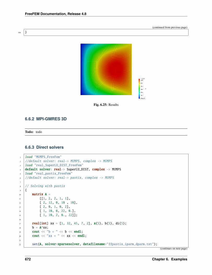
FreeFEM Documentation, Release 4.8
(continued from previous page)
456
Fig. 6.25: Results
6.6.2 MPI-GMRES 3D
Todo: todo
6.6.3 Direct solvers
1 load "MUMPS_FreeFem"2 //default solver: real-> MUMPS, complex -> MUMPS3 load "real_SuperLU_DIST_FreeFem"4 default solver: real-> SuperLU_DIST, complex -> MUMPS5 load "real_pastix_FreeFem"6 //default solver: real-> pastix, complex -> MUMPS7
8 // Solving with pastix9
10 matrix A =11 [[1, 2, 2, 1, 1],12 [ 2, 12, 0, 10 , 10],13 [ 2, 0, 1, 0, 2],14 [ 1, 10, 0, 22, 0.],15 [ 1, 10, 2, 0., 22]];16
17 real[int] xx = [1, 32, 45, 7, 2], x(5), b(5), di(5);18 b = A*xx;19 cout << "b = " << b << endl;20 cout << "xx = " << xx << endl;21
22 set(A, solver=sparsesolver, datafilename="ffpastix_iparm_dparm.txt");(continues on next page)
672 Chapter 6. Examples
FreeFEM Documentation, Release 4.8
(continued from previous page)
23 cout << "solve" << endl;24 x = A^-1*b;25 cout << "b = " << b << endl;26 cout << "x = " << endl;27 cout << x << endl;28 di = xx - x;29 if (mpirank == 0)30 cout << "x-xx = " << endl;31 cout << "Linf = " << di.linfty << ", L2 = " << di.l2 << endl;32 33 34
35 // Solving with SuperLU_DIST36 realdefaulttoSuperLUdist();37 //default solver: real-> SuperLU_DIST, complex -> MUMPS38 39 matrix A =40 [[1, 2, 2, 1, 1],41 [ 2, 12, 0, 10 , 10],42 [ 2, 0, 1, 0, 2],43 [ 1, 10, 0, 22, 0.],44 [ 1, 10, 2, 0., 22]];45
46 real[int] xx = [1, 32, 45, 7, 2], x(5), b(5), di(5);47 b = A*xx;48 cout << "b = " << b << endl;49 cout << "xx = " << xx << endl;50
51 set(A, solver=sparsesolver, datafilename="ffsuperlu_dist_fileparam.txt");52 cout << "solve" << endl;53 x = A^-1*b;54 cout << "b = " << b << endl;55 cout << "x = " << endl;56 cout << x << endl;57 di = xx - x;58 if (mpirank == 0)59 cout << "x-xx = " << endl;60 cout << "Linf = " << di.linfty << ", L2 = " << di.l2 << endl;61 62 63
64 // Solving with MUMPS65 defaulttoMUMPS();66 //default solver: real-> MUMPS, complex -> MUMPS67 68 matrix A =69 [[1, 2, 2, 1, 1],70 [ 2, 12, 0, 10 , 10],71 [ 2, 0, 1, 0, 2],72 [ 1, 10, 0, 22, 0.],73 [ 1, 10, 2, 0., 22]];74
(continues on next page)
6.6. Parallelization 673
FreeFEM Documentation, Release 4.8
(continued from previous page)
75 real[int] xx = [1, 32, 45, 7, 2], x(5), b(5), di(5);76 b = A*xx;77 cout << "b = " << b << endl;78 cout << "xx = " << xx << endl;79
80 set(A, solver=sparsesolver, datafilename="ffmumps_fileparam.txt");81 cout << "solving solution" << endl;82 x = A^-1*b;83 cout << "b = " << b << endl;84 cout << "x = " << endl;85 cout << x << endl;86 di = xx - x;87 if (mpirank == 0)88 cout << "x-xx = " << endl;89 cout << "Linf = " << di.linfty << ", L2 " << di.l2 << endl;90 91
6.6.4 Solver MUMPS
1 load "MUMPS_FreeFem"2
3 // Parameters4 int[int] ICNTL(40); //declaration of ICNTL parameter for MUMPS5
6 //get value of ICNTL from file7 if (mpirank == 0)8 ifstream ff("ffmumps_fileparam.txt");9 string line;
10 getline(ff, line);11 getline(ff, line);12 for (int iii = 0; iii < 40; iii++)13 ff >> ICNTL[iii];14 getline(ff, line);15 16 17
18 broadcast(processor(0), ICNTL);19
20 // Given data of MUMPS solver in array lparams(SYM, PAR, ICNTL)21 // There is no symmetric storage for a matrix associated with a sparse solver.22 // Therefore, the matrix will be considered unsymmetric for parallel sparse solver even
→˓if symmetric.23 24 // Problem25 int SYM = 0;26 int PAR = 1;27 matrix A =28 [29 [40, 0, 45, 0, 0],
(continues on next page)
674 Chapter 6. Examples
FreeFEM Documentation, Release 4.8
(continued from previous page)
30 [0, 12, 0, 0, 0],31 [0, 0, 40, 0, 0],32 [12, 0, 0, 22, 0],33 [0, 0, 20, 0, 22]34 ];35
36 // Construction of integer parameter for MUMPS37 int[int] MumpsLParams(42);38 MumpsLParams[0] = SYM;39 MumpsLParams[1] = PAR;40 for (int ii = 0; ii < 40; ii++)41 MumpsLParams[ii+2] = ICNTL[ii]; //ICNTL begin with index 0 here42
43 real[int] xx = [1, 32, 45, 7, 2], x(5), b(5), di(5);44 b = A*xx;45 if (mpirank == 0)46 cout << "xx = " << xx << endl;47
48 set(A, solver=sparsesolver, lparams=MumpsLParams); //we take the default value for→˓CNTL MUMPS parameter
49
50 // Solve51 if (mpirank == 0)52 cout << "Solve" << endl;53 x = A^-1*b;54 if (mpirank == 0)55 cout << "b = " << b << endl;56 if (mpirank == 0)57 cout << "x = " << endl; cout << x << endl;58 di = xx-x;59 if (mpirank == 0)60 cout << "x-xx = " << endl;61 cout << "Linf = " << di.linfty << ", L2 = " << di.l2 << endl;62 63 64
65 // Read parameter of MUMPS solver in file ffmumps_fileparam.txt66 67 // Problem68 matrix A =69 [70 [40, 0, 45, 0, 0],71 [0, 12, 0, 0 , 0],72 [0, 0, 40, 0, 0],73 [12, 0, 0, 22, 0],74 [0, 0, 20, 0, 22]75 ];76
77 real[int] xx = [1, 32, 45, 7000, 2], x(5), b(5), di(5);78 b = A*xx;79 if (mpirank == 0)80 cout << "b = " << b << endl;
(continues on next page)
6.6. Parallelization 675
FreeFEM Documentation, Release 4.8
(continued from previous page)
81 cout << "xx = " << xx << endl;82 83
84 set(A, solver=sparsesolver, datafilename="ffmumps_fileparam.txt");85
86 // Solve87 if (mpirank == 0)88 cout << "Solve" << endl;89 x = A^-1*b;90
91 if (mpirank == 0)92 cout << "b = " << b << endl;93 cout << "x = " << x << endl;94 95 di = xx-x;96 if (mpirank == 0)97 cout << "x-xx = " << endl;98 cout << "Linf = " << di.linfty << ", L2 = " << di.l2 << endl;99
100
6.6.5 Solver superLU_DIST
Todo: write code (SuperLU_DIST seems to have a bug)
6.6.6 Solver PaStiX
Todo: write code (PaStiX seems to have a bug)
6.7 Developers
6.7.1 FFT
1 load "dfft"2
3 // Parameters4 int nx = 32;5 real ny = 16;6 real N = nx*ny;7 func f1 = cos(2*x*2*pi)*cos(3*y*2*pi);8
9 // Mesh10 //warning: the fourier space is not exactly the unit square due to periodic condition
(continues on next page)
676 Chapter 6. Examples
FreeFEM Documentation, Release 4.8
(continued from previous page)
11 mesh Th = square(nx-1, ny-1, [(nx-1)*x/nx, (ny-1)*y/ny]);12 //warning: the numbering of the vertices (x,y) is13 //given by i = x/nx + nx*y/ny14
15 // Fespace16 fespace Vh(Th,P1);17 Vh<complex> u = f1, v;18 Vh w = f1;19 Vh ur, ui;20
21 // FFT22 //in dfft the matrix n, m is in row-major order and array n, m is23 //store j + m*i (the transpose of the square numbering)24 v[] = dfft(u[], ny, -1);25 u[] = dfft(v[], ny, +1);26 cout << "||u||_\infty " << u[].linfty << endl;27
28 u[] *= 1./N;29 cout << "||u||_\infty " << u[].linfty << endl;30
31 ur = real(u);32
33 // Plot34 plot(w, wait=1, value=1, cmm="w");35 plot(ur, wait=1, value=1, cmm="u");36 v = w - u;37 cout << "diff = " << v[].max << " " << v[].min << endl;38 assert( norm(v[].max) < 1e-10 && norm(v[].min) < 1e-10);39
40 // Other example41 //FFT Lapacian42 //-\Delta u = f with biperiodic condition43 func f = cos(3*2*pi*x)*cos(2*2*pi*y);44 func ue = (1./(square(2*pi)*13.))*cos(3*2*pi*x)*cos(2*2*pi*y); //the exact solution45 Vh<complex> ff = f;46 Vh<complex> fhat;47 Vh<complex> wij;48
49 // FFT50 fhat[] = dfft(ff[],ny,-1);51
52 //warning in fact we take mode between -nx/2, nx/2 and -ny/2, ny/253 //thanks to the operator ?:54 wij = square(2.*pi)*(square(( x<0.5?x*nx:(x-1)*nx)) + square((y<0.5?y*ny:(y-1)*ny)));55 wij[][0] = 1e-5; //to remove div / 056 fhat[] = fhat[] ./ wij[];57 u[] = dfft(fhat[], ny, 1);58 u[] /= complex(N);59 ur = real(u); //the solution60 w = real(ue); //the exact solution61
62 // Plot
(continues on next page)
6.7. Developers 677
FreeFEM Documentation, Release 4.8
(continued from previous page)
63 plot(w, ur, value=1, cmm="ue", wait=1);64
65 // Error66 w[] -= ur[];67 real err = abs(w[].max) + abs(w[].min);68 cout << "err = " << err << endl;69 assert(err < 1e-6);70
71 fftwplan p1 = plandfft(u[], v[], ny, -1);72 fftwplan p2 = plandfft(u[], v[], ny, 1);73 real ccc = square(2.*pi);74 cout << "ny = " << ny << endl;75 map(wij[], ny, ccc*(x*x+y*y));76 wij[][0] = 1e-5;77 plot(wij, cmm="wij");
6.7.2 Complex
1 real a = 2.45, b = 5.33;2 complex z1 = a + b*1i, z2 = a + sqrt(2.)*1i;3
4 func string pc(complex z)5 string r = "(" + real(z);6 if (imag(z) >= 0) r = r + "+";7 return r + imag(z) + "i)";8 9
10 func string toPolar(complex z)11 return "";//abs(z) + "*(cos(" + arg(z) + ")+i*sin(" + arg(z) + "))";12 13
14 cout << "Standard output of the complex " << pc(z1) << " is the pair: " << z1 << endl;15 cout << pc(z1) << " + " << pc(z2) << " = " << pc(z1+z2) << endl;16 cout << pc(z1) << " - " << pc(z2) << " = " << pc(z1-z2) << endl;17 cout << pc(z1) << " * " << pc(z2) << " = " << pc(z1*z2) << endl;18 cout << pc(z1) << " / " << pc(z2) << " = " << pc(z1/z2) << endl;19 cout << "Real part of " << pc(z1) << " = " << real(z1) << endl;20 cout << "Imaginary part of " << pc(z1) << " = " << imag(z1) << endl;21 cout << "abs(" << pc(z1) << ") = " << abs(z1) << endl;22 cout << "Polar coordinates of " << pc(z2) << " = " << toPolar(z2) << endl;23 cout << "de Moivre formula: " << pc(z2) << "^3 = " << toPolar(z2^3) << endl;24 cout << " and polar(" << abs(z2) << ", " << arg(z2) << ") = " << pc(polar(abs(z2),
→˓arg(z2))) << endl;25 cout << "Conjugate of " <<pc(z2) << " = " << pc(conj(z2)) <<endl;26 cout << pc(z1) << " ^ " << pc(z2) << " = " << pc(z1^z2) << endl;
Output of this script is:
1 Standard output of the complex (2.45+5.33i) is the pair: (2.45,5.33)2 (2.45+5.33i) + (2.45+1.41421i) = (4.9+6.74421i)
(continues on next page)
678 Chapter 6. Examples
FreeFEM Documentation, Release 4.8
(continued from previous page)
3 (2.45+5.33i) - (2.45+1.41421i) = (0+3.91579i)4 (2.45+5.33i) * (2.45+1.41421i) = (-1.53526+16.5233i)5 (2.45+5.33i) / (2.45+1.41421i) = (1.692+1.19883i)6 Real part of (2.45+5.33i) = 2.457 Imaginary part of (2.45+5.33i) = 5.338 abs((2.45+5.33i)) = 5.866129 Polar coordinates of (2.45+1.41421i) =
10 de Moivre formula: (2.45+1.41421i)^3 =11 and polar(2.82887, 0.523509) = (2.45+1.41421i)12 Conjugate of (2.45+1.41421i) = (2.45-1.41421i)13 (2.45+5.33i) ^ (2.45+1.41421i) = (8.37072-12.7078i)
6.7.3 String
1 // Concatenation2 string tt = "toto1" + 1 + " -- 77";3
4 // Append5 string t1 = "0123456789";6 t1(4:3) = "abcdefghijk-";7
8 // Sub string9 string t55 = t1(4:14);
10
11 cout << "tt = " << tt << endl;12
13 cout << "t1 = " << t1 << endl;14 cout << "t1.find(abc) = " << t1.find("abc") << endl;15 cout << "t1.rfind(abc) = " << t1.rfind("abc") << endl;16 cout << "t1.find(abc, 10) = " << t1.find("abc",10) << endl;17 cout << "t1.ffind(abc, 10) = " << t1.rfind("abc",10) << endl;18 cout << "t1.length = " << t1.length << endl;19
20 cout << "t55 = " << t55 << endl;
The output of this script is:
1 tt = toto11 -- 772 t1 = 0123abcdefghijk-4567893 t1.find(abc) = 44 t1.rfind(abc) = 45 t1.find(abc, 10) = -16 t1.ffind(abc, 10) = 47 t1.length = 228 t55 = abcdefghijk
6.7. Developers 679
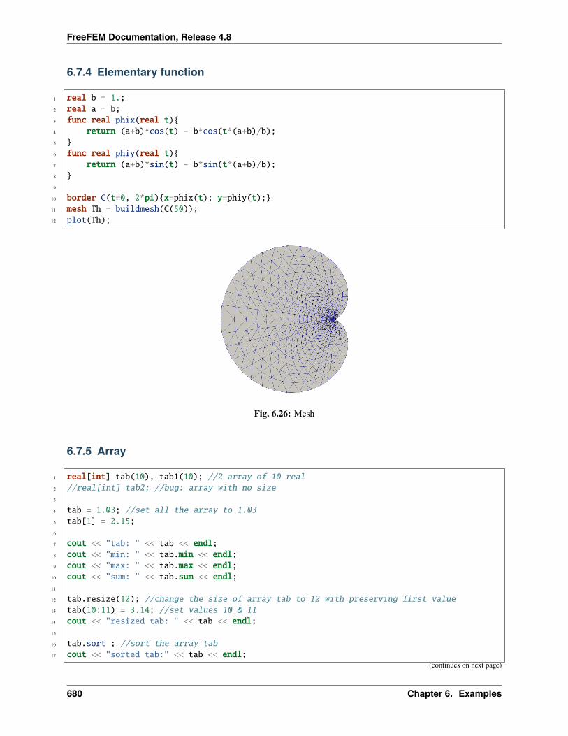
FreeFEM Documentation, Release 4.8
6.7.4 Elementary function
1 real b = 1.;2 real a = b;3 func real phix(real t)4 return (a+b)*cos(t) - b*cos(t*(a+b)/b);5 6 func real phiy(real t)7 return (a+b)*sin(t) - b*sin(t*(a+b)/b);8 9
10 border C(t=0, 2*pi)x=phix(t); y=phiy(t);11 mesh Th = buildmesh(C(50));12 plot(Th);
Fig. 6.26: Mesh
6.7.5 Array
1 real[int] tab(10), tab1(10); //2 array of 10 real2 //real[int] tab2; //bug: array with no size3
4 tab = 1.03; //set all the array to 1.035 tab[1] = 2.15;6
7 cout << "tab: " << tab << endl;8 cout << "min: " << tab.min << endl;9 cout << "max: " << tab.max << endl;
10 cout << "sum: " << tab.sum << endl;11
12 tab.resize(12); //change the size of array tab to 12 with preserving first value13 tab(10:11) = 3.14; //set values 10 & 1114 cout << "resized tab: " << tab << endl;15
16 tab.sort ; //sort the array tab17 cout << "sorted tab:" << tab << endl;
(continues on next page)
680 Chapter 6. Examples
FreeFEM Documentation, Release 4.8
(continued from previous page)
18
19 real[string] tt; //array with string index20 tt["+"] = 1.5;21 cout << "tt[\"a\"] = " << tt["a"] << endl;22 cout << "tt[\"+\"] = " << tt["+"] << endl;23
24 real[int] a(5), b(5), c(5), d(5);25 a = 1;26 b = 2;27 c = 3;28 a[2] = 0;29 d = ( a ? b : c ); //for i = 0, n-1 : d[i] = a[i] ? b[i] : c[i]30 cout << " d = ( a ? b : c ) is " << d << endl;31 d = ( a ? 1 : c ); //for i = 0, n-1: d[i] = a[i] ? 1 : c[i]32 d = ( a ? b : 0 ); //for i = 0, n-1: d[i] = a[i] ? b[i] : 033 d = ( a ? 1 : 0 ); //for i = 0, n-1: d[i] = a[i] ? 0 : 134
35 int[int] ii(0:d.n-1); //set array ii to 0, 1, ..., d.n-136 d = -1:-5; //set d to -1, -2, ..., -537
38 sort(d, ii); //sort array d and ii in parallel39 cout << "d: " << d << endl;40 cout << "ii: " << ii << endl;41
42
43 44 int[int] A1(2:10); //2, 3, 4, 5, 6, 7, 8, 9, 1045 int[int] A2(2:3:10); //2, 5, 846 cout << "A1(2:10): " << A1 << endl;47 cout << "A2(2:3:10): " << A1 << endl;48 A1 = 1:2:5;49 cout << "1:2:5 => " << A1 << endl;50 51 52 real[int] A1(2:10); //2, 3, 4, 5, 6, 7, 8, 9, 1053 real[int] A2(2:3:10); //2, 5, 854 cout << "A1(2:10): " << A1 << endl;55 cout << "A2(2:3:10): " << A1 << endl;56 A1 = 1.:0.5:3.999;57 cout << "1.:0.5:3.999 => " << A1 << endl;58 59 60 complex[int] A1(2.+0i:10.+0i); //2, 3, 4, 5, 6, 7, 8, 9, 1061 complex[int] A2(2.:3.:10.); //2, 5, 862 cout << " A1(2.+0i:10.+0i): " << A1 << endl;63 cout << " A2(2.:3.:10.)= " << A2 << endl;64 cout << " A1.re real part array: " << A1.re << endl ;65 // he real part array of the complex array66 cout << " A1.im imag part array: " << A1.im << endl ;67 //the imaginary part array of the complex array68 69
(continues on next page)
6.7. Developers 681
FreeFEM Documentation, Release 4.8
(continued from previous page)
70 // Integer array operators71 72 int N = 5;73 real[int] a(N), b(N), c(N);74 a = 1;75 a(0:4:2) = 2;76 a(3:4) = 4;77 cout << "a: " << a << endl;78 b = a + a;79 cout <<"b = a + a: " << b << endl;80 b += a;81 cout <<"b += a: " << b << endl;82 b += 2*a;83 cout <<"b += 2*a: " << b << endl;84 b /= 2;85 cout <<" b /= 2: " << b << endl;86 b .*= a; // same as b = b .* a87 cout << "b .*= a: " << b << endl;88 b ./= a; //same as b = b ./ a89 cout << "b ./= a: " << b << endl;90 c = a + b;91 cout << "c = a + b: " << c << endl;92 c = 2*a + 4*b;93 cout << "c = 2*a + 4b: " << c << endl;94 c = a + 4*b;95 cout << "c = a + 4b: " << c << endl;96 c = -a + 4*b;97 cout << "c = -a + 4b: " << c << endl;98 c = -a - 4*b;99 cout << "c = -a - 4b: " << c << endl;
100 c = -a - b;101 cout << "c = -a -b: " << c << endl;102
103 c = a .* b;104 cout << "c = a .* b: " << c << endl;105 c = a ./ b;106 cout << "c = a ./ b: " << c << endl;107 c = 2 * b;108 cout << "c = 2 * b: " << c << endl;109 c = b * 2;110 cout << "c = b * 2: " << c << endl;111
112 //this operator do not exist113 //c = b/2;114 //cout << "c = b / 2: " << c << endl;115
116 //Array methods117 cout << "||a||_1 = " << a.l1 << endl;118 cout << "||a||_2 = " << a.l2 << endl;119 cout << "||a||_infty = " << a.linfty << endl;120 cout << "sum a_i = " << a.sum << endl;121 cout << "max a_i = " << a.max << " a[ " << a.imax << " ] = " << a[a.imax] << endl;
(continues on next page)
682 Chapter 6. Examples
FreeFEM Documentation, Release 4.8
(continued from previous page)
122 cout << "min a_i = " << a.min << " a[ " << a.imin << " ] = " << a[a.imin] << endl;123
124 cout << "a' * a = " << (a'*a) << endl;125 cout << "a quantile 0.2 = " << a.quantile(0.2) << endl;126
127 //Array mapping128 int[int] I = [2, 3, 4, -1, 3];129 b = c = -3;130 b = a(I); //for (i = 0; i < b.n; i++) if (I[i] >= 0) b[i] = a[I[i]];131 c(I) = a; //for (i = 0; i < I.n; i++) if (I[i] >= 0) C(I[i]) = a[i];132 cout << "b = a(I) : " << b << endl;133 cout << "c(I) = a " << c << endl;134 c(I) += a; //for (i = 0; i < I.n; i++) if (I[i] >= 0) C(I[i]) += a[i];135 cout << "b = a(I) : " << b << endl;136 cout << "c(I) = a " << c << endl;137
138 139
140 141 // Array versus matrix142 int N = 3, M = 4;143
144 real[int, int] A(N, M);145 real[int] b(N), c(M);146 b = [1, 2, 3];147 c = [4, 5, 6, 7];148
149 complex[int, int] C(N, M);150 complex[int] cb = [1, 2, 3], cc = [10i, 20i, 30i, 40i];151
152 b = [1, 2, 3];153
154 int [int] I = [2, 0, 1];155 int [int] J = [2, 0, 1, 3];156
157 A = 1; //set all the matrix158 A(2, :) = 4; //the full line 2159 A(:, 1) = 5; //the full column 1160 A(0:N-1, 2) = 2; //set the column 2161 A(1, 0:2) = 3; //set the line 1 from 0 to 2162
163 cout << "A = " << A << endl;164
165 //outer product166 C = cb * cc';167 C += 3 * cb * cc';168 C -= 5i * cb * cc';169 cout << "C = " << C << endl;170
171 //this transforms an array into a sparse matrix172 matrix B;173 B = A;
(continues on next page)
6.7. Developers 683
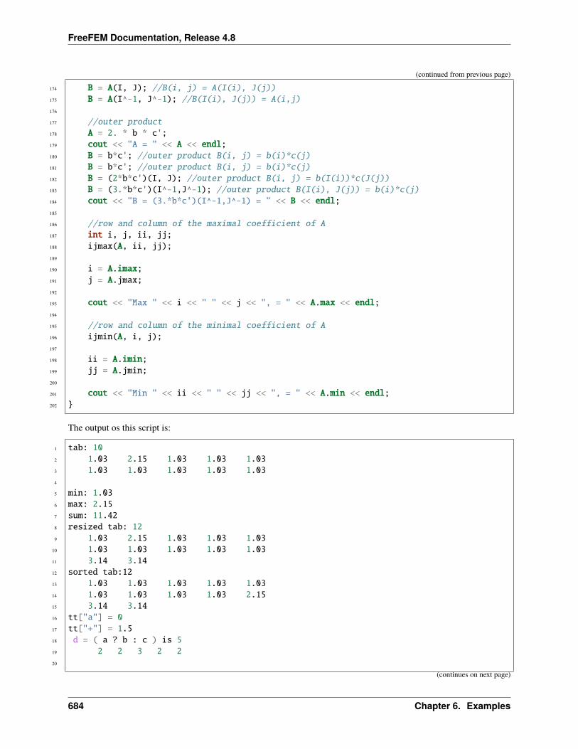
FreeFEM Documentation, Release 4.8
(continued from previous page)
174 B = A(I, J); //B(i, j) = A(I(i), J(j))175 B = A(I^-1, J^-1); //B(I(i), J(j)) = A(i,j)176
177 //outer product178 A = 2. * b * c';179 cout << "A = " << A << endl;180 B = b*c'; //outer product B(i, j) = b(i)*c(j)181 B = b*c'; //outer product B(i, j) = b(i)*c(j)182 B = (2*b*c')(I, J); //outer product B(i, j) = b(I(i))*c(J(j))183 B = (3.*b*c')(I^-1,J^-1); //outer product B(I(i), J(j)) = b(i)*c(j)184 cout << "B = (3.*b*c')(I^-1,J^-1) = " << B << endl;185
186 //row and column of the maximal coefficient of A187 int i, j, ii, jj;188 ijmax(A, ii, jj);189
190 i = A.imax;191 j = A.jmax;192
193 cout << "Max " << i << " " << j << ", = " << A.max << endl;194
195 //row and column of the minimal coefficient of A196 ijmin(A, i, j);197
198 ii = A.imin;199 jj = A.jmin;200
201 cout << "Min " << ii << " " << jj << ", = " << A.min << endl;202
The output os this script is:
1 tab: 102 1.03 2.15 1.03 1.03 1.033 1.03 1.03 1.03 1.03 1.034
5 min: 1.036 max: 2.157 sum: 11.428 resized tab: 129 1.03 2.15 1.03 1.03 1.03
10 1.03 1.03 1.03 1.03 1.0311 3.14 3.1412 sorted tab:1213 1.03 1.03 1.03 1.03 1.0314 1.03 1.03 1.03 1.03 2.1515 3.14 3.1416 tt["a"] = 017 tt["+"] = 1.518 d = ( a ? b : c ) is 519 2 2 3 2 220
(continues on next page)
684 Chapter 6. Examples
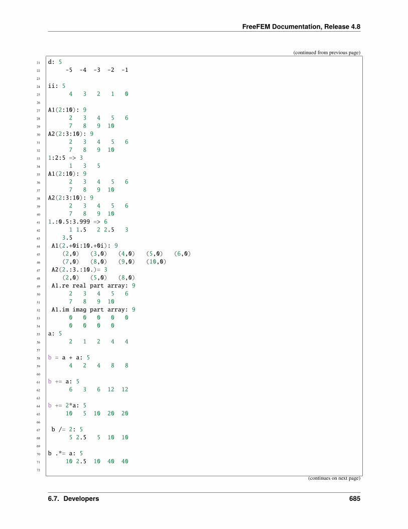
FreeFEM Documentation, Release 4.8
(continued from previous page)
21 d: 522 -5 -4 -3 -2 -123
24 ii: 525 4 3 2 1 026
27 A1(2:10): 928 2 3 4 5 629 7 8 9 1030 A2(2:3:10): 931 2 3 4 5 632 7 8 9 1033 1:2:5 => 334 1 3 535 A1(2:10): 936 2 3 4 5 637 7 8 9 1038 A2(2:3:10): 939 2 3 4 5 640 7 8 9 1041 1.:0.5:3.999 => 642 1 1.5 2 2.5 343 3.544 A1(2.+0i:10.+0i): 945 (2,0) (3,0) (4,0) (5,0) (6,0)46 (7,0) (8,0) (9,0) (10,0)47 A2(2.:3.:10.)= 348 (2,0) (5,0) (8,0)49 A1.re real part array: 950 2 3 4 5 651 7 8 9 1052 A1.im imag part array: 953 0 0 0 0 054 0 0 0 055 a: 556 2 1 2 4 457
58 b = a + a: 559 4 2 4 8 860
61 b += a: 562 6 3 6 12 1263
64 b += 2*a: 565 10 5 10 20 2066
67 b /= 2: 568 5 2.5 5 10 1069
70 b .*= a: 571 10 2.5 10 40 4072
(continues on next page)
6.7. Developers 685
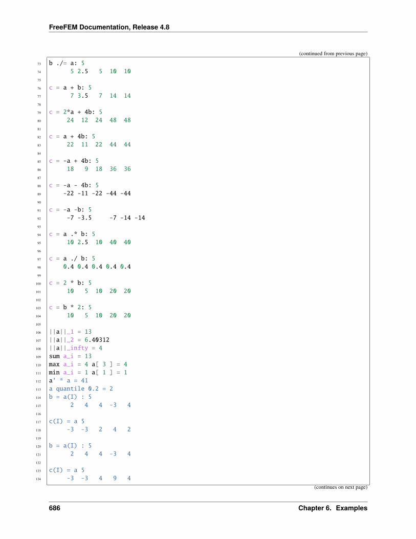
FreeFEM Documentation, Release 4.8
(continued from previous page)
73 b ./= a: 574 5 2.5 5 10 1075
76 c = a + b: 577 7 3.5 7 14 1478
79 c = 2*a + 4b: 580 24 12 24 48 4881
82 c = a + 4b: 583 22 11 22 44 4484
85 c = -a + 4b: 586 18 9 18 36 3687
88 c = -a - 4b: 589 -22 -11 -22 -44 -4490
91 c = -a -b: 592 -7 -3.5 -7 -14 -1493
94 c = a .* b: 595 10 2.5 10 40 4096
97 c = a ./ b: 598 0.4 0.4 0.4 0.4 0.499
100 c = 2 * b: 5101 10 5 10 20 20102
103 c = b * 2: 5104 10 5 10 20 20105
106 ||a||_1 = 13107 ||a||_2 = 6.40312108 ||a||_infty = 4109 sum a_i = 13110 max a_i = 4 a[ 3 ] = 4111 min a_i = 1 a[ 1 ] = 1112 a' * a = 41113 a quantile 0.2 = 2114 b = a(I) : 5115 2 4 4 -3 4116
117 c(I) = a 5118 -3 -3 2 4 2119
120 b = a(I) : 5121 2 4 4 -3 4122
123 c(I) = a 5124 -3 -3 4 9 4
(continues on next page)
686 Chapter 6. Examples
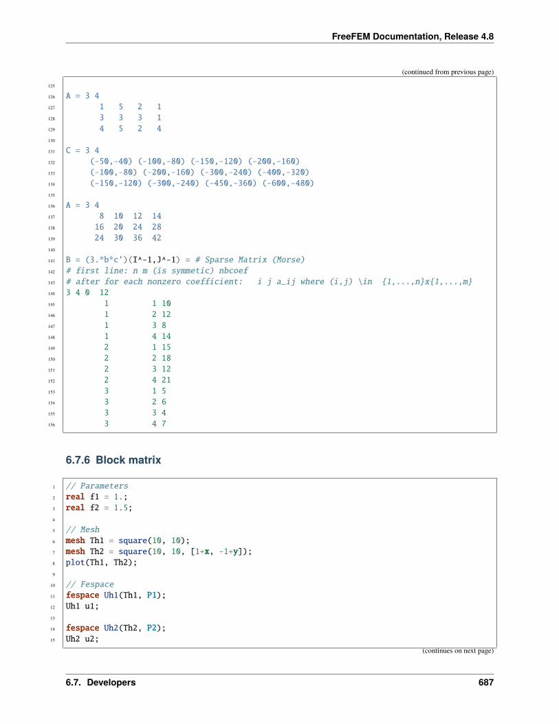
FreeFEM Documentation, Release 4.8
(continued from previous page)
125
126 A = 3 4127 1 5 2 1128 3 3 3 1129 4 5 2 4130
131 C = 3 4132 (-50,-40) (-100,-80) (-150,-120) (-200,-160)133 (-100,-80) (-200,-160) (-300,-240) (-400,-320)134 (-150,-120) (-300,-240) (-450,-360) (-600,-480)135
136 A = 3 4137 8 10 12 14138 16 20 24 28139 24 30 36 42140
141 B = (3.*b*c')(I^-1,J^-1) = # Sparse Matrix (Morse)142 # first line: n m (is symmetic) nbcoef143 # after for each nonzero coefficient: i j a_ij where (i,j) \in 1,...,nx1,...,m144 3 4 0 12145 1 1 10146 1 2 12147 1 3 8148 1 4 14149 2 1 15150 2 2 18151 2 3 12152 2 4 21153 3 1 5154 3 2 6155 3 3 4156 3 4 7
6.7.6 Block matrix
1 // Parameters2 real f1 = 1.;3 real f2 = 1.5;4
5 // Mesh6 mesh Th1 = square(10, 10);7 mesh Th2 = square(10, 10, [1+x, -1+y]);8 plot(Th1, Th2);9
10 // Fespace11 fespace Uh1(Th1, P1);12 Uh1 u1;13
14 fespace Uh2(Th2, P2);15 Uh2 u2;
(continues on next page)
6.7. Developers 687
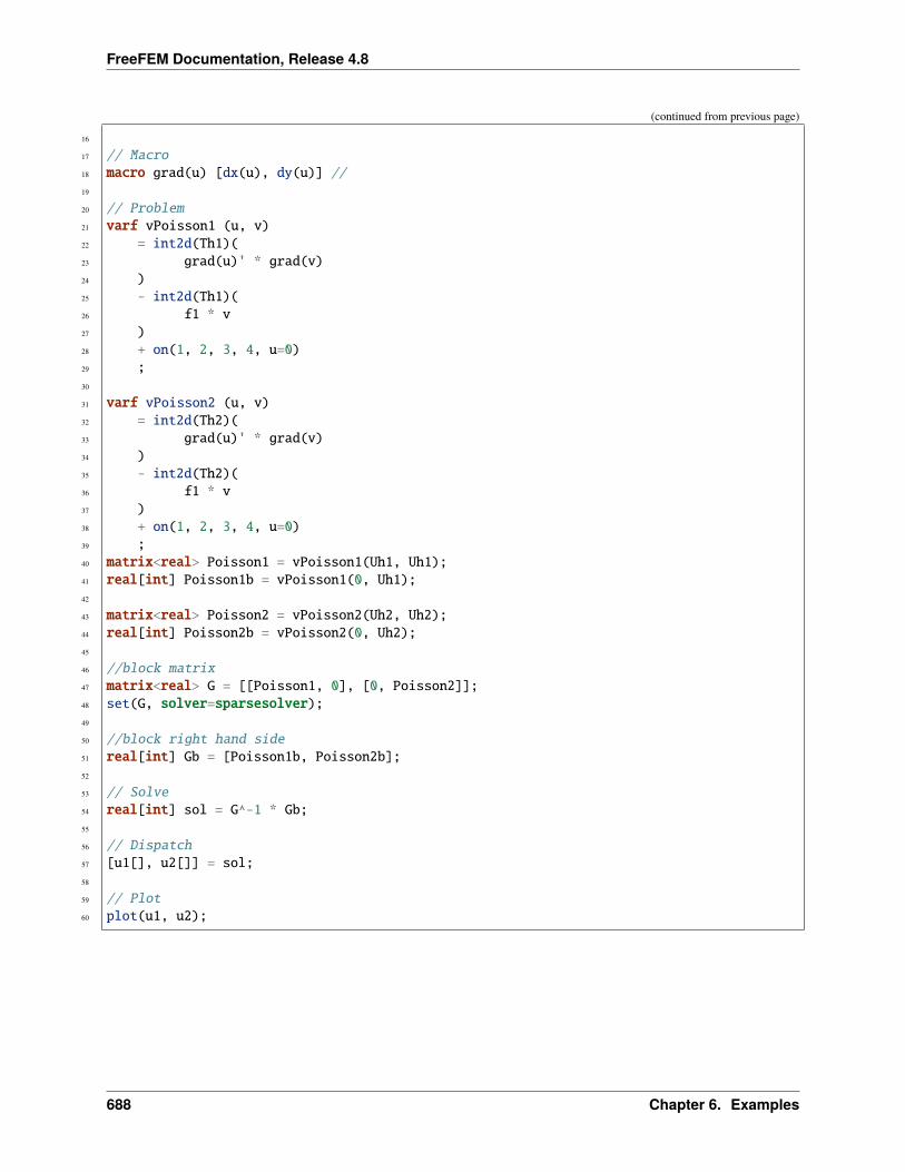
FreeFEM Documentation, Release 4.8
(continued from previous page)
16
17 // Macro18 macro grad(u) [dx(u), dy(u)] //19
20 // Problem21 varf vPoisson1 (u, v)22 = int2d(Th1)(23 grad(u)' * grad(v)24 )25 - int2d(Th1)(26 f1 * v27 )28 + on(1, 2, 3, 4, u=0)29 ;30
31 varf vPoisson2 (u, v)32 = int2d(Th2)(33 grad(u)' * grad(v)34 )35 - int2d(Th2)(36 f1 * v37 )38 + on(1, 2, 3, 4, u=0)39 ;40 matrix<real> Poisson1 = vPoisson1(Uh1, Uh1);41 real[int] Poisson1b = vPoisson1(0, Uh1);42
43 matrix<real> Poisson2 = vPoisson2(Uh2, Uh2);44 real[int] Poisson2b = vPoisson2(0, Uh2);45
46 //block matrix47 matrix<real> G = [[Poisson1, 0], [0, Poisson2]];48 set(G, solver=sparsesolver);49
50 //block right hand side51 real[int] Gb = [Poisson1b, Poisson2b];52
53 // Solve54 real[int] sol = G^-1 * Gb;55
56 // Dispatch57 [u1[], u2[]] = sol;58
59 // Plot60 plot(u1, u2);
688 Chapter 6. Examples
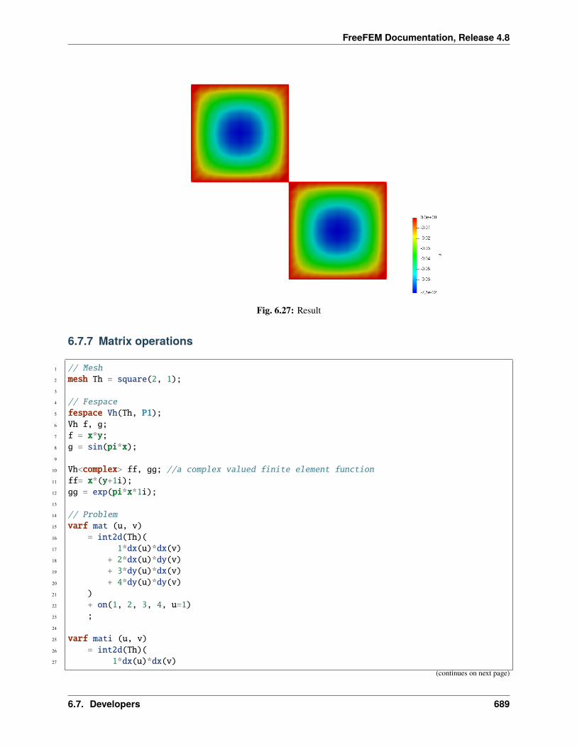
FreeFEM Documentation, Release 4.8
Fig. 6.27: Result
6.7.7 Matrix operations
1 // Mesh2 mesh Th = square(2, 1);3
4 // Fespace5 fespace Vh(Th, P1);6 Vh f, g;7 f = x*y;8 g = sin(pi*x);9
10 Vh<complex> ff, gg; //a complex valued finite element function11 ff= x*(y+1i);12 gg = exp(pi*x*1i);13
14 // Problem15 varf mat (u, v)16 = int2d(Th)(17 1*dx(u)*dx(v)18 + 2*dx(u)*dy(v)19 + 3*dy(u)*dx(v)20 + 4*dy(u)*dy(v)21 )22 + on(1, 2, 3, 4, u=1)23 ;24
25 varf mati (u, v)26 = int2d(Th)(27 1*dx(u)*dx(v)
(continues on next page)
6.7. Developers 689
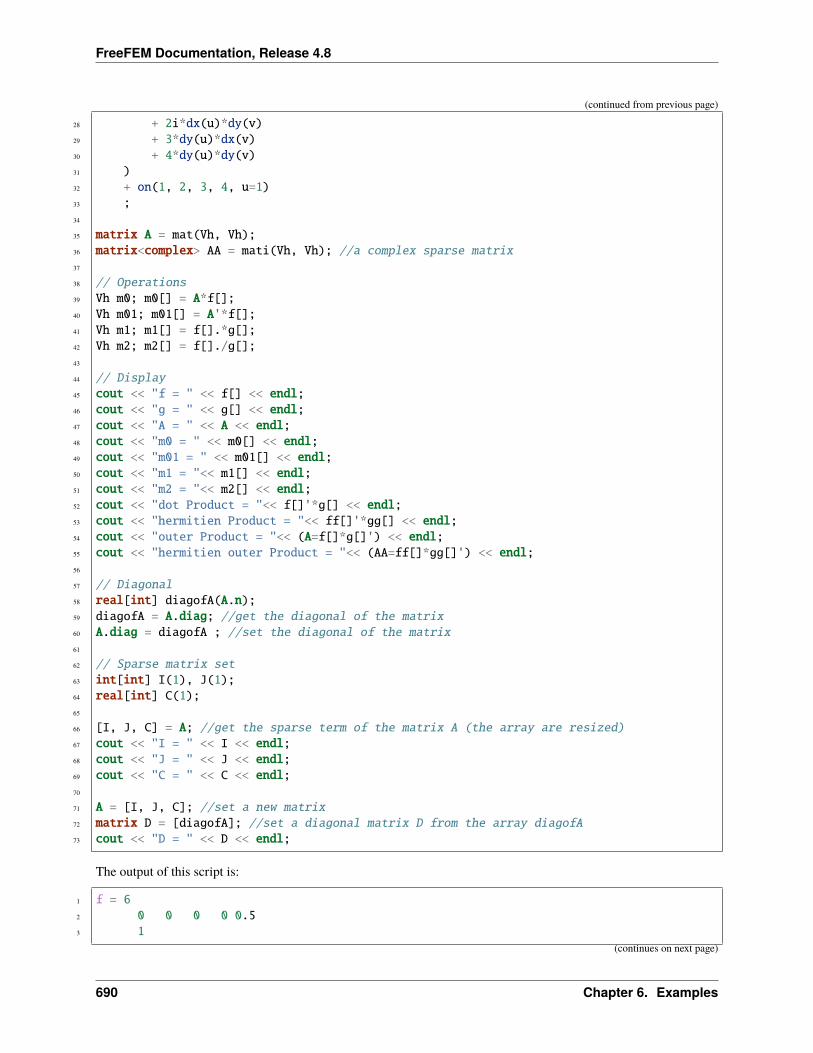
FreeFEM Documentation, Release 4.8
(continued from previous page)
28 + 2i*dx(u)*dy(v)29 + 3*dy(u)*dx(v)30 + 4*dy(u)*dy(v)31 )32 + on(1, 2, 3, 4, u=1)33 ;34
35 matrix A = mat(Vh, Vh);36 matrix<complex> AA = mati(Vh, Vh); //a complex sparse matrix37
38 // Operations39 Vh m0; m0[] = A*f[];40 Vh m01; m01[] = A'*f[];41 Vh m1; m1[] = f[].*g[];42 Vh m2; m2[] = f[]./g[];43
44 // Display45 cout << "f = " << f[] << endl;46 cout << "g = " << g[] << endl;47 cout << "A = " << A << endl;48 cout << "m0 = " << m0[] << endl;49 cout << "m01 = " << m01[] << endl;50 cout << "m1 = "<< m1[] << endl;51 cout << "m2 = "<< m2[] << endl;52 cout << "dot Product = "<< f[]'*g[] << endl;53 cout << "hermitien Product = "<< ff[]'*gg[] << endl;54 cout << "outer Product = "<< (A=f[]*g[]') << endl;55 cout << "hermitien outer Product = "<< (AA=ff[]*gg[]') << endl;56
57 // Diagonal58 real[int] diagofA(A.n);59 diagofA = A.diag; //get the diagonal of the matrix60 A.diag = diagofA ; //set the diagonal of the matrix61
62 // Sparse matrix set63 int[int] I(1), J(1);64 real[int] C(1);65
66 [I, J, C] = A; //get the sparse term of the matrix A (the array are resized)67 cout << "I = " << I << endl;68 cout << "J = " << J << endl;69 cout << "C = " << C << endl;70
71 A = [I, J, C]; //set a new matrix72 matrix D = [diagofA]; //set a diagonal matrix D from the array diagofA73 cout << "D = " << D << endl;
The output of this script is:
1 f = 62 0 0 0 0 0.53 1
(continues on next page)
690 Chapter 6. Examples
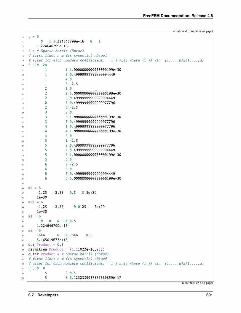
FreeFEM Documentation, Release 4.8
(continued from previous page)
4 g = 65 0 1 1.224646799e-16 0 16 1.224646799e-167 A = # Sparse Matrix (Morse)8 # first line: n m (is symmetic) nbcoef9 # after for each nonzero coefficient: i j a_ij where (i,j) \in 1,...,nx1,...,m
10 6 6 0 2411 1 1 1.0000000000000000199e+3012 1 2 0.4999999999999999444913 1 4 014 1 5 -2.515 2 1 016 2 2 1.0000000000000000199e+3017 2 3 0.4999999999999999444918 2 5 0.4999999999999997779619 2 6 -2.520 3 2 021 3 3 1.0000000000000000199e+3022 3 6 0.4999999999999997779623 4 1 0.4999999999999997779624 4 4 1.0000000000000000199e+3025 4 5 026 5 1 -2.527 5 2 0.4999999999999997779628 5 4 0.4999999999999999444929 5 5 1.0000000000000000199e+3030 5 6 031 6 2 -2.532 6 3 033 6 5 0.4999999999999999444934 6 6 1.0000000000000000199e+3035
36 m0 = 637 -1.25 -2.25 0.5 0 5e+2938 1e+3039 m01 = 640 -1.25 -2.25 0 0.25 5e+2941 1e+3042 m1 = 643 0 0 0 0 0.544 1.224646799e-1645 m2 = 646 -nan 0 0 -nan 0.547 8.165619677e+1548 dot Product = 0.549 hermitien Product = (1.11022e-16,2.5)50 outer Product = # Sparse Matrix (Morse)51 # first line: n m (is symmetic) nbcoef52 # after for each nonzero coefficient: i j a_ij where (i,j) \in 1,...,nx1,...,m53 6 6 0 854 5 2 0.555 5 3 6.1232339957367660359e-17
(continues on next page)
6.7. Developers 691
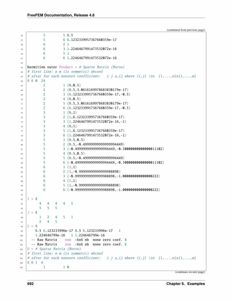
FreeFEM Documentation, Release 4.8
(continued from previous page)
56 5 5 0.557 5 6 6.1232339957367660359e-1758 6 2 159 6 3 1.2246467991473532072e-1660 6 5 161 6 6 1.2246467991473532072e-1662
63 hermitien outer Product = # Sparse Matrix (Morse)64 # first line: n m (is symmetic) nbcoef65 # after for each nonzero coefficient: i j a_ij where (i,j) \in 1,...,nx1,...,m66 6 6 0 2467 2 1 (0,0.5)68 2 2 (0.5,3.0616169978683830179e-17)69 2 3 (6.1232339957367660359e-17,-0.5)70 2 4 (0,0.5)71 2 5 (0.5,3.0616169978683830179e-17)72 2 6 (6.1232339957367660359e-17,-0.5)73 3 1 (0,1)74 3 2 (1,6.1232339957367660359e-17)75 3 3 (1.2246467991473532072e-16,-1)76 3 4 (0,1)77 3 5 (1,6.1232339957367660359e-17)78 3 6 (1.2246467991473532072e-16,-1)79 5 1 (0.5,0.5)80 5 2 (0.5,-0.49999999999999994449)81 5 3 (-0.49999999999999994449,-0.50000000000000011102)82 5 4 (0.5,0.5)83 5 5 (0.5,-0.49999999999999994449)84 5 6 (-0.49999999999999994449,-0.50000000000000011102)85 6 1 (1,1)86 6 2 (1,-0.99999999999999988898)87 6 3 (-0.99999999999999988898,-1.000000000000000222)88 6 4 (1,1)89 6 5 (1,-0.99999999999999988898)90 6 6 (-0.99999999999999988898,-1.000000000000000222)91
92 I = 893 4 4 4 4 594 5 5 595 J = 896 1 2 4 5 197 2 4 598 C = 899 0.5 6.123233996e-17 0.5 6.123233996e-17 1
100 1.224646799e-16 1 1.224646799e-16101 -- Raw Matrix nxm =6x6 nb none zero coef. 8102 -- Raw Matrix nxm =6x6 nb none zero coef. 6103 D = # Sparse Matrix (Morse)104 # first line: n m (is symmetic) nbcoef105 # after for each nonzero coefficient: i j a_ij where (i,j) \in 1,...,nx1,...,m106 6 6 1 6107 1 1 0
(continues on next page)
692 Chapter 6. Examples
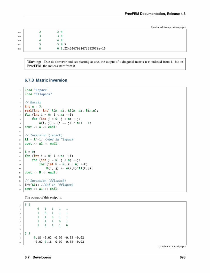
FreeFEM Documentation, Release 4.8
(continued from previous page)
108 2 2 0109 3 3 0110 4 4 0111 5 5 0.5112 6 6 1.2246467991473532072e-16
Warning: Due to Fortran indices starting at one, the output of a diagonal matrix D is indexed from 1. but inFreeFEM, the indices start from 0.
6.7.8 Matrix inversion
1 load "lapack"2 load "fflapack"3
4 // Matrix5 int n = 5;6 real[int, int] A(n, n), A1(n, n), B(n,n);7 for (int i = 0; i < n; ++i)8 for (int j = 0; j < n; ++j)9 A(i, j) = (i == j) ? n+1 : 1;
10 cout << A << endl;11
12 // Inversion (lapack)13 A1 = A^-1; //def in "lapack"14 cout << A1 << endl;15
16 B = 0;17 for (int i = 0; i < n; ++i)18 for (int j = 0; j < n; ++j)19 for (int k = 0; k < n; ++k)20 B(i, j) += A(i,k)*A1(k,j);21 cout << B << endl;22
23 // Inversion (fflapack)24 inv(A1); //def in "fflapack"25 cout << A1 << endl;
The output of this script is:
1 5 52 6 1 1 1 13 1 6 1 1 14 1 1 6 1 15 1 1 1 6 16 1 1 1 1 67
8 5 59 0.18 -0.02 -0.02 -0.02 -0.02
10 -0.02 0.18 -0.02 -0.02 -0.02(continues on next page)
6.7. Developers 693
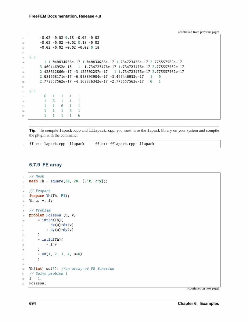
FreeFEM Documentation, Release 4.8
(continued from previous page)
11 -0.02 -0.02 0.18 -0.02 -0.0212 -0.02 -0.02 -0.02 0.18 -0.0213 -0.02 -0.02 -0.02 -0.02 0.1814
15 5 516 1 1.040834086e-17 1.040834086e-17 1.734723476e-17 2.775557562e-1717 3.469446952e-18 1 -1.734723476e-17 1.734723476e-17 2.775557562e-1718 2.428612866e-17 -3.122502257e-17 1 1.734723476e-17 2.775557562e-1719 2.081668171e-17 -6.938893904e-17 -3.469446952e-17 1 020 2.775557562e-17 -4.163336342e-17 -2.775557562e-17 0 121
22 5 523 6 1 1 1 124 1 6 1 1 125 1 1 6 1 126 1 1 1 6 127 1 1 1 1 6
Tip: To compile lapack.cpp and fflapack.cpp, you must have the lapack library on your system and compilethe plugin with the command:
1 ff-c++ lapack.cpp -llapack ff-c++ fflapack.cpp -llapack
6.7.9 FE array
1 // Mesh2 mesh Th = square(20, 20, [2*x, 2*y]);3
4 // Fespace5 fespace Vh(Th, P1);6 Vh u, v, f;7
8 // Problem9 problem Poisson (u, v)
10 = int2d(Th)(11 dx(u)*dx(v)12 + dy(u)*dy(v)13 )14 + int2d(Th)(15 - f*v16 )17 + on(1, 2, 3, 4, u=0)18 ;19
20 Vh[int] uu(3); //an array of FE function21 // Solve problem 122 f = 1;23 Poisson;
(continues on next page)
694 Chapter 6. Examples
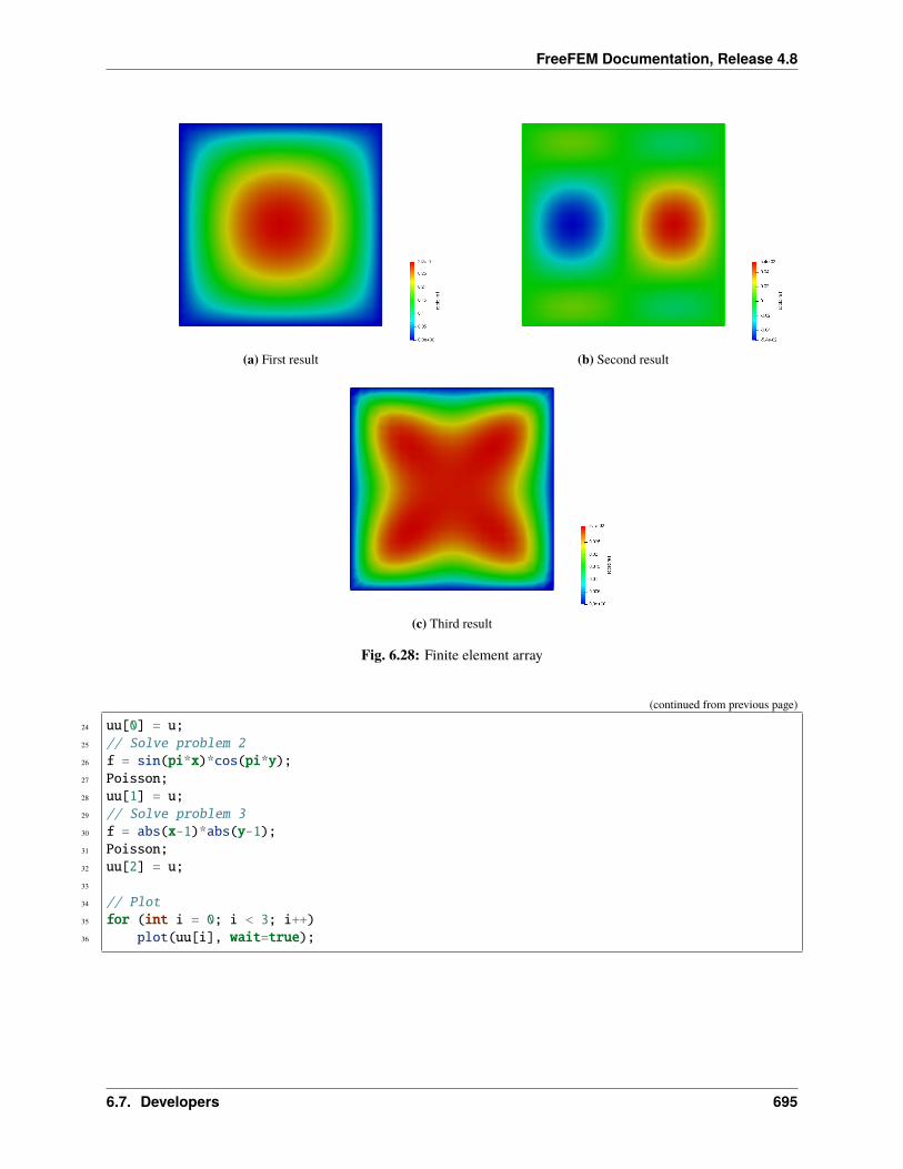
FreeFEM Documentation, Release 4.8
(a) First result (b) Second result
(c) Third result
Fig. 6.28: Finite element array
(continued from previous page)
24 uu[0] = u;25 // Solve problem 226 f = sin(pi*x)*cos(pi*y);27 Poisson;28 uu[1] = u;29 // Solve problem 330 f = abs(x-1)*abs(y-1);31 Poisson;32 uu[2] = u;33
34 // Plot35 for (int i = 0; i < 3; i++)36 plot(uu[i], wait=true);
6.7. Developers 695
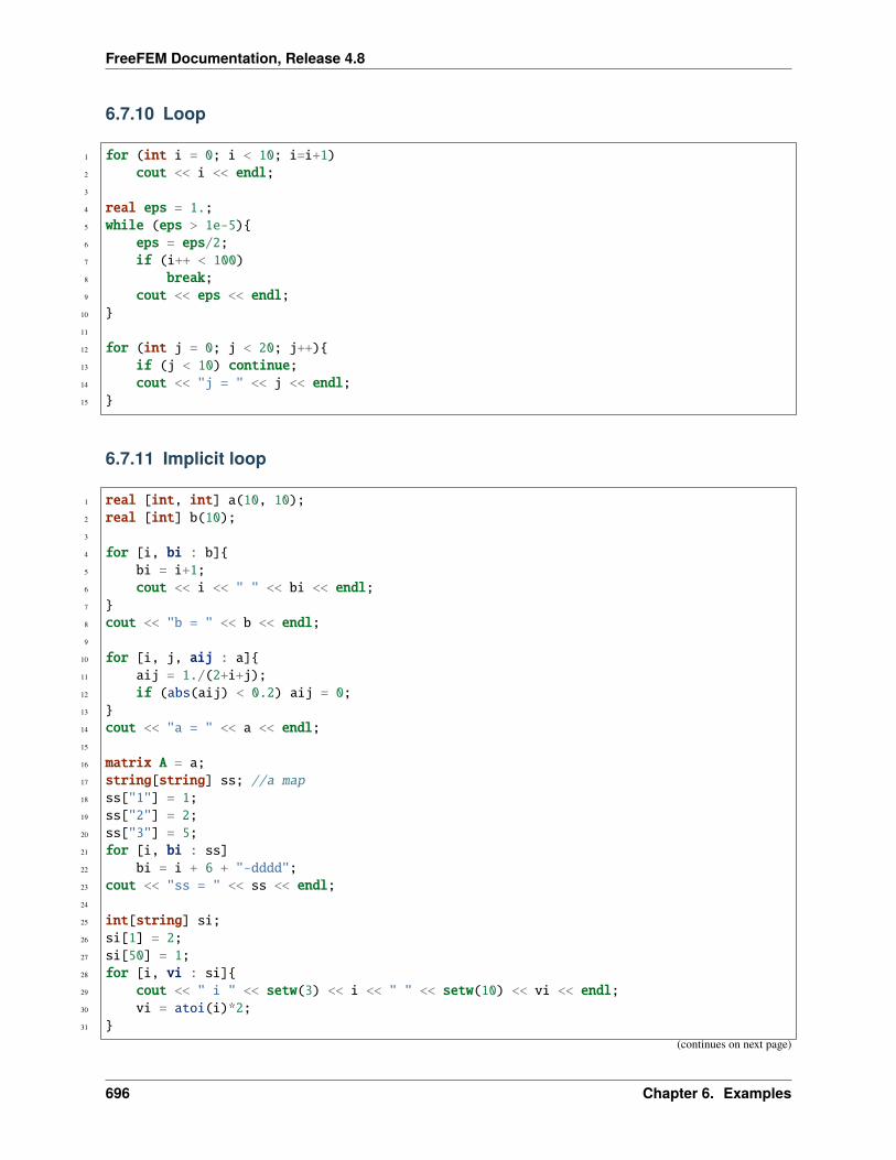
FreeFEM Documentation, Release 4.8
6.7.10 Loop
1 for (int i = 0; i < 10; i=i+1)2 cout << i << endl;3
4 real eps = 1.;5 while (eps > 1e-5)6 eps = eps/2;7 if (i++ < 100)8 break;9 cout << eps << endl;
10 11
12 for (int j = 0; j < 20; j++)13 if (j < 10) continue;14 cout << "j = " << j << endl;15
6.7.11 Implicit loop
1 real [int, int] a(10, 10);2 real [int] b(10);3
4 for [i, bi : b]5 bi = i+1;6 cout << i << " " << bi << endl;7 8 cout << "b = " << b << endl;9
10 for [i, j, aij : a]11 aij = 1./(2+i+j);12 if (abs(aij) < 0.2) aij = 0;13 14 cout << "a = " << a << endl;15
16 matrix A = a;17 string[string] ss; //a map18 ss["1"] = 1;19 ss["2"] = 2;20 ss["3"] = 5;21 for [i, bi : ss]22 bi = i + 6 + "-dddd";23 cout << "ss = " << ss << endl;24
25 int[string] si;26 si[1] = 2;27 si[50] = 1;28 for [i, vi : si]29 cout << " i " << setw(3) << i << " " << setw(10) << vi << endl;30 vi = atoi(i)*2;31
(continues on next page)
696 Chapter 6. Examples
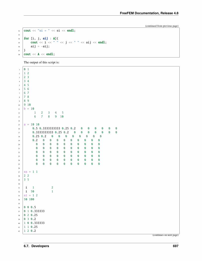
FreeFEM Documentation, Release 4.8
(continued from previous page)
32 cout << "si = " << si << endl;33
34 for [i, j, aij : A]35 cout << i << " " << j << " " << aij << endl;36 aij = -aij;37 38 cout << A << endl;
The output of this script is:
1 0 12 1 23 2 34 3 45 4 56 5 67 6 78 7 89 8 9
10 9 1011 b = 1012 1 2 3 4 513 6 7 8 9 1014
15 a = 10 1016 0.5 0.3333333333 0.25 0.2 0 0 0 0 0 017 0.3333333333 0.25 0.2 0 0 0 0 0 0 018 0.25 0.2 0 0 0 0 0 0 0 019 0.2 0 0 0 0 0 0 0 0 020 0 0 0 0 0 0 0 0 0 021 0 0 0 0 0 0 0 0 0 022 0 0 0 0 0 0 0 0 0 023 0 0 0 0 0 0 0 0 0 024 0 0 0 0 0 0 0 0 0 025 0 0 0 0 0 0 0 0 0 026
27 ss = 1 128 2 229 3 530
31 i 1 232 i 50 133 si = 1 234 50 10035
36 0 0 0.537 0 1 0.33333338 0 2 0.2539 0 3 0.240 1 0 0.33333341 1 1 0.2542 1 2 0.2
(continues on next page)
6.7. Developers 697
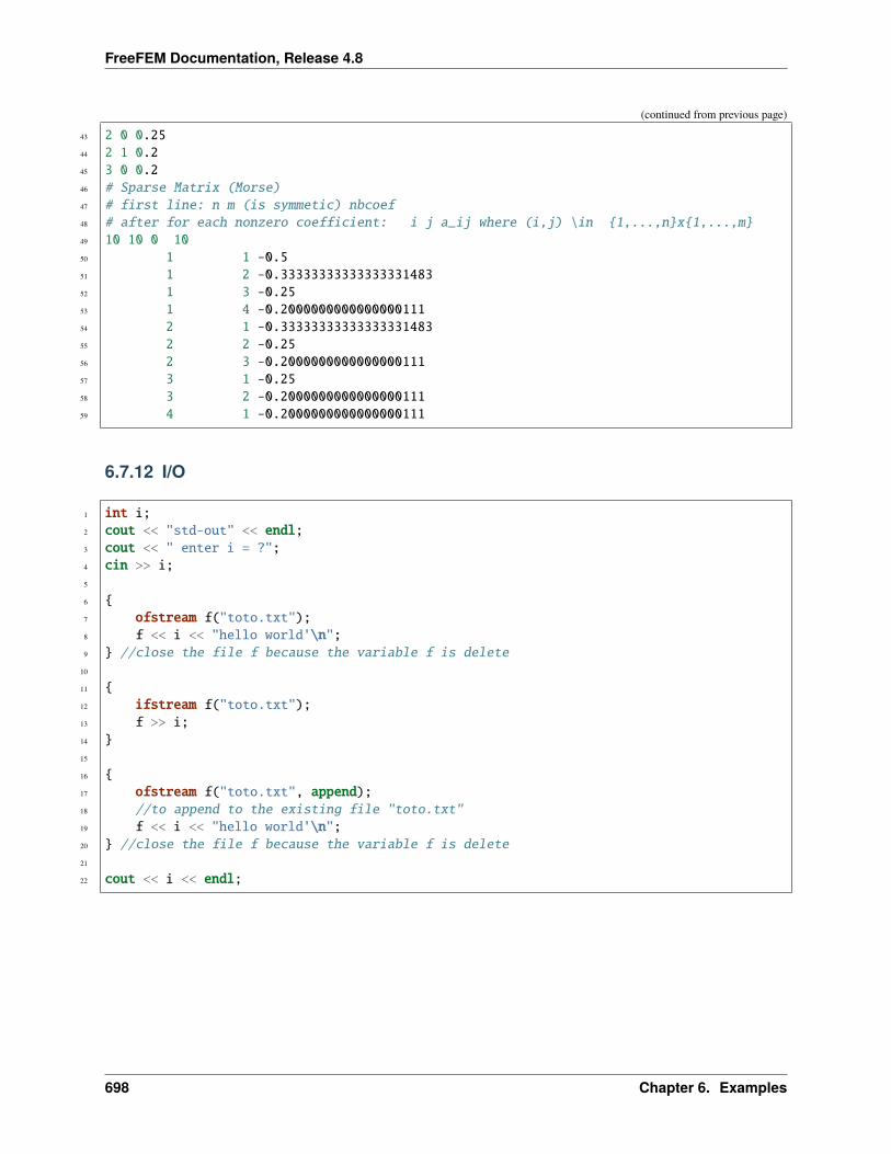
FreeFEM Documentation, Release 4.8
(continued from previous page)
43 2 0 0.2544 2 1 0.245 3 0 0.246 # Sparse Matrix (Morse)47 # first line: n m (is symmetic) nbcoef48 # after for each nonzero coefficient: i j a_ij where (i,j) \in 1,...,nx1,...,m49 10 10 0 1050 1 1 -0.551 1 2 -0.3333333333333333148352 1 3 -0.2553 1 4 -0.200000000000000011154 2 1 -0.3333333333333333148355 2 2 -0.2556 2 3 -0.200000000000000011157 3 1 -0.2558 3 2 -0.200000000000000011159 4 1 -0.2000000000000000111
6.7.12 I/O
1 int i;2 cout << "std-out" << endl;3 cout << " enter i = ?";4 cin >> i;5
6 7 ofstream f("toto.txt");8 f << i << "hello world'\n";9 //close the file f because the variable f is delete
10
11 12 ifstream f("toto.txt");13 f >> i;14 15
16 17 ofstream f("toto.txt", append);18 //to append to the existing file "toto.txt"19 f << i << "hello world'\n";20 //close the file f because the variable f is delete21
22 cout << i << endl;
698 Chapter 6. Examples
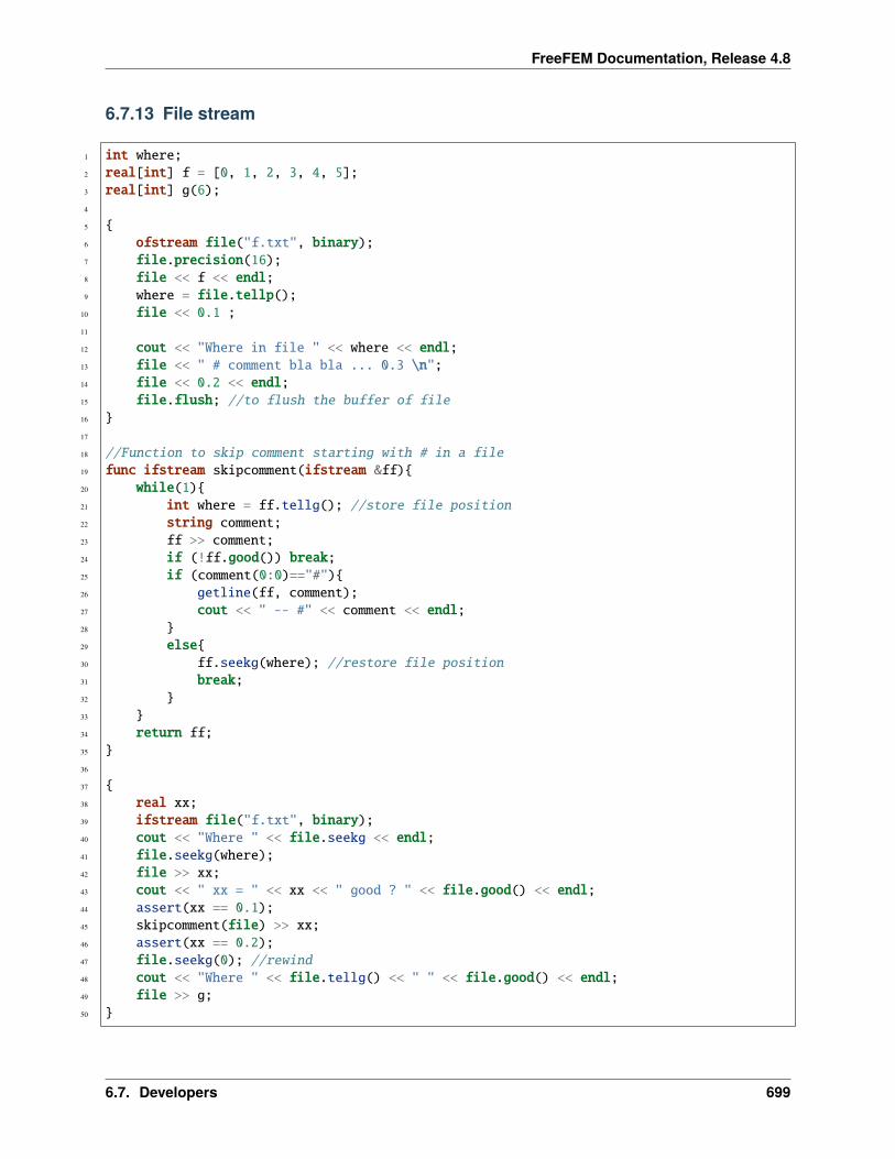
FreeFEM Documentation, Release 4.8
6.7.13 File stream
1 int where;2 real[int] f = [0, 1, 2, 3, 4, 5];3 real[int] g(6);4
5 6 ofstream file("f.txt", binary);7 file.precision(16);8 file << f << endl;9 where = file.tellp();
10 file << 0.1 ;11
12 cout << "Where in file " << where << endl;13 file << " # comment bla bla ... 0.3 \n";14 file << 0.2 << endl;15 file.flush; //to flush the buffer of file16 17
18 //Function to skip comment starting with # in a file19 func ifstream skipcomment(ifstream &ff)20 while(1)21 int where = ff.tellg(); //store file position22 string comment;23 ff >> comment;24 if (!ff.good()) break;25 if (comment(0:0)=="#")26 getline(ff, comment);27 cout << " -- #" << comment << endl;28 29 else30 ff.seekg(where); //restore file position31 break;32 33 34 return ff;35 36
37 38 real xx;39 ifstream file("f.txt", binary);40 cout << "Where " << file.seekg << endl;41 file.seekg(where);42 file >> xx;43 cout << " xx = " << xx << " good ? " << file.good() << endl;44 assert(xx == 0.1);45 skipcomment(file) >> xx;46 assert(xx == 0.2);47 file.seekg(0); //rewind48 cout << "Where " << file.tellg() << " " << file.good() << endl;49 file >> g;50
6.7. Developers 699
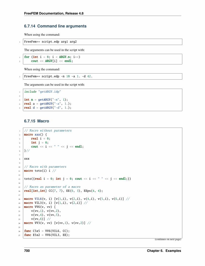
FreeFEM Documentation, Release 4.8
6.7.14 Command line arguments
When using the command:
1 FreeFem++ script.edp arg1 arg2
The arguments can be used in the script with:
1 for (int i = 0; i < ARGV.n; i++)2 cout << ARGV[i] << endl;
When using the command:
1 FreeFem++ script.edp -n 10 -a 1. -d 42.
The arguments can be used in the script with:
1 include "getARGV.idp"2
3 int n = getARGV("-n", 1);4 real a = getARGV("-a", 1.);5 real d = getARGV("-d", 1.);
6.7.15 Macro
1 // Macro without parameters2 macro xxx() 3 real i = 0;4 int j = 0;5 cout << i << " " << j << endl;6 //7
8 xxx9
10 // Macro with parameters11 macro toto(i) i //12
13 toto(real i = 0; int j = 0; cout << i << " " << j << endl;)14
15 // Macro as parameter of a macro16 real[int,int] CC(7, 7), EE(6, 3), EEps(4, 4);17
18 macro VIL6(v, i) [v(1,i), v(2,i), v(4,i), v(5,i), v(6,i)] //19 macro VIL3(v, i) [v(1,i), v(2,i)] //20 macro VV6(v, vv) [21 v(vv,1), v(vv,2),22 v(vv,4), v(vv,5),23 v(vv,6)] //24 macro VV3(v, vv) [v(vv,1), v(vv,2)] //25
26 func C5x5 = VV6(VIL6, CC);27 func E5x2 = VV6(VIL3, EE);
(continues on next page)
700 Chapter 6. Examples
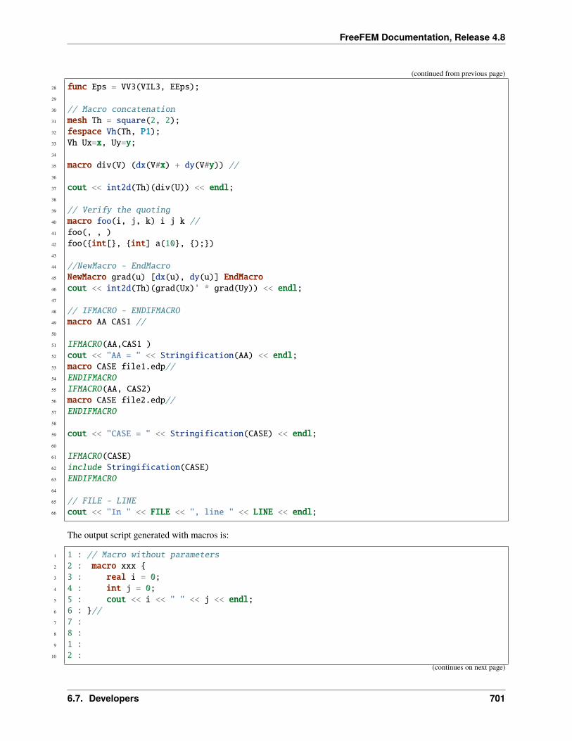
FreeFEM Documentation, Release 4.8
(continued from previous page)
28 func Eps = VV3(VIL3, EEps);29
30 // Macro concatenation31 mesh Th = square(2, 2);32 fespace Vh(Th, P1);33 Vh Ux=x, Uy=y;34
35 macro div(V) (dx(V#x) + dy(V#y)) //36
37 cout << int2d(Th)(div(U)) << endl;38
39 // Verify the quoting40 macro foo(i, j, k) i j k //41 foo(, , )42 foo(int[, int] a(10, );)43
44 //NewMacro - EndMacro45 NewMacro grad(u) [dx(u), dy(u)] EndMacro46 cout << int2d(Th)(grad(Ux)' * grad(Uy)) << endl;47
48 // IFMACRO - ENDIFMACRO49 macro AA CAS1 //50
51 IFMACRO(AA,CAS1 )52 cout << "AA = " << Stringification(AA) << endl;53 macro CASE file1.edp//54 ENDIFMACRO55 IFMACRO(AA, CAS2)56 macro CASE file2.edp//57 ENDIFMACRO58
59 cout << "CASE = " << Stringification(CASE) << endl;60
61 IFMACRO(CASE)62 include Stringification(CASE)63 ENDIFMACRO64
65 // FILE - LINE66 cout << "In " << FILE << ", line " << LINE << endl;
The output script generated with macros is:
1 1 : // Macro without parameters2 2 : macro xxx 3 3 : real i = 0;4 4 : int j = 0;5 5 : cout << i << " " << j << endl;6 6 : //7 7 :8 8 :9 1 :
10 2 :(continues on next page)
6.7. Developers 701
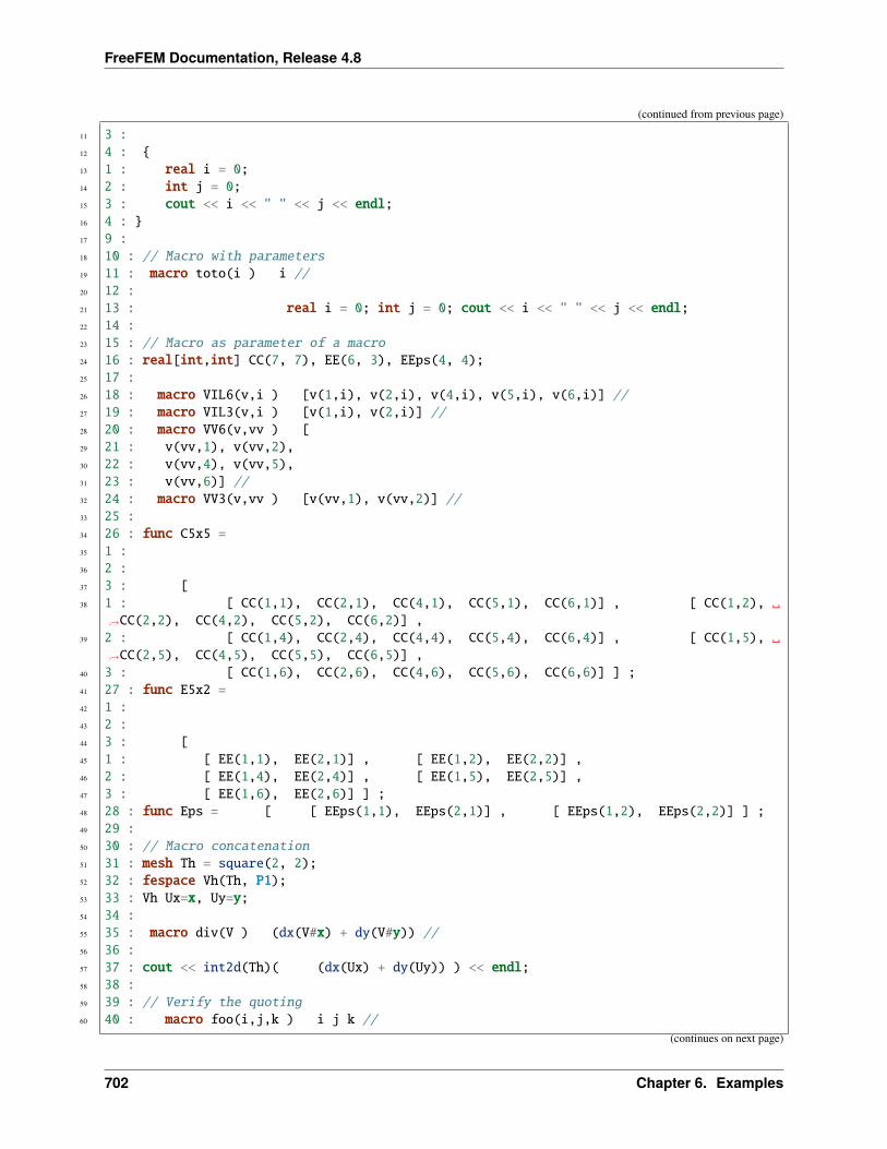
FreeFEM Documentation, Release 4.8
(continued from previous page)
11 3 :12 4 : 13 1 : real i = 0;14 2 : int j = 0;15 3 : cout << i << " " << j << endl;16 4 : 17 9 :18 10 : // Macro with parameters19 11 : macro toto(i ) i //20 12 :21 13 : real i = 0; int j = 0; cout << i << " " << j << endl;22 14 :23 15 : // Macro as parameter of a macro24 16 : real[int,int] CC(7, 7), EE(6, 3), EEps(4, 4);25 17 :26 18 : macro VIL6(v,i ) [v(1,i), v(2,i), v(4,i), v(5,i), v(6,i)] //27 19 : macro VIL3(v,i ) [v(1,i), v(2,i)] //28 20 : macro VV6(v,vv ) [29 21 : v(vv,1), v(vv,2),30 22 : v(vv,4), v(vv,5),31 23 : v(vv,6)] //32 24 : macro VV3(v,vv ) [v(vv,1), v(vv,2)] //33 25 :34 26 : func C5x5 =35 1 :36 2 :37 3 : [38 1 : [ CC(1,1), CC(2,1), CC(4,1), CC(5,1), CC(6,1)] , [ CC(1,2),
→˓CC(2,2), CC(4,2), CC(5,2), CC(6,2)] ,39 2 : [ CC(1,4), CC(2,4), CC(4,4), CC(5,4), CC(6,4)] , [ CC(1,5),
→˓CC(2,5), CC(4,5), CC(5,5), CC(6,5)] ,40 3 : [ CC(1,6), CC(2,6), CC(4,6), CC(5,6), CC(6,6)] ] ;41 27 : func E5x2 =42 1 :43 2 :44 3 : [45 1 : [ EE(1,1), EE(2,1)] , [ EE(1,2), EE(2,2)] ,46 2 : [ EE(1,4), EE(2,4)] , [ EE(1,5), EE(2,5)] ,47 3 : [ EE(1,6), EE(2,6)] ] ;48 28 : func Eps = [ [ EEps(1,1), EEps(2,1)] , [ EEps(1,2), EEps(2,2)] ] ;49 29 :50 30 : // Macro concatenation51 31 : mesh Th = square(2, 2);52 32 : fespace Vh(Th, P1);53 33 : Vh Ux=x, Uy=y;54 34 :55 35 : macro div(V ) (dx(V#x) + dy(V#y)) //56 36 :57 37 : cout << int2d(Th)( (dx(Ux) + dy(Uy)) ) << endl;58 38 :59 39 : // Verify the quoting60 40 : macro foo(i,j,k ) i j k //
(continues on next page)
702 Chapter 6. Examples
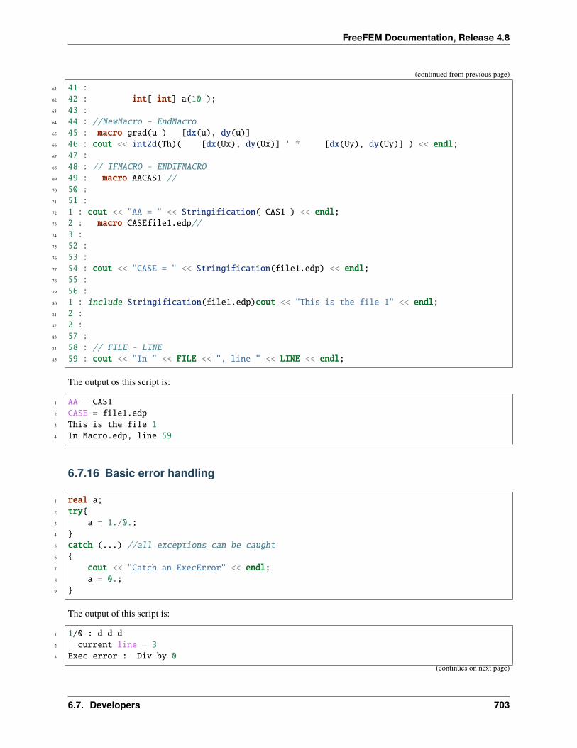
FreeFEM Documentation, Release 4.8
(continued from previous page)
61 41 :62 42 : int[ int] a(10 );63 43 :64 44 : //NewMacro - EndMacro65 45 : macro grad(u ) [dx(u), dy(u)]66 46 : cout << int2d(Th)( [dx(Ux), dy(Ux)] ' * [dx(Uy), dy(Uy)] ) << endl;67 47 :68 48 : // IFMACRO - ENDIFMACRO69 49 : macro AACAS1 //70 50 :71 51 :72 1 : cout << "AA = " << Stringification( CAS1 ) << endl;73 2 : macro CASEfile1.edp//74 3 :75 52 :76 53 :77 54 : cout << "CASE = " << Stringification(file1.edp) << endl;78 55 :79 56 :80 1 : include Stringification(file1.edp)cout << "This is the file 1" << endl;81 2 :82 2 :83 57 :84 58 : // FILE - LINE85 59 : cout << "In " << FILE << ", line " << LINE << endl;
The output os this script is:
1 AA = CAS12 CASE = file1.edp3 This is the file 14 In Macro.edp, line 59
6.7.16 Basic error handling
1 real a;2 try3 a = 1./0.;4 5 catch (...) //all exceptions can be caught6 7 cout << "Catch an ExecError" << endl;8 a = 0.;9
The output of this script is:
1 1/0 : d d d2 current line = 33 Exec error : Div by 0
(continues on next page)
6.7. Developers 703
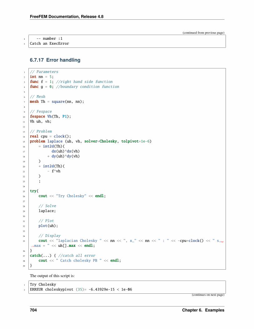
FreeFEM Documentation, Release 4.8
(continued from previous page)
4 -- number :15 Catch an ExecError
6.7.17 Error handling
1 // Parameters2 int nn = 5;3 func f = 1; //right hand side function4 func g = 0; //boundary condition function5
6 // Mesh7 mesh Th = square(nn, nn);8
9 // Fespace10 fespace Vh(Th, P1);11 Vh uh, vh;12
13 // Problem14 real cpu = clock();15 problem laplace (uh, vh, solver=Cholesky, tolpivot=1e-6)16 = int2d(Th)(17 dx(uh)*dx(vh)18 + dy(uh)*dy(vh)19 )20 + int2d(Th)(21 - f*vh22 )23 ;24
25 try26 cout << "Try Cholesky" << endl;27
28 // Solve29 laplace;30
31 // Plot32 plot(uh);33
34 // Display35 cout << "laplacian Cholesky " << nn << ", x_" << nn << " : " << -cpu+clock() << " s,
→˓max = " << uh[].max << endl;36 37 catch(...) //catch all error38 cout << " Catch cholesky PB " << endl;39
The output of this script is:
1 Try Cholesky2 ERREUR choleskypivot (35)= -6.43929e-15 < 1e-06
(continues on next page)
704 Chapter 6. Examples
FreeFEM Documentation, Release 4.8
(continued from previous page)
3 current line = 294 Exec error : FATAL ERREUR dans ./../femlib/MatriceCreuse_tpl.hpp5 cholesky line:6 -- number :6887 catch an erreur in solve => set sol = 0 !!!!!!!8 Catch cholesky PB
6.7. Developers 705

FreeFEM Documentation, Release 4.8
706 Chapter 6. Examples
BIBLIOGRAPHY
[PIRONNEAU1998] PIRONNEAU, Olivier and LUCQUIN-DESREUX, Brigitte. Introduction to scientific comput-ing. Wiley, 1998.
[WÄCHTER2006] WÄCHTER, Andreas and BIEGLER, Lorenz T. On the implementation of an interior-point fil-ter line-search algorithm for large-scale nonlinear programming. Mathematical programming, 2006,vol. 106, no 1, p. 25-57.
[FORSGREN2002] FORSGREN, Anders, GILL, Philip E., and WRIGHT, Margaret H. Interior methods for nonlinearoptimization. SIAM review, 2002, vol. 44, no 4, p. 525-597.
[GEORGE1996] GEORGE, P. L. and BOROUCHAKI, H. Automatic triangulation. 1996.
[HECHT1998] HECHT, F. The mesh adapting software: bamg. INRIA report, 1998, vol. 250, p. 252.
[PREPARATA1985] PREPARATA, F. P. and SHAMOS, M. I. Computational Geometry Springer-Verlag. New York,1985.
[STROUSTRUP2000] STROUSTRUP, Bjarne. The C++ programming language. Pearson Education India, 2000.
[HECHT2002] HECHT, Frédéric. C++ Tools to construct our user-level language. ESAIM: Mathematical Modellingand Numerical Analysis, 2002, vol. 36, no 5, p. 809-836.
[HANG2006] SI, Hang. TetGen Users’ guide: A quality tetrahedral mesh generator and three-dimensional delaunaytriangulator. 2006
[SHEWCHUK1998] SHEWCHUK, Jonathan Richard. Tetrahedral mesh generation by Delaunay refinement. In : Pro-ceedings of the fourteenth annual symposium on Computational geometry. ACM, 1998. p. 86-95.
[HECHT1992] HECHT, F. Outils et algorithmes pour la méthode des éléments finis. HdR, Université Pierre et MarieCurie, France, 1992.
[HECHT1998_2] HECHT, Frédéric. BAMG: bidimensional anisotropic mesh generator. User Guide. INRIA, Roc-quencourt, 1998.
[KARYPIS1995] KARYPIS, George and KUMAR, Vipin. METIS–unstructured graph partitioning and sparse matrixordering system, version 2.0. 1995.
[CAI1989] CAI, Xiao-Chuan. Some domain decomposition algorithms for nonselfadjoint elliptic and parabolicpartial differential equations. 1989.
[SAAD2003] SAAD, Yousef. Iterative methods for sparse linear systems. siam, 2003.
[SMITH1996] SMITH, B. P. Bj rstad and W. Gropp, Domain Decomposition. 1996.
[OGDEN1984] OGDEN, Ray W. Non-linear elastic deformations. 1984.
[RAVIART1998] RAVIART, Pierre-Arnaud, THOMAS, Jean-Marie, CIARLET, Philippe G., et al. Introduction àl’analyse numérique des équations aux dérivées partielles. Paris : Dunod, 1998.
707
FreeFEM Documentation, Release 4.8
[HORGAN2004] HORGAN, Cornelius O. and SACCOMANDI, Giuseppe. Constitutive models for compressible non-linearly elastic materials with limiting chain extensibility. Journal of Elasticity, 2004, vol. 77, no 2,p. 123-138.
[LEHOUCQ1998] LEHOUCQ, Richard B., SORENSEN, Danny C., and YANG, Chao. ARPACK users’ guide: solu-tion of large-scale eigenvalue problems with implicitly restarted Arnoldi methods. Siam, 1998.
[NECAS2017] NECAS, Jindrich and HLAVÁCEK, Ivan. Mathematical theory of elastic and elasto-plastic bodies: anintroduction. Elsevier, 2017.
[OHTSUKA2000] OHTSUKA, K. Theoretical and Numerical analysis of energy release rate in 2D fracture. INFOR-MATION, 2000, vol. 3, p. 303-315.
[TABATA1994] TABATA, M. Numerical solutions of partial differential equations II. Iwanami Applied Math, 1994.
[LUCQUIN1998] PIRONNEAU, O. and LUCQUIN-DESREUX, B. Introduction to scientific computing. Wiley, 1998.
[WILMOTT1995] WILMOTT, Paul, HOWISON, Sam and DEWYNNE, Jeff. A student introduction to mathematicalfinance. 1995.
[ACHDOU2005] ACHDOU, Yves and PIRONNEAU, Olivier. Computational methods for option pricing. Siam, 2005.
[TEMAM1977] TEMAM, Roger. Navier-Stokes equations: theory and numerical analysis. 1977.
[ROBERTS1993] ROBERTS, J. E. and THOMAS, J. M. Mixed and Hybrid Methods, Handbook of Numerical Ana-ysis, Vol. II. North-Holland, 1993, vol. 183, p. 184.
[GLOWINSKI1979] GLOWINSKI, R. and PIRONNEAU, O. On numerical methods for the Stokes problem. In:Energy methods in finite element analysis.(A79-53076 24-39) Chichester, Sussex, England, Wiley-Interscience, 1979, p. 243-264., 1979, p. 243-264.
[GLOWINSKI1985] GLOWINSKI, Roland and ODEN, J. Tinsley. Numerical methods for nonlinear variational prob-lems. Journal of Applied Mechanics, 1985, vol. 52, p. 739.
[GLOWINSKI2003] GLOWINSKI, Roland. Finite element methods for incompressible viscous flow. Handbook ofnumerical analysis, 2003, vol. 9, p. 3-1176.
[ITO2003] ITO, Kazufumi and KUNISCH, Karl. Semi–smooth Newton methods for variational inequalities of thefirst kind. ESAIM: Mathematical Modelling and Numerical Analysis, 2003, vol. 37, no 1, p. 41-62.
[HINTERMULLER2002] HINTERMÜLLER, Michael, ITO, Kazufumi, et KUNISCH, Karl. The primal-dual activeset strategy as a semismooth Newton method. SIAM Journal on Optimization, 2002, vol. 13, no 3, p.865-888.
[OXBORROW2007] OXBORROW, Mark. Traceable 2-D finite-element simulation of the whispering-gallery modesof axisymmetric electromagnetic resonators. IEEE Transactions on Microwave Theory and Techniques,2007, vol. 55, no 6, p. 1209-1218.
[GRUDININ2012] GRUDININ, Ivan S. and YU, Nan. Finite-element modeling of coupled optical microdisk res-onators for displacement sensing. JOSA B, 2012, vol. 29, no 11, p. 3010-3014.
[ERN2006] ERN, A. and GUERMOND, J. L. Discontinuous Galerkin methods for Friedrichs’ symmetric systems.I. General theory. SIAM J. Numer. Anal.
[BERNADOU1980] BERNADOU, Michel, BOISSERIE, Jean-Marie and HASSAN, Kamal. Sur l’implémentationdes éléments finis de Hsieh-Clough-Tocher complet et réduit. 1980. Thèse de doctorat. INRIA.
[BERNARDI1985] BERNARDI, Christine and RAUGEL, Genevieve. Analysis of some finite elements for the Stokesproblem. Mathematics of Computation, 1985, p. 71-79.
[THOMASSET2012] THOMASSET, François. Implementation of finite element methods for Navier-Stokes equa-tions. Springer Science & Business Media, 2012.
708 Bibliography

FreeFEM Documentation, Release 4.8
[CROUZEIX1984] CROUZEIX, Michel and MIGNOT, Alain L. Analyse numérique des équations différentielles.Masson, 1984.
[TAYLOR2005] TAYLOR, Mark A., WINGATE, Beth A. and BOS, Len P. Several new quadrature formulas forpolynomial integration in the triangle. arXiv preprint math/0501496, 2005.
[CHOW1997] CHOW, Edmond and SAAD, Yousef. Parallel Approximate Inverse Preconditioners. In : PPSC. 1997.
Bibliography 709


