Frequency Controller for Standalone Mini Hydropower System

1

Thesis for B.S.C students

CHAPTER1

INTRODUCTION

1.1. Background

Hydropower systems whose capacities ranges are from 100 KW to 1 MW are classified as mini

hydropower systems. Mini hydropower system is thought to be ideal renewable resources to

electrify isolated rural communities, particularly, in developing countries. Most of the rural part

of Ethiopia is not yet electrified. Unfortunately, it is not feasible both technically and cost wise to

extend the national grid to isolated rural communities. As the current international trend in rural

electrification is to utilize renewable energy resources, because of their matured technology and

reasonable construction costs, mini hydropower systems have become paramount. Ethiopia is

naturally endowed with several small and medium sized rivers, which can be exploited for the

development of mini hydropower systems. However, this vast renewable energy resource is not

yet exploited sufficiently for electric generation. One of the challenges in developing mini

hydropower systems is the control system. The control system should be cost effective, less

complex, and more reliable so that isolated rural communities can afford to develop their own

mini hydropower systems. Similar to that of large power systems, the voltages and frequency of

mini hydropower systems should be kept at scheduled values. To keep these parameters at the

scheduled values, the mini hydropower systems should be controlled. In a power system, usually,

voltage and frequency are controlled separately.

Voltage is maintained by Development of a Frequency Controller for Standalone Mini

Hydropower System control of reactive power of the synchronous generator while frequency is

maintained by balancing generation and demand. Most commercial synchronous generators have

built-in automatic voltage regulators. Hence, there is no need for the design of the voltage

control system in standalone mini hydropower systems. Thus, designing the control systems of

standalone mini hydropower systems imply only the design of the frequency control systems.

2


1.2. LITERATURE REVIEW

This thesis has reviewed the basics of mini hydropower systems development focusing on the

control systems. Particularly, the strategies, policies and opportunities in mini hydropower

systems development in Ethiopia can be assessed. Different mechanisms of frequency control

have also reviewed.

1.3. Statement of the Problem

Conventionally, governors are used in the automatic generation control of standalone mini

hydropower systems. Recently, because of their cost, complexity, slow response, heavy

maintenance and problems in accepting big load changes, traditional governors are not

applicable to standalone mini hydropower systems. DC servo motors with spear valves are being

used in frequency control of standalone, mini hydropower systems. In this thesis, a stepper motor

with spear valve is used to achieve automatic generation control. Employing the stepper motor

has made the control system less complex, less expensive and more reliable. On the other hand,

servo motor governors are not suited to the frequency control of standalone, mini hydropower

systems. Generally, automatic load control is used in these systems. Electrical loads change

randomly. It is possible to compensate the change in the electrical load, consequently the change

in frequency, using ballast loads. If a load is increased (or decreased) in the mini hydropower

system, the same amount of load will be removed (or accepted) from the ballast load so that the

total load connected to the synchronous generator remains constant. This is known as automatic

load control. In Ethiopia, there is some mini hydropower systems had been built by former

ELPA. The mini hydropower systems use conventional governor systems. Because of previously

mentioned problems and others, only few of the mini hydropower systems are operational today.

Currently, some nongovernmental organizations and the private sector are developing mini

hydropower systems to electrify rural communities. Thus, in this thesis, a frequency controller

that avoids the problems associated with conventional speed governors and the imported digital

load controllers is modeled, designed, simulated and implemented.

3


1.4. Objectives of the thesis

1.4.1. General objective of the thesis

The primary objective of this thesis is to model, design, simulate and implement a frequency

controller for standalone, mini hydropower systems.

1.4.2. Specific objective of the thesis

• To study frequency control mechanisms of mini hydropower systems.

• To model standalone mini hydropower plants for frequency control.

• To design a frequency control system for standalone mini hydropower systems.

• To simulate the frequency control system using MATLAB.

• To design a cost effective, reliable, and faster frequency controller.

• To design a controller that requires less maintenance and accepts big load changes.

• To design a frequency controller that does not inject harmonics into the power supply.

• To design a frequency controller that permits connection of low priority loads so that the

energy wasted is minimized.

• To design a frequency controller that has good transient as well as steady state performances.

1.5. Relevance of the Thesis Work

Analysis of direct and indirect production costs have shown that the frequency controller costs

only 12% that of a commercial electronic load controller. Moreover, the controller handles not

only mini hydropower systems but also three phase and single phase systems. The controller is

harmonics free; consequently, it doesn’t reduce the power factor of the supply and interfere with

communication devices. In the new controller, the surplus energy is consumed by low priority

loads. It is also fast, less complex, and more reliable. Therefore, the frequency controller is

superior to ordinary electronic load controllers.

4


1.6. Significant of the thesis

This study provides an important study results for cost effective, reliable, and faster

frequency controller. Thus, the result will have the following significances for frequency

controller in standalone, mini hydropower system.

Foremost it will initiate for easy maintenance used by frequency controller.

It will serve the automatic generation control of standalone mini hydropower

systems by frequency controller in standalone mini hydropower system. .

It will prove this project experiences for our country.

Moreover, frequency controller in standalone mini hydropower system could use the

document for farther advantages, applications and developments.

At the end, when the study is valued it will have the following out comes:

It will provide more stable power for the customers by using frequency controller in

standalone mini hydropower system.

It will reduce the cost, complexity, slow response, heavy maintenance, and problems

in accepting big load changes, traditional governors are not applicable to standalone

mini hydropower systems.

It will have use direct benefits if the frequency controller is easily using.

1.7. Scope of the thesis

The scopes of this thesis covers problem identification for design a controller that requires less

maintenance and accepts big load changes and propose solutions so as to provide low cost, easy

maintenance automatic frequency controller for mini hydropower systems by implementing:

Automatic generation control

Automatic load control

1.8. Limitation of the study

The most constraints of this study are: highly variation of frequency to control with

automatic frequency controller in mini hydropower system, the change of water supply

5


capacity seasonally, lack of proper design, lack of costs for buying additional controller

devices, lack of supplying experimental hard ware laboratory equipment, don’t exchange

equipments in their time when expired date finished etc.

1.9. Methodology

The methodology of this thesis employed to undertake the study includes:-

Analyzing recorded data on some projects of our country in mini hydropower

system

To collect data by interviewing professional persons.

Mathematical analysis and modeling.

Simulating the thesis by using MATLAB soft ware

6


CHAPTER 2

2. 222LITERATURE REVIEW

2.1. Introduction

Different types of sources of Energy: In the nature there is having different types of

energy sources are available. These energy sources have different set of applications are

there based up on the utilization of energy. Coming to the electrical industry by using

these sources we are developing the electrical energy. In general we classified the energy

sources in two types they are Conventional and non conventional

Conventional such as :-

solid fuels(Coal, Lignite

Liquid fuels(Diesel petrol)

Gaseous Fuels(Natural &Petroleum gas)

Nuclear

Non conventional(Renewable energy sources) such as :-

Eg. Sun, Ocean, Wind, Biomass, Ocean, Water (Hydro)

Hydropower is the one of renewable energy technology which is presently commercially viable

on a large scale. It has four major advantages: it is renewable, it produces negligible amounts of

greenhouse gases, it is the least costly way of storing large amounts of electricity, and it can

easily adjust the amount of electricity produced to the amount demanded by consumers.

Hydropower accounts for about 17 % of global generating capacity, and about 20 % of the

energy produced each year. Additionally, from these sources of energy the term hydro power is

referring to the electricity generated by hydro power, i.e., the power produced by the use of

gravitational force of falling or flowing of water Hydropower, hydraulic power or water power is

power that is derived from the force or energy of moving water, which may be harnessed for

useful purposes. Water is going through a turbine which converts the water's energy into

mechanical power. The rotation of the water turbines is transferred to a generator which

produces electricity.

Based on generating capacity or power rating hydropower can be classified into four such as

Small hydel plants (less than 10 M Watt), Medium capacity plants ( 10 to 100 M Watt), High

capacity plants (100 to 1000 M Watt), Super plants(above 1000 M Watt)[ MIS.SUNI KUMAR

7


handout, 2013].And the Small Hydro model based on capacity can be classified as shown

below:-

Small hydro;1-10MW

Mini hydro; 100KW-1MW and

Micro hydro.5KW-100KW

[WWW.Small Hydro and Low-Head Hydro Power Technologies and Prospects]

Depending on the types of hydro power this chapter has reviewed the basics of mini hydropower

systems development focusing on the control systems. Particularly, the strategies, policies and

opportunities in mini hydropower systems development in Ethiopia will be assessed. Different

mechanisms of frequency control will also be reviewed.

2.2. Mini Hydropower Systems Development

Small-scale hydropower is one of the most cost-effective and reliable energy technologies to be

considered for providing clean electricity generation. Mini hydro systems have been in use for

many centuries. Before they were used for electricity generation they had been used to run

milling stones to grind cereals. In the case of mini hydropower systems the flowing water is used

to rotate the shaft of a turbine which in turn drives a synchronous generator. Mini hydropower

systems are often of “run of the river” types that don't engage large dams or water storage

reservoirs and moreover, less than 50% of the water from the river flows through the power

house; thus, their impact on the local ecosystem is almost negligible. However, mini hydropower

systems often require small reservoirs.

Excellent reliability, proven technology, low maintenance costs and long life (20 to 30 years)

have proven that mini hydropower systems are economical, renewable sources of electricity.

Especially, for developing countries such as Ethiopia, mini hydropower systems are inevitable

renewable energy sources for electrifying isolated rural communities.[ Paul J. Block, Kenneth

Strzepek, Balaji Rajagopalan, Integrated Management of the BlueNile Basin in Ethiopia, IFPRI

Discussion Paper 00700, University of Colorado, May

2007]

8


Standalone mini hydropower systems are used to electrify residential homes, cottages, ranches,

lodges, camps, parks and small communities. They can also be connected to the grid system.

Development of mini hydropower systems requires the construction of diversion weirs, power

canals, fore bays, penstocks and tail races. It also requires selection of the proper turbines and

synchronous generators. Moreover, the control systems, the transmission lines, and the

distribution systems should be designed. The electrical loads are also studied. The diagram of

small hydro power is shown in fig. 2.1.

In general, the key advantages that small hydro has over wind, wave and solar power are:

A high efficiency (70 - 90%), by far the best of all energy technologies.

A high capacity factor (typically >50%), compared with 10% for solar and 30% for wind

A high level of predictability, varying with annual rainfall patterns

Slow rate of change; the output power varies only gradually from day to day (not from

minute to minute).

A good correlation with demand i.e. output is maximum in winter

It is a long-lasting and robust technology; systems can readily be engineered to last for

50 years or more.

[A UK Guide to Intake Fish Screening Legislation, Policy and Best Practice, Fawley Aquatic,

Crown Copyright, Department of Trade and Industry, 1998.]

9


Figure 2.1: Components of a mini hydropower system [ Micro-Hydropower Systems: A

Buyer’s Guide]

The diversion weir is a small dam that diverts the required flow of water from the river into the

power canal of the mini hydropower system. It is designed and located precisely to ensure that

the full design-flow rate goes to the power canal. Since many mini hydropower systems are run-

of-river types, a low-head weir could be used to hold back the water to provide a steadier flow of

water through the power canal.

The power canal is a channel that extends from the diversion weir to the fore-bay. Generally, the

power canal runs parallel to the river at an ever-increasing difference in elevation, which gives

the mini hydropower system its head. Different alternatives can be used to carry the water from

the diversion weir to the fore bay. For instance, plastic pipes or an open channel can be used.

The fore-bay is a tank which is built at the mouth of the power canal. The tank allows fine silt

particles to settle before the water enters the penstock. The fore-bay consists of a trash rack

which is designed to settle suspended silt and flush the basin. Debris and silt may damage the

turbine and valves.

10


The fore-bay may be constructed from different materials such as concrete, stone and clay, and

woods. The trash racks can also be constructed either from steel or wood (bamboo). The cost of

construction can be reduced by constructing the fore-bay from local materials.

The penstock pipe transports water under pressure from the fore-bay tank to the turbine, where

the potential energy of the water is converted into kinetic energy in order to rotate the turbine.

The penstock is often the most expensive item in the mini hydropower project, as much as 40

percent is not uncommon in high-head installations. It is therefore advisable to optimize its

design in order to minimize the cost.

Hydraulic turbines convert the kinetic energy of flowing water into mechanical energy. The

hydraulic turbine consists of a runner connected to a shaft which may be connected directly to

the generator or connected by means of gears or belts and pulleys, depending on the speed

required by the synchronous generator.

Synchronous generators convert the mechanical energy produced to electrical energy; this is the

heart of any hydro electrical power system. Synchronous generators are standard in electrical

power generation and are used in most power plants. However, in smaller systems less than 10

kW capacities, induction generators can be considered.

The synchronous generator must be driven at a constant speed to generate steady power at 50 Hz

frequency. The speed is determined by the number of poles in the generator. A 1500-rpm, four-

pole synchronous generator is the most commonly used generator in standalone, micro and mini

hydropower systems. To match the speed of the generator to the low speed of the turbine, a drive

system such as belt or gearbox is used. [NRC, Introduction to Micro-Hydropower Systems,

Canada, 2005]

The drive system should transmit power from the turbine to the shaft of generator in the required

direction and at the required speed.

Overhead transmission lines are used to transport the generated power from the synchronous

generator to the customers. The size and type of the conductors required depends on the amount

of electrical power to be transmitted and the length of the lines to the customers. Either a single

or a three phase system can be employed based on the size of the hydropower plant.In mini

hydropower systems, the entire load on the system is the consume load. The consumer load is the

entire load connected to customers. [NRC (A Buyer’s Guide), Micro-Hydropower Systems,

Canada, 2004]

11


Ideally, neglecting the system failure, this load should get power 24 hours a day. In rural

communities, the common electrical loads prevalent are lighting, electronic devices,

refrigerators, small stoves, and simple motors.

2.2.1. Basics of Mini hydro power

2.2.1.1. Head and Flow

Hydraulic power can be captured wherever a flow of water falls from a higher level to a lower

level. This may occur where a stream runs down a hill side or a river passes over a waterfall or

man-made weir, or where a reservoir discharges water back into the main river.

The vertical fall of the water, known as the “head”, is essential for hydropower generation; fast-

flowing water on its own does not contain sufficient energy for useful power production except

on a very large scale, such as offshore marine currents. Hence two quantities are required: a Flow

Rate of water Q, and a Head H. It is generally better to have more head than more flow, since

this keeps the equipment smaller.

The Gross Head (H) is the maximum available vertical fall in the water, from the upstream level

to the downstream level. The actual head seen by a turbine will be slightly less than the gross

head due to losses incurred when transferring the water into and away from the machine. This

reduced head is known as the Net Head. Sites where the gross head is less than 10 m would

normally be classed as “low head”. From 10-50 m would typically be called “medium head”.

Above 50 m would be classed as “high head”.

The Flow Rate (Q) in the river is the volume of water passing per second, measured in m3/sec.

For small schemes, the flow rate may also be expressed in liters/second where 1000 liters/sec is

equal to 1 m3/sec.

2.2.1.2. Potential of mini hydro Systems

Energy is an amount of work done, or a capacity to do work, measured in Joules. Electricity is a

form of energy, but is generally expressed in its own units of kilowatt-hours (kWh) where 1 kWh

= 3,600,000 Joules and is the electricity supplied by 1 kW working for 1 hour.

Power is the energy converted per second, i.e. the rate of work being done, measured in watts

(where 1watt = 1 Joule/sec. and 1 kilowatt = 1000 watts).Hydro-turbines convert water pressure

12


into mechanical shaft power, which can be used to drive an electricity generator, or other

machinery. The power available is proportional to the product of head and flow rate. The general

formula for any hydro system’s power output is:

P=ηQHg [KW ]

Where:

P is the mechanical power produced at the turbine shaft (Watts),

ηis the hydraulic efficiency of the turbine, r is the density of water (1000 kg/m3),

g is the acceleration due to gravity (9.81 m/s2),

Q is the volume flow rate passing through the turbine (m3/s),

H is the effective pressure head of water across the turbine (m).

The best turbines can have hydraulic efficiencies in the range 80 to over 90% (higher than all

other prime movers), although this will reduce with size. Micro-hydro systems (<100kW) tend to

be 60 to 80%efficient and for Mini hydro system the efficiency factor varies from 50 to 70%.

[WWW.AGUIDE TO UK MINI-HYDRO DEVELOPMENTS]

2.2.2. Control systems of mini hydropower systems

Similar to large scale hydropower systems mini hydropower systems should be controlled.

Customers require voltage and frequency at scheduled values. As most synchronous generators

are manufactured with built-in voltage regulators, a separate voltage control system is not

required. Since the frequency of a power system exclusively depends on the real power balance,

the frequency control system is not ready made. Therefore, it should be designed separately. To

keep the frequency at the nominal value, generation and demand should be balanced. This can be

achieved by automatic generation control.[ Approach for Control of Small Hydropower Plants,

Centre for Energy Studies]

13


2.2.3. Automatic generation control

Automatic generation control is achieved through different types of speed governors. The most

common ones are mechanical-hydraulic, electro-hydraulic, mechanical and servo motor

governors. [Approach for Control of Small Hydropower Plants, Centre for Energy Studies]

Mechanical-hydraulic governors are usually applicable to large hydropower systems. They

require heavy maintenance and are expensive to install, making their usage in mini hydropower

systems complex and uneconomical. Electro-hydraulic governors are complex and expensive

devices which require accurate design whereas mechanical governors incorporate massive fly

ball arrangement and usually do not provide flow control. [Approach for Control of Small

Hydropower Plants, Centre for Energy Studies]

Thus, conventional governor systems, because of their cost and complexity, are not suited for

standalone mini hydropower systems. Recently, servo motor governors are used in standalone

mini hydropower systems. Usually, DC servomotors are used. As the cost of the control system

depends on the type of servomotor, in this thesis, a low cost, permanent magnet stepper motor is

used to operate the spear valve of the turbine of a mini hydropower system.

Figure 2.2 shows; the water flow into the turbine is controlled by rotating the spear valve using a

servo motor. The controller controls the servo motor based on the frequency deviation in the

mini hydropower system. [Digital Load Controller for Induction Generator and Synchronous

Generator]

Spear

Valve

Turbine Generator ConsumerLoad

StepperMotor

Controller Frequenc

ySensor

14


Figure 2.2: Frequency control scheme of a mini HPs

2.2.4. Related works

Traditionally, flow control mechanisms similar to that of larger hydropower systems have been

used to control the frequency of mini hydropower systems. Nevertheless, over the last two

decades in mini hydropower systems, because of their complexity, slow response and costs,

hydraulic or mechanical speed governors have been replaced by spear valves controlled by servo

motors are being used. Standalone mini hydropower systems are often used to electrify remote

communities particularly in developing countries. [Approach for Control of Small Hydropower

Plants]

As the rural communities need the electricity primarily for lighting, heating and electronic

devices the frequency control of a rural electricity supply is less rigorous compared to the

interconnected system. Usually, rural communities in developing countries are poor who have

limited finance and skilled labor to install and maintain mini hydropower systems.

Unfortunately, as the capacity of a hydropower plant decreases, the cost per kW increases. Thus,

for a rural community to afford a mini hydropower system the capital cost of the plant must be as

low as possible and the plant must be simple to install, operate and maintain.

The major complex part of hydro systems is the control system. Simplifying the control system

of a mini hydropower system makes the system to be affordable by the rural communities.

Electronic load controllers are simple, maintenance free and low cost frequency control

mechanisms which can be afforded by rural communities in developing countries. Using a spear

valve controlled with a stepper motor for the flow control of mini hydropower systems makes the

control system less complex and less expensive.[ Paul J. Block, Kenneth Strzepek, Balaji

Rajagopalan, Integrated Management of the BlueNile Basin in Ethiopia, MoFED, Status Report

on the Brussels Programme of Action for Least DevelopedCountries, Addis Ababa, 2006]

In, different types of induction generator controllers are described. An induction generator

controller can easily be modified to electronic load controller. There are numerous ways of

constructing electronic load controllers.

Over the last two decades, ELCs have been used to control the frequency of hydropower

systems. Unfortunately, the cost of ELCs is still high for rural communities in developing

15


countries such as Ethiopia. a low cost, less complex, fast, more reliable, and a controller that can

be used for mini HPs is required.[ MoFED, Status Report on the Brussels Programme of Action

for Least DevelopedCountries, Addis Ababa, 2006]

2.3. Mini Hydropower Systems Development in Ethiopia

Ethiopia is endowed with abundant water resources and hydropower potential; however, only a

few percent (approximately) of this potential has been developed. About 90% of the population

relies on fuel wood for daily cooking and heating. This in turn has resulted in depletion of the

natural forest. As a result, there has been a great soil degradation which has increased poverty

among the rural communities Mini hydropower systems can help rural communities to have

access to the modern form of energy, electricity.

The communities can use the electrical energy for lighting, cooking and heating. Access to

electricity, among the rural population, is a key to poverty reduction in Ethiopia. Moreover,

electricity increases awareness, leading to a civilized community. Therefore, mini hydropower

systems are considered as key milestones in poverty reduction. [Paul J. Block, Kenneth Strzepek,

Balaji Rajagopalan, Integrated Management of the BlueNile Basin in Ethiopia]

2.4. Mini hydro systems and the rural communities

Rural communities in Ethiopia are not new to mini hydro systems. They have been using them

for more than half a century for grinding cereals. In most rural part of Ethiopia Mini hydropower

systems are well unknown. Rural communities are still using kerosene for lighting, and fuel

wood for cooking and heating. In some rural towns, diesel generation sets are popular though the

running cost of the plants goes up because of the rising petroleum price. The contribution of

renewable sources of energy like mini HPs, wind and solar energy to rural electrification is least.

[MoFED, Status Report on the Brussels Programme of Action for Least DevelopedCountries,

Addis Ababa, 2006]

Since 2002, the federal government has given high priority to rural electrification, and the policy

encourages those who want to utilize renewable energy in helping the rural community access to

16


electricity. So, gradually, rural communities are becoming familiar with mini hydro electric

systems. [EREDPC (2002), Integrated Rural Energy Development Program, Addis Ababa, 2002]

2.5. Potential and status of mini hydropower systems

With one of the fastest growing economies in Africa, the hunger for energy is alarmingly

increasing in Ethiopia. Currently, the installed capacity of the country has risen above 1500MW

(EEPCO). And the government is planning to build ten additional large hydropower plants. The

sole energy utility company, EEPCO, has a plan to reach a capacity of 10,000MW within 5 year

planning.

Even though this expansion helps to supply cities, towns, industries and rural communities near

to the national grid, it still remains difficult to electrify rural communities which are far away

from the utility grid. According to government’s strategy, these communities will get access to

electricity through renewable energy resources. Mini hydro, wind, and solar systems will be used

to electrify isolated rural communities. [Wind and Micro

Hydropower Generation for Rural Electrification in the Selected Sites of Ethiopia]

Ethiopia has a good deal of hydropower resources. The economically feasible hydropower

potential of Ethiopia is estimated to be 15000MW to 30000MW. Of this, only 10% is suitable for

small scale power generation including Pico, micro, and mini HPs.

The central and South-Western parts of the country have considerable hydro resources. Mini

hydropower systems for rural communities are of the run-of-river type and water availability is

the most important issue. The design flow of the mini hydropower plant must not exceed the

minimum dry-season flow of the river. If the design flow is greater than the minimum dry season

flow, standalone hydro schemes run the risk of insufficient capacity during dry seasons.

Till 1990s, EELPA, (now EEPCO), used to install and operate a number of standalone, mini

hydropower systems to supply rural towns. Most of the mini hydropower systems were built

in 1950s and 1960s. These days, they have become unreliable and extremely costly to operate.

Today, only one of them is operational. Table 2.1 summarizes the existing mini hydropower

systems. Table 2.1: Summary of mini HPs constructed by former EEPCO [

17


Bimrew Tamrat, “Comparative Analysis of Feasibility of Solar PV, Wind and Micro Hydro

Power Generation for Rural Electrification in the Selected Sites of Ethiopia”, a thesis submitted

to the School of Graduate Studies of AAIT, Thermal Engineering Stream, July 2007]

NO. Power

Plant,

Location

Head(m) Type of

scheme

Installed

capacity (kW)

Year

commissioned

Current

status

1 Yadot, Bale

Zone

23 ROR 350 1991 Operational

2 Welega,

Weliso

town

16 ROR 162 1965 Not

operational

3 Sotosomere,

Jimma

30 ROR 147 1954 Not

operational

Table 2.1. Summary of mini HPs constructed by former EELPA

2.6. Overview of energy strategies and policies

According to the economic reform program set in 2002 the government of Ethiopia has

formulated a national energy policy [EREDPC (2002), Integrated Rural Energy Development

Program, Addis Ababa, 2002]. In the policy, the general objectives and priorities of the

government are: development of hydropower resources, shift from traditional fuels to modern

energy, establish standards and codes for efficient energy use, development of human resource

and strong institutions, promote and support private sector participation in development of

renewable energy resources and incorporate environmental considerations in development of

energy programs.

Rural electrification requires huge effort both from the government and nongovernmental

organizations. Indeed, the government has formulated a strategy on rural electrification. This

strategy consists of two alternatives- to extend the national grid where it is possible and promote

18


private sector led off grid rural electrification. In 2002 to implement the rural electrification

strategy, the government established a rural electrification fund having two objectives : to

provide loan and technical support for rural electrification projects utilizing renewable energy

resources, and encourage utilization of electrical energy in production and social welfare among

the rural population.

2.7. Control systems of existing mini hydropower systems

The existing mini hydropower systems use conventional governor systems for frequency control.

A spear valve with stepper motor could have been used, which could have reduced the cost, been

less complex and more reliable. [Cimindi Raya K., Digital Load Controller for Induction

Generator and Synchronous

Generator, Bandung 40514, 2006]

19


CHAPTER 3

3.3 MATERIALS AND METHODS

This chapter deals with the materials and the methods used in accomplishing the thesis. The

materials used are digital computer and MATLAB Modeling, designing, analyzing and

implementing are the methods used. The following sections present each of these in detail.

3.1. Mini Hydropower Systems Modeling

The first step in the analysis and design of the control system of mini hydropower system is

mathematical modeling of the different components. The transfer function method is widely used

in designing control systems. After proper assumptions and approximations are made to line

arise the mathematical equations describing the components, transfer functions are obtained.

Thus, using these transfer functions, the mini hydropower systems are modeled for flow control.

A mode switch is used to switch in the control system. [Kundur P., Neal J.B., and Mark G.L.,

Power System Stability and Control,1994]

The block diagram in Figure 3.1 shows the main components of a standalone, mini hydropower

system. Before designing the frequency control system, the appropriate model for each

component should be obtained.

Spear

Valve

Figure 3.1: Frequency control scheme of a mini HPs

Turbine Generator ConsumerLoad

FrequencySensor

ControllerStepper Motor

20


3.1.1. Modeling the synchronous generator

The model of the synchronous generator is derived from the swing equation. The swing equation

states that the net torque, which causes acceleration or deceleration of the rotor of the

synchronous generator, is the difference between the electromagnetic torque and mechanical

torque applied to the generator. The net torque is the product of the moment of inertia of the

rotor and its couples, and the angular acceleration of the rotor. And the swing equation dynamics

of synchronous generator is under normal condition the relative position of rotor axis and

resulting magnetic field axis is fixed. The angle between rotor axis and field axis is called power

angle/torque angle. During any disturbance the rotor may accelerate/decelerate w.r.t.

synchronously rotating machine. The equation describe this relative motion is known as Swing

equation. Under steady state operation and neglecting loss

Tm = Te

The difference of the two gives acceleration torque (Ta)

Ta = Tm – Te [3.1]

where, Te = Pm

ωm

Tm=Pe

ωe

Ta=Jd2

θm

dt2

By substitution

Jd2θm

dt 2 = Pm

ωm -

pe

ωm (3.2)

Multiply equation (3.2) by ωm

21


Jωmd2 θm

dt 2 = ωm

Pm

ωm - ωm

pe

ωm (3.3)

Jωmd2 θm

dt 2 =Pm – Pe (3.4)

Jd2θm

dt 2 =Tm – Te (3.5)

where J is the combined moment of inertia of the generator and the prime-mover [kgm2],

θm is the angular displacement of the rotor in mechanical radian, Tm is the mechanical torque in

N.m, Te is the electromagnetic torque in N.m, and t is time in seconds. The angular displacement

of the rotor of the synchronous generator and prime-mover of the turbine is given by

ωr Rotor speed less than

Synchronous speed

δ

ωo Rotor speed @synchronous speed

δ o

Reference speed

Figure 3.2 phasor diagram

Thus θm =ωsmt + δm (3.6)

where ωsm is rated angular velocity of the rotor in mechanical radians per sec, and δm is the

angular displacement of the rotor with respect to the rotating magnetic field of the synchronous

generator. [Kundur P., Neal J.B., and Mark G.L., Power System Stability and Control,1994]

Double derivation the above equation yields:

22


d2θm

dt 2 = 0 + d2δm

dt 2

d2θm

dt 2 =d2δm

dt 2 (3.7)

Where d2δm

dt 2 = is change in speed (∆ ω) and

d2θm

dt 2 = is the angular acceleration of the rotor

The equation above can be re written as

Jωmd2 δm

dt2 = Pm – Pe (3.8)

Jd2δm

dt 2 = Tm – Te (3.9)

The angular momentum (M) = Jω

Md2δ m

dt 2 = Pm - Pe (3.10)

It is convenient to write swing equation in terms of electrical power.

Electrical power angleδ , is related to mechanical power angle δm by:

δ e = P2

δm (3.11)

Where p is number of pole

The swing equation can be

M 2p

d2δ e

dt2 = pm - pe (3.12)

The per unit inertia (H) is defined as the kinetic energy in watt-seconds at rated speed divided by

the rated volt-ampere, S base (G) . Thus, usingωm0 to denote rated angular velocity in mechanical

radians per second, the per unit inertia constant is

Mathematically, H=K . E

G = K . ESbase

K .E=12

J ω2=12

Jω∗ω

23


Where, J=momentum of inertia and angular momentum (M) =Jω therefore,

H=

12

Mω

G=1

2J ωm0

2

(Sbase) [ MJMVA ]=[ MW hr

MVA ]=[sec ] (3.13)

Equation (3.13) is normalized in terms of the per unit inertia constant H and solving Equation

(3.9) and (3.13) together and rearranging, the expression in Equation (3.14) is obtained.

2Hωmo

d2 δm

dt2 = Tm−Te

Sbase

ωmo

(3.14)

Equation (3.6) can be simplified to

2Hωmo

d2 δm

dt2 =Pm−Pe

Sbase (3.15)

where Pm= ωmoTmis the mechanical input power to the synchronous generator and

Pe = ωmoTeis the electrical power generated by the same generator.

Thus, the swing Equation in per unit is

2 Hωo

d2 δdt 2 = Pm – Pe [Pm and Pe are in pur unit] (3.16)

2 Hπ f

d2 δdt 2 = Pm(pu) – Pe(pu)

From the network equation we have

Pe = Pmaxsin(¿δ)¿

Where ωo = 0.5 pωm is the synchronous angular velocity of the rotor in electrical rad/s, p is

number of poles and δ = 0.5 pδ m is angular displacement in electrical radians.

When there is a load change in the mini hydropower system, it is reflected as a change in

electrical torque output of the synchronous generator. This introduces a mismatch between the

mechanical and electrical torques and thus accelerating or decelerating the rotor of the

synchronous generator. This in turn results in the deviation of the frequency of the mini

hydropower system from its nominal value.

24


For small deviations (denoted by ∆ ) from initial values, the mechanical power, the electrical

power, and the rotor angle are given by

Pm = Pmo + ∆Pm

Pe= Peo + ∆Pe (3.17)

δ=δ 0+¿ ∆δ ¿

Where δ - is rotor angle after perturbation

δ 0 -is initial rotor angle and

∆ δ- is change in rotor angle due to perturbation

Substituting the expressions in Equation (3.17) into the swing equation (3.16)

2 Hωo

d2¿¿¿ = Pmo + ∆Pm - Peo - ∆Pe (3.18)

Applying the rules of calculus to Equation (3.18) and simplifying results in

2 Hωo

d2 ∆ δdt 2 = ∆Pm - ∆Pe (3.19)

Or in terms of small perturbations in speed,

2Hd ∆ ω

ωo

dt = ∆Pm - ∆Pe (3.20)

With the speed expressed in per unit and without explicit per unit notation, the swing equation is

modified to Equation (3.21).

2H d ∆ ω

dt =∆Pm - ∆Pe (3.21)

d ∆ ωdt =

12 H

¿Pm - ∆Pe ) (3.22)

Taking the Laplace transform of Equation (3.22),

∆ ω(s)= = 1

2Hs¿Pm(s) - ∆Pe(s)] (3.23)

Figure 3.3. Shows the relationship of Equation (3.23) using a block diagram

[Kundur P., Neal J.B., and Mark G.L., Power System Stability and Control,1994]

∆Pm ∆ ω +1

2 Hs

25


∆Pe

Figure 3.3: Block diagram of a synchronous generator

3.1.2. Modeling the hydraulic turbine

In mini hydropower systems, hydraulic turbines are used to derive synchronous generators.

These hydraulic turbines convert the energy of flowing water into mechanical energy which in

turn is converted into electrical energy. . [Kundur P., Neal J.B., and Mark G.L., Power System

Stability and Control,1994]

3.1.2.1. Mathematical modeling of Hydraulic turbine

The representation of the hydraulic turbine and water column in stability studies is usually based

on the following assumptions:-

The hydraulic resistance is negligible.

The penstock pipe is inelastic and the water is incompressible.

The velocity of the water varies directly with the gate opening and with the square root

of the net head.

The turbine output power is proportional to the product of head and volume flow.

Figure 3.4 shows the essential parts of a typical mini hydraulic plant

26


The turbine and penstock characteristic are determined by three basic equations relating to the

following:

a) Velocity of water in the penstock

b) Turbine mechanical power

c) Acceleration of water column

The velocity of water in the penstock is given by

U=KuG √ H

Where

U=water velocity

G=gate position

H=hydraulic head at gate

Ku=a constant of proportionality

For small displacements about an operating point,

∆ U= ∂U∂H

∆ H + ∂ U∂ H

∆ G 3.24

27


Substituting the appropriate expressions for the partial derivatives and dividing through

by

U 0=K uG0 √H 0 yields

∆ UU 0

= ∆ H2 H 0

+ ∆ GG0

Or

∆ U=12

∆ H+∆G 3.25

Where the subscript 0 denotes initial steady-state values, the prefix ∆ denotes small

deviains, and the superbar “_” indicates normalized values based on steady state operating

values.

The turbine mechanical power is proportional to the product of pressure and flow; hence,

Pm=K p HU

Linearizing by considering small displacements, and normalizing by dividing both sides

by

Pm0=K p H 0 U 0 , we have

∆ Pm

Pm0=∆ H

H 0+ ∆ U

U 0

Or

∆ Pm=∆ H +∆ U 3.26

Substituting for ∆ U from equation 3.25 yields

∆ Pm=1.5 ∆ H+∆ G 3.27

28


Alternatively, by substituting for ∆ H from equation 3.25 we may write

∆ Pm=3 ∆ U −2∆ G 3.28

The acceleration of water column due to change in head at the turbine, characterized by

Newton’s second law of motion, may be expressed as

ρLA d ∆ Udt

=−A( ρag)∆ H 3.29

Where

L=length of conduit

A=pipe area

ρ=mass density

ag=accelerationdue ¿gravity

ρLA=mass of water∫h e conduit

ρ ag ∆ H=incremental c h ange∈presure at tur bine gate

t=time∈second

By dividing both side by Aρag H 0U 0 , the acceleration equation in normalized form

becomes

L U0

ag H0

ddt ( ∆ U

U0 )=−∆ HH 0

Or

T wd ∆ U

dt=∆ H 3.30

Where by definition,

T w=L U 0

ag H 0 3.31

Here T w is referred to as the water starting time. It represents the time required for a head

H 0 to accelerate the water in the penstock from standstill to the velocityU 0. It should be

noted that T w varies with load. Typically, T w at full load lies between 0.5s and 4.0s.

Equation… represents an important characteristic of the hydraulic plant. A descriptive

explanation of the equation is that if back pressure is applied at the end of the penstock

29


by closing the gate, then the water in the penstock will decelerate. That is, if there is a

positive pressure change, there will be a negative acceleration change.

From equations 3.28 And 3.30 we can express the relationship between change in

velocity and change in gate position as

T wd ∆ U

dt=2(∆ G−∆ U ) 3.32

Replacing ddt with the Laplace operator s, we may write

T w s∆ U =2(∆G−∆ U )

Or

∆ U= 1

1+ 12

T w s∆ G

3.33

Substituting for ∆ U from equation 3.27 and rearranging, we obtain

∆ Pm

∆ G=

1−T w s1+0.5T w s

3.34

Equation 3.34 represents the classical transfer function of a hydraulic turbine. It shows

how the turbine power output changes in response to a change in gate opening or an ideal

lossless turbine. [Kundur P., Neal J.B., and Mark G.L., Power System Stability and

Control,1994]

∆ G ∆ Pm ∆ ω

∆ Pe

Figure 3.5.: Block diagram of a hydraulic turbine and a generator

3.1.3. Modeling the Load

1−T w s1+0.5T w s +

12Hs

30


As depicted in Figure 3.1 the electrical load connected to the synchronous generator is of

consumer load. The change in the total electrical load is due to changes in the consumer load.

∆ Pe=∆ PCL (3.35)

Where, ∆ PCL is change in consumer load.

The consumer load on a mini hydropower system consists of various types of electrical devices.

Generally, the consumer load can be divided into two: non-frequency sensitive and frequency

sensitive loads [Reference Power System Stability and Control]. Loads such as lighting and

heating are independent of frequency whereas motor loads are sensitive to changes in frequency.

How a load is sensitive to frequency depends on the composite of the speed-load characteristics

of all the driven devices.

The speed load characteristic of a composite load is given by

∆ PCL=∆ PL+D ∆ ω (3.36)

Where ∆ PL and D ∆ ωare non-frequency-sensitive and frequency sensitive load changes in the

consumer load respectively. D is the load damping constant and is expressed as percent change

in load divided by percent change in frequency.

Substituting Equation (3.35) in Equation (3.36), we have

∆ ω (s )= 12Hs [∆ Pm (s )−∆ PL ( s)−D ∆ ω (s ) ](3.37)

The simplified equation is

∆ ω (s )= 12Hs+D

[∆ Pm (s )−∆ PL ( s)] (3.38)

∆ G ∆ Pm ∆ ω

∆ PL

Figure3.6: Turbine, generator and load block diagram

1−T w s1+0.5T w s +

12 Hs+D

31


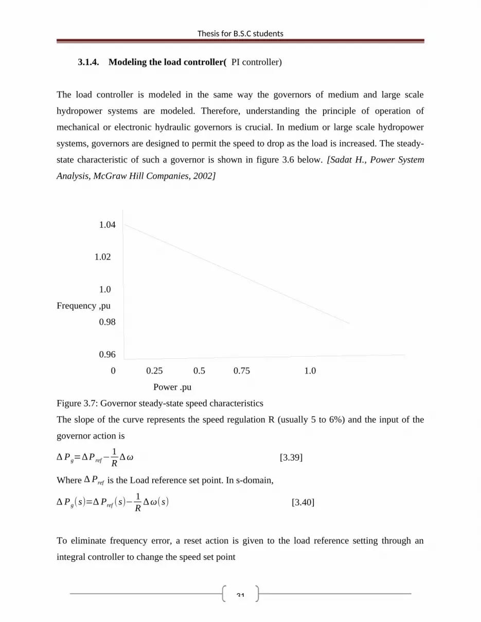
3.1.4. Modeling the load controller( PI controller)

The load controller is modeled in the same way the governors of medium and large scale

hydropower systems are modeled. Therefore, understanding the principle of operation of

mechanical or electronic hydraulic governors is crucial. In medium or large scale hydropower

systems, governors are designed to permit the speed to drop as the load is increased. The steady-

state characteristic of such a governor is shown in figure 3.6 below. [Sadat H., Power System

Analysis, McGraw Hill Companies, 2002]

1.04

1.02

1.0

Frequency ,pu

0.98

0.96

0 0.25 0.5 0.75 1.0

Power .pu

Figure 3.7: Governor steady-state speed characteristics

The slope of the curve represents the speed regulation R (usually 5 to 6%) and the input of the

governor action is

∆ Pg=∆ P ref−1R

∆ ω [3.39]

Where ∆ Pref is the Load reference set point. In s-domain,

∆ Pg(s)=∆ Pref (s)− 1R

∆ ω(s) [3.40]

To eliminate frequency error, a reset action is given to the load reference setting through an

integral controller to change the speed set point

32


Thus, Equation (3.6) becomes

∆ Pg(s)=−K I

s∆ ω (s)− 1

R∆ ω (s ) [3.41]

Where K I is an integral constant.

The second term in Equation (3.41) is similar to a proportional controller. Hence, Equation

(3.8) is obtained.

∆ Pg(s)=−K I

s∆ ω (s)−K p ∆ ω (s)

∆ Pg (s )=∆ ω (s)(K I

s+ K p) [ 3.42]

Where KP = 1/R.

The governor action is similar to the switching, in binary and phase delay load configuration, and

the DC motor, in mechanical load configuration. Therefore, it is concluded that the load

controller is approximated by a PI controller.

3.1.5. Stepper motors and Principles of operation of a stepper motor

Stepping motors fill a unique niche in the motor control world. These motors are commonly used

in measurement and control applications. Sample applications include ink jet printers, CNC

machines and volumetric pumps. Several features common to all stepper motors make them

ideally suited for these types of applications. [Chirau S., Sensorless Control of Stepper Motor

Using Kalman Filter]. These features are as follows:

1. Brushless – Stepper motors are brushless. The commutation and brushes of conventional

motors are some of the most failure-prone components, and they create electrical arcs that are

undesirable or dangerous in some environments.

2. Load Independent – Stepper motors will turn at a set speed regardless of load as long as the

load does not exceed the torque rating for the motor.

3. Open Loop Positioning – Stepper motors move in quantified increments or steps. As long as

the motor runs within its torque specification, the position of the shaft is known at all times

without the need for a feedback mechanism.

4. Holding Torque – Stepper motors are able to hold the shaft stationary.

5. Excellent response to start-up, stopping and reverse.

33


There are three basic types of stepping motors: permanent magnet, variable reluctance and

hybrid. This application note covers all three types. Permanent magnet motors have a magnetized

rotor, while variable reluctance motors have toothed soft-iron rotors. Hybrid stepping motors

combine aspects of both permanent magnet and variable reluctance technology. The stator ,or

stationary part of the stepping motor holds multiple windings. The arrangement of these

windings is the primary factor that distinguishes different types of stepping motors from an

electrical point of view. From the electrical and control system perspective, variable reluctance

motors are distant from the other types. Both permanent magnet and hybrid motors may be

wound using either unipolar windings, bipolar windings or bifilar windings. Each of

these is described in the sections below.

I. Variable Reluctance Motors

Variable Reluctance Motors (also called variable switched reluctance motors) have three to five

windings connected to a common terminal. Figure 3.8 shows the cross section of a three

winding, 30 degree per step variable reluctance motor.

Fig3.8.variable reluctance stepper motor

The rotor in this motor has four teeth and the stator has six poles, with each winding wrapped

around opposing poles. The rotor teeth marked X are attracted to winding 1 when it is energized.

This attraction is caused by the magnetic flux path generated around the coil and the rotor. The

rotor experiences a torque and moves the rotor in line with the energized coils, minimizing the

flux path. The motor moves clockwise when winding 1 is turned off and winding 2 in energized.

The rotor teeth marked Y are attracted to winding 2. This results in 30 degrees of clockwise

motion as Y lines up with winding 2. Continuous clockwise motion is achieved by sequentially

34


energizing and de-energizing windings around the stator. The following control sequence will

spin the motor depicted in Figure 1 clockwise for 12 steps or one revolution.

Figure 3.8 illustrates the most basic variable reluctance stepping motor. In practice, these motors

typically have more winding poles and teeth for smaller step angles. [McComb, Robot Builders

Bonaza, second edition]

The number of poles can be made greater by adding windings, for example, moving to 4 or 5

windings, but for small step angles, the usual solution is to use toothed pole pieces working

against a toothed rotor.

Variable reluctance motors using this approach are available with step angles close to one

degree.

Step in time 1 2 3 4 5 6 7 8 9 10 11 12

Winding 1 1 0 0 1 0 0 1 0 0 1 0 0

Winding 2 0 1 0 0 1 0 0 1 0 0 1 0

Winding 3 0 0 1 0 0 1 0 0 1 0 0 1

Table3.1: switching of variable reactance motor

Uni-polar Motors

Uni-polar stepping motors are composed of two windings, each with a center tap. The center taps

are either brought outside the motor as two separate wires (as shown in Figure 3.9) or connected

to each other internally and brought outside the motor as one wire.

Fig3.9 unipolar stepper motor

35


As a result, unipolar motors have 5 or 6 wires. Regardless of the number of wires, unipolar

motors are driven in the same way. The center tap wire(s) is tied to a power supply and the ends

of the coils are alternately grounded.

Unipolar stepping motors, like all permanent magnet and hybrid motors, operate differently from

variable reluctance motors. Rather than operating by minimizing the length of the flux path

between the stator poles and the rotor teeth, where the direction of current flow through the stator

windings is irrelevant, these motors operate by attracting the north or south poles of the

permanently magnetized rotor to the stator poles. Thus, in these motors, the direction of the

current through the stator windings determines which rotor poles will be attracted to which stator

poles. Current direction in unipolar motors is dependent on which half of a winding is energized.

Physically, the halves of the windings are wound parallel to one another. Therefore, one winding

acts as either a north or South Pole depending on which half is powered.

Figure 3.9 shows the cross section of a 30 degree per step unipolar motor. Motor winding

number 1 is distributed between the top and bottom stator poles, while motor winding number 2

is distributed between the left and right motor poles. The rotor is a permanent magnet with six

poles, three norths’ and three south’s, as shown in Figure 3.9. The difference between a

permanent magnet stepping motor and a hybrid stepping motor are lies in how the multi pole

rotor and multi-pole stator are constructed. These differences will be discussed later.

Step in time 1 2 3 4 5 6 7 8 9 10 11 12

Winding 1a 1 0 0 0 1 0 0 0 1 0 0 0

Winding 1b 0 0 1 0 0 0 1 0 0 0 1 0

Winding 2a 0 1 0 0 0 1 0 0 0 1 0 0

Winding 2b 0 0 0 1 0 0 0 1 0 0 0 1

Table 3.2 unipolar example 1

36


Note: Only half of each winding is energized at a time in the above sequence. As above, the

following sequence will spin the motor clockwise 12 steps or one revolution.

Step in time 1 2 3 4 5 6 7 8 9 10 11 12

Winding 1a 1 1 0 0 1 1 0 0 1 1 0 0

Winding 1b 0 0 1 1 0 0 1 1 0 0 1 1

Winding 2a 0 1 1 0 0 1 1 0 0 1 1 0

Winding 2b 1 0 0 1 1 0 0 1 1 0 0 1

Table 3.3 unipolar example 2

Unlike in the first sequence described, two winding halves are energized at one time in the

second sequence. This gives the motor more torque, but also increases the power usage by the

motor. Each of the above sequences describes single stepping or stepping the motor in its rated

step size (in this case 30 degrees). Combining these two sequences allows for half stepping the

motor. The combined sequence is shown in Example 3 (24 steps per revolution).

Example 3

This method moves the motor in steps that are half its rated step size. It is important to note that

the torque generated by the motor during this sequence is not constant, as alternating steps have

one and two halves of a winding energized respectively. Figure 2 illustrates the most basic

unipolar motor. For higher angular resolutions, the rotor must have more poles. Permanent

magnet rotors with 100 poles have been made, and this pole count is commonly achieved for

hybrid rotors, using toothed end-caps on a simple bipolar permanent magnet. When the rotor has

a high pole count, the stator poles are always toothed so that each stator winding works against a

large number ofrotor poles.

Winding 1a: 11000001110000011100000111Winding 1b: 00011100000111000001110000Winding 2a: 01110000011100000111000001Winding 2b: 00000111000001110000011100 time

37


CHOOSING A MOTOR

There are several factors to take into consideration when choosing a stepping motor for an

application. Some of these factors are what type of motor to use, the torque requirements of the

system, the complexity of the controller, as well as the physical characteristics of the motor. The

following paragraphs discuss these considerations.

Variable Reluctance versus Permanent Magnet or Hybrid

Variable Reluctance Motors (VRM) benefit from the simplicity of their design and these motors

do not require complex permanent magnet rotors, so are generally more robust than permanent

magnet motors. With all motors, torque falls with increased motor speed, but the drop in torque

with speed is less pronounced with variable reluctance motors. With appropriate motor design,

speeds in excess of 10,000 steps per second are feasible with variable reluctance motors, while

few permanent magnet and hybrid motors offer useful torque at 5000 steps per second and most

are confined to speeds below 1000 steps per second. The low torque drop-off with speed of

variable reluctance motors allows use of these motors, without gearboxes, in applications where

other motors require gearing. For example, some newer washing machines use variable

reluctance motors to drive the drum, thus allowing direct drive for both the slow oscillating wash

cycle and the fast spin cycle. Variable reluctance motors do have a drawback. With sinusoidal

exciting currents, permanent magnet and hybrid motors are very quiet. In contrast, variable

reluctance motors are generally noisy, no matter what drive waveform is used. As a result,

permanent magnet or hybrid motors are generally preferred where noise or vibrations are issues.

Unlike variable reluctance motors, permanent magnet and hybrid motors cog when they are

turned by hand while not powered. This is because the permanent magnets in these motors attract

the stator poles even when there is no power. This magnetic detent or residual holding torque is

desirable in some applications, but if smooth coasting is required, it can be a source of problems.

With appropriate control systems, both permanent magnet and hybrid motors can be micro

stepped, allowing positioning to a fraction of a step, and allowing smooth, jerk-free moves from

one step to the next. Micro stepping is not generally applicable to variable reluctance motors.

38


These motors are typically run in full-step increments. Complex current limiting control is

required to achieve high speeds with variable reluctance motors.

Hybrid versus Permanent Magnet

In selecting between hybrid and permanent magnet motors, the two primary issues are cost and

resolution. The same drive electronics and wiring options generally apply to both motor types.

Permanent magnet motors are, without question, some of the least expensive motors made. They

are sometimes described as can-stack motors because the stator is constructed as a stack of two

windings enclosed in metal stampings that resemble tin cans and are almost as inexpensive to

manufacture. In comparison, hybrid and variable reluctance motors are made using stacked

laminations with motor windings that are significantly more difficult to wind. [McComb, Robot

Builders Bonaza, second edition]

Permanent magnet motors are generally made with step sizes from 30 degrees to 3.6 degrees.

The challenge of magnetizing a permanent magnet rotor with more than 50 poles is such that

smaller step sizes are rare! In contrast, it is easy to cut finely spaced teeth on the end caps of a

permanent magnet motor rotor, so permanent magnet motors with step sizes of 1.8 degrees are

very common, and smaller step sizes are widely available. It is noteworthy that, while most

variable reluctance motors have fairly coarse step sizes, such motors can also be made with very

small step sizes. Hybrid motors suffer some of the vibration problems of variable reluctance

motors, but they are not as severe. They generally can step at rates higher than permanent magnet

motors, although very few of them offer useful torque above 5000 steps per second.

3.1.6. Modeling the stepper motor

A permanent magnet stepper motor is used in controlling the spear valve of a mini hydropower

system. The mechanical part of the permanent magnet stepper motor model can be expressed by

[Robust Deadbeat Controller Design using PSO for Positioning a Permanent Magnet Stepper

Motors]:

39


J d2 θdt 2 +D dθ

dt+N r nΦM iA sin(N r θ)+N r nΦM iBsin ¿-λ ¿¿+C sin ¿ (3.43)

This equation is the complete model of the permanent magnet stepping motor consists of the

rotor dynamic equation.

where J is the moment of rotor inertia (Kg.m2), D is the viscous damping coefficient

(N.m.s.rad1), C is the coulomb friction coefficient, iB ,iA are the currents in windings A and B, Nr

is the number of the rotor teeth, n ΦMis the flux linkage, θ is the rotational angle of the rotor and

λ is the tooth pitch in radians and TL is the load torque . On the other hand, the electrical part of

a permanent magnet stepper motor model is described by voltage equations for the stator

windings.

V−r iA−Ld iA

dt−M

d iB

dt− d

dt¿ (3.44)

V−r iB−Ld iB

dt−M

d iA

dt− d

dt¿ (3.45)

These two equations are differential equations for current equation. Where V is the DC terminal

voltage supplied to the stator windings (volt), L denotes the self-inductance of each stator phase

(mH), M represents the mutual inductance between phases (mH) and r is stator circuit resistance

(ohm). Those equations are nonlinear differential equations. Since it is very difficult to deal with

nonlinear differential equations analytically, linearization is needed.

The equilibrium position of the stator is θ= λ2 . When both motor windings will deviate from by

δ θ therefore, θ= λ2+δ θ. Then the nonlinearities expressed by sine and cosine functions in

equations of the above will be approximated with knowledge of trigonometric identities and

when N r δ θ is small angle: cos ( N r δ θ )=1and sin(N r δ θ)=N r δ θ. Then, the linearized model can

be expressed by

40


J d2 θdt 2 +D dδθ

dt+2N2

r nΦM i0 cos (N rλ

2)δ θ+N r nΦM sin ¿)+C sin¿

rδ iA+ Ld (δ i A)

dt+ M

d (δ iB)dt

−N r n ΦM sin ¿ (3.46)

Where, sin ¿) are constants.

The permanent magnet stepping motor transfer function is derived from equations of above are

with the aid of Laplace transform. The coulomb friction coefficient C is considered to be zero.

The resulting form of the transfer function in two-phase excitation is:

Θo

Θi=

rL

w 2np

s3+( rLp

+DJ )s2+( rD

Lp J w2 np (1+K p ))s+(rLp

)w2 np=G p(s) (3.47)

Where: Lp=L−M , w2np=

2 N2

rn ΦM I o cos( N rλ

2 )J

K p=nΦM sin2(

N rλ

2)

Lp I ocos (N rλ

2)

Neglecting the higher orders of the transfer function it can be simplified to the equation shown

below. The transfer function model of the PM stepper motor is required. The transfer function

between the desired and the output angle of a permanent magnet stepper motor is given by

[Erdal C., Determination of the Optimum Parameter Tolerances for a Permanent Magnet -

Step Motor]

θ0(s)θi(s)

=T ( s)=K m I p N r

Js2+βs+ Km I p N r (3.48)

where θ0 is the output angle, θiis the desired angle, J is the moment of inertia of the rotor, Kmis

the torque constant of the permanent magnet stepper motor, I pis the phase current, N r is the

number of rotor teeth, and β is viscous friction coefficient. The stepper motor is controlled by a

41


controller. The controller calculates the deviation in the desired angle based on the frequency

deviation in the mini hydropower system. In general, the block diagram in Figure 3.9 is obtained.

Here again, the controller is assumed to be proportional integral controller similar to the load

controller. [Erdal C., Determination of the Optimum Parameter Tolerances for a Permanent

Magnet -Step Motor]

−∆ PL

Turbine Generator

∆ G ∆ Pm

∆ ω

θ0 θi

Stepper motor PI controller

Figure 3.9: Flow control model of a mini hydropower system

CHAPTER FORE

4. Design and Analysis of the Control System

The frequency controller system is flow control mode. The flow control mode is applied to the

frequency control of standalone and mini hydropower systems. Thus, in this section we will see

the flow control mode.

4.1. Generator selection

Limiter 1−T w s1+0.5T w s

12 Hs+D

+

Km I p N r

Js2+ βs+Km I p N r

K P+K I

s

42


A synchronous generator with the specifications in Table 4.1 is selected.

Table 4.1: Specifications of 1FC2-283-4 synchronous generator

Parameter Value

Current rating 888A

The moment of inertia 3 kgm2

Power factor 0.8

Load damping coefficient 1.5%

Power rating 225kvA

Voltage rating 400 v

Speed 1500rpm

Number of pole 4

The allowable speed variation at full load for the 1FC2-283-4 synchronous generator is shown in

Table 4.1. So, a 5% steady-state frequency variation is set to be the desired specification.

Furthermore, conventional governors should respond to changes in load within five minutes.

Consequently, the specification for the settling time of the frequency in standalone, mini

hydropower systems is set to be five minutes. [Asia Commerce Import and Export Corporation,

1FC2 Brushless Three-Phase Synchronous Generators, Shangai, 2009]

Based on the specifications, the inertia constant (H) of the rotor of the synchronous generator and

turbine coupled together is calculated.

Assuming the overall efficiency of the turbine and generator to be 80%, the moment of inertia of

the rotor of the synchronous generator and its couples is calculated. Since the mechanical power

of the prime mover is 196 kW, the moment of inertia becomes and Sbase=225KVA.

First to find synchronous speed (Ns) = 120 f

p =120∗50

4 =1500rpm

ωm=2 π∗N s

60 =

2π∗150060 = 157.0796rad/sec

43


J= 1960000.5(157.072)

=15.889 kg . m2

Hence, the additional moment of inertia required from the turbine is 12.24 kgm2, and the inertia

constant (H) is found to be

H = 0.5 J ωm

2

Sbase = 0.5∗15.889∗¿¿0.87 sec

The block diagram of the generator is shown below:-

Generator

+ pm ∆ ω

-Pe

Fig 4.1 block diagram of generator

4.2. PI controller

The simplified mini hydropower system model for load control has been indicated in Figure 4.2

shows below the model of a simplified mini hydropower system for flow control.

-∆PL

Generator

0 ∆ ω12 Hs+D

+

11.74 s+1.5

+

44


- ∆PG

PI controller

Fig 4.2: Simplified model of a mini hydropower system

There are different techniques of tuning PI controller are tested for determining the parameters of

these controllers have been developed during past 60 years. Although most of these methods

provide acceptable performances for some transfer functions of the systems, there is not a

general method for tuning the parameters of these controllers, such as the refined Ziegler-Nichols

method, pole-zero cancellation method, and MOCM performance criteria have been proposed to

improve the performance of control systems which especially have a time delay. From these

methods the Ziegler-Nichols (ZN) method which is still widely used in industries for tuning

because it gives a high overshoot and a long settling time.

Ziegler-Nichols tuning rule:

Ziegler-Nichols tuning rule was the first such effort to provide a practical approach to tune a PI

controller. According to the rule, a PI controller is tuned by firstly setting it to the P-only mode

but Adjusting the gain to make the control system in continuous oscillation. The corresponding

gain is referred to as the ultimate gain (Ku) and the oscillation period is termed as the ultimate

period (Pu). Then, the PI controller parameters are determined from Ku and Pu the Ziegler-

Nichols tuning table.

controller kp Ti

P 1a

-

PI 0.9a

3L

Table.4.2 Tuning of PI controller Parameter according to Z-N Tuning

K P+K I

s

45


The most employed PI design technique used in the industry is the Ziegler–Nichols method,

which avoids the need for a model of the plant to be controlled and relies solely on the step

response of the plant. The parameter setting, according to the Ziegler–Nichols method, is carried

out in four steps.

1) Obtain the plant step response.

2) Draw the steepest straight-line tangent to the response.

3) Obtain the measurements

4) Set the parameters according to Table.4.2

The main features of PI controllers are the capacity to eliminate steady-state error of the response

to a step reference signal because of integral action and the ability to anticipate output changes

when derivative action is employed and it provides the steady state error to zero.

In Figure 4.3, the step response of the mini HPs is shown. The parameter a is near to -1 and

L is near to zero. Therefore, the parameters are approximated as a = 0.9 and L = 0.042 so that the

proportional 1 and integral gain constant is 0.125 each. [https://www.Modern control system]

Y(t)

0 L t

a

Fig 4.3: Step response for ZN PI controller design

After plugging the values of the proportional and integral gains, the block diagram in Fig 4.3 is

obtained:

46


- ∆PL

Generator

0 ∆ ω

- ∆PG

PI controller

Fig 4.4: Simplified model of a mini hydropower system with PI controllers

Assuming a step non-frequency sensitive consumer load change, the change in electrical power

in s-domain is given by

∆ Pe (s )=−∆ PL

s−∆ ω(s)(

K I

s+K p) (4.1)

The final value theorem is applied to find the steady state power error,

∆ Pess=lims →0

s [−∆ PL

s−∆ ω (s )( K I

s+K p)] (4.2)

The steady-state power error is zero, and simplifying Equation (4.2), an equation that relates

steady-state frequency error and change in non-frequency sensitive load becomes

∆ PL=−K I ∆ ωss (4.3)

Where ∆ ωssis the steady-state angular frequency error.

11.74 s+1.5

1+ 0.125s

+

47


4.3. Stepper motor selection

A stepper motor with the specifications in Table 4.3 is selected. [Stepper Motor,

www.motionking.com,] Table 4.3: Stepper motor specifications

Parameter Value

Model 43HS2A165-654

Number of teeth (Nr) 50

Rated phase current 6.5A

Phase resistance 0.65ohm

Phase inductance 14mH

Lead wire 4

Weight 11kg

Holding torque 26.0Nm

Step angle 1.8o

Inertia constant 0.0013kg-m2

Torque constant 4 N-m/A

Viscous friction constant(assume) 0.5N-m/rad/sec

The transfer function between the input and output angles of the PM stepper motor is given by

From the table rated current 6.5A, steep angle 1.8 degree, number of rotor teeth

Nr= 3600

p∗step angle= 3600

1.80∗4=50

T(s) = 50∗6.5∗0.5

0.0013 s2+0.5 s+162.5= 162.5

0.0013 s2+0.5 s+162.5 (4.4)

4.4. The water starting time of turbine

The water starting time is calculated by

48


TW = LU 0

gHO (4.5)

Some assumptions should be taken to determine the water starting time. Table 4.3 shows the

assumptions taken.

Table 4.3: Assumptions taken in calculating water starting time

Parameter value

Penstock length 5m, 17.5m,39.6m

Low head ,medium head, high head [Ho] 5m, 10m , 20m

Initial speed of water [Uo] √2 g H 0=9.9m/sec,14m/sec, 19.8m/sec

Acceleration due to gravity [g] 9.8m/sec

The water starting times are Tw 1.0sec, Tw 2.5 sec and Tw 4.0sec for low, medium and high

head mini hydropower systems respectively.

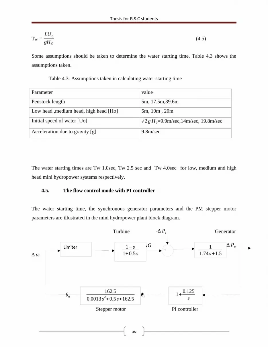
4.5. The flow control mode with PI controller

The water starting time, the synchronous generator parameters and the PM stepper motor

parameters are illustrated in the mini hydropower plant block diagram.

Turbine -∆ Pl Generator

∆ G ∆ Pm

∆ ω

θ0 θi

Stepper motor PI controller

Limiter 1−s1+0.5 s

11.74 s+1.5

+

162.50.0013 s2+0.5 s+162.5

1+ 0.125s

49


Fig 4.5: Block diagram of a low head mini hydropower plant with flow control

The block diagram in Fig 4.5 is checked for internal stability and is found to be well posed.

Based on the desired specifications of the plant, the PI parameters are determined using ZN

method are found to be Kp = 1 and KI = 0.125.

CHAPTER FIVE

5. RESULTS AND DISCUSSION

The transient response of a practical control system often exhibits damped oscillations before

reaching steady state. In specifying the transient-response characteristics of a control system to a

unit-step input, it is common to specify the following:

1. Delay time, td

2. . Rise time, tr

3. Peak time, tp

4. Maximum overshoot, Mp

5. Settling time, ts

These specifications are defined in what follows and are shown graphically in Figure below.

50


1. Delay time, td : The delay time is the time required for the response to reach half the

final value the very first time.

2. Rise time, tr : The rise time is the time required for the response to rise from 10% to

90%, 5% to 95%, or 0% to 100% of its final value. For under damped second order

systems, the 0% to 100% rise time is normally used. For over damped systems, the

10% to 90% rise time is commonly used.

3. Peak time, tp : The peak time is the time required for the response to reach the first

peak of the overshoot.

4. Maximum (percent) overshoot, Mp : The maximum overshoot is the maximum peak

value of the response curve measured from unity. If the final steady-state value of the

response differs from unity, then it is common to use the maximum percent

overshoot. The amount of the maximum (percent) overshoot directly indicates the

relative stability of the system.

5. Settling time, ts: The settling time is the time required for the response curve to reach

and stay within a range about the final value of size specified by absolute percentage

of the final value (usually 2% or 5%). The settling time is related to the largest time

constant of the control system. Which percentage error criterion to use may be

determined from the objectives of the system design in question.

Fig. 5.1 Transient-response characteristics of a control system

51


The frequency controller was modeled, designed and analyzed in the methods section of this

thesis. This chapter deals with the results and discussion of MATLAB simulations and

mathematical model. Besides, contributions of the thesis work are presented. [ Modern Control

system by Gosh, Ogata]

5.1.Simulation Results of the FCM

The transfer function model of a mini hydropower system with FCM is shown in Figure 4.5.

This model with and without the controller was simulated using a MATLAB code presented

below:-

MATLAB CODE WITH AND WITH OUT CONTROLER

%programmer: power engineering

% Date: 2013

%Program: This program plots the step response of frequency of mini

%hydropower system with FCM for low heads

%load change = 3%

TI=8; % the integral time constant

kp=1; %proportional gain

ki=kp/TI; % integral gain

Gen=tf(1,[2*0.87 1.5]); % synchronous generator %transfer function

% H = 0.87 sec and D = 1.5%

52


%---------------with controller---------------

PMstepper=tf(162.5,[0.0013 0.5 162.5]);%transfer function of the stepper motor

PI=tf([kp ki],[1 0]); % PI controller

Hturbine=tf([-1 1],[0.5 1]); %turbine transfer function

Hs=PI*PMstepper*Hturbine; %feedback transfer function

Gc=feedback(Gen,Hs); %Closed loop transfer function

step(50*0.03*Gc) %Step response

hold on

%-------------without controller



Hs=PMstepper*Hturbine; %feedback transfer function



ylabel('Frequency Deviation [Hz]');

xlabel('time');

legend('with controller', 'with out controller');

grid on

53


0 20 40 60 80 100 1200

0.1

0.2

0.3

0.4

0.5

0.6

0.7

0.8

0.9

Step Response

time (sec)

Freq

uenc

y D

evia

tion

[Hz]

w ith controllerw ith out controller

Fig 5.2.simulation result with and without controller low head, mini hydro power

The step response of the frequency deviation of a 492 kW, low head, mini hydropower system

for a 3% load change is shown in Fig 5.2. From the figure, it is seen that the mini hydropower

system is stable and the steady-state frequency deviation is eliminated by the controller.

Therefore, the low head, mini hydropower system with FCM is stable and shows good transient

and steady state performances.

Table 5.1

With controller Settling time Rise time Overshoot Steady state

69.1sec 0 inf 0

With out

controller

Settling time Rise time overshoot Steady state

4.45sec 0.633sec 25.2 0.66

MATLAB CODE OF POWER ERROR

54



% Date: 2013

%Program: This program plot the step response of power error

%of a low head mini hydropower system with FCM

%load change = 3%

%capacity = 492 kW


kp=1; % proportional gain



% H = 0.87sec and D = 1.5%

PMstepper=tf(162.5,[0.0013 0.5 162.5]); %transfer function of the stepper motor




perr= 1/(Gen*Hs+1);

step(492*0.03*perr,-492*0.03*perr); %step response

ylabel('power error [kW]');

xlabel('time');

title('Power error of low head mini hydropower system');

legend('delPL=-14.76 kW', 'delPL=14.76 kW');

55


grid on

Pow er error of low head mini hydropow er system

time (sec)

pow

er e

rror

[kW

]

0 20 40 60 80 100 120 140 160-20

-15

-10

-5

0

5

10

15

20

System: untitled2Final Value: 0

System: untitled2Settling Time (sec): 58.9


System: untitled1Rise Time (sec): 32.1

System: untitled2Rise Time (sec): 32.1

System: untitled1Peak amplitude: 18.4Overshoot (%): InfAt time (sec): 0.549

System: untitled2Peak amplitude: -18.4Overshoot (%): InfAt time (sec): 0.549

delPL=-14.76 kWdelPL=14.76 kW

Fig 5.3.Simulation result of power error for a low head, mini HPs

Figure 5.3 shows the step response of the power error for a 3% load change. As it is seen in

Figure 5.2 and Figure 5.3, both the steady-state frequency and power errors are zero

As it is observed from Figure 5.4 and Table 5.2, the frequency controller shows good transient

and steady-state performances during flow control mode for different heads. Beside this, the

controller was also tested for different capacities of mini hydropower systems. The inertia

constants for mini hydropower systems range from 2.8 seconds to 10 seconds. The steady state

56


frequency error is zero in all the cases and the transient performances for ranging capacities of

mini hydropower systems are summarized in Table 5.2.

MATLAB COD OF LOW HEAD MINI HYDRO POWER


% Date: 2013


%hydropower system with FCM for different heads

%load change = 3%





% H = 5 sec and D = 1.5%



%----------------- low head mini hydropower system -----------------------





57


Step Response

Time (sec)

Ampl

itude

0 20 40 60 80 100 1200

0.1

0.2

0.3

0.4

0.5

0.6

0.7

0.8


System: untitled1Final Value: 0

System: untitled1Rise Time (sec): 0

System: untitled1Peak amplitude: 0.762Overshoot (%): InfAt time (sec): 1.65

Fig.5.4 Frequency deviation step responses of low head mini HPs

Table 5.2: Transient performances for different capacities of low head mini HPs

Inertia Constant (H), D=1.5%,

3%

load change, low head

Settling time Overshoot/undershoot

0.87 69.1 ∞

2.8 71.1

4 69.1

5 66.7

7 59.8

10 82.1

58


Generally, to test the effectiveness of the frequency controller, similar tests had been done for

low, medium and high head mini hydropower systems. Figure 5.5 shows the frequency deviation

step responses of the three types of mini hydropower systems for a 3% load change.

MATLAB CODE OF THREE HEAD MINI HYDROPOWERS


% Date: 2013


%hydropower system with FCM for different heads

%load change = 3%





% H = 5 sec and D = 1.5%



%----------------- low head mini hydropower system -----------------------





59


hold on

%----------------- medium head mini hydropower system ---------------------

Hturbine=tf([-2.5 1],[1.25 1]); %turbine transfer function




hold on

%----------------- high head mini hydropower system -----------------------

Hturbine=tf([-4 1],[2 1]); %turbine transfer function




hold on

ylabel('Frequency Deviation [Hz]');

xlabel('time');

legend('low head','medium head','high head');

grid on

60


0 20 40 60 80 100 120-0.5

0

0.5

1

1.5

2

Step Response

time (sec)

Freq

uenc

y D

evia

tion

[Hz]

low headmedium headhigh head

Fig.5.5 Frequency deviation step responses of low, medium and high head mini HPs

Parameter Low head mini HPs Medium head mini

HPs

High head mini HPs

Settling time 69.1 56.6 54.7

Overshot

Table 5.3 Transient performances of mini HPs with FCM for different heads

As it is observed from Figure 5.5 and Table 5.3 the frequency controller shows good transient

and steady-state performances during flow control of different heads.

Beside this, the controller was also tested for different capacities of mini hydropower systems.

61


The inertia constants for mini hydropower systems range from 2.8 seconds to 10 seconds.

Generally, to test the effectiveness of the frequency controller, similar tests had been done for

low, medium and high head mini hydropower systems. Figure 5.4 shows the frequency deviation

step responses of the three types of mini hydropower systems for a 3% load change. The steady

state frequency error is zero in all the cases and the transient performances for ranging capacities

of mini hydropower systems as shown above in table of low head mini hydro power system.

Table 5.4: Transient performances for different capacities of medium head mini HPs


3%

load change, low head


0.87 56.6

2.8 61.8

4 60.5

5 58

7 50.3

10 81.4

Beside this, the controller was also tested for different capacities of mini hydropower systems.

The inertia constants for mini hydropower systems range from 2.8 seconds to 10 seconds.

The steady state frequency error is zero in all the cases and the transient performances for

ranging capacities of mini hydropower systems as shown above in table of medium head mini

hydro power system.

Table 5.5: Transient performances for different capacities of high head mini HPs


3%

load change, high head


62


0.87 54.7

1 50.3

2.8 53.3

4 52.2

5 49.7

7 39.8

10 77.5

From Table 5.2, Table 5.4 and Table 5.5, it is seen that the mini hydropower systems with the

same FCM have shown good transient performances and the steady state frequency errors were

found to be zero. Therefore, the designed frequency controller is applied to the whole range of

mini hydropower systems.

On the other hand, the frequency controller was also tested for different types of loadings.

The transient performances are summarized in Table 5.6, Table 5.7 and Table 5.8. The steady

state frequency error is zero in all the cases.

Table 5.6: Transient performances for different types of loadings of a low head, mini HPs

Load damping constant (D),

H=5sec, 3% load change, low

head


0.48% 58.8

0.8% 51.5

1.2% 53.9

1.5% 66.7

2% 85.1

63


Table 5.7: Transient performances for different types of loadings of a medium head, mini HPs


H=5sec, 3% load change,

medium head


0.48% 64.8

0.8% 49.7

1.2% 44.9

1.5% 58

2% 76.2

Table 5.8: Transient performances for different types of loadings of a high head, mini HPs


H=5sec, 3% load change, high

head


0.48% 81.6

0.8% 57

1.2% 31.1

1.5% 49.7

2% 67.4

Tables 5.6, Table 5.7 and Table 5.8 show that the frequency controller is efficient for all the

three types of mini hydropower systems for different types of load damping constants. In

general, from the FCM simulation results, it is concluded that the controller performs well for

different heads, capacities and types of loadings of mini hydropower systems.

64


5.2.Contributions of the thesis work

The frequency controller for standalone and mini hydropower systems has been developed in this

thesis. This work is new and original. Through several electronic flow controllers have been

developed flow controller is increased the flexibility of the controller and decreased the cost

significantly.

The other contribution of this thesis work to science is the modeling and analysis of mini hydro

power system is the analysis of the flow control model. A DC motor controlled spear valve is

recently being used to control the flow of water into the turbine. Different from related works,

the flow control analysis in this work was done by employing a permanent magnet stepper motor

controlled spear valve because a stepper motor is cheaper, more reliable and easy to control. This

is a new approach.

5.

c

65


CHAPTER SIX

6. CONCLUSIONS AND RECOMMENDATIONS

6.1. Conclusions

In this thesis, the frequency controller for standalone and mini hydropower systems has been

developed.

Furthermore, simulation using MATLAB has shown that the developed controller is applicable

for different capacities, types of loadings and heads of standalone and mini hydropower systems.

This work is a significant contribution to the engineering capacity of our country to exploit the

large mini hydro potential available. The developed frequency control system can be used in the

Ethiopian Rural Electrification Program using standalone and mini hydropower systems. The

cost of the developed controller is significantly lower than its equivalent to be imported resulting

in foreign currency saving. Besides, the developed controller is harmonics free, reliable and fast.

The controller accepts big load changes and requires less maintenance.

66


6.2. Recommendations

In the future, the performances of the frequency controller with grid connected mini hydropower

systems can be investigated. In addition, the ballast load can be designed further for better

mechanical strength, electrical reliability and cost. Moreover, the steady state frequency accuracy

can be improved.

Documents

Frequency Controller for Standalone Mini Hydropower System