Embed Size (px)
Citation preview
From Classical Mechanics to Quantum Mechanics
Richard Froese
Department of Mathematics
University of British Columbia
May 4, 2018
These are the notes for five one hour lectures delivered at the 2016 CRM summer school in
Spectral Theory at Laval University. They were intended to provide some general background on
classical and quantum mechanics to advanced undergraduate and beginning graduate students in
mathematics. The first four lectures contain an outline of these two theories from a mathematical
point view and a comparison of the classical and quantum descriptions of some simple systems.
The last lecture is about hidden variables and is meant to illustrate the essential strangeness
of the quantum description of nature. I have tried to make these notes more accessible by
including an outline of some basic ideas in measure theory and operator theory. A similar outline
of the basics of manifolds, tangent and cotangent spaces and differential forms would have
been useful for understanding the sections on Lagrangian submanifolds and Hamilton-Jacobi
equations. Unfortunately I did not have time to include this. I am grateful to Cyrus Bhiladvala
and the referee for making suggestions for improvement.
Table of Contents
1. Classical Mechanics
Newton’s equations and Hamilton’s equations . . . . . . . . . . . . . . . . . . . . . . . . . . . . . . . . . . . . . . . . . . . 2
Example 1: Free motion . . . . . . . . . . . . . . . . . . . . . . . . . . . . . . . . . . . . . . . . . . . . . . . . . . . . . . . . . . . . . . . . . 4
Example 2: Harmonic Oscillator . . . . . . . . . . . . . . . . . . . . . . . . . . . . . . . . . . . . . . . . . . . . . . . . . . . . . . . . . 5
Example 3: Two bump potential n = 1 . . . . . . . . . . . . . . . . . . . . . . . . . . . . . . . . . . . . . . . . . . . . . . . . . . . 6
Symplectic form, Poisson bracket and time evolution of observables . . . . . . . . . . . . . . . . . . . . . . 7
Symplectic flow and Poincare recurrence . . . . . . . . . . . . . . . . . . . . . . . . . . . . . . . . . . . . . . . . . . . . . . . .10
Summary of Classical Mechanics (so far) . . . . . . . . . . . . . . . . . . . . . . . . . . . . . . . . . . . . . . . . . . . . . . . . 12
The Hamilton Jacobi Equation . . . . . . . . . . . . . . . . . . . . . . . . . . . . . . . . . . . . . . . . . . . . . . . . . . . . . . . . . . 12
Lagrangian submanifolds . . . . . . . . . . . . . . . . . . . . . . . . . . . . . . . . . . . . . . . . . . . . . . . . . . . . . . . . . . . . . . .13
Legendre transforms . . . . . . . . . . . . . . . . . . . . . . . . . . . . . . . . . . . . . . . . . . . . . . . . . . . . . . . . . . . . . . . . . . . 15
Flow outs . . . . . . . . . . . . . . . . . . . . . . . . . . . . . . . . . . . . . . . . . . . . . . . . . . . . . . . . . . . . . . . . . . . . . . . . . . . . . . 15
1
Extended phase space and the geometry of the Hamilton Jacobi equations . . . . . . . . . . . . . . . 16
Remark on solving for the flow using the Hamilton Jacobi equation . . . . . . . . . . . . . . . . . . . . . 18
An example . . . . . . . . . . . . . . . . . . . . . . . . . . . . . . . . . . . . . . . . . . . . . . . . . . . . . . . . . . . . . . . . . . . . . . . . . . . . 19
2. Review of Probability and Operator theory
Probability . . . . . . . . . . . . . . . . . . . . . . . . . . . . . . . . . . . . . . . . . . . . . . . . . . . . . . . . . . . . . . . . . . . . . . . . . . . . . 21
Two theorems in measure theory . . . . . . . . . . . . . . . . . . . . . . . . . . . . . . . . . . . . . . . . . . . . . . . . . . . . . . . 23
Mixed states in Classical Mechanics . . . . . . . . . . . . . . . . . . . . . . . . . . . . . . . . . . . . . . . . . . . . . . . . . . . . .24
Background and self-adjoint operators . . . . . . . . . . . . . . . . . . . . . . . . . . . . . . . . . . . . . . . . . . . . . . . . . . 24
Spectral theorem for self-adjoint operators . . . . . . . . . . . . . . . . . . . . . . . . . . . . . . . . . . . . . . . . . . . . . . 25
The Fourier transform . . . . . . . . . . . . . . . . . . . . . . . . . . . . . . . . . . . . . . . . . . . . . . . . . . . . . . . . . . . . . . . . . . 26
Uncertainty principle . . . . . . . . . . . . . . . . . . . . . . . . . . . . . . . . . . . . . . . . . . . . . . . . . . . . . . . . . . . . . . . . . . .27
One parameter strongly continuous unitary groups and Stone’s theorem . . . . . . . . . . . . . . . . 27
3. Quantum Mechanics
Abstract Quantum description of a physical system . . . . . . . . . . . . . . . . . . . . . . . . . . . . . . . . . . . . . 29
Quantum particle in an external potential . . . . . . . . . . . . . . . . . . . . . . . . . . . . . . . . . . . . . . . . . . . . . . . 30
Example 1: Free motion . . . . . . . . . . . . . . . . . . . . . . . . . . . . . . . . . . . . . . . . . . . . . . . . . . . . . . . . . . . . . . . . 32
Using the Hamilton Jacobi equation . . . . . . . . . . . . . . . . . . . . . . . . . . . . . . . . . . . . . . . . . . . . . . . . . . . . .34
Example 2: The Harmonic Oscillator . . . . . . . . . . . . . . . . . . . . . . . . . . . . . . . . . . . . . . . . . . . . . . . . . . . .37
Example 3: The two bump potential . . . . . . . . . . . . . . . . . . . . . . . . . . . . . . . . . . . . . . . . . . . . . . . . . . . . 41
4. Hidden variables and non-locality
Introduction . . . . . . . . . . . . . . . . . . . . . . . . . . . . . . . . . . . . . . . . . . . . . . . . . . . . . . . . . . . . . . . . . . . . . . . . . . . .43
Spin observables A and B . . . . . . . . . . . . . . . . . . . . . . . . . . . . . . . . . . . . . . . . . . . . . . . . . . . . . . . . . . . . . . 44
Tensor Product . . . . . . . . . . . . . . . . . . . . . . . . . . . . . . . . . . . . . . . . . . . . . . . . . . . . . . . . . . . . . . . . . . . . . . . . . 46
Hardy’s example . . . . . . . . . . . . . . . . . . . . . . . . . . . . . . . . . . . . . . . . . . . . . . . . . . . . . . . . . . . . . . . . . . . . . . . 46
Bell’s second theorem: non-locality . . . . . . . . . . . . . . . . . . . . . . . . . . . . . . . . . . . . . . . . . . . . . . . . . . . . . 48
References . . . . . . . . . . . . . . . . . . . . . . . . . . . . . . . . . . . . . . . . . . . . . . . . . . . . . . . . . . . . . . . . . . . . . . . . . . . . . . . . .51
1. Classical Mechanics
Newton’s equations and Hamilton’s equations
We begin by showing how Classical Mechanics describes the motion of a single particle of
mass m moving in configuration space Rn under the influence of an external conservative force
2
field. The force felt by the particle at the point x = (x1, . . . , xn) ∈ Rn is F (x) = −∇V (x), where
the potential V is a real valued function. The motion is described by the trajectory x(t), where
t ∈ R is time, and x(t) is the position at time t. According to Newton’s law F = ma, the trajectory
satisfies the equation
mx = −∇V (x). (1.1)
This is a system of n second order ODEs so under suitable conditions on V , there is a unique
solution x(t) if we impose initial conditions
x(0) = x0
x(0) = v0.(1.2)
There is a standard trick for turning a system of n second order equations into an equivalent
system of 2n first order equations. If x(t) solves Newton’s equation (1.1) with initial conditions
(1.2), then, defining the momentum as p(t) = mx(t), we find that (x(t), p(t)) ∈ Rn × Rn satisfies
Hamilton’s equations
x =1
mp
p = mx = −∇V (x),
(1.3)
with initial conditionsx(0) = x0
p(0) = mv0 = p0.(1.4)
On the other hand, if (x(t), p(t)) solves Hamilton’s equations (1.3) with initial condition (1.4), then
x(t) solves Newton’s equation (1.1) with initial conditions (1.2).
Hamilton’s equations are a first order system in phase space Rn × Rn. The right side of (1.3)
defines a vector field on phase space, namely
(x, p) 7→
1
mp
−∇V (x)
.The trajectories (x(t), p(t)) are the corresponding flow.
Although it is not obvious, the vector field on the right of (1.3) is very special. Let H(x, p) be
the real valued function on phase space defined by
H(x, p) =p2
2m+ V (x).
Here p2 = 〈p, p〉 is the square of the standard Euclidean norm of p in Rn. The function H(x, p),
called the Hamiltonian, represents the total energy (kinetic plus potential) of the particle. Written
in terms of H , Hamilton’s equations have the form
x =∂H
∂p(x, p)
p = −∂H∂x
(x, p),
(1.5)
3
where
∂H
∂x=
∂H
∂x1...∂H
∂xn
, ∂H
∂p=
∂H
∂p1...∂H
∂xp
denote the gradients with respect to the position variables x1, . . . , xn and momentum variables
p1, . . . , pn respectively.
To get a feeling for Hamilton’s equations let’s look at three simple examples. For a Hamilto-
nian of the form H(x, p) =p2
2m+ V (x) we can get a mental image of the motion by imagining a
particle sliding without friction on a hill whose height at the point x is V (x).
In these examples we will pay attention to the presence of bound states and scattering states.
Bound states are trajectories for which x(t) remains bounded for all time, while scattering states
are those where |x(t)| tends to infinity when t→ ±∞.
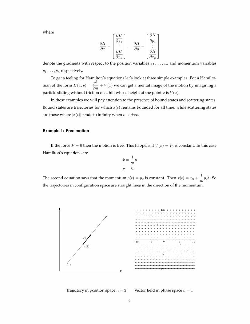
Example 1: Free motion
If the force F = 0 then the motion is free. This happens if V (x) = V0 is constant. In this case
Hamilton’s equations are
x =1
mp
p = 0.
The second equation says that the momentum p(t) = p0 is constant. Then x(t) = x0 +1
mp0t. So
the trajectories in configuration space are straight lines in the direction of the momentum.
x0
x(t)
p0
Trajectory in position space n = 2 Vector field in phase space n = 1
4
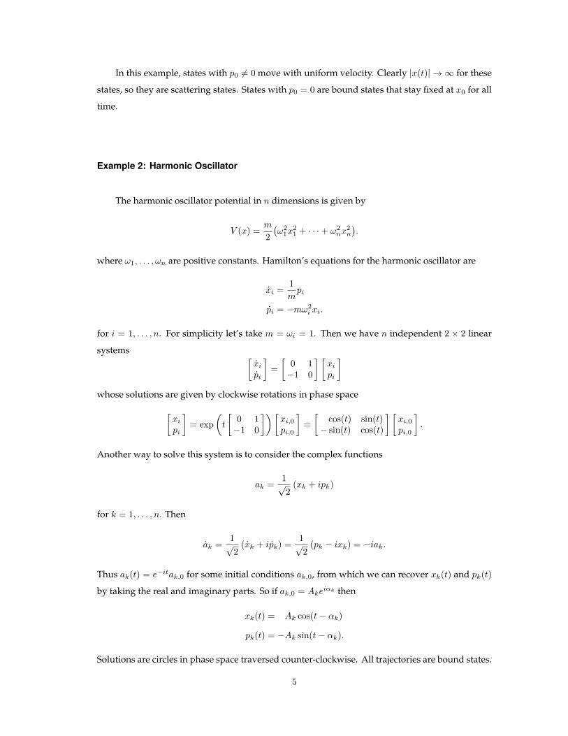
In this example, states with p0 6= 0 move with uniform velocity. Clearly |x(t)| → ∞ for these
states, so they are scattering states. States with p0 = 0 are bound states that stay fixed at x0 for all
time.
Example 2: Harmonic Oscillator
The harmonic oscillator potential in n dimensions is given by
V (x) =m
2
(ω2
1x21 + · · ·+ ω2
nx2n
).
where ω1, . . . , ωn are positive constants. Hamilton’s equations for the harmonic oscillator are
xi =1
mpi
pi = −mω2i xi.
for i = 1, . . . , n. For simplicity let’s take m = ωi = 1. Then we have n independent 2 × 2 linear
systems [xipi
]=
[0 1−1 0
] [xipi
]whose solutions are given by clockwise rotations in phase space[
xipi
]= exp
(t
[0 1−1 0
])[xi,0pi,0
]=
[cos(t) sin(t)− sin(t) cos(t)
] [xi,0pi,0
].
Another way to solve this system is to consider the complex functions
ak =1√2
(xk + ipk)
for k = 1, . . . , n. Then
ak =1√2
(xk + ipk) =1√2
(pk − ixk) = −iak.
Thus ak(t) = e−itak,0 for some initial conditions ak,0, from which we can recover xk(t) and pk(t)
by taking the real and imaginary parts. So if ak,0 = Akeiαk then
xk(t) = Ak cos(t− αk)
pk(t) = −Ak sin(t− αk).
Solutions are circles in phase space traversed counter-clockwise. All trajectories are bound states.
5
Harmonic oscillator potential n = 1 Harmonic oscillator vector field in phase space
Problem 1.1: What are the solutions for general m and ωi?
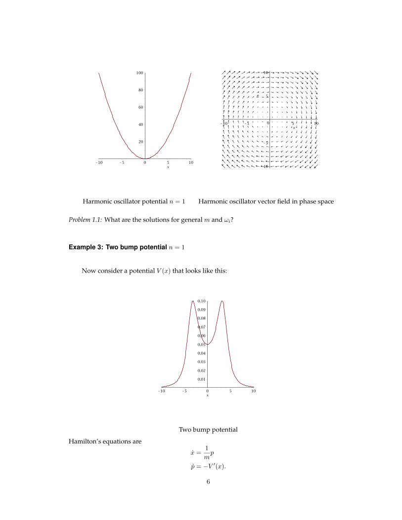
Example 3: Two bump potential n = 1
Now consider a potential V (x) that looks like this:
Two bump potential
Hamilton’s equations are
x =1
mp
p = −V ′(x).
6
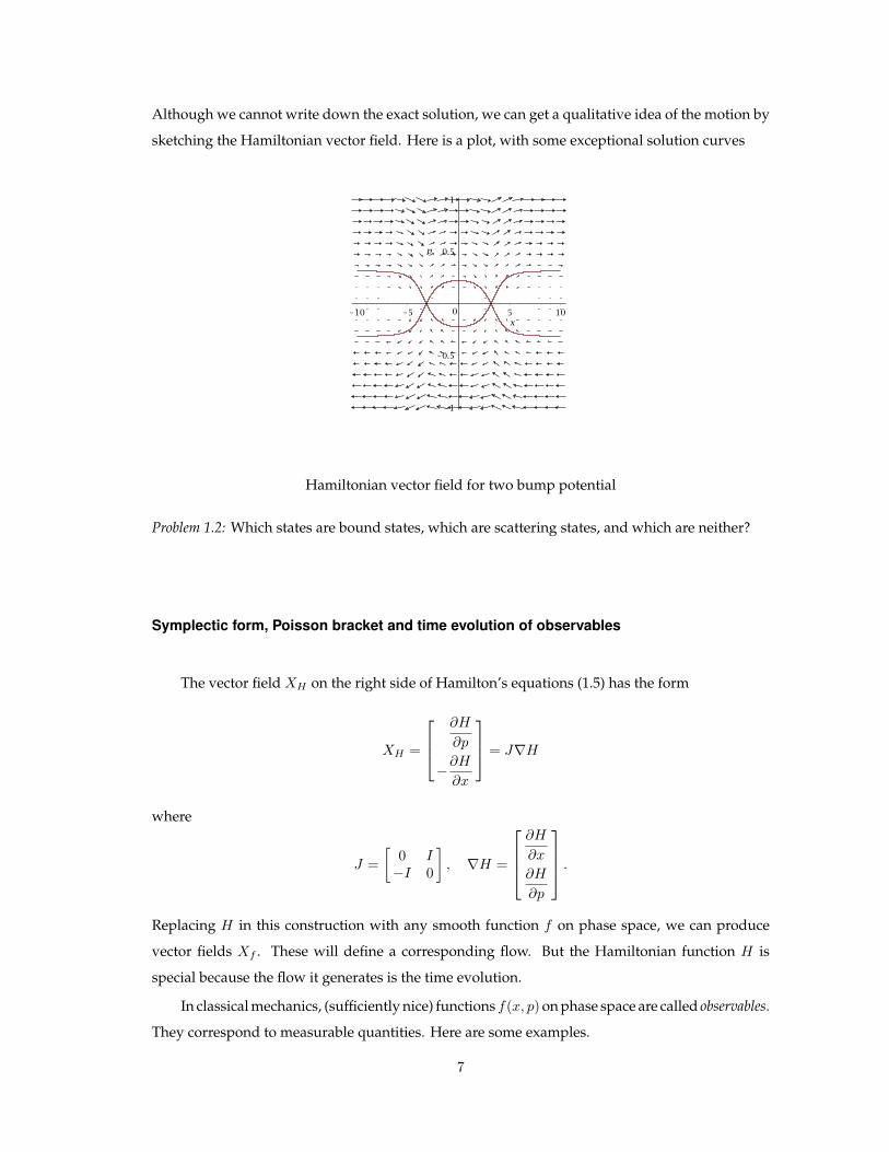
Although we cannot write down the exact solution, we can get a qualitative idea of the motion by
sketching the Hamiltonian vector field. Here is a plot, with some exceptional solution curves
Hamiltonian vector field for two bump potential
Problem 1.2: Which states are bound states, which are scattering states, and which are neither?
Symplectic form, Poisson bracket and time evolution of observables
The vector field XH on the right side of Hamilton’s equations (1.5) has the form
XH =
∂H
∂p
−∂H∂x
= J∇H
where
J =
[0 I−I 0
], ∇H =
∂H
∂x
∂H
∂p
.Replacing H in this construction with any smooth function f on phase space, we can produce
vector fields Xf . These will define a corresponding flow. But the Hamiltonian function H is
special because the flow it generates is the time evolution.
In classical mechanics, (sufficiently nice) functions f(x, p) on phase space are called observables.
They correspond to measurable quantities. Here are some examples.
7
Observable f(x, p)
position xi
momentum pi
angular momentum in 2-d x1p2 − x2p1
energy H(x, p)
To determine how the value of an observable changes in time as the particle moves along a
trajectory we use the chain rule to compute
d
dtf(x(t), p(t)) =
⟨∇f,
[x(t)p(t)
]⟩= 〈∇f, J∇H〉 (1.6)
where the gradients are evaluated at (x(t), p(t)). We now introduce some notation to rewrite
this equation. Define ω to be the antisymmetric bilinear form whose value on vectors X and Y
(thought of as tangent vectors to phase space) is given by
ω[X,Y ] = 〈X, JY 〉 . (1.7)
This ω is called the symplectic form. Then the Poisson bracket of two observables f and g is defined
as
f, g = ω[∇f,∇g] =∑i
∂f
∂xi
∂g
∂pi− f∂
∂pi
∂g
∂xi.
The Poisson bracket is an antisymmetric bilinear form on (differentiable) observables. It is a
derivation, which means that it satisfies the product rule
f, gh = gf, h+ f, gh.
It also satisfies the Jacobi identity
f, g, h+ h, f, g+ g, h, f = 0.
Using this notation, equation (1.6) can be written
d
dtf = f,H
with all functions evaluated at (x(t), p(t)). Since f, f = 0 for any f we see that energy is
conserved:d
dtH = H,H = 0.
Other observables f will be constants of motion provided f,H = 0. Here is an example.
For the harmonic oscillator in n dimensions, we can define n observables I1, . . . , In, called action
variables, as
Ik(x, p) =1
2mp2k +
m
2ω2kx
2k.
8
ClearlyH = I1 + · · ·+In and for j 6= k, Ik, Ij = 0 since they depend on disjoint sets of variables.
Thus Ik, H = Ik, I1 + · · · + In = Ik, Ik = 0. So the action variables are constants of the
motion.
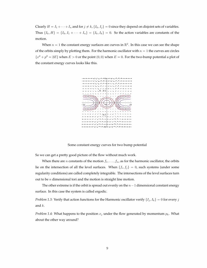
When n = 1 the constant energy surfaces are curves in R2. In this case we can see the shape
of the orbits simply by plotting them. For the harmonic oscillator with n = 1 the curves are circles
x2 + p2 = 2Ewhen E > 0 or the point (0, 0) when E = 0. For the two-bump potential a plot of
the constant energy curves looks like this.
Some constant energy curves for two bump potential
So we can get a pretty good picture of the flow without much work.
When there are n constants of the motion f1, . . . , fn, as for the harmonic oscillator, the orbits
lie on the intersection of all the level surfaces. When fi, fj = 0, such systems (under some
regularity conditions) are called completely integrable. The intersections of the level surfaces turn
out to be n dimensional tori and the motion is straight line motion.
The other extreme is if the orbit is spread out evenly on the n−1 dimensional constant energy
surface. In this case the system is called ergodic.
Problem 1.3: Verify that action functions for the Harmonic oscillator verify Ij , Ik = 0 for every j
and k.
Problem 1.4: What happens to the position xj under the flow generated by momentum pk. What
about the other way around?
9
Symplectic flow and Poincare recurrence
The Hamiltonian flow Φt associated with XH is the map Φt : (x, p) 7→ (x(t), p(t)), where
(x(t), p(t)) solves Hamilton’s equations with intial condition (x, p). In other words
d
dtΦt(x, p) = XH(Φt((x, p))), Φ0((x, p)) = (x, p)
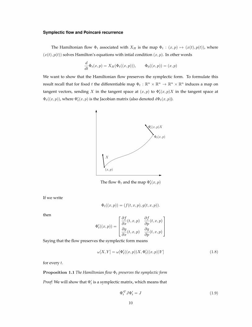
We want to show that the Hamiltonian flow preserves the symplectic form. To formulate this
result recall that for fixed t the differentiable map Φt : Rn × Rn → Rn × Rn induces a map on
tangent vectors, sending X in the tangent space at (x, p) to Φ′t(x, p)X in the tangent space at
Φt((x, p)), where Φ′t(x, p) is the Jacobian matrix (also denoted dΦt(x, p)).
(x, p)
Φt(x, p)
X
Φ′t(x, p)X
The flow Φt and the map Φ′t(x, p)
If we write
Φt((x, p)) = (f(t, x, p), g(t, x, p)).
then
Φ′t((x, p)) =
∂f
∂x(t, x, p)
∂f
∂p(t, x, p)
∂g
∂x(t, x, p)
∂g
∂p(t, x, p)
Saying that the flow preserves the symplectic form means
ω[X,Y ] = ω[Φ′t((x, p))X,Φ′t((x, p))Y ] (1.8)
for every t.
Proposition 1.1 The Hamiltonian flow Φt preserves the symplectic form
Proof: We will show that Φ′t is a symplectic matrix, which means that
Φ′Tt JΦ′t = J (1.9)
10
If (1.9) holds then ω[Φ′tX,Φ′tY ] = 〈Φ′tX, JΦ′tY 〉 = 〈X,Φ′Tt JΦ′tY 〉 = 〈X, JY 〉 = ω[X,Y ]. Thus (1.9)
implies (1.8).
Writing out the equation for the flow, we have
d
dtΦt(x, p) = J∇H(Φt(x, p)).
Computing the Jacobian of both sides, and exchanging the order of the partial differentiation with
respect to x and p with the time derivative gives
d
dtΦ′t(x, p) = JH ′′(Φt(x, p))Φ
′t(x, p)
where H ′′ is the Hessian of H . Now
d
dt(Φ′Tt JΦ′t) = (JH ′′Φ′t)
TJΦ′t + Φ′TJ(JH ′′Φ′t)
= Φ′Tt H′′TJTJΦ′t + Φ′Tt JJH
′′Φ′t
= Φ′Tt H′′Φ′t − Φ′Tt H
′′Φ′t
= 0
Here we used JTJ = I , J2 = −I andH ′′T = H ′′. This implies that Φ′Tt JΦ′t is constant.When t = 0
we have Φ′0 = I so the constant value is J .
Corollary 1.2 (Liouville’s theorem) The Hamiltonian flow preserves the phase space volume.
Proof: Taking the determinant of both sides of (1.9) yields det(Φ′t)2 = 1 so |det(Φ′t)| = 1. Now if A
is a (measurable) set in phase space then
Vol(Φt(A)) =
∫A
|det(Φ′t)(x, p)| dxndpn =
∫A
dxndpn = Vol(A)
Corollary 1.3 (Poincare’s recurrence theorem) Suppose that Φt(V ) ⊂ V for all times t and for some set
V in phase space with Vol(V ) <∞. Let v ∈ V and T > 0. Then any neighbourhood U ⊆ V of v contains
a point that returns to U after time T .
Proof: Let F = ΦT and denote the k fold iterate F F · · · F by F k. Then U,F (U), F 2(U), . . . are
contained in V and have the same non-zero volume. If they were all disjoint then V would have
infinite volume. Thus F k(U) ∩ F j(U) 6= ∅ for some k > j which implies F k−j(U) ∩ U 6= ∅.
Problem 1.5: Show that if M is a symplectic matrix MTJM = J then det(M) = 1.
11
Summary of Classical Mechanics (so far)
A pure state of the system is a point (x, p) in phase space. We call these pure states to
distinguish them from mixed states, introduced later. A pure state is meant to describe the system
completely with no uncertainty.
Observables are smooth real valued functions f on phase space. There is a pairing between
states and observables given by
〈f |(x, p)〉 = f(x, p).
This is a real number representing the result of making a measurement of the observable f when
the system is in the state (x, p).
There is a distinguished observable H(x, p) representing the total energy of the system. The
time evolution of states is given by Hamiltonian flow Φt. This flow preserves the symplectic form.
The time evolution on observables is defined via the pairing. Explicitly, f(x, p, t) = Φ∗t f , where
〈Φ∗t f |(x, p)〉 = 〈f |Φt(x, p)〉. The time evolution on observables obeys
f ′ = f,H,
where ·, · is the Poisson bracket.
The Hamilton Jacobi Equation
One of the points of contact between Classical and Quantum mechanics is the Hamilton Jacobi
equation.
H(x,∇S(x, t)) +∂S
∂t(x, t) = 0 (1.10)
and its variant
H(x,∇s(x,E))− E = 0 (1.11)
We want to explain how these equation can be solved using the Hamiltonian flow for H . Since
the solution to these equations can be used to construct approximate solutions to the Schrodinger
equation in various situations, the equations provide a link between classical and quantum me-
chanics. We will consider an example of this later in the course.
Although it is not really important for us, it is remarkable that sometimes solutions to (1.11)
can be used to determine the Hamiltonian flow for H .
It is maybe not surprising that first order equations can be solved using flows. But there is
some pretty geometry connected with these equations that I’ll try to describe. A reference for this
material (in fact for everything in this section) is Arnold’s classic book on Classical Mechanics
[A]. I have tried to give an informal account of the main ideas. This section uses the language of
12
differential forms. In the context of classical mechanics, these are described in Arnold [A] and in
Marsden and Ratiu [MR].
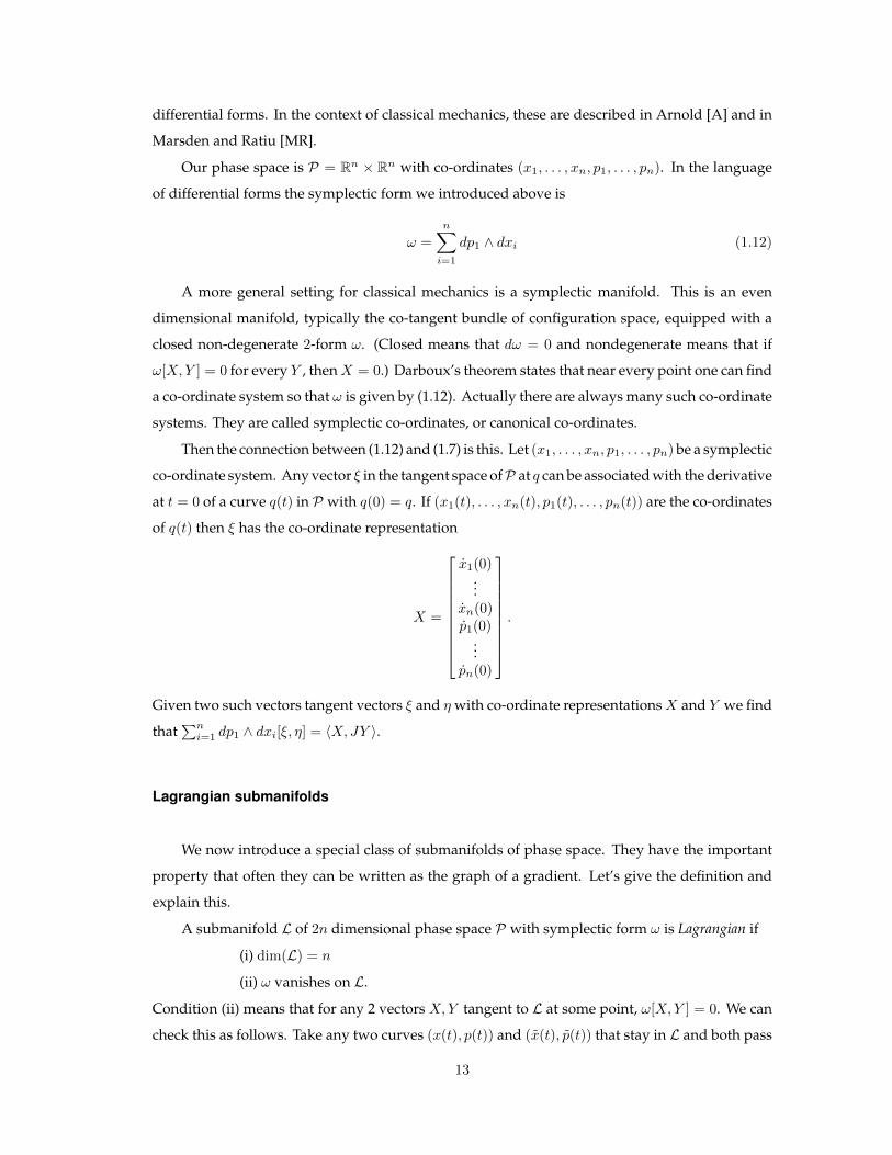
Our phase space is P = Rn × Rn with co-ordinates (x1, . . . , xn, p1, . . . , pn). In the language
of differential forms the symplectic form we introduced above is
ω =
n∑i=1
dp1 ∧ dxi (1.12)
A more general setting for classical mechanics is a symplectic manifold. This is an even
dimensional manifold, typically the co-tangent bundle of configuration space, equipped with a
closed non-degenerate 2-form ω. (Closed means that dω = 0 and nondegenerate means that if
ω[X,Y ] = 0 for every Y , thenX = 0.) Darboux’s theorem states that near every point one can find
a co-ordinate system so that ω is given by (1.12). Actually there are always many such co-ordinate
systems. They are called symplectic co-ordinates, or canonical co-ordinates.
Then the connection between (1.12) and (1.7) is this. Let (x1, . . . , xn, p1, . . . , pn) be a symplectic
co-ordinate system. Any vector ξ in the tangent space ofP at q can be associated with the derivative
at t = 0 of a curve q(t) in P with q(0) = q. If (x1(t), . . . , xn(t), p1(t), . . . , pn(t)) are the co-ordinates
of q(t) then ξ has the co-ordinate representation
X =
x1(0)...
xn(0)p1(0)
...pn(0)
.
Given two such vectors tangent vectors ξ and η with co-ordinate representationsX and Y we find
that∑ni=1 dp1 ∧ dxi[ξ, η] = 〈X, JY 〉.
Lagrangian submanifolds
We now introduce a special class of submanifolds of phase space. They have the important
property that often they can be written as the graph of a gradient. Let’s give the definition and
explain this.
A submanifold L of 2n dimensional phase space P with symplectic form ω is Lagrangian if
(i) dim(L) = n
(ii) ω vanishes on L.
Condition (ii) means that for any 2 vectors X,Y tangent to L at some point, ω[X,Y ] = 0. We can
check this as follows. Take any two curves (x(t), p(t)) and (x(t), p(t)) that stay in L and both pass
13
through q ∈ L when t = 0. Let X =
[x(0)p(0)
]and Y =
[˙x(0)˙p(0)
]. Then we must have 〈X, JY 〉 = 0 .
If L satisfies (ii) but not (i) it is called isotropic.
Here are some examples. When n = 1 then a n-dimensional submanifold of phase space
R × R is a curve. There is only one tangent direction, so all tangent vectors are a multiple of a
single vector X . By the antisymmetry of ω[X,X] = 0. Another example is the submanifold
L1 = (x0, p) : p ∈ Rn.
containing all points in phase space lying above a fixed x0 in configuration space. Tangent vectors
to L1 have the form[
0A
]and
⟨[0A
], J
[0B
]⟩= 0, for any A,B ∈ Rn. A final simple example is
L2 = (x, p) ∈ Rn × Rn : x = p.
In this case tangent vectors have the form[AA
]for A ∈ Rn and
⟨[AA
], J
[BB
]⟩= 0, for any
A,B ∈ Rn.
An n-dimensional submanifold L of phase space is a graph over x = (x1, . . . , xn) if there are
functions p(x) = (p1(x), . . . , pn(x)) so that (x, p) ∈ L ⇔ p = p(x). In this case x = (x1, . . . , xn) are
co-ordinates for L. In the examples above L1 is a graph over p1, . . . , pn but not over x1, . . . , xn.
On the other hand L2 is a graph over both x1, . . . , xn and p1, . . . , pn.
Here is the main point of this section.
Proposition 1.4 Let (x1, . . . , xn, p1, . . . , pn) be symplectic co-ordinates. Suppose that L is a graph over
(x1, . . . , xn). Then L is Lagrangian⇔ there is a function S(x) such that p(x) = ∇S(x).
Remark: This proposition holds more generally for co-ordinates (x1, . . . , xn, p1, . . . , pn) where∑dpi ∧ dxi = fω is a multiple of ω. So (x1, . . . , xn, p1, . . . , pn) could be (x1, . . . , xn, p1, . . . , pn) =
(p1, . . . , pn, x1, . . . , xn) in which case f = −1. Sometimes this extra flexibility is useful.
Proof: If p(x) = ∇S(x), then tangent vectors to L at the point (x, p(x)) have the form[
AS′′(x)A
]where A ∈ Rn and S′′(x) =
[∂2S(x)
∂xi∂xj
]is the Hessian of S. Then⟨[
AS′′(x)A
], J
[B
S′′(x)B
]⟩= 〈A,S′′(x)B〉 − 〈S′′(x)A,B〉 = 0
follows from the symmetry S′′ = S′′T of S′′. Thus L is Lagrangian.
Conversely, if L is Lagrangian then the one form α =∑pidxi satisfies dα =
∑dpi ∧ dxi = ω.
Thus dα = 0 when restricted to L. Since we are in a situation where every closed loop is spanned
by a two dimensional surface (topologically L = Rn), this implies that α = dS for some function
S on L. We can think of S as function of the co-ordinates (x1, . . . , xn). Then
α =∑
pi(x)dxi = dS =∑ ∂S
∂xi(x)dxi
which implies pi(x) =∂S
∂xi(x).
14
The function S(x) is called a generating function.
If we know the functions pi(x) that determine L, we can compute S(x) (which is only
determined up to a constant S(x0)) by choosing a base point x0 and curve γ = ((x(t), p(x(t))) in
L from (x0, p(x0)) to (x, p(x)). Then
S(x) = S(x0) +
∫γ
dS
= S(x0) +
∫γ
∑pidxi
= S(x0) +
∫ 1
0
∑pi(x(t))x(t)dt
Legendre transforms
Suppose that the Lagrangian manifold L is simultaneously a graph over (x1, . . . , xn) and
(p1, . . . , pn). Then there are functions S(x) and s(p) such that
(x, p) ∈ L ⇔ p = ∇S(x)⇔ x = ∇s(p).
In this situation s is called a Legendre transform of S. Notice that if γ is a path connecting (x0, p0)
to (x, p) in L then
S(x)− S(x0) =
∫γ
∑pidxi
=
∫γ
∑d(pixi)− xidpi
= 〈p, x〉 − 〈p0, x0〉 − s(p) + s(p0)
If we choose constants and co-ordinates such that S(x0) + s(p0)− 〈p0, x0〉 = 0 then
S(x) = 〈p, x〉 − s(p)
with p determined by x = ∇s(p). This is the classical formula for the Legendre transform (at least
for differentiable functions).
We can also consider partial Legendre transforms. If L is a graph over say p1, x2, · · · , xnthen we can apply our proposition to the co-ordinate system p1, x2, . . . , xn,−x1, p2, . . . , pn. Then
there is a generating function s(p1, x2, . . . , xn) such that ds = −x1dp1 +∑ni=2 pidxi = −d(x1p1) +∑n
i=1 pidxi so that (up to constants)
s(p1, x2, . . . , xn) = −x1p1 + S(x1, . . . , xn).
In this situation s is a partial Legendre transform of S.
Flow outs
In this section we show how to use the Hamiltonian flow to enlarge a constant energy isotropic
manifold to a constant energy Lagrangian manifold.
15
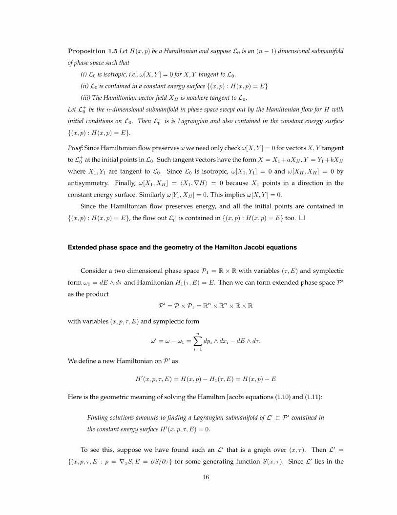
Proposition 1.5 Let H(x, p) be a Hamiltonian and suppose L0 is an (n − 1) dimensional submanifold
of phase space such that
(i) L0 is isotropic, i.e., ω[X,Y ] = 0 for X,Y tangent to L0,
(ii) L0 is contained in a constant energy surface (x, p) : H(x, p) = E
(iii) The Hamiltonian vector field XH is nowhere tangent to L0.
Let L+0 be the n-dimensional submanifold in phase space swept out by the Hamiltonian flow for H with
initial conditions on L0. Then L+0 is is Lagrangian and also contained in the constant energy surface
(x, p) : H(x, p) = E.
Proof: Since Hamiltonian flow preservesωwe need only checkω[X,Y ] = 0 for vectorsX,Y tangent
toL+0 at the initial points inL0. Such tangent vectors have the formX = X1 +aXH , Y = Y1 +bXH
where X1, Y1 are tangent to L0. Since L0 is isotropic, ω[X1, Y1] = 0 and ω[XH , XH ] = 0 by
antisymmetry. Finally, ω[X1, XH ] = 〈X1,∇H〉 = 0 because X1 points in a direction in the
constant energy surface. Similarly ω[Y1, XH ] = 0. This implies ω[X,Y ] = 0.
Since the Hamiltonian flow preserves energy, and all the initial points are contained in
(x, p) : H(x, p) = E, the flow out L+0 is contained in (x, p) : H(x, p) = E too.
Extended phase space and the geometry of the Hamilton Jacobi equations
Consider a two dimensional phase space P1 = R × R with variables (τ, E) and symplectic
form ω1 = dE ∧ dτ and Hamiltonian H1(τ, E) = E. Then we can form extended phase space P ′
as the product
P ′ = P × P1 = Rn × Rn × R× R
with variables (x, p, τ, E) and symplectic form
ω′ = ω − ω1 =
n∑i=1
dpi ∧ dxi − dE ∧ dτ.
We define a new Hamiltonian on P ′ as
H ′(x, p, τ, E) = H(x, p)−H1(τ, E) = H(x, p)− E
Here is the geometric meaning of solving the Hamilton Jacobi equations (1.10) and (1.11):
Finding solutions amounts to finding a Lagrangian submanifold of L′ ⊂ P ′ contained in
the constant energy surface H ′(x, p, τ, E) = 0.
To see this, suppose we have found such an L′ that is a graph over (x, τ). Then L′ =
(x, p, τ, E : p = ∇xS,E = ∂S/∂τ for some generating function S(x, τ). Since L′ lies in the
16
surface H ′ = 0, the generating function S(x, τ) will satisfy H ′(x,∇xS, τ, ∂S/∂τ) = 0. But this is
the Hamilton-Jacobi equation (1.10) (with t = τ ). Similarly, if L′ is a graph over (x,E) then the
generating function s(x,E) will satisfy (1.11). Once we know L′, the generating functions S(x, τ)
and s(x,E) can be found as described above. They will be partial Legendre transforms.
How can we find a Lagrangian submanifold of extended phase space that does the job? One
way of constructingL′ is to start with a Lagrangian submanifoldL ofP and imbed it as an isotropic
submanifold in P ′ contained in the constant energy surface H ′ = 0 via (x, p) 7→ (x, p, 0, H(x, p)).
We can then flow out these points under the Hamiltonian flow for H ′, to obtain a Lagrangian
submanifold in P ′ in the constant enery surface H ′ = 0.
Problem 1.6: Show that the Hamiltonian vector fieldXH′ is never tangent to this imbedded isotropic
submanifold.
To perform the flow out, we can use the following proposition, which we state for more
general products.
Proposition 1.6 Consider the extended phase space
P ′ = Rn × Rn × Rk × Rk
with variables (x1, . . . , xn, p1, . . . , pn, X1, . . . , Xk, P1, . . . , Pk) and symplectic form
ω′ =
n∑i=1
dpi ∧ dxi −k∑j=1
dPj ∧ dXj .
Suppose we have a Hamiltonian of the formH ′(x, p,X, P ) = H(x, p)−H1(X,P ). LetL′ be a Lagrangian
submanifold in P ′ that is contained in the constant energy surface H ′ = 0. Let (x(t), p(t), X(t), P (t)) be
a path in L′. Consider the following statements:
(i) (x(t), p(t), X(t), P (t)) is a Hamiltonian trajectory for H ′
(ii) (x(t), p(t)) is a Hamiltonian trajectory for H
(iii) (X(t), P (t)) is a Hamiltonian trajectory for H
Then (i)⇔ (ii) and (iii). Let π : L′ → Rk×Rk be the projection (x, p,X, P ) 7→ (X,P ) and dπ the induced
map on tangent spaces. If dπ is onto (this requires k ≤ n) then (ii)⇒ (iii) and (i).
Proof: Condition (i) can be written
xpXP
=
[J 00 −J
]∇H ′ =
[J 00 −J
]
∂H
∂x
∂H
∂p
−∂H1
∂X
−∂H1
∂P
17
which is equivalent to ((x(t), p(t)) and (X(t), P (t)) satisfying Hamiltions equations for H and H1
respectively. This shows (i)⇔ (ii) and (iii).
To show that (ii) ⇒ (iii) and (i) assume that (ii) holds. Let X ′ =
abAB
be in the tangent
space to L′. The constant energy condition yields 〈∇H ′, X ′〉 = 0 which implies⟨∇H,
[ab
]⟩=
⟨∇H1,
[AB
]⟩. Since L′ is Lagrangian and
xpXP
is also a tangent vector we also know that
⟨xpXP
, [ J 00 −J
]abAB
⟩ = 0 so that⟨[
xp
], J
[ab
]⟩=
⟨[XP
], J
[AB
]⟩. Condition (ii) says
that (x(t), y(t)) is Hamiltonian flow for H . Thus⟨[XP
], J
[AB
]⟩=
⟨[xp
], J
[ab
]⟩=
⟨J∇H,J
[ab
]⟩=
⟨∇H,
[ab
]⟩=
⟨∇H1,
[AB
]⟩=
⟨J∇H1, J
[AB
]⟩
The condition on dπ means that we hit every vector[AB
]in Rk×Rk asX ′ ranges over the tangent
space ofL′. Thus J[AB
]also ranges over all vectors in Rk×Rk. So we find that
⟨[XP
]⟩= J∇H1.
Thus (iii) holds. We already saw that (ii) and (iii)⇒ (i).
Remark on solving for the flow using the Hamilton Jacobi equation
As an aside, we can now see how the Hamilton Jacobi equation can be used to solve for the
flow. Suppose we can solve a family of Hamilton Jacobi equations ,
H(x,∇S(x, P ))−H1(P ) = 0.
indexed by P ∈ Rk with k = n. Then L′ = (x,∇xS(x, P ),∇PS(x, P ), P ), x ∈ Rn, P ∈ Rk is a
Lagrangian submanifold in the surfaceH(x, p)−H1(P ) = 0. In favourable situations one can solve
for (x, p) as as function of (X,P ) when (x, p,X, P ) ∈ L′. Call this function (x(X,P ), p(X,P )). The
proposition above tells us that if (X(t), P (t)) is a Hamiltonian trajectory for H1 then the image
18
(x(X(t), P (t)), p(X(t), P (t)) is a Hamiltonian trajectory for H . But the equations for (X(t), P (t))
are easy to solve. We have X =∂H1
∂Pand P = 0. Thus P = P0 is constant in time and
X(t) =∂H1
∂P(P0)t.
An example
We now construct the solution to (1.10) corresponding to the set of free trajectories starting at
a given point x0 in configuration space. So the Hamiltonian is H(x, p) =p2
2m.
Start with the Lagrangian submanifold of Rn × Rn given by
L = (x0, p) : p ∈ Rn)
Then we imbed this as an isotropic zero energy (for H ′ = H(p) − E) surface in extended phase
space Rn × Rn × R× R via
(x0, p) 7→ (x0, p, 0,p2
2m).
Flowing out using the flow for H ′ from the initial point (x0, p0, 0,p2
0
2m) yields the trajectory (x0 +
1
mp0t, p0, t,
p20
2m). Thus a typical point in L′ can be written
(x, p, τ, E) = (x0 +1
mp0τ, p0, τ,
1
2mp2
0)
for some choice of p0 and τ . Here we have written it as a graph over (p0, τ). Solving x = x0+1
mp0τ
for p0 =m(x− x0)
τWe can also write points in L′ as
(x, p, τ, E) = (x,m(x− x0)
τ, τ,
m(x− x0)2
2τ2)
A path γ from (x0, p0, 0,1
2mp2
0) to (x, p, τ, E) is provided by
(x(t), p(t), τ(t), E(t)) = (x0 +1
mp0t, p0, t,
1
2mp2
0), t ∈ [0, τ ]
Since dS = pdx− Edτ we find
S(x, τ) =
∫γ
pdx− Edτ
=
∫ τ
0
(〈p0, x(t)〉 − 1
2mp2
0)dt
=1
2mp2
0τ
Since p0 =x− x0
mτ,
S(x, τ) = m|x− x0|2
2τ.
19
The singularity at τ = 0 is connected with the fact that L′ fails to be a graph over (x, τ) at
τ = 0.
There is a connection with the classical action. If we carry out this construction with a more
general Hamiltonian we will find that if x(t) is the path in configuration space corresponding to
a Hamiltonian trajectory we have
S(x(τ), τ) =
∫ τ
t=0
〈p(t), x(t)〉 −H(x(t), p(t))dt
where x(t) =∂H
∂p(x(t), p(t)). This implies that 〈p(t), x(t)〉−H(x(t), p(t)) is the Legendre transform
of H(x, p) with respect to p, namely the Lagrangian L(x(t), x(t)). Thus S(x(τ), τ) is the action
integral for this path.
20
2. Review of Probability and Operator theory
Probability
We now want to consider the situation in Classical Mechanics where we have incomplete
knowledge of our system. This incomplete knowledge is described by a probability measure on
phase space. Probability measures also are basic to Quantum Mechanics, where they appear even
when we have a complete knowledge of the system. So in this section we will review some basic
definitions.
A probability space is a triple
(Ω,F ,P)
where Ω is a set (e.g., phase space), F is a σ–algebra of subsets of Ω and P is a probability measure.
A σ-algebra on Ω is a collection F of subsets of Ω satisfying
(i) Ω ∈ F , ∅ ∈ F ,
(ii) A ∈ F ⇒ Ω\A ∈ F (closed under complements),
(iii) Aii∈N ⊂ F ⇒⋃i∈NAi ∈ F (closed under countable unions),
(iv) Aii∈N ⊂ F ⇒⋂i∈NAi ∈ F (closed under countable intersections).
In fact, for a non-empty collection of subsets, (ii) and (iii)⇒ (i) and (iv). Subsets in F are called
measurable sets and the pair (Ω,F) is called a measurable space. Sets in F are also called events.
For any collectionF0 of subsets of Ω there is a smallest σ–algebra on Ω containingF0, namely
the intersection of all such σ–algebras. This is the σ–algebra generated by F0. If Ω has a topology
then there is a smallest σ–algebra B containing the open sets. This is called the Borel σ–algebra
and its elements are called Borel sets.
A positive measure on a measurable space (Ω,F) is a countably additive function µ : F →
[0,∞]. This means
(i) µ(∅) = 0
(ii) µ(⋃
i∈NAi)
=∑i∈N µ(Ai) for any countable collection sets in Aii∈N ⊂ F that
is pairwise disjoint, i.e., Ai ∩Aj = ∅ for i 6= j.
If F = B, the Borel sets, then µ is called a Borel measure.
Example: a point mass (or delta function)
δx0(A) =
1 if x0 ∈ A0 if x0 6∈ A
If Ω = Rn this is also denoted δ(x− x0). A pure point (or discrete) measure is one of the form
µ =∑i
αiδxi
21
for some countable collection of points xi and positive numbers αi with∑i αi <∞.
The standard measure on Rn defined on Borel sets that reproduces the volume of rectangular
boxes and is invariant under translations and rotations is called Lebesgue measure.
A probability measure on a measurable space (Ω,F) is a positive measure P with P(Ω) = 1. The
number P(A) indicates the likelihood that an outcome in A occurs. In this case (Ω,F ,P) is called
a probability space.
A function f : Ω1 → Ω2 where (Ω1,F1) and (Ω2,F2) are measurable spaces is called measurable
if the pre-image of any set in F2 is contained in F1, that is
(i) f−1(F2) ∈ F1 for any F2 ∈ F2.
Measurable functions on probability spaces are also called random variables.
If f : Ω1 → Ω2 is a measurable function with respect to (Ω1,F1) and (Ω2,F2) and µ is a
measure on F1 then we can define the image measure f∗[µ] as
f∗[µ](F2) = µ(f−1(F2))
If f : Ω1 → Ω2 is a measurable function with respect to (Ω1,F1) and (Ω2,F2) then the
σ–algebra generated by f is f−1(A) : A ∈ F2. It is the smallest σ-algebra for which f is
measurable.
An important case is when Ω2 = R and P is a probability measure. Then the image measure
f∗[P] is a measure on R and called the distribution measure of f . The number f∗[P](I) gives the
probability that the value of f lies in I .
We now discuss integration. Let (Ω,F , µ) be a measure space. Define the indicator function
χA(x) =
1 if x ∈ A0 if x 6∈ A .
Then function of the form s =∑ni=1 αiχAi , for αi ∈ R and Ai ∈ F a finite collection of disjoint
sets, is called a simple function. The integral of s is defined as∫Ω
sdµ =
n∑i=1
αiµ(Ai)
The integral of a positive measurable function f is defined using monotone limits of simple
functions. For a measurable function f that is not necessary positive we can write f = f+ − f−and define the integral of f is the difference of the integrals of f− and f+.
If f is a random variable on a probability space the expected value of f , denoted E[f ] is the
average or mean
E[f ] =
∫Ω
fdP.
22
We have
E[χA] = P(A).
The variance of f is the expected value of (f − E[f ])2
Var(f) = E[(f − E[f ])2] = E[f2]− (E[f ])2.
Two events A and B are independent if
P[A ∩B] = P[A]P[B].
If A is an event with P[A] 6= 0 then the conditional probability of an event B given A is
P[B|A] =P[A ∩B]
P [A]
In this case A and B are independent if and only if P[B|A] = P[B]. Conditional probabilities
appear again in the last lecture where the idea of conditioning with respect to a σ–algebra is also
discussed.
Two theorems in measure theory
We will refer to the following results:
Theorem 2.1 [The Riesz-Markov theorem]. Let X be a locally compact Hausdorff space. Every positive
linear functional λ on Cc(X), is represented by a unique Borel measure µ on X. This means
λ(f) =
∫X
f(x)dµ(x)
for allf ∈ Cc(X).
A Borel measure µ on Rn is absolutely continuous with respect to Lebesgue measure m if
m(A) = 0⇒ µ(A) = 0.
In this case we write µ << m. If µ << m then there exists an integrable function f(x) such that
for every Borel set A
µ(A) =
∫A
f(x)dm(x).
Two measures µ1 and µ2 on (Ω,F) are singular, denoted µ1 ⊥ µ2 if there are disjoint setsA,B ∈ F
with A ∪ B = Ω such that µ1(A) = µ2(B) = 0. A measure µ is continuous if µ(x) = 0 for every
x ∈ Ω.
Theorem 2.2 [Lebesgue decomposition theorem]. Let µ be a regular Borel measure on Rn and let m
denote Lebesgue measure. Then
µ = µac + µsc + µpp
where µac << m, µsc is continuous with µsc ⊥ m and µpp is pure point.
23
Mixed states in Classical Mechanics
We now define a mixed state in Classical Mechanics to be a probability measure µ on phase
space. This represents a situation when we have incomplete knowledge of the system. The pairing
of an observable f and a state µ now does not yield a real number. Instead the value is a measure
on R, namely the distribution measure of f :
〈f |µ〉 = f∗[µ]
A pure state (x, p) now identified with the mixed state δ(x,p).
The time evolution of a mixed state is defined in the obvious way. If Φt is the Hamiltonian
flow on phase space, then the flow on mixed states is Φt∗. In other words
µt(A) = µ(Φ−1t (A))
Background and self-adjoint operators
I’ll assume you know the definitions of Hilbert space (with complex scalars), bounded operators,
adjoints, projections, spectrum, linear functionals and unitary operators.
A bounded operator A is self-adjoint if A∗ = A. I won’t give the definition of unbounded
self-adjoint operators, and will try to get by with examples. An unbounded self-adjoint operator
A acting in a Hilbert space H is only defined on a dense set D(A) ⊂ H called the domain. The
spectrum σ(A) of a self-adjoint operator A is a closed subset of R. The set σ(A) is bounded iff the
operator A is bounded. All eigenvalues of A lie in σ(A), but there may be more points. Here are
some examples.
Examples:
(i)H = Cn, A is Hermitian n× n, σ(A) = eigenvalues.
(ii) H = L2(Rn, dnx), Aψ = V (x)ψ(x) is multiplication by a bounded measureable
function V (x), σ(A) = ess range(V ) (or range(V ) if V is continuous).
(iii) H = L2(Rn, dnx), Aψ = xiψ(x) is multiplication by xi, D(A) = ψ ∈ H : xiψ ∈
H, σ(A) = R.
(iv) H = L2(Rn, dnk), Aφ = −i∂φ/∂ki , D(A) = φ : xi(F−1φ)(x) ∈ L2(Rn, dnx,
σ(A) = R.
In example (iv), F is the Fourier transform (see below). If φ is not differentialble ∂φ/∂ki can
be taken to mean FxiF−1, where xi is the multiplication operator.
24
Spectral theorem for self-adjoint operators
Let A be self-adjoint and (for the moment) bounded. If p(x) is a polynomial then we may
define p(A) in the obvious way by substituting A for x. This is possible for any bounded A, but if
A is self-adjoint then one can show that
‖p(A)‖ ≤ supx∈σ(A)
|p(x)|.
This alllows us to define f(A) for any f ∈ C(σ(A)) by taking limits. Now pick ψ ∈ H. Then the
map
f 7→ 〈ψ, f(A)ψ〉
defines a bounded positive linear functional on C(σ(A)). Thus, by the Riesz-Markov theorem,
there exists a regular positive Borel measure µAψ such that
〈ψ, f(A)ψ〉 =
∫σ(A)
f(λ) dµAψ (λ).
By definition, µAψ is the spectral measure forψ andA. Now notice that the right side of this equation
still makes sense if f is bounded Borel function. This allows us to use the equation (in reverse)
to define and operator f(A) for any bounded Borel functions. The map f 7→ f(A) is a ∗–algebra
homomorphism. This means (among other things) that f(A) = f(A)∗ and (fg)(A) = f(A)g(A).
Now let f(x) = χI(x) be the indicator function for a Borel set I . Then the operator χI(A) is a
projection, called the spectral projection for I and A.
The proof of these facts for unbounded self-adjointA is different, but the results are the same.
Examples:
(i)H = Cn, A is Hermitian n×n: Let λk be the eigenvalues and ek an orthonor-
mal basis of eigenvectors. Then f(A) =∑k f(λk) ek ⊗ e∗k so
〈ψ, f(A)ψ〉 =∑k
f(λk) | 〈ek, ψ〉 |2
µAψ =∑k
δ(λ− λk) | 〈ek, ψ〉 |2
χI(A) =∑
k:λk∈I
ek ⊗ e∗k
(ii)H = L2(R, dx), A is multiplication by x then
〈ψ, f(A)ψ〉 =
∫Rf(x) |ψ(x)|2dx
µAψ = |ψ(x)|2dx
χI(A) = multiplication by χI(x)
25
The Fourier transform
Let S be the Schwartz space of rapidly decreasing functions. The Fourier transform Fψ of
ψ ∈ S is the function
(Fψ)(k) = (2π)−n/2∫Rne−i〈k,x〉ψ(x)dnx.
The Fourier transform maps S → S and has an inverse given by
(F−1φ)(x) = (2π)−n/2∫Rnei〈x,k〉φ(k)dnk.
We will use the notation ψ for Fψ amd φ for F−1φ. Here are some properties of F .
(i) id
dkψ(k) = xψ(x),
(ii) kψ(k) =
−i ddxψ(x),
(iii) (˜ψ)(x) = ψ(x), (
ψ)(k) = ψ(k).
(iv)∫Rn |ψ(x)|2dnx =
∫Rn |ψ(k)|2dnk
(v) Let ϕ0(x) be the Gaussian ϕ0(x) = π−1/4e−x2/2. Then Fϕ0 = ϕ0.
Properties (i) and (ii) say that the Fourier transform exchanges multiplication and differentia-
tion by the co-ordinate functions. Property (iii) says that F and F−1 really are inverses. Property
(iv) lets us extend the definition of F from S to L2(Rn, dnx) by taking limits. The extension is a
unitary operator F : L2(Rn, dnx)→ L2(Rn, dnk).
The unitary operator F allows us to define differentiation operators. Let pi denote the
operator acting inH = L2(Rn, dnx) as
(piψ)(x) = F−1kiFψ
with domain D(pi) = ψ ∈ L2(Rn, dnx) : kiψ ∈ L2(Rn, dnk). Then pi is unitarily equivalent
to a multiplication operator by a real valued function, and hence self-adjoint. If ψ ∈ S, then
piψ = −i∂ψ/∂xi.
We now define three families of unitary operators Tx, Mk and Da as
(Tx0ψ)(x) = ψ(x− x0) (translation by x0 ∈ Rn)
(Mk0ψ)(x) = ei〈k0,x〉ψ(x) (multiplication by ei〈k0,x〉, p0 ∈ Rn)
(Daψ)(x) = a−n/2ψ(x/a) (dilation by a > 0)
and note that
(i) Tx0Mk0 = e−i〈k0,x0〉Mk0Tx0
(ii) FTx0= M−x0
F
26
(iii) FMk0 = Tk0F
(iv) FDa = Da−1F .
We also have (at least when acting on suitable ψ),
(v) Tx0xT−x0
= x− x0, Tx0pT−x0
= p
(vi) Mk0pM−k0 = p− k0, Mk0xM−k0 = x
(vii) DaxDa−1 = a−n/2x, DapDa−1 = an/2p
Uncertainty principle
For simplicity let n = 1 and ψ ∈ S with ‖ψ‖ = 1. Define
Varψ(x) =⟨ψ, x2ψ
⟩−(〈ψ, xψ〉
)2Varψ(p) =
⟨ψ, p2ψ
⟩−(〈ψ, pψ〉
)2=⟨ψ, k2ψ
⟩−(⟨ψ, kψ
⟩)2
Then
Varψ(x)Varψ(p) ≥ 1/4
and equality holds iff ψ = Mp0Tx0Daϕ0 (up to a possible phase factor eiη) where ϕ0 is the
normalized Gaussian.
Proof: Using (iv), (v) and (vi) above we can find x0, k0 and a such that φ = Da−1T−x0M−k0ψ verifies
Varψ(x) =⟨φ, x2φ
⟩= 1/2 and Varψ(p) =
⟨φ, p2φ
⟩. By the unitarity of the operators, ‖φ‖ = 1.
The key ingredient is the commutator formula i[p, x] = 1. This implies
1 = 〈φ, φ〉 = 〈φ, i[p, x]φ〉 = −Re 〈φ′, xφ〉 ≤ ‖φ′‖‖xφ‖ =√
Varψ(x)Varψ(p)
To get equality in the Cauchy-Schwarz inequality we must have 〈φ′, xφ〉 real and the two factors
proportional. This implies φ′ = −λxφ for λ > 0. Integrating, we get φ(x) = Ce−λx2/2 and then
‖φ‖ = 1 and ‖xφ‖2 = 1/2 imply λ = 1 and C = π−1/4. So φ = ϕ0 and ψ = Mp0Tx0Daϕ0.
One parameter strongly continuous unitary groups and Stone’s theorem
A map R→ unitary operators onH is called a one parameter strongly continuous unitary
group if U(0) = I , U(t1 + t2) = U(t1)U(t2) and t 7→ U(t)ψ is continuous inH for any fixed ψ ∈ H.
Theorem 2.3 [Stone’s theorem] Let U(t) be a one parameter strongly continuous unitary group.
Then there is a unique self-adjoint operator A such that U(t) = eitA. Conversely, every self-adjoint
operator A generates a one parameter strongly continuous unitary group U(t) = eitA. The limit
limt→0(U(t)− U(0))ψ
texists and equals iAψ iff ψ ∈ D(A). So we see that in general U(t)ψ is
continuous, but if ψ ∈ D(A) then U(t)ψ is differentiable withd
dtU(t)ψ = iAU(t)ψ.
27

Problem 2.1: The family of operators Tta for a ∈ Rn and Mtb for b ∈ Rn are both one parameter
strongly continuous unitary groups. Their generators are 〈a, p〉 and 〈b, x〉. What can you say
about D(a) for a > 0?
28
3. Quantum Mechanics
Abstract Quantum description of a physical system
Start with a Hilbert space H. Observables are self-adjoint operators acting in H. For an
observable A, the spectrum σ(A) represents possible outcomes of a measurement. Pure states are
one dimensional subspaces of H. We can identify these with normalized vectors ψ ∈ H with
‖ψ‖ = 1, but then ψ and eiηψ (for real η) represent the same state. Given an observable A and a
state ψ, the pairing is given by the spectral measure.
〈A|ψ〉 = µAψ
This is interpreted as the distribution measure for the value of A. So the expected value of A in
the state ψ is ∫λdµAψ (λ) = 〈ψ,Aψ〉
If we repeatedly measure A when the system is in the state ψ this will be the average value.
Similarly the probability of finding the value of A in a Borel set I is
Pψ[A ∈ I] = 〈ψ, χI(A)ψ〉 .
We are using the symbol Pψ rather than P is to emphasize that there is no underlying probability
measure on the set of states. There is only a single state ψ involved. This number represents the
proportion of times a repeated experiment to measureA lands in I when the system is in the state
ψ.
It is important to realize that a pure state ψ ∈ H, represents complete knowledge of the
system, despite the fact that we cannot predict with certainty the outcome of all measurements
of observables. In situations where we have incomplete knowledge, one can define quantum
mixed states , as we did in Classical Mechanics . Briefly, a mixed state is given by a trace class
positive definite operator M with trace equal to 1, called a density matrix. Such an operator has
a spectral representation M =∑∞i=1 µiψi ⊗ ψ∗i , where ψi ⊗ ψ∗i denotes the projection given by
ψi⊗ψ∗i φ = 〈ψi, φ〉ψi, and the µi are postitive numbers summing to 1. The number µi is interpreted
as the probabilty that the system is in state ψi. In this setup, a pure state is represented by a rank
one density matrix.
We will not consider mixed quantum states in this course, except to point out that the
superposition of two states ψ1 and ψ2, given byψ1 + ψ2
‖ψ1 + ψ2‖is a pure state, represented by a single
unit vector and not a mixed state.
29
Every observable A generates a flow on states given by e−itA. There is a distinguished
observable, the HamiltonianH that generates the time evolution e−itH . The trajectoryψt = e−itHψ
is defined for all states, but if ψ ∈ D(H) then ψt satisfies the Schrodinger equation
i∂
∂tψt = Hψt.
We can transfer the time evolution to the observables in such a way that
〈ψt, Aψt〉 = 〈ψ,Atψ〉
by choosing
At = eitHAe−itA
Notice that
At = i[H,At]
where [A,B] = AB −BA.
Now we consider the case of commuting observables. Two bounded operators are said to
commute if [A,B] = 0. Two unbounded self-adjoint operatorsA andB commute if f(A) and g(B)
commute for bounded Borel functions f and g. For commuting self-adjoint operators A and B,
χI(A)χJ(B) is a projection and
P[A ∈ I and B ∈ J ] = 〈ψ, χI(A)χJ(B)ψ〉
gives the joint distribution for A and B if we measure them simultaneously. If A and B don’t
commute, then χI(A)χJ(B) need not be a projection. We interpret this as saying that we cannot
measure A and B simultaneously.
Quantum particle in an external potential
To describe the motion of a particle we need to choose a Hilbert space, and operators to
represent the important observables. For a particle moving in configuration space Rn we may
choose
H = L2(Rn, dnx).
Then it is natural to take the position operator xi to be multiplication by xi. Classical observables
that are functions of x are then represented by multiplication by the same function. The probability
of finding the particle in the set I when the system is in the state ψ is
〈ψ, χI(x)ψ〉 =
∫I
|ψ(x)|2dnx.
30
In other words, the distribution measure for position is |ψ(x)|2dnx. To determine what operator
should represent momentum pi we recall that in Classical Mechanics the flow generated by p is
a translation in x. Therfore it is natural to choose pi to be the generator of the unitary group of
translations. Thus we set
pi = −i ∂∂xi
= F−1kiF .
The distribution measure for the momentum will then be |ψ(k)|2dnk.
We can already see peculiar feature about Quantum Mechanics: the distributions for position
and momentum are not independent. The uncertainty principle for the Fourier transform implies
that if the distribution for the position is sharply peaked in some state ψ, so that Varψ(x) is small,
then Varψ(p) will have to be large.
Finally we define the Hamiltonian operator as
H =p2
2m+ V = − 1
2m∆ + V
where p2 = −∆ is (minus) the Laplacian operator and V is multiplication by V (x).
The first task is to find a domain that makes H self-adjoint. This can be complicated if V is
unbounded. But if V is bounded H is self-adjoint on the domain of ∆ given by
D(H) = ψ ∈ L2(Rn, dnx) : k2ψ(k) ∈ L2(Rn, dnk).
Once we have defined H as a self-adjoint operator, we can ask about the properties of the
time evolution e−itH . These are closely connected to the spectral properties of H .
For example, if H has an eigenvalue E so that Hψ = Eψ, then the eigenfunction ψ evolves in
time as
eitHψ = eitEψ.
This expression represents the same state for all t, since eitE is a number with modulus 1. So
eigenvalues correspond to bound states.
What can we say about the time evolution of ψ if µHψ is absolutely continuous (with respect
to Lebesgue measure).
To answer this question, consider the observable given by the projection Pψ = 〈φ, ψ〉φ onto
the state φ. This observable has spectrum 0, 1 corresponding to whether or not a state in our
system is in the state φ. So the expected value of P , which is the probability that ψ is in the state
φ is
〈ψ, Pψ〉 = | 〈ψ, φ〉 |2.
If ψ is some initial state evolving as ψt = eitHψ, the probability that ψt remains in the initial state
after time t is | 〈ψ,ψt〉 |2 = |⟨ψ, eitHψ
⟩|2. For example, if ψ is an eigenfunction then this quantity
31
is 1 for all time. On the other hand, if the spectral measure µHψ is absolutely continuous, then by
the spectral theorem ⟨ψ, eitHψ
⟩=
∫σ(H)
eitλdµHψ (λ).
The Riemann Lebesgue lemma, a result in measure theory, says that this tends to zero as t→∞.
But is such a state really a scattering state? Does it leave bounded regions of space in the
sense that for a bounded region I in configuration space 〈ψt, χI(x)ψt〉 → 0? And if so, supposing
that the expected value of x2 given by⟨ψ, x2ψ
⟩is initially finite, how does it change in time?
There are many interesting questions like this and answering them for systems of interest can
be challenging. There isn’t time in this course to make a systematic study. Instead we will pick
out a few examples for the simple systems we considered in the classical case. To simplify the
notation, we will stick to one dimensional systems.
Example 1: Free motion
The Hilbert space isH = L2(R, dx) and
H =p2
2m= − 1
2m
d2
dx2.
This operator is easy to study since it is diagonalized by the Fourier transform. This means
that FHF−1 is multiplication byk2
2m, which implies that the spectrum is [0,∞) and is purely
absolutely continuous. Moreover the time evolution ψt is given by
ψt = e−itHψ = F−1e−itk2/(2m)Fψ.
Notice that the momemtum distribution |ψt(k)|2dk doesn’t change in time.
To begin lets take our initial state to be a Gaussian ϕ0 = π−1/4e−x2/2. Then ϕ0(k) = ϕ0(k)
and the constant momentum distribution is π−1/2e−k2
dk. The expected values for both x and p in
this state are zero. So this corresponds to a classical particle sitting at the origin.
How does this state evolve? We can calculate
F(e−itHϕ0)(k) = π−1/4e−itk2/(2m)e−k
2/2
= π−1/4e−(1+it/m)k2/2
= π−1/4e−αk2/2
where α = 1 + it/m is complex. Thus the time evolution is
e−itHϕ0 = π−1/4F−1e−αk2/2
Problem 3.1: Even though the complex dilation D(α−1/2)ψ has no meaning for a general ψ ∈
L2(R, dk), show that D(α−1/2)ϕ0 makes sense and verifies F−1D(α−1/2)ϕ0 = D(α1/2)F−1ϕ0.
32
Using this result we continue the calculation.
(e−itHϕ0)(x) = α−1/4F−1D(α−1/2)ϕ0(k)
= α−1/4D(α1/2)F−1ϕ0(k)
= α−1/2ϕ0(x/√α)
This yields the distribution1
√π√
1 + (t/m)2e
−x2
(1+(t/m)2) dx
for the position x in the state e−itHϕ0. What is happening here? The state is not stationary as in
the classical case, but it is also not moving in any direction. It is just slowly spreading out as time
goes on.
To see some motion, lets start with an initial state where the momentum distribution has been
shifted up. Let ψ = M [k0]ϕ0 so that ψ = FM [k0]ϕ0 = T [k0]Fϕ0. Then the initial momentum
distribution |ψ(k)|2dk = |ϕ0(k − k0)|2dk is centered at k0. Now
e−itHψ = π−1/4F−1e−itk2/(2m)e−(k−k0)2/2
Problem 3.2: Using the expansion
tk2
2m=t(k0 + k − k0)2
2m=t(k0)2
2m+tk0(k − k0)
m+t(k − k0)2
2m
and the commutation properties of T [k0], M [tk0/m] with F−1 show that
|ψt(x)|2 =1
√π√
1 + (t/m)2e−(x−tk0/m)2
(1+(t/m)2)
Now we see the particle moving to the right with velocity k0/m while still spreading at the
same rate.
Even when the initial state is not a Gaussian we can still use the Fourier transform to compute
the time evolution. To begin we assume that ψ ∈ S. Then one can compute
(e−itHψ)(x) = (2πit/m)−1/2
∫Reim
(x−y)22t ψ(y)dy
Then, as with the Fourier transform, we can extend the definition to L2(R, dx) since we know the
operator is unitary.
Now think of expanding (x − y)2 = x2 − 2xy + y2 in the exponent and throwing out the y2
term. The resulting operator is
U(t)ψ =1
(t/m)1/2eimx2
2t ψ(xm/t)
If the momentum distribution ψ is sharply peaked at k0 then ψ(xm/t) is concentrated near where
xm/t = k0, or x = k0t/m which is the classical trajectory starting at x0 = 0. Moreover the
exponent looks like the classical action we computed before.
33
Problem 3.3: Show that ‖(U(t)− e−itH)ψ‖ → 0 as t→∞.
Using the Hamilton Jacobi equation
In this section we will construct approximate scattering solutions to the Schrodinger equation
using the Hamilton Jacobi equation. For the free motion this may seem pointless since we can
already compute the exact solution using the Fourier transform! But there are two reasons to
proceed. So far we have just recognized the classical behaviour in solutions constructed another
way. But now we will use the classical flow to actually build the solution. Secondly, this procedure
works in situations where the Fourier transform is not available. In this section we will go back
to general dimension n.
To get an approximate solution to the time dependent Schrodinger equation(H − i ∂
∂t
)ψ = 0
of the form ψ(x, t) = eiS(x,t)u(x, t), we substitute this expression into the left side of the equation.
This is the key calculation, which we do for V 6= 0.(−1
2m∆ + V (x)− i ∂
∂t
)eiSu
= eiS(|∇S|2
2m+ V (x) +
∂S
∂t
)− ieiS
(1
m∇S · ∇u+
∂u
∂t+
1
2m(∆S)u
)− eiS 1
2m∆u
Then the first term on the right side vanishes if S(x, t) solves the Hamilton Jacobi equation
|∇S|2
2m+ V (x) +
∂S
∂t= 0.
From our previous work, we know that given a Lagrangian submanifold L in extended phase
space that (i) is contained in the constant energy surface (x, p, τ, E) : H(x, p) − E = 0 and (ii)
is a graph over (x, t), then the generating function (action) S(x, t) is a solution to the Hamilton
Jacobi equation. Moreover, we can find S by integrating the 1–form∑i pidxi − Edτ over paths
in L. We constructed such a Lagrangian using a flow out. In this case (x, p, τ, E) ∈ L if there is
an point (x0, p0) in the initial constant energy Lagrangian manifold L0 in the original phase space
(this implies E = H(x0, p0)), and a τ such that the Hamiltonian trajectory (x(t), p(t)) with initial
condition (x0, p0) arrives at (x, p) at time τ .
Now suppose we have solved the Hamilton Jacobi equation so that we know S(x, t). Then
our next task is to solve the equation
1
m∇S · ∇u+
∂u
∂t+
1
2m(∆S)u = 0
for u(x, t). This is a first order equation, called a transport equation, that we can solve using
flows. The standard trick for such equations is to assume we have a solution and determine its
34
values along the flow associated to the vector field in the equation. Of course, here these flows
will be Hamiltonian trajectories. So assume that we have a solution u(x, t). Fix a starting point
(x0, p0) the original Lagrangian of initial conditions. For notational simplicity lets suppose this
Lagrangian is a graph over p so a unique starting point is determined by p0. Now let us determine
the values of u along this trajectory. Setting v(t) = u(x(t), t) we find that
v(t) = x(t) · ∇u(x(t), t) +∂u
∂t(x(t), t)
But
x(t) = p(t)/m = ∇S(x(t), t)/m.
The first equality is Hamilton’s equation and the second follows from the fact that S is a generating
function. Sov(t) = ∇S · ∇u+
∂u
∂t
= ∇S · ∇u+∂u
∂t+
1
2m(∆S)u− 1
2m(∆S)u
= − 1
2m(∆S)(x(t), t)v(t).
Since we know S(x, t), the function 12m (∆S)(x(t), t) is a known function of t, once we specify p0,
which tells us the orbit we are on. Thus we know α(p0, t) = 12m (∆S)(x(t), t) and
v(t) = −α(p0, t)v(t)
Integrating, and keeping in mind that the constant of integration may depend on the orbit we are
on, we find
v(τ) = f(p0)e−∫ τ0α(p0,t)dt.
Now we can verify that any smooth function whose values along the trajectory (x(t), t) labelled
by p0 are given by
u(x(t), t) = f(p0)e−∫ τ0α(p0,t)dt
where α(p0, t) is given above, solves the equation.
If we construct S(x, t) and u(x, t) according to this scheme we find(−1
2m∆ + V (x)− i ∂
∂t
)eiSu = −eiS 1
2m∆u
The term remaining on the left is an error term which may become negligible for large t.
To illustrate this procedure, let us sketch the constructing of scattering solutions for the free
motion. In this case we found that
S(x, t) =m|x− x0|2
2t
35
Thus1
2m∆S(x, t) =
n
2t
which implies that in this case α(p0, t) = n/(2t) is independent of the trajectory and so
u(x, t) = f(p0)e−n∫ t1
log(τ)dτ/2= f(p0)t−n/2.
To complete the construction we must determine p0, the initial momentum, if we know (x, t). The
Hamiltonian trajectory is x = x0 + p0t/m, so p0 = m(x − x0)/t. Thus our approximate solutions
have the form
ψ(x, t) = eim(x−x0)2/(2t)f
(m(x− x0
t
)t−n/2
Now suppose we want to show that
limt→∞
eitHψ(x, t)
exists. This is like a wave operator in scattering theory. We can show existence by writing
eitHψ(x, t) = ψ(x, 1) +
∫ t
1
d
dteitHψ(x, t)
Using what is known as Cook’s method, it suffices to prove∫ ∞1
∥∥∥∥ ddteitHψ(x, t)
∥∥∥∥ <∞.By the calculation above ∥∥∥∥ ddteitHψ(x, t)
∥∥∥∥ =
∥∥∥∥eitH (iH +∂
∂t
)ψ(x, t)
∥∥∥∥=
∥∥∥∥(H − i ∂∂t)ψ(x, t)
∥∥∥∥=
∥∥∥∥ 1
2m∆u
∥∥∥∥where u(x, t) = f
(m(x− x0
t
)t−n/2. So
‖∆u(x, t)‖2 ≤ C∫Rn
∣∣∣∣t−n/2−2f
(m(x− x0)
t
)∣∣∣∣2 dnx= t−4 |f (m(y))|2 dny
This shows ‖∆u(x, t)‖ ≤ Ct−2 and so the integral is finite.
Now given a choice of f set
φ = limt→∞
eitHψ(x, t).
Then
limt→∞
∥∥e−itHφ− ψ(x, t)∥∥ = lim
t→∞
∥∥φ− eitHψ(x, t)∥∥ = 0
36
and we have constructed an approximate scattering solution. A harder question is whether
every scattering solution can be obtained by such a construction. This the question of asymptotic
completeness.
I learned about this construction from Ira Herbst who used related more complicated con-
structions in his work with Erik Skibsted. For the case of Schrodinger operators see [DG].
Example 2: The Harmonic Oscillator
We will again restrict ourselves to one dimension. Then the Hilbert space is L2(R, dx) and
the Hamiltonian operator is
H =1
2(p2 + x2)
(We have setm = 1). The classical motion consist of only bound states. My original intention was
to present a proof of a theorem here that states that if lim|x|→∞ V (x) = ∞ then the spectrum of
H only contains isolated eigenvalues with finite multiplicity. This can be found, for example, in
Reed and Simon IV [RSIV] Theorem XIII.67.
The Harmonic Oscillator is special in many ways, and we can proceed differently using
creation and anihilation operators. This is explained in almost every book on quantum mechanics!
Define the (differential) operators
a =1√2
(x+
d
dx
)anihilation operator
a∗ =1√2
(x− d
dx
)creation operator
N = a∗a number operator
and let ϕ0 = π−1/4e−x2/2 be the normalized Gaussian. Then
H = N +1
2
[a, a∗] = 1
aϕ0 = 0
and one defines ψ0 = ϕ0 and for n = 1, 2, 3, . . .,
ψn =1√n!
(a∗)nψ0.
These can be shown to form an orthonormal set of eigenfunctions for H with eigenvalues En =
n+ 12 . The have the explicit form
ψn(x) =1√
2nn!π−1/4Hn(x)
37
where
Hn(z) = (−1)nez2 dn
dzne−z
2
are the classical Hermite polynomials. There is a theorem that states that the set p(x)ϕ0(x) :
p(x) is a polynomial is dense in L2(R, dx). This implies that ψn : n ∈ N is an orthonormal basis
of eigenvectors for H .
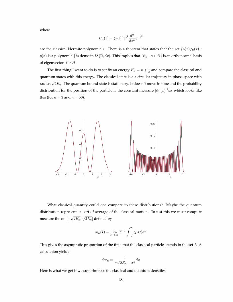
The first thing I want to do is to set fix an energy En = n + 12 and compare the classical and
quantum states with this energy. The classical state is a a circular trajectory in phase space with
radius√
2En. The quantum bound state is stationary. It doesn’t move in time and the probability
distribution for the position of the particle is the constant measure |ψn(x)|2dx which looks like
this (for n = 2 and n = 50):
What classical quantity could one compare to these distributions? Maybe the quantum
distribution represents a sort of average of the classical motion. To test this we must compute
measure the on [−√
2En,√
2En] defined by
mn(I) = limT→∞
T−1
∫ T
−TχI(t)dt.
This gives the asymptotic proportion of the time that the classical particle spends in the set I . A
calculation yields
dmn =1
π√
2En − x2dx
Here is what we get if we superimpose the classical and quantum densities.
38
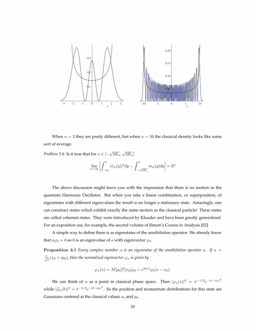
When n = 2 they are pretty different, but when n = 50 the classical density looks like some
sort of average.
Problem 3.4: Is it true that for x ∈ [−√
2En,√
2En]
limn→∞
∣∣∣∣∫ x
−∞|ψn(y)|2dy −
∫ x
−√
2En
mn(y)dy
∣∣∣∣ = 0?
The above discussion might leave you with the impression that there is no motion in the
quantum Harmonic Oscillator. But when you take a linear combination, or superposition, of
eigenstates with different eigenvalues the result is no longer a stationary state. Amazingly, one
can construct states which exhibit exactly the same motion as the classical particle! These states
are called coherent states. They were introduced by Klauder and have been greatly generalized.
For an exposition see, for example, the second volume of Simon’s Course in Analysis [S2]
A simple way to define them is as eigenstates of the annihilation operator. We already know
that aϕ0 = 0 so 0 is an eigenvalue of a with eigenvector ϕ0.
Proposition 3.1 Every complex number α is an eigenvalue of the annihilation operator a. If α =
1√2
(x0 + ip0), then the normalized eigenvector ϕα is given by
ϕα(x) = M [p0]T [x0]ϕ0 = eip0xϕ0(x− x0).
We can think of α as a point in classical phase space. Then |ϕα(x)|2 = π−1/2e−(x−x0)2
while |ϕα(k)|2 = π−1/2e−(k−p0)2 . So the position and momentum distributions for this state are
Gaussians centered at the classical values x0 and p0.
39
Proof: Writing out the equation aϕα = αϕα yields xϕα + ϕ′α =√
2αϕα. whose solution is
ϕα(x) = Ce−x2/2+
√2αx
= Ce−x2/2+(x0+ip0)x
= Ce−(x−x0)2/2eip0x.
The normalization condition then implies C = 1 (up to an inessential phase).
Recall that the Harmonic Oscillator time evolution of a point α in classical phase space,
thought of as a point in C, is α(t) = e−itα. The quantum time evolution of ϕα completely classical
in the following sense.
Proposition 3.2
e−itHϕα = e−it/2ϕα(t)
Of course the phase factor e−it/2 doesn’t change the state.
Proof: Expand ϕα in the orthonormal basis of eigenvectors. We have
ϕα =∑n
〈ψn, ϕα〉ψn
where
〈ψn, ϕα〉 =1√n!〈(a∗)nϕ0, ϕα〉 =
1√n!〈ϕ0, a
nϕα〉 =αn√n!〈ϕ0, ϕα〉
To determine 〈ϕ0, ϕα〉 use
1 = ‖ϕα‖2 =∑n
| 〈ψn, ϕα〉 |2 =∑n
|α|2n
n!| 〈ϕ0, ϕα〉 |2 = e|α|
2
| 〈ϕ0, ϕα〉 |2.
So | 〈ϕ0, ϕα〉 | = e−|α|2/2 and (up to a phase factor)
ϕα = e−|α|2/2∑n
αn√n!ψn
Since each ψn is an eigenvector of H with eigenvalue En = n + 12 we know that e−itHψn =
e−it(n+ 12 )ψn. Therefore
e−itHϕα = e−|α|2/2∑n
αn√n!e−itHψn
= e−|α|2/2∑n
αn√n!e−it(n+ 1
2 )ψn
= e−it/2e−|α|2/2∑n
(e−itα)n√n!
ψn
= e−it/2e−|α(t)|2/2∑n
α(t)n√n!
ψn
= e−it/2ϕα(t)
40
The final topic I intended to cover for the Harmonic Oscillator is the Maslov-WKB construction
of approximate eigenfunctions using the Hamilton-Jacobi equation (1.11). Again, this construction
is only important as an illustration of the method, as we know the eigenfunctions exactly. In this
case, one needs to take large E to get a good approximation.
The difficulty is that the Lagrangian manifold is now a circle, which is not a graph over (x,E).
We can define S =∫pdx as a smooth function on the circle, but the approximate eigenfunction
we get as a function of x blows up at the turning points x = ±√
2E where the manifold fails to be
a graph. The solution is to work locally. Near the turning points project onto p instead. This is
particularly easy for the Harmonic Oscillator since p and x appear symmetrically in Hamiltonian.
The resulting function of p is then changed to a function of x by taking the Fourier transform.
Combining these local function into a smooth function requires the introduction of the Maslov
index at each turning point. Moreover the final definition of the approximate eigenfunction gives
zero unless the Bohr-Sommerfeld quantization condition holds.
There was no time for this, but fortunately there is a beautiful pedagogical paper by Eckmann
and Seneor [ES] that explains the procedure.
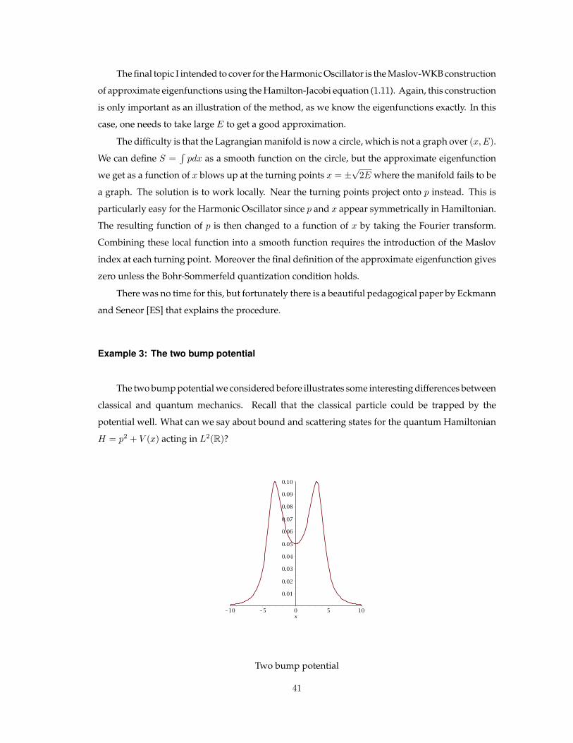
Example 3: The two bump potential
The two bump potential we considered before illustrates some interesting differences between
classical and quantum mechanics. Recall that the classical particle could be trapped by the
potential well. What can we say about bound and scattering states for the quantum Hamiltonian
H = p2 + V (x) acting in L2(R)?
Two bump potential
41
There was no time for this either in the course, but here are some results about this operator
that we could have considered. For simplicity let us assume that V (x) is smooth and compactly
supported.
Theorem 3.3 The spectrum of H is σ(H) = [0,∞) and is absolutely continuous.
So in contrast to the classical case, where there are bound states with positive energy corre-
sponding to particles trapped by the well, there are no bound states in the quantum case. The
physical explanation for this is that the particle can tunnel through the barrier. The mathematical
theory of the absence of eigenvalues imbedded in the continuous spectrum is harder. There are
examples of potentials (e.g., the Wigner–von Neumann potential) which tend to zero (slowly)
for large |x| but do have a positive eigenvalue imbedded in the continuous spectrum. See, for
example, Chapter 4 of [CFKS].
What would happen if we moved the bottom of the central well so that it dipped below zero?
Since we are working in one dimension,H would immediately have a negative eigenvalue (bound
state) in addition to the absolutely continuous spectrum on the postive half line. The proof of this
is a nice application of min-max methods (see [RSIV]).
What would happen if we moved the bottom of the central well so that it’s minimum was
exactly zero, and then multiplied V (x) by a large positive coupling constant µ? If the minimum
was non-degenerate, then the potential would look more and more like a harmonic oscillator as
µ goees to infinity. Yet for each finite µ the potential would satisfy the hypothesis of the theorem.
In this case the spectrum would be absolutely continuous in [0,∞) for every µ. However there
would be resonances in the lower half plane converging to the harmonic oscillator eigenvalues.
For a definition and introduction to resonances, see e.g., [CKFS] [HS]. Resonances could be the
subject of another course like this!
42
4. Hidden variables and non-locality
Introduction
In general, quantum mechanics only provides probability distributions for the measured
values of a quantum observables., and cannot predict the outcomes with certainty. In the early
days of quantum mechanics, Einstein strongly resisted the idea that a physical theory could be
essentially probabilistic in this way. Experiments like the one described by Einstein, Podolsky
and Rosen in 1935 were proposed to show that measurement of spatially separated but quantum
mechanically entangled particles leads to action at a distance. In the intervening eighty years there
has been much philosophical debate on the foundations of quantum mechanics and the nature of
physical reality. A readable account is The Infamous Boundary by David Wick [W]. Remarkably,
recent experiments support the idea that action at a distance is real [FTZWF]. In this lecture, we
will consider an example of Lucien Hardy [H] that is an outgrowth of the fundamental work of
J.S. Bell [B]. This account is based on Faris [F1] [F2] and conversations with David Brydges.
It is possible (and usual) to work on the mathematics of quantum mechanics without worrying
about the philosophical underpinnings. Still, I think it is worthwhile to spend some time to
appreciate the essential weirdness of this theory.
Recall that for a system in the pure state ψ, given a Borel set I ⊆ R, the probability that the
measured value of a quantum observable A will lie in I is
Pψ[A ∈ I] = 〈ψ, χI(A)ψ〉 , (4.1)
where χI(A) is the spectral projection for the operator A corresponding to the set I .
Two commutingA andB can in principle be measured simultaneously. In this case χI(A) and
χJ(B) commute and χI(A)χJ(B) is again a projection. The probability that the simultaneously
measured values of A and B lie in I and J respectively is
Pψ[A ∈ I and B ∈ J ] = 〈ψ, χI(A)χJ(B)ψ〉 (4.2)
Equations (4.1) and (4.2) can be taken as definitions of the quantum probabilities Pψ[A ∈ I]
and Pψ[A ∈ I and B ∈ J ] on the left sides. Alternatively, we can think of Pψ[A ∈ I] and
Pψ[A ∈ I and B ∈ J ] as quantities that can be determined experimentally by running the same
experiment many times. Then (4.1) and (4.2) express the agreement of theory and experiments.
It is natural to ask whether a more complete theory could predict outcomes with certainty.
Perhaps quantum observables have exact values, and saying that a system is in a quantum state
ψ only gives partial information about them. In other words, maybe the situation is like a mixed
state in Classical mechanics, where there is a probability measure on some underlying state space.
43
Could there be a quantum state space Ω with quantum observablesA,B, . . . corresponding to
functions a, b, . . . : Ω→ Rwith a(ω), b(ω), . . . giving the exact value of the observables if the system
is in the state ω. Then each quantum state ψ would correspond to a probability measure Pψ on Ω
such that the spectral measures forA,B, . . . are the image measures of Pψ under a(ω), b(ω), . . .. Or
perhaps this is true for some subset A of observables. Thus we are led to the following question.
Question 1: Given a quantum system and a collection A of observables does there exist
• a measureable space (Ω,F) and
• for each A ∈ A a random variable a : Ω→ R
such that every pure state ψ is associated with a probability measure Pψ that reproduces the
quantum distributions for observables, that is,
〈ψ, PI(A)ψ〉 = Pψ[a ∈ I] (4.3)
and if A and B commute,
〈ψ, PI(A)Pj(B)ψ〉 = Pψ[a ∈ I ∩ b ∈ J]? (4.4)
Example 1: If A = A contains only one observable, then the answer to Question 1 is obviously
yes. We can take Ω = R and Pψ = µAψ .
Example 2: If A a collection of non-commuting observables, then the answer to Question 1 is also
yes. We don’t have to verify (4.4) and can satisfy (4.3) by assuming that measurements of different
observables are independent.
In general the answer to Question 1 is no. Our first goal is to construct an example to illustrate
this.
Spin observables A and B
Our examples are constructed from observablesA,B given by 2×2 Hermitian matrices acting
on the Hilbert space C2. We will assume that they have the same two distinct eigenvalues λ1 and
λ2 but different eigenvectors.
Such matrices occur in Physics when describing the spin of a spin 12 particle. In units where
h2 = 1 these have the form
Se =
3∑i=1
eiσi
where e = [e1, e2, e3] is a unit vector (the spin direction) in R3, and σi are Pauli spin matrices
σ1 =
[0 11 0
]σ2 =
[0 −ii 0
]σ3 =
[1 00 −1
].
44
For any choice or direction e the matrix Se has eigenvalues −1 and 1. These are the possible
outcomes of measuring the spin in this direction. To make the examples easier to follow, we will
think of A and B as spin matrices.
Let φ1, φ2 be an orthonormal basis of eigenvectors for A and denote by Pi, i = 1, 2 the
corresponding spectral projections. Similarly, let ψ1, ψ2 be an orthonormal basis of eigenvectors
for B and denote by Qi, i = 1, 2 the corresponding spectral projections. We will assume that the
bases are related by the unitary change of basis matrix U = [〈ψi, φj〉] given by the rotation matrix
U =
[α −ββ α
],
with α, β ∈ [−1, 1], α2 + β2 = 1. We will assume that neither α nor β is zero.
To begin, let us illustrate explicitly the construction of independent random variables in
Example 2 above. This requires a product measure. We can use A = A,B. Consider a state
ψ = 1√2φ1 + 1√
2φ2. The quantum probabilities are
P[A = λ1] = | 〈ψ, P1ψ〉 |2 =1
2
P[A = λ2] = | 〈ψ, P2ψ〉 |2 =1
2
P[B = λ1] = | 〈ψ,Q1ψ〉 |2 =(α− β)2
2
P[B = λ2] = | 〈ψ,Q2ψ〉 |2 =(α+ β)2
2
Let Ω be the finite probability space
Ω = λ1, λ2 × λ1, λ2 = (λ1, λ1), (λ1, λ2), (λ2, λ1), (λ2, λ2),
F be all subsets of Ω and define the random variables a and b by
a((λi, λj)) = λi, b((λi, λj)) = λj .
Then the probability measure generated by
Pψ[(λ1, λ1) =1
2· (α− β)2
2
Pψ[(λ1, λ2) =1
2· (α+ β)2
2
Pψ[(λ2, λ1) =1
2· (α− β)2
2
Pψ[(λ2, λ2) =1
2· (α+ β)2
2
will work.
45
Tensor Product
We will need to use the tensor product C2 ⊗ C2 in the following examples. Tensor products
are important in describing multi-particle systems in physics and situations where two systems
interact. In our examples they describe two spin measurements, done on the left and the right.
One way to describe the tensor product is with bases. If e1, e2 is a basis for the copy
of C2 on the left and f1, f2 is a basis for the copy of C2 on the right, then C2 ⊗ C2 is a 4
dimensional space with basis e1 ⊗ f1, e2 ⊗ f1, e2 ⊗ f1, e2 ⊗ f2. The inner product is defined on
basis vectors as 〈ei ⊗ fj , ek ⊗ fl〉 = 〈ei, ek〉 〈fj , fl〉 and is then extended by linearity to the whole
space. Similarly, if A, B are operators on C2 (i.e., 2× 2 matrices) then A⊗B acts on basis vectors
via (A⊗B)(ei ⊗ fj) = Aei ⊗Bfj and can be extended by linearity to the whole space.
One way to think about the tensor product is to think of the elements of C2 on the left as
column vectors[a1
a2
]and elements of C2 on the right as row vectors [b1, b2]. Then
[a1
a2
]⊗ [b1, b2]
corresponds to the 2× 2 matrix[a1
a2
][b1, b2] =
[a1b1 a1b2a2b1 a2b2
]and C2 ⊗ C2 can be identified with
the space of 2× 2 matrices. Product states, that is, states of the form[a1
a2
]⊗ [b1, b2] correspond to
matrices of rank 1. However a generic 2× 2 has rank 2 and cannot be factored in this way. Such a
state is called entangled.
Recall that if A, B are operators on C2 then A ⊗ B acts on C2 ⊗ C2. If we represent a vector
in C2 ⊗ C2 as a 2× 2 matrix M , then the action of A⊗B on M is AMBT .
Hardy’s example
Now we present Hardy’s example of a system where a random variable description is not
possible. This system models spin measurement for two particles in an entangled state. The
Hilbert space for this system is C2 ⊗ C2. We can imagine the two particles as being separated
in space, one on the left and one on the right, having been sent there after the state is prepared
in some central location. Let A and B be the spin matrices defined above. We consider the four
observables given byAL = A⊗ I
AR = I ⊗A
BL = B ⊗ I
BR = I ⊗B
and notice that AL commutes with AR and BR. This agrees with the idea that measurements on
the left do not interfere with measurements on the right. Thus we may simultaneously measure
AL and AR, and (in a different experiment) simultaneously measure AL and BR. Similarly AR
commutes with AL and BL, etc.
46
We have four bases for C2 ⊗ C2 at our disposal, namely φi ⊗ φj, ψi ⊗ φj, φi ⊗ ψj, and
ψi ⊗ ψj, for i, j = 1, 2. If we expand a state Ψ ∈ C2 ⊗ C2 in the first of these as
Ψ =∑i,j
ci,jφi ⊗ φj
and write the coefficients as a matrix
C =
[c1,1 c1,2c2,1 c2,2
],
then the corresponding coefficient matrices for the other basis are UC for ψi ⊗ φj, CUT for
φi ⊗ ψj and UCUT for ψi ⊗ ψj.
To calculate the quantum probability that a simultaneous measurement ofAL andAR for two
particles in the state Ψ yieldsAL = λ1 andAR = λ1 we must take the product of the corresponding
spectral projections for AL and AR (which is again a projection since AL and AR commute)
(P1 ⊗ I)(I ⊗ P1) = P1 ⊗ P1.
Then the quantum probability is given by
P[AL = λ1 and AR = λ1] = | 〈Ψ, P1 ⊗ P1Ψ〉 |2 = |c1,1|2.
For our example we take the coefficient matrix for the first basis to be
C =1
N
[0 −α−α β
],
where N is the normalization constant N =√
2α2 + β2 =√
1 + α2. Then the corresponding
coefficient matrices for the other bases are
UC =1
N
[αβ −1−α2 0
]CUT =
1
N
[αβ −α2
−1 0
]UCUT =
1
N
[α2β + β αβ2 − α−α2 −βα2
]The key point is the position of the zero entries, and the fact that the 2, 2 entry of the final matrix
is non-zero. These lead to the quantum probabilities
P[AL = λ1 and AR = λ1] = 0
P[BL = λ2 and AR = λ2] = 0
P[AL = λ2 and BR = λ2] = 0
P[BL = λ2 and BR = λ2] =α4β2
N2> 0
47
We now suppose that there is an underlying probability space such that
P[aL = λ1 ∩ aR = λ1] = 0
P[bL = λ2 ∩ aR = λ2] = 0
P[aL = λ2 ∩ bR = λ2] = 0
P[bL = λ2 ∩ bR = λ2] =α4β2
N2> 0
and derive a contradiction. Here is the key point. When we assume that a probability space exists,
we can write the set aL = λ1 ∩ aR = λ1 as a disjoint union
aL = λ1 ∩ aR = λ1 =
aL = λ1 ∩ bL = λ1 ∩ aR = λ1 ∪ aL = λ1 ∩ bL = λ2 ∩ aR = λ1
This is saying is that even though we don’t know the value of bL, it has some value, and we can
decompose an event into a disjoint union of events depending on that value. We can do this one
more time with the value of bR to produce the disjoint union
aL = λ1 ∩ aR = λ1 =
aL = λ1 ∩ bL = λ1 ∩ aR = λ1 ∩ bR = λ1 ∪
aL = λ1 ∩ bL = λ1 ∩ aR = λ1 ∩ bR = λ2 ∪
aL = λ1 ∩ bL = λ2 ∩ aR = λ1 ∩ bR = λ1 ∪
aL = λ1 ∩ bL = λ2 ∩ aR = λ1 ∩ bR = λ2 ∪
Now let
p(i, j, k, l) = P[aL = λi ∩ bL = λj ∩ aR = λk ∩ bR = λl
]Then we can rewrite our equations as
p(1, 1, 1, 1) + p(1, 1, 1, 2) + p(1, 2, 1, 1) + p(1, 2, 1, 2) = 0p(1, 2, 2, 1) + p(1, 2, 2, 2) + p(2, 2, 2, 1) + p(2, 2, 2, 2) = 0p(2, 1, 1, 2) + p(2, 1, 2, 2) + p(2, 2, 1, 2) + p(2, 2, 2, 2) = 0p(1, 2, 1, 2) + p(1, 2, 2, 2) + p(2, 2, 1, 2) + p(2, 2, 2, 2) = α4β2/N2 > 0
But the p(i, j, k, l) are non-negative numbers. So all the ones that appear in the first three equations
are zero. But this includes all all the terms in the last equation. So they cannot add up to something
positive. This contradiction shows that the probability space cannot exist.
Bell’s second theorem: non-locality
This section follows Faris’ appendix in the book by Wicks. He includes a more careful
explanation of the needed concepts from probability aimed at non-mathematicians.
48
Since we have to set up different experiments for each pair of measurements in the example
above, maybe the probability measure which reproduces the quantum results depends on which
experiment we are performing. In other words we might have a probability space Ω and σ-algebra
F with four different probability measures PAA, PAB , PBA and PBB depending on which spin
direction we are measuring on the left and on the right.
In this case there are some natural restrictions if we want to disallow action at a distance.
Measurements which only involve the equipment on the left should not be influenced by what
happens on the right, and vice versa. Furthermore, simultaneous measurements on the left and
right should be conditionally independent, if we take into account events in the preparation stage.
The idea is that events in the preparation stage in the experiment, for example preparing a singlet
state where the spins on the left and right always have opposite values, can result in correlations
for the measurements on the left and the right. However, if we factor out these effects, the residual
randomness leads to independent outcomes on the left and right.
To put this in a mathematical form we need some more ideas from probability theory. We
assume that there are three sub σ-algebras ofF , denotedFL,FR and F . The events inFL describe
what happens on the left. Knowing whether a experimental outcome is contained in an event
fromFL only tells us about measurements performed on the left. An example would be aL = 1.
Similarly, the events in FR are associated with what happens on the right. The events in F are
associated what happened in the preparation stage of the experiment. Assume we are given four
probability measures PAA, PAB , PBA and PBB such that
1. If E ∈ FL ∪ F then PAA(E) = PAB(E) and PBA(E) = PBB(E).
In other words, events on the left or from the preparation stage have probabilities which don’t
change when we move around the equipment on the right.
2. Similarly, if E ∈ FR ∪ F then PAA(E) = PBA(E) and PAB(E) = PBB(E).
The third assumption expresses the conditional independence of events on the right and left.
Recall that if E is an event and G is another event with P(G) 6= 0 then the conditional probability
of F given G is the number P[E|G] =P(E ∩G)
P(G). If F is a sub σ-algebra of F then the conditional
probability P[E|F ] is not a number, but a random variable. The idea (which is actually correct if
Ω is finite and there are no non-empty events with zero probability) is that
P[E|F ](ω) = P[E|Gω] where Gω =⋂
G∈F :ω∈G
G.
In other words, P[E|F ](ω) is the probability of E given all the information in F about ω. The
situation is more complicated when there are set of measure zero and we can’t talk about the
value of a random variable at a point. We won’t worry about this. What we use the fact that
E[P[E|F ]] = P[E]. The third assumption is
49
3. If E ∈ FL and F ∈ FR then Pxy[E ∩ F |F ] = Pxy[E|F ] Pxy[F |F ]. Here x and y are any
choice of A,B.
These assumptions are reasonable if we don’t believe in action at a distance. Yet we can show that
there can be no hidden variable description of the experiment unless they are violated.
Proposition 4.1 Let the matrices A and B and the coefficients α, β and N be as defined in the previous
section. Suppose that there are probability measures PAA, PAB , PBA and PBB and sub σ–algebras FL,
FR and F satisfying the assumptions above. Then there are no random variables aL, aR, bL, bR such that
PAA[aL = λ1 ∩ aR = λ1] = 0
PBA[bL = λ2 ∩ aR = λ2] = 0
PAB [aL = λ2 ∩ bR = λ2] = 0
PBB [bL = λ2 ∩ bR = λ2] =α4β2
N2> 0
Proof: If the probability of an event is zero, then so is the conditional probability. Thus the first
three equations, together with the conditional independence, imply(PAA[aL = λ1|F ]
)(PAA[aR = λ1|F ]
)= 0(
PBA[bL = λ2|F ])(
PBA[aR = λ2|F ])
= 0(PAB [aL = λ2|F ]
)(PAB [bR = λ2|F ]
)= 0
almost everywhere. Then
PBB [bL = λ2 ∩ bR = λ2|F ]
=(PBB [bL = λ2|F ]
)(PBB [bR = λ2|F ]
)=(PBA[bL = λ2|F ]
)(PAB [bR = λ2|F ]
)=(PBA[bL = λ2 ∩ aR = λ1|F ] + PBA[bL = λ2 ∩ aR = λ2|F ]
)(PAB [aL = λ1 ∩ bR = λ2|F ] + PAB [aL = λ2 ∩ bR = λ2|F ]
)=(PBA[bL = λ2 ∩ aR = λ1|F ]
)(PAB [aL = λ1 ∩ bR = λ2|F ]
)≤ PBA[aR = λ1|F ]PAB [aL = λ1|F ]
= PAA[aR = λ1|F ]PAA[aL = λ1|F ]
= 0
almost everywhere. This implies
PBB [bL = λ2 ∩ bR = λ2] = E[PBB [bL = λ2 ∩ bR = λ2|F ]] = 0,
which contradicts the last line in our original set of equations.
50
References
[A] V.I. Arnold, Mathematical Methods of Classical Mechanics, 2nd Ed., Springer 1997
[B] J.S. Bell, Speakable and Unspeakable in Quantum Mechanics, Cambridge University Press, 2004.
[CFKS] H.L. Cycon, R.G. Froese, W. Kirsch and B. Simon, Schrodinger Operators, with Applications
to Quantum Mechanics and Global Geometry, 2nd ed., Springer, 2007
[DG] J. Derezinski and C. Gerard, Scattering Theory of Classical and Quantum N-Particle Systems,
Springer, 1997
[ES] J.P. Eckmann and R. Seneor, The Maslov-WKB method for the (an-)Harmonic Oscillator, Archive
for Rational Mechanics and Analysis, June 1976, Volume 61, Issue 2, pp 153-173.
[F1] William Faris, Outline of Quantum Mechanics, Contemporary Math. Vol 529, 2010.
[F2] William Faris, Appendix to Wick’s book [W].
[FTZWF] Maria Fuwa, Shuntaro Takeda, Marcin Zwierz, Howard M. Wiseman & Akira Furusawa,
Experimental proof of nonlocal wavefunction collapse for a single particle using homodyne measurements,
Nature Communications, 2015 DOI: 10.1038/ncomms7665
[H] Lucien Hardy, Nonlocality for two particles without inequlalities for almost all entangled states, Phys.
Rev. Letters 71 (1993) 1665–1668
[HS] P.D. Hislop and I.M. Sigal, Introduction to Spectral Theory: With Applications to Schrodinger
Operators, Springer, 1997
[MR] J.E. Marsden and T.S. Ratiu, Introduction to Mechanics and symmetry, Springer, 1999
[RSIV] M. Reed and B. SImon, Methods of Modern Mathematical Physics, vol. IV, Analysis of operators,
Academic Press, 1978
[S2] B. Simon, A Comprehensive Course in Analysis, Volume 2, AMS, 2015
[W] David Wick, The Infamous Boundary: Seven Decades of Heresy in Quantum Physics, Copernicus,
1995.
51


