Embed Size (px)
Citation preview

Available online at www.sciencedirect.com
Physics Reports 386 (2003) 29–222www.elsevier.com/locate/physrep
Front propagation into unstable states
Wim van Saarloos∗
Instituut-Lorentz, Universiteit Leiden, Postbus 9506, 2300 RA Leiden, The Netherlands
Accepted 12 August 2003editor: C.W.J. Beenakker
Abstract
This paper is an introductory review of the problem of front propagation into unstable states. Our presen-tation is centered around the concept of the asymptotic linear spreading velocity v∗, the asymptotic rate withwhich initially localized perturbations spread into an unstable state according to the linear dynamical equationsobtained by linearizing the fully nonlinear equations about the unstable state. This allows us to give a precisede3nition of pulled fronts, nonlinear fronts whose asymptotic propagation speed equals v∗, and pushed fronts,nonlinear fronts whose asymptotic speed v† is larger than v∗. In addition, this approach allows us to clarifymany aspects of the front selection problem, the question whether for a given dynamical equation the frontis pulled or pushed. It also is the basis for the universal expressions for the power law rate of approach ofthe transient velocity v(t) of a pulled front as it converges toward its asymptotic value v∗. Almost half of thepaper is devoted to reviewing many experimental and theoretical examples of front propagation into unstablestates from this uni3ed perspective. The paper also includes short sections on the derivation of the universalpower law relaxation behavior of v(t), on the absence of a moving boundary approximation for pulled fronts,on the relation between so-called global modes and front propagation, and on stochastic fronts.c© 2003 Elsevier B.V. All rights reserved.
PACS: 47.54.+r; 47.20.−k; 02.30.Jr; 82.40.Ck; 47.20.Ky; 87.18.Hf
Contents
1. Introduction . . . . . . . . . . . . . . . . . . . . . . . . . . . . . . . . . . . . . . . . . . . . . . . . . . . . . . . . . . . . . . . . . . . . . . . . . . . . . . . . . . . . . . . . 311.1. Scope and aim of the article . . . . . . . . . . . . . . . . . . . . . . . . . . . . . . . . . . . . . . . . . . . . . . . . . . . . . . . . . . . . . . . . . . . . . 311.2. Motivation: a personal historical perspective . . . . . . . . . . . . . . . . . . . . . . . . . . . . . . . . . . . . . . . . . . . . . . . . . . . . . . . 34
2. Front propagation into unstable states: the basics . . . . . . . . . . . . . . . . . . . . . . . . . . . . . . . . . . . . . . . . . . . . . . . . . . . . . . . . 372.1. The linear dynamics: the linear spreading speed v∗ . . . . . . . . . . . . . . . . . . . . . . . . . . . . . . . . . . . . . . . . . . . . . . . . . 382.2. The linear dynamics: characterization of exponential solutions . . . . . . . . . . . . . . . . . . . . . . . . . . . . . . . . . . . . . . . . 422.3. The linear dynamics: importance of initial conditions and transients . . . . . . . . . . . . . . . . . . . . . . . . . . . . . . . . . . . 46
∗ Tel.: +31-71-5275501; fax: +31-71-5275511.E-mail address: [email protected] (W. van Saarloos).
0370-1573/$ - see front matter c© 2003 Elsevier B.V. All rights reserved.doi:10.1016/j.physrep.2003.08.001

30 W. van Saarloos / Physics Reports 386 (2003) 29–222
2.4. The linear dynamics: generalization to more complicated types of equations . . . . . . . . . . . . . . . . . . . . . . . . . . . . 502.5. The linear dynamics: convective versus absolute instability . . . . . . . . . . . . . . . . . . . . . . . . . . . . . . . . . . . . . . . . . . . 542.6. The two-fold way of front propagation into linearly unstable states:
pulled and pushed fronts . . . . . . . . . . . . . . . . . . . . . . . . . . . . . . . . . . . . . . . . . . . . . . . . . . . . . . . . . . . . . . . . . . . . . . . . 552.7. Front selection for uniformly translating fronts and coherent and incoherent
pattern forming fronts . . . . . . . . . . . . . . . . . . . . . . . . . . . . . . . . . . . . . . . . . . . . . . . . . . . . . . . . . . . . . . . . . . . . . . . . . . . 582.7.1. Uniformly translating front solutions . . . . . . . . . . . . . . . . . . . . . . . . . . . . . . . . . . . . . . . . . . . . . . . . . . . . . . . 592.7.2. Coherent pattern forming front solutions . . . . . . . . . . . . . . . . . . . . . . . . . . . . . . . . . . . . . . . . . . . . . . . . . . . . 662.7.3. Incoherent pattern forming front solutions . . . . . . . . . . . . . . . . . . . . . . . . . . . . . . . . . . . . . . . . . . . . . . . . . . . 682.7.4. EDects of the stability of the state generated by the front . . . . . . . . . . . . . . . . . . . . . . . . . . . . . . . . . . . . . 682.7.5. When to expect pushed fronts? . . . . . . . . . . . . . . . . . . . . . . . . . . . . . . . . . . . . . . . . . . . . . . . . . . . . . . . . . . . . 692.7.6. Precise determination of localized initial conditions which give rise to pulled and pushed fronts,
and leading edge dominated dynamics for non-localized initial conditions . . . . . . . . . . . . . . . . . . . . . . . 702.7.7. Complications when there is more than one linear spreading point . . . . . . . . . . . . . . . . . . . . . . . . . . . . . 70
2.8. Relation with existence and stability of front stability and relation withpreviously proposed selection mechanisms . . . . . . . . . . . . . . . . . . . . . . . . . . . . . . . . . . . . . . . . . . . . . . . . . . . . . . . . . 722.8.1. Stability versus selection . . . . . . . . . . . . . . . . . . . . . . . . . . . . . . . . . . . . . . . . . . . . . . . . . . . . . . . . . . . . . . . . . . 722.8.2. Relation between the multiplicity of front solutions and their stability spectrum . . . . . . . . . . . . . . . . . . 732.8.3. Structural stability . . . . . . . . . . . . . . . . . . . . . . . . . . . . . . . . . . . . . . . . . . . . . . . . . . . . . . . . . . . . . . . . . . . . . . . 742.8.4. Other observations and conjectures . . . . . . . . . . . . . . . . . . . . . . . . . . . . . . . . . . . . . . . . . . . . . . . . . . . . . . . . . 74
2.9. Universal power law relaxation of pulled fronts . . . . . . . . . . . . . . . . . . . . . . . . . . . . . . . . . . . . . . . . . . . . . . . . . . . . 742.9.1. Universal relaxation towards a uniformly translating pulled front . . . . . . . . . . . . . . . . . . . . . . . . . . . . . . . 752.9.2. Universal relaxation towards a coherent pattern forming pulled front . . . . . . . . . . . . . . . . . . . . . . . . . . . 782.9.3. Universal relaxation towards an incoherent pattern forming pulled front . . . . . . . . . . . . . . . . . . . . . . . . . 78
2.10. Nonlinear generalization of convective and absolute instability on the basis of the results for frontpropagation . . . . . . . . . . . . . . . . . . . . . . . . . . . . . . . . . . . . . . . . . . . . . . . . . . . . . . . . . . . . . . . . . . . . . . . . . . . . . . . . . . . . 79
2.11. Uniformly translating fronts and coherent and incoherent pattern forming fronts infourth order equations and CGL amplitude equations . . . . . . . . . . . . . . . . . . . . . . . . . . . . . . . . . . . . . . . . . . . . . . . . 792.11.1. The extended Fisher–Kolmogorov equation . . . . . . . . . . . . . . . . . . . . . . . . . . . . . . . . . . . . . . . . . . . . . . . . . . 802.11.2. The Swift–Hohenberg equation . . . . . . . . . . . . . . . . . . . . . . . . . . . . . . . . . . . . . . . . . . . . . . . . . . . . . . . . . . . . 832.11.3. The Cahn–Hilliard equation . . . . . . . . . . . . . . . . . . . . . . . . . . . . . . . . . . . . . . . . . . . . . . . . . . . . . . . . . . . . . . . 842.11.4. The Kuramoto–Sivashinsky equation . . . . . . . . . . . . . . . . . . . . . . . . . . . . . . . . . . . . . . . . . . . . . . . . . . . . . . . 862.11.5. The cubic complex Ginzburg–Landau equation . . . . . . . . . . . . . . . . . . . . . . . . . . . . . . . . . . . . . . . . . . . . . . 882.11.6. The quintic complex Ginzburg–Landau equation . . . . . . . . . . . . . . . . . . . . . . . . . . . . . . . . . . . . . . . . . . . . . 91
2.12. Epilogue . . . . . . . . . . . . . . . . . . . . . . . . . . . . . . . . . . . . . . . . . . . . . . . . . . . . . . . . . . . . . . . . . . . . . . . . . . . . . . . . . . . . . . 943. Experimental and theoretical examples of front propagation into unstable states . . . . . . . . . . . . . . . . . . . . . . . . . . . . . 95
3.1. Fronts in Taylor–Couette and Rayleigh–BIenard experiments . . . . . . . . . . . . . . . . . . . . . . . . . . . . . . . . . . . . . . . . . . 963.2. The propagating Rayleigh–Taylor instability in thin 3lms . . . . . . . . . . . . . . . . . . . . . . . . . . . . . . . . . . . . . . . . . . . . 1023.3. Pearling, pinching and the propagating Rayleigh instability . . . . . . . . . . . . . . . . . . . . . . . . . . . . . . . . . . . . . . . . . . . 1043.4. Spontaneous front formation and chaotic domain structures in rotating Rayleigh–BIenard convection . . . . . . . 1083.5. Propagating discharge fronts: streamers . . . . . . . . . . . . . . . . . . . . . . . . . . . . . . . . . . . . . . . . . . . . . . . . . . . . . . . . . . . . 1113.6. Propagating step fronts during debunching of surface steps . . . . . . . . . . . . . . . . . . . . . . . . . . . . . . . . . . . . . . . . . . . 1133.7. Spinodal decomposition in polymer mixtures . . . . . . . . . . . . . . . . . . . . . . . . . . . . . . . . . . . . . . . . . . . . . . . . . . . . . . . 1153.8. Dynamics of a superconducting front invading a normal state . . . . . . . . . . . . . . . . . . . . . . . . . . . . . . . . . . . . . . . . 1173.9. Fronts separating laminar and turbulent regions in parallel shear Kows:
Couette and Poiseuille Kow . . . . . . . . . . . . . . . . . . . . . . . . . . . . . . . . . . . . . . . . . . . . . . . . . . . . . . . . . . . . . . . . . . . . . . 1203.10. The convective instability in the wake of bluD bodies: the BIenard–Von Karman vortex street . . . . . . . . . . . . 1233.11. Fronts and noise-sustained structures in convective systems I:
the Taylor–Couette system with through Kow . . . . . . . . . . . . . . . . . . . . . . . . . . . . . . . . . . . . . . . . . . . . . . . . . . . . . . 1253.12. Fronts and noise-sustained structures in convective systems II: coherent and incoherent sources and the
heated wire experiment . . . . . . . . . . . . . . . . . . . . . . . . . . . . . . . . . . . . . . . . . . . . . . . . . . . . . . . . . . . . . . . . . . . . . . . . . . 129

W. van Saarloos / Physics Reports 386 (2003) 29–222 31
3.13. Chemical and bacterial growth fronts . . . . . . . . . . . . . . . . . . . . . . . . . . . . . . . . . . . . . . . . . . . . . . . . . . . . . . . . . . . . . 1343.14. Front or interface dynamics as a test of the order of a phase transition . . . . . . . . . . . . . . . . . . . . . . . . . . . . . . . . 1383.15. Switching fronts in smectic C∗ liquid crystals . . . . . . . . . . . . . . . . . . . . . . . . . . . . . . . . . . . . . . . . . . . . . . . . . . . . . . 1413.16. Transient patterns in structural phase transitions in solids . . . . . . . . . . . . . . . . . . . . . . . . . . . . . . . . . . . . . . . . . . . . 1453.17. Spreading of the Mullins–Sekerka instability along a growing interface and the origin of side-branching . . . 1463.18. Combustion fronts and fronts in periodic or turbulent media . . . . . . . . . . . . . . . . . . . . . . . . . . . . . . . . . . . . . . . . . 1513.19. Biological invasion problems and time delay equations . . . . . . . . . . . . . . . . . . . . . . . . . . . . . . . . . . . . . . . . . . . . . . 1533.20. Wound healing as a front propagation problem . . . . . . . . . . . . . . . . . . . . . . . . . . . . . . . . . . . . . . . . . . . . . . . . . . . . . 1543.21. Fronts in mean 3eld approximations of growth models . . . . . . . . . . . . . . . . . . . . . . . . . . . . . . . . . . . . . . . . . . . . . . 1553.22. Error propagation in extended chaotic systems . . . . . . . . . . . . . . . . . . . . . . . . . . . . . . . . . . . . . . . . . . . . . . . . . . . . . 1583.23. A clock model for the largest Lyapunov exponent of the particle trajectories in a dilute gas . . . . . . . . . . . . . 1603.24. Propagation of a front into an unstable ferromagnetic state . . . . . . . . . . . . . . . . . . . . . . . . . . . . . . . . . . . . . . . . . . . 1623.25. Relation with phase transitions in disorder models . . . . . . . . . . . . . . . . . . . . . . . . . . . . . . . . . . . . . . . . . . . . . . . . . . 1633.26. Other examples . . . . . . . . . . . . . . . . . . . . . . . . . . . . . . . . . . . . . . . . . . . . . . . . . . . . . . . . . . . . . . . . . . . . . . . . . . . . . . . . 165
3.26.1. Renormalization of disorder models via traveling waves . . . . . . . . . . . . . . . . . . . . . . . . . . . . . . . . . . . . . . 1653.26.2. Singularities and “fronts” in cascade models for turbulence . . . . . . . . . . . . . . . . . . . . . . . . . . . . . . . . . . . . 1663.26.3. Other biological problems . . . . . . . . . . . . . . . . . . . . . . . . . . . . . . . . . . . . . . . . . . . . . . . . . . . . . . . . . . . . . . . . . 1663.26.4. Solar and stellar activity cycles . . . . . . . . . . . . . . . . . . . . . . . . . . . . . . . . . . . . . . . . . . . . . . . . . . . . . . . . . . . . 1663.26.5. Digital search trees . . . . . . . . . . . . . . . . . . . . . . . . . . . . . . . . . . . . . . . . . . . . . . . . . . . . . . . . . . . . . . . . . . . . . . 166
4. The mechanism underlying the universal convergence towards v∗ . . . . . . . . . . . . . . . . . . . . . . . . . . . . . . . . . . . . . . . . . . 1674.1. Two important features of the linear problem . . . . . . . . . . . . . . . . . . . . . . . . . . . . . . . . . . . . . . . . . . . . . . . . . . . . . . 1674.2. The matching analysis for uniformly translating fronts and coherent pattern forming fronts . . . . . . . . . . . . . . . 1694.3. A dynamical argument that also holds for incoherent fronts . . . . . . . . . . . . . . . . . . . . . . . . . . . . . . . . . . . . . . . . . . 173
5. Breakdown of moving boundary approximations of pulled fronts . . . . . . . . . . . . . . . . . . . . . . . . . . . . . . . . . . . . . . . . . . 1755.1. A spherically expanding front . . . . . . . . . . . . . . . . . . . . . . . . . . . . . . . . . . . . . . . . . . . . . . . . . . . . . . . . . . . . . . . . . . . . 1765.2. Breakdown of singular perturbation theory for a weakly curved pulled front . . . . . . . . . . . . . . . . . . . . . . . . . . . 1785.3. So what about patterns generated by pulled fronts? . . . . . . . . . . . . . . . . . . . . . . . . . . . . . . . . . . . . . . . . . . . . . . . . . 181
6. Fronts and emergence of “global modes” . . . . . . . . . . . . . . . . . . . . . . . . . . . . . . . . . . . . . . . . . . . . . . . . . . . . . . . . . . . . . . . 1826.1. A front in the presence of an overall convective term and a zero boundary condition
at a 3xed position . . . . . . . . . . . . . . . . . . . . . . . . . . . . . . . . . . . . . . . . . . . . . . . . . . . . . . . . . . . . . . . . . . . . . . . . . . . . . . 1836.2. Fronts in nonlinear global modes with slowly varying �(x) . . . . . . . . . . . . . . . . . . . . . . . . . . . . . . . . . . . . . . . . . . . 185
7. Elements of stochastic fronts . . . . . . . . . . . . . . . . . . . . . . . . . . . . . . . . . . . . . . . . . . . . . . . . . . . . . . . . . . . . . . . . . . . . . . . . . 1867.1. Pulled fronts as limiting fronts in diDusing particle models: strong cutoD eDects . . . . . . . . . . . . . . . . . . . . . . . . 1877.2. Related aspects of Kuctuating fronts in stochastic Langevin equations . . . . . . . . . . . . . . . . . . . . . . . . . . . . . . . . . 1937.3. The universality class of the scaling properties of Kuctuating fronts . . . . . . . . . . . . . . . . . . . . . . . . . . . . . . . . . . . 195
8. Outlook . . . . . . . . . . . . . . . . . . . . . . . . . . . . . . . . . . . . . . . . . . . . . . . . . . . . . . . . . . . . . . . . . . . . . . . . . . . . . . . . . . . . . . . . . . . . 197Acknowledgements . . . . . . . . . . . . . . . . . . . . . . . . . . . . . . . . . . . . . . . . . . . . . . . . . . . . . . . . . . . . . . . . . . . . . . . . . . . . . . . . . . . . . 198Appendix A. Comparison of the two ways of evaluating the asymptotic linear spreading problem . . . . . . . . . . . . . . . . 199Appendix B. Additional observations and conjectures concerning front selection . . . . . . . . . . . . . . . . . . . . . . . . . . . . . . . . 201Appendix C. Index . . . . . . . . . . . . . . . . . . . . . . . . . . . . . . . . . . . . . . . . . . . . . . . . . . . . . . . . . . . . . . . . . . . . . . . . . . . . . . . . . . . . . 202References . . . . . . . . . . . . . . . . . . . . . . . . . . . . . . . . . . . . . . . . . . . . . . . . . . . . . . . . . . . . . . . . . . . . . . . . . . . . . . . . . . . . . . . . . . . . 208
1. Introduction
1.1. Scope and aim of the article
The aim of this article is to introduce, discuss and review the main aspects of front propagationinto an unstable state. By this we mean that we will consider situations in spatio-temporally extendedsystems where the (transient) dynamics is dominated by a well-de3ned front which invades a domain

32 W. van Saarloos / Physics Reports 386 (2003) 29–222
in which the system is in an unstable state. With the statement that the system in the domain intowhich the front propagates is in an unstable state, we mean that the state of the system in the regionfar ahead of the front is linearly unstable. In the prototypical case in which this unstable state is astationary homogeneous state of the system, this simply means that if one takes an arbitrarily largedomain of the system in this state and analyzes its linear stability in terms of Fourier modes,a continuous set of these modes is unstable, i.e., grows in time.
At 3rst sight, the subject of front propagation into unstable states might seem to be an esotericone. After all, one might think that examples of such behavior would hardly ever occur cleanlyin nature, as they appear to require that the system is 3rst prepared carefully in an unstable state,either by using special initial conditions in a numerical simulation or by preparing an experimentalsystem in a state it does not naturally stay in. In reality, however, the subject is not at all of purelyacademic interest, as there are many examples where either front propagation into an unstable state isan essential element of the dynamics, or where it plays an important role in the transient behavior.There are several reasons for this. First of all, there are important experimental examples wherethe system is essentially quenched rapidly into an unstable state. Secondly, fronts naturally arisein convectively unstable systems, systems in which a state is unstable, but where in the relevantframe of reference perturbations are convected away faster than they grow out—it is as if in suchsystems the unstable state is actually dynamically produced since the convective eDects naturallysweep the system clean. Even if this is the case in an in3nite system, fronts do play an importantrole when the system is 3nite. For example, noise or a perturbation or special boundary conditionnear a 3xed inlet can then create patterns dominated by fronts. Moreover, important changes inthe dynamics usually occur when the strength of the instability increases, and the analysis of thepoint where the instability changes over from convectively unstable to absolutely unstable (in whichcase perturbations in the relevant frame do grow faster than they are convected away) is intimatelyconnected with the theory of front propagation into unstable states. Thirdly, as we shall explain inmore detail later, close to an instability threshold front propagation always wins over the growth ofbulk modes.
The general goal of our discussion of front propagation into unstable states is to investigate thefollowing front propagation problem:
If initially a spatially extended system is in an unstable state everywhere except in somespatially localized region, what will be the large-time dynamical properties and speed ofthe nonlinear front which will propagate into the unstable state? Are there classes of initialconditions for which the front dynamics converges to some unique asymptotic front state?If so, what characterizes these initial conditions, and what can we say about the asymptoticfront properties and the convergence to them?
Additional questions that may arise concern the sensitivity of the fronts to noise or a 3xed perturba-tion modeling an experimental boundary condition or an inlet, or the question under what conditionsthe fronts can be mapped onto an eDective interface model when they are weakly curved.
Our approach to introducing and reviewing front propagation into unstable states will be basedon the insight that there is a single unifying concept that allows one to approach essentially allthese questions for a large variety of fronts. This concept is actually very simple and intuitivelyappealing, and allows one to understand the majority of examples one encounters with just a few

W. van Saarloos / Physics Reports 386 (2003) 29–222 33
0 120 0 120 0 120
Fig. 1. Graphical summary of one of the major themes of this paper. From top to bottom: linear spreading, pulledfronts and pushed fronts. From left to right: uniformly translating fronts, coherent pattern forming fronts and incoherentpattern forming fronts. The plots are based on numerical simulations of three diDerent types of dynamical equationsdiscussed in this paper. In all cases, the initial condition was a Gaussian of height 0.1, and the state to the right is linearlyunstable. To make the dynamics visible in these space-time plots, successive traces of the fronts have been moved upward.Thicks along the vertical axes are placed a distance 2.5 apart. Left column: F-KPP equation (1) with a pulled front withf(u) = u − u3 (middle) and a pushed one for f(u) = u + 2
√3u3 − u5 in the lower row, for times up to 42. Middle
column: the Swift–Hohenberg equation of Section 2.11.2 (middle) and an extension of it as in Fig. 14(b) (bottom).Right column: Kuramoto–Sivashinsky equation discussed in Section 2.11.4 (middle) and an extension of it, as in Fig. 16,but with c = 0:17 (bottom).
related theoretical tools. Its essence can actually be stated in one single sentence:
Associated with any given unstable state is a well-de6ned and easily calculated so-called“linear” spreading velocity v∗, the velocity with which arbitrarily small linear perturbationsabout the unstable state grow out and spread according to the dynamical equations obtainedby linearizing the full model about the unstable state; nonlinear fronts can either have theirasymptotic speed vas equal to v∗ (a so-called pulled front) or larger than v∗ (a pushed front).
The name pulled front stems from the fact that such a front is, as it were, being “pulled along” bythe leading edge of the front, the region where the dynamics of the front is to good approximationgoverned by the equations obtained by linearizing about the unstable state. The natural propagationspeed of the leading edge is hence the asymptotic linear spreading speed v∗. In this way of thinking,a pushed front is being pushed from behind by the nonlinear growth in the nonlinear front regionitself [333,334,384].
The fact that the linear spreading velocity is the organizing principle for the problem of frontpropagation is illustrated in Fig. 1 for all three classes of fronts, simple uniformly translating fronts,and coherent and incoherent pattern forming fronts. In the upper panels, we show simulations of thespreading of an initial perturbation into the unstable state according to the linear equations, obtained

34 W. van Saarloos / Physics Reports 386 (2003) 29–222
by linearizing the model equation about the unstable state. This illustrates the linear spreadingproblem associated with the linear dynamics. The asymptotic linear spreading speed v∗ can becalculated explicitly for any given dynamical equation. Note that since the dynamical equations havebeen linearized, there is no saturation: The dynamical 3elds in the upper panels continue to growand grow (in the plots in the middle and on the right, the 3eld values also grow to negative values,but this is masked in such a hidden-line plot). The middle panels show examples of pulled fronts:These are seen to advance asymptotically with the same speed v∗ as the linear spreading problemof the upper panel. The lower panels illustrate pushed fronts, whose asymptotic speed is larger thanthe linear spreading speed v∗. The fronts in the left column are uniformly translating, those inthe middle column are coherent pattern forming fronts, and those in the right incoherent patternforming fronts. We will de3ne these front classi3cations more precisely later in Section 2.7—fornow it suRces to become aware of the remarkable fact that in spite of the diDerence in appearanceand structure of these fronts, it is useful to divide fronts into two classes, those which propagatewith asymptotic speed v∗ and those whose asymptotic speed v† is larger. Explaining and exploringthe origin and rami3cations of this basic fact is one of the main goals of this article.
In line with our philosophy to convey the power of this simple concept, we will 3rst only presentthe essential ingredients that we think a typical non-expert reader should know, and then discussa large variety of experimental and theoretical examples of front propagation that can indeed beunderstood to a large extent with the amount of theoretical baggage that we equip the reader within Section 2. Only then will we turn to a more detailed exposition of some of the more technicalissues underlying the presentation of Section 2, and to a number of advanced topics. Nevertheless,throughout the paper our philosophy will be to focus on the essential ideas and to refer for thedetails to the literature—we will try not to mask the common and unifying features with too manydetails and special cases, even though making some caveats along the lines will be unavoidable.In fact, even in these later chapters, we will see that the above simple insight is the main ideathat also brings together various important recent theoretical developments: the derivation of anexact results for the universal power law convergence of pulled fronts to their asymptotic speed,the realization that many of these results extend without major modi3cation to fronts in diDerenceequations or fronts with temporal or spatial kernels, the realization that curved pulled fronts in morethan one dimension cannot be described by a moving boundary approximation or eDective interfacedescription, as well as the eDects of a particle cutoD on fronts, and the eDects of Kuctuations.
A word about referencing: when referring to several papers in one citation, we will do so in thenumerical order imposed by the alphabetic reference list, not in order of importance of the references.If we want to distinguish papers, we will reference them separately.
1.2. Motivation: a personal historical perspective
My choice to present the theory this way is admittedly very personal and unconventional, but ismade deliberately. The theory of front propagation has had a long and twisted but interesting history,with essential contributions coming from diDerent directions. I feel it is time to take stock. The 3eldstarted essentially some 65 years ago 1 with the work of Fisher [163] and KolmogoroD, Petrovsky,
1 As mentioned by Murray [311, p. 277], the Fisher equation was apparently already considered in 1906 by Luther,who obtained the same analytical form as Fisher for the wave front.

W. van Saarloos / Physics Reports 386 (2003) 29–222 35
and PiscounoD [234] on fronts in nonlinear diDusion type equations motivated by population dynam-ics issues. The subject seems to have remained mainly in mathematics initially, culminating in theclassic work of Aronson and Weinberger [15,16] which contains a rather complete set of results forthe nonlinear diDusion equation (a diDusion equation for a single variable with a nonlinear growthterm, Eq. (1) below). The special feature of the nonlinear diDusion equation that makes most ofthe rigorous work on this equation possible is the existence of a so-called comparison theorem,which allows one to bound the actual solution of the nonlinear diDusion equation by suitably chosensimpler ones with known properties. Such an approach is mathematically powerful, but is essentiallylimited by its nature to the nonlinear diDusion equation and its extensions: A comparison theorembasically only holds for the nonlinear diDusion equation or variants thereof, not for the typical typesof equations that we encounter in practice and that exhibit front propagation into an unstable statein a pattern forming system.
In the early 1980s of the last century, the problem of front propagation was brought to the attentionof physicists by Langer and coworkers [38,111,248], who noted that there are some similarities be-tween what we will call the regime of pulled front propagation and the (then popular) conjecture thatthe natural operating point of dendritic growth was the “marginally stable” front solution [247,248],i.e., the particular front solution for which the least stable stability eigenmode changes from stableto unstable (for dendrites, this conjecture was later abandoned). In addition, they re-interpreted thetwo modes of operation 2 of front dynamics in terms of the stability of front solutions [38]. Thispoint of view also brought to the foreground the idea that front propagation into unstable statesshould be thought of as an example of pattern selection: since there generally exists a continuumof front solutions, the question becomes which one of these is “selected” dynamically for a largeclass of initial conditions. For this reason, much of the work in the physics community followingthis observation was focused on understanding this apparent connection between the stability of frontpro3les and the dynamical selection mechanism [83,333,334,354,380,420,421]. Also in my own workalong these lines [420,421] I pushed various of the arguments for the connection between stabil-ity and selection. This line of approach showed indeed that the two regimes of front propagationthat were already apparent from the work on the nonlinear diDusion equation do in fact have theircounterparts for pattern forming fronts, fronts which leave a well-de3ned 3nite-wavelength patternbehind. In addition, it showed that the power law convergence to the asymptotic speed known forthe nonlinear diDusion equation [54] is just a speci3c example of a generic property of fronts in the“linear marginal stability” [420,421] regime—the “pulled” regime as we will call it here. Neverthe-less, although some of these arguments have actually made it into a review [105] and into textbooks[189,320], they remain at best a plausible set of arguments, not a real theoretical framework; this isillustrated by the fact that the term “marginal stability conjecture” is still often used in the literature,especially when the author seems to want to underline its somewhat mysterious character.
Quite naturally, the starting point of the above line of research was the nonlinear evolution offronts solutions. From this perspective it is understandable that many researchers were intriguedbut also surprised to see that in the pulled (or linear marginal stability) front regime almost all theessential properties of the fronts are determined by the dispersion relation of the linearized dynamicsof arbitrarily small perturbations about the unstable state. Perhaps this also explains, on hindsight,why for over 30 years there was a virtually independent line of research that originated in plasma
2 Their “case I” and “case II” [38] are examples of what we refer to here as pulled and pushed front solutions.

36 W. van Saarloos / Physics Reports 386 (2003) 29–222
physics and Kuid dynamics. In these 3elds, it is very common that even though a system is linearlyunstable (in other words, that when linearized about a homogeneous state, there is a continuousrange of unstable Fourier modes), it is only convectively unstable. As mentioned before, this meansthat in the relevant frame a localized perturbation is convected away faster than it is growing out.To determine whether a system is either convectively unstable or absolutely unstable mathematicallytranslates into studying the long-time asymptotics of the Green’s function of the dynamical equations,linearized about the unstable state. 3 The technique to do so was developed in the 1950s [62] and iseven treated in one of the volumes of the Landau and Lifshitz course on theoretical physics [264],but appears to have gone unnoticed in the mathematics literature. It usually goes by the name of“pinch point analysis” [49,204,205]. As we will discuss, for simple systems it amounts to a saddlepoint analysis of the asymptotics of the Green’s function. In 1989 I pointed out [421] that theequations for the linear spreading velocity of perturbations, according to this analysis, the velocitywe will refer to as v∗, are actually the same as the expressions for the speed in the “linear marginalstability” regime of nonlinear front propagation [38,111,421]. Clearly, this cannot be a coincidence,but the general implications of this observation appear not to have been explored for several moreyears. One immediate simple but powerful consequence of this connection is that it shows that theconcept of the linear spreading velocity v∗ applies equally well to diDerence equations in spaceand time—after all in Fourier language, in which the asymptotic analysis of the Green’s functionanalysis is most easily done, putting a system on a lattice just means that the Fourier integrals arerestricted to a 3nite range (a physicist would say: restricted to the Brillouin zone). The concept oflinear spreading velocity also allows one to connect front propagation with work in recent years onthe concept of global modes in weakly inhomogeneous unstable systems [98,99].
Most of the work summarized above was con3ned to fronts in one dimension. The natural ap-proach to analyze nontrivial patterns in more dimensions on scales much larger than the typical frontwidth is, of course, to view the front on the large pattern scale as a sharp moving interface—intechnical terms, this means that one would like to apply singular perturbation theory to derive amoving boundary approximation or an eDective interface approximation (much like what is oftendone for the so-called phase-3eld models that have recently become popular [29,71,219]). Whenthis was attempted for discharge patterns whose dynamics is governed by “pulled” fronts [141,142],the standard derivation of a moving boundary approximation was found to break down. Mathe-matically, this traced back to the fact that for pulled fronts the dynamically important region isahead of the nonlinear transition zone which one normally associates with the front itself. This wasanother important sign that one really has to take the dynamics in the region ahead of the frontseriously!
My view that the linear spreading velocity is the proper starting point for understanding the tworegimes of front propagation into unstable states, and for tying together the various theoretical devel-opments and experiments—and hence that an introductory review should be organized around it—iscolored by the developments sketched above and in particular the fact that Ebert and I have recently
3 Some readers may be amused to note that there are traces of such arguments in the original paper of Kolmogorovet al. [234]: although hidden, the Green’s function of the diDusion equation plays an important role in their convergenceproofs. This makes me believe that it is likely that it will be possible to prove results concerning front propagation intounstable states for more complicated equations like higher order partial diDerential equations, by putting bounds on theGreen’s function.

W. van Saarloos / Physics Reports 386 (2003) 29–222 37
been able to derive from it important new and exact results for the power law convergence of thevelocity and shape of a pulled front to its asymptotic value [143,144]. The fact that starting fromthis concept one can set up a fully explicit calculational scheme to study the long time power lawconvergence or relaxation and that this yields new universal terms which are exact (and which evenfor the nonlinear diDusion equation [15,16] go beyond those which were previously known [54]),shows more than anything else that we have moved from the stage of speculations and intuitiveconcepts to what has essentially become a well-de3ned and powerful theoretical framework. Mywhole presentation builds on the picture coming out of this work [143–147].
As mentioned before, the subject of front propagation also has a long history in the mathematicsliterature; moreover, especially in the last 10–15 years a lot of work has been done on coherentstructure type solutions like traveling fronts, pulses etc. With such a diverse 3eld, spread throughoutmany disciplines, one cannot hope to do justice to all these developments. My choice to approachthe subject from the point of view of a physicist just reKects that I only feel competent to reviewthe developments in this part of the 3eld, and that I do want to open up the many advances thathave been made recently to researchers with diDerent backgrounds who typically will not scan thephysics literature. I will try to give a fair assessment of some of the more mathematical developmentsbut there is absolutely no claim to be exhaustive in that regard. Luckily, authoritative reviews ofthe more recent mathematical literature are available [170,172,434,442]. The second reason for mychoice is indeed that most of the mathematics literature is focused on equations that admit uniformlytranslating front solutions. For many pattern forming systems, the relevant front solutions are notof this type, they are either coherent or incoherent pattern forming fronts of the type we alreadyencountered in Fig. 1 (these concepts are de3ned precisely in Section 2.7). Even though not muchis known rigorously about these more general pattern forming fronts, our presentation will allow usto approach all types of fronts in a uni3ed way that illuminates what is and is not known. We hopethis will also stimulate the more mathematically inclined reader to take up the challenge of enteringan area where we do know most answers but lack almost any proof. I am convinced a gold mineis waiting for those who dare.
As explained above, we will 3rst introduce in Section 2 the key ingredients of front propagationinto unstable states that provide the basic working knowledge for the non-expert physicist. Theintroduction along this line also allows us to identify most clearly the open problems. We then turnright away to a discussion of a large number of examples of front propagation. After this, we willgive a more detailed discussion of the slow convergence of pulled fronts to their asymptotic velocityand shape. We are then in a position to discuss what patterns, whose dynamics is dominated by frontspropagating into an unstable state, can be analyzed in terms of a moving boundary approximation, inthe limit that the front is thin compared to the pattern scale. This is followed by a discussion of therelation with the existence of “global modes” and of some of the issues related to stochastic fronts.
2. Front propagation into unstable states: the basics
The central theme of this paper is to study fronts in spatio-temporally extended systems whichpropagate into a linearly unstable state. The special character and, to a large extent, simplicity ofsuch fronts arises from the fact that arbitrarily small perturbations about the unstable state alreadygrow and spread by themselves, and thus have a nontrivial—and, as we shall see, rather universal—dynamics by themselves. The “linear spreading speed” v∗ with which small perturbations spread out

38 W. van Saarloos / Physics Reports 386 (2003) 29–222
is then automatically an important reference point. This is diDerent from fronts which separate twolinearly stable states—in that case the perturbations about each individual stable state just damp outand there is not much to be gained from studying precisely how this happens; instead, the motionof such fronts is inherently nonlinear. 4
It will often be instructive to illustrate our analysis and arguments with a simple explicit example;to this end we will use the famous nonlinear diDusion equation with which the 3eld started,
9tu(x; t) = 92xu(x; t) + f(u); with
f(0) = 0; f(1) = 0 ;
f′(0) = 1; f′(1)¡ 0 :(1)
This is the equation studied by Fisher [163] and Kolmogorov et al. [234] back in 1937, and we shalltherefore follow the convention to refer to it as the F-KPP equation. As we mentioned already in theintroduction, this equation and its extensions have been the main focus of (rigorous) mathematicalstudies of front propagation into unstable states, but these are not the main focus of this review—rather, we will use the F-KPP equation only as the simplest equation to illustrate the points which aregeneric to the front propagation problem, and will not rely on comparison-type methods or boundswhich are special to this equation. 5 At this point it simply suRces to note that the state u=0 of thereal 3eld u is an unstable state: when u is positive but small, f(u) ≈ f′(0)u=u, so the second termon the right-hand side of the F-KPP equation drives u away from zero. The front propagation problemwe are interested in was already illustrated in Fig. 1: We want to determine the long time asymptoticbehavior of the front which propagates to the right into the unstable state u=0, given initial conditionsfor which u(x → ∞; t = 0) = 0. A simple analysis based on constructing the uniformly translatingfront solutions u(x − vt) does not suRce, as there is a continuous family of such front solutions.Since the argument can be found at many places in the literature [15,38,105,144,249,268,421,428],we will not repeat it here.
2.1. The linear dynamics: the linear spreading speed v∗
Our approach to the problem via the introduction of the linear spreading speed v∗ is a slightreformulation of the analysis developed over 40 years ago in plasma physics [49,62,264]. We 3rstformulate the essential concept having in mind a simple partial diDerential equation or a set of partialdiDerential equations, and then brieKy discuss the minor complications that more general classes ofdynamical equations entail. We postpone the discussion of fronts in higher dimensions to Section 5,so we limit the discussion here to fronts in one dimension.
Suppose we have a dynamical problem for some 3eld, which we will generically denote by �(x; t),whose dynamical equation is translation invariant and has a homogeneous stationary state �=0 whichis linearly unstable. With this we mean that if we linearize the dynamical equation in � about theunstable state, then Fourier modes grow for some range of spatial wavenumbers k. More concretely,
4 Technically, determining the asymptotic fronts speed then usually amounts to a nonlinear eigenvalue problem. Thespreading of the precursors of such fronts is studied in [227].
5 A physicist’s introduction to comparison type arguments can be found in the appendix of [38]; for recent work onbounds on the asymptotic speed of fronts in the F-KPP equation see in particular [33–37]. A new look at the globalvariational structure was recently given in [310]. A recent example of a convergence proof in coupled equations can befound in [323].

W. van Saarloos / Physics Reports 386 (2003) 29–222 39
Fig. 2. Qualitative sketch of the growth and spreading of the 3eld �(x; t) according to the dynamical evolution equationlinearized about the unstable state �= 0. The successive curves illustrate the initial condition �(x; t0) and the 3eld �(x; t)at successive times t1 ¡t2 ¡t3 ¡t4. Note that there is obviously no saturation of the 3eld in the linearized dynamics:The asymptotic spreading velocity v∗ to the right is the asymptotic speed of the positions xC(t) where �(x; t) reaches thelevel line � = C: �(xC(t); t) = C. The asymptotic spreading velocity to the left is de3ned analogously.
if we take a spatial Fourier transform and write
�(k; t) =∫ ∞
−∞dx �(x; t)e−ikx ; (2)
substitution of the Ansatz
�(k; t) = V�(k)e−i!(k)t (3)
yields the dispersion relation !(k) of Fourier modes of the linearized equation. We will discuss thesituation in which the dispersion relation has more than one branch of solutions later, and for nowassume that it just has a single branch. Then the statement that the state � = 0 is linearly unstablesimply means that
� = 0 linearly unstable : Im !(k)¿ 0 for some range of k-values : (4)
At this stage, the particular equation we are studying is simply encoded in the dispersion relation!(k). 6 This dispersion relation can be quite general—we will come back to the conditions on !(k)in Section 2.4 below, and for now will simply assume that !(k) is an analytic function of k in thecomplex k-plane.
We are interested in studying the long-time dynamics emerging from some generic initial conditionwhich is suRciently localized in space (we will make the term “suRciently localized” more precisein Section 2.3 below). Because there is a range of unstable modes which grow exponentially in timeas eIm !(k)t , a typical localized initial condition will grow out and spread in time under the lineardynamics as sketched in Fig. 2. If we now trace the level curve xC(t) where �(xC(t); t) = C inspace-time, as indicated in the 3gure, the linear spreading speed v∗ is de3ned as the asymptotic
6 The reader who may prefer to see an example of a dispersion relation is invited to check the dispersion relation (86)for Eq. (85).

40 W. van Saarloos / Physics Reports 386 (2003) 29–222
speed of the point xC(t):
v∗ ≡ limt→∞
dxC(t)dt
: (5)
Note that v∗ is independent of the value of C because of the linearity of the evolution equation.However, for systems whose dynamical equations are not reKection symmetric, as happens quiteoften in Kuid dynamics and plasmas, one does have to distinguish between a spreading speed to theleft and one to the right. In order not to overburden our notation, we will in this paper by conventionalways focus on the spreading velocity of the right =ank of �; this velocity is counted positive ifthis Kank spreads to the right, and negative when it recedes to the left.
Given !(k) and V�(k), which according to (3) is just the Fourier transform of the initial condition�(x; t = 0), one can write �(x; t) for t ¿ 0 simply as the inverse Fourier transform
�(x; t) =1
2�
∫ ∞
−∞dk V�(k)eikx−i!(k)t : (6)
The more general Green’s function formulation will be discussed later in Section 2.4. Our de3nitionof the linear spreading speed v∗ to the right is illustrated in Fig. 2. We will work under the assumptionthat the asymptotic spreading speed v∗ is 3nite; whether this is true can always be veri3ed self-consistently at the end of the calculation. The existence of a 3nite v∗ implies that if we look in frame
� = x − v∗t (7)
moving with this speed, we neither see the right Kank grow nor decay exponentially. To determinev∗, we therefore 3rst write the inverse Fourier formula (6) for � in this frame,
�(�; t) =1
2�
∫ ∞
−∞dk V�(k)eik(x−v∗t)−i[!(k)−v∗k]t ;
=1
2�
∫ ∞
−∞dk V�(k)eik�−i[!(k)−v∗k]t ; (8)
and then determine v∗ self-consistently by analyzing when this expression neither leads to exponen-tial growth nor to decay in the limit � 6nite, t → ∞. We cannot simply evaluate the integral byclosing the contour in the upper half of the k-plane, since the large-k behavior of the exponent isnormally dominated by the large-k behavior of !(k). However, the large-time limit clearly calls for asaddle-point approximation [32] (also known as stationary phase or steepest descent approximation):Since t becomes arbitrarily large, we deform the k-contour to go through the point in the complex kplane where the term between square brackets varies least with k, and the integral is then dominatedby the contribution from the region near this point. This so-called saddle point k∗ is given by
d[!(k) − v∗k]dk
∣∣∣∣k∗
= 0 ⇒ v∗ =d!(k)
dk
∣∣∣∣k∗
: (9)
These saddle point equations will in general have solutions in both the upper and the lower half ofthe complex k-plane; the ones in the upper half correspond to the asymptotic decay towards largex in the Fourier decomposition (8) associated with the right Kank of the perturbation sketched inFig. 2, and those in the lower half to an exponentially growing solution for increasing x and thus tothe behavior on the left Kank. By convention, we will focus on the right Kank, which may invadethe unstable state to the right. If we deform the k-contour into the complex plane to go through the

W. van Saarloos / Physics Reports 386 (2003) 29–222 41
saddle point in the upper half plane, and assume for the moment that V�(k), the Fourier transform ofthe initial condition, is an entire function (one that is analytic in every 3nite region of the complexk-plane), the dominant term to the integral is nothing but the exponential factor in (8) evaluatedat the saddle-point, i.e., ei[!(k∗)−v∗k∗]t . The self-consistency requirement that this term neither growsnor decays exponentially thus simply leads to
Im !(k∗) − v∗ Im k∗ = 0 ⇒ v∗ =Im !(k∗)
Im k∗=
!i
ki: (10)
The notation !i which we have introduced here for the imaginary part of ! will be used inter-changeably from now on with Im !; likewise, we will introduce the subindex r to denote the realpart of a complex quantity. Upon expanding the factor in the exponent in (8) around the saddlepoint value given by Eqs. (9) and (10), we then get from the resulting Gaussian integral
�(�; t)� 12�
∫ ∞
−∞dk V�(k)e−i!∗
r t+i(k∗+Wk)�−Dt(Wk)2(Wk = k − k∗) ;
� 12�
eik∗�−(!∗r −krv)t
∫ ∞
−∞dk V�(k)e−Dt[Wk−i�=2Dt]2−�2=4Dt ;
� 1√4�Dt
eik∗�−i!∗r te−�2=4Dt V�(k∗) (� 3xed; t → ∞) ; (11)
where all parameters are determined by the dispersion relation through the saddle point values,
d!(k)dk
∣∣∣∣k∗
=!i(k∗)k∗i
; v∗ =!i(k∗)k∗i
; D =i2
d2!(k)dk2
∣∣∣∣k∗
: (12)
Since ! and k are in general complex, the 3rst equation can actually be thought of as two equationsfor the real and imaginary parts, which can be used to solve for k∗. The second and third equationthen give v∗ and D.
The exponential factor eik∗� gives the dominant spatial behavior of � in the co-moving frame � onthe right Kank in Fig. 2: if we de3ne the asymptotic spatial decay rate �∗ and the eDective di>usioncoe?cient 7 D by
�∗ ≡ Im k∗;1D
≡ Re1D
; (13)
then we see that the modulus of � falls oD as
|�(�; t)| ∼ 1√t
e−�∗�e−�2=4Dt (� 3xed; t → ∞) ; (14)
i.e., essentially as e−�∗� with a Gaussian correction that is reminiscent of diDusion-like behavior.We will prefer not to name the point k∗ after the way it arises mathematically (e.g., saddle point
or “pinch point”, following the formulation discussed in Section 2.4). Instead, we will usually referto k∗ as the linear spreading point; likewise, expressions (11) and (14) for � will be referred to asthe linear spreading pro3les.
7 We stress that D is the eDective diDusion coeRcient associated with the saddle point governing the linear spreadingbehavior of the deterministic equation. In Section 7 we will also encounter a front diDusion coeRcient Dfront which is ameasure for the stochastic front wandering, but this is an entirely diDerent quantity.

42 W. van Saarloos / Physics Reports 386 (2003) 29–222
For an ordinary diDusion process to be stable, the diDusion coeRcient has to be positive. Thus weexpect that in the present case D should be positive. Indeed, the requirement that the linear spread-ing point corresponds to a maximum of the exponential term in (8) translates into the condition,ReD¿0, and this entails D¿0. We will come back to this and other conditions in Section 2.4 below.
In spite of the simplicity of their derivation and form, Eqs. (11) and (12) express the crucialresult that as we shall see permeates the 3eld of front propagation into unstable states:
associated with any linearly unstable state is a linear spreading speed v∗ given by (12); this isthe natural asymptotic spreading speed with which small “su?ciently localized” perturbationsspread into a domain of the unstable state according to the linearized dynamics.
Before turning to the implications for front propagation, we will in the next sections discuss var-ious aspects and generalizations of these concepts, including the precise condition under which“suRciently localized” initial conditions do lead to an asymptotic spreading velocity v∗(the so-called steep initial conditions given in (37) below).
Example. Application to the linear F-KPP equation.
Let us close this section by applying the above formalism to the F-KPP equation (1). Uponlinearizing the equation in u, we obtain
linearized F-KPP: 9tu(x; t) = 92xu(x; t) + u : (15)
Substitution of a Fourier mode e−i!t+ikx gives the dispersion relation
F-KPP: !(k) = i(1 − k2) ; (16)
and from this we immediately obtain from (12) and (13)
F-KPP: v∗FKPP = 2; �∗ = 1; Re k∗ = 0; D = D = 1 : (17)
The special simplicity of the F-KPP equation lies in the fact that !(k) is quadratic in k. This notonly implies that the eDective diDusion coeRcient D is nothing but the diDusion coeRcient enteringthe F-KPP equation, but also that the exponent in (8) is in fact a Gaussian form without higherorder corrections. Thus, the above evaluation of the integral is actually exact in this case. Anotherinstructive way to see this is to note that the transformation u= etn transforms the linearized F-KPPequation (15) into the diDusion equation 9tn = 92
xn for n. The fundamental solution correspondingto delta-function initial condition is the well-known Gaussian; in terms of u this yields
F-KPP: u(x; t) =1√4�t
et−x2=4t (delta function initial conditions) : (18)
2.2. The linear dynamics: characterization of exponential solutions
In the above analysis, we focused immediately on the importance of the linear spreading pointk∗ of the dispersion relation !(k) in determining the spreading velocity v∗. Let us now pay moreattention to the precise initial conditions for which this concept is important.
In the derivation of the linear spreading velocity v∗, we took the Fourier transform of the initialconditions to be an entire function, i.e., a function which is analytic in any 3nite region of the

W. van Saarloos / Physics Reports 386 (2003) 29–222 43
complex plane. Thus, the analysis applies to the case in which �(x; t = 0) is a delta function ( V�(k)is then k-independent 8 ), has compact support (meaning that �(x; t = 0) = 0 outside some 3niteinterval of x), or falls oD faster than any exponential for large enough x (like, e.g., a Gaussian).
For all practical purposes, the only really relevant case in which V�(k) is not an entire function iswhen it has poles oD the real axis in the complex plane. 9 This corresponds to an initial condition�(x; t=0) which falls oD exponentially for large x. To be concrete, let us consider the case in whichV�(k) has a pole in the upper half plane at k = k ′. If we deform the k-integral to also go around thispole, �(x; t) also picks up a contribution whose modulus is proportional to 10
|e−i!(k′)t+ik′x| = e−�(x−v(k′)t); with � ≡ Im k ′ ; (19)
and whose envelope velocity v(k ′) is given by
v(k ′) =Im !(k ′)
Im k ′: (20)
We 3rst characterize these solutions in some detail, and then investigate their relevance for the fulldynamics.
Following [144], we will refer to the exponential decay rate � of our dynamical 3eld as thesteepness. For a given steepness �, !(k ′) of course still depends on the real part of k ′. We chooseto introduce a unique envelope velocity venv(�) by taking for Re k ′ the value that maximizes Im !and hence v(k ′),
venv(� ≡ k ′i ) =!i(k)ki
∣∣∣∣k=k′
with9!i(k)9kr
∣∣∣∣k=k′
= Imd!dk
∣∣∣∣k=k′
= 0 ; (21)
where the second condition determines kr implicitly as a function of � = k ′i . The rationale to focuson this particular velocity as a function of � is twofold: First of all, if we consider for the fullylinear problem under investigation here an initial condition whose modulus falls of as e−�x but inwhose spectral decomposition a whole range of values of kr are present, this maximal growth valuewill dominate the large time dynamics. Secondly, in line with this, when we consider nonlinear frontsolutions corresponding to diDerent values of kr, the one not corresponding to the maximum of !i
are unstable and therefore dynamically irrelevant—see Section 2.8.2. Thus, for all practical purposesthe branch of velocities venv(�) is the real important one.
The generic behavior of venv(�) as a function of � is sketched in Fig. 3(a). In this 3gure, thedotted lines indicate branches not corresponding to the envelope velocity given by (21): For a givenvalue of �, the other branches correspond to a smaller value of !i and hence to a smaller value of
8 Most of the original literature [49,62,204,264] in which the asymptotic large-time spreading behavior of a perturbationis obtained through a similar analysis or the more general “pinch point” analysis, is implicitly focused on this case ofdelta-function initial conditions, since the analysis is based on a large-time asymptotic analysis of the Greens function ofthe dynamical equations. Note in this connection that (18) is indeed the Green’s function solution of the linearized F-KPPequation.
9 Of course, one may consider other examples of non-analytic behavior, such as power law singularities at k = 0. Thiswould correspond to a power law initial conditions �(x; t = 0) ∼ x−� as x → ∞. Such initial conditions are so slowlydecaying that they give an in3nite spreading speed, as �(x; t) ∼ eIm !(0)tx−�. Also the full nonlinear front solutions havea divergent speed in this case [256].
10 We are admittedly somewhat cavalier here; a more precise analysis of the crossover between the various contributionsis given in the next subsection below Eq. (31).

44 W. van Saarloos / Physics Reports 386 (2003) 29–222
(a) (b)
Fig. 3. (a) Generic behavior of the velocity v(�) as a function of the spatial decay rate �. The thick full line and thethick dashed line indicate the envelope velocity de3ned in (21): for a given � this corresponds to the largest value of!i and hence to the largest velocity on these branches. The minimum of venv is equal to the linear spreading speed v∗.(b) The situation in the special case of uniformly translating solutions which obey !=k = v. The dotted line marks thebranch of solutions with velocity less than v∗ given in (27).
v(�). Furthermore, since we are considering the spreading and propagation dynamics at a linearlyunstable state, the maximal growth rate !i(�)¿ 0 as � ↓ 0. Hence venv(�) diverges as 1=� for � → 0.When we follow this branch for increasing values of �, at some point this branch of solutions willhave a minimum. This minimum is nothing but the value v∗: Since along this branch of solutions9!i=9kr = 0, we simply have
dvenv
d�=
1�
(9!i
9� +9!i
9kr
dkr
d�− !i
�
)=
1�
(9!i
9� − !i
�
); (22)
and so at the linear spreading point k∗
dvenv
d�
∣∣∣∣k∗
=1�∗
(9!i
9�
∣∣∣∣k∗
− !∗i
�∗
)= 0 ; (23)
since at the point k∗ the term between brackets precisely vanishes, see Eq. (12). By diDerentiatingonce more, we see that the curvature of venv(�) at the minimum can be related to the eDectivediDusion coeRcient 11 D introduced in (13),
d2venv(�)d�2
∣∣∣∣�∗
=1�∗
[92!i
9�2
∣∣∣∣k∗
+ 292!i
9�9kr
∣∣∣∣k∗
dkr
d�
∣∣∣∣k∗
+92!i
9k2r
∣∣∣∣k∗
(dkr
d�
)2
k∗
]
11 Aside for the reader familiar with amplitude equations [105,155,189]: The relation between the curvature of venv(�)at the minimum and the diDusion coeRcient D bears some intriguing similarities to the relation between the curvature ofthe growth rate as a function of k of the pattern forming mode near the bifurcation to a 3nite-wavelength pattern andthe parameters in the amplitude equation [105,189,193,316,320]. That curvature is also essentially the diDusion constantthat enters the amplitude equation. Nevertheless, one should keep in mind that the minimum of venv(�) is associated withthe saddle point of an invasion mode which falls oD in space, not with the maximum growth rate of a Fourier mode.Moreover, while the amplitude equations only describe pattern formation near the instability threshold, the pulled frontpropagation mechanism can be operative far above an instability threshold as well as in pattern forming problems whichhave no obvious threshold.

W. van Saarloos / Physics Reports 386 (2003) 29–222 45
=2�∗
[Dr + 2Di
(Di
Dr
)−Dr
(Di
Dr
)2]
=2�∗
[Dr +
D2i
Dr
];
=2D�∗
; (24)
where D was de3ned in (12) and where we used the fact that according to the de3nition (13) of D,we can write D = Dr + D2
i =Dr. Furthermore, in deriving these results, we have repeatedly used theCauchy–Riemann relations for complex analytic functions that relate the various derivatives of thereal and imaginary part, and the fact that along the branch of solutions venv, the relation 9!i=9kr = 0implies Di −Dr(dkr=d�) = 0.
If we investigate a dynamical equation which admits a uniformly translating front solution of theform �(x − vt), the previous results need to be consistent which this special type of asymptoticbehavior. Now, the exponential leading edge behavior eikx−i!t we found above only corresponds touniformly translating behavior provided
uniformly translating solutions : v(�) =!(k)k
(� = ki) : (25)
The real part of this equation is consistent with the earlier condition v = !i=ki that holds for allfronts, but for uniformly translating fronts it implies that in addition Im(!=k) = 0.
Hence, the above discussion is only self-consistent for uniformly translating solutions if the branchvenv(�) where the growth rate !i is maximal for a given � coincides with the condition (25). In allthe cases that I know of, 12 the branch of envelope solutions for v¿v∗ coincides with uniformlytranslating solutions because the dispersion relation is such that the growth rate !i is maximized forkr = 0:
uniformly translating solutions with v¿v∗ : kr = !r = 0; Di = 0 : (26)
Obviously, in this case the branch venv(�) corresponds to the simple exponential behavior exp(−�x+!it) which is neither temporally nor spatially oscillatory. 13
We had already seen that there generally are also solutions with velocity v¡v∗, as the brancheswith velocity venv ¿v∗ shown in Fig. 3(a) are only those corresponding to the maximum growthcondition 9!i=9kr = 0, see Eq. (21). It is important to realize that if an equation admits uniformlytranslating solutions, there is in general also a branch of uniformly translating solutions with v¡v∗.Indeed, by expanding the curve venv(�) around the minimum v∗ and looking for solutions withv¡v∗, one 3nds that these are given by 14
�− �∗ ≈ v′′′
3(v′′)2 (v− v∗); kr − k∗r ≈√
2|v− v∗|=v′′ (v¡v∗) : (27)
12 As we shall see in Section 2.11.1, the EFK equation illustrates that when the linear spreading point ceases to obey(26), the pulled fronts change from uniformly translating to coherent pattern forming solutions.
13 For uniformly translating fronts, it would be more appropriate to use in the case of uniformly translating fronts theusual Laplace transform variables s=−i! and �=−ik as these then take real values. We will refrain from doing so sincemost of the literature on the asymptotic analysis of the Green’s function on which the distinction between convectivelyand absolutely unstable states is built, employs the !-k convention.
14 Note that the formula given on p. 53 of [144] is slightly in error.

46 W. van Saarloos / Physics Reports 386 (2003) 29–222
The situation in the special case of uniformly translating solutions is sketched in Fig. 3(b); in this3gure, the dotted line shows the branch of solutions with v¡v∗. Since solutions for v¡v∗ arealways spatially oscillatory (kr = 0), they are sometimes disregarded in the analysis of fronts forwhich the dynamical variable, e.g. a particle density, is by de3nition non-negative. It is importantto keep in mind, however, that they do actually have relevance as intermediate asymptotic solutionsduring the transient dynamics: as we shall see in Section 2.9, the asymptotic velocity v∗ is alwaysapproached slowly from below, and as a result the transient dynamics follows front solutions withv¡v∗ adiabatically. Secondly, this branch of solutions also pops up in the analysis of fronts in thecase that there is a small cutoD in the growth function—see Section 7.1.
The importance of this simple connection between the minimum of the curve venv(�) and thelinear spreading speed v∗ can hardly be overemphasized:
For equations of F-KPP type, the special signi6cance of the minimum of the venv(�) branch asthe selected asymptotic velocity in the pulled regime is well known, and it plays a crucial rolein more rigorous comparison-type arguments for front selection in such types of equations.The line of argument that we follow here emphasizes that v∗ is the asymptotic speed thatnaturally arises from the linearized dynamical problem, and that this is the proper startingpoint both to understand the selection problem, and to analyze the rate of convergence to v∗quantitatively.
Example. Application to the linear F-KPP equation.
We already gave the dispersion relation of the F-KPP equation in (16); using this in Eq. (21)immediately gives for the upper branches with venv¿ v∗ = 2
F-KPP : � =venv ±
√v2
env − 42
⇔ venv = � + �−1 ; (28)
and for the branches below v∗
F-KPP : � = v=2; kr = ±12
√4 − v2 (v¡v∗ = 2) ; (29)
in agreement with the above discussion and with (27).
2.3. The linear dynamics: importance of initial conditions and transients
We now study the dependence on initial conditions and the transient behavior. This question isobviously relevant: The discussion in the previous section shows that simple exponentially decayingsolutions can propagate faster than v∗—at 3rst sight, one might wonder how a pro3le spreading withvelocity v∗ can ever emerge from the dynamics if solutions exist which tend to propagate faster.Moreover, as we shall see, initial conditions which fall with an exponential decay rate �¡�∗ dogive rise to a propagation speed venv(�) which is larger than v∗.
If the initial condition is a delta function, or, more generally, if the initial condition has compactsupport (i.e. vanishes identically outside some 3nite range of x), then the Fourier transform V�(k) isan entire function. This means that V�(k) is analytic everywhere in the complex k-plane. The earlieranalysis shows that whatever the precise initial conditions, the asymptotic spreading speed is alwayssimply v∗, determined by the saddle point of the exponential term.

W. van Saarloos / Physics Reports 386 (2003) 29–222 47
The only relevant initial conditions which can give rise to spreading with a constant 3nite speedare the exponential initial conditions already discussed in some detail in the previous subsection.Let us assume that V�(k) has a pole in the complex k-plane at k ′, with spatial decay rate k ′i = �. Inour 3rst round of the discussion, we analyzed the limit � 3xed, t → ∞, but it is important to keep inmind that the limits � 3xed, t → ∞ and t 3xed, � → ∞ do not commute. Indeed, it follows directlyfrom the inverse Fourier formula that the spatial asymptotic behavior as x → ∞ is the same as thatof the initial conditions, 15
�(x → ∞; t = 0) ∼ e−�x ⇒ �(x → ∞; t) ∼ e−�x : (30)
In order to understand the competition and crossover between such exponential parts and the contri-bution from the saddle point, let us return to the intermediate expression (11) that arises in analyzingthe large-time asymptotics,
�(�; t) � 12�
eik∗�−i!∗r t∫ ∞
−∞dk V�(k)e−Dt[Wk−i�=2Dt]2−�2=4Dt ; (31)
and analyze this integral more carefully in a case in which V�(k) has a pole whose strength is small.The term −i�=2Dt in the above expression gives a shift in the value of the k where the quadraticterm vanishes. For 3xed �, this shift is very small for large t, and the Gaussian integration yieldsthe asymptotic result (11). However, when � is large enough that the point where the growth rate ismaximal moves close to the pole, the saddle point approximation to the integral breaks down. Thisclearly happens when the term between brackets in the exponential in (31) is small at the pole, i.e.,at the crossover point �co for which
�co Re(
12Dt
)∼ (�− �∗) ⇒ �co ∼ 2D(�− �∗)t ; (32)
where we used the eDective diDusion coeRcient D de3ned in (13). This rough argument relates thevelocity and direction of motion of the crossover point to the diDerence in steepness � of the initialcondition and the steepness �∗, and gives insight into how the contributions from the initial conditionand the saddle point dominate in diDerent regions. Before we will discuss this, it is instructive togive a more direct derivation of a formula for the velocity of the crossover region by matching theexpressions for the 3eld � in the two regions. Indeed, the expression for � in the region dominatedby the saddle point is the one given in (14),
|�(�; t)| � 1√4�Dt
e−�∗�e−�2=4Dt| V�(k∗)| ; (33)
while in the large � region the pro3le is simply exponential: in the frame � moving with the linearspreading speed v∗ the pro3le is according to (19)
|�(�; t)| � Ae−�[�−(venv(�)−v∗)t] ; (34)
where A is the pole strength of the initial condition. The crossover point is simply the point wherethe two above expression match; by equating the two exponential factors and writing �co = vcot, weobtain from the dominant terms linear in t
− �∗vco − v2co=4D = −�vco + �[venv(�) − v∗] ; (35)
15 For the F-KPP equation, this is discussed in more detail in Section 2.5 of [144], where this property is referred to as“conservation of steepness”.

48 W. van Saarloos / Physics Reports 386 (2003) 29–222
Fig. 4. Illustration of the crossover in the case of an initial condition which falls of exponentially with steepness �¿�∗,viewed in the frame �=x−v∗t moving with the asymptotic spreading speed. Along the vertical axis we plot the logarithmof the amplitude of the transient pro3le. The dashed region marks the crossover region between the region where thelinear spreading point contribution dominates and which spreads asymptotically with speed v∗ in the lab frame, and theexponential tail which moves with a speed venv ¿v∗. As indicated, the crossover region moves to the right, so the steepfast-moving exponential tail disappears from the scene. The speed of the crossover region is obtained by matching thetwo regions, and is given by (36).
and hence
vco = 2D(�− �∗) ± 2D√
(�− �∗)2 − �[venv(�) − v∗]=D : (36)
It is easy to check that for equations where !(k) is quadratic in k, the F-KPP equation as wellas the Complex Ginzburg Landau equation discussed in Section 2.11.5, the square root vanishes inview of relation (24) between D and the curvature of venv(�) at the minimum. Hence, (36) thenreduces to (32). This is simply because when !(k) is quadratic, the Gaussian integral in the 3rstargument is actually exact. Since the square root term in (36) is always smaller than the 3rst termin the expression, we see that the sign of vco, the velocity of the crossover point, is the sameas the sign of � − �∗. Thus, the upshot of the analysis is that the crossover point to a tail withsteepness � larger than �∗ moves to the right, and the crossover point to a tail which is less steep,to the left. 16
The picture that emerges from this analysis is illustrated in Figs. 4 and 5. When �¿�∗, i.e. forinitial conditions which are steeper than the asymptotic linear spreading pro3le, to the right for largeenough � the pro3le always falls of fast, with the steepness of the initial conditions. However, asillustrated in Fig. 4 the crossover region between this exponential tail and the region spreading with
16 Note that when the velocity is expanded in the term under the square root sign, the terms of order (�− �∗)2 alwayscancel in view of Eq. (24). Thus the argument of the square root term generally grows as (� − �∗)3, and depending onv′′′env(�∗) the roots of Eq. (36) are complex either for �¿�∗ or for �¡�∗. This indicates that the detailed matching in theregime where the roots of (36) are complex is more complicated than we have assumed in the analysis, but the generalconclusion that the direction of the motion of the crossover point is determined by the sign of � − �∗ is unaDected.

W. van Saarloos / Physics Reports 386 (2003) 29–222 49
Fig. 5. As Fig. 4 but now for the case of an initial condition which falls of exponentially with steepness �¡�∗. In thiscase, the dashed crossover region moves to the left, so the slowly decaying exponential tail gradually overtakes the regionspreading with velocity v∗ in the lab frame. In other words, the asymptotic rate of propagation for initial conditions whichdecay slower than exp(−�∗x) is venv ¿v∗.
velocity v∗ moves to the right in the frame moving with v∗, i.e. moves out of sight! Thus, as timeincreases larger and larger portions of the pro3le spread with v∗. 17
Just the opposite happens when the steepness � of the initial conditions is less than �∗. In thiscase vco ¡ 0, so as Fig. 5 shows, in this case the exponential tail expands into the region spreadingwith velocity v∗. In this case, therefore, as time goes on, larger and larger portions of the pro3leare given by the exponential pro3le (34) which moves with a velocity larger than v∗.
Because of the importance of initial conditions whose steepness � is larger than �∗, we willhenceforth refer to these as steep initial conditions:
steep initial conditions: limx→∞�(x; 0)e�∗x = 0 : (37)
We will specify the term “localized initial conditions” more precisely when we will discuss thenonlinear front problem in Section 2.7.6.
In conclusion, in this section we have seen that
According to the linear dynamics, initial conditions whose exponential decay rate(“steepness”) � is larger than �∗ lead to pro6les which asymptotically spread with the linearspreading velocity v∗. Initial conditions which are less steep than �∗ evolve into pro6les thatadvance with a velocity venv ¿v∗.
As we shall see, these simple observations also have strong implications for the nonlinear behavior:according to the linear dynamics, the fast-moving exponential tail moves out of sight. Thus, withsteep initial conditions we can only get fronts which move faster than v∗ if this exponential tail
17 There is an amusing analogy with crystal growth: the shape of a growing faceted crystal is dominated by the slowinggrowing facets, as the fast ones eliminate themselves [420].

50 W. van Saarloos / Physics Reports 386 (2003) 29–222
matches up with a nonlinear front, i.e. if there are nonlinear front solutions whose asymptotic spatialdecay rate �¿�∗. These will turn out to be the pushed front solutions.
Example. Crossover in the linear F-KPP equation.
The above general analysis can be nicely illustrated by the initial value problem u(x; 0)=�(x)e−�x
for the linearized F-KPP equation (15), taken from Section 2.5.1 of [144]. Here � is the unit stepfunction. The solution of the linear problem is
u(x; t) = exp[ − �x − venv(�)t]1 + erf
[(x − 2�t)=
√4t]
2; (38)
where erf (x) = 2�−1=2∫ x
0 e−t2 is the error function and where venv(�) is given in (28). The positionof the crossover region is clearly x ≈ 2�t, which corresponds to a speed 2(�− �∗) in the � = x− 2tframe, in accord with (32) and (36) with D = 1, �∗ = 1 and v∗ = 2 [Cf. (17)]. Moreover, thiscrossover region separates the two regions where the asymptotic behavior is given by
u(x; t)≈ exp[ − �[x − venv(�)t]] ;
= exp[ − �[�− (venv(�) − v∗)t]] for ��2(venv − 2)t ; (39)
and
u(x; t)≈ 1√4�t�(1 − x=(2�t)
exp[ − (x − 2t) − (x − 2t)2=4t] ;
≈ 1√4�t�
exp[ − �− �2=4t] for ��2(venv − 2)t ; (40)
in full agreement with the general expressions (34) and (33). Finally, note that according to (38)the width of the crossover region grows diDusively, as
√t. We expect this width ∼ √
t behavior ofthe crossover region to hold more generally.
2.4. The linear dynamics: generalization to more complicated types of equations
So far, we have had in the back of our minds the simple case of a partial diDerential equationwhose dispersion relation !(k) is a unique function of k. We now brieKy discuss the generalizationof our results to more general classes of dynamical equations, following [144].
First, consider diDerence equations. The only diDerence with the previous analysis is that in thiscase the k-space that we introduce in writing a Fourier transform, is periodic—in the language of aphysicist, the k space can be limited to a 3nite Brillouin zone. Within this zone, k is a continuousvariable and !(k) has the same meaning as before. So, if !(k) has a saddle point in the 3rstBrillouin zone, this saddle point is given by the same saddle point equations (12) as before, and theasymptotic expression (14) for the dynamical 3eld � is then valid as well! 18
18 When !(k) is periodic in k space, there will generally also be saddle points at the boundary of the Brillouin zone.These will usually not correspond to the unstable modes—they correspond to a an oscillatory dependence of the dynamical3eld (like in antiferromagnetism)—but there is no problem in principle with the linear spreading being determined by asaddle point associated with the edges of the Brillouin zone.

W. van Saarloos / Physics Reports 386 (2003) 29–222 51
In passing, we note that although the above conclusion is simple but compelling, one may at3rst sight be surprised by it. For, many coherent solutions like fronts and kinks are susceptible to“locking” to the underlying lattice when one passes from a partial diDerential equation to a diDerenceequation [154,222]. Mathematically this is because perturbations to solutions which on both sidesapproach a stable state are usually governed by a solvability condition. The linear spreading dynamicsinto an unstable state, on the other hand, is simply governed by the balance of spreading and growth,and this is virtually independent of the details of the underlying dynamics.
The concept of linear spreading into an unstable state can be generalized to sets of equationswhose linear dynamics about the unstable state can, after spatial Fourier transformation and temporalLaplace transform, be written in the form
N∑m=1
Snm(k; !)�m(k; !) =N∑
m=1
H nm(k; !)�m(k; t = 0); n = 1; : : : ; N : (41)
Here n is an index which labels the 3elds. The above formulation is the one appropriate when weuse a temporal Laplace transform,
�n(k; !) =∫ ∞
0dt∫ ∞
−∞dx �n(x; t)e−ikx+i!t : (42)
In the Laplace transform language, terms on the right-hand side arise from the partial integration oftemporal derivative terms 9kt �m(x; t) in the dynamical equation; the coeRcients Hnm therefore haveno poles in the complex ! plane but poles in the k plane can arise from exponentially decayinginitial conditions.
It is important to realize that the class of equations where the linearized dynamics about theunstable state can be brought to the form (41) is extremely wide: in includes sets of partial dif-ferential equations, diDerence equations, equations with a spatial and temporal kernels of the form∫
dx′∫ t dt′ K(x− x′; t− t′)�(x′; t′), as well as equations with a mixture of such terms. 19 In addition,
we conjecture that much of the analysis in this section can quite straightforwardly be extended tofront propagation into periodic media (see Section 3.18). We will give a few simple examples basedon extensions of he F-KPP equation below.
The Green’s function G associated with the equations is the inverse of the matrix S,
G(k; !) ≡ S−1(k; !) (43)
and the formal solution of (41) can be written simply in terms of G as
�(k; !) = G(k; !) · H (k; !) · V�(k; t = 0) : (44)
When we invert the Fourier-Laplace transform, the term on the right-hand side has, in view of(43), poles at the points where the determinant |S| of S vanishes. There may generally be various
19 I have the impression that population dynamicists [124,295] realized most clearly 3rst that the front speed of whatwe refer to as pulled fronts can be calculated explicitly also for equations with a memory kernel. Within the physicscommunity, this was realized of course from the start by the plasma physicists when they developed the “pinch pointformulation” discussed below. Quite surprisingly, it appears that many of these early developments have never becomestandard knowledge in the mathematics literature. The “new method” proposed in [164] is essentially a reinvention ofparts of the work half a century before in plasma physics and Kuid dynamics referenced below, and this paper contains noreferences to these earlier developments. Even in this paper, the analysis is presented as a method that applies to partialdiDerential equations only.

52 W. van Saarloos / Physics Reports 386 (2003) 29–222
branches of solutions of the equation |S|=0. In discussing the large-time behavior, one 3rst assumesthat the initial conditions have compact support, so that their spatial Fourier transform is again anentire function of k. The analysis then amounts to extracting the long-time behavior of the Green’sfunction G.
The poles given by the zeroes of |S| determine the dispersion relations !"(k) of the variousbranches ". The branches on which all modes are damped do not play any signi3cant role for thelong-time asymptotics. For each of the branches on which some of the modes are unstable, theanalysis of the previous sections applies, and for the linear problem the linear spreading velocity v∗is simply the largest of the linear spreading speeds v∗" of these branches.
In fact, the long time asymptotics of �n(x; t) can be extracted in two ways from (44), dependingon whether one 3rst evaluates the !-integral or the k-integral. The 3rst method essentially reproducesthe formulation of the previous sections, the second one leads to the so-called pinch-point formulation[49,62,204,264] developed in plasma physics in the 1950s. We discuss their diDerences, as well astheir advantages and disadvantages in Appendix A, and proceed here keeping in mind that the twomethods invariably give the same expressions for the linear spreading velocity v∗ and associatedparameters.
In order to keep our notation simple, we will from now on drop the branch index ", assumingthat the right linear spreading point has been selected if there is more than one, and we will usuallyalso drop the index n or the vector notation for the dynamical 3eld �.
Example. Finite diDerence version of the F-KPP equation.
As a simple example of the implications of the above discussion, imagine we integrate the F-KPPequation with a cubic nonlinearity with a simple Euler scheme. 20 This amounts to replacing theF-KPP equation by the following 3nite diDerence approximation:
uj(t + Wt) − uj(t)Wt
=uj+1(t) − 2uj(t) + uj−1(t)
(Wx)2 + uj(t) − u3j (t) : (45)
If we linearize the equation by ignoring the last term and substitute a linear mode uj ∼ exp(st−�jWx)(this amounts to writing ! = is with s real) we obtain the dispersion relation
exp[sWt] − 1Wt
= 1 +
(sinh 1
2 �Wx12 Wx
)2
: (46)
The saddle point equations or, what amounts to the same, the minimum of the curve venv(�) = s=�is easy to determine numerically. For small Wt and Wx one can also solve the equation analyticallyby expanding about the values for the continuum case given in (17), and one 3nds [144]
Euler approximation to F-KPP
v∗ = 2 − 2Wt + 112(Wx)2 + · · · ;
�∗ = 1 + Wt − 18 (Wx)2 + · · · ;
D = 1 − 4Wt + 12(Wx)2 + · · · ;
(47)
20 The equivalent expressions for the second-order implicit (“Crank–Nicholson”) integration scheme are given inSection 5.6.4 of [144].

W. van Saarloos / Physics Reports 386 (2003) 29–222 53
0.0 1.0 2.0 3.0 4.0 5.00.0
0.5
1.0
1.5
2.0
D
v
λ�
�
τ
Fig. 6. Plot of v∗, �∗ and D as a function of $ for the extension (48) of the F-KPP equation with memory kernel (49).From [144].
Although these expressions look simply like error estimates for the 3nite diDerence approximationof the F-KPP partial diDerential equation, they are actually more than that: they give the exactparameters v∗; �∗ and D of the 3nite diDerence approximation. So when the precise values of theseparameters are not so important, e.g., if one want to study the emergence of patterns or the powerlaw relaxation discussed below in Section 2.9, one can take advantage of this by doing numericalsimulations with relatively large values of Wt and Wx using the above properties as the referencevalues, rather than those obtained in the continuum limit Wt;Wx → 0.
Example. F-KPP equation with a memory kernel.
The extension of the F-KPP equation in which the linear growth term is replaced by a term witha memory kernel,
9tu(x; t) = 92xu +
∫ t
0dt′ K(t − t′)u(x; t′) − uk(x; t) (k ¿ 1) ; (48)
is an example of a dynamical equation which can still be treated along the lines laid out above, asits Fourier transform is of form (41). If we take for instance [144]
K(t − t′) =1√�$
exp[−(t − t′)2
4$2
]; (49)
the implicit equation for s(�) = !i(�) becomes
�2 − s + exp[$2s2] erfc($s) ; (50)
where erfc is the complementary error function. The result for v∗, �∗ and D obtained by solvingnumerically for the minimum of venv = s(�)=�, are shown in Fig. 6.
Note that when $�1 we can to a good approximation expand u(x; t′) in the memory term in (48)around u(x; t) to second order. In this approximation, we then arrive at a second order version of the
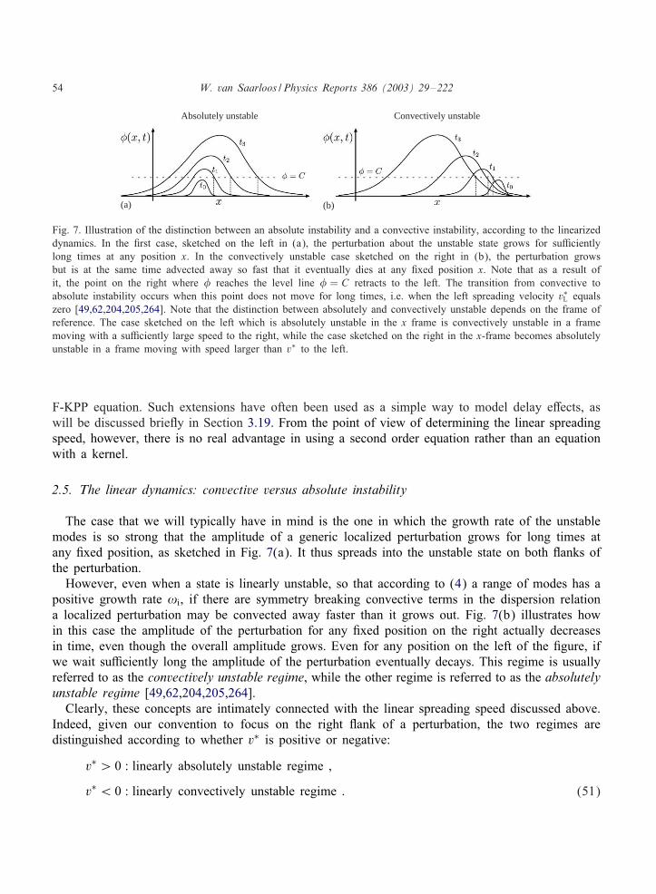
54 W. van Saarloos / Physics Reports 386 (2003) 29–222
(a) (b)
Absolutely unstable Convectively unstable
Fig. 7. Illustration of the distinction between an absolute instability and a convective instability, according to the linearizeddynamics. In the 3rst case, sketched on the left in (a), the perturbation about the unstable state grows for suRcientlylong times at any position x. In the convectively unstable case sketched on the right in (b), the perturbation growsbut is at the same time advected away so fast that it eventually dies at any 3xed position x. Note that as a result ofit, the point on the right where � reaches the level line � = C retracts to the left. The transition from convective toabsolute instability occurs when this point does not move for long times, i.e. when the left spreading velocity v∗L equalszero [49,62,204,205,264]. Note that the distinction between absolutely and convectively unstable depends on the frame ofreference. The case sketched on the left which is absolutely unstable in the x frame is convectively unstable in a framemoving with a suRciently large speed to the right, while the case sketched on the right in the x-frame becomes absolutelyunstable in a frame moving with speed larger than v∗ to the left.
F-KPP equation. Such extensions have often been used as a simple way to model delay eDects, aswill be discussed brieKy in Section 3.19. From the point of view of determining the linear spreadingspeed, however, there is no real advantage in using a second order equation rather than an equationwith a kernel.
2.5. The linear dynamics: convective versus absolute instability
The case that we will typically have in mind is the one in which the growth rate of the unstablemodes is so strong that the amplitude of a generic localized perturbation grows for long times atany 3xed position, as sketched in Fig. 7(a). It thus spreads into the unstable state on both Kanks ofthe perturbation.
However, even when a state is linearly unstable, so that according to (4) a range of modes has apositive growth rate !i, if there are symmetry breaking convective terms in the dispersion relationa localized perturbation may be convected away faster than it grows out. Fig. 7(b) illustrates howin this case the amplitude of the perturbation for any 3xed position on the right actually decreasesin time, even though the overall amplitude grows. Even for any position on the left of the 3gure, ifwe wait suRciently long the amplitude of the perturbation eventually decays. This regime is usuallyreferred to as the convectively unstable regime, while the other regime is referred to as the absolutelyunstable regime [49,62,204,205,264].
Clearly, these concepts are intimately connected with the linear spreading speed discussed above.Indeed, given our convention to focus on the right Kank of a perturbation, the two regimes aredistinguished according to whether v∗ is positive or negative:
v∗ ¿ 0 : linearly absolutely unstable regime ;
v∗ ¡ 0 : linearly convectively unstable regime : (51)

W. van Saarloos / Physics Reports 386 (2003) 29–222 55
It is important to keep in mind that the two regimes are de3ned in relation to a particular frameof reference: if v∗ ¿ 0 in the lab frame, so that the instability is absolute in that frame, the insta-bility becomes convectively unstable for an observer moving to the right with velocity larger thanv∗. Furthermore, a convectively unstable system ideally remains in or will return to the unstablestate according to the linear deterministic dynamics. Nevertheless, small perturbations or Kuctuationsare ampli3ed while they are advected away. This makes convectively unstable systems particularlysensitive to Kuctuations and to small but 3xed perturbations at a particular point. The latter couldarise in real experiments due to imperfections in experimental setup or due to local perturbationsat an inlet in systems with a throughKow. We will encounter a nice experimental illustration of thesensitivity to noise near the convective to absolute transition in Section 3.11.
We 3nally note that we have followed here the standard practice to distinguish the two regimesaccording to the fully linear dynamics. The generalization of these concepts to the nonlinear regimewill be given later in Section 2.10.
Example. The F-KPP equation with a convective term.
Consider the F-KPP equation with a convective term,
9tu(x; t) + s9xu(x; t) = 92xu(x; t) + f(u) ; (52)
where, as in the standard form (1), f(0) = 0 and f′(0) = 1. Since this equation simply becomes thestandard F-KPP equation (1) upon transforming to the moving frame x′ =x− st, the linear spreadingvelocity associated with (52) is v∗=s+v∗FKPP =s+2. Thus the linear instability changes from absoluteto convective at s=−2. Whether nonlinearly the transition also happens at this point depends on thefunction f(u): when f is such that fronts are pulled, the nonlinear transition remains at s=−2, butwhen the fronts become pushed, the transition shifts to more negative values of s—see Section 2.10.In the Taylor–Couette experiments reviewed in Section 3.11 the velocity s in the closely relatedamplitude equation is controlled with a Kow through the cell.
2.6. The two-fold way of front propagation into linearly unstable states:pulled and pushed fronts
In the previous sections, we have analyzed the linear spreading dynamics into a linearly unstablestate. We concluded that starting from suRciently localized initial conditions—the precise conditionbeing given in (37)—the perturbations spread into the unstable state with asymptotic speed v∗. Thisasymptotic spreading speed and associated parameters are determined through the dispersion relation!(k) via Eqs. (12).
We now turn to the genuine nonlinear front propagation problem already stated in the introduction,questions like: If initially a spatially extended system is in a linearly unstable state everywhereexcept in some spatially localized region, what will be the large-time dynamical properties andspeed of the nonlinear front which will propagate into the unstable state? Are there classes ofinitial conditions for which the front dynamics converges to some unique asymptotic front state?If so, what characterizes these initial conditions, and what can we say about the asymptotic frontproperties and the convergence to them?

56 W. van Saarloos / Physics Reports 386 (2003) 29–222
As before, our discussion is aimed to be as general as is possible. The only restriction we willmake, barring pathological cases, is that the nonlinear dynamical equations of the system underinvestigation have a suRcient degree of “locality”: they can involve partial derivative terms andnonlocal terms with a kernel whose range is essentially 3nite, but the dynamics of the dynamicalvariables at a given position should not depend crucially on the nonlinear state of the system in3nitelyfar away. 21 ; 22
A characteristic feature of front propagation into unstable states which carries over from the lineardynamics that we discussed above, is that initial conditions which decay very slowly spatially leadto a large front speed whose value depends on the spatial decay rate. We will come back to thislater. Hence, in order to make precise statements we need to limit the class of initial conditions weconsider. Now, for any given set of deterministic dynamical evolution equations with an unstablestate, the linear spreading speed v∗ and associated steepness �∗ are explicitly and uniquely calculableaccording to the discussion of the previous sections. This motivates us to distinguish the frontpropagation properties of dynamical equations according to the long-time evolution starting fromsteep initial conditions:
Whenever we associate a particular front propagation mechanism with a given dynamicalequation, this is a statement about the dynamical evolution of fronts that evolve from localizedinitial conditions. These include all initial conditions which are steep”, i.e., which as de6nedin (37) fall o> faster than exp[ − �∗x]. 23
Let vfront(t) be some suitably de3ned instantaneous front velocity. The crucial insight on whichour presentation will be based is the following simple insight: For front propagation into a linearlyunstable state, there are only two possibilities if we start from steep initial conditions,
I. vas ≡ limt→∞ vfront(t) = v∗ ⇔ “pulled” front,II. vas ≡ limt→∞ vfront(t) = v† ¿v∗ ⇔ “pushed” front.
This statement amounts to the claim that nonlinear fronts propagating into a linearly unstable statecan asymptotically not propagate with speed slower than v∗ for equations of the type we consider, inwhich the dynamics is “local” in the sense that the linear dynamics is not suppressed by nonlinearbehavior arbitrarily far away. To see this, suppose we start with a front solution which propagateswith speed less than v∗. Any suRciently small perturbation ahead of it will then grow out andspread, asymptotically with the linear spreading speed v∗. Eventually these perturbations will growlarge enough that nonlinear behavior kicks in, but the crossover region where this happens must
21 This requirement is comparable to the fact that in statistical physics the standard universality classes of equilibriumphase transitions only apply to Hamiltonians in which the interactions are suRciently short-ranged. This does includeHamiltonians where the interactions decay as a power r−+ provided + is large enough.
22 A simple example that illustrates this is the following extension of the F-KPP equation: 9tu = 92xu +
u(1 − m tanh[∫∞−∞ dx u2]) − u3. For m¡ 1 fronts in this equation are still pulled, albeit with a spreading speed
renormalized down from the value obtained by linearizing the equation in u about u = 0. For m¿ 1 there is no 3niteasymptotic front speed. This example illustrates that although it is diRcult to specify the general conditions under whichour analysis applies precisely, in practice common sense gets one quite far for any given problem.
23 We will later in Section 2.7.6 enlarge the class of initial conditions which lead to pushed front solutions.

W. van Saarloos / Physics Reports 386 (2003) 29–222 57
asymptotically advance at least with the speed v∗. In other words, since the nonlinearities cannotsuppress the linear growth arbitrarily far ahead of the front, they cannot prevent the linear spreadingto asymptotically move ahead with asymptotic speed v∗ and thus create a front with at least thisspeed. Consequently, nonlinearities can only drive front speeds up, i.e., to v† ¿v∗.
Admittedly, while the above conclusion that fronts can asymptotically not move slower than v∗may be dynamically “obvious”, I know of no general mathematical proof of it. For some of thefourth order equations reviewed in Section 2.11, this conclusion is either implicit or explicit in aformulation in which one proves that in any frame moving with velocity less than v∗ one seesperturbations grow [93,144].
At this point, the names “pulled” and “pushed” front fall fully into place. 24 With a pulled frontwe literally mean one which is pulled along by the linear spreading of small perturbations intothe linearly unstable state. Any front which asymptotically moves with speed v† faster than v∗ issomehow “pushed” into the unstable state by the nonlinear behavior in the front region itself or theregion behind it—if there were no nonlinear behavior, one would 3nd spreading with velocity v∗.We will thus refer to v† as the pushed front speed.
The present line of argument, where one takes the classical linear spreading of perturbations intoan unstable state as the starting point, has several important advantages and rami3cations. First ofall, it allows one to make statements irrespective of the nature of the nonlinear state behind thefront: Quite literally the picture that underlies it and that both the analytical and numerical resultspresented later con3rm, is that a pulled front spreads in the way the linear spreading point conditions(12) force it to do. In other words, the nonlinear dynamics in the region behind the leading edgejust has to adapt to whatever is forced by the linear spreading. Depending on the existence, stabilityand nature of nonlinear front solutions, this behavior can be coherent or incoherent, but this by itselfdoes not really feed back onto the linear spreading. 25 This simple idea can be made explicit andquantitative: it lies at the basis of the exact results for the universal relaxation behavior of pulledfronts discussed in Sections 2.9 and 4.
The second advantage is that the present line of argument focuses on the fact that the most clearand relevant issue is to understand the mechanism through which we can get fronts to propagate atspeeds larger than v∗, i.e., to be pushed.
We 3nally note that the concept of a pulled front is only well-de3ned for propagation into alinearly unstable state: A small perturbation around a linearly stable state dies out and does notspread. As a result, the propagation of a front into a linearly stable state is always driven by thenonlinearities and the nonlinear or dynamical competition between this state and a diDerent one.From this perspective, especially near subcritical bifurcation points, it is sometimes useful to thinkof a front which propagates into a stable state as being “pushed”.
24 The names pulled and pushed were introduced back in 1976 by Stokes [384] and revived in the physics literature inthe mid-90s by Paquette et al. [333,334]. Ben-Jacob et al. [38] referred to them as Case I and Case II marginal stabilityand I initially used the words linear and nonlinear marginal stability [421]. The great advantage of the nomenclature ofStokes is that the notions of “pulled” and “pushed” tie in nicely with the general concept of linear spreading velocity, andhence that they can be de3ned independently of whether or not a uniformly translating or coherent front solution exists.
25 Actually, we can make this quite precise: As we shall see, the 3rst consequence of the feedback of the nonlinearbehavior onto front propagation is the change of the prefactor of the 1=t relaxation term by a factor 3. See Section 2.9.

58 W. van Saarloos / Physics Reports 386 (2003) 29–222
2.7. Front selection for uniformly translating fronts and coherent and incoherentpattern forming fronts
In order to discuss the selection of a particular type of front and its propagation mechanism, it isuseful to distinguish three diDerent classes of nonlinear front dynamics: 26
• Uniformly translating fronts are nonlinear front solutions for the dynamical variable � of form
�(x; t) = ,v(-) ; (53)
where - is the co-moving coordinate
- ≡ x − vt ; (54)
which we will use for general velocity v, to distinguish it from the coordinate � = x − v∗t mov-ing with velocity v∗. We remind the reader that, unless noted otherwise, we do not distinguishnotationally between a single dynamical variable or a set (vector) of them. Eq. (53) expressesthat in a frame moving with velocity v, the front solution is stationary, i.e., invariant in time.Uniformly translating solutions are normally only appropriate solutions for problems in which thefront leaves behind a homogeneous state, i.e., does not generate a pattern. The overwhelmingmajority of asymptotic front solutions which have been analyzed in the mathematics literature areof this type. An example of a pushed front in the F-KPP equation is shown in the lower leftpanel of Fig. 1.
• Coherent pattern forming fronts are the generalization of uniformly translating solutions to sys-tems where the front leaves behind a pattern with a well-de3ned wavenumber. As the middle panelof Fig. 1 and the examples discussed in Sections 2.11 and 3 illustrate, usually the pattern behindthe front is stationary or moves with a velocity diDerent from the front speed. In other words,when viewed in the frame moving with the front, the pattern behind the front is not stationary.Hence the front solution cannot be of form (53). However, we may generalize the concept byintroducing a coherent pattern forming front solution as a front solution which is periodic in theframe - = x − vt moving with speed v, i.e.,
�(x; t) = ,(-; t) with ,(-; t + T ) = ,(-; t) : (55)
We can equivalently write this as
�(x; t) =∑
n=0;±1;:::
e−in/t,nv(-) (/ = 2�=T ) ; (56)
26 With our classi3cation we have in mind fronts which propagate in a homogeneous background medium. If the mediumitself is periodic, fronts which are uniformly translating in a homogeneous medium become automatically periodic; likewiseif the parameters of the dynamical equation are randomly varying the fronts will always be incoherent. Strictly speaking,fronts in a periodic medium, which are sometimes referred to as “periodically pulsating fronts”, are of the type (55) belowbut as stated, we will always have in mind that the medium itself is homogeneous, and when considering periodic frontsolutions concentrate on fronts which then generate a nontrivial pattern. For the linear dynamics of small perturbations aboutthe unstable state of a homogeneous system, the dispersion relation can be obtained from a simple Fourier transformation.As we shall discuss below in Section 3.18, the analysis of pulled fronts can be extended to the case of periodic mediaby recognizing that one simply has to do a Floquet analysis to determine !(k).

W. van Saarloos / Physics Reports 386 (2003) 29–222 59
where for real dynamical 3elds � the complex functions ,nv obey the symmetry
,−nv (-) = ,n
v(-) : (57)
Clearly, Eq. (55) expresses that in the co-moving frame the front solution is periodic. 27 Hence, inrepresentation (56) the functions ,n
v(-) can at every position be viewed as the Fourier coeRcientsof the time-periodic function ,(-; t).These time-periodic coherent front solutions of form (55) or (56) are relevant for e.g. the Swift–Hohenberg equation discussed in Section 2.11.2 and were to my knowledge for the 3rst timeintroduced for the analysis of fronts in this equation by Collet and Eckmann [92]. Moreover, theycan also be viewed as an extension of the “coherent structure solutions” [424] introduced in thecontext of the Complex Ginzburg Landau equations of Sections 2:11:5 and 2:11:6—because of thefact that the Complex Ginzburg Landau equation arises as the lowest order amplitude equationfor traveling wave patterns, only one term in the sum (56) is nonzero in this case. As we shallsee, both pulled and pushed coherent fronts solutions are found in certain parameter ranges.
• Incoherent pattern forming fronts is the name we will use for all the incoherent fronts likethose of the right column of Fig. 1 which do not 3t into one of the two previous classes.We will encounter other pulled and pushed examples of them later, but they are the leastunderstood of all.
We now proceed to discuss the dynamical mechanism that distinguishes pushed and pulled frontsfor these various classes of equations. The essential ingredient will be to maximally exploit theconstraints imposed by the linear dynamics about the unstable state.
2.7.1. Uniformly translating front solutionsWhen a dynamical equation also admits a homogeneous stable stationary state �ss = const: in
addition to the unstable state � = 0, then usually this dynamical equation also admits uniformlytranslating front solutions of form (53), �(x; t) = ,v(-) with - = x − vt. To investigate whether itdoes, one substitutes this Ansatz into the dynamical equation and analyzes its behavior. The simplicityof uniformly translating fronts lies in the fact that the function ,v(-) depend on the single variable- only, so that the function ,v then obeys an ordinary diDerential equation rather than a partialdiDerential equation. The existence of front solutions can from there on be analyzed using standardmethods [13,14,191]: the homogeneous stationary states � = 0 and � = �ss are 3xed points of thisordinary diDerential equation. By linearizing about these 3xed points and studying the dimensions ofthe stable and unstable manifolds (i.e. the dimensions of the manifolds Kowing into and out of each3xed point), one can then study the multiplicity of front solutions (see e.g. [424] for an extensiveuse of such “counting arguments” in the context of CGL equations). For the F-KPP equation theanalysis, which is summarized below, is relatively trivial; one 3nds that there is a one-parameterfamily of front solutions that connect the stable homogeneous state with the unstable state �=0. Forthe F-KPP equation, one can easily go beyond a simple counting argument based on the analysis
27 We prefer to use the general name “coherent pattern forming front solution” instead of periodic front solutions for tworeasons. First of all, this name is consistent with the name “coherent structure solutions” for special type of solutions ofthe CGL equation (see Eq. (101) in Section 2.11.6). Secondly, we wish to stress the fact that we aim at pattern formingsolutions and so want to distinguish them from the simpler periodic or “pulsating” types of fronts that arise in equationslike the F-KPP equation when the medium itself is periodic—see Section 3.18.

60 W. van Saarloos / Physics Reports 386 (2003) 29–222
near the 3xed points to prove more rigorously when there is such a family of solutions. Thesefront solutions can be parametrized by their velocity v. We stress that for an arbitrary dynamicalequation that admits a stable homogeneous state and a homogeneous unstable state, there is notnecessarily always a one-parameter family of front solutions connecting the two. However, this iswhat is typically found and what is intuitively most reasonable based on the fact that a specialfeature of the linear dynamics about an unstable state is that any exponential tail with steepness �less than �∗ can propagate into the unstable state with speed venv(�)—see Section 2.2. 28
Let us 3rst proceed by assuming the equations do admit a one-parameter family of front solutions,parametrized by their velocity. Then this family generically will include a uniformly translating frontsolution ,v∗(�) moving with velocity v∗, to which the front will asymptotically converge in the pulledregime, i.e., starting from steep initial conditions.
The behavior near the 3xed points of the ordinary diDerential equation for ,v(-), obtained bylinearizing the Kow equations around the 3xed point, corresponds to an exponential --dependence.Thus, for an arbitrary velocity v, the solutions ,v(-) will decay to zero exponentially for large -,
,v(-) ≈ a1e−�1- + a2e−�2- + · · · (- → ∞) ; (58)
where all roots �i are positive and where the real coeRcients a1, a2, etc. can only be determinedby solving the equations for the fully nonlinear front solution. 29 We take these roots ordered,0¡�1 ¡�2 · · ·. The relation between the velocity v and the two smallest roots in the generic case 30 isshown in Fig. 3: For v¿v∗ the root �1 ¡�∗ while �2 ¿�∗. In passing we note that at v=v∗ two rootscoincide; general results [13,14,191] for the Kow behavior in the presence of degenerate eigenvaluesthen imply
,v∗(�) ≈ (a1� + a2)e−�∗� + a3e−�3� + · · · : (59)
When do we expect the equation to be pushed, i.e., when do we expect that a pushed front solutionswith velocity v† ¿v∗ will emerge starting from steep initial conditions? The answer lies hidden inFig. 4: according to the fully linear dynamics an exponential tail which is steeper than �∗ and whichcorresponds to the dashed branch �2 in Fig. 3, does run faster than v∗ but disappears from thescene because the crossover point to the linear spreading pro3le moves to the right. According to
28 An explicit counting argument for partial diDerential equations that are symmetric under spatial reKection con3rmsthat for such equations one typically expects a one-parameter family of front solutions (see Appendix A of [420]). Thereare two intimately related ways to understand why this is so often the case: (i) Suppose we 3rst change the dynamicalequation so as to make the unstable state stable. One then expects there to be at least one front solution (or maybe adiscrete set of them) connecting the two stable states. Now when we change the equation back to its original form, atthe moment when the � = 0 state becomes unstable again, the dimension of the stable manifold Kowing into the � = 03xed point increases by one, because a new root appears which is related to the left branch in Fig. 3; (ii) According tothe linear dynamics discussed in Section 2.2, any exponential tail with �¡�∗ can propagate into the unstable state withenvelope velocity venv(�). When the dynamical equation admits a stable homogeneous state as well, it is not unreasonablethat every exponential tail propagating with some velocity v in the leading edge can match up smoothly with a saturatingbehavior behind the front.
29 In (58) we want to bring out that there are contributions from the various roots, or, in more technical language, fromthe various directions that span the stable many-fold of the 3xed point corresponding to �=. If �1 ¡�2=2 then of courseterms exp[ − 2�1-] dominate over terms exp[ − �2-], but this is all hidden in the dots.
30 We assume here for simplicity that there are no other branches at even smaller �; this is usually the case, as thebranch which in Fig. 3 diverges as � ↓ 0 is associated with the instability, the fact that !i(� = 0)¿ 0. We will brieKycome back to the case where other branches intervene in Section 2.7.7.

W. van Saarloos / Physics Reports 386 (2003) 29–222 61
(a) (b)
Fig. 8. Illustration of the fact that when a nonlinear front solution ,v† exists, whose asymptotic steepness is according to(60) larger than �∗, then this front will generically emerge: it is the selected pushed front solution. Figure (a) should becompared to Fig. 4: If the equation would be fully linear, the steep tail on the right, which moves at velocity larger thanv∗, would cross over in the dashed region to the dashed pro3le moving with asymptotic speed v∗. However, this doesnot happen. When the steep pro3le matches up arbitrarily well with a fully nonlinear front pro3le ,v† this steep regiondoes not disappear from the scene: Instead a fully nonlinear pro3le with speed v† emerges. While (a) shows how onlythe pushed front solution ,v† can asymptotically emerge, (b) illustrates how a pushed front solution invades a regionwhere the pro3le is close to that given by the linear spreading analysis. The dashed line indicates the continuation of thepro3le as given by the linear spreading analysis of previous sections, but in the dashed region the pro3le crosses overto the steep tail of the nonlinear pushed pro3le. The fact that the crossover region moves to the right with the speed vco
determined earlier, con3rms that the pushed front solution invades the leading edge.
our “locality” assumption for the dynamics, the same holds arbitrarily far into the leading edge of afront, unless the nonlinearities in the dynamical equation allow the fast exponential tail to matchup perfectly with a nonlinear front solution! This is illustrated in Fig. 8: if a uniformly translatingfront solution with v = v† ¿v∗ exists for which a1 = 0 so that its asymptotic behavior is given bythe root �2,
,v†(-) ≈ a2e−�2- + a3e−�3- + · · · (�2 ¿�∗; - = x − v†t → ∞) ; (60)
then this front solution can and will overtake any transient dynamical tail in the leading edge. Inother words, such a solution is the asymptotic pushed front solution sought for, and if it exists it isthe dynamically relevant front solution emerging from steep initial conditions.
As we noted before, front solutions ,v(-) obey an ordinary diDerential equation or a set thereof;such a diDerential equations can be formulated as a Kow in phase space [13,14,191]. In such aninterpretation, a front solution corresponds to a so-called heteroclinic orbit, an orbit which goesfrom one point (the asymptotic state behind the front) to another (the state � = 0). For generalv, the orbit approaches the 3xed point corresponding to the state � = 0 asymptotically along theeigendirection whose rate of attraction, given by �1, is slowest. The pushed front solution ,v†(-),however, approaches it along the slowest but one eigendirection, the one with eigenvalue �2. Forthis reason, a uniformly translating pushed front solution is sometimes referred to as a stronglyheteroclinic orbit [354].
Let us illustrate the above considerations brieKy for two equations, the F-KPP equation and anextension of it, the EFK equation. Uniformly translating solutions U (x − vt) = U (-) of the F-KPP

62 W. van Saarloos / Physics Reports 386 (2003) 29–222
(a) (b)
Fig. 9. Sketch of the Kow in the phase space (U;U ′) of the Kow equations (62) and (63) that govern the uniformlytranslating solutions of the F-KPP equation. The solid lines at the two 3xed points indicate the shape of the stable andunstable manifolds near each 3xed point, obtained by linearizing the Kow around each 3xed point. The arrows indicate thedirection of the Kow, and the double arrow at the (0; 0) 3xed point indicates that the contraction along this eigendirection isstronger than along the other one (�2 ¿�1). The dashed trajectory is the heteroclinic orbit connecting the two 3xed points;it corresponds to the front solution connecting the stable and the unstable state. (a) Flow in the case v¿max(v†; v∗).The trajectory approaches the (0; 0) 3xed point along the slowest contracting direction. (b) If for some velocity v= v† thedashed trajectory becomes a “strongly heteroclinic orbit” which approaches the (0; 0) 3xed point along the more stronglycontracting direction, the equation admits a pushed front solution.
equation (1) obey the ordinary diDerential equation
− vdUd-
=d2Ud-2 + f(U ) : (61)
It is convenient to use the standard trick of writing this second order equation as a set of 3rst orderequation: by introducing the variable U ′ = dU=d- we can write (61) as
dUd-
= U ′ ; (62)
dU ′
d-= −vU ′ − f(U ) : (63)
These equations describe the Kow in the two-dimensional phase space (U;U ′), with - playing therole of time. Because f(0) = f(1) = 0 according to (1), the points (0; 0) and (1; 0) are 3xed pointsof these Kow equations; the 3rst one corresponds to the stable state and the second one to theunstable state. With our convention that fronts move into the unstable state on the right, a uniformlytranslating front solution corresponds to a trajectory Kowing from the (1; 0) 3xed point to the (0; 0)3xed point. Such a “heteroclinic orbit” is sketched for large arbitrary v in Fig. 9(a). 31 The solid linesnear the two 3xed points in this 3gure denote the directions of the stable and unstable manifoldsKowing into and out of each 3xed point. These are easily determined by linearizing equations (62),(63) about the 3xed point solutions and solving for the eigenvalues of the linearized Kow. Thearrows in Fig. 9 indicate the directions of the Kow for increasing - (“time”). As is indicated inthe 3gure, there is one stable and one unstable stable direction at the (1; 0) 3xed point. For any3xed velocity v, there is hence a unique trajectory coming out of this 3xed point in the direction ofdecreasing u. At the (0; 0) 3xed point, however, both eigendirections are attracting; we have indicatedthe direction along which the contraction is largest with a double arrow. Now, because there is
31 For v¡ v∗ the eigenvalues at the 3xed point (0; 0) are complex so trajectories spiral into this 3xed point.
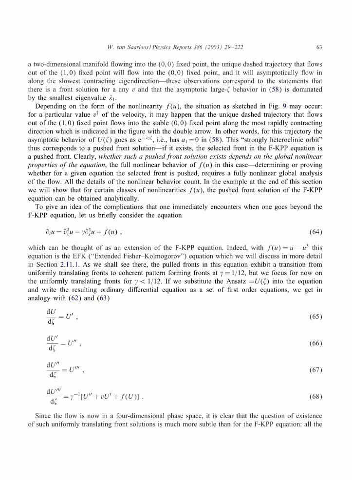
W. van Saarloos / Physics Reports 386 (2003) 29–222 63
a two-dimensional manifold Kowing into the (0; 0) 3xed point, the unique dashed trajectory that Kowsout of the (1; 0) 3xed point will Kow into the (0; 0) 3xed point, and it will asymptotically Kow inalong the slowest contracting eigendirection—these observations correspond to the statements thatthere is a front solution for a any v and that the asymptotic large-- behavior in (58) is dominatedby the smallest eigenvalue �1.
Depending on the form of the nonlinearity f(u), the situation as sketched in Fig. 9 may occur:for a particular value v† of the velocity, it may happen that the unique dashed trajectory that Kowsout of the (1; 0) 3xed point Kows into the stable (0; 0) 3xed point along the most rapidly contractingdirection which is indicated in the 3gure with the double arrow. In other words, for this trajectory theasymptotic behavior of U (-) goes as e−�2-, i.e., has a1 =0 in (58). This “strongly heteroclinic orbit”thus corresponds to a pushed front solution—if it exists, the selected front in the F-KPP equation isa pushed front. Clearly, whether such a pushed front solution exists depends on the global nonlinearproperties of the equation, the full nonlinear behavior of f(u) in this case—determining or provingwhether for a given equation the selected front is pushed, requires a fully nonlinear global analysisof the Kow. All the details of the nonlinear behavior count. In the example at the end of this sectionwe will show that for certain classes of nonlinearities f(u), the pushed front solution of the F-KPPequation can be obtained analytically.
To give an idea of the complications that one immediately encounters when one goes beyond theF-KPP equation, let us brieKy consider the equation
9tu = 92xu− 294
xu + f(u) ; (64)
which can be thought of as an extension of the F-KPP equation. Indeed, with f(u) = u − u3 thisequation is the EFK (“Extended Fisher–Kolmogorov”) equation which we will discuss in more detailin Section 2.11.1. As we shall see there, the pulled fronts in this equation exhibit a transition fromuniformly translating fronts to coherent pattern forming fronts at 2= 1=12, but we focus for now onthe uniformly translating fronts for 2¡ 1=12. If we substitute the Ansatz =U (-) into the equationand write the resulting ordinary diDerential equation as a set of 3rst order equations, we get inanalogy with (62) and (63)
dUd-
= U ′ ; (65)
dU ′
d-= U ′′ ; (66)
dU ′′
d-= U ′′′ ; (67)
dU ′′′
d-= 2−1[U ′′ + vU ′ + f(U )] : (68)
Since the Kow is now in a four-dimensional phase space, it is clear that the question of existenceof such uniformly translating front solutions is much more subtle than for the F-KPP equation: all the

64 W. van Saarloos / Physics Reports 386 (2003) 29–222
(a) (b)
uniformly translating pushed front in the EFK equation
Fig. 10. (a) Space time of a numerical solution of Eq. (64) with nonlinearity f(u) = u+ 9u2 − 10u3. This is an extensionof the EFK equation discussed in Section 2.11.1. For this nonlinearity, the selected front is a pushed front propagatingwith speed v† = 2:751 [421]. The time increment between successive time-slices is 0.75; the initial condition is a smallGaussian peak centered at the origin, and the total simulation time is 22.5. The dashed line indicates a position movingwith the speed v∗ = 1:8934. Although the front might appear to be monotonically decaying to the right, close inspectionof this pushed front in the tip shows that it is actually non-monotonic; the enlargement in panel (b) shows this moreclearly. (b) Blow up of the asymptotic front pro3le in the leading edge. The symbols denote the actual front values atthe grid points in the simulations, while the full line is the pro3le in the leading edge given by the three terms in (60).The dashed line denotes the mode exp(−�1-). Clearly, for the pushed front solution, a1=0 indeed, in accordance with themechanism of pushed front propagation set forth in the main text. From [421].
simpli3cations of Kow in a two-dimensional plane, special to the F-KPP equation, are lost. 32 Letus here simply illustrate that one important simplifying property of the F-KPP equation is immedi-ately lost. From the phase space arguments sketched above for the F-KPP equation, it immediatelyfollows that the selected front is the front solution with the smallest speed for which the frontsolution is monotonically decaying with -. Therefore, this idea has sometimes been proposed inthe literature as a general principle for front selection. However, it is simply a property of theF-KPP equation and a limited class of extensions of it—it is a property that does not really haveanything to do with front selection and just does not hold generally. The simulations of Fig. 10illustrate this for the above Eq. (64) with f(u) = u + 9u2 − 10u3. As the left panel illustrates,the selected front is a uniformly translating pushed front in this case. Although this is hardlyvisible in the space-time plot on the left, this pushed front solution is not monotonically decay-ing towards the right. The enlargement of the leading edge in the right panel shows how U 3rstgoes through zero and then has a local maximum at negative U . This plot also con3rms fully themechanism for pushed fronts that we have identi3ed above: the selected pro3le 3ts the form (58)with a1 = 0.
32 If one again linearizes the Kow near the two 3xed points (0; 0; 0; 0) and (1; 0; 0; 0), the multiplicity of the stable andunstable manifolds is such that one would indeed expect the existence of a one-parameter family of front solutions [421].A more rigorous study of such front solutions and of the Kow in this four-dimensional phase space has been taken uponly recently in the mathematics literature. See in particular [371] for a proof of the existence of front solutions of theabove Kow equations and [340,410] for other types of solutions.

W. van Saarloos / Physics Reports 386 (2003) 29–222 65
Let us return to our general formulation of the mechanism through which pushed fronts arise foruniformly translating fronts. While this scenario is arrived at simply by exploiting our insight intothe leading edge where the dynamics is essentially given by the linear dynamics, it is in completeagreement with (i) what is known rigorously for the second order F-KPP equation, (ii) the (marginal)stability arguments for front selection (Section 2.8) which show that if a strongly heteroclinic frontsolution ,v† exists, all front solutions with lower speed are unstable to invasion by this front, and(iii) all numerical results known to me. Furthermore, the extension of the argument to coherentpattern forming fronts is fully consistent with the analytical and numerical results for the quinticCGL equation discussed in Section 2.11.6).
We 3nally return to the question what happens if the front solutions do not admit a one-parameterfamily of front solutions. If this happens, then we generically expect that the equations will notadmit a uniformly translating pulled front solution moving with velocity v∗. A pulled front canthen not be uniformly translating—the pulled front solution must then show nontrivial dynamics inthe front region. Presumably, the dynamics is then either that of a coherent or incoherent patternforming front, even if the state it 3nally leaves behind is structureless. Furthermore, the absence ofa one-parameter family of uniformly translating front solutions makes it also very unlikely that therewill be uniformly translating pushed front solutions, as these have to obey one additional constrainta1 = 0.
Example. Pushed front solutions of the F-KPP equation and the reduction of order method.For the F-KPP equation, for which the dispersion relation !(k) is quadratic, a general uniformly
translating front solution u(x− vt) = U (-) falls oD to u = 0 with two exponentials—in other words,for a front solution with arbitrary velocity v there are two terms in expression (58) for the large -behavior. However, as we already discussed above, a pushed front solution of the F-KPP equationapproaches u = 0 with a single exponent, as a1 = 0. A good strategy to look for exact pushed frontsolutions of the F-KPP equation is therefore [421] to investigate when front solutions of the 3rstorder equation
dUv
d-= h(Uv) (69)
are also front solutions of the full ordinary diDerential equation for front solutions Uv(-) of theF-KPP equation. This is the case if they satisfy Eq. (61),
− vdUv(-)
d-=
d2Uv(-)d-2 + f(Uv(-)) : (70)
Searching for solutions of the type (69) is very easy; to see this, note that upon substitution of (69)into (70) we get
− vh(Uv) = h′(Uv) h(Uv) + f(Uv) ; (71)
so that we just need to look for combinations of functions h and f which obey this last equation(for any given h one can trivially 3nd a function f but the converse is not true). This is especiallysimple for polynomial functions. Indeed, it is straightforward to check that the functions [144]
h(u) = −�u(1 − un); f(u) = �u + un+1 − (1 + �)u2n+1 (72)

66 W. van Saarloos / Physics Reports 386 (2003) 29–222
solve (71) provided we take
�2 =� + 1n + 1
; v = (n + 2)�− 1=� : (73)
In order that the front solution of these equations corresponds to a pushed front solution of theF-KPP equation, the decay rate � given by (73) needs to be bigger than �∗ =
√�; this is easily
found to be the case for �¡ 1=n. Thus, the F-KPP equation with a nonlinearity f(u) given by 33
(72) has the pushed to pulled transition at � = 1=n, and for �¡ 1=n the pushed front velocity v† isgiven by (73).
For further discussion of these results for the most common cases n = 1 (f a cubic polynomialin u) and n=2 (f a function of u, u3 and u5), we refer to [38,421]. Other examples are discussed in[34,144,198,212,326,355,436,447] and Section 3.15, where we will discuss a nontrivial case relevantto liquid crystals. Quite surprisingly this “reduction of order method”, as it is sometimes called,also allows one to 3nd the pushed front solutions of the quintic CGL equation (see Section 2.11.6)and to construct other types of exact solutions of the CGL equation [95,312,322,424]. Deep down,the method is related to the construction of exact solutions of nonlinear equations using PainlevIeanalysis [95,96,360]. Also symmetry reduction methods have been used to search for exact solutionsof the nonlinear diDusion equation [89,325].
2.7.2. Coherent pattern forming front solutionsLet us now turn to coherent pattern forming front solutions of form (56). Every function ,n
v(-)in this expression also depends only on the co-moving coordinate -. Hence if we substitute theexpansion (56) into the dynamical equation under investigation, the functions ,n
v(-) will in generalobey a set of coupled ordinary diDerential equations. In general, this in3nite set of ordinary diDerentialequations is quite cumbersome; however, for fronts we need to have ,n
v(-) → 0 as - → ∞, andto linear order all the ,m
v obey essentially the same equation obtained by linearizing the dynamicalequation about the unstable state. We then have the freedom to take the term with n=1 to correspondto asymptotic decay exp[ − �1-] associated with the smallest root �1; in analogy with (58) we thenhave
,1v(-) ≈ A1eikr; 1-−�1- + A2eikr2-−�2- + · · · ; (74)
where now the coeRcients A1, A2, etc. are complex. Again it follows from the general argumentsunderlying Fig. 3 that for any v¿v∗, we generally have �1 ¡�∗, �2 ¿�∗.
One may, like in the case of uniformly translating fronts, wonder about the multiplicity of coherentpattern forming fronts. There are even fewer results in this case, but indications are that for frontpropagation into unstable states the typical case is that there is a two-parameter family of frontsolutions. That this is the case has been proved for the Swift–Hohenberg equation [92] and is alsofound [424] for the quintic CGL equation of Section 2.11.6. Moreover, counting-type arguments forthe pattern-forming regime of the EFK equation (Section 2.11.1) are consistent with this—we expectthat the methods developed by Sandstede and Scheel [375] will allow one to establish this moregenerally and cleanly. Intuitively, the existence of a two-parameter family of front solutions is the
33 The prefactor of the term un+1 looks special, but the analysis covers all cases with f(u) of form (72) since all othercases can be brought to this form by a proper scaling of space, time and u—see [355] and Appendix C of [144].

W. van Saarloos / Physics Reports 386 (2003) 29–222 67
natural extension of the existence of a one-parameter family of uniformly translating front solutions,since the leading edge of pattern forming fronts generically is characterized by a wavenumber kr inaddition to the steepness �. In other words, our conjecture that the generic situation is that there isa two-parameter family of coherent pattern forming fronts, means that for every velocity v, there isa one-parameter family of fronts parametrized e.g. by the wavenumber kr in the leading edge or bythe wavenumber of the coherent pattern behind the front. The front solutions whose wavenumberleads to maximal growth in the leading edge for given steepness (9!i=9kr = 0), then correspond tothe left branch in Fig. 3.
Let us proceed 3rst by assuming that indeed the equations for the coherent pattern forming frontsolutions admit a two-parameter family of front solutions. The above considerations then imply thatthere will in general exist a coherent pulled front solution, i.e., a solution whose asymptotic behaviorto the right matches the linear spreading point behavior,
,1v∗(�) ∼ (A1� + A2)e−�∗�+i(k∗r �−(!∗
r −krv)t) (� = x − v∗t → ∞) ; (75)
where in analogy with (59) the term linear in � arises because two roots coincide at v∗. The coherentpulled front solutions determined this way will be the ones that one will observe in the regime ofpulled front propagation.
The mechanism to get coherent pushed solutions moving at a speed v† ¿v∗ is completely anal-ogous to the one we discussed above for uniformly translating solutions with the aid of Fig. 8:starting from steep initial conditions an arbitrary front solution with speed v¿v∗ cannot emerge,since that would be incompatible with the dynamics in the leading edge, but any special coherentfront solution whose asymptotic spatial decay is steeper in that
,1v†(-) ∼ A2e−�2-+ikr2- + · · · ; (76)
can and will invade the leading edge. In other words, if a solution for which A1 = 0 in (74)exists, this is the pushed front solution that will be selected by the dynamics. Note that since thecoeRcients A1, A2, etc. in (74) are complex coeRcients, the condition that A1 = 0 amounts to twoconditions. Whether there are front solutions which obey this condition depends on the equationunder investigation, but since we assume that there is a two-parameter family of front solutions, ifthey exist, pushed front solutions are expected to be isolated solutions.
This selection mechanism for coherent pattern forming front solutions is clearly quite analogous tothe one we discussed for uniformly translating fronts, but for coherent fronts I am not aware of anyrigorous work on the pulled to pushed transition of coherent fronts. The numerical and analyticalwork on a modi3ed version of the Swift–Hohenberg equation and on the quintic CGL equation,summarized brieKy in Sections 2.11.2 and 2.11.6 are in full accord with the above scenario.
It is important to keep in mind that our discussion has been based on the idea that coherentfront solutions come as a two-parameter family if they exist. For a particular equation, it is notguaranteed that they do exist, of course. Indeed, the quintic CGL equation discussed in Section2.11.6 illustrates this: In some parameter ranges one can show that the equation does not admit anycoherent pulled front solution. In the parameter range where this happens, the pulled fronts becomeincoherent—see Fig. 17. Likewise, if the coherent front solutions do not come as a two-parameterfamily, then neither coherent pulled front solutions nor coherent pushed front solutions are expectedto exist: the dynamics is then expected to be incoherent.

68 W. van Saarloos / Physics Reports 386 (2003) 29–222
We 3nally note an important point. We already noted above that the condition A1 =0 is equivalentto two conditions, and that this implies that pushed fronts solutions, if they exist, generically come asisolated (discrete) solutions. Moreover, this simple counting argument also shows that the dominantspatial decay rate �2 of this isolated solution (76) generally does not lie on the thick dashed branchin Fig. 3. 34 By the same token, this implies that at the pulled to pushed transition, i.e. whenv† ↓ v∗, �2 = �∗ in (76). So, while for uniformly translating pro3les the pulled to pushed transitioncorresponds to a continuous transition in the front shape, for coherent pattern forming fronts thetransition is discontinuous in the front shape! Such discontinuous behavior, which was 3rst discoveredfor the quintic CGL equation of Section 2.11.6, imply that “structural stability” conjectures do notapply to pattern forming fronts. We will come back to this in Section 2.8.3.
Examples of pushed coherent fronts will be encountered later in Sections 2.11.1, 2.11.2, 2.11.6,3.8, and 3.17; we also conjecture that pushed coherent fronts can arise in the models of Sections3.2 and 3.3, for which so far only pulled fronts have been found.
2.7.3. Incoherent pattern forming front solutionsIncoherent pattern forming fronts are those fronts which do not leave behind a coherent pattern.
Hence they cannot be of form (56). From the numerical simulations of the cubic and quintic CGLequation discussed in Sections 2.11.5 and 2.11.6 and the full-blown numerical simulations of turbu-lence fronts discussed in Section 3.9 we know that both pulled and pushed incoherent fronts can exist.Of course, as always we can calculate the speed of incoherent pulled fronts, but to my knowledgethere is essentially no good understanding of what drives an incoherent front to be pushed. Thus Icannot give a precise mathematical formulation, analogous to (60) or (76), that identi3es what prop-erty will give rise to a pushed incoherent front. My conjecture is that in analogy with what we foundfor uniformly translating and coherent pattern forming fronts, incoherent pulled fronts are solutionswhich in some average sense do fall oD with a well-de3ned steepness larger than �∗. The simulationsof turbulence fronts discussed in Section 3.9 con3rm this idea, but I do not know how to give pre-dictive power to this statement. Unfortunately, the problem of the transition from pulled to pushedincoherent fronts appears to be as hard as the spatio-temporal chaos and turbulence problem itself!
Examples of pushed incoherent fronts will be encountered in Sections 2.11.4, 2.11.6, 3.9 and 3.22.
2.7.4. E>ects of the stability of the state generated by the frontIn our discussion of how pushed fronts can arise in the various modes of front propagation,
a central role is played by the existence of the special type of uniformly translating or coherentpattern forming solutions which for - → ∞ decay with steepness larger than �∗—these become thepushed front solutions. To what extent does the stability of fronts play a role? As we will discuss inSection 2.8 below, one can relate the above selection mechanism of pushed fronts to the stabilityproperties of front solutions with v¡v†, but it is more appropriate to think of this as a consequencerather than a cause of front selection.
The stability or instability of the state generated by the front does have important consequencesfor the dynamics, however. The examples discussed in Section 2.11 will illustrate this most clearly:it is quite possible that the state which emerges behind the front is itself unstable. When the selected
34 In [421], we suggested that the combinations v†; �2 of pushed fronts of the Swift–Hohenberg equation should lie onthe dashed branch. This suggestion is wrong.

W. van Saarloos / Physics Reports 386 (2003) 29–222 69
state is nonlinearly convectively unstable in the frame moving with the front, the state behind the3rst front is invaded by a second front which moves slower than the 3rst. If, however, the stategenerated by the 3rst front is absolutely unstable in the frame moving with the 3rst front, then thesecond one will catch up with the 3rst and alter its properties. In the examples we will discuss thesecond front is usually an incoherent front, and when the one with which it catches up is a coherentfront, this induces a transition from coherent to incoherent front dynamics in the leading front. Inpractice, therefore, what type of front dynamics one will get is determined both by the existence offront solutions and by the stability of the state these solutions generate.
2.7.5. When to expect pushed fronts?The requirement for existence of a pushed front solution, a1 = 0 according to Eq. (60) for a
uniformly translating front solution to exist, or A1 = 0 according to Eq. (76) for a coherent patternforming solution, is a condition on the global properties of the solution of a nonlinear ordinarydiDerential equation. Hence whether a pushed front solution exists depends on the full nonlinearproperties of the dynamical equation we wish to investigate. There does not appear to be a generalmathematical framework that allows us to predict from the appearance or the global structure ofan equation whether a strongly heteroclinic front solution does exist, and hence whether fronts willbe pulled or pushed. For the F-KPP equation one can derive general conditions on the nonlinearfunction f(u) such that the selected fronts in the equation are pulled [35,37]. One of the simpleresults is that when f(u)=u6f′(0) the fronts are pulled, which con3rms our intuitive understandingthat for a front to become pushed one needs the nonlinearities to enhance the growth. For (sets of)equations that admit uniformly translating fronts one typically 3nds the same trend, namely that theenhancement of the growth by the nonlinear terms in the dynamical equations tends to favor theoccurrence of pushed fronts.
It is important to realize, however, that for coherent and incoherent pattern forming fronts,these intuitive ideas do not necessarily apply. Several of the examples to be discussed inSection 2.11 will illustrate this: in the quintic CGL equation the cubic term enhances the growth,but there are large regions of parameter space where nonlinear dispersion eDects completely sup-press the occurrence of pushed fronts. Likewise, fronts in the Kuramoto–Sivashinsky equation ofSection 2.11.4 are pulled, but if one adds a linear term to the equation, a pulled to pushed tran-sition is found. However, in dynamical pattern forming equations which derive from a Lyapunovfunctional and for which one has an reasonable understanding of whether the nonlinearities enhanceor suppress the growth about the unstable state, one’s intuition of what to expect is usually cor-rect. Our discussion of front dynamics in the Swift–Hohenberg and Cahn–Hilliard equation willillustrate this.
As the example discussed at the end of Section 2.7.1 illustrated, for the second order partial F-KPPequation, the pushed front solutions can in a number of cases be explicitly constructed analytically.The reason is the following. While for an arbitrary v the large-- asymptotics (58) is characterized bytwo diDerent exponentials, the pushed front solutions (60) of the F-KPP equation are characterizedby one root. It is therefore possible (but not necessary) that the pushed solutions obey a 3rst orderequation. The “reduction of order method” brieKy reviewed in Section 2.7.1 is based on substitutinga 3rst order Ansatz into the second order ordinary diDerential equation for the uniformly translatingsolutions. The most remarkable success of this method is that the pushed solutions of the quinticCGL equation have been found this way—see Section 2.11.6.

70 W. van Saarloos / Physics Reports 386 (2003) 29–222
2.7.6. Precise determination of localized initial conditions which give rise to pulled and pushedfronts, and leading edge dominated dynamics for non-localized initial conditions
So far, we have focused on the front dynamics emerging from initial conditions which are “steep”,in the sense that they fall oD faster than exp[− �∗x]. This is because only for such initial conditionsdoes the front selection problem have a sharp and unique answer—whether fronts are pushed orpulled is an inherent property of the dynamical equations. Indeed, the values of the correspondingvelocities v∗ and v† are determined completely by the equation itself.
What happens if the initial conditions are not steep, i.e., fall of slower than exp[ − �∗x]? Givenour assumption of locality of our dynamical equations (no inKuence oD from points arbitrarily faraway) the answer lies hidden again in our analysis of the linear dynamics illustrated in Fig. 5. Ifinitial conditions fall oD with steepness �¡�∗, the spatially slowly decaying leading edge on theright, which moves with velocity venv(�), expands in time. In other words, in the frame movingalong with this leading edge, the crossover region to the slower part of the pro3le recedes to the leftand larger and larger parts of the pro3le move with asymptotic velocity venv. Whatever the nonlineardynamics is, it must be compatible with this dynamical constraint in the leading edge of the pro3le.Indeed, such initial conditions which are not steep necessarily lead to a front moving with speedvenv(�) with �¡�∗, unless a pushed front solution exists whose speed v† is larger than venv. For,if such a pushed front solution with v† ¿venv(�) exists, this solution will invade the leading edgeaccording the mechanism sketched in Fig. 8(b). Thus we conclude:
For an equation whose fronts are pulled, all initial conditions with steepness �¡�∗ lead tofronts moving with speed venv(�)¿v∗. In other words, in the pulled regime we can identify“localized” initial conditions which lead to pulled fronts with initial conditions which are steep,i.e., which fall o> faster than exp[ − �∗x].
For an equation whose fronts are pushed, only initial conditions with steepness �¡�1 lead tofronts moving with speed venv(�)¿v†, where �1 is the smallest root for which venv(�1) = v†.In other words, localized initial conditions which lead to pushed fronts are initial conditionswhich fall o> faster than exp[ − �1x], where �1 is determined implicitly by the pushed frontsolution through the requirement venv(�1) = v†.
Intuitively the mechanism through which non-localized initial conditions lead to fronts that movefaster than the naturally selected pulled or pushed speed, is very much like “pulling along” thenonlinear front. However, in order to distinguish them from the pulled front solutions which naturallyemerge from all localized initial conditions, we refer to this type of dynamics more generally as“leading edge dominated” dynamics [144].
2.7.7. Complications when there is more than one linear spreading pointIn our discussion of the pushed fronts, we have so far assumed that the linear dispersion is such
that the venv(�) versus � diagram is of the type sketched in Fig. 3, i.e., that there is only one branchwhich in the limit � ↓ 0 corresponds to a positive growth rate !i and hence to a divergent venv(�).This is the normal situation for problems where there is essentially one branch of linear modes whichis unstable. We now brieKy discuss the subtleties associated with having more than one unstablebranch of the dispersion relation.

W. van Saarloos / Physics Reports 386 (2003) 29–222 71
(a) (b)
Fig. 11. Illustration of possible venv(�) versus � diagrams in the case in which there is more than one unstable branch ofmodes. The relevant linear spreading velocity in each case is indicated with a 3lled circle. As explained in the text, theasymptotic steepness of a pushed front has to be associated with one of the two dashed branches.
Two examples of possible venv(�) diagrams for the case of two unstable branches are sketchedqualitatively in Fig. 11. As we discussed before, according to the fully linear spreading analysis,the relevant linear spreading velocity v∗ is the largest spreading velocity of the two branches. Thecrucial point to understand for the proper extension of the concept of a pushed front in such cases isthat the linear dynamics associated with the two individual branches is completely independent—wecan repeat the earlier discussion of how pushed fronts can emerge for each branch individually,and this leads to the conclusion that a pushed front is again a front whose asymptotic exponentialdecay is faster than e−�∗-. However, in addition the exponential steepness �† of the pushed frontshould be larger than the value �∗1 or �∗2 associated with the minimum of the branch to which itbelongs [86]. 35 In other words, the leading steepness of a pushed front should correspond to 36 oneof the two dashed branches in the 3gure. In the case of Fig. 11(a), a uniformly translating pushedfront solution is a solutions whose asymptotic decay is as e−�2-, not as e−�′1-. Likewise, for the casesketched in Fig. 11(b) a transition from the pulled front with velocity v∗ to a pushed one, whoseasymptotic behavior is as e−�2-, could occur.
Like before, the possibility of such situations to occur is intimately related with counting argu-ments for the multiplicity of front solutions. E.g., for uniformly translating fronts with a dispersionrelation consistent with one of the cases sketched in Fig. 11, one in general expects there to be atwo-parameter family of front solutions. For the case of Fig. 11(a) pushed front solutions with therequired asymptotic behavior are then expected to come as isolated front solutions, just as before.
35 Another way to arrive at the same conclusion, stressed in particular by Chomaz and Couairon [86], is to note thatasymptotic behavior with steepness given by one of the two left branches �1 or �2 can only emerge dynamically fromnon-localized initial conditions falling oD with this steepness: Chomaz and Couairon [86] call these branches non-causal.In the language of [421] one can understand this from the fact that on these branches the group velocity is less than theenvelope velocity—perturbations cannot work their way up towards the far tip.
36 In the case of coherent pattern forming front solutions, “correspond to” should be read as “analytically connected to”,since as we explained in Section 2.7.2 the asymptotic decay of a pushed front does not correspond to a value on thedashed branch of venv.

72 W. van Saarloos / Physics Reports 386 (2003) 29–222
2.8. Relation with existence and stability of front stability and relation withpreviously proposed selection mechanisms
In this section, we brieKy discuss the relation between front selection and stability, and the relationwith some of the older proposed selection mechanisms.
2.8.1. Stability versus selectionThe main diDerence in perspective with the “marginal stability” selection mechanism of the 1980s
[38,111,420,421] is that we here emphasize that by starting from the classical linear spreadinganalysis [49,62,264] the concept of a linear spreading velocity v∗ naturally arises. This conceptholds irrespective of whether or not there are well-de3ned front solutions, and applies equally wellto partial diDerential equations, diDerence equations and integro-diDerential equations. From thisperspective, the possibility of having pulled fronts arises most naturally and independently of whetherthey are coherent or incoherent. In addition, the saddle point integration immediately shows that theintermediate asymptotic dynamics giving the approach to the asymptotic spreading speed is that ofa diDusion equation, even if the equation itself is not at all a simple diDusion equation. This latterfact lies at the basis of the universal relaxation behavior discussed in the next section. Moreover, byexploring the constraints imposed by the linear dynamics, the essential properties of pulled frontsfollow.
The drawback of the “marginal stability” formulation of [420,421] is that when one wants to relateselection with the stability properties of fronts, one can at best only understand the selection once oneis already close to an asymptotic front solution. 37 Why the intermediate asymptotics bring one thereis less clear—even though the two are quite consistent the attempt in the marginal stability approachto treat selection and linear spreading in one fell swoop makes the problem unnecessarily cumbersomeand masks the generality of the linear spreading concept. Likewise, the universal relaxation behaviorof pulled fronts that we will discuss in the next section is virtually impossible to get from a stabilityanalysis (for uniformly translating or coherent pulled fronts, the spectrum of the stability operator iscontinuous with arbitrarily small eigenvalues), whereas it naturally emerges from the linear spreadingconcept.
Our simple observation that whenever a solution (60) or (76) with v† ¿v∗ exists whose asymp-totic steepness is larger than �∗, this solution can and will invade the leading edge and leadto pushed front propagation, is actually a general formulation which encompasses the “nonlinearmarginal stability” scenario that when one considers fronts as a function of there velocity, frontsolutions with speed v¡v† are unstable [38,421]. One can see this as follows [144, Appendix I].For dynamical equations which are translation invariant, the translation mode is always a mode withzero eigenvalue of the stability operator. At v = v† the front solution is a strongly heteroclinic orbit,and hence the zero eigenmode of the stability operator corresponds to a strongly heteroclinic orbit.Continuity and counting arguments then imply that for v close to but diDerent from v†, there is astrongly heteroclinic solution of the stability operator whose eigenvalue crosses zero at v = v†. Inother words, when the stability of the front solutions is studied for varying velocity v, the stability
37 Booty et al. [53] have also analyzed the dynamics in the leading edge of the F-KPP equation. Conceptually, theirapproach has much in common with that of [420,421].

W. van Saarloos / Physics Reports 386 (2003) 29–222 73
changes at v†—front solutions with velocity v¡v† are unstable due to the invasion of the pushedfront solution into the leading edge.
Another reason for separating front stability from front selection is that the simulations discussedin Section 2.11 will show that the state generated by the front becomes absolutely unstable in theframe moving with the front, this entails a transition from a coherent pattern forming front to anincoherent pattern forming front, not necessarily a change from pulled to pushed dynamics.
2.8.2. Relation between the multiplicity of front solutions and their stability spectrumThe above discussion of the implication of the existence of a pushed front solution for the stability
of fronts also illustrates that there generically is an intimate connection between the multiplicity ofuniformly translating and coherent front solutions and the stability properties. We can illustrate thisfor the other stability modes as follows. As we discussed in the previous section, a uniformlytranslating or coherent front solution corresponds to an orbit in the phase space of the ordinarydiDerential equations that govern these solutions, and the multiplicity of these solutions is determinedby “counting arguments” for the dimension of the manifolds that Kow into and out of the 3xed pointsthat correspond to the asymptotic states. Consider now the case in which the dynamical equationsadmit a one-parameter family of front solutions, parametrized by their speed v—we argued thatthis is the usual case for front propagation into unstable states. If we now pick an arbitrary frontsolution from this family and write down the stability operator for perturbations about the frontsolution, then the counting arguments for the stability modes is essentially unchanged because thelinearization about the asymptotic states before and after the front is unchanged. Hence the existenceof a one-parameter family of fronts, parametrized by v, generically implies that if we 3x v andconsider the stability modes, then we expect there to be in general a one-parameter family of stabilitymodes, parametrized by their growth/decay rate. Together with the fact that translation invariance ofthe dynamical equation implies that there is a zero mode of the stability operator, this also impliesthat there generically is a continuous spectrum of the stability operator near zero. A general analysisof the asymptotic behavior of these modes about the unstable state shows that the modes from thisspectrum which decay faster than the front solution are stable, and that those which decay less fastthan the front solution are unstable [421]. This line of analysis in combination with the one abovefor the possible presence of a localized stability mode if a pushed front solution exists, gives aquite complete generic picture of the stability of the front solutions in the generic case. In short:if no pushed front solution exists, so that the selected fronts are pulled, then the front solutionswith v¿v∗ are stable to perturbations which decay faster than the front itself, and unstable to thosewhich spatially decay less fast than the front itself. If a pushed front solution exists, then the genericpicture is that front solutions with v¡v† are unstable to the localized mode, and those with speedv¿v† are stable to this mode and to perturbations whose spatial decay to the right is faster thanthat of the front solution itself.
For coherent pattern forming fronts, similar arguments apply. Let us again focus on the genericcase (see Section 2.7.2) that these front solutions come into a two parameter family. If we considera particular front solution at a 3xed velocity v, then the generic scenario that results from similarcontinuity arguments is that any arbitrary front solution which in the tail does not match up with themaximal growth rate !i in the leading edge, or, in other words, whose asymptotic behavior does notcorrespond with the left branch drawn with a full line in Fig. 3(a), is unstable. This is the reason we

74 W. van Saarloos / Physics Reports 386 (2003) 29–222
focused on the analysis of venv de3ned in Eq. (21) in Section 2.2: only that branch matches up withasymptotic coherent front solutions which are stable to perturbation that decay spatially faster to theright than the front solutions themselves. The discussion of stability of a possible localized stabilitymode, associated with the existence of a pushed front solution, is analogous to the one given above.
The explicit stability calculation for the uniformly translating fronts in the F-KPP equation orextensions of it can be found in a number of papers [60,72,144,149,216,230,252,317,371] and willnot be repeated here. The results are completely in accord with the above general discussion.
2.8.3. Structural stabilityWe 3nally comment brieKy on the proposal to connect propagating front selection with “structural
stability” ideas. According to this conjecture [83,334], the pulled front is the natural front speed as itis the only front solution which is “structurally stable” to small changes in the dynamical equations(like those which would suppress the instability or make the state � = 0 even linearly stable). Itis easy to convince oneself that uniformly translating pulled solutions do have this property, as thedynamically relevant front solutions are characterized by a real spatial decay rate only, but that as wediscussed at the end of Section 2.7.2 coherent pattern forming front solutions which are characterizedby a decay rate and wavenumber in the leading edge, generically do not have this property. Indeed,the quintic CGL equation provides an explicit counterexample to the “structural stability” postulate:As we shall see under (iii) in Section 2.11.6, for the quintic CGL equation the selected wavenumbercan jump at the pulled to pushed transition.
2.8.4. Other observations and conjecturesThe issue of front selection issue has intrigued many authors, so various other observations and
conjectures have been made. In Appendix B we brieKy discuss some of these: a (wrong) conjectureconcerning the analytic structure of pushed front solutions, an observation about obtaining the selecteduniformly translating front by studying the front solutions on a 3nite interval, and the connectionwith Hamilton-Jacobi theory and renormalization group ideas.
2.9. Universal power law relaxation of pulled fronts
Up to now, we have focused on the asymptotic front velocity. Let us now assume we study anequation whose fronts are pulled, and ask how the asymptotic front velocity is approached. To do so,we 3rst have to state how we de3ne a time-dependent velocity of a front during the transient regimewhen it approaches its asymptotic value. We will be quite pragmatic in our discussion: the asymptoticconvergence to v∗ will turn out to be very slow, so slow that the diDerences between variousconventions do not really matter. We will therefore focus simply on the most natural de3nition.
In this section, we will simply state the results for the convergence to v∗; the essential ingredientsof the derivation are reviewed in Section 4.
It is good to stress that the universal relaxation only holds for pulled fronts. The discussion ofSection 2.8 implies that the stability spectrum of a pushed front solution is gapped, and hence thata pushed front relaxes exponentially fast to its asymptotic velocity and shape [144,227,421]. This isin line with the intuitive idea illustrated in Fig. 8 that a pushed front invades the region ahead of itwith a 3nite speed.
W. van Saarloos / Physics Reports 386 (2003) 29–222 75
2.9.1. Universal relaxation towards a uniformly translating pulled frontIf a pulled front is asymptotically uniformly translating, we can simply follow the same idea as
in our discussion of the linear spreading problem in Section 2.1: In essence our convention willalways be to determine a front speed vC(t) by tracking the position xC(t) of the level line wherethe dynamical 3eld � reaches a level C; the velocity is then the speed of this point
�(xC; t) = C ⇔ vC(t) =dxCdt
: (77)
Of course, for dynamical 3elds with more than one component, the transient velocity could in prin-ciple depend on which component we track, but we will not distinguish this possibility notationally,as we will focus on those aspects which are independent of those details.
The analysis [144] of the convergence of the nonlinear pulled front speed to v∗ is based onmatching the behavior in the leading edge, where corrections to the asymptotic exponential behaviore−�∗� are governed by an equation which in dominant order is a diDusion-type equation, to thebehavior in the fully nonlinear region. In this step, the fact that the asymptotic front solution ,v∗(�)has according to (59) a �e−�∗� behavior plays a crucial role—see Section 4. The 3nal result of thematching analysis [144] is the following exact expression for the velocity v(t) of an asymptoticallyuniformly translating front,
v(t) = v∗ − 32�∗t
+3√�
2√D(�∗)2t3=2
+ O
(1t2
); (78)
which holds provided one starts from steep initial conditions which fall oD faster than e−�∗x. 38 Thisslow power-law like relaxation of the velocity to its asymptotic value v∗ entails a slow relaxation ofthe front pro3le to its asymptotic shape. Indeed, if we de3ne X (t) as the shift of the front positionin the frame moving with speed v∗,
X (t) =∫ t
dt′ (v(t′) − v∗) ⇔ X (t) � − 32�∗
ln t + O(t−1=2) ; (79)
then one 3nds for the relaxation of the front pro3le to its asymptotic shape
�(x; t) � ,v(t)(�X ) + O
(1t2
); �X�
√Dt ; (80)
where �X is the frame
�X ≡ �− X (t) = x − v∗t − X (t) (81)
which includes the logarithmically increasing shift X (t).There are many points to note about these universal relaxation results for pulled fronts and the
physical picture underlying their derivation:
(i) While the above results are exact for all pulled fronts which asymptotically are uniformlytranslating, for the special case of the F-KPP equation, the 1=t term was known for over
38 To be more precise, the result holds provided the initial conditions fall oD exponentially faster than exp[ − �∗x], i.e.,provided there is some �¿ 0 such that �(x; t = 0)e�∗x ¡ e−�x as x → ∞. The special case in which �(x; t = 0) ∼ x4e−�∗x
is discussed in [54,144,255,256,314].

76 W. van Saarloos / Physics Reports 386 (2003) 29–222
165 170 175 180 185 190 195 2000.0
0.5
1.0
u
x
u u uu
t=0 t=5 t=10 t=15
Φ∗ (ξ) Φ∗ (ξ)Φ∗ (ξ)
Fig. 12. Illustration of the logarithmic shift of the transient pro3le relative to the asymptotic pro3le ,v∗ moving withconstant speed v∗, for the case of the F-KPP equation with f(u) = u − u3. The solid line shows the actual shape andposition of the front emerging from an initial condition at time t = 0 at three successive times. The dotted line showsthe uniformly translating solution ,v∗ (labeled ,∗ in the 3gure) at three successive times; at t = 5 this solution wasplaced such that it intersects the actual solution at u = 0:5. The thick solid line indicates that the transient solution andthe asymptotic solution separate more and more as time goes on, even though the shape of the transient front is alwaysclose to the asymptotic one. From [144].
20 years [138,139,291] and was derived rigorously in 1983 by Bramson [54]. Since then it hasbeen re-derived by various methods (including a matching analysis of [64] similar to ours),but to my knowledge even for the F-KPP equation the universal 1=t3=2 term was not knownbefore the matching analysis [144] described in more detail in Section 4.
(ii) The dominant logarithmic shift in X (t) which is driven by the diDusive dynamics in theleading edge implies that when viewed in the frame moving with the asymptotic velocity v∗,the front moves back while it is relaxing. This is illustrated in Fig. 12 for a simulation ofthe F-KPP equation starting from a localized initial condition. The plot shows the actual frontpro3le at times t = 5, 10 and 15 (full line), and compares these with the uniformly translatingasymptotic pro3le ,v∗ (dotted line) which has been placed so that it intersects the transientpro3le at �=1=2 at time t=5. The increase of the length of the thick line with time illustratesthat the actual transient pro3le and the asymptotic pro3le ,v∗ separate more and more in time.
(iii) The results which are illustrated in Fig. 12 show quite clearly that any method based onlinearizing about the asymptotic front solution ,v∗ will not work: the diDerences between theactual front solution and this asymptotic one grow arbitrarily large! This is why the insightto use the logarithmically shifted frame �X is crucial for any theoretical analysis.
(iv) Nevertheless, the 3gure does con3rm that already quite soon the transient front shape is closeto the asymptotic shape ,v∗ . This fact is expressed in precise mathematical terms by (80):to order t−2 the front shape is given by the expression for the uniformly translating frontsolution ,v, provided we use the instantaneous value v(t) given by (78) for the velocity, andput the front at the appropriately shifted position �X . In other words, to O(t−2) the transientfront shape follows the uniformly translating solutions adiabatically. This fact was 3rst notedempirically in simulations by Powell et al. [354].

W. van Saarloos / Physics Reports 386 (2003) 29–222 77
(v) The above results are valid for any pulled front which asymptotically is uniformly translating:it is independent on the precise nonlinearities and applies to all pulled fronts in equationsfor which the linear spreading speed v∗ can be determined according to our discussion ofSection 2.4. The fact that these results apply equally well to diDerence equations like the 3nitediDerence version (45) of the F-KPP equation or the diDerence-diDerential equation discussedin Section 3.23, is that the saddle point expression for v∗ ensures that the corrections to theasymptotic exponential e−�∗x behavior are governed by a diDusion-type equation. In otherwords, as these corrections become arbitrarily smooth for long times, the lattice eDects onlygive higher order corrections [144,146]. See Section 4 for further details.
(vi) Since the above results are independent of the precise form of the nonlinearities in the dy-namical equation as long as the fronts are pulled, one may wonder where the nonlinearitiesare hidden. Comparison with the result for the convergence to v∗ according to the fully lin-ear dynamics discussed in Section 4.1 shows that the prefactor 3/2 of the 1=t term and thesubdominant t−3=2 term both reKect the nonlinear behavior. 39
(vii) In line with the earlier conclusion of Section 2.3 that the limits t → ∞, � 3xed and � → ∞, t3xed do not commute, we stress that the expression (80) is the correct asymptotic expressionfor t → ∞, �X 3xed. At �X � √
Dt, there is a crossover to a diDerent asymptotics that governsthe large �X limit [144].
(viii) Note that the above result for the universal velocity relaxation holds independent of the initialconditions and of the level line which is used to track the position of the front, provided oneis not at the pulled to pushed transition. 40 In fact, the correction to the velocity relaxationassociated with the shape relaxation is according to (80) of order [�,v(-)=�v] dv(t)=dt ∼ t−2.
(ix) The terms displayed in (78) for v(t) and in (80) for the relaxation of the front pro3le arealso the only universal terms. This can easily be seen as follows. Suppose we compare thevelocity formula for two cases, one starting from some steep initial condition at time t = 0and the other one by viewing the dynamical state at time t = Wt as the initial condition. Forlarge times the 1=t terms for the two cases diDer of order Wt=t2. Thus the term of order 1=t2
depends on the initial conditions, i.e., is non-universal.(x) Formula (78) shows that the asymptotic velocity is always approached from below. This
explains why in many 3nite time simulations of pulled fronts the published velocity dataare slightly below v∗ (we will encounter several examples of this later). This fact togetherwith Eq. (80) for the shape relaxation of the front imply that for the transient dynamics thefront solutions with speed v¡v∗ are important. This is the reason for our cautionary note inSection 2.2 about using the phrase “the minimum velocity”.
(xi) Extensive numerical investigations and illustrations of the universal relaxation behavior ofuniformly pulled fronts can be found in [144,146]. An example of such tests will be discussedin Section 4.2.
39 As we will show in Section 4.1, Eq. (203), according to the fully linear dynamics a level line asymptotically recedesas −(ln t)=2�∗ in the frame moving with v∗, rather than as the −3(ln t)=2�∗ term of the nonlinear front pro3le. Hence ifwe would also draw in Fig. 12 the pro3le as it evolves according to the linearized equation, it would for large times andnot too large u lie in between the asymptotic front pro3le ,v∗ and the actual transient pro3le.
40 At the pulled to pushed transition the prefactors of the 1=t and 1=t3=2 term are diDerent—see Appendix G of [144].

78 W. van Saarloos / Physics Reports 386 (2003) 29–222
2.9.2. Universal relaxation towards a coherent pattern forming pulled frontHow to de3ne the instantaneous front velocity for a coherent pattern forming fronts is subtle issue.
If one traces the position of the foremost point where a dynamical 3eld which develops oscillationsreaches a given value, this position will make 3nite jumps when a new oscillatory part in theleading edge grows large enough that it reaches the predetermined level C. Since the time betweensuccessive jumps will be 3nite, averaging over some 3nite time then already gives a crude idea ofthe slow long-time convergence. A better way is to determine numerically an envelope of the frontpro3le from traces of e.g. the maxima of the oscillations during one period, and to then determinethe velocity from the positions of a level line of this empirical envelope of the front [388,383]. Theadvantage of this method is that it also works well when one wants to trace level lines in the rangewhere the nonlinearities in the dynamical equation are clearly important. If, on the other hand, onedecides to track the front velocity in the leading edge only, then a good method is to 3t a decayingoscillatory exponential to the front pro3le, and to determine the position of a given level from that3t. We will not dwell on the advantages and disadvantages of the these methods further, as they areof little relevance when one wants to probe the universal slow long-time relaxation.
Under the same assumptions as before for the uniformly translating fronts (see footnotes 38 and40), the front velocity of a coherent pulled front relaxes to its asymptotic value v∗ as [147,383,388]
v(t) ≡ v∗ + X (t) = v∗ − 32�∗t
+3√�
2(�∗)2t3=2Re
1√D
+ O
(1t2
); (82)
which reduces to the result (78) for uniformly translating fronts when ImD = 0. The relaxation ofthe front pro3le to its asymptotic behavior (56) is characterized by the relaxation of the velocityand a global phase 5(t): it is found that in this case one can write for the long-time asymptotics
�(x; t) ≈∑
n=0;±1;:::
e−in[/t+5(t)] ,nv(t)(�X ) + O
(1t2
); (83)
where 5(t) is given by [147,383,388]
5(t) = −k∗r X (t) − 3√�
2�∗t3=2Im
1√D
+ O
(1t2
): (84)
These equations simply express that to O(t−2) also the pattern forming fronts follow adiabatically afamily of coherent front solutions.
Essentially all the remarks made about the slow relaxation behavior of uniformly translating frontsapply equally well to the relaxation behavior of the pattern forming fronts—the only additionalfeature is the analogous slow convergence of the frequency 5(t): it implies a slow convergence ofthe wavelength of the pattern generated by the front. To our knowledge, this behavior has beenveri3ed both qualitatively as well as quantitatively only for the Swift–Hohenberg equation—seeSection 2.11.2 and Fig. 19 below. It does not appear to have been studied experimentally in asystematic way, although the slow velocity relaxation of pattern forming fronts does appear to playa role in some pattern forming experiments—see Section 3.1.
2.9.3. Universal relaxation towards an incoherent pattern forming pulled frontQuite remarkably, though we cannot make a prediction for the front shape relaxation for an
incoherent pulled front, we will argue in Section 4 that the same velocity relaxation formula (82)

W. van Saarloos / Physics Reports 386 (2003) 29–222 79
applies to an incoherent pattern forming pulled front. The reason for this is that even when a pulledfront is nonlinearly incoherent, the behavior in the leading edge is still very smooth and coherent, asit is governed by the same linear dynamical equation for the expansion about the linear spreadingpoint. This latter observation also implies that the velocity of an incoherent front is in practice mosteasily measured in the leading edge. Even the phase correction 5(t) is well-de3ned there and follows(84)—the results for the quintic CGL equation shown in Fig. 19 provide evidence in support ofthis claim.
2.10. Nonlinear generalization of convective and absolute instability on the basis of the resultsfor front propagation
In Section 2.5 we discussed the diDerence between convective and absolute instabilities in the casethat the evolution of a perturbation around the unstable state evolves according to the linearizedequations. As Fig. 7 illustrated, if we focus on the right Kank of the local perturbation, the linearinstability is absolute if v∗ ¿ 0 and convective if v∗ ¡ 0—in the latter case the perturbation “retreats”so that it eventually dies out at any 3xed position. If perturbations have enough time to grow thatthe nonlinearities become important and that a nonlinear front develops, it is straightforward toextend the distinction between the two regimes to the nonlinear case [85,99,412]. Clearly, in thepulled regime the criterion is the same since the nonlinearities do not aDect the asymptotic frontspeed, so the instability is nonlinearly convectively unstable for v∗ ¡ 0 and nonlinearly absolutelyunstable for v∗ ¿ 0. When the fronts are pushed in the dynamical equation under consideration,the criterion becomes simply that the instability is nonlinearly convectively unstable if v† ¡ 0 andnonlinearly absolutely unstable when v† ¿ 0. That’s all there is to it. A recent nice experiment on theKelvin–Helmholtz instability in which the transition from a nonlinearly convective to a nonlinearlyabsolute instability was observed, can be found in [186].
2.11. Uniformly translating fronts and coherent and incoherent pattern forming fronts infourth order equations and CGL amplitude equations
In this section we illustrate many of the basic issues of front propagation into unstable statesby reviewing the diversity of such fronts in Complex Ginzburg Landau (CGL) equations and ina number of well known fourth order partial diDerential equations which have been introduced inthe literature as model problems for a variety of physical phenomena. 41 In fact, we encounter allthree diDerent modes of front propagation dynamics both for pushed and for pulled fronts in theseequations, so taken together the examples discussed below give a good idea of the richness of frontpropagation into unstable state as well as of the power of the concepts of a pulled and pushed fronts.
We will limit our discussion completely to the dynamics of fronts which propagate into an unstablestate, so it is important to keep in mind that such behavior constitutes just a small fraction of the wide
41 We focus in the section on rather well known model equations. From a historical perspective, it is interesting tonote that pulled propagating fronts were also found back in 1983 in a fourth order caricature model aimed at describingsidebranching in dendrites [248]. The dispersion relation for the sidebranch instability in this model is of the same formas the general form we consider here, Eq. (86) below.
80 W. van Saarloos / Physics Reports 386 (2003) 29–222
range of dynamical behavior that is found in these equations. The books by Greenside and Cross[189] and by Nishiura [320] provide nice complementary introductions to these model equations.
While the nonlinear front dynamics will be found to be diDerent for all of the fourth order equationswe will discuss, the linear dynamics obtained by linearizing the equations about the unstable statewill always be a special case of
9t� = a�− b92x�− 94
x� : (85)
The negative prefactor of the fourth order derivative term is required to ensure stable behaviorof the equations at the short length scales. Indeed, the dispersion relation corresponding to thisequation is
! = i(a + bk2 − k4) ; (86)
so for any value of a and b the short wavelength modes at large k are always damped (!i ¡ 0).The requirement that the state about which we linearize is unstable for a range of modes impliesthat the coeRcients should obey a+ b2=4¿ 0. It is simply a matter of some straightforward algebrato work out the linear spreading point equations (12) and (13) explicitly. We 3nd that there are tworegimes: for a¿ 0 and b¡−√
12 a we get
v∗4th ord(a; b) =2
3√
6(−2b +
√b2 − 12a)(−b−
√b2 − 12a)1=2 ;
�∗4th ord(a; b) =1√6
(−b−√
b2 − 12a)1=2 ;
k∗r;4th ord(a; b) = 0 ;
D4th ord(a; b) =√
b2 − 12a ; (87)
while for a¿ 0 and b¿−√12 a as well as for a¡ 0 but b¿ 2
√−a
v∗4th ord(a; b) =2
3√
6(2b +
√7b2 + 24a)(−b +
√7b2 + 24a)1=2 ;
�∗4th ord(a; b) =1
2√
6(−b +
√7b2 + 24a)1=2 ;
k∗r;4th ord(a; b) = ± 1
2√
2(3b +
√7b2 + 24a) ;
D4th ord(a; b) = 2√
7b2 + 24a ; (88)
As we shall see below, in the 3rst regime a¿ 0, b¡ − √12 a, fronts are uniformly translating,
while in the other regime they are pattern forming.
2.11.1. The extended Fisher–Kolmogorov equationWhile the relevant asymptotic front solutions of the F-KPP equation are uniformly translating
and monotonically decaying in space to the right, if one includes a fourth order derivative termin the equation, the front dynamics becomes much more rich. If we consider the case in which

W. van Saarloos / Physics Reports 386 (2003) 29–222 81
0 40 80 120 1600
5
10
15
20
(a)0 40 80 120 160
0
5
10
15
20
(b)
EFK equationuniformly translating pulled front at γ = 0.06
EFK equationpattern forming pulled front at γ = 0.25
Fig. 13. Space–time plot of simulations results for pulled fronts in the EFK equation (89). The lines denote the frontposition at successive time intervals of 1.5, and are shifted upward relative to each-other for clarity. The initial conditionis a Gaussian of amplitude 0.1 centered at the origin and the total simulation time is 75. (a) Illustration of the frontdynamics in the regime 2¡ 1=12. The plot, made for 2 = 0:06 illustrates that the fronts converge to uniformly translatingsolutions propagating with velocity v∗EFK. (b) The simulation for 2= 0:25 illustrates that in the regime 2¿ 1=12 the pulledfronts generate patterns: they leave behind an array of kinks. As can be seen from the graph, nodes are conserved underthe dynamics, and as a result the wavelength of the pattern is given by the node conservation formula (91). Note also thesmooth uniform propagation of the leading edge, in spite of the complicated nonlinear dynamics in the front region itself.
the nonlinear term is a simple cubic nonlinearity so as to study pulled fronts, we arrive at what isusually referred to as the Extended Fisher–Kolmogorov or EFK equation [113,421]
9tu = 92xu− 294
xu + u− u3 (2¿ 0) : (89)
This form of the equation is the most suitable for studying the behavior in the F-KPP limit 2 → 0.For any nonzero 2, however, upon transforming to the scaled coordinate x′ = x=21=4 the linear termsin this equation are precisely of form (85) with a = 1 and b = −1=
√2. Thus we can use the above
expressions provided we rescale all lengths by a factor 21=4; e.g., the linear spreading speed of theEFK equation is simply
v∗EFK = 21=4 v∗4th ord(1;−1=√2) : (90)
The most interesting aspect of the EFK equation as far as front propagation is concerned is thebifurcation that occurs in the pulled front behavior at 2 = 1=12: For 2¡ 1=12, we are in the regimewhere the pulled front parameters are given by (87) as b¡ − √
12, and hence where we havek∗r = 0. This means that the asymptotic front pro3le falls oD monotonically, just like in the F-KPPequation. Fig. 13(a) shows an example of the front dynamics in this regime. For 2¿ 1=12, however,k∗r = 0, and the leading edge of the pulled front falls oD in an oscillatory manner. The dynamicsthat results from this oscillatory behavior is illustrated in Fig. 13(b): the oscillations in the leadingedge periodically grow in size and “peel oD” from the leading edge to generate an array of kinksbetween the two stable states u = ±1 [113].
In the numerical simulation one empirically observes that, in this process, nodes in the pro3lewhere u goes through zero, never disappear nor are generated spontaneously: They are formed in the

82 W. van Saarloos / Physics Reports 386 (2003) 29–222
far leading edge, and then just gradually drift through the leading edge until they detach and cometo rest as a kink. To our knowledge, there is no real theory which shows under what conditionsor for what type of equations nodes are “conserved” under the dynamics. However, given that weempirically observe it, we can calculate the wavelength of the stationary nonlinear kink patternbehind the front [111,113]! In the frame � moving with the asymptotic speed v∗, the oscillatorypart of the pro3le is for long times given by exp[ − i(!∗
r − k∗r v∗)t], so the angular frequency withwhich nodes pass any 3xed position in the leading edge is |!∗
r − k∗r v∗|. Far behind the front, thekinks come to rest in the x frame. If the wavenumber of the kink pro3le is qstat, then the angularfrequency with which nodes pass a 3xed position � far behind the front in the moving frame issimply v∗qstat. Node conservation together with expressions (88) therefore implies that
qstat = |!∗r =v
∗ − k∗r | =3
8√
2
(3b +√
7b2 + 24a)3=2
2b +√
7b2 + 24a: (91)
The expression for the front speed in both regimes, as well as this one for the pattern wavenumber inthe regime 2¿ 1=12, was found to be fully consistent with the results of numerical simulations. 42
In fact, an ideal periodic kink pattern of the type generated behind the front is not necessarilystable, so the emerging near-periodic state is usually only an intermediate asymptotic state: For1=12¡2¡ 1=8, successive kinks and antikinks attract each other. This attraction is very weak forwidely spaced kinks, and so the bunching instability that it gives rise to is virtually unnoticeable inthe simulations. For 2¿ 1=8, the spatially oscillatory tail of a single kink gives rise to an oscillatoryinteraction between kinks [113,340]. This is just one example of the rich type of behavior that theEFK displays—see [340,410] for further details or [370,371] for work on the existence and stabilityof the front solutions.
Just like the F-KPP equation exhibits a transition to pushed fronts if the cubic nonlinearity u3 ischanged into a nonlinear function f(u) whose growth is enhanced over the linear term at intermediatevalues (e.g. by a quadratic nonlinearity u2), so does the EFK equation [421]—we already illustratedthis in Fig. 10. Even for 2¡ 1=12, when pulled fronts in the EFK equation are spatially monotonic,pushed fronts in this regime can be non-monotonic even though they remain uniformly translating,see Fig. 10 and [421]. So, as we already stressed before, unlike fronts in the F-KPP equation, bothpulled and pushed fronts in the EFK equation can be non-monotonic—monotonicity has nothing todo with front selection.
What else does the EFK equation teach us? Well, this equation with its bifurcation from uniformlytranslating fronts for 2¡ 1=12 to pattern forming fronts for 2¿ 12 is probably the simplest equationthat illustrates the essence of pulled dynamics: the dynamics in the leading edge just does what thelinear spreading point conditions impose, while the rest of the front where the nonlinear saturationterm becomes important just cannot do anything but adjust to the dynamics enforced by the leadingedge dynamics. In the present case, where essentially the only basic coherent structures admitted bythe equation are kinks, the state behind the front is in 3rst approximation an array of such kinks ordomain walls. This state itself may be unstable or have other nontrivial dynamics, but this does notreally aDect the propagation of the pulled front.
42 Inspection of the data points for the velocity in [113] shows that they fall slightly below the predictions for v∗EFK. Thisis due to the fact that in a 3nite time simulation one always observes a velocity slightly less than v∗ due to the powerlaw convergence to v∗ from below discussed in Section 2.9. Similar eDects can be observed in virtually all published dataof studies of pulled fronts, some of which are reviewed in Section 3.

W. van Saarloos / Physics Reports 386 (2003) 29–222 83
As we discussed in Section 2.7, the coherent pattern forming front solutions (56) are coherentin that they are temporally periodic in the frame � moving with velocity v∗. The node-conservationargument is one immediate implication of this. Hence the empirical observation of node-conservationin the EFK equation for 2¿ 0 strongly suggests that the pattern forming solutions are coherent, i.e.,of the form (56). Indeed one can convince oneself [429] term by term in the expansion that theEFK equation for 2¿ 1=12 should admit a two-parameter family of front solutions, parametrized bytheir velocity v and the wavelength of the kink pattern behind the front.
We 3nally note that while the EFK equation has been introduced mainly as a model equation toillustrate the transition from uniformly translating fronts to coherent pattern forming fronts as thespreading points parameters change when 2 is increased beyond 1/12. Zimmermann [450] has shownthat the equation can arise as a type of amplitude equation in electro-hydrodynamic convection inliquid crystals. In this interpretation the point 2=1=12 can be viewed as a dynamical Lifshitz point. 43
2.11.2. The Swift–Hohenberg equationThe Swift–Hohenberg equation
9tu = �u− (92x + 1)2u− u3 = (�− 1)u− 292
xu− 94xu− u3 (92)
was introduced as a simple model equation for the dynamics just above a supercritical 3nite-wavelength instability [389]. 44 In the Swift–Hohenberg equation, the u = 0 state is linearly un-stable for �¿ 0; for 0¡��1 the equation gives rise to patterns of wavenumber about 1 whosedynamics can be analyzed in terms of an amplitude equation. The dispersion relation for smallperturbations about the unstable state is given by (86) with a = �− 1 and b = 2.
For �¿ 0 the Swift–Hohenberg equation admits a band of stable periodic states, and this hasmade the Swift–Hohenberg equation an attractive model equation for front propagation in the past,as fronts propagating into the unstable state u = 0 are found to generate one of these regular andstable periodic patterns behind them—see Fig. 14(a). For this reason the Swift–Hohenberg equationhas played an important role both from a historical and from a practical point of view:
(i) The 3rst numerical study of a pulled pattern forming front was done for this equation andexpression (88) for v∗ was con3rmed in detail [111,421].
(ii) The node conservation that we discussed in the previous subsection on the EFK equation was3rst observed empirically for this equation by Dee and Langer [111] and this lead these authorsto derive Eq. (91) with a= �− 1 and b= 2 for the wave number qstat of the stationary periodicpro3le generated behind the front. Numerical results were found to be in full accord with thisexpression [111,421], indicating, as for the EFK equation, that these front solutions appear tobe of the coherent pattern forming type (56).
(iii) It was the 3rst pattern forming equation for which the transition from pushed to pulled frontswas studied in detail both numerically and analytically by including either a symmetry breakingquadratic term u2 or by changing the sign of the cubic term and adding a stabilizing quintic term[421]. Simulations of a pushed front in the presence of a quadratic term are shown in Fig. 14(b).
43 A Lifshitz point is a point in parameter space where a phase transition from a homogeneous to a modulated stateoccurs.
44 It also arises in the context of laser physics [258] or as an amplitude equation near a particular type of co-dimension2 bifurcation point [369].

84 W. van Saarloos / Physics Reports 386 (2003) 29–222
0 30 60 90 1200
5
10
15
(a)0 120
0
5
10
15
(b)60 9030
Swift–Hohenberg equation Swift–Hohenberg equationpulled front at ε = 0.4 with term 3φ2
added and ε = 0.4:pushed front
Fig. 14. Space–time plot similar to Fig. 13, but now for the Swift–Hohenberg equation. Total run time is 35, and the timediDerence between successive lines is 1; the simulations started from a Gaussian initial condition. The plots in this 3gureare more detailed version of those in the middle column of Fig. 1. (a) A pulled front at � = 0:4. (b) Simulation of theSwift–Hohenberg equation with a symmetry breaking term bu2 added to the right-hand side. For b¿bc(�) fronts in thisequation are pushed, where bc(� ↓ 0)=
√27=38 [421]. The simulation shown is for b=3 and �=0:4, while bc(0:4) ≈ 1:85
[421]. Note that after a while, a second front develops; at later times this moves into the periodic state generated by the3rst front. This front generates a stable homogeneous state u = const.
The dynamics of the pushed fronts generated this way was con3rmed to be associated withthe existence of nonlinear front solutions with steepness larger than �∗, in agreement with thearguments presented in Section 2.7.
(iv) The Swift–Hohenberg equation is to our knowledge essentially the only pattern forming equationfor which the existence of pattern forming fronts has been proved rigorously and for which thepulled front selection has been established with some rigor [91–93]. In fact, the 3rst formulationof what we refer to as coherent pattern forming front solutions appears to have been made forthis equation by Collet and Eckmann [92].
(v) The Swift–Hohenberg equation has recently also been used in extensive numerical tests of thepower law convergence discussed in Section 2.7 of the wavenumber of the pattern generatedbehind a pulled front [388]. The results which are reported in Fig. 19 below are found to bein excellent agreement with the theoretical predictions.
2.11.3. The Cahn–Hilliard equationThe Cahn–Hilliard equation is a simple model equation for the problem of phase separation and
dynamic coarsening [56,192], which we will brieKy review in the context of polymer phase separationin Section 3.7. The dynamical equation is based on the idea that in the phase separation regime thecoarse grained free energy functional F=
∫dx 1
2 (9xu)2−u2=2+u4=4 for the composition 3eld u hastwo minima, at u=±1, and on the idea that this composition 3eld is a “conserved order parameter”.This means that mass is neither created nor destroyed, but that it can exchange due to diDusion inresponse to a free energy gradient. These ingredients lead to the Cahn–Hilliard equation
9tu = 92x
(�F�u
)= −92
x(u− u3) − 94xu : (93)

W. van Saarloos / Physics Reports 386 (2003) 29–222 85
Note that this gradient structure of the equation implies the conservation of composition in thefollowing form: if we imagine taking a large system of size L with zero Kux boundary conditions,then it follows immediately that
ddt
∫ L
0dx u(x; t) = 0 : (94)
Thus the spatially averaged composition is conserved under the dynamics. 45 The long-time dynamicalbehavior implied by (93) is that the system is driven towards a phase consisting of domains whereu is close to one of the two minimal values ±1, separated by domain walls or kinks. In higherdimensions the dynamics of these domains is driven by the curvature of the domains (“droplets”),while in one dimension the coarsening is driven by the interaction between the domain walls. Thisinteraction is exponentially small for large separations, and the coarsening dynamics in one dimensionis therefore quite slow.
Consider now a homogeneous state u = uc = constant. If we linearize the Cahn–Hilliard equationabout uc, the resulting equation for u−uc is of the form (85) with a=0 and b=1−3u2
c. For uc ¡ 1=√
3the homogeneous state is thus unstable and one can consider the following front propagation problem[266,21]: we consider an initial condition where u ≈ uc ¡ 1=
√3 everywhere except in a small
localized region near the left edge, where we impose the boundary conditions u = 1, 9xu = 0, andinvestigate the front which propagates into the linearly unstable state, whose linear spreading pointvalues are given by (88) with a = 0 and b = 1 − 3u2
c.An interesting aspect of the Cahn–Hilliard equation (and of similar equations with conserved
dynamics) is that one can immediately see that even if uniformly translating front solutions of thetype u(x − vt) obeying the boundary conditions exist, they cannot be relevant for the dynamics.To see this, suppose such a solution exists; for such a solution, we would then have
ddt
∫ L
0dx u(x − vt) = −v
∫ L
0dx 9xu(x − vt) = −v(uc − 1) = 0 ; (95)
in contradiction with (94). A more intuitive way to understand this is as follows: because of massconservation, the phase separation in the front region can only occur through the formation ofdomains of the two preferred phases. An isolated wall between two domains has no intrinsic motion.So, the region behind the front is a modulated phase with only a slow coarsening dynamics associatedwith the slow motion of domain walls in either direction, and a coherent solution moving with thefront speed is dynamically impossible. 46
The simulations of the Cahn–Hilliard equation of [21,267] and those shown in Fig. 15 con3rmthat fronts in the Cahn–Hilliard equation are pulled in agreement with intuitive notion that thenonlinearities slow down the growth. Beyond this, not much is known with certainty, as the frontsin this equation do not appear to have been investigated in any detail. The most likely scenario, itappears to us, is that the relevant front solutions are incoherent ones, since the coarsening of thepattern sets in as soon as it is formed. However, it is not excluded that the equation does admitcoherent pattern forming front solutions, and that the state generated by the front is unstable to
45 Moreover, form (93) implies that F is also a Lyapunov function for the dynamics: dF=dt =− ∫ dx [9(�F=�u)=9x]26 0.
46 Such arguments apply of course more generally to conserved equations. As an example of this, the complex dynamicsof bacterial Kagella traces back partially to the conserved nature of the underlying dynamical equations [97].

86 W. van Saarloos / Physics Reports 386 (2003) 29–222
0 40 80 120 1600
5
10
15
20
0 40 80 120 1600
5
10
15
20
(a) (b)
Cahn–Hilliard equation Cahn–Hilliard equationpulled front propagating into unstable state u = 0.475pulled front propagating into unstable state u = 0.4
Fig. 15. Space–time plot similar to Fig. 13, but now for the Cahn–Hilliard equation, starting from a Gaussian initialcondition. (a) A pulled front propagating into the unstable state u = 0:4. Total run time is 300, and the time diDerencebetween successive lines is 6. Note the slow coarsening (domain merging) behind the pro3le at later times. (b) The samefor an homogeneous initial state u= 0:475. The total run time is 500, time diDerence between successive lines is 10. Notethat the front propagates slower than in the case shown in (a), due to the fact that the homogeneous state on the right isless unstable.
coarsening. Indeed, since during the coarsening process domains can merge, a simple node countingargument can not be applied to predict the 3nal state pattern. Nevertheless, it does appear fromthe plots that such an analysis might give a reasonable estimate of the transient domain size inthe regime where the front propagation speed is rather high. 47 Whether there might possibly be atransition from coherent to incoherent pattern forming fronts as uc is increased, has to my knowledgenot been investigated.
Thus, while the linear spreading dynamics of the Cahn–Hillard equation is just a special caseof that of the Swift–Hohenberg equation, the dynamical nonlinear behavior of the patterns that thefront gives rise to is very diDerent. This con3rms the picture that a pulled front just propagates asis dictated in essence by the linear spreading point conditions, while the nonlinear dynamics behindit just follows in whatever way is allowed or imposed by the dynamics in the nonlinear region.
2.11.4. The Kuramoto–Sivashinsky equationThe Kuramoto–Sivashinsky equation [244,386]
9tu = −92xu− 94
xu + u9xu (96)
has played an important role in the study of nonlinear chaotic dynamics. Even though the equationadmits periodic solutions, it has nearby weakly turbulent states. Even though the latter states may betransient, they usually dominate the dynamics, as their survival time grows exponentially fast withthe size of the system [381,448]. The scaling properties of these turbulent states, in particular the
47 If so, the picture is somewhat similar to the one shown in Fig. 17(a) for the cubic CGL equation: the 3rst pulledfront generates a state which is unstable, and which hence is invaded by a second front.
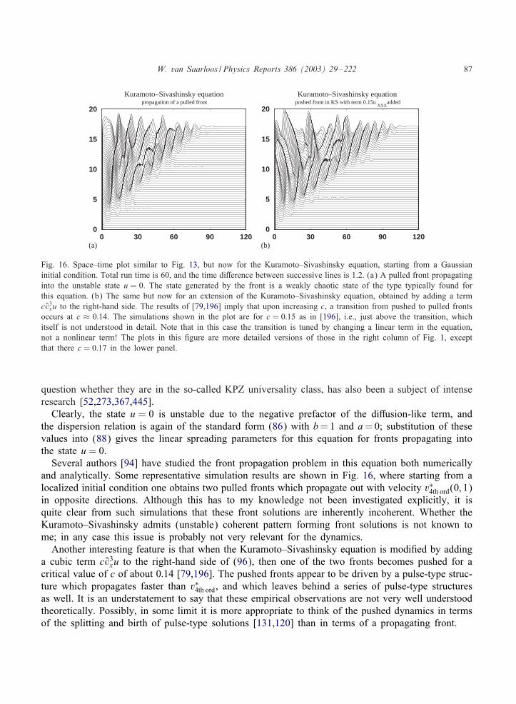
W. van Saarloos / Physics Reports 386 (2003) 29–222 87
0 30 60 90 1200
5
10
15
20
0 30 60 90 1200
5
10
15
20
(a) (b)
Kuramoto–Sivashinsky equation Kuramoto–Sivashinsky equationpropagation of a pulled front pushed front in KS with term 0.15u
XXXadded
Fig. 16. Space–time plot similar to Fig. 13, but now for the Kuramoto–Sivashinsky equation, starting from a Gaussianinitial condition. Total run time is 60, and the time diDerence between successive lines is 1.2. (a) A pulled front propagatinginto the unstable state u = 0. The state generated by the front is a weakly chaotic state of the type typically found forthis equation. (b) The same but now for an extension of the Kuramoto–Sivashinsky equation, obtained by adding a termc93
xu to the right-hand side. The results of [79,196] imply that upon increasing c, a transition from pushed to pulled frontsoccurs at c ≈ 0:14. The simulations shown in the plot are for c = 0:15 as in [196], i.e., just above the transition, whichitself is not understood in detail. Note that in this case the transition is tuned by changing a linear term in the equation,not a nonlinear term! The plots in this 3gure are more detailed versions of those in the right column of Fig. 1, exceptthat there c = 0:17 in the lower panel.
question whether they are in the so-called KPZ universality class, has also been a subject of intenseresearch [52,273,367,445].
Clearly, the state u = 0 is unstable due to the negative prefactor of the diDusion-like term, andthe dispersion relation is again of the standard form (86) with b= 1 and a= 0; substitution of thesevalues into (88) gives the linear spreading parameters for this equation for fronts propagating intothe state u = 0.
Several authors [94] have studied the front propagation problem in this equation both numericallyand analytically. Some representative simulation results are shown in Fig. 16, where starting from alocalized initial condition one obtains two pulled fronts which propagate out with velocity v∗4th ord(0; 1)in opposite directions. Although this has to my knowledge not been investigated explicitly, it isquite clear from such simulations that these front solutions are inherently incoherent. Whether theKuramoto–Sivashinsky admits (unstable) coherent pattern forming front solutions is not known tome; in any case this issue is probably not very relevant for the dynamics.
Another interesting feature is that when the Kuramoto–Sivashinsky equation is modi3ed by addinga cubic term c93
xu to the right-hand side of (96), then one of the two fronts becomes pushed for acritical value of c of about 0:14 [79,196]. The pushed fronts appear to be driven by a pulse-type struc-ture which propagates faster than v∗4th ord, and which leaves behind a series of pulse-type structuresas well. It is an understatement to say that these empirical observations are not very well understoodtheoretically. Possibly, in some limit it is more appropriate to think of the pushed dynamics in termsof the splitting and birth of pulse-type solutions [131,120] than in terms of a propagating front.

88 W. van Saarloos / Physics Reports 386 (2003) 29–222
2.11.5. The cubic complex Ginzburg–Landau equationThe cubic Complex Ginzburg–Landau (CGL) equation
9tA = (1 + ic1)92xA + �A− (1 − ic3)|A|2A (97)
with �¿ 0 is the appropriate amplitude equation just above the onset to 3nite wavelength travelingwave patterns. The amplitude A is a complex quantity, and describes the slow space and timemodulation of the 3nite wavelength mode that goes unstable [9,105,155,189,316,320,413,426,435].The phase diagram of the dynamics behavior of this equation as a function of the real parametersc1 and c3 is extremely rich, and includes chaotic phases as well as coherent dynamics phases[9,81,105,382,418,419].
An important simple set of solutions of the CGL equation are the periodic or phase windingsolutions
A = aeiqx−i/t ; (98)
with a a constant. Upon substitution of this expression in to the cubic CGL, it is easy to check thatthese solutions form a one-parameter family parametrized by q, as we can express a and / in termsof q as
a2 = �− q2; / = (c1 + c3)q2 − c3�; −√�¡q¡
√� : (99)
In an amplitude description, the phase winding solutions represent periodic traveling patterns whosewavenumber diDers by q from the critical mode at the bifurcation. Because the CGL equationadmits a family of these pattern-type solutions, fronts typically generate a pattern and hence arepattern forming fronts—although the CGL equation looks super3cially like the F-KPP equation, thefact that the dynamical 3eld is complex makes its dynamical behavior much more intricate (Onemight even say the pulled front propagation mechanism is virtually the only element they have incommon!).
Not all the phase winding solutions are stable. Those near the edge of the band are always linearlyunstable (the so-called Benjamin–Feir instability), while the stability of those near the center of theband depends strongly on c1 and c3. In fact, for c1c3 ¿ 1 none of the phase winding solutions isstable [105,278,279,315]. Chaotic behavior is typically found in this region of the phase diagram.
The state A = 0 in the cubic CGL (97) is linearly unstable; since the dispersion equation isquadratic in k, it is easy to obtain the spreading point parameters
v∗CGL = 2√
�(1 + c21); �∗ =
√�
1 + c21; k∗r = c1
√�
1 + c21; D = 1 + c2
1 : (100)
CGL equations generally admit an important class of so-called coherent structure solutions of theform
A(x; t) = e−i/t A(x − vt) ; (101)
which is a special case of the general form (56) of coherent pattern forming fronts. Coherentstructure solutions of this type—fronts, sources, sinks, pulses [424] and other types of localizedsolutions [418,419]—turn out to be the crucial building blocks of the dynamics of the CGL, butwe limit our discussion here exclusively to fronts. The simplicity of the coherent fronts in the CGLequation lies in the fact that they are of the coherent pattern forming type (56), but that there

W. van Saarloos / Physics Reports 386 (2003) 29–222 89
is only one nonzero term in this sum (we can think of the function A as the term ,1 in thisexpression). Since A depend only on a single co-moving coordinate - = x− vt, A obeys an ordinarydiDerential equation. The multiplicity of coherent structure solutions (do they come in discrete sets,one- or two parameter families?) can therefore be studied from the number of stable and unstablemanifolds near the 3xed points that describe the asymptotic behavior of these solutions (so-called“counting arguments”). For fronts, these counting arguments show [424] that there generically is atwo-parameter family of front solutions which to the right decay exponentially and on the back sideapproach a phase winding solution. Since k∗ is a complex quantity, this implies that there generallywill be a unique coherent front solution (101) with velocity v∗ and which smoothly connects thelinear spreading point behavior eik∗(x−v∗t) on the right with a phase winding solution like (98) onthe left.
Since the temporal phase factor is a global (x-independent) factor, one can use an argumentreminiscent of the conservation of nodes argument discussed in Section 2.11.1 to calculate thewavenumber of the coherent pulled front solution. Indeed, if we compare in the frame movingwith velocity v∗ two points a 3xed distance apart, this phase di>erence is 6xed since A(�) istime-independent in this frame while the prefactor e−i/t is common to both points. By equating thetemporal phase winding in this frame at the two points we then get the wavenumber q behind thefront: In the leading edge to the right, / simply needs to be equal to the temporal phase winding inthe moving frame, /=!∗
r −v∗k∗r =−c1. Likewise, let us write the asymptotic phase-winding behaviorbehind the front for � → −∞ as A(�) = aeiq�; the amplitude a, wavenumber q and frequency / arethen related by / = (c1 + c3)q2 − c3 � + v∗q, which is the analog of Eq. (99) in the moving frame.Equating the two expressions for / and solving for the root −√
�¡q¡√� simply yields for the
wavenumber qsel selected by the coherent pulled front solution [321]
qsel =
√1 + c2
1 −√
1 + c23
c1 + c3
√� : (102)
Soon after the broader applicability of what we now refer to as the pulled front concept startedto emerge [38,111], Nozaki and Bekki [321] studied the front propagation problem in the CGLnumerically. Their results can be understood simply in combination with the results of the stabilityanalysis of the phase winding solution qsel:
(i) In large parts of the phase diagram, the 3rst front propagating into the unstable state A = 0is a coherent pulled front of the type (101), with velocity v∗CGL given by (100) and selectedwavenumber qsel given by (102).
(ii) If the selected mode ∼ exp(iqselx) is stable, a domain with this state remains behind the front. 48
(iii) As Fig. 17 illustrates, if the qsel is unstable due to the Benjamin–Feir instability, the domainbehind the 3rst coherent front is invaded by a second front. This front is again a pulled front[112,321], whose speed v∗BF can be calculated explicitly in terms of qsel and c1 and c3. 49
Depending on the parameters c1 and c3 this front can give rise either to a more stable phasewinding solution, or a chaotic state. An example of the latter case is shown in Fig. 17(a).
48 Depending on the initial conditions, this domain can subsequently be invaded by a front connecting to another phasewinding solution.
49 Since the Kuramoto–Sivashinsky equation is the amplitude equation for the Benjamin–Feir instability in the limit whenthe instability is weak [105], the second front is essentially a pulled Kuramoto–Sivashinsky front.

90 W. van Saarloos / Physics Reports 386 (2003) 29–222
0 75 150 225 3000
3
6
9
0 80 160 240 3200
6
12
18
24
(a) (b)
Cubic CGL equationpulled fronts at c
1= 1 and c
3=3
quintic CGL equationpulled front at ε = 0.25
Fig. 17. (a) Space–time plot of the amplitude A in a simulation of the cubic GL equation (97) with � = 1, c1 = 1 andc3 = 3. Time diDerence between successive lines is 2 and the total simulation time is 80. The plot illustrates how the 3rstfront is a pulled coherent pattern forming front of the type (101), but that the state behind the front is unstable, so thatthe domain with the state selected by the 3rst front is invaded by a second front. This second front is also a pulled one.Note the similarity between the leading part of the second front and the pulled front found in the Kuramoto–Sivashinskyequation—see Fig. 16(a). This is no accident, as the Kuramoto–Sivashinsky equation is the lowest order amplitude equationjust above the Benjamin–Feir instability [105,189]. (b) Space–time plot of a propagating pulled front in the quintic CGLequation with � = 0:25, c1 = 1, c3 = −1 and c5 = −1. For these parameter values, no coherent nonlinear front solution ofthe type (101) exists [424]. The 3rst front is followed by a region with phase slips (points where A vanishes), beforegiving rise to a state close to a phase-winding solution. At the later stage, this region is invaded by another front.
Clearly, this regime can only exist if the 3rst coherent front outruns the second one, hencein the parameter range where v∗CGL ¿v∗BF. In the frame moving with the 3rst front, the stategenerated by the 3rst front is nonlinearly convectively unstable to the Benjamin–Feir instability.
(iv) In the parameter range where the Benjamin–Feir instability becomes nonlinearly absolutelyunstable in the frame moving with the 3rst front, i.e., in the range where v∗CGL ¡v∗BF (whichis most easily entered by tuning c3 as v∗CGL does not depend on c3) the coherent pulled frontsolution is irrelevant. Instead, one observes a pulled incoherent front: 50 the chaotic behaviorsets in right at the front region front. The dynamical behavior in this regime is similar to thatshown in Fig. 19(a) below for the pulled chaotic behavior of the quintic CGL.
In conclusion, the cubic CGL equation admits a two-parameter family of coherent front solutions.This family includes the pulled front solution, for which the selected wavenumber can be determinedexplicitly. The dynamics behind the 3rst front depends on the stability of this state. When v∗BF ¡v∗CGLthe 3rst front is a coherent pulled front, while in the opposite regime an incoherent pulled frontemerges.
50 Actually, it is conceivable that in some parameter ranges the Benjamin–Feir instability of the nonlinear region is sostrong, that the very 3rst front becomes a pushed incoherent front. To my knowledge this issue has not been studiedsystematically.

W. van Saarloos / Physics Reports 386 (2003) 29–222 91
2.11.6. The quintic complex Ginzburg–Landau equationUnlike the cubic CGL equation, which arises as the lowest order amplitude equation near a
supercritical (forward) bifurcation to traveling wave patterns, the quintic CGL equation
9tA = (1 + ic1)92xA + �A + (1 + ic3)|A|2A− (1 − ic5)|A|4A (103)
is a model equation for the case in which such a bifurcation is subcritical (backward). Becauseof the diDerent sign of the cubic term, this term now enhances the growth of amplitude, whilesaturation is only caused by the quintic term. Indeed, the destabilizing cubic term implies that theonly stable phase winding solutions have a 3nite amplitude for any �. So an expansion based onassuming that the amplitude is small is not really justi3ed. In other words, the quintic CGL is nota consistent lowest order amplitude equation. Nevertheless, the equation has played an importantrole in identifying the main coherent structures and dynamical regimes near a subcritical bifurcation.Note that the terms linear in A are the same in the quintic and cubic CGL, so the linear spreadingpoint expressions (100) apply to the quintic CGL equation for �¿ 0 as well.
In the subcritical range, �¡ 0, the state A=0 is linearly stable, and hence a small perturbation doesnot spread with a 3nite speed: instead it will die out. However, nonlinear states, in particular phasewinding solutions, can perfectly well be stable. In analogy with thermodynamic systems, where oneis used to interface-type solutions between two stable phases separated by a 3rst order transition, oneexpects there to be front solutions in the subcritical range �¡ 0. When � is increased towards smallbut positive values, these front solutions would then be expected to remain dynamically relevant asthey have nonzero speed larger than the linear spreading speed v∗CGL ∼ √
�. In other words, onewould naively expect that for small � fronts in the quintic CGL are pushed.
The remarkable feature of the quintic CGL is that the front solutions corresponding to the pushedfronts can be obtained analytically [423,424] by a generalization of the “reduction of order method”reviewed brieKy in the example at the end of Section 2.7.1: When A(-) with - = x − v†t is writtenin the form A = a(-)ei�(-) and the Ansatz
dad-
=√
e1(a2 − a2N );
d�d-
= qN + e0(a2 − a2N ) ; (104)
is substituted into the equations, one arrives at algebraic equations for the coeRcients e0 and e1 andthe wavenumber qN and amplitude aN of the phase winding solution behind this front solution. Thesecoherent pattern forming pushed front solutions, which are unique for a 3xed set of parameters, onlyexist in parts of the �; c1; c3; c5 parameter space: EDectively they exist only in a band around theline c3 = −c5 where the nonlinear dispersion terms almost cancel and especially in the subcriticalrange �¡ 0.
The main 3ndings of a detailed study of the existence of these solutions and of their competitionwith pulled front solutions are:
(i) Just like we discussed for the pulled front solutions of the cubic CGL equation, the phasewinding solution with wavenumber qN behind the pushed front can be unstable to the Benjamin–Feir instability. If it is, and if the propagation velocity v∗BF is smaller than v†, then the sizeof the domain behind the 3rst front grows as (v† − v∗BF)t in time. If v∗BF ¿v†, however, anincoherent pattern forming pushed front results (see Figs. 13 and 14 of [424]).

92 W. van Saarloos / Physics Reports 386 (2003) 29–222
(ii) Even though the quintic Ginzburg–Landau equation always admits phase winding solutions in asubcritical range �c ¡�¡ 0, outside a band where c3 ≈ −c5 there are no pushed front solutions.This means that the “thermodynamic” intuition formulated above, according to which one alwaysexpects a pushed to pulled transition at some 6nite positive value of �, does not apply to thequintic CGL equation (in line with the fact that there is no standard Lyapunov function for thisequation). In other words, in some parameter ranges, the dynamically relevant fronts for anypositive � are pulled fronts! This is quite remarkable, as it means that in the parameter rangeswhere this happens, from the point of view of the front propagation problem the dynamicalbehavior is more like that found near a supercritical bifurcation. 51 This also illustrates thatwhile for the F-KPP equation the nonlinear behavior of the growth function f(�) determineswhether fronts are pushed or pulled, the distinction between the two regimes is generally moresubtle—in the quintic CGL it is determined by the strength of the nonlinear dispersion, in theextension of the Kuramoto–Sivashinsky equation it is tuned by a symmetry-breaking linear thirdorder derivative term.
(iii) In equations where the relevant front solutions are uniformly translating ones, the pushed so-lutions normally bifurcate oD the pulled ones continuously. In the quintic CGL equation, thisis generically not the case for pattern forming fronts—see the discussion in Section 2.8. As aresult, the selected wavenumber can jump as one goes from a coherent pulled front solutionto a coherent pushed front solution (see Fig. 1(c) of [423] or 23 of [105]). Thus, the coher-ent pattern forming front solutions found in the quintic CGL provide a counterexample to the“structural stability” postulate [333,334] that pulled front solutions are smoothly connected tothe pushed front solutions, as one tunes one of the parameters in the dynamical equation.
(iv) As we discussed, for the cubic CGL equation, so-called “counting arguments” for the multiplic-ity of front solutions indicate that there generally is a two-parameter family of front solutions.Although this has not been checked explicitly, we believe that for any value of the parametersthere is indeed a unique pulled front solution, in line with the fact that (102) 3xes qsel uniquely.For pulled fronts in the quintic CGL equation, a new feature is encountered: an extension ofthe earlier analysis to the quintic case shows that in some parameter ranges the equations forqsel behind the front do not admit a solution. This implies that in these parameter ranges nocoherent front solutions (101) can exist [424]. Fig. 17(b) shows an example of the type ofdynamical behavior that is found in this regime: in the front region the dynamics is very inco-herent and associated with the occurrence of “phase slips” (points in space-time where A = 0).The fact that the incoherent front region is followed by a zone where A is close to a stablephase-winding solution illustrates that the incoherent front dynamics in this case is not due toan instability of the selected state, but to the absence of a coherent pulled front solution.
(v) Because of the subcritical nature of the transition, the quintic CGL equation also has parameterranges at �¡ 0 where a chaotic phase is statistically stable. If one puts such a chaotic phasenext to a domain of the stable A= 0 phase, the front between them can move. Upon increasing� one can then observe a pushed to pulled transition of an incoherent front—see Fig. 18.
(vi) As we discussed in Section 2.9, the universal 1=t power law relaxation even applies to the co-herent and incoherent pattern forming fronts. This was checked numerically for the simulations
51 For �¡ 0, a new class of retracting fronts (v¡ 0) was recently found [103]; these solutions determine much of thedynamical behavior in the subcritical regime, especially outside the band where the pushed front solutions exist.

W. van Saarloos / Physics Reports 386 (2003) 29–222 93
0 120 240 360 4800
7
14
21
0 120 240 360 4800
7
14
21
(a) (b)
quintic CGL equation quintic CGL equationsubcritical range ε = -0.005 pulled front at ε = 0.03
Fig. 18. Space–time plot of A illustrating the pushed to pulled transition for incoherently propagating fronts in the quinticCGL equation (103) [119]. In each plot, the total simulation time is 100, and the time diDerence between successive linesis 2. (a) Simulation for c1 = −2:2, c3 = −0:5, c5 = −2 in the weakly subcritical range � = −0:005. According to Fig. 15of [424], in this range the incoherent domain in the center slowly spreads, corresponding with a pushed incoherent frontwith velocity ≈ 0:15, although this may be a 3nite-size eDect. (b) The same for � = 0:03.
(a) (b) (c)
Fig. 19. (a) Space–time plot of the amplitude |A| of a pulled incoherent front in the quintic CGL at � = 0:25, c1 = 1,c3 = c5 = −3. Note that in the leading edge, where |A| is small, the dynamics is actually quite coherent, in agreementwith the fact that the linear spreading dynamics is always coherent. The front only becomes incoherent once the nonlinearbehavior sets in. (b) Scaling plot of the scaled velocity relaxation [v(t) − v∗]T=C1 versus T=t for simulations of coherentfronts in the Swift–Hohenberg equation and the quintic CGL simulations shown in (a). Here T is a properly de3ned timescale introduced so that both equations fall on the same asymptotic curve, and C1 is an appropriate combination of thelinear spreading point parameters [388]. From left to right, the 3rst three lines are Swift–Hohenberg data with � = 5, atheights u=
√�; 0:01
√� and 0:0001
√�, and the next three lines show the CGL data traced at amplitudes 0:002, 0:0002 and
0:00002. The solid line is the universal asymptote predicted by the analytic theory. (c) The same for the appropriatelyscaled 5(t) relaxation (84). From [388].
of the incoherent fronts of the CGL equation shown in Fig. 19(a). The other panels con3rm thatafter scaling the velocity and time with the predicted values, both the velocity [panel (b)] andwavenumber [panel (c)] relaxation data of the incoherent quintic CGL fronts and the coherentfronts in the Swift–Hohenberg equation are in accord with the universal predictions.
94 W. van Saarloos / Physics Reports 386 (2003) 29–222
2.12. Epilogue
The insight we have attempted to bring across in Section 2 is that the special nature and generalityof front propagation into unstable states lies in the fact that there is a well-de3ned linear spreadingspeed v∗ associated with any linear instability. The linear spreading point is the organizing centerfor all subsequent developments: We can make a large number of general predictions because thelinear dynamics puts a strong constraint on any possible nonlinear dynamics. On the one hand, itforces us to focus on the question “how can a front faster than v∗ emerge?” and this naturallyleads to the concepts of pulled and pushed front. On the other hand it shows that the approachto the asymptotic velocity and state of a pulled front is governed by an equation which in lowestorder is of diDusion-type, and this allows one to derive the universal asymptotic relaxation of apulled front.
For uniformly translating fronts and coherent pattern forming fronts, the regime of pushed frontpropagation is essentially governed by the existence of special solutions which we can think of as“strongly heteroclinic orbits”. For incoherent pushed fronts we are at present unable to formulate thepushed front propagation mechanism sharply, although intuitively we expect it to be very similar tothat of the other two types of fronts.
The various examples in the previous section illustrate that a pulled front essentially does whatit should do, namely propagate with asymptotic speed and shape dictated by the linear spreadingpoint, while the rest of the front just follows in whatever way is allowed by the global nonlinearproperties of the dynamical equation: (i) a bifurcation in the structure of the linear spreading pointis responsible for the transition to coherent pattern forming fronts in the EFK equation; (ii) thequintic CGL equation illustrates that the limited range of existence of coherent pattern formingfronts can lead to a transition from coherent pulled fronts to incoherent pulled fronts; (iii) if thestate generated by a front in the cubic or quintic CGL equation is unstable, the 3rst front remains acoherent front if the spreading speed of the secondary instability is less than v∗ of the 3rst front, whilethe 3rst front becomes incoherent if the pulled speed of the secondary front is larger than v∗ of the3rst front.
The diRculty in making generic statements about pushed fronts is that apart from the fact that theirconvergence to the asymptotic speed v† is exponential, there are few generic features. Because of thestrong heteroclinicity requirements (60) or (76) that the slowest decaying exponential mode is absent,pushed front solutions are technically determined by an analysis which has all the properties of anonlinear eigenvalue problem for an isolated solution. Because of this structure, the relaxation towardsthe asymptotic pushed front speed and shape is generally exponential, and singular perturbation theorycan be applied to pushed fronts (Section 5). Moreover, because of this structure, whether a pushedfront solution exists depends on the full global and hence nonlinear properties of the equations. Asa result, virtually every example is special, and there are few nontrivial examples which one hasbeen able to obtain analytically. The quintic CGL equation is a remarkable exception in this regard.
As we discussed, with few exceptions, most mathematical investigations of front propagation intounstable states have focused on uniformly translating fronts and in particular on systems of equationswhich are closely related to the F-KPP equation. It appears to us that many of the ingredients ofthe theoretical framework that we have discussed here are ready for more rigorous analysis: rigorousdevelopments that I expect are around the corner are (i) rigorous bounds for the Green’s functionof whole classes of linearized equations and, in relation with this, rigorous proofs of the pulled

W. van Saarloos / Physics Reports 386 (2003) 29–222 95
front mechanism of new classes of equations, (ii) proofs of the universal relaxation of pulled fronts,(iii) the development of a mathematical framework for the pulled to pushed transition of coherentpattern forming fronts, and (iv) extension of the approach of Sandstede and Scheel [374,375] toanalyze the interaction between front dynamics and the dynamics of the state behind the front, orto classify defects.
3. Experimental and theoretical examples of front propagation into unstable states
In this section we discuss a number of examples of front propagation into unstable states. We 3rstreview experiments on fronts or in which front propagation plays an important role, and then moveon to discuss examples of fronts in theoretical models. The examples concern mostly fronts in onedimension. The diRculty of analyzing patterns whose dynamics is governed by the propagation ofpulled fronts is discussed later in Section 5.
At 3rst sight, one might well wonder why front propagation into unstable states is a relevantproblem anyway. After all, it seems counterintuitive that a physical system would naturally end upin an unstable steady state and wait for a nice front to develop! On closer inspection, however, thereare many reasons why front propagation into unstable states is not an esoteric problem:
(i) A natural way in which a system can stay in a self-sustained unstable state is when an overallKow or motion makes the instability convective (see Sections 2.5 and 2.10). This happens inparticular in many Kuid dynamic systems. Likewise, in plasma physics the strong asymme-try between the mobility of electrons and ions usually makes plasma instabilities convective.Examples where these considerations apply are discussed in Sections 3.5, 3.9, 3.10, 3.11, 3.12,and 3.17.
(ii) Sometimes a natural way to probe a system is to quench it into an unstable state with a laserpulse, ramping or Kipping a voltage, Kipping a plate, dropping a temperature, scraping a skintissue, etc. In all these cases, the relevant question is whether we can change the system on atimescale shorter than the natural time scale of the evolution of the state into which we quenchit. Examples are encountered in Sections 3.1, 3.2, 3.3, 3.5, 3.6, 3.7, 3.14, 3.15, and 3.20.
(iii) We sometimes encounter intrinsically chaotic systems where the dynamics itself continuouslygenerates states which are transient because they themselves are unstable. We discuss a clearexample of this in Section 3.4.
(iv) In thermodynamic systems with 3rst order transitions, interfaces play a predominant role becausethe bulk nucleation rate is exponentially small near the transition, while interface velocitiesusually vary linearly with the distance from the transition. Although Kuctuations near a secondorder thermodynamic transition are usually too large to allow clear fronts to develop, this is notnecessarily true for polymer systems (Section 3.7). Moreover, near supercritical (“second orderlike”) bifurcations in pattern forming systems, where Kuctuation eDects are usually small [105],a similar argument holds as well: as we shall discuss more explicitly in the next subsection, if� is the dimensionless control parameter measuring the distance from the instability threshold,the front speed scales as
√� while the growth rate of bulk modes scales as �. Hence, front
propagation in principle always dominates for suRciently small � [161]. Of course, the rangeover which fronts do dominate the dynamics depends on the prefactors, i.e. on the time and

96 W. van Saarloos / Physics Reports 386 (2003) 29–222
length scales of the problem under investigation. Such considerations play a role in the examplesof Sections 3.1, 3.2, 3.3, 3.5, 3.7, 3.8, and 3.14.
(v) Front propagation into an unstable state sometimes emerges theoretically from an unexpectedangle through mapping a seemingly unrelated problem onto a front propagation problem—seeSections 3.21, 3.23, 3.25, 3.26.1 and 3.26.5.
3.1. Fronts in Taylor–Couette and Rayleigh–BIenard experiments
Soon after Dee and Langer [111] and Ben-Jacob and co-workers [38] drew the attention of thephysics community to the special simplicity of what we now refer to as pulled fronts, two experimentson pattern forming systems were done that are still very illuminating: One by Ahlers and Cannell[4] on vortex fronts in a Taylor–Couette cell, and one by Fineberg and Steinberg [161] on frontpropagation in a Rayleigh–BIenard cell.
A Taylor–Couette cell consists of two concentric cylinders which can rotate independently. Thegap between the two cylinders is 3lled with a normal Newtonian Kuid. When the inner and outercylinder rotate slowly, the Kow between the two cylinders is laminar and in the azimuthal direction.At higher rotation rates, one 3nds an amazing number of Kuid dynamics instabilities when both theinner and the outer cylinder are rotating with suRciently high frequencies [105,125]. The experimentsthat are of interest to us probed fronts that lead to the 3rst nontrivial patterned state that emerges ifthe rotation rate of the inner cylinder is increased while the outer cylinder does not rotate [4]. Atsome critical rotation rate, there is a bifurcation to a state with so-called Taylor vortices: a patternwhich is periodic in the direction along the axis of the cylinders emerges. This Kow is referred to asTaylor vortex Kow, since the velocity in the r; z plane has the appearance of alternating clockwiseand counterclockwise rotating vortices that span the whole gap between the two cylinders.
A Rayleigh–BIenard cell consists of a Kuid sandwiched between two parallel plates at a 3xedbut diDerent temperature. When the bottom plate is hotter than the top plate, the Kuid density islargest at the top. For small enough temperature diDerences, there is no convection—there is justheat conduction through a quiescent Kuid. However, when the temperature diDerence and hencethe density diDerence becomes larger than some threshold value, this simple state is unstable andconvection sets in spontaneously [105,155,189,282]. The convection patterns that emerge just abovethreshold are often referred to as rolls, but if we look at the velocity pattern in a vertical crosssection, they look like the vortex-type patterns in the r; z cross-section of the Taylor–Couette cell.
The transition to Taylor vortex patterns and to convection patterns in the Rayleigh–BIenard caseare both examples of forward (supercritical) bifurcations to a stationary 3nite wavelength patterns.Just above onset, the patterns can be described by a so-called amplitude expansion by writing thephysical 3elds in terms of the complex amplitude as [105,189,193,316,320]
physical 3elds ˙ Aeikcx + A∗e−ikcx : (105)
For simplicity, we restrict the analysis to one-dimensional patterns as this is the relevant case for thefront experiments; kc is the wavenumber of the pattern at onset, and x is the coordinate along whichthe patterns develop. The amplitude expansion simply implements the observation that just aboveonset the amplitude of the patterns is small, and that the amplitude A varies on slow space and

W. van Saarloos / Physics Reports 386 (2003) 29–222 97
time scales. In lowest order, A then obeys the so-called real Ginzburg–Landau amplitude equation 52
[105,155,189,316,320,413,435]
$09tA = �A + �2092
xA− g|A|2A : (106)
Here � is the dimensionless control parameter, which for �¿ 0 is a measure for how far one is abovethe instability threshold. The time scale $0 and length scale �0 depend on the particular system, andcan be calculated explicitly from the linear dispersion relation of the system under study. Thishas been done both for the transition to Taylor vortices and for the transition to Rayleigh–BIenardconvection patterns. The nonlinear parameter g, which follows from the amplitude expansion, is alsoknown for both systems, but it, of course, does not play a role for the pulled fronts of interest here.
The real amplitude or Ginzburg–Landau equation should in general not be thought of as just asimple straightforward generalization of the F-KPP equation to a complex 3eld—while the F-KPPequation only allows for stable homogeneous solutions u=±1, the amplitude equation admits stablephase winding solutions of the form A = aeiqx with a and q constant [105,155,189,320,435]. As(105) illustrates, these describe physical patterns with a wavenumber kc + q diDerent from thecritical wavenumber. The interaction and competition between the various modes in general makesthe dynamics of the amplitude A much more interesting and complicated than that of the F-KPPequation. Nevertheless, since the dynamics of pulled fronts is dominated by the linear terms in A,and since these are the same for the two equations, both the asymptotic pulled front solutions andthe convergence to them are the same for the two equations.
The attractive feature of the experiments is that because �0 and $0 are known explicitly, they oDerthe possibility to study front propagation quantitatively. Indeed, for the amplitude equation in form(106) we get for the pulled front speed
v∗ampeq = 2�0
$0
√� : (107)
This result explicitly con3rms the assertion made already in point (iv) at the beginning of Section3 that near a supercritical bifurcation, the front speed increases as
√�, while the growth rate of
bulk modes according to (106) increases linearly in �. As stressed by Fineberg and Steinberg [161],front propagation into unstable states can therefore generally be observed at small enough �, i.e. justabove the onset of the transition.
In order to compare the measured front velocities to the F-KPP equation in the standard form inwhich the prefactors of the linear terms are equal to 1, the experimental results have been reportedin terms of the scaled velocity
v = v$0
�0√�
: (108)
Of course, front speeds should only converge to v∗ampeq if the initial condition is suRciently localized,as explained in Section 2.7.6. In both experiments, the system was initially below the instabilitythreshold, corresponding to �¡ 0 in the amplitude equation (106), and then brought above threshold(�¿ 0) at time t = 0. In the Taylor–Couette experiment, even below threshold, when the bulk of
52 The equation—used as the amplitude equation (106) in the discussion of fronts in Rayleigh–BIenard and Taylor–Couette experiments in Section 3.1 below—is called the real Ginzburg–Landau equation because the prefactors of all theterms are real. The amplitude equation for traveling wave patterns is the CGL equation; as discussed in Section 2.11.5,in principle all its terms have complex prefactors [105,189,435].

98 W. van Saarloos / Physics Reports 386 (2003) 29–222
(a) (b)
Fig. 20. (a) Velocity data of fronts in the Taylor vortex experiments of Ahlers and Cannell [4]. Data are plotted on alog–log scale as a function of �. The solid lines have slope 1
2 and hence illustrate the√� scaling of the velocity. The
lower line shows that the data are consistent with a scaled velocity v ≈ 1:1 instead of the asymptotic values vas = 2.(b) Experimental data of Fineberg and Steinberg [161] on fronts in the Rayleigh–BIenard system on a log-linear scale. Thesolid line is the theoretical prediction (107). The inset shows the scaled velocity v which is consistent with the theoreticalasymptotic value 2, within the error bars.
the cell is in the stable laminar Kow state, there are so-called Ekman vortices at the ends of thecylinders. These play the role of localized nonzero initial conditions for the amplitude A when thesystem is brought above threshold at time t = 0. For the Rayleigh–BIenard experiment, Fineberg andSteinberg used a long cell, so as to get one-dimensional fronts, and they turned on an extra heaterat the cell ends as well, when they brought the system to �¿ 0. This made the convection patternsnucleate at the ends and then propagate into the bulk of the cell.
Fig. 20(a) shows the velocity of the Taylor vortex fronts as they propagate into the Taylor–Couettecell over a distance of up to 10 to 15 vortex diameters [4], plotted on a log-log scale. As thetwo solid lines indicate, the
√�-scaling of the vortex velocity is con3rmed, but the prefactor is
only about 55% of the predicted asymptotic values v∗ampeq = 2: the data are consistent with v ≈ 1:1instead of 2.
The fact that the measured front velocity was signi3cantly below the asymptotic value in this 1983Taylor–Couette experiment made many researchers wonder whether there was something cruciallywrong, 53 and stimulated Fineberg and Steinberg a few years later to perform experiments on frontsin Rayleigh–BIenard convection. Actual space–time plots of their convection front pro3les as theypropagate to the right along their cell, are shown in Fig. 21(a). These traces illustrate how these fronts(as well as those in the Taylor–Couette cell) are examples of true pattern forming fronts propagating
53 It was realized that if the measured velocity had been too high, a possible candidate for the discrepancy could havebeen that the initial convection pro3le associated with the Ekman end vortices was not suRciently localized, i.e., that att = 0 the amplitude did not fall oD to the right faster than e−�∗x = e−
√�x=�0 . However, as we discussed in Section 2.6,
asymptotic front speeds below v∗ are impossible.

W. van Saarloos / Physics Reports 386 (2003) 29–222 99
(a) (b)
Fig. 21. (a) Space–time plot of a propagating front in the Rayleigh–BIenard experiment of Fineberg and Steinberg [161]for � = 0:012, made using the shadowgraph technique. The time between successive traces is 0.42 tv, where tv is thevertical diDusion time in the experiments, and distances are measured in units of the cell height d. (b) A space-time plotobtained from a numerical simulation of the Swift–Hohenberg equation at the same value � = 0:012 and length and timescales adjusted to correspond to those in the experiments of (a). After Kockelkoren et al. [233].
into an unstable state, like those observed in simulations of the Swift–Hohenberg equation (92), seethe central panel of Fig. 1, and Figs. 14(b) and 21(b).
The data of Fig. 20(b) for the scaled front velocity v, calculated from the actual data by usingthe theoretical values for �0 and $0 in (108) were found to be consistent to within a few percentwith the asymptotic value vas = 2. At the time, this was considered to be an important experimentalcon3rmation of the quantitative prediction of the pulled front speed, and of the idea that the conceptof a pulled front applies more generally to pattern forming systems. But, as we shall see, there is anew twist to the story.
The reason for the apparent discrepancy between theory and experiment on the Taylor vortex frontsremained unresolved till Niklas et al. [319] performed an explicit numerical simulation of such frontswhich showed that the front speed had not yet relaxed to its asymptotic value, in contrast to whatwas found in numerical studies of the propagating fronts in the Rayleigh–BIenard cell [271]. Indeed,over the range of times probed experimentally, the transient speeds they found for the Taylor vortexfronts were quite consistent with the experimental data. Instead of showing these results, we willapproach this issue by extrapolating back from the asymptotic formula (78) as this allows us todiscuss both experiments in a uni3ed way.
When (78) is applied to the amplitude equation, one 3nds for the long time rate of approach tothe asymptotic speed v∗ = 2
v(t) = 2 − 32�t=$0
+3√�
2(�t=$0)3=2 + · · · : (109)
This formula shows that in any experiments on fronts just above the onset of a 3nite-wavelength su-percritical bifurcation, one can a priori only hope to observe front speeds very close to the asymptoticvalue at times
t�tco ≡ $0�=� : (110)

100 W. van Saarloos / Physics Reports 386 (2003) 29–222
Note that we have de3ned the crossover time tco as the time at which the third correction termis equal in magnitude to the 3rst correction term in (109). Although this asymptotic formula isonly valid in the long-time regime when the third term is much smaller than the second one, andalthough for times of O(tco) one is in the non-universal crossover regime, the important message isthat the velocity always approaches the asymptotic value from below and that transient eDects arevery signi3cant, even for times of order several tco. For example, even at times of O(3tco) whenthe formula becomes reasonably accurate [144], the velocity is still some 8% below its asymptoticvalue, and at tco both corrections terms, though of opposite sign, are about 24% of the asymptoticvalue in magnitude.
When an actual experiment is suddenly brought into the unstable parameter range �¿ 0, bulkmodes also start to grow at a rate proportional to �. Since one can only study fronts properly aslong as bulk Kuctuations have not grown enough that bulk “nucleation” starts to become visible, inpractice experiments like those we consider here can only be done up to a time which scales as �−1
[4,161]. In other words, experiments can in practice only be done up to a time which is a 6nitemultiple of tco!
In the Taylor vortex front experiments, most measurements for � = 0:02 were done in the timeinterval of 1–2 tco. It is therefore not surprising that transient eDects did play an important rolein these experiments [319,422] and that the measured velocity was signi3cantly below the asymp-totic value. However, from our present perspective, it is important to turn the question around andask whether the fronts observed in the Rayleigh–BIenard experiments were indeed propagating withapproximately the asymptotic speed, and if so, why so [233].
As it turns out, in the experiments of Fineberg and Steinberg, growth of bulk modes also limitedthe observation of fronts to times of order tco [161]. Kockelkoren et al. [233] therefore reanalyzedthe experiment from this perspective, and concluded that most likely the actual measured front speedwas some 15% below the asymptotic one. In their interpretation, the theoretical value for �0 usedin converting the observed front speeds to dimensionless front speeds v may have been about 15%smaller than the actual one. 54 If so, the velocity had been overestimated by about this amount inthe interpretation of the experiments, thus hiding a possible transient eDect.
We stress that only new experiments can settle whether this interpretation is the correct one.However, there are also indications in the actual traces of the fronts in Fig. 21(a) that the velocityin this run was slowly increasing in time. The solid line in Fig. 22(a) shows the experimentalvelocity as a function of time, extracted by measuring successive front positions with a ruler andusing a value of �0 which is 15% larger than the theoretical value [233]. For comparison, a plotof the velocity as function of time in a simulation of the real Ginzburg–Landau equation (106) isshown with a dashed line.
One important point has not been included in the theoretical analysis so far. When growth of bulkmodes in practice becomes important for times of order tco, then at the latest times the growth of thebulk Kuctuations may become important. This will have the eDect of increasing the velocity abovethe one studied analytically and numerically with localized initial conditions and in the absence ofKuctuations. With this caveat, we nevertheless tentatively conclude that both experiments on fronts
54 Indications that this may be the case come from fact that the observed wavelength at onset was also about 13% biggerthan the theoretical one. See [233] for further discussion of this.

W. van Saarloos / Physics Reports 386 (2003) 29–222 101
(a) (b)
Fig. 22. (a) Full line: scaled velocity versus time in the Rayleigh–BIenard front [161] whose space-time plot is shown inFig. 21(a). The velocity is obtained by interpolating the maxima of the traces. As explained in the text, a value of �0
which is 15% bigger than used by Fineberg and Steinberg to convert the data. A diDerent value would not change theshape of the curve, only the absolute numbers on the vertical axis. The dashed line shows the measured velocity in asimulation of Eq. (106) with an exponential initial condition A(x; 0) ∼ e−1:2�∗x and the dotted line the asymptotic result(109) with the t−3=2 term excluded. Note that the curves are not 3tted, as only the absolute vertical scale is aDected by ourchoice of �0. (b) Open circles: data-points for the wavenumber selected by the front in the experiments of Fineberg andSteinberg. Dashed curve: q∗=qc for the Swift–Hohenberg equation with parameters corresponding to the Rayleigh–BIenardexperiment. The fact that the data follow the line q∗=qc for small �, indicates that just above threshold the experimentsprobe the leading edge of the front. After Kockelkoren et al. [233].
in pattern forming systems illustrate that such fronts are prone to transient behavior associated withthe slow power law relaxation of pulled fronts from below to v∗.
As a 3nal note, we point out that both experiments also addressed the wavelength selection bythe front. Wavelength selection goes beyond the lowest order amplitude equation (106), since thereal F-KPP-type fronts in this equation simply yield a wavenumber equal to the critical wavenumberkc throughout the front, to order
√�. For the changes in order �, one needs to start from the linear
dispersion relation of the problem, correct to order �. In the original paper on the Rayleigh–BIenardexperiment, the data were compared to the results for the selected wavelength in the Swift–Hohenbergequation (92). Strong deviations were found in this case. The most likely explanation for this is thefollowing [233]: for small �, the full front whose width scales as 1=
√� is too wide to even 3t in the
experimental cell; hence one then cannot measure the selected wavenumber behind a fully developedpulled front, but instead only an eDective wavenumber in the leading edge of the front which isclose to the local wavenumber k∗r given in (88). Fig. 22(b) shows that indeed the Rayleigh–BIenarddata for small � are consistent with this.
More recently, the problem of fronts in the Rayleigh–BIenard and Taylor–Couette system has beenanalyzed in great detail by L]ucke and co-workers [68–70,210,269–271,349,361], both in the casediscussed here and in the presence of a throughKow (see Section 3.11). In these approaches, the frontpredictions based on the lowest order amplitude equation are compared in detail with those for pulledfronts obtained by determining the linear spreading point of the full Navier–Stokes equations for thissystem, and with full numerical simulations. We refer to these papers for a detailed discussion ofhow the full result starts to diDer from the lowest order amplitude result as � increases. In particular,the eDect that the nodes of the 3elds drift in the front region before coming to rest behind the frontis a characteristic eDect that goes beyond the amplitude equation (the Swift–Hohenberg equation alsoshows this, of course).

102 W. van Saarloos / Physics Reports 386 (2003) 29–222
(a) (b)
Fig. 23. (a) Photograph of a well-developed array of pendant drops at the end of the experiments of Fermigier, Limat,Wesfreid et al. [158,159,265]. The drops are seen from above through the glass plate across which the 3lm was spreadbefore the system was made unstable by Kipping the plate. From [265]. (b) Two-dimensional patterns observed in theRayleigh–Taylor instability of a thin layer in the same experiments [159,265]. Note that a “roll” or “stripe” type patterngenerally appears near the boundary of the regions. The two structures labeled A and A6 were initiated by small dustparticles on the interface. When they grow, they usually develop into a six-3eld symmetric hexagonal pattern like in H.The pattern near R was initiated by the thickness gradient close to the edge of the Kuid layer.
3.2. The propagating Rayleigh–Taylor instability in thin 6lms
The name Rayleigh–Taylor instability refers to gravitational instabilities of the interface betweentwo Kuids or of strati3ed Kuids [78]. A simple example is when one has two immiscible Kuidsseparated by a planar interface, in which the heavier Kuid is on top of the lighter one. Moregenerally the instability arises in density-strati3ed Kuids, when the acceleration is directed from theheavier to the lighter Kuid. The instability is important in a variety of practical situations, rangingfrom explosives to the spreading of paint or coating on a solid surface.
About a decade ago, Fermigier, Limat, Wesfreid and co-workers [158,159,265] performed a seriesof experiments on the Rayleigh–Taylor instability of thin 3lms. They studied pattern selection by3rst spreading thin 3lms of silicon oil on a Kat solid plate, and then making the system unstableby Kipping this plate upside down. For 3lms of suitable thickness, the instability develops slowlyenough that it can easily be studied. The photo of Fig. 23(a) illustrates that the typical hexagonalpatterns that one often observes after the instability is well-developed. The experiments illustrateseveral basic issues in pattern formation, 55 but we will focus here on the propagating fronts. Right
55 For example, the generic appearance of hexagonal patterns is associated with the fact that the thin 3lm equations(112) below for the deviation - of the 3lm thickness from the uniform value, are not invariant under a change of signof - (see [51] and references therein). In the Rayleigh–BIenard instability hexagonal patterns generically arise for thesame reason very close to threshold, since very small non-Boussinesq eDects break the symmetry that the Boussinesqequations happen to exhibit. Furthermore, the fact that the pattern looks stripe-like near the edge, even though the patternis hexagonal in the bulk—see Fig. 23(b)—is a generic phenomenon (also known in convection, see e.g. [51]) which canbe understood simply from symmetry considerations [350]: When one considers a front or domain wall solution in theamplitude equations for the three modes necessary to describe a hexagonal pattern, symmetry considerations dictate thatthe prefactor of the spatial second derivative term of the modes whose wavevector is normal to the front is a factor twolarger than those of the other two modes whose wavevector makes an angle of 60◦ with the front normal. This meansthat the “coherence length” or correlation length of this 3rst mode is larger than that of the other two modes, and thatthe pattern in the front region looks stripe-like [350] (see also [106,126]).

W. van Saarloos / Physics Reports 386 (2003) 29–222 103
Fig. 24. Time evolution of the thickness pro3le as a Rayleigh–Taylor front propagates into an unstable state in theexperiments of Fermigier, Limat, Wesfreid and co-workers [158,265]. The pro3les have been shifted up for clarity andare separated by time intervals of 30 s. x designates the coordinate perpendicular to the stripe-type pattern in the frontregion.
after the plate has been Kipped, a 3lm of uniform thickness is linearly unstable. In many cases,the instability 3rst developed near the boundary of the sample and then propagated into the bulkof the sample. Fig. 24 shows experimental traces of such a front as it propagates into the unstablestate [265].
The equations that describe the evolution of a thin liquid 3lm are well known: the separationof length scales allows one to simply integrate out the coordinates perpendicular to the 3lm layer(“lubrication approximation”) [324]. If we denote for the experimental case of the free 3lm Kowthe 3lm height h as the thickness of the 3lm measured from the plane, the dynamical equation forh becomes [324,158]
9th +13;
∇⊥ · [h3∇⊥(<gh + 2∇2⊥h)] = 0 ; (111)
where ; is the viscosity, < the density of the liquid, g the gravity, 2 the surface tension, and ∇⊥the gradient operator in the direction along the surface. To study the stability of a 3lm of uniformthickness h0, we note that if we substitute h = h0 + - into (111), the equation can be writted in theform
9t- +h3
0
3;(<g∇2
⊥- + 2∇4⊥-) = N (-;∇⊥-;∇2
⊥-) : (112)
Here N denotes all terms which are nonlinear in - and its derivatives. As noted in [158], the linearterms in (112) are exactly the same as the linear terms appearing in the various model equationsdiscussed in Section 2.11 (the Kuramoto–Sivashinsky equation, the Cahn–Hilliard equation or theSwift–Hohenberg equation at � = 1). After a proper rescaling of space and time units, the pulledfront velocity v∗ for the Rayleigh–Taylor fronts in the thin 3lm experiments is therefore just givenby Eq. (88).
The experimentally observed front speed was indeed found to be consistent with the pulled speedv∗ within the uncertainty of the experimental measurements and the theoretical estimate (whichwas of order 30%). In addition, there seemed to be a clear trend for the front patterns to have

104 W. van Saarloos / Physics Reports 386 (2003) 29–222
a wavelength some 5% smaller than the wavelength corresponding to the most unstable mode. Thisis also what would be expected from the results for pulled fronts with the above linear dispersionrelation.
Although the results of the experiments thus seem to indicate that the Rayleigh–Taylor fronts inthe experiment are examples of pulled fronts, we do want to express an important caveat: just likethe bifurcation to hexagonal convection patterns is generally subcritical (except when a symmetryimposes the equations to be invariant under a change of sign of the dynamical 3elds), the bifurcationto hexagonal Rayleigh–Taylor patterns should be expected to have a subcritical character too; indeedthis is indicated by the weakly nonlinear results in [158]. This suggests that when the instabilityis weak, one will actually get pushed rather than pulled fronts. However, to my knowledge thispossibility has neither been explored theoretically nor experimentally.
3.3. Pearling, pinching and the propagating Rayleigh instability
Another instability with which Rayleigh’s name is associated is the instability of a cylindricalbody of Kuid [78]. In daily life, we encounter this phenomenon when a stream of water from a tapbreaks up into drops or when the paint on a thin wire or hair of a brush breaks up into droplets.The instability is caused by the surface tension: for a “peristaltic” perturbation of the radius of thecylindrical Kuid, the capillary pressure due to surface tension is enhanced in the narrower region andreduced in the wider regions; this pressure diDerence tends to enhance the perturbation even more.
In tubular membranes, the instability normally does not arise, since membranes generally have asmall surface tension but a high bending rigidity, which measures the resistance of the membraneagainst changes in the curvature. However, Bar-Ziv and Moses [26] observed that when they appliedlaser tweezers to their tubular membranes, a sinusoidal instability developed, see Fig. 25(a). Thisinstability propagated out at a constant velocity in both directions from the point of application of thetweezers. Presumably, the instability is due to the fact that the tweezers pull some lipid moleculesinto the trap, and that as a result the surface tension increases, rendering the cylindrical geometryunstable. Indeed, as pointed out in [26], for a tube with surface tension = and bending modulus >,the free energy F can be written as
F =∫
dS[= + 2>H 2] : (113)
Here H is the mean curvature and the integral is over the surface S. For a tube with cylindricalsymmetry and the z-coordinate along the axis, we can write the terms in F in terms of r(z) as
dS = dz 2�r√
1 + r2z ; H =
rzz(1 + r2
z )3=2 − 1r(1 + r2
z )1=2 : (114)
As pointed out by Bar-Ziv and Moses a tube of constant radius R exhibits the Rayleigh instabilitywhen the surface tension is above a critical value =c ≈ 3>=R2. Above this value the free energy islower for a periodically modulated tube than for a tube of constant radius. As > → 0 one recoversthe pure Rayleigh instability. Thus, the experimental scenario is that the laser tweezers pull in thelipid molecules, and that the increase in surface tension that this entails is large enough for themembrane to become unstable.

W. van Saarloos / Physics Reports 386 (2003) 29–222 105
(a) (b)
Fig. 25. (a) Photographs showing the pearling front along a tubular membrane formed by lipid bilayers in the experimentsof Bar-Ziv et al. [26,27], as it propagates out from the bright laser spot on the right. In this experiment the dimensionlesscontrol parameter �= (=−=c)==c = 6:5. From top to bottom the times are 0.14, 0.68, 0.86, 1.04 and 1:22 s after the laserwas turned on. The arrow indicates the leading edge as it was determined by the authors. The height of each photographscorresponds to a distance of about 10 �m. (b) Results by Powers and Goldstein [356] for the simpli3ed model (115) forthe pearling instability. The top panel shows four snapshots of the pearling obtained from numerical simulation of themodel. The higher snapshots are obtained at later times, so the front is traveling to the left. Bottom panel: dimensionlessfront velocity as a function of the ratio of surface tension and bending modulus. The solid line denotes the pulled frontvelocity v∗, the dots the data obtained in the numerical simulations. Note that the data points lie slightly below the curvefor v∗. Undoubtedly, this is due to the slow convergence of the front speed to the asymptotic speed v∗.
The pearling instability through propagation of the Rayleigh fronts that the experiments suggesthave been studied theoretically by Powers and Goldstein and co-workers [356,185], who pointedout that in the approximation that the Kow pro3le through the tube remains a parabolic Poiseuillepro3le, 56 the dynamical equation for the tubular interface becomes
9tr2 =14;9z(r49z
[�F�r
]); (115)
where F is the interfacial free energy given in Eq. (113) above. The numerical results from [356]for this equation are shown in Fig. 25(b). The top panel shows four snapshots as the Rayleighfront propagates along the tube, generating strongly nonlinear bead-like undulations behind it. In thelower panel the velocity of these fronts is compared to the pulled front velocity v∗ for this model
56 This approximation, which is in the spirit of the the thin-3lm equations described in the previous section, is justi3edin the limit in which distortion of the tube diameter happens on length scales much longer than the tube diameter. This isnot really true for the Rayleigh instability. Nevertheless, the equation is expected to capture the essentials of the pearlinginstability.

106 W. van Saarloos / Physics Reports 386 (2003) 29–222
Fig. 26. Experimentally measured values of the wavenumber of the pearling instability as a function of the dimensionlesscontrol parameter � = (= − =c)==c in the experiments of Bar-Ziv et al. [27]. The line labeled MSC is the wavenumberselected by the pulled front in the model discussed in the text.
(full line) as a function of the dimensionless parameter R2==>. Note that this velocity vanishes ata critical value—as already noted above, below this value the cylindrical tube is stable. Note thatthe data points fall slightly below the pulled speed v∗. Although not enough data are provided in[356] to check this explicitly, this is undoubtedly due to the slow convergence of the front speedto the asymptotic value v∗—as mentioned before, numerical data at long but 3nite times will alwayapproach v∗ very slowly from below, and indeed a discrepancy like the one in this plot is what oneoften encounters if a careful extrapolation of the speed to its asymptotic value is not made.
It is instructive to realize that although the nonlinear behavior of this pearling model is quitediDerent from those encountered before, the dispersion relation for small linear perturbations of theradius is not! Note that when F is expanded to quadratic order in the deviations from a cylindershape, the highest derivative terms it contains are of order r2
zz. Upon taking the functional derivativein (115), we immediately see that the dispersion relation !(k) is a polynomial in k of sixth degree[185,27]. Thus, from the perspective of the linear dispersion relation and the calculation of v∗, theequation can be viewed as an interesting generalization to sixth order of the fourth order modelsequations of Section 2.11!
In more recent experiments, Bar-Ziv et al. [27] have tested the predictions from the above theoryin detail, both for the propagation velocity and for the wavelength of the pattern selected by thefront. Their data for the pattern wavenumber as a function of the dimensionless control parameter� = (= − =c)==c are reproduced in Fig. 26. The full line in this plot (labeled MSC for “MarginalStability Criterion”) shows that the wavenumber of the pattern selected by a pulled front in this modelis slightly larger than the wavenumber corresponding to the fastest growing mode. The experimentaldata are consistent with this trend although they lie somewhat above the predicted values. Whetherthis slight discrepancy is real is not clear. In any case, however, the experiment illustrates animportant point: the data shown in Fig. 26 cover a large range of values of �: if one knows the

W. van Saarloos / Physics Reports 386 (2003) 29–222 107
(a) (b)
Fig. 27. Results from the full hydrodynamical simulations of Powers et al. [357] of the propagating Rayleigh instabilityin the absence of a bending modulus. (a) Sequence of drop shapes for viscosity ratio � ≡ ;inner=;outer = 0:05 at timestn = 6:67n;outerR==, n = 1; 2; 3; : : : ; 15 from top to bottom. The evolution of each connected component was computedindependently of the others. (b) The dimensionless Rayleigh front velocity as a function of the viscosity ratio �. For�¿ 1 the smoothly propagating front behavior is lost.
dispersion relation for a given problem, predictions for the properties of a pulled front can be madefor any value of the parameters, not just close to threshold (��1) where an amplitude equationdescription with F-KPP-type fronts might be appropriate.
Although the driving force is diDerent—gravity in one case, surface tension in the other—there aresome clear similarities between these propagating Rayleigh fronts and the Rayleigh–Taylor fronts inthe thin 3lm equations discussed in the previous section. The analogy even extends to the followingissue: as we remarked at the end of our discussion of the Rayleigh–Taylor fronts, that instability isexpected to be (weakly?) subcritical; therefore when the linear instability is weak, one expects thereto be a transition to pushed fronts. The same might happen here: as pointed out by Bar-Ziv andMoses [26], there is a small regime where the transition to modulated states of the tube is subcritical.In this regime, one might therefore also expect pushed front solutions, but to my knowledge thisissue has not been studied here either.
Powers and co-workers [357] have also studied the pure Rayleigh instability (without bendingrigidity for the interface) numerically using the full hydrodynamic equations using a boundary integraltechnique. As their calculations reproduced in Fig. 27(a) illustrate, in this case droplets pinch oDwhen the viscosity ;inner of the Kuid inside the tube is smaller than ;outer of the outer Kuid.
Fig. 27(b) shows their data for the front velocity as a function of the viscosity contrast � =;inner=;outer. The full line is again the pulled front speed v∗ for the full problem, while the symbolsmark the numerical data. At the smallest values of � these are some 30% lower than v∗, but thereis every reason to believe that this is again due to 3nite simulation time and system size. Providedthis is true, these simulations are one of the most convincing ones that illustrate that pulled frontshave no other choice than to propagate for large times with the linear spreading speed, even if thedynamics behind them is highly nonlinear—what could be more nonlinear and nontrivial than thepinching oD of a droplet?

108 W. van Saarloos / Physics Reports 386 (2003) 29–222
(a) (b)
Fig. 28. (a) Snapshot of a convection pattern in a rotating Rayleigh–BIenard cell in the Kuppers–Lorz unstable regime, madewith the shadowgraph technique. One identi3es domains with essentially three orientations of rolls. From Bodenschatzet al. [51]. (b) A snapshot of the spatial pattern in the statistically steady state in simulations of Tu and Cross [407] ofEq. (116) with g+ = 2 and g− = 0:5. The dark, grey and light regions represent the domains occupied by A1, A2 and A3,respectively. The occupancy is determined by which one of the three amplitudes is largest.
3.4. Spontaneous front formation and chaotic domain structures in rotating Rayleigh–BIenardconvection
In Section 3.1 we already encountered a Rayleigh–BIenard experiment: a Kuid heated from belowexhibits a transition to convection patterns beyond some critical value of the temperature diDerencebetween the top and bottom plate. When a Rayleigh–BIenard cell is rotated as well, the interplaybetween the thermal buoyancy and the rotation-induced Coriolis force gives rise to a whole plethoraof new eDects, including traveling wave patterns [148,240,415]. One of the novel phenomena is theso-called Kuppers–Lorz instability [242]: above a critical rotation rate /c, a standard stripe patternof straight rolls looses stability to a stripe patterns which make an angle of about 2�=3 with theoriginal ones. However, the new pattern that emerges is in turn unstable to stripes which makeagain an angle of about 2�=3 with it, and so on: no homogeneous stationary stable pattern exists.In practice, the systems settles into a statistical steady state of domains of stripes of roughly threeorientations, separated by domains walls or fronts invading these domains: new domains are createdand invaded incessantly. A snapshot from an experiment is shown in Fig. 28(a).
The interpretation of this statistical state was put forward by Tu and Cross [407]. They analyzedthe amplitude equations for the three roll amplitudes A1, A2 and A3 in this system,
9tA1 = 92x1A1 + A1(1 − A2
1 − g−A22 − g+A2
3) ;
9tA2 = 92x2A2 + A2(1 − A2
2 − g−A23 − g+A2
1) ;
9tA3 = 92x3A2 + A3(1 − A2
3 − g−A21 − g+A2
2) ; (116)
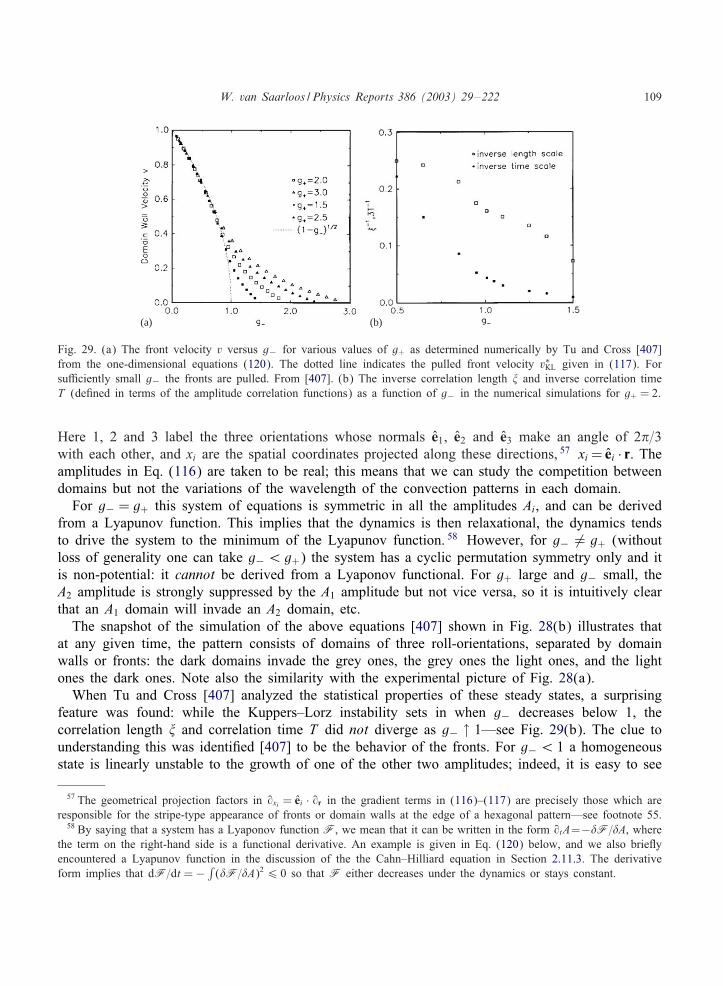
W. van Saarloos / Physics Reports 386 (2003) 29–222 109
(a) (b)
Fig. 29. (a) The front velocity v versus g− for various values of g+ as determined numerically by Tu and Cross [407]from the one-dimensional equations (120). The dotted line indicates the pulled front velocity v∗KL given in (117). ForsuRciently small g− the fronts are pulled. From [407]. (b) The inverse correlation length � and inverse correlation timeT (de3ned in terms of the amplitude correlation functions) as a function of g− in the numerical simulations for g+ = 2.
Here 1, 2 and 3 label the three orientations whose normals e1, e2 and e3 make an angle of 2�=3with each other, and xi are the spatial coordinates projected along these directions, 57 xi = ei · r. Theamplitudes in Eq. (116) are taken to be real; this means that we can study the competition betweendomains but not the variations of the wavelength of the convection patterns in each domain.
For g− = g+ this system of equations is symmetric in all the amplitudes Ai, and can be derivedfrom a Lyapunov function. This implies that the dynamics is then relaxational, the dynamics tendsto drive the system to the minimum of the Lyapunov function. 58 However, for g− = g+ (withoutloss of generality one can take g− ¡g+) the system has a cyclic permutation symmetry only and itis non-potential: it cannot be derived from a Lyaponov functional. For g+ large and g− small, theA2 amplitude is strongly suppressed by the A1 amplitude but not vice versa, so it is intuitively clearthat an A1 domain will invade an A2 domain, etc.
The snapshot of the simulation of the above equations [407] shown in Fig. 28(b) illustrates thatat any given time, the pattern consists of domains of three roll-orientations, separated by domainwalls or fronts: the dark domains invade the grey ones, the grey ones the light ones, and the lightones the dark ones. Note also the similarity with the experimental picture of Fig. 28(a).
When Tu and Cross [407] analyzed the statistical properties of these steady states, a surprisingfeature was found: while the Kuppers–Lorz instability sets in when g− decreases below 1, thecorrelation length � and correlation time T did not diverge as g− ↑ 1—see Fig. 29(b). The clue tounderstanding this was identi3ed [407] to be the behavior of the fronts. For g− ¡ 1 a homogeneousstate is linearly unstable to the growth of one of the other two amplitudes; indeed, it is easy to see
57 The geometrical projection factors in 9xi = ei · 9r in the gradient terms in (116)–(117) are precisely those which areresponsible for the stripe-type appearance of fronts or domain walls at the edge of a hexagonal pattern—see footnote 55.
58 By saying that a system has a Lyaponov function F, we mean that it can be written in the form 9tA=−�F=�A, wherethe term on the right-hand side is a functional derivative. An example is given in Eq. (120) below, and we also brieKyencountered a Lyapunov function in the discussion of the the Cahn–Hilliard equation in Section 2.11.3. The derivativeform implies that dF=dt = − ∫ (�F=�A)26 0 so that F either decreases under the dynamics or stays constant.

110 W. van Saarloos / Physics Reports 386 (2003) 29–222
from Eq. (116) that the linear spreading speed of an A1 perturbation into a domain where A2 = 1equals
v∗KL = 2√
1 − g− : (117)
On the other hand, even though an A2 domain is linearly stable to small perturbations in all theamplitudes, for 1¡g− ¡g+ it is only metastable: an A1 domain will invade an A2 domain eventhough it is linearly stable. We can show this by using the curious feature that two-mode subdynamicsof these equations is actually of potential nature, even though the full three-mode dynamics is not.Let us consider the one-dimensional dynamics of two modes only,
9tA1 = cos2�1 92xA1 + A1(1 − A2
1 − g−A22) ; (118)
9tA2 = cos2�2 92xA2 + A2(1 − A2
2 − g+A21) : (119)
Here �1 and �2 are the angles between the x-axis and the vectors e1 and e2. Upon transforming tothe variables VA1 =
√g+A1 and VA2 =
√g−A2 we can write the equations in the potential form
9 VA1
9t = −�F� VA1
;9 VA2
9t = −�F� VA2
; (120)
where the “free energy”, which plays the role of a Lyapunov functional, is given by
F = 12
∫dx[cos2�1(9x VA1)2 − VA2
1 +1
2g+
VA41 + cos2�2(9x VA2)2 − VA2
2 +1
2g−VA4
2 + VA21
VA22
]: (121)
For g1 ¿ 1, this free energy functional has local minima at VA1 =√g+, VA2 =0 and VA1 =0, VA2 =
√g−.
For g− ¡ 1 the second point becomes a saddle, in agreement with the fact that the state A2 state isunstable to the growth of the A1-mode. However, even though the free energy has two local minimafor g− ¿ 1, for any g− ¡g+ the second one corresponding to the nonzero A2-mode always has ahigher free energy than the 3rst one, which corresponds with the A1-phase. These two minima areseparated by a free energy barrier (very much like two stable phases near a 3rst order transition), butthe relaxational nature of this subdynamics implies that any initial condition which corresponds withan A1-domain on the left and an A2-domain on the right will develop into a coherent front whichmoves to the right. Such “bistable” fronts which connect two linearly stable states are well knownfor such types of equations; they are like pushed fronts and their speed approaches an asymptoticvalue exponentially fast.
Indeed, as Tu and Cross found—see Fig. 29(a)— the scenario which emerges is that for anyg− ¡g+ the dynamical attractor is a statistically steady chaotic domain state. If g− is reducedbelow g+, the invasion of domains is due to pushed fronts up to some critical value of g− belowwhich the fronts are pulled. 59 The Kuppers–Lorz instability is therefore not only a nice illustrationof how fronts propagating into an unstable state can be generated dynamically, but it is also one ofthe few realistic examples we know of where the front propagation mechanism changes from pushed
59 Note that the numerical data-points in the pulled regime in Fig. 29 are slightly below v∗KL; as always, this is a signof the slow power law convergence to the asymptotic pulled front speed.

W. van Saarloos / Physics Reports 386 (2003) 29–222 111
to pulled upon changing a parameter. In this particular experiment this parameter can even be tunedeasily by changing the rotation rate. 60
We 3nally note that as as we will discuss in Section 5, pulled fronts are not amenable to theusual sharp interface approximation or moving boundary approximation. Whether this gives riseto any noticeable diDerence between the transient domains in the pushed regime just above theKuppers–Lorz instability and those in the pulled regime at higher rotation rates, has apparently notbeen explored. However, I consider it unlikely that it does, since as Fig. 29(a) shows, there is onlya large separation of scales between the front thickness and the domain size in the regime nearthreshold.
3.5. Propagating discharge fronts: streamers
When the electric 3eld is large enough, free electrons in a gas accumulate suRcient energyinbetween collisions that they can knock out an electron from a neutral gas molecule in a collision. Inair, the ionization of nitrogen is dominant, and in this case the ionization reaction can be summarizedas e− + N2 ⇒ 2e− + N+
2 . This type of avalanche phenomenon can naturally lead to to the formationof discharge patterns (sparks!) whose dynamics is dominated by the propagation of fronts into theunstable non-ionized state, as is illustrated in Fig. 30. Figures (a) and (b) show two snapshots ofsimulations of Vitello et al. [433] of the formation of a discharge pattern in nitrogen between twoplanar electrodes across which a potential diDerence of 25 kV is applied. Initially, at time t = 0, thegas between the electrodes is non-ionized, except for a small region near the upper electrode. Dueto the large 3eld, the electrons immediately get accelerated downward into the non-ionized region,ionizing neutral molecules along the way. Figs. 30(a) and (b) show the electron density level lines4.75 and 5:5 ns later. The regions inside the 3nger-like regions of these so-called streamer patternsare weakly ionized plasmas; the regions where the level lines crowd mark the zones where theelectron density drops quickly to a very small value, and where most of the ionization takes place.The negative space–charge in this transition zone eDectively shields the outer 3eld in the non-ionizedregion from that in the streamer body where both the space-charge and the 3eld are small.
The propagation of streamer patterns is well described by the following set of equations for theelectron density ne, the ion density n+ and the electric 3eld E [142,433],
9tne = "0|ne@eE|e−E0=|E| −∇ · (−ne@eE− De∇ne) ; (122)
9tn+ = "0|ne@eE|e−E0=|E| ; (123)
∇ · E=e�0
(n+ − ne) : (124)
The 3rst term on the right-hand side of the 3rst two equations is the impact ionization term. As @e
is the electron mobility, −@eE is the electron velocity, so the prefactor is just the impact rate ofelectrons on the ions, while the exponential factor accounts for the ionization rate as a function of
60 For fronts between two locally stable states the front velocity will behave linearly in g+ − g− for g− ≈ g+. Since thedomain dynamics is driven by the front motion, we therefore expect the correlation length � and time scale T to scale as�=T ∼ (g+ − g−) close to the point g− = g+. The correlation length � in Fig. 29(b) does seem to vanish indeed fasterthan T , but there are insuRcient data to test this hypothesis.

112 W. van Saarloos / Physics Reports 386 (2003) 29–222
(a) (b) (c)
(b)
(a)
Fig. 30. (a) and (b): results of the numerical simulations of Vitello et al. [433] of the full three-dimensional simulation ofEqs. (122) – (124) for parameters corresponding to nitrogen gas and a potential diDerence between the planar electrodesof 25 kV. Each line indicates an increase of ne by a factor of 10. Shown are snapshots of the electron density 4.75and 5:5 ns after an initial ionization seed was placed at the upper electrode. (c) Space-time plot of a simulation of theequations by Ebert et al. [142] for the case of a planar streamer front in the case D = De"0=(@eE0) = 1 [142]. Upperpanel: the dimensionless electron density + = nee=(�0"0E0) as a function of time and space. Lower panel: the electric 3eldmeasured in units of E0. The initial condition was a homogeneous 3eld E = −E0 and a small, charge-neutral ionizedregion with Gaussian electron and ion density around x = 55. The front propagating to the right in the same directionas the electron drift velocity is called a negative streamer front; it is a pulled front with asymptotic speed v∗str (=2.21 indimensionless units), given by Eq. (125). The front propagating slowly to the left is a pushed positive streamer front.
the 3eld—small 3elds give a small ionization rate, as the electron speed at impact is small. The othertwo terms on the right-hand side of (122) account for the drift and diDusion of the electrons. Similarterms are absent in the equation for the ion density n+ since on the time scales of interest driftand diDusion of the much heavier ions can be ignored. Finally, Eq. (124) is the Maxwell equationrelating the 3eld strength to the charge density.
Clearly the impact ionization term in these equations makes the non-ionized state with ne =n+ =0linearly unstable. Moreover, since a nonzero charge density tends to screen the 3eld, the 3eld islargest just ahead of a front. The exponential factor in the impact ionization term is an increasingfunction of the 3eld strength, hence the growth is gradually decreased from a large value ahead ofthe front to a small value in the plasma behind the front where the 3eld is screened. At 3rst sight, itmay therefore come as no surprise that discharge fronts which propagate in the same direction asthe electron drift velocity—so-called negative streamers—are examples of pulled fronts [141,142].Now, apart from the drift term, Eq. (122) has, to linear order in ne, the same terms as the F-KPPequation (1), a linear growth term and a diDusion term. We therefore immediately obtain the asymp-totic speed of planar streamer fronts
vasstr = v∗str = −@eE+ + 2
√De|@eE+|e−E0=E+ ; (125)

W. van Saarloos / Physics Reports 386 (2003) 29–222 113
where E+ is the value of the 3eld just ahead of the front. This prediction has been fully con3rmedby extensive numerical simulations by Ebert et al. [141,142], an example of which is shown inFig. 30(c).
The streamer problem is very instructive from a more general point of view. First of all, in theF-KPP equation, it is rigorously known [16,35,37] that one is always in the pulled regime if thegrowth function f(�)=�¡f′|�=0. The streamer problem nicely illustrates that such simple resultsgenerally do not hold in more complicated cases. As we mentioned above, the ionization term inthe streamer equations rapidly decreases when the 3eld strength drops; hence the ionization rateper electron "0@e|E|exp − E0=|E|, which is the analog of the growth ratio f(�)=� in the F-KPPequation, decreases monotonically from the front side to the back side of the front. In spite of this,for each set of parameter values, the streamer equations not only admit pulled negative streamerfront solutions, but also pushed positive streamer front solutions which propagate in the oppositedirection. Fig. 30(c) illustrates this. The reason for this is that streamer front propagation arisesthrough the interplay of ionization and screening of the 3eld. Screening is a nonlocal phenomenonmediated through Eq. (124), and so the monotonic behavior of the 3eld dependence of the localionization term is just half of the story.
Secondly, the negative streamer patterns like those of Figs. 30(a,b) are nice examples of interface-like growth patterns whose dynamics is associated with propagating pulled fronts. Indeed, if we writethe electric 3eld in terms of the electrical potential , as E=−∇,, we see that outside the streamerbody, where the charge density is negligible, the potential obeys to a good approximation the Laplaceequation ∇2, = 0. Moreover, Eq. (125) shows that to a good approximation the normal velocity ofa streamer equals @e∇,. These are precisely the two equations for viscous 3ngering [44,250,338]or for thermal plumes in two dimensions [451], so if we think of the streamer pattern as a movinginterface, we expect their dynamics to have a number of similarities with the dynamics of viscous3ngers or plumes [141,428].
However, the story is not that simple! The problem is that pulled fronts cannot straightforwardlybe mapped onto a moving boundary problem, even when their width is much smaller than thepattern scale [as is clearly the case for the streamer patterns of Figs. 30(a,b)]. As we will discussmore generally in Section 5, the fact that the dynamically important region of pulled fronts is aheadof the front itself entails not only a power law convergence to the asymptotic speed but also abreakdown of the standard moving boundary approximation. The precise implications of this forstreamers are still under active investigation—very much like dendrites, they do show a tip-splittinginstability [18], but the dispersion relation of small perturbations of a planar discharge front doesappear to be diDerent from what one would expect based on the analogy with viscous 3ngeringor dendrites.
3.6. Propagating step fronts during debunching of surface steps
When a crystal is cut with an angle slightly diDerent from one of the principle crystal facets, theresulting “vicinal surface” contains a lot of steps. The predominant mechanism during vapor growthis then that adatoms which have landed on the surface diDuse towards these steps and attach there.The crystal growth is thus accompanied by the propagation of steps along the surface.
It has been known since long that growing mono-atomic steps can “bunch”: instead of stayingequidistant, on average, they bunch together and form macro-steps. Many of these and other step

114 W. van Saarloos / Physics Reports 386 (2003) 29–222
(a) (b)
Fig. 31. ReKection electron microscopy image of a vicinal Si(111) surface 10 s after the a change of direction of thecurrent direction; a series of steps “peel oD” from a large macro-step in a characteristic pattern: steps “debunch” fromthe macro-step that is visible as the thick line meandering through the middle of the 3gure. From Latyshev et al. [253].(b) Snapshot of a Monte Carlo simulation by Kandel and Weeks [215] of the stochastic version of the step model (127).Note the similarity with the experimental observations shown in panel 3gure (a).
instabilities can be understood in terms of the following simple model of step Kow [42,168,214,411],
9tXn = f+(Wn) + f−(Wn−1) + 292yXn : (126)
Here Xn(y; t) is the position of the nth step measured along y, the coordinate along the step.The terms f+(Wn) and f−(Wn−1) describe the growth due to attachment of atoms from the terraceof width Wn = Xn+1 − Xn in front of the step and the terrace of width Wn−1 just behind the step.The last term is a curvature correction analogous to the surface tension type term that occurs inalmost all interfacial problems. Note that from a mathematical point of view, Eq. (126) is of mixedcharacter: it is a partial diDerential equation with respect to the y-variable, but a diDerence equationwith respect to the step index n.
A straightforward stability analysis shows that an equidistant array of steps (all Wn=W ) is unstablewhen the attachment kinetics is such that steps predominantly incorporate atoms from the terracebehind it, i.e. if f′−(W )¿f′
+(W ). This is in full agreement with the intuitive idea that when a steplags a bit behind, the terrace behind it becomes smaller and hence the step will capture fewer atomsfrom this terrace. 61 This instability leads to step bunching in the nonlinear regime.
It has been found in various experiments that application of a current along the surface can inducevery complex patterns. Indeed, one of the new phenomena that occurs is shown in Fig. 31(a): rightafter reversal of the current, steps “peel oD” from a macro-step in a characteristic pattern.
This experimentally observed “debunching” behavior is not found in the above model for thestep dynamics, but Kandel and Weeks [215] have shown that it can be understood in terms of thefollowing extension of it. The shortcoming of model (126) is that the growth functions f±(W ) onlydepend on the terrace width right ahead of and behind the step. However, when steps bunch they
61 Early work on step bunching by Frank [168] described it on a coarse-grained scale in terms of the Burgers equation.If the step velocity decreases as a function of step density, the well-known formation of shocks in the Burgers equationimplies step bunching. From this perspective, the phenomenon is similar to the formation of traRc jams in elementarymodels for traRc Kow.

W. van Saarloos / Physics Reports 386 (2003) 29–222 115
get so close that this simple approximation breaks down: capture of adatoms by steps in a bunch isstrongly suppressed because steps cannot move any closer. Instead, surface diDusion over the entirebunch becomes more probable. Kandel and Weeks [215] therefore replace (126) by
9tXn = f+(Z (f )n ) + f−(Z (b)
n ) + 292yXn ; (127)
for Wn ¿Wmin, while 9tXn = 0 for Wn ¡Wmin. Here Z (f )n (Z (b)
n ) is the width of the 3rst terrace infront of (behind of) the nth step that is larger than Wmin. Note that this introduces a dynamicallygenerated non-locality in the model: the terraces from which a step captures atoms depend on thedynamical state of the step con3guration itself. As a result, as discussed in detail in [215], theseequations also lead to a debunching instability near the edge of a step bunch: one or a series ofsteps can “peel oD” in a characteristic fashion from the bunch, while the other steps in the bunchremain virtually immobilized together. A snapshot of a Monte Carlo simulation [215] of a stochasticversion of this model with
f−(W ) = k−W; f+(W ) = k+W ; (128)
is shown in Fig. 31(b). Clearly, the type of step patterns found in this model is remarkably similarto that seen experimentally.
From our perspective, the interesting aspect is the arrays of steps—the almost parallel lines in the3gure—which cross from one step bunch to the other. As we mentioned above, the step con3gurationnear the edge of a bunch is unstable to the peeling oD of an array of steps, and so the propagationof the detachment point can be viewed an an example of a front propagation into an unstable stateproblem. Indeed, by linearizing the dynamical Eqs. (127) and (128) about an array of straight stepsseparated by a distance ≈ Wmin and assuming a behavior for perturbations �Xn of the form
�Xn(y; t) ∼ e−�(y−nE)++t (129)
one obtains a linear dispersion equation of the form
+(�) = k+(e�E − 1) + k−(1 − e−�E) + 2�2 : (130)
Note that the various terms in this expression do reKect the mixed character of the equation: theexponential terms are characteristic of a 3nite diDerence equation, the last term of a partial diDer-ential equation. The linear spreading speed v∗debunch can of course be obtained straightforwardly bydetermining the minimum of the curve +(�)=�. The comparison of v∗debunch with the simulation datafor various E is shown in Fig. 32. The data clearly show that the debunching point propagates alongthe bunch with the linear spreading velocity, so apparently the debunching process is an exampleof a pulled fronts. Pulled fronts were also found to describe certain aspects of the initial bunchingprocess in the original model (126) [214].
Recent experiments on this debunching instability [438,393] are consistent with the relationbetween growth length � and step spacing E found by Kandel and Weeks [215] but do not testthe predictions for the front velocity directly. More recent theoretical work [207] shows that astrain-induced step bunching instability can be convective.
3.7. Spinodal decomposition in polymer mixtures
When a homogeneous mixture is quenched within the so-called spinodal region, the homogeneousstate is unstable to composition Kuctuations. The lowest free energy state towards which the system

116 W. van Saarloos / Physics Reports 386 (2003) 29–222
Fig. 32. Comparison of the prediction of v∗debunch(E) (full line) with the velocity data (symbols) from the simulationsshown in Fig. 31(b). V0 is the initial step velocity V0 = (k+ + k−)W and Ec =
√22=(k− − k+). From Kandel and Weeks
[215].
evolves at long times is one in which it is demixed into two homogeneous phases of diDerentcomposition. On the way towards this demixed state the system is spatially inhomogeneous onmesoscopic scales. This spatio-temporal demixing process is called spinodal decomposition [56,192].
At intermediate times the dynamics is normally dominated by motion of interfaces between do-mains in which the composition is close to one of the equilibrium compositions. The initial phase,however, depend on the system under study. For most systems (like ordinary liquids), the Kuctua-tions are large enough that right after the quench these Kuctuations grow out due to the instability ofthe bulk mode. Moreover, this regime is often diRcult to probe experimentally, since it happens ontoo short time scales. For suRciently long polymers, however, the dynamics is slow enough that thisregime becomes experimentally accessible [440]. Moreover, the longer the polymers the smaller theKuctuations, so that the coarse-grained mean-3eld like models which have mostly been studied in theliterature become more appropriate for polymer systems. It is also conceivable that the short-timedynamics is then sometimes dominated by the propagation of composition modulation fronts intothe unstable homogeneous state. If so, it is likely that such fronts typically start at the walls of thesample, since a wall is normally preferentially wetted by one of the compositions [21].
A simple model equation for spinodal decomposition is the Cahn–Hilliard equation which wealready introduced in Section 2.11.3. The front propagation problem in this equation in the presenceof noise was studied from the above perspective by Liu and Goldenfeld [266] and by Ball andEssery [21] who both found that the composition modulation fronts in this equation are pulled frontswhich lead to a incoherent pattern which continues to coarsen. 62 The simulations of Fig. 15 alsoshowed this.
Experimental evidence for the above surface-induced front-dominated spinodal decompositionscenario in polymers was found by Jones et al. [208], but no direct quantitative comparison wasmade with the predictions from the theory of front propagation.
62 The data points for the numerical front velocities obtained shown in [266] are as usual slightly below the value v∗:As we remarked already several times, this is true for almost all published data, and reKects the slow convergence of thespeed of a pulled front to its asymptotic value.

W. van Saarloos / Physics Reports 386 (2003) 29–222 117
We 3nally note that the competition between bulk growth and front propagation in a model witha non-conserved order parameter was also studied in [289,409].
3.8. Dynamics of a superconducting front invading a normal state
The equilibrium and dynamical behavior or vortices in type II superconductors is a vast andactive 3eld with many rami3cations, which range from fundamental statistical physical studies toapplications [50]. Even in the area of vortex dynamics, interesting questions concerning the behaviorof propagating fronts separating domains with diDerent vortex properties (e.g. a diDerent density ofvortices) come up [137,285], but most of the issues that arise in this area are diDerent from thosewhich are the main focus of this paper. We therefore limit our discussion here to some interestingtheoretical 3ndings concerning fronts propagating into an unstable state of a type I superconductor,which also raise some new fundamental questions. Some indirect evidence for such fronts have beenfound from measurement of the magneto-optical response of thin 3lms [169] but the time-resolutionhas been insuRcient to study the dynamics directly. Recent advances in magneto-optical techniques[202,437] to visualize vortex patterns may open up the possibility to do so in the near future.
It is well known [394] that in so-called type I superconductors the normal state is linearlyunstable 63 to the superconducting state when the magnetic 3eld H is reduced below the criticalvalue Hc2. For 3elds Hc2 ¡H ¡Hc, the normal state is linearly stable, but has a higher energy thanthe superconducting state; the superconducting state can then only form through nucleation. Thebarrier for this nucleation of superconducting domains vanishes as H approaches Hc2 from above.The dynamical behavior that can result if a type I superconductor is quenched into this unstable statewas studied a number of years ago by Liu et al. [267] and by Frahm et al. [132,167], who pointedout the analogy of these two regimes to the spinodal and nucleation regimes of phase separation(see Section 3.7). Moreover, they drew attention to the fact that when the superconducting phasepropagates into the normal phase, the eDective long-wavelength equations show a strong analogywith the diDusion equations describing diDusion limited growth. As a result, one expects these frontsto have a similar Mullins–Sekerka like long-wavelength instability as crystal growth problems (see[73,220,226,247,251,338,353] and Section 3.17).
In time-dependent Ginzburg–Landau theory the dynamics of a superconductor is governed by thedynamical equation for the complex superconducting wave function (r; t) [132,167,132,394]
9 9t = − �F
� ∗ ; (131)
where the dimensionless free energy functional F is given by
F =∫
dr{−| |2 + 12 | |4 + |[(i>)−1∇ − A] |2 + (∇ × A)2} : (132)
The Ginzburg–Landau parameter >=�(T )=�(T ) in this expression is the ratio of the penetration depth� and the coherence length �; type I superconductors are characterized by >¡ 1=
√2. Furthermore,
63 Tinkham [394] formulates this slightly diDerently, but if the the problem is formulated as a stability analysis, i.e., asthe problem of 3nding the growth rate e+t of the linear eigenmodes, one immediately sees that below Hc2 the normal stateis unstable.

118 W. van Saarloos / Physics Reports 386 (2003) 29–222
(a) (b)
Fig. 33. (a) Penetration of the propagation of a superconducting domain into a normal domain in numerical calculationsby Frahm et al. [167]. The penetration is visualized through the strength of the magnetic 3eld shown in greyscale, withblack corresponding to B ≈ Hc and white corresponding to B ≈ 0. The 3eld strength in the normal phase correspondsto a value of about 0.57 Hc which corresponds to the nucleation regime where the normal phase is linearly stable, while> = 0:3 and = = 0:1. Times are measured in units of the order parameter relaxation time [167,267]. (b) As in (a), butnow for a 3eld H = 0:28Hc which corresponds to the spinodal regime where the normal phase is locally unstable.
A in (132) is the magnetic vector potential which is related to the magnetic 3eld B through B=∇×A;using Ampere’s law and Ohm’s law, the dynamics of A is governed by
=9tA = [>−1Im ( ∗∇ ) − | |2A] − ∇ × (∇ × A) : (133)
Here = is the dimensionless conductivity [167] and the term between square brackets in this expres-sion is the supercurrent contribution in the Ginzburg–Landau formulation. The gradient term in thisterm describes the generation of supercurrents in fronts or interfacial zones and near surfaces, whilethe second term is the Meissner term which is responsible for Kux expulsion from the superconduc-tor state where | |2 = 0 (note that it acts like a linear damping term for A which drives the 3eldto zero).
Fig. 33 shows two examples of the simulations of Frahm et al. [167] of a superconducting statepropagating into the normal state of a two-dimensional sample with the magnetic 3eld B = ∇ ×A perpendicular to the sample. Since the magnetic 3eld is expelled from the superconductor agood way to represent the dynamics is by plotting the strength of the magnetic 3eld in greyscale.Fig. 33(a) shows an example of a superconducting front penetrating the normal state in the nucleationregime (Hc2 ¡H ¡Hc) where the normal state is linearly stable. Due to the Kux expulsion, thesuperconducting region shows up as white in the 3gure, while the black zones illustrate the 3eldenhancement due to the supercurrents in the interfacial region. Note also that the size of the protrusionincreases in time, in agreement with the analogy with diDusion-limited growth problems noted abovewhich suggests that the interface should be unstable on long length scales.
Fig. 33(b) shows that the dynamics is very diDerent when the front propagates into a linearlyunstable normal phase (the spinodal regime). In this regime the front itself appears to become verycomplex, and the dynamics is accompanied by the occurrence of phase slips in the superconductororder parameter (points in space and time where the amplitude | | vanishes so that the phase of can change by a factor 2�).

W. van Saarloos / Physics Reports 386 (2003) 29–222 119
The scenario that one expects for superconductor fronts propagating into a normal state is some-what similar to the one discussed for the quintic CGL equation in Section 2.11.6: for 3eldsHc2 ¡H ¡Hc the behavior is subcritical, and the dynamics of the fronts separating the two phasesis like that of a bistable front or a pushed front. When upon reducing the 3eld the value Hc2 iscrossed, the normal state becomes linearly unstable—this corresponds to � becoming positive in thequintic CGL. The linear spreading speed v∗ then becomes nonzero, but clearly for 3elds just belowHc2 the dynamically relevant fronts will remain pushed. The question then arises, however, whetherupon decreasing the 3eld even more the fronts may become pulled for some range of parameters,just like it happens in the quintic CGL equation. If so, this would be of great advantage, since itmight provide a handle at calculating some of the properties of the complex patterns of Fig. 33(b)analytically, just like the propagating Rayleigh instability of Section 3.3 allows one to obtain mostessential features of the pattern analytically.
To our knowledge, the question whether the full two-dimensional complex patterns in the spinodalregime are governed in some cases by propagating pulled fronts has not been studied yet. Someindication that a transition to pulled front propagation might be possible comes from the work ofDi Bartolo and Dorsey [123]. They studied the propagation of one-dimensional fronts in the absenceof the possibility of phase slip generation (as was taken to be real and equal to f below) and inthe case that the external 3eld in the normal phase vanishes. In dimensionless units, the equationsin this case reduce to
9tf = >−292xf − a2f + f − f3 ; (134)
= 9ta = 92xa− f2a : (135)
The authors studied the case in which the front propagates into the normal state with f = 0 anda = a∞. Since the magnetic 3eld H is this case is simply related to a by H = 9xa, and since a = 0in the superconductor behind the front,
∫∞−∞ H = a∞ is simply the amount of magnetic 3eld trapped
in the front region and the 3eld in the normal phase far ahead of the front vanishes. Di Bartolo andDorsey [123] found that fronts in this restricted equation are pulled for small enough values of a∞but pushed for larger a∞. However, because of the possibility of the generation of phase slips wassuppressed by taking f real, it is conceivable that fronts at some point are unstable to the splittingoD of a localized normal region with some magnetic 3eld trapped and a faster growing growingfront with a smaller amount of trapped 3eld. Clearly, various issues regarding these superconductorfronts still remain to be resolved.
We 3nally note that apart from the practical signi3cance of studying whether fronts might be pulledin the two-dimensional case, this question is also relevant from the following perspective. As we willdiscuss in Section 5, pulled fronts are not amenable to the usual moving boundary approximation.The full implications of this are not known, so the superconductor front problem might be a good oneto explore this issue, if they admit pulled fronts. The only other realistic example known to me wherethis issue appears to have immediate relevance for the pattern formation are the streamer dischargepatterns analyzed in Section 3.5. (See also the remark at the end of Section 3.4 on the Kuppers–Lorzinstability.) The recent advance in increasing the time resolution of magneto-optic techniques [437]may open up the possibility that these dynamical issues will become experimentally relevant in thenear future.

120 W. van Saarloos / Physics Reports 386 (2003) 29–222
planar Couettepipe Poiseuille planar Poiseuille
Reynolds number
5772
Reynolds number
"per
turb
batio
n am
plitu
de"
"per
turb
batio
n am
plitu
de"
turbulence branch
turbulence branch
threshold branchthreshold branch
Fig. 34. Schematic illustration of the subcritical bifurcation structure of the transition to turbulence in Couette and PoiseuilleKow [205]. For planar Couette Kow and pipe Poiseuille Kow (left plot), the laminar base Kow is linearly stable for any3nite Reynolds number, but the threshold to turbulence decreases as Re−2 with some exponent 2 as Re → ∞ [80]. PlanarPoiseuille Kow is linearly unstable for Re¿ 5772 but the transition is subcritical and the linear instability does not playmuch of a role in practice for Re of order 2000 or less, where turbulence is often already observed in practice. Notethat the drawing is schematic only: although only a single curve is drawn in the left plot, there are important diDerencesbetween planar Couette Kow and pipe Poiseuille Kow.
3.9. Fronts separating laminar and turbulent regions in parallel shear =ows:Couette and Poiseuille =ow
In this and the next three sections we will discuss hydrodynamic instabilities in which both frontdynamics and Kuctuation eDects or turbulence play an important role.
Two of the basic textbook examples of hydrodynamic Kow states are Couette Kow and PoiseuilleKow. We have already encountered Couette Kow in Section 3.1 where we considered Kow betweentwo concentric cylinders. For that setup, Couette Kow refers to the basic laminar Kow state. Themany instabilities that are found in this system are due to the interplay of the inertial eDects andthe Coriolis force in a rotating system. In this section, we will be concerned with planar CouetteKow, Kow between two plates sheared in opposite directions. Experimentally, this setup is realizedby moving a transparent plastic band between two glass plates; the Kuid in between is then shearedby the plastic band [108,109,283]. In planar Couette Kow of a normal Newtonian Kuid, the basicKow state for Kow in the x-direction between plates separated by a distance 2d in the y directionis simply a linear velocity pro3le vx = vplatesy=d; thus the shear rate 9vx=9y is constant. The otherclassic example of a shear Kow is Kow through a pipe or between plates (the planar case) drivenby a pressure gradient: Poiseuille Kow. In this case, the basic velocity pro3le is parabolic, so theshear rate is zero on the center line and increases linearly towards the walls.
The control parameter for Couette Kow or Poiseuille Kow is the Reynolds number Re = Ud=4where U is a typical velocity of the Kow (the velocity at the plates in the case of Couette Kow), dthe half spacing of the plates or the radius of the pipe, and 4 the kinematic viscosity of the Kuid.For large enough Reynolds numbers, Couette Kow and Poiseuille Kow become turbulent. However,the transition to turbulence in such systems is not a supercritical bifurcation, in which a nontrivialmode grows gradually in amplitude beyond a threshold at which the basic Kow becomes unstable.Instead, the transition is subcritical [80,190,205], as sketched in Fig. 34. This implies that over some

W. van Saarloos / Physics Reports 386 (2003) 29–222 121
(a) (b)
Fig. 35. Example of a turbulent spot in planar Couette Kow, taken from the review of Manneville and Dauchot [283]. Theseeding of the Kuid with small Kalliroscope Kakes makes the turbulent regions show up brightly, while laminar regionsremain dark (the Kakes are lined up by the shear gradient in laminar regions). The spreading of such turbulent spotsdepends on the Reynolds number of the base Kow [108,109,283]. (b) Snapshot of a turbulent spot in the simulations ofSchumacher and Eckhardt [378]. The Kow is in the x-direction. On the right, a cross-section in the direction normal tothe planes is shown. See Fig. 36 for further details.
range of Re linearly stable laminar Kow can coexist with turbulent regions 64 (very much like neara 3rst order phase transition). An example of a turbulent spot in a planar Couette experiment isshown in Fig. 35(a). The competition between such turbulent and laminar regions as a function ofReynolds number has been explored in detail only in the last decade [108,109,283].
Actually, as Fig. 34 indicates, although the subcritical behavior is common to all three cases, thereis an important conceptual diDerence as well: planar Poiseuille is linearly unstable beyond Re=5772while planar Couette and pipe Poiseuille Kow are stable for any 3nite Reynolds number—the criticalamplitude in the latter cases decreases as Re−2 for Re → ∞ [80,190] and hence we can think ofthis case as an instability which has been pushed to in3nity. In the latter two cases, the absenceof a true instability also implies that there cannot be any pulled fronts: the fronts that separate aturbulent region from a laminar region must always be pushed.
For the case of planar Poiseuille Kow, one might wonder whether the propagation of a tur-bulent region into the laminar Kow state could correspond to a pulled front, as the situation issomewhat similar to the one found for the quintic complex Ginzburg–Landau equation discussed inSection 2.11.6. 65 However, a priori this possibility is already unlikely for realistic Reynolds num-bers: since the generic behavior of planar Poiseuille Kow is so close to that of planar Couette andpipe Poiseuille Kow, where fronts de3nitely have to be pushed, we similarly expect the fronts sep-arating turbulent and laminar domains to be pushed as well. It was indeed found [116] that thelinear instability of the planar Poiseuille pro3le always is always convective, so that pulled frontscould never propagate upstream. As we shall see below, however, the simpli3ed picture based ona straightforward linear stability analysis of the unperturbed Kow does not suRce for studying thespreading of a spot, because a coupling with induced cross Kow has to be taken into account.
64 It is interesting to note that also in turbulent superKuid pipe Kow, there are strong experimental indications for thecoexistence of turbulent and laminar domains [284].
65 In the quintic complex Ginzburg–Landau equation, expanding chaotic spots were observed in numerical simulationsin some parameter ranges [424]. Their behavior is very much like what one would expect intuitively for turbulent spots.See footnote 18.

122 W. van Saarloos / Physics Reports 386 (2003) 29–222
Fig. 36. Snapshots of the stream-wise velocity vx(z; y) as it spreads downward in the simulations of Schumacher andEckhardt [378] for Re = 200. Dotted lines denote contour lines for positive velocity values, solid lines the contour lineswith negative velocity values. Note that the turbulent region propagates downward with a roughly constant speed.
The point at issue here has recently been studied numerically for a closely related situation bySchumacher and Eckhardt [378]. These authors performed direct simulations of the Navier–Stokesequations for the case of shear Kow between planes. However, unlike in the case of plane CouetteKow, for numerical convenience they imposed free-slip boundary conditions on the bounding platesand drove the bulk Kow by bulk force which varies as a cosine in the y-direction normal to theplanes, and which forces the Kow in opposite directions near the two plates.
Fig. 35(b) shows a snapshot of a turbulent spot in the simulations, which evolved from a localizedperturbation of the laminar pro3le in the center of the simulation cell. Note that qualitative similaritywith the turbulent spots observed experimentally: Both spots shows a number of streaks in thestream-wise (horizontal) direction. These streaks can also be recognized in cross-sections in they-direction perpendicular to the planes shown on the right.
The spreading of the turbulent spot in time in the “span-wise” (vertical) direction in these sim-ulations is shown in Fig. 36. It is immediately obvious that the turbulent region spreads verticallythrough some kind of front structure which advances with a rather well-de3ned speed. Moreover,the local turbulent energy v2 averaged over the normal direction was found to decay exponentiallyinto the laminar region, very much as one would expect for a well-de3ned front solution and as hasbeen found in some incoherent regimes of the quintic CGL equation [424]. Since Schumacher andEckhardt found that the turbulent spot also gives rise to an overall “span-wise” outKow Uz in thevertical direction, they analyzed the linear spreading velocity v∗ by linearizing the Kow equationsabout a laminar state which is the sum of the base Kow and this outKow Uz [378], using the so-calledOrr–Sommerfeld equation. 66 The measured front speeds in the numerical simulations were about
66 The Orr–Sommerfeld equation is the linearized equation governing the stability of nearly parallel Kows. It is basedon linearizing the Navier–Stokes equations in the deviations about a base Kow pro3le U . [135]. In the inviscid limit theequation reduces to the so-called Rayleigh stability equation used in some of the work discussed in Section 3.10 on theformation of BIenard–Von Karman vortices.

W. van Saarloos / Physics Reports 386 (2003) 29–222 123
a factor 10 larger than the value of v∗ obtained this way, leaving no doubt that in the parameterregime studied the span-wise spreading of a turbulent spot is not governed by a pulled front: Thesefronts are pushed. An earlier analysis along the same lines of the spreading of turbulent spots inplane Poiseuille Kow lead to the same conclusions [197].
We would like to stress that the above observations are just empirical: the simulations do givestrong indications that it does make sense to associate the expansion of a turbulent spot with a ratherwell-de3ned coherent front, but, as we already pointed out in Section 2.7.3, not much is known aboutthe properties of such fronts. In fact, also in the quintic CGL equation, spreading of chaotic spotswas found to proceed with a more or less constant speed larger than v∗ (see Fig. 18(a)), but to ourknowledge it is a complete mystery why and how this happens, and whether there are still commonmechanisms at play.
From this perspective, it is very intriguing that the simulations show that the turbulence front hasa spatial decay rate � which is about twice as large 67 as �∗: these pushed turbulent fronts apparentlyalso fall oD with an exponential decay rate larger than �∗, just as uniformly translating pushed frontsor coherent pattern forming fronts do!
3.10. The convective instability in the wake of blu> bodies: the BIenard–Von Karmanvortex street
Another classic hydrodynamic instability which was analyzed by some of the founding fathers ofKuid dynamics, BIenard and Von Karman, is the formation of a “vortex street” behind a cylinderin a Kow: for Reynolds numbers Re less than about 4 the Kuid Kow around a cylinder is laminar.When Re increases past this value, two symmetric eddies form behind the cylinder, but when Rebecome larger than about 50, vortices are shed from the cylinder in an asymmetric pattern. This wellknown instability is also of immediate technological interest, since the formation of these vorticescan cause serious damage to suspension bridges if they are in resonance with the eigenfrequenciesof the bridge. Much of the original work focused on the formation and dynamics of these vortices,their spacing, etc., in other words on the well-developed strongly nonlinear Kow regime. In the lasttwo decades, it has become clear from experimental [286] and theoretical work [401,446], however,that the onset of the instability is associated with a linear instability in the wake of the cylinder.
In 1984, Mathis et al. [286] studied the velocity Kuctuations in the region behind the cylinder(the “wake” of the cylinder) using laser Doppler velocimetry. It was found that beyond a thresholdwhich for long cylinders approaches a value Rec = 47, the root mean square velocity Kuctuationsgrow as
√Re − Rec. This is already a strong indication that the transition to vortex formation is
associated with a supercritical (“forward”) bifurcation in the wake, and that the behavior there couldbe modeled by a CGL type of amplitude equation.
Further evidence for this scenario came soon from an analysis of the stability of the Kow inthe wake [203,300–302,401,446]. In this region, the Kow is nearly parallel. It varies rapidly in they-direction normal to the cylinder and the overall Kow direction, but very slowly in the stream-wisedirection itself. If one then ignores in a 3rst approximation the variation of the Kow in the stream-wise
67 According to Fig. 8 of [378], in dimensionless units the exponential decay rate � ≈ 1:05 at Re = 300. From thenumerical values listed after Eq. (19) in this paper, one 3nds �∗ =
√�=D ≈ 0:55 at Re = 300.

124 W. van Saarloos / Physics Reports 386 (2003) 29–222
x-direction, 68 one can then decompose the Kow perturbation in this direction in terms of Fouriermodes by writing
Kow 3eld ∼ f(y; k)eikx−i!(k)t ; (136)
where the eigenfunction f(y; k) and the dispersion relation !(k) are determined by the Orr–Sommerfeld equation. The latter is based on linearizing the Navier–Stokes equations in vy andvx(x; y) −U (y) about a solution for the velocity pro3le vx = U (z) in the wake [135]. Once !(k) isdetermined from the eigenvalue problem of the Orr–Sommerfeld equation (or the Rayleigh equationto which it reduces in the inviscid limit), the linear spreading speed v∗ can easily be determined nu-merically. An analysis along these lines shows that the Kow becomes linearly convectively unstablefor value of Re around 20, and that for Re around 40 the wake becomes linearly absolutely unstable.This means that for Re above this value, a pulled front in the wake will propagate upstream, towardsthe cylinder. The frequency of the mode at the transition point, Re!(k∗), then gives the frequencyof vortex shedding.
The above results imply the following scenario for the BIenard–Von Karman vortex instability. Atsome critical Reynolds number Rec, which the experiments indicates to be about 47 [286], the regionbehind the cylinder changes over from convectively unstable to absolutely unstable. The saturationof the velocity Kuctuations as
√Re − Rec indicates that one can describe the behavior close to
threshold with a cubic CGL equation for the variation of the unstable mode along the stream-wisex-direction. According to the linear dynamics of the Kow equations in the wake, the instabilityis convective below Rec and absolute above Rec: in the latter regime a perturbation also spreadsupstream towards the cylinder. If a perturbation of the wake Kow 3eld grows large enough thatnonlinearities become important, then the perturbation develops into a front. This front is pulled (asfronts which propagate into the zero-amplitude state of the cubic CGL equation are always pulled)and hence its velocity v∗ behaves just as discussed already above: for Re¿Rec the pulled frontmoves upstream towards the cylinder. In this picture, the vortices arise as the highly nontrivial andstrongly nonlinear structures behind the pulled front! The situation is thus analogous to the one forthe propagating Rayleigh instability discussed in Section 3.3, where the propagating Rayleigh frontleft behind pinching droplets.
For a detailed study and discussion of this scenario of vortex shedding, we refer to the recent workby Pier and coworkers [344,345]. We also note that the ideas have been taken further by Lewekeand Provansal and coworkers: they show that secondary transitions in the wake of bluD bodies (likea cylinder) in the regime 180¡Re¡ 350 are both qualitatively as well as quantitatively describedby a CGL equation for the behavior in the wake [5,261,262]. Some of the incoherent behavior ofthe Kuctuations is attributed to a Benjamin–Feir instability [105,189] of the nonlinear mode.
68 At this point, of course, there is a strong connection with the discussion of so-called “global modes” discussedin Section 6. In principle one should take the equation linearized about an overall Kow pattern U (y; x) whose spatialx-dependence in the stream-wise direction is kept. Then the linearized equation has spatially dependent coeRcients, soone cannot do a Fourier-type analysis. Usually, a WKB-type analysis of the resulting global mode is done instead at thisstage. In the limit where the region of instability is large enough, the latter type of analysis reduces to the local one usedhere [84]. See Section 6 for further discussion of this point.

W. van Saarloos / Physics Reports 386 (2003) 29–222 125
3.11. Fronts and noise-sustained structures in convective systems I:the Taylor–Couette system with through =ow
In almost all hydrodynamic systems with advection due to an overall Kow, front propagation is animportant ingredient of the dynamics. We already encountered an example in the previous section onthe BIenard–von Karman instability in the wake of a cylinder. There are also many pattern-formingsystems in which the primary bifurcation is a Hopf-bifurcation to traveling waves. The issue whetherthe instability is convective or absolute then immediately arises, and if the instability is strongenough that nonlinear saturation eDects play a role—as is generally the case near a supercritical(forward) bifurcation—fronts often play an important role in the dynamics and in the emergence ofnoise-sustained structures. E.g., the so-called “blinking” traveling wave state in binary mixtures canbe understood quantitatively in terms of fronts which propagate back and forth in the experimentalcell [104,162], and also incoherent pulse dynamics in traveling wave systems has been analyzed insuch terms [414]. In this and the next section, we focus on two examples where front dynamics isintimately connected with the transition from coherent to incoherent pattern dynamics. In this sectionwe focus on an example of Kow-induced advection, and in the next section we discuss aspects ofthe role of fronts in systems exhibiting a Hopf bifurcation to traveling wave states.
We already introduced the Taylor–Couette cell in Section 3.1: two concentric cylinders whose“gap” between them is 3lled with a Kuid. When the inner cylinder is rotated, at some criticalrotation rate /c a stationary Taylor vortex pattern is formed; this pattern is periodic in the directionalong the axis of the cylinders. Babcock et al. [19,20] and Tsameret and Steinberg [404,405] studiedthe behavior near threshold in the presence of a through Kow in the axial direction. 69 Such athrough Kow has two eDects. Firstly, it changes the onset of the instability to Taylor vortex patterns.Secondly, and more importantly, it changes the nature of the instability, as the through Kow obviouslyadvects perturbations away from the inlet of the Kow at a 3nite rate. Hence just above the instabilitythreshold, when the growth is small, the system is only convectively unstable. This is illustratedin the space–time diagram of Fig. 37(a), which show the evolution of a perturbation which wasinitiated near the inlet. Clearly, the initial perturbation grows out and spreads (the pattern widens intime) while being advected away down the axis. The fact that also the left Kank of the perturbationis moving to the right—hence is retracting—con3rms that the system is convectively unstable inthis case.
By studying whether the center of such a wave packet grows or decays in the co-moving frame,both groups have extracted the threshold �c = [/c(Re)−/c(0)]=/c(0) as a function of the Reynoldsnumber Re of the through Kow. The results from Tsameret and Steinberg [405] are reproduced inFig. 37(b). The experimental variation of the threshold is in excellent agreement with the results ofa direct stability analysis of the Couette Kow with axial through Kow. For values of � above the linein the diagram, the Kow in an in3nitely long system is unstable to the formation of Taylor vortices.
If there were no noise in the system, one would not observe patterns in a 3nite system in theconvectively unstable regime just above the line in Fig. 38(b). In practice, there is of course alwayssome noise, and the type of patterns this gives rise to as � is increased above �c(Re) is illustratedin Fig. 38(a) from Babcock et al. [19].
69 Similar eDects will happen in a Rayleigh–BIenard cell with through Kow [305], but this system does not appear tohave been studied experimentally in as much detail.

126 W. van Saarloos / Physics Reports 386 (2003) 29–222
Fig. 37. The growth of a perturbation in the convectively unstable region of the phase diagram for Re = 6 and � = 0:0477(� − �c(Re) ≈ 0:032) in the experiments by Tsameret and Steinberg [405] on Taylor-Couette Kow with though Kow. Thepulse was generated by a sudden movement of the inlet boundary back and forth. Times are measured in units of thevertical diDusion time $v (=d2=4 with 4 the kinematic viscosity of the Kuid) and the distance along the axis is measuredin units of the gap spacing d. (b) The threshold to the convective instability �c(Re) as a function of Reynolds number Rein similar experiments by Tsameret and Steinberg [405]. The solid line marks the threshold according to a full theoreticalstability calculation, and the solid circles the threshold values determined experimentally by tracing the evolution of apulse generated near the inlet. The open squares are data obtained by extrapolation from a 3t to the CGL equation downfrom higher � values. At small enough values of Re, these agree to within experimental error.
(a) (b)
Fig. 38. (a) Space–time plots of the patterns at Re = 3 for increasing values of � in the experiments by Babcock et al.[19], from bottom to top �= 0:0347, 0.0632, 0.0822 and 0.1020. Only the 3rst quarter of the apparatus behind the inlet isshown. (b) A longer space–time plot in the convectively unstable regime from the experiments of Tsameret and Steinberg[405] at � = 0:04 and Re = 3. The full vertical line marks the position of the front de3ned by the position where thepattern amplitude reaches a 3xed value.
The lower panel corresponds to the case just above threshold (� − �c ≈ 0:031). In this case,incoherent Taylor vortex patterns are found a distance of order 25 down the cylinders away fromthe inlet—small perturbations and Kuctuations near the inlet are ampli3ed while they are advected

W. van Saarloos / Physics Reports 386 (2003) 29–222 127
(c)
(a)
(b)
Fig. 39. Various data from the experiments of Babcock et al. [19]. (a) (Upper left panel) Normalized mean squared width+2 of the peak in the frequency spectrum as a function of � at Re = 3 obtained from the measurement of the patternamplitude as a function of time at a position 100d behind the inlet (note that this is three times further from the inlet thanthe region shown in Fig. 38(a)). The sharp transition at �= 0:065 indicates the change from the small-� regime where thepatterns are incoherent due to phase noise to a coherent large-� regime where pattern are coherent. This value is thereforeassociated with the transition from the convectively unstable to the absolutely unstable regime. (b) (Lower left panel)Corresponding results for the CGL equation (137) with three diDerent noise levels, 10−6(×), 10−5(�), and 10−4(◦). Thedashed line locates the transition �CGL
ca = 0:071 [19]. (c) Stability diagram for axisymmetric Taylor vortex patterns. Thelower line and data points mark the line �c(Re) where the instability sets in. The upper data points locate the transition�ca from the convectively unstable regime to the absolutely unstable regime as determined from the change-over fromcoherent to incoherent patterns via measurements of the spectrum like those in (a), while the dashed line indicates �CGL
ca .Between the lower line and the upper line, the system is convectively unstable, and noise-sustained structures like thosein the one but lowest panel of Fig. 38 occur. Open symbols indicate the boundaries where noise sustained structures occurin simulations, from top to bottom, at z = 25d, 50d, and 100d. The dotted lines indicate estimates of these boundariesfrom the deterministic CGL equation (137) with a 3xed value of A(z = 0) imposed.
away, and only at this point have they grown large enough in size that they are measurable. Behindthis region, they saturate (the plot actually shows only the 3rst quarter of the total cell). In thisregion, the combination of the Kuctuations and perturbations near the inlet and the convective eDectsgive rise to an incoherent front-like state. As Fig. 38(b) from the other group [405] illustrates, theeDective front position (de3ned by tracing the point where the pattern amplitude reaches a certainlevel) is indeed slowly wandering back and forth on a longer time scale.
As we go up in Fig. 38(a), � is increased. The pattern 3lls more and more of the cell, and at thesame time become more coherent, while the width of the front separating the two regions decreases.Clearly, in the upper panel for � = 0:102 the Taylor vortex pattern 3lls the whole cell, and one isin the absolutely unstable regime. The pattern selection in this regime and near the transition wasstudied numerically in [68,69,272,390].
The transition from the convectively unstable to the absolutely unstable regime is reKected in thecoherence of the pattern. A good way to quantify this is to measure the frequency of the patternat a 3xed position. The more coherent the pattern, the sharper the peak associated with the patternfrequency (the position of the peak is simply 3xed by the wavelength and phase velocity of thepattern). The upper panel of Fig. 39(a) shows the mean squared width +2 of the measured peak.
The experimental data on this system have been compared in detail [19,405] with the results ofnumerical studies [318] and with the analytical predictions based on the amplitude equation. Justabove the threshold of supercritical (forward) bifurcation to a 3nite-wavelength pattern, the pattern

128 W. van Saarloos / Physics Reports 386 (2003) 29–222
dynamics can quite generally be described by an amplitude equation [105,189,193,435]. Because ofthe advection of the patterns by the through Kow, the appropriate amplitude equation in this case isthe cubic CGL equation
$09tA + s09zA = �20(1 + ic1)92
zA + �(1 + ic0)A− g0(1 − ic3)|A|2A ; (137)
where the second term on the left-hand side is the group velocity term associated with the advectionof the pattern, and where z is the 3xed coordinate frame along the axis of the cylinders. For animpression of the various types of behavior of the incoherent structures in the CGL equation withan advection term in a 3nite system with noise we refer to the work by Deissler [115–117,119],Deissler and Kaneko 70 [118] and Proctor et al. [358]. In the present case, all parameters associatedwith the terms linear in A in this equation were known directly from the stability analysis [318],while c3 was determined via the standard method of calculating the nonlinear terms in an amplitudeexpansion [318] (the parameter g0 only sets the amplitude scale and hence is not of importance incomparing theory and experiment). This therefore allowed a direct comparison between theory andexperiment to be made with only one adjustable parameter, the eDect of the noise at the inlet. 71
Fig. 39(b) shows the results of simulations of Babcock et al. [19] in which only a random noiseterm of strength E was added to Eq. (137). As can be seen, the behavior of the mean squaredwidth of the spectrum of A in the simulations, sampled at the same distance z = 100d as in theexperiments, quantitatively reproduces the experimental data of Fig. 39(a)! Moreover, it is seen thatthe behavior is quite independent of the value of the noise strength E, so the comparison betweentheory and experiment is eDectively made without adjusting any crucial parameter!
For the CGL equation (137), the transition from the nonlinearly convectively unstable to thenonlinearly absolutely unstable regime can easily be calculated explicitly since the fronts are pulled.For zero group velocity, s0 = 0, the linear spreading velocity v∗ is simply
v∗CGL = 2�0
$0
√�(1 + c2
1) ; (138)
compare Eq. (100) for the case �0 =1, $0 =1. In the presence of the advection term with s0, a pulledfront connecting the A = 0 state on the left to the saturated state on the right moves with velocitys0 − v∗CGL. When this velocity is positive, the front is convected away and the system is convectivelyunstable, while when s0−v∗CGL ¡ 0 the front moves upstream to the inlet and the system is absolutelyunstable. The transition from the convectively unstable to the absolutely unstable regime thereforeoccurs when s0 − v∗CGL = 0, i.e., for
�ca =s2
0$20
4�20(1 + c2
1): (139)
For the parameters corresponding to the experiments of Figs. 39(a) this gives the value marked withthe dashed line in panel (b)—the remarkable agreement con3rms that the transition from coherent,virtually noiseless patterns at larger values of � to noise-induced Kuctuating structures coincides withthe transition from the absolutely unstable to the convectively unstable regime.
70 Deissler and Kaneko [118,213] have introduced in particular the notion of velocity-dependent Lyapunov exponent.This concept will be touched upon brieKy in Section 3.22.
71 Several features of the scaling behavior are actually captured by the deterministic equation if one takes the value ofA at the inlet at z = 0 3xed at a given value [19,405].

W. van Saarloos / Physics Reports 386 (2003) 29–222 129
Finally, Fig. 39(c) from [19] shows the full phase diagram of the present system as a functionof Re. The full symbols along the upper line mark the transition from the coherent patterns to theincoherent noisy patterns determined experimentally from the spectrum, as in panel (a) for Re = 3,and the dashed line marks �ca according to (139). The open symbols denote the values of � wherenoise-sustained structures arise for three diDerent downstream values of z.
A detailed theoretical study of the Taylor–Couette system with through Kow, which goes beyondthe amplitude equation, can be found in [69,349,361]. Also the Rayleigh–BIenard system with throughKow has been analyzed along similar lines [70,210].
In conclusion, these experiments on Taylor–Couette patterns in the presence of through Kow nicelyillustrate several conceptual issues: (i) the distinction between nonlinearly absolutely unstable andconvectively unstable regimes; (ii) the change from coherent to incoherent patterns that this transitionimplies; (iii) the fact that in realistic systems true front structures arise where saturation behind thefront is important; (iv) since fronts in the cubic Complex Ginzburg–Landau equation are pulled,all essential properties can still be calculated explicitly from the linear dispersion relation; (v) theimportance of noise sustained structures in general for convective systems.
The eDect of noise on convective systems has recently been studied systematically for the CGLequation by Proctor et al. [358], who map out the full phase diagram (see also [272,390]). In linewith our discussion of the behavior of fronts in the CGL equation in Sections 2.11.5 and 2.11.6,the behavior as a function of the control parameter � depends strongly on whether or not the stateselected by the front is unstable to the Benjamin–Feir instability.
We 3nally note that recently the eDect of through Kow on chemical reactions has also been studiedexperimentally and theoretically [211,290].
3.12. Fronts and noise-sustained structures in convective systems II: coherent and incoherentsources and the heated wire experiment
In the previous section, we discussed the relation between noise-sustained structures in patternforming system in which an advection of the patterns is induced by externally imposing a Kow.In pattern forming systems which exhibit a Hopf-bifurcation to spatially and temporally periodicpatterns, the ensuing traveling wave patterns intrinsically have a nonzero group velocity, and closeto the threshold the instability to a single mode is always convective. If the transition is supercrit-ical (forward), then close to the threshold in the convectively unstable regime the emergence ofnoise-sustained patterns is again intimately connected with the dynamics of pulled fronts.
We focus here on the discussion of defects in one-dimensional systems which exhibit a super-critical transition to traveling-wave patterns, as these are most intimately connected with the frontpropagation issue of interest in this paper. One should note, however, that the motion of defects hasexperimentally also been studied in great detail in binary mixtures [217,235]. The fact that transitionto traveling wave states in this system is subcritical rather than supercritical gives rise to a numberof interesting additional eDects, like the “locking” of a defect to the underlying period of the pattern[46,352]. We refer to the papers by Kaplan and Steinberg [217] and Kolodner [235] for examplesand for an entry into the literature on these issues.
A new feature, in comparison with the discussion of the previous section, is that if the under-lying system is spatially reKection symmetric, two types of traveling-wave states will be possible,left-moving waves and right-moving waves. If each mode suppresses the other, the long-time

130 W. van Saarloos / Physics Reports 386 (2003) 29–222
dynamical state of the system is often dominated by sources and sinks. A source is a solutionwhich sends out left-moving waves to the left, and right-moving waves to the right, while a sinkabsorbs a right-moving wave from the left and a left-moving wave from the right. Since sourcesare the active generators of the traveling waves, their behavior is most important for the dynamicsof a traveling wave pattern. As we shall see, sources induce a sharp crossover from coherent toincoherent dynamics, which is closely related to the one discussed in Section 3.11 above.
The appropriate amplitude equations for the pattern dynamics just above onset of a Hopf bifurca-tion to traveling wave patterns are [105]
$0(9tAR + s09xAR) = �AR + �20(1 + ic1)92
xAR − g0(1 − ic3)|AR|2AR
− g2(1 − ic2)|AL|2AR ; (140)
$0(9tAL − s09xAL) = �AL + �20(1 + ic1)92
xAL − g0(1 − ic3)|AL|2AL
− g2(1 − ic2)|AR|2AL : (141)
Here AR and AL are the amplitude of the right and left moving waves, and s0 is the linear groupvelocity. 72 The terms on the 3rst line of each equation are the same for each individual mode as inthe single CGL equation (137) for the advected Taylor vortices. The last term on the second linedescribes the coupling of the modes. We will be interested in the regime g2 ¿g0 where one modesuppresses the other one suRciently strongly that standing wave patterns do not form [105,417].
To understand how the dynamical behavior or sources is intimately related to that of fronts andto the transition from the convectively unstable to the absolutely unstable regime, consider 3rst thecase in which there are no left-moving patterns, AL =0. In this case the amplitude equation (140) forAR reduces to the single CGL equation (137) considered in the case of the advected Taylor vortexpattern. As we already mentioned there, fronts in the cubic CGL equation are pulled, and hence thevelocity of the rightmost front in the top panel of Fig. 40 (it is sketched with a dashed line andconnects the unstable state at x → −∞ to the saturated 3nite amplitude state for x → ∞) is simplys0 − v∗CGL, where v∗CGL is the linear spreading velocity of the single CGL equation, given in (138).Furthermore, �ca given by (139) marks the transition from the absolutely unstable regime for larger� to convectively unstable regime for smaller �. Thus, for �¡ �ca the right front actually recedes inthe positive x-direction, for �¿ �ca the growth is strong enough that it moves upstream. See the toppanel of Fig. 40.
The picture of how sources are built from fronts, as it has emerged from theoretical studies[102,417] is the following. Consider two widely separated fronts in AL and AR, as sketched inFig. 40(a). When �¿ �ca the two fronts move towards each other; once they get close they form astationary coherent source solution which sends out waves of the same wavelength and frequencyto both sides [417]. 73 Very much like what we saw in the previous section, suRciently deep into
72 We stress here that the term “right-moving” and “left-moving” refers to the group velocity, in particular also in thede3nition of a source. In principle, it is possible that the phase velocity of the traveling waves is opposite to the groupvelocity. If this is the case, to the eye it appears that the pattern runs into the source instead of being sent out by it. See[417] for further discussion of this.
73 We can thus think of the sources in the absolutely unstable regime �¿ �ca as bound states of two pulled fronts. Thisis somewhat reminiscent of the pulse solutions in the single quintic CGL equation, which can be thought of as a boundstate of two pushed front solutions [424].

W. van Saarloos / Physics Reports 386 (2003) 29–222 131
Fig. 40. Schematic illustration of how incoherent and coherent sources in traveling wave systems are built from frontsolutions. In the upper panel, we start from two isolated front solutions which are so far apart that they are non-interacting.In the absolutely unstable regime, for �¿ �ca, the two fronts move together. The coherent source solution they then formcan be thought of as a bound state of the two fronts (lower left panel). In the convectively unstable regime, �¡ �ca, thetwo fronts would move apart in the absence of interactions and of noise. In practice, a wide incoherent Kuctuating sourceresults. Whether the average source width is determined by the noise or the interactions, is at present unknown. Possibly,this also depends on the initial separation of the fronts.
the absolutely unstable regime �¿ �ca the coherent sources give thus rise to coherent traveling wavepatterns with only very small Kuctuations.
In the convectively unstable regime �¡ �ca the two fronts of Fig. 40(a) would move in3nitelyfar apart if there were no Kuctuations and no interactions. The discussion of the previous sectionwould lead one to expect incoherent pattern dynamics in this regime, which originates from thecenter of the convectively unstable region between the two fronts, as indicated in Fig. 40(c). This isindeed what is found in numerical studies [417], but the origin of the Kuctuations is not completelyunderstood in this case. Clearly, if a suRciently large random noise is added to the coupled equations(140) and (141), one will enter a similar incoherent Kuctuation-dominated regime like the one wediscussed in Section 3.11. The numerical studies give reason to believe, however, that in the smallnoise limit, another intrinsic incoherent dynamical regime exists where the Kuctuations result fromthe interaction of the two fronts in their tails, presumably via the generation of phase slips whichgive rise to intrinsically chaotic behavior which in turn is advected away towards the front-likeregions.
One way in which the crossover between the two results shows up is in the width of the sources,de3ned as the distance between the two points where the two amplitudes reach a 3xed fraction ofthe saturated value. In Fig. 41(a) we show the results for the inverse of the (average) source widthin numerical simulations of Eqs. (140) and (142). When � is decreased towards �ca, the width ofthe coherent source solutions increases rapidly: the width of the coherent source solutions appears

132 W. van Saarloos / Physics Reports 386 (2003) 29–222
(a) (b)
Fig. 41. Results of numerical simulations of the behavior or sources in the coupled CGL equations (140) and (141) inthe absence of external noise. (a) Inverse average source width as a function of � for the coupled equations with s0 = 1:5,c1 = −1:7, c2 = 0, c3 = 0:5, g2=g0 = 2, and �0 = $0 = 1. Note the crossover at �so
c just above �ca = 0:14, and the fact thatthe width diverges inversely proportional to � for small �. (b) Space–time plot of the local wavenumber of the Kuctuatingsource for � = 0:11¡�ca = 0:14, illustrating the Kuctuations of the width and the incoherent dynamics it entails in thetraveling wave domains away from it. In the black region the sum of the modulus of the two amplitudes have fallenbelow 10% of the saturated value; the light and dark streaks correspond to hole-like wavenumbers packets sent out bythe source. From Pastur et al. [335].
to diverge at �ca. Just before �ca, however, the width becomes so large that the Kuctuation eDectsfrom the region where both amplitudes AR and AL are small, take over. This happens at the pointmarked by �so
c in Fig. 41(a). For smaller values of � sources are incoherent and their width scalesas �−1. Fig. 41(b) shows a space–time plot of an incoherent source in this parameter range: the core(black region) Kuctuates in time, and these Kuctuations are reKected in the grey regions where theamplitudes are close to their saturation values. 74 As noted before, whether the incoherent sourceKuctuations arise from numerical noise in the simulations or from intrinsic dynamics in their center,is at present not completely clear. It is possible that there is no unique answer: when we generatesource solutions starting from initial conditions with two widely separated fronts, it is conceivablethat it depends on the initial separation of these fronts, which mechanism dominates.
Recent experiments on traveling waves near a heated wire 75 have con3rmed these theoreticalpredictions [335,336]. In such experiments, a wire is suspended a few millimeters below the surfaceof a Kuid, and heated with the aid of an electrical current [136,431,432]. Above some critical heating,the temperature pattern near the wire exhibits a bifurcation to waves which travel along the wire;by detecting the deformation of the surface, they can be detected with high precision. Measurementsof this type not only con3rm that the bifurcation is supercritical, and hence that the above coupledCGL equations are the appropriate amplitude equations, but also yield all parameters entering formula(139) for the crossover value [335,336]. The value obtained from such measurements is �ca = 0:14±0:02. In agreement with the results of the theoretical and numerical studies, a crossover in theinverse width of the sources is found precisely at this value, see Fig. 42(a) [335,336]. Furthermore,
74 Not only is the phase of the amplitudes Kuctuating in these regions, the source also sends out coherent structuresat irregular intervals. These are visible as the light streaks, and appear to correspond to so-called homoclon solutions[416,418].
75 In a related experiment on hydrothermal waves in a cell heated from the side, the transition from the convectively toabsolutely unstable regime was recently also veri3ed quantitatively [178].

W. van Saarloos / Physics Reports 386 (2003) 29–222 133
0 0.1 0.20
20
40
60
ε
1/w
idth
(m
-1) ↓
x →0
t →
(a) (b)
Fig. 42. (a) Dependence of the inverse of the average width of a source on the reduced control parameter � whichmeasures the distance from the threshold at which traveling waves appear in the heated wire experiment of Pastur et al.[335,336]. The value of �ca which was obtained independently from measurements of the group velocity s0, the correlationlength �0 and the time scale $0, is indicated by an arrow. At this point, a crossover in the inverse source width as afunction of � is observed in the same way as in the numerical simulations, see Fig. 41(a). (b) Space–time diagram of thelocal wave number of a source in the experiments for � = 0:11, i.e., in the incoherent source regime. The extent of thex-axis is 42 cm, the total time is 10485 s.
as Fig. 42(b) illustrates, space–time traces of the dynamics in the convectively unstable regimebelow �ca show that the sources are wildly Kuctuating in this regime. Very much like what wasfound for the width of the frequency peak in the traveling Taylor patterns in Fig. 39(a), the peakin the spectrum rapidly broadens as � is reduced below �ca [336].
We 3nally stress again that just above a supercritical transition, the situation is generally rathersimple because the fronts are pulled: For this reason, the transition from convective to absoluteinstability is given by the linear criterion (the sign of s0 − v∗). When a transition is subcritical(inverted), the fronts near the transition are usually pushed (see Section 2.7.5), and then the dis-tinction between the two regimes is determined by the velocity of the pushed front, for whichno general results are known. As an example of this, we may mention that a secondary bifur-cation observed in a cell heated from the sides is subcritical, and that a pushed-front mediatedtransition from the convectively to absolutely unstable state was recently observed in such anexperiment [179].
The discussion in this session clearly illustrates that fronts are important building blocks of thedynamics of traveling wave systems. Although this behavior has been mapped out suRciently wellthat quantitative predictions can be made in realistic cases, on a more fundamental level many issuesare poorly understood. We already mentioned that the origin of the Kuctuating sources is not un-derstood very well—is external noise necessary or is the deterministic interaction between the tailsof the fronts suRcient to give the incoherent behavior? Can one understand some of the behaviorfrom studying the (non)existence of coherent source solutions following the methods of [374]? Dosources send out homoclon solutions [418,419]? Why do sources seem to conform experimentallyto those arising in amplitude equations, while sinks do not?

134 W. van Saarloos / Physics Reports 386 (2003) 29–222
3.13. Chemical and bacterial growth fronts
The issue of front propagation into unstable states often plays a role indirectly in theoreticalanalysis of waves and fronts in coupled reaction–diDusion equations—e.g., fronts are an importantbuilding block of spirals. Nevertheless, clean examples of single fronts in realistic experimentalsituations do not appear to be abundant. In this section we will 3rst brieKy discuss few of theresults of a series of experiments designed speci3cally to study fronts, and then brieKy touch onthe broader implications of the diDerence between pushed and pulled fronts for pattern dynamics incoupled reaction–diDusion systems.
In the last decade, experimentalists have been able to develop chemical reactors in which theTuring instability and other chemical reaction patterns could be probed [76,120,152,254,263,293,327].The Turing instability is the stationary bifurcation to periodic patterns in coupled reaction diDusionsystems, which may occur when the activator (the component with autocatalytic characteristics) hasa diDusivity which is signi3cantly smaller than that of the inhibitor [152,311,435]. The suppressionof the activator diDusion coeRcient is experimentally achieved by reversibly binding to an immobilespecies attached to an aerogel; this same gel also allows the continuous feeding of the reactantswithout inducing convection.
A few years ago, HorvIath et al. [201,398] and De Kepper and coworkers [110,173] have introducedvariants of such experiments that allow them to systematically produce and study fronts and thetwo-dimensional patterns they give rise to. The basic reaction is a chlorite oxidation of the S4O2−
6ion. In this reaction, the hydrogen H+ ion plays the role of the autocatalyst, and its diDusion issuppressed in a controlled way by incorporating carboxylate groups which reversibly bind it in thepolymer gels (even an electric 3eld may change the eDective diDusion ratio [399]). Initially planarreaction fronts were created by cutting the polymer gel with the reactants into two, treating one ofthe parts so as to induce a reaction, and then putting the two parts carefully back together again ina sealed cell to prevent evaporation.
The dominant reactions in this system can to a good approximation be described by the followingdimensionless coupled reaction–diDusion equations [110,201]
9t" = ∇2"− "J2(> + 7") ; (142)
9tJ = �+−1∇2J + 6+−1"J2(> + 7") ; (143)
where " is the dimensionless S4O2−6 concentration and J the dimensionless H+ concentration, � is
the ratio of diDusion coeRcients of these two components in the absence of the binding of the H+
to the carboxyl groups, and > is a parameter which depends on the relative chlorite excess. ThecoeRcient + accounts for the reversible binding of the hydrogen: as + increases, both the eDectivehydrogen diDusion and the eDective reaction rate is suppressed.
Note that the state J = 0 (no hydrogen) in this system of equations is unstable: as soon as Jbecomes nonzero the autocatalytic reaction term in these equations makes J increase. However, sincethis reaction term is quadratic in J, to linear order in J there is no instability. Hence there is nononzero linear spreading speed v∗, and fronts in this equation are always of the pushed type.
Theoretical studies [200,243,244] of fronts in such coupled reaction–diDusion models have shownthat when the eDective diDusion coeRcient � of the autocatalytic J component is suRciently small,the fronts exhibit a long-wavelength instability of the type found for the Kuramoto–Sivashinsky

W. van Saarloos / Physics Reports 386 (2003) 29–222 135
(a) (b)
Fig. 43. (a) Front images in the experiments by TIoth and HorvIath [398]. The upper image corresponds to the regime wherethe front is stable, while the lower one to the regime where the eDective hydrogen diDusion coeRcient is so small thatthe planar interface is unstable. The fronts are advancing upward. (b) Traces of the front positions in these experimentsat time intervals of 120 min in the regime corresponding to the lower image of (a). The dynamics of the interfaces inthis regime is very similar to that found in the Kuramoto–Sivashinsky equation, the generic lowest order equation justabove threshold of a long-wavelength interface instability.
equation discussed in Section 2.11.4. In agreement with this, TIoth and HorvIath [398] found thatwhen the hydrogen ion diDusion was suRciently suppressed, the fronts exhibited the lateral type ofstructures familiar from the Kuramoto–Sivashinsky equation [243,244,277,351,381,386], in agreementwith the theoretical predictions. An example of some of their observations is shown in Fig. 43.
To what extent are these results of interest from a more general perspective? The answer lies inthe deep connection with the issue discussed later in Section 5: because the fronts in this reaction–diDusion system are pushed, the spectrum of the linear stability operator of a planar front is gapped,and the dynamically important region for the stability modes is the front region itself. Becauseof this, in the thin interface limit the front behavior can be described by a moving boundary oreDective interface approximation, in which the front is viewed as a line (in two dimensions) or asheet (in three dimensions) of vanishing width. As we shall argue below, this immediately impliesthat for suRciently small ratio of diDusion coeRcients, the reaction front exhibits a long-wavelengthinstability, and this in turn means that just above the instability threshold, the interface dynamicsmaps onto that of the Kuramoto–Sivashinsky equation (96). 76
The point now is the following. As we will discuss in Section 5 pulled fronts cannot simplybe viewed as a moving boundary or interface in the limit when their nonlinear transition zone isthin, because their dynamically important region is the semi-in3nite region ahead of the front. Onthe other hand, when a front is pushed, the situation is very diDerent and actually much simpler:in the limit where their width is much smaller than the typical length scale of the pattern (e.g., thetypical front radius of curvature), pushed fronts are amenable to a moving boundary or e>ective
76 The prefactor of the linear terms in the Kuramoto–Sivashinsky equation are 3xed by the coeRcients in the dispersionrelation of the weakly unstable interface mode. The prefactor of the nonlinear term is 3xed by the fact that for an isotropicsystem, the projection of the velocity onto the overall propagation direction of a piece of interface of height h whosenormal makes an angle � with the propagation direction, is simply vplanar=cos � = vplanar(1 + 1
2 (∇h)2 + · · ·). For a moreexplicit derivation of the Kuramoto–Sivashinsky equation and a study of the chaotic behavior in the context of the presenttype of reaction–diDusion equations, see, e.g., [277].

136 W. van Saarloos / Physics Reports 386 (2003) 29–222
enhanced α gradient: - more reagent- destabilizing effect
reduced α gradient: - less reagent supply- destabilizing effect
enhanced β gradient: - more autocatalist- stabilizing effect
reduced β gradient: - less autocatalist- stabilizing effect
α phaseβ phaseα ≈ 0 β ≈ 0
Fig. 44. Schematic illustration of the origin of long-wavelength lateral instabilities of a fronts in coupled reaction diDusionequations which describe the propagation of the domain of an “autocatalytic” substance J (e.g. bacteria in a bacterialgrowth model) into a region with abundant reactant " (nutrient in the bacterial case). The front is indicated by the solidline and is moving to the right. If it is a pushed front, its dynamics can be mapped onto an eDective interface model ormoving boundary problem for perturbations on length scales much larger than the interface width. For long-wavelengthperturbations of this eDective interface or boundary (drawn with a solid line), the supply of the reactant is enhanced atforward protrusions and decreased for the protrusions staying behind. This eDect clearly tends to enhance the instability.On the back side, the situation is the opposite: the diDusion of J towards the interface is reduced behind the forwardprotrusions, and this tends to stabilize the interface. Which of the two eDects dominates, depends the ratio of diDusioncoeRcients. If the diDusion coeRcient of J is suRciently large relative to that of the " reactant, then the stabilizing eDectwins, while if the diDusion coeRcient of J is small enough, the destabilizing eDect dominates and the interface is unstable.For pulled fronts, the argument does not hold because they cannot be described in an eDective interface approximation.
interface approximation in which the front is treated as a line or sheet of zero thickness at whichthe outer 3elds obey certain boundary conditions. As we illustrate in Fig. 44, a propagating reactiondiDusion front which eDectively leads to a replacement of one species ahead of it by another one onthe back, will generically exhibit a long-wavelength instability of the Kuramoto–Sivashinsky typein the limit in which the di>usion coe?cient of the species behind the front (the autocatalyst inthe language used above) is much smaller than that of the one in front (the reactant). 77
We need to stress that the above analysis does not give a prediction concerning the lateral instabil-ity of fronts which are pulled. Indeed, the discharge fronts discussed in Section 3.5 are examples ofpulled fronts which do exhibit a long wavelength instability, while for the fronts in coupled chemical
77 For moving fronts, the long-wavelength instability that arises for suRciently small diDusion coeRcients of the phasebehind the front is intimately related to the Mullins–Sekerka instability discussed in Section 3.17. This may not be obviousat 3rst sight, since the dispersion relation (158) is not analytic in k, while the actual dispersion relation near thresholdof the long-wavelength instability of an interface has of course an expansion in k2. The reason for the diDerence is thatthe usual Mullins–Sekerka dispersion relation is derived in the limit that the interface growth velocity is small enoughthat the diDusion equation of the outer phase ahead of the front can be approximated by the Laplace equation. Deep intothe unstable region of the phase diagram, the dispersion relation of bacterial growth models like the one speci3ed byEqs. (146) and (147) becomes more like the Mullins–Sekerka form (158)—see e.g. [306].

W. van Saarloos / Physics Reports 386 (2003) 29–222 137
reaction–diDusion equations of the form
9t" = ∇2"− >"J − "J2 ; (144)
9tJ = �∇2J + >"J + "J2 ; (145)
HorvIath et al. [200] have found strong numerical indications that the fronts were always weaklystable in the pulled regime >¿ 1
2 . As soon as they were pushed for >¡ 12 , they were found to
exhibit a long-wavelength instability, in accord with the above arguments. From a diDerent angle,Kessler and Levine [228] have also found results which are consistent with our scenario: they pointedout that if a set of continuum reaction–diDusion equations with pulled fronts is simulated with adiscrete lattice model, the resulting model does obey a long-wavelength lateral front instability ofthe type discussed above if the ratio of diDusion coeRcients is suRciently small. This is consistentwith the observation, to be discussed in Section 7, that the eDective cutoD provided by the particlesmakes the front (weakly) pushed, and hence that it should have a long-wavelength instability in thelimits in which the diDusion coeRcient of the phase on the back is much smaller than the one inthe phase ahead of the front.
The general theme of this section is also of immediate relevance for biological growth models. E.g.,bacterial colonies can exhibit growth patterns which are reminiscent of DiDusion Limited Aggregationclusters [292] and other growth patterns [39,40,107,183,288]. Various reaction diDusion models havebeen suggested to explain some of this behavior [41,107,183,298]. In particular, it has been argued[183,231,236] that in cases in which the bacteria secrete a Kuid which acts like a lubricant for theirmotion, a model with a nonlinear diDusion coeRcient of the type
9t" = ∇2"− "Jm ; (146)
9tJ = �∇ · (Jk∇J) + "Jm ; (147)
with m = 1 would be appropriate. In this case, J is the dimensionless bacterial density, and " playsthe role of the nutrient 3eld. As we already mentioned above, fronts in this model are pulled inthe case k = 0, m = 1, and for any m¿ 1 the fronts are pushed and do have a long-wavelengthlateral instability. Likewise, with nonlinear diDusion, k ¿ 0 but bilinear kinetics (m = 1), fronts arepushed and have a long-wavelength lateral instability for small enough � [306], again in accord withour general arguments. 78 Thus, these considerations are an important ingredient for chemical andbiological model building: the above reaction–diDusion model (146), (147) with m=1, k =0 is a bitof a singular case, 79 as for any m¿ 1 or k ¿ 0 the fronts are pushed and exhibit a long wavelengthinstability for small �.
It is important to stress that although I believe the above scenario to be generally true on the basisof the strength of the arguments of Section 5 and those illustrated in Fig. 44, this powerful lineof argument is, to my knowledge, relatively unexplored—I have not seen it discussed explicitly in
78 Technically, the situation for the bacterial growth model (146), (147) with m= 1 is somewhat more complicated thanwe present it here: in the limit � ↓ 0 the growth fronts have all the properties of an interfacial growth model with aMullins–Sekerka like instability, but the moving boundary approximation is probably not rigorously correct, as it is notquite justi3ed on all physically relevant length scales [306].
79 Actually, to my knowledge, neither the singular behavior in the limit k ↓ 0 nor the one in the limit m ↓ 1 has beenworked out; these limits appear to be interesting technical challenges [306].

138 W. van Saarloos / Physics Reports 386 (2003) 29–222
the physics or mathematics 80 literature, and it should be considered as an interesting line of futureresearch to investigate or (dis)prove this argument. The considerations are clearly an importantingredient for chemical or biological model building.
We 3nally note that the fronts we have discussed here connect domains where the system itselfdoes not have a 3nite-wavelength instability. Fronts which generate a state which is unstable to aTuring or Hopf instability, or which propagate into a state with a pattern due to this instability, arediscussed in [374].
3.14. Front or interface dynamics as a test of the order of a phase transition
When the thermodynamic phase transition between two phases is of 3rst order, both individualphases are stable to small perturbations of the order parameter in the neighborhood of the transition.This immediately implies that there is then a nucleation barrier for the formation of a droplet ornucleus of one phase in the other. Since this nucleation barrier is large near the transition (as itproportional to a power of the ratio of the 3nite surface tension of the interface between the twophases and the diDerence in chemical potentials, which becomes arbitrarily small near the transition),the nucleation rate for such droplets of the other phase is small. On the other hand, once an interfaceexists, it can usually grow with a speed which is linear in the driving force, i.e., the diDerence inchemical potentials or free energy WF . 81
v ∼ WF ∼ T − Tc ; (148)
where Tc is the transition temperature. Here we used the fact that near 3rst order transition thediDerence in free energy is linear in the temperature diDerence. The fact that the nucleation rate isexponentially small near the transition, while interfaces respond linearly to the driving force, is thereason for the ubiquity of interfacial growth phenomena in physics.
Near a second order transition, the situation is very diDerent. For our purposes the important pointis that the response is very asymmetric. If the system is rapidly heated up from below Tc where thesystem is ordered to above Tc, the driving force for the order to disappear is 3nite everywhere inthe bulk of the system, so the order parameter relaxes homogeneously in the bulk of the system—one normally will not see a propagation of domains of the disordered phase into ordered domains:Instead, the order just dies away homogeneously. On the other hand, when the system is quenchedfrom above to below Tc, the most common situation is that patches of the stable ordered phase growout; usually the order parameter has a diDerent sign (say magnetization up or down in the cases ofsystems with an Ising symmetry) or direction (in cases where the order parameter is a vector) indiDerent patches, and so the initial phase is then followed by one where the domains coarsen in sizeor where defects anneal out. However, if the Kuctuations are small it may happen that the ordering
80 Apparently, in some cases which we would refer to as an example of a coupled reaction–diDusion problem with pulledfronts, it has been noted that standard analysis trying to prove convergence to a moving boundary description breaks down(D. Hilhorst, private communication), but the connection with the general scenario advanced here appears not to havebeen made.
81 An exception are faceted crystals which in the absence of dislocations grow via the nucleation of new layers ontop of the existing one. This nucleation rate is again small for small driving forces. If there are screw dislocationsat the surface, these can act as sources for step motion, and the growth rate is quadratic in the chemical potentialdiDerence [42].

W. van Saarloos / Physics Reports 386 (2003) 29–222 139
(a) (b)
Fig. 45. Schematic sketch of the relation between the order of a phase transition and the behavior of the interface velocitynear the critical point. The qualitative behavior is indicated within a Landau picture, but the behavior holds more generallyfor non-mean-3eld systems. (a) The case of a second order phase transition. The upper part indicates the behavior of thefree energy density as a function of the order parameter below and above Tc, while the lower part illustrates that theinterface velocity is linear in the deviation of the temperature at the interface from the critical value. (b) Similarly forthe case of a second order phase transition. Note that the steady state propagation of an interface into a domain of theordered state is not possible, as there is a 3nite driving force on the bulk order parameter to relax to zero. On the orderedside, the front velocity depends nonlinearly on the deviation from the critical point. In Landau theory this dependence isas v ∼√|Tc − T |.
in this case occurs mostly through the growth of domains of the stable phase into the disorderedphase. The velocity of these interfaces will scale as �=$ where � is the correlation length whichdiverges as |T −Tc|−4 at a second order transition, and $ is the characteristic correlation time whichdiverges as |T − Tc|−4z [199]. So we generally get a power-law scaling v ∼ |T − Tc|4(z−1). In mean3eld theory, with 4 = 1
2 and z = 2 for diDusive systems, this gives v ∼ |T − Tc|1=2.These considerations can be illustrated simply in a Landau mean 3eld picture for an order param-
eter � described by the dynamical equation
9�9t = −�F
��; with F =
∫dr[ 1
2 (∇�)2 + F(�)] : (149)
The dynamics implied by this equation is such that the free energy F is non-increasing in time(F acts like a Lyapunov function, see footnote 58), so it tends to drive � to the value at whichthe free energy density F(�) is minimal.
In the case of a 3rst-order transition, the function F(�) has the form sketched in Fig. 45(a): thereare two local minima (or three if the order parameter is symmetric under a change of sign). At hightemperatures, the one corresponding to the disordered phase (� = 0) is the absolute minimum, butas the temperature is lowered, the other one corresponding to the ordered phase comes down, andat T = Tc the value of F at the two minima is the same. Below Tc, the latter one is the absoluteminimum. If one consider a planar interface solution � = �(-) in a frame - = x − vt moving with

140 W. van Saarloos / Physics Reports 386 (2003) 29–222
velocity v in this case, Eq. (148) reduces to
− v9�9- = −�F
��; (150)
which upon multiplying with 9-� gives
v =
∫∞−∞ d- 9-�F=��∫∞−∞ d-(9-�)2
=F(�(∞)) − F(�(−∞))∫∞
−∞ d-(9-�)2: (151)
The term in the numerator is a unique number for functions F(�) like those sketched in Fig. 45(a).For stationary interfaces, when the minima of the free energy in the two phases is the same, thisterm is related to the excess energy associated with the presence of the interface [56,192,428]: wecan then interpret it as the surface tension. Since this term is positive, the above expression con3rmsthat the interface velocity is linear in the diDerence in the free energy densities of the two phases itseparates, and hence linear in the temperature, as sketched in the 3gure and anticipated already inEq. (148). Moreover, it propagates in such a direction that the domain with the lowest free energydensity expands.
The function F(�) corresponding to a second order transition is sketched in Fig. 45(b), and theprototypical dynamical equation for this case is of course the F-KPP equation (1) with f(u)=�u−u3
and � ∼ T − Tc. For �¿ 0, i.e., below Tc, we have indeed the possibility of fronts propagating intothe unstable state u=0 with speed v∗=2
√�. As was already stated above, for �¡ 0, (above Tc), any
nonzero initial condition for u is driven rapidly to zero, and hence no front propagation is possible.Thus, as illustrated in the lower part of Fig. 45(b), near a second order transition, propagation offronts is very asymmetric relative to Tc, on one side fronts or interfaces are possible, but their growthvelocity is a nontrivial power law of the distance from criticality, T − Tc, while on the other sideinterface motion does not occur.
Normally, one does not study the motion of an interface in order to determine the order of aphase transition, of course. However, these considerations have been of use in at least one case, thestudy of the so-called Halperin–Lubensky–Ma [194] eDect near a nematic–smectic A transition. Inthe nematic phase, the orientation of the long liquid crystal molecules acquire a directional order:on average they all point in the same direction [114]. This directional order is the slow mode of anematic phase that is responsible for much of the special behavior and applications of these materials.In the smectic phase, the molecules also obtain a layered ordering, and the smectic A phase is theone where the molecules point on average along the normal to these layers. In a classical Landautheory, the nematic to smectic-A transition can be both of 3rst and of second order: if we thinkof � in the discussion above as the smectic layering order parameter, then in a Landau theory,the free energy density F(�) can have either of the forms sketched in Fig. 45. However, Halperinet al. [194] showed that when the coupling to the director Kuctuations is taken into account, andwhen subsequently the director Kuctuations are integrated out, 82 the Landau expression acquiresa cubic term |�|3 which renders the transition weakly 3rst order in the regime where withoutthis term it would be of second order. The Halperin–Lubensky–Ma eDect is thus an example ofa Kuctuation-driven 3rst order transition.
82 The analysis of Halperin et al. [194] also applies to type I superconductors: the coupling to the gauge Kuctuationscan drive the normal to superconductor transition weakly 3rst order in some regimes.
W. van Saarloos / Physics Reports 386 (2003) 29–222 141
The 3rst dynamical indications for the existence of this Kuctuation eDect came from a series ofexperiments near the nematic to smectic-A transition of Cladis et al. [87]. When the temperature waschanged through Tc for a series of liquid crystals mixtures which before had been concluded to spana tricritical point where the transition changed from 3rst order to second order, propagating interfaceswere observed, both upon raising the temperature and upon lowering the temperature through Tc. Asexplained above, this might be taken as a sign that the transition was in fact always at least weakly3rst order for all compositions. 83 A more careful analysis by Anisimov et al. [8] later con3rmedthis and showed the consistency of these dynamical measurements with measurements of the latentheat and the correlation length near the transition [7]. These authors took the Landau free energyexpression
F(�) =∫
dr [ 12 �2
0(∇�)2 + a�2 + b|�|3 + c�4 + d�6] ; (152)
with the cubic term motivated by the analysis of Halperin et al. which as mentioned above alwaysrenders the transition 3rst order. They then 3tted the parameters a and c in this expression to boththe latent heat data and the X -ray measurements of the correlation length of this series (for b = 0,the point where c = 0 marks the tricritical point). The other parameters were 3xed once for thewhole series of mixtures. The 3t of the measurements of the cross-over function for the latent heat(which is always nonzero for b = 0) is shown in Fig. 46(a). Once these coeRcients are determined,one can then calculate the slope v=� ∼ v=|T − Tc of the interface response near the transition, apartfrom an overall factor that sets the scale. As Fig. 46(b) shows, the curve obtained this way fromstatic measurements 3ts the experimental data for the interface mobility v=� remarkably well for the9CB–10CB mixtures. Taken as a whole, the dynamical measurements together with the theoreticalanalysis thus give quite strong evidence for the prediction by Halperin et al. [194] that the couplingto the director Kuctuations drive the nematic to smectic-A transition weakly 3rst order.
3.15. Switching fronts in smectic C∗ liquid crystals
In the previous section, we already encountered the smectic-A phase of a liquid crystal. In thisphase the molecules form layers. Along the layers the molecules are Kuid-like (no ordering), butthe orientation of the molecules is aligned on average along the normal of the layer. In a smectic-Cphase, the molecules again have a layered ordering, but on average they are tilted in each layer witha 3xed angle relative to the normal. The projection of this tilt onto the layers forms an azimuthalangle, which is an important slow hydrodynamic variable for the smectic-C phases. In the smectic-C∗phase, 3nally, this angle rotates over a small angle from layer to layer, so that it makes a full twistof 2� over a mesoscopic distance, the “pitch” of the liquid crystal. This situation is sketched inFig. 47(a). In this 3gure, the local polarization (which is normal to the average orientation of the
83 The tricky part experimentally is to rule out the possibility that there were no temperature gradients in the experimentswhich induced an eDective interface—after all, if the temperature is above Tc on one side of the sample and below Tc onthe other side, one will also create an interface if the transition at constant temperature is second order. Care was takenin the experiments [8,87] to rule out such gradients, but the strongest evidence for the Kuctuation-induced weakly 3rstorder transition actually comes from the consistency of the dynamical measurements with the latent heat measurementsand the X -ray measurements of the correlation length [8].

142 W. van Saarloos / Physics Reports 386 (2003) 29–222
(a) (b)
Fig. 46. (a) Normalized universal scaling form for the change of entropy WS at the transition (which is proportional to thelatent heat) in a three series of liquid crystal mixtures. The full line is a 3t to a scaling form obtained from the Landaufree energy expression (152). The variable along the horizontal axis is a scaled composition variable. In the absence ofthe cubic term proportional to b in Eq. (152), the curve would vanish linearly at y − y∗ = 0, and would be zero to theleft of it: y∗ marks the tricritical point in the scaled parameters and in the absence of the cubic term. From Anisimovet al. [8]. (b) The measured interface mobility v=� plotted as a function of the concentration in the 9CB-10CB mixturesaccording to the analysis by Anisimov et al. [8]. The full line is obtained from the Landau expression obtained by 3ttingthe parameters to latent heat data like in (a) and to measurements of the correlation length, apart from an overall factorthat sets the scale.
molecules) is indicated with little arrows, and the angle this vector makes with the x-axis is denotedby �; the z-axis is the coordinate along the normal of planes.
What makes the smectic-C∗ phase especially interesting from our perspective is that the angle �can be oriented both with an electric 3eld and with a magnetic 3eld. Without a 3eld, the twist ofthe director is uniform, i.e. �=2�z=p, where p is the pitch length, which depending on the materialcan range from a few tenth of a micron to several microns. If we consider for simplicity the casethat the angle � is uniform within each layers, then in the presence of electric and magnetic 3eldsperpendicular to the layers, the free energy per unit area can be written as [88,114,274]
F =∫
dz
[K2
(9�9z − q0
)2
− PE cos� +(
W�E2
8�+
WMH 2
2
)cos2 �
]: (153)
Here P is the ferroelectric polarization, which points normal to the direction in which the moleculesare tilted. The second term describes the dielectric and diamagnetic coupling: W� is the dielectricanisotropy and WM similarly the diamagnetic anisotropy [114]. Note that the electric and magnetic3eld enter the same way. In the theoretical analysis below, we therefore simply put H = 0 andconsider the two cases in which W� is positive or negative. Experimentally, however, the fact thatthere are two diDerent contributions to this term is important. First of all, it allows one to shift theimportance of this term relative to the polarization term. Secondly, if W� and WM have oppositesigns it opens up the possibility to change the sign of this term. As we shall see below, this hasimportant implications for the front dynamics.

W. van Saarloos / Physics Reports 386 (2003) 29–222 143
(a) (b)
Fig. 47. (a) Sketch of a smectic-C∗ phase of a liquid crystal. In this phase the molecules are layered, but their averageorientation is tilted relative to the normal to the planes. The local polarization Ps, which is normal to the c-director, isindicated with arrows in this 3gure. From layer to layer, this angle � makes a small rotation, so that over a large distancethe angle is wound over 2�. From Maclennan et al. [274]. (b) Schematic illustration of the stable angle solution �(z) of asmectic-C∗ in a strong electric 3eld E along pointing in the positive x-direction (full line) and in the negative x-direction(dashed line). Note that in the 3rst case, there are wide plateaus at 0;±2�;±4�; : : :, while in the latter case these are at±�;±3�; : : : . Upon switching the 3eld direction, each domain wall where � changes rapidly before the switching splitsinto two fronts propagating into the two adjacent plateaus, which have been made unstable due to the reversal of the3eld. From [427].
Suppose we start from a case without any 3elds, so that the smectic is in the uniform helical state� = 2�z=p, and switch on the electric 3eld to a large positive value. Then the free energy densityis lowest for � ≈ 0;±2�;±4�, etc. Because of the twist in the initial state, the smectic will forma series of domains of length close to the pitch length p, separated by thin domain walls where �rapidly changes by 2�. This situation is sketched in Fig. 47(b) with the full line. If the 3eld is nowrapidly reversed, E → −E, then the free energy density is lowest in the regions where �=±�;±3�,etc. In the limit in which the 3elds are large so that the domain walls are thin, the original wallswill then split into two fronts which propagate into the domains which have been made high energydomains by the 3eld reversal.
In the absence of the dielectric and diamagnetic terms the situation is very simple: the switchingof the 3elds makes the state in the domains unstable, since the prefactor of the sin � term in the freeenergy changes sign. Hence in the high 3eld limit we have a clear case of pulled front propagationinto unstable states. The general situation is more intricate as it depends on the sign of the dielectricand diamagnetic term; let us de3ne for H = 0
" =W�|E|4�P
(H = 0) : (154)
If " is negative, then the dielectric 3eld contribution has extrema for the same angles where thepolarization term is extremal, while when " is negative, it is minimal for � = ±�=2; 3�=2, etc.The full behavior of the 3eld contributions to the free energy density as a function of � aresketched in Fig. 48(a) for various values ", both for 3eld E¡ 0 (upper panel) and for 3eld E¿ 0

144 W. van Saarloos / Physics Reports 386 (2003) 29–222
(a) (b)
Fig. 48. (a) Electrical free energy density (153) of the smectic-C∗ as for various values of ". The upper panel correspondsto the case E ¡ 0 and the lower panel to the same 3eld positive 3eld strength. From Maclennan et al. [274]. (b) Frontvelocities for the generalization of Eq. (155) to the case H = 0 for three values of the 3eld. The full curve corresponds tothe case H = 0 discussed in the text. The crossover from pulled to pushed fronts occurs at E = 1=2 in this case. Symbolsindicate the velocity obtained numerically from simulations in runs of 3nite length. Note that the data points tend to lieslightly below the asymptotic velocities in the small 3eld range, due to the slow power law convergence to the pulledfront speed v∗. From [427].
(lower panel). Consider 3rst the case "¡ 0, and take initially E¿ 0. As the lower panel shows,the state with � = 0 then has the lowest free energy, so in the domains we have � ≈ 0 (modulus2�). Now, upon switching the electric 3eld, the free energy becomes the one of the upper panel.As the curves indicate, the state in the domains is then unstable for −1¡"¡ 0 and metastable for"¡ − 1. Thus, by increasing the 3eld one can continuously go from a case of front propagationinto unstable states to a case of a front propagating into a metastable state, in this regime.
Clearly, the regime "¿ 0 is diDerent, as Fig. 48(a) illustrates. While upon increasing the 3eld Efor negative values of " the free energy density sharpens at minima, upon increasing the 3eld for"¿ 0 the minimum initially Kattens and then turns into a local maximum. Moreover, upon switchingthe electric 3eld for "¿ 1 the state which was stable before switching experiences a 3nite drivingforce to the new minimum. This implies that in this regime one will not observe front propagation.
For smectic-C∗ liquid crystals, the moment of inertia of the molecules is normally small enoughthat the inertial terms can be neglected in comparison with the viscous torque. In this regime, thedynamical equation for the angle � then becomes ;9t� = −�F=��, where ; is a twist viscosity.In appropriate dimensionless variables this gives for "¡ 0 and E¿ 0 [88,114,274]
9t� = 92z� + f(�) with f(�) = E sin �− E2 sin � cos� ; (155)

W. van Saarloos / Physics Reports 386 (2003) 29–222 145
which is nothing but the prototype equation for front propagation, the F-KPP equation (1); the onlydiDerence with the usual case is that the function f(�) is now a periodic function of �, whichallows for stable arrays of kinks 84 like those sketched in Fig. 47(b).
For a full study of the dynamics exhibited by this equation upon reversal of the 3eld directionwe refer to the work by Maclennan, Clark and Handschy [274]; we focus our discussion here onthe front dynamics which is relevant in the parameter range where the front width is much smallerthan the pitch p.
The surprising feature in this case is that the selected front velocity can be obtained analyticallyboth in the pulled and in the pushed regime, because it turns out that it is possible to solve for thepushed front solutions by making the Ansatz h=E sin(�) in the “reduction of order method” discussedbrieKy in the example at the end of Section 2.7.1. Indeed, for the case H = 0 this yields pushedsolutions for E¿ 1=2 with velocity v† = 1 of (155), whose analytic form is given by [88,387,427]
�†(�) = 2 arctan[exp(−√
|"|�)] : (156)
Since v∗ = 2√E − E2, one indeed immediately sees that v† ¿v∗ for E¿ 1=2. As mentioned earlier,
the results for H = 0 can all be obtained by appropriate transformations that translates this caseback to the case H = 0 summarized above. Nevertheless, from a practical point the possibility toplay with both E and H may be quite important, since when H = 0 the front solutions are pushedboth for small and for large 3elds E. Fig. 48(b) shows the selected front speed as a function of Efor three values of the magnetic 3eld H .
As is well known, liquid crystals are important for displays; if one would want to use the presentswitching eDect in applications, the switching time is of course an important parameter, and this isinversely proportional to the front speed. For a discussion of the transient behavior as well as of thecomparison with experiments, we refer to the review by Maclennan et al. [274].
3.16. Transient patterns in structural phase transitions in solids
One possible way in which a structural phase transition in a solid can occur is when certainatoms or ions which have two diDerent competing sub-lattices available, order below some criticaltemperature. Often, such ordering phenomena in solids are strongly coupled to strain deformationsand lower the symmetry of the crystal structure. About a decade ago, it was conjectured that certaintransient metastable tweed patterns that are sometimes found near structural phase transitions mightbe due to the propagation of a pattern forming front into an unstable state [373].
For the transient patterns of interest—e.g. tweed patterns associated with vacancy ordering inYBCO superconductors or Al,Si ordering in Na feldspar—the equilibrium ordered state is to have ahomogeneous phase in which the ions are (partially) ordered on one of two available sub-lattices.In practice, however, domains with alternating order are sometimes observed upon shock heating.Salje [373] has suggested that these pattern arise from a pattern forming front propagating into thestructurally unstable homogeneous disordered phase. In particular, if � denotes the dimensionlesskinetic order parameter with � = ±1 indicating the two possible sub-lattice ordered states, and� = 0 the disordered state in a coarse-grained description, Salje [373,406] arrived, on the basis of
84 In the usual case, the equation also admits solutions which correspond to a periodic array of kinks where � switchesbetween the stable states of f(�), but these multiple kink arrays are then unstable to pairing.

146 W. van Saarloos / Physics Reports 386 (2003) 29–222
a treatment of the kinetics which approximately includes nonlocal strain eDects, at the followingdynamical equation for the order parameter:
9t� = 92x�− 294
x� + �1(9x�)2 + �2�292x� : (157)
Note that this equation can be viewed as an extension of the EFK equation discussed in Section2.11.1. Like that one, the stable lowest energy states are clearly the homogeneously ordered states�=±1. Moreover, since the terms linear in � are exactly those of the EFK equation, it follows fromthe results of Section 2.11.1 that indeed for 2¿ 1=12 a pulled front propagating into the unstabledisordered �=0 state will give rise to transient patterns. Simulations in [373] also con3rmed this. 85
To our knowledge, there is at present no direct evidence in support of the intriguing conjecturethat the transient modulated order patterns are caused by pattern forming pulled fronts—the diRcultywith solid ordering phenomena is that it is often hard to rule out other possible mechanisms.
3.17. Spreading of the Mullins–Sekerka instability along a growing interface and the origin ofside-branching
When the growth of an interface is limited mainly by how fast the material necessary for growthcan be transported towards it from the phase into which it grows, or by how fast heat producedat the interface can be transported away through diDusion into the phase into which it grows, thena growing planar interface of this type is unstable: A small protrusion of the interface towards thephase into which it grows leads to an enhancement of the gradients in front of the interface. Thisenhanced gradient leads to an enhancement of the diDusion and hence to an enhanced growth: theprotrusion will grow larger and larger, and render the interface unstable. This so-called Mullins–Sekerka instability [73,220,247,308,309], which we essentially already encountered in Section 3.13,underlies an enormous variety of diDusion-limited growth processes, ranging from crystal growthfrom the melt or electric discharge patterns like the streamers of Section 3.5, to fractal growthphenomena like DiDusion Limited Aggregation [22,292].
We focus our discussion on the Mullins–Sekerka instability of a planar crystal interface growinginto an undercooled melt. In this case, the dispersion relation of small perturbation in the height hof the interface of the form h ∼ e−i!t+ikx is [73,247,308]
! = ivn|k|(1 − d0‘Dk2) : (158)
Here vn is the normal velocity of the planar interface, as sketched in Fig. 49, d0 is the capillarylength which is proportional to the surface tension of the interface, and ‘D is the diDusion lengthon the liquid side of the interface.
The linear spreading velocity associated with this dispersion relation is easy to determine; onesimply 3nds
v∗MS =√
3vn ; (159)
85 Note that the term proportional to � in (157) tends to enhance the growth rate, and that it is quadratic in the amplitude.We therefore would expect a transition to pushed fronts for suRciently large �; to our knowledge, this possibility has notbeen explored, however.

W. van Saarloos / Physics Reports 386 (2003) 29–222 147
Fig. 49. Schematic illustration of the spreading of a localized perturbation along a growing crystal melt interface which isunstable as a result of the Mullins–Sekerka instability. The dashed line indicates the unperturbed planar interface, which isgrowing in the vertical direction with a normal velocity vn. The dashed arrows indicate the propagation of the perturbationalong the interface. In accord with the discussion of Section 2.6, the asymptotic Mullins–Sekerka front speed is largerthan or equal to the linear spreading velocity v∗MS given in Eq. (159).
with
�∗ ≡ k∗i =1√
6d0‘D; k∗r =
1√2d0‘D
; (160)
where, as before, k∗r =Re k∗ and k∗i =Im k∗. To our knowledge, the spreading of the Mullins–Sekerkainstability along the interface has not been studied directly, neither theoretically nor experimentally. 86
We therefore do not know whether the propagation of the Mullins–Sekerka along the interfacecorresponds to a pushed or pulled front, although since we know that dendritic growth is such astrong instability without saturation, we might intuitively expect it to be pushed in the case of aKat interface illustrated in Fig. 49. Thus, in line with the arguments of Section 2.6, we simplyconclude that the front will propagate sideways with asymptotic velocity v¿ v∗MS. Note that if thefront would happen to be pulled, the relation (160) shows that the amplitude of the oscillationsgrows exponentially by a factor er∗ over one wavelength 2�=k∗r , with
r∗ ≡ 2�k∗ik∗r
=2�√
3≈ 3:62 : (161)
As was also discussed in Section 2.7.6, even if a front is pulled for suRciently localized initialconditions, it can move faster than v∗ if the initial conditions are falling oD slower than e−�∗x inspace (this case was referred to as “leading edge dominated dynamics” in Section 2.7.6 and in[144]). For pattern forming fronts like these, it was argued in [421] that for a given spatial decayrate � = ki ¡�∗, the wavenumber would be the one maximizing the growth rate Im !, i.e., that kr
would be determined implicitly by the condition 9!i(k)=9kr = 0. In the present case this gives
k2r = k2
i +1
3d0‘D; (162)
86 The experimental diRculty is that it is very hard to prepare an unstable interface in this case; if one starts with astable interface and then tries to bring the interface to the unstable regime, the buildup of the diDusion boundary layerusually gives rise to long transients. Often, the instability already arises during this transient regime.

148 W. van Saarloos / Physics Reports 386 (2003) 29–222
(a)
(b)
Fig. 50. (a) Snapshot of a NH4Br dendrite in the experiments by Dougherty et al. [133,134]. (b) Sketch of a dendrite tipidentifying the various quantities discussed in the text.
and for the velocity v of the leading edge of such pro3les this gives
v ≡ !i
ki= vn
krki
2d0‘D
r= vn
2�3r(1 − r2=(4�2))
¿v∗MS = vn
√3 (for r ≡ 2�ki=kr ¡r∗ = 2�=
√3) : (163)
Let us now explore a simple implication of this idea for dendrites. Dendrites are the tree-likegrowth structures of the type sketched in Fig. 50(a) which the Mullins–Sekerka instability gives riseto. Understanding the shape and velocity selection of a dendritic tip was one of the outstandingproblems in the 3eld of interfacial pattern selection in the 1980s. As discussed in various reviews[39,40,73,226,251,338,353], it is now accepted by most workers that the size and velocity of thenear-parabolic tip are determined by the nonlinear eigenvalue problem for a uniformly growingnear-parabolic tip, and that although surface tension eDects are typically small, they act as a singularperturbation. The picture that has emerged is thus that the occurrence of “sidebranches” on thesedendrite tips is not important for the dynamical mechanism that “selects” the tip shape and velocity.
The accepted view in the 3eld is that the sidebranches occur due to selective ampli3cation of noisefrom the tip: small perturbations and Kuctuations occur at the tip of the dendrite; these grow out,while being convected away in a frame moving with the tip itself. These ideas have been put forwardon the basis of WKB-type analysis of the spreading, growth and advection of side-branch “wavepackets” which start near the tip [23,346,347]. Though there is some evidence for this behavior[359], experiments on this issue have turned out to be hard in general; moreover, it is not clearhow realistic a WKB-type calculation is for the experimentally relevant regime where tip radius andsidebranch spacing are comparable. However, our analysis above gives us a very simple diDerent wayto verify this picture from the data, and in addition suggests a useful way to analyze experimentaldata on sidebranches. The discussion is a slight reformulation of [425].
W. van Saarloos / Physics Reports 386 (2003) 29–222 149
The above picture that sidebranches arise from the ampli3cation of noise near the tip is basedon the idea that the Kanks of the smooth needle solution underlying the dendritic tip region areunstable to the Mullins–Sekerka instability, but that the instability is convective there. Although thesidebranches do not form a coherent front due to the Kuctuations, their envelope must propagate onaverage with a velocity whose projection vsb‖ along the growth direction is equal to the tip velocityvtip. For a region on the side illustrated in Fig. 50(b) where the underlying tip pro3le makes anangle � with the growth direction, this velocity can be expressed in terms of the velocity vsb of thesidebranch front along the interface and the normal velocity:
vtip = vsb‖ = vsb sin � + vn cos � = vsb sin � + vtip cos2 � ; (164)
where we used the fact that vn = vtip cos �. Equating the two sides gives simply
vsb = vtip sin � : (165)
This equation immediately allows us to compare measured quantities and infer the underlying dy-namics from it. Indeed, if we take the interface on the sides as locally planar by ignoring thecurvature of the underlying needle solution in this region and assume that the average wavenumberof the incoherent sidebranches can be associated with kr above, vsb is nothing but the velocity givenin (163). If vsb is indeed signi3cantly bigger than v∗MS, the sidebranch instability is indeed convec-tive, and the selective ampli3cation of noise scenario is corroborated by this analysis too. Sincev∗ =
√3vn =
√3vtip cos �, in our lowest order approximation we may conclude:
sidebranch instability convective
sidebranches = ampli3ed tip noise⇒
�¿ 60o ;
r ¡ 3:62 ;
vsb ¿v∗ [vsb obeys (163)] :
(166)
To illustrate this, let us apply the above line of argument to the dendrite shown in Fig. 50(a).First of all, the angle on the Kanks of the tip region where the sidebranch amplitude is small, isbigger than 60o. Furthermore, the amplitude of the sidebranch amplitude in this experiment wasmeasured explicitly by Dougherty et al. [133,134]. As Fig. 51 shows, this amplitude initially doesrise exponentially; the spatial exponential growth rate ki is easily estimated to be about 1=(16 �m)from these data. This is an indication that indeed in this case, nonlinearities lead to saturationof the sidebranch instability, and hence that if there were no Kuctuations, the sidebranch frontwould correspond to a pulled front. Since the wavelength is about 13 �m in this experiment, we3nd r ≈ 0:8¡r∗. In addition, the sidebranch velocity vsb is also found to obey (163) to a goodapproximation, which indicates that the consistency of this line of argument. Hence, both the angleand the spatial growth rate con3rm that the sidebranches in this experiment are consistent with thescenario [23,346] that they emerge from the ampli3cation and convection of small Kuctuations nearthe tip.
Many dendrites appear very much like the ones shown in Fig. 50(a) at 3rst sight. It therefore doesappear that in most cases the sidebranches are consistent with the above ampli3ed tip-noise scenario.Unfortunately, the dimensionless growth rate r is hardly ever mentioned in experiments, but judgingby the eye this quantity does appear to vary signi3cantly from experiment to experiment.
An interesting question remains whether in some cases, the sidebranch instability might becomeabsolute, in that the projection of the linear spreading velocity v∗MS becomes comparable to the

150 W. van Saarloos / Physics Reports 386 (2003) 29–222
Fig. 51. Measured root mean square amplitude (squares) of the sidebranches of the dendrite shown in Fig. 50(a) as afunction of the distance z from the tip, in the experiments by Dougherty et al. [133]. The crosses give a measure of theamount of coarsening of the sidebranches; they are based on the amount of spectral power at low frequencies [133].
tip velocity (such a scenario was also envisioned in [248,287]). One would expect that tip andsidebranches then become strongly coupled, and possibly that the tip region would show appreciableoscillations. That might happen in some parameter range was already suggested by simulations ofthe so-called Boundary Layer Model by Pieters [346]. Recently, Sakaguchi and Tokunaga [372]observed such behavior in phase 3eld model calculations but the data were not correlated with theparameter r introduced above. A good way to classify sidebranch regimes experimentally and tosearch for this possibility is to measure the dimensionless growth factor r—if this value is found toincrease towards r∗ ≈ 3:6 then the possibility of such a regime becomes more likely. Of course, fora realistic comparison with experiments, eDects of interface kinetics and crystalline anisotropy mayhave to be included, but at the level of the approximations discussed here this poses no technicalproblems.
The above considerations concerning the absolute or convective nature of the sidebranch instabilityin my view help us understand how two competing theories might actually emerge as diDerent limitswithin a more general framework. The usual “solvability theory” which focusses on the existenceof featureless needle solutions, amounts, within a WKB approximation, to the requirement that asmooth tip solution without sidebranch-type modes on the Kanks is stable [45]. In his “InterfacialWave Theory”, on the other hand, Xu [444] develops an approach in which he allows, essentiallywithin the same WKB approximation, a tip mode to match to divergent sidebranch modes on thesides. 87 To my knowledge, the stability of these solutions, constructed this way, has not beenfully investigated. Based on the above analysis, I would expect such dendrite-type solutions to beactually unstable in substantial parts of the parameter range—if so, they would presumably, in theparameter range where this happens, give way to needle-type solutions which are convectively stablein a deterministic approach. In other words, in the range where this happens the usual solvability
87 The turning point in Xu’s WKB analysis becomes, in some limit, the linear spreading point of our analysis, andin principle the “interfacial wave theory” predicts the value of the parameter r introduced above. Also note that thediDerences and similarities between Xu’s approach and the usual solvability theory are brought out most clearly if onethinks of solvability theory in the spirit of the formulation of [45].

W. van Saarloos / Physics Reports 386 (2003) 29–222 151
scenario would hold, both for the selection mechanism and for the ampli3cation of noise. In otherparts of parameter space (roughly identi3ed by generalizations of the ideas presented in this section),needle solutions would be absolutely unstable to sidebranch modes. I would expect Xu’s picture toemerge naturally in this regime.
Unfortunately, the dendrite problem is a hard one, and at present we have to consider the abovescenario as speculative. In addition, the reader should keep in mind that the above view on thedendrite problem is a minority viewpoint—most workers consider the various theories as mutuallyexclusive, rather than as two extreme limits of a more general framework.
3.18. Combustion fronts and fronts in periodic or turbulent media
The classic work of Landau [245], who analyzed the stability of Kame fronts in terms of a Kamesheet of in3nitesimal thickness, separating unburned and burned gases, provides a very early exampleof the clever use of a moving boundary approximation for a problem which more fundamentally isformulated in terms of continuity equations for the temperature and composition of a combustiblemixture. The justi3cation for this approximation was later shown to be that the activation energy ofthe relevant reactions is normally very high, so that the reaction rate is a very steep function of thetemperature [67,90,209,439,449]. Inherently, realistic Kame fronts are therefore in practice almostalways examples of pushed fronts: the reaction rate is very strongly (essentially exponentially)suppressed ahead of the Kame sheet. In other words, the linear spreading speed is essentially zero.
Although the minimal model for Kames amounts to two coupled partial diDerential equations forthe temperature and composition, simple model equations have always played an important role incombustion too. We mention two interesting examples coming from the combustion literature. Infact, an early example of the F-KPP equation (1) with a nonlinearity f(u) which vanishes identicallyin a 3nite interval (e.g. f(u) = 0 for u¡uc, f(u) = (u− uc)(1 − u) for u¿ uc) is due to Gel’fand[180]. This form was motivated by the above observation that the reaction rate drops so fast withdecreasing temperature that it is virtually zero below some critical value.
Two other interesting classes of problems have also emerged from combustion theory: propagationof fronts in periodic media or turbulent media. We 3rst discuss the case of fronts in periodic media.The simple model problem which has often been studied in this context is the following extensionof the F-KPP equation [47,48]
9tu = 92xu + q(x)9xu + f(u; x) ; (167)
and generalization to higher dimensions. In this equation, the advection rate q(x) and nonlineargrowth rate f are periodic functions of x with period L: q(x + L) = q(x), f(u; x + L) = f(u; x).
Two classes of growth functions f have been studied, those analogous to the one by Gel’fandmentioned above, and those which give rise to pulled fronts in the F-KPP equation [e.g. f(u) =a(x)u(1 − u)]. The latter type of problem of a pulled front in a periodic medium is especiallyinteresting from our perspective: It should be possible to obtain the asymptotic propagation speedv∗ of such pulled fronts by extending our general approach using Floquet–Bloch theory for thelinearized equation. To be speci3c, consider the linearized version of (167) with f(u; x) given asabove,
9tu = 92xu + q(x)9xu + a(x)u ; (168)
152 W. van Saarloos / Physics Reports 386 (2003) 29–222
where q(x) and a(x) are L-periodic,
q(x + L) = q(x); a(x + L) = a(x) : (169)
According to Bloch’s theorem in the language of a physicist or Floquet theory in the more generalsetting, the generalization of the Fourier transform become the “Bloch waves”
u(k; t) = e−i!(k)t+ikxU (x) ; (170)
where U (x) is a periodic function of x, U (x + L) = U (x). Just as we did in Section 2.1 for theFourier transform, once the dispersion relation !(k) is obtained, one can analytically continue k intothe complex plane. This immediately leads to the conclusion that the linear spreading velocity v∗is again given by the same saddle-point equations (12)—the periodicity of the medium is simplyencoded in the dispersion equation !(k). For solid state physicists this is no surprise: !(k) is theanalog of the band energy �(k) of Bloch electrons, and as they know, the behavior of free electronsin a solid is completely determined by the band structure.
To the best of my knowledge, the above line of analysis has unfortunately not been tried yet; wedo hope such an approach will be explored in the near future, as it would probably be the mostdirect route to obtaining the asymptotic speed of pulled fronts and as interesting new phenomenamight arise from the band structure. In particular, for the simple case a(x) = 1 + a0 cos(2�x=L) thelinear equation reduces to the Mathieu equation, for which it should be possible to obtain a numberof (semi-)analytic results.
Another class of front problems which has emerged from combustion theory is the propaga-tion of a front in a spatially and/or temporally random medium as a model for turbulent com-bustion [225,241,341,443]. From an applied point of view, an important question is to understandthe enhancement of the combustion rate due to turbulent advection. One way in which this issuehas been approached recently within the context of model problems is to take the function f inEq. (167) x-independent but the advection 3eld q in this equation a space- and time-dependent ran-dom variable. This makes the 3eld u into a stochastic variable as well, and recently several workers[1,2,153,171,172,225,400] have derived results for various probability distributions of the advectedu variable. One reason that progress can be made on this complicated problem is that for a pulledfront, the linear u-equation captures the essential elements of front propagation (more mathemati-cally: bounds can be derived for the nonlinear equation, using the linearized advected dynamics). Itwas recently also found that if the q-variable is a stochastic Levy process, the front propagation canchange drastically [281]—even an exponentially increasing speed is possible. 88
There is one important issue concerning fronts in turbulent or random media that to our knowl-edge has not been discussed explicitly in the literature. Real combustion fronts are pushed fronts,because the combustion rate decreases very rapidly with decreasing temperature. In the limit of largeactivation energies, Kame fronts are very thin and they can be analyzed with a moving boundaryapproximation [341,439]—this amounts to the approximation in which the Kame sheet is treated asan interface of zero thickness. As we discuss in Section 5, for pushed fronts this approximationis indeed justi3ed, but for a pulled fronts it is not: For these, the dynamically important region isthe semi-in3nite domain ahead of the nonlinear front region. It is therefore conceivable that simple
88 We speculate that this may be related to the fact that an F-KPP equation with power law initial conditions can giverise to an in3nite speed [256], and that the probability distribution function of a Levy process has power law tails.

W. van Saarloos / Physics Reports 386 (2003) 29–222 153
models like (167), whose dynamically important fronts are pulled, are not necessarily good modelsfor turbulent combustion. Probability distribution functions in simple combustion models might wellbe very diDerent depending on whether fronts are pushed or pulled.
3.19. Biological invasion problems and time delay equations
As mentioned in the introduction, the 3rst studies of front propagation into an unstable statewere done in the context of population dynamics and biological invasion problems [163,234]. Notsurprisingly, this has therefore remained an active 3eld of research within mathematical biology. Themain focus of a large fraction of the literature is still on proving existence, stability and uniquenessof traveling wave solutions in population dynamics models which can be considered as extensionsof the F-KPP equation. We refer to Section 14 of the books by Britton [63] and Murray [311]or to the recent review of Metz et al. [296] for an introduction and overview of this sub3eld.The book by Shigesada and Kawasaki [385] not only gives a good review of the theory, but alsodiscusses in detail a number of applications of the theory to practical invasion problems. Pulled frontpropagation into unstable states plays a dominant role in a recent model of infection in the Hantavirusepidemics [3].
Also in the bio-mathematical literature the slow power law convergence of pulled fronts to theirasymptotic speed has been discussed [296], but I am not aware of examples in that 3eld where thisphenomenon has played a signi3cant role. In real life, the fact that the entities in invasion problemsare normally discrete may play a more important role—as we shall discuss in Section 7.1, the cutoDin the growth function that the discrete nature of the spreading population gives rise to, alters apulled front in a continuum equation to a (weakly) pushed front in a model for discrete variables.
A recent development in this 3eld, reviewed recently by Fort and MendIez [165] has been toconsider the eDects of time-delay on a front [157,166,174,175]. The motivation for such terms in thecase of the spreading of viruses into an uninfected population is that the time which elapses betweenthe moment a cell gets infected and the moment a cell gets infected and the moment a cell dies andthe virus begins to spread is an inherent part of the dynamics which cannot be neglected. Withinthe context of an F-KPP type equation, these eDects would seem to lead naturally to equations witha memory kernel, like 89
9tu = 92xu +
∫ t
dt′ K(t − t′)u(t′) − un (171)
or equations with a 3nite delay time $ which are obtained when K(t − t′) = �(t − t′ − $). However,in practice most work has concentrated on second order equations of the type [165,174,175]
$92t u + 9tu = 92
xu + u− un (172)
89 In cases in which the growth term is most naturally modeled by delay kernel, it would of course make more senseto also take a delay-type term for the nonlinear term describing saturation [295,296]. Of course, as long as the frontsremained pulled, this does not aDect our conclusions.

154 W. van Saarloos / Physics Reports 386 (2003) 29–222
which after appropriate rescalings are obtained by assuming that the time delay is suRciently shortthat the memory kernel K can be expanded for short times as∫ t
dt′K(t − t′)u(t′) = $0u(t) + $19tu(t) + $292t u(t) · · · ; (173)
$m =1m!
∫ ∞
0d$ $mK($) : (174)
Of course, the transition from a parabolic (3rst order in time) partial diDerential equation to ahyperbolic partial diDerential equation like (172) poses new mathematical challenges concerningexistence, uniqueness and convergence [165,174,175]. However, from our pragmatic more “applied”point of view, we want to stress the following. In practice most of the cases that are considered inthe literature on delay eDects on front propagation into an unstable state, are pulled. Furthermore,the front velocity is the most important property one needs to know in practice. In view of this, itis important to realize there is absolutely no reason to approximate a true time delay equation like(172) by a hyperbolic equation by expanding the delay kernel as in (173). After all, as explainedin Section 2.4, the spreading velocity v∗ and the associated parameters �∗ and D which govern theshape and convergence of a pulled front, can straightforwardly be determined from the more generalclass of models as well. An example was given at the end of Section 2.4.
3.20. Wound healing as a front propagation problem
In the previous sections we already mentioned that front propagation into an unstable state featuresin various models that have been studied in the context of biological growth and invasion problems,as well as in the context of pulse propagation in nerves. Since there have, to our knowledge, beenfew experiments in the life sciences which are directly aimed at testing some of the speci3c frontpropagation predictions, we want to draw attention to a very nice recent experiment [275] on thehealing of epidermal wounds, i.e., wounds on the outer layer of the skin. In the experiments, a 4 mmscrape wound was made; after removal of the displaced cells, the remaining cells were bathed in afresh culture medium and the position of the invading healing front was measured. Fig. 52 shows aphotograph of the wound while it is healing: clearly a rather well-de3ned front is seen to propagateupward into the space made by the scrape. The data for the position of the cell front as a functionof time, extracted from such visual observations, are shown in Fig. 53 with large solid circles. Asone can see from these data, the cell front initially moves ahead fast, and then slows down (arounda time of order 40–60 h), before it 3nally settles to a more or less constant speed.
As discussed in [275] several mechanisms of wound healing have been discussed in the literature.Mathematically, most approaches are formulated as a system of nonlinear partial diDerential equa-tions for cells, whose dynamics is usually taken diDusive, and whose growth responds to variouschemical signals via chemokinesis and chemotaxis, or to mechanical signals. In the most simple-minded approach, one then arrives again at a F-KPP type equation, which then incorporates thediDusion, but lumps all the coupling to chemical and mechanical signals into a simple growth term.For this reason, the results of the experiment on the healing of wounds were compared with numer-ical results for the front dynamics in the F-KPP equation, obtained by tracking the front positionat various levels of the dynamical variable u in Eq. (1) (symbols in Fig. 53); indeed, as the 3gureillustrates, the velocity data for fronts in the F-KPP equation have some similarities with those found

W. van Saarloos / Physics Reports 386 (2003) 29–222 155
Fig. 52. Photograph of a typical human cell front 10 h after wounding. The cells are mesothelial cells from the peritoneum,the cells that form the super3cial layer of the membrane that covers the abdominal cavity and its organs. From Mainiet al. [275,276], courtesy of S. McElwain and B. MacGillavray.
experimentally: initially the velocity is relatively high, then there is a transient regime where it isrelatively low, and then it gradually approaches the asymptotic speed from below (more detailedexamples of such transient behavior and of the dependence on the level curve which is tracked, canbe found in [144]). However, the behavior in the simulations appears to be more gradual then therather sharp crossover seen experimentally after 40–50 h.
It is important to keep in mind that the time-dependent velocity of pulled fronts behaves this wayquite generally—in fact, we already encountered the same behavior in the discussion of fronts inthe Taylor–Couette and Rayleigh–BIenard systems, see Fig. 22(a) of Section 3.1. As we mentionedalready there, and as will be discussed in more detail again in Section 4, for any pulled front emergingfrom suRciently localized initial conditions, the asymptotic speed is approached from below. Theprecise behavior at small and intermediate times does not only depend on the model, but also onthe initial conditions. In particular, when the initial conditions have large gradients (e.g., when theyshow step-function like behavior), the initial front speed at almost all levels of u is initially large,and then undershoots v∗—see Fig. 6 of [144].
If the sharp dip in the velocity of the wound healing is a reproducible eDect, then my own guessis that this is a sign of the importance of other eDects not included in the model, rather than atransient behavior of an F-KPP-type model with which the data have been compared so far.
3.21. Fronts in mean 6eld approximations of growth models
In the last two decades it has become clear that many stochastic interfacial growth processes exhibitscale invariant behavior on long time and length scales: many growth processes are characterized
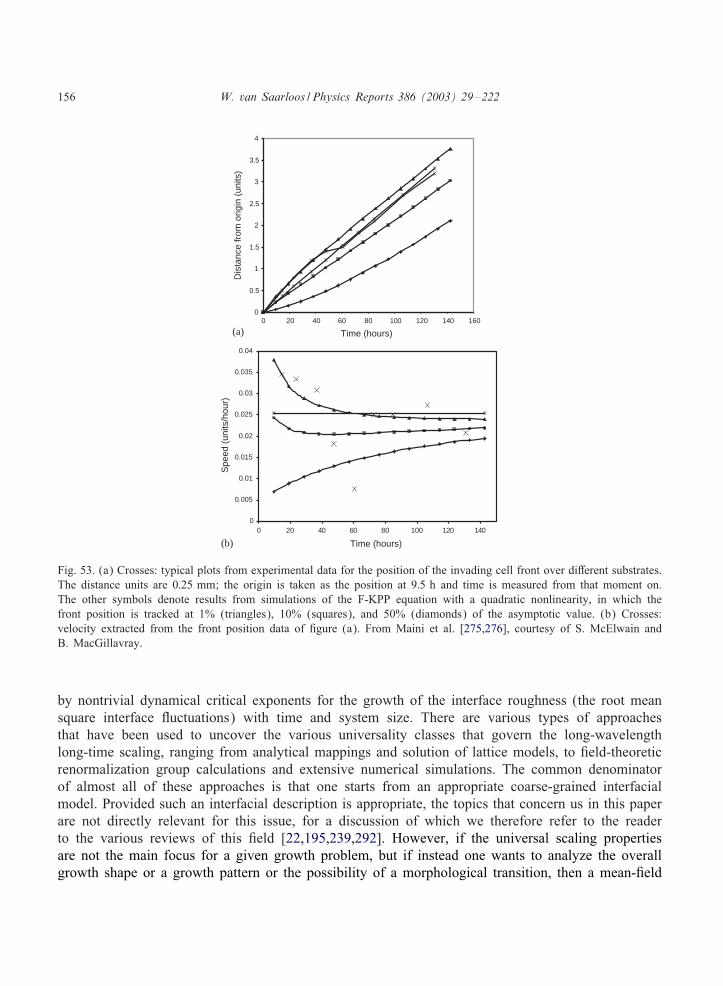
156 W. van Saarloos / Physics Reports 386 (2003) 29–222
0
0.5
1
1.5
2
2.5
3
3.5
4
0 100 120 140 160
Time (hours)
Dis
tanc
e fr
om o
rigin
(un
its)
0
0.005
0.01
0.015
0.02
0.025
0.03
0.035
0.04
0 20 40 60 80 100 120 140
Time (hours)
Spe
ed (
units
/hou
r)
80604020
(a)
(b)
Fig. 53. (a) Crosses: typical plots from experimental data for the position of the invading cell front over diDerent substrates.The distance units are 0:25 mm; the origin is taken as the position at 9:5 h and time is measured from that moment on.The other symbols denote results from simulations of the F-KPP equation with a quadratic nonlinearity, in which thefront position is tracked at 1% (triangles), 10% (squares), and 50% (diamonds) of the asymptotic value. (b) Crosses:velocity extracted from the front position data of 3gure (a). From Maini et al. [275,276], courtesy of S. McElwain andB. MacGillavray.
by nontrivial dynamical critical exponents for the growth of the interface roughness (the root meansquare interface Kuctuations) with time and system size. There are various types of approachesthat have been used to uncover the various universality classes that govern the long-wavelengthlong-time scaling, ranging from analytical mappings and solution of lattice models, to 3eld-theoreticrenormalization group calculations and extensive numerical simulations. The common denominatorof almost all of these approaches is that one starts from an appropriate coarse-grained interfacialmodel. Provided such an interfacial description is appropriate, the topics that concern us in this paperare not directly relevant for this issue, for a discussion of which we therefore refer to the readerto the various reviews of this 3eld [22,195,239,292]. However, if the universal scaling propertiesare not the main focus for a given growth problem, but if instead one wants to analyze the overallgrowth shape or a growth pattern or the possibility of a morphological transition, then a mean-3eld

W. van Saarloos / Physics Reports 386 (2003) 29–222 157
approximation is often an indispensable tool. In this approximation, the analysis of fronts often doesplay an important role. We illustrate this general observation with an old example of a depositionmodel which at the same time is a nice example of a pulled front in a very nontrivial diDerenceequation [238]. The discussion will also prepare us for an issue to which we will return later andwhich is at present not completely resolved: quite often, in a mean-3eld description one arises atpulled fronts. As we shall discuss in more detail in Sections 5 and 7, deterministic pulled frontsdo not converge to the standard type of interfacial description and as a result a standard typemean-3eld analysis may miss some of the essential ingredients of the underlying stochastic model,or even exhibit pathological behavior that the underlying model does not have.
In ballistic deposition, particles rain down ballistically but at random positions onto a cluster andstick to it with a given probability as soon as they come to a site neighboring the cluster. Considerthe special case of a two-dimensional square lattice with the depositing particles coming straightfrom above at discrete times (for simplicity we summarize a special case of the analysis of Krugand Meakin [238], who consider more general dimensions and deposition under and angle). Then aparticle coming down in the ith column can stick with probability p at the 3rst site in that columnwhich is a nearest neighbor of the highest occupied site in that column or in the two neighboringcolumns. In a mean-3eld approximation, one ignores all correlations and formulates this growthprocess in terms of the probability <t(x; z) that a site at x; z is part of the deposit at time t. In thisapproximation and for one-dimensional pro3les, the appropriate dynamical equation is [238]
<t+1(z) − <t(z) = p[1 − <t(z)]{1 − [1 − <t(z − 1)][1 − <t(z)]2}∞∏
z′=z+1
[1 − <(z′)]3 : (175)
The term on the left describes the change in the probability at a site at height z that is part ofthe cluster; it changes when a particle is deposited at that site, and the terms on the right-handside model this eDect in a mean 3eld approximation. The 3rst term on the right-hand side is theprobability that that site at height z is empty, the terms between parentheses is the probability thatat least one of the neighboring sites (at height z−1 in that column or at height z in the neighboringcolumns) is occupied, and the product term is the probability that none of the sites in the columnor its two neighbors is occupied.
Eq. (175) is a diDerence equation in both the discrete space and time variables; its form is un-usual, in that the change at height z depends on all the probabilities at higher sites. 90 A rathercomplete study of the general form of this equation was given by Krug and Meakin [238]; theirnumerical solutions showed that at long times, the dynamics leads to front type solutions. Moreoverthe asymptotic velocity of these fronts turned out to be v∗: empirically, the fronts are found to bepulled. 91 Indeed, although as we discussed in Section 2.4 it is now clear that the linear spreadingvelocity v∗ is given by the same equations for any equation which upon Fourier–Laplace trans-form leads to a linear equation of the form (41), this appears to be one of the earliest exampleswhere the pulled velocity was calculated for a nontrivial diDerence equation, and where the powerlaw convergence to v∗ was also tested. Indeed, by linearizing the equation in < and substituting
90 A continuum version appropriate in the limit p → 0 can be found in [43].91 Intuitively, this can be understood from the observation that the nonlinearities in the dynamical equation express the
suppression of the growth due to screening.

158 W. van Saarloos / Physics Reports 386 (2003) 29–222
< ∼ e+t−�z, one 3nds the dispersion relation [238]
+(�) = ln{1 + p[e� + 2]} (176)
from which �∗ and v∗ can easily be obtained by calculating the minimum of +(�)=�. As mentionedabove, Krug and Meakin also veri3ed that the front velocity converged to v∗ as 1=t, with a prefactorwhich was consistent with (78) to within 15% (presumably, this small discrepancy is due to thehigher order 1=t3=2 correction, which was not known at the time). This slow convergence in time inthis case actually entails a very slow 1=z correction of the frozen-in density pro3le!
A common feature of mean 3eld approximations of growth models that (175) also exhibits is thatthe growth is nonzero for arbitrarily small particle density <. This makes the state < = 0 really alinearly unstable state and gives rise to the existence of a 3nite linear spreading speed. In realityhowever, lattice models have an intrinsic cutoD for growth: there has to be at least one particle fora cluster to be able to grow. As we shall see in Section 7, the fact that the particle occupationnumber is “quantized” has important consequences for growth fronts: they are eDectively alwayspushed rather than pulled.
3.22. Error propagation in extended chaotic systems
In almost all examples we have considered so far, the unstable state into which a front propagatesis a well-de3ned state which is homogeneous in the appropriate variables. 92 An exception to thiswhich deserves to be mentioned is the work by Kaneko [213] and Torcini et al. [396] on frontspropagating into extended chaotic systems. The unstable state in this chase is itself a chaotic statewhich is characterized by positive Lyapunov exponents. Speci3cally, the authors consider the CoupledMap Lattice
xn+1i = f([1 − �]xni + 1
2�[xni−1 + xni+1]) ; (177)
where i and n are the discrete space and time variables. Note that the terms in the argument of fproportional to � have the form of a discretized version of the diDusion term. The function f mapsthe interval onto itself, as is usual in studies of maps.
In general, a Lyapunov exponent of a chaotic system measures how two in3nitesimally closeinitial states grow apart. In this sense a chaotic state is an unstable state, since any small perturbationaway from it grows out in time. The notion of a front introduced for such a system is illustratedin Fig. 54 from [396]. One considers two realizations of extended chaotic states x0
i and y0i which
diDer on one side of the system (say i6 0) but not on the other. The front in this case is thus an“error propagation front” in the diDerence variable xni − yn
i —while each individual state is chaoticeverywhere, the “error” between them spreads more and more to the right.
In the early work of Kaneko [213], the Lyapunov exponent was studied in a frame movingwith 3xed speed. The natural speed of the front was then found to be the speed at which thisvelocity-dependent Lyapunov exponent was equal to zero. In our words, this means that for thenonlinearities studied by Kaneko, the “error fronts” were pulled and that the speed v∗ was givenin terms of the Lyapunov exponent. Here we follow the formulation of Torcini et al. [396], who
92 The unstable phase-winding state into which the fronts discussed in Section 2.11.5 propagate are homogeneous in theamplitude a and wavenumber k.

W. van Saarloos / Physics Reports 386 (2003) 29–222 159
Space
x-y
xy
Fig. 54. Two initial realizations x and y of states of the coupled map lattice considered by Torcini et al. [396], togetherwith the diDerence x−y. Note that while each state is chaotic, the diDerence variable vanished on the right. The propagationof the “error” x − y into this state is then an example of a front propagating into an unstable chaotic state. Both pulledand pushed fronts can occur, depending on the form of the function f.
also studied the transition from pulled to pushed incoherent error fronts (see also [182]). One canindeed extend the notion of a pulled front to this case by analyzing the Lyapunov exponents O(�)for in3nitesimal perturbations un
i of xni of the form
uni ∼ eOn−�i ; (178)
where the evolution of the uni is governed by the linearized tangent map
un+1i = f′([1 − �]xni + 1
2�[xni−1 + xni+1])([1 − �]un
i + 12�[u
ni−1 + un
i+1]) : (179)
Clearly, O(�) is the analogue for an extended chaotic system of the dispersion relation −i!(k), andthe analogue of expression (12) for the linear spreading speed v∗ is
v∗CML =O(�∗)�∗
=dO(�)
d�
∣∣∣∣�∗
: (180)
Although the precise justi3cation of this expression has not been studied, it is intuitively clearthat the basis for it is that the Lyapunov exponent de3nes a 3nite time scale O−1(�∗). Thus, afteraveraging over times suRciently longer than O−1(�∗), one obtains a linear problem characterized byan eDective dispersion relation O(�), in terms of which the asymptotic (t → ∞) spreading problemis well-de3ned.
In the numerical studies, it was found that for various functions f (corresponding to the logisticmap, the cubic map and the tent map), the error propagation fronts were pulled (in the averagesense) while in other cases (e.g., f(x) = rx mod 1 with r ¿ 1), the fronts were pushed in that theiraverage asymptotic speed was larger than v∗. Clearly, these error propagation fronts are examplesof incoherent fronts, and as we noted in Section 2.7.3 we have at present no sharp mathematicalcharacterization of a pushed incoherent front solution—intuitively we expect that enhancement ofthe growth by the nonlinearities will tend to give rise to a pushed front and that, like a coherentpushed front solution, it falls oD spatially faster than the pulled front. But how to identify a pushed

160 W. van Saarloos / Physics Reports 386 (2003) 29–222
front other than by the empirical observation that it moves faster than v∗ I do not know. Indeed,Torcini and co-workers [396,77] have been able to provide a reasonable guidance into what typeof maps give pushed error fronts, building on the insight from the nonlinear diDusion equation thatpushed fronts are generally associated with growth functions f which increase faster than linear forincreasing u. Possibly, further study of the pushed to pulled transition in these fronts might help todevelop a sharp de3nition of pushed incoherent fronts. For recent extensions of such chaotic frontstudies, including the eDective diDusion of such fronts, the reader is referred to [397].
We note in passing that Politi and coworkers [181,348] have argued that upon coarse-graining theeDective equation for the dynamics of the diDerence variable di=xi−yi of the lower graph of Fig. 54becomes a diDusion-type equation with multiplicative noise, 9td =∇2d + ;d where ; is a stochasticnoise term. With the Cole–Hopf transformation d=eh this equation is equivalent to the KPZ equation[22,195,218,239]. It is amusing to realize that the arguments of Section 7.3 indicate that thereforethe scaling properties of such Kuctuating error-propagation fronts are equivalent to those of the KPZequation, but in one dimension higher than one would naively expect: As explained in that section,for pulled fronts the Kuctuations in the direction of propagation continue to contribute to the scalingbehavior, instead of being integrated out.
3.23. A clock model for the largest Lyapunov exponent of the particle trajectories in a dilute gas
One present line of research in kinetic theory touching on the foundations of statistical physicsis the study of the Lyapunov exponents of the trajectories of the constituent particles or atoms ina dilute gas (the largest Lyapunov exponent gives the rate with which two nearby initial conditionsgrow apart under the dynamics, see Section 3.22 above). A few years ago van Zon et al. [430]were able to calculate the largest Lyapunov exponent exactly in a low density hard sphere gasby expressing it in terms of the speed of a pulled front in a diDerential-diDerence equation. Themodel is actually very closely related to a computationally very eRcient lattice model introducedby Brunet and Derrida [64,66] in the context of the connection with phase transitions in disordermodels discussed in Section 3.25.
For calculating the Lyapunov exponents, one has to analyze how the original trajectories of atypical hard sphere grow apart from a shadow one obtained from an in3nitesimally diDerent initialcondition. For the largest Lyapunov exponent, the following picture becomes appropriate in the dilutegas limit. When a sphere collides with another one, the diDerence after the collision between theoriginal trajectory of each sphere and its shadowing trajectory is, on average, equal to the largest ofthe two before the collision, multiplied by a constant factor that accounts for the enlargement dueto the collision. This implies that the largest Lyapunov exponent is, in appropriate units, given bythe front speed of a “clock model”, in which every particle carries a clock with a discrete time kwhich is advanced at every collision [430]. This happens according to the following rule: when twoparticles collide, they both reset their respective clock values, say k and ‘, to either k + 1 or ‘ + 1,whichever is the largest. Thus, if we denote the number of particles with clock value k by Nk , weobtain the following dynamical equation:
dNk
dt= −
∞∑‘=−∞;‘ �=k
Rk;‘ − 2Rk;k + 2k−1∑
‘=−∞Rk−1; ‘ ; (181)

W. van Saarloos / Physics Reports 386 (2003) 29–222 161
where Rk;‘ denotes the rate by which collisions occur between particles with clock values k and‘. In the dilute gas limit correlation eDects become negligible; then Rk;‘ is simply proportional toNkN‘=N 2 when k = ‘ and to N 2
k =(2N2) when two particles with equal clock value k collide. Then,
upon writing fk = Nk=N and scaling the time appropriately, we obtaindfk
dt=−fk + f2
k−1 + 2fk−1Ck−2 ;
=−fk + C2k−1 − C2
k−2 ; (182)
where we have set
Ck =k∑
‘=−∞f‘ : (183)
Adding the equations for f‘ for all values of ‘6 k then yields
dCj(t)=dt = −Cj(t) + C2j−1(t) : (184)
Eq. (184) has two spatially and temporally constant solutions: Cj = 0 and Cj = 1. The 3rst oneis stable and describes the state where all clocks are set to a value larger than j; the second one isunstable and corresponds to the case where all clocks are set to values less than j. As time proceeds,all clock values are continuously increased, and hence in the context of this model it is natural toconsider the invasion of the unstable state Cj = 1 by the state Cj = 0—as indicated above, the frontspeed then determines the largest Lyapunov exponent of the dilute hard sphere gas.
Numerical solutions have shown that the fronts propagating into the unstable state Cj = 1 arepulled fronts [430]. This in itself is maybe not so much of a surprise, as it is easy to convinceoneself that the nonlinearity on the right-hand side tends to reduce the growth relative to that of theterms linearized about the unstable state (very much like in the F-KPP equation with a nonlinearityof the form f(u) = u− u2). However, the equation does illustrate nicely a number of general pointsconcerning pulled fronts:
(i) The dynamical equation (184) is a diDerence-diDerential equation. Nevertheless, as we alreadypointed out so often, the same equations for v∗ and for the rate of approach to v∗ (Eq. (78)of Section 2.9) hold. The convergence of the front speed to its asymptotic value according tothis result was checked explicitly with high precision numerical simulations in [144,146].
(ii) Although the dynamics is very diDerent from that of the F-KPP equation—note the very asym-metric dynamics: the dynamics of Cj is unaDected by that of Ck with k ¿ j—the equation issimple enough that several of the methods that play an important role in proving the existenceand convergence of fronts for the F-KPP equation (like comparison theorems) can be extendedto this equation [146].
(iii) As we will discuss in Section 7, when a mean 3eld equation is simulated with a stochasticequation with a 3nite number of particles N , the convergence as a function of N to the asymp-totic pulled v∗ of the N → ∞ mean-3eld equation is very slow, logarithmically slow. This slowconvergence was also found when the present clock model was simulated with a 3nite numberof particles [430].
(iv) In the context of the clock model the Cj’s are non-decreasing functions of j: Cj6Cj+1 for anyj. However, if we just take Eq. (184) as a general dynamical equation in which the Cj’s are

162 W. van Saarloos / Physics Reports 386 (2003) 29–222
allowed to decrease with increasing j, then we 3nd that the state Cj = 1 is also convectivelyunstable to a front where the Cj decrease for increasing j! This turns out to be a retractingpulled front, a front which moves to the right in accord with the fact that any perturbationor coherent structure solution of (184) can only move towards increasing j. Such a retractingfront corresponds to a negative value of v∗ in our equations, 93 and has an amusing property:whereas the speed of a front which genuinely propagates into the unstable state approaches thepositive asymptotic speed from below due to the negative 1=t correction in (78), the absolutevalue of the speed of a retracting front is larger than |v∗| for large times, since v∗ itself isnegative!
(v) It is easy to modify the equation according to the general rules of thumb of Section 2.7.5 sothat the fronts become pushed; an explicit example is discussed in [146].
3.24. Propagation of a front into an unstable ferromagnetic state
Although it may not be of great practical relevance, we brieKy mention an amusing example whosefront dynamics is governed by two pulled fronts separated by a phase slip region, the dynamicalequations for an anisotropic ferromagnet [150,151]. The width of domain walls and the wavelengthof spin-wave states in ferromagnets is often large enough that a continuum approximation is justi3ed.For a ferromagnet with an easy-plane anisotropy the free energy in dimensionless units reads [246]
F =12
∫dx [(9x�)2 + sin2 �(9x�)2 + cos2 �] : (185)
Here � and � denote the direction of the magnetization M in polar coordinates, and we have assumedthat the magnetization only varies in the spatial x-direction. The last term in the expression showsthat the energy of states with polar angle � = �=2 is lowest, so indeed the free energy densitydescribes a situation with an easy-plane direction.
The dynamics of a ferromagnet is governed by the so-called Landau–Lifshits equations
dMdt
= 2M × dFdM
+ �M ×(M × dF
dM
): (186)
In the high damping limit, the 3rst term which describes the torque can be neglected; in appropriatetime units the equations then become
9t� = 92x� + [1 − (9x�)2] sin � cos � ; (187)
9t� = 92x� + 2(9x�)(9x�) cotg � : (188)
Note that if we could consider 9x� to be 3xed, the 3rst equation would be nothing but the F-KPPequation for �, with the state � = �=2 stable if (9x�)2 ¡ 1 and unstable if (9x�)2 ¿ 1. Thus aphase-winding solution of the form � = �=2; � = kx is unstable for k ¿ 1. Elmer et al. [150,151]considered front propagating into this unstable state; because of the similarity of the 3rst equationwith the F-KPP equation, it is no surprise that these fronts are pulled, but the new feature is the
93 Of course, there is only one dispersion relation for Fourier modes of the dynamical equation linearized about theunstable state. The fronts discussed above and analyzed in [430,146] fall oD as exp(−�∗j) with �∗ =0:768 and v∗ =4:311.The retracting fronts correspond to the solutions of (78) which have negative �∗ = −1:609 and negative v∗ = −0:373.
W. van Saarloos / Physics Reports 386 (2003) 29–222 163
coupling to the �-variable. 94 This front leaves behind a state with � ≈ 0 but with the phasegradient 9x� essentially unaltered. Because of the strong coupling between phase and polar angledue to the cotangent term in the �-equation, this phase-winding state is unstable. As a result, the 3rstfront is followed by a region where phase slips occurs. The state which emerges from here has noappreciable phase gradient: The nonlinear term in the �-equation then Kips sign and this makes the� ≈ 0 state unstable. As a result, this region is in turn invaded by a second pulled F-KPP-like front.The propagation speed of the phase slip region can even be calculated from a conservation-typeargument for the phase winding, as all the properties of the back side of the 3rst front and of theleading edge of the trailing front are known [150,151].
When the dynamical equations are written in terms of a complex amplitude A = sin �ei�, A isfound to obey a Ginzburg–Landau type equation with an unusual nonlinearity [151]. From thisperspective, the problem has some similarity with the problem of front propagation into an Eckhaus-unstable phase winding solution in the real Ginzburg–Landau equation that was mentioned brieKyin Section 2.11.5.
3.25. Relation with phase transitions in disorder models
In hardly any of the situations that we have discussed so far do the front solutions which becomerelevant when the initial conditions are not suRciently localized, play a role. There is one remarkableexception to this: it was discovered by Derrida and Spohn [122] that there are some statisticalphysical disorder models which can be shown to have phase transitions by mapping their generatingfunction onto the F-KPP equation. The two regimes of pulled fronts emerging from localized initialconditions and of leading edge dominated dynamics associated with not suRciently localized initialconditions then translate into two diDerent phases of the disorder model! An amusing aspect isalso that in the 3rst regime, the 1=t power law relaxation and the associated crossover behavior ofthe front solutions translates back into detailed knowledge of the scaling behavior of the statisticalmodel. More recently, the same type of mapping was applied to the renormalization group analysisof disordered XY models [74]—see Section 3.26.1.
Let us sketch the essence of the argument for the case of polymers on a Cayley tree with arandom potential [122]. A Cayley tree is a graph which has branches but no loops, as sketched inFig. 55(a). The hierarchical structure of Cayley trees makes the statistical physical models de3ned onthem amenable to detailed analysis—phase transitions in such models are usually of mean 3eld type,due to the absence of loops, but apart from this they often catch the essence of a transition in higherdimensions. We now consider “polymers” on such Cayley trees—we can think of them in terms ofself-avoiding random walks which step one level down in every “time” step—in the presence of arandom potential V at the bonds. These values of the potential are uncorrelated random variablesdistributed according to some distribution P(V ). The statistical problem for a given realization ofpotentials is then de3ned as follows in terms of the so-called partition function
Z =∑walks
exp[ − J(V1i1 + V2i2 + · · ·)] ; (189)
94 It is amusing to note that the nonlinearity of the �-equation for 3xed phase gradient 9x� is a special case of thedynamical equations for the director angle in the smectic C∗ problem discussed in Section 3.15.

164 W. van Saarloos / Physics Reports 386 (2003) 29–222
time
(a) (b)
Fig. 55. (a) A “polymer” (thick lines) or self-avoiding walk on a Cayley tree. On each bond an independent randompotential is de3ned. (b) Illustration of the statistical problem of a polymer on a Cayley tree with a random potential inthe continuum limit. After Derrida and Spohn [122].
where J is the inverse temperature. The term in the exponents is the sum of all the potentials inlevel 1, level 2, etc. It is convenient to consider the vertical direction as a time coordinate t andto take the time-continuous limit. The potentials V on a branch of length dt are then taken asindependent Gaussian variables with distribution
P(V ) =1
(4� dt)1=2 exp(− V 2
4 dt
): (190)
Because of the branching structure of the Cayley tree, the partition function obeys a simple recursionrelation,
Z(t + dt) =
{e−JVZ(t) with probability 1 − dt ;
e−JV [Z1(t) + Z(2)(t)] with probability dt ;(191)
which expresses that in the 3rst small timespan dt, the walk could remain a single walk withprobability 1 − dt, or have split into two with probability dt (the generalization to Cayley treeswhere every branch splits into n¿ 2 is obvious). Z(1) and Z(2) are the two partition functions onthese two branches.
Because the potentials are random variables, one actually has to study the distribution of partitionfunctions. Instead of doing this, it is more convenient [122] to study the so-called generating functionGt(x) which encodes the average and all moments of Z,
Gt(x) ≡ 〈exp[ − e−JxZ(t)]〉 ; (192)
where the brackets indicate an average over the disorder. From this de3nition, one 3nds immediatelythat for small dt
Gt+dt(x) = (1 − dt)∫
dV1
(4� dt)1=2 exp(− V 2
4 dt
)Gt(x + V ) + dt G2
t (x) : (193)
That the branching process simply leads to a term proportional to G2 relies on the fact that thepartition functions Z(1) and Z(2) in (191) are independent, because on a Cayley tree two branches
W. van Saarloos / Physics Reports 386 (2003) 29–222 165
do not intersect below their common branch point. In the limit dt → 0 the above equation for Gbecomes simply
9tG = 92xG + G(G − 1) ; (194)
which is nothing but the F-KPP equation (1) with quadratic nonlinearity, if we put G = 1 − u.The remarkable 3nding is that the dynamical equation for G does not depend on the temperature
J−1 explicitly: the temperature only enters indirectly through the initial conditions which Derridaand Spohn considered,
G0(x) = exp(−e−Jx) ⇔ u � e−Jx (x → ∞) : (195)
As we know from our discussion of fronts in the F-KPP equation, when J¿ 1, this corresponds tolocalized initial conditions, and the long-time behavior of Gt(x) is then simply given by the pulledfront solution whose speed approaches v∗ according to the asymptotic formula (78). This meansthat the “long-time” asymptotic average properties of the polymers are completely independent oftemperature, and that they approach an asymptotic scaling behavior independently of temperature aswell. Furthermore, when J¡ 1, the fronts correspond to fronts whose dynamics is “leading edgedominated” and whose velocity is determined by the initial condition, i.e., the temperature. This isthe high-temperature regime. The low-temperature (J¿ 1) regime can be associated with a frozenphase: roughly speaking the fact that the front speed is independent of initial conditions translatesinto the free energy sticking at a constant temperature-independent value—we refer for a detaileddiscussion of this and of the translation of the various front results to those for the random polymerproblem to [122]. Below in Section 3.26.1 the connection to renormalization treatments of disordermodels is discussed.
We 3nally note that a lattice model version [64,66] of the statistical–physical disorder problemdiscussed here is closely related to the clock model discussed in Section 3.23.
3.26. Other examples
We 3nally draw attention to a number of issues related to front propagation which we do notreview in detail.
3.26.1. Renormalization of disorder models via traveling wavesIn the previous Section 3.25 we brieKy reviewed how the generating function of a disorder model
on a Cayley tree obeys the F-KPP equation. This connection between traveling waves and disordermodels is actually more general and powerful, as was discovered by Carpentier and Le Doussal[74,75]. Very much like (194) is the evolution equation for the generating function in the “time-wise”direction down the Cayley tree, they found that the renormalization group equation for the distributionfunction of the local fugacity variables of defects in a disordered XY model takes the form of anF-KPP equation, with the length scale ‘ playing the role time. Like we saw in Section 3.25, theuniversal behavior of this distribution function comes from the independence of v∗ on the details ofthe model. Moreover, the results for the universal rate of approach to the asymptotic pulled frontspeed v∗ in the case of localized initial conditions (corresponding to temperatures below the glasstransition) translate into nontrivial predictions for the scaling at the transition. We refer to thesepapers for an in-depth discussion of this.

166 W. van Saarloos / Physics Reports 386 (2003) 29–222
3.26.2. Singularities and “fronts” in cascade models for turbulenceAs is well known, fully developed turbulence is characterized by an energy cascade: energy Kows
from small wave numbers to larger wave numbers, till it is dissipated in the viscous range. In a shellmodel for this energy Kow [408], this energy Kow down the cascade shows similarities with frontpropagation. However, the essential dynamics is more properly analyzed in terms of a similarityanalysis like that for the porous medium equation [17,184,339] than in terms of fronts. If interpretedin terms of front dynamics, these fronts have a nonlinear diDusion equation reminiscent of the onein the bacterial growth model (147) and are pushed.
In fact, as stressed in particular by Barenblatt [24,25], there is a formal connection betweensimilarity analysis and front propagation, since if one write x and t of a propagating front solutionu(x− vt) in terms of logarithmic variables, x = ln X , t = ln T , a uniformly translating front solutionu(x − vt) looks like a similarity solution u(X=T v). In this formulation the propagation velocity ofthe front plays the role of a similarity exponent. This reformulation illustrates that in principle asharp distinction between front propagation and similarity analysis [24,25] is diRcult to make. Inpractice, however, it is often quite clear what the most natural type of analysis is for a given problem:especially if the system admits a linearly unstable state with a well-de3ned dispersion relation for theunstable branch of Fourier modes, the linear spreading analysis and the associated front formulationare the methods of choice.
3.26.3. Other biological problemsAlthough the clearest biological examples of front propagation into an unstable state appear to
be the population spreading phenomena mentioned in Section 3.19 and the bacterial growth patternsdiscussed in Section 3.13, it is important to realize that there are many problems in biology andbiophysics which are closely related. E.g., much work on pulse propagation in bistable systems orexcitable media traces back to the study of the propagation of pulses in nerves [229,379]. Since theseare not examples of front propagation into unstable states proper, and since excellent books in whichthese problems are treated have appeared recently [222,311], we will not explore the diDerences andsimilarities here.
3.26.4. Solar and stellar activity cyclesThere is an extensive literature—see e.g. [28] for a brief introduction and entry into the literature—
associating the sunspot cycle to the occurrence of so-called dynamo waves. The coupled equations forthe azimuthal and radial magnetic 3elds take the form of two reaction–diDusion type equations, and animportant ingredient of the relevant dynamics is associated with the problem of front propagation intounstable states [28,395,441]. Of course, for waves on a spherical rotating object like the sun, there aremany complicating aspects: not only is there the question whether the instability is locally convectiveor absolute, but also the fact that the geometry is intrinsically 3nite and that the background of thewaves is spatially varying plays a role. These latter type of issues are related to the question of theemergence of so-called “global modes” which we will discuss brieKy in Section 6. For a detaileddiscussion of the dynamo waves themselves we refer to the literature cited above.
3.26.5. Digital search treesAfter acceptance of this article, we learnt of a very new exciting line of research: traveling fronts
play an important role in computer science in digital search trees and data compression. Moreover,

W. van Saarloos / Physics Reports 386 (2003) 29–222 167
such types of problems are related to directed DLA on a Caley tree. See [452,453] and referencestherein.
4. The mechanism underlying the universal convergence towards C∗
In Section 2.9 we saw that pulled fronts converge to their asymptotic speed and shape 95 with auniversal power law behavior—e.g., for the velocity we have according to (82)
v(t) = v∗ − 32�∗t
+3√�
2(�∗)2t3=2Re
1√D
+ O
(1t2
): (196)
For uniformly translating fronts, for which D is real, this expression reduces to the simplerversion (78).
In the above expression v∗; �∗ and D are given explicitly by Eq. (12) in terms of the dispersionrelation !(k) of the linearized dynamical equation. This and other remarkable features of this generalexpression were discussed extensively in Section 2.9.3 but we did not justify or derive the resultitself. It is the aim of this section to review the underlying mechanism and derivation [144] in somedetail. The importance of the derivation does not lie in the technicalities themselves, but in the factthat the pulled front picture that we have advanced can be made into a fully explicit and predictiveformalism.
4.1. Two important features of the linear problem
Several of the most important insights on which the full derivation of (196) is based [144] comefrom our understanding of the fully linear problem discussed in Sections 2.1–2.4. In Section 2.1 wesaw that according to the saddle point analysis of the fully linear spreading problem a “steep” initialcondition gives rise to the following long-time expression for a generic dynamical 3eld �,
�(�; t) ∼ e−�∗�+ik∗r �−i(!∗r −k∗r v∗)t e
−�2=(4Dt)
√t
; (197)
where � = x − v∗t, and where �∗; k∗r ; v∗ and D are given by the linear spreading point equations(12). The 3rst exponential factor is the asymptotic exponential fall-of with steepness �∗ in theframe moving with velocity v∗. The second exponential factor, together with the t−1=2 term, is the3rst correction term to the asymptotic behavior—it arises simply from the Gaussian saddle pointintegral. Of course, in this Gaussian term we also recognize the fundamental similarity solution ofthe diDusion equation. Thus, if we de3ne a new 3eld through the transformation
�(�; t) ≡ e−�∗�+ik∗r �−i(!∗r −k∗r v∗)t (�; t) ; (198)
95 The shape convergence only holds for uniformly translating fronts and coherent pattern forming pulled fronts, ofcourse. Nevertheless, the incoherent dynamics of an incoherent pulled front arises from the intrinsic chaotic behavior ofthe nonlinear state behind the front (as, e.g., in panels (a) of Figs. 16–19) or from the fact that the spreading pointdynamics does not match on to a fully coherent front pro3le in the nonlinear region (as, e.g., in Fig. 18(b)). In theleading edge the dynamics of incoherent pulled fronts is still smooth and coherent, as close inspection of these 3guresand Fig. 58 below shows quite clearly. This dynamics is governed by the extension of Eq. (210) below to pattern formingfronts.

168 W. van Saarloos / Physics Reports 386 (2003) 29–222
then we expect that the long-time dynamics of is governed by the equation
9 9t = D
92 9�2 + corrections ; (199)
since its fundamental similarity solution is the Gaussian form = t−1=2e−�2=4Dt of (197). Notethat the transformation (198), which was called the “leading edge transformation” in [144], actslike a mathematical magnifying glass: it allows us to focus on the dynamics of the correction tothe dominant exponential behavior. Moreover, do realize that since the saddle point analysis isquite general (see Section 2.4) the long-time dynamics of the leading edge variable is eDectivelygoverned in dominant order by this diDusion equation even if the underlying dynamical equation isof higher order, a set of equations, a di>erence equation, etc. The reason that obeys a diDerentialequation even when the original dynamical equation is a diDerence equation is that for long times becomes arbitrarily smooth in space and time.
The above line of reasoning is intuitive and based on working backward from the general ex-pression (197). The diDusion-type form of the equation—3rst order in time and second order inspace—is actually an immediate consequence of the fact that two roots k coincide at the linearspreading point k∗. After all, Eqs. (9) and (12) imply that in the neighborhood of the spreadingpoint we have in the co-moving frame �
!− !∗ = −iD(k − k∗)2 + · · · ; (200)
and upon inverse Fourier–Laplace transformation this gives (199) for long times. In fact, the fullgeneralization of (199) for is easy to derive [144]: by expanding about the linear spreading pointand taking an inverse Fourier–Laplace transform, we immediately obtain [144]
9 9t = D
92 9�2 + D3
93 9�3 + w
92 9t 9� + $2
92 9t2 + · · · ; (201)
where the expansion coeRcients D3; w; $2, etc. can all be expressed in terms of the characteristicequation of the branch corresponding to the relevant spreading point—see Eq. (5:64) of [144]. E.g.,we simply have D3 = (1=3!) d3!=dk3|k∗ .
Since we already know from the saddle point analysis that the relevant long-time dynamics of theleading edge variable is a diDusion-type dynamics on slow spatial and temporal scales, the crucialconclusion from these considerations is that 96
the dynamical equation of the leading edge variable that governs the convergence to thelinear spreading behavior in the leading edge is a di>usion equation, with subdominant termswhich are determined explicitly in terms of the dispersion relation !(k) of the linear dynam-ical equation of the original problem. The appropriate similarity variable for the long-timeexpansion of is the similarity variable �=
√t of the di>usion equation.
96 There is actually a surprise here: A priori, one would expect that the second and third terms of (201) would aDectthe subdominant t−3=2 correction term in the expression (196) for v(t). Actually, they do aDect the shape scaling functionbut not the velocity correction—see Eq. (5:70) of [144]. I do not have a real intuitive understanding of this remarkable3nding which comes out of the explicit calculation.

W. van Saarloos / Physics Reports 386 (2003) 29–222 169
Our second important observation concerning the fully linear problem is the following. One maywell wonder “how can the leading edge dynamics ever determine the dominant convergence dynamicsof the full nonlinear pro3le?” To understand this, let us return to (197) and write it as
|�(�; t)| ∼ e−�∗�
∣∣∣∣∣e−�2=(4Dt)
√t
∣∣∣∣∣= e−�∗�− 12 ln t−�2=(4Dt) ; (202)
where, as in (13), D−1 = ReD−1. If we follow the position �C of the level line �(�C; t) = C, thenaccording to the above expression for the linear dynamics we have in dominant order
�C = − 12�∗
ln t + · · · ⇔ �C = − 12�∗t
+ · · · : (203)
We already drew attention to this logarithmic shift in our discussion of the front relaxation inSection 2.9.1, but we now identify more clearly where this behavior originates from: The 1=t re-laxation of the velocity of the level line corresponds to a logarithmic shift in the position, and thisresults from the Gaussian t−1=2 prefactor in combination with the overall e−�∗� spatial decay of theleading edge variable. In other words, the prefactor of the 1=t velocity relaxation is essentially theexponent of the appropriate similarity solution of the di>usion equation (199).
So why then does the logarithmic shift carry over to the fully nonlinear pro3le? The importantpoint to realize is simply that 97
when we track the position of a front whose width of the nonlinear region is 6nite, theunbounded logarithmic shift imposed by the di>usive leading edge dynamics always dominatesthe large time behavior over the relaxation of the front shape itself.
This observation was already illustrated in Fig. 12.
4.2. The matching analysis for uniformly translating fronts and coherent pattern forming fronts
So we know that the leading edge variable , which measures the deviation from the asymptoticexponential pro3le e−�∗�+ik∗r �−i(!∗−k∗v∗)t in the moving frame, obeys a diDusion-type equation withcorrections. To construct the solution to the fully nonlinear font relaxation problem, we have tomatch the behavior in the leading edge (the region where the dynamical equation can be linearizedabout the unstable state) to the nonlinear front region, the region where the nonlinearities in theequation are important.
In order to understand the matching behavior, it is clearest to 3rst consider the case of uniformlytranslating fronts or coherent pattern forming fronts: For these the arguments can be made mostprecise and for these the matching analysis has been worked out in detail. The case of incoherentpattern forming fronts will be discussed in the next section; the analysis given there will give
97 The argument is obvious for the divergent logarithmic term. Actually, since the front shape relaxation is driven by the1=t term in the velocity—see Eq. (211) below—any contribution from the leading edge which gives a time-dependent shiftwhich decays slower than the 1=t intrinsic shape relaxation is universal. This is the reason that even the 1=t3=2 term in thevelocity relaxation is universal: it corresponds to a shift proportional to 1=t1=2. Even incoherent fronts whose Kuctuatingwidth converges faster than 1=t to some average value, still exhibit the subdominant 1=t3=2 velocity relaxation term.

170 W. van Saarloos / Physics Reports 386 (2003) 29–222
a more intuitive dynamical argument why the leading edge variable approaches the behavior thatwe identify with matching arguments here.
At the linear spreading point k∗ two roots coincide—this is illustrated both by Eq. (200) and thefact that v∗ corresponds to the minimum of the curve venv(�) in Fig. 3. It is a general result [13,14]that in the presence of a double root the � → ∞ asymptotic behavior of the uniformly translatingpulled front solutions ,v∗(�) or the leading coherent pulled front solution ,1
v∗(�), is
,v∗(�) ∼ (a1� + a2)e−�∗�; ,1v∗(�) ∼ (A1� + A2)e−�∗�+i(k∗r �−!∗
r t) ; (204)
as we already noted before in Eqs. (59) and (75). As t → ∞, the leading edge dynamics shouldapproach this behavior, so in dominant order the matching condition for the leading edge variable is
(�; t → ∞) ∼ � : (205)
At this point, we can already understand the leading term of the convergence behavior of v(t) in avery simply manner. For simplicity, we will from now on specialize to the case of uniformly translat-ing fronts but the generalization to coherent pattern forming fronts is straightforward [147,383,388].The similarity solution of the diDusion equation which for large times matches the above ∼ �behavior is the “dipole solution”
∼ �t3=2
e−�2=(4Dt) ⇔ � ∼ e−�∗�−3=2 ln t+ln �−�2=(4Dt) : (206)
Analogously to the discussion following Eq. (202), this result implies that to order 1=t the velocityrelaxation is
v(t) = v∗ − 32�∗t
+ · · · ; (207)
which is indeed the leading order term of the full expression (196).To go beyond the leading order term, we have to perform a full systematic matching calculation.
To do so, it is crucial to describe the nonlinear front in the right frame: as we saw in the previoussection, a 1=t relaxation of the velocity corresponds to an ever-increasing logarithmic shift in theposition of a level line, when viewed in the frame � moving with the asymptotic speed v∗. Thus, asFig. 12 illustrates so nicely, if we would attempt to do perturbation theory about the asymptoticfront solution ,v∗(�), the di>erence between the actual transient pro6le and this asymptotic pro6lewould increase without bound. Nevertheless, the shape of the transient pro3le is always close to,v∗ placed at an appropriate position. This suggests to perturb about the asymptotic front solutionin a frame �X which incorporates this shift,
�X = �− X (t) = x − v∗t − X (t) ; (208)
where the shift X (t) has the expansion
X (t) =c1
t+
c3=2
t3=2+
c2
t2+ · · · : ⇔ X (t) = c1 ln t − 2c3=2
t1=2+ · · · : (209)
The expansion in powers of 1=√t results from the fact that the similarity variable governing the
long-time dynamics of is �X =t1=2, so powers of �X generate powers of 1=t1=2.

W. van Saarloos / Physics Reports 386 (2003) 29–222 171
From here on, the matching expansion is conceptually straightforward but technically nontrivial.In the leading edge we make a large-t expansion in terms of the similarity variable �X =t1=2,
=[t1=2 g−1=2(�X =t1=2) + g0(�X =t1=2) +
g1=2(�X =t1=2)t1=2
+ · · ·]
e−�2X =(4Dt) ; (210)
where the matching condition (205) requires that g−1=2(�X =t1=2) ∼ �X =t1=2. In the nonlinear frontregion we expand the pro3le in the form dictated by the above observations, 98
�(x; t) = ,v∗(�X ) +;1(�X )
t+
;3=2(�X )t3=2
+ · · · : (211)
These expansions generate hierarchies of equations which can be solved order by order; in 3rstnontrivial order we straightforwardly recover the 1=t term along the same lines as above, and in thenext order the nontrivial t−3=2 term in the general expression (196) for v(t) is found [144].
The explicit calculation also shows that the functions ;1 and ;3=2 are proportional to the “shapemode” �,v=�v which gives the change in the shape of the pro3le under a change of the velocity v:one 3nds
,v∗(�) +;1(�X )
t+
;3=2(�X )t3=2
= ,v∗(�X ) +�,v(�X )
�v
∣∣∣∣v∗
X (t) + O(t−2) : (212)
Since X (t) is nothing but the deviation v(t)− v∗, this implies that to order t−2 the pro3le shape canbe written in form (80), i.e.,
�(x; t) = ,v(t)(�X ) + O(t−2) : (213)
In other words, to order t−2 the shape of the pro3le follows the shape of a uniformly translatingpro3le with velocity equal to the instantaneous value v(t).
At 3rst sight, it may appear surprising that such a result could hold, since on the one hand v(t)always approaches v∗ from below, and since on the other hand uniformly translating pro3les ,v withv¡v∗ approach the asymptotic state �= 0 in an oscillatory manner. There is no contradiction here,however. The above expression is only the asymptotic expression for �X 3xed, t → ∞. The limitsdo not commute: For any 6xed time, the pro3le crosses over to expression (210) for large enough�X . As one might expect from the diDusive nature of the -equation, this crossover region movesto the right diDusively, as
√t [144].
These analytical predictions for the relaxation of the pro3le shape have been con3rmed ingreat detail numerically for the F-KPP equation (1) with a cubic nonlinearity [144]. Fig. 56 showsa plot of
�(�X ; t) − ,v∗(�X )�,v=�v|v∗(v∗ − v(t))
; (214)
where the shape mode in the denominator was obtained by numerically solving the ordinary diDer-ential equation that it obeys. According to the analytical predictions, the ratio (214) should approachunity for long time; the numerical results clearly con3rm this. Note that since the denominator
98 Remember that we have written here the form for the case that the asymptotic front solution is uniformly translating.For coherent fronts the expansion is similar [147,383,388], we only have to add the upper indices and a phase relaxationterm.

172 W. van Saarloos / Physics Reports 386 (2003) 29–222
-25 0 250.0
0.5
1.0
1.5
ξX
t=20
t=400
Φ∗
(φ−Φv*)/([v*-v(t)]δΦv/δv )
Fig. 56. Numerical con3rmation of the analytical prediction for the shape relaxation of a transient front in the F-KPPequation (1) with cubic nonlinearity for various times ranging from t = 20 to t = 400. Plotted is the normalized deviationfrom the asymptotic pro3le ,v∗ given by (214). As indicated by the dashed vertical line, the co-moving coordinate �X istaken such that �(�X ; t) = 1=2. The fact that ratio (214) converges to 1 con3rms that to order t−2 the shape of the pro3lefollows ,v(t)(�X ) adiabatically. Note the diDusive-type crossover on the far right to the asymptotic behavior (210). Whetherit is accidental or signi3cant that all the lines roughly cross at one point near �X ≈ 10 is at present not understood. FromEbert et al. [144].
approaches zero for long times, plots like Fig. 56 are very accurate con3rmations of the analyti-cal expressions—in some cases the predictions have been veri3ed to within six signi3cant 3gures[144,146]!
As we already indicated, the matching calculation can be extended to the case of coherent patternforming fronts [147,383,388]. We actually already illustrated in Fig. 19 how the results of numericalsimulations of the Swift–Hohenberg equation (92) con3rm the predicted relaxation behavior of thevelocity and the wavenumber just behind the front. That the shape relaxation of the front alsofollows the velocity adiabatically has also been veri3ed in these studies [147,383]. For coherentpattern forming fronts an explicit calculation of the shape modes �,n
v=�v is quite nontrivial, evennumerically, since it in principle involves an in3nite set of coupled ordinary diDerential equations.Therefore in these studies the quantity
〈�(�X ; t) −∑
n=0;±1; ::: e−in/∗t〈,nv∗(�X )〉T
t−1 (215)
was studied. Here the brackets 〈 · 〉T denote an average over one period T ≈ 2�=/∗ in the co-movingframe. According to the analytical predictions, the various plots of this ratio should all fall on top ofeach-other, and the resulting curve is nothing but the shape mode. As Fig. 57 shows, this expectationis borne out by the simulations. Given that for such a coherent pattern forming front obtaining thefront pro3le involves extensive interpolation, it is remarkable how nicely the scaling works [147,383]!To our knowledge this is the only existing explicit demonstration of the universal shape relaxationof a coherent pattern forming pulled front.

W. van Saarloos / Physics Reports 386 (2003) 29–222 173
-40 -20 0
ξ
-0.015
-0.01
-0.005
0
0.005
0.01
0.015
norm
aliz
ed s
hape
mod
e
4020
Fig. 57. Demonstration of the universal relaxation behavior of the shape of a front in the Swift–Hohenberg equation(92), according to Spruijt et al. [147,383]. Plotted is ratio (215) for times 20–160 in steps of 20 for fronts in numericalsimulations of fronts in for � = 1=2. The fact that the various curves fall almost on top of each other con3rms that theshape of the fronts follows the relaxation of the velocity adiabatically. The curve which deviates somewhat on the leftside is taken at the earliest time, t = 20. Up to an overall multiplicative constant, the resulting curve represents the shapemode of the pulled Swift–Hohenberg front. Note that since � is not small, various harmonics contribute to the expansionof the asymptotic pro3le, and the front solution is not close to the front solution of the cubic amplitude equation that onecan derive in the limit 0¡��1.
4.3. A dynamical argument that also holds for incoherent fronts
The matching arguments reviewed above were essentially based on the observation that the asymp-totic uniformly translating and coherent front solutions have a �e−�∗� behavior, and that the long-timedynamics in the leading edge should match this behavior. This essentially gave the requirement that ∼ � in dominant order for long times. From there on the calculation is in essence a straightforwardmatching calculation.
The above argument does not give much insight into how this linear gradient in builds updynamically. Moreover, the argument hinges on the existence and behavior of a coherent pulledfront pro3le. However, the same relaxation holds for incoherent fronts. Let us now clarify why thisis so and how the linear gradient builds up dynamically [388].
The argument can be formulated quite generally, but let us for simplicity just consider the quinticCGL equation (103). If we make a transformation to the leading edge variable =e�∗�−ik∗r �+i(!∗
r −k∗r v∗)tAand write the equation for in the frame �X de3ned in (208), we obtain
9t = D92�X + N ( ) + O(t−1) ; (216)
where the terms of O(t−1) are proportional to X (t) and come from the transformation to the frame�X , and where N ( ) denotes the nonlinear terms
N ( ) = (1 + ic3)e−2�∗�X | |2 − (1 − ic5)e−4�∗�X | |4 : (217)
We normally associate a front with a solution for which the physical 3eld, the amplitude A in thepresent case, saturates behind the front. Because of the exponential term introduced in the leadingedge transformation, this means that the leading edge variable should vanish exponentially ∼ exp ��X
as � → −∞. Thus, to the right, for large positive �X , |N | vanishes exponentially as e−2��X due tothe explicit exponential term in front of the cubic term in (217), while to the left |N | vanishesexponentially as e��X because of the exponential vanishing of the leading edge variable . In other

174 W. van Saarloos / Physics Reports 386 (2003) 29–222
-40 -20 0 20 400
-40 -20 0 20 400
ξX ξX
I II IIItim
e t–
>
time
t–>
I II III
Fig. 58. Results from simulations by Storm et al. [388] of the quintic CGL equation for the same parameter values andrun as in Fig. 19(a), shown from time 35 to 144. Panel (a) shows the nonlinear function |N | de3ned in (217) as afunction of �X . Note that this function falls oD exponentially to both sides. (b) The evolution of the leading edge variable| | for the same run as in panel (a). The region marked I in the 3gure is the region where a linear gradient builds up,II marks the crossover region which moves out as
√t and in region III is falling of in dominant order as a diDusive
Gaussian with width proportional to√t. The solid line indicates the position of the maximum. The regions I, II and III
are also marked in panel (a). Note that the nonlinear function N essentially vanishes in these regions and that buildsup to the right of the region where N is non-vanishing. Intuitively, we can think of the nonlinearities as acting like an“absorbing wall” for the 3eld .
words, |N | is actually nonzero only in some limited spatial range. This is illustrated in the space–timeplot of Fig. 58(a), which shows |N | for the same simulation of the quintic CGL as in Fig. 19(a).The exponential vanishing to the right is clear from the 3gure; the time-dependent behavior of |N |on the left reKects the fact that the front is incoherent.
The leading edge of the front is essentially the region where |N | is negligible. Hence it is thesemi-in3nite interval to the right of N , and this nonlinear term acts like a boundary condition for thedynamics of in the leading edge! Moreover, since in leading order obeys a diDusion equation,let us think of as a density 3eld obeying a diDusion equation. In this analogy, the nonlinearterm N acts like a localized sink term or an absorbing wall which suppresses the density 3eld(it must suppress it as behind the front vanishes). Now, as is well known, when we have anabsorbing wall at long times the density 3eld will build up a linear gradient—from this analogy wesee that the role of the nonlinearities in the equation is to make the dynamical 3eld build up alinear gradient, ∼ �X , at long times! In other words, the long-time behavior (205) is not only amatching condition, but it also naturally emerges dynamically from the fact that the dynamics ofthe leading edge variable is essentially governed by a diDusion equation with an absorbing wall.Fig. 58(b) shows a space-time plot of | | from the simulations of the quintic CGL equation, whichfully con3rms the gradual buildup of a linear gradient to the right of the “absorbing wall” |N |, witha crossover to a diDusive Gaussian behavior to the right of it.
In conclusion, we 3nally understand the universal nature of the power law corrections to theasymptotic pulled front velocity: Only the fact that there is an absorbing wall matters, its internal

W. van Saarloos / Physics Reports 386 (2003) 29–222 175
structure—i.e., the form of the nonlinearities in the equation, or the question whether the front isuniformly translating, coherent or incoherent—is unimportant [144,388]!
5. Breakdown of moving boundary approximations of pulled fronts
So far, we have focused our discussion on the dynamics of fronts in one dimension. Quite often,however, we are interested in the formation of patterns in two or three dimensions which naturally canbe thought of as consisting of domains separated by domain walls or fronts. Usually—think of viscous3ngering or dendritic growth [57,73,220,226,247,249,251,338,353], bacterial growth patterns [39–41],late stage coarsening [56,192], Kames [67,90,209,449], chemical waves [160,292,294], thermal plumes[30,451] etc.—the state of the system inside each domain is asymptotically close to an intrinsicallystable homogeneous state. But we have also encountered examples of such type of pattern formationin higher dimensions which are driven by the motion of a front into a linearly unstable state: streamerpatterns of Section 3.5 are formed when an ionization front propagates into a non-ionized gas, theunstable normal state of a superconductor can give way to the superconducting state through themotion of a front (see Section 3.8), the chaotic dynamics of domains in the rotating Rayleigh–BIenard experiments discussed in Section 3.4 is in one regime driven by the propagation of frontsinto linearly unstable states, and if Kuctuation eDects are suRciently small, front propagation into anunstable state can be relevant to the early stage of spinodal decomposition as well (see Section 3.7).
When the width of the fronts or domain walls separating the domains is much smaller than theradius of curvature which is set by the typical scale of the pattern, then a natural way to analyze thepattern dynamics is in terms of a moving boundary approximation or e>ective interface approxi-mation. This approximation amounts to treating these fronts or transition zones as a mathematicallysharp interface or boundary. In other words, their width is taken to be zero on the outer scale ofthe pattern, and their internal degrees of freedom are eliminated using singular perturbation theory.We shall henceforth use the word boundary or interface to denote this zero width limit and use theword front when we look at a scale where its internal structure can be resolved.
Sometimes, it is numerically advantageous go in the opposite direction, i.e., to translate a modelwith sharp interfaces into what has become known as a phase 6eld model in which the order parame-ter 3eld varies continuously through the interfacial zone. Examples where this idea was exploited fora variety of physical problems can be found in [29,71,187,219,221,232,372]; for careful discussionsof the derivation of a moving boundary problem for a variety of diDerent physical systems, we referto [30,67,132,160,219,306].
Is it true, as one might be tempted to think when looking at pictures like the streamer patternsof Fig. 30, that a moving boundary approximation or eDective interface description can be derivedwhenever the fronts in the system under study are much thinner than the scale of the pattern?Or, to put it more clearly, can one generally derive a moving boundary approximation for frontpropagation into unstable states in the limit that the width of the front is much less than its radiusof curvature? The answer to this question is a de3nite “no” for pulled fronts and “yes” for pushedfronts [145].
How come? The reason for this statement is that for a moving boundary approximation to hold, weneed not only have separation of spatial scales but also separation of time scales: the main physicalidea underlying the derivation of a moving boundary approximation is that the front itself can onlarge length and time scales be viewed as a well-de3ned coherent structure which responds on a “fast”
176 W. van Saarloos / Physics Reports 386 (2003) 29–222
time scale—the internal front relaxation time—to the “slow” change in the local values of the outerdynamical 3elds that characterize the domains. Both elements are missing for a pulled front. Indeed,as we have seen in Section 2, the dynamics of a pulled one-dimensional front is essentially deter-mined in the whole “semi-in3nite” region ahead of the front, not in the nonlinear transition regionitself. As a consequence, the velocity and shape of a pulled front relax very slowly, with a 1=t powerlaw, to their asymptotic velocity and shape. For a pushed front, on the other hand, both conditionsare ful3lled: in one dimension, a pushed front relaxes exponentially fast to its asymptotic velocityand shape, and its dynamics responds essentially only to changes in the nonlinear front region only.
We will clarify the above statements below. We 3rst illustrate how in two and three dimensions therelaxation correction and the curvature correction are of the same order for a spherically symmetricexpanding pulled front, and then trace the main steps of the derivation of a moving boundaryapproximation to discuss the breakdown of singular perturbation theory for pulled fronts.
5.1. A spherically expanding front
It is well known—see e.g. the classic work of Allen and Cahn [6] or the reviews [56,162]—thatwhen the radius of curvature of a front which connects two stable states of an order parameter equa-tion is much larger than the front width, the dominant correction to the front velocity is a curvaturecorrection. Consider now a front expanding radially in two or three dimensions. For large times, thecurvature correction to the front velocity will go as 1=R(t) ≈ 1=(vast), where vas is the asymptoticfront velocity. For a front connecting two stable states, or more generally for a pushed front, this isthe only asymptotic correction. This is simply because such fronts reduce in this limit to an eDectiveinterface—the formal derivation is summarized in the next section—and because for a weakly curvedinterface separating two states of a single order parameter the curvature is the dominant correction.
For a pulled front, on the other hand, the universal power law relaxation term is according to (78)also of order 1=t, i.e., of the same order as the curvature correction in this case. This illustrates thata weakly curved pulled front cannot simply be viewed as a weakly curved interface with velocitygiven uniquely in terms of its local curvature: A moving boundary approximation does not hold.
We can illustrate these considerations by considering the F-KPP equation in three dimensions inthe case of spherical symmetry,
9tu(r; t) = 92r u(r; t) − (2=r)9ru + f(u) : (218)
For a front at a distance R(t)�1 from the origin, the second term on the right-hand side whichaccounts for the curvature of the spherical front, serves as a small perturbation. When the front ispushed, the singular perturbation methods discussed below show that indeed it gives a correction−2=R(t) to the front. Thus, starting from a localized initial condition u(r; t = 0) (nonzero only ina ball around the origin), the velocity of the pushed front for large times is v(t) ≈ v† − 2=R(t) ≈v† − 2=(v†t) + · · ·. For a pulled front with f′(0) = 1, on the other hand, one expects that for largetimes one can add the curvature correction and the asymptotic relaxation term given in (78) withv∗ = 2 and �∗ = 1, to get 99 v(t) ≈ v∗ − 2=R(t) − 3=(2t) ≈ v∗ − 5=2t + · · ·. The numerical resultsshown in Fig. 59 are consistent with this asymptotic expression and hence con3rm the fact that amoving boundary approximation can never hold for a pulled front—one cannot simply characterize
99 This result was 3rst pointed out to me by B. Derrida (private communication).

W. van Saarloos / Physics Reports 386 (2003) 29–222 177
0 0.02 0.04 0.06 0.08 0.1
1/t
1.8
1.825
1.85
1.875
1.9
1.925
1.95
1.975
2
v(t)
pulled front
v(t)=2–5/2t
curvature
(a)
correction
relaxation
contribution
v(t)=2–1/t
0 0.02 0.04 0.06 0.08 0.1
1/t
1.8
1.825
1.85
1.875
1.9
1.925
1.95
1.975
2
v(t)
pushed front
curvature
correction
(b)
v(t)=2–1/t
Fig. 59. Illustration of the fact that while a moving boundary approximation applies to a weakly curved pushed front, aninterfacial description does not apply to weakly curved pulled fronts. In both graphs the full lines show the velocity asa function of time of a spherically expanding front in the F-KPP equation, starting from initial conditions u(r; 0) = 1 forr ¡ 1 and u(r; 0) = exp[ − (r − 1)2] for r ¿ 1. (a) In the pulled case, obtained with f = u− u3, the long time relaxationasymptotically approaches the result v(t) = 2 − 5=2t, illustrating that curvature and relaxation eDects are of the sameorder. The upper dashed line indicates the relaxation that would result if only the curvature term would contribute, inother words if a moving boundary approximation would hold. The slow convergence to the line v(t) = 2 − 5=2t is dueto the subdominant t−3=2 term in the velocity relaxation expression (78). (b) Results for the pushed case, obtained withf(u) = �u + du3 − u5 with � = 1=4 and d = (2 + 2=
√3). According to the exact result discussed in the example at the
end of Section 2.7.1, the velocity of the pushed front for these parameters is v† = 2 (v∗ = 1 in this case). Note the rapidconvergence to the line v(t) = 2 − 2=R(t) = 2 − 1=t which is the result given by the curvature correction to the velocity,in accord with the fact that a moving boundary approximation applies to a weakly curved pushed front.

178 W. van Saarloos / Physics Reports 386 (2003) 29–222
the properties of the weakly curved pulled front in terms of its asymptotic behavior and curvaturecorrection only.
5.2. Breakdown of singular perturbation theory for a weakly curved pulled front
Let us now trace the main steps of the derivation of solvability type expressions for a weaklycurved or weakly perturbed front, to illustrate the breakdown of singular perturbation theory for pulledfronts. Our main goal is to discuss how the crucial diDerences in behavior of pulled and pushedfronts is reKected in the derivation and in the behavior of solvability expressions that underly themoving boundary approximation. Therefore, it suRces here to consider the simplest case, a weaklycurved front in the F-KPP equation with a slowly varying external parameter, rather than a moregeneral “phase 3eld model” of the type referred to in the beginning of Section 5. More detaileddiscussions of the derivation of a moving boundary approximation can be found in virtually any ofthe references cited there. The general and more precise discussion of the breakdown of singularperturbation theory for pulled fronts is given by Ebert et al. [145].
Let us consider the F-KPP equation in two dimensions in the case that the nonlinear function fdepends on a small and spatially slowly varying external 3eld W ,
9u=9t = ∇2u + f(u;W ) : (219)
A moving boundary approximation consists of 3rst matching an inner expansion of the problem onthe scale where the fast variable (usually the order parameter variable in phase 3eld models) variesrapidly to the outer problem on large scales, the scale of variation of the other variables like thetemperature etc. In the present case, when W is a slowly varying external 3eld, the outer problemis simple for the stable states of f(u;W ): u will to lowest order follow the stable stationary statesof f(u;W ).
Let us imagine that the front is also curved on a large length scale, so that the curvature > of thefront is a small parameter. Since > and W are expected to be small and slowly varying, the velocityand shape of the pro3le will diDer only weakly from the velocity and shape of the straight (planar)front, and we expect them to vary only slowly in time and space. One therefore introduces a locallycurvilinear coordinate system, with - measuring distances normal to the front, and s distances alongthe level lines of the front. In the adiabatic approximation we then perturb about the reference frontsolution in the absence of curvature and W , by writing in the front region
u(x; y; t) = U0(-) + U1(-; s; T ) + · · · ; (220)
where T denotes the slow outer time scale and where U0 is the planar front pro3le for W = 0 whichobeys the ordinary diDerential equation
d2U0
d-2 + v0dU0
d-+ f(U0; W ) = 0 : (221)
with v0 the velocity of this pro3le. Since the strongest variation of the pro3le in the front regionis in the - direction, in the weakly curved -; s coordinate system the Laplacian becomes to lowestorder in the curvature
∇2 =92
9-2 + >99- + · · · : (222)
W. van Saarloos / Physics Reports 386 (2003) 29–222 179
Upon substituting (220) with this result into the F-KPP equation (219), expanding in U1 and W ,and making the Ansatz that the velocity correction v1 of the pro3le follows the change due to thecurvature and potential adiabatically, we get
LU1 = −(v1 − >)dU0
d-− 9f(U0; W )
9W
∣∣∣∣W=0
W : (223)
Here L is the linear operator
L ≡(
d2
d-2 + v0dd-
+9f(U; 0)9U
∣∣∣∣U0
); (224)
which results from linearizing about the pro3le about U0 in the frame moving with v0.If we perform a stability analysis of a planar front pro3le in one dimension, the same operator L
arises: for the pro3le U0 to be stable, its eigenvalues have to be non-positive. However, since theF-KPP equation with W = 0 is translation invariant, L always has one eigenmode with eigenvaluezero: dU0=d- gives the change in the uniformly translating pro3le U0 if it is shifted over some smalldistance a, U0(- + a) = U0(-) + a dU0(-)=d- + O(a2), and hence it is a zero eigenmode of L,
LdU0(-)
d-= 0 : (225)
Since the unknown function U1 in (223) is acted on by L, solvability theory (the “Fredholm alterna-tive” in more mathematical terms) requires that the sum of the other terms in (223) are orthogonalto this zero mode. In more technical terms, they have to be orthogonal to the “left zero mode” M0
of L, the zero mode of the adjoint L+
L+ ≡(
d2
d-2 − v0dd-
+9f(U; 0)9U
∣∣∣∣U0
)(226)
of L, which obeys L+M0 = 0. Normally, it is nontrivial to 3nd the zero mode of the adjoint of anon-self-adjoint operator. In this particular case, L can transformed into the self-adjoint Schr]odingeroperator with a simple transformation, a trick that has often been exploited in the stability analysis[72,144,216,230,252,317,376]. Here it suRces to note the result of this analysis, which can be veri3eddirectly by substitution, namely that
M0(-) = ev0- dU0
d-: (227)
The solvability condition obtained from taking the inner product of (223) with M0 simply reads
v1 = −> −∫∞−∞ d- ev0- dU0
d-9f(U0 ;W )9W |W=0∫∞
−∞ d- ev0-(
dU0d-
)2 W : (228)
This equation explicitly gives the change in the velocity of the front due to the curvature and thevariation of the parameter W . The 3rst term is the one we already alluded to in the previous sectionon spherical fronts and gives the “motion by mean curvature” eDect familiar from many models forcoarsening [6,56,192]. The second one which gives the response to the changes in the parameter Wis of the form that one typically encounters in a solvability type approach.

180 W. van Saarloos / Physics Reports 386 (2003) 29–222
The above discussion has been based on the assumption that the curvature and front velocitychange on a slow time scale. Underlying this idea is the assumption that the shape and velocity ofthe front relax exponentially on some time scale of order unity to the shape and velocity of theplanar front we perturb about. One can show this more explicitly [145] by a more careful analysisin which the adiabatic assumption is not made immediately, and in which U1 is expanded explicitlyin terms of the eigenmodes of the stability operator L. The amplitude of these modes are than oforder $i=T , where $i are the relaxation times of these modes and T the time scale of the change ofv1 and >. Thus, if the spectrum of the stability operator L is “gapped”, i.e., if the relaxation times $iassociated with the stability operator are bounded, the separation-of-time-scales-condition underlyingthe derivation of the above expression is ful3lled.
There are two ways in which the diDerence between pushed and pulled fronts shows up in thecontext of the above analysis. First of all, for pushed fronts the results summarized in Section 2.8do indeed show that the stability spectrum of a pushed front is gapped, and hence, pushed frontsobey the conditions underlying the derivation of a moving boundary approximation following thelines sketched above. For pulled fronts, however, the conditions are not ful3lled. That a separationof scales is not possible is immediately clear from the fact that the velocity and shape of a planarpulled front pro3le relax as 1=t to their asymptotic values; within the above analysis, this emergesfrom the fact that the spectrum of the stability operator L of a pulled front is not “gapped”, i.e., therelaxation times $i of the eigenmodes are arbitrarily large.
Secondly, while for pushed fronts the solvability integrals in expressions like (228) are 3nite andwell-de3ned, for pulled fronts they are in3nite. For the F-KPP equation discussed above, one can seethis as follows. As we discussed in Section 2.7.1, a pushed front falls oD for large - as exp[− �2-],where �2 is the second smallest spatial decay rate. According to results (28) for the F-KPP equationgiven in the example at the end of Section 2.2, for the F-KPP equation one has according to (60)
pushed front: U0(-)-�1∼ a2e−�2- with �2 =
v0 +√
v20 − 4
2; (229)
with v0 = v† ¿ 2. Hence the integrand of the term in the denominator of (228) converges as
ev0-
(dU0(-)
d-
)2
∼ e(v0−2�2)--�1= e−
√v2
0−4- (v† = v0 ¿ 2) ; (230)
so that the solvability integral is 3nite. Likewise, if 9f(U0; W )=9W ∼ U0 as - → ∞, the integralin the numerator of the second term in (228) converges. Thus, for a pushed front, the conditionsunderlying the derivation of a moving boundary approximation are ful3lled, and the resulting ex-pressions for the dependence of the velocity of the front on slowly varying parameters like W are3nite, as it should.
It is easy to see that for pulled fronts, on the other hand, the integrand in the solvability integralsdiverges for - → ∞: indeed, according to Eq. (59) for the asymptotic decay of the pulled pro3leU0, we have
pulled front: ev0-
(dU0(-)
d-
)2-�1∼ -2e(v0−2�∗)- = -2 ; (231)
with v∗ = v0 = 2. The divergence of the solvability integrals re=ects the fact that for pulled frontsthe dynamically important region is the semi-in6nite region ahead of the front, while for pushed

W. van Saarloos / Physics Reports 386 (2003) 29–222 181
fronts or fronts between two stable states the dynamically important region for the front dynamicsis the nonlinear front region itself. At the same time, the divergence signals the inapplicability ofsingular perturbation theory for pulled fronts. 100
In this section, we have simply illustrated the breakdown of the singular perturbation theoryapproach to deriving a moving boundary or eDective interface approximation for pulled fronts byconsidering the simple cases of the F-KPP equation. But from our general result that pulled frontsalways relax with the same slow power law to their asymptotic speed, it is clear that this conclusionholds more generally. Indeed, even the divergence of the solvability integrals for pulled fronts canbe derived quite generally [145].
5.3. So what about patterns generated by pulled fronts?
So far, we have focused our discussion on the fact that a moving boundary approximation does nothold for a pulled front. What then are the implications? To my knowledge, there is at present no clearanswer to this question. Clearly, the fact that moving pulled fronts in higher dimensions can strictlyspeaking never be viewed as moving interfaces, reKects that the important dynamics of a pulledfront takes place ahead of the front itself! This makes these fronts especially sensitive to changes inthe initial conditions or even to slight changes in the dynamics 101 (see Section 7). Although thereare some indications for this for the streamer patterns discussed in Section 3.5, this issue has to myknowledge not been explored systematically. More fundamentally, the question is whether in mostcases making a moving boundary approximation in patterns dominated by propagating pulled frontsis “almost right” in the sense that it captures all the gross qualitative features, or whether there arenew eDects which are fundamentally due to the pulled nature of the fronts. To put it concretely: arethere qualitative or quantitative diDerences in the chaotic domain dynamics of the rotating Rayleigh–BIenard patterns of Section 3.4 between the regime where the fronts are pulled and when they arepulled? Could it be that the behavior of the domain correlation function, or the behavior of thecorrelation length and time shown in Fig. 29 for the amplitude model, is fundamentally diDerentin the pulled and pushed regimes? Likewise, does the pulled nature of a discharge front show upin any fundamental way in the shape and dynamics of a propagating streamer front, or does thediDerence between the superconductor patterns of Figs. 33(a) and (b) reKect in a fundamental waythe fact that in the 3rst 3gure the front is pushed, while in the second one it might be pulled? Tomy knowledge, these basic questions have not been studied at all.
One interesting example of a qualitative change in the front behavior, which is related to this issue,is the work of Kessler and Levine [228], who show that the 3nite particle cutoD eDects discussedin Section 7.1 may render a stable pulled front unstable. Likewise, the behavior of the averageoccupation density of an ensemble of DLA 3ngers hinges on the fact that the fronts are pushedrather then pulled, as one 3nds in a mean 3eld approximation—see the introduction of Section 7.
100 It has been proposed [83,333] to regularize the integrals by introducing a cutoD -c which is taken to in3nity at theend of the calculation. Since then only the most divergent terms survive, this procedure reproduces trivially the changein v∗ upon changing the linear term in f, but it does not cure the inapplicability of a moving boundary approximationfor pulled fronts [145].
101 Pulled fronts are therefore also very sensitive numerically to the scheme and grid size in the region ahead of thefront. Adaptive grid size methods that tend to put a dense grid in the nonlinear front region may not converge to theright result. This was pointed out to me by U. Ebert (private communication).

182 W. van Saarloos / Physics Reports 386 (2003) 29–222
"front"
"bulk""tail"
(a)
(c)
(b)
boundarycondition
Fig. 60. (a, b) Examples of a control parameter �(x) which varies in space, and for which the system is locally unstableonly in some 3nite interval [x−; x+]. Case (b) is supplemented with a boundary condition A(x+)=0. (c) Qualitative sketchof a “nonlinear global mode” in the regime where �(x) varies as sketched in (b) and in which the interval [x−; x+] islarge enough that diDerent scaling regimes exist. The steep region on the right is close to a front solution in a spatiallyuniform system.
6. Fronts and emergence of “global modes”
Throughout most of this paper, we have focused our analysis on systems which were in3niteand homogeneous, so that their dynamical equations were spatially invariant. Especially in Kuiddynamics systems in which there is an overall convective Kow, a crucial feature is often the factthat the system is 3nite and that there is a well-de3ned inlet—think of the Taylor–Couette cells withthroughKow discussed in Section 3.11—or the fact that there is a well-de3ned obstacle behind whichthe eDective parameters are slowly varying in space—think of the wake of the Kuid Kow behind abody in the stream-wise direction, where as we discussed in Section 3.10 an instability can give riseto a vortex street. Investigations of these issues in the 3eld of Kuid dynamics have given rise to theconcept of “global mode” [84,203,206,257].
The idea of a “global mode” is essentially the following. Suppose we consider a system whoseproperties are slowly varying as a function of the spatial coordinate x (in the case of the Kowbehind the cylinder of Section 3.10 this would be coordinate in the stream-wise direction). As aresult of this, the dimensionless control parameter �(x) is then a slowly varying function of x. Thedimensionless control parameter � is de3ned as the parameter which marks that when the systemis spatially homogeneous, the basic state of the system exhibits an instability for �¿ 0, while it isstable for �¡ 0. For pattern forming instabilities in homogeneous systems, the control parameter �appears as the prefactor of the linear term in an amplitude description, see Eqs. (97) and (103).When �(x) is a slowly spatially varying function which, as sketched in Figs. 60(a) and (b), is onlypositive in some 3nite range of coordinates x, then we can think of the system as being locallyunstable. Nevertheless, the system only turns globally unstable once the interval [x−; x+] where

W. van Saarloos / Physics Reports 386 (2003) 29–222 183
�(x)¿ 0 is large enough: it is clearly not suRcient that the system is locally unstable (�(x)¿ 0 forsome x)—instability only sets in when a global mode goes unstable. While for the translationallyinvariant system the unstable modes are Fourier modes, the modes which have been termed “globalmodes” and which govern the instability of inhomogeneous systems are essentially localized to thespatial range [x−; x+] where �(x)¿ 0. The global modes that govern the linear instability problemin spatially varying systems have been studied in particular for the cubic CGL equation (97) forgeneral �(x) in the limit that the range over which �(x) varies is much larger than the wavelengthof the pattern, so that a WKB analysis can be employed [84,203,206,257]. In the case sketchedin Fig. 60(b), which might be a reasonable model for the instability in the wake of a cylinder ofSection 3.10, the linear eigenmodes can be calculated explicitly. The nonlinear behavior of suchglobal modes has in recent years also been studied [99,100,342–344,358]. We will only highlighthere those aspects of global modes that connect immediately with the general theme of this paper.
6.1. A front in the presence of an overall convective term and a zero boundary conditionat a 6xed position
As a model problem to investigate the inKuence of a 3xed boundary in a system with a convectiveinstability, Couairon and Chomaz [99] have analyzed the F-KPP equation (or Ginzburg–Landauequation for a real variable)
9tu(x; t) − s09xu = 92xu(x; t) + f(u); f(u) = �u + u3 − u5 ; (232)
in the semi-in3nite axis (−∞; L], with the boundary condition
u(L; t) = 0 : (233)
Note that the second term on the left-hand side models an overall convection with velocity s0 tothe left. 102 As we already discussed in the example at the end of Section 2.5, for an in3nite systemthis term can simply be transformed away by going to a frame moving with velocity s0 to theleft; here, however, the boundary condition at the 3xed position x = L does not allow us to doso. The speci3c choice for the function f(u) in (232) has the advantage that explicit calculationscan be done, since in the pushed regime �¡ 3=4 the pushed front solutions are known explicitly(see the discussion of the “reduction of order method” at the end of Section 2.7.1), but is not neededfor the general scaling arguments below.
Let vsel be the selected front speed in the in3nite system for s0 = 0. If the advection velocity s0 islarger than the selected front speed, s0 ¿vsel, a front naturally retracts to the left and the system isnonlinearly convectively unstable, as discussed in Section 2.10. We then expect that the asymptoticstate is simply u = 0; the explicit analysis [99] con3rms this. Of course, as we already saw inSection 3.11, in this regime s0 ¿vsel, the system remains very sensitive to perturbations. For example,a 3nite forcing at x=L gives rise to a 3nite u front-type pro3le [99], while a small amount of noiseat x = L gives rise to incoherent front-type patterns. The phase diagram of convective systems withnoise has been worked out in particular by Proctor et al. [358].
If s0 ¡vsel the in3nite system is nonlinearly absolutely unstable: virtually any initial perturbationof the state u = 0 for x¡L will evolve into a front that propagates to the right, till the boundary
102 Like in our earlier sections, we use the notation s0 instead of U0 of [99] to denote the overall group velocity; moreover,unlike in [99] the overall convection is to the left rather than to the right.

184 W. van Saarloos / Physics Reports 386 (2003) 29–222
condition at x = L makes itself felt. A full analysis in this regime con3rms our intuitive expectationthat the long-time asymptotic state is a stationary front-type pro3le locked near the right boundary.
When the advection speed is just slightly less than the selected front speed in the in3nite system,for 0¡vsel − s0�1, we expect that the 3nal stationary front pro3le remains very close to the pro3lewith speed s0 just below vsel for essentially all u¿ 0, until a crossover behavior occurs for verysmall u of O(�)�1.
Let us 3rst make this more precise for the pushed regime, i.e., when vsel =v†. The line of analysiswe will present below generalizes many of the results of [99,100] for the speci3c case consideredthere. As we noted in Section 2.7.1, the pushed front pro3le is precisely the one for which thecoeRcient a1 in the asymptotic expression (58) vanishes: a1(v†) = 0. Since a1 will generally gothrough zero linearly in v, the uniformly translating front pro3le Us0(-) with velocity s0 in thein3nite system will to a good approximation in the leading edge be given by
Us0(-�1)≈ a′1(−Wv)e−�1- + a2(v†)e−�2-;
= a2(v†)e−�2-
(1 +
|a′1|Wva2(v†)
e−(�1−�2)-
); (234)
where a′1 = da1=dv and where
Wv ≡ vsel − s0 = v† − s0 (235)
is assumed to be positive but small. As we explained above, the stationary front solution in thepresence of the boundary condition u= 0 at x = L and the convective term −s09xu in the dynamicalequation (232) will be the one given by (234) on the outer scale till it crosses over to diDerentbehavior when u becomes of order �. In this crossover range, clearly the overall term a2e−�2- mustbe of order �, while the perturbative correction term will be comparable to the dominant one. Thelatter implies that the exponential term between parentheses in the second line must be of orderunity in the crossover region. Upon eliminating - from the two expressions obtained from theserequirements, we obtain the scaling relation
� ∼ (Wv)J with J =�2
�2 − �1: (236)
According to this expression the scaling exponent J depends on the properties of the pushed frontthrough the spatial decay rates �1(v†) and �2(v†). Since outside the crossover region we can to agood approximation use the term proportional to e−�2- for the front pro3le, the distance betweenthe point, where the front reaches a 3nite value, and the point, where it is pinned by the boundarycondition u = 0, will for Wv → 0 scale as
1�2
ln � � J�2
ln Wv : (237)
The above scaling behaviour (236) has also been obtained by Kessler et al. [227], and as they pointout this formula gives the scaling of the eDect of a 3nite particle cutoD on the front speed in thepushed regime (see Section 7).
The scaling behavior of a pulled front is very diDerent. In fact, as it turns out the perturbationtheory about a uniformly translating pulled front in the case that the front is “cut oD” at a small value� of the 3eld by a boundary condition that makes the dynamical variable vanish, was also developed

W. van Saarloos / Physics Reports 386 (2003) 29–222 185
by Brunet and Derrida [64] in the context of the stochastic fronts. We will discuss the rather peculiarlogarithmic scaling dependence in more detail in Section 7.1; the 3nal result for the relation betweenWv = v∗ − s0 and � obtained from Eq. (246) below is
Wv � �2D�∗
ln2 �⇔ � � exp
(−�
√D�∗
Wv
); (238)
where as before in this paper D is the eDective diDusion coeRcient which is given in terms of thelinear dispersion relation by Eq. (13) and which according to (24) is related to the curvature ofvenv(�) at the minimum v∗. Since the front pro3le rises approximately as �e−�∗(-−L) away from theboundary in the outer region, the distance between the right boundary and a point where u is 3nitewill to dominant order diverge as |ln �|=�∗, i.e., as
�
√D
�∗Wv: (239)
The detailed matching analysis in [99] and in [100] is fully consistent with the above scaling relationsand also yields the prefactors for the speci3c nonlinearity f(u) used in (232). On the other hand,our arguments show that these scaling results hold more generally for uniformly translating pulledand pushed fronts which are pinned by a zero boundary condition. In fact, the arguments apply tocoherent pattern forming fronts too; indeed the result of [100] for pulled fronts in the quintic CGLequation (103) are consistent with the above dominant scaling behavior as well.
6.2. Fronts in nonlinear global modes with slowly varying �(x)
Just above the threshold to instability of a global mode, a weakly nonlinear description in termsof the single most unstable mode suRces. However, as soon as the interval [x−; x+] and �(x) aresuRciently large, it is more natural to think of the nonlinear structures as being decomposed intovarious regions, as sketched in Fig. 60(c): a front region where the amplitude rises quickly, a bulkregion where a well-developed pattern exists whose properties follow the local variation of �(x) anda tail region where the pattern amplitude decays back to zero. Most of the analysis of such type ofstructures has been done in terms of a cubic or quintic CGL equation with a slowly spatially varying�. To emphasize the separation of scales, let us denote the slow scale on which � is varying by X .Since the CGL equation is of second order in its spatial partial derivatives, there are always tworoots q corresponding with a given amplitude a of a phase winding solution of the form A=aeiqx−i/t
of the homogeneous (translationally invariant) CGL equation—see Sections 2.11.5 and 2.11.6 andin particular Eq. (99). Hence, when � varies on a slow scales X much larger than q−1, it becomespossible to treat the two roots q± as slow variables q±(X ) whose variation can be treated by a non-linear WKB type analysis—as is well known [105,155,193,413], the phase is the slow variable of thetranslation invariant CGL equation, while the amplitude is slaved adiabatically to the phase dynamics.
Intuitively, we expect that when we consider structures of the type sketched in Fig. 60(c), theregion on the right should be close to a front-type solution of the type we have discussed inthis paper for translationally invariant systems, and that depending on the dynamical equation un-der investigation these front-like regions could be either pulled-like or pushed-like. How does thisemerge in the above type of WKB analysis? Very simply: if the translation invariant equation admitspulled front solutions, the existence of a front type region is signaled by the two roots q±(X ) both
186 W. van Saarloos / Physics Reports 386 (2003) 29–222
approaching the linear spreading point values k∗ in some region [342–344], while if the translationinvariant equation admits pushed fronts [101] there is a region where the pro3le is dominated byone of the roots which is locally close to the mode k2 of the underlying pushed front in accord withthe de3ning property (76) of a pushed coherent front solution.
For further discussion of these scenarios and of the detailed scaling analysis of the width of thevarious regions we refer to the literature. In closing it is also useful to point out that while the ideaof a global mode has emerged mostly in the Kuid dynamics literature in recent years, the problem ofpattern selection through a slowly varying control parameter—often called a “ramp”—was alreadyconsidered in the 1980s both from a more general perspective and for various speci3c problems[140,237,280,299,362,368]. Not surprisingly, there are strong similarities between these approachesand those mentioned above.
7. Elements of stochastic fronts
We have so far limited the theoretical analysis of front propagation into unstable states to the casein which the front dynamics is governed by deterministic dynamical equations. In this last sectionon special topics we 3nally brieKy address some elements of the propagation of stochastic frontsinto an unstable state.
We do want to stress that we will only touch on a few selected topics that tie in with this review’smain emphasis on deterministic fronts. First of all, in reading this section, one should keep in mindthat the study of stochastic fronts is a vast 3eld in itself, to which we cannot do full justice. Ourchoice will be to focus on those issues that are connected with the question of how the deterministiclimit can be approached, and on how the front velocity and front diDusion coeRcient behave in thatlimit. Secondly, as is well known, the critical scaling properties of Kuctuating growing interfacesare an active research subject in itself [22,195,239]. We will not directly touch on these interestingissues, except for a brief discussion at the end of this section of the question whether Kuctuatingpulled fronts are in a diDerent universality class from the normal type of Kuctuating interfaces.
In Section 5.2 we have seen that while singular perturbation theory works 3ne for weakly curvedpushed fronts or for one-dimensional fronts in a slowly spatially varying external 3eld, it breaksdown for pulled fronts. We saw that this implied that while the motion of a weakly curved pushedfront can be mapped onto an eDective sharp interface model, such an interfacial description does notapply to Kuctuating pulled fronts. These 3ndings carry over to Kuctuating fronts propagating intoan unstable state: when these are pushed, their asymptotic scaling properties are simply those of anappropriate interface model. For pulled fronts, on the other hand, the situation is more complicated:as we shall discuss, Kuctuating variants of fronts which in the mean 3eld limit are pulled are verysensitive to noise or to the cutoD eDects introduced inherently in simulations with discrete particlesexecuting stochastic jumps. We will focus our discussion on these eDects which are special toKuctuating fronts propagating into a linearly unstable state. A more detailed review of several ofthese issues is given by Panja [332].
It is amusing to note that on hindsight, it is fair to say that the 3rst clear evidence of the strong3nite-particle cutoD eDects on Kuctuating fronts already surfaced in 1991 [58] in the context of amean-3eld analysis of diDusion limited aggregation (DLA) 3ngers. It had been found empirically thatwhen one grows many DLA 3ngers in a channel, the level lines of the average occupation densityof these 3ngers is very close to the shape of viscous 3ngers. When researchers made attempts to

W. van Saarloos / Physics Reports 386 (2003) 29–222 187
study this issue with the aid of the mean-3eld equations for this density, they ran into the problemthat the naive theory, which was based on the existence of pulled fronts in these equations [313],leads to divergences in two dimensions. Brener et al. [58] then showed that if the nonlinear growthterm is modi3ed, the fronts behaved properly and the theory reproduced the observed behavior. Thebroader implications of this empirical trick seem not to have been realized at the time. In hindsight,this was the 3rst sign that in a 3nite-particle model like DLA, the fact that there is no growth ifthere is no particle at all makes the front intrinsically pushed and that this is crucial for the modelto be well-behaved. This will be a recurrent theme in our discussion.
In the next section, we will 3rst discuss the slow convergence to the asymptotic spreading speedv∗ as a function of N , the average number of particles in the saturated state behind the front in astochastic discrete particle model. Then we brieKy review some of the 3eld-theoretic formulationsof stochastic fronts, and we close with a short discussion of the implications or our 3ndings for theasymptotic scaling properties of Kuctuating fronts in more than one dimension.
7.1. Pulled fronts as limiting fronts in di>using particle models: strong cuto> e>ects
The most natural deterministic dynamical equation that arises in the mean 3eld limit from astochastic model is the F-KPP equation. After all, this equation embodies the two essential ingredientsof a lattice model with discrete particles A which make diDusive hops to neighboring sites, and whichhave some reaction of the type A � 2A. The latter type of reaction would after a proper scalinglead to a nonlinearity of the type f(u)=u−u2 in the F-KPP equation (1). In line with the literatureon this subject we will in this section take the F-KPP equation as our reference deterministic frontequation, but one should keep in mind that all our conclusions hold more generally.
One can arrive at the full continuum F-KPP equation from a stochastic lattice model with discreteparticles by taking the limit in which the length ‘D which a particle diDuses before giving birth toanother particle, becomes much larger than the mean inter-particle spacing. A very nice pedagogicaldiscussion of this limit can be found in [304]. Note that while the convergence to a F-KPP typeequation in such limits is rather obvious, the precise way in which the front diDusion coeRcientDfront vanishes is less trivial—stochastic particle models generally give rise to fronts which themselvesexhibit a stochastic wandering around the average front displacement, but Dfront generally dependsin an intricate way on the total front structure (see also below). We will not review the details ofsuch type of scaling limits here as they essentially rely on advanced methods of probability theory,and refer to the literature [31,55,121,127,128,223,224,304] for details.
The approach to the mean 3eld limit that will interest us here in particular is the case in whichwe allow an arbitrary number of particles per lattice site, but in which N , the average number ofparticles per lattice site (or correlation length) in the region behind the front, becomes large. Again,as N increases, Kuctuation eDects are suppressed and we expect a mean 3eld front equation toemerge from the underlying stochastic model as N → ∞. Note that in this case we keep Dpart 3xed(and often of order unity), so we cannot expect the limit to be governed by a continuum F-KPPequation: The mean 3eld limit will be an equation for a continuum density variable u on a discretelattice. Luckily, this is no problem for our discussion as the concepts of pulled and pushed frontsare equally well de3ned for diDerence equations, as we discussed in Section 2.4.
Even though earlier simulations [59] had already given hints of a very slow convergence of thespeed with N to its asymptotic value, Brunet and Derrida [64] were the 3rst to clearly identify this

188 W. van Saarloos / Physics Reports 386 (2003) 29–222
issue and to recognize that the N → ∞ convergence to the mean 3eld limit is very diDerent dependingon whether the limiting front is pulled or pushed. For pushed fronts, the nonlinear front region wherethe particle density u is 3nite determines essentially the front speed. This is also reKected in thefact that the integrands of the solvability integrals that arise in the singular perturbation theory ofSection 5.2 converge exponentially. In this 3nite-density region the relative importance of Kuctuationsdecreases rapidly with N , typically as N−1=2. Hence the convergence to the mean 3eld limit is powerlaw fast if the asymptotic front is pushed. For pulled fronts, on the other hand, the situation isdiDerent: The fact that they are pulled by the growth and spreading of arbitrarily small perturbationsabout the unstable state implies that they are very sensitive to small changes in the dynamics inthe region of very small particle densities. At the very tip of any such front is always a regionwhere there are very few particles per lattice site or correlation length, and where the mean 6eldapproximation breaks down: Pulled fronts are very sensitive to the unavoidable existence of thistip region where the particle density is of order 1=N .
Following Brunet and Derrida [64], we can understand the eDect of this on the front speed asfollows. For F-KPP type equations, the asymptotic front pro3les are uniformly translating, i.e., ofthe type u(-)=u(x−vt). 103 This is true even for pulled fronts on a lattice. As we have discussed inSection 2.2, following Eq. (25), the uniformly translating fronts with velocity v¿v∗ are monotonicand fall oD simply as e−�- (in other words, kr = 0), but for v¡v∗ the solutions in the leading edgeare of the form
uvN ≈ Re ce−�-+ikr- = c1e−�- sin(kr- + c2) ; (240)
where c1 and c2 are real coeRcients.Let us now consider the case in which as N → ∞ the front is pulled, and normalize the density
3eld u such that u ≈ 1 in the region behind the front. Let us furthermore assume that the stochasticmodel we consider is such that in the very tip region of the Kuctuating front—we refer to the regionwhere there are only very few particles per site so that the density 3eld u is of O(1=N ) at the tip ofthe front—the stochastic rules are such that the growth is signi3cantly suppressed. This is what onetypically expects intuitively, as there needs to be at least one particle in order to have any growth atall. In the case of suppression of the growth, one expects that the asymptotic average front velocityvN approaches v∗ from below as N → ∞, and hence that for 3nite but large N the pro3le in mostof the leading edge is given to good approximation by Eq. (240) above.
For uniformly translating pro3les, we already saw in Section 2.2 that by expanding about thelinear spreading point we can for vN ¡v∗ express kr as a function of the velocity as
kr ≈√
�∗(v∗ − vN)D
; (241)
where we have used Eqs. (27) and (24) to write the result in terms of the eDective diDusioncoeRcient D associated with the linear spreading point. The variation of the steepness � is of higherorder in v∗ − vN and to obtain the leading behavior we can therefore take � ≈ �∗; likewise we canin the analysis below replace the co-moving coordinate - by � = x − v∗t.
103 Remember that as in Section 2.7, we use the co-moving coordinate -=x−vt for arbitrary velocities, while �=x−v∗t.

W. van Saarloos / Physics Reports 386 (2003) 29–222 189
leading edge tip
region
relative size
of fluctuations
Fig. 61. Schematic sketch of the front pro3le for a stochastic particle model for very large N . Along the vertical axis, weplot the logarithm of the density u as a function of the co-moving spatial coordinate � plotted along the horizontal axis.The leading edge of the front, where u�1, corresponds to the behavior on the right for positive �. The mean 3eld pro3legiven by (243) is plotted as a full line, while the dotted area gives a qualitative idea of the importance of KuctuationeDects. For very large N , the Kuctuation eDects are small and can be treated perturbatively throughout most of the leadingedge, except near the tip where �c � (�∗)−1 ln N . As the increase in slope of the full line in this region indicates, the3nite particle eDects suppress the growth.
Let us position this coordinate system � suitably so that the nonlinear front region is roughlynear � ≈ 0. As N becomes large, the overall exponential behavior e−�∗� of the density 3eld u thenimplies that the crossover region where u = O(1=N ) is located at
�c � 1�∗
ln N : (242)
Moreover, as Fig. 61 illustrates, upon increasing N the leading edge of the asymptotic pro3le in-creases logarithmically in size, as it spans the region from � small to �c de3ned above. On theother hand, the region where Kuctuations are important is roughly con6ned to a range of 6nitesize near the tip. E.g., a distance of order 5=�∗ behind the tip the typical number of particles perlattice site or correlation length is already of order 100, so their eDect is already relatively small.Stated more clearly, for any 3nite N the leading edge exhibits a crossover at �c � (�∗)−1 ln N to aKuctuation-dominated regime but as N → ∞ the fraction of the leading edge where the Kuctuatingfront pro3le is accurately approximated by the mean 3eld expression (240) approaches 100%!
The asymptotic large-N correction to the velocity now follows directly from simple matchingarguments [64]. For � positive but small, at the left side of the leading edge, we know that thepro3le should converge to the �e−�∗� behavior as vN ↑ v∗ and hence kr → 0. This implies c2 = 0and c1 � 1=kr, so that
uvN � 1kr
sin(kr�)e−�∗� (kr → 0) : (243)
Let us now look at the crossover region at �c; Eq. (243) immediately implies
duvN =d�uvN
∣∣∣∣�c
� kr cotg(kr�c) − �∗ : (244)

190 W. van Saarloos / Physics Reports 386 (2003) 29–222
As we stated above, near and beyond the crossover scale �c the deviations from the mean 3eldexpressions are signi3cant, say of order unity. In order that the above expression in the leading edgeis consistent with this, the matching condition we have to impose is that the right-hand side of theabove expression (244) deviates more than in3nitesimally from the value 1=�c − �∗ it has in thelimit kr → 0, �c 3xed. This is only possible if the argument of the cotangent approaches � in thislimit, 104 hence if in dominant order
kr � ��∗
ln N; (245)
so that according to (241) we 3nally have
vN � v∗ − �2�∗Dln2 N
+ · · · : (246)
This is the central result for the dominant large-N correction that was 3rst obtained by Brunet andDerrida [64]. 105 As our discussion shows, this expression holds generally for Kuctuating pulled frontswhich converge to a pulled front as N → ∞ and for which the Kuctuation-dominated region is inthe large-N limit con3ned to a 3nite range near the tip. 106 Just like the power law convergence tov∗ of a deterministic front is universal and independent of the details of the model (see Sections2.9 and 4), so is this large-N convergence: like the expressions for the temporal convergence itonly depends on �∗ and D, quantities which are completely determined by the linearized equationsof the deterministic (mean 3eld) limit! Note also that the universality is intimately related to thelogarithmic N -dependence: the only input condition for the derivation is the fact that the regionwhere the strength of the Kuctuations is non-vanishing remains 6nite in the limit N → ∞. Sinceln N=a � ln N in dominant order, this implies that the asymptotic behavior is independent of theprecise behavior in the Kuctuation region—it does not matter whether the cutoD is eDectively at100=N or at 1=N—the only thing that matters is that it scales as N−1!
The above logarithmic correction to the front velocity contrasts with the power law dependence ofthe correction in the pushed regime. This was 3rst pointed out by Kessler et al. [227]; the exponentof the power law dependence is given by Eq. (236) above.
To perform an explicit calculation, one of course needs an explicit model. In their paper [64],Brunet and Derrida did the detailed matching analysis for the deterministic F-KPP equation (1) witha cutoD for the nonlinear growth function f of the form sketched in Fig. 62(a), i.e., f(u; �) =S(|u| − �)u(1 − un), where � = 1=N .
This deterministic front model has the advantage that many aspects can be calculated explicitly,and that it helps one to get intuitive insight into the behavior. For instance, since there is nogrowth for |u|¡� arbitrarily small perturbations about the state u = 0 do not grow: a Gaussianinitial condition with maximum less than � = 1=N just spreads out diDusively, without growing inamplitude. Strictly speaking, therefore, the state u = 0 in this model is not linearly unstable in the
104 This is the smallest value of kr satisfying this constraint. Higher values are associated with pro3les which haveoscillations in the leading edge itself, and therefore rejected.
105 It is amusing to note that from a technical point of view the same result emerged the same year in the work ofChomaz and Couairon [99] on global modes from a very diDerent perspective—see Eq. (238).
106 We shall see in Section 7.3 below that when the strength of Kuctuations scales with the density 3eld itself (rather thanwith the square root of it), then the Kuctuations throughout the whole leading edge contribute. The Kuctuation behaviorof such fronts is in a diDerent universality class.

W. van Saarloos / Physics Reports 386 (2003) 29–222 191
(b)(a)
Fig. 62. (a) The nonlinear function f(u; �) used by Brunet and Derrida [64] in the F-KPP equation to study the eDect ofa cutoD on the growth function at � = 1=N . Since ��1, the nonlinear behavior of f for values of u of O(1) is not visibleon this scale. (b) The nonlinear function f(u; �; r) analyzed by Panja et al. [330] (thick line). In a small interval of u oforder � the growth is enhanced. For r ¡ rc = 0:283833 the fronts are pushed in the limit � → 0. Stochastic simulationscon3rm this eDect.
sense we have de3ned it. An immediate consequence of this is that for � = 0 fronts in this equationcannot be of the pulled type 107 —they are pushed! In line with the fact that the stability spectrum ofa pulled front is generally continuous, while it is discrete for a pushed front, one can calculate therelaxation times $m of the slowest relaxation modes of the fronts in the above model to 3nd [227,328]
1$m
� �2[(m + 1)2 − 1]ln2N
(m¿ 1) : (247)
The modes associated with this slow relaxation extend throughout the whole leading edge; that theyare also relevant for Kuctuating fronts is for the same reason that for N → ∞ the dominant velocitycorrection is determined by the matching of the mean 3eld front pro3le to a 3nite cross-over regionwhere Kuctuations are important. Even though the relaxation times diverge as N → ∞ the logarith-mic divergence is so slow that for many practical values of N the relaxation time is still relativelyshort. If so, convergence to the asymptotic speed vN is relatively fast [227], and for all practicalpurposes the front behaves like a pushed front.
Prediction (246) for the asymptotic large-N velocity correction of Kuctuating fronts has beencorroborated 108 by simulations of a variety of stochastic lattice models [59,64–66,227,329,430]; also3eld-theoretic arguments are in agreement with this prediction [337] for reasons we shall come tobelow in the next section.
For any 3nite N , a front in a stochastic model also shows a stochastic wandering about the averageposition. This diDusive wandering, which for the type of models we are interested in can be studiedby tracking, e.g., the position of the point where the particle density reaches a certain fraction of
107 Keep in mind that this is only true for this particular model. If one takes instead a modi3ed models in which f(u)=@ufor |u|¡� and with @¡ 1, then the state u = 0 is linearly unstable, but strictly speaking the linear spreading speed isthen equal to 2
√@. Since this is less than the spreading speed to which the model converges in the limit � → 0, the
velocity correction is than still given by (246). Also from this point of view we conclude that the dynamically relevantfront is a pushed one. The details of the matching analysis and of the calculation of the relaxation spectrum are diDerentin this case, but the 3nal conclusions are the unchanged.
108 Kessler et al. [227] have reported a discrepancy of a factor of 2 in the prefactor of the 1=ln2 N correction, but thesimulations by Panja [329] do not 3nd evidence for such a large deviation.
192 W. van Saarloos / Physics Reports 386 (2003) 29–222
the average particle density behind the front, 109 can be characterized by a front di>usion coe?cientDfront. The large-N asymptotic scaling of Dfront is very diRcult to study by simulations since oneneeds reliable data over several decades while Dfront rapidly becomes very small. Nevertheless, Brunetand Derrida have been able to study the scaling in simulations of a stochastic model which is closelyrelated to the clock model of Section 3.23, by using a clever trick which allowed them to go up tovalues of N of order 10150. They obtained a scaling
Dfront ∼ 1=ln3 N (N → ∞) ; (248)
and empirically found that this asymptotic scaling originates from Kuctuations in the tip region: In asimpli3ed version of their model in which only the very 3rst lattice site of the front shows stochasticKuctuations, they observed the same asymptotic behavior for Dfront as in their full model. It appearsthat the behavior is associated with the Kuctuation behavior of the low-lying modes of the stabilityoperator of the deterministic equation, whose relaxation time $m is given in (247) above. 110
The analysis we have sketched above only identi3es the leading order 3nite-N velocity correction.This term is remarkably universal; it appears that if one wants to go beyond this term, one is forcedto perform a detailed analysis of the Kuctuations in the tip region, and to match the behavior there tothe front pro3le in the rest of the leading edge. This is a complicated problem, because the numberdensities in the tip region are small so that standard perturbation methods do not apply. Although a3rst-principles theory is still lacking, quite a bit of insight is obtained from an approximate analysis[329] in the tip region, which focuses on the stochastic behavior of the foremost occupied latticesite (an idea that has also played a role in earlier stochastic lattice models for small values ofN [31,223,224,331]). This analysis shows that corrections beyond the leading velocity correctionterm depend on virtually all the details of the microscopic model, including the precise mean-3eldbehavior in the region behind the front. In fact, in the tip region the lattice and 3nite-particle eDectsare so important that the pro3le is not truly a uniformly translating pro3le anymore [328].
Finally, it is good to stress once more that the analysis summarized above is based on the assump-tion that the Kuctuation eDects in the tip region suppress the growth. Obviously, if the growth ratefor u of order 1=N is enhanced, the very tip region can move faster than v∗ of the unperturbed case,and this will lead to a pushed front with asymptotic velocity larger than v∗. It easy to show thisexplicitly following the lines of [64] by using the growth function shown in Fig. 62(b). The explicitanalysis shows that for r ¡ rc = 0:283833 the asymptotic front speed in the limit � = 1=N → 0 isindeed larger than v∗. Simulations of a stochastic particle model in which growth rates for particleoccupancies of 3 or less are enhanced in the same way as suggested by the function f(u; �; r) of
109 In models in which the total number of particles remains 3xed, like in the clock model of Section 3.23 or the modelstudied by Brunet and Derrida [64], one can equivalently track the center of mass of the particles. However, in modelswhere the particle density behind the front region is 3nite, one has to be careful not to include the Kuctuations from thisregion—the total mass Kuctuations in this region will grow proportionally to
√NL where L is the size of this region. Since
L grows linearly in time, this will look like a diDusive behavior, but it has nothing to do with the di>usive wandering ofthe front position that is of interest here and in the stochastic Langevin models discussed in the next section.
110 If one follows the arguments of [365] by expanding the Kuctuation behavior of the fronts in terms of the eigenmodesof the stability operator, one 3nds that for large N the coeRcients in this expansion obey Langevin-equations with noisewhich is exponentially dominated by Kuctuations at the tip. Moreover, the noise that drives the diDerent coeRcientsis correlated. It is easy to convince oneself that the resulting expressions (and Eq. (251) below) lead to logarithmicscaling of Dfront but whether such arguments lead to behavior (248) is at present unclear to me. It is also possible thatnon-perturbative eDects like those discussed in the next section are important.
W. van Saarloos / Physics Reports 386 (2003) 29–222 193
Fig. 62(b) already show this enhancement of the average front speed. Note that these results clearlyillustrate that the limits do not commute: if we take the limit � → 0 in the function f, we arrive atthe classic F-KPP equation with asymptotic velocity v∗ = 2, while if we consider fronts with �¿ 0and r ¡ rc and then take the limit � → 0, we get a pushed front with speed v† larger than v∗!
Since the main conclusions of this section aDect the gross features of Kuctuating fronts in morethan one dimension, we summarize them below:
Fronts in stochastic particle models which in the mean 6eld limit N → ∞ converge to a pulledfront solution, are generically pushed fronts for any 6nite N. Their speed relaxes exponentiallyin time to an asymptotic speed vN which for models in which the growth at small particleoccupancies is suppressed relative to the mean 6eld value, is given for large N by (246).Di>erent growth rules at very small particle numbers can give pushed fronts for 6nite N withspeed v† larger than the spreading speed v∗ of the mean 6eld limit.
For a 3xed N one has to consider such Kuctuating fronts as being “pushed” as far as their long-timelarge-size scaling properties is concerned (see Section 7.3 below). On the other hand, all the specialscaling properties as N → ∞ originate from the fact that in this limit one approaches a pulled frontsolution. To remind us of their special character, we have therefore sometimes referred to such frontsas Kuctuating “pulled” fronts [328]. However, as we will see below, even this name does not dofull justice to the fact that in particle models, the Kuctuation properties of the fronts are essentiallylike those of pushed fronts, not like those of pulled fronts.
A remarkable consequence of the eDects discussed in this section has been demonstrated by Kesslerand Levine [228]. As we discussed in Section 3.13, there are deterministic pulled fronts which donow show a long-wavelength instability for any value of the parameters, but which do so for suitablediDusion ratios as soon as they are pushed. As we have just seen, 3nite particle eDects are suRcientto induce this crossover, and as was shown in [228] in this way 3nite particle eDects can induce along-wavelength interfacial instability.
7.2. Related aspects of =uctuating fronts in stochastic Langevin equations
The previous discussion has already mentally prepared us for another surprise concerning Kuctu-ating fronts in 3eld-theoretic approaches to the study of fronts propagating into an unstable state. Ina 3eld theoretic formulation, the natural starting point to study propagating fronts in the presence ofnoise [10,11,129,130,177,176,259,260,289,297,337,377,409] is to start with a stochastic version ofthe F-KPP equation (1),
9tu(x; t) = 92xu(x; t) + f(u(x; t)) + g(u(x; t));(x; t) : (249)
In this Langevin-type equation ; is a stochastic noise term which is delta-correlated in space andtime with strength 2@,
〈;(x; t);(x′; t′)〉 = 2@�(x − x′)�(t − t′) ; (250)

194 W. van Saarloos / Physics Reports 386 (2003) 29–222
Fig. 63. Snapshot of a stochastic front in a simulation by Doering et al. [129] of the stochastic F-KPP equation (249) withf(u)=u(1−u) and g(u)=
√u(1 − u) (full line). With this function g(u) there are no Kuctuations in the stable state u=1
behind the front. The dashed line is a plot of a uniformly translating front pro3le of the deterministic F-KPP equation(1). Note that the stochastic front solution has compact support: the dynamical variable is identically zero beyond somepoint. The deterministic front solution, on the other hand, is nonzero at every position.
where the brackets denote an average over the noise. Since ; is multiplied by some function g(u)of the Kuctuating 3eld u in (249), the noise term is “multiplicative” rather than additive. 111
The form of the function g in (249) that gives the noise strength as a function of the dynamicalvariable u, depends on the physical model for the noise. When the origin of the noise lies in theKuctuations in the number of particles per correlated volume or per lattice site, then it is customaryto take g(u) ˙
√u. The rationale behind this is that quite generally the Kuctuations in the number
of stochastic moves of n independent particles in some correlated volume or at some lattice siteis of order
√n; after normalization this gives Kuctuations of order
√u in the particle density. In
simulations, it is often advantageous to take the function g(u) to vanish too in the saturated statebehind the front, so that Kuctuations in the trivial state behind the front are suppressed (comparefootnote 109).
If the noise originates from independent random Kuctuations in one of the parameters of thefunction f(u), it is natural to take the noise strength g(u) ˙ u for small u (see [366] and referencestherein). We shall come back to this case in the next section.
Let us return to the case in which g(u) ˙√u for small u. The remarkable 3nding [129,130,307]
is that these stochastic fronts have compact support! In other words, these stochastic fronts areidentically zero beyond some 3nite value of x [307]. This is illustrated in Fig. 63. Since for any3nite time front solutions in the deterministic F-KPP equation are nonzero for all x, this implies that
111 As is well known, for a stochastic diDerential equation with multiplicative noise, one faces the question whether thenoise is interpreted in the Ito or in the Stratonovich sense. The issues we address here are unaDected by the particularchoice one makes, so we refer to the literature [12,176,177] for further discussion.

W. van Saarloos / Physics Reports 386 (2003) 29–222 195
this type of noise has a non-perturbative e>ect on fronts—we cannot think of the noise as being asmall stochastic perturbation on top of an underlying smooth front pro3le that obeys a mean-3eldlike deterministic equation!
The fact that fronts in stochastic front equations with multiplicative noise with g˙√u for small
u have compact support has as a remarkable consequence that they show the same surprising 1=ln2 Nscaling of the correction to the front velocity in the small noise limit (@ → 0 in (250)) [337]. Thereason for this is clear from the discussion of the previous section: as long as the non-perturbativeeDects of the noise is limited to a 3nite region near the tip of the front, then as we saw the 1=ln2 Nscaling of the velocity correction results from the matching analysis of the part of the leading edgeof the front where the noise eDect becomes arbitrarily small in the limit N → ∞.
There are many intriguing and open questions regarding such stochastic fronts, but we refer to thetwo recent papers by Doering et al. [129,130] for further discussion of such issues. To my knowledge,an open question is a proper understanding of scaling (248) of the front diDusion coeRcient Dfront,e.g., by exploiting the fact that in some limits the behavior of such Langevin equations can bemapped onto 3nite particle models using a duality transformation [129,130,337].
We stress once more that these considerations are in practice essentially only of importancefor fronts which are pulled in the mean-3eld limit. As we mentioned earlier, the discussion ofSection 5.2 showed that singular perturbation theory does apply to pushed fronts, and this meansthat in the weak noise limit one can study the eDect of noise on the motion of pushed frontsperturbatively. As an example, we note that for small noise strength the diDusion coeRcient Dfront
of pushed fronts is given by
Dfront = @
∫∞−∞ d- e2vas-(dU0=d-)2g2(U0)[∫∞
−∞ d- evas-(dU0=d-)2]2 : (251)
Here g is the multiplicative noise strength in (249) and U0(-) = U0(x − vast) is the pushed frontsolution of the deterministic limit of this stochastic diDerential equation [11,297,365]. This expressionhas the typical structure discussed in Section 5.2, a ratio of two solvability-type integrals with theperturbing term in the numerator—compare, e.g., Eq. (228). For pushed fronts the integrands vanishexponentially for large positive - and hence pushed fronts are quite insensitive to the non-perturbativeeDects in the tip region when the stochastic noise is turned on. But, as we already discussed in Section5.2, for pulled deterministic fronts the integrals do not converge; the anomalous scaling propertiesof Kuctuating pulled fronts that we will discuss in the section below are a result of this. Armeroet al. [11] have compared the above expression for Dfront with extensive numerical simulations ofpushed fronts with noise, and found that the formula works quite well, even at appreciable valuesof the noise strength @.
7.3. The universality class of the scaling properties of =uctuating fronts
Now that we understand some of the important features of the behavior of stochastic fronts inone dimension, let us close with considering the implications for the universality class of the scalingproperties of these propagating fronts in more than one dimension.
As we noted in the very beginning of this section on stochastic fronts, the scaling properties ofKuctuating front and interfaces is usually studied in terms of interface models like the KPZ equation

196 W. van Saarloos / Physics Reports 386 (2003) 29–222
[22,195,218,239]. Now, even though in the limit N → ∞ some stochastic fronts can become pulled,for any 3xed N or noise strength @ the stochastic fronts we have examined all are pushed fronts.Therefore, in view of the conclusion of Section 5.2 that pushed fronts do map onto an eDectiveinterface model for their long-wavelength and long-time dynamics, these models should all eDectivelymap onto one of the familiar type of interface models that have been studied so extensively in theliterature [22,195,218,239]. Or, to put it diDerently:
the particle lattice models or the stochastic di>erential equations with multiplicative noise andg(u) ˙
√u which in the mean 6eld limit map onto dynamical equations with pulled fronts,
are in practice in the same universality classes as the usual interface models that one wouldnaively write down for them.
As a historical note, it is only fair to admit that I got this issue wrong initially [402]. When we startedto wonder about the question whether Kuctuating pulled fronts might be in a diDerent universalityclass, we were motivated by several observations: (i) the fact that deterministic pulled fronts do notmap onto an eDective interface model; (ii) the fact that their dynamics is driven by the dynamicsin the semi-in3nite region ahead of the front itself rather than the dynamics in the front regionitself; and (iii) the fact that there were simulations of stochastic versions of the F-KPP equation[363] which appeared to suggest that in two and higher dimensions such fronts are in a diDerentuniversality class than the KPZ equation. This made us argue [402] that stochastic lattice modelrealizations of the F-KPP equation with pulled fronts would exhibit non-KPZ scaling. The insightsummarized above that both lattice model realizations and Langevin-type versions with multiplicativenoise strength proportional to
√u make the fronts always pushed invalidates this conjecture. In fact,
soon after our proposal, Moro [303] demonstrated this and presented numerical simulation results insupport of this.
There is actually one rather special case where Kuctuating fronts deserve to be viewed as genuinelypulled, and for these the scaling properties seem to be anomalous indeed [364,403]: if one has amedium in which the parameters entering the nonlinear growth function f(u) are Kuctuating (see,e.g., [366]), a natural model is to take g(u) ≈ u for small u in (249). Let us consider the case thatthe growth function f(u) is such that the fronts are pulled, and that f′(0) = 1. In the presence ofnoise the leading edge equation for a front in d bulk dimensions then reads 112
9tu = ∇2xu + (1 + ;)u : (252)
If the front propagates on average in the x direction, then upon transforming to the co-moving frame� = x − v∗t = x − 2t the equation for the leading edge variable = e�u, which already played animportant role in the analysis of the universal relaxation of pulled fronts in Section 4.1, reads
9t = ∇2 + ; : (253)
As is well known, with a Cole–Hopf transformation = eh this equation reduces to the standardKPZ equation [22,195,218,239] for h,
9th = ∇2h + (∇h)2 + ; : (254)
112 We immediately focus on the analysis in the leading edge, where nonlinear terms in u can be ignored. In Section 4.3we showed that the nonlinear terms play the role of a boundary condition for the leading edge dynamics.

W. van Saarloos / Physics Reports 386 (2003) 29–222 197
The point to note about this simple argument is that one arrives at the KPZ equation in the di-mension of the system in which the front propagates: h and the noise ; are functions of both the� coordinate perpendicular to the front and the coordinates parallel to the front. This implies thatthe universality class of such genuinely pulled Kuctuating fronts is that of the KPZ equation, but inone dimension higher than one would naively guess if one would think of the front as a movinginterface [364,403]. One implication of this is that such fronts in one dimension show sub-diDusivebehavior, an observation that is corroborated by numerical simulations [364].
We emphasize again that this anomalous scaling—KPZ-type scaling but in one dimension higherthan one would naively expect—is only expected if the eDective equation is of form (252), i.e., ifthe strength g(u) of the noise is linear in the dynamical 3eld u. As we discussed above, intrinsicKuctuations like those that arise naturally in any particle model correspond naturally to Kuctuationsof strength proportional to
√u and in such models one indeed never sees signs of anomalous
diDusion or scaling behavior. I believe that this is due to the following. Whatever the precise model,the relative strength g(u)=u of intrinsic Kuctuations is stronger the smaller u, i.e., the stronger thesmaller the number of particles. Now, it is easily seen from (251) that whenever g(u)=u behavesas u−2 with 2¿ 0 for small u, the integrand in the numerator is exponentially dominated by thecontributions at the tip of the front. This means that fronts with intrinsic Kuctuations behave likeobjects with Kuctuations in a 6nite region and hence with normal scaling behavior. In other words,only if Kuctuations throughout the whole leading edge contribute equally to the Kuctuating behavior(2 = 0), as they do when they are driven by Kuctuations in an external parameter (or possibly forerror propagating fronts—see the last paragraph of Section 3.22), will one see anomalous (transient)scaling. In realistic particle models, one won’t.
These observations illustrate that the behavior of a Kuctuating front is subtle. Because they operateclose to a bifurcation point, whether or not we should think of them as being close to being pulleddepends on the quantity under consideration. Indeed, regarding their velocity, we can consider suchfronts as being “weakly pulled” for large N in the sense that their velocity approaches v∗ for N → ∞,but when we consider the Kuctuation properties of a front with intrinsic Kuctuations we should notthink of them as being weakly pushed. 113 Hopefully future research will clarify these subtleties andthe scaling behavior (248) of Dfront.
8. Outlook
In this article we have aimed to introduce the subject of front propagation into linearly unstablestates from a unifying perspective, that allows us to bring together essentially all important develop-ments in this 3eld. The concept of linear spreading speed v∗ not only aids in developing an intuitiveunderstanding and in sharply de3ning pulled and pushed fronts, but it also lies at the basis of theformalism that allows one to derive the universal relaxation towards the pulled front speed, usingmatched asymptotic expansions. In addition, “global modes”, the breakdown of an eDective interfaceformulation of pulled fronts or the universal large-N velocity corrections of stochastic fronts canall be naturally approached from this perspective. The many examples that we have discussed show
113 This was stressed in particular to me by E. Moro.
198 W. van Saarloos / Physics Reports 386 (2003) 29–222
the ubiquity of the problem of front propagation into unstable states, and illustrate how one canunderstand an enormous variety of systems with a few simple tools.
There are several open issues. Concerning deterministic fronts, the most pressing one is a sharpde3nition, using an appropriate averaging procedure, of an incoherent pushed front. In what senseare incoherent fronts which arise from the nonexistence of coherent pattern forming fronts diDerentfrom incoherent fronts which originate from the instability of coherent fronts? Furthermore, whileour de3nition of coherent pattern forming pushed fronts is consistent with what is know for thequintic CGL equation or extensions of the Swift–Hohenberg equation, such types of fronts remainrelatively unexplored. For pulled fronts in periodic media, we have conjectured that their asymptoticspeed can be calculated using Floquet analysis, but this proposal remains to be explored. Also ourunderstanding of stochastic fronts, especially when they are close to the mean 3eld limit, is stillincomplete. In addition, I have the impression that the diDerence between pulled and pushed frontsmay be underestimated in the 3elds of turbulent combustion and wave propagation in periodic media.Finally, even though we have argued that there are hints of slow convergence to the asymptotic speedin experiments speci3cally aimed at probing pulled fronts, only very accurate new experiments cansettle this issue.
Of a diDerent nature are the challenges posed by pushed fronts. Even though the mechanism ofpushed front propagation for uniformly translating and coherent pattern forming fronts can be con-sidered known, making concrete predictions for a given problem requires the explicit construction ofthe nonlinear pushed front solution. Even for nonlinearly translating fronts, this is a highly nontrivialproblem for any equation beyond the F-KPP equation. Moreover, I do not think there is much hopethat there will ever be a general framework that allows one to calculate pushed front solutions forlarge classes of equations, as every detail counts. Guessing how one can add a term to a dynamicalequation to make the front propagation become pushed is often trivial, but any serious analysis ofpushed fronts is often virtually impossible—the fact that the pushed front solutions of the quinticCGL equation can be obtained analytically is an exceptional miracle.
For those mathematicians who only accept rigorous proofs, almost everything in this paper canbe considered an open issue. The route we have chosen to follow here is quite diDerent from theusual one favored in the mathematics literature. I believe the approach we have advanced here isready to be put on rigorous footing. If this will be done, it will undoubtedly allow one to approachlarge classes of equations at one fell swoop.
Acknowledgements
I would like to take this opportunity to express my thanks to Ute Ebert for intense collaborationsand discussion on front propagation issues in the last few years. Much of the presentation in thisarticle is shaped by the interaction with her. In addition I want to acknowledge all the other col-laborators, colleagues and friends with whom I have worked on or discussed front propagation andrelated issues in the past decade: Mischa Anisimov, Chiara Baggio, Markus B]ar, David Bensimon,Henri Berestycki, Tomas Bohr, Daniel Bonn, Haim Brezis, Christiane Caroli, Jaume Casademunt,Hugues ChatIe, Pat Cladis, Elaine Crooks, Mike Cross, Greg Dee, Patrick De Kepper, BernardDerrida, Arjen Doelman, George Gilmer, Ray Goldstein, Henry Greenside, Tim Halpin-Healy, DanielleHilhorst, Pierre Hohenberg, Robert Ho lyst, Desz]o HorvIath, Martin Howard, Joost Hulshof, Reijer

W. van Saarloos / Physics Reports 386 (2003) 29–222 199
Jochemsen, Tasso Kaper, Julien Kockelkoren, Lorenz Kramer, Joachim Krug, Philip Maini, HiroshiMatano, Mayan Mimura, Chaouqi Misbah, Esteban Moro, Judith M]uller, Alan Newell, YasumasaNishiura, Alexander Morozov, Peter PalDy-Muhoray, Debabrata Panja, Bert Peletier, Mark Peletier,Werner Pesch, Zoltan Racz, Andrea Rocco, Vivi Rottsch]afer, Bjorn Sandstede, Boris Shraiman,Willem Spruijt, Kees Storm, Alessandro Torcini, Goutam Tripathy, Henk van Beijeren, Jan-Bouwevan den Berg, Martin van Hecke, Willem van de Water, Ramses van Zon, John Weeks and RinkeWijngaarden. Finally, I also want to thank Kees Storm for detailed comments on an earlier versionof the manuscript, Deb Panja and Alexander Morozov for help with some of the 3gures, and Yolandevan der Deijl for her perspective.
Appendix A. Comparison of the two ways of evaluating the asymptotic linear spreading problem
There are two ways to extract the long-time asymptotics of the general equation (44),
�(k; !) = G(k; !) · H (k; !) · V�(k; t = 0) ; (A.1)
depending on whether one 3rst evaluates the !-integral of the inverse Laplace transform, or theinverse k-integral of the Fourier transform. The 3rst route most closely parallels our earlier discussionof Section 2.1. Indeed, if we 3rst evaluate the !-integral—which runs along a line in the upper half!-plane, as (42) converges for suRciently large !i, so the functions are analytic suRciently far upin the upper half !-plane—then the poles where |S|= 0 determine the dispersion relations !"(k) ofthe various branches which we label by ". The remaining spatial Fourier inversion then has a formsimilar to (8), except that there is an additional sum over the branch index ", and that associatedwith each branch " and wavenumber k there is an eigenvector U of the linear dynamical matrix(see Section 5.5 of [144] further details). From there on, the analysis is essentially similar to theone given for a single 3eld in Section 2.1 for each branch. If it so happens that there is more thanone branch where modes are unstable, then it is possible that there is more than one linear spreadingvelocity v∗" . Since we are considering a fully linear problem, it is clear that the largest value of v∗"is the relevant linear spreading velocity for generic initial conditions which have nonzero overlapwith the associated eigenvector U . We refer to the largest velocity of these as the linear associatedwith each of these branches spreading velocity v∗ and likewise associate k∗, �∗ and D with thevalues at the corresponding linear spreading point. 114
The advantage of this line of analysis (3rst evaluating the !-integral by contour integration) isthat the importance of initial conditions is immediately clear. In complete analogy with (37) andthe earlier discussion, so-called steep initial conditions, for which the amplitudes of the compo-nents �m(x; t = 0) decay faster than exp(−�∗x), lead to pro3les which asymptotically spread withvelocity v∗.
The second route to extract the long time asymptotics is the one which was developed since thelate 1950s in plasma physics. We only summarize the essentials here and refer to [49,62,204,264] fordetails. The main idea of the analysis is the following. For each !, there are poles of the integrandin the complex k-plane, so when ! varies along the !-integration path in the upper half of the
114 Since the discussion of Section 2.2 implies that each velocity v∗" corresponds to the minimum of a curve v";env, it issometimes said that the selected speed is the maximum of the minimum velocities. An example where this was checkedfor fronts can be found in [334].

200 W. van Saarloos / Physics Reports 386 (2003) 29–222
complex !-plane which runs parallel to the real axis, the poles trace out curves in the k-plane.Imagine now that we lower the !-integration path; then these lines of poles in the k-plane will shift.If one of these lines of poles tends to cross the k-axis, we just deform the k-integration path, so asto avoid the lines traced out by the poles. Now, we can continue to deform the k-integration pathso as to avoid the lines of poles, until at some point, upon lowering the !-path, two lines of polesin the k-plane come together from opposite sides of the integration path and “pinch oD” this path[49,62,204,264]. Where will this “pinch point” be? Not surprisingly, it is the same as the saddlepoint in the previous formulation. Indeed, since close to the point !∗
" , k∗"
!− !∗" ≈ 1
2d2!dk2
∣∣∣∣k∗"
(k − k∗" )2 = −iD(k − k∗" )2 ; (A.2)
we have
k − k∗" ≈ ±√
i(!− !∗")=D : (A.3)
Hence as the !-integration path is lowered towards !∗" , two poles in the k-plane merge together to
“pinch oD” the k-contour. In this analysis, which is often referred to as the “pinch point analysis”,one thus evaluates the k-integral 3rst and then performs the !-integration. In view of (A.3), afterperforming the k-integration there is a branch cut in the !-plane. Evaluation of the !-integrationaround the branch cut then gives the same expressions as those we found before.
The above discussion of the pinch point analysis gives the long-time asymptotic behavior of theGreen’s function. This implicitly means that delta-function like initial conditions are assumed; thepossibility of exponentially decaying initial conditions is usually not discussed in the literature, butthese do lead to the same conclusions as before: steep initial conditions lead to pro3les spreadingasymptotically with velocity v∗. In fact, since the k-integral is closed 3rst in the pinch-point analysis,poles in the complex k-plane arising from exponentially decaying initial conditions give rise toadditional terms in the !-integral which compete with the contribution from the pinch point in away similar to the one we discussed before in Section 2.2.
One 3nal caveat is important. While the linear spreading point k∗ is determined by a local con-dition, the relevance of this point for the dynamics is subject to some (mild) conditions on theanalytic structure in the k-plane. In the 3rst formulation, where we focus on the k-integral evalua-tion given the dispersion relation !(k), the underlying assumption is that the k-integration path canbe deformed continuously to go through the saddle point. In other words, there should be no branchcuts or non-analyticities to prevent us from reaching this point. Furthermore, the condition that atthe spreading point D¿ 0 is important. For, if this condition is not ful3lled, then if we would write�(�; t) = e−�∗� , the equation for is governed by a negative diDusion coeRcient [see Section 4.1,Eq. (199)]. This means that convergence to a smooth asymptotic exponential behavior is not possiblefor D¡ 0.
Likewise, there are conditions on the analytic behavior in the pinch point formulation: the “pinch-ing oD” of the deformed k-integration path by the two lines of poles in the complex k-plane meansthat these two lines have to be analytical continuations of branches which are below and above thek-integration path when it was running along the real k-axis. It actually appears to me that the precisestatus of such conditions and of the relation between the conditions in the two formulations is not

W. van Saarloos / Physics Reports 386 (2003) 29–222 201
fully understood. E.g., the condition D¿ 0 is not generally found in the pinch point literature. 115
Nevertheless, our pragmatic point of view in this paper is that once can proceed with the generalanalysis laid out in this paper, keeping in mind that for any given problem, one can explicitly checkwhether the conditions underlying the general derivation are satis3ed.
Appendix B. Additional observations and conjectures concerning front selection
It turns out that the exact pushed front solutions of the F-KPP equation obtained by the “reductionof order method” discussed brieKy at the end of Section 2.7.1, do have some special properties inthe complex --plane [188]. This has led to the speculation that these properties hold more generally[188]—if true, this would allow one to obtain the pushed front speed v† without explicitly construct-ing the strongly heteroclinic front pro3le itself. However, the fact that pushed front solutions aresensitive to every change in the equations indicate that such a remarkable property is very unlikely;detailed investigations and the construction of an explicit counterexample have indeed con3rmed thatthe idea is untenable [82].
Another observation which has been proposed as a possible road to understanding the selectionproblem of uniformly translating fronts is to look for front solutions which monotonically connectthe exact unstable state �=0 and the stable state in a 6nite but large interval [0; L] of the co-movingcoordinate - [391,392]. It is clear that this requirement does reproduce the selected speed for uni-formly translating fronts. After all, this requirement amounts to searching for front solutions whichgo trough zero at L when a larger interval is considered. Now, in the uniformly translating regimethe selected front is always the only front solution which is close to a front solution ,v(-) whichwill just go through zero when the velocity is lowered. Indeed, the pushed front solution ,v†(-) hasa1 =0 and so in its neighborhood are the 3rst solutions (58) which have a = 0 and which go throughzero, while in the pulled case the 3rst solutions which go through zero appear just below v = v∗,because the kr = 0. Thus this approach is consistent with known results for uniformly translatingfronts, but it gives no insight into the underlying dynamical mechanism and it does not apply topattern forming fronts. The convergence of the velocity obtained this way to the selected one canbe analyzed using the methods discussed in Section 6.1.
Recently, there has been interest in reformulating the front propagation problem in terms ofHamilton–Jacobi theory (see, e.g., [156]). At present such methods appear to be limited to theobtaining the asymptotic front speed, not the convergence to it. Since these results are alreadycontained within those discussed here, we will not discuss it further.
We 3nally note that the renormalization group approach developed for partial diDerential equations[184] has also been used in the context of front propagation [61,83,333,334]. Viewed as a refor-mulation of singular perturbation theory, the renormalization group method is very useful in reinter-preting the basis of amplitude equations and similar methods [60,184]; however, as we discuss in
115 In view of (A.3) this condition implies a statement about the local orientation of the two lines of poles in the complexk-plane: if the !-contour grazes just over !∗ in the horizontal direction the condition D¿ 0 implies that one of the linesof poles always lies in the upper half Wk-plane and the other one in the lower Wk-plane. The example give in [49] oftwo poles which merge but which do not form a pinch point, is actually an example of a point where D¡ 0, but whetherthis is accidental I do not know. See also Appendix M of [144] for further discussion of the diDerence between the twomethods.

202 W. van Saarloos / Physics Reports 386 (2003) 29–222
Section 5 singular perturbation methods do not apply when one wants to go beyond the asymptoticspeed of pulled fronts, so here its use for the front propagation problem appear to be limited. Inaddition, renormalization group methods can be used to study contraction to the asymptotic speed orfront stability [61]. Whether the universal convergence towards the asymptotic speed can be analyzedor proved with this method, is to my knowledge an open question.
Appendix C. Index
Several colleagues have asked me to supply an index for this paper. Unfortunately, the paperformat of Physics Reports does not allow for an index with references to the page numbers. Wetherefore provide an index to section numbers.
absolute instability 2.5, 2.10, 3.11, 3.12, 3.17, 6absorbing wall 4.3adiabatic relaxation 2.9.1, 2.9.2amplitude equation 3.1, 3.4autocalytic reaction 3.13bacterial front 3.12ballistic deposition 3.21bending rigidity 3.3Benjamin–Feir instability 2.11.5, 3.11biological invasion/growth model 3.13, 3.19, 3.26.3Bloch theorem 3.18bluD body 3.10boundary condition 4.3Boussinesq eDect 3.2branch cut 2.4branches 2.4, 2.7.7Brillouin zone 2.4bunching 3.6Cahn–Hilliard equation 2.7.5, 2.11.3, 3.2, 3.7cascade model 3.26.2Cayley tree 3.25chaotic domain/system 3.4, 3.22chemical front 3.13clock model 3.23coarsening 2.11.3, 3.14, 5coherent pattern forming front 1.1, 2.7, 2.7.2, 2.8.3, 2.9.2,
2.11.2, 2.11.5, 2.11.6, 3.1, 4.2coherent structure solution 2.11.5, 2.11.6combustion 3.18comparison argument/theorem 2.2Complex Ginzburg–Landau equation 2.11, 2.11.5, 3.9, 3.12

W. van Saarloos / Physics Reports 386 (2003) 29–222 203
conservation of steepness 2.3conserved dynamics 2.11.3, 3.7convective instability 1.2, 2.5, 2.10, 2.11.5, 3, 3.6, 3.9, 3.10, 3.11,
3.12, 3.17, 6convective versus absolute instability 2.5, 2.10, 3.10, 3.11Couette Kow 3.9, 3.11counting argument 2.7.1, 2.8.1, 2.11.5coupled map lattice 3.22Crank–Nicholson 2.4crossover region 2.3cubic CGL equation 2.11.5, 3.11curvature correction 5.2cutoD eDect 7.1debunching 3.6delay equation 3.19dendrite 3.5, 3.17, 5deposition model 3.21diDerence equation 2.4, 2.8.1, 2.9.1, 3.23diDusion limited aggregation 3.13, 3.17director Kuctuations 3.14discharge 3.5, 3.17discrete set 2.11.5disordered XY model 3.25dispersion relation 2.1, 2.11eDective diDusion coeRcient D 2.1eDective interface approximation 3.4, 3.5, 3.13, 5, 5.1, 7eDects of stability 2.7.4entire function 2.4Euler approximation 2.4exponential solutions 2.2Extended Fisher–Komogorov equation 2.11.1error propagation 3.22facet 3.6ferromagnet 3.243nite diDerence equation 2.4, 2.9.13rst order phase transition 3.14F-KPP equation 1.2, 2, 2.1, 2.2, 2.3, 2.4, 2.5, 2.7.1, 2.8.2
2.9.1, 2.11.1, 3.15, 3.18, 3.19, 3.23, 3.24,3.25, 4.1, 4.2, 5.1, 5.2, 6, 7.1, 7.2
Kame 3.18, 5Floquet theory 3.18Kuctuations 3.1, 7, 7.1, 7.3Kuid dynamics 3fourth order equations 2.11
204 W. van Saarloos / Physics Reports 386 (2003) 29–222
free energy 2.11.3, 3.3, 3.4, 3.8, 3.14, 3.15front diDusion coeRcient 7.1front propagation/selection problem 1.1, 2.7global mode 1.2, 3.26.4generating function 3.25Ginzburg–Landau theory 3.8Green’s function 2.4, 2.12group velocity 2.8.1, 3.12Halperin–Lubensky–Ma eDect 3.14Hamilton–Jacobi theory Appendix Bhard sphere gas 3.23heated wire experiment 3.12hexagonal pattern 3.2Hopf bifurcation 3.11, 3.12homoclon solution 3.12imperfections 2.5incoherent pattern forming front 1.1, 2.7, 2.7.3, 2.9.3, 2.11.4, 2.11.5, 2.11.6,
3.12, 3.22, 4.3initial conditions 2.3instantaneous front velocity 2.9.1, 2.9.2integration contour 2.4integro-diDerential equation 2.4, 2.8.1intermediate asymptotic 2.8.1invasion model 3.19, 3.26.3kernel 2.4, 3.19kink 2.11.1, 3.15KPZ universality class 2.11.4, 7.3Kuramoto–Sivashinsky equation 1.1, 2.7.5, 2.11.4, 2.11.6, 3.2, 3.13Landau–Lifshitz equation 3.24large-time asymptotics 2.3, 2.4, 2.11.5langevin equation 7.2leading edge 1.1, 2.7.2, 4.1leading edge dominated dynamics 2.7.6, 3.17, 3.25leading edge transformation 4.1leading edge variable 4.1level line 2.9.1Levy process 3.18liquid crystal 3.14, 3.15linearly unstable 2.1linear marginal stability 1.2linear spreading point 2.1, 2.7.7linear spreading speed 2.1lipid 3.3locality 2.6

W. van Saarloos / Physics Reports 386 (2003) 29–222 205
localized initial condition 2.6, 2.7.6locking 2.4logarithmic shift 2.9.1, 4.1long wavelength instability 3.13Lyapunov exponent 3.22, 3.23Lyapunov functional 2.7.5, 2.11.3, 3.4, 3.14marginal stability 1.2, 2.8.1, 3.3matching analysis 2.9.1, 4.2, 4.3, 7.1Mathieu equation 3.18maximum growth condition 2.2mean 3eld growth model 3.21membrane 3.3memory kernel 2.4, 3.19monotonic front pro3le 2.11.1, 3.5motion by mean curvature 5.2moving boundary approximation 3.4, 3.5, 3.13, 5, 5.1, 5.2, 7Mullins–Sekerka instability 3.8, 3.13, 3.17multiplicative noise 7.2nematic 3.14node conservation 2.11.1, 2.11.2, 2.11.3, 2.11.5noise-sustained structures 3.11, 3.12, 3.17non-causal 2.8.1non-conserved dynamics 3.7non-monotonic front pro3le 2.11.1non-perturbative eDect 7.2nucleation 3.1, 3.8one-parameter family 2.7.1, 2.8.2, 2.11.5ordinary diDerential equation 2.7.1Orr–Sommerfeld equation 3.9, 3.10Painleve analysis 2.7.1partition function 3.25pattern selection 1.2pearling 3.3periodic media 3.18periodic front solution 2.7phase 3eld model 3.17, 5, 5.2phase separation 2.11.3phase slip 2.11.6, 3.8, 3.12phase winding solution 2.11.5, 3.1pinching 3.3pinch point 2.1, 2.4, Appendix Apipe Kow 3.9pitch 3.15plasma 2.4, 3.5

206 W. van Saarloos / Physics Reports 386 (2003) 29–222
Poiseuille Kow 3.3, 3.9pole 2.4polymers 3.7population dynamics 3.26.3power law initial conditions 2.2pulled front 1.1, 2.6, 2.7.1, 2.7.2, 2.7.3, 2.7.5
2.9.1, 2.9.3, 2.11.1, 2.11.2, 2.11.3, 2.11.42.11.6, 3.4, 3.5, 3.6, 3.7, 3.12, 3.13, 3.183.21, 3.22, 5, 5.2, 6
“pulled front” 7.1, 7.2, 7.3pulled versus pushed 2.6, 2.7.1, 2.7.2, 2.8.1, 2.11.6, 2.12, 3.4, 3.5,
3.13, 3.21, 3.22, 5.2pulse-type solution 2.11.4, 2.11.5, 3.20pushed front 1.1, 2.6, 2.7.1, 2.7.2, 2.7.3, 2.7.5, 2.11.1,
2.11.2, 2.11.4, 2.11.6, 2.12, 3.4, 3.5, 3.12,3.13, 3.18, 3.22, 5, 5.2, 6
quintic CGL equation 2.7.1, 2.7.2, 2.7.5, 2.8.3, 2.11.6, 3.8, 4.3, 6ramp 6.2Rayleigh instability 3.3, 3.8Rayleigh–Benard instability 3.1, 3.4, 3.20, 5Rayleigh–Taylor instability 3.2reaction–diDusion model 3.13reduction of order methods 2.7.1, 2.7.5, 2.11.6, Appendix Brelaxation mode 7.1renormalization group 3.20, 3.26.1, Appendix Bretracting fronts 2.11.6, 3.23Reynolds number 3.9saddle point 2.1, 2.8.1, 4.1second order phase transition 3.14selected wavenumber 2.11.1, 2.11.5, 3.1separation of scales 5, 5.2sidebranches 2.11, 3.17shape mode 4.2similarity analysis 3.26.2, 4.1similarity variable 4singular perturbation theory Appendix Bsink 2.11.5slowly varying control parameter 6.2smectic 3.14, 3.15solar cycle 3.26.4solvability condition 2.4, 5.2source 2.11.5, 3.12spark 3.5spherically expanding front 5.1

W. van Saarloos / Physics Reports 386 (2003) 29–222 207
spinodal decomposition 3.7, 3.8spots 3.9stability 2.8.1, 2.9.1, 5.2steep initial conditions 2.3, 2.6, 4.1steepness 2.2, 2.8.1stellar activity cycle 3.26.4step instability 3.6stochastic fronts 7strati3ed Kuid 3.2strongly heteroclinic orbit 2.7.1, 2.8.1, 2.12structural phase transition 3.16structural stability 2.8.3, 2.11.6subcritical bifurcation/transition 2.11.6, 3.3, 3.9, 3.12suRciently localized perturbation 2.1superconductor 3.8supercritical bifurcation/transition 3, 3.1, 3.11, 3.12surface tension 3.3surface step 3.6Swift–Hohenberg equation 1.1, 2.7.2, 2.11.2, 2.11.3, 3.1, 4.2switching 3.15Taylor–Couette cell/Kow 3.1, 3.11, 3.20Taylor vortex 3.1, 3.11thermal plume 5thin 3lm (equations) 3.2, 3.3throughKow 2.5, 3.11tip of a front 7.1transients 2.3, 3.16, 3.20traveling wave 3.11tricritical point 3.14tweed pattern 3.16two-parameter family 2.7.2, 2.7.7, 2.8.2, 2.11.5turbulence 3.9, 3.18, 3.26.2Turing instability 3.13uniformly translating front 1.1, 2.2, 2.7, 2.7.1, 2.9.1, 4.2universality classes 2.6, 3.21, 7.3universal relaxation 2.9, 2.9.1, 2.11.2, 3.23, 3.25, 4, 4.1, 4.2,
4.3vco 2.3, 2.122.12venv 2.2, 2.4, 2.7.6, 2.7.7, 3.21, 3.23von Karman vortex street 3.9, 3.10vortex 3.8, 3.9, 3.10WKB-analysis 6.2wound healing 3.20zero mode 2.8.2

208 W. van Saarloos / Physics Reports 386 (2003) 29–222
References
[1] M. Abel, A. Celani, D. Vergni, A. Vulpiani, Front propagation in laminar Kows, Phys. Rev. E 64 (2001) 046307.[2] M. Abel, M. Cencini, D. Vergni, A. Vulpiani, Front speed enhancement in cellular Kows, Chaos 12 (2002) 481.[3] G. Abramson, V.M. Kenkre, T.L. Yates, R.R. Parmenter, Traveling waves of infection in the Hantavirus epidemics,
Bull. Math. Biol. 65 (2003) 519.[4] G. Ahlers, D.S. Cannell, Vortex front propagation in rotating Couette–Taylor Kow, Phys. Rev. Lett. 50 (1983)
1583.[5] P. Albarede, M. Provansal, Quasi-periodic cylinder wakes and the Ginzburg–Landau model, J. Fluid. Mech. 291
(1995) 191.[6] S.M. Allen, J.W. Cahn, A microscopic theory for antiphase boundary motion and its application to antiphase domain
coarsening, Acta Metall. 27 (1979) 1085.[7] M.A. Anisimov, V.P. Voronov, E.E. Gorodetskii, V.E. Prodneks, F.F. Kholmodorov, Observation of the Halperin–
Lubensky–Ma eDect in a liquid crystal, Pis’ma Zh. Exp. Teor. Fiz. 45 (1987) 336 [JETP Lett. 45 (1987) 425].[8] M.A. Anisimov, P.E. Cladis, E.E. Gorodetskii, D.A. Huse, V.E. Podneks, V.G. Taratuta, W. van Saarloos,
V.P. Voronov, Experimental test of Kuctuation induced 3rst order transition: the Nematic–Smectic a transition,Phys. Rev. A 41 (1990) 6749.
[9] I.S. Aranson, L. Kramer, The world of the complex Ginzburg–Landau equation, Rev. Mod. Phys. 74 (2002) 99.[10] J. Armero, J.M. Sancho, J. Casademunt, A.M. Lacasta, L. Ramirez-Piscina, F. Sagues, External Kuctuations in front
propagation, Phys. Rev. Lett. 76 (1996) 3045.[11] J. Armero, J. Casademunt, L. Ramirez-Piscina, J.M. Sancho, Ballistic and diDusive corrections to front propagation
in the presence of multiplicative noise, Phys. Rev. E 58 (1998) 5494.[12] L. Arnold, Stochastic DiDerential Equations: Theory and Applications, Wiley, New York, 1974.[13] V.I. Arnold, Ordinary DiDerential Equations, MIT Press, Cambridge, 1978.[14] V.I. Arnold, Geometrical Methods in the Theory of Ordinary DiDerential Equations, Springer, New York, 1983.[15] D.G. Aronson, H.F. Weinberger, Nonlinear diDusion in population genetics, combustion, and nerve propagation, in:
J.A. Goldstein (Ed.), Partial DiDerential Equations and Related Topics, Springer, Heidelberg, 1975.[16] D.G. Aronson, H.F. Weinberger, Multidimensional nonlinear diDusion arising in population dynamics, Adv. Math.
30 (1978) 33.[17] D.G. Aronson, The porous medium equation, in: A. Fasano, M. Primicario (Eds.), Nonlinear DiDusion Problems,
Springer, Berlin, 1986.[18] M. ArrayIas, U. Ebert, W. Hundsdorfer, Spontaneous branching of anode-directed streamers between planar
electrodes, Phys. Rev. Lett. 88 (2002) 174502.[19] K.L. Babcock, G. Ahlers, D.S. Cannell, Noise-sustained structure in Taylor–Couettee Kow with through Kow,
Phys. Rev. Lett. 67 (1991) 3388.[20] K.L. Babcock, G. Ahlers, D.S. Cannell, Stability and noise in Taylor–Couette with through-Kow, Physica D 61
(1992) 40.[21] R.C. Ball, R.L.H. Essery, Spinodal decomposition and pattern formation near surfaces, J. Phys.: Condens. Matter
2 (1990) 10303.[22] A.-L. BarabIasi, H.E. Stanley, Fractal Concepts in Surface Growth, Cambridge University Press, Cambridge, 1995.[23] M.N. Barber, A. Barbieri, J.S. Langer, Dynamics of dendritic sidebranching in the two-dimensional symmetric
model of solidi3cation, Phys. Rev. A 36 (1987) 3340.[24] G.I. Barenblatt, Similarity, Self-Similarity and Intermediate Asymptotics, Consultants Bureau, New York, 1979.[25] G.I. Barenblatt, Scaling, Self-Similarity and Intermediate Asymptotics, Cambridge University Press, Cambridge,
1996.[26] R. Bar-Ziv, E. Moses, Instability and pearling states produced in tubular membranes by competition of curvature
and tension, Phys. Rev. Lett. 73 (1994) 1392.[27] R. Bar-Ziv, T. Tlusty, E. Moses, Critical dynamics in the pearling instability of membranes, Phys. Rev. Lett. 79
(1997) 1158.[28] A.P. Bassom, K.M. Kuanyan, A.M. Soward, A nonlinear dynamo wave riding on a spatially varying background,
Proc. R. Soc. London A 455 (1999) 1443.

W. van Saarloos / Physics Reports 386 (2003) 29–222 209
[29] P.W. Bates, P.C. Fife, R.A. Gardner, C.K.R.T. Jones, Phase 3eld models for hypercooled solidi3cation, Physica D104 (1997) 1.
[30] M. Ben Amar, Plumes in Hele–Shaw cells, Phys. Fluids A 4 (1992) 2641.[31] D. ben-Avraham, Fisher waves in the diDusion-limited coalescence process A+A � A, Phys. Lett. A 247
(1998) 53.[32] C.M. Bender, S.A. Orszag, Advanced Mathematical Methods for Scientists and Engineers, McGraw-Hill,
New York, 1978.[33] R.D. Benguria, M.C. Depassier, Validity of the linear speed selection mechanism for fronts of the nonlinear diDusion
equation, Phys. Rev. Lett. 73 (1994) 2272.[34] R.D. Benguria, M.C. Depassier, Exact fronts for the nonlinear diDusion equation with quintic nonlinearities, Phys.
Rev. E 50 (1994) 3701.[35] R.D. Benguria, M.C. Depassier, Speed of fronts of the reaction diDusion equation, Phys. Rev. Lett. 77 (1996) 1171.[36] R.D. Benguria, M.C. Depassier, Variational characterization of the speed of propagation of fronts for the nonlinear
diDusion equation, Commun. Math. Phys. 175 (1996) 221.[37] R.D. Benguria, M.C. Depassier, Speed of fronts of generalized reaction–diDusion equations, Phys. Rev. E 57 (1998)
6493.[38] E. Ben-Jacob, H.R. Brand, G. Dee, L. Kramer, J.S. Langer, Pattern propagation in non-linear dissipative systems,
Physica D 14 (1985) 348.[39] E. Ben-Jacob, From snowKake formation to growth of bacterial colonies. 1. DiDusive patterning in azoic systems,
Contemp. Phys. 34 (1993) 247.[40] E. Ben-Jacob, From snowKake formation to growth of bacterial colonies. 2. Cooperative formation of complex
colonial patterns, Contemp. Phys. 38 (1997) 205.[41] E. Ben-Jacob, I. Cohen, H. Levine, Cooperative self-organization of microorganisms, Adv. Phys. 49 (2000) 395.[42] P. Bennema, G.H. Gilmer, in: P. Hartman (Ed.), Crystal Growth: An Introduction, North-Holland, Amsterdam,
1973.[43] D. Bensimon, B. Shraiman, L.P. KadanoD, in: F. Family, D.P. Landau (Eds.), Kinetics of Aggregation and Gelation,
Elsevier, Amsterdam, 1984.[44] D. Bensimon, L.P. KadanoD, S. Liang, B.I. Shraiman, C. Tang, Viscous Kow in two dimensions, Rev. Mod. Phys.
58 (1986) 977.[45] D. Bensimon, P. PelcIe, B.I. Shraiman, Dynamics of curved fronts and pattern selection, J. Phys. (France) 48 (1987)
2081.[46] D. Bensimon, B.I. Shraiman, V. Croquette, Nonadiabatic eDects in convection, Phys. Rev. A 38 (1988) 5461.[47] H. Berestycki, Some nonlinear PDE’s in the theory of Kame propagation, preprint.[48] H. Berestycki, F. Hamel, Front propagation in periodic excitable media, Commun. Pure Appl. Math. 55 (2002)
949.[49] A.N. Bers, Space–time evolution of plasma instabilities—absolute and convective, in: M.N. Rosenbluth,
R.Z. Sagdeev (Eds.), Handbook of Plasma Physics, North-Holland, Amsterdam, 1983.[50] G. Blatter, M.V. Feigel’man, V.B. Geshkenbein, A.I. Larkin, V.M. Vinokur, Vortics in high-temperature
superconductors, Rev. Mod. Phys. 66 (1994) 1125.[51] E. Bodenschatz, D.S. Cannell, R. Ecke, Y. Hu, K. Lerman, G. Ahlers, Experiments on three systems with
nonvariational aspects, Physica D 61 (1992) 77.[52] T. Bohr, G. Grinstein, C. Jayaprakash, M.H. Jensen, J. Krug, Turbulence, power laws, and Galilean invariance,
Physica 59D (1992) 177.[53] M.R. Booty, R. Haberman, A.A. Minzoni, The accommodation of traveling waves of Fisher’s type to the dynamics
of the leading tail, SIAM J. Appl. Math. 53 (1993) 1009.[54] M. Bramson, Convergence of solutions of the Kolmogorov equation to traveling waves, Mem. Am. Math. Soc. 44
(1983) 285.[55] M. Bramson, P. Calderoni, A. De Masi, P.A. Ferrari, J.L. Lebowitz, R.H. Schonmann, Microscopic selection
principle for a diDusion–reaction equation, J. Stat. Phys. 45 (1986) 905.[56] A.J. Bray, Theory of phase ordering kinetics, Adv. Phys. 43 (1994) 357.[57] E.A. Brener, V.I. Mel’nikov, Pattern selection in two-dimensional dendritic growth, Adv. Phys. 40 (1991) 53.

210 W. van Saarloos / Physics Reports 386 (2003) 29–222
[58] E. Brener, H. Levine, Y. Tu, Mean-3eld theory for diDusion-limited aggregation in low dimensions, Phys. Rev.Lett. 66 (1991) 1978.
[59] H. Breuer, W. Huber, F. Petruccione, Fluctuation eDects on wave propagation in a reaction–diDusion process,Physica D 73 (1994) 259.
[60] J. Bricmont, A. Kupiainen, Renormalization group and the Ginzburg–Landau equation, Commun. Math. Phys. 150(1992) 193.
[61] J. Bricmont, A. Kupiainen, Stability of moving fronts in the Ginzburg–Landau equation, Commun. Math. Phys.159 (1994) 287.
[62] R.J. Briggs, Electron-stream Interaction with Plasmas, MIT Press, Cambridge, 1964.[63] N.F. Britton, Reaction–diDusion Equations and their Applications to Biology, Academic, New York, 1986.[64] E. Brunet, B. Derrida, Shift of the velocity of a front due to a cutoD, Phys. Rev. E 56 (1997) 2597.[65] E. Brunet, B. Derrida, Microscopic models of traveling wave equations, Comput. Phys. Commun. 122 (1999) 376.[66] E. Brunet, B. Derrida, EDect of microscopic noise on front propagation, J. Stat. Phys. 103 (2001) 269.[67] J.D. Buckmaster, G.S.S. Lundford, Theory of Laminar Flames, Cambridge University Press, Cambridge, 1982.[68] P. B]uchel, M. L]ucke, D. Roth, R. Schmitz, Pattern selection in the absolutely unstable regime as a nonlinear
eigenvalue problem: Taylor vortices in axial Kow, Phys. Rev. E 53 (1996) 4764.[69] P. B]uchel, M. Lucke, Pattern selection as a nonlinear eigenvalue problem, in: J. Parisi, S.C. M]uller, W. Zimmermann
(Eds.), Nonlinear Physics of Complex Systems, Springer, Berlin, 1996.[70] P. B]uchel, M. L]ucke, Localized perturbations in binary Kuid convection with and without throughKow, Phys. Rev.
E 63 (2000) 016307.[71] G. Caginalp, P. Fife, Higher order phase 3eld models and detailed anisotropy, Phys. Rev. B 34 (1986) 4940.[72] J. Canosa, On a nonlinear diDusion equation describing population growth, IBM J. Res. Dev. 17 (1973) 307.[73] B. Caroli, C. Caroli, B. Roulet, in: C. Godreche (Ed.), Solids Far from Equilibrium, Cambridge University Press,
Cambridge, 1992.[74] D. Carpentier, P. Le Doussal, Disordered XY models and Coulomb gases: renormalization via traveling waves,
Phys. Rev. Lett. 81 (1998) 2558.[75] D. Carpentier, P. Le Doussal, Topolocal transitions and freezing in XY models and Coulomb gases with quenched
disorder: renormalization via traveling waves, Nucl. Phys. B 588 [FS] (2000) 565.[76] V. Castets, E. Dulos, J. Boissonade, P. De Kepper, Experimental evidence of a sustained standing turing-type
nonequilibrium chemical pattern, Phys. Rev. Lett. 64 (1990) 2953.[77] M. Cencini, A. Torcini, Linear and nonlinear information Kow in spatially extended systems, Phys. Rev. E 63
(2001) 056201.[78] S. Chandrasekhar, Hydrodynamics and Hydrodynamic Stability, Clarendon Press, Oxford, 1961.[79] H.-C. Chang, E.A. Demekhin, D.I. Kopelevich, Stability of solitary pulse against wave packet disturbances in an
active medium, Phys. Rev. Lett. 75 (1995) 1747.[80] S.J. Chapman, Subcritical transition in channel Kow, J. Fluid Mech. 451 (2002) 35.[81] H. ChatIe, Spatiotemporal intermittency regimes of the one-dimensional complex Ginzburg–Landau equation,
Nonlinearity 7 (1994) 185.[82] J. Cisternas, M.C. Depassier, Counterexample to a conjecture of Goriely for the speed of fronts of the reaction–
diDusion equation, Phys. Rev. E 55 (1997) 3701.[83] L.-Y. Chen, N. Goldenfeld, Y. Oono, G. Paquette, Selection, stability and renormalization, Physica A 204 (1994)
111.[84] J.M. Chomaz, P. Huerre, L.G. Redekopp, Bifurcations to local and global modes in spatially developing Kows,
Phys. Rev. Lett. 60 (1988) 25.[85] J.M. Chomaz, Absolute and convective instabilities in nonlinear systems, Phys. Rev. Lett. 69 (1992) 1931.[86] J.-M. Chomaz, A. Couairon, Propagating pattern selection and causality reconsidered, Phys. Rev. Lett. 84 (2000)
1910.[87] P.E. Cladis, W. van Saarloos, D.A. Huse, J.S. Patel, J.W. Goodby, P.L. Finn, A dynamical test of phase transition
order, Phys. Rev. Lett. 62 (1989) 1764.[88] P. Cladis, W. van Saarloos, Some non-linear problems in anisotropic systems, in: L. Lam (Ed.), Solitons in Liquid
Crystals, Springer, Berlin, 1991.

W. van Saarloos / Physics Reports 386 (2003) 29–222 211
[89] P.A. Clarkson, E.A. Mans3eld, Symmetry reductions and exact-solutions of a class of nonlinear heat-equations,Physica D 70 (1993) 250.
[90] P. Clavin, DiDuse interfaces, in: J.E. Wesfreid, H.R. Brand, P. Manneville, G. Albinet, N. Boccara (Eds.),Propagation in Systems Far from Equilibrium, Springer, New York, 1988.
[91] P. Collet, J.P. Eckmann, The stability of modulated fronts, Helv. Phys. Acta 60 (1987) 969.[92] P. Collet, J.P. Eckmann, Instabilities and Fronts in Extended Systems, Princeton University Press, Princeton, 1990.[93] P. Collet, J.P. Eckmann, A rigorous upper bound on the propagation speed for the Swift–Hohenberg and related
equations, J. Stat. Phys. 108 (2002) 1107.[94] C.V. Conrado, T. Bohr, Singular growth shapes in turbulent 3eld theories, Phys. Rev. Lett. 72 (1994) 3522.[95] R. Conte, M. Musette, Linearity inside nonlinearity—exact-solutions to the complex Ginzburg Landau equation,
Physica D 69 (1993) 1.[96] R. Conte, Exact solutions of nonlinear partial diDerential equations by singularity analysis, in: A. Greco (Ed.),
Direct and Inverse Methods in Nonlinear Evolution Equations, Springer, Berlin, 2002.[97] D. Coombs, G. Huber, J.O. Kessler, R.E. Goldstein, Periodic chirality transformations propagating on bacterial
Kagella, Phys. Rev. Lett. 89 (2002) 118102.[98] A. Couairon, J.M. Chomaz, Pattern selection in the presence of cross Kow, Phys. Rev. Lett. 79 (1997) 2666.[99] A. Couairon, J.M. Chomaz, Absolute and convective instabilities, front velocities and global mode in nonlinear
systems, Physica D 108 (1997) 236.[100] A. Couairon, J.M. Chomaz, Primary and secondary nonlinear global instability, Physica D 132 (1999) 428.[101] A. Couairon, J.M. Chomaz, Pushed global modes in weakly inhomogeneous subcritical Kows, Physica D 158 (2001)
129.[102] P. Coullet, T. Frisch, F. Plaza, Sources and sinks of wave patterns, Physica D 62 (1993) 75.[103] P. Coullet, L. Kramer, Retracting fronts induce spatio-temporal intermittency, Chaos (2003), to appear
[nlin.PS/0202054].[104] M.C. Cross, Structure of nonlinear traveling-wave states in 3nite geometries, Phys. Rev. A 38 (1988) 3593.[105] M.C. Cross, P.C. Hohenberg, Pattern formation outside of equilibrium, Rev. Mod. Phys. 65 (1992) 851.[106] Z. Csahok, C. Misbah, On the invasion of an unstable structureless state by a stable hexagonal pattern, Europhys.
Lett. 47 (1999) 331.[107] A. CzirIok, Bacterial colonies, in: T. Vicsek (Ed.), Fluctuations and Scaling in Biology, Oxford University Press,
Oxford, 2001.[108] O. Dauchot, F. Daviaud, Finite amplitude perturbation in plane Couette Kow, Europhys. Lett. 28 (1994) 225.[109] F. Daviaud, J. Hegseth, P. BergIe, Subcritical transition to turbulence in plane Couette Kow, Phys. Rev. Lett. 69
(1992) 2511.[110] P.W. Davies, P. Blanchedeau, E. Dulos, P. De Kepper, Dividing blobs, chemical Kowers, and patterned islands in
reaction–diDusion systems, J. Phys. Chem. A 102 (1998) 8236.[111] G. Dee and J.S. Langer, Propagating pattern selection, Phys. Rev. Lett. 50 (1983) 383.[112] G. Dee, Propagation into an unstable state, J. Stat. Phys. 39 (1985) 705.[113] G. Dee, W. van Saarloos, Bistable systems with propagating fronts leading to pattern formation, Phys. Rev. Lett.
60 (1988) 2641.[114] P.G. de Gennes, J. Prost, The Physics of Liquid Crystals, Clarendon Press, Oxford, 1993.[115] R.J. Deissler, Turbulent bursts, spots and slugs in a generalized Ginzburg–Landau equation, Phys. Lett. A 120
(1987) 334.[116] R.J. Deissler, The convective nature of instability in plane Poiseuille Kow, Phys. Fluids 30 (1987) 2303.[117] R.J. Deissler, Spatially growing waves, intermittency, and convective chaos in an open-Kow system, Physica D 25
(1987) 233.[118] R.J. Deissler, K. Kaneko, Velocity-dependent Lyapunov exponents as a measure of chaos for open-Kow systems,
Phys. Lett. 119 (1987) 397.[119] R.J. Deissler, External noise and the origin of dynamics of structure in convectively unstable systems, J. Stat. Phys.
54 (1989) 1459.[120] P. De Kepper, J.J. Perraud, B. Rudovic, E. Dulos, Experimental study of stationary turing patterns and their
interaction with traveling waves in a chemical system, Int. J. Bifurc. Chaos 4 (1994) 1215.

212 W. van Saarloos / Physics Reports 386 (2003) 29–222
[121] A. De Masi, P.A. Ferrari, J.L. Lebowitz, Reaction diDusion equations for interacting particle systems, J. Stat. Phys.44 (1986) 589.
[122] B. Derrida, H. Spohn, Polymers on disordered trees, spin glasses, and traveling waves, J. Stat. Phys. 51 (1988)817.
[123] S.J. Di Bartolo, A.T. Dorsey, Velocity selection for propagating fronts in superconductors, Phys. Rev. Lett. 77(1996) 4442.
[124] O. Diekmann, Run for your life: a note on the asymptotic speed of propagation of an epidemic, J. DiDerentialEquations 33 (1979) 58.
[125] R.C. Di Prima, H.L. Swinney, Instabilities and transition in Kow between concentric rotating cylinders, in: H.L.Swinney, J.P. Gollub (Eds.), Hydrodynamic Instabilities and the Transition to Turbulence, Springer, Berlin, 1981.
[126] A. Doelman, B. Sandstede, A. Scheel, G. Schneider, Propagation of hexagonal patterns near onset, Eur. J. Appl.Math. 14 (2003) 85.
[127] C.R. Doering, M.A. Burschka, W. Horsthemke, Fluctuations and correlations in a diDusion–reaction system—exacthydrodynamics, J. Stat. Phys. 65 (1991) 953.
[128] C.R. Doering, Microscopic spatial correlations induced by external noise in a reaction–diDusion system, Physica A188 (1992) 386.
[129] C.R. Doering, C. Mueller and P. Smereka, Noisy wavefront propagation in the Fisher–Kolmogorov–Petrovsky–Piscounov equation, in: Proceedings of the UPoN 2002 Conference, American Institute of Physics Press,New York, to appear.
[130] C.R. Doering, C. Mueller, P. Smereka, Interacting particles, the stochastic Fisher–Kolmogorov–Petrovsky–Piscounovequation, and duality, Physica A 325 (2003) 243.
[131] A.J. Doelman, T.J. Kaper, P. Zegeling, Pattern formation in the one-dimensional Gray–Scott model, Nonlinearity10 (1997) 523.
[132] A.T. Dorsey, Dynamics of interfaces in superconductors, Ann. Phys. 233 (1994) 248.[133] A. Dougherty, P.D. Kaplan, J.P. Gollub, Development of side branching in dendritic crystal growth, Phys. Rev.
Lett. 58 (1987) 1652.[134] A. Dougherty, J.P. Gollub, Steady-state dendritic growth of NH4Br from solution, Phys. Rev. A 38 (1988) 3043.[135] P.G. Drazin, W.H. Reid, Hydrodynamic Stability, Cambridge University Press, Cambridge, 1981.[136] M. Dubois, F. Daviaud, O. Ronsin, P. BergIe, Traveling waves in pure Kuids locally heated along wires, Physica
D 61 (1992) 140.[137] C.A. DurIan, P.L. Gammel, R.E. Miller, D.J. Bishop, Observation of magnetic-3eld penetration via dendritic growth
in superconducting niobium 3lms, Phys. Rev. B 52 (1995) 75.[138] R. Durrett, Maxima of branching random walks versus independent random walks, Stochastic Process. Appl. 9
(1979) 117.[139] R. Durrett, An in3nite particle system with additive interactions, Adv. Appl. Probab. 11 (1979) 353.[140] P.M. Eagles, Benard convection problem with a perturbed lower wall, Proc. R. Soc. London A 371 (1980) 569.[141] U. Ebert, W. van Saarloos, C. Caroli, Streamer propagation as a pattern formation problem, Phys. Rev. Lett. 77
(1996) 4178.[142] U. Ebert, W. van Saarloos, C. Caroli, Propagation and structure of planar streamer fronts, Phys. Rev. E 55 (1997)
1530.[143] U. Ebert, W. van Saarloos, Universal algebraic relaxation of fronts propagating into unstable state and implications
for moving boundary approximations, Phys. Rev. Lett. 80 (1998) 1650.[144] U. Ebert W. van Saarloos, Front propagation into unstable states: universal algebraic convergence towards uniformly
pulled fronts, Physica D 146 (2000) 1.[145] U. Ebert, W. van Saarloos, Breakdown of the standard perturbation theory and moving boundary approximation for
“pulled” fronts, Phys. Rep. 337 (2000) 139.[146] U. Ebert, W. van Saarloos, L.A. Peletier, Universal algebraic convergence in time of pulled fronts: the common
mechanism for diDerence-diDerential and partial diDerential equations, Eur. J. Appl. Math. 13 (2002) 53.[147] U. Ebert, W. Spruijt and W. van Saarloos, Physica D, submitted.[148] R.E. Ecke, F. Zhong, E. Knobloch, Hopf bifurcation with broken reKection symmetry in rotating Rayleigh–BIenard
convection, Europhys. Lett. 19 (1992) 177.

W. van Saarloos / Physics Reports 386 (2003) 29–222 213
[149] J.-P. Eckmann, C.E. Wayne, Propagating fronts and the center manifold theorem, Commun. Math. Phys. 161 (1994)323.
[150] F.J. Elmer, J. Burns, H. Suhl, Front propagation into an unstable ferromagnetic state, Europhys. Lett. 22 (1993)399.
[151] F.J. Elmer, J.-P. Eckmann, G. Hartsleben, Dual fronts propagating into an unstable state, Nonlinearity 7 (1994)1261.
[152] I.R. Epstein, J.A. Pojman, An Introduction to Nonlinear Chemical Dynamics, Oxford University Press, Oxford,1998.
[153] G. Eyink, J. Xin, Statistical analysis of a semilinear hyperbolic system advected by a time random velocity 3eld,Nonlinearity 15 (2002) 551.
[154] G. FIath, Propagation failure of traveling waves in a discrete bistable medium, Physica D 116 (1998) 176.[155] S. Fauve, Pattern forming instabilities, in: C. Godreche, P. Manneville (Eds.), Hydrodynamics and Nonlinear
Instabilities, Cambridge University Press, Cambridge, 1998.[156] S. Fedotov, Wave front for a reaction–diDusion system and relativistic Hamilton–Jacobi dynamics, Phys. Rev. E
59 (1999) 5040.[157] S. Fedotov, Front propagation into an unstable state of reaction-transport systems, Phys. Rev. Lett. 86 (2001) 926.[158] M. Fermigier, P. Jennfer, L. Limat, J.E. Wesfreid, Fluid–Kuid interaction instabilities induced by gravity, in:
Proceedings VIIIth European Symposium on Materials and Fluid Sciences in Microgravity, ESA, 1992.[159] M. Fermigier, L. Limat, J.E. Wesfreid, P. Boudinet, C. Quillet, Two-dimensional patterns in Rayleigh–Taylor
instability of a thin layer, J. Fluid Mech. 236 (1992) 349.[160] P.C. Fife, Dynamics of Internal Layers and DiDusive Interfaces, SIAM, Philadelphia, 1988.[161] J. Fineberg, V. Steinberg, Vortex front propagation in Rayleigh–BIenard convection, Phys. Rev. Lett. 58 (1987)
1332.[162] J. Fineberg, V. Steinberg, P. Kolodner, Weakly nonlinear states as propagating fronts in convecting binary mixtures,
Phys. Rev. A 41 (1990) 5743.[163] R.A. Fisher, The wave of advance of advantageous genes, Ann. Eugenics 7 (1937) 355.[164] A.S. Fokas, A new transform method for evolution partial diDerential equations, IMA J. Appl. Math. 67 (2002)
559.[165] J. Fort, V. MIendez, Wavefronts in time-delayed reaction–diDusion systems. Theory and comparison to experiment,
Rep. Prog. Phys. 65 (2002) 895.[166] J. Fort, V. MIendez, Time-delayed spread of virusses in growing plaques, Phys. Rev. Lett. 89 (2002) 178101.[167] H. Frahm, S. Ullah, A.T. Dorsey, Flux dynamics and the growth of the superconducting phase, Phys. Lett. 66
(1991) 3067.[168] F.C. Frank, in: R. Doremus, B. Roberts, D. Turnbull (Eds.), Growth and Perfection of Crystals, Wiley, New York,
1958.[169] M.R. Freeman, Picosecond studies of nonequilibrium Kux dynamics in a superconductor, Phys. Rev. Lett. 69 (1992)
1691.[170] M.I. Freidlin, Wave front propagation for FKPP-type equations in: J.B. Keller, D.W. McLaughlin, G.C. Papanicalaou
(Eds.), Surveys in Applied Mathematics, Vol. 2, Plenum, New York, 1995.[171] M.I. Freidlin, T.-Y. Lee, Wave front propagation and large deviations for diDusion–transmutation process, Probab.
Theory Relat. Fields 106 (1996) 39.[172] M. Freidlin, Reaction–diDusion in incompressible Kuid: asymptotic problems, J. DiDerential Equations 179
(2002) 44.[173] M. Fuentes, M.N. Kuperman, P. De Kepper, Propagation and interaction of cellular fronts in a closed system,
J. Phys. Chem. A 105 (2001) 6769.[174] Th. Gallay, G. Raugel, Stability of propagating fronts in damped hyperbolic equations, in: W. J]ager, J. Nebas,
O. John, K. Najzar, J. SatIa (Eds.), Partial DiDerential Equations: Theory and Numerical Solutions, Chapman &Hall, London, 2000.
[175] Th. Gallay, G. Raugel, Scaling variables and stability of hyperbolic fronts, SIAM J. Math. Anal. 32 (2000) 1.[176] GarcIda-Ojalvo, J.M. Sancho, Noise in Spatially Extended Systems, Springer, Berlin, 1999.[177] C.W. Gardiner, Handbook of Stochastic Methods for Physics, Chemistry and the Natural Sciences, Springer, Berlin,
1985.

214 W. van Saarloos / Physics Reports 386 (2003) 29–222
[178] N. Garnier, A. ChiDaudel, Nonlinear transition to a global mode for traveling-wave instability in a 3nite box, Phys.Rev. Lett. 86 (2001) 75.
[179] N. Garnier, A. ChiDaudel, F. Daviaud, Convective and absolute Eckhaus instability leading to modulated waves ina 3nite box, Phys. Rev. Lett. 88 (2002) 134501.
[180] I.M. Gel’fand, Some problems in the theory of quasilinear equations, Usp. Mat. Nauk 14 No. 2 (86) (1959) 87[Am. Math. Soc. Transl. Ser. 2, 29 (1963) 295].
[181] G. Giacomelli, A. Politi, Spatiotemporal chaos and localization, Europhys. Lett. 15 (1991) 387.[182] G. Giacomelli, R. Hegger, A. Politi, M. Vassalli, Convective Lyapunov exponents and propagation of correlations,
Phys. Rev. Lett. 85 (2000) 3616.[183] I. Golding, Y. Kozlovsky, I. Cohen, E. Ben-Jacob, Studies of bacterial branching growth using reaction–diDusion
models for colonial development, Phys. Rev. E 59 (1999) 7025.[184] N. Goldenfeld, Lectures on Phase Transitions and the Renormalization Group, Addison-Wesley, Reading, MA,
1992.[185] R. Goldstein, P. Nelson, T. Powers, U. Seifert, Front propagation in the pearling instability of tubular vesicles,
J. Phys. II France 6 (1996) 767.[186] P. Gondret, P. Ern, L. Meignin, M. Rabaud, Experimental evidence of a nonlinear transition from convective to
absolute instability, Phys. Rev. Lett. 82 (1999) 1442.[187] R. GonzIalez-Cinca, L. RIamirez-Piscina, J. Casademunt, A. HernIandez-Machado, L. Kramer, T. TIoth-Katona,
T. B]orzs]onyi, IA. Buka, Phase-3eld simulations and experiments of faceted growth in liquid crystals, Physica D 99(1996) 359.
[188] A. Goriely, Simple solution to the nonlinear front problem, Phys. Rev. Lett. 75 (1995) 2047.[189] H.S. Greenside, M.C. Cross, Pattern Formation and Dynamics of Nonequilibrium Systems, Cambridge University
Press, Cambridge, 2003.[190] S. Grossmann, The onset of shear Kow turbulence, Rev. Mod. Phys. 72 (2000) 603.[191] J. Guckenheimer, P. Holmes, Nonlinear Oscillations, Dynamical Systems, and Bifurcations of Vector Fields,
Springer, New York, 1983.[192] J.D. Gunton, M. San Miguel, P.S. Sahni, in: C. Domb, J.L. Lebowitz (Eds.), Phase Transitions and Critical
Phenomena, Vol. 8, Academic, New York, 1983.[193] V. Hakim, Asymptotic techniques in nonlinear problems: some illustrative examples, in: C. Godreche, P. Manneville
(Eds.), Hydrodynamics and Nonlinear Instabilities, Cambridge University Press, Cambridge, 1998.[194] B.I. Halperin, T.C. Lubensky, S.K. Ma, First-order transitions in superconductors and smectic-A liquid crystals,
Phys. Rev. Lett. 32 (1974) 292.[195] T. Halpin-Healy, Y.C. Zhang, Kinetic roughening, stochastic growth, directed polymers and all that, Phys. Rep.
254 (1995) 215.[196] J.L. Hansen, T. Bohr, Comment on “Stability of solitary pulse against wave packet disturbances in an active
medium”, Phys. Rev. Lett. 77 (1996) 5441.[197] D.S. Henningson, Wave growth and spreading of a turbulent spot in plane Poiseuille Kow, Phys. Fluids A 1 (1989)
1876.[198] W. Hereman, M. Takaoka, Solitary wave solutions of nonlinear evolution and wave-equations using a direct method
and Macsyma, J. Phys. A. 23 (1990) 4805.[199] P.C. Hohenberg, B.I. Halperin, Theory of dynamical critical phenomena, Rev. Mod. Phys. 49 (1977) 435.[200] D. HorvIath, V. Petrov, S.K. Scott, K. Showalter, Instabilities in propagating reaction–diDusion fronts, J. Chem.
Phys. 98 (1993) 6332.[201] D. HorvIath, A. TIoth, DiDusion-driven front instabilities in the chlorite-tetrathionate reaction, J. Chem. Phys. 108
(1998) 1447.[202] R.P. Huebener, Magnetic Flux Structures in Superconductors, Springer, Berlin, 2001.[203] P. Huerre, P.A. Monkewitz, Local and global instabilities in spatially developing Kows, Annu. Rev. Fluid Mech.
22 (1990) 473.[204] P. Huerre, in: J.E. Wesfreid, H.R. Brand, P. Manneville, G. Albinet, N. Boccara (Eds.), Propagation in Systems
Far from Equilibrium, Springer, New York, 1988.[205] P. Huerre, M. Rossi, Hydrodynamic instabilities in open Kows, in: C. Godreche, P. Manneville (Eds.),
Hydrodynamics and Nonlinear Instabilities, Cambridge University Press, Cambridge, 1998.

W. van Saarloos / Physics Reports 386 (2003) 29–222 215
[206] R.E. Hunt, D.G. Crighton, Instability of Kows in spatially developing media, Proc. R. Soc. London A 435 (1991)109.
[207] N. Israeli, D. Kandel, M.F. Schatz, A. Zangwill, Convective instability of strained layers step Kow, Surf. Sci. 494(2001) L735.
[208] R.A.L. Jones, L.J. Norton, E.J. Kramer, F.S. Bates, P. Wiltzius, Surface-directed spinodal decomposition, Phys.Rev. Lett. 66 (1991) 1326.
[209] G. Joulin, P. Vidal, An introduction to the instability of Kames, shocks and detonations, in: C. Godreche,P. Manneville (Eds.), Hydrodynamics and Nonlinear Instabilities, Cambridge University Press, Cambridge, 1998.
[210] Ch. Jung, M. L]ucke, P. B]uchel, InKuence of through-Kow on linear pattern formation properties in binary mixtureconvection, Phys. Rev. E 54 (1996) 1510.
[211] M. Kaern, M. Menziger, Pulsating wave propagation in reactive Kows: Kow distributed oscillations, Phys. Rev. E61 (2000) 3334.
[212] P. Kaliappan, An exact solution for traveling waves of ut = Duxx + u− uk , Physica D 11 (1984) 368.[213] K. Kaneko, Lyapunov analysis and information Kow in coupled map lattices, Physica 23D (1986) 436.[214] D. Kandel, J.D. Weeks, Step bunching as a chaotic pattern formation process, Phys. Rev. Lett. 69 (1992) 3758.[215] D. Kandel, J.D. Weeks, Simultaneous bunching and debunching of surface steps: theory and relation to experiments,
Phys. Rev. Lett. 74 (1995) 3632.[216] T. Kapitula, On the stability of traveling waves in weighted L∞ spaces, J. DiDerential Equations 112 (1994) 179.[217] E. Kaplan, V. Steinberg, Phase slippage, nonadiabatic eDect, and dynamics of source of traveling waves, Phys.
Rev. Lett. 71 (1993) 3291.[218] M. Kardar, G. Parisi, Y.C. Zhang, Dynamics scaling of growing interfaces, Phys. Rev. Lett. 56 (1986) 889.[219] A. Karma, W.-J. Rappel, Quantitative phase 3eld modeling of dendritic growth in two and three dimensions, Phys.
Rev. E 57 (1998) 4323.[220] K. Kassner, Pattern Formation in DiDusion-Limited Crystal Growth, World Scienti3c, Singapore, 1996.[221] K. Kassner, C. Misbah, J. M]uller, J. Kappey, P. Kohlert, Phase-3eld modeling of stress-induced instabilities, Phys.
Rev. E 63 (2001) 036117.[222] J. Keener, J. Sneyd, A Mathematical Introduction to Medical Physiology, Springer, New York, 1998.[223] A.R. Kerstein, Computational study of propagating fronts in a lattice gas model, J. Stat. Phys. 45 (1986) 921.[224] A.R. Kerstein, A 2-particle representation of front propagation in diDusion–reaction systems, J. Stat. Phys. 53 (1988)
703.[225] A.R. Kerstein, W.T. Ashurst, F.A. Williams, Field equation for interface propagation in an unsteady homogeneous
Kow 3eld, Phys. Rev. A 37 (1998) 2728.[226] D.A. Kessler, J. Koplik, H. Levine, Pattern selection in 3ngered growth phenomena, Adv. Phys. 37 (1988) 255.[227] D.A. Kessler, Z. Ner, L.M. Sander, Front propagation: precursors, cutoDs, and structural stability, Phys. Rev. E 58
(1998) 107.[228] D.A. Kessler, H. Levine, Fluctuation-induced diDusive instabilities, Nature 394 (1999) 556.[229] J. Kinzel, J.B. Keller, Traveling wave solutions of a nerve conduction equation, Biophys. J. 13 (1973) 1313.[230] K. Kirchg]assner, On the nonlinear dynamics of traveling fronts, J. DiDerential Equations 96 (1992) 256.[231] S. Kitsunezaki, Interface dynamics for bacterial colony formation, J. Phys. Soc. Japan 66 (1997) 1544.[232] R. Kobayashi, Modeling and numerical simulations of dendritic crystal growth, Physica 63D (1993) 410.[233] J. Kockelkoren, C. Storm, W. van Saarloos, Evidence for slow velocity relaxation in front propagation in
Rayleigh–BIenard convection, Physica D 174 (2003) 168.[234] A. KolmogoroD, I. Petrovsky, N. PiscounoD, Study of the diDusion equation with growth of the quantity of matter
and its application to a biology problem, Bulletin de l’universitIe d’Ietat a Moscou, Ser. int., Section A, Vol. 1(1937); translated and reprinted in [338].
[235] P. Kolodner, Stable, unstable and defected con3ned states of traveling wave convection, Phys. Rev. E 50 (1994)2731.
[236] Y. Kozlovsky, I. Cohen, I. Golding, E. Ben-Jacob, Lubricating bacteria model for branching growth of bacterialcolonies, Phys. Rev. E 59 (1999) 7025.
[237] L. Kramer, E. Ben-Jacob, H. Brand, M.C. Cross, Wavelength selection in systems far from equilibrium, Phys. Rev.Lett. 49 (1982) 1891.
216 W. van Saarloos / Physics Reports 386 (2003) 29–222
[238] J. Krug, P. Meakin, Columnar growth in oblique incidence ballistic deposition: faceting, noise reduction, andmean-3eld theory, Phys. Rev. A 43 (1991) 900.
[239] J. Krug, Origin of scale invariance in growth processes, Adv. Phys. 46 (1997) 139.[240] E.Y. Kuo, M.C. Cross, Traveling-wave wall states in rotating Rayleigh–BIenard convection, Phys. Rev. E 47 (1993)
R2245.[241] O. Kupervasser, Z. Olami, I. Procaccia, Stability analysis of Kame fronts: dynamical systems approach in the
complex plane (nlin.PS/0302020).[242] G. Kuppers, D. Lorz, Transition from laminar convection to thermal turbulence in a rotating Kuid layer, J. Fluid
Mech. 35 (1969) 609.[243] Y. Kuramoto, T. Tsuzuki, Persistent propagation of concentration waves in dissipative media far from thermal
equilibrium, Prog. Theor. Phys. 55 (1976) 356.[244] Y. Kuramoto, Chemical Oscillations, Waves, and Turbulence, Springer, Berlin, 1984.[245] L.D. Landau, On the theory of slow combustion, Zh. Eksp. Teor. Fiz. 14 (1944) 240.[246] L.D. Landau, E.M. Lifshitz, Electrodynamics of Continuous Media, in: Course of Theoretical Physics, Vol. 8,
Pergamon, New York, 1975.[247] J.S. Langer, Instabilities and pattern formation in crystal growth, Rev. Mod. Phys. 52 (1980) 1.[248] J.S. Langer, H. M]uller-Krumbhaar, Mode selection in a dendritelike nonlinear system, Phys. Rev. A 27 (1983) 499.[249] J.S. Langer, in: G. Grinstein, G. Mazenko (Eds.), Directions in Condensed Matter Physics, World Scienti3c,
Singapore, 1986.[250] J.S. Langer, in: J. Souletie (Ed.), Chance and Matter, North-Holland, Amsterdam, 1987.[251] J.S. Langer, in: C. Godreche (Ed.), Solids Far from equilibrium, Cambridge University Press, Cambridge, 1992.[252] D.A. Larson, Transient bounds and time asymptotic behavior of solutions of nonlinear equations of Fisher type,
SIAM J. Appl. Math. 34 (1978) 93.[253] A.V. Latyshev, A.B. Krasilnikov, A.L. Aseev, UHV REM study of the anti-band structure on the vicinal Si(111)
surface under heating by a direct electric current, Surf. Sci. 311 (1994) 395.[254] I. Lengyel, S. KIadIar, I.R. Epstein, Transient turing structures in a gradient-free closed system, Science 259 (1993)
493.[255] J.A. Leach, D.J. Needham, The evolution of traveling waves in generalized Fisher equations via matched asymptotic
expansions: algebraic corrections, Q. J. Mech. Appl. Math. 54 (2001) 157.[256] J.A. Leach, D.J. Needham, A.L. Kay, The evolution of reaction–diDusion waves in a class of scalar reaction–
diDusion equations: algebraic decay rates, Physica D 167 (2002) 153.[257] S. Le Dizes, P. Huerre, J.M. Chomaz, P.A. Monkewitz, Linear global modes in spatially developing media,
Phil. Trans. R. Soc. London A 454 (1996) 169.[258] J. Lega, J.V. Moloney, A.C. Newell, Swift–Hohenberg equation for lasers, Phys. Rev. Lett. 73 (1994) 2978.[259] A. Lemarchand, A. Lesne, A. Perera, M. Moreau, M. Mareschal, Chemical wave front in two dimensions, Phys.
Rev. E. 48 (1993) 1568.[260] A. Lemarchand, A. Lesne, M. Mareschal, Langevin approach to a chemical wave-front—selection of the propagation
velocity in the presence of internal noise, Phys. Rev. E 51 (1995) 4457.[261] T. Leweke, M. Provansal, Model for the transition in bluD body wakes, Phys. Rev. Lett. 72 (1994) 3174.[262] T. Leweke, M. Provansal, G.D. Miller, C.H.K. Williamson, Cell formation in cylindrical wakes at low Reynolds
numbers, Phys. Rev. Lett. 78 (1997) 1259.[263] G. Li, Q. Ouyang, H.L. Swinney, Transitions in two-dimensional patterns in a ferrocyanide–iodate–sul3te reaction,
J. Chem. Phys. 105 (1996) 10830.[264] E.M. Lifshitz, L.P. Pitaevskii, Physical kinetics, Course of Theoretical Physics, Vol. 10, Pergamon, New York,
1981.[265] L. Limat, P. JenDer, B. Dagens, E. Touron, M. Fermigier, J.E. Wesfreid, Gravitational instabilities of thin liquid
layers: dynamics of pattern selection, Physica D 61 (1992) 166.[266] F. Liu, N. Goldenfeld, Dynamics of phase separation in block co-polymer melts, Phys. Rev. A 39 (1989) 4805.[267] F. Liu, M. Mondello, N. Goldenfeld, Kinetics of the superconducting transition, Phys. Rev. Lett. 66 (1991) 3071.[268] J.D. Logan, An Introduction to Nonlinear Partial DiDerential Equations, Wiley, New York, 1994.[269] M. L]ucke, M. Mihelcic, B. Kowalski, Propagation of Taylor vortex fronts into unstable circular Couette Kow, Phys.
Rev. Lett. 52 (1984) 625.

W. van Saarloos / Physics Reports 386 (2003) 29–222 217
[270] M. L]ucke, M. Mihelcic, B. Kowalski, Front propagation and pattern formation of Taylor vortices growing intounstable circular Couette Kow, Phys. Rev. A 31 (1985) 399.
[271] M. L]ucke, M. Mihelcic, B. Kowalski, Propagating convection fronts, Phys. Rev. A 35 (1987) 4001.[272] M. L]ucke, A. Szprynger, Noise sustained pattern growth: bulk versus boundary eDects, Phys. Rev. E 55 (1997)
5509.[273] V. L’vov, V.V. Lebedev, M. Paton, I. Procaccia, Proof of scale-invariant solutions in the Kardar–Parisi–Zhang and
Kuramoto–Sivashinsky equations in 1+1 dimensions—analytical and numerical results, Nonlinearity 6 (1993) 25.[274] J.E. Maclennan, N.A. Clark, T. Carlsson, in: L. Lam (Ed.), Solitons in liquid Crystals, Springer, Berlin, 1991.[275] P.K. Maini, S. McElwain, D. Leavesley, Traveling Waves in a Wound Healing Assay, Appl. Math. Lett., 2002,
submitted.[276] P.K. Maini, S. McElwain, D. Leavesley, A traveling wave model to interpret a wound healing cell migration assay
for human peritoneal mesothelial cells, unpublished.[277] A. Malevanets, A. Careta, R. Kapral, Biscale chaos in propagating fronts, Phys. Rev. E 52 (1995) 4724.[278] B. Malomed, Nonlinear waves in nonequilibrium systems of the oscillatory type, part I, Z. Phys. B 55 (1984) 241.[279] B. Malomed, Nonlinear waves in nonequilibrium systems of the oscillatory type, part II, Z. Phys. B 55 (1984)
249.[280] B.A. Malomed, A.A. Nepomnyashchy, Two-dimensional stability of convection rolls in the presence of a ramp,
Europhys. Lett. 21 (1993) 195.[281] R. Mancinelli, D. Vergni, A. Vulpiani, Superfast front propagation in reactive systems with anomalous diDusion,
Europhys. Lett. 60 (2002) 532.[282] P. Manneville, Dissipative Structures and Weak Turbulence, Academic Press, Boston, 1990.[283] P. Manneville, O. Dauchot, Patterning and transition to turbulence in subcritical systems: the plane Couette Kow,
in: M. Rubi (Ed.), Coherent Structures in Classical Systems, Springer, Berlin, 2000.[284] G. Marees, R.F. Mudde, H. van Beelen, On the motion of plugs of turbulence in the Kow of helium II, Physica B
144 (1987) 292.[285] M. Marchevsky, L.A. Gurevich, P.H. Kes, J. Aarts, Flux droplet formation in NbSe2 single crystals observed by
decoration, Phys. Rev. Lett. 75 (1995) 2400.[286] C. Mathis, M. Provansal, L. Boyer, The BIenard–Von Karman instability: an experimental study near threshold,
J. Phys. Lett. 45 (1984) L483.[287] O. Martin, N.D. Goldenfeld, Origin of sidebranching in dendritic growth, Phys. Rev. A 35 (1987) 1382.[288] M. Matsushita, in: J.A. Shapiro, M. Dworkin (Eds.), Bacteria as Multicellular Organisms, Oxford University Press,
Oxford, 1997.[289] G.F. Mazenko, O.T. Valls, P. Ruggiero, Front propagation into an unstable state in the presence of noise, Phys.
Rev. B 40 (1989) 384.[290] P.N. McGraw, M. Menziger, Towards a general theory of nonlinear Kow-distributed oscillations, preprint
nlin.PS/030372.[291] H.P. McKean, Application of Brownian motion to the equation of Kolmogorov–Petrovskii–Pikunov, Commun. Pure
Appl. Math. 28 (1975) 323.[292] P. Meakin, Fractals, Scaling and Growth Far from Equilibrium, Cambridge University Press, Cambridge, 1998.[293] E. Meron, Pattern formation in excitable media, Phys. Rep. 218 (1992) 1.[294] A. Hagberg, E. Meron, Domain walls in nonequilibrium systems and the emergence of persistent patterns, Phys.
Rev. E 48 (1993) 705.[295] J.A.J. Metz, in: D. Mollison (Ed.), Epidemic Models, their Structure and Relation to Data, Cambridge University
Press, Cambridge, 1995.[296] J.A.J. Metz, D. Mollison, F. van den Bosch, The dynamics of invasion waves, in: U. Dieckmann, R. Law, J.A.J.
Metz (Eds.), The Geometry of Ecological Interactions: Simplifying Spatial Complexity, Cambridge University Press,Cambridge, 2000.
[297] A.S. Mikhailov, L. Schiemansky-Geier, W. Ebeling, Stochastic motion of the propagating front in bistable media,Phys. Lett. A 46 (1983) 453.
[298] M. Mimura, H. Sakaguchi, M. Matsushita, Reaction–diDusion modelling of bacterial colony patterns, Physica A282 (2000) 283.
[299] C. Misbah, Wavelength selection in rotating solidi3cation of binary mixtures, J. Phys. France 50 (1989) 971.
218 W. van Saarloos / Physics Reports 386 (2003) 29–222
[300] P.A. Monkewitz, The absolute and convective nature of instability in two-dimensional wakes at low Reynoldsnumbers, Phys. Fluids 31 (1988) 999.
[301] P.A. Monkewitz, P. Huerre, J.M. Chomaz, Global instability analysis of weakly non-parallel shear Kows, J. FluidMech. 251 (1993) 1.
[302] P.A. Monkewitz, C.K.H. Williams, G.D. Miller, Phase dynamics of Karman vortices in cylindrical wakes, Phys.Fluids 8 (1996) 91.
[303] E. Moro, Internal Kuctuation eDects on Fisher waves, Phys. Rev. Lett. 87 (2001) 238303.[304] E. Moro, Emergence of pulled fronts in fermionic microscopic particle models, Phys. Rev. E 68 (2003) 025102.[305] H.W. M]uller, M. L]ucke, M. Kamps, Transversal convection pattern in horizontal shear Kow, Phys. Rev. A 45
(1992) 314.[306] J. M]uller, W. van Saarloos, Morphological instability of bacterial growth fronts, Phys. Rev. E 65 (2002) 061111.[307] C. Mueller, R.B. Sowers, Random traveling waves for the KPP equation with noise, J. Funct. Anal. 128 (1995)
439.[308] W.W. Mullins, R.F. Sekerka, Morphological stability of a particle growing by diDusion or heat Kow, J. Appl. Phys.
34 (1963) 323.[309] W.W. Mullins, R.F. Sekerka, Stability of a planar interface during solidi3cation of a dilute binary alloy, J. Appl.
Phys. 35 (1964) 444.[310] C.B. Muratov, A global variational structure and propagation of disturbances in reaction–diDusion systems of
gradient type, Discrete Continuous Dyn. Systems, series B, to appear.[311] J.D. Murray, Mathematical Biology, Springer, Berlin, 1989.[312] M. Musette, R. Conte, Analytic solitary waves of nonintegrable equations, Physica D 181 (2003) 70.[313] M. Nauenberg, Critical growth velocity in diDusion-controlled aggregation, Phys. Rev. B 28 (1983) 449.[314] D.J. Needham, A.N. Barnes, Reaction–diDusion and phase waves occurring in a class of scalar reaction–diDusion
equations, Nonlinearity 12 (1999) 41.[315] A.C. Newell, Envelope equation, in: Lectures in Applied Mathematics, American Mathematical Society, Providence,
RI, 1974.[316] A.C. Newell, T. Passot, J. Lega, Order parameter equations for patterns, Annu. Rev. Fluid Mech. 25 (1993) 399.[317] W.I. Newman, The long-time behavior of solutions to a nonlinear diDusion problem in population genetics and
combustion, J. Theor. Biol. 104 (1983) 473.[318] M. Niklas, M. L]ucke, H. M]uller-Krumbhaar, Propagating front of a propagating pattern: inKuence of group velocity,
Europhys. Lett. 9 (1989) 237.[319] M. Niklas, M. L]ucke, H. M]uller-Krumbhaar, Velocity of a propagating Taylor-vortex front, Phys. Rev. A 40 (1989)
493.[320] Y. Nishiura, Far-From-Equilibrium Dynamics, American Mathematical Society, Providence, RI, 2002.[321] K. Nozaki, N. Bekki, Pattern selection and spatio-temporal transition to chaos in the Ginzburg–Landau equation,
Phys. Rev. Lett. 51 (1983) 2171.[322] K. Nozaki, N. Bekki, Exact solutions of the generalized Ginzburg–Landau equation, J. Phys. Soc. Japan 53 (1984)
1581.[323] T. Ogiwara, H. Matano, Monotonicity and convergence results in order-preserving systems in the presence of
symmetry, Discrete Continuous Dyn. Systems 5 (1999) 1.[324] A. Oras, S.H. Davis, S.G. BankoD, Long-scale evolution of thin liquid 3lms, Rev. Mod. Phys. 69 (1997) 931.[325] A. Oron, P. Rosenau, Some symmetries of the nonlinear heat and wave equations, Phys. Lett. A 118 (1986) 172.[326] M. Otwinowski, R. Paul, W.G. Laidlaw, Exact traveling wave solutions of a class of nonlinear diDusion equations
by reduction to quadrature, Phys. Lett. A 128 (1988) 483.[327] Q. Ouyang, H.L. Swinney, Transition from a uniform state to hexagonal and striped turing patterns, Nature 352
(1991) 610.[328] D. Panja, W. van Saarloos, The weakly pushed nature of “pulled” fronts with a cutoD, Phys. Rev. E 65 (2002)
057202.[329] D. Panja, W. van Saarloos, Fluctuating pulled fronts: the origin and the eDects of a 3nite particle cutoD, Phys. Rev.
E 66 (2002) 036206.[330] D. Panja, W. van Saarloos, Fronts with a growth cutoD but speed higher than v∗, Phys. Rev. E 66 (2002) 015206(R).

W. van Saarloos / Physics Reports 386 (2003) 29–222 219
[331] D. Panja, G. Tripathy, W. van Saarloos, Front propagation and diDusion in the A to 2A hard-core reaction on achain, Phys. Rev. E 67 (2003) 046206.
[332] D. Panja, EDects of Kuctuations on propagating fronts (cond-mat/0307363).[333] G.C. Paquette, L.-Y. Chen, N. Goldenfeld, Y. Oono, Structural stability and renormalization group for propagating
fronts, Phys. Rev. Lett. 72 (1994) 76.[334] G.C. Paquette, Y. Oono, Structural stability and selection of propagating fronts in semi-linear parabolic partial
diDerential equations, Phys. Rev. E 49 (1994) 2368.[335] L. Pastur, M.-T. Westra, W. van de Water, M. van Hecke, C. Storm, W. van Saarloos, Sources and holes in a
one-dimensional traveling wave experiment, Phys. Rev. E 67 (2003) 036305.[336] L. Pastur, M.-T. Westra, W. van de Water, Sources and sinks in 1D traveling waves, Physica D 174 (2003) 71.[337] L. Pechenik, H. Levine, Interfacial velocity correction due to multiplicative noise, Phys. Rev. E 59 (1999) 3893.[338] P. PelcIe, Dynamics of Curved Fronts, Academic Press, San Diego, 1988.[339] L.A. Peletier, The porous media equation, in: H. Amman, N. Bazley, K. Kirchgaessner (Eds.), Application of
Nonlinear Analysis in the Physical Sciences, Pitman, London, 1981.[340] L.A. Peletier, W.C. Troy, Spatial Patterns: Higher Order Models in Physics and Mechanics, Birk]auser, Boston,
2001.[341] N. Peters, Turbulent Combustion, Cambridge University Press, Cambridge, 2000.[342] B. Pier, P. Huerre, J.-M. Chomaz, A. Couairon, Steep nonlinear global modes in spatially developing media, Phys.
Fluids 10 (1998) 2433.[343] B. Pier, P. Huerre, J.M. Chomaz, Bifurcations to fully nonlinear synchronized structures in slowly varying media,
Physica D 148 (2001) 49.[344] B. Pier, P. Huerre, Fully nonlinear global modes in spatially developing media, J. Fluid Mech. 435 (2001) 145.[345] B. Pier, On the frequency selection of 3nite-amplitude vortex shedding in the cylindrical wake, J. Fluid. Mech. 458
(2002) 407.[346] R. Pieters, J.S. Langer, Noise-driven sidebranching in the boundary-layer model of dendritic solidi3cation, Phys.
Rev. Lett. 56 (1986) 1948.[347] R. Pieters, Noise-induced sidebranching in the boundary-layer model of dendritic solidi3cation, Phys. Rev. A 37
(1988) 3126.[348] A. Pikovsky, A. Politi, Dynamic localization of Lyapunov vectors in space–time chaos, Nonlinearity 11 (1998)
1049.[349] A. Pinter, M. L]ucke, Ch. HoDmann, Spiral and Taylor vortex fronts and pulses in axial through Kow, Phys. Rev.
E 67 (2003) 026318.[350] L.M. Pismen, A.A. Nepomnyashchy, Propagation of the hexagonal pattern, Europhys. Lett. 27 (1994) 433.[351] Y. Pomeau, A. Pumir, P. PelcIe, Intrinsic stochasticity with many degrees of freedom, J. Stat. Phys. 37 (1984) 39.[352] Y. Pomeau, Front motion, metastability and subcritical bifurcations in hydrodynamics, Physica 23D (1986) 3.[353] Y. Pomea, M. Ben-Amar, Dendritic growth and related topics, in: C. Godreche (Ed.), Solids Far from Equilibrium,
Cambridge University Press, Cambridge, 1992.[354] J.A. Powell, A.C. Newell, C.K.R.T. Jones, Competition between generic and nongeneric fronts in envelope equations,
Phys. Rev. A 44 (1991) 3636.[355] J.A. Powell, M. Tabor, Nongeneric connections corresponding to front solutions, J. Phys. A 25 (1992) 3773.[356] T.R. Powers, R.E. Goldstein, Pearling and pinching: propagation of Rayleigh instabilities, Phys. Rev. Lett. 78
(1997) 2555.[357] T.R. Powers, D. Zhang, R.E. Goldstein, H.A. Stone, Propagation of a topological transition: the Rayleigh instability,
Phys. Fluids 10 (1998) 1052.[358] M.R.E. Proctor, S. Tobias, E. Knobloch, Noise-sustained structures due to convective instability in 3nite domains,
Physica D 145 (2000) 191.[359] X.W. Qian, H.Z. Cummins, Dendritic sidebranching initiation by a localized heat pulse, Phys. Rev. Lett. 64 (1990)
3038.[360] A. Ramani, B. Grammaticos, T. Bountis, The PainlevIe property and singularity analysis of integrable and
nonintegrable systems, Phys. Rep. 180 (1989) 159.[361] A. Recktenwald, M. L]ucke, H.W. M]uller, Taylor vortex formation in axial through-Kow: linear and weakly nonlinear
analysis, Phys. Rev. E 48 (1993) 4444.

220 W. van Saarloos / Physics Reports 386 (2003) 29–222
[362] H. Riecke, Imperfect wave-number selection by ramps in a model for Taylor vortex Kow, Phys. Rev. A 37 (1988)636.
[363] J. Riordan, C.R. Doering, D. ben-Avraham, Fluctuations and stability of Fisher waves, Phys. Rev. Lett. 75 (1995)565.
[364] A. Rocco, U. Ebert, W. van Saarloos, SubdiDusive Kuctuations of pulled fronts with multiplicative noise, Phys.Rev. E 62 (2000) R13.
[365] A. Rocco, J. Casademunt, U. Ebert, W. van Saarloos, The diDusion coeRcient of propagating fronts withmultiplicative noise, Phys. Rev. E 65 (2002) 012102.
[366] A. Rocco, L. Ramirez-Piscina, J. Casademunt, Kinematic reduction of reaction–diDusion fronts with multiplicativenoise: derivation of stochastic sharp-interface equations, Phys. Rev. E 65 (2002) 056116.
[367] M. Rost, J. Krug, A particle model for the Kuramoto–Sivashinksky equation, Physica D 88 (1995) 1.[368] D. Roth, M. L]cke, M. Kamps, R. Schmitz, Phase dynamics of patterns: the eDect of boundary induced amplitude
variations, Phys. Rev. E 50 (1994) 2756.[369] V. Rottsch]afer, Co-dimension 2 phenomena in pattern formation, Thesis, Utrecht, 1998.[370] V. Rottsch]afer, A. Doelman, On the transition from the Ginzburg–Landau equation to the extended Fisher–
Kolmogorov equation, Physica D 118 (1998) 261.[371] V. Rottsch]afer, C.A. Wayne, Existence and stability of traveling fronts in the extended Fisher–Kolmogorov equation,
J. DiDerential Equations 176 (2001) 532.[372] H. Sakaguchi, S. Tokunaga, Tip oscillation of dendritic patterns in a phase 3eld model, Prog. Theor. Phys. 109
(2003) 43.[373] E.K.H. Salje, On the kinetics of partially conserved order parameters: a possible mechanism for pattern formation,
J. Phys.: Condens. Matter 5 (1993) 4775.[374] B. Sandstede, A. Scheel, Essential instabilities of fronts: bifurcation, and bifurcation failure, Dyn. Systems 16
(2001) 1.[375] B. Sandstede, A. Scheel, Defects in oscillatory media—towards a classi3cation (preprint May 2003).[376] D.H. Sattinger, Weighted norms of the stability of traveling waves, J. DiDerential Equations 25 (1977) 130.[377] L. Schimansky-Geier, Ch. Z]ulicke, Kink propagation induced by multiplicative noise, Z. Phys. B 82 (1991) 157.[378] J. Schumacher, B. Eckhardt, Evolution of turbulent spots in an parallel shear Kow, Phys. Rev. E. 63 (2001) 046307.[379] A.C. Scott, The electrophysics of a nerve 3ber, Rev. Mod. Phys. 47 (1975) 487.[380] B. Shraiman, D. Bensimon, On the dynamical mechanism of velocity selection, Phys. Scr. T9 (1985) 123.[381] B.I. Shraiman, Order, disorder, and phase turbulence, Phys. Rev. Lett. 57 (1986) 325.[382] B.I. Shraiman, A. Pumir, W. van Saarloos, P.C. Hohenberg, H. ChatIe, M. Holen, Spatiotemporal chaos in the
one-dimensional complex Ginzburg–Landau equation, Physica D 57 (1992) 241.[383] W. Spruijt, Master’s thesis, Leiden University 1998 (available from the author).[384] A.N. Stokes, On two types of moving fronts in quasilinear diDusion, Math. Biosci. 31 (1976) 307.[385] N. Shigesada, K. Kawasaki, Biological Invasions: Theory and Practice, Oxford University Press, Oxford, 1997.[386] G.I. Sivashinsky, Nonlinear analysis of hydrodynamic instability in laminar Kames—I. Derivation of basic equations,
Acta Astronaut. 4 (1977) 1177.[387] I.W. Stewart, T. Carlsson, F.M. Leslie, Chaotic instabilities in smectic-C liquid crystals, Phys. Rev. E 49 (1994)
2130.[388] C. Storm, W. Spruijt, U. Ebert, W. van Saarloos, Universal algebraic relaxation of velocity and phase in pulled
fronts generating periodic or chaotic states, Phys. Rev. E 61 (2000) R6063.[389] J. Swift, P.C. Hohenberg, Hydrodynamic Kuctuations at the convective instability, Phys. Rev. A 15 (1977) 319.[390] A. Szprynger, M. L]ucke, Noise sensitivity of sub- and supercritically bifurcating patterns with group velocity close
to the convective-absolute instability, Phys. Rev. E 67 (2003) 046301.[391] S. Theodorakis, E. Leontides, Emergence of approximate translation invariance in 3nite intervals as a speed selection
mechanism for propagating fronts, Phys. Rev. E 62 (2000) 7802.[392] S. Theodorakis, E. Leontides, Speed selection mechanism for propagating fronts in reaction diDusion systems with
multiple 3elds, Phys. Rev. E 65 (2002) 026122.[393] K. Th]urmer, D.J. Liu, E.D. Williams, J.D. Weeks, Onset of stepa anitbanding instability due to surface
electromigration, Phys. Rev. Lett. 83 (1999) 5531.[394] M. Tinkham, Introduction to Superconductivity, McGraw-Hill, New York, 1975.

W. van Saarloos / Physics Reports 386 (2003) 29–222 221
[395] S. Tobias, M.R.E. Proctor, E. Knobloch, Convective and absolute instabilities of Kuid Kows in 3nite geometry,Physica D 113 (1998) 43.
[396] A. Torcini, P. Grassberger, A. Politi, Error propagation in extended chaotic systems, J. Phys. A 28 (1995) 4533.[397] A. Torcini, A. Vulpiani, A. Rocco, Front propagation in chaotic and noisy reaction–diDusion systems: a discrete-time
map approach, Eur. J. Phys. B 25 (2002) 333.[398] A. TIoth, I. Lagzi, D. HorvIath, Pattern formation in reaction–diDusion systems: cellular acidity fronts, J. Phys. Chem.
100 (1996) 14837.[399] A. TIoth, D. HorvIath, W. van Saarloos, Lateral instabilities of cubic autocatalytic reaction fronts in constant electric
3eld, J. Chem. Phys. 111 (1999) 10964.[400] M.V. Tretyakov, S. Fedotov, On the FKPP equation with Gaussian shear advection, Physica D 159 (2001) 190.[401] G.S. Triantafyllou, K. Kupfer, A. Bers, Absolute instabilities and self-sustained oscillations in the wakes of circular
cylinders, Phys. Rev. Lett. 59 (1987) 1914.[402] G. Tripathy, W. van Saarloos, Fluctuation and relaxation properties of pulled fronts: a possible scenario for non-KPZ
behavior, Phys. Rev. Lett. 85 (2000) 3556; Erratum: 87 (2001) 049902.[403] G. Tripathy, A. Rocco, J. Casademunt, W. van Saarloos, The universality class of Kuctuating pulled fronts, Phys.
Rev. Lett. 86 (2001) 5215.[404] A. Tsameret, V. Steinberg, Noise-modulated propagating pattern in a convectively unstable system, Phys. Rev. Lett.
67 (1991) 3392.[405] A. Tsameret, V. Steinberg, Absolute and convective instabilities and noise-sustained structures in the Couette–Taylor
system with axial Kow, Phys. Rev. E 49 (1994) 1291.[406] I. Tsatskis, E.K.H. Salje, V. Heine, Pattern formation during phase transitions: kinetics of partially conserved order
parameters and the role of gradient energies, J. Phys.: Condens. Matter 6 (1994) 11027.[407] Y. Tu, M.C. Cross, Chaotic domain structure in rotating convection, Phys. Rev. Lett. 69 (1992) 2515.[408] C. Uhlig, J. Eggers, Singularities in cascade models of the Euler equation, Z. Phys. B 103 (1997) 69.[409] O.T. Valls, L.M. Lust, EDect of noise on front propagation, Phys. Rev. B 44 (1991) 4326.[410] G.J. van den Berg, Dynamics and equilibria of fourth order diDerential equations, Thesis, Leiden, 2000.[411] J.P. van der Eerden, H. M]uller-Krumbhaar, Dynamics coarsening of crystal surfaces by formation of macrosteps,
Phys. Rev. Lett. 57 (1986) 2431.[412] M. van Hecke, W. van Saarloos, P.C. Hohenberg, Comment on “absolute and convective instabilities in nonlinear
systems”, Phys. Rev. Lett. 71 (1993) 2162.[413] M. van Hecke, P.C. Hohenberg, W. van Saarloos, Amplitude equations for pattern forming systems, in: H. van
Beijeren, M.H. Ernst (Eds.), Fundamental Problems in Statistical Mechanics VIII, North-Holland, Amsterdam, 1994.[414] M. van Hecke, E. de Wit, W. van Saarloos, Coherent and incoherent drifting pulse dynamics in a complex Ginzburg–
Landau equation, Phys. Rev. Lett. 75 (1995) 3830.[415] M. van Hecke, W. van Saarloos, Convection in rotating annuli: Ginzburg–Landau equations with tunable coeRcients,
Phys. Rev. E 55 (1997) R1259.[416] M. van Hecke, Building blocks of spatiotemporal intermittency, Phys. Rev. Lett. 80 (1998) 1896.[417] M. van Hecke, C. Storm, W. van Saarloos, Sources, sinks and wavenumber selection in coupled CGL equations
and experimental implications for counter-propagating wave systems, Physica D 134 (1999) 1.[418] M. van Hecke, M. Howard, Ordered and self-disordered dynamics of holes and defects in the one-dimensional
complex Ginzburg–Landau equation, Phys. Rev. Lett. 86 (2001) 2018.[419] M. van Hecke, M. Howard, Ordered and self-disordered dynamics of holes and defects in the one-dimensional
complex Ginzburg–Landau equation, Phys. Rev. Lett. 86 (2001) 2018.[420] W. van Saarloos, Front propagation into unstable states: marginal stability as a dynamical mechanism for velocity
selection, Phys. Rev. A 37 (1988) 211–229.[421] W. van Saarloos, Front propagation into unstable states II: linear versus nonlinear marginal stability and rate of
convergence, Phys. Rev. A 39 (1989) 6367.[422] W. van Saarloos, in: F.H. Busse, L. Kramer (Eds.), Nonlinear Evolution of Spatio-Temporal Structures in
Continuous Media, Plenum, New York, 1990.[423] W. van Saarloos, P.C. Hohenberg, Pulses and fronts in the complex Ginzburg–Landau equation near a subcritical
bifurcation, Phys. Rev. Lett. 64 (1990) 749.

222 W. van Saarloos / Physics Reports 386 (2003) 29–222
[424] W. van Saarloos, P.C. Hohenberg, Fronts, pulses, sources and sinks in generalized complex Ginzburg–Landauequations, Physica D 56 (1992) 303 [Errata: Physica D 61 (1993) 209].
[425] W. van Saarloos, B. Caroli, C. Caroli, On the stability of low-anisotropy dendrites, J. Phys. I 3 (1993) 26.[426] W. van Saarloos, The complex Ginzburg–Landau equation for beginners, in: P.E. Cladis, P. PalDy-Muhoray (Eds.),
Proceedings of the Santa Fe Workshop on “Spatio-Temporal Patterns in Nonequilibrium Complex Systems”,Addison-Wesley, Chicago, 1994.
[427] W. van Saarloos, M. van Hecke, R. Ho lyst, Front propagation into unstable and metastable states in smectic C∗
liquid crystals: linear and nonlinear marginal stability analysis, Phys. Rev. E 52 (1995) 1773.[428] W. van Saarloos, Three basic issues concerning interface dynamics in nonequilibrium pattern formation, Phys. Rep.
301 (1998) 9.[429] W. van Saarloos, unpublished.[430] R. van Zon, H. van Beijeren, Ch. Dellago, Largest Lyapunov exponent for many-particle systems at low densities,
Phys. Rev. Lett. 80 (1998) 2035.[431] J.M. Vince, M. Dubois, Hot-wire below the free surface of a liquid—structural and dynamic properties of a
secondary instability, Europhys. Lett. 20 (1992) 505.[432] J.M. Vince, M. Dubois, Critical properties of convective waves in a one-dimensional system, Physica D 102 (1997)
93.[433] P.A. Vitello, B.M. Penetrante, J.N. Bardsley, Simulation of negative-streamer dynamics in nitrogen, Phys. Rev.
E 49 (1994) 5574.[434] A.I. Volpert, V.A. Volpert, V.A. Volpert, Traveling Wave Solutions of Parabolic Systems, American Mathematical
Society, Providence, RI, 1994.[435] D. Walgraef, Spatio-Temporal Pattern Formation, with Examples in Physics, Chemistry and Materials Science,
Springer, New York, 1996.[436] X.Y. Wang, S. Fan, T. Kyu, Complete and exact solutions of a class of nonlinear diDusion equations and problem
of velocity selection, Phys. Rev. E 56 (1997) R4931.[437] R.J. Wijngaarden, K. Heeck, M. Welling, R. Limburg, M. Pannetier, K. van Zetten, V.L.G. Roorda, A.R.
Voorwinden, Fast imaging polarimeter for magneto-optical investigations, Rev. Sci. Instrum. 72 (2001) 2661.[438] E.D. Williams, E. Fu, Y.-N. Yang, D. Kandel, J.D. Weeks, Measurement of the anisotropy ratio during
current-induced step bunching, Surf. Sci. 336 (1995) L746.[439] F.A. Williams, Combustion Theory, Benjamin/Cummings, Menlo Park, 1985.[440] P. Wiltzius, F.S. Bates, W.R. HeDner, Spinodal decomposition in isotropic polymer mixtures, Phys. Rev. Lett. 60
(1988) 1538.[441] D. Worledge, E. Knowloch, S. Tobias, M.R.E. Procoto, Dynamo waves in semi-in3nite and 3nite domains, P. R.
Soc. London A 119 (1997).[442] J. Xin, Front propagation in heterogeneous media, SIAM Rev. 42 (2000) 161.[443] J. Xin, KPP front speeds in random shears and the parabolic Anderson problem, Methods Appl. Anal. (2003),
to appear.[444] J.J. Xu, Interfacial Wave Theory of Pattern Formation, Springer, Berlin, 1998.[445] V. Yakhot, Large-scale properties of unstable systems governed by the Kuramoto–Sivashinsky equation, Phys. Rev.
A 24 (1981) 642.[446] X. Yang, A. Zebib, Absolute and convective instability of a cylindrical wake, Phys. Fluids A 1 (1989) 689.[447] Z.J. Yang, Traveling-wave solutions to nonlinear evolution and wave-equations, J. Phys. A 27 (1994) 2837.[448] S. Zaleski, Wavelength selection in one-dimensional cellular structures, Physica D 34 (1989) 427.[449] Ya.B. Zeldovich, G.I. Barenblatt, V.B. Librovich, G.M. Makhviladze, The Mathematical Theory of Combustion and
Explosions, Consultants Bureau, New York, 1985.[450] W. Zimmermann, Propagating fronts near a Lifshitz point, Phys. Rev. Lett. 66 (1991) 1546.[451] G. Zocchi, P. Tabeling, M. Ben Amar, SaDman–Taylor plumes, Phys. Rev. Lett. 69 (1992) 601.[452] S.N. Majumdar, P.L. Kaprivsky, Extreme value statistics and traveling fronts: Application to computer science,
Phys. Rev. E 65 (2002) 036127.[453] S.N. Majumdar, Traveling front solutions to directed diDusion-limited aggregation, digital search trees, and the
Lempel-Ziv data compression algorithm, Phys. Rev. E 68 (2003) 026103.


![Femke Straatsma [DEFINITIEF] - Vrije Universiteit Amsterdam](https://img.pdfslide.net/doc/110x75/63275a0c5c2c3bbfa804227c/femke-straatsma-definitief-vrije-universiteit-amsterdam.jpg)


