Functional Distributional Semantics

Guy Emerson and Ann CopestakeComputer Laboratory

University of Cambridge{gete2,aac10}@cam.ac.uk

Abstract

Vector space models have become popu-lar in distributional semantics, despite thechallenges they face in capturing varioussemantic phenomena. We propose a novelprobabilistic framework which draws onboth formal semantics and recent advancesin machine learning. In particular, we sep-arate predicates from the entities they referto, allowing us to perform Bayesian infer-ence based on logical forms. We describean implementation of this framework us-ing a combination of Restricted Boltz-mann Machines and feedforward neuralnetworks. Finally, we demonstrate the fea-sibility of this approach by training it on aparsed corpus and evaluating it on estab-lished similarity datasets.

1 Introduction

Current approaches to distributional semanticsgenerally involve representing words as points ina high-dimensional vector space. However, vec-tors do not provide ‘natural’ composition oper-ations that have clear analogues with operationsin formal semantics, which makes it challengingto perform inference, or capture various aspectsof meaning studied by semanticists. This is truewhether the vectors are constructed using a countapproach (e.g. Turney and Pantel, 2010) or an em-bedding approach (e.g. Mikolov et al., 2013), andindeed Levy and Goldberg (2014b) showed thatthere are close links between them. Even the ten-sorial approach described by Coecke et al. (2010)and Baroni et al. (2014), which naturally capturesargument structure, does not allow an obvious ac-count of context dependence, or logical inference.

In this paper, we build on insights drawn fromformal semantics, and seek to learn representa-

tions which have a more natural logical structure,and which can be more easily integrated with othersources of information.

Our contributions in this paper are to introduce anovel framework for distributional semantics, andto describe an implementation and training regimein this framework. We present some initial resultsto demonstrate that training this model is feasible.

2 Formal Framework of FunctionalDistributional Semantics

In this section, we describe our framework, ex-plaining the connections to formal semantics, anddefining our probabilistic model. We first motivaterepresenting predicates with functions, and thenexplain how these functions can be incorporatedinto a representation for a full utterance.

2.1 Semantic Functions

We begin by assuming an extensional model struc-ture, as standard in formal semantics (Kamp andReyle, 1993; Cann, 1993; Allan, 2001). In thesimplest case, a model contains a set of entities,which predicates can be true or false of. Mod-els can be endowed with additional structure, suchas for plurals (Link, 2002), although we will notdiscuss such details here. For now, the importantpoint is that we should separate the representationof a predicate from the representations of the enti-ties it is true of.

We generalise this formalisation of predicatesby treating truth values as random variables,1

1The move to replace absolute truth values with probabil-ities has parallels in much computational work based on for-mal logic. For example, Garrette et al. (2011) incorporate dis-tributional information in a Markov Logic Network (Richard-son and Domingos, 2006). However, while their approachallows probabilistic inference, they rely on existing distribu-tional vectors, and convert similarity scores to weighted logi-cal formulae. Instead, we aim to learn representations whichare directly interpretable within in a probabilistic logic.

0

1

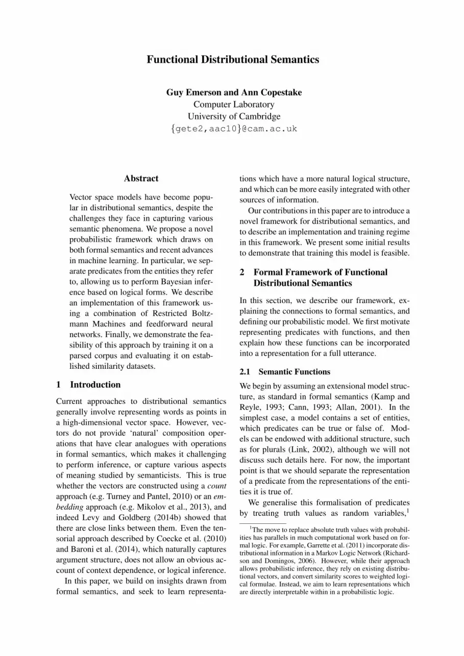
Figure 1: Comparison between a semantic function and a distribution over a space of entities. The veg-etables depicted above (five differently coloured bell peppers, a carrot, and a cucumber) form a discretesemantic space X . We are interested in the truth t of the predicate for bell pepper for an entity x ∈ X .Solid bars: the semantic function P (t|x) represents how much each entity is considered to be a pepper,and is bounded between 0 and 1; it is high for all the peppers, but slightly lower for atypical colours.Shaded bars: the distribution P (x|t) represents our belief about an entity if all we know is that the pred-icate for bell pepper applies to it; the probability mass must sum to 1, so it is split between the peppers,skewed towards typical colours, and excluding colours believed to be impossible.

which enables us to apply Bayesian inference. Forany entity, we can ask which predicates are true ofit (or ‘applicable’ to it). More formally, if we takeentities to lie in some semantic spaceX (whose di-mensions may denote different features), then wecan take the meaning of a predicate to be a func-tion from X to values in the interval [0, 1], denot-ing how likely a speaker is to judge the predicateapplicable to the entity. This judgement is variablebetween speakers (Labov, 1973), and for border-line cases, it is even variable for one speaker at dif-ferent times (McCloskey and Glucksberg, 1978).

Representing predicates as functions allows usto naturally capture vagueness (a predicate can beequally applicable to multiple points), and usingvalues between 0 and 1 allows us to naturally cap-ture gradedness (a predicate can be more applica-ble to some points than to others). To use Labov’sexample, the predicate for cup is equally applica-ble to vessels of different shapes and materials, butbecomes steadily less applicable to wider vessels.

We can also view such a function as a classifier– for example, the semantic function for the pred-icate for cat would be a classifier separating catsfrom non-cats. This ties in with a view of conceptsas abilities, as proposed in both philosophy (Dum-mett, 1978; Kenny, 2010), and cognitive science(Murphy, 2002; Bennett and Hacker, 2008). Asimilar approach is taken by Larsson (2013), whoargues in favour of representing perceptual con-cepts as classifiers of perceptual input.

Note that these functions do not directly de-fine probability distributions over entities. Rather,they define binary-valued conditional distribu-

tions, given an entity. We can write this as P (t|x),where x is an entity, and t is a stochastic truthvalue. It is only possible to get a correspond-ing distribution over entities given a truth value,P (x|t), if we have some background distributionP (x). If we do, we can apply Bayes’ Rule to getP (x|t) ∝ P (t|x)P (x). In other words, the truthof an expression depends crucially on our knowl-edge of the situation. This fits neatly within a ver-ificationist view of truth, as proposed by Dummett(1976), who argues that to understand a sentenceis to know how we could verify or falsify it.

By using bothP (t|x) and P (x|t), we can distin-guish between underspecification and uncertaintyas two kinds of ‘vagueness’. In the first case, wewant to state partial information about an entity,but leave other features unspecified; P (t|x) rep-resents which kinds of entity could be describedby the predicate, regardless of how likely we thinkthe entities are. In the second case, we have uncer-tain knowledge about the entity; P (x|t) representswhich kinds of entity we think are likely for thispredicate, given all our world knowledge.

For example, bell peppers come in manycolours, most typically green, yellow, orange orred. As all these colours are typical, the semanticfunction for the predicate for bell pepper wouldtake a high value for each. In contrast, to definea probability distribution over entities, we mustsplit probability mass between different colours,2

2In fact, colour would be most properly treated as a con-tinuous feature. In this case, P (x) must be a probability den-sity function, not a probability mass function, whose valuewould further depend on the parametrisation of the space.

and for a large number of colours, we would onlyhave a small probability for each. As purple andblue are atypical colours for a pepper, a speakermight be less willing to label such a vegetable apepper, but not completely unwilling to do so –this linguistic knowledge belongs to the semanticfunction for the predicate. In contrast, after ob-serving a large number of peppers, we might con-clude that blue peppers do not exist, purple pep-pers are rare, green peppers common, and red pep-pers more common still – this world knowledgebelongs to the probability distribution over enti-ties. The contrast between these two quantities isdepicted in figure 1, for a simple discrete space.

2.2 Incorporation with Dependency MinimalRecursion Semantics

Semantic dependency graphs have become popu-lar in NLP. We use Dependency Minimal Recur-sion Semantics (DMRS) (Copestake et al., 2005;Copestake, 2009), which represents meaning asa directed acyclic graph: nodes represent predi-cates/entities (relying on a one-to-one correspon-dence between them) and links (edges) repre-sent argument structure and scopal constraints.Note that we assume a neo-Davidsonian approach(Davidson, 1967; Parsons, 1990), where events arealso treated as entities, which allows a better ac-count of adverbials, among other phenomena.

For example (simplifying a little), to represent“the dog barked”, we have three nodes, for thepredicates the, dog, and bark, and two links: anARG1 link from bark to dog, and a RSTR linkfrom the to dog. Unlike syntactic dependencies,DMRS abstracts over semantically equivalent ex-pressions, such as “dogs chase cats” and “catsare chased by dogs”. Furthermore, unlike othertypes of semantic dependencies, including Ab-stract Meaning Representations (Banarescu et al.,2012), and Prague Dependencies (Bohmova etal., 2003), DMRS is interconvertible with MRS,which can be given a direct logical interpretation.

We deal here with the extensional fragment oflanguage, and while we can account for differentquantifiers in our framework, we do not have spaceto discuss this here – for the rest of this paper,we neglect quantifiers, and the reader may assumethat all variables are existentially quantified.

We can use the structure of a DMRS graph todefine a probabilistic graphical model. This givesus a distribution over lexicalisations of the graph –

y zxARG2ARG1

∈ X

tc, x tc, y tc, z

∈ {⊥,>} |V |

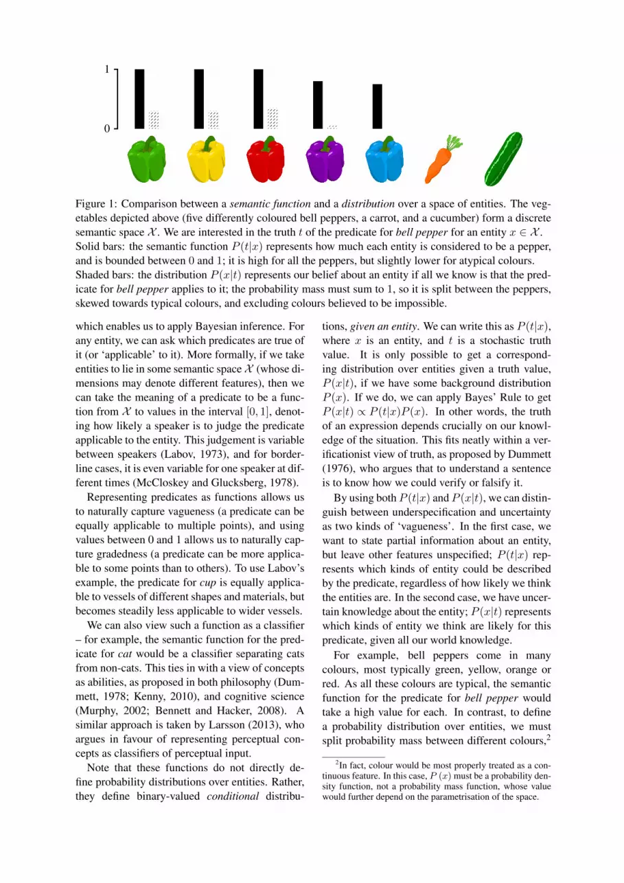
Figure 2: A situation composed of three entities.Top row: the entities x, y, and z lie in a semanticspace X , jointly distributed according to DMRSlinks. Bottom row: each predicate c in the vocab-ulary V has a stochastic truth value for each entity.

given an abstract graph structure, where links arelabelled but nodes are not, we have a process togenerate a predicate for each node. Although thisprocess is different for each graph structure, wecan share parameters between them (e.g. accord-ing to the labels on links). Furthermore, if we havea distribution over graph structures, we can incor-porate that in our generative process, to produce adistribution over lexicalised graphs.

The entity nodes can be viewed as together rep-resenting a situation, in the sense of Barwise andPerry (1983). We want to be able to represent theentities without reference to the predicates – intu-itively, the world is the same however we chooseto describe it. To avoid postulating causal struc-ture amongst the entities (which would be difficultfor a large graph), we can model the entity nodesas an undirected graphical model, with edges ac-cording to the DMRS links. The edges are undi-rected in the sense that they don’t impose condi-tional dependencies. However, this is still compat-ible with having ‘directed’ semantic dependencies– the probability distributions are not symmetric,which maintains the asymmetry of DMRS links.

Each node takes values in the semantic spaceX ,and the network defines a joint distribution overentities, which represents our knowledge aboutwhich situations are likely or unlikely. An exam-ple is shown in the top row of figure 2, of an entityy along with its two arguments x and z – thesemight represent an event, along with the agent andpatient involved in the event. The structure of thegraph means that we can factorise the joint distri-bution P (x, y, z) over the entities as being pro-portional to the product P (x, y)P (y, z).

For any entity, we can ask which predicatesare true of it. We can therefore introduce a

y zxARG2ARG1

∈ X

tc, x tc, y tc, z

∈ {⊥,>} |V |

p q r

∈ V

Figure 3: The probabilistic model in figure 2, ex-tended to generate utterances. Each predicate inthe bottom row is chosen out of all predicateswhich are true for the corresponding entity.

node for every predicate in the vocabulary, wherethe value of the node is either true (>) or false(⊥). Each of these predicate nodes has a sin-gle directed link from the entity node, with theprobability of the node being true being deter-mined by the predicate’s semantic function, i.e.P (tc, x = >|x) = tc(x). This is shown in the sec-ond row of figure 2, where the plate denotes thatthese nodes are repeated for each predicate c in thevocabulary V . For example, if the situation repre-sented a dog chasing a cat, then nodes like tdog, x,tanimal, x, and tpursue, y would be true (with highprobability), while tdemocracy, x or tdog, z would befalse (with high probability).

The probabilistic model described aboveclosely matches traditional model-theoreticsemantics. However, while we could stop oursemantic description there, we do not generallyobserve truth-value judgements for all predicatesat once;3 rather, we observe utterances, whichhave specific predicates. We can therefore definea final node for each entity, which takes valuesover predicates in the vocabulary, and which isconditionally dependent on the truth values of allpredicates. This is shown in the bottom row offigure 3. Including these final nodes means thatwe can train such a model on observed utterances.The process of choosing a predicate from the trueones may be complex, potentially depending onspeaker intention and other pragmatic factors –but in section 3, we will simply choose a truepredicate at random (weighted by frequency).

3This corresponds to what Copestake and Herbelot (2012)call an ideal distribution. If we have access to such informa-tion, we only need the two rows given in figure 2.

The separation of entities and predicates allowsus to naturally capture context-dependent mean-ings. Following the terminology of Quine (1960),we can distinguish context-independent standingmeaning from context-dependent occasion mean-ing. Each predicate type has a correspondingsemantic function – this represents its standingmeaning. Meanwhile, each predicate token has acorresponding entity, for which there is a posteriordistribution over the semantic space, conditioningon the rest of the graph and any pragmatic factors– this represents its occasion meaning.

Unlike previous approaches to context depen-dence, such as Dinu et al. (2012), Erk and Pado(2008), and Thater et al. (2011), we representmeanings in and out of context by different kindsof object, reflecting a type/token distinction. EvenHerbelot (2015), who explicitly contrasts individ-uals and kinds, embeds both in the same space.

As an example of how this separation of pred-icates and entities can be helpful, suppose wewould like “dogs chase cats” and “cats chasemice” to be true in a model, but “dogs chase mice”and “cats chase cats” to be false. In other words,there is a dependence between the verb’s argu-ments. If we represent each predicate by a singlevector, it is not clear how to capture this. However,by separating predicates from entities, we can havetwo different entities which chase is true of, whereone co-occurs with a dog-entity ARG1 and cat-entity ARG2, while the other co-occurs with a cat-entity ARG1 and a mouse-entity ARG2.

3 Implementation

In the previous section, we described a generalframework for probabilistic semantics. Here wegive details of one way that such a frameworkcan be implemented for distributional semantics,keeping the architecture as simple as possible.

3.1 Network ArchitectureWe take the semantic spaceX to be a set of binary-valued vectors,4 {0, 1}N . A situation s is thencomposed of entity vectors x(1), · · · , x(K) ∈ X(where the number of entities K may vary), alongwith links between the entities. We denote a linkfrom x(n) to x(m) with label l as: x(n) l−→ x(m).We define the background distribution over sit-uations using a Restricted Boltzmann Machine

4We use the term vector in the computer science sense ofa linear array, rather than in the mathematical sense of a pointin a vector space.

(RBM) (Smolensky, 1986; Hinton et al., 2006),but rather than having connections between hiddenand visible units, we have connections betweencomponents of entities, according to the links.

The probability of the network being in theparticular configuration s depends on the energyof the configuration, Eb(s), as shown in equa-tions (1)-(2). A high energy denotes an unlikelyconfiguration. The energy depends on the edgesof the graphical model, plus bias terms, as shownin (3). Note that we follow the Einstein sum-mation convention, where repeated indices indi-cate summation; although this notation is not typ-ical in NLP, we find it much clearer than matrix-vector notation, particularly for higher-order ten-sors. Each link label l has a corresponding weightmatrix W (l), which determines the strength of as-sociation between components of the linked enti-ties. The first term in (3) sums these contributionsover all links x(n) l−→ x(m) between entities. Wealso introduce bias terms, to control how likely anentity vector is, independent of links. The secondterm in (3) sums the biases over all entities x(n).

P (s) =1

Zexp

(−Eb(s)

)(1)

Z =∑s′

exp(−Eb(s′)

)(2)

−Eb(s) =∑

x(n)l−→x(m)

W(l)ij x

(n)i x

(m)j −

∑x(n)

bix(n)i (3)

Furthermore, since sparse representations havebeen shown to be beneficial in NLP, both for ap-plications and for interpretability of features (Mur-phy et al., 2012; Faruqui et al., 2015), we can en-force sparsity in these entity vectors by fixing aspecific number of units to be active at any time.Swersky et al. (2012) introduce this RBM variantas the Cardinality RBM, and also give an efficientexact sampling procedure using belief propaga-tion. Since we are using sparse representations, wealso assume that all link weights are non-negative.

Now that we’ve defined the background distri-bution over situations, we turn to the semanticfunctions tc, which map entities x to probabilities.We implement these as feedforward networks, asshown in (4)-(5). For simplicity, we do not in-troduce any hidden layers. Each predicate c hasa vector of weights W ′(c), which determines thestrength of association with each dimension of thesemantic space, as well as a bias term b′(c). These

together define the energy Ep(x, c) of an entity xwith the predicate, which is passed through a sig-moid function to give a value in the range [0, 1].

tc(x) = σ(−Ep(x, c)) = 1

1 + exp (Ep)(4)

−Ep(x, c) =W′(c)i xi − b′(c) (5)

Given the semantic functions, choosing a predi-cate for a entity can be hard-coded, for simplicity.The probability of choosing a predicate c for anentity x is weighted by the predicate’s frequencyfc and the value of its semantic function tc(x)(how true the predicate is of the entity), as shownin (6)-(7). This is a mean field approximation tothe stochastic truth values shown in figure 3.

P (c|x) = 1

Zxfctc(x) (6)

Zx =∑c′

fc′tc′(x) (7)

3.2 Learning AlgorithmTo train this model, we aim to maximise the likeli-hood of observing the training data – in Bayesianterminology, this is maximum a posteriori estima-tion. As described in section 2.2, each data pointis a lexicalised DMRS graph, while our model de-fines distributions over lexicalisations of graphs.In other words, we take as given the observeddistribution over abstract graph structures (wherelinks are given, but nodes are unlabelled), and tryto optimise how the model generates predicates(via the parameters W (l)

ij , bi,W′(c)i , b′(c)).

For the family of optimisation algorithms basedon gradient descent, we need to know the gradientof the likelihood with respect to the model param-eters, which is given in (8), where x ∈ X is a latententity, and c ∈ V is an observed predicate (corre-sponding to the top and bottom rows of figure 3).Note that we extend the definition of energy fromsituations to entities in the obvious way: half theenergy of an entity’s links, plus its bias energy. Afull derivation of (8) is given in the appendix.

∂

∂θlogP (c) = Ex|c

[∂

∂θ

(−Eb(x)

)]− Ex

[∂

∂θ

(−Eb(x)

)]+ Ex|c

[(1− tc(x))

∂

∂θ(−Ep(x, c))

]− Ex|c

[Ec′|x

[(1− tc′(x))

∂

∂θ

(−Ep(x, c′)

)]](8)

There are four terms in this gradient: the firsttwo are for the background distribution, and thelast two are for the semantic functions. In bothcases, one term is positive, and conditioned on thedata, while the other term is negative, and repre-sents the predictions of the model.

Calculating the expectations exactly is infeasi-ble, as this requires summing over all possibleconfigurations. Instead, we can use a MarkovChain Monte Carlo method, as typically done forLatent Dirichlet Allocation (Blei et al., 2003; Grif-fiths and Steyvers, 2004). Our aim is to samplevalues of x and c, and use these samples to ap-proximate the expectations: rather than summingover all values, we just consider the samples. Foreach token in the training data, we introduce a la-tent entity vector, which we use to approximate thefirst, third, and fourth terms in (8). Additionally,we introduce a latent predicate for each latent en-tity, which we use to approximate the fourth term– this latent predicate is analogous to the negativesamples used by Mikolov et al. (2013).

When resampling a latent entity conditioned onthe data, the conditional distribution P (x|c) is un-known, and calculating it directly requires sum-ming over the whole semantic space. For this rea-son, we cannot apply Gibbs sampling (as used inLDA), which relies on knowing the conditionaldistribution. However, if we compare two enti-ties x and x′, the normalisation constant cancelsout in the ratio P (x′|c)/P (x|c), so we can usethe Metropolis-Hastings algorithm (Metropolis etal., 1953; Hastings, 1970). Given the current sam-ple x, we can uniformly choose one unit to switchon, and one to switch off, to get a proposal x′. Ifthe ratio of probabilities shown in (9) is above 1,we switch the sample to x′; if it’s below 1, it is theprobability of switching to x′.

P (x′|c)P (x|c)

=exp

(−Eb(x′)

)1Zx′

tc(x′)

exp (−Eb(x)) 1Zxtc(x)

(9)

Although Metropolis-Hastings avoids the needto calculate the normalisation constant Z of thebackground distribution, we still have the nor-malisation constant Zx of choosing a predicategiven an entity. This constant represents the num-ber of predicates true of the entity (weighted byfrequency). The intuitive explanation is that weshould sample an entity which few predicates aretrue of, rather than an entity which many predi-cates are true of. We approximate this constant

by assuming that we have an independent contri-bution from each dimension of x. We first aver-age over all predicates (weighted by frequency), toget the average predicate W avg. We then take theexponential of W avg for the dimensions that weare proposing switching off and on – intuitively,if many predicates have a large weight for a givendimension, then many predicates will be true ofan entity where that dimension is active. This isshown in (10), where x and x′ differ in dimensionsi and i′ only, and where k is a constant.

ZxZx′≈ exp

(k(W avgi −W avg

i′))

(10)

We must also resample latent predicates given alatent entity, for the fourth term in (8). This cansimilarly be done using the Metropolis-Hastingsalgorithm, according to the ratio shown in (11).

P (c′|x)P (c|x)

=fc′tc′(x)

fctc(x)(11)

Finally, we need to resample entities fromthe background distribution, for the second termin (8). Rather than recalculating the samples fromscratch after each weight update, we used fantasyparticles (persistent Markov chains), which Tiele-man (2008) found effective for training RBMs.Resampling a particle can be done more straight-forwardly than resampling the latent entities – wecan sample each entity conditioned on the otherentities in the situation, which can be done exactlyusing belief propagation (see Yedidia et al. (2003)and references therein), as Swersky et al. (2012)applied to the Cardinality RBM.

To make weight updates from the gradients, weused AdaGrad (Duchi et al., 2011), with exponen-tial decay of the sum of squared gradients. We alsoused L1 and L2 regularisation, which determinesour prior over model parameters.

We found that using a random initialisation ispossible, but seems to lead to a long training time,due to slow convergence. We suspect that thiscould be because the co-occurrence of predicatesis mediated via at least two latent vectors, whichleads to mixing of semantic classes in each di-mension, particularly in the early stages of train-ing. Such behaviour can happen with compli-cated topic models – for example, O Seaghdha(2010) found this for their “Dual Topic” model.One method to reduce convergence time is to ini-tialise predicate parameters using pre-trained vec-tors. The link parameters can then be initialised

as follows: we consider a situation with just oneentity, and for each predicate, we find the mean-field entity vector given the pre-trained predicateparameters; we then fix all entity vectors in ourtraining corpus to be these mean-field vectors, andfind the positive pointwise mutual information ofeach each pair of entity dimensions, for each linklabel. In particular, we initialised predicate pa-rameters using our sparse SVO Word2Vec vectors,which we describe in section 4.2.

4 Training and Initial Experiments

In this section, we report the first experiments car-ried out within our framework.

4.1 Training Data

Training our model requires a corpus of DMRSgraphs. In particular, we used WikiWoods, anautomatically parsed version of the July 2008dump of the full English Wikipedia, distributedby DELPH-IN5. This resource was produced byFlickinger et al. (2010), using the English Re-source Grammar (ERG; Flickinger, 2000), trainedon the manually treebanked subcorpus WeScience(Ytrestøl et al., 2009), and implemented withthe PET parser (Callmeier, 2001; Toutanova etal., 2005). To preprocess the corpus, we usedthe python packages pydelphin6 (developed byMichael Goodman), and pydmrs7 (Copestake etal., 2016).

For simplicity, we restricted attention tosubject-verb-object (SVO) triples, although weshould stress that this is not an inherent limita-tion of our model, which could be applied to ar-bitrary graphs. We searched for all verbs in theWikiWoods treebank, excluding modals, that hadeither an ARG1 or an ARG2, or both. We kept allinstances whose arguments were nominal, exclud-ing pronouns and proper nouns. The ERG doesnot automatically convert out-of-vocabulary itemsfrom their surface form to lemmatised predicates,so we applied WordNet’s morphological processorMorphy (Fellbaum, 1998), as available in NLTK(Bird et al., 2009). Finally, we filtered out situa-tions including rare predicates, so that every pred-icate appears at least five times in the dataset.

As a result of this process, all data was of theform (verb, ARG1, ARG2), where one (but not

5http://moin.delph-in.net/WikiWoods6https://github.com/delph-in/pydelphin7https://github.com/delph-in/pydmrs

both) of the arguments may be missing. A sum-mary is given in table 1. In total, the dataset con-tains 72m tokens, with 88,526 distinct predicates.

Situation type No. instancesBoth arguments 10,091,234ARG1 only 6,301,280ARG2 only 14,868,213Total 31,260,727

Table 1: Size of the training data.

4.2 Evaluation

As our first attempt at evaluation, we chose to lookat two lexical similarity datasets. The aim of thisevaluation was simply to verify that the model waslearning something reasonable. We did not expectthis task to illustrate our model’s strengths, sincewe need richer tasks to exploit its full expressive-ness. Both of our chosen datasets aim to evalu-ate similarity, rather than thematic relatedness: thefirst is Hill et al. (2015)’s SimLex-999 dataset, andthe second is Finkelstein et al. (2001)’s WordSim-353 dataset, which was split by Agirre et al. (2009)into similarity and relatedness subsets. So far, wehave not tuned hyperparameters.

Results are given in table 2. We also trainedMikolov et al. (2013)’s Word2Vec model on theSVO data described in section 4.1, in order togive a direct comparison of models on the sametraining data. In particular, we used the continu-ous bag-of-words model with negative sampling,as implemented in Rehurek and Sojka (2010)’sgensim package, with off-the-shelf hyperparame-ter settings. We also converted these to sparse vec-tors using Faruqui et al. (2015)’s algorithm, againusing off-the-shelf hyperparameter settings. Tomeasure similarity of our semantic functions, wetreated each function’s parameters as a vector andused cosine similarity, for simplicity.

For comparison, we also include the perfor-mance of Word2Vec when trained on raw text. ForSimLex-999, we give the results reported by Hillet al. (2015), where the 2-word window modelwas the best performing model that they tested.For WordSim-353, we trained a model on the fullWikiWoods text, after stripping all punctuationand converting to lowercase. We used the gensimimplementation with off-the-shelf settings, exceptfor window size (2 or 10) and dimension (200, asrecommended by Hill et al.). In fact, our re-trainedmodel performed better on SimLex-999 than Hill

Model SimLex Nouns SimLex Verbs WordSim Sim. WordSim Rel.Word2Vec (10-word window) .28 .11 .69 .46Word2Vec (2-word window) .30 .16 .65 .34SVO Word2Vec .44 .18 .61 .24Sparse SVO Word2Vec .45 .27 .63 .30Semantic Functions .26 .14 .34 .01

Table 2: Spearman rank correlation of different models with average annotator judgements. Note that wewould like to have a low score on the final column (which measures relatedness, rather than similarity).

flood / water (related verb and noun) .06flood / water (related nouns) .43law / lawyer (related nouns) .44sadness / joy (near-antonyms) .77happiness / joy (near-synonyms) .78aunt / uncle (differ in a single feature) .90cat / dog (differ in many features) .92

Table 3: Similarity scores for thematically relatedwords, and various types of co-hyponym.

et al. reported (even when we used less preprocess-ing or a different edition of Wikipedia), althoughstill worse than our sparse SVO Word2Vec model.

It is interesting to note that training Word2Vecon verbs and their arguments gives noticeably bet-ter results on SimLex-999 than training on fullsentences, even though far less data is being used:∼72m tokens, rather than ∼1000m. The betterperformance suggests that semantic dependenciesmay provide more informative contexts than sim-ple word windows. This is in line with previousresults, such as Levy and Goldberg (2014a)’s workon using syntactic dependencies. Nonetheless, thisresult deserves further investigation.

Of all the models we tested, only our semanticfunction model failed on the relatedness subset ofWordSim-353. We take this as a positive result,since it means the model clearly distinguishes re-latedness and similarity.

Examples of thematically related predicates andvarious kinds of co-hyponym are given in table 3,along with our model’s similarity scores. How-ever, it is not clear that it is possible, or even de-sirable, to represent these varied relationships on asingle scale of similarity. For example, it could besensible to treat aunt and uncle either as synonyms(they refer to relatives of the same degree of re-latedness) or as antonyms (they are “opposite” insome sense). Which view is more appropriate willdepend on the application, or on the context.

Nouns and verbs are very strongly distin-guished, which we would expect given the struc-ture of our model. This can be seen in the simi-larity scores between flood and water, when floodis considered either as a verb or as a noun.8

SimLex-999 generally assigns low scores to near-antonyms, and to pairs differing in a single fea-ture, which might explain why the performance ofour model is not higher on this task. However, theseparation of thematically related predicates fromco-hyponyms is a promising result.

5 Related Work

As mentioned above, Coecke et al. (2010) and Ba-roni et al. (2014) introduce a tensor-based frame-work that incorporates argument structure throughtensor contraction. However, for logical inference,we need to know how one vector can entail an-other. Grefenstette (2013) explores one methodto do this; however, they do not show that thisapproach is learnable from distributional informa-tion, and furthermore, they prove that quantifierscannot be expressed with tensors.

Balkır (2014), working in the tensorial frame-work, uses the quantum mechanical notion of a“mixed state” to model uncertainty. However, thisdoubles the number of tensor indices, so squaresthe number of dimensions (e.g. vectors becomematrices). In the original framework, expressionswith several arguments already have a high dimen-sionality (e.g. whose is represented by a fifth-ordertensor), and this problem becomes worse.

Vilnis and McCallum (2015) embed predicatesas Gaussian distributions over vectors. By assum-ing covariances are diagonal, this only doublesthe number of dimensions (N dimensions for themean, and N for the covariances). However, simi-larly to Mikolov et al. (2013), they simply assume

8We considered the ERG predicates flood v causeand flood n of, which were the most frequent predicatesin WikiWoods for flood, for each part of speech.

that nearby words have similar meanings, so themodel does not naturally capture compositionalityor argument structure.

In both Balkır’s and Vilnis and McCallum’smodels, they use the probability of a vectorgiven a word – in the notation from section 2.1,P (x|t). However, the opposite conditional prob-ability, P (t|x), more easily allows composition.For instance, if we know two predicates are true(t1 and t2), we cannot easily combine P (x|t1) andP (x|t2) to get P (x|t1, t2) – intuitively, we’re gen-erating x twice. In contrast, for semantic func-tions, we can writeP (t1, t2|x) = P (t1|x)P (t2|x).

Gardenfors (2004) argues concepts should bemodelled as convex subsets of a semantic space.Erk (2009) builds on this idea, but their model re-quires pre-trained count vectors, while we learnour representations directly. McMahan and Stone(2015) also learn representations directly, consid-ering colour terms, which are grounded in a well-understood perceptual space. Instead of consider-ing a single subset, they use a probability distribu-tion over subsets: P (A|t) forA ⊂ X . This is moregeneral than a semantic function P (t|x), since wecan write P (t|x) =

∑A3v P (A|t). However, this

framework may be too general, since it means wecannot determine the truth of a predicate until weknow the entire set A. To avoid this issue, theyfactorise the distribution, by assuming differentboundaries of the set are independent. However,this is equivalent to considering P (t|x) directly,along with some constraints on this function. In-deed, for the experiments they describe, it is suffi-cient to know a semantic function P (t|x). Fur-thermore, McMahan and Stone find expressionslike greenish which are nonconvex in perceptualspace, which suggests that representing conceptswith convex sets may not be the right way to go.

Our semantic functions are similar to Cooper etal. (2015)’s probabilistic type judgements, whichthey introduce within the framework of Type The-ory with Records (Cooper, 2005), a rich seman-tic theory. However, one difference between ourmodels is that they represent situations in termsof situation types, while we are careful to defineour semantic space without reference to any pred-icates. More practically, although they outlinehow their model might be learned, they assume wehave access to type judgements for observed situ-ations. In contrast, we describe how a model canbe learned from observed utterances, which was

necessary for us to train a model on a corpus.Goodman and Lassiter (2014) propose another

linguistically motivated probabilistic model, usingthe stochastic λ-calculus (more concretely, prob-abilistic programs written in Church). However,they rely on relatively complex generative pro-cesses, specific to individual semantic domains,where each word’s meaning may be representedby a complex expression. For a wide-scale sys-tem, such structures would need to be extended tocover all concepts. In contrast, our model assumesa direct mapping between predicates and seman-tic functions, with a relatively simple generativestructure determined by semantic dependencies.

Finally, our approach should be distinguishedfrom work which takes pre-trained distributionalvectors, and uses them within a richer semanticmodel. For example, Herbelot and Vecchi (2015)construct a mapping from a distributional vectorto judgements of which quantifier is most appro-priate for a range of properties. Erk (2016) usesdistributional similarity to probabilistically inferproperties of one concept, given properties of an-other. Beltagy et al. (2016) use distributional sim-ilarity to produce weighted inference rules, whichthey incorporate in a Markov Logic Network. Un-like these authors, we aim to directly learn in-terpretable representations, rather than interpretgiven representations.

6 Conclusion

We have introduced a novel framework for distri-butional semantics, where each predicate is rep-resented as a function, expressing how applica-ble the predicate is to different entities. We haveshown how this approach can capture semanticphenomena which are challenging for standardvector space models. We have explained how ourframework can be implemented, and trained on acorpus of DMRS graphs. Finally, our initial eval-uation on similarity datasets demonstrates the fea-sibility of this approach, and shows that themati-cally related words are not given similar represen-tations. In future work, we plan to use richer taskswhich exploit the model’s expressiveness.

Acknowledgments

This work was funded by a Schiff Foundation Stu-dentship. We would also like to thank Yarin Gal,who gave useful feedback on the specification ofour generative model.

ReferencesEneko Agirre, Enrique Alfonseca, Keith Hall, Jana

Kravalova, Marius Pasca, and Aitor Soroa. 2009.A study on similarity and relatedness using distribu-tional and WordNet-based approaches. In Proceed-ings of the 2009 Conference of the North AmericanChapter of the Association for Computational Lin-guistics, pages 19–27.

Keith Allan. 2001. Natural Language Semantics.Blackwell Publishers.

Esma Balkır. 2014. Using density matrices in a com-positional distributional model of meaning. Mas-ter’s thesis, University of Oxford.

Laura Banarescu, Claire Bonial, Shu Cai, MadalinaGeorgescu, Kira Griffitt, Ulf Hermjakob, KevinKnight, Philipp Koehn, Martha Palmer, and NathanSchneider. 2012. Abstract meaning representation(amr) 1.0 specification. In Proceedings of the 11thConference on Empirical Methods in Natural Lan-guage Processing, pages 1533–1544.

Marco Baroni, Raffaela Bernardi, and Roberto Zam-parelli. 2014. Frege in space: A program of compo-sitional distributional semantics. Linguistic Issuesin Language Technology, 9.

Jon Barwise and John Perry. 1983. Situations and At-titudes. MIT Press.

Islam Beltagy, Stephen Roller, Pengxiang Cheng, Ka-trin Erk, and Raymond J. Mooney. 2016. Repre-senting meaning with a combination of logical anddistributional models.

Maxwell R Bennett and Peter Michael Stephan Hacker.2008. History of cognitive neuroscience. John Wi-ley & Sons.

Steven Bird, Ewan Klein, and Edward Loper. 2009.Natural language processing with Python. O’ReillyMedia, Inc.

David M Blei, Andrew Y Ng, and Michael I Jordan.2003. Latent Dirichlet Allocation. the Journal ofMachine Learning Research, 3:993–1022.

Alena Bohmova, Jan Hajic, Eva Hajicova, and BarboraHladka. 2003. The Prague dependency treebank. InTreebanks, pages 103–127. Springer.

Ulrich Callmeier. 2001. Efficient parsing with large-scale unification grammars. Master’s thesis, Univer-sitat des Saarlandes, Saarbrucken, Germany.

Ronnie Cann. 1993. Formal semantics: An intro-duction. Cambridge Textbooks in Linguistics. Cam-bridge University Press.

Bob Coecke, Mehrnoosh Sadrzadeh, and StephenClark. 2010. Mathematical foundations for a com-positional distributional model of meaning. Linguis-tic Analysis, 36:345–384.

Robin Cooper, Simon Dobnik, Staffan Larsson, andShalom Lappin. 2015. Probabilistic type theory andnatural language semantics. LiLT (Linguistic Issuesin Language Technology), 10.

Robin Cooper. 2005. Austinian truth, attitudes andtype theory. Research on Language and Computa-tion, 3(2-3):333–362.

Ann Copestake and Aurelie Herbelot. 2012. Lexi-calised compositionality. Unpublished draft.

Ann Copestake, Dan Flickinger, Carl Pollard, andIvan A Sag. 2005. Minimal Recursion Semantics:An introduction. Research on Language and Com-putation.

Ann Copestake, Guy Emerson, Michael Wayne Good-man, Matic Horvat, Alexander Kuhnle, and EwaMuszynska. 2016. Resources for building appli-cations with Dependency Minimal Recursion Se-mantics. In Proceedings of the 10th InternationalConference on Language Resources and Evaluation(LREC 2016). European Language Resources Asso-ciation (ELRA).

Ann Copestake. 2009. Slacker semantics: Why super-ficiality, dependency and avoidance of commitmentcan be the right way to go. In Proceedings of 12thConference of the European Chapter of the Associa-tion for Computational Linguistics.

Donald Davidson. 1967. The logical form of actionsentences. In Nicholas Rescher, editor, The Logic ofDecision and Action, chapter 3, pages 81–95. Uni-versity of Pittsburgh Press.

Georgiana Dinu, Stefan Thater, and Soren Laue. 2012.A comparison of models of word meaning in con-text. In Proceedings of the 13th Conference ofthe North American Chapter of the Association forComputational Linguistics, pages 611–615.

John Duchi, Elad Hazan, and Yoram Singer. 2011.Adaptive subgradient methods for online learningand stochastic optimization. The Journal of Ma-chine Learning Research, 12:2121–2159.

Michael Dummett. 1976. What is a theory of mean-ing? (II). In Gareth Evans and John McDowell, ed-itors, Truth and Meaning, pages 67–137. ClarendonPress (Oxford).

Michael Dummett. 1978. What Do I Know WhenI Know a Language? Stockholm University.Reprinted in Dummett (1993) Seas of Language,pages 94–105.

Katrin Erk and Sebastian Pado. 2008. A structuredvector space model for word meaning in context.In Proceedings of the 13th Conference on Empiri-cal Methods in Natural Language Processing, pages897–906. Association for Computational Linguis-tics.

Katrin Erk. 2009. Representing words as regions invector space. In Proceedings of the 13th Confer-ence on Computational Natural Language Learning,pages 57–65. Association for Computational Lin-guistics.

Katrin Erk. 2016. What do you know about an alliga-tor when you know the company it keeps? Seman-tics and Pragmatics, 9(17):1–63.

Manaal Faruqui, Yulia Tsvetkov, Dani Yogatama, ChrisDyer, and Noah Smith. 2015. Sparse overcompleteword vector representations. In Proceedings of the53rd Annual Conference of the Association for Com-putational Linguistics.

Christiane Fellbaum. 1998. WordNet. Blackwell Pub-lishers.

Lev Finkelstein, Evgeniy Gabrilovich, Yossi Matias,Ehud Rivlin, Zach Solan, Gadi Wolfman, and Ey-tan Ruppin. 2001. Placing search in context: Theconcept revisited. In Proceedings of the 10th Inter-national Conference on the World Wide Web, pages406–414. Association for Computing Machinery.

Dan Flickinger, Stephan Oepen, and Gisle Ytrestøl.2010. WikiWoods: Syntacto-semantic annotationfor English Wikipedia. In Proceedings of the 7th In-ternational Conference on Language Resources andEvaluation.

Dan Flickinger. 2000. On building a more efficientgrammar by exploiting types. Natural LanguageEngineering.

Peter Gardenfors. 2004. Conceptual spaces: The ge-ometry of thought. MIT Press, second edition.

Dan Garrette, Katrin Erk, and Raymond Mooney.2011. Integrating logical representations with prob-abilistic information using Markov logic. In Pro-ceedings of the 9th International Conference onComputational Semantics (IWCS), pages 105–114.Association for Computational Linguistics.

Noah D Goodman and Daniel Lassiter. 2014. Prob-abilistic semantics and pragmatics: Uncertainty inlanguage and thought. Handbook of ContemporarySemantic Theory.

Edward Grefenstette. 2013. Towards a formal distri-butional semantics: Simulating logical calculi withtensors. In Proceedings of the 2nd Joint Conferenceon Lexical and Computational Semantics.

Thomas L Griffiths and Mark Steyvers. 2004. Find-ing scientific topics. Proceedings of the NationalAcademy of Sciences, 101(suppl 1):5228–5235.

W. Keith Hastings. 1970. Monte Carlo samplingmethods using Markov chains and their applications.Biometrika, 57(1):97–109.

Aurelie Herbelot and Eva Maria Vecchi. 2015. Build-ing a shared world: Mapping distributional tomodel-theoretic semantic spaces. In Proceedings ofthe 2015 Conference on Empirical Methods in Natu-ral Language Processing, pages 22–32. Associationfor Computational Linguistics.

Aurelie Herbelot. 2015. Mr Darcy and Mr Toad, gen-tlemen: distributional names and their kinds. InProceedings of the 11th International Conference onComputational Semantics, pages 151–161.

Felix Hill, Roi Reichart, and Anna Korhonen. 2015.Simlex-999: Evaluating semantic models with (gen-uine) similarity estimation. Computational Linguis-tics.

Geoffrey E Hinton, Simon Osindero, and Yee-WhyeTeh. 2006. A fast learning algorithm for deep be-lief nets. Neural computation, 18(7):1527–1554.

Hans Kamp and Uwe Reyle. 1993. From discourseto logic; introduction to modeltheoretic semantics ofnatural language, formal logic and discourse repre-sentation theory.

Anthony Kenny. 2010. Concepts, brains, and be-haviour. Grazer Philosophische Studien, 81(1):105–113.

William Labov. 1973. The boundaries of words andtheir meanings. In Charles-James N. Bailey andRoger W. Shuy, editors, New ways of analyzing vari-ation in English, pages 340–73. Georgetown Univer-sity Press.

Staffan Larsson. 2013. Formal semantics for percep-tual classification. Journal of Logic and Computa-tion.

Omer Levy and Yoav Goldberg. 2014a. Dependency-based word embeddings. In Proceedings of the 52ndAnnual Meeting of the Association for Computa-tional Linguistics, pages 302–308.

Omer Levy and Yoav Goldberg. 2014b. Neuralword embedding as implicit matrix factorization.In Z. Ghahramani, M. Welling, C. Cortes, N. D.Lawrence, and K. Q. Weinberger, editors, Advancesin Neural Information Processing Systems 27, pages2177–2185. Curran Associates, Inc.

Godehard Link. 2002. The logical analysis of pluralsand mass terms: A lattice-theoretical approach. InPaul Portner and Barbara H. Partee, editors, Formalsemantics: The essential readings, chapter 4, pages127–146. Blackwell Publishers.

Michael E McCloskey and Sam Glucksberg. 1978.Natural categories: Well defined or fuzzy sets?Memory & Cognition, 6(4):462–472.

Brian McMahan and Matthew Stone. 2015. ABayesian model of grounded color semantics.Transactions of the Association for ComputationalLinguistics, 3:103–115.

Nicholas Metropolis, Arianna W Rosenbluth, Mar-shall N Rosenbluth, Augusta H Teller, and EdwardTeller. 1953. Equation of state calculations byfast computing machines. The Journal of ChemicalPhysics, 21(6):1087–1092.

Tomas Mikolov, Kai Chen, Greg Corrado, and JeffreyDean. 2013. Efficient estimation of word represen-tations in vector space. In Proceedings of the 1stInternational Conference on Learning Representa-tions.

Brian Murphy, Partha Pratim Talukdar, and Tom MMitchell. 2012. Learning effective and interpretablesemantic models using non-negative sparse embed-ding. In Proceedings of the 24th InternationalConference on Computational Linguistics (COLING2012), pages 1933–1950. Association for Computa-tional Linguistics.

Gregory Leo Murphy. 2002. The Big Book of Con-cepts. MIT Press.

Diarmuid O Seaghdha. 2010. Latent variable mod-els of selectional preference. In Proceedings of the48th Annual Meeting of the Association for Compu-tational Linguistics, pages 435–444. Association forComputational Linguistics.

Terence Parsons. 1990. Events in the Semantics ofEnglish: A Study in Subatomic Semantics. CurrentStudies in Linguistics. MIT Press.

Willard Van Orman Quine. 1960. Word and Object.MIT Press.

Radim Rehurek and Petr Sojka. 2010. Software frame-work for topic modelling with large corpora. In Pro-ceedings of the LREC 2010 Workshop on New Chal-lenges for NLP Frameworks, pages 45–50. ELRA.

Matthew Richardson and Pedro Domingos. 2006.Markov logic networks. Machine learning, 62(1-2):107–136.

Paul Smolensky. 1986. Information processing in dy-namical systems: Foundations of harmony theory.In Parallel Distributed Processing: Explorations inthe Microstructure of Cognition, volume 1, pages194–281. MIT Press.

Kevin Swersky, Ilya Sutskever, Daniel Tarlow,Richard S Zemel, Ruslan R Salakhutdinov, andRyan P Adams. 2012. Cardinality Restricted Boltz-mann Machines. In Advances in Neural InformationProcessing Systems, pages 3293–3301.

Stefan Thater, Hagen Furstenau, and Manfred Pinkal.2011. Word meaning in context: A simple and ef-fective vector model. In Proceedings of the 5th In-ternational Joint Conference on Natural LanguageProcessing, pages 1134–1143.

Tijmen Tieleman. 2008. Training restricted Boltz-mann machines using approximations to the likeli-hood gradient. In Proceedings of the 25th Inter-national Conference on Machine Learning, pages1064–1071. Association for Computing Machinery.

Kristina Toutanova, Christoper D. Manning, DanFlickinger, and Stephan Oepen. 2005. StochasticHPSG parse selection using the Redwoods corpus.Journal of Research on Language and Computation.

Peter D. Turney and Patrick Pantel. 2010. From fre-quency to meaning: Vector space models of seman-tics. Journal of Artificial Intelligence Research.

Luke Vilnis and Andrew McCallum. 2015. Word rep-resentations via Gaussian embedding. In Proceed-ings of the 3rd International Conference on Learn-ing Representations.

Jonathan S. Yedidia, William T. Freeman, and YairWeiss. 2003. Understanding Belief Propagationand its generalizations. In Exploring Artificial In-telligence in the New Millennium, chapter 8, pages239–269.

Gisle Ytrestøl, Stephan Oepen, and Daniel Flickinger.2009. Extracting and annotating Wikipedia sub-domains. In Proceedings of the 7th InternationalWorkshop on Treebanks and Linguistic Theories.

Appendix: Derivation of Gradients

In this section, we derive equation (8). As ourmodel generates predicates from entities, to findthe probability of observing the predicates, weneed to sum over all possible entities. After thenapplying the chain rule to log, and expandingP (x, c), we obtain the expression below.

∂

∂θlogP (c) =

∂

∂θlog∑x

P (x, c)

=∂∂θ

∑x P (x, c)∑

x′ P (x′, c)

=∂∂θ

∑x

1Zxfctc(x)

1Z exp

(−Eb(x)

)∑x′ P (x

′, c)

When we now apply the product rule, we willget four terms, but we can make use of the factthat the derivatives of all four terms are multiplesof the original term:

∂

∂θe−E

b(x) = e−Eb(x) ∂

∂θ

(−Eb(x)

)∂

∂θtc(x) = tc(x) (1− tc(x))

∂

∂θ(−Ep(x, c))

∂

∂θ

1

Zx=−1Z2x

∂

∂θZx

∂

∂θ

1

Z=−1Z2

∂

∂θZ

This allows us to derive:

=∑x

P (x, c)∑x′ P (x

′, c)

[∂

∂θ

(−Eb(x)

)+ (1− tc(x))

∂

∂θ(−Ep(x, c))

− 1

Zx

∂

∂θZx

]−∑

x P (x, c)∑x′ P (x

′, c)

1

Z

∂

∂θZ

We can now simplify using conditional proba-bilities, and expand the derivatives of the normali-sation constants:

=∑x

P (x|c)[∂

∂θ

(−Eb(x)

)+ (1− tc(x))

∂

∂θ(−Ep(x, c))

− 1

Zx

∂

∂θ

∑c′

fc′tc′(x)

]

− 1

Z

∂

∂θ

∑x

exp(−Eb(x)

)

=∑x

P (x|c)[∂

∂θ

(−Eb(x)

)+ (1− tc(x))

∂

∂θ(−Ep(x, c))

−∑c′

fc′tc′(x)

Zx(1− tc′(x))

∂

∂θ

(−Ep(x, c′)

)]

−∑x

exp(−Eb(x)

)Z

∂

∂θ

(−Eb(x)

)

=∑x

P (x|c)[∂

∂θ

(−Eb(x)

)+ (1− tc(x))

∂

∂θ(−Ep(x, c))

−∑c′

P (c′|x) (1− tc′(x))∂

∂θ

(−Ep(x, c′)

)]

−∑x

P (x)∂

∂θ

(−Eb(x)

)

Finally, we write expectations instead of sumsof probabilities:

=Ex|c[∂

∂θ

(−Eb(x)

)+ (1− tc(x))

∂

∂θ(−Ep(x, c))

− Ec′|x[(1− tc′(x))

∂

∂θ

(−Ep(x, c′)

)]]− Ex

[∂

∂θ

(−Eb(x)

)]