Fuzzy Descriptions to Identify Temporal Substructure Changes ofCooccurrence Graphs

Matthias Steinbrecher1 Rudolf Kruse1

1. Department of Knowledge Processing and Language EngineeringOtto-von-Guericke University of Magdeburg

Universitatsplatz 2, 39106 Magdeburg, GermanyE-mail: {msteinbr, kruse}@ovgu.de

Abstract— Cooccurrence graphs easily grow very dense when ap-plied to represent binary association patterns of large amounts ofdata. Therefore, postprocessing is needed to extract valuable infor-mation from them. We propose an approach to identify subgraphsof cooccurrence graphs that show a certain temporal behavior. Thisbehavior is described with linguistic variables and fuzzy connectivesdefined over the change rate domains of certain graph measures.These measures assess graph properties whose change over time theuser is interested in. To justify our proposed method, we are going topresent evidence from a real-world dataset.

Keywords— Cooccurrence graphs, Temporal change, Fuzzy de-scription

1 IntroductionFrequent pattern mining has become a prominent method foridentifying patterns in large volumes of data and led to algo-rithms for postprocessing these patterns [1] or transfer the un-derlying ideas to other data structures such as graphs [2, 3, 4].Since the search for frequent patterns necessarily has to dealwith subsets of input data, one easily runs into the problemof combinatorial explosion which is reflected by the commonproblem of finding more patterns than there are input data.We have addressed this issue in previous work [5], arguingthat the user requires tools that allow to filter the results in or-der to identify only those results that meet his criteria (suchas interestingness, novelty, etc.). In addition to that we alsoprovided arguments and empirical evidence [6] that patternsusually do not arise all of a sudden but evolve or disappearrather slowly as time passes. In consequence we proposed amethod that allows the user to specify linguistically (in termsof fuzzy variables) the temporal behavior of the values of as-sociation rules’ evaluation measures that he is interested in.The presented algorithm thinned out the entire rule set retain-ing just those rules that matched the users’ concepts (to somedegree).

In this paper we develop this idea further while keeping theway of describing temporal behavior (explained in the back-ground section) but transferring it to a different area of appli-cation.

This area of application comprises the identification of in-teresting substructures in cooccurrence graphs. These graphsarise quite naturally wherever, theoretically speaking, one isinterested in the fact that two entities share some property withrespect to a so-called location (which not necessarily has tobe a spatial artifact but often is). Two authors being cited bythe same paper [7], two persons having visited the same web-

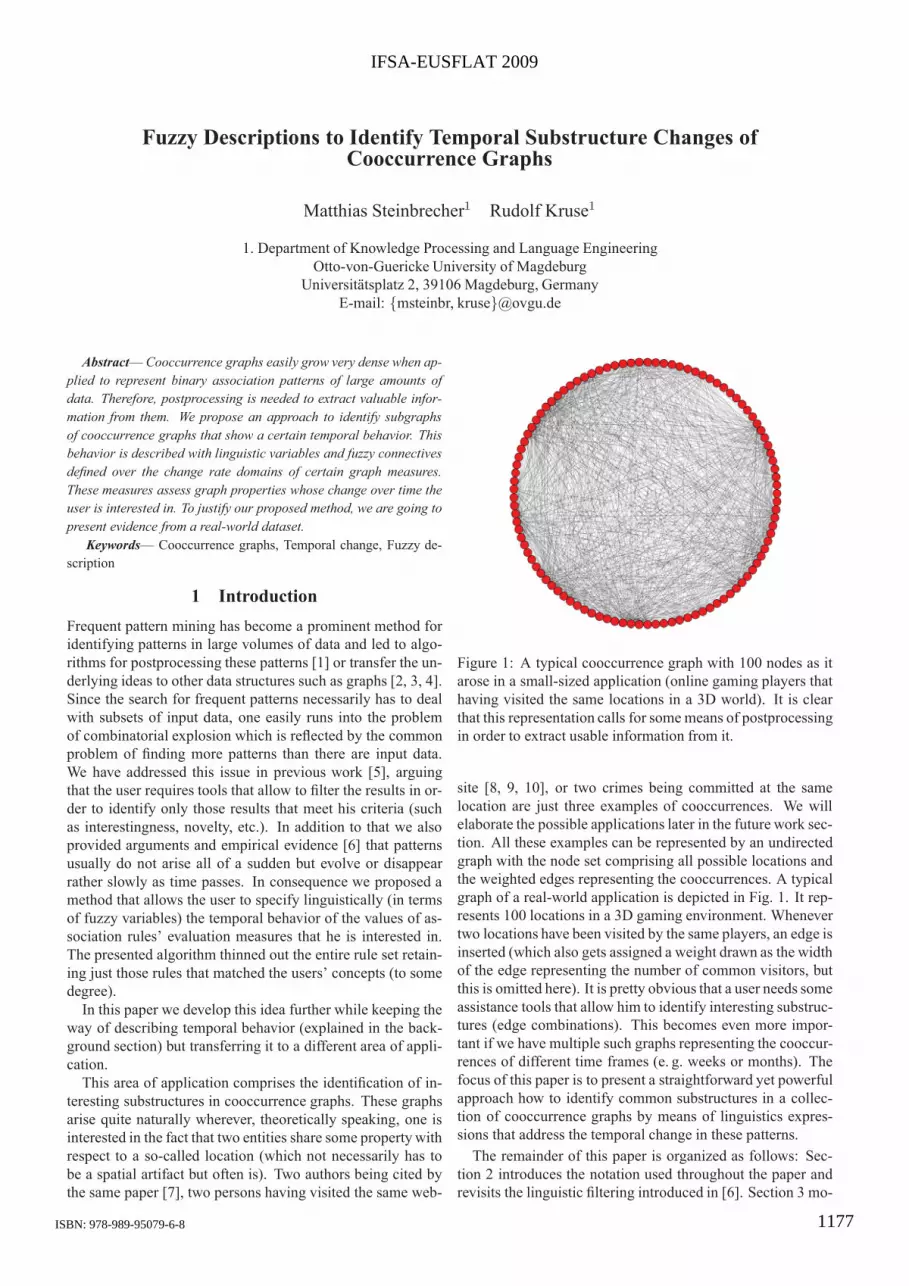
Figure 1: A typical cooccurrence graph with 100 nodes as itarose in a small-sized application (online gaming players thathaving visited the same locations in a 3D world). It is clearthat this representation calls for some means of postprocessingin order to extract usable information from it.

site [8, 9, 10], or two crimes being committed at the samelocation are just three examples of cooccurrences. We willelaborate the possible applications later in the future work sec-tion. All these examples can be represented by an undirectedgraph with the node set comprising all possible locations andthe weighted edges representing the cooccurrences. A typicalgraph of a real-world application is depicted in Fig. 1. It rep-resents 100 locations in a 3D gaming environment. Whenevertwo locations have been visited by the same players, an edge isinserted (which also gets assigned a weight drawn as the widthof the edge representing the number of common visitors, butthis is omitted here). It is pretty obvious that a user needs someassistance tools that allow him to identify interesting substruc-tures (edge combinations). This becomes even more impor-tant if we have multiple such graphs representing the cooccur-rences of different time frames (e. g. weeks or months). Thefocus of this paper is to present a straightforward yet powerfulapproach how to identify common substructures in a collec-tion of cooccurrence graphs by means of linguistics expres-sions that address the temporal change in these patterns.

The remainder of this paper is organized as follows: Sec-tion 2 introduces the notation used throughout the paper andrevisits the linguistic filtering introduced in [6]. Section 3 mo-

ISBN: 978-989-95079-6-8

IFSA-EUSFLAT 2009

1177

tivates and presents the method of extracting substructures ofcooccurrence graphs that exhibit a certain user-specified tem-poral behavior. To underpin our proposal, we use a real-worlddataset to illustrate the different stages of analysis in Section 4.Since this dataset reveals substructures that could not havebeen better generated manually, we refrain from handcraftingan artificial dataset and use selected subsets instead. We con-clude our paper in Section 5 and propose other applications aswell as possible promising extensions.

2 Background and Nomenclature2.1 Graph NotationsIn this paper we are going to deal exclusively with undirectedgraphs which we model as a tuple G = (V, E) with vertices V

and edge set E with

E ⊆ V × V \ {(v, v) | v ∈ V },

and the constraint

(u, v) ∈ E ⇒ (v, u) ∈ E

to emphasize the undirected character. We will interpret thegraphs as cooccurrence graphs where edges determine thenumber of cooccurrences (of whatever kind). This is takeninto account with an edge weight function for every edgee = (u, v):

w : E → N0 with w(e) = w(u, v) = w(v, u).

In the figures, this weight is represented as the edge width,thus we use the notion width and weight interchangeably.Given a subset W ⊆ V , we can induce a subgraphGW = (W, EW ) with

E ⊇ EW = {(u, v) | u, v ∈ W ∧ (u, v) ∈ E}.

In the remainder we will sometimes use such a subset W in thecontext of a graph; it is GW that we then refer to. A thresh-old θ defines the subgraph Gθ = (V, Eθ) with

Eθ = {(u, v) | (u, v) ∈ E ∧ w(u, v) ≥ θ},

i. e., as the graph containing only edges with a weight greateror equal to θ. Both operations can of course be combined, i. e.,GW,θ represents the subgraph of G induced by the node set W

after having removed all edges with weight less than θ.Since we will deal with sequences of graphs, we denote the

temporal index as a superscript. All graphs share the samenode set V and differ only in their edge sets or edge weightsor both. Given a sequence G(1), . . . , G(n) of graphs, we definethe sum of these graphs as follows: GΣ = (V, EΣ) with

EΣ =

n⋃i=1

E(i) and wΣ(u, v) =

n∑i=1

w(i)(u, v).

2.2 Linguistic Filtering RevisitedAs described in [6] it is not only important to find patternsthat meet some predefined constraints (such as minimum sup-port or confidence) but also interpret these patterns in terms oftemporal change. If a pattern describes a problem in somedomain or an interesting customer behavior, it might be of

interest to find such evolving patterns early. The underlyingidea is as follows: given a pattern, we devise a set of evalu-ation measures that characterize the particular pattern (in [6]we used association rule measures such as support, lift, con-fidence, etc.). Next, the time series of a user-selected subsetof these measures is calculated for every pattern. Each timeseries in turn is aggregated to a single value representing theoverall trend, if any. The domain of this aggregate (i. e., thechange rate domain) is equipped with an adequate fuzzy par-tition. Given a fuzzy rule antecedent (representing the user’sintention of what temporal behavior of which measure(s) heis interested in), for every rule a membership degree to thisconcept is computed and an ordered list of rules according tothese degrees is returned.

3 Spatio-temporal Filtering3.1 MotivationThe objective of our approach is to answer questions of thefollowing type (given a sequence of cooccurrence graphs):

“First, what are interesting candidates for subgraphsthat it would be worth looking at over time?”

and

“Second, given a (still intractable large) set of sub-graphs, which graphs become more sparse and lessbalanced over time?”

Before we turn to the algorithmic part of our approach, weneed to negotiate which types of substructures within thegraphs are most interesting to users. We will exploit the edgeweights for this purpose. Several measures are needed toquantify for every subgraph aspects such as size, complete-ness, edge balance, etc.

If the cooccurrence graphs represent visits of different webpages within the same online shop portal, then it might be de-sirable to know whether customers are able to use the webportal as intended by the owners. Are there dead ends whereusers are stuck? What are the “hot spot” sites, i. e., the pagesthat attract the most users and are visitors able to find the re-cently introduced shortcut to related pages? How do the ac-cesses to the support area of the site change after renewing thenavigational aids, etc.

We explicitly stress that subgraphs that are heavily intercon-nected with large edge weights only provide us with a hint thatthere may be an interesting visiting pattern. However, we cannever conclude transitivity just from the cooccurrence graph!This is due to the fact that it only represents binary cooccur-rences. Even a fully connected graph does not tell us anythingabout individual events. The sets of cooccurring events whosecardinality is represented by the edge weights even might bemutually disjoint. However, these subgraphs are found to bevaluable hints that are worth being investigated.

3.2 Graph MeasuresFocussing on the before-mentioned type of aspects one canidentify highly connected subgraphs with large edge weightsto be one type of substructures that are most interesting tousers. Another type may be single edges just connecting twonodes or substructures that are highly interconnected but with

ISBN: 978-989-95079-6-8

IFSA-EUSFLAT 2009

1178

G1

G2

Measure G1 G2

size Size 5.0 5.0comp Completeness 0.7 1.0wght Total Weight 5082.0 7906.0avg Average Weight 726.0 790.6med Median Weight 257.0 770.0dev Std. Dev. 1191.1 129.3

Figure 2: Two graphs with the same number of nodes. G1

lacks three edges to be complete, therefore the completenessis just 0.7, whereas the clique G2 yields 1.0. The rather largedifference between average weight and median weight for G1

(in contrast to G2) indicate an imbalanced edge widths distri-bution which is strengthened by the large standard deviationvalue. The two graphs obviously justify this finding. Thelayout only acts as a visual cue and thus does not have anyinfluence on the graph measures.

a large imbalance in the edge weights. The latter might repre-sent two active sets of websites (large edge weights) betweenwhich users are able to navigate back and forth (numerousedges in between but with small weights since not every useris likely to use the offered navigational freedom).

The last arguments call for measures that on the one handcapture the mentioned properties of subgraphs and on theother hand allow to build a fuzzy partition on their domainssince we are not going to ask for subgraphs with 9 nodes andedges with weights greater than 100 but for large subgraphswith moderately sized edges. We use the following set of(sub)graph measures to quantify different aspects:

Size size(GW ) = |W |

Completeness comp(GW ) =2 |EW |

|W |2 − |W |Edge Weight wght(GW ) =

∑e∈EW

w(e)

The size simply represents the number of nodes of the sub-graph, whereas completeness refers to the relative numberof edges compared to the maximal number. Zero representsan isolated graph (no edges) while a value of 1 designates aclique. Finally, the edge weight simply returns the sum ofall edge weights without giving any clue about the distribu-tion of these weights among the edges. Therefore, three addi-tional measures are used: avg(GW ) calculates the arithmeticmean of all edge weights, med(GW ) returns the median of theweights and dev(GW ) represents the standard deviation of theweights. Fig. 2 illustrates these intentions with two graphs ofthe same size. Note, that these are subgraphs from real-world

data and no artificial graphs that were crafted to meet the re-quirements.

3.3 Candidate Graph GenerationAs we are now equipped with measures to assess certain as-pects of subgraphs that we would like to track over time,the remaining question is how to determine such candidategraphs? It is clear that a brute-force approach (testing allsubsets of nodes as potential subgraph node sets) fails im-mediately due to runtime problems, even for small node sets.We therefore promote the following heuristic: The graphs ofall time frames are added as shown in Section 2 to arriveat the sum graph GΣ (or simply the cooccurrence graph ifwe ignore the time frames). Next, a threshold θ is chosenand the graph’s components (disconnected subgraphs) CGΣ ={C1, . . . , Cj , . . . , Cm} of GΣ,θ are taken as the candidate sub-graphs. The choice of θ can be entirely left to the user (e. g.by offering a graphical preview tool that shows the compo-nents instantly whenever the user selects a new threshold viaa slider) or θ may be determined in such a way to limit eitherthe number of components or the (average) size of the compo-nents.

3.4 Matching Against Linguistic ConceptsWhatever way of determining the granularity of components ischosen, we are left with a set of mutual disjoint node sets CGΣ

that are used to create a sequence of subgraphs⟨G

(i)Cj

⟩, i =

1, . . . , n, j = 1, . . . , m (one sequence for every subgraphinduced by the node set) that are evaluated against the user-specified temporal behavior description. A time series is gen-erated for every measure referenced in this user description.The temporal change within this time series is computed andthe degree of membership to the user description is calculated.We will employ a simple regression approach, i. e., we fit a re-gression line into the time series and interpret its slope as anindicator of decrease, stability and increase.

The example concept from the motivation of this section isrepeated here:

“Completeness is decreasing and std. deviation is increasing”

Translated into a linguistic concept, the user may specify

〈 ∆comp is decr ∧ ∆dev is incr 〉 ,

which is evaluated to

$(µ

(decr)∆comp

(Cj), µ(incr)∆dev

(Cj)),

where $ represents a t-norm modelling the fuzzy conjunction(we use $min(a, b) = min{a, b} in this paper). Fig. 3 depictsan example subgraph consisting of 9 nodes. Five time framesare shown with the respective edge weights. The graph is ob-viously becoming less dense with time, i. e., the completenessis decreasing. The chart for this measure is depicted in Fig. 4.In analogy to this, Fig. 5 shows the increasing deviation ofthe edge weights which is attributed to the emergence of thestrong cooccurrence (the sudden appearance in this case canbe explained with time frames that were too large to appro-priately cover the short period during which this strong cooc-currence emerged). If we equipped the change rate domains

ISBN: 978-989-95079-6-8

IFSA-EUSFLAT 2009

1179

Figure 3: The temporal evolution of the graphs induced by a set of nine nodes. The number of edges is decreasing with timeresulting in an almost isolated graph. Simultaneously, the edges that are remaining grow more and more unbalanced, i. e., thedeviation of the edge weights is increasing. Both time series of the corresponding measures comp and dev are shown in Fig. 4and Fig. 5, respectively.

Figure 4: Time series with decreasing trend for the complete-ness of the edge weights for the five graphs of the time framesdepicted in Fig. 3.

Figure 5: Time series with increasing trend for the standarddeviation of the edge weights for the five graphs of the timeframes depicted in Fig. 3.

(i. e., domains of the slopes of the regressions lines of the twotime series) with appropriate fuzzy partitions (as we will doit in the experiments section) we could calculate the member-ship degree of this node set to the above-mentioned linguisticconcept.

Summarizing, we state the following procedure:

1. Given a sequence G(0), . . . , G(n) of cooccurrence graphswith their sum graph being GΣ.

2. Based on an appropriate value θ, we calculate the can-didate graph node sets {C1, . . . , Cm} which are the ver-tices of the components of GΣ,θ .

3. The user provides a set of linguistic descriptions (fuzzy

rule antecedents) that refer to the temporal change of thegraph measures.

4. Provide fuzzy partitions for every domain of the changerate of the measures used in the descriptions of step 3.

5. Evaluate for every graph GCj the degree of membershipto the linguistic concepts of step 3.

6. For every linguistic concept sort the graphs in descendingorder with respect to their membership degrees.

4 ExperimentsNow that we have a tool at hand that allows us to determine thestructural changes of subgraphs over time, we demonstrate theapplicability with a real-world dataset that was already used toillustrate the examples above.

This dataset contains player contacts at certain locationswithin a 3D environment over a time period of six months.We carefully selected a subset of 100 such locations and dis-cretized month-wise in order to result in a dataset large enoughto justify the need for filtering while simultaneously being ableto extract subgraphs that exhibit a structure and behavior thatcould not have been crafted more exemplary by hand. There-fore, we refrain from creating an artificial dataset with just thesame structures.

Fig. 6 shows the sum graph of the dataset, i. e., the cooccur-rences of six months among 100 locations. The edge weightsindicate some subgraphs that are worth looking closer at. Thethreshold θ has been chosen to be 1000 to induce the candidatenode sets.

We will match two linguistic concepts against these graphcandidates: first, we are interested in decay, i. e., in graphs thatshow kind of a dissolving behavior, translating into a decreas-ing completeness and decreasing total weight. In the sampledata this might indicate locations whose attractiveness is di-minishing. A second concept that we would like to assess isthat of an establishing pattern. An increasing average edgeweight and deviation (of edge weight) might point out a phaseof initial apparent random visiting of multiple locations whichaccumulates into a strong favored visiting pattern.

4.1 Concept 1: Decreasing Completeness and WeightIn order to evaluate the membership degrees to the linguisticconcept

〈 ∆comp is decr ∧ ∆wght is decr 〉 ,

ISBN: 978-989-95079-6-8

IFSA-EUSFLAT 2009

1180

Figure 6: The sum graph of six months of visiting history ofplayers in a 3D environment. We will match the major com-ponents (extracted via a user-specified threshold) against twolinguistic concepts.

Figure 7: Fuzzy partitions for the four graph measures used inthe two experiments.

we need to declare a fuzzy partition on the change rate do-mains of comp and wght. Fig. 7 displays all used fuzzy parti-tions. We apply three fuzzy sets. Note the asymmetric slopesof the borders. This setup has proven to be useful in this con-text since “unchanged” has a more strict semantic to users thanthe adjectives “decreasing” and “increasing”. The respectivevalues that determine the particular fuzzy partition can be readfrom the four different horizontal scales. These values havebeen selected with respect to the dataset since the quantity thatrenders a slope to be highly decreasing or increasing differs,of course, from dataset to dataset.

If we apply the linguistic concept to the candidate graphsand select the one with the highest membership (ignoring theremaining ones here for brevity), the subgraph whose historyis depicted in the upper row in Fig. 8 scores 0.71. Most of thehigh degree can be attributed to the rapid loss of visits in thelast two months. The membership degree was evaluated via

min{µ(decr)∆comp

(C1), µ(decr)∆wght

(C1)} = min{0.71, 0.84} = 0.71,

with C1 being the set containing the five nodes. Data inspec-tion revealed a newly set up structure which was heavily fre-quented shortly after opening followed by abating excitement.

4.2 Concept 2: Increasing Average and DeviationWe follow the same procedure to find the subgraph that scoresbest on the concept

〈 ∆avg is incr ∧ ∆dev is incr 〉 .

The lower part of Fig. 8 shows the resulting graph with a scoreof

min{µ(incr)∆avg

(C2), µ(incr)∆dev

(C2)} = min{0.83, 0.89} = 0.83,

The graph shows an establishing link between two nodes inparallel with a weakening in the remaining edges thus render-ing the graph history becoming more unbalanced.

5 Conclusion and Future WorkIn this paper we discussed the need to postprocess cooccur-rence graphs if they grow very dense in practical use. We putforward a heuristic that allows to restrict the candidate nodesets, and transferred the fuzzy concept matching approachfrom [6] to the graphical setting. We provided empirical ev-idence of the applicability by analyzing a real-world datasetcontaining six months of game player visits to 100 locationsin a 3D environment.

As indicated in the introductory section, there are manyother scenarios for which such an analysis might be inter-esting. We are most interested in applying our method to aweb click stream analysis.

Since the used real-world dataset contained time stamps forevery event, it is possible to generate a directed graph that alsoindicates which nodes were the source and target nodes fordifferent users. This requires, of course, some heuristic withwhich to decide what should be the maximal period in whicha user has to commit two visits to different nodes in order toassume that it was a transition and not just two independentvisits.

A shortcoming of the presented approach is the heuristic togenerate the candidate node sets. It worked well on the un-derlying datasets but one can imagine that it will return fewerand more interconnected components the more the threshold θ

is reduced. Such subgraphs are also referred to as giant con-nected components [11]. To address this problem, we intendto phrase the problem in the setting of the emerging area ofgraph mining, more specific finding common substructures ina single graph [2, 12]. However, we will need a more spe-cific subgraph definition since we have to account for the edgeweights and not only the edge presence. This in turn automat-ically leads to another area of investigation: devising moresophisticated graph measures such as the edge betweennesscentrality [13].

References

[1] Rakesh Agrawal, Tomasz Imielinski, and Arun N. Swami.Mining Association Rules between Sets of Items in LargeDatabases. In Peter Buneman and Sushil Jajodia, editors, Proc.ACM SIGMOD Int. Conf. on Management of Data, Washington,D.C., May 26-28, 1993, pages 207–216. ACM Press, 1993.

[2] Mathias Fiedler and Christian Borgelt. Subgraph support in asingle graph. In Proc. IEEE Int. Workshop on Mining Graphsand Complex Data (MGCS 2007 at ICDM 2007, Omaha, NE),pages 399–404. IEEE Press, Piscataway, NJ, USA, 2007.

ISBN: 978-989-95079-6-8

IFSA-EUSFLAT 2009

1181

Figure 8: The histories of the two subgraphs that scored highest in the two experiments. The upper row shows a six-monthdevelopment of five locations that were heavily visited but declined rather rapidly towards the end. It yielded a membershipdegree of 71% to the concept “completeness is decreasing and total weight is decreasing”. The lower row depicts the best-scoring subgraph of the second experiment resulting in a membership degree of 83% to the concept “average is increasing anddeviation is increasing.”

[3] Christian Borgelt. On canonical forms for frequent graph min-ing. In Workshop on Mining Graphs, Trees, and Sequences(MGTS’05 at PKDD’05, Porto, Portugal), pages 1–12, Porto,Portugal, 2005. ECML/PKDD’05 Organization Committee.

[4] Tobias Werth, Alexander Dreweke, Marc Worlein, Ingrid Fis-cher, and Michael Philippsen. Dagma: Mining directed acyclicgraphs. In IADIS, editor, Proceedings of the ECDM 2008(IADIS European Conference on Data Mining (ECDM) ), pages11–17. IADIS PRESS, 2008.

[5] Rudolf Kruse, Christian Borgelt, Detlef D. Nauck, Nees Janvan Eck, and Matthias Steinbrecher. The role of soft comput-ing in intelligent data analysis. In Proc. 16th IEEE Int. Conf.on Fuzzy Systems (FUZZ-IEEE’07, London, UK), pages 9–17.IEEE Press, Piscataway, NJ, USA, 2007.

[6] Matthias Steinbrecher and Rudolf Kruse. Identifying tempo-ral trajectories of association rules with fuzzy descriptions. InProc. Conf. North American Fuzzy Information Processing So-ciety (NAFIPS 2008), pages 1–6, New York, USA, May 2008.

[7] Levent Bolelli, Seyda Ertekin, and C. Lee Giles. KnowledgeDiscovery in Databases: PKDD 2006, volume 4213/2006,chapter Clustering Scientific Literature Using Sparse CitationGraph Analysis, pages 30–41. Springer Berlin / Heidelberg,2006.

[8] Prasanna Desikan and Jaideep Srivastava. Advances in WebMining and Web Usage Analysis, volume 3932/2006 of Lec-ture Notes in Computer Science, chapter Mining TemporallyChanging Web Usage Graphs, pages 1–17. Springer Berlin /Heidelberg, 2006.

[9] M. E. J. Newman. Modularity and community structure in net-works. PROC.NATL.ACAD.SCI.USA, 103:8577, 2006.

[10] Aaron Clauset, M. E. J. Newman, and Cristopher Moore. Find-ing community structure in very large networks. Physical Re-view E, 70:066111, 2004.

[11] Bela Bollobas. Random Graphs, chapter The Evolution of Ran-dom Graphs — the Giant Component, pages 130–159. Cam-bridge Univ Press, 2nd edition, 2001.

[12] Bjorn Bringmann and Siegfried Nijssen. Advances in Knowl-edge Discovery and Data Mining, volume 5012/2008 of Lec-ture Notes in Computer Science, chapter What Is Frequent in a

Single Graph?, pages 858–863. Springer Berlin / Heidelberg,2008.

[13] U. Brandes and C. Pich. Centrality estimation in large net-works. International Journal of Bifurcation and Chaos 17,7:2303–2318, 2007.

ISBN: 978-989-95079-6-8

IFSA-EUSFLAT 2009

1182