Embed Size (px)
Citation preview
TH
E
U N I V E RS
IT
Y
OF
ED I N B U
RG
H
School of Informatics, University of Edinburgh
Centre for Intelligent Systems and their Applications
Fuzzy rrDFCSP and planning
by
Ian Miguel, Qiang Shen
Informatics Research Report EDI-INF-RR-0199
School of Informatics January 2003http://www.informatics.ed.ac.uk/

Fuzzy rrDFCSP and planning
Ian Miguel, Qiang Shen
Informatics Research Report EDI-INF-RR-0199
SCHOOL of INFORMATICSCentre for Intelligent Systems and their Applications
January 2003
appeared in Artificial Intelligence
Abstract :Constraint satisfaction is a fundamental Artificial Intelligence technique for knowledge representation and infer-
ence. However, the formulation of a static constraint satisfaction problem (CSP) with hard, imperative constraints isinsufficient to model many real problems. Fuzzy constraint satisfaction provides a more graded viewpoint. Prioritiesand preferences are placed on individual constraints and aggregated via fuzzy conjunction to obtain a satisfaction de-gree for a solution to the problem. This paper examines methods for solving an important instance of dynamic flexibleconstraint satisfaction (DFCSP) combining fuzzy CSP and restriction/relaxation based dynamic CSP: fuzzy rrDFCSP.This allows the modelling of complex situations where both the set of constraints may change over time and there isflexibility inherent in the definition of the problem. This paper also presents a means by which classical planning can beextended via fuzzy sets to enable flexible goals and preferences to be placed on the use of planning operators. A rangeof plans can be produced, trading compromises made versus the length of the plan. The flexible planning operators areclose in definition to fuzzy constraints. Hence, through a hierarchical decomposition of the planning graph, the workshows how flexible planning reduces to the solution of a set of fuzzy rrDFCSPs.
Keywords : Constraint satisfaction, Dynamic CSP, Flexible CSP, AI planning, Flexible planning
Copyright c�
2004 by The University of Edinburgh. All Rights Reserved
The authors and the University of Edinburgh retain the right to reproduce and publish this paper for non-commercialpurposes.
Permission is granted for this report to be reproduced by others for non-commercial purposes as long as this copy-right notice is reprinted in full in any reproduction. Applications to make other use of the material should be addressedin the first instance to Copyright Permissions, School of Informatics, The University of Edinburgh, 2 Buccleuch Place,Edinburgh EH8 9LW, Scotland.
ARTICLE IN PRESSS0004-3702(03)00020-1/FLA AID:1973 Vol.•••(•••) P.1 (1-42)ELSGMLTM(ARTINT):m1a v 1.139 Prn:2/04/2003; 15:19 aij1973 by:ML p. 1
Artificial Intelligence ••• (••••) •••–•••www.elsevier.com/locate/artint
Fuzzy rrDFCSP and planning
Ian Miguel a, Qiang Shen b,∗
a Department of Computer Science, University of York, York YO10 5DD, UKb School of Informatics, University of Edinburgh, Edinburgh EH8 9LE, UK
Received 16 July 2002; received in revised form 1 September 2002
Abstract
Constraint satisfaction is a fundamental Artificial Intelligence technique for knowledge represen-tation and inference. However, the formulation of a static constraint satisfaction problem (CSP) withhard, imperative constraints is insufficient to model many real problems. Fuzzy constraint satisfactionprovides a more graded viewpoint. Priorities and preferences are placed on individual constraints andaggregated via fuzzy conjunction to obtain a satisfaction degree for a solution to the problem. Thispaper examines methods for solving an important instance of dynamic flexible constraint satisfaction(DFCSP) combining fuzzy CSP and restriction/relaxation based dynamic CSP: fuzzy rrDFCSP. Thisallows the modelling of complex situations where both the set of constraints may change over timeand there is flexibility inherent in the definition of the problem. This paper also presents a means bywhich classical planning can be extended via fuzzy sets to enable flexible goals and preferences tobe placed on the use of planning operators. A range of plans can be produced, trading compromisesmade versus the length of the plan. The flexible planning operators are close in definition to fuzzyconstraints. Hence, through a hierarchical decomposition of the planning graph, the work shows howflexible planning reduces to the solution of a set of fuzzy rrDFCSPs. 2003 Elsevier Science B.V. All rights reserved.
Keywords: Constraint satisfaction; Dynamic CSP; Flexible CSP; AI planning; Flexible planning
1. Introduction
Constraints are a natural means of knowledge representation in many disparate fields.A constraint often takes the form of an equation or inequality, but in the most abstractsense is a logical relation among several variables expressing a set of admissible value
* Corresponding author.E-mail addresses: [email protected] (I. Miguel), [email protected] (Q. Shen).
0004-3702/03/$ – see front matter 2003 Elsevier Science B.V. All rights reserved.
doi:10.1016/S0004-3702(03)00020-1
ARTICLE IN PRESSS0004-3702(03)00020-1/FLA AID:1973 Vol.•••(•••) P.2 (1-42)ELSGMLTM(ARTINT):m1a v 1.139 Prn:2/04/2003; 15:19 aij1973 by:ML p. 2
2 I. Miguel, Q. Shen / Artificial Intelligence ••• (••••) •••–•••
combinations. The following are simple examples: the sum of two variables must equal
30; adjacent countries on the map cannot be coloured the same; the helicopter is designedto carry one passenger, but a second can be carried in an emergency; the maths class mustbe scheduled between 9 and 11am, but it may later be moved to the afternoon.Constraint satisfaction is the process of identifying a solution to a problem whichsatisfies all specified constraints. The classical Constraint Satisfaction Problem (CSP)[7,18,33] involves a fixed set of problem variables, each with an associated domain ofpotential values. A set of constraints range over the variables, specifying the allowedcombinations of assignments of values to variables. To solve a classical CSP, it is necessaryto find one or all assignments to all variables such that all constraints are satisfied.A constraint satisfaction solution procedure must find one/all such assignments or provethat no such solution exists.
Despite its simplicity, a constraint-based representation can express real, difficultproblems. For example, the problems of interpreting an image, scheduling a collectionof tasks or diagnosing a fault in an electrical circuit can all be viewed as instances of theCSP. One area that involves extensive use of constraint satisfaction is that of AI planning[38]. Graphplan [3] reduces classical domain-independent planning [38] to the solution ofa CSP. By this method, large efficiency gains were made as compared to previous state-of-the-art planning algorithms.
As classical constraint satisfaction has been applied to more complex real problemsit has become increasingly clear that the classical formulation is insufficient. Consider,for instance, the opening example involving the capacity of the helicopter. In reality, ifno other solution could be found the helicopter would carry a second passenger to createa compromise solution. Classical constraint satisfaction supports hard constraints whichare imperative (a valid solution must satisfy all of them) and inflexible (constraints areeither wholly satisfied or wholly violated). In reality problems rarely exhibit this rigidityof structure. It is common for there to be flexibility which can be used to overcomeover-constrainedness (i.e., a problem with no solution) by indicating where a sensiblecompromise can be made [22]. Classical CSP has been extended to incorporate differenttypes of ‘soft’ constraints often found in real problems. One successful example is fuzzyCSP [9]. Rather than enforcing binary satisfaction/dissatisfaction, it provides a moregraded viewpoint through a fuzzy set-based representation. Priorities and preferencesare placed on individual constraints and aggregated via fuzzy conjunction to obtain asatisfaction degree for each solution.
Another weakness of classical constraint satisfaction is that it cannot efficiently supportproblems whose structure is subject to change. Once the sets of variables, domains andconstraints have been defined, they are fixed for the duration of the solution process. Inreality problems may change (e.g., the opening example concerning the scheduling of themaths class) either as a solution is being constructed, or while a constructed solution isin use. If so, the natural approach is to attempt to repair the old solution, disturbing it aslittle as possible. Classical constraint satisfaction can deal at best only clumsily with thissituation, considering the changed problem as an entirely new problem to be solved fromscratch. To address these types of problem, dynamic constraint satisfaction techniques havebeen developed [20]. To model problems which change over time, constraints are addedto (constraint restriction) and removed from (constraint relaxation) the current problem
ARTICLE IN PRESSS0004-3702(03)00020-1/FLA AID:1973 Vol.•••(•••) P.3 (1-42)ELSGMLTM(ARTINT):m1a v 1.139 Prn:2/04/2003; 15:19 aij1973 by:ML p. 3
I. Miguel, Q. Shen / Artificial Intelligence ••• (••••) •••–••• 3
(rrDCSP, [8]). Specialised techniques re-use as much of the solution or partial solution
obtained for a problem before it changed with respect to the new problem state [25,34,35].However, current dynamic constraint satisfaction research is founded almost exclusivelyon classical CSP, unable to take advantage of fuzzy constraints in a dynamic environment,and fuzzy CSP research is limited to static problems. Little has been done to combinedynamic and fuzzy constraint satisfaction to maintain the benefits of both individualapproaches to solve more complex problems. The combined approach will form animportant instance of dynamic flexible CSP [23] which will be referred to as rrDFCSP.In this paper, an extensive empirical analysis is made of the structure and properties offuzzy rrDFCSP.
Furthermore, this paper applies fuzzy rrDFCSP to the field of AI Planning. This fieldis an active and long-established research area with a wide applicability to such tasks asautomating data-processing procedures [5], game-playing [32], and large-scale logisticsproblems [39]. As per classical CSP, classical AI Planning is unable to support flexibilityin the problem description. Providing such an ability is a significant step forward for thereal-world utility of planning research. An extension to the classical AI Planning problemis presented here to incorporate fuzzy constraints to create a flexible planning problemand to show how flexible plan synthesis is reduced to the solution of a hierarchy of fuzzyrrDFCSPs. The flexible planner Flexible Graphplan (FGP) is developed as a means tosolve such problems and its performance is analysed theoretically and empirically.
The next section provides a more detailed background on classical, fuzzy and dynamicCSP. Section 3 describes fuzzy rrDFCSP and solution methods for these problems. Anextensive empirical analysis of fuzzy rrDFCSP, using several solution algorithms, is madein Section 4. Section 5 describes the flexible planning problem. Section 6 presents theFlexible Graphplan algorithm for solving such problems, which is analysed experimentallyin Section 7. Section 8 concludes the paper and points out important future work.
2. Background
A more detailed description of classical, fuzzy and dynamic constraint satisfaction isreviewed here. The Course Scheduling Problem (adapted from [9]), is used to illustrate theutility of each approach and the need for fuzzy dynamic CSP. This problem consists ofdeciding the number of lecture, exercise and training sessions for a course. In total, theremust be 8 sessions. Professor A agrees to give 4 or 5 lectures, Dr B agrees to give 3 or 4exercise sessions and there must be an additional 1 or 2 training sessions.
2.1. Classical constraint satisfaction
A classical constraint satisfaction problem (CSP) comprises n variables, X = {x1, . . . ,
xn}, each with domain Di , describing its potential values. A variable, xi , is assigned oneof the values from Di . The Course Scheduling problem uses x1, x2, x3 for the numberof each session type. A set of constraints, C, ranges over these variables. A constraintc(xi, . . . , xj ) ∈ C specifies a subset of the Cartesian product Di × · · · × Dj , indicating
ARTICLE IN PRESSS0004-3702(03)00020-1/FLA AID:1973 Vol.•••(•••) P.4 (1-42)ELSGMLTM(ARTINT):m1a v 1.139 Prn:2/04/2003; 15:19 aij1973 by:ML p. 4
4 I. Miguel, Q. Shen / Artificial Intelligence ••• (••••) •••–•••
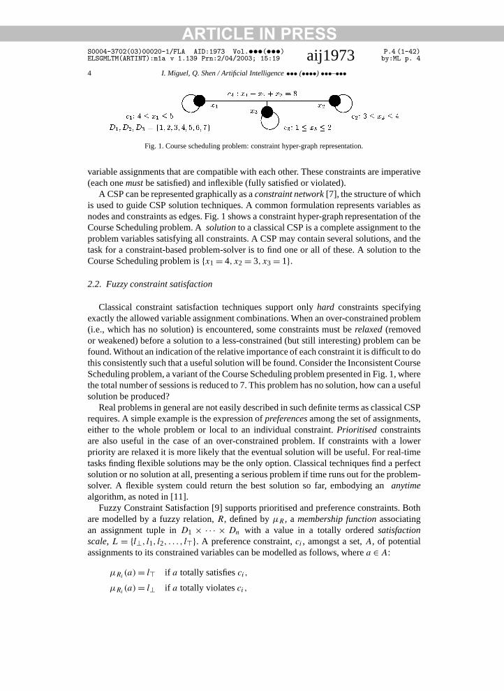
Fig. 1. Course scheduling problem: constraint hyper-graph representation.
variable assignments that are compatible with each other. These constraints are imperative(each one must be satisfied) and inflexible (fully satisfied or violated).
A CSP can be represented graphically as a constraint network [7], the structure of whichis used to guide CSP solution techniques. A common formulation represents variables asnodes and constraints as edges. Fig. 1 shows a constraint hyper-graph representation of theCourse Scheduling problem. A solution to a classical CSP is a complete assignment to theproblem variables satisfying all constraints. A CSP may contain several solutions, and thetask for a constraint-based problem-solver is to find one or all of these. A solution to theCourse Scheduling problem is {x1 = 4, x2 = 3, x3 = 1}.
2.2. Fuzzy constraint satisfaction
Classical constraint satisfaction techniques support only hard constraints specifyingexactly the allowed variable assignment combinations. When an over-constrained problem(i.e., which has no solution) is encountered, some constraints must be relaxed (removedor weakened) before a solution to a less-constrained (but still interesting) problem can befound. Without an indication of the relative importance of each constraint it is difficult to dothis consistently such that a useful solution will be found. Consider the Inconsistent CourseScheduling problem, a variant of the Course Scheduling problem presented in Fig. 1, wherethe total number of sessions is reduced to 7. This problem has no solution, how can a usefulsolution be produced?
Real problems in general are not easily described in such definite terms as classical CSPrequires. A simple example is the expression of preferences among the set of assignments,either to the whole problem or local to an individual constraint. Prioritised constraintsare also useful in the case of an over-constrained problem. If constraints with a lowerpriority are relaxed it is more likely that the eventual solution will be useful. For real-timetasks finding flexible solutions may be the only option. Classical techniques find a perfectsolution or no solution at all, presenting a serious problem if time runs out for the problem-solver. A flexible system could return the best solution so far, embodying an anytimealgorithm, as noted in [11].
Fuzzy Constraint Satisfaction [9] supports prioritised and preference constraints. Bothare modelled by a fuzzy relation, R, defined by µR , a membership function associatingan assignment tuple in D1 × · · · × Dn with a value in a totally ordered satisfactionscale, L = {l⊥, l1, l2, . . . , l}. A preference constraint, ci , amongst a set, A, of potentialassignments to its constrained variables can be modelled as follows, where a ∈A:
µRi (a)= l if a totally satisfies ci,
µRi (a)= l⊥ if a totally violates ci ,
ARTICLE IN PRESSS0004-3702(03)00020-1/FLA AID:1973 Vol.•••(•••) P.5 (1-42)ELSGMLTM(ARTINT):m1a v 1.139 Prn:2/04/2003; 15:19 aij1973 by:ML p. 5
I. Miguel, Q. Shen / Artificial Intelligence ••• (••••) •••–••• 5
l⊥ < µRi (a) < l if a partially satisfies ci .
The scale V = {v⊥, v1, v2, . . . , v} (effectively L in reverse) is used to support prioritisedconstraints, representing possibility of violation (priority) of a constraint. A prioritydegree, vj ∈ V , is associated with each prioritised constraint, cj . A constraint with priorityv is imperative and a constraint with priority v⊥ is totally irrelevant. The bijection b mapsfrom V to L such that L= b(V ). A prioritised constraint cj with priority vj is modelledas follows:
µRj (a)= l if a satisfies cj ,µRj (a)= b(vj ) if a violates cj .
A prioritised-preference constraint is represented by a fuzzy relation Rk , with µRi
describing the preference component. A constraint ck , represented by Rk will be satisfiedto at least the degree b(vk) since the priority degree defines a bound on the damage to thesolution that is incurred by the violation of this constraint. The constraint can be satisfiedabove this level by satisfying the preference component to a higher degree.
µRk (a)=max(b(vk),µRi (a)
).
The consistency level of a partial assignment is calculated from the aggregated membershipvalues of the constraints involving the assigned variables as follows, where a is anassignment to x1, . . . , xk ; ⊗ represents the conjunctive combination of fuzzy relations(usually interpreted as the minimum membership value assigned by all relations); andVars(Ri) is the set of variables constrained by the constraint represented by Ri :
cons(a)=⊗µRi (ΠVars(Ri)x).
This quantity is an upper bound on the consistency of a complete assignment. It iscomputed incrementally during search by considering only constraints that involve thecurrent variable, and is commonly used in a branch and bound search to find the bestsolution [9].
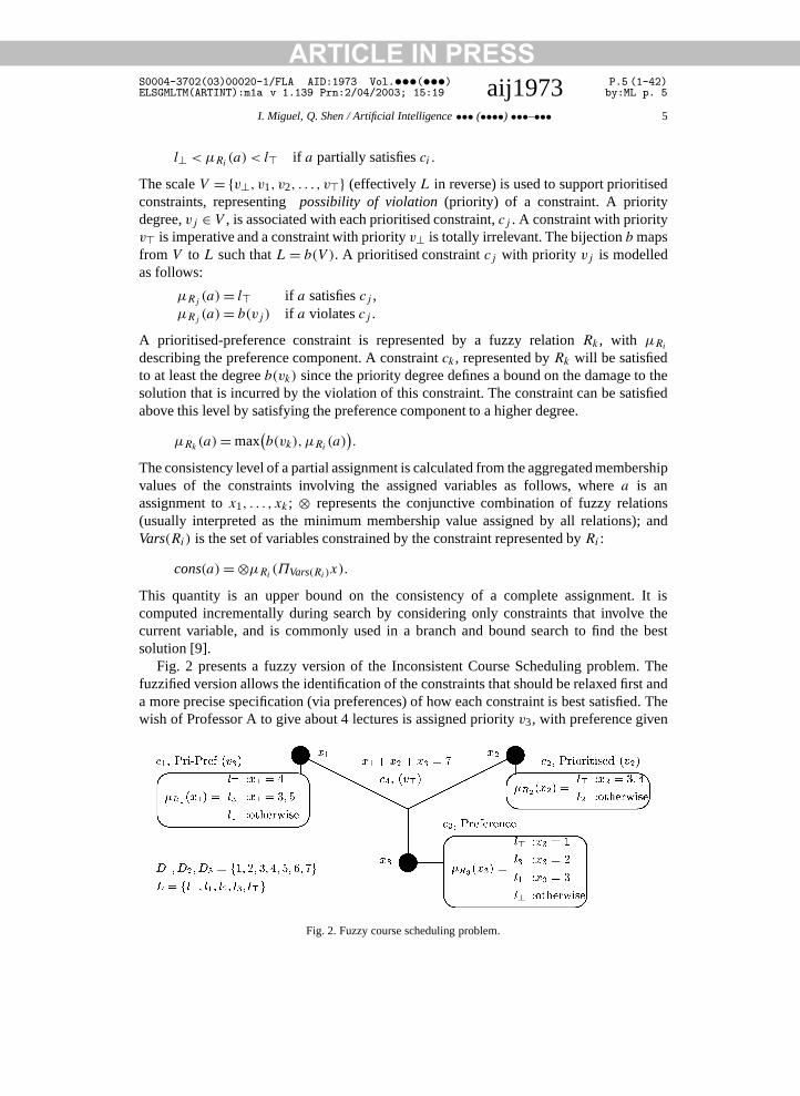
Fig. 2 presents a fuzzy version of the Inconsistent Course Scheduling problem. Thefuzzified version allows the identification of the constraints that should be relaxed first anda more precise specification (via preferences) of how each constraint is best satisfied. Thewish of Professor A to give about 4 lectures is assigned priority v3, with preference given
Fig. 2. Fuzzy course scheduling problem.
ARTICLE IN PRESSS0004-3702(03)00020-1/FLA AID:1973 Vol.•••(•••) P.6 (1-42)ELSGMLTM(ARTINT):m1a v 1.139 Prn:2/04/2003; 15:19 aij1973 by:ML p. 6
6 I. Miguel, Q. Shen / Artificial Intelligence ••• (••••) •••–•••
to values close to 4. Similarly, the wish of Dr B to give 3 or 4 lectures is assigned priority
v2. The fact that there should be about 1 additional training session is represented by apreference constraint. Finally, that there must be 7 sessions in total is a hard constraintand so is assigned priority v. As per the Inconsistent Course Scheduling problem, theFuzzy Course Scheduling problem has no perfect solution. However, a useful compromisesolution can still be found, i.e., {x3 = 3, x2 = 3, x3 = 1}. Since Professor A is relativelyhappy with giving 3 lectures, the satisfaction degree of c1 and of the overall solution is l3.2.3. Dynamic constraint satisfaction
In the description so far, problems have been assumed to be static, precluding anychanges to the problem structure after its initial specification. To a certain extent, fuzzyCSP can be seen as adding dynamicity to the problem, which is effectively changed whenviolated constraints are softened/removed. Many real problems, however, are subject tochange caused not by the need to find a compromise, but by the evolution of the problemstructure. Techniques for solving Dynamic Constraint Satisfaction Problems (DCSPs)address this need.
Although several alternative DCSP formulations exist [20], this paper concentrates onthe earliest and most natural choice, as presented in [8]. A dynamic environment is viewedas a sequence of CSPs linked by restrictions and relaxations, where constraints are addedto and removed from the problem respectively. This type of problem will hereafter bereferred to as rrDCSP. Naively, each individual problem in the sequence may be solvedfrom scratch using static CSP techniques, but this method discards all the work done insolving the previous (probably similar) problem. Efficient rrDCSP solvers re-use as muchas possible of the effort required to solve previous problems in solving the current problem.
The oracles approach [34] searches through previously solved instances for a lessconstrained version of the current problem. If one is found, the part of the searchspace before the associated solution is not explored, since no solution exists in it forthe more constrained current problem. Local repair [25,35] maintains all assignmentsfrom the solution to the previous problem to use as a starting point. Individual variableassignments are modified until an acceptable solution is obtained. Constraint recordingmethods [31,34] infer new constraints from the existing problem definition which disallowinconsistent assignment combinations not directly disallowed by the original constraints.The justifications of inferred constraints are recorded so that they can be used in futureproblems, where the same justifications hold, to converge on a solution more quickly.
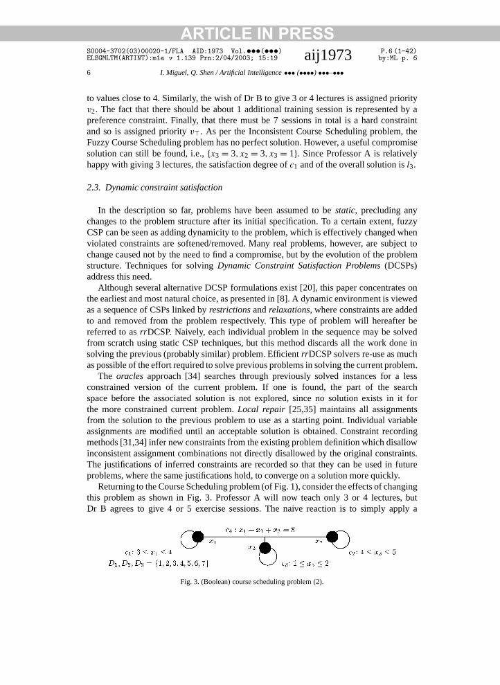
Returning to the Course Scheduling problem (of Fig. 1), consider the effects of changingthis problem as shown in Fig. 3. Professor A will now teach only 3 or 4 lectures, butDr B agrees to give 4 or 5 exercise sessions. The naive reaction is to simply apply a
Fig. 3. (Boolean) course scheduling problem (2).
ARTICLE IN PRESSS0004-3702(03)00020-1/FLA AID:1973 Vol.•••(•••) P.7 (1-42)ELSGMLTM(ARTINT):m1a v 1.139 Prn:2/04/2003; 15:19 aij1973 by:ML p. 7
I. Miguel, Q. Shen / Artificial Intelligence ••• (••••) •••–••• 7
static CSP solution procedure to the whole updated problem. This is wasteful of the work
done on the original problem. A solution to the updated Course Scheduling problem is{x1 = 3, x2 = 4, x3 = 1}. The assignment to x3 is common to both problems. An rrDCSPalgorithm exploits this fact by focusing on the subset of variables whose assignments havebecome inconsistent in light of the changed problem structure. Hence, there is a significantefficiency saving made by avoiding re-solving a large part of the problem. This type oftechnique also offers the benefits of stability: there is as little disruption from one solutionto the next as possible. An rrDCSP technique is more likely to achieve a reasonable level ofstability since a static CSP technique essentially discards all the work done on the previoussolution.3. Fuzzy rrDFCSP
The combination of fuzzy CSP and rrDCSP to form fuzzy rrDFCSP enables themodelling of a changing dynamic environment, retaining the greater expressive powerafforded by fuzzy CSP. In a dynamic environment where time may be limited, the abilityof fuzzy CSP to produce the best current solution anytime will prove even more valuable.A fuzzy rrDFCSP can be thought of as a sequence of static flexible problems as perrrDCSP, with all possible changes being realised through restriction and relaxation. Whenapplied to fuzzy CSPs, these operations can update a problem instance in more subtleways. For example, the priority of a fuzzy prioritised constraint may change, as might thepreferences of the individual tuples of a fuzzy preference constraint.
3.1. Fuzzy rrDFCSP solution techniques
The first solution technique examined for fuzzy rrDFCSP is based on the branchand bound (hereafter referred to as BB) approach to solving static fuzzy CSP [9]. Itsolves each instance in the dynamic sequence from scratch. However, the solution to theprevious problem in the sequence is maintained and used to make savings. The solutionto the previous problem in the dynamic sequence is checked against the current problembefore it is solved. If the previous solution also constitutes a solution with l satisfactiondegree for the current problem, no search is required. If it constitutes a solution for thecurrent problem with a satisfaction degree li , such that l⊥ < li < l, the solution is storedand used to set the necessary bound prior to search. During search, the solution to theprevious problem is used to guide domain element selection for assignment. Given severalpossibilities with equivalent satisfaction degrees, an assignment is preferred which matchesthat of the solution to the previous problem, if possible. This method is a simplification ofthe oracles technique described in Section 2.3.
The second solution technique examined is a recently developed extension of the LocalChanges (LC) local repair algorithm [35]. LC searches for a solution by resolving conflictsthat occur when examining the solution to the previous problem in the sequence, within thecontext of the current problem. It divides the variable set X into three subsets: X1, X2 andX3 (such that X1 ∪X2 ∪X3 =X and Xi ∩Xj = ∅ where i, j ∈ {1, 2, 3}, i �= j ). X1 is theset of variables with fixed assignments and is used to ensure termination of the algorithm;
ARTICLE IN PRESSS0004-3702(03)00020-1/FLA AID:1973 Vol.•••(•••) P.8 (1-42)ELSGMLTM(ARTINT):m1a v 1.139 Prn:2/04/2003; 15:19 aij1973 by:ML p. 8
8 I. Miguel, Q. Shen / Artificial Intelligence ••• (••••) •••–•••
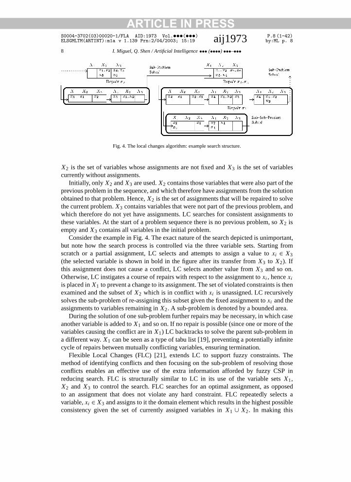
Fig. 4. The local changes algorithm: example search structure.
X2 is the set of variables whose assignments are not fixed and X3 is the set of variablescurrently without assignments.
Initially, only X2 and X3 are used. X2 contains those variables that were also part of theprevious problem in the sequence, and which therefore have assignments from the solutionobtained to that problem. Hence, X2 is the set of assignments that will be repaired to solvethe current problem. X3 contains variables that were not part of the previous problem, andwhich therefore do not yet have assignments. LC searches for consistent assignments tothese variables. At the start of a problem sequence there is no previous problem, so X2 isempty and X3 contains all variables in the initial problem.
Consider the example in Fig. 4. The exact nature of the search depicted is unimportant,but note how the search process is controlled via the three variable sets. Starting fromscratch or a partial assignment, LC selects and attempts to assign a value to xi ∈ X3
(the selected variable is shown in bold in the figure after its transfer from X3 to X2). Ifthis assignment does not cause a conflict, LC selects another value from X3 and so on.Otherwise, LC instigates a course of repairs with respect to the assignment to xi , hence xi
is placed in X1 to prevent a change to its assignment. The set of violated constraints is thenexamined and the subset of X2 which is in conflict with xi is unassigned. LC recursivelysolves the sub-problem of re-assigning this subset given the fixed assignment to xi and theassignments to variables remaining in X2. A sub-problem is denoted by a bounded area.
During the solution of one sub-problem further repairs may be necessary, in which caseanother variable is added to X1 and so on. If no repair is possible (since one or more of thevariables causing the conflict are in X1) LC backtracks to solve the parent sub-problem ina different way. X1 can be seen as a type of tabu list [19], preventing a potentially infinitecycle of repairs between mutually conflicting variables, ensuring termination.
Flexible Local Changes (FLC) [21], extends LC to support fuzzy constraints. Themethod of identifying conflicts and then focusing on the sub-problem of resolving thoseconflicts enables an effective use of the extra information afforded by fuzzy CSP inreducing search. FLC is structurally similar to LC in its use of the variable sets X1,X2 and X3 to control the search. FLC searches for an optimal assignment, as opposedto an assignment that does not violate any hard constraint. FLC repeatedly selects avariable, xi ∈X3 and assigns to it the domain element which results in the highest possibleconsistency given the set of currently assigned variables in X1 ∪ X2. In making this
ARTICLE IN PRESSS0004-3702(03)00020-1/FLA AID:1973 Vol.•••(•••) P.9 (1-42)ELSGMLTM(ARTINT):m1a v 1.139 Prn:2/04/2003; 15:19 aij1973 by:ML p. 9
I. Miguel, Q. Shen / Artificial Intelligence ••• (••••) •••–••• 9
assignment repairs may be necessary to elements of X2. Termination is upon finding an
optimally consistent complete variable assignment.The present work considers finding optimal solutions of fuzzy rrDFCSPs directly usingmin aggregation. An alternative approach is to solve each problem in a dynamic sequencevia iteratively resolving successive classical CSPs, constructed by allowing all constrainttuples with consistency degree greater than a prescribed α level. An optimal solution canbe found by moving α from l⊥ upwards one degree at a time up to the level where theCSP becomes inconsistent. Where |L| is large, a binary search could be adopted to set α
[6,10]. This remains an important avenue of future work, as is the question of how best toincorporate dynamicity into this method.
3.2. Fuzzy arc consistency
The idempotent min/max operators employed by fuzzy constraint satisfaction enable thestraightforward support of consistency enforcing techniques [30]. Fuzzy arc consistency[9] can significantly enhance the performance of both BB and FLC. Fuzzy arc consistencyholds if any assignment involving one variable with a satisfaction degree li ∈ L can beextended to any 2 variables, maintaining a satisfaction degree of li .
Enforcing fuzzy arc consistency is essentially the same process as for classical CSP[17]. The FAC3() procedure [9], based on classical AC3() [17], is used. A queue of arcsfrom the constraint network is maintained. An arc(xi, xj ) is selected and revised, i.e., theconsistency degree of each di ∈Di is updated according to:
cons(xi = di)⊗maxj
(cons(xj = dj )⊗ cons(xi = di, xj = dj )
).
If the consistency degree of any di ∈Di is updated by this revision, further revisions maybe possible to variables related to xi by constraints. Hence each arc(xh, xi), where h �= j ,is added to the queue (if not already present). The algorithm terminates when the queueis empty. The complexity of FAC3() is O(�m3e) [9], where �= |L| and e is the numberof arcs in the network. The upper bound, β , on the consistency of the whole problem isthe minimum over all the variables of the maximum consistency degrees of their domainelements.
A fuzzy version of the classical AC4() arc consistency algorithm has also beendeveloped, with complexity O(m2e) [6]. However, although AC3() has a poorer worstcase time complexity than AC4(), it is often preferred in practice because of its betteraverage case performance [36], hence the choice made here. It is of course important totest the performance of FAC4() in practice, and this is an important item of future work.
Pre-processing a problem with fuzzy arc consistency provides a bound, β , on itsconsistency. Both BB and FLC benefit from β since it facilitates early termination whena solution of satisfaction degree of β is found. Furthermore, when FLC examines theprevious solution with respect to the current problem it is only necessary to repairconstraints whose consistency is below β , leading to a higher percentage of solution reuse.Without β all constraints whose consistency degree is less than l are repaired, regardlessof the fact that a solution of consistency l may not exist. FLC may also employ β whenconsidering which constraints to repair during search.
ARTICLE IN PRESSS0004-3702(03)00020-1/FLA AID:1973 Vol.•••(•••) P.10 (1-42)ELSGMLTM(ARTINT):m1a v 1.139 Prn:2/04/2003; 15:19 aij1973 by:ML p. 10
10 I. Miguel, Q. Shen / Artificial Intelligence ••• (••••) •••–•••
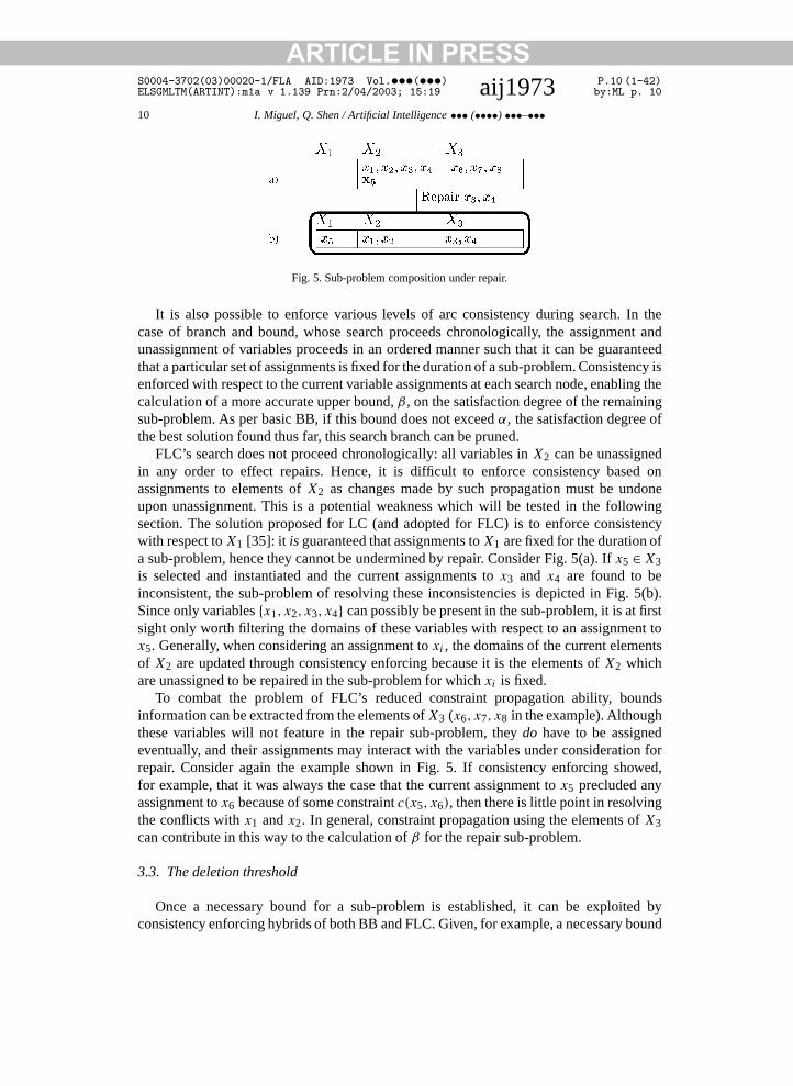
Fig. 5. Sub-problem composition under repair.
It is also possible to enforce various levels of arc consistency during search. In thecase of branch and bound, whose search proceeds chronologically, the assignment andunassignment of variables proceeds in an ordered manner such that it can be guaranteedthat a particular set of assignments is fixed for the duration of a sub-problem. Consistency isenforced with respect to the current variable assignments at each search node, enabling thecalculation of a more accurate upper bound, β , on the satisfaction degree of the remainingsub-problem. As per basic BB, if this bound does not exceed α, the satisfaction degree ofthe best solution found thus far, this search branch can be pruned.
FLC’s search does not proceed chronologically: all variables in X2 can be unassignedin any order to effect repairs. Hence, it is difficult to enforce consistency based onassignments to elements of X2 as changes made by such propagation must be undoneupon unassignment. This is a potential weakness which will be tested in the followingsection. The solution proposed for LC (and adopted for FLC) is to enforce consistencywith respect to X1 [35]: it is guaranteed that assignments to X1 are fixed for the duration ofa sub-problem, hence they cannot be undermined by repair. Consider Fig. 5(a). If x5 ∈X3is selected and instantiated and the current assignments to x3 and x4 are found to beinconsistent, the sub-problem of resolving these inconsistencies is depicted in Fig. 5(b).Since only variables {x1, x2, x3, x4} can possibly be present in the sub-problem, it is at firstsight only worth filtering the domains of these variables with respect to an assignment tox5. Generally, when considering an assignment to xi , the domains of the current elementsof X2 are updated through consistency enforcing because it is the elements of X2 whichare unassigned to be repaired in the sub-problem for which xi is fixed.
To combat the problem of FLC’s reduced constraint propagation ability, boundsinformation can be extracted from the elements of X3 (x6, x7, x8 in the example). Althoughthese variables will not feature in the repair sub-problem, they do have to be assignedeventually, and their assignments may interact with the variables under consideration forrepair. Consider again the example shown in Fig. 5. If consistency enforcing showed,for example, that it was always the case that the current assignment to x5 precluded anyassignment to x6 because of some constraint c(x5, x6), then there is little point in resolvingthe conflicts with x1 and x2. In general, constraint propagation using the elements of X3can contribute in this way to the calculation of β for the repair sub-problem.
3.3. The deletion threshold
Once a necessary bound for a sub-problem is established, it can be exploited byconsistency enforcing hybrids of both BB and FLC. Given, for example, a necessary bound
ARTICLE IN PRESSS0004-3702(03)00020-1/FLA AID:1973 Vol.•••(•••) P.11 (1-42)ELSGMLTM(ARTINT):m1a v 1.139 Prn:2/04/2003; 15:19 aij1973 by:ML p. 11
I. Miguel, Q. Shen / Artificial Intelligence ••• (••••) •••–••• 11
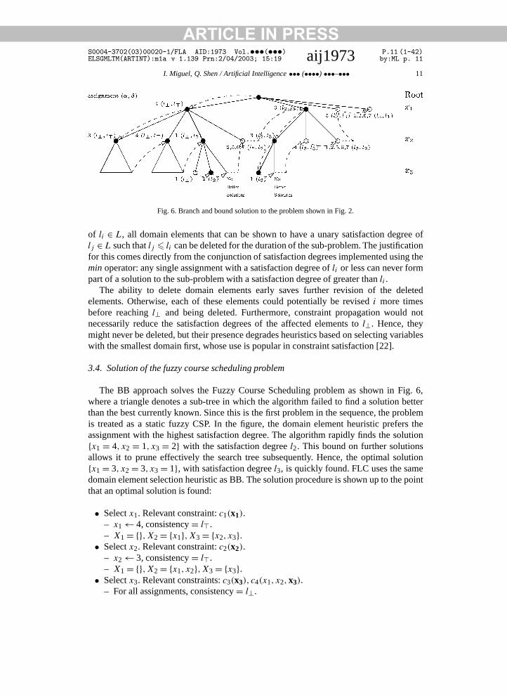
Fig. 6. Branch and bound solution to the problem shown in Fig. 2.
of li ∈ L, all domain elements that can be shown to have a unary satisfaction degree oflj ∈L such that lj � li can be deleted for the duration of the sub-problem. The justificationfor this comes directly from the conjunction of satisfaction degrees implemented using themin operator: any single assignment with a satisfaction degree of li or less can never formpart of a solution to the sub-problem with a satisfaction degree of greater than li .
The ability to delete domain elements early saves further revision of the deletedelements. Otherwise, each of these elements could potentially be revised i more timesbefore reaching l⊥ and being deleted. Furthermore, constraint propagation would notnecessarily reduce the satisfaction degrees of the affected elements to l⊥. Hence, theymight never be deleted, but their presence degrades heuristics based on selecting variableswith the smallest domain first, whose use is popular in constraint satisfaction [22].
3.4. Solution of the fuzzy course scheduling problem
The BB approach solves the Fuzzy Course Scheduling problem as shown in Fig. 6,where a triangle denotes a sub-tree in which the algorithm failed to find a solution betterthan the best currently known. Since this is the first problem in the sequence, the problemis treated as a static fuzzy CSP. In the figure, the domain element heuristic prefers theassignment with the highest satisfaction degree. The algorithm rapidly finds the solution{x1 = 4, x2 = 1, x3 = 2} with the satisfaction degree l2. This bound on further solutionsallows it to prune effectively the search tree subsequently. Hence, the optimal solution{x1 = 3, x2 = 3, x3 = 1}, with satisfaction degree l3, is quickly found. FLC uses the samedomain element selection heuristic as BB. The solution procedure is shown up to the pointthat an optimal solution is found:
• Select x1. Relevant constraint: c1(x1).– x1← 4, consistency = l.– X1 = {},X2 = {x1},X3 = {x2, x3}.• Select x2. Relevant constraint: c2(x2).
– x2← 3, consistency = l.– X1 = {},X2 = {x1, x2},X3 = {x3}.• Select x3. Relevant constraints: c3(x3), c4(x1, x2, x3).
– For all assignments, consistency = l⊥.
ARTICLE IN PRESSS0004-3702(03)00020-1/FLA AID:1973 Vol.•••(•••) P.12 (1-42)ELSGMLTM(ARTINT):m1a v 1.139 Prn:2/04/2003; 15:19 aij1973 by:ML p. 12
12 I. Miguel, Q. Shen / Artificial Intelligence ••• (••••) •••–•••
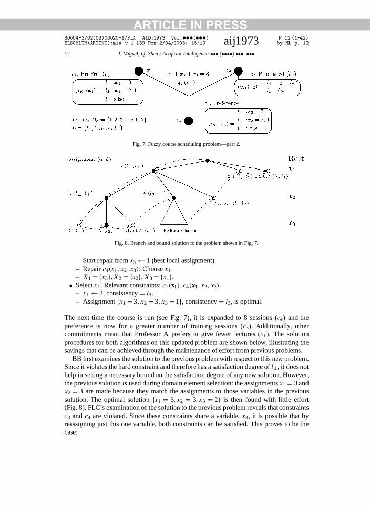
Fig. 7. Fuzzy course scheduling problem—part 2.
Fig. 8. Branch and bound solution to the problem shown in Fig. 7.
– Start repair from x3← 1 (best local assignment).– Repair c4(x1, x2, x3): Choose x1.– X1 = {x3},X2 = {x2},X3 = {x1}.• Select x1. Relevant constraints: c1(x1), c4(x1, x2, x3).
– x1← 3, consistency = l3.– Assignment {x1 = 3, x2 = 3, x3 = 1}, consistency = l3, is optimal.
The next time the course is run (see Fig. 7), it is expanded to 8 sessions (c4) and thepreference is now for a greater number of training sessions (c3). Additionally, othercommitments mean that Professor A prefers to give fewer lectures (c1). The solutionprocedures for both algorithms on this updated problem are shown below, illustrating thesavings that can be achieved through the maintenance of effort from previous problems.
BB first examines the solution to the previous problem with respect to this new problem.Since it violates the hard constraint and therefore has a satisfaction degree of l⊥, it does nothelp in setting a necessary bound on the satisfaction degree of any new solution. However,the previous solution is used during domain element selection: the assignments x1 = 3 andx2 = 3 are made because they match the assignments to those variables in the previoussolution. The optimal solution {x1 = 3, x2 = 3, x3 = 2} is then found with little effort(Fig. 8). FLC’s examination of the solution to the previous problem reveals that constraintsc3 and c4 are violated. Since these constraints share a variable, x3, it is possible that byreassigning just this one variable, both constraints can be satisfied. This proves to be thecase:
ARTICLE IN PRESSS0004-3702(03)00020-1/FLA AID:1973 Vol.•••(•••) P.13 (1-42)ELSGMLTM(ARTINT):m1a v 1.139 Prn:2/04/2003; 15:19 aij1973 by:ML p. 13
I. Miguel, Q. Shen / Artificial Intelligence ••• (••••) •••–••• 13
• Evaluate assignment {x1 = 3, x2 = 3, x3 = 1}: consistency = l⊥.
– Repair c3(x3), c4(x1, x2, x3): Choose x3 to cover both.– X1 = {},X2 = {x1, x2},X3 = {x3}.• Select x3. Relevant constraints: c3(x3), c4(x1, x2, x3).– x3← 2, consistency = l3.– Assignment {x1 = 3, x2 = 3, x3 = 2}, consistency = l3, is optimal.
For brevity of presentation, the steps performed by FLC to verify that this is indeed anoptimal solution are not given.
4. An empirical study of fuzzy rrDFCSPs
This section describes an empirical study of random fuzzy rrDFCSPs. Due to the size ofthe study (almost 40,000 individual instances), selected results are presented to reflect thegeneral trend of the data. The problems are sequences of ten fuzzy CSP instances. Binaryconstraints are considered, following the approach of many studies of classical CSP [13,28]. Each instance is generated using the following parameters:
• n. Number of variables, taking values from {20, 30, 40} in order to gauge the effectsof increasing problem size.• m. Domain size, fixed at 6 throughout to limit the size of this study. Further studies
should examine the effects of varying m.• �= |L|. Takes values from {3, 4, 5} to examine the effects of an increasing amount of
flexibility on the difficulty of finding the best solution.• con. Connectivity of the constraint graph, the proportion of the variables which are
related by a constraint. Takes values from {0.25, 0.5, 0.75}, allowing an examinationof the effects of an increasingly connected graph.• t . Constraint tightness, the proportion of assignment combinations that are disallowed
by each constraint. Takes values from {0.1, 0.2, . . ., 0.8, 0.9}.
The granularities chosen for the connectivity and tightness parameters make this studyfeasible. Interesting phenomena may occur between the values chosen, which futurestudies might investigate. Constraints are divided into an equal number of fuzzy pri-oritised, preference, and prioritised-preference types. Priority degrees are evenly distrib-uted amongst the prioritised and prioritised-preference constraints. Similarly, preferencedegrees are evenly distributed amongst the tuples of each preference and prioritised-preference constraint.
Random restriction/relaxation operations are performed. A further parameter, ch,determines the proportion of constraints that are removed and replaced (when ch = ‘1constraint’, a single constraint is replaced between instances). To maintain a uniformconstraint graph connectivity, the same number of constraints are added as are taken away.Each constraint removed is replaced by a constraint of the same type and tightness. If itis a prioritised or prioritised-preference constraint, the priority assigned is the same as theremoved constraint to maintain the original distribution. The justification for the effort of
ARTICLE IN PRESSS0004-3702(03)00020-1/FLA AID:1973 Vol.•••(•••) P.14 (1-42)ELSGMLTM(ARTINT):m1a v 1.139 Prn:2/04/2003; 15:19 aij1973 by:ML p. 14
14 I. Miguel, Q. Shen / Artificial Intelligence ••• (••••) •••–•••
maintaining a uniform problem structure is to eliminate the effects of differing proportions
of fuzzy constraint types or priority/preference distributions.Five dynamic sequences of ten instances were generated per parameter combination.Mean results are reported, hence each point on the graphs presented represents the solutionof 50 instances. In all, 3645 dynamic sequences were generated, totalling 36450 individualproblem instances to be solved.
4.1. The algorithms studied and evaluation criteria
The performances of basic BB and FLC were so poor compared to refined versions thatthey were not chosen for inclusion in this study. The naming convention for the variantstested is as follows. An ‘AC’ prefix denotes that fuzzy arc consistency is established onceprior to search. If the suffix is ‘FC’, then the consistency enforcing process correspondsto classical Forward Checking [15]: the domains of unassigned variables are revised oncewith respect to each new assignment. Similarly, if the suffix is ‘FMAC’ then, as per theclassical MAC algorithm, fuzzy arc consistency is established initially and with respect toeach new variable assignment. Unless otherwise stated, the deletion-threshold is used toenforce fuzzy arc consistency. A comparison with dynamic backtracking [14] is omittedsince, as recognised by [35], this algorithm has strong similarities with LC. Updatingdynamic backtracking to support dynamic CSPs and flexible constraints would producea very similar algorithm to FLC.
The variants of BB tested are: BBFC, ACBBFC, BBFMAC. A similar number ofbasic variants of FLC are also tested. In addition, three extra hybrids are tested whichalso take into account the domains of variables not immediately in line for repair, asdetailed in Section 3.2. These are denoted by the suffix ‘ft’ (for ‘full test’): FLCFC,FLCFCft, ACFLCFC, ACFLCFCft, FLCFMAC, FLCFMACft. Performance is judged bythree criteria:
• Constraint checks. Every time a constraint is queried for the consistency degree of apair of assignments, this is counted as a constraint check.• Search nodes expanded. Every assignment of di ∈ Di to xi corresponds to a node in
the search tree.• Solution stability. Since, in this study, the set of variables does not change within a
dynamic sequence, the stability of the solution to each problem as compared with thelast can easily be measured as the proportion of assignments that are the same. It isappropriate to use this measure, since there may be a number of solutions with optimalsatisfaction degrees.
Run-times are not reported, although they have been observed to track consistency checks.Due to the size of the study, results were collected over a large network of machines ofvarying capabilities and under differing loads. It would be difficult, therefore, to place anygreat faith in run-time results.
ARTICLE IN PRESSS0004-3702(03)00020-1/FLA AID:1973 Vol.•••(•••) P.15 (1-42)ELSGMLTM(ARTINT):m1a v 1.139 Prn:2/04/2003; 15:19 aij1973 by:ML p. 15
I. Miguel, Q. Shen / Artificial Intelligence ••• (••••) •••–••• 15
4.2. Heuristics investigated
Three operations which are ordered heuristically are the selection of a variable toinstantiate next, the choice of domain element to instantiate, and the order in whichconstraints are checked. Apart from those presented here, a variety of other heuristics weretested extensively (see [23] for details).
As the analogue of classical Backtrack, it is simple to use the Brelaz heuristic [4] withBB. That is, to select the variable with smallest remaining domain first, breaking ties bypreferring the variable with the greatest connectivity to the currently unassigned variables.FLC may also use a Brelaz-type heuristic, but the search structure of this algorithm,controlled by the sets X1, X2 and X3 provides the possibility of creating novel variations onthe variable selection heuristic. The heuristic employed in this study, SmallestD-X23,starts by selecting the variable with the smallest remaining domain and breaks ties usingthe connectivity of the variables in X2∪X3, i.e., all those variables whose assignments arefree to change. Note that even though elements of X3 do not figure in the sub-problem ofrepairing assignments, they do have to be assigned eventually and hence interact with thecurrent variable.
The domain element selection heuristic is the main method by which the BB algorithmsmake use of dynamic information. In order to attempt to find the best solutions first, theelement with the highest consistency degree is chosen first. However, if there are severalsuch elements, ties are broken by examining the solution to the previous problem in thesequence, and if one of the tied elements matches the assignment in the previous solution,it is chosen.
For FLC, value selection is split into two cases, where repairs are and are not necessary.Taking the latter case first, the element with the highest consistency degree is selected firstto find the solution with the highest consistency degree earlier. As per BB, ties are brokenby assigning the same element to a variable as appeared in the previous solution. Thismay appear counter-intuitive, but a conflict commonly necessitates the unassignment ofmultiple variables. Re-assigning each of these may trigger further repairs, and as a sideeffect remove conflicts with some previous solution assignments. If so, it is possible toreinstate the previous solution assignments, promoting stability.
When repairs are necessary, it is intuitive to select a repair that is most likely tosucceed. The domain element selection heuristic used for repair, ConsDeg-PrevSoln-con, follows the approach of the BB algorithm to an extent in first breaking ties by matchingagainst the previous solution. Ties are broken further by preferring to repair the set ofvariables with the least connectivity to the remainder of the problem.
The process of checking constraints is ordered such that the constraint most likely tofail is checked first. This is achieved by examining the size of the domains Di , Dj at theend of each arc(xi, xj ) to be checked. The heuristic prefers those arcs with the smallestsummed domain size. Ties are broken by restricting the comparison to each Di , since thisis the domain being filtered.
4.3. Results: search effort
This section investigates the relative search effort required by each algorithm to solvethe set of random fuzzy rrDFCSPs. The three variants of BB are tested against three
ARTICLE IN PRESSS0004-3702(03)00020-1/FLA AID:1973 Vol.•••(•••) P.16 (1-42)ELSGMLTM(ARTINT):m1a v 1.139 Prn:2/04/2003; 15:19 aij1973 by:ML p. 16
16 I. Miguel, Q. Shen / Artificial Intelligence ••• (••••) •••–•••
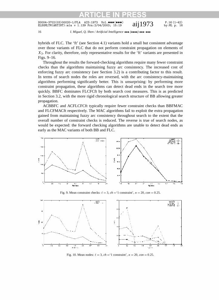
hybrids of FLC. The ‘ft’ (see Section 4.1) variants hold a small but consistent advantage
over those variants of FLC that do not perform constraint propagation on elements ofX3. For clarity, therefore, only representative results for the ‘ft’ variants are presented inFigs. 9–16.Throughout the results the forward-checking algorithms require many fewer constraintchecks than the algorithms maintaining fuzzy arc consistency. The increased cost ofenforcing fuzzy arc consistency (see Section 3.2) is a contributing factor to this result.In terms of search nodes the roles are reversed, with the arc consistency-maintainingalgorithms performing significantly better. This is unsurprising: by performing moreconstraint propagation, these algorithms can detect dead ends in the search tree morequickly. BBFC dominates FLCFCft by both search cost measures. This is as predictedin Section 3.2, with the more rigid chronological search structure of BB allowing greaterpropagation.
ACBBFC and ACFLCFCft typically require fewer constraint checks than BBFMACand FLCFMACft respectively. The MAC algorithms fail to exploit the extra propagationgained from maintaining fuzzy arc consistency throughout search to the extent that theoverall number of constraint checks is reduced. The reverse is true of search nodes, aswould be expected: the forward checking algorithms are unable to detect dead ends asearly as the MAC variants of both BB and FLC.
Fig. 9. Mean constraint checks: �= 3, ch=‘1 constraint’, n= 20, con= 0.25.
Fig. 10. Mean nodes: �= 3, ch=‘1 constraint’, n= 20, con= 0.25.
ARTICLE IN PRESSS0004-3702(03)00020-1/FLA AID:1973 Vol.•••(•••) P.17 (1-42)ELSGMLTM(ARTINT):m1a v 1.139 Prn:2/04/2003; 15:19 aij1973 by:ML p. 17
I. Miguel, Q. Shen / Artificial Intelligence ••• (••••) •••–••• 17
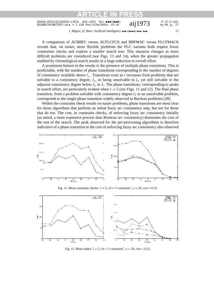
A comparison of ACBBFC versus ACFLCFCft and BBFMAC versus FLCFMACft
reveals that, on easier, more flexible problems the FLC variants both require fewerconstraints checks and explore a smaller search tree. This situation changes as moredifficult problems are considered (see Figs. 13 and 14), when the greater propagationenabled by chronological search results in a large reduction in overall effort.A prominent feature in the results is the presence of multiple phase transitions. This ispredictable, with the number of phase transitions corresponding to the number of degreesof consistency available above l⊥. Transitions exist as t increases from problems that aresolvable to a consistency degree, la , to being unsolvable to la yet still solvable to theadjacent consistency degree below la in L. The phase transitions, corresponding to peaksin search effort, are particularly evident when �= 5 (see Figs. 11 and 12). The final phasetransition, from a problem solvable with consistency degree l1 to an unsolvable problem,corresponds to the single phase transition widely observed in Boolean problems [28].
Within the constraint check results on easier problems, phase transitions are most clearfor those algorithms that perform an initial fuzzy arc consistency step, but not for thosethat do not. The cost, in constraint checks, of enforcing fuzzy arc consistency initially(as noted, a more expensive process than Boolean arc consistency) dominates the cost ofthe rest of the search. The peak observed for the pre-processing algorithms is thereforeindicative of a phase transition in the cost of enforcing fuzzy arc consistency also observed
Fig. 11. Mean constraint checks: �= 5, ch=‘1 constraint’, n= 20, con= 0.25.
Fig. 12. Mean nodes: �= 5, ch=‘1 constraint’, n= 20, con= 0.25.
ARTICLE IN PRESSS0004-3702(03)00020-1/FLA AID:1973 Vol.•••(•••) P.18 (1-42)ELSGMLTM(ARTINT):m1a v 1.139 Prn:2/04/2003; 15:19 aij1973 by:ML p. 18
18 I. Miguel, Q. Shen / Artificial Intelligence ••• (••••) •••–•••
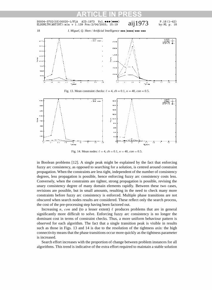
Fig. 13. Mean constraint checks: �= 4, ch= 0.1, n= 40, con= 0.5.
Fig. 14. Mean nodes: �= 4, ch= 0.1, n= 40, con= 0.5.
in Boolean problems [12]. A single peak might be explained by the fact that enforcingfuzzy arc consistency, as opposed to searching for a solution, is centred around constraintpropagation. When the constraints are less tight, independent of the number of consistencydegrees, less propagation is possible, hence enforcing fuzzy arc consistency costs less.Conversely, when the constraints are tighter, strong propagation is possible, revising theunary consistency degree of many domain elements rapidly. Between these two cases,revisions are possible, but in small amounts, resulting in the need to check many moreconstraints before fuzzy arc consistency is enforced. Multiple phase transitions are notobscured when search nodes results are considered. These reflect only the search process,the cost of the pre-processing step having been factored out.
Increasing n, con and (to a lesser extent) � produces problems that are in generalsignificantly more difficult to solve. Enforcing fuzzy arc consistency is no longer thedominant cost in terms of constraint checks. Thus, a more uniform behaviour pattern isobserved for each algorithm. The fact that a single transition peak is visible in resultssuch as those in Figs. 13 and 14 is due to the resolution of the tightness axis: the highconnectivity means that the phase transitions occur more quickly as the tightness parameteris increased.
Search effort increases with the proportion of change between problem instances for allalgorithms. This trend is indicative of the extra effort required to maintain a stable solution
ARTICLE IN PRESSS0004-3702(03)00020-1/FLA AID:1973 Vol.•••(•••) P.19 (1-42)ELSGMLTM(ARTINT):m1a v 1.139 Prn:2/04/2003; 15:19 aij1973 by:ML p. 19
I. Miguel, Q. Shen / Artificial Intelligence ••• (••••) •••–••• 19
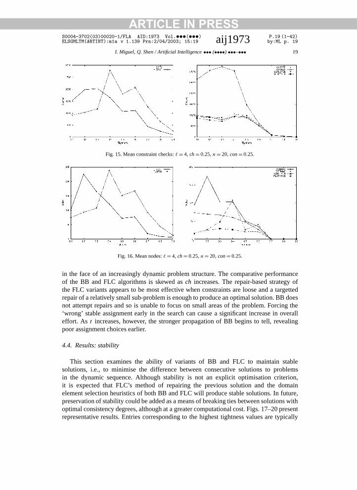
Fig. 15. Mean constraint checks: �= 4, ch= 0.25, n= 20, con= 0.25.
Fig. 16. Mean nodes: �= 4, ch= 0.25, n= 20, con= 0.25.
in the face of an increasingly dynamic problem structure. The comparative performanceof the BB and FLC algorithms is skewed as ch increases. The repair-based strategy ofthe FLC variants appears to be most effective when constraints are loose and a targettedrepair of a relatively small sub-problem is enough to produce an optimal solution. BB doesnot attempt repairs and so is unable to focus on small areas of the problem. Forcing the‘wrong’ stable assignment early in the search can cause a significant increase in overalleffort. As t increases, however, the stronger propagation of BB begins to tell, revealingpoor assignment choices earlier.
4.4. Results: stability
This section examines the ability of variants of BB and FLC to maintain stablesolutions, i.e., to minimise the difference between consecutive solutions to problemsin the dynamic sequence. Although stability is not an explicit optimisation criterion,it is expected that FLC’s method of repairing the previous solution and the domainelement selection heuristics of both BB and FLC will produce stable solutions. In future,preservation of stability could be added as a means of breaking ties between solutions withoptimal consistency degrees, although at a greater computational cost. Figs. 17–20 presentrepresentative results. Entries corresponding to the highest tightness values are typically
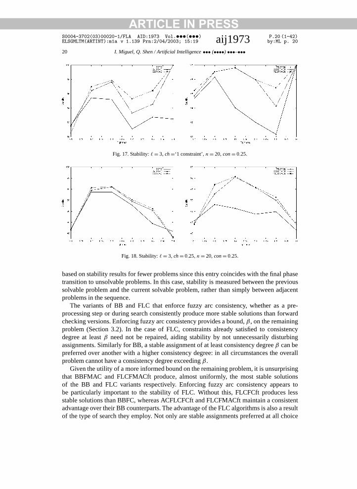
ARTICLE IN PRESSS0004-3702(03)00020-1/FLA AID:1973 Vol.•••(•••) P.20 (1-42)ELSGMLTM(ARTINT):m1a v 1.139 Prn:2/04/2003; 15:19 aij1973 by:ML p. 20
20 I. Miguel, Q. Shen / Artificial Intelligence ••• (••••) •••–•••
Fig. 17. Stability: �= 3, ch=‘1 constraint’, n= 20, con= 0.25.
Fig. 18. Stability: �= 3, ch= 0.25, n= 20, con= 0.25.
based on stability results for fewer problems since this entry coincides with the final phasetransition to unsolvable problems. In this case, stability is measured between the previoussolvable problem and the current solvable problem, rather than simply between adjacentproblems in the sequence.
The variants of BB and FLC that enforce fuzzy arc consistency, whether as a pre-processing step or during search consistently produce more stable solutions than forwardchecking versions. Enforcing fuzzy arc consistency provides a bound, β , on the remainingproblem (Section 3.2). In the case of FLC, constraints already satisfied to consistencydegree at least β need not be repaired, aiding stability by not unnecessarily disturbingassignments. Similarly for BB, a stable assignment of at least consistency degree β can bepreferred over another with a higher consistency degree: in all circumstances the overallproblem cannot have a consistency degree exceeding β .
Given the utility of a more informed bound on the remaining problem, it is unsurprisingthat BBFMAC and FLCFMACft produce, almost uniformly, the most stable solutionsof the BB and FLC variants respectively. Enforcing fuzzy arc consistency appears tobe particularly important to the stability of FLC. Without this, FLCFCft produces lessstable solutions than BBFC, whereas ACFLCFCft and FLCFMACft maintain a consistentadvantage over their BB counterparts. The advantage of the FLC algorithms is also a resultof the type of search they employ. Not only are stable assignments preferred at all choice
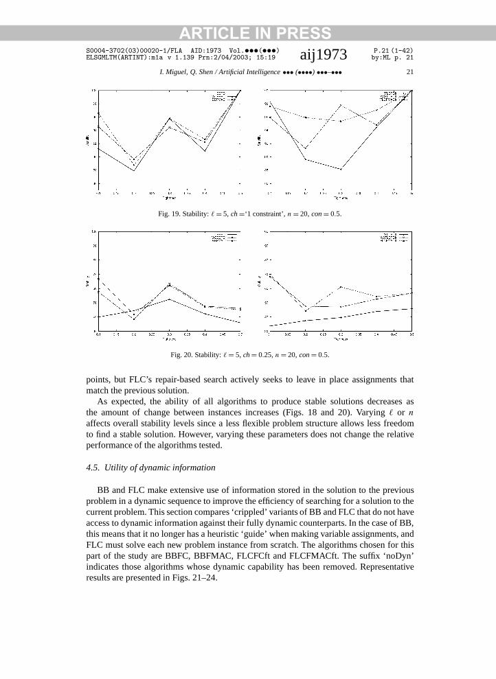
ARTICLE IN PRESSS0004-3702(03)00020-1/FLA AID:1973 Vol.•••(•••) P.21 (1-42)ELSGMLTM(ARTINT):m1a v 1.139 Prn:2/04/2003; 15:19 aij1973 by:ML p. 21
I. Miguel, Q. Shen / Artificial Intelligence ••• (••••) •••–••• 21
Fig. 19. Stability: �= 5, ch=‘1 constraint’, n= 20, con= 0.5.
Fig. 20. Stability: �= 5, ch= 0.25, n= 20, con= 0.5.
points, but FLC’s repair-based search actively seeks to leave in place assignments thatmatch the previous solution.
As expected, the ability of all algorithms to produce stable solutions decreases asthe amount of change between instances increases (Figs. 18 and 20). Varying � or n
affects overall stability levels since a less flexible problem structure allows less freedomto find a stable solution. However, varying these parameters does not change the relativeperformance of the algorithms tested.
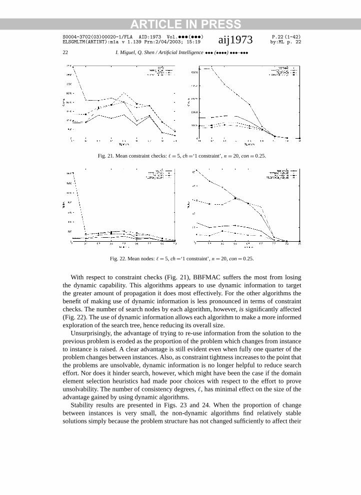
4.5. Utility of dynamic information
BB and FLC make extensive use of information stored in the solution to the previousproblem in a dynamic sequence to improve the efficiency of searching for a solution to thecurrent problem. This section compares ‘crippled’ variants of BB and FLC that do not haveaccess to dynamic information against their fully dynamic counterparts. In the case of BB,this means that it no longer has a heuristic ‘guide’ when making variable assignments, andFLC must solve each new problem instance from scratch. The algorithms chosen for thispart of the study are BBFC, BBFMAC, FLCFCft and FLCFMACft. The suffix ‘noDyn’indicates those algorithms whose dynamic capability has been removed. Representativeresults are presented in Figs. 21–24.
ARTICLE IN PRESSS0004-3702(03)00020-1/FLA AID:1973 Vol.•••(•••) P.22 (1-42)ELSGMLTM(ARTINT):m1a v 1.139 Prn:2/04/2003; 15:19 aij1973 by:ML p. 22
22 I. Miguel, Q. Shen / Artificial Intelligence ••• (••••) •••–•••
Fig. 21. Mean constraint checks: �= 5, ch=‘1 constraint’, n= 20, con= 0.25.
Fig. 22. Mean nodes: �= 5, ch=‘1 constraint’, n= 20, con= 0.25.
With respect to constraint checks (Fig. 21), BBFMAC suffers the most from losingthe dynamic capability. This algorithms appears to use dynamic information to targetthe greater amount of propagation it does most effectively. For the other algorithms thebenefit of making use of dynamic information is less pronounced in terms of constraintchecks. The number of search nodes by each algorithm, however, is significantly affected(Fig. 22). The use of dynamic information allows each algorithm to make a more informedexploration of the search tree, hence reducing its overall size.
Unsurprisingly, the advantage of trying to re-use information from the solution to theprevious problem is eroded as the proportion of the problem which changes from instanceto instance is raised. A clear advantage is still evident even when fully one quarter of theproblem changes between instances. Also, as constraint tightness increases to the point thatthe problems are unsolvable, dynamic information is no longer helpful to reduce searcheffort. Nor does it hinder search, however, which might have been the case if the domainelement selection heuristics had made poor choices with respect to the effort to proveunsolvability. The number of consistency degrees, �, has minimal effect on the size of theadvantage gained by using dynamic algorithms.
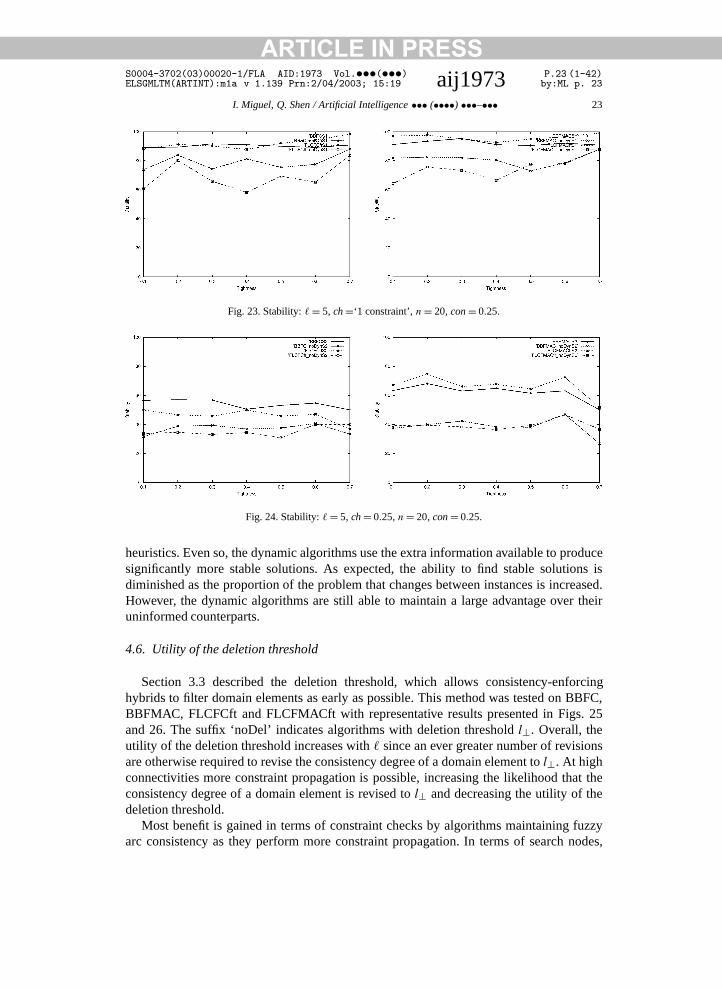
Stability results are presented in Figs. 23 and 24. When the proportion of changebetween instances is very small, the non-dynamic algorithms find relatively stablesolutions simply because the problem structure has not changed sufficiently to affect their
ARTICLE IN PRESSS0004-3702(03)00020-1/FLA AID:1973 Vol.•••(•••) P.23 (1-42)ELSGMLTM(ARTINT):m1a v 1.139 Prn:2/04/2003; 15:19 aij1973 by:ML p. 23
I. Miguel, Q. Shen / Artificial Intelligence ••• (••••) •••–••• 23
Fig. 23. Stability: �= 5, ch=‘1 constraint’, n= 20, con= 0.25.
Fig. 24. Stability: �= 5, ch= 0.25, n= 20, con= 0.25.
heuristics. Even so, the dynamic algorithms use the extra information available to producesignificantly more stable solutions. As expected, the ability to find stable solutions isdiminished as the proportion of the problem that changes between instances is increased.However, the dynamic algorithms are still able to maintain a large advantage over theiruninformed counterparts.
4.6. Utility of the deletion threshold
Section 3.3 described the deletion threshold, which allows consistency-enforcinghybrids to filter domain elements as early as possible. This method was tested on BBFC,BBFMAC, FLCFCft and FLCFMACft with representative results presented in Figs. 25and 26. The suffix ‘noDel’ indicates algorithms with deletion threshold l⊥. Overall, theutility of the deletion threshold increases with � since an ever greater number of revisionsare otherwise required to revise the consistency degree of a domain element to l⊥. At highconnectivities more constraint propagation is possible, increasing the likelihood that theconsistency degree of a domain element is revised to l⊥ and decreasing the utility of thedeletion threshold.
Most benefit is gained in terms of constraint checks by algorithms maintaining fuzzyarc consistency as they perform more constraint propagation. In terms of search nodes,
ARTICLE IN PRESSS0004-3702(03)00020-1/FLA AID:1973 Vol.•••(•••) P.24 (1-42)ELSGMLTM(ARTINT):m1a v 1.139 Prn:2/04/2003; 15:19 aij1973 by:ML p. 24
24 I. Miguel, Q. Shen / Artificial Intelligence ••• (••••) •••–•••
Fig. 25. Mean constraint checks: �= 5, ch= 0.1, n= 20, con= 0.25.
Fig. 26. Mean nodes: �= 5, ch= 0.1, n= 20, con= 0.25.
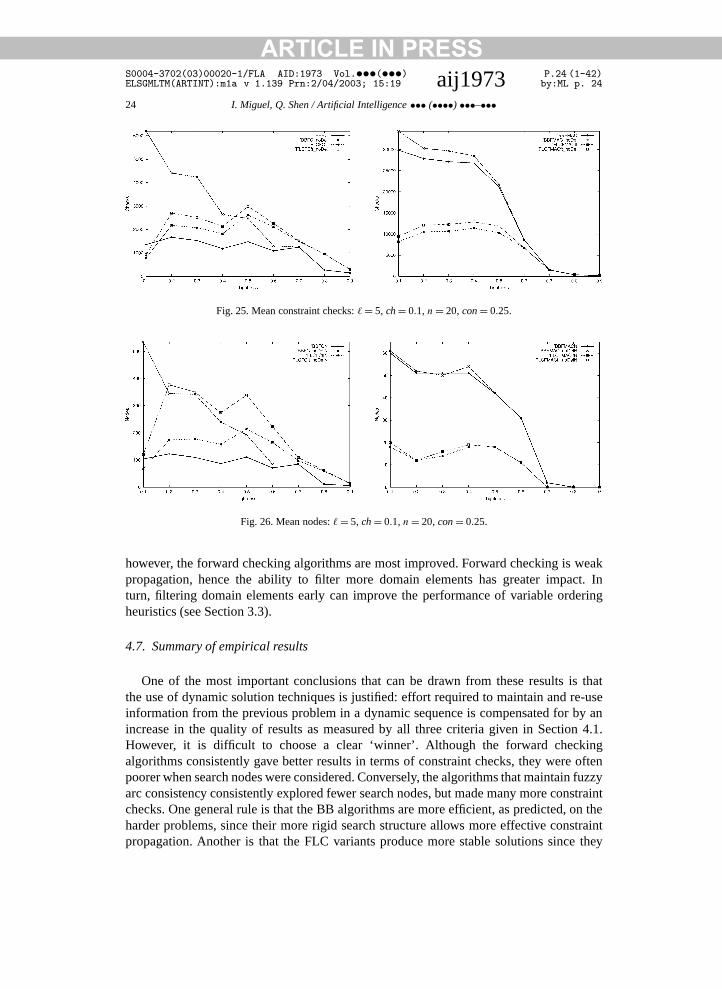
however, the forward checking algorithms are most improved. Forward checking is weakpropagation, hence the ability to filter more domain elements has greater impact. Inturn, filtering domain elements early can improve the performance of variable orderingheuristics (see Section 3.3).
4.7. Summary of empirical results
One of the most important conclusions that can be drawn from these results is thatthe use of dynamic solution techniques is justified: effort required to maintain and re-useinformation from the previous problem in a dynamic sequence is compensated for by anincrease in the quality of results as measured by all three criteria given in Section 4.1.However, it is difficult to choose a clear ‘winner’. Although the forward checkingalgorithms consistently gave better results in terms of constraint checks, they were oftenpoorer when search nodes were considered. Conversely, the algorithms that maintain fuzzyarc consistency consistently explored fewer search nodes, but made many more constraintchecks. One general rule is that the BB algorithms are more efficient, as predicted, on theharder problems, since their more rigid search structure allows more effective constraintpropagation. Another is that the FLC variants produce more stable solutions since they
ARTICLE IN PRESSS0004-3702(03)00020-1/FLA AID:1973 Vol.•••(•••) P.25 (1-42)ELSGMLTM(ARTINT):m1a v 1.139 Prn:2/04/2003; 15:19 aij1973 by:ML p. 25
I. Miguel, Q. Shen / Artificial Intelligence ••• (••••) •••–••• 25
actively work to maintain the assignments in the solution to the previous problem in an
instance rather than simply re-assigning the same domain element as a tie-breaker.5. Flexible planning problems
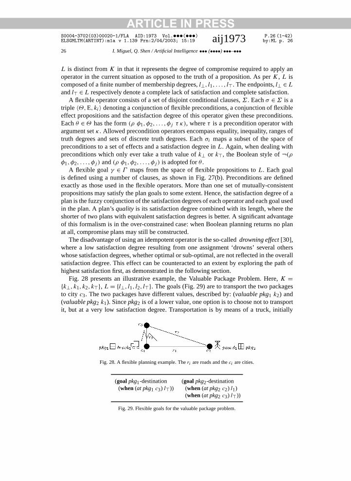
Many real-world planning problems present the need for soft constraints. Consider anexample from the logistics domain where a valuable package must be loaded onto a truck.The preconditions of the Load-truck action state that (i) the truck and (implicitly)valuable package must be co-located, and (ii) a guard must be present. While precondition(i) is imperative, precondition (ii) is a preference or soft constraint and can be relaxed withan associated damage to the resultant plan. Classical AI Planning [1] is too rigid to modelsuch problems, being founded on hard constraints, and hence has no capability of makingcompromises. A flexible planning problem is introduced to allow a tradeoff between planlength and the compromise decisions made. Fuzzy CSP is the formal foundation underlyingthe definition of a flexible planning problem. Subjective truth degrees are associatedwith propositions while satisfaction degrees are associated with plan operators and goals,expressing how well their preconditions are satisfied by a set of flexible propositions.Plan satisfaction degrees are calculated from the satisfaction degrees of their constituentinstantiated operators and goals, enabling a direct comparison amongst a number of planscontaining different compromises.
More formally, a flexible planning problem, Ψ , consists of a 4-tuple, 〈Φ , O, I, Γ 〉,denoting sets of plan objects, flexible operators, initial conditions consisting of flexiblepropositions, and flexible goal conditions. Boolean propositions are herein replaced byflexible propositions, ρ, of the form (ρ φ1, φ2, . . . , φj ki), where each φj ∈ Φ and ki isan element of a totally ordered set, K , which denotes the subjective degree of truth ofthe proposition. K is composed of a finite number of membership degrees, k⊥, k1, . . . , k.The original Boolean proposition type is captured at the end points of K , with k⊥ ∈K andk ∈ K indicating total falsehood and total truth respectively. For brevity, when dealingwith propositions which only ever take a truth value of k⊥ or k, the Boolean style of ¬(ρ
φ1, φ2, . . . , φj ) and (ρ φ1, φ2, . . . , φj ) is adopted.A flexible proposition can easily be described by a fuzzy relation [27], R, defined by a
membership function µR(.) : Φ1×Φ2 × · · · ×Φj →K , where Φ1×Φ2× · · ·×Φj is theCartesian product of the subsets of Φ allowable at this place in the proposition. A flexibleoperator, o ∈ O (Fig. 27(a)) is described by a fuzzy relation mapping from the preconditionspace onto a totally ordered satisfaction scale, L and a set of flexible effect propositions.
a) (operator o b) (goal γ
(params param1, param2, . . .) {when θi li )}σi : {when (preconds θi1 θi2 . . .) {when θj lj )}
(effects ρi1 ρi2 . . .) li} etc)σj : {when (preconds θj1 θj2 . . .)
(effects ρj1 ρj2 . . .) lj }Fig. 27. General formats of flexible operators and goals.
ARTICLE IN PRESSS0004-3702(03)00020-1/FLA AID:1973 Vol.•••(•••) P.26 (1-42)ELSGMLTM(ARTINT):m1a v 1.139 Prn:2/04/2003; 15:19 aij1973 by:ML p. 26
26 I. Miguel, Q. Shen / Artificial Intelligence ••• (••••) •••–•••
L is distinct from K in that it represents the degree of compromise required to apply an
operator in the current situation as opposed to the truth of a proposition. As per K , L iscomposed of a finite number of membership degrees, l⊥, l1, . . . , l. The endpoints, l⊥ ∈Land l ∈ L respectively denote a complete lack of satisfaction and complete satisfaction.A flexible operator consists of a set of disjoint conditional clauses, Σ . Each σ ∈Σ is a
triple 〈Θ, E, ki〉 denoting a conjunction of flexible preconditions, a conjunction of flexibleeffect propositions and the satisfaction degree of this operator given these preconditions.Each θ ∈Θ has the form (ρ φ1, φ2, . . . , φj τ κ), where τ is a precondition operator withargument set κ . Allowed precondition operators encompass equality, inequality, ranges oftruth degrees and sets of discrete truth degrees. Each σi maps a subset of the space ofpreconditions to a set of effects and a satisfaction degree in L. Again, when dealing withpreconditions which only ever take a truth value of k⊥ or k, the Boolean style of ¬(ρ
φ1, φ2, . . . , φj ) and (ρ φ1, φ2, . . . , φj ) is adopted for θ .A flexible goal γ ∈ Γ maps from the space of flexible propositions to L. Each goal
is defined using a number of clauses, as shown in Fig. 27(b). Preconditions are definedexactly as those used in the flexible operators. More than one set of mutually-consistentpropositions may satisfy the plan goals to some extent. Hence, the satisfaction degree of aplan is the fuzzy conjunction of the satisfaction degrees of each operator and each goal usedin the plan. A plan’s quality is its satisfaction degree combined with its length, where theshorter of two plans with equivalent satisfaction degrees is better. A significant advantageof this formalism is in the over-constrained case: when Boolean planning returns no planat all, compromise plans may still be constructed.
The disadvantage of using an idempotent operator is the so-called drowning effect [30],where a low satisfaction degree resulting from one assignment ‘drowns’ several otherswhose satisfaction degrees, whether optimal or sub-optimal, are not reflected in the overallsatisfaction degree. This effect can be counteracted to an extent by exploring the path ofhighest satisfaction first, as demonstrated in the following section.
Fig. 28 presents an illustrative example, the Valuable Package Problem. Here, K ={k⊥, k1, k2, k}, L= {l⊥, l1, l2, l}. The goals (Fig. 29) are to transport the two packagesto city c3. The two packages have different values, described by: (valuable pkg1 k2) and(valuable pkg2 k1). Since pkg2 is of a lower value, one option is to choose not to transportit, but at a very low satisfaction degree. Transportation is by means of a truck, initially
Fig. 28. A flexible planning example. The ri are roads and the ci are cities.
(goal pkg1-destination (goal pkg2-destination(when (at pkg1 c3) l)) (when (at pkg2 c2) l1)
(when (at pkg2 c3) l))
Fig. 29. Flexible goals for the valuable package problem.
ARTICLE IN PRESSS0004-3702(03)00020-1/FLA AID:1973 Vol.•••(•••) P.27 (1-42)ELSGMLTM(ARTINT):m1a v 1.139 Prn:2/04/2003; 15:19 aij1973 by:ML p. 27
I. Miguel, Q. Shen / Artificial Intelligence ••• (••••) •••–••• 27
a) (operator Drive-truck
params (?v vehicle) (?o location) (?d location) (?rMj mj-rd) (?rMt mtn-rd)){when (preconds (at ?v ?o) (connects ?rMj ?o ?d))(effects (not (at ?v ?o)) (at ?v ?d)) l}{when (preconds (at ?v ?o) (connects ?rMt ?o ?d))
(effects (not (at ?v ?o)) (at ?v ?d)) l1})b) (operator Load-truck
params (?t truck) (?p package) (?d location) (?g guard)){when (preconds (at ?t ?l) (at ?p ?l) (valuable ?p <= k1))
(effects (not (at ?p ?l)) (on ?p ?t)) l}{when (preconds (at ?t ?l) (at ?p ?l) (on ?g ?t) (valuable ?p >= k2))
(effects (not (at ?p ?l)) (on ?p ?t)) l}{when (preconds (at ?t ?l) (at ?p ?l) (not (on ?g ?t)) (valuable ?p >= k2))
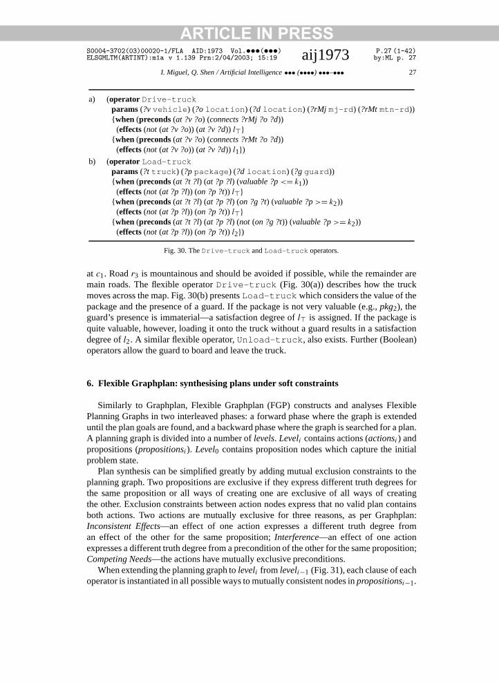
(effects (not (at ?p ?l)) (on ?p ?t)) l2})Fig. 30. The Drive-truck and Load-truck operators.
at c1. Road r3 is mountainous and should be avoided if possible, while the remainder aremain roads. The flexible operator Drive-truck (Fig. 30(a)) describes how the truckmoves across the map. Fig. 30(b) presents Load-truck which considers the value of thepackage and the presence of a guard. If the package is not very valuable (e.g., pkg2), theguard’s presence is immaterial—a satisfaction degree of l is assigned. If the package isquite valuable, however, loading it onto the truck without a guard results in a satisfactiondegree of l2. A similar flexible operator, Unload-truck, also exists. Further (Boolean)operators allow the guard to board and leave the truck.
6. Flexible Graphplan: synthesising plans under soft constraints
Similarly to Graphplan, Flexible Graphplan (FGP) constructs and analyses FlexiblePlanning Graphs in two interleaved phases: a forward phase where the graph is extendeduntil the plan goals are found, and a backward phase where the graph is searched for a plan.A planning graph is divided into a number of levels. Leveli contains actions (actionsi) andpropositions (propositionsi). Level0 contains proposition nodes which capture the initialproblem state.
Plan synthesis can be simplified greatly by adding mutual exclusion constraints to theplanning graph. Two propositions are exclusive if they express different truth degrees forthe same proposition or all ways of creating one are exclusive of all ways of creatingthe other. Exclusion constraints between action nodes express that no valid plan containsboth actions. Two actions are mutually exclusive for three reasons, as per Graphplan:Inconsistent Effects—an effect of one action expresses a different truth degree froman effect of the other for the same proposition; Interference—an effect of one actionexpresses a different truth degree from a precondition of the other for the same proposition;Competing Needs—the actions have mutually exclusive preconditions.
When extending the planning graph to leveli from leveli−1 (Fig. 31), each clause of eachoperator is instantiated in all possible ways to mutually consistent nodes in propositionsi−1.
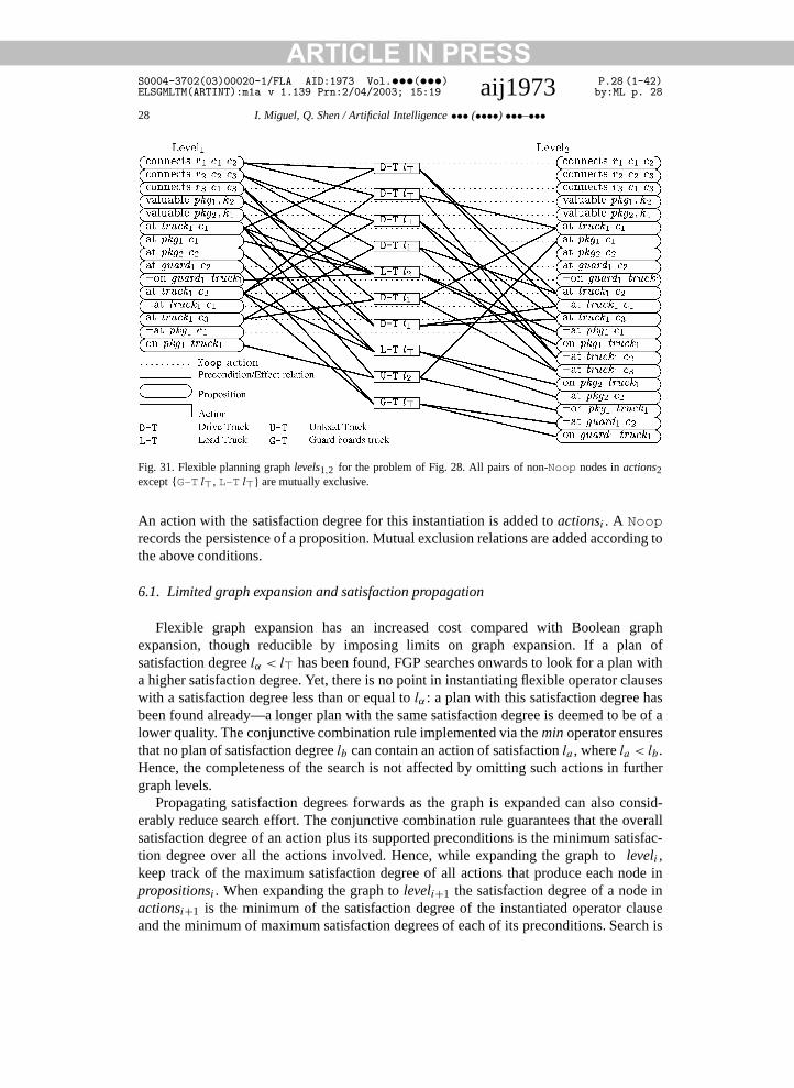
ARTICLE IN PRESSS0004-3702(03)00020-1/FLA AID:1973 Vol.•••(•••) P.28 (1-42)ELSGMLTM(ARTINT):m1a v 1.139 Prn:2/04/2003; 15:19 aij1973 by:ML p. 28
28 I. Miguel, Q. Shen / Artificial Intelligence ••• (••••) •••–•••
Fig. 31. Flexible planning graph levels1,2 for the problem of Fig. 28. All pairs of non-Noop nodes in actions2except {G-T l , L-T l} are mutually exclusive.
An action with the satisfaction degree for this instantiation is added to actionsi . A Nooprecords the persistence of a proposition. Mutual exclusion relations are added according tothe above conditions.
6.1. Limited graph expansion and satisfaction propagation
Flexible graph expansion has an increased cost compared with Boolean graphexpansion, though reducible by imposing limits on graph expansion. If a plan ofsatisfaction degree lα < l has been found, FGP searches onwards to look for a plan witha higher satisfaction degree. Yet, there is no point in instantiating flexible operator clauseswith a satisfaction degree less than or equal to lα : a plan with this satisfaction degree hasbeen found already—a longer plan with the same satisfaction degree is deemed to be of alower quality. The conjunctive combination rule implemented via the min operator ensuresthat no plan of satisfaction degree lb can contain an action of satisfaction la , where la < lb .Hence, the completeness of the search is not affected by omitting such actions in furthergraph levels.
Propagating satisfaction degrees forwards as the graph is expanded can also consid-erably reduce search effort. The conjunctive combination rule guarantees that the overallsatisfaction degree of an action plus its supported preconditions is the minimum satisfac-tion degree over all the actions involved. Hence, while expanding the graph to leveli ,keep track of the maximum satisfaction degree of all actions that produce each node inpropositionsi . When expanding the graph to leveli+1 the satisfaction degree of a node inactionsi+1 is the minimum of the satisfaction degree of the instantiated operator clauseand the minimum of maximum satisfaction degrees of each of its preconditions. Search is

ARTICLE IN PRESSS0004-3702(03)00020-1/FLA AID:1973 Vol.•••(•••) P.29 (1-42)ELSGMLTM(ARTINT):m1a v 1.139 Prn:2/04/2003; 15:19 aij1973 by:ML p. 29
I. Miguel, Q. Shen / Artificial Intelligence ••• (••••) •••–••• 29
reduced because it is obvious at an earlier stage that, say, a certain action can never be part
of a plan with satisfaction degree l. For instance, Unload-truck (Fig. 31) requires‘on pkg1 truck1’ as a precondition. The sole way of asserting this proposition at level1 isvia a Load-truck action which has a satisfaction degree of l2. The other preconditionof Unload-truck, ‘at truck1 c1’, is an initial condition, so the minimum of maximumsatisfaction degrees attached to the preconditions of this action is l2. The satisfaction de-gree of Unload-truck at level2 is the minimum of l2 and the satisfaction degree of theinstantiated operator clause (l), resulting in a satisfaction degree of l2.6.2. Flexible plan extraction via fuzzy rrDFCSP
A node in propositionsi can be viewed as a fuzzy CSP variable, its domain comprisingthe set of nodes in actionsi which assert this proposition as an effect. A unary preferenceconstraint is constructed from the domain elements and their associated satisfactiondegrees. Consider ‘at truck1 c1’ in propositions2 (Fig. 31) with a domain of two Drive-truck actions and a Noop action. A unary preference constraint specifies that theassignment of one of the Drive-truck actions and that of the Noop action havesatisfaction degree l, while the assignment of the other Drive-truck action has asatisfaction degree of l1. Boolean binary constraints are generated directly from the mutual-exclusion relations in the planning graph.
If levelg contains the goal propositions, each set of supporting actions specifies (viapreconditions) a sub-problem at levelg−1. Solutions to these sub-problems specify newsub-problems at levelg−2, etc. A sub-problem sequence associated with a graph level isviewed as a fuzzy rrDFCSP (Fig. 32). FGP uses ACFLCFC to solve these sequencessince individual sub-problems are relatively easy to solve, and ACFLCFC is relativelylightweight. This algorithm is also able to maintain solution stability. A stable solution toa sequence of sub-problems enables FGP to focus on conflicts that prevent the subgoalpropositions under consideration from being supportable.
If solutions to the sub-problem at leveli intersect (likely in all but the most tightlyconstrained cases), there will be similarities between sub-problems at leveli−1. AnrrDFCSP algorithm exploits these similarities, re-using effort applied to the previousproblem in the sequence when solving the current sub-problem. Effort used in levels visitedin a failed plan extraction is also re-used when the graph is expanded and a further attemptis made.
Fig. 32. Plan extraction as a hierarchy of fuzzy rrDCSPs.
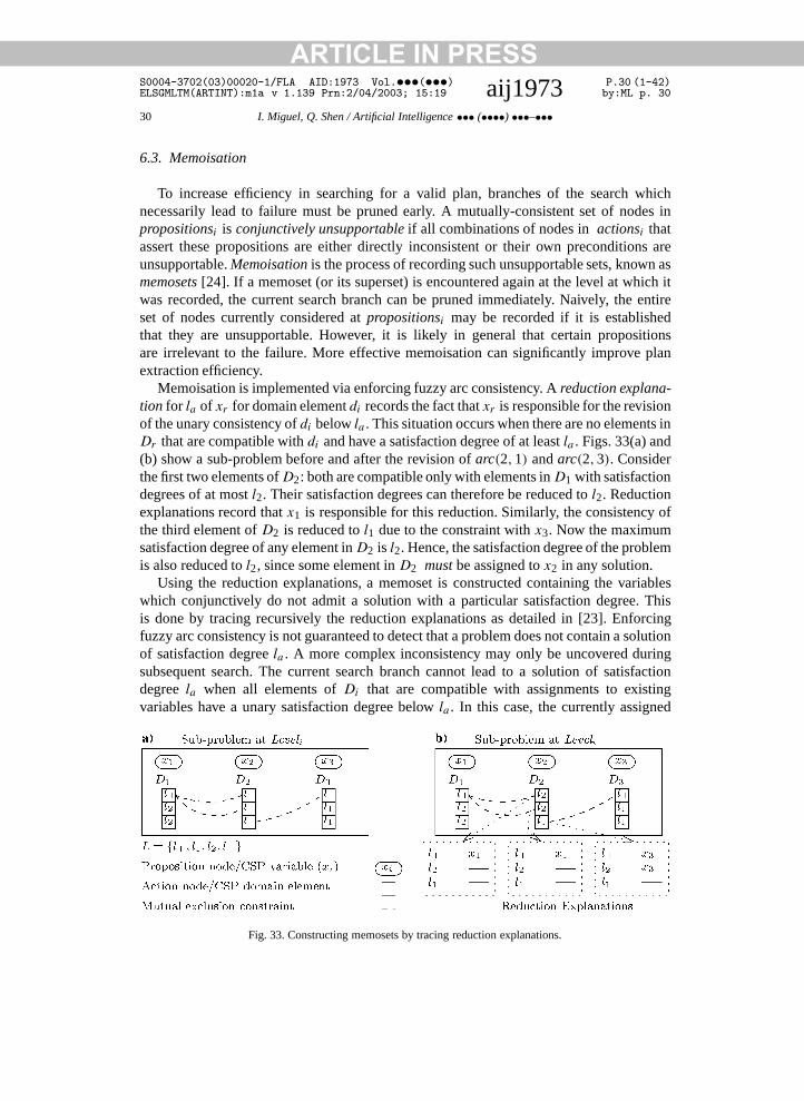
ARTICLE IN PRESSS0004-3702(03)00020-1/FLA AID:1973 Vol.•••(•••) P.30 (1-42)ELSGMLTM(ARTINT):m1a v 1.139 Prn:2/04/2003; 15:19 aij1973 by:ML p. 30
30 I. Miguel, Q. Shen / Artificial Intelligence ••• (••••) •••–•••
6.3. Memoisation
To increase efficiency in searching for a valid plan, branches of the search whichnecessarily lead to failure must be pruned early. A mutually-consistent set of nodes inpropositionsi is conjunctively unsupportable if all combinations of nodes in actionsi thatassert these propositions are either directly inconsistent or their own preconditions areunsupportable. Memoisation is the process of recording such unsupportable sets, known asmemosets [24]. If a memoset (or its superset) is encountered again at the level at which itwas recorded, the current search branch can be pruned immediately. Naively, the entireset of nodes currently considered at propositionsi may be recorded if it is establishedthat they are unsupportable. However, it is likely in general that certain propositionsare irrelevant to the failure. More effective memoisation can significantly improve planextraction efficiency.
Memoisation is implemented via enforcing fuzzy arc consistency. A reduction explana-tion for la of xr for domain element di records the fact that xr is responsible for the revisionof the unary consistency of di below la . This situation occurs when there are no elements inDr that are compatible with di and have a satisfaction degree of at least la . Figs. 33(a) and(b) show a sub-problem before and after the revision of arc(2, 1) and arc(2, 3). Considerthe first two elements of D2: both are compatible only with elements in D1 with satisfactiondegrees of at most l2. Their satisfaction degrees can therefore be reduced to l2. Reductionexplanations record that x1 is responsible for this reduction. Similarly, the consistency ofthe third element of D2 is reduced to l1 due to the constraint with x3. Now the maximumsatisfaction degree of any element in D2 is l2. Hence, the satisfaction degree of the problemis also reduced to l2, since some element in D2 must be assigned to x2 in any solution.
Using the reduction explanations, a memoset is constructed containing the variableswhich conjunctively do not admit a solution with a particular satisfaction degree. Thisis done by tracing recursively the reduction explanations as detailed in [23]. Enforcingfuzzy arc consistency is not guaranteed to detect that a problem does not contain a solutionof satisfaction degree la . A more complex inconsistency may only be uncovered duringsubsequent search. The current search branch cannot lead to a solution of satisfactiondegree la when all elements of Di that are compatible with assignments to existingvariables have a unary satisfaction degree below la . In this case, the currently assigned
Fig. 33. Constructing memosets by tracing reduction explanations.
ARTICLE IN PRESSS0004-3702(03)00020-1/FLA AID:1973 Vol.•••(•••) P.31 (1-42)ELSGMLTM(ARTINT):m1a v 1.139 Prn:2/04/2003; 15:19 aij1973 by:ML p. 31
I. Miguel, Q. Shen / Artificial Intelligence ••• (••••) •••–••• 31
variables form a conflict set with xi with respect to la . This inconsistency can be recorded
as a partial memoset for the satisfaction degree la . Since flexibility is present only inthe unary preference constraints associated with each variable, variables with assignmentshaving a satisfaction degree of la or above are irrelevant to this conflict and removed. If nosolution exists with satisfaction degree la , an la -memoset is constructed from the union ofthe recorded partial memosets.Memoset information from child sub-problems is used to guide further solution extrac-tion at the parent sub-problem. Memosets from a sub-problem at leveli−1 are mapped backonto action nodes in a solution assignment at leveli , which generated the sub-problem atleveli−1, using precondition relations in the planning graph. Sub-assignments thus speci-fied represent new constraints that can be added to the current instance of a sub-problemat leveli , creating a new instance in the dynamic sequence. This process is not the same asconflict recording during the solution of a single CSP, since the new constraints come froman external source. FLC solves the new instance by repairing the previous solution. Propa-gation means that FLC only has to discover one solution for each of a limited sequence ofincreasingly constrained sub-problems, rather than attempting to enumerate all solutionsto a single sub-problem. This is more efficient since each propagated repair can poten-tially exclude many solutions to the original sub-problem. The propagated repair processemphasises the usefulness of rrDFCSP techniques in this hierarchical context.
6.4. The FGP algorithm
FGP is presented in pseudo-code form in Fig. 34. For reasons of space, the proofof the soundness and completeness of FGP is omitted (see [23]). FGP can solveBoolean problems by restricting the truth and satisfaction scales to {k⊥, k} and {l⊥, l}respectively. The procedure FGP( ) is the top level of the algorithm. The planning graph(graph), the current (planβ) and best known (planα) plans have global scope. Lines 4–9extend the graph and search for plans until a compromise-free plan is encountered. At eachgraph level, the goalSets of proposition nodes which are mutually-consistent and match theplan goals are determined (line 6). Since flexible goals associate a satisfaction degree withdifferent propositions, a combined satisfaction degree is generated for each goalSet. ThegoalSets are sorted in descending order of satisfaction degree (line 7) before attempting tofind a plan containing them (line 9). Sorting increases the likelihood of finding a good planearly, which becomes a bound for future search.
The extract( ) and extractLevel( ) procedures control the solution of thehierarchy of fuzzy rrDFCSPs created from the planning graph. The former simplyinitialises a partial plan with the satisfaction degree of the current goalSet (line 2) beforecalling the latter. The base case of this recursion is when level0 of the planning graphis reached (lines 2–4). If the subgoals now match the initial conditions (line 2), a newbest plan has been found and becomes the bound against which future partial plans arecompared (line 3).
At all other levels, FGP first checks whether a previously recorded memoset showsthat the current branch cannot lead to a new best plan. If so, this branch of the search ispruned, and the memoset is returned to the level above for propagation (line 6). Otherwise,the instance of BBFCLex dealing with this level of the graph is retrieved (line 7) and a

ARTICLE IN PRESSS0004-3702(03)00020-1/FLA AID:1973 Vol.•••(•••) P.32 (1-42)ELSGMLTM(ARTINT):m1a v 1.139 Prn:2/04/2003; 15:19 aij1973 by:ML p. 32
32 I. Miguel, Q. Shen / Artificial Intelligence ••• (••••) •••–•••
1. Procedure FGP(ψ)
2. graph← graph-initialise(ψ)3. level← 0, lα← l4. While Not compromise-free(planα)5. level← level+15. extend(graph)6. goalSets← getGoalSets (graph, ψ)7. sort(goalSets)8. Foreach goalSet ∈ goalSets9. If (satDegree(goalSet) > lα) extract(level, goalSet)1. Procedure extract(level, goalSet)2. planβ ← plan-initialise(level, satDegree(goalSet))3. extractLevel(level, getPropositionNodes(goalSet))
1. Procedure extractLevel(level, subGoals)2. If (level = 0 And matchInitConds(subGoals))3. planα ← planβ
4. Return ∅5. memoset← getMemoset(graph, level, subGoals)6. If (memoset �= ∅) Return memoset7. ACFLCFCl← getSolver(graph, level)8. subProb← translate(subGoals)9. memoset← solve(ACFLCFCl, subProb)10. If (memoset �= ∅) recordMemo(memoset, level)11. Return memoset
Fig. 34. Overview of FGP.
new sub-problem in the corresponding rrDFCSP is generated (line 8). This sub-problem issolved, returning a new memoset to be recorded and propagated (lines 9–11). ACFLCFC( )and extractLevel( ) are mutually recursive: once the former has found a solution, itinvokes the latter to search the next level down.
6.5. Complexity issues of FGP
The flexibility inherent in the flexible planning graph contributes to the increasedcomplexity of FGP over Graphplan. As �, the number of satisfaction degrees in the scaleL increases, there is an increase in the number of sub-problems that FLC must solve. Thisis because solutions of all satisfaction degrees above l⊥ must be explored. This increaseis, however, in the average rather than the worst case, since with a constant number ofsub-problem variables and domain size (neither of which are affected by �) the maximumnumber of potential solutions to explore remains the same.
The time complexity of FLC has been established as O(nmn) [23]. If the number ofplan goals in a g-level planning graph is G, m is again the domain size (i.e., the maximumnumber of action nodes that assert a particular proposition) and p is the maximum numberof preconditions for any of the operators in the problem, the worst-case time complexity ofsynthesising a plan can be expressed by (see [23] for proof):
ARTICLE IN PRESSS0004-3702(03)00020-1/FLA AID:1973 Vol.•••(•••) P.33 (1-42)ELSGMLTM(ARTINT):m1a v 1.139 Prn:2/04/2003; 15:19 aij1973 by:ML p. 33
I. Miguel, Q. Shen / Artificial Intelligence ••• (••••) •••–••• 33
g∑i−1 2Gpi−1
i∏Gpj−2 [
g−1 2Gpg−1 Gpg−1]
i=1
Gp m
j=2
m ≈ g Gp m m .
That is,
O(gGpg−1m3Gpg−1)
.
If there are G flexible goals, the worst case occurs when each can be satisfied in all�− 1, producing G�−1 goal combinations. Hence, the worst case time complexity of plansynthesis from levelg of a flexible planning graph is:
O(gG�pg−1m3Gpg−1)
.
The worst-case space required by a flexible planning graph is no greater than thatrequired by a Boolean planning graph. Reconsider the space complexity analysis made in[3] of a Boolean planning problem with n objects, i propositions in the initial conditions,s STRIPS operators each with k parameters and an effects list of size e. Operatorscannot create new objects, so the number of different propositions that can be createdby instantiating an operator is O(enk). Hence, the maximum number of nodes in anyproposition level is O(i + senk). Since any operator can be instantiated in at most O(nk)
different ways, the maximum number of nodes in any action level of the graph is O(enk).Flexible operators have several clauses, but these clauses must be disjoint (Section 5).Hence, the number of ways any operator can be instantiated remains as O(nk). Includingmemoisation, FGP has exponential worst case space complexity because an exponentialnumber of sub-problems is solved in the worst case, each of which can lead to the recordingof a memoset. This result reinforces the need for informed memoisation.
6.6. Synthesised plans for the valuable package problem
The first short plan synthesised by FGP is as follows, the major compromises being theroute across the unsafe track and the fact that only pkg1 is delivered.
(1) Load-truck pkg1 truck1 (l2)
(2) Drive-truck truck1 c1 to c3 via r3 (l1)
(3) Unload-truck pkg1 truck1 (l)
Using main roads, both packages can be carried to c3 in 5 steps, with a satisfaction degreeof l2 since the guard is not present when pkg1 is loaded.
(1) Load-truck pkg1 truck1 (l2)
(2) Drive-truck truck1 c1 to c2 via r1 (l)
(3) Load-truck pkg2 truck1 (l)
(4) Drive-truck truck1 c2 to c3 via r2 (l)
(5) • Unload-truck pkg1 truck1 (l)
• Unload-truck pkg2 truck1 (l)
ARTICLE IN PRESSS0004-3702(03)00020-1/FLA AID:1973 Vol.•••(•••) P.34 (1-42)ELSGMLTM(ARTINT):m1a v 1.139 Prn:2/04/2003; 15:19 aij1973 by:ML p. 34
34 I. Miguel, Q. Shen / Artificial Intelligence ••• (••••) •••–•••
The above plan is still not regarded as having the highest satisfaction degree because
the guard was not present when the first package was loaded. The ‘no compromise’ plancontains seven steps and is shown below.(1) Drive-truck truck1 c1 to c2 via r1 (l)
(2) • Guard-gets-on-truck truck1 guard1 (l)
• Load-truck pkg2 truck1 (l)
(3) Drive-truck truck1 c2 to c1 via r1 (l)
(4) Load-truck truck1 package1 guard1 (l)
(5) Drive-truck truck1 c1 to c2 via r1 (l)
(6) Drive-truck truck1 c2 to c3 via r2 (l)
(7) • Unload-truck pkg1 truck1 (l)
• Unload-truck pkg2 truck1 (l)
This simple example demonstrates how a range of plans of different lengths and containingalternative compromises can be synthesised from a given flexible planning problem. Theuser can then select the one which is deemed to offer the best compromise between lengthand satisfaction degree.
7. FGP: experimental results
A test suite of twelve problems containing plans of three satisfaction degrees atdifferent distributions of plan length is used to examine the relationship between solutiondistribution and search effort. Boolean versions of the twelve problems are also solved toinvestigate the overhead incurred by searching for a range of plans. The utility of limitedgraph expansion and satisfaction propagation (Section 6.1) is also examined. The Rescueproblem [24] is then described. It exhibits complex interactions between flexible operatorsand goals, testing the ability of FGP to trade plan length versus the compromises made.For reasons of space, results on Boolean benchmarks are omitted here, but can be found in[24].
7.1. The test suite
The test suite contains logistics problems of the same type as the example in Section 5:the target is to transport packages to their respective destinations. To compare the effortof searching for a range of solutions with synthesising a single plan from a Booleanversion of the same problem, two sets of operators are used. The first are flexible andallow compromises to be made to synthesise one or more shorter plans as well as aplan containing no compromises. Let K = {k⊥, k1, k2, k} and L = {l⊥, l1, l2, l}. The12 problems have been constructed such that it is always possible to synthesise threedifferent plans (Fig. 35). It is preferred that the guard is present when a package is loadedonto a truck (if not, the satisfaction degree of Load-truck is l2). It is also preferrednot to transport valuable packages through dangerous areas (otherwise the satisfactiondegree of Drive-truck is l1). A second set of Boolean operators make imperative the
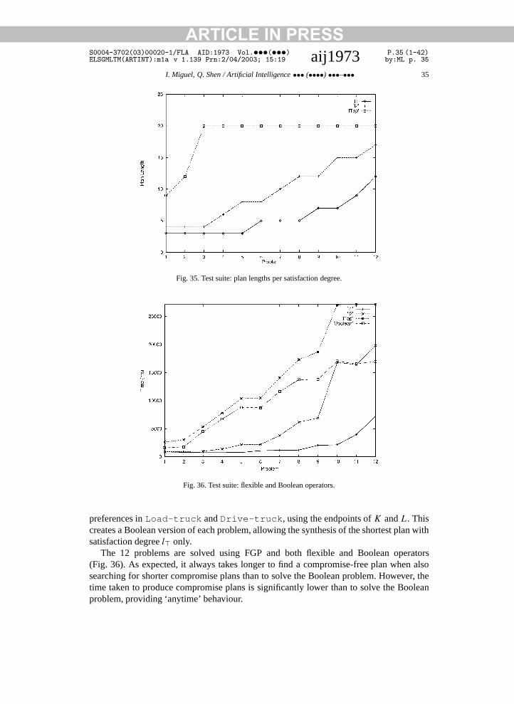
ARTICLE IN PRESSS0004-3702(03)00020-1/FLA AID:1973 Vol.•••(•••) P.35 (1-42)ELSGMLTM(ARTINT):m1a v 1.139 Prn:2/04/2003; 15:19 aij1973 by:ML p. 35
I. Miguel, Q. Shen / Artificial Intelligence ••• (••••) •••–••• 35
Fig. 35. Test suite: plan lengths per satisfaction degree.
Fig. 36. Test suite: flexible and Boolean operators.
preferences in Load-truck and Drive-truck, using the endpoints of K and L. Thiscreates a Boolean version of each problem, allowing the synthesis of the shortest plan withsatisfaction degree l only.
The 12 problems are solved using FGP and both flexible and Boolean operators(Fig. 36). As expected, it always takes longer to find a compromise-free plan when alsosearching for shorter compromise plans than to solve the Boolean problem. However, thetime taken to produce compromise plans is significantly lower than to solve the Booleanproblem, providing ‘anytime’ behaviour.
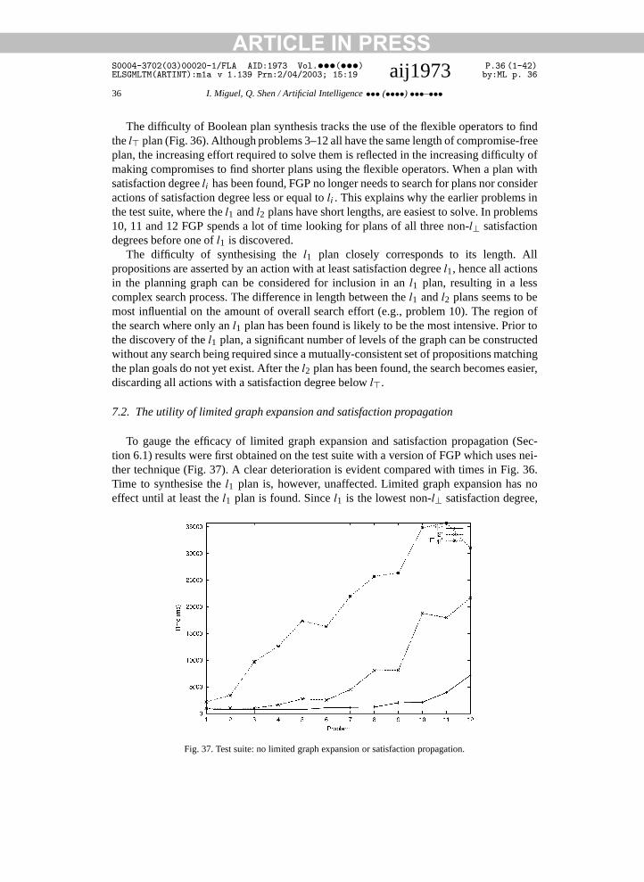
ARTICLE IN PRESSS0004-3702(03)00020-1/FLA AID:1973 Vol.•••(•••) P.36 (1-42)ELSGMLTM(ARTINT):m1a v 1.139 Prn:2/04/2003; 15:19 aij1973 by:ML p. 36
36 I. Miguel, Q. Shen / Artificial Intelligence ••• (••••) •••–•••
The difficulty of Boolean plan synthesis tracks the use of the flexible operators to find
the l plan (Fig. 36). Although problems 3–12 all have the same length of compromise-freeplan, the increasing effort required to solve them is reflected in the increasing difficulty ofmaking compromises to find shorter plans using the flexible operators. When a plan withsatisfaction degree li has been found, FGP no longer needs to search for plans nor consideractions of satisfaction degree less or equal to li . This explains why the earlier problems inthe test suite, where the l1 and l2 plans have short lengths, are easiest to solve. In problems10, 11 and 12 FGP spends a lot of time looking for plans of all three non-l⊥ satisfactiondegrees before one of l1 is discovered.The difficulty of synthesising the l1 plan closely corresponds to its length. Allpropositions are asserted by an action with at least satisfaction degree l1, hence all actionsin the planning graph can be considered for inclusion in an l1 plan, resulting in a lesscomplex search process. The difference in length between the l1 and l2 plans seems to bemost influential on the amount of overall search effort (e.g., problem 10). The region ofthe search where only an l1 plan has been found is likely to be the most intensive. Prior tothe discovery of the l1 plan, a significant number of levels of the graph can be constructedwithout any search being required since a mutually-consistent set of propositions matchingthe plan goals do not yet exist. After the l2 plan has been found, the search becomes easier,discarding all actions with a satisfaction degree below l.
7.2. The utility of limited graph expansion and satisfaction propagation
To gauge the efficacy of limited graph expansion and satisfaction propagation (Sec-tion 6.1) results were first obtained on the test suite with a version of FGP which uses nei-ther technique (Fig. 37). A clear deterioration is evident compared with times in Fig. 36.Time to synthesise the l1 plan is, however, unaffected. Limited graph expansion has noeffect until at least the l1 plan is found. Since l1 is the lowest non-l⊥ satisfaction degree,
Fig. 37. Test suite: no limited graph expansion or satisfaction propagation.
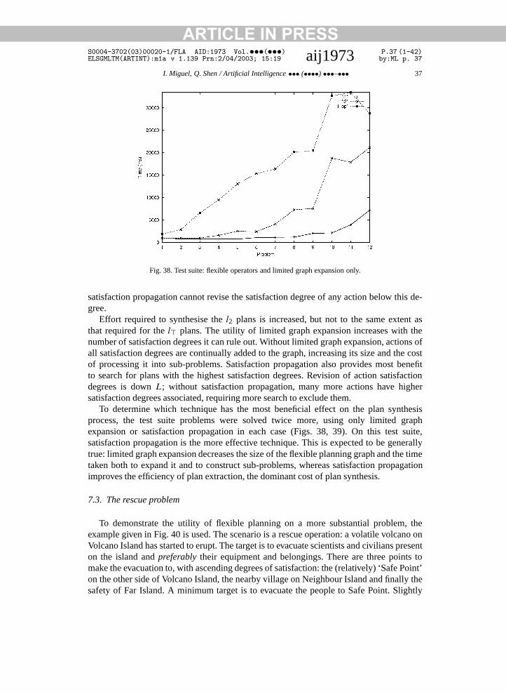
ARTICLE IN PRESSS0004-3702(03)00020-1/FLA AID:1973 Vol.•••(•••) P.37 (1-42)ELSGMLTM(ARTINT):m1a v 1.139 Prn:2/04/2003; 15:19 aij1973 by:ML p. 37
I. Miguel, Q. Shen / Artificial Intelligence ••• (••••) •••–••• 37
Fig. 38. Test suite: flexible operators and limited graph expansion only.
satisfaction propagation cannot revise the satisfaction degree of any action below this de-gree.
Effort required to synthesise the l2 plans is increased, but not to the same extent asthat required for the l plans. The utility of limited graph expansion increases with thenumber of satisfaction degrees it can rule out. Without limited graph expansion, actions ofall satisfaction degrees are continually added to the graph, increasing its size and the costof processing it into sub-problems. Satisfaction propagation also provides most benefitto search for plans with the highest satisfaction degrees. Revision of action satisfactiondegrees is down L; without satisfaction propagation, many more actions have highersatisfaction degrees associated, requiring more search to exclude them.
To determine which technique has the most beneficial effect on the plan synthesisprocess, the test suite problems were solved twice more, using only limited graphexpansion or satisfaction propagation in each case (Figs. 38, 39). On this test suite,satisfaction propagation is the more effective technique. This is expected to be generallytrue: limited graph expansion decreases the size of the flexible planning graph and the timetaken both to expand it and to construct sub-problems, whereas satisfaction propagationimproves the efficiency of plan extraction, the dominant cost of plan synthesis.
7.3. The rescue problem
To demonstrate the utility of flexible planning on a more substantial problem, theexample given in Fig. 40 is used. The scenario is a rescue operation: a volatile volcano onVolcano Island has started to erupt. The target is to evacuate scientists and civilians presenton the island and preferably their equipment and belongings. There are three points tomake the evacuation to, with ascending degrees of satisfaction: the (relatively) ‘Safe Point’on the other side of Volcano Island, the nearby village on Neighbour Island and finally thesafety of Far Island. A minimum target is to evacuate the people to Safe Point. Slightly
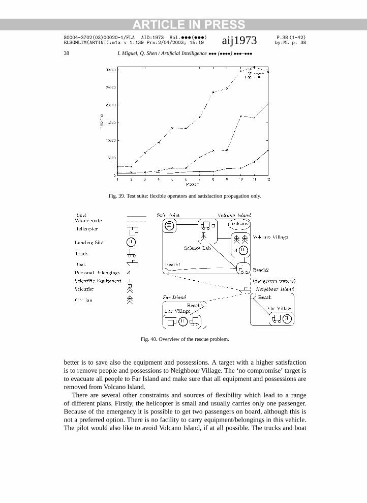
ARTICLE IN PRESSS0004-3702(03)00020-1/FLA AID:1973 Vol.•••(•••) P.38 (1-42)ELSGMLTM(ARTINT):m1a v 1.139 Prn:2/04/2003; 15:19 aij1973 by:ML p. 38
38 I. Miguel, Q. Shen / Artificial Intelligence ••• (••••) •••–•••
Fig. 39. Test suite: flexible operators and satisfaction propagation only.
Fig. 40. Overview of the rescue problem.
better is to save also the equipment and possessions. A target with a higher satisfactionis to remove people and possessions to Neighbour Village. The ‘no compromise’ target isto evacuate all people to Far Island and make sure that all equipment and possessions areremoved from Volcano Island.
There are several other constraints and sources of flexibility which lead to a rangeof different plans. Firstly, the helicopter is small and usually carries only one passenger.Because of the emergency it is possible to get two passengers on board, although this isnot a preferred option. There is no facility to carry equipment/belongings in this vehicle.The pilot would also like to avoid Volcano Island, if at all possible. The trucks and boat

ARTICLE IN PRESSS0004-3702(03)00020-1/FLA AID:1973 Vol.•••(•••) P.39 (1-42)ELSGMLTM(ARTINT):m1a v 1.139 Prn:2/04/2003; 15:19 aij1973 by:ML p. 39
I. Miguel, Q. Shen / Artificial Intelligence ••• (••••) •••–••• 39
can carry people or possessions. One of the routes that the boat may take between Volcano
Island and Neighbour Island is treacherous, and to be avoided if possible.This problem uses the satisfaction scale L = {l⊥, l1, l2, l3, l4, l} and a truth degreescale, K , of the same size. This is not a trivial problem: there are 432 possible flexible goalcombinations alone. FGP synthesises 5 plans for the rescue problem in under 30 seconds,one per satisfaction degree, discounting l⊥. This is not the case for all problems since,as noted, given two plans of the same length the one with the higher satisfaction degreeis returned. There are, of course, alternative plans with the same satisfaction degree andlength, but this is no different from the situation found in Boolean planning.
The shortest plan of four steps is shown below. Although other actions in the plan are‘drowned’ by the fact that the helicopter must fly to Volcano Village, by exploring goalswith highest satisfaction degree first this has been counteracted: the helicopter is flown toFar Village when a plan with an equivalent satisfaction degree would be to take the civiliansto the Safe Point.
(1) LOAD-TRUCK lab-truck scientific-equipment (l)
LOAD-TRUCK lab-truck scientist (l)
FLY-HELICOPTER Far Village, Volcano Village (l1)
(2) LOAD-HELICOPTER civilian1, civilian2 (l4)
DRIVE-TRUCK lab-truck Science-lab, Safe Point (l)
(3) UNLOAD-TRUCK lab-truck scientific equipment (l)
UNLOAD-TRUCK lab-truck scientist (l)
FLY-HELICOPTER Volcano Village, Far Village (l)
(4) UNLOAD-HELICOPTER civilian1, civilian2 (l)
A 5-step plan (satisfaction degree l2) transports people and possessions to Safe Point. Themajor compromise is that the people remain on Volcano island. A 9-step plan (satisfactionl3) evacuates the people from Volcano Island in the least number of steps. The boat takesthe scientist and equipment to Neighbour Island, while a helicopter rescues both civiliansfrom Safe Point. Drowning is avoided: for example, the civilians are flown to Far Village,when flying them to Neighbour Village produces a plan with the same satisfaction degree.An 11-step (satisfaction l4) plan compromises only in the destination of the people: theboat evacuates the people, equipment and possessions (avoiding dangerous waters) toNeighbour Village. A ‘no compromise’ plan takes 12 steps. The helicopter avoids volcanoisland and the boat avoids the dangerous route between Volcano Beach2 and NeighbourBeach. The flexible goals are also completely satisfied, with all people, equipment andpossessions safely at Far Village. Each plan is returned as soon as it is found, providinganytime solutions. Each offers a different balance between compromises made and planlength. A user can select the plan considered to make the optimal tradeoff.
8. Conclusion
This paper has been concerned primarily with fuzzy dynamic flexible constraintsatisfaction problems (fuzzy rrDFCSPs). These problems represent the integration of
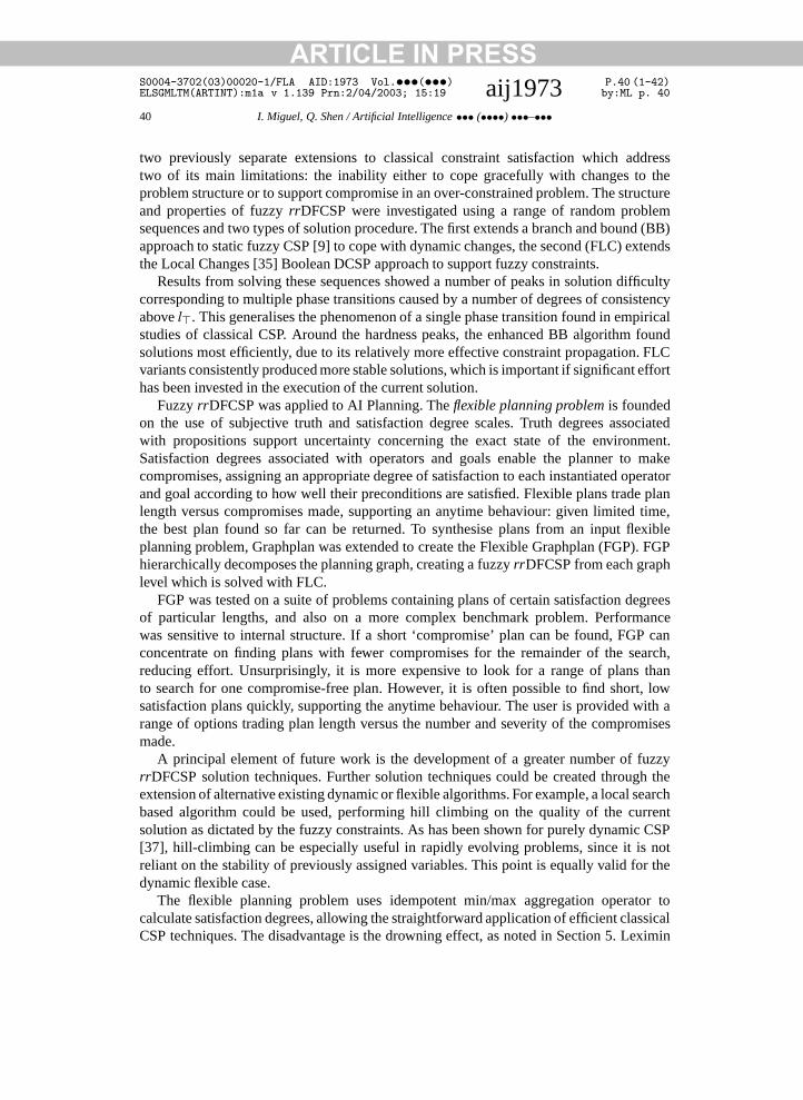
ARTICLE IN PRESSS0004-3702(03)00020-1/FLA AID:1973 Vol.•••(•••) P.40 (1-42)ELSGMLTM(ARTINT):m1a v 1.139 Prn:2/04/2003; 15:19 aij1973 by:ML p. 40
40 I. Miguel, Q. Shen / Artificial Intelligence ••• (••••) •••–•••
two previously separate extensions to classical constraint satisfaction which address
two of its main limitations: the inability either to cope gracefully with changes to theproblem structure or to support compromise in an over-constrained problem. The structureand properties of fuzzy rrDFCSP were investigated using a range of random problemsequences and two types of solution procedure. The first extends a branch and bound (BB)approach to static fuzzy CSP [9] to cope with dynamic changes, the second (FLC) extendsthe Local Changes [35] Boolean DCSP approach to support fuzzy constraints.Results from solving these sequences showed a number of peaks in solution difficultycorresponding to multiple phase transitions caused by a number of degrees of consistencyabove l. This generalises the phenomenon of a single phase transition found in empiricalstudies of classical CSP. Around the hardness peaks, the enhanced BB algorithm foundsolutions most efficiently, due to its relatively more effective constraint propagation. FLCvariants consistently produced more stable solutions, which is important if significant efforthas been invested in the execution of the current solution.
Fuzzy rrDFCSP was applied to AI Planning. The flexible planning problem is foundedon the use of subjective truth and satisfaction degree scales. Truth degrees associatedwith propositions support uncertainty concerning the exact state of the environment.Satisfaction degrees associated with operators and goals enable the planner to makecompromises, assigning an appropriate degree of satisfaction to each instantiated operatorand goal according to how well their preconditions are satisfied. Flexible plans trade planlength versus compromises made, supporting an anytime behaviour: given limited time,the best plan found so far can be returned. To synthesise plans from an input flexibleplanning problem, Graphplan was extended to create the Flexible Graphplan (FGP). FGPhierarchically decomposes the planning graph, creating a fuzzy rrDFCSP from each graphlevel which is solved with FLC.
FGP was tested on a suite of problems containing plans of certain satisfaction degreesof particular lengths, and also on a more complex benchmark problem. Performancewas sensitive to internal structure. If a short ‘compromise’ plan can be found, FGP canconcentrate on finding plans with fewer compromises for the remainder of the search,reducing effort. Unsurprisingly, it is more expensive to look for a range of plans thanto search for one compromise-free plan. However, it is often possible to find short, lowsatisfaction plans quickly, supporting the anytime behaviour. The user is provided with arange of options trading plan length versus the number and severity of the compromisesmade.
A principal element of future work is the development of a greater number of fuzzyrrDFCSP solution techniques. Further solution techniques could be created through theextension of alternative existing dynamic or flexible algorithms. For example, a local searchbased algorithm could be used, performing hill climbing on the quality of the currentsolution as dictated by the fuzzy constraints. As has been shown for purely dynamic CSP[37], hill-climbing can be especially useful in rapidly evolving problems, since it is notreliant on the stability of previously assigned variables. This point is equally valid for thedynamic flexible case.
The flexible planning problem uses idempotent min/max aggregation operator tocalculate satisfaction degrees, allowing the straightforward application of efficient classicalCSP techniques. The disadvantage is the drowning effect, as noted in Section 5. Leximin
ARTICLE IN PRESSS0004-3702(03)00020-1/FLA AID:1973 Vol.•••(•••) P.41 (1-42)ELSGMLTM(ARTINT):m1a v 1.139 Prn:2/04/2003; 15:19 aij1973 by:ML p. 41
I. Miguel, Q. Shen / Artificial Intelligence ••• (••••) •••–••• 41
fuzzy CSP [26] is one possible solution. This approach combines additive and min/max
operations to consider the satisfaction of all constraints, but has a higher computationalcost. Alternatively, additive aggregation could be employed. This supports a finer-grainedform of flexibility, and avoids the drowning effect. Recently developed means of enforcingarc consistency for non-idempotent operators could then be brought to bear [6,29]. Asdescribed in [23], FLC could easily be modified to support various types of flexibleCSP, such as those covered by valued or semiring CSP [2], to support other instances ofdynamic flexible CSP. The structure of the algorithm need not be changed, but the methodof consistency degree aggregation must be considered when enforcing consistency andgenerating bounds for repair sub-problems. A similar empirical analysis to that made herecould then be performed to establish the utility of FLC in each case.Finally, apart from AI Planning, it is interesting to investigate the application of fuzzyrrDFCSP to many other AI problems. Work is, for instance, ongoing in using fuzzyrrDFCSP to the selection of the most preferred model in compositional modelling [16].
Acknowledgements
This work is partially supported by UK EPSRC grants 97305803 and GR/N16129. Theauthors thank Peter Jarvis for his assistance in this research and the anonymous refereesfor their insightful comments which were very useful in revising this paper.
References
[1] J. Allen, J. Hendler, A. Tate, Readings in Planning, Morgan Kaufmann, San Mateo, CA, 1990.[2] S. Bistarelli, U. Montanari, F. Rossi, T. Schiex, G. Verfaillie, H. Fargier, Semiring-based csps and valued
csps: Frameworks, properties, and comparison, Constraints 4 (3) (1999) 199–240.[3] A. Blum, M. Furst, Fast planning through planning graph analysis, Artificial Intelligence 90 (1–2) (1997)
281–300.[4] D. Brelaz, New methods to colour the vertices of a graph, J. ACM 22 (4) (1979) 251–256.[5] S. Chien, Static and completion analysis for planning knowledge base development and verification, in: Proc.
3rd International Conference on Artificial Intelligence Planning Systems, Eidinburgh, UK, 1996, pp. 53–61.[6] M. Cooper, Reduction operations in fuzzy and valued constraint satisfaction, Fuzzy Sets and Systems 134
(2003) 311–342.[7] R. Dechter, Constraint networks, in: Encyclopedia of Artificial Intelligence, Wiley, New York, 1992,
pp. 276–285.[8] R. Dechter, A. Dechter, Belief maintenance in dynamic constraint networks, in: Proc. AAAI-88, St. Paul,
MN, 1988, pp. 37–42.[9] D. Dubois, H. Fargier, H. Prade, Possibility theory in constraint satisfaction problems: Handling priority,
preference and uncertainty, Appl. Intelligence 6 (1996) 287–309.[10] H. Fargier, Problèmes de satisfaction de constraintes flexibles: Application à l’ordonnancement de
production, Ph.D. Thesis, Université Paul Sabatier, Toulouse, 1994.[11] E. Freuder, Partial constraint satisfaction, in: Proc. IJCAI-89, Detroit, MI, 1989, pp. 278–283.[12] I. Gent, E. MacIntyre, P. Prosser, P. Shaw, T. Walsh, The constrainedness of arc consistency, in: Proc.
3rd International Conference on Principles and Practice of Constraint Programming, Linz, Austria, 1997,pp. 327–340.
[13] I. Gent, E. MacIntyre, P. Prosser, B. Smith, T. Walsh, An empirical study of dynamic variable orderingheuristics for the constraint satisfaction problem, in: Proc. 2nd International Conference on Principles andPractice of Constraint Programming, Cambridge, MA, 1996, pp. 179–193.

ARTICLE IN PRESSS0004-3702(03)00020-1/FLA AID:1973 Vol.•••(•••) P.42 (1-42)ELSGMLTM(ARTINT):m1a v 1.139 Prn:2/04/2003; 15:19 aij1973 by:ML p. 42
42 I. Miguel, Q. Shen / Artificial Intelligence ••• (••••) •••–•••
[14] M. Ginsberg, Dynamic backtracking, J. Artificial Intelligence Res. 1 (1993) 25–46.
[15] R. Haralick, G. Elliot, Increasing tree search efficiency for constraint satisfaction problems, ArtificialIntelligence 14 (1980) 263–313.[16] J. Keppens, Q. Shen, On compositional modelling, Knowledge Engineering Rev. 16 (2) (2001) 157–200.[17] A. Mackworth, Consistency in networks of relations, Artificial Intelligence 8 (1) (1977) 99–118.[18] A. Mackworth, Constraint satisfaction problems, in: Encyclopedia of Artificial Intelligence, Wiley, New
York, 1992, pp. 285–293.[19] B. Mazure, L. Saïs, E. Grégoire, Tabu search for SAT, in: Proc. AAAI-97, Providence, RI, 1997, pp. 281–
285.[20] I. Miguel, Q. Shen, Hard, flexible and dynamic constraint satisfaction, Knowledge Engineering Rev. 14 (3)
(1999) 199–220.[21] I. Miguel, Q. Shen, Dynamic flexible constraint satisfacton, Appl. Intelligence 13 (3) (2000) 231–245.[22] I. Miguel, Q. Shen, Solution techniques for constraint satisfaction problems: Advanced approaches, Artificial
Intelligence Rev. 15 (2001) 269–293.[23] I. Miguel, Dynamic flexible constraint satisfaction and its application to ai planning, Ph.D. Thesis, Division
of Informatics, Edinburgh University, 2001.[24] I. Miguel, Q. Shen, P. Jarvis, Efficient flexible planning via dynamic flexible constraint satisfaction, Engrg.
Appl. Artificial Intelligence 14 (3) (2001) 301–327.[25] S. Minton, M. Johnston, A. Philps, P. Laird, Minimizing conflicts: A heuristic repair method for constraint
satisfaction and scheduling problems, Artificial Intelligence 58 (1992) 161–205.[26] J. Moura Pires, F. Moura Pires, R. Almeida Ribeiro, Structure and properties of leximin fcsp and its
influence on optimisation problems, in: Proc. 7th Conference on Information Processing and Managementof Uncertainty in Knowledge-Based Systems, 1998, pp. 188–194.
[27] W. Pedrycz, F. Gomide, An Introduction to Fuzzy Sets: Analysis and Design, MIT Press, Cambridge, MA,1999.
[28] P. Prosser, An empirical study of phase transitions in binary constraint satisfaction problems, ArtificialIntelligence 81 (1996) 81–109.
[29] T. Schiex, Arc consistency for soft constraints, in: Proc. 6th International Conference on Principles andPractice of Constraint Programming, Singapore, 2000, pp. 411–424.
[30] T. Schiex, H. Fargier, G. Verfaillie, Valued constraint satisfaction problems: Hard and easy problems, in:Proc. IJCAI-95, Montreal, Quebec, 1995, pp. 631–637.
[31] T. Schiex, G. Verfaillie, Nogood recording for static and dynamic constraint satisfaction problems, Internat.J. Artificial Intelligence Tools 3 (2) (1994) 187–207.
[32] S. Smith, D. Nau, T. Throop, Total-order multi-agent task-network planning for contract bridge, in: Proc.AAAI-96, Portland, OR, 1996, pp. 108–113.
[33] E. Tsang, Foundations of Constraint Satisfaction, Academic Press, London, 1993.[34] P. van Hentenryck, T. Provost, Incremental search in constraint logic programming, New Generation
Computing 9 (1991) 257–275.[35] G. Verfaillie, T. Schiex, Solution reuse in dynamic constraint satisfaction problems, in: Proc. AAAI-94,
Seattle, WA, 1994, pp. 307–312.[36] R. Wallace, Why AC-3 is almost always better than AC-4 for establishing arc consistency in CSPs, in: Proc.
IJCAI-93, Chambéry, France, 1993, pp. 239–245.[37] R. Wallace, E. Freuder, Stable solutions for dynamic constraint satisfaction problems, in: Proc. 4th
International Conference on Principles and Practice of Constraint Programming, Pisa, Italy, 1998, pp. 447–461.
[38] D. Weld, Recent advances in AI planning, AI Magazine 20 (2) (1999) 93–123.[39] D. Wilkins, K. Myers, A multiagent planning architecture, in: Proc. 4th International Conference on
Artificial Intelligence Planning Systems, Pittsburgh, PA, 1998, pp. 154–162.


