Running head: GCM-based regional projections

GCM-based regional temperature and precipitation changeestimates for Europe under four SRES scenarios applying a

super-ensemble pattern-scaling method

Kimmo Ruosteenoja, Heikki Tuomenvirta and Kirsti Jylhä

Finnish Meteorological Institute

Helsinki

Finland

19 June 2006 (condensed)

Corresponding author: Kimmo Ruosteenoja, Finnish Meteorological Institute,

P.O.Box 503, FIN-00101 Helsinki, Finland

Email: Kimmo.Ruosteenoja@fmi.fi

Abstract

Seasonal GCM-based temperature and precipitation projections for the end of the 21st cen-

tury are presented for five European regions; projections are compared with corresponding

estimates given by the PRUDENCE RCMs. For most of the six global GCMs studied, only

responses to the SRES A2 and B2 forcing scenarios are available. To formulate projec-

tions for the A1FI and B1 forcing scenarios, a super-ensemble pattern-scaling technique has

been developed. This method uses linear regression to represent the relationship between

the local GCM-simulated response and the global mean temperature change simulated by a

simple climate model. The method has several advantages: e.g., the noise caused by internal

variability is reduced, and the information provided by GCM runs performed with various

forcing scenarios is utilized effectively. The super-ensemble method proved especially useful

when only one A2 and one B2 simulation is available for an individual GCM.

Next, 95% probability intervals were constructed for regional temperature and precipitation

change, separately for the four forcing scenarios, by fitting a normal distribution to the set

of projections calculated by the GCMs. For the high-end of the A1FI uncertainty interval,

temperature increases close to 10◦C could be expected in the southern European summer and

northern European winter. Conversely, the low-end warming estimates for the B1 scenario

are∼ 1◦C. The uncertainty intervals of precipitation change are quite broad, but the mean

estimate is one of a marked increase in the north in winter and a drastic reduction in the south

in summer.

In the RCM simulations driven by a single global model, the spread of the temperature

and precipitation projections tends to be smaller than that in the GCM simulations, but it is

possible to reduce this disparity by employing several driving models for all RCMs. In the

present suite of simulations, the difference between the mean GCM and RCM projections is

fairly small, regardless of the number or driving models applied.

1

1 Introduction

Owing to an increase in the concentrations of greenhouse gases, the global mean tempera-

ture is projected to rise by several degrees by the end of the 21st century (IPCC, 2001). The

objective of the PRUDENCE project is to assess how this global change manifests itself in

the climate of Europe (Christensen et al., 2006). The PRUDENCE regional climate model

(RCM) simulations use boundary conditions taken from only one or two global climate mod-

els (GCMs). This strongly constrains the RCM responses; Déqué et al. (2006) report that

differences between the simulations arising from the driving GCM are generally larger than

those due to the internal structures of RCMs. Moreover, most of the RCM projections are

calculated merely for the SRES A2 forcing scenario of the IPCC (2001).

Accordingly, to put the RCM simulations into a wider perspective, near-surface (2 m) air

temperature and precipitation projections based on experiments performed with six coupled

atmosphere-ocean GCMs are analyzed in this paper. These GCMs represent climate sen-

sitivities and patterns of change that are much more variable than those in the smaller set

of GCMs employed to drive the RCM simulations. Projections are composed separately

for four SRES forcing scenarios (A1FI, A2, B2 and B1). For each scenario, we calculate

both the mean estimates and the 95% probability intervals of the GCM- and RCM-based re-

gional temperature/precipitation change. Projections are presented for the 30-year time span

2070-2099 (for RCMs 2071-2100), relative to the baseline period 1961-1990.

In most cases, computationally-demanding GCMs have only been employed for simulating

responses to the A2 and B2 scenarios. Responses to the remaining scenarios are then derived

applying a new version of pattern-scaling developed during this study. The method and its

applicability are discussed in section 3. Generally, pattern-scaling methods can be applied

to such climate parameters for which the local response is linearly proportional to the global

mean temperature change. As will be shown, local temperature and precipitation changes

fulfil this condition fairly well. For some other parameters, such as the number of frost days,

2

the relationship is strongly nonlinear, and a more sophisticated approach is required.

Probability intervals for regional projections, as well as a comparison with simulations per-

formed with the RCMs participating in the PRUDENCE project, are presented in section 4.

The probability intervals are available as numerical values from the authors on request.

2 Climate models and regional subdivision

The main characteristics of the GCMs and the runs performed are summarized in Table 1.

More detailed information and references to model documentation are given in chapter 8 of

IPCC (2001). As a measure of how sensitively the models react to radiative forcing on the

time-scale discussed in this study, Table 1 gives the global mean temperature response to the

A2 forcing scenario for each model.

The responses to the A2 and B2 forcing scenarios had been simulated for all models in Table

1. The low-forcing B1 response was available for HadCM3 and CSIRO Mk2, while the high-

forcing A1FI response was only available for HadCM3. Furthermore, HadCM3 was the only

model for which ensemble runs were available.

The RCM analyzed in this study are HIRHAM, HadRM3P, CHRM, CLM, REMO, RCAO,

PROMES, RACMO and Arpège; information about the RCMs is given in other papers

of this special issue, e.g., Déqué et al. (2006). Most RCMs contain an atmospheric

component only1, the sea surface data and atmospheric lateral boundary values being de-

rived from a global GCM. Experiments with HadCM32 as a driving model have been con-

ducted with all the RCMs, but there are only two models (HIRHAM and RCAO) for which

ECHAM4/OPYC3-forced runs are available. Arpège/OPA as a driving model has been em-

ployed by one RCM only.

An effective method to condense the model-derived information is to represent it as spatial

1In two RCMs there is a submodel for the Baltic Sea.2In fact, the boundary conditions are not taken directly from the HadCM3 runs, but an atmospheric model

HadAM3 is used as a ’bridge’ between the HadCM3 and the RCMs.

3

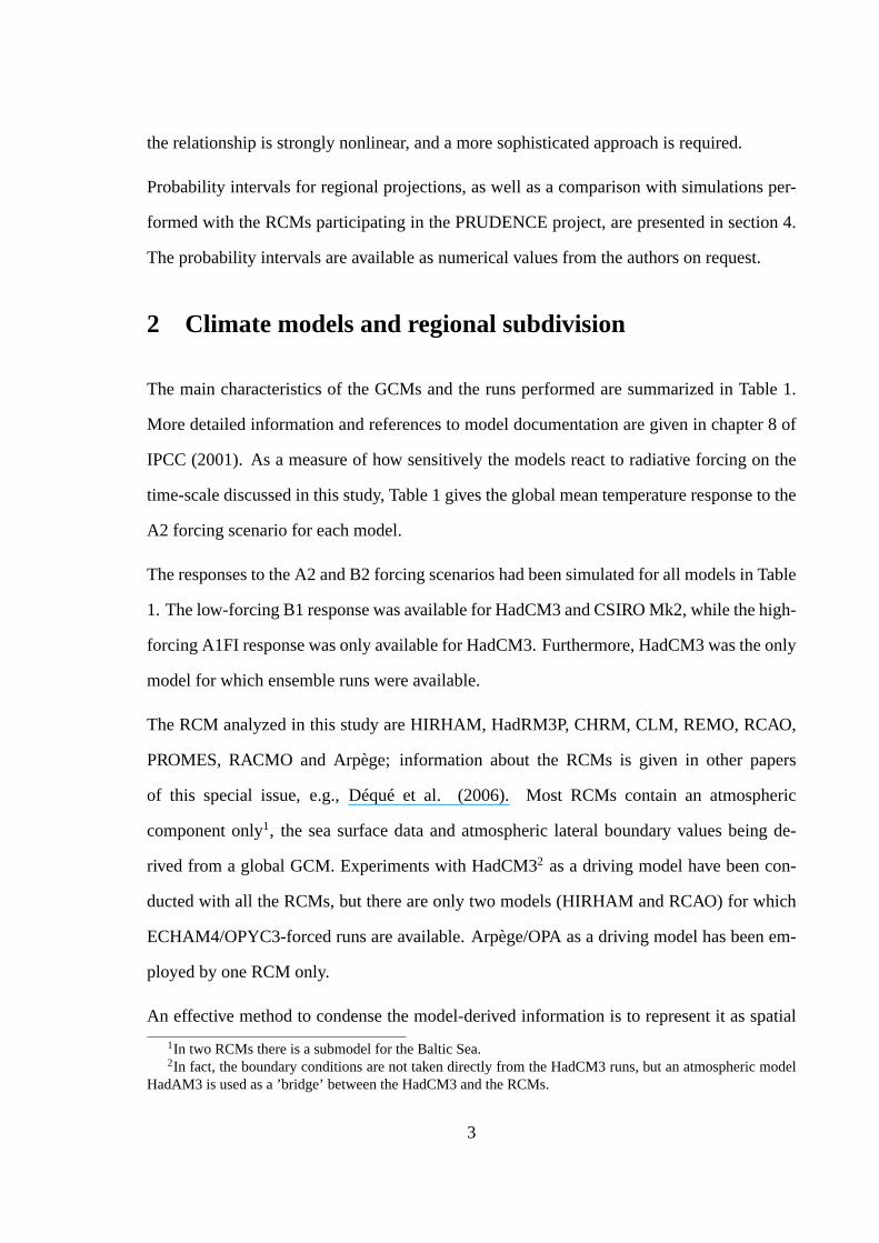
averages over a number of discrete regions. The subdivision into five regions employed in

this study is illustrated in Fig. 1. Henceforth, most of the results to be presented are area-

weighted spatial means over the grid boxes inside the given region.

In addition to externally-forced changes, there occurs in the climate system unforced internal

variability on various timescales. The statistical properties of that variability were inferred

from a 1000-year HadCM3 simulation, in which the composition of the atmosphere and

other external forcing agents were kept constant. Standard deviations of the temperature and

precipitation were calculated from the simulated of 30-year temporal averages of regional

means.

3 The super-ensemble pattern scaling method

3.1 Principle of the method

Pattern-scaling techniques have been widely used to create climate change projections for

scenarios or time spans not simulated by GCMs. Various versions of scaling techniques have

been presented by Mitchell et al. (1999), New and Hulme (2000), Huntingford and Cox

(2000), Mitchell (2003), Ruosteenoja et al. (2003) and Hingray et al. (2004), for instance.

In the RCM experiments employed in this work, however, only two discrete 30-year periods

have been simulated. In order to apply the same scaling technique to both the GCM and

RCM responses, an amended version of the time-slice method has been developed. The

geographical pattern of the temperature, precipitation or other response is assumed to be

independent of the forcing, the amplitude of this fixed pattern being proportional to the global

mean temperature change.

The traditional simple time-slice method calculates the scaled response employing an indi-

vidual GCM response, e.g.:

∆TA1FI,s =〈∆TA1FI〉〈∆TA2〉

∆TA2,g (1)

4

where the subindexg refers to the GCM-simulated ands to the scaled temperature change

for an individual grid-point or region.〈∆T 〉 denotes the global mean temperature change

that is calculated using the simple energy balance climate model MAGICC3 (IPCC, 2001,

Appendix 9.1). Such a computationally simple model can readily be used to calculate global

mean temperature change for all forcing scenarios of interest.

The GCM-simulated climate response includes, besides the actual climate change signal,

random noise caused by internal variability. This noise is transmitted into the scaled re-

sponse. The problem is common to all scaling methods.

One way to reduce the influence of the noise is to carry out the scaling in (1) using an

ensemble mean instead of an individual GCM response. The effective ensemble size can be

further increased by calculating the scaled response from a least-square regression line fitted

to a set consisting of GCM responses to several SRES scenarios:

∆TA1FI,s = aT 〈∆TA1FI〉; aT =

∑ni=1 〈∆Ti〉∆Ti,g∑n

i=1 〈∆Ti〉2(2)

n being the number of the simulations considered, i.e., the size of the super-ensemble. Scaled

responses to the B1 scenario are calculated analogously. The principle of the method is il-

lustrated in Fig. 2. Since〈∆T 〉 = 0 represents a zero climate change, the least-square

regression line is constrained to pass through the origin. The regression fit can also be em-

ployed to scale the precipitation change∆P :

∆PA1FI,s = aP 〈∆TA1FI〉; aP =

∑ni=1 〈∆Ti〉∆Pi,g∑n

i=1 〈∆Ti〉2(3)

One can readily notice that simple time-slice scaling (1) is obtained as a special case (with

n = 1) of the super-ensemble method. Analogously, if all the simulations from whichaT or

aP is calculated belong to an ensemble consisting of responses to the same forcing scenario,

(2)-(3) reduce to a conventional scaling from an ensemble mean.

The idea of modelling the relationship between the local and global climate response by

3Model for the Assessment of Greenhouse-gas Induced Climate Change

5

linear regression has been employed independently by Hingray et al. (2004). Unlike the

present study, they do not give projections separately for individual forcing scenarios.

The MAGICC-emulated time series of global annual mean temperature changes for four

coupled GCMs (CSIRO Mk2, ECHAM4, HadCM3 and NCAR PCM) were supplied to us

by Dr. Sarah Raper. For the CGCM2 and GFDL, we used the average four-GCM emulated

values of〈∆T 〉 in determining the scaling coefficients.

From the MAGICC-emulated time series of〈∆T 〉 for the A1FI, A2, B1 and B2 scenar-

ios, we calculated the temperature response for 2070-2099, relative to 1961-1990. These

global-mean temperature change estimates were employed to calculate the scaled responses

of regional temperature (2) and precipitation (3), separately for each season.

3.2 Applicability of the super-ensemble scaling

The performance of various versions of the scaling technique is analyzed for HadCM3, i.e.,

for the only GCM for which simulations with all four scenarios are available. In applying

pattern-scaling, there are two fundamental sources of uncertainty:

• Nonlinearity error: the local responses of temperature, precipitation and other meteo-

rological variables may not be inherently linear functions of the global mean tempera-

ture change

• Noise due to internal variability

Errors due to random noise always occur in scaled responses. This type of error can be

reduced by increasing the ensemble or super-ensemble size in (1)-(3). The super-ensemble

scaling method is intended to keep in check just this type of error.

On the other hand, the nonlinearity error affects the quality of the scaled response most

seriously if the scaling is based on a ’distant’ simulation, i.e., on a simulation in which〈∆T 〉

is much larger or smaller than in the target scenario to be scaled. In super-ensemble scaling

6

the regression coefficient (aT or aP ) is generally determined by responses to several forcing

scenarios, some of which are usually not very close to the target scenario. Accordingly, in the

super-ensemble method the nonlinearity error tends to be larger than in the simple method

(1), in which the closest existing simulation is typically utilized.

An example illustrating the degree of linearity of the regional temperature and precipitation

responses as a function of〈∆T 〉 is given in Fig. 2. The responses do not exactly lie on the

linear regression line, but for temperature the deviations from linearity are generally of the

same order of magnitude as the variations due to internal variability. For regional precipi-

tation changes, in this example the deviations from linearity are larger than for temperature

changes.

Another conclusion to be drawn from Fig. 2 is that, due to the small size of the ensembles,

the spread among the ensemble members does not generally give a representative picture of

the internal variability.

For a quantitative evaluation of the various scaling methods, the scaled seasonal temperature

and precipitation responses to the A1FI and B1 scenarios were first calculated at each grid

point using the super-ensemble method (Eqs. (2)-(3)). As a measure of the quality of the

scaled responses, we calculated area mean rms differences between the scaled and the corre-

sponding directly GCM-simulated temperature/precipitation reference fields, either over the

entire globe, over global land areas or over European land areas west of 35◦E. The annual

means of these rms differences are reported in Table 2.

In a situation with no ensemble runs (i.e., only one A2 and one B2 simulation available), the

super-ensemble method appears in all cases to work better than the simple method (1); com-

pare rows (i) and (iii) and rows (v) and (vii) in Table 2. When parallel runs are available, scal-

ing from the ensemble mean always improves the result when compared to scaling from an

individual simulation (rows (i) vs (ii), (v) vs (vi)). Furthermore, the super-ensemble method

utilizing three A2 and two B2 responses beats scaling from the simple ensemble mean in

predicting the B1 temperature response (rows (vi) vs (viii)). By contrast, in predicting the

7

A1FI temperature response and the scaling of precipitation in general, the super-ensemble

method and scaling from the ensemble mean could not be ranked.

The A2 and B2 scenario runs are available for all the GCMs, and in this paper the projections

to be presented for these scenarios will be based on the direct GCM data. For the A1FI and

B1 scenarios, on the other hand, simulations are available for one or two models only, and

these projections are mainly formulated employing responses scaled with the super-ensemble

method. Scaled responses are calculated separately for each individual GCM.

For the RCMs, A2 is the only scenario for which there is a run for all models. Other projec-

tions have to be based mainly (B2) or exclusively (A1FI, B1) on scaled responses.

4 95% probability intervals for regional projections

Since we have analyzed six GCMs only, modelled climate change projections applied as

such do not give a statistically representative picture of regional climate change. Instead, we

have fitted the normal (Gaussian) distribution to the set of model projections.

The validity of the normal distribution approximation can be evaluated by means of quantile

plots (Vining, 1998, p. 117-120). Due to the small number of GCMs, projections for all five

regions are incorporated into the same diagram. In order to make the responses for different

regions comparable, all GCM projections are standardized:

∆T sti,j,k = (∆Ti,j,k −∆Tj,k)/s

∆Tj,k ; ∆P st

i,j,k = (∆Pi,j,k −∆Pj,k)/s∆Pj,k (4)

where the subindicesi, j andk refer to the six GCMs, five regions and four seasons, respec-

tively. The overbar stands for a mean over the six models,s for the standard deviation.

In fact, in calculating the means and standard deviations employed in (4), each of the three

members of the HadCM3 ensemble is given a weight of 2/3, the remaining model projections

being unity-weighted. Thus, HadCM3 runs have a double total weight compared to the other

GCMs. Enhanced weighting is given to that model because parallel runs can simulate a part

of the internal variability.

8

In the quantile plots of Fig. 3, the points are mostly concentrated close to thex = y line. In

all, the projections of the various GCMs thus appear to follow the normal distribution fairly

well. Utilizing the Gaussian approximation, we can construct 95% probability intervals for

the temperature and precipitation change for each season and region:

I∆Tj,k = ∆Tj,k ± 1.96s∆T

j,k ; I∆Pj,k = ∆Pj,k ± 1.96s∆P

j,k (5)

Since the projections for the A1FI and B1 scenarios are mainly based on scaled responses,

we assessed what kind of uncertainty for the probability intervals arises from the applica-

tion of pattern scaling. For that purpose, scaled and GCM-derived probability intervals for

the B2 temperature and precipitation changes were compared. The B2 scenario is chosen

for inspection since the original and scaled A2 responses are by definition close to one an-

other; in calculating the regression coefficients, the contribution of the large-amplitude A2

responses is larger than that of the weak B2 responses (see Eqs. (2)-(3)). The scaled and di-

rectly GCM-simulated median changes appeared to be very close to one another. The widths

of both probability intervals are generally nearly the same in summer, but in winter scaling

tends to underestimate the intervals, especially for precipitation in southern Europe. Note

that the super-ensemble scaling reduces the contribution of internal variability, which partly

explains the smaller spread in the scaled projections.

To conclude this section, the differences between the scaled and the original model-derived

projections seem to be small enough for the scaled responses to be used as reasonable ap-

proximations for missing GCM projections.

4.1 Probability intervals for GCM projections

In this study probability intervals are determined separately for all four scenarios. As in

the previous subsection, the summed weight of the HadCM3 ensemble runs is 2, while the

weight of other models is 1. For the B1 and A1F1 scenarios no multiple runs have been per-

formed. In order to reduce the influence of the noise, we have therefore created an artificial

9

2-member HadCM3 ensemble for these scenarios. This ensemble consists of two estimates,

one being the direct GCM response, the other being scaled from the set of three A2 and

two B2 runs. (In fact, the probability intervals obtained with this procedure and with the

inclusion of one double-weighted direct HadCM3 A1FI or B1 response were very similar.)

Probability intervals for temperature change are given in absolute terms, while precipitation

changes are here expressed in percentages to facilitate application of the results to impact

studies. In transforming the precipitation changes into percentages (100% × ∆P/P ), the

denominatorP is the baseline-period precipitation averaged over the six GCMs, the weights

being as stated above.

The probability intervals for temperature change, separately for each season, region and sce-

nario, are depicted in Fig. 4. The intervals are quite broad, reflecting the large scatter among

the various model projections. For example, the extreme estimates for regional springtime

responses to the A1FI forcing range from∼ 2◦C to more than9◦C. Another striking feature

is that the probability intervals representing different forcing scenarios overlap strongly.

The 95% probability intervals for precipitation change are presented in Fig. 5. Note that in

the A1FI and A2 scenarios the southern Europe summertime precipitation manifests a very

large decrease at the lower end of the probability interval. Since−100% is a categorical

limit for the decrease, the normal distribution is inappropriate for describing such strong

decreases. Hence, in Fig. 5 the probability intervals have been truncated at−80%.

With the exception of eastern Europe in winter and northern Europe in the intermediate

seasons, the 95% probability intervals of precipitation change intersect the zero line. Conse-

quently, in most cases even the sign of the future precipitation change cannot be established.

In simulating the wintertime precipitation change in northern Europe, there is one model

(ECHAM4) that yields a very large relative increase (more than 50%) in precipitation com-

pared to the other GCMs. When fitting a normal distribution to that data set, such a distinctly

different data value tends to spuriously widen the probability interval at both ends. In the

10

absence of that model, the width of the interval would be reduced by more than half, and the

lower end of the interval would also be positive. Thus, the Gaussian distribution is not an

ideal tool for studying such a special case.

4.2 Comparison to RCM results

To study how much RCM- and GCM-based climate change projections differ from one an-

other, we chiefly discuss the A2 projections, since this is the only forcing scenario sim-

ulated by all RCMs. Two estimates for the 95% probability intervals of RCM-simulated

climate change are presented. The first one is merely based on HadCM3/HadAM3-driven

simulations that are available for all RCMs. The other estimate utilizes RCM simulations

driven by all three global models (Arpège/OPA, ECHAM4, HadCM3). Since the number of

ECHAM4- and Arpège/OPA-driven simulations is too small (two/one) to yield any statistical

distribution by itself, we have completed the matrix of experiments by creating a synthetic

extended set containing simulations with all RCMs for all the three driving models. The

standard deviation of the ECHAM4- and Arpège/OPA-driven RCM projections is assumed

to be the same as in the HadCM3-driven RCM experiments. The average of these projections

is approximated by adding to the mean of the HadCM3-driven responses the difference of

the responses calculated with the same RCM applying the two driving models. This proce-

dure is rather crude, since there are only one (Arpège/OPA – HadCM3) or two (ECHAM4

– HadCM3) such analogous pairs of RCM runs. Finally, the extended sets of (real and sur-

rogate) RCM runs driven by the three models are combined to give an estimate for the full

probability interval.

The comparison for temperature change is presented in Fig. 6. For the three RCMs

(HIRHAM, HadRM3P, Arpège) with parallel runs, all individual runs have been incorpo-

rated in the analysis with equal weight. In calculating the RCM probability intervals, the

CHRM, PROMES and RACMO models are excluded, since the computational domain of

these three models does not cover all the five regions. The individual RCM projections, by

11

contrast, are depicted for all RCMs that cover the region concerned.

The mean estimates of temperature change inferred from the GCM and RCM experiments

analyzed are mostly fairly close to one another. RCM-simulated warming tends to be smaller

than that of the GCMs in northern Europe in winter and spring, the opposite being true in the

south-east in winter.

Except for summer, scatter among the HadCM3-driven RCM temperature projections is gen-

erally much smaller than among the GCM projections. The single GCM applied as a bound-

ary condition strongly constrains the climate response, especially from autumn to spring

when climate is mainly determined by large-scale weather phenomena. The probability in-

tervals calculated from the extended set of RCM simulations, including simulations with all

RCMs for each of the three driving models, by contrast, are of the same order of magnitude

as the GCM probability intervals.

For precipitation change (Fig. 7), the spread among the HadCM3-driven RCM runs is in

most cases smaller than that among the GCM simulations. The probability intervals inferred

from the expanded RCM set are not systematically broader or narrower than those given by

the GCMs.

Projected temperature responses were compared with the internal variability of temperature

in a millennial HadCM3 control simulation. The standard deviation of internal variability

was multiplied by√

2 to give an expectation for the difference between two arbitrarily-

chosen 30-year means. Both the RCM and GCM temperature responses appeared to be

statistically significant. Moreover, the spread among the various GCM projections was larger

than the measure of internal variability. This indicates that intermodel differences are caused

by the dissimilarity of the model codes rather than by mere internal variability.

Applying the super-ensemble pattern-scaling method introduced in section 3, RCM-based

projections for scenarios other than A2 can be easily formulated. The RCM-based projec-

tions driven by a single model continue to have a smaller spread than the GCM projections.

12

For instance, the A1FI-forced 95% probability interval of summertime temperature change

for south-western Europe, derived from the HadCM3-driven RCMs, was 5.4-8.2◦C, the cor-

responding GCM-derived range being 2.7-10.2◦C.

5 Conclusions

This paper introduces a new version of the pattern-scaling method, which enables one to

create climate parameter projections for those forcing scenarios for which GCM or RCM

simulations are not available. In addition to surface air temperature and precipitation, the

methodology is suited to all such variables for which local responses are linearly dependent

on global mean temperature change. The method treats all available model runs as a super-

ensemble, which may contain both simulations for several forcing scenarios and parallel runs

for the same forcing. Projections for the missing scenarios are inferred from a regression line

representing the relationship between the local or regional response of the meteorological

parameter of interest and the global mean temperature change simulated by a simple energy

balance model.

In our evaluation, the super-ensemble scaling method proved to improve on the conventional

time-slice method in situations with no parallel simulations for individual scenarios avail-

able. If there are multiple simulations for each forcing scenario, differences in the perfor-

mance were small. Due to the smallness of the ensemble sizes, however, these conclusions

should be considered somewhat tentative.

In principle, the super-ensemble pattern-scaling method has several advantages. First, the

method utilizes all the available information in calculating the scaled response, especially

when responses to more than one forcing scenario have been calculated by a sophisticated

GCM or RCM. Second, the method reduces the impact of random noise. This is particularly

advantageous if, in some of the GCM simulations, internal variability happens to be at op-

posite extremes during the control and target periods. Third, several more simple versions of

13

the time-slice scaling method (e.g., (1)) are obtained as special cases of the super-ensemble

method. Note also that strong-amplitude responses (e.g., A2) have the largest weight in

calculating the regression coefficientsaT andaP , which further tends to reduce the noise.

We have formulated mean as well as upper and lower estimates of 2 m air temperature and

precipitation change for five regions covering the bulk of continental Europe. Results are

based on simulations performed with six global coupled atmosphere-ocean GCMs. SRES

A2 and B2 simulations are available for all models, while the A1F1 and B1 projections for

most of the GCMs are based on the super-ensemble scaling. The 95% probability intervals

for the regional temperature/precipitation change have been constructed by approximating

the changes simulated by the various models by a normal distribution.

The upper GCM-based estimates of warming for the A1F1 scenario mostly range from 6 to

about 10◦C, while the lower estimates for the B1 scenario are generally close to 1◦C. If the

driest end of the A1FI probability interval happens to be true, precipitation in the southern

Europe summer might be reduced by more than 80%.

GCM-derived climate change estimates were compared with projections based on RCM out-

put. The RCM response is largely determined by the driving global GCM wherein the RCM

is nested. If only one driving GCM is employed, the spread is generally much smaller in

the RCM than in the GCM climate projections. This problem appears to be partly solved by

utilizing three driving GCMs, but the conclusion remains uncertain due to the small number

of RCM simulations actually performed with driving models other than HadCM3. RCMs

are certainly a valuable tool for resolving spatial details of climate change, but one should

be cautious in basing the actual climate change projections merely on the RCM data if the

number of driving models is small.

In calculating the means and standard deviations of the regional GCM responses, HadCM3

was given, somewhat arbitrarily, a double weight. This was done because the number of

runs performed with that model was large compared to the remaining models. Several more

sophisticated ways to determine the weights are suggested in the literature. For example,

14

Murphy et al. (2004) and Giorgi and Mearns (2003) have given enhanced weight to models

showing a good performance in reproducing the present-day climate. In these studies, prob-

ability distributions obtained by employing equal and unequal weighting appeared to diverge

to some extent, but the main conclusions remained unchanged.

As an example of an alternative approach, New and Hulme (2000) have constructed the

probability distribution of projected regional climate change by performing a large number of

Monte Carlo simulations with a simple energy balance model. The geographical patterns of

the climate response were derived from seven global GCMs, with ensemble runs performed

with HadCM2 given a summed weight greater than that of the remaining six GCMs together.

Pattern-scaling does not seem to be a very large source of error in constructing regional

climate projections for extreme scenarios. It is possible that, for the A2 and B2 scenarios

also, scaled projections may even be better than those inferred directly from model output;

this depends on the ratio of the random noise error to the nonlinearity error.

Acknowledgments: This work was financed by the EU PRUDENCE project (EVK2-

2001-00156) and in the final phase also by Nordic Energy Research. The time se-

ries of the modelled monthly mean temperature and precipitation were downloaded from

the Intergovernmental Panel for Climate Change Data Distribution Centre (http://ipcc-

ddc.cru.uea.ac.uk/dkrz/dkrz_index.html), whilst some of the HadCM3 runs have been pro-

vided by Dr. D. Viner. The PRUDENCE data were downloaded from http://prudence.dmi.dk.

The two anonymous reviewers are thanked for their useful comments.

References

Christensen, J.H., Carter, T.R. and Rummukainen, M.: 2006, ’Evaluating the performance

and utility of regional climate models: the PRUDENCE project’,Clim. Change(this

issue).

Déqué, M., Rowell, D.P., Lüthi, D., Giorgi, F., Christensen, J.H., Rockel, B., Jacob, D.,

15

Kjellström, E., de Castro, M. and van den Hurk, B.: 2006, ’An intercomparison of

regional climate simulations for Europe: assessing uncertainties in model projections’,

Clim. Change(this issue).

Giorgi, F. and Mearns, L.O.: 2003: ’Probability of regional climate change based on the

Reliability Ensemble Averaging (REA) method’,Geophys. Res. Lett.30(12), 1629.

Hingray, B., Mezghani, A. and Buishand, T.A.: 2004, ’Development of probability dis-

tributions for regional climate change from uncertain global mean warming and an

uncertain scaling relationship’, submitted toHydrology and Earth System Sciences.

Huntingford, C. and Cox, P.M.: 2000, ’An analogue model to derive additional climate

change scenarios from existing GCM simulations’,Clim. Dyn.16, 575-586.

IPCC: 2001,Climate Change 2001: The Scientific Basis. Contribution of Working Group

I to the Third Assessment Report of the Intergovernmental Panel on Climate Change

[Houghton, J.T., Ding, Y., Griggs, D.J., Noguer, M., van der Linden, P.J., Dai, X.,

Maskell, K. and Johnson C.A. (eds.)], Cambridge University Press, Cambridge and

New York, 881 p.

Mitchell, J.F.B., Johns, T.C., Eagles, M., Ingram, W.J. and Davis, R.A.: 1999, ’Towards the

construction of climate change scenarios’,Clim. Change41, 547-581.

Mitchell, T.D.: 2003, ’Pattern scaling. An examination of the accuracy of the technique for

describing future climates’,Clim. Change60, 217-242.

Murphy, J.M., Sexton, D.M.H., Barnett, D.N., Jones, G.S., Webb, M.J., Collins, M. and

Stainforth, D.A.: 2004, ’Quantification of modelling uncertainties in a large ensemble

of climate change simulations’,Nature430, 768-772.

New, M. and Hulme, M.: 2000, ’Representing uncertainty in climate change scenarios: a

Monte-Carlo approach’,Integrated Assessment1, 203-213.

16

Ruosteenoja, K., Carter, T.R., Jylhä, K. and Tuomenvirta, H.: 2003, ’Future climate in

world regions: an intercomparison of model-based projections for the new IPCC emis-

sions scenarios’,The Finnish Environment644, Finnish Environment Institute, 83 p.

Vining, G.G.: 1998,Statistical methods for engineers,Brooks/Cole Publishing Company,

Pacific Grove., U.S.A., 479 p.

17

Fig. 1. The five regions employed in reporting subcontinental scale changes of temperature

and precipitation; N, W, E, SW, and SE represent the regions of northern, western, eastern,

south-western and south-eastern Europe, respectively.

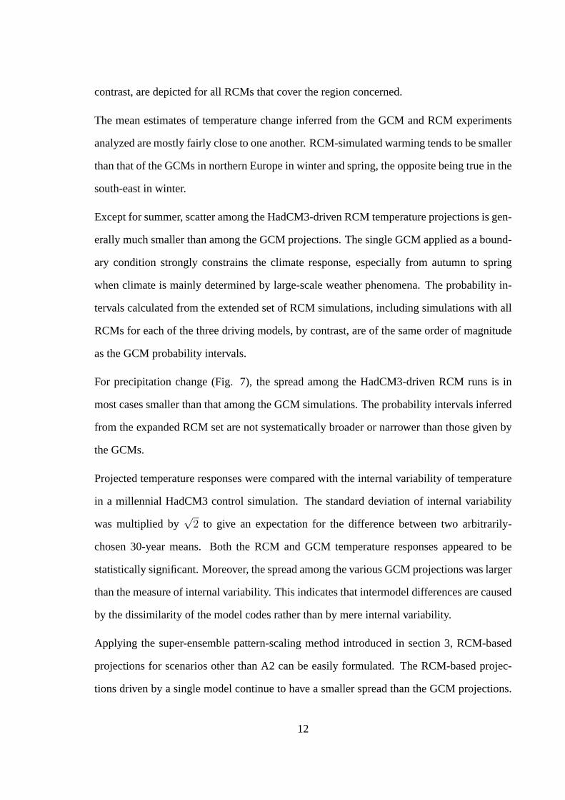
Fig. 2. An example of super-ensemble scaling. Temperature (upper panels) and precipita-

tion (lower panels) change (2070-2099) – (1961-1991) for western Europe (region ’W’ in

Fig. 1) in winter (DJF) and summer (JJA) in various HadCM3 simulations (open circles) are

given as a function of the MAGICC-simulated global annual mean temperature change. Sce-

narios examined are B1 (〈∆T 〉 = 2.34◦C; 1 ensemble member), B2 (2.89◦C; 2 members),

A2 (3.75◦C; 3 members) and A1FI (4.68◦C; 1 member). Each panel includes a regression

line calculated from the three A2 and two B2 responses; the resulting scaled A1FI and B1

responses are denoted by closed squares. The vertical bar on the left side of the points, cen-

tred on the ensemble mean, depicts the± standard deviation of the differences between two

arbitrarily-chosen 30-year averages, derived from the standard deviations of temperature and

precipitation variability in a millennial HadCM3 control run.

Fig. 3. Quantile plots for seasonal temperature (upper panels) and precipitation (lower pan-

els) responses to the A2 forcing. The x-axis represents the standardized GCM-simulated

temperature/precipitation responses rearranged in ascending order. The corresponding quan-

tile values inferred from the standard normal distribution are given by the y-axis. Each

diagram includes data from six GCMs. All the five regions are depicted in the diagrams, see

legend.

Fig. 4. 95% probability intervals of seasonal temperature change (vertical bars) from 1961-

90 to 2070-99 for five regions, derived from SRES-forced simulation performed with six

GCMs. Intervals are given separately for the A1FI (red), A2 (black), B2 (blue) and B1

(green) scenarios. The dot at the centre of the bar denotes the median of the interval.

Fig. 5. Seasonal GCM-derived 95% probability intervals of percentage precipitation change.

For denotations, see Fig. 4. In the diagrams changes< −80% are excluded.

18

Fig. 6. Comparison of the seasonal RCM- and GCM-derived temperature responses to the

A2 forcing for the five regions defined in Fig. 1. The plus signs denote projections of

individual HadCM3-driven RCM runs. The grey bar on the left of each triad denotes the

95% probability interval derived from the HadCM3-driven RCM runs; the middle grey bar

gives an estimate for the interval that would be obtained if simulations with all RCMs had

been available for all the three driving global models (see text). The black bar on the right of

the triad stands for the GCM-based probability intervals.

Fig. 7. Comparison of RCM- and GCM-derived 95% probability intervals of regional pre-

cipitation change. For denotations, see Fig. 6.

19

Table 1. Coupled GCMs analyzed in the present work. Column 1 gives the model acronymand column 2 the country where the model was developed. For horizontal resolution, thetruncation in spherical harmonics space (TRUNC) and the approximate grid distance in grid-point space (GRID) are given (HadCM3 is a grid-point model). L denotes the number ofmodel levels. The next column tells whether flux adjustment is employed.∆Tglob is theglobal mean temperature increase from 1961-1990 to 2070-2099 as a response to the A2forcing. SCENS shows the SRES simulations performed with each model; if parallel runsare available, the number of the ensemble members is given in parentheses.

MODEL COUNTRY TRUNC GRID L ADJ ∆Tglob SCENSCGCM2 Canada T32 3.8× 3.8◦ 10 Yes 3.5◦C A2, B2CSIRO Mk2 Australia R21 3.2× 5.6◦ 9 Yes 3.4◦C A2, B1, B2ECHAM4/OPYC3 Germany T42 2.8× 2.8◦ 19 Yes 3.3◦C A2, B2GFDL R30 U.S.A. R30 2.2× 3.8◦ 14 Yes 3.1◦C A2, B2HadCM3 United Kingdom - 2.5× 3.8◦ 19 No 3.2◦C A1FI, A2 (3), B1, B2 (2)NCAR DOE PCM U.S.A. T42 2.8× 2.8◦ 18 No 2.4◦C A2, B2

20

Table 2. Annual means of rms differences between the scaled and HadCM3-simulated sea-sonal a) 2 m air temperature and b) precipitation responses. Values are presented separatelyfor European land areas west of 35◦E, global land areas and for the entire globe. ’SCEN’denotes the SRES scenario for which the evaluations are calculated, ’SCALING FROM’ thescaling method; N states the number of GCM simulations employed in calculating the scaledresponse. (i) is the mean of the three rms values that are obtained by comparing the patternsscaled from the three individual A2 responses with the GCM-simulated A1FI field. Analo-gously, (v) is the mean of two rms values. (iii) and (vii) are both means of 6 rms differences,each corresponding to a super-ensemble scaling from a pair consisting of one individual A2and one B2 ensemble member. (iv) and (viii) refer to super-ensemble scaling from a set oftwo B2 and three A2 ensemble members.

a) Scaling of temperature response (unit:◦C)

SCEN SCALING FROM N EUROPE LAND AREAS GLOBAL(i) A1FI Individual A2 1 0.557 0.571 0.497(ii) A1FI A2 ensemble mean 3 0.402 0.423 0.384(iii) A1FI Regression 1xA2+1xB2 2 0.531 0.502 0.450(iv) A1FI Regression 3xA2+2xB2 5 0.420 0.402 0.378(v) B1 Individual B2 1 0.654 0.468 0.352(vi) B1 B2 ensemble mean 2 0.617 0.425 0.318(vii) B1 Regression 1xA2+1xB2 2 0.539 0.400 0.321(viii) B1 Regression 3xA2+2xB2 5 0.510 0.377 0.305

b) Scaling of precipitation response (unit: mm/d)

SCEN SCALING FROM N EUROPE LAND AREAS GLOBAL(i) A1FI Individual A2 1 0.242 0.327 0.537(ii) A1FI A2 ensemble mean 3 0.174 0.258 0.383(iii) A1FI Regression 1xA2+1xB2 2 0.229 0.316 0.487(iv) A1FI Regression 3xA2+2xB2 5 0.181 0.269 0.391(v) B1 Individual B2 1 0.230 0.216 0.392(vi) B1 B2 ensemble mean 2 0.206 0.185 0.344(vii) B1 Regression 1xA2+1xB2 2 0.190 0.204 0.357(viii) B1 Regression 3xA2+2xB2 5 0.177 0.194 0.334

21

Fig. 1. The five regions employed in reporting subcontinental scale changes of temperature and precipitation; N, W, E, SW, and SE

represent the regions of northern, western, eastern, south-western and south-eastern Europe, respectively.

Fig. 2. An example of super-ensemble scaling. Temperature (upper panels) and precipitation (lower panels) change (2070-2099) – (1961-

1991) for western Europe (region ’W’ in Fig. 1) in winter (DJF) and summer (JJA) in various HadCM3 simulations (open circles) are

given as a function of the MAGICC-simulated global annual mean temperature change. Scenarios examined are B1 (〈∆T 〉 = 2.34◦C; 1

ensemble member), B2 (2.89◦C; 2 members), A2 (3.75◦C; 3 members) and A1FI (4.68◦C; 1 member). Each panel includes a regression

line calculated from the three A2 and two B2 responses; the resulting scaled A1FI and B1 responses are denoted by closed squares. The

vertical bar on the left side of the points, centred on the ensemble mean, depicts the± standard deviation of the differences between

two arbitrarily-chosen 30-year averages, derived from the standard deviations of temperature and precipitation variability in a millennial

HadCM3 control run.

22

Fig 3. Quantile plots for seasonal temperature (upper panels) and precipitation (lower panels) responses to the A2 forcing. The x-

axis represents the standardized GCM-simulated temperature/precipitation responses rearranged in ascending order. The corresponding

quantile values inferred from the standard normal distribution are given by the y-axis. Each diagram includes data from six GCMs. All the

five regions are depicted in the diagrams, see legend.

23

Fig. 4. 95% probability intervals of seasonal temperature change (vertical bars) from 1961-90 to 2070-99 for five regions, derived from

SRES-forced simulation performed with six GCMs. Intervals are given separately for the A1FI (red), A2 (black), B2 (blue) and B1 (green)

scenarios. The dot at the centre of the bar denotes the median of the interval.

Fig. 5. Seasonal GCM-derived 95% probability intervals of percentage precipitation change. For denotations, see Fig. 4. In the diagrams

changes< −80% are excluded.

24

Fig. 6. Comparison of the seasonal RCM- and GCM-derived temperature responses to the A2 forcing for the five regions defined in Fig.

1. The plus signs denote projections of individual HadCM3-driven RCM runs. The grey bar on the left of each triad denotes the 95%

probability interval derived from the HadCM3-driven RCM runs; the middle grey bar gives an estimate for the interval that would be

obtained if simulations with all RCMs had been available for all the three driving global models (see text). The black bar on the right of

the triad stands for the GCM-based probability intervals.

Fig. 7. Comparison of RCM- and GCM-derived 95% probability intervals of regional precipitation change. For denotations, see Fig. 6.

25