GDQFEM numerical simulations of continuous media with cracks and discontinuities

Copyright © 2013 Tech Science Press CMES, vol.94, no.4, pp.331-369, 2013

GDQFEM Numerical Simulations of Continuous Mediawith Cracks and Discontinuities

E. Viola1, F. Tornabene1 E. Ferretti1 and N. Fantuzzi1

Abstract: In the present paper the Generalized Differential Quadrature Finite El-ement Method (GDQFEM) is applied to deal with the static analysis of plane statestructures with generic through the thickness material discontinuities and holes ofvarious shapes. The GDQFEM numerical technique is an extension of the Gener-alized Differential Quadrature (GDQ) method and is based on the idea of conven-tional integral quadrature. In particular, the GDQFEM results in terms of stressesand displacements for classical and advanced plane stress problems with discon-tinuities are compared to the ones by the Cell Method (CM) and Finite ElementMethod (FEM). The multi-domain technique is implemented in a MATLAB codefor solving irregular domains with holes and defects. In order to demonstrate theaccuracy of the proposed methodology, several numerical examples of stress anddisplacement distributions are graphically shown and discussed.

Keywords: Generalized Differential Quadrature Finite Element Method, Cracksand Discontinuities, Cell Method.

1 Introduction

Dealing with elastic structures containing cracks and material discontinuities hasalways been a complicated problem to solve numerically, due to high-order gradi-ents of the solutions in terms of displacements and stresses at crack tips and edges[Li, Shen, Han, and Atluri (2003); Sladek, Sladek, and Atluri (2004); Viola andMarzani (2004); Viola, Artioli, and Dilena (2005); Han, Liu, Rajendran, and Atluri(2006); Ricci and Viola (2006); Viola, Ricci, and Aliabadi (2007); Li and Atluri(2008a,b)]. Computational problems are connected with the numerical techniquesunder consideration. For instance, the well-known Finite Element Method (FEM)has a lot of numerical issues when line cracks and holes are present in physicalmodels. For this reason many scientists have tried new ways for analysing elasticstructures using alternative numerical techniques [Viola, Li, and Fantuzzi (2012);

1 DICAM Department, University of Bologna, Italy.

332 Copyright © 2013 Tech Science Press CMES, vol.94, no.4, pp.331-369, 2013

Viola, Fantuzzi, and Marzani (2012); Li and Viola (2013); Li, Fantuzzi, and Torn-abene (2013)]. However, in this work it is assumed that there is no contact betweentwo separated parts of a body and the singularity effects at the crack tip or at theends of material discontinuities are not investigated. The same assumption wasconsidered by other researchers in recent papers [Huang, Leissa, and Liao (2008);Huang and Leissa (2009); Huang, Leissa, and Chan (2011); Huang, Leissa, andLi (2011)] when fracture mechanics is not the main purpose of the study, such asthe one presented in this paper. In addition, concerning the materials and the loadsconsidered in this paper, the plastic zone is very small with respect to the crackdimensions. Thus, the crack can be considered equal to the initial crack length,due to the fact that it does not propagate. In a future study, the fracture mechanicsanalysis according to the approach outlined in the papers [Dong and Atluri (2012,2013a,b)] will be taken into account. Here, the Generalized Differential Quadra-ture Finite Element Method (GDQFEM) is investigated, nevertheless any specialelement is considered for treating the singularity connected with fracture mechan-ics problems. In fact, any kind of discontinuity is treated as a free edge boundary.There are some other methods which differ from FEM that can deal with cracksand discontinuities, too. In particular, the Cell Method (CM) [Tonti (2001); Ferretti(2001, 2003, 2004a,b,c, 2005, 2009, 2012); Ferretti, Casadio, and Di Leo (2008)].The works by [Ferretti (2014, 2013a,b)] are also used in the following.

The main aim of this paper is to compare the numerical solutions obtained throughGDQFEM, FEM and CM. The advantages and disadvantages of each method arepointed out. The GDQFEM is an advanced version of the Generalized DifferentialQuadrature (GDQ) method, which has been applied by the authors to compositeplates and shells over the years [Artioli, Gould, and Viola (2005); Viola and Torn-abene (2005, 2006, 2009); Tornabene, Fantuzzi, Viola, and Ferreira (2013)]. Itshould be mentioned that irregular GDQ implementation [Civan and Sliepcevich(1985); Lam (1993); Bert and Malik (1996)] has been introduced in order to solvestructures that do not have a regular shape. This occurs in civil, mechanical andaerospace engineering applications, as well as in other fields of science. One of themain advantages of GDQ is linked to its mesh-less behaviour, which is based onthe strong formulation of any mathematical problem. Furthermore, it can lead toaccurate and reliable results, also using a very small amount of grid points. How-ever, for the classic GDQ application, a regular physical geometry is required, thatis the one described by orthogonal Cartesian or curvilinear coordinates [Tornabene(2009, 2011b,a,c)]. In the present work, the geometrical and material discontinu-ities are treated by dividing the whole physical domain into several sub-domains.The GDQFEM mesh should follow the irregularities of the problem under consid-eration. Nevertheless, for every sub-domain the mechanical and geometric proper-

Continuous Media with Cracks and Discontinuities 333

Bn

mB =m

n

Ω(n)

Ω(n)Ω(m)

Ω(m)

(1)Ω (2)Ω

Figure 1: Generic irregular domain configuration and sub-domain decomposition.

ties must be at least continuous. For 2D plane problems these parameters are thethickness and the elastic constants.

2 Plane elasticity equations

As far as plane elastic problems with material discontinuities and holes are con-cerned, in this paper the basic mathematical formulation is related to two- dimen-sional elasticity. Thus, the general 2D plane elastic theory is summarized follow-ing the book by [Timoshenko (1934)]. The main hypothesis of a 2D plane strainproblem concerns the strain components which are εz = γxz = γyz = 0. When aplane stress problem is taken into account the out-of-plane stresses are negligibleσz = τxz = τyz = 0. It should be noted that a plane strain state does not correspondto a plane stress one, since σz 6= 0. Analogously, when a plane stress is consideredresults εz 6= 0 and the deformation problem is not plane. The very well-known elas-tic kinematic relationships, valid both for the plane stress and strain cases, assumethe aspect

εεε = Du, where D =

[∂

∂x 0 ∂

∂y0 ∂

∂y∂

∂x

]T

(1)

where D is the kinematic operator, and the strain vector and the displacement vec-tor are defined as εεε =

[εx εy γxy

]T , u =[u v

]T , respectively. The constitutiveequations, connecting the states of stress and strain, in concise form are

σσσ = Cεεε , where C =

2G+λ λ 0λ 2G+λ 00 0 G

(2)


and the stress vector is σσσ =[σx σy τxy

]T . In all the numerical examples, theYoung’s modulus E and Poisson’s ratio ν are used in place of the Lamè’s elasticconstants λ and G [Timoshenko (1934)]. The equilibrium equations are reportedin compact matrix form

D∗σσσ + f = 0, where D∗ =

[∂

∂x 0 ∂

∂y0 ∂

∂y∂

∂x

](3)

and the force vector, which identifies the body forces, is defined by f =[

fx fy]T .

Since the strong form of the differential problem has to be solved, the fundamentalsystem of equations in terms of displacements parameters u and v must be found.Substituting the kinematic equations in the constitutive ones and the results in theequilibrium equations, the fundamental system for the static case becomes

Lu+ f = 0 (4)

where L=D∗CD is named the fundamental operator. The formulation for dynamicplane problems can be obtained from Eq. 4, by adding the inertia forces

Lu+ f = fI (5)

In Eq. 5 fI =[ρ u ρ v

]T , ρ denotes the material density and u, v stand for thetranslational accelerations. As it is well-known, the partial differential system ofequations Eq. 5 can be only solved when the boundary conditions are included. Inthe 2D elasticity problems in hand, two types of boundary conditions are enforced:a condition on the displacements u = u and another condition on the derivativesof the displacement parameters ∂u

∂n = q. The first condition on the displacementsis called the kinematic boundary condition or Dirichlet type boundary condition.The second condition on the displacements derivatives is called static boundarycondition or Neumann type boundary condition. In particular, for a fixed edgeu = 0 the vector q is called the flux vector and in the present paper can be given bythe external applied loads to the fixed physical domain, such as normal and shearforces. Since GDQFEM operates on sub-domains, the elements connectivity mustbe introduced. In the present case the C 1 continuity conditions are enforced. Inusing the GDQFEM, a domain can have any shape. Using a mapping technique, itis transformed into a set of regular Cartesian parent elements. Thus, the externalflux boundary conditions must be written following the outward unit normal vectorn as reported in [Xing, Liu, and Liu (2010); Zhong and He (1998); Zhong and Yu(2009)]

σσσn = Nσσσ , where N =

[n2

x n2y 2nxny

−nxny nxny n2x−n2

y

](6)


and nx, ny are the components of the unit normal vector n, also termed directioncosines. For the sake of completeness, the theoretical development of GDQFEM isexplained in the following, in order to show the implementation procedure for thecurrent methodology.

3 Generalized differential quadrature finite element method

As it is well-known from literature [Chen (1999a,b, 2003); Fantuzzi (2013)], theGDQFEM decomposes a domain Ω into several sub-domains or elements Ω(n), forn = 1, . . . ,ne, where ne is the total number of sub-domains of the current mesh. Asample of the GDQFEM mesh is depicted in Fig. 1, where four sub-domains areindicated and the external and internal boundary conditions are also underlined. Itis important to note that all the couples of sub-domains are considered as disjoint,such as Ω(n) ∩Ω(m) = /0, for n 6= m. The symbol /0 is referred to as the emptyset. Moreover, the whole physical domain Ω is obtained as Ω = Ω(1)∪ ·· ·∪Ω(ne),namely the union of a collection of sets. For 2D plane problems, the total degreesof freedom per node are related to the number of constrains. The mathematicalproblem is regulated by two in-plane displacement parameters u, v. Two boundaryconditions per node are involved at the domain external boundary. As a result,the total number of degrees of freedom for any of the following problems can becomputed as N ·N ·ne ·nd , where N are the number of collocation points on a singleedge and nd = 2 for 2D plane problems. The inter-element compatibility conditionsare enforced by the connection between two adjacent elements, concisely indicatedby Bm

n = Bnm. B indicates one of the two conditions that can be imposed for each

element edge. The subscripts and superscripts n, m are referred to the two adjacentelements. Indeed the two conditions are algebraically different as it is illustrated inthe following. The compatibility, or continuity, conditions between elements entailkinematic and static conditions. These conditions, with reference to Fig. 1, can beindicated as

u(n) = u(m) kinematic condition

σ(n)n = σ

(m)n static condition

(7)

For instance, the kinematic condition is imposed on the left edge that belongs toelement Ω(n) and the static condition is enforced on the right edge that belongsto Ω(m). In particular the kinematic conditions can be imposed directly, never-theless the static ones, since they are functions of the outward unit normal vectorn =

[nx ny

]T , follow relation 6. For example, when the kinematic condition isconcerned Bm

n indicates the boundary displacements of element Ω(n) and Bnm re-

ports the boundary displacements of element Ω(m). At the same time regarding the


static condition Bmn contains the stresses σ

(n)n of element Ω(n) that act towards ele-

ment Ω(m) and Bnm, vice versa, are the stresses σ

(m)n of element Ω(m) that correspond

to element Ω(n). Due to the form of the continuity conditions the inter-element ac-curacy is of C 1 type. Therefore it is higher than the connectivity of standard FEMprocedure. In addition to the element edge conditions, the corner type boundaryconditions must be considered. The implementation of the corner type boundaryconditions for higher-order numerical schemes is still an open problem. In fact veryfew papers hitherto have been published about this topic [Wang, Wang, and Chen(1998); Wang, Wang, and Zhou (2004); Viola, Tornabene, and Fantuzzi (2013b)].In the present paper, where the corner belongs to two adjacent elements, the samecontinuity conditions of the facing sides can be used. When more than two elementsshare a single corner point a problem arises, since more than two algebraic condi-tions have to be enforced. For the sake of conciseness, the reference for the actualcorner points boundary conditions is the work by [Viola, Tornabene, and Fantuzzi(2013b)]. The numerical integration upon each element is performed through GDQ[Marzani, Tornabene, and Viola (2008); Tornabene and Ceruti (2013a,b)]. How-ever, the GDQ method can be applied only to regular coordinate systems, such asCartesian or orthogonal curvilinear coordinates [Tornabene, Fantuzzi, Viola, andReddy (2014); Tornabene, Fantuzzi, Viola, and Ferreira (2013); Tornabene, Viola,and Fantuzzi (2013)]. Thus, mapping technique must refer to every sub-domainin order to transform the physical coordinates x-y into the parent element coordi-nates ξ -η . The general mapping transformation, that is the same as in FEM, canbe written as follows

x = x(ξ ), y = y(η) (8)

Deriving the Cartesian mapping and applying the derivative laws, from Eq. 8 onegets

∂

∂x=

∂ξ

∂x∂

∂ξ+

∂η

∂x∂

∂η,

∂

∂y=

∂ξ

∂y∂

∂ξ+

∂η

∂y∂

∂η(9)

Since a higher order computational scheme is solved in this work, the second orderderivatives have to be calculated

∂ 2

∂x2 =∂ 2ξ

∂x2∂

∂ξ+

∂ 2η

∂x2∂

∂η+

(∂ξ

∂x

)2∂ 2

∂ξ 2 +

(∂η

∂x

)2∂ 2

∂η2 +2∂ξ

∂x∂η

∂x∂ 2

∂ξ ∂η

∂ 2

∂y2 =∂ 2ξ

∂y2∂

∂ξ+

∂ 2η

∂y2∂

∂η+

(∂ξ

∂y

)2∂ 2

∂ξ 2 +

(∂η

∂y

)2∂ 2

∂η2 +2∂ξ

∂y∂η

∂y∂ 2

∂ξ ∂η

∂ 2

∂x∂y=

∂ 2ξ

∂x∂y∂

∂ξ+

∂ 2η

∂x∂y∂

∂η+

∂ξ

∂x∂ξ

∂y∂ 2

∂ξ 2 +∂η

∂x∂η

∂y∂ 2

∂η2+

+

(∂ξ

∂x∂η

∂y+

∂ξ

∂y∂η

∂x

)∂ 2

∂ξ ∂η

(10)


The first and second order Cartesian derivatives of Eqs. 9, 10 are used to mapthe fundamental equations and the boundary conditions of the two-dimensionalplane problem at hand. The interested reader can find all the details about coordi-nate transformation and mapping technique applied to differential quadrature in theworks by [Cen, Chen, Li, and Fu (2009); Liu (1999); Xing and Liu (2009); Zongand Zhang (2009)]. As it is well-known, the GDQ technique evaluates a partial,or total, derivative of a function at a point as a weighted sum of some coefficientsa(n)i j for the corresponding values of the function at issue. In considering a one-dimensional problem, the GDQ technique allows to write the first order derivativeas

d f (x)dx

∣∣∣∣x=xi

∼=N

∑j=1

ax,(1)i j f (x j), i = 1,2, . . . ,N (11)

where N is the total number of collocation points and ax,(1)i j are the weighting coeffi-

cients, evaluated using Lagrange interpolation polynomials L. These test functionscan be found in literature [Civan and Sliepcevich (1984); Bert and Malik (1997);Tornabene, Viola, and Inman (2009); Viola, Dilena, and Tornabene (2007); Torn-abene, Marzani, Viola, and Elishakoff (2010); Tornabene, Fantuzzi, Viola, Cinefra,Carrera, Ferreira, and Zenkour (2014)] and have the form

L(1)(xi) =N

∏q=1,q6=i

(xq− xi), L(1)(x j) =N

∏q=1,q6= j

(xq− x j) (12)

The weighting coefficients of the second and higher order derivatives can be com-puted from recurrence relationships [Shu (2000); Viola, Rossetti, and Fantuzzi(2012); Ferreira, Viola, Tornabene, Fantuzzi, and Zenkour (2013); Tornabene, Fan-tuzzi, Viola, and Carrera (2014)]. A generalized higher order derivative can bewritten as

dn f (x)dxn

∣∣∣∣x=xi

= f (n)x (xi) =N

∑j=1

ax,(n)i j f (x j)

for i = 1,2, . . . ,N, n = 2,3, . . . ,N−1

(13)

This general approach based on the polynomial approximation, as shown in [Viola,Tornabene, and Fantuzzi (2013a,c); Tornabene, Fantuzzi, Viola, and Reddy (2014);


Tornabene and Reddy (2013)], allows to write the following weighting coefficients

ax,(n)i j = n

(ax,(n−1)

ii ax,(1)i j −

ax,(n−1)i j

xi− x j

)for i 6= j, n = 2,3, . . . ,N−1

ax,(n)ii =−

N

∑k=1,k 6=i

ax,(n)ik for i = j

(14)

There are various articles about the GDQ weighting coefficients calculation, thatit is impossible to cite them all. Among others, here are mentioned the ones by[Shu, Chen, and Du (2000); Tornabene, Liverani, and Caligiana (2011, 2012a,b,c);Tornabene and Viola (2007, 2008, 2009a,b, 2013)]. Since cracks lead to high stressconcentrations at their tips, in the following numerical examples a localized ver-sion of GDQ has been worked out. In particular, Local Generalized DifferentialQuadrature (LGDQ) has been considered as introduced in literature by [Sun andZhu (2000); Zong and Lam (2002); Lam, Zhang, and Zong (2004); Shen, Young,Lo, and Sun (2009); Tsai, Young, and Hsiang (2011); Hamidi, Hashemi, Talebbey-dokhti, and Neill (2012); Tornabene (2012); Nassar, Matbuly, and Ragb (2013);Wang, Cao, and Ge (2013); Yilmaz, Girgin, and Evran (2013)]. The main differ-ence between LGDQ and GDQ is that in the former the nth-order derivative of f (x)is computed locally as

dn f (x)dxn

∣∣∣∣x=xi

∼=Ni

∑j=1

ax,(n)i j f (x j), i = 1,2, . . . ,Ni (15)

where Ni are the points of the local domain around the point xi as depicted in Fig. 2.The overline of a(n)i j in Eq. 15 denotes the different weighting coefficients from theones corresponding to the GDQ method. In this way, the local numerical error atthe crack tip does not propagate through the GDQ domain due to its local numericalscheme.

Ni

1 2 N... i ...Figure 2: Local GDQ scheme.


4 Examples

In the study, the static and dynamic behaviour of two dimensional structures con-taining cracks and discontinuities is mainly investigated by the GDQFEM. It is re-called that the aim of this paper is not to study the fracture mechanics of 2D solids,but to show some numerical applications and comparisons of plane structures withdiscontinuities that do not consider the stress and strain singularities at the cracktip. The numerical analysis can be divided into two main parts. In the first partsome benchmark tests are performed. A comparison with the FEM results is alsoperformed. Moreover, some unpublished results about composite structures withdiscontinuities are presented. In the second part of this section, a cracked structureis examined by considering not only homogeneous materials but also compositematerials. In particular two different numerical techniques are used in the follow-ing. In the first part the classic GDQ is applied. A Chebyshev-Gauss-Lobatto(C-G-L) grid distribution is used for all the computations. The C-G-L points arelocated as

ξi,ηi =−cos(

i−1N−1

π

), for i = 1, . . . ,N (16)

where ξ and η are the parent element coordinates involved in the mapping trans-formation and ξ ,η ∈ [−1,1]. When cracked structures are investigated the localGDQ method is used, since it reduces the error propagation. Hence, a uniform griddistribution is employed

ξi,ηi =i−1N−1

, for i = 1, . . . ,N (17)

4.1 Cantilever wall

The accuracy of the GDQFEM technique is explored by examining the in-planevibration of the square cantilever plate shown in Fig. 3. It can be viewed as a kindof beam under the plane stress condition. This cantilever wall is a consolidatedFEM benchmark through literature [Gupta (1978); Cook and Avrashi (1992); Zhaoand Steven (1996); de Miranda, Molari, and Ubertini (2008)]. In fact, this problemhas been studied in great detail and a reference solution was obtained by using avery fine FEM mesh of the plane stress under consideration. In addition to theother assessments that can be found in the aforementioned papers, here a differentand alternative solution for the same problem is worked out using GDQFEM. Thepresent solution is searched through the strong formulation of the elasticity problemat issue. The previous papers [Gupta (1978); Cook and Avrashi (1992); Zhao andSteven (1996); de Miranda, Molari, and Ubertini (2008)] used FEM and adopted a


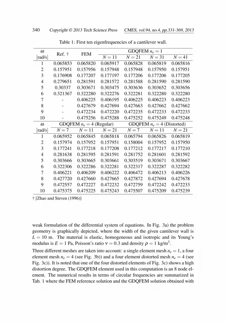
Table 1: First ten eigenfrequencies of a cantilever wall.

ωRef. † FEM

GDQFEM ne = 1[rad/s] N = 11 N = 21 N = 31 N = 41

1 0.065853 0.065820 0.065917 0.065828 0.065819 0.0658162 0.157951 0.157956 0.157948 0.157948 0.157950 0.1579513 0.176908 0.177207 0.177197 0.177206 0.177206 0.1772054 0.279651 0.281591 0.281572 0.281588 0.281590 0.2815905 0.30337 0.303671 0.303475 0.303636 0.303652 0.3036566 0.321367 0.322280 0.322276 0.322281 0.322280 0.3222807 - 0.406225 0.406195 0.406225 0.406223 0.4062238 - 0.427679 0.427694 0.427663 0.427662 0.4276629 - 0.472234 0.472220 0.472235 0.472233 0.472233

10 - 0.475256 0.475288 0.475252 0.475249 0.475248ω GDQFEM ne = 4 (Regular) GDQFEM ne = 4 (Distorted)

[rad/s] N = 7 N = 11 N = 21 N = 7 N = 11 N = 211 0.065952 0.065845 0.065818 0.065794 0.065826 0.0658192 0.157974 0.157952 0.157951 0.158004 0.157952 0.1579503 0.177241 0.177218 0.177208 0.177212 0.177217 0.1772104 0.281638 0.281595 0.281591 0.281752 0.281601 0.2815925 0.303666 0.303665 0.303661 0.303519 0.303671 0.3036676 0.322306 0.322286 0.322281 0.322317 0.322287 0.3222827 0.406221 0.406209 0.406222 0.406472 0.406213 0.4062268 0.427720 0.427660 0.427665 0.427872 0.427694 0.4276789 0.472557 0.472227 0.472232 0.472759 0.472242 0.472233

10 0.475375 0.475225 0.475243 0.475507 0.475209 0.475239

† [Zhao and Steven (1996)]

weak formulation of the differential system of equations. In Fig. 3a) the problemgeometry is graphically depicted, where the width of the given cantilever wall isL = 10 m. The material is elastic, homogeneous and isotropic and its Young’smodulus is E = 1 Pa, Poisson’s ratio ν = 0.3 and density ρ = 1 kg/m3.

Three different meshes are taken into account: a single element mesh ne = 1, a fourelement mesh ne = 4 (see Fig. 3b)) and a four element distorted mesh ne = 4 (seeFig. 3c)). It is noted that one of the four distorted elements of Fig. 3c) shows a highdistortion degree. The GDQFEM element used in this computation is an 8 node el-ement. The numerical results in terms of circular frequencies are summarized inTab. 1 where the FEM reference solution and the GDQFEM solution obtained with


y

x

L

(a) (b) (c)

Figure 3: Cantilever wall: a) Model geometry; b) GDQFEM four element regularmesh; c) GDQFEM four element highly distorted mesh.

(a)

(b)

Figure 4: Convergence tests for a cantilever wall: a) Four regular elements; b) Fourelements within a highly distorted mesh.


several meshes are shown. Very good agreement is observed among all the com-putations. For each numerical case the same number of points along the masterelement coordinates is considered N = M. A detailed accuracy test is presented inFig. 4, where the logarithm of the absolute error E = |ωGDQFEM−ωFEM|, betweenGDQFEM and FEM numerical solutions, is reported as a function of the numberof grid points per element. In particular, in Fig. 4a) the four element regular meshis examined, whereas in Fig. 4b) the four element distorted mesh is investigated. Itis noted that the error increases if a distorted mesh is used. However, for each fre-quency the graphs always tend to decrease when the number of points per elementN is increased. The convergence tests of Fig. 4 involve the first ten circular fre-quencies. For both meshes a good agreement is achieved for the higher frequencymodes, which are usually the controlling factors for the accuracy assessment of afinite element solution.

4.2 Tapered cantilever plate with a central circular hole

In the second benchmark the vibration of a tapered cantilever plate with a centralcircular hole under plane stress conditions is considered. The aim of this applica-tion is to examine the accuracy and applicability of the present methodology whenirregular and unstructured meshes are used. In fact, it should be noted that in theprevious case multi-domain GDQ could be applied when regular squared elementswere used. On the contrary, distorted elements with curved boundaries are used inthe following. The plate geometry is represented in Fig. 5a) where the greatest sideis L = 10 m and the inner hole radius is R = 1.5 m. In particular the hole centre hascoordinates (5,5) m and the shortest side is l = 5 m. The tapered plate shows onesymmetry axis. This geometry has been also studied by several authors [Zhao andSteven (1996); de Miranda, Molari, and Ubertini (2008)]. Regarding the material,it is assumed, isotropic and homogeneous with elastic modulus E = 1 Pa, Poisson’sratio ν = 0.3 and density ρ = 1 kg/m3. The reference FEM solution is evaluated us-ing the mesh illustrated in Fig. 5b) where ne = 7312 using S8R element type. Twodifferent GDQFEM meshes were used in the computations: a four element meshne = 4 (see Fig. 5c)) and an eight element mesh ne = 8 (see Fig. 5d)). This choicehas been made in order to map differently the circular internal hole. It has beenshown from Figs. 5c)-d) that four elements are the minimum number of elementsfor a good mapping of circular shapes. The first ten circular frequencies of Tab. 2show that the eight node mesh leads to a more accurate convergence than the fourelement mesh. To summarize, the absolute circular frequency error, of the first tenfrequencies, is plotted as a function of the number of grid points per element forthe two meshes at issue. The accuracy tests represented in Fig. 6a) show the resultsobtained with a four element mesh. In Fig. 6b) an eight element mesh has been


used. It appears that the solution obtained with ne = 8 is 10 times more accuratethan the solution with ne = 4 for the same amount of grid points per element.

x

y

L

L l

(a) (b)

(c) (d)

Figure 5: Cantilever tapered plate with a central circular hole: a) Model geometry;b) FEM mesh with ne = 3712 using 8 node S8R Abaqus elements; c) Four elementmesh; d) Eight element mesh.

4.3 Square plate with circular hole

In the next numerical application, the classic problem of a homogeneous plate witha circular centred hole is considered under static loading. In Fig. 7a) the problemgeometry is depicted, where the dimensional plate parameter is L = 5 m and theapplied normal tension is σ = 100 N/m. The material has a Young’s modulusE = 3 ·107 Pa and Poisson’s ratio ν = 0.3. The numerical solutions are presentedin terms of the normal stress σy calculated at any point of the line segment AB,from the point A at the circular edge to the external point B of the plate straightedge. Every stress distribution is computed for a fixed value of the geometricalratio χ = D/L between the diameter D of the hole and the plate side length L. Theside L remains constant in all the calculations. The GDQFEM mesh used in the


Table 2: First ten eigenfrequencies of a tapered cantilever plate with a circularcentral hole.

ωFEM

GDQFEM ne = 4 GDQFEM ne = 8[rad/s] N = 11 N = 21 N = 41 N = 11 N = 21 N = 31

1 0.0700 0.071226 0.070128 0.070120 0.069976 0.069978 0.0699782 0.1558 0.155596 0.155998 0.155998 0.155851 0.155863 0.1558643 0.1999 0.199411 0.199967 0.199962 0.199874 0.199880 0.1998794 0.2620 0.262110 0.262643 0.262636 0.262028 0.262070 0.2620715 0.2917 0.292303 0.292199 0.292197 0.291744 0.291732 0.2917326 0.4192 0.419199 0.419846 0.419847 0.419260 0.419256 0.4192597 0.4208 0.420896 0.420925 0.420918 0.420825 0.420818 0.4208188 0.4678 0.468142 0.468025 0.468024 0.467834 0.467844 0.4678459 0.4801 0.480427 0.480894 0.480894 0.480190 0.480122 0.480124

10 0.5281 0.525467 0.528197 0.528203 0.528079 0.528074 0.528076

(a)

(b)

Figure 6: Convergence tests for a tapered cantilever plate with a central circularhole: a) Four element mesh; b) Eight element mesh.


x

y

D BA L

σ

(a) (b)

Figure 7: Square plate with a centred circular hole subjected to tension σ : a) Geo-metric representation; b) GDQFEM mesh.

Figure 8: Stress profiles of a square plate subjected to tension σ = 100 N/m with acentral circular hole .

computations, for χ = 0.5 and χ = 0.25, is an eight element mesh with 8 node perelement as shown in Fig. 7b). For every calculation a N = 21 C-G-L grid points isused. For the other two cases (χ = 0.1 and χ = 0.05) sixteen elements and N = 15are used. As it can be noted from Fig. 8 the GDQFEM solution is superimposed tothe FEM solution for every χ value. Furthermore, when the plate side is four timesgreater than the circle diameter the normal stress σy tends to the applied stress valueσ = 100 N/m and the tip stress value tends to be three times the applied load, asit is very well-known from the literature, when the dimension L→ ∞. It should beunderlined that the abscissa of Fig. 8 is the horizontal line between point A and B


Figure 9: Square plate subjected to tensile stress σ with a centred hollow inclusion.

Figure 10: Stress profile of a square plate subjected to tensile stress σ = 100 N/mwith a centred elastic hollow inclusion.

of Fig. 7a), where the point B is fixed at x = 5 m and point A moves from x = 2.625m to x = 3.75 m (because the circular hole diameter decreases, whereas the plateremains of the same size).

In order to study the interaction effect between a matrix containing a circular holeand a hollow elastic inclusion, the system depicted in Fig. 9 is investigated. Theplate side is L = 5 m, the outer radius is R1 = 1.5625 m and the inner radius R2 =1.25 m. The external normal load is σ = 100 N/m. The soft matrix has Em = 3 ·106

Pa and Poisson’s ratio νm = 0.25, whereas the inner hollow inclusion is made ofa harder material with Ei = 3 · 107 Pa and νi = 0.3. In Fig. 10 the stress profileinvolving the points between A and B is graphically shown. The single dashedcurve represents the homogeneous case, presented above and where only the matrix


material is present. The presence of a hollow inclusion gives rise to an abrupt jumpat the material interface between the two materials. The GDQFEM solution withblack circles is superimposed to the solid FEM line.

4.4 Soft-core elliptic arch

In the last benchmark the free vibrations of a composite three layer soft-core ellipticarch with elliptic holes is presented. The two external layers are made of a materialwhich is stiffer than the one that the core layer is made of. Fig. 11 shows theGDQFEM mesh used in the computation. The soft-core arch is clamped on thehorizontal axis and free along its curvilinear edges, as well as along the boundaryof the holes. The darker elements refer to the two stiffer sheets with Es = 3 ·109 Pa,νs = 0.3 and ρs = 1000 kg/m3. The inner soft-core has Ec = 3 ·107 Pa, νc = 0.25and ρc = 500 kg/m3, instead. The dimensions of the outer ellipse are a1 = 10 m,b1 = 5 m, whereas the inner ellipse is defined by a2 = 5 m, b2 = 2.5 m, where a1, b1and a2, b2 are the semi-diameters of the ellipses in hand. The structure has a verticalsymmetry and variable radii of curvature. The location and the dimensions of thethree elliptic holes can be deducted according to the drawing scale of the ellipticsoft-core embedded between the external layers of the arch shown in Fig. 11. Themajor axis of symmetry of each elliptic hole is tangent to the elliptic soft-core axisat the point specified by the center of the elliptic hole itself. The GDQFEM uses 44elements of irregular shape with various grid point number as reported in Tab. 3,where the GDQFEM convergence is also shown. Very good agreement is observedbetween the FEM solution and the GDQFEM numerical results obtained with themesh of Fig. 11. It appears that few grid points are sufficient to obtain an accuratesolution, since here a high number of elements has been used. For the sake ofcompleteness, the first four modal shapes of the structure at issue are shown inFig. 12, where the soft-core behaviour of the structure is clearly displayed by thedeformed mode shapes.

Figure 11: Geometric representation of an elliptic soft-core arch with holes.


1st mode

2nd mode

3rd mode

4th modeFigure 12: First four modal shapes for an elliptic soft-core arch with holes.

Table 3: First ten frequencies of the hollow soft-core elliptic arch.

f [Hz] FEM GDQFEMN = 9 N = 11 N = 13

1 25.2318 25.2320 25.2691 25.27572 31.0079 31.8934 31.5975 31.46763 45.6878 45.9543 45.8373 45.82054 46.5109 47.9696 47.4468 47.13755 56.1484 57.5597 57.1569 56.80996 65.019 65.3243 65.2754 65.22597 70.9465 71.0756 70.9368 70.92308 74.8534 75.7430 75.4100 75.14309 87.995 88.2576 88.2303 88.2124

10 91.3028 91.5527 91.6743 91.6779


4.5 Bi-material edge crack problem

In the following a bi-material edge crack problem is studied. The structure underconsideration is a rectangular plate with an edge linear through-the-thickness crackwhere L = 16 m, D = 7 m and a = 3.5 m as depicted in Fig. 13. Different con-figurations are shown in dealing with homogeneous and bi-material cases undertensile stress and shear force. The two homogeneous and isotropic materials usedin the following computations are characterized by the corresponding mechanicalparameters: E1 = 1000 Pa, ν1 = 0.3 for material 1 and E2 = 100 Pa, ν2 = 0.3 formaterial 2. Both tangential and normal loads have the same intensity: q = 3.42857N/m. For each loading condition, the normal stress σy has been computed usingFEM, CM and GDQFEM for the three distinct sections indicated in Figs. 13a)-b) (θ = 0,+45,−45). The meshes used for computations according to CM, FEMand GDQFEM are shown in Fig. 14. It is noted that the CM mesh is composedof ne = 2668. The FEM mesh has ne = 6125, where a strong refinement is presentaround the crack tip with collapsed eight node elements [Pu, Hussain, and Lorensen(1978); Anderson (1995)]. Finally, the GDQFEM mesh is made of four elements(ne = 4), where 21× 21 grid points per elements are used. In the following sev-eral representations are shown for different cases. For the edge cracked plate undershear loading, the σy numerical results are reported in Figs. 15-20. In the secondgroup of figures depicted in Figs. 21-26, the same plate model is studied under uni-form tension. For each group four different cases are studied: two homogeneouscases (when material 1 and material 2 are the same) and two bi-material systems,where the material 1 is set below the crack and material 2 above and vice versa.The static analysis results are presented in terms of σy stress comparison. Plotsinvolving points of the contour, and cross sections of the system for the crack tip,are shown and discussed. Starting from the uniform shear stress applied at the topof the cracked plate (see Figure 13a)), the stress contour plot comparison for thetwo homogeneous cases are depicted in Fig. 15 for the material 1 case and in Fig.16 for the material 2 case. It is observed that the color maps obtained though theCM, FEM and GDQFEM are similar among them. On the other hand, looking atthe composite system graphically reported in Fig. 17, when material 1 is below theline crack and material 2 is above the crack itself, and in Fig. 18, when material 2is below the line crack and material 1 is above the crack, very good agreement isobserved between all the computations.

As far as the normal stress σy comparison is concerned, the plots in Figs. 19-20 show the solid blue line to indicate the CM solution, the line made of blackcrosses is the FEM solution and, finally, the line made of black circles representsthe GDQFEM solution. In detail, Figs. 19a)-c) show the homogeneous material 1case, where σy is represented at θ = 0, θ = +45 and θ = −45. Figs. 19d)-f)


x

y

1

2

L

θ = −45

θ = 0

a

D

θ = +45

(a)

y

x

1

2

L θ = 0

θ = +45

θ = −45

a

D(b)

Figure 13: Edge crack plate configurations: a) when a shear force is applied; b)when a normal stress is applied.

(a) (b) (c)Figure 14: Used meshes: a) CM; b) FEM; c) GDQFEM.


(a) (b) (c)Figure 15: Normal stress σy comparison for the homogeneous material 1 undershear: a) CM; b) FEM; c) GDQFEM.

(a) (b) (c)Figure 16: Normal stress σy comparison for the homogeneous material 2 undershear: a) CM; b) FEM; c) GDQFEM.

present the homogeneous material 2 solution under shear for the same three sec-tions (θ = 0,+45,−45). Comparisons for the bi-material system are reported inFigs. 20a)-f). Very good agreement is observed for all the investigated sections andall the numerical techniques. As second numerical application the uniform tensilestress σ = 100 N/m is considered. As in the previous example, the numerical re-sults obtained by GDQFEM are compared with FEM and CM results at different


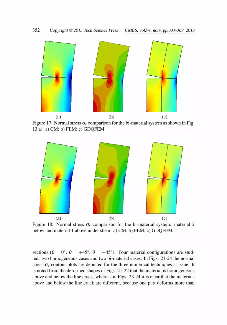
(a) (b) (c)Figure 17: Normal stress σy comparison for the bi-material system as shown in Fig.13 a): a) CM; b) FEM; c) GDQFEM.

(a) (b) (c)Figure 18: Normal stress σy comparison for the bi-material system: material 2below and material 1 above under shear: a) CM; b) FEM; c) GDQFEM.

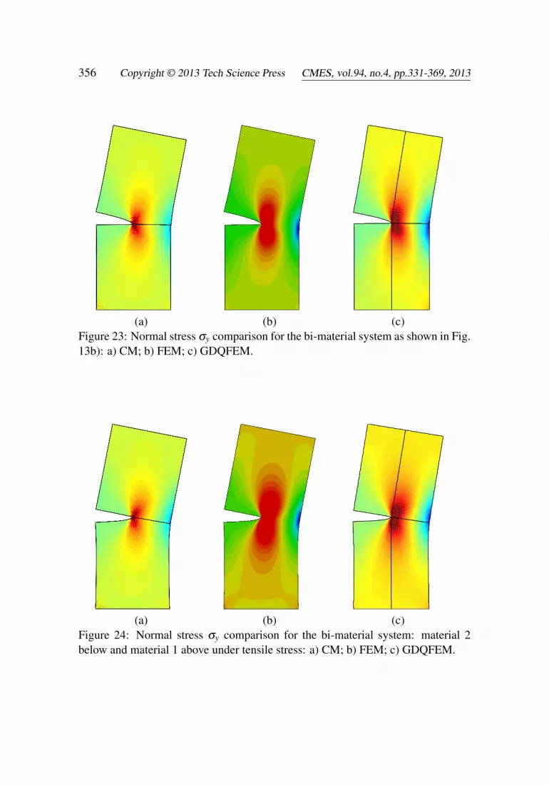
sections (θ = 0, θ = +45, θ = −45). Four material configurations are stud-ied: two homogeneous cases and two bi-material cases. In Figs. 21-24 the normalstress σy contour plots are depicted for the three numerical techniques at issue. Itis noted from the deformed shapes of Figs. 21-22 that the material is homogeneousabove and below the line crack, whereas in Figs. 23-24 it is clear that the materialsabove and below the line crack are different, because one part deforms more than


(a) (b)

(c) (d)

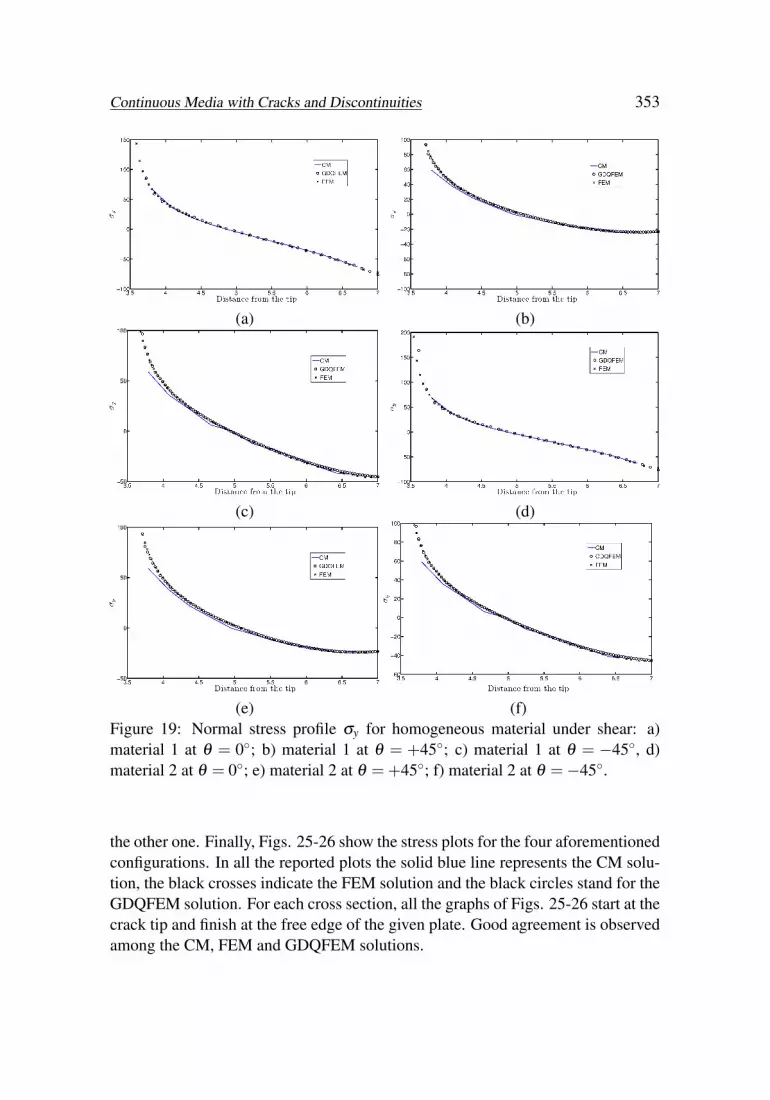
(e) (f)Figure 19: Normal stress profile σy for homogeneous material under shear: a)material 1 at θ = 0; b) material 1 at θ = +45; c) material 1 at θ = −45, d)material 2 at θ = 0; e) material 2 at θ =+45; f) material 2 at θ =−45.

the other one. Finally, Figs. 25-26 show the stress plots for the four aforementionedconfigurations. In all the reported plots the solid blue line represents the CM solu-tion, the black crosses indicate the FEM solution and the black circles stand for theGDQFEM solution. For each cross section, all the graphs of Figs. 25-26 start at thecrack tip and finish at the free edge of the given plate. Good agreement is observedamong the CM, FEM and GDQFEM solutions.


(a) (b)

(c) (d)

(e) (f)Figure 20: Normal stress profile σy for a bi-material system under shear: a) material1 below and material 2 above at θ = 0; b) material 1 below and material 2 aboveat θ =+45; c) material 1 below and material 2 above at θ =−45, d) material 2below and material 1 above at θ = 0; e) material 2 below and material 1 above atθ =+45; f) material 2 below and material 1 above at θ =−45.


(a) (b) (c)Figure 21: Normal stress σy comparison for the homogeneous material 1 undertensile stress: a) CM; b) FEM; c) GDQFEM.

(a) (b) (c)Figure 22: Normal stress σy comparison for the homogeneous material 2 undertensile stress: a) CM; b) FEM; c) GDQFEM.


(a) (b) (c)Figure 23: Normal stress σy comparison for the bi-material system as shown in Fig.13b): a) CM; b) FEM; c) GDQFEM.

(a) (b) (c)Figure 24: Normal stress σy comparison for the bi-material system: material 2below and material 1 above under tensile stress: a) CM; b) FEM; c) GDQFEM.


(a) (b)

(c) (d)

(e) (f)Figure 25: Normal stress profile σy for homogeneous material under tensile stress:a) material 1 at θ = 0; b) material 1 at θ = +45; c) material 1 at θ = −45, d)material 2 at θ = 0; e) material 2 at θ =+45; f) material 2 at θ =−45.


(a) (b)

(c) (d)

(e) (f)Figure 26: Normal stress profile σy for a bi-material system under tensile stress: a)material 1 below and material 2 above at θ = 0; b) material 1 below and material2 above at θ = +45; c) material 1 below and material 2 above at θ = −45, d)material 2 below and material 1 above at θ = 0; e) material 2 below and material1 above at θ =+45; f) material 2 below and material 1 above at θ =−45.


5 Conclusions

The main aim of this paper is to present several GDQFEM solutions to plane elasticproblems with cracks and holes. The GDQFEM methodology differs from theFEM approach, since the former numerical procedure is based on the strong formof the differential system of equations, whereas the latter one starts from a weakformulation. As a result, the numerical solution gives the physical displacementsof the model under consideration directly when the system is numerically solved.

It can be noted throughout the paper that GDQFEM leads to accurate and reliableresults, in terms of both frequencies and stresses when compared with FEM andCM. Furthermore, the mesh-free GDQ character remains at the sub-domain level.Therefore, cracks and holes are treated through element decomposition, namelyby dividing the physical domain into smaller parts. Since the approximation ordercan be imposed by the user, selecting more grid points N for each element, theGDQFEM elements have better convergence properties than the standard low or-der FEM elements implemented in commercial FEM codes. Finally, the GDQFEMnumerical applicability is also general, because it can treat the model discontinu-ities increasing the number of elements in the global mesh ne, having C 1 continuityamong them.

In the near future the cracked plate problem could be developed by consideringan inclined crack and a biaxial loading condition [Carloni, Piva, and Viola (2003);Nobile, Piva, and Viola (2004)]. In addition, a comparison between the results as-sociated to the plane stress condition at issue and the ones related to the formulationof a cracked beam element will be made [Viola, Nobile, and Federici (2002)].

Acknowledgement: This research was supported by the Italian Ministry forUniversity and Scientific, Technological Research MIUR (40 % and 60 %). Theresearch topic is one of the subjects of the Centre of Study and Research for theIdentification of Materials and Structures (CIMEST)-"M. Capurso" of the Univer-sity of Bologna (Italy).

References

Anderson, T. (1995): Fracture Mechanics: Fundamentals and Applications,Second Edition. CRC Press.

Artioli, E.; Gould, P. L.; Viola, E. (2005): A differential quadrature methodsolution for shear-deformable shells of revolution. Engineering Structures, vol.27, no. 13, pp. 1879–1892.


Bert, C.; Malik, M. (1996): The differential quadrature method for irregulardomains and application to plate vibration. International Journal of MechanicalSciences, vol. 38, no. 6, pp. 589–606.

Bert, C. W.; Malik, M. (1997): Differential quadrature: a powerful new techniquefor analysis of composite structures. Composite Structures, vol. 39, no. 3-4, pp.179–189.

Carloni, C.; Piva, A.; Viola, E. (2003): An alternative complex variable for-mulation for an inclined crack in an orthotropic medium. Engineering FractureMechanics, vol. 70, no. 15, pp. 2033–2058.

Cen, S.; Chen, X.-M.; Li, C. F.; Fu, X.-R. (2009): Quadrilateral membraneelements with analytical element stiffness matrices formulated by the new quadri-lateral area coordinate method (QACM-II). International Journal for NumericalMethods in Engineering, vol. 77, no. 8, pp. 1172–1200.

Chen, C.-N. (1999): The development of irregular elements for differentialquadrature element method steady-state heat conduction analysis. Computer Meth-ods in Applied Mechanics and Engineering, vol. 170, no. 1-2, pp. 1–14.

Chen, C.-N. (1999): The differential quadrature element method irregular elementtorsion analysis model. Applied Mathematical Modelling, vol. 23, no. 4, pp. 309–328.

Chen, C.-N. (2003): DQEM and DQFDM for the analysis of composite two-dimensional elasticity problems. Composite Structures, vol. 59, no. 1, pp. 3–13.

Civan, F.; Sliepcevich, C. (1984): Differential quadrature for multi-dimensionalproblems. Journal of Mathematical Analysis and Applications, vol. 101, no. 2, pp.423–443.

Civan, F.; Sliepcevich, C. M. (1985): Application of differential quadrature tosolution of pool boiling in cavities. Proceedings of the Oklahoma Academy ofScience, vol. 65, pp. 73–78.

Cook, R.; Avrashi, J. (1992): Error estimation and adaptive meshing for vibrationproblems. Computers & Structures, vol. 44, no. 3, pp. 619–626.

de Miranda, S.; Molari, L.; Ubertini, F. (2008): A consistent approach for mixedstress finite element formulations in linear elastodynamics. Computer Methods inApplied Mechanics and Engineering, vol. 197, no. 13-16, pp. 1376–1388.

Dong, L.; Atluri, S. (2012): Development of 3D T-Trefftz Voronoi cell finiteelements with/without spherical voids &/or elastic/rigid inclusions for microme-chanical modeling of heterogeneous materials. CMC: Computers, Materials, &Continua, vol. 29, no. 2, pp. 169–211.


Dong, L.; Atluri, S. (2013): Fracture & fatigue analyses: SGBEM-FEM orXFEM? Part 2: 3D solids. CMES - Computer Modeling in Engineering and Sci-ences, vol. 90, no. 5, pp. 379–413.

Dong, L.; Atluri, S. (2013): Fracture & fatigue analyses: SGBEM-FEM orXFEM? Part1 1: 2D structures. CMES - Computer Modeling in Engineering andSciences, vol. 90, no. 2, pp. 91–146.

Fantuzzi, N. (2013): Generalized Differential Quadrature Finite Element Methodapplied to Advanced Structural Mechanics. PhD thesis, University of Bologna,2013.

Ferreira, A. J. M.; Viola, E.; Tornabene, F.; Fantuzzi, N.; Zenkour, A. M.(2013): Analysis of sandwich plates by generalized differential quadraturemethod. Mathematical Problems in Engineering, vol. 2013, pp. 1–12. ArticleID 964367, doi:10.1155/2013/964367.

Ferretti, E. (2001): Modellazione del Comportamento del Cilindro Fasciato inCompressione. PhD thesis, Università del Salento, 2001.

Ferretti, E. (2003): Crack propagation modeling by remeshing using the CellMethod (CM). CMES: Computer Modeling in Engineering & Sciences, vol. 4, pp.51–72.

Ferretti, E. (2004): A Cell Method (CM) code for modeling the pullout teststep-wise. CMES: Computer Modeling in Engineering & Sciences, vol. 6, pp.453–476.

Ferretti, E. (2004): Crack-path analysis for brittle and non-brittle cracks: A CellMethod approach. CMES: Computer Modeling in Engineering & Sciences, vol. 6,pp. 227–244.

Ferretti, E. (2004): A discrete nonlocal formulation using local constitutive laws.International Journal of Fracture, vol. 130, no. 3, pp. L175–L182.

Ferretti, E. (2005): A local strictly nondecreasing material law for modelingsoftening and size-effect: a discrete approach. CMES: Computer Modeling inEngineering & Sciences, vol. 9, pp. 19–48.

Ferretti, E. (2009): Cell Method analysis of crack propagation in tensionedconcrete plates. CMES: Computer Modeling in Engineering & Sciences, vol. 54,pp. 253–281.

Ferretti, E. (2012): Shape-effect in the effective law of plain and rubberizedconcrete. CMC: Computers, Materials, & Continua, vol. 30, pp. 237–284.


Ferretti, E. (2013): The Cell Method: an enriched description of physics startingfrom the algebraic formulation. CMC: Computers, Materials, & Continua, vol.36, no. 1, pp. 49–72.

Ferretti, E. (2013): A Cell Method stress analysis in thin floor tiles subjected totemperature variation. CMC: Computers, Materials, & Continua, vol. 36, no. 3,pp. 293–322.

Ferretti, E. (2014): The Cell Method: a purely algebraic computational methodin physics and engineering science. Momentum Press.

Ferretti, E.; Casadio, E.; Di Leo, A. (2008): Masonry walls under shear test: aCM modeling. CMES: Computer Modeling in Engineering & Sciences, vol. 30,pp. 163–190.

Gupta, K. K. (1978): Development of a finite dynamic element for free vibra-tion analysis of two-dimensional structures. International Journal for NumericalMethods in Engineering, vol. 12, no. 8, pp. 1311–1327.

Hamidi, M.; Hashemi, M.; Talebbeydokhti, N.; Neill, S. (2012): Numer-ical modelling of the mild slope equation using localised differential quadraturemethod. Ocean Engineering, vol. 47, pp. 88–103.

Han, Z. D.; Liu, H. T.; Rajendran, A. M.; Atluri, S. N. (2006): The ap-plications of Meshless Local Petrov-Galerkin (MLPG) approaches in high-speedimpact, penetration and perforation problems. CMES - Computer Modeling inEngineering and Sciences, vol. 14, no. 2, pp. 119–128.

Huang, C.; Leissa, A. (2009): Vibration analysis of rectangular plates with sidecracks via the Ritz method. Journal of Sound and Vibration, vol. 323, no. 3-5, pp.974–988.

Huang, C.; Leissa, A.; Chan, C. (2011): Vibrations of rectangular plates withinternal cracks or slits. International Journal of Mechanical Sciences, vol. 53, no.6, pp. 436–445.

Huang, C.; Leissa, A.; Li, R. (2011): Accurate vibration analysis of thick,cracked rectangular plates. Journal of Sound and Vibration, vol. 330, no. 9, pp.2079–2093.

Huang, C.; Leissa, A.; Liao, S. (2008): Vibration analysis of rectangular plateswith edge v-notches. International Journal of Mechanical Sciences, vol. 50, no. 8,pp. 1255–1262.

Lam, K.; Zhang, J.; Zong, Z. (2004): A numerical study of wave propagation ina poroelastic medium by use of localized differential quadrature method. AppliedMathematical Modelling, vol. 28, no. 5, pp. 487–511.


Lam, S. (1993): Application of the differential quadrature method to two-dimensional problems with arbitrary geometry. Computers & Structures, vol. 47,no. 3, pp. 459–464.

Li, Q.; Shen, S.; Han, Z. D.; Atluri, S. N. (2003): Application of Meshless LocalPetrov-Galerkin (MLPG) to problems with singularities, and material discontinu-ities, in 3-D elasticity. CMES - Computer Modeling in Engineering and Sciences,vol. 4, no. 5, pp. 571–585.

Li, S.; Atluri, S. N. (2008): The MLPG mixed collocation method for materialorientation and topology optimization of anisotropic solids and structures. CMES- Computer Modeling in Engineering and Sciences, vol. 30, no. 1, pp. 37–56.

Li, S.; Atluri, S. N. (2008): Topology-optimization of structures based on theMLPG mixed collocation method. CMES - Computer Modeling in Engineeringand Sciences, vol. 26, no. 1, pp. 61–74.

Li, Y.; Fantuzzi, N.; Tornabene, F. (2013): On mixed mode crack initiationand direction in shafts: Strain energy density factor and maximum tangential stresscriteria. Engineering Fracture Mechanics, vol. 109, pp. 273 – 289.

Li, Y.; Viola, E. (2013): Size effect investigation of a central interface crackbetween two bonded dissimilar materials. Composite Structures, vol. 105, pp.90–107.

Liu, F.-L. (1999): Differential quadrature element method for static analysisof shear deformable cross-ply laminates. International Journal for NumericalMethods in Engineering, vol. 46, no. 8, pp. 1203–1219.

Marzani, A.; Tornabene, F.; Viola, E. (2008): Nonconservative stability prob-lems via generalized differential quadrature method. Journal of Sound & Vibration,vol. 315, no. 1-2, pp. 176–196.

Nassar, M.; Matbuly, M. S.; Ragb, O. (2013): Vibration analysis of structuralelements using differential quadrature method. Journal of Advanced Research,vol. 4, no. 1, pp. 93–102.

Nobile, L.; Piva, A.; Viola, E. (2004): On the inclined crack problem in anorthotropic medium under biaxial loading. Engineering Fracture Mechanics, vol.71, no. 4, pp. 529–546.

Pu, S. L.; Hussain, M. A.; Lorensen, W. E. (1978): The collapsed cubic isopara-metric element as a ingular element for crack probblems. International Journalfor Numerical Methods in Engineering, vol. 12, no. 11, pp. 1727–1742.

Ricci, P.; Viola, E. (2006): Stress intensity factors for cracked T-sections anddynamic behaviour of T-beams. Engineering Fracture Mechanics, vol. 73, no. 1,pp. 91–111.


Shen, L. H.; Young, D. L.; Lo, D. C.; Sun, C. P. (2009): Local differen-tial quadrature method for 2-D flow and forced-convection problems in irregulardomains. Numerical Heat Transfer, Part B: Fundamentals, vol. 55, no. 2, pp.116–134.

Shu, C. (2000): Differential quadrature and its applications in engineering.Springer Verlag.

Shu, C.; Chen, W.; Du, H. (2000): Free vibration analysis of curvilinear quadri-lateral plates by the differential quadrature method. Journal of ComputationalPhysics, vol. 163, no. 2, pp. 452–466.

Sladek, J.; Sladek, V.; Atluri, S. N. (2004): Meshless Local Petrov-Galerkinmethod for heat conduction problem in an anisotropic medium. CMES - ComputerModeling in Engineering and Sciences, vol. 6, no. 3, pp. 309–318.

Sun, J.-A.; Zhu, Z.-Y. (2000): Upwind local differential quadrature method forsolving incompressible viscous flow. Computer Methods in Applied Mechanicsand Engineering, vol. 188, no. 1-3, pp. 495–504.

Timoshenko, S. (1934): Theory of Elasticity. Engineering Societies Monographs.McGraw-Hill book Company, Incorporated.

Tonti, E. (2001): A direct discrete formulation of field laws: the Cell Method.CMES: Computer Modeling in Engineering & Sciences, vol. 2, pp. 237–258.

Tornabene, F. (2009): Free vibration analysis of functionally graded conical,cylindrical and annular shell structures with a four-parameter power-law distribu-tion. Computer Methods in Applied Mechanics and Engineering, vol. 198, no.37-40, pp. 2911–2935.

Tornabene, F. (2011): 2-D GDQ solution for free vibrations of anisotropicdoubly-curved shells and panels of revolution. Composite Structures, vol. 93,pp. 1854–1876.

Tornabene, F. (2011): Free vibration of laminated composite doubly-curvedshells and panels of revolution via GDQ method. Computer Methods in AppliedMechanics and Engineering, vol. 200, pp. 931–952.

Tornabene, F. (2011): Free vibrations of anisotropic doubly-curved shells andpanels of revolution with a free-form meridian resting on Winkler-Pasternak elasticfoundations. Composite Structures, vol. 94, pp. 186–206.

Tornabene, F. (2012): Meccanica delle strutture a guscio in materiale composito.Il metodo generalizzato di quadratura differenziale. Esculapio.


Tornabene, F.; Ceruti, A. (2013): Free-form laminated doubly-curved shells andpanels of revolution on Winkler-Pasternak elastic foundations: A 2D GDQ solutionfor static and free vibration analysis. World Journal of Mechanics, vol. 3, pp. 1–25.

Tornabene, F.; Ceruti, A. (2013): Mixed static and dynamic optimizazionof four-parameter functionally graded completely doubly-curved and degenerateshells and panels using GDQ method. Mathematical Problems in Engineering,vol. 2013, pp. 1–33. Article ID 867079, http://dx.doi.org/10.1155/2013/867079.

Tornabene, F.; Fantuzzi, N.; Viola, E.; Carrera, E. (2014): Static analysisof doubly-curved anisotropic shells and panels using CUF approach, differentialgeometry and differential quadrature method. Composite Structures, vol. 107, pp.675–697.

Tornabene, F.; Fantuzzi, N.; Viola, E.; Cinefra, M.; Carrera, E.; Ferreira, A.;Zenkour, A. (2014): Analysis of thick isotropic and cross-ply laminated plates bygeneralized differential quadrature method and a unified formulation. CompositePart B Engineering. In Press.

Tornabene, F.; Fantuzzi, N.; Viola, E.; Ferreira, A. J. M. (2013): Radialbasis function method applied to doubly-curved laminated composite shells andpanels with a general higher-order equivalent single layer theory. Composite PartB Engineering, vol. 55, pp. 642–659.

Tornabene, F.; Fantuzzi, N.; Viola, E.; Reddy, J. (2014): Winkler-Pasternakfoundation effect on the static and dynamic analyses of laminated doubly-curvedand degenerate shells and panels. Composite Part B Engineering, vol. 57, pp.269–296.

Tornabene, F.; Liverani, A.; Caligiana, G. (2011): FGM and laminated doubly-curved shells and panels of revolution with a free-form meridian: a 2-D GDQ so-lution for free vibrations. International Journal of Mechanical Sciences, vol. 53,pp. 446–470.

Tornabene, F.; Liverani, A.; Caligiana, G. (2012): General anisotropic doubly-curved shell theory: a differential quadrature solution for free vibrations of shellsand panels of revolution with a free-form meridian. Journal of Sound & Vibration,vol. 331, pp. 4848–4869.

Tornabene, F.; Liverani, A.; Caligiana, G. (2012): Laminated composite rect-angular and annular plates: A GDQ solution for static analysis with a posteriorishear and normal stress recovery. Composites Part B Engineering, vol. 43, pp.1847–1872.

Tornabene, F.; Liverani, A.; Caligiana, G. (2012): Static analysis of laminatedcomposite curved shells and panels of revolution with a posteriori shear and normal


stress recovery using generalized differential quadrature method. InternationalJournal of Mechanical Sciences, vol. 61, pp. 71–87.

Tornabene, F.; Marzani, A.; Viola, E.; Elishakoff, I. (2010): Critical flowspeeds of pipes conveying fluid by the generalized differential quadrature method.Advances in Theoretical and Applied Mechanics, vol. 3, no. 3, pp. 121–138.

Tornabene, F.; Reddy, J. (2013): FGM and laminated doubly-curved and de-generate shells resting on nonlinear elastic foundation: a GDQ solution for staticanalysis with a posteriori stress and strain recovery. Journal of Indian Institute ofScience, vol. 93, no. 4. In Press.

Tornabene, F.; Viola, E. (2007): Vibration analysis of spherical structural ele-ments using the GDQ method. Computers & Mathematics with Applications, vol.53, no. 10, pp. 1538–1560.

Tornabene, F.; Viola, E. (2008): 2-D solution for free vibrations of parabolicshells using generalized differential quadrature method. European Journal of Me-chanics - A/Solids, vol. 27, no. 6, pp. 1001–1025.

Tornabene, F.; Viola, E. (2009): Free vibration analysis of functionally gradedpanels and shells of revolution. Meccanica, vol. 44, no. 3, pp. 255–281.

Tornabene, F.; Viola, E. (2009): Free vibrations of four-parameter functionallygraded parabolic panels and shell of revolution. European Journal of Mechanics -A/Solids, vol. 28, no. 5, pp. 991–1013.

Tornabene, F.; Viola, E. (2013): Static analysis of functionally graded doubly-curved shells and panels of revolution. Meccanica, vol. 48, pp. 901–930.

Tornabene, F.; Viola, E.; Fantuzzi, N. (2013): General higher-order equivalentsingle layer theory for free vibrations of doubly-curved laminated composite shellsand panels. Composite Structures, vol. 104, pp. 94–117.

Tornabene, F.; Viola, E.; Inman, D. (2009): 2-D differential quadrature solutionfor vibration analysis of functionally graded conical, cylindrical and annular shellstructures. Journal of Sound & Vibration, vol. 328, no. 3, pp. 259–290.

Tsai, C.; Young, D.; Hsiang, C. (2011): The localized differential quadraturemethod for two-dimensional stream function formulation of navier-stokes equa-tions. Engineering Analysis with Boundary Elements, vol. 35, no. 11, pp. 1190–1203.

Viola, E.; Artioli, E.; Dilena, M. (2005): Analytical and differential quadratureresults for vibration analysis of damaged circular arches. Journal of Sound andVibration, vol. 288, no. 4-5, pp. 887–906.


Viola, E.; Dilena, M.; Tornabene, F. (2007): Analytical and numerical resultsfor vibration analysis of multi-stepped and multi-damaged circular arches. Journalof Sound & Vibration, vol. 299, no. 1-2, pp. 143–163.

Viola, E.; Fantuzzi, N.; Marzani, A. (2012): Cracks interaction effect on thedynamic stability of beams under conservative and nonconservative forces. KeyEngineering Materials, vol. 488-489, pp. 383–386.

Viola, E.; Li, Y.; Fantuzzi, N. (2012): On the stress intensity factors of crackedbeams for structural analysis. Key Engineering Materials, vol. 488-489, pp. 379–382.

Viola, E.; Marzani, A. (2004): Crack effect on dynamic stability of beams underconservative and nonconservative forces. Engineering Fracture Mechanics, vol.71, no. 4-6, pp. 699–718.

Viola, E.; Nobile, L.; Federici, L. (2002): Formulation of cracked beam elementfor structural analysis. Journal of Engineering Mechanics, vol. 128, no. 2, pp.220–230.

Viola, E.; Ricci, P.; Aliabadi, M. (2007): Free vibration analysis of axially loadedcracked timoshenko beam structures using the dynamic stiffness method. Journalof Sound and Vibration, vol. 304, no. 1-2, pp. 124–153.

Viola, E.; Rossetti, L.; Fantuzzi, N. (2012): Numerical investigation of function-ally graded cylindrical shells and panels using the generalized unconstrained thirdorder theory coupled with the stress recovery. Composite Structures, vol. 94, pp.3736–3758.

Viola, E.; Tornabene, F. (2005): Vibration analysis of damaged circular archeswith varying cross-section. Structural Integrity & Durability (SID-SDHM), vol. 1,no. 2, pp. 155–169.

Viola, E.; Tornabene, F. (2006): Vibration analysis of conical shell structuresusing GDQ method. Far East Journal of Applied Mathematics, vol. 25, no. 1, pp.23–39.

Viola, E.; Tornabene, F. (2009): Free vibrations of three parameter functionallygraded parabolic panels of revolution. Mechanics Research Communications, vol.36, no. 5, pp. 587–594.

Viola, E.; Tornabene, F.; Fantuzzi, N. (2013): General higher-order shear defor-mation theories for the free vibration analysis of completely doubly-curved lami-nated shells and panels. Composite Structures, vol. 95, pp. 639–666.

Viola, E.; Tornabene, F.; Fantuzzi, N. (2013): Generalized differential quadra-ture finite element method for cracked composite structures of arbitrary shape.Composite Structures, vol. 106, pp. 815–834.


Viola, E.; Tornabene, F.; Fantuzzi, N. (2013): Static analysis of completelydoubly-curved laminated shells and panels using general higher-order shear defor-mation theories. Composite Structures, vol. 101, pp. 59–93.

Wang, T.; Cao, S.; Ge, Y. (2013): Generation of inflow turbulence using thelocal differential quadrature method. Journal of Wind Engineering and IndustrialAerodynamics. In press.

Wang, X.; Wang, Y.-L.; Chen, R.-B. (1998): Static and free vibrational analysisof rectangular plates by the differential quadrature element method. Communica-tions in Numerical Methods in Engineering, vol. 14, no. 12, pp. 1133–1141.

Wang, Y.; Wang, X.; Zhou, Y. (2004): Static and free vibration analyses ofrectangular plates by the new version of the differential quadrature element method.International Journal for Numerical Methods in Engineering, vol. 59, no. 9, pp.1207–1226.

Xing, Y.; Liu, B. (2009): High-accuracy differential quadrature finite elementmethod and its application to free vibrations of thin plate with curvilinear domain.International Journal for Numerical Methods in Engineering, vol. 80, no. 13, pp.1718–1742.

Xing, Y.; Liu, B.; Liu, G. (2010): A differential quadrature finite element method.International Journal of Applied Mechanics, vol. 2, pp. 207–227.

Yilmaz, Y.; Girgin, Z.; Evran, S. (2013): Buckling analyses of axially function-ally graded nonuniform columns with elastic restraint using a localized differentialquadrature method. Mathematical Problems in Engineering, vol. 2013, pp. 1–12.Article ID 793062, http://doi:10.1155/2013/793062.

Zhao, C.; Steven, G. (1996): Asymptotic solutions for predicted natural frequen-cies of two-dimensional elastic solid vibration problems in finite element analysis.International Journal for Numerical Methods in Engineering, vol. 39, no. 16, pp.2821–2835.

Zhong, H.; He, Y. (1998): Solution of poisson and laplace equations by quadri-lateral quadrature element. International Journal of Solids and Structures, vol. 35,no. 21, pp. 2805–2819.

Zhong, H.; Yu, T. (2009): A weak form quadrature element method for planeelasticity problems. Applied Mathematical Modelling, vol. 33, no. 10, pp. 3801–3814.

Zong, Z.; Lam, K. (2002): A localized differential quadrature (LDQ) methodand its application to the 2D wave equation. Computational Mechanics, vol. 29,no. 4-5, pp. 382–391.


Zong, Z.; Zhang, Y. (2009): Advanced differential quadrature methods. Chap-man & Hall/CRC Applied Mathematics & Nonlinear Science. Taylor & Francis.

Documents

GDQFEM numerical simulations of continuous media with cracks and discontinuities