Generalized Analysis of Molecular VarianceCaroline M. Nievergelt1,3,4,5, Ondrej Libiger1,3,4, Nicholas J. Schork1,2,3,4,5,6*

1 Department of Psychiatry, University of California at San Diego, La Jolla, California, United States of America, 2 Department of Family and Preventive Medicine, University of

California at San Diego, La Jolla, California, United States of America, 3 Rebecca and John Moores UCSD Cancer Center, University of California at San Diego, La Jolla,

California, United States of America, 4 The Center for Human Genetics and Genomics, University of California at San Diego, La Jolla, California, United States of America, 5 The

Stein Institute for Research on Aging, University of California at San Diego, La Jolla, California, United States of America, 6 Scripps Genomic Medicine and Department of

Molecular and Experimental Medicine, The Scripps Research Institute, La Jolla, California, United States of America

Many studies in the fields of genetic epidemiology and applied population genetics are predicated on, or require, anassessment of the genetic background diversity of the individuals chosen for study. A number of strategies have beendeveloped for assessing genetic background diversity. These strategies typically focus on genotype data collected onthe individuals in the study, based on a panel of DNA markers. However, many of these strategies are either rooted incluster analysis techniques, and hence suffer from problems inherent to the assignment of the biological and statisticalmeaning to resulting clusters, or have formulations that do not permit easy and intuitive extensions. We describe avery general approach to the problem of assessing genetic background diversity that extends the analysis of molecularvariance (AMOVA) strategy introduced by Excoffier and colleagues some time ago. As in the original AMOVA strategy,the proposed approach, termed generalized AMOVA (GAMOVA), requires a genetic similarity matrix constructed fromthe allelic profiles of individuals under study and/or allele frequency summaries of the populations from which theindividuals have been sampled. The proposed strategy can be used to either estimate the fraction of genetic variationexplained by grouping factors such as country of origin, race, or ethnicity, or to quantify the strength of therelationship of the observed genetic background variation to quantitative measures collected on the subjects, such asblood pressure levels or anthropometric measures. Since the formulation of our test statistic is rooted in multivariatelinear models, sets of variables can be related to genetic background in multiple regression-like contexts. GAMOVA canalso be used to complement graphical representations of genetic diversity such as tree diagrams (dendrograms) orheatmaps. We examine features, advantages, and power of the proposed procedure and showcase its flexibility byusing it to analyze a wide variety of published data sets, including data from the Human Genome Diversity Project,classical anthropometry data collected by Howells, and the International HapMap Project.

Citation: Nievergelt CM, Libiger O, Schork NJ (2007) Generalized analysis of molecular variance. PLoS Genet 3(4): e51. doi:10.1371/journal.pgen.0030051

Introduction

Genetic and genetic epidemiologic studies involving largenumbers of individuals and/or populations are being pursuedmore and more often as a result of the development of high-throughput genotyping technologies and the creation ofgenotype data repositories such as the dbSNP (http://www.ncbi.nlm.nih.gov/SNP) and the International HapMap Projectdatabases (http://www.hapmap.org). Many of these studies areconcerned with the identification and characterization of therelationships of the populations and/or subsets of individualsin those populations on the basis of their genomic profiles or‘‘genetic backgrounds’’ (i.e., whether or not these popula-tions/individuals carry the same sets of genetic variations [1–8]). In addition, genetic epidemiologic studies are oftenconducted to identify relationships between specific sets ofgenetic variations possessed by individuals and phenotypicendpoints they might have, such as a disease. The collectionof variations that an individual possesses that contribute, e.g.,to his or her disease susceptibility, may vary from populationto population (e.g., as defined geographically, ethnically,racially, or linguistically). This may be due to the underlyingheterogeneity of disease pathogenesis, the origins of thevariations both in terms of time and place, and the frequencywith which those variations are transmitted across popula-tions (e.g., via migration patterns, interpopulation matings,etc.). Thus, the genetic background of an individual—at leastwith respect to relevant disease-contributing variations—is ascrucial in these types of investigations as it is in other types of

population genetic studies. In addition, it has been shownthat, due to phenomena such as varying degrees of admixtureand/or cryptic relatedness in the study population, ignoringgenetic background in epidemiologic studies testing associ-ations between particular genetic variations and a phenotypecan result in false positive and false negative results [9–19],which underscores the importance of genetic backgroundanalysis even in very simple genetic association studies.Many innovative analytical methods have been developed

recently to assess and accommodate genetic backgroundheterogeneity [20–37]. The vast majority of these methodsinvolve some form of cluster analysis, although some morerecent methods do not (e.g., [29,32]). For example, hierarch-

Editor: David B. Allison, University of Alabama at Birmingham, United States ofAmerica

Received October 26, 2006; Accepted February 22, 2007; Published April 6, 2007

A previous version of this article appeared as an Early Online Release on February22, 2007 (doi:10.1371/journal.pgen.0030051.eor).

Copyright: � 2007 Nievergelt et al. This is an open-access article distributed underthe terms of the Creative Commons Attribution License, which permits unrestricteduse, distribution, and reproduction in any medium, provided the original authorand source are credited.

Abbreviations: AIM, ancestry informative marker; AMOVA, analysis of molecularvariance; ANOVA, analysis of variance; CEPH, Foundation Jean Dausset-Centred’Etude du Polymorphisme Humain; FRS, nasion-bregma subtense; GAMOVA,generalized analysis of molecular variance; HGDP, CEPH Human Genome DiversityProgram; IBS, identical by state; LR, Lynch-Ritland; SNPs, single nucleotidepolymorphism

* To whom correspondence should be addressed. E-mail: nschork@ucsd.edu

PLoS Genetics | www.plosgenetics.org April 2007 | Volume 3 | Issue 4 | e510467

ical clustering strategies can be used to assess geneticbackground clustering, and, like other cluster analysismethods, require the construction of a measure of thesimilarity or dissimilarity (genetic distance) between all pairsof the N individual genomes or population allele frequencyprofiles (e.g., between-group variation, FST) comprising asample. The resulting N 3 N similarity or distance matrix isthen explored statistically to identify clusters of individualsor populations that exhibit greater or lesser similarity.Problems inherent to this approach involve the choice of asimilarity metric, deciding which cluster method is mostappropriate (e.g., single linkage, complete linkage, etc.), thedetermination of the optimal number of clusters represent-ing the data, and the biological meaning of the clusters.

With respect to the choice of a similarity metric for clusteranalysis, the simplest marker-based method for the assess-ment of genetic similarity between two individuals is tocalculate the fraction of alleles shared identical by state (IBS)by those individuals over all the loci for which the individualshave been genotyped. If N individuals have been genotyped,then all N3N pairs of individuals can be assessed in this way.In addition to providing a foundation for some clusteranalysis methods, graphical displays of the similarity matrixcan be produced that allow visual assessment of the potentialthat subgroups of individuals with similar genetic back-grounds exist in the data. This approach has been usedwidely, and is often referred to, when presented in graphicalform as a dendrogram, or as an allele-sharing ‘‘tree ofindividuals’’ (e.g., [7,38–40]). One problem, however, with thesimple IBS sharing measure of genetic background similarityis that it does not account for allele frequencies. Consider, forexample, two individuals who share rare alleles. Theseindividuals are more likely to have arisen from the same(unique) population in which those alleles arose. In thissituation one may want to consider ‘‘weighting’’ allele sharingat each locus by the frequency of the shared (or unshared)alleles. Pairwise measures of genetic similarity that accom-modate allele frequencies have been put forward and are

used often in ecological and nonhuman population geneticsanalysis settings (e.g., [41–45]).Cluster analysis approaches can be extended by making

more explicit and rigorous assumptions about the ancestralpopulations from which the individuals in a sample arose.Thus, specific ancestry informative markers (AIMs), whichshow large frequency differences between ancestral popula-tions, can be used to quantify the degree of admixture amongindividuals in a sample [18,46–49]. When an individualgenotyped on such markers possesses variations that aremore frequent in one of the chosen ancestral populations,then that individual’s ancestral relationship to this popula-tion can be inferred. Obviously, one needs to have identifiedthe appropriate AIMs in advance of such analyses and thisrequires assumptions about the ancestral populations con-tributing to the individual genetic backgrounds reflected in asample.In the following we describe a flexible alternative to cluster

analysis–based methods for the statistical assessment ofgenetic background similarities among populations or indi-viduals. The proposed method does not necessarily rely onAIMs, but does require genotype information on at least a fewhundred (possibly less when including AIMs) genetic markers(null loci) such as microsatellites, single nucleotide poly-morphisms (SNPs), and/or insertion–deletion polymorphisms.Although one can use markers that are not completelyindependent in the sense that they have alleles in linkagedisequilibrium, this practice may require the use of a greaternumber of markers to make up for the lack of independenceof the markers. Null loci can include genotype data availablefrom, e.g., a previous genome-wide association or linkagestudies involving the subjects or populations of interest, andcould thus allow for a retrospective analysis of sample geneticbackground structure without additional genotyping. As incluster analysis, the proposed method involves the construc-tion of a genetic similarity matrix. However, it does notrequire cluster analysis to test hypotheses about the relation-ships of the individuals or populations in a sample. Rather,the method assumes that interest lies in testing the relation-ship between a particular grouping factor (e.g., race, countryof origin, cohort, or geographical locale) or quantitativemeasure (such as age, cholesterol level, or weight) andvariations in the genetic similarities of the individuals orpopulations collected. Therefore, it does not require thedetermination of the optimal number of clusters or, e.g.,principal components, representing the data.The proposed method is similar to the analysis of

molecular variance (AMOVA) method introduced by Excoff-ier and colleagues, but is more flexible and provides a muchmore intuitive and generalizable derivation of relevant teststatistics [50]. The description of the AMOVA procedureprovided by Excoffier et al.[50] includes relevant sum-of-squares calculations to formulate analysis of variance(ANOVA)-like hypothesis-oriented test statistics that considerdifferences between groups of individuals or populationswith respect to genetic background. As described in theMethods section, the proposed approach builds off ananalysis method we have termed multivariate distance matrixregression analysis and can be used to test hypotheses aboutnot only categorical or grouping factors and genetic back-ground, but quantitative traits as well [51,52]. In addition, theformulation of the proposed test statistics can be adapted for

PLoS Genetics | www.plosgenetics.org April 2007 | Volume 3 | Issue 4 | e510468

Generalized AMOVA

Author Summary

Humans exhibit great genetic diversity. Understanding the factorsthat contribute to and sustain this diversity is an important researcharea. Not only can such understanding shed light on human origins,but it can also assist in the discovery of genes and genetic factorsthat contribute to debilitating diseases. Statistical analysis methodsthat can facilitate the identification of factors contributing to orassociated with human genetic diversity are growing in number asnew high-throughput molecular genetic assays and technologiesare developed. We consider the use of an analysis method termedgeneralized analysis of molecular variance (GAMOVA), which buildsoff of previously proposed analysis methods for testing hypothesesabout the factors associated with genetic background diversity. Weapply the method in a wide variety of settings and show that it isboth flexible and powerful. GAMOVA has great potential to assist inpopulation-based human genetic studies, as it can be used toaddress questions such as: Is a sample of affected cases andunaffected controls from a homogeneous population, or is thereevidence of heterogeneity that could affect the results of anassociation study? Is there reason to believe that the ancestry of aset of individuals influences the traits that they have?

use in multiple regression-like test settings, so that therelationships of multiple factors to genetic background canbe explored. As a result of the connections between theproposed approach and the AMOVA approach of Excoffier etal. [50], we have labeled the proposed approach generalizedmolecular analysis of variance (GAMOVA).

In addition to the AMOVA procedure, the proposedGAMOVA procedure also has some similarities to theMantel-based test statistic approach reviewed and extendedby Smouse et al. [53]. The Mantel test is used to test therelationship between the entries or cells in two (or more)distance/similarity matrices. Thus, one could have a geneticbackground similarity matrix computed from differentpopulations whose relationship to, e.g., a geographic distancematrix computed for the populations is of interest. Theproposed GAMOVA procedure considers the relationshipbetween the N3N entries (or cells; where N is the number ofindividuals or populations being studied) in a geneticbackground distance matrix and information, representedas N-dimensional vectors, on the N individuals or populationswhose genetic background distances are reflected in thematrix.

Below we apply the GAMOVA procedure to three data setsavailable in the public domain to address some prevailingquestions: (1) an analysis of the Foundation Jean Dausset-Centre d’Etude du Polymorphisme Humain (CEPH)–HumanGenome Diversity Project (HGDP) Cell Line Panel, (2) ananalysis of the morphological data made available by Howells[54,55] on human craniometric characters, and (3) an analysisof the International HapMap Project data addressing ques-tions about the similarity of the individual chromosomespossessed by the subjects genotyped as part of the project. Inaddition, we also consider aspects of the power of theGAMOVA procedure via simulation studies.

Results

Analysis of the CEPH-HGDP Cell Line Panel DatasetWe considered the use of the proposed GAMOVA analysis

to analyze the CEPH-HGDP Cell Line Panel data [56] in anumber of ways. We constructed several distance matricesover 1,040 subjects collected from 51 worldwide populationsbased on: (1) individual IBS allele sharing and (2) Lynch-Ritland (LR) frequency weighted allele-sharing distance, and(3) the standard between-population genetic distance meas-ure FST (see Methods). We then considered the relationshipbetween additional information collected on those individ-uals (and/or populations) and variation in the similarityamong the individuals and populations using the proposedGAMOVA procedure. The additional information included,for each individual, which of the 51 populations or ethnicgroups they were from, the geographic location of thatpopulation (i.e., one of the five or seven global world regionsassociated with populations), and its distance from AddisAbaba in Africa [8]. In addition to the analyses based onindividuals, geographic location and distance from AddisAbaba were also considered in analyses involving the 51populations as a whole. By considering the distance of eachpopulation from Addis Ababa we could address hypothesesabout global historical migration patterns and the impactthese migration patterns have on genomic diversity, as has

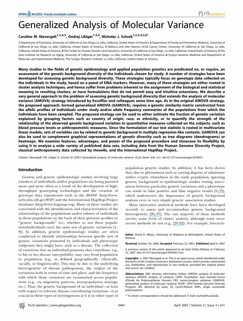
been recently pursued through the use of different statisticalmethods [6,57].To visually assess the potential for genetic background

clustering we first constructed neighbor-joining trees basedon the IBS distance matrix of the CEPH-HGDP individuals.We color-coded each branch (representing an individual)based on: (1) which of 5 major geographic regions (Figure 1A,left panel) and (2) which of 51 populations an individual wasfrom (Figure 1B, right panel). Figure 1 shows a fairly dramaticclustering of the individuals that is roughly consistent withthe population of origin for each individual. Note that, asobserved by Rosenberg et al. [1], the Mozabite (the populationlabeled with a ‘‘6’’), a Berber ethnic group living in the Saharain Northern Africa, clusters with Middle Eastern populations(assigned labels ‘‘4,’’ ‘‘5,’’ and ‘‘7’’).We then considered two analyses designed to assess how

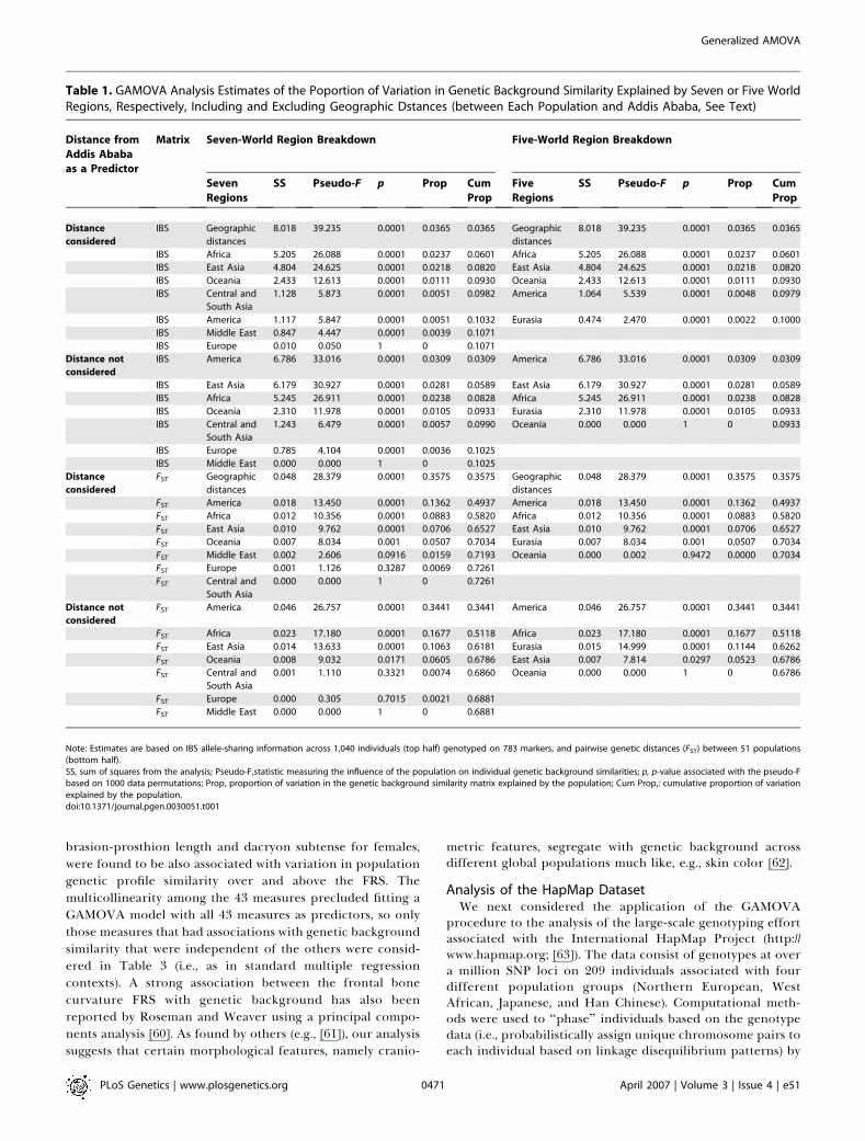
much of the genetic background variation exhibited by theCEPH-HGDP individuals and ethnic groups could be ex-plained by the world regions each individual or populationwas associated with, as well as the distance of that worldregion from Addis Ababa, using the GAMOVA procedure. Wecreated simple 0–1 indicator variables that reflected whichworld region an individual or population was associated withand used these indicator variables as independent orpredictor variables in the GAMOVA regression procedure(see the Methods section for details) along with distance fromAddis Ababa as a continuous variable. Table 1 provides theresults assuming either a seven-world region breakdown(Table 1; East Asia, Africa, Oceania, Central and South Asia,America, the Middle East, and Europe) or a five-world regionbreakdown (Table 1; Eurasia, East Asia, Oceania, America,and Africa) as defined previously [1]. We also compareGAMOVA regression models that did not consider (Table 1)distance from Addis Ababa as a predictor to contrast theresults with the findings of models that included it (Table 1).The top half‘ of Table 1 reflects the analysis of the IBS allele

sharing among individuals and suggests that approximately9%–11% of the variation in the similarity of individualgenetic backgrounds can be explained by world region eitherin conjunction with the distance of that world region fromAddis Ababa or not. Approximately 68%–72% of thevariation in genetic background similarity of the populationsas a whole, assuming the FST measure of genetic distance,could be explained by world region and distance of thoseworld regions from Addis Ababa (Table 1; bottom half). Thisclearly reflects the greater diversity among individualgenomes within a population than allele frequency differ-ences between populations as a whole.It is also interesting to note that, as found by others [6,57],

the distance from Addis Ababa is the strongest predictor ofgenetic background similarity among the individuals andpopulations, but the world regions explain variation ingenetic background similarity over and above this measure,suggesting that diversity among individuals within popula-tions situated within the same world region is not completelycaptured by their distance from Addis Ababa. Also of note isthe strength of the contributions of the various world regionsto variation in genetic background similarity, which reflectfactors such as the populations’ individual demographichistories and selective environmental pressures. For example,Africa is the strongest contributor to individual geneticbackground similarity after accounting for each world

PLoS Genetics | www.plosgenetics.org April 2007 | Volume 3 | Issue 4 | e510469

Generalized AMOVA

region’s distance from Addis Ababa (Distance considered/IBSMatrix portion of Table 1), which is consistent with the deepgenetic structure of this continent [58]. On the other hand,the strongest contributor to pairwise population distances(FST) after accounting for geographic distance from AddisAbaba (Distance considered/FST portion of Table 1) wasfound to be America, consistent with findings by Ramachan-dran et al. [58].

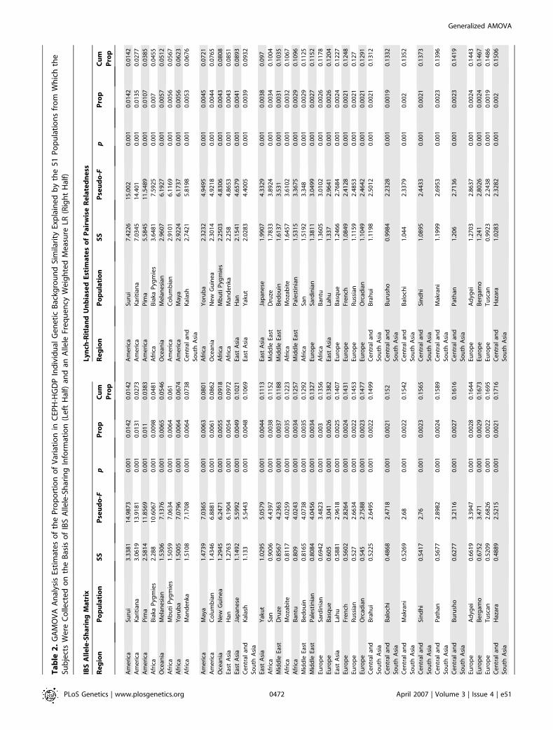
We also considered analyses that took into considerationall the populations studied, assuming both the IBS allele-sharing measure of genetic background similarity and the LRallele frequency-weighted measure (Table 2). Overall, theindividual populations that the study subjects were fromcould explain approximately 16%–19% of the variation ingenetic background similarity exhibited by the individuals inthe CEPH-HGDP database. Interestingly, the analyses usingthe IBS and LR measures did not agree perfectly—althoughthey are similar—suggesting that allele frequency weightingcan make a difference in assessing individual genetic back-ground similarity. In addition, our GAMOVA analysissuggests that individuals from three populations in theAmericas (the Surui, the Karitiana, and the Pima) have themost divergent genomes from the other individuals’ genomes,which has been observed by others as well (e.g., [1,58]).

Analysis of the Craniometric Data Collected by HowellsWe also considered analyses involving morphological data

made available by Howells [54,55] on human craniometric

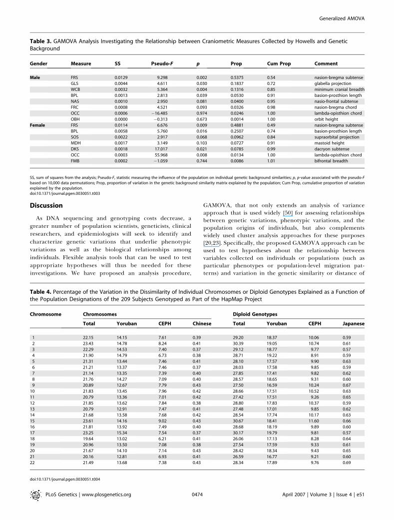
characters collected on individuals from ten worldwidepopulations. We computed the median of each of 43craniometric measures for males and females separately fromeach of these populations. We combined the data with thegenetic data on the CEPH-HGDP subjects by geographicallymatching the countries and regions represented in theCEPH-HGDP with those for which we had craniometric datain a fashion identical to the one outlined by Roseman [59].The median values for each of the 43 craniometric measureswere then considered as a regressor or covariate in aGAMOVA analysis of the genetic distance matrix computedfor the ten corresponding CEPH-HGDP populations. Thegoal was to test associations between craniometric features ofthe people within the populations and genetic backgroundsimilarities those people might have with people in otherpopulations. We want to emphasize that many of thecraniometric measures are correlated so that associationsbetween any one of these measures and genetic backgroundsuggest that other measures may also be associated withgenetic background, just not necessarily independently of theothers.Table 3 describes the results of the analyses for males and

females. The cranial feature most strongly associated withgenetic background similarity is the nasion-bregma subtense(FRS), which ‘‘explains’’ ;54% and ;49% of the variation ingenetic background similarity for males and females, respec-tively. Other measures, such as glabella projection, minimumcranial breadth and basion-prosthion length for males, and

Figure 1. Neighbor-Joining Trees Depicting the Genetic Relationships of 1,040 Individuals from 51 World Populations Collected by the CEPH-HGDP

(A) Individuals are color coded according to which of five major geographic regions of the globe they are collected from.(B) Individuals are color coded according to which of the 51 populations they are associated with (1: Biaka Pygmy, 2: San, 3: Mbuti Pygmy, 4: Druze; 5:Bedouin, 6: Mozabite, 7: Palestinian, 8: Kalash, 9: Pima, 10: Columbian, 11: Karitiana, 12: Surui, 13: New Guinea, 14: Yakut).doi:10.1371/journal.pgen.0030051.g001

PLoS Genetics | www.plosgenetics.org April 2007 | Volume 3 | Issue 4 | e510470

Generalized AMOVA

brasion-prosthion length and dacryon subtense for females,were found to be also associated with variation in populationgenetic profile similarity over and above the FRS. Themulticollinearity among the 43 measures precluded fitting aGAMOVA model with all 43 measures as predictors, so onlythose measures that had associations with genetic backgroundsimilarity that were independent of the others were consid-ered in Table 3 (i.e., as in standard multiple regressioncontexts). A strong association between the frontal bonecurvature FRS with genetic background has also beenreported by Roseman and Weaver using a principal compo-nents analysis [60]. As found by others (e.g., [61]), our analysissuggests that certain morphological features, namely cranio-

metric features, segregate with genetic background acrossdifferent global populations much like, e.g., skin color [62].

Analysis of the HapMap DatasetWe next considered the application of the GAMOVA

procedure to the analysis of the large-scale genotyping effortassociated with the International HapMap Project (http://www.hapmap.org; [63]). The data consist of genotypes at overa million SNP loci on 209 individuals associated with fourdifferent population groups (Northern European, WestAfrican, Japanese, and Han Chinese). Computational meth-ods were used to ‘‘phase’’ individuals based on the genotypedata (i.e., probabilistically assign unique chromosome pairs toeach individual based on linkage disequilibrium patterns) by

Table 1. GAMOVA Analysis Estimates of the Poportion of Variation in Genetic Background Similarity Explained by Seven or Five WorldRegions, Respectively, Including and Excluding Geographic Dstances (between Each Population and Addis Ababa, See Text)

Distance from

Addis Ababa

as a Predictor

Matrix Seven-World Region Breakdown Five-World Region Breakdown

Seven

Regions

SS Pseudo-F p Prop Cum

Prop

Five

Regions

SS Pseudo-F p Prop Cum

Prop

Distance

considered

IBS Geographic

distances

8.018 39.235 0.0001 0.0365 0.0365 Geographic

distances

8.018 39.235 0.0001 0.0365 0.0365

IBS Africa 5.205 26.088 0.0001 0.0237 0.0601 Africa 5.205 26.088 0.0001 0.0237 0.0601

IBS East Asia 4.804 24.625 0.0001 0.0218 0.0820 East Asia 4.804 24.625 0.0001 0.0218 0.0820

IBS Oceania 2.433 12.613 0.0001 0.0111 0.0930 Oceania 2.433 12.613 0.0001 0.0111 0.0930

IBS Central and

South Asia

1.128 5.873 0.0001 0.0051 0.0982 America 1.064 5.539 0.0001 0.0048 0.0979

IBS America 1.117 5.847 0.0001 0.0051 0.1032 Eurasia 0.474 2.470 0.0001 0.0022 0.1000

IBS Middle East 0.847 4.447 0.0001 0.0039 0.1071

IBS Europe 0.010 0.050 1 0 0.1071

Distance not

considered

IBS America 6.786 33.016 0.0001 0.0309 0.0309 America 6.786 33.016 0.0001 0.0309 0.0309

IBS East Asia 6.179 30.927 0.0001 0.0281 0.0589 East Asia 6.179 30.927 0.0001 0.0281 0.0589

IBS Africa 5.245 26.911 0.0001 0.0238 0.0828 Africa 5.245 26.911 0.0001 0.0238 0.0828

IBS Oceania 2.310 11.978 0.0001 0.0105 0.0933 Eurasia 2.310 11.978 0.0001 0.0105 0.0933

IBS Central and

South Asia

1.243 6.479 0.0001 0.0057 0.0990 Oceania 0.000 0.000 1 0 0.0933

IBS Europe 0.785 4.104 0.0001 0.0036 0.1025

IBS Middle East 0.000 0.000 1 0 0.1025

Distance

considered

FST Geographic

distances

0.048 28.379 0.0001 0.3575 0.3575 Geographic

distances

0.048 28.379 0.0001 0.3575 0.3575

FST America 0.018 13.450 0.0001 0.1362 0.4937 America 0.018 13.450 0.0001 0.1362 0.4937

FST Africa 0.012 10.356 0.0001 0.0883 0.5820 Africa 0.012 10.356 0.0001 0.0883 0.5820

FST East Asia 0.010 9.762 0.0001 0.0706 0.6527 East Asia 0.010 9.762 0.0001 0.0706 0.6527

FST Oceania 0.007 8.034 0.001 0.0507 0.7034 Eurasia 0.007 8.034 0.001 0.0507 0.7034

FST Middle East 0.002 2.606 0.0916 0.0159 0.7193 Oceania 0.000 0.002 0.9472 0.0000 0.7034

FST Europe 0.001 1.126 0.3287 0.0069 0.7261

FST Central and

South Asia

0.000 0.000 1 0 0.7261

Distance not

considered

FST America 0.046 26.757 0.0001 0.3441 0.3441 America 0.046 26.757 0.0001 0.3441 0.3441

FST Africa 0.023 17.180 0.0001 0.1677 0.5118 Africa 0.023 17.180 0.0001 0.1677 0.5118

FST East Asia 0.014 13.633 0.0001 0.1063 0.6181 Eurasia 0.015 14.999 0.0001 0.1144 0.6262

FST Oceania 0.008 9.032 0.0171 0.0605 0.6786 East Asia 0.007 7.814 0.0297 0.0523 0.6786

FST Central and

South Asia

0.001 1.110 0.3321 0.0074 0.6860 Oceania 0.000 0.000 1 0 0.6786

FST Europe 0.000 0.305 0.7015 0.0021 0.6881

FST Middle East 0.000 0.000 1 0 0.6881

Note: Estimates are based on IBS allele-sharing information across 1,040 individuals (top half) genotyped on 783 markers, and pairwise genetic distances (FST) between 51 populations(bottom half).SS, sum of squares from the analysis; Pseudo-F,statistic measuring the influence of the population on individual genetic background similarities; p, p-value associated with the pseudo-Fbased on 1000 data permutations; Prop, proportion of variation in the genetic background similarity matrix explained by the population; Cum Prop,: cumulative proportion of variationexplained by the population.doi:10.1371/journal.pgen.0030051.t001

PLoS Genetics | www.plosgenetics.org April 2007 | Volume 3 | Issue 4 | e510471

Generalized AMOVA

Ta

ble

2.

GA

MO

VA

An

alys

isEs

tim

ate

so

fth

eP

rop

ort

ion

of

Var

iati

on

inC

EPH

-HG

DP

Ind

ivid

ual

Ge

ne

tic

Bac

kgro

un

dSi

mila

rity

Exp

lain

ed

by

the

51

Po

pu

lati

on

sfr

om

Wh

ich

the

Sub

ject

sW

ere

Co

llect

ed

on

the

Bas

iso

fIB

SA

llele

-Sh

arin

gIn

form

atio

n(L

eft

Hal

f)an

dan

Alle

leFr

eq

ue

ncy

We

igh

ted

Me

asu

reLR

(Rig

ht

Hal

f)

IBS

All

ele

-Sh

ari

ng

Ma

trix

Ly

nch

-Rit

lan

dU

nb

iase

dE

stim

ate

so

fP

air

wis

eR

ela

ted

ne

ss

Re

gio

nP

op

ula

tio

nS

SP

seu

do

-Fp

Pro

pC

um

Pro

p

Re

gio

nP

op

ula

tio

nS

SP

seu

do

-Fp

Pro

pC

um

Pro

p

Am

eri

caSu

rui

3.3

38

11

4.9

87

30

.00

10

.01

42

0.0

14

2A

me

rica

Suru

i7

.42

26

15

.00

20

.00

10

.01

42

0.0

14

2

Am

eri

caK

arit

ian

a3

.06

19

13

.91

81

0.0

01

0.0

13

10

.02

73

Am

eri

caK

arit

ian

a7

.03

45

14

.40

10

.00

10

.01

35

0.0

27

7

Am

eri

caP

ima

2.5

81

41

1.8

56

90

.00

10

.01

10

.03

83

Am

eri

caP

ima

5.5

84

51

1.5

48

90

.00

10

.01

07

0.0

38

5

Afr

ica

Bia

kaP

ygm

ies

2.2

88

10

.60

67

0.0

01

0.0

09

80

.04

81

Afr

ica

Bia

kaP

ygm

ies

3.6

48

17

.59

25

0.0

01

0.0

07

0.0

45

5

Oce

ania

Me

lan

esi

an1

.53

06

7.1

37

60

.00

10

.00

65

0.0

54

6O

cean

iaM

ela

ne

sian

2.9

60

76

.19

27

0.0

01

0.0

05

70

.05

12

Afr

ica

Mb

uti

Pyg

mie

s1

.50

59

7.0

63

40

.00

10

.00

64

0.0

61

Am

eri

caC

olu

mb

ian

2.9

10

16

.11

69

0.0

01

0.0

05

60

.05

67

Afr

ica

Yo

rub

a1

.50

05

7.0

79

60

.00

10

.00

64

0.0

67

4A

me

rica

May

a2

.92

24

6.1

73

70

.00

10

.00

56

0.0

62

3

Afr

ica

Man

de

nka

1.5

10

87

.17

08

0.0

01

0.0

06

40

.07

38

Ce

ntr

alan

d

Sou

thA

sia

Kal

ash

2.7

42

15

.81

98

0.0

01

0.0

05

30

.06

76

Am

eri

caM

aya

1.4

73

97

.03

65

0.0

01

0.0

06

30

.08

01

Afr

ica

Yo

rub

a2

.32

32

4.9

49

50

.00

10

.00

45

0.0

72

1

Am

eri

caC

olu

mb

ian

1.4

34

66

.88

81

0.0

01

0.0

06

10

.08

62

Oce

ania

Ne

wG

uin

ea

2.3

01

44

.92

18

0.0

01

0.0

04

40

.07

65

Oce

ania

Ne

wG

uin

ea

1.2

94

56

.24

71

0.0

01

0.0

05

50

.09

18

Afr

ica

Mb

uti

Pyg

mie

s2

.25

03

4.8

30

60

.00

10

.00

43

0.0

80

8

East

Asi

aH

an1

.27

63

6.1

90

40

.00

10

.00

54

0.0

97

2A

fric

aM

and

en

ka2

.25

84

.86

53

0.0

01

0.0

04

30

.08

51

East

Asi

aJa

pan

ese

1.1

49

25

.59

92

0.0

01

0.0

04

90

.10

21

East

Asi

aH

an2

.15

41

4.6

57

90

.00

10

.00

41

0.0

89

3

Ce

ntr

alan

d

Sou

thA

sia

Kal

ash

1.1

33

5.5

44

30

.00

10

.00

48

0.1

06

9Ea

stA

sia

Yak

ut

2.0

28

34

.40

05

0.0

01

0.0

03

90

.09

32

East

Asi

aY

aku

t1

.02

95

5.0

57

90

.00

10

.00

44

0.1

11

3Ea

stA

sia

Jap

ane

se1

.99

07

4.3

32

90

.00

10

.00

38

0.0

97

Afr

ica

San

0.9

00

64

.43

97

0.0

01

0.0

03

80

.11

52

Mid

dle

East

Dru

ze1

.78

33

3.8

92

40

.00

10

.00

34

0.1

00

4

Mid

dle

East

Dru

ze0

.85

67

4.2

36

30

.00

10

.00

37

0.1

18

8M

idd

leEa

stB

ed

ou

in1

.61

37

3.5

31

0.0

01

0.0

03

10

.10

35

Afr

ica

Mo

zab

ite

0.8

11

74

.02

59

0.0

01

0.0

03

50

.12

23

Afr

ica

Mo

zab

ite

1.6

45

73

.61

02

0.0

01

0.0

03

20

.10

67

Afr

ica

Ban

tu0

.80

94

.02

43

0.0

01

0.0

03

40

.12

57

Mid

dle

East

Pal

est

inia

n1

.53

15

3.3

67

50

.00

10

.00

29

0.1

09

6

Mid

dle

East

Be

do

uin

0.8

16

54

.07

38

0.0

01

0.0

03

50

.12

92

Afr

ica

San

1.5

19

23

.34

80

.00

10

.00

29

0.1

12

5

Mid

dle

East

Pal

est

inia

n0

.80

84

4.0

45

60

.00

10

.00

34

0.1

32

7Eu

rop

eSa

rdin

ian

1.3

81

13

.04

99

0.0

01

0.0

02

70

.11

52

Euro

pe

Sard

inia

n0

.69

42

3.4

82

30

.00

10

.00

30

.13

56

Afr

ica

Ban

tu1

.36

05

3.0

10

20

.00

10

.00

26

0.1

17

8

Euro

pe

Bas

qu

e0

.60

53

.04

10

.00

10

.00

26

0.1

38

2Ea

stA

sia

Lah

u1

.33

72

.96

41

0.0

01

0.0

02

60

.12

04

East

Asi

aLa

hu

0.5

88

12

.96

18

0.0

01

0.0

02

50

.14

07

Euro

pe

Bas

qu

e1

.24

66

2.7

68

40

.00

10

.00

24

0.1

22

7

Euro

pe

Fre

nch

0.5

60

22

.82

64

0.0

01

0.0

02

40

.14

31

Euro

pe

Fre

nch

1.0

84

92

.41

28

0.0

01

0.0

02

10

.12

48

Euro

pe

Ru

ssia

n0

.52

72

.66

34

0.0

01

0.0

02

20

.14

53

Euro

pe

Ru

ssia

n1

.11

59

2.4

85

30

.00

10

.00

21

0.1

27

Euro

pe

Orc

adia

n0

.54

52

.75

88

0.0

01

0.0

02

30

.14

77

Euro

pe

Orc

adia

n1

.10

49

2.4

64

20

.00

10

.00

21

0.1

29

1

Ce

ntr

alan

d

Sou

thA

sia

Bra

hu

i0

.52

25

2.6

49

50

.00

10

.00

22

0.1

49

9C

en

tral

and

Sou

thA

sia

Bra

hu

i1

.11

98

2.5

01

20

.00

10

.00

21

0.1

31

2

Ce

ntr

alan

d

Sou

thA

sia

Bal

och

i0

.48

68

2.4

71

80

.00

10

.00

21

0.1

52

Ce

ntr

alan

d

Sou

thA

sia

Bu

rush

o0

.99

84

2.2

32

80

.00

10

.00

19

0.1

33

2

Ce

ntr

alan

d

Sou

thA

sia

Mak

ran

i0

.52

69

2.6

80

.00

10

.00

22

0.1

54

2C

en

tral

and

Sou

thA

sia

Bal

och

i1

.04

42

.33

79

0.0

01

0.0

02

0.1

35

2

Ce

ntr

alan

d

Sou

thA

sia

Sin

dh

i0

.54

17

2.7

60

.00

10

.00

23

0.1

56

5C

en

tral

and

Sou

thA

sia

Sin

dh

i1

.08

95

2.4

43

30

.00

10

.00

21

0.1

37

3

Ce

ntr

alan

d

Sou

thA

sia

Pat

han

0.5

67

72

.89

82

0.0

01

0.0

02

40

.15

89

Ce

ntr

alan

d

Sou

thA

sia

Mak

ran

i1

.19

99

2.6

95

30

.00

10

.00

23

0.1

39

6

Ce

ntr

alan

d

Sou

thA

sia

Bu

rush

o0

.62

77

3.2

11

60

.00

10

.00

27

0.1

61

6C

en

tral

and

Sou

thA

sia

Pat

han

1.2

06

2.7

13

60

.00

10

.00

23

0.1

41

9

Euro

pe

Ad

yge

i0

.66

19

3.3

94

70

.00

10

.00

28

0.1

64

4Eu

rop

eA

dyg

ei

1.2

70

32

.86

37

0.0

01

0.0

02

40

.14

43

Euro

pe

Be

rgam

o0

.67

52

3.4

71

0.0

01

0.0

02

90

.16

73

Euro

pe

Be

rgam

o1

.24

12

.80

26

0.0

01

0.0

02

40

.14

67

Euro

pe

Tu

scan

0.5

20

92

.68

26

0.0

01

0.0

02

20

.16

95

Euro

pe

Tu

scan

0.9

92

32

.24

38

0.0

01

0.0

01

90

.14

86

Ce

ntr

alan

d

Sou

thA

sia

Haz

ara

0.4

88

92

.52

15

0.0

01

0.0

02

10

.17

16

Ce

ntr

alan

d

Sou

thA

sia

Haz

ara

1.0

28

32

.32

82

0.0

01

0.0

02

0.1

50

6

PLoS Genetics | www.plosgenetics.org April 2007 | Volume 3 | Issue 4 | e510472

Generalized AMOVA

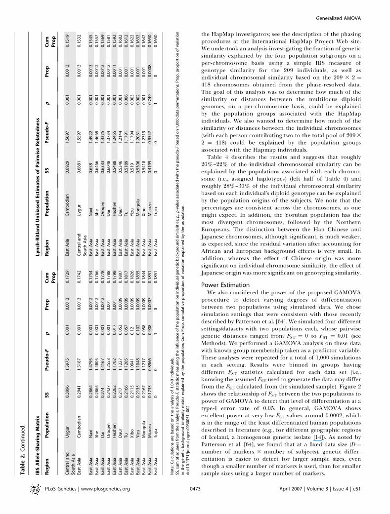
the HapMap investigators; see the description of the phasingprocedures at the International HapMap Project Web site.We undertook an analysis investigating the fraction of geneticsimilarity explained by the four population subgroups on aper-chromosome basis using a simple IBS measure ofgenotype similarity for the 209 individuals, as well asindividual chromosomal similarity based on the 209 3 2 ¼418 chromosomes obtained from the phase-resolved data.The goal of this analysis was to determine how much of thesimilarity or distances between the multilocus diploidgenomes, on a per-chromosome basis, could be explainedby the population groups associated with the HapMapindividuals. We also wanted to determine how much of thesimilarity or distances between the individual chromosomes(with each person contributing two to the total pool of 2093

2 ¼ 418) could be explained by the population groupsassociated with the Hapmap individuals.Table 4 describes the results and suggests that roughly

20%–22% of the individual chromosomal similarity can beexplained by the populations associated with each chromo-some (i.e., assigned haplotypes) (left half of Table 4) androughly 28%–30% of the individual chromosomal similaritybased on each individual’s diploid genotype can be explainedby the population origins of the subjects. We note that thepercentages are consistent across the chromosomes, as onemight expect. In addition, the Yoruban population has themost divergent chromosomes, followed by the NorthernEuropeans. The distinction between the Han Chinese andJapanese chromosomes, although significant, is much weaker,as expected, since the residual variation after accounting forAfrican and European background effects is very small. Inaddition, whereas the effect of Chinese origin was moresignificant on individual chromosome similarity, the effect ofJapanese origin was more significant on genotyping similarity.

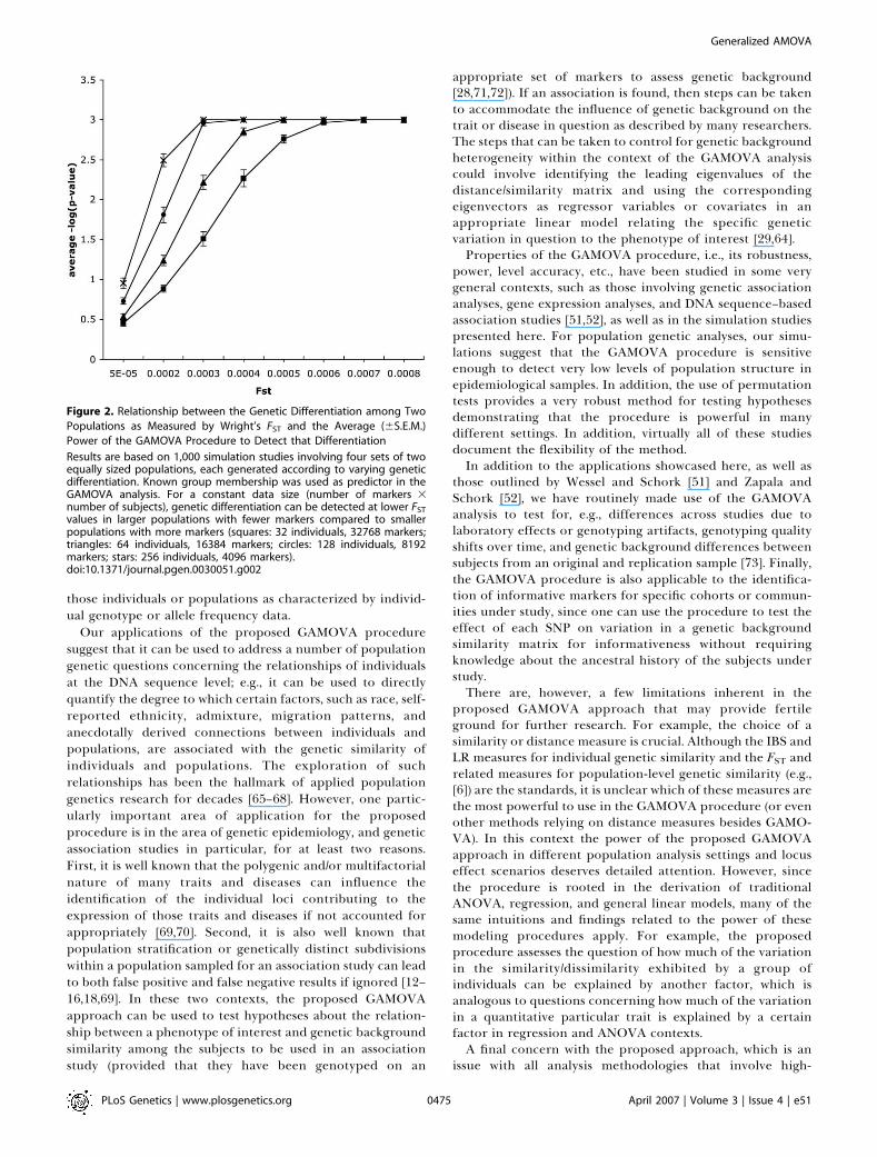
Power EstimationWe also considered the power of the proposed GAMOVA

procedure to detect varying degrees of differentiationbetween two populations using simulated data. We chosesimulation settings that were consistent with those recentlydescribed by Patterson et al. [64]. We simulated four differentsettings/datasets with two populations each, whose pairwisegenetic distances ranged from FST ¼ 0 to FST ¼ 0.01 (seeMethods). We performed a GAMOVA analysis on these datawith known group membership taken as a predictor variable.These analyses were repeated for a total of 1,000 simulationsin each setting. Results were binned in groups havingdifferent FST statistics calculated for each data set (i.e.,knowing the assumed FST used to generate the data may differfrom the FST calculated from the simulated sample). Figure 2shows the relationship of FST between the two populations topower of GAMOVA to detect that level of differentiation at atype-I error rate of 0.05. In general, GAMOVA showsexcellent power at very low FST values around 0.0002, whichis in the range of the least differentiated human populationsdescribed in literature (e.g., for different geographic regionsof Iceland, a homogenous genetic isolate [14]). As noted byPatterson et al. [64], we found that at a fixed data size (D ¼number of markers 3 number of subjects), genetic differ-entiation is easier to detect for larger sample sizes, eventhough a smaller number of markers is used, than for smallersample sizes using a larger number of markers.T

ab

le2

.C

on

tin

ue

d.

IBS

All

ele

-Sh

ari

ng

Ma

trix

Ly

nch

-Rit

lan

dU

nb

iase

dE

stim

ate

so

fP

air

wis

eR

ela

ted

ne

ss

Re

gio

nP

op

ula

tio

nS

SP

seu

do

-Fp

Pro

pC

um

Pro

p

Re

gio

nP

op

ula

tio

nS

SP

seu

do

-Fp

Pro

pC

um

Pro

p

Ce

ntr

alan

d

Sou

thA

sia

Uyg

ur

0.3

09

61

.59

75

0.0

01

0.0

01

30

.17

29

East

Asi

aC

amb

od

ian

0.6

92

91

.56

97

0.0

01

0.0

01

30

.15

19

East

Asi

aC

amb

od

ian

0.2

94

11

.51

87

0.0

01

0.0

01

30

.17

42

Ce

ntr

alan

d

Sou

thA

sia

Uyg

ur

0.6

88

11

.55

97

0.0

01

0.0

01

30

.15

32

East

Asi

aN

axi

0.2

86

41

.47

95

0.0

01

0.0

01

20

.17

54

East

Asi

aN

axi

0.6

58

1.4

92

20

.00

10

.00

13

0.1

54

5

East

Asi

aSh

e0

.28

65

1.4

80

50

.00

10

.00

12

0.1

76

6Ea

stA

sia

She

0.6

46

61

.46

69

0.0

01

0.0

01

20

.15

57

East

Asi

aD

ai0

.27

41

.41

67

0.0

01

0.0

01

20

.17

78

East

Asi

aO

roq

en

0.6

33

31

.43

75

0.0

01

0.0

01

20

.15

69

East

Asi

aO

roq

en

0.2

42

71

.25

53

0.0

01

0.0

01

0.1

78

8Ea

stA

sia

Dai

0.6

04

81

.37

34

0.0

01

0.0

01

20

.15

81

East

Asi

aH

ezh

en

0.2

26

21

.17

02

0.0

17

0.0

01

0.1

79

8Ea

stA

sia

He

zhe

n0

.54

88

1.2

46

50

.00

10

.00

11

0.1

59

2

East

Asi

aD

aur

0.2

17

1.1

22

70

.05

30

.00

09

0.1

80

7Ea

stA

sia

Dau

r0

.53

46

1.2

14

40

.00

10

.00

10

.16

02

East

Asi

aT

u0

.21

66

1.1

20

50

.05

70

.00

09

0.1

81

7Ea

stA

sia

Tu

0.5

18

91

.17

91

0.0

06

0.0

01

0.1

61

2

East

Asi

aX

ibo

0.2

11

51

.09

41

0.1

20

.00

09

0.1

82

6Ea

stA

sia

Yiz

u0

.51

91

.17

94

0.0

03

0.0

01

0.1

62

2

East

Asi

aY

izu

0.2

13

51

.10

48

0.1

02

0.0

00

90

.18

35

East

Asi

aM

on

go

la0

.53

06

1.2

06

10

.00

20

.00

10

.16

32

East

Asi

aM

on

go

la0

.21

67

1.1

21

70

.05

80

.00

09

0.1

84

4Ea

stA

sia

Xib

o0

.54

18

1.2

31

90

.00

10

.00

10

.16

42

East

Asi

aM

iao

zu0

.17

33

0.8

96

60

.90

80

.00

07

0.1

85

1Ea

stA

sia

Mia

ozu

0.4

19

90

.95

47

0.7

49

0.0

00

80

.16

50

East

Asi

aT

ujia

00

10

0.1

85

1Ea

stA

sia

Tu

jia0

01

00

.16

50

No

te:

Cal

cula

tio

ns

are

bas

ed

on

the

anal

ysis

of

1,0

40

ind

ivid

ual

s.SS

,su

mo

fsq

uar

es

fro

mth

ean

alys

is;P

seu

do

-F,s

tati

stic

me

asu

rin

gth

ein

flu

en

ceo

fth

ep

op

ula

tio

no

nin

div

idu

alg

en

eti

cb

ackg

rou

nd

sim

ilari

ties

;p,:

p-v

alu

eas

soci

ate

dw

ith

the

pse

ud

o-F

bas

ed

on

1,0

00

dat

ap

erm

uta

tio

ns;

Pro

p,p

rop

ort

ion

of

vari

atio

nin

the

ge

ne

tic

bac

kgro

un

dsi

mila

rity

mat

rix

exp

lain

ed

by

the

po

pu

lati

on

;C

um

Pro

p,

cum

ula

tive

pro

po

rtio

no

fva

riat

ion

exp

lain

ed

by

the

po

pu

lati

on

.d

oi:1

0.1

37

1/j

ou

rnal

.pg

en

.00

30

05

1.t

00

2

PLoS Genetics | www.plosgenetics.org April 2007 | Volume 3 | Issue 4 | e510473

Generalized AMOVA

Discussion

As DNA sequencing and genotyping costs decrease, agreater number of population scientists, geneticists, clinicalresearchers, and epidemiologists will seek to identify andcharacterize genetic variations that underlie phenotypicvariations as well as the biological relationships amongindividuals. Flexible analysis tools that can be used to testappropriate hypotheses will thus be needed for theseinvestigations. We have proposed an analysis procedure,

GAMOVA, that not only extends an analysis of varianceapproach that is used widely [50] for assessing relationshipsbetween genetic variations, phenotypic variations, and thepopulation origins of individuals, but also complementswidely used cluster analysis approaches for these purposes[20,23]. Specifically, the proposed GAMOVA approach can beused to test hypotheses about the relationship betweenvariables collected on individuals or populations (such asparticular phenotypes or population-level migration pat-terns) and variation in the genetic similarity or distance of

Table 3. GAMOVA Analysis Investigating the Relationship between Craniometric Measures Collected by Howells and GeneticBackground

Gender Measure SS Pseudo-F p Prop Cum Prop Comment

Male FRS 0.0129 9.298 0.002 0.5375 0.54 nasion-bregma subtense

GLS 0.0044 4.611 0.030 0.1837 0.72 glabella projection

WCB 0.0032 5.364 0.004 0.1316 0.85 minimum cranial breadth

BPL 0.0013 2.813 0.039 0.0530 0.91 basion-prosthion length

NAS 0.0010 2.950 0.081 0.0400 0.95 nasio-frontal subtense

FRC 0.0008 4.521 0.093 0.0326 0.98 nasion-bregma chord

OCC 0.0006 �16.485 0.974 0.0246 1.00 lambda-opisthion chord

OBH 0.0000 �0.313 0.673 0.0014 1.00 orbit height

Female FRS 0.0114 6.676 0.009 0.4881 0.49 nasion-bregma subtense

BPL 0.0058 5.760 0.016 0.2507 0.74 basion-prosthion length

SOS 0.0022 2.917 0.068 0.0962 0.84 supraorbital projection

MDH 0.0017 3.149 0.103 0.0727 0.91 mastoid height

DKS 0.0018 17.017 0.021 0.0785 0.99 dacryon subtense

OCC 0.0003 55.968 0.008 0.0134 1.00 lambda-opisthion chord

FMB 0.0002 �1.059 0.744 0.0086 1.01 bifrontal breadth

SS, sum of squares from the analysis; Pseudo-F, statistic measuring the influence of the population on individual genetic background similarities; p, p-value associated with the pseudo-Fbased on 10,000 data permutations; Prop, proportion of variation in the genetic background similarity matrix explained by the population; Cum Prop, cumulative proportion of variationexplained by the population.doi:10.1371/journal.pgen.0030051.t003

Table 4. Percentage of the Variation in the Dissimilarity of Individual Chromosomes or Diploid Genotypes Explained as a Function ofthe Population Designations of the 209 Subjects Genotyped as Part of the HapMap Project

Chromosome Chromosomes Diploid Genotypes

Total Yoruban CEPH Chinese Total Yoruban CEPH Japanese

1 22.15 14.15 7.61 0.39 29.20 18.37 10.06 0.59

2 23.43 14.78 8.24 0.41 30.39 19.05 10.74 0.61

3 22.29 14.53 7.40 0.37 29.12 18.77 9.77 0.57

4 21.90 14.79 6.73 0.38 28.71 19.22 8.91 0.59

5 21.31 13.44 7.46 0.41 28.10 17.57 9.90 0.63

6 21.21 13.37 7.46 0.37 28.03 17.58 9.85 0.59

7 21.14 13.35 7.39 0.40 27.85 17.41 9.82 0.62

8 21.76 14.27 7.09 0.40 28.57 18.65 9.31 0.60

9 20.89 12.67 7.79 0.43 27.50 16.59 10.24 0.67

10 21.83 13.45 7.96 0.42 28.66 17.51 10.52 0.63

11 20.79 13.36 7.01 0.42 27.42 17.51 9.26 0.65

12 21.85 13.62 7.84 0.38 28.80 17.83 10.37 0.59

13 20.79 12.91 7.47 0.41 27.48 17.01 9.85 0.62

14 21.68 13.58 7.68 0.42 28.54 17.74 10.17 0.63

15 23.61 14.16 9.02 0.43 30.67 18.41 11.60 0.66

16 21.81 13.92 7.49 0.40 28.68 18.19 9.89 0.60

17 23.25 15.34 7.54 0.37 30.17 19.79 9.81 0.57

18 19.64 13.02 6.21 0.41 26.06 17.13 8.28 0.64

19 20.96 13.50 7.08 0.38 27.54 17.59 9.33 0.61

20 21.67 14.10 7.14 0.43 28.42 18.34 9.43 0.65

21 20.16 12.81 6.93 0.41 26.59 16.77 9.21 0.60

22 21.49 13.68 7.38 0.43 28.34 17.89 9.76 0.69

doi:10.1371/journal.pgen.0030051.t004

PLoS Genetics | www.plosgenetics.org April 2007 | Volume 3 | Issue 4 | e510474

Generalized AMOVA

those individuals or populations as characterized by individ-ual genotype or allele frequency data.

Our applications of the proposed GAMOVA proceduresuggest that it can be used to address a number of populationgenetic questions concerning the relationships of individualsat the DNA sequence level; e.g., it can be used to directlyquantify the degree to which certain factors, such as race, self-reported ethnicity, admixture, migration patterns, andanecdotally derived connections between individuals andpopulations, are associated with the genetic similarity ofindividuals and populations. The exploration of suchrelationships has been the hallmark of applied populationgenetics research for decades [65–68]. However, one partic-ularly important area of application for the proposedprocedure is in the area of genetic epidemiology, and geneticassociation studies in particular, for at least two reasons.First, it is well known that the polygenic and/or multifactorialnature of many traits and diseases can influence theidentification of the individual loci contributing to theexpression of those traits and diseases if not accounted forappropriately [69,70]. Second, it is also well known thatpopulation stratification or genetically distinct subdivisionswithin a population sampled for an association study can leadto both false positive and false negative results if ignored [12–16,18,69]. In these two contexts, the proposed GAMOVAapproach can be used to test hypotheses about the relation-ship between a phenotype of interest and genetic backgroundsimilarity among the subjects to be used in an associationstudy (provided that they have been genotyped on an

appropriate set of markers to assess genetic background[28,71,72]). If an association is found, then steps can be takento accommodate the influence of genetic background on thetrait or disease in question as described by many researchers.The steps that can be taken to control for genetic backgroundheterogeneity within the context of the GAMOVA analysiscould involve identifying the leading eigenvalues of thedistance/similarity matrix and using the correspondingeigenvectors as regressor variables or covariates in anappropriate linear model relating the specific geneticvariation in question to the phenotype of interest [29,64].Properties of the GAMOVA procedure, i.e., its robustness,

power, level accuracy, etc., have been studied in some verygeneral contexts, such as those involving genetic associationanalyses, gene expression analyses, and DNA sequence–basedassociation studies [51,52], as well as in the simulation studiespresented here. For population genetic analyses, our simu-lations suggest that the GAMOVA procedure is sensitiveenough to detect very low levels of population structure inepidemiological samples. In addition, the use of permutationtests provides a very robust method for testing hypothesesdemonstrating that the procedure is powerful in manydifferent settings. In addition, virtually all of these studiesdocument the flexibility of the method.In addition to the applications showcased here, as well as

those outlined by Wessel and Schork [51] and Zapala andSchork [52], we have routinely made use of the GAMOVAanalysis to test for, e.g., differences across studies due tolaboratory effects or genotyping artifacts, genotyping qualityshifts over time, and genetic background differences betweensubjects from an original and replication sample [73]. Finally,the GAMOVA procedure is also applicable to the identifica-tion of informative markers for specific cohorts or commun-ities under study, since one can use the procedure to test theeffect of each SNP on variation in a genetic backgroundsimilarity matrix for informativeness without requiringknowledge about the ancestral history of the subjects understudy.There are, however, a few limitations inherent in the

proposed GAMOVA approach that may provide fertileground for further research. For example, the choice of asimilarity or distance measure is crucial. Although the IBS andLR measures for individual genetic similarity and the FST andrelated measures for population-level genetic similarity (e.g.,[6]) are the standards, it is unclear which of these measures arethe most powerful to use in the GAMOVA procedure (or evenother methods relying on distance measures besides GAMO-VA). In this context the power of the proposed GAMOVAapproach in different population analysis settings and locuseffect scenarios deserves detailed attention. However, sincethe procedure is rooted in the derivation of traditionalANOVA, regression, and general linear models, many of thesame intuitions and findings related to the power of thesemodeling procedures apply. For example, the proposedprocedure assesses the question of how much of the variationin the similarity/dissimilarity exhibited by a group ofindividuals can be explained by another factor, which isanalogous to questions concerning how much of the variationin a quantitative particular trait is explained by a certainfactor in regression and ANOVA contexts.A final concern with the proposed approach, which is an

issue with all analysis methodologies that involve high-

Figure 2. Relationship between the Genetic Differentiation among Two

Populations as Measured by Wright’s FST and the Average (6S.E.M.)

Power of the GAMOVA Procedure to Detect that Differentiation

Results are based on 1,000 simulation studies involving four sets of twoequally sized populations, each generated according to varying geneticdifferentiation. Known group membership was used as predictor in theGAMOVA analysis. For a constant data size (number of markers 3number of subjects), genetic differentiation can be detected at lower FST

values in larger populations with fewer markers compared to smallerpopulations with more markers (squares: 32 individuals, 32768 markers;triangles: 64 individuals, 16384 markers; circles: 128 individuals, 8192markers; stars: 256 individuals, 4096 markers).doi:10.1371/journal.pgen.0030051.g002

PLoS Genetics | www.plosgenetics.org April 2007 | Volume 3 | Issue 4 | e510475

Generalized AMOVA

dimensional data types, involves missing genotype data. Onecan handle missing genotype data in a number of ways. First,one could restrict the construction of the similarity measureto only those individuals with complete data—which mayresult in a substantially reduced sample—or simply constructthe measure with the data that are available on each pair ofsubjects. This latter approach will be problematic if a numberof individuals are missing genotype data at the most heavilyweighted (e.g., functional or informative) loci. Anotherapproach to handling missing data would involve imputingor assigning individuals genotype data based on linkagedisequilibrium information. This approach would only be asuseful as the strength of the linkage disequilibrium betweenalleles at the loci with missing data and those without. Theapproach we took to handling missing data was to usewhatever genotype information was available on the subjectsfor the similarity calculations.

Finally, we note that a web-based GAMOVA tool isavailable from the authors at http://polymorphism.scripps.edu/;cabney/cgi-bin/mmr.cgi.

Materials and Methods

Computing a similarity matrix. As noted, the proposed procedurerequires the computation of a ‘‘distance’’ matrix that reflects thedissimilarity of the genetic backgrounds of the individuals orpopulations being analyzed. There are many possible measures thatcould be used to construct such a matrix, and we considered twomethods for computing the similarity of individuals’ genetic back-grounds based on genotype data collected on them. The resultingsimilarity measure can be translated into a distance or dissimilaritymeasure as described later. The first similarity measure is widely usedand is based on simple IBS allele sharing [38] and can be calculated asthe fraction of alleles shared identical by state for each pair ofindividuals in a sample over all the loci for which the individuals havebeen genotyped:

12L

XLl¼1

rIBS; l ð1Þ

where rIBS is the individual, locus-specific allele-sharing value and L¼number of loci considered in the calculations.

The second similarity measure essentially considers weighting lociin the computation of IBS-based allele sharing by allele frequencyand was introduced by Lynch and Ritland [44]. The LR regression-based method-of-moments estimator has been shown to have somedesirable properties relative to other methods, especially in the caseof populations consisting of individuals with a low degree ofrelatedness [45,74], and has been widely discussed in the populationgenetics and behavioral ecology literature (e.g., [75–77]). The LRestimator uses a regression approach to infer relationships (i.e., oneindividual of a pair serves as a ‘‘reference’’ individual and theprobabilities of the locus-specific genotypes of the second individualare then conditioned on those of the reference individual). The LRcoefficient of relatedness is:

rxy ¼paðSbc þ SbdÞ þ pbðSac þ SadÞ � 4papb

ð1þ SabÞðpa þ pbÞ � 4papbð2Þ

where pa and pb equal the frequencies of alleles a and b in thepopulation. The reference individual is assumed to have alleles a andb (such that if this individual is homozygous, Sab¼1, if heterozygous, Sab¼ 0), and the proband has alleles c and d. Multilocus estimates ofgenetic background similarity can be obtained by summing the singleestimates, weighted by the inverse of their sampling variance:

rxy ¼1

Wr;x

XLl¼1

Wr;xðlÞrxyðlÞ ð3Þ

where

Wr;xðlÞ ¼1

Var½rxyðlÞ�ð1þ SabÞðpa þ pbÞ � 4papb

2papb; ð4Þ

which is computed under the assumption that the two individuals inquestion are unrelated (i.e., have 0.0 relatedness).

The similarity matrices were transformed into a dissimilarity or‘‘distance’’ matrix by subtracting the components of the matrix from1.0 if the IBS measure is used, or subtracting them from 1.0 after eachcomponent in the matrix is divided by the theoretical or empiricalmaximum of the similarity measure to scale the entries to lie between0 and 1.

Multivariate distance matrix regression analysis. Once one hascomputed a distance matrix it can be subjected to a regressionanalysis testing hypotheses regarding, e.g., whether or not variation inthe level of similarity/dissimilarity exhibited by pairs of individualsreflected in that matrix can be explained by other features thoseindividuals posses (e.g., whether they are from a particular ethnicgroup or a specific country). To describe the regression model, weassume that each of N individuals or study subjects has beengenotyped at L unlinked polymorphic loci (bi- or multiallelic) andthatM grouping or phenotypic variables have been collected on the Nsubjects. These grouping or phenotypic variables could includeinformation about the country of origin (coded using dummyvariables, such as a 1 assigned to individuals from a particularcountry, and 0 assigned to individuals from a different country), thecontinental origin of that country and its distance from Addis Ababa,and craniometric diversity data, as we have considered.

We note that the proposed regression procedure, which is anextension of the procedure described by McArdle and Anderson [78]and a general reformulation of the AMOVA procedure discussed byExcoffier et al. [50], does not require that the distance matrix usedhave metric properties. Let this distance matrix and its elements bedenoted by D¼ dij (i,j¼ 1,. . .,N), for the N subjects. The possibility thatN � L will not pose problems in the proposed regression analysissetting. Let X be an N 3 M matrix harboring information on the Mgrouping or phenotypic variables, which will be modeled as predictoror regressor variables whose relationships to the values in thegenomic similarity matrix are of interest. Compute the standardprojection matrix, H ¼ X(X9X)�1X9, typically used to estimatecoefficients relating the predictor variables to outcome variables inmultiple regression contexts. Next, compute the matrixA ¼ ðaijÞ ¼ ð�½1=2�d2ijÞ and center this matrix using the transforma-tion discussed by Gower [79] and denote this matrix G:

G ¼ I � 1n119

� �A I � 1

n119

� �ð5Þ

An F-statistic can be constructed to test the hypothesis that the Mregressor variables have no relationship to variation in the genomicdistance or dissimilarity of the N subjects reflected in the N 3 Ndistance/dissimilarity matrix as [78]:

F ¼ trðHGHÞtr½ðI �HÞGðI �HÞ� ð6Þ

If the Euclidean distance is used to construct the distance matrixon a single quantitative variable (i.e., as in a univariate analysis of thatvariable) and appropriate numerator and denominator degrees offreedom are accommodated in the test statistics, the F-statistic aboveis equivalent to the standard ANOVA F-statistic [78]. The distribu-tional properties of the F-statistic are complicated for alternativedistance measures computed for more than one variable, especially ifthose variables are discrete, as in genotype data. However, permu-tation tests can then be used to assess statistical significance of thepseudo F-statistic [80,81]. The M regressor variables can be testedindividually or in a step-wise manner. All matrix-based regressionanalyses we have performed in this paper used 10,000 permutationsto calculate p-values, except for the analysis of the CEPH-HGDP datain Table 2, for which we used 1,000 permutations. In addition, onecan calculate the percentage of variation in similarity/distanceswithin the distance matrix explained by the regressor variables, r2,through the formula:

r2 ¼ trðHGHÞtrðGÞ ð7Þ

Graphical display of similarity matrices. Similarity matrices of thetype we have described can be represented graphically in a number ofways (e.g., heatmaps and trees) that can facilitate interpretation. Weconsidered trees that are constructed such that individuals withgreater genomic similarity are placed next to each other (i.e., they arerepresented as adjacent branches of the tree) and less similarindividuals are represented as branches some distance away fromeach other, using the module neighbor of the program PHYLIP v.

PLoS Genetics | www.plosgenetics.org April 2007 | Volume 3 | Issue 4 | e510476

Generalized AMOVA

3.64 (http://evolution.genetics.washington.edu/phylip.html) to con-struct a neighbor-joining tree. By color coding the individualbranches based on the phenotype values possessed by the individualsthey represent, one can see if there are patches of a certain color onneighboring branches, which would indicate that phenotype valuescluster along with genetic similarity (e.g., using HyperTree v.1.0.0,http://www.kinase.com/tools/HyperTree.html).

The CEPH-HGDP Cell Line Panel.We used genotype data from thepublicly available CEPH-HGDP Cell Line Panel [56], which have beeninvestigated recently in numerous studies (e.g., reviewed in [4]). Thedatasets used here include 377 and 783 autosomal microsatellitestyped on 1,040 people from 51 populations distributed worldwide(China and United States Han subjects were pooled). We included thesame 1,040 subjects as originally described in Rosenberg et al. [1],with the exception of 16 duplicated or mislabeled samples [5]. Inaddition, we also used geographic data (i.e., the distance from AddisAbaba to each of the 51 CEPH-HGDP populations), kindly providedby Dr. Francois Balloux [8], and pairwise FST values [82] between 51populations based on 783 microsatellites kindly provided by Dr. NoahRosenberg [83].

The anthropometric data of Howells. We used craniometricdiversity data (the median across the subjects of each of 45 featuresfor each gender) gathered on 489 males and 459 females from tenpopulations (nine populations for females) made available throughthe work by Howells [54,55]. The craniometric data was pairedaccording to geographic regions with genetic data from 415 subjectsfrom 19 populations from the CEPH-HGDP panel genotyped on 783markers as described in Table 1 of Roseman [59]. Pairwise FSTbetween the ten populations (merged from an original 19 CEPH-HGDP populations to represent the locations sampled from, for thecraniometric data) was calculated according to standard formulae[82] for diploid data using genotypes at 786 microsatellite loci fromthe CEPH-HGDP. The pairwise FST analysis produced a 10 3 10genetic distance matrix that we used in the proposed GAMOVAprocedure to determine if relationships exist between the 45 cranialmeasurements and genetic background similarity.

The HapMap data set. We downloaded the ;700,000 SNP markersfrom the phase I data available on the 209 individuals genotyped aspart of the International HapMap Project (http://www.hapmap.org;[60]). These 209 individuals included 60 individuals of NorthernEuropean descent (i.e., the ‘‘CEPH-HGDP’’ derived individuals), 44individuals of Japanese descent, 45 individuals of Han Chinesedescent, and 60 individuals of West African descent (i.e., the‘‘Yoruban’’ population-derived individuals). Since these 209 individ-uals had been phased (i.e., assigned haplotypes), we considered thedata as providing both 209 multilocus genotypes on each of the 22autosomes, as well as providing 418 individual chromosomes, fromeach of the four populations, and analyzed it in this light.

Power estimations. A Python computer program was used togenerate four sets of two populations, each with M markers and Nsubjects with the same constant data size (D ¼ N 3 M ¼ 220) asdiscussed by Patterson et al. [64]. Allele frequencies of all biallelic locifor the first population were generated by assuming they followed abeta-distribution with parameters 0.75 and 0.75. For the secondpopulation, for each locus, the allele frequencies of the firstpopulation were modified by adding random numbers so that thetwo populations would exhibit certain genetic distances based onWright’s FST measure of population differentiation ([82], Formula5.12). For each of the four sets, 1,000 populations were simulated withFST values that ultimately were randomly distributed between 0 and0.01. We assigned hypothetical individuals in the simulated samplesalleles at each of the M loci based on the allele frequencies. AGAMOVA analysis was then performed on an IBS distance matrixconstructed from the allelic profiles of the simulated individuals asdescribed above with known population membership taken as apredictor variable. Permutations (1,000) of the data were performedto determine the significance of each pseudo-F statistic from theGAMOVA analysis.

Acknowledgments

The authors would like to thank Drs. Noah Rosenberg and FrancoisBalloux for providing insight into, and data associated with, theCEPH-HGDP Cell Line Panel. The authors would also like to thankDr. Marti Anderson for advice and encouragement regarding themultivariate distance matrix regression method that forms the basisof the proposed GAMOVA procedure.

Author contributions. CMN and NJS conceived and designed theexperiments, performed the experiments, analyzed the data, andwrote the paper. CMN, OL, and NJS contributed reagents/materials/analysis tools.

Funding. NJS and his laboratory are supported in part by thefollowing research grants: the National Heart, Lung, and BloodInstitute Family Blood Pressure Program (FBPP; U01 HL064777–06);the National Institute on Aging Longevity Consortium (U19AG023122–01); the National Institute of Mental Health Consortiumon the Genetics of Schizophrenia (COGS; 5 R01 HLMH065571–02);National Institutes of Health R01s HL074730–02 and HL070137–01;Scripps Genomic Medicine; and the Donald W. Reynolds Foundation(Helen Hobbs, Principal Investigator).

Competing interests. The authors have declared that no competinginterests exist.

References1. Rosenberg NA, Pritchard JK, Weber JL, Cann HM, Kidd KK, et al. (2002)

Genetic structure of human populations. Science 298: 2381–2385.2. Bamshad M, Wooding S, Salisbury BA, Stephens JC (2004) Deconstructing

the relationship between genetics and race. Nat Rev Genet 5: 598–609.3. Serre D, Paabo S (2004) Evidence for gradients of human genetic diversity

within and among continents. Genome Res 14: 1679–1685.4. Cavalli-Sforza LL (2005) The Human Genome Diversity Project: Past,

present and future. Nat Rev Genet 6: 333–340.5. Mountain JL, Ramakrishnan U (2005) Impact of human population history

on distributions of individual-level genetic distance. HumGenomics 2: 4–19.6. Ramachandran S, Deshpande O, Roseman CC, Rosenberg NA, Feldman

MW, et al. (2005) Support from the relationship of genetic and geographicdistance in human populations for a serial founder effect originating inAfrica. Proc Natl Acad Sci U S A 102: 15942–15947.

7. Shriver MD, Mei R, Parra EJ, Sonpar V, Halder I, et al. (2005) Large-scaleSNP analysis reveals clustered and continuous patterns of human geneticvariation. Hum Genomics 2: 81–89.

8. Liu H, Prugnolle F, Manica A, Balloux F (2006) A geographically explicitgenetic model of worldwide human-settlement history. Am J Hum Genet79: 230–237.

9. Kittles RA, Chen W, Panguluri RK, Ahaghotu C, Jackson A, et al. (2002)CYP3A4-V and prostate cancer in African Americans: Causal or confound-ing association because of population stratification? Hum Genet 110: 553–560.

10. Cardon LR, Palmer LJ (2003) Population stratification and spurious allelicassociation. Lancet 361: 598–604.

11. Freedman ML, Reich D, Penney KL, McDonald GJ, Mignault AA, et al.(2004) Assessing the impact of population stratification on geneticassociation studies. Nat Genet 36: 388–393.

12. Marchini J, Cardon LR, Phillips MS, Donnelly P (2004) The effects of human

population structure on large genetic association studies. Nat Genet 36:512–517.

13. Campbell CD, Ogburn EL, Lunetta KL, Lyon HN, Freedman ML, et al.(2005) Demonstrating stratification in a European American population.Nat Genet 37: 868–872.

14. Helgason A, Yngvadottir B, Hrafnkelsson B, Gulcher J, Stefansson K (2005)An Icelandic example of the impact of population structure on associationstudies. Nat Genet 37: 90–95.

15. Reiner AP, Ziv E, Lind DL, Nievergelt CM, Schork NJ, et al. (2005)Population structure, admixture, and aging-related phenotypes in AfricanAmerican adults: The cardiovascular health study. Am J Hum Genet 76:463–477.

16. Voight BF, Pritchard JK (2005) Confounding from cryptic relatedness incase-control association studies. PLoS Genet 1: e32. doi:10.1371/journal.pgen.0010032

17. Berger M, Stassen HH, Kohler K, Krane V, Monks D, et al. (2006) Hiddenpopulation substructures in an apparently homogeneous population biasassociation studies. Eur J Hum Genet 14: 236–244.

18. Seldin MF, Shigeta R, Villoslada P, Selmi C, Tuomilehto J, et al. (2006)European population substructure: Clustering of northern and southernpopulations. PLoS Genet 2: e143. doi:10.1371/journal.pgen.0020143

19. Foll M, Gaggiotti O (2006) Identifying the environmental factors thatdetermine the genetic structure of populations. Genetics 174: 875–891.

20. Pritchard JK, Stephens M, Donnelly P (2000) Inference of populationstructure using multilocus genotype data. Genetics 155: 945–959.

21. Dawson KJ, Belkhir K (2001) A Bayesian approach to the identification ofpanmictic populations and the assignment of individuals. Genet Res 78: 59–77.

22. Satten GA, Flanders WD, Yang Q (2001) Accounting for unmeasuredpopulation substructure in case-control studies of genetic association usinga novel latent-class model. Am J Hum Genet 68: 466–477.

PLoS Genetics | www.plosgenetics.org April 2007 | Volume 3 | Issue 4 | e510477

Generalized AMOVA

23. Falush D, Stephens M, Pritchard JK (2003) Inference of populationstructure using multilocus genotype data: linked loci and correlated allelefrequencies. Genetics 164: 1567–1587.

24. Hoggart CJ, Parra EJ, Shriver MD, Bonilla C, Kittles RA, et al. (2003)Control of confounding of genetic associations in stratified populations.Am J Hum Genet 72: 1492–1504.

25. Stassen HH, Hoffman K, Scharfetter C (2003) Similarity by state/descentand genetic vector spaces: Analysis of a longitudinal family study. BMCGenet 4 Suppl 1: S59.

26. Kohler K, Bickeboller H (2005) Case-control association tests correcting forpopulation stratification. Ann Hum Genet 69: 98–115.

27. Tang H, Peng J, Wang P, Risch NJ (2005) Estimation of individualadmixture: Analytical and study design considerations. Genet Epidemiol28: 289–301.

28. Tsai HJ, Choudhry S, Naqvi M, Rodriguez-Cintron W, Burchard EG, et al.(2005) Comparison of three methods to estimate genetic ancestry andcontrol for stratification in genetic association studies among admixedpopulations. Hum Genet 118: 424–433.

29. Price AL, Patterson NJ, Plenge RM, Weinblatt ME, Shadick NA, et al. (2006)Principal components analysis corrects for stratification in genome-wideassociation studies. Nat Genet 38: 904–909.

30. Redden DT, Divers J, Vaughan LK, Tiwari HK, Beasley TM, et al. (2006)Regional admixture mapping and structured association testing: Con-ceptual unification and an extensible general linear model. PLoS Genet 2:e137. doi:10.1371/journal.pgen.0020137

31. Rosenberg NA, Nordborg M (2006) A general population-genetic model forthe production by population structure of spurious genotype-phenotypeassociations in discrete, admixed, or spatially distributed populations.Genetics 173: 1665–1678.

32. Setakis E, Stirnadel H, Balding DJ (2006) Logistic regression protectsagainst population structure in genetic association studies. Genome Res 16:290–296.

33. Yu J, Pressoir G, Briggs WH, Vroh Bi I, Yamasaki M, et al. (2006) A unifiedmixed-model method for association mapping that accounts for multiplelevels of relatedness. Nat Genet 38: 203–208.

34. McKeigue PM (1998) Mapping genes that underlie ethnic differences indisease risk: methods for detecting linkage in admixed populations, byconditioning on parental admixture. Am J Hum Genet 63: 241–251.

35. Wu B, Liu N, Zhao H (2006) PSMIX: An R package for population structureinference via maximum likelihood method. BMC Bioinformatics 7: 317.

36. Zhang S, Zhu X, Zhao H (2003) On a semiparametric test to detectassociations between quantitative traits and candidate genes usingunrelated individuals. Genet Epidemiol 24: 44–56.

37. Chen HS, Zhu X, Zhao H, Zhang S (2003) Qualitative semi-parametric testfor genetic associations in case-control designs under structured popula-tions. Ann Hum Genet 67: 250–264.

38. Bowcock AM, Ruiz-Linares A, Tomfohrde J, Minch E, Kidd JR, et al. (1994)High resolution of human evolutionary trees with polymorphic micro-satellites. Nature 368: 455–457.

39. Mountain JL, Cavalli-Sforza LL (1997) Multilocus genotypes, a tree ofindividuals, and human evolutionary history. Am J Hum Genet 61: 705–718.

40. Shriver MD, Kennedy GC, Parra EJ, Lawson HA, Sonpar V, et al. (2004) Thegenomic distribution of population substructure in four populations using8,525 autosomal SNPs. Hum Genomics 1: 274–286.

41. Li CC, Weeks DE, Chakravarti A (1993) Similarity of DNA fingerprints dueto chance and relatedness. Hum Hered 43: 45–52.

42. Queller DC, Goodnight KF (1989) Estimating relatedness using geneticmarkers. Evolution 43: 258–275.

43. Ritland K (1996) Estimators for pairwise relatedness and individualinbreeding coefficients. Genet Res: 175–185.

44. Lynch M, Ritland K (1999) Estimation of pairwise relatedness withmolecular markers. Genetics 152: 1753–1766.

45. Wang J (2002) An estimator for pairwise relatedness using molecularmarkers. Genetics 160: 1203–1215.

46. Rosenberg NA, Li LM, Ward R, Pritchard JK (2003) Informativeness ofgenetic markers for inference of ancestry. Am J Hum Genet 73: 1402–1422.

47. Collins-Schramm HE, Chima B, Morii T, Wah K, Figueroa Y, et al. (2004)Mexican American ancestry-informative markers: examination of popula-tion structure and marker characteristics in European Americans, MexicanAmericans, Amerindians and Asians. Hum Genet 114: 263–271.

48. Smith MW, Patterson N, Lautenberger JA, Truelove AL, McDonald GJ, et al.(2004) A high-density admixture map for disease gene discovery in AfricanAmericans. Am J Hum Genet 74: 1001–1013.

49. Tian C, Hinds DA, Shigeta R, Kittles R, Ballinger DG, et al. (2006) Agenomewide single-nucleotide-polymorphism panel with high ancestryinformation for African American admixture mapping. Am J Hum Genet79: 640–649.

50. Excoffier L, Smouse PE, Quattro JM (1992) Analysis of molecular varianceinferred from metric distances among DNA haplotypes: Application tohuman mitochondrial DNA restriction data. Genetics 131: 479–491.

51. Wessel J, Schork NJ (2006) Generalized genomic distance-based regressionmethodology for multilocus association analysis. Am J Hum Genet 79: 792–806.

52. Zapala MA, Schork NJ (2006) Multivariate regression analysis of distance

matrices for testing associations between gene expression patterns andrelated variables. Proc Natl Acad Sci U S A 103: 19430–19435.

53. Smouse PE, Long JC (1992) Matrix correlation analysis in anthropology andgenetics. American Journal of Physical Anthropology 35: 187–213.

54. Howells WW (1973) Cranial variation in man: A study of multivariateanalysis of patterns of difference among recent human populations.Cambridge (Massachusetts): Harvard University Press, Peabody Museum ofArchaeology and Ethnology. 259 p.

55. Howells WW (1989) Skull shapes and the map: craniometric analyses in thedispersion of modern Homo. Cambridge (Massachusetts): Harvard Uni-versity Press, Peabody Museum of Archaeology and Ethnology. 189 p.

56. Cann HM, de Toma C, Cazes L, Legrand MF, Morel V, et al. (2002) A humangenome diversity cell line panel. Science 296: 261–262.

57. Manica A, Prugnolle F, Balloux F (2005) Geography is a better determinantof human genetic differentiation than ethnicity. Hum Genet 118: 366–371.

58. Zhivotovsky LA, Rosenberg NA, Feldman MW (2003) Features of evolutionand expansion of modern humans, inferred from genomewide micro-satellite markers. Am J Hum Genet 72: 1171–1186.

59. Roseman CC (2004) Detecting interregionally diversifying natural selectionon modern human cranial form by using matched molecular andmorphometric data. Proc Natl Acad Sci U S A 101: 12824–12829.

60. Roseman CC, Weaver TD (2004) Multivariate apportionment of globalhuman craniometric diversity. Am J Phys Anthropol 125: 257–263.

61. Martinez-Abadias N, Gonzalez-Jose R, Gonzalez-Martin A, Van der Molen S,Talavera A, et al. (2006) Phenotypic evolution of human craniofacialmorphology after admixture: a geometric morphometrics approach. Am JPhys Anthropol 129: 387–398.

62. Parra EJ, Kittles RA, Shriver MD (2004) Implications of correlationsbetween skin color and genetic ancestry for biomedical research. Nat Genet36: S54–S60.

63. Consortium TIH (2005) A haplotype map of the human genome. Nature437: 1299–1320.

64. Patterson N, Price AL, Reich D (2006) Population Structure andEigenanalysis. PLoS Genet 2: e190. doi:10.1371/journal.pgen.0020190

65. Lewontin R (1972) The apportionment of human diversity. EvolutionaryBiology 6: 381–398.

66. Cavalli-Sforza LL, Feldman MW (2003) The application of moleculargenetic approaches to the study of human evolution. Nat Genet 33 Suppl:266–275.

67. Barbujani G, Goldstein DB (2004) Africans and Asians abroad: Geneticdiversity in Europe. Annu Rev Genomics Hum Genet 5: 119–150.

68. Mountain JL, Risch N (2004) Assessing genetic contributions to phenotypicdifferences among ‘‘racial’’ and ‘‘ethnic’’ groups. Nat Genet 36: S48–S53.

69. Lander ES, Schork NJ (1994) Genetic dissection of complex traits. Science265: 2037–2048.

70. Tishkoff SA, Kidd KK (2004) Implications of biogeography of humanpopulations for ‘‘race’’ and medicine. Nat Genet 36: S21–S27.

71. Turakulov R, Easteal S (2003) Number of SNPS loci needed to detectpopulation structure. Hum Hered 55: 37–45.

72. Yang BZ, Zhao H, Kranzler HR, Gelernter J (2005) Characterization of alikelihood based method and effects of markers informativeness inevaluation of admixture and population group assignment. BMC Genet 6:50.

73. Nievergelt C, Kelsoe J, Shimizu C, Burns J, Schork N. (2006) Multivariatedistance based methods for testing and accommodating populationsubstructure [abstract 2203]. Annual meeting of The American Society ofHuman Genetics, 12 October 2006, New Orleans, Louisiana. Available:http://www.ashg.org/genetics/ashg06s/index.shtml. Accessed 5 March 2007.

74. Van de Casteele T, Galbusera P, Matthysen E (2001) A comparison ofmicrosatellite-based pairwise relatedness estimators. Mol Ecol 10: 1539–1549.

75. Widdig A, Nurnberg P, Krawczak M, Streich WJ, Bercovitch FB (2001)Paternal relatedness and age proximity regulate social relationships amongadult female rhesus macaques. Proc Natl Acad Sci U S A 98: 13769–13773.

76. Parsons K, Durban J, Claridge D, Balcomb K, Noble L, et al. (2003) Kinshipas a basis for alliance formation between male bottlenose dolphins, Tursiopstruncatus, in the Bahamas. Anim Behav 66: 185–194.

77. Lobo JA, Quesada M, Stoner KE (2005) Effects of pollination by bats on themating system of Ceiba pentandra (Bombacaceae) populations in two tropicallife zones in Costa Rica. Am J Bot 92: 370–376.

78. McArdle BH, Anderson MJ (2001) Fitting multivariate models tocommunity data: A comment on distance-based redundancy analysis.Ecology 82: 290–297.

79. Gower JC (1966) Some distance properties of latent root and vectormethods used in multivariate analysis. Biometrika 53: 325–338.

80. Good P (1994) Permutation tests. New York: Springer-Verlag. 228 p.81. Edington ES (1995) Randomization tests. New York: Marcel Dekker. 409 p.82. Weir BS (1996) Genetic data analysis II: Methods for discrete population

genetic data. Sunderland (Massachusetts): Sinauer Associates. 445 p.83. Rosenberg NA (2007) Human genetic variation: Answers to frequently

asked questions. In: Bamshad M, editor. Human genetic diversity:Implications for race, ancestry, and health. Oxford: Oxford UniversityPress.

PLoS Genetics | www.plosgenetics.org April 2007 | Volume 3 | Issue 4 | e510478

Generalized AMOVA