Journal of Geometry and Physics xxx (2003) xxx–xxx

Generalized BRST models and topologicalYang–Mills theories

Marcelo CarvalhoDepartment of Mathematics, Waseda University, 3-4-1 Okubo, Shinjuku-ku, Tokyo 169-8050, Japan

Received 31 May 2003

Abstract

We present a general framework for models admitting a decomposition of the typed = [δ, b],with b the BRST operator andδ a certain (even) derivation. We focus our attention on models whosefields can be described as components of two laddersW = c+A+ · · · andF = φ+ψ+ · · · andshow how they relate to some aspects of topological Yang–Mills theory. We relate our constructionto the standard mathematical ideas of Cartan’sG-operation and interpretWandFas pair of algebraicconnection and curvature in a certain bigraded differential algebra.© 2003 Elsevier B.V. All rights reserved.

MSC:81T13; 81T45

JGP SC:Quantum field theories

Keywords:Topological field theory; BRST algebras

1. Introduction

In this work we intend to investigate a class of models defined by ladders of the type:

W ≡D∑i=0

ϕ1−ii = c + A+

D∑i=2

ϕ1−ii , (1)

F ≡D∑i=0

η2−ii = φ + ψ + B +

D∑i=3

η2−ii (2)

E-mail address:marcelocarv@hotmail.com (M. Carvalho).

0393-0440/$ – see front matter © 2003 Elsevier B.V. All rights reserved.doi:10.1016/j.geomphys.2003.09.003

2 M. Carvalho / Journal of Geometry and Physics xxx (2003) xxx–xxx

containing the basic fieldsc,A, φ,ψ of TYMT as given in[1–3]. These ladders satisfyconnection-curvature like equations:

dW+ 12[W,W ] = F, (3)

dF+ [W,F ] = 0 (4)

with

d = b+ d +D∑i=2

∆1−ii . (5)

In this formulation, the presence of high component fieldsϕ1−ii , η2−i

i in the laddersW, F,and of additional operators∆1−i

i in the general derivatived offers an attempt to extend the

superfield approach of TYMT originally introduced in[2]. Here, an object written asXji issupposed to have bidegree(i, j) wherei denotes form degree andj the ghost number. Theoperators∆1−i

i are superderivations that acting on a fieldXrk produce a field with bidegree(i+ k, r+1− i). The fieldB is a two-form, generally not depending on the curvature ofA,F = dA+A2. The general derivatived contains the BRST operatorb, which is determinedfrom (3) and (4)after expanding these equations in terms with same form degree. Theoperatord denotes the exterior derivative.

One motivation for the study of such models is to look for possible extensions of theChern–Simons term, the gauge anomaly and the Donaldson polynomials. The extensionsof the Chern–Simons term and the gauge anomaly were developed in[4] for a model definedbyD-dimensional laddersW = c+A+ϕ−1

2 +· · ·+ϕ1−DD ,F = φ+ψ+B+η−1

3 +· · ·+η2−DD

and derivatived = b + d. The power of this formulation is that it allows to encode in asingle model both expressions for the Chern–Simons term and the gauge anomaly.

As for the Donaldson polynomials, the strategy is to consider descent equations:

bω04 + dω1

3 = 0, bω13 + dω2

2 = 0, bω22 + dω3

1 = 0,

bω31 + dω4

0 = 0, bω40 = 0 (6)

with the cyclesω4−ii (0 ≤ i ≤ 4)being polynomials in the functional spaceV = c,A, ϕ1−i

i ,

φ, ψ,B, η2−ii ;dc,dA, dϕ1−i

i , dφ, dψ,dB, dη2−ii . When we consider a simple model, de-

fined on the functional spaceV = c,A, φ,ψ,dc,dA, dφ, dψ, one finds the generators ofDonaldson polynomials[1–5] as a possible solution to the descent equations, i.e.:

ω40 = Tr(1

2φ2), ω3

1 = Tr(φψ), ω22 = Tr(φF + 1

2ψ2),

ω13 = Tr(ψF), ω0

4 = Tr(12F

2). (7)

As it was shown in[5], for a model with laddersW = c + A, F = φ + ψ and differentiald = b + d + ∆−1

2 + ∆−23 + ∆−3

4 we have obtained solutionsω4−ii ≡ ω4−i

i (α1, . . . , α8),which reduce to(7)when the parameters(α1, . . . , α8) are set to zero. The interesting aspectof this solution is that it shows the existence of other quantum field theory models providinga description for the Donaldson polynomials that differs from the approach of[1–3].

The purpose of our study is twofold. First, we intend to complete the study of modelsdescribed by ladders(1) and (2) [4–7]by considering the case of negative ghost number

M. Carvalho / Journal of Geometry and Physics xxx (2003) xxx–xxx 3

fields and a general derivative as in(5). Thus, we expect that the presence of negativeghost number fields, the fieldB and operators∆1−i

i will modify the solution(7) giving ageneralization for the Donaldson polynomials for a model described by(1), (2) and (5).In general, even though these extensions may not define interesting topological invariants,they still contain the terms associated to the generators of Donaldson polynomials (seeEqs. (110)–(114)).

Second, we try to put our work into a general perspective by showing how an appro-priate choice of ladders and derivatived allow us to describe several distinct models,e.g. Yang–Mills, TYMT, Chern–Simons, BF, etc. In this respect, our model is a partic-ular case of asuperfieldformalism which consists on accommodating gauge fields, ghosts,antighosts, etc. as component of certain ladders. Essentially, these models can be dividedinto two categories: (I) those admitting ladders satisfying connection-curvature like equa-tions (e.g.[2–10]); and (II) those where this requirement is absent (e.g.[11–14]). Theideas underlying the models in category (I) constitute a general approach for determin-ing the BRST transformations for a set of fields given thatEqs. (3)–(5)are satisfied fora certain choice of laddersW, F and derivatived. In these models, the general deriva-tive containsat least the BRST operator and the exterior derivative, while the laddersmay contain several others component fields. The combined use of extended ladders andderivatives has found applications in many different models (see, for example, the re-cent development of[10] for the stochastic quantization of Yang–Mills theory in fivedimensions, and[5,7] for the description of TYMT and four-dimensional Yang–Millstheory).

The main feature of our model lies on the existence of a(1,−1) derivationδ that allows usto exhibit aparticular solution for the descentequations (6)once we have solvedbω4

0 = 0.Mathematically,δ converts a problem of determining the cohomology ofbmodulod into asimple one, the cohomology ofb alone. It was in this context thatδ has originally appearedin [15], and since then it has been successfully applied in the algebraic renormalization ofseveral models[16,17]. Formally, we defineδ throughEqs. (26)–(28). In particular, from(28)we obtain the form of the operators∆1−i

i as given in(31), and conditiond = [δ, b]. Theδoperator is closely related to the so-called VSUSY symmetry discovered in the quantizationof Chern–Simons[18,19]and BF topological theories[20]. This symmetry is determined byan odd derivationδτ parameterized by a vector fieldτ = τµ∂µ, and it satisfies an equationof the type1 [δτ, b] = Lτ [21] withLτ the Lie derivative alongτ. Another common aspect isthat many VSUSY models are formulated adopting a superfield formalism[19–22], whichresembles(3)–(5). Nonetheless, in all these models the VSUSY operatorδτ is not restrictedby (26)–(28).

From a mathematical point of view, it is difficult to adopt the interpretation of[2,3] andconsider the negative ghost number fields as components of a curvature and connection ontheG-bundle2 ((P×C)/G,M×C/G). In addition, the operators∆1−i

i cannot be interpretedas components of a general derivative in this bundle. This lead us to look for anotherdescription.

1 In the literature of VSUSY there are some modifications on the form assumed by [δτ , b].2 C andG denotes, respectively, the space of connections and the group of gauge transformations on a principal

fiber bundleP .

4 M. Carvalho / Journal of Geometry and Physics xxx (2003) xxx–xxx

One possibility is to use the construction of BRST differential algebras as given byDubois-Violette[8,9]. This treatment has been applied successfully in[5] for a modelcontaining only positive ghost number fields and the operators∆1−i

i . Our task here is tointroduce in a consistent way negative ghost number fields into the approach of BRST dif-ferential algebras used in[5,8,9]. We recall that, even before the formulation of TQFT,the two lowest componentsc, A of W were already geometrically understood as theMaurer–Cartan form on the group of gauge transformations[23] and a connection one-formon a principal bundle. Therefore, sincec is a field with ghost number one, it will be con-sidered here as a one-form on the group of gauge transformations. We cannot think ofϕ1−ii (i ≥ 2) as a(i − 1)-form on the same space. In fact, ifϕ1−i

i were a(i − 1)-formon the same space asc it would be natural to take the multiplication between them asthe exterior product of forms. Then,c ∧ ϕ1−i

i would be ai-form. Nonetheless, the ad-ditive Z-graded structure (associated to the ghost number) of the space which they be-long would forcec ∧ ϕ1−i

i to be a(i − 2)-form. Therefore, we will have an ambiguity ifwe consider the positive and negative ghost number fields belonging to the same space.The solution is to define the negative ghost number fieldϕ1−i

i as a(i − 1)-form on thedual of the algebra of the group of gauge transformations. A similar argument shows thatthe negative ghost number fieldsη2−i

i should be defined as(i − 2)-forms on this samespace.

The other problem, on the meaning ofd, is solved as a consequence of the first one,e.g. once we know the spaceK(m,n) (m andn labeling, respectively, form degree and ghostnumber) each of the fields inW andF belongs, we can define a spaceK = ⊕(m,n)K(m,n)on which d acts as a derivation. Indeed, we will see thatK = ⊕(m,n)∈Z+×ZK(m,n) willhave the structure of a bigraded differential algebra withK(m,n) being the space ofn-linearantisymmetric maps onG or G∗, polynomial inC and with values inΩm(P), i.e.K(m,n) =F(C×Gn,Ωm(P)) F(C,∧n G∗ ⊗Ωm(P)) if n > 0 andK(m,n) = F(C×G∗n,Ωm(P)) F(C,

∧n G ⊗ Ωm(P)) if n < 0. Here,G denotes the Lie algebra of the group of gaugetransformations,Ω(P) the space of forms inP andC the space of connections onP . TheladdersW andF will be elements of a subalgebraH ⊂ K that is generated by the fieldsϕ1−ii , dϕ1−i

i , η2−ii , dη2−i

i , i ≥ 0.Our work is organized as follows. InSection 2we introduce two generalized laddersW,

F whose components will accommodate the fields of our model. We impose the ladderssatisfy a couple of connection-curvature like equations that will be related to the BRSTtransformations of the fields. We adopt a step-by-step procedure for determining the BRSTtransformations, we introduce theδ operator, determine∆1−i

i and all constraints they satisfy.In Section 3we discuss a four-dimensional model with ladders of the typeW = c+A+ϕ−1

2 ,F = φ + ψ + B and differentiald = b + d + ∆−1

2 + ∆−23 + ∆−3

4 . We analyze how theexpression for the Donaldson polynomials are modified by the presence of the fieldsϕ−1

2 ,B and the operators∆−1

2 ,∆−23 ,∆−3

4 . In Section 4we show how the original zero-curvaturemodels of[6,7] are obtained as a particular case of imposingF = 0. In Section 5we givea mathematical interpretation of our model. We relate our construction to the set up ofBRST algebras following closely the approach developed in[8,9]. We review the conceptsof gauge group and gauge algebra, and finally present an explicit realization of our modelin terms of the algebra of differential forms on a principal fiber bundleP .

M. Carvalho / Journal of Geometry and Physics xxx (2003) xxx–xxx 5

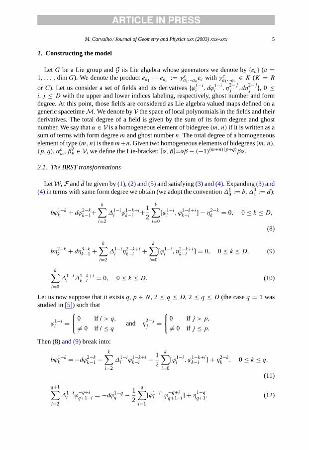
2. Constructing the model

Let G be a Lie group andG its Lie algebra whose generators we denote byea (a =1, . . . ,dimG). We denote the productea1 · · · ean := γca1···anec with γca1···an ∈ K (K = R

or C). Let us consider a set of fields and its derivativesϕ1−ii , dϕ1−i

i , η2−jj , dη

2−jj , 0 ≤

i, j ≤ D with the upper and lower indices labeling, respectively, ghost number and formdegree. At this point, those fields are considered as Lie algebra valued maps defined on ageneric spacetimeM. We denote byV the space of local polynomials in the fields and theirderivatives. The total degree of a field is given by the sum of its form degree and ghostnumber. We say thatα ∈ V is a homogeneous element of bidegree(m, n) if it is written as asum of terms with form degreem and ghost numbern. The total degree of a homogeneouselement of type(m, n) is thenm+n. Given two homogeneous elements of bidegrees(m, n),(p, q), αnm, βqp ∈ V, we define the Lie-bracket: [α, β]

.=αβ − (−1)(m+n)(p+q)βα.

2.1. The BRST transformations

LetW,F andd be given by(1), (2) and (5)and satisfying(3) and (4). Expanding(3) and(4) in terms with same form degree we obtain (we adopt the convention∆1

0 := b,∆01 := d):

bϕ1−kk + dϕ2−k

k−1+k∑i=2

∆1−ii ϕ1−k+i

k−i +1

2

k∑i=0

[ϕ1−ii , ϕ1−k+i

k−i ] − η2−kk = 0, 0 ≤ k ≤ D,

(8)

bη2−kk + dη3−k

k−1 +k∑i=2

∆1−ii η2−k+i

k−i +k∑i=0

[ϕ1−ii , η2−k+i

k−i ] = 0, 0 ≤ k ≤ D, (9)

k∑i=0

∆1−ii ∆1−k+i

k−i = 0, 0 ≤ k ≤ D. (10)

Let us now suppose that it existsq, p ∈ N, 2 ≤ q ≤ D, 2 ≤ q ≤ D (the caseq = 1 wasstudied in[5]) such that

ϕ1−ii =

0 if i > q,

= 0 if i ≤ qand η

2−jj =

0 if j > p,

= 0 if j ≤ p.

Then(8) and (9)break into:

bϕ1−kk =−dϕ2−k

k−1 −k∑i=2

∆1−ii ϕ1−k+i

k−i − 1

2

k∑i=0

[ϕ1−ii , ϕ1−k+i

k−i ] + η2−kk , 0 ≤ k ≤ q,

(11)

q+1∑i=2

∆1−ii ϕ

−q+iq+1−i = −dϕ1−q

q − 1

2

q∑i=1

[ϕ1−ii , ϕ

−q+iq+1−i] + η1−q

q+1, (12)

6 M. Carvalho / Journal of Geometry and Physics xxx (2003) xxx–xxx

k∑i=k−q

∆1−ii ϕ1−k+i

k−i = −1

2

q∑i=k−q

[ϕ1−ii , ϕ1−k+i

k−i ] + η2−kk , k ≥ q+ 2, (13)

bη2−kk = −dη3−k

k−1 −k∑i=2

∆1−ii η2−k+i

k−i −k∑i=0

[ϕ1−ii , η2−k+i

k−i ], 0 ≤ k ≤ p, (14)

p+1∑i=2

∆1−ii η

−p+1+ip+1−i = −dη2−p

p −p+1∑i=1

[ϕ1−ii , η

−p+1+ip+1−i ], (15)

k∑i=2

∆1−ii η2−k+i

k−i = −k∑i=0

[ϕ1−ii , η2−k+i

k−i ], k ≥ p+ 2. (16)

Eqs. (11) and (14)cannot be taken as the BRST transformations of the fields unless wespecify the form of the operators∆1−i

i (i ≥ 2) on their right-hand side. One way of dealingwith this is to impose

k∑i=2

∆1−ii ϕ1−k+i

k−i = 0, 0 ≤ k ≤ q, (17)

k∑i=2

∆1−ii η2−k+i

k−i = 0, 0 ≤ k ≤ p, (18)

which then fix the BRST transformations as

bϕ1−kk = −dϕ2−k

k−1 −1

2

k∑i=0

[ϕ1−ii , ϕ1−k+i

k−i ] + η2−kk , 0 ≤ k ≤ q, (19)

bη2−kk = −dη3−k

k−1 −k∑i=0

[ϕ1−ii , η2−k+i

k−i ], 0 ≤ k ≤ p. (20)

2.2. Implementing the conditions[b, d] = 0 andb2 = 0

Let us now consider(10). Takingk = 0 andk = 1 we obtainb2 = 0 and [b, d] = 0.These two conditions should be satisfied on the setϕ1−i

i , dϕ1−ii , η

2−jj , dη

2−jj (0 ≤ i ≤

q,0 ≤ j ≤ p). Implementing the condition [b, d] = 0 fixes the BRST transformation ofthe field derivatives:

bdϕ1−kk =

k∑i=0

[dϕ1−ii , ϕ1−k+i

k−i ] − dη2−kk , 0 ≤ k ≤ q, (21)

bdη2−kk =

k∑i=0

[dϕ1−ii , η2−k+i

k−i ] −k∑i=0

[ϕ1−ii , dη2−k+i

k−i ], 0 ≤ k ≤ p. (22)

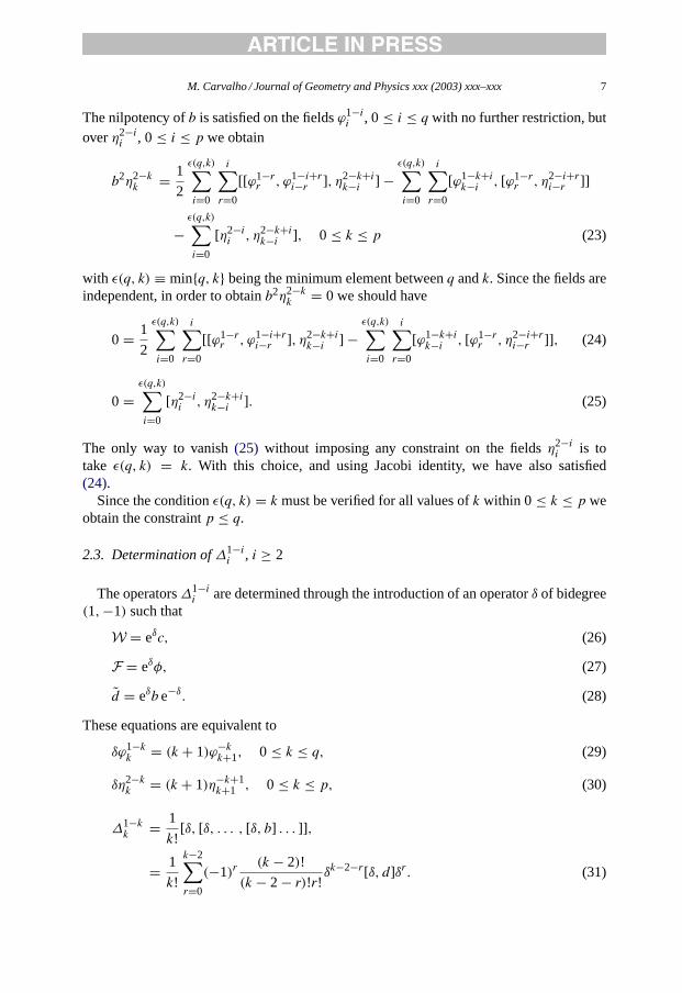
M. Carvalho / Journal of Geometry and Physics xxx (2003) xxx–xxx 7

The nilpotency ofb is satisfied on the fieldsϕ1−ii , 0≤ i ≤ q with no further restriction, but

overη2−ii , 0≤ i ≤ p we obtain

b2η2−kk = 1

2

ε(q,k)∑i=0

i∑r=0

[[ϕ1−rr , ϕ1−i+r

i−r ], η2−k+ik−i ] −

ε(q,k)∑i=0

i∑r=0

[ϕ1−k+ik−i , [ϕ1−r

r , η2−i+ri−r ]]

−ε(q,k)∑i=0

[η2−ii , η2−k+i

k−i ], 0 ≤ k ≤ p (23)

with ε(q, k) ≡ minq, k being the minimum element betweenq andk. Since the fields areindependent, in order to obtainb2η2−k

k = 0 we should have

0= 1

2

ε(q,k)∑i=0

i∑r=0

[[ϕ1−rr , ϕ1−i+r

i−r ], η2−k+ik−i ] −

ε(q,k)∑i=0

i∑r=0

[ϕ1−k+ik−i , [ϕ1−r

r , η2−i+ri−r ]] , (24)

0=ε(q,k)∑i=0

[η2−ii , η2−k+i

k−i ]. (25)

The only way to vanish(25) without imposing any constraint on the fieldsη2−ii is to

take ε(q, k) = k. With this choice, and using Jacobi identity, we have also satisfied(24).

Since the conditionε(q, k) = k must be verified for all values ofk within 0≤ k ≤ p weobtain the constraintp ≤ q.

2.3. Determination of∆1−ii , i ≥ 2

The operators∆1−ii are determined through the introduction of an operatorδ of bidegree

(1,−1) such that

W = eδc, (26)

F = eδφ, (27)

d = eδb e−δ. (28)

These equations are equivalent to

δϕ1−kk = (k + 1)ϕ−kk+1, 0 ≤ k ≤ q, (29)

δη2−kk = (k + 1)η−k+1

k+1 , 0 ≤ k ≤ p, (30)

∆1−kk = 1

k![δ, [δ, . . . , [δ, b] . . . ]] ,

= 1

k!

k−2∑r=0

(−1)r(k − 2)!

(k − 2− r)!r! δk−2−r[δ, d]δr. (31)

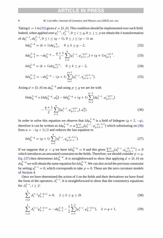
8 M. Carvalho / Journal of Geometry and Physics xxx (2003) xxx–xxx

Takingk = 1 in(31)givesd = [δ, b]. This condition should be implemented over each field.Indeed, when applied overϕ1−i

i ,η2−jj , 0≤ i ≤ q, 0≤ j ≤ pwe obtain theδ-transformation

of dϕi−1i , dη2−j

j , 0≤ i ≤ (q− 1), 0≤ j ≤ (p− 1) as

δdϕ1−kk = (k + 1)dϕ−kk+1, 0 ≤ k ≤ q− 2, (32)

δdϕ2−qq−1 = −dϕ1−q

q − q+ 1

2

q∑i=1

[ϕ1−ii , ϕ

−q+iq+1−i] + (q+ 1)η−q+1

q+1 , (33)

δdη2−kk = (k + 1)dη−k+1

k+1 , 0 ≤ k ≤ p− 2, (34)

δdη3−pp−1 = −dη2−p

p − (p+ 1)p+1∑i=1

[ϕ1−ii , η

−p+1−ip+1−i ]. (35)

Acting d = [δ, b] on dϕ1−qq and usingp ≤ q we are let with

bδdϕ1−qq = [δdϕ1−q

q , ϕ10] − δdη2−q

q + (q+ 1)q−1∑1=1

[dϕ1−ii , ϕ

−q+iq+1−i]

− q+ 1

2

q∑i=1

[[ϕ1−ii , ϕ

−q+iq+1−i], ϕ

01]. (36)

In order to solve this equation we observe thatδdϕ1−qq is a field of bidegree(q + 2,−q),

therefore it can be written asδdϕ1−qq = α

∑q

i=2[ϕ1−ii , ϕ

−q−1+iq+2−i ] which substituting on(36)

fixesα = −(q+ 1)/2 and reduces the last equation to

δdη2−qq = (q+ 1)

q∑i=2

[η2−ii , ϕ

−q−1+iq+2−i ]. (37)

If we suppose thatp < q we haveδdη2−qq = 0 and this gives

∑q

i=2[η2−ii , ϕ

−q−1+iq+2−i ] = 0

which introduces an unwanted constraint on the fields. Therefore, we should considerp = q.Eq. (37)then determinesδdη2−q

q . It is straightforward to show that applyingd = [δ, b] on

dη2−qq we will obtain the same equation forδdη2−q

q . We can also avoid the previous constraintby settingη2−i

i = 0, which corresponds to takep = 0. These are the zero curvature modelsof Section 4.

Once we have determined the action ofδ on the fields and their derivatives we have fixedthe form of the operators∆1−i

i . It is straightforward to show that the consistency equationsfor ∆1−i

i , i ≥ 2:

k∑i=2

∆1−ii ϕ1−k+i

k−i = 0, 2≤ k ≤ q ≤ D, (38)

k∑i=2

∆1−ii ϕ1−k+i

k−i = −dϕ2−kk−1 −

1

2

k−1∑i=1

[ϕ1−ii , ϕ1−k+i

k−i ], k = q+ 1, (39)

M. Carvalho / Journal of Geometry and Physics xxx (2003) xxx–xxx 9

k∑i=k−q

∆1−ii ϕ1−k+i

k−i = −1

2

q∑i=k−q

[ϕ1−ii , ϕ1−k+i

k−i ], q+ 2≤ k ≤ D, (40)

k∑i=2

∆1−ii η2−k+i

k−i = 0, 2≤ k ≤ q ≤ D, (41)

k∑i=2

∆1−ii η2−k+i

k−i = −dη3−kk−1 −

k−1∑i=1

[ϕ1−ii , η2−k+i

k−i ], k = q+ 1, (42)

k∑i=k−q

∆1−ii η2−k+i

k−i = −q∑

i=k−q[ϕ1−ii , η2−k+i

k−i ], q+ 2≤ k ≤ D (43)

are satisfied for this choice of∆1−ii .

For convenience we collect below all transformations of our model (withp = q):

bϕ1−kk = −dϕ2−k

k−1 −1

2

k∑i=0

[ϕ1−ii , ϕ1−k+i

k−i ] + η2−kk , 0 ≤ k ≤ q, (44)

bη2−kk = −dη3−k

k−1 −k∑i=0

[ϕ1−ii , η2−k+i

k−i ], 0 ≤ k ≤ q, (45)

bdϕ1−kk =

k∑i=0

[dϕ1−ii , ϕ1−k+i

k−i ] − dη2−kk , 0 ≤ k ≤ q, (46)

bdη2−kk =

k∑i=0

[dϕ1−ii , η2−k+i

k−i ] −k∑i=0

[ϕ1−ii , dη2−k+i

k−i ], 0 ≤ k ≤ q, (47)

δϕ1−kk = (k + 1)ϕ−kk+1, 0 ≤ k ≤ q, (48)

δdϕ1−kk = (k + 1)dϕ−kk+1, 0 ≤ k ≤ q− 2, (49)

δdϕ2−qq−1 = −dϕ1−q

q − q+ 1

2

q∑i=1

[ϕ1−ii , ϕ

−q+iq+1−i], (50)

δdϕ1−qq = −q+ 1

2

q∑i=2

[ϕ1−ii , ϕ

−q−1+iq+2−i ], (51)

δη2−kk = (k + 1)η−k+1

k+1 , 0 ≤ k ≤ q, (52)

10 M. Carvalho / Journal of Geometry and Physics xxx (2003) xxx–xxx

δdη2−kk = (k + 1)dη−kk+1, 0 ≤ k ≤ q− 2, (53)

δdη3−qq−1 = −dη2−q

q − (q+ 1)q∑i=1

[ϕ1−ii , η

−q+1−iq+1−i ], (54)

δdη2−qq = −(q+ 1)

q∑i=2

[ϕ1−ii , η

−q+iq+2−i]. (55)

It is important to notice that in the caseq = D, Eqs. (50), (51), (54) and (55)vanish trivially.In this case, allδ transformations of the field derivatives are encoded on(49) and (53)thatessentially mean [δ, d] = 0. Then, from(31) we have∆1−i

i = 0, i ≥ 2 and consequentlyall consistencyequations (38)–(43)will vanish.

3. A model with q = 2q = 2q = 2,D = 4D = 4D = 4

Let

W = c + A+ ϕ−12 , (56)

F = φ + ψ + B, (57)

d = b+ d +∆−12 +∆−2

3 +∆−34 . (58)

The BRST transformations corresponding to the generalized connection and curvatureequations (3)–(5)are given by

bc= −c2 + φ, (59)

bA= −dc− [c,A] + ψ, (60)

bϕ−12 = −F − [c, ϕ−1

2 ] + B, (61)

bφ = −[c, φ], (62)

bψ = −dφ − [c, ψ] − [A, φ], (63)

bB= −dψ − [c, B] − [A,ψ] − [ϕ−12 , φ], (64)

theδ transformations have the form:

δc = A, δdc= dA, (65)

δA = 2ϕ−12 , δdA= −dϕ−1

2 − 3[A, ϕ−12 ], (66)

δϕ−12 = 0, δdϕ−1

2 = −3ϕ−12 ϕ−1

2 , (67)

δφ = ψ, δdφ = dψ, (68)

δψ = 2B, δdψ = −dB− 3[A,B] − 3[ϕ−12 , ψ], (69)

M. Carvalho / Journal of Geometry and Physics xxx (2003) xxx–xxx 11

δB = 0, δdB= −3[ϕ−12 , B] (70)

and the∆ transformations are given by

∆−12 c = 0 (71)

∆−12 A = −3

2dϕ−12 − 3

2[A, ϕ−12 ], (72)

∆−12 ϕ−1

2 = −32ϕ

−12 ϕ−1

2 , (73)

∆−12 φ = 0, (74)

∆−12 ψ = −3

2dB− 32[A,B] − 3

2[ϕ−12 , ψ], (75)

∆−12 B = −3

2[ϕ−12 , B], (76)

∆−12 dc= 0, (77)

∆−12 dA= −3

2[ϕ−12 ,dA] − 3

2[A, dϕ−12 ], (78)

∆−12 dϕ−1

2 = −32[ϕ−1

2 , dϕ−12 ], (79)

∆−12 dφ = 0, (80)

∆−12 dψ = −3

2[B,dA] − 32[A,dB] − 3

2[ψ, dϕ−12 ] − 3

2[ϕ−12 , dψ], (81)

∆−12 dB= −3

2[B, dϕ−12 ] − 3

2[ϕ−12 ,dB], (82)

∆−23 c = 1

2dϕ−12 + 1

2[A, ϕ−12 ], (83)

∆−23 A = 1

2ϕ−12 ϕ−1

2 , (84)

∆−23 ϕ−1

2 = 0, (85)

∆−23 φ = 1

2dB+ 12[A,B] + 1

2[ϕ−12 , ψ], (86)

∆−23 ψ = 1

2[ϕ−12 , B], (87)

∆−23 B = 0, (88)

∆−23 dc= 1

2[ϕ−12 ,dA] + 1

2[A, dϕ−12 ], (89)

∆−23 dA= 1

2[ϕ−12 , dϕ−1

2 ], (90)

∆−23 dϕ−1

2 = 0, (91)

∆−23 dφ = 1

2[B,dA] + 12[A,dB] + 1

2[ψ, dϕ−12 ] + 1

2[ϕ−12 , dψ], (92)

∆−23 dψ = 1

2[B, dϕ−12 ] + 1

2[ϕ−12 ,dB], (93)

12 M. Carvalho / Journal of Geometry and Physics xxx (2003) xxx–xxx

∆−23 dB= 0, (94)

∆−34 ≡ 0. (95)

Let us consider now the system of descent equations given in(6). We can rewrite it in theform (b+d)ω ≡ (d−∆)ω = 0 with ω

.=ω40+ω3

1+ω22+ω1

3+ω04 and∆

.=∆−12 +∆−2

3 +∆−34 .

A particular solution is given by

ω = eδ(ω40 +Ω) (96)

with Ω.=Ω3

1 +Ω22 +Ω1

3 +Ω04 satisfying

bΩ04 = ∆−1

2 Ω22 − 2∆−2

3 Ω31 + 3∆−3

4 ω40, (97)

bΩ13 = ∆−1

2 Ω31 − 2∆−2

3 ω40, (98)

bΩ22 = ∆−1

2 ω40, (99)

bΩ31 = 0. (100)

In terms of theseΩ’s we have

ω04 =

δ4

4!ω4

0 +δ3

3!ω3

1 +δ2

2!Ω2

2 + δΩ13 +Ω0

4, (101)

ω13 =

δ3

3!ω4

0 +δ2

2!Ω3

1 + δΩ22 +Ω1

3, (102)

ω22 =

δ2

2!ω4

0 + δΩ31 +Ω2

2, (103)

ω31 = δω4

0 +Ω31. (104)

Here we notice that the cycles exhibited in(101)–(104)are obtained fromΩ’s by theaction ofδ. TheseΩ’s are solutions of the intermediateequations (97)–(100), which do notinvolve the exterior derivative. It is the combination of theδ-operator and these equations((97)–(100)) that allow us to transform a problem of cohomology ofb modulod (6) intoa simple one. In order to solve(101)–(104)we should first determineω4

0, the solution ofbω4

0 = 0. Our intention is to analyze how the cocycle Tr(1/2)φ2 (which appears in[1,3])is modified by the presence of the negative ghost number fieldϕ−1

2 , the fieldB, and theoperators∆−1

2 ,∆−23 ,∆−3

4 . Therefore we take

ω40 = Tr(1

2φ2). (105)

Then, we obtainΩ’s solving(97)–(100). Replacing them in(101)–(104)we obtain

ω31 = Tr2

3β1(c2ψ − c2dc+ c[A, φ])+ 2

3(β2 − β4)(φψ − φdc)

+ 23β3(−c2ψ + c2dc− φψ + φdc− c[A, φ])

+ σ(c2dc+ cdφ + φdc)+ 13φψ + 2

3φdc, (106)

M. Carvalho / Journal of Geometry and Physics xxx (2003) xxx–xxx 13

ω22 = Tr2

3β1(2c2B − c2dA+ 2A2φ + 2c[A,ψ] − c[A,dc] + 2c[ϕ−1

2 , φ]

+ 23(β2 − β4)(2φB − φdA+ ψ2 − ψdc)+ 2

3β3(−2c2B + c2dA− 2A2φ

−2φB + φdA− ψ2 + ψdc− 2c[A,ψ] + c[A,dc] − 2c[ϕ−12 , φ])

+α1(c2A2 − c2B + c2dA− c[ϕ−1

2 , φ])+ α2(A2φ − φB + φdA)

+α3(c2B + cdψ + φB + c[A,ψ] + c[ϕ−1

2 , φ])

+α4(−c2dA− cdψ − φdA− c[A,dc])+ α5(Adφ+12ψ

2 + φB−φdA−12dcdc)

+α6(−12ψ

2 + ψdc− φB + φdA− 12dcdc)+ σ(c2dA+ cdψ + Adφ

+φdA+ ψdc+ c[A,dc])− 13φB + 2

3φdA− 16ψ

2 + 23ψdc, (107)

ω13 = Tr2β1(

23c

2dϕ−12 + A2ψ − 1

3A2dc+ c2[A, ϕ−1

2 ] + c[A,B] − 13c[A,dA]

+ c[ϕ−12 , ψ] − 1

3c[ϕ−12 ,dc] + A[ϕ−1

2 , φ])+ 2β2(23φdϕ

−12 + ψB − 1

3ψdA

− 13Bdc+ A[ϕ−1

2 , φ])+ β3(−13c

2dϕ−12 + cdB− 2A2ψ + 2

3A2dc− 1

3φdϕ−12

−2ψB + 23ψdA+ 2

3Bdc− c2[A, ϕ−12 ] − c[A,B] + 2

3c[A,dA] − c[ϕ−12 , ψ]

+ 23c[ϕ

−12 ,dc] − 3A[ϕ−1

2 , φ])+ β4(−43φdϕ

−12 − ψB − 1

3ψdA− 13Bdc

+dcdA− A[ϕ−12 , φ])+ β5(c

2ϕ−12 A+ cA3 + cϕ−1

2 ψ − cϕ−12 dc− cBA

+ cdAA− Aφϕ−12 )+ β6(A

2dc− ϕ−12 dφ − Bdc+ dcdA)

+β7(A2ψ − ϕ−1

2 dφ−Bdc+dcdA)+ β8(c2dϕ−1

2 + cdB+ φdϕ−12 + c[A,dA]

+ c[ϕ−12 ,dc])+ β9(Adψ + 2ϕ−1

2 dφ + ψdA+ 2Bdc− 3dcdA)

+α1(−c2dϕ−12 − c2[A, ϕ−1

2 ] − c[A,B] + c[A,dA] − c[ϕ−12 , ψ]−A[ϕ−1

2 , φ])

+α2(A2ψ − φdϕ−1

2 − ψB + ψdA− A[ϕ−12 , φ])+ α3(−cdB+ 2A2ψ

+Adψ + ψB + A[ϕ−12 , φ])+ α4(c

2dϕ−12 + cdB− 2A2dc− Adψ

+φdϕ−12 − ψdA+ 3c2[A, ϕ−1

2 ] + 3c[A,B] − 2c[A,dA] + 3A[ϕ−12 , φ]

+3c[ϕ−12 , ψ] − 2c[ϕ−1

2 ,dc])+ α5(Adψ + 2ϕ−12 dφ + φdϕ−1

2 + 3ψB − ψdA

−dcdA+ 3A[ϕ−12 , φ])+ α6(−φdϕ−1

2 − 3ψB + 2ψdA+ 2Bdc− dcdA

−3A[ϕ−12 , φ])+ σ(−1

2c2dϕ−1

2 − 12cdB+ A2dc+ Adψ + ϕ−1

2 dφ − 12φdϕ

−12

+ψdA+ Bdc− 32c

2[A, ϕ−12 ] − 3

2c[A,B] + c[A,dA] − 32c[ϕ

−12 , ψ]

+ c[ϕ−12 ,dc]−3

2A[ϕ−12 , φ])−1

3φdϕ−12 − ψB + 2

3ψdA+ 23Bdc− A[ϕ−1

2 , φ],(108)

ω04 = Tr2β1(c

2ϕ−12 ϕ−1

2 + 43A

2B − 13A

2dA+ ϕ−12 ϕ−1

2 φ + c[A2, ϕ−12 ] + c[A, dϕ−1

2 ]

+ c[ϕ−12 , B] + 4

3A[ϕ−12 , ψ] − 1

3A[ϕ−12 ,dc])+ 2β2(

43ϕ

−12 ϕ−1

2 φ + ψdϕ−12

+ 23B

2 − 13BdA− 1

3dcdϕ−12 + 4

3A[ϕ−12 , ψ] − 1

3A[ϕ−12 ,dc])

+β3(−c2ϕ−12 ϕ−1

2 − 23A

2B + 23A

2dA+ AdB− 113 ϕ

−12 ϕ−1

2 φ − ψdϕ−12 − 4

3B2

+ 23BdA+ 2

3dcdϕ−12 − c[A2, ϕ−1

2 ] − c[A, dϕ−12 ] − c[ϕ−1

2 , B] − 103 A[ϕ−1

2 , ψ]

14 M. Carvalho / Journal of Geometry and Physics xxx (2003) xxx–xxx

+ 43A[ϕ−1

2 ,dc])+ β4(43ϕ

−12 ϕ−1

2 φ − ψdϕ−12 + 2

3B2 − 7

3BdA− 13dcdϕ−1

2

+dAdA+ 43A[ϕ−1

2 , ψ] − 73A[ϕ−1

2 ,dc])+ β5(2c2ϕ−1

2 ϕ−12 − cϕ−1

2 dA

+2cdAϕ−12 − cdϕ−1

2 A+ A4 + A2B − A2dA− Aϕ−12 dc+ 2ϕ−1

2 ϕ−12 φ

+2c[A2, ϕ−12 ] + 2c[ϕ−1

2 , B] + A[ϕ−12 , ψ])+ β6(A

2dA− ϕ−12 dψ − BdA

−dcdϕ−12 + dAdA− A[ϕ−1

2 ,dc])+ β7(2A2B − ϕ−1

2 dψ − BdA− dcdϕ−12

+dAdA+ 2A[ϕ−12 , ψ] − 3A[ϕ−1

2 ,dc])+ β8(−3c2ϕ−12 ϕ−1

2 + 2A2dA

+AdB− 3ϕ−12 ϕ−1

2 φ + ψdϕ−12 − 3c[A2, ϕ−1

2 ] − 3c[ϕ−12 , B] + 3c[ϕ−1

2 ,dA]

+A[ϕ−12 ,dc])+ β9(−6A2B − AdB+ 4ϕ−1

2 dψ − ψdϕ−12 + 4BdA

+3dcdϕ−12 − 3dAdA− 6A[ϕ−1

2 , ψ] + 9A[ϕ−12 ,dc])+ α1(−2c2ϕ−1

2 ϕ−12

−A2B + A2dA− 2ϕ−12 ϕ−1

2 φ − 2c[A2, ϕ−12 ] − c[A, dϕ−1

2 ] − 2c[ϕ−12 , B]

+ c[ϕ−12 ,dA] − A[ϕ−1

2 , ψ])+ α2(A2B − 2ϕ−1

2 ϕ−12 φ − ψdϕ−1

2 − B2 + BdA

−A[ϕ−12 , ψ])+ α3(−A2B − AdB+ 2ϕ−1

2 ϕ−12 φ + ϕ−1

2 dψ + B2 + A[ϕ−12 , ψ])

+α4(92c

2ϕ−12 ϕ−1

2 + 6A2B − 3A2dA+ AdB+ 92ϕ

−12 ϕ−1

2 φ − ϕ−12 dψ + ψdϕ−1

2

−BdA+ 92c[A

2, ϕ−12 ] + 3c[A, dϕ−1

2 ] + 92c[ϕ

−12 , B] − 3

2c[ϕ−12 ,dA]

+6A[ϕ−12 , ψ] − 3A[ϕ−1

2 ,dc])+ α5(−3A2B − 12AdB+ 6ϕ−1

2 ϕ−12 φ

+2ϕ−12 dψ + 5

2ψdϕ−12 + 3B2 − BdA+ 1

2dcdϕ−12 − 1

2dAdA+ 3A[ϕ−12 , ψ]

+ 32A[ϕ−1

2 ,dc])+ α6(−6ϕ−12 ϕ−1

2 φ − 3ψdϕ−12 − 3B2 + 3BdA+ 2dcdϕ−1

2

− 12dAdA− 6A[ϕ−1

2 , ψ] + 3A[ϕ−12 ,dc])+ γ1(c

2ϕ−12 ϕ−1

2 + ϕ−12 ϕ−1

2 φ

+ c[A2, ϕ−12 ] + c[ϕ−1

2 , B] − c[ϕ−12 ,dA])+ γ2(−A2B + A2dA

−A[ϕ−12 , ψ] + A[ϕ−1

2 ,dc])+ γ3(2A2B + AdB+ ψdϕ−1

2 − dcdϕ−12

+2A[ϕ−12 , ψ] − A[ϕ−1

2 ,dc])+ γ4(−A2B + 2ϕ−12 ϕ−1

2 φ + ϕ−12 dψ + B2

−BdA+ A[ϕ−12 , ψ])+ γ5(A

2B − ϕ−12 dψ − BdA+ dAdA+ A[ϕ−1

2 , ψ]

−2A[ϕ−12 ,dc])+ σ(−3

2c2ϕ−1

2 ϕ−12 − 3A2B + A2dA− 1

2AdB− 32ϕ

−12 ϕ−1

2 φ

+ϕ−12 dψ − 1

2ψdϕ−12 + BdA+ dcdϕ−1

2 − 32c[A

2, ϕ−12 ] − 3

2c[A, dϕ−12 ]

− 32c[ϕ

−12 , B] − 3A[ϕ−1

2 , ψ] + 2A[ϕ−12 ,dc])− 5

3ϕ−12 ϕ−1

2 φ − ψdϕ−12 − 5

6B2

+ 23BdA+ 2

3dcdϕ−12 − 5

3A[ϕ−12 , ψ] + 2

3A[ϕ−12 ,dc]. (109)

Considered in this form, this previous solution forω1−ii does not relate to any familiar model.

Here, let us consider some specific cases. First, let us consider the two-formB decomposingasB = F+B [5] withF the curvature ofA. In this decomposition, the two-formB should beintroduced in order to maintain the nilpotency of the BRST transformation ofϕ−1

2 . We haveb2ϕ−1

2 = 0 ⇒ bB = −[c, B] + [φ, ϕ−12 ]. Then, takingβ2 = 1 with all other parameters

set to zero we obtainω1−ii as

ω40 = Tr(1

2φ2), (110)

M. Carvalho / Journal of Geometry and Physics xxx (2003) xxx–xxx 15

ω31 = Tr(φψ), (111)

ω22 = Tr(φF + 1

2ψ2 + φB), (112)

ω13 = Tr(ψF + φDAϕ−1

2 + ψB), (113)

ω04 = Tr(1

2F2 + 1

2B2 + FB + ϕ−1

2 ϕ−12 φ + ψDAϕ−1

2 ). (114)

We observe that the inclusion of additional fieldsϕ−12 , B in the ladders, and of additional

derivations∆1−ii in dmodify the previous solution(7)of the descent equations. Nonetheless,

(110)–(114)still containsthe terms associated to the Donaldson polynomials. A similar be-havior has been observed in[5] for the caseϕ−1

2 = 0,B = F , which also generates a solutionincluding additional terms to the Donaldson polynomials. Now, if we look at our generalsolution(106)–(109)we see that they represent a family of solutions parameterized by 21 pa-rameters(β1, . . . , σ)which writes asω = (1/2)(φ+ψ+F)2+((1/2)B2+φB+ψB+FB+φDAϕ

−12 +ψDAϕ−1

2 +ϕ−12 ϕ−1

2 φ)+Θ(β1, . . . , σ). Here, there is no possibility to choose theparameters(β1, . . . , σ) in such a way thatω reduces to the Donaldson polynomials. From[5], it seems then that the only cases having a complete agreement with(7) areϕ−1

2 = 0,B = F that gives the same result as(7), andϕ−1

2 = 0, B = 0 that represents a family ofsolutions parameterized by points ofR8 and such that to the origin we have associated(7),i.e.ω = (1/2)(φ+ψ+F)2+Θ(α1, . . . , α8)with ω|(α1,... ,α8)=0 = (1/2)(φ+ψ+F)2. Thissolution is interesting because it shows Donaldson generators as a particular case of a moregeneral expression. Therefore, it may be possible that other extended formulations may ad-mit, as a limit case, other topological invariants. Nonetheless, up to the analysis of this exam-ple, it is not known if a choice of higher components ladders would generate a solution of thistype.

The cycleω04 is particularly important since it defines a BRST invariant action:

S =∫

Tr

(1

2F2 + 1

2B2 + FB + ϕ−1

2 ϕ−12 φ + ψDAϕ−1

2

), (115)

which can be taken as the starting point for a pertubative analysis of our model. Thisaction incorporates, from the beginning, extra terms onϕ−1

2 , B in addition to the usualnon-gauge fixed TYMT action

∫Tr F2. Thus, in much the same way as it was done in[24],

we may interpret the fieldsϕ−12 , B as part of the additional fields necessary to perform

the gauge fixing of the action∫

Tr F2. If we want to proceed further on finding a fullygauge fixed action, we will have to introduce other fields (antifields, antighosts) with totaldegree different than 0 and 1, which will be accommodated as component fields of otherladders.

Another application of the model given by(56)–(58)is on the description of four-dimen-sional BF model. In fact, consider the cycleω0

4 (109). Let us takeγ1 = 1,γ2 = 0,γ3 = 1/3,γ4 = −(1/2), γ5 = −1/6,β2 = 1 with all other parameters equal to zero. Then, we obtainan invariant action given by3

3 Here, we may also interpretϕ−12 as one of the fields necessary to perform the gauge fixing of the BF action.

16 M. Carvalho / Journal of Geometry and Physics xxx (2003) xxx–xxx

S =∫ω0

4 =∫

Tr(BF+ ψDAϕ−12 + ϕ−1

2 ϕ−12 φ + B[c, ϕ−1

2 ]

+ c2ϕ−12 ϕ−1

2 − c[ϕ−12 , F ]), (116)

which contains the usual term of the BF model. It is important to notice that this derivationof four-dimensional BF action is based on a pair of connection and curvature ladders(56)and (57)with the assumption thatB = F . In contrast, the usual superfield formulation ofD-dimensional BF models[6,25] employs a gauge ladder together with a matter ladderBhaving the two-formB as its highest component field, i.e.B|D = B. In Section 4.2we willobtain the equivalent of action(116)for the zero curvature formulation of four-dimensionalBF model.

4. The zero-curvature models

As we have seen, the model presented inSection 2is based on gauge and curvatureladdersW,F satisfyingdW+ (1/2)[W,W] = F, dF+ [W,F] = 0. As a limit case of thismodel we can pose a zero curvature conditionF = 0 that reduces the previous equationsto dW+ (1/2)[W,W] = 0. Here,(44)–(55)become

bϕ1−kk = −dϕ2−k

k−1 −1

2

k∑i=0

[ϕ1−ii , ϕ1−k+i

k−i ], 0 ≤ k ≤ q, (117)

bdϕ1−kk =

k∑i=0

[dϕ1−ii , ϕ1−k+i

k−i ], 0 ≤ k ≤ q, (118)

δϕ1−kk = (k + 1)ϕ−kk+1, 0 ≤ k ≤ q, (119)

δdϕ1−kk = (k + 1)dϕ−kk+1, 0 ≤ k ≤ q− 2, (120)

δdϕ2−qq−1 = −dϕ1−q

q − q+ 1

2

q∑i=1

[ϕ1−ii , ϕ

−q+iq+1−i], (121)

δdϕ1−qq = −q+ 1

2

q∑i=2

[ϕ1−ii , ϕ

−q−1+iq+2−i ] (122)

that agree with the same equations obtained in the non-complete ladder case (i.e. withq = D) of [7]. In our approach we treat both casesq = D (referred in[6] as the completeladder case) andq = D in the same way, with the fundamental equations given as above.Indeed, the equations for the complete ladder case are a particular case of(117)–(122)whenone takesq = D. Basically, what differs one and another situation is just the definitionof the generalized derivative that assumes the formd = b + d whenq = D andd =b + d + ∑D

i=2∆1−ii whenq = D. The main role of the operators∆1−i

i , i ≥ 2 is to avoidpossible constraints that would arise from the zero curvature condition in the case ofq = D.

M. Carvalho / Journal of Geometry and Physics xxx (2003) xxx–xxx 17

For example, in the absence of∆1−ii we would have from(39) and (40)the two constraints

below

dϕ1−qq = −1

2

q∑i=1

[ϕ1−ii , ϕ

−q+iq+1−i], 0=

q∑i=k−q

[ϕ1−ii , ϕ1−k+i

k−i ], k ≥ q+ 2.

As we have pointed out at the end ofSection 2, q = D determines∆1−ii = 0 and this

explains why these operators are absent in the complete ladder case of[6].Let us consider general descent equations of the type

bωG+iD−i + dωG+i+1D−i−1 = 0, 0 ≤ i ≤ D− 1, bωG+D0 = 0. (123)

This system of descent equations can be solved following the same procedure ofSection 3,e.g. writing ω ≡ ∑G+D

i=0 ωG+Di and∆ ≡ ∑Di=2∆

1−ii the descent equations assume the

form 0 = (b + d)ω = (d − ∆)ω. A particular solution isω.=eδ(ωG+D0 + Ω) with Ω ≡∑D

i=1ΩG+D−ii satisfying

bΩG+D−kk = (−1)k(k − 1)∆1−k

k ωG+D0 +k−1∑i=2

(−1)i(i− 1)∆1−ii ΩG+D−k+i

k−i ,

1≤ k ≤ D. (124)

We note that whenq = D we haveΩ = 0 and∆ = 0, thenω = eδωG+D0 andd = b + d.WhenG+D = 4, (124)agrees with(97)–(100).

4.1. The Chern–Simons term

Consider a model withq = 3,D = 3 andF = 0. Let us take the cocycleω03 such that

b∫ω0

3 = 0. This will be related to the Chern–Simons form. As it was shown in[6], ω03

can be obtained by expandingω = eδω30 = eδ((1/3!)Tr c3) and taking the terms with form

degree equal to 3. This results in

S = 1

2

∫Tr

(AF− 1

3A3

)− 1

2b

∫Tr(cϕ−2

3 + Aϕ−12 ). (125)

Nonetheless, the presence of the fieldϕ−12 allow us to consider a more general solution by

introducing on(125)the term∫ (dcϕ−1

2 + 1

2AdA

). (126)

Then, the action given by(125)+ (126) is also possible and represents a contribution dueto the extra fieldϕ−1

2 .

4.2. BF system

TheD-dimensional BF system can be formulated as a zero curvature system by intro-ducing two complete ladders[6]:

18 M. Carvalho / Journal of Geometry and Physics xxx (2003) xxx–xxx

W =D∑i=0

ϕ1−ii , B =

D∑i=0

BD−2−jj , (127)

whereW is a gauge ladder with total degree 1, which satisfies a zero curvature condition.The other ladderB has total degree(D−2) and satisfiesdB+ [W,B] = 0. For the completeladder case, we have seen thatd = b+ d. Let us consider the caseD = 4. Here, the gaugeand the matter ladderB are taken as

W = c + A+ ϕ−12 + ϕ−2

3 + ϕ−34 , (128)

B = φ + ψ + B + B−13 + B−2

4 . (129)

The BRST transformations for the component fields follow from the equations satisfied byW andB and are given by

bc= −c2, (130)

bA= −dc− [c,A], (131)

bϕ−12 = −F − [c, ϕ−1

2 ], (132)

bϕ−13 = −dϕ−1

2 − [c, ϕ−13 ] − [A, ϕ−1

2 ], (133)

bϕ−34 = −dϕ−1

3 − [c, ϕ−34 ] − [A, ϕ−2

3 ] − 12[ϕ−1

2 , ϕ−12 ], (134)

bφ = −[c, φ], (135)

bψ = −dφ − [c, ψ] − [A, φ], (136)

bB= −dψ − [c, B] − [A,ψ] − [ϕ−12 , φ], (137)

bB−13 = −dB− [c, B−1

3 ] − [A,B] − [ϕ−12 , ψ] − [ϕ−1

3 , φ], (138)

bB−24 = −dB−1

3 − [c, B−24 ] − [A,B−1

3 ] − [ϕ−12 , B] − [ϕ−2

3 , ψ] − [ϕ−34 , φ]. (139)

The BRST transformations forφ,ψ,B agree with the ones given in(62)–(64). Nonetheless,sinceW is a connection with zero curvature, the BRST transformations for the componentsc,A, ϕ−1

2 differ from (59)–(61).From[6] we obtain an invariant action as

S =∫

TrB(dW+W2)|04, (140)

S =∫

Tr(BF+ ψDAϕ−12 + ϕ−1

2 ϕ−12 φ + B[c, ϕ−1

2 ] + φ[c, ϕ−34 ] + ψ[c, ϕ−2

3 ]

+φDAϕ−23 + B−1

3 DAc + B−24 c2). (141)

This previous action agrees with the one given in(116)except by the presence of highercomponents fieldsϕ−2

3 , ϕ−34 , B−1

3 , B−24 that does not enter in the ladders(56) and (57).

Conversely, there are also the presence of terms onϕ−12 in (116)that do not appear in(141),

M. Carvalho / Journal of Geometry and Physics xxx (2003) xxx–xxx 19

those terms being brought by the derivations∆1−ii , which are absent on the generalized

derivative d = b + d. Both approaches are entirely different since they are based onladders that satisfy different equations. As for the general formulation of BF models indimensions other thanD = 4, we emphasize that a matter ladderB, satisfying dB +[W,B] = 0, should be used to accommodate the fieldB. It is a particular feature offour dimensions that we can take the ladderB (57) as the generalized curvature ofW(56).

5. Mathematical aspects

5.1. BRSTG-operation

In this section we review some basic definitions concerning the structure of graded com-mutative differential algebras and BRSTG-operations. Although our approach is based onthe formalism exposed in[8,9] we will adopt some definitions in a different context.

A Z-graded supercommutative algebrais a structure defined by(A, ∗) such that: (1)(A, ∗) is an algebra in the usual sense (we are considering algebras defined over a fieldK that can beR or C), (2) the graded structure is defined by a direct sum decompositionA = ⊕m∈ZAm such thatAm ∗An ⊂ Am+n and the supercommutativity stands forα ∗β =(−1)mnβ ∗ α ∀α ∈ Am, ∀β ∈ An. From now on we will use the term commutative asmeaning supercommutative. All graded (bigraded) structure to be considered here will bedefined either overZ orZ+ .=N ∪ 0.

A superderivation onA of degree kis a linear mapΨ : A• → A•+k such thatΨ(αβ) =(Ψα)β + (−1)kmαΨβ ∀α ∈ Am. We denote the set ofk-superderivations onA asDk(A).Defining a product between two superderivations onA as the composition map we havethatD(A) ≡ ∑

k∈ZDk(A) together with this product becomes a graded algebra.

A graded commutative differential algebrais a structure defined by(A, ∗, d) with (1)(A, ∗) a graded commutative algebra and (2)d a superderivation onA of degree 1 suchthatd2 = 0.

A G-operation is defined by(A, ∗, d, I, L) with (1) (A, ∗, d) a graded commutativedifferential algebra and (2)I : G → D−1(A), X → IX andL : G → D0(A), X →LX

.=[d, IX] such thatI[X,Y ] = LXIY − IYLX andL[X,Y ] = LXLY − LYLX ∀X, Y ∈ G.We extend these two operations toG⊗A asIX(Y ⊗ α) .=Y ⊗ IXα, LX(Y ⊗ α) .=Y ⊗ LXα∀X, Y ∈ G, ∀α ∈ A.

Given aG-operation over a graded algebraA we define analgebraic connectiononA asan elementω ∈ G ⊗ A1 such thatIXω = X ⊗ 1 X, LXω = [ω,X] ∀X ∈ G. Given aG-operation we denote its set of algebraic connections byC.

Thecurvatureof an algebraic connection is an element8 ∈ G⊗A2 that satisfiesdω +(1/2)[ω,ω] = 8. In particular this condition impliesd8 + [ω, 8] = 0, IX8 = 0, LX8 =[8,X] ∀X ∈ G.

Givenωi ≡∑

ai eai ⊗ ωaii ∈ G⊗A1, i ∈ N, we defineω1 · · ·ωn .=

∑ai ea1 · · · ean ⊗

ωa11 · · ·ωann = ∑

c ec⊗(ω1 · · ·ωn)c ∈ G⊗An with (ω1 · · ·ωn)c ≡∑

ai γca1···anω

a11 · · ·ωann .

Now, let us consider bigraded algebras. The definitions will be immediate extensionsfrom the graded case.

20 M. Carvalho / Journal of Geometry and Physics xxx (2003) xxx–xxx

A bigraded commutative algebrais a pair(Υ, ∗) such thatΥ is an algebra that admits adirect sum decomposition of the typeΥ = ⊕(m,n)∈Z×ZΥ (m,n) and the product∗ satisfiesΥ(m,n) ∗ Υ(r,s) ⊂ Υ(m+r,n+s), with commutativity meaningα ∗ β = (−1)(m+n)(r+s)β ∗ α∀α ∈ A(m,n), ∀β ∈ A(r,s). Given a bigraded algebra,Υr ≡ ⊕m∈ZΥ (m,r−m) defines agraded structure onΥ , i.e.Υ = ⊕r∈ZΥ r.

We also have the same concept ofsuperderivationonΥ : a(r, s)-superderivation is a linearmapΨ : Υ(m,n) → Υ(m+r,n+s) with Ψ(αβ) = (Ψα)β + (−1)(r+s)(m+n)αΨβ ∀α ∈ Υ(m,n).We denoteD(Υ) ≡ ⊕(m,n)∈Z×ZD(m,n)(Υ) = ⊕r∈ZDr(Υ) where the total degree of asuperderivation is given by the sum of its bidegree indices.

A bigraded commutative differential algebrais defined as(Υ, ∗, d) with (1) (Υ, ∗) abigraded commutative algebra and (2)d a superderivation of total degree 1,d =⊕m∈Zd(m,1−m).

A bigradedG-operationis defined as(Υ, ∗, d, I, L) with (1) (Υ, ∗, d) a bigraded com-mutative differential algebra and (2)I : G → D−1(Υ) with IX ≡ ∑

m∈Z I(m,−1−m)X , and

L : G→ D0(Υ) with [d, IX] = LX ≡∑m∈Z L

(m,−m)X .

An algebraic connectionon a bigradedG-operationΥ is an elementω ∈ G ⊗ Υ 1,ω.=∑D

k=0 ω1−kk satisfyingIXω = X⊗ 1, LXω = [ω, X].

Thecurvatureof the algebraic connectionω is an element8 ∈ G ⊗ Υ 2, 8.=∑D

i=0 82−ii

such thatdω + (1/2)[ω, ω] = 8.This previous definition of bigradedG-operation is too general. In the next definition we

will restrict it in order to fit our purposes.

Definition 1 (BRST G-operation). A BRSTG-operation is the structure determined by(Υ, ∗, d, I, L, ω, ρ) where (1)(Υ, ∗, d, I, L) is aG-operation with

(i) Υ(m,n) = 0 if m < 0 orm > D with D ∈ N;

(ii) d ≡∑m∈Z+

d(m,1−m) .=b+ d +D∑i=2

∆1−ii , d2 = 0; (142)

(iii) IX ≡∑m∈Z

I(m,−1−m)X

.=I(−1,0)X ; (143)

(iv) LX ≡∑m∈Z

L(m,−m)X

.=L(0,0)X with L = [d, I] (144)

and (2)ω is an algebraic connection onΥ with curvatureρ.

Theorem 1. For a BRSTG-operation we have

IXd + dIX = LX, (145)

IXb+ bIX = 0, (146)

IX∆1−ii +∆1−i

i IX = 0 ∀ i ≥ 2, (147)

IXω1−ii = 0, i = 1, (148)

IXω01 = X⊗ 1, (149)

M. Carvalho / Journal of Geometry and Physics xxx (2003) xxx–xxx 21

LXω1−ii = [ω1−i

i , X], 0 ≤ i ≤ D, (150)

IX82−ii = 0, 0 ≤ i ≤ D, (151)

LX82−ii = [82−i

i , X], 0 ≤ i ≤ D. (152)

Proof. This follows immediately fromDefinition 1.

We extendIX, LX toG⊗Υ in the same way as we did for the graded case. Note that ourdefinition of BRSTG-operation is an extension of that one adopted in[8] in which we allowthe differentiald to have components∆1−k

k other thand(0,1) = b andd(1,0) = d. We alsoallow the algebraic connection and curvature to contain other component fields in additionto ω1

0, ω01, 82

0, 811, 80

2.Finally, we consider aut0(A) = ξ ∈ G⊗A0|LXξ = [ξ,X] ∀X ∈ G that will correspond

later on to the concept of the infinitesimal gauge transformations, and aut∗0(A) its dual. Interms of the generators ofG we writeξ = ∑

a ea ⊗ ξa with ξa ∈ A0. Here, the spaceA0 isa subalgebra ofA, therefore it has a structure of aK-vector space. The spaceA∗0 is thenunderstood as the space of K-linear mappings onA0. Givenξ ∈ aut0(A) we define

Iξ : A→ A, α→ Iξα.=

∑a

ξaIaα,

Lξ : A→ A, α→ Lξα.=

∑a

((dξa)Iaα+ ξaLaα)

and we extend them toG⊗A asIξ(X⊗α) = X⊗Iξα,Lξ(X⊗α) = X⊗Lξα. In particular,they act on the space of algebraic connectionsC ⊂ G⊗A1 giving

Lξ(ω) = dξ + [ω, ξ], (153)

Iξ(ω) = ξ. (154)

It is immediate to check that

IXLξω = 0, (155)

LXLξω = [Lξω,X], (156)

thereforeLξω is not an algebraic connection. We obtain an algebraic connection throughthe combinationω+Lξω. HereLξω is interpreted as the infinitesimal gauge transformationof ω. Given an algebraic connectionω we also define

Dω : G⊗A→ G⊗A, Dω = d + [ω, . . . ] (157)

and we haveLξω = Dωξ. It is straightforward to derive the following properties:

DωLξω = [ρ, ξ], (158)

IXDωLξω = 0, LXDωLξω = [DωLξω,X]. (159)

22 M. Carvalho / Journal of Geometry and Physics xxx (2003) xxx–xxx

5.2. An example of bigraded algebra:(K, ∗)

Let us denoteK(0,0) ≡ 1 : C→ A0, 1(ω) = 1 ∈ A0 ∀ω ∈ C:

K(m,n) =F(C× (aut0(A))n,Am) F(C,∧n

(aut0∗(A))⊗Am) if n ≥ 0,

F(C× (aut0∗(A))n,Am) F(C,∧n(aut0(A))⊗Am) if n < 0

(160)

andK.=⊕(m,n)∈Z+×Z K(m,n). Here,F(C× (aut0(A))n,Am) denotes the space ofn-linear

antisymmetric maps in aut0(A)with values inAm, and analogouslyF(C×(aut0∗(A))n,Am)denotes the space ofn-linear antisymmetric maps in aut0∗(A) with values inAm.

We write τnm ≡ ∑τ,ω τn ⊗ wm with τn : C → ∧n

(aut0∗(A)) if n > 0 or τn : C →∧n(aut0(A)) if n < 0 andwm : C → Am. The last sum is done over decomposable

elementsτn, wm. Let us introduce a product among elements ofF(C,∧(aut0∗(A))) ∪

F(C,∧(aut0(A))),

Definition 2. Let n, n′ ∈ N. Given τn, τn′, τ−n, τ−n′ ∈ F(C,∧(aut0∗(A))) ∪ F(C,∧

(aut0(A))) we define

τnτn′(ω; ξ1, . . . , ξn+n′)

.= 1

(n+ n′)!∑

σ∈Pn+n′εστ

n(ω; ξσ1, . . . , ξσn)τn′(ω; ξσn+1, . . . , ξσn+n′ ), (161)

τ−nτ−n′(ω; ξ∗1, . . . , ξ∗n+n′)

.= 1

(n+ n′)!∑

σ∈Pn+n′εστ

−n(ω; ξ∗σ1, . . . , ξ∗σn)τ

−n′(ω; ξ∗σn+1, . . . , ξ∗σn+n′ ), (162)

τ−n′τn(ω; ξ∗1, . . . , ξ∗n′−n).=τ−n′(ω; ξ∗1, . . . , ξ∗n′−n, τn(ω))

τnτ−n′ .=(−1)nn′ τ−n′τn

for n′ > n, (163)

τnτ−n′(ω; ξ1, . . . , ξn−n′) .=τn(ω; ξ1, . . . , ξn−n′ , τ−n′(ω))τ−n′τn .=(−1)nn′ τnτ−n′

for n > n′. (164)

Notice that fixing(n′−n) elementsξ∗1, . . . , ξ∗n′−n on the right-hand side of(163)we have

τ−n′ as an-linear antisymmetric map on(aut∗0(A)). For simplicity let us considerτn(ω) asa decomposable elementθ∗1∧· · ·∧θ∗n. Using the isomorphismFlinear(

∧n(aut∗0(A)),K)

F(aut∗0(A)×· · ·×aut∗0(A),K) (the rhs denoting the space ofn-linear antisymmetric mapsin aut0∗(A)) we interpretτ−n′(ω; ξ∗1, . . . , ξ∗n′−n, τn(ω)) = τ−n′(ω; ξ∗1, . . . , ξ∗n′−n, θ∗1, . . . ,θ∗n) that is the exact meaning to the rhs of(163).

Definition 3. We define a product inK as

∗ : K(m,n) ×K(m′,n′) → K(m+m′,n+n′)

M. Carvalho / Journal of Geometry and Physics xxx (2003) xxx–xxx 23

(τnm, τn′m′)→ τnm ∗ τn

′m′.=τnτn

′ ⊗ (−1)mn′wm ∧ wm′ . (165)

Theorem 2. (K, ∗) is a bigraded commutative algebra.

Proof. The product∗ satisfiesK(m,n) ∗ K(m′,n′) ⊂ K(m+m′,n+n′) which makesK

.=⊕(m,n)∈Z+×Z K(m,n) a graded algebra. The product satisfiesτnτn

′ = (−1)nn′ τn′τn,

and we haveτnm ∗ τn′m′ = (−1)(n+m)(n′+m′)τn′

m′ ∗ τnm, i.e.∗ is commutative.

5.2.1. Extending(K, ∗) to a bigradedG-operationLet (A, ·, d, I, L) be aZ+-gradedG-operation. Define onK the mapsd, IX, LX ∀X ∈ G

as

d : K(m,n) → K(m+1,n)

(dαnm)(ω; ζ1, . . . , ζn) .=d(αnm(ω; ζ1, . . . , ζn)), (166)

IX : K(m,n) → K(m−1,n)

(IXαnm)(ω; ζ1, . . . , ζn) .=IX(αnm(ω; ζ1, . . . , ζn)), (167)

LX : K(m,n) → K(m,n)

(LXαnm)(ω; ζ1, . . . , ζn)) .=LX(αnm(ω; ζ1, . . . , ζn)) (168)

∀αnm ∈ K(m,n) and withζi, i = 1, . . . , n denoting elements of either aut0(A) or aut0∗(A).I andL satisfy

I[X,Y ] = LXIY − IY LX, (169)

L[X,Y ] = LXLY − LY LX ∀X, Y ∈ G (170)

and this makes(K, ∗, d, I, L) a bigradedG-operation.

5.3. A particular example of a BRSTG-operation:H

Let us define the following elements ofG⊗K:

• ϕ10.=c ≡ ∑

a ea ⊗ ca ∈ G⊗ F(C× aut0(A),A0):

ca(ω; ξ) .=ξa +N∑i=1

θ∗i(ξ)(Iθiω)a = ξa +

N∑i=1

θ∗i(ξ)θai ; (171)

• ϕ01.=A ≡ ∑

a ea ⊗ Aa ∈ G⊗ F(C,A1):

Aa(ω).=ωa +

N∑i=1

Ai(Lθiω)a, Ai ∈ K; (172)

24 M. Carvalho / Journal of Geometry and Physics xxx (2003) xxx–xxx

• ϕ1−kk ≡ ∑

a ea ⊗ ϕa,1−kk ∈ G⊗ F(C× (aut0∗(A))k−1;Ak) k ≥ 2:

ϕa,1−kk (ω, ξ∗1, . . . , ξ

∗k−1)

=∑

i1,... ,ik−1⊂1,... ,Nθi1 ∧ · · · ∧ θik−1(ξ

∗1 . . . ξ

∗k−1)⊗ (Dω(Lθi1ω · · ·Lθik−1

ω))a;

(173)

• η20.=φ ≡ ∑

a ea ⊗ φa ∈ G⊗ F(C× (aut0(A))2,A0):

φa(ω, ξ1, ξ2) =∑

i1,i2⊂1,... ,Nθ∗i1 ∧ θ∗i2(ξ1, ξ2)⊗ [θi1, θi2]a; (174)

• η11.=ψ ≡ ∑

a ea ⊗ ψa ∈ G⊗ F(C× (aut0(A))1,A1):

ψa(ω; ξ) =N∑i=1

θ∗i(ξ)⊗ (Lθiω)a; (175)

• η02.=B ≡ ∑

a ea ⊗ Ba ∈ G⊗ F(C,A2):

Ba(ω) = F a(ω)+N∑

i,j=1

Bij (LθiωLθjω)a with F = d + 1

2[A, A], Bij ∈ K;

(176)

• η2−kk ≡ ∑

a ea ⊗ ηa,2−kk ∈ G⊗ F(C× (aut0∗(A))k−2,Ak), k ≥ 3:

ηa,2−kk (ω; ξ∗1, . . . , ξ∗k−2)

=∑

i1,... ,ik−2⊂1,... ,Nθi1 ∧ · · · ∧ θik−2(ξ

∗1, . . . , ξ

∗k−2)⊗ (Lθi1ω · · ·Lθik−2

ωρ)a

(177)

∀ ξk ∈ aut0(A), ∀ ξ∗k ∈ aut0∗(A) and forθi ∈ aut0(A) andθ∗i ∈ aut0∗(A), i = 1, . . . , N.The integerN may denote any number of elements of aut0(A) and its dual. In this sense, toany choice ofN pairs(θi, θ∗i) we have a specific form forϕ1−i

i , η2−ii given by(171)–(177).

In addition, given a certain fieldϕ1−ii or η2−i

i we have associated a finite sequence of fields

c→ A→ · · · ϕ1−kk → · · · ϕ1−N

N

↓↑φ→ ψ→ · · · η2−k

k → · · · η2−NN ,

(178)

each of them defined by(171)–(177)in terms of the sameN pairs(θi, θ∗i) that appear inϕ1−ii or η2−i

i .From(153)–(156)we notice that they also satisfy

IXϕ1−ii = 0, i = 1, (179)

M. Carvalho / Journal of Geometry and Physics xxx (2003) xxx–xxx 25

IXϕ01 = X⊗ 1, (180)

LXϕ1−ii = [ϕ1−i

i , X], 0 ≤ i ≤ D, (181)

IXη2−ii = 0, 0 ≤ i ≤ D, (182)

LXη2−ii = [η2−i

i , X], 0 ≤ i ≤ D. (183)

Once again, let(A, ., d, I, L) be aG-operation andC ⊂ G ⊗ A1 be the space of algebraicconnections onA. We introduce a particular BRSTG-operation as follows.

Definition 4. (H, ∗, d, I, L, ω, ρ) is a BRSTG-operation with (1)(H, ∗, d, I, L) a G-operation such that

(i) H is the subalgebra ofK generated byϕ1−ii , dϕ1−i

i , η2−ii , dη2−i

i i=1,... ,N . The gradedstructure ofH is obtained from the graded structure ofK and we writeH =⊕(m,n)∈Z+×ZH(m,n) withH(m,n) = K(m,n) ∩H.

(ii) The product inH is defined by the same product inK as given in(165).(iii) The differential inH is a mapd : H(m,n) → Hm+n+1 .= ⊕r∈Z+ H(r,m+n+1−r), d ≡∑D

i=0∆1−ii

.=b + d + ∑Di=2∆

1−ii with d2 = 0 andd a superderivation of degree

(1,0) defined as(166). The BRST operator is a superderivation of bidegree (0,1),b : H(m,n) → H(m,n+1) defined by(44)–(47), and∆1−i

i : H(m,n) → H(m+i,n−i+1) isa superderivation of degree (i,1-i) defined as in(31)with δ given as in(48)–(55).4

(iv) The interior productI is given by(167) and the Lie derivativeL is given by(168).(2) The algebraic connection and curvature are defined asω = ∑N

i=0 ϕ1−ii and 8 =∑N

i=0 η2−ii . From(179)–(183)we obtain thatIXω = X⊗ 1, LXω = [ω, X], IX8 = 0,

LX8 = [8, X].

The zero curvature limit is a particular case of the previous construction whenH is gener-ated byϕ1−i

i , dϕ1−ii i=1,... ,N and the algebraic connection satisfiesdω+ (1/2)[ω, ω] = 0.

6. The gauge group and the gauge algebra

In this section we review the concepts of gauge group and gauge algebra. Our mainpurpose is to set up our notations and give an intuitive development of these concepts.

Letπ : P →Mbe a principal fiber bundle with structure groupG. Let us denoteG the Liealgebra ofG andR = P ×G→ P , Rg : P → P the right action ofG onP . ForX ∈ G we

have associated aX ∈ F(1,0)fund (P), withF(1,0)fund (P) the space of fundamental vector fields onP .

Givenf ∈ F(P,R), X ∈ F(1,0)fund (P)we define(f · X)(p) = f(p)X(p). This turnsF(1,0)fund (P)

into aF(P,R)-module that we denote asℵfund(P). We have the isomorphismsF(P,G) F(P,R) ⊗ G ℵfund(P) where the second isomorphism is defined asF(P,R) ⊗ G !f ⊗X↔ f · X ∈ ℵfund(P).

4 Hered replacesd in the expressions forb,∆, δ given in(44)–(55).

26 M. Carvalho / Journal of Geometry and Physics xxx (2003) xxx–xxx

Thegauge groupofP is denoted byG and can be identified in three equivalent ways:G =Autv(P) Feq(P,G) Γ(AdP) [23,26]. Here,f ∈ Autv(P) ⊂ Diff (P) is such thatπf =π, Rg f = f Rg ∀ g ∈ G. The group structure of Autv(P) is defined by the compositionof maps. Next,f ∈ Feq(P,G) is a mapf : P → G such thatf (pg) = Ad(g−1)f (p). Thegroup structure ofFeq(P,G) is given by pointwise multiplication,(f ·f ′)(p) = f (p)f ′(p).Finally, Γ(AdP) denotes the space ofC∞ sections on the adjoint bundleAdP≡ P ×AdG

with Ad the adjoint map onG [23,26]. In this work we will consider just the first twoidentifications.

The 1−1 map between Autv(P) andFeq(P,G) is defined as follows. Givenf ∈ Autv(P)we can definef ∈ Feq(P,G) [8,23,26]such thatf(p) = pf (p) ∀p ∈ P . Conversely, givenf ∈ Feq(P,G) we definef ∈ Autv(P), f = R (id, f ) with id the identity map onP .Those two maps allow us to identify Autv(P) Feq(P,G).

The concept of tangent space on a space of maps[27] can be used to define the tangentspace of Autv(P) atf . This will give a definition for the gauge algebra in the same way asone defines the Lie algebra of a Lie group as the tangent space to the identity. We defineXf ∈ Tf (Autv(P)) as a mapXf : P → Tf (P) such thatXf (p) ∈ Tf(p)(P) with

Xf ≡ d

dtφt

∣∣∣∣t=0

(184)

and

• φt ∈ Autv(P) (i.e.π φt = π, Rg φt = φt Rg, φ0 ≡ f );• φp : R→ P is a differentiable curve inP such thatφp(t) = φt(p).

Then we have

π∗Xf (p) = d

dtπ φt(p)

∣∣∣∣t=0

= d

dtπ(p)

∣∣∣∣t=0

= 0,

i.e.Xf (p) ∈ Vf(p) ≡ Tf(p)(π−1(x)), (π(p) = π(f(p)) = x). Also

Rg∗Xf (p) = d

dtRg φt(p)

∣∣∣∣t=0

= d

dtφt(p · g)

∣∣∣∣t=0

= Xf (p · g),

i.e. Rg∗Xf = Xf .Now, sincef is a 1–1 map we note thatp = p′ ⇒ Xf (p) ∈ Tf(p) = Tf(p′) ! Xf (p′),

therefore it is possible to choose a vector fieldX ∈ F(1,0)(P) such that∀p ∈ P , Xf (p) ≡εf(p)X(f(p)) (εf(p) ∈ R), or Xf ≡ (ε · X) f with ε ∈ F(P,R), i.e.Xf ∈ ℵ(P). The

first condition restrictsX ∈ F(1,0)fund (P) and consequentlyXf = (ε · X) f ∈ ℵfund(P). Thesecond condition givesε(f(p))Rg∗Xf(p) = ε(f(pg))Xf(pg). Let e, i = 1, . . . ,dimG be

a basis forF(1,0)fund (P). ThenX = λiei andXf ≡ (ε · X) f = (εi · ei) f with εi = λiε.We have then characterized.

• Tf (Autv(P)) = (εi · ei) f |εi ∈ F(P,R), ei ∈ F(1,0)fund (P) with

εi(f(p))Rg∗ei(f(p)) = εi(f(pg))ei(f(pg)). (185)

M. Carvalho / Journal of Geometry and Physics xxx (2003) xxx–xxx 27

Let us now consider the tangent space on the identity mapI ∈ Autv(P). From the previousdevelopment we obtain thatXI ∈ TI(Autv(P)) has the formXI = εiei and should satisfyεi(p)Rg∗ei(p) = εi(pg)ei(pg). We then have

εi(p)Rg∗ei(p) = εi(p)Rg∗Rp∗ei(e) = εi(p)Rp∗Rg∗ei(e) = Rp∗(εi(p)Rg∗ei(e)),(186)

εi(pg)ei(pg) = εi(pg)Rpg∗ei(e) = εi(pg)Rp∗Lg∗ei(e) = Rp∗(εi(pg)Lg∗ei(e)).(187)

Since the action ofG on P is free we obtain,εi(p)Rg∗ei(e) = εi(pg)Lg∗ei(e) and thenad(g−1)(εi(p)ei(e)) = εi(pg)ei(e). We then defineFeq(P,G) as the set of elements of thistype, i.e.Feq(P,G) = ε = εi ⊗ ei|ε(pg) = ad(g−1)ε(p), εi ∈ F(P,R), ei ∈ G. Thisresult defines an isomorphismTI(Autv(P)) Feq(P,G) that provides another descriptionfor the gauge algebraG.

Here, for the case ofTI(Autv(P)) let us find an explicit form for the diffeomorphismsφt (184). ConsiderXI = εiei ≡ (d/dt)φt|t=0. Let us take local charts(Uα,ψα) of G and(Vβ, χβ) of P in terms of which we can writeRrp(x) ≡ χr Rp ψ−1(x). We denoteψ(g) =x ≡ (x1, . . . , xn), ψi(g) = xi andχ(p) = y ≡ (y1, . . . , ym), χr(p) = yr. We can writeei(p) ≡ Rp∗ei(e) = (∂Rrp(x)/∂x

i)|ψ(e)(∂/∂yr)|χ(p) andεi(p) = (d/dt)ψi exp(tε(p))|t=0then

XI(p)= εi(p)ei(p) = d

dtψi exp(tε(p))

∣∣∣∣t=0

∂Rrp(x)

∂xi

∣∣∣∣∣ψ(e)

∂

∂yr

∣∣∣∣χ(p)

= d

dtRrp(exp(tε(p)))

∣∣∣∣t=0

∂

∂yr

∣∣∣∣χ(p)

= d

dtRp(exp(tε(p)))

∣∣∣∣t=0

(188)

that suggest us to defineφt = Rexp(tε) with φt(p).=R(p, (exp(tε(p)))) = Rp(exp(tε(p))).

(188) agrees with the same expression given in Schmid[26] for the elementsZε of thegauge algebra.

7. An explicit realization forHHH

LetP(M,G) be a principal fiber bundle with structure groupG. We defineA.=Ω(P) =

⊕r∈Z+Ωr(P) ≡ ⊕r∈Z+Ar. Considering the interior product and Lie derivative onΩ(P)wedefine∀X (with G ! X↔ X ∈ F(1,0)fund (P)):

IX.=IX, LX

.=LXthat satisfies conditionsI[X,Y ] = LXIY − IYLX, L[X,Y ] = LXLY − LYLX ∀X, Y ∈ G.Therefore, taking the multiplication onΩ(P) as the exterior product and the differentialas the exterior derivative it is straightforward to see that(Ω(P),∧, d, I, L) becomes aG-operation.

28 M. Carvalho / Journal of Geometry and Physics xxx (2003) xxx–xxx

A connection onP is an elementω ∈ G ⊗ Ω1(P) that satisfiesR∗gω = ad(g−1) · ω,

ω(X) = X with ad(g) = Lg∗Rg−1∗. These conditions imply

LXω = [ω,X], IXω = X⊗ 1.

With the choiceAr.=Ωr(P) we have that aut0(A) is the gauge algebra, i.e. aut0(A) ≡

Feq(P,G). Indeed, letξ ∈ Feq(P,G). SinceF(P,G) G ⊗ Ω0(P) we can writeξ =∑a ea ⊗ ξa. Then∀X ∈ G, LXξ = [ξ,X] (see[5]). We have analogue expressions for

Lξ : Ω(P)→ Ω(P) (153)andDω : G⊗Ω(P)→ G⊗Ω(P) (157).The components of the algebraic connection and the curvature will depend on the as-

signment of at leastN = D linearly independent elements of aut0(P) and its dual aut∗0(P).Their definition follow the same procedure given in(171)–(177)and they are functions(0 ≤ i ≤ q ≤ D, with q ∈ Z and D the spacetime dimension):

ca.=ϕa,10 ∈ H(0,1) ⊂ F(C× G,Ω0(P)), Aa

.=ϕa,01 ∈ H(1,0) ⊂ F(C,Ω1(P)),

ϕa,1−ii ∈ H(i,1−i) ⊂ F(C× G∗i−1,Ωi(P)), φa

.=ηa,20 ∈ H(0,2)⊂F(C×G2,Ω0(P)),

ψa.=ηa,11 ∈ H(1,1) ⊂ F(C× G1,Ω1(P)), Ba

.=ηa,02 ∈ H(2,0) ⊂ F(C,Ω2(P)),

ηa,2−ii ∈ H(i,2−i) ⊂ F(C× G∗i−2,Ωi(P))

and they generate a bigraded differential algebraH = ⊕(m,n)∈Z+×ZH(m,n). The algebraicconnection and its curvature are elements:

ω ∈ G⊗H1 .=G⊗ (H(0,1) ⊕H(1,0) ⊕ · · · ⊕H(q,1−q)),8 ∈ G⊗H2 .=G⊗ (H(0,2) ⊕H(1,1) ⊕H(2,0) ⊕ · · · ⊕H(q,2−q)).

Theδ operator is a(1,−1)-bigraded derivation onH and eδ defines homomorphisms:

eδ : G⊗H(0,1) → G⊗H1, eδ : G⊗H(0,2) → G⊗H2,

c→ eδc = ω, φ→ eδφ = 8,

which transforms

bc + 12[c, c] = φ

eδ−→dω + 12[ω, ω] = 8, bφ + [c, φ] = 0

eδ−→d8+ [ω, 8] = 0.

8. Concluding remarks

(1) Our model extends the original TYMT defined for positive ghost number fields to moregeneral models containing negative ghost number fields as well. The main ideas behindone and another formulation is to accommodate the fields either as components of aconnection with total degree 1 or as components of a curvature which has total degree 2.Nonetheless, in the process of obtaining Witten’s action for TYMT as the gauge fixingof the symmetries of the classical action

∫Tr F ∧ F [2,24] we have to introduce other

fields with total degree other than 1 or 2 that cannot be components ofW orF. We can,however, define other ladders in order to accommodate those fields in the same way as

M. Carvalho / Journal of Geometry and Physics xxx (2003) xxx–xxx 29

it was done in[6]. For example, for fields with total degrees−1 and 0 it is possible tointroduce two laddersB = ∑

i θ−1−ii , Ψ = ∑

i λ−ii and impose BRST transformations

from dB+ [W,B] = Ψ . Then, we can develop our model following the same procedureof Section 2. Other choices of ladders and transformations are possible and will dependon what type of model one intends to build.

(2) A parallel development that is close to ours, and that presents an equivalent form ofequations (26) and (27), was proposed in[13] in the study of two- and four-dimensionaltopological matter. In fact, the operatorsδ andb satisfying [δ, b] = d and [b, d] = 0suggest that they are related to the odd generatorsGµ andQ of the topological algebra.Here, identifyingδ = δµ ⊗ dxµ ↔ G = Gµ ⊗ dxµ and−b ↔ Q we obtain that[G,Q] = d, [Q, d] = 0. In addition to these relations, we may have models witheither [δ, d] = 0 or [δ, d] = 0 which would correspond to [G, d] = 0 or [G, d] = 0.This last possibility, however, does not appear in the topological algebras of[13]. Since[δ, d] = ∆−1

2 , it may be possible to have topological algebras with extra generators∆1−kk = 1/k![δ,∆2−k

k−1], k = 2, . . . , D. The existence in[13] of a set of descendents

fields given byφ(n)µ1µ2···µn(x) = 1/n![Gµ1, [Gµ2 . . . [Gµn, φ(x)] . . . ]] is equivalent tothe imposition of(26) and (27). A quite similar approach was presented in[14] in thestudy of balanced topological field theory. Despite these analogies, the details behindone and another formulation are completely different. In[28] we show how to constructtopological algebras for models defined by ladders(1) and (2)and derivatived = b+d.In particular, by taking the case of two dimensions we also show how theδ operatorinduces a supersymmetry algebra.

(3) It may be possible to interpret our model in terms of equivariant cohomology. First,we introduce the Weil algebraW(G)

.=S(G∗)⊗∧(G∗) where we assumeca as the odd

generators of degree 1, andφa as the even generators of degree 2. The differential inW(G) is defined asdWca = −fabcc

bcc + φa, dWφa = −fabccbφc. In the construction of

[29,30], TYMT is understood in terms of the BRST model for equivariant cohomology,i.e. as a differential algebra(B, dB) with B = (W(G) ⊗Ω(M))basic the subalgebra ofW(G) ⊗ Ω(M) invariant by the action ofIa ⊗ 1+ 1⊗ Ia andLa ⊗ 1+ 1⊗ La (wedenote byIa ⊗ 1 andLa ⊗ 1 the action of the interior derivative and the Lie derivativeonW(G), and 1⊗ Ia and 1⊗ La the respective action onΩ(M)). The differential isdB = dW ⊗ 1+ 1⊗ dM + ca ⊗ La − φa ⊗ Ia. Since the generators ofB contain onlythe positive ghost number fieldsca andφa there is no possibility to introduce negativeghost number fields inB. A solution would be to replaceΩ(M) by an appropriateG-algebraB such thatW(G)⊗Bwould accommodate the negative ghost number fields.In this approach, the BRST operator is considered as the differential in the algebraB = W(G)⊗B [29,31]. The problem then reduces to find an appropriate differential forB so that it gives the correct transformations for all the fields. The increasing complexityof the transformations of negative ghost number fields make this program difficult tobe implemented.

(4) We have seen thatbTr φN = 0−→eδ d TrFN = 0 (b + d)TrFN + ∆TrFN = 0.TrFN is theNth Chern class withF given by(2). In the problem of cohomology ofb(modulod) (b+d)Ω(2N) = 0, the solutionΩ(2N) does not coincide with TrFN (unless∆ = 0). This is a major difference from the results of[1–3] where the Chern class

30 M. Carvalho / Journal of Geometry and Physics xxx (2003) xxx–xxx

TrFN (being a solution of descent equations) also belonged to the cohomology ofb

modulod. In our model, when [δ, d] = 0, Ω(2N) and TrFN will not agree. A directconsequence of this was observed in the model ofSection 3, as it is explicitly seen inthe differences between(110)–(114) and (7).

Acknowledgements

The author thanks Professors Tosiaki Kori and Kimio Ueno of Waseda University formany helpful discussions on this work, and the support from Professors Jose A. Helayel(CBPF), Sebastião A. Dias (CBPF) and Alexandre L. Oliveira (GFAR-UFRJ). The authoralso thanks Japanese monbusho for the scholarship, Miss Miho Tanaka from Internationalcenter of Waseda university, Aurelina Carvalho,Ying Chen, Teodora Pereira, Jose E. Car-valho, IC XC Nika.

References

[1] E. Witten, Topological quantum field theory, Commun. Math. Phys. 117 (1988) 353.[2] L. Balieu, I.M. Singer, Topological Yang–Mills symmetry, Nucl. Phys. B (Proc. Suppl.) 5B (1988) 12.[3] H. Kanno, Weil algebra structure and geometrical meaning of BRST transformation in topological quantum

field theory, Z. Phys. C 43 (1989) 477.[4] M. Carvalho, Some properties of models exhibiting gauge and curvature ladders, Phys. Lett. B 506 (2001)

215.[5] M. Carvalho, Thed = [δ, b] decomposition of topological Yang–Mills theory, Lett. Math. Phys. 57 (2001)

253.[6] M. Carvalho, L.C.Q. Vilar, C.A.G. Sasaki, S.P. Sorella, BRS cohomology of zero curvature systems: (1) the

complete ladder case, J. Math. Phys. 37 (1996) 5310.[7] M. Carvalho, L.C.Q. Vilar, C.A.G. Sasaki, S.P. Sorella, BRS cohomology of zero curvature systems: (2) the

noncomplete ladder case, J. Math. Phys. 37 (1996) 5325.[8] M. Dubois-Violette, The Weil-BRS algebra of a Lie algebra and the anomalous term in gauge theories, J.

Geom. Phys. 3 (1986) 525.[9] M. Dubois-Violette, A bigraded version of the Weil algebra and of the Weil homomorphism for Donaldson

invariants. Elementary algebra and cohomology behind the Balieu–Singer approach to Witten’s topologicalYang–Mills quantum field theory, J. Geom. Phys. 19 (1996) 18.

[10] L. Baulieu, P. Grassi, D. Zwanziger, Gauge and topological symmetries in the bulk quantization of gaugetheories, Nucl. Phys. B 597 (2001) 583.

[11] J.H. Horne, Superspace versions of topological theories, Nucl. Phys. B 318 (1989) 22.[12] S. Axelrod, I.M. Singer, Chern–Simons pertubation theory, in: Proceedings of the XXth Conference on Diff.

Geometric Methods in Physics, New York, June 1991.[13] J.M.F. Labastida, P.M. Llatas, Topological matter in two dimensions, Nucl. Phys. B 379 (1992) 220;

M. Alvarez, J.M.F. Labastida, Topological matter in four dimensions, Nucl. Phys. B 437 (1995) 356.[14] R. Dijkgraaf, G. Moore, Balanced topological field theories, Commun. Math. Phys. 185 (1997) 411.[15] S.P. Sorella, Algebraic characterization of the Wess–Zumino consistency conditions in gauge theories,

Commun. Math. Phys. 157 (1993) 231.[16] O. Piguet, S.P. Sorella, Algebraic renormalization, Monographs Series, m28, Springer, Berlin, 1995;

S.P. Sorella, L. Tataru, Some remark on consistent anomalies in gauge theories, Phys. Lett. B 324 (1994)351;O. Moritsch, M. Schweda, S.P. Sorella, Algebraic structure of gravity with torsion, Class. Quant. Grav. 11(1994) 1225;

M. Carvalho / Journal of Geometry and Physics xxx (2003) xxx–xxx 31

C. Lucchesi, O. Piguet, S.P. Sorella, Renormalization and finiteness of topological BF theories, Nucl. Phys.B 395 (1993) 325;M. Carvalho, L.C.Q. Vilar, S.P. Sorella, Algebraic characterization of anomalies in chiralW3 gravity, Int. J.Mod. Phys. A 10 (1995) 3877.

[17] O. Piguet, K. Sibold, Renormalized Supersymmetry, Progress in Physics, vol. 12, Birkhauser, Boston, 1986;L.C.Q. Vilar, C.A.G. Sasaki, S.P. Sorella, Zero curvature formalism of the 4D Yang–Mills theory insuperspace, J. Math. Phys. 40 (1999) 2735.

[18] D. Birmingham, M. Rakowski, G. Thompson, Renormalization of topological field theory, Nucl. Phys. B 329(1990) 83;D. Birmingham, M. Rakowski, Superfield formulation of Chern–Simons supersymmetry, Mod. Phys. Lett.A 4 (1989) 1753.

[19] F. Delduc, F. Gieres, S.P. Sorella, Supersymmetry of thed = 3 Chern–Simons action in the Landau gauge,Phys. Lett. B 225 (1989) 367.

[20] E. Guadagnini, N. Maggiore, S.P. Sorella, Supersymmetry of the three-dimensional Einstein–Hilbert gravityin the Landau gauge, Phys. Lett. B 247 (1990) 543;E. Guadagnini, N. Maggiore, S.P. Sorella, Supersymmetric structure of four-dimensional antisymmetrictensor fields, Phys. Lett. 255 (1990) 65.

[21] F. Gieres, J. Grimstrup, T. Pisar, M. Schweda, Vector supersymmetry in topological field theories, J. HighEnergy Phys. 0006 (2000) 18.

[22] D. Birmingham, M. Rakowski, Vector supersymmetry in topological field theory, Phys. Lett. B 269 (1991)103;D. Birmingham, M. Rakowski, Vector supersymmetry in the universal bundle, Phys. Lett. B 272 (1991) 217;D. Birmingham, M. Rakowski, On the universal bundle for gravity, Phys. Lett. B 272 (1991) 223.

[23] L. Bonora, P. Cotta-Ramusino, Some remarks on BRS transformations, anomalies and the cohomology ofthe Lie algebra of the group of gauge transformations, Commun. Math. Phys. 87 (1983) 589.

[24] S. Ouvry, R. Stora, P. Van Baal, On the algebraic characterization of Witten’s topological Yang–Mills theory,Phys. Lett. B 220 (1989) 159;J.M.F. Labastida, M. Pernici, A gauge invariant action in topological quantum field theory, Phys. Lett. B 212(1988) 56.

[25] J.C. Wallet, Algebraic set-up for the gauge-fixing of BF and super BF systems, Phys. Lett. B 235 (1990) 71.[26] R. Schmid, The geometry of BRS transformations, Illinois J. Math. 34 (1990) 87;

P. Cotta-Ramusino, C. Reina, The action of the group of bundle-automorphisms on the space of connectionsand the geometry of gauge theories, J. Geom. Phys. 1 (1984) 121;P.K. Mitter, C.M. Viallet, On the bundle of connections and the gauge orbit manifold in Yang–Mills theory,Commun. Math. Phys. 79 (1981) 457;P.K. Mitter, in: G. t’Hooft, et al. (Eds.), Recent Developments in Gauge Theories, Plenum Press, New York,1980;M. Atiyah, N. Hitchin, I. Singer, Self-duality in four-dimensional Riemannian geometry, Proc. Roy. Soc.Lond. A 362 (1978) 425.

[27] D.W. Kahn, Introduction to Global Analysis, Pure and Applied Mathematics, Academic Press, New York,1981.

[28] M. Carvalho, A.L. Oliveira, A new realization for thed = 2 topological algebra, J. Math. Phys. 44 (2003) #2215.

[29] J. Kalkman, BRST model for equivariant cohomology and representatives for the equivariant Thom class,Commun. Math. Phys. 153 (1993) 447.

[30] S. Cordes, G. Moore, S. Ramgoolam, Lectures on 2D Yang–Mills theory, equivariant cohomology andtopological field theories. hep-th/9411210.

[31] V.W. Guillemin, S. Sternberg, Supersymmetry and Equivariant de Rham Theory, Springer, Berlin, 1999.