arX

iv:0

807.

1110

v2 [

hep-

lat]

4 N

ov 2

008

Generalising the Ginsparg-Wilson relation:

Lattice Supersymmetry from Blocking Transformations

Georg Bergner,1 Falk Bruckmann,2 and Jan M. Pawlowski3

1Theoretisch-Physikalisches Institut, Universitat Jena, D-07743 Jena, Germany2Institut fur Theoretische Physik, Universitat Regensburg, D-93040 Regensburg, Germany3Institut fur Theoretische Physik, Universitat Heidelberg, D-69120 Heidelberg, Germany

The Ginsparg-Wilson relation is extended to interacting field theories with general linear symme-tries. Our relation encodes the remnant of the original symmetry in terms of the blocked fields andguides the construction of invariant lattice actions. We apply this approach in the case of latticesupersymmetry. An additional constraint has to be satisfied because of the appearance of a deriva-tive operator in the symmetry transformations. The solution of this constraint leads to non-localSLAC-type derivatives. We investigate the corresponding kinetic operators on the lattice within anexact solution of supersymmetric quantum mechanics. These solutions – analogues of the overlapoperator for supersymmetry – can be made local through a specific choice of the blocking kernel.We show that the symmetry relation allows for local lattice symmetry operators as well as locallattice actions. We argue that for interacting theories the lattice action is polynomial in the fieldsonly under special circumstances, which is exemplified within an exact solution.

I. INTRODUCTION

Lattice simulations of the path integral are a power-ful tool to study quantum field theories, especially theirnon-perturbative properties. The first step in this pro-gram is to find a correct discretisation of the continuumaction and its symmetries (and appropriate discrete ob-servables). In that respect a lot of experience has beencollected in the case of gauge and chiral theories.

There have also been efforts to simulate supersymmet-ric (SUSY) theories on the lattice for many years. For aquadratic, i.e. free theory, a supersymmetric lattice ac-tion can be constructed. However, one encounters greatdifficulties in finding more general lattice actions thatare invariant under the (naively) discretised supersym-metry transformations. One of them can be traced backto the fact that SUSY transformations contain deriva-tives of fields and that the continuum SUSY actions areinvariant up to total derivative terms. In general thecorresponding terms on the lattice do not vanish becausethe Leibniz and chain rule of differentiation is violated byany lattice derivative operator [1]. The optimal choice inthis respect is the SLAC derivative [2], which preservesthe Leibniz rule in the first Brillouin zone (BZ) (see [3]for recent works), but leads to non-localities [4].

Simulations without a realisation of supersymmetry onthe lattice [5] generically suffer from fine-tuning problemsin the continuum limit. In higher SUSY theories it is pos-sible to realise a part of the supersymmetry, and one canhope that this partial realisation already ensures the cor-rect continuum limit. Many approaches to lattice super-symmetry rely on such constructions, as e.g. [6]. Anotherpossibility is to use a (nonlinear) deformation of the con-tinuum transformations on the lattice [7]. One then stillhas to show that such lattice transformations resemblethe SUSY transformations in the continuum limit even inthe presence of quantum corrections to all orders of per-turbation theory, as done for a specific model in [8]. This

can ensure the correct continuum limit of these deformedtransformations, but a non-perturbative argument wouldbe desirable. A further attempt to keep the full SUSYby representing it on non-commutative objects or linkobjects [9] has been criticised in [10]. For more detailson lattice supersymmetry we refer the reader to [11]. Theconclusion of all these studies seems to be that there isa fundamental obstacle against interacting local latticetheories with exact SUSY implemented in the naive way.

This situation resembles very much that of chiral the-ories on the lattice. The Nielsen-Ninomiya theorem [12]forbids exact chiral symmetry on the lattice under a fewvery reasonable assumptions like locality. Ginsparg andWilson have derived a modified symmetry relation for achiral lattice theory [13]; in particular, the lattice Diracoperator anticommutes with γ5 except for a term thatvanishes in the continuum limit a → 0. A solution tothis relation was found by Neuberger [14], which is notultra-local [15], but local if the background gauge field issmooth (the plaquette is close to the identity) [16].

The Ginsparg-Wilson (GW) relation is not a meremodification of the naive lattice symmetry with termsthat formally vanish in the limit a→ 0; its justification isthe analysis of the Wilsonian renormalisation group [17],for the general setting see also [18, 19, 20, 21]. Thus it isa non-perturbative construction of a deformed symmetrytransformation. Our strategy in putting supersymmetryon the lattice is therefore to revisit the correspondingprocedure (this was already suggested in [22] and someearlier but incomplete attempts can be found in [23]). Itleads to a lattice theory in an effective Wilsonian sense.This can be viewed as integrating out quantum fluctua-tions up to a finite number of lattice degrees of freedom,the integration over which is performed numerically. It iswell-known that in such a process of quantisation classicalsymmetries get deformed. The aim of the present work isnot only to extend the Ginsparg-Wilson approach to su-persymmetry. We will also generalise the investigationsof Ginsparg and Wilson for an arbitrary linear symmetry.

2

The reduction of the degrees of freedom is done with anappropriate blocking transformation and the results willdepend on the choice of a blocking kernel.

If only a quadratic theory is considered the effectivelattice action for a given continuum action can be calcu-lated. This was done in [24] for a supersymmetric model.Here we are not attempting to find such explicit solu-tions, since this is possible only for a free theory. Ratherwe investigate the implications of a continuum symmetryfor the effective lattice action. If these implications arefulfilled a symmetric theory should be approached in thecontinuum limit.

As our main result, we derive an exact relation that alattice theory has to obey in order to represent the contin-uum symmetry. Also interacting theories are included inthis generalisation of the GW relation to a general linearsymmetry. By contrast, the GW relation deals only withthe chiral symmetry acting on the quadratic fermion partof the action; the gauge fields are mere spectators. As inthe GW case the naive lattice symmetry will be modifiedby terms that are proportional to the inverse blockingkernel. If this relation should represent a proper latticesymmetry certain conditions, especially locality, must besatisfied. These conditions exclude e.g. the Wilson oper-ator as a solution for chiral symmetry.

Applying the formalism to supersymmetry with itsderivative transformations, an additional constraint hasto be fulfilled in order to derive a lattice remnant of thecontinuum symmetry. The solution of this constraintgenerically leads to the non-local SLAC operator in thelattice transformations. We also investigate the contin-uum limit of the blocking kernel, which is less restrictive.

We are able to solve the relation for the quadratic (ki-netic plus mass) sector of supersymmetric quantum me-chanics (SUSYQM). In the case of this one-dimensionaltoy model the relation already yields non-trivial differ-ence operators – analogues of the overlap operator forthe case of supersymmetry.

The locality of these derivative operators can be im-proved using the freedom in the blocking kernel. Thisis an important result of our strategy: The blocking ker-nel helps in achieving the desired properties of the latticetheory, ‘at the expense of’ introducing a rhs in the latticesymmetry relation rendering it different from the naiveone.

Concerning interacting SUSY theories, the symmetryrelation generically couples different powers of the fieldsin the action beyond second order. It is thereforevery intricate to truncate the interaction in the powerof fields. As an example displaying these difficultieswe solve the case of constant fields in SUSYQM. Forgeneral theories we give a necessary criterion for theconstruction of polynomial interactions.

The paper is organised as follows: First we introducethe blocking procedure in detail and derive the symme-try relation. It is particularly simple when a quadraticaction is considered, and for chiral symmetry we recover

the GW relation. The next section is devoted to theadditional constraint and its solutions. Their continuumlimit as well as the continuum limit of the blocking kernelis analysed carefully in Sect. IV.

In Sect. V we start to apply the approach to SUSYQM,giving the general solution for the quadratic case and dis-cussing its properties, especially locality. Afterwards inSect. VI we solve the constant field case and investigatethe possibility of polynomial actions fulfilling the sym-metry relation, both in general and for SUSY. We endwith a summary of our results and a discussion of theirimplications.

II. WILSONIAN EFFECTIVE ACTION

In this chapter the Wilsonian effective action com-puted from a general blocking transformation is intro-duced. The key result of the following investigation arethe blocked symmetry transformations. These are speci-fied later for the case of supersymmetry. The simple formof the symmetry transformations in case of a quadraticaction is derived in section II D. With this result thegeneral concepts are elucidated at the example of chiralsymmetry where the well-known Ginsparg-Wilson rela-tion is reproduced.

A. Blocking

The starting point is the generating functional of ageneral quantum theory

Z[j] =1

N

∫

dϕ e−Scl[ϕ]+R

jϕ , (1)

with classical action Scl[ϕ] and fields ϕ(x) =(ϕ1(x) , ... ϕA(x)) comprising both, bosonic andfermionic degrees of freedom.

The theory is reduced to a finite number of degrees offreedom by introducing averaged or blocked fields φf (an)at lattices sites n ∈ N1×N2×. . .×Nd by a linear blockingprocedure,

φf (an) :=

∫

ddx f(an− x)ϕ(x) , (2)

where a is the lattice distance, and a blocking function fpeaked at 0. f should have the dimension inverse to thed-dimensional integral, such that the original and blockedfields have the same dimension.

This blocking can be easily generalised to finite block-ing steps and fields ϕi where i comprises internal indicesand species of fields. Then a general blocking reads

(φf )in = f ijnxϕ

jx , (3)

where a summation/integration over indices is under-stood. The blocking matrix f ijnx is rectangular, and usu-ally relates only the same species, but in general it also

3

mixes the internal indices. In (3) x can be a discreteindex, then ϕx is already understood as a blocked con-tinuum field ϕx = (φf0 )x. In that case the blocking mapsa lattice with a smaller lattice spacing and consequentlymore degrees of freedom onto a smaller one with a largerlattice spacing.

The blocking procedure amounts to rewriting the gen-erating functional Z in eqn. (1) in terms of a path integralon the lattice defined by the image of f . For the sake ofsimplicity we concentrate on the generating functional atvanishing sources for now, the general case, important forthe discussion of the continuum limit, will be discussedin section IV. We proceed with rewriting the generatingfunctional Z[0] as

Z[0] =1

N

∫

dφ e−S[φ] , (4)

where the φin live on the lattice given by the blocking f ,and S is the Wilsonian effective action with

e−S[φ] = SDet−1/2α

∫

dϕ e−1

2(φ−φf )α(φ−φf )−Scl[ϕ] . (5)

SDet is the super-determinant, i.e. the determinant forbosons and its inverse for fermions1. In (5) we have in-troduced a quadratic smearing with a blocking kernel

(φ− φf )α(φ − φf ) = (φ− φf )inα

ijnm(φ− φf )

im . (6)

By inserting (5) into (4) and performing the Gaußianintegration over φ it can be straightforwardly checkedthat (4) gives Z[0] in (1). Note that the above smearingalso encompasses α’s with diverging or vanishing deter-minants. This and further details will be discussed insection IV. The explicit examples of quadratic actionsand chiral symmetry are shown in section II D and sec-tion II E respectively.

For illustration of the smearing procedure we brieflydiscuss a specifically simple case with αijnm = α δijδmnwith α → ∞. Then the smearing term turns into a δ-function in field space,

SDet−1/2α e−1

2(φ−φf )α(φ−φf ) = δ(φ − φf ) , (7)

and the smearing is removed. Removing the smearingin the continuum limit, a → 0, is necessary in order torecover the original action in this limit, S → Scl, apartfrom the blocking f becoming the delta-distribution, thatis φf → ϕ. Furthermore, for achieving (7), α/ad hasto diverge. More general restrictions for the continuumlimit will be addressed in detail in section IV.

The blocking kernel shall connect bosons and fermionsonly among themselves and in these subspaces it obeys

αijnm = αjimn(−1)|φi||φj| , (8)

1 Strictly speaking SDet−1/2α in our case means the Pfaffian of α

for fermionic fields and det−1/2 α for the bosonic part.

where

|φi| =

{

1 φi fermionic0 φi bosonic

. (9)

In other words, α is antisymmetric for fermions andsymmetric for bosons, α = ±αT , where the minus signapplies whenever fermionic indices are interchanged inthe transposition of the matrix.

B. Symmetries

The primary concern of this construction is the block-ing transformation of symmetries of the classical action.We now investigate in what form the lattice action inher-its this symmetry. Our main result will be the relation(18) that corresponds to the Ginsparg-Wilson relation,but is valid for a general linear symmetry. Continuumimplementations of the related ideas close to the presentline of arguments can be found in e.g. [20, 21], for reviewssee [18, 19].

Let the classical action S be invariant under a lineartransformation

ϕ→ ϕ+ δϕ , (δϕ)ix = ǫM ijxyϕ

jy , (10)

where M in general relates different field species (i, j),but may also act non-trivially on the coordinates (x,y).ǫ is the small parameter of the transformation. In theapplication to SUSY, ǫ is Grassmann-valued as M mixesbosons and fermions, and M also contains derivatives.We have introduced the notation that for a given latticequantity O the O refers to the corresponding continuumquantity.

In combination with the averaging function f , see eqn.s(2) and (3), this symmetry transformation induces a cor-responding transformation on the blocked field φf

(δφf )in = ǫf ijnyM

jkyxϕ

kx . (11)

Of course we want to represent this transformation solelyon the lattice fields. Indeed, the transformation can belifted to φ as

φ→ φ+ δφ , (δφ)in = ǫM ijnmφ

jm , (12)

with a lattice transformation M , if

M iknmf

kjmx = f iknyM

kjyx . (13)

holds.This property can be viewed as a constraint ensuring

the compatibility of the lattice symmetry transformationwith the blocking. One might be tempted to use it todefine M , but f has no right-inverse, since it maps ontofewer degrees of freedom. This constraint has been men-tioned without further investigation in [23]. We will anal-yse it in full detail in Section III and argue that it has

4

severe consequences, if M contains a derivative. Since thetransformations defined by M act on lattice fields theycan be regarded as a naive realisation of the symmetrytransformations on the lattice.

According to eq. (12) this naive transformation δ hasthe operator representation

δ = ǫM ijnmφ

jm

δ

δφin(14)

on the space of fields φ. In the fermionic sector the leftderivative is used, e.g. δ

δψ ψψ = −ψ.

Now we can transform the classical symmetry into arelation of the effective theory on the lattice. To thatend we apply in equation (5) the naive symmetry trans-formation φ → φ + δφ defined above to the Wilsonianaction as well as the classical symmetry transformationϕ → ϕ + δϕ to the integration variable using that theinvariance of the classical action, δScl[ϕ] = 0. To linearorder in ǫ we arrive at

M ijnmφ

jm

δ

δφinS[φ] = −STr M − eS[φ]

∫

dϕ e−Scl[ϕ]

×M ijnm(φ− φf )

jm

δ

δφine−

1

2(φ−φf )α(φ−φf ) . (15)

The supertrace term STr M on the rhs comes from the

expansion of the Jacobi determinant and comprises thepossible anomaly of the symmetry transformation δ.

The difference (φ − φf ) in this equation can be ex-pressed as a φ-derivative using

(φ− φf )jm

δ

δφine−

1

2(φ−φf )α(φ−φf ) = −

(

(−1)|φi|δmnδ

ij

+α−1jkmr

δ

δφkr

δ

δφin

)

e−1

2(φ−φf )α(φ−φf ) . (16)

When inserted into (15), the first term on the rhs of thisidentity contracts to the supertrace +ǫ STrM of the lat-tice symmetryM , while the rest only contains derivativesw.r.t. the blocked field φ and can be pulled outside theϕ integral. Then (15) turns into

M ijnmφ

jm

δS[φ]

δφin= STrM − STrM

+eS[φ](Mα−1)ijnmδ

δφjm

δ

δφine−S[φ] . (17)

Finally, performing the derivatives leads to a nonlinearrelation for the blocked action S containing up to secondorder derivatives in φ,

M ijnmφ

jm

δS

δφin= (Mα−1)ijnm

(

δS

δφjm

δS

δφin− δ2S

δφjmδφin

)

+ (STrM − STrM) . (18)

This is the key relation for the Wilsonian or lattice ac-tion S[φ], the naive symmetry transformation M and theblocking kernel α. While the lhs. of this relation is justthe naive symmetry variation of the action S, the rhsconstitutes some nontrivial modification of it, that hasbeen derived in the blocking procedure. The behaviourof this term with respect to the continuum limit will beinvestigated in section IV. Note furthermore that eq. (18)represents the lattice version of the (modified) quantummaster equation, see e.g. [18, 19, 20, 21, 25].

A few comments are in order here. The supertraces ofM and M -terms in this relation carry the non-invarianceof the measures dϕ and dφ respectively, and hence com-prise possible (integrated) anomalies of the theory. More

precisely, STrM carries the full anomaly related to themeasure dϕ. The blocking removes a part of the integra-tions from the path integral leaving only the field φ tobe integrated. The related part of the anomaly leads toSTrM − STrM .

The above derivation also works for a finite blockingstep where ϕ is already a blocked field and x, y are latticecoordinates. Then, however, the starting point must be

regarded as a Wilsonian action for a fine lattice (Scl[ϕ] =S[ϕ]) that already satisfies the relation (18), which e.g.brings in the continuum anomaly. This again leads to(18) for the blocked effective action on the coarser lattice.

If the right hand side of (18) vanishes, we are left withthe invariance of the action under the naive symmetrytransformations,

M ijnmφ

jm

δS

δφin= 0 . (19)

This happens for symmetric blocking matrices αS fulfill-ing

Mα−1S ± (Mα−1

S )T = 0 , (20)

since only the (anti)symmetric part of Mα−1 enters therhs of the relation. The minus sign appears only ifthe matrix M connects fermions with fermions, i.e. iffermionic fields are transformed into themselves by thesymmetry. The above condition just means that theblocking kernel is invariant under the naive symmetryvariation. More generally, α−1 + α−1

S leads to the same

5

symmetry relation (18) for all α−1S . This defines a family

of equivalent blocking kernels α−1(α−1S ).

For the chiral case α = αS is excluded by the vectorsymmetry as we will elaborate in Section II E. For thecase of supersymmetry, there is in general not such an ar-gument and, indeed, such a matrix has been used e.g. in[23]. However, we shall show below, that the naive sym-metry M in the systematic blocking approach to SUSYis inherently non-local and hence excluded. Instead, anon-symmetric blocking kernel α must be used.

Then the relevant symmetry can be written in terms ofa modified field-dependent symmetry operator, Mdef(φ),defined as

(Mdef)ijnmφ

jm := M ij

nm

(

φjm − (α−1)jkmrδS

δφkr

)

. (21)

Inserting this definition into the symmetry relation (18),we are led to the relation

(Mdef)ijnmφ

jm

δS

δφin= (−1)|φ

i||φj| δ

δφin

[

(Mdef)ijnmφ

jm

]

− STrM , (22)

the right hand side being related to a total field-derivative. The above derivation of Mdef follows closelythe analogous continuum arguments as used in [18, 19,20, 21]. A discussion of various representations of (22)and their use can be found in [18].

C. Local lattice symmetries

It is important to emphasise that (22) in general doesnot comprise a symmetry, as the above construction ap-plies to any blocking kernel α. Thus, in general (22)only disguises an explicit symmetry breaking induced bythe blocking. We shall exemplify this statement in sec-tion II E at the standard Wilson Dirac operator that ex-plicitly breaks chiral symmetry, but still satisfies (22).

The question arises what are the additional conditionson Mdef that make it to a deformed symmetry. For lo-cal continuum symmetries it is important that the corre-sponding lattice version of the symmetry carries this lo-cality. More generally, for a given symmetry the blockingshould only induce a local symmetry breaking or defor-mation generated by f and α. Consequently we are ledto two conditions:

(1) a mandatory condition for a deformed lattice sym-metry is the locality of Mdef . This guarantees awell-defined continuum limit in which the latticeartefacts related to the deformation tend to zero ina controlled way as they are local. Hence, in orderto have a deformed symmetry the family of block-ings α−1(α−1

S ) must contain at least one blocking

α−1local that leads to a local symmetry operatorMdef .

We emphasise that this does not necessarily imply

that α−1local is local. Locality of Mdef reads

lim|x−y|→∞

|Mdef(x, y)| < e−c|x−y| (23)

for some c > 0. In the present investigation weshall relax (23), and demand

|xrMdef(x, y)| <∞ ∀ r ∈ N, x, y ∈ aN , (24)

for explanations see Appendix H. Clearly opera-tors Mdef with (23) satisfy (24) but (24) also allowsfor softer decay, e.g. polynomial times exponentialdecay. Moreover, for interacting theories the lo-cality conditions (23),(24) involve field-dependentterms as Mdef(φ) in (21) is field-dependent.

(2) Mdef has to carry the original continuum symmetry

related to the symmetry operator M . This condi-tion excludes e.g. the trivial solution Mdef ≡ 0. Forthis solution it is clear that the symmetry pattern ofthe lattice action is not entailed in Mdef , and Mdef

does not tend towards the continuum symmetry Min the continuum limit. We can summarise thiscondition in the demand that Mdef is identical tothe continuum symmetry operator Mcont up to lat-tice artefacts at p = 0, where the continuum limitis located. Hence, the condition that Mdef carriesthe continuum symmetry can be formulated as

limp→0

Mdef = Mcont(1l +O(ap)) . (25)

Note that Mcont = M only for α−1 = 0 in the con-tinuum, see the discussion in Section IVB.

The above conditions (21)-(25) should be seen as a def-inition of a deformed symmetry, and put constraints onthe blocking kernel α. In order to formally obtain a sym-metric continuum limit, one might use actions withoutsuch a symmetry, but the above considerations guaran-tee the existence of a local lattice symmetry for everyfinite lattice spacing that converges locally towards thecontinuum symmetry. The latter property is very impor-tant for a successful numerical implementation.

In the case of lattice supersymmetry the question iswhether such a deformed symmetry operator Mdef ac-cording to this definition can be constructed.

D. Quadratic action

The general results above simplify greatly for quadraticactions

S =1

2φinK

ijnmφ

jm , (26)

with the kernel K comprising kinetic and mass terms. Atfirst sight this case seems trivial as it describes a free fieldtheory. Nonetheless, it already includes the non-trivial

6

case of Ginsparg-Wilson fermions [13] with backgroundgauge fields, see the next subsection. Moreover, localityof a symmetry operator Mdef of an interacting theory re-lates directly to the locality of its kinetic non-interactingpart.

With this action the general symmetry relation (18)simplifies to

φMTKφ = φKT (Mα−1)TK φ

−tr (Mα−1)KT + (STrM − STrM) . (27)

In many cases the second line vanishes. In case of fieldindependent transformation matrices M and kinetic op-erators K it anyway is just an irrelevant constant. How-ever, in the case of anomalous symmetries it contributesto the anomaly. If one considers non-quadratic actionsthe corresponding term in general becomes φ-dependent.

The first line in (27) has to be valid for general fieldsφ and hence we conclude that

MTK ± (MTK)T

= KT (Mα−1)TK ± (KT (Mα−1)TK)T . (28)

Again the minus signs appear on the left and right handside only if fermions are transformed into fermions by thenaive symmetry M .

The interesting information in the symmetry relationis that of the propagation of symmetry breaking on thelattice. This propagation can be seen from

(K−1)TMT ±MK−1 = (α−1)TMT ±Mα−1 . (29)

This equation high-lightens how the breaking of the sym-metry by the blocking matrix α and the breaking by thekernel K must compensate each other. It also enables usto read-off the general solution K,

K−1 = α−1 − α−1S . (30)

Here, α−1S is a general symmetry-preserving term fulfill-

ing (20). We emphasise that (30) can also be used for de-termining a family α(K) for a givenK. We conclude thatpairs (K−1, α−1) are unique up to symmetry-preservingterms α−1

S . The symmetry relation can be also rewrittenby introducing the deformed symmetry matrix Mdef asdefined in (21). Here we find a φ-independent Mdef with

Mdef := M(

1l − α−1K)

= −Mα−1S K . (31)

Mdef may, however, now depend on background fields viaK and α−1

S , e.g. link variables if K is the Dirac operator.Note that (31) defines a family of symmetry matrices, asα−1S is a general symmetric matrix satisfying (20). For

the modified symmetry the relation (28) reads

MTdefK ± (MT

defK)T = 0 (32)

As already mentioned in the previous section, (32) ingeneral does not comprise a symmetry, as the above con-struction applies to any kinetic operator. Thus, in gen-eral (32) only disguises an explicit symmetry breaking

induces by the blocking kernel. We also clearly see thenecessity of the second condition (25): for α−1 = K−1

we have α−1S = 0 and hence Mdef ≡ 0. Then the modified

symmetry relation (32) carries no information about thesymmetry at hand.

In turn, only Mdef ’s in (31) with (32) and the localityand continuum limit properties (24) and (25) respectivelydefine deformed lattice symmetries.

E. Chiral symmetry

We shall first discuss the above construction and condi-tions at the example of the chiral symmetry. Consider anaction out of the field multiplet of two fermionic fields:φ = (ψ, ψT ). The related kinetic operator is given interms of the Dirac operator

K

ad=

(

0 −DT

D 0

)

, (33)

and the action (26) reads S = ad ψDψ. As explainedabove, in our units the quantities relevant for the con-tinuum must get additional factors of ad to account forthe integral. The continuum action is invariant undersymmetry transformations generated by

Mϕ =

(

γ5 00 γT5

)(

ψψT

)

, (34)

with γ†5 = γ5 . Since the transformation acts only alge-braically on spinor indices it is easy to fulfil the constraint(13). The naive transformation is just the same as thecontinuum transformation. A general blocking matrix αcarries the fermionic anti-symmetry and reads:

α

ad=

(

0 −αT1α1 0

)

, (35)

with a general α1. Note that in order to get a real actionboth D and α1 must be hermitian. Inserting the kineticoperator (33), the chiral transformation matrix (34), andthe general blocking (35) into (27) we are led to

{D , γ5} = D{γ5 , α−11 }D , (36)

which comes from the field dependent part of (27). It canbe rewritten in terms of a deformed symmetry, cf. [22],which is according to the general definition of Mdef in(31) given as

Mdef =

(

γ5,def 00 (γ5,def)

T

)

(37)

with

γ5,def = γ5(1 − α−11 D) , γ5,def = (1 −Dα−1

1 )γ5.(38)

In terms of the deformed γ5’s the symmetry relation reads

γ5,defD + Dγ5,def = 0 . (39)

7

For hermitian α−11 and D we arrive at γ5,def = γ†5,def .

In case of a theory with vector-symmetry the blockingshould respect it. Hence the simplest α1 is a fermionicmass term with mass 1/a, α1 = 1/a1l, where 1l is diagonalwith respect to the lattice sites and the identity in Diracspace. The result,

{D , γ5} = 2aDγ5D , (40)

is the Ginsparg-Wilson relation [13].The deformed symmetry operator Mdef from (37), (38)

is local due to the ultra-locality of α−1 and the localityof D. It should, however, be noted that γ5,def is not nor-malised, γ2

5,def 6= 1l, and even vanishes at the doublers.We conclude that γ5,def does not define a chiral projec-tion. Indeed no such normalised γ5,def can be constructedfor a single Weyl fermion, see [26], as a consequence ofthe Nielsen-Ninomiya no-go theorem. In the given exam-ple the normalisation of γ5,def fails at the doublers, it isneither smooth nor local.

The part of equation (27), that is independent of φ,carries the integrated chiral anomaly,

Trγ5D + (Trlatticeγ5 − Trcontγ5) = 0 . (41)

This constrains the continuum regularisation in terms ofthe lattice blocking and vice versa. The blocking matrix,(35), was chosen to have vector symmetry. It is thus pre-serving the vector symmetry of the kinetic term (33). Itfollows that Trγ5α

−1D = 2Trγ5D = (n+ − n−)lattice,where n+lattice, n−lattice are the numbers of fermioniczero modes with positive and negative chirality respec-tively related to the (background) gauge field on thelattice. If we choose a blocking compatible with axialsymmetry, the related term would vanish. Then, how-ever, vector symmetry is broken, and we would loose(background) gauge symmetry. This analysis is reflectedin the well-known fact that Trcontγ5 is regularisation-dependent. Choosing a vector symmetric regularisationof the trace, e.g.

Trcontγ5 := limǫ→0

Trcontγ5eǫD2

cont , (42)

we are led to Trcontγ5 = n+ − n−, where n+, n− are thenumbers of fermionic zero modes with positive and neg-ative chirality respectively related to the (background)gauge field in the continuum. In turn, an axially sym-metric regularisation leads to Trcontγ5 = 0. The cor-responding trace on the lattice vanishes, Trlatticeγ5 = 0.Note that the sum of zero modes on the lattice here comesfrom the functional relation involving S. In summary weconclude from (41) that full chiral symmetry in the pres-ence of a background gauge field is maintained iff thelattice gauge field permits the same difference of positiveand negative chirality zero modes.

As an example for an explicit breaking of chiral sym-metry we consider Wilson fermions with Dirac operatorDW ,

aDW = iγµ sin(apµ) + r∑

µ

(1 − cos(apµ)) . (43)

In this case chiral symmetry is explicitly broken due tothe momentum-dependent Wilson mass. We start withthe relation (30) for general Dirac operators D. The cor-responding blocking kernel (cf. (35)) is given by

α−11 = D−1 + α−1

1,S , (44)

The singularity of D−1 at the centre of the Brillouin zonehas to be removed from α−1

1,S in order to guarantee the

continuum limit of Mdef →Mcont, (25). This is achievedwith

α−11,S = γµ

1

dtr γµD−1 + ∆α−1

1,S , (45)

with trγµγν = −dδµν , and d is the space-time dimension.

We conclude that α−11 is given by

α−11 = 1l

1

dtrD−1 − ∆α−1

1,S . (46)

with a scalar first term proportional to 1l, and a sym-metric contribution ∆α−1

1,S proportional to γµfµ(p). Note

that the first term cannot be changed by ∆α−11,S and hence

carries the unique information about the symmetry-breaking part of the kinetic operator K. This part isthe same for all members of the family α(K) of blockingscorresponding to a given K. Restrictions on this partwill hence constrain the class of possible lattice actions.

For Ginsparg-Wilson fermions we have α−11 = a1l and

∆α−11,S = 0, that is α−1 has no symmetric part. For

Wilson fermions the choice ∆α−11,S = 0 leads to a non-

local α−11 : some higher derivative of trD−1

W (p) is notbounded at the origin and this contradicts locality, seeAppendix H. Furthermore this non-locality cannot bechanged by the symmetric term ∆α−1

1,S except in one di-

mension. We conclude that the blocking α−1 related tothe Wilson-Dirac operator is inherently non-local. Still apriori this does not entail that the corresponding Mdef isnon-local. However, the product of this α−1 (including∆α−1

1,S) with the Wilson-Dirac operator is also inherentlynon-local and enters Mdef . Actually, the non-locality ofMdef is most easily seen from the non-locality of the lefthand side of (29) in a Taylor expansion about p = 0.We conclude that there is no deformed chiral symmetryoperator Mdef for Wilson fermions.

We summarise that the lattice blocking induces thecontinuum regularisation. In turn, if we have chosen aspecific continuum regularisation, this restricts the latticeblocking compatible in the continuum limit. We concludethis analysis with the remark, that an analysis of chiraltransformations ψ → (1±γ5)/2ψ completely fixes the re-lations, as the related integrated anomaly is independentof the regularisation. This is at the heart of the latticeobservations made in [27, 28].

F. Explicit solution for a quadratic action

For a quadratic action it is also possible to solve (5)for the effective action S explicitly. Assuming Scl[ϕ] =

8

12ϕ

ixK

ijxyϕ

jy, the lattice action S[φ] = 1

2φKφ can be ob-tained via performing the Gaussian integration. It leadsto

K = α− αf(fTαf + K)−1fTα. (47)

After some manipulations that can be found in ap-pendix A the resulting fixed point operator reads in mo-mentum space

K(pk) =

(

∑

l∈Z f∗(pk + l 2πa )f(pk + l 2πa )

K(pk + l 2πa )+ α−1(pk)

)−1

.

(48)Note that such a solution of the Ginsparg-Wilson relationwas already mentioned in [13]. It is often called perfectlattice action.

In most cases f(x) is considered to be the averagingover one lattice spacing, e.g. in one dimension

f(x) =

{

1/a if |x| < a/20 otherwise

, (49)

which means f(pk) = 2La

sin(pka/2)pk

. Such an averaging

was applied in [24] to construct a free supersymmetric(perfect) lattice theory. However, since the constraint(13) was not considered there the symmetry propertiesof the resulting effective action can not be expressed interms of a lattice symmetry involving only lattice fields:equation (13) demands for the derivative operator ap-pearing in the supersymmetry transformations

∑

m

∇nmφ(am) =1

a(ϕ(an+ a/2)− ϕ(an− a/2)) (50)

and this can not be fulfilled for any ∇nm since the trans-formation involves the continuum fields.

To interpret the rhs of equation (50) a new field wasintroduced in [24], which is defined to be 1

aϕ(an + a/2)at the lattice point an. Then the lattice fields are trans-formed into such fields under the supersymmetry trans-formations. They are, however, rather a continuum thana blocked lattice quantity. The correct SUSY continuumlimit is therefore ensured in this approach because thelattice action is a direct solution of the blocking. Butthis property can not be expressed in terms of a latticesymmetry, that contains only lattice fields. A well de-fined lattice symmetry is, however, desirable as a guid-ing principle for the construction of a more general latticeaction.

III. ADDITIONAL CONSTRAINT

A. Discussion

In the derivation of the relation of the effective actionthere has emerged a novel constraint, eq. (13),

Mf = fM , (51)

on the symmetries M, M and the averaging function f .It is trivially fulfilled if the symmetry transformationmerely acts on the multiplet indices, e.g. with γ5 in thechiral case.

However, whenever the symmetry transformation Mcontains a derivative – as in the case of supersymmetry– the constraint becomes nontrivial. The problem canbe considered in each space-time direction separately. Itstates, that the derivative ∂ (in M) is ‘pulled through’the averaging function f to become a lattice derivativeoperator ∇ (in M) that acts among the averaged fields:

∇nm

∫

dx f(am−x)ϕ(x) =

∫

dx f(an−x) ∂xϕ(x) (52)

for all continuum fields ϕ(x) (neglecting internal indicesi, j) and for all lattice points n. This constraint willrestrict the possible lattice derivatives ∇ to be used inthe lattice symmetry transformationsM as we show now.

In order to satisfy hermiticity and translational invari-ance, ∇ should be an antisymmetric circulant matrix

∇nm =1

2a

(N−1)/2∑

l=−(N−1)/2

cl δn−m,−l , (53)

with real coefficients cl fulfilling c−l = −cl. For simplic-ity we have specialised to an odd number N of latticepoints. The Kronecker symbol δ on the rhs is periodicwith periodicity N .

We use a partial integration in (52) and a Fourier trans-form with a discrete momentum pq = 2πq/L with q ∈ Z

f

f

ϕ φf

M ∼ ∂x M ∼ ∇

FIG. 1: A sketch of the blocking procedure: The averagingfunction f maps from continuum fields ϕ to averaged fieldsφf (that are connected to the lattice fields φ via α). The ad-ditional constraint eq. (13) comes about because the diagram

of f with the continuum symmetry M ∼ ∂x and the latticesymmetry M ∼ ∇ has to commute.

9

and a lattice volume L = Na (for details see appendixB) to arrive at

f(pq)[

∇(pq) − i pq]

= 0 ∀ q ∈ Z . (54)

Hence, the constraint states that the averaging functioncan have non-vanishing Fourier components f(pq) foreach wave number pq for which the difference operatorhas the ‘ideal’ continuum dispersion relation ∇(pq) = ipq.The latter condition means that the naive translation

(∂xeipqx)

∣

∣

x=an=∑

m

∇nmeipqam (55)

holds for all lattice points n for this wave number.At this point let us stress that because of the period-

icity ∇(pq+N ) = ∇(pq) the square bracket in eq. (54)can vanish only once for every q mod N , for all other qf(pq) has to vanish. With regard to the correct contin-uum limit of ∇ we demand this to happen – if at all – inthe first Brillouin zone, thus

f(pq) = 0 for |pq| >π

a(1 − 1

N) . (56)

This limits the spatial resolution of f to |∆x| ∼ a which,however, is a natural scale in the blocking approach to alattice (see (49) for comparison).

B. Solutions

Inside the first Brillouin zone the constraint (54) intro-duces a kind of uncertainty relation between the averag-ing function f and the lattice difference operator ∇. Forinstance, if one demands an ultra-local operator rangingover only one neighbouring point, ∇ will be proportionalto the symmetric difference,

∇ = c1 ∇symm, ∇symmnm =

1

2a(δn+1,m − δn−1,m) .

(57)The dispersion relation is in this case

∇(pq) = c1i

asin(

apq)

, (58)

and the bracket in (54) vanishes for p = 1 iff

c1 =2π/N

sin(2π/N). (59)

The proportionality factor c1 indeed approaches 1 inthe continuum limit and hence ∇ approaches the con-tinuum derivative as ∇symm does. As a consequence,f has only the lowest (and zeroth) Fourier-components(pk = {−2π/L, 0, 2π/L}):

f(x) = f0 + f1 cos(2πx/L) . (60)

Hence for this ultra-local difference operator the averag-ing function f is very broad as it probes the whole spacex ∈ [−L/2, L/2].

The solution allowing for the next (p = 2) Fourier com-ponent in f demands the difference operator to spreadover at least nearest and next-to-nearest neighbours withcoefficients

∇nm =1

2a

(

c1(δn+1,m − δn−1,m) + c2(δn+2,m − δn−2,m))

(61)with the solutions

c1 =2π

N

2 sin(4π/N) − sin(8π/N)

sin2(4π/N) − sin(2π/N) sin(8π/N)(62)

c2 = −2π

N

2 sin(2π/N) − sin(4π/N)

sin2(4π/N) − sin(2π/N) sin(8π/N)(63)

which correctly approach 4/3 and −1/6 in the limit N →∞.

One can proceed in this way. The more Fourier co-efficients are included in the averaging function, the lesslocalised gets the derivative operator. In general, ∇ needsto spread to the nth neighbours to enable n non-vanishingFourier coefficients in f(p) 2.

At the extreme, in order to make f as narrow as itcan get, all Fourier components f(pq) (in the first Bril-louin zone) are needed. The constraint (54) then leadsto the non-local SLAC-operator by definition [2]. Thecoefficients in this case are

cSLACl = (−1)l2π/N

sin(πl/N). (64)

All of these operators can in principle be used inside Mto generate the lattice supersymmetry transformations.But there are additional restrictions on f further reduc-ing these possibilities.

IV. CONTINUUM LIMIT

The results of the last section III necessitate a care-ful investigation of the continuum limit. We have arguedin Section II A, that the averaging function f needs toapproach the delta-distribution in the continuum limit.Hence, approaching this limit, more and more Fouriercomponents f(pq) are needed. As a consequence of theadditional constraint (54), the lattice derivative operator∇ agrees in Fourier space with the SLAC derivative forthe increasing number of modes pq with non-vanishingf(pq). In other words, the difference operator becomesmore and more extended over neighbouring lattice sites,while f gets narrower. The more neighbours are includedin the lattice derivative ∇, the more demanding numeri-cal simulations will become. One is therefore tempted touse the most localised solution from this constraint.

2 In this way derivatives interpolating between the symmetricderivative and the SLAC derivative are constructed.

10

Moreover, if combined with an appropriate blockingkernel α, the numerical effort could be reduced further.Thus it is advantageous to determine the general settinggiving access to the full set of allowed blockings f ’s and,in particular, α’s.

For that purpose we reconsider the full generatingfunctional in the presence of external sources. Thephysics of the blocked fields φf with blocking f , (2),is carried by general correlation functions of this field,〈φf (an1) · · ·φf (anr)〉. These correlation functions aregenerated by

Zf [J ] =1

N

∫

dϕ e−Scl[ϕ]+Jφf [ϕ] . (65)

The correlations functions of φf naturally live on a latticedefined by n ∈ N1 × N2 × . . . × Nd resulting from theblocking f .

A. Continuum limit of the blocking f

In the limit φf [ϕ] → ϕ the correlation functions〈φf (an1) · · ·φf (anr)〉 tend towards the continuum corre-lations functions. Accordingly, the most restrictive con-straint coming from the comparison of the lattice ob-servables with their continuum counterparts is that fmust approach the delta function in the continuum limit.Then the lattice theory resembles the continuum up tominor modifications. As stated in the previous sectionthis means that equation (54) must be fulfilled for anincreasing number of modes.

Let us work on a lattice with N points and let ∇ bemore localised than the SLAC derivative, i.e. have an‘ideal’ dispersion relation ∇(pq) = ipq up to some mo-mentum pmax < π(1− 1/N)/a. The corresponding f hasnon-vanishing Fourier components up to this momentum.Doublers will appear in the spectrum of such operators;they can be removed as shown in App. C within our solu-tion for supersymmetric quantum mechanics. Analysingthe consequences for f , however, we will argue againstthese solutions in the following.

The momentum of the lattice fields φ(pk) is restrictedby this momentum cutoff of f (for an explicit formulasee (B.9)). That means one introduces an additional mo-mentum cutoff smaller than the usual lattice cutoff. Inother words the number of degrees of freedom (Fouriermodes) induced from the continuum via f is smaller thanthe actual number N of lattice degrees of freedom. Thiscontradicts the blocking philosophy where all the latticedegrees of freedom should come from blocked continuumdegrees of freedom. To be more precise, in the definingequation (5), the averaged fields φf span a vector spacesmaller than the one of the lattice fields φ. Thereforesome lattice fields φ have no counterpart φf . Rather,their contribution to the lattice action S[φ] is a simplequadratic one with kernel α. This mismatch is depictedin Fig. 2.

f

ϕ φf φ

α

FIG. 2: A sketch of the mismatch in the blocking procedure,if f – in order to generate a local lattice derivative in theconstraint (54) – has a limited number of Fourier components:the averaged fields φf have fewer degrees of freedom then thenumber of lattice points N used for φ. In other words, theφf transfer information from the continuum only to a coarserlattice (see text).

Another way of stating the problem is that the blockingf gives rise to a resolution (an ‘effective lattice spacing’)of π(1 − 1/N)/pmax > a. On this coarser lattice thederivative is actually again SLAC. It is very unlikely thatit yields any improvement to work on the finer latticewith lattice spacing a, where not all of the degrees offreedom are induced by a blocking from continuum fields.

We conclude that the lattice derivative ∇ entering thelattice symmetry relation as M has to be the SLAC oper-ator or some degrees of freedom on the lattice will haveno continuum counterparts. In any case relation (54)must hold for an increasing number of lattice modes inthe continuum limit if f should approach the delta dis-tribution.

B. Continuum limit of the generating functional

It is left to discuss the consequences of a the generalchoice for α. This is best done in terms of the generatingfunctional Zf [J ] defined in (65). The path integral in (65)can be conveniently rewritten in terms of a path integralover lattice fields φ. In section II A we have done this al-ready for vanishing external currents J , and a quadraticblocking kernel 1

2 (φ − φf )α(φ − φf ), see (5), with sym-metry properties (8) and (9). This procedure is readilyextended to the general case with non-vanishing currentsby rewriting the source term exp

∫

Jφf via the quadraticblocking kernel,

eJφf =e−

12Jα−1J

∫

dφ e−1

2φαφ

∫

dφ e−1

2(φ−φf )α(φ−φf )+Jφ . (66)

Inserting (66) into (65) the generating functional Zf canbe rewritten as a lattice generating functional

Zf [J ] =1

N [J ]

∫

dφ e−S[φ]+Jφ , (67)

11

with Wilsonian action S as defined in (5),

e−S[φ] = SDet1/2α

∫

dϕ e−1

2(φ−φf )α(φ−φf )−Scl[ϕ] . (68)

The normalisation N [J ] carries a trivial quadratic depen-dence on the current J and reads

N [J ] = N e12Jα−1J . (69)

It reduces to N for vanishing current. We emphasiseagain that Zf [J ] in (67) has no dependence on α, andreduces to (4) for vanishing current J = 0. Note alsothat the generating functional in (67) with N [0] is thestandard lattice generating functional. As N [J ] is a triv-ial Gaußian, lattice simulations for correlation functionsstraightforwardly relate to those from (67).

The above construction allows us to evaluate generalchoices of α. The blocking function f will be discussed inthe next subsection, here we will assume f to approachthe delta-distribution such that φf → ϕ. We have al-ready argued in section II A that a diverging α ensuresthat the lattice field φ agrees with the blocked field φf [ϕ].A simple α is a diagonal one, αijnm = cδijδmn with c→ ∞,see also section II A. Then we are lead to

SDet1/2α e−1

2(φ−φf )α(φ−φf ) = δ(φ − φf ) , (70)

see (7), and the integral in (66) is trivially done. More-over, the normalisation looses its J-dependence, N [J ] →N , as α−1 vanishes for c → ∞. Finally, the Wilsonianaction is given by

e−S[φ] =

∫

dϕ δ(φ − φf [ϕ])e−Scl[ϕ] . (71)

This can be viewed as the canonical form of the Wilsonianaction. Note also that in this case the symmetry relation(18) simplifies to the standard one, as the rhs vanisheswith α−1 = 0.

In consequence the limit α−1 → 0 is the natural choicefor the continuum limit. In order to see how a general αscales with the lattice spacing a, we rewrite the blockingterm as

(φ− φf )α(φ − φf ) (72)

= ad∑

i, n

ad∑

j,m

(φ − φf )in

αijnma2d

(φ− φf )im .

Firstly we remark that ad∑

n →∫

ddx in the continuumlimit a → 0. Secondly, for symmetric smearings α wecan always diagonalise the matrix α. Thirdly, a factor ad

appears because δnm/ad → δ(x − y). We conclude that

all eigenvalues αn have to satisfy

αn/ad → ∞ , (73)

for guaranteeing that the Wilsonian action tends towardsthe classical action in the continuum limit.

In other words, the inverse α−1 has to vanish forS → Scl. For practical purposes it might be advanta-geous to work with some vanishing eigenvalues of α−1

already at finite lattice spacing. Then the related eigen-values αn diverge already for finite lattice spacing, andthe right hand side of (70) will be proportional to delta-functions for the related eigenfunctions ψn, leading to(ψn, φ) = (ψn, φf [ϕ]). We also note that the symmetryrelation (18) contains only α−1, which shows no divergen-cies for αn → ∞ but zeros. Indeed we show in appendixD, that (18) can be derived without using α explicitly,and hence noninvertible α−1 are not problematic. Onthe contrary, vanishing eigenvalues of α−1 mean that thefactor N [J ] in (69) is actually a J-independent constantin that subspace of fields.

Likewise, the eigenvalues of α−1 can have any signwhereas (68) would require positive eigenvalues of α.

What happens if some eigenvalues of α−1 do not vanishin the continuum limit? As the generating functionalsZf [J ], and in particular Z[J ], do not depend on α, it isnot mandatory that the Wilsonian action S approachesthe classical action Scl. Assuming φf [ϕ] → ϕ, a finiteα in (68) amounts to equivalence classes of actions withmeasures

dφ exp−S[φ] . (74)

related by Gaussian integrations in the continuum. Onthe level of classical actions this is nothing but the intro-duction of auxiliary fields φ via the equations of motion.

The case of vanishing eigenvalues αn (diverging α−1),however, is different. From the path integral in (68) onereads off that the corresponding subspace of fields ϕ issimply integrated out and the Wilsonian action S doesnot depend on the corresponding eigenfunctions ψn. Thecorresponding singularities of α−1 in the normalisation(69) can be avoided by considering currents J only inthe orthogonal subspace, that is (ψn, J) = 0. Then theabove derivations are unaltered, but with this procedurewe have removed the ϕ-modes in the singular subspacefrom our theory. A simple example for vanishing α isgiven by the Wilson mass term in a fermionic theory.Assume that we start with the naive lattice Dirac actionwith doublers. The blocking kernel α can be chosen suchthat it vanishes at the doublers. In turn α−1 providesa diverging mass for the doublers. More details on thisand the general case with vanishing α is deferred to Ap-pendix E.

We summarise our findings as follows: in order to re-cover the original action Scl = S in the continuum limitf → δ, the blocking kernel α has to lead to a delta-function in field space, see (70). It might, however, beadvantageous to rely on a non-trivial classical Wilsonianaction in the continuum limit, generated by other choicesof α, in order to optimise the locality and hence to min-imise the numerical effort.

12

V. FREE SUPERSYMMETRY ON THE

LATTICE

We will now apply the blocking formalism to Super-symmetric quantum mechanics (SUSYQM) which is asupersymmetric theory in one dimension, i.e. all ‘fields’depend only on a time x1 = t. It serves as a toy modelfor supersymmetric theories. After fixing the notation,only a quadratic theory is considered in this section; in-teracting SUSY theories will be considered in the nextsection.

A. Brief review of SUSYQM in the continuum

The field content of SUSYQM is the multiplet

ϕx = {χ(t), F (t), ψ(t), ψ(t)} (75)

where χ and F are real bosons, ψ is a complex fermion(Grassmannian) and ψ its complex conjugate. (The

length dimensions of these fields are√L, 1/

√L and L0,

respectively.)The Euclidean action in the continuum has the follow-

ing form

Scl[ϕ] =

∫

dt[1

2(∂tχ)2+ψ∂tψ−

1

2F 2+ψ

∂W

∂χψ−FW (χ)

]

,

(76)where the first three terms are kinetic ones (F is an auxil-iary nondynamical field) and the last two terms representa potential term for χ and Yukawa interactions.

This action is invariant under the supersymmetrytransformations

δχ = −ǫψ + ǫψ δF = −ǫ∂tψ − ǫ∂tψδψ = −ǫ∂tχ− ǫF δψ = ǫ∂tχ− ǫF.

(77)

up to the following surface term

δScl =

∫

dt ∂t(

ǫψ(∂tχ+ F ) + ǫψW (χ) + ǫψW (χ))

. (78)

According to our general notation we write

δϕ = (ǫM + ǫ ¯M)ϕ (79)

where

M =

0 0 0 10 0 0 −∂t

−∂t −1 0 00 0 0 0

¯M =

0 0 −1 00 0 −∂t 00 0 0 0∂t −1 0 0

.

(80)

B. Transformations on the lattice

On the lattice it is very natural to take the same fieldmultiplet, now evaluated at discrete lattice points

φn = {χn, Fn, ψn, ψn} (81)

In the corresponding lattice transformations (as definedby (12))

δφin = (ǫM ijnm + ǫM ij

nm)φjm (82)

the matrices M and M will be of the same form as in thecontinuum,

M ijnm =

0 0 0 10 0 0 −∇

−∇ −1 0 00 0 0 0

nm

(83)

M ijnm =

0 0 −1 00 0 −∇ 00 0 0 0∇ −1 0 0

nm

. (84)

∇ is subject to the discussion in previous sections. Wewill come back to its locality properties in Section VE.

C. Ansatz for the quadratic lattice action

For the rest of this section we restrict ourselves to aquadratic theory. Even in this simple case one obtains anontrivial action with nontrivial lattice derivative oper-ators. These operators solve the relation (18) for SUSYjust as the overlap operator solves it for the chiral sym-metry.

We choose the following matrix K for the quadraticaction (cf. sect. II D):

Kijmn

a=

−� −mb 0 0−mb −1 0 0

0 0 0 ∇ −mf

0 0 ∇ +mf 0

mn

, (85)

which means

S[φ]

a= −1

2χ�χ+ ψ(∇+mf )ψ− 1

2F1F −Fmbχ . (86)

(again, a sum over the lattice indices is understood).Though the symbols of the matrices K suggest them tobe similar to the objects in a quadratic continuum actionwith W = mχ, they are so far undetermined. (In partic-ular the lattice masses and derivatives can be different forfermions and bosons.) �, mb and mf must be symmet-

ric and ∇ antisymmetric circulant matrices to guaranteehermiticity and translational invariance. In the contin-uum limit we expect the behaviour � → ∂2, ∇ → ∂ andmb,f → m1, while at finite lattice spacing these matricesare chosen according to relation (18). This also means

that the matrix ∇ can be different from the derivativeoperator ∇ in the naive generators M and M . Generali-sations of the mentioned ansatz for the quadratic actionare possible. One could, for example, introduce an addi-tional undetermined matrix in the F 2-term, but this isnot necessary for the solution of the relation in the nexttwo sections. In the last section of this chapter we willconsider the most general ansatz to derive some state-ments for the general locality of the solutions.

13

D. First solution for an ultralocal blocking

To start with the simplest form of the blocking matrixα we take its inverse to be

a(α−1)ijmn =

a2 0 0 00 a0 0 00 0 0 a1

0 0 −a1 0

mn

, (87)

where all ai are symmetric circulant matrices of lengthdimension i (and allowed to be zero, cf. Section IVB).Note that these considerations also include a much moregeneral ansatz. This happens because (87) is the sameas a general blocking ansatz up to a symmetric part αSas shown in appendix F.

Circulant matrices commute. Using this property, asolution of the symmetry relation (18) for the quadraticSUSY action (86) is straightforward. In Section II Dwe have already specified the symmetry relation forquadratic theories. From the first line of (27) one canread the following equations

−� + ∇∇ + ∇(mf −mb)

= −[

(a2∇ + a1)� + (a1∇ + a0)mb

]

(∇ +mf ) (88)

∇ − ∇ +mf −mb

= −[

(a2∇ + a1)mb + (a1∇ + a0)]

(∇ +mf ) . (89)

Two additional equations can be identified with thetransposed of these if one reconsiders the symmetricor antisymmetric form of the matrices. The field-independent second line of (27) vanishes as M and henceMα−1KT always connect bosons with fermions. The cor-responding relation for the generator M induces the sameset of equations.

At first we proceed in the same manner as in the deriva-tion of the Ginsparg-Wilson-relation: we use an ultralo-cal blocking with ai’s diagonal in lattice sites and derivea solution for the lattice action in terms of these matri-ces. This solution corresponds to the overlap operator,that also is a function of the blocking (appearing in thechiral case).

The second equation (89) can easily be solved for ∇+

mf in terms of mb and ∇. One gets ∇ and mf as theantisymmetric resp. symmetric part of

[

(1 + a1mb + a0) − (a2mb + a1)∇]

(∇ +mb)

X, (90)

where

X = (1 + a1mb + a0)2 − (a2mb + a1)

2∇2 . (91)

The first equation (88) then gives � and the complete

solution reads

∇ =(1 + a0 − a2m

2b)∇

X(92)

mf =(1 + a1mb + a0)mb − (a2mb + a1)∇2

X(93)

−� +m2b =

−∇2 +m2b

1 + a0 − a2∇2. (94)

The last part is presented in terms of −� +m2b because

this operator appears in the bosonic sector after integrat-ing out F , i. e. in the on shell action.

As expected, in the limit ai → 0 one has � → ∇2, ∇ →∇ andmf → mb. At finite lattice spacing, however, theseoperators are nontrivial because each of them containsboth the derivative operator ∇ and the mass term mb.∇ and mf are nonsingular because X is positive since ∇is antihermitian; � is nonsingular, if a0 and a2 are notlargely negative and the denominator in (94) vanishes.

Now we have to check the locality of our resulting lat-tice action. As explained in section IV, the solution of theadditional constraint, (51), leads to the non-local SLACderivative ∇(p) ∼ p. As the operators of the lattice ac-tion (92)-(94) are given in terms of ∇, one might expectthat they inherit this locality problem. Therefore, the lo-cality properties of the lattice action need to be examinedcarefully.

Since α is similar to a mass term (diagonal in latticesites) the form of the denominators in (92)-(94) rendersthe appearing operators very similar to massive propa-gator. In the continuum similar expressions lead to anexponential decay for large distances. On the lattice,however, the corresponding behaviour is spoiled by termsdecaying only algebraically. This is shown in appendixG using methods of complex analysis.

E. Solution with a local action

Since we insist on the locality of the lattice action,more general blocking kernels α must be considered.With these it is possible to enforce locality in the SUSYlattice action. In our point of view this is a crucial featureof the modified symmetry including the blocking kernelcompared to the naive symmetry without it.

Allowing now for an arbitrary momentum dependenceof α one can solve the equations (88) and (89) for thecirculant matrices a0, a1 and a2. Consequently thesematrices are dependent on ∇, �, mf and mb. Given∇(pk) = ipk the solution in terms of the matrices of thelattice action is

a0(pk) =�

m2b − �

− i∇pkm2f − ∇2

(95)

a1(pk) =−mb

m2b − �

+mf

m2f − ∇2

(96)

a2(pk) =1

m2b − �

+i∇/pkm2f − ∇2

. (97)

14

Now one could use the simplest ultra-local operators(without doublers) in the action and read off the cor-responding α−1 for a solution of the relation. Additionalrestrictions for these operators appear since singularitiesin the ai must be excluded. A possible singularity ap-pears at pk = 0 if the mass is zero in the theory. Toavoid this singularity one can use mb = mf and � = ∇∇.Note that in this way the fermionic and bosonic sectorare treated in a similar manner. So possible doublers ofthe fermionic sector also appear in the bosonic one, butcan be removed with the same mass term. The resultthen simplifies to

a0(pk) =∇(∇ − ipk)

m2f − ∇2

, a2(pk) =1 + i∇/pkm2f − ∇2

, (98)

and a1(pk) = 0. Just as expected all ai vanish if the

derivative operator ∇ is the SLAC derivative and thedeformed symmetry is reduced to the naive one.

The simplest solution for the fermionic operators isthe standard Wilson fermion. With the correspondingbosonic operators one finally arrives at

∇(pk) =i

asin(apk) , � = ∇∇ (99)

mb(pk) = mf (pk) = m+1

a

(

1 − cos(apk))

. (100)

In this realisation all possible doublers are removed bythe Wilson mass terms in the bosonic and fermionic sec-tor.

Such a form for the quadratic lattice action was chosenin [29] and other lattice simulations. It has been shownthat the choice of the same mass and derivative opera-tors in the fermionic and bosonic sector leads to a majorimprovement with respect to the lattice supersymmetry.

Note, however, that a major requirement is still notconsidered. One should not only insinst on the localityof the action. To get a well defined representation ofthe symmetry on the lattice also the deformed symmetrytransformations must be local.

F. Local supersymmetry

In order to get a well defined lattice supersymmetry,the deformed symmetry operatorMdef has to be local andapproach the continuum supersymmetry, as explained inSection II D. The solutions we have obtained so far con-tain the SLAC operator, either in the action, eqn.s (92)-(94), or in the inverse blocking kernel, eqn.s (95)-(98).This leads to a non-local behaviour in α−1K, which inMdef = M − Mα−1K can enhance or reduce the non-locality of M (whereas in the chiral case a non-localα−1K immediately induces a non-local Mdef). Here weinvestigate the conditions under which the locality of theaction and the deformed symmetry generator Mdef canbe achieved. We first derive a special solution which ful-fils the locality condition (24) for the action and Mdef .

At the end of the section we will argue that this condition(and not (23)) is the best one can achieve in the presentsetup.

For the special solution we consider now a slightly gen-eralised form of the deformed supersymmetry and thelattice action. Since the corresponding inverse blockingkernel has no direct physical implication it is adjustedaccordingly.

In the ansatz for the quadratic lattice SUSY action,eq.. (85), a general symmetric circulant matrix −I is usedin the F 2-term instead of the diagonal matrix −1. As adeformed supersymmetry generator we take

Mdef =

0 0 0 Ib0 0 0 −∇b

−∇f −If 0 00 0 0 0

. (101)

If α−1 vanishes in the continuum limit, it follows thatMdef → M , and hence Ib,f → 1 and ∇b,f → ∂t.

Demanding that Mdef is a symmetry of the lattice ac-tion K, eqn. (32), one arrives at the following sets ofequations:

IbIf

=mb

mf=

∇b

∇f(102)

∇f

Ib=

�

∇(103)

∇b

Ib=

∇I. (104)

This can be solved easily, e.g. for the choice (99), (100)of straightforward operators in K one obtains I = 1. Inthat case a natural solution is

Ib = If = 1, ∇b = ∇f = ∇ . (105)

With ∇ as defined in (99)), for example, the deformedsymmetry is ultra-local and obviously approaches thecontinuum supersymmetry. So it seems that there existsa local deformed symmetry of the considered local latticeaction. The reason for the absence of locality problemsis that the SLAC operator from the blocked lattice sym-metry M has not appeared yet.

The deformed symmetry must, however, not only be alocal symmetry of the lattice action. A further condition,eq. (31), implies a relation between M and Mdef . Thisadditional condition is a direct consequence of the sym-metry relation (18). Since α−1 is so far undetermined itis apparently not difficult to satisfy this condition. Butrestrictions of the lattice action, due to e.g. hermiticity,impose further constraints on the blocking kernel. Inthe case of supersymmetry these constraint are of greatimportance since α−1 can only connect fermions withfermions whereas Mdef connects fermions and bosonswith each other. So one has to investigate whether ornot there exists an α−1 to ensure that this deformed sym-metry Mdef is indeed the result of a blocking procedure

15

and hence fulfils Mdef = M(1l − α−1K). As M is notinvertible we use a general ansatz for α−1, namely

a(α−1)ijmn =

b2 b′1 0 0b′1 b0 0 00 0 0 b1 + b′′10 0 −b1 + b′′1 0

mn

, (106)

and compare the two sides of Mα−1 = (M −Mdef)K−1

yielding

0 0 (−1)(b1 − b′′1) 00 0 ∇b(b1 − b′′1) 0

−∇b2 − b′1 −∇b′1 − b0 0 00 0 0 0

=

0 0 (1 − Ib)/(∇ −mf ) 0

0 0 (∇b −∇)/(∇ −mf ) 0. . . . . . 0 00 0 0 0

. (107)

The lower left block of this matrix equation can be satis-fied by an appropriate choice of b0, b

′1 and b2. The upper

right block fixes b1 − b′′1 and in addition implies

∇b

Ib= ∇ . (108)

Together with eq. (104) this yields

I∇ = ∇ . (109)

We remind the reader that ∇ is the SLAC derivative ap-pearing in the lattice symmetry M due to the additionalconstraint and I and ∇ are the matrices for the F 2 andthe kinetic fermion term in the lattice action, which bothshould be local.

The SLAC operator is non-local because of its discon-tinuity at the boundary of the Brillouin zone. To ensurea local ∇ = I∇, i.e. to make it periodic in momentumspace, I and all its derivatives must vanish at the bound-aries of the Brillouin zone. Then the behaviour is notanalytic in momentum space, but a stronger than poly-nomial decay is guaranteed (see appendix H). With sucha result for the matrix I all symmetry conditions for theaction can be fulfilled with

mf = mb , If = Ib = I (110)

∇f = ∇b = ∇ = I∇ , � = I∇2 . (111)

All of these operators of the action satisfy localitystronger than polynomial. Note that this solutionamounts to Mdef = IM .

The only remaining problem arises since I vanishesat the boundaries of the Brillouin zone. This meansthat the on-shell bosonic mass term inherits a divergencemb(p)

2/2I(p) at the edge of the Brillouin zone. Hence anon-shell problem is expected although the off-shell actionis local in the sense of condition (24).

It is instructive to recall that these results rely on thespecific structure of the transformations in the case ofsupersymmetry. They transform fermions into bosonsand vice versa. By contrast the blocking matrix and theaction relates fermions with fermions and bosons withbosons. In case of other symmetries the transformations,α−1, and K would have the same block diagonal struc-ture, which makes it easier to find a local solution for Kand Mdef .

One may still wonder whether the current approachcan be generalised to get a result that satisfies the moresevere condition (23) for locality. To investigate thisproblem we look at the relation Mdef = −Mα−1

S K (see

(31)), where only the symmetric part of α−1S of the block-

ing appears. To get an exponential decay for both Mdef

and the action K, also Mα−1S has to fulfil this condition.

The SLAC-derivative in the generator M , (83), violatesthe locality of this matrix. Taking the most general α−1

S ,

(F.27), the only entries of Mα−1S are d1 + d′′1 (d1 − d′′1 for

the second supersymmetry, Mα−1S ) and the same matrix

multiplied by the SLAC-derivative. So both d1 + d′′1 and∇(d1 + d′′1) must be local. In analogy to I and I∇ weconclude that it is impossible to get an exponential decayon the lattice for both matrices. So the condition (24)and not (23) can be fulfilled for both Mdef and K.

VI. TOWARDS INTERACTING

SUPERSYMMETRY ON THE LATTICE

The final goal of our investigations of lattice SUSY isto write down a lattice action for an interacting theory.According to the usual argument, that is not blocking in-spired, a supersymmetric lattice action for the quadraticcase can be found. The lattice supersymmetry transfor-mations are in that case defined as the continuum trans-formations with the derivative operator replaced by alocal lattice derivative.

For the case of a quadratic action we have given a so-lution above, that preserves the modified symmetry andis hence guided by the blocking of the symmetry. In thiscase it is also possible to derive a direct solution of theblocking transformations, cf. eq. (47). Therefore it isdesirable to extend the above results to interacting the-ories.

For actions beyond second order we go back to the orig-inal equation (18) which provides a systematic relationto be fulfilled in order to keep the considered symmetry.The solutions are, however, much more complicated thanin the quadratic case. This can already be observed byan analysis of a specific solvable example, namely con-stant fields in SUSYQM, which gives nontrivial resultsand displays a new issue: the polynomial nature of theaction.

16

A. Solution for constant fields in SUSYQM

In this subsection we work with the same parametri-sations for M , M and α−1, see (83) and (87), but studyonly constant fields χn = χ and so on. This amounts tothe zero mode sector of the lattice derivative ∇, i.e. wecan replace ∇ → 0. Note that in this approximation Fis invariant under the naive lattice transformations. Ofcourse, locality will not be an issue for this toy model.

For the action we use the following ansatz:

S

a= N [ψψ g(χ) − h(χ, F )] (112)

where N , the number of lattice sites, is a remnant ofthe summation. In view of the continuum limit we haverestricted ourselves to an F -independent function g cou-pling the boson and the fermion, like ∂W/∂χ in the con-tinuum action (76). Likewise, we expect the Fg = ∂h/∂χto hold in the continuum limit.

For such an action the relation (18) becomes a partialdifferential equation in g and h:

Fg − ∂h

∂χ= −Na1g

∂h

∂χ−Na0g

∂h

∂F− a1

a

∂g

∂χ. (113)

This indeed approaches Fg = ∂h/∂χ in the limit wherethe ai vanish.

For finite a0 and a1 this equation can be solved forh for different choices of g. Among these solutions weconsider those, that consist of a term F 2/2 plus termslinear in F with an arbitrary χ-dependence, such thatthe auxiliary field F can be integrated out easily.

The simplest case is g(χ) = 0, which should include the‘kinetic term’, that in the zero mode sector degeneratesto −F 2/2. Indeed, any function h(F ) is a solution ofeq. (113) in this case.

The case g(χ) = mf resembles an additional massterm. The corresponding solution

h(χ, F ) =1

2F 2 +

1 + a0N

1 − a1NmfmfFχ

+a0

2

(1 + a0N)Nm2f

(1 − a1Nmf)2χ2 . (114)

becomes F 2/2 +mfFχ in the limit ai → 0 as required.For finite ai we obtain a bosonic mass different from mf

and an additional term proportional to χ2. This actioncould also be gotten from Section VC, eqn.s (86) and(92)-(94), since putting ∇ → 0 there also yields differentbosonic and fermionic mass and a χ2-term surviving from�.

The most interesting case is an interacting theory witha truly χ-dependent term g(χ). For the lowest possiblepower

g(χ) = λχ , (115)

one obtains the common Yukawa interaction. The gen-eral solution of (113) is again restricted by the require-ment that for vanishing constants ai the term h should

resemble the continuum result F 2/2 + λFχ2/2. One ob-tains the non-polynomial solution

h(χ, F ) =1

2F 2 − 1 + a0N

a1NχF +

a0(1 + a0N)

2a21N

χ2

−(

1

aN+

1 + a0N

a21λN

2F − a0(1 + a0N)

a31λN

2χ

)

log(1− a1λNχ)

+a0(1 + a0N)

2a41λ

2N3(log(1 − a1λNχ))2 , (116)

which upon expanding in a1 becomes polynomial

h(χ, F ) =1

2F 2 +

λ

2(1 + a0N)Fχ2

+a0

8λ2N(1 + a0N)χ4 +O(a1) . (117)

Now it is obvious that the correct continuum limit is ap-proached and that this interaction term does not divergein the limit a1 → 0 as one might have expected from(116).

Note that in the zero mode sector there is no failureof the Leibniz rule. Hence the direct translations of thecontinuum action are naively supersymmetric fulfilling(19) which amounts to setting a1,2 = 0 (in other wordsusing a SUSY preserving blocking αS). The presentedsolutions are deformations thereof. Already in the sim-ple case of constant fields these deformations lead to anon-polynomial solutions if an interacting theory is con-sidered.

One might expect that the non-polynomial form of theaction is a generic consequence of the symmetry relation(18), not only for supersymmetry. Indeed, similar resultshave been obtained in the context of chiral symmetry[17]. We will discuss this in the next sections as well asthe circumstances under which a polynomial action like(117) is possible.

B. Polynomial solutions of the symmetry relation

As shown in the previous subsection it seems difficultto find a polynomial solution of the lattice symmetry re-lation (18) beyond second order. In the following weargue that a non-polynomial action is indeed the genericsolution of this relation for an arbitrary linear symmetry.Only if special conditions are fulfilled, the series in thefields can be truncated. To show this general behaviourwe generalise the considerations of section II D to inter-acting systems.

We consider a lattice action consisting of polynomialsup to order R in the fields represented as

S[φ] =

R∑

r=1

s(r)[φ] , s(r)[φ] = Ki1...irn1...nr

φi1n1. . . φirnr

, (118)

where s(r) contains the rth order in the fields. The purelyquadratic case R = 2 (and s(1) = 0) has been discussed

17

in section V. The coefficients K are so far not furtherspecified, they can imply a simple multiplication of fieldsat the same lattice point, but are also allowed to containlattice derivatives or to smear the powers of the fieldsover several lattice sites, as long as they obey the correct

continuum limit.The relation (18) is in general a complicated nonlinear

differential equation coupling derivatives with respect tothe fields at different lattice points. An expansion in theorder of the fields using the ansatz (118) yields

O(φ0) : 0 = Mα−1(δs(1)

δφ

δs(1)

δφ− δ2s(2)

δφδφ

)

+ (STrM − STrM) (119)

O(φr=1...R−2) : Mφδs(r)

δφ= Mα−1

∑

s+t=r+2

(δs(s)

δφ

δs(t)

δφ− δ2s(r+2)

δφδφ

)

(120)

O(φr=R−1,R) : Mφδs(r)

δφ= Mα−1

∑

s+t=r+2

δs(s)

δφ

δs(t)

δφ(121)

O(φr=R+1...2R−2) : 0 = Mα−1∑

s+t=r+2

δs(s)

δφ

δs(t)

δφ, (122)

where we used a short-hand notation without indices.These coupled equations can be read as restrictions fortheKi1...ir

n1...nrparametrising s(r) imposed by the symmetry.

In the case of R=2 only the conditions (119),(120) arerelevant giving (27).

For interacting theories, R > 2, a set of equations withvanishing left hand sides, eqn.s (122), appears. The verydifficulty to obtain a polynomial solution is to fulfil theseequations with a finite number of interacting terms s(r)[φ](which in addition shall give the desired theories in thecontinuum). If this turns out to be impossible for someorder R, this order has to be increased and finally onemight be forced to non-polynomial interactions.

As an example we consider the relation of the highestorder O(φ2R−2), which reads

0 = (Mα−1)ijnm

(δs(R)

δφjm

δs(R)

δφin

)

, (123)

and can be rewritten in matrix-vector notation as

0 = vT (Mα−1) v with vin =∂s(R)

∂φin. (124)

This relation is a severe constraint, because it impliesthat

Mα−1 + (Mα−1)T = 0 (125)

within the subspace of lattice fields spanned by the vin.If the vin span the whole space of φin, the relation is im-mediately reduced to the naive symmetry.

If the vin do not span the whole space of the fields theymust be linearly dependent. Then some linear combina-tions of the vin vanish and from the definition (124) it isclear that the highest part of the action s(R) does not de-pend on some particular combinations of fields. On thissubspace there is no constraint like (125).

So after all it is only possible to get a truncation ofthe action, if (125) is fulfilled on that subspace of φ’s,on which the highest term of the action, s(R), depends.Keeping translational invariance, it is impossible to haves(R) independent of fields at particular lattice points n,but s(R) may be independent of a whole field component(φi) of the multiplet. Such a case appears in the caseof constant fields (see eq. (117)) when a1 is set to zero.Then the highest term of the action, χ4, depends only onχ, and Mα−1 + (Mα−1)T has no matrix entries for thisfield component. In this way a polynomial solution canbe achieved.

We stress that so far we only discussed one necessarycondition for a truncation of the action down to a poly-nomial. The remaining equations (119)-(122) need to besolved as well.

The continuum limit of the resulting actions needsin general a careful investigation since additional inter-action terms must be introduced to solve the relation.These terms have no corresponding continuum counter-parts and should vanish in the continuum limit. It is easyto ensure this in a naive way, where one just introducesthe appropriate power of the lattice spacing, a, in front ofthe terms to let them vanish when a goes to zero. Notice,however, that the additional interaction terms introducenew vertices in a perturbative expansion. Because of di-vergences (for a → 0) the corresponding diagrams arenot necessarily vanishing even though the vertices them-selves vanish. So it seems non-trivial to find the correctform of the action in the continuum limit.

The situation gets even more difficult if the truncationconstraint is not fulfilled. Then one has to accept a non-polynomial actions. Beside the feasibility of such actionsfor numerical simulations, one has to analyse fundamen-tal aspects of them like renormalisability. Nevertheless,these solutions obey the deformed lattice symmetry that

18

approaches the continuum one in the continuum limit.This limits the possible actions, e.g. by relating the dif-ferent couplings, and might even determine the entireform of the action.

How the discussion specialises to supersymmetry willbe discussed in the next subsection.

C. Interacting SUSY

To illustrate the above rather formal general state-ments, we specify them to SUSY theories. For the sakeof the argument we consider now a higher order actionof SUSYQM, other SUSY theories will lead to a similarsituation.

We mimic the interaction term of the continuum the-ory, ψψχ + Fχ2 (see eq. (76) with W = χ2/2), by thefollowing lattice action:

s(3) = Kn1,n2,n3ψn1

ψn2χn3

+K ′n1,n2,n3

Fn1χn2

χn3(126)

with parameters K and K ′ as in (118).The (super)vector v following from this action reads

vin =

Kn1,n2,nψn1ψn2

+ 2K ′n1,n2,nFn1

χn2

K ′n,n1,n2

Fn1χn2

−Kn1,n,n2ψn1

χn2

Kn,n1,n2ψn1

χn2

. (127)

It is not hard to see that v takes all values in the con-sidered space of lattice fields upon varying the fields(χn, Fn, ψn, ψn) at all lattice sites. The rationale for thisis, as explained above, the ‘completeness’ of the highestterm in the action s(3), eq. (126), if it contains all fields ofthe multiplet. As a consequence, (125) has to be fulfilledin general, but this reduces the symmetry relation (18)to the naive symmetry. One can easily convince oneselfthat the same argument applies to all continuum-inspiredactions of the form (R− 1)ψψχR−2 + FχR−1.

There are two options to proceed at this point. Thefirst one is to accept non-polynomial actions like (116),which induces many new complications.

The second and rather intricate possibility is to fulfil(125) only on a subspace of the fields. For SUSY this canbe achieved, e. g., by building the highest order term (inthis case s(3)) out of purely bosonic or purely fermionicfields. As Mα−1 has only entries mixing bosons andfermions (124) is fulfilled easily in this way. We repeatthe constant field result, where setting a1 = 0 and a0 6= 0in eq. (117) the highest term is of the form χ4. In thepresent case with ‘smearing’ in K, such a term could berepresented as Kn1,n2,n3,n4

χn1χn2

χn3χn4

.Of course, such incomplete parts of the actions on their

own are not giving the desired continuum limit since inthe continuum SUSY actions all fields are present at anygiven order (i.e. in every s(r)). The only meaning suchterms could have is to be lattice artifacts needed to solvethe symmetry relation (18) at finite lattice spacing and to

vanish in the continuum limit, such that the continuumaction contains only terms of lower order in the fields.

Again, in this approach we so far have discussed onlythe highest relation. To solve the remaining relations isa non-trivial task to be done in further investigations.

With the help of such additional terms it might bepossible to fulfil the symmetry relation which then guar-antees the (super)symmetry in the continuum limit.

VII. SUMMARY

In this work we have systematically approached latticesupersymmetry, and have extended the Ginsparg-Wilsonrelation to general linear symmetries and interacting the-ories.

For a general blocking procedure we have derived alattice relation, eq. (18), from the continuum symmetryof the theory at hand. This relation can be viewed asthe ‘remnant’ of the continuum symmetry on the lattice,and has to be satisfied by the lattice action. The relationalso includes potential anomalies and reduces to the well-known Ginsparg-Wilson relation for chiral theories.

As this relation is derived for all possible blockingsit does in general not comprise a lattice symmetry, butrather describes the breaking of the continuum symme-try by the blocking procedure. It can be interpreted asa deformed symmetry only for those blockings for whichthe symmetry operator in (21) is local, as defined in (24),and tends towards the continuum symmetry operator inthe continuum limit. These important properties are dis-cussed in section II C. These requirements exclude forinstance the Wilson fermion action as a solution for achiral lattice theory.

Interestingly enough, the averaging function f definesthe lattice formulation, but does not appear in the re-lation of the lattice action. Instead, f is involved inan additional constraint encountered in the derivation ofthe relation. This constraint is of particular importancewhen the symmetry transformations include derivatives,which is one of the characteristic features of supersymme-try (as opposed to e.g. the algebraic γ5-transformationsin the chiral case). In order to keep the resolution of theaveraging function as demanded by the lattice cutoff, thederivative operator in the lattice transformations mustbe the SLAC derivative or approach the SLAC deriva-tive in the continuum limit. Such a non-local operatoris of course problematic in view of the locality of latticeaction and symmetry.

The other ingredient of the blocking transformation,the blocking kernel α, appears explicitly in the symmetryrelation of the lattice action. An α that respects the sym-metry leads to a vanishing rhs of this relation and thusto a naive symmetry. For chiral theories this is forbiddenbecause of vector symmetry. In case of supersymmetry asymmetric α can in principle be chosen, but the result-ing deformed symmetry would then contain the SLACderivative and hence be non-local. The corresponding in-

19

variant lattice actions inherit this problem. Thus we arelead to non-symmetric α’s and a non-vanishing rhs of ourrelation to have a chance to obtain local lattice actionsand local symmetry transformations for supersymmetry.

In the concrete example of quadratic SUSYQM onecan find how α improves the locality of the action: Anultra-local α−1 introduces propagator-like denominatorsin the lattice operators, which however are not enough tocompensate for the non-locality of the emerging SLACoperator. Considering α−1 as a momentum-dependentquantity allows (ultra-) local lattice actions as a solu-tion of the symmetry relation. Beside the lattice actionalso the deformed lattice symmetry must be local. Toget a connection to the blocking procedure, only a re-laxed version of locality can be guaranteed (cf. sectionVF). Hence this rather simple example already revealsa lot about the interplay of the blocking ingredients, thelocality of actions and symmetries on the lattice.

One of the main differences between SUSY and chiraltheories is that the symmetry of the former acts on non-quadratic terms. Correspondingly, the relation for latticeSUSY extends beyond second order and couples differentpowers of fields. We have discussed that this genericallyresults in non-polynomial actions. This finding is notcompletely surprising as our construction is half way to-wards the full quantum effective action: we integrate outthe original fields and represent the remaining path in-tegral in terms of the blocked lattice fields. The non-polynomial actions are derived from the continuum the-ory in a prescribed way. One might for instance speculatethat certain cancellations between bosons and fermionsare still present and help to renormalise the system. Wehave given a necessary condition for a truncation in theaction. Indeed, in the very special example of constantfields in SUSYQM this criterion could be satisfied andthe action is local.

We conclude with a short outlook. To date, themain problem for performing SUSY lattice simulationsis the implementation of the symmetry. We hope touse the blocking formalism to obtain local interactingtheories, which are invariant under a local deformedsymmetry. The corresponding solutions to the symmetryrelation should either be obtained through reasonableapproximations or by a resummation. This is work inprogress.

Acknowledgement

We thank J. Bloch, A. Feo, C. Gattringer, H. Gies,T. Kastner, G. Munster, K. Schoutens, S. Uhlmann,U. Wenger, A. Wipf, and in particular Y. Igarashi for dis-cussions. FB has been supported by DFG (BR 2872/4-1).GB acknowledges support by the Evangelisches Studien-werk.

Appendix

A. Solution for a quadratic action

The starting point to get the fixed point operator inits usual form is the result of the Gaussian integration,

K = α− αf(fTαf + K)−1fTα

= α[

1 − f(fTαf + K)−1fTα]

. (A.1)

A direct inversion of fTαf + K is difficult since fTαf is,unlike K, non-diagonal in frequency space. This propertycomes from the f , that maps a larger space onto a smallerone. So fTαf acts on a larger space than the diagonal αand is in general non-diagonal. Therefore, one first getsa closed expression of the inverse of K. Assuming K andα to be invertible an expansion in terms of a Neumannseries yields

K−1 =∞∑

n=0

[

f(fTαf + K)−1fTα]nα−1

= α−1 + f

∞∑

n=0

[

(fTαf + K)−1(fTαf + K − K)]n

×(fTαf + K)−1fT

= α−1 + f

∞∑

n=0

[

1 − (fTαf + K)−1K]n

×(fTαf + K)−1fT . (A.2)

After a resummation the result becomes

K−1 = α−1 + f[

(fTαf + K)−1K]−1

×(fTαf + K)−1fT

= α−1 + fK−1fT . (A.3)

An inversion of this expression is the know result men-tioned in equation (48).

An other way to derive it is done via the introductionof auxiliary fields σin,

e−S[φ] =

∫

dϕ e−1

2(φ−fϕ)α(φ−fϕ)− 1

2ϕKϕ

= N ′

∫

dϕ

∫

dσ e−1

2ϕKϕ+iσ(φ−fϕ)− 1

2σα−1σ .

After a Gaußian integration (first of the ϕ then of the σ)one gets again the desired expression for K

e−S[φ] = N ′′e−1

2φ(fK−1fT +α−1)−1φ

= N ′′e−1

2φi

nKijnmφm . (A.4)

With the same conventions as in section B one can easilyderive the Fourier representation of K.

20

B. Fourier analysis of the additional constraint

For simplicity we work in a one-dimensional finite vol-ume of size L. A general continuum field has the Fourierseries representation

ϕ(x) =∞∑

q=−∞

ϕ(pq)eipqx (B.5)

ϕ(pq) =1

L

∫ L

0

dxϕ(x)e−ipqx , (B.6)

with dimensionless wave numbers q (∈ Z) and pq = 2πqL .

The same representation can be applied to the averagingfunction f(an− x).

We discretise L = Na with an odd number N of latticepoints and lattice spacing a. Functions on the latticecan be parametrised by N independent waves which wechoose to be in the first Brillouin zone,

φ(an) =

(N−1)/2∑

k=−(N−1)/2

φ(pk)eipkan (B.7)

φ(pk) =1

N

(N−1)∑

n=0

φ(an)e−ipkan . (B.8)

From this relation it is clear that φ(pk) is periodic inpk, φ(pk) = φ(pk + l2π/a) = φ(pk+lN ) ∀l ∈ Z. The sametransformation is used for the φf (an). (For φf (pk) k runsfrom −(N − 1)/2 to (N − 1)/2.)

In Fourier space the convolution in the averaged fieldof eq. (2) becomes a product,

φf (pk) =L

N

∞∑

n=−∞

(N−1)∑

m=0

ei(pq−pk)anf(pq)ϕ(pq)

= L

∞∑

l=−∞

f(pk + l2π

a)ϕ(pk + l

2π

a) . (B.9)

This shows how the averaging projects the Fourier com-ponents of ϕ onto the first Brillouin zone. In additionone easily observes that the Fourier components of φfand the lattice fields are determined by f , which meansthat f introduces a cutoff for the lattice momentum iff(pq) vanishes for all pq greater than the cutoff.

Because of the constraint (56), the sum on the rhsactually has at most one term.

The additional constraint (52) reads after partial inte-gration∑

m

∇nmf(am− x) + ∂xf(an− x) = 0 ∀n, x . (B.10)

Because of the circulant form of ∇ (cf. eq. (53)) we defineits Fourier transform as

∇nm =1

N

(N−1)/2∑

k=−(N−1)/2

∇(pk) eipka(n−m) , (B.11)

with

∇(pk)δkl =1

N

(N−1)∑

m=0, n=0

∇nmeipkaneiplam , (B.12)

where k and l are integer numbers between −(N − 1)/2and (N − 1)/2. For greater values of k the result of theFourier transformation again fulfils ∇(pk+lN ) = ∇(pk)and δkl has the same periodicity (which means it is oneonly for k = l mod N and otherwise zero).

With these Fourier transforms the constraint becomes

∞∑

q=−∞

f(pq)[

∇(pq) − ipq

]

eipq(an−x) = 0 , (B.13)

which for every individual component pq gives the con-straint (54).

C. Doubler problem

In this appendix we discuss solutions ∇ of the addi-tional constraint which are ultra-local. These include the(slightly modified) symmetric difference, (57), (59) andextensions thereof spreading over neighbours at largerdistances, e.g. (61). They come with blocking functionsf extended over the whole volume, (60), or subvolumes,depending on how many Fourier components f can have.In Section IVA we have argued that only the f withthe highest resolution O(a) leads to a reasonable, namelynon-redundant lattice theory. This amounts to ∇ beingthe SLAC operator.

Although the use of these ultra-local ∇’s is question-able, we nevertheless want to point out that doublers inthem can be removed. For supersymmetric theories it isnatural that also bosons have a doubling problem [29], sowe investigate the kinetic operator in the bosonic sector,too.

Consider the solutions (92)-(94). The operator ∇ inthem has doublers at the edge of the Brillouin zone, un-less ∇ is the SLAC-operator, and ∇ inherits them viathe solution (92).

To resolve the doubler problem we make use of the fact,that the matrix mb in our ansatz (86) and in (92)-(94)is only restricted to be symmetric and circulant. In thespirit of the Wilson term, we will now replace mb by

(mb)nm = mδnm +r

2a(2δnm− δn+1,m− δn−1,m) (C.14)

with r a dimensionless parameter. Such a momentum-dependent correction will then also occur in mf throughour solution3 and all – bosonic and fermionic – doublersare removed as long as the parameter a2 remains small.

3 In our setting, where mf (mb), it is the simplest to change mb.One could also have solved mb(mf ) and then change mf .

21

The dispersion relations of mb and ∇ are

mb(pk) = m+r

a(1 − cos(apk)) (C.15)

∇(pk) =i

a

(N−1)/2∑

l=1

cl sin(lapk) . (C.16)

We consider massless fields m = 0. Then because ofmb(0) = 0 and ∇(0) = 0 it is clear that the bilinears

1

2χ(−� +m2

b)χ , ψ(∇ +mf )ψ (C.17)

according to (92)-(94) have zeroes at vanishing p as theyshould. At the edge of the Brillouin zone, p = π/a, theywould vanish as well because of ∇(π/a) = 0, if therewere no r-corrections. The finite value mb(π/a) = 2r/a,however, removes the doublers since

(−� +m2b)(p =

π

a) =

(

2r

a

)21

1 + a0(C.18)

(∇ +mf )(p =π

a) =

2r

a

1

1 + 2ra1/a+ a0(C.19)

These values are non-zero and scale depending on thebehaviour of the ai.

What remains to be shown is that there are no otherzeroes at intermediate values of p. For that we specialiseto the solution of ∇ ranging to next-to-nearest neigh-bours with c1,2 from eqn.s (62),(63) and plot in Fig. 3

the operators −�+m2b and ∇+mf in momentum space.

As −�+m2b andmf are real symmetric (also after includ-

ing r), their Fourier transforms are real, whereas that of

the real antisymmetric ∇ is purely imaginary. In orderto seek for zeroes, we therefore plot (−� + m2

b)(p) and

|(∇ +mf )(p)| =√

∇2(p) +m2f (p), both as functions of

p. As one can see from that figure, the doublers are re-moved and no additional zeroes appear, unless a2 is toobig.

D. Alternative derivation of the symmetry relation

Let us discuss how the symmetry relation emerges inthe setting of section IVB with currents. Here we takethe point of view that the Wilsonian action S is definedto give the same generating functional Zf [J ] in (67),

Zf [J ] =1

N e12Jα−1J

∫

dφ e−S[φ]+Jφ , (D.20)

for all currents J as the classical action in (65), .

Zf [J ] =1

N

∫

dϕ e−Scl[ϕ]+Jφf [ϕ] . (D.21)

This yields the same expectation values for all observ-ables composed out of the blocked fields φf .

Now performing a symmetry variation ϕ → ϕ + ǫMϕon the classical fields ϕ and changing the integration vari-able in (D.21) accordingly, one gets to O(ǫ):

ǫSTrMZf [J ] =1

N

∫

dϕ e−Scl[ϕ]+Jφf [ϕ]ǫJφf [Mϕ](D.22)

The second term can be rewritten as ǫJMφf [ϕ] using theadditional constraint. Then it is just the change of Zf [J ]under J → J + ǫJM ,

ǫSTrMZf [J ] = Zf [J + ǫJM ] − Zf [J ] (D.23)

This can be computed in the representation (D.20),where again we change the integration variable φ →φ+ǫMφ. This yields a STrM part, the variation of S anda bilinear term in J from the variation of the prefactor:

0 = ǫ{

STrM − STrM + δS − JMα−1J}

Zf [J ] (D.24)

The currents in the last term can be rewritten as φ-derivatives of exp(Jφ) in Zf [J ] and, by partial integra-tion, of exp(−S[φ]):

0 = ǫ

∫

dφ e−S[φ]+Jφ{

STrM − STrM + δS

−eS[φ] ∂

∂φMα−1 ∂

∂φe−S[φ]

}

Zf [J ] (D.25)

Demanding this equality for all currents J , the curlybracket in the integrand has to vanish giving (17) andthus our symmetry relation (18).

Notice that we have used the same ingredients as inthe original derivation of the relation, including the ad-ditional constraint and the inverse blocking kernel α−1,but we have not relied on the definition (68) of the Wilso-nian action based on α itself.

E. Singular α−1

The results of section IVB extend to α’s with some di-verging matrix elements αmn. The corresponding eigen-modes αφsing = λsingφsing with λsing → ∞ are fixed:φsing = φsing,f [ϕ]. The remaining modes in φ still un-dergo the smearing procedure.

The other extremal case is Psingα−1Psing → ∞, where

Psing is the projection operator on the singular partof α−1. Still (66) is valid but the definitions of theWilsonian action (68) and the normalisation (69) de-velop singularities. If we want to keep these definitionwe could simply change the generating functional Zf [J ]to Zf [(1−Psing)J ] which generates correlation functions〈φf,reg · · ·φf,reg〉. Here φf,reg = Pregφf with Preg =(1 − Psing). Then the above derivations are unalteredwith α → αreg = PregαPreg and α−1

reg = Pregα−1Preg.

With this procedure we have removed the φsing-modesfrom our theory. In particular the definition of the Wilso-nian action (68) with αreg leads to S[φ] = S[φreg].

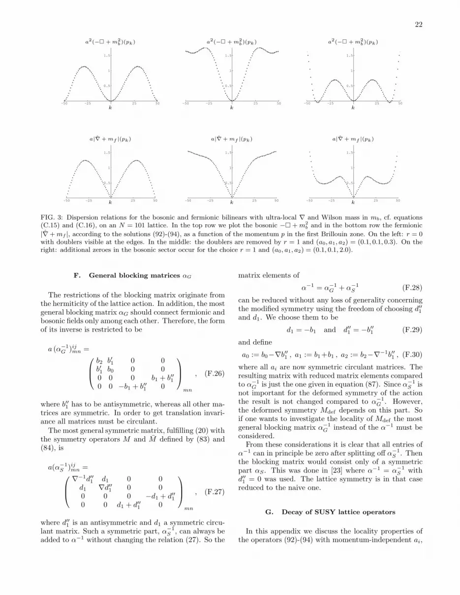
22

-50 -25 25 50

0.5

1

1.5

B

-50 -25 25 50

0.5

1

1.5

B

-50 -25 25 50

0.5

1

1.5

B

-50 -25 25 50

0.5

1

1.5

F

-50 -25 25 50

0.5

1

1.5

F

-50 -25 25 50

0.5

1

1.5

F

k k k

k k k

a2(−� + m2

b)(pk) a2(−� + m2

b)(pk) a2(−� + m2

b)(pk)

a|∇ + mf |(pk) a|∇ + mf |(pk) a|∇ + mf |(pk)

FIG. 3: Dispersion relations for the bosonic and fermionic bilinears with ultra-local ∇ and Wilson mass in mb, cf. equations(C.15) and (C.16), on an N = 101 lattice. In the top row we plot the bosonic −� + m2

b and in the bottom row the fermionic

|∇ + mf |, according to the solutions (92)-(94), as a function of the momentum p in the first Brillouin zone. On the left: r = 0with doublers visible at the edges. In the middle: the doublers are removed by r = 1 and (a0, a1, a2) = (0.1, 0.1, 0.3). On theright: additional zeroes in the bosonic sector occur for the choice r = 1 and (a0, a1, a2) = (0.1, 0.1, 2.0).

F. General blocking matrices αG

The restrictions of the blocking matrix originate fromthe hermiticity of the lattice action. In addition, the mostgeneral blocking matrix αG should connect fermionic andbosonic fields only among each other. Therefore, the formof its inverse is restricted to be

a (α−1G )ijmn =

b2 b′1 0 0b′1 b0 0 00 0 0 b1 + b′′10 0 −b1 + b′′1 0

mn

, (F.26)

where b′′1 has to be antisymmetric, whereas all other ma-trices are symmetric. In order to get translation invari-ance all matrices must be circulant.

The most general symmetric matrix, fulfilling (20) withthe symmetry operators M and M defined by (83) and(84), is

a(α−1S )ijmn =

∇−1d′′1 d1 0 0d1 ∇d′′1 0 00 0 0 −d1 + d′′10 0 d1 + d′′1 0

mn

, (F.27)

where d′′1 is an antisymmetric and d1 a symmetric circu-lant matrix. Such a symmetric part, α−1

S , can always beadded to α−1 without changing the relation (27). So the

matrix elements of

α−1 = α−1G + α−1

S (F.28)

can be reduced without any loss of generality concerningthe modified symmetry using the freedom of choosing d′′1and d1. We choose them to be

d1 = −b1 and d′′1 = −b′′1 (F.29)

and define

a0 := b0−∇b′′1 , a1 := b1+b1 , a2 := b2−∇−1b′′1 , (F.30)

where all ai are now symmetric circulant matrices. Theresulting matrix with reduced matrix elements comparedto α−1

G is just the one given in equation (87). Since α−1S is

not important for the deformed symmetry of the actionthe result is not changed compared to α−1

G . However,the deformed symmetry Mdef depends on this part. Soif one wants to investigate the locality of Mdef the mostgeneral blocking matrix α−1

G instead of the α−1 must beconsidered.

From these considerations it is clear that all entries ofα−1 can in principle be zero after splitting off α−1

S . Thenthe blocking matrix would consist only of a symmetricpart αS . This was done in [23] where α−1 = α−1

S withd′′1 = 0 was used. The lattice symmetry is in that casereduced to the naive one.

G. Decay of SUSY lattice operators

In this appendix we discuss the locality properties ofthe operators (92)-(94) with momentum-independent ai,

23

which due to the denominators resemble massive propa-gators. Nonetheless, we will demonstrate that the posi-tion space representations of these operators do not decayexponentially on the lattice.

Let us, as common in the discussion of locality, con-sider the limit of large lattices. That is, we replace ∇ ineqn. (92) by pk for k = −(N−1)/2 . . . (N−1)/2 and takeN to infinity. Then for the position space representationof the (circulant) fermionic operator ∇

∇nm =1

2a

(N−1)/2∑

l=−(N−1)/2

cl δn−m,−l , (G.31)

cf. (53), the discrete Fourier transformation turns into aFourier integral

cl = limN→∞

1

N

(N−1)/2∑

k=−(N−1)/2

∇(pk)eipkl

=

∫ π/a

−π/a

dp ∇(p) eipla , (G.32)

where p is a continuous momentum and

∇(p) = i(1 + a0 − a2m

2b)p

(1 + a1mb + a0)2 + (a2mb + a1)2p2. (G.33)

from the solution (92).In the limit a → 0 and with p-independent ai, the

Fourier transform gives an exponential decay because

∫ ∞

−∞

dpp

η21 + η2

2p2eipla ∼ exp

(

−sign(l)la|η1||η2|

)

.(G.34)

At finite lattices the Fourier transform (G.32) can becomputed in the complexified p-space. The Fourier in-tegral consists of contributions from poles where the de-nominator of ∇(p) vanishes and an additional part fromthe corresponding complex contours that encloses thepoles.

Because of the regularity of ∇(p) on the real axis, thepoles appear away from it. For positive l we enclosethe poles with positive imaginary parts by adding pathsp = ±π/a + iζ, ζ ∈ [0,∞). The residue at each pole

is some number coming from ∇, which we assume to benon-zero, times a term decaying exponentially in l fromthe Fourier factor in (G.32). For the same reason thereis no contribution from the asymptotic contour at largeIm p parallel to the real interval [−π/a, π/a].

The two new contours contribute

±∫ ∞

0

dζ ∇(p) eipla∣

∣

∣

p=±π/a+iζ, (G.35)

which turn into Laplace transforms

∫ ∞

0

dζ[

∇(π/a+ iζ) − ∇(−π/a+ iζ)]

e−ζla . (G.36)

For large spatial distances l only the value of ∇ at p =π/a remains, namely

[

∇(π/a) − ∇(−π/a)]

∫ 1/la

0

dζ(1 − ζla) = ∇(π/a)1

la(G.37)

where we used that ∇ is odd. Hence the additional con-tours give algebraic corrections to ∇ in position space,unless ∇ vanishes at the boundary of the Brillouin zonep = π/a. Of course the problem of algebraic tails is ab-sent, if ∇ is ultra-local. Here, however, we have consid-ered ∇ as a function of the SLAC operator ∇ accordingto the solution (92). The way out, which is followed inthe body of the paper, section VE, is to consider generalmomentum-dependent blocking kernels.

We remark that the discussion is similar for negativel (where one encloses the poles with negative imaginaryparts). Furthermore, the algebraic corrections do notappear in mf and −� + m2

b , eqn.s (93),(94), becausethese are even functions in p.

H. Locality condition

All of the following one dimensional considerations canbe extended easily to higher dimensions. The consideredlattice operators O are, because of translational invari-ance, circulant matrices,

Omn = On−m = F (a(n−m)) . (H.38)

The slightly modified condition for locality demands thatF decays faster than any polynomial. That means

|xrF (x)| <∞ ∀ r ∈ N, x, y ∈ aN . (H.39)

If the Fourier transform of F (x), f(p), and its derivativeshave no singularities and fulfil periodic boundary condi-tions at edge of the BZ the following estimation can bemade

|xrF (x)| = |∫

BZ

(∂rpf(p))eipx|

≤∫

BZ

|∂rpf(p)| ≤ Cr <∞ . (H.40)

Consider now a non-local operator similar to the SLACderivative. This non-local operator should have no sin-gularities within the BZ for all of its derivatives. Theboundary conditions are, however, not periodic. Accord-ing to the discussion of the locality of K and Mdef itshould support the modified locality after a multiplica-tion with a local operator. In view of the above argumentthe boundary conditions must hence be enforced by thislocal operator without spoiling the differentiability of f .Its representation in Fourier space, I(p), must thereforebe a function that vanishes together with all its deriva-tives at the edge of the BZ. In addition no singularities

24

should appear within the BZ for any of its derivatives.One function that fulfils these requirements is

I(p) =

{

exp(

− ǫ2

ǫ2−p2

)

|p| < ǫ

0 |p| ≥ ǫwith ǫ ≤ π

a. (H.41)

It is clear that I(p) can not be analytic since any analyticfunction that vanishes with all its derivatives at a specific

point must be identical to zero. So the common definitionof locality in terms of analyticity in momentum space cannot be satisfied.

[1] P. H. Dondi and H. Nicolai, Nuovo Cim. A41 (1977) 1.[2] S. D. Drell, M. Weinstein and S. Yankielowicz, Phys.

Rev. D14 (1976) 487; S. D. Drell, M. Weinstein andS. Yankielowicz, Phys. Rev. D14 (1976) 1627.

[3] G. Bergner, T. Kaestner, S. Uhlmann and A. Wipf, An-nals Phys. 323 (2008) 946; M. Kato, M. Sakamoto andH. So, arXiv:0803.3121[hep-lat].

[4] L. H. Karsten and J. Smit, Nucl. Phys. B 183 (1981)103.

[5] I. Montvay, Nucl. Phys. B445 (1995) 399-428.[6] S. Catterall and S. Karamov, Phys. Rev. D65 (2002)

094501; D. B. Kaplan, E. Katz and M. Unsal, JHEP 05

(2003) 037; S. Elitzur and A. Schwimmer, Nucl. Phys.B226 (1983) 109.

[7] M. Bonini and A. Feo, JHEP 09 (2004) 011.[8] M. F. L. Golterman and D. N. Petcher, Nucl. Phys. B319

(1989) 307-341.[9] A. D’Adda, I. Kanamori, N. Kawamoto and K. Nagata,

Nucl. Phys. B707 (2005) 100; A. D’Adda, I. Kanamori,N. Kawamoto and K. Nagata, Phys. Lett. B633 (2006)645; A. D’Adda, I. Kanamori, N. Kawamoto andK. Nagata, Nucl. Phys. B 798 (2008) 168; K. Nagata,arXiv:0805.4235 [hep-lat]; S. Arianos, A. D’Adda, A. Feo,N. Kawamoto and J. Saito, arXiv:0806.0686 [hep-lat].

[10] F. Bruckmann and M. de Kok, Phys. Rev. D73 (2006)074511; F. Bruckmann, S. Catterall and M. de Kok,Phys. Rev. D75 (2007) 045016.

[11] A. Feo, Mod. Phys. Lett. A 19 (2004) 2387; J. Giedt,Int. J. Mod. Phys. A21 (2006) 3039-3094; D. B. Kaplan,Eur. Phys. J. ST 152 (2007) 89.

[12] H. B. Nielsen and M. Ninomiya, Phys. Lett. B105 (1981)219; D. Friedan, Commun. Math. Phys. 85 (1982) 481-490.

[13] P. H. Ginsparg and K. G. Wilson, Phys. Rev. D25, 2649(1982).

[14] H. Neuberger, Phys. Lett. B427 (1998) 353.[15] I. Horvath, Phys. Rev. Lett. 81, 4063 (1998); W. Bieten-

holz, arXiv:hep-lat/9901005; I. Horvath, Phys. Rev. D 60

(1999) 034510; I. Horvath, C. T. Balwe and R. Mendris,Nucl. Phys. B 599 (2001) 283.

[16] P. Hernandez, K. Jansen and M. Luscher, Nucl. Phys.B552 (1999) 363; H. Neuberger, Phys. Rev. D61 (2000)085015; D. H. Adams, Phys. Rev. D68 (2003) 065009.

[17] Y. Igarashi, H. So and N. Ukita, Phys. Lett. B535 (2002)363; Nucl. Phys. B640 (2002) 95; Nucl. Phys. Proc.Suppl. 119 (2003) 778.

[18] J. M. Pawlowski, Annals Phys. 322 (2007) 2831.[19] D. F. Litim and J. M. Pawlowski, in The Exact Renor-

malization Group, Eds. Krasnitz et al, World Sci (1999)168; H. Gies, hep-ph/0611146.

[20] M. Bonini, M. D’Attanasio and G. Marchesini, Nucl.Phys. B 418 (1994) 81; Nucl. Phys. B 421 (1994) 429;U. Ellwanger, Phys. Lett. B 335 (1994) 364; C. Becchi,hep-th/9607188.

[21] Y. Igarashi, K. Itoh and H. So, Prog. Theor. Phys. 106

(2001) 149; Phys. Lett. B 526 (2002) 164; H. Sonoda, J.Phys. A 40 (2007) 9675; Y. Igarashi, K. Itoh and H. Son-oda, Prog. Theor. Phys. 118 (2007) 121.

[22] M. Luscher, Phys. Lett. B428 (1998) 342.[23] H. So and N. Ukita, Phys. Lett. B457 (1999) 314.[24] W. Bietenholz, Mod. Phys. Lett. A14 (1999) 51.[25] G. Barnich, F. Brandt and M. Henneaux, Phys. Rept.

338 (2000) 439; J. Gomis, J. Paris and S. Samuel, Phys.Rept. 259 (1995) 1; M. Henneaux and C. Teitelboim,Quantization of gauge systems, Univ. Pr., Princeton,USA, 1992.

[26] O. Jahn and J. M. Pawlowski, Nucl. Phys. B642 (2002)357.

[27] C. Gattringer and M. Pak, arXiv:0802.2496 [hep-lat].[28] P. Hasenfratz and R. von Allmen, JHEP 0802 (2008)

079.[29] S. Catterall and E. Gregory, Phys. Lett. B487 (2000)

349; J. Giedt, R. Koniuk, E. Poppitz and T. Yavin, JHEP0412 (2004) 033.