Embed Size (px)
Citation preview
GENETIC NONINVASIVE CAPTURE-RECAPTURE TECHNIQUES TO MANAGE POLAR BEARS: A PILOT STUDY
by
Christopher M. Harris
A thesis submitted to the Department of Biology
In conformity with the requirements for
the degree of Master of Science
Queen’s University
Kingston, Ontario, Canada
(December, 2010)
Copyright ©Christopher Matthew Harris , 2010
ii
Abstract
Global polar bear (Ursus maritimus) population numbers are expected to decline steadily
over the next 50 years. A noninvasive genetic survey of polar bear numbers may be a
useful addition to traditional aerial capture mark recapture (CMR) surveys undertaken
throughout the Canadian polar bear population. We attempted a pilot study of
noninvasive genetic survey techniques in M’Clintock Channel between May-June 2006-
2009. Throughout the survey, we compared our values to the most recent (CMR) survey,
conducted by Taylor et al. (2006) between March-June 1998-2000 where 133 cubs, sub-
adults and adults were tagged. A total population size of 300 bears was estimated from
this aerial CMR survey (Taylor et al. 2006). We found noninvasive sampling stations are
sufficient for the capture of a large amount of data on individual bears in an area. Across
4 years, we collected a total of 300 hair samples, and found between 59 and 82 individual
bears entered our sampling stations, depending on the stringency of our identification
parameters. We estimated genotyping error from duplicated samples, and found this was
low (range: 0%-6%), but large enough to not be ignored. There appeared to be a
discrepancy between the capture ratio of male adult bears; the CMR survey (1998-2000)
captured 25% male bears, while we estimated approximately 64% of our captured bears
were male. We felt the most likely explanation of this result is that our traps have a sex
bias. However, further research is required to confirm this hypothesis. On the whole, our
methods are very important for the management of polar bears, but more research must
be done before it can be fully implemented.

iii
Acknowledgements
“I love deadlines. I like the whooshing sound they make as they fly by.”- Douglas Adams
To the Peters; Peter Boag and Peter de Groot, without your input I would have nothing. Peter
Boag I thank for the guidance of this thesis from an idea into something readable, presentable,
and for infinite patience with me. Peter de Groot I thank for his input, ideas, support and
friendship, I’ve enjoyed your tutelage.
To Candace Scott, your input was always needed, and your impact was immeasurable, I thank
you for always being there for me in the lab and in life. Thank you for taking the time out of your
always-busy schedule for me.
To Markus Dyck, and Pam Wong: “Get out of here!”. Markus, thanks for your lessons, your
friendship and, you know, my life. Pam, thanks for being just as clueless as me at times.
To all the hunters and community members who helped in the collection of the hairs, thank you
for your acceptance and support of us throughout our time in the North. Especially Teddy Carter,
Willy Aglukkaq and George Konana; I thank you for your knowledge of the land and
understanding that in hard times, the best remedy is laughter.
To all the lab members who helped collect data and made me laugh, this single line is not
sufficient for the amount of work you have done. Tim St. Amand, Troy Arthur, Dianna Lang,
Stephanie McCormick, Ozgë Danisment, Thomas Van Zuiden, Emily Jibb and Kim McClellend.
To Terri Thompson-Leduc and Michelle Viengkone thanks for that last push at the end, the long
hours and the excellent gels (and not breaking too many things). You made the lab a cheery place.
To James Knowles, you are the reason I have this, and for that I am in your debt; how about a
beer at the Brew Pub sometime?

iv
To my friends: Jay, John, Ben, Yo, Mel, Tyler (N+C), Shar and Antony. Thank you all for the
restoration of joy in difficult times, and the pleasant nagging that helped to get me where I am
now. The theme of the party is ‘hats’. Tyler, thanks for the expertise in those ‘annoying’ (all
ArcGIS) times.
To Erica and the Youngs; your support and love rivaled only that of my own family, I am
infinitely grateful for it, there really is no way for me to repay you.
To my parents: See? I told you I’d finish it. Thank you both so much for your support and love
throughout my life. I don’t think I would be where I am now without your drive and my never-
ending need to justify the amount of love you give me. You two are my ultimate role models, and
I can only hope my life turns out like yours has.

v
Table of Contents
Abstract ............................................................................................................................................ ii Acknowledgements ......................................................................................................................... iii Table of Contents ............................................................................................................................. v List of Figures ................................................................................................................................ vii Chapter 1 Introduction and Literature Review ................................................................................ 1
1.1 Wildlife Surveys .................................................................................................................... 3 1.1.1 DNA Collection and Extraction ...................................................................................... 5 1.1.2 Individual Identification via Microsatellite Genotyping ................................................. 6 1.1.3 Genotyping Error ............................................................................................................ 8 1.1.4 Cost Effectiveness ......................................................................................................... 10 1.1.5 Data Management and Analysis ................................................................................... 11
1.2 Polar Bear Surveys ............................................................................................................... 13 1.3 Polar Bear Behavior and Habitat ......................................................................................... 13
1.3.1 M’Clintock Channel ...................................................................................................... 16 1.4 Objectives ............................................................................................................................ 17
Chapter 2 Methods ......................................................................................................................... 20 2.1 Field Methods ...................................................................................................................... 20
2.1.1 Sampling Station Design ............................................................................................... 21 2.2 Laboratory Methods ............................................................................................................. 22
2.2.1 Sample Extraction and Genotyping .............................................................................. 23 2.2.2 Consensus Genotypes ................................................................................................... 24 2.2.3 Consensus Matching ..................................................................................................... 25 2.2.4 Population Statistics and Final Bear Number ............................................................... 25 2.2.5 Genetic Sexing .............................................................................................................. 26 2.2.6 Error Estimation ............................................................................................................ 26
Chapter 3 Results ........................................................................................................................... 28 3.1 Sampling Stations ................................................................................................................ 28
3.1.1 Sampling Station Construction and Placement ............................................................. 28 3.1.2 Sample Collection ......................................................................................................... 28
3.2 Laboratory Results ............................................................................................................... 29 3.2.1 Locus selection, sample removal and number of individual bears ............................... 29
vi
3.2.2 Re-sampled bears .......................................................................................................... 30 3.2.3 Sex Ratio ....................................................................................................................... 39 3.2.4 Population Genetics Statistics ....................................................................................... 39 3.2.5 Error .............................................................................................................................. 40
Chapter 4 Discussion ..................................................................................................................... 42 4.1 Sampling Station Location, Time Frame and Construction ................................................. 42 4.2 Procedures of Loci Choice and Genotyping Error ............................................................... 43 4.3 Trap Bias .............................................................................................................................. 47 4.4 Bear Numbers and Capture Effort ....................................................................................... 49 4.5 Polar Bear Movement .......................................................................................................... 51 4.6 Inuit Community Interaction ................................................................................................ 54 4.7 Conclusions, Status of Objectives and Future Directions .................................................... 55
Bibliography .................................................................................................................................. 58 Appendix A Contact Consensus Information ................................................................................ 67 Appendix B Trap Capture Effort ................................................................................................... 70
vii
List of Figures
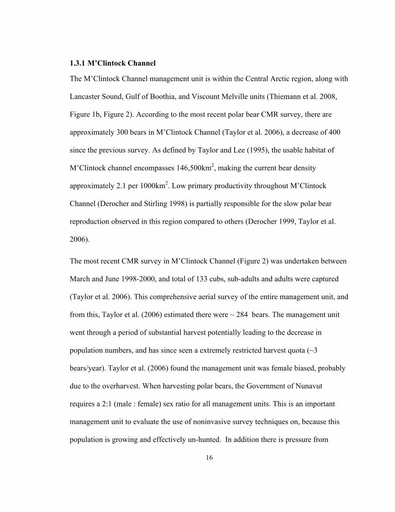
Figure 1. a) Thirteen Canadian polar bear management units, of interest are M’Clintock Channel
(MC), and Gulf of Boothia (GB) b) proposed boundaries of the 5 distinct units: Beaufort Sea,
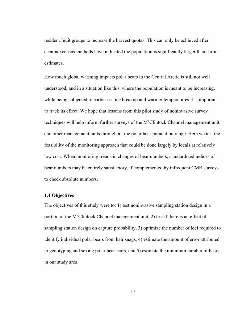
High Arctic, Central Arctic, Hudson Bay, and Davis Strait; from Thiemann et al. (2008). .......... 18 Figure 2. The M’Clintock Channel management unit, and capture locations for the 133 bears
captured during the most recent CMR survey (1998-2000; Taylor et al. 2006). ........................... 19 Figure 3. Activity areas of high bear density in M’Clintock channel (black circles) and
noninvasive sampling station locations across all 4 years of sample. Activity areas were identified
by Inuit collaborators, Stirling (1988), Taylor et al. (2006), and bear harvest GPS locations.
Capture locations were placed at a higher density in activity areas, while outside of activity areas,
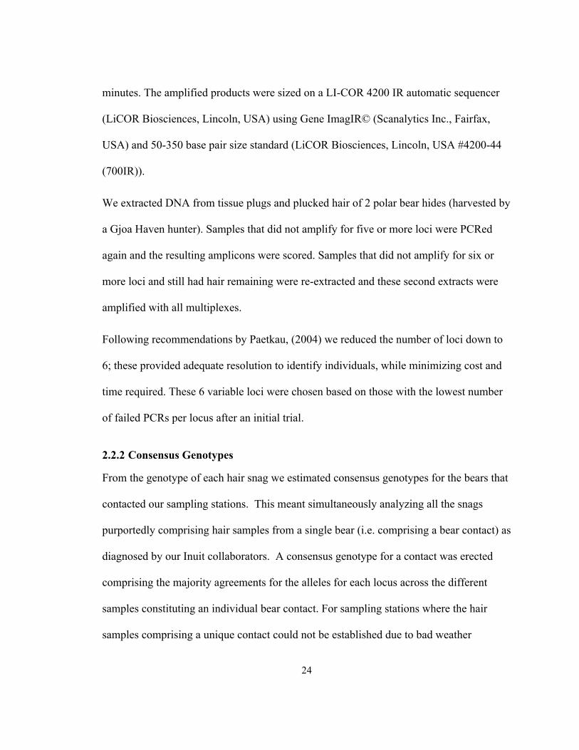
they were placed along a transect every ~15km. ........................................................................... 21 Figure 4. Frequency of the number of individual bears hypothesized to have entered each
sampling station per contact across years. ..................................................................................... 29 Figure 5. Map of across-year bear recaptures from the 2006-2009 noninvasive surveys, letters
correspond to complete genotype matches. ................................................................................... 31 Figure 6. Map of across-survey bear recaptures from the 2006-2009 noninvasive surveys and the
1998-2000 CMR surveys in M’Clintock Channel and Gulf of Boothia, letters correspond to
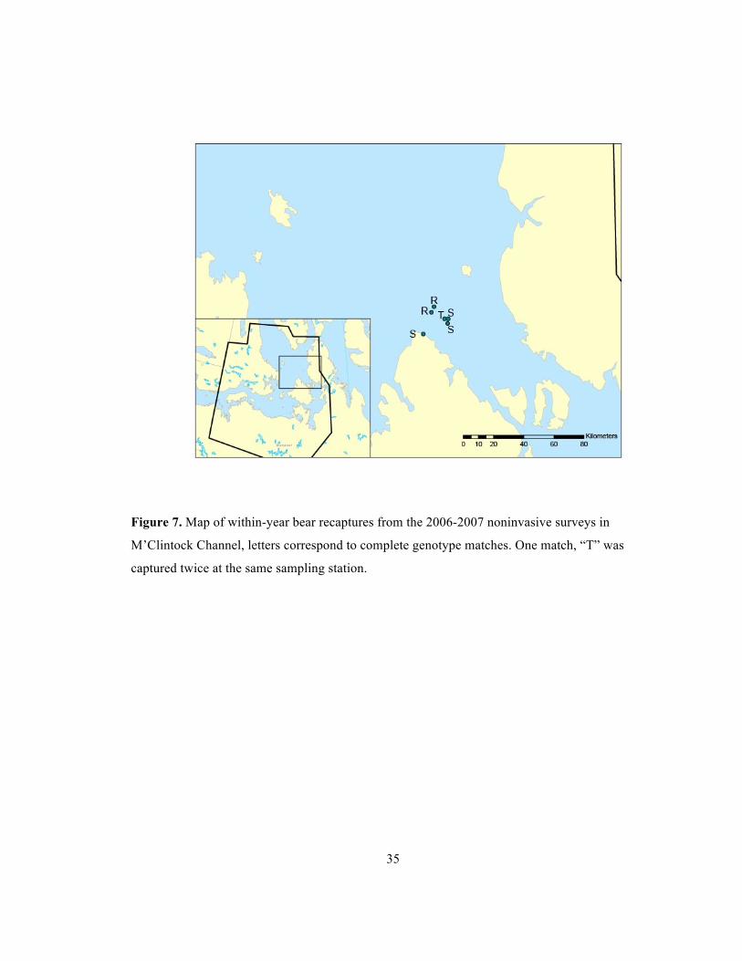
complete genotype matches (see Table 2). .................................................................................... 33 Figure 7. Map of within-year bear recaptures from the 2006-2007 noninvasive surveys in
M’Clintock Channel, letters correspond to complete genotype matches. One match, “T” was
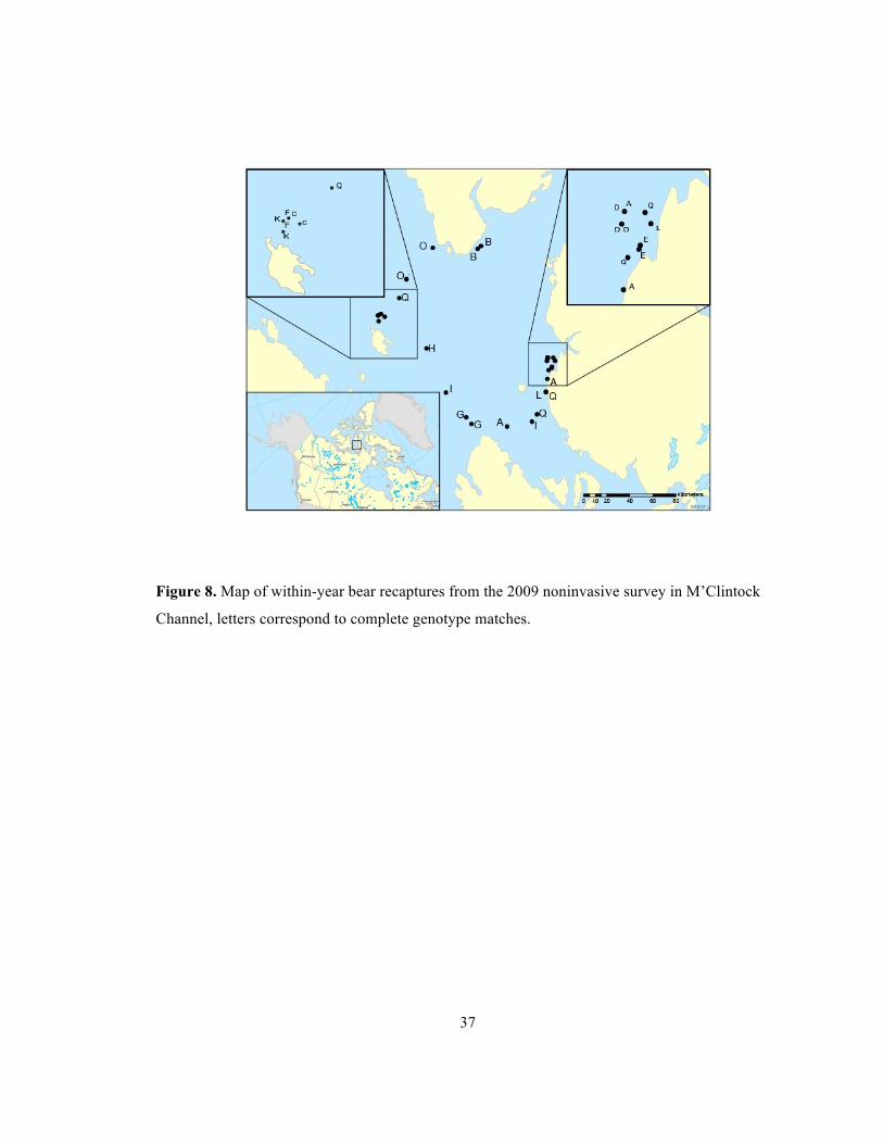
captured twice at the same sampling station. ................................................................................. 35 Figure 8. Map of within-year bear recaptures from the 2009 noninvasive survey in M’Clintock
Channel, letters correspond to complete genotype matches. ......................................................... 37
viii
List of Tables
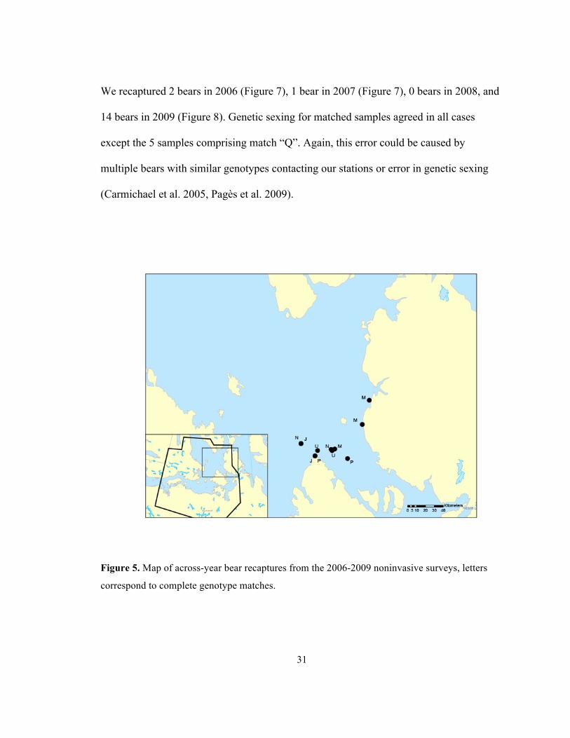
Table 1. Across-year complete genotype matches from the 2006-2009 noninvasive surveys.
Genetic sex as diagnosed by Marie Pagès, “U” denotes samples that had insufficient amounts to
be amplified or could not be diagnosed. Straight-line distance for match M was only measured
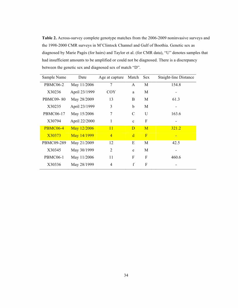
between sample PBMC06- 20 and the two 2009 samples. ............................................................ 32 Table 2. Across-survey complete genotype matches from the 2006-2009 noninvasive surveys and
the 1998-2000 CMR surveys in M’Clintock Channel and Gulf of Boothia. Genetic sex as
diagnosed by Marie Pagès (for hairs) and Taylor et al. (for CMR data), “U” denotes samples that
had insufficient amounts to be amplified or could not be diagnosed. There is a discrepancy
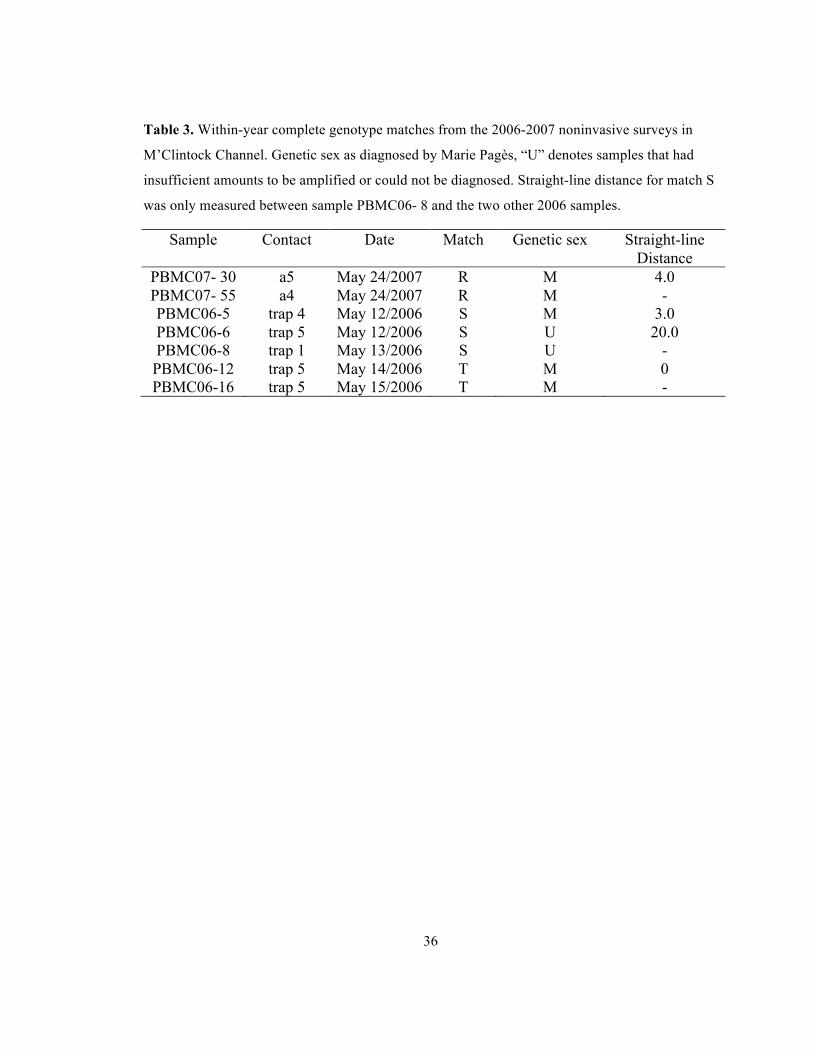
between the genetic sex and diagnosed sex of match “D”. ............................................................ 34 Table 3. Within-year complete genotype matches from the 2006-2007 noninvasive surveys in
M’Clintock Channel. Genetic sex as diagnosed by Marie Pagès, “U” denotes samples that had
insufficient amounts to be amplified or could not be diagnosed. Straight-line distance for match S
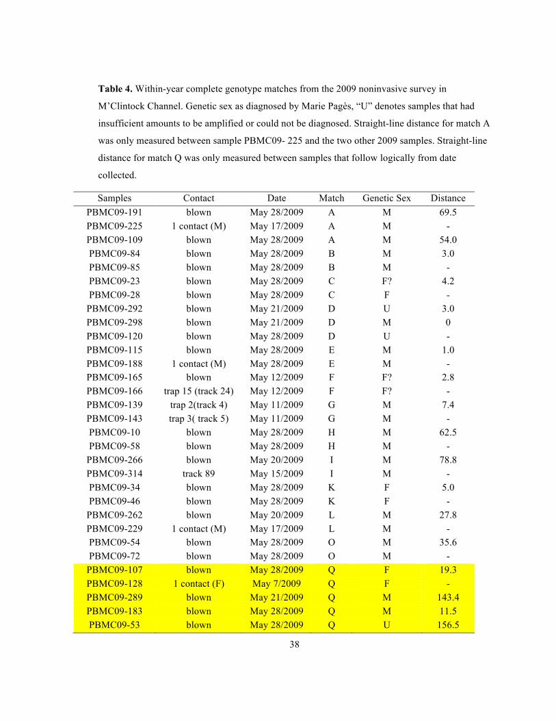
was only measured between sample PBMC06- 8 and the two other 2006 samples. ..................... 36 Table 4. Within-year complete genotype matches from the 2009 noninvasive survey in
M’Clintock Channel. Genetic sex as diagnosed by Marie Pagès, “U” denotes samples that had
insufficient amounts to be amplified or could not be diagnosed. Straight-line distance for match A
was only measured between sample PBMC09- 225 and the two other 2009 samples. Straight-line
distance for match Q was only measured between samples that follow logically from date
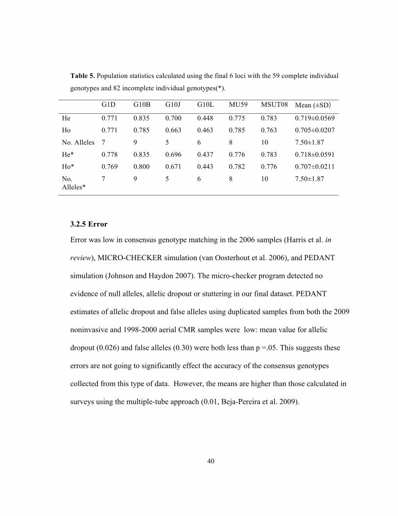
collected. ........................................................................................................................................ 38 Table 5. Population statistics calculated using the final 6 loci with the 59 complete individual
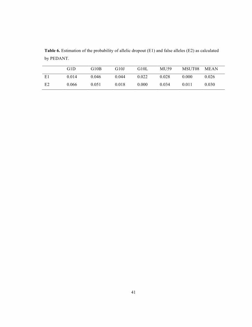
genotypes and 82 incomplete individual genotypes(*). ................................................................. 40 Table 6. Estimation of the probability of allelic dropout (E1) and false alleles (E2) as calculated
by PEDANT. .................................................................................................................................. 41

1
Chapter 1
Introduction and Literature Review
In 2008, the United States Geological Survey released a report outlining the challenges
threatening polar bears (Ursus maritimus) in the near future (Durner et al. 2009). The
report warns that climate warming is expected to decrease polar bear habitat so
drastically that their population will decrease by more than half in 50 years. Due to these
predictions, the US banned all import of polar bear parts and products into the country,
listing polar bears as a threatened species. Controversy still surrounds this listing, with
both Inuit and some researchers disputing the findings (Dyck et al. 2007, Dyck and
Kebreab 2009, Wenzel 2009).
In total, 19 management units of polar bears exist throughout the Arctic, 13 of which lie
either entirely or partially in Canada (COSEWIC 2008, Figure 1a). Radio-telemetry data
on female bears suggests overlap of most subpopulations (Mauritzen et al. 2002, Taylor
et al. 2001), but they remain sufficiently distinct for management purposes (Aars et al.
2006). Surveys are done on management units every 12-15 years (COSEWIC 2008), with
the long interval between surveys due to cost. This survey frequency is sufficient for
normal management of conservation hunting efforts, however it is not frequent enough to
monitor the rapid decline of populations envisaged by the ban on polar bear goods.
Recent studies on the health of polar bears in habitats with declining sea ice are largely
focused on three management units (S. Beaufort Regehr et al. 2010, Hunter et al. 2010;
W. Hudson Bay Regehr et al. 2007, Obbard et al. 2006; and the Chukchi Sea Durner et al.
2009). Surveys in these areas are done every 2 years or less. This is important
2
information, but these three management units make up a small portion of the total polar
bear population (%, COSEWIC, 2008), may have atypical polar bear behavior (Latour
1981, Lunn 1989, Rockwell and Gormezano 2008), and have different environmental
conditions to the rest of the population (Stirling and Parkinson 2006, Rockwell and
Gormezano 2008). The trends observed at these intensive study areas have been applied
throughout the population range regardless of these limitations (Thiemann et al. 2008).
More frequent studies need to be undertaken in all management units in order to fully
understand the scope of the problems facing polar bears across their range.
On the whole, the scientific community agrees that the Arctic climate is changing rapidly
(Post et al. 2009), that this change in climate will result in a decline in sea ice (Rahmstorf
and Ganopolski 1999), and that habitat loss is a major factor in population decline of
most species (Schmiegalow et al. 2002). All arctic species relying on sea ice are at risk
for population decline, but the scale of impact will likely vary considerably between
species (Burek et al. 2008). One way to complement traditional aerial surveys of polar
bears is the use of non-invasive genetic surveys, which are less expensive (Woods et al.
1999), and have been proven effective in other carnivore species (e.g. Boulanger et al.
2004, Solberg et al. 2006, Straley et al. 2009, Luikart et al. 2010 and Stetz et al. 2010). In
this thesis, I examine the feasibility of large scale noninvasive genetic surveys of polar
bears in the Canadian Arctic.

3
1.1 Wildlife Surveys
In a managed wildlife population, the most important metrics calculated through wildlife
surveys are population census size and effective population size (Luikart et al. 2010).
One of the common methods used is a capture-mark-recapture (CMR) survey. Generally,
they are conducted in two phases: initially capturing live animals, tagging and then
releasing them; then surveying the population again, and counting the recaptures and new
captures (Seber 1982). Using these procedures, census size and effective population size
often remain difficult to measure accurately, especially in rare or elusive species.
Traditional CMR surveys may fail when extremely elusive, rare or hard to handle species
are studied (Petit and Valerie 2006). A large number of captures are required for analyses
to be accurate (Mills et al. 2000), which can be costly when working with large
mammals. Another group of methods are simpler sign surveys that have been used to
obtain population information at lower cost. In the case of bears, such surveys consist of
following trails and visually looking for signs of bear density (Heinemeyer et al. 2008).
In theory, areas of high bear abundance should have more frequent bear sightings and
more fresh bear prints, hair snags and scat. Sign surveys based on tracks can be more
useful than microscopic hair surveys alone due to the ability to measure pad size, thus
offering a general idea of the number of unique individuals sampled. Sign surveys are
still used throughout Africa, and photographic track surveys are used in Southern Africa
to monitor populations of rhinos (Jewell et al. 2001). However, there are many
limitations with the collection and analysis of such data, due to similarities between
individuals tracks.
4
The advent of modern, non-invasive genetic identification methods circumvents
difficulties of recognizing individuals from their signs (Garshelis 2006). The first use of
non-invasive genetic techniques were on Pyrenean brown bears (Ursus arctos) in Europe
(Taberlet and Bouvet, 1992). With large carnivores (including bears), the traditional
survey methods of darting and tagging are difficult due to individuals being rare,
secretive and elusive, and therefore difficult to track and trap (Kendall et al, 1992).
Noninvasive genetic sampling has since been used in a number of bear wildlife
population surveys (e.g. Boulanger et al. 2006, Gervasi et al. 2008, Immell and Anthony
2008, Brøseth et al. 2010, Gardner et al. 2010, Harris et al. 2010). The noninvasive
sample collection method can vary. Faecal or hair samples can be collected
opportunistically along trails or at rub sites (faecal: Harris et al. 2010, rub sites: Gervasi
et al. 2008). In other surveys, baited stations or traps are placed throughout the population
range using systematic sampling designs (Gervasi et al. 2010), and in some cases a
combination of opportunistic and systematic sampling approaches (De Barba et al.
2010). Early studies relying on low quality DNA sources were often inconclusive due to
concerns over high genotyping errors. However studies recent have demonstrated
reduced error rates, comparable to those of tissue plugs and blood samples (Beja-Pereira
et al. 2009, see necessary laboratory precautions discussed below). The Ursid family has
been extensively surveyed with noninvasive techniques (black bears (Ursus americanus,
Triant et al. 2004, Dreher et al. 2007), as have American brown bears (Ursus arctos,
Kendall et al. 2009, Stetz et al. 2010) and panda bears (Aliuropoda melanoleuca, Durnin
et al. 2006)).
5
In order for population data to be collected using noninvasive means, survey methods
must first be tested in the field and laboratory. This includes sample collection
techniques, DNA extraction, individual identification techniques, and data management
and analysis methods (Valière et al. 2006).
1.1.1 DNA Collection and Extraction
Non-invasive DNA collection techniques may be divided into two categories: passive and
active sampling. Passive sampling can either be done indirectly (opportunistic) or directly
(systematic, e.g. the use of traps). Indirect collection does not include setting up any type
of trap, but instead collecting samples such as faeces or shed hair while walking along
tracks or trails (Beja-Pereira et al. 2009). Direct collection consists of setting up sampling
stations (traps) along high traffic areas on trails or at movement bottlenecks such as
highway underpasses, or near objects the target species is likely to visit, (e.g. rubbing
sites). Active traps, on the other hand, consist of stations where the species is attracted to
the sampling station itself either with scent or bait. Hair corrals and tree/post snares are
the most commonly used of these active techniques. Tree or post snares are trees or posts
wrapped in barbed wire, with bait attached on top (Woods et al. 1999). Hair corrals are
the most common type of active sampling station, and usually consist of one string of
barbed wire pulled taut so a central bait or lure is far enough from the wire that an
individual must enter the trap to inspect it. For bears, Woods et al. (1999) compared
several variations of corrals and post stations, finding a corral to be most efficient.
Boulanger et al. (2006) found a single strand of barbed wire at a height of 60cm was
sufficient to record bear family groups entering a station.
6
Placement of sampling stations dictates the population inference possible from the
sampling stations. One important component of these models is that each individual in a
population has an equal probability of capture (Long and Zielinski, 2008). Generally,
each home range-sized area should include one or more sampling stations, depending on
individual density within the range (Otis et al. 1978, Karnath and Nichols 2002,
Boulanger et al. 2008). This ensures that each animal in a population will be sampled
during the course of its normal movements.
There are several methods of DNA extraction once sources of DNA such as hair or faeces
have been collected (Poole et al., 2001). The two protocols most often used in wildlife
management surveys are silica and chelex based extractions. Chelex extractions can be
done quickly and at a low cost (Beja-Periera et al. 2009), however the extracted DNA is
not always pure, and the process itself can inhibit subsequent PCR amplification (Rossen
et al. 1992). Silica protocols are found in several commercial kits, such as the QIAGEN
DNeasy Blood and Tissue kits (cat#69506). Although more expensive than their chelex
counterparts, silica protocols often have markedly better yields of DNA (Bhagavatula and
Singh, 2006), with little inhibition of PCR.
1.1.2 Individual Identification via Microsatellite Genotyping
Microsatellites are standard genetic markers used in population genetics, population
dynamics and forensic science research. Their abundance in eukaryotic genomes, along
with the ability of PCR to amplify sequences from small samples, and the fact that alleles
are co-dominant and easily scorable through automated gel electrophoresis make them
extremely useful compared to other methods (Paetkau and Strobeck 1998).
7
Microsatellites are short tandem repeats of nuclear DNA (e.g. CAGCAGCAG or
CACACACA), and although their function within the genome is not well understood,
their polymorphisms have important uses in the fields of population genetics and forensic
science. Originally microsatellites were assumed to be nonfunctional, ‘neutral’ markers,
and although this appears to remain a valid assumption, some studies suggest
microsatellites can be subject to selection (Kashi and Soller 1999, Neff and Gross 2001).
Microsatellite alleles are thought to arise by two mechanisms during DNA replication:
slipped-strand mispairing (Levinson and Gutman 1987) and recombination (Smith 1976,
Jeffreys et al. 1994). In slipped-strand mispairing, a DNA strand in the process of
replication disassociates from the template strand, re-anneals at a different location on the
template strand due to the microsatellite repeats and continues replicating. This causes
either shorter or longer final sequences to be created. Recombination can affect
microsatellite length through unequal crossing over or through gene conversion (Hancock
1999). In unequal crossing over, two DNA strands that are misaligned cross over, and
exchange unequal portions of DNA (Smith 1976). Gene conversion is the transfer of
genetic information in one direction through recombination, thought to arise as a result of
DNA damage (Jeffreys et al. 1994). Slippage appears to be the major factor in the
creation and elongation of microsatellites, but the possibility of recombination cannot be
ignored (Hancock 1999). The above technical details are critical in determining which of
a large number of potential microsatellite markers prove useful for a given application,
insofar as they affect marker properties such as ease of PCR amplification, the level of
8
heterozygosity and number of alleles at a locus, the likelihood of allelic dropout or other
genotyping errors.
In wildlife studies, a multi-locus genotype is used to distinguish individuals, compiled
from several variable microsatellite loci. In the case of polar bears, Paetkau et al. (2004)
found the optimal number of loci to be 6; sufficient to keep error relatively low, while
still arriving at an unique genotype for each individual at relatively low cost.
1.1.3 Genotyping Error
Genotyping error is an important consideration in noninvasive genetic surveys, yet is an
issue that goes underreported in many studies (but see van Oosterhout et al. 2004,
Mckelvey and Schwartz 2005, Pompanon et al. 2005, Beja-Pereira et al. 2009, Luikart et
al. 2010). The need to understand and account for genotyping error in forensic science as
well as wildlife studies has led to a number of studies on the causes of error and
procedures to mitigate their effect in non-invasive genetic studies (Pompanon et al.
2005).
Genotyping error is defined as a difference between the reported genotype, and the true
genotype for a sample, not including failed PCR or extractions (Pompanon et al. 2005).
The three main causes of genotyping error include false alleles, allelic dropout, and
human error (Beja-Pereira et al. 2009, Pompanon et al. 2005). False alleles are novel
alleles created due to a slippage event in an early PCR cycle, which are then replicated to
a significant level in the absence of large amounts of original DNA template (Taberlet et
al. 1996). Allelic dropout occurs when a locus is scored as homozygous in an individual,
9
when the true genotype is heterozygous (Taberlet et al. 1996). This occurs when only one
of two alleles amplifies in the PCR. Human error encompasses a wide range of
phenomena, ranging from cross contamination in the field or lab, to miss-labeling tubes
or miss-scoring genotypes, or entering incorrect information during any of several stages
of data assembly. Human-induced error is the most common source of genotyping error
(Paetkau 2003), and is difficult to eliminate completely or estimate accurately; one study
showed over 93% of their genotyping errors were human-induced (Hoffman and Amos
2005). Allelic dropout is the most common of the non-human induced error (Beja-Pereira
et al. 2009).
There are many approaches to dealing with genotyping error. Careful selection and
optimization of marker loci can reduce problems significantly, while the inclusion of
additional markers confers redundancy. Both these approaches add to the cost and time
required for analyses. More specifically, four analytical methods have been developed to
track error rates (Beja-Pereira et al. 2009): 1) the multiple tube approach in which
multiple PCRs are done for each (or a set proportion of) sample and compared (Taberlet
et al. 1996); 2) a DNA concentration-dependent multiple-tubes approach where sample
concentration is first adjusted across multiple PCR’s and the subsequent reactions
adjusted from these results (Morin et al. 2001); 3) use of computer algorithms to flag
error prone loci (Van Oosterhout et al. 2004, McKelvey and Schwartz 2005), test for
Hardy-Weinberg equilibrium departures (Van Oosterhout et al. 2004), or estimate total
error in replicated sample analyses (Johnson and Haydon 2007); and 4) modeling error
rates during statistical analyses of population size (Lukacs and Burnham 2005, Knapp et
10
al. 2009). The main ways to minimize human-induced error include education about
common errors and vigilance during lab work and sample collection; along with periodic
double-checks at all stages of sample processing in particular the use of using double
blind methods is advised. The acceptable level of genotyping error depends heavily on
the purpose of a given analysis; in human forensic work minor error may be
unacceptable, while in most wildlife surveys nonsystematic genotyping error can be
larger without materially affecting population-level conclusions.
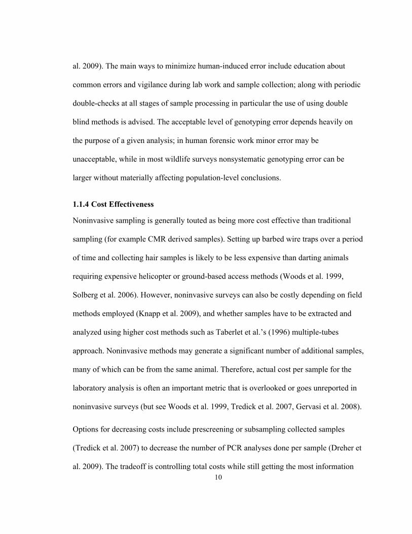
1.1.4 Cost Effectiveness
Noninvasive sampling is generally touted as being more cost effective than traditional
sampling (for example CMR derived samples). Setting up barbed wire traps over a period
of time and collecting hair samples is likely to be less expensive than darting animals
requiring expensive helicopter or ground-based access methods (Woods et al. 1999,
Solberg et al. 2006). However, noninvasive surveys can also be costly depending on field
methods employed (Knapp et al. 2009), and whether samples have to be extracted and
analyzed using higher cost methods such as Taberlet et al.’s (1996) multiple-tubes
approach. Noninvasive methods may generate a significant number of additional samples,
many of which can be from the same animal. Therefore, actual cost per sample for the
laboratory analysis is often an important metric that is overlooked or goes unreported in
noninvasive surveys (but see Woods et al. 1999, Tredick et al. 2007, Gervasi et al. 2008).
Options for decreasing costs include prescreening or subsampling collected samples
(Tredick et al. 2007) to decrease the number of PCR analyses done per sample (Dreher et
al. 2009). The tradeoff is controlling total costs while still getting the most information
11
out of the collected data. Tredick et al. (2007) attempted to decrease costs through
subsampling from large sets of samples at each trap. They found subsampling randomly
or by barb-location could negatively bias population estimates. However, Dreher et al.
(2009) argued this conclusion was specific to only one study area and species and
therefore was not generalizable to all non-invasive studies. They took this idea further by
simulating the impact of different subsampling regimes in model wildlife management
surveys and found that information on the estimated number of different animals
depositing hairs was critical in guiding subsampling in laboratory analyses. With respect
to this thesis, one of their general conclusions was that that genotyping more than three
hair samples per barb did not improve abundance estimates.
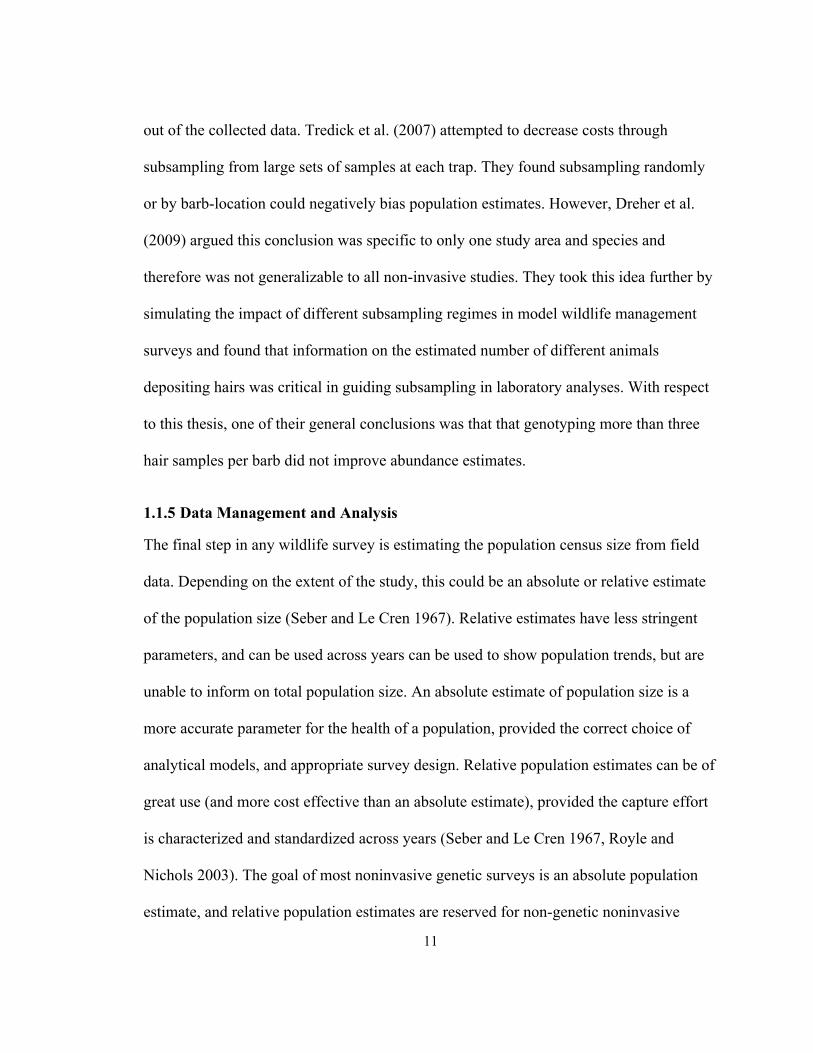
1.1.5 Data Management and Analysis
The final step in any wildlife survey is estimating the population census size from field
data. Depending on the extent of the study, this could be an absolute or relative estimate
of the population size (Seber and Le Cren 1967). Relative estimates have less stringent
parameters, and can be used across years can be used to show population trends, but are
unable to inform on total population size. An absolute estimate of population size is a
more accurate parameter for the health of a population, provided the correct choice of
analytical models, and appropriate survey design. Relative population estimates can be of
great use (and more cost effective than an absolute estimate), provided the capture effort
is characterized and standardized across years (Seber and Le Cren 1967, Royle and
Nichols 2003). The goal of most noninvasive genetic surveys is an absolute population
estimate, and relative population estimates are reserved for non-genetic noninvasive
12
surveys. This trend may be due to the cost of genetic analysis, with decreased laboratory
costs, genetic surveys based on relative population estimates will become the preferred
non-invasive method.
Many computer programs have been developed for use in CMR studies, be they
noninvasive or invasive (see Luikart et al. 2010, Tables 1 and 3 for an extensive but not
exhaustive list). Survey approaches are divided into open and closed population models.
Invasive survey methods require two or more sampling sessions, while noninvasive
surveys appear robust with single sampling sessions (Kohn et al. 1999, Knapp et al. 2009,
Petit and Valerie 2006, Harris et al. 2010). Closed population models assume no changes
to the population during the survey (no change in death and birth rates, and limited
immigration and/or emigration), whereas open population models allow for changes in
these population parameters (Pollock 1982).
Model choice is an important portion of any wildlife survey, many of the models do not
require spatial data apart from a general understanding of the area being sampled (Miller
et al. 2005), but ensuring all individuals have an equal probability of capture is often
necessary. CAPWIRE (Miller et al. 2005), a program written for population estimation
from a noninvasive survey, can accurately estimate population size, provided certain
survey benchmarks are met. For example, the results are most robust when estimating
populations that are smaller than 100 individuals and estimates are the most accurate
when there is capture heterogeneity (Miller et al. 2005). This last point is important, as
programs written for traditional capture-recapture surveys are specifically not robust with
heterogeneous capture probabilities.

13
1.2 Polar Bear Surveys
Over the past 25 years, polar bear surveys have traditionally been conducted via
helicopter and fixed wing aircraft, along line transects in March and early June (Stirling
1988). The fixed wing aircraft normally acts as a spotter and is used to carry extra fuel for
the helicopter. Transects are planned so that large geographic areas are surveyed (Taylor
et al. 2006). Once located, bears are darted from the helicopter and sedated using Telazol
(Tiletamine HCl and Zolazepam HCl) delivered via syringe rifle (Stirling et al. 1989).
Early tests of this drug in polar bears revealed no short term negative impacts (Stirling
1988), but fully controlled comparisons of such impacts are difficult, and Inuit hunters
and community members have blamed the drugs for changes in the taste of polar bear
meat, and for a decline in body mass (Shannon and Freeman 2009). While the longer
term affects on polar bears have not been quantified, Cattet et al. (2008) have tied adverse
long-term health effects and poorer body condition to repeated capture and handling of
grizzly and black bears. Plastic tags with a unique capture ID are affixed to both ears of
polar bears, and a lip tattoo is applied with the same ID. A premolar tooth is removed to
estimate age, and body weight (kg), body length (cm) and skull length are all recorded.
Total cost for a management unit survey can run between 1-1.5 million dollars (Canadian
Dollars, Dyck personal comm.), during which anywhere from 100 to over 1000 bears
would typically be processed.
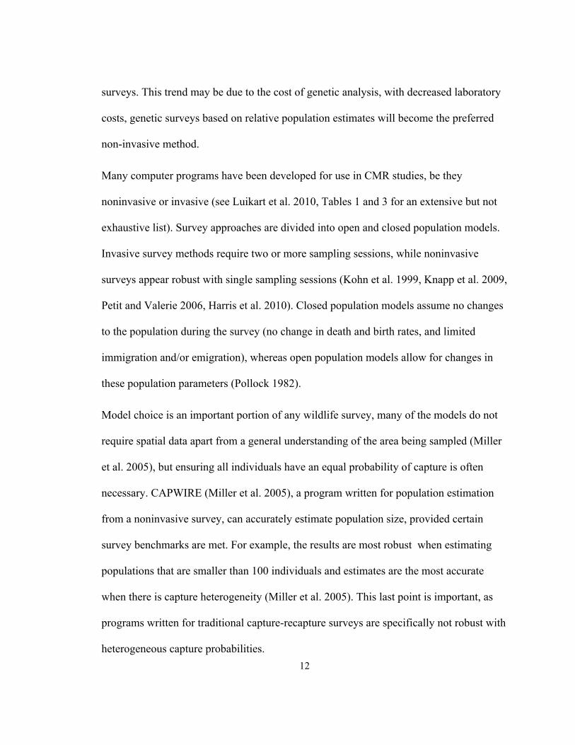
1.3 Polar Bear Behavior and Habitat
Polar bears are always moving, with indistinct home ranges showing only some
specificity for breeding and denning sites (Ramsay and Stirling, 1990). As a result, they
14
are only territorial during the breeding season (March – May), when males have been
known to spar over access to mates in estrous. Their primary food source are three arctic
seal species: harp seal (Pagophilus groenlandicus), bearded seal (Erignathus barbatus)
and ringed seal (Pusa hispida). In general, after emerging from winter dens, polar bears
track prey along cracks (leads) in the sea ice throughout the early spring to early summer,
until they are forced back on the land by retreating sea ice (Stirling 1988). Movement
patterns differ between years and are based on these habitat dynamics (Mauritzen et al.
2001). The home range size of female bears depends on geography and habitat fidelity;
coastal bears travel less (1,000km2), whereas pelagic bears travel more (100,000km2;
Mauitzen et al. 2001). Due to difficulty attaching satellite telemetry to males compared to
females, little is known about male bear migration and home range. However females are
generally found closer to the coast, and males are generally found further from the coast
(Stirling 1988). Bears generally avoid rough ice and flat ice with drifting snow, both
areas of low seal density. Pressure ridges are the ideal locations for seal breathing holes,
and it is around the areas with a high density of pressure ridges that bears tend to
congregate.
Understanding the impact of climate change on polar bear populations means
understanding their unique ecology and adaptation to the arctic seasons. Polar bears are
marine mammals insofar as their productivity is tied to marine ecosystems (Stirling
1988). However their persistence in a given area is determined by their ability to survive
the arctic winter in sheltered terrestrial denning areas, without feeding for months.
Survival during winter and late summer periods of starvation depends on predictable sea

15
ice distributions allowing bears to easily access abundant food sources during intense
spring and fall feeding periods (Stirling 1988). For census methods to reliably detect
long-term trends in polar bear demography, they must be able to sample bear populations
at similar stages of their annual cycle from one year to the next. Otherwise changes in the
timing of various behaviours linked to climate change might influence census counts,
even though actual population size remains constant.
Polar bear longevity is relatively high for a large carnivore; one wild caught female was
captured that was 32 years old, while the oldest captured male was 28 years old (Stirling
1988). Females start mating at age 4, and generally have their first litter at age 5, with
litters consisting of 1-3 cubs. The cubs remain with their mothers until the spring of their
second year, and thus females generally only have cubs every three years, although
mixed-age family groups (females with old and new cubs) have been observed (Stirling,
1988). Additionally, there have been examples of females adopting cubs, although this
behavior is not well understood and appears uncommon (Saunders, 2005).
Genetic analyses suggest the 13 Canadian management units contain 5 biologically
discrete subpopulations, mirroring the ecological and geological boundaries of the arctic
(Paetkau et al. 1999). Some researchers believe the management units should be merged
into these 5 distinct units due to their genetic, ecological, and geographic similarities
(Thiemann et al. 2008). However the geography and desires of local Inuit communities
continue to impact the ways in which polar bears are managed and studied (Wenzel 1999,
Dowsley 2007, ITK and NRI 2007).
16
1.3.1 M’Clintock Channel
The M’Clintock Channel management unit is within the Central Arctic region, along with
Lancaster Sound, Gulf of Boothia, and Viscount Melville units (Thiemann et al. 2008,
Figure 1b, Figure 2). According to the most recent polar bear CMR survey, there are
approximately 300 bears in M’Clintock Channel (Taylor et al. 2006), a decrease of 400
since the previous survey. As defined by Taylor and Lee (1995), the usable habitat of
M’Clintock channel encompasses 146,500km2, making the current bear density
approximately 2.1 per 1000km2. Low primary productivity throughout M’Clintock
Channel (Derocher and Stirling 1998) is partially responsible for the slow polar bear
reproduction observed in this region compared to others (Derocher 1999, Taylor et al.
2006).
The most recent CMR survey in M’Clintock Channel (Figure 2) was undertaken between
March and June 1998-2000, and total of 133 cubs, sub-adults and adults were captured
(Taylor et al. 2006). This comprehensive aerial survey of the entire management unit, and
from this, Taylor et al. (2006) estimated there were ~ 284 bears. The management unit
went through a period of substantial harvest potentially leading to the decrease in
population numbers, and has since seen a extremely restricted harvest quota (~3
bears/year). Taylor et al. (2006) found the management unit was female biased, probably
due to the overharvest. When harvesting polar bears, the Government of Nunavut
requires a 2:1 (male : female) sex ratio for all management units. This is an important
management unit to evaluate the use of noninvasive survey techniques on, because this
population is growing and effectively un-hunted. In addition there is pressure from
17
resident Inuit groups to increase the harvest quotas. This can only be achieved after
accurate census methods have indicated the population is significantly larger than earlier
estimates.
How much global warming impacts polar bears in the Central Arctic is still not well
understood, and in a situation like this, where the population is meant to be increasing,
while being subjected to earlier sea ice breakup and warmer temperatures it is important
to track its effect. We hope that lessons from this pilot study of noninvasive survey
techniques will help inform further surveys of the M’Clintock Channel management unit,
and other management units throughout the polar bear population range. Here we test the
feasibility of the monitoring approach that could be done largely by locals at relatively
low cost. When monitoring trends in changes of bear numbers, standardized indices of
bear numbers may be entirely satisfactory, if complemented by infrequent CMR surveys
to check absolute numbers.
1.4 Objectives
The objectives of this study were to: 1) test noninvasive sampling station design in a
portion of the M’Clintock Channel management unit, 2) test if there is an effect of
sampling station design on capture probability, 3) optimize the number of loci required to
identify individual polar bears from hair snags, 4) estimate the amount of error attributed
to genotyping and sexing polar bear hairs, and 5) estimate the minimum number of bears
in our study area.
18
Figure 1. a) Thirteen Canadian polar bear management units, of interest are M’Clintock Channel
(MC), and Gulf of Boothia (GB) b) proposed boundaries of the 5 distinct units: Beaufort Sea,
High Arctic, Central Arctic, Hudson Bay, and Davis Strait; from Thiemann et al. (2008).
19
Figure 2. The M’Clintock Channel management unit, and capture locations for the 133 bears
captured during the most recent CMR survey (1998-2000; Taylor et al. 2006).
20
Chapter 2
Methods
2.1 Field Methods
In May of four sequential years (2006-2009) we sampled the M’Clintock Channel
population of polar bears using noninvasive survey techniques. We chose four areas to
place a higher density of sampling stations (Cape Sydney, Gateshead Island, Boothia
Peninsula, and Prince of Wales Island, Figure 3). These locations are known by Inuit as
denning and mating areas, and overlapped well with the locations of marked bears in the
most recent Government of Nunavut population survey (Taylor et al. 2006), GPS
locations of past Inuit hunter harvest and the locations of high bear density as defined by
Stirling (1988). Travel to and from each site was done by snow machine and sled.
Frequency of travel to the sampling stations was limited by time and cost, and we were
only able to sample all four areas in one year (2009). One location (Cape Sydney) was
sampled all four years. Boothia Peninsula (2007, 2009) and Gateshead Island (2008,
2009) were sampled in two years. Prince of Wales island was only sampled in 2009.
21
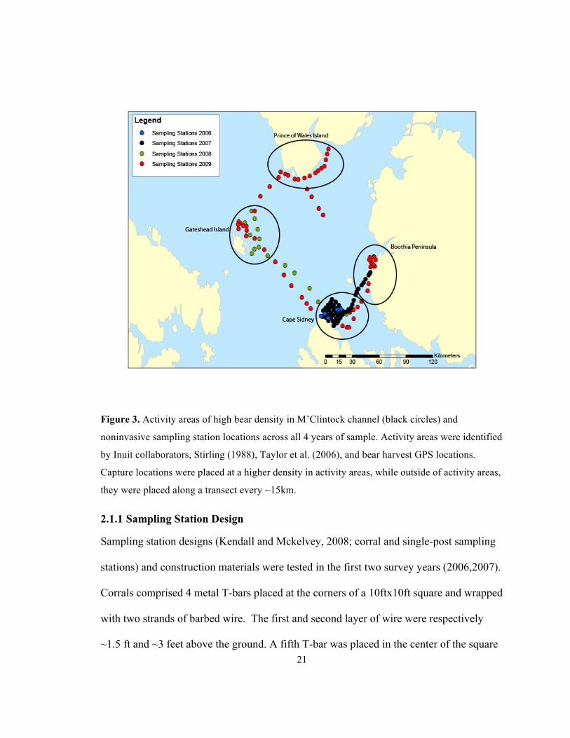
Figure 3. Activity areas of high bear density in M’Clintock channel (black circles) and
noninvasive sampling station locations across all 4 years of sample. Activity areas were identified
by Inuit collaborators, Stirling (1988), Taylor et al. (2006), and bear harvest GPS locations.
Capture locations were placed at a higher density in activity areas, while outside of activity areas,
they were placed along a transect every ~15km.
2.1.1 Sampling Station Design
Sampling station designs (Kendall and Mckelvey, 2008; corral and single-post sampling
stations) and construction materials were tested in the first two survey years (2006,2007).
Corrals comprised 4 metal T-bars placed at the corners of a 10ftx10ft square and wrapped
with two strands of barbed wire. The first and second layer of wire were respectively
~1.5 ft and ~3 feet above the ground. A fifth T-bar was placed in the center of the square
22
with bait attached (usually a piece of seal meat). Single-post stations consisted of single
posts made of wood or metal, wrapped in barbed wire, with a bait item attached to the
top. Two strand corrals were used throughout the 2008 and 2009 surveys.
Sites were chosen based on polar bear behavior, which usually corresponded to the nature
of the sea ice and use of snow machines to travel out to each site. We avoided rough ice,
and did not place traps in these locations, and placed traps at a higher density in medium-
ice areas, spreading them out in areas of flat ice, where bears are unlikely to travel
(Stirling 1988). In 2007, a 6x6 grid layout with stations every 6 km was used around the
Cape Sydney location, to test this method of trap layout (Figure 3).
When available, our Inuit collaborators would diagnose the tracks in the snow and pack-
ice of the bears entering the sampling stations. These data were recorded, and used in
conjunction with the genotype data to make the consensus genotype (see below) for each
bear contacting the station.
We will use the term ‘sample’ for all hairs attached to a single barb which were collected
and placed into a 1.5mL cryovials. A ‘contact’ was all samples collected on the same day
from the same trap.
2.2 Laboratory Methods
The hair samples in 1.5mL cryovials were immediately frozen; subsequently they were
then transported to the Queen’s University Molecular Ecology Lab (QUMEL) in
Kingston, Ontario via iced cooler. Tissue plug samples from the M’Clintock Channel and
23
Gulf of Boothia CMR surveys of all polar bear samples collected from 1998-200 were
previously deposited at Queen’s University.
2.2.1 Sample Extraction and Genotyping
No more than half of the hairs or tissue from each sample was extracted using the
Invitrogen Genomic DNA blood and tissue kit© (Cat# K2100-11; San Diego, USA). The
samples were digested in a 55°C water bath for 2 to 3 hours, followed by overnight
digestion at 37°C on a rocking tray. The extraction procedure followed manufacturers’
instructions, until the elution step where the elution buffer was warmed to 55°C and 2
elutions were completed, the first using 100µL elution buffer, and the second using 50µL
buffer.
We amplified microsatellite DNA from polar bear hairs using four multiplex polymerase
chain reactions (PCRs) containing primers for eleven variable polar bear loci. These
multiplexes were optimized using polar bear skin or blood extracts in a past study (Harris
et al. in review). The loci in the multiplexes included: G1A, G1D, G10B, G10L, G10P,
G10U (Paetkau et al. 1995); G10H, G10J UarMU26, UarMU59 (Taberlet et al. 1997);
and Msut08 (Kitahara et al. 2000). Multiplexes were optimized using QIAGEN Multiplex
kits (cat# 206143; Germantown, USA). Each Multiplex PCR contained: 4 µL template
DNA, 5µL multiplex mix (PCR buffer, MgCl2, dNTPs, and HotStarTMTaq), 1 µL 1X
primer cocktail (mix of 1µL 10X forward primers and 1µL 10X reverse primers mixed
with 18µL ddH2O), 1.0µL 1.0µM M13F-IRD700 primer and 3.0µL ddH2O. Cycling
conditions were as follows: 95°C for 15 minutes followed by 35 cycles of 94°C for 1
minute, 55°C for 1.5 minutes, 72°C for 1.5 minutes and a final extension of 72°C for 15
24
minutes. The amplified products were sized on a LI-COR 4200 IR automatic sequencer
(LiCOR Biosciences, Lincoln, USA) using Gene ImagIR© (Scanalytics Inc., Fairfax,
USA) and 50-350 base pair size standard (LiCOR Biosciences, Lincoln, USA #4200-44
(700IR)).
We extracted DNA from tissue plugs and plucked hair of 2 polar bear hides (harvested by
a Gjoa Haven hunter). Samples that did not amplify for five or more loci were PCRed
again and the resulting amplicons were scored. Samples that did not amplify for six or
more loci and still had hair remaining were re-extracted and these second extracts were
amplified with all multiplexes.
Following recommendations by Paetkau, (2004) we reduced the number of loci down to
6; these provided adequate resolution to identify individuals, while minimizing cost and
time required. These 6 variable loci were chosen based on those with the lowest number
of failed PCRs per locus after an initial trial.
2.2.2 Consensus Genotypes
From the genotype of each hair snag we estimated consensus genotypes for the bears that
contacted our sampling stations. This meant simultaneously analyzing all the snags
purportedly comprising hair samples from a single bear (i.e. comprising a bear contact) as
diagnosed by our Inuit collaborators. A consensus genotype for a contact was erected
comprising the majority agreements for the alleles for each locus across the different
samples constituting an individual bear contact. For sampling stations where the hair
samples comprising a unique contact could not be established due to bad weather
25
conditions, or other factors, each hair sample was treated individually as a separate
contact, and matched in the next step.
2.2.3 Consensus Matching
Consensus genotypes were then matched across all 6 microsatellite loci simultaneously
using MICROSATELLITE TOOLKIT (Park 2001). All pairs of genotypes different at
less than 4 alleles were scrutinized to ensure numbers were not overestimated due to
allelic dropout (Tablerlet et al. 1996; Tredick et al. 2007). Consensus genotypes
consisting of less than 3 separate samples or re-runs (where a PCR product was run at
least twice), were held less rigidly than consensus genotypes consisting of more.
Therefore, when matching samples, 2 or more consensus genotypes matching at all but 2
or less alleles were scored as the same bear if there were a) empirical evidence they were
the same bear (collected from the same trap on the same day), and b) had at least one
allele at the mismatched loci that matched. Straight-line distance in kilometers was
measured between all matching samples. Additionally, we compared our collected
genotypes from the same loci with those collected during the 1998-2000 CMR survey in
M’Clintock Channel and Gulf of Boothia using the same matching criteria above.
2.2.4 Population Statistics and Final Bear Number
Using the genotyped tissue plugs from the 1998-2000 M’Clintock channel, we calculated
PID (Paetkau et al. 1995) values for our 6 loci together, and all the possible permutations
of 1,2 and 3 loci missing. Using these values, we were able to find the amount of missing
loci we should allow in our minimum known alive estimates. Minimum known alive
estimates were given as a range: no loci missing-most loci missing.
26
Using this range of samples (no missing loci-most loci missing), we then calculated
observed heterozygosity (Ho), expected heterozygosity (He; Nei, 1987), and probability
of identity (PID) (Paetkau et al. 1995).
2.2.5 Genetic Sexing
A collaborator specializing in the genetic sexing of degraded Ursid samples sexed a
number of extracts from each of the bears that contacted our stations samples. Pagès et al.
(2009) use a multiplex of an x-linked zinc-finger domain, and a bear specific section of
the SRY construct to distinguish male from female. Samples were amplified in a 25µL
reaction volume containing 1.25 U of Amplitaq Gold DNA polymerase (Applied
Biosystems), 0.5 mg/ml BSA (Roche, 1 mg/ml), 1.5 mM MgCl2, 250 µM each dNTP, 0.4
µM of ZF primers, 0.12 µM of SRY primers and 2 µl of DNA (Pagès et al. 2009). DNA
was amplified with 48 cycles of denaturation (94°C, 30 s), annealing (55°C, 30 s) and
elongation (72°C, 45s; Pagès et al. 2009).
2.2.6 Error Estimation
Four sets of paired hair-tissue samples were tested against all four multiplex PCRs for
error checking purposes.
The computer programs PEDANT and MICRO-CHECKER were used to test error rate
per locus and allelic dropout respectively (van Oosterhout et al. 2006, Johnson and
Haydon 2007). Samples from the 2009 surveys were randomly replicated and chosen to
be included in the pedant simulation tests, due to the higher number of samples collected
during that year. Samples from 2007 and 2008 were extracted and genotyped along with

27
the 2009 samples, so the same error rates are assumed throughout. We ran MICRO-
CHECKER on the final set of complete consensus genotypes to assess loci prone to
allelic dropout error (van Oosterhout et al. 2006). Error associated with samples collected
in 2006 was compared using Inuit contact information (Harris et al. in review).

28
Chapter 3
Results
3.1 Sampling Stations
3.1.1 Sampling Station Construction and Placement
The dark-colored t-bars tend to heat up during the day, and often sink into the sea ice, so
the bottom strand often ends up on the ice; and bears found it easy to step over the barbs
without leaving samples, thus we found dual-strand corrals to be the best for our needs.
Wood and metal single-pole traps were too flimsy for our survey. Posts were easily
ripped from the ground and thrown around, shaking off any hair samples collected during
the contact.
3.1.2 Sample Collection
A total of 595 hair samples were collected over 4 years of surveying M’Clintock
Channel. Genetic results suggested contacts consisted mainly of one bear entering the
trap between each sampling event (Figure 4).
29
Figure 4. Frequency of the number of individual bears hypothesized to have entered each
sampling station per contact across years.
3.2 Laboratory Results
3.2.1 Locus selection, sample removal and number of individual bears
Of the 11 assayed, the 6 most complete loci (% incomplete) were G1D (13.2%),
G10B(17.0%), G10J(12.1%), G10L(10.4%), UarMU59(11.0%), and MSUT08(17.0%).
Consensus genotypes were created using these loci, however when diagnosis was unclear
we did check other 5 loci. A total of 17 samples were removed when they showed greater
than 50% failed amplification. After consensus genotype creation and genotype
matching, we estimated a total of 90 bears were captured over the 4 years with 50% or
greater loci amplification.
We calculated mean PID values from tissue sample genotypes collected during the 1998-
2000 CMR surveys of M’Clintock Channel. The PID for all 6 loci was 1.69E-06, the mean
30
PID for 5 loci was 1.22E-05 ±3.40E-06, the mean PID for 4 loci was 1.45E-4 ±1.01E-4, and
the mean PID for 3 loci was 1.64E-3 ±1.29E-3. A PID of 1.64E-3 ±1.29E-3 means the
probability of mistaken identity is approximately 1-2 for every 1000 individuals
genotyped, which is approaching our total estimated sample size of 284 bears (Taylor et
al. 2006). Using these values, we decided the mean PID at 3 loci was sufficiently low to
allow for genotype matching errors, and removed any individuals with only 3 complete
loci. We found 59 individuals had complete genotypes (all 6 loci typed, conservative
estimate), whereas when samples with up to two loci missing were included, we found 82
individuals. Therefore, we estimate the range of individuals captured within our survey
was 59-82.
3.2.2 Re-sampled bears
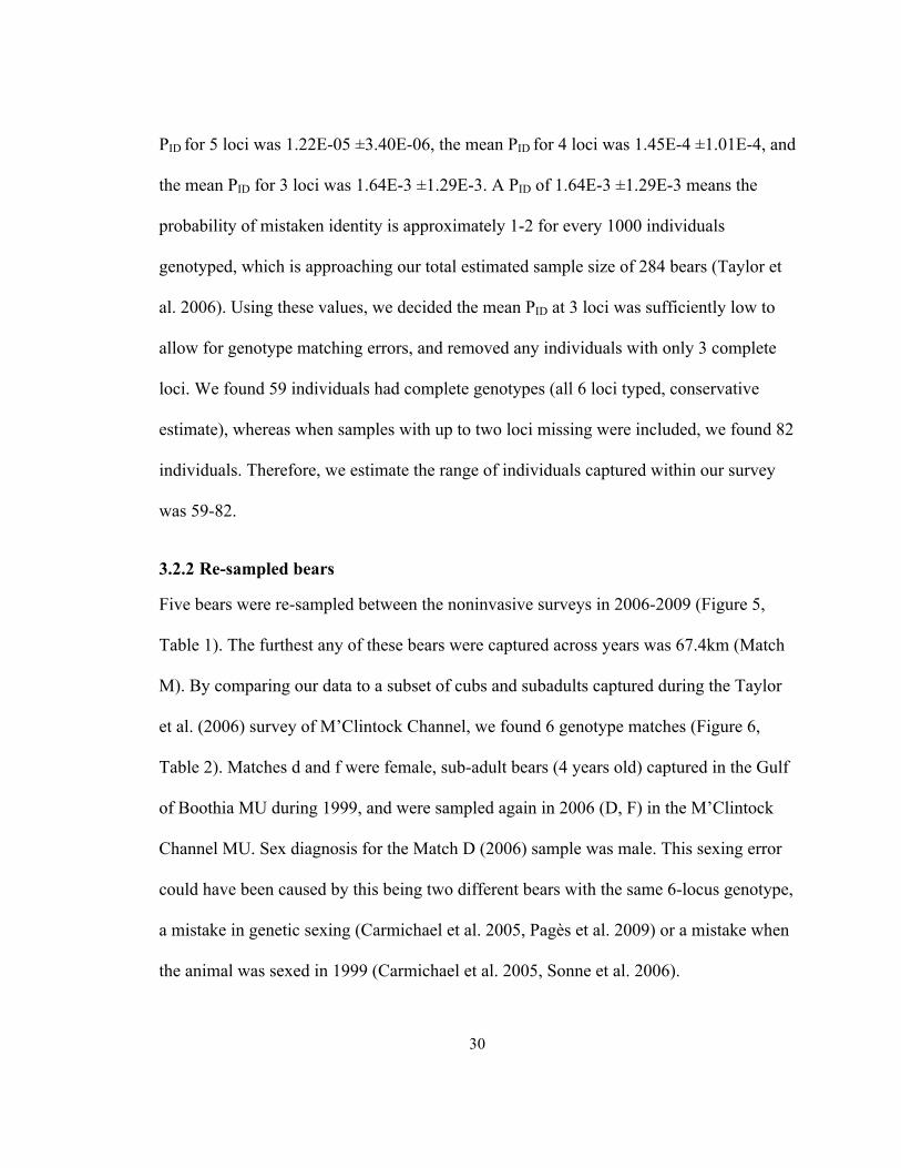
Five bears were re-sampled between the noninvasive surveys in 2006-2009 (Figure 5,
Table 1). The furthest any of these bears were captured across years was 67.4km (Match
M). By comparing our data to a subset of cubs and subadults captured during the Taylor
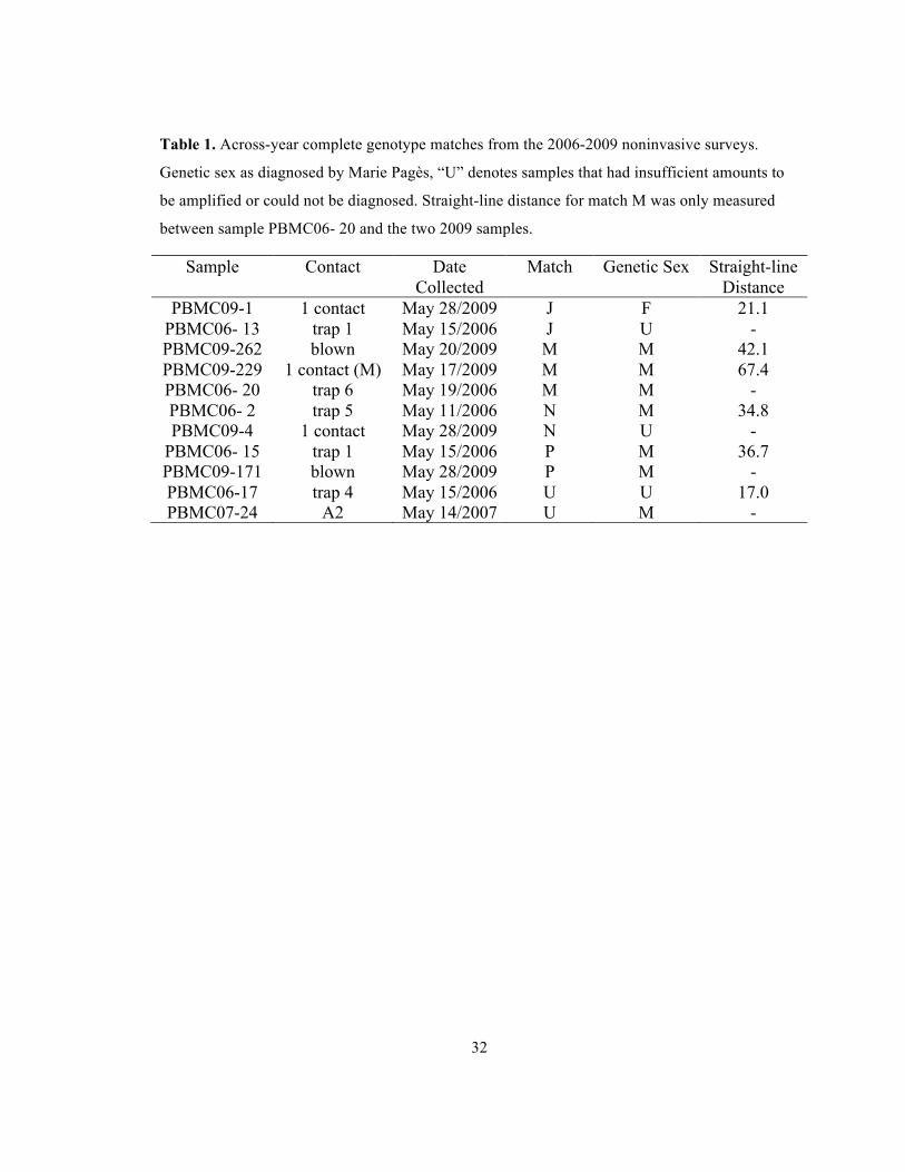
et al. (2006) survey of M’Clintock Channel, we found 6 genotype matches (Figure 6,
Table 2). Matches d and f were female, sub-adult bears (4 years old) captured in the Gulf
of Boothia MU during 1999, and were sampled again in 2006 (D, F) in the M’Clintock
Channel MU. Sex diagnosis for the Match D (2006) sample was male. This sexing error
could have been caused by this being two different bears with the same 6-locus genotype,
a mistake in genetic sexing (Carmichael et al. 2005, Pagès et al. 2009) or a mistake when
the animal was sexed in 1999 (Carmichael et al. 2005, Sonne et al. 2006).
31
We recaptured 2 bears in 2006 (Figure 7), 1 bear in 2007 (Figure 7), 0 bears in 2008, and
14 bears in 2009 (Figure 8). Genetic sexing for matched samples agreed in all cases
except the 5 samples comprising match “Q”. Again, this error could be caused by
multiple bears with similar genotypes contacting our stations or error in genetic sexing
(Carmichael et al. 2005, Pagès et al. 2009).
Figure 5. Map of across-year bear recaptures from the 2006-2009 noninvasive surveys, letters
correspond to complete genotype matches.
32
Table 1. Across-year complete genotype matches from the 2006-2009 noninvasive surveys.
Genetic sex as diagnosed by Marie Pagès, “U” denotes samples that had insufficient amounts to
be amplified or could not be diagnosed. Straight-line distance for match M was only measured
between sample PBMC06- 20 and the two 2009 samples.
Sample Contact Date Collected
Match Genetic Sex Straight-line Distance
PBMC09-1 1 contact May 28/2009 J F 21.1 PBMC06- 13 trap 1 May 15/2006 J U - PBMC09-262 blown May 20/2009 M M 42.1 PBMC09-229 1 contact (M) May 17/2009 M M 67.4 PBMC06- 20 trap 6 May 19/2006 M M - PBMC06- 2 trap 5 May 11/2006 N M 34.8 PBMC09-4 1 contact May 28/2009 N U -
PBMC06- 15 trap 1 May 15/2006 P M 36.7 PBMC09-171 blown May 28/2009 P M - PBMC06-17 trap 4 May 15/2006 U U 17.0 PBMC07-24 A2 May 14/2007 U M -
33
Figure 6. Map of across-survey bear recaptures from the 2006-2009 noninvasive surveys and the
1998-2000 CMR surveys in M’Clintock Channel and Gulf of Boothia, letters correspond to
complete genotype matches (see Table 2).
34
Table 2. Across-survey complete genotype matches from the 2006-2009 noninvasive surveys and
the 1998-2000 CMR surveys in M’Clintock Channel and Gulf of Boothia. Genetic sex as
diagnosed by Marie Pagès (for hairs) and Taylor et al. (for CMR data), “U” denotes samples that
had insufficient amounts to be amplified or could not be diagnosed. There is a discrepancy
between the genetic sex and diagnosed sex of match “D”.
Sample Name Date Age at capture Match Sex Staight-line Distance
PBMC06-2 May 11/2006 7 A M 154.8
X30236 April 23/1999 COY a M -
PBMC09- 80 May 28/2009 13 B M 61.3
X30235 April 23/1999 3 b M -
PBMC06-17 May 15/2006 7 C U 163.6
X30794 April 22/2000 1 c F -
PBMC06-4 May 12/2006 11 D M 321.2
X30373 May 14/1999 4 d F -
PBMC09-289 May 21/2009 12 E M 42.5
X30345 May 30/1999 2 e M -
PBMC06-1 May 11/2006 11 F F 460.6
X30336 May 28/1999 4 f F -
35
Figure 7. Map of within-year bear recaptures from the 2006-2007 noninvasive surveys in
M’Clintock Channel, letters correspond to complete genotype matches. One match, “T” was
captured twice at the same sampling station.
36
Table 3. Within-year complete genotype matches from the 2006-2007 noninvasive surveys in
M’Clintock Channel. Genetic sex as diagnosed by Marie Pagès, “U” denotes samples that had
insufficient amounts to be amplified or could not be diagnosed. Straight-line distance for match S
was only measured between sample PBMC06- 8 and the two other 2006 samples.
Sample Contact Date Match Genetic sex Straight-line Distance
PBMC07- 30 a5 May 24/2007 R M 4.0 PBMC07- 55 a4 May 24/2007 R M - PBMC06-5 trap 4 May 12/2006 S M 3.0 PBMC06-6 trap 5 May 12/2006 S U 20.0 PBMC06-8 trap 1 May 13/2006 S U - PBMC06-12 trap 5 May 14/2006 T M 0 PBMC06-16 trap 5 May 15/2006 T M -
37
Figure 8. Map of within-year bear recaptures from the 2009 noninvasive survey in M’Clintock
Channel, letters correspond to complete genotype matches.
38
Table 4. Within-year complete genotype matches from the 2009 noninvasive survey in
M’Clintock Channel. Genetic sex as diagnosed by Marie Pagès, “U” denotes samples that had
insufficient amounts to be amplified or could not be diagnosed. Straight-line distance for match A
was only measured between sample PBMC09- 225 and the two other 2009 samples. Straight-line
distance for match Q was only measured between samples that follow logically from date
collected.
Samples Contact Date Match Genetic Sex Distance PBMC09-191 blown May 28/2009 A M 69.5 PBMC09-225 1 contact (M) May 17/2009 A M - PBMC09-109 blown May 28/2009 A M 54.0 PBMC09-84 blown May 28/2009 B M 3.0 PBMC09-85 blown May 28/2009 B M - PBMC09-23 blown May 28/2009 C F? 4.2 PBMC09-28 blown May 28/2009 C F -
PBMC09-292 blown May 21/2009 D U 3.0 PBMC09-298 blown May 21/2009 D M 0 PBMC09-120 blown May 28/2009 D U - PBMC09-115 blown May 28/2009 E M 1.0 PBMC09-188 1 contact (M) May 28/2009 E M - PBMC09-165 blown May 12/2009 F F? 2.8 PBMC09-166 trap 15 (track 24) May 12/2009 F F? - PBMC09-139 trap 2(track 4) May 11/2009 G M 7.4 PBMC09-143 trap 3( track 5) May 11/2009 G M - PBMC09-10 blown May 28/2009 H M 62.5 PBMC09-58 blown May 28/2009 H M -
PBMC09-266 blown May 20/2009 I M 78.8 PBMC09-314 track 89 May 15/2009 I M - PBMC09-34 blown May 28/2009 K F 5.0 PBMC09-46 blown May 28/2009 K F -
PBMC09-262 blown May 20/2009 L M 27.8 PBMC09-229 1 contact (M) May 17/2009 L M - PBMC09-54 blown May 28/2009 O M 35.6 PBMC09-72 blown May 28/2009 O M -
PBMC09-107 blown May 28/2009 Q F 19.3 PBMC09-128 1 contact (F) May 7/2009 Q F - PBMC09-289 blown May 21/2009 Q M 143.4 PBMC09-183 blown May 28/2009 Q M 11.5 PBMC09-53 blown May 28/2009 Q U 156.5
39
3.2.3 Sex Ratio
Using the 1998-2000 CMR dataset for M’Clintock Channel only, we found a capture
ratio of 42.1% males. When cubs of the year and yearlings (1 year old) were removed
from the dataset, the bears captured were 37.7% males. Finally, when only adults were
included (≥5 years old) the capture ratio was 25% males (Taylor et al. 2006).
Genetic sexing of the noninvasive survey samples revealed a large male bias. Of the 82
individual genotypes, we found 52 male bears (63.9%), 17 female bears (20.5%), and 13
(15.6%) unknown. For the 59 individuals with full genotypes, we found 38 male bears
(64.4%), 14 female bears (23.7%), and 7 (11.9%) unknown. It is unknown if all male
bears were distributed across multiple age groups or restricted to a single age group.
3.2.4 Population Genetics Statistics
Population genetics statistics were calculated using the final dataset comprising 59
complete genotypes (Table 5). We also calculated the heterozygosities for the dataset
containing 82 samples with >3 complete loci (discussed above). Expected and observed
heterozygosities were close, suggesting our population is in Hardy-Weinberg
equilibrium.
40
Table 5. Population statistics calculated using the final 6 loci with the 59 complete individual
genotypes and 82 incomplete individual genotypes(*).
G1D G10B G10J G10L MU59 MSUT08 Mean (±SD)
He 0.771 0.835 0.700 0.448 0.775 0.783 0.719±0.0569
Ho 0.771 0.785 0.663 0.463 0.785 0.763 0.705±0.0207
No. Alleles 7 9 5 6 8 10 7.50±1.87
He* 0.778 0.835 0.696 0.437 0.776 0.783 0.718±0.0591
Ho* 0.769 0.800 0.671 0.443 0.782 0.776 0.707±0.0211
No. Alleles*
7 9 5 6 8 10 7.50±1.87
3.2.5 Error
Error was low in consensus genotype matching in the 2006 samples (Harris et al. in
review), MICRO-CHECKER simulation (van Oosterhout et al. 2006), and PEDANT
simulation (Johnson and Haydon 2007). The micro-checker program detected no
evidence of null alleles, allelic dropout or stuttering in our final dataset. PEDANT
estimates of allelic dropout and false alleles using duplicated samples from both the 2009
noninvasive and 1998-2000 aerial CMR samples were low: mean value for allelic
dropout (0.026) and false alleles (0.30) were both less than p =.05. This suggests these
errors are not going to significantly effect the accuracy of the consensus genotypes
collected from this type of data. However, the means are higher than those calculated in
surveys using the multiple-tube approach (0.01, Beja-Pereira et al. 2009).
41
Table 6. Estimation of the probability of allelic dropout (E1) and false alleles (E2) as calculated
by PEDANT.
G1D G10B G10J G10L MU59 MSUT08 MEAN
E1 0.014 0.046 0.044 0.022 0.028 0.000 0.026
E2 0.066 0.051 0.018 0.000 0.034 0.011 0.030

42
Chapter 4
Discussion
I discuss these findings in the context of my five thesis objectives. I then discuss the
inferences that can be drawn from my finding regarding polar bear movement, the
importance of this method in terms of local community involvement and end with a
discussion of implications of this work and next steps.
4.1 Sampling Station Location, Time Frame and Construction
The metal t-bar corrals were the best design for our sampling stations. Single-post
sampling stations are cost-effective in many small mammal studies, but the strength of
polar bears renders the single post stations useless for hair-collection. Even the corrals are
often disturbed by bears entering them, as the t-bars were sometimes bent or even ripped
from the sea-ice. This does not always make the trap ineffective for further contacts, but
it can make them less effective. Additionally, the central seal bait bar was sometimes
ripped out of the station and thrown elsewhere. We also noted that t-bars sometimes
melted down into the ice under certain conditions; this could be minimized in the future
by painting posts white before use. These confounding factors make it imperative that the
sampling stations are checked frequently.
In other bear studies there can be constant movement of sampling stations (Gervasi et al.
2008), or static sampling station placement (Gardner et al. 2010) depending on the nature
of the study. Due to the distances we needed to cover, and the harsh conditions that go
along with work in the arctic, it was most practical to keep the stations where originally
placed and generally distributed along linear transects.
43
Animal density across the habitat is used to determine sampling station density (Dreher et
al. 2007). Equal capture probabilities for all individuals is an imperative metric in
capture-recapture surveys, which is why trap density and placement is so important.
We found that when stations are placed too close to one another, bears will follow the
tracks and smell leading them from one trap to the next.
Most within-year recaptures came from bears entering sampling stations one after
another, perhaps because traps were placed too close together. Recaptures spaced far
apart were generally further apart in time, for example, individual K had hair samples
collected on May 13, 2009 around Cape Sydney, then was found on May 28, 2009 near
Gateshead Island. The general correlation between time and distance between recaptures
confirms the anecdotal observation that in the spring bears are on the move continuously,
and do not remain in any particular area for extended time periods.
Checking traps at 1-2 day intervals allowed the best diagnoses of polar bear contacts with
the traps. Allocating the hair collected at any given sampling station into individual
contacts was easiest when there were good Inuit diagnoses of likely contact number,
something which was difficult to rely on after 5 days.
4.2 Procedures of Loci Choice and Genotyping Error
There is some question about the number of loci to use in genetic studies, and the answer
usually stems from the type of study undertaken. In our survey, we use the “industry
standard” of 6 loci (Paetkau 2004). We chose the 6 loci from our original 11 based on the
amount of information we could derive from each and which amplified best. According
44
to Paetkau, (2004) 6 loci is where the cost and error are at a minimum while maximizing
the amount of information gained. In a past survey, we used all 11 loci, and found they
had relatively similar heterozygosity values, and similar number of alleles (Harris et al. in
review), so they all gave approximately equal amounts of information. Where we found
they differed was their ability to amplify our samples, and it was for this reason that we
chose the loci that amplified the most individual hair samples.
Genotype error rates of all tissue types can range from negligible to 15%, with most
genotyping between 0.5%-1% (Pamponon et al. 2005). Noninvasive samples such as hair
or faeces are considered to be lower quality than tissue plugs or blood, and error rates are
generally higher than 1% (Taberlet et al. 1996). Error that goes unnoticed or unquantified
can cause unfounded support or dismissal of a hypothesis, even at lower error ranges
(Bonin et al. 2004, Pampanon et al. 2005). We used several methods to estimate error in
our study, and all showed sufficiently low per locus error rates using DNA derived from
hairsnags. Although the error rates were lower than those found in other noninvasive
studies (Bonin et al. 2004), they should not be ignored. Three factors explain the low
error rates observed here: 1) high-throughput multiplex PCRs, 2) conservative genotype
scoring, and 3) immediate sample preservation via freezing.
High throughput multiplex PCRs have only recently become an option in noninvasive
surveys (Beja-Pereira et al. 2009). The amalgamation of multiple loci within one PCR
cocktail not only decreases the amount of DNA used per complete genotype, but also
decreases the amount of handling per sample, decreasing probability of contamination
(Beja-Pereira et al. 2009). The addition of a fluorescent tag (M13) to the 5’ primer end
45
allows detailed study of genotypes, through computer sizing and analyzing of each allele.
In one working day, using one LiCor polyacrylamide gel, we were able to run all 4
multiplexes for a set of 60 samples, a task that would take at least 11 separate single-
locus polyacrylamide gels. Additionally, single-locus reactions often require different
conditions for each PCR, further increasing the probability for researcher error and time
per reaction. The commercially available multiplex PCR kits (e.g. QIAGEN Multiplex
PCR kit Cat#206143) are extremely robust in amplifying multiple polar bear loci, and run
at the same PCR conditions regardless of the number of loci used in each multiplex.
Human error is the greatest source of error in any noninvasive study (Beja-Pereira et al.
2009), and one way to decrease human error is to increase the amount of automation, thus
decreasing the amount of human handling of samples (Li et al. 2001). Although we
cannot directly measure its contribution to the error rates we were able to calculate in this
study, we believe our high-throughput method decreased the amount of human error in
our study.
When scoring genotypes we were extremely conservative, thus only samples with bright
M13 fluorescence on the run image were used. Low yield, degraded samples with
contamination are more likely to be incorrectly scored due to the contamination. Positive
controls and repeated PCR’s suggest we do not have much contamination in our samples,
but it is one of the concerns attributed to human error (Pompanon et al. 2005). Keeping a
conservative limit on what constituted scorable bands allowed us to decrease the amount
of human error.
46
Sample storage and transport may account for some of the difference in error between our
study, and others. Over the 4 years of our survey, the temperature in Gjoa Haven
averaged -5°C to -12°C, and most days the temperature remained below 0°C. We believe
this was a large factor in our low observed error rates, as in other studies which collected
samples across seasons, samples in winter often yielded the best genotyping success (e.g.
Harris et al. 2010). When we used protocols with immediately frozen plucked hair and
tissue plugs from the same individual, we found 100% agreement and 100% genotyping
success between the PCRs. Most other noninvasive surveys have been done in temperate
or tropical areas, where ambient temperature is well above 0°C (e.g. Taberlet et al. 1997,
Bonin et al 2004, Hájková et al. 2006, Mondol et al. 2009, Stenglein et al. 2010), and this
may account for part of the lower genotyping success, and high error in many other
noninvasively collected samples (e.g. Hájková et al. 2006). The dry, cold climate of the
Arctic spring is well suited to preserving samples for future extraction in noninvasive
surveys.
Our PEDANT (Johnson and Haydon 2009) output estimated false allele error to be higher
than allelic dropout in all loci except two (G10J, G10L). This may have been caused by
our small duplicate genotype sample set, which was on the low end of the recommended
input parameters in PEDANT documentation. When scoring genotypes, we were
conservative in assigning homologous alleles for each locus, due to the increased
probability of heterozygous individuals with allelic dropout (Taberlet et al. 1996). As
discussed by Johnson and Haydon (2009), PEDANT will calculate a higher false allele
error rate when AB/AC duplicate genotypes outnumber AA/AB duplicates. It is likely
47
that our small random subset, and the errors within these duplicated samples that the
program used to generate error rates was the cause of these differences. With a larger set
of duplicates, calculated error rate estimate should be corrected.
If the PEDANT results are good representations of the genotyping error in our survey,
then our calculated PID values will only be marginally affected. PID is calculated using the
number and frequencies of alleles per loci, therefore if we have a large amount of false
alleles, we may see an increase in the calculated PID value. Because the estimated false
error rates are quite low, our PID values are not likely to be inaccurate and since we are
only using PID as a metric for choosing the number of loci we require for individuals to
be included in our minimum known alive estimate, we assume there is not a large effect
of error on our sample set.
4.3 Trap Bias
After the genetic sexing of individuals with complete genotypes, we found only 21.1%
were female bears. There are three ways we can explain this significant difference from a
1:1 sex ratio: 1) the M’Clintock Channel management unit is male-biased, 2) our genetic
sexing is error prone, 3) our sampling stations are male-biased.
As discussed earlier, the M’Clintock Channel management unit went through a long
period of sustained harvest, and was placed under an indefinite harvest moratorium in
2001 (Aars et al. 2006). Taylor et al. (2006) studied this population in the years preceding
the moratorium, and in the 1998-2000 CMR period they found a large female sex bias in
captured adults and sub-adults (60% Female). Polar bear sustainable harvest rules state
48
hunters must follow the ratio of 2:1 males to females taken, and generally hunters favor
this due to a male’s larger average size. The M’Clintock Channel management unit has a
slow reproductive and growth rate (Derocher and Stirling 1995, Taylor et al. 2006), thus,
we do not believe the population should have changed so dramatically in adult sex ratio.
In genetic sexing studies amplifying the SRY fragment, two possible errors are 1)
pseudo-SRY amplification, and 2) allelic dropout or PCR failure (Taberlet et al 1993,
Woods et al. 1999, Pagès et al. 2009). Pseudo-SRY amplification causes a female sample
to be diagnosed as a male, and allelic dropout causes a male sample to be diagnosed as a
female. PCR repetition, replication and use of the ZF positive control ensure that errors
caused by allelic dropout and PCR failure are caught early and have negligible impact.
The frequency of pseudo-SRY amplification has not been characterized well in studies
using noninvasively collected hairs, however in Ursids, Pagès et al. (2009) found
negligible amplification of pseudo-SRY fragments using the Ursid-specific primers
published in their study.
Homogeneity in capture probability of all individuals is extremely important in capture
recapture surveys, and thus an important aspect of our study. In this regard, we observed:
1) predominantly male bears visiting traps in what should be a female-biased population;
2) bears under the age of 9 do enter sampling stations – so stations do not appear to be
age biased (Table 2) and 3) a large amount of heterogeneity in bear movement. The fact
we get predominantly male bears in traps is disconcerting, however, there are several
CMR simulation models that can correct for individual variation in capture probability
(e.g. Valiére 2002, Miller et al. 2005, Gimenez and Choquet 2010). In large carnivores,

49
male and female habitat use is often different (Conde et al. 2010), so capture
heterogeneity between sexes is not unheard of.
The age of bears entering the traps is by and large unknown, however our recapture data
suggest bears of all ages enter the traps. In addition coupled with this field work another
researcher was conducting a study on the reliability of Inuit diagnoses of sex and age of
bears from polar bear tracks (Wong, 2010). She found a male bias for track diagnoses
throughout the study, and found the average bear age from track diagnoses at sampling
stations to be 8 years old. This finding suggests that bears of all ages beyond weaning
may be entering the traps. The determination of age-bias for the sampling stations awaits
the confirmation of Hunters ability to diagnose bear age from tracks. Further to this, there
is evidence that age could be estimated through quantitative PCR techniques assessing
telomere length (Criscuolo et al. 2009), but this technology is very early in its
development.
Young male bears (≤ 6 years old) tend to be hungrier and these bears are less cautious,
and are the most common to be killed in defense of life and property (Stirling 1988, Dyck
2006). Female bears with cubs tend to avoid areas frequented by males (which regularly
kill cubs) (Stirling 1988). Some combination of these effects may explain the sex bias
observed at our traps.
4.4 Bear Numbers and Capture Effort
A total minimum of 59 and a maximum of 82 distinct bears were sampled between 2006-
2009 using a hair-snag noninvasive survey. This range would have been higher with less
50
stringent parameters, but we felt it was important to be conservative in our estimates.
With increasing number of failed loci, there is more emphasis placed on each remaining
locus, therefore any error could make it more likely to match two different individuals,
and less likely to match one individual captured multiple times. Still, we are confident in
our use of 82 bears as a minimum known alive estimate. The error we estimated in
PEDANT (Johnson and Haydon 2009), and that we calculated directly from the 2006
samples (Harris et al. in review) was relatively low. Additionally, the population genetic
parameters (Table 5) were very close between the two estimates (82 and 59 animals).
Finally, we showed the PID values do not change significantly when up to two loci are
removed.
Over the course of 3 years (March-June 1998-2000), the aerial CMR survey over the area
we sampled was able to capture and tag a total of 133 adults, sub-adults and cubs and
used a mark-recapture model to estimate a total population of 284 bears (Taylor et al.
2006). Taylor et al. (2006) sampled the entire management unit (146,500 km2 of active
habitat, Taylor and Lee 1995), in a systematic and geographically uniform sweep. Cubs
comprised approximately 10% of the captured bears, given this, the estimated population
would be 270 sub-adults and adults. Our sea-ice survey covered around 45,000 km2,
approximately 1/3 of the total active habitat, and sampled 22%-30% of this population.
So, even if our sampling stations are biased in the age or sex of bear they are attracting,
they appear to be sampling a substantial portion of the population.
Appendix B illustrates the capture effort throughout the 4 noninvasive sampling years.
Effort, or an estimated effort metric, can be broken up into several components: traps set

51
up, number of weeks and transect distance (km). Here, transect distance covered is the
straight-line distance between the two traps of furthest extent, approximately following
the path we took to place the transect traps. Although the trends are not perfect, we see a
general increase in the number of hair snags with an increase of the number of traps. This
lack of fit may partially be caused by the fact that 36 traps in 2007 were placed in a grid
pattern around the area the 7 traps were set up in 2006. This high density of traps in one
area may have unfairly skewed the number of traps metric. Removing these traps, there is
a moderate trend linking effort and capture amounts. In other polar bear studies,
helicopter flying hours and transect distance is often used as the estimate of capture
effort. In future surveys around the same area, we could estimate and compare relative
abundance scores, either through comparing hair snag number or number of individual
bears to the amount of effort.
4.5 Polar Bear Movement
Our results show interesting patterns of bear movement that are well supported in the
literature. Satellite radiotelemetry studies have shown female movement is individually
heterogeneous (Ferguson et al. 2001, Mauritzen et al. 2002), however due to difficulty in
attaching collars to males, there is little data on male movement and how this impacts
CMR surveys. In a study by Ferguson et al. (2001), the average distance travelled by
females was 8.4 ±0.6 - 12.7±1.0 km/day (depending on ice-type), however these amounts
were the straight-line distance between two points (Ferguson et al. 2001). The distances
covered by our recaptured bears all fell well within the projected timeframe between
sample recaptures using this average movement metric.

52
The single-line distance of our transect, is 650km. The area bounded by our traps, is
45,000km2. The distance moved by individuals resampled in this study indicates our
coverage of the area exceeds the immediate proximity of the trapline. The immediate
inference is that the erection of more traps in M’Clintock Channel would better sample
the bear population. This addition should be weighed against more frequent visitation (by
researchers) of a trap line consisting of fewer but more separated traps. The former
implies significantly more costs and few sampling bouts by the researcher.
We found some support for bears having a multi-annual activity range. Our multi-year
surveys yielded 5 bears recaptured in different years, all of which stayed within 67km of
their original capture point. In our between-year matches, only one of our recaptured
bears moved more than 80 km. Due to infrequent sampling, we were unable to accurately
diagnose the amount of time it took each recaptured individual to move these distances.
The seemingly small amount of recaptures between years is probably due to a large
amount of bear movement. As discussed by Mauritzen et al. (2002) the home range size
varies between bears (202km2-964,264km2), which may contribute to our small amount
of recaptures. If there are many bears in this population with the proclivity to move large
distances, then it is likely they move to an area where we did not survey (2/3 of
management unit). Additionally, we may have less recaptures because the traps can be
rendered useless or less efficient after 1 contact (Figure 4), thereby decreasing the chance
of another contact.
The contact, ‘bear Q’ (Table 4, Figure 8) has a few inconsistencies linked with it: 1) we
are less convinced of the consensus genotype, as 2 of the 5 locus matches within this
53
contact are based on possible genotyping errors; 2) the genetic sexing of the 5 samples
did not agree 3) the bear would have had to make two trips of over 140 km in a span of
21 days. Due to these factors, it is unlikely that this is just one bear, but instead are two
bears, either closely related with the “same” genotype across our 6 loci, or with the same
genotype due to error.
We found 6 separate genetic matches between bears captured in the 1998-2000 survey of
M’Clintock Channel and Gulf of Boothia and the bears we captured in our noninvasive
surveys (Table 2, Figure 6), with an average of 200.6 km between the CMR capture site
and our trap sites. Two bears that were originally darted in Gulf of Boothia in 1999
(Match d, Match f), were recaptured in the 2006 noninvasive survey. All of the resampled
bears were originally captured as subadults or younger in the 1998-2000 survey. The
immigration and emigration of bears between the Gulf of Boothia and M’Clintock
Channel populations is well supported genetically (Paetkau et al. 1999), but very little
information exists on the immigration and emigration rates between this or any adjacent
management unit. Taylor and Lee (1995) found 8 bears out of 48 tagged in Gulf of
Boothia were recaptured or killed in M’Clintock Channel, so such movement appears to
be more frequent than suspected. Further research into this would be interesting, because
if the transfer of individuals is high enough, management unit policy should be modified
to reflect this. Comparing the recaptures between the CMR study and ours, one 4 year old
subadult was sexed a female in 1999, whereas the matching hair sample from 2006 was
genetically sexed as a male. It is unlikely this individual is a pseudo-hermaphrodite, as
these individuals are normally miss-sexed as males on site, and later genetically sexed as

54
female (Carmichael et al. 2005). However, it is possible the genetic sexing amplified a
pseudo-SRY band in this case, forcing the incorrect sex diagnosis (Carmichael et al.
2005, Pagès et al. 2010). The rate of pseudo-SRY amplification using the Pagès et al.
(2010) method has not been explored. Although unlikely, these two samples could also
be two different individuals either matching at all 6 loci, or due to allelic dropout and
false alleles happened to have the same genotype.
4.6 Inuit Community Interaction
One of the most important features of our surveys was interaction with local Inuit hunters
and communities. Our field costs were largely wages and snow machine time for the
hunters, which is important as guiding is no longer a viable source of income since sport
hunts were banned in 2001. Inuit organizations are opposed to the aerial polar bear mark
recapture surveys, as they believe the tranquilizing and handling of bears is detrimental to
their overall population health. Some of the current animosity between the Government
of Nunavut and the communities is due to a lack of communication between them
(Puxley 2009, Nirlungayuk and Lee 2008). This concern is based on research and Inuit
experiences concerning the toxicological effect of the tranquilizing and handling of
managed ursids (Shannon and Freeman 2009, Cattet et al. 2008). Addressing the
communication issue between ‘Western’ science and Inuit communities has been the
topic of several publications, and has become an important portion of research plans for
many studies now taking place in Nunavut (ITK and NRI 2007). While in Gjoa Haven,
we met with the community leaders to explain our research, discussed with the Inuit
hunters our final plans and whom they selected to go out with us, and went into the local
55
schools to give presentations about our research and the science behind it. It is critical to
include the Inuit hunters and community leaders in decisions, provide a source of income
for the hunters, and a learning experience for schoolchildren in the community.
4.7 Conclusions, Status of Objectives and Future Directions
This study was meant to investigate the components of a range-wide noninvasive survey
of polar bear populations using genetic data from non-invasively collected samples. On
the whole, the results are encouraging, but at this stage, it will not replace traditional
capture-recapture surveys. We found that the corral trap design works well for collecting
polar bear hairs, but it is really a one-contact device. In contrast to other ursid non-
invasive sampling methods, the inclusion of Inuit track diagnoses concerning bear
contacts at these stations significantly improved the inferences from our genetic data by
assigning hiarsnags to specific bears in those cases where multiple bears visiting the
stations between sampling (Dreher et al. 2009). We found a large proportion of our
captured bears were male, in a management unit that is thought to be female-biased,
which leads us to believe our traps attract males preferentially. Another CMR survey in
the M’Clintock Channel management unit, will validate this claim. We found the
‘industry standard’ 6 loci was sufficient for the identification of individuals from our
samples, and we included samples that had at least 4 complete loci. The error associated
with these 6 loci was sufficiently low in comparison to similar noninvasive surveys and
this genetic data is as reliable as tissue plug DNA data. The amount of error associated
with genetic sexing is still unknown, however, preliminary studies indicate it is minimal
(Pagès personal comm.). With our largest estimated minimum known alive estimate (82

56
bears), we captured a large proportion (~30%) of the estimated management unit
population, after surveying a limited portion of the MC management unit. Our survey
methods may inherently be more effective in small populations with relatively low
densities, as most sampling stations had 1 bear/contact. We believe this was due mainly
to trap design: either the lure was completely removed, or the trap was ripped out of
ground.
To make inferences from these data beyond the estimate of minimum number alive of
each sex from hair-snag data, at a minimum, three critical developments must occur. First
one must be able to determine the accurate age of a bear from tissue samples. Second the
probability of capture for each age and sex class must be quantified. This can only
happen with a complementary aerial survey – either fixed wing (by sight) or helicopter
(CMR). Third, alternative sampling designs using our corrals should be rigorously
evaluated against the backdrop of known polar bear behavior. Once these have been
answered the true potential of hair-snag DNA to augment CMR studies can be
determined.
In the immediate future, two steps may provide a more accurate estimate of minimum
number known alive. We would like to extend the survey to cover the entire management
unit. The area we surveyed did not include at least 2/3 of the management unit. We
should extend the survey up to the area below Lancaster Sound, further around Prince of
Wales Island and the area to the west of King William Island, near Cambridge Bay
(Figure 3). These first two areas (South of Lancaster Sound, and the area around Prince
of Wales) had the largest density of bear captures during the 1998-2000 CMR surveys

57
(Figure 2). This survey will also increase sampling coverage but also confirm a potential
sampling bias of our traps. The second step is the evaluation of the collection of genetic
data from faecal samples encountered on the sea ice. Over the four year periods we
collected 67 individual faeces. At first glance the encounter rate of faecals of each sex
suggest no evident sampling bias (data not presented). Should these data yield reliable
genotypes, the assay of repeated years of non-invasive faecal and hair samples will
provide accurate estimate of the minimum number alive for a polar bear population.
Currently, our methods can be used in addition to the aerial CMR surveys, helping to
inform on the relative distribution and activity of areas throughout the management unit.
However, before it can be used as a management tool in the same capacity as the aerial
CMR survey, the difficulties raised in this thesis must be researched further.
58
Bibliography
Aars, J., Lunn, N.J. & Derocher, A.E. (2006) Polar Bears. Occasional paper 32. Proceedings of the 14th Working Meeting of the IUCN/SSC Polar Bear Specialist Group. p. Seattle, Washington, USA.
Beja-Pereira, A., Oliveira, R., Alves, P.C., Schwartz, M.K. & Luikart, G. (2009) Advancing Ecological Understandings Through Technological Transformations In Noninvasive Genetics. Molecular Ecology Resources, 9, 1279-1301.
Bhagavatula, J. & Singh, L. (2006) Genotyping Faecal Samples Of Bengal Tiger Panthera tigris tigris for Population Estimation: A Pilot Study. BMC genetics, 7, 1-12.
Bonin, A., Bellemain, E., Bronken Eidesen, P., Pompanon, F., Brochmann, C. & Taberlet, P. (2004) How To Track And Assess Genotyping Errors In Population Genetics Studies. Molecular ecology, 13, 3261-3273.
Boulanger, J., Himmer, S. & Swan, C. (2004) Monitoring Of Grizzly Bear Population Trends And Demography Using DNA Mark–Recapture Methods In The Owikeno Lake Area Of British Columbia. Canadian Journal of Zoology, 82, 1267-1277.
Boulanger, J., Kendall, K.C., Stetz, J.B., Roon, D.A., Waits, L.P. & Paetkau, D. (2008) Multiple Data Sources Improve DNA-Based Mark-Recapture Population Estimates Of Grizzly Bears. Ecological Applications, 18, 577-589.
Boulanger, J., Proctor, M., Himmer, S., Stenhouse, G., Paetkau, D. & Cranston, J. (2006) An Empirical Test Of DNA Mark–Recapture Sampling Strategies For Grizzly Bears. Ursus, 17, 149-158.
Brøseth, H., Flagstad, Ø., Wärdig, C., Johansson, M. & Ellegren, H. (2010) Large-Scale Noninvasive Genetic Monitoring Of Wolverines Using Scats Reveals Density Dependent Adult Survival. Biological Conservation, 143, 113-120.
Burek, K. a, Gulland, F.M.D. & O’Hara, T.M. (2008) Effects Of Climate Change On Arctic Marine Mammal Health. Ecological Applications, 18, S126-134.
Carmichael, L.E., Krizan, P., Polischuk Blum, S. & Strobeck, C. (2005) Genotyping of Pseudohermaphrodite Polar Bears in Nunavut and Advances in Dna Sexing Techniques. Journal of Mammalogy, 86, 160-169.
Cattet, M., Boulanger, J., Stenhouse, G., Powell, R. a & Reynolds-Hogland, M.J. (2008) An Evaluation of Long-term Capture Effects in Ursids: Implications for Wildlife Welfare and Research. Journal of Mammalogy, 89, 973-990.
Committee On The Status of Endangered Wildlife In Canada. (2008) COSEWIC Assessment Update Status Report on the Polar Bear (Ursus maritimus) in Canada. Ottawa, Ontario, Canada.
59
Conde, D.A., Colchero, F., Zarza, H., Christensen Jr., N.L., Sexton, J.O., Manterola, C., Chávez, C., Rivera, A., Azuara, D. & Ceballos, G. (2010) Sex Matters: Modeling Male And Female Habitat Differences For Jaguar Conservation. Biological Conservation, 143, 1980-1988.
Criscuolo, F., Bize, P., Nasir, L., Metcalfe, N.B., Foote, C.G., Griffiths, K., Gault, E.A. & Monaghan, P. (2009) Real-Time Quantitative PCR Assay For Measurement Of Avian Telomeres. Journal of Avian Biology, 40, 342-347.
De Barba, M., Waits, L.P., Genovesi, P., Randi, E., Chirichella, R. & Cetto, E. (2010) Comparing Opportunistic And Systematic Sampling Methods For Non-Invasive Genetic Monitoring Of A Small Translocated Brown Bear Population. Journal of Applied Ecology, 47, 172-181.
Derocher, A.E. (1999) Latitudinal Variation In Litter Size Of Polar Bears: Ecology Or Methodology? Polar Biology, 22, 350-356.
Derocher, A.E. & Stirling, I. (1998) Geographic Variation In Growth Of Polar Bears (Ursus maritimus). Journal of Zoology, 245, 65-72.
Derocher, A.E. & Stirling, I. (1995) Temporal Variation In Reproduction And Body Mass Of Polar Bears In Western Hudson Bay. Canadian Journal of Zoology, 73, 1657-1665.
Dowsley, M. (2007) Inuit Perspectives on Polar Bears ( Ursus maritimus ) and Climate Change in Baffin Bay , Nunavut , Canada. Social Sciences, 2, 53-74.
Dreher, B.P., Rosa, G.J.M., Lukacs, P.M., Scribner, K.T. & Winterstein, S.R. (2009) Subsampling Hair Samples Affects Accuracy and Precision of DNA-Based Population Estimates. Journal of Wildlife Management, 73, 1184-1188.
Dreher, B.P., Winterstein, S.R., Scribner, K.T., Lukacs, P.M., Etter, D.R., Rosa, G.J.M., Lopez, V.A., Libantz, S. & Filcek, K.B. (2007) Noninvasive Estimation Of Black Bear Abundance Incorporating Genotyping Errors And Harvested Bear. Journal of Wildlife Management, 71, 2684-2693.
Durner, G.M., Douglas, D.C., Nielson, R.M., Amstrup, S.C., McDonald, T.L., Stirling, I., Mauritzen, M., Born, E.W., Wiig, Ø., DeWeaver, E., Serreze, M.C., Belikov, S.E., Holland, M.M., Maslanik, J., Aars, J., Bailey, D. a & Derocher, A.E. (2009) Predicting 21st-Century Polar Bear Habitat Distribution From Global Climate Models. Ecological Monographs, 79, 25-58.
Durnin, M.E., Palsbøll, P.J., Ryder, O. a & McCullough, D.R. (2006) A Reliable Genetic Technique For Sex Determination Of Giant Panda (Ailuropoda melanoleuca) From Non-Invasively Collected Hair Samples. Conservation Genetics, 8, 715-720.
Dyck, M.G. (2006) Characteristics Of Polar Bears Killed In Defense Of Life And Property in Nunavut, Canada, 1970-2000. Ursus, 17, 52-62.
Dyck, M.G. & Kebreab, E. (2009) Estimating the Energetic Contribution of Polar Bear (Ursus maritimus) Summer Diets to the Total Energy Budget. Journal of Mammalogy, 90, 585-593.
Dyck, M.G., Soon, W., Baydack, R., Legates, D., Baliunas, S., Ball, T. & Hancock, L. (2007) Polar Bears Of Western Hudson Bay And Climate Change: Are Warming Spring Air Temperatures The Ultimate Survival Control Factor? Ecological Complexity, 4, 73-84.
60
Ferguson, S.H., Taylor, M.K., Born, E.W. & Rosing-asvid, A. (2001) Activity and Movement Patterns of Polar Bears Inhabiting Consolidated versus Active Pack Ice. Arctic, 54, 49 - 54.
Gardner, B., Royle, J.A., Wegan, M.T., Rainbolt, R.E. & Curtis, P.D. (2010) Estimating Black Bear Density Using DNA Data From Hair Snares. Journal of Wildlife Management, 74, 318-325.
Garshelis, D.L. (2006) On The Allure Of Noninvasive Genetic Sampling-Putting A Face To The Name. Ursus, 17, 109-123.
Gervasi, V., Ciucci, P., Davoli, F., Boulanger, J., Boitani, L. & Randi, E. (2010) Addressing Challenges In Non Invasive Capture-Recapture Based Estimates Of Small Populations: A Pilot Study On The Apennine Brown Bear. Conservation Genetics, 11, 2299-2310.
Gervasi, V., Ciucci, P., Boulanger, J., Posillico, M., Sulli, C., Focardi, S., Randi, E. & Boitani, L. (2008) A Preliminary Estimate of The Apennine Brown Bear Population Size Based on Hair-Snag Sampling and Multiple Data Source Mark–Recapture Huggins Models. Ursus, 19, 105-121.
Gimenez, O. & Choquet, R. (2010) Individual Heterogeneity In Studies On Marked Animals Using Numerical Integration: Capture-Recapture Mixed Models. Ecology, 91, 951-957.
Gompper, M.E., Kays, R.W., Ray, J.C., Lapoint, S.D., Bogan, D. a & Cryan, J.R. (2006) A Comparison of Noninvasive Techniques to Survey Carnivore Communities in Northeastern North America. Wildlife Society Bulletin, 34, 1142-1151.
Hajkova, P., Zemanova, B., Bryja, J., Hajek, B., Roche, K., Tkadlec, E. & Zima, J. (2006) Factors Affecting Success Of PCR Amplification Of Microsatellite Loci From Otter Faeces. Molecular Ecology Notes, 6, 559-562.
Hancock, J.M. (1999) Microsatellites and Other Simple Sequences: Genomic Context and Mutational Mechanisms. Microsatellites: Evolution and Applications. (eds D.B. Goldstein & C. Schlotterer), pp. 1-9. Oxford University Press, New York, NY, USA.
Harris, C.M. (2008) Optimization Of Microsatellite Genotyping And Genetic Sexing Of Non-Invasively Collected Polar Bear (Ursus maritimus) Hair Samples. BScH Thesis. Queen’s University.
Harris, C.M., de Groot, P.J., Dyck, M.G., Qiniq, S. & Boag, P.T. Microsatellite Genotyping of Wild Polar Bear Hairs: Implications for Noninvasive Genetic Tagging. in review, Ursus.
Harris, R.B., Winnie, J., Amish, S.J., Beja-Pereira, A., Godinho, R., Costa, V. & Luikart, G. (2010) Argali Abundance in the Afghan Pamir Using Capture–Recapture Modeling From Fecal DNA. Journal of Wildlife Management, 74, 668-677.
Heinemeyer, K.S., Ulizio, T.J. & Harrison, R.L. (2008) Natural Sign: Tracks and Scats. Noninvasive Survey Methods for Carnivores. (eds R.A. Long, P. Mackay, W.J. Zielinski & J.C. Ray), pp. 45-74. Island Press, Washington, DC, USA.
61
Hoffman, J.I. & Amos, W. (2005) Microsatellite Genotyping Errors: Detection Approaches, Common Sources And Consequences For Paternal Exclusion. Molecular ecology, 14, 599-612.
Hunter, C.M., Caswell, H., Runge, M.C., Regehr, E.V., Amstrup, S.C. & Stirling, I. (2010) Climate Change Threatens Polar Bear Populations : A Stochastic Demographic Analysis. Ecology, 91, 2883-2897.
Immell, D. & Anthony, R.G. (2008) Estimation of Black Bear Abundance Using a Discrete DNA Sampling Device. Journal of Wildlife Management, 72, 324-330.
ITK and NRI. (2007) Negotiating Research Relationships with Inuit Communities: A Guide for Researchers (S Nickels, J Shirley, and G Laidler, Eds.). Inuit Tapiriit Kanatami and Nunavut Research Institute, Ottawa and Iqaluit.
Jeffreys, A.J., Tamaki, K., Macleod, A.C., Monckton, D.G., Neil, D.L. & Armour, J.A.L. (1994) Complex Gene Conversion Events In Germline Mutation At Human Minisatellites. Nature Genetics, 6, 136-145.
Jewell, Z.C., Alibhai, S.K. & Law, P.R. (2001) Censusing and Monitoring Black Rhino (Diceros bicornis) Using an Objective Spoor (Footprint) Identification Technique. Journal of Zoology, 254, 1-16.
Johnson, P.C.D. & Haydon, D.T. (2007) Maximum-Likelihood Estimation of Allelic Dropout and False Allele Error Rates From Microsatellite Genotypes in the Absence of Reference Data. Genetics, 175, 827-842.
Johnson, P.C.D. & Haydon, D.T. (2009) Software for Quantifying and Simulating Microsatellite Genotyping Error. Bioinformatics and Biology Insights, 1, 71-75.
Karnath, K.U. & Nichols, J.D. (2002) Monitoring tigers and their prey: A Manual for Researchers, Managers and Conservationists in Tropical Asia. Centre for Wildlife Studies, Bangalore, India.
Kashi, Y. & Soller, M. (1999) Functional Roles of Microsatellites and Minisatellites. Microsatellites: Evolution and Applications. (eds D.B. Goldstein & C. Schlotterer), pp. 10-23. Oxford University Press, New York, NY, USA.
Kendall, K.C. & Mckelvey, K.S. (2008) Hair Collection. Noninvasive Survey Methods for Carnivores. (eds R. a Long, P. Mackay, W.J. Zielinski & J.C. Ray), pp. 141-182. Island Press, Washington, DC, USA.
Kendall, K.C., Metzgar, L.H., Patterson, D.A. & Steele, B.M. (1992) Power of Sign Surveys to Monitor Population Trends. Ecological Applications, 2, 422-430.
Kendall, K.C., Stetz, J.B., Boulanger, J., Macleod, A.C., Paetkau, D. & White, G.C. (2009) Demography and Genetic Structure of a Recovering Grizzly Bear Population. Journal of Wildlife Management, 73, 3-17.
Kitahara, E., Isagi, Y., Ishibashi, Y. & Saitoh, T. (2000) Polymorphic Microsatellite DNA Markers in the Asiatic Black Bear (Ursus thibetanus). Molecular Ecology, 9, 1661–1686.
Knapp, S.M., Craig, B. a & Waits, L.P. (2009) Incorporating Genotyping Error into Non-Invasive DNA-Based Mark–Recapture Population Estimates. Journal of Wildlife Management, 73, 598-604.
62
Kohn, M.H., York, E.C., Kamradt, D.A., Haught, G., Sauvajot, R.M. & Wayne, R.K. (1999) Estimating Population Size by Genotyping Faeces. Proceedings of The Royal Society: Biological sciences, 266, 657-663.
Latour, P.B. (1981) Interactions Between Free-Ranging, Adult Male Polar Bears (Ursus maritimus): A Case of Adult Social Play. Canadian Journal of Zoology, 59, 1775-1783.
Levinson, G. & Gutman, G.A. (1987) Slipped-Strand Mispairing: A Major Mechanism for DNA Sequence Evolution. Molecular Biology and Evolution, 4, 203-221.
Li, J.L., Deng, H., Lai, D.B., Xu, F., Chen, J., Gao, G., Recker, R.R. & Deng, H.W. (2001) Toward High-Throughput Genotyping: Dynamic and Automatic Software for Manipulating Large-Scale Genotype Data Using Fluorescently Labeled Dinucleotide Markers. Genome Research, 11, 1304-1314.
Long, R.A. & Zielinski, W.J. (2008) Designing Effective Noninvasive Carnivore Surveys. Noninvasive Survey Methods for Carnivores. (eds R.A. Long, P. Mackay, W.J. Zielinski & J.C. Ray), pp. 8-44. Washington, DC, USA.
Luikart, G., Ryman, N., Tallmon, D. a, Schwartz, M.K. & Allendorf, F.W. (2010) Estimation of Census and Effective Population Sizes: The Increasing Usefulness of DNA-Based Approaches. Conservation Genetics, 11, 355-373.
Lukacs, P.M. & Burnham, K.P. (2005) Review of Capture-Recapture Methods Applicable to Noninvasive Genetic Sampling. Molecular Ecology, 14, 3909-3919.
Lunn, N.J. (1989) Observations of Nonagressive Behavior Between Polar Bear Family Groups. Canadian Journal of Zoology, 64, 2035-2037.
Mauritzen, M., Derocher, A.E., Wiig, O., Belikov, S.E., Boltunov, A.N., Hansen, E. & Garner, G.W. (2002) Using Satellite Telemetry to Define Spatial Population Structure in Polar Bears in the Norwegian and Western Russian Arctic. Journal of Applied Ecology, 39, 79-90.
Mauritzen, M., Derocher, A.E. & Wiig, Ø. (2001) Space-Use Strategies of Female Polar Bears in a Dynamic Sea Ice Habitat. Canadian Journal of Zoology, 79, 1704-1713.
Mckelvey, K.S. & Schwartz, M.K. (2005) Dropout: a Program To Identify Problem Loci and Samples for Noninvasive Genetic Samples in a Capture-Mark-Recapture Framework. Molecular Ecology Notes, 5, 716-718.
Miller, C.R., Joyce, P. & Waits, L.P. (2005) A New Method for Estimating the Size of Small Populations from Genetic Mark-Recapture Data. Molecular Ecology, 14, 1991-2005.
Mills, L.S., Citta, J.J., Lair, K.P., Schwartz, M.K. & Tallmon, D.A. (2000) Estimating Animal Abundance Using Noninvasive DNA Sampling: Promise and Pitfalls. Ecological Applications, 10, 283-294.
Mondol, S., Ullas Karanth, K., Samba Kumar, N., Gopalaswamy, A.M., Andheria, A. & Ramakrishnan, U. (2009) Evaluation of Non-Invasive Genetic Sampling Methods for Estimating Tiger Population Size. Biological Conservation, 142, 2350-2360.
63
Morin, P.A., Chambers, K.E., Boesch, C. & Vigilant, L. (2001) Quantitative Polymerase Chain Reaction Analysis of DNA from Noninvasive Samples for Accurate Microsatellite Genotyping of Wild Chimpanzees (Pan troglodytes verus). Molecular Ecology, 10, 1835-1844.
Neff, B.D. & Gross, M.R. (2001) Microsatellite Evolution in Vertebrates: Inference from AC Dinucleotide Repeats. Evolution, 55, 1717-1733.
Nei, M. (1987) Molecular Evolutionary Genetics. Columbia University Press, New York, NY, USA.
Nirlungayuk, G. & Lee, D.S. (2009) A Nunavut Inuit Perspective on Western Hudson Bay Polar Bear Management and the Consequences for Conservation Hunting. Inuit, Polar Bears, and Sustainable Use: Local, National and International Perspectives. (eds M.M.R. Freeman & L. Foote), pp. 135-142. CCI Press, Edmonton, Alberta, Canada.
Obbard, M., Cattet, M., Moody, T., Walton, L.R., Potter, D., Inglis, J. & Chenier, C. (2006) Temporal Trends in the Body Condition of Southern Hudson Bay Polar Bears. Climate Change Research Information Note, 3, 1-8.
Otis, D.L., Burnham, K.P., White, G.C. & Anderson, D.R. (1978) Statistical Inference from Capture Data on Closed Animal Populations. Wildlife Monographs, 62, 1-135.
Paetkau, D. (2003) An Empirical Exploration of Data Quality in DNA-Based Population Inventories. Molecular Ecology, 12, 1375-1387.
Paetkau, D. (2004) The Optimal Number of Markers in Genetic Capture Mark Recapture Studies. Journal of Wildlife Management, 68, 449-452.
Paetkau, D., Amstrup, S.C., Born, E.W., Calvert, W., Derocher, A.E., Garner, G., Messier, F., Stirling, I., Taylor, M.K., Wiig, Ø. & Strobeck, C. (1999) Genetic structure of the Worlds Polar Bear Populations. Molecular Ecology, 8, 1571 - 1584.
Paetkau, D., Calvert, W., Stirling, I. & Strobeck, C. (1995) Microsatellite Analysis of Population Structure in Canadian Polar Bears. Molecular Ecology, 4, 347-354.
Paetkau, D. & Strobeck, C. (1998) Ecological Genetic Studies of Bears Using Microsatellite Analysis. Ursus, 10, 299–306.
Pagès, M., Maudet, C., Bellemain, E., Taberlet, P., Hughes, S. & Hänni, C. (2009) A system for Sex Determination from Degraded DNA: a Useful Tool for Palaeogenetics and Conservation Genetics of Ursids. Conservation Genetics, 10, 897-907.
Park, S.D.E. (2001) Trypanotolerance in West African Cattle and the Population Genetic Effects of Selection. PhD Thesis. University of Dublin.
Petit, E. & Valière, N. (2006) Estimating Population Size with Noninvasive Capture-Mark-Recapture Data. Conservation Biology, 20, 1062-1073.
Pollock, K.H. (1982) A Capture-Recapture Design Robust to Unequal Probability of Capture. Journal of Wildlife Management, 46, 752-757.
64
Pompanon, F., Bonin, A., Bellemain, E. & Taberlet, P. (2005) Genotyping Errors: Causes, Consequences and Solutions. Nature Reviews Genetics, 6, 847-859.
Poole, K.G., Mowat, G. & Fear, D.A. (2001) DNA-Based Population Estimate for Grizzly Bears (Ursus arctos) in Northeastern British Columbia, Canada. Wildlife Biology, 7, 105-115.
Post, E., Brodie, J., Hebblewhite, M., Anders, A., Maier, J.A.K. & Wilmers, C.C. (2009) Global Population Dynamics and Hot Spots of Response to Climate Change. BioScience, 59, 489-497.
Puxley, C. (2009) Science Clashes with Inuit Tradition as Experts Meet to Decide Fate of Polar Bear. Toronto Star. http://www.thestar.com/article/572497.
Rahmstorf, S. & Ganopolski, A. (1999) Long-Term Global Warming Scenarios Computed with an Efficient Coupled Climate Model. Climatic Change, 43, 353-367.
Ramsay, M.A. & Stirling, I. (1990) Fidelity of Female Polar Bears to Winter-Den Sites. Journal of Mammology, 71, 233-236.
Regehr, E.V., Hunter, C.M., Caswell, H., Amstrup, S.C. & Stirling, I. (2010) Survival and Breeding of Polar Bears in the Southern Beaufort Sea in Relation to Sea Ice. Journal of Animal Ecology, 79, 117-127.
Regehr, E.V., Lunn, N.J., Amstrup, S.C. & Stirling, I. (2007) Effects of Earlier Sea Ice Breakup on Survival and Population Size of Polar Bears in Western Hudson Bay. Journal of Wildlife Management, 71, 2673-2683.
Rockwell, R.F. & Gormezano, L.J. (2008) The Early Bear Gets The Goose: Climate Change, Polar Bears And Lesser Snow Geese In Western Hudson Bay. Polar Biology, 32, 539-547.
Rossen, L. (1992) Inhibition of PCR By Components of Food Samples, Microbial Diagnostic Assays And DNA-Extraction Solutions. International Journal of Food Microbiology, 17, 37-45.
Royle, J.A. & Nichols, J.D. (2003) Estimating Abundance From Repeated Presence–Absence Data or Point Counts. Ecology, 84, 777-790.
Saunders, B.L. (2005) The Mating System of Polar Bears in the Central Canadian Arctic. MSc Thesis. Queen’s University.
Schmiegelow, F.K.A. & Mönkkönen, M. (2002) Habitat Loss And Fragmentation In Dynamic Landscapes: Avian Perspectives From The Boreal Forest. Ecological Applications, 12, 375-389.
Seber, G.A.F. & Le Cren, E.D. (1967) Estimating Population Parameters from Catches Large Relative to the Population. Journal of Animal Ecology, 36, 631 - 643.
Seber, G.A.F. (1982) The Estimation Of Animal Abundance And Related Parameters. Macmillan, New York, NY, USA.
Shannon, K.A. & Freeman, M.M.R. (2009) Inuit Observations of Polar Bears in Salliq/Coral Harbour, Nunavut, and the Management of the Conservation Hunt. Inuit, Polar Bears, and Sustainable Use:
65
Local, National and International Perspectives. (eds M.M.R. Freeman & L. Foote), pp. 39-50. CCI Press, Edmonton, Alberta, Canada.
Smith, G.P. (1976) Evolution Of Repeated DNA Sequences By Unequal Crossover. Science, 191, 528-535.
Solberg, K., Bellemain, E., Drageset, O., Taberlet, P. & Swenson, J. (2006) An Evaluation Of Field And Non-Invasive Genetic Methods To Estimate Brown Bear (Ursus Arctos) Population Size. Biological Conservation, 128, 158-168.
Solberg, K., Bellemain, E. & Drageset, O. (2006) An Evaluation Of Field And Non-Invasive Genetic Methods To Estimate Brown Bear (Ursus arctos) Population Size. Biological, 128, 158-168.
Sonne, C., Leifsson, P.S., Dietz, R., Born, E.W., Letcher, R.J., Hyldstrup, L., Riget, F.F., Kirkegaard, M. & Muir, D.C.G. (2006) Xenoendocrine Pollutants May Reduce Size Of Sexual Organs In East Greenland Polar Bears (Ursus maritimus). Environmental science & technology, 40, 5668-5674.
Stenglein, J.L., Waits, L.P., Ausband, D.E., Zager, P. & Mack, C.M. (2010) Efficient, Noninvasive Genetic Sampling for Monitoring Reintroduced Wolves. Journal of Wildlife Management, 74, 1050-1058.
Stetz, J.B., Kendall, K.C. & Servheen, C. (2010) Evaluation of Bear Rub Surveys to Monitor Grizzly Bear Population Trends. Journal of Wildlife Management, 74, 860-870.
Stirling, I. (1988) Polar Bears. The University of Michigan Press, Ann Arbor, Michigan, USA.
Stirling, I., Spencer, C. & Andriashek, D. (1989) Immobilization of polar bears (Ursus maritimus) with Telazol in the Canadian Arctic. Journal of Wildlife Diseases, 25, 159-168.
Straley, J.M., Quinn II, T.J. & Gabriele, C.M. (2009) Assessment Of Mark-Recapture Models To Estimate The Abundance Of A Humpback Whale Feeding Aggregation In Southeast Alaska. Journal of Biogeography, 36, 427-438.
Taberlet, P. & Bouvet, J. (1992) Genetique de l’Ours brun des Pyrenees (Ursus arctos): premiers resultats. C.R.Acad. Sci. Paris, 314, 15-21.
Taberlet, P., Camarra, J.J., Griffin, S., Uhrès, E., Hanotte, O., Waits, L.P., Dubois-Paganon, C., Burke, T. & Bouvet, J. (1997) Noninvasive Genetic Tracking Of The Endangered Pyrenean Brown Bear Population. Molecular ecology, 6, 869-876.
Taberlet, P., Griffin, S., Goossens, B., Questiau, S., Manceau, V., Escaravage, N., Waits, L.P. & Bouvet, J. (1996) Reliable Genotyping of Samples with Very Low DNA Quantities Using PCR. Nucleic Acids Research, 24, 3189-3194.
Taberlet, P., Mattock, H., Dubois-Paganon, C. & Bouvet, J. (1993) Sexing Free-Ranging Brown Bears Ursus Arctos Using Hairs Found In The Field. Molecular ecology, 2, 399-403.
Taylor, M.K., Akeeagok, S., Andriashek, D., Barbour, W., Born, E.W., Calvert, W., Cluff, H.D., Ferguson, S.H., Laake, J. & Rosing-asvid, A. (2001) Delineating Canadian And Greenland Polar Bear (Ursus Maritimus) Populations By Cluster Analysis Of Movements. Canadian Journal of Zoology, 79, 690-709.

66
Taylor, M.K., Laake, J., Mcloughlin, P.D., Cluff, H.D. & Messier, F. (2006) Demographic Parameters and Harvest-Explicit Population Viability Analysis for Polar Bears in M’Clintock Channel, Nunavut, Canada. Journal of Wildlife Management, 70, 1667-1673.
Taylor, M.K. & Lee, J. (1995) Distribution and Abundance of Canadian Polar Bear Populations : A Management Perspective. Arctic, 2, 147-154.
Thiemann, G.W., Derocher, A.E. & Stirling, I. (2008) Polar Bear Ursus Maritimus Conservation In Canada: An Ecological Basis For Identifying Designatable Units. Oryx, 42, 504-515.
Tredick, C.A., Vaughan, M.R., Stauffer, D.F., Simek, S.L. & Eason, T. (2007) Sub-sampling Genetic Data to Estimate Black Bear Population Size: A Case Study. Ursus, 18, 179-188.
Triant, D.A., Pace III, R.M. & Stine, M. (2004) Abundance, Genetic Diversity And Conservation Of Louisiana Black Bears (Ursus Americanus Luteolus) As Detected Through Noninvasive Sampling. Conservation Genetics, 5, 647-659.
Valière, N. (2002) a computer program for analysing genetic GIMLET: Molecular Ecology Notes. 10.1046/j.1471-8278 .2002.00228.x
Valière, N., Bonenfant, C., Toïgo, C., Luikart, G., Gaillard, J.-M. & Klein, F. (2006) Importance Of A Pilot Study For Non-Invasive Genetic Sampling: Genotyping Errors And Population Size Estimation In Red Deer. Conservation Genetics, 8, 69-78.
Van Oosterhout, C., Hutchinson, W.F., Wills, D.P.M. & Shipley, P. (2004) Micro-Checker: Software for Identifying and Correcting Genotyping Errors in Microsatellite Data. Molecular Ecology Notes, 4, 535-538.
Van Oosterhout, C., Weetman, D. & Hutchinson, W.F. (2006) Estimation And Adjustment Of Microsatellite Null Alleles In Nonequilibrium Populations. Molecular Ecology Notes, 6, 255-256.
Wenzel, G.W. (1999) Traditional Ecological Knowledge and Inuit : Reflections on TEK Research and Ethics. Arctic, 52, 113 - 124.
Wenzel, G.W. (2009) Subsistence and Conservation Hunting: a Nunavut case study. Inuit, Polar Bears, and Sustainable Use: Local, National and International Perspectives. (eds M.M.R. Freeman & L. Foote), pp. 51-64. CCI Press, Edmonton, Alberta, Canada.
Wong, P. (2010) Reliability, Accuracy, And Tracking Techniques Of Inuit Hunters In Estimating Polar Bear Characteristics From Tracks. MSc Thesis. Queen’s University.
Woods, J.G., Paetkau, D., Lewis, D., McLellan, B.N., Proctor, M. & Strobeck, C. (1999) Genetic tagging of free-ranging black and brown bears. Wildlife Society Bulletin, 27, 616-627.
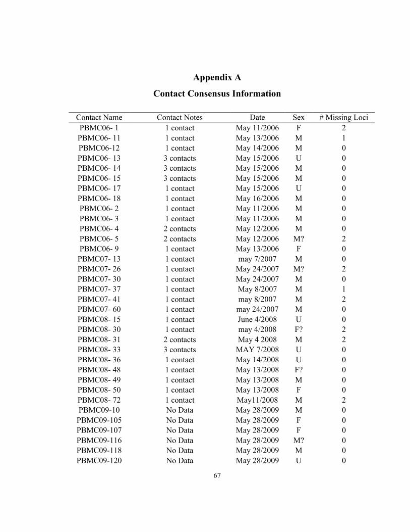
67
Appendix A
Contact Consensus Information
Contact Name Contact Notes Date Sex # Missing Loci PBMC06- 1 1 contact May 11/2006 F 2 PBMC06- 11 1 contact May 13/2006 M 1 PBMC06-12 1 contact May 14/2006 M 0 PBMC06- 13 3 contacts May 15/2006 U 0 PBMC06- 14 3 contacts May 15/2006 M 0 PBMC06- 15 3 contacts May 15/2006 M 0 PBMC06- 17 1 contact May 15/2006 U 0 PBMC06- 18 1 contact May 16/2006 M 0 PBMC06- 2 1 contact May 11/2006 M 0 PBMC06- 3 1 contact May 11/2006 M 0 PBMC06- 4 2 contacts May 12/2006 M 0 PBMC06- 5 2 contacts May 12/2006 M? 2 PBMC06- 9 1 contact May 13/2006 F 0 PBMC07- 13 1 contact may 7/2007 M 0 PBMC07- 26 1 contact May 24/2007 M? 2 PBMC07- 30 1 contact May 24/2007 M 0 PBMC07- 37 1 contact May 8/2007 M 1 PBMC07- 41 1 contact may 8/2007 M 2 PBMC07- 60 1 contact may 24/2007 M 0 PBMC08- 15 1 contact June 4/2008 U 0 PBMC08- 30 1 contact may 4/2008 F? 2 PBMC08- 31 2 contacts May 4 2008 M 2 PBMC08- 33 3 contacts MAY 7/2008 U 0 PBMC08- 36 1 contact May 14/2008 U 0 PBMC08- 48 1 contact May 13/2008 F? 0 PBMC08- 49 1 contact May 13/2008 M 0 PBMC08- 50 1 contact May 13/2008 F 0 PBMC08- 72 1 contact May11/2008 M 2 PBMC09-10 No Data May 28/2009 M 0 PBMC09-105 No Data May 28/2009 F 0 PBMC09-107 No Data May 28/2009 F 0 PBMC09-116 No Data May 28/2009 M? 0 PBMC09-118 No Data May 28/2009 M 0 PBMC09-120 No Data May 28/2009 U 0

68
PBMC09-126 1 contact May 7/2009 U 2 PBMC09-133 1 contact May 7/2009 M 0 PBMC09-135 1 contact May 11/2009 U 1 PBMC09-139 1 contact May 11/2009 M 0 PBMC09-149 1 contact May 11/2009 F 0 PBMC09-151 No Data May 12/2009 F? 0 PBMC09-157 No Data May 12/2009 M 1 PBMC09-159 No Data May 12/2009 M 0 PBMC09-16 No Data May 28/2009 M 1 PBMC09-162 No Data May 12/2009 M 0 PBMC09-165 No Data May 12/2009 F? 0 PBMC09-175 1 contact May 28/2009 U 2 PBMC09-18 No Data May 28/2009 M 1 PBMC09-185 1 contact May 28/2009 U 1 PBMC09-192 1 contact May 28/2009 M 1 PBMC09-193 1 contact May 28/2009 M 0 PBMC09-194 1 contact May 28/2009 M 0 PBMC09-2 1 contact May 28/2009 F 1
PBMC09-229 1 contact May 17/2009 M 0 PBMC09-23 No Data May 28/2009 F 0 PBMC09-232 No Data May 20/2009 M 0 PBMC09-242 No Data May 20/2009 M 0 PBMC09-25 No Data May 28/2009 F 0 PBMC09-26 No Data May 28/2009 M 0 PBMC09-281 No Data May 21/2009 M 1 PBMC09-285 No Data May 21/2009 U 0 PBMC09-296 No Data May 21/2009 M? 0 PBMC09-30 No Data May 28/2009 M 0 PBMC09-302 No Data May 21/2009 M? 0 PBMC09-314 1 contact May 15/2009 M 0 PBMC09-317 1 contact may 17/2009 M 0 PBMC09-36 No Data May 28/2009 M 1 PBMC09-41 No Data May 28/2009 M 0 PBMC09-46 No Data May 28/2009 F 0 PBMC09-50 No Data May 28/2009 M 0 PBMC09-54 No Data May 28/2009 M 0 PBMC09-56 No Data May 28/2009 M 0 PBMC09-6 No Data May 28/2009 U 2 PBMC09-65 No Data May 28/2009 F 0 PBMC09-67 No Data May 28/2009 M 0

69
PBMC09-68 No Data May 28/2009 U 1 PBMC09-73 No Data May 28/2009 M 0 PBMC09-76 No Data May 28/2009 F? 0 PBMC09-80 No Data May 28/2009 M 0 PBMC09-81 No Data May 28/2009 M 0 PBMC09-82 No Data May 28/2009 F? 0 PBMC09-85 No Data May 28/2009 M 0 PBMC09-91 No Data May 28/2009 M 1
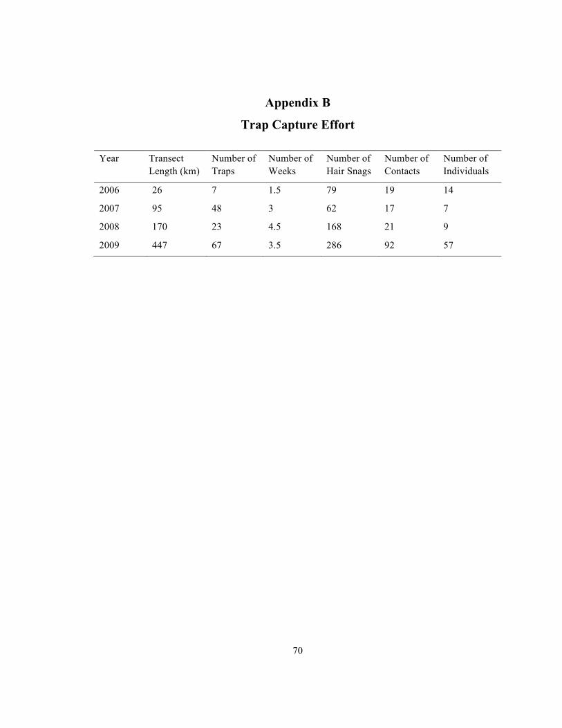
70
Appendix B
Trap Capture Effort
Year Transect Length (km)
Number of Traps
Number of Weeks
Number of Hair Snags
Number of Contacts
Number of Individuals
2006 26 7 1.5 79 19 14
2007 95 48 3 62 17 7
2008 170 23 4.5 168 21 9
2009 447 67 3.5 286 92 57