Energy Procedia 63 ( 2014 ) 4684 – 4707

Available online at www.sciencedirect.com

ScienceDirect

1876-6102 © 2014 The Employers. Published by Elsevier Limited. This is an open access article under the CC BY-NC-ND license (http://creativecommons.org/licenses/by-nc-nd/3.0/).Peer-review under responsibility of the Organizing Committee of GHGT-12doi: 10.1016/j.egypro.2014.11.502

GHGT-12

Geochemical impacts of carbon dioxide, brine, trace metal and organic leakage into an unconfined, oxidizing limestone aquifer

Diana H. Bacona,*, Zhenxue Daib, Liange Zhengc

aPacific Northwest National Laboratory, Richland, Washington, USA bLos Alamos National Laboratory, Los Alamos, New Mexico, USA

cLawrence Berkeley National Laboratory, Berkeley, California, USA

Abstract

An important risk at CO2 storage sites is the potential for groundwater quality impacts. As part of a system to assess the potential for these impacts a geochemical scaling function has been developed, based on a detailed reactive transport model of CO2 and brine leakage into an unconfined, oxidizing carbonate aquifer. Stochastic simulations varying a number of geochemical parameters were used to generate a response surface predicting the volume of aquifer that would be impacted with respect to regulated contaminants. The brine was assumed to contain several trace metals and organic contaminants. Aquifer pH and TDS were influenced by CO2 leakage, while trace metal concentrations were most influenced by the brine concentrations rather than adsorption or desorption on calcite. Organic plume sizes were found to be strongly influenced by biodegradation. © 2013 The Authors. Published by Elsevier Ltd. Selection and peer-review under responsibility of GHGT.

Keywords: geochemistry; limestone; trace metals; calcite adsorption; STOMP; reactive transport.

1. Introduction

The National Risk Assessment Partnership (NRAP) is a U.S. Department of Energy program to develop and demonstrate a methodology and toolset for predicting long-term risk profiles needed for quantifying potential liabilities at a carbon dioxide (CO2) storage project. Five national laboratories participate in the partnership: the National Energy Technology Laboratory, Lawrence Berkeley National Laboratory, Los Alamos National Laboratory

* Corresponding author. Tel.: +1-509-372-6132; fax: +1-509-372-6089. E-mail address: diana.bacon@pnnl.gov

© 2014 The Employers. Published by Elsevier Limited. This is an open access article under the CC BY-NC-ND license (http://creativecommons.org/licenses/by-nc-nd/3.0/).Peer-review under responsibility of the Organizing Committee of GHGT-12

Diana H. Bacon et al. / Energy Procedia 63 ( 2014 ) 4684 – 4707 4685

(LANL), Lawrence Livermore National Laboratory (LLNL) and Pacific Northwest National Laboratory (PNNL). The approach taken by NRAP is to first divide the system into components, including injection target reservoirs, wellbores, natural pathways including faults and fractures, groundwater, and the atmosphere. Next, a detailed, physics- and chemistry-based model of each component is developed. Using the results of the detailed models, efficient, simplified models, termed reduced order models (ROMs) are developed for each component. Finally, the component ROMs are integrated into a system model that calculates risk profiles for the site.

A groundwater component model was developed based on a portion of the unconfined, oxidizing carbonate Edwards Aquifer of south-central Texas. For practical reasons of computational efficiency, two sets of detailed multiphase reactive-transport simulations were performed separately: one varying complex hydrogeology factors and assuming simple geochemistry, the other with a single realization of hydrogeologic parameters and varying detailed geochemical parameters. These results were combined into a single groundwater ROM that considered both hydrogeologic and geochemical factors that might be expected to influence the fate and transport of brine and carbon dioxide (CO2) in a shallow aquifer. This paper details the detailed geochemical simulations used to develop a geochemistry scaling function to link the two sets of simulations.

The approach used to develop the groundwater ROM for the Edwards Aquifer was to develop complex models of groundwater flow and reactive transport in the shallow, urban, unconfined portion of the aquifer near San Antonio, Texas. Brine and CO2 leak rates were applied at the base of the aquifer using a generalized wellbore leakage function provided by LLNL. The brine was assumed to contain sodium (Na), chloride (Cl), arsenic (As), barium (Ba), cadmium (Cd), lead (Pb), benzene, naphthalene and phenol. Simulation results were post-processed to calculate volumes of groundwater exceeding regulatory thresholds for pH, total dissolved solids (TDS), As, Ba, Cd, Pb, benzene, naphthalene and phenol plumes.

The geochemical scaling functions were developed using a set of complex reactive-transport simulations performed using the STOMP (Subsurface Transport Over Multiple Phases) simulator, under a single set of hydraulic conditions. The STOMP models included equilibrium, kinetic mineral, and adsorption reactions related to the carbonate and clay minerals in the aquifer reacting with major ions and trace metals in groundwater, as well as CO2and brine leaking from the wellbore. To facilitate the development of the geochemical linking functions, a model was also developed using a simpler geochemical reaction network, similar to that used in developing the hydraulic response surface for the Edwards Aquifer, where the trace metals and organics were considered nonreactive solutes. Both models were run for the same set of input parameters in order to determine the relationship between plume sizes predicted using the simple and complex geochemistry.

To provide a basis for response surface development, model input parameters were varied using Latin hypercube sampling for each of these suites of simulations. The geochemical suite included 512 runs with both the simple and complex geochemical reaction networks. Polynomial nonlinear regression was used to interpolate the response surfaces for these suites of simulations. These fitted polynomial or spline functions are the basis of the groundwater ROM for the Edwards Aquifer that predicts the pH, TDS, trace-metal and organic plume sizes.

2. Methods

2.1. Numerical Simulator

The simulations conducted for this investigation were executed with the STOMP-CO2 (water, CO2, salt) simulator [1]. Partial differential conservation equations for fluid mass and salt mass compose the fundamental equations for STOMP-CO2. Coefficients within the fundamental equations are related to the primary variables through a set of constitutive relations. The conservation equations for fluid mass and energy are solved simultaneously, whereas the salt transport equations are solved sequentially after the coupled flow solution. The fundamental coupled flow equations are solved following an integral volume finite-difference approach with the nonlinearities in the discretized equations resolved through Newton-Raphson iteration.

The dominant nonlinear functions within the STOMP simulator are the relative permeability-saturation-capillary pressure (k-s-p) relations. The STOMP simulator allows the user to specify these relations through a large variety of popular and classic functions. Two-phase (gas-aqueous) k-s-p relations can be specified with hysteretic or nonhysteretic functions or nonhysteretic tabular data. Entrapment of CO2 with imbibing water conditions can be

4686 Diana H. Bacon et al. / Energy Procedia 63 ( 2014 ) 4684 – 4707

modeled with the hysteretic two-phase k-s-p functions [2]. Two-phase k-s-p relations span both saturated and unsaturated conditions. The aqueous phase is assumed to never completely disappear through extensions to the s-p function below the residual saturation and a vapor pressure-lowering scheme. Supercritical CO2 has the role of a gas in these two-phase k-s-p relations.

The chemistry module ECKEChem (Equilibrium-Conservation-Kinetic-Equation Chemistry) solves mass balance equations, mass action equations, and kinetic equations simultaneously using the Newton-Raphson approach [3]. STOMP has been verified against other codes used for simulation of geologic disposal of CO2 as part of the GeoSeq code comparison study [4], and has been used in previous investigations of CO2 injection potential at several sites [5-7].

2.2. Grid

A three-dimensional, heterogeneous model of groundwater flow and reactive transport in the Edwards Aquifer is focused on a shallow, unconfined portion of the aquifer near San Antonio, Texas. The aquifer is assumed to be 150 m thick, and we focus on an 8-km × 5-km area (Figure 1). The grid is refined at the assumed leak point at X = 2500 m, Y = 7000 m. There are 38 grid cells in the X direction, 35 cells in the Y direction and 10 cells in the Z direction.

Figure 1. Three-dimensional model grid of the Edwards Aquifer used to develop geochemical scaling function

2.3. Hydraulic Properties

A three-dimensional stochastic realization of porosity (Figure 2) and permeability (Figure 3) was used for the model domain.

Diana H. Bacon et al. / Energy Procedia 63 ( 2014 ) 4684 – 4707 4687

Figure 2. Porosity distribution in the Edwards Aquifer used to develop geochemical scaling function

Figure 3. X-direction intrinsic permeability (darcys) in the Edwards Aquifer used to develop geochemical scaling function

2.4. Geochemical Reactions

In order to develop the geochemical scaling function, two reaction networks were developed. The first, hereafter referred to as the simple geochemistry reaction network, is equivalent to the geochemical reactions used in developing the hydraulic ROM. The second, hereafter referred to as the complex geochemistry reaction network, contains a larger set of equilibrium aqueous, kinetic mineral and surface complexation reactions. The scaling function is designed to calculate the ratio between plume sizes calculated using complex and simple geochemistry.

The simple geochemical reaction network is based on simple carbonate equilibria in order to calculate the pH (Table 1). The equilibrium coefficients were taken from the THEMODDEM database [8]. To develop the complex geochemical reaction network, 90 water samples from the Edwards Aquifer [9] were modeled with the PHREEQC program [10] using the THEMODDEM database [8] to determine the significant equilibrium aqueous reactions involving the elements Ca, Mg, Na, Cl, S, O, C, P, As, Ba, Cd, and Pb. The relevant equilibrium aqueous reactions are listed in Table 2.

4688 Diana H. Bacon et al. / Energy Procedia 63 ( 2014 ) 4684 – 4707

Table 1. Equilibrium aqueous reactions for simple geochemistry

Equilibrium Reaction Equilibrium Coefficient at 25°C, log H2O = OH- + H+ 14.001HCO3

- + H+ = CO2 + H2O 6.353 HCO3

- = CO32- + H+ 10.327

The Edwards limestone consists mostly of calcite and dolomite [11], but little information is available on the minor minerals in the limestone. Samples obtained recently from the surficial aquifer in the study area consist mostly of calcite. For the complex geochemical reaction network, the aquifer is assumed to consist entirely of calcite with witherite, cerussite, otavite, dolomite, and calcium arsenate included as potential secondary minerals (Table 3). For the simple geochemical reaction network, only calcite precipitation and dissolution is considered.

Surface complexation reactions for relevant cations and anions on calcite were included in the complex geochemical reaction network for the Edwards Aquifer. A surface complexation model for calcite was first presented by van Cappellen, Charlet, Stumm and Wersin [12] and further developed for divalent cations [13], and then extended to arsenate [14] and phosphate [15]. The model has two types of surface sites, >Ca+ and >CO3

-, each with a density of 8.22 mol/m2. Cations are assumed to sorb to the >CO3

- sites (Table 4), and anions to the >Ca+ sites (Table 5). Surface complexation reactions are not considered in the simple geochemical reaction network.

Three organic compounds, (benzene, naphthalene and phenol), are included in the model. Benzene is included as a representative of benzene, toluene, ethylbenzene, and xylenes (BTEX), naphthalene as a representative of polycyclic aromatic hydrocarbons (PAHs), and phenol as a representative of phenols. BTEX, phenols and PAHs have been identified as the organic compounds that are most likely to be leached out along with CO2 and posed threats on the shallow groundwater [16, 17]. The adsorption of the organic compounds is assumed to be controlled by a linear adsorption isotherm, proportional to the organic carbon content of the aquifer material. The organic carbon content of the limestone aquifer is assumed to range between 0.1 and 1% by volume. Adsorption and biodegradation of organic compounds (Table 6) is not considered in the simple geochemical reaction network.

The concentration of NaCl, trace metals and organics in the brine are assumed to be uncertain variables, with ranges shown in Table 7.

2.5. Boundary Conditions

Groundwater flows into the domain at the north boundary (Y = 8 km) at a rate that varies with permeability. A horizontal pressure gradient of 8.5×10-6 MPa/m in the Y direction is based on observed heads [18]. The south boundary (Y = 0) is an outflow boundary. The east (X = 5 km) and west (X = 0) boundaries are no-flow. The bottom boundary is no-flow, except for the CO2 and brine leaks at X = 2.5 km, Y = 7 km. The top boundary is the water table, which is a no-flow boundary for the liquid phase, but is a constant-pressure boundary of 0.101325 MPa (atmospheric pressure) for the gas phase. The species concentrations on the inflow boundary are the same as the initial conditions.

2.6. Initial Conditions

Initial conditions for pH, H2AsO4-, Ba2+, Cd2+, Pb2+, benzene, naphthalene and phenol and other aqueous species

were based on the median aqueous concentrations for the 90 groundwater samples from the shallow, urban, unconfined portion of the Edwards Aquifer [9, 19].

Diana H. Bacon et al. / Energy Procedia 63 ( 2014 ) 4684 – 4707 4689

Table 2. Equilibrium aqueous reactions for complex geochemistry

Equilibrium Reaction Equilibrium Coefficient at 25°C, log

Ba2+ + HCO3- = Ba(HCO3)+ 1.034

Ca2+ + H2PO4- = CaH2PO4

+ 1.500

Ca2+ + H2PO4- = CaHPO4 + H+ 4.370

Ca2+ + H2PO4- = CaPO4

- + 2H+ 13.110

Ca2+ + SO42- = CaSO4 2.310

Cd2+ + Cl- = CdCl+ 1.970

Cd2+ + H2PO4- = CdHPO4 + H+ 2.380

Cd2+ + SO42- = CdSO4 3.440

H2AsO4- + Ca2+ = CaH2AsO4

+ 1.398

H2AsO4- + Ca2+ = CaHAsO4 + H+ 4.080

H2AsO4- + Mg2+ = MgH2AsO4

+ 1.512

H2AsO4- + Mg2+ = MgHAsO4 + H+ 4.539

H2AsO4- = HAsO4

2- + H+ 6.960

H2O = OH- + H+ 14.001

H2PO4- = HPO4

2- + H+ 7.212

HCO3- + Ca2+ = Ca(HCO3)+ 1.103

HCO3- + Cd2+ = CdCO3 + H+ 5.627

HCO3- + Cd2+ = CdHCO3

+ 1.503

HCO3- + H+ = H2CO3 + H2O 6.353

HCO3- + Mg2+ = Mg(HCO3)+ 1.038

HCO3- + Na+ = NaHCO3 0.247

HCO3- + Pb2+ = Pb(CO3) + H+ 3.327

HCO3- + Pb2+ = PbHCO3

+ 3.443

HCO3- = CO3

2- + H+ 10.327

Mg2+ + H2PO4- = MgH2PO4

+ 1.170

Mg2+ + H2PO4- = MgHPO4 + H+ 4.303

Mg2+ + SO42- = MgSO4 2.230

Pb2++ H2O = PbOH+ + H+ 7.510

Pb2+ + SO42- = PbSO4 2.820

2HCO3- + Pb2+ = Pb(CO3)2

2- + 2H+ 10.524

4690 Diana H. Bacon et al. / Energy Procedia 63 ( 2014 ) 4684 – 4707

Table 3. Kinetic mineral reactions for complex geochemical reaction network

Kinetic Reaction Equilibrium Coefficient at 25°C, log

Forward Rate at 25°C, mol/m2/s

Activation Energy, kJ/mol

Calcite + H+ = HCO3- + Ca2+ 1.847 1.5E-6 23.5

Ca3(AsO4)2:3.66H2O + 4H+ = 2H2AsO4- + 3Ca2+ + 3.66H2O 16.774 5.0E-10 same as dolomite

Cerussite + H+ = HCO3- + Pb2+ 2.963 5.0E-11 same as dolomite

Dolomite(dis) + 2H+ = 2HCO3- + Ca2+ + Mg2+ 4.299 2.9E-8 52.2

Otavite + H+ = HCO3- + Cd2+ 1.773 3.0E-11 same as dolomite

Witherite = Ba2+ + CO32- 1.765 2.9E-8 same as dolomite

Table 4. Surface complexation reactions of cations on calcite

Reactions Log kint

>CO3H0 + Ca2+ = >CO3Ca+ + H+ 1.7>CO3H0 + Mg2+ = >CO3Mg+ + H+ 2.2>CO3H0 + Ba2+ = >CO3Ba+ + H+ 2.5>CO3H0 + Cd2+ = >CO3Cd+ + H+ 1.8>CO3H0 + Pb2+ = >CO3Pb+ + H+ 2.4

Table 5. Surface complexation reactions of anions on calcite

Reactions Log kint

>CaCO3- + H2AsO4

- = >CaHAsO4- + H+ + CO3

2- 8.97>CaCO3

- + CaHAsO40 = >CaAsO4Ca0 + H+ + CO3

2- 9.07>CaCO3

- + HPO42- = >CaHPO4

- + CO32- 1.75

>CaCO3- + CaPO4

- = >CaPO4Ca0 + CO32- 0.79

Table 6. Input parameters for organic adsorption and biodegradation

Description Minimum Maximum Units Reference Organic carbon volume fraction 0.001 0.01 — Benzene organic carbon partition coefficient 30.90 53.70 L/kg [20] Naphthalene organic carbon partition coefficient 9.93 954.99 L/kg [20] Phenol organic carbon partition coefficient 16.1 30.2 L/kg [21, 22] Benzene aerobic biodegradation rate 1.00E-03 4.95E-01 day-1 [23] Naphthalene aerobic biodegradation rate 6.40E-03 5.00E+00 day-1 [23] Phenol aerobic biodegradation rate 6.00E-03 1.00E+01 day-1 [23]

Table 7. Brine concentration ranges

Species in Brine Minimum Maximum Units Chloride 5.00E-01 5.40E+00 mol/L Arsenic 1.00E-09 1.00E-05 mol/L Barium 7.94E-06 5.01E-03 mol/L Cadmium 1.00E-09 1.00E-06 mol/L Lead 3.16E-09 1.00E-05 mol/L Benzene 1.00E-10 6.31E-04 mol/L Naphthalene 1.00E-10 7.94E-05 mol/L

Diana H. Bacon et al. / Energy Procedia 63 ( 2014 ) 4684 – 4707 4691

Table 8. Initial aqueous species concentrations

Species Concentration Unit HCO3

- 4.00E-04 Aqueous Mass Fraction Ca2+ 2.48E-03 mol/liter Cl- 3.31E-04 mol/liter pH 6.86 -- Mg2+ 3.17E-04 mol/liter Na+ 3.34E-04 mol/liter HPO4

2- 1.32E-06 mol/liter SO4

2- 3.47E-04 mol/liter H2AsO4

- 4.19E-09 mol/liter Ba2+ 2.62E-07 mol/liter Cd2+ 3.56E-13 mol/liter Pb2+ 3.09E-10 mol/liter Benzene 0 mol/liter Naphthalene 0 mol/liter Phenol 0 mol/liter

2.7. Generalized Wellbore Leak Model

A generalized wellbore leak model was used to generate the CO2 and brine source terms for the groundwater flow and reactive-transport simulations described in following sections. The generalized wellbore leak model was developed based on output from the Generation II Wellbore Leakage ROM [24]. The generalized wellbore leak model has several input parameters, shown diagrammatically in Figure 4. The input parameter ranges are listed in Table 9. Note that T2c = T1c + dT2c, T3c = T2c + dT3c, and T2b = T1b + dT2b.

The outputs of the wellbore leak ROM are the CO2 leakage rate and the brine leakage rate, both in units of kilograms per second. The CO2 leak rate and the brine leak rate vs. time for median values of the well-leak ROM input parameters are shown in Figure 5 and Figure 6, respectively.

3. Results

A base-case simulation was run using the median value of each model parameters described in the methods section (Table 10). The calcite specific surface area is assumed to be 5.5 cm2/g and the organic carbon volume fraction is assumed to be 0.55%. The output variables to be considered are the volume, length, width and height of plumes delineated by the threshold values that were defined as either the no-impact limits [19] or the drinking water MCLs, both of which are listed in Table 11.

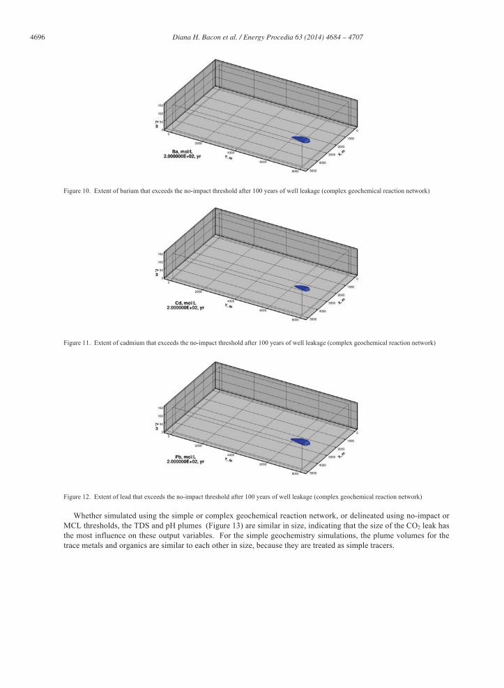
As CO2 leaks into the aquifer, the pH is lowered from a background value of 6.86 to a minimum value of 4.86 (Figure 7). The decrease in pH drives the dissolution of calcite, increasing aqueous concentrations of calcium and carbonate. In addition, the brine leak increases the concentrations of sodium and chloride as well as the trace metals. As a result, both the CO2 and brine leaks contribute to an increase in TDS (Figure 8), with the extent of the TDS plume similar in shape to that of the pH plume. Arsenic (Figure 9), barium (Figure 10), cadmium (Figure 11) and lead (Figure 12) plumes are relatively small, representing the extent of the brine leak.

4692 Diana H. Bacon et al. / Energy Procedia 63 ( 2014 ) 4684 – 4707

Figure 4. Input parameters for the generalized wellbore leak model

Table 9. Input parameter ranges for the generalized wellbore leak model

Parameter Description Minimum Maximum Units qCO2 Maximum CO2 leakage rate 0.001 0.5 kg s-1

qBRN Maximum brine leakage rate 0.005 0.075 kg s-1

Ratio of brine-leakage tail to qBRN 0.2 0.3 T1c End of first CO2 leak period 5 50 yr dT2c Duration of second CO2 leak period 0 100 yr dT3c Duration of third CO2 leak period 5 50 yr T1b End of first brine leak period 1 50 yr dT2b Duration of second brine leak period 1 10 yr Tm Mitigation time 0.5 200 yr

Diana H. Bacon et al. / Energy Procedia 63 ( 2014 ) 4684 – 4707 4693

Figure 5. CO2 leakage rate for median values of the generalized wellbore leak model input parameters

Figure 6. Brine leakage rate for median values of the generalized wellbore leak model input parameters

4694 Diana H. Bacon et al. / Energy Procedia 63 ( 2014 ) 4684 – 4707

Table 10. Input parameters for the base-case simulation

Description Value Units

Maximum CO2 leakage rate 2.24E-02 kg s-1

Maximum brine leakage rate 1.94E-02 kg s-1

Ratio of brine-leakage tail to maximum rate 2.50E-01 End of first CO2 leak period 2.75E+01 yr Duration of second CO2 leak period 5.00E+01 yr Duration of third CO2 leak period 2.75E+01 yr End of first brine leak period 2.55E+01 yr Duration of second brine leak period 5.50E+00 yr Mitigation time 1.00E+02 yr Chloride concentration in brine 1.64E+00 mol/L Arsenic concentration in brine 1.00E-07 mol/L Barium concentration in brine 2.00E-04 mol/L Cadmium concentration in brine 3.16E-08 mol/L Lead concentration in brine 1.78E-07 mol/L Benzene concentration in brine 2.51E-07 mol/L Naphthalene concentration in brine 8.91E-08 mol/L Phenol concentration in brine 1.41E-07 mol/L Calcite specific surface area 5.50E-03 m2/gOrganic carbon volume fraction 5.50E-03 — Benzene organic carbon partition coefficient 4.07E+01 L/kg Naphthalene organic carbon partition coefficient 9.55E+02 L/kg Phenol organic carbon partition coefficient 2.21E+01 L/kg Benzene aerobic biodegradation rate 3.13E+01 day-1 Naphthalene aerobic biodegradation rate 3.94E+00 day-1 Phenol aerobic biodegradation rate 2.63E+00 day-1

Table 11. Threshold levels

Species No-Impact MCL Unit

pH < 6.6 < 6.5

TDS > 420 > 500 mg/L

As > 7.34E-09 > 1.33E-07 mol/L

Ba > 3.93E-07 > 1.46E-05 mol/L

Cd > 3.56E-10 > 4.45E-08 mol/L

Pb > 7.24E-10 > 7.24E-08 mol/L

Benzene > 2.05E-10 > 6.40E-08 mol/L

Naphthalene > 3.12E-09 > 1.56E-09 mol/L

Phenol > 5.31E-11 > 1.06E-04 mol/L

Diana H. Bacon et al. / Energy Procedia 63 ( 2014 ) 4684 – 4707 4695

Figure 7. Extent of pH that exceeds the no-impact threshold after 100 years of well leakage (complex geochemical reaction network)

Figure 8. Extent of TDS that exceeds the no-impact threshold after 100 years of well leakage (complex geochemical reaction network)

Figure 9. Extent of arsenic that exceeds the no-impact threshold after 100 years of well leakage (complex geochemical reaction network)

4696 Diana H. Bacon et al. / Energy Procedia 63 ( 2014 ) 4684 – 4707

Figure 10. Extent of barium that exceeds the no-impact threshold after 100 years of well leakage (complex geochemical reaction network)

Figure 11. Extent of cadmium that exceeds the no-impact threshold after 100 years of well leakage (complex geochemical reaction network)

Figure 12. Extent of lead that exceeds the no-impact threshold after 100 years of well leakage (complex geochemical reaction network)

Whether simulated using the simple or complex geochemical reaction network, or delineated using no-impact or MCL thresholds, the TDS and pH plumes (Figure 13) are similar in size, indicating that the size of the CO2 leak has the most influence on these output variables. For the simple geochemistry simulations, the plume volumes for the trace metals and organics are similar to each other in size, because they are treated as simple tracers.

Diana H. Bacon et al. / Energy Procedia 63 ( 2014 ) 4684 – 4707 4697

Figure 13. TDS and pH plume volumes due to abandoned well leakage

Some of the trace-metal plume sizes are influenced by adsorption on calcite and mineral precipitation. The arsenic plume size, delineated by the no-impact threshold, is smaller at 200 years for the complex geochemistry simulation than for the simple simulation (Figure 14) due to adsorption on calcite. Arsenic does not exceed the MCL threshold for this simulation for either the simple or complex geochemistry cases. The barium plume size, delineated by the no-impact threshold, is smaller at 200 years for the complex geochemistry simulation than for the simple simulation due to adsorption on calcite and precipitation of witherite. The barium plume sizes are significantly smaller when delineated by the MCL threshold, and in the case of the complex geochemistry simulation, can be seen to be shrinking after the mitigation time of 100 years. The cadmium plume sizes are not significantly different for the simple and complex geochemistry cases, and do not exceed the MCL threshold in either case. Although Cd2+ is the most prevalent cadmium species, there are significant amounts of cadmium found in aqueous carbonate and sulfate complexes, relative to the amount sorbed on calcite. The lead plume volumes are also not significantly different for the simple and complex geochemistry cases. Lead is found in greater amounts as lead-carbonate complexes than is adsorbed on the >CO3

- adsorption sites. Lead does exceed the MCL threshold in both the simple and complex geochemistry cases, although the plume shrinks after the mitigation time of 100 years and all lead concentrations are below the MCL threshold at 200 years.

A comparison of the complex and simple geochemistry cases shows that the organic compounds are influenced significantly by biodegradation. Benzene does not exceed the MCL threshold for the complex geochemistry case, and all benzene concentrations fall below the no-impact threshold directly after the mitigation time of 100 years (Figure 15). Naphthalene does not exceed either threshold throughout the duration of the complex geochemistry simulation due to its high adsorption coefficient. Phenol does not exceed the MCL threshold for the complex geochemistry case, and all phenol concentrations fall below the no-impact threshold directly after the mitigation time of 100 years.

3.1. Geochemical Scaling Functions

The purpose of the geochemical scaling function is to correct the plume volumes predicted by simple geochemistry based on more complex geochemistry. The input parameters for the geochemistry scaling function are shown in Table 12. The first 9 parameters are used as input to the wellbore leak ROM, and parameters 10-25 are used as input to STOMP. To determine the relationship between the complex and simple geochemistry models for the Edwards Aquifer, 512 simulations were run using each reaction network. Latin hypercube sampling was used to

4698 Diana H. Bacon et al. / Energy Procedia 63 ( 2014 ) 4684 – 4707

generate 512 samples of the parameters for input into STOMP. The first geochemical parameters were assumed to have a uniform or log-uniform distribution as shown in Table 12. The simulations were run for 200 years.

Figure 14. Trace metal plume volumes due to abandoned well leakage. Arsenic does not exceed the MCL threshold for the complex simulation. Cadmium does not exceed the MCL threshold for either the simple or complex simulation.

After 512 simulations were run for both the simple and complex geochemistry reaction networks, thirty-seven output variables were calculated at 10-year intervals to construct the response surfaces (Table 13). Volumes and spatial dimensions of plumes exceeding either the no-impact or MCL threshold values for TDS, pH, trace metals (arsenic, barium, cadmium, lead) and organics (benzene, naphthalene, phenol) were calculated for both the simple and complex geochemistry cases.

The next step was to perform some transformations on the response surfaces to facilitate scaling with the wellbore leakage ROM. Each of the 37 output variables was recorded at 21 different times, from 0 to 200 years in 10-year increments. Because of this, the original response surface had 37 variables × 21 times = 777 output variables. The response surface was transformed so that time became an additional input parameter, and the output variables became functions of time. The transformed response surface then effectively had 512 × 21 = 10,752 input samples, one additional input parameter (time) for a total of 26, and only 37 output variables.

Diana H. Bacon et al. / Energy Procedia 63 ( 2014 ) 4684 – 4707 4699

A second transformation of the response surface input parameters was performed to decouple the well leak ROM from the groundwater geochemistry ROM. For a given input sample at a particular time, input parameters 1–9 from Table 12were used to run the wellbore leak ROM and to calculate the CO2 leak rate, the brine leak rate, as well as the cumulative mass of CO2 and brine leaked up to that time. These four values then became four new input parameters, replacing the nine input parameters used as input to the well leak ROM. After this second transformation, the response surfaces for the simple and complex geochemistry each had 26 – 9 + 4 = 21 input parameters. A third and final transformation was applied in order to develop the geochemical scaling function, which is just the relationship between the value of a given output variable predicted by the complex and simple geochemistry reaction networks. For each parameter sample, the value of an output variable predicted by the simple geochemistry reaction network was added as an additional input parameter to the response surface for the complex geochemistry reaction network. So in the end there are 22 input parameters for the geochemical scaling function response surface for each output variable: parameters 10-25 from Table 12, time, the CO2 leak rate, the brine leak rate, as well as the cumulative mass of CO2 and brine leaked up to that time, and the output variable value predicted by the simple geochemical reaction network.

A polynomial curve fit to the geochemical scaling function response surfaces using quadratic polynomial regression. Each of the output variables was regressed against the input parameters to determine the coefficients for the linear terms of the polynomial equations that minimized the sum of squared error between the observed and predicted output variables. The output variables were designated as Y1 to Y37, the input parameters were designated as X1 through X22, and the fitting coefficients as a:

Yk = + ai,j,kXiXj + ai,i,kXi2, where i = 1,22 and j=1,22 and k = 1,37

The goodness-of-fit (R2) for each output variable is shown in Table 13. In general the R2 values were high for the TDS (Figure 16), pH (Figure 17) and arsenic (Figure 18) and cadmium (Figure 20) plume volumes. The fit was less good for barium (Figure 19) due to the nonlinear effect of mineral precipitation. The no-impact threshold fit was less good for lead (Figure 21) because this limit is relatively close to the background value. The goodness-of-fit for the benzene (Figure 22), naphthalene (Figure 23) and phenol (Figure 24) plumes was the lowest, because they are very small in size relative to the simple geochemistry cases. In fact, none of the phenol plumes exceeded the relatively high MCL threshold.

4. Discussion

In this oxidizing, unconfined carbonate aquifer, plume sizes of pH and TDS beyond the MCL and no-impact threshold are predicted to be correlated with the size of the CO2 leak, due to dissolution of gaseous CO2 and calcite. Conversely, trace metal concentrations are more closely related to the size of the brine leak, with adsorption of trace metals from the brine leak predicted to be more likely than desorption of trace metals due to lowered pH. Biodegradation of benzene, naphthalene and phenol is predicted to have the most influence on organic plume size.

The geochemical scaling function ROM predicts the plume sizes based on complex geochemistry, relative to the plume size predicted by simple geochemistry. The predictions of the ROM compare favorably with those of a reactive transport model developed using STOMP, but run in a much shorter amount of time. This computational efficiency makes the ROM a useful part of NRAP’s system-scale risk assessment model.

Acknowledgements

The U.S. Department of Energy’s (DOE’s) Office of Fossil Energy has established the National Risk Assessment Partnership (NRAP). The research presented in this report was completed as part of the groundwater protection working group of NRAP. Funding was provided to PNNL under DOE contract number DE-AC05-76RL01830. A portion of the modeling research was performed using PNNL Institutional Computing at Pacific Northwest National Laboratory. This document has been approved for release from Pacific Northwest National Laboratory with information release number PNNL-SA-105080.

4700 Diana H. Bacon et al. / Energy Procedia 63 ( 2014 ) 4684 – 4707

Figure 15. Organic plume volumes due to abandoned well leakage. Phenol does not exceed the MCL threshold in either case. Naphthalene does not exceed either threshold for the complex case. Benzene does not exceed the MCL threshold for the complex geochemistry case.

Diana H. Bacon et al. / Energy Procedia 63 ( 2014 ) 4684 – 4707 4701

Table 12. Input parameters and their ranges for geochemical scaling function

Parameter Minimum Maximum Units Distribution Reference Maximum CO2 leakage rate 0.001 0.5 kg s-1 log uniform [24] Maximum brine leakage rate 0.005 0.075 kg s-1 log uniform [24] Ratio of brine-leakage tail to max rate 0.2 0.3 Uniform [24] End of first CO2 leak period 5 50 yr Uniform [24] Duration of second CO2 leak period 0 100 yr Uniform [24] Duration of third CO2 leak period 5 50 yr Uniform [24] End of first brine leak period 1 50 yr Uniform [24] Duration of second brine leak period 1 10 yr Uniform [24] Mitigation time 0.5 200 yr Uniform [24]

Chloride concentration in brine 5.00E-01 5.40E+00 mol/L log uniform [25]

Arsenic concentration in brine 1.00E-09 1.00E-05 mol/L log uniform [26]

Barium concentration in brine 7.94E-06 5.01E-03 mol/L log uniform [27, 28]

Cadmium concentration in brine 1.00E-09 1.00E-06 mol/L log uniform [26]

Lead concentration in brine 3.16E-09 1.00E-05 mol/L log uniform [26]

Benzene concentration in brine 1.00E-10 6.31E-04 mol/L log uniform [29]

Naphthalene concentration in brine 1.00E-10 7.94E-05 mol/L log uniform [29]

Phenol concentration in brine 1.00E-10 2.00E-04 mol/L log uniform [29] Calcite specific surface area 0.001 0.01 m2/g Uniform [30] Organic carbon volume fraction 0.001 0.01 --- UniformBenzene organic carbon partition coefficient

30.90 53.70 L/kg

log uniform [20]

Naphthalene organic carbon partition coefficient

9.93 954.99 L/kg

log uniform [20]

Phenol organic carbon partition coefficient

16.1 30.2 L/kg

log uniform [21, 22]

Benzene aerobic biodegradation rate 1.00E-03 4.95E-01 day-1 log uniform [23] Naphthalene aerobic biodegradation rate 6.40E-03 5.00E+00

day-1log uniform [23]

Phenol aerobic biodegradation rate 6.00E-03 1.00E+01 day-1 log uniform [23]

4702 Diana H. Bacon et al. / Energy Procedia 63 ( 2014 ) 4684 – 4707

Table 13. Output variables for geochemical scaling function, and their regression goodness-of-fit (R2)

Variable Unit R2 (No-Impact) R2 (MCL) Volume of TDS plume m3 9.55E-01 9.87E-01

Length of TDS plume M 7.04E-01 7.14E-01

Width of TDS plume M 7.15E-01 6.32E-01

Height of TDS plume M 9.97E-01 9.93E-01

Volume of pH plume m3 9.96E-01 9.99E-01

Length of pH plume M 9.76E-01 9.78E-01

Width of pH plume M 9.71E-01 9.74E-01

Height of pH plume M 9.94E-01 9.94E-01

Volume of arsenic plume m3 9.92E-01 9.68E-01

Length of arsenic plume M 9.69E-01 9.80E-01

Width of arsenic plume M 8.53E-01 9.87E-01

Height of arsenic plume M 9.13E-01 9.73E-01

Volume of barium plume m3 9.92E-01 8.81E-01

Length of barium plume M 9.65E-01 8.51E-01

Width of barium plume M 9.59E-01 8.75E-01

Height of barium plume M 8.41E-01 7.96E-01

Volume of cadmium plume m3 9.99E-01 1.00E+00

Length of cadmium plume M 9.86E-01 9.98E-01

Width of cadmium plume M 9.92E-01 9.99E-01

Height of cadmium plume M 9.83E-01 9.97E-01

Volume of lead plume m3 5.80E-01 1.00E+00

Length of lead plume M 7.20E-01 9.98E-01

Width of lead plume M 7.73E-01 9.99E-01

Height of lead plume M 6.56E-01 9.95E-01

Volume of benzene plume m3 7.12E-01 4.60E-01

Length of benzene plume M 8.40E-01 7.58E-01

Width of benzene plume M 8.45E-01 7.63E-01

Height of benzene plume M 6.90E-01 5.91E-01

Volume of naphthalene plume m3 5.60E-01 5.45E-01

Length of naphthalene plume M 7.07E-01 7.27E-01

Width of naphthalene plume M 6.98E-01 7.22E-01

Height of naphthalene plume M 7.18E-01 7.31E-01

Volume of phenol plume m3 5.30E-01 *

Length of phenol plume M 8.54E-01 *

Width of phenol plume M 8.53E-01 *

Height of phenol plume M 8.60E-01 *

*Phenol concentrations did not exceed the MCL threshold value, so all plume dimensions equal zero.

Diana H. Bacon et al. / Energy Procedia 63 ( 2014 ) 4684 – 4707 4703

Figure 16. Comparison of TDS plume size predicted by ROM and STOMP using MCL (left) and no-impact (right) limits

Figure 17. Comparison of pH plume size predicted by ROM and STOMP using MCL (left) and no-impact (right) limits

Figure 18. Comparison of As plume size predicted by ROM and STOMP using MCL (left) and no-impact (right) limits

4704 Diana H. Bacon et al. / Energy Procedia 63 ( 2014 ) 4684 – 4707

Figure 19. Comparison of Ba plume size predicted by ROM and STOMP using MCL (left) and no-impact (right) limits

Figure 20. Comparison of Cd plume size predicted by ROM and STOMP using MCL (left) and no-impact (right) limits

Figure 21. Comparison of Pb plume size predicted by ROM and STOMP using MCL (left) and no-impact (right) limits

Diana H. Bacon et al. / Energy Procedia 63 ( 2014 ) 4684 – 4707 4705

Figure 22. Comparison of benzene plume size predicted by ROM and STOMP using MCL (left) and no-impact (right) limits

Figure 23. Comparison of naphthalene plume size predicted by ROM and STOMP using MCL (left) and no-impact (right) limits

Figure 24. Comparison of phenol plume size predicted by ROM and STOMP using MCL (left) and no-impact (right) limits

4706 Diana H. Bacon et al. / Energy Procedia 63 ( 2014 ) 4684 – 4707

References

[1] M.D. White, D.H. Bacon, B.P. McGrail, D.J. Watson, S.K. White, Z.F. Zhang, STOMP Subsurface Transport Over Multiple Phases: STOMP-CO2 and STOMP-CO2e Guide: Version 1.0, in, Pacific Northwest National Laboratory, Richland, WA, 2012. [2] M.D. White, M. Oostrom, STOMP: Subsurface Transport Over Multiple Phases, Version 4.0, User's Guide, in, Pacific Northwest National Laboratory, Richland, Washington, 2006. [3] M.D. White, B.P. McGrail, STOMP, Subsurface Transport Over Multiple Phases, Version 1.0, Addendum: ECKEChem, Equilibrium-Conservation-Kinetic Equation Chemistry and Reactive Transport, in, Pacific Northwest National Laboratory, Richland, Washington, 2005. [4] K. Pruess, J. García, T. Kovscek, C. Oldenburg, J. Rutqvist, C. Steefel, T. Xu, Code intercomparison builds confidence in numerical simulation models for geologic disposal of CO2, Energy, 29 (2004) 1431-1444. [5] D.H. Bacon, J.R. Sminchak, J.L. Gerst, N. Gupta, Validation of CO2 Injection Simulations with Monitoring Well Data, Energy Procedia, 1 (2009) 1815-1822. [6] D.H. Bacon, M.D. White, N. Gupta, J.R. Sminchak, M.E. Kelley, CO2 Injection Potential in the Rose Run Formation at the Mountaineer Power Plant, New Haven, West Virginia, in: AAPG Studies in Geology # 59: Carbon Dioxide Sequestration in Geological Media - State of the Science, American Association of Petroleum Geologists, Tulsa, Oklahoma, 2009. [7] D.A. Barnes, D.H. Bacon, S.R. Kelley, Geological sequestration of carbon dioxide in the Cambrian Mount Simon Sandstone: Regional storage capacity, site characterization, and large-scale injection feasibility, Michigan Basin, Environmental Geosciences, 16 (2009) 163-183. [8] P. Blanc, A. Lassin, P. Piantone, M. Azaroual, N. Jacquemet, A. Fabbri, E.C. Gaucher, Thermoddem: a geochemical database focused on low temperature water/rock interactions and waste materials, Applied Geochemistry, 27 (2012) 2107-2116. [9] M. Musgrove, L. Fahlquist, N.A. Houston, R.J. Lindgren, P.B. Ging, Geochemical evolution processes and water-quality observations based on results of the National Water-Quality Assessment Program in the San Antonio segment of the Edwards aquifer, 1996-2006, in, U.S. Geological Survey, Washington, D.C., 2010. [10] D.L. Parkhurst, C.A.J. Appelo, User's guide to PHREEQC (Version 2) : a computer program for speciation, batch-reaction, one-dimensional transport, and inverse geochemical calculations, in, U.S. Geological Survey, Washington, D.C., 1999. [11] J.S. Pittman, Silica in Edwards Limestone, Travis County, Texas, in: Silica in Sediments, SEPM Society for Sedimentary Geology, Tulsa, Oklahoma, 1959. [12] P. van Cappellen, L. Charlet, W. Stumm, P. Wersin, A Surface Complexation Model of the Carbonate Mineral-Aqueous Solution Interface, Geochimica Et Cosmochimica Acta, 57 (1993) 3505-3518. [13] O.S. Pokrovsky, J. Schott, Surface chemistry and dissolution kinetics of divalent metal carbonates, Environmental Science & Technology, 36 (2002) 426-432. [14] H.U. Sø, D. Postma, R. Jakobsen, F. Larsen, Sorption and desorption of arsenate and arsenite on calcite, Geochimica et Cosmochimica Acta, 72 (2008) 5871-5884. [15] H.U. Sø, D. Postma, R. Jakobsen, F. Larsen, Sorption of phosphate onto calcite; results from batch experiments and surface complexation modeling, Geochimica et Cosmochimica Acta, 75 (2011) 2911-2923. [16] K.J. Cantrell, C.F. Brown, Source term modeling for evaluating the potential impacts to groundwater of fluids escaping from a depleted oil reservoir used for carbon sequestration, International Journal of Greenhouse Gas Control, 27 (2014) 139-145. [17] L.G. Zheng, N. Spycher, J. Birkholzer, T.F. Xu, J. Apps, Y. Kharaka, On modeling the potential impacts of CO2 sequestration on shallow groundwater: Transport of organics and co-injected H2S by supercritical CO2 to shallow aquifers, International Journal of Greenhouse Gas Control, 14 (2013) 113-127. [18] W.R. Hutchison, M.E. Hill, Recalibration of the Edwards (Balcones Fault Zone) Aquifer - Barton Springs Segment - Groundwater Flow Model, in, Texas Water Development Board, Austin, Texas, 2011. [19] G.V. Last, C.J. Murray, C.F. Brown, P.D. Jordan, M. Sharma, No-Impact Threshold Values for NRAP’s Reduced Order Models, in, Pacific Northwest National Laboratory, Richland, Washington, 2013, pp. 72. [20] S.J. Lawrence, Description, Properties, and Degradation of Selected Volatile Organic Compounds Detected in Ground Water — A Review of Selected Literature, in, U.S. Geological Survey, Reston, Virginia, 2006.

Diana H. Bacon et al. / Energy Procedia 63 ( 2014 ) 4684 – 4707 4707

[21] S.A. Boyd, D.R. Shelton, D. Berry, J.M. Tiedje, Anaerobic Biodegradation of Phenolic-Compounds in Digested-Sludge, Appl Environ Microb, 46 (1983) 50-54. [22] G.G. Briggs, Theoretical and Experimental Relationships between Soil Adsorption, Octanol-Water Partition-Coefficients, Water Solubilities, Bioconcentration Factors, and the Parachor, J. Agric. Food Chem., 29 (1981) 1050-1059.[23] D. Aronson, M. Citra, K. Shuler, H. Printup, P.H. Howard, Aerobic Biodegradation of Organic Chemicals in Environmental Media: A Summary of Field and Laboratory Studies, in, Prepared for the U.S. EPA by the Environmental Science Center, North Syracuse, New York, 1999. [24] K. Mansoor, Y. Sun, S. Carroll, Development of a general form CO2 and brine flux input model, in: NRAP Technical Report Series, National Energy Technology Laboratory, Morgantown, West Virginia, 2013, pp. 23. [25] T.R. Carr, A. Iqbal, N. Callaghan, D. Adkins-Heljeson, K. Look, S. Saving, K. Nelson, A national look at carbon capture and storage - National carbon sequestration database and geographical information system (NatCarb), Greenhouse Gas Control Technologies 9, 1 (2009) 2841-2847. [26] A.K. Karamalidis, S.G. Torres, J.A. Hakala, H.B. Shao, K.J. Cantrell, S. Carroll, Trace Metal Source Terms in Carbon Sequestration Environments, Environmental Science & Technology, 47 (2013) 322-329. [27] J.M. Lu, Y.K. Kharaka, J.J. Thordsen, J. Horita, A. Karamalidis, C. Griffith, J.A. Hakala, G. Ambats, D.R. Cole, T.J. Phelps, M.A. Manning, P.J. Cook, S.D. Hovorka, CO2-rock-brine interactions in Lower Tuscaloosa Formation at Cranfield CO2 sequestration site, Mississippi, USA, Chemical Geology, 291 (2012) 269-277. [28] C.W. Kreitler, C.E. W., G.E. Fogg, M.P.A. Jackson, S.J. Seni, Hydrogeological characterization of the saline aquifers, East Texas Basin—implications to nuclear waste storage in East Texas salt domes, in, The University of Texas at Austin, Bureau of Economic Geology, 1984, pp. 156. [29] L. Zheng, N. Spycher, J. Birkholzer, T. Xu, J. Apps, Modeling Studies on the Transport of Benzene and H2S in CO2-Water Systems, in, Lawrence Berkeley National Laboratory, Berkeley, California, 2010. [30] M.E. Malmstrom, G. Destouni, S.A. Banwart, B.H.E. Stromberg, Resolving the scale-dependence of mineral weathering rates, Environmental Science & Technology, 34 (2000) 1375-1378.