“garcia de galdeano”

garcía de galdeano

seminariomatemático n. 17

PRE-PUBLICACIONES delseminario matematico 2008

F. GasparJ.L. Gracia

F.J. LisbonaC. Rodrigo

Geometric multigrid methodsfor non-rectangular grids

Universidad de Zaragoza

Geometric multigrid methods for non-rectangular

grids

Francisco Gaspara, J.L. Graciaa, F.J. Lisbonaa and C. Rodrigoa

aDepartment of Applied MathematicsUniversity of Zaragoza, Spain.

Abstract

This paper deals with a stencil–based implementation of a geometricmultigrid method on semi–structured grids for linear finite element meth-ods. An efficient and elegant procedure to construct these stencils usinga reference stencil associated to a canonical hexagon is proposed. LocalFourier Analysis (LFA) is applied to obtain asymptotic convergence es-timates. Numerical experiments are presented to illustrate the efficiencyof this geometric multigrid algorithm, which is based on a three–colorsmoother.

Keywords: Geometric multigrid; semi–structured grids; finite element im-plementation; Local Fourier Analysis.MSC: 65N55, 65N30

1 Introduction

Multigrid methods [4, 8, 10] are among the most efficient numerical algorithmsfor solving the large algebraic linear equation systems arising from discretiza-tions of partial differential equations. In geometric multigrid, a hierarchy ofgrids must be proposed. For an irregular domain, it is very common to applya refinement process to an unstructured input grid, such as Bank’s algorithm,used in the codes PLTMG [1] and KASKADE [6], obtaining a particular hierar-chy of globally unstructured grids suitable for use with geometric multigrid. Asimpler approach to generating the nested grids consists in carrying out severalsteps of repeated regular refinement, for example by dividing each triangle intofour congruent triangles [2].

An important step in the analysis of PDE problems using FEM is the con-struction of the large sparse matrix A corresponding to the system of equationsto be solved. The standard algorithm for computing matrix A is known asassembly: this matrix is computed by iterating over the elements of the mesh

1

and adding from each element of the triangulation the local contribution to theglobal matrix A. For discretizations of problems defined on structured gridswith constant coefficients, explicit assembly of the global matrix for the finiteelement method is not necessary, and can be implemented using stencil-basedoperations. For the previously described hierarchical grid, one stencil sufficesto represent the discrete operator at nodes inside a triangle of the coarsest grid,and standard assembly process is only used on the coarsest grid. Therefore,this technique can be very efficient and is not subject to the same memorylimitations as unstructured grid representation.

LFA (also called local mode analysis [3]) is a powerful tool for the quanti-tative analysis and design of efficient multigrid methods for general problemson rectangular grids. Recently, a generalization to structured triangular grids,which is based on an expression of the Fourier transform in new coordinate sys-tems in space and frequency variables, has been proposed in [7]. In that papersome smoothers (Jacobi, Gauss–Seidel, three–color and block–line) have beenanalyzed and compared by LFA, the three–color smoother turning out to be thebest choice for almost equilateral triangles.

In this paper an efficient implementation of geometric multigrid methodson semi–structured grids for linear finite element methods is described using areaction–diffusion problem as a model. In Section 2, a suitable data structure isintroduced; after that, we describe the discrete operator in a stencil–based form,and a procedure using a canonical stencil associated to a reference hexagon isproposed. The different components of the multigrid algorithm are also given. InSection 3, an LFA is applied to determine the efficiency of the proposed multigridmethod from the convergence factors provided by the two–grid analysis. Finally,in Section 4 two numerical experiments illustrate the good performance of themethod for an H–shaped domain, and it is shown that the ideas developed inthis paper can be extended to systems of equations.

2 Description of the algorithm

The main features of this algorithm are described in this section. In the firstplace, we will consider a particular triangulation of the domain consisting in asemi–structured grid obtained by local regular refinement of an input unstruc-tured grid. The semi–structured character of the grid allows use of low costmemory storage of the discrete operator based on stencil form. Such storagepermits simpler implementation of the geometric multigrid method. The dif-ferent multigrid components are described in the last subsection paying specialattention to the relaxation process.

2

2.1 Semi-structured grids

Let T0 be a coarse triangulation of a bounded open polygonal domain Ω ofR2, satisfying the usual admissibility assumption, i.e. the intersection of twodifferent elements is either empty, a vertex, or a whole edge. This triangulationis assumed to be rough enough in order to fit the geometry of the domain. Oncethe coarse triangulation is given, each triangle is divided into four congruenttriangles connecting the midpoints of their edges, and this is repeated untila mesh Tl is obtained with the desired fine scale to approximate the solutionof the problem. This strategy generates a hierarchy of conforming meshes,T0 ⊂ T1 ⊂ · · · ⊂ Tl, where transfer operators between two consecutive grids canbe defined geometrically.

As the number of neighbors of the vertices of the coarsest grid T0 is not fixed,the corresponding unknowns must be treated as unstructured data. Thus, twodifferent types of data structure must be used, one of them totally unstructured,whereas the other is a hierarchical structure. For a refinement level i of atriangle of the coarsest grid, a local numeration with double index (n,m), n =1, . . . , 2i + 1, m = 1, . . . , n, is used in such a way that the indexes of its verticesare (1, 1), (2i + 1, 1), (2i + 1, 2i + 1), as we can observe in Figure 1 for oneand two refinement levels. This way of numbering nodes is very convenient foridentifying the neighboring nodes, which is crucial in performing the geometricmultigrid method.

(3,3)

(2,2) (3,2)

(1,1) (2,1) (3,1)

(5,5)

(4,4) (5,4)

(3,3) (4,3) (5,3)

(2,2) (3,2) (4,2) (5,2)

(1,1)(2,1) (3,1) (4,1)

(5,1)

Figure 1: Numeration of the nodes for one and two refinement levels.

Due to the fact that the multigrid method uses a block-wise structure, thereare several points in the algorithm, such as relaxation and residual calculation,where information from neighboring triangles must be transferred. To facilitatethis communication, each triangle is augmented by an overlap-layer of so-calledghost nodes that surround it. The width of this overlap region is mainly de-termined by the extent of the stencil operators involved; in this case we use anoverlap of one grid point. See Figure 2.

3

a) b)

Figure 2: a) Ghost nodes on the overlap region of a triangle, b) Exchangebetween two triangles of the coarsest grid.

2.2 A stencil-based finite element implementation

Let us consider the model problem

−Δu + u = f, in Ω, u = 0, on Γ, (1)

where Ω ⊂ R2 is a bounded domain with boundary Γ and, for simplicity ofpresentation, homogeneous Dirichlet boundary conditions are imposed. Let Th

be a triangulation in the hierarchy of conforming meshes T0 ⊂ T1 ⊂ · · · ⊂ Tl,defined in the previous section. Let Vh be the finite element space of continuouspiecewise linear functions associated with Th vanishing on the boundary Γ. Thediscrete approximation uh ∈ Vh solves the problem

a(uh, vh) = (f, vh), ∀vh ∈ Vh, (2)

where

a(uh, vh) =∫

Ω

∇uh · ∇vh dx +∫

Ω

uhvh dx, (f, vh) =∫

Ω

fvh dx.

Let {ϕ1, . . . , ϕN} be the nodal basis of Vh, i.e., ϕi(xj) = δij , with xj a node ofthe triangulation Th. If uh =

∑Ni=1 uiϕi, problem (2) yields the linear system

of equationsAhUh = bh, (3)

where Uh = (u1, u2, . . . , uN )t ∈ RN and the coefficient matrix Ah = (aij) ∈RN×N and the right-hand side bh = (b1, b2, . . . , bN )t ∈ RN are defined as

aij =∫

Ω

∇ϕj · ∇ϕi dx +∫

Ω

ϕjϕi dx, bi =∫

Ω

fϕi dx.

4

In the following, we will refer to system (3) as the discrete problem associatedto the corresponding grid level.

Instead of constructing the discrete problem with the standard assemblyprocess, we wish to describe the discrete operator using a stencil–wise procedure,since a few types of stencils are enough to store Ah. This methodology resemblesthe way of working with finite difference methods on block–structured grids.Depending on the location of the node in the grid, there are several ways toconstruct the associated stencils. We distinguish the following sets of nodeswithin the grid Th (see Figure 3):

• Interior nodes of a triangle of the coarsest grid T0.

• Nodes laying on the edges of the coarsest grid which are not vertices ofT0.

• Vertices of T0.

Figure 3: Different kinds of nodes on a coarsest triangle.

In the same way that matrix Ah is the sum of the stiffness and the massmatrices, the stencils are also the sum of a stiffness stencil and a mass stencil.For the sake of brevity, we will refer to the construction of the stiffness part ofthe stencil.

Let xi be an interior node of a triangle of the coarsest grid T0. This point isthe center of a hexagon H of six congruent triangles Ti which is the support ofthe basis function ϕi associated to it. Using local numeration, we denote by nn,m

the central point xi (following the local numeration established in Subsection2.1), nn+1,m,nn−1,m,nn,m+1,nn,m−1,nn+1,m+1,nn−1,m−1, the vertices of thishexagon and ϕk,l their corresponding nodal basis functions (see Figure 4).

5

The stencil form for the equation associated to node xi reads⎡⎢⎢⎢⎢⎢⎢⎣

0∫

T2∪T3

∇ϕn,m+1 · ∇ϕn,m dx∫

T1∪T2

∇ϕn+1,m+1 · ∇ϕn,m dx∫T3∪T4

∇ϕn−1,m · ∇ϕn,m dx∫∪6

i=1Ti

∇ϕn,m · ∇ϕn,m dx∫

T1∪T6

∇ϕn+1,m · ∇ϕn,m dx∫T4∪T5

∇ϕn−1,m−1 · ∇ϕn,m dx∫

T5∪T6

∇ϕn,m−1 · ∇ϕn,m dx 0

⎤⎥⎥⎥⎥⎥⎥⎦

.

(4)To compute this stencil we will use a reference hexagon H with center n0,0 =(0, 0) and vertices n1,0 = (1, 0), n1,1 = (1, 1), n0,1 = (0, 1), , n−1,0 = (−1, 0),n−1,−1 = (−1,−1), and n0,−1 = (0,−1), and an affine transformation FH

mapping hexagon H onto H given by x = FH(x) = BH x + bH , satisfyingFH(ni,j) = nn+i,m+j . We can easily show that

BH =(

xn+1,m − xn,m xn+1,m+1 − xn+1,m

yn+1,m − yn,m yn+1,m+1 − yn+1,m

), bH =

(xn,m

yn,m

),

where (xk,l, yk,l) are the coordinates of the nodes nk,l. Note that matrix BH

is proportional with factor 2−i, where i is the refinement level, to the matrixassociated to the affine transformation between T1 and the current triangle ofthe input coarsest grid. With these definitions, we can translate the degrees

Figure 4: Reference hexagon and corresponding affine mapping FH .

of freedom and basis functions on the reference hexagon (denoted here by ϕ)to degrees of freedom and basis functions on the arbitrary hexagon H. Inparticular, we have

ϕk,l = ϕk,l ◦ FH , ∇ϕk,l = BtH∇ϕk,l ◦ FH .

6

By applying the change of variable associated to the affine mapping, the integralsof the stencil (4) yield the following expression

SΔ,h = |det BH |

⎡⎣ 0 a01 a11

a−10 a00 a10

a−1−1 a0−1 0

⎤⎦ ,

where

a01 =∫

T2(B−1

H )t∇ϕ0,1 · (B−1H )t∇ϕ0,0dx +

∫T3

(B−1H )t∇ϕ0,1 · (B−1

H )t∇ϕ0,0dx,

a11 =∫

T1(B−1

H )t∇ϕ1,1 · (B−1H )t∇ϕ0,0dx +

∫T2

(B−1H )t∇ϕ1,1 · (B−1

H )t∇ϕ0,0dx,

a−10 =∫

T3(B−1

H )t∇ϕ−1,0 · (B−1H )t∇ϕ0,0dx +

∫T4

(B−1H )t∇ϕ−1,0 · (B−1

H )t∇ϕ0,0dx,

a00 =∑6

i=1

∫Ti

(B−1H )t∇ϕ0,0 · (B−1

H )t∇ϕ0,0dx,

a10 =∫

T1(B−1

H )t∇ϕ1,0 · (B−1H )t∇ϕ0,0dx +

∫T6

(B−1H )t∇ϕ1,0 · (B−1

H )t∇ϕ0,0dx,

a−1−1 =∫

T4(B−1

H )t∇ϕ−1,−1 · (B−1H )t∇ϕ0,0dx +

∫T5

(B−1H )t∇ϕ−1,−1 · (B−1

H )t∇ϕ0,0dx,

a0−1 =∫

T5(B−1

H )t∇ϕ0,−1 · (B−1H )t∇ϕ0,0dx +

∫T6

(B−1H )t∇ϕ0,−1 · (B−1

H )t∇ϕ0,0dx.

Now, defining the 2 × 2 matrix CH = B−1H (B−1

H )t,

CH =(

cH11 cH

12

cH21 cH

22

),

the stencil (4) has the expression

SΔ,h = |det BH |(cH11Sxx + (cH

12 + cH21)Sxy + cH

22Syy

),

where

Sxx =

⎡⎣ 0 0 0

−1 2 −10 0 0

⎤⎦ , Sxy =

12

⎡⎣ 0 1 −1

1 −2 1−1 1 0

⎤⎦ , Syy =

⎡⎣ 0 −1 0

0 2 00 −1 0

⎤⎦ ,

are the stencils associated to the operators −∂xx, −∂xy and −∂yy respectivelyin the reference hexagon.

Following a similar process, the mass stencil S0,h = |det BH |S0 can be com-puted, where

S0 =112

⎡⎣ 0 1 1

1 6 11 1 0

⎤⎦ .

Then, the equation associated to the node xi reads

(SΔ,h + S0,h)[Uh]i =∫

H

fϕidx.

We normalize this equation with the factor |det BH |, to obtain the equation(cH11Sxx + (cH

12 + cH21)Sxy + cH

22Syy + S0

)[Uh]i =

1|det BH |

∫H

fϕidx,

7

and the right–hand side can be approximated by f(xi). With obvious modifica-tions of the previous process, it is possible to construct the stencil associated tothe nodes located at the edges. Finally, as the number of neighbors of the nodeslocated at the vertices of T0 is not fixed, the corresponding equations cannotbe represented in stencil form. For this reason, we will assemble and normalizethe stiffness and mass matrices for the coarsest grid with the integral of ϕi overits support. Therefore, the intrinsic operations associated to these nodes in themultigrid algorithm will be performed by appropriately using the correspondingequations of the assembled matrix on the coarsest grid.

2.3 Components of the multigrid method

Once the hierarchy of grids has been introduced and the equations associatedto each point have been described, we will specify the components of a multi-grid method which permits solving the considered problem on the finest mesh.The main components of the multigrid method are the smoother Sh, inter-gridtransfer operators: restriction I2h

h and prolongation Ih2h, and the coarse grid

operator L2h. These components are chosen so that they efficiently interplaywith each other. In this paper, a linear interpolation has been chosen and therestriction operator has been taken as its adjoint. The discrete operator cor-responding to each mesh results from the direct discretization of the partialdifferential equation, as has been described in the previous subsection. Thechoice of a suitable smoother is an important feature for the design of an effi-cient geometric multigrid method. A three-color smoother on triangular gridsfor the Poisson problem was proposed in [7], and the good convergence factorsof this smoother for almost equilateral triangles were reported. To apply thissmoother, the grid associated to a fixed coarsest triangle is split into three dis-joint sets with each set having a different color (red, black or green), so thatthe unknowns of the same color have no direct connection with each other, seeFigure 5. This partition corresponds to the sets

Gih = {(n,m) ∈ Z2, n + m ≡ i (mod 3)}, i = 0, 1, 2.

One iteration of the three-color smoother is carried out in three partial steps,updating the unknowns of the same color (see [7] for further details).

Due to the semi–structured character of the grid, we use a block-wise multi-grid algorithm. In the smoothing process the unknowns are updated in thefollowing way: Firstly, we loop over unknowns located at the vertices of thecoarsest grid, and then we loop over the rest of the unknowns using a three-colorsmoother for each triangular block as we make clear in the following algorithm:

8

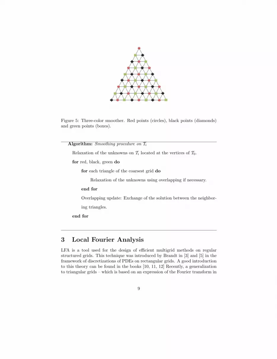
Figure 5: Three-color smoother. Red points (circles), black points (diamonds)and green points (boxes).

Algorithm: Smoothing procedure on Ti

Relaxation of the unknowns on Ti located at the vertices of T0.

for red, black, green do

for each triangle of the coarsest grid do

Relaxation of the unknowns using overlapping if necessary.

end for

Overlapping update: Exchange of the solution between the neighbor-

ing triangles.

end for

3 Local Fourier Analysis

LFA is a tool used for the design of efficient multigrid methods on regularstructured grids. This technique was introduced by Brandt in [3] and [5] in theframework of discretizations of PDEs on rectangular grids. A good introductionto this theory can be found in the books [10, 11, 12] Recently, a generalizationto triangular grids – which is based on an expression of the Fourier transform in

9

new coordinate systems in space and frequency variables – has been proposedin [7]. In the context of discretizations on semi–structured grids, particularly inthe case of the hierarchical triangular meshes considered in this paper, an LFAis used to predict the behavior of the multigrid method on each triangular blockof the coarsest grid. The quality of the general algorithm will depend on thelocal results obtained for each coarse triangle.

In Fourier smoothing analysis, the influence of a smoothing operator on thehigh-frequency error components is investigated. To get more insight into thestructure of a multigrid algorithm, it is useful to perform a two-grid analysis inorder to investigate the interplay between relaxation and coarse-grid correction,which is crucial for an efficient multigrid method.

The best known example of multi–color relaxation is the red-black Gauss–Seidel smoother for the five-point Laplace stencil. Such a scheme has also beenextensively analyzed, see for example [9, 13, 14]. A three-color smoother ontriangular grids for the Poisson problem was proposed and analyzed by Fourieranalysis in [7].

Now we examine the smoothing and the two–grid properties of the algorithmproposed in Section 2.3 for the model problem (1). The Fourier results ontriangular grids strongly depend on the shape of the mesh, namely the shapeof a representative triangle which can be characterized by two of its angles (seeFigure 6). Straightforward calculations make it possible to write the stiffnessstencil of an interior point of the triangular grid as follows

⎡⎣ a0,1 a1,1

a−1,0 a0,0 a1,0

a−1,−1 a0,−1

⎤⎦ ,

where the coefficients ai,j for 0 < α, β < π/2 are:

a1,0 = a−1,0 = − 1h2

1

tan α tan β − 1tan α tan β

, a1,1 = a−1,−1 = − 1h2

1

tan α + tan β

tan α tan2 β,

a0,1 = a0,−1 = − 1h2

1

tan α + tan β

tan2 α tan β, a0,0 = −2(a1,0 + a1,1 + a0,1),

where h1 is the length of the edge between the angles α and β. In the limit caseof a rectangular triangle, we obtain the classical five–point stencil for rectangulargrids.

Applying an LFA on triangular grids, the smoothing factor μ, and thetwo-grid convergence factor ρ for triangles with angles α = β = 600 andα = 350, β = 750 are shown in Table 1 for different pre-smoothing (ν1) andpost-smoothing (ν2) steps. For comparison, experimentally measured F-cycleconvergence factors, ρh, obtained with a right-hand side zero and a large initialguess to allow the convergence factors to stabilize, are also included.

We can observe that the correspondence between theoretical and practicalvalues is excellent, and that the smoothing factors are slightly worse than the

10

RED

BLACK

GREEN

Figure 6: A triangle of the coarsest mesh and its corresponding angles.

Table 1: LFA smoothing factors μ, LFA two–grid convergence factors ρ andmeasured F–cycle convergence rates ρh for the equilateral and a scalene trian-gles.

Equilateral triangle Scalene triangle (750, 350)ν1, ν2 μ ρ ρh μ ρ ρh

1, 0 0.230 0.134 0.132 0.515 0.488 0.4871, 1 0.053 0.039 0.038 0.265 0.238 0.2372, 1 0.029 0.015 0.015 0.136 0.116 0.1152, 2 0.021 0.013 0.013 0.070 0.063 0.062

two-grid convergence factors. Moreover, from Table 1 we can see that the con-vergence factor depends on the shape of the coarsest triangle. Thus, very goodconvergence factors are obtained for the equilateral triangle, whereas these fac-tors worsen whenever any of the angles tend to be small. This behavior is similarto that observed in [7], where an exhaustive analysis for the Poisson problemwas performed. In that paper, other smoothers, namely block–line smoothers,were used for anisotropic meshes.

4 Numerical experiments

Our aim in this section is to present two numerical experiments using reaction-diffusion models. Firstly, the scalar case is considered and then the methodologydeveloped in this work is applied to a reaction-diffusion system.

11

4.1 Scalar reaction-diffusion problem

We start with the study of the model problem (1) introduced in Section 2.2. Theright-hand side and the Dirichlet boundary conditions are such that the exactsolution is u(x, y) = sin(πx) sin(πy). This problem is solved in an H-shapeddomain, as it is shown in Figure 7a, and the coarsest mesh is composed of fiftytriangles with different geometries, which are also depicted in the same figure.Nested meshes are constructed by regular refinement and the grid resulting afterrefining each triangle twice is shown in Figure 7b.

X

Y

-2 -1 0 1 2

-2

-1

0

1

2

X

Y

-2 -1 0 1 2

-2

-1

0

1

2

a) b)

Figure 7: a) Computational domain and coarsest grid, b) Hierarchical gridobtained after two refinement levels

The considered problem has been discretized with linear finite elements, andthe corresponding algebraic linear system has been solved with the geometricmultigrid method proposed in previous sections. An LFA two-grid analysis hasbeen applied, using the three-color smoother with ν1 = ν2 = 1 relaxation steps,on each triangle of the coarsest grid. From the local convergence factors pre-dicted by LFA on each triangle, a global convergence factor of 0.243 is predictedby taking into account the worst of them, which corresponds to the four trianglesshaded in Figure 8.

In order to see the robustness of the multigrid method with respect to thespace discretization parameter h, in Figure 9 we show the convergence ob-tained, with an F(1,1)-cycle and the three-color smoother, for different num-bers of refinement levels. The initial guess is taken as u(x, y) = 1 and thestopping criterion is chosen as the maximum residual to be less than 10−6. Anh-independent convergence of the method is displayed in this figure, and we

12

X

Y

-2 -1 0 1 2

-2

-1

0

1

2

Figure 8: Triangles on the coarsest grid with the worst convergence factor pre-dicted by LFA.

can also see the efficiency of this method, since the residual becomes less than10−6 after twelve/fifteen iterations of the multigrid algorithm. An average con-vergence factor about 0.185 has been obtained. We would like to indicate thatthe small discrepancy between the predicted two-grid and the F(1,1) measuredconvergence factors is due to LFA’s providing asymptotic convergence factors.Taking a large enough initial guess, we have measured convergence factors veryclose to the predicted value.

4.2 Reaction-diffusion system

Now we apply the developed methodology to the reaction-diffusion system

−Δu + u − v = f1

−Δv + v − u = f2in Ω. (5)

Dirichlet conditions for both unknowns are taken on the whole boundary andthese boundary conditions and the right-hand sides, f1, f2, are such that theexact solution is u(x, y) = v(x, y) = sin(πx) sin(πy). The computational domainfor this problem and its coarsest triangulation are the same considered for thescalar case.

To solve the corresponding system of algebraic equations efficiently, a geo-metric multigrid algorithm has been applied. A collective three-color smoother,that is, the straightforward extension from its scalar version, is chosen as therelaxation process. As its scalar counterpart, this relaxation performs a sweep

13

1e-006

0.0001

0.01

1

100

10000

1e+006

5 10 15 20 25

maxim

um

resid

ual

cycles

’5 levels’’6 levels’’7 levels’’8 levels’’9 levels’

’10 levels’’11 levels’

Figure 9: Multigrid convergence F(1,1)-cycle for the scalar reaction-diffusionproblem.

over each one of the subgrids corresponding to different colors. Note that asmall 2 × 2 system must be solved per node.

Using vector Fourier modes, an LFA on triangular grids can be extendedto systems of PDEs. A two-grid analysis has been performed for the reaction-diffusion system, using the collective three-color smoother with ν1 = ν2 = 1relaxation steps, on each triangle of the coarsest grid. Analogously to the scalarcase, a global convergence factor of 0.243 is predicted, as would be expected.

To perform the numerical experiment, the initial guess is u(x, y) = v(x, y) =1 and the stopping criterion is chosen as the maximum residual over all un-knowns to be less than 10−6. A F(1,1)-cycle has also been used to study thebehavior of the multigrid method for different refinement levels. In Table 2,the number of cycles, the average convergence factor between brackets, and cputime, measured in seconds on a Pentium IV of 2.4GHz, are shown for differentrefinement levels. Associated to each level the corresponding number of trian-gles and the number of unknowns are also displayed. In Table 2, robustness withrespect to the number of unknowns is again observed for this reaction-diffusionsystem. Note again the small discrepancy between the predicted two-grid andthe F(1,1) measured convergence factors shown in this table. The predictedvalue is obtained if a large enough initial guess is taken and many iterations areperformed.

14

Table 2: Number of elements, unknowns and cycles, average convergence factorsin brackets, and cpu time for several refinement levels.

N. of levels N. of elements N. of unknowns N. of cycles (ρh) cpu time5 12800 13154 11 (0.13) < 1′′

6 51200 51906 11 (0.12) 1′′

7 204800 206210 12 (0.12) 4′′

8 819200 822018 13 (0.12) 14′′

9 3276800 3282434 14 (0.13) 50′′

5 Acknowledgement

This work was partially supported by FEDER/MCYT Projects MTM2007-63204 and the DGA (Grupo consolidado PDIE.)

References

[1] R. Bank, PLTMG Users Guide Version 7.0, SIAM, Philadelphia, 1994.

[2] B. Bergen, T. Gradl, F. Hulsemann, U. Ruede, A massively parallel multigridmethod for finite elements, Comput. Sci. Eng., 8 (2006), 56–62.

[3] A. Brandt, Multi-level adaptive solutions to boundary-value problems, Math.Comput., 31 (1977), 333–390.

[4] A. Brandt, Multigrid techniques: 1984 guide with applications to fluid dy-namics, GMD-Studie Nr. 85, Sankt Augustin, Germany, 1984.

[5] A. Brandt, Rigourous quantitative analysis of multigrid I. Constant coef-ficients two level cycle with L2 norm, SIAM J. Numer. Anal., 31 (1994),1695–1730.

[6] P. Deuflhard, P. Leinenand, H. Yserentant, Concepts of an adaptive hierar-chical finite element code, Impact Comput. Sci. Engrg., 1 (1989), 3–35.

[7] F.J. Gaspar, J.L. Gracia, F.J. Lisbona, Fourier analysis for multigrid meth-ods on triangular grids, Preprint Seminario Matematico Garcıa de Galdeanode Universidad de Zaragoza, 2 (2008).

[8] W. Hackbusch, Multi-grid methods and applications, Springer, Berlin, 1985.

[9] C.-C.J. Kuo and B.C. Levy, Two-color Fourier analysis of the multigridmethod with red-black Gauss-Seidel smoothing, Appl. Math. Comput., 29(1989), 69–87.

15

[10] U. Trottenberg, C.W. Oosterlee and A. Schuller. Multigrid Academic Press,New York, 2001.

[11] P. Wesseling, An introduction to multigrid methods. John Wiley, Chichester,UK, 1992.

[12] R. Wienands and W. Joppich, Practical Fourier analysis for multigridmethods. Chapman and Hall/CRC Press, 2005.

[13] I. Yavneh, Multigrid smoothing factors for red–black Gauss-Seidel relax-ation applied to a class of elliptic operators, SIAM J. Numer. Anal., 32(1995), 1126–1138.

[14] I. Yavneh, On red–black SOR smoothing in multigrid, SIAM J. Sci. Com-put., 17 (1996), 180–192.

16