Geophysical study of the Ota–VF Xira–Lisbon–Sesimbra fault zone and the lower Tagus

Cenozoic basin

This article has been downloaded from IOPscience. Please scroll down to see the full text article.

2011 J. Geophys. Eng. 8 395

(http://iopscience.iop.org/1742-2140/8/3/001)

Download details:

IP Address: 193.137.43.157

The article was downloaded on 07/09/2011 at 16:00

Please note that terms and conditions apply.

View the table of contents for this issue, or go to the journal homepage for more

Home Search Collections Journals About Contact us My IOPscience

IOP PUBLISHING JOURNAL OF GEOPHYSICS AND ENGINEERING

J. Geophys. Eng. 8 (2011) 395–411 doi:10.1088/1742-2132/8/3/001

Geophysical study of the Ota–VFXira–Lisbon–Sesimbra fault zoneand the lower Tagus Cenozoic basinJoao Carvalho1, Taha Rabeh2,8,9, Miroslav Bielik3, Eva Szalaiova3,Luıs Torres4, Marisa Silva5, Fernando Carrilho6, Luıs Matias7 andJorge Miguel Miranda7

1 Laboratorio Nacional de Energia e Geologia, Apartado 7586, 2721-866 Amadora, Portugal2 National Research Institute of Astronomy and Geophysics, Helwan, Cairo, Egypt3 Comenius University, Faculty of Natural Sciences, Mlynska dolina, 842 15 Bratislava 4,Slovak Republic4 LTGEO, Estrada do Paco do Lumiar 22, 1649-038 Lisboa, Portugal5 Instituto Geografico Portugues, R. da Artilharia 107, 1099-052 Lisboa, Portugal6 Instituto de Meteorologia, Av. do Aeroporto, 2300-313 Lisboa, Portugal7 University of Lisbon, CGUL, IDL. Campo Grande, 1749-016 Lisboa, Portugal8 Geophysical Institute of the Slovak Academy of Sciences, Dubravska cesta 9, 845 28 Bratislava,Slovak Republic

E-mail: taharabeh@yahoo.com

Received 2 November 2010Accepted for publication 5 May 2011Published 7 July 2011Online at stacks.iop.org/JGE/8/395

AbstractThis paper focuses on the interpretation of seismic reflection, gravimetric, topographic, deepseismic refraction and seismicity data to study the recently proposed Ota–Vila Franca deXira–Lisbon–Sesimbra (OVLS) fault zone and the lower Tagus Cenozoic basin (LTCB). Thestudied structure is located in the lower Tagus valley (LTV), an area with over 2 millioninhabitants that has experienced historical earthquakes which caused significant damage andeconomical losses (1344, 1531 and 1909 earthquakes) and whose tectonic sources are thoughtto be local but mostly remain unknown. This study, which is intended as a contribution toimprove the seismic hazard of the area and the neotectonics of the region, shows that theabove-proposed fault zone is probably a large crustal thrust fault that constitutes the westernlimit of the LTCB. Gravimetric, deep refraction and seismic reflection data suggest that theLTCB is a foreland basin, as suggested previously by some authors, and that the OVLSnorthern and central sectors act as the major thrusts. The southern sector fault has beendominated by strike-slip kinematics due to a different orientation to the stress field. Indeed,geological outcrop and seismic reflection data interpretation suggests that, based on faultgeometry and type of deformation at depth, the structure is composed of three major segments.These data suggest that these segments have different kinematics in agreement with theirorientation to the regional stress field. The OVLS apparently controls the distribution of theseismicity in the area. Geological and geophysical information previously gathered also pointsthat the central segment is active into the Quaternary. The segment lengths vary between 20and 45 km. Since faults usually rupture only by segments, maximum expectable earthquakemagnitudes and other parameters have been calculated for the three sectors of the OVLS faultzone using empirical relationships between earthquake statistics and geological parametersavailable from the literature. Calculated slip rates are compatible with previous estimates forthe area (0.33 mm yr–1). A more accurate estimation of the OVLS throw in the Quaternary

9 Author to whom any correspondence should be addressed.

1742-2132/11/030395+17$33.00 © 2011 Nanjing Geophysical Research Institute Printed in the UK 395

J Carvalho et al

sediments is therefore of vital importance for a more accurate evaluation of theseismic hazard of the area.

Keywords: neotectonics, reflection seismology, gravimetric data, seismicity, seismic hazard

(Some figures in this article are in colour only in the electronic version)

1. Introduction

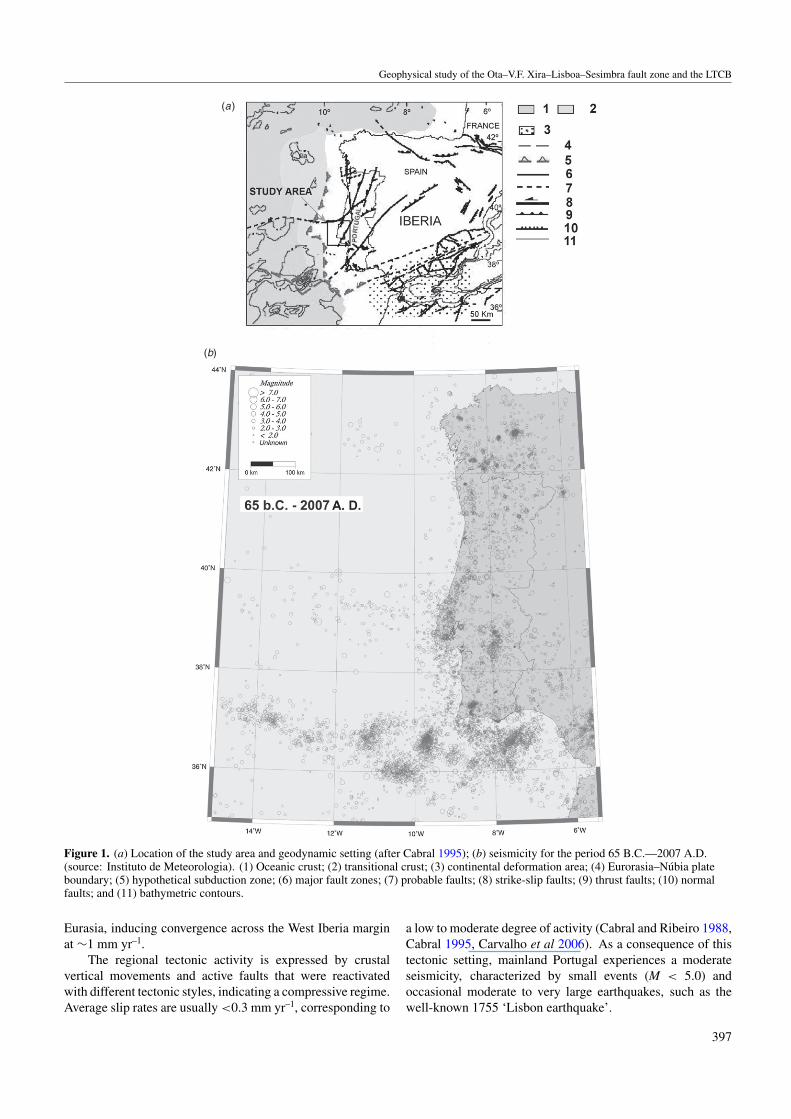
This paper focuses on the seismic hazard evaluation of thelower Tagus valley (LTV), sited in central-western Portugalmainland in the Eurasian Plate, close (about 200 km) tothe Eurasia-Africa plate boundary (Azores-Gibraltar faultzone, figure 1(a)). This setting has resulted in significanttectonic and seismic activity throughout history (figure 1(b)).The study area includes the densely populated metropolitanLisbon area, stressing the need to identify and characterizeregional seismogenic faults as a condition for seismic potentialassessment.

Besides the offshore sources, the study area suffers theeffects of moderate events generated by local sources (Pelaezet al 2002, e.g.) that also cause loss of life and significantdamage like in 1344, 1531 and 1909 (Moreira 1985, Henriqueset al 1988). The sources of these historical events are stillunder debate. Due to the scarcity of historical descriptions,the earthquakes in 1344 and 1531 are poorly located, beingpositioned in the LTV based upon the destruction generated inthe Lisbon area. The 1531 event caused severe damage andmany casualties in the town of Lisbon, reaching an intensityof VIII–IX MM (Justo and Salwa 1998).

The source of the MW = 6 (MS = 6.3) 1909 earthquake(Teves-Costa et al 1999, Dineva et al 2002), which destroyedthe village of Benavente, is still unknown. The V. F. de Xirafault zone, or the southern, hidden sector of the Azambujafault (AZF) is the nearest, NNE–SSW trending, candidates(Carvalho 2003, Cabral et al 2003, 2004). An alternative,as proposed by Stich et al (2005), is that the Benaventeearthquake was generated by an ENE–WSW trending blindthrust beneath the Tagus valley sedimentary basin.

The geometry of the Cenozoic sedimentary basin alsoplays an important role in local energy enhancement and siteeffects, masking the relationship between the historical eventlocation based on seismic intensity studies and the earthquakesources.

The correlation between instrumental seismicity andknown active faults is also generally poor. The lowslip rates indicate long recurrence times for maximum(M 6.5–7 co-seismic ruptures) earthquakes (about 2000–5000 years), evidencing the shortness of the historical recordand stressing the need to refine the geological knowledge(neotectonic/paleoseismological).

However, fault recognition at the surface is oftencomplicated due to the lack of outcrops and also due to the lowslip rates in the study area, which causes sedimentation ratesto erase surface ruptures. Therefore, faults are buried beneaththe recent sedimentary cover and cannot be recognized at thesurface. Even with well-located hypocentres, return periods

are large in intraplate environments, and large earthquakes canbe generated in previously undetected structures.

Therefore, the use of geophysical methods in the studyarea has been carried out in the last years in an attempt toimprove knowledge regarding the deep structure, in particularthe location and characterization of hidden faults, which maybe the source of the regional seismicity (e.g. Cabral et al 2003,Vilanova and Fonseca 2004, Carvalho et al 2006, 2008).Reprocessing and reinterpretation of seismic reflection dataacquired for oil exploration in the LTV and surrounding areashas been carried out, as well as of aeromagnetic (Carvalhoet al 2008) and seismicity data (Carrilho et al 2004).

The Ota–Vila Franca de Xira–Lisbon–Sesimbra (OVLS)is one of the most important structures detected, basedupon its near-surface expression on the seismic reflectionprofiles at several locations (Carvalho et al 2008), theremarkable signature it produces on aeromagnetic data(id; Domzalski 1969), its significance in the lowerTagus Cenozoic basin (LTCB) structural pattern, apparentrelationship with the regional seismicity, its closeness toLisbon and its foreseen seismic potential. Here, making useof gravimetric, topographic, deep-seismic refraction data andunpublished seismic reflection data, the importance of theOVLS as a crustal, regional boundary basin feature that canproduce large earthquakes in the study area is proposed.

2. Tectonic and geological setting

The regional geodynamics is controlled by the NW–SE convergence of Eurasia and Africa at ∼4 mm yr–1

(NUVEL-1 model). Satellite geodesy indicates that theEurasia–Africa motion changed significantly since ∼3 Ma(20◦ dextral rotation, 25–40% slowing). The present tectonicstress pattern in the study region has been assessed usingvarious stress indicators (Ribeiro et al 1996, Borges et al2001). While the nature of the Eurasia–Africa plate boundaryin Ibero-Maghreb region is still a matter of debate (a diffuseborder across the frontier between the oceanic and continentaldomains or a discrete but very complex plate boundary havebeen proposed), the level of seismotectonic activity in theWest-Iberian continental margin indicates that it is not a typicalpassive margin.

A model suggesting that this margin is in transition frompassive to active convergent has been proposed (Ribeiro et al1996, Ribeiro 2002). In the last 15–20 years, data have beenacquired offshore in the SW Iberian margin that revealed majorNNE–SSW trending active faults. These faults confirm amodel according to which the Iberian microplate is becomingindividualized and is rotating clockwise between Africa and

396

Geophysical study of the Ota–V.F. Xira–Lisboa–Sesimbra fault zone and the LTCB

(a)

(b)

Figure 1. (a) Location of the study area and geodynamic setting (after Cabral 1995); (b) seismicity for the period 65 B.C.—2007 A.D.(source: Instituto de Meteorologia). (1) Oceanic crust; (2) transitional crust; (3) continental deformation area; (4) Eurorasia–Nubia plateboundary; (5) hypothetical subduction zone; (6) major fault zones; (7) probable faults; (8) strike-slip faults; (9) thrust faults; (10) normalfaults; and (11) bathymetric contours.

Eurasia, inducing convergence across the West Iberia marginat ∼1 mm yr–1.

The regional tectonic activity is expressed by crustalvertical movements and active faults that were reactivatedwith different tectonic styles, indicating a compressive regime.Average slip rates are usually <0.3 mm yr–1, corresponding to

a low to moderate degree of activity (Cabral and Ribeiro 1988,Cabral 1995, Carvalho et al 2006). As a consequence of thistectonic setting, mainland Portugal experiences a moderateseismicity, characterized by small events (M < 5.0) andoccasional moderate to very large earthquakes, such as thewell-known 1755 ‘Lisbon earthquake’.

397

J Carvalho et al

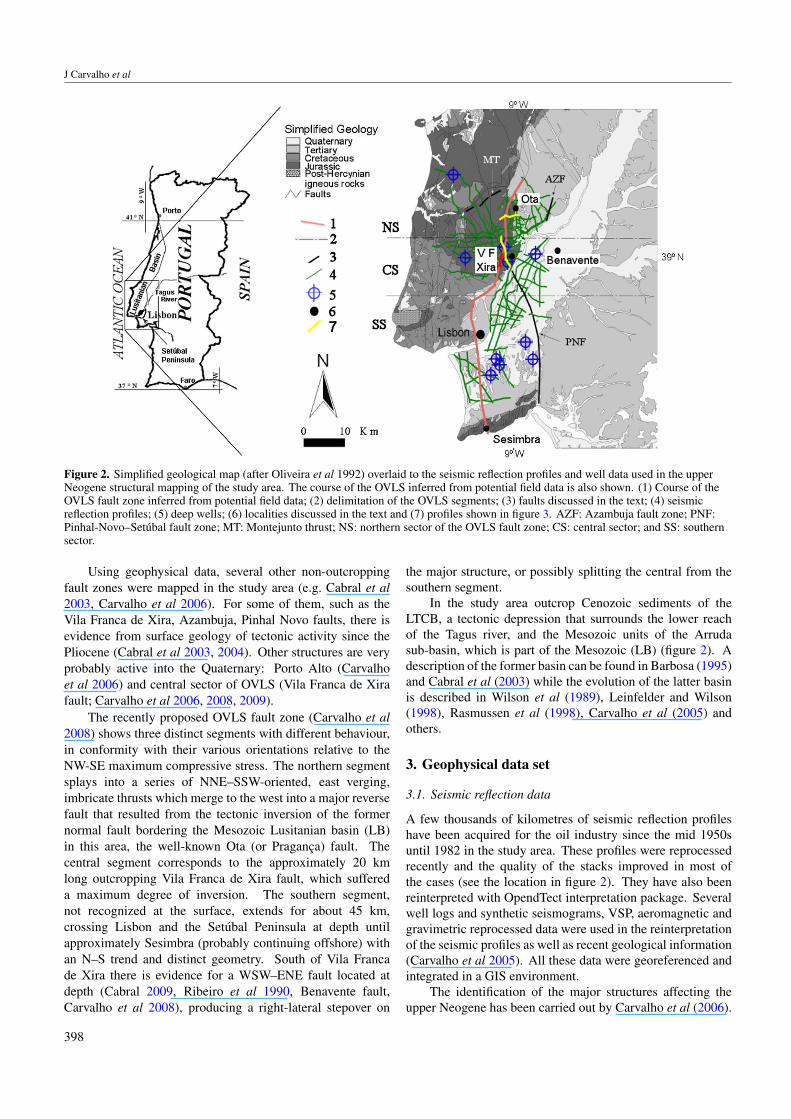
Figure 2. Simplified geological map (after Oliveira et al 1992) overlaid to the seismic reflection profiles and well data used in the upperNeogene structural mapping of the study area. The course of the OVLS inferred from potential field data is also shown. (1) Course of theOVLS fault zone inferred from potential field data; (2) delimitation of the OVLS segments; (3) faults discussed in the text; (4) seismicreflection profiles; (5) deep wells; (6) localities discussed in the text and (7) profiles shown in figure 3. AZF: Azambuja fault zone; PNF:Pinhal-Novo–Setubal fault zone; MT: Montejunto thrust; NS: northern sector of the OVLS fault zone; CS: central sector; and SS: southernsector.

Using geophysical data, several other non-outcroppingfault zones were mapped in the study area (e.g. Cabral et al2003, Carvalho et al 2006). For some of them, such as theVila Franca de Xira, Azambuja, Pinhal Novo faults, there isevidence from surface geology of tectonic activity since thePliocene (Cabral et al 2003, 2004). Other structures are veryprobably active into the Quaternary: Porto Alto (Carvalhoet al 2006) and central sector of OVLS (Vila Franca de Xirafault; Carvalho et al 2006, 2008, 2009).

The recently proposed OVLS fault zone (Carvalho et al2008) shows three distinct segments with different behaviour,in conformity with their various orientations relative to theNW-SE maximum compressive stress. The northern segmentsplays into a series of NNE–SSW-oriented, east verging,imbricate thrusts which merge to the west into a major reversefault that resulted from the tectonic inversion of the formernormal fault bordering the Mesozoic Lusitanian basin (LB)in this area, the well-known Ota (or Praganca) fault. Thecentral segment corresponds to the approximately 20 kmlong outcropping Vila Franca de Xira fault, which suffereda maximum degree of inversion. The southern segment,not recognized at the surface, extends for about 45 km,crossing Lisbon and the Setubal Peninsula at depth untilapproximately Sesimbra (probably continuing offshore) withan N–S trend and distinct geometry. South of Vila Francade Xira there is evidence for a WSW–ENE fault located atdepth (Cabral 2009, Ribeiro et al 1990, Benavente fault,Carvalho et al 2008), producing a right-lateral stepover on

the major structure, or possibly splitting the central from thesouthern segment.

In the study area outcrop Cenozoic sediments of theLTCB, a tectonic depression that surrounds the lower reachof the Tagus river, and the Mesozoic units of the Arrudasub-basin, which is part of the Mesozoic (LB) (figure 2). Adescription of the former basin can be found in Barbosa (1995)and Cabral et al (2003) while the evolution of the latter basinis described in Wilson et al (1989), Leinfelder and Wilson(1998), Rasmussen et al (1998), Carvalho et al (2005) andothers.

3. Geophysical data set

3.1. Seismic reflection data

A few thousands of kilometres of seismic reflection profileshave been acquired for the oil industry since the mid 1950suntil 1982 in the study area. These profiles were reprocessedrecently and the quality of the stacks improved in most ofthe cases (see the location in figure 2). They have also beenreinterpreted with OpendTect interpretation package. Severalwell logs and synthetic seismograms, VSP, aeromagnetic andgravimetric reprocessed data were used in the reinterpretationof the seismic profiles as well as recent geological information(Carvalho et al 2005). All these data were georeferenced andintegrated in a GIS environment.

The identification of the major structures affecting theupper Neogene has been carried out by Carvalho et al (2006).

398

Geophysical study of the Ota–V.F. Xira–Lisboa–Sesimbra fault zone and the LTCB

(a)

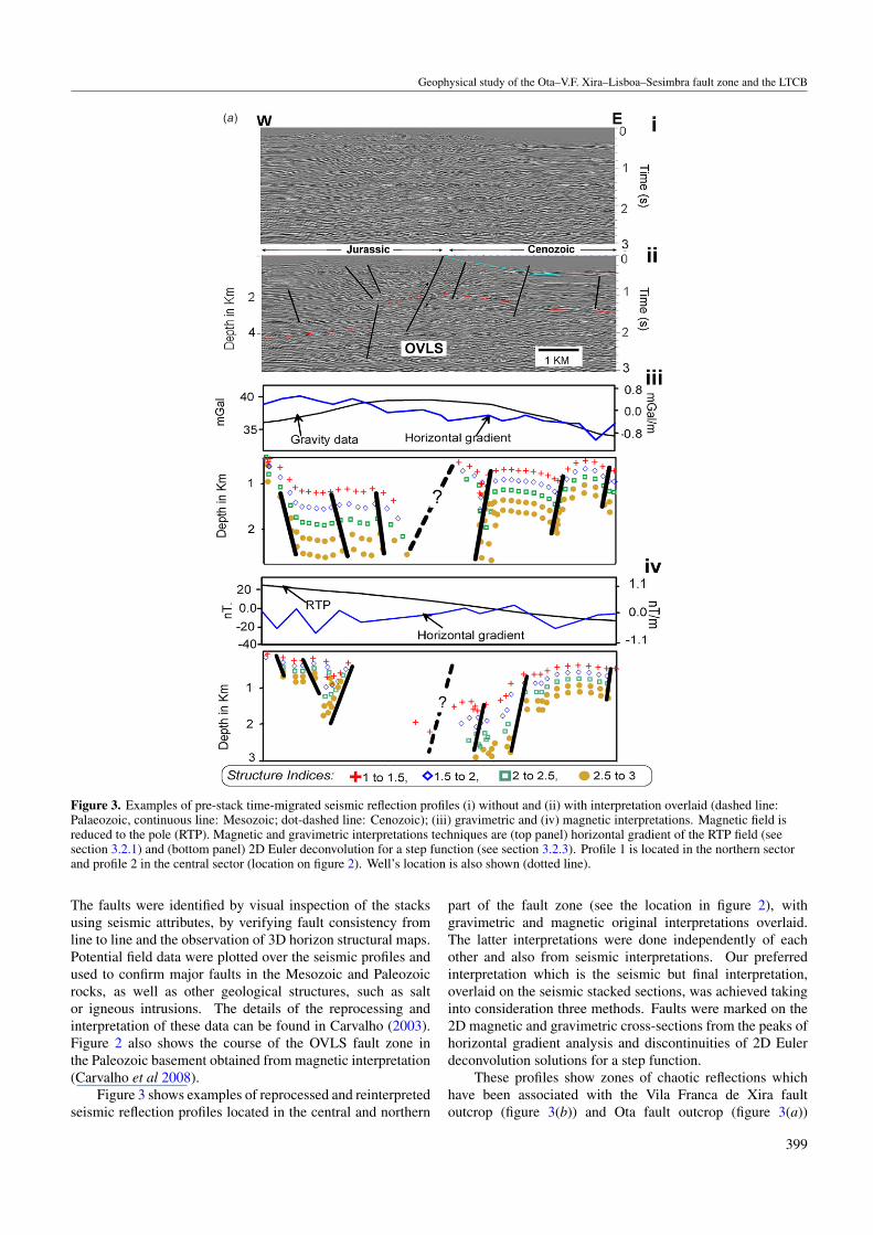
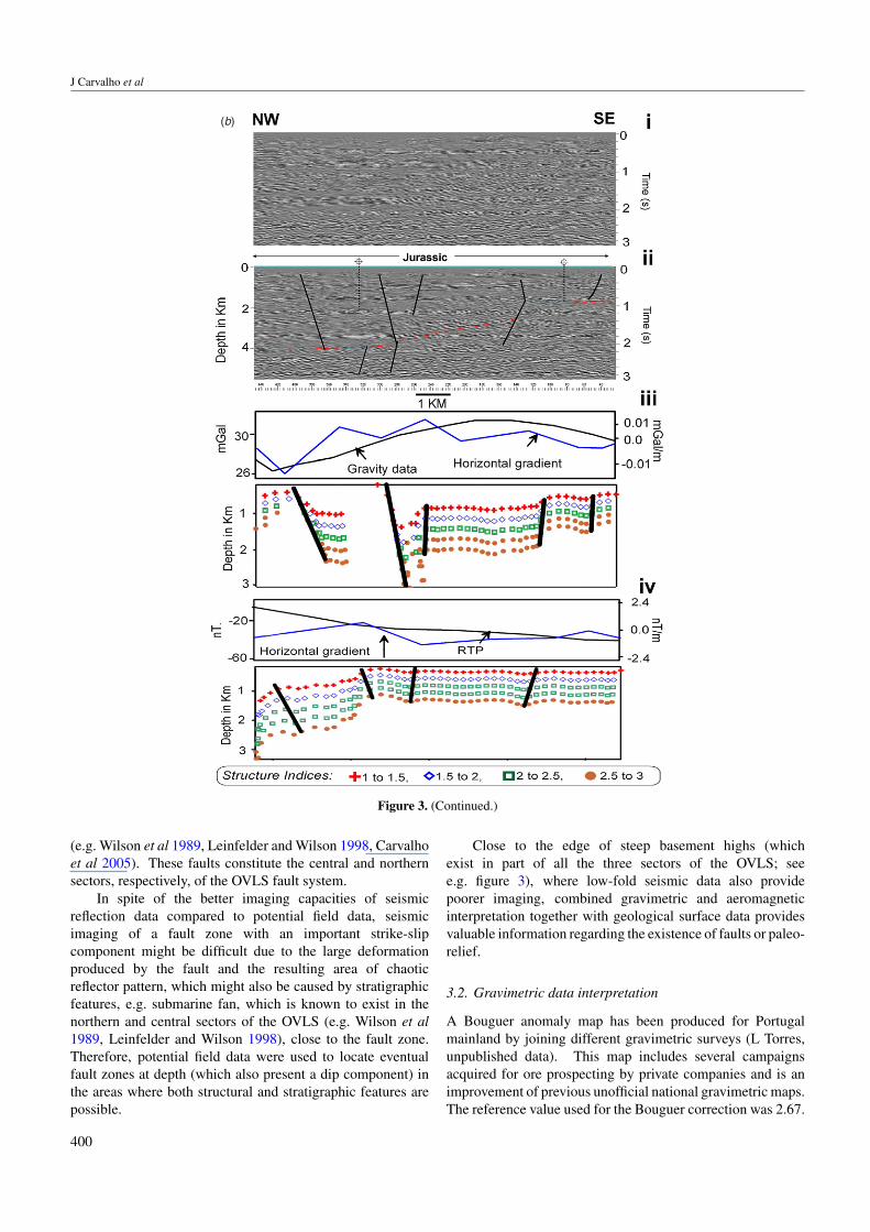
Figure 3. Examples of pre-stack time-migrated seismic reflection profiles (i) without and (ii) with interpretation overlaid (dashed line:Palaeozoic, continuous line: Mesozoic; dot-dashed line: Cenozoic); (iii) gravimetric and (iv) magnetic interpretations. Magnetic field isreduced to the pole (RTP). Magnetic and gravimetric interpretations techniques are (top panel) horizontal gradient of the RTP field (seesection 3.2.1) and (bottom panel) 2D Euler deconvolution for a step function (see section 3.2.3). Profile 1 is located in the northern sectorand profile 2 in the central sector (location on figure 2). Well’s location is also shown (dotted line).

The faults were identified by visual inspection of the stacksusing seismic attributes, by verifying fault consistency fromline to line and the observation of 3D horizon structural maps.Potential field data were plotted over the seismic profiles andused to confirm major faults in the Mesozoic and Paleozoicrocks, as well as other geological structures, such as saltor igneous intrusions. The details of the reprocessing andinterpretation of these data can be found in Carvalho (2003).Figure 2 also shows the course of the OVLS fault zone inthe Paleozoic basement obtained from magnetic interpretation(Carvalho et al 2008).

Figure 3 shows examples of reprocessed and reinterpretedseismic reflection profiles located in the central and northern

part of the fault zone (see the location in figure 2), withgravimetric and magnetic original interpretations overlaid.The latter interpretations were done independently of eachother and also from seismic interpretations. Our preferredinterpretation which is the seismic but final interpretation,overlaid on the seismic stacked sections, was achieved takinginto consideration three methods. Faults were marked on the2D magnetic and gravimetric cross-sections from the peaks ofhorizontal gradient analysis and discontinuities of 2D Eulerdeconvolution solutions for a step function.

These profiles show zones of chaotic reflections whichhave been associated with the Vila Franca de Xira faultoutcrop (figure 3(b)) and Ota fault outcrop (figure 3(a))

399

J Carvalho et al

(b)

Figure 3. (Continued.)

(e.g. Wilson et al 1989, Leinfelder and Wilson 1998, Carvalhoet al 2005). These faults constitute the central and northernsectors, respectively, of the OVLS fault system.

In spite of the better imaging capacities of seismicreflection data compared to potential field data, seismicimaging of a fault zone with an important strike-slipcomponent might be difficult due to the large deformationproduced by the fault and the resulting area of chaoticreflector pattern, which might also be caused by stratigraphicfeatures, e.g. submarine fan, which is known to exist in thenorthern and central sectors of the OVLS (e.g. Wilson et al1989, Leinfelder and Wilson 1998), close to the fault zone.Therefore, potential field data were used to locate eventualfault zones at depth (which also present a dip component) inthe areas where both structural and stratigraphic features arepossible.

Close to the edge of steep basement highs (whichexist in part of all the three sectors of the OVLS; seee.g. figure 3), where low-fold seismic data also providepoorer imaging, combined gravimetric and aeromagneticinterpretation together with geological surface data providesvaluable information regarding the existence of faults or paleo-relief.

3.2. Gravimetric data interpretation

A Bouguer anomaly map has been produced for Portugalmainland by joining different gravimetric surveys (L Torres,unpublished data). This map includes several campaignsacquired for ore prospecting by private companies and is animprovement of previous unofficial national gravimetric maps.The reference value used for the Bouguer correction was 2.67.

400

Geophysical study of the Ota–V.F. Xira–Lisboa–Sesimbra fault zone and the LTCB

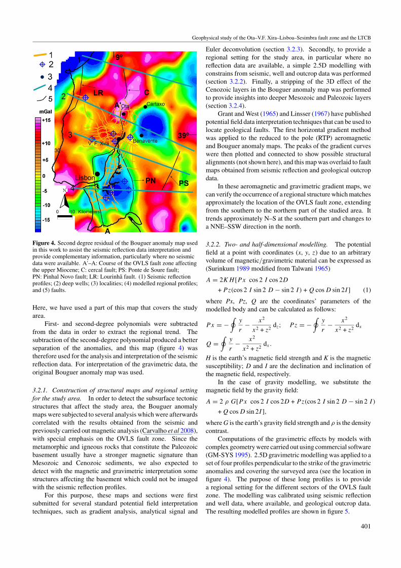
Figure 4. Second degree residual of the Bouguer anomaly map usedin this work to assist the seismic reflection data interpretation andprovide complementary information, particularly where no seismicdata were available. A′–A: Course of the OVLS fault zone affectingthe upper Miocene; C: cercal fault; PS: Ponte de Soure fault;PN: Pinhal Novo fault; LR: Lourinha fault. (1) Seismic reflectionprofiles; (2) deep wells; (3) localities; (4) modelled regional profiles;and (5) faults.

Here, we have used a part of this map that covers the studyarea.

First- and second-degree polynomials were subtractedfrom the data in order to extract the regional trend. Thesubtraction of the second-degree polynomial produced a betterseparation of the anomalies, and this map (figure 4) wastherefore used for the analysis and interpretation of the seismicreflection data. For interpretation of the gravimetric data, theoriginal Bouguer anomaly map was used.

3.2.1. Construction of structural maps and regional settingfor the study area. In order to detect the subsurface tectonicstructures that affect the study area, the Bouguer anomalymaps were subjected to several analysis which were afterwardscorrelated with the results obtained from the seismic andpreviously carried out magnetic analysis (Carvalho et al 2008),with special emphasis on the OVLS fault zone. Since themetamorphic and igneous rocks that constitute the Paleozoicbasement usually have a stronger magnetic signature thanMesozoic and Cenozoic sediments, we also expected todetect with the magnetic and gravimetric interpretation somestructures affecting the basement which could not be imagedwith the seismic reflection profiles.

For this purpose, these maps and sections were firstsubmitted for several standard potential field interpretationtechniques, such as gradient analysis, analytical signal and

Euler deconvolution (section 3.2.3). Secondly, to provide aregional setting for the study area, in particular where noreflection data are available, a simple 2.5D modelling withconstrains from seismic, well and outcrop data was performed(section 3.2.2). Finally, a stripping of the 3D effect of theCenozoic layers in the Bouguer anomaly map was performedto provide insights into deeper Mesozoic and Paleozoic layers(section 3.2.4).

Grant and West (1965) and Linsser (1967) have publishedpotential field data interpretation techniques that can be used tolocate geological faults. The first horizontal gradient methodwas applied to the reduced to the pole (RTP) aeromagneticand Bouguer anomaly maps. The peaks of the gradient curveswere then plotted and connected to show possible structuralalignments (not shown here), and this map was overlaid to faultmaps obtained from seismic reflection and geological outcropdata.

In these aeromagnetic and gravimetric gradient maps, wecan verify the occurrence of a regional structure which matchesapproximately the location of the OVLS fault zone, extendingfrom the southern to the northern part of the studied area. Ittrends approximately N–S at the southern part and changes toa NNE–SSW direction in the north.

3.2.2. Two- and half-dimensional modelling. The potentialfield at a point with coordinates (x, y, z) due to an arbitraryvolume of magnetic/gravimetric material can be expressed as(Surinkum 1989 modified from Talwani 1965)

A = 2KH [Px cos 2 I cos 2D

+ Pz(cos 2 I sin 2 D − sin 2 I ) + Q cos D sin 2I ] (1)

where Px, Pz, Q are the coordinates’ parameters of themodelled body and can be calculated as follows:

Px = −∮

y

r− x2

x2 + z2dz; Pz = −

∮y

r− x2

x2 + z2dx

Q =∮

y

r− x2

x2 + z2dx.

H is the earth’s magnetic field strength and K is the magneticsusceptibility; D and I are the declination and inclination ofthe magnetic field, respectively.

In the case of gravity modelling, we substitute themagnetic field by the gravity field:

A = 2 ρ G[Px cos 2 I cos 2D + Pz(cos 2 I sin 2 D − sin 2 I )

+ Q cos D sin 2I ],

where G is the earth’s gravity field strength and ρ is the densitycontrast.

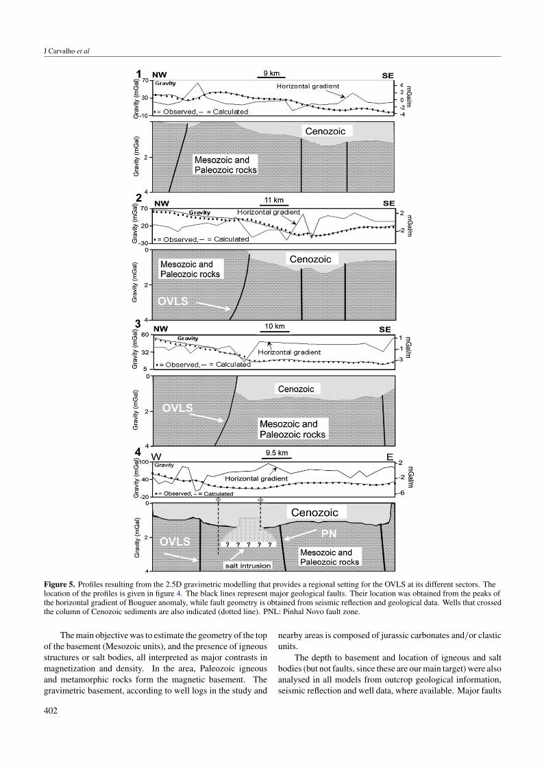
Computations of the gravimetric effects by models withcomplex geometry were carried out using commercial software(GM-SYS 1995). 2.5D gravimetric modelling was applied to aset of four profiles perpendicular to the strike of the gravimetricanomalies and covering the surveyed area (see the location infigure 4). The purpose of these long profiles is to providea regional setting for the different sectors of the OVLS faultzone. The modelling was calibrated using seismic reflectionand well data, where available, and geological outcrop data.The resulting modelled profiles are shown in figure 5.

401

J Carvalho et al

Figure 5. Profiles resulting from the 2.5D gravimetric modelling that provides a regional setting for the OVLS at its different sectors. Thelocation of the profiles is given in figure 4. The black lines represent major geological faults. Their location was obtained from the peaks ofthe horizontal gradient of Bouguer anomaly, while fault geometry is obtained from seismic reflection and geological data. Wells that crossedthe column of Cenozoic sediments are also indicated (dotted line). PNL: Pinhal Novo fault zone.

The main objective was to estimate the geometry of the topof the basement (Mesozoic units), and the presence of igneousstructures or salt bodies, all interpreted as major contrasts inmagnetization and density. In the area, Paleozoic igneousand metamorphic rocks form the magnetic basement. Thegravimetric basement, according to well logs in the study and

nearby areas is composed of jurassic carbonates and/or clasticunits.

The depth to basement and location of igneous and saltbodies (but not faults, since these are our main target) were alsoanalysed in all models from outcrop geological information,seismic reflection and well data, where available. Major faults

402

Geophysical study of the Ota–V.F. Xira–Lisboa–Sesimbra fault zone and the LTCB

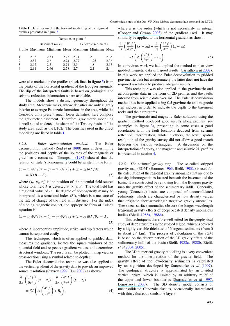
Table 1. Densities used in the forward modelling of the regionalprofiles presented in figure 5.

Densities in g cm−3

Basement rocks Cenozoic sediments

Profile Maximum Minimum Mean Maximum Minimum Mean

1 2.93 2.53 2.73 2.71 2 2.352 2.87 2.61 2.74 2.77 1.95 2.363 2.92 2.51 2.71 2.5 1.8 2.154 2.91 2.66 2.78 2.7 2.1 2.4

were also marked on the profiles (black lines in figure 5) fromthe peaks of the horizontal gradient of the Bouguer anomaly.The dip of the interpreted faults is based on geological andseismic reflection information where available.

The models show a distinct geometry throughout thestudy area. Mesozoic rocks, whose densities are only slightlyinferior to average Paleozoic formations in the area, while theCenozoic units present much lower densities, here composethe gravimetric basement. Therefore, gravimetric modellingis well suited to detect the shape of the Tertiary basins of thestudy area, such as the LTCB. The densities used in the directmodelling are listed in table 1.

3.2.3. Euler deconvolution method. The Eulerdeconvolution method (Reid et al 1990) aims at determiningthe positions and depths of the sources of the magnetic orgravimetric contrasts. Thompson (1982) showed that therelation of Euler’s homogeneity could be written in the form

(x − x0)∂F/∂x − (y − y0)∂F/∂y + (z − z0)∂F/∂z

= N(B − F), (2)

where (x0, y0, z0) is the position of the potential field sourcewhose total field F is detected at (x, y, z). The total field hasa regional value of B. The degree of homogeneity N may beinterpreted as a structural index (SI), which is a measure ofthe rate of change of the field with distance. For the indexof sloping magnetic contact, the appropriate form of Euler’sequation is

(x − x0)∂F/∂x − (y − y0)∂F/∂y + (z − z0)∂F/∂z = A,

(3)

where A incorporates amplitude, strike, and dip factors whichcannot be separated easily.

This technique, which is often applied to gridded data,measures the gradients, locates the square windows of thepotential field and respective gradient values, and determinesstructural windows. The results can be plotted in map view orcross-section using a symbol related to depth z.

The Euler deconvolution technique was also applied tothe vertical gradient of the gravity data to provide an improvedsource resolution (Stavrev 1997, Hsu 2002) as shown:

∂

∂x

(∂nf

∂zn

)(x − x0) +

∂

∂z

(∂nf

∂zn

)(z − z0)

= SI

(�

(∂nf

∂zn

)+ Bz

), (4)

where n is the order (which is not necessarily an integer(Cooper and Cowan 2003) of the gradient used. It maysimilarly be applied to the horizontal gradient as shown:

∂

∂x

(∂nf

∂xn

)(x − x0) +

∂

∂z

(∂nf

∂xn

)(z − z0)

= SI

(�

(∂nf

∂xn

)+ Bx

). (5)

In a previous work we had applied the method to plan viewgridded magnetic data with good results (Carvalho et al 2008).In this work we applied the Euler deconvolution to griddedgravimetric data but unfortunately the latter does not have therequired resolution to produce adequate results.

This technique was also applied to the gravimetric andaeromagnetic data in the form of 2D profiles and the faultsinferred from seismic data overlaid. The Euler deconvolutionmethod has been applied using 0.5 gravimetric and magneticstep indices, in order to indicate the depth to the basementrocks and their structures.

The gravimetric and magnetic Euler solutions using thegradient method produced good results along profiles (seeexamples in figure 3), presenting in some cases a goodcorrelation with the fault locations deduced from seismicreflection interpretation, while in others, the lower spatialresolution of the gravity survey did not allow a good matchbetween the various techniques. A discussion on theinterpretation of gravity, and magnetic and seismic 2D profilesis presented in section 4.

3.2.4. The stripped gravity map. The so-called strippedgravity map (SGM) (Hammer 1963, Bielik 1988a) is used forthe calculation of the regional gravity anomalies that are due todensity inhomogeneities located beneath the basement of thebasin. It is constructed by removing from the Bouguer gravitymap the gravity effect of the sedimentary infill. Generally,young (Cenozoic) basins are composed of unconsolidatedsediments, which are characterized by low density valuesthat originate short-wavelength negative gravity anomalies.These near-surface anomalies obscure the longer wavelength(regional) gravity effects of deeper-seated density anomalousbodies (Bielik 1988a, 1988b).

This technique is therefore well suited for the geophysicalstudy of deep structures in the studied region, which is coveredby a highly variable thickness of Neogene sediments (from 0to about 2.4 km). The process of calculation of the SGMis based on the determination of the 3D gravity effect of thesedimentary infill of the basin (Bielik 1988a, 1988b, Bieliket al 2004, 2005).

The 3D numerical gravity modelling is a very convenientmethod for the interpretation of the gravity field. Thegravity effect of the low-density sediments is calculatedby an algorithm developed by Starostenko et al (1997).The geological structure is approximated by an n-sidedvertical prism, which is limited by an arbitrary relief ofthe upper and lower boundaries (Starostenko et al 1997,Legostaeva 2000). The 3D density model consists ofunconsolidated Cenozoic clastics, occasionally intercalatedwith thin calcareous sandstone layers.

403

J Carvalho et al

(a) (b)

(c) (d )

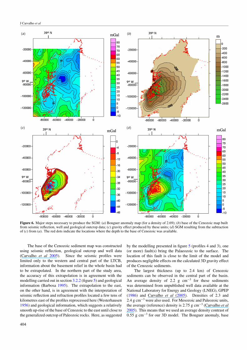
Figure 6. Major steps necessary to produce the SGM: (a) Bouguer anomaly map (for a density of 2.69); (b) base of the Cenozoic map builtfrom seismic reflection, well and geological outcrop data; (c) gravity effect produced by these units; (d) SGM resulting from the subtractionof (c) from (a). The red dots indicate the locations where the depth to the base of Cenozoic was available.

The base of the Cenozoic sediment map was constructedusing seismic reflection, geological outcrop and well data(Carvalho et al 2005). Since the seismic profiles werelimited only to the western and central part of the LTCB,information about the basement relief in the whole basin hadto be extrapolated. In the northern part of the study area,the accuracy of this extrapolation is in agreement with themodelling carried out in section 3.2.2 (figure 5) and geologicalinformation (Barbosa 1995). The extrapolation to the east,on the other hand, is in agreement with the interpretation ofseismic reflection and refraction profiles located a few tens ofkilometres east of the profiles reprocessed here (Westerhausen1956) and geological information, which suggests a relativelysmooth up-rise of the base of Cenozoic to the east until close tothe generalized outcrop of Paleozoic rocks. Here, as suggested

by the modelling presented in figure 5 (profiles 4 and 3), one(or more) fault(s) bring the Palaeozoic to the surface. Thelocation of this fault is close to the limit of the model andproduces negligible effects on the calculated 3D gravity effectof the Cenozoic sediments.

The largest thickness (up to 2.4 km) of Cenozoicsediments can be observed in the central part of the basin.An average density of 2.2 g cm−3 for these sedimentswas determined from unpublished well data available at theNational Laboratory for Energy and Geology (LNEG), GPEP(1986) and Carvalho et al (2005). Densities of 2.3 and2.4 g cm−3 were also used. For Mesozoic and Paleozoic units,the average (reference) density is 2.75 g cm−3 (Carvalho et al2005). This means that we used an average density contrast of0.55 g cm−3 for our 3D model. The Bouguer anomaly, base

404

Geophysical study of the Ota–V.F. Xira–Lisboa–Sesimbra fault zone and the LTCB

of Cenozoic, gravimetric effect of Cenozoic units and SGMsare shown in figure 6.

A striking outcome of this map is a strong positiveanomaly located at the lower Tagus estuary. The amplitudeof this anomaly is reduced when higher densities are usedfor the sedimentary Cenozoic infill but its shape and presenceremained. We emphasize that the obtained SGM is conditionedby the thickness of the Cenozoic sedimentary infill, leadingto this rather localized positive anomaly where the thicknessof sediments is more than 2 km. It is expected that if thestrong negative anomaly located further north is also partiallycaused by a thicker Cenozoic column as is the one overthe Tagus estuary (this is suggested by an unpublished deeprefraction line acquired in the 1950s (Westerhausen 1956) andby seismic reflection line ar8–81 located at the border of thisanomaly), this correction of the base of the Cenozoic mapwill produce a spatial enlargement of the referred positiveanomaly that will be in better agreement with the shape of theLTCB.

3.3. Deep seismic refraction data and digital terrain model

In order to obtain information from the structure of the studyarea and assess the presence (or not) of the OVLS fault zoneat depth, deeper crustal data were required. Such data havebeen collected in Portugal mainland since the 1970s from deeprefraction profiles (e.g. Mueller et al 1973, Moreira et al 1980,Mendes-Victor et al 1980 and reinterpreted by Matias 1996).

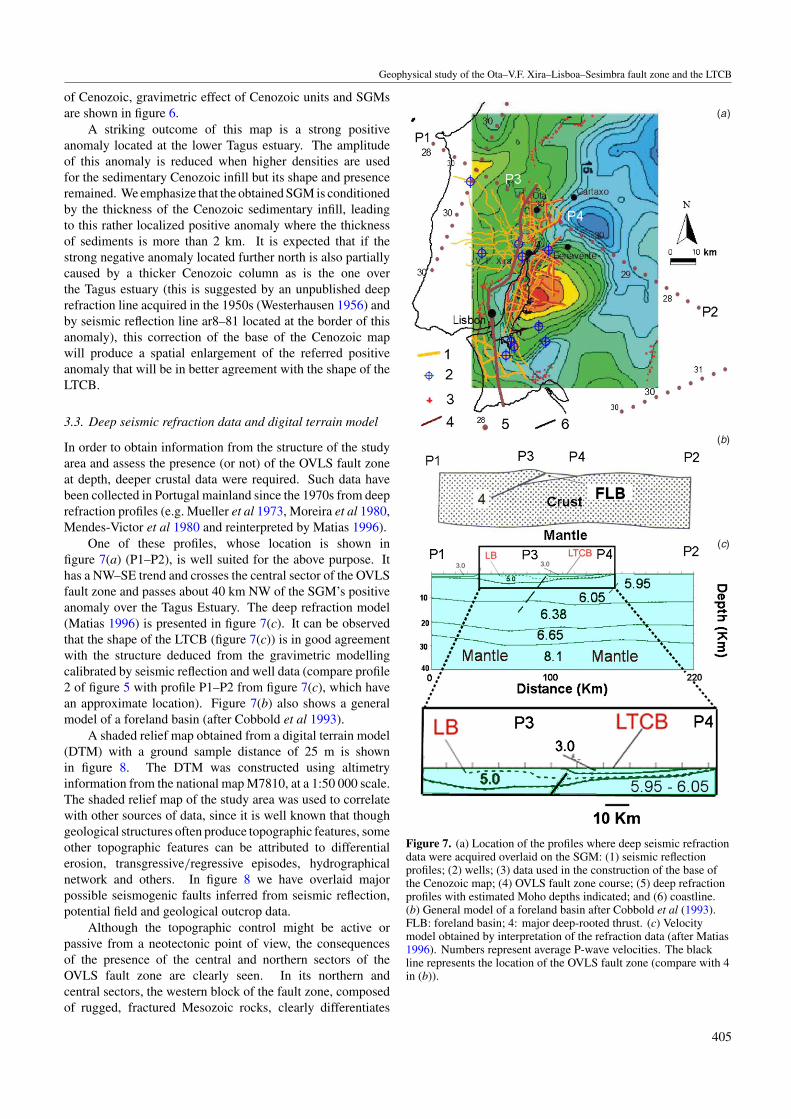
One of these profiles, whose location is shown infigure 7(a) (P1–P2), is well suited for the above purpose. Ithas a NW–SE trend and crosses the central sector of the OVLSfault zone and passes about 40 km NW of the SGM’s positiveanomaly over the Tagus Estuary. The deep refraction model(Matias 1996) is presented in figure 7(c). It can be observedthat the shape of the LTCB (figure 7(c)) is in good agreementwith the structure deduced from the gravimetric modellingcalibrated by seismic reflection and well data (compare profile2 of figure 5 with profile P1–P2 from figure 7(c), which havean approximate location). Figure 7(b) also shows a generalmodel of a foreland basin (after Cobbold et al 1993).

A shaded relief map obtained from a digital terrain model(DTM) with a ground sample distance of 25 m is shownin figure 8. The DTM was constructed using altimetryinformation from the national map M7810, at a 1:50 000 scale.The shaded relief map of the study area was used to correlatewith other sources of data, since it is well known that thoughgeological structures often produce topographic features, someother topographic features can be attributed to differentialerosion, transgressive/regressive episodes, hydrographicalnetwork and others. In figure 8 we have overlaid majorpossible seismogenic faults inferred from seismic reflection,potential field and geological outcrop data.

Although the topographic control might be active orpassive from a neotectonic point of view, the consequencesof the presence of the central and northern sectors of theOVLS fault zone are clearly seen. In its northern andcentral sectors, the western block of the fault zone, composedof rugged, fractured Mesozoic rocks, clearly differentiates

(b)

(c)

(a)

Figure 7. (a) Location of the profiles where deep seismic refractiondata were acquired overlaid on the SGM: (1) seismic reflectionprofiles; (2) wells; (3) data used in the construction of the base ofthe Cenozoic map; (4) OVLS fault zone course; (5) deep refractionprofiles with estimated Moho depths indicated; and (6) coastline.(b) General model of a foreland basin after Cobbold et al (1993).FLB: foreland basin; 4: major deep-rooted thrust. (c) Velocitymodel obtained by interpretation of the refraction data (after Matias1996). Numbers represent average P-wave velocities. The blackline represents the location of the OVLS fault zone (compare with 4in (b)).

405

J Carvalho et al

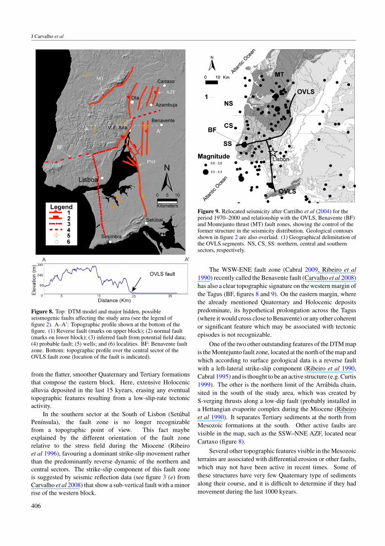
Figure 8. Top: DTM model and major hidden, possibleseismogenic faults affecting the study area (see the legend offigure 2). A–A′: Topographic profile shown at the bottom of thefigure. (1) Reverse fault (marks on upper block); (2) normal fault(marks on lower block); (3) inferred fault from potential field data;(4) probable fault; (5) wells; and (6) localities. BF: Benavente faultzone. Bottom: topographic profile over the central sector of theOVLS fault zone (location of the fault is indicated).

from the flatter, smoother Quaternary and Tertiary formationsthat compose the eastern block. Here, extensive Holocenicalluvia deposited in the last 15 kyears, erasing any eventualtopographic features resulting from a low-slip-rate tectonicactivity.

In the southern sector at the South of Lisbon (SetubalPenınsula), the fault zone is no longer recognizablefrom a topographic point of view. This fact maybeexplained by the different orientation of the fault zonerelative to the stress field during the Miocene (Ribeiroet al 1996), favouring a dominant strike-slip movement ratherthan the predominantly reverse dynamic of the northern andcentral sectors. The strike-slip component of this fault zoneis suggested by seismic reflection data (see figure 3 (e) fromCarvalho et al 2008) that show a sub-vertical fault with a minorrise of the western block.

Figure 9. Relocated seismicity after Carrilho et al (2004) for theperiod 1970–2000 and relationship with the OVLS, Benavente (BF)and Montejunto thrust (MT) fault zones, showing the control of theformer structure in the seismicity distribution. Geological contoursshown in figure 2 are also overlaid. (1) Geographical delimitation ofthe OVLS segments. NS, CS, SS: northern, central and southernsectors, respectively.

The WSW-ENE fault zone (Cabral 2009, Ribeiro et al1990) recently called the Benavente fault (Carvalho et al 2008)has also a clear topographic signature on the western margin ofthe Tagus (BF, figures 8 and 9). On the eastern margin, wherethe already mentioned Quaternary and Holocenic depositspredominate, its hypothetical prolongation across the Tagus(where it would cross close to Benavente) or any other coherentor significant feature which may be associated with tectonicepisodes is not recognizable.

One of the two other outstanding features of the DTM mapis the Montejunto fault zone, located at the north of the map andwhich according to surface geological data is a reverse faultwith a left-lateral strike-slip component (Ribeiro et al 1990,Cabral 1995) and is thought to be an active structure (e.g. Curtis1999). The other is the northern limit of the Arrabida chain,sited in the south of the study area, which was created byS-verging thrusts along a low-dip fault (probably installed ina Hettangian evaporite complex during the Miocene (Ribeiroet al 1990). It separates Tertiary sediments at the north fromMesozoic formations at the south. Other active faults arevisible in the map, such as the SSW–NNE AZF, located nearCartaxo (figure 8).

Several other topographic features visible in the Mesozoicterrains are associated with differential erosion or other faults,which may not have been active in recent times. Some ofthese structures have very few Quaternary type of sedimentsalong their course, and it is difficult to determine if they hadmovement during the last 1000 kyears.

406

Geophysical study of the Ota–V.F. Xira–Lisboa–Sesimbra fault zone and the LTCB

4. Seismicity

Relocated epicentres from the period 1970–2000 (Carrilhoet al 2004) using the software Hypocent (Lienert et al 1986,Lienert and Havskov 1995) are plotted in figure 9. The averageerror (90% confidence level) in the epicentral locations is 5 km.The OVLS fault zone course proposed in this paper, inferredfrom seismic reflection and potential field data, is also shownin figure 9.

The vast majority of earthquakes are located to the westof the fault course in the three sectors, in agreement withthe model of a foreland basin where most of the deformationoccurs in the upthrust block. In the northern sector, at thenorthern part of the study area, there is also a clear correlationbetween the Montejunto thrust and seismicity (please comparefigures 8 and 9) which strongly suggests that it is an activestructure, as already recognized by Cabral (1995) and Curtis(1999), for example.

In the northern and central sectors of the OVLS, to theeast of the fault zone course there is a N–S-oriented gap inseismicity of about 20 km long. The events at the far east ofthe figure after the gap cannot be correlated with any knownactive faults (no coverage of seismic reflection data in thisarea).

In the southern sector, there is also a relative gap inseismicity at the east of the OVLS fault but about ten eventsare located close to the fault plane. About five to six of theseevents make an alignment that can be associated with a largestructure deduced from Landsat data (Cabral and Ribeiro 1988,Cabral 1995) but which was found later not to affect Cenozoicsediments (e.g. Cabral et al 2003): the LTV fault (Cabraland Ribeiro 1988). The reprocessing and reinterpretationof seismic reflection data carried out in this work suggeststhe existence of this structure at depth, in Mesozoic terrains.The other events located further east in this sector cannot beassociated with known active faults as well.

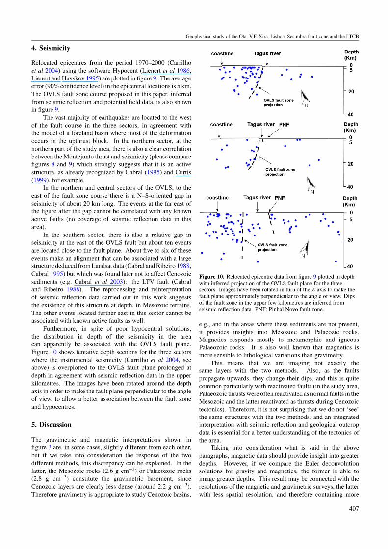
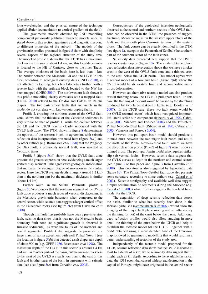
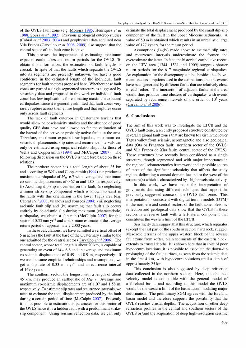
Furthermore, in spite of poor hypocentral solutions,the distribution in depth of the seismicity in the areacan apparently be associated with the OVLS fault plane.Figure 10 shows tentative depth sections for the three sectorswhere the instrumental seismicity (Carrilho et al 2004, seeabove) is overplotted to the OVLS fault plane prolonged atdepth in agreement with seismic reflection data in the upperkilometres. The images have been rotated around the depthaxis in order to make the fault plane perpendicular to the angleof view, to allow a better association between the fault zoneand hypocentres.

5. Discussion

The gravimetric and magnetic interpretations shown infigure 3 are, in some cases, slightly different from each other,but if we take into consideration the response of the twodifferent methods, this discrepancy can be explained. In thelatter, the Mesozoic rocks (2.6 g cm−3) or Palaeozoic rocks(2.8 g cm−3) constitute the gravimetric basement, sinceCenozoic layers are clearly less dense (around 2.2 g cm−3).Therefore gravimetry is appropriate to study Cenozoic basins,

Figure 10. Relocated epicentre data from figure 9 plotted in depthwith inferred projection of the OVLS fault plane for the threesectors. Images have been rotated in turn of the Z-axis to make thefault plane approximately perpendicular to the angle of view. Dipsof the fault zone in the upper few kilometres are inferred fromseismic reflection data. PNF: Pinhal Novo fault zone.

e.g., and in the areas where these sediments are not present,it provides insights into Mesozoic and Palaeozic rocks.Magnetics responds mostly to metamorphic and igneousPalaeozoic rocks. It is also well known that magnetics ismore sensible to lithological variations than gravimetry.

This means that we are imaging not exactly thesame layers with the two methods. Also, as the faultspropagate upwards, they change their dips, and this is quitecommon particularly with reactivated faults (in the study area,Palaeozoic thrusts were often reactivated as normal faults in theMesozoic and the latter reactivated as thrusts during Cenozoictectonics). Therefore, it is not surprising that we do not ‘see’the same structures with the two methods, and an integratedinterpretation with seismic reflection and geological outcropdata is essential for a better understanding of the tectonics ofthe area.

Taking into consideration what is said in the aboveparagraphs, magnetic data should provide insight into greaterdepths. However, if we compare the Euler deconvolutionsolutions for gravity and magnetics, the former is able toimage greater depths. This result may be connected with theresolutions of the magnetic and gravimetric surveys, the latterwith less spatial resolution, and therefore containing more

407

J Carvalho et al

long-wavelengths, and the physical nature of the techniqueapplied (Euler deconvolution to vertical gradient of the field).

The gravimetric models obtained by 2.5D modellingcomplement previously published magnetic models since, asstated above in this section, gravimetry and magnetics respondto different properties of the subsoil. The models of thegravimetric profiles presented in figure 5 show with simplicityseveral aspects of the regional structure of the study area.The model of profile 1 shows that the LTCB has a maximumthickness in this area of about 1.4 km, and this local depocentreis located to the NE of Cartaxo, close to the river Tagus.The average thickness of the basin here is less than 1 km.The border between the Mesozoic LB and the LTCB in thisarea, according to geological outcrop data (LNEG 2010), isnot affected by faulting, but a few kilometres further north areverse fault with the upthrust block located to the NW hasbeen mapped (LNEG 2010). The northwestern fault shown inthis profile modelling clearly correlates with a mapped fault(LNEG 2010) related to the Obidos and Caldas da Rainhadiapirs. The two easternmost faults that are visible in themodel do not correlate with known outcropping faults.

Profile 2, crossing the northern sector of the OVLS faultzone, shows that the thickness of the Cenozoic sediments isvery similar to that of profile 1, while the contact betweenthe LB and the LTCB here is clearly associated with theOVLS fault zone. The DTM shown in figure 8 demonstratesthe upthrust of the western block, in agreement with seismicreflection data interpretation presented here (figure 3(a)) andby other authors (e.g. Rasmussen et al 1998) that the Praganca(or Ota) fault, a previously normal fault, was inverted inCenozoic times.

Profile 3 (figure 5(c)) shows that the OVLS fault zonepresents the greatest expression here, evidencing a much largervertical displacement. This agrees with geological informationthat indicates the strongest degree of inversion in the centralsector. Here the LTCB average depth is larger (around 1.2 km)than in the northern part but the maximum thickness is similar(about 1.4 km).

Further south, in the Setubal Peninsula, profile 4(figure 5(d)) evidences that the southern segment of the OVLSfault zone produces a much reduced vertical displacement inthe Mesozoic gravimetric basement when compared to thecentral sector, while seismic data suggest a larger vertical offsetin the Palaeozoic rocks (see figure 3(e) from Carvalho et al2008).

Though this fault may probably have been a pre-inversionfault, seismic data show that it was not the Mesozoic basinboundary fault zone (no significant growth is observed inJurassic sediments), as were the faults of the northern andcentral segments. Profile 4 also suggests the presence of alarge mass of salt in agreement with well Pinhal Novo 1 (seethe location in figure 5(d)) that detected a salt diaper at a depthof about 900 m (e.g. GPEP 1986, Rasmussen et al 1998). Themaximum depth of the LTCB in this sector is around 1.4 kmand similar to other parts of the basin, but the average thicknessto the west of the OVLS is clearly less than to the east of thisfault and in other parts of the basin in agreement with seismicdata (see also figure 3(e) from Carvalho et al 2008).

Consequences of the geological inversion geologicallyobserved at the central and northern sectors of the OVLS faultzone can be observed in the DTM: the presence of rugged,fractured, Mesozoic rocks on the western upper block of thefault and the smooth plain Cenozoic terrains of the easternblock. The fault course can be clearly identified in the DTM(see figure 8), except in the Penınsula of Setubal (the southernpart of the southern sector of the fault zone).

Seismicity data presented here support that the OVLSreaches crustal depths (figure 10). The model obtained fromdeep refraction data interpretation shows that we have a thickercrust to the west of the OVLS fault zone and a thinned crustto the east, below the LTCB basin. This model agrees witha general model of a foreland basin (figure 7(b)) where theOVLS would be its western limit and accommodate majorthrust deformation.

However, an alternative tectonic model can also producecrustal thinning below the LTCB: a pull-apart basin. In thiscase, the thinning of the crust would be caused by the stretchingproduced by two large strike-slip faults (e.g. Dooley et al2007). In the LTCB case, these two fault zones would bethe OVLS (central sector) which has a recognized importantleft-lateral strike-slip component (Ribeiro et al 1990, Cabralet al 2003, Vilanova and Fonseca 2004) and the left-lateralPinhal Novo–Setubal fault (Ribeiro et al 1990, Cabral et al2003, Vilanova and Fonseca 2004).

However, this pull-apart basin model should produce athinned crust between the two major fault zones and not tothe north of the Pinhal Novo–Setubal fault, where we havethe deep refraction profile (P1–P2 of figure 7) which shows athinned crust. The pull-apart basin model also requires strike-slip sub-vertical faults. However, seismic data suggest thatthe OVLS curves at depth in the northern and central sectors(see figure 3 of this paper and figure 3 from Carvalho et al2008). This curvature is also suggested by hypocentre data(figure 10). The Pinhal Novo–Setubal fault zone also presentssome curvature according to some authors (e.g. Cabral et al2003). Seismic stratigraphy and available well data suggesta rapid accumulation of sediments during the Miocene (e.g.Cabral et al 2003) which further suggests the foreland basinmodel for the LTCB.

The acquisition of deep seismic reflection data acrossthe basin, similar to what has recently been done in theIberian Pyrite Belt (Schmelzbach et al 2007), would allow theimaging of the major fault plane rooting and simultaneouslythe thinning (or not) of the crust below the basin. Additionaldeep refraction profiles would also allow studying in moredetail the thinning of the crust below the LTCB and help toestablish the tectonic model for the LTCB. Together with aSGM obtained using a more detailed base of the Cenozoicmap followed by gravimetric modelling that would result in abetter understanding of tectonics of the study area.

Independently of the tectonic model proposed for theLTCB, seismic reflection data show that the OVLS is rooted atleast to a depth of 4 km, while seismicity data suggest that itmight reach 25 km depth. According to the available historicaldata, the 1531 event that caused widespread destruction in thecapital of Portugal might have originated in the central sector

408

Geophysical study of the Ota–V.F. Xira–Lisboa–Sesimbra fault zone and the LTCB

of the OVLS fault zone (e.g. Moreira 1985, Henriques et al1988, Sousa et al 1992). Previous geological outcrop studies(Cabral et al 2003, 2004) and geophysical data acquired nearVila Franca (Carvalho et al 2006, 2009) also suggest that thecentral sector of the fault zone is active.

This stresses the importance of estimating maximumexpected earthquakes and return periods for the OVLS. Toobtain this information, the estimation of fault lengths iscrucial. In spite of that the faults which separate the OVLSinto its segments are presently unknown, we have a goodconfidence in the estimated length of the individual faultsegments (or fault sectors) proposed here. Whether these faultzones are part of a single segmented structure as suggested byseismicity data and proposed in this work or individual faultzones has few implications for estimating maximum expectedearthquakes, since it is generally admitted that fault zones veryrarely rupture across their entire length and that ruptures occuronly across fault segments.

The lack of fault outcrops in Quaternary terrains thatwould allow paleoseismicity studies and the absence of goodquality GPS data have not allowed so far the estimation ofthe hazard of the active or probably active faults in the area.Therefore, maximum expected earthquakes, maximum co-seismic displacements, slip rates and recurrence intervals canonly be estimated using empirical relationships like those ofWells and Coppersmith (1994) and McCalpin (2007). Thefollowing discussion on the OVLS is therefore based on theserelations.

The northern sector has a total length of about 25 kmand according to Wells and Coppersmith (1994) can produce amaximum earthquake of MW 6.7 with average and maximumco-seismic displacements of 0.67 m and 1.08 m, respectively.(i) Assuming dip-slip movement on the fault, (ii) neglectinga minor strike-slip component which is known to exist inthe faults with this orientation in the lower Tagus area (e.g.Cabral et al 2003, Vilanova and Fonseca 2004), (iii) neglectingaseismic fault slip and (iv) assuming that fault slip occursentirely by co-seismic slip during maximum (characteristic)earthquake, we obtain a slip rate (McCalpin 2007) for thissector of 0.33 mm yr–1 and a maximum estimate of the averagereturn period of approximately 2000 years.

In these calculations, we have admitted a vertical offset of5 m across the fault at the base of the Quaternary similar to theone admitted for the central sector (Carvalho et al 2006). Thecentral sector, whose total length is about 20 km, is capable ofgenerating an event of MW 6.6 and an average and maximumco-seismic displacement of 0.49 and 0.9 m, respectively. Ifwe use the same empirical relationships and assumptions, weget a slip rate of 0.33 mm yr–1 and a recurrence intervalof 1470 years.

The southern sector, the longest with a length of about45 km, may produce an earthquake of MW 7. Average andmaximum co-seismic displacements are of 1.07 and 1.58 m,respectively. To estimate slip rates and recurrence intervals, weneed to estimate the total displacement produced by the faultduring a certain period of time (McCalpin 2007). Presentlyit is not possible to estimate this parameter for this sector ofthe OVLS since it is a hidden fault with a predominant strike-slip component. Using seismic reflection data, we can only

estimate the total displacement produced by the small dip-slipcomponent of the fault in the upper Miocene sediments. Avalue of 50 m is obtained which results in an unrealistic largevalue of 127 kyears for the return period.

Assumptions (i)–(iv) made above to estimate slip ratesand recurrence intervals underestimate the former andoverestimate the latter. In fact, the historical earthquake recordon the LTV area (1344, 1531 and 1909) suggests shorterreturn periods for the 6–7 magnitude regional earthquakes.An explanation for the discrepancy can be, besides the above-mentioned assumptions used in the estimations, that the eventshave been generated by different faults that are relatively closeto each other. The interaction of adjacent faults in the areawould thus produce time clusters of earthquakes with eventsseparated by recurrence intervals of the order of 102 years(Carvalho et al 2006).

6. Conclusions

The aim of this work was to investigate the LTCB and theOVLS fault zone, a recently proposed structure constituted byseveral regional fault zones that are known to exist in the lowerTagus valley from seismic, aeromagnetic and also geologicaldata (Ota or Praganca fault: northern sector of the OVLS,and Vila Franca de Xira fault: central sector of the OVLS).These structures have recently been considered as a singlestructure, though segmented and with major importance inthe regional seismotectonics framework and a possible sourceof most of the significant seismicity that affects the studyregion, delimiting a crustal domain located to the west of thestructure(s) which is characterized by a higher seismic activity.

In this work, we have made the interpretation ofgravimetric data using different techniques that support thepreviously suggested course of the OVLS fault zone. Thisinterpretation is consistent with digital terrain models (DTM)in the northern and central sectors of the fault zone. Seismicreflection and geological data show that the OVLS in thesesectors is a reverse fault with a left-lateral component thatconstitutes the western limit of the LTCB.

Seismicity data suggest that this structure, which separates(except the last part of the southern sector) hard rock, rugged,Mesozoic terrains of the upper western block of the reversefault zone from softer, plain sediments of the eastern block,extends to crustal depths. It is shown here that in spite of poorhypocentre locations, it is possible to associate the down-dipprolonging of the fault surface, as seen from the seismic datain the first 4 km, with hypocentre solutions until a depth ofapproximately 25 km.

This conclusion is also suggested by deep refractiondata collected in the northern sector. Here, the obtainedvelocity model is compatible with the general model ofa foreland basin, and according to this model the OVLSwould be the western limit of the basin accommodating majordeformation. The preliminary SGM agrees with the forelandbasin model and therefore supports the possibility that theOVLS reaches crustal depths. The acquisition of other deeprefraction profiles in the central and southern sectors of theOVLS or/and the acquisition of deep high-resolution seismic

409

J Carvalho et al

reflection data together with a more detailed SGM can confirmthis possibility. This confirmation is extremely important forseismic hazard studies since if the OVLS is an active structureinto the Quaternary, as supported by several geophysical,seismological and geological data, such a structure will beable to produce large earthquakes.

The estimation of the segment lengths made in this work,based mostly on seismic reflection and geological outcropdata, has a good accuracy and is extremely important foran appropriate evaluation of local seismic hazard. Whetherthe Ota fault, V. F. Xira fault and southern sector of theOVLS fault are indeed fault segments of the OVLS asproposed here or independent fault zones has no practicalimpact on the estimation of maximum expected magnitudes,average and maximum displacements, recurrence intervalsand slip rates, since most of the times faults rupture onlyby segments. Therefore, preliminary maximum expectedmagnitudes, average and maximum displacements, recurrenceintervals and slip rates have been estimated for the threesectors of the OVLS fault zone. The slip rates obtained here(0.33 mm yr–1) are in agreement with the values inferredfor active faults in the lower Tagus valley and other areasin Portugal mainland.

Acknowledgments

The Department of Prospeccao e Exploracao de Petroleosfrom the Direccao Geral de Geologia e Energia isgratefully acknowledged for supplying the seismic reflectiondata and Mohave Oil for allowing the publication oftheir pre-stack time migrated reprocessed data. Theportuguese Foundation for Science and Technology andProjects POCTI/CTE-GIN/58250/2004 Sismotecto andPTDC/CTE-GIN/82704/2006 Sismod/Lismot is gratefullyacknowledged. We are also indebted to the Centro deGeofısica da Universidade de Lisboa for several contributionsto this study. We would also like to thank those whocontributed to the final results presented here: RubenDias, Catarina Moniz, and Manuela Costa for discussionson the interpretation of the seismic reflection profiles andgeodynamic implications of the results. We are particularlygrateful to two anonymous reviewers for their comments andsuggestions which greatly improved this work.

References

Barbosa Bernardo A P S 1995 Alostratigrafia e litostratigrafia dasunidades continentais da Bacia Terciaria do Baixo Tejo,Relacoes com o eustatismo e a tectonica PhD Thesis Universityof Lisbon 253 pp

Bielik M 1988a A preliminary stripped gravity map of thePannonian basin Phys. Earth Planet. Inter. 51 185–9

Bielik M 1988b Analysis of the stripped gravity map of thePannonian basin Geol. Carpathica 39 99–108

Bielik M, Makarenko I, Legostaeva O, Starostenko V, Dererova Jand Sefara J 2004 Stripped gravity map of theCarpathian-Pannonian basin region Osterr. Beitr. Meteorol.Geophys. 31 107–17

Bielik M, Makarenko I, Legostaeva O, Starostenko V, Dererova J,Sefara J and Pasteka R 2005 New 3D gravity modeling in the

Carpathian-Pannonian basin region Contrib. Geophys. Geod.35 65–78

Borges J F, Fitas A J S, Bezzeghoud M and Teves-Costa P 2001Seismotectonics of Portugal and its adjacent Atlantic areaTectonophysics 337 373–87

Cabral J 2009 Tectonica Notıcia Explicativa da Folha 34-B (Loures),Geological Map of Portugal 1/50.000, INETI, Lisbon-Portugal

Cabral J 1995 Neotectonica em Portugal Continental Mem. Inst.Geol. Mineiro 31 265

Cabral J, Moniz C, Ribeiro P, Terrinha P and Matias L 2003Analysis of seismic reflection data as a tool for theseismotectonic assessment of a low activity intraplatebasin—the Lower Tagus Valley (Portugal) J. Seismol.7 431–47

Cabral J and Ribeiro P 1988 Carta Neotectonica de PortugalContinental (escala 1:1000.000), Map Geological Survey ofPortugal, Geology Department, Faculty of Sciences, Cabinet ofNuclear Safety and Protection

Cabral J, Ribeiro P, Figueiredo P, Pimentel N and Martins A 2004The Azambuja fault: an active structure located in an intraplatebasin with significant seismicity (Lower Tagus Valley,Portugal) J. Seismol. 8 347–62

Carrilho F, Nunes J C, Pena J and Senos M L 2004 CatalogoSısmico de Portugal Continental e Regiao Adjacente para operıodo 1970–2000 Report Instituto de Meteorologia ISBN972-9083-12-6

Carvalho J 2003 Sısmica de alta resolucao aplicada a prospeccao,geotecnia e risco sısmico PhD Thesis University of Lisbon264 pp

Carvalho J, Ghose R, Pinto C and Borges J 2009 Characterization ofa concealed fault zone using P and S-wave seismic reflectiondata Extended Abstracts of the EAGE Near Surface 2009/15thMeeting of Environmental and Engineering Geophysics(Dublin, Ireland, 7–9 September 2009) p A14

Carvalho J, Cabral J, Goncalves R, Torres L and Mendes-Victor L2006 Geophysical methods applied to fault characterizationand earthquake potential assessment in the Lower Tagus Valley,Portugal Tectonophysics 418 277–97

Carvalho J, Matias H, Torres L, Manupella G, Pereira R andMendes-Victor L 2005 The structural and sedimentaryevolution of the Arruda and Lower Tagus sub-basins, PortugalMar. Pet. Geol. 22 427–53

Carvalho J, Taha R, Cabral J, Carrilho F and Miranda M 2008Geophysical characterization of the Ota-Vila Franca deXira-Lisbon-Sesimbra fault zone, Portugal Geophys. J.Int. 174 567–84

Cobbold P R, Davy P, Gapais D, Rossello E A, Sadybakasov E,Thomas J C, Tondji Biyo J J and de Urreiztieta M 1993Sedimentary basins and crustal thickness SedimentaryGeol. 86 77–89

Cooper G R J and Cowan D R 2003 Applications of fractionalcalculus to potential field data Explor. Geophys. 34 51–6

Curtis M 1999 Structural and kinematic evolution of a Miocene torecent sinistral restraining bend: the Montejunto massif,Portugal J. Struct. Geol. 21 39–54

Dineva S, Batllo J, Mihaylov D and van Eck T 2002 Sourceparameters of four strong earthquakes in Bulgaria and Portugalat the beginning of the 20th century J. Seismol. 6 99–123

Domzalski W 1969 Interpretation of an aeromagnetic surveyoffshore Portugal (1:200.000) Report Fairey Surveys Ltd,Maidenhead, Berkshire, England

Dooley T P, Monastero F C and McClay K R 2007 Effects of aweak crustal layer in a transtensional pull-apart basin: resultsfrom a scaled physical modeling study American GeophysicalUnion, Fall Meeting 2007 abstract no V53F-04

GM-SYS 1995 Gravity and magnetic modelling version 3.6,Northwest Geophysical Association, Inc. (NGA), OR, USA

GPEP (Gabinete para a Pesquisa e Exploracao de Petoleos)1986 Petroleum Potential of Portugal (Lisboa: GPEP)p 62

410

Geophysical study of the Ota–V.F. Xira–Lisboa–Sesimbra fault zone and the LTCB

Grant F S and West G F 1965 Interpretation Theory in AppliedGeophysics (New York: McGraw-Hill)

Hammer S 1963 Deep gravity interpretation by strippingGeophysics 28 369–78

Henriques M C, Mouzinho M T and Ferrao N M 1988 Sismicidadede Portugal. O Sismo de 26 de Janeiro de 1531 (Portugal:Comission for the National Earthquake Catalogue) 100 pp

Hsu S-K 2002 Imaging magnetic sources using Euler’s equationGeophys. Prospect. 50 15–25

Justo J L and Salwa C 1998 The 1531 Lisbon earthquake Bull.Seismol. Soc. Am. 88 319–28

Legostaeva O 2000 On optimal scheme of computing doubleintegrals in solving direct gravimetric and magnetometricproblems Geophys. J. 19 693–9

Leinfelder R R and Wilson R C L 1998 Third-order sequences in anUpper Jurassic rift-related second-order sequence, CentralLusitanian Basin, Portugal Mesozoic and Cenozoic SequenceStratigraphy of European Basins ed P C Graciansky,J Hardenbol, T Jacquin and P R Vail (Tulsa, OK: SEPMSpecial Publication 60) pp 507–25

Lienert B, Berg E and Neil Frazer L 1986 Hypocenter: anearthquake location method using centered, scaled andadaptively damped least squares Bull. Seismol. Soc. Am.76 771–83

Lienert B and Havskov J 1995 A computer program for locatingearthquakes both locally and globally Seismol. Res. Lett.66 26–36

Linsser H 1967 Investigation of tectonic by gravity detailingGeophys. Prospect. 15 480–515

LNEG 2010 Geological Map of Portugal, scale 1: 1.000.000,Laboratorio Nacional de Energia e Geologia, Ministry ofEconomy, Innovation and Development, Alfragide

Matias L 1996 A sismologia experimental na modelacao daestrutura da crusta em Portugal continental PhD ThesisUniversity of Lisbon 398 pp

McCalpin J P 2007 Paleoseismology (New York: Academic)Mendes-Victor L A, Hirn A and Veinant J L 1980 A seismic section

across the Tagus Valley, Portugal: possible evolution of thecrust Ann. Geophys. 36 469–76

Moreira V S 1985 Seismotectonics of Portugal and its adjacent areain the Atlantic Tectonophysics 117 85–96

Moreira V S, Prodehl C, Mueller St and Mendes A S 1980 CrustalStructure of Western Portugal Proc. 17th Assembly of the ESC(Budapest) pp 529–32

Mueller S, Prodehl C, Mendes A S and Moreira V S 1973 Crustalstructure in the southwestern part of the Iberian peninsulaTectonophysics 20 307–18

Oliveira T (coord.) et al 1992 Carta Geologica de Portugal, escala 1:500.000, Map, Servicos Geologicos de Portugal, Lisboa

Pelaez J A M, Casado C L and Romero J H 2002 Deaggregation inmagnitude, distance, and azimuth in the south and west of theIberian peninsula Bull. Seismol. Soc. Am. 92 2177–85

Rasmussen E S, Lomholt S, Anderson C and Vejbaek O V 1998Aspects of the structural evolution of the Lusitanian Basin inPortugal and the shelf and slope area offshore PortugalTectonophysics 300 199–225

Reid A B, Allsop J M, Granser H, Millett A J and Somerton I W1990 Magnetic interpretation in three dimensions using Eulerdeconvolution Geophysics 55 80–91

Ribeiro A 2002 Soft Plate and Impact Tectonics (Berlin: Springer)324 pp

Ribeiro A, Cabral J, Baptista R and Matias L 1996 Stress pattern inPortugal mainland and the adjacent Atlantic region, West IberiaTectonics 15 641–59

Ribeiro A, Kullberg M C, Kullberg J C, Manupella G and Phipps S1990 A review of Alpine tectonics in Portugal: forelanddetachment in basement and cover rocks Tectonophysics184 357–66

Schmelzbach C, Juhlin C, Carbonell R and Simancas J F 2007Prestack and poststack migration of crooked-line seismicreflection data: a case study from the South Portuguese Zonefold belt, southwestern Iberia Geophysics 72 B9–18

Sousa M L, Matins A and Oliveira C S 1992 Compilacao deCatalogos Sısmicos da Regiao Iberica Report 36/92 NDA,Dept Estruturas, Nucleo Dinamica Aplicada, Proc.036/11/9295, LNEC, Lisboa

Starostenko V I, Matsello V V, Aksak I N, Kulesh V A,Legostaeva O V and Yegorova T P 1997 Automation of thecomputer input of images of geophysical maps and their digitalmodelling Geophys. J. 17 1–19

Stavrev P Y 1997 Euler deconvolution using differential similaritytransformations of gravity or magnetic anomalies Geophys.Prospect. 45 207–46

Stich D, Batllo J, Macia R, Teves-Costa P and Morales J 2005Moment tensor inversion with single-component historicalseismograms: the 1909 Benavente (Portugal) and Lambesc(France) earthquakes Geophys. J. Int. 162 850–8

Surinkum A 1989 Geological interpretation of airborne and groundmagnetic survey Master Thesis University of Western Ontario,Canada pp 34–40

Talwani M 1965 Computation with the help of a digital computer ofmagnetic anomalies caused by bodies of arbitrary shapeGeophysics 30 797–817

Teves-Costa P, Rio I, Marreiros C, Ribeiro R and Borges J F 1999Source parameters of old earthquakes: semi-automaticdigitalization of analog records and seismic momentassessment Nat. Hazards 19 205–20

Thompson D T 1982 EULDPH—a new technique for makingcomputer-assisted depth estimates from magnetic dataGeophysics 47 31–7

Vilanova S P and Fonseca J F B D 2004 Seismic hazard impact ofthe Lower Tagus Valley Fault Zone (SW Iberia)J. Seismol. 8 331–45

Wells D L and Coppersmith K J 1994 New empirical relationshipsamong magnitude, rupture length, rupture width, rupturearea and surface displacement Bull. Seismol. Soc. Am.84 974–1002

Westerhausen H 1956 Report on reflection and refraction seismicinvestigations carried out in South Tejo Basin for Companhiados Petroleos de Portugal and Mobil Exploration CompanyLisboa (Portugal) by Prakla 20 pp

Wilson R C L, Hiscott R N, Willis M G and Gradstein F M 1989The Lusitanian Basin of west central Portugal: Mesozoic andTertiary tectonics, stratigraphy and subsidence historyExtensional Tectonics and Stratigraphy of the North AtlanticMargins (American Association Petroleum Geologists Memoirvol 46) ed A J Tankard and H Balkwill (Tulsa, OK: AmericanAssociation of Petroleum Geologists) pp 341–61

411